arX

iv:c

ond-

mat

/050

4408

v1 [

cond

-mat

.sta

t-m

ech]

16

Apr

200

5

Exactly Integrable Analogue of a One-dimensional Gravitating

System

Bruce N. Miller, Kenneth R. Yawn, and Bill Maier

Department of Physics and Astronomy,

Texas Christian University,

Fort Worth, Texas 76129

Abstract

Exchange symmetry in acceleration partitions the configuration space of an N particle, one-

dimensional, gravitational system into N ! equivalent cells. We take advantage of the resulting

small angular extent of each cell to construct a related integrable version of the system that takes

the form of a central force problem in N − 1 dimensions. The properties of the latter, including

the construction of trajectories, as well as several continuum limits, are developed. Dynamical

simulation is employed to compare the two models. For a class of initial conditions, excellent

agreement is observed.

PACS numbers: 05.10.-a, 05.45.-a , 56.25.EF , 05.70.Fh

Keywords: integrable dynamical system, N -body simulations, gravity, Vlasov equation

1

One dimensional systems have played a central role in the development of physical models.

Because of their relative simplicity, they form the starting point for the study of a wide

variety of interactions. One-dimensional models of gases have been studied extensively in

statistical mechanics and one-dimensional lattice models have been used in solid state physics

to study metal alloys, magnetic spin systems, glasses, phonon propagation, electronic bands

and a host of other systems. One dimensional gravitational systems have been used to

investigate relaxation to equilibrium, phase transitions, the gravothermal catastrophe, and

cosmology[1]. An important example is the system consisting of a one-dimensional chain

of coupled, nonlinear, oscillators. Known as the Fermi-Pasta-Ulam (FPU) problem[2], it

has had an enormous impact on the development of dynamics in the last fifty years. Its

failure to come to thermal equilibrium in simulations on the earliest electronic computers

stimulated intense research in the theory of conservative dynamical systems and resulted

in major breakthroughs such as the KAM theorem and developments in soliton theory [2].

The analogous system in astronomy consists of N parallel planar mass sheets of infinite

extent that are restricted to move perpendicular to their surface. Like the FPU problem,

this is a nonlinear, one-dimensional system. The only forces on a given sheet (or particle)

are gravitational, and the system obeys the Poisson equation in one dimension. Since each

particle experiences a constant acceleration until it encounters a neighboring particle, the

motion can be expressed analytically and it is straightforward to simulate the system on the

computer [3].

The one dimensional self-gravitating system (OGS) was the first gravitational system to

be investigated numerically [4] and, like the FPU system, it resists relaxing to statistical

equilibrium. Early studies showed that the system virialized within 50 or so characteristic

system crossing times, τc, [4] as a consequence of ”violent relaxation” [5]. Following this

period the system appears to approximate a stationary Vlasov state which evolves extremely

slowly, perhaps on the order of millions of τc. Evidence of the approach to thermal equilib-

rium has only been recently established for a two component system [6, 7]. For an extensive

review of the history of the relevant investigations see [1, 7]. In this paper we offer a possible

explanation for the incredibly slow exploration of phase space these systems exhibit. We

demonstrate analytically and with numerical simulation that an exactly integrable Hamil-

tonian system (EIS) exists which closely represents the OGS as its population increases.

Further we derive a continuum (Vlasov) limit for the EIS and show that it is characterized

2

by two integral invariants, as well as an exactly periodic radius. We also show that the

continuum model can be extended to the pair space and provide information concerning

correlations in position and velocity.

Consider an OGS consisting of N parallel mass sheets (particles) of equal mass surface

density m and let the real x axis be perpendicular to their surface. Label the sheets in terms

of their increasing ordering from left to right so their positions are xj with xj+1 > xj(j =

1, ..., N − 1) . Then, from Gauss’ law, the acceleration Aj experienced by particle j is a

constant proportional to the net difference in the number of particles to its right and left:

Aj = 2πmG(N + 1 − 2j). (1)

As the system evolves, each particle undergoes uniform acceleration until a pair of par-

ticles crosses, at which time their accelerations are exchanged. Since the system is isolated

from external forces, the total momentum and energy are conserved, while the center of

mass moves with uniform velocity. Without loss of generality we may assume we are in a

frame where the total momentum is zero and the center of mass is at rest. To establish a

connection with the Vlasov limit, it is more convenient to represent the system in terms of

positions and velocities (xj , vj) of the particles. Thus

N∑

1

xj = 0,N

∑

1

vj = 0, E =m

2

N∑

1

v2j + 2πm2G

∑

i<j

|xi − xj | (2)

where E is the total energy. It is also convenient to introduce a system of unit vectors ,

ej , in the N dimensional configuration space. Then we can represent the system in terms

of N dimensional position, velocity (in the tangent space), and acceleration vectors,

x =

N∑

1

xjej , v =

N∑

1

vjej , A =

N∑

1

Ajej . (3)

In this context, the system is represented by a single point moving with constant accel-

eration until a crossing occurs, whereby two of the acceleration components are exchanged;

i.e. the actual components of A depend on the ordering of the particle positions. Letting

ec=1N

∑

j ej, the constraints on the total momentum and the center of mass can be expressed

by v · ec= x · ec= 0. As a result of the dynamical constraints (including energy conserva-

tion), the trajectories lie on a 2N − 3 hyper-surface of the 2N dimensional phase space. We

3

can also introduce a generalized angular momentum tensor as a two form, or dyadic in the

older formalism [8], and its square:

L = x ∧ mv = m

N∑

i,j=1

xivjei ∧ ej =m√2

N∑

i,j=1

(xivj − xjvi)eiej (4)

L2 =m2

2

N∑

i,j=1

(xivj − xjvi)2. (5)

It is straightforward to show that, for N = 3, these definitions reduce to the familiar

equations of three dimensional orbital mechanics. For completeness, and to compare with

our further development below, we mention that the system has a well defined continuum

(Vlasov) limit. By projecting the single point representing the system in its 2N dimensional

phase space onto a single (x, v) plane, the system is represented by a cloud of N points. If

we let N → ∞ while constraining the total mass, M = Nm , and energy E, the system

is described by a fluid in the µ(x, v) space with normalized distribution function f(x, v; t)

satisfying the Vlasov (or Vlasov-Poisson) equation

∂f

∂t+ v

∂f

∂x+ A[f ]

∂f

∂v= 0 , (6)

A[f ] = 2πMG

∫

dv′

∫

dx′f(x′, v′, t)[Θ(x′ − x) − Θ(x − x′)] (7)

where Θ(x)is the usual step function [1, 7]. This system has been studied in the literature

extensively and is known to have an infinite number of stationary solutions [1, 7, 9]. In

particular, the maximum entropy solution is f ∼ exp(−βv2/2) cosh−2(2πM2Gx/2E).

To understand our approach, we first consider a simpler system of a single particle moving

in the plane in which we introduce the usual polar coordinates, (r, θ). We imagine that

the plane is segmented into P pie shaped ”wedges” which share a common vertex at the

origin and subtend 2π/P radians. In the kth wedge the particle experiences a constant

acceleration gk, with |gk| = g,(k = 1, ..., P ) , directed along the wedge bisector, thus pointing

approximately towards the origin (common vertex, see Fig. 1). Then within each segment

the particle executes a parabolic trajectory until it reaches a wedge boundary, which it

crosses and begins a new parabolic segment with a rotated acceleration. If, as in Fig. 1,

P = 6 it has been shown that this system is isomorphic to the system of three parallel mass

4

sheets [10]. Note that the constraint on the center of mass constrains the motion to the

plane. We now imagine what happens as P becomes large. In each wedge the acceleration

is directed more nearly in the radial direction, i.e. towards the origin. Thus the system is

very close to another one where the acceleration g = −gr/r varies smoothly and is defined

everywhere except at the origin. This latter system is exactly integrable: both energy and

angular momentum are exactly conserved. For large, but finite, P , most orbits in the former

system will lie close to their integrable counterparts for long times. However, for any P < ∞,

there will be time intervals where dθdt

changes sign for some of the orbits in the segmented

system and the orbits will start to diverge from their integrable cousins.

Now let’s shift our attention back to the OGS. Note that there are N ! possible orderings of

the particle labels. Associated with each ordering is a pyramidal segment in the configuration

space in which the acceleration, A, is a unique constant. To explore how the geometry

changes with increasing N , let’s compute cos(φ) := A · A∗/A2 where A∗ has the permuted

particle ordering to A obtained by interchanging the positions of a pair of adjacent particles,

and A2 =∑

A2j . With a little work we obtain,

2(2πMG)2

N2A2= sin2(φ/2) , A2 =

1

3(2πMG)2N(1 − N−2). (8)

Therefore, for N ≫ 1, φ ∼= 2√

6/N3/2 becomes vanishingly small, and we are faced with

a similar situation to the planar example discussed above, i.e. there are N ! cells within

which the acceleration is approximately in the radial direction in the N − 1 dimensional

space obtained by projecting out the center of mass direction ec. As a consequence we

can identify the OGS with a different system consisting of a single particle moving in N

dimensions with a radial acceleration of constant magnitude A. As we shall quickly see, the

latter is an exactly integrable system. Let us signify the coordinates and velocities of the

smooth system by (yj, uj) so its position and velocity are y =∑

yjej , u =∑

ujej . Then

the new equations of motion are

dyj

dt= uj ,

duj

dt= −Ayj

R, R2 =

N∑

1

y2j . (9)

This is a central force problem in N dimensions with a potential energy Φ = mAR. Direct

substitution in the above quickly shows that the energy, H := m2u2 + Φ, the generalized

angular momentum two form L =my ∧ v, and L2 are exact dynamical invariants of the

5

FIG. 1: Partition of the plane into six segments. Arrows indicate direction of acceleration. Note

that within each wedge shaped segment the acceleration is pointing inward and exactly parallel to

the wedge bisector.

motion. Moreover, if at an initial time, ec·y = ec·u = 0, then by taking successive derivatives

of y and u with respect to t it can be seen that these quantities don’t change their value,

and the trajectories remain constrained to an N − 1 dimensional manifold. It is remarkable

that, in spite of the arbitrary number of dimensions, since dudt

∼ y , the motion remains in

the two-plane defined by the initial vectors y0 and u0 ! Therefore the motion is simple to

6

describe: If we impose polar coordinates (R, θ) in the plane of the motion we obtain

d2R

dt2= −A +

L2

m2R3,

dθ

dt=

L

mR2(10)

Alternatively, a first order equation for R(t),

dR

dt= ±

√

2

m

[

H − mAR − L2

2mR2

]

, (11)

can be obtained directly from the energy equation and shows that turning points of the

orbit occur where the argument of the radical vanishes. Consequently R(t) is a periodic

function of the time with period, say, τR. However, we must be careful to note that θ(t)

does not advance by 2π radians in the time τR , so the orbits are not closed in space. By

inverting the equation (solving for t = t(R)) it can be shown that the solution is a linear

combination of elliptic integrals.

To obtain the complete set of coordinates and velocities, we use the initial position and

velocity, y0 = y(t = 0), u0 = u(t = 0), to define orthogonal unit vectors in the plane, b1 ,

b2 :

b1 =y0

R0

, b2 =(u0 − (u0 · ey)ey)

(u20 − (u0 · ey)2)

. (12)

Then we can impose Cartesian coordinates (z1, z2) such that

y(t) = z1b1 + z2b2 , u(t) =dz1

dtb1 +

dz2

dtb2 (13)

where (z1,z2) satisfy

d2z1

dt2= −A

z1√

z21 + z2

2

,d2z2

dt2= −A

z2√

z21 + z2

2

. (14)

The complete set of coordinates and velocities are obtained from yj(t) = ej · y(t) ,

uj(t) = ej · u(t). Note that the Cartesian pair (z1,z2) can be obtained either by solving this

pair of coupled second order equations, or by simply noting that z1 = R cos θ, z2 = R sin θ.

Several continuum limits for the exactly integrable gravitational analogue (EIS) can be

constructed by focusing on R2=∑

y2j . As for the OGS, project the phase space onto a single

two dimensional plane (y, u) to obtain a cloud of N points, and take the limit N −→ ∞while constraining the total mass, M = Nm , and energy H . Let fI(y, u; t) be the normalized

7

density pdf in the (y, u) plane. Then in the continuum limit we can immediately identify

R2 =∑

y2j with N

∫

dy∫

duy2fI := N 〈y2〉 which, in general, depends on the time.We will

see that in the large N limit the factors of N will scale out of the equations. Recalling that

A ∼√

N , the equations of motion of a point in the (y, u) plane in the continuum limit are

dy

dt= u ,

du

dt= − Ay

√

N 〈y2〉= −(2πMG)y

√

3 〈y2〉, (15)

which results in the following Vlasov equation for fI(y, u, t):

∂fI

∂t+ u

∂fI

∂y− (2πMG)y

√

3 〈y2〉∂fI

∂u= 0. (16)

It’s important to keep in mind that, because of the dependence of 〈y2〉 on fI(y, u; t) (it

is a functional), this is not simply the equation of a distribution of independent harmonic

oscillators.

We have seen that explicit N dependence disappears from the equations of motion in the

fluid limit. In the continuum limit it’s convenient, and in fact necessary, to introduce scaled

quantities r, h, a, l2,

r :=R√N

, h :=H

mN, a :=

A√N

, l2 :=L2

m2N2. (17)

Then their limiting values are

r2 =⟨

y2⟩

, h =1

2

⟨

u2⟩

+ ar , a =2πMG√

3, l2 =

⟨

y2⟩ ⟨

u2⟩

− 〈yu〉2 . (18)

A remarkable feature of the fluid limit is that the radial equation is still preserved, i.e.

substituting the scaled variables gives the identical differential equation in terms of the

scaled variables, so that r(t) is still a periodic function of time. With a little work, we find

from the Vlasov equation for fI that both h and l2 are integral invariants of the fluid motion

defined by Eq. (15). In common with the OGS, there are an infinite number of stationary

solutions of Eq.(16). We can construct a family of such solutions by defining the combined

energy-like function (and functional) g :

g(y, u, [fI]) :=1

2u2 +

1

2

ay2

√

〈y2〉. (19)

8

Note that ∂g∂u

is the local velocity and - ∂g∂y

is the local acceleration. Therefore any integrable

functional of g satisfies the Vlasov equation and yields a stationary solution fI [g]. Note also

that 〈g〉 6= 〈h〉. It is also possible to use the invariance of h and l2 to construct the family

of maximum entropy solutions.

The standard derivation of the Vlasov equation starts with the BBGKY hierarchy for a

system of pairwise interacting particles and proves that, in the Vlasov limit, the higher order

distribution functions factor into products of the singlet distribution f [11], so that pairs

of particles become statistically independent. In fact, we implicitly made this assumption

in determining the expression for l2. However, in contrast with the OGS, the EIS does not

have pairwise additive interactions so it may be possible to construct additional continuum

representations which include correlations. This possibility is suggested by the form of the

generalized angular momentum, Eq.(4), which depends on the coordinates and velocities of

pairs of particles. Note that, in the continuum limit, both lp := (yu′ − y′u) and its square

are invariants of the motion. Let f(2)I (x, u; x′, u′; t) be a normalized distribution in the four

dimensional pair space and assume that it satisfies the extended Vlasov equation

∂f(2)I

∂t+ u

∂f(2)I

∂y+ u′

∂f(2)I

∂y′− (2πMG)y

√

3 〈y2〉∂f

(2)I

∂u− (2πMG)y′

√

3 〈y′2〉∂f

(2)I

∂u′= 0. (20)

Then, as in the standard formulation, one class of solutions can always be constructed by

the product fI(y, u; t)fI(y′, u′; t). However, there are now other possibilities. For example,

the integrable functionals of lp (e.g. f(2)I ∼ exp(−cl2p)) will generate a family of stationary

solutions in which pairs of points are obviously correlated. It will be interesting to look for

connections with earlier studies of correlation in the OGS [12].

Of course, due to their dynamical instability, nearly all orbits generated by the OGS will

diverge from their EIS counterparts sooner or later. To get an idea of how well the orbits

generated by the EIS follow the those of the OGS, we carried out numerical simulations of the

OGS and integrated the radial equation numerically for the EIS. For the initial conditions we

selected random initial positions and velocities that are uniformly distributed in a rectangle

in (x, v). We chose units of mass and time where M := mN = 1 and 2πG = 1.We made

small translations to guarantee that the total momentum and center of mass are null, and

scaled the positions and velocities so that the total energy is exactly 0.75 and the virial ratio

(twice the kinetic energy divided by the potential energy) is exactly 1.0. In each case we

9

Time [dimensionless]

0 5 10 15 20

Rad

ius

[dim

ensi

onle

ss]

0.54

0.56

0.58

0.60

0.62

0.64SimulationTheory

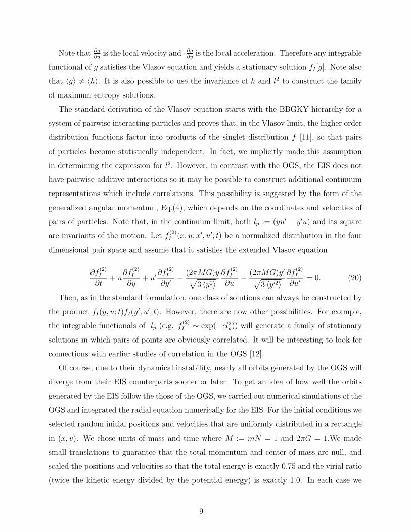
FIG. 2: Comparison of the radial coordinate R(t) computed for the OGS and EIS with the same

initial condition. Note the close agreement for this initial condition.

computed the initial values of R2 and L2 which are all that is required to solve the radial

equation, Eq.(11).

Below we present graphs comparing the theory, from the EIS, and simulations. Although

the results are not exhaustive, there seems to be a well established trend. In cases where the

simulations exhibit a very regular variation of the radius, there is a remarkable agreement

between theory (as given by the EIS) and simulation. This can be seen in Figure 2. For

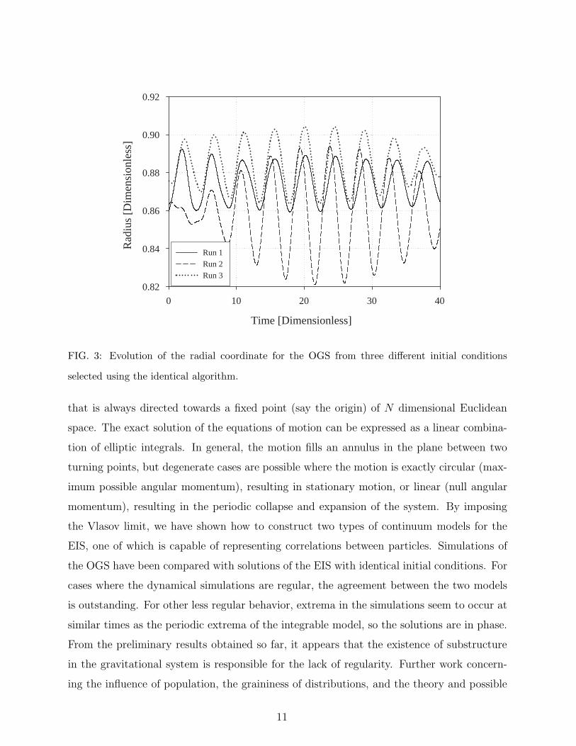
other, equally likely, initial conditions the simulated R(t) is not regular and, therefore, is

not well represented by the theory (see Figure 3). However, even in these cases, we find that

the maxima and minima of the simulations line up fairly closely with those of the theory,

i.e. they are in phase. This seems to be a general trend whether we are modelling the initial

behavior or letting the system anneal for a while before comparisons are made.

Starting from the N particle one-dimensional self-gravitating system (OGS), we have

shown how to construct an exactly integrable Hamiltonian system of arbitrary dimension

(EIS) in which the motion is always confined to a plane in the configuration space. The

system consists of a single point which experiences an acceleration of constant magnitude

10

Time [Dimensionless]

0 10 20 30 40

Rad

ius

[Dim

ensi

onle

ss]

0.82

0.84

0.86

0.88

0.90

0.92

Run 1Run 2Run 3

FIG. 3: Evolution of the radial coordinate for the OGS from three different initial conditions

selected using the identical algorithm.

that is always directed towards a fixed point (say the origin) of N dimensional Euclidean

space. The exact solution of the equations of motion can be expressed as a linear combina-

tion of elliptic integrals. In general, the motion fills an annulus in the plane between two

turning points, but degenerate cases are possible where the motion is exactly circular (max-

imum possible angular momentum), resulting in stationary motion, or linear (null angular

momentum), resulting in the periodic collapse and expansion of the system. By imposing

the Vlasov limit, we have shown how to construct two types of continuum models for the

EIS, one of which is capable of representing correlations between particles. Simulations of

the OGS have been compared with solutions of the EIS with identical initial conditions. For

cases where the dynamical simulations are regular, the agreement between the two models

is outstanding. For other less regular behavior, extrema in the simulations seem to occur at

similar times as the periodic extrema of the integrable model, so the solutions are in phase.

From the preliminary results obtained so far, it appears that the existence of substructure

in the gravitational system is responsible for the lack of regularity. Further work concern-

ing the influence of population, the graininess of distributions, and the theory and possible

11

applications of the continuum representations of the EIS is ongoing. In addition we are

investigating the extension of the theory to higher dimensional systems.

Acknowledgments

The authors benefitted from conversations with John Hopkins, George Gilbert, Tony

Burgess, and Igor Prokhorenkov, as well as the support of the Research Foundation and

Department of Information Services of Texas Christian University.

[1] B. N. Miller, Transport Theory and Statistical Physics, (2005), in Press.

[2] T. P. Weissert, The Genesis of Simulation in Dynamics (Springer-Verlag, New York, 1997).

[3] A. Noullez, D. Fanelli, and E. Aurell, cond-mat/0101336v1 (2001).

[4] L. Cohen and M. Lecar, Bull. Astr. 3, 213 (1968).

[5] D. Lynden-Bell, Mon. Not. R. Astron. Soc. 136, 101 (1967).

[6] K. Yawn and B. Miller, Phys. Rev. Letters 79, 3561 (1997).

[7] K. R. Yawn and B. N. Miller, Physical Review E 68, 056120 (2003).

[8] T. Frankel, The Geometry of Physics (Cambridge University Press, Cambridge, UK, 1997).

[9] S. Cuperman, A. Harman, and M. Lecar, Astrophys. Sp. Sci. 13, 397 (1971).

[10] H. E. Lehtihet and B. N. Miller, Physica D 21, 93 (1986).

[11] W. Braun and K. Hepp, Commun. Math. Phys. 56, 101 (1977).

[12] Monaghan, Aust. J. Phys. 31, 95 (1978).

12