AN INTRODUCTION TO SELF-GRAVITATING MATTER
338
AN INTRODUCTION TO SELF-GRAVITATING MATTER Philippe LeFloch Universit´ e Pierre et Marie Curie – Paris 6 Laboratoire Jacques-Louis Lions Centre National de la Recherche Scientifique [email protected] General topic § Einstein equations for self-gravitating matter G αβ “ 8π T αβ § Cauchy developments from prescribed initial data sets on a spacelike hypersurface § Global dynamics of the matter content § Global geometry of the spacetimes SERIES of LECTURES given at the Institut Henri Poincar´ e in the Fall 2015 Three-Month Program on MATHEMATICAL GENERAL RELATIVITY Celebration of the 100th Anniversary of the publication of Einstein’s papers VIDEOS available at /www.youtube.com/user/PoincareInstitute http://philippelefloch.org
-
Upload
khangminh22 -
Category
Documents
-
view
0 -
download
0
Transcript of AN INTRODUCTION TO SELF-GRAVITATING MATTER

AN INTRODUCTIONTO SELF-GRAVITATING MATTER
Philippe LeFlochUniversite Pierre et Marie Curie – Paris 6
Laboratoire Jacques-Louis LionsCentre National de la Recherche Scientifique
General topic§ Einstein equations for self-gravitating matter Gαβ “ 8πTαβ
§ Cauchy developments from prescribed initial data sets on a spacelikehypersurface
§ Global dynamics of the matter content
§ Global geometry of the spacetimes
SERIES of LECTURES given at the Institut Henri Poincare in the Fall 2015Three-Month Program on MATHEMATICAL GENERAL RELATIVITYCelebration of the 100th Anniversary of the publication of Einstein’s papersVIDEOS available at /www.youtube.com/user/PoincareInstitute
http://philippelefloch.org

MAIN OBJECTIVES
Introduction to Matter Models
Three main results
Weakly Regular Vacuum Spacetimes with T2 Symmetryimpulsive gravitational waves
Weakly Regular Matter Spacetimes with Spherical Symmetryshock waves in self-gravitating compressible fluids
Stability of Minkowski Space for Self-Gravitating MassiveFields
Einstein-Klein-Gordon equation, theory of modified gravity
Remarks.
§ techniques of analysis
§ matter models or/and weak solutions
§ scope of the lectures
§ selected results with full proofs§ overview of more advanced statements
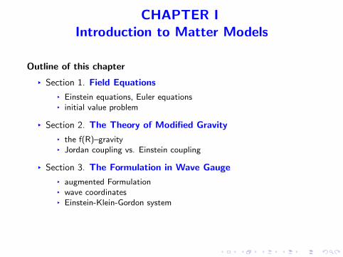
CHAPTER IIntroduction to Matter Models
Outline of this chapter
§ Section 1. Field Equations
§ Einstein equations, Euler equations§ initial value problem
§ Section 2. The Theory of Modified Gravity
§ the f(R)–gravity§ Jordan coupling vs. Einstein coupling
§ Section 3. The Formulation in Wave Gauge
§ augmented Formulation§ wave coordinates§ Einstein-Klein-Gordon system

Section 1. FIELD EQUATIONS
EINSTEIN EQUATIONS
Lorentzian metric g on a four-dimensional manifold M§ Inner product with signature p´,`,`,`q
§ A vector X P TpM at p P M is said to be time-like, null, orspace-like iff gpX ,X q is negative, zero, or positive.
§ Time-orientation: future or past timelike vectors(observers, worldlines)
Differential gemetry§ Local coordinates pxαq with Greek indices α, β, . . . “ 0, 1, 2, 3§ BBxα defines a basis of the tangent space TM
§ Vector fields X “ Xα BBxα and metric g “ gαβdx
αdxβ
(summation over repeated indices)
Riemann curvature tensor Rαβγδ§ Riemannian geometry (see below)§ Ricci curvature Rαγ :“ gβδRαβγδ§ scalar curvature R “ gαγRαγ
Minkowski spacetime M “ R4 and g “ ´pdx0q
2` pdx1
q2` pdx2
q2` pdx3
q2
§ Vanishing curvature

VACUUM EINSTEIN EQUATIONS
Rαβ “ 0 (vacuum spacetime)
§ Vanishing scalar curvature
Decomposition of the Riemann curvature:
Rαβγδ “R
12
`
gαγgβδ´gαδgβγ¯
`1
2
´
gαγSβδ´gαδSβγ`gβδSαγ´gβγSαδ¯
`Wαβγδ
§ Sαβ :“ Rαβ ´14Rgαβ (traceless part)
§ Only the Weyl curvature is non-vanishing. (gravitation radiation)
FIELD EQUATIONS
Gαβ “ 8πTαβ
§ Einstein’s gravitation tensor Gαβ “ Rαβ ´R2 gαβ
§ Tαβ stress-energy tensor / matter content of the spacetime
§ 8π: gravitational constant after normalization

EULER EQUATIONS
Levi-Civita connection ∇ associated with the metric g§ Preserves the metric ∇g “ 0
§ Torsion-free ∇XY ´∇YX “ rX ,Y s (Lie bracket)
Riemann curvature tensor
RpX ,Y qZ “ ∇X∇YZ ´∇Y∇XZ ´∇rX ,Y sZ
(second contracted) Bianchi identities
∇βRαβ “1
2∇αR
EULER EQUATIONS∇βTαβ “ 0
Proof.
∇βTαβ “1
8π∇βGαβ “
1
8π∇β
´
Rαβ ´R
2gαβ
¯
“1
8π
´
∇βRαβ ´1
2∇βR gαβ
¯
“ 0

CAUCHY DEVELOPMENTS
Initial data set.
§ Riemannian 3-manifold pM, gq
§ Symmetric 2-covariant tensor field k(second fundamental form, embedding)
§ Notation§ g ij , k ij (with i , j “ 1, 2, 3)§ ∇: connection associated with g R: scalar curvature of g§ Trace Trk “ k
jj “ g ijk ij norm |k|2 “ k ijk
ij“ g ii 1g jj1k i 1j1k ij
§ Einstein’s constraint equations
R ``
Trk˘2´ |k |2 “ 16πT00 pHamiltonian G00 “ 8πT00q
∇jkj
i ´∇i pTrkq “ 8πT0j pMomentumT0j “ 8πT0jq
(Gauss-Codazzi equations, nonlinear elliptic equations)
§ Matter fields (components T00, T0j)(scalar field, perfect fluid, modified gravity, etc.)

INITIAL VALUE PROBLEM. Future development of the initial dataset
§ Lorentzian manifold satisfying the Einstein equations pM, gq
§ Embedding ψ : M Ñ H Ă M
§ Induced metric ψ‹g “ g
§ Second fundamental form k (extrinsic curvature) ψ‹k “ k
In coordinates gαβBψα
Bx iBψβ
Bx j“ g ij
§ Matter fields (scalar field, perfect fluid, modified gravity, etc.)
FORMULATION AS PARTIAL DIFFERENTIAL EQUATIONS.
§ Einstein equation as a hyperbolic-elliptic system of PDE’s
§ choice of coordinates / diffeomorphism invariance
§ wave gauge
§ coordinate functions such thatlgx
α :“ ∇α∇αxα“ 0
§ system of coupled nonlinear wave equations for the metriclggαβ “ Qαβpg , Bgq

SELF-GRAVITATING MASSIVE FIELDS
Massive scalar field with potential V pφq (minimally coupled)
Tαβ :“ ∇αφ∇βφ´´1
2∇γφ∇γφ` V pφq
¯
gαβ
Write the Euler equations ∇αTαβ “ 0 for φ
Einstein-Klein-Gordon system
lgφ´ V 1pφq “ 0
Rαβ ´ 8π`
∇αφ∇βφ` V pφq gαβ˘
“ 0
for instance with the quadratic potential V pφq “ c2
2 φ2 with mass c ą 0
The theory of modified gravity. (next section)
OUR OBJECTIVE: Long-time behavior of perturbations of Minkowskispacetime by a self-gravitating massive field
§ system of coupled wave-Klein-Gordon equations§ global nonlinear stability problem§ future geodesically complete spacetime§ Hyperboloidal Foliation Method

SPACETIMES WITH SYMMETRY
Symmetry assumptions
§ spherical symmetry (SO(3) isometry group action)
§ T2 symmetry (T2 isometry group action)
§ Gowdy/plane symmetry (vanishing twists/polarization)
§ 1+1 nonlinear wave systems arbitrary large data
rich global dynamics
Long-time issues
§ maximal hyperbolic Cauchy developments
§ property of the future boundary
§ late-time asymptotics, geodesic completeness
§ formation of trapped surfaces, (critical) collapse of matter,censorship conjectures (generic data)
Remarks. Bianchi models (even further symmetry assumptions and vacuum)
§ techniques of dynamical systems, bifurcation theory
§ still many open problems
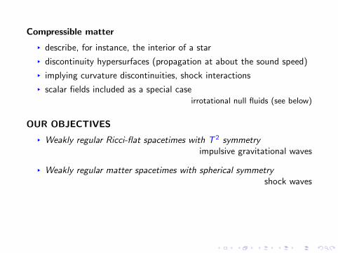
Compressible matter
§ describe, for instance, the interior of a star
§ discontinuity hypersurfaces (propagation at about the sound speed)
§ implying curvature discontinuities, shock interactions
§ scalar fields included as a special caseirrotational null fluids (see below)
OUR OBJECTIVES
§ Weakly regular Ricci-flat spacetimes with T 2 symmetryimpulsive gravitational waves
§ Weakly regular matter spacetimes with spherical symmetryshock waves
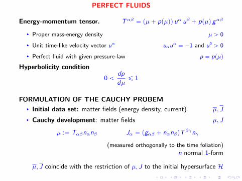
PERFECT FLUIDS
Energy-momentum tensor. Tαβ “ pµ` ppµqq uα uβ ` ppµq gαβ
§ Proper mass-energy density µ ą 0
§ Unit time-like velocity vector uα uαuα“ ´1 and u0
ą 0
§ Perfect fluid with given pressure-law p “ ppµq
Hyperbolicity condition
0 ădp
dµď 1
FORMULATION OF THE CAUCHY PROBEM
§ Initial data set: matter fields (energy density, current) µ, J
§ Cauchy development: matter fields µ, J
µ :“ Tαβnαnβ Jα “ pgαβ ` nαnβqTβγnγ
(measured orthogonally to the time foliation)
n normal 1-form
µ, J coincide with the restriction of µ, J to the initial hypersurface H
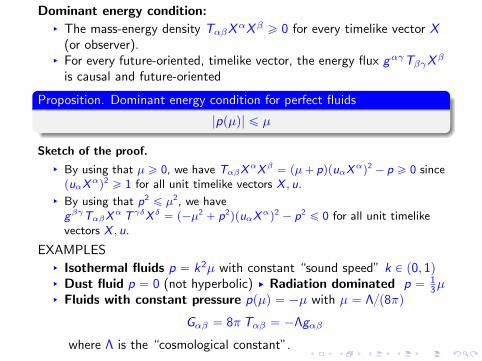
Dominant energy condition:§ The mass-energy density TαβX
αXβ ě 0 for every timelike vector X(or observer).
§ For every future-oriented, timelike vector, the energy flux gαγTβγXβ
is causal and future-oriented
Proposition. Dominant energy condition for perfect fluids
|ppµq| ď µ
Sketch of the proof.
§ By using that µ ě 0, we have TαβXαXβ
“ pµ` pqpuαXαq
2´ p ě 0 since
puαXαq
2ě 1 for all unit timelike vectors X , u.
§ By using that p2ď µ2, we have
gβγTαβXα T γδX δ
“ p´µ2` p2
qpuαXαq
2´ p2
ď 0 for all unit timelikevectors X , u.
EXAMPLES§ Isothermal fluids p “ k2µ with constant “sound speed” k P p0, 1q§ Dust fluid p “ 0 (not hyperbolic) § Radiation dominated p “ 1
3µ§ Fluids with constant pressure ppµq “ ´µ with µ “ Λp8πq
Gαβ “ 8πTαβ “ ´Λgαβ
where Λ is the “cosmological constant”.
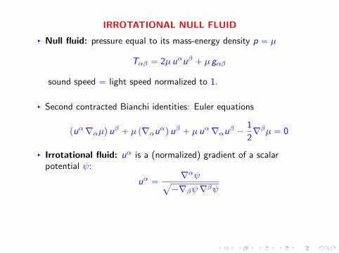
IRROTATIONAL NULL FLUID
§ Null fluid: pressure equal to its mass-energy density p “ µ
Tαβ “ 2µ uαuβ ` µ gαβ
sound speed “ light speed normalized to 1.
§ Second contracted Bianchi identities: Euler equations
puα∇αµq uβ ` µ p∇αu
αq uβ ` µ uα∇αuβ ´
1
2∇βµ “ 0
§ Irrotational fluid: uα is a (normalized) gradient of a scalarpotential ψ:
uα “∇αψ
a
´∇βψ∇βψ
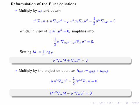
Reformulation of the Euler equations
§ Multiply by uβ and obtain
uα∇αµ` µ∇αuα ` µ uαuβ∇αu
β ´1
2uα∇αµ “ 0
which, in view of uβ∇αuβ “ 0, simplifies into
1
2uα∇αµ` µ∇αu
α “ 0.
Setting M :“ 12 logµ
uα∇αM `∇αuα “ 0
§ Multiply by the projection operator Hαβ :“ gαβ ` uαuβ :
µ uα∇αuβ ´
1
2Hαβ∇αµ “ 0
Hαβ∇αM ´ uα∇αuβ “ 0

Reduced equations for irrotational null fluids
Impose that uα “ ∇αψ?´∇βψ∇βψ
for some potential ψ.
After some elementary computations:
∇α
˜
µ12 ∇αψa
´∇βψ∇βψ
¸
“ 0
∇β
´
M ´ loga
´∇αψ∇αψ¯
“ Ω∇βψ
where the scalar factor Ω reads Ω “ ∇αψ∇αM∇αψ∇αψ ´
∇αψ∇βψ∇αβψp∇αψ∇αψq2
§ The gradient of M ´ log?´∇αψ∇αψ is parallel to ∇ψ,
§ so that M ´ log?´∇αψ∇αψ is simply a function F pψq for some F .
§ Replace the chosen potential ψ by some function Gpψq (ifnecessary), so that
M ´ loga
´∇αψ∇αψ “ 0.
µ “ ´∇αψ∇αψ

Proposition. Einstein-Euler system for irrotational null fluids
The fluid potential satisfies the wave equation on the curved spacelgψ “ 0
coupled to the Einstein equations for the metricRαβ ´ 8π∇αφ∇βφ “ 0
Recover the fluid unknowns
§ Velocity vector field uα “ ∇αψ?´∇βψ∇βψ
§ Mass -energy density function µ “ ´∇αψ∇αψ
§ Relativistic analogue of Bernoulli’s law:
§ irrotational flows in classical fluid dynamics§ determines µ explicitly, once we know the velocity

OUTLINE OF THIS COURSE
Introduction to Matter Models
Einstein equations, matter models, modified gravity
Weakly Regular Ricci-Flat Spacetimes with T2 Symmetry§ weak solutions with singular curvature / impulsive gravitational waves
§ weakly regular geodesics, late-time asymptotics
§ future geodesic completeness (Gowdy case, polarized T2)
Weakly Regular Matter Spacetimes with Spherical Symmetry§ spacetimes with bounded variation / shock waves in self-gravitating
compressible fluids
§ Riemann problem, random choice method
§ global geometry of weakly regular matter spacetimes
Stability of Minkowski Space for Self-Gravitating Massive Fields§ Einstein-massive scalar field system & theory of modified gravity
§ wave gauge: system of coupled wave-Klein-Gordon equations
§ hyperboloidal foliation method
§ future geodesic completeness

SELECTED REFERENCE
Textbooks
§ Y. Choquet-Bruhat, Oxford University Press, 2009
§ G. Galloway, http://www.math.miami.edu/rgalloway/paris.pdf, 2015
§ B. O’Neill, Academic Press, 1983
§ R.M. Wald, University of Chicago Press, 1984
Long-time dynamics (Bianchi spacetimes)
§ F. Beguin, Aperiodic oscillatory asymptotic behavior for some Bianchispacetimes, Classical Quantum Gravity, 2010.
§ T. Damour, Cosmological singularities, Einstein billiards and LorentzianKac-Moody algebras, J. Hyper. Differ. Equ. (2005)
§ A.D. Rendall, Oxford University Press, 2008
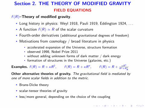
Section 2. THE THEORY OF MODIFIED GRAVITY
FIELD EQUATIONS
f pRq–Theory of modified gravity.
§ Long history in physics: Weyl 1918, Pauli 1919, Eddington 1924, . . .
§ A function f pRq » R of the scalar curvature
§ Fourth-order derivatives (additional gravitational degrees of freedom)
§ Motivations from cosmology / broad literature in physics
§ accelerated expansion of the Universe, structure formation§ observed 1998, Nobel Prize 2011§ without adding unknown forms of dark matter / dark energy§ formation of structures in the Universe (galaxies, etc.)
Examples. f pRq “ R ` κR2, f pRq “ R ` κRn, f pRq “ R ` κRn
Rn`Rn˚
Other alternative theories of gravity. The gravitational field is mediated byone of more scalar fields in addition to the metric.
§ Brans-Dicke theory
§ scalar-tensor theories of gravity
§ less/more general, depending on the choice of the coupling
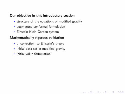
Our objective in this introductory section
§ structure of the equations of modified gravity
§ augmented conformal formulation
§ Einstein-Klein-Gordon system
Mathematically rigorous validation
§ a ‘correction’ to Einstein’s theory
§ initial data set in modified gravity
§ initial value formulation

EINSTEIN’S THEORY p3` 1q–dimensional spacetime pM, gq
Lorentzian signature p´,`,`,`q
Hilbert-Einstein’s action
AHErφ, g s :“
ż
M
´
Rg ` 16πLrφ, g s¯
dVg
§ massless scalar field (minimally coupled) Lrφ, g s “ ´ 12∇γφ∇γφ
§ stress-energy tensor Tαβrφ, g s “ ∇αφ∇βφ´12
`
∇γφ∇γφ˘
gαβ
Principle of least action.
Critical metrics δAHErφ, g s ” 0
Einstein equationsGαβ :“ Rαβ ´
12Rg gαβ “ 8πTαβrφ, g s
Example. In the vacuum case Tαβ ” 0, we obtain the Ricci-flat condition
Rαβ “ 0.

f pRq-MODIFIED GRAVITY THEORY
AMGrφ, g s :“ş
M
´
f pRg q ` 16πLrφ, g s¯
dVg
§ Prescribed function f : RÑ R§ f pRq “ R ` κ
´
R2
2`OpκR3
q
¯
§ sign of κ :“ f 2p0q ą 0 essential for global stability
§ Critical points δAMGrφ, g s ” 0
Curvature tensor of modified gravity
Nαβ :“f 1pRg qRαβ ´1
2f pRg qgαβ `
´
gαβ lg ´∇α∇β
¯
`
f 1pRg q˘
“f 1pRg qGαβ ´1
2
´
f pRg q ´ Rg f1pRg q
¯
gαβ `´
gαβ lg ´∇α∇β
¯
`
f 1pRg q˘
Proposition. Field equations of modified gravity
Nαβ “ 8πTαβrφ, g s
§ Fourth-order derivatives of the unknown metric
§ When f is linear, Nαβ reduces to Gαβ .

Derivation of the field equations.
§ Variation with respect to gαβ with dVg “?´gdx and g “ detpgαβq
§ Variation of the action
δA “ş
M
˜
δδgαβ
´
?´gf pRq
¯
` 16π δδgαβ
´
?´gLrφ, g s
¯
¸
δgαβdx
§ Field equations
1?´g
δ
δgαβ
´?´gf pRq
¯
“ ´16π1
?´g
δ
δgαβ
´?´gLrφ, g s
¯
“: 8πTαβ
Observe
1?´g
δ
δgαβ
´?´gf pRq
¯
“ f pRqδ
δgαβ
´
lnp?´g q
¯
` f 1pRqδR
δgαβ
and it thus suffices to check that
δR
δgαβ“ Rαβ ´ 2
δ
δgαβ
´
lnp?´g q
¯
“ gαβ

Variation of the volume form.
δg “ δ detpgαβq “ g gαβδgαβ
δ?´g “ ´
1
2?´g
δg “1
2
?´ggαβδgαβ “ ´
1
2
?´ggαβδg
αβ
by differentating gαγgγβ “ Kroneckerβα
1?´g
δ?´g
δgαβ“ ´
1
2gαβ
´2δ
δgαβ
´
lnp?´g q
¯
“ gαβ

Variation of the scalar curvature.
Rρσαβ “ BαΓρβσ ´ BβΓρασ ` ΓραλΓλβσ ´ ΓραλΓλβσ
δRρσαβ “ BαδΓρβσ´BβδΓρασ` δΓραλΓλβσ`ΓραλδΓλβσ´ δΓραλΓλβσ´ΓραλδΓλβσCovariant derivative of the Christoffel symbols:
∇λ
`
δΓρβα˘
“ Bλ`
δΓρβα˘
` ΓρσλδΓσβα ´ ΓρσλδΓσβα,
henceδRρσαβ “ ∇αδΓρβσ ´∇βδΓρασ
and, after contraction of two indices,
δRαβ “ ∇αδΓρβρ ´∇βδΓραρ
For the scalar curvature R “ gαβRαβ
δR “ gαβδRαβ ` δgαβRαβ “ ∇α
´
gαβδΓρβρ ´ gαβδΓρβρ
¯
` Rαβδgαβ
The divergence term does not contribute the variation the action.
δR
δgαβ“ Rαβ

MATTER CONTENT AND EVOLUTION
Lemma
The contracted Bianchi identities ∇αRαβ “12∇βR or ∇αGαβ “ 0 imply
the divergence equation∇αNαβ “ 0.
Proof. We compute the three relevant terms
∇αpf 1pRqRαβq “ Rαβ∇αpf 1pRqq ` f 1pRq∇αRαβ
“ Rαβ∇αpf 1pRqq `1
2f 1pRq∇βR
1
2∇α
´
f pRq gαβ
¯
“1
2∇βpf pRqq “
1
2f 1pRq∇βR
∇α´
∇α∇βf1pRq ´ gαβlg f
1pRq¯
“
´
∇α∇α∇β ´∇β∇λ∇λ
¯
f 1pRq
“
´
∇α∇β∇α ´∇β∇α∇α¯
f 1pRq
“ Rαβ∇αpf 1pRqq

Matter model.§ Coupling between the gravity field and the matter fields
§ From a physical standpoint, need to choose the frame in whichmeasurements are made: ongoing debate
§ “Jordan frame”: original metric gαβ considered as physically relevant
§ “Einstein frame”: conformally-transformed metric
g:αβ :“ f 1pRg qgαβ
§ Lead to different systems of PDE’s
Massless scalar field.§ Jordan’s coupling (minimal in the Jordan metric)
Tαβ :“ ∇αφ∇βφ´1
2gαβ∇γφ∇γφ
§ Einstein’s coupling (non-minimal in the Jordan metric)
T :αβ :“ f 1pRg q
´
∇αφ∇βφ´1
2gαβ∇γφ∇γφ
¯
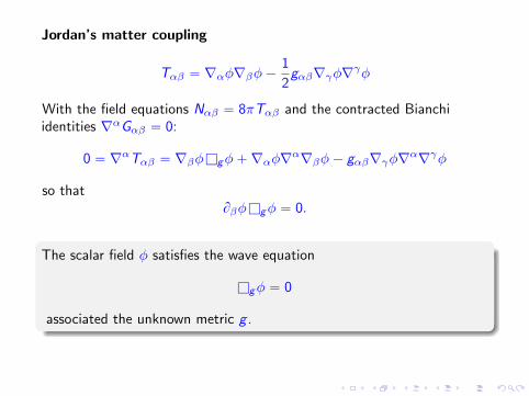
Jordan’s matter coupling
Tαβ “ ∇αφ∇βφ´1
2gαβ∇γφ∇γφ
With the field equations Nαβ “ 8πTαβ and the contracted Bianchiidentities ∇αGαβ “ 0:
0 “ ∇αTαβ “ ∇βφlgφ`∇αφ∇α∇βφ´ gαβ∇γφ∇α∇γφ
so thatBβφlgφ “ 0.
The scalar field φ satisfies the wave equation
lgφ “ 0
associated the unknown metric g .
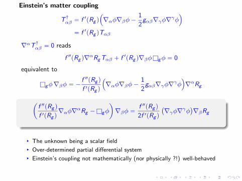
Einstein’s matter coupling
T :αβ “ f 1pRg q
´
∇αφ∇βφ´1
2gαβ∇γφ∇γφ
¯
“ f 1pRg qTαβ
∇αT :αβ “ 0 reads
f 2pRg q∇αRgTαβ ` f 1pRg q∇βφlgφ “ 0
equivalent to
lgφ∇βφ “ ´f 2pRg q
f 1pRg q
´
∇αφ∇βφ´1
2gαβ∇γφ∇γφ
¯
∇αRg
ˆ
f 2pRg q
f 1pRg q∇αφ∇αRg ´lgφ
˙
∇βφ “f 2pRg q
2f 1pRg q
`
∇γφ∇γφ˘
∇βRg
§ The unknown being a scalar field
§ Over-determined partial differential system
§ Einstein’s coupling not mathematically (nor physically ?!) well-behaved

MATHEMATICAL VALIDITY OF THE MODIFIED GRAVITY
CAUCHY DEVELOPMENTS.
Field equations of modified gravity Nαβ “ 8πTαβ
§ based on f pRq » R, assumed to satisfy f 1pRq ą 0 and f 2pRq ą 0.
§ matter described by a massless scalar field with Jordan coupling
Initial data set.
§ Geometry of the initial hypersurface pM, g , kq
§ Matter content: initial data φ0, φ1 for the scalar field and its timederivative
§ Fourth-order field equations: need two additional data R0,R1 relatedto the spacetime curvature on M

An initial data set pM, g , k ,R0,R1, φ0, φ1q consists of:
§ a Riemannian 3-manifold pM, gq and a symmetric p0, 2q-tensor k
§ two scalar fieds φ0, φ1 on M (matter field, its time derivative)
§ two scalar fields R0,R1 on M (spacetime curvature, its timederivative)
Hamiltonian constraint of modified gravity“
N00 “ 8πT00
‰
f 1pR0q
´
R ´ k ijkij` pk
j
jq2¯
` 2 kj
j f2pR0qR1 ´
´
2∆g f1pR0q ´ f pR0q ` R0f
1pR0q
¯
“ 8π´
pφ1q2 `∇jφ0∇
jφ0
¯
Momentum constraint of modified gravity“
N0j “ 8πT0j
‰
f 1pR0q
´
∇jki
i ´∇iki
j
¯
´ Bj`
f 2pR0qR1
˘
´ ki
jBi`
f 1pR0q˘
“ 8πφ1 ∇iφ0

Definition
A modified gravity Cauchy development: Lorentzian manifold pM, gqand matter field φ defined on M
§ Field equations of modified gravity Nαβ “ 8πTαβ§ An embedding i : M Ñ M such that:
§ pull-back metric g “ i‹g and second fundamental form k§ R0 coincides with the restriction of the spacetime curvature R on M§ R1 coincides with the Lie derivative LnR, n being the normal to M§ φ0, φ1 coincide with the restriction of φ,Lnφ on M.
Theorem. Cauchy developments in the theory of modified gravity
§ Given an (asymptotically flat, say) initial data setpM » R3, g , k ,R0,R1, φ0, φ1q, there exists a unique maximal globallyhyperbolic development pM, gq.
§ If an initial data set pM, g , k ,R0,R1, φ0, φ1q for modified gravity is“close” (in Sobolev norms) to another initial data set
pM, g 1, k1, φ10, φ
11q of Einstein’s theory, then its development is also
close to the corresponding Einstein development.

Highly singular limit problem.
§ Einstein’s vacuum corresponds to vanishing φ0 “ φ1 “ R0 “ R1 ” 0.
§ In the limit f pRq Ñ R, we recover Einstein equations.
§ convergence of a fourth-order system (with no well-defined type) toa system of second-order (hyperbolic-elliptic) PDE’s
§ recover R Ñ 8π∇αφ∇αφ
Elementary notions of causality
§ Time-like curve: γ : r0, 1s Ñ M whose tangent vector 9γptq is time-like:9γptq, 9γptqq ă 0
§ Causal curve (observer or light), whose tangent vector 9γptq is time-like ornull 9γptq, 9γptqq ď 0
§ Global hyperbolicity.
Existence of a Cauchy surface H Ă M, that is,
§ H is spacelike (Riemannian induced metric)§ every inextendible causal curve intersects H exactly once
§ Maximal globally hyperbolic development
Any other such development isometric to a subset of it

SELECTED REFERENCES
Maximal developments
§ Y. Choquet-Bruhat, Oxford University Press, 2009
§ G. Galloway, http://www.math.miami.edu/rgalloway/paris.pdf, 2015
Modified gravity
§ E. Babichev and D. Langlois, Relativistic stars in f(R) gravity, Phys. Rev.2009.
§ S. Capozziello et al., Phys. Lett. B 639 (2006)
§ P.G. LeFloch and Y. Ma, Mathematical validity of the f(R) theory ofmodified gravity, ArXiv:1412.8151
§ G. Magnano and L.M. Sokolowski, Phys. Rev. D 50 (1994)

Section 3. THE FORMULATION IN WAVE GAUGE
Field equations of modified gravity Nαβ “ 8πTαβ
§ Fourth-order system (with no specific PDE type)while Einstein equations Gαβ “ 8πTαβ are second-order
§ Conformal transformation leading to a third-order system
§ Wave coordinates lgxα “ 0 associated with the spacetime metric g
while Einstein equations are
hyperbolic with differential constraints
§ Augmented formulation
§ spacetime scalar curvature taken as an independent variable§ leading to a second-order system of nonlinear wave-Klein-Gordon
equations
§ “Equivalence” with the Einstein-massive field system

THE CONFORMAL FORMULATION
Gravitational curvature tensor of modified gravity
Nαβ “ f 1pRg qRαβ `´
gαβ lg ´∇α∇β
¯
f 1pRg q ´1
2f pRg qgαβ “ 8πTαβ
Hessian of the scalar curvature ∇α∇βf1pRg q (fourth-order term)
CONFORMAL METRIC
g :αβ :“ e2ρ gαβ , ρ :“1
2ln f 1pRg q
Conformal transformation for the Ricci curvature
Rαβ “ R:αβ ``
2∇α∇βρ` gαβ lgρ˘
` 2`
´∇αρ∇βρ` gαβ ∇γρ∇γρ˘
Notation. Change of variable R ÞÑ ρ “: 12
ln f 1pRq, assumed to be one-to-one.We also define (function f , its Legendre transform)
§ w1pρq :“ f pRq
§ w2pρq :“ f pRq´R f 1pRqf 1pRq
§ wpρq :“ f pRq´R f 1pRq
pf 1pRqq2

Observing that
Nαβ “ f 1pRg qRαβ ´1
2f pRg qgαβ `
`
gαβlg ´∇α∇β
˘
f 1pRg q
TrpNq “ f 1pRg qRg ´ 2f pRg q ` 3 lg f1pRg q
∇α∇βe2ρ“ 2e2ρ∇α∇βρ` 4e2ρ∇αρ∇βρ
lge2ρ“ 2e2ρ
lgρ` 4e2ρ∇γρ∇γρwe can express the gravity tensor in terms of ρ
Nαβ “ e2ρRαβ ´w1pρq
2gαβ ` 2e2ρ
`
gαβlg ´∇α∇β
˘
ρ` 4e2ρ´
gαβ∇γρ∇γρ´∇αρ∇βρ¯
With the conformal identity for the Ricci curvature, we deduce that
Nαβ “ e2ρ´
R:αβ ´w1pρq
2e2ρgαβ ` 3 gαβlgρ´ 6∇αρ∇βρ` 6 gαβ∇γρ∇γρ
¯
Finally, with the following expression of the trace`
gα1β1Nα1β1
˘
“ 6e2ρlgρ´ w1pρq ` 12e2ρ∇γρ∇γρ´ e2ρw2pρq
we arrive at e2ρ´
R:αβ ´ 6∇αρ∇βρ`w2pρq
2gαβ
¯
“ Nαβ ´12gαβ
`
gα1β1Nα1β1
˘
Field equations of modified gravity in the Einstein frame
R:αβ ´ 6∇:αρ∇:
βρ`wpρq
2 g :αβ “ 8π e´2ρ`
Tαβ ´12g:αβ
`
g :α1β1
Tα1β1˘˘

EULER EQUATIONS. Conformal transformation for Christoffel symbols
Γ:γαβ “ Γγαβ ` gγα ∇βρ` gγβ ∇αρ´ gαβ∇γρ
∇:αNαβ “ e´2ρgαγ∇:γNαβ “ e´2ρgαγ´
BγNαβ ´ Γ:δ
γαNβδ ´ Γ:δ
γβNαδ
¯
“ e´2ρgγα´´
BγNαβ ´ ΓδγαNβδ ´ ΓδγβNαδ
¯
´
´
gδγ∇αρ` gδα∇γρ´ gγα∇δρ¯
Nβδ ´´
gδγ∇βρ` gδβ∇γρ´ gγβ∇δρ¯
Nαδ
¯
Thus we have
∇:αNαβ “ e´2ρ´
∇αNαβ ´`
∇δρ`∇δρ´ 4∇δρ˘
Nβδ
´`
∇βρ`
gα1β1Nα1β1
˘
`∇αρNαβ ´∇αρNαβ˘
¯
in which we already have proven that ∇αNαβ “ 0.
Evolution of the matter field in the Einstein frame
∇:αNαβ “ 2g :γδNδβ∇:γρ´
`
g :α1β1
Nα1β1˘
∇:βρ
Together with Nαβ “ 8πTαβ , we obtain
∇:αTαβ “ 2g :γδTδβ∇:γρ´
`
g :α1β1
Tα1β1˘
∇:βρ

RICCI CURVATURE IN GENERAL COORDINATESIntroduce the Christoffel coefficients
Γ:λ
:“ g :αβ
Γ:λαβ and Γ:λ :“ g :λβΓ:
β
Motivation. Reduced wave operator rlg:u :“ g:αβBαBβu, therefore
lg:u “ g:α1β1
Bα1Bβ1u ` Γ:δBδu “ rlg:u ` Γ:
δBδu
Calculation. To express the Ricci curvature, we proceed as follows. Recalling
R:αβ “ BλΓ:λ
αβ ´ BαΓ:λ
βλ ` Γ:λ
αβΓ:δ
λδ ´ Γ:λ
αδΓ:δ
βλ
Γ:λ
αβ “1
2g:λλ1`
Bαg:βλ1 ` Bβg
:αλ1 ´ Bλ1g
:αβ
˘
we obtain
BλΓ:λ
αβ ´ BαΓ:λ
βλ
“1
2Bλ
´
g:λδpBαg
:βδ ` Bβg
:αδ ´ Bδg
:αβq
¯
´1
2Bα
´
g:λδpBβg
:λδ ` Bλg
:βδ ´ Bδg
:βλq
¯
“ ´1
2Bλ
´
g:λδBδg
:αβ
¯
`1
2Bλ
´
g:λδpBαg
:βδ ` Bβg
:αδq
¯
´1
2Bα
´
g:λδBβg
:λδ
¯
.
Therefore, we have
BλΓ:λ
αβ ´ BαΓ:λ
βλ “´1
2g:λδBλBδg
:αβ
`1
2g:λδBαBλg
:δβ `
1
2g:λδBβBλg
:δα ´
1
2g:λδBαBβg
:λδ ` l.o.t.

On the other hand, we compute the term BαΓ:β ` BβΓ:α as follows:
Γ:γ“ Γ:
γ
αβg:αβ “
1
2g :αβ
g :γδ`Bαg
:βδ ` Bβg
:αδ ´ Bδg
:αβ
˘
“ g :γδg :αβBαg
:βδ ´
1
2g :αβ
g :γδBδg
:αβ
and Γ:λ “ g :λγΓ:γ“ g :
αβBαg
:βλ ´
12g:αβBλg
:αβ . So, we have
BαΓ:β “ Bα`
g :λδBδg
:λβ
˘
´1
2Bα
`
g :λδBβg
:λδ
˘
and, therefore,
BαΓ:β ` BβΓ:α “ g :γδBαBλg
:δβ ` g :
λδBβBλg
:δα ´ g :
λδBαβg
:λδ ` l.o.t.
Ricci curvature in general coordinates
R:αβ “ ´1
2g :α1β1
Bα1Bβ1g:αβ `
1
2
`
BαΓ:β ` BβΓ:α˘
`1
2Fαβpg
:; Bg :q,
where Fαβpg:; Bg :q are quadratic in Bg :.
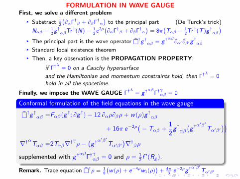
FORMULATION IN WAVE GAUGEFirst, we solve a different problem
§ Substract 12
`
BαΓ:β ` BβΓ:α˘
to the principal part (De Turck’s trick)
Nαβ ´12g:αβTr :pNq ´ 1
2e2ρ
`
BαΓ:β ` BβΓ:α˘
“ 8π`
Tαβ ´12Tr :pT qg:αβ
˘
§ The principal part is the wave operator rl:g:αβ “ g:
αβBα1Bβ1g
:αβ
§ Standard local existence theorem
§ Then, a key observation is the PROPAGATION PROPERTY:
if Γ:λ“ 0 on a Cauchy hypersurface
and the Hamiltonian and momentum constraints hold, then Γ:λ“ 0
hold in all the spacetime.
Finally, we impose the WAVE GAUGE Γ:λ“ g:
αβΓ:γαβ “ 0
Conformal formulation of the field equations in the wave gauge
rl:g :αβ “Fαβpg:; Bg :q ´ 12 BαρBβρ` wpρqg :αβ
` 16π e´2ρ`
´ Tαβ `1
2g :αβ
`
g :α1β1
Tα1β1˘˘
∇:αTαβ “2Tγβ∇:γρ´
`
g :α1β1
Tα1β1˘
∇:βρ
supplemented with g :αβ
Γ:γαβ “ 0 and ρ “ 1
2 f1pRg q.
Remark. Trace equation rl:ρ “ 1
6
`
wpρq ` e´4ρw1pρq˘
` 4π3e´2ρg:
α1β1
Tα1β1

THE AUGMENTED CONFORMAL FORMULATION
Still third-order and not of a specific PDE type !
THE AUGMENTED FORMULATION
§ relation e2ρ “ f 1pRg q no longer imposed
§ ρ replaced by a new independent variable %
§ algebraic constraint e2ρ “ f 1pRg q replaced by the trace equation
§ new notation for the metric g ;αβ “ e2%gαβ
Main unknowns: the function % and the metric g ;αβ
Introduce the tensor field N; defined by the relation
N;αβ ´1
2g ;αβTr;pN;q :“ e2%
´
R;αβ ´ 6e2%Bα%Bβ%`1
2g ;αβwp%q
¯

Definition and Proposition. Conformal augmented formulation of modifiedgravity (second-order system in g ;, ρ)
N;αβ “ 8πTαβ
lg;% “1
6
`
wp%q ` e´4%w1p%q˘
`4π
3e2%
´
g ;δγTδγ
¯
which, put together, imply the evolution equation for the matter field
∇;αTαβ “ 2Tγβ∇;γ%´´
g ;δγTδγ
¯
∇;β%
(proof given below)
PROPAGATION PROPERTY
§ By considering the equation satisfied by lg;`
%´ f 1pRg q˘
, one cancheck that:
If e2%“ f 1pRg q with g:αβ “ e2%gαβ is satisfied on a Cauchy
hypersurface and the wave gauge together with the Hamiltonian andmomentum constraints hold, then the condition e2%
“ f 1pRg q issatisfied everywhere in the spacetime.
Hence, we have truly extended the system of modified gravity.

Proof. We need to check that
∇;αN;αβ “ e´2%`
2gαα1
Bα1%N;αβ ´ TrpN;qBβ%
˘
From our definition of the “extended” gravity tensor, we have
N;αβ “ e2%G ;αβ ´ 6e2%`
Bα%Bβ%´1
2g ;αβ |∇;%|2g;
˘
´1
2g ;αβw2p%q,
where G ;αβ :“ R;αβ ´12g;αβR
; is the Einstein curvature of g ;.
We observe that ∇;αG ;αβ “ 0, as well as the obvious identities
∇;α´
Bα%Bβ%´1
2g ;αβ |∇;%|2g;
¯
“ Bβ%lg;%
∇;αβ`
g ;αβw2p%q˘
“ Bβ`
w2p%q˘
“ ´2e´2%w1p%qBβ%

This allows us to compute the divergence
∇;αN;αβ “ 2e2%G%αβ∇;α%´ 12e2%
`
Bα%Bβ%´1
2g ;αβ |∇;%|2g;
˘
∇;α%
´ 6e2%Bβ%lg;%` e2%Bβw1p%q
“ 2N;αβ∇;α%´ Bβ%
´
6e2%lg;%´w1p%q
e2%´ w2p%q
¯
,
in which we use
lg;% “1
6
`
wp%q ` e´4%w1p%q˘
`4π
3e2%
´
g ;δγTδγ
¯
We thus have derived the desired evolution equation for the matter field
∇;αTαβ “ 2Tγβ∇;γ%´´
g ;δγTδγ
¯
∇;β%
l

Formulation for general matter models
g ;α1β1
Bα1Bβ1g;αβ “Fαβpg
;; Bg ;q ´ 12Bα%Bβ%` wp%qg ;αβ
´ 16π`
Tαβ ´1
2g :αβg
;α1β1
Tα1β1˘
g ;α1β1
Bα1Bβ1% “1
6
`
wp%q ` w1p%qe´4%
˘
`4π
3e´2%g ;
α1β1
Tα1β1
∇;αTαβ “2 Bγ% g;δγTγβ ´ Bβ% g
;α1β1
Tα1β1
in which Fαβpg;; Bg :q are quadratic in Bg ;.
(Jordan coupling and wave coordinates associated with the Einsteinmetric)
Remark. ∇;α`
ρ´2Tαβ¯
“ Tr ;pT qBβ`
%´1˘
‰ 0.
A stress-energy tensor which is conserved in the Jordan frameis not conserved in the Einstein frame (and vice versa).
Except if the matter Tαβ is trace-free (conformally invariant)

Finally, we assume that the matter is a (massless) scalar field.
§ rlg; :“ g ;α1β1
Bα1Bβ1
§ Fαβpg;; Bg ;q quadratic in Bg ;
§ V “ V p%q and W “W p%q of quadratic order as %Ñ 0
The augmented conformal formulation of modified gravity in wave gauge
rlg;g;αβ “ Fαβpg
;; Bg ;q ´ 12 Bα%Bβ%´ 16π BαφBβφ` V p%qg ;αβ
rlg;φ “ ´2 g ;αβBαφBβ%
rlg;%´%
3κ“ ´
4π
3e2%g ;αβBαφBβφ`W p%q
“massive scalaron”
additional gravitational degree of freedom
§ supplemented with constraints (propagating from a Cauchy hypersurface)
§ g;αβ
Γ:λαβ “ 0
§ e2%“ f 1pRe´2%g;q
§ Hamiltonian and momentum constraints of modified gravity

CONCLUSIONS for this chapter
Nonlinear wave-Klein-Gordon system
§ Einstein-massive scalar field system
§ The theory of modified gravity (additional constraints)
§ Brans-Dicke theory, scalar-tensor theories
Nonlinear stability of Minkowski spacetime
§ The Klein-Gordon potential drastically modifies the global dynamics.
§ Must exclude dynamically unstable, self-gravitating massive modes.(trapped surfaces, black hole)
§ Initial data set
§ a small perturbation of an asymptotically flat, spacelike hypersurfacein Minkowski space
§ massive scalar field with sufficiently small mass
§ This perturbation disperses in timelike directions, and the spacetimeis timelike geodesically complete.
§ Main challenge: time decay, the Hyperboloidal Foliation Method
SELECTED REFERENCES
Modified gravity
§ P.G. LeFloch and Y. Ma, Mathematical validity of the f(R) theory ofmodified gravity, ArXiv:1412.8151
Global nonlinear stability of Minkowski spacetime
§ Vacuum or massless scalar fields
§ D. Christodoulou & S. Klainerman (1993)
§ H. Lindblad & I. Rodnianski (2010)
§ Massive scalar fields
§ P. LeFloch & Y. Ma (2015)
Numerical work
§ H. Okawa, V. Cardoso, and P. Pani, Collapse of self-interacting fieldsin asymptotically flat spacetimes: do self-interactions renderMinkowski spacetime unstable?, Phys. Rev., 2014.

CHAPTER II. Weakly RegularRici-flat Spacetimes with T2 Symmetry.
The weak formulation
RICCI FLAT LORENTZIAN MANIFOLDS WITH T 2–SYMMETRY
Initial data
§ Invariant under a T 2-group action
§ Defined on a manifold diffeomorphic to the 3-torus T 3
§ Suitable setup for studying the propagation of gravitational waves
Cauchy developments
§ Define a suitable class of weakly regular Ricci-flat spacetimes
§ Local geometry of Cauchy developments
§ Global causal structure (geodesics, late-time asymptotics)
OUTLINESection 1. Geometric formulation
Section 1.1 Weakly regular manifolds
Section 1.2 Weak version of Einstein’s constraints
Section 1.3 Weak version of Einstein’s evolution equations
Section 2. Formulation in admissible coordinates

BACKGROUND MATERIAL
STANDARD FORMULATION for regular data
Initial data set
§ a Riemannian 3-manifold pΣ, hq, a symmetric 2-tensor field K
§ Einstein’s constraints (∇p3q and Rp3q determined by h)
Hamiltonian Rp3q´|K |2`pTrKq2 “ 0 Momentum ∇p3qj K ji ´∇
p3qi K j
j “ 0
Globally hyperbolic Cauchy developments
§ A p3` 1q-Lorentzian manifold pM, gq
§ Ricci-flat condition Rµν “ 0
§ An embedding φ : Σ ÑM such that φpΣq is a Cauchy surface in pM, gq.
(intersected exactly once by any inextendible timelike curve)
§ The pull-back of the first and second fundamental forms of Σ Ă Mcoincides with h,K .
Gauss equation for a hypersurface Σpn´1qĂ Mpnq (Riemannian manifold) with
(not nec. unit) normal N and second fundamental form χ
Rpn´1q“ Rpnq ´ 2gpN,Nq´1Rpnqij N iN j
´ |χ|2 ``
Trχ˘2

SOBOLEV SPACES ON MANIFOLDSM: connected, oriented, differentiable m-manifold
‚ Standard notation.
§ tangent space TxM at x P M, co-tangent space T˚x M
§ local moving frame pejq, j “ 1, . . . ,m
§ local coordinates x “ px jq, j “ 1, . . . ,m with ej “BBx j
‚ Regularity of a vector field X “ pX jq expressed in terms of itscomponents (checked in any local coordinate chart)
§ Lebesgue spaces LplocpMq
§ Sobolev spaces HklocpMq and W k,p
loc pMq
‚ Tensor fields (see below). HklocT
qp pMq, etc.
Remarks.‚ Change of coordinates are taken to be C8
‚ Notion of local convergence, but there need not exist a canonical norm in thesespaces.
‚ Space of SCALAR DISTRIBUTIONS
F P D1pMq: dual of the space DΛmpMq of all compactly supported, C8
m-form fields
§ Continuity property@
F , ωpkqD
Ñ@
F , ωp8qD
if ωpkq ´ ωp8qC ppMq Ñ 0 for any p and all
ωpkq, ωp8q smooth and (uniformly) compactly supported
§ Example: canonical embedding f P L1locpMq ÞÑ F P D1pMq, via
ă F , ω ąD1,D:“
ż
M
f ω, ω P DΛmpMq
‚ LIE DERIVATIVE.
§ Functions LX f “ X pf q. Vector fields LXY “ rX ,Y s
§ 1-form fields pLXαqpY q :“ X pαpY qq ´ αprX ,Y sq
§ 2-covariant tensor fields (e.g. for a metric)
pLXhqpT ,Z q :“ X phpT ,Z qq ´ hpLXT ,Z q ´ hpT ,LXZ q

‚ DISTRIBUTIONAL DERIVATIVE XF of a scalar distributionF P D1pMq by a smooth vector field X
ă XF , ω ąD1,D:“ ´ ă F ,LXω ąD1,D, ω P DΛmpMq
§ Motivated from Cartan identity: for a smooth function f and a smooth,compactly supported m-form on Mm
f LXω “ f dpiXωq “ dpf iXωq ´ df ^ iXω
and with Stokes formulaż
M
pXf qω “ ´
ż
M
f LXω
§ In local coordinates px iq (i “ 1, . . . ,m) one has
ż
X jBj f ωdx
1^ . . .^ dxm
“ ´
ż
f BjpXjωq dx1
^ . . .^ dxm
‚ Space of DISTRIBUTION DENSITIESD1ΛmpMq: dual of the space DpMq of compactly supported functions.
§ ă Ω, f ąD1,D for f P DpMq§ Example: canonical embedding ω P L1
locpMq ÞÑ ω P D1ΛmpMq, via
ă ω, f ąD1,D:“
ż
M
f ω, f P DpMq
Notation: TpqpMq :“ C8T p
q pMq
‚ Space of TENSOR DISTRIBUTIONS D1T pq pMq: C8pMq-multi-linear
maps
A : T10pMq ˆ . . .ˆ T1
0pMqloooooooooooomoooooooooooon
q times
ˆT01pMq ˆ . . .ˆ T0
1pMqloooooooooooomoooooooooooon
p times
Ñ D1pMq
§ ApaX ` bY , cω ` kθq “ acApX , ωq ` bcApY , ωq ` akApX , θq ` bkApY , θq
§ Example: canonical embedding A P L1locT
pq pMq ÞÑ A P D1T p
q pMq:
ă ApXp1q, . . . ,Xpqq, θp1q, . . . , θppqq, ω ąD1,D:“
ż
M
ApXp1q, . . . ,Xpqq, θp1q, . . . , θppqqω

Section 1. GEOMETRIC FORMULATION
Section 1.1 WEAKLY REGULAR MANIFOLDS
‚ Lie derivative in the weak sense. LXh is defined for a measurable andlocally integrable 2-tensor h on a smooth manifold, for any C 1 vectorfields X ,Y ,Z , by
pLXhqpY ,Z q :“ X phpY ,Z qq ´ hpLXY ,Z q ´ hpY ,LXZ q
‚ T 2 Symmetry on a smooth (connected, orientable) 3-manifold Σendowed with a metric h P L1
locpΣq
§ Torus group action: smooth, linearly independent commuting vector
fields X ,Y with closed orbits defining an action with no fixed point
§ Killing property: LXh “ LY h “ 0 in the weak sense

Definition. Weakly regular T 2–symmetric Riemannian manifold pΣ, hq
§ L8 Riemannian structure. Σ » T 3 (compact, C8 3-manifold)endowed with a Riemannian metric h P L8pΣq
§ T 2 Symmetry. Two Killing fields X ,Y as aboveLXh “ LY h “ 0 in the weak sense
§ H1 and Lipschitz regularity on the T 2-symmetry orbits.
hXX “ hpX ,X q, hXY “ hpX ,Y q, hYY “ hpY ,Y q P H1pΣq
§ Lipschitz regularity on the area of T 2–orbits.
`
R˘2
:“ hXX hYY ´`
hXY˘2PW 1,8pΣq
§ W 1,1 Regularity on the orthogonal of the orbits.
§ Consider a smooth frame of commuting vector fieldspX ,Y ,Θq (therefore LXΘ “ LY Θ “ 0)
§ An adapted frame pX ,Y ,Zq where Z is the (non-smooth!) field
Z :“ Θ` ra X ` rb Y P
X ,Y(K
§ hZZ PW 1,1pΣq

Remarks. ‚ Fully geometric definition, independent of the choice of theKilling fields within the generators of the T 2-symmetry.
‚ Regularity
§ Since h is Riemannian and R ą 0 is continuous on a compact set,one has minΣ R ą 0.
§ From the T 2–symmetry and hZZ PW1,1pΣq, we will deduce that
hZZ is continuous and infΣ hZZ ą 0.
§ The inverse metric components hXX , hXY and hYY are also H1.
§ No regularity on the derivatives of the coefficients hXθ, hY θ P L8pΣq
‚ Isomorphisms transforming vectors into co-vectors (and vice-versa)
§ Multiplicative operators with L8 coefficients.
§ In the frame pe1, e2, e3q “ pX ,Y ,Z q
Vj “ hijVi (with i , j “ 1, 2, 3)
with coefficients in L8 (or more regular).
Polarized spaces. Special class having hXY “ 0.

Definition. Weakly regular T 2–symmetric triple pΣ, h,K q
A weakly regular T 2–symmetric Riemannian manifold pΣ, hq with adaptedframe pX ,Y ,Z q, endowed with a symmetric 2-tensor field K such that:
§ (Square) integrability conditions.
§ KUV P L2pΣq for all pU,V q ‰ pZ ,Zq P
X ,Y ,Z(2
§ KZZ P L1pΣq
§ L8 Trace on the symmetry orbits.
Trp2qpK q :“habKab “ hXX KXX ` 2hXY KXY ` hYY KYY P L8pΣq
§ T 2 Symmetry. K is invariant under the action of the T 2 groupgenerated by pX ,Y q: LXK “ LYK “ 0
Remark. For the Einstein equations, the sup- norm bound will be a bound onthe time derivative of the area R (defined later within the spacetime):
§ Trp2qpKq is essentially BtR
§ Therefore, Trp2qpKq P L8pΣq is natural in view of R PW 1,8pΣq.
Definition
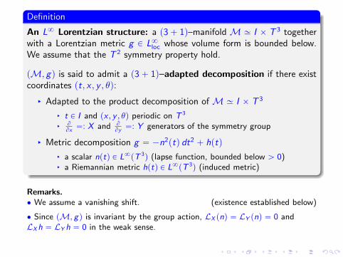
An L8 Lorentzian structure: a p3` 1q–manifold M » I ˆ T 3 togetherwith a Lorentzian metric g P L8loc whose volume form is bounded below.We assume that the T 2 symmetry property hold.
pM, gq is said to admit a p3` 1q–adapted decomposition if there existcoordinates pt, x , y , θq:
§ Adapted to the product decomposition of M » I ˆ T 3
§ t P I and px , y , θq periodic on T 3
§ B
Bx“: X and B
By“: Y generators of the symmetry group
§ Metric decomposition g “ ´n2ptq dt2 ` hptq
§ a scalar nptq P L8pT 3q (lapse function, bounded below ą 0)
§ a Riemannian metric hptq P L8pT 3q (induced metric)
Remarks.‚ We assume a vanishing shift. (existence established below)
‚ Since pM, gq is invariant by the group action, LX pnq “ LY pnq “ 0 andLXh “ LY h “ 0 in the weak sense.

Notation from now on: pM » T 3, gq is an L8 Lorentzian structure
§ enjoys the T 2 symmetry, admits an adapted p3` 1q–decomposition
§ adapted frame pT ,X ,Y ,Θq associated with a global chart pt, x , y , θq
§ we write Σt » ttu ˆ T 3 for the level sets of the function t
Definition. Weakly regular T 2–symmetric Lorentzian manifold
§ Timelike regularity.LTh P L
1pΣtq for almost every t and L8loc in time(uniform bounds within any compact subset of I )
§ Spacelike regularity. For almost every t (and L8loc in time)
§ Consider the second fundamental form of the slicesKptq :“ ´ 1
2nptqpLThqptq P L1
pΣtq
§ pΣt , hptq,Kptqq is a weakly regular T 2–symmetric triple
(the group action being the one induced on Σt)
§ Conformal regularity. Introduce Z :“ Θ` ra X ` rb Y P
T ,X ,Y(K
ρ2 :“hZZn2
“ ´gZZgTT
PW 2,1pΣtq LTρ PW1,1pΣtq

Application to the Einstein equations. (see below)
§ Dependence upon the foliation.
§ We will construct first a specific foliation along which the regularityand integrability conditions hold
§ and, next, deduce the same regularity for more general foliations.
§ The conformal quotient metric ´dt2` ρ2dθ2 determines the relevant
wave operator.
§ Additional regularity in time (in suitable topologies in space)
Observations. § n PW 1,1pΣtq since hZZ has this regularity.
§ From the decomposition Z “ θ ` ra X ` rb Y and the commutationproperties, we immediately obtain:
LTZ “ T praqX ` T prbqY with T praq,T prbq P L1pΣtq
§ Expression of the second fundamental form. Using that T ,X ,Y ,Zcommute while Z is orthogonal to X ,Y ,T , we obtain
(with ea, ea P
X ,Y(
and hab “ hpea, ebq)
Kab “ ´1
2nT phabq P L2
pΣtq
KaZ “1
2nhpea,LZT q P L2
pΣtq
KZZ “ ´1
2nT`
hZZ˘
P L1pΣtq
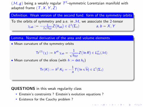
pM, gq being a weakly regular T 2–symmetric Lorentzian manifold withadapted frame pT ,X ,Y ,Z q
Definition. Weak version of the second fund. form of the symmetry orbits
To the orbits of symmetry and a.e. in M, we associate the 2-tensorχab :“ ´ 1
2?hZZ
Z`
hab˘
P L2pΣtq a, b “ X ,Y
Lemma. Normal derivative of the area and volume elements
‚ Mean curvature of the symmetry orbits
Trp2qpχq :“ hab χab “1
?hZZ
Z`
lnR˘
P L8locpMq
‚ Mean curvature of the slices (with h :“ det hij)
TrpKq :“ hij Kij “ ´1
nT`
ln?h˘
P L1pΣtq
QUESTIONS in this weak regularity class
§ Einstein’s constraints ? Einstein’s evolution equations ?
§ Existence for the Cauchy problem ?
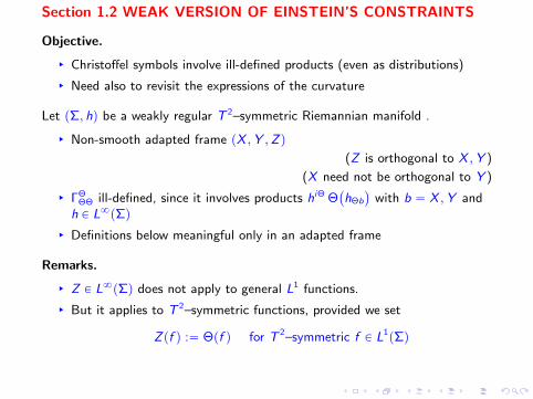
Section 1.2 WEAK VERSION OF EINSTEIN’S CONSTRAINTS
Objective.
§ Christoffel symbols involve ill-defined products (even as distributions)
§ Need also to revisit the expressions of the curvature
Let pΣ, hq be a weakly regular T 2–symmetric Riemannian manifold .
§ Non-smooth adapted frame pX ,Y ,Zq
(Z is orthogonal to X ,Y )
(X need not be orthogonal to Y )
§ ΓΘΘΘ ill-defined, since it involves products hiΘ Θ
`
hΘb
˘
with b “ X ,Y andh P L8pΣq
§ Definitions below meaningful only in an adapted frame
Remarks.
§ Z P L8pΣq does not apply to general L1 functions.
§ But it applies to T 2–symmetric functions, provided we set
Zpf q :“ Θpf q for T 2–symmetric f P L1pΣq

Preliminary computation. We first consider regular data:
§ X ,Y , θ commute
§ orthogonality condition Z P
X ,Y(K
§ T 2-symmetry properties
For i “ X ,Y ,Z and a, b “ X ,Y
Γiab “
1
2hij phaj,b ` hjb,a ´ hab,jq “ ´
1
2hiZZ phabq
ΓZaZ “
1
2hZj phaj,Z ` hjZ ,a ´ haZ ,jq “ 0
ΓbaZ “
1
2hbj phaj,Z ` hjZ ,a ´ haZ ,jq “
1
2
´
hbX Z phaX q ` hbY Z phaY q¯
ΓaZZ “
1
2haj p2hjZ ,Z ´ hZZ ,jq “ 0
ΓZZZ “
1
2hZj p2hZj,Z ´ hZZ ,jq “
1
2hZZ Z phZZ q “ log
?hZZ

Definition-Proposition. Weak version of the Christoffel symbols
Γcab :“ 0 a, b P
X ,Y(
ΓbaZ :“
1
2
´
hbX Z phaX q ` hbY Z phaY q¯
ΓZab :“ ´
1
2hZZ Z phabq
ΓZaZ “ Γa
ZZ :“ 0
ΓZZZ :“
1
2hZZ Z phZZ q
These expressions do make sense (in the frame pX ,Y ,Z q)
§ Γijk P L
2pΣq for all pi , j , kq ‰ pZ ,Z ,Z q
§ ΓZZZ P L
1pΣq
§ trace ΓaaZ P L
8pΣq
Furthermore, if pΣ, hq is regular, these functions coincide with the standardChristoffel symbols.
Observation. Mean curvature of the T 2-orbits
L8pΣq Q Zp`
R˘2q “ ZphXX q hYY ` hXX ZphYY q ´ 2 hXYZphXY q
“1
R2
´
hXX ZphXX q ` hYY ZphYY q ` 2hXYZphXY q¯
“2
R2 Γa
aZ

WEAK VERSION OF THE HAMILTONIAN CONSTRAINT
Let now pΣ, h,K q be a weakly regular T 2–symmetric triple.
§ ΓZZZ P L1
pΣq cannot be multiplied by Christoffel coefficients in L2pΣq or
L1pΣq.
§ We will rely on the trace property ΓaaZ P L8pΣq.
Strategy.
§ First, we define the Ricci component Rp3qZZ “ RichpZ ,Zq of the manifoldpΣ, hq.
§ Then, we rely on the Gauss equation for the T 2–orbits in order to definethe scalar curvature Rp3q of the manifold pΣ, hq.
§ Next, we suitably decompose the second fundamental form K of the slices.
§ Finally, we arrive at a weak version of the Hamiltonian constraint.

Preliminary computation. Compute Rp3qZZ “ Ω1 ` Ω2 with
Ω1 :“ ΓiZZ ,i ´ Γi
iZ ,Z Ω2 :“ ΓjijΓ
iZZ ´ Γj
iZΓijZ
§ Since ΓaZZ ,a “ 0:
Ω1 “ ΓaZZ ,a ` ΓZ
ZZ ,Z ´ ΓZZZ ,Z ´ Γa
aZ ,Z “ ´ZpΓaaZ q
§ Since ΓZaZ “ Γa
ZZ “ 0:
Ω2 “ ΓZZZΓZ
ZZ ` ΓaaZΓZ
ZZ ` ΓZaZΓa
ZZ ` ΓaabΓb
ZZ
´ ΓZZZΓZ
ZZ ´ ΓZbZΓb
ZZ ´ ΓaZZΓZ
aZ ´ ΓabZΓb
aZ
“ ΓaaZΓZ
ZZ ´ ΓabZΓb
aZ
after cancelling out the ill-defined terms ˘ΓZZZΓZ
ZZ P L1pΣtqL
1pΣtq
Definition–Proposition. Weak version of the Ricci component in the direc-tion pZ ,Z q
Rp3qZZ :“´ Z pΓa
aZ q ` ΓaaZΓZ
ZZ ´ ΓabZ Γb
aZ
W´1,8pΣq ` L8pΣqL1pΣq ´ L2pΣqL2pΣq
where the first term is defined only in the weak sense.Furthermore, when sufficient regularity is assumed, our definition for Rp3qZZ agrees
with the standard definition.

From the Gauss equation and since the T 2 orbits are flat:
0 “ Rp3q ´ |χ|2 ``
Trp2qχ˘2´
2
hZZRp3qZZ for regular metrics
(Z is not a unit vector field)
This formula does not make sense:
§ Rp3qZZ defined in the weak sense only
§ Need to “remove’ the factor hZZ PW1,1pΣq
Definition. Weak version of the weighted scalar curvature
Rpwqp3q :“2Rp3qZZ ` hZZ
`
|χ|2 ´ pTrp2qχq2˘
PW´1,8loc pΣq ` L1pΣq
in the weak sense, in which:
§ χ is the second fundamental form of the T 2–orbits.
§ Rp3qZZ is the weak version of the Ricci component pZ ,Z q.

Our final observation is the following algebraic decomposition of the tensor Kfor regular metrics:
`
TrK˘2´ |K |2 “
`
Trp2qK˘2` 2
´
Trp2qK¯
KZZ ´ KabK
ab´ 2KaZK
aZ
Definition-Proposition. Weak version of the Hamiltonian constraint
Rpwqp3q ` hZZ
´
`
Trp2qK˘2` 2
`
Trp2qK˘
KZZ ´ KabK
ab ´ 2KaZKaZ¯
“ 0
W´1,8pΣq ` L8pΣqL8pΣq ` L8pΣqL1pΣq ` L2pΣqL2pΣq
understood in the weak sense.Furthermore, if pΣ, h,Kq is sufficiently regular, then pΣ, h,Kq satisfies the weak
version of the Hamiltonian constraint equation iff it satisfies this equation in the
classical sense.
Recall here thatRpwqp3q :“2Rp3qZZ ` hZZ
`
|χ|2 ´ pTrp2qχq2˘
Rp3qZZ :“´ ZpΓaaZ q ` Γa
aZΓZZZ ´ Γa
bZ ΓbaZ
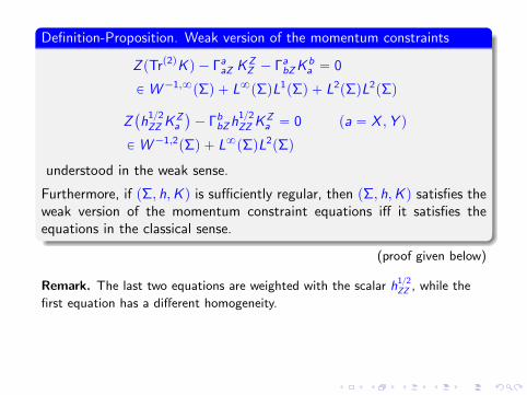
Definition-Proposition. Weak version of the momentum constraints
Z pTrp2qK q ´ ΓaaZ KZ
Z ´ ΓabZK
ba “ 0
PW´1,8pΣq ` L8pΣqL1pΣq ` L2pΣqL2pΣq
Z`
h12ZZ K
Za
˘
´ ΓbbZh
12ZZ K
Za “ 0 pa “ X ,Y q
PW´1,2pΣq ` L8pΣqL2pΣq
understood in the weak sense.
Furthermore, if pΣ, h,K q is sufficiently regular, then pΣ, h,K q satisfies theweak version of the momentum constraint equations iff it satisfies theequations in the classical sense.
(proof given below)
Remark. The last two equations are weighted with the scalar h12ZZ , while the
first equation has a different homogeneity.

COMPATIBILITY WITH THE STANDARD DEFINITION.
Assume sufficient regularity.
Derivation of the momentum constraint in the Z -direction.
∇p3qj K jZ “Z pKZ
Z q ` K aZ ,a ´ Γi
jZKji ` Γj
ijKiZ
“Z pKZZ q ´ ΓZ
ZZKZZ ´ Γa
ZZKZa ´ ΓZ
aZKaZ ´ Γa
bZKba
` ΓZZZK
ZZ ` ΓZ
aZKaZ ` Γb
bZKZZ ` Γb
baKaZ
“Z pKZZ q ´ Γa
bZKba ` Γb
bZKZZ
§ We used ΓZaZ “ Γa
ZZ “ 0
§ and cancelled out ill-defined terms ˘ΓZZZK
ZZ P L
1pΣqL1pΣq.
§ Recall that Trp2qK “ TrK ´ KZZ .
We conclude that ∇p3qj K jZ ´∇p3qZ TrK “ 0 is equivalent to our
formulation above.

Derivation of momentum constraints in the symmetry orbits.
∇p3qj K ja “ K j
a,j ´ ΓiajK
ji ` Γj
ijKia
“ Z pKZa q ´ ΓZ
aZKZZ ´
ÿ
pi,jq‰pZ ,Zq
ΓiajK
ji ` ΓZ
ZZKZa `
ÿ
pi,jq‰pZ ,Zq
ΓjijK
ia
“ Z pKZa q ` ΓZ
ZZKZa `
ÿ
pi,jq‰pZ ,Zq
´
ΓjijK
ia ´ Γi
ajKji
¯
while ∇p3qa K jj “ 0.
The product involving ΓZZZ P L
1pΣq and KZa P L
2pΣq is ill-defined forweakly regular spacetimes. We thus proceed as follows:
§ (Formally) multiply the above equations by h12ZZ
§ From the expression of the Christoffel symbol of the second term(using hZZ “ phZZ q
´1)
h12ZZ ∇
p3qj K j
a “ h12ZZ
´
Z pKZa q `
1
2h´1ZZZ phZZ qK
Za
¯
` h12ZZ
ÿ
pi,jq‰pZ ,Zq
´
ΓjijK
ia ´ Γi
ajKji
¯
§ Combine the first two terms in the right-hand side as Z`
h12ZZ KZ
a
˘
.

Section 1.3 WEAK VERSION OF EINSTEIN’S EVOLUTIONEQUATIONS
Let pM, gq be a weakly regular T 2–symmetric Lorentzian manifold with
adapted frame pT ,X ,Y ,Zq, spacelike slices Σt (t P I ), and second
fundamental form K .
Sketch of the preliminary computation when the spacetime is regular:
§ Since the frame pT ,X ,Y ,Zq “ pe0, e1, e2, e3q is not (fully) induced bycoordinates:
Γαβγ “1
2gαδ
´
gβδ,γ ` gγδ,β ´ gβγ,δ ` cδβγ ` cδγβ ` cβγδ¯
cβγδ :“ reβ , eγsδ “ gδρ reβ , eγsρ
§ re0, e1s “ re0, e2s “ re1, e2s “ 0
§ Moreover, rT ,Z s “ T praqX ` T prbqY , which, in particular, is orthogonalto both Z and T .
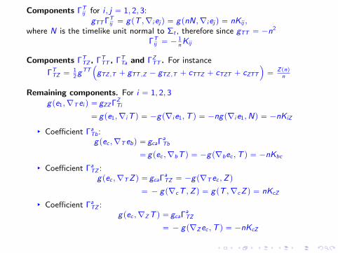
Components ΓTij for i , j “ 1, 2, 3:
gTTΓTij “ gpT ,∇iejq “ gpnN,∇iejq “ nKij ,
where N is the timelike unit normal to Σt , therefore since gTT “ ´n2
ΓTij “ ´
1nKij
Components ΓTTZ , ΓT
TT , ΓTTa and ΓZ
TT . For instance
ΓTTZ “
12gTT
´
gTZ ,T ` gTT ,Z ´ gTZ ,T ` cTTZ ` cTZT ` cZTT¯
“Zpnqn
Remaining components. For i “ 1, 2, 3gpe1,∇T ei q “ gZZΓZ
Ti
“ gpe1,∇iT q “ ´gp∇ie1,T q “ ´ngp∇ie1,Nq “ ´nKiZ
§ Coefficient ΓaTb:gpec ,∇T ebq “ gcaΓa
Tb
“ gpec ,∇bT q “ ´gp∇bec ,T q “ ´nKbc
§ Coefficient ΓaTZ :gpec ,∇TZq “ gcaΓa
TZ “ ´gp∇T ec ,Zq
“ ´ gp∇cT ,Zq “ gpT ,∇cZq “ nKcZ
§ Coefficient ΓaTZ :
gpec ,∇ZT q “ gcaΓaTZ
“ ´ gp∇Zec ,T q “ ´nKcZ
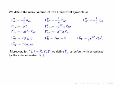
We define the weak version of the Christoffel symbols as
ΓTab :“ ´
1
nKab ΓT
ZZ :“ ´1
nKZZ ΓT
aZ :“ ´1
nKaZ
ΓaTZ :“ nK a
Z ΓZTZ :“ ´gZZ n KZZ
ΓZTa :“ ´ngZZ KaZ Γa
Tb :“ ´g ac n Kbc
ΓTTZ :“ Z plog nq ΓT
Ta “ ΓaTT :“ 0 ΓZ
TT :“1
2gZZ Z pn2q
ΓTTT :“ T plog nq
Moreover, for i , j , k “ X ,Y ,Z , we define Γijk as before, with h replaced
by the induced metric hptq.
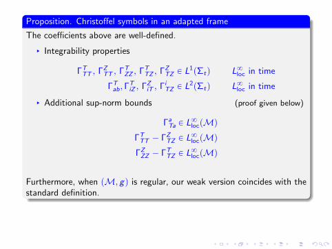
Proposition. Christoffel symbols in an adapted frame
The coefficients above are well-defined.
§ Integrability properties
ΓTTT , ΓZ
TT , ΓTZZ , ΓT
TZ , ΓZTZ P L
1pΣtq L8loc in time
ΓTab, Γ
TiZ , ΓZ
iT , ΓiTZ P L
2pΣtq L8loc in time
§ Additional sup-norm bounds (proof given below)
ΓaTa P L
8locpMq
ΓTTT ´ ΓZ
TZ P L8locpMq
ΓZZZ ´ ΓT
TZ P L8locpMq
Furthermore, when pM, gq is regular, our weak version coincides with thestandard definition.

PROOF of the additional PROPERTIES.
§ Trace regularity.
ΓaTa “ ´nTr p2qpK q P L8locpMq
§ Conformal regularity.
We rely on the (space and time) Lipschitz regularityof the conformal metric ρ2
“ n´2 gZZ PW 1,8pMq
ΓTTT ´ ΓZ
TZ “1
2n2
´
T pn2q ´ T pgZZ qn2gZZ
¯
“1
2n2gZZT pρ
´2q P L8locpMq
ΓZZZ ´ ΓT
TZ “1
2gZZZ pgZZ q ´
1
nZ pn2q
“n2
2gZZZ
´gZZn2
¯
“n2
2gZZZ pρ2q P L8locpMq

EINSTEIN EVOLUTION EQUATIONS
§ Let pM, gq be a weakly regular T 2–symmetric Lorentzian manifold.
§ It remains to consider the components Rij .
Definition
Weak version of the component RZZ of the Ricci tensor
RZZ :“T pΓTZZ q ´ Z pΓT
TZ q ´ Z pΓaaZ q PW´1,1
loc pMq
` ΓTZZ
`
ΓTTT ´ ΓZ
TZ
˘
` ΓTTZ
`
ΓZZZ ´ ΓT
TZ
˘
P L1pΣtqL8pΣtq
` ΓaTa ΓT
ZZ ` ΓaaZ ΓZ
ZZ P L1pΣtqL8pΣtq
´ ΓabZ Γb
aZ ` 2ΓTaZΓa
TZ P L2pΣtqL2pΣtq
Weak version of the components RaZ of the Ricci tensor
RaZ :“ T pΓTaZ q `
`
ΓTTT ´ ΓZ
TZ
˘
ΓTaZ ` Γb
TbΓTaZ
PW´1,8loc pMq ` L8pΣtqL
2pΣtq ` L8pΣtqL2pΣtq

The components Rcd , c, d “ X ,Y need to be suitably weighted, as follows.
Definition. Weak version of the Ricci components Rpwqcd
Rpwqcd :“T
´
n g12ZZ ΓT
dc
¯
` Z´
n g12ZZ ΓZ
dc
¯
` n g12ZZ
ˆ
ΓaTaΓT
dc ` ΓaaZΓZ
dc ´ ΓTdZΓZ
Tc ´ ΓZTdΓT
cZ
´ ΓTdaΓa
Tc ´ ΓaTdΓT
ac ´ ΓZdaΓa
cZ ´ ΓadZΓZ
ac
˙
PW´1,2loc pMq ` L1pΣtq
Definition. Weak version of Einstein’s evolution equations
RZZ “ 0 in W´1,1loc pMq
RZd “ 0 in W´1,8loc pMq
Rpwqab “ 0 in W´1,2
loc pMq
in the weak sense above.
See the proof below

Proposition. Equivalence with the classical definition
For any regular T 2–symmetric spacetime pM, gq:
the weak version of the Einstein’s evolution equations is satisfied iff
the Ricci flat condition Ricg pei , ejq “ 0 for ei , ej P
X ,Y ,Z(
holds,where Ric denotes the Ricci tensor of g defined in the classical sense.
Theorem. Weak formulation of the Einstein equations
§ If pΣ, h,K q is a weakly regular T 2–symmetric triple, then Einstein’sconstraint equations make sense in a weak form.
§ If pM, gq is a weakly regular T 2–symmetric Lorentzian manifold,Einstein’s evolution equations make sense in a weak form.
§ All of the weak notions above coincide with the classical ones whenthe space is sufficient regular.
Terminology
§ weakly regular T 2–symmetric initial data set
§ weakly regular T 2–symmetric Ricci-flat spacetime
OUR NEXT OBJECTIVE will be to express these geometric equations inwell-chosen coordinates as a system of nonlinear PDE’s.
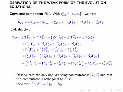
DERIVATION OF THE WEAK FORM OF THE EVOLUTIONEQUATIONS.
Curvature component RZZ . With cγαβ “ reα, eβsγ , we have
RZZ “ RαZαZ “ ΓαZZ ,α ´ ΓααZ ,Z ` ΓααβΓβZZ ´ ΓαZβΓβYZ ´ cβαZΓαZβ
and, therefore,
RZZ “Z pΓZZZ q ` T pΓT
ZZ q ´
´
Z pΓZZZ q ` Z pΓT
TZ q ` Z pΓaaZ q
¯
` ΓTTTΓT
ZZ ` ΓZZZΓZ
ZZ ` ΓTTZΓZ
ZZ ` ΓZTZΓT
ZZ
` ΓTTaΓa
ZZ ` ΓaatΓ
TZZ ` ΓZ
aZΓaZZ ` Γa
aZΓZZZ
` ΓaabΓb
ZZ ´
´
ΓTTZΓT
TZ ` ΓZZZΓZ
ZZ ` ΓTZZΓZ
TZ ` ΓZTZΓT
ZZ
¯
´
´
ΓTaZΓa
TZ ` ΓaTZΓT
aZ ` ΓZaZΓa
ZZ ` ΓaZZΓZ
aZ
¯
´ ΓabZΓb
aZ ´ cbTZΓTbZ
§ Observe that the only non-vanishing commutator is rT ,Z s and thatthis commutator is orthogonal to Z ,T .
§ Moreover, rT ,Z sb “ ΓbTZ ´ Γb
TZ

§ Take into account the cancellations of Z pΓZZZ q, ΓZ
ZZΓZZZ and ΓZ
TZΓTZZ
(ill-defined L1L1 products),
§ as well as the antisymmetry of ΓaTZ
§ and the fact that ΓTTa “ ΓZ
aZ “ 0
RZZ “T pΓTZZ q ´ Z pΓT
TZ q ´ Z pΓaaZ q `
´
ΓTTTΓT
ZZ ` ΓTTZΓZ
ZZ
¯
`
´
ΓaatΓ
TZZ ` Γa
aZΓZZZ
¯
` ΓaabΓb
ZZ
´
´
ΓTTZΓT
TZ ` ΓTZZΓZ
TZ
¯
´ ΓabZΓb
aZ ` 2ΓTaZΓa
TZ
and, after factoring out ΓZTZ and ΓZ
TT :
RZZ :“T pΓTZZ q ´ Z pΓT
TZ q ´ Z pΓaaZ q PW´1,1
loc pMq
` ΓTZZ
`
ΓTTT ´ ΓZ
TZ
˘
` ΓTTZ
`
ΓZZZ ´ ΓT
TZ
˘
P L1pΣtqL8pΣtq
` ΓaTa ΓT
ZZ ` ΓaaZ ΓZ
ZZ P L1pΣtqL8pΣtq
´ ΓabZ Γb
aZ ` 2ΓTaZΓa
TZ P L2pΣtqL2pΣtq
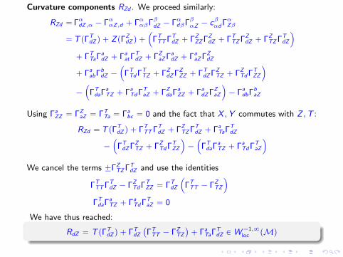
Curvature components RZd . We proceed similarly:
RZd “ ΓαdZ ,α ´ ΓααZ ,d ` ΓααβΓβdZ ´ ΓαdβΓβαZ ´ cβαdΓαZβ
“T pΓTdZ q ` ZpΓZ
dZ q `
´
ΓTTTΓT
dZ ` ΓZZZΓZ
dZ ` ΓTTZΓZ
dZ ` ΓZTZΓT
dZ
¯
` ΓTTaΓa
dZ ` ΓaatΓ
TdZ ` ΓZ
aZΓadZ ` Γa
aZΓZdZ
` ΓaabΓb
dZ ´
´
ΓTTdΓT
TZ ` ΓZdZΓZ
ZZ ` ΓTdZΓZ
TZ ` ΓZTdΓT
ZZ
¯
´
´
ΓTdaΓa
TZ ` ΓaTdΓT
aZ ` ΓZdaΓa
ZZ ` ΓadZΓZ
aZ
¯
´ ΓadbΓb
aZ
Using ΓaZZ “ ΓZ
aZ “ ΓTTa “ Γa
bc “ 0 and the fact that X ,Y commutes with Z ,T :
RZd “T pΓTdZ q ` ΓT
TTΓTdZ ` ΓZ
TZΓTdZ ` Γa
TaΓTdZ
´
´
ΓTdZΓZ
TZ ` ΓZTdΓT
ZZ
¯
´
´
ΓTdaΓa
TZ ` ΓaTdΓT
aZ
¯
We cancel the terms ˘ΓZTZΓT
dZ and use the identities
ΓTTTΓT
dZ ´ ΓZTdΓT
ZZ “ ΓTdZ
´
ΓTTT ´ ΓZ
TZ
¯
ΓTdaΓa
TZ ` ΓaTdΓT
aZ “ 0
We have thus reached:
RdZ “ T pΓTdZ q ` ΓT
dZ
`
ΓTTT ´ ΓZ
TZ
˘
` ΓaTaΓT
dZ PW´1,8loc pMq

Curvature components Rcd .
Rcd “ Γαdc,α ´ Γααc,d ` ΓααβΓβdc ´ ΓαdβΓβαc ´ cβαdΓαcβ
“T pΓTdcq ` Z pΓz
dcq `
´
ΓTTTΓT
dc ` ΓZZZΓZ
dc
¯
`
´
ΓTTZΓZ
dc ` ΓZTZΓT
dc
¯
`
´
ΓTTaΓa
dc ` ΓZaZΓa
dc
¯
`
´
ΓaTaΓT
dc ` ΓaaZΓZ
dc
¯
` ΓaabΓb
dc ´
´
ΓTTdΓT
Tc ` ΓzdzΓZ
cZ
¯
´
´
ΓTdZΓz
Tc ` ΓZTdΓT
cZ
¯
´
´
ΓTdaΓa
Tc ` ΓaTdΓT
ac
¯
´
´
ΓZdaΓa
cZ ` ΓadZΓZ
ac
¯
´ ΓbdaΓa
bc
and, using ΓZaZ “ ΓT
Ta “ Γabc “ 0, we find
Rcd “T pΓTdcq ` Z pΓz
dcq `
´
ΓTTTΓT
dc ` ΓZZZΓZ
dc
¯
`
´
ΓTTZΓZ
dc ` ΓZTZΓT
dc
¯
`
´
ΓaatΓ
Tdc ` Γa
aZΓZdc
¯
´
´
ΓTdzΓZ
Tc ` ΓzTdΓT
cZ
¯
´
´
ΓTdaΓa
Tc ` ΓaTdΓT
ac
¯
´
´
ΓZdaΓa
cZ ` ΓadZΓZ
ac
¯
.
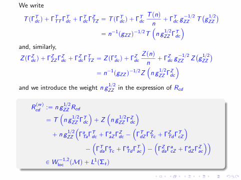
We write
T pΓTdcq ` ΓT
TTΓTdc ` ΓT
dcΓZTZ “ T pΓT
dcq ` ΓTdc
T pnq
n` ΓT
dc g´12ZZ T
`
g12ZZ
˘
“ n´1pgZZ q´12T
´
n g12ZZ ΓT
dc
¯
and, similarly,
Z pΓZdcq ` ΓZ
ZZΓZdc ` ΓZ
dcΓTTZ “ Z pΓz
dcq ` ΓZdc
Z pnq
n` ΓZ
dc g´12ZZ Z
`
g12ZZ
˘
“ n´1pgZZ q´12Z
´
n g12ZZ ΓZ
dc
¯
and we introduce the weight n g12ZZ in the expression of Rcd
Rpwqcd :“ n g
12ZZ Rcd
“ T´
n g12ZZ ΓT
dc
¯
` Z´
n g12ZZ ΓZ
dc
¯
` n g12ZZ
´
ΓaTaΓT
dc ` ΓaaZΓZ
dc ´
´
ΓTdZΓZ
Tc ` ΓZTdΓT
cZ
¯
´
´
ΓTdaΓa
Tc ` ΓaTdΓT
ac
¯
´
´
ΓZdaΓa
cZ ` ΓadZΓZ
ac
¯¯
PW´1,2loc pMq ` L1pΣtq

Section 1.4 TWIST COEFFICIENTS
Regular case Eαβγδ being the volume form of pM, gq
CX :“ EαβγδXαY β∇γX δ CY :“ EαβγδY αY β∇γX δ
Under weak regularity and within an adapted frame pT ,X ,Y ,Z q:
CX :“ EαβγδXαY βgργΓδXρ, CY :“ EαβγδY αY βgργΓδYρ P L8locpL
1pT 3qq
involving only products L8pT 3qL1pT 3q or L2pT 3qL2pT 3q.
Constant twist property
§ The twist coefficients of any weakly regular T 2–symmetric, Ricci-flatspacetime are constants.
§ Furthermore, one can always choose the Killing fields X ,Y in such away that, one of them vanishes identically.
Special case of interest. T 2 symmetry with vanishing twists (Gowdy
symmetry)

Proof. From ∇αeβ “ Γγαβeγ and the anti–symmetry of the volume form:
CX “ EαβγδXαY β∇γX δ “ EXYTZgTTΓZTX ` EXYZT gZZΓT
ZX .
In view of the relations ΓZTX “ n2 gZZΓT
ZX and gTTn2 “ 1:
CX “ 2EXYZTgZZΓTZX
and, thanks to EXYZT “ ´a
n2gZZR2 and ρ2 “gZZn2 , we find:
CX “ ´2R
ρΓTXZ P L
8locpMq
§ We claim that CX is a constant. (See details next page.)
§ From the evolution equation RXZ “ 0, we obtain T pCX q “ 0.§ From the constraint equation RTX “ 0, we obtain ZpCX q “ 0.
§ Same property for CY .
One of the twists can be made to vanish:
§ Introduce a linear combination X 1 “ a X ` b Y and Y 1 “ c X ` d Y
§ ad ´ bc “ 1 to preserve the area of the T 2 orbits.
§ The conclusion follows from
CX 1 “ EαβγδX 1αY 1
β∇γX 1δ“ pad ´ bcq
´
a CX ` b CY
¯
.
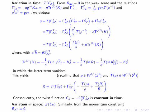
Variation in time: T pCX q. From RXZ “ 0 in the weak sense and the relationsΓaTa “ ´ng
abKab “ ´nTr p2qpKq and ΓTTT ´ ΓZ
TZ “1
2n2 gZZT pρ´2q and
ρ2n2“ gZZ , we deduce
0 “T pΓTXZ q ` ΓT
XZ
´
ΓTTT ´ ΓZ
TZ
¯
` ΓbTbΓT
XZ
“T pΓTXZ q ` ΓT
XZ
˜
ρ2
2T pρ´2
q ´ nTr p2qpKq
¸
“T pΓTXZ q ´ ΓT
XZ
˜
T pρq
ρ` nTr p2qpKq
¸
where, with?h “ Rh12
ZZ ,
Tr p2qpKq “ ´1
nT pln
?hq ´ KZ
Z “ ´1
nT plnRq ´
1
nT pln h12
ZZ q ´ KZZ
in which the latter term vanishes.This yields (recalling that ρ PW 2,1
pS1q and T pρq PW 1,1
pS1q)
0 “ T pΓTXZ q ` ΓT
XZ
˜
´T pρq
ρ`
T pRq
R
¸
Consequently, the twist function CX “ ´2Rρ
ΓTXZ is constant in time.
Variation in space: ZpCX q. Similarly, from the momentum constraintRXT “ 0.
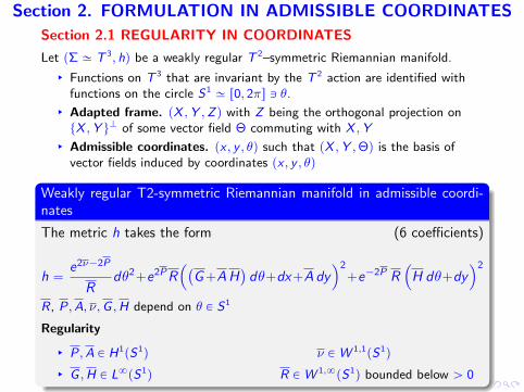
Section 2. FORMULATION IN ADMISSIBLE COORDINATES
Section 2.1 REGULARITY IN COORDINATES
Let pΣ » T 3, hq be a weakly regular T 2–symmetric Riemannian manifold.
§ Functions on T 3 that are invariant by the T 2 action are identified withfunctions on the circle S1
» r0, 2πs Q θ.
§ Adapted frame. pX ,Y ,Zq with Z being the orthogonal projection ontX ,Y uK of some vector field Θ commuting with X ,Y
§ Admissible coordinates. px , y , θq such that pX ,Y ,Θq is the basis ofvector fields induced by coordinates px , y , θq
Weakly regular T2-symmetric Riemannian manifold in admissible coordi-nates
The metric h takes the form (6 coefficients)
h “e2ν´2P
Rdθ2`e2PR
´
`
G`AH˘
dθ`dx`Ady¯2
`e´2P R´
H dθ`dy¯2
R, P,A, ν,G ,H depend on θ P S1
Regularity
§ P,A P H1pS1q ν PW 1,1
pS1q
§ G ,H P L8pS1q R PW 1,8
pS1q bounded below ą 0
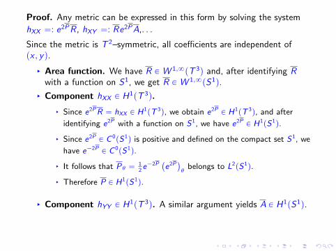
Proof. Any metric can be expressed in this form by solving the system
hXX “: e2PR, hXY “: Re2PA,. . .
Since the metric is T 2–symmetric, all coefficients are independent ofpx , yq.
§ Area function. We have R PW 1,8pT 3q and, after identifying Rwith a function on S1, we get R PW 1,8pS1q.
§ Component hXX P H1pT 3q.
§ Since e2PR “ hXX P H1pT 3
q, we obtain e2PP H1
pT 3q, and after
identifying e2P with a function on S1, we have e2PP H1
pS1q.
§ Since e2PP C 0
pS1q is positive and defined on the compact set S1, we
have e´2PP C 0
pS1q.
§ It follows that Pθ “12e´2P
`
e2P˘
θbelongs to L2
pS1q.
§ Therefore P P H1pS1q.
§ Component hYY P H1pT 3q. A similar argument yields A P H1pS1q.

§ Component hXZ “ e2PRpG ` AHq P L8pT 3q, in which e2P and Rare bounded away from zero, therefore
pG ` AHq P L8pS1q
§ Component hYZ “ Re2PApG ` AHq ` e´2P R H P L8pT 3q
§ Therefore e´2PR H P L8pS1q.
§ Using the lower bound on R, we get e2P
RP L8pS1
q.
§ Thus H P L8pS1q
§ It follows that G P L8pS1q.
§ Component hZZ PW1,1pT 3q. From Z “ Θ` raX ` rbY and the
identity
hZZ “ hθθ ´ praq2hXX ´ 2rarbhXY ´ prbq
2hYY “e2ν´2P
R
we obtain a control of e2ν and, specifically, ν PW 1,1pS1q.

pΣ, h,K q: a weakly regular T 2–symmetric triple in admissible coordinates.
Weakly regular tensor fields in admissible coordinates
There exist 6 functions P0
, A0
, G0
, H0
, R0
, ν0
defined on S1 such that
Kab “ ´R
12
2e´ν`P hab
0hab
0“
hab
RR0` R Fab
0
KXZ “ ´1
2e´ν`3P
`
G0` AH
0
˘
KYZ “ ´1
2e´ν`P
`
R˘2e´2P H
0` AKXZ
KZZ “ ´eν´P
R12
´
ν0´ P
0´
1
2RR0
¯
Fab0epaqepbq “ e2P2P
0
`
dx ` Ady˘2´ 2P
0e´2Pdy2 ` e2P
`
2A0dxdy ` 2AA
0dy2
˘
RegularityP0, A
0P L2pS1q G
0, H
0P L2pS1q
R0P L8pS1q ν
0P L1pS1q
Notation: Rt “ nR12
e´ν`PR0
Observe that Tr p2qK “ ´ e´ν`P
R12 R
0

Let pM, gq be a weakly regular T 2–symmetric spacetime and pt, x , y , θqbe admissible coordinates.
Weakly regular Lorentzian manifolds in admissible coordinates
Metric in admissible coordinates
g “´ n2 dt2 `e2ν´2 P
Rdθ2
` e2PR´
pG ` AHq dθ ` dx ` Ady¯2
` e´2PR`
H dθ ` dy˘2
with coefficients R,P,A, ν,G ,H depending on t P I and θ P S1:
§ P,A P L8locpI ,H1pS1qq n, ν P L8locpI ,W
1,1pS1qq
§ G ,H P L8locpI , L8pS1qq
§ R P L8locpI ,W1,8pS1qq bounded below ą 0
Timelike regularity in admissible coordinates:
Pt ,At P L8locpI , L
2pS1qq Rt P L8locpI , L
8pS1qq
νt P L8locpI , L
1pS1qq Gt ,Ht P L8locpI , L
2pS1qq

Proof.L1pS1q Q 2n KZZ “ ´
´
e2ν´2PR´1 ` Re2PpG ` AHq2 ` e´2PH2R¯
twhile
all other components are in L2pS1q
2n KXZ “ ´
´
e2PRpG ` AHq¯
t
2n KYZ “ ´
´
e2PRA`
G ` AH˘
` e´2PR H¯
t
2n KXX “ ´
´
e2PR¯
t2n KXY “ ´
`
e2PRA˘
t
2n KYY “
´
e2PRA2 ` Re´2P¯
t
L8pS1q Q Trp2qpK q
„`
e2PA2 R´1 ` e´2PR´1˘
KXX ´ 2Ae2P R´1KXY ` e2P R´1KYY
Consequently:
§ Components KXX ,KXY ,KYY P L2pT 3
q:`
e2PR˘
tand
`
e´2PR˘
tand
At P L2pS1q, therefore Pt ,At P L2
pS1q
§ Trace regularity Trp2qpKq „ e´2PRt P L8pS1q
§ Components KXZ and KYZ P L2pT 3
q Gt ,Ht P L2pS1q
§ Component KZZ P L1pT 3
q νt P L1pS1q
Section 2.2 CONSTRAINTS IN ADMISSIBLE COORDINATES
Let pΣ, h,K q be a weakly regular T 2–symmetric triple.
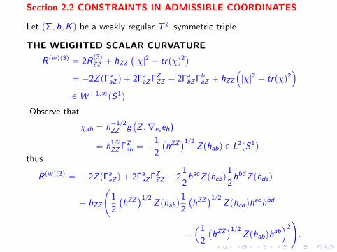
THE WEIGHTED SCALAR CURVATURE
Rpwqp3q “ 2Rp3qZZ ` hZZ
`
|χ|2 ´ trpχq2˘
“ ´2Z pΓaaZ q ` 2Γa
aZΓZZZ ´ 2Γa
bZΓbaZ ` hZZ
´
|χ|2 ´ trpχq2¯
PW´1,8pS1q
Observe that
χab “ h´12ZZ g
`
Z ,∇eaeb˘
“ h12ZZ ΓZ
ab “ ´1
2
`
hZZ˘12
Z phabq P L2pS1q
thus
Rpwqp3q “ ´ 2Z pΓaaZ q ` 2Γa
aZΓZZZ ´ 2
1
2hacZ phcbq
1
2hbdZ phdaq
` hZZ
˜
1
2
`
hZZ˘12
Z phabq1
2
`
hZZ˘12
Z phcdqhachbd
´
´1
2
`
hZZ˘12
Z phabqhab¯2¸
.

Hence, we obtain
Rpwqp3q “ ´2Z pΓaaZ q`2Γa
aZΓZZZ´
1
4Z phcbqZ phdaqh
achbd´1
4
`
Z phabqhab˘2.
Using the identity for the variation of the area R2 “ detphabq
1
2habZ phabq “ Z plnRq “ Γa
aZ “ ´h12ZZ Tr p2qχ
and ΓZZZ “
12 h
ZZ Z phZZ q, we find
Rpwqp3q “ ´ 2Z pZ plnRqq ` 2Z plnRq´
´Rθ2R
` νθ ´ Pθ
¯
´ pZ plnRqq2
´1
4Z phcbqZ phadqh
achbd
and, since there is no dependency in x , y ,
Rpwqp3q “ ´2
ˆ
RθR
˙
θ
` 2RθRpνθ ´ Pθq ´ 2
ˆ
RθR
˙2
´1
4habhcdZ phadqZ phbcq
PW´1,8pS1q

VARIATIONS OF THE 2-METRIC. Second fund. form of theT 2-orbits
To evaluate habhcdZ phadqZ phbcq P L1pS1q we decompose hab in the
form hab “ RFab with detpFabq “ 1:
Z phcbqZ phdaqhachbd “ Z pRF qpRF q´1 ¨ Z pRF qpRF q´1
“ Z pF qF´1 ¨ Z pF qF´1 ` 2Z pF qRθR
F´1 `2
R2
`
Z pRq˘2
“ Z pF qF´1 ¨ Z pF qF´1 `2
R2
`
Z pRq˘2
by using Tr p2q´
Z pF qF´1¯
“ 0 (since F has constant determinant).
§ Observe that F “
ˆ
e2P Ae2P
Ae2P A2e2P ` e´2P
˙
§ A straightforward computation gives14Z pF qF
´1 ¨ Z pF qF´1 “ 2P2θ `
12A
2θe
4P
Rpwqp3q “ ´2
ˆ
RθR
˙
θ
` 2RθRpνθ ´ Pθq ´
5
2
ˆ
RθR
˙2
´ 2P2θ ´
1
2A2θe
4P
PW´1,8loc pS1q
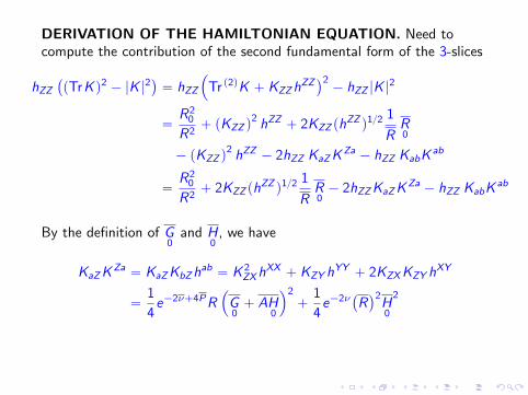
DERIVATION OF THE HAMILTONIAN EQUATION. Need tocompute the contribution of the second fundamental form of the 3-slices
hZZ`
pTrK q2 ´ |K |2˘
“ hZZ
´
Tr p2qK ` KZZhZZ˘2´ hZZ |K |
2
“R2
0
R2` pKZZ q
2 hZZ ` 2KZZ phZZ q12
1
RR0
´ pKZZ q2 hZZ ´ 2hZZ KaZK
Za ´ hZZ KabKab
“R2
0
R2` 2KZZ ph
ZZ q121
RR0´ 2hZZKaZK
Za ´ hZZ KabKab
By the definition of G0
and H0
, we have
KaZKZa “ KaZKbZh
ab “ K 2ZXh
XX ` KZY hYY ` 2KZXKZY h
XY
“1
4e´2ν`4PR
´
G0` AH
0
¯2
`1
4e´2ν
`
R˘2H0
2
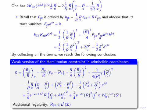
One has 2KZZ phZZ q12 1
RR0“ 2
1
RR0
˜
ν0´ P
0´
1
2RR0
¸
§ Recall that Fab0
is defined by hab0“
1
RR0hab ` R Fab
0, and observe that its
trace vanishes: Fab0hab
“ 0.
hZZKabKab “
1
2
ˆ
1
RR0
˙2
`
`
R˘2
4Fab
0Fcd
0hadhbd
“1
2
ˆ
1
RR0
2˙2
` 2P0
2`
1
2A0
2e4P
By collecting all the terms, we reach the following conclusion:
Weak version of the Hamiltonian constraint in admissible coordinates
0 “
ˆ
Rθ
R
˙
θ
´RθR
`
νθ ´ Pθ˘
`5
4
ˆ
RθR
˙2
`1
4`
R˘2
´
R0
¯2
´1
RR0
´
ν0´ P
0
¯
`
´
P2
θ ` P0
2¯
`1
4
´
A2
θ ` A0
2¯
e4P
`1
4e´2ν`4PR
´
G0` AH
0
¯2
`1
4e´2ν
`
R˘2H0
2PW´1,8
loc pS1q
Additional regularity: Rθθ P L1pΣq
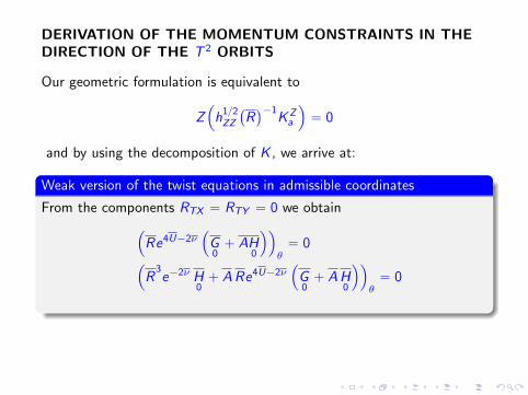
DERIVATION OF THE MOMENTUM CONSTRAINTS IN THEDIRECTION OF THE T 2 ORBITS
Our geometric formulation is equivalent to
Z´
h12ZZ
`
R˘´1
KZa
¯
“ 0
and by using the decomposition of K , we arrive at:
Weak version of the twist equations in admissible coordinates
From the components RTX “ RTY “ 0 we obtain
´
Re4U´2ν´
G0` AH
0
¯¯
θ“ 0
´
R3e´2ν H
0` ARe4U´2ν
´
G0` AH
0
¯¯
θ“ 0
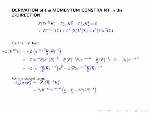
DERIVATION of the MOMENTUM CONSTRAINT in theZ -DIRECTION
Z pTrp2qK q ´ ΓaaZ KZ
Z ´ ΓabZK
ba “ 0
PW´1,8pΣq ` L8pΣqL1pΣq ` L2pΣqL2pΣq
For the first term:
´ZpTr p2qKq “ ´Z´
e´ν`UR0
`
R˘´1
¯
“ ´Zpe´νR0qeU
`
R˘´1
` R0pRq´2Rθe
´ν`U´ R
0
`
R˘´1p´νθ ´ Uθqe
´ν`U
“ ´Z´
e´νR0pRq´12
¯
eP ´ ZpPqe´ν`PR0pRq´12
For the second term:´h12
ZZ trχKZZ “ ´Rθ
`
R˘´1
KZZ
“ RθR´12e´ν`P
´
ν0´ P
0´ 2R
0p2Rq´1
¯

For the last term:
´ΓabZK
ba “ ´
1
2hacZphbcqh
bdKad “ ´1
4e´ν`UhachbdZphbcqhbd
0
Using the fact that the traces of Fab0
and ZpF q vanish:
´ΓabZK
ba “ ´
1
2e´ν`P
`
R˘´32
R0Rθ ´
1
4e´ν`P R
12hbdhacZpFbcqFad
0
Finally, ´ 14e´ν`PR
12hbdhacZpFbcqFad
0“ ´R12e´ν`P
ˆ
2P0Pθ `
1
2A0Aθe
4P
˙
We have reached the following conclusion:
Remaining momentum equation in admissible coordinates
0 “ pR0qθ ´ pνθ ´ PθqR
0´ pν
0´ P
0qRθ `
1
2RRθR
0` R
´
2P0Pθ `
1
2A0Aθe
4P¯
PW´1,8pS1q
Additional regularitypR
0qθ P L
1pS1q

Section 2.3 WEAK VERSION of the EVOLUTION EQUATIONSin ADMISSIBLE COORDINATES
Let pM, gq be a weakly regular T 2–symmetric Ricci-flat spacetime withadmissible coordinates pt, x , y , θq.
DERIVATION FOR THE RICCI COMPONENTS RaZ “ 0.
From our expression of the twist constants, we have:
Ricci components RXZ “ RYZ “ 0 Ordinary diff. equations
0 “´
ρR2e´2νHt
¯
t0 “
´
ρR2e´2ν`4PpGt ` AHtq
¯
t

DERIVATION FOR THE RICCI COMPONENTS Rab “ 0.
0 “T´
n g12ZZ ΓT
dc
¯
` Z´
n g12ZZ ΓZ
dc
¯
` n g12ZZ
ˆ
ΓaTaΓT
dc ` ΓaaZΓZ
dc ´ ΓTdZΓZ
Tc
˙
` n g12ZZ
ˆ
´ ΓZTdΓT
cZ ´ ΓTdaΓa
Tc ´ ΓaTdΓT
ac ´ ΓZdaΓa
cZ ´ ΓadZΓZ
ac
˙
First, we note the following identities:
n g12ZZ “ ρn2 ΓT
dc “1
2n2T pgdcq T
´
n g12ZZ ΓT
dc
¯
“1
2T`
ρT pgdcq˘
Z´
n g12ZZ ΓZ
dc
¯
“ ´1
2Z`
ρ´1Z pgdcq˘
ΓaTaΓT
dc “Rt
R
1
2n2T pgdcq
ΓaaZΓZ
dc “ ´RθR
1
2gZ ,ZZ pgdcq ´ 2ΓT
dZΓZTc “ ´
1
2
KdKc
R2
ΓTdaΓa
Tc “1
4n2T pgdaqT pgbcqg
ab ΓZdaΓa
cZ “ ´1
4ρ2n2Z pgdaqZ pgbcqg
ab
where Kd “ K if d “ y and 0 otherwise.

Investigate the last two expressions: we set gab “: RFab
T pgdaqT pgbcqgab “ 2RtT pFdcq `
R2t
RFdc ` RT pFdaqT pFbcqF
ab
“ 2Rt
RT pgdcq ´
R2t
R2gdc ` RT pFdaqT pFbcqF
ab
§ For d “ c “ x :
T pFaxqT pFbxqFab “
`
2Pte2P˘2 `
e´2P ` A2e2P˘
` 2p´Ae2Pq`
2Pte2P˘ `
2PtAe2P ` Ate
2P˘
``
2PtAe2P ` Ate
2P˘2
e2P
“e2P`
4P2t ` A2
t e4P˘
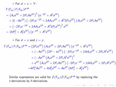
§ For d “ c “ Y :
T pFay qT pFby qFab
“`
Ate2P ` 2PtAe
2P˘2 `
e´2P ` A2e2P˘
` 2p´Ae2Pq`
´2Pte´2P ` 2AAte
2P ` A22Pte2P˘ `
Ate2P ` 2PtAe
2P˘
``
´2Pte´2P ` 2AAte
2P ` A22Pte2P˘2
e2P
“`
4P2t ` A2
t e4P˘ `
e´2P ` A2e2P˘
§ For d “ x and c “ y :
T pFaxqT pFby qFab “
`
2Pte2P˘ `
Ate2P ` 2PtAe
2P˘ `
e´2P ` A2e2P˘
` p´Ae2Pq`
2P ´ te2P˘ `
´2Pte´2P ` 2AAte
2P ` 2PtA2e2P
˘
` p´Ae2P`
Ate2P ` 2PtA
2e2P˘2
` e2P`
Ate2P ` 2PtAe
2P˘ `
´2Pte´2P ` 2AAte
2P ` 2PtA2e2P
˘
“4P2t Ae
2P ` AA2t e
6P “ Ae2P`
4P2t ` A2
t e4P˘
Similar expressions are valid for Z pFacqZ pFbdqFab by replacing the
t-derivatives by θ-derivatives.
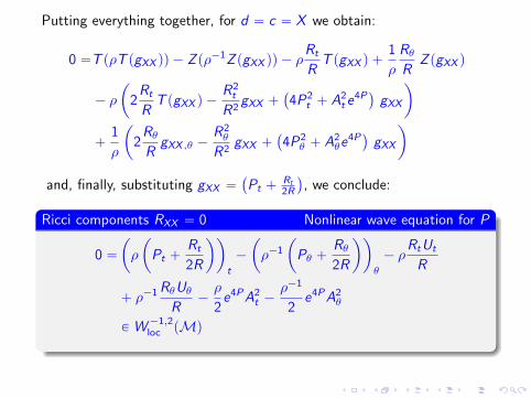
Putting everything together, for d “ c “ X we obtain:
0 “T pρT pgXX qq ´ Z pρ´1Z pgXX qq ´ ρRt
RT pgXX q `
1
ρ
RθR
Z pgXX q
´ ρ
ˆ
2Rt
RT pgXX q ´
R2t
R2gXX `
`
4P2t ` A2
t e4P˘
gXX
˙
`1
ρ
ˆ
2RθR
gXX ,θ ´R2θ
R2gXX `
`
4P2θ ` A2
θe4P˘
gXX
˙
and, finally, substituting gXX “`
Pt `Rt
2R
˘
, we conclude:
Ricci components RXX “ 0 Nonlinear wave equation for P
0 “
ˆ
ρ
ˆ
Pt `Rt
2R
˙˙
t
´
ˆ
ρ´1
ˆ
Pθ `Rθ2R
˙˙
θ
´ ρRtUt
R
` ρ´1 RθUθR
´ρ
2e4PA2
t ´ρ´1
2e4PA2
θ
PW´1,2loc pMq
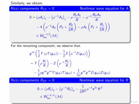
Similarly, we obtain:
Ricci components RYY “ 0 Nonlinear wave equation for A
0 “pρAtqt ´`
ρ´1At
˘
t´ ρ
RtAt
R´ ρ´1 RθAθ
R
´ 4
ˆ
ρ´1Aθ
ˆ
Pθ `Rθ2R
˙
´ ρAt
ˆ
Pt `Rt
2R
˙˙
PW´1,2loc pMq
For the remaining component, we observe that:
g cd
ˆ
1
2T pρT pgcdqq ´
1
2Z´
ρ´1Zpgcdq¯
˙
“ T
ˆ
ρRt
R
˙
´ Z
ˆ
ρ´1 RθR
˙
´1
2ρg adg cdT pgabqT pgcdq `
1
2ρg adg cdZpgabqZpgcdq
Ricci components RXY “ 0 Nonlinear wave equation for R
0 “ pρRtqt ´`
ρ´1Rθ˘
θ´
1
2R3ρ´1e2νK 2
PW´1,8loc pMq

DERIVATION FOR THE RICCI COMPONENT RZZ “ 0.
RZZ “T pΓTZZ q ´ Z pΓT
TZ q ´ Z pΓaaZ q ´ Γa
bZΓbaz ` Γa
aZΓZZZ ` Γa
atΓTZZ ` 2ΓT
aZΓaTZ
` ΓTZZ
`
ΓTTT ´ ΓZ
TZ
˘
` ΓTTZ
`
ΓZZZ ´ ΓT
TZ
˘
We evaluate sucessively each of the terms above:
T pΓTZZ q “ T
´
´1
nKZZ
¯
“ T´ 1
2n2T pgZZ q
¯
PW´1,1pMq
´Z pΓTTZ q “ ´Z
ˆ
1
nZ pnq
˙
PW´1,1pΣtq
´Z pΓaaZ q “ ´Z pZ plnRqq PW´1,8pΣtq
ΓaatΓ
TZZ “ T plnRq
1
2n2T pgZZ q P L8pΣtqL
1pΣtq

The expressions of
ΓabZ Γb
aZ ΓaaZ ΓZ
ZZ ΓTaZ Γa
TZ
have already been computed in terms of the metric (for the derivation ofthe constraint equations), i.e.
´ΓabZΓb
aZ “ ´1
4Z phcbqZ phadqh
achbd “ ´2P2θ ´
1
2A2θe
4P
ΓaaZΓZ
ZZ “ Z plnRq
ˆ
´Rθ2R
` νθ ´ Pθ
˙
ΓTaZΓa
TZ “ K aZKaZ “ ρ2
ˆ
1
4e´2ν`4PRpGt ` AHtq
2 `1
4e´2νR2H2
t
˙
“1
4R2e´2νK 2
where K denotes here the only (possibly) non-vanishing twist constant.
The last two terms in the definition of RZZ :
ΓTZZ
`
ΓTTT ´ ΓZ
TZ
˘
“1
4n4T pgZZ q g
ZZT pρ´2q
ΓTTZ
`
ΓZZZ ´ ΓT
TZ
˘
“n
2gZZZ pnqZ pρ2q

Adding all the terms together, we obtain:
0 “T
ˆ
ρ2
ˆ
νt ´ Pt ´Rt
2R
˙˙
´ ρρt
ˆ
νt ´ Pt ´Rt
2R
˙
´ Z
ˆ
νθ ´ Pθ ´Rθ2R
˙
`ρθρ
ˆ
νθ ´ Pθ ´Rθ2R
˙
´ Z
ˆ
RθR
˙
`Rt
Rρ2
ˆ
νt ´ Pt ´Rt
2R
˙
`RθR
ˆ
νθ ´ Pθ ´Rθ2R
˙
´ 2P2θ ´
1
2A2θe
4P`
1
4R2e´2νK 2
Finally, we eliminate all second-order derivatives of P,R by using theconstraint equations derived earlier.
Ricci components RZZ “ 0 Nonlinear wave equation for ν
0 “pρνtqt ´ pρ´1νθqθ ´ ρ
´
Pt ´Rt
2R
¯2
` ρ´1´
Pθ ´Rθ2R
¯2
´e4P
4
`
ρA2t ´ ρ
´1A2θ
˘
`3
4R4ρ´1e2νK 2
PW´1,1loc pMq
REFERENCES FOR THIS CHAPTER
P.G. LeFloch and J. Smulevici, J. Eur. Math. Soc. (2015).
P.G. LeFloch, Lecture Notes, in preparation.

CONCLUSIONSIn admissible coordinates adapted to the symmetry, our weak version ofthe Einstein equations is equivalent to a coupled system:
§ 4 nonlinear wave equations understood in the weak sense
§ 4 ordinary differential equations
Observation
§ Robust framework (spherical symmetry as well)
§ Allow for matter content
§ Compressible fluids
§ Shock waves (Chapter IV)
OUR NEXT OBJECTIVETechniques of functional analysis (Chapters III and IV)
§ Work with weak solutions in suitable functional spaces
§ Choice of gauge ? Conformal coordinates, areal coordinates
§ Local-in-time existence ?
§ Global geometry of these spacetimes ?

CHAPTER III. Weakly RegularRicci-flat Spacetimes with T2 Symmetry.
The Cauchy problem
pM, gq: a Ricci-flat, weakly regular T 2–symmetric spacetime on T 3
Exploit the gauge freedom to simplify the analysis of the Einsteinequations
§ Coordinate systems adapted to the problem
§ Two different gauges: conformal (null coordinates), areal(geometrically-based)
§ Functional analysis: energy-type norm, monotonicity (area of the T 2
orbits of symmetry), compactness property, continuation principle
OUTLINE.
§ Section 1. Conformal and areal gauges
§ Section 2. Weakly regular Cauchy developments
§ Section 3. Global geometry in areal coordinates
§ Section 4. Additional properties

Section 1. CONFORMAL and AREAL GAUGES
CONFORMAL COORDINATES for weakly regular metrics
Let pt, x , y , θq be admissible coordinates, with t P I “ rt0, t1q and x , y , θ P S1.
Proposition. Existence of conformal coordinates
There exist functions τ, ξ : MÑ R such that:
§ τ, ξ depend on pt, θq and belong to W 1,8loc pI ˆ S1
q.
§ In the chart pτ, ξ, x , yq, the metric reads P “ U ` ln R2
g “e2ν´2P
R
`
´ dτ 2` dξ2
˘
` e2PR´
`
G ` AH˘
dξ ` dx ` Ady¯2
` e´2PR`
H dξ ` dy˘2
with P,A,R, ν,G ,H depending on τ P J and ξ P S1
Furthermore: § The hypersurface t “ t0 coincides with a level set τ “ τ0.
§ τ, ξ, x , y determine a global chart on M, hence define a C8 differentialstructure on M.
§ The charts pτ, ξ, x , yq and pt, θ, x , yq are W 1,8loc compatible (even slightly
more regular), but need not be C8 compatible.

Proof. We focus our attention to the quotient metric on MT 2
pg “e2ν´2P
R
`
´ρ2 dt2 ` dθ2˘
with ρ P L8locpI ,W2,1pS1qq
and establish the existence of two functions τ, ξ:
pg “e2ν´2P
R
`
´ dτ 2 ` dξ2˘
(the relation between ν and ν specified below)
Objective. Construct null coordinates u, v : MT 2 Ñ R:
§ u, v depend pt, θq and belong to W 1,8loc pI ˆ S1q.
§ ut ` ρ uθ “ 0, vt ´ ρ vθ “ 0
§ Periodicity property: upt, θ ` 2πq “ upt, θq ´ 2π andvpt, θ ` 2πq “ vpt, θq ` 2π
§ pt, θq P I ˆ S1 ÞÑ pu, vq is a W 1,8loc diffeomorphism on its image.

From the null coordinates to the conformal coordinates.τ :“ v`u
2 and ξ :“ v´u2 satisfy our requirements:
§ ν and ν (in the expressions of the metric) are related by writingdu “ utdt ` uθdθ and dv “ vtdt ` vθdθ P L
8locpMq
§ which yields us e2ν “ e2νuθvθ.
EXISTENCE OF THE NULL COORDINATES
§ Setting I “ rt0, t1q, we choose the initial data for u, v at the initialtime as:
upt0, ¨q :“ t0 ´ θ vpt0, ¨q :“ t0 ` θ
§ Denote by θ˘ “ θ˘pt, θq the solutions to the characteristicequations with initial conditions on S1 imposed at the time t0:
Bθ˘Btpt, θq “ ˘ρ
`
t, θ˘pt, θq˘
θ˘pt0, θq “ θ
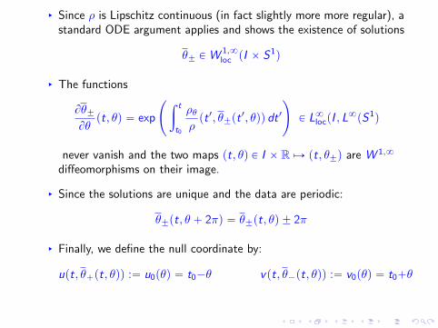
§ Since ρ is Lipschitz continuous (in fact slightly more more regular), astandard ODE argument applies and shows the existence of solutions
θ˘ PW1,8loc pI ˆ S1q
§ The functions
Bθ˘Bθpt, θq “ exp
˜
ż t
t0
ρθρpt 1, θ˘pt
1, θqq dt 1
¸
P L8locpI , L8pS1q
never vanish and the two maps pt, θq P I ˆ R ÞÑ pt, θ˘q are W 1,8
diffeomorphisms on their image.
§ Since the solutions are unique and the data are periodic:
θ˘pt, θ ` 2πq “ θ˘pt, θq ˘ 2π
§ Finally, we define the null coordinate by:
upt, θ`pt, θqq :“ u0pθq “ t0´θ vpt, θ´pt, θqq :“ v0pθq “ t0`θ
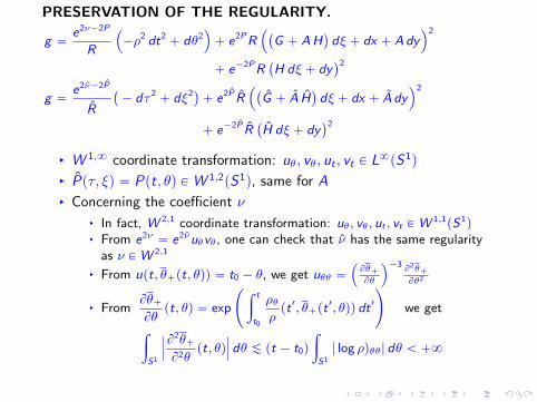
PRESERVATION OF THE REGULARITY.
g “e2ν´2P
R
´
´ρ2 dt2` dθ2
¯
` e2PR´
`
G ` AH˘
dξ ` dx ` Ady¯2
` e´2PR`
H dξ ` dy˘2
g “e2ν´2P
R
`
´ dτ 2` dξ2
˘
` e2P R´
`
G ` A H˘
dξ ` dx ` A dy¯2
` e´2P R`
H dξ ` dy˘2
§ W 1,8 coordinate transformation: uθ, vθ, ut , vt P L8pS1q
§ Ppτ, ξq “ Ppt, θq PW 1,2pS1q, same for A
§ Concerning the coefficient ν
§ In fact, W 2,1 coordinate transformation: uθ, vθ, ut , vt PW 1,1pS1q
§ From e2ν“ e2νuθvθ, one can check that ν has the same regularity
as ν PW 2,1
§ From upt, θ`pt, θqq “ t0 ´ θ, we get uθθ “´
Bθ`Bθ
¯´3B2θ`Bθ2
§ FromBθ`Bθpt, θq “ exp
˜
ż t
t0
ρθρpt 1, θ`pt
1, θqq dt 1¸
we get
ż
S1
ˇ
ˇ
ˇ
B2θ`B2θ
pt, θqˇ
ˇ
ˇdθ À pt ´ t0q
ż
S1
| log ρqθθ| dθ ă `8

NORMALIZATION OF THE TWIST CONSTANTS.
Under weak regularity and within an adapted frame pT ,X ,Y ,Z q:
CX :“ EαβγδXαY βgργΓδXρ, CY :“ EαβγδY αY βgργΓδYρ P L8locpL
1pT 3qq
§ We proved that CX “ ´2Rρ ΓT
XZ P L8locpMq and T pCX q “ Z pCX q “ 0
§ Normalize CY “ 0 by a suitable linear combination of the Killingfields X ,Y .
§ Define K :“ CX
§ Moreover, we normalize K to be positive (or zero) by changing Yinto ´Y , if necessary.
Shift-type coefficients
G ,H satisfy equations that are decoupled from the “essential” Einsteinequations.

FIELD EQUATIONS in conformal coordinates. P “ U ` ln R2
g “ e2pν´Uq`
´dτ 2`dξ2
˘
`e2U`
dx`Ady``
G`AH˘
dξ˘2`e´2UR2
`
dy`H dξ˘2
Four evolution equations
Uττ ´ Uξξ “RξUξR
´RτUτR
`e4U
2R2pA2τ ´ A2
ξq W´1,2loc pMq RicpX ,X q
Aττ ´ Aξξ “RτAτR
´RξAξR
` 4pAξUξ ´ AτUτ q W´1,2loc pMq RicpY ,Y q
Rττ ´ Rξξ “e2ν
2R3K 2 W´1,`8
loc pMq RicpX ,Y q
νττ ´ νξξ “ U2ξ ´ U2
τ `e4U
4R2pA2τ ´ A2
ξq ´3e2ν
4R4K 2 W´1,1
loc pMq RicpZ ,Zq
Two (non-trivial) constraint equations
0 “ U2τ ` U2
ξ `e4U
4R2pA2τ ` A2
ξq `RξξR´ντ RτR
´νξRξR
`e2ν
4R4K 2 L1
pS1q RicpT ,T q
0 “ 2UτUξ `e4U
2R2AτAξ `
RξτR´νξRτR
´ντRξR
L1pS1q RicpT ,Zq
Four twist conditions
Gτ ` AHτ “ 0 Hτ “e2ν
R3K RicpT ,X q& RicpX ,Zq
Kξ “ 0, Kτ “ 0 RicpT ,Y q& RicpY ,Zq
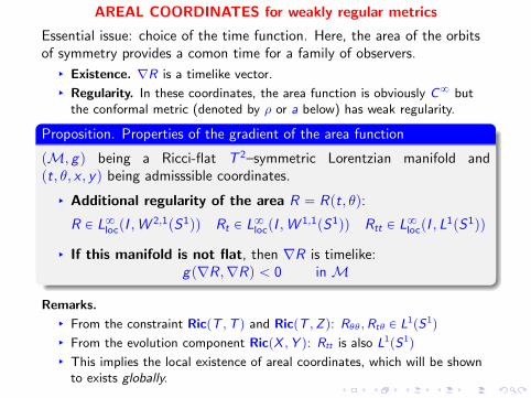
AREAL COORDINATES for weakly regular metrics
Essential issue: choice of the time function. Here, the area of the orbitsof symmetry provides a comon time for a family of observers.
§ Existence. ∇R is a timelike vector.
§ Regularity. In these coordinates, the area function is obviously C8 butthe conformal metric (denoted by ρ or a below) has weak regularity.
Proposition. Properties of the gradient of the area function
pM, gq being a Ricci-flat T 2–symmetric Lorentzian manifold andpt, θ, x , yq being admisssible coordinates.
§ Additional regularity of the area R “ Rpt, θq:
R P L8locpI ,W2,1pS1qq Rt P L
8locpI ,W
1,1pS1qq Rtt P L8locpI , L
1pS1qq
§ If this manifold is not flat, then ∇R is timelike:gp∇R,∇Rq ă 0 in M
Remarks.
§ From the constraint RicpT ,T q and RicpT ,Zq: Rθθ,Rtθ P L1pS1q
§ From the evolution component RicpX ,Y q: Rtt is also L1pS1q
§ This implies the local existence of areal coordinates, which will be shownto exists globally.
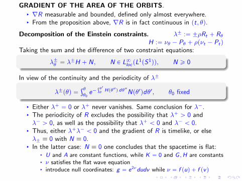
GRADIENT OF THE AREA OF THE ORBITS.§ ∇R measurable and bounded, defined only almost everywhere.§ From the proposition above, ∇R is in fact continuous in pt, θq.
Decomposition of the Einstein constraints. λ˘ :“ ˘ρRt ` RθH :“ νθ ´ Pθ ` ρpνt ´ Ptq
Taking the sum and the difference of two constraint equations:
λ˘θ “ λ˘H ` N, N P L8locpL1pS1qq, N ě 0
In view of the continuity and the periodicity of λ˘
λ˘pθq “şθ
θ0e´
şθ1
θHpθ2q dθ2Npθ1qdθ1, θ0 fixed
§ Either λ` “ 0 or λ` never vanishes. Same conclusion for λ´.§ The periodicity of R excludes the possibility that λ` ą 0 andλ´ ą 0, as well as the possibility that λ` ă 0 and λ´ ă 0.
§ Thus, either λ`λ´ ă 0 and the gradient of R is timelike, or elseλ˘ ” 0 with N ” 0.
§ In the latter case: N ” 0 one concludes that the spacetime is flat:§ U and A are constant functions, while K “ 0 and G ,H are constants§ ν satisfies the flat wave equation§ introduce null coordinates: g “ e2νdudv while ν “ f puq ` f pvq

FIELD EQUATIONS in areal coordinates
Let pM, gq be a Ricci-flat, non-flat weakly regular T 2-symmetricspacetime and let pR, x , y , θq be areal admissible coordinates withR P I Ă p0,`8q.
Observations.
§ Notation η instead of ν
§ Areal coordinates are admissible and the weak regularity holds.
Metric in areal coordinates
g “ e2pη´Uq`
´ dR2 ` a´2 dθ2˘
` e2U``
G ` AH˘
dθ ` dx ` Ady˘2
` e´2UR2`
H dθ ` dy˘2
U,A, η, a,G ,H being functions of R P I and θ P S1
Regularity properties:UR ,AR ,Uθ,Aθ P L
8locpI , L
2pS1qq ηR , ηθ P L8locpI , L
1pS1qq
G ,H P L8locpI , L8pS1qq a P L8locpI ,W
2,1pS1qq
GR ,HR P L8locpI , L
8pS1qq

Four evolution equations for the metric coefficients U,A, η, a
pR a´1URqR ´ pR aUθqθ “ 2R´
p2Rq´2e4U`
a´1 A2R ´ a A2
θ
˘
¯
W´1,2loc pMq
pR´1 a´1ARqR ´ pR´1 a Aθqθ
“ e´2U´
4R´1e2U`
´ a´1 URAR ` a UθAθ˘
¯
W´1,2loc pMq
pa´1ηRqR ´ pa ηθqθ “ ´R´32
`
R32`
a´1˘
R
˘
R` p´a´1U2
R ` a U2θq
` p2Rq´2e4Upa´1A2
R ´ a A2θq W´1,1
loc pMq
p2 ln aqR “ ´R´3K 2 e2η W 1,1
loc pMq
Two constraints ηθ “ R´
2URUθ ` 2R´2e2UARAθ¯
L1pS1q
ηR `1
4R´3 e2ηK 2
“ a R´
`
a´1 U2R ` a U2
θ
˘
` p2Rq´2e4U`
a´1 A2R ` a A2
θ
˘
¯
L1pS1q
Four twist conditionsKR “ 0 Kθ “ 0
GR “ ´AKe2η a´1R´3 HR “ Ke2η a´1R´3

Section 2WEAKLY REGULAR CAUCHY DEVELOPMENTS
OUTLINE OF THE METHODStep 0. Local-in-time smooth solutions from smooth initial data
standard fixed point arguments
Step 1. Local existence in conformal coordinates§ compactness property§ given any weakly regular initial data set, existence of a local-in-time
solution in conformal time rτ0, τ1q
§ τ1 ´ τ0 only depends on a natural norm of the initial data
Step 2. Local existence in areal coordinates§ arrange that the hypersurface
τ “ τ1
(
coincides with
R “ R1
(
§ R is strictly increasing with τ§ a weak solution to the conformal Einstein system can be transformed
to a weak solution to the areal Einstein system§ a local solution to the equations in areal time rR0,R1q
Step 3. Global and causal geometry in areal coordinates (Chapter V)§ global-in-time control of the natural norms§ all values of the area R P p0,`8q but for some “exceptional” (flat
Kasner) spacetimes§ asymptotic behavior when R Ñ 0 or R Ñ `8 (some open problems)

Theorem. Local theory in conformal coordinates
A weakly regular T 2–symmetric initial data set pΣ » T 3, h,Kq and admissiblecoordinates pξ, x , yq
§ Assume the data are non-flat
M0 :“ infS1 |R0´ Rξ1 | inf
S1|R
0` Rξ1 | ‰ 0 (time-like gradient)
§ Normalize the data to be future expanding: Tr p2qK ă 0
Recall that Tr p2qK “ ´e´ν`P R´12
R0
Then, there exists a Ricci-flat, weakly regular T 2–symmetric Lorentzianmanifold pM, gq endowed with a global chart of admissible conformal co-ordinates pτ, ξ, x , yq:
§ M “ I ˆ Σ with I :“ rτ0, τ1q for some τ0 ă τ1
§ g takes the conformal form where R strictly increasing in τ
§ τ1 ´ τ0 ą 0 depends only the natural norm defined from the initialdata set
N0 :“U,AH1pS1q ` U0,A
0L2pS1q ` νW 1,1pS1q ` ν
0L1pS1q
` RW 2,1pS1q ` R0W 1,1pS1q ` 1RL8pS1q `
1
M0.

Regularity of the metric coefficients
U,A P C 0locpI ,H
1pS1qq X C 1locpI , L
2pS1qq
ν P C 0locpI ,W
1,1pS1qq X C 1locpI , L
1pS1qq
R P C 0locpI ,W
2,1pS1qq X C 1locpI ,W
1,1pS1qq
Initial data set. For the embedding ψ : Σ ÑM, pξ, x , yq ÞÑ pτ0, ξ, x , yq:´
U,Uτ ,A,Aτ , ν, ντ ,R,Rτ ,G ,Gτ ,H,Hτ
¯
pτ0q
“
´
U,U0,A,A
0, ν, ν
0,R,R
0,G ,G
0,H,H
0
¯
˝ ψ
Remark. The uniqueness is proven in Section 4 below.
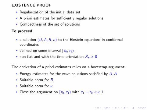
EXISTENCE PROOF
§ Regularization of the initial data set
§ A priori estimates for sufficiently regular solutions
§ Compactness of the set of solutions
To proceed
§ a solution pU,A,R, νq to the Einstein equations in conformalcoordinates
§ defined on some interval rτ0, τ1q
§ non-flat and with the time orientation Rτ ą 0
The derivation of a priori estimates relies on a bootstrap argument:
§ Energy estimates for the wave equations satisfied by U,A
§ Suitable norm for R
§ Suitable norm for ν
§ Close the argument on rτ0, τ1q with τ1 ´ τ0 ăă 1

REGULARIZATION OF INITIAL DATA SETSFor simplicity in the presentation, we do the analysis in areal coordinatesand for a slice with constant area.
Proposition. Regularization of initial data sets
Let X :“`
U0,A0,U1,A1, a, η0, η1
˘
be a weakly regular initial data set forthe (essential) Einstein equations in areal coordinates. Then, there existsa sequence of smooth initial data sets
Xn“
`
Un
0,An
0,Un
1,An
1, an, ηn0, η
n1
˘
, n “ 1, 2, . . .
satisfying Einstein constraint equations and converging almost everywhere
pUn
0,An
0,Un
1,An
1q Ñ pU0,A0,U1,A1q in L2pS1q
an Ñ a in W 2,1pS1q
pηn0, ηn1q Ñ pη0, η1q in L1pS1q
Remarks.
§ The functions G ,H do not appear in the constraint equations.
§ With the same arguments: existence of weakly regular T 2–symmetricinitial data sets with constant R having precisely the weak regularity.

Proof. Standard convolution of the data X .Pick up an arbitrary regularization U
n
0, An
0, Un
1, An
1, an defined on S1,such that:
§ Un
0, An
0, Un
1, An
1 converge in L2pS1q toward U0, A0, U1, A1
§ an converges to a in W 2,1pS1q
‚ It remains to regularize η0 and η1 so that the constraint equations hold.
To any regularized data set Yn
:“ pUn
0,An
0,Un
1,An
1, anq, we associate the
average
ΛrYns :“
ż
S1
λrYns dθ, λrY
ns :“ 2R
´
Un
0Un
1 ` R´2e2Un
An
0An
1
¯
§ λrYns converges in L1pS1q toward η1.
§ The sequence ΛrYns converges to 0
(η1 is the spatial derivative of a periodic function on S1.
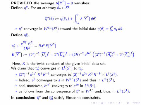
PROVIDED the average ΛrYns “ 0 vanishes:
Define ηn. For an arbitrary θ˚ P S1
ηnpθq :“ ηpθ˚q `
ż θ
θ˚
λrYns dθ1
§ ηn converge in W 1,1pS1q toward the initial data ηpθq “şθ
0η1 dθ.
Define ηn0.
ηn0 `e2ηn K 2
4R3“ Ran E rY
ns
E rYns :“ panq´1 pU
n
0q2 ` anpU
n
1q2 ` p2Rq´2 e4U
n´
panq´1 pAn
0q2 ` anpA
n
1q2¯
Here, K is the twist constant of the given initial data set.We claim that ηn0 converges in L1pS1q to η0:
§ panq´1 e2ηn K 2 R´3 converges to paq´1 e2η K 2 R´3 in L1pS1q.
§ Indeed, an converges to a in W 2,1pS1q and thus in L8pS1q,
§ and, moreover, e2ηn converges to e2η in L1pS1q,
§ as follows from the convergence of ηn in W 1,1 and, thus, in L8pS1q.
In conclusion: ηn and ηn0 satisfy Einstein’s constraints.

Existence of a regularization such that ΛrYns “ 0.
Start from a regularized set Yn
that may not satisfy the constraints.
§ First of all, whenş
S1pU1q2 and
ş
S1pA1q2 both vanish:
§ Then, U and A must be constant, say U “ U˚, A “ A˚.§ Keeping the regularization under considerationY
n‹ “ pU˚,U
n0,A˚,A
n0, a
nq, we do obtain ΛrY
ns “ 0.
Otherwise, assume, for instance, thatş
S1pU1q2 “: c ą 0. Setting
δn :“ ´ ΛrYns
2Rş
S1 pUn1q
2, we claim that the rescaled expression
Yn
‹ :“`
Un,U
n
0 ` δn U
n
1,An,A
n
0, an˘
satisfies Einstein’s constraints.
§ It is well-defined: for all sufficiently large n we haveş
S1pUn
1q2 ě c2.
§ By construction, ΛrYn
‹s “ 0.
§ Convergence to the given initial data set
§ ΛrYns converges to 0.
§ |δn| Àˇ
ˇΛrYnsˇ
ˇ converges to 0 when nÑ `8.
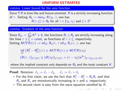
UNIFORM ESTIMATES
Lemma. Lower bound for the area function
Since ∇R is time like and future-oriented, R is a strictly increasing functionof τ . Setting R0 :“ minS1 Rpτ0, ¨q, one has
Rpτ, ξq ě R0 for all τ P rτ0, τ1q and ξ P S1
Lemma. Gradient of the area function
Since Ruv “e2ν
2R3 K2 ě 0, the functions Rτ˘Rξ are strictly increasing along
the lines τ ˘ ξ “ const, as functions of τ ¯ ξ, respectively.Setting Mp∇Rqpτq :“ infS1 Rupτ, ¨q infS1 Rv pτ, ¨q, one has
infS1
`
R2τ ´ R2
ξ
˘
pτq ě Mp∇Rqpτq ě Mp∇Rqpτ0q
Rpτ, ¨qC 1pS1q À Rpτ0qC 1pS1q ` pτ ´ τ0qe2νL8prτ0,τsˆS1q
where the implied constant only depends on R0 and the twist constant K .
Proof. Notation: Bu :“ Bτ ´ Bξ, Bv :“ Bτ ` Bξ§ For the first claim, we use the fact that R2
τ ´ R2ξ “ RuRv and that
Ru and Rv are monotonically increasing in v and u, respectively.§ The second claim is easy from the wave equation satisfied by R.

Lemma. Conformal energy estimate
Econfpτq :“
ż
S1
˜
R`
U2τ ` U2
ξ
˘
`e4U
4R
`
A2τ ` A2
ξ
˘
`e2νK 2
4R3
¸
ďEconfpτ0q eCpR0q
`
1`RC1prτ0,τsˆS1q
˘
pτ´τ0q
Proof. From the constraint equations:
Econfpτq “
ż
S1
´Rξξ ´ ντRτ ´ νξRξ “
ż
S1
´ντRτ ´ νξRξ
and, after integrations by parts,
d
dτEconfpτq “
ż
S1
´ντ pRττ ´ Rξξq ´ Rτ pνττ ´ νξξq.
Using the wave equations for ν and R:
d
dτEconfpτq ď CpR0qRC1prτ0,τsˆS1q Econfpτq ´
ż
S1
ντe2ν K 2
2R3.
Integrate by parts the term ντ and apply Gronwall’s lemma:
´
ż τ
τ0
ż
S1
ντe2ν K 2
2R3“ ´
ż
S1
e2νpτq K 2
4Rpτq3`
ż
S1
e2νpτ0qK 2
4Rpτ0q3´
ż τ
τ0
ż
S1
e2ν 3K 2
4R4Rτ

Consequence of the (non-trivial) constraint equations
ντ RτR
`νξRξR
“ U2τ ` U2
ξ `e4U
4R2pA2τ ` A2
ξq `RξξR`
e2ν
4R4K 2 L1
pS1q
νξRτR
`ντRξR
“ 2UτUξ `e4U
2R2AτAξ `
RξτR
L1pS1q
§ Solve for ντ , νξ in term of the energy densities.
§ Factor |R2τ ´ R2
ξ |, which needs to be bounded below.
Lemma. First-order estimate on ν
νξpτ, ¨qL1pS1q ` ντ pτ, ¨qL1pS1q
À RC 1prτ0,τsˆS1q
´
Econfpτq ` Rξξpτ, ¨qL1 ` Rξτ pτ, ¨qL1
¯
,
where the implied constant depends on R0 and Mp∇Rqpτ0q.
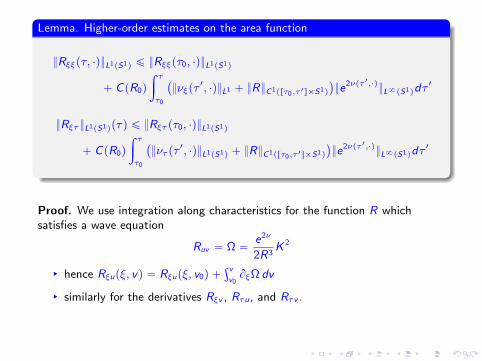
Lemma. Higher-order estimates on the area function
Rξξpτ, ¨qL1pS1q ď Rξξpτ0, ¨qL1pS1q
` CpR0q
ż τ
τ0
`
νξpτ1, ¨qL1 ` RC1prτ0,τ 1sˆS1q
˘
e2νpτ 1,¨qL8pS1qdτ
1
Rξτ L1pS1qpτq ď Rξτ pτ0, ¨qL1pS1q
` CpR0q
ż τ
τ0
`
ντ pτ1, ¨qL1pS1q ` RC1prτ0,τ 1sˆS1q
˘
e2νpτ 1,¨qL8pS1qdτ
1
Proof. We use integration along characteristics for the function R whichsatisfies a wave equation
Ruv “ Ω “e2ν
2R3K 2
§ hence Rξupξ, vq “ Rξupξ, v0q `şv
v0BξΩ dv
§ similarly for the derivatives Rξv , Rτu, and Rτv .

Observe also
νL8pS1qpτq ď1
2πνpτ0qL1pS1q ` νξpτqL1pS1q `
1
2πpτ ´ τ0qντ pτqL1pS1q
RC 1prτ0,τsˆS1q ď 2´
RC 1pS1q ` R0C 0pS1q
¯
We arrive at the following conclusion for a sufficiently small interval ofconformal time.
Proposition. A priori estimates in conformal coordinates
There exist δ,C0 ą 0 depending only on the norm N0 “ Npτ0q of the initialdata such that on the interval rτ0, τ0 ` δs:
Npτq : “ U,AH1pS1q ` Uτ ,Aτ L2pS1q ` νW 1,1pS1q ` ντ L1pS1q
` RW 2,1pS1q ` Rτ W 1,1pS1q ` R´1L8pS1q `Mp∇Rq´1
ď C0 “ C pN0q
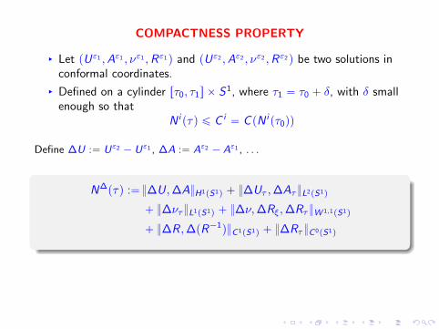
COMPACTNESS PROPERTY
§ Let pUε1 ,Aε1 , νε1 ,Rε1q and pUε2 ,Aε2 , νε2 ,Rε2q be two solutions inconformal coordinates.
§ Defined on a cylinder rτ0, τ1s ˆ S1, where τ1 “ τ0 ` δ, with δ smallenough so that
N i pτq ď C i “ C pN i pτ0qq
Define ∆U :“ Uε2 ´ Uε1 , ∆A :“ Aε2 ´ Aε1 , . . .
N∆pτq :“∆U,∆AH1pS1q ` ∆Uτ ,∆Aτ L2pS1q
` ∆ντ L1pS1q ` ∆ν,∆Rξ,∆Rτ W 1,1pS1q
` ∆R,∆pR´1qC 1pS1q ` ∆Rτ C 0pS1q

Proposition. Continuous dependence on the initial data
Provided that δ ăă 1, one has for all τ P rτ0, τ0 ` δq
N∆pτ1q ď C N∆pτ0q,
where C ą 0 only depends on the constants C pN i pτ0qq.
Proof.
§ Follows similar lines as in the derivation of the uniform bound.
§ We provide a lemma, which is used repeatedly in the proof.
§ Express the wave equations as first-order equations in w˘ “ Uτ ˘ Uθ, etc.
§ Extend the functions by periodicity to the real line R.

Lemma. Higher–integrability estimate
Let w´,w` : rτ0, τ1q ˆ R Ñ R be weak solutions in L8locprτ0, τ1q, L2locpRqq
to the equations Bτw˘ ˘ Bθw˘ “ h˘. with h˘ P L8locprτ0, τ1s, L
2locpRqq.
Then, for each τ ă L, one has
ddτN
I ` 2N II ď N III
N I pτq :“
ż L´τ
´L`τ
ż L´τ
θ`
|w`pτ, θ`q|2 |w´pτ, θ´q|
2 dθ`dθ´
N II pτq :“
ż L´τ
´L`τ
|w`pτ, ¨q|2 |w´pτ, ¨q|
2 dθ
N III pτq :“ÿ
˘
ż L´τ
´L`τ
´
|h˘pτ, ¨q|2 ` |w˘pτ, ¨q|
2¯
dθ
ż L´τ
´L`τ
|w¯pτ, ¨q|2 dθ
Corollary
U2τ ´ U2
ξ and A2τ ´ A2
ξ belong to L2locprτ0, τ1q ˆ S1q

Proof. By regularization, we have
Bτ |w˘|2 ˘ Bθ
`
|w˘|2˘
ď 2 |w˘| |h˘|
Next, from the definitions:
d
dτN I pτq ď
ż L´τ
´L`τ
ż L´τ
θ`
´
´ Bθp|w`|2q ` |h`|
¯
pτ, θ`q |w´pτ, θ´q|2 dθ´dθ`
`
ż L´τ
´L`τ
ż L´τ
θ`
|w`pτ, θ`q|2´
Bθp|w´|2q ` |h´| |w´|
¯
pτ, θ´q dθ´dθ`
´
ż L´τ
´L`τ
|w`pτ,´L` τq|2 |w´pτ, θq|
2 dθ
´
ż L´τ
´L`τ
|w`pτ, θq|2 |w´pτ, L´ τq|
2 dθ
Therefore:
d
dτN I pτq ď ´ 2
ż L´τ
´L`τ
apτ, θq |w`pτ, θq|2 |w´pτ, θq|
2 dθ
`
ż L´τ
´L`τ
ż L´τ
θ`
´
|h`pτ, θ`q| |w`pτ, θ`q| |w´pτ, θ´q|2
` |w`pτ, θ`q|2 |h´pτ, θ´q| |w´pτ, θ´q|
¯
dθ´dθ`

Section 3. GLOBAL GEOMETRY IN AREAL COORDINATES
EXISTENCE AND CONTINUATION CRITERION
Theorem. The global geometry
Given any, non-flat, weakly regular T 2-symmetric initial data set pΣ, h,K qwith topology T 3 and with constant area R0 ą 0 and beign future expand-ing Tr p2qpK q ă 0.
§ there exists a weakly regular, vacuum spacetime pM, gq withT 2–symmetry on T 3,
§ which is a future Cauchy development of pΣ, h,K q,
§ is maximal among all weakly regular T 2-symmetric developments,
§ and admits a unique global foliation by the level sets of the areaR P rR0,`8q.
First observation:
§ The conformal time of existence only depends on the initial norm N0.
§ Hence, the areal time of existence of the solution is bounded below by aconstant depending only on N0.

§ We will have the the existence of global solutions in arealcoordinates, provided we can derive uniform estimates for thenatural norm.
§ More precisely, from the previous section, we have immediately:
Proposition. Continuation criterion
Let pU,A, η, aq be a solution to the areal equations defined on an interval oftime R P rR0,R1q and with the regularity U,A P C 0
RpH1pS1qq X C 1
RpL2pS1qq,
η P C 0RpW
1,1pS1qq X C 1
RpL1pS1qq, a, a´1
P C 0RpW
2,1pS1qq X C 1
RpW1,1pS1qq.
Assume that R1 ă `8 and
NpRq :“U,AH1pS1q ` UR ,ARL2pS1q ` η, aR , aθW 1,1pS1q
` ηR , aRR , aRθ, aθθL1pS1q ` a, a´1L8pS1q
is uniformly bounded on rR0,R˚q. Then, the solution can be extended beyond
R1 with the same regularity.

UNIFORM ESTIMATES IN AREAL COORDINATES
We now derive bounds that are uniform on the interval rR0,R‹q:
§ C : constants depending on the norm NpR0q of the initial data
§ C‹: constants also depending on the final time R‹
ENERGY FUNCTIONALS
EpRq :“
ż
S1
E pR, θq dθ
E :“a´1pURq2 ` a pUθq
2 `e4U
4R2
`
a´1pARq2 ` a pAθq
2˘
and
EK pRq :“
ż
S1
EK pR, θq dθ EK :“ E `K 2
4R4e2η a´1
are non-increasing:
d
dREpRq “ ´ K 2
2R3
ż
S1
E e2η dθ ´2
R
ż
S1
ˆ
a´1 pURq2 `
1
4R2e4U a pAθq
2
˙
dθ
d
dREK pRq “ ´
K 2
R5
ż
S1
a´1e2η dθ ´2
R
ż
S1
ˆ
a´1 pURq2 `
e4U
4R2a pAθq
2
˙
dθ

Lemma. H1 Energy estimates in areal gauge
supRPrR0,R‹q
EpRq ď EpR0q supRPrR0,R‹q
EK pRq ď EK pR0q
ż 8
R0
ż
S1
´
c1 pURq2 a´1`c2 pUθq
2 a`c3 pARq2 a´1`c4 pAθq
2 a¯
dRdθ ď EpR0q
ż `8
R0
ż
S1
K 2
R5e2η a´1 dRdθ ď EK pR0q
c1 :“2
R`
K 2
2R3e2η c2 :“
K 2
2R3e2η
c3 :“K 2
8R5e4U`2η c4 :“
1
2R3e4U `
K 2
8R5e4U`2η

Initial slice. Since the function a is bounded above and below on theinitial slice R “ R0, the initial energy EpR0q controls the H1 norm of thedata U,A:
EpR0q À pU,U0,A,A
0qL2pS1q À EpR0q
with implied constants C1,C2 ą 0 depending on the sup norm of thedata at time R “ R0.
To have similar inequalities at arbitrary times requires a sup-norm bound.
We begin with an upper bound.
Lemma. Upper bound for the function a
suprR0,R‹qˆS1
a ď supS1
a
1
2R
ż
S1
|p1aqR | dθ ď EK pR0q
Proof. ‚ a decreases when R increases.‚ The other estimate follows from since
0 ď ´2 aR a´2 “K 2
R3e2η a´1 “ 4R pEK ´ E q ď 4R EK .

Lemma. W 1,1 estimates for the function η
1
R
ż
S1
|ηR |dθ
aď EK pR0q
1
R
ż
S1
|ηθ| dθ ď EpR0q
and the pointwise estimate
supS1
|ηpR, ¨q| ď R EpR0q `1
2π
ˇ
ˇ
ˇ
ż
S1
η dθ1ˇ
ˇ
ˇ`
1
2
`
supS1
a˘ `
R2 ´ R20
˘
EK pR0q.
Proof. |ηθ| ď R E |ηR | a´1 ď R E `
a´1
4R3e2ηK 2 “ R EK

For the pointwise bound, we proceed as follows: any θ, θ1 P S1:
|ηpR, θq ´ ηpR, θ1q| ď R EpRq
and by integrating in θ1
|ηpR, θq| ď R EpRq ` 1
2π
ˇ
ˇ
ˇ
ˇ
ˇ
ż
S1
ηpR, θ1q dθ1
ˇ
ˇ
ˇ
ˇ
ˇ
.
On the other hand, we haveˇ
ˇ
ˇ
ˇ
ż
S1
ηpR, θ1qdθ1ˇ
ˇ
ˇ
ˇ
ď
ˇ
ˇ
ˇ
ˇ
ż
S1
η dθ1ˇ
ˇ
ˇ
ˇ
`
ˇ
ˇ
ˇ
ˇ
ż
S1
ż R
R0
ηRpR, θ1qdθ1
ˇ
ˇ
ˇ
ˇ
and we evaluate the second term above byˇ
ˇ
ˇ
ˇ
ż
S1
ż R
R0
ηRpR, θ1qdθ1
ˇ
ˇ
ˇ
ˇ
ď supS1
apRq1
2
`
R2 ´ R20
˘
EK pRq.
Finally, we use the energy estimate on EK pRq and the upper bound on a.
supS1
|ηpR, ¨q| ď R EpR0q `1
2π
ˇ
ˇ
ˇ
ż
S1
η dθ1ˇ
ˇ
ˇ`
1
2
`
supS1
a˘ `
R2 ´ R20
˘
EK pR0q.
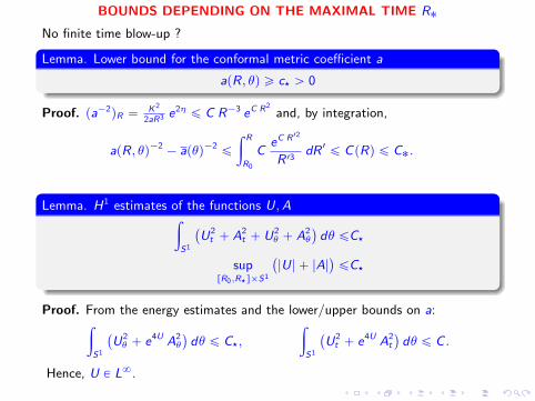
BOUNDS DEPENDING ON THE MAXIMAL TIME R˚
No finite time blow-up ?
Lemma. Lower bound for the conformal metric coefficient a
apR, θq ě c‹ ą 0
Proof. pa´2qR “
K2
2aR3 e2ηď C R´3 eC R2
and, by integration,
apR, θq´2´ apθq´2
ď
ż R
R0
CeC R12
R 13dR 1 ď CpRq ď C˚.
Lemma. H1 estimates of the functions U,Aż
S1
`
U2t ` A2
t ` U2θ ` A2
θ
˘
dθ ďC‹
suprR0,R‹sˆS1
`
|U| ` |A|˘
ďC‹
Proof. From the energy estimates and the lower/upper bounds on a:ż
S1
`
U2θ ` e4U A2
θ
˘
dθ ď C‹,
ż
S1
`
U2t ` e4U A2
t
˘
dθ ď C .
Hence, U P L8.

Lemma. Higher-regularity of the function a
|pln aqRθ| ďK 2
2R2e2ηE
supRPrR0,R˚q
aRθ, aRR , aθθL1pS1q ď C‹
Term aRθ. By differentiating pln aqR “ ´e2η K 2p2R3q, with respect to
θ:ˇ
ˇpln aqRθˇ
ˇ “ˇ
ˇ
K 2
4R3e2η2ηθ
ˇ
ˇ
ˇď
K 2
2R3e2η R E ,
since |ηθ| ď R E . Then, we use the pointwise estimate on η and theenergy bound on E .
Term aRR . We use the L1 estimate on ηR by writing
pln aqRR “ ´´
e2η K 2p2R3q
¯
R“ . . .

Term aθθ. Argument more involved.
§ From pln aqR “ ´K 2
2R3 e2η, we find
pln aqRθθ “´K 2
2R3
`
e2η˘
θθ“ ´
K 2
2R3
´
`
a´2pe2ηqR˘
R` F
¯
F “2e2η``
a´2ηR˘
R´ ηθθ
˘
` 4e2η`
a´2η2R ´ η
2θ
˘
.
If we can show that F is bounded in L1locprR0,R˚s ˆ S1q, then the
desired conclusion follows§ by integration in R§ using integration by parts§ and the L1 estimate on ηR in order to control the term arising from`
a´2pe2η
qR˘
R.
§ On the other hand, concerning the term F :§ The first term is bounded in L1
loc, thanks to the wave equation for η.§ The second term involves the product pa´1ηR ` ηθqpa
´1ηR ´ ηθq,which has the null structure.
§ That is, up to uniformly bounded terms, it a linear combination ofthe null products
pa´1UR ` Uθq2pa´1UR ´ Uθq
2, pa´1AR ` Aθq2pa´1AR ´ Aθq
2
§ These terms are bounded in L1 thanks to the higher-integrability:a´2U2
R ´ U2θ and a´2A2
R ´ A2θ P L2
locprR0,R˚q ˆ S1q

We can now reformulate our existence result in areal coordinates.
Theorem. Global existence theory in areal coordinates
For any weakly regular initial data set with area R “ R0 ą 0, the system ofpartial differential equations describing T 2–symmetric spacetimes in arealcoordinates
§ admits a unique, global weak solution U,A, ν, a,G ,H defined on theinterval I “ rR0,`8q
§ satisfying the regularity conditions UR ,AR ,Uθ,Aθ P L8locpI , L
2pS1qq
ηR , ηθ,G ,H P L8locpI , L
1pS1qq and a P L8locpI ,W1,8pS1qq
Additional regularity
U,A P C 0locpI ,H
1pS1qq X C 1locpI , L
2pS1qq
η P C 0locpI ,W
1,1pS1qq X C 1locpI , L
1pS1qq
a, a´1 P C 0locpI ,W
2,1pS1qq X C 1locpI ,W
1,1pS1qq
G ,H P C 0locpI , L
8pS1qq GR ,HR P C0locpI ,W
1,1pS1qq X C 1locpI , L
1pS1qq
Remark. The additional regularity was not required to express Einsteinequations in the weak sense.

Section 4. ADDITIONAL PROPERTIES
WEAK REGULARITY FROM CONFORMAL TO AREAL coordinates
§ Two coordinate systems
§ local-in-time analysis in conformal coordinates
§ long-time analysis in areal coordinates
§ Construction of coordinates depends on the metric
§ Restriction on the regularity of these coordinates as functions of thegiven coordinates
“The convergence-continuity lemma”
Consider a 2-dimensional Lorentzian manifold pQ, rgq with Q “ rt0, t1qˆS1
and rg “ ´ρ dt2 ` ρ´1 dθ2 with ρ “ ρpt, θq PW 2,1pQq.Then, any weak solution
p P L8loc
`
rt0, t1q,H1pS1q
˘
XW 1,8loc
`
rt0, t1q, L2pS1q
˘
to the wave equation lrgp “ q with q P L2
loc
`
rt0, t1q, L2pS1q
˘
can be realized as the limit of Lipschitz continuous solutions to the samewave equation, belonging to
C 0loc
`
rt0, t1q,H1pS1q
˘
X C 1loc
`
rt0, t1q, L2pS1q
˘
.
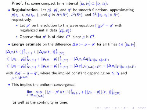
Proof. Fix some compact time interval rt0, t2s Ă rt0, t1q.
‚ Regularization. Let pε0 , pε1 , and qε be smooth functions, approximatingppt0, ¨q, ptpt0, ¨q, and q in H1pS1q, L2pS1q, and L2prt0, t2s ˆ S1q,respectively.
§ Let pε be the solution to the wave equation lrgpε “ qε with
regularized initial data ppε0 , pε1q.
§ Observe that pε is of class C 1, since ρ is C 1.
‚ Energy estimate on the difference ∆p :“ p ´ pε for all times t P rt0, t2s
∆ptpt, ¨q2L2pS1q ` ∆pθpt, ¨q
2L2pS1q
À p0 ´ pε02H1pS1q ` pt,0 ´ pε1
2L2pS1q ` ∆pt ∆qL1prt0,t2sˆS1q
À p0 ´ pε02H1pS1q ` pt,0 ´ pε1
2L2pS1q ` ∆qL2prt0,t2sˆS1q ` ∆ptL2prt0,t2sˆS1q
with ∆q :“ q ´ qε, where the implied constant depending on t0, t1 andρ PW 1,8.
‚ This implies the uniform convergence
limεÑ0
suptPrt0,t2s
pp ´ pεqpt, ¨q2H1pS1q ` ppt ´ pεt qpt, ¨q
2L2pS1q
as well as the continuity in time.

Application of the Einstein equations.
pQ, rgq: quotient space MT 2 with its induced metric and C8
differential structure given by either conformal or areal coordinates
§ In conformal coordinates: ρ ” 1
§ In areal coordinates: ρ “ a´1 proven to be W 2,1 (and thus C 1)
§ The source terms of the wave equations for U,A are L2locpMq.
Claim
The weak regularity of the metric coefficients does not change undera change of coordinates from/to conformal to/from arealcoordinates.
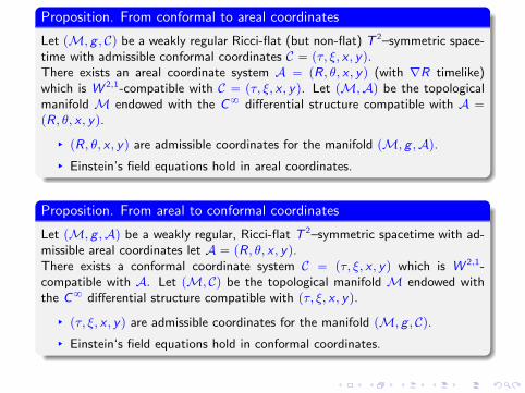
Proposition. From conformal to areal coordinates
Let pM, g , Cq be a weakly regular Ricci-flat (but non-flat) T 2–symmetric space-time with admissible conformal coordinates C “ pτ, ξ, x , yq.There exists an areal coordinate system A “ pR, θ, x , yq (with ∇R timelike)which is W 2,1-compatible with C “ pτ, ξ, x , yq. Let pM,Aq be the topologicalmanifold M endowed with the C8 differential structure compatible with A “
pR, θ, x , yq.
§ pR, θ, x , yq are admissible coordinates for the manifold pM, g ,Aq.§ Einstein’s field equations hold in areal coordinates.
Proposition. From areal to conformal coordinates
Let pM, g ,Aq be a weakly regular, Ricci-flat T 2–symmetric spacetime with ad-missible areal coordinates let A “ pR, θ, x , yq.There exists a conformal coordinate system C “ pτ, ξ, x , yq which is W 2,1-compatible with A. Let pM, Cq be the topological manifold M endowed withthe C8 differential structure compatible with pτ, ξ, x , yq.
§ pτ, ξ, x , yq are admissible coordinates for the manifold pM, g , Cq.§ Einstein‘s field equations hold in conformal coordinates.
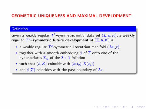
GEOMETRIC UNIQUENESS AND MAXIMAL DEVELOPMENT
Definition
Given a weakly regular T 2–symmetric initial data set pΣ, h,K q, a weaklyregular T 2–symmetric future development of pΣ, h,K q is
§ a weakly regular T 2-symmetric Lorentzian manifold pM, gq,
§ together with a smooth embedding φ of Σ onto one of thehypersurfaces Σt0 of the 3` 1 foliation
§ such that ph,K q coincide with phpt0q,K pt0qq
§ and φpΣq coincides with the past boundary of M.

Definition
§ A development pM, gq is said to be a proper extension ofanother development pM1, g 1q if there exists a C 1 isometricembedding of pM1, g 1q into a proper subset of pM, gq.
§ A maximal development is a development admitting no properextension.
Partial order relation induced by this notion of extension.
Theorem. Uniqueness theory for weakly regular T 2–symmetric develop-ments
For any weakly regular T 2–symmetric initial data set pΣ, h,K q with con-stant area of symmetry R0, there exists a weakly regular T 2–symmetricfuture development defined for with R ě R0, which
§ is unique (up to C 1 diffeomorphisms) and
§ is maximal
and, therefore, coincides with the spacetime we already constructed in arealcoordinates.

Proof. Let pΣ, h,K q be a weakly regular initial data set pΣ, h,K q withconstant area of symmetry R0.
§ Let pM, gq be a future development of pΣ, h,K q with R ě R0.
§ We have proven that the function R enjoys additional regularity and,in particular, is C 1.
§ Hence, we may introduce a new coordinate system, with R as thetime function, which is C 1 compatible with the differential structureof pM, gq.
§ The regularity of all metric functions is preserved.
Hence, areal coordinates may be introduced on pM, gq and the essentialEinstein system are satisfied.
It then follows from the uniqueness of the solution of the essentialEinstein system that pM, gq can be identified with a subset of thesolution that we already constructed.

REFERENCES for this Chapter
§ Moncrief V., Global properties of Gowdy spacetimes with T3 x Rtopology, Ann. of Phys. (1981)
§ Berger B.K., Chrusciel P., Isenberg J., and Moncrief V., Global foliationsof vacuum spacetimes with T2 isometry, Ann. Phys. (1997)
§ P.G. LeFloch and J. Smulevici, J. Eur. Math. Soc. (2015)
§ P.G. LeFloch, Lecture Notes, in preparation.
OUR NEXT OBJECTIVES (Chapters IV and V)
§ Self-gravitating compressible perfect fluids with shock waves
§ Global geometry of weakly regular spacetimes
§ Causality properties (completeness, etc.)
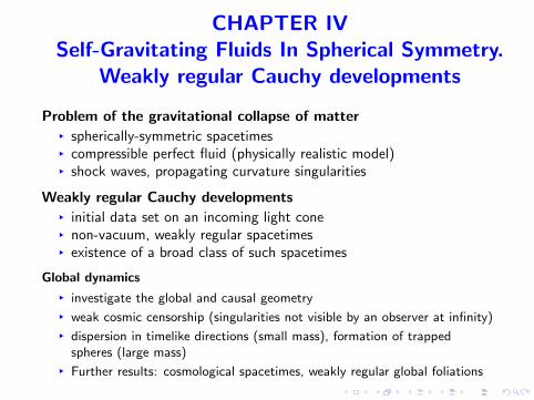
CHAPTER IVSelf-Gravitating Fluids In Spherical Symmetry.
Weakly regular Cauchy developments
Problem of the gravitational collapse of matter§ spherically-symmetric spacetimes§ compressible perfect fluid (physically realistic model)§ shock waves, propagating curvature singularities
Weakly regular Cauchy developments§ initial data set on an incoming light cone§ non-vacuum, weakly regular spacetimes§ existence of a broad class of such spacetimes
Global dynamics
§ investigate the global and causal geometry
§ weak cosmic censorship (singularities not visible by an observer at infinity)
§ dispersion in timelike directions (small mass), formation of trappedspheres (large mass)
§ Further results: cosmological spacetimes, weakly regular global foliations

OUTLINE
§ Section 1. The formulation in Eddington-Finkelstein coordinates
initial data set prescribed on an incoming light cone
§ Section 2. Einstein-Euler spacetimes with bounded variation (BV)
shock waves, curvature discontinuities
§ Section 3. BV regular Cauchy developments
converging method of approximation to the Einstein-Euler system
§ Section 4. Riemann problem on an Eddington Finkelstein background
Monotonicity properties (sup-norm, total variation)
§ Section 5. Spherically symmetric static Einstein-Euler spacetimes
Hawking quasi-local mass
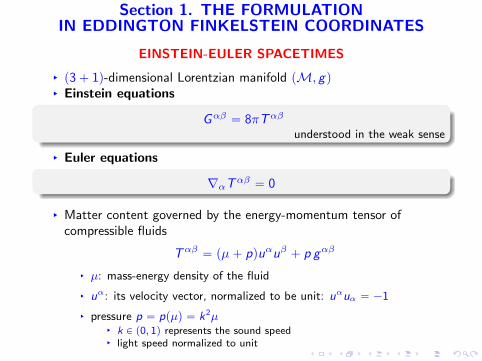
Section 1. THE FORMULATIONIN EDDINGTON FINKELSTEIN COORDINATES
EINSTEIN-EULER SPACETIMES
§ p3` 1q-dimensional Lorentzian manifold pM, gq§ Einstein equations
Gαβ “ 8πTαβ
understood in the weak sense
§ Euler equations
∇αTαβ “ 0
§ Matter content governed by the energy-momentum tensor ofcompressible fluids
Tαβ “ pµ` pquαuβ ` p gαβ
§ µ: mass-energy density of the fluid
§ uα: its velocity vector, normalized to be unit: uαuα “ ´1
§ pressure p “ ppµq “ k2µ§ k P p0, 1q represents the sound speed§ light speed normalized to unit

INITIAL DATA SET
§ Spherical symmetry: SOp3q acts as an isometry group and
§ there exists a central wordline invariant by the group
§ the group orbits through any point (not on the central line) arespacelike 2-spheres
§ From the area A of these 2-spheres, we define the “area radius” byA “ 4πr 2.
§ Initial hypersurface:
§ incoming light cone with vertex at r “ 0
§ Initial data:
§ spatially compact (and weakly regular) perturbation of a (regular)static solution —representing a fluid at equilibrium
§ Later, we will consider “short-pulse data” (Chapter V).
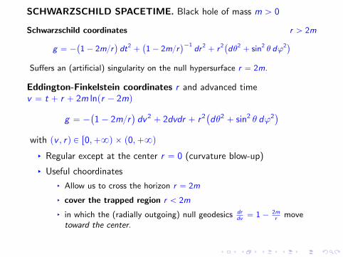
SCHWARZSCHILD SPACETIME. Black hole of mass m ą 0
Schwarzschild coordinates r ą 2m
g “ ´`
1´ 2mr˘
dt2``
1´ 2mr˘´1
dr 2` r 2
`
dθ2` sin2 θ dϕ2
˘
Suffers an (artificial) singularity on the null hypersurface r “ 2m.
Eddington-Finkelstein coordinates r and advanced timev “ t ` r ` 2m lnpr ´ 2mq
g “ ´`
1´ 2mr˘
dv2 ` 2dvdr ` r2`
dθ2 ` sin2 θ dϕ2˘
with pv , rq P r0,`8q ˆ p0,`8q
§ Regular except at the center r “ 0 (curvature blow-up)
§ Useful choordinates
§ Allow us to cross the horizon r “ 2m
§ cover the trapped region r ă 2m
§ in which the (radially outgoing) null geodesics drdv“ 1´ 2m
rmove
toward the center.

EINSTEIN EQUATIONS IN EDDINGTON-FINKELSTEIN coord.
Coordinates that may include a possibly trapped region of the Cauchydevelopment
g “ ´ab2 dv2 ` 2b dvdr ` r2 gS2
§ advanced time v P rv0, v˚s and area radius r P r0,`8q
§ gS2 “`
dθ2 ` sin2 θdϕ2˘
with pθ, ϕq coord. on S2
§ two metric coefficients
§ b “ bpv , rq is positive, but a “ apv , rq may change sign
§ regularity at the center limrÑ0pa, bqpv , rq “ p1, 1q for all v(no mass concentration at the center)

EINSTEIN EQUATIONS Gαβ “ 8πTαβ
§ Two ordinary differential equations
br “ 4π rb3 T 00
rarb ` ab ´ b ` 2rabr “ 8π r2b2 T 01
§ Two partial differential equations
a2b ´ ab ` raarb ` 2ra2br ´ rav “ 8π r2b T 11
2arb3 ` rarrb
3 ` 3rarb2br ` 2ab2br ` 2rab2brr ´ 2rbvbr ` 2rbbvr “ 16π r3b3 T 22
§ The remaining Einstein components impose compatibility/restrictionconditions on the matter model:
T 02 “ T 03 “ 0
T 12 “ T 13 “ 0
T 23 “ T 22 ´ psin θq2 T 33 “ 0
(cf. below)

Geometry determined from the matter content of the spacetime
1. Combining the T 00 and T 01 equations
Br prp1´ aqq ` rp1´ aq 8πrb2 T 00 “ 8πr2b`
bT 00 ´ T 01˘
and using the regularity at the center:
apv , rq “ 1`8π
r
ż r
0
`
bT 00 ´ T 01˘
exp´
´ 8π
ż r
r 1T 00 r2b2 dr2
¯
bpv , r 1qr 12dr 1
provided the integrand is in L1locpr0,`8qq with respect to r
2. With the T 00 equation and by using the regularity at the center:
bpv , rq “ exp´
4π
ż r
0
b2pv , r 1qT 00pv , r 1q r 1dr 1¯
provided r ÞÑ rb2T 00 is in L1locpr0,`8qq
3. The T 11 and T 22 equations will be deduced from the above two.(See below.)
Implicit expressions, depending also on the (unknown) matter content ofthe spacetime.

EULER EQUATIONS IN EDDINGTON-FINKELSTEIN coord.
MATTER MODEL
§ Two unknowns: mass-energy density µ “ µpv , rq ą 0 and thevelocity vector uα “ uαpv , rq
§ normalization ´1 “ uαuα, so that that u0‰ 0.
§ Components β “ 0, 1 of the Euler equations ∇αTαβ “ 0
§ The remaining two components β “ 2, 3 will be deduced from theabove two. (See below.)
§ Remaining Einstein curvature components
T 02 “ T 03 “ T 12 “ T 13 “ T 23 “ T 22 ´ psin θq2 T 33 “ 0
§ Several components of the energy-momentum tensor do vanish.§ The last two components of the velocity vector vanish: u2
“ u3“ 0

The T 00 Euler equation 0 “ ∇αTα0
BvT00 ` BrT
01 `
´2bvb`
arb
2` abr
¯
T 00 `
ˆ
brb`
2
r
˙
T 01 ´2r
bT 22 “ 0
The T 01 Euler equation 0 “ ∇αTα1
BvT01 ` BrT
11 `
ˆ
´avb
2`
aarb2
2` a2bbr
˙
T 00
`
ˆ
bvb´ arb ´ 2abr
˙
T 01 `
ˆ
2brb`
2
r
˙
T 11 ´ 2raT 22 “ 0
Recall the expression of the energy-momentum tensor
Tαβ “ pµ` pquαuβ ` p gαβ

Essential Euler equations in Eddington-Finkelstein coordinates
0 “Bv`
µp1` k2qu0u0˘
` Br
´
µp1` k2qu0u1 ` k2µ
b
¯
`
ˆ
2bvb`
arb
2` abr
˙
µp1` k2qu0u0
`
ˆ
brb`
2
r
˙
´
µp1` k2qu0u1 ` k2µ
b
¯
´2k2
rbµ
0 “Bv
´
µp1` k2qu0u1 ` k2µ
b
¯
` Br
´
µp1` k2qu1u1 ` k2µa¯
`
ˆ
´avb
2`
aarb2
2` a2bbr
˙
µp1` k2qu0u0
`
ˆ
bvb´ arb ´ 2abr
˙
´
µp1` k2qu0u1 ` k2µ
b
¯
`
ˆ
2brb`
2
r
˙
`
µp1` k2qu1u1 ` k2µa˘
´2k2a
rµ
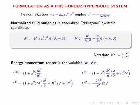
FORMULATION AS A FIRST-ORDER HYPERBOLIC SYSTEM
The normalization ´1 “ gαβuαuβ implies u1 “ ´ 1
2b2pu0q2
Normalized fluid variables in generalized Eddington-Finkelsteincoordinates
M :“ b2µ u0u0 P p0,`8q, V :“u1
b u0´
a
2P p´8, 0q
Notation: K 2 :“ 1´k2
1`k2
Energy-momentum tensor in the variables pM,V q:
T 00 “ p1` k2qM
b2T 01 “ p1` k2q
M
b
´a
2` K 2V
¯
T 11 “ p1` k2qM´a2
4` K 2aV ` V 2
¯
T 22 “ ´2k2
r2MV
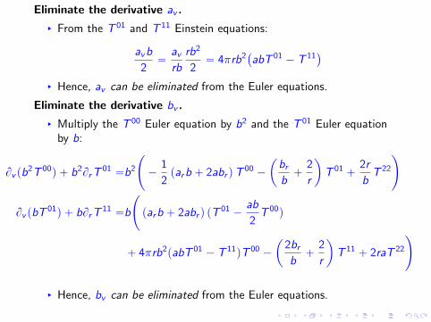
Eliminate the derivative av .
§ From the T 01 and T 11 Einstein equations:
avb
2“
avrb
rb2
2“ 4πrb2
`
abT 01 ´ T 11˘
§ Hence, av can be eliminated from the Euler equations.
Eliminate the derivative bv .
§ Multiply the T 00 Euler equation by b2 and the T 01 Euler equationby b:
Bv pb2T 00q ` b2BrT
01 “b2
˜
´1
2parb ` 2abr qT
00 ´
ˆ
brb`
2
r
˙
T 01 `2r
bT 22
¸
Bv pbT01q ` bBrT
11 “b
˜
parb ` 2abr q pT01 ´
ab
2T 00q
` 4πrb2pabT 01 ´ T 11qT 00 ´
ˆ
2brb`
2
r
˙
T 11 ` 2raT 22
¸
§ Hence, bv can be eliminated from the Euler equations.

Eliminate the derivative br .
Bv pb2T 00
q ` Br pb2T 01
q “ ´`
arb ` 2abr˘b2
2T 00
`
´
br ´2b
r
¯
bT 01` 2rbT 22
Bv pbT01q ` Br pbT
11q “
`
arb ` 2abr˘
b´
T 01´
ab
2T 00
¯
` 4πrb3`
abT 01´ T 11
˘
T 00
´
´
br `2b
r
¯
T 11` 2rabT 22
§ arb ` 2abr can be eliminated thanks to the T 01 Einstein equation:
arb ` 2abr “1
r
´
8πr 2b2T 01´ pa´ 1qb
¯
§ br can be eliminated thanks to the T 00 Einstein equation: br “ 4πrb3T 00
Consequently, the right-hand sides are free of derivatives:
Bv pb2T 00q ` Br pb
2T 01q “pa´ 1qb3
rT 00 ´
2b2
rT 01 ` 2rbT 22
Bv pbT01q ` Br pbT
11q “1
rb
ˆ
1
2ab2pa´ 1qT 00 ´ pa´ 1qbT 01 ´ 2T 11
˙
` 2rb`
4πb2pT 01q2 ´ 4πb2T 00T 11 ` aT 22˘

Proposition. Essential Euler equations for the normalized fluid variables
BvU ` BrF pU, a, bq “ SpU, a, bq
U :“ M
ˆ
1a2 ` K 2V
˙
F pU, a, bq :“ bM
ˆ a2 ` K 2V
a2
4 ` K 2aV ` V 2
˙
SpU, a, bq :“
ˆ
S1pM,V , a, bqS2pM,V , a, bq
˙
S1pM,V , a, bq :“ ´ 12rbM p1` a` 4V q
S2pM,V , a, bq :“ ´1
2rbM
´
a2` 2aV p2` K 2
q ´ 2K 2V ` 4V 2¯
´ 16πp1´ K 2q rb M2V 2
§ Curved spacetime geometry determined from its matter content
§ No dynamical gravitational degree of freedom
apv , rq “ 1´4πp1` k2
q
r
ż r
0
Mpv , r 1q´
2K 2|V pv , r 1q| ` 1
¯ bpv , r 1q
bpv , rqr 1
2dr 1
bpv , rq “ exp´
4πp1` k2q
ż r
0
Mpv , r 1q r 1dr 1¯
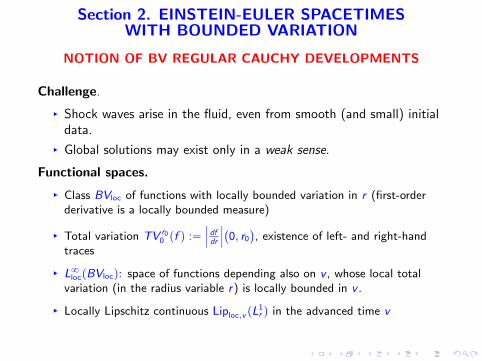
Section 2. EINSTEIN-EULER SPACETIMESWITH BOUNDED VARIATION
NOTION OF BV REGULAR CAUCHY DEVELOPMENTS
Challenge.
§ Shock waves arise in the fluid, even from smooth (and small) initialdata.
§ Global solutions may exist only in a weak sense.
Functional spaces.
§ Class BVloc of functions with locally bounded variation in r (first-orderderivative is a locally bounded measure)
§ Total variation TV r00 pf q :“
ˇ
ˇ
ˇ
dfdr
ˇ
ˇ
ˇ
`
0, r0
˘
, existence of left- and right-handtraces
§ L8locpBVlocq: space of functions depending also on v , whose local totalvariation (in the radius variable r) is locally bounded in v .
§ Locally Lipschitz continuous Liploc,v pL1r q in the advanced time v

Spherically symmetric Einstein-Euler spacetimes with bounded variation
Generalized Eddington-Finkelstein coordinatesg “ ´ab2 dv2 ` 2b dvdr ` r2
`
dθ2 ` sin2 θdϕ2˘
§ Metric coefficients a, b
§ Fluid variables M “ b2µ u0u0P p0,`8q and V “ u1
b u0 ´a2P p´8, 0q
§ Defined for v P I :“ rv0, v˚s and r P J :“ r0, r0q
§ Regularity at the center: limrÑ0pa, bqpv , rq “ p1, 1q at all v P I
§ BV regularityrM, V P L8locpI ,BVlocpJqq X LiplocpI , L
1locpJqq
av , rar , br P L8locpI ,BVlocpJqq X LiplocpI , L
1locpJqq
§ The Einstein and Euler equations are satisfied in the weak sense.

Essential EINSTEIN EQUATIONS
br “ 4πrbM p1` k2q BVloc functions
ar “ 4πrM p1` k2q`
2K 2V ´ a˘
`1´ a
rBVloc functions
Essential EULER EQUATIONS
BvU`BrF pU, a, bq “ SpU, a, bq loc. bounded measures
Additional EINSTEIN EQUATIONSˆ
brb
˙
v
`1
2parbqr ` pabr qr “ ´
1
rpabqr ´ 16πbM k2V loc. bounded measures
av “ 2πrbMp1` k2q`
a2 ´ 4V 2˘
BVloc functions
Observations.1. No regularity required on the first-order derivative bv .
2. The integral formulas for a, b make sense under our integrability conditions.
3. Einstein equations Gαβ “ 8πTαβ satisfied as equalities within locallybounded measures.

INITIAL DATA SET
§ Initial hypersurface: an incoming light cone v “ v0
§ Initial matter content on this hypersurface
§ Prescribe the (normalized) matter variables (geometric data)
Mpv0, rq “ M0prq, V pv0, rq “ V0prq, r P J
§ Here, M0 ą 0 and V0 ă 0 are functions with locally boundedvariation.
§ Initial geometry a0, b0 on the initial hypersurface
§ determined from the data M0,V0
§ satisfy the required regularity conditions:
rBra0, Brb0, P BVlocpJq
limrÑ0
a0prq “ limrÑ0
b0prq “ 1
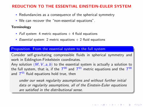
REDUCTION TO THE ESSENTIAL EINSTEIN-EULER SYSTEM
§ Redundancies as a consequence of the spherical symmetry
§ We can recover the “non-essential equations”.
Terminology
§ Full system: 4 metric equations + 4 fluid equations
§ Essential system: 2 metric equations + 2 fluid equations
Proposition. From the essential system to the full system
Consider self-gravitating compressible fluids in spherical symmetry andwork in Eddington-Finkelstein coordinates.Any solution pM,V , a, bq to the essential system is actually a solution tothe full system, that is, if the T 00 and T 01 metric equations and the T 00
and T 01 fluid equations hold true, then
under our weak regularity assumptions and without further initialdata or regularity assumptions, all of the Einstein-Euler equationsare satisfied in the distributional sense.
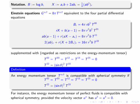
Notation. B :“ log b, X :“ arb ` 2abr “1bpab2
qr
Einstein equations Gαβ “ 8πTαβ equivalent to the four partial differentialequations
Br “ 4π rb2 T 00
rX ` bpa´ 1q “ 8π r 2b2 T 01
abpa´ 1q ` rpaX ´ av q “ 8π r 2b T 11
2pabqr ` rpX ` 2Bv qr “ 16π r 3b T 22
supplemented with (regarded as restrictions on the energy-momentum tensor)
T 02“ T 03
“ T 12“ T 13
“ T 23“ 0
T 22“ psin θq2 T 33
Definition
An energy momentum tensor Tαβ is compatible with spherical symmetry ifT 02
“ T 03“ T 12
“ T 13“ T 23
“ 0
T 22“ psin θq2 T 33
For instance, the energy momentum tensor of perfect fluids is compatible with
spherical symmetry, provided the velocity vector uα has u2“ u3
“ 0.
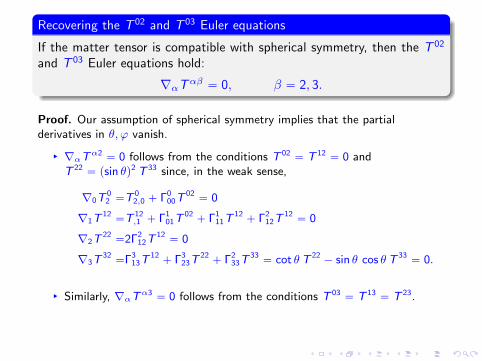
Recovering the T 02 and T 03 Euler equations
If the matter tensor is compatible with spherical symmetry, then the T 02
and T 03 Euler equations hold:
∇αTαβ “ 0, β “ 2, 3.
Proof. Our assumption of spherical symmetry implies that the partialderivatives in θ, ϕ vanish.
§ ∇αTα2“ 0 follows from the conditions T 02
“ T 12“ 0 and
T 22“ psin θq2 T 33 since, in the weak sense,
∇0T02 “T
02,0 ` Γ0
00T02“ 0
∇1T12“T 12
,1 ` Γ101T
02` Γ1
11T12` Γ2
12T12“ 0
∇2T22“2Γ2
12T12“ 0
∇3T32“Γ3
13T12` Γ3
23T22` Γ2
33T33“ cot θT 22
´ sin θ cos θT 33“ 0.
§ Similarly, ∇αTα3“ 0 follows from the conditions T 03
“ T 13“ T 23.

Recovering the T 22 Einstein equation
If the T 00 and T 01 Einstein equations and T 00 Euler equation hold andthe matter tensor is compatible with spherical symmetry, then the T 22
Einstein equation holds.
Proof. From theT 00 Euler equation
0 “ ∇αT0α“T 00
,0 ` T 01,1 `
ˆ
2Bv `X
2
˙
T 00`
ˆ
Br `2
r
˙
T 01´
2r
bT 22
in which, thanks to the T 00 and T 01 Einstein equations in the weak sense,
T 00,0 “
1
4πr
ˆ
Br
b2
˙
v
“Brv ´ 2BrBv
4πrb2“
Brv
4πrb2´ 2BvT
00
T 01,1 “
1
8π
ˆ
rX ` bpa´ 1q
r 2b2
˙
r
“ ´2
ˆ
Br `1
r
˙
T 01`
X ` rXr ` pabqr8πr 2b2
´Br
8πr 2b
Therefore, again with the T 00 and T 01 Einstein equations in the weak sense,
2r
bT 22
“Brv
4πrb2´ BrT
01`
X ` rXr ` pabqr8πr 2b2
´Br
8πr 2b`
X
2T 00
“1
8πr 2b2
´
rp2Brv ` Xr q ` X ´ abBr ` pabqr¯
“1
8πr 2b2
´
rp2Bv ` X qr ` 2pabqr¯
.

Recovering the T 11 Einstein equation
If the T 00, T 01, and T 22 Einstein equations and the T 01 Euler equationhold and the matter tensor is compatible with spherical symmetry, thenthe T 11 Einstein equation holds provided:
§ Regularity of the metric at the centerlimrÑ0pa, bq “ p1, 1q
§ Regularity of the fluid at the center:limrÑ0 r
2`
G 11 ´ 8πT 11˘
“ 0
Proof. The Euler equation ∇αTα1“ 0 reads
0 “ T 01,0 ` T 11
,1 ` paX ´ av qb
2T 00
` pBv ´ X qT 01` 2
ˆ
Br `1
r
˙
T 11´ 2raT 22
From the T 00, T 01, and T 22 Einstein equations and with the notation
Ωpa, bq :“ ´T 01,0 ` pav ´ aX q
b
2T 00
` pX ´ Bv qT01` 2raT 22
we find a linear equation for T 11 in the variable r
T 11,1 ` 2
ˆ
Br `1
r
˙
T 11“ Ωpa, bq.

Claim: The only solution is
T 11 “`
8π r2b˘´1
´
abpa´ 1q ` rpaX ´ av q¯
“ G 11
8π
§ The solutions to the homogeneous equation
BrF “ ´Br`
logprbq2˘
F
are multiples of 1r2b2 .
§ G 11
8π is a particular solution, as follows from the Bianchi identities:§ Gαβ is divergence-free§ In particular, ∇αG
α1“ 0, which reads (using the matter
compatibility condition T 12“ 0)
BrG11` 2
ˆ
Br `1
r
˙
G 11“ 8πΩpa, bq.
§ General solution
T 11 “1
8πr2b2
´
C`ab2pa´1q`raarb2`2ra2bbr´ravb
¯
, C P R.
§ Recall the regularity condition at the center:
0 “ limrÑ0
r2`
G 11 ´ 8πT 11˘
“ limrÑ0
´C
b2“ ´C .

Section 3. BV REGULAR CAUCHY DEVELOPMENTS
THE COMPACT FLUID PERTURBATION PROBLEM
Consider a self-gravitating compressible fluid in spherical symmetry and seek for
weak solutions pM,V , a, bq to the essential Einstein-Euler system in
Eddington-Finkelstein coordinates.
INITIAL DATA SET.§ Fluid at equilibrium. Consider the unique static spacetime
rM, rV , ra, rb with mass-energy fluid density prescribed at the centerr “ 0. (See below.)
§ Initial hypersurface: an incoming light cone Hv0 :“
v “ v0
(
§ Prescribed data§ BV regular perturbation of this static solution
M0 » rM V0 » rV , a0 » ra b0 » rb§ spatially compact: localized within two spheres Sr˚´δ and Sr˚`δ
r˚ ´ δ ď r ď r˚ ` δ
CAUCHY DEVELOPMENT. Evolution of the fluid toward the future§ Singularity formation. Shock waves, curvature measures§ Domain of dependence. By the property of finite speed of
propagation, the spacetime remains static in a neighborhood of thecenter of symmetry.

Domain of dependence. Finite speed of propagation
§ Perturbation initially localized within rr˚ ´ δ, r˚ ` δs
§ Define the radius functions
R´˚ pvq “ r˚ ´ δ ´ C˚pv ´ v0q R`˚ pvq “ r˚ ` δ ` C˚pv ´ v0q
§ C˚: upper bound of the wave speeds λ1, λ2 of the Euler equations(cf. the explicit expressions above)
§ Perturbation on the hypersurface Hv supported within the region
supp`
pM,V qpv , ¨q ´ p rM, rV q˘
Ă
R´˚ pvq ď r ď R`˚ pvq(
§ solutions defined for times v P rv0, v˚s
§ spacetime is static outside
!
v0 ď v ď v˚, R´˚ pvq ď r ď R`˚ pvqs)

Theorem. Existence of BV regular Cauchy developments
Consider the compact fluid perturbation problem with data prescribed onsome light cone Hv0 and formulated in generalized Eddington-Finkelsteincoordinates. Then, there exists a BV regular Cauchy development
§ spherically symmetric Einstein-Euler spacetime with boundedvariation
§ satisfying the prescribed initial data M0,V0, a0, b0 on Hv0
§ includes the spacetime region rv0, v˚s ˆ p0,`8q where the maximaltime v˚ is only restricted by the condition that the spacetimeremains static near the center line r “ 0.
§ BV regularity in spacelike directions
supvPrv0,v˚s
TV´
prM,V , rar , br , av qpv , ¨q ´ pr rM, rV , rrar , rbr , 0q¯
À N0
§ Lipschitz continuity in timelike directions v , v 1 P rv0, v˚s
prM,V qpv , ¨q ´ prM,V qpv 1, ¨qL1p0,`8q À N0 |v ´ v 1|
with N0 :“ TV`80
`
rpM0 ´ rMq˘
` TV`80
`
V0 ´ rV˘
.
Remark. Geometric singularities typically emanate from the center r “ 0.

OUTLINE OF THE METHOD
Converging sequence of approximate solutionsM7,V 7, a7, b7 containing (many !) shock waves
Discretization of the initial data set on Hv0
§ Discretization of pM0,V0, a0, b0q by a piecewise constant initial dataset with finitely many jumps
§ Do not increase the total variation
Solve the Riemann problem§ Cauchy problem with a single initial discontinuity§ Approximate solution in a neighborhood of each discontinuity
Advance in timelike directions§ Introduce a discrete foliation by incoming null cones Hv for v ě v0
§ Advance forward in time up to the next slice of the foliation
Global construction§ Randomly choose of a state within each Riemann problem
(equidistributed sequence)§ Continue this construction inductively for each hypersurface§ Compactness property
§ Bound on the sup-norm and on the total variation of the unknowns§ Independent of the discretization parameters

The Riemann problem
§ Simplest, non-trivial Cauchy problem
§ Initial value problem with piecewise constant data prescribed on alight cone Hv 1
§ The Euler system BvU ` BrF pU, a1, b1q “ SpU, a1, b1q
§ Initial jump at time v 1 centered at some radius r 1:
pM7,V 7qpv 1, ¨q “
#
pM7,L,V 7,Lq r ă r 1
pM7,R ,V 7,Lq, r ą r 1
§ Cannot be solved in a closed form, except “infinitesimally” near thepoint pv 1, r 1q, as we do below in Section 4.
§ Approximate solution, which is sufficiently accurate in a smallneighborhood of the intersection Hv 1 X Sr 1

Approximate solution to the Riemann problem§ An approximate solutionRpv , rq “ Rpv , r ; v 1, r 1;ML,VL,MR ,VR , a
1, b1q§ Homogeneous Riemann problem (See Section 4.)
pRpv , rq “ pRpv , r ; v 1, r 1;ML,VL,MR ,VR , a1, b1q satisfying
BvU ` BrF pU, a1, b1q “ 0
§ Evolution of the geometry described by
Rpv , rq :“ pRpv , rq `ż v
v 1
rSpv2,X pv2, rq, a1, b1q dv2,
where X pv2, rq denotes the solution associated with thesource-terms of the essential Euler equations:
d
dvX “ rSpX , a1, b1q,
X pv 1, rq “ pRpv 1, rq
§ rS takes the geometry into account:rS :“ S ´ arBaF ´ brBbF
“ ´b1M
2r
ˆ
2` 4Va1 ` 4a1V ` 4V 2
˙
´ πp1` k2qrb1M2
ˆ
8K 2V´pa1q2 ` 4K 2a1V ` 12V 2
˙

APPROXIMATE SOLUTIONSto the Compact Fluid Perturbation Problem
§ Discrete foliation of incoming light cones. v0 ă v1 ă v2 ă . . .Hv0 ,Hv1 ,Hv1 , . . .
§ Discrete foliation of spheres. 0 ă r1 ă r2 ă r3 ă . . .Sr1 ,Sr2 ,Sr3 , . . .
§ Converging foliations. We let ∆v :“ suppvi`1 ´ vi q and∆r :“ supprj`1 ´ rjq tend to zero, while the ratio ∆v∆r satisfiesthe stability condition
C˚∆v∆r ă 1
§ Equidistributed sequence pωi q in the interval p0, 1q and set
ri,j :“ rj´1 ` ωi rj`1
(relevant only in the domain of dependence of the initial data)
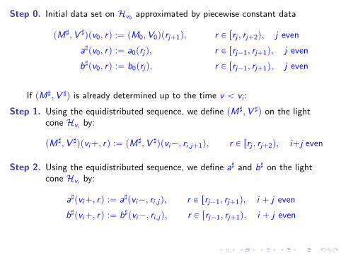
Step 0. Initial data set on Hv0 approximated by piecewise constant data
pM7,V 7qpv0, rq :“ pM0,V0qprj`1q, r P rrj , rj`2q, j even
a7pv0, rq :“ a0prjq, r P rrj´1, rj`1q, j even
b7pv0, rq :“ b0prjq, r P rrj´1, rj`1q, j even
If pM7,V 7q is already determined up to the time v ă vi :
Step 1. Using the equidistributed sequence, we define pM7,V 7q on the lightcone Hvi by:
pM7,V 7qpvi`, rq :“ pM7,V 7qpvi´, ri,j`1q, r P rrj , rj`2q, i`j even
Step 2. Using the equidistributed sequence, we define a7 and b7 on the lightcone Hvi by:
a7pvi`, rq :“ a7pvi´, ri,jq, r P rrj´1, rj`1q, i ` j even
b7pvi`, rq :“ b7pvi´, ri,jq, r P rrj´1, rj`1q, i ` j even

Step 3. The approximation within the spacetime region limited by the lightcones Hvi and Hvi`1 and the spheres Srj´1 and Srj`1
vi ă v ă vi`1, rj´1 ď r ă rj`1, i ` j even(
from the Riemann problem:
pM7,V 7qpv , rq :“ R´
v , r ; vi , rj ; pM7,V 7qpvi`, rj˘1q, pa
7, b7qpvi`, rjqq¯
Step 4. Define the metric coefficients using the integral formulas:
a7pv , rq “ 1´4πp1` k2q
r
ż r
0
M7pv , sq`
1´ 2K 2V 7pv , sq˘ b7pv , sq
b7pv , rqs2ds
b7pv , rq “ exp´
4πp1` k2q
ż r
0
M7pv , r 1q r 1dr 1¯
, v P pvi , vi`1q
It remains to repeat Steps 1 to 4 within the next region limited by twolight cones Hvi`1 and Hvi`2 , and continue inductively for allhypersurfaces Hv1 ,Hv2 , . . .

UNIFORM BOUNDSindependent of the parameters of the discrete foliation
Invariant region principles Sup-norm bound
§ Positivity M ą 0 and condition V ă 0 preserved by the Riemannproblem
§ Invariant region principle for the Riemann invariants:
Total variation principle BV bound
§ logM enjoys a monotonicity property
IN THE REST OF THIS CHAPTER
§ These two principles are now presented in the simplified situation ofthe homogeneous Riemann problem where the coupling to thegeometry is “neglected”.
§ The full proof is quite technical (uniform estimates for the sup-normand total variation, convergence of the approximation scheme) andwill not be presented here (cf. the references below).

Section 4. THE RIEMANN PROBLEM INEDDINGTON-FINKELSTEIN COORDINATES
LOCAL PROPERTIES OF THE ESSENTIAL EULER SYSTEM
§ Geometry/matter coupling: we suppress the geometric terms.
§ Local behavior: metric coefficients a, b treated as prescribedfunctions and, even, constants
BvU ` BrF pU, a, bq “ 0
U “ M
ˆ
1a2 ` K 2V
˙
, F pU, a, bq “ bM
ˆ a2 ` K 2V
a2
4 ` K 2aV ` V 2
˙
§ unknowns: mass-energy density M ą 0 and velocity V ă 0
§ fixed metric coefficients a P R and b ą 0
K 2“ 1´k2
1`k2 P p0, 1q

Strict hyperbolicity property. Fluid variables M and V in terms of U:
M “ U1, V “1
K 2
ˆ
U2
U1´
a
2
˙
Flux vector F pU, a, bq “ b
˜
U2
k2
p1´k2q2
`
a2U1 ´ 4aU2
˘
` 1K 4
U22
U1
¸
Eigenvalues (wave speeds of the system)
λ1 :“ b
ˆ
1` k2
p1´ kq2U2
U1´
k
p1´ kq2a
˙
λ2 :“ b
ˆ
1` k2
p1` kq2U2
U1`
k
p1` kq2a
˙
Since k P p0, 1q and b ą 0 and V ă 0, one has λ1 ă λ2.
Genuine nonlinearity property. Right-eigenvectors
r1 :“ ´
ˆ
1λ1
b
˙
“ ´
ˆ
11`k1´kV `
a2
˙
, r2 :“
ˆ
1λ2
b
˙
“
ˆ
11´k1`kV `
a2
˙
∇λ1 ¨ r1 “ ´2kp1` kq
p1´ kq3bV
M∇λ2 ¨ r2 “ ´
2kp1´ kq
p1` kq3bV
M
∇λ1 ¨ r1 ą ∇λ2 ¨ r2 ą 0
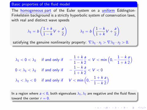
Basic properties of the fluid model
The homogeneous part of the Euler system on a uniform Eddington-Finkelstein background is a strictly hyperbolic system of conservation laws,with real and distinct wave speeds
λ1 “ b
ˆ
1` k
1´ kV `
a
2
˙
λ2 “ b
ˆ
1´ k
1` kV `
a
2
˙
satisfying the genuine nonlinearity property: ∇λ1 ¨ r1 ą ∇λ2 ¨ r2 ą 0.
λ1 ă 0 ă λ2 if and only if ´1` k
1´ k
a
2ă V ă min
´
0,´1´ k
1` k
a
2
¯
0 ă λ1 ă λ2 if and only if ´1´ k
1` k
a
2ă V ă 0
λ1 ă λ2 ă 0 if and only if V ă min´
0,´1` k
1´ k
a
2
¯
In a region where a ă 0, both eigenvalues λ1, λ2 are negative and the fluid flows
toward the center r “ 0.

FORMATION OF SHOCK WAVES
§ In view of the genuine nonlinearity property, the gradient of solutionsblow-up in finite time.
§ A Riccati-type equation along characteristic curves of the hyperbolicsystem. Analogue to Burgers equation Bvu ` uBru “ 0
THE HOMOGENEOUS RIEMANN PROBLEM
§ Initial value problem with data prescribed on Hv 1
§ A single jump located at some r 1 P p0,`8q
Upv 1, rq “
#
UL, r ă r 1
UR , r ą r 1
§ UL (determined by ML,VL) and UR (determined by MR ,VR) aregiven constants: ML,MR ą 0 and VL,VR ă 0
Observations.
§ Invariance of the Riemann problem by self-similar scaling
§ Solution depending upon the variable pr ´ r 1qpv ´ v 1q
Theorem. The Riemann problem on an Eddington-Finkelstein background
The Riemann problem associated with the homogeneous Euler system, ona uniform Eddington-Finkelstein background
§ admits a unique self-similar weak solution depending upon theself-similarity variable pr ´ r 1qpv ´ v 1q
§ made of two waves, each being
§ a rarefaction wave§ or a shock wave (see below)
Moreover, for each constant ρ ą 0, the set Ωρ :“
pw , zq | ´ρ ď w , z ď ρ(
is an invariant domain for the Riemann problem:
§ If the data UL,UR belong to Ωρ for some ρ ą 0, then so does thesolution for times v ě v 1.
(Riemann invariants w , z defined below)

SHOCK CURVES AND RAREFACTION CURVES
Riemann invariants w , z associated with the Euler system
§ By definition, w , z are constant along the integral curves of theeigenvectors, that is, DUwpUq ¨ r1pUq “ 0 and DUzpUq ¨ r2pUq “ 0
§ In the coordinates pM,V q:
wpM,V q :“ log |V | ´2k
p1´ kq2logM
zpM,V q :“ log |V | `2k
p1` kq2logM
RAREFACTION WAVES: Continuous solutions determined fromintegral curves of r1, r2.
§ Solutions U “ Uppr ´ r 1qpv ´ v 1qq satisfying the equation in theself-similar variable ξ :“ pr ´ r 1qpv ´ v 1q, that is,
pDUF pUq ´ ξ Idq BξU “ 0
§ Characterization of the rarefaction curves passing through pM0,V0q
in the phase space:§ The 1-rarefaction curve Ă
wpUq “ wpU0q(
§ The 2-rarefaction curve Ă
zpUq “ zpU0q(

In Riemann invariant coordinates:
RÑ1 pULq “
!
pw , zqˇ
ˇwpM,V q “ wpML,VLq and zpM,V q ď zpML,VLq
)
RÐ2 pURq “
!
pw , zqˇ
ˇwpM,V q ě wpMR ,VRq and zpM,V q “ zpMR ,VRq
)
Rarefaction curves associated with the Euler system
The 1-rarefaction curve RÑ1 pULq from UL “ pML,VLq
RÑ1 pULq “
!
M “ ML
´
VVL
¯
p1´kq2
2k
; VVLP p0, 1s
)
The 2-rarefaction curve RÐ2 pURq from UR “ pMR ,VRq
RÐ2 pURq “
!
M “ MR
´
VVR
¯´p1`kq2
2k
; VVRP r1,`8q
)
Monotonicity properties
§ Along RÑ1 pULq, the wave speed λ1pV q is increasing when Vincreases from VL.
§ Along RÐ2 pURq, the wave speed λ2pV q is decreasing when Vdecreases from VR .
M is decreasing in both cases andlimVÑ0 M|RÑ1 pULq “ limVÑ´8M|RÐ2 pURq “ 0

Proof of the monotonicity property.
§ The associated speeds λ1pV q and λ2pV q increase when V increases.
§ The monotonicity and limiting behavior for M follows.
§ Along the curve RÑ1 pU0q:
zpM,V q “ log |V | `2k
p1` kq2logM
“ log |V | `2k
p1` kq2logM0 `
p1` kq2
p1´ kq2log
V
V0
ď log |V0| `2k
p1` kq2logM0 “ zpM0,V0q.
§ Similarly, along the curve RÐ2 pU0q, we obtainwpM,V q ě wpM0,V0q.

SHOCK WAVES
§ Rankine-Hugoniot conditions: Two constant states UL,UR
separated by a single discontinuity, propagating at the speeds “ spUL,URq determined by
s rUs “ rF pUqs
rUs :“ UR ´ UL, rF pUqs :“ F pURq ´ F pULq
§ Shock admissibility inequalities
λi pVLq ą si ą λi pVRq i-shock
together with s1 ă λ2pVRq and λ1pVLq ă s2 are imposed in order toguarantee uniqueness (and stability) of the Riemann solution.
Notation.
Φ˘pβq :“1
2p1´ K 4qβ2
´
1´ 2K 4β ` β2˘ p1´ βq
a
p1` βq2 ´ 4K 4β¯
Σ˘pV0, βq :“ab
2`
bV0
2K 2
˜
1` β ˘a
p1` βq2 ´ 4K 4β
¸

Shock curves associated with the Euler system
The 1-shock curve issuing from a state UL and the corresponding speed:
SÑ1 pULq “
!
M “ ML Φ´
´ V
VL
¯
andV
VLP r1,8q
)
s1pUL,Uq “ Σ`
´
VL,V
VL
¯
The 2-shock curve issuing from the state UR and the shock speed:
SÐ2 pURq “
!
M “ MR Φ`
´ V
VR
¯
andV
VRP p0, 1s
)
s2pU,URq “ Σ´`
VR ,V
VR
˘
Monotonicity properties
§ The 1-shock speed s1 is increasing for V decreasing.
§ The 2-shock speed s2 is decreasing for V increasing.
§ The shock admissibility inequalities hold.
– Along SÑ1 pULq, the mass density M increases and reaches ML1´K4 as V Ñ ´8.
– Along SÐ2 pURq, M increases and blows up as V Ñ 0.

Shock curves in Riemann invariant coordinates pw , zq
For β “ VVLP r1,`8q:
SÑ1 pULq :
#
w ´ wL “ log β ´ 2kp1´kq2 logpΦ´pβqq
z ´ zL “ log β ` 2kp1`kq2 logpΦ´pβqq
For β “ VVRP p0, 1s:
SÐ2 pURq :
#
w ´ wR “ log β ´ 2kp1´kq2 logpΦ`pβqq
z ´ zR “ log β ` 2kp1`kq2 logpΦ`pβqq

Existence of the Riemann solution. Constructed by pasting togetherconstant states, shock waves, and rarefaction waves.
Construction in the phase space.
§ 1-wave curve issuing from the data UL,
WÑ1 pULq :“ RÑ1 pULq Y SÑ1 pULq
parametrized by β P p0, 1s within the rarefaction part RÑ1 pULq, andβ P r1,`8q within the shock part SÑ1 pULq.
§ 2-wave curve WÑ2 pURq defined similarly
Construction in the physical space. The Riemann problem is solved byobserving that
§ These two curves intersect at a unique pointU˚ P WÑ
1 pULq XWÐ2 pURq.
§ The Riemann solution is a 1-wave connecting UL to U˚, followed bya 2-wave from U˚ to UR .

Validity of this construction. For any initial states UL,UR satisfyingML,MR ą 0 and VL,VR ă 0:
§ The wave speeds arising in the Riemann solution do increase fromleft to right.
§ V decreases from 0 toward ´8, while M increases from 0 to ML
1´K 4
along the curve WÑ1 pULq.
§ Along WÑ2 pURq, the velocity V decreases from 0 to ´8, while the
mass density M decreases from `8 toward 0.
In view of these global monotonicity properties, the intersection pointU˚ P WÑ
1 pULq XWÐ2 pURq exists and is unique.

Invariant domains. Any Ωρ is an invariant region for the Riemannproblem.
§ We write wL for wpULq, etc. and, for definiteness, we supposeU˚ P RÐ1 pULq X RÑ2 pURq.
§ Then, we have w “ wL and z ď zL for all states between UL and U˚,
§ while w ě wR and z “ zR for all states between U˚ and UR .
Therefore:wR ď w “ wL, zR “ z ď zL
along the solution of the Riemann problem, and, in particularw , z P r´ρ, ρs if wL,wR , zL, zR P r´ρ, ρs.
Furthermore, both shock curves SÑ1 pULq and SÐ2 pURq
§ remain within an upper-left triangle in the pw , zq-plane, so that
§ if intersected with each other or with RÐ2 pURq and RÑ1 pULq,respectively, the corresponding Riemann solution belongs to theregion Ωρ.

Tangent to the shock curve SÑ1 pULq in the pw , zq-plane:
dw
dz“
dpw ´ wLq
dpz ´ zLq“
dpw ´ wLq
dβ
ˆ
dpz ´ zLq
dβ
˙´1
“
p1` kq2ˆ
1` k2´
2kp1`βq?p1`βq2´4K4β
˙
p1´ kq2ˆ
1` k2 `2kp1`βq?p1`βq2´4K4β
˙ ă 1
The shock curve SÑ1 is convex in z :
d
dβ
dw
dz“
8kp1` kq2K 2p´1` βq
a
p1` βq2 ´ 4K 4β´
a
p1` βq2 ´ 4K 4β ` k´
2` 2β ` ka
p1` βq2 ´ 4K 4β¯¯
is non-negative since β ě 1.
Since 2k?1´K 4 “ 1` k2, we have
limβÑ1`
dw
dz“
p1` kq2´
1` k2 ´ 2k?1´K 4
¯
p1´ kq2´
1` k2 ` 2k?1´K 4
¯ “ 0,
and the second–order derivative being positive, we conclude thatdwdz P r0, 1s.
Similarly, the curve SÐ2 pURq is increasing and concave in the pw , zq-plane.

TOTAL VARIATION MONOTONICITY PRINCIPLE
BV estimate for a pair of Riemann solutions associated with the Eulersystem
§ Assume that the initial fluid data consists of three equilibriaUL,UM ,UR .
§ Given 0 ă r 1 ă r2 ă `8, prescribe the following initial data atv “ v 1
Upv 1, rq “
$
’
&
’
%
UL, r ă r 1
UM , r 1 ă r ă r2
UR , r ą r2
Combine the Riemann solutions associated with the data UL,UM andUM ,UR

Total variation EpUL,URq of a Riemann solution pUL,URq
§ Sum the magnitude of shock and rarefaction waves
§ Use the variable logM Recall that M :“ b2µ u0u0
We introduce
EpUL,URq :“ |logMR ´ logM˚| ` |logM˚ ´ logML|
where M˚ denotes the mass-energy density for the intermediate stateU˚ P WÐ
1 pULq XWÑ2 pURq.
Proposition. Total Variation Monotonicity Principle
Given arbitrary states UL,UM ,UR , the total variation of the solutions tothe Riemann problems pUL,UMq, pUM ,URq, and pUL,URq satisfy
EpUL,URq ď EpUL,UMq ` EpUM ,URq.

Proof. Consider the wave curves in the plane of the Riemann invariants.
§ Rarefaction curves are straightlines§ The shock curves have the same shape independently of the base
points UL or UR . and are described by the functions Φ˘We observe the identity
Φ´pβqΦ`pβq “´
4p1´ K 4q
2β4¯´1´
p1´ 2K 4β ` β2˘2´ p1´ βq2
`
p1` βq2 ´ 4K 4β˘
¯
“
´
4p1´ K 4q
2β4¯´1
¨
´
p1´ βq2 ` 2βp1´ K 4q˘2´ p1´ βq2
`
p1´ βq2 ´ 4βp1´ K 4βq˘
¯
“ 1
logpΦ´pβqq “ ´ logpΦ`pβqq
§ The expressions for the shock curves coincide up to a change of the roleof w , z .
§ The shock curves are symmetric with respect to the w “ z axis.
§ We observe that the total variation, by definition, is measured along thew “ z axis in the Riemann invariant coordinates.
§ These symmetry properties imply the desired monotonicity property.

Section 5. SPHERICALLY SYMMETRICSTATIC EINSTEIN-EULER SPACETIMES
FORMULATION of the STATIC FLUID PROBLEM
Static solutions pM,V q satisfying BvM “ BvV “ 0, thus
BrF pU, a, bq “ SpU, a, bq.§ Timelike Killing field Y α, foliation whose leaves are orthogonal to Y α
§ Example: outer domain of communication of Schwarzschild (r ą 2m)
Rescaled mass-energy density M “ Mprq and Hawking massm “ mprq “ r
2
`
1´ |∇r |2˘
(defined by a “ 1´ 2mr ):
mr “ 2πr2Mp1` k2q
ˆ
1´2m
r` 2K 2 |V |
˙
mv “ πr2bMp1` k2q
ˆ
4V 2 ´
´
1´2m
r
¯2˙
§ The function r ÞÑ mpv , rq is increasing, provided a2Vă K 2.
§ holds if, for instance, a is positive§ but remains true even for negative values of a (trapped region) if the
normalized velocity is sufficient large.
§ The function v ÞÑ mpv , rq is decreasing provided the ratio |a|2|V |
is greaterthan 1.

Curved geometry
§ The condition BvU “ 0 implies that Mv “ 0 and, thus, bv and av(resp. mv ) vanish.
§ By the T 11 Einstein equation, we have a2 “ 4V 2.
Fluid variables. Returning to the definitions of M,V , we find
§ u1 “ 0 and ab2pu0q2 “ 1
§ which implies aM “`
1´ 2mr
˘
M “ µ.
§ Velocity V “ ´ a2 “
mr ´
12

Formulation of the static problem
All solution to the static Euler equations having a ą 0 satisfy a systemof first-order ordinary differential equations in m, µ defined for all radiusr P p0,`8q:
mr “ 4πr2µ
µr “ ´p1` k2qµ
r ´ 2m
´
4πr2µ`m
rk2
¯
§ The functions V ,M, a are recovered by algebraic formulas
§ The metric coefficient b is given by
bprq “ exp´
4πp1` k2q
ż r
0
r 12µpr 1q
r 1 ´ 2mpr 1qdr 1
¯
provided r2µr´2m is integrable at the center.

EXISTENCE OF STATIC EQUILIBRIA
– Prescribe initial conditions at the center r “ 0, specifically µ0 ą 0 andm0 “ 0.
– The condition on the initial value on m is consistent with m being
non-negative, however, we need (in the proof of the following theorem) to
check whether the second equation makes sense.
Theorem
There exists a unique global solution pm, µq to the static Einstein-Eulersystem with prescribed initial conditions m0 “ 0 and µ0 ą 0 at the center:
limrÑ0 mprq “ 0, limrÑ0 µprq “ µ0.
§ The functions m, µ are smooth and positive on p0,`8q andlimrÑ`8 µprq “ 0.
§ These static solutions pM,V , a, bq satisfy our weak regularityconditions.
§ In particular, the regularity at the center is satisfied
limrÑ0pa, bqprq “ p1, 1q
REFERENCES for this Chapter
Self-gravitating collapse
§ Andreasson H. and Rein G., J. Hyperbolic Differ. Equ. (2010).
§ Burtscher A. and LeFloch P.G., J. Math. Pures Appl. (2014).
§ Christodoulou D., Comm. Math. Phys. (1986).
§ Christodoulou D., Comm. Pure Appl. Math. (1992).
§ Rendall A.D. and Schmidt B.G., Class. Quantum Grav. (1991).
Weakly regular self-gravitating fluids (Gowdy and plane symmetry)
§ LeFloch P.G. and Rendall A.D., A global foliation of Einstein-Eulerspacetimes with Gowdy-symmetry on T3, Arch. Rational Mech. Anal.(2011).
§ LeFloch P.G. and Stewart J.M., The characteristic initial value problemfor plane-symmetric spacetimes with weak regularity, Class. QuantumGrav. (2011).
NEXT OBJECTIVE. Some results on the global geometry and causalproperties of weakly regular spacetimes
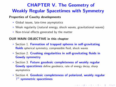
CHAPTER V. The Geometry ofWeakly Regular Spacetimes with Symmetry
Properties of Cauchy developments
§ Global issues, late-time asymptotics
§ Weak regularity (natural energy, shock waves, gravitational waves)
§ Non-trivial effects generated by the matter
OUR MAIN OBJECTIVE in this chapter
§ Section 1. Formation of trapped spheres in self-gravitatingfluids spherical symmetry, compressible fluid, shock waves
§ Section 2. Crushing singularities in self-gravitating fluids inGowdy symmetry
§ Section 3. Future geodesic completeness of weakly regularGowdy spacetimes define geodesics, rate of energy decay, sharp
asymptotics
§ Section 4. Geodesic completeness of polarized, weakly regularT 2 symmetric spacetimes

Section 1. FORMATION OF TRAPPED SPHERESin self-gravitating fluids
Section 1.1 THE BOUNDED VARIATION (BV) FORMULATION
Gravitational collapse of compressible matter with shocksTwo typical behaviors
§ Dispersion of the matter in future timelike directions (sufficientlysmall mass-energy)
§ Collapse of the matter (focusing of light rays)
Set-up
§ Spherically symmetric, weakly regular spacetimes with boundedvariation
§ Converging sequence of solutions to the Einstein-Euler system
§ The Riemann problem (evolution of a single discontinuity)
Objective
§ Short-pulse ansatz (following Christodoulou)
§ Formation of trapped surfaces

MAIN STATEMENT in a rough form. Initial value problem for
§ spherically-symmetric initial data sets pH, g , ρ, jq§ a large class specified explicitly by a short-pulse ansatz
§ weak regularity (bounded variation)
a spherically symmetric, Einstein-Euler future Cauchy developmentpM, g , µ, uq containing shock waves
§ the initial hypersurface does not contain trapped spheres and
§ the Cauchy development does contain trapped spheres.
Remark. Large data result. Geodesically incomplete spacetime
(Penrose-Hawking’s singularity theorem)
Eddington-Finkelstein coordinates
§ g “ ´ab2 dv2 ` 2b dvdr ` r2 gS2 with v P rv0, v˚q, r P r0, r0q
§ b “ bpv , rq ą 0 but a “ apv , rq may change sign
§ regularity at the center: limrÑ0pa, bqpv , rq “ p1, 1q
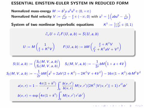
ESSENTIAL EINSTEIN-EULER SYSTEM IN REDUCED FORM
Normalized mass-energy M :“ b2µ u0u0P p0,`8q
Normalized fluid velocity V :“ u1
b u0 ´a2P p´8, 0q with u1
“ 12
´
abu0´ 1
bu0
¯
System of two nonlinear hyperbolic equations K 2 :“ 1´k2
1`k2 P p0, 1q
BvU ` BrF pU, a, bq “ SpU, a, bq
U :“ M
ˆ
1a2` K 2V
˙
F pU, a, bq :“ bM
ˆ a2` K 2V
a2
4` K 2aV ` V 2
˙
SpU, a, bq :“
ˆ
S1pM,V , a, bqS2pM,V , a, bq
˙
S1pM,V , a, bq :“ ´1
2rbM
´
1` a` 4V¯
S2pM,V , a, bq :“ ´1
2rbM
´
a2` 2aV p2` K 2
q ´ 2K 2V ` 4V 2¯
´ 16πp1´ K 2q rb M2V 2
apv , rq “ 1´4πp1` k2
q
r
ż r
0
bpv , r 1q
bpv , rqMpv , r 1q
`
2K 2|V pv , r 1q| ` 1
˘
r 12dr 1
bpv , rq “ exp´
4πp1` k2q
ż r
0
Mpv , r 1q r 1dr 1¯

BOUNDED VARIATION SOLUTIONS
§ strictly hyperbolic, genuinely nonlinear
§ formation of shocks in finite time
Definition
A spherically symmetric, Einstein-Euler spacetime with boundedvariation in Eddington-Finkelstein coordinates
g “ ´ab2 dv2 ` 2b dvdr ` r2`
dθ2 ` sin2 θdϕ2˘
with v P I :“ rv0, v˚q and r P J :“ r0, r0q is a weak solution to theEinstein-Euler system with the following regularity:
§ Normalized mass density and velocity
rM, V P L8locpI ,BVlocpJqq X LiplocpI , L1locpJqq
§ Metric coefficients a, b
av , rar , br P L8locpI ,BVlocpJqq X LiplocpI , L
1locpJqq

STATIC EINSTEIN-EULER EQUATIONS
Closed system for the Hawking mass m “ r2
`
1´ |∇r |2˘
“ r2 p1´ aq and
the fluid density µ
mr “ 4πr2µ
µr “ ´p1` k2qµ
r ´ 2m
´
4πr2µ`m
rk2
¯
The remaining unknowns V ,M, a, b are recovered by
Mprq “µprq
1´ 2mprqr
V prq “mprq
r´
1
2
aprq “ 1´2mprq
rbprq “ exp
´
4πp1` k2q
ż r
0
r 12µpr 1q
r 1 ´ 2mpr 1qdr 1
¯
Theorem
Given any mass-energy density µ0 ą 0 at the center r “ 0, there exists a uniqueglobal solution pm, µq to the static Einstein-Euler system in Eddington-Finkelsteincoordinates with prescribed values at the center of spherical symmetry
limrÑ0
mprq “ 0, limrÑ0
µprq “ µ0.
m, µ are smooth and positive on p0,`8q with limrÑ`8 µprq “ 0.

Section 1.2 THE FORMATION OF TRAPPED SURFACES
§ A given static spacetime p rM, rV , ra, rbq : a fluid at equilibrium
§ Initial data set prescribed on the incoming null cone Hv0
§ Localized (compactly supported) and large perturbation
M0 “ rM `Mp1q0 V0 “ rV ` V
p1q0
a0 “ ra` ap1q0 b0 “ rb ` b
p1q0
§ Initial data assumed to be untrappeda0 ą 0 on the hypersurface Hv0
Challenge
§ existence on a sufficiently long interval rv0, v˚q so that trappedsurfaces do form in the development
§ need to carefully monitor the evolution (and sign) of the metriccoefficient a !
§ bounds uniforms along the sequence of approximate solutions to theEinstein-Euler system
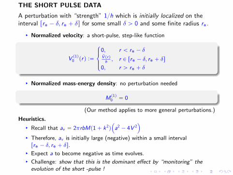
THE SHORT PULSE DATA
A perturbation with “strength” 1h which is initially localized on theinterval rr˚ ´ δ, r˚ ` δs for some small δ ą 0 and some finite radius r˚.
§ Normalized velocity: a short-pulse, step-like function
V p1q0 prq :“
$
’
&
’
%
0, r ă r˚ ´ δrV prqh, r P rr˚ ´ δ, r˚ ` δs
0, r ą r˚ ` δ
§ Normalized mass-energy density: no perturbation needed
Mp1q0 “ 0
(Our method applies to more general perturbations.)
Heuristics.
§ Recall that av “ 2πrbMp1` k2q
´
a2´ 4V 2
¯
§ Therefore, av is initially large (negative) within a small intervalrr˚ ´ δ, r˚ ` δs.
§ Expect a to become negative as time evolves.
§ Challenge: show that this is the dominant effect by “monitoring” theevolution of the short -pulse !

Domain of influence / Domain of dependence
The spacetime remains static in a neighborhood of the center ofsymmetry
§ Radius functions R˘˚¯pvq “ r˚ ˘ δ ¯ C˚pv ´ v0q
§ C˚: Bound on the sound speed, determined by the speed ofpropagation of the (rarefaction, shock) waves
§ The support of the solution expands in time:
§ domain of influence of the initial dataperturbation on the hypersurface Hv supported within
supp`
pM,V qpv , ¨q ´ p rM, rV q˘
Ă
R´˚´pvq ď r ď R`˚`pvq(
§ domain of dependence of the initial data
R´˚`pvq ď r ď R`˚´pvq(
§ uniform a priori bound on the support: we will work in the intervalrr˚ ´∆, r˚ `∆s within the time interval of interest.

Recall that
apv , rq “ 1´4πp1` k2
q
r
ż r
0
bpv , r 1q
bpv , rqMpv , r 1q
`
2K 2|V pv , r 1q| ` 1
˘
r 12dr 1
bpv , rq “ exp´
4πp1` k2q
ż r
0
Mpv , r 1q r 1dr 1¯
Observe that bp1q0 “ 0 and a0 “ ra` a
p1q0
a0prq “ 1´4πp1` k2q
r
ż r
0
bp0qpsq
bp0qprqMp0qpsq
´
1`K 2´
1`1
hχrr˚´δ,r˚`δs
¯
rapsq¯
s2ds
where χrr˚´δ,r˚`δs denotes the characteristic function of the interval.
Lemma
Given r˚ ą ∆ ą 0, there exist constants C1,C2,C3 ą 0 depending on r˚and ∆ such that for all δ, h ą 0 with δ
h ď1C1
0 ă a0prq ď raprq, r P r0, r˚ `∆s (non-trapped)
av pv0, rq
$
’
&
’
%
“ 0, r P r0, r˚ ´ δq (static region)
ď ´C2δh3 r P rr˚ ´ δ, r˚ ` δs (short-pulse region)
ď ´C3δh , r P pr˚ ` δ, r˚ `∆s
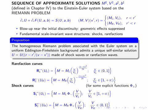
SEQUENCE OF APPROXIMATE SOLUTIONS M7,V 7, a7, b7
(defined in Chapter IV) to the Einstein-Euler system based on theRIEMANN PROBLEM
BvU ` BrF pU, a, bq “ SpU, a, bq pM,V qpv 1, rq “
#
pML,VLq, r ă r 1
pMR ,VRq, r ‘ ă r
§ Blow-up near the initial discontinuity: geometric effects suppressed
§ Fundamental scale-invariant wave structures: shocks, rarefactions
Proposition
The homogeneous Riemann problem associated with the Euler system on auniform Eddington-Finkelstein background admits a unique self-similar solutionU “ Uppr ´ r 1pv ´ v 1qq made of shock waves or rarefaction waves.
Rarefaction curves
RÑ1 pULq “
!
M “ ML
´
VVL
¯
p1´kq2
2k; V
VLP p0, 1s
)
RÐ2 pURq “
!
M “ MR
´
VVR
¯´p1`kq2
2k; V
VRP r1,`8q
)
Shock curves (for some explicit functions Φ˘)
SÑ1 pULq “
!
M “ ML Φ´´ V
VL
¯
;V
VLP r1,`8q
)
SÐ2 pURq “
!
M “ MR Φ`´ V
VR
¯
;V
VRP p0, 1s
)

Definition
An approximate solution M7,V 7, a7, b7 (as defined in Chapter IV) to theEuler–Einstein system is said to satisfy the short-pulse property if
§ there exist constants C0,C ,Cb,Λ ą 0 (depending only on the chosenstatic solution)
§ an exponent κ ą 1 (depending on the sound speed k),§ defined for all v P rv0, v˚q with v˚ :“ v0 ` τh
κ
§ In the domain of influence of the initial pulse
1
C0e´C
v´v0hκ
´
1`1
h
¯´κ0
ď M7pv , rq ď C0eC
v´v0hκ
´
1`1
h
¯κ0
1
C0e´C
v´v0hκ ď ´V 7pv , rq ď C0e
Cv´v0hκ
´
1`1
h
¯
§ In the domain of dependence of the initial pulse (boundedmatter density + very large negative velocity)
1
C0e´C
v´v0hκ ď M7pv , rq ď C0e
Cv´v0hκ
1
C0e´C
v´v0hκ
´
1`1
h
¯
ď ´V 7pv , rq ď C0eC
v´v0hκ
´
1`1
h
¯

Theorem
Fix k P p0, 1q small enough. Given any µ0 ą 0, let rM, rV , ra, rb be the staticsolution with density µ0 at the center.Initial data set
§ Fix any r˚ ą ∆ ą 0 together with perturbation parameters h, δ ą 0satisfying δ ď h
C1with C1 as above.
§ Let pM0,V0, a0, b0q be a short-pulse perturbation of this staticsolution.
There exist τ, κ ą 0 such that for all light-cones Hv0 ,Hv1 ,Hv2 , . . . andspheres Sr1 ,Sr2 ,Sr3 , . . . of the discrete spacetime foliation:
§ the approximate solutions M7,V 7, a7, b7 to the Einstein-Euler system(defined in Chapter IV) are well-defined on the (large) time intervalrv0, v˚q with v˚ “ v0 ` τh
κ
§ satisfy the short-pulse property
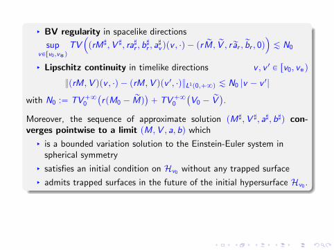
§ BV regularity in spacelike directions
supvPrv0,v˚q
TV´
prM7,V 7, ra7r , b7r , a
7v qpv , ¨q ´ pr
rM, rV , rrar , rbr , 0q¯
À N0
§ Lipschitz continuity in timelike directions v , v 1 P rv0, v˚q
prM,V qpv , ¨q ´ prM,V qpv 1, ¨qL1p0,`8q À N0 |v ´ v 1|
with N0 :“ TV`80
`
rpM0 ´ rMq˘
` TV`80
`
V0 ´ rV˘
.
Moreover, the sequence of approximate solution pM7,V 7, a7, b7q con-verges pointwise to a limit pM,V , a, bq which
§ is a bounded variation solution to the Einstein-Euler system inspherical symmetry
§ satisfies an initial condition on Hv0 without any trapped surface
§ admits trapped surfaces in the future of the initial hypersurface Hv0 .

Section 2. CRUSHING SINGULARITIESin self-gravitating fluids in Gowdy symmetry
‚ Einstein equations in the weak sense Rαβ ´R2gαβ “ Tαβ
‚ Compressible fluids Tαβ “ pµ` ppµqquαuβ ` ppµq gαβ
future unit timelike velocity vector uα, mass-energy density µisothermal pressure law ppµq “ k2 µ
‚ Gowdy symmetry on T 3
§ Action by a group of isometries generated by two commuting, spacelikeKilling fields X ,Y
§ Vanishing twists εαβγδXαY β∇γX δ
“ εαβγδXαY β∇γY δ
“ 0
§ Inhomogeneous cosmology: big bang / big crunch
§ Include gravitational waves (contrary to spherical symmetry)
‚ Weak solutions to the Einstein equations
§ Weak formulation of the Einstein equations
§ Allows for impulsive gravitational waves, shock waves
‚ Existence of weakly regular Cauchy developments
§ foliation by spacelike hypersurfaces, areal time function
§ behavior near the future boundary of the spacetime
We state here a typical result based on the methods in Chapters II to IV.

Metric in areal coordinates R P rt0, t1q, θ P S1 and x , y P S1
g “ e2pν´Uq`
´ dR2 ` α´1dθ2˘
` e2U´
dx ` Ady¯2
` e´2UR2dy2
Einstein evolution equations in a weak sense
`
t´1 a´1At
˘
t´`
t´1 aAθ˘
θ“ ´
4
at
`
UtAt ´ a2UθAθ˘
`
t a´1pUt ´ 1p2tq˘
t´`
t aUθ˘
θ“
e4U
2ta
`
A2t ´ a2A2
θ
˘
`
ta´1pνt ` te2pν´Uqµp1´ k2qq˘
t´ ptaνθqθ “ 2atU2
θ `e4U
2atA2t
` ta´1 e2pν´Uqµp1` k2q
1´ v2
Einstein constraint equations in a weak sense
at “ ´ate2pν´Uqµp1´ k2q
νt “ tpU2t ` a2U2
θ q `e4U
4tpA2
t ` a2A2θq ` te2pν´Uqµ
k2 ` v2
1´ v2
νθ “ ´2tUtUθ ´e4U
2tAtAθ ´ a´1te2pν´Uqµ
p1` k2qv
1´ v2

Theorem. Existence of Cauchy developments and global areal foliations
pM » T 3, g , k, µ, Jq: BV regular Gowdy symmetric, initial data set with con-stant area R0 “ t0 and which is either expanding or contracting.
§ Existence of BV regular Cauchy developments
§ BV regular Gowdy symmetric spacetime pM, g , µ, uαq§ A future Cauchy development, globally covered by a single
coordinate chart
§ Global foliation by spacelike hypersurfaces
§ A global geometrically-defined time function t coinciding with ˘ thearea R
§ R : two-dimensional spacelike orbits of the T 2 isometry group
§ R increasing or decreasing toward the future
§ Expanding spacetime t “ R P rt0,`8q t0 ą 0(the area grows without bound)
§ Contracting spacetime t “ ´R P rt0, t1q t0 ă t1 ď 0
§ Crushing singularity property for Gowdy-symmetric matter spacetimes
For future contracting Einstein-Euler spacetimes with Gowdysymmetry, and for generic initial data, one has t1 “ 0, that is, thearea of the T 2 orbits of symmetry approaches 0 in the future.

Remark. Our genericity condition is optimal within the class of spatiallyhomogeneous spacetimes.
Spatially homogeneous spaces - Bianchi type I solutions (three-dim.
Abelian group of isometries) α˚ “3k2`1
4
d
dt
˜
t Ut ´ 12
a
¸
“e4U
2atA2
t
d
dt
˜
e2UAt
at
¸
“ ´2e2U
a tUtAt
d
dta “ ´ate2pν´Uqµp1´ k2
q
d
dt
˜
te2pν´Uq
aµ
¸
“te2pν´Uq
aµp1´ k2
q
˜
´1
p1´ k2q
α˚t` at E
¸
a E “
ˆ
Ut ´1
2t
˙2
`e4U
4t2A2
t
§ Normalized mass-energy density M :“ 4t2
3 e2pν´Uqµ
§ New time function τ P r0,`8q τ “ ´ log´
tt0
¯1´α˚
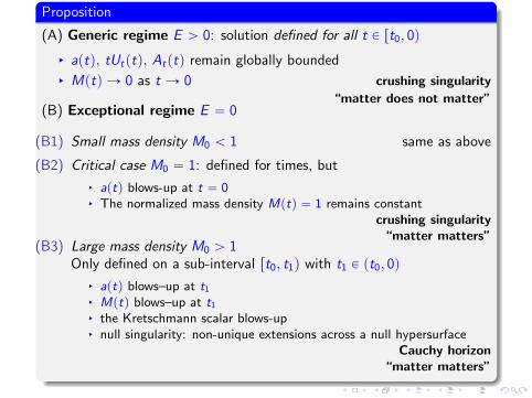
Proposition
(A) Generic regime E ą 0: solution defined for all t P rt0, 0q
§ aptq, tUtptq, Atptq remain globally bounded
§ Mptq Ñ 0 as t Ñ 0 crushing singularity
“matter does not matter”(B) Exceptional regime E “ 0
(B1) Small mass density M0 ă 1 same as above
(B2) Critical case M0 “ 1: defined for times, but
§ aptq blows-up at t “ 0§ The normalized mass density Mptq “ 1 remains constant
crushing singularity“matter matters”
(B3) Large mass density M0 ą 1Only defined on a sub-interval rt0, t1q with t1 P pt0, 0q
§ aptq blows–up at t1
§ Mptq blows–up at t1
§ the Kretschmann scalar blows-up§ null singularity: non-unique extensions across a null hypersurface
Cauchy horizon“matter matters”

Section 3. FUTURE GEODESIC COMPLETENESSOF WEAKLY REGULAR GOWDY SPACETIMES
Section 3.1 MAIN STATEMENT
From our result in Chapter III.
Theorem
Given any non–flat, weakly regular T 2-symmetric initial data set pΣ, h,K qwith topology T 3 whose initial area R0 ą 0 of the orbits of symmetry is aconstant, there exists a weakly regular, Ricci-flat spacetime pM, gq withT 2–symmetry on T 3
§ a development of pΣ, h,K q, maximal among all such developments
§ a unique global foliation by level sets of the area R
R P rR0,8q in the future expanding direction
R P p0,R0s in the past contracting direction, except for flat Kasner(homogeneous) spacetimes
In other words:
§ Generic initial data sets lead to a global foliation
§ But there exist exceptional solutions (incomplete geodesics, nullsingularities)
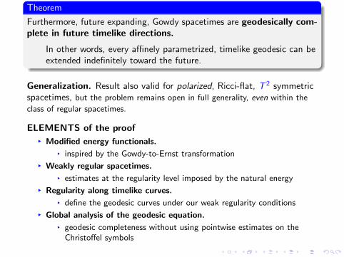
Theorem
Furthermore, future expanding, Gowdy spacetimes are geodesically com-plete in future timelike directions.
In other words, every affinely parametrized, timelike geodesic can beextended indefinitely toward the future.
Generalization. Result also valid for polarized, Ricci-flat, T 2 symmetricspacetimes, but the problem remains open in full generality, even within the
class of regular spacetimes.
ELEMENTS of the proof§ Modified energy functionals.
§ inspired by the Gowdy-to-Ernst transformation
§ Weakly regular spacetimes.§ estimates at the regularity level imposed by the natural energy
§ Regularity along timelike curves.§ define the geodesic curves under our weak regularity conditions
§ Global analysis of the geodesic equation.§ geodesic completeness without using pointwise estimates on the
Christoffel symbols

COORDINATES general T 2 symmetryAreal coordinates. R coincides with the time variable
g “ e2pη´Uq`
´ dR2 ` a´2 dθ2˘
` e2U´
dx ` Ady ``
G ` AH˘
dθ¯2
` e´2UR2`
dy ` H dθ˘2
§ unknowns U,A, η, a,G ,H Two Killing fields X ,Y
§ functions of the area (of the symmetry orbits) R and θ P S1
§ R describes an interval rR0,R1q, and x , y , θ describe S1
WEAK REGULARITY CONDITIONS
U,A P C 0prR0,R1q,H1pS1qq η P C 0prR0,R1q,W
1,1θ pS1qq
a, a´1 P C 0prR0,R1q,W2,1pS1qq G ,H P C 0prR0,R1q, L
8pS1qq
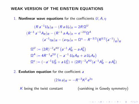
WEAK VERSION OF THE EINSTEIN EQUATIONS
1. Nonlinear wave equations for the coefficients U,A, η
pR a´1URqR ´ pR aUθqθ “ 2R ΩU
pR´1 a´1ARqR ´ pR´1 a Aθqθ “ e´2UΩA
pa´1ηRqR ´ pa ηθqθ “ Ωη ´ R´32`
R32`
a´1˘
R
˘
R
ΩU :“ p2Rq´2e4U`
a´1 A2R ´ a A2
θ
˘
ΩA :“ 4R´1e2U`
´ a´1 URAR ` a UθAθ˘
Ωη :“ p´a´1U2R ` a U2
θ q ` p2Rq´2e4Upa´1A2
R ´ a A2θq
2. Evolution equation for the coefficient a
p2 ln aqR “ ´R´3K 2 e2η
K being the twist constant (vanishing in Gowdy symmetry)
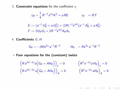
3. Constraint equations for the coefficient η
ηR `1
4R´3 e2ηK 2 “ a RE ηθ “ R F
E :“`
a´1 U2R ` a U2
θ
˘
` p2Rq´2e4U`
a´1 A2R ` a A2
θ
˘
F :“ 2URUθ ` 2R´2e2UARAθ
4. Coefficients G ,H
GR “ ´AKe2η a´1R´3 HR “ Ke2η a´1R´3
§ Four equations for the (constant) twists
´
R e4U´2ηa´
GR ` AHR
¯¯
θ“ 0
´
R3 e´2ηaHR
¯
θ“ 0
´
R e4U´2η a´
GR ` AHR
¯¯
R“ 0
´
R3 e´2η aHR
¯
R“ 0
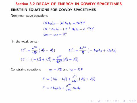
Section 3.2 DECAY OF ENERGY IN GOWDY SPACETIMES
EINSTEIN EQUATIONS FOR GOWDY SPACETIMES
Nonlinear wave equations
pR URqR ´ pR Uθqθ “ 2R ΩU
pR´1 ARqR ´ pR´1 Aθqθ “ e´2UΩA
ηRR ´ ηθθ “ Ωη
in the weak sense
ΩU :“e4U
4R2
`
A2R ´ A2
θ
˘
ΩA :“4e2U
R
`
´ URAR ` UθAθ˘
Ωη :“`
´ U2R ` U2
θ
˘
`e4U
4R2
`
A2R ´ A2
θ
˘
Constraint equations ηR “ RE and ηθ “ R F
E :“`
U2R ` U2
θ
˘
`e4U
4R2
`
A2R ` A2
θ
˘
F :“ 2URUθ `e4U
2R2ARAθ

ENERGY FUNCTIONALS. Basic energy
EpRq :“
ż
S1
E pR, θq dθ E :“ EU ` EA
EU :“ pURq2 ` pUθq
2 EA :“e4U
4R2
´
pARq2 ` pAθq
2¯
d
dREpRq “ ´ 2
R
ż
S1
´
pURq2 `
e4U
4R2pAθq
2¯
dθ
Proposition. Integral energy decay for UR and Aθ
EpRq ď EpR0q R P rR0,`8q
1
RηRpR, ¨qL1pS1q ď EpR0q
1
RηθpR, ¨qL1pS1q ď EpR0q
›
›
›
4
RpURq
2›
›
›
L1ppR0,`8qˆS1qq`
›
›
›
1
R3e4U pAθq
2›
›
›
L1ppR0,`8qˆS1qqď 2 EpR0q

Gowdy-to-Ernst transformation and decay property for AR
§ Only a partial dissipation estimate on UR and Aθ§ Decay for AR derived now from another functional
Recall the Gowdy-to-Ernst transformation:
U 1 :“ lnpR12q ´ U
A1R :“ e4UR´1Aθ A1θ :“ e4UR´1AR
U 1,A1 satisfy the same evolution equations:
pR U 1RqR ´ pR U 1θqθ “ 2R ΩU1
pR´1 A1RqR ´ pR´1 A1θqθ “ e´2U1ΩA1
Modified energy an arbitrary parameter b P R(interpolation between b “ 0 and b “ 12)
Eb :“
ż
S1
´
UR ´ bR´1¯2
` pUθq2 `
e4U
4R2
´
pARq2 ` pAθq
2¯
“E ´ 2b
R
ż
S1
UR `b2
R2
ż
S1
dθ
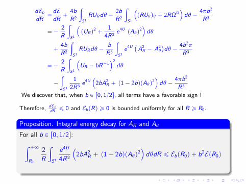
dEb
dR“dEdR
`4b
R2
ż
S1
RURdθ ´2b
R2
ż
S1
´
pRUθqθ ` 2RΩU¯
dθ ´4πb2
R3
“´2
R
ż
S1
´
pURq2`
1
4R2e4U
pAθq2¯
dθ
`4b
R2
ż
S1
RURdθ ´b
R3
ż
S1
e4U`
A2R ´ A2
θ
˘
dθ ´4b2π
R3
“´2
R
ż
S1
´
UR ´ bR´1¯2
dθ
´
ż
S1
1
2R3e4U
´
2bA2R ` p1´ 2bqpAθq
2¯
dθ ´4πb2
R3
We discover that, when b P r0, 12s, all terms have a favorable sign !
Therefore, dEbdRď 0 and EbpRq ě 0 is bounded uniformly for all R ě R0.
Proposition. Integral energy decay for AR and Aθ
For all b P r0, 12s:
ż `8
R0
2
R
ż
S1
e4U
4R2
´
2bA2R ` p1´ 2bqpAθq
2¯
dθdR ď EbpR0q ` b2EpR0q

We ned yet another energy functional Fix some b P r0, 12q
pEpRq :“EbpRq ` GUpRq
GU :“1
R
ż
S1
`
U ´@
UD˘
UR dθ
with the average of a function f “ f pθq defined by@
fD
:“ 12π
ş
S1 f dθ.
Specifically, we will use this strategy
§ with b “ 14 and therefore pEpRq “ E14pRq ` GUpRq
§ only for sufficiently large R
Theorem. The rate of decay of energy
For all Gowdy spacetimes, one has
EpRq » pEpRq ď C0
RR P rR0,`8q
where C0 ą 0 depends only on the initial data U0 “ UpR0, ¨q and A0 “
ApR0, ¨q.

Heuristics when R Ñ `8
§ one might expect that
d
dRpEpRq ď ´ 2
RpEpRq (modulo higher order terms)
§ pE should decay like 1R2
§ indeed correct for spatially homogeneous (Gowdy or general T 2)spacetimes
However, for non-spatially homogeneous spacetimes
§ asymptotic equi-partition of energy
§ space derivatives = time derivatives
§ we expect
d
dRpEpRq ď ´ 1
RpEpRq (modulo higher order terms)
§ pE should decay like 1R
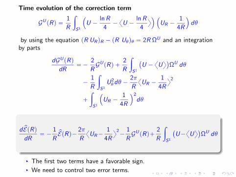
Time evolution of the correction term
GUpRq “1
R
ż
S1
´
U ´lnR
4´@
U ´lnR
4
D
¯´
UR ´1
4R
¯
dθ
by using the equation pR URqR ´ pR Uθqθ “ 2R ΩU and an integrationby parts
dGUpRq
dR“´
2
RGUpRq `
2
R
ż
S1
`
U ´@
UD˘
ΩU dθ
´1
R
ż
S1
U2θdθ ´
2π
R
@
UR ´1
4R
D2
`
ż
S1
´
UR ´1
4R
¯2
dθ
d pEpRqdR
“ ´1
RpEpRq´ 2π
R
@
UR´1
4R
D2´
1
RGUpRq`
2
R
ż
S1
`
U´@
UD˘
ΩU dθ
§ The first two terms have a favorable sign.§ We need to control two error terms.
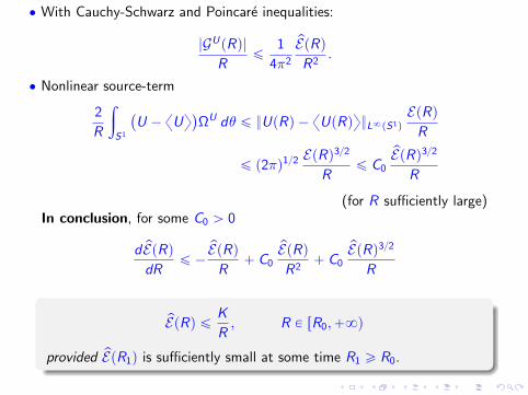
‚ With Cauchy-Schwarz and Poincare inequalities:
|GUpRq|
Rď
1
4π2
pEpRqR2
.
‚ Nonlinear source-term
2
R
ż
S1
`
U ´@
UD˘
ΩU dθ ď UpRq ´@
UpRqD
L8pS1q
EpRqR
ď p2πq12EpRq32
Rď C0
pEpRq32
R
(for R sufficiently large)In conclusion, for some C0 ą 0
d pEpRqdR
ď ´pEpRqR
` C0
pEpRqR2
` C0
pEpRq32
R
pEpRq ď K
R, R P rR0,`8q
provided pEpR1q is sufficiently small at some time R1 ě R0.

The energy decreases to zero.
§ Recall that an integral decay property was already established forU2R ,A
2R ,A
2θ.
§ To control Uθ, we return to our functional GUpRq
dGUpRq
dRď´
2
RGUpRq `
2
R
ż
S1
ΩU`
U ´@
UD˘
dθ `
ż
S1
´
UR ´1
4R
¯2
dθ
´1
R
ż
S1
U2θdθ
§ All the terms therein are controled by U2R ,A
2R ,A
2θ, except U2
θ whichhowever has a favorable sign.
§ Use the integrability of EA
R , etc. in order to deduce that 1R
ş
S1 U2θdθ
is integrable in time.
Therefore, 1RpEpRq is integrable in time and, since pEpRq is decreasing,
pEpRq Ñ 0.
Rate of decay of energy for all Gowdy spacetimes: EpRq ď C0
R
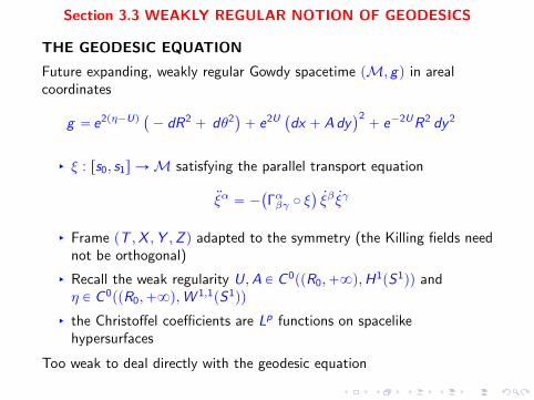
Section 3.3 WEAKLY REGULAR NOTION OF GEODESICS
THE GEODESIC EQUATION
Future expanding, weakly regular Gowdy spacetime pM, gq in arealcoordinates
g “ e2pη´Uq`
´ dR2 ` dθ2˘
` e2U`
dx ` Ady˘2` e´2UR2 dy2
§ ξ : rs0, s1s ÑM satisfying the parallel transport equation
:ξα “ ´`
Γαβγ ˝ ξ˘
9ξβ 9ξγ
§ Frame pT ,X ,Y ,Z q adapted to the symmetry (the Killing fields neednot be orthogonal)
§ Recall the weak regularity U,A P C 0ppR0,`8q,H1pS1qq and
η P C 0ppR0,`8q,W1,1pS1qq
§ the Christoffel coefficients are Lp functions on spacelikehypersurfaces
Too weak to deal directly with the geodesic equation

Theorem. Existence of weakly regular geodesics
Given ξ0 PM, and a future-oriented timelike vector ξ1 P Tξ0M and someinitial affine parameter s0:
§ There exist s1 ą s0 and a curve ξ PW 1,8pps0, s1q,Mq satisfying
:ξα “ ´`
Γαβγ ˝ ξ˘
9ξβ 9ξγ , ξps0q “ ξ0, 9ξps0q “ ξ1
§ pΓαβγ ˝ ξq P L1ps0, s1q along any (uniformly) timelike curve, so that
9ξ PW 1,1ps0, s1q.
§ For every pξ0, ξ1q, there exists at least one maximal geodesic definedon some interval rs0, s‹q.
Elements of proof
§ Uniform bounds for a sequence of curves in weakly regularspacetimes
§ L1 regularity of the Christoffel symbols along timelike curves
§ Formulation of the geodesic problem as a nonlinear equation for thetime component 9ξR with algebraic constraints
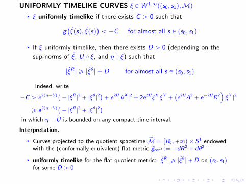
UNIFORMLY TIMELIKE CURVES ξ PW 1,8pps0, s1q,Mq
§ ξ uniformly timelike if there exists C ą 0 such that
g`
9ξpsq, 9ξpsq˘
ă ´C for almost all s P ps0, s1q
§ If ξ uniformly timelike, then there exists D ą 0 (depending on the
sup-norms of 9ξ, U ˝ ξ, and η ˝ ξ) such that
| 9ξR | ě | 9ξθ| ` D for almost all s P ps0, s1q
Indeed, write
´C ą e2pη´Uq`
´ |ξR |2 ` |ξθ|2˘
` e2U|θX |2 ` 2e2UξX ξY `
`
e2UA2` e´2UR2
¯
|ξY |2
ě e2pη´Uq`
´ |ξR |2 ` |ξθ|2˘
in which η ´ U is bounded on any compact time interval.
Interpretation.
§ Curves projected to the quotient spacetime ĂM “ rR0,`8q ˆ S1 endowedwith the (conformally equivalent) flat metric rgconf :“ ´dR2
` dθ2
§ uniformly timelike for the flat quotient metric: | 9ξR | ě | 9ξθ| `D on ps0, s1q
for some D ą 0

Using our earlier analysis of weakly regular T 2 symmetric spacetimes
§ the structure of the Einstein equations
§ energy arguments
§ integration in a domain bounded by two timelike curves ξ1, ξ2 and twospacelike hypersurfaces
Proposition. Higher-integrability of Christoffel symbols along timelike curves
Let ξ PW 1,8pps0, s1q,Mq be a uniformly timelike curve.
§ The metric coefficients pU ˝ ξq and pA ˝ ξq along this curve belong toH1ps0, s1q. Consequently, for α “ R, θ and a, b “ X ,Y , the trace of Γαβγ
on ξ is well-defined, with Γαab ˝ ξ P L2ps0, s1q
§ η ˝ ξ belongs to W 1,1ps0, s1q. Consequently, for all α, β, γ “ R, θ, x , y , the
trace of Γαβγ on ξ is well-defined and Γαβγ ˝ ξ P L1ps0, s1q.
Stability of Christoffel symbols along timelike curves:
§ Γγαβ ˝ ξL1ps0,s1qď δps0 ´ s1q (equi-integrability)
§ δ is a continuous function satisfying δp0q “ 0§ depending only on D, Rpξps0qq, and Rpξps1qq
§ independent of ξ
§ For every sequence ξε approaching ξ in W 1,8pps0, s1q,Mq :
pΓγαβ ˝ ξεq9ξαε ´ pΓ
γαβ ˝ ξq
9ξαL1ps0,s1qÑ 0
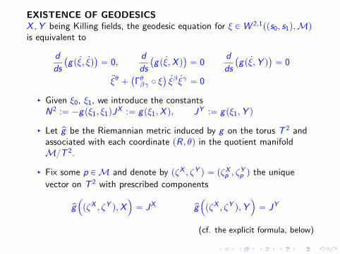
EXISTENCE OF GEODESICSX ,Y being Killing fields, the geodesic equation for ξ PW 2,1pps0, s1q,Mq
is equivalent to
d
ds
`
gp 9ξ, 9ξq˘
“ 0,d
ds
`
gp 9ξ,X q˘
“ 0d
ds
`
gp 9ξ,Y q˘
“ 0
:ξθ ``
Γθβγ ˝ ξ˘
9ξβ 9ξγ “ 0
§ Given ξ0, ξ1, we introduce the constantsN2 :“ ´gpξ1, ξ1qJ
X :“ gpξ1,X q, JY :“ gpξ1,Y q
§ Let pg be the Riemannian metric induced by g on the torus T 2 andassociated with each coordinate pR, θq in the quotient manifoldMT 2.
§ Fix some p PM and denote by pζX , ζY q “ pζXp , ζYp q the unique
vector on T 2 with prescribed components
pg´
pζX , ζY q,X¯
“ JX pg´
pζX , ζY q,Y¯
“ JY
(cf. the explicit formula, below)
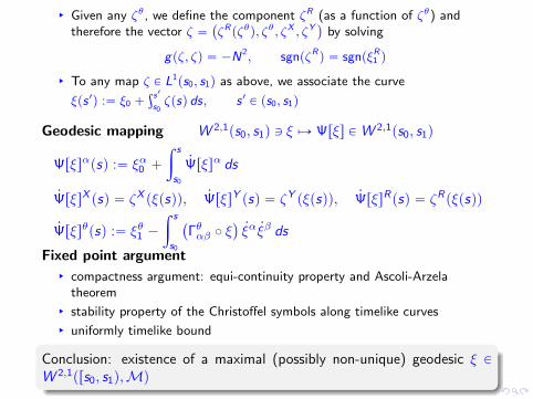
§ Given any ζθ, we define the component ζR (as a function of ζθ) andtherefore the vector ζ “
`
ζRpζθq, ζθ, ζX , ζY˘
by solving
gpζ, ζq “ ´N2, sgnpζRq “ sgnpξR1 q
§ To any map ζ P L1ps0, s1q as above, we associate the curve
ξps 1q :“ ξ0 `şs1
s0ζpsq ds, s 1 P ps0, s1q
Geodesic mapping W 2,1ps0, s1q Q ξ ÞÑ Ψrξs PW 2,1ps0, s1q
Ψrξsαpsq :“ ξα0 `
ż s
s0
9Ψrξsα ds
9ΨrξsX psq “ ζX pξpsqq, 9ΨrξsY psq “ ζY pξpsqq, 9ΨrξsRpsq “ ζRpξpsqq
9Ψrξsθpsq :“ ξθ1 ´
ż s
s0
`
Γθαβ ˝ ξ˘
9ξα 9ξβ ds
Fixed point argument§ compactness argument: equi-continuity property and Ascoli-Arzela
theorem
§ stability property of the Christoffel symbols along timelike curves
§ uniformly timelike bound
Conclusion: existence of a maximal (possibly non-unique) geodesic ξ PW 2,1prs0, s1q,Mq
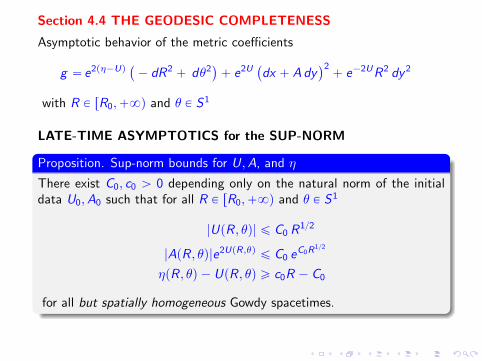
Section 4.4 THE GEODESIC COMPLETENESS
Asymptotic behavior of the metric coefficients
g “ e2pη´Uq`
´ dR2 ` dθ2˘
` e2U`
dx ` Ady˘2` e´2UR2 dy2
with R P rR0,`8q and θ P S1
LATE-TIME ASYMPTOTICS for the SUP-NORM
Proposition. Sup-norm bounds for U,A, and η
There exist C0, c0 ą 0 depending only on the natural norm of the initialdata U0,A0 such that for all R P rR0,`8q and θ P S1
|UpR, θq| ď C0 R12
|ApR, θq|e2UpR,θq ď C0 eC0R
12
ηpR, θq ´ UpR, θq ě c0R ´ C0
for all but spatially homogeneous Gowdy spacetimes.

Arguments for U.
Upθ,Rq “ 12π
ş
S1
´
şθ
θ1Uθpθ
2,Rqdθ2¯
dθ1 ` 12π
ş
S1 Upθ1,Rq dθ1
Using Cauchy-Schwarz inequality, for all θ P S1 and R ě R0
|Upθ,Rq| ď p2πq12´
ż
S1
|Uθ|2pθ2,Rqdθ2
¯12
`
ˇ
ˇ
ˇ
ˇ
1
2π
ż
S1
Upθ1,Rq dθ1ˇ
ˇ
ˇ
ˇ
§ First term in R´12 thanks to our energy decay property
§ Second termˇ
ˇ
ˇ
ˇ
ż
S1
Upθ1,Rq dθ1ˇ
ˇ
ˇ
ˇ
ď
ˇ
ˇ
ˇ
ˇ
ż
S1
ż R
R0
URpθ1,R 1qdR 1dθ1
ˇ
ˇ
ˇ
ˇ
`
ˇ
ˇ
ˇ
ˇ
ż
S1
U0 dθ1
ˇ
ˇ
ˇ
ˇ
§ first term
ˇ
ˇ
ˇ
ˇ
ż
S1
ż R
R0
URpθ1,R 1qdR 1dθ1
ˇ
ˇ
ˇ
ˇ
À
ż R
R0
ˇ
ˇ
ˇ
ˇ
ż
S1
U2Rpθ
1,R 1q dθ1ˇ
ˇ
ˇ
ˇ
12
dR 1
À
ż R
R0
pR 1q´12dR 1 À R12
§ second term controlled by the H1 norm of U0

Arguments for rA :“ Ae2U . For all θ P S1 and R ě R0
rApR, θq “1
2π
ż
S1
rApR, ¨q dθ1 `1
2π
ż
S1
ż θ
θ1
´
Ae2U¯
θpR, θ2q dθ2dθ1
§ First termˇ
ˇ
ˇ
ˇ
ż
S1
rApR, θ1q dθ1ˇ
ˇ
ˇ
ˇ
“
ˇ
ˇ
ˇ
ˇ
ˇ
ż
rA0 dθ1`
ż R
R0
ż
S1
pARe2U` 2AURe
2Uq dθ1dR 1
ˇ
ˇ
ˇ
ˇ
ˇ
ď C0 ` p2πq12
ż R
R0
´
ż
S1
A2Re
4U dθ1¯12
dθ1dR 1
`
ż R
R0
´
ż
S1
A2e4U dθ1¯12´
ż
S1
U2R dθ1
¯12
dR 1.
By setting N8pRq :“ ApR, ¨qe2UpR,¨qL8pS1q
ˇ
ˇ
ˇ
ˇ
ż
S1
rApR, θ1q dθ1ˇ
ˇ
ˇ
ˇ
À 1` R32`
ż R
R0
N8pR 1q
R 112dR 1
§ Second termˇ
ˇ
ˇ
ˇ
ż θ
θ1
´
Ae2U¯
θpR, θ2q dθ2
ˇ
ˇ
ˇ
ˇ
ď
ż
S1
|Aθ| e2UpR, θ2q dθ2 `
ż
S1
ˇ
ˇ
ˇAe2U2Uθ
ˇ
ˇ
ˇpR, θ2q dθ2
À R12` R´12N8pRq
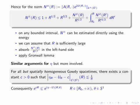
Hence for the norm N8pRq :“ ApR, ¨qe2UpR,¨qL8pS1q
N8pRq À 1` R12 ` R32 `N8pRq
R12`
ż R
R0
N8pR 1q
R 112dR 1
§ on any bounded interval, N8 can be estimated directly using theenergy
§ we can assume that R is sufficiently large
§ absorb N8pRqR12 in the left-hand side
§ apply Gronwall lemma
Similar arguments for η but more involved.
For all but spatially homogeneous Gowdy spacetimes, there exists a con-
stant c ą 0 such that›
›
›ηR ´ UR ´ c
›
›
›
L1pS1qpRq À 1
R
Consequently ecR À epη´UqpR,θq R P rR0,`8q, θ P S1

FORMULATION IN TERMS OF THE TIME COMPONENT 9ξR
Reduction based on the angular momentum
One says that a geodesic curve is future complete if it is global in the futuredirection, i.e. its interval of definition in the affine parameter is of the formrs0,`8q ∇ 9ξ
9ξ “ 0 9ξR ą 0
§ Let ξ PW 2,1pprs0, s1q,Mq be a future directed, maximal solution to the
geodesic equation.
§ Denote by K ą 0 the (conserved) norm of 9ξ defined by ´K 2“ gp 9ξ, 9ξq
§ Denote by JX and JY the (conserved) angular momenta gp 9ξ,X q andgp 9ξ,Y q
∇ 9ξgp9ξ,X q “ gp 9ξ,∇ 9ξX q “
9ξi 9ξj∇iXj “12
9ξi 9ξj`
∇iXj `∇jXi
˘
“ 0
Conservation along ξ of the two angular momenta
JX ps0q “ JX psq :“ gp 9ξ,X q “ e2U`
9ξX ` A 9ξY˘
JY ps0q “ JY psq :“ gp 9ξ,Y q “ e2UA`
9ξX ` A 9ξY˘
` e´2UR2 9ξY
9ξX “´
R´2A2e2U ` e´2U¯
JX ´ Ae2UR´2JY
9ξY “ ´Ae2UR´2JX ` R´2e2UJY

9ξX “´
R´2A2e2U` e´2U
¯
JX ´ Ae2UR´2JY
9ξY “ ´Ae2UR´2JX ` R´2e2UJY
Recall our sup-norm bounds
|UpR, θq| ď C0 R12
|ApR, θq|e2UpR,θqď C0 e
C0R12
Lemma. Asymptotics of the X ,Y components of a geodesic
There exists a constant C0 ą 0 depending on the initial metric U0,A0 andthe initial momenta JX , JY of the geodesic ξ such that for all s P rs0, s1q
| 9ξX | ` | 9ξY | ď C0 eC0 Rpξq
12
in W 1,1prs0, s1qq
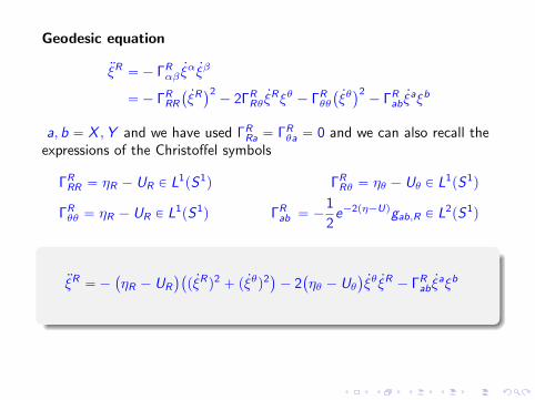
Geodesic equation
:ξR “´ ΓRαβ
9ξα 9ξβ
“´ ΓRRR
`
9ξR˘2´ 2ΓR
Rθ9ξRξθ ´ ΓR
θθ
`
9ξθ˘2´ ΓR
ab9ξaξb
a, b “ X ,Y and we have used ΓRRa “ ΓR
θa “ 0 and we can also recall theexpressions of the Christoffel symbols
ΓRRR “ ηR ´ UR P L
1pS1q ΓRRθ “ ηθ ´ Uθ P L
1pS1q
ΓRθθ “ ηR ´ UR P L
1pS1q ΓRab “ ´
1
2e´2pη´Uqgab,R P L
2pS1q
:ξR “´`
ηR ´ UR
˘`
p 9ξRq2 ` p 9ξθq2˘
´ 2`
ηθ ´ Uθ˘
9ξθ 9ξR ´ ΓRab
9ξaξb

Recall now the Einstein equations for η
ηR ´ UR “ R´
UR ´1
2R
¯2
` R U2θ `
e4U
4R2
´
A2R ` A2
θ
¯
´1
4R
ηθ ´ Uθ “ 2R´
UR ´1
2R
¯
Uθ `e4U
2RARAθ
|ηθ ´ Uθ| ď´
ηR ´ UR `1
4R
¯
We have
:ξR “ ´´
ηR ´ UR
¯´
p 9ξRq2 ` p 9ξθq2¯
´ 2´
ηθ ´ Uθ¯
9ξθ 9ξR ´ ΓRab
9ξaξb
ď1
4R
´
p 9ξRq2 ` p 9ξθq2¯
´ ΓRab
9ξaξb ď1
2Rp 9ξRq2 ´ ΓR
ab9ξaξb
since
§ the matrix´
ηR ´ UR `1
4Rηθ ´ Uθ
ηθ ´ Uθ ηR ´ UR `1
4R
¯
is negative definite
§ p 9ξθq2 ď p 9ξRq2, since the curve is timelike
In view of dRds“ 9ξR , we obtain :ξR ď 1
2RdRds
9ξR ´ ΓRab
9ξa 9ξb
Proposition. Evolution equation for 9ξR
d
ds
´
R´12 9ξR¯
ď ´R´12ΓRab
9ξa 9ξb
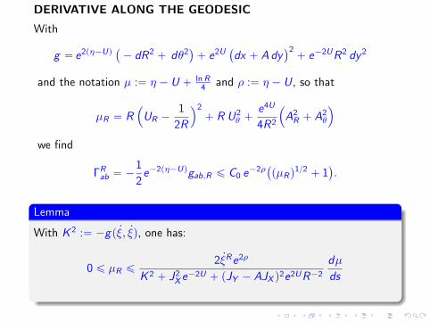
DERIVATIVE ALONG THE GEODESIC
With
g “ e2pη´Uq`
´ dR2 ` dθ2˘
` e2U`
dx ` Ady˘2` e´2UR2 dy2
and the notation µ :“ η ´ U ` ln R4 and ρ :“ η ´ U, so that
µR “ R´
UR ´1
2R
¯2
` R U2θ `
e4U
4R2
´
A2R ` A2
θ
¯
we find
ΓRab “ ´
1
2e´2pη´Uqgab,R ď C0 e
´2ρ`
pµRq12 ` 1
˘
.
Lemma
With K 2 :“ ´gp 9ξ, 9ξq, one has:
0 ď µR ď2 9ξRe2ρ
K 2 ` J2X e´2U ` pJY ´ AJX q2e2UR´2
dµ
ds

Proof. The length of the tangent vector K 2 :“ ´gp 9ξ, 9ξq is conserved along thegeodesic:
e´2pη´Uq´
K 2` e2U
`
9ξX ` A 9ξY˘2` e´2UR2
`
9ξY˘2¯
“`
9ξR˘2´`
9ξθ˘2
and in terms the conserved momenta JX , JY
9ξX “´
R´2A2e2U` e´2U
¯
JX ´ Ae2UR´2JY
9ξY “ ´Ae2UR´2JX ` R´2e2UJY
˜
9ξθ
9ξR
¸2
“ 1´e´2ρ
p 9ξRq2
´
K 2` J2
X e´2U
` pJY ´ AJX q2e2UR´2
¯
“: 1´ χ
In other words, | 9ξθ| “ p1´ χq12 9ξR (strictly timelike vector)
First-order derivative ρR “ ηR ´ UR and µR “ ρR `1
4Rě |ρθ| (Einstein
constraints):dρ
ds“
`
µR ´1
4R
˘
9ξR ` ρθ 9ξθ
ě
´
1´ p1´ χq12¯
µR9ξR ´
1
4R9ξR
Hence: µR ď19ξRp1´ p1´ χq12q´1 dµ
dsand we finally use that
1´ p1´ αq12 ě α2
for α P r0, 1s.
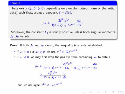
Lemma
There exists C0,C1 ě 0 (depending only on the natural norm of the initialdata) such that, along a geodesic ξ “ ξpsq,
µR ď2 9ξR e2ρ
K 2 ` C1 e´C0R12
dµ
ds.
Moreover, the constant C1 is stricly positive unless both angular momentaJX , JY vanish.
Proof. If both JX and JY vanish, the inequality is already established.
§ If JX “ 0 but JY ‰ 0, we use e2Uď C0e
C0R12
.
§ If JX ‰ 0, we may first drop the positive term containing JY to obtain
µR ď2 9ξRe2ρ
K 2 ` J2X e´2U ` pJY ´ AJX q2e2UR´2
dµ
ds
ď2 9ξRe2ρ
K 2 ` J2X e´2U
dµ
ds
and we use again e2Uď C0e
C0R12
.
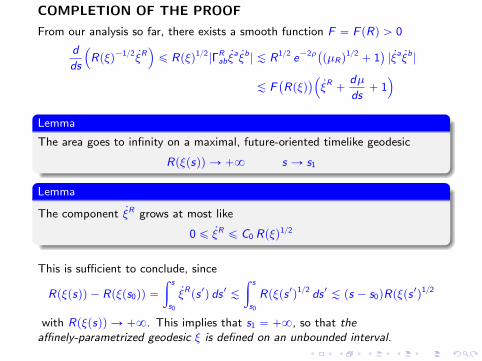
COMPLETION OF THE PROOF
From our analysis so far, there exists a smooth function F “ F pRq ą 0
d
ds
´
Rpξq´12 9ξR¯
ď Rpξq12|ΓRab
9ξa 9ξb| À R12 e´2ρ`
pµRq12` 1
˘
| 9ξa 9ξb|
À F`
Rpξq˘
´
9ξR `dµ
ds` 1
¯
Lemma
The area goes to infinity on a maximal, future-oriented timelike geodesic
Rpξpsqq Ñ `8 s Ñ s1
Lemma
The component 9ξR grows at most like
0 ď 9ξR ď C0 Rpξq12
This is sufficient to conclude, since
Rpξpsqq ´ Rpξps0qq “
ż s
s0
9ξRps 1q ds 1 À
ż s
s0
Rpξps 1q12 ds 1 À ps ´ s0qRpξps1q
12
with Rpξpsqq Ñ `8. This implies that s1 “ `8, so that theaffinely-parametrized geodesic ξ is defined on an unbounded interval.
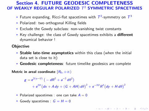
Section 4. FUTURE GEODESIC COMPLETENESSOF WEAKLY REGULAR POLARIZED T 2 SYMMETRIC SPACETIMES
§ Future expanding, Ricci-flat spacetimes with T 2-symmetry on T 3
§ Polarized: two orthogonal Killing fields
§ Exclude the Gowdy subclass: non-vanishing twist constants
§ Key challenge: the class of Gowdy spacetimes exhibits a differentdynamical behavior !
Objective
§ Stable late-time asymptotics within this class (when the initialdata set is close to it)
§ Geodesic completeness: future timelike geodesics are complete
Metric in areal coordinate rR0,`8q
g “ e2pη´Uq`
´ dR2` a´2 dθ2
˘
` e2U`
dx ` Ady ` pG ` AHq dθ˘2` e´2UR2
`
dy ` H dθ˘2
§ Polarized spacetimes : one can take A “ 0
§ Gowdy spacetimes : G “ H “ 0
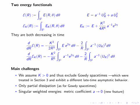
Two energy functionals
EpRq :“
ż
S1
E pR, θq dθ E “ a´1 U2R ` a U2
θ
EK pRq :“
ż
S1
EK pR, θq dθ EK :“ E `K 2
4R4a´1e2η
They are both decreasing in time
d
dREpRq “ ´ K 2
2R3
ż
S1
E e2η dθ ´2
R
ż
S1
a´1 pURq2dθ
d
dREK pRq “ ´
K 2
R5
ż
S1
a´1e2η dθ ´2
R
ż
S1
a´1 pURq2 dθ
Main challenges
§ We assume K ą 0 and thus exclude Gowdy spacetimes —which were
treated in Section 3 and exhibit a different late-time asymptotic behavior.
§ Only partial dissipation (as for Gowdy spacetimes)
§ Singular weighted energies: metric coefficient aÑ 0 (new feature)

VOLUME-RESCALED ENERGY FUNCTIONALS
Volume of the slice R “constant for the conformal 2-metric´dR2 ` a´2 dθ2
FpRq “ PpRqEpRq PpRq “ż
S1
dθ
apR, θq
Heuristic leading to the asymptotic behavior
PpRq „ R12 PRpRq „ R´12
e2η „ R2 a „ R´12
(instead of PpRq being constant for Gowdy spacetimes !)
Corrected energy
GpRq :“ PpRq`
EpRq ` GUpRq˘
GUpRq :“1
R
ż
S1
`
U ´@
UD˘
UR a´1 dθ
@
UD
: volume-weighted average

Formal derivation of an asymptotic model
§ From the energies G “ P´
E ` GU¯
and
GK “K 2
2
ż
S1
e2ηa´1 dθ
we define the (dimensionless) rescaled energies
c :“P
R?G, d :“
GK
R3?G
§ Neglect second- and higher-order contributions
§ The functions c , d satisfy the asymptotic ODE model
cR “d
R´
c
R`
c
2R
dR “2dc´2
R´
3
Rd `
d
2R
§ Global stable equilibrium and shifted variables
c1 “ c ´2?
5, d1 “ d ´
1?
5
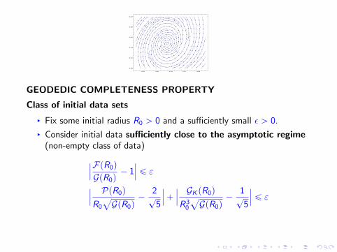
0.86 0.88 0.90 0.92 0.94
0.40
0.42
0.44
0.46
0.48
0.50
GEODEDIC COMPLETENESS PROPERTY
Class of initial data sets
§ Fix some initial radius R0 ą 0 and a sufficiently small ε ą 0.
§ Consider initial data sufficiently close to the asymptotic regime(non-empty class of data)
ˇ
ˇ
ˇ
FpR0q
GpR0q´ 1
ˇ
ˇ
ˇď ε
ˇ
ˇ
ˇ
PpR0q
R0
a
GpR0q´
2?
5
ˇ
ˇ
ˇ`
ˇ
ˇ
ˇ
GK pR0q
R30
a
GpR0q´
1?
5
ˇ
ˇ
ˇď ε

Theorem. Weakly regular, T2-symmetric polarized Ricci-flat spacetimes
If the initial data set is sufficiently close to the asymptotic regime on someinitial slice of area R0 then the spacetime asymptotically approaches theasymptotic regime
Volume of a slice PpRq “ 2C120?5
R12 ` OpR14q
Energy of a slice EpRq “ OpR´32q
Rescaled energy GpRq “ C0R´1 ` OpR´32q
Rescaled twist energy GK pRq “C
120?5R52 ` OpR94q
where C0 ą 0 is a constant depending on the initial data set.Polarized T 2 symmetric, weakly regular, Ricci-flat spacetimes are geodesi-cally complete in future timelike directions.
Open problems
§ asymptotics far from the asymptotic regime
§ asymptotics of non-polarized T 2 spacetimes
REFERENCES for this Chapter
§ H. Andreasson, Ann. Henri Poincare (2012). [Vlasov matter]
§ A. Burtscher and P.G. LeFloch, J. Math. Pures Appl. (2014).
[compressible fluid]
§ D. Christodoulou, The formation of black holes in general relativity, 2009.
[Ricci-flat]
§ N. Grubic N. and P.G. LeFloch, Arch. Rational Mech. Anal. (2013).
[compressible fluid]
§ J. Isenberg and M. Weaver, Class. Quantum Grav. (2003). [Ricci-flat]
§ P.G. LeFloch and J. Smulevici, J. Differ. Equa. (2015). [Ricci-flat]
§ H. Ringstrom, Comm. Pure Appl. Math. (2004).
NEXT (and final) TOPIC
§ The global nonlinear stability of Minkowski spacetime
§ Einstein-matter system for a massive scalar field
§ The Hyperboloidal Foliation Method (LeFloch-Ma, 2014)

CHAPTER VITHE GLOBAL NONLINEAR STABILITY OFMINKOWSKI SPACE for MASSIVE FIELDS
Global existence problem for the Einstein equations§ Self-gravitating massive scalar field§ Choice of gauge (De Donder): wave coordinates lgxα “ 0§ Nonlinear stability of Minkowski spacetime
Hyperboloidal Foliation Method§ New method of analysis for quasilinear wave-Klein-Gordon systems§ A framework leading to sharp decay rates§ A p3` 1q-foliation of Minkowski spacetime by hyperboloids
Section 1 The general strategy
1.1 Wave-Klein-Gordon problems1.2 The hyperboloidal foliation1.3 Wave-Klein-Gordon systems with weak metric interactions
Section 2 The Einstein-massive field system
2.1 Statement of the nonlinear stability2.2 The quasi-null structure in wave gauge
Section 3 The Hyperboloidal Foliation Method
3.1 Wave equations with null interactions3.2 Wave-Klein-Gordon systems with strong metric interactions

REFERENCES for this Chapter
§ PG. LeFloch and Yue Ma, The hyperboloidal foliation method,World Scientific Press, 2014. ArXiv:1411.4910
§ PG. LeFloch and Yue Ma, The nonlinear stability of Minkowskispace for self-gravitating massive fields
§ Part 1: The wave-Klein-Gordon model ArXiv:1507.01143
§ Part 2: Analysis of the Einstein equations ArXiv:1511.03324
§ Further results
§ Qian Wang and Jinhua Wang, Global existence for the Einsteinequations with massive scalar fields, lecture given at IHP, Paris,November 2015 (independent proof by a different method)
§ D. Fajman, J. Joudioux, and J. Smulevici, A vector field method forrelativistic transport equations with applications, ArXiv:1510.04939
§ PG. LeFloch and Yue Ma, The nonlinear stability of Minkowski spacefor self-gravitating massive fields. Part 3: The f(R) theory ofmodified gravity, in preparation.

Section 1. THE GENERAL STRATEGY
Section 1.1 WAVE-KLEIN-GORDON PROBLEMS
§ Systems of coupled nonlinear wave-Klein-Gordon equationsposed on a four-dimensional curved spacetime
§ Simplest wave-Klein-Gordon model: posed in flat space
lu “ PpBu, Bvq
lv ´ v “ QpBu, Bvq
P,Q: quadratic nonlinearities in Bu “ pBαuq and Bv “ pBαvq
§ Many models arising in mathematical physics§ Interacting massive/massless fields§ Massive Einstein equations§ Modified gravity theory
ż
M
f pRq dvg with, typically, f pRq “ R ` κR2
§ Other models§ Dirac-Klein-Gordon equations§ Proca equation (massive spin-1 field in Minkowski spacetime)
§ Objective: solve the Cauchy problem, global-in-time solutions,small initial data

VECTOR FIELD METHOD
Based on the conformal Killing fields of Minkowski space§ suitably weighted energy estimates (Klainerman, from 1985)§ Klainerman-Sobolev inequalities§ bootstrap arguments
§ nonlinearities satisfying the ‘null condition’, typically ∇αu∇αv§ sufficient time decay§ derivatives tangential to the light cone
EXTENSIVE LITERATURE§ Nonlinear wave equations
§ John, Klainerman, Christodoulou (conformal compactification),Lindblad (blow-up), Bachelot, Machedon, Delort.
§ Strichartz estimates: Bahouri, Bourgain, Chemin, Klainerman,Machedon, Tataru.
§ Extension to the Einstein equations: Christodoulou-Klainerman(stability of Minkowski), Lindblad, Alinhac, Lindblad-Rodnianski(wave coordinates), Dafermos-Rodnianski,Klainerman-Rodnianski-Szeftel.
§ Nonlinear Klein-Gordon equations§ Klainerman, Shatah, Hormander, Bachelot.
Much less is known on coupled problems

COUPLED WAVE-KLEIN-GORDON SYSTEMS§ Major challenge
§ Smaller symmetry group: scaling field tBt ` rBr is not conformalKilling for KG
§ Decay for Klein-Gordon equation t´32, but t´1 for wave equation(in 3` 1 dimensions)
§ Need a robust technique for the coupling of wave equations andKlein-Gordon equations
§ Relying on fewer Killing fields§ Georgiev (1990): strong assumption on the nonlinearities
§ Katayama (2012): weaker conditions on the nonlinearities
§ PLF & YM (2014, 2015): The Hyperboidal Foliation Method
Remark. Earlier work based on hyperboloidal foliations§ Friedrich (1981): global existence result for the Einstein equations
(conformal transformation, Penrose’s compactification)§ Klainerman (1985): global existence of small amplitude solutions to
nonlinear Klein-Gordon equations in four spacetime dimensions(pseudo-spherical coordinates, uniform decay rate t54)
§ Christodoulou (1986): existence for nonlinear wave equations(conformal transformation)
§ Hormander (1997): sharp decay for the linear Klein-Gordon equation§ Numerical computations of the Einstein equations: Frauendiener,
Moncrief, Rinne, Zenginoglu

Section 1.2 THE HYPERBOLOIDAL FOLIATION
§ Family of conformal Killing fields (of Minkowski spacetime) reducedin presence of a massive field
§ Scaling vector field not conformal Killing for Klein-Gordon
OUR STRATEGY§ Foliation (of the interior of a light cone) of Minkowski space by
hyperboloidal hypersurfaces (of constant Lorentzian distance)§ Generated by the Lorentz boosts La :“ xaBt ` tBa for a “ 1, 2, 3§ Revisit standard vector field arguments, but new weighted norms,
better adapted to the Minkowski geometry§ Hyperboloidal energy§ Sobolev inequality on hyperboloids§ Hardy-type inequality for the hyperboloidal foliation
Encompass successively broader classes of coupled systems
§ Nonlinear wave equations with null forms (Section 3.1)
§ Systems with weak metric interactions and null forms (Section 1.3)
§ Systems with strong metric interactions and null forms (Section 3.2)
§ The Einstein-massive field system: strong metric interactions andquasi-null forms (Section 2)

HYPERBOLOIDAL FOLIATION
§ Hyperboloidal hypersurfaces Hs :“
pt, xqL
t ą 0; t2´ |x |2 “ s2(
parametrized by their hyperbolic radius s ą s0 ą 1§ Foliation of the future light cone from pt, xq “ p1, 0q
K :“
pt, xq |x | ď t ´ 1(
(s ď t ď s2`12 )
§ Initial data prescribed on the spacelike hypersurface t “ s0 ą 1
§ Energy estimate in domains limited by two hyperboloids
Krs0,s1s :“
pt, xq |x | ď t ´ 1, ps0q2 ď t2 ´ |x |2 ď ps1q
2, t ą 0(

HYPERBOLOIDAL VECTOR FRAME§ Lorentz boosts (hyperbolic rotations) La :“ xaBt ` tBa (a “ 1, 2, 3)§ Semi-hyperboloidal frame
§ Three vectors tangent to the hyperboloids Ba :“ Lat
§ A timelike vector B0 :“ Bt§ Semi-hyperboloidal decomposition of the wave operator
lu “ ´s2
t2B0B0u ´
3
tBtu ´
xa
t
`
B0Bau ` BaB0u˘
`ÿ
a
BaBau
HYPERBOLOIDAL ENERGY§ Weigthed directional derivatives
§ Use full expression of the energy flux on the hyperboloids
§ For instance, for the linear Klein-Gordon equation lu ´ c2 u “ f inMinkowski space s2
“ t2´ r 2 and r 2
“ř
apxaq
2
E rs, us “ Em,σrs, us :“
ż
Hs
˜
s2
t2pBtuq
2`
3ÿ
a“1
´xa
tBtu ` Bau
¯2
`c2
2u2
¸
dx
“
ż
Hs
˜
s2
s2 ` r 2pB0uq
2`
3ÿ
a“1
`
Bau˘2`
c2
2u2
¸
dx

Summary of the features of the method
§ Lorentz invariance.
§ Foliation of Minkowski space by hyperboloids: level sets of constantLorentzian distance from some origin
§ Invariance under Lorentz transformations§ Hyperboloids asymptotic to the same limiting light cone and
approaching the same sphere at infinity.§ No energy can “escape” through null infinity.
§ Smaller set of Killing fields.
§ Avoid using the scaling vector field S :“ rBr ` tBt§ The key in order to be able to handle Klein-Gordon equations§ Apply to the Einstein-matter system when the matter model is not
conformally invariant
§ Sharp decay rates in time.
§ Need to control interaction terms related to the curved geometry§ Sharp pointwise bounds for nonlinear wave equations and nonlinear
Klein-Gordon equations
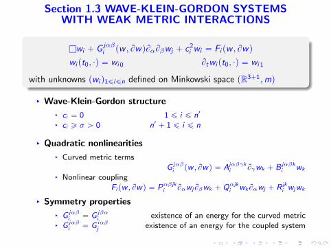
Section 1.3 WAVE-KLEIN-GORDON SYSTEMSWITH WEAK METRIC INTERACTIONS
lwi ` G jαβi pw , BwqBαBβwj ` c2
i wi “ Fi pw , Bwq
wi pt0, ¨q “ wi 0 Btwi pt0, ¨q “ wi 1
with unknowns pwi q1ďiďn defined on Minkowski space pR3`1,mq
§ Wave-Klein-Gordon structure
§ ci “ 0 1 ď i ď n1
§ ci ě σ ą 0 n1 ` 1 ď i ď n
§ Quadratic nonlinearities
§ Curved metric termsG jαβ
i pw , Bwq “ Ajαβγki Bγwk ` B jαβk
i wk
§ Nonlinear couplingFi pw , Bwq “ Pαβjki BαwjBβwk ` Qαjk
i wkBαwj ` R jki wjwk
§ Symmetry properties
§ G jαβi “ G jβα
i existence of an energy for the curved metric§ G jαβ
i “ G iαβj existence of an energy for the coupled system

Index convention§ Wave-Klein-Gordon structure
§ ci “ 0, 1 ď i ď n1
§ ci ě σ ą 0, n1 ` 1 ď i ď n
§ Wave components upı :“ w
pı pı “ 1, . . . , n1
§ Klein-Gordon components vqı :“ w
qı qı “ n1 ` 1, . . . , n
MAIN ASSUMPTIONS§ Null condition for wave components: for pξ0q
2 ´ř
a“1,2,3pξaq2 “ 0
Apαβγpkpı ξαξβξγ “ Bpαβpk
pı ξαξβ “ Pαβppk
pı ξαξβ “ 0
§ Imposed only on the quadratic forms associated with wavecomponents
§ No such restriction for Klein-Gordon components§ Structural condition on the sources (essentially to avoid blow-up)
(excludes terms like uBu, uBv , and u2)
Qαjpki “ 0, R jpk
i “ Rpki “ 0
§ Weak metric interactions (excludes metric terms like uBBv)
Bqαβpki “ 0

Theorem. (2014) Global existence theory for nonlinear wave-KG systemswith weak metric interactions
Consider the initial value problem
§ coupled nonlinear wave-Klein Gordon systems with weak metricinteractions
§ smooth and localized (compactly supported) initial data posed on aspacelike hypersurface of constant time t “ t0.
Then, there exists ε ą 0 such that
§ provided the initial data satisfy wi 0H6pR3q ` wi 1H5pR3q ă ε
§ the Cauchy problem admits a unique global-in-time solution pwi q.
Proof.
§ A complex bootstrap argument based on three levels of regularity
§ A family of L2 norms based on the collection of admissible vectorfields Z P
Bα, La(
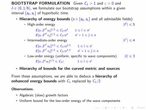
BOOTSTRAP FORMULATION Given C1 ą 1 and ε ą 0 andδ P p0, 16q, we formulate our bootstrap assumptions within a giveninterval rs0, s1s of hyperbolic time.
§ Hierarchy of energy bounds (s P rs0, s1s and all admissible fields):§ High-order energy |I 7| ď 5
E rs,Z I7upıs
12 ď C1εsδ 1 ď pı ď n1
E rs,Z I7vqs
12 ď C1εsδ n1 ` 1 ď q ď n
§ Intermediate-order energy |I :| ď 4
E rs,Z I:upıs
12 ď C1εsδ2 1 ď pı ď n1
E rs,Z I:vqs
12 ď C1εsδ2 n1 ` 1 ď q ď n
§ Low-order energy (uniform, specific to wave components) |I | ď 3
E rs,Z Iupıs
12 ď C1ε 1 ď pı ď n1
§ Hierarchy of bounds for the curved metric and sources
From these assumptions, we are able to deduce a hierarchy ofenhanced energy bounds with C1 replaced by C12
Observations.
§ Algebraic (slow) growth factors
§ Uniform bound for the low-order energy of the wave components

Section 2. THE EINSTEIN-MASSIVE FIELD SYSTEM
Section 2.1 STATEMENT OF THE NONLINEAR STABILITY
New approach for proving the nonlinear stability of Minkowskispace
§ Covers self-gravitating massive fields§ Previous works concern vacuum spacetimes or massless scalar fields
§ Christodoulou-Klainerman 1993: null foliation / maximal foliation(fully geometric proof, Bianchi identities, geometry of null cones)
§ Lindblad-Rodnianski 2010: wave coordinates (standard foliation)§ Massless models: Bieri-Zipser (2009, weaker decay assumptions),
Speck (2014)
Einstein equations for a spacetime pM, gq Rαβ ´R2 gαβ “ Tαβ
§ Stress-energy tensor Tαβ :“ ∇αφ∇βφ´´
12∇γφ∇γφ` V pφq
¯
gαβ
§ Potential V pφq :“ c2
2 φ2 with c ą 0
§ Klein-Gordon equation lgφ “ V 1pφq “ c2φ§ Perturbation of a spacelike hypersurface in Minkowski space
§ Wave gauge Γγ :“ gαβΓγαβ “ 0 (see Chapter 1)
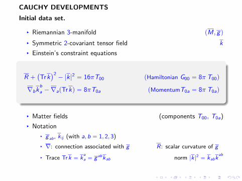
CAUCHY DEVELOPMENTS
Initial data set.
§ Riemannian 3-manifold pM, gq
§ Symmetric 2-covariant tensor field k
§ Einstein’s constraint equations
R ``
Trk˘2´ |k |2 “ 16πT00 pHamiltonian G00 “ 8πT00q
∇bkb
a ´∇apTrkq “ 8πT0a pMomentumT0a “ 8πT0aq
§ Matter fields (components T00, T0a)
§ Notation
§ g ab, k ij (with a, b “ 1, 2, 3)
§ ∇: connection associated with g R: scalar curvature of g
§ Trace Trk “ kaa “ g abkab norm |k|2 “ kabk
ab

INITIAL VALUE PROBLEM. Future development of the initial dataset
§ Lorentzian manifold satisfying the Einstein equations pM, gq
§ Embedding ψ : M Ñ H Ă M
§ Induced metric ψ‹g “ g
§ Second fundamental form k ψ‹k “ k
§ Matter fields
FORMULATION AS PARTIAL DIFFERENTIAL EQUATIONS
§ choice of coordinates / diffeomorphism invariance
§ wave gauge
§ coordinate functions such thatlgx
α :“ ∇α∇αxα“ 0
§ system of coupled nonlinear wave equations for the metriclggαβ “ Qαβpg , Bgq
§ hyperbolic-elliptic system of PDE’s

Theorem. The global nonlinear stability of Minkowski spacetime for self-gravitating massive fields. The geometric formulation
Rαβ “ 8π`
∇αφ∇βφ` V pφq gαβ˘
lgφ “ V 1pφq
with an initial data set pM, g , k , φ0, φ1q satisfying the constraint equations
R ``
Trk˘2´ |k |2 “ 16πT00 pHamiltonian G00 “ 8πT00q
∇bkb
a ´∇apTrkq “ 8πT0a pMomentumT0a “ 8πT0aq
§ is close to an asymptotically flat slice of the (vacuum) Minkowskispacetime (suitable decay at spatial infinity)
§ more precisely, in a neighborhood of spacelike infinity coincides with a
spacelike slice of Schwarzschild spacetime with sufficiently small ADM
mass (Compact Matter Perturbation Problem)
Then, the corresponding initial value problem admits a globally hyperbolicCauchy development
§ which is an asymptotically flat and future geodesically complete spacetime.
§ In other words, every affinely parametrized, timelike geodesic can be
extended indefinitely toward the future.
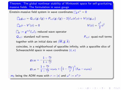
Theorem. The global nonlinear stability of Minkowski space for self-gravitatingmassive fields. The formulation in wave gauge
Einstein-massive field system in wave coordinates lgxα“ 0
rlggαβ “ Qαβpg ; Bgq ` Pαβpg ; Bgq ´ 2`
BαφBβφ` V pφqgαβ˘
rlgφ´ V 1pφq “ 0 V pφq “c2
2φ2
rlg :“ gαβBαBβ reduced wave operator
Qαβ : standard null terms Pαβ : quasi-null terms
together with an initial data set pM, g , kq
coincides, in a neighborhood of spacelike infinity, with a spacelike slice ofSchwarzschild space in wave coordinates pt, xq
gS,00 “ ´1´ mS
r
1` mSr
gS,ab “1` mS
r
1´ mSr
ωaωb `
´
1´mS
r
¯2
pδab ´ ωaωbq
mS being the ADM mass with r :“ |x | and ωa :“ xar

That is, consider an initial data set prescribed on the hypersurface tt “ 2u:
gαβp2, ¨q “ g0,αβ Btgαβp2, ¨q “ g1,αβ
φp2, ¨q “ φ0 Btφp2, ¨q “ φ1
which coincides with gS outside the ball tr ă 1u, i.e. for all r ě 1gαβp2, ¨q “ gS,αβ Btgαβp2, ¨q “ 0 φp2, ¨q “ Btφp2, ¨q “ 0
Then, there exist constants ε0, δ ą 0 and C1 ą 0 and an integer N such thatprovided (with hαβ “ gαβ ´mαβ)
ÿ
α,β,γ
Bγh0,αβHN ptră1uq ` φ0HN`1ptră1uq ``φ1HN ptră1uq `mS ď ε ď ε0,
then the initial value problem for the Einstein-massive field system
§ admits a global-in-time solution in wave coordinates pgαβ , φq
§ satisfying the following energy bounds for all s ě 2
EMps, BILJhαβq
12ď C1εs
δ|I | ` |J| ď N
EM,c2ps, BILJφq12 ď C1εsδ`12
|I | ` |J| ď N
EM,c2ps, BILJφq12 ď C1εsδ
|I | ` |J| ď N ´ 4
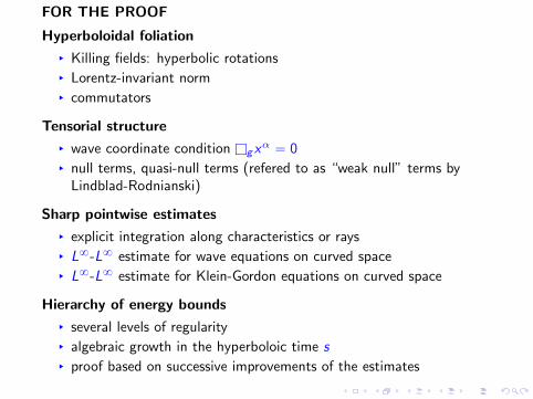
FOR THE PROOF
Hyperboloidal foliation
§ Killing fields: hyperbolic rotations§ Lorentz-invariant norm§ commutators
Tensorial structure
§ wave coordinate condition lgxα “ 0
§ null terms, quasi-null terms (refered to as “weak null” terms byLindblad-Rodnianski)
Sharp pointwise estimates
§ explicit integration along characteristics or rays§ L8-L8 estimate for wave equations on curved space§ L8-L8 estimate for Klein-Gordon equations on curved space
Hierarchy of energy bounds
§ several levels of regularity§ algebraic growth in the hyperboloic time s§ proof based on successive improvements of the estimates
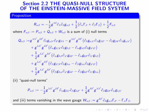
Section 2.2 THE QUASI-NULL STRUCTUREOF THE EINSTEIN-MASSIVE FIELD SYSTEM
Proposition
Rαβ “ ´1
2gλδBλBδgαβ `
1
2
`
BαΓβ ` BβΓβ˘
`1
2Fαβ
where Fαβ :“ Pαβ ` Qαβ `Wαβ is a sum of (i) null terms
Qαβ :“gλλ1
gδδ1
Bδgαλ1Bδ1gβλ ´ gλλ1
gδδ1`
Bδgαλ1Bλgβδ1 ´ Bδgβδ1Bλgαλ1˘
` gλλ1
gδδ1`
Bαgλ1δ1Bδgλβ ´ BαgλβBδgλ1δ1˘
`1
2gλλ
1
gδδ1`
BαgλβBλ1gδδ1 ´ Bαgδδ1Bλ1gλβ˘
` gλλ1
gδδ1`
Bβgλ1δ1Bδgλα ´ BβgλαBδgλ1δ1˘
`1
2gλλ
1
gδδ1`
BβgλαBλ1gδδ1 ´ Bβgδδ1Bλ1gλα˘
(ii) “quasi-null terms”
Pαβ :“ ´1
2gλλ
1
gδδ1
Bαgδλ1Bβgλδ1 `1
4gδδ
1
gλλ1
Bβgδδ1Bαgλλ1
and (iii) terms vanishing in the wave gauge Wαβ :“ gδδ1
BδgαβΓδ1 ´ ΓαΓβ .

CONSEQUENCES.§ Vacuum Einstein equation Rαβ “ 0
rlggαβ “ Pαβ ` Qαβ `Wαβ ``
BαΓβ ` BβΓα˘
.
Under the wave condition gαβΓγαβ “ 0, we have Γβ “ 0 andtherefore:
rlggαβ “ Pαβpg ; Bgq ` Qαβpg ; Bgq
§ Einstein-massive field system
Gαβ “8πTαβ
Tαβ “BαφBβφ´1
2gαβ
`
gµνBµφBνφ` c2φ2˘
therefore
Rαβ “ 8π´
∇αφ∇βφ`c2
2φ2gαβ
¯
and the system in wave coordinates reads
rlggαβ “ Pαβpg ; Bgq ` Qαβpg ; Bgq ´ 16πBαφBβφ´ 8πc2φ2gαβ
rlgφ´ c2φ “ 0
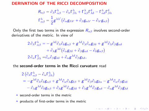
DERIVATION OF THE RICCI DECOMPOSITION
Rαβ “ BλΓλαβ ´ BαΓλβλ ` ΓλαβΓδλδ ´ ΓλαδΓδβλ
Γλαβ “1
2gλλ
1`
Bαgβλ1 ` Bβgαλ1 ´ Bλ1gαβ˘
Only the first two terms in the expression Rαβ involves second-orderderivatives of the metric. In view of
2 BλΓλαβ “´ gλδBλBδgαβ ` gλδBλBαgβδ ` gλδBλBβgαδ
` Bλgλδ`
Bαgβδ ` Bβgαδ ´ Bδgαβ˘
2 BαΓλβλ “BαBβgλδ ` BαgλδBβgλδ,
the second-order terms in the Ricci curvature read
2`
BλΓλαβ ´ BαΓλβλ˘
“ ´gλδBλBδgαβ ` gλδBαBλgδβ ` gλδBβBλgδα ´ gλδBαBβgλδ
´ BλgλδBδgαβ ` Bλg
λδBαgβδ ` BλgλδBβgαδ ´ Bαg
λδBβgλδ
§ second-order terms in the metric
§ products of first-order terms in the metric

On the other hand, consider the term BαΓβ ` BβΓα (which appears in ourdecomposition):
§ Christoffel symbols
Γγ “ gαβΓγαβ “1
2gαβgγδ
`
Bαgβδ ` Bβgαδ ´ Bδgαβ˘
“ gγδgαβBαgβδ ´1
2gαβgγδBδgαβ
and, therefore, Γλ “ gλγΓγ “ gαβBαgβλ ´12g
αβBλgαβ .
§ Derivatives of Christoffel symbols
BαΓβ “Bα`
gδλBδgλβ˘
´1
2Bα
`
gλδBβgλδ˘
“gδλBαBδgλβ ´1
2gλδBαBβgλδ ´
1
2Bαg
λδBβgλδ ` BαgδλBδgλβ .
The term of interest is thus:
BαΓβ ` BβΓα “gλδBαBλgδβ ` gλδBβBλgδα ´ gλδBαBβgλδ
` BαgλδBδgλβ ` Bβg
λδBδgλα
´1
2Bβg
λδBαgλδ ´1
2Bαg
λδBβgλδ

Observe that
§ The second-order terms in BαΓβ ` BβΓα are exactly three of the(four) second-order terms arising in the expression of BλΓλαβ ´BαΓλβλ.
§ The last term in BαΓβ ` BβΓα coincides with the last term inBλΓλαβ ´ BαΓλβλ.
2`
BλΓλαβ ´ BαΓλβλ˘
“ ´gλδBλBδgαβ ``
BαΓβ ` BβΓα˘
´ BλgλδBδgαβ ` Bλg
λδBαgβδ ` BλgλδBβgαδ
´ BαgλδBδgλβ ´ Bβg
λδBδgλα ´1
2Bαg
λδBβgλδ `1
2Bβg
λδBαgλδ
2`
BλΓλαβ ´ BαΓλβλ˘
“ ´BλgλδBδgαβ `
`
BαΓβ ` BβΓα˘
` gλλ1
gδδ1
Bλgλ1δ1Bδgαβ ´ gλλ1
gδδ1
Bλgλ1δ1Bαgβδ
´ gλλ1
gδδ1
Bλgλ1δ1Bβgαδ `1
2gλλ
1
gδδ1
Bαgλ1δ1Bβgλδ
` gλλ1
gδδ1
Bαgλ1δ1Bδgλβ ` gλλ1
gδδ1
Bβgλ1δ1Bδgλα
´1
2gλλ
1
gδδ1
Bβgλ1δ1Bαgλδ

§ We have used the identity Bαgλδ “ ´gλλ
1
gδδ1
Bαgλ1δ1 .
§ The two underlined terms above are opposite to each other.
Second-order terms in the Ricci curvature
2`
BλΓλαβ ´ BαΓλβλ˘
“ ´BλgλδBδgαβ `
`
BαΓβ ` BβΓα˘
` gλλ1
gδδ1
Bλgλ1δ1Bδgαβ ´ gλλ1
gδδ1
Bλgλ1δ1Bαgβδ
´ gλλ1
gδδ1
Bλgλ1δ1Bβgαδ
` gλλ1
gδδ1
Bαgλ1δ1Bδgλβ ` gλλ1
gδδ1
Bβgλ1δ1Bδgλα
We need to deal with the five terms above.

Quadratic terms in the expression of the Ricci curvature
4 ΓλαβΓδλδ “gλλ1gδδ
1´
Bλgδδ1Bαgβλ1 ` Bβgαλ1Bλgδδ1 ´ Bλ1gαβBλgδδ1¯
4 ΓλαδΓδβλ “gλλ1gδδ
1´
Bαgδλ1Bβgλδ1 ` Bαgδλ1Bλgβδ1 ´ Bαgδλ1Bδ1gβλ
` Bδgαλ1Bβgλδ1 ` Bδgαλ1Bλgβδ1 ´ Bδgαλ1Bδ1gβλ
´ Bλ1gαδBβgλδ1 ´ Bλ1gαδBλgβδ1 ` Bλ1gαδBδ1gβλ
¯
We deduce that
4`
ΓλαβΓδλδ ´ ΓλαδΓδβλ˘
“ ´gλλ1
gδδ1
Bλ1gαβBλgδδ1 ` gλλ1
gδδ1
Bδgαλ1Bδ1gβλ ` gλλ1
Bλ1gαδBλgβδ1
´ gλλ1
gδδ1
Bαgδλ1Bβgλδ1
` gλλ1
gδδ1
Bλgδδ1Bαgβλ1 ` gλλ1
gδδ1
Bλgδδ1Bβgαλ1 ´ 2 gλλ1
gδδ1
Bδgαλ1Bλgβδ1 .
Observe that:
§ The first three terms are “null terms”.
§ The fourth term is a quasi-null term.
§ The two underlined terms will be the opposite to two other (underlined)terms derived below.
Hence, only the last term remains to be dealt with.

In summary, in the Ricci expression, we need to deal with six terms:
Ω1 :“1
2gλλ
1
gδδ1
Bλgλ1δ1Bδgαβ Ω2 :“ ´1
2gλλ
1
gδδ1
Bλgλ1δ1Bαgβδ
Ω3 :“ ´1
2gλλ
1
gδδ1
Bλgλ1δ1Bβgαδ Ω4 :“1
2gλλ
1
gδδ1
Bαgλ1δ1Bδgλβ
Ω5 :“1
2gλλ
1
gδδ1
Bβgλ1δ1Bδgλα Ω6 :“ ´1
2gλλ
1
gδδ1
Bδgαλ1Bλgβδ1
General identities for the metric
gαβBαgβδ ´1
2gαβBδgαβ “ Γδ gβδBαg
αβ ´1
2gαβBδg
αβ “ Γδ
First three terms
Ω1 “1
2gδδ
1
BδgαβΓδ1 `1
4gλλ
1
gδδ1
BδgαβBδ1gλλ1
Ω2 “ ´1
2gδδ
1
BαgβδΓδ1 ´1
4gλλ
1
gδδ1
Bδ1gλλ1Bαgβδ
Ω3 “ ´1
2gδδ
1
BβgαδΓδ1 ´1
4gλλ
1
gδδ1
Bδ1gλλ1Bβgαδ
§ The last term in Ω1 is one of the quasi-null term.
§ The two underlined terms are opposite to the two underlined terms above.
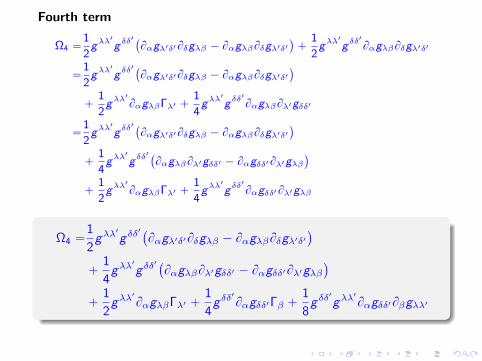
Fourth term
Ω4 “1
2gλλ
1
gδδ1`
Bαgλ1δ1Bδgλβ ´ BαgλβBδgλ1δ1˘
`1
2gλλ
1
gδδ1
BαgλβBδgλ1δ1
“1
2gλλ
1
gδδ1`
Bαgλ1δ1Bδgλβ ´ BαgλβBδgλ1δ1˘
`1
2gλλ
1
BαgλβΓλ1 `1
4gλλ
1
gδδ1
BαgλβBλ1gδδ1
“1
2gλλ
1
gδδ1`
Bαgλ1δ1Bδgλβ ´ BαgλβBδgλ1δ1˘
`1
4gλλ
1
gδδ1`
BαgλβBλ1gδδ1 ´ Bαgδδ1Bλ1gλβ˘
`1
2gλλ
1
BαgλβΓλ1 `1
4gλλ
1
gδδ1
Bαgδδ1Bλ1gλβ
Ω4 “1
2gλλ
1
gδδ1`
Bαgλ1δ1Bδgλβ ´ BαgλβBδgλ1δ1˘
`1
4gλλ
1
gδδ1`
BαgλβBλ1gδδ1 ´ Bαgδδ1Bλ1gλβ˘
`1
2gλλ
1
BαgλβΓλ1 `1
4gδδ
1
Bαgδδ1Γβ `1
8gδδ
1
gλλ1
Bαgδδ1Bβgλλ1

Fifth term
Ω5 “1
2gλλ
1
gδδ1`
Bβgλ1δ1Bδgλα ´ BβgλαBδgλ1δ1˘
`1
4gλλ
1
gδδ1`
BβgλαBλ1gδδ1 ´ Bβgδδ1Bλ1gλα˘
`1
2gλλ
1
BβgλαΓλ1 `1
4gδδ
1
Bβgδδ1Γα `1
8gδδ
1
gλλ1
Bβgδδ1Bαgλλ1
Sixth and last term Ω6
´1
2gλλ
1
gδδ1`
Bδgαλ1Bλgβδ1 ´ Bδgβδ1Bλgαλ1˘
´1
2gλλ
1
gδδ1
Bδgβδ1Bλgαλ1
“´1
2gλλ
1
gδδ1`
Bδgαλ1Bλgβδ1 ´ Bδgβδ1Bλgαλ1˘
´1
2gλλ
1
Bλgαλ1Γβ ´1
4gλλ
1
gδδ1
Bβgδδ1Bλgαλ1
“´1
2gλλ
1
gδδ1`
Bδgαλ1Bλgβδ1 ´ Bδgβδ1Bλgαλ1˘
´1
2gλλ
1
Bλgαλ1Γβ ´1
4gδδ
1
Bβgδδ1Γα
´1
8gλλ
1
gδδ1
Bαgλλ1Bβgδδ1
Ω6 “´1
2gλλ
1
gδδ1`
Bδgαλ1Bλgβδ1 ´ Bδgβδ1Bλgαλ1˘
´1
2ΓαΓβ
´1
4gδδ
1
Bαgδδ1Γβ ´1
4gδδ
1
Bβgδδ1Γα
´1
8gλλ
1
gδδ1
Bαgλλ1Bβgδδ1

In conclusion the quadratic terms in the Ricci curvature Rαβ read:
1
2gλλ
1
gδδ1
Bδgαλ1Bδ1gβλ ´1
2gλλ
1
gδδ1`
Bδgαλ1Bλgβδ1 ´ Bδgβδ1Bλgαλ1˘
`1
2gλλ
1
gδδ1`
Bαgλ1δ1Bδgλβ ´ BαgλβBδgλ1δ1˘
`1
4gλλ
1
gδδ1`
BαgλβBλ1gδδ1 ´ Bαgδδ1Bλ1gλβ˘
`1
2gλλ
1
gδδ1`
Bβgλ1δ1Bδgλα ´ BβgλαBδgλ1δ1˘
`1
4gλλ
1
gδδ1`
BβgλαBλ1gδδ1 ´ Bβgδδ1Bλ1gλα˘
´1
4gλλ
1
gδδ1
Bαgδλ1Bβgλδ1 `1
8gδδ
1
gλλ1
Bβgδδ1Bαgλλ1
`1
2gδδ
1
BδgαβΓδ1 ´1
2ΓαΓβ .
By collecting all the terms above, we arrive at the desired identity.

Section 3. THE HYPERBOLOIDAL FOLIATION METHOD
3.1 WAVE EQUATIONS WITH NULL INTERACTIONS
The simplest model
lu “ PαβBαu Bβu u|Hs0“ u0, Btu|Hs0
“ u1 p‹q
§ initial data u0, u1 compactly supported in the intersection of the spacelikehypersurface Hs0 and the cone K “
pt, xq |x | ă t ´ 1(
with s0 ą 1
§ standard null condition: Pαβξαξβ “ 0 for all ξ P R4 satisfying´ξ2
0 `ř
a ξ2a “ 0
§ hyperboloidal energy EM “ EM,0: Minkowski metric and zero K-G mass
§ admissible vector fields Z P Z : spacetime translations Bα, boosts La
Theorem. Global existence theory for wave equations with null interactions
There exist ε0 ą 0 and C1 ą 1 such that for all initial data satisfyingř
|I |ď3
ř
ZPZ EMps0,ZIuq12 ď ε ď ε0
the Cauchy problem p‹q admits a global-in-time solution, satisfying theuniform energy bound
ÿ
|I |ď3
ÿ
ZPZ
EMps,ZIuq12 ď C1ε
and the uniform decay estimateˇ
ˇBαupt, xqˇ
ˇ ď C1εt pt´|x|q12 .

Bootstrap strategy. For some (sufficiently large) constant C1 ą 1, letus assume that the local-in-time solution satisfies within some timeinterval rs0, s1s
ÿ
|I |ď3,ZPZ
EMps,ZIuq12 ď C1ε, s P rs0, s1s. p‹‹q
More precisely:
§ let s1 be the largest hyperboloidal time such that p‹‹q holds true.
§ Since C1 ą 1, by the local existence theory and by a continuityargument, we do have s1 ą s0.
Suppose s1 is finite. We are going to prove that
§ for suitably chosen constants ε0 and C1 ą 1 and for all ε ď ε0
ÿ
|I |ď3,ZPZ
EMps,ZIuq12 ď
C1
2ε, s P rs0, s1s.
§ Consequently, s1 cannot be the largest time and we get acontradiction
§ unless s1 “ `8.

Proposition
Let u be a solution defined in rs0, s1s whose initial data satisfies
ÿ
|I |ď3,ZPZ
EMps0,ZIuq12 ď ε.
Then, there exist constants ε0 ą 0 and C1 ą 1 such that ifÿ
|I |ď3,ZPZ
EMps,ZIuq12 ď C1ε, s P rs0, s1s
for ε ď ε0, then the following stronger estimate holds
ÿ
|I |ď3,ZPZ
EMps,ZIuq12 ď
C1
2ε, s P rs0, s1s.
Recall our notation
§ The semi-hyperboloidal frame consists of three vectors tangent to thehyperboloids Ba :“ La
t“ xa
tBt ` Ba and the timelike vector B0 :“ Bt .
§ Admissible vector fields Z P
Bα, La
(

Lemma. The energy estimate for hyperboloids
ÿ
|I |ď3,ZPZ
EMps,ZIuq12
ďÿ
|I |ď3,ZPZ
EMps0,ZIuq12 `
ż s
s0
ÿ
|I |ď3,ZPZ
›
›Z I`
PαβBαuBβu˘›
›
L2f pHs1 q
ds 1
Notation. uL2fpHs q
:“ş
Hs|u| dx “
ş
|upa
s2 ` |x |2, xq| dx
Proof. Using the product Z I (with |I | ď 3) and the commutation propertyrZ I ,ls “ 0:
l`
Z Iu˘
“ Z I`
PαβBαuBβu˘
.
By multiplication by BtZIu, we see that ru :“ Z Iu satisfies
1
2Bt
´
pBt ruq2`ÿ
a
pBaruq2¯
´ Ba`
BaruBt ru˘
“ Bt ru ZI`
PαβBαruBβ ru˘
.
By integrating in the region Krs0,ss limited by two hyperboloidsż
Krs0,ss
´1
2Bt
´
pBt ruq2`ÿ
a
pBaruq2¯
´ Ba`
BaruBt ru˘
¯
dtdx “
ż
Krs0,ssBt ru Z
I`
PαβBαruBβu˘
dtdx .
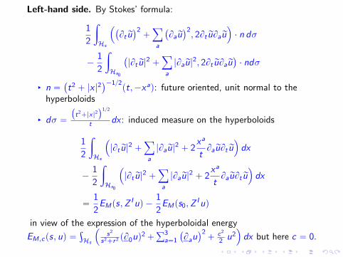
Left-hand side. By Stokes’ formula:
1
2
ż
Hs
´
`
Bt ru˘2`ÿ
a
`
Baru˘2, 2Bt ruBaru
¯
¨ n dσ
´1
2
ż
Hs0
`
|Bt ru|2 `
ÿ
a
|Baru|2, 2Bt ruBaru
˘
¨ ndσ
§ n “`
t2 ` |x |2˘´12
pt,´xaq: future oriented, unit normal to thehyperboloids
§ dσ “
`
t2`|x|2
˘12
t dx : induced measure on the hyperboloids
1
2
ż
Hs
´
|Bt ru|2 `
ÿ
a
|Baru|2 ` 2
xa
tBaruBt ru
¯
dx
´1
2
ż
Hs0
´
|Bt ru|2 `
ÿ
a
|Baru|2 ` 2
xa
tBaruBt ru
¯
dx
“1
2EMps,Z
Iuq ´1
2EMps0,Z
Iuq
in view of the expression of the hyperboloidal energy
EM,cps, uq “ş
Hs
´
s2
s2`r2 pB0uq2`
ř3a“1
`
Bau˘2` c2
2 u2¯
dx but here c “ 0.

Right-hand side. With the change of variable s 1 “ pt2 ´ |x |2q12 and theidentity dtdx “ ps 1tqds 1dx :
ż s
s0
ż
Hs1
ps 1tqBtuZI`
PαβBαuBβu˘
dxds 1
Consequently
1
2EMps,Z
Iuq ´1
2EMps0,Z
Iuq “
ż s
s0
ż
Hs1
ps 1tqBtuZI`
PαβBαuBβu˘
ds 1dx
After differentiation in s:
E ps,Z Iuq12d
dsE ps,Z Iuq12 “
ż
Hs
ps 1tqBtuZI`
PαβBαuBβu˘
dx
ďpstqBtuL2f pHsq
›
›Z I`
PαβBαuBβu˘›
›
L2f pHsq
.
By the definition of the hyperboloidal energy:E ps, uq12 ě pstqBtuL2
f pHsqand therefore
d
ds
ÿ
|I |ď3,ZPZ
E ps,Z Iuq12 ďÿ
|I |ď3,ZPZ
›
›Z I`
PαβBαuBβu˘›
›
L2f pHsq
.
We conclude by integrating over the hyperbolic time interval rs0, ss.
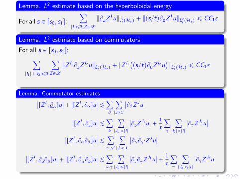
Lemma. L2 estimate based on the hyperboloidal energy
For all s P rs0, s1s:
ÿ
|I |ď3,ZPZ
BaZIuL2
f pHsq` pstqB0Z
IuL2f pHsq
ď CC1ε
Lemma. L2 estimate based on commutators
For all s P rs0, s1s:
ÿ
|I1|`|I2|ď3
ÿ
ZPZ
Z I1BaZI2uL2
f pHsq` Z I1
`
pstqB0ZI2u
˘
L2f pHsq
ď CC1ε
Lemma. Commutator estimatesˇ
ˇrZ I , Bαsuˇ
ˇ`ˇ
ˇrZ I , Bαsuˇ
ˇ Àÿ
β
ÿ
|J|ăI
ˇ
ˇBβZJuˇ
ˇ
ˇ
ˇrZ I , Basuˇ
ˇ Àÿ
b
ÿ
|J1|ă|I |
ˇ
ˇBbZJ1u
ˇ
ˇ`1
t
ÿ
γ
ÿ
J2|ă|I |
ˇ
ˇBγZJ2u
ˇ
ˇ
ˇ
ˇrZ I , BαBβsuˇ
ˇ Àÿ
γ,γ1
ÿ
|J|ă|I |
ˇ
ˇBγBγ1ZJuˇ
ˇ
ˇ
ˇrZ I , BaBβsuˇ
ˇ`ˇ
ˇrZ I , BαBbsuˇ
ˇ Àÿ
c,γ
ÿ
|J1|ď|I |
ˇ
ˇBcBγZJ1u
ˇ
ˇ`1
t
ÿ
γ
ÿ
|J2|ď|I |
ˇ
ˇBγZJ2u
ˇ
ˇ
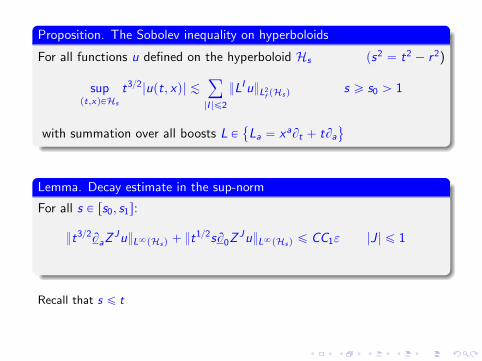
Proposition. The Sobolev inequality on hyperboloids
For all functions u defined on the hyperboloid Hs ps2 “ t2 ´ r2)
suppt,xqPHs
t32|upt, xq| Àÿ
|I |ď2
LIuL2f pHsq
s ě s0 ą 1
with summation over all boosts L P
La “ xaBt ` tBa(
Lemma. Decay estimate in the sup-norm
For all s P rs0, s1s:
t32BaZJuL8pHsq ` t
12sB0ZJuL8pHsq ď CC1ε |J| ď 1
Recall that s ď t
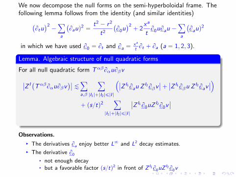
We now decompose the null forms on the semi-hyperboloidal frame. Thefollowing lemma follows from the identity (and similar identities)
`
Btu˘2´ÿ
a
`
Bauq2 “
t2 ´ r2
t2
`
B0u˘2` 2
xa
tB0uBau ´
ÿ
a
`
Bauq2
in which we have used B0 “ Bt and Ba “xa
t Bt ` Ba (a “ 1, 2, 3).
Lemma. Algebraic structure of null quadratic forms
For all null quadratic form TαβBαuBβv
ˇ
ˇZ I`
TαβBαuBβv˘ˇ
ˇ Àÿ
a,β
ÿ
|I1|`|I2|ď|I |
´
ˇ
ˇZ I1Bau ZI2Bβv
ˇ
ˇ`ˇ
ˇZ I1Bβu ZI2Bav
ˇ
ˇ
¯
` pstq2ÿ
|I1|`|I2|ď|I |
ˇ
ˇZ I1B0uZI2B0v
ˇ
ˇ
Observations.
§ The derivatives Ba enjoy better L8 and L2 decay estimates.
§ The derivative B0
§ not enough decay§ but a favorable factor pstq2 in front of Z I1B0uZ
I2B0v

Lemma. Decay estimate for the interaction term›
›Z I`
PαβBαuBβu˘›
›
L2f pHsq
ď C pC1εq2s´32
C ą 0 being a universal constant
Proof.ˇ
ˇZ I`
PαβBαuBβu˘ˇ
ˇ ď C pstq2ÿ
|I1|`|I2|ď|I |
ˇ
ˇZ I1BtuZI2Btu
ˇ
ˇ
` Cÿ
a,β,|I1|`|I2|ď|I |
´
ˇ
ˇZ I1Bau ZI2Bβu
ˇ
ˇ`ˇ
ˇZ I1Bβu ZI2Bau
ˇ
ˇ
¯
“: T1 ` T2
We now combine the L2 and L8 estimates together.

Terms in T1
Observe that |I1| ` |I2| ď |I | ď 3 implies that |I1| ď 1 or |I2| ď 1. Without lossof generality, we can assume |I2| ď 1 and write
›
›pstq2Z I1BtuZI2Btu
›
›
L2fpHs q
ď›
›pstqZ I1Btu›
›
L2fpHs q
›
›t´32`
t12sZ I2Btu˘›
›
L8pHs q
ď CpC1εq2s´32 since t ě s
Terms in T2
When |I1| ď 1 we write
›
›Z I1Bau ZI2Bβu
›
›
L2fpHs q
ďs´32›
›t32Z I1Bau›
›
L8pHs q
›
›pstqZ I2Bβu›
›
L2fpHs q
ď CpC1εq2s´32
When |I2| ď 1, we write
›
›Z I1Bau ZI2Bβu
›
›
L2fpHs q
ďs´32›
›Z I1Bau›
›
L2fpHs q
›
›t12sZ I2Bβu›
›
L8pHs qď CpC1εq
2s´32

CONCLUSION.
We combine the null form estimate with the energy estimate:
ÿ
|I |ď3,ZPZ
EMps,ZIuq12 ď
ÿ
|I |ď3,ZPZ
EMps0,ZIuq12 ` C pC1εq
2
ż s
s0
ps 1q´32 ds 1
ď ε` C pC1εq2 ď
1
2C1ε
by choosing C1 ą 2 and ε ď ε0 :“ C1´22CC 2
1.

Section 3.2 WAVE-KLEIN-GORDON SYSTEMSWITH STRONG METRIC INTERACTIONS
From the Einstein equations in wave gauge, we can formally derive thefollowing model:
´lu “ PαβBαvBβv ` Rv2
´lv ` u HαβBαBβv ` c2v “ 0
with arbitrary Pαβ ,Hαβ ,R
Theorem. Global existence theory for wave-Klein-Gordon systems withstrong metric interactions
Consider the nonlinear wave-Klein-Gordon model with given Pαβ ,R,Hαβ
and c ą 0. Given any N ě 8, there exists ε “ εpNq ą 0 such that
§ if the initial data satisfy pu0, v0qHN`1pR3q ` pu1, v1qHNpR3q ă ε
§ then the Cauchy problem for the model problem admits aglobal-in-time solution.
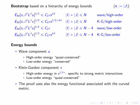
Bootstrap based on a hierarchy of energy bounds (k :“ |J|)
EM rs, BILJus12 ď C1εs
kδ |I | ` |J| ď N wave/high-order
EM rs, BILJv s12 ď C1εs
12`kδ |I | ` |J| ď N K-G/high-order
EM rs, BILJus12 ď C1ε |I | ` |J| ď N ´ 4 wave/low-order
EM rs, BILJv s12 ď C1εs
kδ |I | ` |J| ď N ´ 4 K-G/low-order
Energy bounds
§ Wave component u
§ High-order energy “quasi-conserved”§ Low-order energy “conserved”
§ Klein-Gordon component v
§ High-order energy in s12`: specific to strong metric interactions§ Low-order energy “quasi-conserved”
§ The proof uses also the energy functional associated with the curvedmetric.
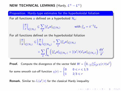
NEW TECHNICAL LEMMAS (Hardy, L8 ´ L8)
Proposition. Hardy-type estimates for the hyperboloidal foliation
For all functions u defined on a hyperboloid Hs :
›
›
›
u
r
›
›
›
L2f pHsq
Àÿ
a
BauL2f pHsq
with Ba “ t´1La
For all functions defined on the hyperboloidal foliation›
›
›
u
s
›
›
›
L2f pHsq
À
›
›
›
u
s0
›
›
›
L2f pHs0
q`ÿ
a
BauL2f pHsq
`ÿ
a
ż s
s0
´
BauL2f pHs1 q
` ps 1tqBauL2f pHs1 q
¯ ds 1
s 1
Proof. Compute the divergence of the vector field W “
´
0, t xa
p1`r2qs2χprtqu2¯
for some smooth cut-off function χprq “
#
0 0 ď r ď 13
1 23 ď r
Remark. Similar to Br pu2rq for the classical Hardy inequality

Lemma. Decomposition for Klein-Gordon in curved space
v being a solution to ´rlgv ` c2v “ f
§ metric gαβ “ mαβ ´ hαβ
§ sup |h00| ď 12 (component in the hyperboloidal frame)
The function wt,xpλq :“ λ32vpλts, λxsq (with s “?t2 ´ r 2)
satisfies the second-order ODE in λ
d2
dλ2wt,x `
c2
1` h00 wt,x “ kt,x
with h00“ h
00pλts, λxsq and a right-hand side kt,x “ kt,xpλq defined below
§ We do this analysis in hyperboloidal coordinates px0, xaq “ ps, xa
q
§ hαβ
: components
§ in the hyperboloidal frame
B0 :“ Bs “s
tBt “
?t2 ´ r 2
tBt
Ba :“ Bxa “xa
tBt ` Ba “
xa
tBt ` Ba

kt,x :“ R1rvs`R2rvs`R3rvs`s32f
1`h00 Ψ
αβ : matrix of change of frame
R1rv s :“s32BaB
av `
1
s12
˜
xaxbBaBbv `
3
4v ` 3xa
Bav
¸
R2rv s :“3 h00´ 1
4s12v ` s12
B0v¯
´ s32´
2h0bB0Bbv ` h
abBaBbv ` hαβBαΨ
β1
β Bβ1v¯
R3rv s :“h00´
2xas12B0Bav `
2xa
s12Bav `
xaxb
s12BaBbv
¯
Lemma. Technical ODE estimate
Given G : rs0, s1q Ñ r´12, 12s and k : rs0, s1q Ñ R with s1 P rs0,`8q
and G 1, k integrable, the solution z to z2pλq ` c2
1`Gpλqzpλq “ kpλq with
prescribed initial data zps0q “ z0 and z 1ps0q “ z1 satisfies for all s P rs0, s1q
|zpsq| ` |z 1psq| À |z0| ` |z1| ` K psq
`
ż s
s0
´
|z0| ` |z1| ` K ps 1q¯
|G 1ps 1q|eCşss1|G 1pλq|dλ ds 1
with K psq :“şs
s0|kps 1q| ds 1 and C ą 0.

Proposition. L8-L8 estimate for Klein-Gordon equations on curved space
For the Klein-Gordon equation on a curved background ´rlgv ` c2v “ f
§ metric gαβ “ mαβ ´ hαβ perturbation of the Minkowski metric
§ data prescribed on a hyperboloid v |Hs0“ v0, Btv |Hs0
“ v1
Then, in the future of Hs0 , one has
s32|vpt, xq| ` t s12|BKvpt, xq| À V pt, xq
with V defined below. BK :“ Bt `xa
t Ba
Notation. ht,xpλq :“ h00pλts, λxsq s2 “ t2 ´ r2
The derivative in λ reads BK “ Bt `xa
t Ba
h1t,xpλq “t
sBth
00pλts, λxsq `
xa
sBah
00pλts, λxsq
“t
spBKh
00qpλts, λxsq
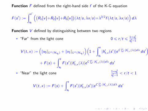
Function F defined from the right-hand side f of the K-G equation
F ps 1q :“
ż s1
s0
´
`
R1rv s`R2rv s`R3rv s˘
pλts, λxsq`λ32f pλts, λxsq¯
dλ
Function V defined by distinguishing between two regions
§ “Far” from the light cone 0 ď rt ď1`s2
0
s20´1
V pt, xq :“´
v0L8pHs0q ` v1L8pHs0
q
¯´
1`
ż s
s0
|h1t,xps1q|eC
şss1|h1t,x pλq|dλ ds 1
¯
` F psq `
ż s
s0
F ps 1q|h1t,xpλq|eCşss1|h1t,x pλq|dλ ds 1
§ “Near” the light cone1`s2
0
s20´1
ă rt ă 1
V pt, xq :“ F psq `
ż s
s0
F ps 1q|h1t,xps1q|eC
şss1|h1t,x pλq|dλ ds 1

Proposition. L8-L8 estimate for the wave equation with source
u being a spatially compactly supported to the wave equation ´lu “ fin the cone K
§ assume vanishing initial data
§ the right-hand side satisfies |f | À 1t2`νpt´rq1´µ , t ě 2
for some exponents 0 ă µ ď 12 and 0 ă |ν| ď 12.
Then, one has the decay property
t |upt, xq| À
$
’
’
’
’
&
’
’
’
’
%
1
νµ
1
pt ´ rqν´µ0 ă ν ď 12
1
|ν|µpt ´ rqµtν ´12 ď ν ă 0
Proof based on the solution formula for the wave equation

OUTLINE OF THE BOOTSTRAP ARGUMENTSFIRST PART: energy, commutators, Sobolev
§ Basic L2 estimates (bootstrap assumptions) |I | ` |J| ď N
pstqBαBILJuL2
f pHsq` . . . À C1εs
kδ
pstqBαBILJvL2
f pHsq` . . . À C1εs
12`kδ
§ Consequence based on commutators |I | ` |J| ď N
pstqBILJBαuL2f pHsq
` . . . À C1εskδ
pstqBILJBαvL2f pHsq
` . . . À C1εs12`kδ
§ Basic sup-norm estimates (Sobolev ineq. on hyperboloids)|I | ` |J| ď N ´ 2
t12sBαBILJuL8pHsq ` . . . À C1εs
pk`2qδ
t12sBαBILJvL8pHsq ` . . . À C1εs
12`pk`2qδ
§ Consequence based on commutators |I | ` |J| ď N ´ 2
t12sBILJBαuL8pHsq ` . . . À C1εspk`2qδ
t12sBILJBαvL8pHsq ` . . . À C1εs12`pk`2qδ

SECOND PART: sharp pointwise bounds (|I | ` |J| ď N ´ 4)
t |LJu| À C1εskδ
t32|BILJv | À C1εskδpstq12´4δ
t32|BKBILJv | À C1εs
kδpstq32´4δ
§ First bound for the wave component : low-order BILJ
(L8–L8 for the wave component)
|I | ` |J| ď N ´ 7
|BILJu| À C1εt´32 ` pC1εq
2ptsq´pk`4qδt´1spk`4qδ
§ Second/first bounds for wave/KG components at zero-order(L8–L8 for the wave and K-G equations)
t |upt, xq| À C1ε
s32 |v | ` ts12|BKvpt, xq| À C1εptsq´2`7δ
(uniform integrability for the coefficients of the ODE)

§ Second bound for the KG component: only BI and again L8–L8
|I | ď N ´ 4
|BKBI vpt, xq| À C1εptsq
´32`4δt´32
|BI vpt, xq| À C1εptsq´12`4δt´32
§ Final estimate for wave/KG components: applying now LJ
|I | ` |J| ď N ´ 4
t |LJu| À C1εskδ
`
ptsq3´7δs32|BKBILJv |
˘
``
ptsq2´7δs32|BILJv |˘
À C1εskδ
`
ptsq1´7δs32|BαBILJv |
˘
À C1εskδ
To conclude the bootstrap argument we return to the systemdifferentiated with BILJ (|I | ` |J| ď N and |J| “: k)
´lBILJu “ BILJ`
PαβBαvBβv˘
` BILJ`
Rv2˘
´lBILJv ` u HαβBαBβBILJv ` c2BILJv “ ´rBILJ , u HαβBαBβsv
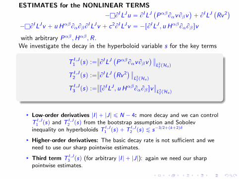
ESTIMATES for the NONLINEAR TERMS
´lBILJu “ BILJ`
PαβBαvBβv˘
` BILJ`
Rv2˘
´lBILJv ` u HαβBαBβBILJv ` c2BILJv “ ´rBILJ , u HαβBαBβsv
with arbitrary Pαβ ,Hαβ ,R.We investigate the decay in the hyperboloid variable s for the key terms
T I ,J1 psq :“
›
›BILJ`
PαβBαvBβv˘›
›
L2f pHsq
T I ,J2 psq :“
›
›BILJ`
Rv2˘›
›
L2f pHsq
T I ,J3 psq :“
›
›rBILJ , u HαβBαBβsv›
›
L2f pHsq
§ Low-order derivatives |I | ` |J| ď N ´ 4: more decay and we can controlT I ,J
1 psq and T I ,J2 psq from the bootstrap assumption and Sobolev
inequality on hyperboloids T I ,J1 psq ` T I ,J
2 psq À s´32`pk`2qδ
§ Higher-order derivatives: The basic decay rate is not sufficient and weneed to use our sharp pointwise estimates.
§ Third term T I ,J3 psq (for arbitrary |I | ` |J|): again we need our sharp
pointwise estimates.

The sharp L8–L8 estimates have allowed us to improve the basicpointwise bounds and get |I | ` |J| ď N ´ 4
t |LIu| À C1ε skδ
s32|BILJv | À C1ε pstq2´4δskδ À C1ε s
kδ
s32|BILJBαv | À C1ε pstq1´7δskδ À C1ε s
kδ
Controling Pαβ and R
§ For |I | ` |J| ď N and by assuming, without loss of generality,|I1| ` |J1| ď N ´ 4 i the following calculation
›
›BILJ pBαvBβvq›
›
L2f pHsq
»ÿ
I1`I2“IJ1`J2“J
BI1LJ1Bαv BI2LJ2BβvL2
f pHsq
ÀC1εs´32s |J1|δ BI2LJ2BβvL2
f pHsq
À pC1εq2s´1`kδ
§ Similarly, we obtain BILJ`
v2˘
L2f pHsq
À pC1εq2s´1`kδ.
We thus control T I ,J1 psq and T I ,J
2 psq (for all relevant I , J) and we arrive at thedesired improved energy bounds for the wave component.
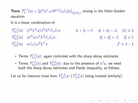
Term T I ,J3 psq “
›
›rBILJ , u HαβBαBβsv›
›
L2f pHsq
arising in the Klein-Gordon
equation.
It is a linear combination of
T I ,J3,1 psq pBI1LJ1uq BI2LL2BαBβv I1 ` I2 “ I , J1 ` J2 “ J, |I1| ě 1
T I ,J3,2 psq pLJ
11uq BILJ
12BαBβv J 11 ` J 12 “ J, J 11 ě 1
T I ,J3,3 psq u BαBβB
ILJ1
v J 1 ď J ´ 1
§ Terms T I ,J3,1 psq: again controled with the sharp decay estimates
§ Terms T I ,J3,2 psq and T I ,J
3,3 psq: due to the presence of LJu, we needboth the sharp decay estimates and Hardy inequality, as follows.
Let us for instance treat here T I ,J3,2 psq (T I ,J
3,3 psq being treated similarly).

Higher-order derivatives
§ For all |J 11| ď N ´ 4, we use the sharp decay bound t |LIu| À C1εskδ
combined with the energy bound on BαBβv (implied by ourbootstrap assumption).
§ For |I | ` |J 12| ď N ´ 4, we use the sharp bound
|BILJBαv | À C1ε pstq1´7δs´32`kδ and Hardy’s inequality for LJ
11u.
We are led to the slow growth (after integration in s)
›
›rBILJ ,HαβBαBβsv›
›
L2f pHsq
À pC1εq2s´12`kδ.
Lower-order derivatives: this is easier
§ For |J 11| ď |I | ` |J| ď N ´ 4, we apply directly the sharp boundt |LIu| À C1ε s
kδ
§ together with the energy bound given by our bootstrap assumption.
This leads us to the decay
›
›rBILJ ,HαβBαBβsv›
›
L2f pHsq
À pC1εq2s´1`kδ.

DEALING WITH THE EINSTEIN EQUATIONSArXiv:1511.03324
This requires a number of additional ideas:
§ The wave gauge condition
§ The quasi-null terms
§ Much involved algebraic structure
§ Specific hierarchy of (low-order, high-order) energy bounds
§ Integration along the characteristics of the curved metric
§ Non-compact solutions (Schwarzschild at spatial infinity)
FINAL REMARKS
§ Dynamically unstable solutions to the Einstein equations do notexist for self-gravitating massive fields with sufficiently small massand spacetimes sufficiently close to flat space.
§ The f pRq theory of modified gravity: nonlinear stability ofMinkowski spacetime for f pRq » R ` κR2 with κ ą 0.

OPEN PROBLEMS§ PROBLEM 1: Appli. of the Hyperboloidal Foliation Method
§ Encompass a large class of nonlinear wave-Klein-Gordon systemswith quasi-null coupling
Rely on the earlier work: S. Alinhac, H. Lindblad
§ PROBLEM 2: Investigate the growing rate s12
§ Investigate whether it is necessary in the wave gauge underconsideration (by constructing explicit examples)
§ Improve this rate by introducing additional geometric arguments(hyperboloidal foliation based on the curved metric)
Ongoing work by Q. Wang and J. Wang
§ PROBLEM 3: Extend our method to other massive fields§ Kinetic models (density fc.), Vlasov eq. (collisionless), Boltzmann eq.
Rely on: D. Fajman, J. Joudioux, and J. Smulevici for the Vlasov eq.
§ PROBLEM 4: Establish Penrose’s peeling estimates§ Precise asymptotics for the spacetime curvature along timelike
directions (D. Christodoulou and S. Klainerman’s geometric method)§ Very challenging in wave coordinates (H. Lindblad and I. Rodnianski)
The Hyperboloidal Foliation Method provides sharp bounds (for instance a uni-
form energy bound in presence of null forms and without metric coupling) and
could allow one to establish the peeling estimates in wave gauge.