Acta Applicandae Mathematicae 83: 199–220, 2004.© 2004 Kluwer Academic Publishers. Printed in the Netherlands.

199

Integrable Hierarchy, 3 × 3 Constrained Systems,and Parametric Solutions

ZHIJUN QIAODepartment of Mathematics, University of Texas-Pan American, Edinburg, TX 78539, U.S.A. andT-CNLS, Los Alamos National Laboratory, Los Alamos, NM 87545, U.S.A. and Institute ofMathematics, Fudan University, Shanghai 200433, P.R. China

(Received: 20 March 2003; in final form: 16 December 2003)

Abstract. This paper provides a new integrable hierarchy. The DP equation: mt +umx +3mux = 0,m = u − uxx , proposed recently by Degasperis and Procesi, is the first member in the negativeorder hierarchy while the first equation in the positive order hierarchy is: mt = 4(m−2/3)x −5(m−2/3)xxx + (m−2/3)xxxxx. The whole hierarchy is shown Lax-integrable through solving a keymatrix equation. To obtain the parametric solutions for the whole hierarchy, we separately discussthe negative order and the positive order hierarchies. For the negative order hierarchy, its 3 × 3Lax pairs and corresponding adjoint representations are cast in Liouville-integrable Hamiltoniancanonical systems under the Dirac–Poisson bracket defined on a symplectic submanifold of R

6N .Based on the integrability of those finite-dimensional canonical Hamiltonian systems we give theparametric solutions of all equations in the negative order hierarchy. In particular, we obtain theparametric solution of the DP equation. Moreover, for the positive order hierarchy, we consider adifferent constraint and process a procedure similar to the negative case to obtain the parametricsolutions of the positive order hierarchy. In a special case, we give the parametric solution of the5th-order PDE mt = 4(m−2/3)x −5(m−2/3)xxx +(m−2/3)xxxxx. Finally, we discuss the stationarysolutions of the 5th-order PDE, which may be included in the parametric solution.

Mathematics Subject Classifications (2000): 35Q53, 58F07, 35Q35.

Key words: Hamiltonian system, matrix equation, zero curvature representation, integrable equation,parametric solution.

1. Introduction

The inverse scattering transformation (IST) method is a powerful tool to solve inte-grable nonlinear evolution equations (NLEEs) (Gardner et al., 1967). This methodhas been successfully applied to get soliton solutions of the integrable NLEEs.These examples include the well-known KdV equation (Korteweg and de Vries,1895), which is related to a 2nd-order operator (i.e. Schrödinger operator) spectralproblem (Levitan and Gasymov, 1964; Marchenko, 1950), the remarkable Ab-lowitz–Kaup–Newell–Segur (AKNS) equations (Ablowitz et al., 1973, 1974),which is associated with the Zakharov–Shabat (ZS) spectral problem (Zakharovand Shabat, 1972), and other higher-dimensional integrable equations.

200 ZHIJUN QIAO

To seek for new integrable systems has been an important topic in the theoryof integrable system. Kaup (1980) studied the inverse scattering problem for cubiceigenvalue equations of the form ψxxx + 6Qψx + 6Rψ = λψ , and showed a 5th-order partial differential equation (PDE) Qt + Qxxxxx + 30(QxxxQ + 5

2QxxQx) +180QxQ

2 = 0 (called the KK equation) integrable. Afterwards, Kupershmidt(1984) constructed a super-KdV equation and presented the integrability of theequation through giving bi-Hamiltonian property and Lax form. Konopelchenkoand Dubrovsky (1984) presented a 5th-order equation ut = (u−2/3)xxxxx andpointed out that this equation is a reduction of some (2 + 1)-dimensional equa-tion. We have already found the parametric solution and singular traveling wavesolutions of this equation (Qiao, 2002c).

Recently, Degasperis and Procesi (1999) proposed a new integrable equation:mt +umx +3mux = 0, m = u−uxx , called the DP equation, which has the peakedsoliton solution. The DP equation is an extention of the shallow water Camassa–Holm (CH) equation (Camassa and Holm, 1993), and is proven to be associatedwith a 3rd-order spectral problem (Degasperis et al., 2002): ψxxx = ψx −λmψ andto have a close relationship to a canonical Hamiltonian system under a new non-linear Poisson bracket (called Peakon Bracket) (Holm and Hone, 2002). The shal-low water equation (Camassa and Holm, 1993) was shown to be bi-Hamiltonianand integrable and to have the peaked soliton solution. Families of integrable equa-tions inexplicitly implying the shallow water equation were known to be deriv-able in the general context of hereditary symmetries in Fuchssteiner and Fokas(1981). The shallow water equation’s billiard solutions, piece-wise smooth so-lutions and algebro-geoemtric solutions were successively treated in Alber et al.(1994, 1995, 1999, 2001), Constantin and McKean (1999) and in Qiao (2003).

The purpose of the present paper is twofold:

• we extend the DP equation to a new integrable hierarchy through studying thefunctional gradient of the spectral problem and a pair of Lenard’s operators;

• we connect the DP equation to finite-dimensional integrable systems, giveits parametric solution from the point of constraint view, and discuss thestationary solutions.

The whole paper is organized as follows. Next section is saying how to connecta spectral problem to the DP equation and how to cast it into a new hierarchy ofNLEEs, and is also giving the pair of Lenards operators for the whole hierarchy.In Section 3, we construct the zero curvature representations for this new hierar-chy through solving a key 3 × 3 matrix equation, and therefore this hierarchy isintegrable. In particular, we give the matrix Lax pair of the DP equation, whichis equivalent to the form in (Degasperis et al., 2002), as well as the Lax pair fora 5th-order equation mt = 4(m−2/3)x − 5(m−2/3)xxx + (m−2/3)xxxxx. We will seethat the DP equation is included in the negative order hierarchy while the 5th-orderequation in the positive order hierarchy. To obtain the parametric solutions for thewhole hierarchy, we separately discuss the negative order and the positive order hi-

INTEGRABLE HIERARCHY 201

erarchies. In Section 4, we deal with the negative order hierarchy. Its 3×3 Lax pairsand corresponding adjoint representations are cast in Liouville-integrable canoni-cal Hamiltonian systems under the Dirac–Poisson bracket defined on a symplecticsubmanifold of R

6N . Based on the integrability of those finite-dimensional canon-ical Hamiltonian systems we give the parametric solutions of all equations in thenegative order hierarchy. In particular, we obtain the parametric solution of the DPequation. Section 5 deals with the positive order hierarchy. We consider a differentconstraint between the potential and the eigenfunctions. Under the constraint the3 × 3 Lax pairs and corresponding adjoint representations of the positive hierarchyare changed to Liouville-integrable canonical Hamiltonian systems in the wholeR

6N . Then we obtain the parametric solutions of the positive order hierarchy. Inparticular, we give the parametric solution of the 5th-order PDE mt = 4(m−2/3)x −5(m−2/3)xxx+(m−2/3)xxxxx. Finally, in Section 6 we discuss the stationary solutionsof the 5th-order PDE, which may be included in the parametric solution.

2. Spectral Problems and Lenards Operators

Let us consider the following spectral problem

ψxxx = 1

α2ψx − λmψ (1)

and its adjoint problem

ψ∗xxx = 1

α2ψ∗

x + λmψ∗, (2)

where λ is a spectral parameter, m is a scalar periodic potential function, ψ and ψ∗are the spectral wave functions corresponding to the same λ, α = constant, and thedomain of x is one period: � = (x0, x0 + T ). Then, we have

∇λ = δλ

δm= λψψ∗

E, (3)

where

E = −∫

�

mψψ∗ dx = const.

Here during our computation about the functional gradient δλ/δm of the spectralparameter λ with respect to the potential m, we need the boundary conditions ofdecaying at infinities or periodical condition for the potential function m. A generalcalculated method can be found in (Fuchssteiner and Fokas, 1981; Cao, 1989; Tu,1990).

Now, we denote the function ∇1λ by

∇1λ = λ(ψψ∗x − ψ∗ψx)

E. (4)

202 ZHIJUN QIAO

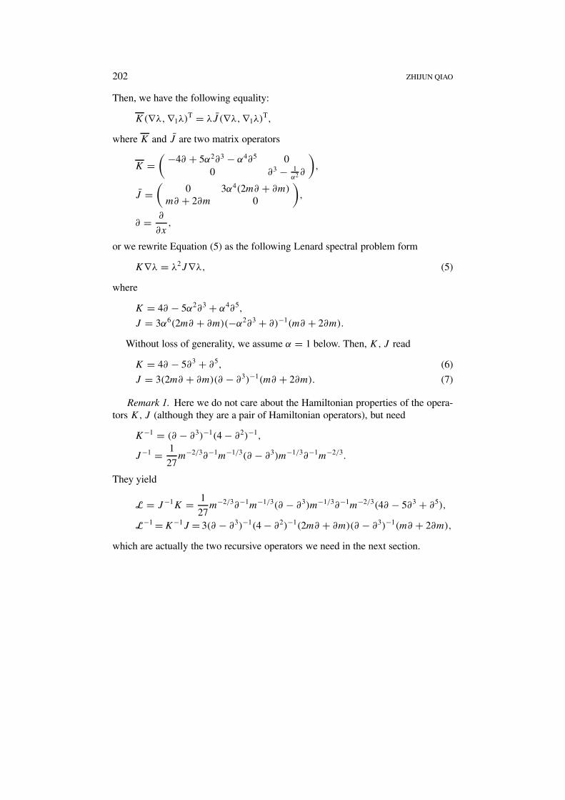
Then, we have the following equality:

K(∇λ,∇1λ)T = λJ̄ (∇λ,∇1λ)T,

where K and J̄ are two matrix operators

K =( −4∂ + 5α2∂3 − α4∂5 0

0 ∂3 − 1α2 ∂

),

J̄ =(

0 3α4(2m∂ + ∂m)

m∂ + 2∂m 0

),

∂ = ∂

∂x,

or we rewrite Equation (5) as the following Lenard spectral problem form

K∇λ = λ2J∇λ, (5)

where

K = 4∂ − 5α2∂3 + α4∂5,

J = 3α6(2m∂ + ∂m)(−α2∂3 + ∂)−1(m∂ + 2∂m).

Without loss of generality, we assume α = 1 below. Then, K, J read

K = 4∂ − 5∂3 + ∂5, (6)

J = 3(2m∂ + ∂m)(∂ − ∂3)−1(m∂ + 2∂m). (7)

Remark 1. Here we do not care about the Hamiltonian properties of the opera-tors K, J (although they are a pair of Hamiltonian operators), but need

K−1 = (∂ − ∂3)−1(4 − ∂2)−1,

J −1 = 1

27m−2/3∂−1m−1/3(∂ − ∂3)m−1/3∂−1m−2/3.

They yield

L = J −1K = 1

27m−2/3∂−1m−1/3(∂ − ∂3)m−1/3∂−1m−2/3(4∂ − 5∂3 + ∂5),

L−1 =K−1J = 3(∂ − ∂3)−1(4 − ∂2)−1(2m∂ + ∂m)(∂ − ∂3)−1(m∂ + 2∂m),

which are actually the two recursive operators we need in the next section.

INTEGRABLE HIERARCHY 203

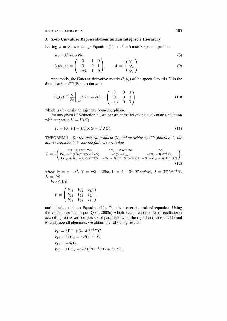
3. Zero Curvature Representations and an Integrable Hierarchy

Letting ψ = ψ1, we change Equation (1) to a 3 × 3 matrix spectral problem

�x = U(m, λ)�, (8)

U(m, λ) = 0 1 0

0 0 1−mλ 1 0

, � =

ψ1

ψ2

ψ3

. (9)

Apparently, the Gateaux derivative matrix U∗(ξ) of the spectral matrix U in thedirection ξ ∈ C∞(R) at point m is

U∗(ξ)�= d

dε

∣∣∣∣ε=0

U(m + εξ) = 0 0 0

0 0 0−ξλ 0 0

(10)

which is obviously an injective homomorphism.For any given C∞-function G, we construct the following 3×3 matrix equation

with respect to V = V (G)

Vx − [U,V ] = U∗(KG − λ2JG). (11)

THEOREM 1. For the spectral problem (8) and an arbitrary C∞-function G, thematrix equation (11) has the following solution

V = λ

G + 3λ∂�−1ϒG 3Gx − 3λ�−1ϒG −6G

Gx + 3λ(∂2�−1ϒG + 2mG) −2(G − Gxx) −3Gx − 3λ�−1ϒG

Gxx + 3λ(∂ + λm)�−1ϒG −�G − 3λ(∂−1ϒG − 2mG) −2G − Gxx − 3λ∂�−1ϒG

,

(12)

where � = ∂ − ∂3, ϒ = m∂ + 2∂m, = 4 − ∂2. Therefore, J = 3ϒ∗�−1ϒ ,K = �.

Proof. Let

V = V11 V12 V13

V21 V22 V23

V31 V32 V33

,

and substitute it into Equation (11). That is a over-determined equation. Usingthe calculation technique (Qiao, 2002a) which needs to compare all coefficientsaccording to the various powers of parameter λ on the right-hand side of (11) andto analysize all elements, we obtain the following results:

V11 = λG + 3λ2∂�−1ϒG,

V12 = 3λGx − 3λ2�−1ϒG,

V13 = −6λG,

V21 = λGx + 3λ2(∂2�−1ϒG + 2mG),

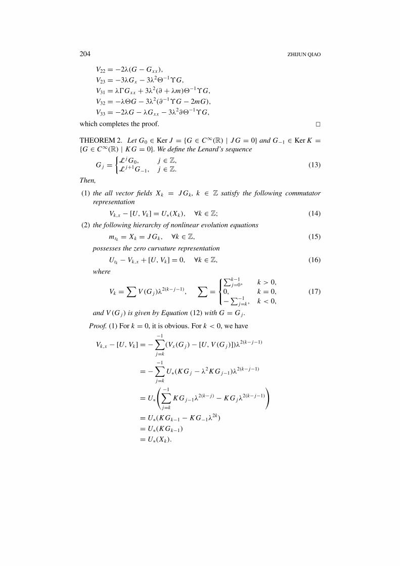
204 ZHIJUN QIAO

V22 = −2λ(G − Gxx),

V23 = −3λGx − 3λ2�−1ϒG,

V31 = λGxx + 3λ2(∂ + λm)�−1ϒG,

V32 = −λ�G − 3λ2(∂−1ϒG − 2mG),

V33 = −2λG − λGxx − 3λ2∂�−1ϒG,

which completes the proof. �THEOREM 2. Let G0 ∈ Ker J = {G ∈ C∞(R) | JG = 0} and G−1 ∈ Ker K ={G ∈ C∞(R) | KG = 0}. We define the Lenard’s sequence

Gj ={LjG0, j ∈ Z,

Lj+1G−1, j ∈ Z.(13)

Then,

(1) the all vector fields Xk = JGk, k ∈ Z satisfy the following commutatorrepresentation

Vk,x − [U,Vk] = U∗(Xk), ∀k ∈ Z; (14)

(2) the following hierarchy of nonlinear evolution equations

mtk = Xk = JGk, ∀k ∈ Z, (15)

possesses the zero curvature representation

Utk − Vk,x + [U,Vk] = 0, ∀k ∈ Z, (16)

where

Vk =∑

V (Gj)λ2(k−j−1),

∑=

∑k−1j=0, k > 0,

0, k = 0,

−∑−1j=k, k < 0,

(17)

and V (Gj) is given by Equation (12) with G = Gj .

Proof. (1) For k = 0, it is obvious. For k < 0, we have

Vk,x − [U,Vk] = −−1∑j=k

(Vx(Gj) − [U,V (Gj )])λ2(k−j−1)

= −−1∑j=k

U∗(KGj − λ2KGj−1)λ2(k−j−1)

= U∗

( −1∑j=k

KGj−1λ2(k−j) − KGjλ

2(k−j−1)

)

= U∗(KGk−1 − KG−1λ2k)

= U∗(KGk−1)

= U∗(Xk).

INTEGRABLE HIERARCHY 205

For the case of k > 0, it is similar to prove.(2) Noticing Utk = U∗(mtk ), we obtain

Utk − Vk,x + [U,Vk] = U∗(mtk − Xk).

The injectiveness of U∗ implies that result (2) is correct. �So, the hierarchy (15) has Lax pair and is therefore integrable. In particular,

through choosing G−1 = − 16 ∈ Ker K, (15) reads

mtk = −JLk+1 · 1

6, k = −1,−2, . . . , (18)

where L = J −1K. Set m = u − uxx , then it is easy to see the first equation in thehierarchy is exactly the DP equation (Degasperis and Procesi, 1999)

mt + umx + 3mux = 0, t = t−1. (19)

This equation has the following Lax pair:

�x = U(m, λ)�,

�t = V (m, λ)�, (20)

where U(m, λ) is defined by Equation (9), and V (m, λ) is given by

V (m, λ) = ux + 2

3λ−1 −u −λ−1

u − 13λ

−1 −u

ux + umλ 0 −ux − 13λ

−1

, (21)

which can be changed to the form in (Degasperis et al., 2002)

ψt + λ−1ψxx + uψx −(

ux + 2

3λ−1

)ψ = 0, ψ = ψ1. (22)

Let us choose a kernel element G0 from Ker J : G0 = m−2/3. Then Equa-tion (15) reads the following integrable hierarchy

mtk = JLkm−2/3, k = 0, 1, 2, . . . . (23)

In particular, the equation

mt = 4(m−2/3)x − 5(m−2/3)xxx + (m−2/3)xxxxx, (24)

has the Lax pair:

�x = U(m, λ)�,

�t = V1(m, λ)�, (25)

206 ZHIJUN QIAO

where U(m, λ) is defined by Equation (9), and V1(m, λ) is given by

V1(m, λ)= λ

m−2/3 3(m−2/3)x −6m−2/3

(m−2/3)x + 6λm1/3 2(m−2/3)xx − 2m−2/3 −3(m−2/3)x

(m−2/3)xx (m−2/3)xxx − (m−2/3)x + 6λm1/3 −2m−2/3 − (m−2/3)xx

(26)

with the operator = 4−∂2. Equation (24) is therefore a new integrable equation.In the next two sections we will give parametric solutions for the negative order

hierarchy (18) and the positive order hierarchy (23).

4. Parametric Solution of the Negative Order Hierarchy

To get the parametric solution, we use the constrained method which leads finite-dimensional integrable systems to the PDEs. Becasue Equation (8) is a 3rd-ordereigenvalue problem, we have to investigate itself together with its adjoint problemwhen we adopt the nonlinearized procedure (Cao, 1989). Ma and Strampp (1994)already studied the AKNS and its its adjoint problem, a 2 × 2 case, by using theso-called symmetry constraint method. Now, we are discussing a 3 × 3 problemrelated to the hierarchy (15). Let us return to the spectral problem (8) and considerits adjoint problem

�∗x =

0 0 mλ

−1 0 −10 −1 0

�∗, �∗ =

ψ∗

1ψ∗

2ψ∗

3

, (27)

where ψ∗ = ψ∗3 .

4.1. NONLINEARIZED SPECTRAL PROBLEMS ON A SYMPLECTIC

SUBMANIFOLD

Let λj (j = 1, . . . , N) be N distinct spectral values of (8) and (27), and q1j , q2j , q3j

and p1j , p2j , p3j be the corresponding spectral functions, respectively. Then wehave

q1x = q2,

q2x = q3,

q3x = −m q1 + q2,

(28)

and

p1x = m p3,

p2x = −p1 − p3,

p3x = −p2,

(29)

where = diag(λ1, . . . , λN), qk = (qk1, qk2, . . . , qkN)T, pk = (pk1, pk2, . . . ,

pkN)T, k = 1, 2, 3.

INTEGRABLE HIERARCHY 207

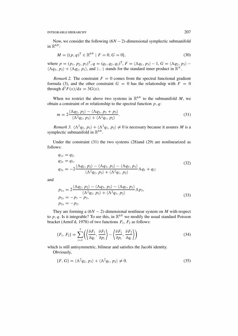
Now, we consider the following (6N − 2)-dimensional symplectic submanifoldin R

6N :

M = {(p, q)T ∈ R6N | F = 0,G = 0}, (30)

where p = (p1, p2, p3)T, q = (q1, q2, q3)

T, F = 〈 q1, p3〉 − 1, G = 〈 q2, p3〉 −〈 q3, p2〉 + 〈 q2, p1〉, and 〈·, ·〉 stands for the standard inner product in R

N .

Remark 2. The constraint F = 0 comes from the spectral functional gradientformula (3), and the other constraint G = 0 has the relationship with F = 0through d3F(x)/dx = 3G(x).

When we restrict the above two systems in R6N to the submanifold M, we

obtain a constraint of m relationship to the spectral function p, q:

m = 2〈 q2, p2〉 − 〈 q3, p1 + p3〉

〈 2q2, p3〉 + 〈 2q1, p2〉 . (31)

Remark 3. 〈 2q2, p3〉 + 〈 2q1, p2〉 = 0 is necessary because it assures M is asymplectic submanifold in R

6N .

Under the constraint (31) the two systems (28)and (29) are nonlinearized asfollows:

q1x = q2,

q2x = q3,

q3x = −2〈 q2, p2〉 − 〈 q3, p3〉 − 〈 q3, p1〉

〈 2q2, p3〉 + 〈 2q1, p2〉 q1 + q2;(32)

and

p1x = 2〈 q2, p2〉 − 〈 q3, p3〉 − 〈 q3, p1〉

〈 2q2, p3〉 + 〈 2q1, p2〉 p3,

p2x = −p1 − p3,

p3x = −p2.

(33)

They are forming a (6N − 2)-dimensional nonlinear system on M with respectto p, q. Is it integrable? To see this, in R

6N we modify the usual standard Poissonbracket (Arnol’d, 1978) of two functions F1, F2 as follows:

{F1, F2} =3∑

i=1

(⟨∂F1

∂qi

,∂F2

∂pi

⟩−

⟨∂F1

∂pi

,∂F2

∂qi

⟩)(34)

which is still antisymmetric, bilinear and satisfies the Jacobi identity.Obviously,

{F,G} = 〈 2q2, p3〉 + 〈 2q1, p2〉 = 0. (35)

208 ZHIJUN QIAO

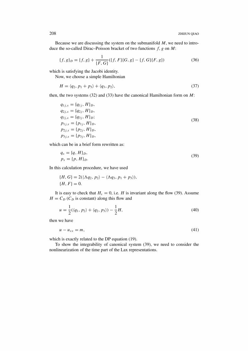
Because we are discussing the system on the submanifold M, we need to intro-duce the so-called Dirac–Poisson bracket of two functions f, g on M:

{f, g}D = {f, g} + 1

{F,G} ({f, F }{G, g} − {f,G}{F, g}) (36)

which is satisfying the Jacobi identity.Now, we choose a simple Hamiltonian

H = 〈q2, p1 + p3〉 + 〈q3, p2〉, (37)

then, the two systems (32) and (33) have the canonical Hamiltonian form on M:

q1j,x = {q1j , H }D,

q2j,x = {q2j , H }D,

q3j,x = {q3j , H }D;p1j,x = {p1j , H }D,

p2j,x = {p2j , H }D,

p3j,x = {p3j , H }D,

(38)

which can be in a brief form rewritten as:

qx = {q,H }D,

px = {p,H }D.(39)

In this calculation procedure, we have used

{H,G} = 2(〈 q2, p2〉 − 〈 q3, p1 + p3〉),{H,F } = 0.

It is easy to check that Hx = 0, i.e. H is invariant along the flow (39). AssumeH = CD (CD is constant) along this flow and

u = 1

2(〈q1, p2〉 + 〈q2, p3〉) − 1

2H, (40)

then we have

u − uxx = m, (41)

which is exactly related to the DP equation (19).To show the integrability of canonical system (39), we need to consider the

nonlinearization of the time part of the Lax representations.

INTEGRABLE HIERARCHY 209

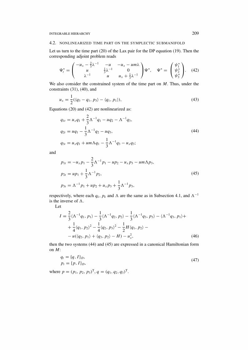
4.2. NONLINEARIZED TIME PART ON THE SYMPLECTIC SUBMANIFOLD

Let us turn to the time part (20) of the Lax pair for the DP equation (19). Then thecorresponding adjoint problem reads

�∗t =

−ux − 2

3λ−1 −u −ux − umλ

u 13λ−1 0

λ−1 u ux + 13λ−1

�∗, �∗ =

ψ∗

1ψ∗

2ψ∗

3

. (42)

We also consider the constrained system of the time part on M. Thus, under theconstraints (31), (40), and

ux = 1

2(〈q3 − q1, p3〉 − 〈q1, p1〉), (43)

Equations (20) and (42) are nonlinearized as:

q1t = uxq1 + 2

3 −1q1 − uq2 − −1q3,

q2t = uq1 − 1

3 −1q2 − uq3,

q3t = uxq1 + um q1 − 1

3 −1q3 − uxq3;

(44)

and

p1t = −uxp1 − 2

3 −1p1 − up2 − uxp3 − um p3,

p2t = up1 + 1

3 −1p2,

p3t = −1p1 + up2 + uxp3 + 1

3 −1p3,

(45)

respectively, where each qk, pk and are the same as in Subsection 4.1, and −1

is the inverse of .Let

I = 2

3〈 −1q1, p1〉 − 1

3〈 −1q2, p2〉 − 1

3〈 −1q3, p3〉 − 〈 −1q3, p1〉+

+ 1

4〈q1, p2〉2 − 1

4〈q2, p3〉2 − 1

2H 〈q1, p2〉 −

− u(〈q2, p1〉 + 〈q3, p2〉 − H) − u2x, (46)

then the two systems (44) and (45) are expressed in a canonical Hamiltonian formon M:

qt = {q, I }D,

pt = {p, I }D,(47)

where p = (p1, p2, p3)T, q = (q1, q2, q3)

T.

210 ZHIJUN QIAO

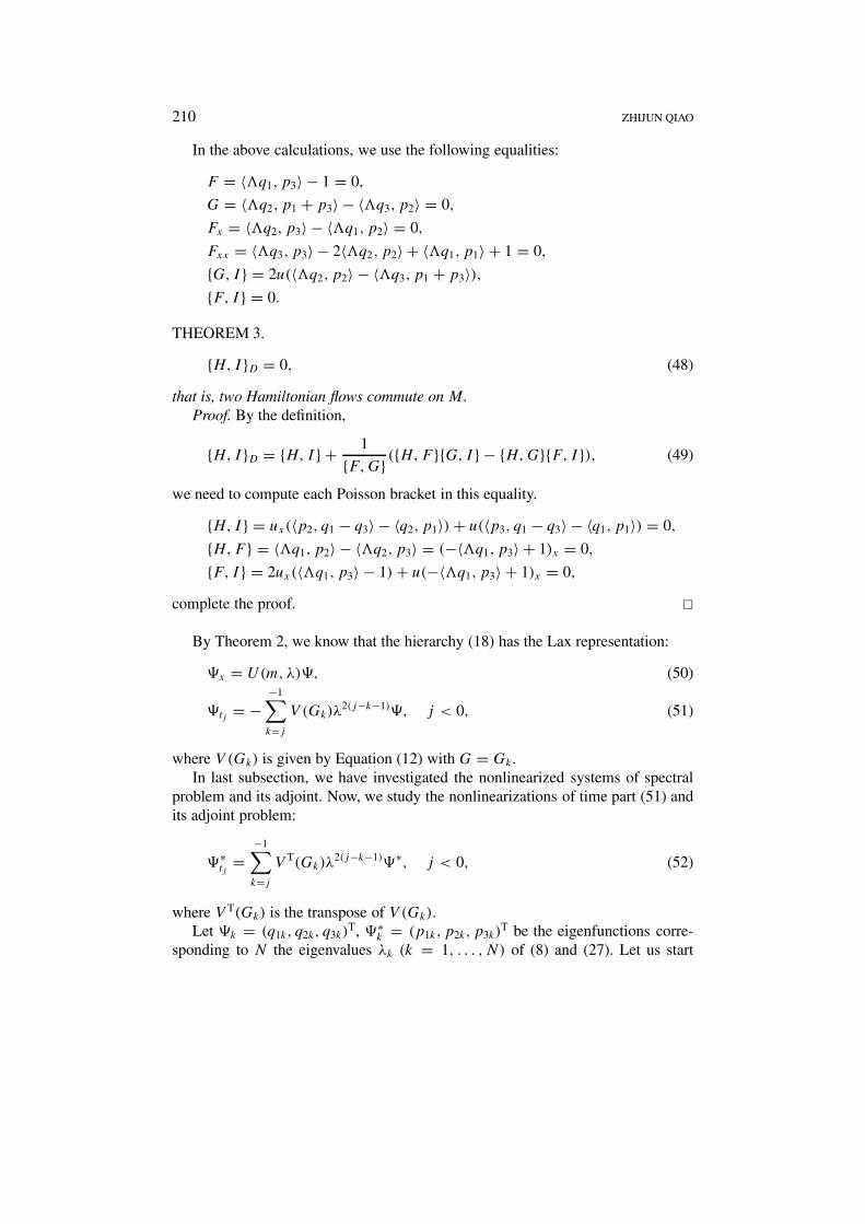
In the above calculations, we use the following equalities:

F = 〈 q1, p3〉 − 1 = 0,

G = 〈 q2, p1 + p3〉 − 〈 q3, p2〉 = 0,

Fx = 〈 q2, p3〉 − 〈 q1, p2〉 = 0,

Fxx = 〈 q3, p3〉 − 2〈 q2, p2〉 + 〈 q1, p1〉 + 1 = 0,

{G, I } = 2u(〈 q2, p2〉 − 〈 q3, p1 + p3〉),{F, I } = 0.

THEOREM 3.

{H, I }D = 0, (48)

that is, two Hamiltonian flows commute on M.Proof. By the definition,

{H, I }D = {H, I } + 1

{F,G} ({H,F }{G, I } − {H,G}{F, I }), (49)

we need to compute each Poisson bracket in this equality.

{H, I } = ux(〈p2, q1 − q3〉 − 〈q2, p1〉) + u(〈p3, q1 − q3〉 − 〈q1, p1〉) = 0,

{H,F } = 〈 q1, p2〉 − 〈 q2, p3〉 = (−〈 q1, p3〉 + 1)x = 0,

{F, I } = 2ux(〈 q1, p3〉 − 1) + u(−〈 q1, p3〉 + 1)x = 0,

complete the proof. �By Theorem 2, we know that the hierarchy (18) has the Lax representation:

�x = U(m, λ)�, (50)

�tj = −−1∑k=j

V (Gk)λ2(j−k−1)�, j < 0, (51)

where V (Gk) is given by Equation (12) with G = Gk.In last subsection, we have investigated the nonlinearized systems of spectral

problem and its adjoint. Now, we study the nonlinearizations of time part (51) andits adjoint problem:

�∗tj

=−1∑k=j

V T(Gk)λ2(j−k−1)�∗, j < 0, (52)

where V T(Gk) is the transpose of V (Gk).Let �k = (q1k, q2k, q3k)

T, �∗k = (p1k, p2k, p3k)

T be the eigenfunctions corre-sponding to N the eigenvalues λk (k = 1, . . . , N) of (8) and (27). Let us start

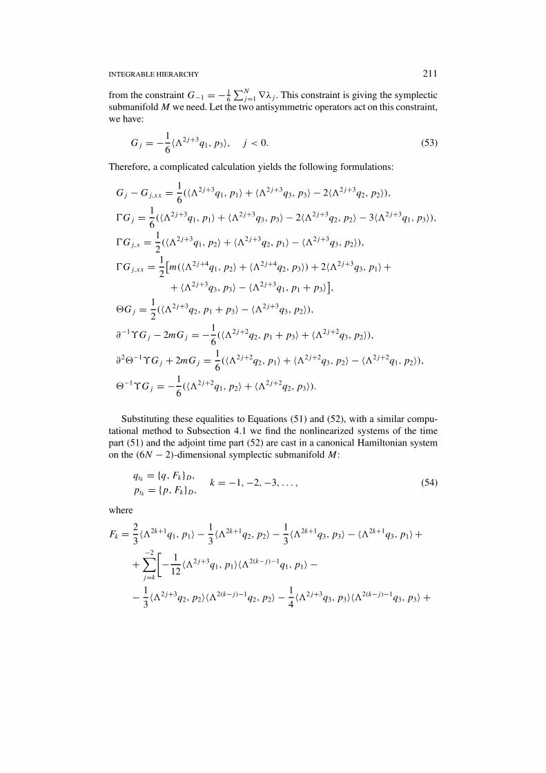
INTEGRABLE HIERARCHY 211

from the constraint G−1 = − 16

∑Nj=1 ∇λj . This constraint is giving the symplectic

submanifold M we need. Let the two antisymmetric operators act on this constraint,we have:

Gj = −1

6〈 2j+3q1, p3〉, j < 0. (53)

Therefore, a complicated calculation yields the following formulations:

Gj − Gj,xx = 1

6(〈 2j+3q1, p1〉 + 〈 2j+3q3, p3〉 − 2〈 2j+3q2, p2〉),

Gj = 1

6(〈 2j+3q1, p1〉 + 〈 2j+3q3, p3〉 − 2〈 2j+3q2, p2〉 − 3〈 2j+3q1, p3〉),

Gj,x = 1

2(〈 2j+3q1, p2〉 + 〈 2j+3q2, p1〉 − 〈 2j+3q3, p2〉),

Gj,xx = 1

2

[m(〈 2j+4q1, p2〉 + 〈 2j+4q2, p3〉) + 2〈 2j+3q3, p1〉++ 〈 2j+3q3, p3〉 − 〈 2j+3q1, p1 + p3〉

],

�Gj = 1

2(〈 2j+3q2, p1 + p3〉 − 〈 2j+3q3, p2〉),

∂−1ϒGj − 2mGj = −1

6(〈 2j+2q2, p1 + p3〉 + 〈 2j+2q3, p2〉),

∂2�−1ϒGj + 2mGj = 1

6(〈 2j+2q2, p1〉 + 〈 2j+2q3, p2〉 − 〈 2j+2q1, p2〉),

�−1ϒGj = −1

6(〈 2j+2q1, p2〉 + 〈 2j+2q2, p3〉).

Substituting these equalities to Equations (51) and (52), with a similar compu-tational method to Subsection 4.1 we find the nonlinearized systems of the timepart (51) and the adjoint time part (52) are cast in a canonical Hamiltonian systemon the (6N − 2)-dimensional symplectic submanifold M:

qtk = {q, Fk}D,

ptk = {p,Fk}D,k = −1,−2,−3, . . . , (54)

where

Fk = 2

3〈 2k+1q1, p1〉 − 1

3〈 2k+1q2, p2〉 − 1

3〈 2k+1q3, p3〉 − 〈 2k+1q3, p1〉+

+−2∑j=k

[− 1

12〈 2j+3q1, p1〉〈 2(k−j)−1q1, p1〉 −

− 1

3〈 2j+3q2, p2〉〈 2(k−j)−1q2, p2〉 − 1

4〈 2j+3q3, p3〉〈 2(k−j)−1q3, p3〉 +

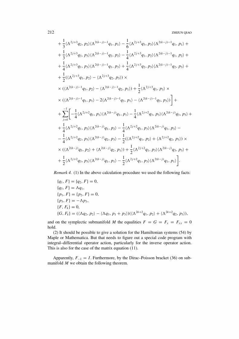
212 ZHIJUN QIAO

+ 1

3〈 2j+3q2, p2〉〈 2(k−j)−1q1, p1〉 − 1

6〈 2j+3q3, p3〉〈 2(k−j)−1q1, p1〉 +

+ 1

3〈 2j+3q3, p3〉〈 2(k−j)−1q2, p2〉 − 1

4〈 2j+3q1, p2〉〈 2(k−j)−1q1, p2〉 +

+ 1

4〈 2j+3q1, p3〉〈 2(k−j)−1q1, p3〉 + 1

4〈 2j+3q2, p3〉〈 2(k−j)−1q2, p3〉 +

+ 1

2(〈 2j+3q1, p2〉 − 〈 2j+3q2, p3〉) ×

× (〈 2(k−j)−1q3, p2〉 − 〈 2(k−j)−1q2, p1〉) + 1

2〈 2j+3q1, p3〉 ×

× (〈 2(k−j)−1q1, p1〉 − 2〈 2(k−j)−1q3, p1〉 − 〈 2(k−j)−1q3, p3〉)]

+

+−1∑j=k

[−1

4〈 2j+2q1, p1〉〈 2(k−j)q1, p1〉− 1

4〈 2j+2q3, p3〉〈 2(k−j)q3, p3〉+

+ 1

4〈 2j+2q1, p2〉〈 2(k−j)q1, p2〉 − 1

4〈 2j+2q1, p3〉〈 2(k−j)q1, p3〉 −

− 1

4〈 2j+2q2, p3〉〈 2(k−j)q2, p3〉 − 1

2(〈 2j+2q1, p2〉 + 〈 2j+2q2, p3〉) ×

× (〈 2(k−j)q3, p2〉 + 〈 2(k−j)q2, p1〉) + 1

2〈 2j+2q1, p3〉〈 2(k−j)q3, p3〉 +

+ 1

2〈 2j+2q3, p3〉〈 2(k−j)q1, p1〉 − 1

2〈 2j+2q1, p3〉〈 2(k−j)q1, p1〉

].

Remark 4. (1) In the above calculation procedure we used the following facts:

{q1, F } = {q2, F } = 0,

{q3, F } = q1,

{p1, F } = {p2, F } = 0,

{p3, F } = − p3,

{F,Fk} = 0,

{G,Fk} = (〈 q2, p2〉 − 〈 q3, p1 + p3〉)(〈 2k+2q1, p2〉 + 〈 2k+2q2, p3〉),and on the symplectic submanifold M the equalities F = G = Fx = Fxx = 0hold.

(2) It should be possible to give a solution for the Hamiltonian systems (54) byMaple or Mathematica. But that needs to figure out a special code program withintegral–differential operator action, particularly for the inverse operator action.This is also for the case of the matrix equation (11).

Apparently, F−1 = I . Furthermore, by the Dirac–Poisson bracket (36) on sub-manifold M we obtain the following theorem.

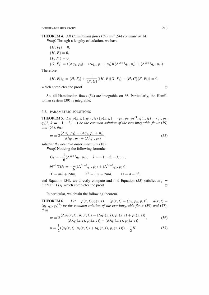
INTEGRABLE HIERARCHY 213

THEOREM 4. All Hamiltonian flows (39) and (54) commute on M.Proof. Through a lengthy calculation, we have

{H,Fk} = 0,

{H,F } = 0,

{F,Fk} = 0,

{G,Fk} = (〈 q2, p2〉 − 〈 q3, p1 + p3〉)(〈 2k+2q1, p2〉 + 〈 2k+2q2, p3〉).Therefore,

{H,Fk}D = {H,Fk} + 1

{F,G} ({H,F }{G,Fk} − {H,G}{F,Fk}) = 0,

which completes the proof. �So, all Hamiltonian flows (54) are integrable on M. Particularly, the Hamil-

tonian system (39) is integrable.

4.3. PARAMETRIC SOLUTIONS

THEOREM 5. Let p(x, tk), q(x, tk ) (p(x, tk) = (p1, p2, p3)T, q(x, tk ) = (q1, q2,

q3)T, k = −1,−2, . . .) be the common solution of the two integrable flows (39)

and (54), then

m = 2〈 q2, p2〉 − 〈 q3, p1 + p3〉

〈 2q2, p3〉 + 〈 2q1, p2〉 , (55)

satisfies the negative order hierarchy (18).Proof. Noticing the following formulas

Gk = −1

6〈 2k+3q1, p3〉, k = −1,−2,−3, . . . ,

�−1ϒGk = −1

6(〈 2k+2q1, p2〉 + 〈 2k+2q2, p3〉),

ϒ = m∂ + 2∂m, ϒ∗ = ∂m + 2m∂, � = ∂ − ∂3,

and Equation (54), we directly compute and find Equation (55) satisfies mtk =3ϒ∗�−1ϒGk which completes the proof. �

In particular, we obtain the following theorem.

THEOREM 6. Let p(x, t), q(x, t) (p(x, t) = (p1, p2, p3)T, q(x, t) =

(q1, q2, q3)T) be the common solution of the two integrable flows (39) and (47),

then

m = 2〈 q2(x, t), p2(x, t)〉 − 〈 q3(x, t), p1(x, t) + p3(x, t)〉

〈 2q2(x, t), p3(x, t)〉 + 〈 2q1(x, t), p2(x, t)〉 , (56)

u = 1

2(〈q1(x, t), p2(x, t)〉 + 〈q2(x, t), p3(x, t)〉) − 1

2H, (57)

214 ZHIJUN QIAO

satisfy the DP equation:

mt + umx + 3mux = 0. (58)

Proof. Let

A = 〈 q2, p2〉 − 〈 q3, p1 + p3〉,B = 〈 2q2, p3〉 + 〈 2q1, p2〉,C = 〈 2q3, p3〉 − 〈 2q1, p1 + p3〉.

Then through a lengthy calculation we have

At = uG + umC − 2uxA = umC − 2uxA,

Bt = G − uC + uxB = −uC + uxB,

Ax = −2G − mC = −mC,

Bx = C.

By the above equalities, we obtain

mt + umx + 3mux = 2

B2[AtB − ABt + u(AxB − ABx) + 3uxAB]

= 2

B2(umBC + uAC + uAxB − uABx)

= 2u

B2(B(mC + Ax) + A(C − Bx))

= 0.

In the above proof procedures, we have used the following equalities: F = G = 0,Fx = Fxx = 0 on M. �

Similarly, we can discuss the parametric solution of the positive order hierar-chy (23). That needs us to consider a new kind of constraint and related integrablesystem, which we deal with in the next section.

5. Parametric Solution of the Positive Order Hierarchy

Let us directly consider the following constraint:

G0 =N∑

j=1

Ej∇λj , (59)

where Ej∇λj = λjq1jp3j is the functional gradient of λj for the spectral prob-lems (8) and (27), and qkj , pkj (k = 1, 2, 3) are the related eigenfunctions of λj .Then Equation (59) is saying

m = 〈 q1, p3〉−3/2 (60)

INTEGRABLE HIERARCHY 215

which composes a new constraint in the whole space R6N . Under this constraint,

the spectral problem (8) and its adjoint problem (27) are able to be cast in aHamiltonian canonical form in R

6N :

(H+):qx = {q,H+},px = {p,H+}, (61)

with the Hamiltonian

H+ = 〈q2, p1 + p3〉 + 〈q3, p2〉 + 2√〈 q1, p3〉 . (62)

To see the integrability of the system (61), we take into account of the time part�t = V1(m, λ)� and its adjoint �t = −V T

1 (m, λ)�, where V1(m, λ) is definedby Equation (26). Under the constraint (60), the time part and its adjoint are alsononlinearized as a canonical Hamiltonian system in R

6N

(F1):qt = {q, F1},pt = {p,F1}, (63)

with the Hamiltonian

F1 = 6〈 2q1, p2〉 + 〈 2q2, p3〉√〈 q1, p3〉 −

− 1

2(〈 q1, p1〉2 + 4〈 q2, p2〉2 + 〈 q3, p3〉2) +

+ 3

2(〈 q1, p3〉2 + 〈 q2, p3〉2 − 〈 q1, p2〉2) +

+ 3〈 q1, p3〉(〈 q1, p1〉 − 2〈 q3, p1〉 − 〈 q3, p3〉) ++ 2〈 q1, p1〉〈 q2, p2〉 + 2〈 q2, p2〉〈 q3, p3〉 − 〈 q1, p1〉〈 q3, p3〉 ++ 3(〈 q1, p2〉 − 〈 q2, p3〉)(〈 q3, p2〉 − 〈 q2, p1〉). (64)

After a calculation of the Poisson bracket of {H+, F1}, we know that the twocanonical Hamiltonian flows commute, i.e.

{H+, F1} = 0.

Furthermore, under the constraint (60) the nonlinearized systems of the generaltime part �tk = ∑k−1

j=0 V (Gj)λ2(k−j−1)� (k > 0, k ∈ Z) and its adjoint problem

produce the following canonical Hamiltonian system in R6N :

(Fk):qtk = {q, Fk},ptk = {p,Fk}, k = 1, 2, 3, . . . , (65)

with the Hamiltonian

Fk = 6〈 2kq1, p2〉 + 〈 2kq2, p3〉√〈 q1, p3〉 +

216 ZHIJUN QIAO

+k−1∑j=0

[−1

2〈 2j+1q1, p1〉〈 2(k−j)−1q1, p1〉 −

− 2〈 2j+1q2, p2〉〈 2(k−j)−1q2, p2〉 − 1

2〈 2j+1q3, p3〉〈 2(k−j)−1q3, p3〉 +

+ 2〈 2j+1q2, p2〉〈 2(k−j)−1q1, p1〉 − 〈 2j+1q3, p3〉〈 2(k−j)−1q1, p1〉 ++ 2〈 2j+1q3, p3〉〈 2(k−j)−1q2, p2〉 − 3

2〈 2j+1q1, p2〉〈 2(k−j)−1q1, p2〉 +

+ 3

2〈 2j+1q1, p3〉〈 2(k−j)−1q1, p3〉 + 3

2〈 2j+1q2, p3〉〈 2(k−j)−1q2, p3〉 +

+ 3(〈 2j+1q1, p2〉 − 〈 2j+1q2, p3〉) ×× (〈 2(k−j)−1q3, p2〉 − 〈 2(k−j)−1q2, p1〉) + 3〈 2j+1q1, p3〉 ×× (〈 2(k−j)−1q1, p1〉 − 2〈 2(k−j)−1q3, p1〉 − 〈 2(k−j)−1q3, p3〉)

]+

+k−1∑j=1

[−3

2〈 2jq1, p1〉〈 2(k−j)q1, p1〉 − 3

2〈 2j q3, p3〉〈 2(k−j)q3, p3〉 +

+ 3

2〈 2jq1, p2〉〈 2(k−j)q1, p2〉 − 3

2〈 2j q1, p3〉〈 2(k−j)q1, p3〉 −

− 3

2〈 2jq2, p3〉〈 2(k−j)q2, p3〉 − 3(〈 2j q1, p2〉 + 〈 2jq2, p3〉) ×

× (〈 2(k−j)q3, p2〉 + 〈 2(k−j)q2, p1〉) + 3〈 2j q1, p3〉〈 2(k−j)q3, p3〉 ++ 3〈 2j q3, p3〉〈 2(k−j)q1, p1〉 − 3〈 2j q1, p3〉〈 2(k−j)q1, p1〉

].

Apparently, when k = 1, Fk is exactly Equation (64). Furthermore, through alengthy computation, we obtain

{H+, Fk} = 0, k = 1, 2, . . . , (66)

which represents each Hamiltonian t-flow (Fk) commutes with Hamiltonian x-flow (H+). Thus, all Hamiltonian canonical systems (Fk) are integrable in R

6N .Particularly, the nonlinearized spectral problems (61) is integrable.

Like last section, we also have a similar theorem

THEOREM 7. Let p(x, tk), q(x, tk ) (p(x, tk) = (p1, p2, p3)T, q(x, tk) =

(q1, q2, q3)T, k = 1, 2, 3, . . .) be the common solution of the two integrable flows (61)

and (65), then

m = 1√〈 q1(x, tk), p3(x, tk)〉3, k = 1, 2, 3, . . . , (67)

satisfy the positive order hierarchy (23).

INTEGRABLE HIERARCHY 217

In particular, we have the following theorem.

THEOREM 8. Let p(x, t), q(x, t) (p(x, t) = (p1, p2, p3)T, q(x, t) =

(q1, q2, q3)T) be the common solution of the two integrable flows (61) and (63),

then

m = 1√〈 q1(x, t), p3(x, t)〉3(68)

is a parametric solution of the 5th-order equation:

mt = 4(m−2/3)x − 5(m−2/3)xxx + (m−2/3)xxxxx. (69)

Proof. A direct check is done through substitution of Equations (61) and (63). �

6. Summaries

We have known that the DP equation mt + umx + 3mux = 0, m = u − mxx

has peaked soliton solution u = e−|x+t |, and moreover it has multi-peaked-solitonsolutions (Holm and Staley, 2002; Holm and Hone, 2002). For more general case,all b-balanced equations mt + umx + bmux = 0, m = u − mxx , b = constantare also found to have this kind of solutions (Holm and Staley, 2002). But thefinite-dimensional systems, derived from the all b-balanced equations (includingthe DP equation (b = 3) but except the CH equation (b = 2)) through multisoli-ton solutions setting, are not canonical Hamiltonian system (see Holm and Hone,2002). Here our results show that the DP spectral problem can be developed asa completely integrable canonical Hamiltonian system under a constraint betweenthe potential and the eigenfunctions. Furthermore, we give the parametric solutionsfor the whole hierarchy, in particular for the DP equation. Our parametric solutionsare not given in an explicit form, but from our experience (Qiao, 2001, 2002a,2003) we believe that our parametric solutions should give perodic/quasi-perodicsolutions which are explicit instead of multi-soliton solutions. Our parametric solu-tions can not include the peaked soliton solutions because the parametric solutionsare smooth but the peaked soliton solutions only continous.

Nevertheless, we would like to directly derive possible traveling wave solutionsfor the 5th-order PDE

mt = 4(m−2/3)x − 5(m−2/3)xxx + (m−2/3)xxxxx

which is the second equation in the positive order hierarchy (23). Let us setm−2/3 = v, then this equation becomes

−3

2v−2/3vt = 4vx − 5vxxx + vxxxxx. (70)

218 ZHIJUN QIAO

Assume this equation has the solution v = f (ξ), ξ = x − ct , c = constant, thenwe have

2cf −1/2 = 2f 2 − 5

2f ′2 + f ′f ′′′ − 1

2f ′′2. (71)

The right-hand side of this equation is quadratically homogeneous and the lefthand side not. Therefore, we set f = eaξ , a = constant and substitute it intoEquation (71), and obtain

c = 0, (72)

a4 − 5a2 + 4 = 0, (73)

which implies

a = ±1, a = ±2. (74)

So, the 5th-order equation (70) has the following stationary solutions:

1, e−x, ex, e−2x, e2x, (75)

which exactly composes the basis of the solution space of the stationary equation4vx − 5vxxx + vxxxxx = 0. Therefore, the 5th-order PDE mt = 4(m−2/3)x −5(m−2/3)xxx + (m−2/3)xxxxx possesses the stationary solutions

m(x) = (c0 + c1e−x + c2ex + c3e−2x + c4e2x)−3/2,

∀ck ∈ R, k = 0, 1, 2, 3, 4. (76)

Apparently, e− 32 x , e

32 x , e−3x , e3x satisfy the 5th-order PDE mt = 4(m−2/3)x −

5(m−2/3)xxx + (m−2/3)xxxxx.

COMPARISON WITH THE PARAMETRIC SOLUTION

All the stationary solutions (76) may be included in the parametric solution (68).For example, the function m(x) = e− 3

2 x is cast in Equation (68) when we choosedynamical variables q1, p3 such that the following constraint

〈 q1(x), p3(x)〉 = ex (77)

holds, where q1, p3 are the solutions of the integrable Hamiltonian system (61).The 5th-order PDE (70) is not located in the Harry–Dym hierarchy, and there-

fore it has no cusp (Wadati et al., 1980) solution. As for what kind of PDEs havethe cusp solution, see (Qiao, 2002b).

INTEGRABLE HIERARCHY 219

Acknowledgements

The author would like to express his sincere thanks to D. Holm, M. Mineev andK. Vixie for their fruitful discussions, and also to B. Konopelchenko and F. Magrifor their helpful suggestions during their visit at Los Alamos National Laboratory.

This work has been supported by the LANL LDRD Project 20020006ER “Un-stable Fluid/Fluid Interfaces”, the Data Driven Modeling and Analysis Group, theFoundation for the Author of National Excellent Doctoral Dissertation (FANEDD)of P.R. China, and also the research grant of University of Texas-Pan American,USA.

References

Ablowitz, M. J., Kaup, D. J., Newell, A. C. and Segur, H. (1973) Nolinear evolution equations ofphysical significance, Phys. Rev. Lett. 31, 125–127.

Ablowitz, M. J., Kaup, D. J., Newell, A. C. and Segur, H. (1974) Stud. Appl. Math. 53, 249–315.Alber, M. S., Camassa, R., Holm, D. D. and Marsden, J. E. (1994) The geometry of peaked solitons

and billiard solutions of a class of integrable PDE’s, Lett. Math. Phys. 32, 137–151.Alber, M. S., Camassa, R., Holm, D. D. and Marsden, J. E. (1995) On the link between umbilic

geodesics and soliton solutions of nonlinear PDE’s, Proc. Roy. Soc. 450, 677–692.Alber, M. S., Camassa, R., Fedorov, Y. N., Holm, D. D. and Marsden, J. E. (1999) On billiard

solutions of nonlinear PDE’s, Phys. Lett. A 264, 171–178.Alber, M. S., Camassa, R., Fedorov, Y. N., Holm, D. D. and Marsden, J. E. (2001) The complex

geometry of weak piecewise smooth solutions of integrable nonlinear PDE’s of shallow waterand Dym type, Comm. Math. Phys. 221, 197–227.

Arnol’d, V. I. (1978) Mathematical Methods of Classical Mechanics, Springer-Verlag, Berlin.Camassa, R. and Holm, D. D. (1993) An integrable shallow water equation with peaked solitons,

Phys. Rev. Lett. 71, 1661–1664.Cao, C. W. (1989) Nonlinearization of Lax system for the AKNS hierarchy, Sci. China A 32, 701–707

(in Chinese); also see English Edition: Nonlinearization of Lax system for the AKNS hierarchy,Sci. Sin. A 33 (1990), 528–536.

Constantin, A. and McKean, H. P. (1999) A shallow water equation on the circle, Comm. Pure Appl.Math. 52, 949–982.

Degasperis, A., Holm, D. D. and Hone, A. N. W. (2002) A new integrable equation with peakonsolutions, Theoret. and Math. Phys. 133, 1463–1474.

Degasperis, A. and Procesi, M. (1999) Asymptotic integrability, in A. Degasperis and G. Gaeta (eds),Symmetry and Perturbation Theory, World Scientific, pp. 23–37.

Fokas, A. S. and Anderson, R. L. (1982) On the use of isospectral eigenvalue problems for obtaininghereditary symmetries for Hamiltonian systems, J. Math. Phys. 23, 1066–1073.

Fuchssteiner, B. and Fokas, A. S. (1981) Symplectic structures, their Baecklund transformations andhereditaries, Physica D 4, 47–66.

Gardner, C. S., Greene, J. M., Kruskal, M. D. and Miura, R. M. (1967) Method for solving theKorteweg–de Vries equation, Phys. Rev. Lett. 19, 1095–1097.

Holm, D. D. and Hone, A. N. W. (2002) Note on Peakon bracket, Private communication.Holm, D. D. and Staley, M. (2002) Private communication.Kaup, D. J. (1980) On the inverse scattering problem for cubic eigenvalue problems of the class

ψxxx + 6Qψx + 6Rψ = λψ , Stud. Appl. Math. 62, 189–216.Konopelchenko, B. G. and Dubrovsky, V. G. (1984) Some new integrable nonlinear evolution

equations in 2 + 1 dimensions, Phys. Lett. A 102, 15–17.

220 ZHIJUN QIAO

Kupershmidt, B. A. (1984) A super Korteweg–de Vries equation: An integrable system, Phys. Lett. A102, 213–215.

Korteweg, D. J. and de Vries, G. (1895) On the change of form long waves advancing in a rectangularcanal, and on a new type of long stationary waves, Phil. Mag. 39, 422–443.

Levitan, B. M. and Gasymov, M. G. (1964) Determination of a differential equation by two of itsspectra, Russian Math. Surveys 19(2), 1–63.

Ma, W. X. and Strampp, W. (1994) An explicit symmetry constraint for the Lax pairs and the adjointLax pairs of AKNS systems, Phys. Lett. A 185, 277–286.

Marchenko, V. A. (1950) Certain problems in the theory of second-order differential operators, Dokl.Akad. Nauk SSSR 72, 457–460 (Russian).

Qiao, Z. J. (2001) Generalized r-matrix structure and algebro-geometric solution for integrablesystem, Rev. Math. Phys. 13, 545–586.

Qiao, Z. J. (2002a) Finite-Dimensional Integrable System and Nonlinear Evolution Equations,Higher Education Press, P.R. China.

Qiao, Z. J. (2002b) Equations possessing cusp solitons and cusp-like singular traveling wavesolutions, Preprint.

Qiao, Z. J. (2002c) A new integrable hierarchy, parametric solutions, and traveling wave solutions,Preprint, to appear in Math. Phys. Anal. Geom.

Qiao, Z. J. (2003) The Camassa–Holm hierarchy, N-dimensional integrable systems, and algebro-geometric solution on a symplectic submanifold, Comm. Math. Phys. 239, 309–341.

Tu, G. Z. (1990) An extension of a theorem on gradients of conserved densities of integrable systems,Northeast. Math. J. 6, 26–32.

Wadati, M., Ichikawa, Y. H. and Shimizu, T. (1980) Cusp soliton of a new integrable nonlinearevolution equation, Prog. Theor. Phys. 64, 1959–1967.

Zakharov, V. E. and Shabat, A. B. (1972) Exact theory of two dimensional self focusing and onedimensional self modulation of waves in nonlinear media, Sov. Phys. JETP 34, 62–69.