COMPARISON OF CLASSICAL ANALYTIC HIERARCHY ...

University of Nebraska - Lincoln University of Nebraska - Lincoln

DigitalCommons@University of Nebraska - Lincoln DigitalCommons@University of Nebraska - Lincoln

Industrial and Management Systems Engineering -- Dissertations and Student Research

Industrial and Management Systems Engineering

11-2010

COMPARISON OF CLASSICAL ANALYTIC HIERARCHY PROCESS COMPARISON OF CLASSICAL ANALYTIC HIERARCHY PROCESS

(AHP) APPROACH AND FUZZY AHP APPROACH IN MULTIPLE-(AHP) APPROACH AND FUZZY AHP APPROACH IN MULTIPLE-

CRITERIA DECISION MAKING FOR COMMERCIAL VEHICLE CRITERIA DECISION MAKING FOR COMMERCIAL VEHICLE

INFORMATION SYSTEMS AND NETWORKS (CVISN) PROJECT INFORMATION SYSTEMS AND NETWORKS (CVISN) PROJECT

Liyuan Zhang University of Nebraska-Lincoln, [email protected]

Follow this and additional works at: https://digitalcommons.unl.edu/imsediss

Part of the Industrial Engineering Commons

Zhang, Liyuan, "COMPARISON OF CLASSICAL ANALYTIC HIERARCHY PROCESS (AHP) APPROACH AND FUZZY AHP APPROACH IN MULTIPLE-CRITERIA DECISION MAKING FOR COMMERCIAL VEHICLE INFORMATION SYSTEMS AND NETWORKS (CVISN) PROJECT" (2010). Industrial and Management Systems Engineering -- Dissertations and Student Research. 11. https://digitalcommons.unl.edu/imsediss/11

This Article is brought to you for free and open access by the Industrial and Management Systems Engineering at DigitalCommons@University of Nebraska - Lincoln. It has been accepted for inclusion in Industrial and Management Systems Engineering -- Dissertations and Student Research by an authorized administrator of DigitalCommons@University of Nebraska - Lincoln.

https://digitalcommons.unl.edu/

https://digitalcommons.unl.edu/imsediss



https://digitalcommons.unl.edu/imse

https://digitalcommons.unl.edu/imse

https://digitalcommons.unl.edu/imsediss?utm_source=digitalcommons.unl.edu%2Fimsediss%2F11&utm_medium=PDF&utm_campaign=PDFCoverPages

http://network.bepress.com/hgg/discipline/307?utm_source=digitalcommons.unl.edu%2Fimsediss%2F11&utm_medium=PDF&utm_campaign=PDFCoverPages

https://digitalcommons.unl.edu/imsediss/11?utm_source=digitalcommons.unl.edu%2Fimsediss%2F11&utm_medium=PDF&utm_campaign=PDFCoverPages

COMPARISON OF CLASSICAL ANALYTIC HIERARCHY PROCESS (AHP)

APPROACH AND FUZZY AHP APPROACH IN MULTIPLE-CRITERIA

DECISION MAKING FOR COMMERCIAL VEHICLE INFORMATION

SYSTEMS AND NETWORKS (CVISN) PROJECT

By

Liyuan Zhang

A Thesis

Presented to the Faculty of

The Graduate College at University of Nebraska

In Partial Fulfillment of Requirements

For the Degree of Master of Science

Major: Industrial and Management Systems Engineering

Under the Supervision of Professor Erick C. Jones

Lincoln, Nebraska

November, 2010

COMPARISON OF CLASSICAL ANALYTIC HIERARCHY PROCESS (AHP)

APPROACH AND FUZZY AHP APPROACH IN MULTIPLE-CRITERIA

DECISION MAKING FOR COMMERCIAL VEHICLE INFORMATION

SYSTEMS AND NETWORKS (CVISN) PROJECT

Liyuan Zhang, M.S.

University of Nebraska, 2010

Adviser: Erick C. Jones

Radio Frequency Identification (RFID) has emerged as an important technology

with many possible applications in a wide variety of fields. It is said that RFID can

perform well in transportation system. Nebraska Department of Motor Vehicles

(NEDMV) is using this technique to perform an analysis on utilizing RFID license

plates to assist with Commercial Vehicle Information Systems and Networks (CVISN)

program with the cooperation of many other stakeholders. Previous House of Quality

(HOQ) analysis evaluates stakeholders’ needs and provides the pairwise comparison

values of six important technical requirements for each stakeholder. Based on these,

this research aims to seek for the comprehensive ranking of the six technical

requirements.

The weights of different technical requirements vary a lot according to different

stakeholders. As a result, assumptions are made to make it possible that fuzzy analytic

hierarchy process (AHP) approach could be used to give weight rankings of this

multiple-criteria decision making problem. Problem comes out naturally that whether

or not fuzzy AHP is appropriate to solve this problem. To verify the feasibility of

application of fuzzy AHP to CVISN project problem, benchmarking comparison of

classical AHP and fuzzy AHP approaches is performed. The comparison bases on a

series of statistical models with 240 randomly generated statistical data. Results of

comparison indicate that the pairwise weight values of AHP approach positively affect

the difference between the two approaches, and fuzzy AHP could narrow the

differences of weights among different criteria.

Benchmarking models provide basic parameters, based on which prediction

intervals are built to verify the outcomes of CVISN project given by fuzzy AHP.

Results show that fuzzy AHP is an appropriate approach for CVISN project. Finally a

comprehensive weight vector of six technical requirements is provided by fuzzy AHP,

catering to the requirements of further research on choosing a best RFID system.

i

TABLE OF CONTENTS

TABLE OF CONTENTS ................................................................................................ i

LIST OF FIGURES ...................................................................................................... iv

LIST OF TABLES ......................................................................................................... v

CHAPTER 1. INTRODUCTION .................................................................................. 1

CHAPTER 2. BACKGROUND .................................................................................... 4

2.1. History of AHP and Fuzzy AHP .................................................................. 4

2.1.1. Multiple-Criteria Decision Making (MCDM) and AHP ................... 4

2.1.2. Fuzzy Set Theory (FST) and Fuzzy AHP .......................................... 9

2.2. Literature review of Ratio Frequency Identification (RFID) ..................... 13

2.2.1. History of RFID ............................................................................... 13

2.2.2. Component of RFID ........................................................................ 15

2.2.3. Advantages of RFID ........................................................................ 20

2.2.4. Application of RFID in transportation system ................................. 20

2.3. Previous research of CVISN project .......................................................... 21

CHAPTER 3. RESEARCH QUESTIONS .................................................................. 24

3.1. Need for Research ...................................................................................... 24

3.2. Overall Research Objective ........................................................................ 25

3.3. Specific Objectives ..................................................................................... 26

3.4. Hypothesis Statements ............................................................................... 26

CHAPTER 4. METHOD ............................................................................................. 28

4.1. Rationale of AHP approach, fuzzy AHP approach and prediction intervals

28

4.1.1. AHP approach .................................................................................. 28

4.1.2. Chang’s extent fuzzy AHP approach ............................................... 29

4.1.3. Prediction interval principles ........................................................... 32

4.2. Research procedure .................................................................................... 34

ii

4.2.1. Random data scenario ...................................................................... 35

4.2.2. CVISN project scenario ................................................................... 36

4.2.3. Prediction interval demonstration scenario ...................................... 37

4.3. Analysis plan .............................................................................................. 37

4.3.1. Random data scenario ...................................................................... 37

4.3.2. CVISN project scenario ................................................................... 46

4.3.3. Prediction interval demonstration secario ........................................ 52

CHAPTER 5. RESULTS ............................................................................................. 54

5.1. Random data scenario ................................................................................ 54

5.1.1. Model 1: V-F1 vs R1 and V-A1 ...................................................... 54

5.1.2. Model 2: D1 vs R1 and V-A1 .......................................................... 55

5.1.3. Model 3: ABS-D1 vs R1 and V-A1 ................................................. 57

5.1.4. Model 4: V-F2 vs R2 and V-A2 ...................................................... 58

5.1.5. Model 5: D2 vs R2 and V-A2 .......................................................... 59

5.1.6. Model 6: ABS-D2 vs R2 and V-A2 ................................................. 60

5.1.7. Results .............................................................................................. 61

5.2. CVISN project scenario .............................................................................. 61

5.3. Predicted interval senario ........................................................................... 63

5.3.1. Basic variables for statistical models ............................................... 63

5.3.2. Prediction intervals for output variables .......................................... 64

5.3.3. Verification of output variables ....................................................... 67

CHAPTER 6. DISCUSSION ....................................................................................... 71

6.1. Comparison of AHP and fuzzy AHP approaches ...................................... 71

6.2. Criteria ranking for CVISN project ............................................................ 72

6.3. Overall conclusions .................................................................................... 74

6.4. Limitations .................................................................................................. 75

CHAPTER 7. CONTRIBUTION TO THE BODY OF KNOWLEDGE .................... 77

iii

CHAPTER 8. REFERENCES ..................................................................................... 80

iv

LIST OF FIGURES

Figure 2.1. Structure of AHP process .................................................................. 7

Figure 2.2. Structure of a RFID system .............................................................. 16

Figure 2.3. Passive RFID tags ............................................................................ 17

Figure 2.4. Active RFID tags ............................................................................. 17

Figure 2.5. Handheld RFID reader ..................................................................... 19

Figure 2.6. Forklift RFID reader ........................................................................ 19

Figure 2.7. Fix reader and antenna of Savi Company ........................................ 19

Figure 4.1. Research procedure .......................................................................... 35

Figure 5.1. Data base for model 1. ..................................................................... 54






v

LIST OF TABLES

Table 2.1. Fundamental scale for pairwise comparisons ..................................... 8

Table 2.2. Triangular Fuzzy Number (TFN) value ........................................... 12

Table 2.3. Relative priorities of individual stakeholder of CVISN project

scenario ........................................................................................................ 23

Table 4.1. Pairwise comparison values for group one scenario of random dara

scenario ........................................................................................................ 41

Table 4.2. Judgment matrix for ahp approach of random dara scenario ............ 42

Table 4.3. Judgment matrix for fuzzy ahp approach of random dara scenario .. 42

Table 4.4. Input and output variables of random dara scenario ......................... 46

Table 4.5. Judgment matrix given by CED of CVISN project scenario ............ 49

Table 4.6. Judgment matrix given by CSI of CVISN project scenario .............. 49

Table 4.7. Judgment matrix given by DMV of CVISN project scenario .......... 49

Table 4.8. Judgment matrix given by NDR-ITS of CVISN project scenario .... 50

Table 4.9. Judgment matrix given by NDR-Tr of CVISN project scenario ...... 50

Table 4.10. Judgment matrix given by NSP of CVISN project scenario ........... 50

Table 4.11. Pairwise comparison values of CVISN project scenario ................. 51

Table 4.12. Judgment matrix for AHP approach of CVISN project scenario .... 51

Table 4.13. Judgment matrix for fuzzy AHP approach of CVISN project

scenario ........................................................................................................ 51

Table 5.1. ANOVA table for model 1 ............................................................... 55

Table 5.2. Coefficient table for model 1 ........................................................... 55







vi


Table 5.10. Coefficient table for model 5 .......................................................... 60

Table 5.11. ANOVA table for model 6 ............................................................. 61

Table 5.12. Coefficient table for model 6 .......................................................... 61

Table 5.13. Input and output variables of CVISN project scenario ................... 62

Table 5.14. Basic output variables for six models ............................................. 63

Table 5.15. Prediction interval for model 1 ....................................................... 64






Table 5.21. Verification for model 1 ................................................................. 68






Table 6.1. Verification for model 6 with different confidence level ................ 76

1

CHAPTER 1. INTRODUCTION

Radio Frequency Identification (RFID) was commercially introduced in the early

1980’s and it has become a mature technology as a replacement for other technologies

such as barcodes (Stone et al.). Its application has been intended to many fields.

A RFID system contains four components: RFID tags, RFID antennas, RFID

readers, and middleware. RFID tags have the ability to read, write, transmit, store and

upload information. With such advantages compared to bar codes, RFID technology

offers an inexpensive and non-labor intensive way to track and identify objectives in

real time without contact or line-of-sight.

The transportation system, which requires a high level of accurate and reliable

tracking information, is a preeminent field which allows RFID technology to

showcase its advantages. RFID is a useful technology to improve the transportation

efficiency, safety and visibility. In order to utilize automated technologies for more

effective roadside enforcement, pertinent information must be accessible and

collected in a reliable way. Therefore studies on the factors that influence data gaining

are important to the implementation of RFID technology in the transportation system.

Nebraska has currently attained Commercial Vehicle Information Systems and

Networks (CVISN) Core Compliance, with the aim of offseting the costs of

conducting a feasibility study on RFID embedded license plates in transportation

systems that may ultimately be expanded for national use. Previous studies on this

project showed that six significant technical factors affected the performance of

embedding RFID into license plates most. These factors are: the RFID tag

2

(transponder) and reader distance, physical limitation, read rate, display of relevant

information, RFID tag number, and manufacturing cost. This research studies further

on the importance of these six factors to find out which one is the most important to

the embedding of RFID systems into license plates. Results of this research provide

theoretical foundation to future study on selecting the best RFID system on the basis

of the factors, which can be seen as multiple criteria.

The factors given by previous studies were in the form of house of quality

(HOQ). However, they were weighted differently among stakeholders, making the

criteria ranking confusing. In order to avoid misleading solutions, a fuzzy Analytic

Hierarchy Process (AHP) was used, which considered more possible pairwise

comparisons presented by different stakeholders.

AHP is an approach for decision making under complex criteria at different

levels. It gives the ranking of multiple criteria by multiple decision makers based on

pairwise comparison of these criteria. Thus, it is a robust way to mathematically

transform decision makers’ judgments and references into numerical results.

Unfortunately, some of the decision data cannot be assessed exactly in reality, or

different decision makers may express their opinions differently by means of

preference relations [1]. To avoid these uncertainties, fuzzy AHP is developed and

applied under those fuzzy circumstances, with respect to possible pairwise

comparison values among different stakeholders.

Instead of restricted comparison value, Fuzzy AHP allows decision makers to

present their references within a reasonable interval if they are not sure about them.

3

These intervals result in fuzzy judgment matrix, corresponding to the constant value

judgment matrix of classical AHP. The significance of difference stakeholders are

equal to each other. Thus, the comparison values given by difference stakeholders for

a certain pair of factors are considered as the interval of the comparison value for such

pair of factors given by a virtual single decision maker. In this way, fuzzy AHP can be

applied to rank the factors based on HOQ for CVISN project.

This research is divided into three parts. First, this research compares fuzzy AHP

approach with classical AHP approach based on a series of randomly generated data.

Results include what factors that affect the difference between these two approaches

most and in what way they affect the difference. In addition, statistical models about

the relationship between the factors and the difference are also built to present the

visually numerical influence. Second, this research ranks the six factors given by

previous HOQ studies by both AHP and fuzzy AHP approaches for CVISN project.

Likewise, statistical data about independent and predicted variables according to the

models in the first part, which need to be verified, were calculated. Third, this

research estimates the predicted intervals for each predicted variable based on the

models. Then the intervals were used to verify the results given by part two. Finally,

conclusions about whether fuzzy AHP was appropriate for CVISN project and the

rank of six factors were provided.

4

CHAPTER 2. BACKGROUND

2.1. History of AHP and Fuzzy AHP

2.1.1. Multiple-Criteria Decision Making (MCDM) and AHP

Decision situations involve a multitude of objectives or decision criteria which

may be incommensurate and conflict with one another [2]. Decision analysis

considers the paradigm in which an individual decision maker (or decision group)

contemplates a choice of action in an uncertain environment. Decision analysis is

designed to help the individual make a choice among a set of pre-specified

alternatives. The decision making process relies on information about the alternatives.

The quality of information in any decision situation can vary from the

scientifically-derived hard data to subjective interpretations; from certainty about

decision outcomes (deterministic information) to uncertain outcomes represented by

probabilities and fuzzy numbers. This diversity in type and quality of information

about a decision problem calls for methods and techniques that can assist in

information processing. Ultimately, these methods and techniques such as

Multiple-Criteria Decision Making (MCDM) may lead to better decisions [3].

MCDM is often supported by a set of techniques to help decision makers who

are faced with such decision situations of making numerous and sometimes

conflicting evaluations. MCDM aims at identifying these conflicts, comparing and

evaluating these alternatives according to the diverse criteria, deriving a way to come

to a best compromise solution in a transparent process [4].

Unlike methods that assume the availability of measurements, measurements in

MCDM are derived or interpreted subjectively as indicators of the strength of various

5

preferences. Preferences differ from decision maker to decision maker, so the

outcome depends on who is making the decision and what their goals and preferences

are [5]. Since MCDM involves a certain element of subjectiveness, the morals and

ethics of the persons implementing MCDM play a significant part in the accuracy and

fairness of MCDM's conclusions. The ethical point is very important when one is

making a decision that seriously impacts on other people, as opposed to a personal

decision.

There are many MCDM methods in use today, the main one of which is Analytic

Hierarchy Process (AHP). AHP method, which was pioneered by Satty in 1971, is

developed to meet the great challenges of decision situations that are brought by

multiple or even conflicting criteria [6]. Rather than prescribing a "correct" decision,

the AHP helps the decision makers find the one that best suits their needs and their

understanding of the problem.

AHP approach is most useful where teams of people are working on complex

problems, especially those with high stakes, involving human perceptions and

judgments, whose resolutions have long-term repercussions [7]. It has unique

advantages when important elements of the decision are difficult to quantify or

compare, or where communication among team members is impeded by their

different specializations, terminologies, or perspectives. It is a widely used decision

making analysis aid that models unstructured problems in political, economic, social,

and management sciences [8]. It aims to rank decision alternatives and select the best

one for a complex multi-criteria decision-making problem [9] by using pairwise

6

comparison of those criteria.

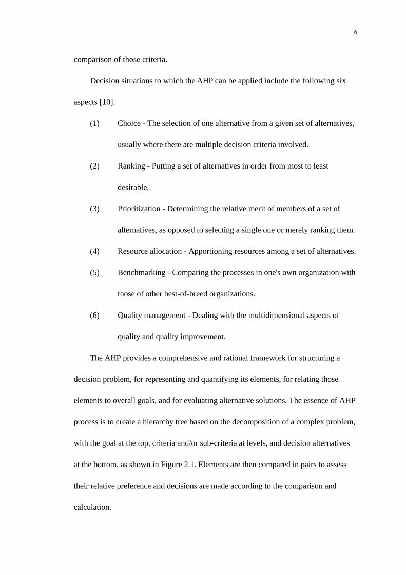
Decision situations to which the AHP can be applied include the following six

aspects [10].

(1) Choice - The selection of one alternative from a given set of alternatives,

usually where there are multiple decision criteria involved.

(2) Ranking - Putting a set of alternatives in order from most to least

desirable.

(3) Prioritization - Determining the relative merit of members of a set of

alternatives, as opposed to selecting a single one or merely ranking them.

(4) Resource allocation - Apportioning resources among a set of alternatives.

(5) Benchmarking - Comparing the processes in one's own organization with

those of other best-of-breed organizations.

(6) Quality management - Dealing with the multidimensional aspects of

quality and quality improvement.

The AHP provides a comprehensive and rational framework for structuring a

decision problem, for representing and quantifying its elements, for relating those

elements to overall goals, and for evaluating alternative solutions. The essence of AHP

process is to create a hierarchy tree based on the decomposition of a complex problem,

with the goal at the top, criteria and/or sub-criteria at levels, and decision alternatives

at the bottom, as shown in Figure 2.1. Elements are then compared in pairs to assess

their relative preference and decisions are made according to the comparison and

calculation.

7

Figure 2.1. Structure of AHP process

The basic principle of AHP includes the following procedures [11, 12, 13, and

14]:

(1) Define the unstructured problem and state clearly the goal of the

problem;

(2) Identify the factors that influence the overall goal;

(3) Decompose the complex overall evaluation goal into hierarchical

structure with detailed decision criteria and variables, which are

manageable;

(4) Select a scale method, employ pairwise comparisons among decision

criteria and form comparison matrices;

(5) Estimate the relative priorities of the decision criteria by using method

like eigenvalue or the geometric mean;

(6) Check the consistency property of matrices to ensure the judging

consistence; aggregate the relative priorities of decision criteria;

(7) Aggregate the final weight coefficient vector which represents the

relative importance of each alternative with respect to the goal stated at

the top of the hierarchy.

8

Among all, the pairwise comparison matrix is particularly important because it is

the key to transform subjective priorities to computable values according to decision

makers’ preferences.

These pairwise comparisons are usually gained by experts via questionnaire and

other approach like Delphi methodology. They are made by using a preference scale to

assign numerical values to different levels of preference [15]. Usually, scale used for

AHP is from 1 to 9 to reflect the importance of one factor over another. The

fundamental scale for pairwise comparisons is shown in Table 2.1.

Table 2.1. Fundamental scale for pairwise comparisons

Intensity of

Importance Definition Explanation

1 Equal importance Two elements contribute equally to the objective

3 Moderate importance Experience and judgment slightly favor one element

over another

5 Strong importance Experience and judgment strongly favor one element

over another

7 Very strong importance One element is favored very strongly over another; its

dominance is demonstrated in practice

9 Extreme importance The evidence favoring one element over another is of

the highest possible order of affirmation

Intensities of 2, 4, 6, and 8 can be used to express intermediate values. Intensities 1.1, 1.2, 1.3,

etc can be used for elements that are very close in importance.

The reciprocals, such as 1/3, 1/5, 1/7, 1/9, etc., indicate the opposite respectively

of the values 3, 5, 7, 9, etc. [16].

Selection of numerical scale provided by the experts is important in the validity of

the decision making tool. It aims to quantify the priorities of the linguistic pairwise

comparisons and it can be presented by means of different numerical scales and the

geometrical scale is the most commonly used ones [17, 18]. Technically, the priorities

9

must capture the dominance of the order expressed in the judgments of pairwise

comparisons, and for classic AHP method they should be unique [19].

2.1.2. Fuzzy Set Theory (FST) and Fuzzy AHP

Nevertheless, there is an extensive literature which addresses the situation in the

real world where the comparison ratios are imprecise judgments. In many practical

cases, the human preference is uncertain or decision makers might be reluctant or

unable to assign exact numerical values to the comparison judgments or individual

judgments in group decision making might be variant. Since some of the evaluation

criteria are subjective and qualitative in nature, it is very difficult for the decision

maker to express the preferences using exact numerical values and to provide exact

pairwise comparison judgments. It is more desirable for the decision maker to use

interval or fuzzy evaluations [20]. Essentially, the uncertainty in the preference

judgments gives rise to uncertainty in the ranking of alternatives as well as difficulty in

determining consistency of preferences [21]. The classical deterministic AHP method

tends to be less effective in conveying the imprecision and vagueness characteristics.

This led to the development of Fuzzy Set Theory (FST) by Zadeh (1965), who

proposed that the key elements in human thinking are not numbers but labels of fuzzy

sets.

FST is a powerful tool to handle imprecise data and fuzzy expressions that are

more natural for humans than rigid mathematical rules and equations [19]. It has been

used to model systems that are hard to define precisely. As a methodology, it

incorporates imprecision and subjectivity into the model formulation and solution

10

process. FST is now applied to problems in extensive fields, involving engineering,

business, medical and related health sciences, and the natural sciences [22].

FST permits the gradual assessment of the membership of elements in a set; this is

described with the aid of a membership function valued in the real unit interval [0, 1].

Fuzzy sets generalize classical sets, since the indicator functions of classical sets are

special cases of the membership functions of fuzzy sets, if the latter only take values 0

or 1 [23].

FST defines set membership as a possibility distribution. On the basis of the

possibility distribution of FST, fuzzy AHP technique is developed as an advanced

analytical method developed from the traditional AHP. Despite the convenience of

AHP in handling both quantitative and qualitative criteria of multiple criteria decision

making problems based on decision makers’ judgments, fuzzy AHP can reduce or

even eliminate the fuzziness and vagueness existing in many decision making

problems may contribute to the imprecise judgments of decision makers in

conventional AHP approaches [24].

There are researches compare fuzzy AHP and classical AHP. These research

studies are divided mainly into two aspects. The first are the methods to make fuzzy

comparison matrices. Early studies on fuzzy AHP approach were classified in that

aspect. Researchers worked on the theoretical methods and what the differences were

between the two approaches. Once the factors that affected the differences were

understood, methods based on the factors were made to improve the fuzzy AHP. The

second aspect was the practical application of both approaches. Later studies were

11

mainly categorized in this second aspect. Research was focused simply on the

difference between the results given by these two approaches, in the form of two

weight vectors given by corresponding approaches. The connection between these

two aspects is a gap in previous studies. This paper combined them together to

explore how the factors that give rise to the differences affect the weight vector given

by Fuzzy AHP and the differences.

The earliest method work in fuzzy AHP appeared in a paper by van Laarhoven and

Pedrycz, who suggested a fuzzy logarithmic least squares method (LLSM) to obtain

triangular fuzzy weights from a triangular fuzzy comparison matrix. Then Lootsma's

logarithmic least square was used to derive local fuzzy priorities. Later, Buckley

utilized the geometric mean method to calculate fuzzy weights. Recently in 1996,

Chang used the extent analysis method and the principle of Triangular Fuzzy Numbers

(TFN) comparison to obtain the priorities of alternatives from pairwise comparisons

[25, and 26]. Among all, Chang’s extent analysis method is the most popular one

because the steps of this approach are simpler and also it has been successfully applied

in many fields [21].

Chang’s extent analysis on fuzzy AHP depends on the degree of possibilities of

each criterion. On the basis of different possible weight values gained by different

decision makers, for a particular level on the hierarchy the pairwise comparison

matrix is constructed and the corresponding TFN for the criterion are placed, which

contains three levels of comparison values. These values are following the scale

showed in Table 2.2. Then definite steps are conducted to find the overall triangular

12

fuzzy values for each criterion. After the weights are obtained, they are normalized

and called the final importance weights. At last, according to the criterion weights, the

weights for each alternative are calculated and a final decision made.

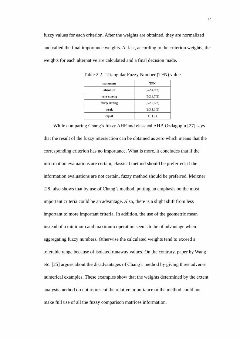
Table 2.2. Triangular Fuzzy Number (TFN) value

statement TFN

absolute (7/2,4,9/2)

very strong (5/2,3,7/2)

fairly strong (3/2,2,5/2)

weak (2/3,1,3/2)

equal (1,1,1)

While comparing Chang’s fuzzy AHP and classical AHP, Ozdagoglu [27] says

that the result of the fuzzy intersection can be obtained as zero which means that the

corresponding criterion has no importance. What is more, it concludes that if the

information evaluations are certain, classical method should be preferred; if the

information evaluations are not certain, fuzzy method should be preferred. Meixner

[28] also shows that by use of Chang’s method, putting an emphasis on the most

important criteria could be an advantage. Also, there is a slight shift from less

important to more important criteria. In addition, the use of the geometric mean

instead of a minimum and maximum operation seems to be of advantage when

aggregating fuzzy numbers. Otherwise the calculated weights tend to exceed a

tolerable range because of isolated runaway values. On the contrary, paper by Wang

etc. [25] argues about the disadvantages of Chang’s method by giving three adverse

numerical examples. These examples show that the weights determined by the extent

analysis method do not represent the relative importance or the method could not

make full use of all the fuzzy comparison matrices information.

13

Once the factors that influence the difference between classical AHP and fuzzy

AHP and the numerical weight results gained by these two approaches are defined,

the problem is how the factors affect the difference. The relationship between these

two parts is a gap in knowledge. If the effects of the factors were know, the

application of fuzzy AHP will be used more properly in situations that are more

suitable to utilize fuzzy AHP other than classical AHP.

2.2. Literature review of Ratio Frequency Identification (RFID)

2.2.1. History of RFID

RFID technologies originated from radar theories that were discovered by the

allied forces during World War II and have been commercially available since the

early 1980’s. Over the last three decades, RFID has been used for a wide variety of

applications such as transportation freight tracking, retail theft prevention, library

systems, automotive manufacturing, postal services, animal tracking, and so on [29]

to improve the efficiency of object tracking and management.

The demonstration of the first continuous wave radio generation and

transmission of radio signals by Ernst F.W. Alexanderson in 1906 indicated the

beginning of modern radio communication. Later in the early 20th century,

technologies of radar appeared. They were used to detect and locate objects by

sending out radio waves and receiving the reflection of them. Then the position and

speed of the objective could be determined by the radio wave reflection. Since RFID

is based on the combination of radio broadcast technology and radar, it is not

14

unexpected that the convergence of these two radio disciplines and the thoughts of

RFID occurred on the heels of the development of radar [30].

In 1945 Léon Theremin invented an espionage tool for the Soviet Union. This

device converted listening by retransmitting incident radio waves with audio

information. The principle that supported this device was that sound waves vibrated a

diaphragm which slightly altered the shape of the resonator and the resonator

modulated the reflected radio frequency. This device, even though it was not an

identification tag, was considered to be a predecessor of RFID technology, because it

was likewise passive, being energized and activated by electromagnetic waves from

an outside source [31].

Another early work exploring RFID is the landmark paper by Harry Stockman,

―Communication by Means of Reflected Power,‖ published in 1948, where the author

stated that ―Evidently, considerable research and development work has to be done

before the remaining basic problems in reflected-power communication are solved,

and before the field of useful applications is explored.‖

The 1960s were the prelude to the RFID explosion of the 1970s. In the 1970s

developers, inventors, companies, academic institutions, and government laboratories

were actively working on RFID, and notable advances were being realized at research

laboratories and academic institutions [32].

In 1973, Mario Cardullo received the patent for his device, which was typically

the first true ancestor of modern RFID. This is because the device was a passive radio

transponder with memory that can be read and wrote [33]. At the same year, another

15

patent was awarded to Charles Walton who used a passive transponder to unlock a

door without a key. Walton embedded a transponder storing a valid identity number

into a card so as to communicate a signal to a reader near the door. Then the door

would be unlocked when the reader detected this number. Also at the year of 1973,

Steven Depp, Alfred Koelle, and Robert Freyman showed reflected power RFID tags

for both passive and semi-passive at the Los Alamos National Laboratory.

The first patent to be associated with the abbreviation RFID was granted to

Charles Walton in 1983 [34]. The decade of the 1980s, RFID technology had been

fully implemented and entered the mainstream as a commercially application. Untill

the 1990s, the standards of RFID emerged, which allowed this technology extent to

international wide deployment.

Nowadays, RFID explosion is continuing. The application is trying to break new

paths to different fields, calling for new advanced techniques to back up. A typical

way for future application is the micro of RFID, which requests special raw material

and manufacturing technique. Reasonable assumptions state that this micro RFID has

a brilliant application foreground in the field of medicine.

2.2.2. Component of RFID

RIFD is basically a technology to identify or track objects such as a product,

animal, or person automatically using communication via electromagnetic waves

without human intervention. A RFID system allows wireless data communication

between a stationary location and a movable object or between movable objects from

a distance [30, 35].

16

A RFID system comprises three components, tags, readers, antennas, and

middleware software, as shown in Figure 2.2. The components are introduced here

one by one.

Figure 2.2. Structure of a RFID system

2.2.2.1. RFID tags

RFID tags are the heart of an RFID system due to their duty of storing the basic

information of the tracked object, which consist of identity, location, date, price, state,

speed, etc. Tags often consist of a microchip with an internally attached coiled

antenna. This digital memory chip stores the information of a unique object. RFID

tags could be in different shapes for different purpose.

Some tags include batteries, expandable memory, and sensors [36]. According to

the capability, tags are divided into the following types [37].

2.2.2.1.1. Passive tags

Passive tags have no battery and the communication range of them is limited to

approximately 3 meters or less. Once the passive tag enters the response range of a

reader, RF signal powers the tag and the chip inside modulates the waves and

transmits the information, which was captured by the reader who then sends back to

17

the terminal system. Figure 2.3 shows two samples of passive tags.

Figure 2.3. Passive RFID tags

2.2.2.1.2. Active tag

Active tags have a battery inside and are usually strong enough to be read in a far

distance around 100 meters or more. Other than passive tags, active tags can directly

broadcasts RF signals wirelessly on their own when they enter the response range of a

reader. Figure 2.4 shows two samples of active tags, coming from RF Code and Savi

companies respectively.

Figure 2.4. Active RFID tags

2.2.2.1.3. Read-only tags

Read-only tags contain data that are pre-written onto them by the tag

manufacturer or distributor. The lack of capability of being rewritten with any

additional information all through the whole supply chain makes them the least

expensive RFID tags.

2.2.2.1.4. Write-once tags

Write-once tags could be added with information by the user for just one time.

18

2.2.2.1.5. Full read-write tags

Full read-write tags enable the users to rewrite data whenever needed.

2.2.2.2. RFID antennas

A RFID antenna is a conductive element that permits data exchanging between

tags and readers. Coiled antenna is used for passive tags. By using the energy

provided by the reader's carrier signal, coiled antenna emits electromagnetic range to

activate the passive tags which enter in this response range. Then it receives

information which is broadcasted by the tags’ antenna and transmits them back to

readers. Sometimes RFID antennas are attached to RFID readers as an integrative

component.

2.2.2.3. RFID readers

RFID readers have the function of converting radio waves from RFID tags into a

form that can be passed to middleware. They interrogate tags’ information by

broadcasting a specific RF signal. Then the tags will respond to this signal by

transmitting back a unique serial number or Electronic Product Code (EPC). Finally

RFID readers receive the information and convert and send them to middleware uses

as CPU data [38].

There are two types of RFID readers according to the capacity of removability.

2.2.2.3.1. Mobile readers

Mobile readers are usually in the form of two common devices. One is handheld

reader which is the same as handheld barcode scanner; and the other one is readers

attached to a mobile device such as a forklift embedding RFID reader. Mobile readers

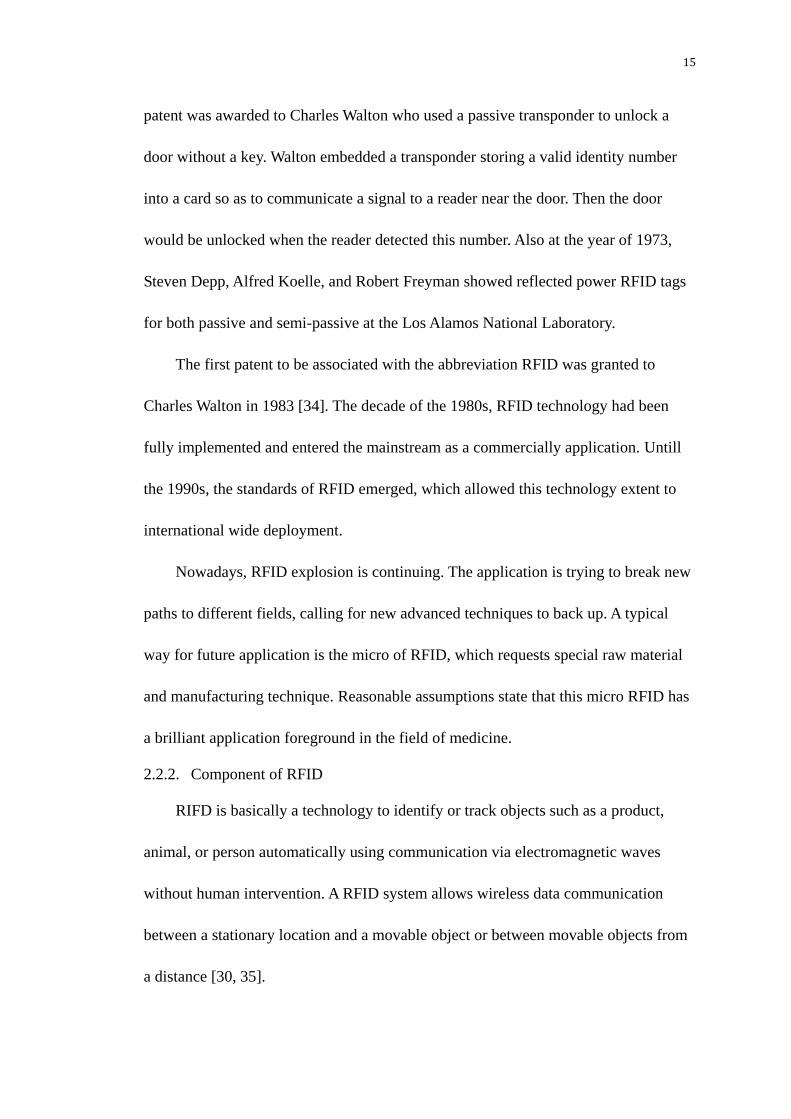
19

have the advantage of portability. Figure 2.5 shows a handheld RFID reader and

Figure 2.6 shows a forklift RFID reader.

Figure 2.5. Handheld RFID reader

Figure 2.6. Forklift RFID reader

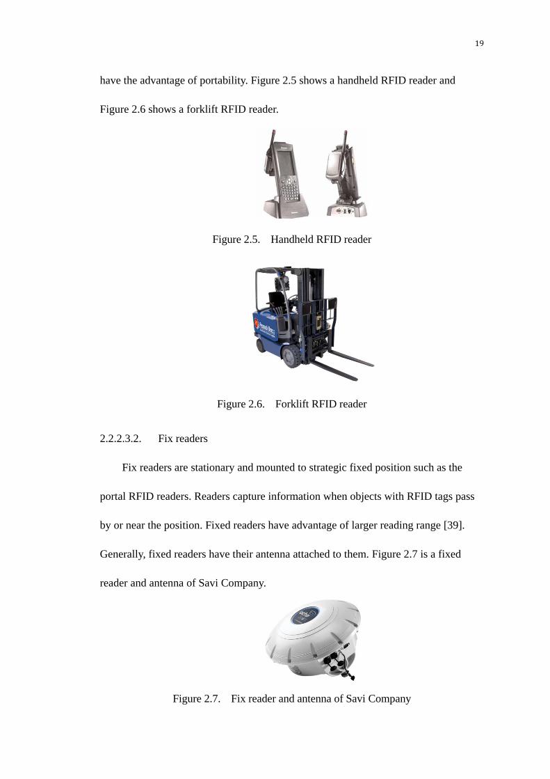
2.2.2.3.2. Fix readers

Fix readers are stationary and mounted to strategic fixed position such as the

portal RFID readers. Readers capture information when objects with RFID tags pass

by or near the position. Fixed readers have advantage of larger reading range [39].

Generally, fixed readers have their antenna attached to them. Figure 2.7 is a fixed

reader and antenna of Savi Company.

Figure 2.7. Fix reader and antenna of Savi Company

20

2.2.2.4. RFID middleware

RFID middleware is ―system software that collects a large volume of raw data

from heterogeneous RFID environments, filters them and summarizes into meaningful

information, and delivers the information to application services‖ [38]. Middleware

software has the function of managing the flow of data and sending them to back-end

management systems.

2.2.3. Advantages of RFID

An advanced automatic identification system based on RFID has several

advantages over other data capturing technologies such as a bar coding system.

(1) The visibility provided by the RFID system allows for an accurate

knowledge on the inventory level by eliminating conflicts between physical

inventory and recorded inventory.

(2) RFID reduces the source of errors by eliminating some of the human

interaction in the process. This reduces the labor costs, the inventory

inaccuracies, and simplifies the business as a whole.

(3) RFID provides higher security because each tag is extremely unique and

almost impossible to duplicate [40].

(4) RFID has higher durability because that the container of bar codes, which are

usually paper products or hard metals, exposes them to harsh environments

and makes them vulnerable.

2.2.4. Application of RFID in transportation system

The RFID market is already a multimillion dollar industry and the applications of

smart chip technologies are limitless. A wide range of emerging applications in the

21

RFID field are being improved by RFID such as: identification of passports at port of

entry, tracking baggage, tracking people in a secure environment, animal

identification, health care and usage at public facilities (libraries and transportation).

The transportation system, which requires a high level of accurate and reliable

tracking information, is a preeminent field which allows RFID technology to

showcase its advantages. Compared to other data capture technology, RFID is more

efficient with higher accuracy and security for inspection and tracking purposes.

RFID can increase substantially the accuracy of current location data as well as the

carrier name and unit number. This ability enables RFID system to perform real time

surveillance which allows fleet data capture and also improves transportation process

efficiency.

The applications of RFID system in transportation are usually used for traffic

management such as toll road RFID system, public transit (such as bus, subway and

rail) RFID system, and Car-sharing service RFID system.

2.3. Previous research of CVISN project

Nebraska has currently attained Commercial Vehicle Information systems and

Networks (CVISN) Core Compliance. Nebraska Department of Motor Vehicles

(NEDMV) is the lead agency with the Motor Carrier Services Division the primary

contact. CVISN project requests NEDMV to perform a stakeholder analysis on

utilizing Radio Frequency Identification (RFID) license plates to assist with CVISN

objectives at roadside. The project also requires cooperation between the University

22

of Nebraska (Transportation Center and Radio Frequency Supply Chain Logistics

(RfSCL) lab), the NEDMV, the Nebraska Department of Roads (NDOR), The

Nebraska Department of Corrections, Cornhusker State Industries (CSI) and the

Nebraska State Patrol (NSP)) to perform stakeholder analysis, RFID license plate

prototype testing, software and database security testing, and a return on investment

analysis in comparison to other technologies.

This program aims to offset the costs of conducting a feasibility study on RFID

embedded license plates that may ultimately be expanded for national use. The goal of

this program is to investigate the variability of embedding RFID tags into license

plates so that strategically located readers alongside streets and roads within the state

can capture tag information, and finally select a most valuable RFID system to embed

into license plates of the whole nation.

Previous studies have worked on stakeholder analysis. First, questionnaires were

designed and stakeholders’ requirements were collected during the kickoff meeting.

Second, for each stakeholder House of Quality (HOQ) analysis was performed to

evaluate the technical requirements. Finally, a ranking of technical requirements was

tallied.

Six technical requirements were highlighted to be the most significant to the

implementation of RFID system over the national wide. They were separately RFID

tag (transponder) reader distance, physical limitation, read rate, display relevant

information, RFID tag number, and manufacturing cost. Then considering special

customer concerns of each stakeholder, questionnaires were designed aiming at

23

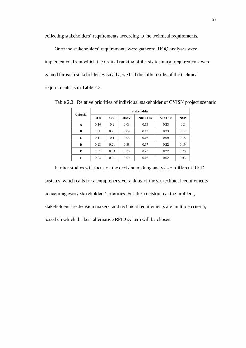
collecting stakeholders’ requirements according to the technical requirements.

Once the stakeholders’ requirements were gathered, HOQ analyses were

implemented, from which the ordinal ranking of the six technical requirements were

gained for each stakeholder. Basically, we had the tally results of the technical

requirements as in Table 2.3.

Table 2.3. Relative priorities of individual stakeholder of CVISN project scenario

Criteria Stakeholder

CED CSI DMV NDR-ITS NDR-Tr NSP

A 0.16 0.2 0.03 0.03 0.23 0.2

B 0.1 0.21 0.09 0.03 0.23 0.12

C 0.17 0.1 0.03 0.06 0.09 0.18

D 0.23 0.21 0.38 0.37 0.22 0.19

E 0.3 0.08 0.38 0.45 0.22 0.28

F 0.04 0.21 0.09 0.06 0.02 0.03

Further studies will focus on the decision making analysis of different RFID

systems, which calls for a comprehensive ranking of the six technical requirements

concerning every stakeholders’ priorities. For this decision making problem,

stakeholders are decision makers, and technical requirements are multiple criteria,

based on which the best alternative RFID system will be chosen.

24

CHAPTER 3. RESEARCH QUESTIONS

3.1. Need for Research

Previous CVISN research systemically chose six technical requirements which

were the most important to the implementation of RFID systems. In addition, previous

research built House of Quality analysis for these technical requirements according to

the customer requirements of each stakeholder. As a result, these technical

requirements were tallied respectively by different stakeholders. Future research

concentrates on choosing the best RFID system according to these technical

requirements. In this decision making problem, technical requirements are playing the

role of multiple criteria, which are the crucial keys to solving this problem. Previous

research developed the rankings of the criteria by each stakeholder, who are the

decision makers in this decision making problem. These separate scores represent

only the priorities of the individual stakeholders, which are not general enough to be

utilized in the final decision making. Consequently, a comprehensive ranking of these

criteria needs to be prudentially decided.

Classical AHP is thought to be a robust way to solve determined decision making

problem. However, it neglects the uncertainty and vagueness caused by subjective

preference of decision maker in criteria scoring. Accordingly, fuzzy AHP was used to

improve this situation.

For the CVISN project, there are six decision makers who had the equal power to

contribute to the final decision. Although classical multiple decision makers AHP

approach could solve this problem, its pairwise comparison value seems not strong

25

enough to cover most decision makers’ options. This is because that there are too

many decision makers and the comparison value for classical AHP is constant.

Therefore, this research builds a fuzzy AHP scenario for CVISN project by assuming

that the weights of the criteria given by different decision makers are possible weights

given by a fictitious decision maker. In this way, this multiple decision maker problem

is turned into a one decision maker with a range of comparison values problem, which

can be solved by fuzzy AHP approach. Whether or not fuzzy AHP approach is suitable

for this situation is then considered.

To verify the applicability of fuzzy AHP to this specified problem, the research

first compares classical AHP and fuzzy AHP with a series of random data. The

comparison is then used as critical models. By calculating prediction intervals for

each individual outcome, the fuzzy AHP approach results of CVISN project are

judged. If the results are within the prediction intervals, it tells that fuzzy AHP is

appropriate; otherwise, it is not appropriate to this specified problem, and the results

of classical AHP is accepted.

3.2. Overall Research Objective

This research is a pilot study for further research of the CVISN project. The

overall research objective is to provide a comprehensive rank of the six significant

technical requirements, which is the basic criterion for further RFID system chosen.

The methods used in this research are both fuzzy AHP and classical AHP

approaches, and results given by the more proper one will be the final rank.

26

3.3. Specific Objectives

The main goal of this research will be reached by meeting the following specific

objectives.

SO#1 Compare classical AHP and fuzzy AHP approaches with randomly

generated data to seek for the relationship between the hypothetic potential factors

and the differences of the two approaches’ outcomes by building statistical models.

SO#2 Compute the ranking of six significant technical requirements for CVISN

project by both classical AHP and fuzzy AHP approaches.

SO#3 Evaluate the results of SO#2 determining whether or not each outcome is

within the prediction interval on the basis of the critical models given by SO#1. If the

results given by fuzzy AHP approach are appropriate, select them; otherwise, select

results given by classical AHP approach. Finally, the overall ranking of the six

significant technical requirements is given by the verified method.

3.4. Hypothesis Statements

This research proposes that the differences between classic AHP and fuzzy AHP

are raised by two potential factors. One, it has been illustrated by previous studies that

if the weight of one criterion is weaker than the weights of the others, fuzzy AHP may

give extreme factor weight to this criterion such as zero [5]. This situation does not

happen to classical AHP. So this paper takes the pairwise comparison of one criterion

over another given by AHP as a factor. Two, fuzzy AHP can provide the decision

makers with flexible value options which are in-between a certain range, rather than

27

deterministic value options. This gives an advantage over classic AHP in solving

fuzzy problems. The range of the fuzzy number for pairwise comparison is hence the

second factor. In this paper, the influences of these two factors are evaluated.

In conclusion, there are two hypotheses in this research. First, we hypothesize

that two factors affect the difference between the outcomes given by classical AHP

and fuzzy AHP approaches, which are the pairwise comparison of one criterion over

another given by AHP and the range of the fuzzy number for pairwise comparison

given by fuzzy AHP. Second, we hypothesize that fuzzy AHP approach is suitable for

CVISN project and it provides decision makers with more effective and accurate

assistance for selecting RFID system. It is envisioned that, taking into all

stakeholders’ preferences, fuzzy AHP provides a more comprehensive ranking of the

six significant technical requirements for CVISN project.

28

CHAPTER 4. METHOD

4.1. Rationale of AHP approach, fuzzy AHP approach and prediction intervals

This research uses both classical AHP approach and Chang’s extent fuzzy AHP

approach as the basic methodologies to find the criteria weights of the multiple

decision making problem for CVISN project. Then prediction intervals are used as a

judgment to evaluate weight results gained by fuzzy AHP approach compared with

classical AHP approach.

4.1.1. AHP approach

Let n be the number of criterion and z1, z2, …, zn be their corresponding relative

priority given by one decision maker. Then the judgment matrix A which contains

pairwise comparison value aij for all i, j ∈ ｛1,2,…,n｝is given by (1).

11 12 1 1 2 1 n

21 22 2 2 1 2 n

1 2 n 1 n 2

1 z /z z /z

z /z 1 z /zA= =

z /z z /z 1

n

n

n n nn

a a a

a a a

a a a

(1)

For multiple decision makers, let h be the number of decision maker and aijk be

the pairwise comparison value of criteria i and j given by decision maker k, where k =

1, 2, …, h. Then by using geometric mean of the aijk conducted by each decision

maker, we have a new judgment matrix with element given by (2).

1 2 k h 1/h h k 1/h

k 1=( * *...* *...* ) ( )ij ij ij ij ij ija a a a a a (2)

The basic procedure for AHP approach by the mean of normalized values

method is given as following:

(1) Normalize each column to get a new judgment matrix A’.

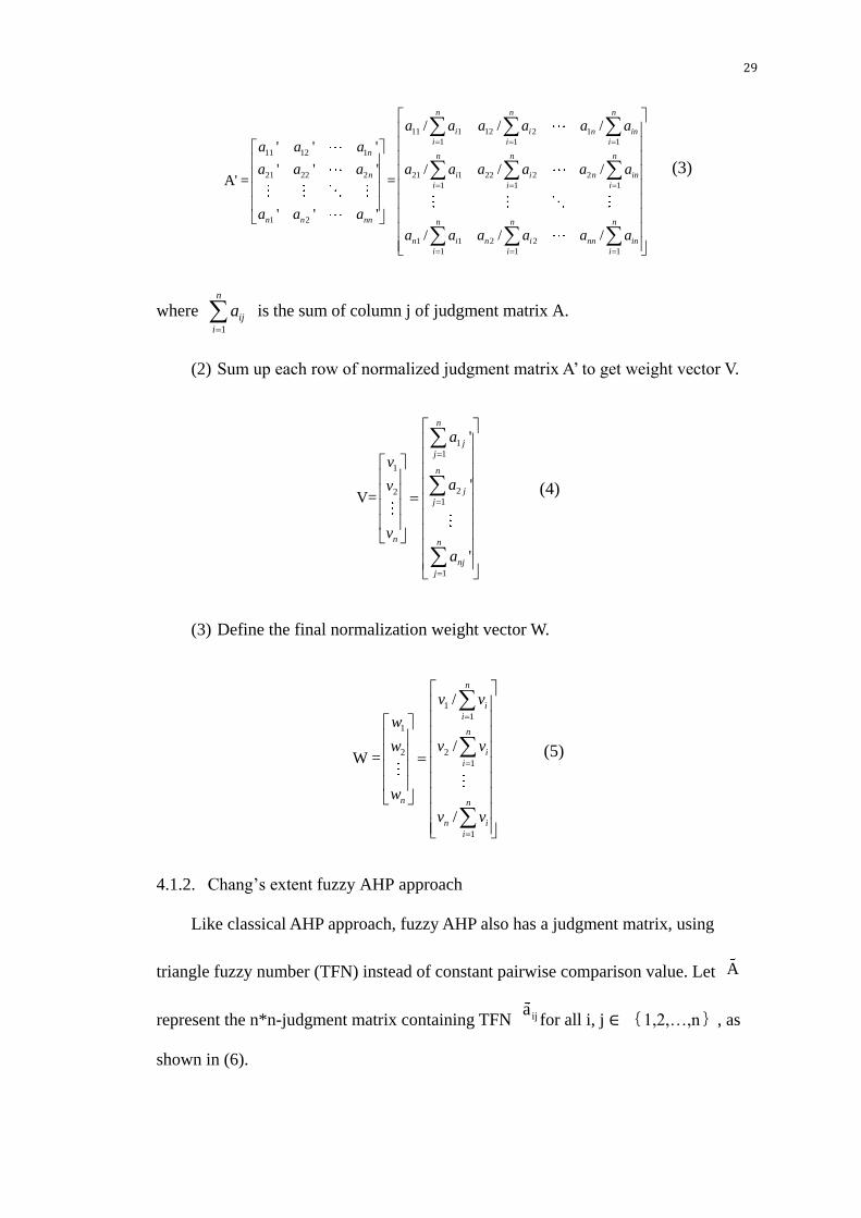
29

11 1 12 2 1

1 1 1

11 12 1

21 22 2 21 1 22 2 2

1 1 1

1 2

1 1 2 2

1 1 1

/ / /

' ' '

' ' ' / / /A' = =

' ' '

/ / /

n n n

i i n in

i i i

n n n n

n i i n in

i i i

n n nn n n n

n i n i nn in

i i i

a a a a a a

a a a

a a a a a a a a a

a a a

a a a a a a

(3)

where 1

n

ij

i

a

is the sum of column j of judgment matrix A.

(2) Sum up each row of normalized judgment matrix A’ to get weight vector V.

1

1

1

221

1

'

'V=

'

n

j

j

n

j

j

n n

nj

j

a

v

av

v

a

(4)

(3) Define the final normalization weight vector W.

1

1

1

2 2

1

1

/

/W =

/

n

i

i

n

i

i

n n

n i

i

v v

w

w v v

w

v v

(5)

4.1.2. Chang’s extent fuzzy AHP approach

Like classical AHP approach, fuzzy AHP also has a judgment matrix, using

triangle fuzzy number (TFN) instead of constant pairwise comparison value. Let A

represent the n*n-judgment matrix containing TFN ijafor all i, j ∈ ｛1,2,…,n｝, as

shown in (6).

30

12 1n

21 2n

n1 n2

(1,1,1) a a

a (1,1,1) aA=

a a (1,1,1)

(6)

where ija =(lij, mij, uij) with lij is the lower and uij is the upper limit and mij is the most

likely value, where we use the geometric mean of lij and uij in this paper. So

ij ij ijm l *u .

Assume that 1M and 2M

are two triangular fuzzy numbers with 1M=(l1, m1,

u1) and 2M=(l2, m2, u2). The basic operations are given by (7)~(9).

1 2 1 2 1 2 1 2M M ( , , )l l m m u u (7)

1 2 1 2 1 2 1 2M M ( , , )l l m m u u (8)

1

1

1 1 1

1 1 1M ( , , )

u m l

(9)

The basic procedure of Chang’s extent fuzzy AHP approach is given as following

[18, 27].

(1) Sum up each row of fuzzy judgment matrix A to get the fuzzy number

vector RS.

1 1 1 1

1 1 1 1

1

2 2 2 221 1 1 1

1 1 1 1

( , , )

rs

( , , )rsRS= =

rs

( , , )

n n n n

j j j j

j j j j

n n n n

j j j j

j j j j

n n n n n

nj nj nj nj

j j j j

a l m u

a l m u

a l m u

(10)

31

(2) Normalize the row fuzzy number vector RS to get the fuzzy synthetic extent

value vector S.

1

1

=1

1

1

22=1

1

n

=1

rs ( rs )

rs ( rs )S= =

rs ( rs )

n

j

j

n

j

j

n n

j

j

s

s

s

(11)

where 1

=1

( rs )n

j

j

is the derivative of the sum of the fuzzy number vector RS and it is

calculated by (12).

1

=1

1 =1 1 =1 1 =1

1 1 1( rs ) =( , , ,)

n

j n n n n n nj

kj kj kj

k j k j k j

u m l

(12)

(3) Compute the degree of possibility to get the non-fuzzy weight vector V.

1 1

2 2

minV(S S )

minV(S S )V= =

minV(S S )

k

k

n n k

v

v

v

(13)

where for element i, the subscript k ∈ ｛1,2,…,n｝ and k i. Also the degree of

possibility of 2S = (l2, m2, u2)

1S = (l1, m1, u1) is obtained by (14).

2 1

2 1 1 2

1 2

2 2 1 1

1, if

V(S S )= 0, if

, otherwise( ) ( )

m m

l u

l u

m u m l

(14)

32

(4) Define the final non-fuzzy normalization weight vector W.

1

1

1

2 2

1

1

/

/W =

/

n

i

i

n

i

i

n n

n i

i

v v

w

w v v

w

v v

(15)

4.1.3. Prediction interval principles

Assume a simple linear regression model with one response variable Y and one

independent variable X. In general, this model can be written as:

0 1Y= + X (16)

where 0 is the intercept of the regression and 1 is the slope of X. These

parameters can be unbiased as b0 and b1estimated by a series of data set (xi, yi), where i

indicates the ith

number of data set and i∈ ｛1,2,…,n｝, where n is the total number of

set.

With this regression model, the predicted interval of any single predicted value

can be calculated on the basis of a population with n data by the following procedure.

(1) Estimate model parameters.

1

xy

xx

Sb

s (17)

0 1b y b x (18)

where x and y are the means of the two variables, and 1

1 n

i

i

x xn

, 1

1 n

i

i

y yn

.

33

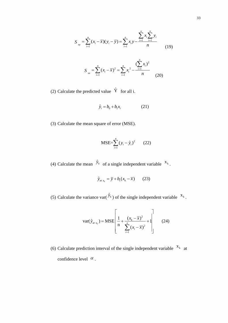
1 1

1 1

( )( )

n n

i in ni i

i i ixy

i i

x y

x x y y x ySn

(19)

2

2 2 1

1 1

( )

( )

n

in ni

i ixx

i i

x

x x xSn

(20)

(2) Calculate the predicted value Y for all i.

0 1ˆ

i iy b b x (21)

(3) Calculate the mean square of error (MSE).

2

1

ˆMSE= ( )n

i i

i

y y

(22)

(4) Calculate the mean ˆ

ky of a single independent variable kx

.

1ˆ ( )

kat x ky y b x x (23)

(5) Calculate the variance var(ˆ

ky) of the single independent variable kx

.

2

2

1

( )1ˆvar( ) MSE 1

n( )

k

kat x n

i

i

x xy

x x

(24)

(6) Calculate prediction interval of the single independent variable kx at

confidence level .

34

2

/ 2, 22

1

( )1ˆ MSE 1

n( )

k

kat x n n

i

i

x xy t

x x

(24)

where / 2, 2nt is the statistic value for t distribution, where n-2 is the degree of

freedom. This critical value can be found out at all most every statistic textbook or via

internet.

4.2. Research procedure

This research is divided into three scenarios, which are respectively random data

scenario, CVISN project scenario, and prediction interval demonstration scenario. The

first scenario is running comparison models for classical AHP and fuzzy AHP

approaches with randomly generated simulation data to search for the relationship

between input variables and output variables so as to give technique supports for the

following two parts. The second scenario is dealing with the real multiple-decision

problem for CVISN project by both classical AHP and fuzzy AHP approaches. The

third scenario is building models with significant input variables and output variables

for the CVISN project to check whether the fuzzy AHP approach fits this real

problem.

Followings are the detailed procedure of each scenario and the whole research

procedure can be demonstrated as a flow chart shown in Figure 4.1.

35

Figure 4.1. Research procedure

4.2.1. Random data scenario

The following steps are used to generate random data and build benchmark

Start

Random Data

Scenario

CVISN Project

Scenario

AHP Fuzzy AHP

F-AHP

Pairwise

Value

Generate

Random Data

Diff. Abs.

Diff.

Range

Sig.?

AHP

Value

Sig.?

Range

Sig.?

AHP

Value

Sig.?

AHP

Value

Sig.?

Range

Sig.?

Take Off

Create

triangle fuzzy

number

AHP Fuzzy AHP

F-AHP

Pairwise

Value

Diff. Abs.

Diff.

No No No No No No P. I.

Demonstration

Yes

End

Yes Yes Yes Yes Yes Modeling

36

comparison models between classical AHP and fuzzy AHP approaches.

(1) Generate simulation random data with Excel to represent TFNs for fuzzy

AHP approach.

(2) Calculate weight values for both AHP and fuzzy AHP approaches based on

the data from step 1.

(3) Collect input data, which are range and AHP pairwise weight values, as well

as output data, which includes fuzzy AHP pairwise weight values, difference

of the pairwise weight values between the two approaches, and absolute

difference of pairwise weight values between the two approaches, for

modeling.

(4) Built six models for each pair of input and output data.

(5) Check whether the input variables are significant or not to the each output

variable.

(6) If the input variable is significant, find the relationship between it and the

output variables; otherwise take it off.

4.2.2. CVISN project scenario

The following steps are used to apply both classical AHP and fuzzy AHP to

CVISN project and obtain the final weight vectors.

(1) Analysis previous CVISN project data and denote the multiple decision

making problem.

(2) Create TFNs for fuzzy AHP approach by house of quality from previous

research.

37

(3) Calculate weight values for both AHP and fuzzy AHP approaches based on

the data from step 1.

(4) Collect input and output data for modeling.

(5) Build models with output variables and input variables which have been

proved significant in step 5 of random data scenario.

4.2.3. Prediction interval demonstration scenario

The following three steps are verify the outcomes of CVISN project, using

benchmark comparison models.

(1) For every model in step 5 of CVISN project scenario, calculate prediction

interval for each single output value based on the modeling data from step 6

of random data scenario.

(2) Check whether the output values are in-between their corresponding

prediction intervals.

(3) If the output values are in-between the prediction intervals, it proves that the

fuzzy AHP is appropriate for CVISN project; otherwise use classic AHP

approach to solve this problem.

4.3. Analysis plan

Analysis plan gives the explanation of input and output variables, detailed

analysis steps, as well as final models for each scenario.

4.3.1. Random data scenario

4.3.1.1 Basic assumption

This set uses random data to represent the totally arbitrary decision makers’

38

preferences when weighing pairwise criteria. Excel® is used in the generation of the

random data as well as the simulation.

The following assumptions are made before conducting the simulation and

modeling:

(1) Four criteria and one decision maker are considered in this research to

simplify the model;

(2) Random data are generated to represent the TFNs for each pair of criteria,

given by the decision maker with totally arbitrary preference;

(3) In order to make the simulation more reasonable and common, the random

data are generated from 0 to 10, with the higher value reflecting the stronger

importance of one criterion over another and lower value reflecting the

weaker importance of one criterion over another. This makes the simulation

make sense according to the standard preference scales of pairwise

comparison used for classical AHP approach ;

(4) In order to weigh the comparison more fairly, each random data has the

probability between (0, 1) equal to 0.5 and the probability between (1, 10)

equal to 0.5. In this way, for instance, the importance of criterion A over

another one B has the same chance to be larger than one and to be smaller

than one, which means that criterion A has the same chance to be more

important than B and less important than B;

(5) Geometric mean is used to gain the AHP pairwise values from the TFNs;

(6) All TFNs and AHP pairwise values, including both aij and its corresponding

39

reciprocal aji, are taken into statistic analysis for the final comparison.

4.3.1.2 Notation

The following notations are used to represent different parameters.

i, j: the subscript for criterion i and criterion j. Since there are four criteria in this

research simulation, i, j = 1, 2, 3, 4;

ija: TFN for criterion i over criterion j of fuzzy AHP approach;

aij : pairwise comparison value for criterion i over criterion j of AHP approach;

T

FW : Final weight values vector of fuzzy AHP approach;

T

AW : Final weight values vector of AHP approach;

VFij (V-F in short): pairwise weight value for criterion i over criterion j of fuzzy

AHP approach;

VAij (V-A in short): pairwise weight value for criterion i over criterion j of AHP

approach;

Rij (R in short): The range of fuzzy number for criterion i over criterion j of

fuzzy AHP approach;

Diffij (D in short): Difference of the pairwise weight value for criterion i over

criterion j between Fuzzy AHP approach and AHP approach, and

ABS-Diffij (ABS-D in short): Absolute difference of pairwise weight value for

criterion i over criterion j between fuzzy AHP approach and AHP approach.

4.3.1.3 Analysis step

The section of analysis step shows the specific steps of calculation.

(1) For each pairwise comparison of criteria i and j, two random data, rij1 and rij2,

40

are created, with the meaning of the importance of criterion i over criterion j

(i, j = 1, 2, 3, 4);

(2) For fuzzy AHP approach, ija= (lij, mij, uij) is then formed by lij = minimum

(rij1, rij2), mij = geometric mean (rij1, rij2) and uij = maximum (rij1, rij2);

(3) For classical AHP approach, aij = geometric mean (rij1, rij2);

(4) The importance of criterion j over criterion i for each approach is then given

by jia=1/ ija

=(1/ uij, 1/mij, 1/lij) and aji = 1/ aij;

(5) Calculation results by using Chang’s extent fuzzy AHP approach and

classical AHP approach are two vectors of weights T

FW =(WF1, WF2, WF3,

WF4) and T

AW =(WA1, WA2, WA3, WA4);

(6) Pairwise weight values between criterion i and criterion j for the two

approaches are computed by VFij = WFi/ WFj and VAij = WAi/ WAj;

(7) Range of pairwise TFNs of Fuzzy AHP for criterion i over criterion j is given

by Rij = uij - lij, and

(8) Difference and absolute difference of pairwise weight values are then

calculate by Diffij = VFij - VAij and ABS-Diffij = absolute (Diffij).

4.3.1.4 Data collection

The following parts are used for data generation and specification.

(1) Generate initial data: a series of 240 data are generated randomly, and then

another 240 accordingly reciprocal data are calculated. Since two random

data are necessary to represent one pairwise comparison value, these 480 data

are used to form 240 sets of pairwise comparison values for both fuzzy AHP

41

and AHP, including 20 groups of scenarios, each of which contains 12

pairwise comparison values (since there are 4 criteria).

(2) Calculate statistic model data: calculate the following five variable values

group by group: V-A, R, V-F, D, and ABS-D, the first two of which are input

random variables for the modeling and the last three are output variables.

(3) In order to analyze the variables’ effects more specifically, the data are

divided into two subgroups, one includes 120 series of data with comparison

weight values given by AHP approach greater than 1 and the other group

includes the left 120 series of data with comparison weight values given by

AHP approach smaller than 1. To distinguish them, this research describes

every parameter in the first group with subscript 1 and the second group with

subscript 2. In this way, there are 6 models in total.

4.3.1.5 Demonstrated sample calculation and procedure

This set gives the data collection and calculation procedure for one of the 24

group scenarios as a demonstrated sample.

(1) Let A, B, C, D represent the four criteria of the first group scenario.

(2) Generate two random data rij1 and rij2 for each pairwise comparison values of

criterion i over criterion j, so there are totally 12 data for the six pariwise

comparison, as shown in Table 4.1.

Table 4.1. Pairwise comparison values for group one scenario of random dara scenario

Series

No.

Pairwise

Comparison

Random Data Fuzzy AHP (ija ) AHP (aij)

rij1 rij2 lij mij uij aij

1 A/B 3.962 5.005 3.962 4.453 5.005 4.453

2 A/C 3.276 6.886 3.276 4.749 6.886 4.749

42

3 A/D 1.140 0.165 0.165 0.433 1.140 0.433

4 B/C 2.688 0.120 0.120 0.569 2.688 0.569

5 B/D 9.151 4.923 4.923 6.712 9.151 6.712

6 C/D 0.160 2.059 0.160 0.574 2.059 0.574

7 B/A 0.252 0.200 0.200 0.225 0.252 0.225

8 C/A 0.305 0.145 0.145 0.211 0.305 0.211

9 D/A 0.877 6.075 0.877 2.308 6.075 2.308

10 C/B 0.372 8.307 0.372 1.758 8.307 1.758

11 D/B 0.109 0.203 0.109 0.149 0.203 0.149

12 D/C 6.250 0.486 0.486 1.742 6.250 1.742

(3) Calculate the reciprocals of the 12 data as the pairwise comparison values of

criterion j over criterion i, so there are 24 data in total.

(4) Generate judgment matrix A for AHP approach and judgment matrix A

with TFNs for fuzzy AHP approach, as shown in Table 4.2 and 4.3.

Table 4.2. Judgment matrix for ahp approach of random dara scenario

Criterion A B C D

No. 1 2 3 4

A 1 1.000 4.453 4.749 0.433

B 2 0.225 1.000 0.569 6.712

C 3 0.211 1.758 1.000 0.574

D 4 2.308 0.149 1.742 1.000

Table 4.3. Judgment matrix for fuzzy ahp approach of random dara scenario

Criterion A B C D

No. 1 2 3 4

A 1 (1.000,1.000,1.000) (3.962,4.453, 5.005) (3.276, 4.749, 6.886) (0.165, 0.433, 1.140)

B 2 (0.200, 0.225, 0.252) (1.000,1.000,1.000) (0.120, 0.569, 2.688) (4.923, 6.712, 9.151)

C 3 (0.145, 0.211, 0.305) (0.372, 1.758, 8.307) (1.000,1.000,1.000) (0.160, 0.574, 2.059)

D 4 (0.877, 2.308, 6.075) (0.109, 0.149, 0.203) (0.486, 1.742, 6.250) (1.000,1.000,1.000)

(5) For AHP approach, the calculations of final weight vector WT are as

following:

Get a new judgment matrix A’.

4

1

1

i

i

a

= 1+0.225+0.211+2.308 = 3.743,

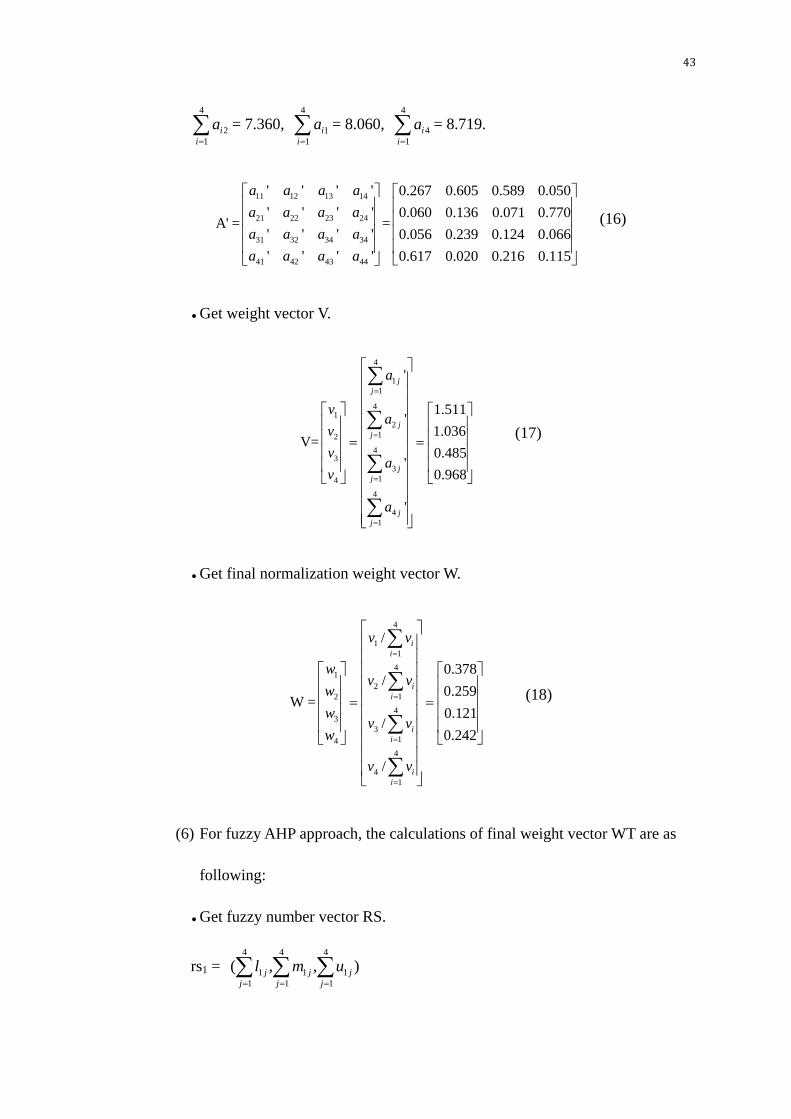
43

4

2

1

i

i

a

= 7.360, 4

1

1

i

i

a

= 8.060, 4

4

1

i

i

a

= 8.719.

11 12 13 14

21 22 23 24

31 32 34 34

41 42 43 44

' ' ' ' 0.267 0.605 0.589 0.050

' ' ' ' 0.060 0.136 0.071 0.770A' = =

' ' ' ' 0.056 0.239 0.124 0.066

' ' ' ' 0.617 0.020 0.216 0.115

a a a a

a a a a

a a a a

a a a a

(16)

Get weight vector V.

4

1

1

41

2

12

43

3

14

4

4

1

'

1.511'

1.036V=

0.485'

0.968

'

j

j

j

j

j

j

j

j

a

va

v

va

v

a

(17)

Get final normalization weight vector W.

4

1

1

41

2

12

43

3

14

4

4

1

/

0.378/

0.259W =

0.121/

0.242

/

i

i

i

i

i

i

i

i

v v

wv v

w

wv v

w

v v

(18)

(6) For fuzzy AHP approach, the calculations of final weight vector WT are as

following:

Get fuzzy number vector RS.

rs1 = 4 4 4

1 1 1

1 1 1

( , , )j j j

j j j

l m u

44

= ((1+3.962+3.276+0.165), (1+4.453+4.749+0.433), (1+5.005+6.886+1.140))

= (8.403, 10.636, 14.031)

4 4 4

1 1 1

1 1 1

4 4 41

2 2 2

1 1 12

4 4 43

3 3 3

1 1 14

4 4 4

4 4 4

1 1 1

( , , )

rs (8.403,10.636,14.031)( , , )

rs (6.243,8.505RS= =

rs( , , )

rs

( , , )

j j j

j j j

j j j

j j j

j j j

j j j

j j j

j j j

l m u

l m u

l m u

l m u

,13.092)

(1.677,3.543,11.672)

(2.472,5.199,13.528)

(19)

Get fuzzy synthetic extent value vector S.

4

=1

rs j

j

= (8.403, 10.636, 14.031) (6.243, 8.505, 13.092)

(1.677, 3.534, 11.672) (2.472, 5.199, 13.528)

= (8.403+6.243+1.677+2.472, 10.636+8.505+3.534+5.199,

14.031+13.092+11.672+13.528)

= (18.794, 27.883, 52.323)

1s = 4

1

1

=1

rs ( rs )j

j

= (8.403, 10.636, 14.031) (18.794, 27.883, 52.323)-1

= (8.403, 10.636, 14.031) (1/52.323, 1/27.883, 1/52.323)

= (8.403/52.323, 10.636/27.883, 14.031/52.323)

= (0.161, 0.381, 0.747)

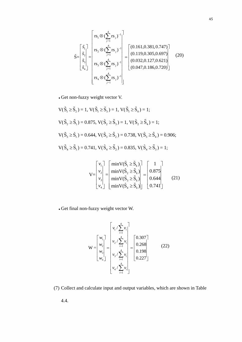
45

41

1

=1

411

2

=12

413

3

=14

41

4

=1

rs ( rs )

(0.161,0.381,0.747)rs ( rs )

(0.119,0.305,0.697)S= =

(0.032,0.127,0.621)rs ( rs )

(0.047,0.186,0.720)

rs ( rs )

j

j

j

j

j

j

j

j

s

s

s

s

(20)

Get non-fuzzy weight vector V.

V( 1 2S S ) = 1, V( 1 3S S ) = 1, V( 1 4S S ) = 1;

V( 2 1S S ) = 0.875, V( 2 3S S ) = 1, V( 2 4S S ) = 1;

V( 3 1S S ) = 0.644, V( 3 2S S ) = 0.738, V( 3 4S S ) = 0.906;

V( 4 1S S ) = 0.741, V( 4 2S S ) = 0.835, V( 4 3S S ) = 1;

1 1

2 2

3 3

4 4

1minV(S S )

0.875minV(S S )V= =

0.644minV(S S )

0.741minV(S S )

k

k

k

k

v

v

v

v

(21)

Get final non-fuzzy weight vector W.

4

1

1

41

2

12

43

3

14

4

4

1

/

0.307/

0.268W =

0.198/

0.227

/

i

i

i

i

i

i

i

i

v v

wv v

w

wv v

w

v v

(22)

(7) Collect and calculate input and output variables, which are shown in Table

4.4.

46

Table 4.4. Input and output variables of random dara scenario

Subgroup No. Pairwise

Comparison

Input Variable Output Variable

R V-A V-F D ABS-D

1 A/B 1.043 10.968 6.040 -4.927 4.927

1 A/C 3.610 8.346 2.562 -5.784 5.784

2 A/D 0.975 0.708 0.752 0.045 0.045

2 B/C 2.568 0.761 0.424 -0.337 0.337

2 B/D 4.228 0.065 0.125 0.060 0.060

2 C/D 1.899 0.085 0.294 0.209 0.209

2 B/A 0.052 0.091 0.166 0.074 0.074

2 C/A 0.160 0.120 0.390 0.271 0.271

1 D/A 5.198 1.413 1.329 -0.084 0.084

1 C/B 7.935 1.314 2.358 1.044 1.044

1 D/B 0.094 15.501 8.027 -7.474 7.474

1 D/C 5.764 11.796 3.404 -8.392 8.392

4.3.2. CVISN project scenario

4.3.2.1 Basic assumptions

Previous research of CVISN project built House of Quality (HOQ) for each of

the six stakeholders via questionnaires to analyze the importance of six significant

technical requirements (which are denoted as capital A to capital F in the following

research). The numerical results for the technical requirements from the HOQ are in

the form of relative priorities for each stakeholder as seen in the pre-mentioned table

in the previous research of CVISN project section of chapter 2.

In order to further analyze the importance of the six technical requirements in a

more comprehensive perspective, the following assumptions are made.

(1) The weights for the six stakeholders are the same to each other. This means

that they have the equal right to evaluate the technical requirements.

(2) This problem can be considered as a multiple decision maker with multiple

criteria decision making problem. In this way, classical AHP approach could

47

be applied to solve it.

(3) This problem can be considered as a single decision maker with multiple

criteria decision making problem. In this way, weights of the six technical

requirements given by an individual stakeholder are considered as one

possible series of weights given by this fictitious decision maker. So there are

six possible series of weights given by the decision maker. Therefore, fuzzy

AHP approach could be applied to solve it.

(4) Geometric mean method is applied to calculate the most likely value when

obtaining the TFNs of fuzzy AHP approach.

4.3.2.2 Notation

The following notations are used to represent different parameters.

i, j: the subscript for criterion i and criterion j. Since there are six criteria in this

research simulation, i, j = 1, 2, 3, 4, 5, 6;

k: the superscript for the kth

decision maker for AHP approach. There are six

stakeholders, so k = 1, 2, 3, 4, 5, 6;

zik: relative priority of criterion i given by the kth

decision maker;

ija: TFN for criterion i over criterion j of fuzzy AHP approach;

aijk : pairwise comparison value for criterion i over criterion j given by decision

maker k of AHP approach;

T

FW : Final weight values vector of fuzzy AHP approach;

T

AW : Final weight values vector of AHP approach;

VFij (V-F in short): pairwise weight value for criterion i over criterion j of fuzzy

48

AHP approach;

VAij (V-A in short): pairwise weight value for criterion i over criterion j of AHP

approach;

Rij (R in short): The range of fuzzy number for criterion i over criterion j of

fuzzy AHP approach;

Diffij (D in short): Difference of the pairwise weight value for criterion i over

criterion j between fuzzy AHP approach and AHP approach, and

ABS-Diffij (ABS-D in short): Absolute difference of pairwise weight value for

criterion i over criterion j between fuzzy AHP approach and AHP approach.

4.3.1.3 Analysis steps

The section of analysis step shows the specific steps of calculation.

(1) Gain judgment matrix Ak with element aijk = zik/zjk for each stakeholder by

(1);

(2) For fuzzy AHP approach, ija= (lij, mij, uij) is then formed by lij = minimum

(aijk), mij = geometric mean (aijk) and uij = maximum (aijk), for k = 1~6;

(3) Gain judgment matrix A with TFNs for Fuzzy AHP approach;

(4) For classical AHP approach, aij = geometric mean (aijk) , for k = 1~6;

(5) Gain new judgment matrix A for AHP approach.

(6) Calculation results by using Chang’s extent fuzzy AHP approach and

classical AHP approach are two vectors of weights T

FW =(WF1, WF2, WF3,

WF4) and T

AW =(WA1, WA2, WA3, WA4);

(7) Pairwise weight values between criterion i and criterion j for the two

49

approaches are computed by VFij = WFi/ WFj and VAij = WAi/ WAj;

(8) Range of pairwise TFNs of Fuzzy AHP for criterion i over criterion j is given

by Rij = uij - lij;

(9) Difference and absolute difference of pairwise weight values are then

calculate by Diffij = VFij - VAij and ABS-Diffij = absolute (Diffij).

4.3.2.4 Data collection

Table 4.5~4.10 give the judgment matrix given by individual stakeholder. These

are the initial data for the following analysis and calculation, by which the input and

output variables for the modeling could be obtained. For example, the comparison

value of criterion A over criterion B given by CED is calculated based on Table 2.3,

which is 0.16/0.1 = 1.6.

Table 4.5. Judgment matrix given by CED of CVISN project scenario

Criteria CED

A B C D E F

A 1.000 1.600 0.941 0.696 0.533 4.000

B 0.625 1.000 0.588 0.435 0.333 2.500

C 1.063 1.700 1.000 0.739 0.567 4.250

D 1.438 2.300 1.353 1.000 0.767 5.750

E 1.875 3.000 1.765 1.304 1.000 7.500

F 0.250 0.400 0.235 0.174 0.133 1.000

Table 4.6. Judgment matrix given by CSI of CVISN project scenario

Criteria CSI

A B C D E F

A 1.000 0.952 2.000 0.952 2.500 0.952

B 1.050 1.000 2.100 1.000 2.625 1.000

C 0.500 0.476 1.000 0.476 1.250 0.476

D 1.050 1.000 2.100 1.000 2.625 1.000

E 0.400 0.381 0.800 0.381 1.000 0.381

F 1.050 1.000 2.100 1.000 2.625 1.000

Table 4.7. Judgment matrix given by DMV of CVISN project scenario

50

Criteria DMV

A B C D E F

A 1.000 0.333 1.000 0.079 0.079 0.333

B 3.000 1.000 3.000 0.237 0.237 1.000

C 1.000 0.333 1.000 0.079 0.079 0.333

D 12.667 4.222 12.667 1.000 1.000 4.222

E 12.667 4.222 12.667 1.000 1.000 4.222

F 3.000 1.000 3.000 0.237 0.237 1.000

Table 4.8. Judgment matrix given by NDR-ITS of CVISN project scenario

Criteria NDR-ITS

A B C D E F

A 1.000 1.000 0.500 0.081 0.067 0.500

B 1.000 1.000 0.500 0.081 0.067 0.500

C 2.000 2.000 1.000 0.162 0.133 1.000

D 12.333 12.333 6.167 1.000 0.822 6.167

E 15.000 15.000 7.500 1.216 1.000 7.500

F 2.000 2.000 1.000 0.162 0.133 1.000

Table 4.9. Judgment matrix given by NDR-Tr of CVISN project scenario

Criteria NDR-Tr

A B C D E F

A 1.000 1.000 2.556 1.045 1.045 11.500

B 1.000 1.000 2.556 1.045 1.045 11.500

C 0.391 0.391 1.000 0.409 0.409 4.500

D 0.957 0.957 2.444 1.000 1.000 11.000

E 0.957 0.957 2.444 1.000 1.000 11.000

F 0.087 0.087 0.222 0.091 0.091 1.000

Table 4.10. Judgment matrix given by NSP of CVISN project scenario

Criteria NSP

A B C D E F

A 1.000 1.667 1.111 1.053 0.714 6.667

B 0.600 1.000 0.667 0.632 0.429 4.000

C 0.900 1.500 1.000 0.947 0.643 6.000

D 0.950 1.583 1.056 1.000 0.679 6.333

E 1.400 2.333 1.556 1.474 1.000 9.333

F 0.150 0.250 0.167 0.158 0.107 1.000

4.3.2.5 Demonstrated sample calculation and procedure

This set gives example of calculations and demo-procedure of this senario.

(1) Combine the six judgment matrixes given by different stakeholders together

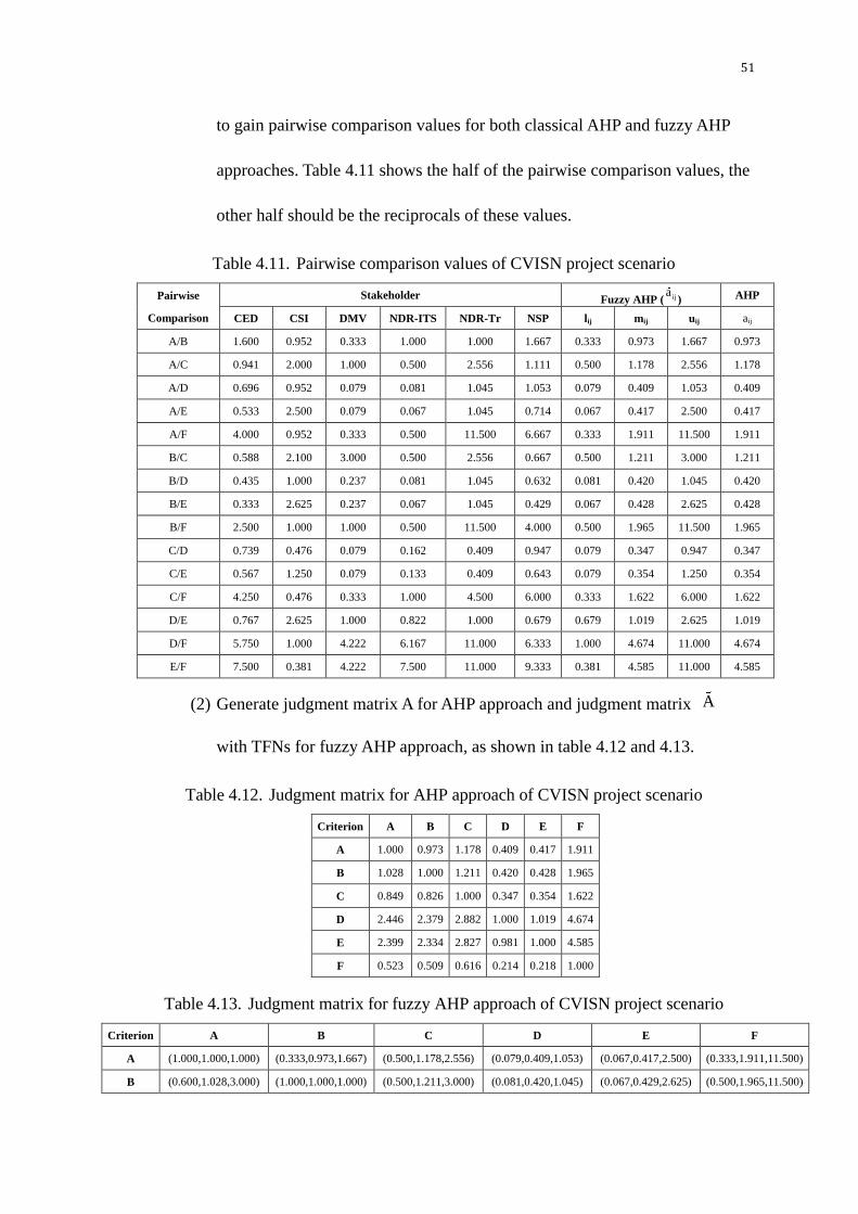
51

to gain pairwise comparison values for both classical AHP and fuzzy AHP

approaches. Table 4.11 shows the half of the pairwise comparison values, the

other half should be the reciprocals of these values.

Table 4.11. Pairwise comparison values of CVISN project scenario

Pairwise

Comparison

Stakeholder Fuzzy AHP ( ija) AHP

CED CSI DMV NDR-ITS NDR-Tr NSP lij mij uij aij

A/B 1.600 0.952 0.333 1.000 1.000 1.667 0.333 0.973 1.667 0.973

A/C 0.941 2.000 1.000 0.500 2.556 1.111 0.500 1.178 2.556 1.178

A/D 0.696 0.952 0.079 0.081 1.045 1.053 0.079 0.409 1.053 0.409

A/E 0.533 2.500 0.079 0.067 1.045 0.714 0.067 0.417 2.500 0.417

A/F 4.000 0.952 0.333 0.500 11.500 6.667 0.333 1.911 11.500 1.911

B/C 0.588 2.100 3.000 0.500 2.556 0.667 0.500 1.211 3.000 1.211

B/D 0.435 1.000 0.237 0.081 1.045 0.632 0.081 0.420 1.045 0.420

B/E 0.333 2.625 0.237 0.067 1.045 0.429 0.067 0.428 2.625 0.428

B/F 2.500 1.000 1.000 0.500 11.500 4.000 0.500 1.965 11.500 1.965

C/D 0.739 0.476 0.079 0.162 0.409 0.947 0.079 0.347 0.947 0.347

C/E 0.567 1.250 0.079 0.133 0.409 0.643 0.079 0.354 1.250 0.354

C/F 4.250 0.476 0.333 1.000 4.500 6.000 0.333 1.622 6.000 1.622

D/E 0.767 2.625 1.000 0.822 1.000 0.679 0.679 1.019 2.625 1.019

D/F 5.750 1.000 4.222 6.167 11.000 6.333 1.000 4.674 11.000 4.674

E/F 7.500 0.381 4.222 7.500 11.000 9.333 0.381 4.585 11.000 4.585

(2) Generate judgment matrix A for AHP approach and judgment matrix A

with TFNs for fuzzy AHP approach, as shown in table 4.12 and 4.13.

Table 4.12. Judgment matrix for AHP approach of CVISN project scenario

Criterion A B C D E F

A 1.000 0.973 1.178 0.409 0.417 1.911

B 1.028 1.000 1.211 0.420 0.428 1.965

C 0.849 0.826 1.000 0.347 0.354 1.622

D 2.446 2.379 2.882 1.000 1.019 4.674

E 2.399 2.334 2.827 0.981 1.000 4.585

F 0.523 0.509 0.616 0.214 0.218 1.000

Table 4.13. Judgment matrix for fuzzy AHP approach of CVISN project scenario

Criterion A B C D E F

A (1.000,1.000,1.000) (0.333,0.973,1.667) (0.500,1.178,2.556) (0.079,0.409,1.053) (0.067,0.417,2.500) (0.333,1.911,11.500)

B (0.600,1.028,3.000) (1.000,1.000,1.000) (0.500,1.211,3.000) (0.081,0.420,1.045) (0.067,0.429,2.625) (0.500,1.965,11.500)

52

C (0.391,0.849,2.000) (0.333,0.826,2.000) (1.000,1.000,1.000) (0.079,0.347,0.947) (0.079,0.354,1.250) (0.333,1.622,6.000)

D (0.950,2.446,12.667) (0.957,2.379,12.333) (1.056,2.882,12.667) (1.000,1.000,1.000) (0.679,1.019,2.625) (1.000,4.674,11.000)

E (0.400,2.399,15.000) (0.381,2.334,15.000) (0.800,2.827,12.667) (0.381,0.981,1.474) (1.000,1.000,1.000) (0.381,4.585,11.000)

F (0.087,0.523,3.000) (0.087,0.509,2.000) (0.167,0.616,3.000) (0.091,0.214,1.000) (0.091,0.218,2.625) (1.000,1.000,1.000)

(3) The following procedures to compute the final weight vector WA for AHP

approach and non-fuzzy weight vector WF for fuzzy AHP approach are

totally the same as previous steps for random data scenario part.

1

2

3

A

4

5

6

0.121

0.125

0.103W =

0.297

0.291

0.063

w

w

w

w

w

w

(23)

1

2

3

F

4

5

6

0.165

0.167

0.147 W =

0.191

0.189

0.142

w

w

w

w

w

w

4.3.3. Prediction interval demonstration secario

The following five steps are used to specify the procedure of prediction interval

part.

(1) Assume the confidence level α=0.05 for this research.

(2) The six simple linear regression models for each combination of input and

output variables obtained in random data scenario part are used to illustrate

the relationship of these variables and to predict the single response variables

in the CVISN project scenario part.

53

(3) Prediction intervals for every single response variables in each model are

calculated based on the six models.

(4) Check whether or not the actual response values of the CVISN project that

are attained by fuzzy AHP approach are in-between the predicted intervals.

(5) Since all of these calculations in this part are based on the previous two parts,

detailed calculations will be posted later in the result chapter.

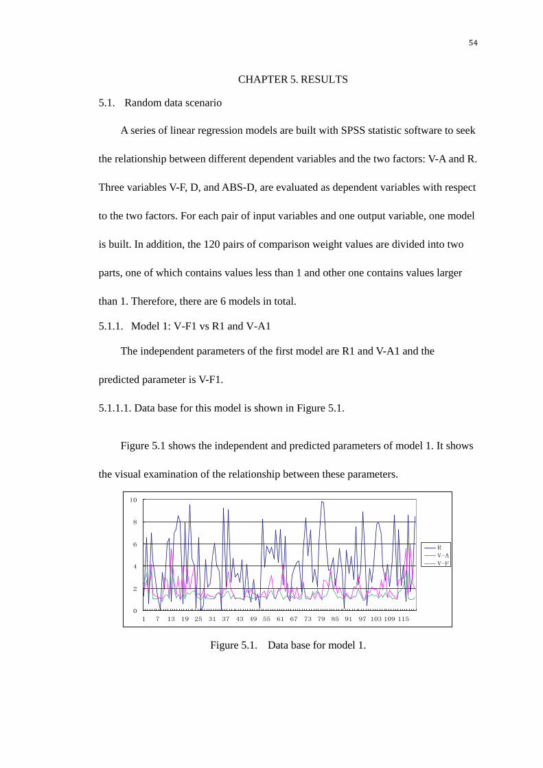
54

CHAPTER 5. RESULTS

5.1. Random data scenario

A series of linear regression models are built with SPSS statistic software to seek

the relationship between different dependent variables and the two factors: V-A and R.

Three variables V-F, D, and ABS-D, are evaluated as dependent variables with respect

to the two factors. For each pair of input variables and one output variable, one model

is built. In addition, the 120 pairs of comparison weight values are divided into two

parts, one of which contains values less than 1 and other one contains values larger

than 1. Therefore, there are 6 models in total.

5.1.1. Model 1: V-F1 vs R1 and V-A1

The independent parameters of the first model are R1 and V-A1 and the

predicted parameter is V-F1.

5.1.1.1. Data base for this model is shown in Figure 5.1.

Figure 5.1 shows the independent and predicted parameters of model 1. It shows

the visual examination of the relationship between these parameters.

0

2

4

6

8

10

1 7 13 19 25 31 37 43 49 55 61 67 73 79 85 91 97 103 109 115

R

V-A

V-F

Figure 5.1. Data base for model 1.

55

5.1.1.2. SPSS output

Table 5.1 and 5.2 shows the ANOVA and coefficient table. Useful information of

the output includes Mean Square of Error/Residual (MSE) from ANOVA table, the

coefficients and the significant of each independent parameter from coefficient table.

Table 5.1. ANOVA table for model 1

Model Sum of

Squares df

Mean

Square F Sig.

Regression 16.441 2 8.221 45.727 .000

Residual 21.034 117 .180

Total 37.475 119

Table 5.2. Coefficient table for model 1

Model

Unstandardized

Coefficients

Standardized

Coefficients t Sig.

B S.E. a Beta

Const. .687 .110 6.248 .000

R1 -2.331E-03 .015 -.011 -.155 .877

V-A1 .372 .039 .661 9.522 .000

a. Standard Error

5.1.1.3 Numerical model

Since the significance for R1 is 0.877, which is larger than the α level (0.05), it is

not significant to the dependent variable V-F1, which means that it has no influence to

V-F1. Also from the coefficient table it is easy to see that the coefficient of

independent parameter V-A1 is 0.372 and the coefficient of the constant parameter is

0.687, as a result, the model for V-F1 is presented as: V-F1 = 0.687 + 0.372 V-A1.

5.1.2. Model 2: D1 vs R1 and V-A1


predicted parameter is D1.

56




-6

-4

-2

0

2

4

6

8

10

1 7 13 19 25 31 37 43 49 55 61 67 73 79 85 91 97 103 109 115

R

V-A

D



Table 5.3 and 5.4 shows the ANOVA and coefficient table.


Model Sum of

Squares df

Mean

Square F Sig.

Regression 46.503 2 23.252 129.337 .000

Residual 21.034 117 .180

Total 67.537 119


Model

Unstandardized

Coefficients

Standardized

Coefficients t Sig.

B S.E. a Beta

Const. .687 .110 6.248 .000

R1 -2.331E-03 .015 -.008 -.155 .877

V-A1 -.628 .039 -.830 -16.05 .000

5.1.2.3. Numerical model

R1 is not significant to D1, so the model for D1 is then presented as: D1 = 0.687

– 0.628 V-A1.

57

5.1.3. Model 3: ABS-D1 vs R1 and V-A1


predicted parameter is ABS-D1.




0

2

4

6

8

10

1 8 15 22 29 36 43 50 57 64 71 78 85 92 99 106 113 120

R

V-A

ABD-D





Model Sum of

Squares df

Mean

Square F Sig.

Regression 45.055 2 22.528 160.505 .000

Residual 16.422 117 .140

Total 61.477 119


Model

Unstandardized

Coefficients

Standardized

Coefficients t Sig.

B S.E. a Beta

Const. -.591 .097 -6.088 .000

R1 -4.526E-03 .013 -.016 -.342 .733

V-A1 .616 .035 .855 17.83 .000

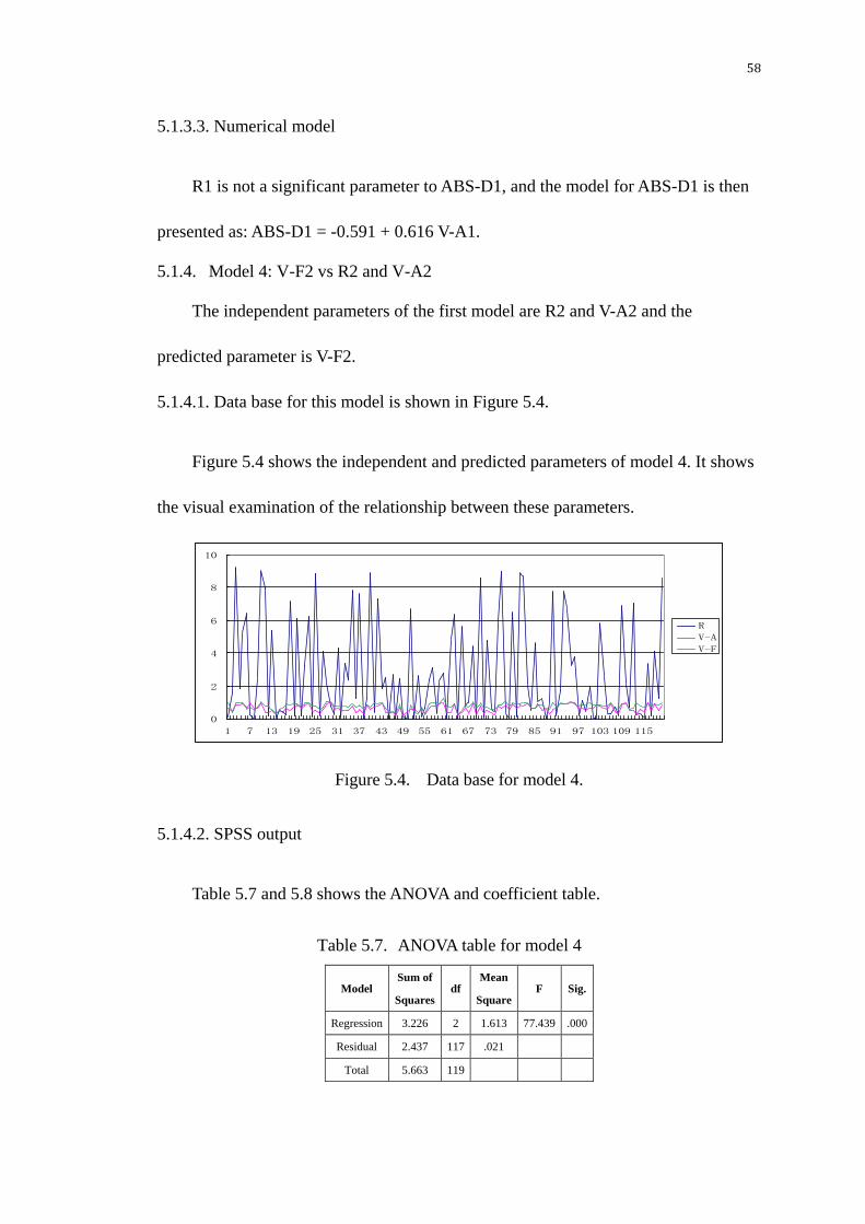
58


R1 is not a significant parameter to ABS-D1, and the model for ABS-D1 is then

presented as: ABS-D1 = -0.591 + 0.616 V-A1.

5.1.4. Model 4: V-F2 vs R2 and V-A2


predicted parameter is V-F2.




0

2

4

6

8

10

1 7 13 19 25 31 37 43 49 55 61 67 73 79 85 91 97 103 109 115

R

V-A

V-F





Model Sum of

Squares df

Mean

Square F Sig.

Regression 3.226 2 1.613 77.439 .000

Residual 2.437 117 .021

Total 5.663 119

59


Model

Unstandardized

Coefficients

Standardized

Coefficients t Sig.

B S.E. a Beta

Const. .327 .038 8.630 .000

R2 5.596E-03 .005 .076 1.175 .242

V-A2 .688 .062 .724 11.18 .000


R2 has only slight influence on V-F2, so the model for V-F2 is then presented as:

V-F2 = 0.327 + 0.688 V-A2.

5.1.5. Model 5: D2 vs R2 and V-A2


predicted parameter is D2.


Figure 5.5 shows the independent and predicted parameters of model 5.

-2

0

2

4

6

8

10

1 7 13 19 25 31 37 43 49 55 61 67 73 79 85 91 97 103 109 115

R

V-A

D





Model Sum of

Squares df

Mean

Square F Sig.

60

Regression .545 2 .273 13.092 .000

Residual 2.437 117 .021

Total 2.983 119


Model

Unstandardized

Coefficients

Standardized

Coefficients t Sig.

B S.E. a Beta

Const. .327 .038 8.630 .000

R2 5.596E-03 .005 .105 1.175 .242

V-A2 -.312 .062 -.453 -5.073 .000


R2’s influence is not significant, so the model for D2 is then presented as: D2 =

0.327 - 0.312 V-A2.

5.1.6. Model 6: ABS-D2 vs R2 and V-A2


predicted parameter is ABS-D2.


Figure 5.6 shows the independent and predicted parameters of model 6.

0

2

4

6

8

10

1 8 15 22 29 36 43 50 57 64 71 78 85 92 99 106 113 120

R

V-A

ABD-D




61


Model Sum of

Squares df

Mean

Square F Sig.

Regression .469 2 .234 19.092 .000

Residual 1.436 117 .012

Total 1.905 119

a. R-Square = 0.246


Model

Unstandardized

Coefficients

Standardized

Coefficients t Sig.

B S.E. a Beta

Const. .345 .029 11.88 .000

R2 -1.045E-03 .004 -.025 -.286 .775

V-A2 -.268 .047 -.487 -5.67 .000


R2 hardly affects ABS-D2, so the model for ABS-D2 is then presented as:

ABS-D2 = 0.345 - 0.268 V-A2.

5.1.7. Results

Results show that the range of fuzzy values for fuzzy AHP approach has no

significant affect in all models, so it is not an important factor to the difference of the

two approaches. Thus, it is omitted from the model.

On the other hand, the pairwise weight value of AHP is an important factor to all

six models. In conclusion, in the following research there is only one input variable

V-A.

5.2. CVISN project scenario

Previous study in Chapter 4 has worked out the final weight vector WA for

classical AHP approach and non-fuzzy weight vector WF for fuzzy AHP approach,

62

which are listed below.

1

2

3

A

4

5

6

0.121

0.125

0.103W =

0.297

0.291

0.063

w

w

w

w

w

w

1

2

3

F

4

5

6

0 . 1 6 5

0 . 1 6 7

0 . 1 4 7 W =

0 . 1 9 1

0 . 1 8 9

0 . 1 4 2

w

w

w

w

w

w

Then by previous definition of input and output variables, the input and output

variables for CVISN project are collect and calculate in Table 5.13.

Table 5.13. Input and output variables of CVISN project scenario

Subgroup 1 Subgroup 2

Pairwise

Comparison

Input Variable Output Variable Pairwise

Comparison

Input Variable Output Variable

R V-A V-F D ABS-D R V-A V-F D ABS-D

A/C 2.056 1.178 1.122 -0.056 0.056 A/B 1.333 0.973 0.986 0.013 0.013

A/F 11.167 1.911 1.160 -0.751 0.751 A/D 0.974 0.409 0.863 0.455 0.455

B/C 2.500 1.211 1.138 -0.073 0.073 A/E 2.433 0.417 0.870 0.453 0.453

B/F 11.000 1.965 1.177 -0.787 0.787 B/D 0.964 0.420 0.876 0.456 0.456

C/F 5.667 1.622 1.034 -0.588 0.588 B/E 2.558 0.428 0.883 0.454 0.454

D/E 1.946 1.019 1.008 -0.012 0.012 C/D 0.868 0.347 0.770 0.423 0.423

D/F 10.000 4.674 1.344 -3.330 3.330 C/E 1.171 0.354 0.776 0.422 0.422

E/F 10.619 4.585 1.333 -3.251 3.251 C/A 1.609 0.849 0.891 0.043 0.043

B/A 2.400 1.028 1.015 -0.014 0.014 F/A 2.913 0.523 0.862 0.339 0.339

D/A 11.717 2.446 1.158 -1.288 1.288 C/B 1.667 0.826 0.879 0.053 0.053

E/A 14.600 2.399 1.149 -1.250 1.250 F/B 1.913 0.509 0.849 0.340 0.340

D/B 11.377 2.379 1.142 -1.238 1.238 F/C 2.833 0.616 0.967 0.350 0.350

E/B 14.619 2.334 1.133 -1.201 1.201 E/D 1.093 0.981 0.992 0.011 0.011

D/C 11.611 2.882 1.299 -1.582 1.582 F/D 0.909 0.214 0.744 0.530 0.530

E/D 11.867 2.827 1.289 -1.537 1.537 F/E 2.534 0.218 0.750 0.532 0.532

These variables will be divided into six models consistent with the ones in

random rata part and will be evaluated in the next section.

63

5.3. Predicted interval senario

In this section, basic variables for six statistical models are calculated by

pre-introduced methods firstly. Then for each model, prediction intervals of every

output variable are calculated for CVISN project. Finally, all output variables are

verified based on the prediction intervals.

5.3.1. Basic variables for statistical models

Basic variables for statistical models that are required to calculate prediction

intervals in the future include: mean of all input data from the population data ( x ),

sum of mean square of input variable (Sxx), mean square error (MSE) of population

data, and the critical value of t test ( 0.05/ 2, 2nt ).

Since only one input variable is significant, the mean of input data, sum of mean

square of input variable and the MSE indicate the mean, sum of mean square and the

MSE of V-A. What is more, every three models come from one subgroup which

consists of 120 data, so the degree of freedom for t distribution is 120-2=118 stays the

same for all six models.

The confidence level is α = 0.05, which is the most common level for judgment

in practice.

These variables for the six models are calculated and given in Table 5.14.

Table 5.14. Basic output variables for six models

Model Output Variables

x Sxx MSE 0.05/ 2,120 2t

V-F1 vs V-A1 1.9482 118.2269 0.180 1.98

D1 vs V-A1 1.9482 118.2269 0.180 1.98

ABS-D1 vs V-A1 1.9482 118.2269 0.140 1.98

V-F2 vs V-A2 0.6168 6.2846 0.021 1.98

D2 vs V-A2 0.6168 6.2846 0.021 1.98

64

ABS-D2 vs V-A2 0.6168 6.2846 0.012 1.98

5.3.2. Prediction intervals for output variables

Based on Table 5.1, prediction intervals for every output variable are calculated

for each model. Prediction intervals are represented by two characteristic values:

lower prediction limit (LPL) and upper prediction limit (UPL). To obtain these two

values, predicted values ( y ) and square of the difference between the specific input

value and x ((xi- x )2) should be calculated first.

Prediction intervals for six models are shown in Table 5.15~5.20.

5.3.2.1 Model 1: V-F1 vs V-A1

Table 5.15 shows the prediction intervals of each predicted parameter, that is

V-F1 based on the SPSS outcome of Model 1 in the random data scenario.

Table 5.15. Prediction interval for model 1

Pairwise Comparison Predicted Value y (xi- x )2 Prediction Interval

LPL UPL

A/C 1.1252 0.5932 0.2796 1.9709

A/F 1.3978 0.0014 0.5543 2.2414

B/C 1.1376 0.5432 0.2921 1.9830

B/F 1.4178 0.0003 0.5743 2.2614

C/F 1.2904 0.1064 0.4465 2.1343

D/E 1.0663 0.8625 0.2197 1.9128

D/F 2.4258 7.4315 1.5564 3.2953

E/F 2.3926 6.9520 1.5248 3.2604

B/A 1.0695 0.8465 0.2229 1.9160

D/A 1.5970 0.2480 0.7526 2.4414

E/A 1.5796 0.2036 0.7353 2.4238

D/B 1.5721 0.1858 0.7279 2.4163

E/B 1.5551 0.1486 0.7111 2.3992

D/C 1.7590 0.8714 0.9124 2.6056

E/D 1.7385 0.7715 0.8922 2.5847

5.3.2.2 Model 2: D1 vs V-A1

65

Table 5.16 shows the prediction intervals of each predicted parameter, that is D1

based on the SPSS outcome of Model 2 in the random data scenario. LPL and UPL

represent the lower and upper bonds of prediction limits.



LPL UPL

A/C -0.0528 0.5932 -0.8984 0.7928

A/F -0.5130 0.0014 -1.3565 0.3305

B/C -0.0736 0.5432 -0.9191 0.7718

B/F -0.5468 0.0003 -1.3903 0.2968

C/F -0.3317 0.1064 -1.1756 0.5123

D/E 0.0468 0.8625 -0.7998 0.8933

D/F -2.2484 7.4315 -3.1179 -1.3790

E/F -2.1923 6.9520 -3.0601 -1.3245

B/A 0.0413 0.8465 -0.8052 0.8878

D/A -0.8492 0.2480 -1.6936 -0.0048

E/A -0.8198 0.2036 -1.6641 0.0244

D/B -0.8072 0.1858 -1.6513 0.0370

E/B -0.7786 0.1486 -1.6226 0.0655

D/C -1.1227 0.8714 -1.9693 -0.2761

E/D -1.0881 0.7715 -1.9343 -0.2418

5.3.2.3 Model 3: ABS-D1 vs V-A1


ABS-D1 based on the SPSS outcome of Model 3 in the random data scenario.



LPL UPL

A/C 0.1347 0.5932 -0.6111 0.9803

A/F 0.5861 0.0014 -0.1579 1.4296

B/C 0.1551 0.5432 -0.5905 1.0005

B/F 0.6192 0.0003 -0.1247 1.4627

C/F 0.4082 0.1064 -0.3361 1.2521

D/E 0.0370 0.8625 -0.7096 0.8836

D/F 2.2884 7.4315 1.5216 3.1578

E/F 2.2333 6.9520 1.4680 3.1011

66

B/A 0.0423 0.8465 -0.7042 0.8889

D/A 0.9159 0.2480 0.1712 1.7603

E/A 0.8870 0.2036 0.1425 1.7313

D/B 0.8746 0.1858 0.1301 1.7188

E/B 0.8466 0.1486 0.1022 1.6906

D/C 1.1841 0.8714 0.4375 2.0307

E/D 1.1502 0.7715 0.4038 1.9964

5.3.2.4 Model 4: V-F2 vs V-A2


V-F2 based on the SPSS outcome of Model 4 in the random data scenario.



LPL UPL

A/B 0.9962 0.9518 0.7052 1.2871

A/D 0.6083 2.3698 0.3191 0.8974

A/E 0.6137 2.3453 0.3247 0.9028

B/D 0.6162 2.3345 0.3272 0.9052

B/E 0.6218 2.3095 0.3329 0.9107

C/D 0.5657 2.5638 0.2760 0.8555

C/E 0.5704 2.5422 0.2807 0.8601

C/A 0.9110 1.2085 0.6217 1.2004

F/A 0.6871 2.0302 0.3987 0.9754

C/B 0.8950 1.2601 0.6059 1.1842

F/B 0.6772 2.0713 0.3888 0.9656

F/C 0.7512 1.7734 0.4630 1.0393

E/D 1.0018 0.9357 0.7107 1.2930

F/D 0.4742 3.0077 0.1824 0.7660

F/E 0.4771 2.9932 0.1853 0.7688

5.3.2.5 Model 5: D2 vs V-A2

Table 5.19 shows the prediction intervals of each predicted parameter, that is D2

based on the SPSS outcome of Model 5 in the random data scenario.



LPL UPL

A/B 0.0235 0.9518 -0.2674 0.3145

67

A/D 0.1995 2.3698 -0.0896 0.4886

A/E 0.1970 2.3453 -0.0921 0.4860

B/D 0.1959 2.3345 -0.0931 0.4849

B/E 0.1933 2.3095 -0.0956 0.4822

C/D 0.2187 2.5638 -0.0710 0.5085

C/E 0.2166 2.5422 -0.0731 0.5063

C/A 0.0621 1.2085 -0.2272 0.3515

F/A 0.1637 2.0302 -0.1246 0.4520

C/B 0.0694 1.2601 -0.2197 0.3585

F/B 0.1682 2.0713 -0.1202 0.4566

F/C 0.1347 1.7734 -0.1535 0.4228

E/D 0.0210 0.9357 -0.2702 0.3121

F/D 0.2603 3.0077 -0.0315 0.5520

F/E 0.2590 2.9932 -0.0328 0.5507

5.3.2.6 Model 6: ABS-D2 vs V-A2


ABS-D2 based on the SPSS outcome of Model 1 in the random data scenario.



LPL UPL

A/B 0.0843 0.9518 -0.1356 0.3043

A/D 0.2354 2.3698 0.0169 0.4540

A/E 0.2333 2.3453 0.0148 0.4518

B/D 0.2324 2.3345 0.0139 0.4508

B/E 0.2302 2.3095 0.0118 0.4486

C/D 0.2520 2.5638 0.0330 0.4710

C/E 0.2502 2.5422 0.0312 0.4692

C/A 0.1175 1.2085 -0.1012 0.3362

F/A 0.2047 2.0302 -0.0132 0.4227

C/B 0.1237 1.2601 -0.0948 0.3423

F/B 0.2086 2.0713 -0.0094 0.4266

F/C 0.1798 1.7734 -0.0380 0.3976

E/D 0.0821 0.9357 -0.1379 0.3022

F/D 0.2877 3.0077 0.0671 0.5082

F/E 0.2865 2.9932 0.0660 0.5071

5.3.3. Verification of output variables

In this section, output variables of CVISN project are verified according to their

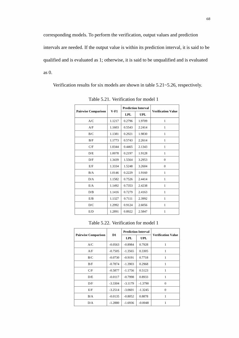
68

corresponding models. To perform the verification, output values and prediction

intervals are needed. If the output value is within its prediction interval, it is said to be

qualified and is evaluated as 1; otherwise, it is said to be unqualified and is evaluated

as 0.

Verification results for six models are shown in table 5.21~5.26, respectively.

Table 5.21. Verification for model 1

Pairwise Comparison V-F1 Prediction Interval

Verification Value LPL UPL

A/C 1.1217 0.2796 1.9709 1

A/F 1.1603 0.5543 2.2414 1

B/C 1.1381 0.2921 1.9830 1

B/F 1.1773 0.5743 2.2614 1

C/F 1.0344 0.4465 2.1343 1

D/E 1.0078 0.2197 1.9128 1

D/F 1.3439 1.5564 3.2953 0

E/F 1.3334 1.5248 3.2604 0

B/A 1.0146 0.2229 1.9160 1

D/A 1.1582 0.7526 2.4414 1

E/A 1.1492 0.7353 2.4238 1

D/B 1.1416 0.7279 2.4163 1

E/B 1.1327 0.7111 2.3992 1

D/C 1.2992 0.9124 2.6056 1

E/D 1.2891 0.8922 2.5847 1


Pairwise Comparison D1 Prediction Interval


A/C -0.0563 -0.8984 0.7928 1

A/F -0.7505 -1.3565 0.3305 1

B/C -0.0730 -0.9191 0.7718 1

B/F -0.7874 -1.3903 0.2968 1

C/F -0.5877 -1.1756 0.5123 1

D/E -0.0117 -0.7998 0.8933 1

D/F -3.3304 -3.1179 -1.3790 0

E/F -3.2514 -3.0601 -1.3245 0

B/A -0.0135 -0.8052 0.8878 1

D/A -1.2880 -1.6936 -0.0048 1

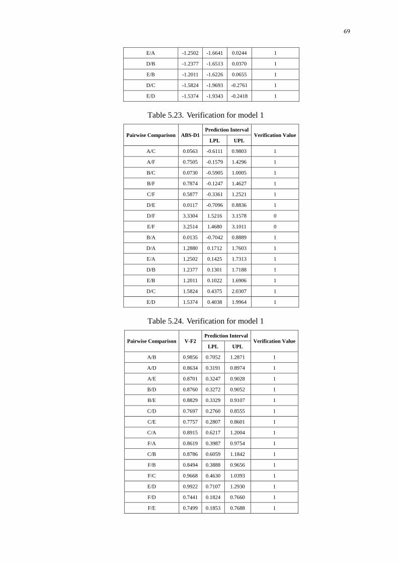
69

E/A -1.2502 -1.6641 0.0244 1

D/B -1.2377 -1.6513 0.0370 1

E/B -1.2011 -1.6226 0.0655 1

D/C -1.5824 -1.9693 -0.2761 1

E/D -1.5374 -1.9343 -0.2418 1


Pairwise Comparison ABS-D1 Prediction Interval


A/C 0.0563 -0.6111 0.9803 1

A/F 0.7505 -0.1579 1.4296 1

B/C 0.0730 -0.5905 1.0005 1

B/F 0.7874 -0.1247 1.4627 1

C/F 0.5877 -0.3361 1.2521 1

D/E 0.0117 -0.7096 0.8836 1

D/F 3.3304 1.5216 3.1578 0

E/F 3.2514 1.4680 3.1011 0

B/A 0.0135 -0.7042 0.8889 1

D/A 1.2880 0.1712 1.7603 1

E/A 1.2502 0.1425 1.7313 1

D/B 1.2377 0.1301 1.7188 1

E/B 1.2011 0.1022 1.6906 1

D/C 1.5824 0.4375 2.0307 1

E/D 1.5374 0.4038 1.9964 1


Pairwise Comparison V-F2 Prediction Interval


A/B 0.9856 0.7052 1.2871 1

A/D 0.8634 0.3191 0.8974 1

A/E 0.8701 0.3247 0.9028 1

B/D 0.8760 0.3272 0.9052 1

B/E 0.8829 0.3329 0.9107 1

C/D 0.7697 0.2760 0.8555 1

C/E 0.7757 0.2807 0.8601 1

C/A 0.8915 0.6217 1.2004 1

F/A 0.8619 0.3987 0.9754 1

C/B 0.8786 0.6059 1.1842 1

F/B 0.8494 0.3888 0.9656 1

F/C 0.9668 0.4630 1.0393 1

E/D 0.9922 0.7107 1.2930 1

F/D 0.7441 0.1824 0.7660 1

F/E 0.7499 0.1853 0.7688 1

70


Pairwise Comparison D2 Prediction Interval


A/B 0.0130 -0.2674 0.3145 1

A/D 0.4546 -0.0896 0.4886 1

A/E 0.4534 -0.0921 0.4860 1

B/D 0.4557 -0.0931 0.4849 1

B/E 0.4544 -0.0956 0.4822 1

C/D 0.4227 -0.0710 0.5085 1

C/E 0.4219 -0.0731 0.5063 1

C/A 0.0426 -0.2272 0.3515 1

F/A 0.3385 -0.1246 0.4520 1

C/B 0.0530 -0.2197 0.3585 1

F/B 0.3404 -0.1202 0.4566 1

F/C 0.3503 -0.1535 0.4228 1

E/D 0.0113 -0.2702 0.3121 1

F/D 0.5302 -0.0315 0.5520 1

F/E 0.5318 -0.0328 0.5507 1




A/B 0.0130 -0.1356 0.3043 1

A/D 0.4546 0.0169 0.4540 0

A/E 0.4534 0.0148 0.4518 0

B/D 0.4557 0.0139 0.4508 0

B/E 0.4544 0.0118 0.4486 0

C/D 0.4227 0.0330 0.4710 1

C/E 0.4219 0.0312 0.4692 1

C/A 0.0426 -0.1012 0.3362 1

F/A 0.3385 -0.0132 0.4227 1

C/B 0.0530 -0.0948 0.3423 1

F/B 0.3404 -0.0094 0.4266 1

F/C 0.3503 -0.0380 0.3976 1

E/D 0.0113 -0.1379 0.3022 1

F/D 0.5302 0.0671 0.5082 0

F/E 0.5318 0.0660 0.5071 0

71

CHAPTER 6. DISCUSSION

6.1. Comparison of AHP and fuzzy AHP approaches

In the first scenario of this research, a comparison of classic AHP and fuzzy AHP

approaches were performed to give a numerical illustration on how some factors

affect the difference given by the two approaches. In this way, it adds useful

knowledge to the relationship between two existing problems: (1) What factors bring

the difference between classic AHP and Fuzzy AHP? (2) How different the results are

given by the two approaches?

According to the hypothesis given by Chapter 3, result in this part concludes that

in general situation, the pairwise weight values of AHP approach is a significant

factor to the differences while the range of fuzzy values for Fuzzy AHP approach is

not. Furthermore, the fuzzy AHP narrows the span of the criteria weights, excluding

two extreme circumstances in which fuzzy AHP may increase the comparative

weights of specific criterion.

To be specify, the first subgroup of model illustrates that, for fuzzy AHP, the

pairwise weight values increase when the pairwise weight values of AHP increase; but

the incremental rate is smaller, which means that the larger the pairwise weight values,

the larger the differences between the two approaches are. The second subgroup of

models illustrates that, for fuzzy AHP, the pairwise weight values decrease when the

pairwise weight values of AHP decrease; but the decremental rate is smaller, which

means that the smaller the pairwise weight values, the larger the differences between

the two approaches are.

72

In conclusion, fuzzy AHP approach produces the weight for each pair of criteria

with the same tendency as classic AHP approach, but it narrows them. This outcome

is attributed to the uncertainty of evaluators’ preferences on the criteria. The

uncertainty results in the span of fuzzy pairwise comparison numbers which balances

the weights of each criterion.

There are two extreme situations, under which the conclusion by previous

modeling does not hold true.

(1) Weight value equals to 0

There is one extreme circumstance that if one criterion whose weight is weaker

than all of the others, fuzzy AHP will have the weight of this criterion equals to 0. For

example, for criterion i, aij < 1 for all j, then Wi = 0. In this situation, fuzzy AHP

enlarges the comparative weight of this criterion.

(2) Weight value equals to 1

There is another extreme circumstance that if one criterion whose weight is

stronger than all of the others, fuzzy AHP will have the weight of this criterion equals

to 1. For example, for criterion i, aij < 1 for all j, then Wi = 1. In this situation, fuzzy

AHP also magnifies the comparative weight of this criterion.

6.2. Criteria ranking for CVISN project

The verification based on prediction intervals suggested that fuzzy AHP is an

appropriate approach to deal with the multiple criteria decision making problem for

CVISN project. This conclusion is on the basis of the assumption that the pairwise

73

comparison values gained from stakeholders, who have the equal influence on the

scores of criteria, are considered to be a series of possible pairwise comparison values

obtained by a fictitious decision maker. Only in this way can this problem be solved in

a fuzzy AHP circumstance.

The detailed information for fuzzy AHP being appropriate in this specified

problem is stated below:

(1) For each of the first subgroup of models which have the pairwise comparison

value larger than 1, 13 out of 15 predicted variables are within prediction

intervals.

(2) The only two predicted variables that are out of prediction intervals are the

pairwise comparison value between D and F, and E and F. By careful

observation of these three criteria, it is easy to find out from the final weight

vector gained by classical AHP that criteria D and E are the most important

criteria with the highest scores (0.297 and 0.291 respectively) while criterion

F is the weakest criteria with the lowest score (0.063). As well, fuzzy AHP

approach provided the same trend results that criteria D and E get the highest

scores (0.191 and 0.189 respectively) and criterion F gets the lowest score

(0.142), even though these results are greatly narrowed.

(3) This fact makes the existence of these two outliers make sense. Firstly, fuzzy

AHP narrows the weights among criteria; secondly, the more extreme the

weights given by classical AHP are, the greater the fuzzy AHP narrows them;

thirdly, these two pairs of criteria are all the combinations of the most

74

important criterion and the least important criterion, which means that they

are all combinations of criterion with extreme weight. As a result, the

differences between fuzzy AHP and classical AHP on these two pairs of

criteria are large enough to go beyond the predicted intervals.

(4) For the first two of the second subgroup of models which have the pairwise

comparison value smaller than 1, all 15 predicted variables are within the

prediction intervals. These two models indicate that this problem is well

satisfied by fuzzy AHP.

(5) For the last model, there are 6 predicted variables out of 15 failed to be

within the prediction intervals.

(6) It is obviously that these 6 variables do not exceed the prediction intervals a

lot. Hence, it is hard to confirm the conclusion that according to this model,

fuzzy AHP is not suitable.

6.3. Overall conclusions

First, this research works on the comparison of classical AHP and fuzzy AHP

with 240 randomly generated data. By building a series of statistic models, this

research concludes that criteria weights given by fuzzy AHP follow the same

tendency as the ones given by classic AHP approach; they concentrate to a smooth

vector of weights. This conclusion is not acceptable for two extreme situations. These

models are benchmarks for the application of these two approaches into CVISN

project.

75

Second, this research uses both classical AHP and fuzzy AHP approaches to deal

with the multiple criteria decision making problem of CVISN project. Two weight

vectors show the same trends, which are coincident with the outcomes from the

random data.

Third, according to the benchmark, this research verifies the results of the

CVISN project using prediction interval. Except two pairs of extreme criteria, other

predicted variables are all within the prediction interval. Moreover, these two outliers

are understandable and acceptable. Hence, fuzzy AHP is appropriate for CVISN

project.

In conclusion, fuzzy AHP is a suitable approach for the CVISN project based on

some assumptions. Again, it takes care of more stakeholders’ preferences compared

with classical AHP. As a result, this research takes the weight vector of the criteria

given by fuzzy AHP approach to provide support for further research.

The final weight ranking of the six technical requirements is:

1

2

3

F

4

5

6

0.165

0.167

0.147 W =

0.191

0.189

0.142

w

w

w

w

w

w

6.4. Limitations

There are three limitations for this research.

(1) The number of criterion was arbitrarily chosen as 4. This limitation came

from the assumption.

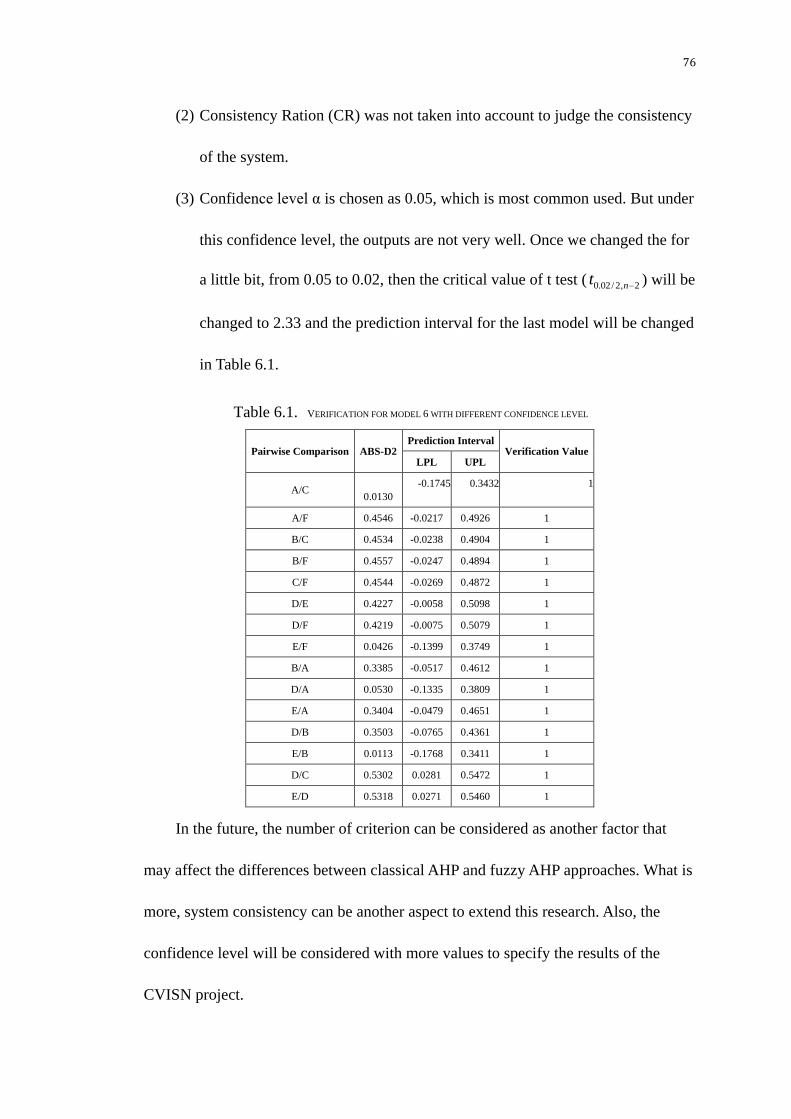
76

(2) Consistency Ration (CR) was not taken into account to judge the consistency

of the system.

(3) Confidence level α is chosen as 0.05, which is most common used. But under

this confidence level, the outputs are not very well. Once we changed the for

a little bit, from 0.05 to 0.02, then the critical value of t test ( 0.02/ 2, 2nt ) will be

changed to 2.33 and the prediction interval for the last model will be changed

in Table 6.1.

Table 6.1. VERIFICATION FOR MODEL 6 WITH DIFFERENT CONFIDENCE LEVEL



A/C 0.0130

-0.1745 0.3432 1

A/F 0.4546 -0.0217 0.4926 1

B/C 0.4534 -0.0238 0.4904 1

B/F 0.4557 -0.0247 0.4894 1

C/F 0.4544 -0.0269 0.4872 1

D/E 0.4227 -0.0058 0.5098 1

D/F 0.4219 -0.0075 0.5079 1

E/F 0.0426 -0.1399 0.3749 1

B/A 0.3385 -0.0517 0.4612 1

D/A 0.0530 -0.1335 0.3809 1

E/A 0.3404 -0.0479 0.4651 1

D/B 0.3503 -0.0765 0.4361 1

E/B 0.0113 -0.1768 0.3411 1

D/C 0.5302 0.0281 0.5472 1

E/D 0.5318 0.0271 0.5460 1

In the future, the number of criterion can be considered as another factor that

may affect the differences between classical AHP and fuzzy AHP approaches. What is

more, system consistency can be another aspect to extend this research. Also, the

confidence level will be considered with more values to specify the results of the

CVISN project.

77

CHAPTER 7. CONTRIBUTION TO THE BODY OF KNOWLEDGE

Decision making problem is one of most common problem in Operations

Research field. AHP approach is an effective and popular way to deal with this

problem. As a result, it is well known in Operations Research field as a decision

structuring tool. In 2008, the major international society for operations research

formally recognized AHP's broad impact on its field.

This paper works on the differences between classical AHP and fuzzy AHP

approaches, with the purpose of finding out how the factors influence the differences

between the two approaches. In this way, this paper contributes to the development of

Operations Research.

In addition, based on the comparison, this paper provides the CVISN project

with reasonable and comprehensive criteria ranking of six important technical

requirements. As a result, this paper has practical contribution.

The two AHP approaches used in this paper have been maturely developed and

well applied into many fields. Also their operations are proved to be simple. One is

classical AHP approach, with the geometric mean as the average of different pairwise

comparison values. The other one is Chang’s extent Fuzzy AHP approach.

Literature research has found that there are many studies on the differences

between classical AHP and fuzzy AHP. These studies can be divided into two aspects.

One is about the theoretical methods, which is focusing on how the differences come

out; the other one is about the final results, which is emphasizing the differences

between two weight vectors given by corresponding approaches. The connection

78

between these two aspects is a gap in previous studies.

The detailed contributions to the Operation Research of this paper are listed

below.

In the first place, this paper proposes two potential impacts which affect the

differences between classical AHP and fuzzy AHP approaches. They are the pairwise

comparison of one criterion over another given by classical AHP and the range of the

fuzzy number for pairwise comparison given by fuzzy AHP.

In the second place, this paper generates useful information for the relationship

between the two aspects of previous researches. This paper explores how the factors

that give rise to the differences affect the weight vectors given by these two AHP

approaches. In other words, this paper works out the relationships between the two

proposed impacts and the differences coming from classical AHP and fuzzy AHP.

Results show that the range of fuzzy values of fuzzy AHP approach is not an

important factor to the differences of the two approaches while the pairwise

comparison values of classical AHP significantly affect the differences. Moreover,

fuzzy AHP approach produces the weight for each pair of criteria with the same

tendency as classic AHP approach, but it narrows them.

In the third place, data used in the comparison are randomly generated data. 240

random data are more enough to perform statistic modeling. Simple linear regression

models are built to generate the relationships between the differences given by the

two approaches and the potential impacts. Hence, this paper compares the differences

between classical AHP and fuzzy AHP approaches in a statistical way and the

79

differences are in the form of statistical linear regression models.

In the forth place, this paper is a case study of the comparison of classical AHP

and fuzzy AHP approaches. Data coming from CVISN project are used to be an

example to conduct the comparison.

In the fifth place, prediction intervals are used to verify the results given by the

CVISN project. Prediction interval is a common method for validation of any single

predicted value in statistics. 240 random data are data population to create the

benchmark for prediction intervals by building the statistical regression models.

In the sixth place, this paper meets the research objective and provides the

CVISN project with a comprehensive ranking of the six technical requirements. This

ranking will be used in future research of CVISN project for the purpose of RFID

system selection.

80

CHAPTER 8. REFERENCES

[1] E. Herrera-Viedma, F. Herrera, F. Chiclana, and M. Luque, ―Some issues on

consistency of fuzzy preference relations,‖ European Journal of Operational

Research, vol., 2004, pp. 98-109.

[2] H. R. Weistroffer and S. C. Narula, Implementation of mcdm methodology in

decision support systems, systems, Man and Cybernetics, IEEE, Vol. 3, 1989, pp.

1011-1014.

[3] R. L. Keeney and H. Raïffa, Decisions with multiple objectives, Cambridge

University Press, Business & Economics, 1993.

[4] Y. Chen, D. M. Kilgour, and K. W. Hipel, Using a benchmark in case-based

multi-criteria ranking, IEEE transactions on systems, man, and cybernetics, vol.

39, no. 2, march 2009, pp. 358-368.

[5] T. L. Saaty, Theory and applications of the analytic network process: decision

making with benefits, Opportunities, Costs, and Risks, Pittsburgh, Pennsylvania:

RWS Publications, 2005, pp. ix.

[6] S. T. Chen, and C. L. Hwang, Fuzzy multiple attribute decision making methods

and applications, New York: Springer-Verlag, 1992, pp. 1-5.

[7] N. Bhushan and R. Kanwal, Strategic decision making: applying the analytic

hierarchy process. London: Springer-Verlag, January 2004.

[8] C. Yu and C. Li, A group decision making fuzzy AHP model and its application to

a plant location selection problem, IFSA World Congress and 20th NAFIPS

International Conference, Vol 1, 2001, pp. 76–80.

81

[9] B. Taylor, Introduction to management science, Pearson Education Inc., New

Jersey, 2004.

[10] E. H. Forman and S. I. Gass, The analytical hierarchy process—an exposition.

Operations Research, Vol 49, 2001, pp. 469–487.

[11] H. Y. Kang and A. H. I. Lee , Priority mix planning for semiconductor fabrication

by fuzzy AHP ranking, Expert Systems with Applications, 2006,

http://www.sciencedirect.com/science/journal/09574174.

[12] Z. Luo and S. Yang, Comparative study on several scales in AHP, Systems

Engineering - Theory & Practice, 2004, 9, pp. 51-60.

[13] Y. Ge, Q. Xu, and H. Li, The design and application of a generic AHP evaluation

system, IEEE transitions on Wireless Communications, Networking and Mobile

Computing, Oct 2008, pp. 1-4.

[14] Pohekar, S. D., and Ramachandran, M., Application of Multi-Criteria Decision

Making to Sustainable Energy Planning, A Review Renewable and Sustainable

Energy Reviews, 8, 2004, pp.365-381.

[15] H. A. Taha, Operations research, Pearson Education Inc., Fayetteville, 2003.

[16] J. Sarkis and S. Talluri, Evaluating and selecting e-commerce software and

communication systems for a supply chain, European Journal of Operational

Research, 159, 2004, pp. 318-329.

[17] A. I. Olcer, and A. Y. Odabasi, ―A new fuzzy multiple attributive group decision

making methodology and its application to propulsion/manoeuvring system

82

selection problem,‖ European Journal of Operational Research, Vol, 166, 2005, pp.

93-114.

[18] D. Chang, Extent analysis and synthetic decision, optimization techniques and

applications, World Scientific, Singapore, Vol 1, 1992, pp. 352.

[19] V. B. Kreng and C. Y. Wu, ―Evaluation of knowledge portal development tools

using a fuzzy AHP approach: The case of Taiwanese stone industry,‖ European

Journal of Operational Research, Vol, 176, 2007, pp. 1795-1810.

[20] F. T. S. Chan and N. Kumar, Global supplier development considering risk factors

using fuzzy extended AHP-based approach, Omega, Volume 35, Issue 4, 2007, pp.

417-431.

[21] Y. Ding, Z. Yuan, and Y. Li, ―Performance evaluation model For transportation

corridor based on Fuzzy-AHP approach,‖ IEEE Computer Science, Fifth

International Conference on Fuzzy Systems and Knowledge Discovery, 2008, pp.

608-612.

[22] A. L. Guiffrida and R. Nagi, Fuzzy set theory applications in production

management research: A Literature Survey, Journal of Intelligent Manufacturing,

Vol9, No. 1, 1998, pp. 39-56.

[23] D. Dubois and H. Prade, Fuzzy sets and systems. Academic Press, New York,

1988.

[24] D. Bouyssou, P. Perny, and M. Pirlot, Nontransitive deomposable conjoint

measurement as a general framework for MCDM and decision under uncertainty.

Communication to EURO XVII, Budapest, Hungary, July 2000.

[25] Y. M. Wang, Y. Luo, and Z. Hua, On the extent analysis method for fuzzy AHP

and its applications, European Journal of Operational Research, Vol 186, 2008, pp.

735-747.

83

[26] L. C. Leung, and D. Cao, On consistency and ranking of alternatives in fuzzy

AHP, European Journal of Operational Research, Vol, 124, 2000, pp. 102-113.

[27] A. ÖZDAĞOĞLU, G. ÖZDAĞOĞLU, Comparison of AHP and Fuzzy AHP for

the multi-criteria decision making processes with linguistic evaluations, İstanbul

Ticaret Üniversitesi Fen Bilimleri Dergisi Yıl, 2007/1, pp. 65-85

[28] O. Meixner, fuzzy AHP group decision analysis and its application for the

evaluation of energy sources, Proceedings of the 10th

International Symposium on

the Analytic Hierarchy/Network Process, Pittsburtgh/PA, 2009.

[29] H. Smith and B. Konsynski, Developments in practice X: Radio Frequency

Identification (RFID) – An Internet for Physical Objects. Communications of the

Association for Information Systems, Vol 12, 2003, pp. 301-311.

[30] J. Landt, The history of RFID, IEEE, Vol. 24, 2005, pp. 8-11.

[31] B. Hatch, J. B. Lee, and G. Kurtz, Hacking exposed linux: linux security secrets &

solutions, third edition, McGraw-Hill Osborne Media, 2008, pp. 298.

[32] J. Landt, Shrouds of time: the history of RFID, AIM Inc. 2001.

[33] Cardullo et al. Transponder apparatus and system, U.S. Patent 3,713,148, 1973.

[34] C. A. Walton, Portable radio frequency emitting identifier, U.S. Patent, issue date

May 17, 1983.

[35] B. Nath, F. Reynolds, and R. Want, RFID technology and applications, IEEE

Pervasive Computing, Vol 5, 2006, pp. 22-24.

[36] Paul G. Ranky, An introduction to radio frequency identification (RFID) methods

and solutions, Assembly Automation, Vol. 26, 2006, pp.28-33.

84

[37] Knowledgeleader, What Every Internal Auditor Should Know About RFID. 2006.

Overview of RFID components. [Online] June 2006. [Cited: 1 November, 2010]

http://www.theiia.org/download.cfm?file=93793.

[38] G. Oh, D. Kim, S. Kim, and S. Rhew, A quality evaluation technique of rfid

middleware in ubiquitous computing, IEEE Computer Science on Hybrid

Information Technology, 2006, pp. 730-735.

[39] M. Schneider, Radio Frequency Identification (RFID) Technology and its

Applications in the Commercial Construction Industry, University of Kentucky

Civil Engineering Department, Master’s of Science in Civil Engineering

Examination, April 24, 2003, pp. 6-7.

[40] Durfee Adam and Paul Goodrum, ―RFID, MEMS, and their Applications in the

Field of Construction‖, White Paper, 11 January, 2002.

http://www.theiia.org/download.cfm?file=93793

COMPARISON OF CLASSICAL ANALYTIC HIERARCHY ...

Documents

Transcript of COMPARISON OF CLASSICAL ANALYTIC HIERARCHY ...