
Analytic Solver Optimization Analytic Solver Simulation User ...
564
Version 2020 For Use With Excel 2010-2019 Analytic Solver Optimization Analytic Solver Simulation User Guide
-
Upload
khangminh22 -
Category
Documents
-
view
0 -
download
0
Transcript of Analytic Solver Optimization Analytic Solver Simulation User ...

Version 2020 For Use With Excel 2010-2019
Analytic Solver Optimization
Analytic Solver Simulation
User Guide

Copyright
Software copyright 1991-2019 by Frontline Systems, Inc.
User Guide copyright 2019 by Frontline Systems, Inc.
GRG/LSGRG Solver: Portions copyright 1989 by Optimal Methods, Inc. SOCP Barrier Solver: Portions
copyright 2002 by Masakazu Muramatsu. LP/QP Solver: Portions copyright 2000-2010 by International Business Machines Corp. and others. Neither the Software nor this User Guide may be copied, photocopied,
reproduced, translated, or reduced to any electronic medium or machine-readable form without the express
written consent of Frontline Systems, Inc., except as permitted by the Software License agreement below.
Trademarks Frontline Solvers®, XLMiner®, Analytic Solver®, Risk Solver®, Premium Solver®, Solver SDK® and Rason® are trademarks of Frontline Systems, Inc. Windows and Excel are trademarks of Microsoft Corp. Gurobi is a
trademark of Gurobi Optimization, Inc. Knitro is a trademark of Artelys. MOSEK is a trademark of MOSEK
ApS. OptQuest is a trademark of OptTek Systems, Inc. XpressMP is a trademark of FICO, Inc.
Acknowledgements
Thanks to Dan Fylstra and the Frontline Systems development team for a 25-year cumulative effort to build the
best possible optimization and simulation software for Microsoft Excel. Thanks to Frontline’s customers who
have built many thousands of successful applications, and have given us many suggestions for improvements.
Earlier versions of Risk Solver Pro and Risk Solver Platform have benefited from reviews, critiques, and
suggestions from several risk analysis experts:
• Sam Savage (Stanford Univ. and AnalyCorp Inc.) for Probability Management concepts including SIPs,
SLURPs, DISTs, and Certified Distributions.
• Sam Sugiyama (EC Risk USA & Europe LLC) for evaluation of advanced distributions, correlations, and
alternate parameters for continuous distributions.
• Savvakis C. Savvides for global bounds, censor bounds, base case values, the Normal Skewed distribution
and new risk measures.
How to Order
Contact Frontline Systems, Inc., P.O. Box 4288, Incline Village, NV 89450.
Tel (775) 831-0300 Fax (775) 831-0314 Email [email protected] Web http://www.solver.com

Frontline Solvers 2020 User Guide Page 3
Contents
Start Here: V2020 Essentials 12
Getting the Most from This User Guide ....................................................................... 12 Desktop and Cloud Versions .......................................................................... 12 Installing the Software ................................................................................... 12 Understanding License and Upgrade Options ................................................. 12 Getting Help Quickly ..................................................................................... 12 Finding the Examples .................................................................................... 13 Using Existing Models ................................................................................... 13 Using Large-Scale Solver Engines ................................................................. 13 Getting Started with Tutorials ........................................................................ 13 Getting and Interpreting Results ..................................................................... 13 Mastering Optimization and Simulation Concepts .......................................... 14 Using the Traditional Solver Parameters Dialog ............................................. 14 Automating Your Model with VBA ............................................................... 14
Installation and Add-Ins 15
What You Need ........................................................................................................... 15 Installing the Software ................................................................................................. 15
Installing Analytic Solver Cloud .................................................................... 15 Installing Analytic Solver Desktop ................................................................. 16
Logging in the First Time ............................................................................................ 20 Uninstalling the Software ............................................................................................ 21 Activating and Deactivating the Software .................................................................... 21
Excel 2019, 2016, 2013, and 2010 .................................................................. 21 If Something Goes Wrong ........................................................................................... 22 Cloud Versions ............................................................................................................ 23
Security and Privacy Considerations............................................................... 24 Analytic Solver Cloud .................................................................................... 24 AnalyticSolver.com ....................................................................................... 25
Using Solver Server to Solve Models ........................................................................... 25 Adding a Server ............................................................................................. 25 Solving Your Model on a Server .................................................................... 29
Analytic Solver Overview 30
Analytic Solver Product Line ....................................................................................... 30 Desktop and Cloud versions ........................................................................... 30 Analytic Solver Basic .................................................................................... 31 Analytic Solver Upgrade ................................................................................ 31 Analytic Solver Optimization ......................................................................... 31 Analytic Solver Simulation ............................................................................ 31 Analytic Solver Data Mining .......................................................................... 32 Analytic Solver Comprehensive ..................................................................... 32
Enhancements in Recent Years .................................................................................... 32 2017: Power BI, Analytic Solver Basic, and More ........................................................ 33 2018: Tableau, Data Mining Workflows, and More ...................................................... 34 2019: Analytic Solver Cloud ........................................................................................ 35

Frontline Solvers 2020 User Guide Page 4
Business Rules and DMN Decision Tables ..................................................... 36 What’s New in Analytic Solver V2020 ........................................................................ 36
Faster Solver Engines, Using Multiple Cores .................................................. 36 Monte Carlo Simulation Enhancements .......................................................... 37
Optimization and Resource Allocation ......................................................................... 37 Simulation and Risk Analysis ...................................................................................... 38 Optimal Solutions for Models with Uncertainty............................................................ 39 Automatic Model Transformation to RASON .............................................................. 39 Sensitivity Analysis and Model Parameters .................................................................. 40 Multiple Optimizations and Simulations ...................................................................... 40 Decision Trees on the Spreadsheet ............................................................................... 40 Bringing Big Data into Excel using Apache Spark........................................................ 41 Forecasting and Data Mining ....................................................................................... 41 Large-Scale Solver Engines ......................................................................................... 42 Automatic Mode and Solution Time ............................................................................ 43 Help, Guided Mode and Proactive Support................................................................... 44
Help, Support, Licenses and Product Versions 45
Introduction ................................................................................................................. 45 Working with Licenses in V2020 ................................................................................. 45
Licenses Tied to You, Not Your Computer ..................................................... 45 Analytic Solver Basic .................................................................................... 46 Renamed Products Offering More .................................................................. 46
Getting Help ................................................................................................................ 47 Accessing Resources ...................................................................................... 48 User Guides ................................................................................................... 48 Example Models ............................................................................................ 48 Knowledge Base ............................................................................................ 48 Operating Mode ............................................................................................. 49 Support Mode ................................................................................................ 49 Submit a Support Ticket ................................................................................. 49 Solver Academy ............................................................................................ 50 Video Tutorials/Live Webinars ...................................................................... 50 Learn more! ................................................................................................... 50
License Button ............................................................................................................ 50 Product Selection Wizard ............................................................................................ 53 Using the Welcome Screen in Analytic Solver Desktop ................................................ 55 License/Subscription in Analytic Solver Desktop ......................................................... 56 Context-Sensitive Help in Analytic Solver Desktop ...................................................... 57
Examples: Conventional Optimization 59
Introduction ................................................................................................................. 59 A First Optimization Model ......................................................................................... 59
The Model in Algebraic and Spreadsheet Form .............................................. 60 Defining and Solving the Optimization Model ................................................ 61 Using the Classical Solver Parameters Dialog ................................................. 65 Using Buttons on the Task Pane ..................................................................... 66 Exporting Data to Microsoft's Power BI ......................................................... 68 Exporting Data to Tableau ............................................................................. 71 Tablea Data Extract ....................................................................................... 72 Tableau Web Connector ................................................................................. 73
Introducing the Standard Example Models ................................................................... 76 Opening the Examples ................................................................................... 76 More Readable and Expandable Models ......................................................... 78

Frontline Solvers 2020 User Guide Page 5
Models, Worksheets and Workbooks.............................................................. 78 Linear Programming Examples .................................................................................... 79
Using the Output Tab and Creating Reports .................................................... 79 A Model with No Feasible Solution................................................................ 82 An ‘Accidentally’ Nonlinear Model ............................................................... 83
Nonlinear Optimization Examples ............................................................................... 86 Portfolio Optimization: Quadratic Programming ............................................. 86 Charts of the Objective and Constraints .......................................................... 87 A Model with IF Functions ............................................................................ 91 A Model with Cone Constraints ..................................................................... 94
Solving an Optimization Model using Excel Online or Google Sheets .......................... 97
Examples: Simulation and Risk Analysis 106
Introduction ............................................................................................................... 106 A First Simulation Example ....................................................................................... 106
A Business Planning Example ...................................................................... 107 A What-If Spreadsheet Model ...................................................................... 108 Defining a Simulation Model ....................................................................... 108 Selecting Uncertain Functions ...................................................................... 113 Running a Simulation .................................................................................. 114 Interactive Simulation in Desktop Solver ...................................................... 119 Viewing the Full Range of Profit Outcomes ................................................. 120 Analyzing Factors Influencing Net Profit ..................................................... 122 Interactive Simulation with Charts and Graphs ............................................. 124 Charts and Graphs for Presentations ............................................................. 125 Exporting Data to Microsoft's Power BI ....................................................... 126 Exporting Data to Tableau ........................................................................... 129 Tableau Web Connector ............................................................................... 131
An Airline Revenue Management Model ................................................................... 134 A Single Simulation ..................................................................................... 135 Multiple Parameterized Simulations ............................................................. 138 Simulation Optimization .............................................................................. 141
Using a Compound Distribution ................................................................................. 143 Discrete Distribution passed to 1st Argument ................................................ 145 Constant passed to 1st Argument................................................................... 147
Publishing a Simulation Model to Excel Online or Google Sheets .............................. 148
Examples: Stochastic Optimization 162
Introduction ............................................................................................................... 162 A Project Selection Model ......................................................................................... 162
Solving with Simulation Optimization .......................................................... 164 Solving Automatically ................................................................................. 166
A Model with Chance Constraints .............................................................................. 168 Solving with Robust Optimization ................................................................ 170
A Model with Recourse Decisions ............................................................................. 173 Solving with Robust Optimization ................................................................ 174
Creating Your Own Application 178
Introduction ............................................................................................................... 178 The Create App Icon.................................................................................................. 178 Solving a Model Using the RASON Desk IDE ........................................................... 181
Conversion Exceptions ................................................................................ 194 Problem Limits ............................................................................................ 195
Solving a Model Using the RASON Web IDE ........................................................... 195

Frontline Solvers 2020 User Guide Page 6
Note on RASON Subscriptions .................................................................... 195 Creating a Web Page ................................................................................................. 204
Using Decision Tables 208
Introduction ............................................................................................................... 208 Decision Table Structure............................................................................................ 208 Decision Tables at Work ............................................................................................ 212
Optional Arguments ..................................................................................... 214 Additional Examples .................................................................................... 214 Hit Policies .................................................................................................. 216
Merging Decision Table Results ................................................................................ 221 Using Cascading Decision Tables .............................................................................. 223 Using Decision Tables in Optimization and Simulation .............................................. 227
Optimization ................................................................................................ 227 Simulation ................................................................................................... 228
Using Decision Tables with Data Mining ................................................................... 229 Input Parameters .......................................................................................... 229 Loan Strategy .............................................................................................. 229
More Information on Decision Tables ........................................................................ 233
Creating Power BI Custom Visuals 235
Installing Power BI .................................................................................................... 235 Creating a Custom Visual from an Optimization Model.............................................. 236
PsiDataSrc() Arguments ............................................................................... 244 Troop Rotation Optimization Example ......................................................... 255 Using Optimization Parameters in Power BI ................................................. 261 Simulation Example Model .......................................................................... 262 Error Messages ............................................................................................ 267
Creating Custom Extensions in Tableau 268
Introduction ............................................................................................................... 268 Installing Tableau ...................................................................................................... 268 Solving Optimization Models in Tableau ................................................................... 268
PsiDataSrc() Arguments ............................................................................... 270 Troop Rotation Optimization Example ......................................................... 287 Using Optimization Parameters in Tableau ................................................... 294 Simulation Example Model .......................................................................... 295 Error Messages ............................................................................................ 300
Examples: Parameters and Sensitivity Analysis 301
Introduction ............................................................................................................... 301 Parameters and Results .............................................................................................. 301
Viewing Parameters in the Task Pane ........................................................... 301 Defining a Parameter ................................................................................... 302 Automatic Parameter Identification .............................................................. 303 Defining Results .......................................................................................... 306
Sensitivity Analysis Reports and Charts ..................................................................... 307 How Parameters are Varied .......................................................................... 307 Creating Sensitivity Reports ......................................................................... 308 Creating Sensitivity Charts ........................................................................... 309
Optimization and Simulation Reports and Charts ....................................................... 310 When Optimizations and Simulations are Run .............................................. 310

Frontline Solvers 2020 User Guide Page 7
Examples: Decision Trees and Discriminant Analysis 311
Introduction ............................................................................................................... 311 Creating Decision Trees............................................................................................. 312
Creating Trees in Analytic Solver Desktop ................................................... 312 Create Trees in Analytic Solver Cloud.......................................................... 312 Creating and Editing Nodes.......................................................................... 313 Creating and Editing Branches ..................................................................... 314
Highlighting a Decision Strategy ............................................................................... 316 Decision Trees in the Task Pane ................................................................................ 317
Model Tab in Analytic Solver Desktop ......................................................... 317 Model Tab in Analytic Solver Cloud ............................................................ 318 Platform Tab ................................................................................................ 319
Multiple Discriminant Analysis ................................................................................. 320 Discriminant Analysis Example ................................................................................. 320
Getting Results: Optimization 324
Introduction ............................................................................................................... 324 What Can Go Wrong, and What to Do About It ......................................................... 324
Review Messages in the Output Tab ............................................................. 325 Click the Solver Result Message for Help ..................................................... 326 Choose Available Optimization Reports ....................................................... 328 When Solving Takes a Long Time ............................................................... 328 When the Solution Seems Wrong ................................................................. 331 Problems with Poorly Scaled Models ........................................................... 331 The Integer Tolerance Option ....................................................................... 332
When Things Go Right: Getting Further Results ....................................................... 333 Dual Values ................................................................................................. 333 Multiple Solutions ....................................................................................... 335 Multiple Parameterized Optimizations .......................................................... 336
Getting Results: Simulation 342
Introduction ............................................................................................................... 342 What Can Go Wrong, and What to Do About It ......................................................... 342
Review Messages in the Output Tab ............................................................. 343 Click the Error Message for Help ................................................................. 343 Role of the Random Number Seed ............................................................... 344 When Simulation Takes a Long Time ........................................................... 345 When Simulation Results Seem Wrong ........................................................ 347
When Things Go Right: Getting Further Results ....................................................... 348 Using the Simulation Report ........................................................................ 348 Using the Uncertain Function Dialog............................................................ 349 Fitting a Distribution to Simulation Results .................................................. 350 Fitting a Meta-Log Distribution .................................................................... 352 Charting Multiple Uncertain Functions ......................................................... 356 Multiple Parameterized Simulations ............................................................. 357 Time Series Forecasting ............................................................................... 359 Time Series Simulation ................................................................................ 363 Excel 2016 Forecast Functions ..................................................................... 368
Getting Results: Stochastic Optimization 376
Introduction ............................................................................................................... 376 What Can Go Wrong, and What to Do About It ......................................................... 376
Review Messages in the Output Tab ............................................................. 377

Frontline Solvers 2020 User Guide Page 8
Click the Solver Result Message for Help ..................................................... 379 Choose Available Optimization Reports ....................................................... 380 When Solving Takes a Long Time ............................................................... 382 When the Solution Seems Wrong ................................................................. 383
When Things Go Right: Getting Further Results ....................................................... 384
Dimensional Modeling 386
Introduction ............................................................................................................... 386 Dimensions and Cubes .............................................................................................. 387 An Example Dimensional Model ............................................................................... 388 Using Dimensional Modeling in Optimization............................................................ 390
Defining a Dimension .................................................................................. 390 Defining a Cube ........................................................................................... 393 Cube Formulas: Operations and Dimensions ............................................... 395 Defining Outputs in Dimensional Models ..................................................... 397 Building the Model ...................................................................................... 398 Solving the Model........................................................................................ 399
Additional Functions ................................................................................................. 399 Parametric Dimensions with Optimization ................................................................. 401 Using Dimensional Modeling in Simulation ............................................................... 411
Defining a Dimension .................................................................................. 411 Defining a Cube ........................................................................................... 411 Defining an Output ...................................................................................... 412 Parametric Dimensions ................................................................................ 415
Using Dimensional Modeling with Pivot Tables ......................................................... 423 Using Sparse Cubes ................................................................................................... 426
Automating Optimization in VBA 432
Introduction ............................................................................................................... 432 Why Use the Object-Oriented API? .............................................................. 432 Running Predefined Solver Models .............................................................. 433 Using the Macro Recorder ........................................................................... 433 Adding a Reference in the VBA Editor ......................................................... 434
Analytic Solver Object Model .................................................................................... 434 Using the VBA Object Browser ................................................................... 436
Programming the Object Model ................................................................................. 436 Example VBA Code Using the Object Model ............................................... 437 Evaluators Called During the Solution Process ............................................. 437 Refinery.xls: Multiple Blocks of Variables and Functions ............................ 438 Adding New Variables and Constraints to a Model ....................................... 439 CuttingStock.xls: Multiple Problems and Dynamically Generated Variables 440
Automating Simulation in VBA 445
Introduction ............................................................................................................... 445 Adding a Reference in the VBA Editor ......................................................... 445
Activating Interactive Simulation ............................................................................... 445 Using VBA to Control Analytic Solver ...................................................................... 446
Analytic Solver Object Model ...................................................................... 447 Using the VBA Object Browser ................................................................... 447
Using Analytic Solver Objects ................................................................................... 448 Using Variable and Function Objects ........................................................... 449 Controlling Simulation Parameters in VBA .................................................. 450 Evaluators Called During the Simulation Process ......................................... 451
Working with Trials and Simulations in VBA ............................................................ 452

Frontline Solvers 2020 User Guide Page 9
Displaying Normal or Error Trials ................................................................ 452 Using Multiple Simulations .......................................................................... 452
Creating Uncertain Variables and SLURPs in VBA.................................................... 453
Mastering Conventional Optimization Concepts 455
Introduction ............................................................................................................... 455 Elements of Solver Models ........................................................................................ 455
Decision Variables and Parameters ............................................................... 455 The Objective Function ................................................................................ 456 Constraints .................................................................................................. 456 Solutions: Feasible, “Good” and Optimal .................................................... 457
More About Constraints............................................................................................. 459 Functions of the Variables ......................................................................................... 462
Convex Functions ........................................................................................ 463 Linear Functions .......................................................................................... 464 Quadratic Functions ..................................................................................... 465 Nonlinear and Smooth Functions.................................................................. 466 Discontinuous and Non-Smooth Functions ................................................... 467 Derivatives, Gradients, Jacobians, and Hessians ........................................... 468
Optimization Problems and Solution Methods ............................................................ 470 Linear Programming .................................................................................... 470 Quadratic Programming ............................................................................... 471 Quadratically Constrained Programming ...................................................... 472 Second Order Cone Programming ................................................................ 472 Nonlinear Optimization ................................................................................ 473 Global Optimization .................................................................................... 474 Non-Smooth Optimization ........................................................................... 476
Integer Programming ................................................................................................. 478 The Branch & Bound Method ...................................................................... 479 Cut Generation ............................................................................................ 479 The Alldifferent Constraint .......................................................................... 480
Looking Ahead to Models with Uncertainty ............................................................... 480
Mastering Simulation and Risk Analysis Concepts 482
Introduction ............................................................................................................... 482 What Happens During Monte Carlo Simulation.......................................................... 482
Random Number Generation and Sampling .................................................. 483 The PSI Interpreter and Simulation............................................................... 485
Uncertain Functions, Statistics, and Risk Measures .................................................... 486 Measures of Central Tendency ..................................................................... 486 Measures of Variation .................................................................................. 486 Risk Measures ............................................................................................. 487 Quantile Measures ....................................................................................... 487 Confidence Intervals .................................................................................... 487
Uncertain Variables and Probability Distributions ...................................................... 488 Discrete Vs. Continuous Distributions .......................................................... 488 Bounded Vs. Unbounded Distributions ......................................................... 488 Analytic Vs. Custom Distributions ............................................................... 488 Creating your Own Distributions When Past Data is Available ..................... 489 When Past Data is Not Available.................................................................. 489 Using the Fit feature .................................................................................... 490 More Hints and Warnings ............................................................................ 493
Dependence and Correlation ...................................................................................... 494 Measuring Observed Correlation .................................................................. 494

Frontline Solvers 2020 User Guide Page 10
Inducing Correlation Among Uncertain Variables ........................................ 495 Modeling Correlation Using Copulas ........................................................... 497 Archimedean Copulas .................................................................................. 497 Elliptical Copulas ........................................................................................ 502 Correlation Fitting ....................................................................................... 504
Using the Correlations Dialog .................................................................................... 508 Creating a Correlation Matrix ....................................................................... 508 Managing Copulas ....................................................................................... 511 Removing a Correlation Matrix .................................................................... 513 Editing a Correlation Matrix ........................................................................ 513 Making a Matrix Consistent ......................................................................... 514
Probability Management Concepts ............................................................................. 517 Analytic Distributions .................................................................................. 517 Certified Distributions and Stochastic Libraries ............................................ 518 Publishing and Using Certified Distributions ................................................ 518
Stochastic Libraries: SIPs and SLURPs ..................................................................... 519 Creating Stochastic Libraries........................................................................ 520 Using the DIST Feature ............................................................................... 521
Creating and Using Certified Distributions ................................................................. 523 Publishing Distributions with PsiCertify ....................................................... 524 Using Distributions with PsiCertified ........................................................... 524 Packaging Analytic Distributions ................................................................. 526
Mastering Stochastic Optimization Concepts 527
Introduction ............................................................................................................... 527 Certain and Uncertain Parameters................................................................. 527 Decision-Dependent Uncertainties ............................................................... 528 Resolving Uncertainty and Recourse Decisions ............................................ 528 Uncertainty and Conventional Optimization ................................................. 529
Elements of Solver Models ........................................................................................ 529 Uncertain Variables ..................................................................................... 529 Decision Variables ....................................................................................... 530 Functions of the Variables and Uncertainties ................................................ 530 The Objective Function ................................................................................ 531 Constraints: Normal, Chance, Recourse ....................................................... 532 Solutions: Feasible, Optimal, Well-Hedged ................................................. 533 More on Chance Constraints ........................................................................ 534 Diagnosing Your Model’s Use of Uncertainty .............................................. 537
Problems and Solution Methods ................................................................................. 537 Decision-Dependent Uncertainties ............................................................... 538 Resolving Uncertainty and Recourse Decisions ............................................ 538
Classes of Problems Involving Uncertainty ................................................................ 539 One-Stage Problems .................................................................................... 539 Two-Stage Problems .................................................................................... 540
Advanced Topics ....................................................................................................... 542 Bounds, Discretization, and Correlation ....................................................... 542 Uncertainty Sets and Norms ......................................................................... 542
Best Practices for Building Large-Scale Models 546
Introduction ............................................................................................................... 546 Designing Large Solver Models ................................................................................. 546
Spreadsheet Modeling Hints ......................................................................... 547 Optimization Modeling Hints ....................................................................... 548 Using Multiple Worksheets and Data Sources .............................................. 548

Frontline Solvers 2020 User Guide Page 11
Quick Steps Towards Better Performance .................................................................. 549 Improving the Formulation of Your Model ................................................................ 550
Techniques Using Linear and Quadratic Functions ....................................... 551 Techniques Using Linear Functions and Binary Integer Variables ................. 552 Using Piecewise-Linear Functions................................................................ 554
Organizing Your Model for Fast Solution .................................................................. 555 Fast Problem Setup ...................................................................................... 556 Using Array Formulas .................................................................................. 557 Using the Add-in Functions.......................................................................... 558
References and Further Reading 562
Introduction ............................................................................................................... 562 Textbooks Using Analytic Solver ................................................................. 562 Textbooks Using Solver or Premium Solver ................................................. 563 Other Textbooks .......................................................................................... 563 Academic References ................................................................................... 563

Frontline Solvers 2020 User Guide Page 12
Start Here: V2020 Essentials
Getting the Most from This User Guide
Desktop and Cloud Versions
Analytic Solver V2020 comes in two versions: Analytic Solver Desktop – a
traditional “COM add-in” that works only in Microsoft Excel for Windows PCs
(desktops and laptops), and Analytic Solver Cloud – a modern “Office add-in”
that works in Excel for Windows and Excel for Macintosh (desktops and
laptops), and also in Excel for the Web using browsers such as Chrome, FireFox
and Safari. Your license gives you access to both versions, and your Excel
workbooks and optimization, simulation and data mining models work in both versions, no matter where you save them (though OneDrive is most convenient).
Your license also gives you access in 2020 1H to Frontline Systems’ website
AnalyticSolver.com – a third way to create and solve models, if you don’t have
an Office 365 subscription and you don’t have a Windows PC. But we highly
recommend an Office 365 subscription to make your work easier and faster.
Installing the Software
Read the chapter “Installation and Add-Ins” for complete information on
installing Analytic Solver Cloud and (if you wish) Analytic Solver Desktop.
This chapter also explains how the Cloud and Desktop versions interact when
both are installed, and how to install and uninstall both versions.
In brief, to add Analytic Solver Cloud version to your copy of Excel, you use
the Excel Ribbon option Insert – Get Add-ins – no Setup program download or
installation is required. To install Analytic Solver Desktop on Windows PCs,
visit https://analyticsolver.com, login using the same email and password you
used to register on Solver.com, download and run the SolverSetup program.
Understanding License and Upgrade Options
Frontline Solvers V2020 feature a revised, simpler product line that gives you
access to all features, all the time for small models, and a new licensing system,
tied to you and usable on more than one computer. Read about this in the
chapter “Help, Support, Licenses and Product Versions.”
Getting Help Quickly
Choose Help on the Ribbon. You’ll see several options, starting with Help –
Help Center. Support Live Chat, Example Models, and User Guides are also
available here. In Analytic Solver Desktop (only) you can also get quick online
Help by clicking any underlined caption or message in the Task Pane.
Frontline Solvers 2020 User Guide Page 13
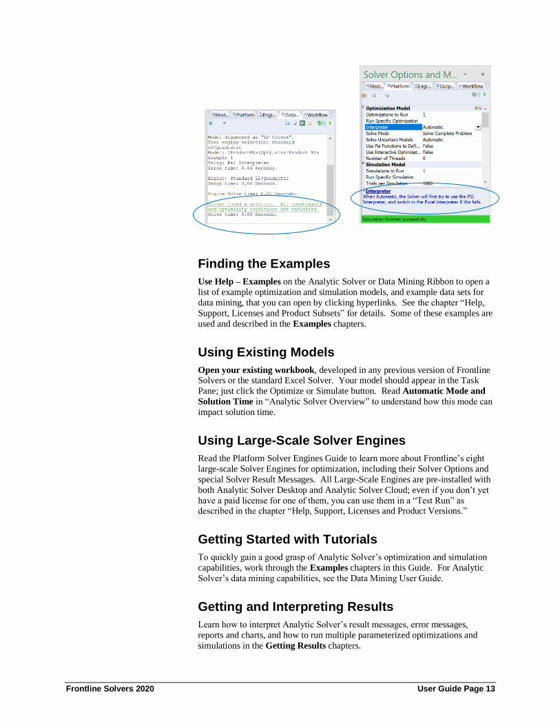
Finding the Examples
Use Help – Examples on the Analytic Solver or Data Mining Ribbon to open a
list of example optimization and simulation models, and example data sets for
data mining, that you can open by clicking hyperlinks. See the chapter “Help,
Support, Licenses and Product Subsets” for details. Some of these examples are
used and described in the Examples chapters.
Using Existing Models
Open your existing workbook, developed in any previous version of Frontline Solvers or the standard Excel Solver. Your model should appear in the Task
Pane; just click the Optimize or Simulate button. Read Automatic Mode and
Solution Time in “Analytic Solver Overview” to understand how this mode can
impact solution time.
Using Large-Scale Solver Engines
Read the Platform Solver Engines Guide to learn more about Frontline’s eight
large-scale Solver Engines for optimization, including their Solver Options and
special Solver Result Messages. All Large-Scale Engines are pre-installed with
both Analytic Solver Desktop and Analytic Solver Cloud; even if you don’t yet
have a paid license for one of them, you can use them in a “Test Run” as described in the chapter “Help, Support, Licenses and Product Versions.”
Getting Started with Tutorials
To quickly gain a good grasp of Analytic Solver’s optimization and simulation
capabilities, work through the Examples chapters in this Guide. For Analytic
Solver’s data mining capabilities, see the Data Mining User Guide.
Getting and Interpreting Results
Learn how to interpret Analytic Solver’s result messages, error messages,
reports and charts, and how to run multiple parameterized optimizations and
simulations in the Getting Results chapters.
Frontline Solvers 2020 User Guide Page 14
Mastering Optimization and Simulation Concepts
This guide can give you a professional education in simulation/risk analysis,
conventional optimization, and stochastic optimization (with uncertainty). Go
from beginner to expert and learn how to fully exploit the software by reading
the Mastering Concepts chapters, and the Frontline Solvers Reference Guide.
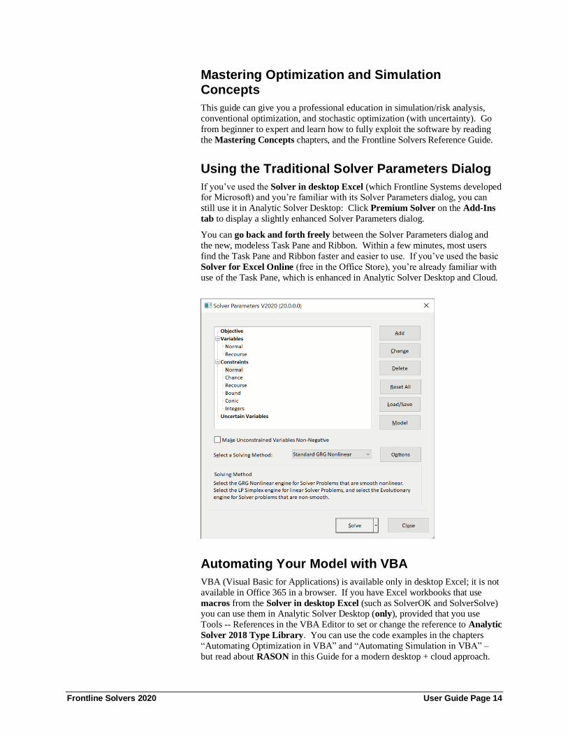
Using the Traditional Solver Parameters Dialog
If you’ve used the Solver in desktop Excel (which Frontline Systems developed for Microsoft) and you’re familiar with its Solver Parameters dialog, you can
still use it in Analytic Solver Desktop: Click Premium Solver on the Add-Ins
tab to display a slightly enhanced Solver Parameters dialog.
You can go back and forth freely between the Solver Parameters dialog and
the new, modeless Task Pane and Ribbon. Within a few minutes, most users
find the Task Pane and Ribbon faster and easier to use. If you’ve used the basic
Solver for Excel Online (free in the Office Store), you’re already familiar with
use of the Task Pane, which is enhanced in Analytic Solver Desktop and Cloud.
Automating Your Model with VBA
VBA (Visual Basic for Applications) is available only in desktop Excel; it is not
available in Office 365 in a browser. If you have Excel workbooks that use
macros from the Solver in desktop Excel (such as SolverOK and SolverSolve) you can use them in Analytic Solver Desktop (only), provided that you use
Tools -- References in the VBA Editor to set or change the reference to Analytic
Solver 2018 Type Library. You can use the code examples in the chapters
“Automating Optimization in VBA” and “Automating Simulation in VBA” –
but read about RASON in this Guide for a modern desktop + cloud approach.

Frontline Solvers 2020 User Guide Page 15
Installation and Add-Ins
What You Need You can use Analytic Solver Cloud in Excel for the Web through a browser
(such as Edge, Chrome, Firefox or Safari), without installing anything else. This
is the simplest and most flexible option, but it requires a constant Internet
connection.
To use Analytic Solver Cloud in Excel Desktop on a PC or Mac, you must have
a current version of Windows or iOS installed, and you will need the latest
Excel version installed via your Office 365 subscription – older non-subscription versions, even Excel 2019, do not have all the features and APIs
needed for modern Office add-ins like Analytic Solver Cloud.
To use Analytic Solver Desktop (Windows PCs only), you must have first
installed Microsoft Excel 2010, 2013, 2016, 2019, or the latest Office 365
version on Windows 10, Windows 8, Windows 7, or Windows Server 2019,
2016 or 2012. (Windows Vista or Windows Server 2008 may work but are no
longer supported.). It’s not essential to have the standard Excel Solver installed.
Installing the Software
Installing Analytic Solver Cloud
Analytic Solver V2020 includes our next-generation offering, Analytic Solver
Cloud – usable in the latest versions of Excel for Windows and Macintosh, and in Excel for the Web. Analytic Solver Cloud is divided into two add-ins that
work closely together (since an Office add-in currently can have only one
Ribbon tab): the Analytic Solver add-in builds optimization and simulation
models, and the Data Mining add-in builds data mining or forecasting models.
Both the Analytic Solver and Data Mining add-ins support existing models
created in previous versions of Analytic Solver. Your license for Analytic
Solver allows you to use Analytic Solver Desktop in desktop Excel or Analytic
Solver Cloud in either desktop Excel (latest version) or Excel for the Web.
To use the Analytic Solver and Data Mining add-ins, you must first “insert”
them for use in your copy of desktop Excel or Excel for the Web, while you are
logged into your Office 365 account. Once you do this, the Analytic Solver and Data Mining tabs will appear on the Ribbon in each new workbook you use.
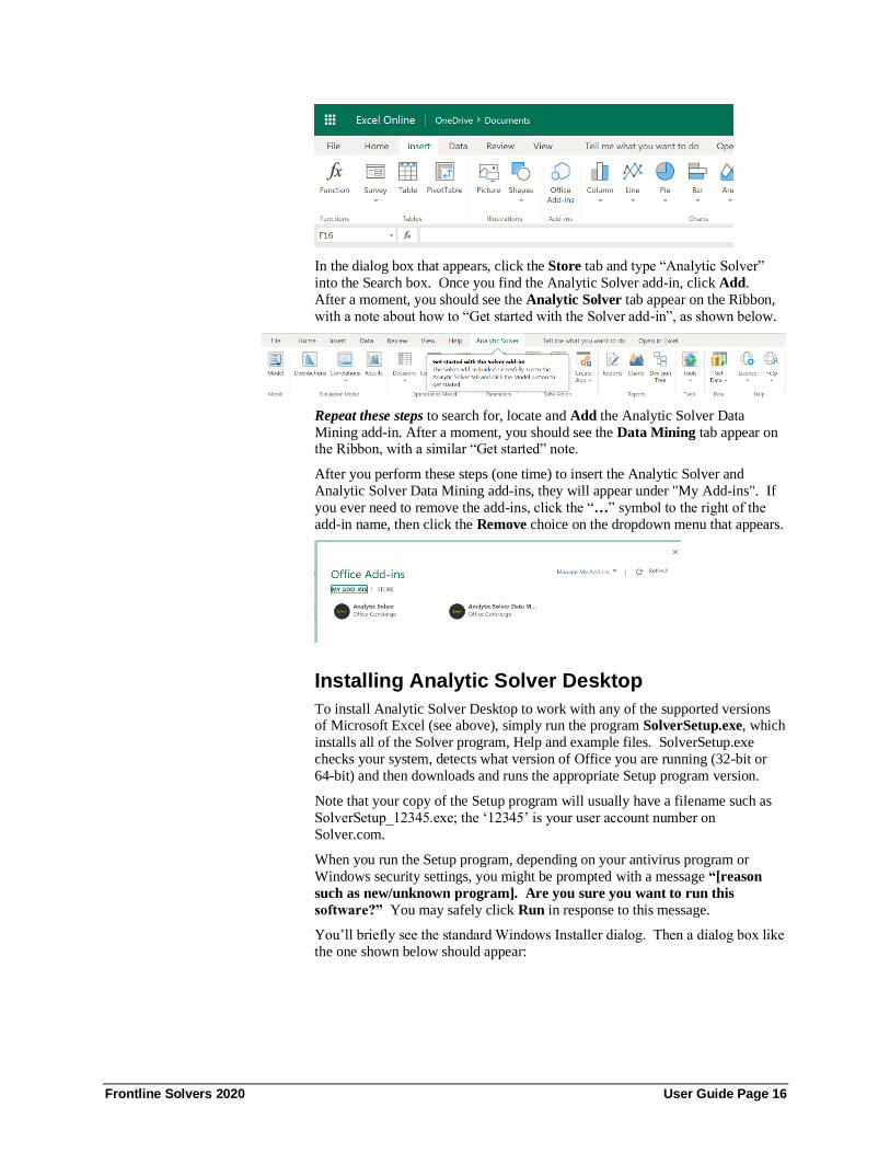
To insert the add-ins for the first time, open desktop Excel (latest version) or
Excel for the Web, click the Insert tab on the Ribbon, then click the button
Office Add-ins or (if you see it) the smaller button Get Add-ins.
Frontline Solvers 2020 User Guide Page 16
In the dialog box that appears, click the Store tab and type “Analytic Solver”
into the Search box. Once you find the Analytic Solver add-in, click Add.
After a moment, you should see the Analytic Solver tab appear on the Ribbon,
with a note about how to “Get started with the Solver add-in”, as shown below.
Repeat these steps to search for, locate and Add the Analytic Solver Data
Mining add-in. After a moment, you should see the Data Mining tab appear on the Ribbon, with a similar “Get started” note.
After you perform these steps (one time) to insert the Analytic Solver and
Analytic Solver Data Mining add-ins, they will appear under "My Add-ins". If
you ever need to remove the add-ins, click the “…” symbol to the right of the
add-in name, then click the Remove choice on the dropdown menu that appears.
Installing Analytic Solver Desktop
To install Analytic Solver Desktop to work with any of the supported versions of Microsoft Excel (see above), simply run the program SolverSetup.exe, which
installs all of the Solver program, Help and example files. SolverSetup.exe
checks your system, detects what version of Office you are running (32-bit or
64-bit) and then downloads and runs the appropriate Setup program version.
Note that your copy of the Setup program will usually have a filename such as
SolverSetup_12345.exe; the ‘12345’ is your user account number on
Solver.com.
When you run the Setup program, depending on your antivirus program or
Windows security settings, you might be prompted with a message “[reason
such as new/unknown program]. Are you sure you want to run this
software?” You may safely click Run in response to this message.
You’ll briefly see the standard Windows Installer dialog. Then a dialog box like
the one shown below should appear:

Frontline Solvers 2020 User Guide Page 17
Read this, so you know the difference between Analytic Solver Basic and the
upgrades to handle larger models and datasets. Then click Next to proceed – you’ll see a dialog like the one below.
Read this to learn how you can use Analytic Solver Cloud (our new Office add-
in version) – “Excel Online” is another name for “Excel for the Web”.
Next, the Setup program will ask if you accept Frontline’s software license
agreement. You must click “I accept” and Next in order to be able to proceed.

Frontline Solvers 2020 User Guide Page 18
The Setup program then displays a dialog box like the one shown below, where
you can select or confirm the folder to which files will be copied (normally
C:\Program Files\Frontline Systems\Analytic Solver Platform, or if you’re
installing Analytic Solver for 32-bit Excel on 64-bit Windows, C:\Program Files
(x86)\Frontline Systems\Analytic Solver Platform). Click Next to proceed.
You’ll see a dialog confirming that the preliminary steps are complete, and the installation is ready to begin.

Frontline Solvers 2020 User Guide Page 19
After you click Install, the Analytic Solver files will be installed, and the
program file RSPAddin.xll will be registered as a COM add-in (which may take
some time). A progress dialog may appear; be patient, since this process could
take longer than it has in previous Solver Platform releases.
When the installation is complete, you’ll see a dialog box like the one below. Click Finish to exit the installation wizard.

Frontline Solvers 2020 User Guide Page 20
The full Analytic Solver product family is now installed. With your trial and
paid license, you can access every feature of the software, including forecasting
and data mining, simulation and risk analysis, and conventional and stochastic
optimization. Simply click “Finish” and Microsoft Excel will launch with a
Welcome workbook containing information to help you get started quickly.
Logging in the First Time In Analytic Solver V2020, your license is associated with you, and may be used
on more than one PC. For example, you can run SolverSetup to install the
desktop software on your office PC, your company laptop, and your PC at home.
But only you can use Analytic Solver, and only on one of these computers at a
time. It is unlawful to “share” your license with another human user.
The first time you run Analytic Solver (Desktop or Cloud) after installing the
software on a new computer, when you next start Excel and visit the Analytic
Solver tab on the Ribbon, you will be prompted to login. Enter the email
address and password that you used to register on Solver.com or
AnalyticSolver.com. Once you’ve done this in Analytic Solver Desktop, your
identity will be “remembered,” so you won’t have to login every time you start
Excel and go to one of the Analytic Solver tabs. In Analytic Solver Cloud, you
may be asked to login more frequently.

Frontline Solvers 2020 User Guide Page 21
You can login and logout at any time, by clicking License – Login/Logout in
both Analytic Solver Desktop and Analytic Solver Cloud. If you share use of a
single physical computer with other Analytic Solver users, be careful to login
with your own email and password, and log out when you’re done – if you
don’t, other users could access private files in your cloud account, or use up your allotted CPU time or storage.
When you move from one computer to another, you should log out on one and
log in on the other. As a convenience, if you log in to Analytic Solver on a new
computer when you haven’t logged out on the old computer, Analytic Solver
will let you know, and offer to automatically log you out on the other computer.
Uninstalling the Software To uninstall Analytic Solver Desktop, just run the SolverSetup program as
outlined above. You’ll be asked to confirm that you want to remove the
software.
You can also uninstall by choosing Control Panel from the Start menu, and
double-clicking the Programs and Features or Add/Remove Programs applet. In the list box below “Currently installed programs,” scroll down if necessary
until you reach the line, “Frontline Excel Solvers 2020,” and click the
Uninstall/Change or Add/Remove… button. Click OK in the confirming dialog
box to uninstall the software.
Activating and Deactivating the Software Analytic Solver Desktop’s main program file RSPAddin.xll is a COM add-in, an
XLL add-in, and a COM server. A reference to the add-in Solver.xla is needed
if you wish to use the “traditional” VBA functions to control Analytic Solver,
instead of its new VBA Object-Oriented API.
Excel 2019, 2016, 2013, and 2010
In Excel 2019, 2016, 2013, and 2010, you can manage all types of add-ins from one dialog, reached by clicking File – Options -- Addins.

Frontline Solvers 2020 User Guide Page 22
You can manage add-ins by selecting the type of add-in from the dropdown list
at the bottom of this dialog. For example, if you select COM Add-ins from the
dropdown list and clock the Go button, the dialog shown below appears.
If you uncheck the box next to “Analytic Solver Addin” and click OK, you will
deactivate the Analytic Solver COM add-in, which will remove the Analytic
Solver tab from the Ribbon in desktop Excel, and also remove the PSI functions
for optimization from the Excel Function Wizard.
If Something Goes Wrong Under certain circumstances, desktop Microsoft Excel can “crash” or shut down,
so it must be restarted. This can happen for a variety of reasons, including bugs
in Excel itself, in the Analytic Solver software, or in other add-ins.
When Excel restarts, you may see one of the following messages:

Frontline Solvers 2020 User Guide Page 23
If you see these messages, you should usually click the No button. If you’ve
experienced a problem while using Analytic Solver software, please contact
Frontline Systems Technical Support as described below. If you click the Yes
button, Excel will disable the Analytic Solver add-in, and the Analytic Solver and Data Mining tabs will no longer appear on the Ribbon. To re-enable
Analytic Solver and restore these Ribbon tabs, see the preceding section
“Activating and Deactivating the Software:” you should select File – Options,
then Add-Ins, then Manage COM Add-ins, Go. Then check the box next to
“Analytic Solver Addin” and click OK.
In rare circumstances, Analytic Solver users have reported the following error
message appearing upon opening of Excel.
This is a generic error from Microsoft Excel that can occur if you have been
running Excel for a long period of time without ever deleting Microsoft Excel’s
temp files. (Note: These temp files are not generated by Analytic Solver
software; they are generated through Microsoft Excel.) To resolve this error,
click OK on the error message, then using Windows Explorer browse to
C:\Users\<username>\AppData\Roaming\Microsoft\Excel and delete all files in
this folder. Restart Excel. The issue should be resolved.
Frontline Systems Technical Support team may be contacted via phone (888-
831-0333), email ([email protected]) or Live Chat (Help – Support Live Chart on the Analytic Solver ribbon).
Cloud Versions With your free trial or paid license, you can use Analytic Solver in desktop
Excel, and its cloud-based counterparts: AnalyticSolver.com and, introduced in
V2019, Analytic Solver Cloud.
AnalyticSolver.com is a comprehensive, SaaS (Software as a Service) toolkit for
predictive and prescriptive analytics that shares technology with Analytic Solver
desktop version.
Analytic Solver Cloud is a “modern Office add-in” that works in Excel for the
Web, Excel for Windows and Excel for Mac (latest versions).

Frontline Solvers 2020 User Guide Page 24
• All versions offer a Ribbon user interface featuring nearly-identical buttons
and menus, and a Task Pane that summarizes models and provides access to
Platform and Engine options.
• All versions use the same modeling languages (Excel formulas and our
RASON® modeling language, handled by our PSI Interpreter), and both use the same algorithmic "engines" for mathematical optimization, Monte Carlo
simulation and risk analysis, forecasting, data mining and text mining.
• All versions can create or open existing optimization, simulation and data
mining models and datasets in Excel workbooks – and you can easily move
such workbooks back and forth between desktop and cloud.
Security and Privacy Considerations
When you use Analytic Solver Desktop in Excel for Windows, your model is
solved on the same computer, in the same memory and running process where
Excel for Windows runs. You can save your workbook on your own computer,
on Microsoft OneDrive “in the cloud”, or elsewhere.
When you use either Analytic Solver Cloud or AnalyticSolver.com, your
workbook is stored, at least temporarily, “in the cloud”, and your model is
solved “in the cloud”, using Frontline’s RASON servers on Microsoft Azure.
While many steps are taken to ensure your security and privacy, you should
understand and be comfortable with how the technology works:
When the browser running on your computer communicates with either Excel
for the Web or AnalyticSolver.com, all the information transmitted is encrypted
using Transport Layer Security (TLS) 1.2, as is true for all “https” websites.
When you run or solve a data mining, optimization or simulation model, a copy
of your Excel workbook is transmitted to Frontline’s RASON servers, again using TLS 1.2. A copy of your workbook is stored temporarily on these Azure-
based servers, but is always encrypted “at rest” and “in motion”. After the
model is run or solved, all copies of your workbook are deleted; only a log of
filename, model size and time taken to solve remains on the RASON servers.
Analytic Solver Cloud
In AnalyticSolver.com, you are using a spreadsheet-like grid, rendered in
HTML and “powered by” JavaScript code. This grid has many common
spreadsheet editing features, but it is not native Excel, and some common
editing steps work differently. Analytic Solver Cloud can be used with ‘true’
Excel for the Web, Excel for Windows and Excel for Mac (latest versions).
Excel for the Web functions very similarly to desktop Excel so there's no learning curve; you can immediately be up to speed.
It's easy to move files between Analytic Solver Desktop and Analytic Solver
Cloud products by simply saving your existing files to your Microsoft OneDrive
account. Files saved on OneDrive may be opened in Microsoft Online or
desktop Office. For Analytic Solver Cloud, you will need the latest version
installed via your Office 365 subscription – older non-subscription versions,
even Excel 2019, do not have all the features and APIs needed for modern
Office add-ins like Analytic Solver Cloud.

Frontline Solvers 2020 User Guide Page 25
AnalyticSolver.com
AnalyticSolver.com offers point-and-click, enterprise-strength optimization,
simulation/risk analysis, and prescriptive analytics, and data mining, text
mining, forecasting, and predictive analytics in your browser. Your license for
Analytic Solver includes access in 2020 1H to AnalyticSolver.com and contains
all the same features as desktop Analytic Solver. Simply login at
AnalyticSolver.com to begin using this service. You don't need access to Excel for the Web - AnalyticSolver.com is self-contained, and will load and save
Excel workbooks containing optimization, simulation, and data mining models.
Solver Home Tab Removed
The Solver Home tab was removed from Analytic Solver Desktop V2019 and
V2020. You can use the License menu to Login and Logout, browse to
www.solver.com, start a Live Chat, etc. See the section below for more information.
To upload a dataset in AnalyticSolver.com, click Solver Home – Upload to open
the Upload File dialog. Browse to C:\Program Files\Frontline Systems\Analytic
Solver Platform\Datasets to open an example dataset. (If using 32 bit Excel on a
64 bit Operating System, browse to: C:\Program Files (x86)\Frontline
Systems\Analytic Solver Platform\Datasets.) Click the Open the dataset,
SandlerFilms.xlsx, then click Upload.
Using Solver Server to Solve Models With Analytic Solver Desktop (only), you also have an option to solve your
optimization model, or run your simulation model on a corporate server, that
may be more powerful than your desktop or laptop computer. Results appear in your spreadsheet, just as if you had solved the model on your own PCD instead
of the server. To do this, you use a separate software tool called Solver Server.
Solver Server is shipped as part of our Solver SDK Platform product; a client for
Solver Server is built into each copy of Analytic Solver software, and each copy
of Solver SDK Platform or Pro. You can also create your own client programs,
even on mobile devices, using JavaScript and/or PHP.
If you would like more information on this service, please contact us at
[email protected]. Note that Solver Server is a separate offering from our
cloud versions, Analytic Solver Cloud and https://AnalyticSolver.com, and from
the Analytic Solver “Create App” feature that translates your model into our RASON modeling language and may open it to be run at https://Rason.com.
Note: SolverServer is not used with, or applicable to Analytic Solver Cloud or
AnalyticSolver.com.
Adding a Server
To set up a connection to Solver Server from a client machine running Analytic
Solver software, click the Options button on the Solver Ribbon, then click the
General tab.

Frontline Solvers 2020 User Guide Page 26
Next, click Add Server to display the following dialog.
Enter information into this dialog as follows:

Frontline Solvers 2020 User Guide Page 27
Name: Enter a convenient name for your server here. The name will appear as
the name of this server in the Options dialog General tab display.
Address: Enter an IP address such as 10.1.1.3 or a public domain name such as
SolverServer.cloud.net or a private domain or computer name such as Frontline-
PC\Machine1.
Port: The TCP/IP port entered here must match the port entered in the Solver
Server application (SAdmin.exe). Solver Server is “listening” on this port. The
default is 2050.
A “pre-filled”field appears under the Register Certificate on the Server button.
This field holds the Solver Server Certificate. When connecting to Solver
Server, the certificate will be inspected and if the same certificate is found on
Solver Server, permission to solve the model will be granted.
Once you’ve filled in the Name, Address and Port fields, click Test Connection to confirm a connection to the Server. If the connection is successful, click
Register Certificate on the Server to display the following dialog. (If the test
was not successful, please confirm that the Server Address and Port number are
correct and that both machines (the client and server) are online.)
If registration was successful, you will see the dialog below. Click OK to clear
this dialog and OK again to clear the Add Solver Server dialog.
You should now see the Server listed on the General tab with a check inside the
checkbox, as shown on the next page. To disable the server, simply uncheck the
checkbox. Click OK to close the Options dialog and return to your spreadsheet.

Frontline Solvers 2020 User Guide Page 28
Note that if you are not the administrator, you should send the contents of your
Certificate field to the server administrator, who can manually add the certificate on the server. This must be done within 24 hours or the certificate will expire.
Solver Server includes tools for a server administrator to manage certificates for
clients. But it’s also possible for the administrator to manage certificates by
“logging in” to the server from your Excel-based client software, using the
dialog shown below.
Days Permitted: An integer value, or 0 for a “permanent” certificate.
Administrator Name: Used by your server administrator.
Administrator Password: Used by your server administrator.

Frontline Solvers 2020 User Guide Page 29
Solving Your Model on a Server
To solve a model on a server that you’ve set up previously as shown above,
simply open your workbook, click the down arrow under the Optimize icon, and
select Run on a SolverServer from the menu.
The Task Pane Output tab will display the Solver results, and the final variable
values will be placed in your variable cells. Sending document to the server.
The document is in the server queue.
Automatic engine selection: LP/Quadratic
Parse time: 0.00 Seconds.
Engine: LP/Quadratic
Setup time: 0.00 Seconds.
Engine Solve time: 0.00 Seconds.
Server finished solving the document.
Downloading the results.
Finished!
Solver found a solution. All constraints and optimality conditions are satisfied.
For more information on Solver Server or if you are experiencing any problems
with this service, please contact us at [email protected].

Frontline Solvers 2020 User Guide Page 30
Analytic Solver Overview
Analytic Solver Product Line This Guide shows you how to create and solve conventional optimization,
Monte Carlo simulation, and stochastic optimization models using Analytic
Solver – Frontline Systems’ “secret weapon” for business analysts. The
companion Data Mining User Guide shows you how to create and evaluate
forecasting and data mining models using Analytic Solver.
In Frontline Solvers V2020, every license starts with Analytic Solver Basic,
which allows you to use every feature described in this User Guide, the companion Reference Guide, and the Data Mining User Guide, for learning
purposes with small models. Upgrade versions enable you to ‘scale up’ and
solve commercial-size models for optimization, simulation or data mining,
paying for only what you need – but you keep access to all the features of
Analytic Solver Basic.
Analytic Solver combines and integrates the features of Frontline’s products for
conventional optimization (formerly called Premium Solver Pro and Premium
Solver Platform), Monte Carlo simulation and stochastic optimization
(formerly Risk Solver Pro and Risk Solver Platform), and forecasting and data
mining (formerly XLMiner Pro and XLMiner Platform), in a common user
interface that’s available both in Excel (Desktop) and in your browser (Cloud).
Analytic Solver’s optimization features are fully compatible upgrades for the
Solver bundled with Microsoft Excel, which was developed by Frontline
Systems for Microsoft. Your Excel Solver models and macros will work
without changes. In Analytic Solver Desktop, you can use either the classical
Solver Parameters dialog, or a newer Task Pane user interface to define
optimization models.
Desktop and Cloud versions
The release of Analytic Solver V2020 includes our latest offering, Analytic
Solver Cloud – a “modern Office add-in” usable in both Excel for the Web and
latest versions of desktop Excel, for Windows and Macintosh. Analytic Solver
Cloud handles optimization and simulation models, and forecasting and data
mining models, and is fully compatible with models created in previous versions
of Analytic Solver. Your license for Analytic Solver will allow you to use
Analytic Solver Desktop in desktop Excel or Analytic Solver Cloud in either
Cloud Products
Desktop
Products

Frontline Solvers 2020 User Guide Page 31
desktop Excel or Excel for the Web. For example, a license for Analytic Solver
Optimization in desktop Excel will also grant you a license for Analytic Solver
Optimization in Analytic Solver Cloud. The overwhelming majority of features
in Analytic Solver Desktop are also included in Analytic Solver Cloud.
However, there will be some small differences between the two versions.
Analytic Solver for desktop or cloud may be purchased in several different ways
starting with the most basic version, Analytic Solver Basic, up to our most
complete version, Analytic Solver Comprehensive. Continue reading to see
which product will best meet your needs.
Analytic Solver Basic
As described above, Analytic Solver Basic allows you to use every feature of
Frontline Solvers V2020, for learning purposes with small models. Its model
size limits for optimization are identical to those of the Solver bundled with
Microsoft Excel (200 decision variables and 100 constraints); it doesn’t support
plug-in large-scale Solver Engines. Its size limits for Monte Carlo simulation,
data mining and text mining are sufficient to run all the examples that we install with the software.
Analytic Solver Upgrade
Analytic Solver Upgrade (formerly Premium Solver Pro) is Frontline’s basic
upgrade for the Excel Solver – enabling you to solve linear models 10 times
larger (up to 2,000 variables), and nonlinear models 2.5 times larger (up to 500
variables). It includes faster versions of the LP/Quadratic, GRG Nonlinear, and
Evolutionary Solvers), but it doesn’t support plug-in large-scale Solver Engines.
This product includes all the features of Analytic Solver Basic.
Analytic Solver Optimization
Analytic Solver Optimization (formerly Premium Solver Platform) is Frontline’s most powerful product for conventional optimization. It includes the
PSI Interpreter, five built-in Solvers (LP/Quadratic, SOCP Barrier, GRG
Nonlinear, Interval Global, and Evolutionary), solves linear models up to 8,000
variables and nonlinear models up to 1,000 variables, and it supports plug-in
large-scale Solver Engines to handle much larger models. When used with
Analytic Solver Simulation, you can also solve models with uncertainty using
simulation optimization, stochastic linear programming, and robust
optimization. In addition, this product includes all the features of Analytic
Solver Basic.
Analytic Solver Simulation
Analytic Solver Simulation (expanded from Risk Solver Pro) is Frontline’s full-function product for Monte Carlo simulation and simulation optimization.
It includes decision tree capabilities and the PSI Interpreter – which gives you
the fastest Monte Carlo simulations available in any Excel-based products,
unique interactive simulation capabilities, multiple parameterized simulations,
and simulation optimization using the Evolutionary Solver. When used with
Analytic Solver Optimization, you can also solve models with uncertainty using
stochastic linear programming and robust optimization. In addition, this product
includes all the features of Analytic Solver Basic.
Frontline Solvers 2020 User Guide Page 32
Together, Analytic Solver Optimization and Analytic Solver Simulation provide
all the capabilities of Frontline’s former product Risk Solver Platform.
Analytic Solver Data Mining
Analytic Solver Data Mining (formerly XLMiner Platform) is Frontline’s most
powerful product for data mining, text mining, forecasting and predictive analytics. It includes data access and sampling, data exploration and
visualization, text mining, data transformation, and feature selection capabilities;
time series forecasting with ARIMA and exponential smoothing; and a wide
range of data mining methods for classification, prediction and affinity analysis,
from multiple regression to neural networks. This product includes all the
features of Analytic Solver Basic.
Analytic Solver Comprehensive
Analytic Solver Comprehensive (formerly Analytic Solver Platform) combines
the optimization capabilities of Analytic Solver Optimization, the simulation
capabilities of Analytic Solver Simulation, and the data mining capabilities of
Analytic Solver Data Mining. It includes the PSI Interpreter, five built-in Solvers (LP/Quadratic, SOCP Barrier, GRG Nonlinear, Interval Global, and
Evolutionary) and it accepts a full range of plug-in large- scale Solver Engines.
It supports optimization, Monte Carlo simulation, simulation optimization,
stochastic programming and robust optimization, and large-scale data mining
and forecasting capabilities.
Enhancements in Recent Years Frontline Solver products have been rapidly and continually enhanced for more
than two decades. Below is a brief summary of enhancements in the last 6 years.
• In our V10.x (2010) releases, we included faster algorithms, 64-bit versions,
and new Windows HPC Server cluster computing capabilities.
• In our V11.x (2011) releases, we introduced tabu and scatter search
methods in the Evolutionary Solver, Guided Mode in Premium Solver Pro,
and the Distribution Wizard and Constraint Wizard.
• In our V12.0 (2012) release, we included Excel 2013 support, GPU support
in the Evolutionary Solver, new stochastic decomposition, and solving on a
corporate server with Solver Server.
• In V12.5 (2013) release, we introduced Analytic Solver Platform with data
mining capabilities, new data visualization features for both data mining
and Monte Carlo results, improved Guided Mode, and Support Live Chat
integrated into Excel.
• In our V2014 release, we introduced a fundamental new way to build Excel-
based optimization and simulation models: Dimensional Modeling, with
concepts such as dimensions and cubes, and tools to build and solve larger
scale, better structured, more maintainable models using these concepts.
• In our V2014-R2 release, we introduced a completely re-engineered, far
more powerful data mining and forecasting capability named XLMiner
Platform. New data mining algorithms were up to 100 times faster,
constantly exploit multiple processor cores, and offer greater accuracy and
numeric stability.

Frontline Solvers 2020 User Guide Page 33
• Our V2015 release introduced a wide range of new features, including
powerful text mining, ensemble methods for classification and prediction,
feature selection, partitioning “on-the-fly,” ROC/RROC curves, and
enhanced linear and logistic regression; extensive chart enhancements,
distribution fitting, and new Six Sigma functions in Monte Carlo simulation; and support for “publishing” optimization and simulation
models to Excel Online and Google Sheets.
• Our V2015-R2 release made it easy to share analytic model results in
popular Business Intelligence software, including Microsoft Power BI and
Tableau, both popular interactive data visualization tools, and it linked your
Excel workbook with Big Data in compute clusters running Apache Spark.
• Our V2016 release introduced a new Create App feature that translates
your Excel optimization or simulation model into Frontline’s new RASON
modeling language – radically simplifying the path to create an application
that can run in a web browser, or a mobile app for phones or tablets. New SQP-GS and Feasibility Pump methods greatly improved the performance
of the Evolutionary Solver on challenging non-smooth models.
• Our V2016-R2 release added support for compound distributions and
correlation using copulas (Gaussian, Student and Archimedean forms), in
Monte Carlo simulation; new “GA methods’ for integer variables in the
Evolutionary Solver, speed and memory improvements in Dimensional
Modeling, and support for the Web Data Connector in Tableau 9.1.
2017: Power BI, Analytic Solver Basic, and More In Frontline Solvers V2017, we introduced commercial users to
AnalyticSolver.com, a new cloud-based platform for both predictive and
prescriptive analytics models that you can use via a web browser – including all the optimization, simulation, and data mining power found in the desktop
version. The AnalyticSolver.com user interface works just like our Excel user
interface, with a Ribbon and Task Pane. And access to AnalyticSolver.com is
included with your Analytic Solver license for desktop Excel.
V2017 also uses a new licensing system that offers you more flexible ways to
use the software, both desktop and cloud. Your license is associated with you,
and may be used on more than one PC. For example, you can install the
software on your office PC, your company laptop, and your PC at home. But
only you can use Analytic Solver, and only on one of these computers at a time.
V2017 introduced Analytic Solver Basic, as described above, to give you
access to all Analytic Solver features, all the time, for learning purposes using small models. It also includes a new License/Subscription Manager and a
Product Selection Wizard that makes it much easier to upgrade or change your
license subscription on a self-service basis, and a new Test Run/Summary
feature that lets you see exactly how your model will run with an Analytic
Solver upgrade, even a plug-in large-scale Solver Engine, before you purchase
the upgrade – and do this any time, not just during a 15-day free trial.
Feature Enhancements in V2017
V2017 introduced major enhancements to data mining: Automatic support for
categorical variables in many classification and prediction algorithms that
‘normally’ require continuous variables; ensembles that combine nearly any
type of algorithm as a ‘weak learner’, not just (for example) classification and

Frontline Solvers 2020 User Guide Page 34
regression trees; general-purpose Rescaling as a new Data Transformation
method that can also be applied ‘on-the-fly’ when training a model; greatly
enhanced multilayer neural networks; ability to export models in PMML; and
many report and chart enhancements.
The V2017 Evolutionary Solver includes another set of major enhancements in its handling of non-smooth models with integer variables – enough so that most
such models will solve significantly faster.
And there’s support for the Tableau Web Data Connector 2.0, and a new
SolverSetup program that automatically installs the correct 32-bit or 64-bit
version of the software.
Feature Enhancements in V2017-R2
V2017-R2 introduced major enhancements to Monte Carlo simulation/risk
analysis and optimization. It’s now possible to fit copula parameters to
historical data – a complement to distribution fitting that is sometimes called
“correlation fitting.” You can use a new family of probability distributions,
called the Metalog distributions, even more general than the Pearson
distributions – members of the family can be chosen based directly on historical
data (even just a few observations), without a distribution fitting process.
The V2017-R2 PSI Interpreter includes major speed enhancements for large
linear and nonlinear optimization models – users with large models are likely to
see a dramatic speedup in “Setting Up Problem…” Also part of this release were new, higher performance versions of the Gurobi Solver Engine (based on
Gurobi 7.5), the Xpress Solver Engine (based on Xpress 30.1), and the Knitro
Solver Engine (based on Knitro 10.3).
Creating Power BI Custom Visuals
The most exciting new feature of V2017-R2 was the ability to turn your Excel-
based optimization or simulation model into a Microsoft Power BI Custom
Visual, with just a few mouse clicks! Where others must learn JavaScript (or TypeScript) programming and a whole set of Web development tools to even
begin to create a Custom Visual, you’ll be able to create one right away.
You simply select rows or columns of data to serve as changeable parameters,
then choose Create App – Power BI, and save the file created by V2017-R2.
You click the Load Custom Visual icon in Power BI, and select the file you just
saved. What you get isn’t just a chart – it’s your full optimization or simulation
model, ready to accept Power BI data, run on demand on the web, and display
visual results in Power BI! You simply need to drag and drop appropriate
Power BI datasets into the “well” of inputs to match your model parameters.
How does that work? The secret is that V2017-R2 translates your Excel model into RASON® (RESTful Analytic Solver Object Notation, embedded in JSON),
then “wraps” a JavaScript-based Custom Visual around the RASON model. See
the chapter “Creating Your Own Application” for full details!
2018: Tableau, Data Mining Workflows, and More Analytic Solver V2018 extended our forecasting and data mining features with a
new capability called data mining workflows that can save a lot of time and
eliminate repetitive steps. You can combine nearly any of Analytic Solver’s

Frontline Solvers 2020 User Guide Page 35
data retrieval, data transformation, forecasting and data mining methods into a
single, all-inclusive workflow, or pipeline.
Using the new Workflow tab in the Task Pane, you can either “drag and drop”
icons onto a “canvas” to create a workflow diagram, or you can simply turn on a
workflow recorder, carry out the steps as you’ve always done by choosing menu options and dialog selections, and the workflow diagram will be created
automatically. Once the diagram or pipeline is created, you can “run” it in one
step – each data mining method in the workflow will be executed in sequence.
In previous releases, you could use the trained model from a single data mining
method (such as a Classification Tree or Neural Network) to “score” new data,
by mapping features (columns) between the training set and new data set. In
V2018, you can apply an entire workflow – including data transformations,
partitioning, model training, and more – to a new dataset, by mapping features
(columns) between the dataset used to create the workflow, and a new dataset.
Creating Tableau Dashboard Extensions
Another exciting new feature of V2018 was the ability to turn your Excel-based
optimization or simulation model into a Tableau Dashboard Extension, with
just a few mouse clicks! This is quite similar to the ability to create Power BI
Custom Visuals introduced in Analytic Solver V2017-R2. It works (only) with
Tableau version 2018.2 or later.
You simply select rows or columns of data to serve as changeable parameters, then choose Create App – Tableau, and save the file created by V2018. In
Tableau, drag the Extensions object onto your dashboard, and choose the file
you just saved. You’ll be prompted to match the parameters your model needs
with data in Tableau. What you get isn’t just a chart – it’s your full optimization
or simulation model, ready to accept Tableau data, run on demand (using our
RASON server), and display visual results in Tableau!
2019: Analytic Solver Cloud In Frontline Solvers V2019, we introduced Analytic Solver Cloud – a next-
generation product that’s the result of five years of development using new
cloud technologies, that we can now bring to you – since Microsoft has released
a complete set of JavaScript APIs for new Excel features, such as functions like
PsiNormal() and PsiMean() used in simulation and risk analysis.
In our first V2019 release, we focused on a consistent user experience between
Analytic Solver Desktop and Analytic Solver Cloud. In a few cases, this has
involved modifications to Analytic Solver Desktop. For example, older versions
of Analytic Solver Desktop used “cascading submenus” to select probability
distributions, and results in Monte Carlo simulations. Since an Office add-in
cannot define or use cascading submenus, we have modified Analytic Solver
Desktop and Analytic Solver Cloud so that the Distributions button on the
Ribbon displays a dialog, rather than a cascading submenu, where you can select
an appropriate probability distribution. Yet the order and layout of probability
distributions remains the same as in previous Analytic Solver versions.

Frontline Solvers 2020 User Guide Page 36
Business Rules and DMN Decision Tables
In Frontline Solvers V2019-R2, we introduced another completely new
capability to Analytic Solver: Making it easy to capture rule-based decisions in the form of decision tables, with multiple columns for inputs, and multiple rows
that express business rules. See the new chapter “Using Decision Tables”.
While Business Rule Management Systems (BRMS) have been around for 15
years, with the increasing use of predictive and prescriptive analytics (like those
found in Analytic Solver), these systems have begun to give way to Decision
Management Systems that support a mix of rules and analytics. Where older
BRMS systems used proprietary rules languages, the new trend embraces an
open standard called DMN (Decision Model and Notation), with a language
called FEEL (Friendly Enough Expression Language) for business rules.
Analytic Solver V2019-R2 and V2020 make it easy for you to create and test DMN 1.2-compatible decision tables with business rules expressed in FEEL.
And it’s equally easy to use Analytic Solver’s forecasting, machine learning,
simulation and optimization capabilities to create analytic inputs for decision
tables, or use to decision table results in simulation and optimization models.
What’s New in Analytic Solver V2020 With each new release, Analytic Solver gives you more! Our latest enhance-
ments apply to both Analytic Solver Desktop and Analytic Solver Cloud.
Faster Solver Engines, Using Multiple Cores
In V2020, the LP/Quadratic Solver – probably the most-used Solver Engine in
Analytic Solver – features significantly improved performance on linear mixed-
integer models. Prior versions of this Solver would use only one processor core at a time, but V2020 will use multiple processor cores to speed your solution.
The plug-in large-scale Solver Engines in Analytic Solver V2020 also feature
significantly improved performance (they continue to utilize multiple processor

Frontline Solvers 2020 User Guide Page 37
cores). These include the Gurobi Solver V9.0, with a new ability to solve non-
convex quadratic models; the Xpress Solver V35, with a new Solution Refiner,
and the Artelys Knitro Solver V12.1, with SOCP and MIP speedups.
Monte Carlo Simulation Enhancements
Analytic Solver V2020 includes 12 new probability distribution functions, enhanced property functions for the PSI Distribution functions, new property
functions for the PSI Statistics functions, and new “theoretical” functions that
return analytic moments of distributions. Full details are in the Frontline
Solvers Reference Guide, but here’s a partial list of new/enhanced functions:
PsiBurr PsiLevyAlt PsiTheoMin
PsiDagum PsiHypSecantAlt PsiTheoMax
PsiDblTriang PsiCumulD PsiTheoVariance
PsiFatigue PsiLaplace PsiTheoStdDev
PsiFdist PsiCauchy PsiTheoSkewness
PsiFrechet PsiTruncate PsiTheoKurtosis
PsiHypSecant PsiCensor PsiTheoRange
PsiJohnsonSB PsiLock PsiTheoPercentile
PsiJohnsonUB PsiOutput PsiTheoPercentileD
PsiKumaraswamy PsiTheoMean PsiTheoTarget
PsiReciprocal PsiTheoMedian PsiTheoTargetD
PsiLevy PsiTheoMode PsiCategory
These functions make it even easier to adapt risk analysis models developed
with other popular Excel add-ins to work with Analytic Solver. A simple Find
and Replace of the function name prefix with ‘Psi’ is often all you need. And
unlike those other Excel add-ins, with Analytic Solver you can easily run your
model in the cloud with Excel for the Web, translate your model to RASON,
and use it in Power BI, Tableau, or your own web or mobile application!
Optimization and Resource Allocation Analytic Solver includes five bundled Solver Engines to find solutions for the
full spectrum of optimization problems, up to certain size limits:
The nonlinear GRG Solver in Analytic Solver Comprehensive, Analytic Solver
Optimization, Analytic Solver Upgrade, and Analytic Solver Basic handles large-scale smooth nonlinear (NLP) problems and includes Multistart or
“clustering” methods for global optimization that can utilize multiple processor
cores. In Analytic Solver Basic, this engine can solve NLP problems with up to
200 decision variables and 100 constraints, plus bounds on the variables.
In Analytic Solver Upgrade, this engine is an upgraded version of the nonlinear
GRG engine included in the Microsoft Excel Solver, and can solve NLP
problems with up to 500 variables and 250 constraints, plus bounds on the
variables. In Analytic Solver Comprehensive and Analytic Solver Optimization,
this engine can handle NLP problems with up to 1,000 decision variables and
1,000 constraints, plus bounds on the variables.

Frontline Solvers 2020 User Guide Page 38
The LP/Quadratic Solver in Analytic Solver Comprehensive, Analytic Solver
Optimization, Analytic Solver Upgrade and Analytic Solver Basic handles both
linear programming (LP) and quadratic programming (QP) problems. In
Analytic Solver Comprehensive and Analytic Solver Optimization, this engine
can handle models with up to 8,000 decision variables and 8,000 constraints – four times the size of Analytic Solver Upgrade, and 40 times the size of Excel
Solver. In Analytic Solver Upgrade, this engine can solve LPs and QPs with up
to 2,000 variables and 8,000 constraints and in Analytic Solver Basic LPs and
QPs with up to 200 variables and 100 constraints. Advanced methods for
LP/MIP problems yield solutions as much as hundreds of times faster than the
Excel Solver, and 5 to 20 times faster than Analytic Solver Upgrade.
The Evolutionary Solver (in all products with optimization capabilities) uses a
combination of genetic and evolutionary algorithms, tabu and scatter search
methods, and classical optimization methods. In Analytic Solver Basic, it
handles non-smooth (NSP) problems of up to 200 variables and 100 constraints,
plus bounds on the variables. In Analytic Solver Upgrade, it handles non-smooth problems of up to 500 decision variables and 250 constraints, plus
bounds on the variables. In Analytic Solver Comprehensive and Analytic Solver
Optimization, an enhanced version of this Solver handles up to 1,000 variables
and 1,000 constraints, exploits multiple processor cores in many of its
algorithms, and exploits GPU processors in its local search.
The Interval Global Solver in (in all products with optimization capabilities)
uses state-of-the-art interval methods to find the globally optimal solution to a
nonlinear optimization problem, all real solutions to a system of nonlinear
equations, or an “inner solution” to a system of nonlinear inequalities. In
Analytic Solver Basic and Analytic Solver Upgrade, this engine handles smooth
nonlinear (NLP) problems of up to 200 decision variables and 100 constraints, plus bounds on the variables. In Analytic Solver Comprehensive and Analytic
Solver Optimization, it handles smooth nonlinear problems of up to 500 decision
variables and 250 constraints, plus bounds on the variables.
The SOCP Barrier Solver in (in all products with optimization capabilities)
uses an interior point method to solve linear (LP), quadratic (QP), quadratically
constrained (QCP), and second order cone programming (SOCP) problems – the
natural generalization of linear and quadratic programming – with up to 2,000
variables and 8,000 constraints in Analytic Solver Comprehensive and Analytic
Solver Optimization. In Analytic Solver Upgrade and Analytic Solver Basic this
engine has limits fo 200 variables and 100 constraints. In Analytic Solver
Comprehensive and Analytic Solver Optimization with Analytic Solver Simulation, the SOCP Barrier Solver can be used to solve linear programming
models with uncertainty via robust optimization with the L2 norm.
Simulation and Risk Analysis Analytic Solver includes a full-featured Monte Carlo simulation capability.
Unlike other Excel-based simulation products, this feature enables you to play
‘what if’ with uncertain values as easily as you do with ordinary numbers. Each
time you run a simulation, thousands of trials are executed, and a full range of
simulation results and statistics will be displayed on the spreadsheet. It uses
Frontline’s Polymorphic Spreadsheet Interpreter technology to achieve
breakthrough simulation speeds – up to 100 times faster than normal Excel-
based Monte Carlo simulation.
Analytic Solver supports over 50 analytic and custom distributions (continuous
and discrete), over 30 statistics and risk measures, rank order correlation,

Frontline Solvers 2020 User Guide Page 39
distribution fitting, multiple random number generators and sampling methods
with variance reduction, and powerful capabilities for multiple parameterized
simulations.
In addition, Analytic Solver's graphics help you assess uncertainty, including
charts of probability distributions, output frequency charts, sensitivity (“Tornado”) charts, scatter plots, and Overlay, Trend, and Box-Whisker charts,
in two or three dimensions. You can customize chart colors, titles, legends, grid
lines, and markers, resize and rotate charts, and print charts or use them in
PowerPoint presentations.
Optimal Solutions for Models with Uncertainty Analytic Solver Comprehensive, Analytic Solver Upgrade, Analytic Solver
Basic and Analytic Solver Optimization with Analytic Solver Simulation
support several powerful methods for finding robust solutions to optimization
problems with uncertainty:
• High-speed simulation optimization methods for more general (non-
linear, non-smooth or non-convex) problems, where uncertainties may depend on the first-stage decisions. Normal and chance constraints
may be used, and a wide range of statistical aggregates can be used to
summarize uncertainty in the objective and constraints. A simulation is
performed on each major iteration of the optimization. This method is
very general, but computationally very expensive, and usually not
scalable to large size problems.
• Robust optimization (RO) methods for linear programming problems
with uncertainties affecting the objective and constraints. Chance con-
straints specify a probability of satisfaction, which is converted to a
‘budget of uncertainty.’ Monte Carlo simulation is used to obtain bound and shape information for the uncertainties. This information is
used to automatically create a robust counterpart problem, which is
then solved. This method is scalable to large size models.
• Robust optimization methods and stochastic programming (SP)
methods for two-stage stochastic linear programming problems with
recourse (“wait and see”) decisions. Scenarios are automatically
created via built-in Monte Carlo simulation, or they may be drawn from
user-defined cell ranges of sample values on the spreadsheet. With the
benefit of second stage or recourse decisions, solutions are typically
‘well-hedged’ but not overly conservative. The RO and SP methods
are relatively scalable to large size. A state-of-the-art implementation of stochastic decomposition, the most powerful and scalable method
known for solving two-stage stochastic linear programming problems,
is also included. Note: Stochastic decomposition is supported only in
Analytic Solver Desktop.
Automatic Model Transformation to RASON All Analytic Solver products include facilities for automatic transformation of
an existing model into the RASON modeling language.
RASON (which stands for Restful Analytic Solver Object Notation) is Frontline
Systems modeling language embedded in JSON and a REST API that makes it

Frontline Solvers 2020 User Guide Page 40
easy to create, test and deploy analytic models using optimization, simulation,
and data mining, in web and mobile applications.
Users of Frontline's Excel Solvers will find that converting an existing Solver
model in Excel to RASON is as easy as clicking a button. But we didn't stop
there, in V2016, we created the ability to create an entire custom web application in seconds! Months of development work have been reduced to a
single click of your mouse.
Web Application Developers who are familiar with AJAX and the use of REST
API's, can immediately see first-hand how exceptionally easy it is to embed
RASON models as JSON by viewing the automatically generated code. In just
a few seconds, you can see how to solve the models using Frontline's RASON
server, which exposes a simple REST API that's scalable to handle very large,
compute-intensive analytic models.
Sensitivity Analysis and Model Parameters All Analytic Solver products include facilities for sensitivity analysis of your
Excel model, that can be used before even starting an optimization or simulation model. It is especially easy to identify the model parameters with the most
impact on your computed results – you can simply select any formula cell and
choose Parameters – Identify from the Ribbon to quickly find the input cells
with the greatest impact on this formula, ranked and shown in a Tornado chart.
You can choose some of these input cells to serve as Sensitivity Parameters, and
then produce reports and charts that show the impact on computed results of
varying these parameters over a range you specify. You can also turn these
parameters into (or define other cells as) Simulation Parameters or Optimization
Parameters and produce reports and charts of simulation and optimization results
as your parameters are automatically varied.
Multiple Optimizations and Simulations All Analytic Solver Products (except Analytic Solver Data Mining or Data
Mining Cloud) have powerful capabilities to perform multiple optimizations or
simulations, automatically varying the values of parameters you specify, and
collecting both optimization and simulation results, which may be displayed on
the spreadsheet, or summarized in a variety of built-in reports and charts. Many
operations that would require a programming language in other systems, or
VBA in the Excel Solver, can be easily performed without programming.
The Dimensional Modeling capability available in the Analytic Solver Desktop
products greatly enriches the scope of multiple parameterized optimizations and
simulations. You can define multiple dimensions and multiple parameters
indexed over each dimension, run an optimization or simulation for various combinations of these parameter values, and create tabular reports, Pivot Tables,
and charts of the results. This functionality is not supported in Analytic Solver
Cloud products.
Decision Trees on the Spreadsheet All Analytic Solver Products (except Analytic Solver Data Mining and the Data
Mining Cloud app) also include a facility to create decision trees on your Excel
spreadsheet. Using the Ribbon, you can easily create decision nodes and

Frontline Solvers 2020 User Guide Page 41
branches, event nodes and branches, and terminal nodes. The tree is drawn in
graphic form on the spreadsheet; standard Excel worksheet formulas compute
‘rollback’ values at each node, and the best-choice value at the root node, based
on either expected value or utility function (certainty equivalent) criteria. With
a Ribbon choice, you can graphically highlight the optimal path through the tree.
Since all computations for decision trees are performed via standard Excel
worksheet formulas, you can use decision trees in your simulation and
optimization models. You must make discrete choices for decisions, and define
discrete alternatives for events, but you can, for example, define distributions for
event outcomes and/or costs incurred for decisions, and view the composite
distribution of outcomes at the root node.
Bringing Big Data into Excel using Apache Spark All Analytic Solver products include the ability to compute summary measures
(sum, average, standard deviation, minimum or maximum) for variables in a
dataset with up to billions of rows, stored across many hard disks in an external
compute cluster running Apache Spark (https://spark.apache.org/), by clicking the Get Data icon. The results, which can be obtained immediately upon
completion or at a later time, will include the number of variables included in
the dataset and their names along with data counts for categorical variables. This
kind of summary data is often what you need as input parameters to an
optimization or simulation model. See the Analytic Solver Data Mining User
Guide for more help on this new feature.
Forecasting and Data Mining
Analytic Solver Comprehensive, Analytic Solver Data Mining and the Data
Mining Cloud app include powerful features for data visualization, forecasting
and data mining. You can explore these features using Analytic Solver Basic –
just click the Data Mining tab on the Excel Ribbon, and consult the Analytic
Solver Data Mining User Guide:
Desktop Analytic Solver Data Mining
Data Mining Cloud
• Click the Model button to display the Solver Task Pane. This new feature
(added in V2016) allows you to quickly navigate through datasets and
worksheets containing Analytic Solver Data Mining results.
• Click the Get Data button to draw a random sample of data, or summarize
data from a (i) an Excel worksheet, (ii) the PowerPivot “spreadsheet data

Frontline Solvers 2020 User Guide Page 42
model” which can hold 10 to 100 million rows of data in Excel, (iii) an
external SQL database such as Oracle, DB2 or SQL Server, or (iv) a dataset
with up to billions of rows, stored across many hard disks in an external Big
Data compute cluster running Apache Spark (https://spark.apache.org/).
• You can use the Data Analysis group of buttons to explore your data, both visually and through methods like cluster analysis, transform your data with
methods like Principal Components, Missing Value imputation, Binning
continuous data, and Transforming categorical data, or use the Text Mining
feature to extract information from text documents.
• Use the Time Series group of buttons for time series forecasting, using both
Exponential Smoothing (including Holt-Winters) and ARIMA (Auto-
Regressive Integrated Moving Average) models, the two most popular time
series forecasting methods from classical statistics. These methods forecast
a single data series forward in time.
• The Data Mining group of buttons give you access to a broad range of
methods for prediction, classification and affinity analysis, from both classical statistics and data mining. These methods use multiple input
variables to predict an outcome variable or classify the outcome into one of
several categories. Introduced in V2015, Analytic Solver Data Mining and
now the Data Mining Cloud app, offer Ensemble Methods for use with
Classification Trees, Regression Trees, and Neural Networks.
• Use the Predict button to build prediction models using Multiple Linear
Regression (with variable subset selection and diagnostics), k-Nearest
Neighbors, Regression Trees, and Neural Networks. Use Ensemble
Methods with Regression Trees and Neural Networks to create more
accurate prediction models.
• Use the Classify button to build classification models with Discriminant
Analysis, Logistic Regression, k-Nearest Neighbors, Classification Trees, Naïve Bayes, and Neural Networks. Use Ensemble Methods with
Classification Trees and Neural Networks to create more accurate
classification models.
• Use the Associate button to perform affinity analysis (“what goes with
what” or market basket analysis) using Association Rules.
If forecasting and data mining are new for you, don’t worry – you can learn a lot
about them by consulting our extensive in-product Help. Click Help – Help
Text on the Data Mining tab, or click Help – Help Text – Forecasting/Data
Mining on the Analytic Solver tab (these open the same Help file).
If you’d like to learn more and get started as a ‘data scientist,’ consult the excellent book Data Mining for Business Intelligence, which was written by the
original Data Mining (formally known as XLMiner) designers and early
academic users. You’ll be able to run all the Data Mining examples and
exercises in Analytic Solver.
Analytic Solver Data Mining, along with the Data Mining Cloud app, can be
purchased as a stand-alone product. A stand-alone license for Analytic Solver
Data Mining includes all of the data analysis, time series data capabilities,
classification and prediction features available in Analytic Solver
Comprehensive but does not support optimization or simulation. See the
Analytic Solver Data Mining User Guide Data Specifications for each product.
Large-Scale Solver Engines Frontline’s Analytic Solver Comprehensive and Analytic Solver Optimization
(in both Desktop and Cloud apps) support multiple optional, plug-in Solver

Frontline Solvers 2020 User Guide Page 43
engines, in addition to their “bundled” Solver engines. Such Solver engines are
licensed as separate products; they provide additional power and capacity to
solve problems much larger and/or more difficult than the problems handled by
the bundled Solver engines. Unlike most other optimization software, a license
for one of Frontline’s Solver engines enables you to use that Solver in desktop Excel or Excel Online. In addition, if using Solver SDK Platform, you may call
the engine through C/C++, C#, Visual Basic, VB.NET, as MATLAB, Java,
PHP, JavaScript and other languages.
These Solver engines are seamlessly integrated – to use one, you simply select
the Solver engine by name in the dropdown list that appears in the Task Pane
Engine tab. They produce reports as Excel worksheets, like the bundled Solver
engines; their options can be set in the Task Pane, or, if using Analytic Solver
Desktop, in Solver Options dialogs; and they can be controlled by VBA code in
your custom applications. The Solver engines are also seamlessly integrated
into the Solver Platform SDK. Trial licenses for these Solver engines are
available, allowing you to evaluate how well they perform on a challenging Solver model that you’ve developed.
The large-scale Solver Engines are more valuable than ever in our Analytic
Solver products, where you can create large, structured models more easily with
Dimensional Modeling, and transform linear programming models with
uncertainty into larger, conventional linear programming or second order cone
programming models, using stochastic programming and robust optimization.
Note: Dimensional Modeling is not supported in Analytic Solver Cloud.
Automatic Mode and Solution Time Analytic Solver has many performance enhancements, ranging from faster
startup and faster switching among workbooks to faster Solver engines, and a
deeply parallelized design that exploits multi-core processors. But its Automatic mode can sometimes increase solution time.
If using Analytic Solver Desktop, Automatic mode refers to the Automatic
choice available for several Platform options, which formerly required some
thought and manual setting by the user. (Since Analytic Solver Cloud always
uses Automatic mode, this option is not applicable in Analytic Solver Cloud.)
In the desktop products, Automatic is the default choice for these options in
newly created models. The options (found on the Task Pane Platform tab)
include:
Optimization Model Interpreter Simulation Model Interpreter
Solve Uncertain Models Supply Engine With
Nonsmooth Model Transformation Automatically Select Engine
(on the Task Pane Engine tab) Stochastic Transformation
Each Automatic choice means that Analytic Solver can analyze your model and
automatically choose the best setting for these options. This normally results in
better solutions and faster times; however, the process of analyzing your model
and trying certain alternatives can take extra time, especially for large models.
To improve solution time when you re-run your model, you can inspect the
solution log in the Task Pane Output tab to see what choices were made
automatically, manually set the Platform options to these same choices, and save your workbook. This will save time when you next run the model.

Frontline Solvers 2020 User Guide Page 44
The desktop version of Analytic Solver Upgrade includes Automatic Mode for
analyzing the model and selecting the best available engine. However, this
product does not include the ability to automatically transform models.
Help, Guided Mode and Proactive Support Frontline’s Solvers include User Guides, Reference Guides and over a hundred example models – but we’ve gone much further to provide help. If using a
desktop product, the in-product help will open whenever you click any
hyperlinked element in the Task Pane or Help icon in the Ribbon
Our Wizards can help you with the hardest parts of defining a simulation model
(probability distributions) or an optimization model (constraints). Guided
Mode helps you step-by-step with optimization solutions, when you’re first
getting started. Auto-Help Mode, the default setting, is something you can use
all the time, since it displays explanatory dialogs only when you encounter a
problem!
Support Live Chat enables you to connect instantly to Frontline’s technical
support personnel from inside Excel, send your last error message, model diagnosis and other information , and get help from a live person, and Proactive
Support, which automatically creates a support ticket in our Help Desk when
you’re struggling with repeated error messages or modeling problems.

Frontline Solvers 2020 User Guide Page 45
Help, Support, Licenses and Product Versions
Introduction This chapter summarizes the Frontline Solvers V2020 product line, explains the
licensing system in V2020 and how it benefits you, and describes how to use the
newly introduced Cloud apps and the new License and Help Centers.
Working with Licenses in V2020 A license is a grant of rights, from Frontline Systems to you, to use our software in specified ways. As we learned in the last chapter, when you run the
SolverSetup program to install Analytic Solver Desktop, software for the full
Analytic Solver product family is installed. However, the product features you
see in Analytic Solver Desktop, Analytic Solver Cloud and AnalyticSolver.com,
and the size of models you can solve, depends on the license you have.
Frontline Solvers V2020 uses a licensing system, developed in V2017-R2, that
offers you more flexible ways to use the software, both desktop and cloud.
Licenses Tied to You, Not Your Computer
Information about a license, including the features and size limits it enables and
its expiration date, is maintained on Frontline’s cloud servers, associated with
your user account ID, email address and password on Solver.com and AnalyticSolver.com. When you’re using Analytic Solver on your desktop,
license information is periodically downloaded or ‘refreshed’ from the cloud
servers, but is stored on your PC for short periods, to enable you to run even
when not connected to the Internet.
In Analytic Solver V2020, your license is associated with you, and may be used
on more than one PC. For example, you can run SolverSetup to install the
software on your office PC, your company laptop, and your PC at home. But
only you can use Analytic Solver, and only on one of these computers at a time.
Using Your License: Login and Logout
When you first use Analytic Solver either in the cloud or on a new computer,
you will be prompted to login. Enter the email address and password that
you used to register on Solver.com or AnalyticSolver.com. Once you’ve done
this in Analytic Solver Desktop, your identity will be “remembered,” so you
won’t have to login every time you start Excel, and go to one of the Analytic
Solver tabs. If you are using Analytic Solver Cloud or AnalyticSolver.com, you
will need to login at the beginning of each session.
You can login and logout at any time, using Login/Logout on the License
menu. If you share use of a single physical computer with other Analytic Solver
users, be careful to login with your own email and password, and log out when

Frontline Solvers 2020 User Guide Page 46
you’re done – if you don’t, other users could access private files in your cloud
account, or use up your allotted CPU time or storage.
When you move from one computer to another, you should log out on one and
log in on the other. As a convenience, if you log in to Analytic Solver on a new
computer when you haven’t logged out on the old computer, Analytic Solver will let you know, and offer to automatically log you out on the other computer.
Upgrading from Earlier Desktop Versions
A new license will not be required for V2020 if you’re upgrading from Frontline
Solvers V2017/V2018. Old license codes for V2016 and earlier have no
negative effect in 2018. If they exist in the obsolete Solver.lic file (located at
C:\ProgramData\Frontline Systems), they will be ignored. A new license will be issued at the time of purchase.
Analytic Solver Basic
In previous Frontline Solvers releases, SolverSetup installed a family of
integrated products, where Analytic Solver Platform was the ‘superset’ product
that included all features of ‘subset’ products’ such as Premium Solver Platform
or Premium Solver Pro. After a free trial, most licenses would allow you to use
only a subset of features, for example features related to optimization.
In Frontline Solvers V2018, we changed this, to give you more: A free trial
gives you a license for a product called Analytic Solver Basic. This product is
closely related to Analytic Solver Platform for Education, the leading software used in MBA education – but it’s available to everyone, not just to students.
With a trial or paid license for Analytic Solver Basic, you can access every
feature of the software either on the Cloud or in desktop Excel, including
forecasting and data mining, simulation and risk analysis, and conventional and
stochastic optimization – but only for small models and datasets. A license for
Analytic Solver Upgrade, Analytic Solver Optimization, Analytic Solver
Simulation, or Analytic Solver Data Mining (see below) enables you to solve
much larger models, and also enables speed and memory use features to
efficiently handle these larger models.
Renamed Products Offering More
In Frontline Solvers V2017-R2, we simplified the names of products that are subsets of full Analytic Solver Platform, which is now called Analytic Solver
Comprehensive:
• Analytic Solver Upgrade – Formerly Premium Solver Pro, our basic
‘Excel Solver Upgrade’
• Analytic Solver Optimization – Formerly Premium Solver Platform, full-
size conventional optimization
• Analytic Solver Simulation – Full size Monte Carlo simulation, risk
analysis and decision trees, plus simulation optimization (only)
• Analytic Solver Data Mining – Formerly XLMiner Platform, with major enhancements in this release
• Analytic Solver Comprehensive – Formerly Analytic Solver Platform
• Analytic Solver Large-Scale – A special bundle of Analytic Solver
Comprehensive, Large-Scale LP/QP Solver, and Large-Scale GRG Solver
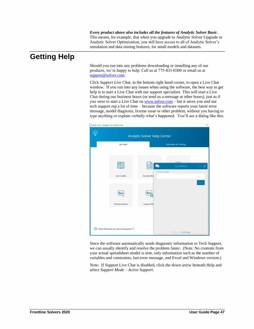
Frontline Solvers 2020 User Guide Page 47
Every product above also includes all the features of Analytic Solver Basic.
This means, for example, that when you upgrade to Analytic Solver Upgrade or
Analytic Solver Optimization, you still have access to all of Analytic Solver’s
simulation and data mining features, for small models and datasets.
Getting Help Should you run into any problems downloading or installing any of our
products, we’re happy to help. Call us at 775-831-0300 or email us at
Click Support Live Chat, in the bottom right hand corner, to open a Live Chat
window. If you run into any issues when using the software, the best way to get
help is to start a Live Chat with our support specialists This will start a Live Chat during our business hours (or send us a message at other hours), just as if
you were to start a Live Chat on www.solver.com – but it saves you and our
tech support rep a lot of time – because the software reports your latest error
message, model diagnosis, license issue or other problem, without you having to
type anything or explain verbally what’s happened. You’ll see a dialog like this:
Since the software automatically sends diagnostic information to Tech Support,
we can usually identify and resolve the problem faster. (Note: No contents from
your actual spreadsheet model is sent, only information such as the number of
variables and constraints, last error message, and Excel and Windows version.)
Note: If Support Live Chat is disabled, click the down arrow beneath Help and
select Support Mode – Active Support.

Frontline Solvers 2020 User Guide Page 48
Accessing Resources
To open Analytic Solver Help, simply click the Help icon on the Analytic Solver
ribbon in either App to gain access to video demos, User Guides, online Help,
example models, and Website support pages to learn how to use our software tools, and
how to build an effective model.
User Guides Click the User Guides menu choice to open PDF files of the Analytic Solver
Optimization and Simulation User and Reference Guides, Analytic Solver Data
Mining User or Reference Guides, or our Quick Start Guides.
Example Models
Clicking this menu item will open a browser pointing to the workbook, Frontline
Example Models Overview.xlsx, located at C:\Program Files\Frontline Systems\
Analytic Solver Platform\Examples. See the table below for a description of
each example dataset.
By going to Help – Welcome Screen you can easily access a range of support
and training resources.
Knowledge Base
Click Knowledge Base to peruse a multitude of online articles related to support
and installation issues or to locate articles that will help you to quickly build accurate, efficient optimization, simulation, and data mining models.

Frontline Solvers 2020 User Guide Page 49
Operating Mode
Click Operating Mode to switch between three different levels of help. The
Excel formulas and functions you use in your model have a huge impact on how
fast it runs and how well it solves. If you learn more about this, you can get
better results, but if you don't, your results will be limited. Guided Mode can
help you learn.
• Guided Mode prompts you step-by-step when solving, with dialogs.
• Auto-Help Mode shows dialogs or Help only when there’s a problem or
error condition.
• Expert Mode provides only messages in the Task Pane Output tab.
(This mode not supported when using a trial license.)
Support Mode
Click Support Mode to switch between three different levels of support. No
information (cell contents etc.) from your Excel model is ever reported
automatically to Frontline Systems, in any of these Support Modes. Only events
in Frontline's software, such as menu selections, Solver Result messages, or error messages are reported.
• Active Support automatically reports events, errors and problems to
Frontline Support, receives and displays messages to you from Support,
and allows you to start a Live Chat with Support while working in
Excel (Recommended).Auto-Help Mode shows dialogs or Help only
when there’s a problem or error condition.
• Standard Support automatically reports events, errors and problems
anonymously (not associated with you) to Frontline Support, but does
not provide a means to receive messages or start a Live Chat with
Support.
• Basic Support provides no automatic connection to Frontline Support.
You will have to contact Frontline Support manually via email, website
or phone if you need help.
Submit a Support Ticket
If you're having installation, technical, or modeling issues, submit a Support
Ticket to open an online support request form. Submit your email address and a
short, concise description of the issue that you are experiencing. You'll receive
a reply from one of Frontline's highly trained Support Specialists within 24
hours, and generally much sooner.
Our technical support service is designed to supplement your own efforts: Getting you over stumbling blocks, pointing out relevant sections of our User Guides or example
models, helping you fix a modeling error, or -- in rare cases -- working around an issue
with our software (always at our expense).

Frontline Solvers 2020 User Guide Page 50
Solver Academy
Solver Academy is Frontline Systems' own learning platform. It's the place
where business analysts can gain expertise in advanced analytics: forecasting,
data mining, text mining, mathematical optimization, simulation and risk
analysis, and stochastic optimization.
Video Tutorials/Live Webinars
Click Video Tutorials to be directed to Frontline's You Tube Channel. Browse videos on how to create an optimization or simulation model or construct a data
mining or prediction model using Analytic Solver.
Click Live Webinars to be redirected to www.solver.com to join a live or pre-
recorded webinar. Topics include Using Analytic Solver Data Mining to Gain
Insights from your Excel Data, Overview of Monte Carlo Simulation
Applications, Applications of Optimization in Excel, etc.
Learn more!
Click any of the three Learn More buttons to learn more about how you can
solve large-scale optimization, simulation, and data mining models, reduce
costs, quantify and mitigate risk, and create forecasting, data mining and text
mining models using Analytic Solver.
License Button Click the License button to open the License Manager where you can manage
your current licenses and accounts, open our Product Selection Wizard, connect
to Live Chat or peruse through a list of FAQs.

Frontline Solvers 2020 User Guide Page 51
Click License – Manage License/Manage Account to open the Licensing Center.
The "MyLicenses" tab displays your current license and license type, along with
the expiration date.
Click About Analytic Solver to open the following dialog containing information
on this release.
Click the Account tab to view your account on www.solver.com. Click Edit
Profile to edit the information. Click Live Chat to open a Live Chat window or
Log Out to log out of the product.

Frontline Solvers 2020 User Guide Page 52
Click the Product Guide tab to view a list of products and pricing information.
Click Product Selection Wizard to open the Product Selection Wizard. See the
next section for information on this feature.
Click the Questions tab to review a list of FAQs, submit a support ticket or start
a live chat.

Frontline Solvers 2020 User Guide Page 53
Product Selection Wizard Select Product Selection Wizard from the Product Guide tab in the Licensing
Center to open a series of dialogs that will help you determine which product
will best meet your needs based on your recent pattern of use.
Select the Product that you'd like to purchase and then click Next. Click the
Optimization Choices link to learn more about Analytic Solver products that can
solve optimization models and to find more information on speed, memory, and
the use of plug-in Solver Engines.

Frontline Solvers 2020 User Guide Page 54
On this screen, the Product Selection Wizard will recommend a product or
products based on your answers on the previous screens. Click Upgrade to
purchase the recommended product. Click the Optimization Choices link to
learn more about Analytic Solver products that can solve optimization models. If at any time you'd like to chat with a member of our Technical Support staff,
click Live Chat. Or if you'd like to amend your answers on a previous dialog,
click Back.
When you run a simulation or optimization model that contains too many
decision variables/uncertain variables or constraints/uncertain functions for the
selected engine, the Product Wizard will automatically appear and recommend a
product that can solve your model.
When you click “Test Run”, the Product Wizard will immediately run the
optimization or simulation model using the recommended product. (Only
summary information will be available.) At this point, you can purchase the
recommended product(s), or close the dialog.
This same behavior will also occur when solving smaller models, if you select a
specific external engine, from the Engine drop down menu on the Engine tab of
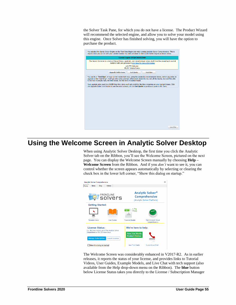
Frontline Solvers 2020 User Guide Page 55
the Solver Task Pane, for which you do not have a license. The Product Wizard
will recommend the selected engine, and allow you to solve your model using
this engine. Once Solver has finished solving, you will have the option to
purchase the product.
Using the Welcome Screen in Analytic Solver Desktop When using Analytic Solver Desktop, the first time you click the Analytic Solver tab on the Ribbon, you’ll see the Welcome Screen, pictured on the next
page. You can display the Welcome Screen manually by choosing Help –
Welcome Screen from the Ribbon. And if you don’t want to see it, you can
control whether the screen appears automatically by selecting or clearing the
check box in the lower left corner, “Show this dialog on startup.”
The Welcome Screen was considerably enhanced in V2017-R2. As in earlier
releases, it reports the status of your license, and provides links to Tutorial Videos, User Guides, Example Models, and Live Chat with tech support (also
available from the Help drop-down menu on the Ribbon). The blue button
below License Status takes you directly to the License / Subscription Manager

Frontline Solvers 2020 User Guide Page 56
(also available from the Options drop-down menu). The Local License button to
the right opens Frontline Solvers License Manager. And the green button
displays an explanation of Analytic Solver Basic, your free trial, and upgrade
options – much like this section.
There’s more: Click the News, Blog and Videos tabs at the top of the dialog to see the latest application news and case studies, Frontline Systems blog posts,
and videos from Solver.com. And from time to time, you’ll see a Messages tab
at the top of this dialog, with individual messages for you from Frontline’s Tech
Support and Customer Success teams.
License/Subscription in Analytic Solver Desktop Since Frontline Solvers V2015, our products have been offered on an annual
subscription basis, including the software license and Annual Support (technical
support and software upgrades). But in order to renew your subscription, or
upgrade or change the product you were using, you had to talk to someone in
Frontline Systems sales or customer service, who would make the change, and
email you a new license code that you’d copy and paste into a dialog box.
With Frontline Solvers V2018, all those steps have been automated: You can
review your subscription status, renew, upgrade or downgrade your subscription,
or add plug-in Solver Engines, all ‘self-service’ using the License / Subscription
Manager – accessible via the blue button in the Welcome Screen, or Options -
License / Subscription on the Analytic Solver Ribbon. The next page shows a
example of the License / Subscription Manager dialog.
The Products tab in the License / Subscription Manager dialog shows you a list of the products that are ‘upgrade options’ for your current subscription. You can
click the hyperlinks for more information about the products on Solver.com, or
click the buttons to go step-by-step through the upgrade process.

Frontline Solvers 2020 User Guide Page 57
Context-Sensitive Help in Analytic Solver Desktop Analytic Solver Desktop 2020 has a significant amount of context-sensitive
Help. You can quickly access Help on any Solver Result message that appears
in the Task Pane Output tab, any option that appears on the Engine tab or
Platform tab, or any element of your model that appears on the Model tab.
Solver Result messages appear as underlined links – you can simply click them.
For example, here’s the Help that appears when you click the Solver Results
message for the Gas Company Chance example in StochasticExamples.xls:
To access Help on any Platform option, Engine option, or Model element, click the underlined link in the brief explanation that appears at the bottom of the
Task Pane. For example, here’s the Help that appears when you click the Type
field link for a chance constraint in your model:

Frontline Solvers 2020 User Guide Page 58
To access help in Analytic Solver Cloud, click Help – Help Center or Help – Analytic
Solver Help in AnalyticSolver.com.

Frontline Solvers 2020 User Guide Page 59
Examples: Conventional Optimization
Introduction This chapter introduces conventional optimization (with no uncertainty) in both
the Desktop and Cloud apps using Analytic Solver Comprehensive, Analytic
Solver Optimization, Analytic Solver Upgrade, and Analytic Solver Basic with a
series of examples. Except as noted in specific sections, all of these examples
can be used in any of the above product subsets.
• “A First Optimization Model” takes you step-by-step through the process of
creating an optimization model from scratch. It illustrates use of the Ribbon
and Task Pane, and its relationship to the Excel Solver Parameters dialog.
• “Introducing the Standard Examples,” “Linear Programming Examples”
and “Nonlinear Optimization Examples” takes you through the workbook
StandardExamples.xls, with seven examples that illustrate a number of
Analytic Solver features.
A First Optimization Model This section is meant for you if you’re familiar with optimization, but you’ve
never used Excel Solver or Analytic Solver Basic. It shows how you can translate from the algebraic statement of an optimization problem to a spread-
sheet Solver model. If optimization is new to you, consult the chapter
“Mastering Conventional Optimization Concepts.”
Note: This first step-by-step example is a ‘quick and dirty’ approach that can be
used to solve the example problem, but is not well documented or easy to
maintain. If using Analytic Solver Desktop or Cloud you'll have access to
Microsoft Excel's many features that can help you organize and display the
structure of your model, through tools such as defined names, formatting and
outlining. The models in the StandardExamples.xls workbook illustrate some
of these features. This workbook is normally installed into C:\Program
Files\Frontline Systems\Analytic Solver Platform\Examples. As models become larger, the problems of managing data for constraints, coefficients, and so on
become more significant, and a properly organized spreadsheet model can help
manage this complexity.
Setting Up a Model
To set up an optimization model in a spreadsheet either in Microsoft Excel,
Excel Online or in AnalyticSolver.com, you will follow these essential steps:
1. Reserve a cell to hold the value of each decision variable. We’ll use A1:A3
in the example below.
2. Pick a cell to represent the objective function, and enter a formula that
calculates the objective function value in this cell. We’ll use A4 in the
example below.
Frontline Solvers 2020 User Guide Page 60
3. Pick other cells and use them to enter the formulas that calculate the left
hand sides of the constraints. We’ll use B1:B5 in the example below.
4. The constraint right hand sides can be entered as numbers in other cells, or
entered directly in the Solver’s Add Constraint dialog. We’ll use C1:C5 for
this purpose in the example below.
Within this overall framework, you have a great deal of flexibility in choosing
cells to use, and calculating the objective and constraints. For example, the
objective function will ultimately depend on the decision variable cells, but you
don’t have to calculate the entire function in one formula cell. You can use any
number of formula cells to compute intermediate results, and use these to
calculate the objective function or the constraints.
In desktop Excel and Excel Online, you can write a linear expression easily with
Excel’s SUMPRODUCT function, or you can use + and * operators, as shown
below. You can use Excel’s array formulas, and Excel functions that return
vector and matrix results. And you can use Excel’s rich facilities to access data in external text files, Web pages, and relational and multidimensional databases
to ‘populate’ your model.
AnalyticSolver.com offers a spreadsheet-like grid that works much like Excel
but does not include the rich array of features that Excel offers.
The Model in Algebraic and Spreadsheet Form
Consider the following problem. Our factory is building three products: TV
sets, stereos and speakers. Each product is assembled from parts in inventory,
and there are five types of parts: chassis, picture tubes, speaker cones, power
supplies and electronics units. Our goal is to produce the mix of products that
will maximize profits, given the inventory of parts on hand. This is a simple
linear programming problem, also used to illustrate other ideas later in “Linear Programming Examples.”
The Algebraic Form
The problem can be described in algebraic form as follows. The decision
variables are the number of products of each type to build: x1 for TV sets, x2 for
stereos and x3 for speakers. There is a fixed profit per unit for each product, so
the objective function (the quantity we want to maximize) is:
Maximize 75 x1 + 50 x2 + 35 x3 (Profit)
Building each product requires a certain number of parts of each type. For
example, TV sets and stereos each require one chassis, but speakers don’t use
one. The number of parts used depends on the mix of products built (the left
hand side of each constraint), and we have a limited number of parts of each
type on hand (the corresponding constraint right hand side):
Subject to 1 x1 + 1 x2 + 0 x3 <= 400 (Chassis)
1 x1 + 0 x2 + 0 x3 <= 200 (Picture tubes)
2 x1 + 2 x2 + 1 x3 <= 800 (Speaker cones)
1 x1 + 1 x2 + 0 x3 <= 400 (Power supplies) 2 x1 + 1 x2 + 1 x3 <= 600 (Electronics)
Since the number of products built must be nonnegative, we also have the
constraints x1, x2, x3 >= 0. Note that terms like 0 x3 are included purely to show
the structure of the model – they can be either omitted or included when entering
formulas in Excel.

Frontline Solvers 2020 User Guide Page 61
The Spreadsheet Formulas
The fastest (though not necessarily the best) way to lay out this problem on the
spreadsheet is to pick (for example) cell A1 for x1, cell A2 for x2 and cell A3 for
x3. Then the objective can be entered in cell A4, much like the algebraic form
above:
A4: =75*A1+50*A2+35*A3
We can go on to enter a formula in (say) cell B1 for the first constraint left hand
side (Chassis) as =1*A1+1*A2+0*A3, or the simpler form:
B1: =A1+A2
Similarly, we can use cell B2 for the formula =A1 (Picture tubes), B3 for the formula =2*A1+2*A2+A3 (Speaker cones), B4 for the formula =A1+A2 (Power
supplies), and B5 for the formula =2*A1+A2+A3 (Electronics):
B2: =A1
B3: =2*A1+2*A2+A3
B4: =A1+A2
B5: =2*A1+A2+A3
Finally, we’ll enter the constraint right hand side values in cells C1:C5:
C1: 400
C2: 200
C3: 800 C4: 400
C5: 600
We now have a simple spreadsheet model that we can use to play ‘what if.’ For
any values we enter for the decision variables in cells A1, A2 and A3, the
objective (Total Profit) and the corresponding values of the constraint left hand
sides (the numbers of parts used) will be calculated.
We want to turn this ‘what if’ spreadsheet model into an optimization model,
where the Solver will automatically find optimal values for the cells A1:A3, so
that the objective function at A4 is maximized, and the constraints are satisfied.
Defining and Solving the Optimization Model
To begin, click the Analytic Solver tab on the Ribbon. Your worksheet with an
empty Task Pane (“Solver Options and Model Specifications”) Model tab
should appear, as shown on the next page.
To define the optimization problem, we’ll use the Ribbon to point out to the
Solver (i) the cells that we’ve reserved for the decision variables, (ii) the cell
that calculates the value of the objective function, and (iii) the cells that
calculate the constraint left hand sides. We’ll also enter values for the constraint
right hand sides, and non-negativity constraints on the variables. We can
perform these steps in any order.

Frontline Solvers 2020 User Guide Page 62
Defining Decision Variables
To define the decision variables, use your mouse to select the range A1:A3 on
the worksheet. Then click the Decisions button to open the dropdown gallery
(shown below), and click Normal to define A1:A3 as normal decision variables
or, if using Analytic Solver Desktop or AnalyticSolver.com, simply click the
Decisions button to define A1:A3 as normal decision variables.
Defining the Objective
To define the objective, use your mouse to select cell A4 on the worksheet. In
Analytic Solver Desktop and AnalyticSolver.com, click the down arrow under
Objective, then select Max and Normal from the menu to define A4 as a
normal objective to be maximized – as shown on the next page. Alternatively,
you can click the Objective button to open the Add Objective dialog. Click OK
to accept the defaults and to define A4 as a normal objective to be maximized.

Frontline Solvers 2020 User Guide Page 63
In Analytic Solver Cloud, click the down arrow under Objective and select
Add/Change Objective. Click OK to accept the defaults and to define A4 as a
normal objective to be maximized.
Defining Constraints
To define the constraints, use your mouse to select the range B1:B5 on the
worksheet. Then, if using Analytic Solver Desktop or AnalyticSolver.com, click
the Constraints button to open the Add Constraint dialog.
Alternatively, you could also click the down arrow under Constraints, then click
Normal Constraint and <= to define B1:B5 as the left hand sides of five <=
constraints.
If using Analytic Solver Cloud, click the down arrow under Constraints, then
click Add Constraint to open the Add Constraint dialog.

Frontline Solvers 2020 User Guide Page 64
Within this dialog, you can enter the right hand side(s) as a constant number, a
cell range, or a defined name. Click in the Constraint edit box, or click the
range selector icon to its right, and use your mouse to select the cell range
C1:C5 for the right hand sides:
Then click OK. This will define five constraints: B1 <= C1, B2 <= C2, B3 <=
C3, B4 <= C4, and B5 <= C5.
The Task Pane Model tab now shows all the elements of the optimization model
you’ve just defined in outline form.
You can solve the model immediately by clicking the Optimize button on the
Ribbon, or by clicking the green arrow at the top right of the Task Pane.

Frontline Solvers 2020 User Guide Page 65
The optimal values of the decision variables at A1:A3, the objective at A4, and
the constraints at B1:B5 appear on the worksheet, and a Solver Result message
(“Solver found a solution. All constraints and optimality conditions are
satisfied”) appears in green at the bottom of the Task Pane.
You can view a log of solution messages on the Task Pane Output tab in
Analytic Solver Desktop, and you can produce optimization reports by selecting
Reports – Optimization from the Ribbon. For more information about these
features, keep reading!
Using the Classical Solver Parameters Dialog
When using Analytic Solver Desktop, you can also view – and create or edit – this model through the classical Solver Parameters dialog (as used in the
standard Excel Solver). To do so simply click Premium Solver on the Add-Ins
tab on the Ribbon to display the Solver Parameters dialog. Note: This dialog is
not supported in Analytic Solver Cloud or AnalyticSolver.com.

Frontline Solvers 2020 User Guide Page 66
Comparing the Task Pane and Solver Parameters Dialog
As you can see, the Task Pane Model tab and the Solver Parameters dialog
contain the same information. But where the Solver Parameters dialog is modal (moving the mouse outside the dialog displays a wait cursor – you must close
the dialog to do anything else), the Task Pane is modeless: You can move the
mouse outside the pane, edit formulas on the worksheet, or use other commands.
The Task Pane is initially docked to the right side of the Excel window, but you
can select its title bar with your mouse, drag it to another position, and resize it,
as shown on the next page. To “re-dock” the Task Pane, select its title bar with
the mouse, drag to a position just beyond the right edge of the Excel window,
then release the mouse.
Use the Model tab to view your model in outline form, and optionally edit
model elements in-place. Use the Platform tab to view or change Platform options, such as the number of optimizations or simulations to run, or default
bounds on decision variables or uncertain variables. Use the Engine tab to
select a Solver Engine and view or change its options. Use the Output tab to
view a log of solution messages, or a chart of the objective values.
Using Buttons on the Task Pane
Use the buttons at the top of the Model tab to add or remove model elements
(you can also use the Ribbon options to do this, as shown earlier), refresh the
model outline when you’ve made unusual changes to the worksheet, analyze the
structure of your model, or solve (run) the optimization or simulation model:
Analytic Solver Desktop and Cloud
Remove
element
Add
eleme
nt
Refresh
model
Analyze model
Solve
model

Frontline Solvers 2020 User Guide Page 67
AnalyticSolver.com
Use the buttons at the top of the Output tab to pause or stop the Solver, restore
the original values of the decision variables, copy the solution message log to
the Windows Clipboard (so you can paste the text into another application –
Analytic Solver Desktop only), erase the solution log, analyze/solve the model and upload your results to Microsoft's Power BI or Tableau (see step by step
instructions below – Analytic Solver Desktop only).
Analytic Solver Desktop
Analytic Solver Cloud
d
AnalyticSolver.com
Pause
Solver
Restore Variables
Copy to Clipboard Erase Soltion Log Anlyze Model
Sove
Model
Export to
Poer BI Export to
Tabeau
Solve
model
Refresh
model
Pause
Solver
Restore Variables
Erase Solution Log Analyze Model
Solve
Model
Pause Solver
Restore Variables
Erase Solution Log
Solve
Model

Frontline Solvers 2020 User Guide Page 68
Exporting Data to Microsoft's Power BI
Microsoft's POWER BI, for use with Office 365, is a cloud-based service that
works with Excel to help you visualize your data using various charts and
reports. Analytic Solver Desktop includes the ability to export a fixed set of
data from your optimization model, including final variable values, final
constraint values, final objective function values, variable shadow prices or constraint reduced costs, etc., directly into a dataset in Power BI.
Note: Exporting your model to Power BI via the Output Pane on the Solver
Task Pane is not supported in Analytic Solver Cloud or AnalyticSolver.com.
However, it is possible to upload your model to Power BI using the Create App
menu. See the chapter, Creating Power BI Custom Visuals, that appears later on
in this guide for more information.
Once Solver has stopped with a final result message (even if a solution was not
found), click the icon on the Output tab to upload the model to the Power
BI dashboard. If this is the first time that the icon has been clicked within the
current Excel instance, you will be asked to log in to Power BI.
Once logged in, you will be asked to either update an existing dataset or create a
new dataset.

Frontline Solvers 2020 User Guide Page 69
In the screenshot above, we have created a new dataset, ProductMix, which will
contain the objective, variable and constraint final values, shadow prices, dual
values, etc from our optimization model. Once the upload is complete, the
following message will appear.
Logon to Power BI (http://powerbi.microsoft.com/). The newly created dataset
will be listed under Datasets.
Select ProductMix, then determine the components to be included in the graph.
In the screenshot below we have created a pie chart displaying the final variable
values by clicking the icon to the right of the graph.

Frontline Solvers 2020 User Guide Page 70
Use the icon to pin this graph to the Dashboard.
Now, each time the model is solved, the results may be uploaded to your Power
BI dashboard. Click back to Excel and change the number of Speaker Cones in
inventory from 800 to 825, then resolve either by clicking the green arrow on
the Model tab in the Solver Task Pane or by clicking the Optimize icon on the
Analytic Solver ribbon. Once Solver stops with the final result message,
"Solver found a solution. All constraints and optimality conditions are
satisfied.", click the icon on the Output tab to upload the most recent
results. (Note: We are not asked to log in to the Power BI site a second time
since we are using the same instance of Excel.) Click back to Power BI in your
browser and refresh, the chart will update automatically with the new final
variable values, as shown below.

Frontline Solvers 2020 User Guide Page 71
Exporting Data to Tableau
Tableau is a popular interactive software package that allows you to visually
explore and analyze your data. Tableau can import data from a wide range of
sources, including Excel workbooks, and it is often used in conjunction with
Excel. Because Tableau is designed to import data in table form, it hasn’t been easy to import the results of an optimization model (such as final values of the
decision variables, constraints and objective) into Tableau, unless those model
elements occur in table form by themselves in your spreadsheet (which usually
isn’t the case).
Analytic Solver simplifies this process considerably. With a single click, you
can convert the results of your optimization model into a set of Tableau Data
Extract (.tde) files or HTML files using the Tableau Web Connector, open them
directly in Tableau, and visualize them with a few clicks.
Note: Exporting your model to Tableau via the Output Pane on the Solver Task
Pane is not supported in Analytic Solver Cloud or AnalyticSolver.com. However, it is possible to upload your model to Tableau using the Create App
menu. See the chapter, Creating Custom Extensions in Tableau, that appears
later on in this guide for more information.
Click the green arrow on the Output Tab to solve your optimization model.
Once Solver has stopped with a final result message, click the icon on the
Task Pane Output tab to save the values for the objective function, constraints
and variables to *.tde files or HTML files. You will be prompted to select a
folder where the Tableau files will be saved along with the type of Tableau export desired: Tableau Data Extract or Tableau Web Connector.
Note: If exporting to an existing .tde file, data will be appended rather than
overwritten. As a result, when exporting to an existing .tde file, all data must be
of the same structure as when the .tde file was first created.

Frontline Solvers 2020 User Guide Page 72
Tablea Data Extract
If Tableau Data Extract is selected, static data is exported to three files:
Constraints.tde, Objective.tde and Variables.tde. (Although .tde files are
designed to hold multiple tables, currently Tableau’s software allows only one
table per file.) When you import this data into Tableau, Variables.tde will have
one row for each decision variable, Constraints.tde will have one row for each
constraint and Objective.tde will have just one row for the objective.
• Each row of Variables.tde will contain the Excel cell address, the
values of the variables at the time of extraction, the lower and upper
bound of each variable, the optimization index and sensitivity
information such as the reduced cost and allowable increase/decrease.
• Each row of Constraints.tde will contain the Excel cell address where
the constraint is located, the value of each constraint at time of
extraction, the constraint lower and upper bounds, and information that
would appear on a sensitivity report such as the shadow price, slack
value, a 1 or 0 to indicate if the constraint was binding (1) or not (0),
and the allowable increase/decrease.
• Objective.tde will contain the Excel cell address where the objective is located, the value of the objective function at the time of extraction,
and the optimization index.
Note: If exporting to an existing .tde file, data will be appended rather than
overwritten. As a result, when exporting to an existing .tde file, all data must be
of the same structure as when the .tde file was first created.
Once you select a folder, the *.tde files will be created, and the following
message will appear.

Frontline Solvers 2020 User Guide Page 73
To open the files in Tableau, either double click each file (if using Desktop
Tableau) or click Other Files under Connect and open the desired file(s).
Tableau Web Connector
The Tableau Web Connector offers much more flexibility over Tableau Data
Extract by allowing you to refresh your data dynamically inside of Tableau.
If Tableau Web Connector is selected, you will be prompted to select a folder in
which to save OptimizationResults.html. This file will hold all contents
described above for Constraints.tde, Objective.tde and Variables.tde. The
following message will appear.
Note: If exporting to an existing .tde file, data will be appended rather than
overwritten. As a result, when exporting to an existing .tde file, all data must be
of the same structure as when the .tde file was first created.

Frontline Solvers 2020 User Guide Page 74
To open the files in Tableau, open a new workbook in Tableau and click
Connect to Data.
On the connect menu, select More Servers – Web Data Connector on the
Connect menu.

Frontline Solvers 2020 User Guide Page 75
On the Web Data Connector dialog, enter the location displayed on the dialog
shown above (i.e., http://localhost:8080/) and press Enter.
When the following dialog appears, click Constraints.html.
Note: The error highlighted in red is a simple warning that the URL is not
pointing to a Tableau Web Data Connector file. If we had entered a file name,
such as http://localhost:8080/Constraints.html, the results would have
immediately been uploaded to Tableau.
To add more data, click Data – New Data Source on the Tableau ribbon, then
repeat the actions described above.

Frontline Solvers 2020 User Guide Page 76
If your Solver results have changed, you'll need to refresh the results within the
Tableau Web Connector HTML files. To do so:
1. In ASP, re-run your model
2. Click the Tableau icon on the Output tab in the Solver Task Pane.
3. Select Tableau Web Connector and the folder where the files should
be saved.
4. Click OK.
5. In Tableau, click Data – Refresh All Extracts to update your data.
For more information on using Tableau, please refer to the Tableau
documentation found at http://www.tableau.com/.
Introducing the Standard Example Models The approach outlined above in “From Algebra to Spreadsheets” is a ‘quick and
dirty’ way to translate from a model in algebraic form to an equivalent
spreadsheet model, ready for optimization. However, that approach will soon
prove to be short-sighted when you wish to change the data (for example unit
profits or parts on hand), expand the model to include more products or parts, or
show the model to someone unfamiliar with the problem or uncomfortable with
algebraic notation.
Opening the Examples
To see a better approach to defining this model, click Help – Examples on the
Ribbon, which opens the workbook, Frontline Example Models Overview.xls.
Click Optimization on the Overview tab.

Frontline Solvers 2020 User Guide Page 77
Then click the link StandardExamples.xls to open the workbook, showing the
first worksheet EXAMPLE1. In AnalyticSolver.com click Help – Examples –
Optimization Examples and scroll down to StandardExamples.xlsx.
An optimization model – like the one we created ‘from scratch’ in the previous
section – is already defined on this worksheet, and appears in the Task Pane
Model tab, as shown below. We could immediately solve this model by clicking
the green arrow on the Model tab of the Solver Task pane.
How did this optimization model appear pre-defined in the workbook, you ask?
We simply used the Ribbon (or the Solver Parameters dialog) to select the

Frontline Solvers 2020 User Guide Page 78
decision variables, objective and constraints, and the Solver engine (and any
options or settings it requires). Then we saved the workbook, in the usual way,
with Excel’s Save command. Models created in the standard Excel Solver, or an
earlier version of Analytic Solver, Premium Solver, or Risk Solver can also be
saved this way, and opened and immediately solved in Analytic Solver.
More Readable and Expandable Models
Worksheet EXAMPLE1 models the same problem we described in the previous
section “From Algebra to Spreadsheets,” but the model is organized and laid out
for easier readability and expandability.
The decision variables (A1:A3 in the previous section) are in cells D9:F9, and
nearby labels show their meaning. The left hand sides of the constraints (B1:B5
in the previous section) are in cells C11:C15, and the right hand sides are in cells
B11:B15 – since these constant values can be in any position on the worksheet.
Instead of using constants such as 75, 50 and 35 directly in the formula for the
objective – as we did in the previous section – we’ve put these numbers in cells D17:F17. The formula for the objective is =SUMPRODUCT(D17:F17,D9:F9)
in cell D18. This makes it easier to change product selling prices, or to obtain
this data from an external data source, such as a database or accounting data file.
Similarly, we’ve placed the coefficients of the constraints in cells D11:F15.
These are exactly the constant values we saw in the algebraic statement of the
problem in the previous section:
Subject to 1 x1 + 1 x2 + 0 x3 <= 450 (Chassis)
1 x1 + 0 x2 + 0 x3 <= 250 (Picture tubes)
2 x1 + 2 x2 + 1 x3 <= 800 (Speaker cones)
1 x1 + 1 x2 + 0 x3 <= 450 (Power supplies)
2 x1 + 1 x2 + 1 x3 <= 600 (Electronics)
In EXAMPLE1, the formula at cell C11 – the left hand side of the first
constraint – is =SUMPRODUCT(D11:F11,$D$9:$F$9). The formulas at
C12:C15 were created by copying C11 downward.
To enhance readability, borders and labels have been used to draw attention to
the decision variables, the constraints, and the objective function. If you haven’t
used these Excel features before, select one or more cells, then choose the Home
tab in Excel to see how to do this.
EXAMPLE1 is also much easier to maintain and expand than a model
constructed with ‘hardwired’ formulas, as in the previous section. You can add
products by inserting new columns, and add more parts by inserting rows, and copying any one of the existing left hand side formulas to the new rows; Excel
will automatically adjust the formula cell references.
In the next section, we’ll solve EXAMPLE1, and create and examine the
Answer Report and Sensitivity Report for this model.
Models, Worksheets and Workbooks
There are several worksheets (EXAMPLE1, EXAMPLE2, etc.) in the
StandardExamples.xls workbook. As we proceed through this chapter, you’ll
see that we can simply click a worksheet tab to display a new and different
model in the Task Pane on that worksheet. Each of these models was created in
the same way, and all of them are saved when you save the Excel workbook.

Frontline Solvers 2020 User Guide Page 79
In StandardExamples.xls, each model is entirely contained on one worksheet.
But this is not required – one model can include cells from many different
worksheets in the same workbook, and it can refer to constant information in
other workbooks. By default, models have the same names as the worksheets on
which they are created, but you can give your own names to models, and create as many of them as you like. This is described in the Frontline Solvers
Reference Guide.
Linear Programming Examples This section takes you on a quick tour of Analytic Solver features for linear
programming (LP) problems. We highly recommend that you ‘follow along’ by
opening and actually solving the examples in this section.
The first three examples are variants of the Product Mix model introduced
earlier in this chapter. Our factory is building three products: TV sets, stereos
and speakers. Each product is assembled from parts in inventory, and there are
five types of parts: chassis, picture tubes, speaker cones, power supplies and
electronics units. Our goal is to produce the mix of products that will maximize profits, given the inventory of parts on hand. Be sure to read “Introducing the
Standard Example Models” above.
Using the Output Tab and Creating Reports
Click the tab to display the EXAMPLE1 worksheet. To solve this linear
programming problem;
• In Analytic Solver Desktop, click the Optimize button on the Ribbon
or click the green arrow at the top right of the Task Pane.
• In Analytic Solver Cloud, click the Model button to open the task pane,
then click the green arrow at the top right of the Task Pane or click the
down arrow beneath Optimize on the Ribbon and select Solve
Complete Problem.
• In AnalyticSolver.com, click the Optimize button on the Ribbon or
click the green arrow at the top right of the Task Pane.
Almost immediately, the solution values appear in the decision variable cells:
To maximize profit, we should make 200 TV sets, 200 stereos, and 0 speakers.
The Solver Results message “Solver found a solution. All constraints and
optimality conditions are satisfied” appears in green at the bottom of the Task Pane. Don’t ignore this message, because it provides critical information about

Frontline Solvers 2020 User Guide Page 80
what happened during the solution process, and what you can and cannot
assume about the solution on the worksheet!
If using Analytic Solver Desktop, click the Output tab at the top of the Task
Pane to learn more about the solution process. The solution log in the upper part
of this pane reports what happened during the solution process. If you are puzzled by the Solver Result message, simply click the underlined message in
the log to open online Help to a full explanation of that message.
If solving takes more than a few seconds, the Output tab automatically appears,
and current best objective and other information, plus a running chart of the
objective value, appears in the bottom part of the Task Pane.
If using Analytic Solver Cloud or AnalyticSolver.com, the output pane will
display the status of the model on the Solver Server as shown below.
After solving, you can produce reports (such as the Answer Report and
Sensitivity Report) by selecting Reports – Optimization from the Ribbon.
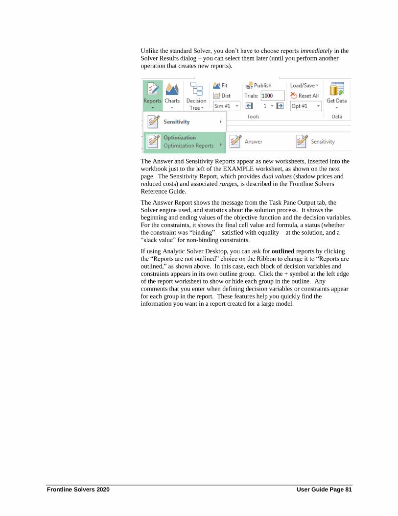
Frontline Solvers 2020 User Guide Page 81
Unlike the standard Solver, you don’t have to choose reports immediately in the
Solver Results dialog – you can select them later (until you perform another
operation that creates new reports).
The Answer and Sensitivity Reports appear as new worksheets, inserted into the
workbook just to the left of the EXAMPLE worksheet, as shown on the next
page. The Sensitivity Report, which provides dual values (shadow prices and
reduced costs) and associated ranges, is described in the Frontline Solvers
Reference Guide.
The Answer Report shows the message from the Task Pane Output tab, the
Solver engine used, and statistics about the solution process. It shows the beginning and ending values of the objective function and the decision variables.
For the constraints, it shows the final cell value and formula, a status (whether
the constraint was “binding” – satisfied with equality – at the solution, and a
“slack value” for non-binding constraints.
If using Analytic Solver Desktop, you can ask for outlined reports by clicking
the “Reports are not outlined” choice on the Ribbon to change it to “Reports are
outlined,” as shown above. In this case, each block of decision variables and
constraints appears in its own outline group. Click the + symbol at the left edge
of the report worksheet to show or hide each group in the outline. Any
comments that you enter when defining decision variables or constraints appear
for each group in the report. These features help you quickly find the information you want in a report created for a large model.

Frontline Solvers 2020 User Guide Page 82
Analytic Solver Desktop
Analytic Solver Cloud
A Model with No Feasible Solution
What does it mean when the Solver can find no feasible solution – no
combination of values for the decision variables that satisfies all the constraints?
It may be that the underlying business problem has no feasible solution – if so,

Frontline Solvers 2020 User Guide Page 83
you’d like to focus on the ‘hardest-to-satisfy’ constraints, to see if you can do
anything about them. Or you might have just made a mistake setting up the
model – for example choosing <= when you meant to choose >=.
But in a large model, with thousands of constraints, how do you find your
mistake, or focus on the ‘hardest-to-satisfy’ constraints? Analytic Solver can help, by producing a Feasibility Report.
Click the tab to display the EXAMPLE2 worksheet. This is the same Product
Mix model as in EXAMPLE1, but the supply of Chassis parts at B11 has been
changed from 450 to -1. Click the Optimize button in Analytic Solver Desktop
or AnalyticSolver.com or Optimize then Solve Complete Problem in Analytic
Solver Cloud. The message “Solver could not find a feasible solution” appears
in red at the bottom of the Task Pane.
Still TBD Click Reports – Optimization – Feasibility on the Ribbon. A
Feasibility Report worksheet is inserted into the workbook, immediately to the
left of EXAMPLE2 – with the contents shown on the next page.
Notice that the report highlights the constraint on Chassis parts used, and the
non-negativity constraints on products that are built from Chassis parts. To
satisfy the constraint C11 <= B11 where B11 is -1, we’d have to build a negative
number of stereos (or TV sets). In a large model with thousands of constraints
with no feasible solution, this report can focus your attention on the “trouble
spots” – the constraints that make the problem infeasible. The set of constraints
shown is called an IIS or Irreducibly Infeasible Subset of all the constraints. For
more information, please see the Frontline Solvers Reference Guide.
An ‘Accidentally’ Nonlinear Model
What if you intended to build a linear programming model, but you made a mistake and introduced a nonlinear function into the model? Even if you
understand the requirements of linear functions (explained in the chapter
“Mastering Conventional Optimization Concepts”), in a large model with
thousands of variables and constraints, where each constraint is computed by a
chain of formulas, an accidentally introduced nonlinearity may be difficult to
find. Sometimes, a first-generation LP model is modified to make a previously
fixed parameter into a decision variable – and this leads to an accidental
multiplication of two variables.
Click the tab to display the EXAMPLE3 worksheet. This is the same Product
Mix model as in EXAMPLE1, but the constraint left hand side formula for
Chassis parts at C11 has been changed to read =SUMPRODUCT(D11:F11,D9:F9)^0.9. (The power function clearly makes the
constraint nonlinear.) Click the Optimize button, or the down arrow beneath
Optimize then Solve Complete Problem. The message “The linearity
conditions required by this Solver Engine are not satisfied” appears in red at the
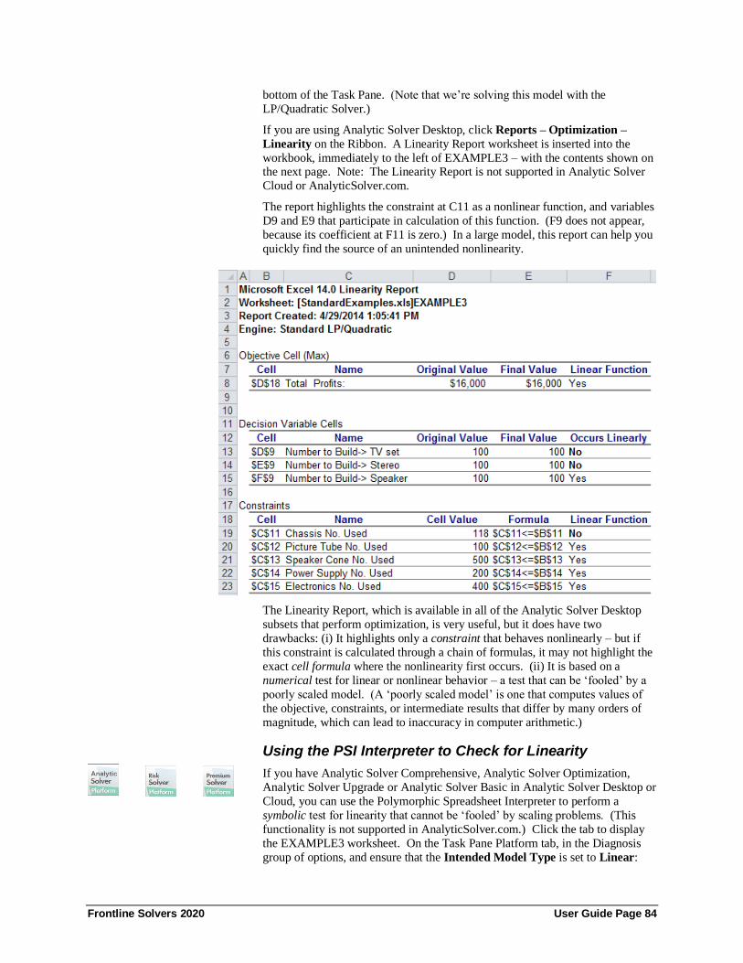
Frontline Solvers 2020 User Guide Page 84
bottom of the Task Pane. (Note that we’re solving this model with the
LP/Quadratic Solver.)
If you are using Analytic Solver Desktop, click Reports – Optimization –
Linearity on the Ribbon. A Linearity Report worksheet is inserted into the
workbook, immediately to the left of EXAMPLE3 – with the contents shown on the next page. Note: The Linearity Report is not supported in Analytic Solver
Cloud or AnalyticSolver.com.
The report highlights the constraint at C11 as a nonlinear function, and variables
D9 and E9 that participate in calculation of this function. (F9 does not appear,
because its coefficient at F11 is zero.) In a large model, this report can help you
quickly find the source of an unintended nonlinearity.
The Linearity Report, which is available in all of the Analytic Solver Desktop
subsets that perform optimization, is very useful, but it does have two
drawbacks: (i) It highlights only a constraint that behaves nonlinearly – but if
this constraint is calculated through a chain of formulas, it may not highlight the
exact cell formula where the nonlinearity first occurs. (ii) It is based on a
numerical test for linear or nonlinear behavior – a test that can be ‘fooled’ by a
poorly scaled model. (A ‘poorly scaled model’ is one that computes values of
the objective, constraints, or intermediate results that differ by many orders of
magnitude, which can lead to inaccuracy in computer arithmetic.)
Using the PSI Interpreter to Check for Linearity
If you have Analytic Solver Comprehensive, Analytic Solver Optimization,
Analytic Solver Upgrade or Analytic Solver Basic in Analytic Solver Desktop or
Cloud, you can use the Polymorphic Spreadsheet Interpreter to perform a
symbolic test for linearity that cannot be ‘fooled’ by scaling problems. (This
functionality is not supported in AnalyticSolver.com.) Click the tab to display
the EXAMPLE3 worksheet. On the Task Pane Platform tab, in the Diagnosis
group of options, and ensure that the Intended Model Type is set to Linear:
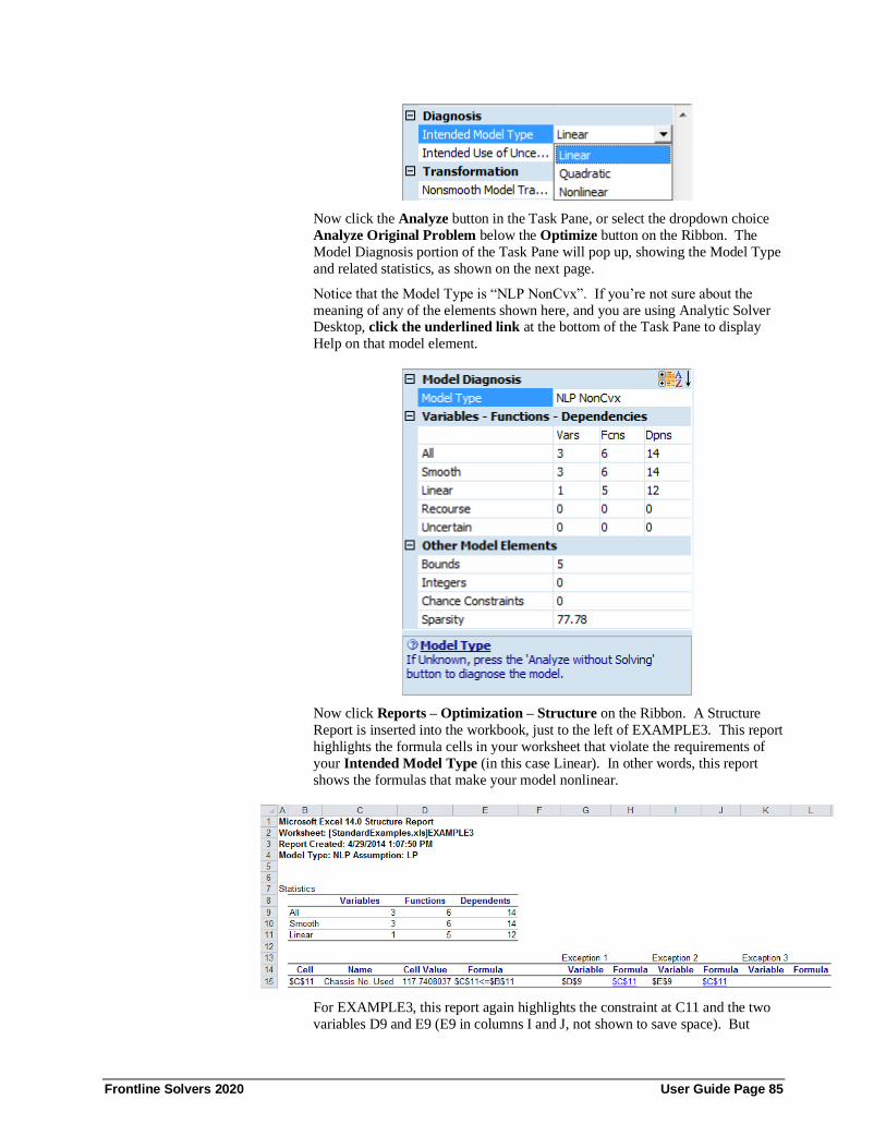
Frontline Solvers 2020 User Guide Page 85
Now click the Analyze button in the Task Pane, or select the dropdown choice
Analyze Original Problem below the Optimize button on the Ribbon. The
Model Diagnosis portion of the Task Pane will pop up, showing the Model Type
and related statistics, as shown on the next page.
Notice that the Model Type is “NLP NonCvx”. If you’re not sure about the
meaning of any of the elements shown here, and you are using Analytic Solver Desktop, click the underlined link at the bottom of the Task Pane to display
Help on that model element.
Now click Reports – Optimization – Structure on the Ribbon. A Structure
Report is inserted into the workbook, just to the left of EXAMPLE3. This report
highlights the formula cells in your worksheet that violate the requirements of
your Intended Model Type (in this case Linear). In other words, this report
shows the formulas that make your model nonlinear.
For EXAMPLE3, this report again highlights the constraint at C11 and the two
variables D9 and E9 (E9 in columns I and J, not shown to save space). But

Frontline Solvers 2020 User Guide Page 86
when a constraint or objective is calculated through a chain of formulas, this
report normally finds the formula cell that first introduces a nonlinear
relationship (such as a power operator, a function such as LOG, or
multiplication of two cells that both depend on decision variables).
EXAMPLE3!$C$11 in this report can be clicked to jump directly to that cell, so you can quickly inspect its formula.
Note: The Structure Report in Analytic Solver does not include the Name or
Cell Value columns.
Nonlinear Optimization Examples This section takes you on a quick tour of Analytic Solver features for nonlinear
programming (NLP) and non-smooth optimization (NSP) problems, using the
SOCP Barrier Solver, GRG Nonlinear Solver, and Evolutionary Solver. We
highly recommend that you ‘follow along’ by opening and actually solving the
examples in this section.
Portfolio Optimization: Quadratic Programming
The simplest kind of nonlinear optimization model is a quadratic programming (QP) model, with a quadratic objective and all linear constraints. Such a
problem can be solved with a quadratic extension to the linear programming
Simplex method – as in the LP/Quadratic Solver in Analytic Solver
Comprehensive or Analytic Solver Optimization – or with the GRG Nonlinear
Solver included in Analytic Solver Upgrade and Analytic Solver Basic.
A classic example of this kind of model, shown in EXAMPLE4 in
StandardExamples.xls, is a Markowitz-style portfolio optimization problem.
In this model, we want to choose the mix of stocks to form an ‘efficient
portfolio’ with the lowest possible risk (measured by portfolio variance) for a
specified target rate of return. Click the EXAMPLE4 tab to display the model.

Frontline Solvers 2020 User Guide Page 87
This model uses Excel defined names for certain cell ranges: The objective cell
I17 has the name Portfolio_Variance, which appears to the left of the formula
bar when I17 is selected. Cell I19 has the name Portfolio_Return. The decision
variables – the percentage of funds to invest in each of five stocks – are cells
B9:F9, and this cell range has the name Allocations. Cell H9 has the name Total_Portfolio. These defined names appear in the Task Pane Model tab, as
shown on the next page.
We can see immediately that this model will find values for the stock allocations that minimize portfolio variance, subject to constraints that (i) all funds are used
(the sum of the stock allocations is 100% or 1.0) and (ii) the portfolio return is at
least 9.5%.
Cell I17 computes the portfolio variance using a special function
QUADPRODUCT, which is defined by Analytic Solver. This function can be
used to compute any ‘quadratic form’ such as xTQx + cx. In EXAMPLE4, the
elements of the matrix Q are the covariances of returns of pairs of stocks, and
the elements of the vector c (at B11:F11) are all zero. You could instead
compute portfolio variance using a series of Excel formulas using multiplication
and addition, but it’s more convenient to use QUADPRODUCT.
Charts of the Objective and Constraints
Analytic Solver can help you visualize the shape of your problem functions (the
objective and constraints). If you haven’t been sure of the difference between a
linear, quadratic, smooth nonlinear, and non-smooth function, you can use
Analytic Solver to plot it.
As an example, select cell I19 (the Portfolio Return) on the worksheet, and
choose Decisions – Plot from the Ribbon. This will plot I19 (whose formula is
=SUMPRODUCT(Allocations,Stock_Returns)) as a function of the decision
variables for Stock 1 through Stock 5, as shown on the next page.

Frontline Solvers 2020 User Guide Page 88
The SUMPRODUCT function is a linear function, so unsurprisingly, Portfolio
Return plots as a straight. In contrast, select cell I17 (Portfolio Variance, the
QUADPRODUCT function), and choose Decisions – Plot from the Ribbon.
This function plots as a parabola – as expected for a quadratic function –
showing only the positive values, since the decision variables are non-negative.
Both of these plots are actually projections of a function in five dimensions
(Stock 1 through Stock 5) onto two dimensions, along a vector from Point A to
Point B, shown in the side panel. You have many choices for Points A and B.

Frontline Solvers 2020 User Guide Page 89
To find an optimal allocation of funds to stocks, just click the Optimize button.
In an instant, the message “Solver found a solution. All constraints and
optimality conditions are satisfied” appears in green at the bottom of the Task
Pane, the Portfolio Variance is 0.85% and the Portfolio return is 9.5%, and the
decision variables contain:
Solving with the GRG Nonlinear Solver yields the same values (to two decimal
places) for the decision variables. If you have Analytic Solver Comprehensive,
Analytic Solver Optimization, Analytic Solver Upgrade or Analytic Solver
Basic, you can also use the Standard SOCP Barrier Solver – just select it from
the dropdown list at the top of the Task Pane Engine tab and click the Optimize
button again. This yields nearly the same values for the decision variables,
Portfolio Return at I19, and Portfolio Variance at I17.
We can also “turn this problem around” and seek to maximize Portfolio Return,
subject to a constraint that Portfolio Variance is (say) no more than 1%. To do
this in Analytic Solver Desktop, we can edit the optimization model directly in
the Task Pane:
1. Select “Portfolio_Variance (Min)” under Objective in the outline.
2. In the Objective Properties area below the outline, click the Address
property and type or select cell I19 (or type “Portfolio_Return”).
Change the Sense dropdown choice from Minimize to Maximize.
3. Select “Portfolio_Return >= 0.095” under Constraints in the outline.
4. In the Normal Constraint Properties area below the outline, click the
Address property and type or select cell I17 (or type
“Portfolio_Variance”), change the Relation dropdown choice to <=,
and type 0.01 as the Right Hand Side) value.
Since the Task Pane is not editable in neither Analytic Solver Cloud nor
AnalyticSolver.com, we must perform a few different steps to edit the model
when using either of these products.

Frontline Solvers 2020 User Guide Page 90
1. Double click Portfolio_Variance (Min) under Objective, change
Set Cell to I19 and set the "sense" of the objective to Max, then
click OK.
2. Double click Portfolio_Return >= 0.095 under Constraints, change Cell Reference to I17, change the constraint sense to <= and type
0.01 as the Right Hand Side Constraint value. Then click OK.
The Task Pane Model tab should now appear similar to the one shown below.

Frontline Solvers 2020 User Guide Page 91
This problem now has a linear objective and a quadratic constraint; it is called a
quadratically constrained or QCP problem. It can no longer be solved by the
methods used in the LP/Quadratic Solver (a quadratic extension of the Simplex
method), but it can be solved by the GRG Nonlinear Solver, or (more
efficiently) by the SOCP Barrier Solver.
Solving with the SOCP Barrier Solver yields a Portfolio Return of 10.2%, a
Portfolio Variance of 1% as expected, and the following values for the decision
variables:
In “Multiple Parameterized Optimizations” in the chapter “Getting Results:
Optimization,” we return to EXAMPLE4 and show how to automatically vary the Portfolio Return threshold, solve multiple instances of this portfolio
optimization model, and create a chart of the efficient frontier.
The original EXAMPLE4 QP model can be ‘scaled up’ to portfolios of many
thousands of stocks, and solved quickly to optimality by the Large-Scale LP/QP
Solver, the XPRESS Solver and the MOSEK Solver. The modified QCP model
can also be scaled up to portfolios of thousands of stocks, and solved quickly to
optimality by the MOSEK Solver.
A Model with IF Functions
EXAMPLE5 in the StandardExamples.xls workbook was adapted from an
actual user model, and illustrates a common situation seen by Frontline Systems
in technical support. This model was meant to be a linear mixed-integer (LP/MIP) model, but the user calculated the objective function based on several
IF functions. IF functions are certainly not linear functions – in fact they aren’t
even smooth nonlinear functions!
One of the remarkable things about Analytic Solver is that, in Automatic mode,
it will transform this model to a linear mixed-integer model, and solve it to
optimality in seconds, without any user intervention. But in this Guide, we’ll
first see how Analytic Solver behaves without Automatic mode. Click the
EXAMPLE5 tab to display the model.

Frontline Solvers 2020 User Guide Page 92
The model has 9 decision variables, all constrained to be integer. The general
constraints are linear functions of the decision variables. But the objective
depends on I14, J14 and K14, each of which is a sum of three IF functions.
To turn off Automatic mode, in the Task Pane Platform tab Transformation
group of options, set the Nonsmooth Model Transformation option to Never.
If we now click the Optimize button with the LP/Quadratic Solver selected, the
message “The linearity conditions required by this Solver engine are not
satisfied” appears in red at the bottom of the Task Pane.
If we click the Analyze button in the Task Pane, or select the dropdown choice
Analyze Original Problem below the Optimize button on the Ribbon, Analytic
Solver reports that the model is nonsmooth with integers (NSP/MIP), as shown
on the next page.

Frontline Solvers 2020 User Guide Page 93
This type of model commonly arises, but is difficult to solve with the standard
Excel Solver, or with Analytic Solver Upgrade. But Analytic Solver
Comprehensive, Analytic Solver Optimization, Analytic Solver Upgrade and
Analytic Solver Basic in Analytic Solver Desktop or Cloud can transform the
model to eliminate the IF functions, replacing them with additional binary and
continuous variables and linear constraints that have the same effect on the
model as the IF functions. The additional variables and constraints don’t appear
on the worksheet, but they are handled internally by the PSI Interpreter and the selected Solver engine. To do this, we simply set the Nonsmooth Model
Transformation option to Automatic:
If we again analyze the model by clicking the Analyze button in the Task Pane,
or by selecting the dropdown choice Analyze Transformed Problem below the
Optimize button on the Ribbon, Analytic Solver reports that the the transformed
model has 27 variables (18 of them integer) and 67 constraints, as shown on the next page. But it’s now a linear programming (LP) model – so it can be solved
by the LP/Quadratic Solver. By solving this transformed model, we can find a
solution to the original model on the EXAMPLE5 worksheet.
When we now click the Optimize button, the message “Solver found a solution.
All constraints and optimality conditions are satisfied” appears in green at the
bottom of the Task Pane, and the objective function value at cell B19 is 2400.

Frontline Solvers 2020 User Guide Page 94
The message indicates that the Solver has found a proven optimal solution for
the original problem with IF functions.
The PSI Interpreter can automatically transform models containing IF, AND,
OR, NOT, ABS, MIN and MAX, and relations <, <=, >= and > into equivalent
models where these non-smooth functions are eliminated. When this transformation is sufficient to make the overall model linear – as it was in this
case – you can use the LP/Quadratic Solver or a large-scale LP/MIP Solver
engine to solve the problem.
A Model with Cone Constraints
In the EXAMPLE6 and EXAMPLE7 worksheets, we wish to solve a model to
optimize the location of an airline hub. The hub will serve six cities, each of
which is located at some latitude and longitude (in these models, we use simple
X, Y coordinates). We want to choose a location (X, Y coordinate) for the
airline hub that will minimize the maximum distance from the hub to any of the
six cities. The distance from the hub (X, Y) to a city (Xc, Yc) is SQRT( (Xc -
X)2 + (Yc - Y)2 ). The model is pictured below. In EXAMPLE6, we model and solve the problem using the GRG Nonlinear Solver. In EXAMPLE7, which
requires Analytic Solver Comprehensive, Analytic Solver Optimization,
Analytic Solver Upgrade or Analytic Solver Basic, we model the problem using
cone constraints, and solve it using the SOCP Barrier Solver.
Modeling the Problem with Nonlinear Functions
In EXAMPLE6, our decision variables are the (X, Y) coordinates of the airline
hub, at cells D12:E12, and a third decision variable at F19. Cell F19 also serves
as the objective function, to be minimized. We calculate the distance from the
hub to each of the six cities in cells F13:F18. We define a block of constraints
F13:F18 <= F19 – this means that the distance from the hub to each city must be less than or equal to the decision variable F19, which the Solver will minimize.

Frontline Solvers 2020 User Guide Page 95
The effect of these constraints is to cause the Solver to find values for D12:E12
– the (X, Y) coordinates of the hub – that minimize the maximum distance to
any of the cities.
Click the EXAMPLE6 tab to display the model, and click Analyze – Analytic
Original Problem. We see that the model is diagnosed as smooth nonlinear (NLP), with 3 variables and 7 functions. Notice that the Standard GRG
Nonlinear Solver is selected.
Click the Optimize button. The message “Solver found a solution” appears in
green at the bottom of the Task Pane. The optimal location for the airline hub is
at X = 1.25, Y = 4.0, and the maximum distance from this location to any of the
six cities is 2.1360 units.
Modeling the Problem with Cone Constraints
In EXAMPLE4, we solved the simplest kind of nonlinear optimization problem,
a portfolio optimization QP model with a quadratic objective and all linear
constraints, and a variation that was a QCP model, with a quadratic constraint .
We saw that we could solve the problem with the GRG Nonlinear Solver, but
we could also solve both variations of the problem with the SOCP Barrier
Solver – and we learned that we could more easily ‘scale up’ the SOCP problem
to large size, with thousands of stocks or more.
We can do the same thing with the airline hub problem. The model is a little
more complex, with more variables and constraints – but this allows the Solver to exploit the structure of the model, and solve it more quickly and reliably. To
do this, we will explicitly use cone constraints.
We have actually used a simple kind of cone constraint before – in EXAMPLE1,
our first linear programming problem, at the beginning of this chapter. In that
model, we used an objective and constraints that were linear functions of the
decision variables, and non-negativity constraints on the variables. These
constraints specified that the variables must lie within a simple kind of cone,
called the non-negative orthant. This first order cone places a bound on the L1-
norm of the vector of decision variables:
In our reformulation of the airline hub problem in EXAMPLE7, we’ll specify
that groups of variables must lie within a second order cone (also called a
Lorentz cone, or “ice cream cone”) – a convex set that looks like this:
This cone places a bound on the L2-norm of the vector of decision variables. If
A1:A3 are variables that lie within this cone, then

Frontline Solvers 2020 User Guide Page 96
A1 >= SQRT(SUMSQ(A2:A3)) must hold. A problem with a linear objective
and linear or second order cone (SOC) constraints is called a second order cone
programming (SOCP) problem; it is always a convex optimization problem.
Second order cone programming is the natural generalization of linear program-
ming. It offers the same advantages of convexity and scalability to large problems offered by linear programming – but for a broader class of models.
For history buffs, Premium Solver Platform V6.0 was the first commercial
software product to offer broad support for second order cone programming.
The EXAMPLE7 worksheet is shown below. In this model, we compute the
simple differences Xc – X and Yc – Y between the airline hub coordinates and
the coordinates of each city. We define new variables F21:F26, G21:G26, and
H21:H26. We use constraints to make G21:G26 equal to the Xc – X
differences, and H21:H26 equal to the Yc – Y differences.
Then we specify that each set of three variables (for example F21, G21, H21)
must belong to a second order cone – hence F21 >= SQRT(SUMSQ(G21:H21)) – and likewise for F22, G22, H22, etc. Finally, we use one more variable F27 as
the objective to be minimized, and we add a block of constraints F21:F26 <=
F27 – much as we did in EXAMPLE6. The effect of these constraints is to
cause the Solver to find values for the (X, Y) coordinates of the hub – now at
D14:D15 – that minimize the maximum distance to any of the cities.
Click the EXAMPLE7 tab to display the model, and click Analyze – Analyze
Original Model. We see that this formulation of the model is diagnosed as
second order cone programming problem (SOCP), with 21 variables and 19
functions. Notice that the SOCP Barrier Solver is selected to solve the problem.
Frontline Solvers 2020 User Guide Page 97
Click the Optimize button. After a moment, the same optimal solution as in
EXAMPLE6 is found. In this simple example, both the Standard GRG
Nonlinear Solver and the SOCP Barrier Solver solve the problem in sub-second
time. But if we were to scale up this model to large size – say with 1,000 cities
– the SOCP Barrier Solver would likely show a speed advantage.
Solving an Optimization Model using Excel Online or Google Sheets
In late 2014, Frontline Systems released Solver App for use with Excel 2013 and
Solver Add-on for use with Google Sheets. With the Solver App you can define and solve optimization problems in your Excel workbook, using Excel Online in
Office 365, the Excel Web App in SharePoint 2016 or 2013, or desktop Excel
2016 or 2013. With the Solver Add-on, you can define and solve optimization
problems in Google Sheets. You can create and solve models on tablets,
phones, or anywhere a Web browser can be used. Solver models that you may
already have created in old or new versions of Microsoft Excel, are
automatically recognized by the Solver App and , after the existing worksheet is
published, with the Solver Add-on.
In Analytic Solver Desktop and AnalyticSolver.com, the Freeze and Thaw
buttons were combined into a single Publish button, as shown in the screenshot
below. (In Premium Solver Pro/Platform where there was no Freeze/Thaw function, the Ribbon now includes a Publish icon.) Note: This functionality is
not supported in Analytic Solver Cloud.
Like the “Freeze” button, the Publish button can be used to prepare a workbook
for distribution to other users who don’t have Analytic Solver or its subsets
installed: All formulas containing Psi function calls (which would yield #NAME? for other users) are replaced by their values, and the formulas are
saved, so they can be restored later by choosing “Unpublish” (equivalent to the
old “Thaw”).
But the major use of the Publish button in ASP and later, is to prepare a
workbook for use with our Solver/Risk Solver Apps for Excel Online and our
Solver/Risk Solver Add-on for Google Sheets (the online spreadsheets have
limited or no support for user-defined functions).
In ASP, when a model is published, the limits for Solver App (for Excel Online)
and Solver Add-on (for Google Sheets) will be automatically adjusted to match
the problem limits of your license. For example, if you purchased a license for Analytic Solver, then you will be able to solve linear models using the Solver
App or Solver Add-on with up to 8,000 variables and constraints and nonlinear
or nonsmooth models with up to 1,000 variables and constraints, if you publish
your model first by clicking the Publish button on the Analytic Solver ribbon.
Let’s go back to the model on the Example1 tab used in the section above, click
the Publish icon on the Ribbon to display the following dialog.

Frontline Solvers 2020 User Guide Page 98
Select Google Sheets then Publish. (If you are a user of Excel Online, please
see the example below.) Make sure to save the workbook before uploading to
Google Drive.
Note: Only the Active Worksheet is published. To solve a model on a different
worksheet within the same Workbook (say Example2), you’ll need to publish
that worksheet separately. This is important when solving an optimization
model. If solving a simulation model, this does not apply. (For an example on how to solve a simulation model with Excel Online or Google Sheets, please see
the next chapter.)
Log on to your Google Drive account and upload Standard Example.xls, then
open this file in Google Sheets.
Uploading and Opening Files in Google Sheets
Click the orange New button then select File Upload to upload the StandardExamples.xls spreadsheet to Google Drive.
Browse to the location of the file, typically C:\Program Files (x86)\Frontline
Systems\Analytic Solver Platform\Examples (if using 32 bit Excel with 64 bit
Windows) or C:\Program Files\Analytic Solver Platform\Examples (if using 64
bit Excel or 32 bit Excel with 32 bit Windows). StandardExamples.xls will
appear under My Drive.
Double click the file to open in Google Drive Preview Viewer (shown below).
Click Open – Google Sheets.

Frontline Solvers 2020 User Guide Page 99
To add the Solver Add-on, choose the menu option Add-ons - Get Add-ons...
In the Add-ons dialog, scroll until you see Solver. Click to select and install.
Once these steps are finished, Solver should now appear on the Add-ons
menu.
Choose Add-ons - Solver - Start. The Solver Task Pane (Google calls this a
Sidebar) will appear containing the Solver model: objective, variables, and
constraints.

Frontline Solvers 2020 User Guide Page 100
Since this is a linear model, click the down arrow to the right of GRG Nonlinear
under Solving Method to select the LP/Quadratic engine.
Click Solve to run the Simplex LP engine to solve the linear model. The Solver
Add-on solves the model, inserting the final variable values of 200/200/0 in cells
D9:F9 and finding an objective equal to $25,000. Note: Reports, such as
Answer Report, Sensitivity Report, and/or Limits reports, are not supported in
the Solver Add-on.
The Solver Sidebar behaves much like the Excel Solver dialog. To change a
constraint, simply highlight the desired constraint and click Change. To delete a constraint, highlight the desired constraint and click Delete. Click Reset All to
clear the objective, all variables and constraints, and all options settings. Select
Options to change an engine option such as Constraint Precision, Automatic

Frontline Solvers 2020 User Guide Page 101
Scaling, Convergence, etc. For more information on each of these options,
please see the Engine Option chapter in Frontline Solvers Reference Guide.
Now let’s Publish this same model to Excel Online. Let’s go back to Excel and
StandardExamples.xls. Click Publish – Unpublish.
Reopen the Publish dialog by clicking Publish. Confirm that Excel Online is
selected. Click Publish to publish the worksheet to Excel Online.
Note: Only the Active Worksheet is published. To solve a model on a different
worksheet within the same workbook (say Example2), you’ll need to publish
that worksheet separately. This is important when solving an optimization
model. If solving a simulation model, this does not apply. (For an example on
how to solve a simulation model with Excel Online or Google Sheets, please see
the next chapter.)

Frontline Solvers 2020 User Guide Page 102
Now Save the file as StandardExamples.xlsx on your SharePoint or Office 365
site.
Note: In order to use the Solver App, your file must be saved on SharePoint or
Office 365 site. This app cannot solve models saved on your local hard drive.
Open the workbook using Excel Online, then click Edit Workbook – Edit in
Excel Online.
Click Insert – Office Add-ins.
Select the Store tab and search for Solver, then select (2nd app in the list) and
Install. Note: A Premium Solver app which solves linear models with more
than 200 variables and nonlinear models with more than 200 variables and 200
constraints is available for purchase. Please contact Frontline Systems for more
information at [email protected].
Please see the next chapter for an example on the use of the Risk Solver App.

Frontline Solvers 2020 User Guide Page 103
The Solver App task pane opens to the right on your screen.
Simplex LP has already been selected for Solving Method. Click Solve to run
this engine to solve this simple linear model. If running for the first time, you
will be asked to Trust the App.
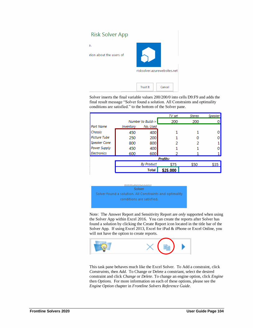
Frontline Solvers 2020 User Guide Page 104
Solver inserts the final variable values 200/200/0 into cells D9:F9 and adds the
final result message “Solver found a solution. All Constraints and optimality
conditions are satisfied.” to the bottom of the Solver pane.
Note: The Answer Report and Sensitivity Report are only supported when using
the Solver App within Excel 2016. You can create the reports after Solver has
found a solution by clicking the Create Report icon located in the title bar of the
Solver App. If using Excel 2013, Excel for iPad & iPhone or Excel Online, you
will not have the option to create reports.
This task pane behaves much like the Excel Solver. To Add a constraint, click
Constraints, then Add. To Change or Delete a constriant, select the desired
constraint and click Change or Delete. To change an engine option, click Engine
then Options. For more information on each of these options, please see the
Engine Option chapter in Frontline Solvers Reference Guide.
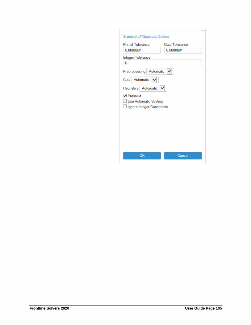
Frontline Solvers 2020 User Guide Page 105

Frontline Solvers 2020 User Guide Page 106
Examples: Simulation and Risk Analysis
Introduction This chapter introduces simulation and risk analysis in Analytic Solver, with a
series of examples. Each of these examples with the exception of the last one
can be used in Analytic Solver Simulation.
• “A First Simulation Example” takes you step-by-step through the process of building and analyzing a risk analysis model using Monte Carlo simulation.
• “Airline Revenue Management Example” takes you through three versions
of an airline yield management problem, to illustrate a single simulation,
multiple parameterized simulations, and simulation optimization.
A First Simulation Example Building a simulation model in Analytic Solver is straightforward: You simply
build a conventional spreadsheet model, designed for ‘what-if’ analysis. Next,
you identify the inputs to your model that are uncertain, and use PSI
Distribution functions to describe the uncertainty. Then, you identify the
outputs of special interest (such as Net Profit), and use PSI Statistics functions
to examine or summarize how they behave in light of the uncertainty.
To open this example in Analytic Solver Desktop or Analytic Solver Cloud,
click Help – Examples on the Ribbon, which opens a workbook Frontline
Example Models Overview.xls. Click the Simulation link.
Frontline Solvers 2020 User Guide Page 107
To open this example in AnalyticSolver.com click Help – Examples –
Simulation Examples – Business Forecast User Guide.
We’ll build the simulation model step-by-step in this section using the model in
the worksheet, BusinessForecast. To view the completed model, see the 2nd tab
in the workbook, BusinessForecastPsi.
Uncertain Variables
In any problem, there are factors or inputs that you can control – for example,
the price you set for a product, and factors or inputs that you cannot control –
for example, customer demand, interest rates, etc. Analytic Solver uses
uncertain variables (random variables in mathematics) to represent inputs that
are uncertain and beyond your control. (It uses decision variables to represent factors or inputs that you can control.)
Uncertain Functions
You will also have outputs or results of interest – such as Net Profit – that you
can compute, using formulas that depend on the factors influencing the problem
– possibly both decision variables and uncertain variables. We’ll use the term
uncertain functions for quantities whose calculation depends on uncertain variables (in mathematics these are called functions of random variables).
A Business Planning Example
We’ll illustrate the process of building a simulation model step by step, using a
simple business planning example. Imagine you are the marketing manager for
a firm that is planning to introduce a new product. You need to estimate the first
year profit from this product, which will depend on:
• Sales in units
• Price per unit sold
• Unit manufacturing cost
• Fixed costs and overhead
Profit will be calculated as Profit = Sales * (Price - Unit cost) - Fixed costs.
Fixed costs are known to be $120,000. But the other factors all involve some
uncertainty. Sales in units can cover quite a range, and the selling price per unit
will depend on competitor actions. Unit manufacturing costs will also vary
depending on vendor prices and production experience.
Uncertain Variables: Sales and Price
Based on your market research, you believe that there are equal chances that the
market demand will be Slow, OK, or Hot for this product:
• In the Slow market demand scenario, you expect to sell 50,000 units at an
average price of $11.00 per unit.
• In the OK market scenario, you expect to sell 75,000 units, but you'll likely
realize a lower average selling price of $10.00 per unit.
• In the Hot market scenario, you expect to sell 100,000 units, but this will
bring in competitors who will drive down the average selling price to $8.00 per unit.

Frontline Solvers 2020 User Guide Page 108
Since the scenarios are equally likely, your average volume is 75,000 units, and
your average price per unit is $9.67. But think: How likely is this average case?
(Will it ever actually occur?)
Uncertain Variables: Unit Cost
Your firm’s production manager advises you that unit costs may be anywhere
from $5.50 to $7.50, with a most likely cost of $6.50. The most likely cost is
also the average cost.
Uncertain Function: Net Profit
Net Profit is calculated as Profit = Sales * (Price - Unit cost) -Fixed costs.
Sales, Price and Unit costs are all uncertain variables, so Net Profit is an
uncertain function.
A What-If Spreadsheet Model
At this point, you can summarize the problem in the Excel model pictured
below, which calculates Net Profit based on average sales, price, and unit cost.
The Net Profit figure of $117,750 (=B4*(B5-B6)-B7) calculated by this model,
based on average values for the uncertain factors, is quite misleading, as we’ll see in a moment. The true average Net Profit is closer to $93,000! In the spirit
of Prof. Sam Savage’s book The Flaw of Averages, we’ll refer to the model
above as the Flawed Average model.
Defining a Simulation Model
To “stress test” this model, we need to replace the fixed Sales, Price and Unit
cost amounts with variable amounts that reflect their uncertainty.
Since there are equal chances that the market will be Slow, OK, or Hot, we want
to create an uncertain variable that selects among these three possibilities, by
drawing a random number – say 1, 2 or 3 – with equal probability. We can do
this easily in Analytic Solver using an integer uniform probability distribution. We’ll then base our Sales Volume and Selling Price on this uncertain variable.
If using Analytic Solver Desktop or AnalyticSolver.com, we’ll choose a
currently empty cell, B9, to hold this distribution by clicking on it and selecting

Frontline Solvers 2020 User Guide Page 109
Distributions - Discrete on the Ribbon. This displays a cascading menu, as
shown on the next page.
Analytic Solver Desktop
A sample drawn from a discrete distribution is always one of a set of discrete
values, such as integer numbers. We click to choose IntUniform from the
gallery or menu. Analytic Solver displays the Uncertain Variable dialog for a
integer uniform distribution, initially with parameters lower 0 and upper 10:
We click in the Value column and change the parameters to read lower 1 and
upper 3. This means that on each trial, we’ll draw a number 1, 2 or 3 from this
distribution. As we do, the chart of probability mass (density) is updated:

Frontline Solvers 2020 User Guide Page 110
When we click the Save icon in the dialog toolbar in Analytic Solver
Desktop or the Save button at the bottom of the dialog in Analytic Solver Cloud
or AnalyticSolver.com, a formula =PsiIntUniform(1,3) is written to B9. B9 is
now an uncertain variable. For each trial of the Monte Carlo simulation, a
different value – either 1, 2 or 3 – will appear in cell B9. When we run a Monte
Carlo simulation of (say) 1,000 trials, 1,000 different values of 1, 2 or 3 will be sampled for this cell’s value.
Now, we need to select one of the three sales scenarios in formulas for Sales
Volume and Selling Price. With cell B4 selected, we enter the formula:
=CHOOSE(B9,E5,E6,E7) for Sales Volume
This will cause B4 to return 100,000, 75,000, or 50,000, depending on the value
in B9. Next, with cell B5 selected, we enter the formula:
=CHOOSE(B9,F5,F6,F7) for Selling Price
This will cause B5 to return $8, $10 or $11, depending on the value in B9.
Notice that the values returned by B4 and B5 are related, or correlated: Higher sales volume is accompanied by lower selling prices, and vice versa. If we had
scenarios with 100,000 units sold at $11 each, our model would be unrealistic.
Analytic Solver has more versatile ways to specify correlation between
uncertain variables, but this approach is easy to understand in this example.
Next, we’ll deal with Unit Cost. We have not just three, but many possible
values for this variable: It can be anywhere from $5.50 to $7.50, with a most
likely cost of $6.50. A crude but effective way to model this is to use a
triangular distribution. Analytic Solver provides a function called
PsiTriangular() for this distribution.
With cell B6 selected, we select Distributions – Common – Triangular from the Ribbon.
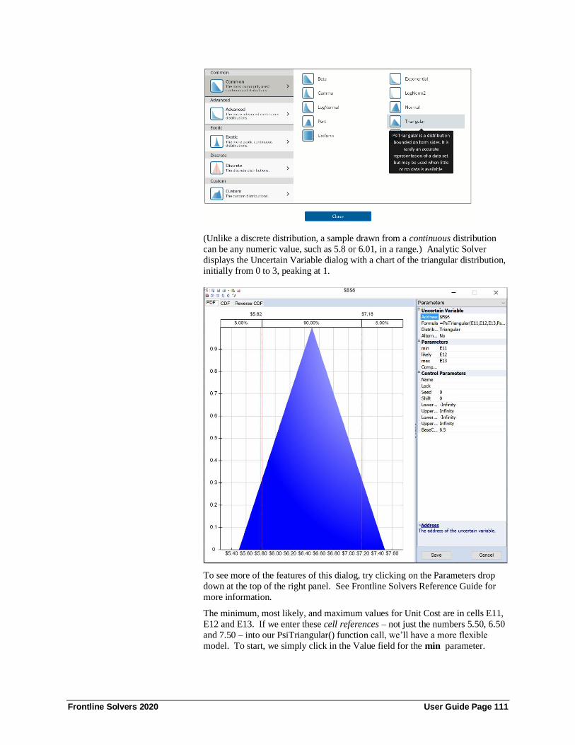
Frontline Solvers 2020 User Guide Page 111
(Unlike a discrete distribution, a sample drawn from a continuous distribution
can be any numeric value, such as 5.8 or 6.01, in a range.) Analytic Solver
displays the Uncertain Variable dialog with a chart of the triangular distribution,
initially from 0 to 3, peaking at 1.
To see more of the features of this dialog, try clicking on the Parameters drop
down at the top of the right panel. See Frontline Solvers Reference Guide for
more information.
The minimum, most likely, and maximum values for Unit Cost are in cells E11,
E12 and E13. If we enter these cell references – not just the numbers 5.50, 6.50
and 7.50 – into our PsiTriangular() function call, we’ll have a more flexible
model. To start, we simply click in the Value field for the min parameter.

Frontline Solvers 2020 User Guide Page 112
Now we can either type in a number or cell reference, or we can click the
button at the right edge of the field: When we do this, a small dialog appears.
Type “E11”, then click OK.
If using Analytic Solver Cloud or AnalyticSolver.com, simply type the cell
address into the min field.
Now E11 appears as the min (a) parameter. Since at this moment, the min (a)
value of 5.50 is greater than the max (b) value of 3, the error “The distribution is
invalid with the current values of the parameters” is displayed instead of the
chart. This is a hint that the parameters are inconsistent. (If using Analytic
Solver Cloud, click OK to clear the error and continue editing the Parameter
fields.) The chart reappears once we enter references to cell E12 for likely (c)
and E13 for max (b). When we click the Save icon, =PsiTriangular(E11,E12,E13) is inserted into cell B6.
We’ve now defined the uncertain variables in our model. Anything calculated
from these uncertain variables is an uncertain function, but usually we’re interested only in specific results such as Net Profit at cell B11. When we run a
simulation, B11 will effectively hold an array of values, each one calculated
from different values sampled for B4, B5, B6 and B7.
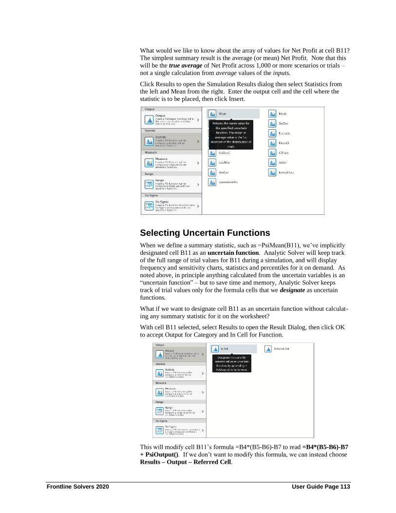
Frontline Solvers 2020 User Guide Page 113
What would we like to know about the array of values for Net Profit at cell B11?
The simplest summary result is the average (or mean) Net Profit. Note that this
will be the true average of Net Profit across 1,000 or more scenarios or trials –
not a single calculation from average values of the inputs.
Click Results to open the Simulation Results dialog then select Statistics from the left and Mean from the right. Enter the output cell and the cell where the
statistic is to be placed, then click Insert.
Selecting Uncertain Functions
When we define a summary statistic, such as =PsiMean(B11), we’ve implicitly
designated cell B11 as an uncertain function. Analytic Solver will keep track
of the full range of trial values for B11 during a simulation, and will display
frequency and sensitivity charts, statistics and percentiles for it on demand. As
noted above, in principle anything calculated from the uncertain variables is an
“uncertain function” – but to save time and memory, Analytic Solver keeps
track of trial values only for the formula cells that we designate as uncertain
functions.
What if we want to designate cell B11 as an uncertain function without calculat-
ing any summary statistic for it on the worksheet?
With cell B11 selected, select Results to open the Result Dialog, then click OK
to accept Output for Category and In Cell for Function.
This will modify cell B11’s formula =B4*(B5-B6)-B7 to read =B4*(B5-B6)-B7
+ PsiOutput(). If we don’t want to modify this formula, we can instead choose
Results – Output – Referred Cell.

Frontline Solvers 2020 User Guide Page 114
If we click in cell B12, this cell will contain =PsiOutput(B11). Any one of
these three actions – defining a summary statistic such as PsiMean() on B11, add
PsiOutput() to the formula in cell B11, or placing =PsiOutput(B11) in another
cell – is sufficient to designate cell B11 as an uncertain function.
Our model now looks like the one pictured below. Notice that the Task Pane
Model tab shows our simulation model in outline form, and cell B12, where we
placed the PsiMean() function, displays as #N/A – because a simulation has not
yet been executed.
Running a Simulation
Click the green arrow on the Model tab to start a simulation. With an old-
fashioned simulation software package, you’d press a button to start a
simulation, then perhaps get a cup of coffee. Because simulations ran slowly,
software packages were designed for “batch” operation: You’d spend time
getting everything set up just right, run a simulation and wait (sometimes quite a
while), then spend time analyzing the results. But with Analytic Solver, you'll
find that in the blink of an eye, your first Monte Carlo simulation is complete!
Since there is one uncertain function, and this is the first time a simulation has
been performed, the following dialog opens. Subsequent simulations will not
produce this report. However, it is possible to reopen this frequency chart
simply by double clicking cell B11. (See below for more information on this chart.)

Frontline Solvers 2020 User Guide Page 115
If your simulation model contains more than one output function, then a chart
containing frequency graphs of up to 9 output functions and uncertain variables
will appear. For example, if the uncertain variable in cell B6 was also selected
to be an output cell (B6 = PsiTriangular(0, 1, 3) + PsiOutput()) and a simulation
was performed, the following graph would appear at the end of the simulation.
Analytic Solver Desktop
Analytic Solver Cloud and AnalyticSolver.com display only output functions;
B6 and B11 in this example.
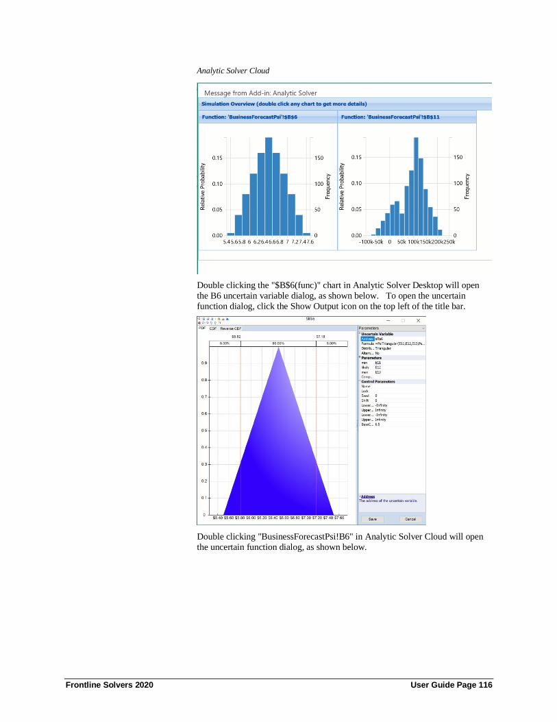
Frontline Solvers 2020 User Guide Page 116
Analytic Solver Cloud
Double clicking the "$B$6(func)" chart in Analytic Solver Desktop will open
the B6 uncertain variable dialog, as shown below. To open the uncertain
function dialog, click the Show Output icon on the top left of the title bar.
Double clicking "BusinessForecastPsi!B6" in Analytic Solver Cloud will open
the uncertain function dialog, as shown below.

Frontline Solvers 2020 User Guide Page 117
If you select Percentiles from the drop down menu on the top right, you’ll notice
that the the vertical red lines displayed on the chart denote the 5% and the 95%
percentiles values of 5.82 and 7.18, respectively.
Each of the 5 values at the top of the chart can be edited in Analytic Solver
Desktop. For example, the red lines can be moved to the left or right until the
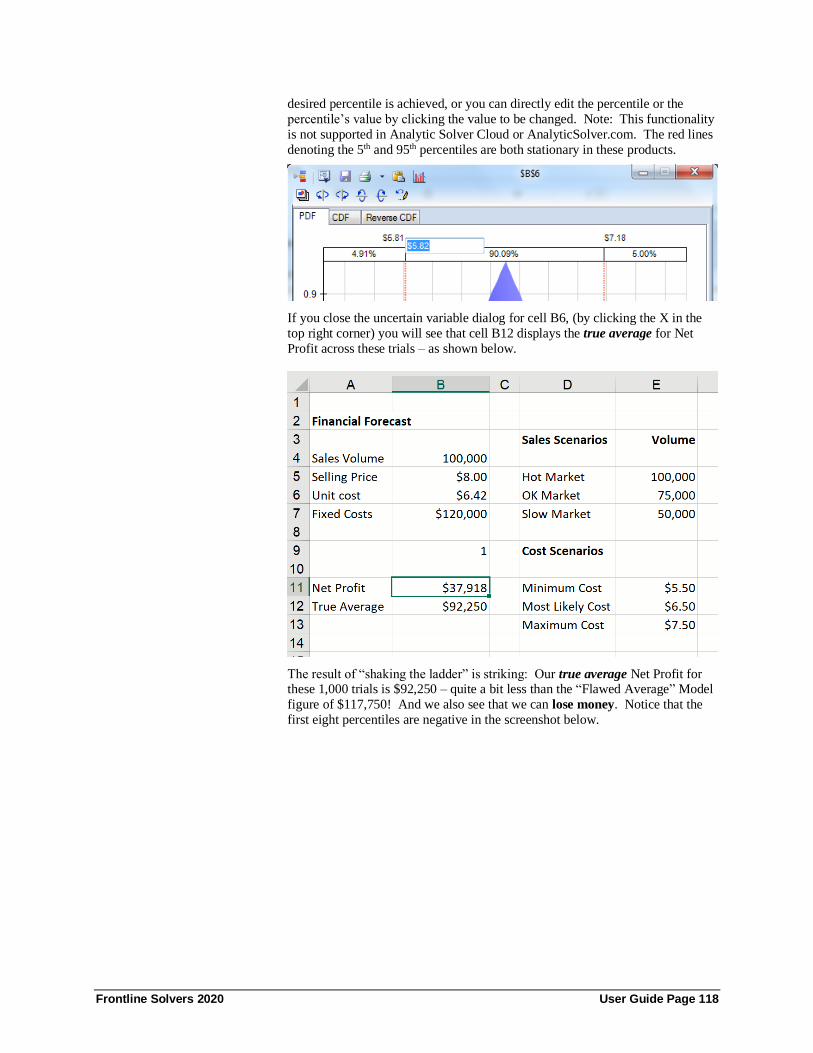
Frontline Solvers 2020 User Guide Page 118
desired percentile is achieved, or you can directly edit the percentile or the
percentile’s value by clicking the value to be changed. Note: This functionality
is not supported in Analytic Solver Cloud or AnalyticSolver.com. The red lines
denoting the 5th and 95th percentiles are both stationary in these products.
If you close the uncertain variable dialog for cell B6, (by clicking the X in the
top right corner) you will see that cell B12 displays the true average for Net
Profit across these trials – as shown below.
The result of “shaking the ladder” is striking: Our true average Net Profit for these 1,000 trials is $92,250 – quite a bit less than the “Flawed Average” Model
figure of $117,750! And we also see that we can lose money. Notice that the
first eight percentiles are negative in the screenshot below.

Frontline Solvers 2020 User Guide Page 119
In Analytic Solver Desktop you can try pressing F9 (the Excel recalculate key)
on this model: Each time you do, another 1,000 Monte Carlo trials are run, and
a slightly different true average Net Profit figure will be displayed – but
normally much less than $117,750.
Interactive Simulation in Desktop Solver
We’ve just seen that the mean or ‘True Average’ Net Profit, over 1,000 different
simulated outcomes, is less than we expected from our naïve “Flawed Average”
model. We’ve also seen that in some outcomes, our Net Profit is actually a loss.
A quick look at the dropdown galleries for Results – Statistic, Measure and
Range on the Ribbon suggests that we can easily compute and view many other
statistics about Net Profit. But we’d really like to see the full range of outcomes
in this model. This is very easy to do in Analytic Solver Desktop using
Interactive Simulation. Note: Interactive Simulation is not supported in
Analytic Solver Cloud or AnalyticSolver.com.
With Interactive Simulation turned on, simply move the mouse pointer to B11 and wait about 1 second. A miniature, live frequency distribution chart of the
simulation trial values for cell B11 appears automatically:
To see and do more, just double-click on B11, the output cell calculating Net Profit, to display the same frequency chart that was automatically opened after
our first simulation run.

Frontline Solvers 2020 User Guide Page 120
Viewing the Full Range of Profit Outcomes
We see immediately that in some outcomes, we can lose of lot of money – over
$60,000! We also see that we make a profit in most outcomes – but how many
exactly? Analytic Solver automatically sets a Lower-Cutoff of “0” in the
Frequency chart by displaying a vertical red bar. The probabilities are
automatically shown above the chart. In this case there is an 8.4% chance of a
loss and a 91.60% chance of a profit. In Analytic Solver Desktop, the lower
cutoff can be changed by clicking the $0 at the top of the chart. The percentile
values can be edited in the same way.
Note: If you change the lower cutoff from 0 to -10, you’ll notice the red vertical line denoting the lower cutoff of $0 has now moved to -$10
and the percentile values have also changed accordingly. Percentile
values can be edited in the same way or by simply moving the red
vertical line to the left or right.

Frontline Solvers 2020 User Guide Page 121
Looking at the right panel you can see the Statistics view, which includes
summary statistics for the full range of Net Profit outcomes. We can see that the
worst case outcome (Minimum) of this simulation was -$66,629, and the best
case outcome (Maximum) was +$213,347. Value at Risk 95% shows that we
have a 5% chance of making $15,629 or less. The Conditional Value at Risk
95% value indicates that the average profit we will see (up to the 95%
percentile) is $87,012.
Another view of the full range of outcomes is shown on the Cumulative
Frequency tab.
Click on the Statistics drop down at the top of the right panel and choose
Percentiles from the list.

Frontline Solvers 2020 User Guide Page 122
The Percentiles tab shows the same information as the Cumulative Frequency
tab, but in numeric form. Below, we’ve shown the 75th through 99th percentiles:
Note that you can close and open the right hand panel simply by clicking on the
two arrows on the vertical bar between the chart and the right hand panel.
Analyzing Factors Influencing Net Profit
Other tabs on the Uncertain Function dialog can help us understand how the
uncertain variables in our model influence our Net Profit.
Sensitivity Tab
The Sensitivity tab displays a “Tornado chart” that shows you how much Net Profit changes with a change in the uncertain variables – the Triangular
distribution for Unit Cost at cell B6, and the integer uniform distribution at cell
B9. In this model there are only two uncertain variables, but in a large model
with many such variables, it’s usually not obvious which ones have the greatest
impact on outcomes such as Net Profit. A Tornado chart highlights the key
variables: B6 has a negative correlation with Net Profit, whereas B9 has a
positive correlation.

Frontline Solvers 2020 User Guide Page 123
The fact that Net Profit goes down as our Unit Cost at B6 goes up is expected. But why does Net Profit go up as cell B9 goes up? Note that B9 = 1 corresponds
to the Hot market scenario, 2 corresponds to the OK market, and 3 corresponds
to the Slow market scenario. The fact that B9 is positively correlated with Net
Profit is telling us that we make higher profits when the market is slow, not
when it’s hot. Our typical Selling Price is lower when the market is hot, and the
increased Sales Volume doesn’t make up for this.
Scatter Plots Tab
The Scatter Plots tab, shown on the next page, gives us a different view of the
relationship of Net Profit to our uncertain variables: Unit Cost at cell B6, and the
integer uniform distribution at cell B9.
Notice that the scatter plot against Unit Cost has three downward-sloping lines:
Each line corresponds to a different market scenario (Hot, OK or Slow), and
shows that as Unit Cost rises, our Net Profit drops – dropping fastest in the Hot
Market scenario, because our profit margin is so narrow.
The scatter plot against the integer uniform distribution shows three high-low
ranges for Net Profit, again corresponding to a different market scenario – Hot,
OK, or Slow. We see again that the range of Net Profit is lowest in the Hot Market scenario.

Frontline Solvers 2020 User Guide Page 124
Interactive Simulation with Charts and Graphs
With an old-fashioned simulation software package, you’d press a button to start
a simulation, then perhaps get a cup of coffee. Because simulations ran slowly,
software packages were designed for “batch” operation: You’d spend time
getting everything set up just right, run a simulation and wait (sometimes quite a
while), then spend time analyzing the results. But with Analytic Solver,
simulations run so fast that fully Interactive Simulation is practical.
Now 1,000 Monte Carlo simulation trials (the default number) will be executed each time we change the spreadsheet. Since there is one uncertain function, and
this is the first time a simulation has been performed, the following dialog
opens. Subsequent simulations will not produce this report. However, it is
possible to reopen this frequency chart simply by double clicking cell B11. (See
below for more information on this chart.)
To turn on Interactive Simulation, simply click the light bulb on the Ribbon.
It will “light up,” as shown below.
Interactive Simulation makes Analytic Solver Simulation fundamentally
different from other Monte Carlo simulation tools for Excel. The kinds of charts
we’ve just seen can be produced by other tools, but only at the end of a
“simulation run.” In contrast, Analytic Solver makes these charts live as you
play what-if with your model.
After seeing this model, your production manager might think of a way to
reduce the maximum Unit Cost to $7.00 instead of $7.50. What would be the
impact of this change on Net Profit, over the full range outcomes? With
Analytic Solver Comprehensive or Analytic Solver Simulation, this is as easy as
any other ‘what-if’ question in Excel:
Click the Frequency tab to re-display the frequency chart of outcomes for cell
B11. Then simply change the number in cell E13 from 7.50 to 7. Immediately,
a thousand Monte Carlo trials are performed, and the chart is updated. The
effect is striking: We have a 97.7% chance of making a profit, and – checking
the Percentiles tab – we see that instead of a 1% chance of losing about $48,000,
we have a 1% chance of losing just $5,285!
But Analytic Solver Simulation is even faster than this: Click the Options
button on the Ribbon, and change the number of Monte Carlo trials from 1,000

Frontline Solvers 2020 User Guide Page 125
to 100,000 (or more). In a second or less on most modern PCs, one hundred
thousand Monte Carlo trials are performed, and the chart is updated!
The Flawed Average model presented a limited and misleading picture of this
business situation. In contrast, the Analytic Solver model has illuminated the
situation considerably. We can see what can go right, and what can go wrong. We can make an informed decision about whether the reward is worth the risk.
And – most important – we can interactively explore ways to improve the
reward and reduce the risk. This is risk analysis at work.
Charts and Graphs for Presentations
Often, you may be called up to present your results to others. One great way to
do this is in Excel itself, live! But at times you may need to print a chart, or
copy it into a Word document or PowerPoint presentation. This is very easy to
do in Analytic Solver Desktop, with the toolbar buttons in the title bar of the
Uncertain Variable or Uncertain Function dialog. Note: This functionality is
not supported in Analytic Solver Cloud or AnalyticSolver.com.
Click the Clipboard icon to copy the currently displayed chart to the Windows
Clipboard. You can then choose Edit Paste in Word, Excel, PowerPoint and
many other applications to paste the chart image into your document. (Choosing
Edit Paste in Excel inserts a static, non-updating chart image in the worksheet.)
Click the Print icon to immediately print the currently displayed chart on your
default printer, or click the down arrow next to this icon to display the menu choices shown above: Print Preview, Printer Settings and Page Settings. You

Frontline Solvers 2020 User Guide Page 126
can choose a printer and set printer options, set page margins, and preview your
output using these menu choices.
Analytic Solver also makes it easy to control the format of your charts. Below,
we’ve re-opened the right hand panel and clicked on the drop down menu to
choose Chart Type.
You can control the chart type, color, dimensionality and transparency, bin
density, titles and legends, axis labels and number formats, horizontal axis
scaling, and more. As you change chart options in the right pane, the chart is
immediately updated so you can see the results (unlike some other simulation products for Excel). When you’re satisfied with the chart format, you can save
and apply it to just this chart, to all charts on this worksheet, or to all charts in
the workbook when you click the Apply button at the bottom of the right pane.
Exporting Data to Microsoft's Power BI
Microsoft's POWER BI, for use with Office 365, is a cloud-based service that
works with Excel to help you visualize your data using various charts and
reports. Analytic Solver Desktop includes the ability to export a fixed set of
data from your simulation model, including all trial values, output function
statistics, percentiles, etc., directly into a dataset in Power BI. This
functionality is not present in Analytic Solver Cloud or AnalyticSolver.com.
See the chapter, Creating Power BI Custom Visuals, that appears later on in this guide for more information on using Power BI with these two products.
Once Solver has stopped with a final result message, click the icon on the
Output tab or on the Uncertain Function dialog to upload the model results to
the Power BI dashboard. If this is the first time that the icon has been clicked
within the current Excel instance, you will be asked to log in to Power BI.
Power BI Icon as shown on the Output tab on the Solver Task Pane.
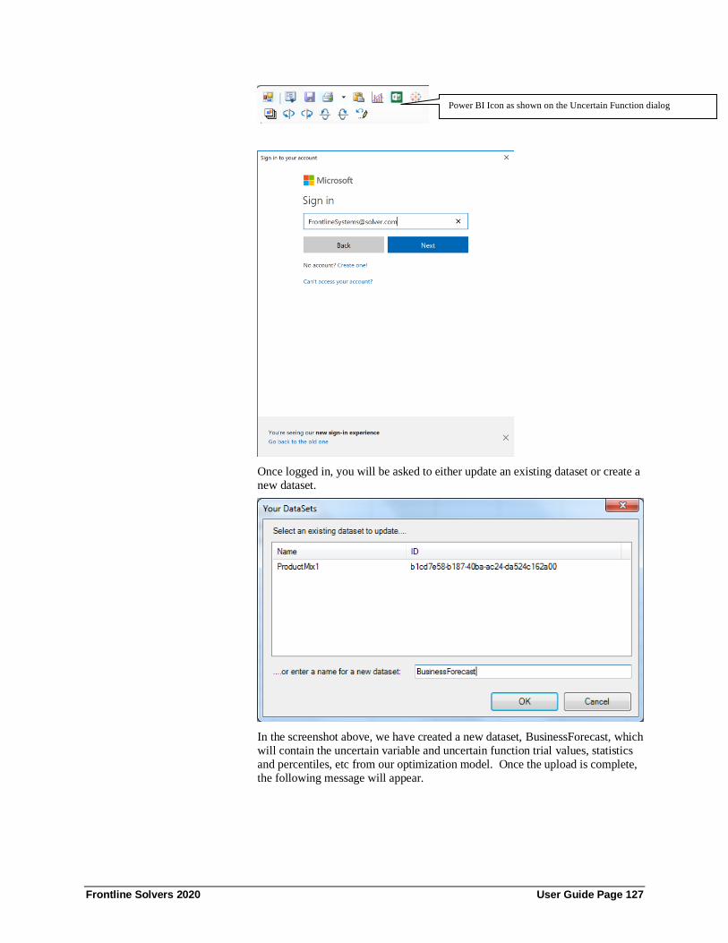
Frontline Solvers 2020 User Guide Page 127
Once logged in, you will be asked to either update an existing dataset or create a
new dataset.
In the screenshot above, we have created a new dataset, BusinessForecast, which
will contain the uncertain variable and uncertain function trial values, statistics
and percentiles, etc from our optimization model. Once the upload is complete,
the following message will appear.
Power BI Icon as shown on the Uncertain Function dialog

Frontline Solvers 2020 User Guide Page 128
Logon to Power BI (http://powerbi.microsoft.com/). The newly created dataset
will be listed under Datasets.
Select BusinessForecast, then determine the components to be included in the
graph. In this example, we have created a bar chart by clicking (to the
right of the graph) and selecting the Maximum, Mean, Minimum, and Mode
Output Statistics.
Use the icon to pin this graph to the Dashboard.

Frontline Solvers 2020 User Guide Page 129
Now, each time the model is solved, the results may be uploaded to your Power
BI dashboard. Click back to Excel and change the Price of the Slow Market from $11 to $15, then run a 2nd simulation either by clicking the green arrow on
the Model tab in the Solver Task Pane or by clicking the Simulate icon on the
Analytic Solver ribbon. Once Solver stops, click the icon on either the
Output tab or the Uncertain function dialog to upload the most recent results.
Note: We are not asked to log in to the Power BI site a second time since we are
using the same instance of Excel. However, we are asked if we would like to
select an existing dataset to update. Select BusinessForecast and then click OK.
Click back to Power BI in your browser and refresh, the chart will update
automatically with the new final statistic values, as shown below.
Exporting Data to Tableau
Tableau is a popular interactive software package that allows you to visually
explore and analyze your data. Tableau can import data from a wide range of
sources, including Excel workbooks, and it is often used in conjunction with
Excel. Because Tableau is designed to import data in table form, it hasn’t been
easy to import the results of a simulation model (such as final values of the
uncertain functions, uncertain variables, percentiles and statistic values) into

Frontline Solvers 2020 User Guide Page 130
Tableau, unless those model elements occur in table form by themselves in your
spreadsheet (which usually isn’t the case).
Analytic Solver Desktop simplifies this process considerably. With a single
click, you can convert the results of your simulation model into a set of Tableau
Data Extract files (*.tde), open them directly in Tableau, and visualize them with a few clicks.
This functionality is not present in Analytic Solver Cloud or
AnalyticSolver.com. See the chapter, Creating Custom Extensions in Tableau,
that appears later on in this guide for more information on using Tableau with
these two products.
Click the green arrow on the Output tab in the Solver Task Pane to run a
simulation. Once Solver has stopped with a final result message, click the
icon on the Task Pane Output tab or Uncertain Function dialog to save the
values for the uncertain functions, uncertain variables, percentiles and statistics
to *.tde files. You will be prompted to select a folder where the Tableau files
will be saved along with the type of Tableau export desired: Tableau Data
Extract or (introduced in V2016-R2) Tableau Web Connector.
Note: If exporting to an existing .tde file, data will be appended rather than
overwritten. As a result, when exporting to an existing .tde file, all data must be
of the same structure as when the .tde file was first created.
If Tableau Data Extract is selected, static data is exported to files saved on your
hard drive.
Once you select a folder, the .tde files will be created, and the following
message will appear.
Four files will be saved in the folder you selected: InputTrials.tde,
OutputStatistics.tde, OutputTrials.tde, and Percentiles.tde. (Although .tde files
are designed to hold multiple tables, currently Tableau’s software allows only

Frontline Solvers 2020 User Guide Page 131
one table per file.) When you import this data into Tableau, InputTrials.tde and
OutputTrials.tde will have one row for each trial, Percentiles.tde will have one
row for percentile and OutputStatistics.tde will have one row for each output
function.
• Each row of InputTrials.tde will contain the trial value for each uncertain variable and the simulation index. The number of rows will
equal the number of trials.
• Each row of OutputTrials.tde will contain the trial value for each
uncertain function and the simulation index. The number of rows will
equal the number of trials.
• Each row of Percentiles.tde will contain the percentile value for each
uncertain function and the simulation index. The number of rows will
equal 99.
• Each row of OutputStatistics.tde will contain the Excel cell address where the uncertain function is located along with 9 statistical functions
(mean, standard deviation, variance, kurtosis, skewness, mode,
minimum, maximum, and range) and the simulation index.
Note: If exporting to an existing .tde file, data will be appended rather than
overwritten. As a result, when exporting to an existing .tde file, all data must be
of the same structure as when the .tde file was first created.
To open the files in Tableau, either double click each file (if using Desktop
Tableau) or click Other Files under Connect and open the desired file(s).
Tableau Web Connector
The Tableau Web Connector offers much more flexibility over Tableau Data
Extract by allowing you to refresh your data dynamically inside of Tableau.

Frontline Solvers 2020 User Guide Page 132
If Tableau Web Connector is selected, you will be prompted to select a folder in
which to save SimulationResults.html. This file will hold all contents described
above for InputTrials.tde, OutputStatistics.tde, OutputTrials.tde, and
Percentiles.tde. The following message will appear.
Note: If exporting to an existing .tde file, data will be appended rather than
overwritten. As a result, when exporting to an existing .tde file, all data must be
of the same structure as when the .tde file was first created.
To open the files in Tableau, open a new workbook in Tableau and click
Connect to Data.

Frontline Solvers 2020 User Guide Page 133
On the Connect menu, select More Servers – Web Data Connector.
On the Web Data Connector dialog, enter the location displayed on the dialog shown above, i.e. http://localhost:8080/, and press Enter.
When the following dialog appears, click Constraints.html.
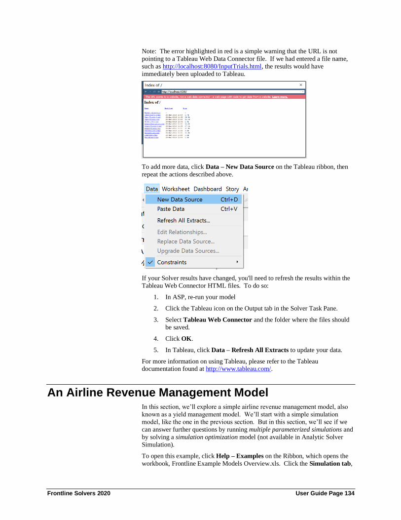
Frontline Solvers 2020 User Guide Page 134
Note: The error highlighted in red is a simple warning that the URL is not
pointing to a Tableau Web Data Connector file. If we had entered a file name,
such as http://localhost:8080/InputTrials.html, the results would have
immediately been uploaded to Tableau.
To add more data, click Data – New Data Source on the Tableau ribbon, then
repeat the actions described above.
If your Solver results have changed, you'll need to refresh the results within the
Tableau Web Connector HTML files. To do so:
1. In ASP, re-run your model
2. Click the Tableau icon on the Output tab in the Solver Task Pane.
3. Select Tableau Web Connector and the folder where the files should
be saved.
4. Click OK.
5. In Tableau, click Data – Refresh All Extracts to update your data.
For more information on using Tableau, please refer to the Tableau documentation found at http://www.tableau.com/.
An Airline Revenue Management Model In this section, we’ll explore a simple airline revenue management model, also
known as a yield management model. We’ll start with a simple simulation
model, like the one in the previous section. But in this section, we’ll see if we
can answer further questions by running multiple parameterized simulations and
by solving a simulation optimization model (not available in Analytic Solver
Simulation).
To open this example, click Help – Examples on the Ribbon, which opens the
workbook, Frontline Example Models Overview.xls. Click the Simulation tab,

Frontline Solvers 2020 User Guide Page 135
then the Yield Management Model 1 (a simple simulation model) and Yield
Management Model 2 (a model with multiple parameterized simulations) links.
Click the Simulation Optimization tab to open Yield Management Model 3, a
simulation optimization model. In AnalyticSolver.com, click Help – Examples
– Simulation to open Yield Management Model 1 and Yield Management Model 2 and Help – Examples – Simulation Optimization Examples to open Yield
Management Model 3.
A Single Simulation
The model YieldManagement1.xls opened in Analytic Solver Desktop is shown
on the next page.
The model depicts a hypothetical airline flight from San Francisco to Seattle.
The flight has 100 seats, and tickets are $200 per seat. Some passengers who
purchase tickets are “no-shows” whose seats will be empty; in this example we assume that such passengers receive a refund of 50% of their purchase price.
To utilize their ‘perishable inventory’ of seats, the airline would like to sell more
than 100 tickets for each flight. But we assume that Federal regulations require
that any ticketed passenger who is unable to board the flight due to overbooking
is entitled to compensation of 125% of the ticket price.
The airline would like to know how much revenue it will generate from each
flight, less refunds for no-shows and compensation for ‘bumped’ passengers.
As shown above, this total revenue amount is calculated at cell C31, for any
specific number of tickets sold (110 above) and number of no-shows (6 above).
The uncertain quantity in this model is the number of no-shows; hence we should model this with an uncertain variable. We quickly realize that the
number of no-shows will depend on the number of tickets sold. After some
research, we decide that we can use a LogNormal distribution for the number of
no-shows: Cell H27 contains the formula
=PsiLogNormal(0.1*G32,0.06*G32). Cell G27 contains =ROUND(H27,0) to
ensure that the number of no-shows is an integer value – and this is used to
compute Total Revenue at cell G36.
Note that the bottom area of the Task Pane is showing the properties of cell
H27: for example, the mean of the distribution is 10% of the number of tickets
sold.

Frontline Solvers 2020 User Guide Page 136
See the chapter “Mastering Simulation and Risk Analysis Concepts” for advice
on choosing distributions for your uncertain variables.
As shown in the Task Pane, cell G36 is an uncertain function; it is defined as such because cell G38 contains =PsiMean(G36) to compute the expected (or
average) revenue across all Monte Carlo trials.
Performing the Simulation
To perform a single simulation (with 1,000 Monte Carlo trials), we click the
green arrow on the Model tab of the Solver Task Pane. At the end of the
simulation the following dialog appears displaying the distribution of outcomes in the Uncertain Function dialog:
The right hand panel shows the statistics from cell G36. We see that the mean
or expected net revenue is about $20,000. From the Cumulative Frequency
tab over the chart or by clicking on the drop down menu in the right hand panel
(currently showing “Statistics”) and selecting Percentiles, we can see that the
10% percentile is $19,950 – if we sell 110 tickets, we’ll earn approximately as
much revenue as a full flight (100 seats * $200), 90% of the time. You can see
why airlines find that overbooking makes sense as a policy!

Frontline Solvers 2020 User Guide Page 137
The Scatter Plots tab (click the graph to enlarge) shows you a quick scatter plot
of this uncertain function against one or more uncertain variables, or other
uncertain functions. In this example – shown on the next page – it shows a
scatter plot of G36 (net revenue) against H27 (number of no-shows).
Using Interactive Simulation
If using Analytic Solver Desktiop, we can explore the question of how many
tickets to sell with Interactive Simulation: We simply click the Simulate button
to “turn on the lights.”
Now we can simply type a new number of Tickets Sold, such as 125, into cell G32. Instantly, Analytic Solver (Desktop) performs a new simulation of 1,000
Monte Carlo trials, and updates the Uncertain Function dialog and the worksheet
with the results – as shown on the next page.
The new distribution of outcomes is quite different – we have more high-
revenue data points – but the mean or expected revenue is not so different --
$20,503. Selling 125 tickets does seem to be better than selling 110 tickets, but
we’re not yet sure that this is the best number of tickets to sell. (We’ll answer
that question in the next two sections.)
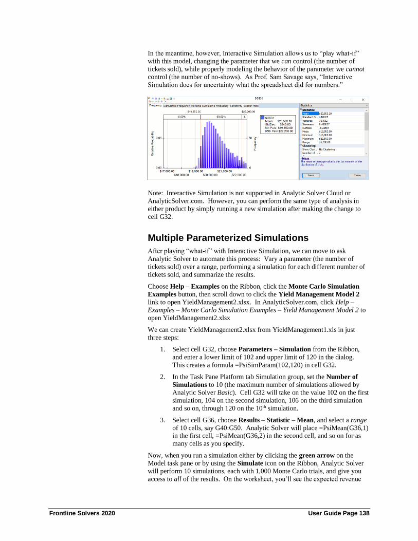
Frontline Solvers 2020 User Guide Page 138
In the meantime, however, Interactive Simulation allows us to “play what-if”
with this model, changing the parameter that we can control (the number of
tickets sold), while properly modeling the behavior of the parameter we cannot
control (the number of no-shows). As Prof. Sam Savage says, “Interactive
Simulation does for uncertainty what the spreadsheet did for numbers.”
Note: Interactive Simulation is not supported in Analytic Solver Cloud or
AnalyticSolver.com. However, you can perform the same type of analysis in
either product by simply running a new simulation after making the change to
cell G32.
Multiple Parameterized Simulations
After playing “what-if” with Interactive Simulation, we can move to ask
Analytic Solver to automate this process: Vary a parameter (the number of
tickets sold) over a range, performing a simulation for each different number of
tickets sold, and summarize the results.
Choose Help – Examples on the Ribbon, click the Monte Carlo Simulation
Examples button, then scroll down to click the Yield Management Model 2
link to open YieldManagement2.xlsx. In AnalyticSolver.com, click Help –
Examples – Monte Carlo Simulation Examples – Yield Management Model 2 to
open YieldManagement2.xlsx
We can create YieldManagement2.xlsx from YieldManagement1.xls in just
three steps:
1. Select cell G32, choose Parameters – Simulation from the Ribbon,
and enter a lower limit of 102 and upper limit of 120 in the dialog.
This creates a formula =PsiSimParam(102,120) in cell G32.
2. In the Task Pane Platform tab Simulation group, set the Number of
Simulations to 10 (the maximum number of simulations allowed by
Analytic Solver Basic). Cell G32 will take on the value 102 on the first
simulation, 104 on the second simulation, 106 on the third simulation
and so on, through 120 on the 10th simulation.
3. Select cell G36, choose Results – Statistic – Mean, and select a range
of 10 cells, say G40:G50. Analytic Solver will place =PsiMean(G36,1) in the first cell, =PsiMean(G36,2) in the second cell, and so on for as
many cells as you specify.
Now, when you run a simulation either by clicking the green arrow on the
Model task pane or by using the Simulate icon on the Ribbon, Analytic Solver
will perform 10 simulations, each with 1,000 Monte Carlo trials, and give you
access to all of the results. On the worksheet, you’ll see the expected revenue

Frontline Solvers 2020 User Guide Page 139
for 100, 102, …, 120 tickets sold. And you can use the Uncertain Function
dialog to display the full distribution of outcomes for any of the 10 simulations.
Examining Results Across Simulations
Once the simulation finishes, the uncertain function dialog for cell G36 will
open automatically or you can double-click the cell to open.
The dialog now includes a dropdown list that allows you to select a simulation
to display. You can examine the Frequency, Cumulative Frequency, Reverse
Cumulative Frequency, Sensitivity, or Scatter Plots tabs for any simulation.
The worksheet will initially display values for the last Monte Carlo trial of the
last simulation performed (except for the cells containing PSI Statistics function
calls such as PsiMean()). But you can display any trial from any simulation, by
changing the selections in the Sim # and Trial # controls on the Ribbon:
By examining this data, you can get a better idea of how many tickets to sell.
But Analytic Solver can help your further.
Reports and Charts of Multiple Simulations
Analytic Solver Comprehensive and Analytic Solver Optimization with Analytic
Solver Simulation, in Analytic Solver Desktop or Analytic Solver Cloud, has
rich facilities for reports and charts across multiple simulations. We’ll cover
just two chart examples; see the Frontline Solvers Reference Guide for further
information.
First, select Charts – Multiple Simulations – Trend from the Ribbon.
Analytic Solver displays a dialog where you can select one or more simulations
to include in the chart. Click the >> button to select all 10 simulations:

Frontline Solvers 2020 User Guide Page 140
Analytic Solver then draws the Trend Chart:
The number of tickets sold is on the horizontal axis. Analytic Solver shows the
mean, 25th and 75th percentile, and 10th and 90th percentile values of net revenue
at G36 (this was the only choice in the dropdown list at the top left of the
Multiple Simulations dialog). We can see that the mean or expected net revenue
peaks at about 116 or 177 tickets sold.
For another view of this information, select Charts – Multiple Simulations –
Box-Whisker from the Ribbon, and again select all 10 simulations to be
included in the chart. Analytic Solver Comprehensive draws the following
chart:
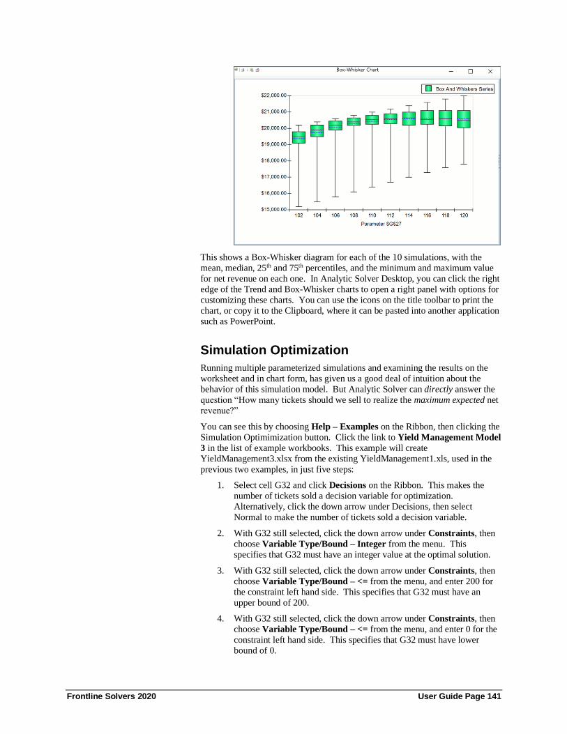
Frontline Solvers 2020 User Guide Page 141
This shows a Box-Whisker diagram for each of the 10 simulations, with the
mean, median, 25th and 75th percentiles, and the minimum and maximum value
for net revenue on each one. In Analytic Solver Desktop, you can click the right
edge of the Trend and Box-Whisker charts to open a right panel with options for
customizing these charts. You can use the icons on the title toolbar to print the
chart, or copy it to the Clipboard, where it can be pasted into another application
such as PowerPoint.
Simulation Optimization
Running multiple parameterized simulations and examining the results on the
worksheet and in chart form, has given us a good deal of intuition about the
behavior of this simulation model. But Analytic Solver can directly answer the
question “How many tickets should we sell to realize the maximum expected net
revenue?”
You can see this by choosing Help – Examples on the Ribbon, then clicking the
Simulation Optimimization button. Click the link to Yield Management Model
3 in the list of example workbooks. This example will create
YieldManagement3.xlsx from the existing YieldManagement1.xls, used in the
previous two examples, in just five steps:
1. Select cell G32 and click Decisions on the Ribbon. This makes the
number of tickets sold a decision variable for optimization.
Alternatively, click the down arrow under Decisions, then select
Normal to make the number of tickets sold a decision variable.
2. With G32 still selected, click the down arrow under Constraints, then
choose Variable Type/Bound – Integer from the menu. This
specifies that G32 must have an integer value at the optimal solution.
3. With G32 still selected, click the down arrow under Constraints, then
choose Variable Type/Bound – <= from the menu, and enter 200 for
the constraint left hand side. This specifies that G32 must have an
upper bound of 200.
4. With G32 still selected, click the down arrow under Constraints, then
choose Variable Type/Bound – <= from the menu, and enter 0 for the
constraint left hand side. This specifies that G32 must have lower
bound of 0.

Frontline Solvers 2020 User Guide Page 142
5. Select cell G38, click the down arrow under Objective, then choose
Max – Normal from the menu. The optimizer will maximize G38: =
PsiMean(G31), the expected value of net revenue.
The model in Task Pane will now look like the one pictured below.
In YieldManagement3.xls, we’ve made just these selections, and we’ve also chosen the GRG Nonlinear Solver from the dropdown list on the Engine tab, to
solve the problem. (Other choices are possible, but this one is simplest for this
example problem.)
Now we can simply click the green arrow on the Task Pane. After a moment
of solving, Analytic Solver returns the solution of 116 or 117 tickets sold
appears in G32 (the exact number depends on the simulation Random Seed), and
the expected value of net revenue for this number of tickets appears at G32
(about $20,500). “Solver found a solution. All constraints and optimality
conditions are satisfied” appears in green in the Output tab of the Task Pane, as
shown on the next page.
Note that this required less than a page to explain how you can get answers to questions like “How many tickets should we sell to realize the maximum
expected net revenue?”
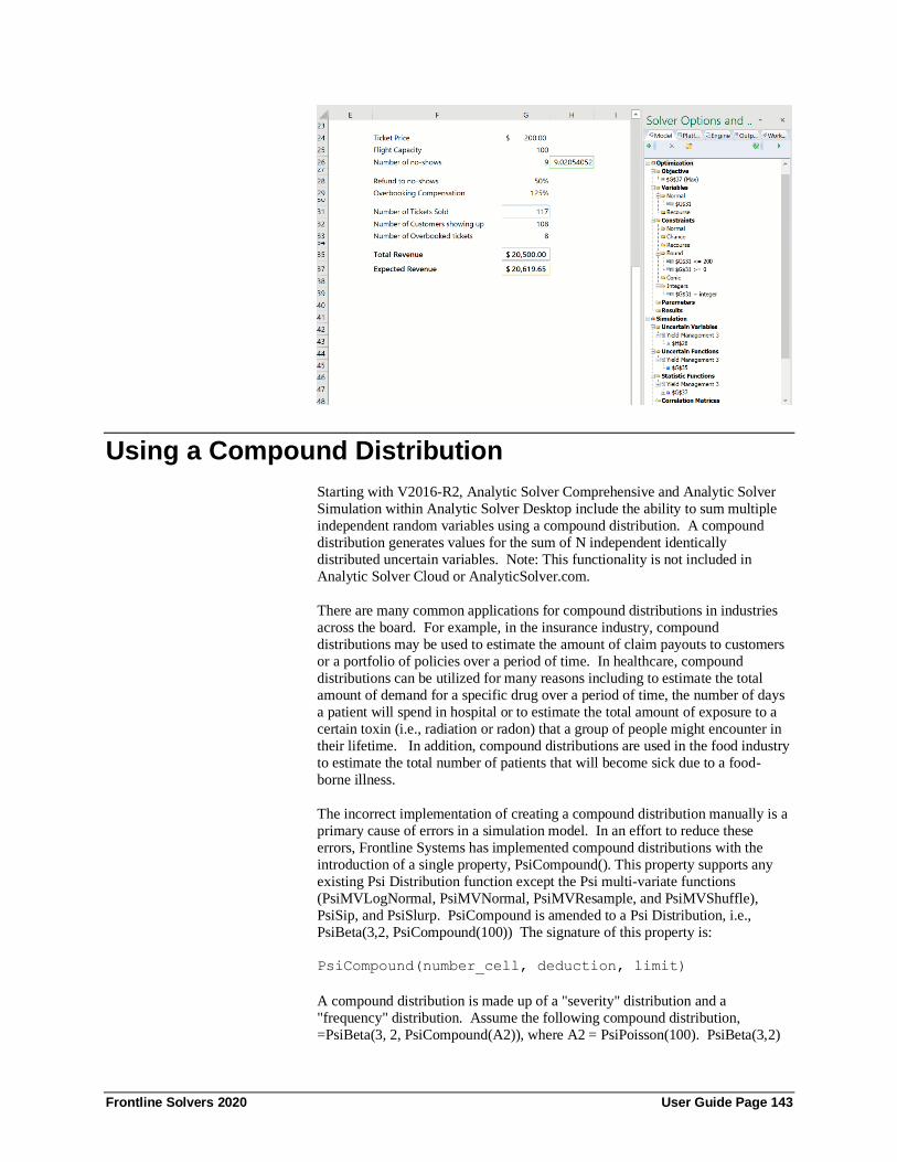
Frontline Solvers 2020 User Guide Page 143
Using a Compound Distribution
Starting with V2016-R2, Analytic Solver Comprehensive and Analytic Solver
Simulation within Analytic Solver Desktop include the ability to sum multiple
independent random variables using a compound distribution. A compound
distribution generates values for the sum of N independent identically
distributed uncertain variables. Note: This functionality is not included in
Analytic Solver Cloud or AnalyticSolver.com.
There are many common applications for compound distributions in industries
across the board. For example, in the insurance industry, compound
distributions may be used to estimate the amount of claim payouts to customers
or a portfolio of policies over a period of time. In healthcare, compound
distributions can be utilized for many reasons including to estimate the total
amount of demand for a specific drug over a period of time, the number of days
a patient will spend in hospital or to estimate the total amount of exposure to a
certain toxin (i.e., radiation or radon) that a group of people might encounter in
their lifetime. In addition, compound distributions are used in the food industry
to estimate the total number of patients that will become sick due to a food-
borne illness.
The incorrect implementation of creating a compound distribution manually is a
primary cause of errors in a simulation model. In an effort to reduce these
errors, Frontline Systems has implemented compound distributions with the
introduction of a single property, PsiCompound(). This property supports any
existing Psi Distribution function except the Psi multi-variate functions
(PsiMVLogNormal, PsiMVNormal, PsiMVResample, and PsiMVShuffle),
PsiSip, and PsiSlurp. PsiCompound is amended to a Psi Distribution, i.e.,
PsiBeta(3,2, PsiCompound(100)) The signature of this property is:
PsiCompound(number_cell, deduction, limit)
A compound distribution is made up of a "severity" distribution and a
"frequency" distribution. Assume the following compound distribution,
=PsiBeta(3, 2, PsiCompound(A2)), where A2 = PsiPoisson(100). PsiBeta(3,2)

Frontline Solvers 2020 User Guide Page 144
is referred to as the "severity" distribution. The severity distribution is the
distribution to be added N times. PsiPoisson(100) is referred to as the
"frequency" distribution. The frequency distribution determines the size N of
the sum (i.e, how many PsiBeta to sum). N can be a constant but can also be
computed at each trial by drawing from a discrete distribution.
• The number_cell argument passes the number of random trial values
to be summed. Number_cell can be an integer, a cell containing an
integer, a formula evaluating to an integer, or a cell containing a
discrete distribution.
If a fractional value is passed directly or indirectly (by using a formula)
or a continuous distribution is passed to this argument, the result will
be rounded down to the nearest integer.
Note: If a discrete distribution is passed to the number_cell argument,
the frequency distribution must be formulated in such a way that the
trial values generated by the distribution must be greater than 1. If not,
trial values < 1 will be set equal to 1.
• The value passed to the deduction argument is subtracted from every
term of the compound sum which results in a shift of the compound
distribution by -N * deduction.
• If a trial value is larger than a specified limit, then the trial value is
reset to the limit.
Depending on what is passed to the number_cell argument, PsiCompound()
automatically selects from several different compounding methods.
• First, ASP tries to compute the distribution analytically. For
example "=PsiExponential(par, PsiCompund(N))" can be
computed as PsiGamma(N, par). Analytic Solver can immediately
sample from this "shortcut" distribution.
• If Analytic Solver is unable to compute a compound distribution analytically, but the frequency of the severity function (N) is
greater than the value for the CLT Threshold option, then the
distribution will be computed according to the Central Limit
Theorem as PsiNormal(m, s). The parameters m and s will be
computed analytically from the corresponding analytical moments
of the severity distribution. The maximum value allowed for the
CLT Threshold option is 1000 while the minimum value allowed is
1. The default setting is 100.
• Otherwise, the compound distribution will be computed using
Monte Carlo simulation to sum up N independent variates of the
severity distribution.
The following examples illustrate how to use the PsiCompound() property when
a discrete distribution or a constant value is passed to the number_cell argument

Frontline Solvers 2020 User Guide Page 145
Discrete Distribution passed to 1st Argument
Imagine an insurance policy has two basic classes of insured members, class A
and class B; there are 50 class A members and 10 class B members. The number
of claims from class A members follows a Negative Binomial distribution with
parameters (5, 0.25), and the number of claims from class B members follows a
geometric distribution with parameter 0.25. The size of a claim from class A
members follows an exponential distribution with mean $40,000, and the claim size from class B members is distributed with a Pearson 5 distribution with
parameters (10, 2000000). In other words, if there are six Class A claims, the
size of the payout for each of the six claims will follow the
PsiExponential(40000) distribution. Calculate the expected claim payment for
both classes.
1. Let's start by formulating the compound distribution for the Class A
members. Recall that the number of Class A claims follows a Negative
Binomial distribution using a success parameter = 5 and probability
parameter = 0.25 while the size of a Class A claim follows an
exponential distribution with mean $40,000.
In this example, PsiExponential(40000) is the severity distribution.
This is the distribution that will be added together. If there are six
claims, then PsiExponential(40000) will be compounded six times.
The frequency distribution is the number of Class A claims,
=PsiNegBinomial(5, 0.25, PsiTruncate(0, 50)).
Note: Since there are 50 class A members, the PsiTruncate property is
used to ensure that sample values always lie within the range from 0 to
50.
If A1 = PsiNegBinomial(5, 0.25, PsiTruncate(0, 50), the full
compounding formula for the amount paid to Class A claims can be
entered into cell A2 as "=PsiExponential(40000, PsiCompound(A1))".
2. Now we can formulate the compound distribution to calculate the
payouts for the Class B members. The second compound distribution
may be formulated in the same manner. PsiPearson5(10, 2000000) is
the severity distribution while =PsiGeometric(0.25, PsiTruncate(0, 10))
is the frequency function. Since there are 10 class B members,
PsiTruncate is used to ensure that sample values lie within the range 0
to 10.
If B1 = PsiGeometric(0.25, PsiTruncate(0, 10), the full compounding
formula for the amount paid to Class B claims can be entered into cell
B2 as "= PsiPearson5(10,2000000, PsiCompound(B1))".
3. Enter =PsiMean(A1) and =PsiMean(A2) in cells A3 and B3,
respectively, to calculate the total expected payout to each class.
Run a simulation by clicking the green arrow on the Output tab on the
Solver Task Pane. Instantly, Analytic Solver performs a new simulation of
1,000 Monte Carlo trials, and updates the Uncertain Function dialog and the
worksheet with the results – as shown on the next page.

Frontline Solvers 2020 User Guide Page 146
Double click the distribution for $A$2(var) to open the uncertain function dialog
for cell A2.
If an uncertain variable uses the PsiCompound() property to create a compound
distribution, you will see added fields on both the Parameter and Analytic
Moments menus. Curves displayed in the Uncertain Variable dialog and
statistics listed under the Parameters tab are related to the "severity" distribution.
On the Parameter tab, the Compound field will appear under Parameters. (If the
distribution is not a compound distribution, this field will be blank.) This field
holds the arguments passed to the PsiCompound property.
Click the down arrow next to Parameters and select Analytic Moments from the
menu.
On the Analytic Moments menu, four additional statistics relating to the
compound distribution appear under Compound Analytic Moments: Mean,

Frontline Solvers 2020 User Guide Page 147
Variance, Standard Deviation and Skewness. Statistics listed under Analytic
Moments relate to the severity distribution.
Constant passed to 1st Argument
Recall that it is also possible to pass an integer, a cell containing an integer or a
formula evaluating to an integer to the number_cell argument, the first argument of PsiCompound().
Imagine a department store manager predicting demand for snowboards for the
coming winter season. From past analysis, she knows that the purchasing
behavior of customers that visit her store follow the PsiGamma distribution with
parameters of shape = 4 and scale = 1. She expects 1000 customers in the
month of October. Using a compound distribution, calculate the expected
number of snowboard purchases.
The severity distribution in this example is PsiGamma(4,1). Since N = 1000, a
constant, no frequency distribution exists. Therefore, the syntax for this
compound distribution would be =PsiGamma(4, 1, PsiCompound(1000).
Select the cell containing the compound distribution, then click Results –
Output – In Cell on the Analytic Solver ribbon; "+ PsiOutput()" will be
amended to the existing formula.
Again, run a simulation by clicking the green arrow on the Output tab of the
Solver Task Pane. Instantly, Analytic Solver Simulation performs a new
simulation of 1,000 Monte Carlo trials, and updates the Uncertain Function
dialog and the worksheet with the results. If the worksheet only contains this
one output function, the following dialog appears.
To view the compound distribution results, click the Show Input icon, circled
below.

Frontline Solvers 2020 User Guide Page 148
The Uncertain Variable dialog opens. Again, we see the Compound field, but
this time, the constant 10 appears here.
Click the down arrow next to Parameters to view the Analytic Moments for both
the severity distribution (under Analytic Moments) and the compound
distribution (under Compound Analytic Moments).
Publishing a Simulation Model to Excel Online or Google Sheets
In late 2014, Frontline Systems released Solver App for use with Excel 2013 and Solver Add-on for use with Google Sheets. With the Solver App you can define

Frontline Solvers 2020 User Guide Page 149
and solve simulation problems in your Excel workbook, using Excel Online in
Office 365, the Excel Web App in SharePoint 2016 or 2013, or desktop Excel
2016 or 2013. With the Solver Add-on, you can define and solve simulation
problems in Google Sheets. You can create and solve models on tablets,
phones, or anywhere a Web browser can be used. Solver models that you may already have created in old or new versions of Microsoft Excel, are
automatically recognized by the Solver App and , after the existing worksheet is
published, with the Solver Add-on.
In Analytic Solver Desktop and AnalyticSolver.com, the Freeze and Thaw
buttons have been combined into a single Publish button, as shown in the
screenshot below. (In Premium Solver Pro/Platform where there was no
Freeze/Thaw function, the Ribbon now includes a Publish icon.)
Note: This functionality is not supported in Analytic Solver Cloud.
Like the “Freeze” button, the Publish button can be used to prepare a workbook
for distribution to other users who don’t have Analytic Solver or its subsets
installed: All formulas containing Psi function calls (which would yield
#NAME? for other users) are replaced by their values, and the formulas are
saved, so they can be restored later by choosing “Unpublish” (equivalent to the
old “Thaw”).
But the major use of the Publish button is to prepare a workbook for use with our Risk Solver App for Excel Online and our Risk Solver Add-on for Google
Sheets (the online spreadsheets have limited or no support for user-defined
functions).
In Analytic Solver, when a model is published, the limits for Solver App (for
Excel Online) and Solver Add-on (for Google Sheets) will be automatically
adjusted to match the problem limits of your license. For example, if you
purchased a license for Analytic Solver, then you will be able to run simulation
models with an unlimited number of uncertain variables and functions, if you
publish your model first by clicking the Publish button on the Analytic Solver
ribbon.
Let’s go back to the YieldManagement1.xls example used in the section above,
click the Publish icon on the Ribbon to display the following dialog.

Frontline Solvers 2020 User Guide Page 150
Select Google Sheets then Publish. (If you are a user of Excel Online, please
see the example below.) If you inspect the worksheet, you’ll notice that all Psi
functions have been replaced with actual values. For example, cell C16 which
used to contain the PsiMean() function, now contains a value of $19,00.40.
Make sure to save the workbook before uploading to Google Drive.
Log on to your Google Drive account and upload YieldManagement1.xls, then
open this file in Google Sheets.
Uploading and Opening Files in Google Sheets
Click the orange New button then select File Upload to upload the
YieldManagement1.xls spreadsheet to Google Drive.
Browse to the location of the file, typically C:\Program Files (x86)\Frontline
Systems\Analytic Solver Platform\Examples (if using 32 bit Excel with 64 bit
Windows) or C:\Program Files\Analytic Solver Platform\Examples (if using 64
bit Excel or 32 bit Excel with 32 bit Windows). The
YieldManagementModel1.xls will appear under My Drive.

Frontline Solvers 2020 User Guide Page 151
Double click YieldManagementModel1.xls, the file opens in Google Drive
Preview Viewer (shown below). Click Open – Google Sheets.
To add the Solver Add-on, choose the menu option Add-ons - Get Add-ons...
In the Add-ons dialog, scroll until you see Risk Solver. Click to select and
install.
Once these steps are finished, Risk Solver should now appear on the Add-ons
menu.

Frontline Solvers 2020 User Guide Page 152
Choose Add-ons - Risk Solver - Start. The Risk Solver Task Pane (Google calls this a Sidebar) will appear. The uncertain variable that appears in cell C7 is
displayed in this tab.
Click the distribution to change the distribution type and parameters or to view
the cell formula and address.

Frontline Solvers 2020 User Guide Page 153
Click Cancel to leave everything “as is” or OK for Risk Solver to accept any
changes. For this example, we’ll click the Cancel button to leave the
Distribution as PsiLogNormal.
Click the green arrow at the top of the sidebar to run a simulation. (Click the
Cancel button to stop the simulation before finishing.)

Frontline Solvers 2020 User Guide Page 154
In the sidebar, the Output tab appears with a small frequency chart containing
the uncertain function in cell C15. Click the chart to enlarge it. Click the
Frequency tab to view statistics (mean, standard deviation, variance, skewness,
kurtosis, mode, minimum, maximum, and range) or Percentiles (1 – 100).

Frontline Solvers 2020 User Guide Page 155
For more information on the statistics, please see the corresponding Psi function
(PsiMean, PsiMean, PsiStdDev (Standard Deviation), PsiVariance,
PsiSkewness, PsiKurtosis, PsiMode, PsiMin, PsiMax or PsiRange) in the Psi
Function Reference chapter in Frontline Solvers Reference Guide.
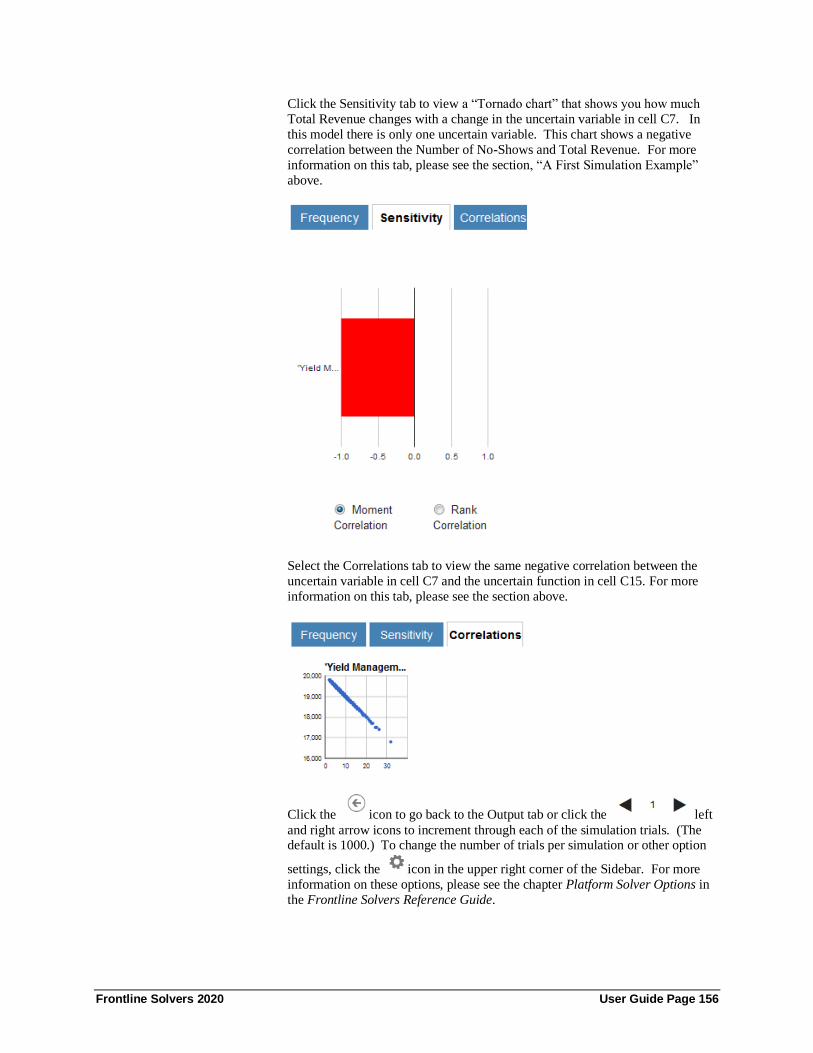
Frontline Solvers 2020 User Guide Page 156
Click the Sensitivity tab to view a “Tornado chart” that shows you how much
Total Revenue changes with a change in the uncertain variable in cell C7. In
this model there is only one uncertain variable. This chart shows a negative
correlation between the Number of No-Shows and Total Revenue. For more
information on this tab, please see the section, “A First Simulation Example”
above.
Select the Correlations tab to view the same negative correlation between the
uncertain variable in cell C7 and the uncertain function in cell C15. For more
information on this tab, please see the section above.
Click the icon to go back to the Output tab or click the left
and right arrow icons to increment through each of the simulation trials. (The default is 1000.) To change the number of trials per simulation or other option
settings, click the icon in the upper right corner of the Sidebar. For more
information on these options, please see the chapter Platform Solver Options in
the Frontline Solvers Reference Guide.

Frontline Solvers 2020 User Guide Page 157
Now let’s Publish this same model to Excel Online. Let’s go back to Excel and
YieldManagement1.xls. Afterwards, click Publish – Unpublish. Immediately,
all PsiFunctions are restored in cells C7 and C16.
Click Publish – Publish again, but this time select Excel Online, then click
Publish.
Click File – Save As and save this file as YieldManagement1.xlsx on your
SharePoint or Office 365 site.
Note: In order to use the Risk Solver App, your file must be saved on
SharePoint or Office 365 site. This app cannot solve models saved on your
local hard drive.
Open the workbook using Excel Online, then click Edit Workbook – Edit in
Excel Online.

Frontline Solvers 2020 User Guide Page 158
Click Insert – Apps for Office.
Select the Store tab and search for Risk Solver, then select (1st app in the list) and Install. Note: A Premium Solver app which solves linear models with more
than 200 variables and nonlinear models with more than 200 variables and 200
constraints is available for purchase. Please contact Frontline Systems for more
information at [email protected].
The Risk Solver App task pane opens on the right of your screen.
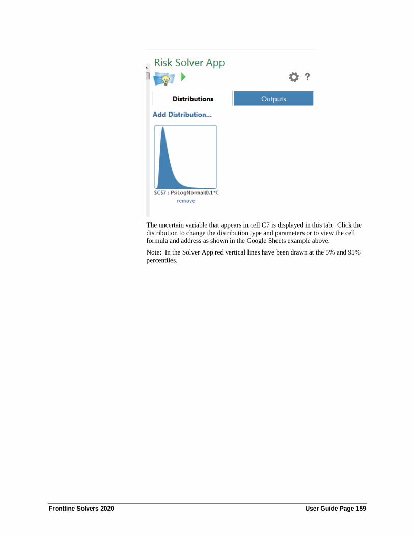
Frontline Solvers 2020 User Guide Page 159
The uncertain variable that appears in cell C7 is displayed in this tab. Click the
distribution to change the distribution type and parameters or to view the cell
formula and address as shown in the Google Sheets example above.
Note: In the Solver App red vertical lines have been drawn at the 5% and 95%
percentiles.

Frontline Solvers 2020 User Guide Page 160
Click the green arrow at the top of the task pane to run a simulation. (Click the
Cancel button to stop the simulation before finishing.) If running for the first
time, you will be asked to “Trust” the app.
To cancel the simulation before completion, click Cancel.

Frontline Solvers 2020 User Guide Page 161
In the sidebar, the Output tab appears with a small frequency chart containing
the uncertain function in cell C15. Click the chart to enlarge it. Click the
Frequency tab to view statistics (mean, standard deviation, variance, skewness,
kurtosis, mode, minimum, maximum, and range) or Percentiles (1 – 100). Click
the Sensitivity tab to view a “Tornado chart” which illustrates the negative
correlation between the Number of no-shows (uncertain variables) and Total
Revenue (uncertain function) and the Correlations tab to view the relationship
between the uncertain variable in cell C7 and the uncertain function in cell C15
as a scatter chart. For more information on either of these tabs, please see the
Google Sheets example above.
Click the icon to go back to the Output tab or click the left
and right arrow icons to increment through each of the simulation trials. (The
default is 1000.) To change the number of trials per simulation or other option
settings, click the icon in the upper right corner of the Task Pane. For more
information on these options, please see the chapter Platform Solver Options in
the Frontline Solvers Reference Guide.

Frontline Solvers 2020 User Guide Page 162
Examples: Stochastic Optimization
Introduction This chapter introduces stochastic optimization in Analytic Solver
Comprehensive (Desktop or Cloud) with a series of examples.
We use the term stochastic optimization to mean optimization of models that
include uncertainty, using any solution method. Analytic Solver offers an exceptional level of power to find robust optimal solutions to models with
uncertainty, using three different solution methods:
• Simulation optimization
• Stochastic programming
• Robust optimization
The first method, simulation optimization, is also available in Analytic Solver
Optimization with Analytic Solver Simulation, Analytic Solver Upgrade and
Analytic Solver Basic (Desktop or Cloud), and is the only method in other
software products such as Crystal Ball Professional and @RISK Industrial. It
handles very general models, but it is not scalable to large models (with thousands of variables and constraints), and it doesn’t support the important
modeling concept of recourse decisions.
Stochastic programming and robust optimization can be applied only to
linear and quadratic programming models with uncertainty, but they are scalable
to large models. Either Analytic Solver Comprehensive, Analytic Solver
Simulation with Analytic Solver Optimization, Analytic Solver Upgrade or
Analytic Solver Basic (Desktop or Cloud) are required to use these methods.
A Project Selection Model To open the examples, click Help – Examples on the ribbon. Click the
Stochastic link on the Overview tab to open the workbook
StochasticExamples.xls which includes three worksheets. In AnalyticSolver.com, click Help – Examples – Stochastic Optimization
Examples, then scroll down to the Stochastic Examples link.

Frontline Solvers 2020 User Guide Page 163
Click the Project Selection tab within the StochasticExamples.xls workbook to
open the first example, which may surprise you: It is a capital budgeting
problem, where the projects being considered for funding have uncertain future
cash flows. Models similar to Project Selection have been used with other
software products for many years to illustrate how simulation optimization can
be used to optimize models with uncertainty. We’ll show how to do this in
Analytic Solver Comprehensive, Analytic Solver Simulation with Analytic
Solver Optimization, Analytic Solver Upgrade, or Analytic Solver Basic, using simulation optimization and the Evolutionary Solver – with much better
performance. But when we use Analytic Solver to analyze the structure of this
model, we’ll see that this model doesn’t require simulation optimization at all.
We can solve this model in a fraction of a second – using the LP/Quadratic
Solver!
In Project Selection, eight different capital projects are proposed for funding.
Each one has a known initial investment. Each project has a 90% chance of
success, and if a project succeeds, it will have an uncertain (but positive) future
cash flow. Funding all eight projects would require a total initial investment of
$2.5 million, but our capital budget is only $1.5 million. Hence, we must
choose a subset of the projects to fund that will maximize our expected total future cash flow, while ensuring that our total initial investment doesn’t exceed
our $1.5 million budget.
Click the tab for the Projection Selection model, shown below.
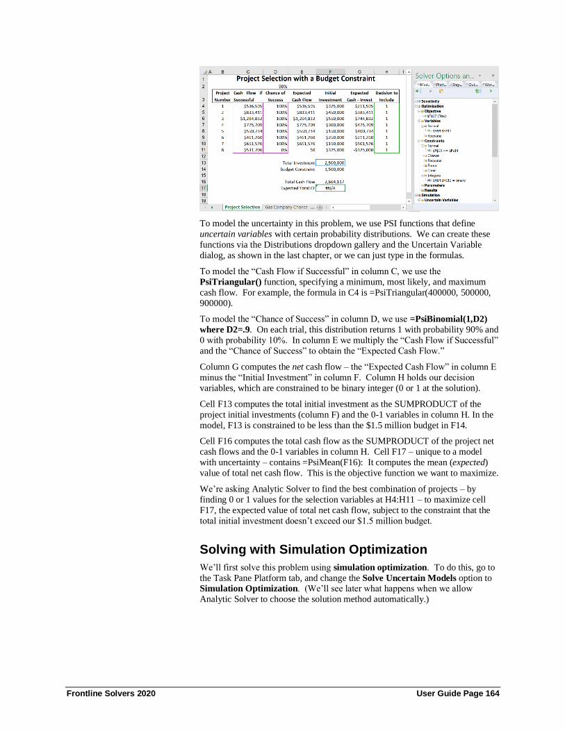
Frontline Solvers 2020 User Guide Page 164
To model the uncertainty in this problem, we use PSI functions that define
uncertain variables with certain probability distributions. We can create these
functions via the Distributions dropdown gallery and the Uncertain Variable
dialog, as shown in the last chapter, or we can just type in the formulas.
To model the “Cash Flow if Successful” in column C, we use the
PsiTriangular() function, specifying a minimum, most likely, and maximum
cash flow. For example, the formula in C4 is =PsiTriangular(400000, 500000,
900000).
To model the “Chance of Success” in column D, we use =PsiBinomial(1,D2)
where D2=.9. On each trial, this distribution returns 1 with probability 90% and
0 with probability 10%. In column E we multiply the “Cash Flow if Successful”
and the “Chance of Success” to obtain the “Expected Cash Flow.”
Column G computes the net cash flow – the “Expected Cash Flow” in column E
minus the “Initial Investment” in column F. Column H holds our decision
variables, which are constrained to be binary integer (0 or 1 at the solution).
Cell F13 computes the total initial investment as the SUMPRODUCT of the
project initial investments (column F) and the 0-1 variables in column H. In the
model, F13 is constrained to be less than the $1.5 million budget in F14.
Cell F16 computes the total cash flow as the SUMPRODUCT of the project net
cash flows and the 0-1 variables in column H. Cell F17 – unique to a model
with uncertainty – contains =PsiMean(F16): It computes the mean (expected)
value of total net cash flow. This is the objective function we want to maximize.
We’re asking Analytic Solver to find the best combination of projects – by
finding 0 or 1 values for the selection variables at H4:H11 – to maximize cell
F17, the expected value of total net cash flow, subject to the constraint that the
total initial investment doesn’t exceed our $1.5 million budget.
Solving with Simulation Optimization
We’ll first solve this problem using simulation optimization. To do this, go to
the Task Pane Platform tab, and change the Solve Uncertain Models option to Simulation Optimization. (We’ll see later what happens when we allow
Analytic Solver to choose the solution method automatically.)

Frontline Solvers 2020 User Guide Page 165
On the Engine tab, select the Evolutionary Solver from the dropdown list.
Why do we choose these settings? In the case of other software products, it’s
because simulation optimization is the only technology they have – and “if your
only tool is a hammer, every problem looks like a nail.” Simulation
optimization is also a very general approach that can handle nonlinear and non-
smooth functions, and it’s comparatively easy to understand.
The idea behind simulation optimization is straightforward: For each set of
values for the decision variables considered by the optimizer, we perform one
simulation, a compute user-specified summary measures – such as
=PsiMean(F16) in the Project Selection model – for the constraints and/or objective that depend on uncertainty. The optimizer uses these summary
measures to decide what set of values it should try next for the decision variables
– and the process is repeated.
The great strength of simulation optimization is its generality – but this is also
its weakness: It requires a new simulation at each step of the optimization, and
because the method assumes no structure in the model, in general the number of
steps can grow exponentially with the number of variables and constraints.
Now click the green arrow in the Task Pane to run a simulation. If you are using
Analytic Solver Desktop, after a second or two (much faster than other software
products), you can press ESC to stop the Evolutionary Solver and display the
best solution found so far – as shown on the next page.

Frontline Solvers 2020 User Guide Page 166
We’ve decided to fund projects #1, 3, 4, 5, and 7 for an expected total net cash
flow of $1,389,477. That’s a great result. But – how much work did we do to
solve this model, and did we need to do that much work? It might not matter for
a small model like this one – but for a ‘scaled-up’ model that might involve
hundreds or thousands of projects, the solution might have taken far more time.
Solving Automatically
Let’s allow Analytic Solver Comprehensive (or Analytic Solver Simulation with
Analytic Solver Optimization) to choose the solution method and the Solver
Engine automatically. To do this, go to the Task Pane Platform tab, and change the Solve Uncertain Models option to Automatic.
On the Engine tab, check the box to automatically select a Solver Engine in
Analytic Solver Deskop or select Automaticaly select engine at the top of the
menu for Analytic Solver Cloud or AnalyticSolver.com.
Analytic Solver Desktop
Analytic Solver Cloud
Now click the green arrow on the Task Pane. The results are shown on the next page.

Frontline Solvers 2020 User Guide Page 167
In a fraction of a second, a solution appears with the same objective value of
$1,389,477 and the same projects selected, with the message “Solver found a
solution. All constraints and optimality conditions are satisfied.” This means
that Analytic Solver found a proven globally optimal solution – whereas with
simulation optimization, we never know whether the solution we found is
optimal. How did this happen?
If you examine the solution log, you’ll see these messages:
---- Start Solve ----
Using: Full Reparse.
Parsing started...
Diagnosis started...
Warning: Canceled diagnostics *0 at 'Project Selection'!F16;
6 Canceled diagnostics found.
Uncertain input cells detected.
Attempting Stochastic Transformations...
Using: Full Reparse.
Parsing started...
Diagnosis started...
Convexity testing started...
Warning: Canceled diagnostics *0 at 'Project Selection'!F16;
22 Canceled diagnostics found.
Stochastic Transformation succeeded using Deterministic
Equivalent.
Transformed model is "LP/MIP".
Automatic engine selection: Standard LP/Quadratic
Model: [StochasticExamples.xlsx]Project Selection
Using: Psi Interpreter
Parse time: 0.66 Seconds.
Engine: Standard LP/Quadratic
Setup time: 0.01 Seconds.
Engine Solve time: 0.33 Seconds.
Solver found a solution. All constraints and optimality
conditions are satisfied.

Frontline Solvers 2020 User Guide Page 168
Solve time: 1.56 Seconds.
Analytic Solver Comprehensive analyzed the model and diagnosed it as a
Stochastic LP (linear programming) problem, with 8 variables, 2 functions
(objective and budget constraint), and 16 uncertainties (the PsiTriangular() and
PsiBinomial() functions) that affect the objective. As you’ll see in the chapter
“Mastering Simulation and Risk Analysis Topics,” Analytic Solver can solve a
Stochastic LP using two other methods besides simulation optimization –
stochastic programming and robust optimization. For this model, it chose a
transformation to Stochastic Programming Deterministic Equivalent form.
But this model is so simple that Analytic Solver determined that no
transformations were needed to solve the problem. Despite the presence of
uncertainty, this model doesn’t require simulation optimization at all. There
was no need to run hundreds of Monte Carlo simulations (or many more, with
some alternative software products). It was sufficient to run one Monte Carlo
simulation at the beginning, to compute the constant linear coefficients of the
objective function. Project Selection is simply an LP/MIP (linear mixed-integer
programming) model!
In this small model, we found the same solution within seconds using both
methods. But in a ‘scaled-up’ model in a large company, with hundreds or even thousands of projects, Analytic Solver’s ability to analyze the structure of the
model could make all the difference – between a solution of unknown quality,
found after a long wait using the wrong approach – and a proven optimal
solution, found within seconds using the right approach.
A Model with Chance Constraints The worksheets Gas Company Chance and Gas Company Recourse in
StochasticExamples.xls are related – they both describe the same problem, but
with different assumptions about when a certain decision must be made. With
Gas Company Chance, we’ll show how a problem with uncertainty can be
formulated with a chance constraint and solved using robust optimization
methods. With Gas Company Recourse, we’ll show how to use a “wait and see” or recourse decision – a capability not available at all with simulation
optimization – to obtain a better optimal solution.
We hope these examples will motivate you to read the chapter “Mastering
Simulation and Risk Analysis Topics,” which will give you a unified view of the crucial characteristics of models with uncertainty, and the options of solving
them with simulation optimization, stochastic programming, and robust
optimization methods.
Click the Gas Company Chance tab to display the model, which is pictured on
the next page.
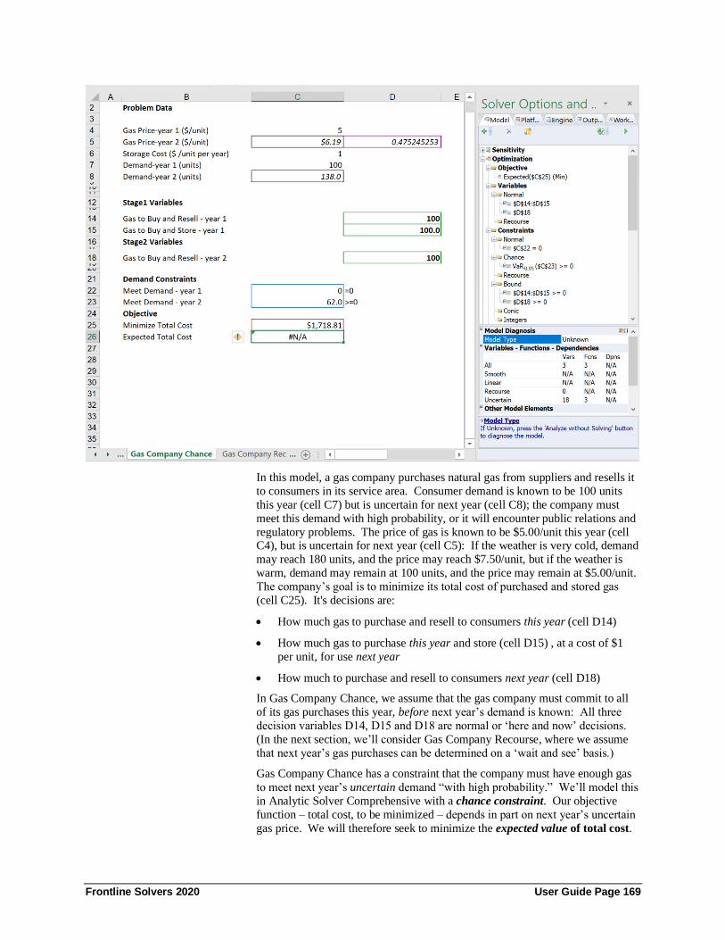
Frontline Solvers 2020 User Guide Page 169
In this model, a gas company purchases natural gas from suppliers and resells it
to consumers in its service area. Consumer demand is known to be 100 units
this year (cell C7) but is uncertain for next year (cell C8); the company must
meet this demand with high probability, or it will encounter public relations and
regulatory problems. The price of gas is known to be $5.00/unit this year (cell C4), but is uncertain for next year (cell C5): If the weather is very cold, demand
may reach 180 units, and the price may reach $7.50/unit, but if the weather is
warm, demand may remain at 100 units, and the price may remain at $5.00/unit.
The company’s goal is to minimize its total cost of purchased and stored gas
(cell C25). It's decisions are:
• How much gas to purchase and resell to consumers this year (cell D14)
• How much gas to purchase this year and store (cell D15) , at a cost of $1
per unit, for use next year
• How much to purchase and resell to consumers next year (cell D18)
In Gas Company Chance, we assume that the gas company must commit to all
of its gas purchases this year, before next year’s demand is known: All three
decision variables D14, D15 and D18 are normal or ‘here and now’ decisions.
(In the next section, we’ll consider Gas Company Recourse, where we assume
that next year’s gas purchases can be determined on a ‘wait and see’ basis.)
Gas Company Chance has a constraint that the company must have enough gas
to meet next year’s uncertain demand “with high probability.” We’ll model this
in Analytic Solver Comprehensive with a chance constraint. Our objective
function – total cost, to be minimized – depends in part on next year’s uncertain
gas price. We will therefore seek to minimize the expected value of total cost.

Frontline Solvers 2020 User Guide Page 170
The objective appears as “Expected($C$25) (Min)” – in Gas Company Chance,
we used the Ribbon to define the objective interactively, rather than a PsiMean()
function on the worksheet, as we did earlier in Project Selection. The decision
variables are cells D14, D15 and D18, as explained earlier; each of these is
constrained to be non-negative, as shown in the Bound section of the outline.
At C22 we calculate =D14-C7 (this year’s gas purchases minus this year’s
demand), and at C23 we calculate =D15+D18-C8 (gas purchased and stored this
year, plus gas purchased next year, minus next year’s uncertain demand).
The normal constraint $C$22 = 0 specifies that we must meet this year’s
consumer demand exactly (forcing D14 to 100). The chance constraint
VaR0.95($C$23) >= 0 requires that the 95th percentile of C23, over all
realizations of the uncertainty, must be non-negative – in other words, we must
meet demand with 95% probability.
We could express this chance constraint by placing =PsiPercentile(D15+D18-
C8,0.95) in cell C23, and using the Ribbon to define a normal constraint C23 >= 0. But while PsiPercentile and other PSI Statistics functions are acceptable for
simulation optimization, the transformation for robust optimization requires that
we express the chance property directly in the constraint itself, not in a formula.
Solving with Robust Optimization
We could solve this model using simulation optimization, as we did for Project
Selection in the previous section. But here, we want to show how Analytic
Solver Comprehensive (or Analytic Solver Simulation with Analytic Solver
Optimization) can automatically transform this stochastic linear programming
problem – with its expected value objective and chance constraint – into a larger
conventional optimization model, using the methods of robust optimization.
The idea behind robust optimization is to transform an optimization problem
with known structure – such as a stochastic linear programming problem – into
a larger, conventional ‘robust counterpart’ problem that accounts for the impact
of bounded uncertainty on the constraints and objective. Analytic Solver
performs one simulation at the outset, to assess the impact of uncertainty and construct the robust counterpart problem. Solving the robust counterpart – a
single LP or SOCP problem – gives us an approximate solution to the original
stochastic problem.
The strength of robust optimization is its scalability to very large problems –
since only one simulation and one optimization of an LP or SOCP problem is
required. But robust optimization cannot solve more general nonlinear, non-
convex problems.
As saved, the model is ready to be solved using robust optimization. But to see
the difference between the original model – a stochastic linear programming
model – and the robust counterpart model that is the result of the transformation,
we’ll first set the Solve Uncertain Models option to Simulation Optimization:

Frontline Solvers 2020 User Guide Page 171
and then click Analyze – Analyze Transformed Model (on the Model tab) to
analyze the structure of the model. The Model Diagnosis section of the Task
Pane Model tab “pops up” to show the results, as shown below.
The model is diagnosed as a Stochastic LP, with 3 variables, 3 functions, and 1
uncertainty (the Beta distribution at cell D5, which models the weather). Now,
we’ll set the Solve Uncertain Models option to Automatic:
and click the Analyze – Analyze Transformed model again – this will analyze
the structure of the transformed robust counterpart model.

Frontline Solvers 2020 User Guide Page 172
The transformed model has 9 variables and 8 functions (instead of 3 and 3), but
it has 0 uncertainties – it’s a conventional linear programming model. Solving
this robust counterpart model will give us an approximate (and somewhat
conservative) solution to the original stochastic LP problem.
Technical note, explained in the chapter “Mastering Simulation and Risk
Analysis Topics:” The robust counterpart model is an LP because the Platform
tab Chance Constraints Use option is set to D Norm. If it had been set to L2
Norm, the robust counterpart model would have been an SOCP.
Now click the green arrow on the Task Pane. In a fraction of a second, the
solution appears, with the message “Solver found a conservative solution to the
robust chance constrained problem. All constraints are satisfied.” You can
click this message to display Help with a more complete explanation of what
this means. To resolve the formula in cell C26, click the Simulate icon to run a
simulation. The results are shown below.
We run one simulation to see the expected value of the objective, which is about $1,509,
lower than the initial value of $1,693. But our chance constraint is not only satisfied but

Frontline Solvers 2020 User Guide Page 173
over-satisfied – we meet consumer demand about 99% of the time, when we asked for
only 95%. This solution is more conservative than necessary.
But Analytic Solver Comprehensive within Analytic Solver Desktop can automatically
improve this solution, by adjusting the size of the uncertainty set for the chance
constraint. To do this, click the special button to “Auto Adjust Chance Constraints”
that appears at the top of the Task Pane. After a moment, a new solution appears with the
message “Solver has converged to the current solution of the robust chance constrained
problem. All constraints are satisfied.” To resolve cell C26, double click cell C25 and
click "Yes" to run a simulation.
To find this same solution in Analytic Solver Cloud, click the Platform tab and set Auto
Adjust Chance Constraints to True and then resolve by clicking the green arrow on the
Model tab. To resolve cell C26, click the Simulation button to run a simulation.
The results are shown on the next page.
We run one simulation to see the expected value of the objective, which is about $1,447.
As noted earlier, this very simple model could have been solved via simulation
optimization; but with robust optimization, we can scale up a model like this one to large
size, and solve it efficiently using the LP/Quadratic Solver, or any of several large-scale
Solver Engines.
A Model with Recourse Decisions We now have a good solution to the Gas Company problem, found with either
simulation optimization or robust optimization. But we can do better than this –
we can reduce our expected total cost to $1,276, a significant improvement.
We can do this provided that the business situation permits us to make the decision of how much gas to purchase next year on a ‘wait and see’ basis, after
the uncertainty of the weather is resolved – a so-called recourse decision. In
this example, our gas supplier must accept our purchase order next year, and not
require us to commit to a specific amount of gas this year for delivery next year.
One of the most important messages we can convey is this: If the business
situation permits you to make some decisions on a ‘wait and see’ basis, it’s

Frontline Solvers 2020 User Guide Page 174
crucial to include this in your optimization model. If you don’t do this, you
may find an optimal solution to the wrong model for the actual business
problem.
We emphasize this because so many people have built models that don’t include
‘wait and see’ decisions, because (i) they haven’t learned this concept and (ii)
their software hasn’t allowed them to create models with recourse decisions.
Simulation optimization is very popular, but as described in the technical
literature and implemented in software, it has no concept of recourse decisions.
In the next example, Gas Company Recourse, we’ll assume that our decision of
how much gas to purchase next year can be made on a ‘wait and see’ basis, after
the uncertainty of the weather has been resolved. Click the Gas Company
Recourse tab to display the model, which is pictured on the next page.
This model has the same objective (C25), the same decision variables (D14, D15
and D18), and the same constraints (C22 and C23) as in EXAMPLE2. It differs in just two ways: (i) Cell D18 – the amount of gas to purchase next year –
appears as a recourse decision variable. (ii) Cell C23 is no longer a chance
constraint – it is a normal constraint, and in fact it’s = rather than >= – we
expect to satisfy next year’s consumer demand exactly. The recourse decision
variable allows us to do this – in each possible future scenario, once the weather
uncertainty is resolved and consumer demand is known, we will purchase just
the amount of gas we need to meet demand.
Solving with Robust Optimization
We cannot solve Gas Company Recourse with simulation optimization,
since this method has no concept of recourse decisions. But we can use robust
optimization methods to transform and solve Gas Company Recourse, much as we did with Gas Company Chance. We can proceed in much the same way. If
we analyze the structure of the original model (by clicking Analyze – Analyze
Transformed Model with the Solve Uncertain Models option set to Simulation
Optimization), we find that it is a stochastic LP:
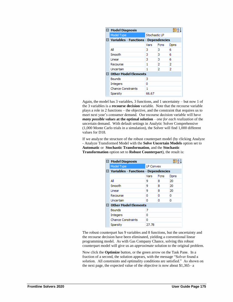
Frontline Solvers 2020 User Guide Page 175
Again, the model has 3 variables, 3 functions, and 1 uncertainty – but now 1 of
the 3 variables is a recourse decision variable. Note that the recourse variable
plays a role in 2 functions – the objective, and the constraint that requires us to
meet next year’s consumer demand. Our recourse decision variable will have
many possible values at the optimal solution – one for each realization of the
uncertain demand. With default settings in Analytic Solver Comprehensive
(1,000 Monte Carlo trials in a simulation), the Solver will find 1,000 different
values for D18.
If we analyze the structure of the robust counterpart model (by clicking Analyze - Analyze Transformed Model with the Solve Uncertain Models option set to
Automatic or Stochastic Transformation, and the Stochastic
Transformation option set to Robust Counterpart), the result is:
The robust counterpart has 9 variables and 8 functions, but the uncertainty and
the recourse decision have been eliminated, yielding a conventional linear
programming model. As with Gas Company Chance, solving this robust
counterpart model will give us an approximate solution to the original problem.
Now click the Optimize button, or the green arrow on the Task Pane. In a
fraction of a second, the solution appears, with the message “Solver found a
solution. All constraints and optimality conditions are satisfied.” As shown on
the next page, the expected value of the objective is now about $1,365– a
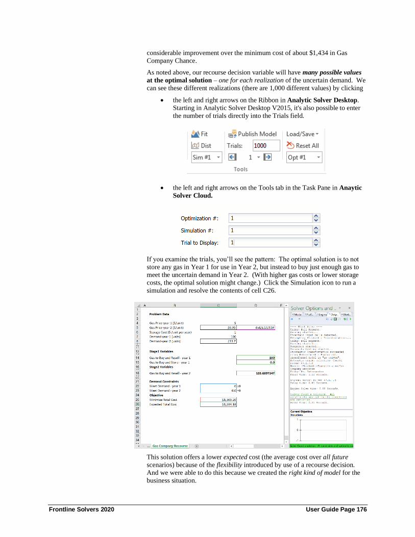
Frontline Solvers 2020 User Guide Page 176
considerable improvement over the minimum cost of about $1,434 in Gas
Company Chance.
As noted above, our recourse decision variable will have many possible values
at the optimal solution – one for each realization of the uncertain demand. We
can see these different realizations (there are 1,000 different values) by clicking
• the left and right arrows on the Ribbon in Analytic Solver Desktop.
Starting in Analytic Solver Desktop V2015, it's also possible to enter
the number of trials directly into the Trials field.
• the left and right arrows on the Tools tab in the Task Pane in Anaytic
Solver Cloud.
If you examine the trials, you’ll see the pattern: The optimal solution is to not
store any gas in Year 1 for use in Year 2, but instead to buy just enough gas to
meet the uncertain demand in Year 2. (With higher gas costs or lower storage
costs, the optimal solution might change.) Click the Simulation icon to run a
simulation and resolve the contents of cell C26.
This solution offers a lower expected cost (the average cost over all future
scenarios) because of the flexibility introduced by use of a recourse decision.
And we were able to do this because we created the right kind of model for the
business situation.

Frontline Solvers 2020 User Guide Page 177
The ‘moral of this story’ is that Analytic Solver Comprehensive (Desktop or
Cloud) gives you the power to solve such problems, using three different
technologies – simulation optimization, stochastic programming, and robust
optimization. But it’s up to you to take advantage of the concept of recourse
decisions – when they can be used – and create the right kind of model for your company’s business situation.

Frontline Solvers 2020 User Guide Page 178
Creating Your Own Application
Introduction When using Analytic Solver you have the ability to not only create, design and
solve your optimization, simulation and stochastic optimization models in
Microsoft Excel, but also have the ability to embed your model into your own
application and solve it on the Web by calling our RASON Server.
RASON (which stands for Restful Analytic Solver Object Notation) is Frontline
Systems' modeling language embedded in JSON and a REST API that makes it
easy to create, test and deploy analytic models using optimization, simulation and data mining, in web and mobile applications.
Users of Frontline's Excel Solvers will find that it's easy to translate Excel
models into RASON models, that your knowledge of Excel formulas and
functions is immediately usable, but that RASON models can be more flexibly
"bound" to data from a variety of sources.
When you click the newly added Create App icon located on the Analytic Solver
ribbon, your existing Excel model will be automatically converted to a mobile
application written in JavaScript. Web App Developers will be able to
immediately find how exceptionally easy it is to embed RASON models as
JSON and solve them using Frontline's RASON server, which exposes a simple
REST API that's scalable to handle very large, compute-intensive analytic models. Months of work, that would have previously been required, have been
reduced to a single command button click!
The Create App Icon When you click the Create App icon on the Analytic Solver ribbon, a drop down
menu appears with four items:
• RASON IDE (Not supported in Analytic Solver Cloud)
• RASON.com
• Web Page
• Power BI
• Tableau
Clicking the first menu item in Analytic Solver Desktop (only) opens the
RASON Desk IDE. Clicking the second menu item in either Analytic Solver
Desktop or Cloud, automatically opens the RASON Web IDE (located on
www.rason.com). Both menu items will open the corresponding IDE containing
your existing Excel model converted into the RASON modeling language.
From here, you simply need to click the appropriate button to solve the
optimization model or run a simulation.
When solving with the RASON IDE in Analytic Solver Desktop, the Solver
SDK Platform (installed along with Analytic Solver) will be called to solve the model. When using RASON.com, the RASON Server will be called to solve the
model. See the labeled screenshots below. Each contain the Product Mix

Frontline Solvers 2020 User Guide Page 179
model, discussed in the earlier Conventional Optimization chapter, written in the
RASON modeling language.
RASON Desk IDE
RASON Web IDE
Clicking the third menu item, Web Page, will result in the creation of a web
application written in JavaScript that solves your existing Excel model.

Frontline Solvers 2020 User Guide Page 180
Follow the steps below to convert an optimization and simulation model into a
RASON model solved in both the Desk IDE (Analytic Solver Desktop only) and
the Web IDE and publish a Web App, in seconds.
NOTE: New in V2019, when creating a RASON model through desktop Analytic
Solver or AnalyticSolver.com, model elements (objective function, decision
variables, constraints, uncertain variables and/or uncertain functions) may now appear on multiple worksheets within the same Excel workbook.
Clicking the fourth option, Power BI, gives you the ability to turn your Excel-
based optimization or simulation model into a Microsoft Power BI Custom
Visual. First, you simply select rows or columns of data to serve as changeable
parameters, next, you select Create App – Power BI, and thirdly, you save the
file created by Analytic Solver. Afterwards, you click the Load Custom Visual
icon in Power BI and select the file you just saved. What you get isn’t just a
chart – it’s your full optimization or simulation model, ready to accept Power BI
data, run on demand on the web, and display visual results in Power BI! You
simply need to drag and drop appropriate Power BI datasets into the “well” of
inputs to match your model parameters. This is possible because Analytic Solver translates your Excel model into RASON® then “wraps” a JavaScript-
based Custom Visual around the RASON model. For more information on this
feature, see the next chapter “Creating Power BI Custom Visuals”.
The last option on the Create App menu, Tableau, allows you to turn your
Excel-based optimization or simulation model into a Tableau Dashboard
Extension. You simply select rows or columns of data to serve as changeable
parameters, then choose Create App – Tableau, and save the file created by
Analytic Solver. In Tableau, you’ll see the newly-created file under Extensions
on the left side of the dashboard, where you can drag it onto your dashboard.
You’ll be prompted to match the parameters your model needs, with data in
Tableau. Much like with Power BI, what you get isn’t just a chart – it’s your full optimization or simulation model, ready to accept Tableau data, run on
demand (using our RASON server), and display visual results in Tableau!
Note: This feature works (only) with Tableau version 2018.2 or later. For more

Frontline Solvers 2020 User Guide Page 181
information on this feature, see the chapter “Creating Custom Extensions in
Tableau”.
Solving a Model Using the RASON Desk IDE In Analytic Solver Desktop, open the Product Mix(RASON).xlsx model by
clicking Help – Examples on the ribbon, clicking Optimization Examples and then the Product Mix RASON link. A similar version of this model was
previously discussed in the Conventional Optimization chapter. Recall this
example model determines the optimal mix of products that a company should
produce in order to maximize profits.
The optimization model is included in the Model tab in the Solver Task Pane.
This model written in algebraic form is below.
Maximize: Total Profit = $75x1 + $50x2 + $35x3
Subject To:
Chassis: 1x1 + 1x2 + 0x3 <= 450
LCD Screen: 1x1 + 0x2 + 0x3 <= 250
Speaker: 2x1 + 2x2 + 1x3
Power Supply: 1x1 + 1x2 + 0x3
Electronics: 2x2 + 1x2 + 1x3
x1, x2, x3 > 0
Click Create App on the ribbon, then select RASON IDE.
NOTE 1: There is no need to solve the model first unless a change has been
made to an already existing RASON model. If a change has been made to the
workbook after a RASON model has been created, then you MUST either solve
or diagnose the Excel model in order for the changes to be reflected in the new
RASON model.
NOTE 2: When creating a RASON model through desktop Analytic Solver or
AnalyticSolver.com, model elements (objective function and all variables and

Frontline Solvers 2020 User Guide Page 182
constraints) may now exist on multiple worksheets within the same Excel
workbook.
Immediately, the RASON Desk IDE is opened and the product mix model is
inserted into the model window.
A RASON model begins with an opening { and closes with a closing }. Within
the two braces, our model is made up of various "sections" – there are a total of
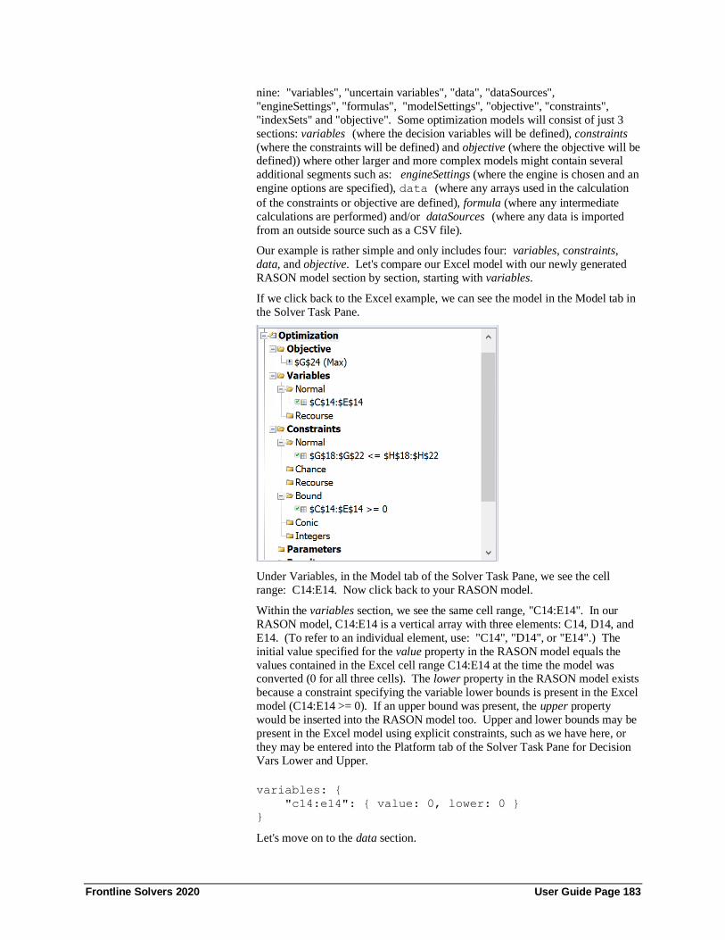
Frontline Solvers 2020 User Guide Page 183
nine: "variables", "uncertain variables", "data", "dataSources",
"engineSettings", "formulas", "modelSettings", "objective", "constraints",
"indexSets" and "objective". Some optimization models will consist of just 3
sections: variables (where the decision variables will be defined), constraints
(where the constraints will be defined) and objective (where the objective will be defined)) where other larger and more complex models might contain several
additional segments such as: engineSettings (where the engine is chosen and an
engine options are specified), data (where any arrays used in the calculation
of the constraints or objective are defined), formula (where any intermediate
calculations are performed) and/or dataSources (where any data is imported
from an outside source such as a CSV file).
Our example is rather simple and only includes four: variables, constraints,
data, and objective. Let's compare our Excel model with our newly generated
RASON model section by section, starting with variables.
If we click back to the Excel example, we can see the model in the Model tab in
the Solver Task Pane.
Under Variables, in the Model tab of the Solver Task Pane, we see the cell
range: C14:E14. Now click back to your RASON model.
Within the variables section, we see the same cell range, "C14:E14". In our
RASON model, C14:E14 is a vertical array with three elements: C14, D14, and
E14. (To refer to an individual element, use: "C14", "D14", or "E14".) The
initial value specified for the value property in the RASON model equals the
values contained in the Excel cell range C14:E14 at the time the model was converted (0 for all three cells). The lower property in the RASON model exists
because a constraint specifying the variable lower bounds is present in the Excel
model (C14:E14 >= 0). If an upper bound was present, the upper property
would be inserted into the RASON model too. Upper and lower bounds may be
present in the Excel model using explicit constraints, such as we have here, or
they may be entered into the Platform tab of the Solver Task Pane for Decision
Vars Lower and Upper.
variables: {
"c14:e14": { value: 0, lower: 0 }
}
Let's move on to the data section.

Frontline Solvers 2020 User Guide Page 184
The data is contained in the Excel model within the cell range: C18:E22
(constraint coefficients) and also C24:E24 (objective function coefficients).
The exact same values have been inserted into 6 vertical arrays containing three
elements each: C18:E18, C19:E19, C20:E20, C21:E21, C22:E22, and C24:E24.
Again, to refer to individual elements of, say, the c18:e18 array, use: c18, d18, or e18.
data: {
"c18:e18": { value: [[1, 1, 0]] },
"c19:e19": { value: [[1, 0, 0]] },
"c20:e20": { value: [[2, 2, 1]] },
"c21:e21": { value: [[1, 1, 0]] },
"c22:e22": { value: [[2, 1, 1]] },
"c24:e24": { value: [[75, 50, 35]] }
},
Click back to the Excel model. Under Constraints in the Model tab of the Solver
Task pane, we see the entry: G18:G22 <= H18:H22. If we inspect the first cell
in the range, G18, we find the formula: =SUMPRODUCT(C18:E18,
$C$14:$E$14) while H18=450. The other four cells, G19:G22, hold similar
formulas.
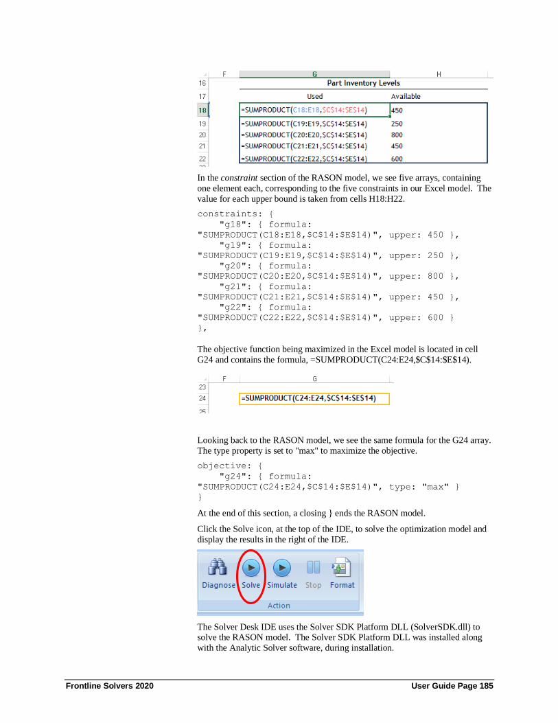
Frontline Solvers 2020 User Guide Page 185
In the constraint section of the RASON model, we see five arrays, containing
one element each, corresponding to the five constraints in our Excel model. The
value for each upper bound is taken from cells H18:H22.
constraints: {
"g18": { formula:
"SUMPRODUCT(C18:E18,$C$14:$E$14)", upper: 450 },
"g19": { formula:
"SUMPRODUCT(C19:E19,$C$14:$E$14)", upper: 250 },
"g20": { formula:
"SUMPRODUCT(C20:E20,$C$14:$E$14)", upper: 800 },
"g21": { formula:
"SUMPRODUCT(C21:E21,$C$14:$E$14)", upper: 450 },
"g22": { formula:
"SUMPRODUCT(C22:E22,$C$14:$E$14)", upper: 600 }
},
The objective function being maximized in the Excel model is located in cell
G24 and contains the formula, =SUMPRODUCT(C24:E24,$C$14:$E$14).
Looking back to the RASON model, we see the same formula for the G24 array.
The type property is set to "max" to maximize the objective.
objective: {
"g24": { formula:
"SUMPRODUCT(C24:E24,$C$14:$E$14)", type: "max" }
}
At the end of this section, a closing } ends the RASON model.
Click the Solve icon, at the top of the IDE, to solve the optimization model and
display the results in the right of the IDE.
The Solver Desk IDE uses the Solver SDK Platform DLL (SolverSDK.dll) to solve the RASON model. The Solver SDK Platform DLL was installed along
with the Analytic Solver software, during installation.

Frontline Solvers 2020 User Guide Page 186
The Solver SDK Platform DLL was able to find a solution to the model with an
objective equal to $25,000.
Now let's solve a simulation model. Click back to Help – Examples on the
ribbon, click Simulation Examples and then the Business Forecast link. Click
the Forecast with Uncertainty tab. Recall this example model from the
Simulation & Risk Analysis chapter which finds the True Average of a sales
forecast.
NOTE: When creating a RASON model through desktop Analytic Solver or AnalyticSolver.com, model elements (objective function, decision variables,
constraints, uncertain variables and/or uncertain functions) may now appear on
multiple worksheets within the same Excel workbook.
Click Create App – RASON IDE. The RASON Desk IDE opens displaying the
code for the converted simulation model.
Again, the RASON model opens with an opening {. Most simulation models
will be comprised of two components: uncertainVariables (where the uncertain variables are defined) and uncertainFunctions (where the uncertain functions
are defined). However, a simulation model could also contain additional
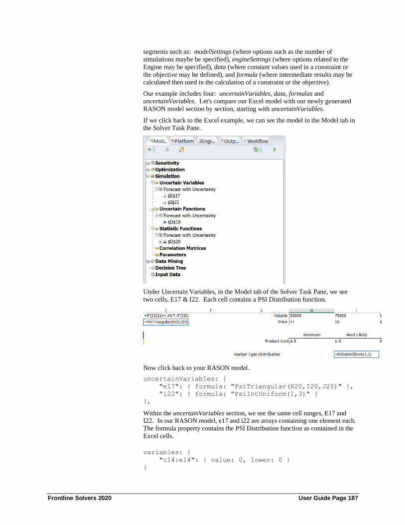
Frontline Solvers 2020 User Guide Page 187
segments such as: modelSettings (where options such as the number of
simulations maybe be specified), engineSettings (where options related to the
Engine may be specified), data (where constant values used in a constraint or
the objective may be defined), and formula (where intermediate results may be
calculated then used in the calculation of a constraint or the objective).
Our example includes four: uncertainVariables, data, formulas and
uncertainVariables. Let's compare our Excel model with our newly generated
RASON model section by section, starting with uncertainVariables.
If we click back to the Excel example, we can see the model in the Model tab in
the Solver Task Pane.
Under Uncertain Variables, in the Model tab of the Solver Task Pane, we see
two cells, E17 & I22. Each cell contains a PSI Distribution function.
Now click back to your RASON model.
uncertainVariables: {
"e17": { formula: "PsiTriangular(H20,I20,J20)" },
"i22": { formula: "PsiIntUniform(1,3)" }
},
Within the uncertainVariables section, we see the same cell ranges, E17 and I22. In our RASON model, e17 and i22 are arrays containing one element each.
The formula property contains the PSI Distribution function as contained in the
Excel cells.
variables: {
"c14:e14": { value: 0, lower: 0 }
}

Frontline Solvers 2020 User Guide Page 188
Let's move on to the data section.
The data is contained in the Excel model within the cell ranges: H16:J17 and
also H20:J20.
The exact same values have been inserted into 10 single element arrays: h20,
i20, j20, h17, i17, j17, h16, i16, j16, and d18. data: {
"h20": { value: 4.5 },
"i20": { value: 6.5 },
"j20": { value: 8.5 },
"h17": { value: 11 },
"i17": { value: 10 },
"j17": { value: 8 },
"h16": { value: 50000 },
"i16": { value: 75000 },
"j16": { value: 100000 },
"d18": { value: 120000 }
},
Within the RASON model, intermediate results contained in cells e16, d15, d16,
and d17 are calculated in the formulas section.
If you compare the cell formulas in Excel to the formula property in RASON,
you will find they match.
formulas: {
"e16": { formula: "IF($I$22=1,H17,IF($I$22=2,
I17, IF($I$22 = 3,J17)))" },
"d15": { formula: "IF($I$22=1,$H$16,IF($I$22=2,
$I$16, IF($I$22 = 3,$J$16 )))" },
"d16": { formula: "E16*D15" },
"d17": { formula: "E17*D15" }
},
In the last section, uncertainFunctions, we find the calculation of D19. In
Excel, the formula in cell D20 makes cell D19 an uncertain function using the
formula, =PSIMeanD19. In the previous chapter, Examples: Simulation & Risk
Analysis, we learned that whenever a PSI Statistic function (such as PsiMean,
PsiStdDev, etc.) is applied to a formula containing uncertainty, that cell will
become an uncertain function. Therefore, in the RASON model, the definition
for the uncertain function d19 contains the statistic property mean:[]. This
property will be returned in the solution.

Frontline Solvers 2020 User Guide Page 189
uncertainFunctions: {
"d19": { formula: "D16-D17-D18", mean: [] }
}
At the end of this section, a closing } ends the RASON model.
Click the Simulate icon, at the top of the IDE, to run a simulation and display
the results in the right of the IDE.
Solver SDK Platform was able to run a simulation and return the mean of the uncertain function, d19.
Now let's quickly run through one more example using a simulation
optimization model. Click back to Help – Examples on the ribbon, click
Simulation Optimization Examples and then the Yield Management Model 3
link to open YieldManagementModel3.xlsx. In this example, we will maximize
the expected revenue of a proposed flight. This model contains 1 integer
decision variable (number of tickets sold) and one uncertain variable. The
uncertain variable models the uncertainty of the number of no-shows.
NOTE: When creating a RASON model through desktop Analytic Solver or
AnalyticSolver.com, model elements (objective function, decision variables, constraints, uncertain variables and/or uncertain functions) may now appear on
multiple worksheets within the same Excel workbook.

Frontline Solvers 2020 User Guide Page 190
Click Create App – RASON IDE. The RASON Desk IDE opens displaying the
code for the converted simulation model.
Again, the RASON model opens with an opening {. Simulation optimization
models will contain at the very least, the following sections: variables (where
the decision variables will be defined), uncertainVariables (where the
uncertainty will be defined) and objective. Our simulation optimization
example includes three more: modelSettings, formulas and data. This
simulation model is unconstrained, meaning there are no constraints in the
model, only variable bounds. However, most simulation optimization models
will have at least one constraint. Let's compare our Excel model with our newly
generated RASON model section by section, starting with modelSettings.
Click back to the Excel model and then click the Platform tab on the Model Task pane.

Frontline Solvers 2020 User Guide Page 191
Within this pane, we see that Solve Uncertain Models is set to Simulation
Optimization, Simulations to Run equals 1 and Trials Per Simulation equals 1000. These settings will cause Solver to solve the model with the Evolutionary
Engine and simulation optimization using 1000 trials per simulation.
After the opening {, the first section of the RASON model is modelSettings. In
this section, options relevant to the solve, such as the number of optimizations or
simulations to run, the number of trials to perform in a simulation model, if
simulation optimization is to be used, etc., are specified. In this example, the
simulationOptimization property is set to "true", the Number of Trails to be
performed within the simulation is set to 1000 (numtrials: 1000) and the random
seed is set to 1 (randomSeed: 1). The random seed option is used so that our
results will be reproducible. Any option that is set on the Platform tab on the
Solver Task Pane will be recorded in this section. See the Frontline Solvers Reference Guide for a complete description of each option that may be specified
in modelSettings.
modelSettings : { simulationOptimization: true,
numTrials: 1000, randomSeed: 1 },
If we click back to the Excel example, we can see the model in the Model tab in the Solver Task Pane.

Frontline Solvers 2020 User Guide Page 192
Under Normal Variables, in the Model tab of the Solver Task Pane, we see the
Excel range, G30. Lower down, the same Excel range is listed as "integer"
under Integers. A little further up under Bound, we see the upper and lower
bound for this cell as 200 and 0, respectively. This means that the values in this
cell must be an integer greater than or equal to 0 and less than or equal to 200.
In the variables section of the RASON model, you'll see the following line of
code.
variables: {
"g31": { value: 117, type: "int", lower: 0,
upper: 200, finalValue: [] }
},
In these three lines of code, the single element array g31 is created and given an
initial value of 117 using the value property. (This is because cell G31 in the
Excel model contained that same value at the time of conversion.) The type
property indicates that the variable must be an "int" or "integer". The lower
property holds the lower bound of 0 and the upper property holds the upper
bound of 200. The finalValue property asks the RASON Server to return the
final value of this variable in the results.
Click back to Excel. Under Uncertain Variables, we see the Excel cell address, H25. If you inspect this cell, you will see that it contains the Psi Distribution
function PsiLogNormal. This function simulates the number of people who will
not show up or miss their flight.

Frontline Solvers 2020 User Guide Page 193
Within the uncertainVariables section, the single element array h26 is created
with the same formula that is contained in the Excel worksheet cell H25,
=PsiLogNormal(0.1 * G31, 0.06*G31).
uncertainVariables: {
"h26": { formula:
"PsiLogNormal(0.1*G31,0.06*G31)" }
},
Let's move on to the data section where we will define the data used in the
model.
In the Excel model, the data is contained in cells: G24 (Ticket Price), G25
(Flight Capacity), G28 (% Refund to No-shows) and G29 (Overbooking
Compensation).
The exact same values have been inserted into 4 single element arrays within the
data section of the RASON model.
data: {
"g24": { value: 200 },
"g28": { value: 0.5 },
"g29": { value: 1.25 },
"g25": { value: 100 }
},
The formulas section, within the RASON model, holds the intermediate
formulas contained in the Excel worksheet cells G26, G32, and G33.
Notice the formula properties for each of the four single element arrays matches
the formula in the matching Excel cell.

Frontline Solvers 2020 User Guide Page 194
formulas: {
"g26": { formula: "ROUND(H26,0)" },
"g32": { formula: "G31-G26" },
"g33": { formula: "MAX(0,G32-G25)" }
},
If you click back to the Excel worksheet, the objective is listed at the top of the
Model pane. "Max" which appears to the immediate right of the cell address
G37, indicates that the model is a maximization. The formula contained in cell
G37 = PsiMean(G35). This formula will return the mean value for the uncertain
function in cell G35. (See the screenshot above.)
In the RASON model, the single element array g37 holds the objective function
definition. As in the Excel model, the objective function will be maximized as indicated by the type property (type: "max").
objective: {
"g37": { formula: "PsiMean(G35)", type: "max" }
}
At the end, a closing } ends the RASON model.
Click the Solve icon, at the top of the IDE, to run an optimization simulation and
display the results in the right of the IDE.
Solver SDK Platform solves the simulation optimization model and returns the
mean of the objective function.
For more information on designing and writing a model in the RASON
Modeling Language, please see the RASON User Guide and/or RASON
Reference Guide.
Conversion Exceptions
There are several types of models that Frontline Excel Solvers are not able to
convert to RASON models. For example, it is not possible to convert NLP/NSP
models with conic constraints or Excel models containing errors such as #NUM,
#VALUE, etc. For all unsupported features, the conversion generator returns an
appropriate message.

Frontline Solvers 2020 User Guide Page 195
Problem Limits
Your Frontline Excel Solver license determines the size and type of model that
can be solved with the RASON Desk IDE. If you have a license for Analytic
Solver Comprehensive, then the same problem limits will apply when solving a
RASON model using the RASON Desk IDE, i.e. linear models with up to 8,000
variables (2,000 integers) and 8,000 constraints; smooth, nonlinear models with
up to 1,000 variables and 1,000 constraints; nonsmooth models with up to 1,000 variables and 1,000 constraints and SOCP models with up to 2,000 variables and
8,000 constraints.
Solving a Model Using the RASON Web IDE Now let's solve the same three models using the RASON Web IDE. Click back
to the Product Mix example, then click Create App – RASON.com.
NOTE: When creating a RASON model through desktop Analytic Solver or
AnalyticSolver.com, model elements (objective function, decision variables,
constraints, uncertain variables and/or uncertain functions) may now appear on
multiple worksheets within the same Excel workbook.
In a matter of seconds, a browser opens and navigates to the Web IDE on the
Try It page at www.RASON.com. The Product Mix model, now written in the
RASON modeling language, is displayed in the Model Editor.
Note on RASON Subscriptions
If you have already registered for an account on www.RASON.com, you will be automatically logged in using your existing credentials. If
you are a subscriber to a premium plan, you will be subject to the
problem limits of the purchased plan.
If you have not registered for an account on www.RASON.com, you
will be automatically registered for a free account and logged in using
information obtained from your registration on the Frontline Systems
website, www.Solver.com. Your User Name to log in to
www.RASON.com will be the same as your User Name for
www.solver.com and your default password will be: {your email
address} + !A123. You will be subject to the size limits of the free
Basic subscription, unless or until you subscribe to a higher level plan.
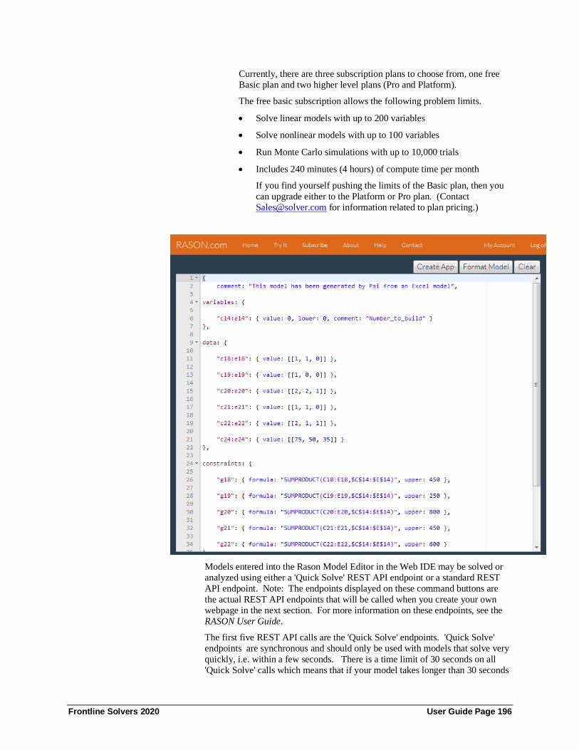
Frontline Solvers 2020 User Guide Page 196
Currently, there are three subscription plans to choose from, one free
Basic plan and two higher level plans (Pro and Platform).
The free basic subscription allows the following problem limits.
• Solve linear models with up to 200 variables
• Solve nonlinear models with up to 100 variables
• Run Monte Carlo simulations with up to 10,000 trials
• Includes 240 minutes (4 hours) of compute time per month
If you find yourself pushing the limits of the Basic plan, then you
can upgrade either to the Platform or Pro plan. (Contact
[email protected] for information related to plan pricing.)
Models entered into the Rason Model Editor in the Web IDE may be solved or
analyzed using either a 'Quick Solve' REST API endpoint or a standard REST
API endpoint. Note: The endpoints displayed on these command buttons are
the actual REST API endpoints that will be called when you create your own
webpage in the next section. For more information on these endpoints, see the
RASON User Guide.
The first five REST API calls are the 'Quick Solve' endpoints. 'Quick Solve'
endpoints are synchronous and should only be used with models that solve very
quickly, i.e. within a few seconds. There is a time limit of 30 seconds on all
'Quick Solve' calls which means that if your model takes longer than 30 seconds

Frontline Solvers 2020 User Guide Page 197
to solve, the RASON Server will return the result: "status" : { "code" : 10, "codeText" : "Stop chosen when the maximum time
limit was reached." }. In addition, the "model resource ID" for these
endpoints are not saved to the RASON server which means that a model
optimized, simulated, data mine, calculated or diagnosed with a 'Quick Solve'
endpoint cannot be saved, edited, retrieved or solved at a later time.
Select Optimize from the Quick Runs drop down menu to call the RASON
endpoint, POST rason.net/api/optimize.
The model is submitted to the RASON Server which solves the model and
returns the result in the Result window, shown above.
For all but the smallest / most quickly solved models, you'll need to use the
second set of REST API calls. You'll first need to make a call to the REST API endpoint POST rason.net/api/model which will create a "model resource". Then
you'll need to start an optimization via the REST API endpoint GET
rason.net/api/model/id/optimize. You can check on its progress at any time with
the REST API endpoint GET rason.net/api/model/id/status and obtain results
when finished with the REST API endpoint GET rason.net/api/model/id/result.
Submits a model to be optimized
to the queue and returns the
results when completed.
Submits a model to be diagnosed to the queue and returns the
results when completed.
Submits a simulation model
to the queue and returns the
results when completed. Submits a data mining or forecasting model to the queue
and returns the results when
completed.
Submits a decision table
model to the queue and
returns the results when
completed.

Frontline Solvers 2020 User Guide Page 198
Click to call the REST API endpoint POST
rason.net/api/model to post the model to the RASON Server. In return you will
receive a similar result.
Model submitted to location:
https://rason.net/api/model/2590+2019-05-15-20-33-31-
034142
Calling this endpoint creates the Model Resource, 2590+2019-05-15-20-33-31-
034142. We can now easily retrieve this model by clicking the down arrow next
to "Please select a model ID" and selecting this value from the menu.
Click to call the REST API endpoint GET
rason.net/api/model/id/optimize to optimize (or solve) the model . Since we did
not specify a specific engine, and we are solving a linear model, the
LP/Quadratic engine will be selected automatically.
Model has been placed in the queue to be optimized.
Call to call the REST API endpoint GET
Rason.net/api/model/id/status to obtain the status of the solve.
{"status": "Complete" }
Status: Complete means that the optimization has been completed. If the
optimization was still in-progress we would have received an incomplete status
with intermediate results, for example: {"status": "Incomplete", "Milliseconds" : -2147483648,"Iterations" : 0,
"Subproblems" : 287, "LocalSolutions" : 8,
"Objective" : 3849 }
Submits an optimization,
simulation, data mining or
decision table model to either be
solved or diagnosed into the
queue.
Click the down arrow to load a
previously saved RASON
model.
Returns all available model
resource ids. Saves the model and creates a
model resource ID that may be
retrieved at a later time.
Updates a previously saved
model. Retrieves the model associated
with the model ID.
Returns the status of the
optimization, simulation, or
simulation optimization.
Returns the result of a
completed optimization,
simulation, or simulation
optimization.
Stops the execution of a
previously submitted model. Deletes a previously saved model
Returns the contents of the
writeable data source.

Frontline Solvers 2020 User Guide Page 199
Click to call the REST API endpoint GET
rason.net/api/model/id/result to obtain the result of the optimization.
{
"status" : { "code" : 0, "codeText" : "Solver found a
solution. All constraints and optimality conditions
are satisfied." },
"objective" : {
"total" : { "finalValue" : 25000 }
}
}
The result "Solver found a solution. All constraints and optimality conditions
are satisfied" means that no other solution exists that is better than the solution found. (For more information on this and all possible Solver Result messages,
please see the RASON Reference Guide.) To maximize profit, we should make
200 TV sets, 200 stereos, and 0 speakers. The final objective value of 25,000 is
the maximum profit that we can attain.
Now let's solve the simulation model from the previous section. Click back to
Business Forecast example (on the BusinessForecastPsi tab), then click Create
App – RASON.com.
NOTE: When creating a RASON model through desktop Analytic Solver or
AnalyticSolver.com, model elements (objective function, decision variables,
constraints, uncertain variables and/or uncertain functions) may now appear on
multiple worksheets within the same Excel workbook.
In a matter of seconds, a browser opens and navigates to the Web IDE on the
Try It page at www.RASON.com. The Business Forecast model, now written in
the RASON modeling language, is displayed in the Model Editor.

Frontline Solvers 2020 User Guide Page 200
We can solve this model using either the Quick Solve method, by using the
Quick Solver endpoint POST rason.net/api/simulate, or by calling the REST API endpoints, POST rason.net/api/model which will create a "model resource".
Afterwards, we can run a simulation via the REST API endpoint GET
rason.net/api/model/id/simulate, check the progress of the simulation at any
time with the REST API endpoint GET rason.net/api/model/id/status and obtain
results when finished with the REST API endpoint GET
rason.net/api/model/id/result.
First, we will solve via the Quick Solve method. Simply click POST
rason.net/aip/simulate under Quick runs of small models.
The model is submitted to the RASON Server and the results are returned in the
Output window.
Now, we will solve using the alternative method. Click
to call the REST API endpoint POST
rason.net/api/model to post the model to the RASON Server. In return you will
receive a similar result in the output window.
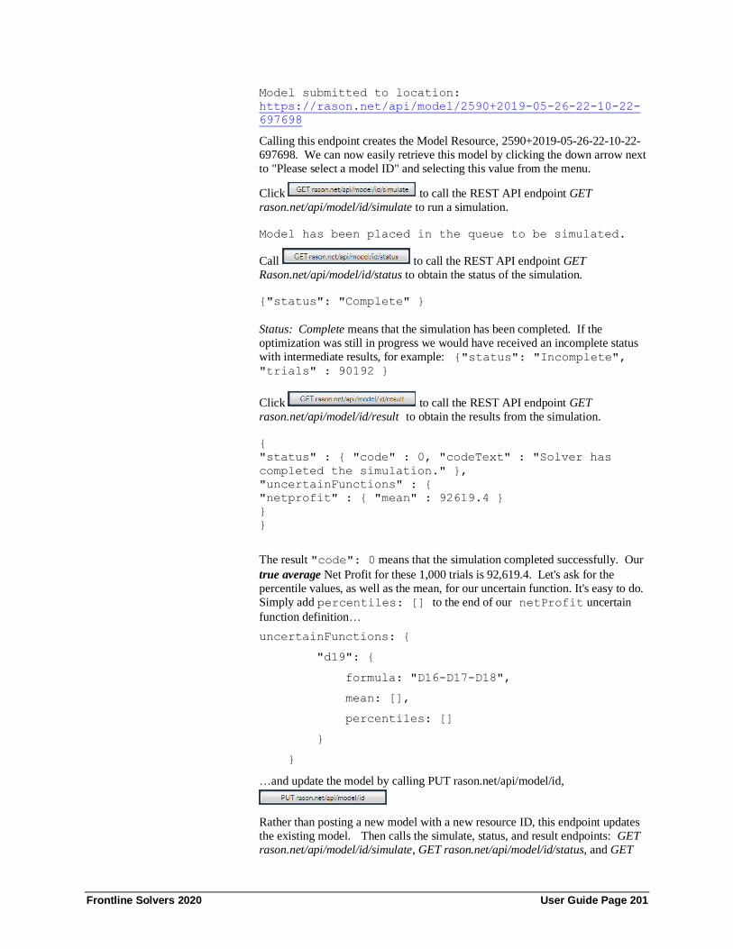
Frontline Solvers 2020 User Guide Page 201
Model submitted to location:
https://rason.net/api/model/2590+2019-05-26-22-10-22-
697698
Calling this endpoint creates the Model Resource, 2590+2019-05-26-22-10-22-
697698. We can now easily retrieve this model by clicking the down arrow next
to "Please select a model ID" and selecting this value from the menu.
Click to call the REST API endpoint GET
rason.net/api/model/id/simulate to run a simulation.
Model has been placed in the queue to be simulated.
Call to call the REST API endpoint GET
Rason.net/api/model/id/status to obtain the status of the simulation.
{"status": "Complete" }
Status: Complete means that the simulation has been completed. If the
optimization was still in progress we would have received an incomplete status
with intermediate results, for example: {"status": "Incomplete",
"trials" : 90192 }
Click to call the REST API endpoint GET
rason.net/api/model/id/result to obtain the results from the simulation.
{
"status" : { "code" : 0, "codeText" : "Solver has
completed the simulation." },
"uncertainFunctions" : {
"netprofit" : { "mean" : 92619.4 }
}
}
The result "code": 0 means that the simulation completed successfully. Our
true average Net Profit for these 1,000 trials is 92,619.4. Let's ask for the
percentile values, as well as the mean, for our uncertain function. It's easy to do.
Simply add percentiles: [] to the end of our netProfit uncertain
function definition…
uncertainFunctions: {
"d19": {
formula: "D16-D17-D18",
mean: [],
percentiles: []
}
}
…and update the model by calling PUT rason.net/api/model/id,
Rather than posting a new model with a new resource ID, this endpoint updates
the existing model. Then calls the simulate, status, and result endpoints: GET
rason.net/api/model/id/simulate, GET rason.net/api/model/id/status, and GET

Frontline Solvers 2020 User Guide Page 202
rason.net/api/model/id/result, respectively. The response from the call to GET
rason.net/API/Model/id/result is below.
{
"status" : { "code" : 0, "codeText" : "Solver has
completed the simulation." },
"uncertainFunctions" : {
"d19" : { "mean" : 92466.1, "percentiles" : [-118840,
-100391, -81334.3, -70724.2, -56747.6, -47834.3, -
40197.9, -32682, -24831.7, -18744.9, -11788.1, -
4115.7, 3307.15, 8315.06, 12122.9, 16532.8, 20759.9,
26048.7, 30466.5, 32783.8, 36265.2, 39119.5, 41986.6,
44494.7, 46610.2, 48617.1, 51235.5, 53433.6, 55426.9,
58206.9, 59982.7, 63790.1, 65192.6, 68161.3, 70423.9,
73774.1, 76082.1, 78690.2, 81592.3, 83482.2, 85839.8,
87874.8, 89193.1, 91678.2, 92688.5, 94500.3, 95305.2,
97737.5, 99549.8, 100662, 102015, 103733, 105426,
107313, 109452, 110920, 111992, 113645, 114718,
117848, 119716, 121420, 123089, 124623, 127574,
129610, 130882, 132028, 133942, 136053, 137770,
139250, 141293, 142686, 144987, 147803, 148731,
150397, 154362, 157480, 159889, 162513, 164131,
166126, 169100, 171524, 173488, 176816, 179111,
183990, 187680, 194224, 200666, 205383, 211525,
222330, 233473, 243391, 257954, 284032] }
}
}
Using the results from percentiles: []we see that we can lose money
12% of the time. See the 1st through 12th negative percentile values.
Finally, let's solve our last example, the simulation optimization model, Yield
Management 3. Click back to the example, then click Create App –
RASON.com. A browser opens and displays the model, converted to the RASON Modeling language, in the RASON Web IDE Model window.
NOTE: When creating a RASON model through desktop Analytic Solver or
AnalyticSolver.com, model elements (objective function, decision variables,
constraints, uncertain variables and/or uncertain functions) may now appear on
multiple worksheets within the same Excel workbook.
This time, let's diagnose the model first using the Diagnose Quick Solve
Endpoint: POST rason.net/api/diagnose.

Frontline Solvers 2020 User Guide Page 203
The model is diagnosed as a "simulation" model containing 1 integer variable, 1 function,
and 2 variable bounds, an upper and a lower.
Now, let's use the Quick Solve Optimize Endpoint to solve this model. Click the
optimize Quick Solver endpoint POST rason.net/api/optimize.
The simulation optimization was terminated after the 30 second solving limit
elapsed. The result shown in the Output window displays the result code, "Stop
chosen when the maximum time limit was reached" along with the intermediate
final variable value of 117.
Now let's solve using the RASON Rest API Endpoints. Click
to call the REST API endpoint POST
rason.net/api/model to post the model to the RASON Server. In return you will
receive a similar result in the output window.
Model submitted to location:
https://rason.net/api/model/2590+2019-10-14-19-27-12-
984092
Calling this endpoint creates the Model Resource, 2590+2019-10-14-19-27-12-
984092. We can now easily retrieve this model by clicking the down arrow next to "Please select a model ID" and selecting this value from the menu.
Click to call the REST API endpoint GET
rason.net/api/model/id/simulate to start the simulation optimization.

Frontline Solvers 2020 User Guide Page 204
Model has been placed in the queue to be optimized.
Call to call the REST API endpoint GET
Rason.net/api/model/id/status to obtain the status of the simulation optimization.
{"status": "Complete", "Milliseconds" :
31203,"Iterations" : 0, "Subproblems" : 22658,
"LocalSolutions" : 22656, "Objective" : 20620.15 }
Status: Complete means that the simulation optimization has been completed. If it was still in progress we would have received an incomplete status with
intermediate results like we saw with the Quick Solve endpoint.
Click to call the REST API endpoint GET
rason.net/api/model/id/result to obtain the results from the simulation
optimization.
Getting model results: GET
https://rason.net/api/model/2590+2020-02-26-23-10-38-
393105/result
{ "status": {
"code": 2,
"codeText": "Solver cannot improve the current
solution. All constraints are satisfied."
},
"variables": {
"g27": { "finalValue": 117 }
}
}
Creating a Web Page Analytic Solver includes the ability to bypass months of development work by
creating a web application that solves the optimization, simulation, and/or
simulation optimization model in Excel. Click back to Excel, and the Product
Mix example, then click Create App – Web Page.

Frontline Solvers 2020 User Guide Page 205
NOTE: When creating a RASON model through desktop Analytic Solver or
AnalyticSolver.com, model elements (objective function, decision variables,
constraints, uncertain variables and/or uncertain functions) may now appear on
multiple worksheets within the same Excel workbook.
Immediately, a browser opens displaying the newly created Web Application.
See Note on RASON Subscriptions in the section above for log in and
subscription information pertaining to solving models via the RASON Server.
Click Optimize.
Automatically, the model is submitted to the RASON Server using the RASON Rest API Endpoint POST rason.net/api/model, an optimization is started with
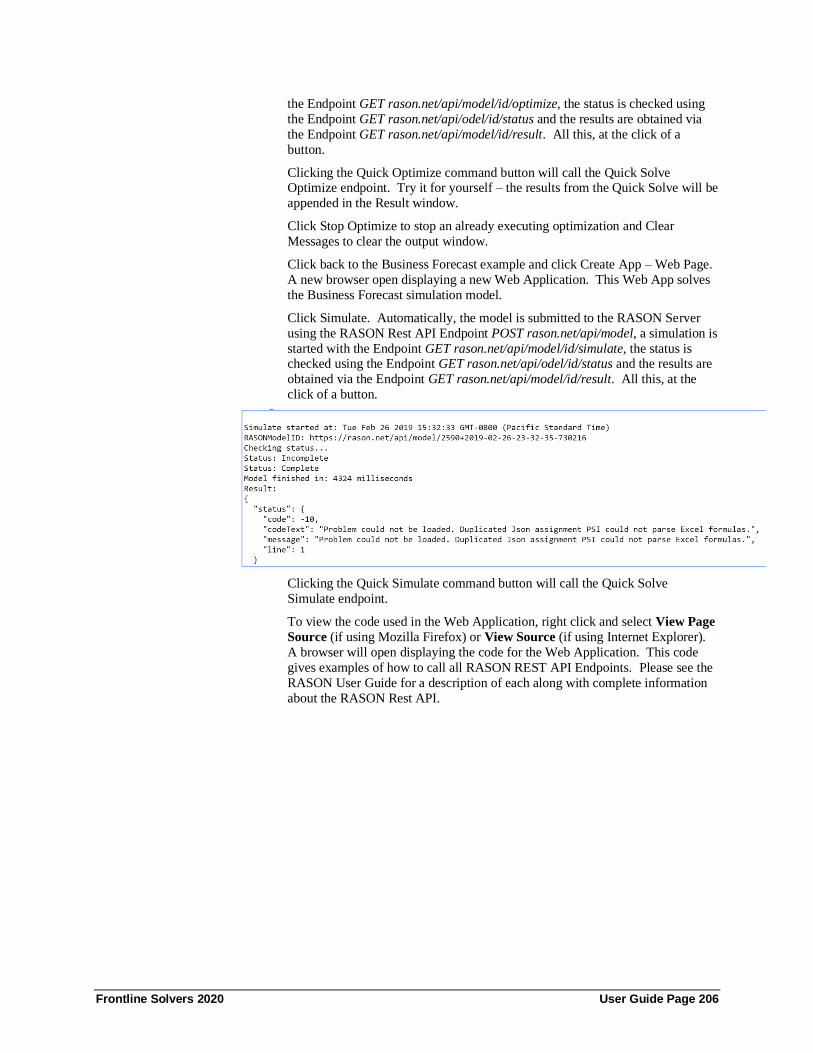
Frontline Solvers 2020 User Guide Page 206
the Endpoint GET rason.net/api/model/id/optimize, the status is checked using
the Endpoint GET rason.net/api/odel/id/status and the results are obtained via
the Endpoint GET rason.net/api/model/id/result. All this, at the click of a
button.
Clicking the Quick Optimize command button will call the Quick Solve Optimize endpoint. Try it for yourself – the results from the Quick Solve will be
appended in the Result window.
Click Stop Optimize to stop an already executing optimization and Clear
Messages to clear the output window.
Click back to the Business Forecast example and click Create App – Web Page.
A new browser open displaying a new Web Application. This Web App solves
the Business Forecast simulation model.
Click Simulate. Automatically, the model is submitted to the RASON Server
using the RASON Rest API Endpoint POST rason.net/api/model, a simulation is
started with the Endpoint GET rason.net/api/model/id/simulate, the status is checked using the Endpoint GET rason.net/api/odel/id/status and the results are
obtained via the Endpoint GET rason.net/api/model/id/result. All this, at the
click of a button.
Clicking the Quick Simulate command button will call the Quick Solve
Simulate endpoint.
To view the code used in the Web Application, right click and select View Page
Source (if using Mozilla Firefox) or View Source (if using Internet Explorer).
A browser will open displaying the code for the Web Application. This code
gives examples of how to call all RASON REST API Endpoints. Please see the
RASON User Guide for a description of each along with complete information
about the RASON Rest API.

Frontline Solvers 2020 User Guide Page 207

Frontline Solvers 2020 User Guide Page 208
Using Decision Tables
Introduction Decision Tables were introduced to Analytic Solver starting in V2019. A
decision table contains a set of rules which specify actions to perform based on
specific conditions. Decision tables are a good tool to use when there is a
consistent number of rules, or conditions, to be evaluated followed by a specific
set of actions to be performed once a rule, or condition, is met. For example,
the simple decision table below returns an employee's pay based on the number
of hours worked.
C+ hours pay
number 27,5,3,2
1 [1..40] 25*hours
2 >40 45*(hours – 40)
If the employee worked from 1 to 40 hours in a week, the pay is $25 * hour. If
any overtime is worked, the employee gets paid $45 an hour for any hour above 40.
In Analytic Solver, a decision table is a specific realization of a custom function.
A table has a name, input/output parameters and a body implementing the logic
through a structured framework. A decision table is invoked in the same way as
a VBA function when computing one or more output parameters for the passed
one or more input values. In Analytic Solver, a decision table is invoked using
the Psi function, PsiDecTable(). The modeling language inside of Analytic
Solver's Decision Table tool is S-FEEL extended to standard conversion
functions in FEEL. For more information on Decision Tables, we invite you to
reference the following: DMN Method and Style by Bruce Silver (Cody
Cassidy Press, September 28, 20180 and DMN Cookbook by Bruce Silver & Edson Tirelli (Cody-Cassidy Press, April 4, 2018).
Decision Table Structure Open the example model, DT Structure.xlsx by clicking Help – Examples –
Decision Trees/Decision Tables on the Ribbon. This table returns the number
of holidays apportioned to an employee based on his/her age and number of
years in service. This file defines the regions of the decision table as illustrated
in the screenshot below.

Frontline Solvers 2020 User Guide Page 209
A Decision Table is created using the newly introduced PsiDecTable() function
where the cell range of the table is passed as the first argument. See the PsiDecTable() function as it appears in cell J17,
=PsiDecTable(G7:K16,2,age,service,"holidays") where:
• G7:K16 - The cell address range of the table is G7:K16.
• 2 – The number of input variables
• age, service – input variables
• "holidays" – output
The steps required to create the decision table above are listed below.
Step 1: Enter a unique Name for the table immediately above the upper left corner of the table, to define the table. (This argument creates the decision table
object and identifies the table.) In this example, the table name is specified as
"Policy Output Order". When Excel generates the RASON Code, the name
component is used to identify this specific table.
Step 2: Enter a header, consisting of one or two rows, separated to the right
and below by a double horizontal line. The first row in the header is mandatory.
Two headers are contained in the table above, age, and service.
Step 3: Enter a Hit Policy, usually a capital letter or a name, entered in the
upper left cell of the table. The Hit policy specifies how the table will be
evaluated when multiple rules are applicable and hence, multiple output values
are returned. The entered value identifies the supported policies by a capital letter and an operator when applicable. You may enter the 1st letter of the policy
or the whole word. The currently supported Hit types and their meanings are:
Unique (U): A unique rule must "hit" evaluating to a unique result. If
multiple rules are "hit", an error will be returned.
Any (A): If rules overlap, but point to the same result, that unique
result is returned.
Priority(P): If multiple rules are "hit" and multiple results collected,
return only one result with the highest priority; the priorities are defined
by the order of the output values.
First (F): Only 1 result is returned for this policy. Once a rule is
evaluated successfully, or a hit occurs, the search stops.
Rule Order (R) - If multiple rules are hit, return the collection of
results as created in the rule order

Frontline Solvers 2020 User Guide Page 210
Output Order (O) – Currently entered value in cell G7. If multiple
rules are hit, return the collection of results in the priority order of the
listed output values.
Collect (C) – The same as (R). However, we may make this policy
more specific by adding an operator to it in order to allow aggregation.
Note: If aggregating a date, a scalar is returned. If using an operator,
output must not be a string, but only a numerical value.
C+ - sum the matched output values
C< - return the min of matched output values
C> - return the max of matched output values
C# - return the number of matched output values
Step 4: Enter Input Parameters in the 1st header row next to Hit policy and up
to the double vertical lines. The input parameter names are listed to the left of the double vertical line. In this example, age and service are the input
parameters. These input parameters belong to the local scope of this table.
Step 5: Enter Output Parameters in the 1st header row to the right side of the
double vertical lines. In this example, holidays and rule are the output
parameters. After calculation, a table returns a few selected or all output
parameter values in the form of a dynamic array. If a table has a single output or
a single output has been selected, the result will be a scalar value. These input
parameters belong to the local scope of this table
Step 6: (Optional) Enter the Input Values in the 2nd header row, to the left of
the double vertical line, beneath the input parameter to which they are releated.
Input Values may be a list of values separated by a commas (i.e. 27, 5, 3, 2), a list of unary tests (i.e. <10, >=20, [18..20]), or a data type (i.e. boolean, number,
text, data, time, and duration).
Data Types
Boolean: The entered words TRUE and FALSE are interpreted as
Boolean reserved words, not strings.
Number: Maybe an integer or fraction. This is the data type entered
in the example above.
Text: Any string
Date: Any valid date, such as 05-05-1964
Time: Any valid time
Duration: There are two formats for duration, one measuring periods
in months and another measuring periods in seconds. For example,
P1DT1H2M3S denotes:
• P for "period"
• 1D for 1 day
• T for "time"
• 1H for 1 hour
• 2M for 2 minutes and
• 3S for 3 seconds.

Frontline Solvers 2020 User Guide Page 211
When testing a value against a list of values or unary tests, the OR operator is
used. For example, in the first example above, the list of values is evaluated as
27 OR 5 OR 3 OR 2. Likewise, the list of unary tests is evaluated as <10 OR
>=20. It's possible to negate a list as well. For example, NOT(27, 5, 3, 2)
would result in a selection of a record that does not includes 27 OR 5 OR 3 OR 2. Similarly, NOT(<10, >=20) would equate to neither <10 OR >=20 being
selected.
All input entries in the relevant input column should cover the entered domain,
otherwise, an error will be generated indicating that the table is not complete. If
an input value does not exist, the completeness test is not performed.
Step 7: Enter Output values in the 2nd header row, to the right side of the
double vertical line, beneath the output parameter to which they are related.
Similar to Input Values, an Output value may be a list of values separated by a
commas (i.e. 27, 5, 3, 2), a list of unary tests (i.e. <10, >=20, [18..20]), or a data
type (i.e. boolean, number, text, data, time, and duration). Similarly, to an Input
values, if a value appears in the table that does not match the output value, an error will be returned.
In this example, the list "27, 5,3,2" is entered beneath "holidays" and "text" is
entered beneath "rule". The list beneath "holidays" gives the priority when
returning the results. In other words, the results are to be returned largest to
smallest. The output value, "text" specifies that the appropriate text contained
in cells K9:K16 is to be returned along with the holiday.
Step 8: Enter the Decision Table Rules (or Unary tests) in each row below the
double horizontal line. The unary test returns information (true or false) about
the rule. Supported unary tests may have one of the following syntax forms:
value(Boolean, number, text, date, time, duration), < value, > value, <= value, >= value, [value..value], (value..value], [value..value), (value..value), "-". Note:
Currently, rules may only be entered as rows.
The first test examines whether the value being tested is equal to the value inside
the parenthesis. For example, if the Unary test consists of the single value
'medium', the resulting test would ensure that the variable being tested was equal
to 'medium'. The forms, [value..value], (value..value], [value..value) and
(value..value), are interval tests. The [ ] operators denote a closed interval while
the ( ) operators denote an open interval. The last test, "-" returns TRUE against
any value. Note: To return a default value for a table, simply use "-" "-" for the
unary tests.
Expressions
Variables and constants can be combines through operations called literal
expressions. Literal expressions in S-FEEL are similar to formulas in Excel and
in the RASON modeling language.
The following operators are supported in combination with decision table rules:
addition (+), subtraction (-), multiplication (*), division (/) and exponentiation
(**). Variables and constants can be combined using only these supported operators and parentheses. An example of an expression is: 2 * age – service
where two variables, age and service, and a constant, 2, are linked by two
arithmetic operations (* and -). Note that an expression is a FEEL expression,
NOT an Excel formula. In this example, the expression "age – service" appears
in the first rule where "age" and "service" refer to cells H7 and I7. This
expression does not refer to any appearances of "age" or "service" outside of the
scope of this table. For more information on supported conversion expressions,
please see the Expressions heading at the end of this chapter.

Frontline Solvers 2020 User Guide Page 212
Step A: (Optional) Enter the Rule numbers in the first column
under the Hit policy starting with "1". Although optional, this
component of the table is strongly recommended.
Step B: Enter the Input entries in the input columns
Step C: Enter the Output entries in the output columns.
Decision Tables at Work The decision table contained within DT Structure.xlsx is shown below. This
table returns the number of vacation days allotted to an employee based on his
age and number of years in service. Notice cells H1:I2 at the top of the
screenshot below containing age and service in the first row and 58 and 31 in the
second. Cells H2 and I2 have been given the defined names (Insert – Name –
Define) of age and service, respectively. These are the input variables on which
the table depends. Each time the values of 58 and 31 are changed and a
recalculation is performed (by clicking the green arrow on the task pane), the decision table function (PsiDecTable) will return the appropriate computed
result in cell J17.
J17 = PsiDecTable(G7:K16, 2, age, service) where:
• G7:K16 is the location of the decision table on the Excel worksheet,
• 2 is the number of inputs, and
• Age and service are the two input variables. Alternative, we could
have specified the cell address (H2 and I2) or the values (58 and 31).
=PsiDecTable(G7:K16, 2, H2, I2) or =PsiDecTable(G7:K16, 2, 58, 31)
Two additional optional arguments are described below: output and ret_header.
The PsiDecTable() signature above includes only 2 input parameters, age and service. If using Excel 2019, the result will "spill" into 3 rows and 2 columns as
shown in the screenshot above starting with cell J17. In the first column you see
the rule output: 27, 5, and 3. The second column contains the rule numbers, r1,
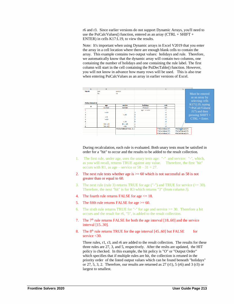
Frontline Solvers 2020 User Guide Page 213
r6 and r3. Since earlier versions do not support Dynamic Arrays, you'll need to
use the PsiCalcValues() function, entered as an array (CTRL + SHIFT +
ENTER) in cells K17:L19, to view the results.
Note: It's important when using Dynamic arrays in Excel V2019 that you enter
the array in a cell location where there are enough blank cells to contain the array. This example contains two output values: holidays and rule. Therefore,
we automatically know that the dynamic array will contain two columns, one
containing the number of holidays and one containing the rule label. The first
column will start in the cell containing the PsiDecTable() function. However,
you will not know in advance how many rows will be used. This is also true
when entering PsiCalcValues as an array in earlier versions of Excel.
During recalculation, each rule is evaluated. Both unary tests must be satisfied in
order for a "hit" to occur and the results to be added to the result collection.
1. The first rule, under age, uses the unary tests age: "-" and service: "-", which,
as you will recall, returns TRUE against any value. Therefore, the first "hit"
occurs with R1, as age – service or 58 – 31 = 27.
2. The next rule tests whether age is >= 60 which is not successful as 58 is not
greater than or equal to 60.
3. The next rule (rule 3) returns TRUE for age ("-") and TRUE for service (>= 30).
Therefore, the next "hit" is for R3 which returns "3" (from column J).
4. The fourth rule returns FALSE for age <= 18.
5. The fifth rule returns FALSE for age >= 60.
6. The sixth rule returns TRUE for "-" for age and service >= 30. Therefore a hit
occurs and the result for r6, "5", is added to the result collection.
7. The 7th rule returns FALSE for both the age interval [18..60] and the service
interval [15..30].
8. The 8th rule returns TRUE for the age interval [45..60] but FALSE for
service <30.
Three rules, r1, r3, and r6 are added to the result collection. The results for these
three rules are 27, 3, and 5, respectively. After the reslts are updated, the HIT
policy is checked. In this example, the hit policy is "O" or "Output Order"
which specifies that if multiple rules are hit, the collection is retuned in the priority order of the listed output values which can be found beneath "holidays"
or 27, 5, 3, 2. Therefore, our results are returned as 27 (r1), 5 (r6) and 3 (r3) or
largest to smallest.
Must be entered
as an array by
selecting cells
K17:L19, typing
"=PsiCalcValues(
J17) and then
pressing SHIFT +
CTRL + Enter.

Frontline Solvers 2020 User Guide Page 214
Open the example DT Hit Policy Examples.xlsx to see how the different Hit
policies work.
Note: During parse-time, each PsiDecTable() function is uniquely identified by
it's cell address. A "completeness test" ensures that all input/output entries per
column cover the domain of the input/output values in the same column, as long as the output values are not expressions against the output values. If so, these
expressions are evaluated at run-time. Type verification is performed for those
columns in which a data type is specified rather than an input/output value.
Optional Arguments
PsiDecTable() supports two optional arguments: output and ret_header.
To return the result for a given output only, we must pass an additional
argument to the PsiDecTable() function. For example, to only receive the
number of holidays, rather than both holidays and the rule label, add "holidays"
as the last arguent to our existing formula in cell J17. In this instance, only one
column will be returned containing the values: 27, 5, 3.
J17=PsiDecTable(G7:K16, 2, age, service, "holidays") where
• G7:K16 is the location of the decision table on the Excel worksheet,
• 2 is the number of inputs,
• age and service are the two input variables and
• "holidays" (optional) to ensure that the returned results only include the
specified output.
You can pass as many output arguments as needed.
It's also possible to use a 2nd optional argument, ret_header, this time a Boolean argument, as the last argument to PsiDecTable(). When TRUE is passed for this
argument, a header containing the names of the output(s) is included in the
result. In this instance, one column will be returned containing the values:
"holidays", 27, 4, 3.
J17=PsiDecTable(G7:K16, 2, age, service, "holidays", TRUE) where
• G7:K16 is the location of the decision table on the Excel worksheet,
• 2 is the number of inputs,
• age and service are the two input variables,
• "holidays" (optional) to ensure that the returned results only include the specified output and
• TRUE to add a header to the result.
This is the complete signature for the PsiDecTable() function.
Additional Examples
This section presents a special class of tables, in which the specific Date, Time,
and Duration data types are utilized.
Decision Table Containing Dates
Open the first tab within the workbook DT Date & Time Examples.xlsx. This
table returns the credit risk rating of an individual based on their age and

Frontline Solvers 2020 User Guide Page 215
medical history. The PsiDecTable function appears in cell G19 =
PsiDecTable(B13:E19, 2, bd, mh) where
• B13:E19 is the location of the decision table,
• 2 is the number of input variables and
• bd (cell G14 containing "1964-05-05") and mh (cell H14 containing
"good") are the input variables.
Notice that the string values in columns D (medHistory) and E (riskRating) in
the table are entered without quotes. This is because Analytic Solver always
assumes any output as an expression requiring parsing. If a single word or
"token" is detected, the Psi Interpreter first checks if it is a local scope variable
name. If not, the word-token is assumed to be a string. In the first example table
the expression age – service existed in the "holidays" column. Since age and
service are variables connected through the operator ‘-‘, the Psi Interpreter
assumed the entry as an expression to be evaluated. If instead, we wanted to
enter that expression as a string value, then we would need to surround the expression with quotation marks.
The situation with dates is however, different. While in Excel we may enter a
date without “ “, when a Date is part of a Decision table, we must surround the
date with single ‘ ‘ or double “ “. S-FEEL defines a single format for the Date
type ‘yyyy-mm-dd’. Optionally a date may begin with the letter D, for example
“D1964-05-05”. Other date type formats in Excel are not valid in S-FEEL.
When we pass a date as an input parameter to a Decision table, the date must be
a string formatted as S-FEEL Date. If we enter an Excel date in that cell, it will
be automatically converted into the date representing number and the Decision
table will still recognize it as date. However, we strongly recommend using the
S-FEEL format outside of Decision tables for readability of the model.
In this example,the unique rule which matches the input birthdate “1964-05-05”
is rule #3, because “1964-05-05” is in the date interval [‘1935-05-05’..’1970-05-
05’].
Decision Table Containing Time
The Psi Interpreter will convert any time entries in a decision table into the Time
format, “hh:mm:ss”. Optionally, we could enter the times using the format beginning with the letter T such as in “T18:29:30”. Usually this time format
denotes local time. If we want to specify the UTC time, we can simply add z at
the end of the format, for example “T18:29:30z”. However, it’s important to
note that the z time format is just a readable format. The Psi Interpreter cannot
effectively convert local and zulu times, because the location of the local time is
not specified in the supported format.

Frontline Solvers 2020 User Guide Page 216
Click the 2nd tab in the workbook to open the example shown above which
returns the traffic prediction (low, medium, or high) for a toll station based on the time of day.
To avoid the downward spill of the result for the two outputs, we use the
optional output argument in both PsiDecTable() functions in cells G16 and G17.
G16 = PsiDecTable(B14:E20, 1, byNow, "toll")
G17 = PsiDecTable(B14:E20, 1, byNow, "traffic")
Decision Table Containing Duration
Finally, let’s take a look into an example using the data type, duration. Click the
third tab in the workbook to open the decision table, shown below, which
computes the output parking fee according to the input parking time. The table is
invoked through the Excel formula in cell F16 = PsiDecTable(B11:D16, 1,
period).
There are two types of formats for Duration:
• P1Y2M - measures duration in months
• P1DT1H20M10S – measures duration in seconds
The individual components in these formats are optional. For example, if we have 0 hours to represent, we may skip the hour component. For example, we
can represent a 20 minutes duration using either: PT0H20M0S or PT20M.
While we can skip a duration component in the format, the order of components
in a format must be followed. For example, we cannot first enter minutes and
then hours; PT20M1H is not a currently supported syntax.
Hit Policies
This section presents a collection of tables to illustrate each of the 7 Hit policies
currently supported by Analytic Solver: Any, Collect, First, Rule Order, Output
Order, Priority Order and Unique. Open the example workbook, DT Hit Policy
Examples.xlsx. This workbook contains 7 tabs, one tab for each example.
Hit Policy: Any
The decision table appearing on the Any tab returns the loan compliance for an
individual given their credit rating, current card balance, and current student
loan balance.

Frontline Solvers 2020 User Guide Page 217
The PsiDecTable() function is located in cell F19. This function returns
"compliant" or "not compliant" given a credit rating of "B", a credit card balance
of $12,000, and a student loan balance of $75,000. The Hit policy Any will
return only one result even if multiple rules overlap.
F19 = PsiDecTable(B13:F18, 3, "B", 12000, 75000)
In this table, all rules except for rule 1 are evaluated successfully for a "hit".
However, the result collection only includes 1 "not compl" entry.
Hit Policy: Collect
Click the Collect tab to display the 2nd Hit Policy example. This decision table
returns the total number of holidays allotted to an employee based on their age
and number of years in service. In the previous example, the Hit Policy was
equal to Unique which resulted in all successfully hit rules returning their unique
result. In this example, the Collect policy is used with the "+" operator. This
operator returns the sum of the collection of results in rule order when multiple
rules are applicable. The Collect Policy allows 4 operators, + (sum), < (return
the minimum of matched output values), > (return the maximum of matched output values) and # (return the number of matched output values).
In this example, the PsiDecTable() function appears in cell E24 =
PsiDecTable(B14:E23, 2, 58, 31). As in the previous example, three rules, 1, 3
and 6, are included in the results returning the values, 22, 3 and 5, respecitvely.
However, since this Hit policy sums the results, the answer 30 is returned.
Let's see what happens when we change the Hit Policy to C<. Simply select cell
C+ and enter C<, then click the green arrow on the Model tab of the Solver Task Pane to recalculate the table. When the Hit Policy is equal to C<, PsiDecTable()
returns the minimum result value, 3.

Frontline Solvers 2020 User Guide Page 218
Let's repeat these steps for "C"> to find the maximum result value of 22,
and "C#" to find the number of returned results, 3.
Hit Policy: First
Click the First tab to display the next Hit Policy example. In this example, a
percentage discount is returned based on where an order originated, on the web
or by phone, the location of the order, inside or outside the US, and customer
type, wholesaler or retail according to the First Hit Policy. When this policy is
in use, only the first entry in the result collection is returned.

Frontline Solvers 2020 User Guide Page 219
The PsiDecTable() function appears in cell F19.
F19=PsiDecTable(B13:F18, 3, "web", "non_US", "retailer")
Two rules are "hit", rule 3 and rule 4. However, since we are using the First Hit
Policy, only the result for rule 3 is returned, 0.
Hit Policy: Rule Order
Click the next tab to display the Rule Order Hit Policy example. This table
returns the amount of money available to a student based on their grade point
average and number of times they took the ACT. Funds may be provided via a
scholarship, loan, or work study program. The "Rule Order" Hit policy returns
the collection of results in priority order of the listed output values. The
PsiDecTable() function is located in cell F19 = PsiDecTable(B13:G18, 3, 3.6, 4,
TRUE). Given an honors student with a gpa = 3.6 and an act_count = 4, this
student would be eligible to receive a scholarship covering 20% of tuition (rule
1) and a student loan covering 30% of tuition (rule 2).
Rules 3 and 4 are not applicable because the student is an honor student
(honor_member = TRUE) and the student's GPA is greater than 3.0.
Adding the last two optional arguments, returns the header "eligibility", and only
the eligibility text.
F19 = PsiDecTable(B13:G18, 3, 3.6, 4, TRUE).
Cells F22:G24 contain PsiCalcValue(F19). Use these values to return the
contents of the result collection when using a version of Excel that does not
support Dynamic Arrays. Note that if this function is entered into more than the number of cells required, #N/A is returned.
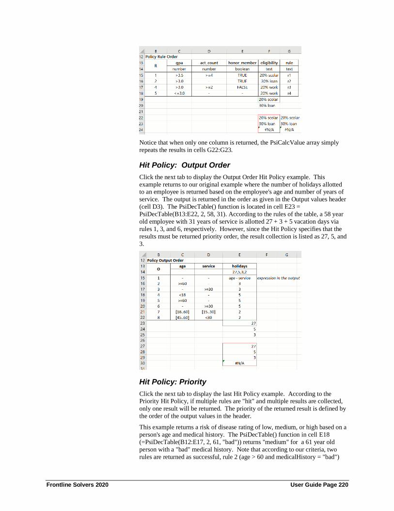
Frontline Solvers 2020 User Guide Page 220
Notice that when only one column is returned, the PsiCalcValue array simply
repeats the results in cells G22:G23.
Hit Policy: Output Order
Click the next tab to display the Output Order Hit Policy example. This
example returns to our original example where the number of holidays allotted to an employee is returned based on the employee's age and number of years of
service. The output is returned in the order as given in the Output values header
(cell D3). The PsiDecTable() function is located in cell E23 =
PsiDecTable(B13:E22, 2, 58, 31). According to the rules of the table, a 58 year
old employee with 31 years of service is allotted 27 + 3 + 5 vacation days via
rules 1, 3, and 6, respectively. However, since the Hit Policy specifies that the
results must be returned priority order, the result collection is listed as 27, 5, and
3.
Hit Policy: Priority
Click the next tab to display the last Hit Policy example. According to the Priority Hit Policy, if multiple rules are "hit" and multiple results are collected,
only one result will be returned. The priority of the returned result is defined by
the order of the output values in the header.
This example returns a risk of disease rating of low, medium, or high based on a
person's age and medical history. The PsiDecTable() function in cell E18
(=PsiDecTable(B12:E17, 2, 61, "bad")) returns "medium" for a 61 year old
person with a "bad" medical history. Note that according to our criteria, two
rules are returned as successful, rule 2 (age > 60 and medicalHistory = "bad")

Frontline Solvers 2020 User Guide Page 221
and rule 3 (age = "-" and medHistory = "medium"). Why isn't "high" returned?
Because the priority list in cell B13 (low, medium, high) specifies that
"medium" should have higher priority than "high".
Hit Policy: Unique
Click the last tab to display the last Hit Policy example. According to the Unique Hit Policy, only one rule may "hit". If multiple rules are "hit" and
multiple results are collected, an error will be returned.
E18 = PsiDecTable(B11:F17, 2, 54, "good")
This table also returns a risk rating for an individual based on their age and
medical history (medHistory). In this example, given an age or 54 and a "good" medical history, a "medium" risk rating is returned by rule 3.
Merging Decision Table Results The DT Loan Recommend Example illustrates how to use the PsiJoin() function
to merge the results of one decision table with a 2nd table.
The decision table, in cells B18:I34, returns a loan or loans meeting various
criteria. Cell K27 includes the PsiDecTable() formula. Two types of loans meet
the 4 loan requirements (reqObj = payment, reqType = fixed 30, conforming =
TRU and reqDown = 30): a conventional Arm 3\1 and a conventional Fixed 40.
(See the results in cells J32:L34).
K27=PsiDecTable(B18:I34, 4, reqObj, reqType, conforming, reqDown, TRUE)
The PsiCalcValue() functions located in cells Loan Types!K32:M34 are used to
persist the results from PsiDecTable().
Notice that the optional "header" argument has been passed to PsiDecTable() in
cell K27. This was done in preparation for the use of the PsiJoin() function to
merge the results (cells K32:M34) with the table on the Bank Rates tab.

Frontline Solvers 2020 User Guide Page 222
Click the Bank Rates tab to view the 2nd table in cells A2:I8. This table lists six
banks offering loans in the area. Notice that no bank is offering the Fixed 40
loan.
The PsiJoin function has been entered as an array in cells A12:L15.
A12:L15{= PsiJoin('Loan Types'!J32:L34, A2:I8, "loanType = loanType,
confType = confType, downPct >= 'minDown %'")}
This function joins results from the decision table function in Loan Types!J27
with the second table on the Bank Rates tab.
PsiJoin() takes three arguments, Table1, Table2, and Clause. The Table1
argument passes the first table, in this example, the table in Loan
Types!A18:H34. The Table2 argument passes the second table, in this example,
the table in Bank Rates!A2:I8. The third argument, Clause, passes the
conditions for joining the table. In this example, the results and the table are
joined via three columns: loanType, confType, and downPct. This argument must be surround by quotes.
Note that in this example, two conditions used to join the results from
PsiDecTable() and the Bank Rates table are the same, i.e. loanType = loanType
and confType = confType. This is not a requirement; table headers can be
different.
The third condtion, downPct >= 'minDown %' requires that the downPct in the
Loan Types decision table must be greater than the "minDown %" in the Bank
Rates table. In other words, the down payment percentage in the Loan Types
table must be greater than the minimum percentage down in the Bank Rates
table in order for the loan to be selected and displayed by PsiJoin().
Note: Recall that the PsiDecTable() function in cell Loan Types!J27 included
the optional "header" argument. If the results had not included this argument, it
would not have been possible to use the PsiJoin() function complete the merge.
All three columns are common to both the PsiDecTable() results and the Bank
Rates table. Three banks offer a conventional ARM 3\1 loan: Mount Diablo,
AimLoan, and America One. The first three columns (A12:L15) are the three
columns passed to the Clause argument: loanType, confType, and downPct.
Columns D through L contain the remaining information for each offered loan:
Lender, loanType, confType, minDown%, Term, APR %, Rate %, Points, and
feesAmt.

Frontline Solvers 2020 User Guide Page 223
Using Cascading Decision Tables Open the DT Loan Strategy Model to learn how to use cascading decision tables
where the output of one decision table is the input to another.
This Input worksheet contains the input parameters to the Loan Strategy model
contained on the Loan Strategy and Post Bureau worksheets. Input parameters
are all constant values.
Click the Loan Strategy worksheet. This worksheet contains six cascading
decision tables. The first table appears in cells A2:E14. This table returns a
partial "risk of default" score based on a loan applicant's age, marital and
employment status. Higher scores are given to older, employed, married applicants. Cell E15 contains the PsiDecTable() function.
E15=PsiDecTable(A2:E14, 3, custAge, maritalSt, employSt)

Frontline Solvers 2020 User Guide Page 224
The input parameters from the Input worksheet are: custAge="40", maritalSt =
"s", employSt = "selfemployed". The applicable rules for these input parameters
are: 4, 6, and 11 resulting in partial scores of 43, 25, and 36, respectively. Since
the Hit Policy is "C+" the result collection is added together, 43 + 25, + 36 =
104.
The next decision table is located in cells G5:J14, the Bureau Risk Cat table.
This table returns a risk category of high, medium, or low based on their
customer status (existing or not) and their application risk score. Non-existing
customers are allowed a higher risk score. Cell J15 contains the PsiDecTable()
function
J15 =PsiDecTable(G5:J14, 2, custExist, tblAppRiskScore) where custExist =
False and tblAppRiskScore() refers to the value in cell E15, or 104. Based on
these conditions, one rule is "hit", rule 2. This rule returns "medium" for the
bureau risk category. Since the hit policy is equal to U (Unique) only one result
is returned, even if multiple results are returned.
The next decision table, Bureau Call Type, is located in cells L11:N14. This
table returns the bureau call type based on the bureau risk category found in the
previous decision table, Bureau Risk Cat. Cell N15 contains the PsiDecTable() function.
N15=PsiDecTable(L11:N14, 1, tblBureauRiskCat) where tblBureauRiskCat is
equal to the result of the PsiDecTable() function in cell J15, or "medium". Only
1 rule is "hit", rule 1, which returns "full".
The nextdecision table, Eligibility, is located in cells A20:E25. This table
returns the applicant's eligibility based on three criteria: the bureau risk
category, from cell J15, bureau afford, calculated in cell C36, and customer age,
located in cell Input!C13. Since the Hit Policy is equal to P (Priority), the result
collection will be returned in the order listed according to the list in cell E21. The PsiDecTable() function is located in cell E26.

Frontline Solvers 2020 User Guide Page 225
E26 = PsiDecTable(A20:E25, 3, tblBureauRiskCat, bureauAfford, custAge)
Intermediate Formulas
Cell C36 calculates the bureau afford statistic, =IF(disposIncome *
tblCreditContFactor > monthInstall, TRUE, FALSE)
where disposIncome is calculated in cell C34, tblCreditContFactor is
calculated in cell N26 (more on this later) and monthInstall is
calculated in cell C32.
Cell 34 calculates an applicant's disposable income using the formula,
=monthIncome - (monthRepay + monthExpenses) where monthIncome = 2500, monthRepay is calculated in cell C30 and monthExpenses =
1000.
Cell C30 calculates the monthly loan replayment amount using the
formula, -PMT(loanRate%/12, loanTerm*12, loanAmnt) where
loanRate is 5%, loanTerm = 30 and loanAmnt = 100,000.
Finally, cell C28 calculates the monthly fee using the IF statement, =
IF(loanType = "standard", 20, IF(loanType = "special", 25, 0)), where
loanType = standard.
Using the final input values of tblBureauRiskCat = medium, bureauAfford =
True, and custAge = 40, the last rule, rule 4, is the only rule "hit", returning
"eligible".
The next decision table is located in cells G22:J25. This table returns the loan
strategy based on the applicant's eligibility and bureau call type. The
PsiDecTable() function is located in cell J26.
J26=PsiDecTable(G22:J25, 2, tblEligibility, tblBureauCallType) where tblEligibility is calculated in cell E26 and tblBureauCallType is calculated in
cell N15. Both of these inputs are outputs of earlier decision tables. Based on
the results calculated by the previous decision tables, this PsiDecTable()
function results in a "bureau" strategy.
Finally, the last decision table, Credit Cont Factor, is contained in cells
L22:N25. The PsiDecTable() function is located in cell N26.
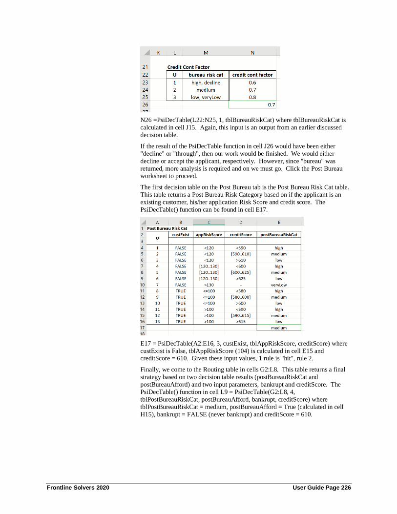
Frontline Solvers 2020 User Guide Page 226
N26 =PsiDecTable(L22:N25, 1, tblBureauRiskCat) where tblBureauRiskCat is
calculated in cell J15. Again, this input is an output from an earlier discussed
decision table.
If the result of the PsiDecTable function in cell J26 would have been either
"decline" or "through", then our work would be finished. We would either
decline or accept the applicant, respectively. However, since "bureau" was
returned, more analysis is required and on we must go. Click the Post Bureau worksheet to proceed.
The first decision table on the Post Bureau tab is the Post Bureau Risk Cat table.
This table returns a Post Bureau Risk Category based on if the applicant is an
existing customer, his/her application Risk Score and credit score. The
PsiDecTable() function can be found in cell E17.
E17 = PsiDecTable(A2:E16, 3, custExist, tblAppRiskScore, creditScore) where
custExist is False, tblAppRiskScore (104) is calculated in cell E15 and creditScore = 610. Given these input values, 1 rule is "hit", rule 2.
Finally, we come to the Routing table in cells G2:L8. This table returns a final
strategy based on two decision table results (postBureauRiskCat and
postBureauAfford) and two input parameters, bankrupt and creditScore. The
PsiDecTable() function in cell L9 = PsiDecTable(G2:L8, 4,
tblPostBureauRiskCat, postBureauAfford, bankrupt, creditScore) where
tblPostBureauRiskCat = medium, postBureauAfford = True (calculated in cell
H15), bankrupt = FALSE (never bankrupt) and creditScore = 610.

Frontline Solvers 2020 User Guide Page 227
The input parameter postBureauAfford is calculated in cell H15 according to the
formula, =IF(disposIncome * postCreditContFactor > monthInstall, TRUE,
FALSE). Since the product of disposIncome and postCreditContFactor (963.18
* .7) is greater than the monthly installment (556.82), the IF function returns
TRUE.
The input parameter postCreditContFactor is calculated in cell H12 =
PsiDecTable('Loan Strategy'!L22:N25, 1, tblPostBureauRiskCat). Note that this PsiDecTable() function refers to the App Risk Score decision table in cells Loan
Strategy!L22:N25. Analytic Solver supports multiple PsiDecTable() functions
that refer to the same table, as long as the input variables are different. Multiple
PsiDecTable() functions with identical input variables are not supported and will
result in an error. Two PsiDecTable() functions return to the App Risk Score
decision table.
With these criteria, the last rule, rule 5, is hit, accept the loan application.
Using Decision Tables in Optimization and Simulation It's also possible to build an optimization and simulation model using a decision
table as input. See the Data Mining User Guide for an example on how to use a
decision tree in conjunction with a data mining model saved in PMML format.
Optimization
Open DT Opt & Sim Examples.xlsx and click the Optimization tab. The
decision table appearing in cells B12:F24 returns the collective score, due to the
Hit Policy of "Collect +", of a set of partial scores based on a customer's age,
marital status, and employment status. The PsiDecTable() function appearing in
cell F25 = PsiDecTable(B12:F24, 3, I12, maritalSt, employSt) where I12
currently refers to the age "1", "maritalSt" refers to cell Input!B15 ("s" for
single) and "employSt" refers to cell Input!B17 ("selfemployed").
The Model tab on the Solver Task Pane shows the optimization model which is
maximizing the PsiDecTable() function in cell F25 by varying cell I12 subject to
the variable bounds of 18 and 65. Click Optimize – Analyze Original Model.
Analytic Solver will report the model type as "NSP" meaning "nonsmooth
problem". The model is nonsmooth due to the use of the decision table. As a

Frontline Solvers 2020 User Guide Page 228
result, you will need to either select the Evolutionary Engine to solve the model
or set Automatically Select Engine on the Engine tab. Then click the green
arrow on the Model tab to solve the optimization model.
Almost immediately, the Evolutionary Engine stops with the result, "Solver has
converged to the current solution. All constraints are satisfied." This result means that the Solver has been unable to find a new, better member of the
population whose “fitness” represents a relative (percentage) improvement over
the current best member’s fitness. For more information on this result, see the
"Solver Result Messages" chapter within the Frontline Solvers Reference Guide.
The final variable age results in the largest collective score according to the
decision table rules, based on the initial starting point. (For more information on
optimizing with the Evolutionary Engine, see the Frontline Solvers Reference
Guide.)
Simulation
Click the Simulation tab to open the simulation example. This example uses the
same decision table as in the optimization example. However, in this example,
the PsiDecTable() function in cell E26 = PsiDecTable(A13:F25, 3, custAge,
maritalSt, employSt), where "custAge" refers to Input!C11 which holds a
PsiNormal() function. This function will pull 1000 values from the PsiNormal()
distribution, with a mean of 40 and a standard deviation of 7, during the simulation. The PsiMean() function in cell E28 will summarize the 1000 trial
values into one mean value. In addition, the PsiMean function will also denote
cell E26, the cell containing the PsiDecTable() function, as an output cell. For
simulations, Analytic Solver tracks the values of all uncertain functions
(simulation outputs, referenced in PsiOutput() or PSI Statistics function calls).
Click the green arrow on the Model tab to run a simulation. Immediately, the
simulation finishes and the uncertain function dialog opens displaying a discrete
distribution where we can see that over 70% of the time, the values for the
collective sum of the partial scores is over 101 when the age parameter follows a
normal distribution with mean 40 and standard deviation 7. For more
information on simulation with Analytic Solver, see the Examples: Simulation chapter that appears previously in this guide.

Frontline Solvers 2020 User Guide Page 229
Using Decision Tables with Data Mining This DT Loan Strategy + Predictive.xlsx example expands on the DT Loan
Strategy Model by adding an element to the APP Risk Score table on the Loan
tab. The formula in cell Loan!E15 returns the minimum of 2 outputs. The first
output is produced from a linear regression model scoring new data contained in cells Input!F26:I27. The second output is from the decision table.
Input Parameters
This Input worksheet contains the input parameters to the Loan Strategy model
contained on the Loan Strategy and Post Bureau worksheets. Input parameters
are all constant values.
Loan Strategy
Click the Loan Strategy worksheet. Like in the DT Loan Strategy Model.xlsx
workbook, this worksheet contains six cascading decision tables. The first table
appears in cells A2:E14. This table returns a partial "risk of default" score based
on a loan applicant's age, marital and employment status. Higher scores are
given to older, employed, married applicants. Cell E15 contains the
PsiDecTable() function.
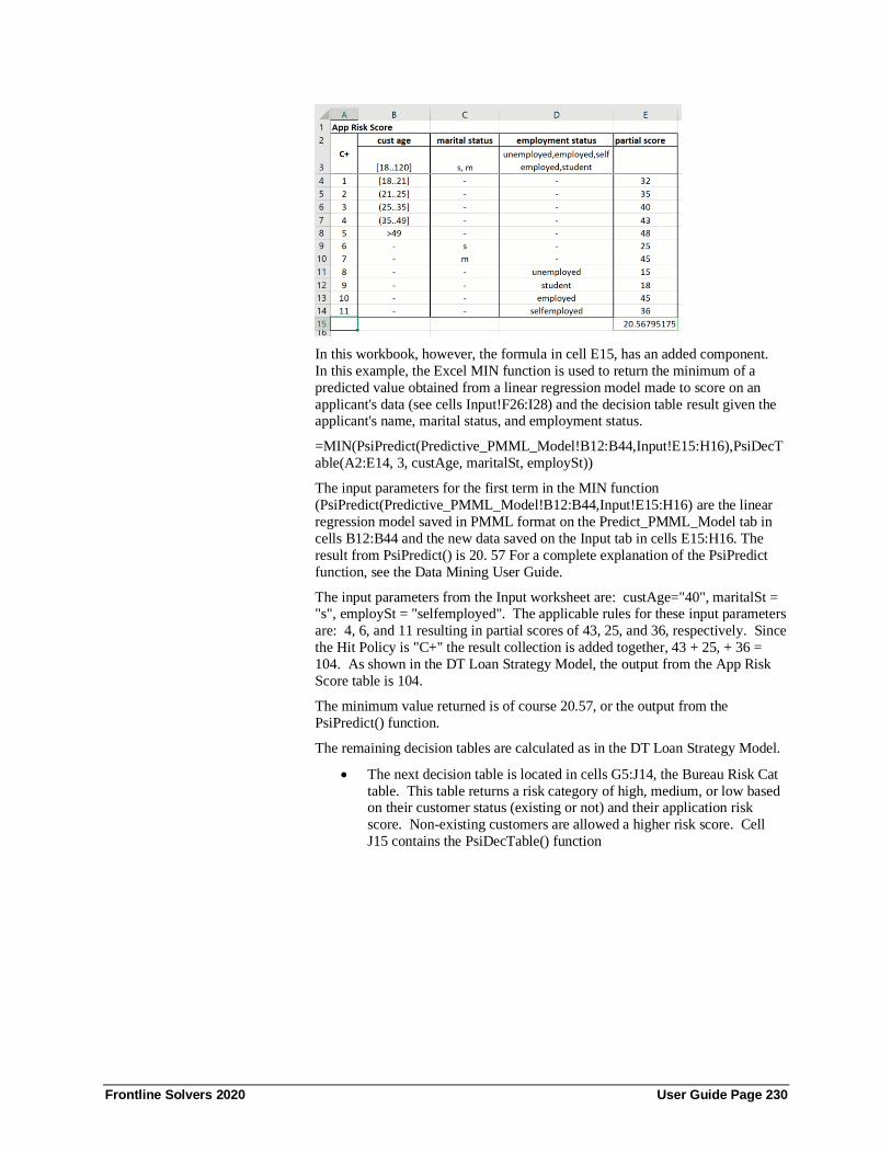
Frontline Solvers 2020 User Guide Page 230
In this workbook, however, the formula in cell E15, has an added component.
In this example, the Excel MIN function is used to return the minimum of a
predicted value obtained from a linear regression model made to score on an
applicant's data (see cells Input!F26:I28) and the decision table result given the applicant's name, marital status, and employment status.
=MIN(PsiPredict(Predictive_PMML_Model!B12:B44,Input!E15:H16),PsiDecT
able(A2:E14, 3, custAge, maritalSt, employSt))
The input parameters for the first term in the MIN function
(PsiPredict(Predictive_PMML_Model!B12:B44,Input!E15:H16) are the linear
regression model saved in PMML format on the Predict_PMML_Model tab in
cells B12:B44 and the new data saved on the Input tab in cells E15:H16. The
result from PsiPredict() is 20. 57 For a complete explanation of the PsiPredict
function, see the Data Mining User Guide.
The input parameters from the Input worksheet are: custAge="40", maritalSt = "s", employSt = "selfemployed". The applicable rules for these input parameters
are: 4, 6, and 11 resulting in partial scores of 43, 25, and 36, respectively. Since
the Hit Policy is "C+" the result collection is added together, 43 + 25, + 36 =
104. As shown in the DT Loan Strategy Model, the output from the App Risk
Score table is 104.
The minimum value returned is of course 20.57, or the output from the
PsiPredict() function.
The remaining decision tables are calculated as in the DT Loan Strategy Model.
• The next decision table is located in cells G5:J14, the Bureau Risk Cat
table. This table returns a risk category of high, medium, or low based on their customer status (existing or not) and their application risk
score. Non-existing customers are allowed a higher risk score. Cell
J15 contains the PsiDecTable() function

Frontline Solvers 2020 User Guide Page 231
J15 =PsiDecTable(G5:J14, 2, custExist, tblAppRiskScore) where custExist =
False and tblAppRiskScore() refers to the value in cell E15, or 20.57. Based
on these conditions, one rule is "hit", rule 2. This rule returns "high" for the
bureau risk category. Since the hit policy is equal to U (Unique) only one result is returned, even if multiple results are returned.
The next decision table, Bureau Call Type, is located in cells L11:N14. This
table returns the bureau call type based on the bureau risk category found in the
previous decision table, Bureau Risk Cat. Cell N15 contains the PsiDecTable()
function.
N15=PsiDecTable(L11:N14, 1, tblBureauRiskCat) where tblBureauRiskCat is
equal to the result of the PsiDecTable() function in cell J15, or "medium". Only
1 rule is "hit", rule 1, which returns "full" This means that a full evaluation by
the bureau must be performed.
The next decision table, Eligibility, is located in cells A20:E25. This table
returns the applicant's eligibility based on three criteria: the bureau risk
category, from cell J15, bureau afford, calculated in cell C36, and customer age,
located in cell Input!C13. Since the Hit Policy is equal to P (Priority), the result
collection will be returned in the order listed according to the list in cell E21.
The PsiDecTable() function is located in cell E26.
E26 = PsiDecTable(A20:E25, 3, tblBureauRiskCat, bureauAfford, custAge)

Frontline Solvers 2020 User Guide Page 232
Intermediate Formulas
Cell C36 calculates the bureau afford statistic, =IF(disposIncome *
tblCreditContFactor > monthInstall, TRUE, FALSE)
where disposIncome is calculated in cell C34, tblCreditContFactor is
calculated in cell N26 (more on this later) and monthInstall is
calculated in cell C32.
Cell 34 calculates an applicant's disposable income using the formula,
=monthIncome - (monthRepay + monthExpenses) where monthIncome
= 2500, monthRepay is calculated in cell C30 and monthExpenses =
1000.
Cell C30 calculates the monthly loan replayment amount using the
formula, -PMT(loanRate%/12, loanTerm*12, loanAmnt) where
loanRate is 5%, loanTerm = 30 and loanAmnt = 100,000.
Finally, cell C28 calculates the monthly fee using the IF statement, =
IF(loanType = "standard", 20, IF(loanType = "special", 25, 0)), where
loanType = standard.
Using the final input values of tblBureauRiskCat = high, bureauAfford = True,
and custAge = 40, the last rule, rule 4, is the only rule "hit", returning "eligible".
The next decision table is located in cells G22:J25. This table returns the loan
strategy based on the applicant's eligibility and bureau call type. The PsiDecTable() function is located in cell J26.
J26=PsiDecTable(G22:J25, 2, tblEligibility, tblBureauCallType) where
tblEligibility is calculated in cell E26 and tblBureauCallType is calculated in
cell N15. Both of these inputs are outputs of earlier decision tables. Based on
the results calculated by the previous decision tables, this PsiDecTable()
function results in a "bureau" strategy.
Finally, the last decision table, Credit Cont Factor, is contained in cells L22:N25. The PsiDecTable() function is located in cell N26.
N26 =PsiDecTable(L22:N25, 1, tblBureauRiskCat) where tblBureauRiskCat is calculated in cell J15. Again, this input is an output from an earlier discussed
decision table.

Frontline Solvers 2020 User Guide Page 233
If the result of the PsiDecTable function in cell J26 would have been either
"decline" or "through", then our work would be finished. We would either
decline or accept the applicant, respectively. However, since "bureau" was
returned, more analysis is required.
More Information on Decision Tables Supported conversion functions are listed below.
• date(string date) returns a date serial number, the same as Excel
DATEVALUE
• date(number y, number m, number d)
• time(string time) returns a time serial number, the same as Excel
TIMEVALUE
• time(number h, number m, number s[, number offset]) the optional
offset is duration in seconds, which can be used to model UTC
• duration(string dur) returns duration in months or seconds depending on format
• yearsAndMonthsDuration(string from_date, string to_date) return
difference between two dates as a duration in months
• number(string num, string group_sep, string dec_sep) returns a
number from a string
• string(float num) returns a float number as a string
• Supported numeric functions are:
• ceiling(number num) rounds up a number
• decimal(number num, number decimals) rounds a number to the given
number of decimals
• floor(number num) rounds down a number
• Supported string functions:
• substring(string str, number pos, number num_chars)
• stringLength(string str)
• upperCase(string str)
• lowerCase(string str)
• substringBefore(string str, string match)
• substringAfter(string str, string match)
• contains(string str, string match)
• startsWith(string str, string match)
• endsWith(string str, string match)
• Supported list functions are:
• min(number n1, number n2,…) returns the minimum number
• max(number n1, number n2,…)

Frontline Solvers 2020 User Guide Page 234
• sum(number n1, number n2,…)
• mean(number n1, number n2,…)
• and(bool b1, bool b2,…)
• or(bool b1, bool b2,…)

Frontline Solvers 2020 User Guide Page 235
Creating Power BI Custom Visuals
Starting with V2017-R2, Analytic Solver can turn your Excel-based
optimization or simulation model into a Microsoft Power BI Custom Visual.
Where others must learn JavaScript (or TypeScript) programming and a whole
set of Web development tools to even begin to create a Custom Visual in Power
BI, after reading this section, Analytic Solver users will be able to create one
right away.
To summarize, users simply select rows or columns of data to serve as
changeable parameters, then choose Create App – Power BI, and save the file
created by Analytic Solver. Afterwards, users click the Load Custom Visual
icon in Power BI and select the file just saved. What is produced isn’t just a chart – it’s a full optimization or simulation model, ready to accept Power BI
data, run on demand on the web, and display visual results in Power BI. Users
simply need to drag and drop appropriate datasets into the “well” of inputs in
Power BI to match the model parameters.
Analytic Solver translates the Excel model into RASON® (RESTful Analytic
Solver Object Notation, embedded in JSON), then “wraps” a JavaScript-based
Custom Visual around the RASON model. See the previous chapter “Creating
Your Own Application” for more information on RASON.
Installing Power BI Power BI is Microsoft’s desktop or cloud-based interactive data visualization
business intelligence tool. In past versions of Analytic Solver, users have only been able to upload their model parameters (model data) to Power BI after
solving an optimization or simulation model. Starting with V2017-R2, Analytic
Solver can turn your Excel based optimization or simulation model into a
Microsoft Power BI Custom Visual, that is your full optimization or simulation
model, ready to accept power BI data, run on demand on the web, and display
visual results in Power BI.
Note: Click this link to download Power BI for desktop.
In order to use this new feature in Analytic Solver, you must first open desktop
Power BI or the free cloud based version of Power BI. (Power BI is part of the
office 365 suite.) For more information on this business tool, see the following
website: https://powerbi.microsoft.com/en-us/documentation/powerbi-custom-visuals-getting-started-with-developer-tools/
It is important to note, that in order to create a custom visual in Power BI, you
will first need to install Power BI’s Developer Tools which is comprised of
NodeJS and the Power BI tools. Follow the steps below to install both required
items.
1. Click here to download NodeJS.
2. Click the Download v6.11.2 LTS button to download NodeJS for 64-bit
Windows.
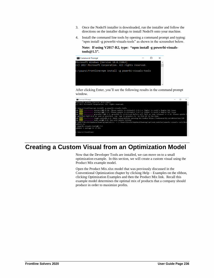
Frontline Solvers 2020 User Guide Page 236
3. Once the NodeJS installer is downloaded, run the installer and follow the
directions on the installer dialogs to install NodeJS onto your machine.
4. Install the command line tools by opening a command prompt and typing:
“npm install -g powerbi-visuals-tools” as shown in the screenshot below.
Note: If using V2017-R2, type: “npm install -g powerbi-visuals-
After clicking Enter, you’ll see the following results in the command prompt
window.
Creating a Custom Visual from an Optimization Model Now that the Developer Tools are installed, we can move on to a small
optimization example. In this section, we will create a custom visual using the
Product Mix example model.
Open the Product Mix.xlsx model that was previously discussed in the
Conventional Optimization chapter by clicking Help – Examples on the ribbon,
clicking Optimization Examples and then the Product Mix link. Recall this
example model determines the optimal mix of products that a company should
produce in order to maximize profits.

Frontline Solvers 2020 User Guide Page 237
The optimization model is included in the Model tab in the Solver Task Pane.
This model written in algebraic form is below.
Maximize: Total Profit = $75x1 + $50x2 + $35x3
Subject To:
Chassis: 1x1 + 1x2 + 0x3 <= 450
LCD Screen: 1x1 + 0x2 + 0x3 <= 250
Speaker: 2x1 + 2x2 + 1x3 <= 800
Power Supply: 1x1 + 1x2 + 0x3 <= 450
Electronics: 2x2 + 1x2 + 1x3 <= 600
x1, x2, x3 > 0
The engine selected to solve this model is the Standard LP/Quadratic Engine as
shown on the Engine tab in the Solver Task Pane.
Click Create App on the ribbon, then select Power BI.
NOTE 1: There is no need to solve the model first unless a change has been
made to an already existing RASON model. If a change has been made to the
workbook after a RASON model has been created, then you MUST either solve or diagnose the Excel model in order for the changes to be reflected in the new
RASON model.
NOTE 2: When creating a Power BI custom visual through desktop Analytic
Solver, model elements (objective function and all variables and constraints)
may now appear across multiple worksheets within the same Excel workbook.
Immediately, the Save As dialog appears. Enter a file name in the location of
your choice and then click Save.

Frontline Solvers 2020 User Guide Page 238
• The screenshot below displays a file name of “ProductMix1” being
saved into the Power BI folder, in Analytic Solver Desktop.
Analytic Solver Desktop
• In Analytic Solver Cloud, you'll first receive a dialog where you'll
name the file to be exported.
After you click OK and the file downloads, you'll be asked if you'd like
to open or save the file. Choose "Save As" to open the Save As dialog
and browse to where you'd like to save the Power BI export.

Frontline Solvers 2020 User Guide Page 239
Note the Custom Visual Source Code checkbox at the bottom of the dialog. This feature will be explained a little later in this chapter.
Save ProductMix1.pbiviz. Two command prompt windows will appear on your
screen. After several moments, both will disappear. It is during this time that
your Excel model is being translated into the RASON® modeling language, and
your Power BI custom visual is created.
Open either desktop or cloud-based Power BI. The screenshot below depicts the opening screen of desktop Power BI. Click the icon containing three horizontal
dots that appears at the bottom of Visualizations (in the top right-hand corner).

Frontline Solvers 2020 User Guide Page 240
Then select Import from file from the menu.
Click Import on the Import custom visual dialog that appears. (You can select
Don’t show this dialog again if you’d rather not see this dialog each time you
import a custom visual.)

Frontline Solvers 2020 User Guide Page 241
Navigate to the location of the saved ProductMix1.pbiviz file.
Then click Open. If the import was successful, you will see a message
indicating as such. Click OK to clear this dialog.
A new icon, bearing the Frontline Solvers logo is added under Visualizations.
Click this icon to open Frontline Solvers’ custom visual. At first you’ll see two
gears moving to indicate that the RASON model has been submitted to Frontline

Frontline Solvers 2020 User Guide Page 242
Solvers’ RASON server for solving. If the model is an optimization or
stochastic optimization model, the RASON server will use the engine selected in
the Excel model to solve the model. Recall that the LP/Quadratic engine was
selected in the Product Mix example model, above. (If the model is a simulation
model, Frontline Systems’ Risk Solver engine will be used.)
After the model is solved, values for the objective function, variables and
constraints, or uncertain variables and uncertain functions, are imported back
into Power BI and the results are displayed in the Power BI window. After
enlarging the custom visual, your screen should appear similar to the screenshot
below.
At the bottom of the custom visual, we find Solver’s result message: Solver
found a solution. All constraints and optimality conditions are satisfied. Recall that since we are solving a linear model, this message indicates that Solver has
found the globally optimal solution: There is no other solution satisfying the
constraints that has a better value for the objective. For more information on
this Solver result, please see the chapter “Solver Results Messages” within the
Frontline Solvers Reference Guide.

Frontline Solvers 2020 User Guide Page 243
In the first chart, we see that final variable values are: Var1 (LCD TV) equal to
200, Var2 (Stereo) equal to 200 and Var3 (Speakers) equal to 0. These variable
values result in an objective function value equal to $25,000. In the chart to the
right, we see the final constraint values are: Con1 (number of Chassis used) =
400, Con2 (number of LCD Screens used) = 200, Con3 (number of Speakers used) = 800, Con4 (number of Power Supplies used) = 400, and Con5 (number
of Electronics used) = 600.
Solving this model in Power BI could be useful and the chart is certainly
informative. However, what if we wanted to change the inventory? What if
Purchasing was able to obtain a discount on Speakers and our inventory
increased from 800 to 1,000? In order to solve the new model with the updated
inventory parameters, we would have to go back to the Excel model, update the
chassis inventory, save the model, create a new .pbiviz file, Import the new
.pbiviz file into Power BI and then finally open the new custom visual. That’s a
lot of effort to change just one model parameter!
Thankfully, there is an easier way. By using the Psi function, PsiDataSrc(), we are able to specify the parameters in the Excel model that could change in the
future, for example, the amount of inventory on hand for each part, the profit
point for each product or the number of parts that makeup each product.
Click back to the Excel model and select a blank cell, say J6. In Analytic Solver
Desktop, click Formulas – Insert Function to open the Insert Function dialog,
then select Psi Dimension for Category. Afterwards, highlight the function
PsiDataSrc, and click OK.
In Analytic Solver Desktop or AnalyticSolver.com, you can simply type the
formula directly into the cell.
The Function Arguments dialog opens displaying 5 arguments: Src_name,
Data_name, Data, Idx1_name, and Idx1_elem. We will use this dialog to create
a PsiDataSrc() in cell J6 that will allow us the ability to change the inventory
values and resolve the Product Mix example model not in Excel, but in Power
BI.

Frontline Solvers 2020 User Guide Page 244
PsiDataSrc() Arguments
Src_name – This argument names the text file, created by the custom visual,
which is submitted, along with the RASON model, to the RASON server. For
this example, type: inventory_src.
Data_name – This is the name given to the “data well” that will appear in Power
BI. This “data well” will hold the actual data. For this example, type: inventory.
Data – Enter the Excel range where the data is located on the spreadsheet for
this argument. For this example, use your mouse to click the upward pointing
arrow to the right of the Data argument and select cells H18:H22. You can also
simply type this range into the edit box. Notice that if you select cells
H18:H22 in the spreadsheet when entering the range into the Data argument, the
selection automatically changes to “Number_available” in the Function
Arguments dialog. This is because cells H18:H22 have been assigned to the
Excel defined name, Number_available.
Idx1_name – Enter the name of the (1st ) index set for the data specified in the
Data argument. In this example, our Index set is simply the inventory available
for each Part. Therefore, enter “parts” for this argument.
Idx1_elem – Enter the Excel range containing the data (or elements) for the first
index set. For this example, either type or select cells: B18:B22
Since this index set is 1-dimensional, nothing further is needed and we can click
OK to enter the PsiDataSrc() function into cell J6.
In Analytic Solver Cloud or AnalyticSolver.com, you can type the formula directly into cell J26.
=PsiDataSrc("inventory_src", "inventory",
Number_available, "parts", B18:B22)
Afterwards, cell J26 will display the value given to the Src_name argument,
inventory_src. Save the Excel model and then click Create App – Power BI to
save a new file using a new name such as ProductMix2.pbiviz.
In order to provide our new data to Power BI, we must create a data file. This
data file, containing the new inventory levels by part, will be imported into
Power BI. This data file can be of any format supported by Power BI such as a
CSV file, a text file, a database, etc. In this example, we will use an Excel
workbook to hold the data. For more information on what types of files Power

Frontline Solvers 2020 User Guide Page 245
BI supports, please see the Power BI documentation at:
https://powerbi.microsoft.com/en-us/documentation/powerbi-landing-page/
Open a blank worksheet and create a table with two columns. List the parts by
name in the first column using the column heading “Part” and the inventory
levels in the second column using the column heading “Inventory”, as shown in the screenshot below. Make sure to pass the new inventory value of 1,000
Speakers.
Note: Column headings must be identical to the names of the Index Sets passed
to the PsiDataSrc function. Make sure there are no spaces before or after
column headings or row elements.
Recall that we labeled the IndexSet as “Parts” (4th argument of PsiDataSrc) and
Data_name as Inventory (2nd argument of PsiDataSrc) so the title for column A
must be Parts and the title for column B must be Inventory. Now save the
workbook to a desired location.
Open either desktop or cloud-based Power BI, click the icon containing three
horizontal dots at the bottom of Visualizations, then select Import from file from
the menu. Navigate to the location of the saved ProductMix2.pbiviz file. Select
the file, then click Open. If the import was successful, you will see a message indicating as such. Click OK to clear this dialog. A new second icon, bearing
the Frontline Solvers logo is added under Visualizations.
Click this icon to open Frontline Solvers’ custom visual. Your Power BI screen
should appear similar to the screenshot below.

Frontline Solvers 2020 User Guide Page 246
Click the newly added custom visual, the black and white chart. At this point
you should see newly added items such as “Part” and “Inventory” under Visualizations in the task pane on the right. Recall that these are the same
names that we passed to the PsiDataSrc() function within the Excel example
model, ProductMixOpt.xlsx.

Frontline Solvers 2020 User Guide Page 247
Now we are ready to upload our data file that contains the data for the part
inventory. Within Power BI, click Get Data – Excel.
Navigate to the location of your data file, select the appropriate file, and then click Open.
sele
Select the Data table on the Navigator window, then click Load.

Frontline Solvers 2020 User Guide Page 248
Two fields are added under Inventory in the Fields section of the Task Pane:
Inventory and Part.
Click Part Under Fields and move to Part under Visualizations where the words
“Drag data fields here” is located.
Now drag Inventory on the right to Inventory on the left.
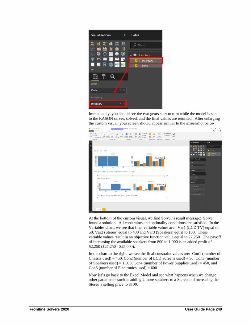
Frontline Solvers 2020 User Guide Page 249
Immediately, you should see the two gears start to turn while the model is sent
to the RASON server, solved, and the final values are returned. After enlarging
the custom visual, your screen should appear similar to the screenshot below.
At the bottom of the custom visual, we find Solver’s result message: Solver found a solution. All constraints and optimality conditions are satisfied. In the
Variables chart, we see that final variable values are: Var1 (LCD TV) equal to
50, Var2 (Stereo) equal to 400 and Var3 (Speakers) equal to 100. These
variable values result in an objective function value equal to 27,250. The payoff
of increasing the available speakers from 800 to 1,000 is an added profit of
$2,250 ($27,250 - $25,000).
In the chart to the right, we see the final constraint values are: Con1 (number of
Chassis used) = 450, Con2 (number of LCD Screens used) = 50, Con3 (number
of Speakers used) = 1,000, Con4 (number of Power Supplies used) = 450, and
Con5 (number of Electronics used) = 600.
Now let’s go back to the Excel Model and see what happens when we change other parameters such as adding 2 more speakers to a Stereo and increasing the
Stereo’s selling price to $100.
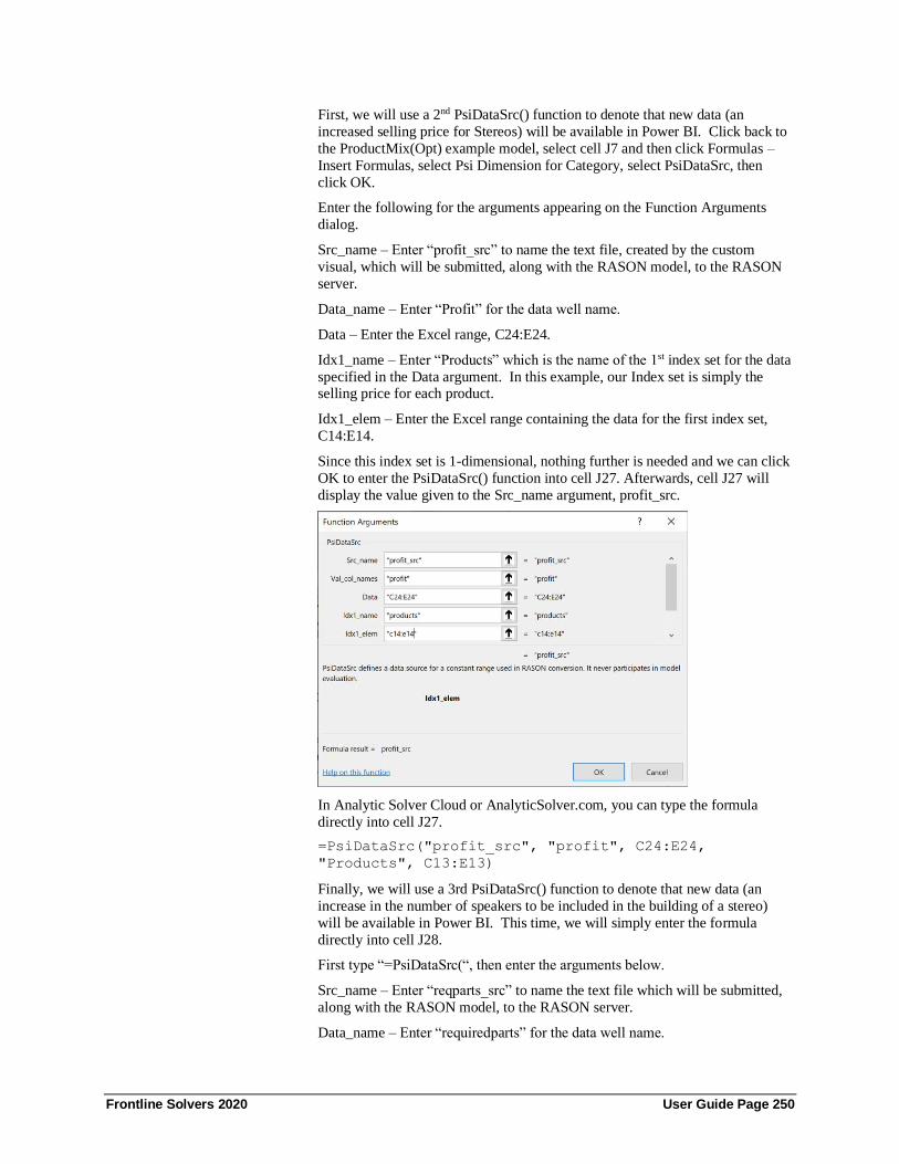
Frontline Solvers 2020 User Guide Page 250
First, we will use a 2nd PsiDataSrc() function to denote that new data (an
increased selling price for Stereos) will be available in Power BI. Click back to
the ProductMix(Opt) example model, select cell J7 and then click Formulas –
Insert Formulas, select Psi Dimension for Category, select PsiDataSrc, then
click OK.
Enter the following for the arguments appearing on the Function Arguments
dialog.
Src_name – Enter “profit_src” to name the text file, created by the custom
visual, which will be submitted, along with the RASON model, to the RASON
server.
Data_name – Enter “Profit” for the data well name.
Data – Enter the Excel range, C24:E24.
Idx1_name – Enter “Products” which is the name of the 1st index set for the data
specified in the Data argument. In this example, our Index set is simply the selling price for each product.
Idx1_elem – Enter the Excel range containing the data for the first index set,
C14:E14.
Since this index set is 1-dimensional, nothing further is needed and we can click
OK to enter the PsiDataSrc() function into cell J27. Afterwards, cell J27 will
display the value given to the Src_name argument, profit_src.
In Analytic Solver Cloud or AnalyticSolver.com, you can type the formula
directly into cell J27.
=PsiDataSrc("profit_src", "profit", C24:E24,
"Products", C13:E13)
Finally, we will use a 3rd PsiDataSrc() function to denote that new data (an
increase in the number of speakers to be included in the building of a stereo)
will be available in Power BI. This time, we will simply enter the formula
directly into cell J28.
First type “=PsiDataSrc(“, then enter the arguments below.
Src_name – Enter “reqparts_src” to name the text file which will be submitted,
along with the RASON model, to the RASON server.
Data_name – Enter “requiredparts” for the data well name.

Frontline Solvers 2020 User Guide Page 251
Data – Enter the Excel range, C18:E22.
Idx1_name – Enter “parts” which is the name of the 1st index set for the data
specified in the Data argument. In this example, there are two index sets. When
data is 2-dimensional, we must enter the index set that describes the rows first.
Idx1_elem – Enter the Excel range containing the data for the first index set,
B18:B22.
Idx2_name – Enter “products” which is the name of the 2nd index set for the data
specified in the Data argument.
Idx2_elem – Enter the Excel range containing the data for the second index set,
C13:E13.
Now we can type “)” to close the function, then press Enter to enter the
PsiDataSrc() function into cell J8. Afterwards, cell J8 will display the value
given to the Src_name argument, reqparts_src.
Your PsiDataSrc function should be similar to the screenshot below.
At this point, cell J26 displays “inventory_src”, cell J27 displays “profit_src”
and cell J28 displays “reqparts_src”. Save the Excel model and then click
Create App – Power BI to save a new file using a new name such as
ProductMix3.pbiviz.
Now we are ready to add a new data table to the ProductMixData.xlsx file.
Open the ProductMixData.xlsx workbook.
Important Note: All data for a custom visual MUST be contained within the
same Excel table or from within multiple tables with the same number of
rows and columns. As a result, we must create a new table in Excel and enter
all data into this new table, including the information from the Inventory
worksheet.
In a new Excel sheet, create a table (Insert – Table) with 16 rows and 5 columns,
then list the products in the first column using the column heading “products”,
the parts by name using the column heading “parts” in the 2nd column, the parts
required per product (requiredparts) in the 3rd column, the selling price or
“profit” per product in the 4th column, and the part inventory for each product in
the last column. Make sure to pass the new selling price for Stereos ($100) and
the increased number of speakers per stereo (4).

Frontline Solvers 2020 User Guide Page 252
Notice that in order to list all of the required parts for each product, we must list
each part and selling price for each part. In addition, each column heading
matches the index sets used in the PsiDataSrc() functions. Rename the
worksheet “AllData” then save the workbook. If there are any leading or
trailing spaces for the column headings or elements, Power BI will stop with an
error.
Open either desktop or cloud-based Power BI, click the icon containing three
horizontal dots at the bottom of Visualizations, then select Import from file from
the menu. Navigate to the location of the saved ProductMix3.pbiviz file. Select the file, then click Open. If the import was successful, you will see a message
indicating as such. Click OK to clear this dialog. A new third icon, bearing the
Frontline Solvers logo is added under Visualizations.
Click this icon to open Frontline Solvers’ custom visual.
If you look to the right of the screen, you will see new data wells appearing
under Visualizations. Recall that the “parts” and “inventory” data wells were
created by the PsiDatasrc() function in the ProductMix(Opt) example model cell J6, inventory_src. Data wells “products” and “profit” were created by the
PsiDatasrc() function in cell J7, profit_src. The PsiDataSrc() function in cell
j28, requiredparts_src, created the data well “requiredparts”.

Frontline Solvers 2020 User Guide Page 253
Now it is time to upload our data. Click to Power BI, then click Get Data –
Excel and open the ProductMixData.xlsx file.
Select AllData on the left, then click Load on the right.
The table headings from the AllData worksheet are uploaded to the Fields task
pane in Power BI.

Frontline Solvers 2020 User Guide Page 254
Drag the fields into the data wells according to the following table.
Field Data Well
inventory Inventory
parts Parts
products Products
profit Profit
requiredparts Requiredparts
Afterwards, your task pane should match the following screenshot.

Frontline Solvers 2020 User Guide Page 255
Immediately, the RASON model is submitted to the RASON Server, the model
is solved and the final variable values are imported back into Power BI.
Troop Rotation Optimization Example
In this example, we will create a Power BI Custom Visual using a slightly more
complex example. In this section, we will create a custom visual using the
Troop Rotation example model by clicking Help – Examples on the Analytic
Solver ribbon, then click Optimization Models and scroll down to Troop
Rotation. Click this hyperlink to open the example model. This example model determines how army troops should be moved to minimize costs.

Frontline Solvers 2020 User Guide Page 256
The optimization model is included in the Model tab in the Solver Task Pane.
This model written in algebraic form is below.
Maximize: Total Cost = 34 * x1 + 42 * x5 + 36 * x9 + 26 * x2 + 33 * x6 + 29 *
x10 + 29 * x3 + 28 * x7 + 32 * x11 + 31 * x4 + 35 * x8 + 38 * x12
Subject To:
Number of troops from Camps 1, 2 and 3 moved to Bases 1, 2, 3 and 4 must not
exceed the number of troops available
Camp1: x1 + x2 + x3 + x4 <= 500
Camp2: x5 + x6 + x7 + x8 <= 400
Camp3: x9 + x10 + x11 + x12 <= 400
Number of troops assigned per base must not be less than the amount required.
Base 1: x1 + x5 + x9 >= 200
Base 2: x2 + x6 + x10 >= 250
Base 3: x3 + x7 + x11 >= 350
Base 4: x4 + x8 + x12 >= 300
x1, x2, x3, x4, x5, x6, x7, x8, x9, x10, x11, x12 > 0
The engine selected to solve this model is the Standard LP/Quadratic Engine as
shown on the Engine tab in the Solver Task Pane.
Next, we will enter four PsiDataSrc() functions into cells P27, P28, P29, and
P30.

Frontline Solvers 2020 User Guide Page 257
In P27, we will expose the moving costs per soldier according to base and camp
in cells C13:F15. To open the Function Arguments dialog, click Formulas –
Insert Function, select Psi Dimension for Category, select PsiDataSrc, then click
OK.
Src_name = Enter “cost_src” for this argument. This names the text file that will be submitted to the RASON server, along with the RASON model.
Data_name – Enter “MovingCost” for this argument. This will be the name of
the data well associated with the data passed in the next argument.
Data – Enter C13:F15 which is the actual cells containing the moving price per
soldier.
Idx1_name – Enter “camps” which is the name of the 1st index set, the row-wise
index set. Remember, you must pass the row-wise index set before the column-
wise index set.
Idx1_elem – Enter the elements of the “camps” index set. These appear in cells B13:B15.
Idx2_name – Enter “bases” which is the name of the 2nd index set, the column
wise index set.
Idx2_elem – Enter the elements of the “bases” index set. These appear in cells
C12:F12.
The Function Arguments dialog should now appear as shown in the screenshots
below.
Click OK to save this function to cell P27.
In Analytic Solver Cloud or AnalyticSolver.com, you can type the formula
directly into cell P7.
=PsiDataSrc("cost_src", "MovingCost", C13:F15,
"camps", B13:B15, "bases", C12:F12)
Click cell P28 and open the Function Arguments dialog to enter the next
PsiDataSrc() function.
In P28, we will expose the variables that indicate the number of troops moved
by camp and base in cells C14:F16. To open the Function Arguments dialog,
click Formulas – Insert Function, select Psi Dimension for Category, select
PsiDataSrc, then click OK.
Src_name = Enter “vars_src” for this argument.
Data_name – Enter “TroopsMoved” for this argument. This will be the name of the Data Well in Power BI that is associated with this data.

Frontline Solvers 2020 User Guide Page 258
Data – Enter C19:F21 which is the actual cells containing the moving price per
soldier. Note: The data range C19:F21 will automatically convert to
“Troops_moved” which is the defined name for this Excel range.
Idx1_name – Enter “camps” which is the name of the 1st index set, the row-wise
index set.
Idx1_elem – Enter the elements of the “camps” index set. These appear in cells
B13:B15.
Idx2_name – Enter “bases” which is the name of the 2nd index set, the column-
wise index set.
Idx2_elem – Enter the elements of the “bases” index set. These appear in cells
C12:F12.
The Function Arguments dialog should now appear as shown in the screenshots
below.
Click OK to save this function to cell P28.
In Analytic Solver Cloud or AnalyticSolver.com, you can type the formula
directly into cell P28.
=PsiDataSrc("vars_src", "TroopsMoved", Troops_moved,
"camps", B13:B15, "bases", C12:F12)
Let’s enter the last two PsiDataSrc() functions by typing the formulas directly
into the Excel cells, starting with the function in cell P29 that will expose the
number of troops available for movement.
In cell P29, enter: “=PsiDataSrc(“
First the first argument, Src_name, enter “available_src”.
For the second argument, Data_name, enter: available. The Data Well
associated with this data will be given this name.
For the Data argument, the third argument, enter: Troops_available. This is the
defined name for cells H19:H21. Alternatively, we could have typed this Excel
range.
Type “camps” for the 4th argument, Idx1_name, which is the name given to the
row-wise index set.
Enter the range for this index set, B13:B15, for Idx1_elem.
Your PsiDataSrc() function should match the one in the screenshot shown below.
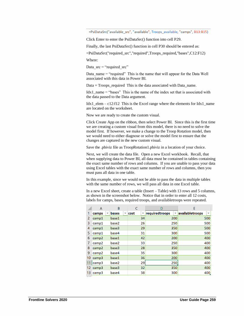
Frontline Solvers 2020 User Guide Page 259
Click Enter to enter the PsiDataSrc() function into cell P29.
Finally, the last PsiDataSrc() function in cell P30 should be entered as:
=PsiDataSrc("required_src","required",Troops_required,"bases",C12:F12)
Where:
Data_src = “required_src”
Data_name = “required” This is the name that will appear for the Data Well
associated with this data in Power BI.
Data = Troops_required This is the data associated with Data_name.
Idx1_name = “bases” This is the name of the index set that is associated with
the data passed to the Data argument.
Idx1_elem – c12:f12 This is the Excel range where the elements for Idx1_name
are located on the worksheet.
Now we are ready to create the custom visual.
Click Create App on the ribbon, then select Power BI. Since this is the first time
we are creating a custom visual from this model, there is no need to solve the
model first. If however, we make a change to the Troop Rotation model, then
we would need to either diagnose or solve the model first to ensure that the changes are captured in the new custom visual.
Save the .pbiviz file as TroopRotation1.pbiviz in a location of your choice.
Next, we will create the data file. Open a new Excel workbook. Recall, that
when supplying data to Power BI, all data must be contained in tables containing
the exact same number of rows and columns. If you are unable to pass your data
using Excel tables with the exact same number of rows and columns, then you
must pass all data in one table.
In this example, since we would not be able to pass the data in multiple tables
with the same number of rows, we will pass all data in one Excel table.
In a new Excel sheet, create a table (Insert – Table) with 13 rows and 5 columns, as shown in the screenshot below. Notice that in order to enter all 12 costs,
labels for camps, bases, required troops, and availabletroops were repeated.
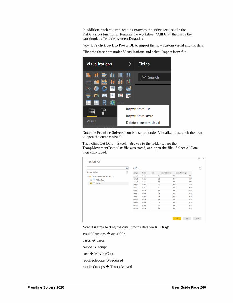
Frontline Solvers 2020 User Guide Page 260
In addition, each column heading matches the index sets used in the
PsiDataSrc() functions. Rename the worksheet “AllData” then save the
workbook as TroopMovementData.xlsx.
Now let’s click back to Power BI, to import the new custom visual and the data.
Click the three dots under Visualizations and select Import from file.
Once the Frontline Solvers icon is inserted under Visualizations, click the icon
to open the custom visual.
Then click Get Data – Excel. Browse to the folder where the
TroopMovementData.xlsx file was saved, and open the file. Select AllData,
then click Load.
Now it is time to drag the data into the data wells. Drag:
availabletroops → available
bases → bases
camps → camps
cost → MovingCost
requiredtroops → required
requiredtroops → TroopsMoved

Frontline Solvers 2020 User Guide Page 261
Note: Since “TroopsMoved” holds the variable values, we can simply drag
“requiredtroops”, which contains the same number of rows and columns as
TroopsMoved, as a starting point for the algorithm. A starting point for this
model is not needed because our model is linear, however, if our model was
nonlinear or nonsmooth, this would be more important.
The resultant Power BI custom visual is shown in the screenshot below. Now
each time new data is imported into Power BI, the Troop Movement example
data will be solved from within Power BI.
Using Optimization Parameters in Power BI
Now what happens when we would like to see how our final variable values and
objective function value change as the number of troops required changes. For
this type of “What If’ analysis, we can use the PsiOptParam() optimization parameter. Recall from the chapter, Examples: Parameters and Sensitivity
Analysis, an optimization parameter (PsiOptParam) is automatically varied
when you perform multiple optimizations. You do this by clicking the Optimize
button on the Ribbon, or the green arrow in the Task Pane, with the Number of
Optimizations set to a value greater than 1.
Let’s go back to our example Excel model and enter an optimization parameter
for the number of troops required in Base 1. In cell C13, enter
“=PsiOptParam({34,24,14})”, then click the Platform tab in the Solver Task
pane and change the Number of Optimizations to “3”. When I click Solve,
Analytic Solver will solve 3 optimizations. In the first optimization, cell C13
will be set to 34, in the second, 24, and in the third, 14.
Click the Output tab, then click the green arrow to solve the model. After the
solving process is over, we can select the three different optimizations in the
Optimization drop down menu (in the Tools section of the Analytic Solver
ribbon), to see how the objective function changes according to the value set for
this parameter.

Frontline Solvers 2020 User Guide Page 262
In the first optimization, cell C13 = 34 and the resultant objective function value
was $32,950. In the second optimization, cell C13 = 24 and the resultant
objective function value was $31,150 and in the third optimization cell C13 j =
14 with an objective function value of 29,150.
Save the Excel file, then click Create App – Power BI to create a new custom
visual file. This time, we will name the custom visual file,
TroopRotationOptParam.pbiviz.
Click back to Power BI and import the newly created custom visual file. Click
the new Frontline Solvers icon to open the custom visual. Immediately, the
model will solve and the results will be displayed in the Power BI window. To view each solution, click the down arrow within the newly added Multiple
Optimization drop-down menu.
Note: When entering PsiOptParam manually (i.e. simply typing the function
into an Excel cell) in Analytic Solver Cloud, the taskpane must be refreshed
before performing a parameter analysis report.
Simulation Example Model
Now let’s create a custom visual from a simulation example. The process is
exactly the same when using an optimization model. Open the Business Forecast
Example by clicking Help – Examples – Simulation Models, click the Business Forecast hyperlink to open the file, then click the Forecast with Uncertainty tab.

Frontline Solvers 2020 User Guide Page 263
First, we will use a PsiDataSrc() function to generate data wells for use in the
Power BI custom visual.
Click a blank cell, such as cell G24, then type: “=PsiDataSrc(“market_src”,
“market”, H16:J17, “parameters”, G16:G17, “mktdemand”, H15:J15)
where:
market_src – Is the name used to identify the text file that will be submitted to
the RASON server.
market – Will be the name of the data well in Power BI.
H16:J17 – Is the data range for “market”.
parameters – Is the name of the 1st index set for the data specified in the “data”
argument, market.
G16:G17 – Is the Excel range where the data for “parameters” is located.
mktdemand – Is the name of the 2nd index set for the data specified in the “data”
argument.
H15:J15 – Is the Excel range where the data for “mktdemand” is located.
Type “)” to close the formula and then press the Enter key to enter the formula
into the Excel cell.
Click a 2nd blank cell, such as G25, then enter the following function.
=PsiDataSrc(“price_src”, “mktprice”, H20:J20, “price”, H19:J19)
where:
price_src – Is the name used to identify the text file that will be submitted to the
RASON server.
mktprice – Will be the name of the data well in Power BI.
H20:J20 – Is the data range for “mktprice”.
price – Is the name of the 2nd index set for the data specified in the Data argument, market.
H19:J19 – Is the Excel range where the data for “price” is located.
Click Create App – Power Bi to create a new Power BI custom visual file with a
name, such as BusinessForecast1.pbiviz.
Click back to Excel and open a new workbook to enter the following data into
an Excel table. Then save the workbook as BusinessForecastData.xlsx.

Frontline Solvers 2020 User Guide Page 264
Open Power BI and add in the custom visual, then click Get Data – Excel to
import the data. Afterwards, drag the data fields to the appropriate data wells as
shown in the table below.
Fields Data Wells
market market
mktdemand mktdemand
mktprice mktprice
parameters parameters
price price
Your task pane should match the following screenshot.
Immediately, once the data wells are filled with the appropriate data fields, a
simulation will be run.
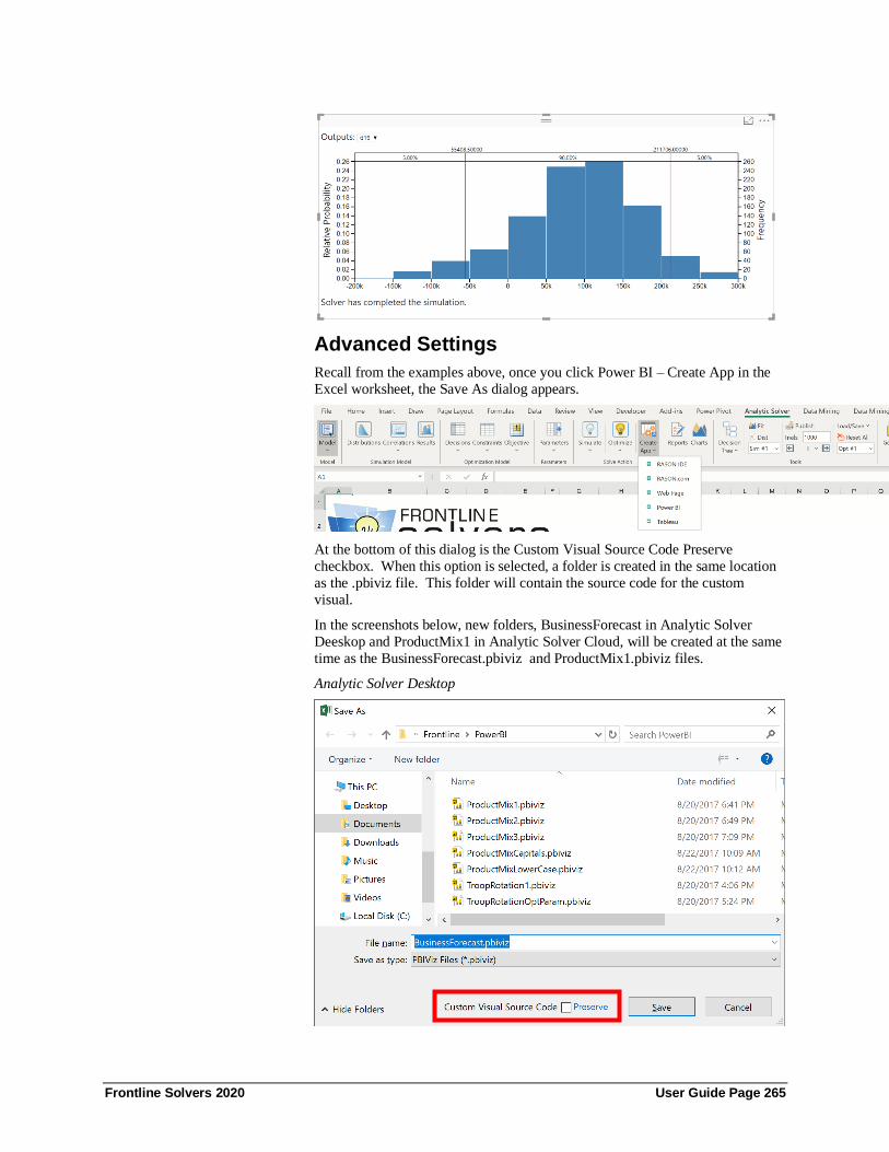
Frontline Solvers 2020 User Guide Page 265
Advanced Settings
Recall from the examples above, once you click Power BI – Create App in the
Excel worksheet, the Save As dialog appears.
At the bottom of this dialog is the Custom Visual Source Code Preserve
checkbox. When this option is selected, a folder is created in the same location
as the .pbiviz file. This folder will contain the source code for the custom
visual.
In the screenshots below, new folders, BusinessForecast in Analytic Solver
Deeskop and ProductMix1 in Analytic Solver Cloud, will be created at the same
time as the BusinessForecast.pbiviz and ProductMix1.pbiviz files.
Analytic Solver Desktop

Frontline Solvers 2020 User Guide Page 266
Analytic Solver Cloud
You will find the type script file, visual.ts within the src folder. Users can
manipulate this file to customize the look and feel of the custom visual, such as
the face of the custom visual icon (within Visualizations), alter the RASON model, etc. For more information on customizing the visual.ts file, see the
webpage: https://powerbi.microsoft.com/en-us/documentation/
Note: If the visual.ts file is altered, a new pbiviz package must be created. To
do so, open a command prompt, change the directory to the root directory of the custom visual, and enter “pbiviz package”, as shown in the screenshot below.
The new custom visual file (.pbiviz) will be saved to the Dist folder.

Frontline Solvers 2020 User Guide Page 267
Error Messages
If you’ve made an error in your PsiDataSrc() function or in your data file, your
custom visual will display an error such as “Inconsistent Data source definition
PSI could not parse Excel formulas" or “Invalid binding source definition PSI
could not parse Excel formulas”.
If your custom visual is displaying either of these errors or a different error, first, check the PsiDataSrc() function in your Excel model to make sure that you have
not mixed up the order of your index sets. In addition, check your data to make
sure that it is 1. Contained within an Excel table, 2. That the column headings
match the index sets defined in PsiDataSrc() and 3. That your model parameters
match the elements in your data table.
For more information on an error message displayed in your custom visual,
contact Frontline Systems Support Team by emailing [email protected] or by
calling 888-831-0333.
Frontline Solvers 2020 User Guide Page 268
Creating Custom Extensions in Tableau
Introduction Starting with V2018, Analytic Solver includes the ability to turn your Excel-
based optimization or simulation model into a Tableau Dashboard Extension,
with just a few mouse clicks! This is quite similar to the ability to create Power
BI Custom Visuals as discussed in the previous chapter. This feature is only
compatible with versions of Tableau version 2018.2 or later.
To start, simply select rows or columns of data to serve as changeable
parameters, then choose Create App – Tableau, and save the file created
byAnalytic Solver. In Tableau, you’ll see the newly-created file under
Extensions on the left side of the dashboard, where you can drag it onto your
dashboard. You’ll be prompted to match the parameters your model needs with
data in Tableau. What you get isn’t just a chart – it’s your full optimization or
simulation model, ready to accept Tableau data, run on demand (using our
RASON server), and display visual results in Tableau!
Installing Tableau Tableau is an industry leading desktop or cloud-based interactive business
intelligence tool that centers on data visualization, dashboarding and data discovery. In past versions of Analytic Solver, users have only been able to
upload their model parameters (or their model data) to Tableau after solving an
optimization or simulation model. However, starting with V2018, Analytic
Solver now includes the ability to turn your Excel based optimization or
simulation model into a Tableau Extension, that is your full optimization or
simulation model, ready to accept Tableau data, run on demand on the web
(using our RASON server) and display visual results in Tableau.
In order to use this new feature in Analytic Solver, you must first install Tableau
V2018.2 or later or open the free cloud based version of Tableau. For more
information on this business intelligence tool, see the following website:
https://www.tableau.com/
Solving Optimization Models in Tableau In this section, we will create a custom Tableau Extension using the Product
Mix example model.
Open the Product Mix.xlsx model, previously discussed in the Conventional
Optimization and Power BI chapters, by clicking Help – Examples on the
ribbon, clicking Optimization Examples and then the Product Mix link. Recall
that this example model determines the optimal mix of products that a company
should produce in order to maximize profits.

Frontline Solvers 2020 User Guide Page 269
The optimization model is included in the Model tab in the Solver Task Pane.
This model written in algebraic form is below.
Maximize: Total Profit = $75x1 + $50x2 + $35x3
Subject To:
Chassis: 1x1 + 1x2 + 0x3 <= 450
LCD Screen: 1x1 + 0x2 + 0x3 <= 250
Speaker: 2x1 + 2x2 + 1x3 <= 800
Power Supply: 1x1 + 1x2 + 0x3 <= 450
Electronics: 2x2 + 1x2 + 1x3 <= 600
x1, x2, x3 > 0
The engine selected to solve this model is the Standard LP/Quadratic Engine as
shown on the Engine tab in the Solver Task Pane. This is the engine that will be
used to solve the model within Tableau.
In past versions of Analytic Solver, you only had the option of uploading your
final solution values (final variable, constraint and objective values) to Tableau.
As a result, any time there was a change to the model, the model had to be
solved in Excel first and then the data could be (again) uploaded to Tableau. All
of this changed with V2018. Now you can change your model parameters and
resolve your model within Tableau - without ever having to go back to Excel!
To start, we will use the PsiDataSrc() function to “flag” or specify the
parameters in the Excel model that might possibly change in the future; for
example, in the product mix model, the amount of inventory on hand for each
part, the profit point for each product or the number of parts that makeup each
product.
Select a blank cell on the Product Mix Example 1 tab, say J6. Click Formulas –
Insert Function to open the Insert Function dialog, then select Psi Dimension for
Category. Afterwards, highlight the function PsiDataSrc, and click OK.
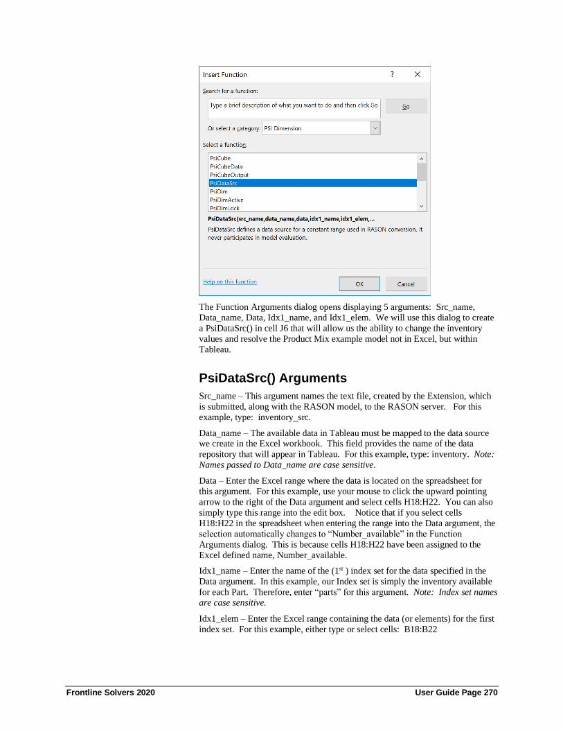
Frontline Solvers 2020 User Guide Page 270
The Function Arguments dialog opens displaying 5 arguments: Src_name,
Data_name, Data, Idx1_name, and Idx1_elem. We will use this dialog to create
a PsiDataSrc() in cell J6 that will allow us the ability to change the inventory
values and resolve the Product Mix example model not in Excel, but within
Tableau.
PsiDataSrc() Arguments
Src_name – This argument names the text file, created by the Extension, which
is submitted, along with the RASON model, to the RASON server. For this
example, type: inventory_src.
Data_name – The available data in Tableau must be mapped to the data source we create in the Excel workbook. This field provides the name of the data
repository that will appear in Tableau. For this example, type: inventory. Note:
Names passed to Data_name are case sensitive.
Data – Enter the Excel range where the data is located on the spreadsheet for
this argument. For this example, use your mouse to click the upward pointing
arrow to the right of the Data argument and select cells H18:H22. You can also
simply type this range into the edit box. Notice that if you select cells
H18:H22 in the spreadsheet when entering the range into the Data argument, the
selection automatically changes to “Number_available” in the Function
Arguments dialog. This is because cells H18:H22 have been assigned to the
Excel defined name, Number_available.
Idx1_name – Enter the name of the (1st ) index set for the data specified in the
Data argument. In this example, our Index set is simply the inventory available
for each Part. Therefore, enter “parts” for this argument. Note: Index set names
are case sensitive.
Idx1_elem – Enter the Excel range containing the data (or elements) for the first
index set. For this example, either type or select cells: B18:B22

Frontline Solvers 2020 User Guide Page 271
Since this index set is 1-dimensional, nothing further is needed and we can click OK to enter the PsiDataSrc() function into cell J6.
In Analytic Solver Cloud or AnalyticSolver.com, you can type the formula
directly into cell J226.
=PsiDataSrc("inventory_src", "inventory",
Number_available, "parts", B18:B22)
Afterwards, cell J26 will display the value given to the Src_name argument,
inventory_src. Save the Excel model and then click Create App – Tableau to
save a new Tableau Extension file.
• In Analytic Solver Desktop, immediately, the Save As dialog appears.
Select a folder to save the tableau extension files to, and then click
Save. For example, the screenshot below displays a folder name of
“TableauExtensions”.
Analytic Solver Desktop
• In Analytic Solver Cloud, first, you will receive the following dialog.
Type the filename of the folder, for example, TableauExtensions.

Frontline Solvers 2020 User Guide Page 272
After the file is downloading, you'll be asked if you'd like to open or
save the file, choose Save As, then save the file in the desired location.
Click Select Folder or Save. At this point your Excel model is translated into
the RASON® modeling language, and your Tableau extension is created. After
a moment, the following message appears.
NOTE 1: There is no need to solve the model first unless a change has been
made to an already existing RASON model. If a change has been made to the
workbook after a RASON model has been created, or since Create App –
RASON IDE/RASON.com/Web Page/Power Bi/Tableau has been selected, then
you MUST either solve or diagnose the Excel model in order for the changes to
be reflected in the new RASON model.
NOTE 2: When creating a RASON model through desktop Analytic Solver or AnalyticSolver.com, model elements (objective function and all variables and
constraints) may now exist on multiple worksheets within the same Excel
workbook.
Viewing the Tableau Extension File
Open File Explorer and browse to the folder where you saved the Tableau
extension. Within in that folder will be an Extensions folder. Click that folder and open the Solver.trex file using Notepad.

Frontline Solvers 2020 User Guide Page 273
This file contains information such as the extensions name (or how it will appear
in Tableau) and the url where the extension is hosted. To publish the html file to
a website, simply replace http://localhost:8000 with the desired url.
Starting up the Server
Since Tableau extensions are simply web pages, we will first need to start up a
web server to serve our content. For this example, we will serve up the webpage
to the default location. To do so, open a command prompt, navigate to the root
of the extensions repository and run “http-server -p 8000”.
This command starts up a simple http server listening on port 8000.
Creating a Data File
In order to provide the data for the Product Mix example file to Tableau, we
must create a data file. Within this file, we will pass the inventory levels by part.
This data file can be of any format supported by Tableau such as a CSV file, a
text file, a database, etc. In this example, we will use an Excel workbook to
hold the data. For more information on the types of files supported by Tableau,
please see the Tableau documentation at:
http://onlinehelp.tableau.com/current/pro/desktop/en-us/default.html
Open a blank worksheet and create a table with two columns. List the parts by
name in the first column using the column heading “parts” and the inventory
levels in the second column using the column heading “inventory”, as shown in
the screenshot below.

Frontline Solvers 2020 User Guide Page 274
Note: Column headings must be identical to the names of the Index Sets passed
to the PsiDataSrc() function. Make sure there are no spaces before or after
column headings or row elements.
Recall that we labeled the IndexSet as “parts” (4th argument of PsiDataSrc) and
Data_name as “inventory” (2nd argument of PsiDataSrc) so the title for column
A must be “parts” and the title for column B must be “inventory”. Now save the
workbook to a desired location.
Opening Extension within Tableau
Open either desktop, server or cloud-based Tableau. The screenshot below
depicts the opening screen of desktop Tableau. Click Microsoft Excel under
Connect.
An Open dialog opens.

Frontline Solvers 2020 User Guide Page 275
Browse to the location of your data file and click Open.
A new worksheet, Sheet 1, is automatically created. Click on the Sheet 1 tab.
On Sheet 1, drag Parts (under Dimensions) to Sheet 1 rows…

Frontline Solvers 2020 User Guide Page 276
… and then drag Inventory (under Measures) to
Hover over , click the down arrow that appears to the right,
then select Dimensions from the menu.
Note that the information in ProductMixDataSource matches the data in Sheet 1.
Right click the Sheet 1 tab and rename the worksheet to “Inventory”, then click
the New Dashboard icon at the bottom of Tableau to open a new dashboard.

Frontline Solvers 2020 User Guide Page 277
First, drag the Inventory worksheet onto the dashboard canvas.
Then drag the Extension icon, under Objects, onto the canvas.
On the Select an Extension dialog, click Browse…

Frontline Solvers 2020 User Guide Page 278
… and browse to the location of the Tableau Extension file (Solver.trex). In this
example, the file was saved to the TableauExtensions folder. Within this folder,
select All Files, then double click the Extensions folder and select the
Solver.trex file.
Click Open to open the Tableau extension. A dialog opens asking to select a
data source for “parts”. Confirm that “Inventory” is selected for “Sheet” and
“Parts” is selected for “Column”. Note that these are the same names passed to
the PsiDataSrc() function in the Excel Product Mix.xlsx workbook.

Frontline Solvers 2020 User Guide Page 279
Click OK.
On the Select data source for: inventory dialog, select “Inventory” for “Sheet”
and “Inventory” for “Column”. Then click OK.
Immediately, two gears appear and start to turn while the model is sent to the
RASON server, solved with the LP/Quadratic engine, and the final values are
returned. Your screen should appear similar to the screenshot below.

Frontline Solvers 2020 User Guide Page 280
Once the RASON server has imported the final solution values into Tableau,
Solver’s result message, “Solver found a solution. All constraints and optimality conditions are satisfied”, is displayed at the bottom of the Extension
window. In the Variables chart, we see that the final variable values are: Var1
(LCD TV) equal to 200, Var2 (Stereo) equal to 200 and Var3 (Speakers) equal
to 0. These variable values result in an objective function value equal to
$25,000. In the chart to the right, we see the final constraint values are: Con1
(number of Chassis used) = 400, Con2 (number of LCD Screens used) = 200,
Con3 (number of Speakers used) = 800, Con4 (number of Power Supplies used)
= 400, and Con5 (number of Electronics used) = 600.
Now let’s go back to the Excel Model and see what happens when we change a
few parameters such as increasing the inventory of speakers from 800 to 1,000,
adding 2 more speakers to a Stereo during manufacturing and increasing the
Stereo’s selling price to $100.
First, we will use a 2nd PsiDataSrc() function to denote that new data (an
increased selling price for Stereos) will be available in Tableau. Click back to
the ProductMix(Opt) example model, select cell J27 and then click Formulas –
Insert Function, select Psi Dimension for Category, select PsiDataSrc, then click OK.
Enter the following for the arguments appearing on the Function Arguments
dialog.
Src_name – Enter “profit_src” to name the text file, created by the custom
visual, which will be submitted, along with the RASON model, to the RASON
server.

Frontline Solvers 2020 User Guide Page 281
Data_name – Enter “Profit” for the data repository name. Note: Names passed
to Data_name are case sensitive.
Data – Enter the Excel range, C24:E24.
Idx1_name – Enter “Products” which is the name of the 1st index set for the data specified in the Data argument. In this example, our Index set is simply the
selling price for each product. Note: Index set names are case sensitive.
Idx1_elem – Enter the Excel range containing the data for the first index set,
C13:E13.
Since this index set is 1-dimensional, nothing further is needed and we can click
OK to enter the PsiDataSrc() function into cell J7. Afterwards, cell J7 will
display the value given to the Src_name argument, profit_src.
In Analytic Solver Cloud or AnalyticSolver.com, you can type the formula
directly into cell J27.
=PsiDataSrc("profit_src", "profit", C24:E24,
"products", C13:E13)
Finally, we will use a 3rd PsiDataSrc() function to denote that new data (an increase in the number of speakers to be included in the building of a stereo)
will be available in Tableau. This time, we will simply enter the formula
directly into cell J28.
First type “=PsiDataSrc(“, then enter the arguments below.
Src_name – Enter “reqparts_src” to name the text file which will be submitted,
along with the RASON model, to the RASON server.
Data_name – Enter “requiredparts” for the data repository name. Note: Names
passed here are case sensitive.
Data – Enter the Excel range, C18:E22.
Idx1_name – Enter “parts” which is the name of the 1st index set for the data
specified in the Data argument. In this example, there are two index sets. When
data is 2-dimensional, we must enter the index set that describes the rows first.
Note: Index set names are case sensitive.
Idx1_elem – Enter the Excel range containing the data for the first index set,
B18:B22.

Frontline Solvers 2020 User Guide Page 282
Idx2_name – Enter “products” which is the name of the 2nd index set for the data
specified in the Data argument.
Idx2_elem – Enter the Excel range containing the data for the second index set,
C13:E13. Note: Index set names are case sensitive.
Now we can type “)” to close the function, then press Enter to enter the
PsiDataSrc() function into cell J28. Afterwards, cell J228 will display the value
given to the Src_name argument, reqparts_src.
Your PsiDataSrc function should be similar to the screenshot below.
At this point, cell J26 displays “inventory_src”, cell J27 displays “profit_src”
and cell J28 displays “reqparts_src”. Save the Excel model and then click
Create App – Tableau to save a new file Tableau extension file, Solver.trex.
Now we are ready to add a new data table to the ProductMixDataSource.xlsx
file.
Open the ProductMixDataSource.xlsx workbook.
Important Note: In Tableau, unlike when creating a Power BI custom visual, it
is not necessary that all data be contained within the same Excel table or from
within multiple tables with the same number of rows and columns. However,
for ease of use, this example includes all data within the same Excel table.
In a new Excel sheet, create a table (Insert – Table) with 16 rows and 5 columns,
then list the products in the first column using the column heading “products”,
the parts by name using the column heading “parts” in the 2nd column, the parts
required per product (requiredparts) in the 3rd column, the selling price or
“Profit” per product in the 4th column, and the part inventory for each product in the last column. Make sure to pass the new selling price for Stereos ($100)
and the increased number of speakers per stereo (4).
Notice that in order to list all of the required parts for each product, we must list each part and selling price for each part. In addition, each column heading
matches the index sets used in the PsiDataSrc() functions. Rename the
worksheet “AllData” then save the workbook. If there are any leading or
trailing spaces for the column headings or elements, Tableau will stop with an
error.
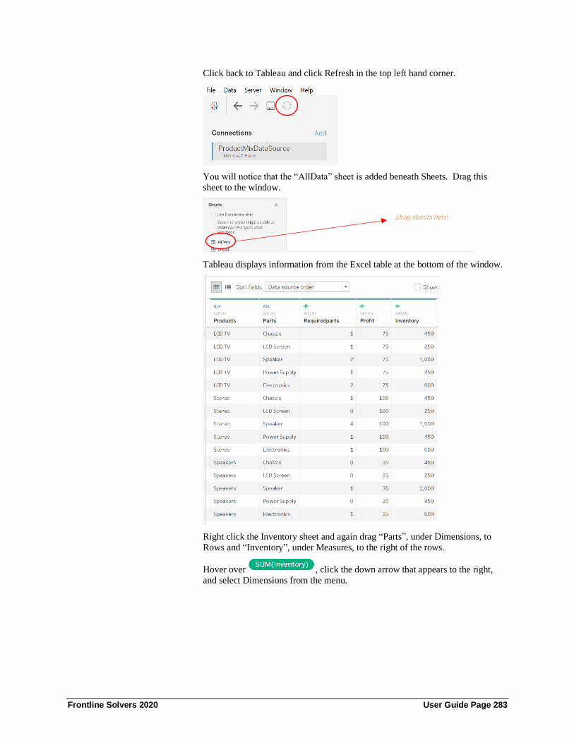
Frontline Solvers 2020 User Guide Page 283
Click back to Tableau and click Refresh in the top left hand corner.
You will notice that the “AllData” sheet is added beneath Sheets. Drag this
sheet to the window.
Tableau displays information from the Excel table at the bottom of the window.
Right click the Inventory sheet and again drag “Parts”, under Dimensions, to
Rows and “Inventory”, under Measures, to the right of the rows.
Hover over , click the down arrow that appears to the right,
and select Dimensions from the menu.

Frontline Solvers 2020 User Guide Page 284
Add a new worksheet and drag “Parts”, under Dimensions, to Rows and
“Products”, under Dimensions, to “Columns”. Then drag “RequiredParts”,
under Measures, to the field elements.
Hover over , click the down arrow that appears to the right,
and select Dimensions from the menu.
Name the sheet “Required Parts” and then add a third sheet. In Sheet 3, drag
“Products”, under Dimensions, to “Columns” and drag “Profit”, under
Measures, to the column elements.
Hover over , click the down arrow that appears on the right
then select Dimensions from the menu.

Frontline Solvers 2020 User Guide Page 285
Rename the sheet from Sheet 3 to Profit and then create a new dashboard. Drag
all three sheets, Inventory, Required Parts and Profit, to the canvas and then drag
a new Extension to the canvas. Open the Solver.trex file in
…\TableauExtensions\Extensions.
At this point we will connect the dimensions created by the PsiDataSrc()
function in Excel with the actual data in Tableau. A dialog appears asking to
“Select a datasource for: parts”. Select “Inventory” for Sheet and “Parts” for
Column to match the “parts” dimension in the Excel sheet to the “Parts”
dimension in the Tableau Inventory sheet.
Click OK.
On the “Select data source for: inventory” dialog, select “Inventory” for Sheet
and “Inventory” for Column to match the “inventory” dimension in the Excel
sheet to the “Inventory” dimension in the Tableau Inventory sheet.
Click OK.
On the “Select data source for: products” dialog, select “Required Parts” for
Sheet and “Products” for Column to match the “products” dimension in the
Excel sheet to the “Products” dimension in the Tableau Required Parts sheet.
Click OK.

Frontline Solvers 2020 User Guide Page 286
On the “Select data source for: profit” dialog, select “Profit” for Sheet and
“Profit” for Column to match the “profit” dimension in the Excel sheet to the
“Profit” dimension in the Tableau Profit sheet.
Click OK.
On the “Select data source for: requiredparts” dialog, select “Required Parts” for
Sheet and “RequiredParts” for Column to match the “requiredparts” dimension
in the Excel sheet to the “RequiredParts” dimension in the Tableau Required
Parts sheet.
Click OK.
Immediately, the RASON model is submitted to the RASON Server, the model
is solved with the LP/Quadratic engine and the final variable values are
imported back into Tableau.
At the bottom of the extension, we find Solver’s result message: Solver found a
solution. All constraints and optimality conditions are satisfied. In the
Variables chart, we see that the final variable values are: Var1 (LCD TV) equal to 233, Var2 (Stereo) equal to 133 and Var3 (Speakers) equal to 0. These
variable values result in an objective function value equal to 30,833. In the chart
to the right, we see the final constraint values are: Con1 (number of Chassis
used) = 367, Con2 (number of LCD Screens used) = 233, Con3 (number of
Speakers used) = 1,000, Con4 (number of Power Supplies used) = 367, and
Con5 (number of Electronics used) = 600. Notice that with the addition of 2
more speakers required to manufacturing Speakers, the increased unit profit of
Stereos to $100 and the added Speaker inventory, our profit has increased by
$5,833.

Frontline Solvers 2020 User Guide Page 287
Troop Rotation Optimization Example
In this example, we will create a Tableau Extension using a slightly more
complex example. In this section, we will create an Extension using the Troop
Rotation example model by clicking Help – Examples on the Analytic Solver
ribbon, then clicking Optimization Models and scrolling down to Troop
Rotation. Click the hyperlink to open the example model. This example model
determines how army troops should be moved to minimize costs.
The optimization model is included in the Model tab in the Solver Task Pane.
This model written in algebraic form is below.
Minimize: Total Cost = 34 * x1 + 42 * x5 + 36 * x9 + 26 * x2 + 33 * x6 + 29 *
x10 + 29 * x3 + 28 * x7 + 32 * x11 + 31 * x4 + 35 * x8 + 38 * x12

Frontline Solvers 2020 User Guide Page 288
Subject To:
Number of troops from Camps 1, 2 and 3 moved to Bases 1, 2, 3 and 4 must not
exceed the number of troops available
Camp1: x1 + x2 + x3 + x4 <= 500
Camp2: x5 + x6 + x7 + x8 <= 400
Camp3: x9 + x10 + x11 + x12 <= 400
Number of troops assigned per base must not be less than the amount required.
Base 1: x1 + x5 + x9 >= 200
Base 2: x2 + x6 + x10 >= 250
Base 3: x3 + x7 + x11 >= 350
Base 4: x4 + x8 + x12 >= 300
x1, x2, x3, x4, x5, x6, x7, x8, x9, x10, x11, x12 > 0
The engine selected to solve this model is the Standard LP/Quadratic Engine as
shown on the Engine tab in the Solver Task Pane. This is the engine that will be
used to solve the model within Tableau.
Next, we will enter three PsiDataSrc() functions into cells P27, P28, and P29.
In cell P27, we will expose the moving costs per soldier according to the base
and camp dimensions in cells C12:F112. To open the Function Arguments
dialog, click Formulas – Insert Function, select Psi Dimension for Category,
select PsiDataSrc, then click OK.
Src_name = Enter “cost_src” for this argument. This names the text file that will be submitted to the RASON server, along with the RASON model.
Data_name – Enter “cost” for this argument. This will be the name of the data
repository associated with the data passed in the next argument.
Data – Enter C13:F15 which is the actual cells containing the moving price per
soldier.
Idx1_name – Enter “camps” which is the name of the 1st index set, the row-wise
index set. Remember, you must pass the row-wise index set before the column-
wise index set.
Idx1_elem – Enter the elements of the “camps” index set. These appear in cells B13:B15.
Idx2_name – Enter “bases” which is the name of the 2nd index set, the column
wise index set.
Idx2_elem – Enter the elements of the “bases” index set. These appear in cells
C12:F12.

Frontline Solvers 2020 User Guide Page 289
The Function Arguments dialog should now appear as shown in the screenshots
below.
Click OK to save this function to cell P27.
In Analytic Solver Cloud or AnalyticSolver.com, you can type the formula
directly into cell J27.
=PsiDataSrc("cost_src", "cost", C13:F15, "camps",
B13:B15)
Click cell P28 and open the Function Arguments dialog to enter the next
PsiDataSrc() function.
Let’s enter the last two PsiDataSrc() functions by typing the formulas directly
into the Excel cells, starting with the function in cell P28 that will expose the
number of troops available for movement.
In cell P28, enter: “=PsiDataSrc(“
First the first argument, Src_name, enter “available_src”.
For the second argument, Data_name, enter: “availabletroops”. The Data Well
associated with this data will be given this name.
For the Data argument, the third argument, enter: “Troops_available”. This is
the defined name for cells H19:H21. Alternatively, we could have typed this
Excel range.
Type “camps” for the 4th argument, Idx1_name, which is the name given to the
row-wise index set.
Enter the range for this index set, B13:B15, for Idx1_elem.
Your PsiDataSrc() function should match the one in the screenshot shown
below.
Click Enter to enter the PsiDataSrc() function into cell P28.
Finally, the last PsiDataSrc() function in cell P9 should be entered as:
=PsiDataSrc("required_src","requiredtroops",Troops_required,"bases",C12:F12)
Where:
Data_src = “required_src”
Data_name = “requiredtroops” This is the name that will appear for the data
repository associated with this data in Tableau
Data = Troops_required This is the data associated with Data_name.

Frontline Solvers 2020 User Guide Page 290
Idx1_name = “bases” This is the name of the index set that is associated with
the data passed to the Data argument.
Idx1_elem – C12:F12 This is the Excel range where the elements for
Idx1_name are located on the worksheet.
Now we are ready to create the Tableau Extension.
Click Create App on the ribbon, then select Tableau. Since this is the first time
we are creating an Extension from this model, there is no need to solve the
model first. If, however, we make a change to the Troop Rotation model, then
we would need to either diagnose or solve the model first to ensure that the
changes are captured in the new extension.
Save the Solver.trex file (the Tableau Extension file) in a location of your
choice.
Next, we will create the data file. Open a new Excel workbook.
For convenience sake, in this example, we will pass all data in one Excel table.
In a new Excel workbook, create a table (Insert – Table) with 13 rows and 5
columns, as shown in the screenshot below. Notice that in order to enter all 12
costs, labels for camps, bases, required troops, and availabletroops were
repeated.
Note that each column heading matches the index sets used in the PsiDataSrc()
functions. Rename the worksheet “AllData” then save the workbook as TroopMovementData.xlsx.
Now let’s click back to the Data Source tab in Tableau, to import the new
Extension and the data. First, just to keep our choices limited to the Troop
Movement example, hover over ProductMixDataSource, click the down arrow
that appears on the right and select remove. Right click the Extension tab and
select Delete, then Delete all worksheets associated with the Product Mix
extension. Then, on the Data Source tab, click Add – Microsoft Excel, browse
to the location of TroopMovementData.xlsx and click Open.

Frontline Solvers 2020 User Guide Page 291
The AllData sheet appears under Sheets and the data from that sheet appears at
the bottom of the Tableau window. Click Sheet 1. Under Dimensions, drag
“Bases” to Columns and “Camps” to Rows. Under Measures, drag “Cost” to the
table elements. Hover over (in the Marks section), click the
down arrow that appears to the right, and select Dimension.
Rename the worksheet to Cost and then add a new Sheet.

Frontline Solvers 2020 User Guide Page 292
On Sheet 2, drag “Bases”, under Dimensions, to Columns and “Requiredtroops”,
under Measures, as the table elements. Hover over , click the
down arrow that appears to the right, then select Dimensions from the menu.
Raname the worksheet to Required Troops and then add a new Sheet.
On Sheet 3, drag “Camps”, under Dimensions, to Rows and “Availabletroops”,
under Measures, to the table elements. Hover over , click the
down arrow that appears to the right, then select Dimensions from the menu.
Rename the sheet to Available Troops and then open a new Dashboard.
Drag each of the three sheets (Cost, Required Troops and Available Troops) and
the Extension to the Tableau canvas as described in the Product Mix example.

Frontline Solvers 2020 User Guide Page 293
Match the dimensions from the Excel sheet to the dimensions and measures in
the Tableau sheets as follows.
The resultant Tableau Extension is shown in the screenshot below. Now each
time new data is imported into Tableau, the Troop Movement example data will
be solved from within Tableau without the need to ever return to the original
Excel workbook.

Frontline Solvers 2020 User Guide Page 294
Using Optimization Parameters in Tableau
Now what happens when we would like to see how our final variable values and
objective function value change as the number of troops required changes. For
this type of “What If’ analysis, we can use the PsiOptParam() optimization
parameter. Recall from the chapter, Examples: Parameters and Sensitivity
Analysis, an optimization parameter (PsiOptParam) is automatically varied
when you perform multiple optimizations. You do this by clicking the Optimize
button on the Ribbon, or the green arrow in the Task Pane, with the Number of
Optimizations set to a value greater than 1.
Let’s go back to our example Troop Movement Excel model and enter an
optimization parameter for the number of troops required in Base 1. In cell C13, enter “=PsiOptParam({34,24,14})”, then click the Platform tab in the Solver
Task pane and change the Number of Optimizations to “3”. When I click
Solve, Analytic Solver will solve 3 optimizations. In the first optimization, cell
C13 will be set to 34, in the second, 24, and in the third, 14.
Click the Output tab, then click the green arrow to solve the model. After the
solving process is over, we can select the three different optimizations in the
Optimization drop down menu (in the Tools section of the Analytic Solver
ribbon), to see how the objective function changes according to the value set for
this parameter.
In the first optimization, cell C13 = 34 and the resultant objective function value
was $32,950. In the second optimization, cell C13 = 24 and the resultant
objective function value was $31,150 and in the third optimization cell C13 =
14 with an objective function value of 29,150.

Frontline Solvers 2020 User Guide Page 295
Save the Excel file, then click Create App – Tableau to create a new Tableau
Extension.
Click back to Tableau and import the newly created Tableau Extension.
Immediately, the model solves and the results will be displayed on the Tableau canvas. To view each solution, click the down arrow within the newly added
Multiple Optimization drop-down menu.
Simulation Example Model
Now let’s create a Tableau extension using a simulation example. The process
is exactly the same as when using an optimization model. Open the Business
Forecast Example by clicking Help – Examples – Simulation Models, click the
Business Forecast hyperlink to open the file.
First, we will use a PsiDataSrc() function to generate data repositories for use in
the Tableau Extension.
Click a blank cell, such as cell G24, then type: “=PsiDataSrc(“market_src”,
“market”, H16:J17, “parameters”, G16:G17, “mktdemand”, H15:J15)
where:
market_src – Is the name used to identify the text file that will be submitted to
the RASON server.

Frontline Solvers 2020 User Guide Page 296
market – Will be the name of the data repository in Tableau.
H16:J17 – Is the data range for “market”.
parameters – Is the name of the 1st index set for the data specified in the “data”
argument, market.
G16:G17 – Is the Excel range where the data for “parameters” is located.
mktdemand – The name of the 2nd index set for the data specified in the “data”
argument.
H15:J15 – Is the Excel range where the data for “mktdemand” is located.
Type “)” to close the formula and then press the Enter key to enter the formula
into the Excel cell.
Click a 2nd blank cell, such as G25, then enter the following function.
=PsiDataSrc(“price_src”, “mktprice”, H20:J20, “price”, H19:J19)
where:
price_src – Is the name used to identify the text file that will be submitted to the
RASON server.
mktprice – Is the name of the data repository in Tableau.
H20:J20 – Is the data range for “mktprice”.
price – Is the name of the 2nd index set for the data specified in the Data
argument, market.
H19:J19 – Is the Excel range where the data for “price” is located.
Click Create App – Tableau to create a new Tableau Extension, Solver.trex.
Click back to Excel and open a new workbook to enter the following data into
an Excel table. Rename the worksheet as “Data” and save the workbook as
BusinessForecastData.xlsx.
Open Tableau, connect to Microsoft Excel, browse to the location of the
BusinessForecastData.xlsx file, then click Open.

Frontline Solvers 2020 User Guide Page 297
Click on the Sheet 1 tab, under Dimensions, drag “Mktdemand” to Columns and
“Parameters” to Rows. Then, under Measures, drag “Market” to the table
elements. Hover over , click the down arrow that appears to the right
and select Dimension.
Rename Sheet 1 to Market and add a new worksheet. On Sheet 2, under
Dimensions, drag “Price” to Columns. Under Measures, drag “Mktprice” to the
table elements. Hover over , click the down arrow that appears to the
right and select Dimension.
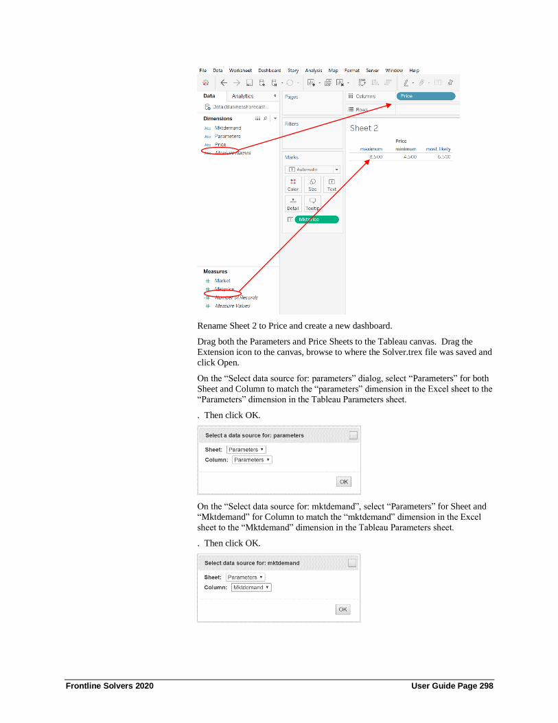
Frontline Solvers 2020 User Guide Page 298
Rename Sheet 2 to Price and create a new dashboard.
Drag both the Parameters and Price Sheets to the Tableau canvas. Drag the
Extension icon to the canvas, browse to where the Solver.trex file was saved and
click Open.
On the “Select data source for: parameters” dialog, select “Parameters” for both
Sheet and Column to match the “parameters” dimension in the Excel sheet to the
“Parameters” dimension in the Tableau Parameters sheet.
. Then click OK.
On the “Select data source for: mktdemand”, select “Parameters” for Sheet and
“Mktdemand” for Column to match the “mktdemand” dimension in the Excel
sheet to the “Mktdemand” dimension in the Tableau Parameters sheet.
. Then click OK.

Frontline Solvers 2020 User Guide Page 299
On the “Select data source for: market”, select “Parameters” for Sheet and
“Market” for Column to match the “market” dimension in the Excel sheet to the
“Market” measure in the Tableau Parameters sheet.
On the “Select data source for: price”, select “Price” for both Sheet and Column,
then click OK to match the “price” dimension in the Excel sheet to the “Price”
dimension in the Tableau Price sheet. .
On the “Select data source for: mktprice”, select “Price” for Sheet and
“Mktprice” for Column, then click OK to match the “mktprice” dimension in the
Excel sheet to the “Mktprice” measure in the Tableau Price sheet.
Immediately, once the data repositories are filled with the appropriate data
fields, a simulation will be run.

Frontline Solvers 2020 User Guide Page 300
Error Messages
If you’ve made an error in your PsiDataSrc() function or in your data file, your
Tableau extension will display an error such as “Inconsistent Data source
definition PSI could not parse Excel formulas" or “Invalid binding source
definition PSI could not parse Excel formulas”.
If your Tableau extension is displaying either of these errors or a different error,
first, check the PsiDataSrc() function in your Excel model to make sure that you
have not mixed up the order of your index sets. In addition, check your data to make sure that it is 1. Contained within an Excel table, 2. That the column
headings match the index sets defined in PsiDataSrc() and 3. That your model
parameters match the elements in your data table.
For more information on an error message displayed in your custom visual, see
the Frontline Solvers Reference Guide or contact Frontline Systems Support
Team by emailing [email protected] or by calling 888-831-0333.

Frontline Solvers 2020 User Guide Page 301
Examples: Parameters and Sensitivity Analysis
Introduction This chapter introduces the use of parameters, and functions for sensitivity
analysis in Analytic Solver, with examples. In Version 11, the role of
parameters – for optimization, simulation, and sensitivity analysis – was
enhanced, and the sensitivity analysis functions were introduced. The use of
parameters and sensitivity analysis has also been extended to Analytic Solver Cloud.
Sensitivity analysis is designed to help you explore a conventional Excel
spreadsheet model, often before you define an optimization or simulation model.
The goal of sensitivity analysis is to identify the key input parameters that have
the greatest impact on results of interest in your model (such as Net Profit), and
to see the effect of varying these key input parameters over a range, in reports
and graphs. Analytic Solver helps you automatically identify sensitivity
parameters, and automatically vary them to produce reports and graphs.
Parameters and Results All Analytic Solver products support three kinds of parameters:
• A sensitivity parameter (PsiSenParam) is automatically varied when
you perform a sensitivity analysis. You do this by selecting Sensitivity
from the Reports or Charts galleries on the Ribbon.
• An optimization parameter (PsiOptParam) is automatically varied
when you perform multiple optimizations. You do this by clicking the
Optimize button on the Ribbon, or the green arrow in the Task Pane,
with the Number of Optimizations set to a value greater than 1. (Not
available in Analytic Solver Simulation.)
• A simulation parameter (PsiSimParam) is automatically varied when
you perform multiple simulations. You do this by clicking the Simulate button on the Ribbon, or the green arrow in the Task Pane,
with the Number of Simulations set to a value greater than 1. (Not
available in Analytic Solver Optimization.)
Note: When entering PsiOptParam, PsiSenParam PsiSimParam manually (i.e.
simply typing the function into an Excel cell) in Analytic Solver Cloud, the
taskpane must be refreshed before performing a parameter analysis report.
Viewing Parameters in the Task Pane
All three types of parameters appear in the Task Pane Model outline. In the
example on the next page, two sensitivity parameters at G11 and H17 have been
defined by the user. Parameter G11 is selected, and its properties are shown in
the lower part of the Task Pane. It is possible to change the type of a

Frontline Solvers 2020 User Guide Page 302
parameter, by simply selecting from the dropdown list in the lower part of the
Task Pane as shown: For example, to use G11 in a simulation model,
automatically varied across multiple simulations, you would select Simulation
from the dropdown list.
Defining a Parameter
You can manually define an input cell as a parameter by simply selecting the
cell, choosing Parameters and Sensitivity, Optimization or Simulation from
the Ribbon, and entering a lower and upper limit on values for the parameter, or
a list of explicit values for the parameter. In the example on the next page, we
are defining a sensitivity parameter.

Frontline Solvers 2020 User Guide Page 303
You can also simply type a formula such as =PsiSenParam(1,9) in a cell, which
has the same effect as the above steps. In both cases, the parameter appears in
the Task Pane Model outline.
If you specify a lower and upper limit, the step size for successive values is
determined when you perform a parameterized sensitivity analysis, or multiple parameterized optimizations or simulations. Analytic Solver will subdivide the
range from the lower to the upper limit into equal-size intervals.
For example, for the above sensitivity parameter, you would select Reports or
Charts – Sensitivity – Parameter Analysis and specify the number of points
on the major axis. If you specified 18 points, the step size would be 0.5.
Automatic Parameter Identification
Analytic Solver can automatically find the input cells with the greatest impact
on any selected formula cell. You can then choose one or more of these input
cells to serve as sensitivity (or optimization or simulation) parameters.

Frontline Solvers 2020 User Guide Page 304
To do this, select any formula cell in an Excel model, and choose Parameters
– Identify from the Ribbon.
Analytic Solver traces through all ‘precedent’ formulas to find input cells
(leaves of the formula tree) on which the selected formula cell depends. It then
varies each input cell independently, computing its impact on the selected formula cell. The input cells are ranked in descending order by (absolute)
impact, and the highest-impact cells are displayed in the Tornado chart.
In the example below, we’ve clicked Help – Examples on the ribbon to open
the StandardExamples.xlsx. nicole
Click the Example 8 tab and set cells B17:G17 to 1. (If these cells are all 0, then
no projects are selected and the Total NPV is always 0). To see which cells
have the greatest impact on Total NPV, we simply select cell (I28) and choose
Parameters – Identify from the Ribbon. After a moment, a Tornado chart like
the one below appears.

Frontline Solvers 2020 User Guide Page 305
The chart shows us, at a glance, that Total NPV is most sensitive to cell E13 –
which is a large positive cash flow in Year 6 for Opportunity 4. It is next most
sensitive (in the opposite direction, decreasing when the parameter increases) to
the interest rate in cell F4.
The right panel of the chart shows the lower value and upper value that were used for each input cell when computing the formula value. An ordinary cell
containing a number is set to its current value – n% and its current value + n%,
where n% (initially 10%) is specified in the edit box in the lower right corner of
the chart. If any input cell is already defined as a parameter, the lower and
upper limit arguments of its PsiXxxParam() call are used instead.
By choosing the radio button corresponding to “Show Current Parameters”,
“Show Candidate Cells”, or “Show both” at the top of the right panel, you can
show either one or both types of input cells in the Tornado chart. By checking
the box on the same row as the cell, you can define a candidate cell as a
sensitivity parameter (or, if you change the selection in the dropdown list in
the lower right corner of the chart, an optimization or simulation parameter). These definitions take effect when you click the Save icon at the upper left
corner of the chart. For this example, we’ll check the boxes on the same rows as
cells E13 and F4; we’ll also set F4’s Lower value to 0.01 (1%) and the Upper
Value to 0.10 (10%).
Now, when you click Charts – Sensitivity Analysis – Parameter Analysis, you'll
see both parameters appear under Parameters in the Sensitivity Report dialog.
Continue reading to discover how to create a parameter report using Analytic
Solver.

Frontline Solvers 2020 User Guide Page 306
The simplest way to remove a parameter is to select the parameter cell on the
worksheet and press the DEL key – which erases its cell formula – or type a
number value that will overwrite the formula in the cell. The parameter will
then disappear from the Task Pane.
Defining Results
When you perform a sensitivity analysis (which will automatically vary
sensitivity parameters), or multiple optimizations or simulations (which will
vary optimization or simulation parameters), Analytic Solver will keep track of
one or more result cell values, corresponding to each parameter value.
• For optimizations, Analytic Solver tracks the final objective and
decision variable values found by the Solver; you can also track a
constraint value by setting its Monitor property in the Task Pane.
• For simulations, Analytic Solver tracks the values of all uncertain
functions (simulation outputs, referenced in PsiOutput() or PSI
Statistics function calls).
• For sensitivity analysis, Analytic Solver tracks results from the cell
currently selected at the time you perform the analysis, and any other
results you define.
To define a sensitivity result cell in Analytic Solver Desktop, select the cell (such as A3 below – always a formula cell) on the worksheet, and choose
Parameters – Monitor Value from the Ribbon. A small “balloon” will appear,
containing a function call such as =PsiSenValue(A3). You can move the mouse
to “drag and drop” this formula into an empty cell. When you do this, cell A3 is

Frontline Solvers 2020 User Guide Page 307
defined as a sensitivity result cell, and appears in the Task Pane Model outline
under Sensitivity Results.
To define a sensitivity result cell in Analytic Solver Cloud, select the cell (such
as A3 below) on the worksheet, and choose Parameters – Monitor Value from
the Ribbon. A small dialog will appear, containing the location of the selected
cell, a second Target field and three radio buttons. Select the type of parameter
you would like to add, Sensitivity, Optimization or Simulation, then enter an empty cell for the Target field, such as A4. Click Save to define cell A3 as a
sensitivity result cell which will appear in the Task Pane Model outline under
Sensitivity Results.
Sensitivity Analysis Reports and Charts The Parameters – Identify step just described performs a simple kind of
sensitivity analysis; in some situations, this may be all that you need. But it is
often useful to document the sensitivity of some computed result to systematic
variations in the values of one or more parameters. Analytic Solver can produce
both reports and charts to document these results.
How Parameters are Varied
In reports and charts, Analytic Solver can automatically vary your parameters’
values in two ways:
1. Varying all parameters simultaneously, from their respective lower to upper limits, for the number of steps that you specify.
2. Varying two parameters independently, from their lower to upper
limits, computing a result for all combinations of the two parameters.
You select the second choice by checking the box “Vary Parameters
Independently” at the bottom of the dialog shown on the next page. If you do
this, you must select exactly one result cell, and exactly two parameter cells in

Frontline Solvers 2020 User Guide Page 308
the dialog below. A report will appear as a two dimensional table, and a chart
will appear in 3-D with the two parameters on the axes.
If you don’t check this box – meaning that all parameters will be varied
simultaneously – you can select one or more parameter cells, and one or more
result cells in the dialog below. A report will contain a column for each parameter and each result, and a chart will contain a plot of each result cell.
Creating Sensitivity Reports
To create a sensitivity analysis report, select a formula cell on the worksheet
(whose value should be computed in the report say, cell I28 (Total_NPV)), and
choose Reports – Sensitivity – Parameter Analysis from the Ribbon. A dialog
like the one shown below will appear.
Use the arrow buttons in the top section to select one or more result cells
(exactly one if you check the box “Vary Parameters Independently”). Use the
arrow buttons in the bottom section to select one or more sensitivity parameter
cells (exactly two if you check the box “Vary Parameters Independently”).
Then click OK to produce the report, as a new worksheet in into your Excel
workbook, just to the left of the active worksheet. An example is shown below.

Frontline Solvers 2020 User Guide Page 309
Creating Sensitivity Charts
To create a sensitivity analysis chart, select a formula cell on the worksheet
(whose value should be computed in the chart), and choose Charts – Sensitivity
– Parameter Analysis from the Ribbon. A dialog like the one on the previous
page will appear. Follow the same steps as for sensitivity analysis reports, and
click OK. A chart like the one below will appear:
You can use icons on the toolbar at the top of the chart to resize and rotate the
chart, print the chart, or copy it to the Windows Clipboard (where you can paste it into other applications).

Frontline Solvers 2020 User Guide Page 310
Optimization and Simulation Reports and Charts Reports and charts for multiple parameterized optimizations and simulations
work in much the same way as the reports and charts for sensitivity analysis
shown in the previous section. But where for sensitivity analysis, Analytic
Solver simply performs a worksheet recalculation, for these reports and charts,
Analytic Solver performs a complete optimization or simulation for each set
of parameter values.
To produce these reports and charts, select Reports or Charts – Multiple
Optimizations from the Ribbon. For multiple parameterized simulations, select
Reports or Charts – Multiple Simulations from the Ribbon.
When Optimizations and Simulations are Run
As shown in the earlier Examples chapters, optimizations are run when you
click the Optimize button on the Ribbon, or the green arrow in the Task Pane,
and simulations are run when you click the Simulate button on the Ribbon, or
(assuming there’s no optimization model) when you click the green arrow in the
Task Pane. When you select Reports and Charts of Multiple Optimizations or
Multiple Simulations other than Parameter Analysis, the results cached in
memory from the last optimization or simulation run are used to create the
reports or charts.
However, when you select Reports and Charts of Multiple Optimizations or
Multiple Simulations with Parameter Analysis, which gives you greater control
over how parameters are varied, Analytic Solver cannot use the results cached in memory. Instead, a new set of optimizations or simulations is run, varying the
values of the parameters as you’ve specified; you can for example vary two
parameters independently, yielding all combinations of these parameter values.
The number of optimizations or simulations to run is independent of the settings
you use for Number of Optimizations or Number of Simulations in the Task
Pane Platform tab; it is the product of the number of Major Axis Points and
Minor Axis Points you select in the Reports or Charts selection dialog. With
the default value of 10 points each, 100 optimizations or simulations are
required. This can take some time, especially for optimizations; a progress
dialog is displayed during this process.

Frontline Solvers 2020 User Guide Page 311
Examples: Decision Trees and Discriminant Analysis
Introduction This chapter introduces decision trees in Analytic Solver. Such trees are a
useful graphical and computational aid for problems that involve sequential
decisions and events, where there are a small number of decision alternatives at
each step, and a small number of alternative outcomes for each event.
In the example below, we’ve clicked Help – Examples on the ribbon, clicked
Decision Tree Examples on the Overview Tab, and clicked on
TreeExample.xls, which is based on an example by Prof. Mike Middleton.
In this example, a firm must decide (1) whether to prepare a proposal for a
contract, and (2) if the contract is awarded, what method to use to satisfy the contract. The first number shown below each branch (horizontal line) is the
amount the firm pays out (if negative) or receives (if positive) when it follows
that branch. For example, in the path that ends at the terminal node at cell S18,
the firm (1) pays $50,000 to prepare the proposal, (2) receives $250,000 up front
when awarded the contract, (3) spends $50,000 to try the electronic method, and
since that method fails, (4) spends $120,000 on the mechanical method. The net
result is a positive cash flow of $30,000 shown at cell T18.
A decision tree is “solved” by Excel fomulas calculating each of the numbers
you see on the worksheet. Terminal values such as T18 sum all the partial cash
flows along the path leading to that terminal node. The tree is then rolled back
by computing expected values (or certainty equivalents) at event nodes, and by maximizing (or minimizing) the alternative values at decision nodes. The
rollback values appear below and just to the left of each node, showing the value
of the subtree rooted at that node. The numbers “inside the boxes” at decision
nodes show which alternative is optimal for that decision. In the example, the
1 in the decision node at C31 indicates that it is optimal to prepare the proposal,
and the 2 in the decision node at K16 indicates the firm should try the electronic

Frontline Solvers 2020 User Guide Page 312
method because that alternative leads to a higher expected value ($90,000) than
the mechanical method ($80,000).
Since all the computations are performed with Excel worksheet formulas, a
decision tree is a ‘regular’ Excel worksheet model, where you can ask what-if,
perform sensitivity analysis, or create simulation or optimization models if desired. For example, the formula at cell F25, for the event where we are or are
not awarded the contract, is =IF(ABS(1-SUM($I$14,$I$31))<=0.00001,SUM($I$14*$J$17,$I$31*$J$34),NA()) – an
expected value calculation – and the formula at B32, for the decision whether to
prepare a proposal, is simply =MAX(F25,F39), since we are maximizing EV.
The Task Pane Platform tab includes a Decision Tree group of options, where
you can choose to maximize or minimize values at decision nodes, and to
compute expected values (which are risk neutral) or certainty equivalents (which
reflect risk aversion) at each node. If you choose certainty equivalents, you can
specify the parameters of an exponential utility function.
Creating Decision Trees A decision tree consists of nodes and branches. Nodes may be either decision nodes, event nodes, or terminal nodes; branches represent alternative choices
at decision nodes, and alternative outcomes at event nodes.
You create and edit a decision tree with the Decision Tree choice on the Ribbon.
Creating Trees in Analytic Solver Desktop
In Analytic Solver Desktop, click the Decision Tree icon on the Ribbon to open
the menu choices.
You can also create and edit a decision tree in Analytic Solver Desktop in the
Task Pane Model tab, using the Add (+) and Remove (X) icons and the
properties area at the bottom of the Task Pane; but you can highlight the best or
worst decision strategy (see below) only from the Ribbon.
Create Trees in Analytic Solver Cloud
In Analytic Solver Cloud, click the Decision Tree icon on the Ribbon to open
the Decision Tree dialog. You can create and edit decision trees in the Cloud
app using menu items at the top of the dialog (Add Node, Change Node, and
Delete Node) and also in the fields on the right under Decision Tree. To

Frontline Solvers 2020 User Guide Page 313
highlight the best and worst decision strategies, click Highlight Best or
Highlight Works, respectively.
Creating and Editing Nodes
In Analytic Solver Desktop
Selecting Node in the dropdown presents choices for working with nodes:
The Add Node and Change Node options display the dialog shown on the next
page. To change a node, you must first select it on the Excel worksheet – you
may select either the node graphic or one of the immediately adjacent cells.
The Copy Node and Paste Node choices can be used to copy a subtree (rooted
at the selected node) and paste the copy at another position in the decision tree;
this is very useful when there are identical choices at later stages in the tree.
In Analytic Solver Cloud
In Analytic Solver Cloud, click Add Node to open the Add Node dialog.
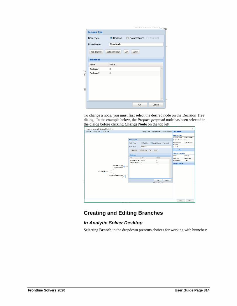
Frontline Solvers 2020 User Guide Page 314
To change a node, you must first select the desired node on the Decision Tree
dialog. In the example below, the Prepare proposal node has been selected in
the dialog before clicking Change Node on the top left.
Creating and Editing Branches
In Analytic Solver Desktop
Selecting Branch in the dropdown presents choices for working with branches:

Frontline Solvers 2020 User Guide Page 315
The Add Branch and Change Branch options display the Decision Tree dialog
shown below. To change a branch, you must first select it on the Excel
worksheet – you may select either the branch graphic or one of the immediately
adjacent cells. Note that Add/Change Node and Add/Change Branch options
display the same Decision Tree dialog: Branches are associated with the node to their left, and you can edit properties of the node and its branches in this dialog.
In this dialog, you can change the type of the node, the name of the node, and
you can add, edit, reorder, or remove branches for this node. Each branch for a
decision node has a value (the cost or payoff of taking that decision); each
branch for an event node has a value and a probability (the cost or payoff, and
the probability of occurrence, of that outcome).
In Analytic Solver Cloud
In Analytic Solver Cloud, clicking Add Node\Change Node also allows you to
add\change a branch using the Add Branch and Change Branch options. To
change a branch, you must first select it on the Excel worksheet. Branches are
associated with the node to their left, and you can edit properties of the node and
its branches here.
In this dialog, as in Analytic Solver Desktop, you can change the type of the node, the name of the node, and you can add, edit, reorder, or remove branches
for this node. Each branch for a decision node has a value (the cost or payoff of
taking that decision); each branch for an event node has a value and a

Frontline Solvers 2020 User Guide Page 316
probability (the cost or payoff, and the probability of occurrence, of that
outcome).
Highlighting a Decision Strategy A decision strategy is a complete sequence of decisions that you can make
through the decision tree. You can highlight the best or worst decision strategy
by selecting Highlight in the Decision Tree dropdown list in Analytic Solver
Desktop or by clicking Highlight Best in the Decision Tree dialog in Analytic
Solver Cloud, as shown on the next page. If you are maximizing, the best
strategy maximizes EV or CE, and the worst strategy minimizes EV or CE. If you are minimizing, the opposite applies.
Analytic Solver Desktop

Frontline Solvers 2020 User Guide Page 317
Analytic Solver Cloud
The next page shows the example decision tree shown earlier, with Excel
worksheet gridlines turned off, and the best decision strategy highlighted.
Analytic Solver Desktop
Decision Trees in the Task Pane
Model Tab in Analytic Solver Desktop
In Analytic Solver Desktop, decision trees may also be viewed and edited
directly in the Task Pane Model tab, and choices for tree evaluation (see
“Platform tab” below) can only be made in the Task Pane. When a node or
branch is selected in the Task Pane outline, properties of that node or branch
may be viewed and edited in the lower portion of the Task Pane, as shown on
the next page. You can also double-click a node in the Model outline to display

Frontline Solvers 2020 User Guide Page 318
the same Decision Tree dialog that appears when you add or change a node from
the Ribbon.
In this example, we’ve selected the decision node named Method, represented
by the graphic symbol at cell K16 on the worksheet. The optimal choice at this
node (given that we’re maximizing expected value or EV) is branch #2, and the
rollback value of the subtree rooted at this node is 90,000.
Note the small Copy icon in the upper right corner of the Decision Tree Node
properties pane: You can click this icon to copy a subtree rooted at this node. When you’ve selected a Terminal node in the Model outline, you’ll notice a
small Paste icon in this same area: You can click this icon to paste a subtree at
the position of the Terminal node.
Model Tab in Analytic Solver Cloud
In Analytic Solver Cloud, decision trees may only be viewed and edited directly
in the Decision Trees dialog, but choices for tree evaluation can be made either
in the Decision Tree dialog or in the Task Pane on the Platform tab (see
“Platform tab” below).

Frontline Solvers 2020 User Guide Page 319
Platform Tab
By default, rollback values for a decision tree are computed assuming that you want to Maximize Expected Value or EV. You can change this by setting
options in the Decision Tree section of the Task Pane Platform tab, as shown on
the next page.
You can select Maximize or Minimize in the dropdown list for the Decision
Node EV/CE option. For the Certainty Equivalents option, you can choose
either Expected Value or Exponential Utility Function. The remaining three
options come into play only when you choose Exponential Utility Function –
they set parameters of this function.
For the Maximize option with exponential utility, the rollback formulas are U =
A–B*EXP(X/RT) and CE = -LN((A-EU)/B)*RT, where X and EU are cell
references. For the Minimize option with exponential utility, the formulas are U
= A-B*EXP(X/RT) and CE = LN((A-EU)/B)*RT. RT is the value you specify
for the Risk Tolerance option on the Platform tab, and A and B are the values
of the Scalar A and Scalar B options on the Platform tab.
When you use an Exponential Utility Function, the utility (U =) and certainty
equivalent (CE =) formulas are computed in extra cells on the worksheet, as
shown on the next page. For example, B33 computes the utility of the decision

Frontline Solvers 2020 User Guide Page 320
at B32; B32 contains =MAX(F25,F39) as before, to choose the decision with the
maximum certainty equivalent value; F25 contains =-LN((A-$F$26)/B)*RT.
Multiple Discriminant Analysis Discriminant analysis is a statistical technique for analyzing a data set,
consisting of cases or observations of one or more variables, and classifying the cases into different groups. MDA is sometimes called discriminant factor
analysis or canonical discriminant analysis. It has many applications in financial
services and consumer marketing, among other fields.
Analytic Solver Data Mining and the Data Mining Cloud app include a powerful
version of multiple discriminant analysis on the Data Mining tab on the Ribbon,
through the menu option Classify – Discriminant Analysis, and described in
depth in the Analytic Solver Data Mining User Guide.
But since a discriminant analysis facility historically was included with Risk
Solver Platform (a predecessor to Analytic Solver), before Frontline acquired
and integrated the XLMiner software (known today as Analytic Solver Data
Mining), this facility is still available on the Analytic Solver Desktop tab, through the menu option Reports – Discriminant Analysis – Discriminant
Analysis, and is documented here. Note: Discriminant Analysis is not
supported in Analytic Solver Cloud or AnalyticSolver.com.
Discriminant Analysis Example In the example described below, a winery maintains a dataset which includes 13
variables describing various properties of three different types of wines
produced at their vineyard. The three different types of wines produced are
classified as Type1, Type 2 and Type 3. The characteristics of each wine type
include Alcohol content, Malic Acid content, Ash content, Ash Alkalinity
content, Magnesium content, Total Phenols, Flavonoid content, etc. There are
59 observations for Type 1, 71 observations for Type 2, and 48 observations for
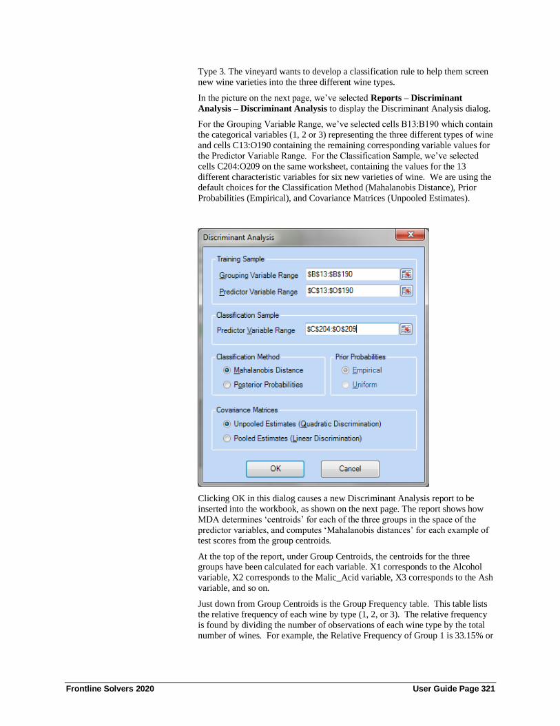
Frontline Solvers 2020 User Guide Page 321
Type 3. The vineyard wants to develop a classification rule to help them screen
new wine varieties into the three different wine types.
In the picture on the next page, we’ve selected Reports – Discriminant
Analysis – Discriminant Analysis to display the Discriminant Analysis dialog.
For the Grouping Variable Range, we’ve selected cells B13:B190 which contain
the categorical variables (1, 2 or 3) representing the three different types of wine
and cells C13:O190 containing the remaining corresponding variable values for
the Predictor Variable Range. For the Classification Sample, we’ve selected
cells C204:O209 on the same worksheet, containing the values for the 13
different characteristic variables for six new varieties of wine. We are using the
default choices for the Classification Method (Mahalanobis Distance), Prior
Probabilities (Empirical), and Covariance Matrices (Unpooled Estimates).
Clicking OK in this dialog causes a new Discriminant Analysis report to be
inserted into the workbook, as shown on the next page. The report shows how
MDA determines ‘centroids’ for each of the three groups in the space of the
predictor variables, and computes ‘Mahalanobis distances’ for each example of
test scores from the group centroids.
At the top of the report, under Group Centroids, the centroids for the three groups have been calculated for each variable. X1 corresponds to the Alcohol
variable, X2 corresponds to the Malic_Acid variable, X3 corresponds to the Ash
variable, and so on.
Just down from Group Centroids is the Group Frequency table. This table lists
the relative frequency of each wine by type (1, 2, or 3). The relative frequency
is found by dividing the number of observations of each wine type by the total
number of wines. For example, the Relative Frequency of Group 1 is 33.15% or

Frontline Solvers 2020 User Guide Page 322
the number of observations of type (50) divided by the total number of
observations (178).
The values listed in the Training Sample Classification Table for Group 1,
Group 2, and Group 3 are the distance calculations from the individual
observations to the group centroid or "center". The minimum value of the three groups determines the group assignment.
The ‘Test Sample Classification’ at the bottom of the report shows the
predictions obtained by MDA for how the six new wine varieties will be typed.
All have been assigned to Type 2.
Just above the ‘Test Sample Classification’ is a table, often called a ‘confusion
matrix,’ that evaluates how well the classification rule would have handled the
178 historical cases. (The types of these 178 cases are all “known”.)
The matrix shows that all 59 of the Group 1 observations would have been
assigned to Group 1 correctly. All 71 of the Group 2 observations would have
been assigned to Group 2 and all 48 of the Group three assignments would have been assigned to Group 3. The Totals in row 211 show that 178 out of 178, or
100% of the cases w correctly classified.

Frontline Solvers 2020 User Guide Page 323

Frontline Solvers 2020 User Guide Page 324
Getting Results: Optimization
Introduction This chapter explains how to obtain and interpret results from optimization in
Analytic Solver Comprehensive and its subset optimization products: Analytic
Solver Optimization, Analytic Solver Upgrade and Analytic Solver Basic when
using either Analytic Solver Desktop or Cloud. We’ll also discuss what can go
wrong, and what to do about it, and also how to get more than a single optimal
solution from your model.
Analytic Solver Optimization has many powerful optimization algorithms, and will fully exploit the power of your PC. But the model that you create may be
relatively easy to optimize (if you use linear functions like SUM) or extremely
difficult to optimize (if you use non-convex and non-smooth functions like
LOOKUP). The results you get depend on the model you create.
In the following sections, we’ll focus on immediate actions you can take when
you get an unexpected result – but if you read the chapter “Mastering
Conventional Optimization Concepts,” you’ll learn more about optimization
models and solution methods, and better understand why the unexpected result
appeared, and how to design your model to get the solutions you want.
What Can Go Wrong, and What to Do About It When you click the Optimize button on the Ribbon, or the green arrow on the Task Pane to solve, you’ll normally get one of these outcomes:
1. A solution that makes sense to you. This is normally accompanied by a
Solver Result message in green at the bottom of the Task Pane. You
can proceed to “When Things Go Right: Getting Further Results.”
2. A Solver Result error message that you understand and can correct, in
red at the bottom of the Task Pane. You can take corrective action.
3. A Solver Result error message that you don’t understand, in red at the
bottom of the Task Pane. You should read the solution log in the
Output tab, click the error message and read Help about the message.
4. A solution that you don’t understand, or that seems wrong. Again before doing anything else, you should read the solution log in the
Output tab, click the error message to display Help, run available
reports as described below, and read the section below “When the
Solution Seems Wrong.”
5. Solving runs for a very long time, and you don’t get a solution or a
Solver Result message until you press ESC or click Pause/Stop. You
should read the section below “When Solving Takes a Long Time.”
In rare cases, you might find Excel shutting down or “locking up” (so nothing
happens when you click Pause on the Solver Task Pane). In this case please
contact Frontline Systems Technical Support at (775) 831-0300 x4 or [email protected]. Some Solver Result error messages ask you to contact
Technical Support. If you can send us your model, this will be very helpful.

Frontline Solvers 2020 User Guide Page 325
But experience shows that 99% of all technical support cases involve “pilot
error” by the user, and that 90% of all such cases could be easily resolved by
reading online Help or the User Guide. So we hope you’ll keep reading, and
that you’ll take these steps before calling technical support!
Review Messages in the Output Tab
If using Analytic Solver Desktop, your first step should be to review the
messages in the solution log in the Task Pane Output tab. Below is an example
of the Output tab at the solution of EXAMPLE5 in StandardExamples.xls
(described more fully in the chapter “Examples: Conventional Optimization”):
If you click the Copy icon, the contents of the solution log will be copied to
the Windows Clipboard, where you can paste it into Microsoft Word, NotePad,
or an email message to Frontline Systems Technical Support. Below is the
complete solution log from the above example:
---- Start Solve ----
Using: Full Reparse.
Parsing started...
No uncertain input cells.
Diagnosis started...
Model diagnosed as "NSP".
Attempting Transformation.
Using: Full Reparse.
Parsing started...
Diagnosis started...

Frontline Solvers 2020 User Guide Page 326
Model transformed into an LP. Transformation will be used.
User engine selection: Standard LP/Quadratic
Model: [OptimizationExamples.xls]EXAMPLE5
Using: Psi Interpreter
Parse time: 0.22 Seconds.
Engine: Standard LP/Quadratic
Setup time: 0.00 Seconds.
Engine Solve time: 0.20 Seconds.
Solver found a solution. All constraints and optimality conditions are satisfied.
Solve time: 0.62 Seconds.
This was a successful solution – but in cases where you have a Solver Result
error message that you don’t understand, or a solution that you don’t under-
stand, the solution log can be quite helpful.
Note: Information related to the solving process in Analytic Solver Cloud is not
available during parsing of the model. As a result, feedback is only available
once the Solver Engine starts to solve the model.
More Detail in the Solution Log
You can obtain more detailed output in the solution log by setting the Task Pane
Platform tab General group Log Level option to Verbose before you solve:
Below is a portion of the solution log (from the LP/Quadratic Solver) for the
EXAMPLE5 model:
Integer solution of 3100 found by Feasibility Pump after 0 iterations and 0 nodes (0.01
seconds)
After 0 nodes, 1 on tree, 3100 best solution, best possible 2355.01 (0.18 seconds)
After 1 nodes, 2 on tree, 3100 best solution, best possible 2355.01 (0.18 seconds)
Integer solution of 2630 found by Unknown after 285 iterations and 2 nodes (0.19 seconds)
After 2 nodes, 2 on tree, 2630 best solution, best possible 2361.69 (0.19 seconds)
Integer solution of 2400 found after 294 iterations and 3 nodes (0.20 seconds)
After 3 nodes, 1 on tree, 2400 best solution, best possible 2361.69 (0.20 seconds)
Engine Solve time: 0.20 Seconds.
If you are having problems finding the solution you want or expect, this detailed
log can sometimes be helpful.
Note: This functionality is not supported in Analytic Solver Cloud.
Click the Solver Result Message for Help
The Solver Result message is always underlined – it is a hyperlink to Help. If you aren’t sure that you fully understand it, click the link to open online Help to
a detailed discussion of the message.
Below is an example of Help that appears in Analytic Solver Desktop when you
solve EXAMPLE3 in StandardExamples.xls, and click on the Solver Result
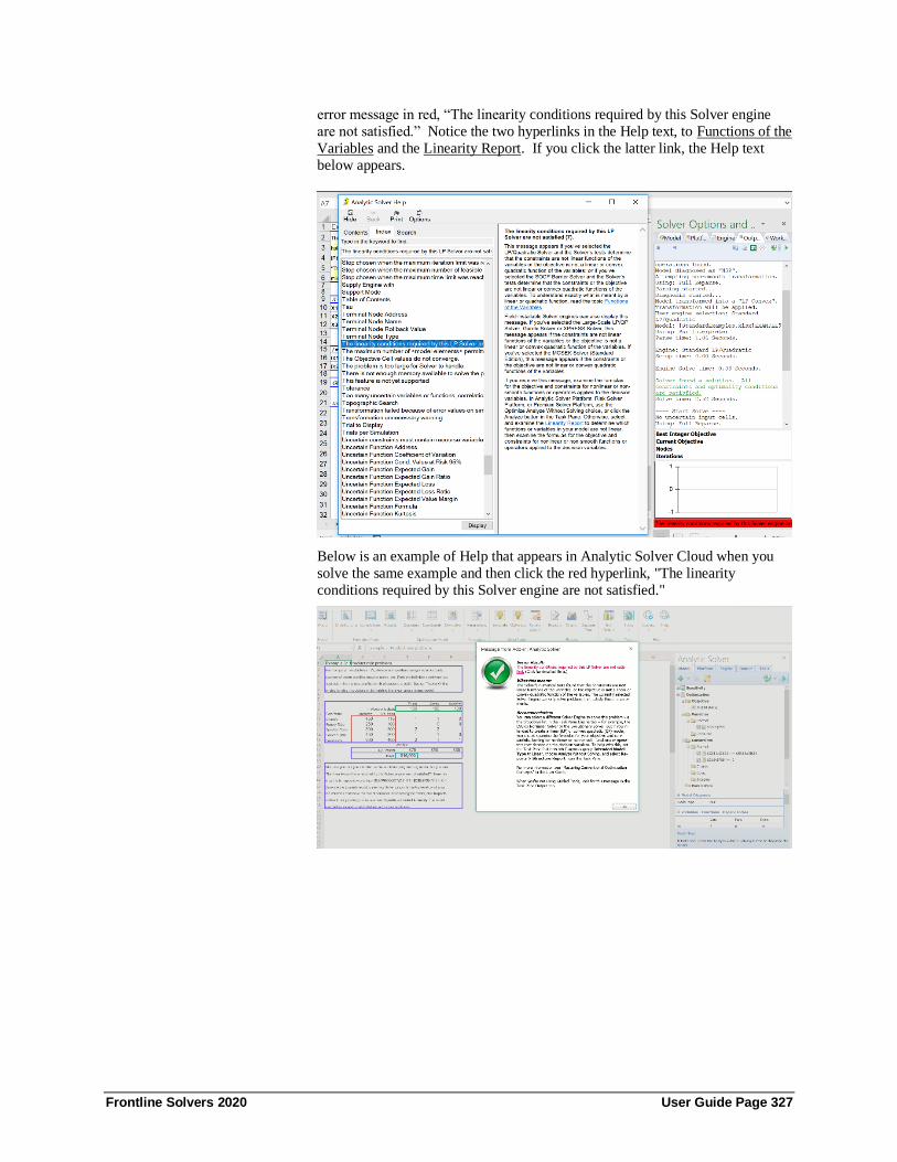
Frontline Solvers 2020 User Guide Page 327
error message in red, “The linearity conditions required by this Solver engine
are not satisfied.” Notice the two hyperlinks in the Help text, to Functions of the
Variables and the Linearity Report. If you click the latter link, the Help text
below appears.
Below is an example of Help that appears in Analytic Solver Cloud when you
solve the same example and then click the red hyperlink, "The linearity
conditions required by this Solver engine are not satisfied."

Frontline Solvers 2020 User Guide Page 328
Given our experience that 90% of technical support cases could be easily
resolved by reading online Help or the User Guide, you can save yourself, as well as Frontline Systems, time if you do read online Help first.
Choose Available Optimization Reports
The Help above suggests that we select the Linearity Report when we receive
this Solver Result error message. As a general rule, it’s good idea to examine
the available reports and produce the reports that may help you understand
what’s wrong with your model. Just select Reports – Optimization Reports on
the Ribbon – the reports in the gallery are updated each time you solve.
• The Linearity Report and the Structure Report can help when you
encounter “The linearity conditions required by this Solver engine are not
satisfied.”
• The Feasibility Report and Feasibility-Bounds Report can help when you
encounter “Solver could not find a feasible solution.”
• The Scaling Report can help when you encounter either of these messages,
or other unexpected messages or solution values. See the section below
“Problems with Poorly Scaled Models.”
See the section “An ‘Accidentally’ Nonlinear Model” in the chapter “Examples:
Conventional Optimization” to see how the Linearity Report, and the
Structure Report produced by the PSI Interpreter can help us pinpoint the
nonlinear formulas in this model.
When Solving Takes a Long Time
When your model takes a long time to solve, the Task Pane Output tab can be
helpful during the solution process – at a minimum, to reassure you that the

Frontline Solvers 2020 User Guide Page 329
Solver is still making progress, and has not “hung up.” If it is not already visible
when you first start solving in Analytic Solver Desktop, the Output tab will
appear automatically after a few seconds of solution time, as long as the Task
Pane itself is visible.
The Output tab shows the objective of the best solution found so far, and for problems with integer constraints, the Best Integer Objective (“incumbent”), the
Best Possible Objective (“best bound”), and the Integer Gap or percentage
difference between these two objectives.
In Analytic Solver Cloud, the Task Pane Output tab will display a moving task
pane to indicate the status of the model during the solution process.
Running Chart of the Objective
The bottom part of the Output tab shows a running chart of the objective of the
best solution found so far. On the next page is an example of the Output tab on
a problem called Ads.xlsx that takes about 1 minutes to solve, with the
Evolutionary Solver, on a modern 8 - core PC:
Interrupting the Solution Process
You can interrupt the solution process at any time, by pressing the ESC key in
Analytic Solver Desktop, or by clicking the button in either Desktop or Cloud, in the Task Pane Output tab. If your model is very large, you might have
to hold down the ESC key for a second or two. Since the input focus may not be
on the Task Pane when you click with the mouse, you might have to click the
button twice. A dialog like the one below will appear:
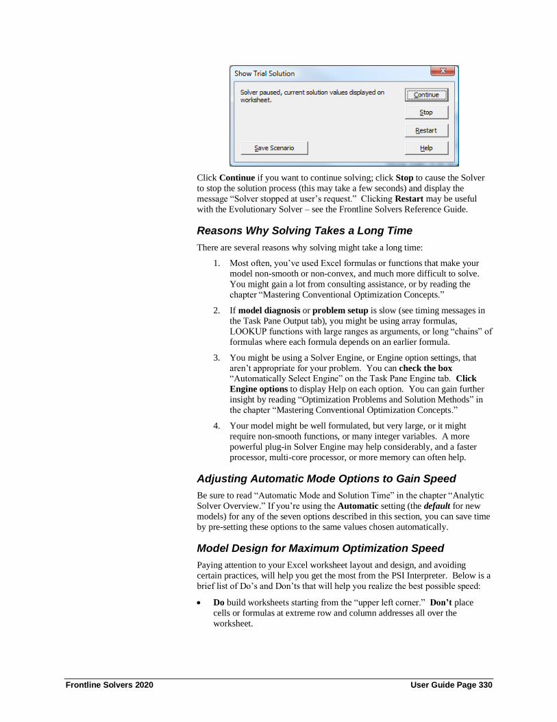
Frontline Solvers 2020 User Guide Page 330
Click Continue if you want to continue solving; click Stop to cause the Solver
to stop the solution process (this may take a few seconds) and display the
message “Solver stopped at user’s request.” Clicking Restart may be useful
with the Evolutionary Solver – see the Frontline Solvers Reference Guide.
Reasons Why Solving Takes a Long Time
There are several reasons why solving might take a long time:
1. Most often, you’ve used Excel formulas or functions that make your
model non-smooth or non-convex, and much more difficult to solve.
You might gain a lot from consulting assistance, or by reading the
chapter “Mastering Conventional Optimization Concepts.”
2. If model diagnosis or problem setup is slow (see timing messages in
the Task Pane Output tab), you might be using array formulas,
LOOKUP functions with large ranges as arguments, or long “chains” of
formulas where each formula depends on an earlier formula.
3. You might be using a Solver Engine, or Engine option settings, that
aren’t appropriate for your problem. You can check the box “Automatically Select Engine” on the Task Pane Engine tab. Click
Engine options to display Help on each option. You can gain further
insight by reading “Optimization Problems and Solution Methods” in
the chapter “Mastering Conventional Optimization Concepts.”
4. Your model might be well formulated, but very large, or it might
require non-smooth functions, or many integer variables. A more
powerful plug-in Solver Engine may help considerably, and a faster
processor, multi-core processor, or more memory can often help.
Adjusting Automatic Mode Options to Gain Speed
Be sure to read “Automatic Mode and Solution Time” in the chapter “Analytic
Solver Overview.” If you’re using the Automatic setting (the default for new
models) for any of the seven options described in this section, you can save time
by pre-setting these options to the same values chosen automatically.
Model Design for Maximum Optimization Speed
Paying attention to your Excel worksheet layout and design, and avoiding
certain practices, will help you get the most from the PSI Interpreter. Below is a
brief list of Do’s and Don’ts that will help you realize the best possible speed:
• Do build worksheets starting from the “upper left corner.” Don’t place
cells or formulas at extreme row and column addresses all over the
worksheet.

Frontline Solvers 2020 User Guide Page 331
• Do build the model on a small number of worksheets. Don’t include
references on these worksheets to other worksheets that aren’t required for
the simulation model.
• Do use numeric and logical formulas and functions. Don’t create string
results in the middle of numeric calculations (see example below).
• Do use built-in Excel functions (including Analysis ToolPak functions)
freely. Don’t use third-party or user-written functions unless truly needed.
Such functions must not have “side-effects” other than the value returned.
• Do use operators like + - * / ^ and functions like SUM, AVERAGE, MAX,
MIN, AND, OR, NOT, IF, CHOOSE. Don’t use INDIRECT, OFFSET, or
TEXT, SEARCH, REPLACE, FIXED, DOLLAR, or ROMAN.
• If possible, Don’t use array formulas, LOOKUP functions with large ranges
as arguments, or long “chains” of formulas where each formula depends on
an earlier formula (and hence on all earlier formulas). Each of these things can slow down analysis of your model considerably (by 10x in some cases).
A common practice that slows down the PSI Interpreter, and is easy to avoid, is
illustrated by the following:
A1: =IF(B1>100,"Yes","No") and later A10: =IF(A1="Yes",A2,50)
You don’t need "Yes" and "No" when Excel provides built-in values TRUE and
FALSE. You could write =IF(B1>100,TRUE,FALSE), but this is simpler:
A1: =B1>100 and later A10: =IF(A1,A2,50)
The formula =B1>100 evaluates to either TRUE or FALSE. A1 holds this value
and you can test it later in another formula.
When the Solution Seems Wrong
When the solution on the worksheet seems wrong, before doing anything else,
you should read the solution log in the Output tab, click the error message to
display Help, and run available reports as described above. We emphasize
this, because very often when we are contacted in technical support, the user has
not taken these basic steps.
Although software bugs are always possible, consider carefully the possibility
that the solution found by the Solver is correct for the model you’ve defined,
and that your expectation is wrong. This may mean that what your model
actually says is different from what you intended. In the majority of cases we
see in technical support, the user has an error in a formula or in the expression of a constraint that leads to the unexpected solution.
Problems with Poorly Scaled Models
Many unexpected Solver Result messages are due to a poorly scaled model.
A poorly scaled model is one that computes values of the objective, constraints,
or intermediate results that differ by several orders of magnitude. A classic
example is a financial model that computes a dollar amount in millions or
billions and a return or risk measure in fractions of a percent. Because of the
finite precision of computer arithmetic, when these values of very different
magnitudes (or others derived from them) are added, subtracted, or compared –
in the user’s model or in the Solver’s own calculations – the result will be
accurate to only a few significant digits. After many such steps, the Solver may detect or suffer from “numerical instability.”

Frontline Solvers 2020 User Guide Page 332
The effects of poor scaling in a large, complex optimization model can be
among the most difficult problems to identify and resolve. It can cause Solver
engines to return messages such as “Solver could not find a feasible solution,”
“Solver could not improve the current solution,” or even “The linearity
conditions required by this Solver engine are not satisfied,” with results that are suboptimal or otherwise very different from your expectations. The effects may
not be apparent to you, given the initial values of the variables, but when the
Solver explores Trial Solutions with very large or small values for the variables,
the effects will be greatly magnified.
Dealing with Poor Scaling
Most Solver engines include a Use Automatic Scaling option on the Task Pane Engine tab. When this option is set to True, the Solver rescales the values of the
objective and constraint functions internally in order to minimize the effects of
poor scaling. But this can only help with the Solver’s own calculations – it can’t
help with poorly scaled results that arise in the middle of your Excel formulas.
The best way to avoid scaling problems is to carefully choose the “units”
implicitly used in your model so that all computed results are within a few
orders of magnitude of each other. For example, if you express dollar amounts
in units of (say) millions, the actual numbers computed on your worksheet may
range from perhaps 1 to 1,000.
If you’re experiencing results that may be due to poor scaling, you can check
your model for scaling problems that arise in the middle of your Excel formulas by selecting the Scaling Report after solving your model. If you’re using
Analytic Solver Upgrade, you’ll have to go through each of your formulas and
play “what-if” manually to identify such problems.
The Integer Tolerance Option
Users who solve problems with integer constraints using the standard Excel
Solver occasionally report that “Solver claims it found an optimal solution, but I
manually found an even better solution.” What happens in such cases is that the
Solver stops with the message “Solver found a solution” because it found a
solution within the range of the true integer optimal solution allowed by the
Tolerance option in the standard Solver’s Options dialog. In similar cases,
Analytic Solver displays a message “Solver found an integer solution within tolerance,” to avoid confusion.
When you solve a problem with integer constraints, the solution process in
almost all Solver engines is governed by the Integer Tolerance option on the
Task Pane Engine tab. When this option value is non-zero – say 0.05, as in the
standard Excel Solver – the Solver engine stops when it has found a solution
satisfying the integer constraints whose objective is within 5% of the true integer
optimal solution. Therefore, you may know of or be able to discover an integer
solution that is better than the one found by the Solver.
To avoid this common problem, the default Integer Tolerance value in Analytic
Solver Platform V9.0 and beyond is 0 or 0.001 (depending on the engine used) rather than 0.05. But this has an important consequence for solution time: The
solution process for integer problems often finds a near-optimal solution
(sometimes the optimal solution) relatively quickly, and then spends far more
time exhaustively checking other possibilities to find (or verify that it has found)
the very best integer solution.

Frontline Solvers 2020 User Guide Page 333
To avoid this extra time, you can either set the Integer Tolerance to a non-zero
value – say 0.025 or 0.05 – or you can watch the Task Pane Output tab during
the solution process, which displays the current Integer Gap – the value against
which the Integer Tolerance is compared. Here’s an example from the solution
of the EXAMPLE5 model shown earlier, where the Integer Gap was 1.6% just before the Solver “proved optimality” and reported the solution:
You can make a real-time decision that the current solution is “good enough,”
and press ESC or click the Pause/Stop button, then click the Stop button in the
Show Trial Solution dialog, to stop the Solver with the current solution.
When Things Go Right: Getting Further Results When you do receive a solution that makes sense to you, and you have a Solver
Result message in green at the bottom of the Task Pane, there are several ways
you can get further results. We’ll cover three possibilities:
1. Obtaining dual values from a linear or smooth nonlinear optimization
problem.
2. Obtaining multiple solutions from an integer programming problem,
or a global optimization problem.
3. Performing multiple parameterized optimizations, and capturing all
the solutions in reports and charts.
Dual Values
When you formulate and solve a linear programming problem, or a smooth
nonlinear optimization problem, the solution process also yields numbers, called
dual values, for the decision variables and constraints that are “pressed to the limit” at the optimal solution. A dual value can tell you, for example, how much
you could pay to acquire more units of a scarce resource that is fully utilized in
the solution; it is sometimes called a shadow price or marginal value.
• The dual value for a decision variable is nonzero only when the variable’s
value is equal to its upper or lower bound at the optimal solution. This is
called a nonbasic variable, and its value was driven to the bound during the
optimization process. Moving the variable’s value away from the bound
will worsen the objective function’s value; conversely, “loosening” the
bound will improve the objective. The dual value measures the change in
the objective function’s value per unit change in the variable’s value.
• The dual value for a constraint is nonzero only when the constraint is equal to its bound. This is called a binding constraint, and its value was
driven to the bound during the optimization process. Moving the constraint
left hand side’s value away from the bound will worsen the objective
function’s value; conversely, “loosening” the bound will improve the
objective. The dual value measures the change in the objective function’s
value per unit change in the constraint’s bound.

Frontline Solvers 2020 User Guide Page 334
In nonlinear optimization problems, the dual values are valid only at the single
point of the optimal solution – if there is any curvature involved, the dual values
begin to change as soon as you move away from the optimal solution. In linear
programming problems, the dual values remain constant over a range of
increases and decreases in the variables’ objective coefficients and the constraints’ right hand sides, respectively.
To obtain dual values in report form, simply select Reports – Optimization –
Sensitivity from the Ribbon. An example Sensitivity Report appears below.
In Analytic Solver Desktop, you can also obtain dual values via the Analytic
Solver Object-Oriented API, with simple references such as
myProb.VarDecision.DualValue(i) or myProb.FcnConstraint.DualValue(i) in
your VBA code. This is described in greater depth in the chapter “Automating
Optimization in VBA.”
On the next page is a Sensitivity Report for EXAMPLE1, the Product Mix
model which is the first example in the chapter “Examples: Conventional Optimization.” (Note: Number formatting has been expanded in cells E15 and
E22 to show decimal values.) At the optimal solution, we use all 800 Speaker
Cones and 600 Electronics units, but not all of the other components. We don’t
produce any Speakers – cell F9 is driven to its lower bound of 0. What do the
dual values tell us about the two binding constraints, and the one “nonbasic”
decision variable?
The dual value of 12.5 for Speaker Cones tells us that we could increase Total
Profits by $12.50 for every additional Speaker Cone we can acquire, up to 100
more. Similarly, the dual value of 25 for Electronics units tells us we could use
up to 50 more units and increase Total Profits by $25.00 for each extra unit.
The dual value of -2.5 for F9 tells us that, if we were forced to produce some Speakers, we would reduce Total Profits by $2.50 for each Speaker we made
(because we’d give up production of another product that is more profitable).
Frontline Solvers 2020 User Guide Page 335
Multiple Solutions
When you solve an integer programming problem or a global optimization
problem, the final solution you see on the Excel worksheet is typically the best
of several candidate solutions that were found during the solution process. You
can obtain and examine these other solutions; this can be useful, especially if
you have other criteria, not captured in the formulation of the optimization
model, for preferring one solution over another. For each candidate solution, you can examine the final values of the decision variables and the objective.
To obtain multiple solutions in report form, select Reports – Optimization –
Solutions from the Ribbon.
• For integer programming problems, the report shows each ‘incumbent’ or
feasible integer solution found by the Branch & Bound method during the
solution process.
• For global optimization problems, the report shows each locally optimal
solution found by the Multistart method.
• For non-smooth optimization problems solved with the Evolutionary Solver, the report shows key members of the final population of solutions.
For all types of problems, if only one candidate solution was found, the
Solutions choice will not appear in the Reports – Optimization gallery. For
example, advanced Solvers for integer programming problems may find optimal
solutions at the root node of the Branch & Bound tree, without considering any
other incumbent solutions. For integer programming problems solved with the
LP/Quadratic or Large-Scale LP/QP Solver, the Engine tab Integer group
PreProcessing option must be set to None in order to create a Solutions Report.
On the next page is an example of a Solutions Report created when the GRG
Nonlinear Solver with Multistart was used to solve a model called SPACE2, a global optimization problem with many locally optimal solutions. (Given more
time, the Solver would find an even better solution than the ones shown.)

Frontline Solvers 2020 User Guide Page 336
You can also obtain multiple solutions via the Analytic Solver Object-Oriented
API, by accessing a property such as myProb.Solver.NumSolutions, setting the
property myProb.Solver.SolutionIndex to choose a solution, then accessing the
solution in the usual manner.
Multiple Parameterized Optimizations
Once you have a model where you’re getting an optimal solution that makes
sense for one set of inputs or parameters, it’s often useful to vary one or more
parameters across a range of values, and find the optimal solution for each
individual parameter value. With Analytic Solver, you can easily define
optimization parameters, run multiple optimizations and save the solutions to
each optimization, and summarize the results in reports and charts.
The earlier chapter “Examples: Parameters and Sensitivity Analysis” gives an
overview of the role of parameters for optimization, simulation, and sensitivity
analysis, and the Frontline Solvers Reference Guide fully documents the
features available for multiple parameterized optimization.
In this chapter, we’ll illustrate what you can do with EXAMPLE4, the Marko-
witz portfolio optimization model in StandardExamples.xls described in the
chapter “Examples: Conventional Optimization” under “Nonlinear Program-
ming Examples.” The model is pictured on the next page.
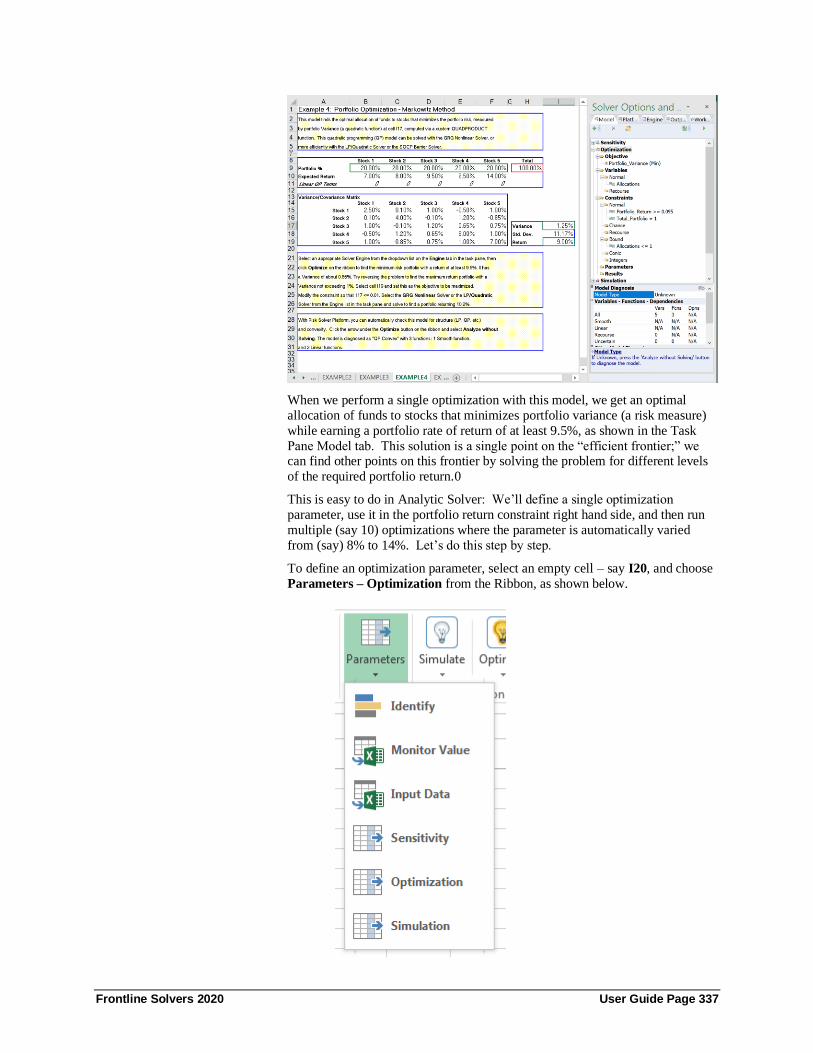
Frontline Solvers 2020 User Guide Page 337
When we perform a single optimization with this model, we get an optimal
allocation of funds to stocks that minimizes portfolio variance (a risk measure)
while earning a portfolio rate of return of at least 9.5%, as shown in the Task
Pane Model tab. This solution is a single point on the “efficient frontier;” we can find other points on this frontier by solving the problem for different levels
of the required portfolio return.0
This is easy to do in Analytic Solver: We’ll define a single optimization
parameter, use it in the portfolio return constraint right hand side, and then run
multiple (say 10) optimizations where the parameter is automatically varied
from (say) 8% to 14%. Let’s do this step by step.
To define an optimization parameter, select an empty cell – say I20, and choose
Parameters – Optimization from the Ribbon, as shown below.

Frontline Solvers 2020 User Guide Page 338
Analytic Solver displays a dialog where you can enter a lower and upper limit
for the parameter value, or alternatively a list of values or a cell range:
When you click OK, the formula =PsiOptParam(0.08,0.14) appears in cell I20.
Next, we’ll use this parameter in the portfolio return constraint. To do this, we
select the constraint ‘Portfolio Return >= 0.095’ in the Task Pane Model tab,
and edit its properties in the lower part of the Task Pane.
We click the cell selector icon to the right of the field containing 0.095, and then
point and click to select cell I20. The properties of the constraint are updated to
use cell I20 for the right hand side, as shown on the next page.
Note: Editing optimization parameters in the task pane is not supported in
Analytic Solver Cloud. To change a constraint in the Cloud, simply double
click the I19 >= 0.095 constraint in the task pane to open the Add Constraint
dialog, then change 0.095 to I20.
Just one more step is required: We must specify how many optimizations we
want to perform. On the Task Pane Platform tab, we set the very first option
Optimizations to Run to 10, as shown on the next page.

Frontline Solvers 2020 User Guide Page 339
Now we simply click the Optimize button on the Ribbon, or the green right
arrow on the Task Pane, to run all 10 optimizations. By default, Analytic Solver
saves the optimal objective and decision variable values from all 10
optimizations; you can save other results, such as constraint values, by setting their Monitor property in the Task Pane to True.
Just after solving, Analytic Solver Optimization displays the results of the last
optimization on the worksheet. But you can display the results of any of the
other 9 optimizations by selecting from the Opt # dropdown list on the Ribbon:
Analytic Solver has built-in facilities to create charts of multiple parameterized
optimizations. Just select Charts – Multiple Optimizations – Monitored Cells
from the Ribbon.
Select the optimization result you would like to chart: In this example,
we want to plot the optimal objective (Portfolio Variance) across the 10

Frontline Solvers 2020 User Guide Page 340
optimizations, where the Portfolio Return threshold is varied on each
optimization.
When you click OK, Analytic Solver draws the chart, as shown below. That’s a
lot more useful results than a single optimal solution!

Frontline Solvers 2020 User Guide Page 341
Frontline Solvers 2020 User Guide Page 342
Getting Results: Simulation
Introduction This chapter explains how to obtain and interpret results from simulation in
Analytic Solver Comprehensive and its subset product Analytic Solver
Simulation. We’ll discuss what can go wrong, and what to do about it, and also
how to get maximum insight from the results of a simulation.
Simulation is ‘simpler’ than optimization in the sense that it requires only (i)
sampling of input values, (ii) calculation of your Excel model with these values,
and (iii) collection of the results; no ‘search for a best solution’ is involved. A simulation can be performed on almost any model, using any Excel functions.
But the way you build your model does affect the speed of simulation, or the
time required to get results. And the structure of your model will become even
more important in the next chapter, when we consider optimization and models
that include uncertainty.
In the following sections, we’ll focus on immediate actions you can take when
you get an unexpected result – but if you read the chapter “Mastering Simulation
and Risk Analysis Concepts,” you’ll learn more about the Monte Carlo
simulation process, and better understand how to design your model to get the
best results in the least time.
What Can Go Wrong, and What to Do About It When you click the Simulate button on the Ribbon, or the green arrow on the
Task Pane to run a simulation, you’ll normally get one of these outcomes:
1. Results on the worksheet, and the message “Simulation finished
successfully” in green at the bottom of the Task Pane. You can
proceed to “When Things Go Right: Getting Further Results.”
2. An error message that you understand and can correct, in red at the
bottom of the Task Pane. You can take corrective action.
3. An error message that you don’t understand, in red at the bottom of the
Task Pane. You should read the solution log in the Output tab, click
the error message and read Help about the message.
4. Results on the worksheet that you don’t understand. Again, before
doing anything else, you should read the solution log in the Output
tab, click the error message to display Help, and read the section
below “When Simulation Results Seem Wrong.”
5. Simulation runs for a very long time, and you don’t get results or a
message in the Task Pane until you press ESC or click Pause/Stop.
You should read the section “When Simulation Takes a Long Time.”
In rare cases, you might find Excel shutting down or “locking up” (so nothing
happens when you press and hold the ESC key for several seconds). In this case
please contact Frontline Systems Technical Support at (775) 831-0300 x4 or [email protected]. Some error messages ask you to contact Technical
Support. If you can send us your model, this will be very helpful.

Frontline Solvers 2020 User Guide Page 343
But experience shows that 99% of all technical support cases involve “pilot
error” by the user, and that 90% of all such cases could be easily resolved by
reading online Help or the User Guide. So we hope you’ll keep reading, and
that you’ll take these steps before calling technical support!
Review Messages in the Output Tab
If using Analytic Solver Desktop, your first step should be to review the
messages in the solution log in the Task Pane Output tab. Below is an example
of the most common simulation error message, and Help that appears when you
click the message:
Note: Information related to the solving process in Analytic Solver Cloud is not available during parsing of the model. As a result, feedback is only available on
the Output tab once the Solver Engine (for a simulation, Risk Solver Engine)
starts to solve the model.
Click the Error Message for Help
Most simulation error messages are underlined – they are hyperlinks to online
Help. If you aren’t sure that you fully understand it, click the link to open Help
to a detailed discussion of the message.
As the Help text explains in the example above, if your model doesn’t define
any simulation outputs, either via a PsiOutput() function that is added to the
formula in an output cell or that refers to the output cell, or via a PSI Statistics
function that refers to the output cell, there will be no results when you run a simulation. As corrective action, you simply need to define the formula cells for
which you want results as simulation outputs.
Here is this same error in Analytic Solver Cloud.

Frontline Solvers 2020 User Guide Page 344
Hyperlinks are not supported in Analytic Solver Cloud.
Role of the Random Number Seed
The seed, or initial value, of the random number generator used in the
simulation process determines whether your results are exactly reproducible
when you re-run a simulation, or whether your results are similar but not
identical because a different random sample was drawn.
By default, the seed for each simulation is set from the value of the system
clock, which is different each time you run a simulation. If you set a seed value
as explained below, the same seed value is used on each simulation, which
means that the entire stream of random numbers drawn, and hence your
simulation results, will be exactly reproducible on each simulation run.
To set the seed, use the Task Pane Engine tab. From the dropdown list at the top of the tab, select Risk Solver Engine, the software engine that actually
performs a simulation. The options for Risk Solver Engine will be displayed:
Enter a positive number for the option Sim. Random Seed. A value of 0 here means “use the value of the system clock as the seed on each simulation.”
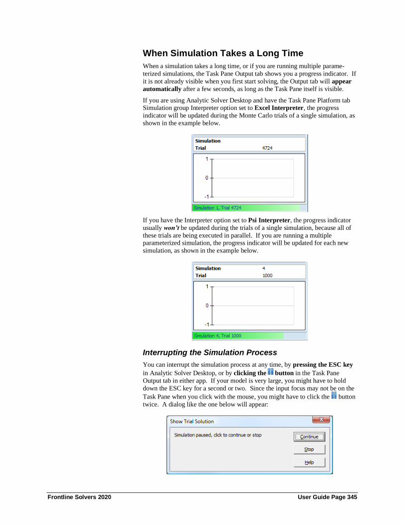
Frontline Solvers 2020 User Guide Page 345
When Simulation Takes a Long Time
When a simulation takes a long time, or if you are running multiple parame-
terized simulations, the Task Pane Output tab shows you a progress indicator. If
it is not already visible when you first start solving, the Output tab will appear
automatically after a few seconds, as long as the Task Pane itself is visible.
If you are using Analytic Solver Desktop and have the Task Pane Platform tab Simulation group Interpreter option set to Excel Interpreter, the progress
indicator will be updated during the Monte Carlo trials of a single simulation, as
shown in the example below.
If you have the Interpreter option set to Psi Interpreter, the progress indicator
usually won’t be updated during the trials of a single simulation, because all of
these trials are being executed in parallel. If you are running a multiple parameterized simulation, the progress indicator will be updated for each new
simulation, as shown in the example below.
Interrupting the Simulation Process
You can interrupt the simulation process at any time, by pressing the ESC key
in Analytic Solver Desktop, or by clicking the button in the Task Pane
Output tab in either app. If your model is very large, you might have to hold
down the ESC key for a second or two. Since the input focus may not be on the
Task Pane when you click with the mouse, you might have to click the button
twice. A dialog like the one below will appear:

Frontline Solvers 2020 User Guide Page 346
Click Stop to stop the simulation or Continue if you want to continue.
Reasons Why Simulation Takes a Long Time
Analytic Solver Simulation is by far the fastest Monte Carlo simulation software
for Excel on the market, and it takes full advantage of multi-core processors for
even faster simulations. But it’s still possible to create a model where a
simulation takes a long time. There are several reasons for this:
1. If you have the Platform tab Simulation group Interpreter option set to
Excel Interpreter in Analytic Solver Desktop, Excel is used to
recalculate the worksheet on each Monte Carlo trial. This is usually an
order of magnitude slower than the PSI Interpreter, though it requires
significantly less memory. This functionality is not supported in Analytic Solver Cloud.
2. If you have Platform tab Simulation group Interpreter option set to Psi
Interpreter (this is always the case in Analytic Solver Cloud), and the
simulation is slow, you may be using certain Excel functions in ways
that slow down the PSI Interpreter. See below for Do’s and Don’ts to
get the most from the PSI Interpreter.
3. Your model may simply be very large, with many complex formulas,
references to other worksheets or workbooks, etc. that take a long time
to evaluate. If your workbook includes sizable elements that aren’t
essential to the simulation model and its results, these extra elements may be slowing down the simulation process.
Time Versus Memory Tradeoffs in Analytic Solver Desktop
The PSI Interpreter is designed to take maximum advantage of available
memory, and trade off memory against time. When Excel interprets
=A1+A2*(A3-4), it uses memory for only four numbers – the values of A1, A2,
A3 and the constant 4. But when PSI interprets this formula, it uses memory for
3,001 numbers – 1,000 each for A1, A2 and A3. If your PC has plenty of
memory, PSI will help you take advantage of it. But if you are tight on memory,
you may find that simulations slow down, because Windows will use ‘virtual memory’ and swap your data between main memory and your hard disk. You
can add more memory -- DRAM chips for PCs and notebooks are an amazing
value today. However, the best solution is simply to run your simulation model
using Analytic Solver Cloud! Since the Cloud app runs on Microsoft's Azure
App Service, memory is not an issue in the cloud!
Model Design for Maximum Simulation Speed
Paying attention to your Excel worksheet layout and design, and avoiding
certain practices, will help you get the most from the PSI Interpreter. Below is a
brief list of Do’s and Don’ts that will help you realize the best possible speed:
• Do build worksheets starting from the “upper left corner.” Don’t place
cells or formulas at extreme row and column addresses all over the
worksheet.
• Do build the model on a small number of worksheets. Don’t include
references on these worksheets to other worksheets that aren’t required for
the simulation model.
• Do use numeric and logical formulas and functions. Don’t create string results in the middle of numeric calculations (see example below).
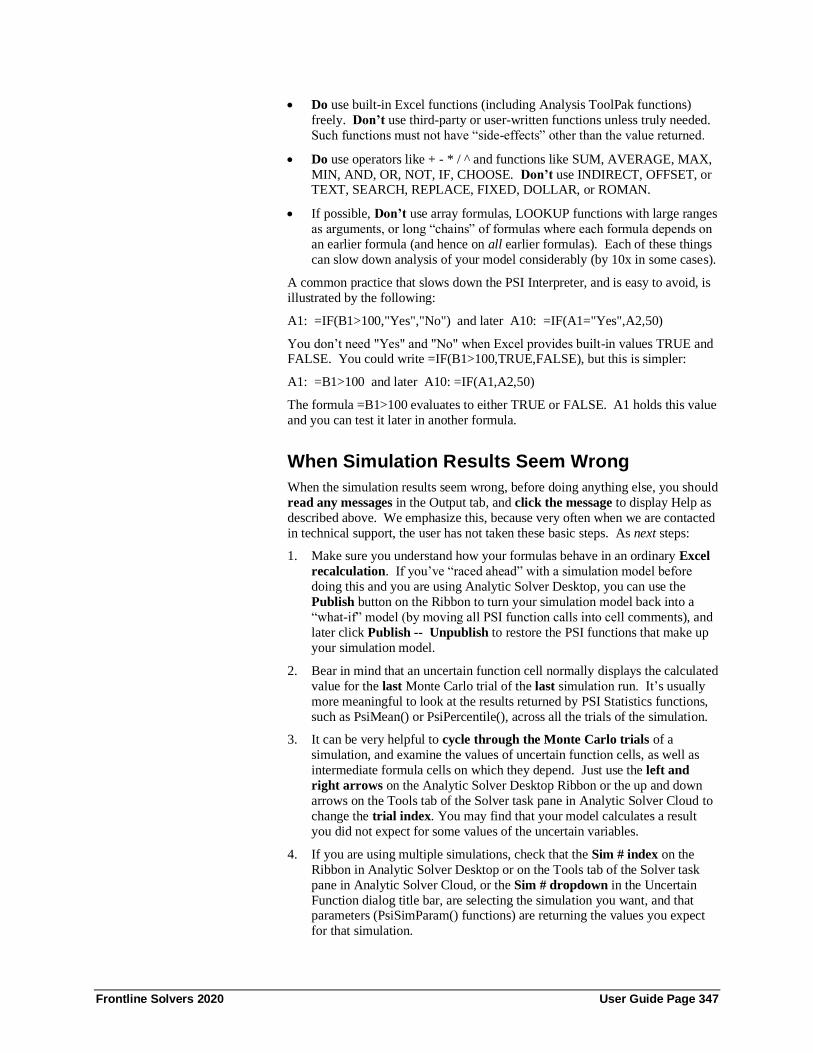
Frontline Solvers 2020 User Guide Page 347
• Do use built-in Excel functions (including Analysis ToolPak functions)
freely. Don’t use third-party or user-written functions unless truly needed.
Such functions must not have “side-effects” other than the value returned.
• Do use operators like + - * / ^ and functions like SUM, AVERAGE, MAX,
MIN, AND, OR, NOT, IF, CHOOSE. Don’t use INDIRECT, OFFSET, or TEXT, SEARCH, REPLACE, FIXED, DOLLAR, or ROMAN.
• If possible, Don’t use array formulas, LOOKUP functions with large ranges
as arguments, or long “chains” of formulas where each formula depends on
an earlier formula (and hence on all earlier formulas). Each of these things
can slow down analysis of your model considerably (by 10x in some cases).
A common practice that slows down the PSI Interpreter, and is easy to avoid, is
illustrated by the following:
A1: =IF(B1>100,"Yes","No") and later A10: =IF(A1="Yes",A2,50)
You don’t need "Yes" and "No" when Excel provides built-in values TRUE and FALSE. You could write =IF(B1>100,TRUE,FALSE), but this is simpler:
A1: =B1>100 and later A10: =IF(A1,A2,50)
The formula =B1>100 evaluates to either TRUE or FALSE. A1 holds this value
and you can test it later in another formula.
When Simulation Results Seem Wrong
When the simulation results seem wrong, before doing anything else, you should
read any messages in the Output tab, and click the message to display Help as
described above. We emphasize this, because very often when we are contacted
in technical support, the user has not taken these basic steps. As next steps:
1. Make sure you understand how your formulas behave in an ordinary Excel
recalculation. If you’ve “raced ahead” with a simulation model before
doing this and you are using Analytic Solver Desktop, you can use the
Publish button on the Ribbon to turn your simulation model back into a
“what-if” model (by moving all PSI function calls into cell comments), and
later click Publish -- Unpublish to restore the PSI functions that make up
your simulation model.
2. Bear in mind that an uncertain function cell normally displays the calculated
value for the last Monte Carlo trial of the last simulation run. It’s usually
more meaningful to look at the results returned by PSI Statistics functions,
such as PsiMean() or PsiPercentile(), across all the trials of the simulation.
3. It can be very helpful to cycle through the Monte Carlo trials of a
simulation, and examine the values of uncertain function cells, as well as
intermediate formula cells on which they depend. Just use the left and
right arrows on the Analytic Solver Desktop Ribbon or the up and down
arrows on the Tools tab of the Solver task pane in Analytic Solver Cloud to
change the trial index. You may find that your model calculates a result
you did not expect for some values of the uncertain variables.
4. If you are using multiple simulations, check that the Sim # index on the
Ribbon in Analytic Solver Desktop or on the Tools tab of the Solver task
pane in Analytic Solver Cloud, or the Sim # dropdown in the Uncertain
Function dialog title bar, are selecting the simulation you want, and that parameters (PsiSimParam() functions) are returning the values you expect
for that simulation.

Frontline Solvers 2020 User Guide Page 348
5. If you haven’t already done so, double-click uncertain function cells and
examine the Frequency tab chart and Percentiles tab numbers to see how
the values of this function were distributed across Monte Carlo trials in the
simulation. This will help explain the values of PSI Statistics functions.
Although software bugs are always possible, consider carefully the possibility that the simulation results are correct for the model you’ve defined, and that
your expectation is wrong. We sometimes find in technical support that what
your model actually says is different from what you intended.
When Things Go Right: Getting Further Results When you have simulation results on the worksheet that make sense to you, and
you have the message “Simulation finished successfully” in green at the bottom
of the Task Pane, there are several ways you can get further results. We’ll cover
five possibilities:
1. Documenting your results in a Simulation Report.
2. Using all the features of the Uncertain Function dialog.
3. Fitting an analytic distribution to uncertain function results.
4. Charting multiple uncertain functions, typically over time.
5. Performing multiple parameterized simulations, and capturing the
results on the worksheet or in charts.
Using the Simulation Report
One quick step you can take, when you have simulation results that you want to
recall later, is to select Reports – Simulation – Simulation to produce a report
worksheet, inserted into your workbook, like the one for the example model
BusinessForecastPsi.xls, shown on the next page.

Frontline Solvers 2020 User Guide Page 349
The Simulation Report in Analytic Solver Desktop documents the option
settings used to perform the simulation and provides summary information about
the uncertain variables and uncertain functions in your simulation model. You
are much more likely to use simulation charts, or snapshots of your own
worksheet layout when you are presenting reports to others, but this report can be quite useful when you want to refer later to the assumptions behind a
simulation analysis.
This report has been completely redesigned in Analytic Solver Cloud. Select
Reports – Simulation – Simulation Report to produce a report worksheet,
inserted into your Excel Online or Desktop Excel workbook, like the one for the
example model BusinessForecast.xlsx, as shown on the next page.
In Analytic Solver Cloud, this report displays the number of input and output functions in the simulation model, the number of simulations and the number of
trials. The body of the report contains the distribution of values for all uncertain
variables and functions along with the cell address, the mean, the standard
deviation, the 5th and 95th percentiles of each.
Using the Uncertain Function Dialog
The Uncertain Function dialog has many features, described in the Frontline
Solvers Reference Guide, that you can use to get enhanced results from your
simulation. For an introduction to these features, refer back to “A First
Simulation Example” in the chapter “Simulation and Risk Analysis,” especially
the sections starting with “Viewing the Full Range of Profit Outcomes.” Here,
we’ll just reiterate the results available at your fingertips in the Uncertain Function dialog:
Dialog Tabs
• The Frequency, Cumulative Frequency, and Reverse Cumulative
Frequency tabs provide three different views of the full range of outcomes

Frontline Solvers 2020 User Guide Page 350
for an uncertain function. In Analytic Solver Desktop, you can click to
display “crosshairs” with numerical values on these charts or add Lower
and Upper bounds to see the estimated probability of a profit or loss.
• The Tornado chart on the Sensitivity tab quickly shows you which
uncertain variables have the greatest impact on this uncertain function, across the full range of Monte Carlo trials. The Scatter Plots tab often
reveals further insights about the behavior of this uncertain function versus
each uncertain variable, or versus other uncertain functions.
Panels and Toolbars
• Using the right panel of the dialog, you can access a drop down menu
including Statistics, Percentiles, Chart Type, Chart Options (Analytic
Solver Desktop), Axis Options (Analytic Solver Desktop), and Markers
(Analytic Solver Desktop). From the Options dialog (accessible from the
Options button on the Analytic Solver Desktop Ribbon), on the Charts and
Markers tabs, you can set default chart and marker settings for all of your
charts.
• Using the title toolbar icons in Analytic Solver Desktop, you can save your
settings, print the charts or numbers from any of the dialog tabs, or copy
the charts or numbers to the Windows Clipboard, where they can be pasted
into other applications. You can also fit a distribution (as shown below) to
the simulation results or upload the simulation results to Microsoft's Power
BI application or Tableau. (See the previous chapter, Examples: Simulation and Risk Analysis, for instructions on exporting model results to Power BI
and Tableau.)
• Click the rightmost icon on the title toolbar in Analytic Solver Desktop to
display the 3-D toolbar that lets you – with a single click – shift between 2-
D and 3-D, shrink or magnify the chart, or move or rotate the chart to a
different perspective.
Fitting a Distribution to Simulation Results
One way to analyze your simulation results is to see whether the distribution of
outcomes is similar to a well-known analytic distribution. Frontline Solver's
Analytic Solver supports a wide range of analytic distributions, and can fit a
distribution and its parameters to sample data. To fit your sample simulation
results, click the icon on the Uncertain Function dialog title toolbar in
Analytic Solver Desktop or click Tools – Fit on the Analytic Solver Cloud ribbon.
Click cell B11 on the BusinessForecastPsi tab within BusinessForecast.xlsx.
When the Fit icon on the Analytic Solver Desktop Ribbon is clicked or Tools –
Fit on the Analytic Solver Cloud ribbon, the Fit Options dialog appears.

Frontline Solvers 2020 User Guide Page 351
If we accept the default settings and click the Fit button, in a few seconds,
Analytic Solver fits a wide range of distributions to the sample data, ranks them
in order of the selected goodness-of-fit criterion (AIC/BIC statistics by default, for more information see the Frontline Solvers Reference Guide), and displays
the best-fitting distribution.
If you select the checkboxes adjacent to the additional distributions in the left panel, they will be superimposed on the frequency chart in the middle of the
dialog. Other tabs of this dialog give you a visual picture of the fit, in the form
of P-P and Q-Q charts, and a chart of CDF Differences, shown below.

Frontline Solvers 2020 User Guide Page 352
The P-P tab displays the Probability-Probability chart. This graph is used to
determine how well a specific distribution fits the observed data. This chart will
be approximately linear (or lie on the y = x line) if the specified distribution is
the correct choice.
Click the Q-Q tab to see the Quantile – Quantile chart. Again, if the two
distributions being compared are a good fit, the plot will lie approximately on
the y = x line.
The Cumulative Distribution Function Differences chart quantifies the
difference between the empirical distribution function and the cumulative
distribution function of the distribution.
You can also fit an analytic distribution to data that you obtain from another
source, such as historical observations of the process you want to model. If you
have this sample data on your Excel worksheet, you can simply select the cell
range containing the data and click the Fit icon on the Analytic Solver Desktop
Ribbon or Tools – Fit on the Analytic Solver Cloud ribbon. Using this tool, you
can easily create an uncertain variable whose distribution models this data.
Note: When using Analytic Solver Cloud or AnalyticSolver.com, fitting a
PsiMetalog function is supported only when using the PsiMetalogFit() function.
Fitting a Meta-Log Distribution
A meta-log distribution is an alternative distribution to a fitted distribution. The
metalog distributions are a collection of continuous univariate probability
distributions which can be used when cumulative distribution function data is
available. For more information on this distribution, see the descriptions for
PsiMetalog() in the Continuous Analytic Distribution subsection within the “Psi
Function Reference” chapter that appears in the Frontline Solvers Reference
Guide.
A general meta-log distribution is defined in a simulation model by using the Psi
distribution, PsiMetalog(). This function has as arguments a vector of coefficients (coefficients) and optionally lower (min) and upper (max) bounds.
The metalog distribution family is designed to be determined from historical

Frontline Solvers 2020 User Guide Page 353
data, without requiring a distribution fitting process. They are computed from a
set of historical data pairs {y, x}, where y is a cumulative probability and x is
the corresponding percentile. The coefficients argument is either a range or an
array of 2 to 10 numerical elements.
Fitting the PsiMetalog() function in Analytic Solver Desktop may be performed in two ways, by using the Psi function PsiMetalogFit() or by using the Metalog
Fit Options dialog. Currently, this function may be used in Analytic Solver
Cloud only by using the Psi function PsiMetalogFit().
To open this dialog on Analytic Solver Desktop, click on a blank Excel cell,
then click the Fit Distribution icon on the PsiMetalog() uncertain variable
dialog.
Note: In Analytic Solver Cloud, the PsiMetalogFit return a Dynamic Array. To
use this function in the Cloud, you need only enter the Psi function in one cell as
a normal function, i.e., not as a control array. The contents of the Dynamic
Array will "spill" down the column. If a nonblank cell is "blocking" the contents of the Dynamic Array, PsiMetalogFit will return #SPILL until such
time as the blockage is removed. When used in the Cloud apps, the first
argument, numCoef, is a scalar, the number of coefficients to produce.

Frontline Solvers 2020 User Guide Page 354
Argument Descriptions
• Cumulative Probabilities - Excel range containing the historical
cumulative probabilities (y values)
• Percentiles – Select the Excel range containing the percentile values (x
values)
• Rank – If omitted, the rank is equal to 3. The value entered for Rank
must be greater than or equal to 2 and less than or equal to 10. In

Frontline Solvers 2020 User Guide Page 355
addition, this value should be less or equal to the number of historical
pairs given in the Cumulative probability and Percentiles arguments.
• Upper Bound – The function may be limited on the right by the upper
bound. If omitted, positive infinity is used for the upper bound.
• Lower Bound – The function may be limited on the left by the lower
bound. If omitted, negative infinity isused for the lower bound.
Click Fit in Analytic Solver Desktop to fit the Meta-log distribution. (Click
Cancel to close the dialog without performing the distribution fitting.) Analytic
Solver replaces the distribution currently in the Uncertain Variable dialog with
the PsiMetalog() distribution parameters. If you click the Save button or close
the dialog by clicking the “X” in the upper right hand corner in the title bar of
this dialog, the PSIMetalog() distribution function with the fitted parameters is
written to the current cell.
For example, given the following input parameters.
The arguments in the Metalog Fit Options dialog would be as follows. Note that
since the Upper and Lower Bound fields are empty, the fitted distribution will be
unbounded. Distributions may be bounded on both sides, semi-bounded
(bounded on one side) or unbouded. Note: Rank is equal to 2 which falls
between the rank argument lower bound, which is equal to 2, and the number of
historical pairs passed for Cumulative probability and Percentiles, 5.

Frontline Solvers 2020 User Guide Page 356
After clicking Fit, the uncertain variable dialog changes to the following.
Click Save to close the uncertain variable dialog and save the fitted parameters
to the Excel cell. To inspect the coefficients obtained by the fitting, see the
resultant PsiMetalog() function that was saved to this cell. In this example, the
coefficients obtained were 31.6 and 4.431777.
Charting Multiple Uncertain Functions
In some simulation models, you will have a series of uncertain functions that
represent the evolution of some process over time. The individual cells might
represent sales or inventory levels, interest rates or exchange rates, or some
other uncertain factor. You want to understand how this uncertain function
changes over time, taking into account its uncertainty.
Analytic Solver Comprehensive has a general facility for creating charts of
multiple simulation results, including Overlay, Trend, and Box-Whisker charts.
Below, we’ve used this facility to visualize the evolution of a stock price over

Frontline Solvers 2020 User Guide Page 357
time, using the example model GBMSimpleModel.xls, which simulates stock
prices using a Geometric Brownian Motion model. When we perform a
simulation, select Charts – Multiple Simulation Results – Trend, and select
the first 24 uncertain functions for inclusion in the chart, we get a Trend Chart
like the one below:
Here we can see a slow upward drift of the mean value of the stock price, and
also its volatility around the mean, depicted here with the 25th and 75th, and the
10th and 90th percentiles.
Multiple Parameterized Simulations
Once you have results from a single simulation, you normally want to explore
“what if” scenarios, where you change some parameter that is under your
control and run simulations to observe the effects of the uncertain variables that
are not under your control.
Using Interactive Simulation in Analytic Solver Desktop
Analytic Solver Simulation offers a powerful facility to do this through
Interactive Simulation: You can simply click the Simulate button on the
Analytic Solver Cloud Ribbon to enter Interactive mode, then change a number
on your worksheet and instantly see new simulation results. This is illustrated in
“A First Simulation Example” in the earlier chapter “Simulation and Risk Analysis.” Analytic Solver is fast enough to make this sort of “what-if” analysis
practical.

Frontline Solvers 2020 User Guide Page 358
Using Multiple Simulations
But after exploring the model and its results through Interactive Simulation,
you’ll likely want to automate the “what-if” process, and more systematically
evaluate the effects of changing some parameter or parameters under your
control on the simulation results. Analytic Solver makes this easy, with multiple
parameterized simulations. This is illustrated in “An Airline Revenue
Management Model” in the chapter “Simulation and Risk Analysis.”
Setting Up Multiple Parameterized Simulations
Two simple steps are required to set up a multiple parameterized simulation:
1. Define one or more simulation parameters, and use them in your model.
2. Set the number of simulations option to a value greater than 1, and run the
simulation.
To define a simulation parameter, simply select Parameters – Simulation from
the Ribbon:
Analytic Solver Simulation displays a dialog box, where you can enter a lower
limit and upper limit for the parameter value, or a specific list of values that you
would like the parameter to take on successive simulations. If you specify a
lower and upper limit, then when you set the number of simulations, the
parameter will take on equally-spaced values from the lower to the upper limit.
To set the number of simulations, simply edit the option in the Task Pane
Platform tab Simulation group option Simulations to Run:

Frontline Solvers 2020 User Guide Page 359
When you next click the green arrow in the Task Pane, or choose Simulate –
Run Once from the Analytic Solver Desktop Ribbon, all 10 (in this example) simulations will be run, automatically varying each simulation parameter over
its range or list of values, and all the results will be collected and stored. (If you
click the Simulate icon in Analytic Solver Desktop to activate Interactive
Simulation, all 10 simulations will be run each time you make a change on the
worksheet.)
Viewing Results of Multiple Simulations
After running multiple parameterized simulations, you can view the results on the worksheet, or in the Uncertain Function dialog, by selecting the simulation
of interest from the Sim # dropdown. You can create reports and charts of
results that span all or some of the simulations. We highly recommend that you
read “An Airline Revenue Management Model” in the earlier chapter
“Simulation and Risk Analysis,” which illustrates how this is done – creating a
Trend Chart and a Box-Whisker Chart across all 10 simulations in this model.
Once you become familiar with multiple parameterized simulations, you’ll
likely want to use them in nearly every simulation analysis you do. They’re a
natural way to get further results from the effort you’ve put into a simulation
model, and communicate those results to colleagues or clients.
Time Series Forecasting
Starting with version 2014-R2, Analytic Solver Data Mining includes the ability
to forecast a future point in a time series in one of your spreadsheet formulas
(without using the Score button on the Ribbon) using a PsiForecast() function in
conjunction with a model created using ARIMA or one of our smoothing
methods (Exponential, Double Exponential, Moving Average, or Holt Winters).
PsiForecast() is similar to the previous PSIForecastXXX functions supported in
V2014, 2015, and 2016: it will compute future-looking forecasts based on the
fitted model, using the provided new time series observations as initial points.
The number of forecasts is determined by the number of selected cells in array-
formula entry. The result of PsiForecast() can be deterministic, if the Simulate argument is FALSE, or non-deterministic, if the Simulate argument is TRUE– in
which case the forecasts are adjusted with random normally distributed errors,
defined by the forecasts’ statistics.
Open the Airpass.xlsx example dataset by clicking Help – Examples on the Data
Mining ribbon, then clicking Forecasting/Data Mining Examples. This example

Frontline Solvers 2020 User Guide Page 360
dataset includes International Airline Passenger Information by month for years
1949 – 1960. Since the number of airline passengers increases during certain
times of the year, for example Spring, Summer, and in the month of December,
we can say that this dataset includes “seasonality”.
First, we will partition this dataset into two datasets: a training dataset and a validation dataset. We’ll use the training dataset to create the ARIMA model
and then we’ll apply the model to the validation dataset to forecast six future
data points, or one half year of data.
Click Partition in the Time Series section of the Data Mining ribbon to open the
Time Series Partition Data dialog. Select Passengers for the Variables in the
Partition Data and Month for the Time Variable.
Click OK to accept the defaults for Specify Partitioning Options and Specify
Percentages for Partitioning. Recall that when a time series dataset is
partitioned, the dataset is partitioned sequentially. Therefore, 60% or the first 86
records, will be assigned to the training dataset and the remaining 40%, or 58
records, will be assigned to the validation dataset. (For more information on
partitioning a time series dataset, see the previous chapter Exploring a Time
Series Dataset.)
The TSPartition worksheet will be inserted into the Model tab of the Analytic Solver task pane under Transformations – Time Series Partition. Recall the
steps needed to produce the forecast. Click ARIMA -- ARIMA to open the
ARIMA dialog. Month has been pre selected as the Time variable. Select
Passengers as the Selected variable.

Frontline Solvers 2020 User Guide Page 361
This example will use a SARIMA model, or Seasonal Autoregressive Integrated
Moving Average model, to predict the next six datapoints in the dataset. (For
more information on this type of time series model, please see the earlier
chapter, “Exploring a Time Series Dataset.”) A seasonal ARIMA model
requires 7 parameters, 3 nonseasonal (autoregressive (p), integrated (d), and moving average (q)), 3 seasonal (autoregressive (P), integrated (D), and moving
average (Q)), and period. Each parameter must be a non-negative integer.
Selecting appropriate values for p, d, q, P, D, Q and period is beyond the scope
of this User Guide. Consequently, this example will use a well documented
SARIMA model with parameters p = 0, d = 1, q = 1, P = 0, D = 1, Q = 2 and
period (P) = 12. Please refer to the classic time series analysis text Time Series
Analysis: Forecasting and Control written by George Box and Gwilym
Jenkins for more information on parameter selection.
Select Fit seasonal model and enter 12 for Period since it takes a full 12 months
for the seasonal pattern to repeat. Set the Non-seasonal Parameters as
Autoregressive (p) = 0, Difference (d) = 1, Moving Average (q) = 1 and the Seasonal Parameters as Autoregressive (P) = 0, Difference (D) = 1, and Moving
Average (Q) = 2.
Click OK to create the SARIMA model.
ARIMA_Output will be inserted into the Model tab of the XLMiner task pane
under Reports – ARIMA. This output contains the Training Error Measures and
Fitted Model Statistics. (For more information on this report, please see the chapter Exploring a Time Series Dataset within the Analytic Solver Data Mining
Reference Guide.) ARIMA_Stored contains the stored model parameters.
Now we’ll use this ARIMA model to predict new data points in the validation
dataset using the PsiForecast() function. (Note: The first forecasted point will
be more accurate than the second, the second forecasted point more accurate
than the third and so on.) The PsiForecast() function will be interactive in the

Frontline Solvers 2020 User Guide Page 362
sense that if any of the input values (values passed in the 2nd argument) change,
the forecast will be recomputed.
In later versions of desktop Excel, the PsiForecast() function returns a Dynamic
Array. To use this function in the Cloud, you need only enter the Psi function in
one cell as a normal function, i.e., not as a control array. The contents of the Dynamic Array will "spill" down the column. If a nonblank cell is "blocking"
the contents of the Dynamic Array, the Psi Data Mining function will return
#SPILL until such time as the blockage is removed. In Excel versions that do
not support Dynamic Arrays, PsiForecast() must be entered as an Excel array.
The PsiForecastARIMA function takes five arguments: Model, Input Data,
Simulate, Num_forecasts, and Header. Select a blank cell on the Data
worksheet and enter =PsiForecast(. If using a version of Excel that does not
support Dynamic Arrays, select B146:B152 on the Data worksheet, then enter
=PsiForecast(.
The first argument, Model, is the range of cells used by Analytic Solver Data Mining to store the ARIMA model on the ARIMA_Stored worksheet. This data
range will change as the forecast method changes. Select or enter
ARIMA_Stored!B12:B38, for this argument.
The second argument, Input_Data, is the range containing the initial starting
points from the validation data set. The minimum number of initial points that
should be specified for a seasonal ARIMA model is the larger of p + d + s * (P +
D) and q + s * Q. In this example, p + d + s * (P + D) is equal to 13 (0 + 1 + 12
* (0 + 1) and q + s * Q is equal to 13 (1 + 12 * 1), therefore the minimum
number of initial starting points required is 13 (MAX (13, 13)). If you provide
fewer than the minimum required number of starting points, PsiForecast() will
return a column of zeros. (See the table below for the minimum number of initial starting points required by each Forecasting method included in Analytic
Solver Data Mining.) The maximum number of starting points is the number of
points in the validation dataset. All points supplied in the second argument will
be used in the forecast. Select or enter Data!A1:B145, for this argument.
Pass True or False for the third argument. Passing False will result in a static
forecast that will only update if a cell passed in the 2nd argument is changed. If
True is passed for this argument, a random error will be included in the
forecasted points. See the Time Series Simulation example below for more
information on passing True for this argument. In this case, Pass False) for this
argument.
Your formula should now be the following: =PsiForecast(ARIMA_Stored!B12:B38,Data!A1:B145, False). If using a
version of Excel that does not support Dynamic Arrays, press CTRL + SHIFT
+ ENTER to enter this formula as an array in all seven cells (B146:B152).
It’s also possible to enter this formula using the Insert Function dialog by
clicking Formulas – Insert Function, select PSI Data Mining for Category, then
PsiForecastARIMA.

Frontline Solvers 2020 User Guide Page 363
The results from this function are displayed below.
Enter True for the Header argument to insert a heading above the forecasted
values.
Notice that the formula is entered into cell B146 and the contents of the
PsiForecast() Dynamic Array "spill" down into cells B147:B152.
If any values change in the ranges ARIMA_Stored!B12:B38 or Data!B2:B145,
the forecast will be recomputed; but if the input argument values stay the same,
the PsiForecast() function will always return the same forecast values. As
mentioned above, the first forecasted value in cell B146 is the most accurate
predicted point. Accuracy declines as the number of forecasted points increases.
See the Frontline Solvers Reference Guide for specifications on PsiForecast().
Time Series Simulation
Analytic Solver Data Mining includes the ability to perform a time series
simulation, where future points in a time series are forecast on each Monte Carlo
trial, using a model created via ARIMA or one of our smoothing methods
(Exponential, Double Exponential, Moving Average, or Holt Winters).
To run a time series simulation, we must pass “True” as the third argument to
PsiForecast(). When the third argument is set to True, Analytic Solver will add
a random (positive or negative) “epsilon” value to each forecasted point. Each
time a simulation is run, 1000 trial “epsilon” values are generated using the PsiNormal distribution with parameters mean and standard deviation computed

Frontline Solvers 2020 User Guide Page 364
by the PsiForecast() function. You can view the output of this simulation in the
same way as you would view “normal” simulation results in Analytic Solver
Comprohensive, Analytic Solver Simulation, Analytic Solver Upgrade, or
Analytic Solver Basic, simply by creating a PsiOutput() function and then
double clicking the Output cell to view the Simulation Results dialog.
Select a blank cell, or Data!C146:C152 if using a version of Excel that does not
support Dynamic Arrays, then click Formulas – Insert Function to display the
Function Argument dialog.
As discussed previously, the first argument, ARIMA_Stored!B12:B38, is the
range of cells used by Analytic Solver to store the ARIMA model on the
ARIMA_Stored worksheet.
For the second argument the range containing the initial points in the series must
be greater than the minimum number of initial points for a static forecast. For a
seasonal ARIMA model when Simulate = True, the minimum number of initial
points must be greater than Max((p + d + s * (P + D), (q + s * Q). In this example, p + d + s * (P + D) is equal to 13 (0 + 1 + 12 * (0 + 1) and q + s * Q is
equal to 13 (1 + 12 * 1), therefore the minimum number of initial starting points
required is 13 (Minimum #Initial Points > MAX (13, 13)). However, when
PsiForecastARIMA() is called with Simulate = True, it is recommended to add
an additional number of datapoints, equal to the #Periods, to the minimum
number required. In this instance the number of initial points will be 25: 13
(minimum # of points) + 12 (# of points for Period in the Time Series - ARIMA
dialog). If you provide fewer than the minimum required number of starting
points (13 in this example) PsiForecastARIMA() will return #VALUE. (See the
table below for the minimum number of initial starting points required by each
forecast method in Analytic Solver.) All points supplied in the second argument
will be used in the forecast. Select or enter Data!A1:B145, for this argument.
Passing TRUE for the third argument indicates to Analytic Solver Data Mining
that you plan to use this function call in a Monte Carlo simulation, so it should
add a random epsilon value (different on each Monte Carlo trial) to each
forecasted point.
In versions of Excel supporting Dynamic Arrays, this formula is entered into
cell C146 and the contents of the PsiForecast() Dynamic Array "spills" down
into cells C147:C152. If versions of Excel that do not support Dynamic Arrays,
the formula must be entered as an Excel array.
To view the results of the simulation including frequency and sensitivity charts,
statistics, and percentiles for the full range of trial values, we must first create an
output cell. Select cell C147, then click Analytic Solver – Results – Referred
Cell. Select cell D147 (or any blank cell on the spreadsheet) to enter the
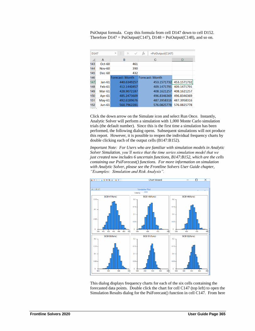
Frontline Solvers 2020 User Guide Page 365
PsiOutput formula. Copy this formula from cell D147 down to cell D152.
Therefore D147 = PsiOutput(C147), D148 = PsiOutput(C148), and so on.
Click the down arrow on the Simulate icon and select Run Once. Instantly,
Analytic Solver will perform a simulation with 1,000 Monte Carlo simulation
trials (the default number). Since this is the first time a simulation has been
performed, the following dialog opens. Subsequent simulations will not produce
this report. However, it is possible to reopen the individual frequency charts by
double clicking each of the output cells (B147:B152).
Important Note: For Users who are familiar with simulation models in Analytic
Solver Simulation, you’ll notice that the time series simulation model that we just created now includes 6 uncertain functions, B147:B152, which are the cells
containing our PsiForecast() functions. For more information on simulation
with Analytic Solver, please see the Frontline Solvers User Guide chapter,
“Examples: Simulation and Risk Analysis”.
This dialog displays frequency charts for each of the six cells containing the
forecasted data points. Double click the chart for cell C147 (top left) to open the
Simulation Results dialog for the PsiForecast() function in cell C147. From here

Frontline Solvers 2020 User Guide Page 366
you can view frequency and sensitivity charts, statistics and percentiles for each
forecasted point.
The frequency chart displays the distribution of all 1000 trial values for cell
C147 with and observed mean 440.76 and standard deviation of 16.90 shown in
the Chart Statistics. Select Simulate – Run Once a few more times (or click the
green “play” button on the Solver Pane Model tab). Each time you do, another
1,000 Monte Carlo trials are run, and a slightly different mean will be displayed.
Enter 444 for the Lower Cutoff in the Chart Statistics section of the right panel, A vertical bar appears over the Frequency chart to display the
frequency with which the forecasted value was greater than this value during the
simulation. You can use this as an estimate of the probability that the actual
value will be less than the forecasted value. In this case there was a 58.20%
chance that the number of international airline passengers would be less than
444,000 in January 1961 and a 41.80% chance that the number of passengers
would be greater than 444,000.
Looking to the right, you’ll find the Statistics pane, which includes
summary statistics for the full range of forecasted outcomes. We can see that the
minimum forecasted value during this simulation was 397.78, and the maximum
forecasted value was 493.37. Value at Risk 95% shows that 95% of the time, the
number of international airline passengers was 469.72 or less in January 1961, in
this simulation. The Conditional Value at Risk 95% value indicates
that the average number of passengers we would have seen (up to the 95%
percentile) was 438.86. For more information on Analytic Solver Platform’s
full range of features, see the Frontline Solvers User Guide chapter, “Examples: Simulation and Risk Analysis”.

Frontline Solvers 2020 User Guide Page 367
Select cells E147:E156 and then enter the formula, =PsiData(C147) If using a
version of Excel that does not support Dynamic Arrays, press CTRL + SHIFT +
ENTER to array enter the formula into all 10 cells. Repeat the same steps to
array enter “=PsiData(C148)” in cells F147:F156, “=PsiData(C149)” in cells
G147:G156, “=PsiData(C150)” in cells H147:H156, “PsiData(C151)” in cells
I147:I156, and “=PsiData(C152)” in cells J147:J156. Then click Simulate – Run Once to run a simulation.
The ten Excel cells in these columns will update with trial values for each of the
PsiForecast() functions in column C. For example, cells E147:N147 will
contain the first 10 trial values for the PsiForecast() function in cell C147, Cells
E147:N147 will contain the first 10 trial values for cell C148 and so on. (For
more information on the PsiData() function, please see the Excel Solvers
Reference Guide chapter, “Psi Function Reference.”)
Note: In Analytic Solver Cloud and in later versions of desktop Excel, the
PsiData() function returns a Dynamic Array. To use this function in the Cloud,
you need only enter the Psi function in one cell as a normal function, i.e., not as a control array. The contents of the Dynamic Array will "spill" down the
column. If a nonblank cell is "blocking" the contents of the Dynamic Array,
PsiData() will return #SPILL until such time as the blockage is removed. Use
the optional numTrials argument to specify the number of trials returned in the
Dynamic Array. If not present, all trials will be returned.
If we create an Excel chart of these values, you’ll see a chart similar to the one
below where each of Series1 through Series6 represents a different Monte Carlo
trial. The random “epsilon” value added to each forecast value accounts for (all
of) the variation among the lines. If the third argument were FALSE or omitted,

Frontline Solvers 2020 User Guide Page 368
all of the lines would overlap, assuming that the table or parameters and the
starting values were not changing.
The remaining Forecasting methods can be used in the same way using
PsiForecast() with information from their respective Stored Model sheets.
Forecasting
Algorithm
Stored Model Sheet Minimum # of
Initial Points when
Simulate = False
Minimum # of
Initial Points when
Simulate = True
Non- Seasonal ARIMA ARIMA_Stored Max(p + d, q) Max(p + d, q)
Seasonal ARIMA ARIMA_Stored Max((p + d + s *(P
+ D), (q + s * Q)
1 + Max((p + d + s
*(P + D), (q + s *
Q)**
Exponential Smoothing Expo_Stored 1 1
Double Exponential
Smoothing
DoubleExpo_Stored 1 1
Moving Average
Smoothing
MovingAvg_Stored # of Intervals # of Intervals
Holt Winters
Smoothing
MulHoltWinters_Stored
AddHoltWinters_Stored
NoTrendHoltWinters_Stored
2 * #Periods 2 * #Periods
**Adding a number of data points equal to the Number of Periods (as shown on the Time Series – ARIMA dialog)
to the Minimum # of Initial Points when Simulate = True is recommended when calling PsiForecast() with Simulate
= True.
Excel 2016 Forecast Functions
Users of Analytic Solver Comprehensive, Analytic Solver Simulation and
Analytic Solver Basic will notice two Psi Forecast functions:

Frontline Solvers 2020 User Guide Page 369
PsiForecastLinear() and PsiForecastETS(). These two functions were
introduced to coincide with the new Excel 2016 Forecast functions:
Forecast.Linear and Forecast.ETS.
PsiForecastLinear predicts future values for a time series data set (containing
known or historical data) using linear regression. PsiForecastETS uses exponential smoothing to predict future values in a time series dataset with the
option to either automatically detect seasonality in the data set or pass a
seasonality period. Passing False as the last argument to either function will
result in a static forecast. If True is passed for this argument, a random error
will be included in the forecasted points.
Note: When comparing the results of the Psi functions with the Excel functions,
you may see slightly different calculated forecast values depending on whether
the Psi Interpreter or Excel Interpreter is selected on the Task Pane Platform tab.
When the Psi Interpreter is used, a slightly different (but arguably better)
methodology is used to compute these forecast functions. When the Excel
Interpreter is selected, Microsoft Excel is used to calculate the worksheet, and thus Excel's methodology will be used.
To illustrate an example of how to use these two functions, we'll reuse the
Airpass time series dataset. Click back to the Data tab within Airpass.xlsx.
Recall that the Airpass time series dataset contains international airline
passenger data from January 1949 to December 1960. Using this historical data,
we will forecast the number of passengers in 1961.
PsiForecastLinear() performs linear regression of known_y values with
known_x time variables to forecast the value at time, X. This function takes the
following arguments.
PsiForecastLinear(X, known_ys, known_xs[, simulate])
• X: The target date. A data point for which you want the predicted value. A
data point may be date/time or numeric.
• known_ys: An Excel range containing the independent variables in the
given dataset.
• known_xs: An Excel range containing the time variables in the given
dataset.
• simulate: (Optional) Pass True or False for the third argument. Passing
False (the default) will result in a static forecast that will only update if a
cell passed in the known_ys argument is changed. If True is passed for this
argument, a random error will be included in the forecasted points.
Click a blank cell on the worksheet, say cell E3, then in Analytic Solver Desktop
click Formulas – Insert Function on the Ribbon to display the Function Argument dialog. In Analytic Solver Cloud, you'll need to type the formula
directly into cell E3.
Select PsiData Mining form the Category drop-down menu, then scroll down to
PsiForcastLinear and click OK. The Function Arguments dialog opens.
• X: Select cell Data!E3 for the target argument.
• Known_ys: Select or enter B3:B146. These are the independent y
values. Be sure to anchor this range of cells (as shown in the
screenshot below) so that we can easily copy the formula.

Frontline Solvers 2020 User Guide Page 370
• Known_ys: Select or type A3:A146 for the third argument,
known_xs. Again, anchoring this Excel range now allows easy
copying and pasting later.
• Simulate: Pass False for this argument. See the Time Series
Simulation example below for more information on passing True for
this argument.
Click OK to enter the formula into the Excel cell, then copy and paste this
formula into cells E4:E14.
If any values change in the ranges Data!A3:A146 or Data!B3:B146, the forecast
will be recomputed; however, if the input argument values remain the same,
PsiForecastLinear() will always return the same forecast values. As mentioned
above, the first forecasted value in cell E3 is the most accurate predicted point.
Accuracy declines as the number of forecasted points increases.
We can create a similar forecast using PsiForecastETS(). PsiForecastETS()
performs Exponential Triple Smoothing on known values to forecast future
values at time, target. The fourth argument, seasonality, is optional. If not
given, seasonality is automatically detected from the the data. If given,
automatic seasonality detection is turned off, and the given seasonality period is
enforced. This function takes the following arguments.

Frontline Solvers 2020 User Guide Page 371
PsiForecastETS(target_date, values, timeline[,
seasonality][, data_completion][, aggregation][,
simulate])
• target_date: A data point for which you want the predicted value. A
data point may be date/time or numeric. If a target date is given that appears
before the start of the timeline in the dataset, PsiForecastETS will return
#NUM (i.e., if 1940 is passed for X).
• values: An Excel range containing the historical values in the given data
set.
• timeline: An Excel range containing the time variables in the given
data set. Both functions require the historical data to be structured using a
constant interval between data points. Since the Airpass data set presents
monthly passenger data, the forecast must also predict the number of
passengers by month.
• seasonality: (Optional) This argument indicates the length of the
seasonal pattern. The following values are accepted as valid inputs. All
other values will return a #NUM error.
0: Signifies no seasonality exists in the data. The result is a linear
prediction.
1: (Default Value) Triggers Solver to automatically detect seasonality
within the data.
1 < N < 8,760: Positive integer values greater than 1 but less than 8,760,
will can be entered as the seasonality period.
• data_completion: (Optional) This argument specifies how to handle
missing values. The default value of 1 replaces missing values by
interpolation. If 0 is passed, missing values will be replaced with 0's.
• aggregation: (Optional) PsiForecastETS can aggregate multiple points
with the same time stamp. Pass an integer value from 0 to 6 to indicate
which method should be used.
0: (Default) Average
1: SUM
2: COUNT
3: COUNTA
4: MIN
5: MAX
6: MEDIAN
• simulate: (Optional) Pass True or False for the third argument. Passing
False (the default) will result is a static forecast that will only update if a
cell passed in the second argument is changed. If True is passed for this
argument, a random error will be added to each forecasted point.
On the Excel ribbon, click Formulas – Insert Function to display the Function
Argument dialog.
Select PsiData Mining form the Category drop-down menu, then scroll down to
PsiForcastETS and click OK.
• Target_date: Select cell Data!E3.

Frontline Solvers 2020 User Guide Page 372
• Values: Select or enter B3:B146. These are the independent y
values. Anchoring the cell range (as shown in the screenshot below)
will allow us to easily cut and paste the formula later.
• Timeline: Enter the dates January 1961 – December 1961 in cells
D3:D11 for timeline. These are our target dates or the dates that we
want to predict. These are our time variables. Anchoring the cell
range, as shown in the screenshot below, will allow us to easily cut and
paste the formula.
• Seasonality: Enter 1 for this argument to automatically detect the
seasonality within the data.
• data_completion: Enter 0 for this argument to substitue any
empty value with 0.
• aggregation: Enter 0 for this argument to aggregate multiple points
with the same date using AVERAGE.
• Simulate: Passing TRUE for the third argument indicates to
XLMiner that you plan to use this function call in a Monte Carlo
simulation. Therefore, a random epsilon value (different on each
Monte Carlo trial) will be added to each forecasted point.
Click OK to enter the formula into the Excel cell. This formula can easily be
copied to cells E4:E14.
As with the PsiForecast Data Mining functions, to view the results of the
simulation, including frequency and sensitivity charts, statistics, and percentiles

Frontline Solvers 2020 User Guide Page 373
for the full range of trial values, we must first create an output cell. Select cell
F3, then click Analytic Solver Platform – Results – Referred Cell on the
Excel ribbon. Select cell F17 (or any blank cell on the spreadsheet) to enter the
PsiOutput formula. Copy this formula from cell F17 down to cell F28.
Therefore F17 = PsiOutput(F3), F18 = PsiOutput(F4), and so on.
Click the down arrow on the Simulate icon on the Analytic Solver Platform
ribbon and select Run Once. Instantly, Analytic Solver Simulation performs a
simulation with 1,000 Monte Carlo simulation trials (the default number). Since
this is the first time a simulation has been performed, the following dialog
opens. Subsequent simulations will not produce this report. However, it is
possible to reopen the individual frequency charts by double-clicking each of the
output cells (F17:F28).
Important Note: For users who are familiar with simulation models in Analytic
Solver, you will notice that the time series simulation model that we just created
now includes 12 uncertain functions (F17:F28) which are the cells containing
our PsiForecastETS() functions.
The dialog above displays frequency charts for the first nine, of the total 12,
uncertain function cells containing the forecasted data points. Double-click the
chart for cell F3 (top-left) to open the Simulation Results dialog displaying
PsiForecastETS() function in cell F3. From here, you can view frequency and
sensitivity charts, statistics and percentiles for each forecasted point.
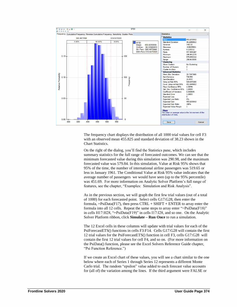
Frontline Solvers 2020 User Guide Page 374
The frequency chart displays the distribution of all 1000 trial values for cell F3
with an observed mean 455.825 and standard deviation of 38.23 shown in the
Chart Statistics.
On the right of the dialog, you’ll find the Statistics pane, which includes
summary statistics for the full range of forecasted outcomes. We can see that the
minimum forecasted value during this simulation was 290.98, and the maximum
forecasted value was 579.84. In this simulation, Value at Risk 95% shows that
95% of the time, the number of international airline passengers was 519.65 or
less in January 1961. The Conditional Value at Risk 95% value indicates that the
average number of passengers we would have seen (up to the 95% percentile)
was 451.69. For more information on Analytic Solver Platform’s full range of
features, see the chapter, “Examples: Simulation and Risk Analysis”.
As in the previous section, we will graph the first few trial values (out of a total
of 1000) for each forecasted point. Select cells G17:G28, then enter the formula, =PsiData(F17), then press CTRL + SHIFT + ENTER to array enter the
formula into all 12 cells. Repeat the same steps to array enter “=PsiData(F18)”
in cells H17:H28, “=PsiData(F19)” in cells I17:I28, and so one. On the Analytic
Solver Platform ribbon, click Simulate – Run Once to run a simulation.
The 12 Excel cells in these columns will update with trial values for each of the
PsiForecastETS() functions in cells F3:F14. Cells G17:G28 will contain the first
12 trial values for the PsiForecastETS() function in cell F3, cells G17:G28 will
contain the first 12 trial values for cell F4, and so on. (For more information on
the PsiData() function, please see the Excel Solvers Reference Guide chapter,
“Psi Function Reference.”)
If we create an Excel chart of these values, you will see a chart similar to the one
below where each of Series 1 through Series 12 represents a different Monte
Carlo trial. The random “epsilon” value added to each forecast value accounts
for (all of) the variation among the lines. If the third argument were FALSE or

Frontline Solvers 2020 User Guide Page 375
omitted, all of the lines would overlap, assuming that the table or parameters and
the starting values were not changing.

Frontline Solvers 2020 User Guide Page 376
Getting Results: Stochastic Optimization
Introduction This chapter explains how to obtain and interpret results from stochastic
optimization (optimization of models with uncertainty) in Analytic Solver
Comprehensive or Analytic Solver Simulation with Analytic Solver
Optimization. We’ll discuss what can go wrong, and what to do about it, and
also how to get more than a single optimal solution from your model.
Analytic Solver Comprensive has powerful algorithms for automatically
transforming and solving optimization models with uncertainty. But since a
stochastic optimization model includes decision variables, uncertain
variables, and constraints and an objective that may depend on both, there are
“more things that can go wrong.” Indeed, everything you’ve read in the
previous two chapters, “Getting Results: Optimization” and “Getting Results:
Simulation” will apply to stochastic optimization – plus there are a variety of
special result messages and error messages that apply only to stochastic
optimization models.
The good news is that everything you’ve learned so far about conventional optimization and Monte Carlo simulation does apply to stochastic optimization
in Analytic Solver Comprehensive. Unlike most other software packages,
Analytic Solver Comprehensive has one consistent user interface, set of terms,
and model elements for all types of simulation and optimization models.
In the following sections, we’ll focus on immediate actions you can take when
you get an unexpected result – but if you read the chapter “Mastering Stochastic
Optimization Concepts,” you’ll learn far more about stochastic optimization
models and solution methods, and better understand why the unexpected result
appeared, and how to design your model to get the solutions you want.
What Can Go Wrong, and What to Do About It When you click the Optimize button on the Ribbon, or the green arrow on the Task Pane to solve, you’ll normally get one of these outcomes:
1. A solution that makes sense to you. This is normally accompanied by a
Solver Result message in green at the bottom of the Task Pane. You
can proceed to “When Things Go Right: Getting Further Results.”
2. A Solver Result error message that you understand and can correct, in
red at the bottom of the Task Pane. You can take corrective action.
3. A Solver Result error message that you don’t understand, in red at the
bottom of the Task Pane. You should read the solution log in the
Output tab (in Analytic Solver Desktop), click the error message and
read Help about the message.
4. A solution that you don’t understand, or that seems wrong. Again
before doing anything else, you should read the solution log in the

Frontline Solvers 2020 User Guide Page 377
Output tab (in Analytic Solver Desktop), click the error message to
display Help, run available reports as described below, and read the
section below “When the Solution Seems Wrong.”
5. Solving runs for a very long time, and you don’t get a solution or a
Solver Result message until you press ESC or click Pause/Stop. You should read the section below “When Solving Takes a Long Time.”
In rare cases, you might find Excel shutting down or “locking up” (so nothing
happens when you press and hold the ESC key for several seconds in Analytic
Solver Desktop or the Pause button in Analytic Solver Cloud). In this case
please contact Frontline Systems Technical Support at (775) 831-0300 x4 or
[email protected]. Some Solver Result error messages ask you to contact
Technical Support. If you can send us your model, this will be very helpful.
But experience shows that 99% of all technical support cases involve “pilot
error” by the user, and that 90% of all such cases could be easily resolved by
reading online Help or the User Guide. So we hope you’ll keep reading, and that you’ll take these steps before calling technical support!
Review Messages in the Output Tab
If using Analytic Solver Desktop, your first step should be to review the
messages in the solution log in the Task Pane Output tab. This is especially
important when you’re solving a stochastic optimization model, to ensure that
you understand the solution method that Analytic Solver Comprehensive used,
and how your model was transformed and solved.
A Model Solved with Simulation Optimization
On the next page is an example of the Output tab at the solution of the example
model YieldManagementModel3.xls (described more fully in the chapter
“Examples: Simulation and Risk Analysis”).
If you are using Analytic Solver Desktop, you can click the Copy icon to
copy the contents of the solution log to the Windows Clipboard, where you can
paste it into Microsoft Word, NotePad, or an email message to Frontline
Systems Technical Support. Also, on the next page is the complete solution
log from the Gas Company Chance model (before clicking the button to
automatically improve the solution).
Note what happened during the solution process: Analytic Solver
Comprehensive found that a Stochastic Transformation could not be applied to this model, because it has a decision-dependent uncertainty (the number of no-
shows at cell C7 depends on the number of tickets sold, our decision variable, at
C11). See the chapter “Mastering Stochastic Optimization Concepts” for more
information on this important property of your model.
Analytic Solver diagnosed the model as “SIM NonCvx,” and solved it using
simulation optimization – the most general, but least scalable stochastic
optimization method in Analytic Solver Comprehensive. It used the GRG
Nonlinear Solver Engine (selected by the user) for optimization, and on every
trial solution explored by the GRG Solver, it automatically performed a
simulation.
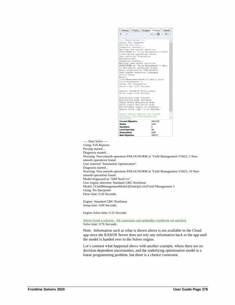
Frontline Solvers 2020 User Guide Page 378
---- Start Solve ----
Using: Full Reparse.
Parsing started...
Diagnosis started...
Warning: Non-smooth operation PSILOGNORM at 'Yield Management 3'!H25; 5 Non-
smooth operations found.
User selected "Simulation Optimization".
Diagnosis started...
Warning: Non-smooth operation PSILOGNORM at 'Yield Management 3'!H25; 10 Non-
smooth operations found.
Model diagnosed as "SIM NonCvx".
User engine selection: Standard GRG Nonlinear
Model: [YieldManagementModel3(SimOpt).xls]Yield Management 3
Using: Psi Interpreter
Parse time: 0.30 Seconds.
Engine: Standard GRG Nonlinear
Setup time: 0.00 Seconds.
Engine Solve time: 0.22 Seconds.
Solver found a solution. All constraints and optimality conditions are satisfied.
Solve time: 0.76 Seconds.
Note: Information such as what is shown above is not available in the Cloud
app since the RASON Server does not rely any information back to the app until
the model is handed over to the Solver engine.
Let’s contrast what happened above with another example, where there are no
decision-dependent uncertainties, and the underlying optimization model is a
linear programming problem, but there is a chance constraint.

Frontline Solvers 2020 User Guide Page 379
A Model Solved with Robust Optimization
Below is an example of the Output tab in Analytic Solver Desktop at the
solution of the Gas Company Chance model in StochasticExamples.xls
(described more fully in the chapter “Examples: Stochastic Optimization”).
Again, if you click the Copy icon, the contents of the solution log will be
copied to the Windows Clipboard, where you can paste it into Microsoft Word,
NotePad, or an email message to Frontline Systems Technical Support.
Below is the solution log from the Gas Company Chance model (before clicking
the button to automatically improve the solution).
---- Start Solve ----
Using: Full Reparse.
Parsing started...
Uncertain input cells detected.
User requested Robust Counterpart.
Diagnosis started...
Convexity testing started...
Stochastic Transformation succeeded using Robust Counterpart with D Norm.
Transformed model is "LP Convex".
Model: [StochasticExamples.xls]Gas Company Chance
Using: Psi Interpreter
Parse time: 1.19 Seconds.
Engine: Standard LP/Quadratic
Setup time: 0.02 Seconds.
Engine Solve time: 0.00 Seconds.
Solver found a conservative solution to the robust chance constrained problem. All constraints
are satisfied.
Solve time: 1.36 Seconds.
Click the Solver Result Message for Help
The Solver Result message in Analytic Solver Desktop is always underlined –
it is a hyperlink to Help. If you aren’t sure that you fully understand it, click
the link to open online Help to a detailed discussion of the message.
Below is an example of Help that appears when you solve the Gas Company
Chance model, and click on the Solver Result error message in green, “Solver
found a conservative solution to the robust chance constrained problem. All constraints are satisfied.”

Frontline Solvers 2020 User Guide Page 380
Notice that the Help topic points out the option to Auto Adjust Chance
Constraints. This is one key to better solutions when robust optimization is
used, as in this example. Clicking the icon at the top of the Task Pane yields
an improved solution, and the following solution log:
---- Start Solve ----
Model: [StochasticExamples.xls]Gas Company Chance
Using: Psi Interpreter
Using: Full Reparse.
Parsing started...
Diagnosis started...
Parse time: 0.19 Seconds.
Engine: Standard LP/Quadratic
Setup time: 0.00 Seconds.
Engine Solve time: 0.00 Seconds.
(above lines appear 7 times)
Solver has converged to the current solution of the robust chance constrained problem. All
constraints are satisfied.
Solve time: 0.39 Seconds.
This was a successful solution – but in cases where you have a Solver Result
error message that you don’t understand, or a solution that you don’t under-
stand, the solution log can be even more helpful.
Note: If you are using Analytic Solver Cloud, set Operating Mode (Help –
Operating Mode) to either Guided Mode or Auto Help Mode to find detailed
information on the Solver result messages.
Choose Available Optimization Reports
As for conventional optimization, the available reports can help you understand
the properties of a solution found by Analytic Solver. Just select Reports –
Optimization Reports on the Ribbon – the available reports in the gallery are
updated each time you solve.
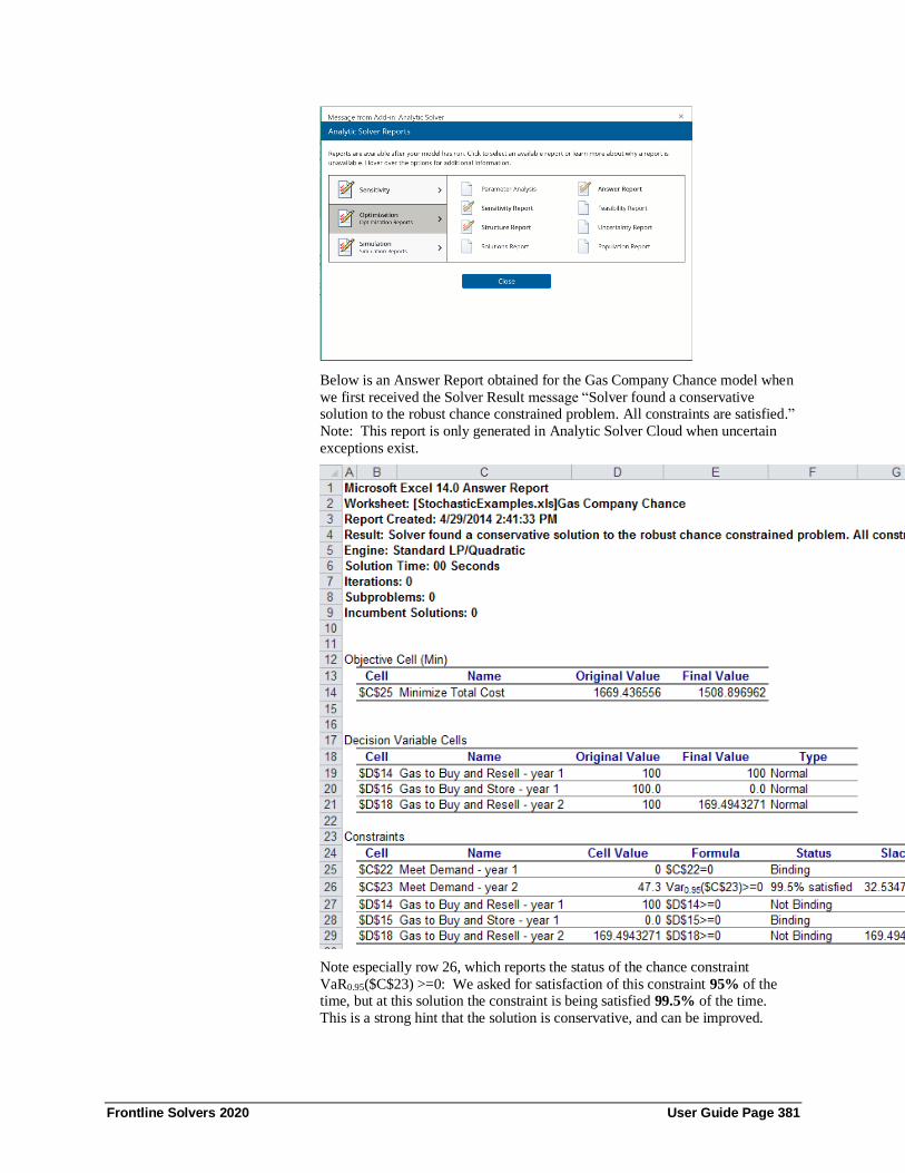
Frontline Solvers 2020 User Guide Page 381
Below is an Answer Report obtained for the Gas Company Chance model when
we first received the Solver Result message “Solver found a conservative solution to the robust chance constrained problem. All constraints are satisfied.”
Note: This report is only generated in Analytic Solver Cloud when uncertain
exceptions exist.
Note especially row 26, which reports the status of the chance constraint
VaR0.95($C$23) >=0: We asked for satisfaction of this constraint 95% of the time, but at this solution the constraint is being satisfied 99.5% of the time.
This is a strong hint that the solution is conservative, and can be improved.
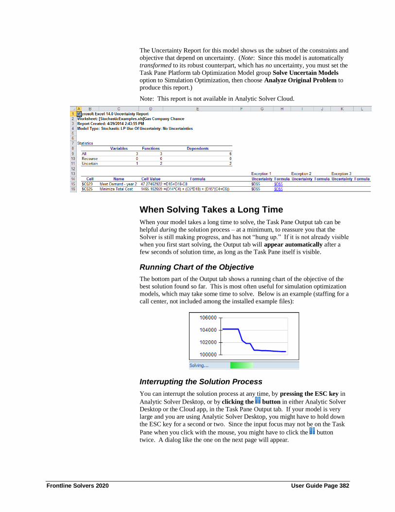
Frontline Solvers 2020 User Guide Page 382
The Uncertainty Report for this model shows us the subset of the constraints and
objective that depend on uncertainty. (Note: Since this model is automatically
transformed to its robust counterpart, which has no uncertainty, you must set the
Task Pane Platform tab Optimization Model group Solve Uncertain Models
option to Simulation Optimization, then choose Analyze Original Problem to produce this report.)
Note: This report is not available in Analytic Solver Cloud.
When Solving Takes a Long Time
When your model takes a long time to solve, the Task Pane Output tab can be
helpful during the solution process – at a minimum, to reassure you that the
Solver is still making progress, and has not “hung up.” If it is not already visible
when you first start solving, the Output tab will appear automatically after a
few seconds of solution time, as long as the Task Pane itself is visible.
Running Chart of the Objective
The bottom part of the Output tab shows a running chart of the objective of the
best solution found so far. This is most often useful for simulation optimization
models, which may take some time to solve. Below is an example (staffing for a
call center, not included among the installed example files):
Interrupting the Solution Process
You can interrupt the solution process at any time, by pressing the ESC key in
Analytic Solver Desktop, or by clicking the button in either Analytic Solver
Desktop or the Cloud app, in the Task Pane Output tab. If your model is very
large and you are using Analytic Solver Desktop, you might have to hold down
the ESC key for a second or two. Since the input focus may not be on the Task
Pane when you click with the mouse, you might have to click the button
twice. A dialog like the one on the next page will appear.
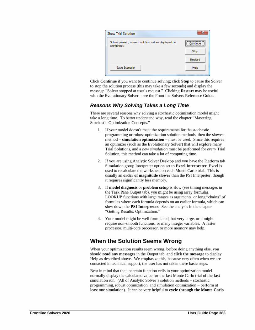
Frontline Solvers 2020 User Guide Page 383
Click Continue if you want to continue solving; click Stop to cause the Solver
to stop the solution process (this may take a few seconds) and display the
message “Solver stopped at user’s request.” Clicking Restart may be useful
with the Evolutionary Solver – see the Frontline Solvers Reference Guide.
Reasons Why Solving Takes a Long Time
There are several reasons why solving a stochastic optimization model might take a long time. To better understand why, read the chapter “Mastering
Stochastic Optimization Concepts.”
1. If your model doesn’t meet the requirements for the stochastic
programming or robust optimization solution methods, then the slowest
method – simulation optimization – must be used. Since this requires
an optimizer (such as the Evolutionary Solver) that will explore many
Trial Solutions, and a new simulation must be performed for every Trial
Solution, this method can take a lot of computing time.
2. If you are using Analytic Solver Desktop and you have the Platform tab
Simulation group Interpreter option set to Excel Interpreter, Excel is used to recalculate the worksheet on each Monte Carlo trial. This is
usually an order of magnitude slower than the PSI Interpreter, though
it requires significantly less memory.
3. If model diagnosis or problem setup is slow (see timing messages in
the Task Pane Output tab), you might be using array formulas,
LOOKUP functions with large ranges as arguments, or long “chains” of
formulas where each formula depends on an earlier formula, which can
slow down the PSI Interpreter. See the analysis in the chapter
“Getting Results: Optimization.”
4. Your model might be well formulated, but very large, or it might
require non-smooth functions, or many integer variables. A faster processor, multi-core processor, or more memory may help.
When the Solution Seems Wrong
When your optimization results seem wrong, before doing anything else, you
should read any messages in the Output tab, and click the message to display
Help as described above. We emphasize this, because very often when we are
contacted in technical support, the user has not taken these basic steps.
Bear in mind that the uncertain function cells in your optimization model
normally display the calculated value for the last Monte Carlo trial of the last
simulation run. (All of Analytic Solver’s solution methods – stochastic
programming, robust optimization, and simulation optimization – perform at least one simulation). It can be very helpful to cycle through the Monte Carlo

Frontline Solvers 2020 User Guide Page 384
trials, and examine the values of uncertain function cells, as well as interme-
diate formula cells on which they depend. Just use the left and right arrows on
the Ribbon to change the trial index. You may find that your model calculates a
result you did not expect for some values of the uncertain variables.
Although software bugs are always possible, consider carefully the possibility that the simulation results are correct for the model you’ve defined, and that
your expectation is wrong. We sometimes find in technical support that what
your model actually says is different from what you intended.
When Things Go Right: Getting Further Results When you do receive a solution that makes sense to you, and you have a Solver
Result message in green at the bottom of the Task Pane for your stochastic
optimization model, you have available all the optimization and simulation
reports and charts that apply to your model and solution. Since a simulation is
performed for every stochastic optimization model, you can double-click the
uncertain function cells in your model (in Analytic Solver Desktop) or on the
Model tab of the Solver Task Pane (in Desktop or the Cloud) to display the Uncertain Function dialog, and obtain many different views of the uncertainty in
your model:
Dialog Tabs
• The Frequency, Cumulative Frequency, and Reverse Cumulative
Frequency tabs provide three different views of the full range of outcomes
for an uncertain function. In Analytic Solver Desktop, you can click to display “crosshairs” with numerical values on these charts, or add Lower
and Upper bounds to see the estimated probability of a profit or loss, for
example.
• The Tornado chart on the Sensitivity tab quickly shows you which
uncertain variables have the greatest impact on this uncertain function,
across the full range of Monte Carlo trials. The Scatter Plots tab often
reveals further insights about the behavior of this uncertain function versus
each uncertain variable, or versus other uncertain functions.
• The Statistics and Percentiles tabs give you a full range of numerical
results for this uncertain function, across the full range of Monte Carlo
trials. Using PSI Statistics functions, you can place any of these values into a worksheet cell.
Panels and Toolbars
Analytic Solver Desktop includes rich charting abilities that are currently not
available in Anlaytic Solver Cloud, but are coming soon. The suggestions
below all pertain to Analytic Solver Desktop.
• Using the right panel of the dialog, you can change the chart type and color
in both Analytic Solver Desktop and Cloud apps. In Analytic Solver
Desktop you can additionally add titles, legends, gridlines, or chart markers.
From the Options dialog (accessible from the Options button on the
Analytic Solver Desktop Ribbon), on the Charts and Markers tabs, you
can set default chart and marker settings for all of your charts.
• Using the title toolbar icons in Analytic Solver Desktop, you can save your
settings, print the charts or numbers from any of the dialog tabs, or copy
the charts or numbers to the Windows Clipboard, where they can be pasted

Frontline Solvers 2020 User Guide Page 385
into other applications. You can also fit a distribution to the simulation
results or export your results to either Power BI or Tableau.
• In Analytic Solver Desktop, click the leftmost icon on the second row to
display the 3-D toolbar that lets you – with a single click – shift between 2-
D and 3-D, shrink or magnify the chart, or move or rotate the chart to a different perspective.

Frontline Solvers 2020 User Guide Page 386
Dimensional Modeling
Introduction Dimensional Modeling is a fundamental new capability in Analytic Solver
Comprehensive when using Analytic Solver Desktop. It introduces new
concepts such as dimensions and cubes, and provides all the tools you need to
build and solve models using these concepts. If you’re used to spreadsheet
modeling, Dimensional Modeling will require some learning and practice. But
when you want to construct larger models for common business situations
where there are multiple products, projects or investments, multiple customer
types, geographic regions, or time periods, multiple sources and destinations, dimensional modeling can turn a very complex, hard-to-maintain spreadsheet
problem into a simple, well-structured, easily maintained and expandable model.
Note: Dimensional modeling is not currently supported in Analytic Solver
Cloud.
If you’ve used Pivot Tables or PowerPivot in Excel, or if you’ve used a
multidimensional database, data warehouse or business intelligence tool, the
concepts behind Dimensional Modeling will probably be familiar. But these
tools primarily deal with multidimensional data, generally reflecting the past.
Dimensional Modeling makes it easy to construct multidimensional models,
mostly composed of formulas, that you can use in planning for the future.
Unlike other tools, in Analytic Solver you can use everything you know about
Excel formulas in Dimensional Modeling. For example, if cell A1 contains a
number and cells B2 and C3 contains =PsiCube() functions, a formula like
=A1+B2*C3 in a cell will yield a “cube result,” multiplying and adding the
appropriate values along several dimensions. You can also define B2 and C3
based on Pivot Tables containing input data, and easily obtain a Pivot Table that
displays the results of like =A1+B2*C3.
Very often, a successful model is expanded to include more products, regions,
time periods, etc. This is much easier to do with a Dimensional Model than
with a traditional spreadsheet model. Formulas like =A1+B2*C3 need not
change at all when you add elements (more cell or database values) to the existing dimensions. You can even add new dimensions to B2 and C3, or turn
A1 from a single cell to a cube, and =A1+B2*C3 will automatically calculate
results across the additional dimensions.
Dimensional Modeling in Optimization and Simulation
Dimensional Modeling can be used to create multidimensional “what if” models
– a very powerful capability by itself. But you can also use it to create better structured, more compact and easily readable optimization and simulation
models. For example, blocks of constraints that once required large ranges of
repetitive formulas can now be entered in one or a few cells, drastically reducing
the number of formulas. Similarly, in a simulation model, blocks of uncertain
functions that once required large numbers of repetitive formula cells can be
reduced to one or a few cells. You can define as many “structural dimensions”
as you like, and use up to 8 of them at one time, in any PsiCube() function or
calculated “cube intermediate result” in a formula.

Frontline Solvers 2020 User Guide Page 387
Dimensional Modeling and Parametric Analysis
Dimensional Modeling also offers a powerful extension of Analytic Solver’s
capabilities for multiple parameterized optimization and simulation (described in
the earlier chapters “Examples: Parameters and Sensitivity Analysis,” “Getting
Results: Optimization” and “Getting Results: Simulation”). It enables you to
perform sensitivity analysis, or run many optimizations or simulations, varying
parameters across multiple dimensions on each run, and capture all the results –
optionally in Pivot Tables and Pivot Charts.
Without Dimensional Modeling, you define parameters for sensitivity analysis,
optimization and simulation, using PsiSenParam(), PsiOptParam() and
PsiSimParam() functions, respectively. These parameters function like simple “cubes” defined over just one dimension – the “run index” 1, 2, 3, etc. You run
multiple calculations, optimizations or simulations, where all the parameters of a
given type “move together” through their arrays of values.
With Dimensional Modeling, you can define as many “parametric dimensions”
as you like, and create cubes of parameter values that are defined over one or
more dimensions. You can then perform sensitivity analysis or run multiple
optimizations or simulations, where any subset of your parametric dimensions
are “active” (the others are “locked”), and get results for all combinations of the
parameter values you’ve defined.
Just as you can expand a model by adding a structural dimension and generalize one or more cubes over the new dimension, without changing your formulas,
you can add a parametric dimension, use it in one or more cubes, and expand
your sensitivity analysis, optimization or simulation runs to include more
scenarios, without changing any formulas.
Visualizing Dimensional Modeling Results
As mentioned earlier, you can define cubes based on Pivot Tables containing
input data, and easily create new Pivot Tables that displays results of formulas like =A1+B2*C3. But creating a Pivot Table does require several steps, as well
as “real estate” on your spreadsheet. If you want to inspect the results of
intermediate calculations, you might need a separate table area for each “cube
formula” cell in your model.
Analytic Solver makes this much easier. Just double-click on any cube formula
to see a pop-up window that behaves like an “instant Pivot Table,” allowing you
to ‘drag and drop’ both structural and parametric dimensions across the columns
and rows, and reorganize and display the data or calculated results. You’ll see a
number of examples of these pop-up windows in this chapter. For final results
and reporting, you can use Pivot Tables and Charts.
Dimensions and Cubes Let’s define the concepts in Dimensional Modeling more formally. You can
define two types of dimensions, Structural and Parametric, and use them in
calculation/sensitivity analysis, optimization and simulation models. You give a
name (such as “Region”) for the dimension, and you provide names/labels or
numbers for the elements of the dimension – for example “North,” “South,”
“East” and “West.” Note that a dimension doesn’t define the data itself – it
defines a structure, relevant for your business situation, for the data.
Cubes are multi-dimensional arrays that hold the data. Other names used in data
warehouse and business intelligence systems, are measures and/or fact tables.

Frontline Solvers 2020 User Guide Page 388
A cube has an element (data value) for each combination of elements of the
dimensions you specify when defining the cube. For example, you might create
a cube named “Sales,” defined over the “Regions” dimension, with four numeric
values representing sales in the North, South, East and West regions. The
structure of a cube is very much like a Pivot Table, and you can create a cube by placing a PsiPivotCube() function in a cell, referencing an existing Pivot Table.
A single cube holds a single “measure” or type of value. For example, a person
has many attributes such as height, weight, hair color, and eye color. You might
define a dimension “Person” with elements such as “John”, “Mary” and
“Susan.” But since a cube holds a single attribute or measure, you’d need four
different cubes, each defined over the “Person” dimension, to hold the values of
height, weight, hair color, and eye color.
There are three main steps involved in creating a Dimensional Model. Step 1 is
to define at least one dimension, either parametric or structural. Step 2 is to
define at least one (usually several) cubes. Step 3 is to define at least one output cell – for example, the objective cell in an optimization model – with a
formula that depends on a cube. Often, you’ll have outputs that are cubes and
contain many – even thousands of – result values.
An Example Dimensional Model
This chapter will use the Product Mix example, introduced at the beginning of
the chapter “Examples: Conventional Optimization,” to illustrate Dimensional Modeling concepts, and the menu choices and Psi functions you can use to build
a Dimensional Model step by step. The example is very simple, with just two
structural dimensions – Products and Parts. This will make it easier to fully
grasp the concepts and step-by-step operations, but since you can usually “lay
out” two-dimensional data in regular spreadsheet columns and rows, Dimen-
sional Modeling might seem like “overkill” for this simple example. The
advantages of Dimensional Modeling will be apparent when you are modeling a
more realistic business situation with many dimensions.
Click Help -- Examples on the Analytic Solver ribbon, to open the Frontline
Example Models Overview workbook. Click the Optimization Examples
button, or select the Optimization tab, and scroll down to find and click
Structural Dimensions from the list. When this workbook opens, click the
Product Mix Original tab, which displays a conventional version of the Product
Mix model.
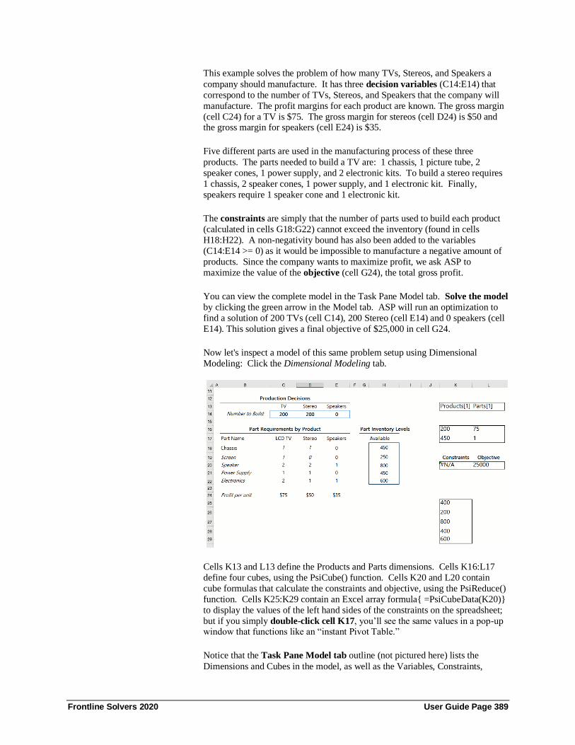
Frontline Solvers 2020 User Guide Page 389
This example solves the problem of how many TVs, Stereos, and Speakers a
company should manufacture. It has three decision variables (C14:E14) that
correspond to the number of TVs, Stereos, and Speakers that the company will
manufacture. The profit margins for each product are known. The gross margin
(cell C24) for a TV is $75. The gross margin for stereos (cell D24) is $50 and the gross margin for speakers (cell E24) is $35.
Five different parts are used in the manufacturing process of these three
products. The parts needed to build a TV are: 1 chassis, 1 picture tube, 2
speaker cones, 1 power supply, and 2 electronic kits. To build a stereo requires
1 chassis, 2 speaker cones, 1 power supply, and 1 electronic kit. Finally,
speakers require 1 speaker cone and 1 electronic kit.
The constraints are simply that the number of parts used to build each product
(calculated in cells G18:G22) cannot exceed the inventory (found in cells
H18:H22). A non-negativity bound has also been added to the variables
(C14:E14 >= 0) as it would be impossible to manufacture a negative amount of
products. Since the company wants to maximize profit, we ask ASP to
maximize the value of the objective (cell G24), the total gross profit.
You can view the complete model in the Task Pane Model tab. Solve the model
by clicking the green arrow in the Model tab. ASP will run an optimization to
find a solution of 200 TVs (cell C14), 200 Stereo (cell E14) and 0 speakers (cell
E14). This solution gives a final objective of $25,000 in cell G24.
Now let's inspect a model of this same problem setup using Dimensional
Modeling: Click the Dimensional Modeling tab.
Cells K13 and L13 define the Products and Parts dimensions. Cells K16:L17
define four cubes, using the PsiCube() function. Cells K20 and L20 contain
cube formulas that calculate the constraints and objective, using the PsiReduce()
function. Cells K25:K29 contain an Excel array formula{ =PsiCubeData(K20)}
to display the values of the left hand sides of the constraints on the spreadsheet;
but if you simply double-click cell K17, you’ll see the same values in a pop-up window that functions like an “instant Pivot Table.”
Notice that the Task Pane Model tab outline (not pictured here) lists the
Dimensions and Cubes in the model, as well as the Variables, Constraints,
Frontline Solvers 2020 User Guide Page 390
Objective and other model elements. To keep things simple for users who aren’t
using Dimensional Modeling, these outline elements appear only when you have
functions such as PsiDim() and PsiCube() in cells on your worksheet.
The decision variables are still in cells C14:E14. Try changing one of these
cells to a new value such as 100. You’ll see that the worksheet recalculates just
like a normal Excel model, even though it is composed of dimensions and cubes.
Dimensional optimization models continue to use a separate cell for each
decision variable – whereas they might have thousands of constraints in a single
cell. Keeping decision variables in individual cells makes it easy to capture final
solution values, save them in your workbook, and use Excel to recalculate the
spreadsheet later. Cube formulas appear to Excel as ordinary formulas (with
single values) using user-defined functions such as PsiCube() and PsiReduce();
the actual multidimensional calculations are performed “behind the scenes” by
the PSI Interpreter.
Solve the model by clicking the green arrow in the Model tab, just as you did on
the Original sheet. You’ll see the same optimal solution appear in cells C14:E14.
The following sections will take you step by step through the process of building
a Dimensional Model like the one above. You can use the Analytic Solver
menu choices, grouped under the Model button, to define dimensions, cubes and
results, or you can type functions such as PsiCube() and PsiReduce() directly
into cells, without using the GUI at all.
Using Dimensional Modeling in Optimization
Keep in mind the following three steps when using Dimensional Modeling:
1. Define a Dimension.
2. Define a Cube.
3. Define a Cube Output cell. (This step is optional).
Defining a Dimension
Two dimensions have been created in cells K13 and L13, Products and Parts,
respectively. The Products dimension (cell K13) contains three items or
elements: TVs, Stereos, and Speakers. The Parts dimension (cell L13) contains
five items or elements: Chassis, LCD Screens, Speakers, Power Supply, and
Electronics.
To create a dimension, you may either type the PsiDim() function call directly
into a cell, or use the Model menu, shown below, to insert the PsiDim() formula
into the active (selected) cell.
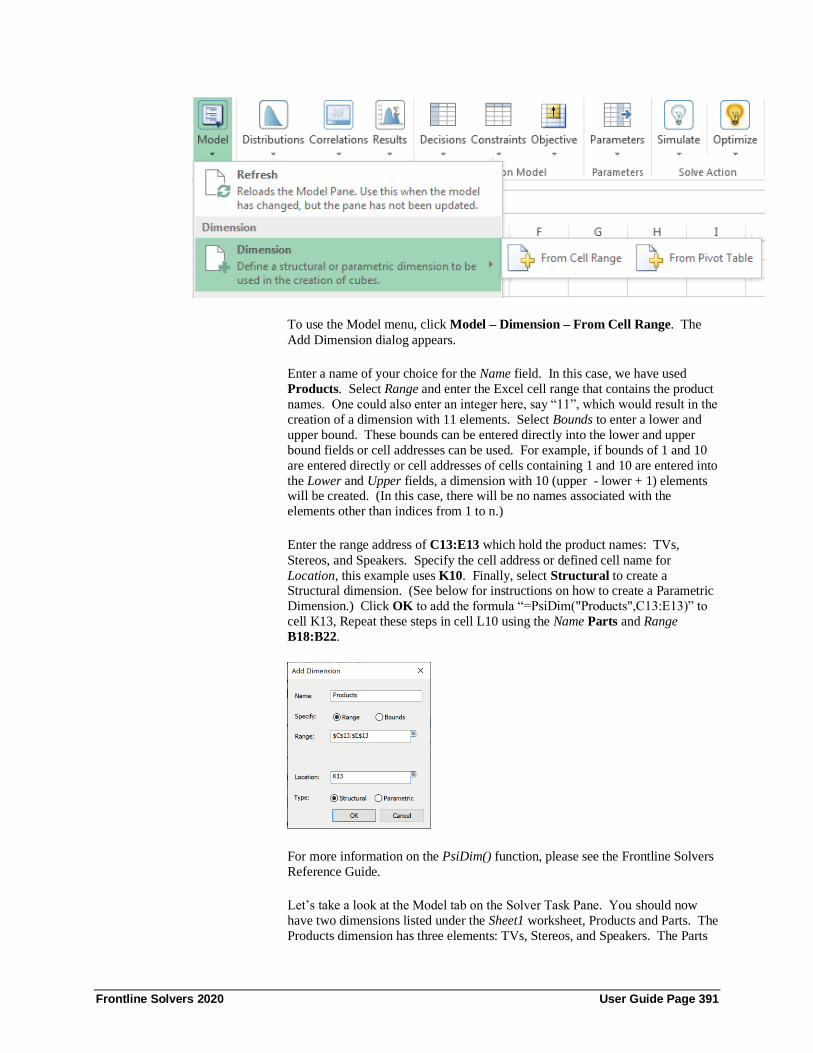
Frontline Solvers 2020 User Guide Page 391
To use the Model menu, click Model – Dimension – From Cell Range. The
Add Dimension dialog appears.
Enter a name of your choice for the Name field. In this case, we have used
Products. Select Range and enter the Excel cell range that contains the product
names. One could also enter an integer here, say “11”, which would result in the
creation of a dimension with 11 elements. Select Bounds to enter a lower and
upper bound. These bounds can be entered directly into the lower and upper
bound fields or cell addresses can be used. For example, if bounds of 1 and 10
are entered directly or cell addresses of cells containing 1 and 10 are entered into
the Lower and Upper fields, a dimension with 10 (upper - lower + 1) elements will be created. (In this case, there will be no names associated with the
elements other than indices from 1 to n.)
Enter the range address of C13:E13 which hold the product names: TVs,
Stereos, and Speakers. Specify the cell address or defined cell name for
Location, this example uses K10. Finally, select Structural to create a Structural dimension. (See below for instructions on how to create a Parametric
Dimension.) Click OK to add the formula “=PsiDim("Products",C13:E13)” to
cell K13, Repeat these steps in cell L10 using the Name Parts and Range
B18:B22.
For more information on the PsiDim() function, please see the Frontline Solvers
Reference Guide.
Let’s take a look at the Model tab on the Solver Task Pane. You should now
have two dimensions listed under the Sheet1 worksheet, Products and Parts. The
Products dimension has three elements: TVs, Stereos, and Speakers. The Parts

Frontline Solvers 2020 User Guide Page 392
dimension has five elements: Chassis, Screen, Speaker, Power Supply and
Electronics.
Select the Products dimension.
Several options will appear at the bottom of the task pane under Dimension (as
shown in the screenshot above). Here you can view the cell where the
dimension is located (cell K13), the formula, the name of the dimension and the
type of dimension (structural or parametric). These fields are all read-only. Current Value, however, controls the values displayed in the cell containing the
cube. For example, select Speakers for Current Value. Values in cells K16,
K17, L16, and L17 will change to reflect values for Speakers. For example,
K13 will change to Products[3] to indicate that the third element of the Products
dimension has been selected. K16 will change to 0 (the value of cell C13), K17
will change to 450 (the value of cell H18), L16 will change to 35 (the value of
cell E24), and cell L17 will change to 0 to reflect that 0 chassis are used in the
production of speakers.

Frontline Solvers 2020 User Guide Page 393
Defining a Cube
Four Cubes have been created in cells K16 (which holds the variable cells), L16
(which holds the Profit values for each product), K17 (which holds the
constraint right hand sides), and L17 (which holds the amount of parts used per
product). To create a cube, you may either type the PsiCube() formula into a
cell or use the Model menu, shown below, to insert the formula into the selected
cell.
To use the Model menu, click Model – Cube – From Cell Range. The Add
Cube dialog appears.
Enter an Excel cell range for Range, in this instance, select cells C14:E14, the
variable values. Select Products from the Dimension drop down menu. To add
more than one dimension to the cube, click “+” button. Select a blank cell for
Location – this example uses cell K16. Click OK to create the cube. The following formula will be entered into cell K16,
=PsiCube($C$14:$E$14,"Products"). (This formula may also be entered
directly.)
The first argument of any cube is the cell address of the data. In the cube
located in cell K16, the first argument is C14:E14 (the variable cells). The
second thru ninth arguments are the dimensions for which the data will be
calculated. (At least one dimension is required.) This 1-dimensional cube,
calculated over the Products dimension, holds the data in cells C14:E14 which

Frontline Solvers 2020 User Guide Page 394
are the number of products to build - the decision variables. The data for the
cube located in cell L16 can be found in cells C24:E24. This 1 dimensional
cube contains the profit values for each of the products. This cube is also
calculated over the Products dimension. In the 1 – dimensional cube located in
cell K17 (the cube holding the constraint right hand sides), the data is contained in cells H18:H22. In cell L17, a 2-dimensional cube has been created using the
Products and Parts dimensions. This cube holds the fact table containing the
parts required per product (cells C18:E22).
Note: When calculating a cube over multiple dimensions, the “most
rapidly changing” dimension must be first, while the “most slowly
changing” dimension must appear last. Take the example table below.
Starting from cell B2 (the start of the fact table) and reading from left
to right, the 1st element of the cube will be 1 (Chassis & LCD TV), the
2nd element of the cube will be 1 (Chassis & Stereo), the 3rd element of
the cube will be 0 (Chassis & Speakers). The 4th element of the cube
will be 1 (Screen & LCD TV), the 5th element of the cube will be 0
(Screen & Stereo) and the 6th element of the cube will be 0 (Screen &
Speakers). Between Products and Parts, which dimension is changing
more frequently as we read from left to right? Correct! Products is
changing more frequently which means this dimension should come
first in the AddCube dialog or PSICube() function.
Double click cell L17 to open the fact table for the cube located in this cell. The
following window appears. The data contained in this fact table is the same data
contained in cells C18:E22. Click the arrows on the right side of the dialog to
open an additional pane. Here you can control the display formatting of the
cube by selecting Cube Rows or Cube Columns from the drop down menu or
by simply dragging Parts to Products and vice versa.

Frontline Solvers 2020 User Guide Page 395
Click the Refresh Cube Data icon when changes have been made to the
contents of the cube on the spreadsheet. Click the Export Pivot Table icon to
export the contents of the cube to an Excel Pivot Table. Click the Copy icon
(or click the down arrow to the right of the icon) to copy the grid to the
spreadsheet, to Outlook, Word, etc. Click the Autosize Pivot Table icon to
autosize the columns in the grid. Click the Print icon (or click the down arrow
to the right of the icon) to send the grid to the printer, see a print preview, or
to change printer or page settings.
Cube Formulas: Operations and Dimensions
When executing an operation over cubes, if all participating cubes have the
same dimensions, then the result cube will have the same dimensions too. For
example, if a cube with 4 dimensions is multiplied (or added, subtracted,
divided, etc.) with another cube also containing the same 4 dimensions, the
result cube will contain the same 4 dimensions.
Otherwise, the result cube will be a union of the participating dimension sets.
For example, if a cube B2 with two dimensions is multiplied by a cube C3 with
one dimension that also appears in the first cube, the result B2*C3 will be two-
dimensional. If C3 is defined over a dimension different from either of the two
dimensions in B2, the result cube will be three-dimensional.
You can use almost any Excel arithmetic or intrinsic operations, as well as
almost all Excel built-in functions in cube formulas. There are a few Excel
functions that are not supported by the PSI Interpreter and are thus not supported
in Dimensional Modeling. These functions include: CubeX(), Call(), Cell(),
EuroConvert(), GetPivotData(), Info(), Hyperlink(), Indirect(), RegisterID() and
SQLRequest().
Now let’s calculate the constraints. In the original model, the constraints are the
number of parts used (cells G18:G22) must be less than the inventory (found in
cells H18:H22).
To calculate the constraint in this example using Dimensional Modeling, we must use the PsiReduce() function. This function reduces or aggregates a multi-
dimensional cube along one dimension. A cube may be aggregated using the
following supported functions: average, sum, max, min, stdev, or var. (For
example, if PsiReduce() is used to aggregate a 3 –dimensional cube, the
resultant cube would contain 2 dimensions.) A cube reduced along all its
dimensions is called a Degenerated Cube and will be a single value, or scalar.
Select cell K20, then click Model – Reduction. The Add Reduction dialog
appears.
Select Other Cell from the Cube drop down menu, then enter L17*K16 into the
empty field. Since we want to reduce the cube along the Products dimension,
select Products from the Dimension drop down menu. Next select Sum from the Reduce By drop down menu. This is how the cube will be aggregated.
Refresh Cube Data
Export Pivot Table
Copy Autosize Pivot Table

Frontline Solvers 2020 User Guide Page 396
Confirm that Location is cell K20, then click OK. The formula,
=PsiReduce($L$17*$K$16, "sum","Products"), is entered into cell K20. In
general, the equation for this cube is: , for each i= 1 to 5,
where X equals the products (TVs, stereos, and speakers), Y equals the parts
(chassis, screen, speaker, power supply, & electronics) and R is a 1-dimensional
vector containing 5 elements.
The multiplication of the two cubes in cells L17 and K16 in the first argument of
PsiReduce will result in a third cube containing the product of the number of
parts per product and the variable values in cells C14:E14. The cube in cell
L17 contains 15 elements and is calculated along two dimensions, Products and
Parts. The cube in cell K16 has 3 elements and holds the fact table for only 1 dimension, Products. Remember, when multiplying two cubes with different
dimension sets, the resultant cube will be structured along the Union of both
dimension sets. In this case, the resultant cube will be structured along both the
Products and Parts dimensions and will also contain 15 elements. PsiReduce()
reduces or eliminates the specified dimension in the third argument, in this case
the Products dimension. The cube multiplication and reduction occurring in
this single cell (cell K20) perform the same operations as cells G18:G22 in the
original problem! Since Cubes are single cells, they can display only the first
element of their cube result. In order to see all cube elements, simply double
click cell K20. A popup window appears containing the following fact table.

Frontline Solvers 2020 User Guide Page 397
It’s also possible to check the contents of a cube on the worksheet using the
PsiCubeData() function. Please see the Frontline Solvers Reference Guide for
more information on this function.
PsiReduce() is also used to calculate the objective function. To compute the
objective, we must multiply the cube containing the decision variables (cell
K16) by the cube containing the Profit values (cell L16). Select cell L20 and
click Model – Reduction. The Add Reduction dialog appears.
Select Other Cell from the Cube drop down menu and enter K16*L16 in the
blank field. Since we are looking to sum over the Products dimension (sum the
products of Products * Profits), select Products from the Dimension menu and
Sum from the Reduce By menu. Confirm the Location is cell L20 and then click OK. The formula, =PsiReduce($K$16*$L$16, "sum","Products"), is entered
into cell L20. The result of this cube is a scalar or a single value.
Defining Outputs in Dimensional Models
It’s also possible to use an output function such as PsiOptData() to observe the
contents of a fact table on the spreadsheet, rather than in a pop up fact table.
Let’s designate cells K25:K29 as output cells to observe the final values of all five constraints calculated in cell K20. To do so highlight cells K25:K29, then
enter “=PsiOptData(K20)”, then CTRL + SHIFT + ENTER on the keyboard to
enter this formula as an array. Once Solver finds a solution, these cells will be
populated with the left hand side of each constraint. For example, cell K25 will
display the left hand side of the first constraint, cell K26 will display the left
hand side of the 2nd constraint, cell K27 will display the left hand side of the 3rd
constraint, and so on.
It’s also possible to create “what if” scenarios using Dimensional Modeling
without ever having to run an optimization (or simulation) using a 2nd type of
output function, PsiCubeOutput(). For more information, please see below
under Additional Functions.
Now let’s create our Solver model by adding the variables and constraints to the
Platform Task Pane.

Frontline Solvers 2020 User Guide Page 398
Building the Model
At this point we can now start building our model in the Platform Task Pane.
1. Add the Variables: Select cells C14:E14, then click Decisions on the
Ribbon. (Alternatively, click Decisions – Normal on the Ribbon.) If
you inspect the Task Pane, you will find that cells C14:E14 now appear
under the Normal Variables section.
2. Add the Constraints: Select cell K20, then click Constraints on the
Ribbon. The Add Constraint dialog will appear. (Alternatively, click
the down arrow under Constraints, then select Normal -- <= from the
menu.) Enter cell K20 as the left hand side of the constraint and cell
K17 as the right hand side of the constraint, then click OK. If you
inspect the Task Pane, you will find K20 <= K17 now appears under
Normal Constraints.
3. Add the Objective: Select cell L20, then click Objective, then OK.
(Alternatively click the down arrow under Objective, then select Max
– Normal from the menu.) If you inspect the Task Pane, you will find
that cell L20 now appears under Objective with “(Max)” appearing to
the right.
4. Add Variable Bounds: Since it would be impossible to make a
negative amount of products, we must add a non-negativity bound. To
do so, select cells C14:E14, then click Constraints. (Alternatively,
click the down arrow under Constraints, and select Variable
Type/Bound -- >= from the menu.) The Add Constraint dialog will
open. Select >= for the “sense” of the constraint (drop down menu in the middle). Enter “0” as the constraint left hand side, then click OK.
If you inspect the Task Pane, you will find C14:E14 >= 0 now appears
under Bound.
The Task Pane will look like the following.

Frontline Solvers 2020 User Guide Page 399
Solving the Model
Enter 0’s into cells C14:E14 then solve the model by clicking the green arrow on
the Model Task Pane.
Solver will solve the model and display the final variable values in cells
C14:E14: 200, 200, and 0, respectively. The status bar (found beneath the Task Pane) will display the message Solver found a solution with a green background.
Analytic Solver will populate the objective formula located in L20 when the
optimization finishes successfully. Note: All Solver engines except Interval
Global Solver support Dimensional Modeling.
Double click cell K20 to open a grid displaying the right hand sides of the
constraints or the number of parts used to manufacture the three products.
As you can see by the comparison of these two models, using a cube to model a
problem will result in a more compact and easier to read model. Continue
reading the next section to learn about the 2nd goal of dimensional modeling, the
parametric dimension.
Now close this example, and continue reading to discover how to use a
parametric dimension within an optimization model.
Additional Functions
Using Dimensional Modeling, it’s possible to create what if scenarios without
ever having to run an optimization (or simulation). The function PsiCubeData()
will list the contents of any cube on the spreadsheet much like PsiOptData()
listed the left hand sides of the constraints in the example above. The difference
between these two functions is that PsiOptData() will only be populated after an
optimization is run, while PsiCubeData can be populated at any time. Let use
PsiCubeData() to list the contents of the Cube located in cell K17. (This cube
holds the constraint right hand sides.) First, highlight 5 blank cells, say
K31:K35, enter “=PsiCubeData(K17)”, then press CTRL + SHIFT + ENTER to enter the formula as an array in all five cells. Next, click Model – Cube Result
– Calculate to calculate the cube without performing an optimization.
Afterwards, Cell K31 will display 450, cell K32 will display 250, cell K33 will
display 800, cell K34 will display 450, and cell K35 will display 600. These
values correspond to the values in cells H18:H22.

Frontline Solvers 2020 User Guide Page 400
You’ll notice that after you performed a manual cube calculation (by clicking
Model – Cube Result – Calculate), the objective function cell (cell L20) now
displays #NA. To calculate and display the value of a degenerated cube (a cube
that has been reduced to a scalar value), click Model – Cube Result – Output
to append “+PsiCubeOutput()” to the existing formula to designate this cell as a cube output. Afterwards, click Model – Cube Result – Calculate to recalculate
all cubes on the worksheet. Note: PsiCubeOutput is not required in cell L20
when running an optimization as Solver will calculate and display the contents
of the objective function after a solution is found.
Now let’s use PsiCubeData() to display the multidimensional cube in cell L17.
First, we need to determine whether the result in L17 is a cube and which dimensions constitute that cube. Since no more than two dimensions (Parts and
Products) are defined in the worksheet, we’ll highlight two blank cells and enter
PsiCubeData() as an array formula in these cells. (Note: If you aren’t sure how
many dimensions are contained in a cube, select a few extra columns and rows
for the array formula. The excess cells will simply display #N/A.) Let’s pretend
that we aren’t sure of the number of dimensions contained in this cube, we know
there are at least two, so let’s highlight three cells, K32:M32. With all three
cells highlighted, enter the following formula: =PsiCubeData(L17, “dims”).
When “dims” is passed for the struc_format argument (2nd argument), the name
and size of each dimension will be returned. Afterwards, press SHIFT + CTRL
+ ENTER to enter this formula as an array in cells K32:M32. Afterwards, K32 will display “Parts[5]” indicating that there are 5 elements in the Parts
dimension. L32 will display “Products[3]” indicating that there are 3 elements
in the Products dimension. M32 will display “#N/A” indicating that a third
dimension does not exist in the cube. Now that we know the number of
elements (or size) of the dimensions, we can display the fact table again by
entering PsiCubeData() as an array, but this time we’ll use “vals” for the
struc_format argument.
When passing “vals” for this argument, PsiCubeData(), when entered as an
array, will display the data as a relational table. Since there are 3 elements in the
Products table and 5 elements in the Parts table, the fact table for this cube will
contain 15 (3 x 5) elements. Therefore, we will need to highlight 1 column for
the first dimension (Parts), a 2nd column for the 2nd dimension (Products), a 3rd
column for the actual values and 15 rows to hold all 15 values in the fact table.
In this example, we’ll use the blank cells K33:M47. (This area encompasses
three columns and 15 rows.) Select these cells, enter “=PsiCubeData(L17,
“vals”), then press SHIFT + CTRL + ENTER to enter this formula as an array
formula. The following table will be displayed.
Important Note: While PsiCubeData() formulas are populated when Model –
Cube Result – Calculate is selected, these formulas will not be populated
during the optimization unless Dimensional Calculation is set to Automatic on
the Platform tab in the Task Pane. If Dimensional Calculation is set to Manual,
PsiOptData() can be used in place of PsiCubeData() but only with cubes holding
an optimization model component, such as a cube holding decision variables (K16) or calculating constraints (K20). PsiOptData() will be populated after an
optimization even when Dimensional Calculation is set to Manual. However,
PsiOptData() will not be populated when Model – Cube Result – Calculate is
selected on the Ribbon. Please see PsiOptData() in the Frontline Solvers
Reference Guide for more information on this function.

Frontline Solvers 2020 User Guide Page 401
If you wanted to display only the values in the fact table, then you would need to
highlight 15 blank cells, in say the M column (we’ll use cells M33:M47), then
enter PsiCubeData() without the 2nd argument or “=PsiCubeData(L17)” then
press SHIFT + CTRL + ENTER to enter the formula as an array formula in cells
M33:M47. Afterwards, these cells would display only the values of the fact
table as shown in cells M33:M47 in the above screenshot.
PsiCubeData() can also be used to display a slice or even a single element of the
fact table. For example, to display the cube data only for Part: Screen and
Product: TV, select three cells, say N36:P36 and enter the following formula:
=PsiCubeData(L17, “[Parts].[Screen], [Products].[TV]”). Then press SHIFT +
CTRL + ENTER to enter as an array formula. Afterwards, the following table
will be displayed.
Parametric Dimensions with Optimization
You can define and use a Parametric Dimension to run multiple optimizations,
simulations, and/or calculations. Analytic Solver treats all data included in a
parametric cube as parameter values, such as ones defined by PsiOptParam(),
PsiSimParam() and PsiSenParam(). Recall that these parameters are
automatically varied by ASP in order to create a type of “what-if” analysis.
Please see the chapter “Examples: Parameters and Sensitivity Analysis” in this
Guide for more information on the PsiOptParam(), PsiSimParam() and PsiSenParam() functions. If a model only includes Parametric Dimensions,
each value in the Output cube will be associated with a different simulation or
optimization parameter, rather than a set of model functions.
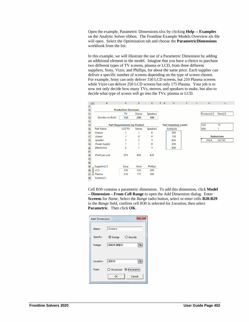
Frontline Solvers 2020 User Guide Page 402
Open the example, Parametric Dimensions.xlsx by clicking Help -- Examples
on the Analytic Solver ribbon. The Frontline Example Models Overview.xls file
will open. Select the Optimization tab and choose the ParametricDimensions
workbook from the list.
In this example, we will illustrate the use of a Parametric Dimension by adding
an additional element to the model. Imagine that you have a choice to purchase
two different types of TV screens, plasma or LCD, from three different
suppliers, Sony, Vizio, and Phillips, for about the same price. Each supplier can
deliver a specific number of screens depending on the type of screen chosen.
For example, Sony can only deliver 150 LCD screens, but 210 Plasma screens
while Vizio can deliver 250 LCD screens but only 175 Plasma. Your job is to now not only decide how many TVs, stereos, and speakers to make, but also to
decide what type of screen will go into the TVs: plasma or LCD.
Cell B30 contains a parametric dimension. To add this dimension, click Model
– Dimension – From Cell Range to open the Add Dimension dialog. Enter
Screens for Name, Select the Range radio button, select or enter cells B28:B29
in the Range field, confirm cell B30 is selected for Location, then select
Parametric. Then click OK.

Frontline Solvers 2020 User Guide Page 403
The following formula is entered into cell B30, = PsiParamDim("Screens",
B28:B29). As you can see, the arguments for PsiParamDim() are identical to
PsiDim(). The first argument is the name of the dimension and the 2nd argument
is an Excel range. It’s also possible to enter upper and lower bounds for the 2nd
argument (select Bounds on the Add Dimension dialog) or to simply enter an integer n which will create a parametric dimension with n elements. (In this
case, there will be no names associated with the elements other than indices
from 1 to n.) Repeat the steps above to create a second Parametric Dimension
in cell H19 using the name Suppliers and the Excel range C27:E27.
Now select cell H19 and click Model – Cube – From Cell Range to bring up
the Add Cube dialog. This cube will contain the values from cells C28:E29. Therefore, select cells C28:E29 for Range. Select Suppliers for Dimensions,
then click the “+” command button to add a 2nd dimension, Screens. Note: As
mentioned above, when calculating over multiple dimensions, the “columns”
dimension, or the dimension that is most often changing, must always come
first. Confirm that H19 is listed for Location and click OK.
The formula =PsiCube($C$28:$E$29,"Suppliers","Screens") will be entered
into cell H19.
If you inspect the Model tab on the Task Pane, you’ll see that two more
dimensions (Suppliers and Screens) and one more cube ($H$19) appear under
the appropriate headings.
Now click the green arrow on the Model tab to run Solver. Solver will run six
different optimizations each time using a different value from the cell range
C28:E29 for cell H19. For example, for the first optimization, Solver will use
150 for the value of H19, for the 2nd optimization, Solver will use 210 for the
value in cell H19, for the 3rd optimization, Solver will use 250 for the value in
cell H19, etc.
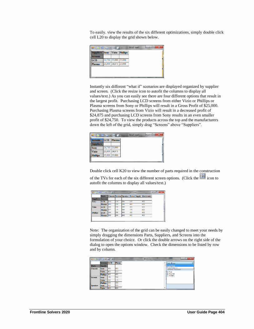
Frontline Solvers 2020 User Guide Page 404
To easily. view the results of the six different optimizations, simply double click
cell L20 to display the grid shown below.
Instantly six different “what if” scenarios are displayed organized by supplier
and screen. (Click the resize icon to autofit the columns to display all
values/text.) As you can easily see there are four different options that result in
the largest profit. Purchasing LCD screens from either Vizio or Phillips or
Plasma screens from Sony or Phillips will result in a Gross Profit of $25,000.
Purchasing Plasma screens from Vizio will result in a decreased profit of $24,875 and purchasing LCD screens from Sony results in an even smaller
profit of $24,750. To view the products across the top and the manufacturers
down the left of the grid, simply drag “Screens” above “Suppliers”.
Double click cell K20 to view the number of parts required in the construction
of the TVs for each of the six different screen options. (Click the icon to
autofit the columns to display all values/text.)
Note: The organization of the grid can be easily changed to meet your needs by
simply dragging the dimensions Parts, Suppliers, and Screens into the
formulation of your choice. Or click the double arrows on the right side of the
dialog to open the options window. Check the dimensions to be listed by row
and by column.

Frontline Solvers 2020 User Guide Page 405
If you wanted to view the final objective value when Sony Plasmas as used in
the construction of the TVs, first select Screens on the Model tab, then select
Plasma for Current Value.
Now select Suppliers on the Model tab, then select Sony for Current Value.
Cell H19 will change to 210 to reflect the value in cell C29 which is the number
of Plasma screens Sony can supply. In addition, the final variable values in cells
C14:E14 will change to 200, 200, 0, the objective shown in cell L20 will change to $25,000, the parametric dimensions in cells B27 and B30 will change to
Suppliers[1] (to reflect that the first element of the Suppliers dimension is

Frontline Solvers 2020 User Guide Page 406
selected as the current value) and Screens[2] (to reflect that the 2nd element of
the Screens dimension is selected as the current value).
As with PsiParamDim(), several options will appear at the bottom of the task
pane under Dimension (as shown in the screenshot above). Here you can view
the cell where the dimension is located (B27), the formula, the name of the
dimension (Suppliers) and the type of dimension (structural or parametric).
These fields are all read-only. However, Current Value, Locked, Active in
Optimization, Active in Simulation, and Active in Sensitivity Analysis can all be
edited. Current Value controls the values displayed in the cube cells. For
example, select Vizio for Current Value. The value in cell H19 will change to
reflect the Vizio value for the Current Value of the Screens dimension (210).
Setting Locked to True, will result in the dimension being “locked” or “frozen”
to the Current Value element during optimization. For example, if Current
Value is set to Sony for the Suppliers Parametric Dimension and Locked is set to
True only two optimizations will be ran when the green arrow is clicked, one
optimization for the value 150 (cell C28) and one optimization for the value 210
(cell C29). Double click the objective cell (L20) to display the results for the two different screens supplied by Sony.
You can also reduce the dimensions displayed in the grid by performing a
Parametric Analysis. Click Reports – Optimization – Parameter Analysis to
open the Cube Optimization Report dialog.
All seven cubes appear under Cubes and Selection, select cells L20 and K20 and
click > to select. Both dimensions (Suppliers and Screens) appear under
Parametric Dimensions, select one dimension, say Suppliers, then click > to select. Afterwards, click OK. The following grid appears.

Frontline Solvers 2020 User Guide Page 407
Here the “slices” of the structural dimensions can be viewed. Click the two
arrows on the right of the dialog to open the “options” pane.
This grid displays the number of chassis parts required when Screens are
purchased from each Supplier. For example, if the screens are purchased from
Sony, only 350 chassis will be needed. If screens are purchased from Vizio or
Phillips, 400 chassis will be required. Note: When a dimension is deactivated, it
is essentially locked to its first element. In this case, the Screens dimension is locked to the LCD values of 150, 250, and 200. Click the down arrow under
Parts to see how many of each part will be required when screens are purchased
from each supplier.
Currently both the Screens and Suppliers Parametric Dimensions are active in
all three types of analyses: optimization, simulation and sensitivity. As stated earlier, this means that if you wanted to use these dimensions for a parameter
analysis, you could do so as an optimization parameter, sensitivity parameter,
and/or simulation parameter. To remove this Parametric dimension from any of
these analyses, simply change True to False. If Active in Optimization is set to
False, this dimension will be ignored in the next optimization. Likewise, if
Active in Simulation or Active in Sensitivity Analysis is set to False, then this
dimension will be ignored in the next simulation or sensitivity analysis.
For example, select Screens in the Model Task Pane, select Plasma for Current
Value, then change Active in Optimization to False.

Frontline Solvers 2020 User Guide Page 408
Now run an optimization either by clicking the green arrow on the Task Pane or
Optimize – Solve Complete Problem on the ribbon.
Solver will run three optimizations – one each for values 150, 250, and 200 or
the number of LCD screens (the first element in the Screens dimension) that can
be supplied by Sony, Vizio and Phillips, respectively (cells C28:E28). To view the results of each value, simply select Suppliers on the Model Task Pane and
select Sony, Vizio, or Phillips or double click any of the cubes to display the
values for these three optimizations. For example, click cell L20 and K20 to
display the following grids. Both grids only reveal the optimization results for
the three suppliers calculated using the first element from the Screens
dimension.
It’s also possible to view all Parametric Dimensions included in the workbook
by clicking Parameters – Dimension on the Ribbon to bring up the Parametric
Dimension Participation dialog. From here you can select which dimensions are

Frontline Solvers 2020 User Guide Page 409
active for Optimization, Sensitivity Analysis and Simulation, all on one screen.
For example, to remove the Suppliers Parametric Dimension from Simulation,
select Suppliers and click <. To remove all Parametric Dimensions from
Simulation, click <<.
After an optimization has finished, click Charts – Multiple Optimizations –
Monitored Cells to open the Optimizations Chart dialog.

Frontline Solvers 2020 User Guide Page 410
Expand Variables (by clicking the “+”), then expand C14:E14. Select C14, then
click > to add the decision variable to the chart. Repeat this step for cells D14
and E14, then click OK to create the chart below, which tracks the decision
variable values for each of the three optimizations.

Frontline Solvers 2020 User Guide Page 411
Using Dimensional Modeling in Simulation
Dimensional modeling can also be used with simulation models as well as with
simulation optimization models. (Note: Dimensional Modeling is not available
with Stochastic Transformation.) Open the example, CityCube.xlsx by clicking
Help -- Examples on the Analytic Solver ribbon. The Frontline Example
Models Overview.xls file will open. Select the Simulation tab and choose
CityCube.xlsx from the list.
Defining a Dimension
In this simple example, a dimension, City, has been created in cell F15 which is
comprised of the names of major cities in California (cells B15:B18). Cells
C15:C18 contain the gross income per city. Each Gross Income is uncertain.
The Gross Income for San Francisco follows the Gamma distribution, Gross
Income for San Diego follows a Triangular distribution, San Jose follows a
Normal distribution and Los Angeles follows a Uniform distribution.
Defining a Cube
One key benefit of this model is that it defines a simulation output in one cell
which would require four cells without dimensional modeling. In cell F16, a
cube has been created along the City dimension which is comprised of each
city’s gross income in $Millions. Double click this cell to display the grid.
(Click the icon to autofit the columns to display all values/text.)
In cell F17, a 2nd cube has been created by using the cube in cell F16 in the
formula, =F16*(1-C12), which multiplies the elements of the cube in cell F16 by
the after tax rate or 91% (1-.09). If dimensional modeling is not used, four
output cells would be required to capture the simulation statistics, percentiles,
etc, for the after-tax income of each city. However, in this example, the cube in cell F17 captures all relevant information.

Frontline Solvers 2020 User Guide Page 412
Notice that “calc” follows the cell address in the dialog title. This means that a
trial value is being displayed.
Defining an Output
Cell F18 contains the PsiMean() function which creates both a simulation output
as well as a dimensional modeling output. To view the statistics and percentiles
for each city’s Gross Income, simply set the Current Value of the City
dimension to the desired city. For example, to view the simulation results for
San Diego, select City under Dimensions in the Model tab of the Task Pane,
then set Current Value to San Jose.
Now click the green arrow on the Output tab to run a simulation. The
Simulation results window that appears contains simulation results for San
Jose’s after-tax income.
To view the mean results for each city, double click cell F18 to display the
following grid. Notice that (sim-mean) now follows the cell address ($F$18) in

Frontline Solvers 2020 User Guide Page 413
the dialog title. This title signifies that these results are the mean from a
simulation.
Note: PsiMean() can be substituted with any PsiXxx statistic function except
PsiCorrelation and PsiFrequency.
Double click cell F17.
Currently, this grid displays the mean results from the simulation. Click the
down arrow next to Mean and select Trials.
All 1000 trial values for each city are listed. Drag “City” above “All Trials” to
list the trials vertically.

Frontline Solvers 2020 User Guide Page 414
To see mini histograms for each uncertain function, click the down arrow next to
Trials and select Histogram.
Cells F18:F21 contain the PsiMean() simulation statistic entered as an array
formula. The results of this function are similar to the results of PsiCubeData()
and PsiOptData() (for objective and constraint cubes only) in that when entered as an array, the function will display the fact table for the desired cube.
When a Psi Statistic function (such as PsiMean(), PsiStdDev(), PsiVariance(),
etc.) is entered as an array formula and used with a simulation model using
Dimensional Modeling, the statistic function will display all elements of the
cube fact table formatted according to the optional 3rd argument, struc_format.
To begin, we’ll need to determine the size of our array. Since the cube in cell F17 is comprised of one dimension (Cities), we’ll need to select one cell and
enter “=PsiMean(F17, 1, “dims”)” in this cell. (When “dims” is passed for the
struc_format argument (3rd argument), the size of each dimension contained in
the cube in cell F17 will be returned.) Afterwards, this cell will display
“City[4]” indicating that there are 4 elements in the City dimension. Now that
we know the number of elements (or size) of the dimensions, we can display the
entire fact table by entering PsiMean() as an array, but this time we’ll use “vals”
for the struc_format argument. When passing “vals” for this argument,
PsiMean(), when entered as an array, will display the data as a relational table.
Since there are 4 elements in the City dimension, the fact table for this cube will
contain 4 elements. Therefore, we will need to highlight 1 column for the first dimension (City) and a 2nd column for the actual values and 4 rows to hold all 4

Frontline Solvers 2020 User Guide Page 415
values in the fact table. In this example, we’ll use the blank cells H15:I18. (This
area encompasses 2 columns and 4 rows.) Select these cells, enter
“=PsiMean(F17, 1, “vals”), then press SHIFT + CTRL + ENTER to enter this
formula as an array formula. The following table will be displayed. Note:
PsiMean() can be substituted with any PsiXxx statistic function except PsiCorrelation and PsiFrequency.
Now we’ll use a different statistic, PsiStdDev() but this time we’ll list only the
values in the fact table To do so, select cells K15:K18, then enter
“=PsiStdDev(F17)”, then press SHIFT + CTRL + ENTER to enter the formula
as an array. Notice we are only supplying the first argument. Afterwards, these
cells will display only the values of the fact table as shown in cells K15:K18 in
the screenshot below. Repeat the same steps in cell L15:L18 but this time using
the statistic, PsiVariance() (“=PsiVariance(F17)”).
A statistics function can also be used to display a slice or even a single element
of the fact table. For example, to display the mean gross margin for the City of
San Diego, select two blank cells, say H20:I20, and enter the following
formula: =PsiMean(F17,1, “[City].[SanDiego]”). Then press SHIFT + CTRL +
ENTER to enter as an array formula. Afterwards, the following table will be
displayed.
Now let’s close this example and continue on to the next section to learn about
using a parametric dimension in a simulation model.
Parametric Dimensions
Now let’s see how Parametric Dimensions can be used with simulation. Open
the example, ParametricCube_SimExample.xlsx by clicking Help -- Examples on the Analytic Solver ribbon. The Frontline Example Models Overview.xls file
will open. Select the Simulation tab and choose Parametric Cube Simulation
Example. ParametricCube_SimExample.xls opens.

Frontline Solvers 2020 User Guide Page 416
This example models the Estimated Technology costs for two years in the future
(year 1 and year 2) for JoeBen Gaming based on which computer manufacturer
the company selects. This model includes a structural dimension and a
parametric dimension. The structural dimension is held in cell H16. This
dimension contains the type of technology that JoeBen gaming will purchase for
their employees: Tablets, Desktops, and Laptops. The parametric dimension is
contained in cell H17. This dimension contains the manufacturers of the
technology: Apple, Sony, Samsung, HP, and Dell.
Cells L22 and L23 contain the projected number of machines needed for years 1
and 2, respectively, based on the projected growth distributions in cells K17 and
L17. The ratio of tablets, desktops, and laptops, to the total number of machines
will remain constant. Therefore, the percentage of tablets will remain at 33%,
the percentage of desktops will remain at 46.7%, and the percentage of laptops will remain at 20% for the next two years. As a result, the values in cells
I28:K29 are calculated by multiplying the number of machines (cells L22 and
L23) by the percentages in cells I21:K21.
Three cubes are located in cells I27:K27. These cubes contain the data for the
Manufacturer dimension. The values in these cells will determine the total
technology costs for each year. Cell I27 contains pricing data for each tablet by manufacturer, cell J27 contains pricing data for each desktop by manufacturer,
and cell K27 contains pricing data for each laptop by manufacturer. Double
click each of these cells to display their data values. For example, double
clicking cell I27 brings up the following dialog which displays tablet pricing for
each manufacturer.
Once the green arrow has been clicked in the Model tab of the Solver task pane,
or Simulate – Run Once is clicked on the ASP Ribbon, five different simulations
will be run simultaneously in less than one second – one simulation for each
manufacturer.
Double click cell L28 to display a grid revealing the total technology costs for
Year 1 for each manufacturer. (Click the icon to expand the columns to

Frontline Solvers 2020 User Guide Page 417
display the full text in the first column.) With Dimensional Modeling, you can
perform a What If analysis with the double click of one button!
Click the down arrow next to Mean and select Trials from the drop-down menu.
1000 trial values are displayed for each manufacturer. (Click the icon to
expand the columns to display the full text in the first column.) 1000 what-if
scenarios are again available at the double click of a button!
To view the trial values vertically (rather than horizontally), simply drag
Manufacturer above All Trials in the grid or simply click the double arrows on
the right of the dialog and select Manufacturer on the Cube Columns menu.

Frontline Solvers 2020 User Guide Page 418
Let’s view the results for Dell only. First, select the Manufacturer parametric
dimension in the Model tab of the Solver task pane. Then select Dell for
Current Value.
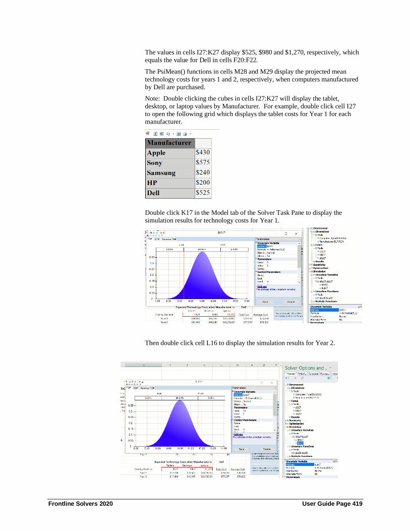
Frontline Solvers 2020 User Guide Page 419
The values in cells I27:K27 display $525, $980 and $1,270, respectively, which
equals the value for Dell in cells F20:F22.
The PsiMean() functions in cells M28 and M29 display the projected mean
technology costs for years 1 and 2, respectively, when computers manufactured
by Dell are purchased.
Note: Double clicking the cubes in cells I27:K27 will display the tablet,
desktop, or laptop values by Manufacturer. For example, double click cell I27
to open the following grid which displays the tablet costs for Year 1 for each
manufacturer.
Double click K17 in the Model tab of the Solver Task Pane to display the
simulation results for technology costs for Year 1.
Then double click cell L16 to display the simulation results for Year 2.
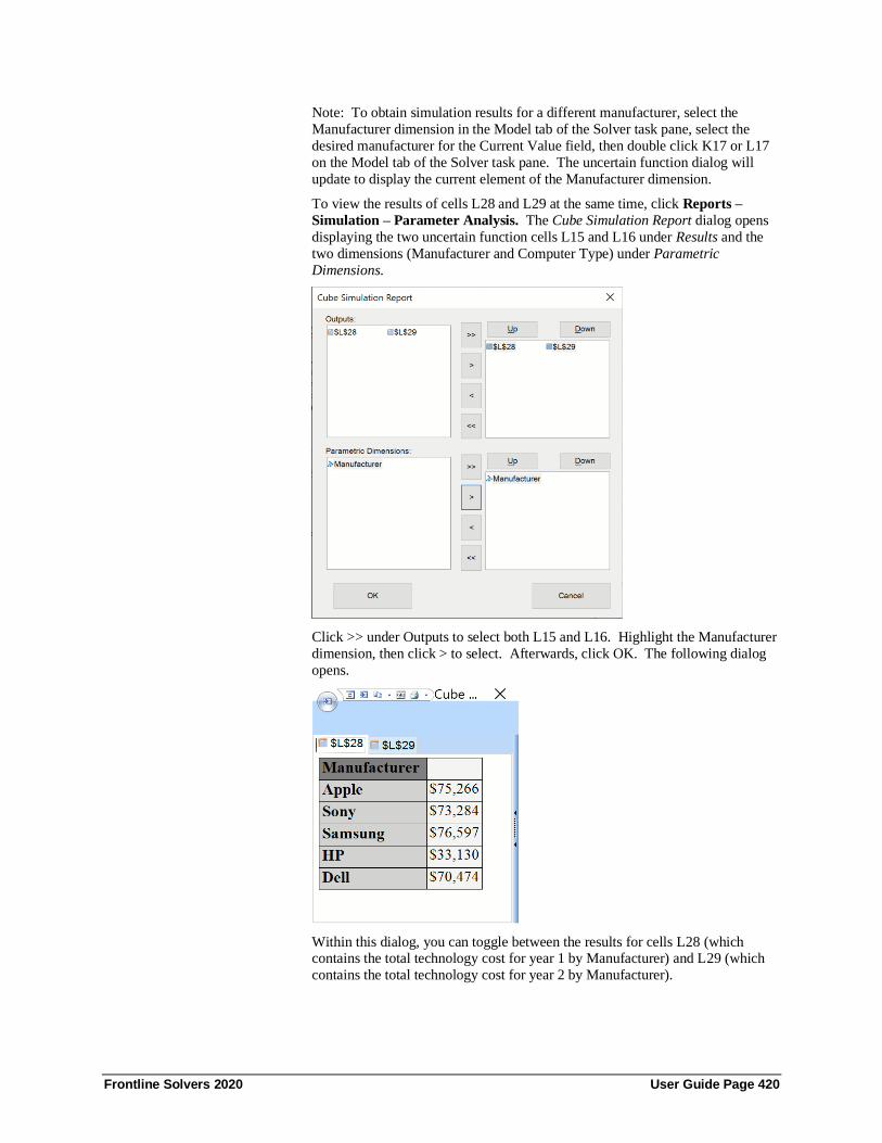
Frontline Solvers 2020 User Guide Page 420
Note: To obtain simulation results for a different manufacturer, select the
Manufacturer dimension in the Model tab of the Solver task pane, select the
desired manufacturer for the Current Value field, then double click K17 or L17
on the Model tab of the Solver task pane. The uncertain function dialog will
update to display the current element of the Manufacturer dimension.
To view the results of cells L28 and L29 at the same time, click Reports –
Simulation – Parameter Analysis. The Cube Simulation Report dialog opens
displaying the two uncertain function cells L15 and L16 under Results and the
two dimensions (Manufacturer and Computer Type) under Parametric
Dimensions.
Click >> under Outputs to select both L15 and L16. Highlight the Manufacturer
dimension, then click > to select. Afterwards, click OK. The following dialog
opens.
Within this dialog, you can toggle between the results for cells L28 (which contains the total technology cost for year 1 by Manufacturer) and L29 (which
contains the total technology cost for year 2 by Manufacturer).

Frontline Solvers 2020 User Guide Page 421
As you can easily see, purchasing machines from HP will yield the least amount
of technology costs for both Years 1 and 2.
All charts under Multiple Simulations now also support Dimensional Modeling.
(“Locked” or non-active dimensions will not appear in the charts.) Click
Charts – Multiple Simulations – Box-Whisker to open the Multiple
Simulations Chart dialog. Click >> to select Simulation 1 and click OK. Analytic Solver draws the following chart.
This shows a Box-Whisker diagram for each of the 15 simulations, with the
mean, median, 25th and 75th percentiles, and the minimum and maximum value for net revenue on each one. You can click the right edge of the Trend and Box-
Whisker charts to open a right panel with options for customizing these charts.
You can use the icons on the title toolbar to print the chart, or copy it to the
Clipboard, where it can be pasted into another application such as PowerPoint.
Perform the same steps for each of the remaining charts: Trend, Overlay, and
Statistics. For more information on these charts, please see the Frontline Solvers
Reference Guide.

Frontline Solvers 2020 User Guide Page 422
In addition, the three reports under Charts – Multiple Simulation Results are also
supported in Dimensional Modeling. Click Charts – Multiple Simulation
Results -- Trend to open the Multiple Simulation Results dialog.
Click >> to select both output cells L28 and L29, then click OK. A trend chart
of both uncertain functions is produced.
Here we can see a steep upward climb of the mean value of the total technology
costs, and also the volatility around the mean, depicted here with the 25th and
75th percentiles.
Repeat the same steps to produce the remaining charts: Overlay and Box-
Whisker. For an explanation of these reports, please see the Frontline Solvers
Reference Guide.
Now close this example and continue onto the next section to learn how to use a
pivot table with Dimensional Modeling.

Frontline Solvers 2020 User Guide Page 423
Using Dimensional Modeling with Pivot Tables In general, cubes are defined as multi-dimensional, not just two – dimensional as
shown in the examples above. Unfortunately, a normal Excel worksheet is not
the easiest medium for working with multidimensional cubes. An Excel pivot
table, however, lends itself to this very practice. An Excel Pivot Table is a tool
within Excel that can be used to summarize data located in an Excel worksheet.
Once data is inserted into a pivot table, it can easily be sorted, counted, totaled,
etc. by dragging and dropping the fields into the desired layout.
Click Help -- Examples on the Analytic Solver ribbon. The Frontline Example
Models Overview.xls file will open. Select the Simulation tab and choose Pivot
Table Simulation Example from the list. (This example uses parametric dimensions but structural dimensions are also supported.)
An Excel Pivot table is located in cells B13:F27. This table is comprised of the
Product Line for Mark’s Breakfast Delights. This company has two product
lines: Waffle Mix and Pancake Mix. Each of these product lines contain two
flavors: blueberry and plain. The Sales team is comprised of 4 individuals who
are responsible for a specific region of the Las Vegas area where the company is
based: Henderson, Summerlin, North Las Vegas, and Fremont Street. Sales
figures for each product and region are located in the Sales column. Note:
Since values in a pivot table cannot be evaluated, pivot table values must be
constants.
How to create the Pivot Table
Highlight the data on the worksheet, then click Insert – Pivot Table – Pivot
Table on the Excel ribbon. The Create PivotTable dialog opens. Select a
table or range is prefilled, leave this selection as is. Select New Worksheet,
then select a blank cell for Location. Then click OK.
The pivot table will be inserted into a new worksheet. Manipulate the table as
desired. Afterwards, click Design – Report Layout – Show in Tabular
Form.
Next, we’ll create three dimensions, one each for Product, Product_Line, and
Region. Select a blank cell, in this case cell I15 was used, then click Model –
Dimension – From Pivot Table to open the Add Dimension dialog. Select the
name of the pivot table, in this case PivotTable1, select Product for
Dimensions, select Parametric for Type and cell I15 for Location. Then click
OK. The formula =PsiPivotDim(B13,"Product", TRUE) will be inserted into
cell I15. Repeat these steps in cells I16 and I17 to create parametric
dimensions for Product_Line and Region, respectively. Alternatively, this
formula could also be typed directly into the cell.

Frontline Solvers 2020 User Guide Page 424
Now we will create a cube from the pivot table. Select a blank cell, in this
example cell I19, then click Model – Cube – From Pivot Table to open the Add Pivot Table Cube dialog.
Leave PivotTable1 and Location at their defaults, and click OK. The following
formula will be inserted into cell I19 =PsiPivotCube($B$13:$F27).
Alternatively, this formula could have been entered into the cell directly.
From here we can create a simulation or optimization model. In this example,
we’ve created a simulation model. Cell I21 holds an uncertain variable which
calculates a selling price using a triangular distribution with a minimum
parameter of 100, a maximum parameter of 200, and a likely parameter of 160.
This sales price is multiplied by the cube result in cell I19.
To simulate gross sales for the Western region, select the Product Dimension
on the Model tab in the Task Pane, then change Current Value to “Blueberry”.
Afterwards, perform the same steps for the remaining dimensions (Product_Line
and Region) changing the current value of the Product_Line dimension to
“Pancake Mix” and the current value of the Region dimension to “Blueberry”.
Cell I15 will display the value in cell F15, 18. Now click the green arrow on the Model tab to run a simulation. The simulation runs using the value of 18 as the
number of products sold. The simulation results for the uncertain function in
cell I22 are below.
Important Note: Pivot tables cannot be evaluated by the PSI Interpreter. This
means that decision variables, uncertain variables, uncertain functions, and
constraint or objective functions must not be used within an Excel Pivot Table.
All values inside of a pivot table must be constant, or computed from constants.

Frontline Solvers 2020 User Guide Page 425
Double click the cube in cell I22 to display a grid containing the Gross Sales by
product and region.
Click the down arrow next to Mean and select Trials to display the 1000 trial
values used in the simulation.

Frontline Solvers 2020 User Guide Page 426
Double click cell I23 to open the grid containing the Mean Gross Sales by
product and region.
It’s also possible to list the trial values in cells in the spreadsheet. Cells I25:I39
contain the function PsiData(I22) entered as an array function. These cells
display the first 15, of 1000, trial values for cell I22, or Gross Sales.
Using Sparse Cubes Analytic Solver provides the option to calculate cubes defined by PsiCube() or
PsiTableCube() when the Optimization or Simulation Interpreter option is set to
Psi Interpreter.
Most large cubes are sparse in nature. While they may contain thousands of
elements, in practice, not all combinations of dimension elements are possible;
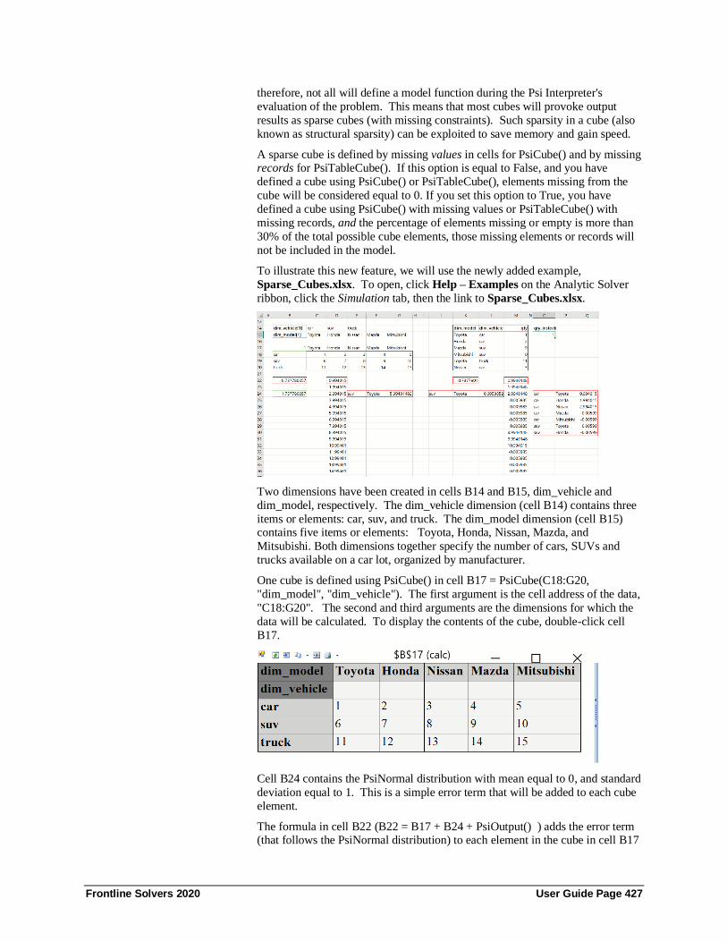
Frontline Solvers 2020 User Guide Page 427
therefore, not all will define a model function during the Psi Interpreter's
evaluation of the problem. This means that most cubes will provoke output
results as sparse cubes (with missing constraints). Such sparsity in a cube (also
known as structural sparsity) can be exploited to save memory and gain speed.
A sparse cube is defined by missing values in cells for PsiCube() and by missing records for PsiTableCube(). If this option is equal to False, and you have
defined a cube using PsiCube() or PsiTableCube(), elements missing from the
cube will be considered equal to 0. If you set this option to True, you have
defined a cube using PsiCube() with missing values or PsiTableCube() with
missing records, and the percentage of elements missing or empty is more than
30% of the total possible cube elements, those missing elements or records will
not be included in the model.
To illustrate this new feature, we will use the newly added example,
Sparse_Cubes.xlsx. To open, click Help – Examples on the Analytic Solver
ribbon, click the Simulation tab, then the link to Sparse_Cubes.xlsx.
Two dimensions have been created in cells B14 and B15, dim_vehicle and
dim_model, respectively. The dim_vehicle dimension (cell B14) contains three
items or elements: car, suv, and truck. The dim_model dimension (cell B15) contains five items or elements: Toyota, Honda, Nissan, Mazda, and
Mitsubishi. Both dimensions together specify the number of cars, SUVs and
trucks available on a car lot, organized by manufacturer.
One cube is defined using PsiCube() in cell B17 = PsiCube(C18:G20,
"dim_model", "dim_vehicle"). The first argument is the cell address of the data,
"C18:G20". The second and third arguments are the dimensions for which the
data will be calculated. To display the contents of the cube, double-click cell
B17.
Cell B24 contains the PsiNormal distribution with mean equal to 0, and standard
deviation equal to 1. This is a simple error term that will be added to each cube
element.
The formula in cell B22 (B22 = B17 + B24 + PsiOutput() ) adds the error term (that follows the PsiNormal distribution) to each element in the cube in cell B17

Frontline Solvers 2020 User Guide Page 428
(i.e., the first element of the cube = 1 + PsiNormal(0,1), the second element of
the cube = 2 + PsiNormal(0, 1) and so on). PsiOutput is used to designate cell
B22 as an output function. For details on the PsiOuput() function see the
previous chapter, "Examples: Stochastic Optimization."
PsiMean() has been array entered into cells D22:D36. After a simulation has been run, these cells will display the PsiMean() value as calculated for each of
the 15 elements of the cube (i.e., cell D22 will contain the mean for the first
cube element, D21 will contain the mean for the second cube element, and so
on).
The formula, = PsiMean(B22, 1, "[dim_vehicle].[suv], [dim_model].[maz]"),
has been array entered into cells E24:G24 to illustrate how to display just one
element of the cube (i.e., the number of Toyota SUVs available).
Run a simulation by clicking the down arrow beneath Simulate and selecting
Run Once. Instantly, Analytic Solver performs a new simulation of 1,000
Monte Carlo trials, and updates each of the 15 cube elements and the worksheet with the results. The mean of each element can be found in cells D22:D36 or by
double clicking cell B22, as shown in the screenshot below.
Notice that the value of the first cube element (Toyota/Car) corresponds to the
value in cell D22, the value of the second cube element (Honda/Car)
corresponds to the value in cell D23, and so on. In addition, the value for the
number of available Toyota SUVs in cell G24 corresponds to the number of
Toyota SUVs in the cube display.
Next, let's move to the right of the spreadsheet. Cell O15 contains
PsiTableCube(). PsiTableCube() defines a sparse table. The first argument
passes the dimension elements, while the second argument passes the values.
(For more information on PsiTableCube, see PsiTableCube() in the Frontline
Solvers Reference Guide.)
Notice that only 6 out of a possible 15 elements are used in the table. When Use
Sparse Cubes is set to False (the default), the missing 9 elements will be set to
0 during the Psi Interpreter's evaluation of the problem. To display the
following cube, double-click cell O15.
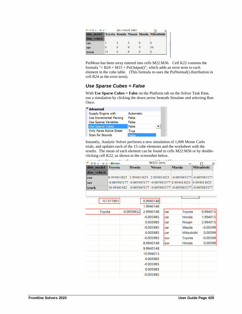
Frontline Solvers 2020 User Guide Page 429
PsiMean has been array entered into cells M22:M36. Cell K22 contains the
formula "= B24 + M15 + PsiOutput()", which adds an error term to each
element in the cube table. (This formula re-uses the PsiNormal() distribution in
cell B24 as the error term).
Use Sparse Cubes = False
With Use Sparse Cubes = False on the Platform tab on the Solver Task Pane,
run a simulation by clicking the down arrow beneath Simulate and selecting Run
Once.
Instantly, Analytic Solver performs a new simulation of 1,000 Monte Carlo
trials, and updates each of the 15 cube elements and the worksheet with the
results. The mean of each element can be found in cells M22:M36 or by double-
clicking cell K22, as shown in the screenshot below.
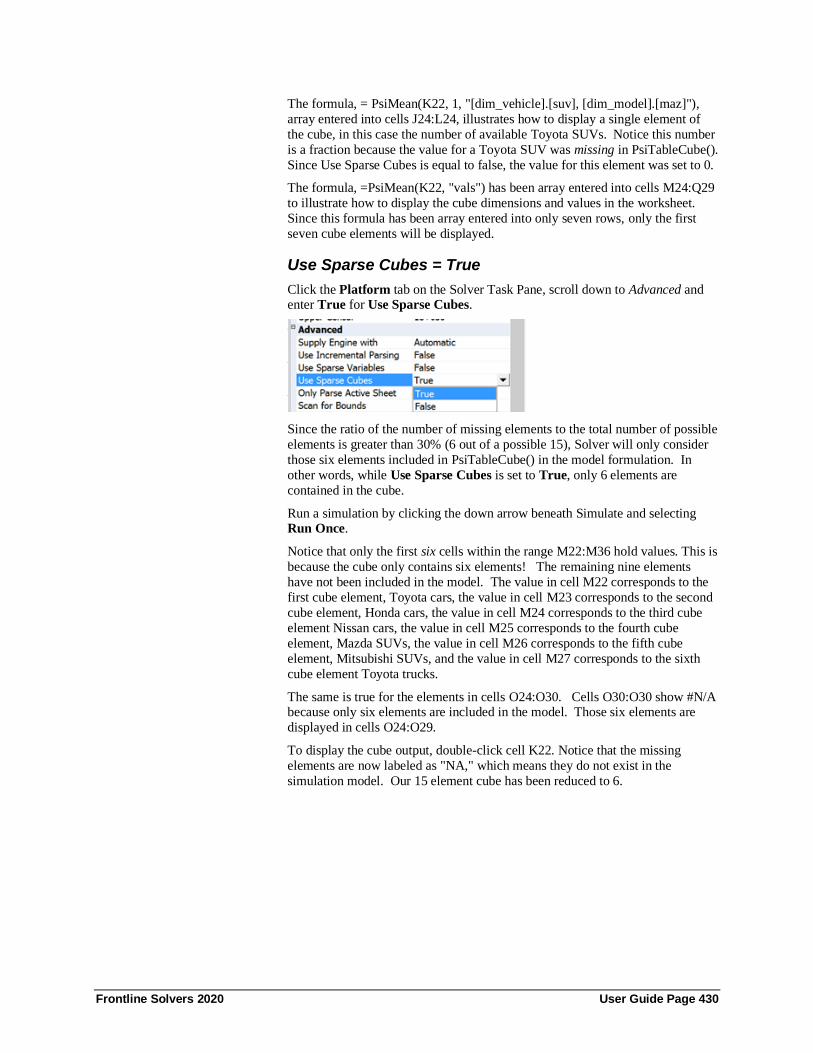
Frontline Solvers 2020 User Guide Page 430
The formula, = PsiMean(K22, 1, "[dim_vehicle].[suv], [dim_model].[maz]"),
array entered into cells J24:L24, illustrates how to display a single element of
the cube, in this case the number of available Toyota SUVs. Notice this number
is a fraction because the value for a Toyota SUV was missing in PsiTableCube().
Since Use Sparse Cubes is equal to false, the value for this element was set to 0.
The formula, =PsiMean(K22, "vals") has been array entered into cells M24:Q29
to illustrate how to display the cube dimensions and values in the worksheet.
Since this formula has been array entered into only seven rows, only the first
seven cube elements will be displayed.
Use Sparse Cubes = True
Click the Platform tab on the Solver Task Pane, scroll down to Advanced and enter True for Use Sparse Cubes.
Since the ratio of the number of missing elements to the total number of possible
elements is greater than 30% (6 out of a possible 15), Solver will only consider
those six elements included in PsiTableCube() in the model formulation. In
other words, while Use Sparse Cubes is set to True, only 6 elements are
contained in the cube.
Run a simulation by clicking the down arrow beneath Simulate and selecting Run Once.
Notice that only the first six cells within the range M22:M36 hold values. This is
because the cube only contains six elements! The remaining nine elements
have not been included in the model. The value in cell M22 corresponds to the
first cube element, Toyota cars, the value in cell M23 corresponds to the second
cube element, Honda cars, the value in cell M24 corresponds to the third cube
element Nissan cars, the value in cell M25 corresponds to the fourth cube
element, Mazda SUVs, the value in cell M26 corresponds to the fifth cube
element, Mitsubishi SUVs, and the value in cell M27 corresponds to the sixth
cube element Toyota trucks.
The same is true for the elements in cells O24:O30. Cells O30:O30 show #N/A because only six elements are included in the model. Those six elements are
displayed in cells O24:O29.
To display the cube output, double-click cell K22. Notice that the missing
elements are now labeled as "NA," which means they do not exist in the
simulation model. Our 15 element cube has been reduced to 6.

Frontline Solvers 2020 User Guide Page 431

Frontline Solvers 2020 User Guide Page 432
Automating Optimization in VBA
Introduction This chapter explains how to use the Object-Oriented API in Analytic Solver
Desktop to create, modify and solve optimization models under the control of
your custom application written in VBA.
Note: Analytic Solver Cloud does not currently support this functionality.
This API is compatible with the object-oriented API offered by Frontline’s
Solver SDK Platform and Solver SDK Pro, used to build custom applications of
optimization and simulation using C++, C#, VB.NET, Java, MATLAB and other languages.
Analytic Solver also supports “traditional” VBA functions, which are upward
compatible from the VBA functions supported by the standard Excel Solver.
This API is described in the Frontline Solvers Reference Guide.
Why Use the Object-Oriented API?
The new object-oriented API is more powerful and much more convenient for
programming than the “traditional” VBA functions.
With the “traditional” VBA functions:
• You work with procedural functions that correspond to operations – such as SolverOK and SolverSolve – you can perform interactively in the Solver
dialogs. To access the model and its variables and constraints, you must
process the arrays of text and numbers returned by the SolverGet function.
• To obtain solution values, you must use the Excel object model (usually the
Range object) to access the decision variable cells on the worksheet. You
must take care to access the correct cells for specific decision variables.
• To obtain dual values and ranges, you must call the SolverFinish function
to insert a report worksheet into the workbook, then use the Excel object
model to access cells in the report. You must take extra care to access the
correct report cells containing dual values and ranges.
With the new Object-Oriented API:
• You work with objects that correspond to the Problem, Model, Solver,
Engine, Variables, and Functions. You can access sets of variables and
constraints in the current model directly with expressions such as
myProb.VarDecision and myProb.FcnConstraint.
• You can obtain solution values directly, with expressions such as
myProb.VarDecision.FinalValue(i). If you need the cell address for a set of
decision variable cells, you can write myProb.VarDecision.Name.
• You can access dual values and ranges for variables and constraints directly,
with expressions such as myProb.VarDecision.DualValue(i) or myProb.FcnConstraint.DualValue(i).
The result is VBA code that’s easier to read, and easier to write in the first place.
Since the VBA Editor recognizes the object model exposed by Analytic Solver –

Frontline Solvers 2020 User Guide Page 433
just as it recognizes the object model exposed by Excel – you’ll receive
IntelliSense prompts as you write code. For example, if you type a line Dim
myProb as New Problem, then start a new line with myProb., you’ll be
prompted with the properties and methods available for Problems:
If you select FcnConstraint and then type a period, you’ll be prompted with the
properties and methods available for Functions:
This makes it much easier to write correct code, without consulting the manual.
What’s more, you can use this object-oriented API when programming Excel
and Analytic Solver from new languages such as VB.NET and C#, working in
Visual Studio, and receive IntelliSense prompts in the syntax of these languages!
If you’re using new functionality in Analytic Solver, the object-oriented API is
your best bet. And if you’re planning to move your application outside of Excel
in the future – so it will run as a standalone program – you’ll find that
Frontline’s Solver Platform SDK offers an object-oriented API that closely resembles the new APIs in Analytic Solver.
Running Predefined Solver Models
Controlling the Solver can be as simple as adding two lines to your VBA code!
Each worksheet in a workbook may have a Solver problem defined, which is
saved automatically with the workbook. You can create this Solver model
interactively if you wish. If you distribute such a workbook, with a worksheet
containing a Solver model and a VBA module, you can simply add a reference
to the Analytic Solver COM server (see below), activate the worksheet, and add
these two lines of code:
Dim prob As New Problem prob.Solver.Optimize
Using the Macro Recorder
If you want to set up a Solver model “from scratch” programmatically, one easy
way to see how to use the object-oriented API is to turn on the Excel Macro
Recorder (click Record Macro on the Developer tab in Excel 2010 and then set

Frontline Solvers 2020 User Guide Page 434
up a Solver model interactively. Microsoft Excel will record a macro in VBA
that calls the object-oriented API to mimic the actions you perform. You can
then edit and customize this macro, and incorporate it into your application.
Note: You must use the classic Solver dialog to record a macro, rather than the
Solver Task Pane. To open, click Add-ins – Premium Solver. By default, the Excel Macro Recorder will record calls to the object-oriented API.
Adding a Reference in the VBA Editor
To use the new object-oriented API in VBA, you must first add a reference to
the type library for the Analytic Solver COM server. To do this:
1. Press Alt-F11 to open the VBA Editor.
2. Select menu choice Tools References.
3. Scroll down until you find Analytic Solver 2020 Type Library.
4. Check the box next to this entry, and click OK to close the dialog.
5. Use File Save to save your workbook.
Note that this is a different reference from Solver, which is the reference you
add in order to use the “traditional” VBA functions.
Analytic Solver Object Model Analytic Solver makes available a hierarchy of objects for describing
optimization problems, as pictured on the next page. Note that the same objects
are used for both optimization and simulation problems; see the next chapter,
“Automating Simulation in VBA,” for more information.

Frontline Solvers 2020 User Guide Page 435
The Problem object represents the whole problem, and the Model object
represents the internal structure of the model, which in Analytic Solver is
defined by your formulas on the spreadsheet. The Solver object represents the
optimization process – you call its Optimize method to find an optimal solution. The Engine object represents either a built-in or plug-in Solver engine. A
Variable object represents a range of one or more contiguous cells that contains
decision variables, while a Function object represents a range of cells that
contains either constraint left hand sides or the objective. Each Problem has a
collection of Variable objects, and a collection of Function objects. An
Evaluator represents a function you write that the Solver will call on each
iteration (Trial Solution), or on each subproblem in a larger problem.
The Model has a collection of ModelParam objects, each representing a single
option or parameter of the PSI Interpreter (appearing in the Task Pane Platform
tab). An Engine has a collection of EngineParam objects, each representing a
single option or parameter of a Solver engine (appearing in the Task Pane Engine tab). It also has an EngineLimit object, holding problem size limits for
this Solver engine, and an EngineStat object, holding performance statistics for
the last optimization problem solved by this engine. An OptIIS object holds
results of an infeasibility analysis of the problem.
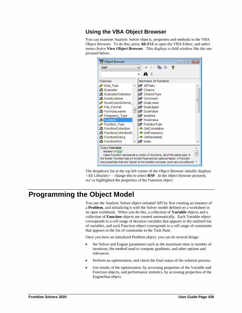
Frontline Solvers 2020 User Guide Page 436
Using the VBA Object Browser
You can examine Analytic Solver objects, properties and methods in the VBA
Object Browser. To do this, press Alt-F11 to open the VBA Editor, and select
menu choice View Object Browser. This displays a child window like the one
pictured below.
The dropdown list at the top left corner of the Object Browser initially displays
<All Libraries> – change this to select RSP. In the object browser pictured,
we’ve highlighted the properties of the Function object
Programming the Object Model You use the Analytic Solver object-oriented API by first creating an instance of
a Problem, and initializing it with the Solver model defined on a worksheet in
an open workbook. When you do this, a collection of Variable objects and a
collection of Function objects are created automatically. Each Variable object
corresponds to a cell range of decision variables that appears in the outlined list
of variables, and each Function object corresponds to a cell range of constraints
that appears in the list of constraints in the Task Pane.
Once you have an initialized Problem object, you can do several things:
• Set Solver and Engine parameters such as the maximum time or number of
iterations, the method used to compute gradients, and other options and
tolerances.
• Perform an optimization, and check the final status of the solution process.
• Get results of the optimization, by accessing properties of the Variable and
Function objects, and performance statistics, by accessing properties of the
EngineStat object.

Frontline Solvers 2020 User Guide Page 437
Example VBA Code Using the Object Model
Below is an example of VBA code that could be linked to a command button on
the worksheet:
Private Sub CommandButton1_Click()
Dim prob As New RSP.Problem
prob.Engine = prob.Engines("Standard LP/Quadratic")
prob.Engine.Params("MaxTime") = 600
prob.Solver.Optimize
MsgBox "Status = " & prob.Solver.OptimizeStatus
MsgBox "Obj = " & prob.FcnObjective.FinalValue(0)
For i = 0 To prob.Variables.Count – 1
For j = 0 To prob.Variables(i).Size - 1
MsgBox prob.Variables(i).FinalValue(j)
Next j
Next i
Set prob = Nothing
End Sub
The first line creates an instance of a Problem, which by default is associated
with the Solver model defined on the active worksheet. You could associate the
Problem object with a different worksheet by calling the prob.Init method:
Private Sub CommandButton1_Click()
‘create new problem
Dim prob As New RSP.Problem
‘initialize model on Invent2 worksheet
prob.Init Worksheets("Invent2")
The second line selects the Standard LP/Quadratic Solver engine, and the third
line sets the maximum solution time to 600 seconds. The string names of
parameters such as "MaxTime" are documented in the Frontline Solvers
Reference Guide.
The next set of three lines performs the optimization, displays the Solver Result
status code (for example 0), and displays the final value of the objective.
The double for-loop in the next five lines steps through the Variable objects –
each one representing a range of contiguous cells – and displays the final value for each variable cell in each range.
Evaluators Called During the Solution Process
You can write a VBA function that Analytic Solver will call at certain points
during the solution process. In this “callback function,” you can access
information about the problem and solution so far, to monitor or report progress
and decide whether to stop or continue the solution process.
The object-oriented API defines an Evaluator object that is associated with your
“callback function” and specifies when Analytic Solver should call it. You can
define Evaluators to be called on each iteration or Trial Solution, or on each
subproblem or each new solution (“incumbent”) when the solution process involves multiple subproblems (global optimization problems, and problems
with integer variables).
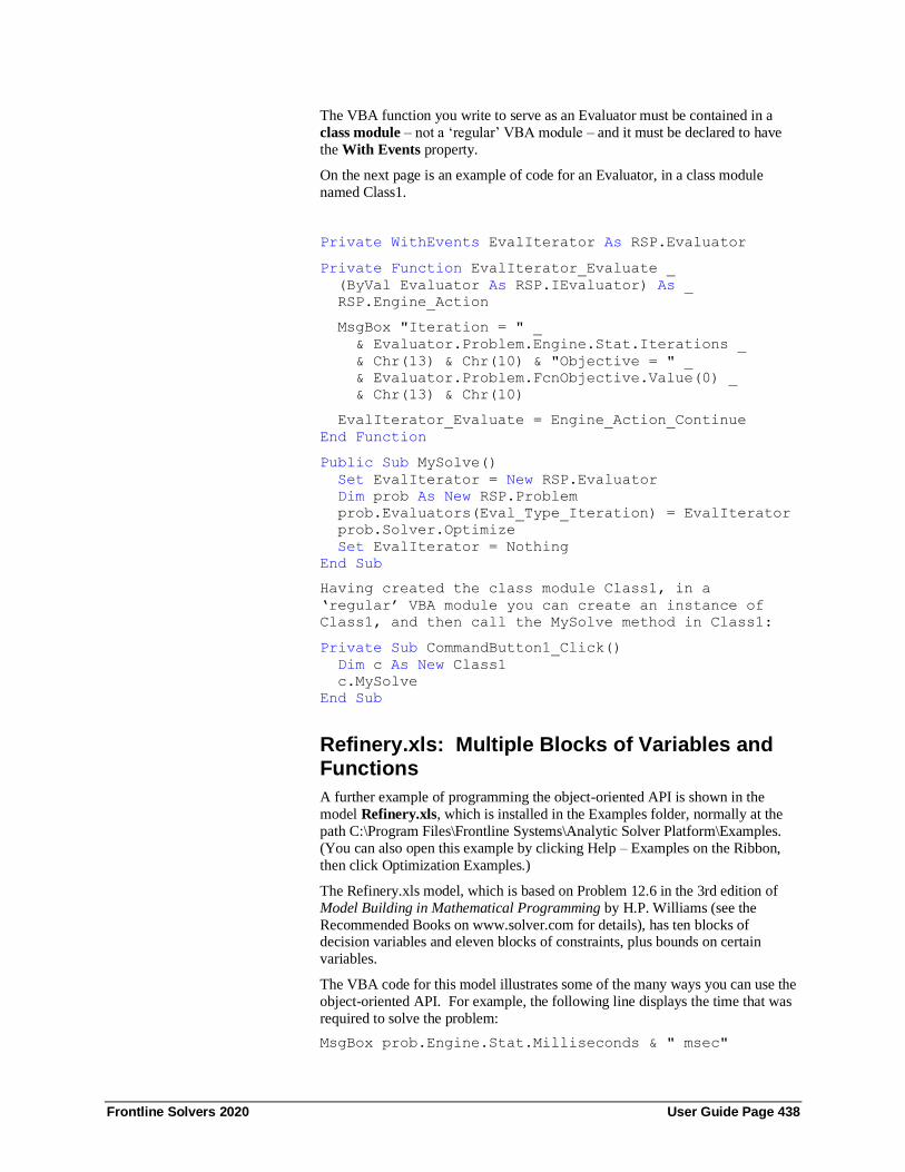
Frontline Solvers 2020 User Guide Page 438
The VBA function you write to serve as an Evaluator must be contained in a
class module – not a ‘regular’ VBA module – and it must be declared to have
the With Events property.
On the next page is an example of code for an Evaluator, in a class module
named Class1.
Private WithEvents EvalIterator As RSP.Evaluator
Private Function EvalIterator_Evaluate _
(ByVal Evaluator As RSP.IEvaluator) As _
RSP.Engine_Action
MsgBox "Iteration = " _
& Evaluator.Problem.Engine.Stat.Iterations _
& Chr(13) & Chr(10) & "Objective = " _
& Evaluator.Problem.FcnObjective.Value(0) _
& Chr(13) & Chr(10)
EvalIterator_Evaluate = Engine_Action_Continue
End Function
Public Sub MySolve()
Set EvalIterator = New RSP.Evaluator
Dim prob As New RSP.Problem
prob.Evaluators(Eval_Type_Iteration) = EvalIterator
prob.Solver.Optimize
Set EvalIterator = Nothing
End Sub
Having created the class module Class1, in a
‘regular’ VBA module you can create an instance of
Class1, and then call the MySolve method in Class1:
Private Sub CommandButton1_Click()
Dim c As New Class1
c.MySolve
End Sub
Refinery.xls: Multiple Blocks of Variables and Functions
A further example of programming the object-oriented API is shown in the
model Refinery.xls, which is installed in the Examples folder, normally at the
path C:\Program Files\Frontline Systems\Analytic Solver Platform\Examples.
(You can also open this example by clicking Help – Examples on the Ribbon,
then click Optimization Examples.)
The Refinery.xls model, which is based on Problem 12.6 in the 3rd edition of
Model Building in Mathematical Programming by H.P. Williams (see the
Recommended Books on www.solver.com for details), has ten blocks of decision variables and eleven blocks of constraints, plus bounds on certain
variables.
The VBA code for this model illustrates some of the many ways you can use the
object-oriented API. For example, the following line displays the time that was
required to solve the problem:
MsgBox prob.Engine.Stat.Milliseconds & " msec"

Frontline Solvers 2020 User Guide Page 439
The following line inserts an Answer Report into the active workbook:
prob.Solver.Report "", "Answer"
The VBA code on the next page illustrates one way to display final solution
values for each of the ten blocks of decision variables in this problem:
For i = 0 To prob.Variables.Count – 1
prob.Variables(i).MakeCurrent
For j = 0 To prob.VarDecision.Size - 1
MsgBox prob.VarDecision.Name _
& "[" & j+1 & "] = " & _
prob.VarDecision.FinalValue(j)
Next j
Next i
When executed, this code displays MessageBoxes such as:
The line prob.Variables(i).MakeCurrent associates the Problem
property VarDecision (a single block of decision variables) with each of the ten
blocks of variables in turn, allowing you to refer to solution values and dual values of this block in more compact notation. A similar line of code can be
used to make the Problem property FcnConstraint represent one of the eleven
blocks of constraints. The .Name property of the block, which usually returns a
string such as “$A$1:$A$10”, returns “Distilled_oil” in this case, since the
Excel model has a defined name for this block of cells.
Adding New Variables and Constraints to a Model
So far, we’ve seen how to access variables and constraints that were defined
interactively through the Ribbon and Task Pane (or the Solver Parameters
dialog), using the Problem object and its VarDecision and FcnConstraint
properties, as well as the Variables and Functions collections. But you can also
add new variables and constraints to a model through the Object-Oriented API,
and have them appear in the Task Pane Model tab. To illustrate some additional properties used in full Analytic Solver Comprehensive, let’s add a recourse
decision variable and a chance constraint.
To add a new decision variable, we create a Variable object, associate it with a
worksheet cell, set its properties, and add it to the Variables collection. To make
this a recourse decision variable, we simply set its VariableType property:
Dim v As New RSP.Variable v.Init "$D$18"
v.VariableType = Variable_Type_Recourse
v.NonNegative
prob.Variables.Add v

Frontline Solvers 2020 User Guide Page 440
Similarly, to add a new constraint, we create a Function object, associate it with
a formula cell on the worksheet, set its properties, and add it to the Functions
collection. To make this a chance constraint, we simply set its FunctionType,
ChanceType and Chance properties:
Dim f As New RSP.Function f.Init "$C$23"
f.FunctionType = Function_Type_Chance
f.ChanceType = Chance_Type_VaR
f.Chance = 0.95
f.LowerBound.Array = 0 '>= 0
prob.Functions.Add f
CuttingStock.xls: Multiple Problems and Dynamically Generated Variables
A more ambitious example of programming the object-oriented API is shown in
the model CuttingStockVBA(Opt).xls, which is installed in the Examples
folder, normally at the path C:\Program Files\Frontline Systems\Analytic Solver
Platform\Examples. (You can also open this example by clicking Help –
Examples on the Ribbon, then click Optimization Examples.)
This application uses the object-oriented API to define and repeatedly solve two
optimization problems, passing information back and forth between the two
problems. One problem is instantiated from a worksheet with the prob.Init
method as mentioned earlier; the other problem is created “from scratch,” with
new dynamically generated decision variables added each time the problem is
solved.
Cutting Stock Problem
CuttingStockVBA(Opt).xls solves a classical “cutting stock” problem, which
arises for example in lumber and paper mills. Imagine that you have a number
of sheets of wood or rolls of paper of a fixed width, waiting to be cut; you have
customer orders for sheets or rolls of various different widths. Your task is to
cut the larger, fixed-width sheets or rolls into different sizes in a way that
minimizes the total stock used while meeting customer demand.
You might for example cut a 100 inch sheet into two sheets of 45 inches
(leaving 10 inches wasted), three sheets of 31 inches (leaving 7 inches wasted),
one 45-inch sheet and one 31-inch sheet (leaving 24 inches wasted), etc. Each of these is called a pattern, and the main problem will have a decision variable
representing the number of copies of that pattern to cut. In a ‘real-life”
application, the number of possible patterns is exponentially large, yielding a
model that’s too large to solve.
Column Generation Method
We can instead use the technique of column generation (‘columns’ here refers to
variables in the main problem). We choose a small initial set of patterns to include in the model, and solve the main problem (an LP). Since it is unlikely
that we chose the perfect set of patterns initially, we use the dual variable
information from the main problem to generate a new pattern. We generate this
new pattern by solving a second optimization problem, called a ‘knapsack’
problem. A decision variable for the new pattern is dynamically created and
added to the main problem, which is solved again. These two problems, the
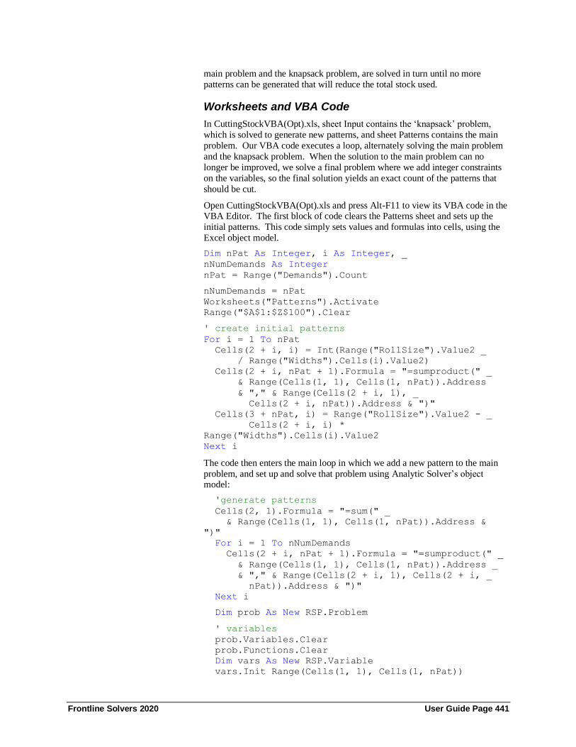
Frontline Solvers 2020 User Guide Page 441
main problem and the knapsack problem, are solved in turn until no more
patterns can be generated that will reduce the total stock used.
Worksheets and VBA Code
In CuttingStockVBA(Opt).xls, sheet Input contains the ‘knapsack’ problem,
which is solved to generate new patterns, and sheet Patterns contains the main
problem. Our VBA code executes a loop, alternately solving the main problem
and the knapsack problem. When the solution to the main problem can no
longer be improved, we solve a final problem where we add integer constraints
on the variables, so the final solution yields an exact count of the patterns that
should be cut.
Open CuttingStockVBA(Opt).xls and press Alt-F11 to view its VBA code in the VBA Editor. The first block of code clears the Patterns sheet and sets up the
initial patterns. This code simply sets values and formulas into cells, using the
Excel object model.
Dim nPat As Integer, i As Integer, _
nNumDemands As Integer
nPat = Range("Demands").Count
nNumDemands = nPat
Worksheets("Patterns").Activate
Range("$A$1:$Z$100").Clear
' create initial patterns
For i = 1 To nPat
Cells(2 + i, i) = Int(Range("RollSize").Value2 _
/ Range("Widths").Cells(i).Value2)
Cells(2 + i, nPat + 1).Formula = "=sumproduct(" _
& Range(Cells(1, 1), Cells(1, nPat)).Address
& "," & Range(Cells(2 + i, 1), _
Cells(2 + i, nPat)).Address & ")"
Cells(3 + nPat, i) = Range("RollSize").Value2 - _
Cells(2 + i, i) *
Range("Widths").Cells(i).Value2
Next i
The code then enters the main loop in which we add a new pattern to the main
problem, and set up and solve that problem using Analytic Solver’s object model:
'generate patterns
Cells(2, 1).Formula = "=sum(" _
& Range(Cells(1, 1), Cells(1, nPat)).Address &
")"
For i = 1 To nNumDemands
Cells(2 + i, nPat + 1).Formula = "=sumproduct(" _
& Range(Cells(1, 1), Cells(1, nPat)).Address _
& "," & Range(Cells(2 + i, 1), Cells(2 + i, _
nPat)).Address & ")"
Next i
Dim prob As New RSP.Problem
' variables
prob.Variables.Clear
prob.Functions.Clear
Dim vars As New RSP.Variable
vars.Init Range(Cells(1, 1), Cells(1, nPat))

Frontline Solvers 2020 User Guide Page 442
vars.NonNegative
prob.Variables.Add vars
Set vars = Nothing
' objective
Dim objective As New RSP.Function
objective.Init Range(Cells(2, 1), Cells(2, 1))
objective.FunctionType = Function_Type_Objective
prob.Functions.Add objective
Set objective = Nothing
' constraints
ReDim constraints(1 To nNumDemands) As _
New RSP.Function
For i = 1 To nNumDemands
constraints(i).Init Range(Cells(2 + i, nPat + 1),
_
Cells(2 + i, nPat + 1))
constraints(i).LowerBound(0) = _
Range("Demands").Cells(i).Value2
prob.Functions.Add constraints(i)
Next i
prob.Solver.SolverType = Solver_Type_Minimize
prob.Engine = prob.Engines("Standard LP/Quadratic")
prob.Solver.Optimize
Next, the code obtains the dual values from the solution to the main problem, via
the Analytic Solver object model, and stores these values as parameters of the
knapsack problem on the Input worksheet, via the Excel object model:
' capture shadow prices
For i = 1 To nNumDemands
Worksheets("Input").Cells(2 + i, 5) = _
prob.Functions(Range(Cells(2 + i, nPat + 1), _
Cells(2 + i, nPat + 1))).DualValue(0)
Next
Worksheets("Input").Activate
Dim j As Integer
j = 1
For i = 1 To prob.Functions.Count
If prob.Functions(i - 1).FunctionType = _
Function_Type_Constraint Then
Cells(2 + j, 5) = _
prob.Functions(i - 1).DualValue(0)
j = j + 1
End If
Next i
The code then sets up and solves the knapsack problem, again using the Analytic
Solver object model:
Dim prob1 As New RSP.Problem
prob1.Init Worksheets("Input")
prob1.Engine = prob1.Engines("Standard
LP/Quadratic")
prob1.Engine.Params("IntTolerance").Value = 0
prob1.Solver.Optimize

Frontline Solvers 2020 User Guide Page 443
If the objective value of the knapsack problem is less than 1 (allowing for
rounding error) – meaning that there are no more patterns that will improve the
solution – we can exit the loop.
If 1 - prob1.FcnObjective.FinalValue(0) _
>= -0.00001 Then
Exit Do
End If
Otherwise, the code writes the new pattern to the Patterns (main problem)
worksheet, using the Excel object model:
Worksheets("Patterns").Activate
Cells(nNumDemands + 3, nPat + 1) = _
Range("RollSize").Value2
' write out new pattern, and associated waste
For i = 1 To nNumDemands
Cells(2 + i, nPat + 1) = _
prob1.VarDecision.FinalValue(i - 1)
Cells(nNumDemands + 3, nPat + 1) = _
Cells(nNumDemands + 3, nPat + 1).Value2 - _
prob1.VarDecision.FinalValue(i - 1) * _
Range("widths").Cells(i).Value
Next i
nPat = nPat + 1
Set prob1 = Nothing
When the Do … Loop is exited, all patterns have been generated. Finally, the
code solves one more problem with integer constraints on the variables, to
ensure that we produce the exact count needed to meet customer demand:
Worksheets("Patterns").Activate prob.Init Worksheets("Patterns")
prob.Functions.Clear
prob.Variables.Clear
' variables
Dim finalvars As New RSP.Variable
finalvars.Init Range(Cells(1, 1), Cells(1, nPat))
For i = 1 To nPat
finalvars.IntegerType(i - 1) =
Integer_Type_Integer
Next i
finalvars.NonNegative
prob.Variables.Add finalvars
' objective
Cells(3 + nNumDemands, nPat + 1).Formula = _
"=sumproduct(" & Range(Cells(1, 1), _
Cells(1, nPat)).Address & "," _
& Range(Cells(3 + nNumDemands, 1), _
Cells(3 + nNumDemands, nPat)).Address & ")"
Dim TotalWaste As New RSP.Function
TotalWaste.Init Range(Cells(3 + nNumDemands, _
nPat + 1), Cells(3 + nNumDemands, nPat + 1))
TotalWaste.FunctionType = Function_Type_Objective
prob.Functions.Add TotalWaste
' constraints
ReDim constraints(1 To nNumDemands) As _

Frontline Solvers 2020 User Guide Page 444
New RSP.Function
For i = 1 To nNumDemands
Cells(2 + i, nPat + 1).Formula = "=sumproduct(" _
& Range(Cells(1, 1), Cells(1, nPat)).Address _
& "," & Range(Cells(2 + i, 1), Cells(2 + i, _
nPat)).Address & ")"
constraints(i).Init Range(Cells(2 + i, nPat + 1),
_
Cells(2 + i, nPat + 1))
constraints(i).LowerBound(0) = _
Range("Demands").Cells(i).Value2
prob.Functions.Add constraints(i)
Next i
prob.Engine = prob.Engines("Standard LP/Quadratic")
prob.Engine.Params("IntTolerance").Value = 0
prob.Solver.Optimize
Set prob = Nothing
This example illustrates some of the power of the object-oriented API.
Although you could use the “traditional” VBA functions to obtain similar
results, it would require quite a bit more code to do so, especially at the step of
obtaining the dual values from the solution of the main problem and using them
to solve the next knapsack problem.
If you wanted to move this application from Excel to a standalone program,
you’d find that nearly all the code in CuttingStockVBA(Opt).xls that references
the Analytic Solver object model could be re-used, with few or no changes, in building an application for the Solver Platform SDK. You’d have to rewrite the
code that references cells via the Excel object model to use arrays in a
programming language instead, but this would not be difficult.

Frontline Solvers 2020 User Guide Page 445
Automating Simulation in VBA
Introduction This chapter explains how to use the Object-Oriented API in Analytic Solver
Desktop to create, modify and solve simulation models under the control of your
custom application written in VBA.
Note: Analytic Solver Cloud does not currently support this functionality.
In the simplest case, you can use a few standard lines of VBA code to enable
and disable Interactive Simulation, as described below. But you can do much
more in VBA, to create custom risk analysis applications.
You can define a Problem and instantiate it from the spreadsheet with two lines
of code, then access the uncertain elements of your model via Variable and
Function objects. You can perform simulations, access trials and summary
statistics, and present them the way you want to your end user. All the power of
the Excel object model is available, including database access, charts and
graphs, and custom dialogs and controls.
Analytic Solver’s VBA object model closely resembles the object-oriented API
of Frontline’s Solver SDK Platform or Solver SDK Pro – which both include a
complete toolkit for Monte Carlo simulation. This makes it easier to move an
application from Excel to a custom program written in C/C++, Visual Basic, VB.NET, Java or MATLAB.
Adding a Reference in the VBA Editor
To use the new object-oriented API in VBA, you must first add a reference to
the type library for the Analytic Solver COM server. To do this:
1. Press Alt-F11 to open the VBA Editor.
2. Select menu choice Tools References.
3. Scroll down until you find Analytic Solver 2020 Type Library.
4. Check the box next to this entry, and click OK to close the dialog.
5. Use File Save to save your workbook.
Note that this is a different reference from Solver, which is the reference you
add in order to use the “traditional” VBA functions.
You need this reference if your VBA code uses the Event Listener as described
in the next section, or uses other elements of the Analytic Solver VBA object
model, described in later sections of this chapter (or both).
Activating Interactive Simulation If you simply want to activate or deactivate Interactive Simulation under
program control, you need a few standard lines of VBA code. You can place
this code in any VBA procedure you write, and cause it to be run in any manner
that is convenient for your application. For example, you could use:

Frontline Solvers 2020 User Guide Page 446
Public Sub ISActivate
Dim ev As New EventListener
ev.AttachEvent Application
Set ev = Nothing
End Sub
Public Sub ISDeactivate
Dim ev As New EventListener
ev.DetachEvent
Set ev = Nothing
End Sub
You could use the Tools Macro Run menu choice in Excel to run these VBA
procedures, or you could associate a Ctrl-Key combination with each procedure,
so it is run when that key combination is pressed.
Another approach appears in the example workbook BusinessPlanPsiChart.xls
(normally installed at C:\Program Files\Frontline Systems\Analytic Solver
Platform\Examples): Two buttons named CommandButton1 and
CommandButton2 are placed on the spreadsheet, along with two images named
Picture Bulb On and Picture Bulb Off, that are stacked on top of each other. The
VBA code is:
Private Sub CommandButton1_Click()
Dim ev As New EventListener
ev.AttachEvent Application
Set ev = Nothing
Me.Shapes("Picture Bulb On").Visible = True
Me.Shapes("Picture Bulb Off").Visible = False
End Sub
Private Sub CommandButton2_Click()
Dim ev As New EventListener
ev.DetachEvent
Set ev = Nothing
Me.Shapes("Picture Bulb On").Visible = False
Me.Shapes("Picture Bulb Off").Visible = True
End Sub
When the “On” button (CommandButton1) is clicked, Interactive Simulation is
activated, and the light bulb is “turned on.” When the “Off” button is clicked,
Interactive Simulation is deactivated, and the light bulb is “turned off.”
Using VBA to Control Analytic Solver You can do much more with VBA: You can perform simulations under your
control, rather than on every worksheet recalculation. You can obtain results of
the simulation – statistics, percentiles, or even raw trial data – that you’d
otherwise obtain through worksheet functions such as PsiMean(),
PsiPercentile(), or PsiData(). You can even define certain worksheet cells as uncertain variables and supply trial data for them in a simulation, without using
functions such as PsiNormal() or PsiUniform() in cell formulas.
You also have access in VBA to the Excel object model, which provides a very
rich source of high-level functions for manipulating cells and ranges, creating
charts and graphs, accessing external databases, and much more. This gives you
a powerful set of tools for developing custom risk analysis applications.

Frontline Solvers 2020 User Guide Page 447
Analytic Solver Object Model
Analytic Solver makes available a hierarchy of objects for describing Monte
Carlo simulation problems, pictured below. This object model is a simplified
subset of the object hierarchy offered by Frontline’s Solver Platform SDK
product, which is used to build custom applications in C/C++, Visual Basic,
VB.NET, Java or MATLAB. Note that the same objects are used for both
optimization and simulation problems.
The Problem object represents the whole problem, and the Model object
represents the internal structure of the model, which in Analytic Solver is defined by your formulas on the spreadsheet. The Solver object represents the
Monte Carlo process – you call its Simulate method to perform a simulation.
The Engine object represents the PSI Technology “engine” – its parameters
include the sampling method, for example. A Variable object represents a
range of one or more contiguous cells that contains uncertain variables, while a
Function object represents a range of cells that contains uncertain functions.
You may have a collection of Variable objects, and a collection of Function
objects in one Problem.
Using the VBA Object Browser
You can examine the Analytic Solver objects, properties and methods in the
VBA Object Browser. To do this, press Alt-F11 to open the VBA Editor, and select menu choice View Object Browser. This displays a child window like the
one pictured below. The dropdown list at the top left corner of the Object
Browser initially displays <All Libraries> – change this to select RSP. Below,
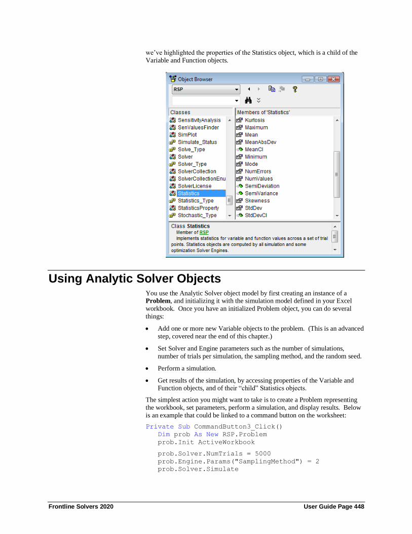
Frontline Solvers 2020 User Guide Page 448
we’ve highlighted the properties of the Statistics object, which is a child of the
Variable and Function objects.
Using Analytic Solver Objects You use the Analytic Solver object model by first creating an instance of a Problem, and initializing it with the simulation model defined in your Excel
workbook. Once you have an initialized Problem object, you can do several
things:
• Add one or more new Variable objects to the problem. (This is an advanced
step, covered near the end of this chapter.)
• Set Solver and Engine parameters such as the number of simulations,
number of trials per simulation, the sampling method, and the random seed.
• Perform a simulation.
• Get results of the simulation, by accessing properties of the Variable and Function objects, and of their “child” Statistics objects.
The simplest action you might want to take is to create a Problem representing
the workbook, set parameters, perform a simulation, and display results. Below
is an example that could be linked to a command button on the worksheet:
Private Sub CommandButton3_Click()
Dim prob As New RSP.Problem
prob.Init ActiveWorkbook
prob.Solver.NumTrials = 5000
prob.Engine.Params("SamplingMethod") = 2
prob.Solver.Simulate

Frontline Solvers 2020 User Guide Page 449
For i = 0 To prob.Functions.Count – 1
MsgBox prob.Functions(i).Statistics.Mean(0)
Next i
Set prob = Nothing
End Sub
The first two lines create an instance of a Problem, and initialize it with the
simulation model defined in your Excel workbook. The next two lines set the
number of trials in the simulation to 5000, and the sampling method to Latin
Hypercube. The fifth line performs a simulation.
The for-loop in the next three lines will step through the Function objects –
assuming, for simplicity here, that each Function object represents just one cell –
and display the Mean property of the child Statistics object (the mean or average
value of the function across all trials) for each one.
Using Variable and Function Objects
When you create and initialize a Problem, a collection of Variable objects and
a collection of Function objects are created automatically. Each Variable object
corresponds to a range of one or more cells that contain PSI Distribution
functions. Each Function object corresponds to a formula cell referenced as the
first argument of a PSI Statistics function, or a range of one or more formula
cells referenced by PsiOutput(). For more information on the grouping of cells into Function objects, please see the Frontline Solvers Reference Guide.
Indexing Variable and Function Objects
The VBA code example above assumes that any cells containing =PsiOutput()
are separated from each other on the worksheet. When uncertain variable and
uncertain function cells lie in a contiguous range – for example A1:A5 or A1:E1
– one Variable or Function object is created to represent all the cells in the range. The Size property of this object tells you the number of cells in the
range, and its other properties may be indexed to access statistics – for example
– of individual cells. The for-loop above could be written in more general form
as:
For i = 0 To prob.Functions.Count – 1 For j = 0 To prob.Functions(i).Size - 1
MsgBox prob.Functions(i).Statistics.Mean(j)
Next j
Next i
Percentiles and AllTrials Properties
In addition to the Statistics child object used above, Variable and Function objects have properties named Percentiles and AllTrials (the raw trial data).
The Percentiles property plays the same role as the PsiPercentile() function on
the spreadsheet. It yields a DoubleMatrix object that takes two subscripts: the
index (starting from 0) of the cell in the range represented by the Variable or
Function object, and the percentile index, which runs from 0 to 98 for the 1st
through 99th percentile.
The AllTrials property plays the same role as the PsiData() function on the
spreadsheet. It yields a DoubleMatrix object that takes two subscripts: the
index (starting from 0) of the cell in the range represented by the Variable or
Function object, and the index of the Monte Carlo trial (starting from 0).

Frontline Solvers 2020 User Guide Page 450
The example code below illustrates how to obtain and display the values of the
uncertain functions for each simulation trial.
For i = 0 To prob.Functions.Count - 1
For j = 0 To prob.Functions(i).Size - 1
MsgBox prob.Functions(i).Percentiles(j,94)
For k = 0 To prob.Solver.NumTrials -1
MsgBox prob.Functions(i).AllTrials(j, k)
Next k
Next j
Next i
GetFrequency Method
Variable and Function objects also have a GetFrequency method, that plays the same role as the PsiFrequency() function on the spreadsheet. It takes an argu-
ment specifying the type of frequency distribution (density, cumulative, etc.)
and an array argument specifying the upper limits of the “bins” for which you
want to obtain frequency data. It yields a DoubleMatrix object that takes two
subscripts: the index (starting from 0) of the cell in the range represented by the
Variable or Function object, and the index (starting from 0) of the frequency bin.
The example code below illustrates the use of the Get Frequency method to
create 14 different "bins" for categorizing the values of the uncertain functions
for each simulation trial.
For i = 0 To prob.Functions.Count - 1
For j = 0 To prob.Functions(i).Size - 1
Dim binlimits(14) As Double
binlimits(0) = -125000
For Count = 1 To 13
binlimits(Count) =
binlimits(Count - 1) + 25000
Next
Dim mymat As New RSP.DoubleMatrix
Set mymat =
prob.Functions(i).GetFrequency(Frequency_Type_Density
, binlimits)
For Count = 0 To 13
MsgBox "Upper Bin Limit"
& ": " & binlimits(Count) & " = " &
mymat(0, Count)
Next Count
Next j
Next i
Controlling Simulation Parameters in VBA
Analytic Solver provides a number of parameters you can use to control the
simulation process, such as the number of Monte Carlo trials to perform, or the
random number seed. You can set these parameters interactively, or by setting
certain Solver properties or Engine.Params properties in VBA.
For example, the first line below sets the number of Monte Carlo trials to 5000.
The second line set the random number seed to a fixed value – so the same

Frontline Solvers 2020 User Guide Page 451
random number sequence is used on each run. The third line sets the sampling
method to Latin Hypercube:
prob.Solver.NumTrials = 5000
prob.Engine.Params("RandomSeed") = 12345
prob.Engine.Params("SamplingMethod") = 2
For a list of simulation parameters that you can set in VBA, see the descriptions
of the “EngineParam Object” and the “ModelParam Object” in the Frontline
Solvers Reference Guide.
Evaluators Called During the Simulation Process
You can write a VBA function that Analytic Solver will call at certain points
during the simulation process. In this “callback function,” you can access
information about the problem and simulation so far, to monitor or report
progress and decide whether to stop or continue the simulation process.
The object-oriented API defines an Evaluator object that is associated with your “callback function” and specifies when Analytic Solver should call it. The VBA
function you write to serve as an Evaluator must be contained in a class module
– not a ‘regular’ VBA module – and it must be declared to have the WithEvents
property.
Here is an example of code for an Evaluator, in a class module named Class1:
Private WithEvents EvalSim As RSP.Evaluator
Private Function EvalSim_Evaluate _
(ByVal Evaluator As RSP.IEvaluator) As _
RSP.Engine_Action
MsgBox "Current Simulation = " _
& Evaluator.Problem.Engine.Stat.Simulations
EvalSim_Evaluate = Engine_Action_Continue
End Function
Public Sub MySim()
Set EvalSim = New RSP.Evaluator
Dim prob As New RSP.Problem
prob.Init ActiveWorkbook
prob.Evaluators(Eval_Type_Simulation) = EvalSim
prob.Solver.Simulate
Set EvalSim = Nothing
End Sub
Having created the class module Class1, in a ‘regular’ VBA module you can
create an instance of Class1, and then call the MySim method in Class1:
Private Sub CommandButton1_Click()
Dim c As New Class1
c.MySim
End Sub
You can define Evaluators to be called when the random sample for all
uncertain variables is generated (Eval_Type_Sample), after each simulation is
completed (Eval_Type_Simulation), or after each trial is completed (Eval_Type_Trial). However, because PSI Technology evaluates all trials in
parallel, an Evaluator to be called on each trial is meaningful only if you use the
Frontline Solvers 2020 User Guide Page 452
Excel Interpreter rather than the PSI Interpreter to calculate the worksheet on
each trial.
Working with Trials and Simulations in VBA Analytic Solver can perform multiple simulations in one run, where each
simulation consists of a number of Monte Carlo trials that you specify. Multiple simulations can be run whenever you choose Simulate – Run Once, whenever
you change a number with Interactive Simulation, or whenever you call the
Problem.Solver.Simulate method in VBA.
In VBA, you can set the property Problem.Solver.NumSimulations = n to
perform n different simulations on a single call to Problem.Solver.Simulate.
After a simulation is run, Analytic Solver Simulation can display each Monte
Carlo trial from the simulation on the Excel worksheet, if desired. In VBA, you
can set the property Problem.Solver.TrialIndex = n to display the nth trial, or
you can call the method Problem.Solver.TrialStep to cycle through the trials.
Displaying Normal or Error Trials
Analytic Solver filters out ‘error trials’ from your simulation results when
computing statistics and displaying charts. An ‘error trial’ is a Monte Carlo trial
where any uncertain function returns an Excel error value. However, all trials
are saved in memory, and you can access the values of uncertain variables and
uncertain functions for each trial, or display each trial on the Excel worksheet.
The Variable and Function objects contain an embedded Statistics object
(described later in this chapter). The property Statistics.NumValues gives the
number of ‘normal’ trials, over which statistics were calculated, and property
Statistics.NumErrors gives the number of error trials that occurred.
You can cause a specific Monte Carlo trial to be displayed on the Excel
worksheet by setting the property Problem.Solver.TrialIndex = n to the index (starting from 1) of the trial you want. This causes the PSI Distribution function
for each uncertain variable to return the sample value it had on the nth trial. The
worksheet is then recalculated, so that each uncertain function will have the
value it had on the nth trial.
To “step through” all trials, normal trials only, or error trials only, and display
them on the Excel worksheet, call the method Problem.Solver.TrialStep
stepsize, trialtype. Trialtype is 0 for all trials, 1 for normal trials, and 2 for error
trials. The stepsize may be positive (1, 2, etc.) or negative (-1, -2, etc.). After
each call to the TrialStep method, the TrialIndex property is set to the index of
the trial just displayed. If stepsize is so large that it would go beyond the last
trial (if positive, or the first trial if negative), the TrialIndex will be set to the last (or first) trial, and that trial will be displayed.
Using Multiple Simulations
For multiple simulations to be useful, some parameter of the model – normally
something you can control – must have a different value in each individual
simulation. Also, you must access statistics, percentiles, and trial data (if used)
for each simulation, so you can compare the results.
If you set Problem.Solver.NumSimulations = n to perform several simulations
on each run, you can use the function PsiSimParam(). This function takes

Frontline Solvers 2020 User Guide Page 453
either two arguments lower and upper, as in PsiSimParam(1,3), or one argument
that’s a cell range or array of numbers, such as PsiSimParam({6.0, 7.5, 9.0}).
On the nth simulation, PsiSimParam() returns the nth value from its argument
list, held constant for all the trials in that simulation. In calls to the PSI
Statistics functions, you can select the simulation for which you want results. For example, if you have an uncertain function in cell F1, you can write
=PsiMean(F1,1), =PsiMean(F1,2), and =PsiMean(F1,3) to access the mean
value of F1 across all the trials in the first simulation, second simulation, and
third simulation, respectively.
If you leave the NumSimulations property at its default value of 1, and call
Problem.Solver.Simulate inside a for-loop, you can set parameter values that
you compute on-the-fly in cells before each simulation using the Excel Range
object. You can either get the values of PSI Statistics functions through the
Excel object model, or (often better) you can access the Statistics, Percentiles
and AllTrials properties, or call the GetFrequency method of your Variables and
Functions, to retrieve the results of that simulation.
Creating Uncertain Variables and SLURPs in VBA The chapter “Mastering Simulation and Risk Analysis Concepts” describes
Stochastic Library Units, Relationships Preserved or SLURPs, and shows how
to create a SLURP on the spreadsheet. You can also create SLURPs in VBA,
and use the SLURP trial data for uncertain variables in your spreadsheet model.
To do this, you first create a Problem object, and initialize it with the simulation
model defined in your Excel workbook. At this point, the Problem’s collection
of Variables will contain Variable objects for each contiguous range of cells
containing PSI Distribution functions in the workbook (if any). You can then:
1. Create a new Variable object in VBA.
2. Set its Name property to an unused cell range (say “Sheet1:A1:A5”).
3. Set its AllTrials property to the SLURP trial data.
4. Add the Variable object to the Problem’s collection of Variables.
The simulation model then behaves just as if these cells contained =PsiSlurp()
function calls that referred to the SLURP trial data you supplied via VBA. The
SLURP data could be generated by your VBA program, read from a database, or
otherwise obtained – it never appears on the Excel spreadsheet. For example:
Dim prob As New RSP.Problem prob.Init ActiveWorkbook
Dim trials As RSP.DoubleMatrix
Set trials = New RSP.DoubleMatrix
trials.InitDense 1, prob.Solver.NumTrials
Randomize
For i = 0 To prob.Solver.NumTrials – 1
trials(0, i) = Rnd()
Next i
Dim var As New RSP.Variable
var.VariableType = Variable_Type_Uncertain
var.Init Range("Sheet1$A$1")
var.AllTrials = trials

Frontline Solvers 2020 User Guide Page 454
prob.Variables.Add var
prob.Solver.Simulate
The first two lines create an instance of a Problem, and initialize it with the
simulation model defined in your Excel workbook. The next three lines create a
DoubleMatrix object named trials to hold SLURP data, and set its dimensions –
just 1 x NumTrials in this case, since we’re adding just one uncertain variable.
The next four lines show how the trials matrix can be initialized with newly
generated values. Of course, you’d want to use a better, application-specific
method – not the Rnd() function – to generate this trial data, or perhaps read the
trial data from a database or external file.
In the next three lines, we create a Variable object, set its Name property to the
cell address Sheet1!A1 (this must be an empty cell on the spreadsheet), and set
its AllTrials property to the trial data we just generated.
In the last two lines, we add the new Variable object to the Problem’s collection
of Variables, and then perform a simulation.
The newly added Variable object, and the SLURP data represented by its
AllTrials property, participates in the simulation model only for so long as the
VBA Problem object exists – it is “transient” and is not saved in the workbook.
Of course, your VBA program code is saved with the workbook, and it can be
run at a later time to re-create the Variable object and re-generate or retrieve the
SLURP data.

Frontline Solvers 2020 User Guide Page 455
Mastering Conventional Optimization Concepts
Introduction This chapter explains basic and advanced concepts of optimization, such as the
types of problems you can solve, types of constraints (regular, integer, conic,
alldifferent) you can specify, the nature of linear, quadratic and nonlinear
functions, convex and non-convex functions, smooth and non-smooth functions,
and the algorithms and methods used by Analytic Solver (or its optimization sub-set products) and plug-in Solver engines.
This chapter focuses on conventional or deterministic optimization models,
which do not include any uncertainty. The next chapter “Mastering Simulation
and Risk Analysis Concepts” explains the concepts of stochastic optimization
models – those that do include uncertainty – and solution methods such as
robust optimization, stochastic programming, and simulation optimization.
If you are using Analytic Solver for the first time, we recommend that you try
out the examples described in the chapter “Examples: Conventional
Optimization” before tackling this material. If you are relatively new to
optimization, you may find it useful to read the first section below, “Elements of Solver Models,” and then proceed to the Examples chapters. If you’ve been
using the Solver for a while, and you’d like a more in-depth review of the
mathematical relationships found in Solver models, and the optimization
methods and algorithms used by the Solver, read the more advanced sections of
this chapter, and the next chapter.
Elements of Solver Models The basic purpose of the Solver is to find a solution – that is, values for the
decision variables in your model – that satisfies all of the constraints and maxi-
mizes or minimizes the objective function value (if there is one). Let’s examine
this framework more closely.
The model you create for use with the Solver is no different from any other spreadsheet model. It consists of input values; formulas that calculate values
based on the input values or on other formulas; and other elements such as
formatting. You can play “what if” with a Solver model just as easily as with
any other spreadsheet model. This familiar concept can be very useful when
you wish to present your results to managers or clients, who are usually
“spreadsheet literate” even if they are unfamiliar with Solvers or optimization.
Decision Variables and Parameters
Some of the input values may be numbers that you use, but you cannot change
on your own – for example, prevailing interest rates or supplier’s prices. We’ll
call these values parameters of the model. You may have several cases,
scenarios, or variations of the same problem to solve, and the parameter values

Frontline Solvers 2020 User Guide Page 456
will change in each problem variation; you can define these parameters via the
Parameters button on the Ribbon. In this chapter, we’ll assume that parameter
values are certain, but the chapter “Mastering Stochastic Optimization
Concepts” will cover situations where the parameter values are uncertain.
Other input values may be quantities that are variable, or under your control in the course of finding a solution. We’ll refer to these as the variables or decision
variables; the Excel Solver refers to them as Changing Cells. The Solver will
find optimal values for these variables or cells. Often, some of the same cell
values you use to play “what if” are the ones for which you’ll want the Solver to
find solution values. These cells are listed in the Variables group in the Task
Pane Model tab, or the Solver Parameters dialog.
The Objective Function
The quantity you want to maximize or minimize is called the objective or
objective function; the Excel Solver often uses the term Set Cell for the
objective. For example, this could be a calculated value for projected profits (to
be maximized), or costs, risk, or error values (to be minimized). It appears under ‘Objective’ in the Task Pane Model tab, or the Solver Parameters dialog.
You may have a Solver model that has nothing to maximize or minimize, in
which case no cell will be listed for the objective. In this situation the Solver
will simply find a solution that satisfies the constraints. Typically this will be
only one of many such solutions, located close to the starting values of the
decision variables.
The Solver also permits you to enter a specific value that you want the objective
function to achieve. This feature was originally included in the Excel Solver to
match the Excel Goal Seek... command, which allows you to seek a specific
value for a cell by adjusting the value of one other cell on which it depends. Using the ‘Value Of’ option for the objective cell has the same effect as adding
an = constraint in the outlined list, with the objective cell on the left hand side
and the constant value on the right hand side; again there is nothing to maximize
or minimize.
There is rarely a good reason to use the Value of option. If your problem
requires only a single objective cell and a single variable cell with no
constraints, you can just use the Goal Seek... command. If you have nothing to
maximize or minimize, we recommend that you omit the objective and enter all
of your constraints in the outlined list under “Constraints.”
Constraints
Constraints are relations such as A1 >= 0. A constraint is satisfied if the condition it specifies is true within a small tolerance. This is a little different
from a logical formula such as =A1>=0 evaluating to TRUE or FALSE which
you might enter in a cell. In this example, if A1 were -0.0000001, the logical
formula would evaluate to FALSE, but with the default Solver Precision setting,
the constraint would be satisfied. Because of the numerical methods used to
find solutions to Solver models and the finite precision of computer arithmetic,
it would be unrealistic to require that constraints like A1 >= 0 be satisfied
exactly – such solutions would rarely be found.
In the Excel Solver, constraints are specified by giving a cell reference such as
A1 or A1:A5 (the “left hand side”), a relation (<=, = or >=), and an expression
for the “right hand side.” Although Excel allows you to enter any numeric expression on the right hand side, for reasons that will be explained in the

Frontline Solvers 2020 User Guide Page 457
chapter “Best Practices for Building Large-Scale Models,” we strongly
encourage you to use only constants, or references to cells that contain constant
values on the right hand side. (A constant value to the Solver is any value that
does not depend on any of the decision variables.)
A constraint such as A1:A5 <= 10 is shorthand for A1 <= 10, A2 <= 10, A3 <= 10, A4 <= 10, A5 <=10. A constraint such as A1:A5 <= B1:B5 is shorthand for
A1 <= B1, A2 <= B2, A3 <= B3, A4 <= B4, A5 <= B5.
Another type of constraint is of the form A1:A5 = integer, where A1:A5 are
decision variables. This specifies that the solution values for A1 through A5
must be integers or whole numbers, such as -1, 0 or 2, to within a small
tolerance. This form of constraint, and related forms such as A1:A5 = binary,
A1:A5 = semicontinuous, and A1:A5 = alldifferent, are explored in the section
“More About Constraints.”
A new type of constraint supported by Analytic Solver is of the form A1:A5 =
conic, where A1:A5 are decision variables. This is called a second order cone constraint and is further described in “More About Constraints.”
Solutions: Feasible, “Good” and Optimal
A solution (set of values for the decision variables) for which all of the
constraints in the Solver model are satisfied is called a feasible solution. In
some problems, a feasible solution is already known; in others, finding a feasible
solution may be the hardest part of the problem.
An optimal solution is a feasible solution where the objective function reaches
its maximum (or minimum) value – for example, the most profit or the least
cost. A globally optimal solution is one where there are no other feasible
solutions with better objective function values. A locally optimal solution is one
where there are no other feasible solutions “in the vicinity” with better objective function values – you can picture this as a point at the top of a “peak” or at the
bottom of a “valley” which may be formed by the objective function and/or the
constraints.
The Solver is designed to find feasible and optimal solutions. In the best case, it
will find the globally optimal solution – but this is not always possible. In other
cases, it will find a locally optimal solution, and in still others, it will stop after a
certain amount of time with the best solution it has found so far. But like many
users, you may decide that it’s most important to find a good solution – one that
is better than the solution, or set of choices, you are using now.
The kind of solution the Solver can find depends on the nature of the mathematical relationships between the variables and the objective function and
constraints (and the solution algorithm used). As explained below, if your
model is smooth convex, you can expect to find a globally optimal solution; if it
is smooth but non-convex, you will usually be able to find a locally optimal
solution; if it is non-smooth, you may have to settle for a “good” solution that
may or may not be optimal.
Below, we summarize the capabilities of the five Solver engines bundled with
Analytic Solver Comprehensive and Analytic Solver Optimization within both
Analytic Solver Desktop and the Cloud app: the LP/Quadratic Solver, SOCP
Barrier Solver, nonlinear GRG Solver, Interval Global Solver, and Evolutionary
Solver. (Analytic Solver Upgrade uses the LP/Quadratic Solver, the nonlinear GRG Solver, and the Evolutionary Solver.) Later sections of this chapter
provide an overview of the optimization methods and algorithms employed by
each of these Solver engines.

Frontline Solvers 2020 User Guide Page 458
Linear Simplex and LP/Quadratic Solver
The Simplex LP Solver with the Excel Solver finds optimal solutions to
problems where the objective and constraints are all linear functions of the
variables. (The term linear function is explained below, but you can imagine its
graph as a straight line.) Since all linear functions are convex, the Solver
normally can find the globally optimal solution, if one exists. Because a linear
function (a straight line) can always be increased or decreased without limit, the
optimal solution is always determined by the constraints; there is no natural
“peak” or “valley” for the objective function itself.
In Analytic Solver Comprehensive, Analytic Solver Optimization, Analytic
Solver Upgrade and Analytic Solver Basic, the linear Simplex Solver is extended to the LP/Quadratic Solver. This Solver handles problems where the
constraints are all linear, and the objective may be linear or quadratic (explained
further below). If the quadratic objective function is convex (if minimizing, or
concave if maximizing) the Solver will normally find a globally optimal
solution. If the objective is non-convex (further explained below), the Solver
will find only a locally optimal solution.
SOCP Barrier Solver
The SOCP Barrier Solver, included in all optimization products, finds optimal
solutions to problems where the objective and constraints are all linear or
convex quadratic functions of the variables. (This is in contrast to the
LP/Quadratic Solver, which permits only the objective function to be quadratic.)
It also finds optimal solutions to problems with a linear objective, linear
constraints, and second order cone (SOC) constraints; this is called a second
order cone programming (SOCP) problem, as explained further below. Since all
linear functions and SOC constraints are convex, the SOCP Barrier Solver
normally finds a globally optimal solution, if one exists.
Nonlinear GRG Solver
The nonlinear GRG Solver (in all Analytic Solver products except Analytic
Solver Simulation) finds optimal solutions to problems where the objective and
constraints are all smooth (convex or non-convex) functions of the variables.
(The term smooth function is explained below, but you can imagine a graph –
whether straight or curved – that contains no “breaks.”) For non-convex
problems, the Solver normally can find a locally optimal solution, if one exists –
but this may or may not be the globally optimal solution. A nonlinear objective function can have a natural “peak” or “valley,” but in most problems the optimal
solution is partly or wholly determined by the constraints. The nonlinear GRG
Solver can be used on problems with all-linear functions, but it is much less
effective and efficient than the LP/Quadratic Solver or the SOCP Barrier Solver
on such problems.
If you use multistart methods for global optimization with the nonlinear GRG
Solver, you will have a better chance (but not a guarantee) of finding the
globally optimal solution. The idea behind multistart methods is to
automatically start the Solver from a variety of starting points, to find the best of
the locally optimal solutions – ideally the globally optimal solution. These
methods are more fully described (and contrasted with other methods for global search) below under “Global Optimization” and in the chapter “Solver Engine
Option Reference” in the Frontline Solvers Reference Guide.

Frontline Solvers 2020 User Guide Page 459
Interval Global Solver
The Interval Global Solver, included in all optimization products, finds globally
optimal solutions to problems where the objective and constraints are all smooth
(convex or non-convex) functions of the variables. Unlike the Evolutionary
Solver or the GRG Solverswith multistart methods, the Interval Global Solver is
normally able to determine for certain that the solution is globally optimal. The
tradeoff is that the Interval Global Solver usually takes much more time to solve
a given problem than the GRG Solver, and this time rises steeply as the number
of variables and constraints in the problem increases. Hence, the Interval Global
Solver is practically able to solve only smaller problems, compared to the GRG
Solver.
Evolutionary Solver
The Evolutionary Solver in Analytic Solver, and all subsets except Analytic
Solver Simulation, usually finds good solutions to problems where the objective
and constraints include non-smooth or discontinuous functions of the variables –
in other words, where there are no restrictions on the formulas that are used to
compute the objective and constraints. For example, if your model uses IF,
LOOKUP or similar functions of the variables, it’s likely that the graphs of these functions will contain “jumps” or “breaks.” For this class of problems, the
Solver will return the best feasible solution (if any) that it can find in the time
allowed.
The Evolutionary Solver can be used on problems with all-smooth functions that
may have multiple locally optimal solutions, in order to seek a globally optimal
solution, or simply a better solution than the one found by the nonlinear GRG
Solver alone; however, the Interval Global Solver or the combination of
multistart methods and the GRG Solver are likely to do as well or better than the
Evolutionary Solver on such problems. It can be used on problems with smooth
convex functions, but it is usually less effective and efficient than the nonlinear
GRG oSolver on such problems. Similarly, it can be used on problems with all-linear functions, but there is little point in doing so when the Simplex (Excel
Solver), LP/Quadratic, or SOCP Barrier Solver is available.
More About Constraints This section explains in greater depth the role of certain types of constraints,
including bounds on the decision variables, equality and inequality constraints,
second order cone constraints, and different forms of integer constraints.
Bounds on the Variables
Constraints of the form A1 >= -5 or A1 <= 10 (for example), where A1 is a
decision variable, are called bounds on the variables and are treated specially by
the Solver. These constraints affect only one variable, whereas general
constraints have an indirect effect on several variables that have been used in a
formula such as A1+A2. Each of the Solver engines takes advantage of this fact
to handle bounds on the variables more efficiently than general constraints.
The most common type of bound on a variable is a lower bound of zero (A1 >=
0), which makes the variable non-negative. Many variables represent physical
quantities of some sort, which cannot be negative. As a convenience, most
Solver Engines offer an option “Assume Non-Negative,” which automatically places a lower bound of zero on every variable which has not been given an
explicit lower bound in the model outline. If you need bounds other than zero,

Frontline Solvers 2020 User Guide Page 460
the Task Pane Platform tab Default Bounds section lets you set default lower
and upper bounds on every decision variable.
Regardless of the Solver engine chosen, bounds on the variables always help
speed up the solution process, because they limit the range of values that the
Solver must explore. In many problems, you will be aware of realistic lower and upper bounds on the variables, but they won’t be of any help to the Solver
unless you include them in the Constraints list box! Bounds on the variables are
especially important to the performance of the Evolutionary Solver, the Interval
Global Solver, and multistart methods for global optimization. They are also
very important if you want the Solver to automatically transform your model,
replacing non-smooth functions (such as IF) with additional variables and linear
constraints.
Equations and Inequalities
Constraints such as A1 = 0 are called equality constraints or equations;
constraints such as A1 <= 0 are called inequality constraints or simply
inequalities. An equality is much more restrictive than an inequality. For
example, if A1 contains the formula =C1+C2, where C1 and C2 are decision
variables, then A1 <= 0 restricts the possible solutions to a half plane, whereas
A1 = 0 restricts the solutions to a line where all possible values of C1and C2
must sum to 0 (C1 = -C2 within a small tolerance, as explained above). Since
there is only a tiny chance that two randomly chosen values for C1 and C2 will
satisfy C1+C2 = 0, solution methods that rely on random choices, such as genetic algorithms, may have a hard time finding any feasible solutions to
problems with equality constraints. To satisfy equality constraints, the Solver
generally must exploit properties of the constraint formula – such as linearity or
smoothness, discussed below – to solve for one variable in terms of another.
A linear equality constraint (like C1+C2 = 0 above) maintains the convexity of
the overall problem, but a nonlinear equality constraint is non-convex, and
makes the overall problem non-convex. Interior point methods may have
difficulty solving problems with nonlinear equality constraints, since they
restrict the ability of the Solver to follow the “central path” inside the feasible
region.
A problem with only equality constraints (and no objective) is sometimes called a system of equations. The Solver can be used to find solutions to systems of
both linear and nonlinear equations. If there are several different solutions (sets
of values for the decision variables) that satisfy the equations, most Solver
engines will find just one solution that is “close” to the starting values of the
variables; but the Interval Global Solver can be used to find all real solutions to
a system of smooth nonlinear equations – a capability that was once felt to be
beyond the limits of any known algorithm.
Second Order Cone Constraints
Analytic Solver supports constraints of the form A1:A5 = conic. This is called a
second order cone (SOC) constraint; it specifies that the vector formed by the
decision variables A1:A5 must lie within the second-order cone (also called the
Lorentz cone, or “ice cream cone”) of dimension 5 – a convex set that looks like
the figure below in three dimensions.

Frontline Solvers 2020 User Guide Page 461
Algebraically, a second-order cone constraint specifies that, given a value for
one variable, the L2-norm of the vector formed by the remaining variables must
not exceed this value: In linear algebra notation, a1 ≥ ║a2:a5║2. In Excel, this
could be written as A1 >= SQRT(SUMSQ(A2:A5)). You can also use a variant
called a “rotated second order cone” constraint. A problem with a linear
objective and linear or SOC constraints is called a second order cone
programming (SOCP) problem; it is always a convex optimization problem.
Decision variables that are constrained to be non-negative also belong to a cone,
called the non-negative orthant. A problem with all linear functions – a linear
programming problem – is a special case of an SOCP problem, where the only cone constraint is non-negativity.
A convex quadratic objective or constraint can be transformed into an equivalent
second order cone constraint. Hence, a problem with a quadratic objective – a
quadratic programming or QP problem – or a problem with quadratic constraints
– called a QCP problem – is also a special case of an SOCP problem. The
SOCP Barrier Solver and the MOSEK Solver will automatically transform
quadratics into SOC form internally; you can simply define your quadratic
objective and/or constraints using ordinary Excel formulas and <= or >=
relations, and use these Solver engines to obtain fast, reliable, globally optimal
solutions to your problem.
Integer and Binary Constraints
As explained in the last section, integer constraints are of the form A1:A5 =
integer, where A1:A5 are decision variables. This specifies that the solution
values for A1 through A5 must be integers or whole numbers, such as -1, 0 or 2,
to within a small tolerance. A common special case that can be entered directly
in the Add Constraint dialog is A1 = binary, which is equivalent to specifying
A1 = integer, A1 >= 0 and A1 <= 1. This implies that A1 must be either 0 or 1 at the solution; hence A1 can be used to represent a “yes/no” decision. Integer
constraints have many important applications, but the presence of even one such
constraint in a Solver model makes the problem an integer programming
problem (discussed below), which may be much more difficult to solve than a
similar problem without the integer constraint.
Semi-Continuous Constraints
It is often useful to place a semi-continuous constraint on a decision variable.
This specifies that, at the solution, the variable must be either 0, or else a
continuous value within a range, determined by the bounds on the variable. For
example, if a machine is either “off” or running at a speed between 5 and 50,
you can model the machine’s speed with A1 = semicontinuous, A1 >= 5 and A1
<= 50. In situations where you might need a binary integer variable and a
regular (continuous) variable, you can sometimes use a single semi-continuous
variable instead – and such a variable can be handled very efficiently by most
Solver engines.

Frontline Solvers 2020 User Guide Page 462
Alldifferent Constraints
A special type of integer constraint supported by Analytic Solver and its subset
products is called an “alldifferent” constraint. Such a constraint is of the form
(for example) A1:A5 = alldifferent, where A1:A5 is a group of decision
variables, and it specifies that these variables must be integers in the range 1 to
N (N = 5 in this example), with each variable different from all the others at the
solution. Hence, A1:A5 will contain a permutation of integers, such as 1,2,3,4,5
or 1,3,5,2,4. The alldifferent constraint can be used to model problems
involving ordering of choices, such as the Traveling Salesman Problem.
Functions of the Variables Since there are large differences in the time it takes to find a solution and the kinds of solutions – globally optimal, locally optimal, or simply “good” – that
you can expect for different types of problems, it pays to understand the
differences between linear, quadratic, smooth nonlinear, and non-smooth
functions, and especially convex and non-convex functions. To begin, let’s
clarify what it means to say that the spreadsheet cells you select for the objective
and constraints are “functions of the decision variables.”
The objective function in a Solver problem is a cell calculating a value that
depends on the decision variable cells; the job of the Solver is to find some
combination of values for the decision variables that maximizes or minimizes
this cell’s value. During the optimization process, only the decision variable
cells are changed; all other “input” cells are held constant. If you analyze the chain of formulas that calculates the objective function value, you will find that
parts of those formulas (those which refer to non-decision variable cells) are
unchanging in value and could be replaced by a numeric constant for the
purposes of the optimization.
If you have constant values on the right hand sides of constraints, then the same
observation applies to the left hand sides of constraints: Parts of the constraint
formulas (those which refer to non-decision variable cells) are unchanging in
value, and only the parts that are dependent on the decision variables “count”
during the optimization.
When you consider whether your objective and constraints are linear, quadratic,
smooth nonlinear, or non-smooth, or convex or non-convex functions of the variables, always bear in mind that only the parts of formulas that are dependent
on the decision variables “count.” Below, we explain that linear functions are
most desirable, and non-smooth and non-convex functions are least desirable in
a Solver model (if you want the fastest and most reliable solutions). A formula
such as =IF(C1>=10,D1,2*D1) is non-smooth if C1 depends on the decision
variables; but if C1 doesn’t depend on the variables, then only D1 or 2*D1 – not
both – can be selected during the solution process. Hence if D1 is a linear
function of the variables, then the IF expression is also a linear function of the
variables.
You may also find that a function that is “bad” (non-smooth or non-convex)
over its full domain (any possible values for the decision variables) can still be “good” (smooth and/or convex) over the domain of interest to you, determined
by other constraints including bounds on the variables. For example, if C1
depends on the variables, then =IF(C1>=10,D1,2*D1) is non-smooth over its
full domain, but smooth – in fact linear – if C1 is constrained to be 10 or more.
=SIN(C1) is non-convex over its full domain, but is convex from –pi to 0, or
from pi to 2*pi.

Frontline Solvers 2020 User Guide Page 463
Convex Functions
The key property of functions of the variables that makes a problem “easy” or
“hard” to solve is convexity. If all constraints in a problem are convex functions
of the variables, and if the objective is convex if minimizing, or concave if
maximizing, then you can be confident of finding a globally optimal solution (or
determining that there is no feasible solution), even if the problem is very large
– thousands to hundreds of thousands of variables and constraints.
In contrast, if any of the constraints are non-convex, or if the objective is either
non-convex, concave if minimizing, or convex if maximizing, then the problem
is far more difficult: You cannot be certain of finding a feasible solution even if
one exists; you must either “settle for” a locally optimal solution, or else be
prepared for very long solution times and rather severe limits on the size of
problems you can solve to global optimality (a few hundred to perhaps one
thousand variables and constraints), even on the fastest computers. So it pays to
understand convexity!
Geometrically, a function is convex if, at any two points x and y, the line drawn
from x to y (called the chord from x to y) lies on or above the function – as shown in the diagram below, for a function of one variable. A function is
concave if the chord from x to y lies on or below the function. This property
extends to any number of ‘dimensions’ or variables, where x = (x1, x2, …, xn)
and y =( y1, y2, …, yn).
Algebraically, a function f is convex if, for any points x and y, and any t between
0 and 1, f( tx + (1-t)y ) <= tf(x) + (1-t)f(y). A function f is concave if –f is
convex, i.e. if f( tx + (1-t)y ) >= tf(x) + (1-t)f(y). A linear function – described
below – is both convex and concave: The chord from x to y lies on the line, and
f( tx + (1-t)y ) = tf(x) + (1-t)f(y). As we’ll see, a problem with all linear
functions is the simplest example of a convex optimization problem that can be
solved efficiently and reliably to very large size.
A non-convex function “curves up and down.” A familiar example is the sine
function (SIN(C1) in Excel), which is pictured below.
The feasible region of an optimization problem is formed by the intersections of
the constraints. The intersection of several convex constraints is always a
convex region, but even one non-convex function can make the whole region
non-convex – and hence make the optimization problem far more difficult to
solve.

Frontline Solvers 2020 User Guide Page 464
Linear Functions
In many common cases, the objective and/or constraints are linear functions of
the variables. This means that the function can be written as a sum of terms,
where each term consists of one decision variable multiplied by a (positive or
negative) constant. Algebraically, we can write:
a1x1 + a2x2 + ... + anxn
where the ais, which are called the coefficients, stand for constant values and the
xis stand for the decision variables. A common example is =SUM(C1:C5),
where C1:C5 are decision variables and the ais are all 1. Note that a linear
function does not have to be written in exactly the form shown above on the
spreadsheet. For example, if cells C1 and C2 are decision variables, B1 =
C1+C2, and B2 = A1*B1 where A1 is constant in the problem, then B2 is a
linear function (=A1*C1+ A1*C2).
Geometrically, a linear function is always a straight line, in n-dimensional space
where n is the number of decision variables. On the next page is a perspective
plot of 2x1 +1x2. As noted above, a linear function is always convex.
Remember that the ais need only be constant in the optimization problem, i.e.
not dependent on any of the decision variables. For example, suppose that the
function is =B1/B2*C1 + (D1*2+E1)*C2, where only C1 and C2 are decision
variables, and the other cells contain constants (or formulas that don’t depend on
the variables). This would still be a linear function, where a1 = B1/B2 and a2 =
(D1*2+E1) are the coefficients, and x1 = C1 and x2 = C2 are the variables.
Note that the SUMPRODUCT and DOTPRODUCT functions compute exactly
the algebraic expression shown above. If we were to place the formula =B1/B2
in cell A1, and the formula =(D1*2+E1) in cell A2, then we could write the
example function above as:
=SUMPRODUCT(A1:A2,C1:C2)
This is simple and clear, and is also useful for fast problem setup as described in
the chapter “Best Practices for Building Large-Scale Models.” If the decision
variable cells that should participate in the expression are not all contiguous on
the spreadsheet, the DOTPRODUCT function can be used instead of
SUMPRODUCT.
As explained below in the section “Derivatives, Gradients, Jacobians and
Hessians,” each coefficient ai in the linear expression a1x1 + a2x2 + ... + anxn is the
first partial derivative of the expression with respect to variable xi. These partial
derivatives are always constant in a linear function – and all higher-order
derivatives are zero.
Frontline Solvers 2020 User Guide Page 465
A nonlinear function (explained further below), as its name implies, is any
function of the decision variables which is not linear, i.e. which cannot be
written in the algebraic form shown above – and its partial derivatives are not
constant. Examples would be = 1/C1, =LOG(C1), =C1^2 or =C1*C2 where
both C1 and C2 are decision variables. If the objective function or any of the constraints are nonlinear functions of the variables, then the problem cannot be
solved with an LP Solver.
Testing for a Linear Model
What if you have already created a complex spreadsheet model without using
functions like SUMPRODUCT, and you aren’t sure whether your objective
function and constraints are linear or nonlinear functions of the variables? If you have Analytic Solver, you can easily find out by pressing the Analyze
button in the Task Pane. Moreover, you can easily obtain a report showing
exactly which cells contain formulas that are nonlinear.
You can try solving the model with the standard LP/Quadratic Solver. If the
problem contains nonlinear functions of the variables, you will (in virtually all
cases) receive the message “The linearity conditions required by this Solver
engine are not satisfied.” You can then ask the Solver to produce a Linearity
Report, which shows whether the objective and each of the constraints is a linear
or nonlinear function of the variables. This report also shows which variables
occur linearly, and which occur nonlinearly in your model – another way of
summarizing the same information. You should next look closely at the objective or constraint formulas that the Linearity Report indicates are
nonlinear, and decide whether (or not) the formula can be written in linear form.
Quadratic Functions
The last two examples of nonlinear functions above, =C1^2 or =C1*C2, are
simple instances of quadratic functions of the variables. A more complex
example is:
=2*C1^2+3*C2^2+4*C1*C2+5*C1
A quadratic function is a sum of terms, where each term is a (positive or
negative) constant (again called a coefficient) multiplied by a single variable or
the product of two variables. In linear algebra notation, we can write xTQx + cx where x is a vector of n decision variables, Q is an n x n matrix of coefficients,
and c is an n vector of linear coefficients. The QUADPRODUCT function
computes values of exactly this form. If we put the constant 5 in A1, 0 in B1, 2
in A2, 4 in B2, 0 in A3 and 3 in B3, then we could write the above example as:
=QUADPRODUCT(C1:C2,A1:B1,A2:B3)
Common uses for quadratic functions are to compute the mean squared error in
a curve-fitting application, or the variance or standard deviation of security
returns in a portfolio optimization application.
As explained below in the section “Derivatives, Gradients, Jacobians and
Hessians,” the coefficients that multiply single variables in a quadratic function are the first partial derivatives of the function with respect to those variables; the
coefficients that multiply the products of two variables are the second partial
derivatives of the function, with respect to those two variables. In a quadratic
function, these first and second order derivatives are always constant, and higher
order derivatives are zero. The matrix Q of second partial derivatives is called
the Hessian of the function.

Frontline Solvers 2020 User Guide Page 466
Convex, Concave and Non-Convex Quadratics
A quadratic function of at least two variables may be convex, concave, or non-
convex. The matrix Q in the general form xTQx has a closely related algebraic
property of definiteness. If the Q matrix is positive definite, the function is
convex; if the Q matrix is negative definite, the function is concave. You can
picture the graph of these functions as having a “round bowl” shape with a
single bottom (or top). If the Q matrix is semi-definite, the function has a bowl
shape with a “trough” where many points may have the same objective value,
but it is still convex or concave. If the Q matrix is indefinite, the function is
non-convex: It has a “saddle” shape, but its true minimum or maximum is not
found in the “interior” of the function but on its boundaries with the constraints, where there may be many locally optimal points. Below is a plot of an example
non-convex quadratic x12 + 2x1x2 – ½ (x2
2 – 1):
A problem with convex quadratic functions is easily solved to global optimality
up to very large size, but a problem with non-convex quadratic functions is a difficult global optimization problem that, in general, will require solution time
that grows exponentially with the number of variables. The way that the Solver
handles such functions is explained further below under “Quadratic
Programming.”
Nonlinear and Smooth Functions
A nonlinear function is any function of the variables that is not linear, i.e. which
cannot be written in the algebraic form:
a1x1 + a2x2 + ... + anxn
Examples, as before, are =1/C1, =LOG(C1), and =C1^2, where C1 is a decision
variable. All of these are called continuous functions, because their graphs are curved but contain no “breaks.” =IF(C1>10,D1,2*D1) is also a nonlinear
function, but it is “worse” (from the Solver’s viewpoint) because it is
discontinuous: Its graph contains a “break” at C1=10 where the function value
jumps from D1 to 2*D1. At this break, the rate of change (i.e. the derivative) of
the function is undefined. As explained below in the section “Derivatives,
Gradients, Jacobians and Hessians,” most Solver algorithms rely on derivatives
to seek improved solutions, so they may have trouble with a Solver model
containing functions like =IF(C1>10,D1,2*D1). The Interval Global Solver
does not accept discontinuous functions at all.
If the graph of the function’s derivative also contains no breaks, then the original
function is called a smooth function. If it does contain breaks, then the original function is non-smooth. Every discontinuous function is also non-smooth. An
example of a continuous function that is non-smooth is =ABS(C1) – its graph is

Frontline Solvers 2020 User Guide Page 467
an unbroken “V” shape, but the graph of its derivative contains a break, jumping
from –1 to +1 at C1=0. Many nonlinear Solver algorithms rely on second order
derivatives of at least the objective function to make faster progress, and to test
whether the optimal solution has been found; they may have trouble with
functions such as =ABS(C1). The Interval Global Solver does not accept any non-smooth functions.
As explained below in the section “Derivatives, Gradients, Jacobians and
Hessians,” general nonlinear functions have first, second, and sometimes higher
order derivatives that change depending on the point (i.e. values of the decision
variables) at which the function is evaluated.
Convex, Concave and Non-Convex Smooth Functions
A general nonlinear function of even one variable may be convex, concave or
non-convex. A function can be convex but non-smooth: =ABS(C1) with its V
shape is an example. A function can also be smooth but non-convex: =
SIN(C1) is an example. But the “best” nonlinear functions, from the Solver’s
point of view, are both smooth and convex (concave for the objective if you are
maximizing).
If a smooth function’s second derivative is always nonnegative, it is a convex
function; if its second derivative is always nonpositive, it is a concave function.
This property extends to any number of ‘dimensions’ or variables, where the
second derivative becomes the Hessian and “nonnegative” becomes “positive
semidefinite.”
Discontinuous and Non-Smooth Functions
Microsoft Excel provides a very rich formula language, including many
functions that are discontinuous or non-smooth. As noted above, discontinuous
functions cause considerable difficulty, and non-smooth functions cause some
difficulty for most nonlinear Solvers; such functions are not accepted by the
Interval Global Solver. Some models can only be expressed with the aid of
these functions; in other cases, you have a degree of choice in how you model
the real-world problem, and which functions you use. Even when you have a
“full arsenal” of Solver engines available, as you do with Analytic Solver
Comprehensive and its subset products, you’ll get better results if you try to use
the most “Solver-friendly” functions in your model.
By far the most common discontinuous function in Excel is the IF function
where the conditional test depends on the decision variables, as in the example
=IF(C1>10,D1,2*D1). Here is a short list of common discontinuous Excel
functions:
IF, CHOOSE
LOOKUP, HLOOKUP, VLOOKUP
COUNT
INT, ROUND
CEILING, FLOOR
Here is a short list of common non-smooth Excel functions:
ABS
MIN, MAX
Formulas involving relations such as <=, = and >= (on the worksheet, not in
constraints) and logical functions such as AND, OR and NOT are discontinuous
at their points of transition from FALSE to TRUE values. Functions such as

Frontline Solvers 2020 User Guide Page 468
SUMIF and the database functions are discontinuous if the criterion or
conditional argument depends on the decision variables.
If you aren’t sure about a particular function, try graphing it (by hand or in
Microsoft Excel) over the expected range of the variables; this will usually
reveal whether the function is discontinuous or non-smooth. If using Analytic Solver, just create a model using the function, and use the Analyze button to
automatically diagnose the model type.
Analytic Solver Comprehensive, Analytic Solver Optimization, Analytic Solver
Upgrade and Analytic Solver Basic can automatically transform a model that
uses IF, AND, OR, NOT, ABS, MIN and MAX, and relations <, <=, >= and > to
an equivalent model where these functions and relations are replaced by
additional binary integer and continuous variables and additional constraints,
that have the same effect – for the purpose of optimization – as the replaced
functions. This powerful facility may be able to transform your non-smooth
model into a smooth or even linear model with integer variables. An example is
shown in the EXAMPLE5 worksheet of the StandardExamples.xls workbook, which is normally installed into C:\Program Files\Frontline Systems\Analytic
Solver Platform\Examples.
Derivatives, Gradients, Jacobians, and Hessians
To find feasible and optimal solutions, most optimization algorithms rely
heavily on derivatives of the problem functions (the objective and constraints)
with respect to the decision variables. First derivatives indicate the direction in
which the function is increasing or decreasing, while second derivatives provide
curvature information.
The partial derivatives of a function f (x1,x2,...,xn) with respect to each variable
are denoted ∂f/∂x1, ∂f/∂x2, …, ∂f/∂xn. They give the rate of change of the function in each dimension. For a linear function a1x1 + a2x2 + ... + anxn, the
partial derivatives are the coefficients: ∂f/∂x1 = a1, ∂f/∂x2 = a2, and so on.
To recap the comments about derivatives made in the sections above:
• Linear functions have constant first derivatives – the coefficients ai – and all
higher order derivatives (second, third, etc.) are zero.
• Quadratic functions have constant first and second derivatives, and all
higher order (third, etc.) derivatives are zero.
• Smooth nonlinear functions have first and second derivatives that are
defined, but not constant – they change with the point at which the function is evaluated.
• Non-smooth functions have second derivatives that are undefined at some
points; discontinuous functions have first derivatives that are undefined at
some points.
The gradient of a function f (x1,x2,...,xn) is the vector of its partial derivatives:
[ ∂f/∂x1, ∂f/∂x2, …, ∂f/∂xn ]
This vector points in the direction (in n-dimensional space) along which the
function increases most rapidly. Since a Solver model consists of an objective
and constraints, all of which are functions of the variables x1,x2,...,xn, it is often
useful to collect these gradients into a matrix, where each row is the gradient
vector for one function:
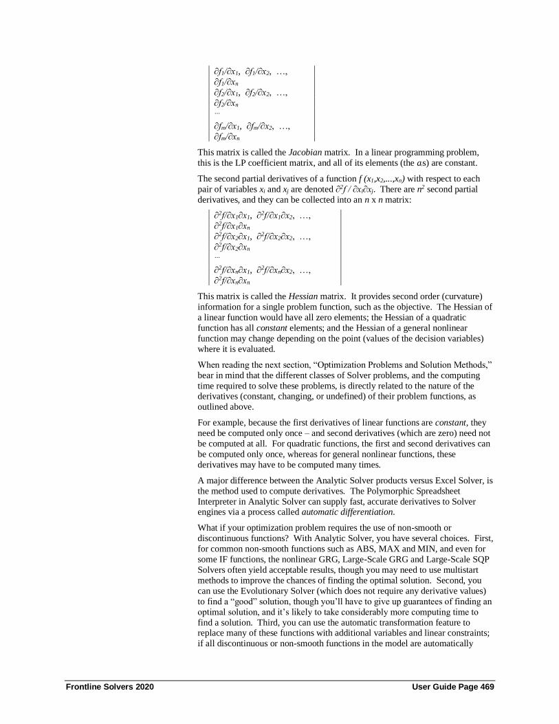
Frontline Solvers 2020 User Guide Page 469
∂f1/∂x1, ∂f1/∂x2, …,
∂f1/∂xn
∂f2/∂x1, ∂f2/∂x2, …,
∂f2/∂xn
…
∂fm/∂x1, ∂fm/∂x2, …,
∂fm/∂xn
This matrix is called the Jacobian matrix. In a linear programming problem,
this is the LP coefficient matrix, and all of its elements (the ais) are constant.
The second partial derivatives of a function f (x1,x2,...,xn) with respect to each
pair of variables xi and xj are denoted ∂2f / ∂xi∂xj. There are n2 second partial
derivatives, and they can be collected into an n x n matrix:
∂2f/∂x1∂x1, ∂2f/∂x1∂x2, …,
∂2f/∂x1∂xn
∂2f/∂x2∂x1, ∂2f/∂x2∂x2, …,
∂2f/∂x2∂xn
…
∂2f/∂xn∂x1, ∂2f/∂xn∂x2, …,
∂2f/∂xn∂xn
This matrix is called the Hessian matrix. It provides second order (curvature)
information for a single problem function, such as the objective. The Hessian of
a linear function would have all zero elements; the Hessian of a quadratic
function has all constant elements; and the Hessian of a general nonlinear
function may change depending on the point (values of the decision variables)
where it is evaluated.
When reading the next section, “Optimization Problems and Solution Methods,”
bear in mind that the different classes of Solver problems, and the computing
time required to solve these problems, is directly related to the nature of the derivatives (constant, changing, or undefined) of their problem functions, as
outlined above.
For example, because the first derivatives of linear functions are constant, they
need be computed only once – and second derivatives (which are zero) need not
be computed at all. For quadratic functions, the first and second derivatives can
be computed only once, whereas for general nonlinear functions, these
derivatives may have to be computed many times.
A major difference between the Analytic Solver products versus Excel Solver, is
the method used to compute derivatives. The Polymorphic Spreadsheet
Interpreter in Analytic Solver can supply fast, accurate derivatives to Solver engines via a process called automatic differentiation.
What if your optimization problem requires the use of non-smooth or
discontinuous functions? With Analytic Solver, you have several choices. First,
for common non-smooth functions such as ABS, MAX and MIN, and even for
some IF functions, the nonlinear GRG, Large-Scale GRG and Large-Scale SQP
Solvers often yield acceptable results, though you may need to use multistart
methods to improve the chances of finding the optimal solution. Second, you
can use the Evolutionary Solver (which does not require any derivative values)
to find a “good” solution, though you’ll have to give up guarantees of finding an
optimal solution, and it’s likely to take considerably more computing time to
find a solution. Third, you can use the automatic transformation feature to replace many of these functions with additional variables and linear constraints;
if all discontinuous or non-smooth functions in the model are automatically

Frontline Solvers 2020 User Guide Page 470
replaced, the problem should be solvable with the nonlinear Solvers, or even
with the linear Solvers in some cases. Fourth, you can manually reformulate
your model with binary integer variables and associated constraints. You can
then use the nonlinear GRG Solver, or even the LP/Quadratic Solver, in
combination with the Branch & Bound method, to find the true optimal solution to your problem. These ideas are explored further in the chapter “Best Practices
for Building Large-Scale Models.”
Optimization Problems and Solution Methods A model in which the objective function and all of the constraints (other than
integer constraints) are linear functions of the decision variables is called a
linear programming (LP) problem. (The term “programming” dates from the
1940s and the discipline of “planning and programming” where these solution
methods were first used; it has nothing to do with computer programming.) As
noted earlier, a linear programming problem is always convex.
If the problem includes integer constraints, it is called an integer linear
programming problem. A linear programming problem with some “regular” (continuous) decision variables, and some variables that are constrained to
integer values, is called a mixed-integer programming (MIP) problem. Integer
constraints are non-convex, and they make the problem far more difficult to
solve; see below for details.
A quadratic programming (QP) problem is a generalization of a linear
programming problem. Its objective is a convex quadratic function of the
decision variables, and all of its constraints must be linear functions of the
variables. A problem with linear and convex quadratic constraints, and a linear
or convex quadratic objective, is called a quadratically constrained (QCP)
problem.
A model in which the objective function and all of the constraints (other than integer constraints) are smooth nonlinear functions of the decision variables is
called a nonlinear programming (NLP) or nonlinear optimization problem. If
the problem includes integer constraints, it is called an integer nonlinear
programming problem. A model in which the objective or any of the constraints
are non-smooth functions of the variables is called a non-smooth optimization
(NSP) problem.
Linear Programming
Linear programming (LP) problems are intrinsically easier to solve than
nonlinear (NLP) problems. First, they are convex, where a general nonlinear
problem is often non-convex. Second, since all constraints are linear, the
globally optimal solution always lies at an “extreme point” or “corner point” where two or more constraints intersect. (In some problems there may be
multiple solutions with the same objective value, all lying on a line between two
corner points.) This means that an LP Solver needs to consider many fewer
points than an NLP Solver, and it is always possible to determine (subject to the
limitations of finite precision computer arithmetic) that an LP problem (i) has no
feasible solution, (ii) has an unbounded objective, or (iii) has a globally optimal
solution.
Frontline Solvers 2020 User Guide Page 471
Problem Size and Numerical Stability
Because of their structural simplicity, the main limitations on the size of LP
problems that can be solved are time, memory, and the possibility of numerical
“instabilities” which are the cumulative result of the small errors intrinsic to
finite precision computer arithmetic. The larger the model, the more likely it is
that numerical instabilities will be encountered in solving it.
Most large LP models are sparse in nature: While they may include thousands
of decision variables and constraints, the typical constraint will depend upon
only a few of the variables. This means that the Jacobian matrix of partial
derivatives of the problem functions, described earlier, will have many elements
that are zero. Such sparsity can be exploited to save memory and gain speed in solving the problem.
The Simplex Method
LP problems are most often solved via the Simplex method. The standard
Microsoft Excel Solver uses a straightforward implementation of the Simplex
method to solve LP problems, when the Assume Linear Model box is checked in
the Solver Options dialog. Analytic Solver Comprehensive, Analytic Solver Optimization, Analytic Solver Upgrade and Analytic Solver Basic use a far
more sophisticated implementation of the Simplex method which exploits
sparsity in the LP model and uses techniques such as presolving, matrix
factorization using the LU decomposition , a fast, stable LU update, and
dynamic Markowitz refactorization.
The Large-Scale LP/QP Solver and MOSEK Solver engines use even more
powerful implementations of the methods mentioned above. They have been
used to solve LP problems with millions of variables and constraints.
The Large-Scale SQP Solver engine includes a powerful linear programming
Solver that uses “active set” methods (closely related to the Simplex method). It
is practical for problems up to 100,000 variables and constraints. This same Solver engine also handles large-scale QP and NLP problems very efficiently.
The Gurobi Solver and XPRESS Solver engine are Frontline’s fastest and most
powerful Solvers for linear programming and especially mixed-integer linear
programming problems. Their advanced primal and dual Simplex and Barrier
methods, combined with state-of-the-art Branch and Cut methods for integer
problems, yield solutions in record time.
Quadratic Programming
Quadratic programming problems are more complex than LP problems, but
simpler than general NLP problems. They have only one feasible region with
“flat faces” on its surface (due to their linear constraints), but the optimal solution may be found anywhere within the region or on its surface. Since a QP
problem is a special case of an NLP problem, it can be solved with the standard
nonlinear GRG Solver, but this may take considerably more time than solving
an LP of the same size. The LP/Quadratic Solver in Analytic Solver
Comprehensive and Analytic Solver Optimization solves QP problems using a
variant of the Simplex method to determine the feasible region, and special
methods based on the properties of quadratic functions to find the optimal
solution.
Most quadratic programming algorithms are specialized to handle only positive
definite (or negative definite) quadratics. The LP/Quadratic Solver, however,
can also handle semi-definite quadratics; it will find one of the equivalent

Frontline Solvers 2020 User Guide Page 472
(globally) optimal solutions – which one depends on the starting values of the
decision variables. When applied to an indefinite quadratic objective function,
the LP/Quadratic Solver provides only the guarantees of a general nonlinear
Solver: It will converge to a locally optimal solution (either a saddle point in the
interior, or a locally optimal solution on the constraint surface).
The Large-Scale LP/QP Solver, Large-Scale GRG Solver, Large-Scale SQP
Solver, Knitro Solver, Gurobi Solver, MOSEK Solver, and XPRESS Solver
engines can all be used to efficiently solve large QP problems.
Quadratically Constrained Programming
A problem with linear and convex quadratic constraints, and a linear or convex
quadratic objective, is called a quadratically constrained (QCP) problem. Such
a problem is more general than a QP or LP problem, but less general than a
convex nonlinear problem. The Simplex-based methods used in the
LP/Quadratic Solver, the Large-Scale LP/QP Solver, and the XPRESS Solver
Engine handle only quadratic objectives, not quadratic constraints. But QCP
problems – since they are convex – can be solved efficiently to global optimality with Barrier methods, also called Interior Point methods.
The SOCP Barrier Solver uses a Barrier method to solve LP, QP, and QCP
problems. The MOSEK Solver Engine uses an even more powerful Barrier
method to solve very large scale LP, QP, and QCP problems, as well as smooth
convex nonlinear problems. Both of these Solvers form a logarithmic “barrier
function” of the constraints, combine this with the objective, and take a step
towards a better point on each major iteration. Unlike the Simplex method,
which moves from one corner point to another on the boundary of the feasible
region, a Barrier method follows a path – called the central path – that lies
strictly within the feasible region.
A Barrier method relies heavily on second derivative information, specifically
the Hessian of the Lagrangian (combination of the constraints and objective) to
determine its search direction on each major iteration. The ability of the Poly-
morphic Spreadsheet Interpreter to efficiently compute this second derivative
information is key to the performance of this method.
Second Order Cone Programming
Second order cone programming (SOCP) problems are a further generalization
of LP, QP, and QCP problems. An SOCP has a linear objective and one or more
linear or second order cone (SOC) constraints. As explained earlier, a second
order cone constraint such as “A1:A5 = conic” specifies that the vector formed
by the decision variables A1:A5 must lie within the second-order cone (also called the Lorentz cone) of dimension 5. Algebraically, the constraint specifies
that a1 ≥ ║a2:a5║2. SOCPs are always convex; the SOCP Barrier Solver and the
MOSEK Solver Engine are both designed to solve SOCP problems, efficiently
to global optimality.
Any convex quadratic constraint can be converted into an SOC constraint, with
several steps of linear algebra. A convex quadratic objective xTQx + cx can be
handled by introducing a new variable t, making the objective minimize t,
adding a constraint xTQx + cx <= t, and converting this constraint to SOC form.
The SOCP Barrier Solver and the MOSEK Solver Engine both make these
transformations automatically; in effect they solve all LP, QP, QCP and SOCP
problems in the same way. Second order cone programming can be viewed as

Frontline Solvers 2020 User Guide Page 473
the natural generalization of linear programming, and is bound to become more
popular in the future.
You can also solve an SOCP with the GRG Nonlinear Solver or the Large-Scale
GRG, Large-Scale SQP, or Knitro Solver engines. Although these Solvers do
not recognize SOC constraints directly, Analytic Solver products will compute values and derivatives for SOC constraints, based on their algebraic form shown
above. Hence, these general nonlinear Solvers handle SOC constraints like
other general nonlinear constraints. Using these Solvers, you can find optimal
solutions for problems containing a mix of linear, general nonlinear, and SOC
constraints – bearing in mind that such problems may be non-convex.
Nonlinear Optimization
As outlined above, nonlinear programming (NLP) problems are intrinsically
more difficult to solve than LP, QP, QCP or SOCP problems. They may be
convex or non-convex, and since their second derivatives are not constant, an
NLP Solver must compute or approximate the Hessians of the problem functions
many times during the course of the optimization. Since a non-convex NLP may have multiple feasible regions and multiple locally optimal points within
such regions, there is no simple or fast way to determine with certainty that the
problem is infeasible, that the objective function is unbounded, or that an
optimal solution is the “global optimum” across all feasible regions. But some
NLP problems are convex, and many problems include linear or convex
quadratic constraints in addition to general nonlinear constraints. Frontline’s
field-installable nonlinear Solver engines are each designed to take advantage of
NLP problem structure in different ways, to improve performance.
If you use the GRG Nonlinear Solver – the only choice for NLPs in the standard
Excel Solver and Analytic Solver Upgrade – bear in mind that it applies the
same method to all problems, even those that are really LPs or QPs. If you don’t select another Solver engine from the Task Pane Engine tab dropdown list
box (or, in the standard Microsoft Excel Solver, if you don’t check the Assume
Linear Model box in the Solver Options dialog), this Solver will be used – and it
may have difficulty with LP or QP problems that could have been solved easily
with one of the other Solvers. Analytic Solver Comprehensive can
automatically determine the type of problem, and select only the “good” or
“best” Solver engine(s) for that problem.
The GRG Method
Analytic Solver includes the enhanced GRG Solver while the Excel Solver uses
the Generalized Reduced Gradient method as implemented in Lasdon and
Waren’s GRG2 code. The GRG method can be viewed as a nonlinear extension
of the Simplex method, which selects a basis, determines a search direction, and
performs a line search on each major iteration – solving systems of nonlinear
equations at each step to maintain feasibility. This method and specific
implementation have been proven in use over many years as one of the most
robust and reliable approaches to solving difficult NLP problems.
As with the Simplex method, the GRG method in the standard Excel Solver uses a “dense” problem representation, and its memory and solution time increases
with the number of variables times the number of constraints. It is also subject
to problems of numerical instability, which may be even more severe than for
LP and QP problems. The GRG Solver engine uses sparse storage methods and
better numerical methods for nonlinear models, such as matrix condition testing
and degeneracy handling, to solve much larger NLP problems.

Frontline Solvers 2020 User Guide Page 474
The SQP Method
The Large-Scale SQP Solver engine for Analytic Solver Comprehensive and
Analytic Solver Optimization uses a Sequential Quadratic Programming (SQP)
method to solve nonlinear optimization problems. This method forms and
solves a QP subproblem, with a quadratic merit function and linearized
constraints, on each major iteration. Because it includes a highly efficient QP
solver, a powerful linear programming solver using “active set” methods, and
sparsity-exploiting matrix factorization, updating and refactorization methods,
the Large-Scale SQP Solver engine is very fast in solving all types of LP, QP
and NLP problems. However, the SQP method typically follows a path of
infeasible trial points until it finds the solution that is both feasible and optimal. Hence, if you stop the Solver before it reports an optimal solution, the GRG
method is far more likely than the SQP method to return a feasible solution as its
“best point so far.”
Interior Point and SLQP Methods
The Knitro Solver engine for Analytic Solver Comprehensive and Analytic
Solver Optimization uses a Barrier or Interior Point method, specialized for non-
convex problems, to solve general nonlinear optimization problems. As with the SOCP Barrier and MOSEK Solvers, this method forms a logarithmic
“barrier function” of the constraints, combines this with the objective, and takes
a step towards a better point on each major iteration. (The actual process of
taking a step and the path followed are more complex, because Knitro assumes
that the problem may be non-convex.) The Knitro Solver uses the PSI
Interpreter to efficiently compute second derivative information, but it also has
options to work with only first derivative information.
The Knitro Solver engine also includes a new, high performance Sequential
Linear-Quadratic (SLQP) method, which is an “active set” method similar to the
SQP method. On highly constrained problems, notably those with equality
constraints, this method typically outperforms the Interior Point method. On loosely constrained or unconstrained problems, the Interior Point method can
greatly outperform SQP and GRG methods, solving problems much larger than
either of these methods. Benchmark studies in the academic literature have
demonstrated exceptionally good performance for the Knitro Solver, on a wide
range of test problems.
The GRG, SQP and Interior Point methods are all subject to the intrinsic
limitations cited above for nonlinear optimization problems: For smooth convex
nonlinear problems, they will (subject to the limitations of finite precision
computer arithmetic) find the globally optimal solution; but for non-convex
problems, they can only guarantee a locally optimal solution. To have a
reasonable chance – let alone a guarantee – that you’ll find the globally optimal solution to a non-convex problem, you must use special methods for global
optimization.
Global Optimization
Analytic Solver Comprehensive and its subset products include powerful tools
to help you find the globally optimal solution for a smooth nonlinear non-
convex problem. These tools include multistart methods, which can be used
with the nonlinear GRG Solver, the Large-Scale GRG Solver, the Large-Scale
SQP Solver, and the Knitro Solver; the Interval Global Solver offers powerful
interval methods for global optimization in a commercial software product; and

Frontline Solvers 2020 User Guide Page 475
the Evolutionary Solver, for global solutions of smooth and non-smooth
problems.
The Multistart Method
The basic idea of the multistart method is to automatically run a nonlinear
Solver from different starting points, reaching different locally optimal
solutions, then select the best of these as the proposed globally optimal solution.
Both clustering and topographic search multistart methods are included in
Analytic Solver and its subset products.
The multistart method operates by generating candidate starting points for the
nonlinear Solver (with randomly selected values between the bounds you
specify for the variables). These points are then grouped into “clusters” – through a method called multi-level single linkage – that are likely to lead to the
same locally optimal solution, if used as starting points for the Solver. The
nonlinear Solver is then run repeatedly, once from (a representative starting
point in) each cluster. The process continues with successively smaller clusters
that are increasingly likely to capture each possible locally optimal solution. A
Bayesian test is used to determine whether the process should continue or stop.
For many smooth nonlinear problems, the multistart method has a limited
guarantee that it will “converge in probability” to a globally optimal solution.
This means that as the number of runs of the nonlinear Solver increases, the
probability that the globally optimal solution has been found also increases
towards 100%. (To attain convergence for constrained problems, an exact penalty function is used in the process of “clustering” the starting points.) For
most nonlinear problems, this method will at least yield very good solutions. As
discussed below, the multistart method, like the Evolutionary Solver, is a
nondeterministic method, which by default may yield different solutions on
different runs. (To obtain the same solution on each run, you can set a Random
Seed option for either of these solution algorithms, as discussed in the chapter
“Solver Engine Option Reference” in the Frontline Solvers Reference Guide.)
As discussed below, the Evolutionary Solver has been enhanced with “filtered
local search” methods that offer many of the benefits of multistart methods –
making the Evolutionary Solver even more effective for global optimization
problems.
The multistart method can be used on smooth nonlinear problems that also
contain integer variables and/or “alldifferent” constraints. But this can take a
great deal of solution time, since the multistart method is used for each
subproblem generated by the Branch & Bound method for integer problems, and
it can also impact the Solver’s ability to find feasible integer solutions. If you
have many integer variables, or alldifferent constraints, try the Evolutionary
Solver as an alternative to the multistart method.
The Interval Branch & Bound Method
In contrast to the multistart methods and the Evolutionary Solver’s methods,
which are nondeterministic methods for global optimization that offer no firm
guarantees of finding the globally optimal solution, the Interval Global Solver in
uses a deterministic method: An Interval Branch & Bound algorithm that will
find the globally optimal solution – given enough time, and subject to some
limitations related to roundoff error, as discussed in the Frontline Solvers
Reference Guide.
The Interval Branch & Bound algorithm processes a list of “boxes” that consist
of bounded intervals for each decision variable, starting with a single box

Frontline Solvers 2020 User Guide Page 476
determined by the bounds that you specify. On each iteration, it seeks lower and
upper bounds for the objective and the constraints in a given box that will allow
it to discard all or a portion of the box (narrowing the intervals for some of the
variables), by proving that the box can contain no feasible solutions, or that it
can contain no objective function values better than a known best bound on the globally optimal objective. Boxes that cannot be discarded are subdivided into
smaller boxes, and the process is repeated. Eventually, the boxes that remain
each enclose a locally optimal solution, and the best of these is chosen as the
globally optimal solution.
Several methods are used to obtain good bounds on the values of the objective
and constraints within a box or region. Classic interval methods rely on the
ability of the PSI Interpreter to evaluate Excel functions over intervals and
interval gradients. Local constraint propagation methods (also known as hull
consistency methods) are used to narrow intervals at each stage of evaluation of
the problem functions. Second-order methods rely on the Interpreter’s ability to
compute interval Hessians of Excel functions, and use a variant of the Interval Newton method to rapidly minimize function values within a region. Innovative
linear enclosure methods – implemented for the first time in the Interval Global
Solver – bound each problem function with a linear approximation that can be
used in a Simplex method-based test for feasibility and local optimality.
The Interval Global Solver also has a unique ability to find all real solutions for
a system of nonlinear equations – which can be listed in the Solutions Report. It
can also find an “inner solution” for a system of nonlinear inequalities – a region
or “box” (bounds on the variables) within which all points satisfy the
inequalities. These capabilities are summarized in the chapter “Getting Results:
Optimization.”
Non-Smooth Optimization
The most difficult type of optimization problem to solve is a non-smooth
problem (NSP). Such a problem may not only have multiple feasible regions
and multiple locally optimal points within each region – because some of the
functions are non-smooth or even discontinuous, derivative or gradient
information generally cannot be used to determine the direction in which the
function is increasing (or decreasing). In other words, the situation at one
possible solution gives very little information about where to look for a better
solution.
In all but the simplest problems, it is impractical to exhaustively enumerate all
of the possible solutions and pick the best one, even on a fast computer. Hence,
most methods rely on some sort of controlled random search, or sampling of possible solutions – combined with deterministic (non-random) methods for
exploring the search space. The Evolutionary Solver, based on genetic
algorithms, relies fairly heavily on controlled random search, whereas the
OptQuest Solver Engine, based on tabu search and scatter search, relies more
heavily on deterministic search methods.
A drawback of these methods is that a solution is “better” only in comparison to
other, presently known solutions; both the Evolutionary and OptQuest Solvers
normally have no way to test whether a solution is optimal. This also means that
these methods must use heuristic rules to decide when to stop, or else stop after a
length of time, or number of iterations or candidate solutions, that you specify.

Frontline Solvers 2020 User Guide Page 477
Genetic and Evolutionary Algorithms
A non-smooth optimization problem can be attacked – though not often solved
to optimality – using a genetic or evolutionary algorithm. (In a genetic
algorithm the problem is encoded in a series of bit strings that are manipulated
by the algorithm; in an “evolutionary algorithm,” the decision variables and
problem functions are used directly. Most commercial Solver products are
based on evolutionary algorithms.)
An evolutionary algorithm for optimization is different from “classical”
optimization methods in several ways. First, it relies in part on random
sampling. This makes it a nondeterministic method, which may yield different
solutions on different runs. (To obtain the same solution on each run, you can set a Random Seed option for the Evolutionary Solver.)
Second, where most classical optimization methods maintain a single best
solution found so far, an evolutionary algorithm maintains a population of
candidate solutions. Only one (or a few, with equivalent objectives) of these is
“best,” but the other members of the population are “sample points” in other
regions of the search space, where a better solution may later be found. The use
of a population of solutions helps the evolutionary algorithm avoid becoming
“trapped” at a local optimum, when an even better optimum may be found
outside the vicinity of the current solution.
Third – inspired by the role of mutation of an organism’s DNA in natural evolution – an evolutionary algorithm periodically makes random changes or
mutations in one or more members of the current population, yielding a new
candidate solution (which may be better or worse than existing population
members). There are many possible ways to perform a “mutation,” and the
Evolutionary Solver actually employs five different mutation strategies. The
result of a mutation may be an infeasible solution, and the Evolutionary Solver
attempts to “repair” such a solution to make it feasible; this is sometimes, but
not always, successful.
Fourth – inspired by the role of sexual reproduction in the evolution of living
things – an evolutionary algorithm attempts to combine elements of existing
solutions in order to create a new solution, with some of the features of each “parent.” The elements (e.g. decision variable values) of existing solutions are
combined in a crossover operation, inspired by the crossover of DNA strands
that occurs in reproduction of biological organisms. As with mutation, there are
many possible ways to perform a “crossover” operation – some much better than
others – and the Evolutionary Solver actually employs multiple variations of
four different crossover strategies.
Fifth – inspired by the role of natural selection in evolution – an evolutionary
algorithm performs a selection process in which the “most fit” members of the
population survive, and the “least fit” members are eliminated. In a constrained
optimization problem, the notion of “fitness” depends partly on whether a
solution is feasible (i.e. whether it satisfies all of the constraints), and partly on its objective function value. The selection process is the step that guides the
evolutionary algorithm towards ever-better solutions.
Hybrid Evolutionary and Other Algorithms
You might imagine that better results could be obtained by combining the
strategies used by an evolutionary algorithm with the “classical” optimization
methods used by the nonlinear GRG and LP/Quadratic Solver. Frontline
Systems has done just that.

Frontline Solvers 2020 User Guide Page 478
The Evolutionary Solver operates as described above, but it also employs
classical methods in two situations: First, when the evolutionary algorithm
generates a new best point, a local search is conducted to try to improve that
point. This step can use a “random local search” method, a gradient-free,
deterministic direct search method, a gradient-based quasi-Newton method, or a “linearized local gradient” method. Second, when the evolutionary algorithm
generates an infeasible point, the Solver can use “repair methods”, a quasi-
Newton method, or even a specialized Simplex method (for subsets of the
constraints that are linear) to transform the infeasible point into a feasible one.
The Evolutionary Solver takes advantage of the diagnostic information available
from the PSI Interpreter: It automatically applies genetic algorithm methods to
non-smooth variable occurrences (where classical methods cannot be used) and
classical methods to smooth and linear variable occurrences. In the local search
phase, it can either fix non-smooth variables, or allow them to vary. And it can
automatically select the most appropriate local search method, based on linearity
and smoothness of the problem functions.
The Evolutionary Solver uses a “distance filter” and a “merit filter” to determine
whether to carry out a local search when the genetic algorithm methods find an
improved starting point. The “distance filter” plays a role similar to “clustering”
in the multistart methods described earlier; both filters contribute to the
excellent performance of the Evolutionary Solver on global optimization
problems.
The “Achilles’ heel” of most evolutionary algorithms is their handling of
constraints – they are typically unable to handle more than a few inequalities, or
any equality constraints at all. In contrast, the hybrid Evolutionary Solver has
been able to find good solutions to non-smooth problems with many – even
hundreds – of constraints.
Tabu Search and Scatter Search
The OptQuest Solver Engine for Analytic Solver Comprehensive and Analytic
Solver Optimization is based on the principles of tabu search and scatter search.
These methods have strong analogies with – and actually predate – genetic
algorithm methods, but they rely less heavily on random choice. They work
with a population of solutions, which are modified and combined in different ways, then subjected to a selection process. Scatter search methods can sample
the space of possible solutions, avoid becoming “trapped” in regions close to
local optima, and adaptively diversify or intensify the search. Tabu search uses
memory of past search steps to avoid repeated steps and improve future
searches. Use of the OptQuest Solver is described in more depth in the
Frontline Solvers Engine User Guide.
Integer Programming When a Solver model includes integer constraints (for example A1:A10 =
integer, A1:A10 = binary, A1:A10 = semicontinuous, or A1:A10 = alldifferent),
it is called an integer programming problem. Integer constraints make a model
non-convex, and finding the optimal solution to an integer programming problem is equivalent to solving a global optimization problem. Such problems
may require far more computing time than the same problem without the integer
constraints.
The standard Microsoft Excel Solver uses a basic Branch & Bound method, in
conjunction with the linear LP/Quadratic or nonlinear GRG Solver, to find
Frontline Solvers 2020 User Guide Page 479
optimal solutions to problems involving general integer or binary integer
variables. Analytic Solver Upgrade and Analytic Solver Basic use a much more
sophisticated Branch & Bound method that is extended to handle alldifferent
constraints, and that often greatly speeds up the solution process for problems
with integer variables. In Analytic Solver Comprehensive and Analytic Solver Optimization, the LP/Quadratic Solver uses improved pseudocost-based branch
and variable selection, reduced cost fixing, primal heuristics, cut generation,
Dual Simplex and preprocessing and probing methods to greatly speed up the
solution of integer linear programming problems.
The Evolutionary Solver handles integer constraints, in the same form as the
other Solver engines (including alldifferent constraints), but it does not make use
of the Branch & Bound method; instead, it generates many trial points and uses
“constraint repair” methods to satisfy the integer constraints. (The constraint
repair methods include classical methods, genetic algorithm methods, and
integer heuristics from the local search literature.) The Evolutionary Solver can
often find good solutions to problems with integer constraints, but where the Branch & Bound algorithm can guarantee that a solution is optimal or is within
a given percentage of the optimal solution, the Evolutionary Solver cannot offer
such guarantees.
The Branch & Bound Method
The Branch & Bound method begins by finding the optimal solution to the
“relaxation” of the integer problem, ignoring the integer constraints. If it
happens that in this solution, the decision variables with integer constraints
already have integer values, then no further work is required. If one or more
integer variables have non-integral solutions, the Branch & Bound method
chooses one such variable and “branches,” creating two new subproblems where
the value of that variable is more tightly constrained. For example, if integer variable A1 has the value 3.45 at the solution, then one subproblem will have the
additional constraint A1 <= 3 and the other subproblem will add the constraint
A1 >= 4. These subproblems are solved and the process is repeated,
“branching” as needed on each of the integer decision variables, until a solution
is found where all of the integer variables have integer values (to within a small
tolerance).
Hence, the Branch & Bound method may solve many subproblems, each one a
“regular” Solver problem. The number of subproblems may grow exponentially.
The “bounding” part of the Branch & Bound method is designed to eliminate
sets of subproblems that do not need to be explored because the resulting
solutions cannot be better than the solutions already obtained.
Cut Generation
The LP/Quadratic Solver, the Large-Scale LP/QP Solver, Large-Scale SQP
Solver, MOSEK Solver, Gurobi Solver, and XPRESS Solver all make use of
“cut generation” methods to improve performance on integer linear program-
ming problems. Cut generation derives from so-called “cutting plane” methods
that were among the earliest methods applied to integer programming problems,
but they combine the advantages of these methods with the Branch & Bound
method to yield a highly effective approach, often referred to as a “Branch &
Cut” algorithm.
A cut is an automatically generated linear constraint for the problem, in addition
to the constraints that you specify. This constraint is constructed so that it “cuts off” some portion of the feasible region of an LP subproblem, without

Frontline Solvers 2020 User Guide Page 480
eliminating any possible integer solutions. Many cuts may be added to a given
LP subproblem, and there are many different methods for generating cuts. For
example, Gomory cuts are generated by examining the reduced costs at an LP
solution, while knapsack cuts, also known as lifted cover inequalities, are
generated from constraints involving subsets of the 0-1 integer variables. Cuts add to the work that the LP solver must perform on each subproblem (and hence
they do not always improve solution time), but on many problems, cut
generation enables the overall Branch & Cut algorithm to more quickly discover
integer solutions, and eliminate branches that cannot lead to better solutions than
the best one already known.
The Alldifferent Constraint
In Analytic Solver Comprehensive and its subset products, a constraint such as
A1:A5 = alldifferent specifies that the variables A1:A5 must be integers in the
range 1 to 5, with each variable different from all the others at the solution.
Hence, A1:A5 will contain a permutation of the integers from 1 to 5, such as
1,2,3,4,5 or 1,3,5,2,4.
To solve problems involving alldifferent constraints, Analytic Solver employs
an extended Branch & Bound method that handles these constraints as a native
type. Whenever variables in an “alldifferent group” have non-integral solution
values, or integral values that are not all different, the Branch & Bound method
chooses one such variable and “branches,” creating two new subproblems where
the value of that variable is more tightly constrained.
The nonlinear GRG Solver, Large-Scale GRG Solver, Large-Scale SQP Solver,
and Knitro Solver engines use this extended Branch & Bound method to solve
problems with integer and alldifferent constraints.
The Large-Scale LP/QP Solver, MOSEK Solver, Gurobi Solver, and XPRESS Solver use their own Branch & Cut methods. They transform alldifferent
constraints into equivalent sets of binary integer variables and additional linear
constraints, then apply their preprocessing, probing and cut generation methods
to these variables and constraints.
The Evolutionary Solver uses methods from the genetic algorithm literature to
handle alldifferent constraints as permutations, including several mutation
operators that preserve the “alldifferent property,” and several crossover
operators that generate a “child” permutation from “parents” that are also
permutations.
Since Solver engines use quite different methods to handle the alldifferent
constraint, you’ll want to try a variety of Solver engines to see which one performs best on your model. This is especially true if your model uses smooth
nonlinear or – even better – linear functions aside from the alldifferent
constraint.
Looking Ahead to Models with Uncertainty If you’ve read through this chapter, congratulations – you’ve learned a great
deal about the nature of optimization problems, and how they are solved! But as
we said in “Elements of Solver Models” at this chapter’s beginning, we’ve
assumed that all parameters of the model are certain. The chapter “Mastering
Stochastic Optimization Concepts” will cover situations where the parameter
values are uncertain – and the problems are called stochastic optimization

Frontline Solvers 2020 User Guide Page 481
problems. In these problems, it’s more important than ever to know how the
objective and constraints depend on the decision variables.
We’ll see that stochastic linear programming problems can be transformed
and solved to optimality far more easily and quickly than stochastic nonlinear,
non-convex problems. We’ll also see that certain ways of summarizing the uncertainty involved in the model, in chance constraints and expected-value
and risk-measure objectives, allow us to form a convex optimization model, that
can be solved quickly and ‘scaled up’ to large size. We’ll see that even one
decision-dependent uncertainty usually makes a model non-convex and non-
smooth, and far more difficult to solve – but we can still find good solutions for
such a model, using high-speed simulation optimization in Analytic Solver.
We explained in this chapter that it’s usually a mistake to apply a general-
purpose Solver to a problem that has a simpler structure – for example, applying
the GRG Solver or Evolutionary Solver to a linear programming problem:
Solution times are much longer than necessary, solutions are less reliable, and
the problem typically cannot be scaled up to large size and still solved by these methods.
In a similar way, we’ll see that it’s usually a mistake to apply a general-purpose
stochastic optimization method to a problem that has a simpler structure – for
example, applying simulation optimization (which requires a general-purpose
Solver) to a stochastic linear programming problem. Again solution times will
be much longer than necessary, solutions are much less reliable, and the problem
typically cannot be scaled up to large size and still solved by these methods.
Frontline Solvers 2020 User Guide Page 482
Mastering Simulation and Risk Analysis Concepts
Introduction To build a Monte Carlo simulation model in Excel, you begin with a
conventional spreadsheet model, designed for ‘what-if’ analysis. Next, you
identify the inputs to your model that are uncertain, and use PSI Distribution
functions to describe the uncertainty. Then, you identify the outputs of special
interest (such as Net Profit), and use PSI Statistics functions to examine or summarize how they behave in light of the uncertainty.
This User Guide assumes you have some experience building conventional
spreadsheet models, and you almost certainly have experience using such
models to ask ‘what if’ questions, by manually changing input values on the
spreadsheet. The key step in risk analysis is to think in terms, not of just one
‘what if’ scenario at a time, but of a range of scenarios, considered at once.
Think of your spreadsheet cells as representing not just single numbers, that you
change once in a while to explore alternatives, but arrays of numbers that cover
the range of possibilities.
Although you can usually visualize the range of values for one input value at a time, it is very difficult to foresee – without computer assistance – the range of
outcomes for an output value that depends on several interacting inputs, each
one subject to uncertainty. But Analytic Solver Comprehensive, Analytic Solver
Simulation and Analytic Solver Basic (in both the Desktop and Cloud apps)
automatically compute the full range of outcomes for every cell in your
spreadsheet model, and enables you to quickly see statistics such as the mean,
standard deviation, or 10th and 90th percentiles of the range of outcomes.
What Happens During Monte Carlo Simulation You’ll find it easier to understand simulation results if you have a good grasp of
the Monte Carlo simulation process. At its heart, this process is very simple. It
consists of the following steps:
1. Generate a random sample for the uncertain variables in your model. If
you specify (say) 1,000 Monte Carlo trials per simulation, then 1,000
randomly chosen values will be generated for each uncertain variable.
2. For each of 1,000 Monte Carlo trials, recalculate your model, with the right
sample values in each uncertain variable cell. When Excel is used to
recalculate, the PSI Distribution function in each uncertain variable cell
returns the correct sample value for that trial. When the PSI Interpreter is
used (as is always the case in Analytic Solver Cloud), this is done internally
(much faster) by Analytic Solver.
3. On each Monte Carlo trial, monitor and save the calculated value of each
uncertain function in your model. (Recall that any formula cell containing a call to PsiOutput(), or referenced in the first argument of PsiOutput() or a

Frontline Solvers 2020 User Guide Page 483
PSI Statistics function, is monitored as an uncertain function cell.) For
1,000 trials, there will be 1,000 saved values for each uncertain function.
When the simulation process is complete, Analytic Solver Simulation uses the
1,000 saved values of each uncertain function to calculate statistics and
percentiles, draw frequency distributions, scatter plots and other charts, and compute values for each PSI Statistic function call in your model.
Random Number Generation and Sampling
On each Monte Carlo trial, sample values are drawn from the probability
distributions represented by the PSI Distribution functions in your model.
Sample values are computed by first drawing a “random number” between 0 and
1, then transforming this uniform random sample value into a sample value that:
• Constrains the samples drawn to obtain better coverage of the sample space,
where each PSI Distribution function is a ‘dimension’ of that space
• Ensures that the frequency distribution of samples drawn properly reflects
the shape and parameters of the PSI Distribution function
• Ensures that the samples drawn for multiple PSI Distribution functions
properly reflect the correlation of distributions with each other
Random Number Generator
Analytic Solver Simulation includes an advanced set of random number
generation capabilities. In common applications, any good random number generator is sufficient – but for challenging applications (for example in
financial engineering) that involve many uncertain variables and many
thousands of trials, the advanced features of Analytic Solver Simulation can
make a real difference.
Computer-generated numbers are never truly “random,” since they are always
computed by an algorithm – they are called pseudorandom numbers. A random
number generator is designed to quickly generate sequences of numbers that are
as close to statistically independent as possible. Eventually, an algorithm will
generate the same number seen sometime earlier in the sequence, and at this
point the sequence will begin to repeat. The period of the random number
generator is the number of values it can generate before repeating.
A long period is desirable, but there is a tradeoff between the length of the
period and the degree of statistical independence achieved within the period.
Hence Analytic Solver Simulation offers a choice of four random number
generators:
• Park-Miller “Minimal” Generator with Bayes-Durham shuffle and
safeguards. This generator has a period of 231-2. Its properties are good,
but the following choices are usually better.
• Combined Multiple Recursive Generator (CMRG) of L’Ecuyer. This
generator has a period of 2191, and excellent statistical independence of
samples within the period.
• Well Equidistributed Long-period Linear (WELL1024) generator of
Panneton, L’Ecuyer and Matsumoto. This very new generator combines a
long period of 21024 with very good statistical independence.

Frontline Solvers 2020 User Guide Page 484
• Mersenne Twister generator of Matsumoto and Nishimura. This generator
has the longest period of 219937-1, but the samples are not as “equidistrib-
uted” as for the WELL1024 and CMRG generators.
Random Number Seeds
As explained in the chapter “Getting Results: Simulation,” the seed, or initial
value, of the random number generator determines whether your results are
exactly reproducible when you re-run a simulation, or whether your results are
similar but not identical because a different random sample was drawn.
You can set a seed for the entire simulation run using the Sim. Random Seed
option – the first option on the Task Pane Engine tab when you select Risk
Solver Engine (the simulation engine) from the dropdown list. Any positive integer sets a specific seed; 0 means the seed will be different on every run.
You can also set a seed for any specific uncertain variable, using the Seed option
in the Uncertain Variable dialog, or by supplying a PsiSeed() property function
as an argument to the PSI Distribution function call. This means the uncertain
variable will have its own independent stream of random numbers starting from
the given seed, whether or not you’ve set a seed for the whole simulation run.
Sampling Method
In standard Monte Carlo sampling, numbers generated by the chosen random
number generator are used directly to obtain sample values for the uncertain
variables (PSI Distribution functions) in the model. With this method, the
variance or estimation error in computed samples for uncertain functions is
inversely proportional to the square root of the number of trials; hence to cut the
error in half, four times as many trials are required.
Analytic Solver Simulation provides two other sampling methods than can
significantly improve the ‘coverage’ of the sample space, and thus reduce the
variance in computed samples for output functions. This means that you can
achieve a given level of accuracy (low variance or error) with fewer trials. You
choose this via the Sampling Method option on the Engine tab, shown above.
Latin Hypercube Sampling. Latin Hypercube sampling begins with a
stratified sample in each dimension (one for each uncertain variable), which
constrains the random numbers drawn to lie in a set of subintervals from 0 to 1.
Then these one-dimensional samples are combined and randomly permuted so
that they ‘cover’ a unit hypercube in a stratified manner. This often reduces the
variance of uncertain functions.
Sobol numbers (Randomized QMC). Sobol numbers are an example of so-
called “Quasi Monte Carlo” or “low-discrepancy numbers,” which are
generated with a goal of coverage of the sample space rather than “randomness”
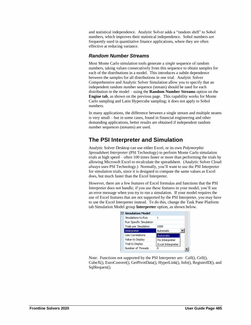
Frontline Solvers 2020 User Guide Page 485
and statistical independence. Analytic Solver adds a “random shift” to Sobol
numbers, which improves their statistical independence. Sobol numbers are
frequently used in quantitative finance applications, where they are often
effective at reducing variance.
Random Number Streams
Most Monte Carlo simulation tools generate a single sequence of random
numbers, taking values consecutively from this sequence to obtain samples for
each of the distributions in a model. This introduces a subtle dependence
between the samples for all distributions in one trial. Analytic Solver
Comprehensive and Analytic Solver Simulation allow you to specify that an
independent random number sequence (stream) should be used for each distribution in the model – using the Random Number Streams option on the
Engine tab, as shown on the previous page. This capability works for Monte
Carlo sampling and Latin Hypercube sampling; it does not apply to Sobol
numbers.
In many applications, the difference between a single stream and multiple strams
is very small – but in some cases, found in financial engineering and other
demanding applications, better results are obtained if independent random
number sequences (streams) are used.
The PSI Interpreter and Simulation
Analytic Solver Desktop can use either Excel, or its own Polymorphic
Spreadsheet Interpreter (PSI Technology) to perform Monte Carlo simulation trials at high speed – often 100 times faster or more than performing the trials by
allowing Microsoft Excel to recalculate the spreadsheet. (Analytic Solver Cloud
always uses PSI Technology.) Normally, you’ll want to use the PSI Interpreter
for simulation trials, since it is designed to compute the same values as Excel
does, but much faster than the Excel Interpreter.
However, there are a few features of Excel formulas and functions that the PSI
Interpreter does not handle; if you use these features in your model, you’ll see
an error message when you try to run a simulation. If your model requires the
use of Excel features that are not supported by the PSI Interpreter, you may have
to use the Excel Interpreter instead. To do this, change the Task Pane Platform
tab Simulation Model group Interpreter option, as shown below.
Note: Functions not supported by the PSI Interpreter are: Call(), Cell(),
CubeX(), EuroConvert(), GetPivotData(), HyperLink(), Info(), RegisterID(), and
SqlRequest().

Frontline Solvers 2020 User Guide Page 486
More About the PSI Interpreter
So, how does the PSI Interpreter work, and how can it be so much faster than
Excel alone for simulation? To answer this, we must look at how Excel itself
computes values for your formulas.
Microsoft Excel is an interpreter for spreadsheet formulas. When you enter a
formula such as =A1+A2*(A3-4) in cell B1, Excel first scans and parses the
formula, storing the results in a coded internal form. It also maintains storage
for A1, A2, A3 and thousands of other cells. When you change a number and
recalculate, Excel refers to the coded internal form, looks up the values of A1,
A2 and A3 and fetches the constant 4, performs the arithmetic, and saves the
result in storage reserved for B1. Only a small part of the time is spent on the actual arithmetic – most of the time goes into processing the encoded formula,
and looking up and saving cell values.
PSI stands for Polymorphic Spreadsheet Interpreter. PSI is also an interpreter
for spreadsheet formulas, that accepts the same formula syntax and built-in
functions as Microsoft Excel. But where Excel evaluates formulas only for one
datatype – single numbers, PSI can evaluate formulas for many different
datatypes. (The word “polymorphic” comes from object-oriented programming,
where it has essentially the same meaning.)
One of the special PSI datatypes is Monte Carlo trials, where each number is
replaced by a vector of 1,000 or more trial values. The heart of PSI speed comes from the fact that it processes the encoded formula once, fetches 1,000 data
values at once, and performs the arithmetic for all 1,000 values at once. Hence,
the “overhead” of the interpreter is incurred once rather than 1,000 times; most
of the time is spent doing the actual arithmetic. PSI is so fast because it is
specialized for simulation (and optimization).
Uncertain Functions, Statistics, and Risk Measures Once a Monte Carlo simulation is complete, what statistics should you use to
evaluate the outputs of special interest in your model? The answer depends on
your application, but some general guidelines can be given.
Descriptive statistics are usually classified into measures of central tendency,
and measures of variation or dispersion. You should look at both kinds of measures, and at some kind of quantile measure, to assess almost any output in
your model.
Measures of Central Tendency
Analytic Solver provides several measures of central tendency:
• PsiMean, the average of all the values
• PsiPercentile for the median or 50th percentile
• PsiMode, the most frequently occurring single value
Measures of Variation
Analytic Solver provides several standard measures of variation:
• PsiVariance, which describes the spread of the distribution of values
• PsiStdDev for standard deviation, the square root of variance
Frontline Solvers 2020 User Guide Page 487
• PsiSkewness, which describes the asymmetry of the distribution of values
• PsiKurtosis, which describes the peakedness of the distribution of values
• PsiMin, PsiMax, and PsiRange for the minimum and maximum values,
and the difference between them
Risk Measures
Analytic Solver also provides several risk measure functions that are most often
used in quantitative finance applications, but may be used in any model.
• PsiAbsDev for ‘MAD’, which measures absolute deviations from the mean
• PsiSemiVar for semivariance or lower partial moment, which measures and
weights negative deviations from the mean
• PsiSemiDev for semideviation, the square root of semivariance (qth root for
the lower partial moment)
PsiSemiVar and PsiSemiDev are useful in situations where ‘upward’ variation – for example, higher stock prices or increased profits – is desirable, but ‘down-
ward’ variation – lower prices or losses – is undesirable.
Quantile Measures
To get a complete grasp of the range of outcomes, it’s essential to look at
quantile measures, such as percentiles and Value at Risk, in addition to
measures of central tendency and variation. Quantile measures allow you to
answer questions such as ‘How much money might we lose, with 5% or 10%
probability?” or “What is the probability that we’ll make at least $100,000?”
based on your simulation model. Analytic Solver provides:
• PsiPercentile, which provides percentile values from 1% to 99%
• PsiTarget, which returns the proportion of values less than or equal to a
target value
• PsiBVaR, which measures standard (‘Basel’) Value at Risk
• PsiCVaR, which measures Conditional Value at Risk
Confidence Intervals
Every Monte Carlo simulation uses a sample of the possible values of your
uncertain variables; hence any statistic resulting from the simulation involves
some degree of sampling error. For the mean and standard deviation of an
output value, Analytic Solver Simulation provides functions that help you assess this error, and estimate the range or interval in which you can be confident that
the true mean or standard deviation lies, at a confidence level that you specify:
• PsiMeanCI, which returns a confidence interval for the mean
• PsiStdDevCI, which returns a confidence interval for the standard
deviation
• PsiCITrials, which returns the number of simulation trials needed to obtain
a confidence interval of a given size, at a given confidence level

Frontline Solvers 2020 User Guide Page 488
Uncertain Variables and Probability Distributions For experienced spreadsheet modelers, the most challenging task in creating a
Monte Carlo simulation model is usually not identifying the key inputs and
outputs, but selecting an appropriate probability distribution and parameters to
model the uncertainty of each input variable.
Analytic Solver provides over 40 analytic probability distributions – which one
should you use? Again the answer depends on your application, but some
general guidelines can be given.
If a Certified Distribution (see below under “Probability Management
Concepts”) is available for an uncertain variable – for example, your company’s
estimate of the range and probabilities for prices of certain chemical feedstocks, or a service provider’s estimate of the range and probabilities for stock or bond
prices – you can simply use the Certified Distribution.
Discrete Vs. Continuous Distributions
If you must choose or create your own distribution, the first step is to determine
whether to use a discrete or continuous form. If there are a small number of
possible values for the uncertain variable, you may be able to use a discrete
analytic distribution, or construct a discrete custom distribution. If the under-
lying physical process involves discrete, countable entities – such as the number
of customers arriving at a service window – you can use a discrete distribution.
If the possible values are highly divisible – such as most prices, volumes,
interest rates, exchange rates, weights, distances, etc. – you will likely use a continuous distribution. In some cases, you may use a continuous distribution to
approximate a discrete distribution.
Bounded Vs. Unbounded Distributions
Another characteristic that distinguishes input distributions is the range of
sample values they can generate. Some distributions are intrinsically bounded –
samples are guaranteed to lie between a known minimum and maximum value.
Examples are the Uniform, Triangular, Beta, and Binomial distributions. Other
analytic distributions are unbounded – sample values may cluster around the
distribution’s mean, but may sometimes have extreme negative or positive
values. Examples are the Normal, Logistic, and Extreme Value distributions.
Still other distributions are partially bounded, with a known minimum such as zero, but no maximum value. Examples are the Exponential, Poisson, and
Weibull distributions.
At times, you may find that the most appropriate distribution (say the Normal) is
unbounded, but you know that the realistic values of the physical process are
bounded, or your model is designed to handle values only up to some realistic
limit. You can impose bounds on any distribution using Analytic Solver
Simulation’s Uncertain Variable dialog. For information about “cutoff bounds”
and “censor bounds” (both may be used), consult the Frontline Solvers
Reference Guide.
Analytic Vs. Custom Distributions
A third characteristic of input distributions is whether they are analytic (also
called parametric) or custom (sometimes called non-parametric) distributions.
An analytic distribution has a form derived from certain theoretical assumptions

Frontline Solvers 2020 User Guide Page 489
about the problem. For example, a Poisson distribution is derived from an
assumption that events are independent and occur at a known average rate, and
an Exponential distribution is derived from an assumption of a constant rate of
decay in some process. A custom distribution has a form dictated by either past
data or expert opinion about the range and frequency of sample values. Analytic Solver offers five general-purpose functions – PsiCumul, PsiDiscrete,
PsiDisUniform, PsiGeneral and PsiHistogram – to help you model custom
distributions. Generally speaking, you should choose an analytic distribution if
– and only if – the theoretical assumptions truly apply in your situation.
Creating your Own Distributions When Past Data is Available
If you have, or you can collect data on the past performance of the uncertain
variable – and if you believe that ‘past performance’ is likely to be
representative of future performance – you have three options:
• If you can fit the data (past observations) to a specific type of analytic
distribution and its parameters, and if there is reason to believe that the
underlying process that the uncertain variable is measuring is consistent with the assumptions from which the analytic distribution is derived, you
can use this distribution (for example PsiNormal, PsiWeibull, etc.) for the
variable. See “Using the Fit Feature” section below. Note: Data used in
fitting a distribution should be independent.
• If you have a reasonably large number of observations of past performance
of the variable, compared to the number of simulation trials you want to
run, you can use the past data itself for simulation trials, in the form of a
SIP (Stochastic Information Packet) or a DIST (Distribution String), and
use the PsiSip() or PsiSlurp() distribution function for the uncertain
variable. See “Probability Management Concepts” and, for DISTs,
“Stochastic Libraries: SIPs and SLURPs” below.
• If – as is often the case – you have a relatively small number of
observations of past performance compared to the number of trials you want
to run, you may be better off resampling the past performance data. To do
this, store the past data in a cell range or SIP, and use the PsiDisUniform()
function (single values) or the PsiResample() function (multiple values).
The difference is that, instead of using all of the past observations (one per
simulation trial), you randomly sample the past observations on each trial.
You can use the Analytic Solver GUI to find the best-fitting analytic
distribution. Both discrete and continuous distributions can be fitted to data; 29
common distributions (out of the 40+ available) are used for fitting. You can
also call the Distribution object Fit and AutoFit methods in your VBA code, as described in the chapter “VBA Object Model Reference” within the Frontline
Solvers Reference Guide.
When Past Data is Not Available
If you don’t have, and you cannot easily collect data on the past performance of
the uncertain variable – or if past performance is not likely to be representative
of future performance – you must tackle the problem in a different way:
• Consult the literature for your industry, if available, to find examples of
applications like yours where simulation models were built. Find out – by
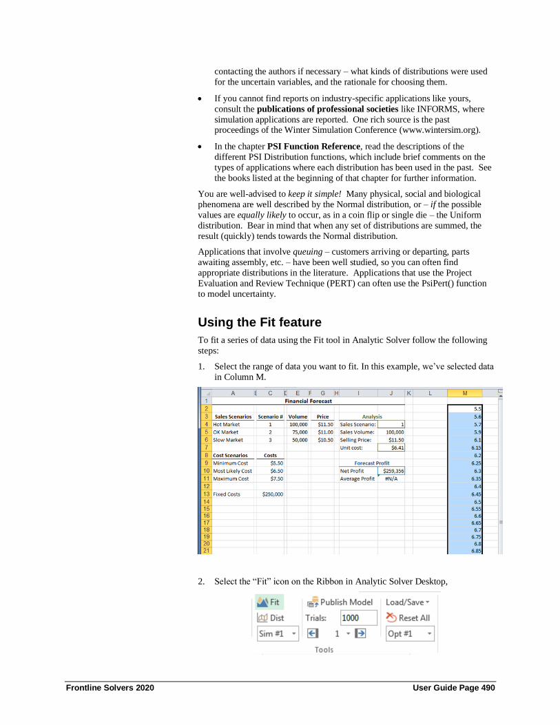
Frontline Solvers 2020 User Guide Page 490
contacting the authors if necessary – what kinds of distributions were used
for the uncertain variables, and the rationale for choosing them.
• If you cannot find reports on industry-specific applications like yours,
consult the publications of professional societies like INFORMS, where
simulation applications are reported. One rich source is the past proceedings of the Winter Simulation Conference (www.wintersim.org).
• In the chapter PSI Function Reference, read the descriptions of the
different PSI Distribution functions, which include brief comments on the
types of applications where each distribution has been used in the past. See
the books listed at the beginning of that chapter for further information.
You are well-advised to keep it simple! Many physical, social and biological
phenomena are well described by the Normal distribution, or – if the possible
values are equally likely to occur, as in a coin flip or single die – the Uniform
distribution. Bear in mind that when any set of distributions are summed, the
result (quickly) tends towards the Normal distribution.
Applications that involve queuing – customers arriving or departing, parts
awaiting assembly, etc. – have been well studied, so you can often find
appropriate distributions in the literature. Applications that use the Project
Evaluation and Review Technique (PERT) can often use the PsiPert() function
to model uncertainty.
Using the Fit feature
To fit a series of data using the Fit tool in Analytic Solver follow the following
steps:
1. Select the range of data you want to fit. In this example, we’ve selected data
in Column M.
2. Select the “Fit” icon on the Ribbon in Analytic Solver Desktop,

Frontline Solvers 2020 User Guide Page 491
In Analytic Solver Cloud, select Fit on the Tools ribbon.
3. Make any changes to the default settings on the Fit Options dialog.
For the Type, select Continuous if the uncertain variable’s values are highly
divisible – such as most prices, volumes, interest rates, exchange rates, weights, and distances – or Discrete if the underlying physical process involves discrete,
countable entities.
The checkbox Allow Shifted Distributions allows Analytic Solver to shift the
center of analytic distribution (equivalent to using the PsiShift() property
function) to better fit the sample data; sometimes this is not desirable, so the box
may be unchecked.
When fitting a sample to a distribution, it is important that the trial values are
not in any way correlated with each other. In other words it is important that
each trial is independent. If the checkbox Run Sample Independence Test is
checked, the Psi Interpreter will run an independence test and will report an
error if the trial values are found to be dependent.
Note: This option is not included in Analytic Solver Cloud. In the Cloud app,
this feature is always on.
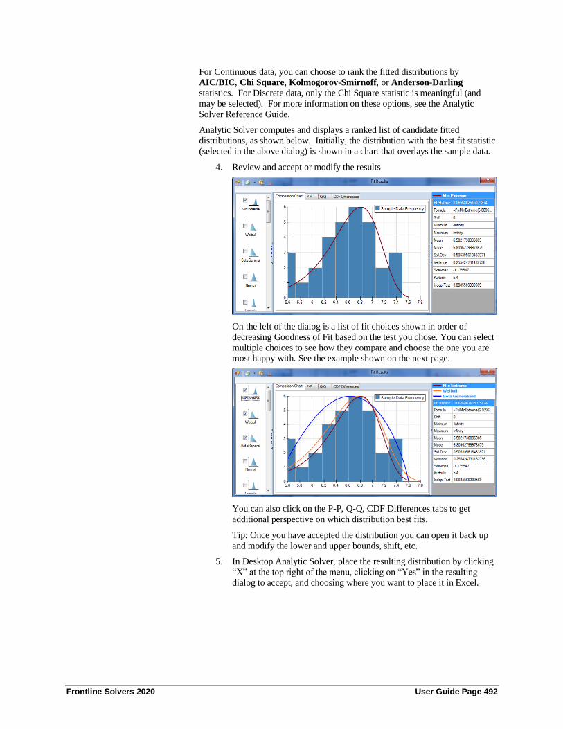
Frontline Solvers 2020 User Guide Page 492
For Continuous data, you can choose to rank the fitted distributions by
AIC/BIC, Chi Square, Kolmogorov-Smirnoff, or Anderson-Darling
statistics. For Discrete data, only the Chi Square statistic is meaningful (and
may be selected). For more information on these options, see the Analytic
Solver Reference Guide.
Analytic Solver computes and displays a ranked list of candidate fitted
distributions, as shown below. Initially, the distribution with the best fit statistic
(selected in the above dialog) is shown in a chart that overlays the sample data.
4. Review and accept or modify the results
On the left of the dialog is a list of fit choices shown in order of
decreasing Goodness of Fit based on the test you chose. You can select
multiple choices to see how they compare and choose the one you are
most happy with. See the example shown on the next page.
You can also click on the P-P, Q-Q, CDF Differences tabs to get
additional perspective on which distribution best fits.
Tip: Once you have accepted the distribution you can open it back up
and modify the lower and upper bounds, shift, etc.
5. In Desktop Analytic Solver, place the resulting distribution by clicking
“X” at the top right of the menu, clicking on “Yes” in the resulting
dialog to accept, and choosing where you want to place it in Excel.

Frontline Solvers 2020 User Guide Page 493
In Analytic Solver Cloud, you'll be asked for the cell address. Simply
type the cell address and then click OK.
You can see the new distribution where you placed it by clicking the cell. It will show up in the formula bar and if you leave the mouse over
that cell a pop-up will show your distribution.
More Hints and Warnings
Using a Triangular Distribution
If you have only estimates of the minimum, maximum, and most likely values of
an uncertain variable – and no other past data or literature references – you can
create a PsiTriangular distribution from these three numbers. This is unlikely
to be a highly accurate representation of the uncertainty, but it will allow you to
get started, and it is far better than a single average value. If your ‘minimum’ and ‘maximum’ values are really low- and high-percentile estimates rather than
the absolute lowest and highest values that can occur, consider using the
PsiTriangGen distribution instead.
Define Each Uncertain Variable Only Once
Often, you’ll need to use the same uncertain variable in several different
formulas in your model. A very common error is to enter the same distribution function, with the same parameters (say PsiNormal(100, 10)), several times in a
model – in a belief that these instances will yield the same results on each trial.
This is incorrect – by doing this, you’ve actually defined several independent
uncertain variables that may well sample different values on each trial. You
should instead enter =PsiNormal(100, 10) in a cell such as A1, and use A1 in
each cell formula where the variable is needed.

Frontline Solvers 2020 User Guide Page 494
Compute Statistics Only on Final Outputs
Another common error is to use formulas in your model to compute a statistic
across two or more uncertain variables, and then use this statistic in further
calculations that are part of the same simulation model.
For example, suppose you have two uncertain variables, =PsiUniform(0,10) in
cell A1 and =PsiUniform(0,20) in B1. You want to know the mean or average
value of these two variables, across the trials of the simulation. The wrong way
to do this is to put = (A1+B1)/2 or =AVERAGE(A1,B1) in cell C1. This takes
the average of A1 and B1 on each trial – the result will be a distribution that
tends to the Normal, with a different (larger) mean than you probably intended.
The right way to do this is to put =PsiDisUniform(A1,B1) in cell C1. Now the distribution of cell C1 is “flat:” On each trial only one of A1 or B1 is selected.
David Vose, principal of Vose Consulting, offers his cardinal rule of risk
analysis modeling: “Every trial of a risk analysis model must be a scenario that
could actually occur.” To ensure that this is true, you may need to specify
correlations between your uncertain variables, as described in the next section.
Dependence and Correlation Unless you specify otherwise, Monte Carlo simulation assumes that each of your
uncertain variables is independent of all the other uncertain variables. When
two variables are independent, the value of one variable on a given trial conveys
no information about the value of the other variable. When two variables are
dependent, there is a statistical relationship between them: On average, the value of one variable on a given trial does convey information about the value of
the other variable on that trial.
Measuring Observed Correlation
Correlation is a statistical measure of the degree to which one variable is related
to another. When we observe that two variables are correlated, it may be that
one variable is dependent on the other, or that both variables are dependent on a
third variable, or that the correlation appeared by chance and there is no real
dependence of one variable on the other.
The most common parametric measure of correlation is the Pearson product
moment correlation coefficient. You can use the PsiCorrelation function to compute this correlation coefficient, across the trials of a simulation, for any pair
of uncertain functions or variables in your model. The value of a product
moment correlation coefficient can range from -1 to +1.
A correlation coefficient captures a simple linear relationship between two
variables; it cannot capture all of the ways one variable may depend on another.
A low or zero correlation coefficient between two uncertain variables or func-
tions does not necessarily mean that the variables or functions are independent –
the two variables or functions might have a strong relationship, but one that
cannot be captured by a single correlation coefficient.
The figure below is a scatter plot of two variables X and Y. There is an obvious
relationship between these two variables – when X is 1, Y is about 2, when X is 5, Y is about 15, when X is 9, Y is about 2, and so on – yet the Pearson product
moment correlation coefficient between X and Y is zero.

Frontline Solvers 2020 User Guide Page 495
More complex relationships among variables can be expressed in several ways
including newly supported copulas or a very general way using SLURPs
(Stochastic Library Units, Relationships Preserved). For more information on
copulas, see below. For more information SLURPs, see below under
“Probability Management Concepts.”
Inducing Correlation Among Uncertain Variables
If you can compute a value for A1 with a formula based on an uncertain variable
B1, then certainly A1 is dependent on B1. But in many modeling situations,
both A1 and B1 are uncertain variables, you have no way to directly compute one from the other, yet A1 may statistically depend on B1. For example,
mortgage interest rates depend on bond market interest rates (since mortgages
are pooled and sold as securities in the bond market), and both rates depend on
inflation expectations, but it is quite difficult to specify a formula that relates
these variables.
In cases like these, you’ll need to specify the statistical dependence between
uncertain variables using PSI Property functions, supplied as arguments to PSI
Distribution functions. This is called inducing correlation between uncertain
variables, that would otherwise be considered independent. For example, you
can write =PsiNormal (100, 10, PsiCorrIndep("MyCorr")) in cell B1 and
write =PsiUniform( 0, 100, PsiCorrDepen("MyCorr", 0.9)) in cell A1 to specify that A1 depends heavily on B1. "MyCorr" is an arbitrary string name.
The number 0.9 in the example above is a Spearman rank order correlation
coefficient. This is a nonparametric measure of correlation that is computed
from a rank ordering of the trial values drawn for both variables. It can be used
to induce correlations between any two uncertain variables, whether they have
the same or different analytic distributions, or even custom distributions. Like
the product moment correlation coefficient, its value can range from -1 to +1.
Meaning of Rank Correlation Coefficients
• A correlation coefficient of +1 forces the sampled values of the uncertain
variables to be exactly positively correlated, meaning that the pth percentile
value from one distribution will be sampled on the same trial as the pth
percentile value from the other distribution. Coefficients from 0 to +1 will
produce varying degrees of positive correlation.
• A correlation coefficient of -1 forces the sampled values of the uncertain
variables to be exactly negatively correlated, meaning that the pth percentile

Frontline Solvers 2020 User Guide Page 496
value from one distribution will be sampled on the same trial as the (100-
pth) percentile value from the other distribution. Coefficients from 0 to -1
will produce varying degrees of negative correlation.
• A correlation coefficient of 0 means there is no induced relationship
between the variables. In practice, one usually uses coefficients less than +1 or -1, and uses 0 only in a correlation matrix that defines relationships
among several variables (see below).
Computing Rank Correlations from Sample Data
If you have sufficient data on the past performance of two uncertain variables
where the observations occurred at the same time for each variable, you can
compute the Spearman rank correlation coefficient r as follows, where ΔR is the difference between the ranks of corresponding observations of the two variables:
( )
2
1
2
1 2
6
11
is the difference between the ranks of observation
for the two variables
is the rank of observation for variable , 1,2
n
i
i
i i i
i
ij
R
rn n
R R R
R i
R i j j
=
= −−
= −
=
You can easily compute this value on a spreadsheet, using Excel’s RANK
function, which returns the rank of a given cell value within a range of values.
Suppose that A1:A100 contains trial values for uncertain variable A, and B1:B100 contains trial values for uncertain variable B. In C1 enter the formula
=RANK(A1, $A$1:$A$100,1), in D1 enter =RANK(B1,$B$1:$B$100,1), and in
E1 enter the formula =(C1-D1)^2. Then copy C1:E1 down to row 100. Then
the rank order correlation coefficient is =1-(6*SUM(E1:E100)/(100*(100^2-1)).
If you don’t have data on past performance of the uncertain variables, you will
have to use judgment to estimate rank correlation coefficients.
Using a Rank Correlation Matrix for Several Variables
What if you have three, four, or more uncertain variables that should all be
correlated with each other? You can create a small table or matrix of rank
correlation coefficients in a cell range on the worksheet, and use this cell range
in the PSI Property function PsiCorrMatrix. Below is an example of a 3x3
correlation matrix:
You pass PsiCorrMatrix (matrix cell range, position) as an argument to the PSI
Distribution function, for example =PsiNormal (10,5,PsiCorrMatrix(A1:C3,1))
for the first uncertain variable covered by the correlation matrix. You’d pass
PsiCorrMatrix(A1:C3,2) to the PSI Distribution function for the second variable, and PsiCorrMatrix(A1:C3,3) for the third. This specifies that the first variable

Frontline Solvers 2020 User Guide Page 497
has a rank correlation coefficient of 0.8 with the second variable, and 0.5 with
the third variable. The second and third variables are correlated with each other,
with a rank correlation coefficient of 0.2.
Note that a correlation matrix must always have 1’s on the diagonal, because an
uncertain variable is always perfectly correlated with itself. Also, the matrix must be symmetric: If row 2, column 1 contains 0.8, then row 1, column 2 must
also contain 0.8. Finally, the correlation coefficients must be consistent with
each other: For example, if uncertain variable 1 is strongly positively correlated
with variable 2, and variable 2 is strongly positively correlated with variable 3,
then variable 1 cannot be negatively correlated with variable 3. Formally, the
matrix must be positive semidefinite – it cannot have any negative eigenvalues.
Analytic Solver tests for this condition, and displays #N/A in the PSI
Distribution cells for the uncertain variables that refer to an inconsistent
correlation matrix.
To learn more about rank correlation and its uses in Monte Carlo simulation,
consult the book Risk Analysis: A Quantitative Guide by David Vose, mentioned in the Introduction.
Modeling Correlation Using Copulas
Analytic Solver includes copulas to improve the method of defining the
correlation or dependence between two or more uncertain variables. Copulas
offer more flexibility over the rank order correlation method, and are able to
capture complex correlations between multiple uncertain variables. In recent
years, the popularity of copulas in finance and insurance risk models has
skyrocketed.
An n – dimensional copula C is a multi-variate probability distribution where the
marginal probability distribution of each variable follows the Uniform(0,1) distribution. A major benefit of copulas is that they allow two or more uncertain
variables to be correlated without changing the shape of the original uncertain
variable distributions.
For some copula C, a multi-variate distribution F with distributions of F1, F2, …
Fn can be written as:
F(x1, …, xn) = C(F1 (x1), F2 (x2), …, Fn (xn))
Analytic Solver Desktop supports five types of copulas: three Archimedean
copulas (clayton, frank, and gumbel) and two elliptical copulas (Gauss and
Student). Analytic Solver Cloud supports one type: Gaussian.
Each of these copulas may be bi-variate (correlating only two uncertain variables), or multi-variate (correlating more than two uncertain variables).
Each copula type has its own parameter domain and method of calculation. The
signatures for each copula are the same, except that multi-variate Archimedean
copulas lack the "reflection" argument. For details regarding Archimedian
copulas, see the following sections. For a complete discussion of the theory
behind all five copula types, see the section Psi Property Functions in the
Frontline Solvers Reference Guide.
Archimedean Copulas
Archimedean copulas can be bi-variate (correlating two uncertain variables) or
multi-variate (correlating more than two uncertain variables). A bi-variate
copula has a density function associated with it, which is similar to the

Frontline Solvers 2020 User Guide Page 498
probability density of a bi-variate distribution. Archimedean Copulas are not
supported in Analytic Solver Cloud.
To create a bi-variate Archimedean copula, enter two uncertain variable
distributions into two Excel cells, and then use the PsiCopula property as an
argument to both. See the screenshot below for an example.
Cell A1 contains an uncertain variable that follows the PsiNormal distribution
with mean = 0 and standard deviation = 1. Cell A2 contains an uncertain
variable following the PsiBeta distribution with shape parameters equal to 3 and
4. The PsiCopula property is passed as the third argument to each uncertain
variable. All three Archimedean copulas use the same signature.
PsiCopula(type, param, [reflection], [instance])
Type: As previously mentioned, Analytic Solver supports three types of
Archimedean copulas: clayton, frank, and gumbel. The copula type should be
passed in quotes as, "clayton", "frank", or "gumbel". In this example, "clayton"
is passed. The two elliptical copulas have their own Psi property names:
PsiCopulaGauss and PsiCopulaStudent. See the example below for their
signatures.
Param: The parameter of a copula determines the strength of the correlation. In
this example, a parameter equal to 10 is passed. See the following parameter
restrictions for each Archimedean copula type.
Clayton:
• Bi-variate: param >= -1, param ≠ 0.
• Muilti-variate: param > 0
Gumbrel
• Bi-variate or Multi-variate: param >= 1
Frank
• Bi-variate: param ≠ 0.
• Muilti-variate: param > 0
Note: Param = 0 for a multi-variate Archimedean copula is supported, but
indicates no correlation between the uncertain variables.
Reflection: (Optional) Analytic Solver allows you to control the direction
of a bi-variate Archimedean copula using an optional reflection parameter. This
argument may take on values of 0, 1, 2, or 3, which control the reflection of no
variables using the value of 0, the first variable using the value of 1, the second
variable using the value of 2 or both variables using the value of 3. By default,
the reflection option is set to 0, which indicates no reflection. In this example, a
0 is passed for the reflection argument to illustrate how this parameter should be
passed. In practice, a value of 0 need not be present.
The scatter plots below illustrate the four different positions of a clayton copula
correlating two uncertain variables with distributions PsiNormal(0,1) and
PsiBeta(3,4).

Frontline Solvers 2020 User Guide Page 499
Reflection = 0 Reflection = 1
Reflection = 2 Reflection = 3
The scatter plots below illustrate the four different positions of a type gumbel
copula correlating two uncertain variables with distributions PsiNormal(0,1) and
PsiBeta(3,4).
Reflection = 0 Reflection = 1
Reflection = 2 Reflection = 3
The scatter plots below illustrate the four different positions of a type frank
copula correlating two uncertain variables with distributions PsiNormal(0,1) and

Frontline Solvers 2020 User Guide Page 500
PsiBeta(3,4). Note: Since the Frank copula is symmetric, this type of copula
has only one reflection.
Reflection = 0 Reflection = 1
Reflection = 2 Reflection = 3
Instance: (Optional) Instance is the string name given to the copula. An
Archimedean copula is explicitly identified by the Instance argument, and
implicitly identified by its argument values. When multiple copulas are present
in the same workbook, it is considered "best practice" to use this argument.
In this example, we correlate the two uncertain variables using the PsiCopula
property, =PsiCopula("clayton", 10, 0). Since the Instance property is missing,
the copula is identified implicitly by its unique set of arguments, in this case
"clayton" and "10". When not passing the Instance property, the PsiCopula
property within each uncertain variable signature, MUST use the same arguments. Otherwise, the correlation between the uncertain variables will not
be invoked.
Note: PsiCopula("clayton", 10) and PsiCopula("clayton", 10, 0) is considered as
the same copula since 0 is the default for Reflection argument.
To correlate a new group of uncertain variables using a second copula, such as
PsiCopula("clayton", 12) or PsiCopula("frank", 10), the Instance argument is
still not required since either copula is identified by its unique parameters of
"clayton" and "12" or "frank" and "10". However, if correlating this same new
group of uncertain variables with a copula using the same arguments of
"clayton" and "10", we MUST pass a unique name to the Instance argument, for
example, "copula2".
Finally, to view the output of the copula, we must make each uncertain variable
an uncertain function. We can easily do so by clicking cell A1, then Results –
Output -- Referred on the Analytic Solver ribbon. Next, select an empty Excel
cell, say C1. The formula, =PsiOutput(A1), is inserted into this cell. Perform
similar steps to make cell A2 an output function. (See the screenshot below for
an example.)

Frontline Solvers 2020 User Guide Page 501
Double-click cell A1 to open the Uncertain Variable dialog, then click the Show
Results icon.
When Analytic Solver Simulation prompts you to perform a simulation, click
Yes.
Instantly, a simulation with 1,000 trial values is executed. Excel cells A1 and
A2 return 1,000 trial values from the sampled distribution, generating the pattern
of correlation defined by the copula.
Click the Scatter Plots tab to view the results of the copula. In this example, a
copula of type "clayton" is created correlating two uncertain variables with
distributions of PsiNormal(0,1) and PsiBeta(3, 4). The distribution generated
for the first uncertain variable will still follow the Normal(0,1) distribution, and
the distribution generated for the second variable will still follow the Beta(3,4) distribution. The scatter plot below displays the copula correlating the two
uncertain variables using a parameter of 10.
Note: If the copula is multi-variate, the associated scatter plots will be 2-D
projections.

Frontline Solvers 2020 User Guide Page 502
Elliptical Copulas
Analytic Solver Comprehensive supports two elliptical copulas that can be either
bi-variate or multi-variate: Gaussian and Student. Each elliptical copula has its
own signature. Student copulas are not supported in Analytic Solver Coud.
To create a multi-variate Student copula, enter three or more uncertain variable
distributions into three (or more) different Excel cells, and then use the PsiCopulaStudent() property as an argument to each. See the screenshot below
for an example.
Cells A1 and A3 contain an uncertain variable that follows the PsiNormal
distribution with mean equal 0 and standard deviation = 1. Cell A2 contains an
uncertain variable following the PsiBeta distribution with shape parameters
equal to 3 and 4. The PsiStudentCopula property is passed as the third argument
to each uncertain variable. The PsiCopulaStudent property uses the following
signature. Note: The signature for PsiCopulaGauss() is the same minus the "df"
argument.
PsiCopulaStudent(number_range, position, df,
[instance])
Number range: If bi-variate, a number between -1 and 1; if multi-variate,
the Excel cell range where the correlation matrix is located in the Excel spreadsheet. In this instance, the copula is multi-variate, so the correlation
matrix in cells N2:P4 is passed.

Frontline Solvers 2020 User Guide Page 503
Position: Specifies the uncertain variable index in the correlation matrix.
For example, the "2" passed in the formula, =PsiBeta(3, 4,
PsiCopulaStudent(N2:P4, 2, 1, "mycop") specifies that the correlation
coefficients in the second column of the correlation matrix in cells N2:P4 will be
applied to the PsiBeta() uncertain variable.
df: Enter an integer greater than 1. This parameter specifies the degrees of
freedom for the PsiCopulaStudent function. In this example, 1 degree of
freedom is used. (Note: The formula for PsiCopulaGauss() does not include this
argument.)
Instance: (Optional) Instance is the string name given to the copula. An
elliptical copula is explicitly identified by the Instance argument and implicitly
identified by the location of the correlation matrix. PsiCopulaStudent and
PsiCopulaGauss support multiple copulas using the same correlation matrix. If
passing the same type of elliptical copula using the same correlation matrix
within the same workbook, this argument must be present. If the workbook contains multiple copulas of different types, then this argument may be omitted.
When multiple copulas are present in the same workbook, it is considered "best
practice" to use this argument.
In this example, we correlate the three uncertain variables using the
PsiCopulaStudent property, =PsiCopulaStudent(N2:P4, 1, 1, "mycop"). Since
the Instance property is present, the copula is identified explicitly by the name
given in the last argument, "mycop". When not passing the Instance property,
the PsiCopulaStudent property within each uncertain variable signature, MUST
use the same correlation matrix. Otherwise, the correlation between the
uncertain variables will not be invoked.
To view the output of the copula, we must make each uncertain variable an uncertain function. We can easily do so by clicking cell A1, and then Results –
Output -- Referred on the Analytic Solver ribbon. Next, select an empty Excel
cell, say C1. The formula, =PsiOutput(A1), is inserted into this cell. Perform
similar steps to make cells A2 and A3 output functions. (See the screenshot
below for an example.)
On the Analytic Solver ribbon, click the down arrow under Simulate, then select
Run Once from the menu. Instantly, a simulation with 1000 trial values is
executed. The result is a correlated uncertain function following the
Uniform(0,1) distribution. Excel cells A1, A2 and A3 return 1000 trial values
from the sampled distribution generating the pattern of correlation defined by
the copula.
In this example, a copula of type "student" is created correlating three uncertain
variables with distributions of PsiNormal(0,1) and PsiBeta(3, 4). The

Frontline Solvers 2020 User Guide Page 504
distributions generated for the first and third uncertain variables will still follow
the Normal(0,1) distribution and the distribution generated for the second
variable will still follow the Beta(3,4) distribution. The scatter plots below show
plots from the PsiNormal(0,1) distribution, the PsiBeta(3,4) distribution and the
copula correlating the three uncertain variables.
Correlation Fitting
The previous chapter, "Getting Results: Simulation”, discussed how to fit a
distribution to simulation results. Recall that, in this chapter, the simulation
results from the BusinessForecast(Sim).xlsx model were fit to the Min-Extreme
uncertain variable distribution. Analytic Solver calculated the parameters of
several distributions from the data within the example model and listed the
distributions with the best fit, with Min-Extreme at the top of the list.
Similarly, the goal of correlation fitting is to find the parameters of the
correlation function that match the existing (but unknown) correlation between
two or more samples of historical data. Each sample is assumed to come from
an independent uncertain variable. Analytic Solver offers correlation fitting
using 6 correlation types: rank, clayton, gumbel, frank, gauss and student. It is
up to the user to determine which correlation type results in the best fit to the
data. Note: Rank is not a copula correlation, but rather a stand-alone type of
correlation.

Frontline Solvers 2020 User Guide Page 505
For example, if a scatter plot is drawn from two independent samples
resembling a tilted ellipse, one can assume that the correlation will be a “Gauss”
correlation. If the correlation is fit, using the Gauss fitting algorithm, one rank-
correlation coefficient will be returned. If more than 2 samples are drawn, the
fitting algorithm will return a correlation matrix of size n.
Analytic Solver users can fit a correlation using the Copula Fit dialog which can
be opened from the Analytic Solver ribbon by clicking the down arrow beneath
the Correlations icon and selecting Fitting.
Two or more Excel cell ranges containing independent samples can be added to
the Copula Fit dialog by clicking Add Range. Data may exist in row form,
column form, or in a matrix. For example, if you had two independent samples located in cells A1:A100 and B1:B100 you would select Column Data, then
click Add Range on the Copula Fit dialog.
If the data were contained by row, then you would select Row data and if data
were contained in, say, a 10 x 10 matrix in cells A1:J10, then you would select
Range data.
Then either select or enter A1:100 on the Select Data Range dialog.
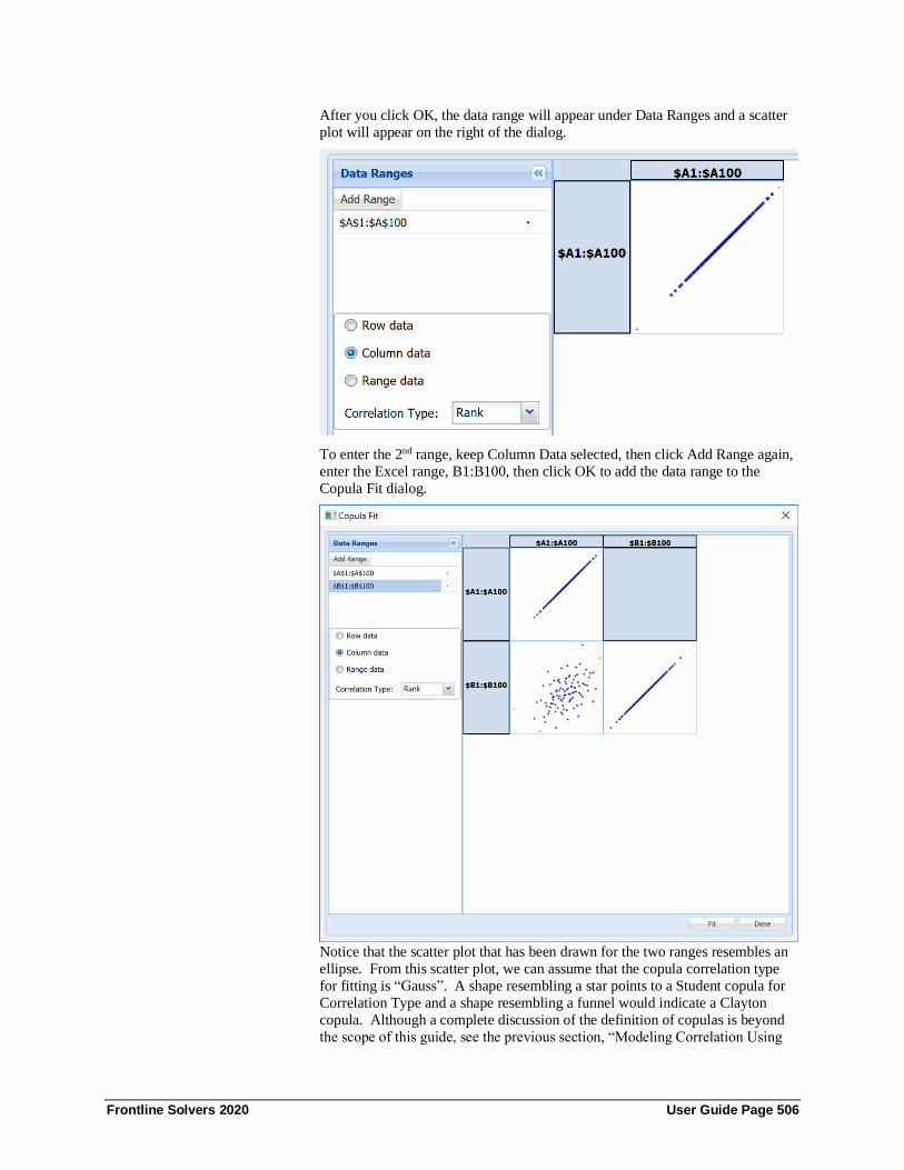
Frontline Solvers 2020 User Guide Page 506
After you click OK, the data range will appear under Data Ranges and a scatter
plot will appear on the right of the dialog.
To enter the 2nd range, keep Column Data selected, then click Add Range again,
enter the Excel range, B1:B100, then click OK to add the data range to the
Copula Fit dialog.
Notice that the scatter plot that has been drawn for the two ranges resembles an
ellipse. From this scatter plot, we can assume that the copula correlation type
for fitting is “Gauss”. A shape resembling a star points to a Student copula for
Correlation Type and a shape resembling a funnel would indicate a Clayton
copula. Although a complete discussion of the definition of copulas is beyond
the scope of this guide, see the previous section, “Modeling Correlation Using

Frontline Solvers 2020 User Guide Page 507
Copulas” for a brief introduction of each type of copula defined in the
Correlation Type drop down menu.
Select Gauss as Correlation Type…
…then click Fit at the bottom of the Copula Fit dialog to fit the correlation.
The Fit Results Parameters dialog opens to display the Correlation Type (Gauss)
and the Probability and Sigma fitting parameters. Select a blank cell, say D1, to
save the fitting parameters to the worksheet, then click Save.
Note: The cell entered for “Save to” on the Fit Results dialog will become the
top left corner of the data range on the Excel sheet. Any value or text contained in this cell or in any cell used to save the Fit Results Parameters, will be
overwritten.
Then click Done to close the Copula Fit dialog and return to the worksheet.
Notice that the information from the Fit Results dialog has been saved to the
Excel range, D1:E3. The size of this range will vary depending on the
Correlation Type and number of Data Ranges present in the Copula Fit dialog.

Frontline Solvers 2020 User Guide Page 508
Using the Correlations Dialog The Correlation dialog offers an easy way to create, edit, and remove correlation
matrices in your model. It appears when you click the Correlations button on
the Ribbon.
You use a correlation matrix to induce a statistical correlation among two or more uncertain variables. When you do this, the trial values of these variables in
a Monte Carlo simulation will tend to be drawn from related percentiles of their
distributions on each trial. Starting with V2016-R2, the numbers in a correlation
matrix may be Spearman rank order correlation coefficients or specifying an
Archimedean or Elliptical copula. For more information on correlation
matrices, see “Inducing Correlation Among Uncertain Variables” in the
Dependence and Correlation section above.
A correlation matrix is stored in a contiguous cell range, with an equal number
of columns and rows. To correlate N variables together, you need a matrix of N
columns and N rows. Here’s an example of a 3x3 correlation matrix:
You can type in values for a correlation matrix directly on the Excel worksheet,
and then reference this matrix in the PsiCorrMatrix() property function, passed
as an argument to PSI Distribution functions for each of the correlated variables.
But it is easier to use the Correlation Dialog to create the matrix for you.
Creating a Correlation Matrix
When you first click the Correlations button on the Ribbon, the Correlation dialog appears with an empty matrix area, and a left pane (similar to the Task
Pane displayed by the Model button) that lists the uncertain variables in the
model:

Frontline Solvers 2020 User Guide Page 509
You can either choose the specific cells for the uncertain variables you want to
correlate (press Ctrl or Shift and click for more than one) and then click the “>”
button to include them in the matrix, or you can click the “>>” button to include
all of them. The initial matrix with correlation values set to zero will display
similar to the example below:
The preview for the correlation Matrix has three parts:
1. Black numerical values for each correlation in the top right of the matrix. In
this case we have three values initially set with a zero correlation which you
can edit. Since correlation matrices have to be symmetrical (the correlation
between A1 and A2 must be the same as the correlation between A2 and
A1) we only show one value. Note: Both values are shown in Analytic
Solver Cloud.
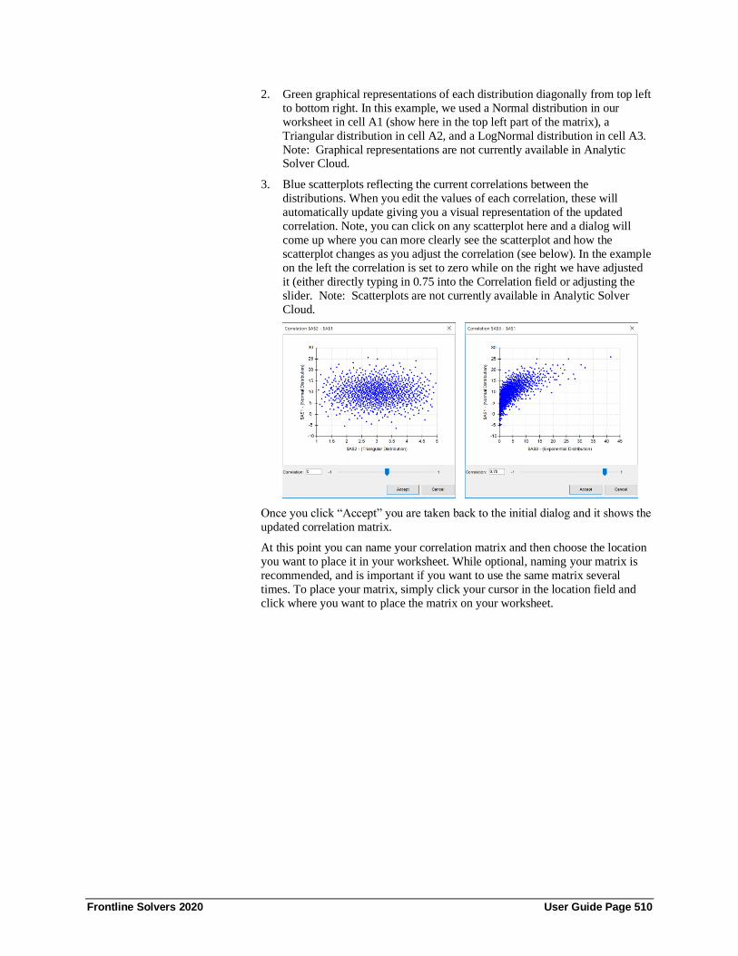
Frontline Solvers 2020 User Guide Page 510
2. Green graphical representations of each distribution diagonally from top left
to bottom right. In this example, we used a Normal distribution in our
worksheet in cell A1 (show here in the top left part of the matrix), a
Triangular distribution in cell A2, and a LogNormal distribution in cell A3.
Note: Graphical representations are not currently available in Analytic Solver Cloud.
3. Blue scatterplots reflecting the current correlations between the
distributions. When you edit the values of each correlation, these will
automatically update giving you a visual representation of the updated
correlation. Note, you can click on any scatterplot here and a dialog will
come up where you can more clearly see the scatterplot and how the
scatterplot changes as you adjust the correlation (see below). In the example
on the left the correlation is set to zero while on the right we have adjusted
it (either directly typing in 0.75 into the Correlation field or adjusting the
slider. Note: Scatterplots are not currently available in Analytic Solver
Cloud.
Once you click “Accept” you are taken back to the initial dialog and it shows the
updated correlation matrix.
At this point you can name your correlation matrix and then choose the location
you want to place it in your worksheet. While optional, naming your matrix is
recommended, and is important if you want to use the same matrix several
times. To place your matrix, simply click your cursor in the location field and
click where you want to place the matrix on your worksheet.

Frontline Solvers 2020 User Guide Page 511
Analytic Solver Desktop
Analytic Solver Cloud
Managing Copulas
Analytic Solver includes the ability to correlate uncertain variables using Gaussian, Student or Archimedean Copulas. To correlate the three uncertain
variables in cells A1, A2, and A3 using an Archimedian Copula, select
Archimedian Copula from the Correlation/Copula drop down menu. Note:
Only Rank Order and Gaussian Copulas are supported in Analytic Solver Cloud.
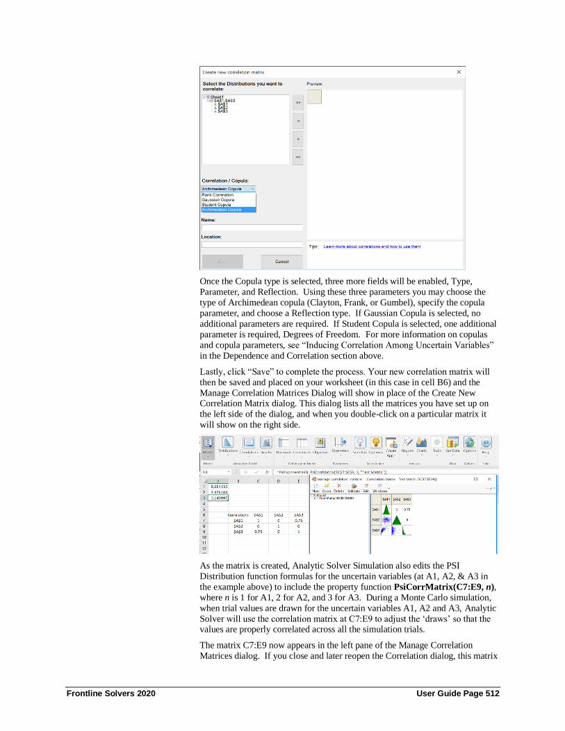
Frontline Solvers 2020 User Guide Page 512
Once the Copula type is selected, three more fields will be enabled, Type,
Parameter, and Reflection. Using these three parameters you may choose the
type of Archimedean copula (Clayton, Frank, or Gumbel), specify the copula
parameter, and choose a Reflection type. If Gaussian Copula is selected, no
additional parameters are required. If Student Copula is selected, one additional
parameter is required, Degrees of Freedom. For more information on copulas
and copula parameters, see “Inducing Correlation Among Uncertain Variables”
in the Dependence and Correlation section above.
Lastly, click “Save” to complete the process. Your new correlation matrix will
then be saved and placed on your worksheet (in this case in cell B6) and the
Manage Correlation Matrices Dialog will show in place of the Create New Correlation Matrix dialog. This dialog lists all the matrices you have set up on
the left side of the dialog, and when you double-click on a particular matrix it
will show on the right side.
As the matrix is created, Analytic Solver Simulation also edits the PSI
Distribution function formulas for the uncertain variables (at A1, A2, & A3 in
the example above) to include the property function PsiCorrMatrix(C7:E9, n),
where n is 1 for A1, 2 for A2, and 3 for A3. During a Monte Carlo simulation,
when trial values are drawn for the uncertain variables A1, A2 and A3, Analytic
Solver will use the correlation matrix at C7:E9 to adjust the ‘draws’ so that the values are properly correlated across all the simulation trials.
The matrix C7:E9 now appears in the left pane of the Manage Correlation
Matrices dialog. If you close and later reopen the Correlation dialog, this matrix

Frontline Solvers 2020 User Guide Page 513
will reappear in the lower left pane. If you create a correlation matrix ‘by hand’
on the Excel worksheet, and insert the PsiCorrMatrix() calls yourself into the
PSI Distribution function calls for the variables, the matrix you create will also
appear in this left pane the next time you open the Correlation dialog. You can
double-click on each matrix to display and edit that matrix.
Removing a Correlation Matrix
To remove a correlation matrix from your model, in the Manage Correlation
Matrices dialog click on the matrix you want to remove and then click on the
“Delete” icon in the dialog’s ribbon menu. The matrix will disappear from the
Correlations dialog, and the PsiCorrMatrix() property function formula
referencing this matrix will be removed from the PSI Distribution function calls
for the corresponding uncertain variables. However, the cell range on the
worksheet where the matrix elements were written is left undisturbed – you can
either delete them in Excel worksheet mode, or re-use them later.
To remove a correlation matrix in Analytic Solver Cloud, simply select the
matrix in the Model task pane, then click the red X to delete.
Editing a Correlation Matrix
As shown in the both the Create Correlations and Manage Correlations dialogs,
the value of each correlation is numerically shown in the top right portion of the
matrix. To edit the value of a correlation you can simply click on the correlation
you wish to edit and enter a new value from -1 (exactly negatively correlated) to
+1 (exactly positively correlated). The default value of 0 means the two
variables have zero correlation.
When you are finished, click the “X” button in the top right of the dialog to
close it and your change(s) will be saved. Importantly, we will automatically
check to make sure your matrices are valid (Positive Semi-Definite; see “Making a Matrix Consistent” below) and if they are not will offer help to
correct them.
Alternatively, you can click on the Edit button on the Manage Correlations
Ribbon to go to the Edit Matrix Dialog. The Edit Matrix dialog (see below) will
appear, which looks very similar to the Create Matrix dialog. At this point you
can change the name and location of the matrix, add or remove uncertain
variables, and change correlation values. When done, simply hit Save.
In Analytic Solver Cloud, double click the correlation matrix in the Model task
pane to edit. Click save when finished.

Frontline Solvers 2020 User Guide Page 514
Making a Matrix Consistent
A correlation matrix must be not just symmetrical, but consistent. This means
for example that if variable A has a high positive correlation with variable B,
and B has a positive correlation with C, then variable A cannot have a high
negative correlation with C. In mathematical terms, the correlation matrix must
be positive semidefinite. This property depends on all of the elements of the
matrix. If the matrix you create by hand does not satisfy this property (the
example matrix above does not), Analytic Solver can automatically adjust the
matrix elements so that the matrix is positive semidefinite.
To check whether the matrix you’ve entered is positive semidefinite, in the Manage Correlations dialog simply click the Validate icon in the dialog’s ribbon
menu:
In our example, the matrix is valid so the following message is displayed and no
action is needed:
If, for example, we set all our correlations to be -1, we would have a matrix
which could not be valid and you will see the following message instead:

Frontline Solvers 2020 User Guide Page 515
If you click No, the matrix remains as-is. If you click Yes, a new dialog
appears:
In this dialog, we can simply click the Update Matrix button to allow Analytic
Solver to adjust the matrix to be consistent (positive semidefinite). This may
involve changing all of the elements of the matrix, by various amounts. But Analytic Solver can do more than this.
In many applications, you can determine ‘good’ values for correlations between
certain pairs of variables, but for other pairs you have no special information.
Analytic Solver Simulation can adjust the matrix to make it positive
semidefinite while minimizing changes to the matrix elements you care about,
and making greater changes in the elements you don’t care about.
In the example above, let’s say we feel very confident there is a strong negative
correlation between A1 and A2 but are less sure about A1 and A3 and very
uncertain about any correlation between A2 and A3. We can click first on the
radio button on the left relating to the amount of change we are comfortable with and then click on the cell(s) we want changed by that general amount.
Using the information above we would click on the “Moderate Change” radio
button and then click on the correlation for A1 and A3 and then click on the
“Largest Change” radio button followed by clicking on the correlation for A2
and A3. Our Matrix will now look like the following:

Frontline Solvers 2020 User Guide Page 516
At this point we just click the “Update Matrix” button and our matrix is updated
to be consistent (Positive Semi-Definite) with new correlation values as shown
below:
We can now accept the update or undo the changes. We can of course further refine our correlation values if/as we wish.
In Analytic Solver Cloud, each time the Save button is clicked on the
Correlations dialog, the matrix is checked for consistency (positive semi-
definite). If the matrix is not consistent, you will be asked if you would like
Analytic Solver to modify the matrix. Click yes, to accept Analytic Solver's
modifications. Click No to save the matrix without any modifications. Click
Cancel to go back to the matrix.

Frontline Solvers 2020 User Guide Page 517
Probability Management Concepts In the February and April 2006 issues of the publication OR/MS Today, Dr. Sam Savage and coauthors Stefan Scholtes (University of Cambridge) and Daniel
Zweidler (Shell Global Exploration) advance a series of ideas called
“Probability Management.” They argue for much broader use of risk analysis
methods in planning and management, especially in large enterprises, based on
three ideas:
• Interactive Simulation
• Stochastic Libraries
• Certification Authority
Probability Management calls for an up-front investment in the creation of
standardized Certified Distributions, created or reviewed by an expert authority,
and distributed to simulation modelers, often in the form of Stochastic Libraries.
The payoffs of Probability Management include:
• Much easier creation of new simulation models
• Ability to capture complex dependencies – beyond what’s possible with
correlation coefficients
• ‘Apples-to-apples’ comparison of simulation model results
• Valid ‘roll-ups’ of simulation models from different groups
Analytic Solver Comprehensive is the first product designed to support the
concepts of Probability Management. In addition to best-in-class support for
Interactive Simulation, it provides direct support for creating, ‘publishing’ and
using Certified Distributions and Stochastic Libraries, as discussed in this
chapter.
Analytic Distributions
As described above, and documented in the Reference Guide, Analytic Solver
provides a wide range of analytic probability distributions – more than 40
distributions are available, from PsiBernoulli() to PsiWeibull(). Given
knowledge and experience, you can choose and use these distributions in your simulation models. But as discussed above, this is often the most challenging

Frontline Solvers 2020 User Guide Page 518
part of creating a Monte Carlo simulation model, especially for users with
spreadsheet modeling expertise, but limited math and statistics background.
Moreover, when different end user modelers choose their own analytic
distributions and parameters, they will often create models that cannot be
compared or combined (‘rolled up’), because the relationships between uncertain variables and functions would not be preserved. In large firms
especially, where different business units must take into account common
uncertainties, a better approach is needed.
Certified Distributions and Stochastic Libraries
A Certified Distribution is a custom probability distribution, created and/or
reviewed by an expert, that is made available to end user modelers as a
‘prepackaged unit.’ These modelers need only the name of the Certified
Distribution; they need not choose, or even be aware of, its analytic form,
parameters or correlations.
An analytic Certified Distribution can be given its own random number seed, which overrides a user-specified seed for the model. This ensures that end user
modelers employing the Certified Distribution will use the same samples
(sequence of Monte Carlo trials) each time they run a simulation – as long as
they use the same simulation software package and version.
Given the capacity of modern computers and networks, an even better idea is to
create and distribute Certified Distributions in the form of Stochastic Libraries.
Such libraries contain pre-generated trial data for a group of (potentially
statistically dependent) distributions. The sequence of trials is predetermined, so
that if two or more end users develop and run simulation models using the same
Stochastic Library, their model results can be compared and combined, on a
trial-by-trial basis if necessary.
Analytic Solver Desktop supports the use of both analytic distributions and
Stochastic Libraries as Certified Distributions. But since they contain pre-
generated trial data, the use of Stochastic Libraries can guarantee that models
will be run with exactly the trial data intended, regardless of the software (or
version thereof) installed on end user modelers’ PCs – as long as it accepts
Stochastic Libraries. This functionality is not currently supported in Analytic
Solver Cloud.
Publishing and Using Certified Distributions
Certified Distributions can be prepared and tested using a variety of tools. One
of these tools is Analytic Solver Desktop itself, as illustrated below. When
creating a Stochastic Library, any good Monte Carlo simulation software package can be used, inside or outside of Excel, as long as it offers a way to
save all the Monte Carlo trials. Once prepared, Certified Distributions should be
approved and ‘published’ in a form where they can be made available to end
user modelers.
Analytic Solver Simulation provides a property function PsiCertify() that you
can use to name and “certify” a distribution as ready for publication. It also
provides a distribution function PsiCertified() that end user modelers can use to
access the Certified Distribution using only its name.
Certified Distributions can be physically distributed or made accessible in a
variety of ways: On CDs or DVDs, via a network file share, or via email or

Frontline Solvers 2020 User Guide Page 519
Web download. The data for Monte Carlo trials may be easily stored in a
relational database or a multidimensional data warehouse.
Analytic Solver Simulation, with its Interactive Simulation facilities, is the ideal
‘client’ tool for end user modelers using Certified Distributions. It provides an
easy way to access Certified Distributions by name, using Microsoft Excel as a “universal data access client” to access distributions and Stochastic Libraries.
Analytic Solver Simulation makes it easy for an expert or CPO to create an
Excel workbook, separate from any end user’s simulation model workbook,
where Certified Distributions are defined. This may be a standard workbook
or an Excel add-in workbook; the latter provides certain advantages, since it is
normally hidden from display and loaded automatically when Excel starts.
For example, it is straightforward to create an Excel add-in workbook that
defines a Certified Distribution that draws its trial data from a Stochastic Library
(see below) that is actually stored in a relational database or data warehouse.
When the add-in workbook is (automatically) opened, either Excel data access functions or VBA code can be used to query the database for the trial data.
Stochastic Libraries: SIPs and SLURPs As described by Dr. Savage in OR/MS Today, the simplest element of a coherent
Stochastic Library is a Stochastic Information Packet or SIP, which is just a list
of trial values for a single uncertain variable. An example might be 1,000
sample values, in a specific sequence, for the future price of oil at some point or
interval of time. In a Monte Carlo simulation, trials will be drawn from the SIP
in the order in which they were generated.
If the SIPs for several different uncertain variables are generated as a group, in a
manner that preserves the statistical dependence between them, they may be
combined into a Stochastic Library Unit, Relationships Preserved, or SLURP. A SLURP is a table of trial values, where each column represents a specific uncer-
tain variable, and each row represents a distinct trial. The SLURP’s uncertain
variables may be dependent in ways not measured by traditional correlation.
But if a Monte Carlo simulation draws trials in the specific order given by the
SLURP, this dependence will be reflected in the simulation model results.
On an Excel spreadsheet, a SIP is naturally represented by a column of cell
values, and a SLURP is most easily represented by a two-dimensional table of
cell values. As noted above, the data for this table of cell values may be easily
drawn from a relational database or multidimensional data warehouse, or it may
be created and maintained directly in Excel.
Analytic Solver provides two PSI Distribution functions, PsiSip() and PsiSlurp(), that make it easy to define distributions using SIPs and SLURPs.
PsiSip() takes one argument: a cell range (normally a column) containing the
trial values for one uncertain variable. PsiSlurp() takes two arguments: a two-
dimensional cell range containing the SLURP data, and a column index (starting
from 1) for the uncertain variable whose trials should be returned by the
PsiSlurp() function. You’ll want to ensure that the number of rows in the first
argument range is at least as large as the number of simulation trials to be run.
PsiSip() and PsiSlurp(), like other PSI Distribution functions, can be used
directly in simulation models to return sample values from a SIP or SLURP.
But they are especially powerful when you name and publish a Certified
Distribution based on them. Doing this is as simple as including a PsiCertify()

Frontline Solvers 2020 User Guide Page 520
function call as an argument to PsiSip() or PsiSlurp() – as described below in the
section “Creating and Using Certified Distributions.”
Creating Stochastic Libraries
Of course, a Stochastic Library must first be created before it can be used. In
some cases, you may have a data source from which you can draw SLURP data directly. For example, if you are working with demographic data such as age,
family size, income, and taxes paid, you might be able to use a representative
sample directly as a SLURP. But in many cases, an expert (perhaps like you)
will have to select appropriate analytic probability distributions and their
parameters, determine whether and how they should be correlated, and then
generate the trial data through a Monte Carlo process.
Analytic Solver is a great tool for creating Stochastic Libraries, as well as using
them. It supports a wide range of analytic distributions, shifting and truncation
of distributions, and rank order correlation of different distributions. When you
run a simulation, the trial data is generated, and with the PsiData() function, you
can easily save the trial data in a column on the spreadsheet – this will create a SIP. Several PsiData() functions in adjacent spreadsheet columns will create a
SLURP. To see an example, open the simulation example workbook Creating
aSlurp(Sim).xls (normally installed into C:\Program Files\Frontline
Systems\Analytic Solver Platform\Examples), pictured below.
In this workbook, we generate SLURP data for the BusinessPlanPsi.xls model
(also included as an example workbook). This model has three uncertain
variables: Sales in units, Price per unit, and Unit cost. In cells E14 and E15 we
have PsiUniform() and PsiTriangular() functions, and in cells H15, I15 and
J15 we generate trial data as we did in the BusinessPlanPsi.xls model. For
example, H15 contains the formula =IF(E14>0.5,100000,50000).

Frontline Solvers 2020 User Guide Page 521
In the cell range B18:B1017, we’ve array-entered the formula {=PsiData(H15)}.
This will cause 1,000 trial values for H15 – a SIP for Sales in units – to be
inserted in this cell range, each time a simulation is performed. Similarly,
C18:C1017 contains {=PsiData(I15)}, and D18:D1017 contains
{=PsiData(J15)}.
To create and save the SLURP, simply run a simulation, by pressing the
Simulate button on the Analytic Solver ribbon. The SLURP data will appear
starting at cells B18, C18 and D18. Also note that cell range B18:B1017 has the
defined name ‘Sales’, B18:B1017 is named ‘Price’, and C18:C1017 is named
‘UnitCost’. BusinessPlanSLURP.xls should then be saved. We’ve generated
1,000 trials for each uncertain variable, enough to match the number of trials in
our simulation.
Then select cells B18:D1017, press CTRL + C to copy, then select cell H18 and
press CTRL + V to paste the contents of cells B18:D1017 to the cell range
H18:J1017.
Using the DIST Feature
Another way to use historical data is to use the DIST feature. This tool allows
you to encode your specific historical data as a distribution and then use the
PsiSip function to sample that data during the simulation trials.
1. Select your data just as you did for the Fit process above.
2. Click on the Dist button on the Analytic Solver Desktop ribbon.

Frontline Solvers 2020 User Guide Page 522
Or select Dist from the Analytic Solver Cloud Tools menu.
3. You will see a “Generate DIST from Data” Dialog. Click “OK”.
4. The next dialog will allow you to choose where to place the DIST after it is
generated as well as add information to it such as a name, comments on
where the data came from, as well as the type of encoding.

Frontline Solvers 2020 User Guide Page 523
Tip” The default encoding choice is “Double”. If you have 0-10,000 data
points you can use this setting. If you have 10,001 to 20,000 data points you
should use “Single”. If you have more than 20,000 data points you should
use the Fit feature.
5. You can see the results after you hit “OK” below.
Note: In this case we chose cell L4 to place the data. You will see the DIST
in the formula bar (only part of the DIST is visible above). The more data
points you have the longer the DIST string will be.
Tip: The DIST you’ve created can now be copied and used in any spreadsheet. The data that created it no longer needs to be kept for it to
work.
6. Use the PsiSip function to add the DIST to your model.
To use this DIST we enter “=PsiSip(L4)” in cell J7. Now our simulation
model will use the DIST we just created.
Tip: When you run a simulation using a DIST you won’t see the value in
the cell containing it change as it will always show the first data point in
your distribution and is working correctly.
Creating and Using Certified Distributions As described above, Analytic Solver supports the use of both analytic
distributions and Stochastic Libraries as Certified Distributions. It provides a
property function PsiCertify() that you can use to name and certify a distribution as ready for publication. It also provides a distribution function
PsiCertified() that end user modelers can use to access the Certified
Distribution via its name.

Frontline Solvers 2020 User Guide Page 524
Certified Distributions may be defined in an Excel workbook different from the
end user modeler’s workbook. This may be a standard workbook or an Excel
add-in workbook; the latter provides certain advantages, since it is normally
hidden from display and may be loaded automatically when Excel starts up.
Note: The workbook that defines Certified Distributions must be a ‘complete model’ on its own: It must define at least one output by using a PSI Statistics
function (PsiMean(), PsiOutput(), etc.) in a formula.
Publishing Distributions with PsiCertify
To name and certify an analytic distribution, you simply include the PsiCertify()
property function in the formula that defines the distribution. For example:
=PsiNormal(0.1, 1, PsiTruncate(-2,2), PsiSeed(3), PsiCertify("MyDist",0.1))
will define a Certified Distribution named “MyDist” based on a Normal
distribution with mean 0.1 and standard deviation 1, truncated so that its samples
lie in the interval -2 to 2, and generated using a random number seed of 3 (this
overrides any random seed specified in the end user’s model). To use this distribution, the end user modeler enters =PsiCertified(“MyDist”) in his or her
own workbook. When no simulation has been performed, the cell containing the
PsiCertified() call will display the default value 0.1.
To name and certify a distribution based on trial data in a Stochastic Library,
you also use the PsiCertify() property function in the formula defining the
distribution. For example:
=PsiSip(A1:A1000, PsiCertify("MyDist",100))
will define a Certified Distribution named “MyDist” whose trials are drawn
sequentially from the range A1:A1000, with default value 100 to be displayed
when no simulation has been performed.
When (as is often the case) the SIPs for several different uncertain variables are
generated as a group, in a manner that preserves the statistical dependence
between them, they should be combined into a SLURP, i.e. a table of trial values
where each column represents an uncertain variable, and each row represents a
Monte Carlo trial. Analytic Solver allows you to place a character string name
for each column (uncertain variable) in the first row of the SLURP data. You
can then name and certify the entire SLURP, for example:
=PsiSlurp(A10:C1010, PsiCertify("MyPlan"))
where range A10:C10 contains labels such as “Sales”, “Price” and “UnitCost”,
and A11:C1010 contains the SLURP trial data.
Now the end user modeler can write =PsiCertified(“MyPlan”, “Sales”) to
define an uncertain variable in a model whose samples will be sales figures.
The PsiCertify() function allows you to define more properties of the Certified
Distribution than just its name. It is good practice to document the name,
description, author, history of creation, and other relevant information about a
Certified Distribution using PsiCertify(). The full set of arguments is:
=PsiCertify( name, default value, short description, full description, version,
author, copyright, trademark, history)
Using Distributions with PsiCertified
To use a Certified Distribution, the end user modeler simply enters:

Frontline Solvers 2020 User Guide Page 525
=PsiCertified(name) or =PsiCertified(slurp,sip)
in his or her own workbook, where name or slurp and sip are quoted strings.
The user needs no knowledge of the form or parameters of the distribution, or of
the name or folder path of the workbook that defines the distribution.
Analytic Solver scans the open workbooks (including regular workbooks and
add-in workbooks) for distributions that include the PsiCertify() function, and
adds the names found in PsiCertify() calls to the Certified dropdown gallery.
Certified Distributions may also be used with Risk Solver Engine, when the
Analytic Solver GUI is not available. The PSI Interpreter matches calls to
=PsiCertified() to the known Certified Distributions. If a named distribution is
not found, the PsiCertified() call will return the error value #NAME?
To see an example of publishing and using Certified Distributions, open the
simulation example workbook BusinessForecastingCertified(Sim).xls
(normally installed into C:\Program Files\Frontline Systems\Analytic Solver
Platform\Examples), shown on the next page. This example uses a regular workbook, rather than an add-in. Look for "Creating and Using a Certified
Distribution" in the Cloud app. Click the Certified Distributions tab.
This worksheet contains the function call
=PsiSlurp(H17:J1017,PsiCertify(“ForecastDist”)) in cell D13. This cell (D13)
displays #VALUE! since there are labels rather than numbers in the first row of
the SLURP range, but this doesn’t affect use of the Certified Distribution.
To use the certified distribution, simply insert a function call =PsiCertified(“ForecastDist”) into the currently selected cell. That’s all there is
to it.
To see how this set of Certified Distributions can be used, click the Forecast
using Certified Dist tab, shown on the next page.

Frontline Solvers 2020 User Guide Page 526
This model uses =PsiCertified (“ForecastDist”, “Sales Volume”) in cell D13,
=PsiCertified (“ForecastDist”, “Sales Price”) in C14, and =PsiCertified
(“ForecastDist”, “Unit Cost”) in C15. It no longer requires an Excel ‘external reference’ to a specific folder path, workbook filename, or cell range. In fact,
there might not exist a single cell range containing fixed trial data – the trials
might be loaded from an external database, or generated dynamically from one
or more analytic distributions – as illustrated below.
Packaging Analytic Distributions
As described above, you can use PsiCertify() to name and publish an analytic
distribution, with a specific form and parameters and a pre-specified random
number seed, as a Certified Distribution. Further, you can “package” several
analytic distributions that are correlated through a rank correlation matrix in the
form of Certified Distributions. You can place these definitions in a standard
workbook, or in an add-in workbook that is automatically loaded when Excel starts, hiding a good deal of complexity from end users who simply need to use
these Certified Distributions.

Frontline Solvers 2020 User Guide Page 527
Mastering Stochastic Optimization Concepts
Introduction Analytic Solver offers you one unified framework for modeling and solving
optimization problems, with or without uncertainty. Models may include
‘normal’ decision variables, constraints and an objective, plus uncertainties,
recourse decision variables, chance constraints, and recourse constraints. This
chapter seeks to explain this framework, starting from the basics of Solver models. It assumes only a limited knowledge of optimization – but if you’ve
first read the chapter “Mastering Conventional Optimization Concepts,” you’ll
gain a much deeper understanding from reading this chapter.
Our goal is to find a solution – values for the decision variables in our model –
that satisfies the constraints and that maximizes or minimizes the objective. In
computing the objective and constraints, we use parameters of the model – for
example quantities, distances, shipping costs, interest rates, etc.
Certain and Uncertain Parameters
In conventional optimization, all the parameters are assumed to be numbers
known with certainty. If estimation of a parameter involves uncertainty or noise, an average or other ‘nominal’ value is used. This is a simplification and
idealization of the real world situation: In almost all business and engineering
problems, there is at least some uncertainty in the values of the parameters.
In some models, the uncertainty or variation in the parameters may be small
enough to be ignored. But in many models, it is large enough to be of concern.
And in some models, the uncertainty is so large that it is a major feature of the
problem, and much effort is (or should be) invested in modeling the uncertainty.
In the discussion to follow, by uncertain parameter we mean a parameter of
your optimization model, such as an objective coefficient or constraint right
hand side, that is subject to uncertainty. Such parameters might be computed
from a “primitive uncertainty,” such as a future interest rate or rainfall amount; we will call this an uncertain variable, and in Analytic Solver, we’ll use the
Uncertain Variable dialog to define and quantify this primitive uncertainty.
Realizations of Uncertain Parameters
Where a certain parameter has a single, known value, we can think of an
uncertain parameter as having many possible values. We call each such value a
realization of the uncertainty. Below, we’ve pictured one certain and three uncertain parameters.
Frontline Solvers 2020 User Guide Page 528
An uncertain parameter might have an infinite number of possible realizations,
but – as discussed near the end of this chapter – normally we can work with a
finite sample of possible realizations. We just don’t know which one of the
sample values is the ‘true’ value, or closest to this true value.
Decision-Dependent Uncertainties
In many real-world problems, the uncertainties being modeled are independent
of the decision variables. For example, in a crop planning model where the
acres to plant of different crops are decision variables, and the rainfall in a future
period is an uncertainty, the uncertainty is almost surely independent of the
decisions.
In other real-world problems, the uncertain parameters being modeled are
dependent on the decision variables – they change if the decisions change. For
example, in a market response model that includes competitor actions in a future
period, where your product prices are decision variables, and your competitors’
product prices are uncertainties, it is quite likely that the uncertainties will
depend on the decisions.
In portfolio models where one is investing in publicly traded, large capitalization
stocks, a decision to purchase some number of shares is unlikely to affect the
uncertain future returns on those stocks. On the other hand, a large institution
investing in thinly traded small-capitalization stocks may find that decisions to
purchase a large number of shares may move the market price and impact the
uncertain future returns. So both types of problems arise in practice. As we’ll
see later, the presence of decision-dependent uncertainties has a huge impact
on how, and even whether, our model can be solved.
Resolving Uncertainty and Recourse Decisions
In some real-world problems, we are uncertain about the value of a parameter today, and we will remain uncertain about its value in the future; we have to
make decisions in the presence of this uncertainty. This often arises in
engineering design models, where there is uncertainty about the exact strength
of a steel girder or the exact resistance or capacitance of an electronic
component. The uncertainty may be irreducible – perhaps inherent in nature –
or it may be reducible through better data collection, measurement or calibration
– but these steps may be impractical for us.
In other real-world problems, we are uncertain about the value of a parameter
today, but we will know its value with certainty at some point in the future.
This often arises in marketing and finance models, where a competitor’s price or
next year’s commodity prices or interest rates are uncertain today, but will become known at some future date. We say that the uncertainty will be resolved
at the future date; its many possible values will be reduced to a single value, and
the uncertain parameter will become certain.
If we are dealing with uncertainty that will not be resolved, we must find values
of the decision variables that yield feasible (or nearly feasible) solutions for
many possible realizations of the uncertainty. On the other hand, if we are
dealing with uncertainty that will be resolved at a future date, we can ask what
decisions we must make ‘here and now,’ before the uncertainty becomes known,
and what decisions we can make on a ‘wait and see’ basis, after the uncertainty
is known. This leads to the concept of recourse decisions, described below –
and it has a huge impact on how our model should be formulated and solved.
Frontline Solvers 2020 User Guide Page 529
Uncertainty and Conventional Optimization
The impact of uncertainty is magnified by conventional optimization. By its
nature, optimization drives the decision variables to values that just satisfy
certain constraints, while maximizing or minimizing the objective function. In
doing so, optimization exploits any ‘noise’ or error, as well as the ‘true value,’
captured in the fixed numbers used in the model for uncertain parameters.
This effect is very evident in investment portfolio optimization, where the
parameters of the model are estimated returns, variances, and covariances
between securities. Practitioners often describe portfolio allocations from an
optimizer as “unrealistic,” and such allocations often do not perform well in
practice. When the actual security returns, variances and covariances in future
periods vary from the parameters used in the optimization, even by small
amounts, the ‘optimized’ portfolio return often suffers by large amounts.
As shown by Ben-Tal and Nemirovski in a 2000 study of the NETLIB linear
programming problems, “In real-world applications of linear programming, one
cannot ignore the possibility that a small uncertainty in the data can make the
usual optimal solution completely meaningless from practical viewpoint.” Summarizing the effects of conventional investment portfolio optimization,
Michaud wrote in a 1998 book “The result is that optimized portfolios are ‘error
maximized’ and often have little, if any, investment value.” Conventional
optimization is not enough!
Elements of Solver Models We’ll now describe all the elements of a Solver model with uncertainty. Again
our goal is to find a solution – values for the decision variables in our model –
that satisfies the constraints and that maximizes or minimizes the objective. In
computing the objective and constraints, we may use many parameters – some
of which are computed from primitive uncertain variables. In Excel, the
decision variables and parameters are represented by worksheet cells; the
objective and constraints are computed by formulas in other worksheet cells.
Uncertain Variables
A certain parameter is easy to model, in a worksheet cell containing a number.
A primitive uncertainty requires a way to specify the range and ‘shape’ of the
values it can assume. In Analytic Solver, we model primitive uncertainties as
uncertain variables in worksheet cells that contain special add-in functions.
For example:
=PsiUniform(0,1) – a uniform distribution ranging from 0 to 1
=PsiNormal(2,1.5) – a Normal distribution with mean 2, standard deviation 1.5
=PsiBeta(A1,B1) – a Beta distribution with shape parameters A1 and B1
=PsiSip(A1:A1000) – a ‘Stochastic Information Packet’ containing a range of
user-supplied sample values, or realizations, for this uncertainty
Any of the 40-odd PSI Distribution functions that you can use for Monte Carlo
simulation may also be used as uncertain variables for stochastic optimization.
You can think of the cell for an uncertain variable, containing a formula such as
=PsiUniform(0,1), as holding an array of sample values, each one selected at
random from the range 0 to 1 inclusive. Each value is one possible realization
Frontline Solvers 2020 User Guide Page 530
of the uncertainty. Analytic Solver can generate such an array of sample values
automatically, using Monte Carlo simulation ‘behind the scenes’.
Looking ahead to the section “Functions of the Variables and Uncertainties,”
note that any formula cell that depends on an uncertain variable cell must also
compute an array of sample values. Each value corresponds to one possible realization of all the uncertain variables on which the formula depends.
In the example PsiBeta(A1,B1), it is important to know whether A1 or B1 is
dependent on the decision variables. A model that includes such a decision-
dependent uncertainty is much harder to solve, and will require the methods of
simulation optimization. Analytic Solver can automatically diagnose your
model and determine whether any uncertain variables depend – possibly through
a chain of formula cells – on the decision variables.
Decision Variables
Conventional optimization deals with only one type of decision variable, which
represents a decision that must be made ‘here and now,’ irrespective of any uncertainty in the model. We call this a normal or first-stage variable.
If we are dealing with uncertainty that will be resolved in the future, then at
some point the array of sample values for the uncertainty is effectively replaced
by a single value, the realization of the uncertainty as it actually occurs.
If the situation we are modeling allows us to make certain decisions after the
uncertainty becomes known, on a ‘wait and see’ basis, we can model these
decisions with recourse variables, also called second-stage variables. (At the
‘second stage,’ the uncertainty has become known.)
Normal or First-Stage Variables
A normal variable for a ‘here and now’ decision is represented by a worksheet
cell – say A1 – containing a number; the Solver will replace this number with an
optimal value, when the problem is solved. (The term ‘normal’ here is unrelated
to a Normal distribution, which is one way to define an uncertain variable.)
Recourse or Second-Stage Variables
A recourse variable for a ‘wait and see’ decision is also represented by a
worksheet cell – say A2 – containing a number. But at the time the optimization
is performed, a single recourse variable effectively represents an array of
solution values, one for each realization of the uncertainties in the model.
Functions of the Variables and Uncertainties
Any formula that participates (in the objective and constraints, see below) in
your model will normally depend on the decision variables and the parameters.
As a simple example, the objective of the Product Mix model EXAMPLE1in the Examples.xls workbook, is SUMPRODUCT(D17:F17,D9:F9) which can also
be written as D17*D9 + E17*E9 + F17*F9. Here, D17:F17 are parameters (the
selling prices of the three products), and D9:F9 are decision variables (the
amounts of each product to build). In this model, the parameters are assumed to
be certain.
An objective or constraint might be computed, from the parameters and the
decision variables, through a chain of several formula cells. For example, in the
Gas Company Chance and Recourse models in StochasticExamples.xls,

Frontline Solvers 2020 User Guide Page 531
illustrated in the chapter “Examples: Stochastic Optimization,” the constraint at
cell C23 is D15+D18-C8 >= 0, where D15 and D18 are decision variables
(amounts of gas to purchase), C8 = 100+80*D5 (estimated demand next year),
and D5 is an uncertain variable in the model.
Model Uncertainty and Optimization Methods
Recall that an uncertain variable effectively holds an array of sample values.
For example, D5 =PsiUniform(0,1) represents an array of realizations of the
uncertainty, each one selected at random from the range 0 to 1. If your objective
or constraint (say C8 = 100+80*D5) depends on D5, it must also compute an
array of sample values. Each value corresponds to one possible realization of
all the uncertainties on which the formula depends.
Traditional Solver Engines cannot handle an objective or constraints that depend
on uncertainty, and hence represent an array of sample values. To solve a
problem with such an objective and constraints, we must choose one of three
possible approaches:
1. Use the ‘Stochastic Decomposition Engine’ that can handle constraints
that depend on uncertainty. Note: This engine is not supported in
Analytic Solver Cloud.
2. Transform a model whose objective and/or constraints depend on
uncertainty into a ‘deterministic equivalent’ or ‘robust counterpart’
model that may be much larger, but whose objective and constraints no longer depend on uncertainty. Then we can solve the transformed
model using a traditional Solver Engine, and translate the results into a
solution for the original model. To be transformed successfully, the
original model must have only uncertainties that are independent of the
decisions, and have an objective and constraints that are linear (or
certain other) functions of the decision variables.
3. Ensure that all ‘top-level’ formula cells computing the objective and
constraints represent only single values – statistical summaries of the
arrays of sample values. We can do this manually, with formulas in
top-level cells that call PSI Statistics functions such as PsiMean(),
PsiVariance() or PsiPercentile() – or Analytic Solver can do this automatically and implicitly, when we define our objective and
constraints as described in the next two sections. This choice is flexible,
but it requires that we use simulation optimization – the most general,
but also the slowest and least scalable optimization method.
In all these approaches, we must specify what it means to maximize or minimize
an objective, or to satisfy a constraint that depends on uncertainty – implicitly or
explicitly reducing an array of sample values to a single value. The next two
sections explain how we can do this.
The Objective Function
The quantity you want to maximize or minimize is called the objective function.
In Excel, the objective is calculated by a formula cell – say A1 – listed in the Task Pane Model tab or the Solver Parameters dialog, in the outline list box
under Objective. This could be a calculated value for projected profits (to be
maximized), or costs, risk, or error values (to be minimized).
If the objective function depends on uncertainties, we must specify how we want
to ‘optimize’ this function. The most common practice is to maximize or
minimize the expected value (informally, the mean value) of the objective, over

Frontline Solvers 2020 User Guide Page 532
all realizations of the uncertainties. In Analytic Solver, you do this by selecting
the objective in the Task Pane Model tab, and in the lower Properties area,
selecting Expected from the Type dropdown list in the Stochastic group.
Instead of maximizing or minimizing the expected value of a function of the
decision variables and uncertainties, you can maximize or minimize a measure of the uncertainty in a function. Analytic Solver converts the objective to the
form max t or min t, where t is a new variable, and the model includes a chance
constraint A1 >= t or A1 <= t with the measure of uncertainty that you specify.
Implicit and Explicit Forms for the Objective
When you select Expected from the Type dropdown list in the Stochastic group,
Analytic Solver treats the objective cell as implicitly containing E[objective], or using sample realizations of the uncertainty PsiMean(objective). To make this
explicit on the worksheet, you can direct Analytic Solver to automatically create
a PsiObj() function call with an "Expected" argument – using either the “Use
Psi Functions to Define Model” option, or the Save Model button. You can also
manually enter a PsiMean() function call in the objective cell. Similar options
apply to the constraints, as discussed below.
Constraints: Normal, Chance, Recourse
Constraints are relations such as f(x1 , x2 …, ,xn) <= b, where x1 , x2 …, ,xn are
decision variables. In Excel, each xi corresponds to a cell, f(x1 , x2 …, ,xn) is
computed by a formula in another cell (say A1), the constant b is in another cell
(say B1), and we enter A1 <= B1 via the Ribbon or Task Pane. A constraint is satisfied when the relation it specifies is true within a small tolerance.
When your model includes uncertainty, we must examine how each constraint
depends on the uncertainties and the decision variables:
• If a constraint depends only on certain parameters and normal decision
variables, it is ‘deterministic’ and is handled in the usual way by the Solver.
We call this a normal constraint.
• If a constraint depends on uncertain variables and normal decision
variables, we must specify what it means for the constraint to be satisfied.
There are many possible realizations for the uncertain variables, but only
single values for the decision variables. The Solver must find values for the decision variables that cause the constraint to be satisfied for all, or perhaps
most but not all, realizations of the uncertainties. We call this a chance
constraint. For example, we might specify that the constraint must be
satisfied 95% or 99% of the time; it can be violated 5% or 1% of the time.
For 95%, we denote such a constraint as VaR 0.95 A1 <= B1. But this form
may not be your best choice – alternatives called CVaR and USet are
discussed in the section “More on Chance Constraints.”
• If a constraint depends on uncertain variables and recourse decision
variables, then the Solver will find an array of values for each of the
recourse variables, corresponding to the realizations of the uncertain
variables. Recourse decisions give the Solver flexibility to satisfy constraints that involve uncertainty; but in effect, each such constraint has
many realizations – one for each realization of the uncertainties. We call
this a recourse constraint.
• A constraint may also depend on recourse decision variables, and possibly
normal decision variables, but not depend on any uncertain variables. This
is also a recourse constraint, with many realizations. The Solver must find

Frontline Solvers 2020 User Guide Page 533
values for the recourse variables that satisfy all the constraints where they
appear – some with uncertainties, and some without.
Implicit and Explicit Forms for Constraints
When you select VaR from the dropdown list in the Constraint dialog and enter
a Chance of 0.95, Analytic Solver treats the constraint cell as implicitly
containing VaR 0.95 [constraint], or using sample realizations of the uncertainty
PsiPercentile(constraint, 0.95) where constraint is the left hand side. To make
this explicit on the worksheet, you can direct Analytic Solver to automatically
create a PsiCon() function call with a "VaR" argument – using either the “Use
Psi Functions to Define Model” option, or the Save Model button. You can also
manually enter a PsiPercentile() function in the constraint left hand side cell. For more information on the PsiObj() and PsiCon() functions, see the chapter
“Psi Function Reference” within Frontline Solvers Reference Guide.
Multiple Uncertainties May Offset Each Other
What happens when a constraint depends on several different uncertainties? Is
such a constraint harder or easier to satisfy than a constraint that depends on just
one uncertainty?
In the simplest case, suppose we have a linear constraint, with coefficients ai
and decision variables xi:
a1x1 + a2x2 + ... + anxn b
Suppose that each coefficient ai is uncertain (and independent of all the others),
with sample values drawn randomly from PsiUniform (ai – 0.5, ai + 0.5).
The average or nominal value of each coefficient is ai. The ‘worst’ that can
happen is that a sample is drawn where every coefficient is ai + 0.5 – this makes
the left hand side (LHS) as large as possible, so it is very likely to violate the
condition LHS b. But this case is very unlikely to occur.
In most realizations of the uncertainties, some coefficients (randomly drawn
from the range ai – 0.5 to ai + 0.5) will be less than ai, and some will be greater
than ai. The more uncertainties are involved, the greater the chance that some of
them will draw samples less than ai.
If we use a chance constraint to specify that the relation must be satisfied (say)
95% or 99% of the time, we actually have a better chance of satisfying this
constraint when it depends on many uncertainties than when it depends on just
one – as long as the uncertainties are independent, or at least not highly corre-
lated with each other.
Solutions: Feasible, Optimal, Well-Hedged
A solution (set of values for the normal and recourse variables) for which all of
the constraints in the Solver model are satisfied is called a feasible solution. For
constraints that depend on uncertainties, this means that chance and recourse
constraints meet their criteria for satisfaction over all the realizations of the uncertainties considered in the optimization.
An optimal solution is a feasible solution where the objective function reaches
its maximum (or minimum) value – for example, the most profit or the least
cost. When the objective function depends on uncertainties, this normally
means that the expected value of the objective reaches a maximum (minimum) –
but you can also use max t or min t with a chance constraint A1 >= t or A1 <= t,
as described earlier.

Frontline Solvers 2020 User Guide Page 534
The optimal solution to a problem with uncertainty (the ‘stochastic solution’)
will never have an objective value that is better than one could obtain ‘with
20/20 hindsight,’ by solving a conventional optimization problem where the
uncertainties are known. The difference between the objective value obtained
‘in hindsight’ and the optimal value obtained ‘in foresight’ is called the expected value of perfect information (EVPI).
The stochastic solution will often be (quite) different from the optimal solution
to a problem where all uncertain variables are replaced with their nominal or
average values. The latter optimization will exploit the ‘point values’ of the
parameters, with no consideration for their variability; this will often yield a
better objective value for the nominal problem, but the solution may not be
feasible, let alone optimal, for many different realizations of the uncertain
variables. Compared to the ‘nominal’ solution, the stochastic solution is more
robust or ‘well-hedged’ against possible variations in the uncertain variables.
Solving for Recourse Variables
If we are dealing with uncertainty that will be resolved in the future, then at that
future date, each uncertain variable will be replaced by a single value, the
realization of the uncertainty that actually occurs. In Analytic Solver, you can
enter these single values for uncertain variables in the Lock value field in the
Uncertain Variable dialog, then choose to solve for single values of the recourse
variables, given known single values for both the normal variables (determined
by an earlier optimization) and for the uncertainties.
When Analytic Solver solves a problem by transforming the model, using the
Deterministic Equivalent or the Robust Counterpart transformation, it computes
an array of values for the recourse variables, one for each realization of the
uncertainties considered during the optimization. Using the left and right Trial #
arrows on the Ribbon, you can display on the worksheet the different sample
values of the uncertain variable cells, and the corresponding values of the
recourse variable cells – the ‘wait and see’ decisions in many possible scenarios.
Now, the actual values of the uncertainties, once they become known, might be
different from any one of these scenarios – so it is still useful to solve for single
values of the recourse variables as described above.
More on Chance Constraints
As explained above, if a constraint depends on uncertain variables and normal
decision variables, we can seek solution values for the variables that cause the
constraints to be satisfied for all, or perhaps most but not all, realizations of the
uncertainties. If we insist that the constraints are satisfied for all realizations,
we may not be able to find values for the decision variables that meet this
requirement – and if we do, we will very likely ‘pay for this’ via worse values
for the objective function.
Instead, we can seek solution values for the variables that cause the constraints
to be satisfied for most, but not necessarily all, realizations of the uncertainties.
We might specify that the constraint must be satisfied (it must not exceed a
given limit) 95% or 99% of the time; it can be violated 5% or 1% of the time.
This is depicted in the chart below, where 95% of the area under the curve is to
the left of the bar (i.e. the constraint right hand side value), and 5% is to its right.
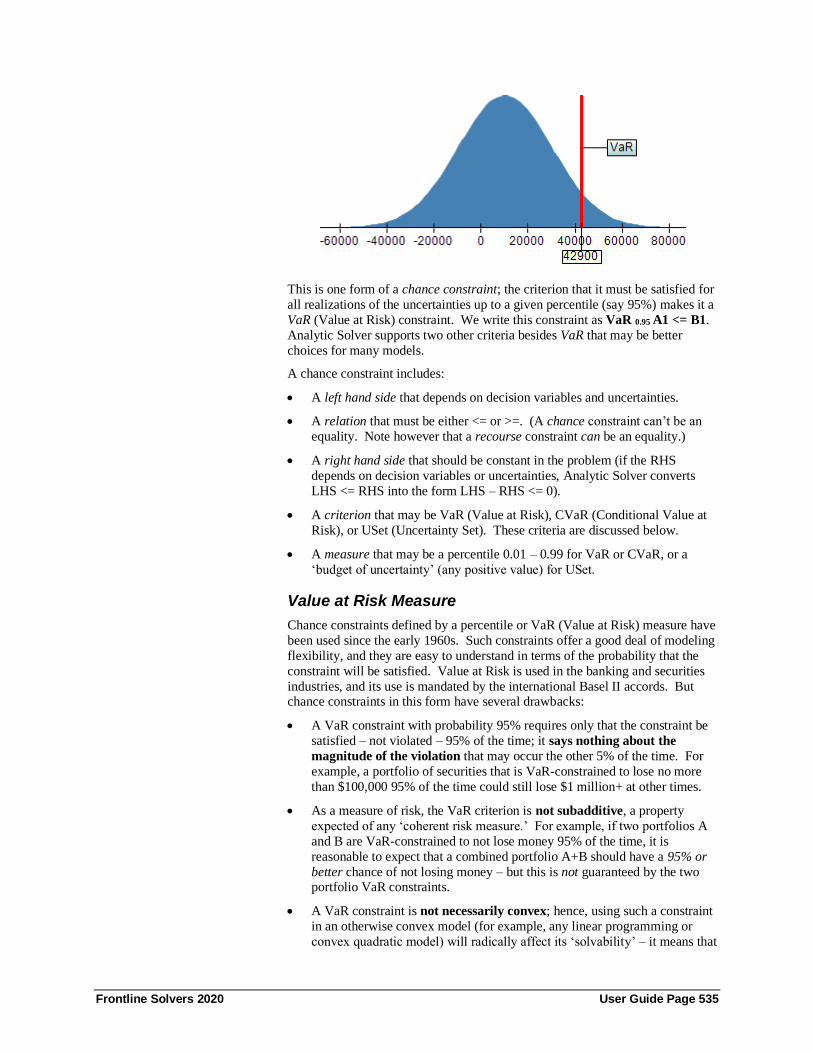
Frontline Solvers 2020 User Guide Page 535
This is one form of a chance constraint; the criterion that it must be satisfied for
all realizations of the uncertainties up to a given percentile (say 95%) makes it a
VaR (Value at Risk) constraint. We write this constraint as VaR 0.95 A1 <= B1.
Analytic Solver supports two other criteria besides VaR that may be better
choices for many models.
A chance constraint includes:
• A left hand side that depends on decision variables and uncertainties.
• A relation that must be either <= or >=. (A chance constraint can’t be an
equality. Note however that a recourse constraint can be an equality.)
• A right hand side that should be constant in the problem (if the RHS
depends on decision variables or uncertainties, Analytic Solver converts
LHS <= RHS into the form LHS – RHS <= 0).
• A criterion that may be VaR (Value at Risk), CVaR (Conditional Value at
Risk), or USet (Uncertainty Set). These criteria are discussed below.
• A measure that may be a percentile 0.01 – 0.99 for VaR or CVaR, or a
‘budget of uncertainty’ (any positive value) for USet.
Value at Risk Measure
Chance constraints defined by a percentile or VaR (Value at Risk) measure have
been used since the early 1960s. Such constraints offer a good deal of modeling
flexibility, and they are easy to understand in terms of the probability that the
constraint will be satisfied. Value at Risk is used in the banking and securities
industries, and its use is mandated by the international Basel II accords. But chance constraints in this form have several drawbacks:
• A VaR constraint with probability 95% requires only that the constraint be
satisfied – not violated – 95% of the time; it says nothing about the
magnitude of the violation that may occur the other 5% of the time. For
example, a portfolio of securities that is VaR-constrained to lose no more
than $100,000 95% of the time could still lose $1 million+ at other times.
• As a measure of risk, the VaR criterion is not subadditive, a property
expected of any ‘coherent risk measure.’ For example, if two portfolios A
and B are VaR-constrained to not lose money 95% of the time, it is
reasonable to expect that a combined portfolio A+B should have a 95% or
better chance of not losing money – but this is not guaranteed by the two portfolio VaR constraints.
• A VaR constraint is not necessarily convex; hence, using such a constraint
in an otherwise convex model (for example, any linear programming or
convex quadratic model) will radically affect its ‘solvability’ – it means that

Frontline Solvers 2020 User Guide Page 536
a globally optimal solution cannot be guaranteed, and solution time may
rise exponentially with model size.
Further, when Analytic Solver uses robust optimization methods to
automatically transform a model with VaR constraints into a larger but
deterministic ‘robust counterpart’ model, it first approximates the non-convex VaR constraint with a convex CVaR constraint, and then transforms the CVaR
constraint. Since CVaR is always more conservative than VaR as a risk
measure, the robust counterpart solution will ‘pay a price’ in conservativeness,
with a worse objective value. Users are often better off using CVaR directly.
Note: VaR 0.95 A1 <= B1 specifies that the 95th percentile of the realizations of
A1 must be less than or equal to B1. Since VaR only describes the left side of
the graph, not the right or “tail”, VaR 0.95 A1 >= B1 specifies that the 5th
percentile of the realizations of A1 must be less than or equal to B1.
Conditional Value at Risk Measure
To deal with the problems of Value at Risk cited above, an alternative risk
measure called Conditional Value at Risk or CVaR (also called Expected Tail
Loss or ETL) was developed in the late 1990s. VaR 0.95 A1 <= B1 specifies that
the 95th percentile of the realizations of A1 must be less than or equal to B1;
realizations beyond the 95th percentile may be greater than B1 by any amount.
In contrast, CVaR 0.95 A1 <= B1 specifies that the expected value of all the
realizations of A1 up to the 95th percentile must be less than or equal to B1.
Below is a chart that compares VaR and CVaR. VaR is the value (42,900) that
lies at the 95th percentile of the realizations of the constraint left hand side; 5%
of the realizations are greater than 42,900 and lie in the graph to the right of this
point. CVaR (54,000) is the expected value (i.e. the mean or average value) of
all the realizations that lie in the ‘tail’ to the right of the VaR (Note that, if
CVaR 0.05 A1 <= B1 is satisfied for some B1, then VaR 0.05 A1 <= B1 is also
(more than) satisfied.
As a risk measure, Conditional Value at Risk has several advantages over VaR:
• Unlike VaR, a CVaR constraint at 95% places a bound on the average
magnitude of the violations that may occur 95% of the time.
• CVaR is a ‘coherent risk measure.’ It is subadditive, so if two portfolios A and B are CVaR-constrained to not lose money 95% of the time, then a
combined portfolio A+B has the same or better chance of not losing money.
• A CVaR constraint is always convex. Models consisting of all convex
functions can be solved to global optimality, and solved to very large size
using modern interior point optimization methods.

Frontline Solvers 2020 User Guide Page 537
Uncertainty Set Measure
Analytic Solver supports a third criterion for uncertainty in a chance constraint,
which reflects the approach taken in most of the literature on robust optimization
methods. This criterion, called USet (for uncertainty set), is applicable only to
linear constraints, with coefficients ai and variables xi:
a1x1 + a2x2 + ... + anxn b
where some or all of the coefficients ai may depend on the uncertainties. It is
useful to think of the vector [a1 a2 ... an] as having a nominal or expected value,
and a variation from this value for each realization of the uncertainties.
A constraint of the form USetΩ A1 <= B1, where a1x1 + a2x2 + ... + anxn is in A1,
and b is in B1, specifies that A1 <= B1 must be satisfied for all variations from
the nominal value of [a1 a2 ... an] that do not exceed a bound Ω, measured by a norm. The bound Ω is often called the budget of uncertainty for the constraint.
A very large Ω says that the constraint must be satisfied for practically all
variations of the coefficients from nominal; a Ω of 0 effectively ignores uncer-
tainty, requiring only that A1 <= B1 for the nominal value of [a1 a2 ... an], and
saying nothing about departures from this value.
Analytic Solver allows you to choose among four different norms to measure
variation from the nominal value: The L1, L2, L-Infinity and D norms – as
described in “Uncertainty Sets and Norms” later in this chapter.
Diagnosing Your Model’s Use of Uncertainty
When you create a large model, or modify a large conventional optimization model to include many uncertainties and many constraints, you may or may not
realize exactly how the model depends on the uncertainties. Just as you might
accidentally use a formula that creates a nonlinear dependence on a decision
variable, when you intended to create a linear programming model, you might
introduce a dependence on uncertainty in a constraint that you intended to be
deterministic. Analytic Solver can diagnose the use of uncertainty in your
model, comparing it to an ‘intended’ use of uncertainty that you specify in the
Task Pane Platform tab Diagnosis group Intended Use of Uncertainty option.
After clicking the Analyze button, you can select Reports – Optimization –
Uncertainty for a report of exceptions to your intended use of uncertainty.
Problems and Solution Methods Previous sections of this chapter have described how you can create models
that involve uncertainty in Analytic Solver, using certain and uncertain
parameters, normal and recourse decision variables, normal and chance
constraints, and your objective function. You create your models in the same
way, regardless of the model transformation or solution method that will be used
to solve the problem.
As outlined in the Introduction chapter, Analytic Solver is designed to find good
solutions – given enough time – to models involving uncertainty in their most
general form. But Analytic Solver is also designed to automatically recognize
common special cases such as stochastic linear programming models, and find
proven optimal solutions at much faster speeds. As with conventional LPs, the modeling assumptions of stochastic LPs are somewhat restrictive, but in a wide
range of real-world applications, these assumptions can be satisfied. The great

Frontline Solvers 2020 User Guide Page 538
advantage of a stochastic LP is its potential scalability to tens of thousands of
variables and constraints or more.
Before we can discuss classes of problems and how they are solved using
Analytic Solver, we must explain how two key concepts – decision-dependent
uncertainties and recourse decisions – affect the use of two key solution methods – stochastic programming and simulation optimization.
Decision-Dependent Uncertainties
As described in the Introduction section, in many real-world problems, the
uncertain variables being modeled are independent of the decision variables. In
other real-world problems, the uncertainties are dependent on the decision
variables – they change when the decision variables change.
The methods of stochastic programming (SP) were created, more than fifty
years ago, to deal with problems where the uncertainties are independent of the
decisions. Much more recently, methods of robust optimization (RO) were
created, also to deal with problems where uncertainties are independent of the decisions. Most methods in the SP and RO literature cannot be applied to
problems where the uncertainties are dependent on decision variables. But
where they can be applied, these methods are scalable to large models, and they
generally yield optimal solutions.
The methods of simulation optimization were created, also more than fifty years
ago, to deal with problems where the uncertainties may be dependent on the
decisions. This dependence makes the problem much harder to solve. Where
SP and RO methods often are based on linear programming and conic
optimization, simulation optimization is usually based on methods such as
genetic and evolutionary algorithms, and tabu and scatter search. These
methods are more flexible and general – but they require far more solution time, are generally not scalable to large models, and yield only ‘improved’ solutions,
not optimal solutions.
In Microsoft Excel, you can create models where the uncertainties are either
independent of, or dependent on the (normal or ‘first stage’) decision variables.
Analytic Solver can detect decision-dependent uncertainties and report this
when you choose Optimize – Analyze Original Problem or click the Analyze
button in the Task Pane:
To solve SIM NonCvx (non-convex) problems using simulation optimization,
you can use the built-in Evolutionary Solver (based on genetic algorithms) or the
plug-in OptQuest Solver (which uses tabu and scatter search). You can also use
built-in or plug-in nonlinear Solver Engines, in conjunction with Analytic
Solver’s multistart methods, to solve many such problems.
Resolving Uncertainty and Recourse Decisions
The methods of simulation optimization were developed to solve problems where the uncertainty will not be resolved over the horizon of interest. Hence,
these solution methods find optimal values only for normal or ‘here and now’
decision variables; virtually all simulation optimization methods in the literature
have no concept of recourse decisions.

Frontline Solvers 2020 User Guide Page 539
Unfortunately, simulation optimization has often been misapplied to problems
where the uncertainty will be resolved over the horizon of interest. Users may
believe that their simulation optimization model will find the best possible
decision in the presence of uncertainty. But this is very unlikely to be true, if
it’s possible to make certain decisions on a ‘wait and see’ basis. Recourse decisions create flexibility for the optimizer, making it easier to satisfy the
constraints and attain a better objective.
The methods of stochastic programming were developed to solve problems
where the uncertainty will be resolved over the horizon of interest. Recourse
decisions – the ability to make certain decisions on a ‘wait and see’ basis – have
been extensively studied in the SP literature, and many high-performance
solution methods for two-stage SP problems with recourse have been developed.
Classes of Problems Involving Uncertainty An optimization problem that includes uncertain variables is usually called a
stochastic optimization or stochastic programming problem.
Below, we’ll classify such problems based on the following factors:
• How the objective and constraints depend on the decision variables
• Whether the uncertain variables depend on the decision variables
• Whether the problem includes recourse decisions (i.e. whether it is one-
stage with only normal variables, or two-stage with recourse variables)
• Whether the problem includes chance constraints
We’ll also briefly describe how the three solution methods currently supported
by Analytic Solver – robust optimization, stochastic programming, and
simulation optimization – can be applied to these problems.
One-Stage Problems
One-Stage Linear Programming Problems
The simplest case is a one-stage stochastic linear programming problem:
• The objective and constraints depend linearly on the decision variables.
• The uncertain variables are independent of the decision variables.
• The problem includes no recourse decisions.
• The problem includes chance constraints to deal with the uncertainty.
This kind of problem arises if you start with a conventional, deterministic linear
programming model (where all coefficients are certain), you add uncertain
variables using functions such as =PsiUniform(0,1) or =PsiNormal(2,1.5) in
cells, and you add formulas to compute the objective or certain constraints based
on these cells, so that the LP coefficients are now uncertain.
Since no recourse decisions are available, the Solver must find values for the
(normal or first-stage) decision variables that satisfy the constraints (normal and
chance constraints) and maximize or minimize the objective.
We could solve this problem with simulation optimization methods. But since
it is linear, this problem is especially well suited for robust optimization
methods. With RO methods we can solve much larger models, hundreds of

Frontline Solvers 2020 User Guide Page 540
times faster than with simulation optimization. In the Task Pane Platform tab,
we set the Optimization Model group option Solve Uncertain Models to
Stochastic Transformation, and we set the Transformation group option
Stochastic Transformation to Robust Counterpart. When we click Optimize,
the transformed model is created and solved.
One-Stage Quadratic Programming Problems
A slightly more complex case is a one-stage stochastic problem with a quadratic
objective and all linear constraints:
• The objective is a deterministic, convex quadratic function of the decision
variables – it doesn’t depend on the uncertainties.
• The uncertain variables are independent of the decision variables.
• The problem includes no recourse decisions.
• The problem includes chance constraints to deal with the uncertainty.
The situation here is basically the same as for one-stage stochastic linear
programming problems. We can apply simulation optimization methods, but
we can also apply more scalable robust optimization methods, as long as the
objective doesn’t depend on the uncertainties.
One-Stage Nonlinear Optimization Problems
The situation changes if we have a one-stage stochastic nonlinear problem:
• The objective or the constraints are general nonlinear, convex or non-
convex functions of the decision variables.
• The uncertain variables may be dependent on the decision variables.
• The problem includes no recourse decisions.
• The problem includes chance constraints to deal with the uncertainty.
We cannot use Analytic Solver’s robust optimization methods or stochastic
programming methods on problems with general nonlinear, possibly non-convex
functions. Our only option is to use simulation optimization; this is feasible
since the problem does not include any recourse decisions. Given that we are
using simulation optimization, we can allow the uncertainties to be dependent on
the decisions, although some speed gains are possible if they are not.
Two-Stage Problems
Two-Stage Linear Programming Problems
A very common case is a two-stage stochastic linear programming problem:
• The objective and constraints depend linearly on the decision variables.
• The uncertain variables are independent of the decision variables.
• The problem includes both normal decisions and recourse decisions.
• The problem may or may not include chance constraints.
The presence of recourse decisions in the problem implies that at least some (and usually all) of the uncertainty will be resolved over the horizon of interest.
Hence the problem is called ‘two-stage,’ where the normal decisions are made at
the first stage – before the uncertainties are resolved – and the recourse
Frontline Solvers 2020 User Guide Page 541
decisions are made at the second stage – after they are resolved. The Solver
must find single values for the normal variables, and multiple values for the
recourse variables (for each realization of the uncertainties) that satisfy the
constraints and optimize the objective.
We cannot solve this problem with conventional simulation optimization methods, because these methods have no concept of recourse decisions. But
since the problem is linear, we can use either stochastic programming or
robust optimization methods – and with these methods we can solve much
larger models, hundreds of times faster than with simulation optimization. In
the Task Pane Platform tab, we set the Optimization Model group option Solve
Uncertain Models to Stochastic Transformation, and we set the Transformation
group option Stochastic Transformation to either Deterministic Equivalent or
Robust Counterpart. When we click Optimize, the transformed model is created
and solved.
If we choose the ‘Determ Equivalent,’ we can place integer constraints on the
normal and recourse variables (though this may make the model more difficult to solve). But the model cannot include chance constraints, and the transformed
model may become quite large (its size depends on the product of the number of
recourse variables and constraints, and the number of simulation trials).
If we choose the ‘Robust Counterpart’, the model can include chance
constraints, and the transformed model will be significantly smaller and solve
faster than if we choose ‘Determ Equivalent.’ But we cannot place integer
constraints on the recourse variables, and the solution may be more conservative
than with ‘Determ Equivalent.’
Two-Stage Quadratic Programming Problems
A slightly more complex case than the one above is a two-stage stochastic
problem with a quadratic objective and all linear constraints:
• The objective is a deterministic, convex quadratic function of the decision
variables – it doesn’t depend on the uncertainties or the recourse variables.
• The uncertain variables are independent of the decision variables.
• The problem includes both normal decisions and recourse decisions.
• The problem includes no chance constraints.
Again the presence of recourse decisions in the problem implies that at least
some (and usually all) of the uncertainty will be resolved over the horizon of
interest. We cannot solve this problem with conventional simulation
optimization methods, because these methods have no concept of recourse
decisions. But we can use stochastic programming methods – and these
methods are far more scalable than simulation optimization methods would be.
In the Task Pane Platform tab, we set the Optimization Model group option
Solve Uncertain Models to Stochastic Transformation, and we set the
Transformation group option Stochastic Transformation to either Deterministic Equivalent. When we click Optimize, the transformed model is
created and solved.
Two-Stage Nonlinear Optimization Problems
If we have a two-stage stochastic nonlinear problem:
• The objective or the constraints are general nonlinear, convex or non-
convex functions of the decision variables.

Frontline Solvers 2020 User Guide Page 542
• The uncertain variables may be dependent on the decision variables.
• The problem includes recourse decisions.
• The problem may or may not include chance constraints.
We cannot use Analytic Solver’s robust optimization methods or stochastic
programming methods on problems with general nonlinear functions, and we
cannot use conventional simulation optimization methods either, because these
methods have no concept of recourse decisions. But future Frontline Systems
products may be able to solve such problems; contact us for more information.
Advanced Topics
Bounds, Discretization, and Correlation
An uncertainty specified via a probability distribution such as PsiUniform(0,1)
has finite bounds of 0 and 1, but it has a practically infinite set of possible values
between 0 and 1; we can only consider a sample of the possible values during an
optimization. An uncertainty specified via PsiNormal(0,1) has infinite bounds,
as well as an infinite set of possible values. In practice, however, most of the probability mass of the Normal distribution lies within three standard deviations
on either side of the mean, and a reasonable sample of values from the Uniform
and Normal distributions can be used for computations.
Analytic Solver uses Monte Carlo simulation to generate samples of
uncertainties, based on the probability distributions specified by the user. It uses
the minimum and maximum values for each distribution obtained during the
simulation as ‘effective’ lower and upper bounds, which are used in constructing
the robust counterpart to an uncertain model.
When Analytic Solver solves a stochastic LP (as explained above) by forming
the ‘deterministic equivalent’ problem, the Monte Carlo trials are used as ‘scenarios’ in constructing this problem; hence they serve as a discretization of
any continuous probability distributions specified by the user.
The impacts of uncertainties on each coefficient of the objective and the
constraints may be correlated – either because multiple coefficients depend on
the same primitive uncertainty, or because correlation was deliberately induced
among several uncertain variables. When Analytic Solver solves a stochastic LP
by forming the ‘deterministic equivalent’ problem, the correlations are reflected
in the Monte Carlo trials used to construct the problem. When it solves a
stochastic LP using robust optimization methods, the robust transformation takes
into account the observed correlations in the sample.
Uncertainty Sets and Norms
As described in the earlier section “More on Chance Constraints,” if a chance
constraint is linear in the decision variables, you can use the USet (uncertainty
set) criterion, in lieu of the VaR or CVaR criterion. The advantage of using this
criterion is that the robust counterpart model more accurately reflects the degree
to which you want the chance constraint to be satisfied, which can lead to less
conservative solutions, with better objective values. Consider a constraint:
a1x1 + a2x2 + ... + anxn b
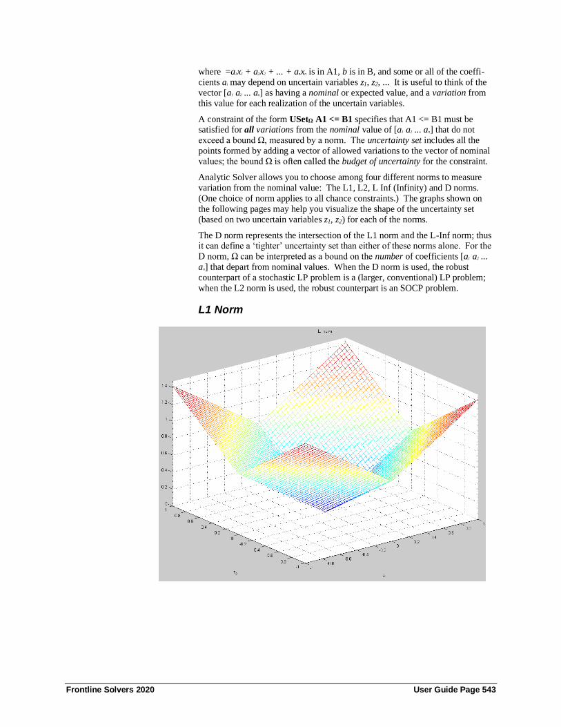
Frontline Solvers 2020 User Guide Page 543
where =a1x1 + a2x2 + ... + anxn is in A1, b is in B, and some or all of the coeffi-
cients ai may depend on uncertain variables z1, z2, ... It is useful to think of the
vector [a1 a2 ... an] as having a nominal or expected value, and a variation from
this value for each realization of the uncertain variables.
A constraint of the form USetΩ A1 <= B1 specifies that A1 <= B1 must be satisfied for all variations from the nominal value of [a1 a2 ... an] that do not
exceed a bound Ω, measured by a norm. The uncertainty set includes all the
points formed by adding a vector of allowed variations to the vector of nominal
values; the bound Ω is often called the budget of uncertainty for the constraint.
Analytic Solver allows you to choose among four different norms to measure
variation from the nominal value: The L1, L2, L Inf (Infinity) and D norms.
(One choice of norm applies to all chance constraints.) The graphs shown on
the following pages may help you visualize the shape of the uncertainty set
(based on two uncertain variables z1, z2) for each of the norms.
The D norm represents the intersection of the L1 norm and the L-Inf norm; thus it can define a ‘tighter’ uncertainty set than either of these norms alone. For the
D norm, Ω can be interpreted as a bound on the number of coefficients [a1 a2 ...
an] that depart from nominal values. When the D norm is used, the robust
counterpart of a stochastic LP problem is a (larger, conventional) LP problem;
when the L2 norm is used, the robust counterpart is an SOCP problem.
L1 Norm

Frontline Solvers 2020 User Guide Page 544
L2 Norm
L Inf Norm

Frontline Solvers 2020 User Guide Page 545
D Norm

Frontline Solvers 2020 User Guide Page 546
Best Practices for Building Large-Scale Models
Introduction It’s a maxim that a successful Solver model will grow in size over time. When
the initial results from an optimization model demonstrate ways to achieve
significant cost savings, improved schedules, higher quality or increased profits,
management is naturally interested in applying these methods to bigger
problems. This might involve extending the model to include more plants, warehouses, assembly lines, or personnel; to bring in other divisions or
geographic regions; or to cover more time periods, more detailed process steps,
or more specific parts or products. The result is an increase in the number of
decision variables, constraints, and cells in your model.
When your model grows in size, it becomes more challenging to design and
maintain, and also more challenging to solve. Good modeling practices –
touched upon in the chapter “Examples: Conventional Optimization” – become
far more important, so your model remains comprehensible to other Excel users,
auditable for errors, and easy to modify. Issues such as your model type (LP,
QP, QCP, SOCP, NLP or NSP), sparsity, and scaling also become far more
important, since they strongly influence the time it takes to solve your model, and the reliability of the solutions you obtain.
This chapter can only briefly survey good modeling practices – entire books
have been devoted to this subject (we will recommend some). It focuses on
steps you can take to obtain faster and more reliable solutions for large models
using the Analytic Solver including:
• Steps towards better performance that are easy to apply in most situations
• Steps you can take – with more design and modeling effort – to improve the
formulation of your model, by replacing non-smooth or nonlinear
constraints with linear (or integer linear) constraints
• Steps you can take to enable Analytic Solver to analyze your model more
efficiently
Designing Large Solver Models A large Solver model in Microsoft Excel is both a large spreadsheet workbook
and a large optimization model. If you plan to build such a model, you’ll be
well advised to learn about good spreadsheet modeling practices, and about
good optimization modeling techniques.
We highly recommend the textbook Management Science: The Art of Modeling
with Spreadsheets by Stephen G. Powell and Kenneth R. Baker, published by
John Wiley & Sons, listed in the following chapter “References and Further
Reading.” Unlike other management science textbooks, this book teaches you “best practices” in modeling and spreadsheet engineering, as well as techniques
of linear and nonlinear optimization using Excel.

Frontline Solvers 2020 User Guide Page 547
Other books on good spreadsheet design are hard to find, but through resources
like the Amazon.com Marketplace, you may be able to locate a copy of John
Nevison’s book Microsoft Excel Spreadsheet Design (Prentice-Hall, 1990), or
his earlier works 1-2-3 Spreadsheet Design (1989) or The Elements of
Spreadsheet Style (1987), both of which are still useful in designing modern spreadsheets. A relatively new (2003) book, Excel Best Practices for Business
by Loren Abdulezer, includes chapters on spreadsheet construction techniques,
“makeovers” of spreadsheets developed by others, and spreadsheet auditing.
Training courses in Microsoft Excel often cover at least some elements of good
spreadsheet design. They are offered in many venues, from universities and
community colleges to public seminars, in-house corporate training, and classes
sponsored by computer dealers. Check the course outline or syllabus to see if it
features spreadsheet design and good modeling practices, and other topics most
relevant to you.
A readily available book on optimization modeling techniques is H. Paul
William’s Model Building in Mathematical Programming, 4th Edition (John Wiley, 1999), listed at the end of the chapter “Introduction.” Focusing on
modeling for linear and integer programming problems, it includes a treatment
of large-scale model structure and decomposition methods that is hard to find
elsewhere.
Spreadsheet Modeling Hints
Below is a brief set of suggestions for planning, designing and constructing
large Solver models:
Start with a Plan. Plunging in and entering numbers and formulas immediately
will quickly lead to problems when constructing a large spreadsheet. Write
down your objectives and sketch out a design before you begin working on the real spreadsheet.
Build a Prototype. Plan in advance to build a prototype, throw it away, and
then build the real spreadsheet model. What you learn from building and
solving the prototype will probably save you time in the long run.
Create a Table of Contents. In the upper left corner of your first worksheet,
include comments that point readers to the major areas or sections of the
spreadsheet.
Separate Data and Formulas. Avoid using constants in formulas, unless they
are intrinsic to the mathematical definition of the function you are using.
Instead, place constants in cells, and refer to those cells in formulas. Create separate areas on the spreadsheet for input data and for calculations, and identify
these with distinct colors, borders or shading.
Document Assumptions, Parameters and Methods. As John Nevison
suggested, seek to “surface and label every assumption” in your model. Use
labels or cell comments to document key formulas and complex calculations.
Use defined names. Use Excel’s Insert Name Define and Insert Name Create
commands to assign meaningful names to individual cells and cell ranges. This
will help make your formulas clearer and more flexible.
Use and Separate Two-Dimensional Tables. Many elements of your model
will lend themselves to a row-column table representation. Create separate table areas, with distinct colors, borders and shading. Collect non-table data (such as
individual parameters) into a separate area.

Frontline Solvers 2020 User Guide Page 548
Use Excel Tools to View and Audit Your Spreadsheet. Use the slider to
zoom in Excel 2010/2013/2016 to get a high-level view of your spreadsheet’s
structure. Select ‘Show Formulas’ on the Formulas tab in Excel
2010/2013/2016 to display formulas instead of values, and scan them for
consistency. Learn to use Excel’s auditing functions to trace precedents and dependents of your formulas.
Use a Spreadsheet Auditing Tool. Several auditing tools are available,
including SpACE from the UK Customs and Excise Audit unit, OAK from
Operis Ltd. in the UK, and the Spreadsheet Detective from Southern Cross
Software in Australia.
Optimization Modeling Hints
Identify Your Model’s Index Sets. Your decision variables, constraints, and
many intermediate calculations will fall into groups that are indexed by elements
such as products (A, B, …), regions (North, South, …), time periods (January,
February, …) and similar factors. Identify and write down these index sets and
their members. Then organize the columns and rows of your table areas using these index sets. Use the top row and left column of each table area for index
set member names as labels.
Identify Your Decision Variables. Once you’ve identified the quantities that
will be decision variables, and how they are indexed (for example, units made
by product A, B,… or shipments by region North, South,…), it’s usually easier
to determine the constraints and their indexing.
Determine the Data You’ll Need. In building large optimization models, you
will frequently spend a good part of your time figuring out what data you need,
how you will get it (and keep it up to date), and how you’ll have to summarize
or transform it for the purposes of the model. This may involve getting help from your IT department or from other groups that create or maintain the data.
Define Balance Constraints. It is easy to overlook “balance” or “continuity”
constraints that arise from the physical or logical structure of your model. For
example, in a multi-period inventory model, the ending inventory at time t must
equal the beginning inventory at time t+1. At each node of a network model
(such as a warehouse), the beginning item quantity plus incoming deliveries
minus outgoing shipments must equal the ending item quantity (“what goes in
must come out”).
Learn to Use Binary Integer Variables. Many relationships that you might
find difficult to model at all, and many where you might otherwise use IF,
CHOOSE or other non-smooth or discontinuous functions, can be effectively modeled with binary integer variables. The section below “Improving the
Formulation of Your Model” describes many situations where you can use such
variables to organize your model.
Using Multiple Worksheets and Data Sources
Large Solver models and their data are often organized into multiple worksheets
of a single workbook. Some large models reference data found in other
workbooks. Given the large number of data elements, the sources from which
you are getting the data, and the procedures you use to keep the data up to date,
multiple worksheets are often necessary or at least useful for organizing your
data.

Frontline Solvers 2020 User Guide Page 549
Analytic Solver Pro, Risk/Premium Solver Pro and Premium Solver Pro require
that cells containing decision variables and constraint left hand sides are on the
active worksheet. But Analytic Solver allows you to define decision variables
and constraint left hand sides on any worksheet of a workbook. For this and
many other reasons, you are well advised to upgrade to one of these products if your model grows in size. With either product, the formulas in your objective
and constraint cells can refer to cells on other worksheets, and those cells on
other worksheets can contain formulas that depend, directly or indirectly, on
decision variable cells. For more information, see the Frontline Solvers
Reference Guide.
Several commentators on good spreadsheet modeling practice feel that models
defined on a single worksheet are easier to understand and maintain. In Excel
2010 and beyond, a single worksheet can have up to 16,384 columns and
1,048,576 rows. So you may want to keep the core of your Solver model – the
formulas (i) that are used to compute your objective and constraints and (ii) that
depend on the decision variables – on a single worksheet. If you find that you can better structure your model by placing decision variables and constraints on
different worksheets, it’s highly recommended that you adopt a consistent
scheme for choosing blocks of variable and constraint (and other formula) cells,
and referencing these cells across worksheets.
Some of the data you need may be available in relational databases, OLAP
databases or data warehouses. Microsoft Excel provides rich facilities, such as
external data ranges and PivotTables, to bring such data into an Excel
worksheet. The raw data, even if partially summarized from database records or
transactional data, often needs to be further transformed and summarized on
your worksheet(s). This is usually easy to do with Excel formulas. But for
clarity in your model, we recommend that you use separate worksheet areas, with distinct colors, borders or shading, for formulas that simply massage the
data and do not participate in the solution process (i.e. do not depend on the
variables). The Solver can determine which formulas depend on the variables,
but you or your colleagues may find it difficult to do so if the formulas are
intermixed.
Quick Steps Towards Better Performance The rest of this chapter focuses on steps you can take to obtain faster and more
reliable solutions for large models from Analytic Solver. This section describes
steps that are easy to apply in most situations.
For users of Analytic Solver Basic and Analytic Solver Upgrade, the best
recommendation we can make to improve performance is to upgrade to Analytic Solver Comprehensive, Analytic Solver Optimization or Analytic Solver
Simulation. This is more than just a “sales pitch” – every step you take costs
something, either in terms of money or your effort. For most professionals, the
cost of upgrading will be repaid if it saves just a few hours of time. And you
can find out at no cost whether the upgrade will be worthwhile.
For users of Analytic Solver Comprehensive or Analytic Solver Optimization,
we highly recommend that you try solving your model with our field-installable
Solver Engines – especially the Large-Scale SQP Solver, Knitro Solver,
MOSEK Solver Engine, and XPRESS Solver Engine. While the difference in
cost may be greater, the same rationale applies: If you can solve your model
more quickly or more reliably by upgrading the software, this is almost always cheaper (and yields results sooner) than spending many hours or days of
valuable professional time.
Frontline Solvers 2020 User Guide Page 550
Ensure that You Have Enough Memory
If the Solver seems unusually slow and you are using Analytic Solver Desktop,
check whether the hard disk activity LED (present on most PCs) is flickering
during the solution process. If it is, memory demands may be causing Windows
to swap data between main memory and disk, which greatly slows down the
Solver. If you’re investing money and, especially, hours of your time to develop
an optimization model, consider that RAM is very cheap, and relatively easy to
install. We recommend at least 1 GB RAM if you are working with large
Solver models – 2 GB or more is certainly desirable. However, the best solution
is simply to run your simulation model using Analytic Solver Cloud. Since the
Cloud app runs on Microsoft's Azure App Service, memory is not an issue in the cloud!
Analyze Your Model for Scaling Problems
Poorly scaled calculations are a frequent cause of long solution times and
unreliable solution results, for both linear and nonlinear problems. For a further
discussion, see “Problems with Poorly Scaled Models” in the chapter “Getting
Results: Conventional Optimization.”
Add Constraints to Your Model
Frequently, you can improve solution time by adding constraints to your model
which may not be essential in defining the problem, but which do further
constrain the search space that the Solver must explore. It’s true that the Solver
must do more work to handle the additional constraints, but this extra work
usually has an excellent payoff if the constraints are “binding” (i.e. satisfied with
equality) at some point during the solution process.
The greatest payoff often comes from additional constraints that are simple
bounds on the decision variables. This is because (i) it’s usually easier for you
to determine realistic lower and upper bounds on the variables than to formulate
new general constraints, (ii) it’s easy to enter bounds on the variables via the
Ribbon Constraints choice, and (iii) each of the Solver engines is able to handle
bounds on the variables more efficiently than general constraints.
Users often omit upper bounds on their decision variables, and sometimes omit
lower bounds as well. A first step towards improving performance is to enter
the tightest bounds on the variables that you can, without eliminating possible
good solutions.
Since bounds on the variables are especially important for the performance of
the Evolutionary Solver and for multistart methods for global optimization used
with the nonlinear Solver engines, the Engine tab options for these Solver
engines include an option Require Bounds on Variables, which is True by
default. When this box is checked, the Solver will stop with an error message if
some variables do not have lower or upper bounds at the time you click Solve.
If you are using the Interval Global Solver or the OptQuest Solver, bounds on all
variables are required – the Solver will always stop with an error message if
bounds on the variables are missing.
Improving the Formulation of Your Model The type of problem you are trying to solve, and the solution method or Solver engine that must be used, has a major impact on solution time:
• Linear programming problems can be solved most quickly.

Frontline Solvers 2020 User Guide Page 551
• Quadratic programming problems take somewhat more time.
• Nonlinear optimization problems take considerably more time.
• Non-smooth problems take by far the greatest amount of time.
This section discusses techniques you can use to replace nonlinear functions,
and even non-smooth functions, with equivalent (or nearly equivalent) linear or
quadratic functions, or with linear functions and binary integer variables. As
explained in the chapter “Mastering Conventional Optimization Concepts,” a
problem with integer variables can take much longer to solve than a problem
without such variables. However, an integer linear problem formulated using
the techniques described in this section may still take significantly less time to
solve than the equivalent nonlinear or non-smooth problem. Moreover, if your
problem is integer linear, you can find a guaranteed optimal solution, or a
solution that is guaranteed to be within at least x% of optimal, whereas with a
nonlinear or non-smooth problem you will have no such guarantees. As a rough
guide, non-smooth models with more than 1,000 variables may be difficult or impossible to solve in a reasonable amount of time – but equivalent models
formulated with linear functions and binary integer variables can often be solved
efficiently with the LP/Quadratic Solver. And with the Large-Scale LP/QP
Solver, MOSEK Solver or XPRESS Solver, you can often solve linear integer
problems of 10,000, 100,000 or more variables in a reasonable amount of time.
A caveat: If you currently have a model with many nonlinear or non-smooth
functions, and you decide to implement some of these techniques to speed up
solution of your model, bear in mind that you can use the LP/Quadratic Solver,
Large-Scale LP/QP Solver, or XPRESS Solver only for models where all of the
problem functions are linear (except for the objective function, which may be
quadratic). If you create a model with a mix of nonlinear or non-smooth functions and linear functions using binary integer variables, it may still take a
long time to solve.
Techniques Using Linear and Quadratic Functions
Below are three common situations where you might at first expect that a
nonlinear function is required to express the desired relationship – but with a
simple transformation or approximation, you can use a linear or quadratic
function instead.
Ratio Constraints
You may want to express a relationship that seems to require dividing one or
more variables by other variables. Suppose that you have a portfolio of 1-
month, 3-month and 6-month CDs, with the amounts of each CD in cells C1, D1
and E1, and you wish to limit the average maturity to 3 months. You might
write a constraint such as:
(1*C1 + 3*D1 + 6*E1) / (C1 + D1 + E1) <= 3
This constraint left hand side is a nonlinear function of the variables, so you
would have to use the GRG Solver to find a solution. However, the same
constraint can be rewritten (multiplying both sides by the denominator, then collecting terms) as:
(1*C1 + 3*D1 + 6*E1) <= 3*(C1 + D1 + E1), i.e. -2*C1 + 3*E1 <= 0

Frontline Solvers 2020 User Guide Page 552
This constraint is a linear function of the variables, so you would be able to use
the much faster LP/Quadratic Solver to find a solution. (This transformation
above relies on the fact that C1 + D1 + E1 >= 0.)
Mini-Max and Maxi-Min
You may want to minimize the maximum of a group of cells such as C1:C5 (or
maximize the minimum of a group of cells). It is tempting to use an objective
function such as MAX(C1:C5)– but as explained in the chapter “Mastering
Conventional Optimization Concepts,” MAX (and MIN) are non-smooth
functions, so you’d need to use at least the GRG Solver, and perhaps the
Evolutionary Solver to find a solution. Instead, you can introduce another
variable D1, make D1 the objective to be minimized, and add the constraint:
C1:C5 <= D1
The effect of this constraint is to make D1 equal to the maximum of C1:C5 at
the optimal solution. And if the rest of your model is linear, you can use the
much faster LP/Quadratic Solver to find a solution.
Quadratic Approximations
If you cannot represent the entire problem using linear functions of the variables, try to formulate it as a quadratic (QP) or quadratically constrained
(QCP) problem, with a quadratic objective and/or constraints. You may be able
to use a local, quadratic approximation to a smooth nonlinear function f near a
point a:
f (x) f (a) + f ´(a)(x - a) + ½ f ´´(a)(x - a)2
where f ´(a) denotes the first derivative, and f ´´(a) denotes the second derivative
of the function f at the point a. Several Solver engines offer excellent
performance on QP problems, and the SOCP Barrier Solver and the MOSEK
Solver offer good to excellent performance on QCP problems.
Even if you cannot eliminate nonlinear functions from your problem altogether,
you can improve solution time by making an effort to ensure that as many variables as possible occur linearly in the objective and all of the constraints. If
you’re using the GRG Solver, you can set its Engine tab option Recognize
Linear Variables to True, to save time during the solution process. And the
Large-Scale GRG Solver and Large-Scale SQP Solver engines also recognize
both linearly occurring variables and linear constraints automatically, for still
faster solutions. The Large-Scale SQP Solver is particularly effective when
used with Analytic Solver Comprehensive or Analytic Solver Optimization
because it uses the Interpreter’s Structure analysis to break down each function
into linear and nonlinear terms, which it handles as efficiently as possible.
You can use the Ribbon choice Optimize – Analyze Original Problem or the
Task Pane Analyze button to easily determine the number of linear variables, functions, and occurrences of variables in functions, as illustrated in the chapter
“Examples: Conventional Optimization.”
Techniques Using Linear Functions and Binary Integer Variables
Below are three common situations where you might at first expect that a non-
smooth function such as IF is required to express the desired relationship – but
you can instead use a binary integer variable and one or two linear functions to
define an equivalent relationship. The techniques described here are similar to

Frontline Solvers 2020 User Guide Page 553
those used when Analytic Solver automatically transforms your model, but you
can apply these techniques yourself to handle situations where the automatic
transformation is not available.
Fixed-Charge Constraints
You may have a quantity x in your model that must “jump” from zero to some
(fixed or variable) non-zero value, under certain conditions. For example, a
machine on a production line may have a fixed setup time or cost if it is used at
all, plus a time or cost per unit produced. You can avoid creating a non-smooth
function for x by introducing a binary integer variable y (which is 1 if x is used
and 0 if it isn’t), and adding a constraint x <= My, where M is a constant that is
larger than any possible value for x.
For example, suppose you have a machine that has a setup time of 10 minutes,
but once set up will process a widget every 30 seconds. Let cell C1 hold the
number of widgets you are producing on this machine, and use cell E1 for a
binary integer variable y that is 1 if you produce any widgets on this machine.
Then the total production time can be computed as =0.5*C1+10*E1. Assuming
that C1 can be at most 10,000, let M1 = 10000 and add a constraint:
C1 <= M1*E1 (or C1 – M1*E1 <= 0)
If variable C1 is nonnegative (C1 >= 0) and variable E1 is binary integer (E1 =
binary), then C1 is forced to be 0 whenever E1 is 0, or equivalently E1 is forced
to be 1 whenever C1 is greater than 0. Since the production time calculation and the constraint are both linear functions, you can solve the problem with the
LP/Quadratic Solver and the Branch & Bound method. This is called a fixed-
charge constraint.
You can sometimes use a semi-continuous variable to model this kind of
situation, instead of a binary variable, continuous variable, and “Big M”
constraint. At the optimal solution, a semi-continuous variable must either be
zero, or must lie within a specified continuous range. This is usually even more
efficient than using a fixed-charge constraint as outlined above.
Either-Or Constraints
Constraints in an optimization problem are implicitly connected by the logical
operator AND – all of them must be satisfied. Sometimes, however, your model
may call for either one constraint (say f(x) <= F) or another constraint (say g(x)
<= G) to be satisfied. You might consider using the OR function in Excel, but
as noted in the chapter “Mastering Conventional Optimization Concepts,” this
function is non-smooth. Instead, you can introduce a binary integer variable y
and a constant M, where M is greater than any possible value for f(x) or g(x), and
add the constraints f(x) – F <= My and g(x) – G <= M(1-y). Now, when y=0,
g(x) is unrestricted and f(x) <= F; when y=1, f(x) is unrestricted and g(x) <= G.
For example, imagine you want to allocate your purchases among several
suppliers in different geographic regions, each of whom has imposed certain
conditions on their price bids. Suppose that one supplier’s bid requires that you
either purchase at least 400 units from their Chicago warehouse or else purchase
at least 600 units from their Phoenix warehouse, in order to obtain their most
favorable pricing. Let cell C1 hold the number of units you would purchase
from Chicago, and cell D1 hold the number of units you would purchase from
Phoenix. Assume that cell M1 contains 10,000 which is more than the
maximum number of units you intend to purchase. You can model the
supplier’s either-or requirement with a binary integer variable in cell E1 and the
following constraints:

Frontline Solvers 2020 User Guide Page 554
400 – C1 <= M1*E1
600 – D1 <= M1*(1-E1)
Notice that we have reversed the sense of the constraint left hand sides to reflect
the “at least” (>=) requirement. If E1=0, then C1 (units purchased from
Chicago) must be at least 400, and the second constraint has no effect. If E1=1, then D1 (units purchased from Phoenix) must be at least 600, and the first
constraint has no effect.
IF Functions
In the chapter “Mastering Conventional Optimization Concepts,” we used
=IF(C1>10,D1,2*D1), where C1 depends on the decision variables, as an
example of a non-smooth function: Its value “jumps” from D1 to 2*D1 at C1=10. If you use this IF function directly in your model, you’ll either have to
try the Task Pane Platform tab Nonsmooth Model Transformation option, or
solve the model with the Evolutionary Solver. Instead, you can avoid the IF
function and solve the problem with the nonlinear GRG Solver – or even the
LP/Quadratic Solver – by introducing a binary integer variable (say E1) that is 1
if the conditional argument of the IF is TRUE, and 0 otherwise. Add the
constraints:
C1 – 10 <= M1*E1
10 – C1 <= M1*(1–E1)
When E1 is 0, the first constraint forces C1 <= 10, and the second constraint has no effect. When E1 is 1, the first constraint has no effect, and the second
constraint forces C1 >= 10. (If C1=10 exactly, this formulation allows either
E1=0 or E1=1, whichever one yields the better objective.) The value of the IF
function can then be calculated as D1*E1 + 2*D1*(1-E1), which simplifies to
D1*(2-E1) in this example. If D1 is constant in the problem, this is a linear
function; if D1 depends linearly on the variables, it is a quadratic; otherwise, it is
smooth nonlinear. In all cases, the non-smooth behavior has been eliminated.
Depending on how you use the result of the IF function in the rest of your
model, you may be able to take this strategy further. Suppose, for example, that
if f(x) >= F then you want to impose the constraint g(x) <= G; if f(x) < F then
you don’t need this constraint. You can then use a binary variable y (cell E1 in the example above), and impose constraints like the pair above plus an
additional constraint on g(x):
f(x) – F <= My
F – f(x) <= M(1-y)
g(x) – G <= M(1-y)
If y is 0, f(x) <= F is enforced, and the second and third constraints have no
effect. If y is 1, f(x) >= F and g(x) <= G are enforced, and the first constraint
has no effect. If f(x) and g(x) are linear functions of the variables, the
constraints involving y remain linear, and the problem can be solved with
Branch & Bound and the LP/Quadratic Solver.
Using Piecewise-Linear Functions
Many problems involve “stepped” price schedules or quantity discounts, where
you might at first expect that a non-smooth function such as CHOOSE or
LOOKUP is required to express the relationship. You might be surprised to
learn that you can instead use linear functions and binary integer variables to
express the relationship.

Frontline Solvers 2020 User Guide Page 555
For example, you might be purchasing parts from a vendor who offers discounts
at various quantity levels. The graph on the next page represents such a
discount schedule, with three prices and three “breakpoints.” You have a
decision variable x representing the quantity to order.
The three prices (slopes of the line segments) are c1, c2 and c3. V1 represents a
fixed initial cost; V2 and V3 are also constant in the problem and can be computed
from:
V2 = V1 + c1*B1 - c2*B1
V3 = V2 + c2*B2 - c3*B2
In the model, the variable x is replaced by three variables x1, x2 and x3,
representing the quantity ordered or shipped at each possible price. Also
included are three 0-1 or binary integer variables y1, y2 and y3. Since you want to
minimize costs, the objective and constraints are:
Minimize V1*y1 + V2*y2 + V3*y3 + c1*x1 + c2*x2 + c3*x3
Subject to x1 B1*y1, x2 B2*y2, x3 B3*y3
If the cost curve is concave as shown above, this is sufficient; but if the function
is non-concave (it may vary up and down), additional “fill constraints” are
needed:
y1 + y2 + y3 1
x1 B1*y2
x2 B2*y3
This approach is called a “piecewise-linear” function. It can be used in place of a CHOOSE or LOOKUP function, and it results in a linear integer model instead
of a difficult-to-solve non-smooth model. Piecewise-linear functions can also be
used to approximate a smooth nonlinear function, by using line segments with
slopes matching the gradient of the nonlinear function at various intermediate
points.
Organizing Your Model for Fast Solution This section describes ways you can organize your model so that Analytic
Solver can analyze it more efficiently. Most of this section is devoted to an in-
depth discussion of “fast problem setup” for linear and quadratic models
(possibly with integer variables); it is not applicable to nonlinear and non-
smooth models. Because the Polymorphic Spreadsheet Interpreter in Analytic
Solver has largely superseded this form of fast problem setup, this section is

Frontline Solvers 2020 User Guide Page 556
relevant primarily for very large LP models (100,000 variables or more), where
memory required for the Interpreter may be greater than available RAM and
cause swapping to disk.
Fast Problem Setup
If your model is linear or quadratic, you may find that the Solver spends most of its time with “Setting Up Problem...” on the Excel status bar, then speeds
through the “Trial Solutions” very quickly. The setup time is required to extract
the LP coefficients of the problem functions by recalculating the worksheet.
(The LP coefficients are the first partial derivatives of the problem functions
with respect to the variables, and they are obtained by the method of finite
differencing, which requires n + 1 recalculations if there are n decision
variables.)
Although the time taken to extract the LP coefficients was drastically decreased
in V2017-R2, even more of this setup time can be avoided if you write the
formulas for the objective function and all of the constraint left hand sides using
the functions recognized for fast problem setup: SUM, SUMPRODUCT, DOTPRODUCT, QUADPRODUCT and MMULT. This may require some
work on your part to revise a model you have already constructed, but you’ll be
rewarded with a 5- to 100-fold speed improvement in setup time, compared to
the time taken by the Excel Solver or the Excel Interpreter.
You can always express a linear or quadratic programming problem using these
functions for the objective and all of the constraints, although you may need to
introduce new sets of cells to hold the calculated coefficients so that these cells
can be referenced by one of the fast problem setup functions.
The PSI Interpreter in Analytic Solver uses the techniques of automatic
differentiation to obtain the LP coefficients faster and more accurately than they can be obtained via finite differencing. Because the Interpreter handles almost
every kind of Excel formula and built-in function, you don’t have to do the work
of designing your model – or revising an existing model – to use only the small
set of functions recognized for fast problem setup.
Fast problem setup is still available in Analytic Solver as a specialized method
of extracting the constant Jacobian matrix (the LP coefficients) of a linear or
quadratic problem, and the constant Hessian matrix (the QP coefficients) of a
quadratic objective function – but it is used only if you set the Task Pane
Platform tab Optimization group Interpreter option to Excel Interpreter. If
your LP or QP model is very large, defining it in fast problem setup format may
still save time compared to use of the PSI Interpreter – but the advantage is not nearly as great as the 5- to 100-fold speed improvement mentioned above.
The following subsections describe the functions supported for fast problem
setup, and the form of the function arguments that you must use to ensure that
they are recognized for fast setup purposes.
The SUM Function
The simplest case of a function recognized for fast problem setup is a formula such as =SUM(C1:C10) where C1 through C10 are decision variables. An
example of the use of SUM to define constraints can be found in the “Shipping
Routes” sheet in the SOLVSAMP.XLS workbook included with Microsoft
Excel. Note that a SUM of decision variables is a linear function where all of
the coefficients are 1. To be recognized in fast problem setup, your formula
must consist only of =SUM(cells) (with no constants) where every cell

Frontline Solvers 2020 User Guide Page 557
referenced is a decision variable. You may use absolute or relative references or
defined names in the arguments to SUM.
The SUMPRODUCT Function
The SUMPRODUCT function is documented in Microsoft Excel online Help. It
returns the sum of the products of corresponding elements in its two arguments,
which is exactly the form of a linear function:
a1x1 + a2x2 + ... + anxn
SUMPRODUCT requires that its two arguments refer to the same number of
cells in the same orientation (either a row, a column or a rectangular area of
cells). Only single selections, not multiple selections, are permitted in the arguments. If SUMPRODUCT is used in an array formula (see below), it will
return the same value in every resulting array element, which is usually not the
result you want. (The DOTPRODUCT function, described below, has more
flexible arguments and is far more useful in array formulas.) To be recognized
in fast problem setup, your formula must consist only of =SUMPRODUCT(cell
range, cell range) where one of the cell ranges consists entirely of decision
variables, and the other cell range consists entirely of cells that are constant in
the Solver problem. You may list the arguments in either order, using absolute
or relative references or defined names.
Other Functions for Fast Problem Setup
Use of the MMULT function is illustrated below under “Using Array
Formulas.” To be recognized in fast problem setup, your formula must follow
the same rules as for SUMPRODUCT: It must consist only of =MMULT(cell
range, cell range) where one cell range specifies the decision variables, and the
other cell range specifies the corresponding coefficients.
The DOTPRODUCT and QUADPRODUCT functions are described in their
own sections below. To be recognized in fast problem setup, your usage of
these two functions must follow the same rules as for SUMPRODUCT.
To qualify as a quadratic programming (QP) problem – which can be solved
efficiently by the LP/Quadratic Solver engine – only the objective function (not
any of the constraints) may use QUADPRODUCT, or any other quadratic form.
Using Array Formulas
Optimization models in algebraic form can often be expressed more compactly
using indexing and summation notation. For example, the five constraints in
EXAMPLE1 could be written as:
3
aij xj, i=1,...,5 j=1
The SUMPRODUCT function corresponds to the summation expression above
for one constraint. The entire set of five constraint formulas could be defined
with the array form of the DOTPRODUCT function (described in detail later in
this section). In EXAMPLE1, you would select cells C11 to C15 and “array-
enter” the following formula:
{=DOTPRODUCT(D9:F9,D11:F15)}
The braces above are not typed, but they appear when you “array-enter” the
formula by pressing CTRL-SHIFT-ENTER instead of just ENTER. If you

Frontline Solvers 2020 User Guide Page 558
aren’t familiar with array formulas in Microsoft Excel, you can read about them
in Excel’s online Help. They are one of the most useful features of Microsoft
Excel.
If your LP model is “dense” and regular in form rather than “sparse,” you may
wish to consider use of Microsoft Excel’s matrix built-in functions, such as MMULT which (when array-entered into a group of cells) yields the matrix
product of its two operands. For example, the five constraints in EXAMPLE1
(normally installed into C:\Program Files\Frontline Systems\Analytic Solver
Platform\Examples\StandardExamples.xls could be written in vector-matrix
form as:
Ax <= b
where A is the matrix of coefficients, x is the vector of decision variables and b
is the vector of constraint right hand sides. In the Microsoft Excel formula
language, the left hand side of this expression could be written as:
{=MMULT(_A,TRANSPOSE(_X))}
(The TRANSPOSE function is needed only to “match up” the orientation of the
matrix _A with the row vector _X.) In worksheet EXAMPLE1, if you insert
defined names _A for the coefficients D11:F15 and _X for the variables D9:F9,
then select cells C11:C15 and array-enter the above formula, it will compute the
values of all five constraints.
The PSI Interpreter in Analytic Solver recognizes most kinds of array formulas
supported by Microsoft Excel. But (for rather technical reasons) the use of array
formulas actually involves a speed disadvantage in the PSI Interpreter when the
coefficients are extracted via automatic differentiation.
If you’re using Analytic Solver, we recommend that you use array formulas where they make sense, and focus on making your model simple and easy to
maintain. In a large model, you’ll probably find that you want or need to use
multiple tabular areas for the formulas that define your constraints, and it may
be inconvenient or impractical to define entire constraint left hand sides with
functions like MMULT and TRANSPOSE.
Using the Add-in Functions
Analytic Solver products define two special Excel functions: DOTPRODUCT
and QUADPRODUCT. These functions behave just like Excel built-in
functions: You can use them in formulas in any spreadsheet (not only in Solver
models). When you use the Insert Function… menu option, these functions will
appear in the “Select a Function” or “Paste Function” list (classified as Math & Trig functions), and you’ll be prompted with named edit fields for their
arguments.
In addition, DOTPRODUCT and QUADPRODUCT are recognized for
purposes of fast problem setup as described earlier in this chapter. They are also
recognized by the PSI Interpreter.
Using DOTPRODUCT
DOTPRODUCT is a generalized version of the Excel function SUMPRODUCT,
and it is very useful for defining the objective function and constraints of linear
programming problems. DOTPRODUCT is also recognized for fast problem
setup as described above, provided that you follow the rules outlined earlier:
Your formula must consist only of =DOTPRODUCT(cell reference, cell
reference) where all of the cells in one of the cell references are decision
Frontline Solvers 2020 User Guide Page 559
variables, and all of the cells in the other cell reference are constant in the Solver
problem. Each cell reference must be either an individual selection or a defined
name, but the cell ranges specified by the two arguments need not have the same
“shape” (row, column, or rectangular area).
For use in Excel and for purposes of fast problem setup, DOTPRODUCT will accept defined names that specify multiple selections for either of its arguments.
For example, if you had designed a model where the decision variables
consisted of several rectangular cell selections, you could still calculate the
objective function for your model with one call to DOTPRODUCT.
DOTPRODUCT always processes its arguments in column, row, area order – in
an individual selection it reads cells across columns, wrapping around to
subsequent rows, and in a multiple selection it reads the individual cell
selections in the order in which they are listed. For example, the formula:
=DOTPRODUCT(A1:C2,D1:D6)
will calculate as =A1*D1+B1*D2+C1*D3+A2*D4+B2*D5+C2*D6.
The Array Form of DOTPRODUCT
If SUMPRODUCT is used in an array formula, it returns a scalar (single
number) result, which is returned in every cell of the array. However, if
DOTPRODUCT is used (with the proper arguments) in an array formula, it
returns an array result. You can use this capability to calculate the left hand
sides of several constraints with a single array formula. In a sparse model where you’d like to use the built-in function MMULT to compute the constraint values,
but the variables and constraints aren’t laid out in a single matrix, you can use
the array form of DOTPRODUCT instead.
Further, when you use the array form of DOTPRODUCT, Analytic Solver will
recognize this form and use it to process many constraints at once in problem
setup. (The array form is recognized for fast problem setup, and it’s also
recognized by the PSI Interpreter.) If you can’t use the array form, even the
simple form of DOTPRODUCT will save time in problem setup.
DOTPRODUCT will return an array value when the number of cells in one of
its arguments is an even multiple of the number of cells in its other argument. As an example, consider the calculation of parts used in the LP model
EXAMPLE1. The decision variables are in cells D9 to F9 (3 cells), and the
coefficients of the constraint left hand sides – the number of parts used for each
product – are in cells D11 to F15 (15= 3*5 cells). We want to calculate the left
hand sides of the constraints in cells C11 to C15. To do this, we would first
select the group of five cells C11:C15 with the mouse. Then we would type:
=DOTPRODUCT(D9:F9,D11:F15)
completing the entry with CTRL+SHIFT+ENTER instead of just ENTER. The
formula will display as {=DOTPRODUCT(D9:F9,D11:F15)} – the braces are
added by Microsoft Excel when the formula is array-entered. With the cell
values shown in EXAMPLE1 prior to solution (e.g. 100 for each of the decision variables), this array formula will calculate 200 in C11, 100 in C12, 500 in C13,
200 in C14 and 400 in C15. Hence, it will compute the same set of values as the
array expression shown earlier: {=MMULT(_A, TRANSPOSE(_X))}.
Whether it is used in the simple form or the array form, DOTPRODUCT always
processes its arguments in column, row, area order. In the array form, when the
cells in the “shorter” argument have all been processed and cells remain to be
processed in the “longer” argument, DOTPRODUCT “wraps around” to the
beginning of the “shorter” argument. In the example above, cell C11 calculates

Frontline Solvers 2020 User Guide Page 560
the value =D9*D11+E9*E11+F9*F11; cell C12 computes
=D9*D12+E9*E12+F9*F12; and so on. Keep this rule in mind when you use
the array form of DOTPRODUCT, and keep your spreadsheet layouts as simple
as possible!
Using QUADPRODUCT
The QUADPRODUCT function can be used to define the objective for
quadratic programming problems in a single function call, as required for fast
problem setup.
As explained in “Quadratic Functions” in the chapter “Mastering Conventional
Optimization Concepts,” a quadratic function is a sum of terms, where each term
is a (positive or negative) constant (called a coefficient) multiplied by a single variable or the product of two variables. This means that in order to represent
the most general quadratic function, we might have a coefficient for each
instance of a single variable, and a coefficient for each possible pair of two
variables. The QUADPRODUCT function is designed to supply coefficients for
each single variable and each pair of variables, in a manner similar to
SUMPRODUCT and DOTPRODUCT.
You supply the arguments of QUADPRODUCT as shown below:
=QUADPRODUCT(variable cells, single coefficients, pair coefficients)
The first argument must consist entirely of decision variable cells. The second
and third arguments must consist entirely of cells whose values are constant in the optimization problem; if these cells contain formulas, those formulas must
not refer to any of the decision variables. The second argument supplies the
coefficients to be multiplied by each single variable in the first argument, using
an element-by-element correspondence. The third argument supplies the
coefficients to be multiplied by each pair of variables drawn from the first
argument. Hence, if there are n cells in the first argument, there must be n2 cells
in the third argument. If the variables are represented by x1,x2,...,xn, the single
coefficients by a1,a2,...,an, and the pair coefficients by c1,c2,...,cN where N = n2,
QUADPRODUCT computes the function:
n n n
cn(i-1)+j xi xj + aj xj i=1 j=1 j=1
The pairs are enumerated starting with the first cell paired with itself, then the
first cell paired with the second cell, and so on. For example, if the first
argument consisted of the cells A1:A3, there should be nine cells in the third
argument, and the values in those cells will be multiplied by the following pairs
in order: A1*A1, A1*A2, A1*A3, A2*A1, A2*A2, A2*A3, A3*A1, A3*A2, and A3*A3. The value returned by QUADPRODUCT is the sum of all of the
coefficients multiplied by their corresponding single variables or pairs of
variables.
Multiple selections can be used for each argument of QUADPRODUCT, subject
to the same considerations outlined above for DOTPRODUCT: You can use the
general syntax for multiple selections in Microsoft Excel, but defined names are
needed for purposes of fast problem setup, and multiple selections are not
accepted by the PSI Interpreter.
A common application of quadratic programming is to find an “efficient
portfolio” of securities – often called portfolio optimization. Worksheet EXAMPLE4 in the StandardExamples.xls workbook, used in the chapter
“Examples: Conventional Optimization,” illustrates portfolio optimization using

Frontline Solvers 2020 User Guide Page 561
the Markowitz method. This model uses the QUADPRODUCT function to
compute the variance of a portfolio of five securities, and uses this quantity as
the objective to be minimized, subject to a constraint that gives a lower limit on
the portfolio return. Because the objective is a quadratic function, and the
constraints (including the bound on return) are all linear functions, this Solver model is a quadratic programming (QP) problem which can be handled by the
LP/Quadratic Solver in Analytic Solver Comprehensive and Analytic Solver
Optimization.

Frontline Solvers 2020 User Guide Page 562
References and Further Reading
Introduction Although this Guide provides many valuable hints for making effective use of
Analytic Solver, it does not attempt to teach you everything about optimization,
Monte Carlo simulation, and stochastic optimization. We strongly recommend
that you consult one of the books cited below, or discuss your problem with a
knowledgeable consultant at Frontline Systems, at a nearby university, or at a
firm specializing in optimization and simulation methods. There’s a vast
literature on problems of various types and for various industries and business
situations that have been solved successfully with the methods available in the Solver. Don’t reinvent the wheel – find out how others have solved problems
similar to yours!
You may also want to attend a training seminar on risk analysis and
simulation, optimization, and other advanced techniques in Excel, presented by
Frontline Systems instructors or consultants who work closely with us. For
current information on training seminars, visit www.solver.com or contact us at
Textbooks Using Analytic Solver
Management Science: The Art of Modeling with Spreadsheets, 4th Edition by
Stephen G. Powell and Kenneth R. Baker, published by John Wiley & Sons, ISBN 978-1118582695.
Management Science, written by faculty members at Dartmouth’s Tuck School
of Business, helps business professionals gain the essential skills needed to
develop real expertise in business modeling. The 4th Edition uses Analytic
Solver Platform throughout the text, and describes how to use most of its
features. Overall, this book teaches you "best practices" in modeling and
spreadsheet engineering, methods for data visualization, analysis and data
mining, and techniques of linear and nonlinear optimization, Monte Carlo
simulation, and stochastic optimization using Excel. Additional open-ended case
studies that are less structured are included, along with new exercises.
Spreadsheet Modeling and Decision Analysis: A Practical Introduction to
Management Science, 7th Edition by Cliff T. Ragsdale, published by Cengage
Publishing, ISBN 978-1285418681.
Cliff Ragsdale's book was first to base all of its optimization examples on the Microsoft Excel Solver, and it has become the best-selling MBA textbook for
management science. You'll find a discussion of linear, nonlinear and integer
programming; an explanation of sensitivity analysis and how to use the Solver's
reports; topics like goal programming and multiobjective optimization; and
additional coverage of regression, time series analysis, queuing, project
management, decision analysis, and other topics. The 7th Edition uses Analytic
Solver Platform for its examples.
Frontline Solvers 2020 User Guide Page 563
Essentials of Business Analytics, 1st Edition by Jeffrey D. Camm, James J.
Cochran, Michael J. Fry, Jeffrey W. Ohlmann and David R. Anderson,
published by Cengage Publishing, ISBN 978-1285187273.
This book provides coverage over the full range of descriptive analytics
(classical statistics), predictive analytics (data mining), and prescriptive
analytics (optimization and simulation), integrating several important analytics
topics not covered by any other single book. It includes step-by-step instructions to help students learn how to use Excel and Analytic Solver Platform. Practical,
relevant problems at a variety of difficulty levels help students learn the
material. Applications are drawn from all functional business areas: finance,
marketing, operations, etc. Data sets are available for most exercises and cases.
Business Analytics, 1st Edition by James Evans, published by Pearson
Publishing, ISBN 978-0132950619.
This book provides readers with the fundamental concepts and tools needed to
understand the emerging role of business analytics in organizations, how to
apply basic business analytics tools in Excel, and how to communicate with
analytics professionals to effectively use and interpret analytic models and
results for making better business decisions. The 1st Edition (which appeared
before Analytic Solver Platform was released) teaches both forecasting and data
mining methods using XLMiner, and optimization, simulation and other topics
using Risk Solver Platform.
Textbooks Using Solver or Premium Solver
VBA for Modelers - Developing Decision Support Systems Using Microsoft
Excel, 4th Edition by S. Christian Albright, published by Cengage Publishing.
This unique book will prove invaluable to anyone seeking to use VBA (Visual
Basic Application Edition) to programmatically control Microsoft Excel and
build custom applications. It includes a basic introduction to VBA and the
Excel object model, and 16 example applications developed in depth with VBA
source code, many of them calling the Solver’s VBA functions. The
applications include blending, product mix, production scheduling and similar
models, plus capital budgeting, stock trading, option pricing and portfolio
optimization.
Other Textbooks
Model Building in Mathematical Programming, 5th Edition by H.P. Williams,
published by John Wiley, ISBN 978-1118443330. Though it doesn’t cover
spreadsheet optimization, this book is still valuable for its explanation of model-
building approaches, especially if you are building large-scale optimization
models. It provides an in-depth treatment of modeling for linear and integer
programming problems. It mentions nonlinear models only briefly, but it offers
a unique treatment of large-scale model structure and decomposition methods. It
also includes a complete discussion of 24 models drawn from various industries.
Academic References
The following academic journal articles, written by the developers of the Excel
Solver, Premium Solver Pro, Analytic Solver Pro, Premium Solver Platform,

Frontline Solvers 2020 User Guide Page 564
Risk Solver Platform and Analytic Solver Platform, describe many of the
algorithms and technical methods used in these products. The first article
describes the design of the original Excel Solver. You can download PDF
versions of the first three articles at http://www.solver.com/academic.htm:
D. Fylstra, L. Lasdon, J. Watson and A. Waren. Design and Use of the Microsoft Excel Solver. INFORMS Interfaces 28:5 (Sept-Oct 1998), pp. 29-55.
I. Nenov and D. Fylstra. Interval Methods for Accelerated Global Search in the
Microsoft Excel Solver. Reliable Computing 9 (2003): pp. 143–159.
D. Fylstra, “Introducing Convex and Conic Optimization for the Quantitative
Finance Professional,” Wilmott Magazine (March 2005), pp. 18-22.
For a technical description of the nonlinear GRG solver included with the
standard Microsoft Excel Solver and the Premium Solver, please consult the
following:
L.S. Lasdon, A. Waren, A. Jain and M. Ratner. Design and Testing of a Generalized Reduced Gradient Code for Nonlinear Programming. ACM
Transactions on Mathematical Software 4:1 (1978), pp. 34-50.
L.S. Lasdon and S. Smith. Solving Sparse Nonlinear Programs Using GRG.
INFORMS Journal on Computing 4:1 (1992), pp. 2-15.