arX

iv:h

ep-t

h/92

1105

3v1

11

Nov

199

2

ISAS/EP/92/146

Imperial/TP/91-92/31

Form Factors for Integrable Lagrangian Field Theories, the

Sinh-Gordon Model

A. Fring

The Blackett Laboratory,

Imperial College, London SW7 2BZ UK

G. Mussardo, P. Simonetti

International School for Advanced Studies,

34014 Trieste, Italy

Abstract

Using Watson’s and the recursive equations satisfied by matrix elements of

local operators in two-dimensional integrable models, we compute the form

factors of the elementary field φ(x) and the stress-energy tensor Tµν(x) of

Sinh-Gordon theory. Form factors of operators with higher spin or with

different asymptotic behaviour can easily be deduced from them. The value

of the correlation functions are saturated by the form factors with lowest

number of particle terms. This is illustrated by an application of the form

factors of the trace of Tµν(x) to the sum rule of the c-theorem.

1 Introduction

Recent investigations on two-dimensional quantum field theories have established

the exact integrability for a variety of physically interesting models with massive

excitations. A rather simple characterization of such theories may be given in terms

of their scattering data, i.e. their properties on mass-shell. In fact, the existence

of an infinite number of commuting conserved charges implies that the scattering

processes which occur in these theories preserve the number of particles and the

set of their asymptotic momenta [1]. The computation of the exact factorized S-

matrix may be performed by combining the standard requirements of unitarity and

crossing symmetry together with the symmetry properties of the model [1-7]. In

many cases, the conjectured S-matrix may be supported by perturbative checks

[1, 6, 7, 8].

The knowledge of the exact S-matrix can then be used to compute off-shell

quantities, like correlation functions of elementary or composite fields of the inte-

grable models under investigation. This can be achieved by considering the form

factors of local fields, which are matrix elements of operators between asymptotic

states. General properties of unitarity, analyticity and locality lead to a system of

functional equations for these matrix elements which permit in many cases their

explicit determination [10-17]. The correlation functions are then written in terms

of an infinite sum over the multi-particle form factors.

In this paper we investigate one of the simplest integrable Lagrangian system,

namely the Sinh-Gordon theory. Many properties of this model are well established,

the exact S-matrix for instance was obtained in [6], whereas the quantization of this

theory has been studied in [18]. Our objective is to derive expressions for the form

factors of the elementary field φ(x) and the energy-momentum tensor Tµν(x), which

are the most representative operators of the odd and even sector of the Z2 symmetry

of this model.

1

The paper is organized as follows: in section 2 we discuss general properties of

form factors for integrable models, i.e. their analytic structure, Watson’s and the

recursive equations which they satisfy. In section 3 we recall the basic properties of

the Sinh-Gordon theory. Section 4 is devoted to the explicit computation of form

factors for this theory. In section 5 we investigate the natural grading introduced

in the space of the form factors by the arbitrariness inherent Watson’s equations

and, in particular, we show how form factors of operators with higher spin can be

obtained from the ones for φ(x) and Tµν(x). In section 6 we make use of the form

factors of the stress-energy tensor in order to illustrate the c-theorem. In the last

section there are our conclusions.

2 General Properties of Form Factors

Essential input for the computation of form factors is the knowledge of the scattering

matrix S. For two-dimensional integrable systems the expression of the S-matrix is

particularly simple and may be obtained explicitly for several systems [1-7]. Since

the dynamics is governed by an infinite number of higher conservation laws, the

scattering processes for integrable models are purely elastic and the general n-

particle S-matrix defined by

Sn(p1, . . . , pn) = out < p1, . . . , pn | p1, . . . , pn >in , (2.1)

factorizes into n(n − 1)/2 two-particle S-matrices [1]

S(n)(p1, p2, . . . , pn) =∏

i<j

S(2)ij (pi, pj) . (2.2)

It is convenient to use instead of the momenta the rapidities βi, defined by

p0i = mi cosh βi , p1

i = mi sinh βi . (2.3)

By Lorentz invariance, the scattering amplitudes will be functions of the rapidity

differences βij = βi − βj . The two-particle S-matrix satisfies the usual axioms of

2

unitarity and crossing symmetry

Sij(βij) = Sji(βij) = S−1ij (−βij) , (2.4)

Si(βij) = Sij(iπ − βij) .

Possible bound states will occur as simple or higher odd poles in the S-matrix for

purely imaginary values of β in the physical strip 0 < Imβ < π.

Once the S-matrix is known, it is possible to analyze the off-shell quantum field

theory by considering the form-factors which are matrix elements of local operators

O(x) between the asymptotic states. Pioneering work on this subject has been

carried out by the authors of ref. [10] and more recently advances have been made

by Smirnov and Kirillov [11, 12, 13]. In order to provide a self-consistent account

of the paper, we recall some essential properties of the form-factors, staying close

to the notations of ref. [11].

2.1 Zamolodchikov algebra

At the heart of the construction of the form factors lies the assumption that there

exists a set of vertex operators, of creation and annihilation type, i.e. V †αi

(βi),

Vαi(βi), which provide a generalization of the bosonic and fermionic algebras. Here

the αi denotes some quantum number indicating the different types of particles

present in the theory. These operators are assumed to obey the following non-

Abelian, associative algebra, involving the S-matrix

Vαi(βi)Vαj

(βj) = Sij(βij) Vαj(βj)Vαi

(βi) (2.5)

V †αi

(βi)V†αj

(βj) = Sij(βij) V †αj

(βj)V†αi

(βi) (2.6)

Vαi(βi)V

†αj

(βj) = Sij(βji) V †αj

(βj)Vαi(βi) + 2πδαiαj

δ(βij) . (2.7)

Each commutation of these operators is thus interpreted as a scattering process. The

Poincare group generated by the Lorentz transformation L(ǫ) and the translation

3

Ty is expected to act on these operators in the following way

ULVα(β)U−1L = Vα(β + ǫ) (2.8)

UTyVα(β)U−1

Ty= eipµ(β)yµ

Vα(β). (2.9)

Clearly, the explicit form of these vertex operators depends crucially on the nature

of the theory under consideration and a realization of such a construction remains

hitherto an open challenge for most theories.

2.2 Physical States

We can use the vertex operators introduced in the previous section in order to define

a space of physical states. For this aim, let us consider the vacuum |0〉 which is the

state annihilated by the operator Vα(β),

Vα(β)|0〉 = 0 = 〈0|V †α(β). (2.10)

The Hilbert space is then defined by a successive action of V †α (β) on |0〉, i.e.

|Vα1(β1) . . . Vαn

(βn)〉 ≡ V †α1

(β1) . . . V †αn

(βn)|0〉 . (2.11)

From equation (2.7), the one particle states are normalized as

〈Vαi(βi)|Vαj

(βj)〉 = 2π δαiαjδ(βij) . (2.12)

The algebra of the vertex operators implies that the vectors (2.11) are not linearly

independent and in order to obtain a basis of linearly independent states we require

some additional restrictions. In [1] the following prescription was proposed: Select

as a basis for the in-states those which are ordered with decreasing rapidities

β1 > . . . > βn

and as a basis for the out-states those with increasing rapidities

β1 < . . . < βn .

These conditions select a set of linearly independent vectors which serve as a unique

basis.

4

2.3 Form Factors

If not explicitly mentioned, in the following we will consider matrix elements be-

tween in-states and out-states of hermitian local scalar operators O(x) of a theory

with only one self-conjugate particle

out〈V (βm+1) . . . V (βn)|O(x)|V (β1) . . . V (βm)〉in. (2.13)

Matrix elements of higher spin operators will be discussed later on. We can always

shift the matrix elements (2.13) to the origin by means of a translation on the

operator O(x), i.e. UTyO(x)U−1

Ty= O(x + y) and by using eq. (2.9),

exp

i

n∑

i=m+1

pµ(βi) −m∑

i=1

pµ(βi)

xµ

(2.14)

× out〈V (βm+1) . . . V (βn)|O(0)|V (β1) . . . V (βm)〉in .

It is convenient to introduce the following functions, called form factors (fig. 1)

FOn (β1, β2, . . . , βn) = 〈0 | O(0, 0) | β1, β2, . . . , βn〉in. (2.15)

which are the matrix elements of an operator at the origin between an n-particle

in-state and the vacuum∗. For local scalar operators O(x), relativistic invariance

implies that the form factors Fn are functions of the difference of the rapidities βij

Fn(β1, β2, . . . , βn) = Fn(β12, β13, . . . , βij, . . .) , i < j . (2.16)

Crossing symmetry also implies that the most general matrix element (2.14) is

obtained by an analytic continuation of (2.15), and equals

Fn+m(β1, β2, . . . , βm, βm+1 − iπ, . . . , βn − iπ) = Fn+m(βij, iπ − βsr, βkl) (2.17)

where 1 ≤ i < j ≤ m, 1 ≤ r ≤ m < s ≤ n, and m < k < l ≤ n.

∗ Here and in the following we use a more simplified notation for the physical states

| . . . Vα′

n

(β′n) . . .〉 ≡ | . . . βn . . .〉. In most cases we will also suppress the superscript O and only use

it when considering form factors related to different local operators.

5

Except for the poles corresponding to the one-particle bound states in all sub-

channels, we expect the form factors Fn to be analytic inside the strip 0 < Imβij <

2π.

2.4 Watson’s Equations

The form factors of a hermitian local scalar operator O(x) satisfy a set of equations,

known as Watson’s equations [9], which for integrable systems assume a particularly

simple form

Fn(β1, . . . , βi, βi+1, . . . , βn) = Fn(β1, . . . , βi+1, βi, . . . , βn)S(βi − βi+1) , (2.18)

Fn(β1 + 2πi, . . . , βn−1, βn) = Fn(β2, . . . , βn, β1) =n∏

i=2

S(βi − β1)Fn(β1, . . . , βn) .

The first equation is simply a consequence of (2.5), i.e. as a result of the commuta-

tion of two operators we get a scattering process. Concerning the second equation,

it states which is the discontinuity on the cuts β1i = 2πi. In the case n = 2,

eqs. (2.18) reduce to

F2(β) = F2(−β)S2(β) ,

F2(iπ − β) = F2(iπ + β) .(2.19)

Smirnov [11, 13] has shown that eqs. (2.18), together with eqs. (2.25) and (2.27)

which will be discussed in the next section, can be regarded as a system of axioms

which defines the whole local operator content of the theory.

The general solution of Watson’s equations can always be brought into the form

[10]

Fn(β1, . . . , βn) = Kn(β1, . . . , βn)∏

i<j

Fmin(βij) , (2.20)

where Fmin(β) has the properties that it satisfies (2.19), is analytic in 0 ≤ Im β ≤ π,

has no zeros in 0 < Im β < π, and converges to a constant value for large values of β.

These requirements uniquely determine this function, up to a normalization. The

remaining factors Kn then satisfy Watson’s equations with S2 = 1, which implies

6

that they are completely symmetric, 2πi-periodic functions of the βi. They must

contain all the physical poles expected in the form factor under consideration and

must satisfy a correct asymptotic behaviour for large value of βi. Both requirements

depend on the nature of the theory and on the operator O.

Postponing the discussion on the pole structure of Fn to the next section, let

us notice that one condition on the asymptotic behaviour of the form factors is

dictated by relativistic invariance. In fact, a simultaneous shift in the rapidity

variables results in

FOn (β1 + Λ, β2 + Λ, . . . , βn + Λ) = FO

n (β1, β2, . . . , βn) , (2.21)

For form factors of an operator O(x) of spin s, the previous equation generalizes to

FOn (β1 + Λ, β2 + Λ, . . . , βn + Λ) = esΛ FO

n (β1, β2, . . . , βn) , (2.22)

Secondly, in order to have a power-law bounded ultraviolet behaviour of the two-

point function of the operator O(x) (which is the case we will consider), we have

to require that the form factors behave asymptotically at most as exp(kβi) in the

limit βi → ∞, with k being a constant independent of i. This means that, once

we extract from Kn the denominator which gives rise to the poles, the remaining

part has to be a symmetric function of the variables xi ≡ eβi, with a finite number

of terms, i.e. a symmetric polynomial in the xi’s. It is convenient to introduce

a basis in this functional space given by the elementary symmetric polynomials

σ(n)k (x1, . . . , xn) which are generated by [25]

n∏

i=1

(x + xi) =n∑

k=0

xn−k σ(n)k (x1, x2, . . . , xn). (2.23)

Conventionally the σ(n)k with k > n and with n < 0 are zero. The explicit expressions

7

for the other cases are

σ0 = 1 ,

σ1 = x1 + x2 + . . . + xn ,

σ2 = x1x2 + x1x3 + . . . xn−1xn ,...

...

σn = x1x2 . . . xn .

(2.24)

The σ(n)k are homogeneous polynomials in xi of total degree k and of degree one in

each variable.

2.5 Pole Structure and Residue Equations for the Form

Factors

The pole structure of the form factors induces a set of recursive equations for the Fn

which are of fundamental importance for their explicit determination. As function

of the rapidity differences βij, the form factors Fn possess two kinds of simple poles.

The first kind of singularities (which do not depend on whether or not the model

possesses bound states) arises from kinematical poles located at βij = iπ. They are

related to the one-particle pole in a subchannel of three-particle states which, in

turn, corresponds to a crossing process of the elastic S-matrix. The corresponding

residues are computed by the LSZ reduction [12, 13] and give rise to a recursive

equation between the n-particle and the (n + 2)-particle form factors (fig. 2)

− i limβ→β

(β − β)Fn+2(β + iπ, β, β1, β2, . . . , βn) =

(

1 −n∏

i=1

S(β − βi)

)

Fn(β1, . . . , βn).

(2.25)

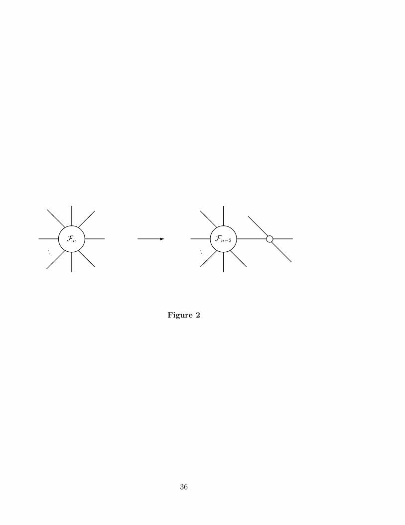
The second type of poles in the Fn only arise when bound states are present in

the model. These poles are located at the values of βij in the physical strip which

correspond to the resonance angles. Let βij = iukij be one of such poles associated

8

to the bound state Ak in the channel Ai × Aj . For the S-matrix we have (fig. 3)

− i limβ→iuk

ij

(β − iukij) Sij(β) =

(

Γkij

)2(2.26)

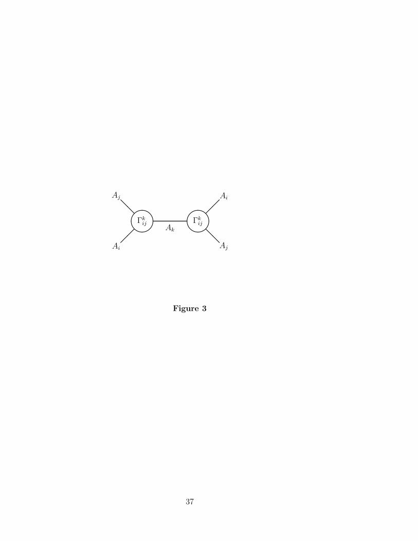
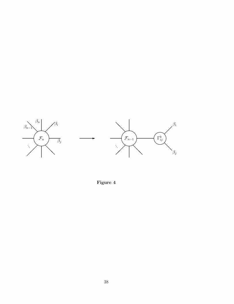
where Γkij is the three-particle vertex on mass-shell. The corresponding residue for

the Fn is given by [12, 13]

− i limǫ→0

ǫ Fn+1(β + iujik − ǫ, β − iui

jk + ǫ, β1, . . . , βn−1) = Γkij Fn(β, β1, . . . , βn−1) ,

(2.27)

where ucab ≡ (π − uc

ab). This equation establishes a recursive structure between the

(n + 1)- and n-particle form factors (fig. 4).

2.6 Correlation Functions from Form Factors

Once the form factors of a theory are known, the correlation functions of local

operators can be written as an infinite series over multi-particle intermediate states.

For instance, the two-point function of an operator O(x) in real Euclidean space is

given by

〈O(x)O(0)〉 =∞∑

n=0

∫

dβ1 . . . dβn

n!(2π)n< 0|O(x)|β1, . . . , βn >in in < β1, . . . , βn|O(0)|0 >

=∞∑

n=0

∫

dβ1 . . . dβn

n!(2π)n| Fn(β1 . . . βn) |2 exp

(

−mrn∑

i=1

cosh βi

)

(2.28)

where r denotes the radial distance, i.e. r =√

x20 + x2

1. All integrals are convergent

and one expects a convergent series as well. Similar expressions can be derived for

multi-point correlators.

3 The Sinh-Gordon Theory

In this paper the model we are concerned with is the Sinh-Gordon theory, defined

by the action

S =∫

d2x

[

1

2(∂µφ)2 − m2

g2cosh gφ(x)

]

. (3.1)

9

It is the simplest example of an affine Toda Field Theories [19], possessing a Z2

symmetry φ → −φ. By an analytic continuation in g, i.e g → ig, it can formally

be mapped to the Sine-Gordon model.

There are numerous alternative viewpoints for the Sinh-Gordon model. First,

it can be regarded either as a perturbation of the free massless conformal action by

means of the relevant operator† cosh gφ(x). Alternatively, it can be considered as

a perturbation of the conformal Liouville action

S =∫

d2x[

1

2(∂µφ)2 − λegφ

]

(3.2)

by means of the relevant operator e−gφ or as a conformal affine A1-Toda Theory

[20] in which the conformal symmetry is broken by setting the free field to zero.

Furthermore, it is interesting to notice that the Sinh-Gordon model can be

mapped into a Coulomb Gas system with an integer set of charges. To illustrate

this, let us consider the (Euclidean) partition function of the model

Z(m, g) =∫

Dφ e−S . (3.3)

Using the identity

exp

(

−m2

g2cosh gφ(x)

)

=+∞∑

n(x)=−∞

In(x)

(

−m2

g2

)

exp (g n(x)φ(x)) , (3.4)

where In(a) denotes the Bessel function of integer order n, the functional integral

in (3.3) becomes Gaussian and can be performed explicitly. Hence Z(m, g) can be

cast in the following form

Z(m, g) = Z(0)+∞∑

n(x)=−∞

In(x)

(

−m2

g2

)

exp

[

g2

2

∫

dxdy n(x)∆(x − y) n(y)

]

,

(3.5)

†Although the anomalous dimension of this operator (computed with respect to the free confor-

mal point), is negative, ∆ = −g2/8π, the resulting theory is unitary. This is due to the existence

of non a nonzero vacuum expectation values of some of the fields Oi in the theory. A detailed

discussion of this point can be found in [15].

10

where Z(0) is the partition function of a massless free theory and ∆(x−y) is the two-

dimensional massless propagator. The model is therefore equivalent to a Coulomb

Gas system with integer charges and with weight functions for the configurations

given by the In’s.

In a perturbative approach to the quantum field theory defined by the action

(3.1), the only ultraviolet divergences which occur in any order in g come from

tadpole graphs and can be removed by a normal ordering prescription with respect

to an arbitrary mass scale M . All other Feynman graphs are convergent and give

rise to finite wave function and mass renormalisation. The coupling constant g does

not renormalise.

An essential feature of the Sinh-Gordon theory is its integrability, which in the

classical case can be established by means of the inverse scattering method [23]. In

order to obtain the expressions of the (classical) conserved currents, let us consider

the Euclidean version of the model in terms of the complex coordinates z and z

z = (x0 + ix1) ; z = (x0 − ix1) , (3.6)

and define a field φ(z, z, ǫ) which satisfies the following (Backlund) equations

∂

∂z(φ + φ) =

m

gǫ sinh

(

g

2(φ − φ)

)

, (3.7)

∂

∂z(φ − φ) =

m

gǫsinh

(

g

2(φ + φ)

)

.

Given that φ(z, z) is a solution of the equation of motion originated by (3.1),

eqs. (3.7) define a new solution φ(z, z, ǫ) and imply as well the following conser-

vation laws

ǫ−1 ∂z

(

coshg

2(φ + φ)

)

− ǫ ∂z

(

coshg

2(φ − φ)

)

= 0 . (3.8)

φ(z, z, ǫ) can be expressed in terms of a power series in ǫ

φ(z, z, ǫ) =∞∑

n=0

φ(n)(z, z) ǫn (3.9)

11

with the fields φ(n)(z, z) calculated by using eqs. (3.7). Placing (3.9) into (3.8) and

matching equal power in ǫ, one obtains an infinite set of conservation laws

∂z Ts+1 = ∂z Θs−1 . (3.10)

The corresponding charges Qs are given by

Qs =∮

[Ts+1 dz + Θs−1 dz] . (3.11)

The integer-valued index s which labels the integrals of motion is the spin of the

operators. Non-trivial conservation laws are obtained for odd values of s

s = 1, 3, 5, 7, . . . (3.12)

In analogy to the Sine-Gordon theory [22], an infinite set of conserved charges Qs

with spin s given in (3.12) also exists for the quantized version of the Sinh-Gordon

theory. They are diagonalised by the asymptotic states with eigenvalues given by

Qs |β1, . . . , βn > = χs

n∑

i=1

esβi |β1, . . . , βn > , (3.13)

where χs is the normalization constant of the charge Qs. The existence of these

higher integrals of motion precludes the possibility of production processes and

hence guarantees that the n-particle scattering amplitudes are purely elastic and

factorized into n(n − 1)/2 two-particle S-matrices. The exact expression for the

Sinh-Gordon theory is given by [6]

S(β, B) =tanh 1

2(β − iπB

2)

tanh 12(β + iπB

2)

, (3.14)

where B is the following function of the coupling constant g

B(g) =2g2

8π + g2. (3.15)

This formula has been checked against perturbation theory in ref. [6] (more recently

to higher orders in [8]) and can also be obtained by analytic continuation of the

12

S-matrix of the first breather of the Sine-Gordon theory [1]. For real values of g the

S-matrix has no poles in the physical sheet and hence there are no bound states,

whereas two zeros are present at the crossing symmetric positions

β =

iπB2

iπ(2−B)2

(3.16)

The absence of bound states in the Sinh-Gordon model is also supported by the

general fusing rule of affine Toda Field Theories [24].

An interesting feature of the S-matrix is its invariance under the map [7]

B → 2 − B (3.17)

i.e. under the strong-weak coupling constant duality

g → 8π

g. (3.18)

This duality is a property shared by the unperturbed conformal Liouville theory

(3.2) [21] and it is quite remarkable that it survives even when the conformal sym-

metry is broken.

4 Form Factors for the Sinh-Gordon Theory

The Z2 symmetry of the model is realized by a map σ, whose effect on the ele-

mentary field of the theory is σ(φ) = −φ. We assume that it has the same effect

on the vertex operator, that is σ(V (β)) = −V (β) together with σ(V (β1)V (β2)) =

σ(V (β1))σ(V (β2)). According to this symmetry we can label the operators by their

Z2 parity.

For operators which are Z2-odd the only possible non-zero form factors are those

involving an odd number of particles, i.e.

FO2n(β1, . . . , β2n) = 0 for σ(O) = −O. (4.19)

13

This implies in particular that O cannot acquire a non-zero vacuum expectation

value. On the other hand, for Z2-even operators the only possible non-zero form

factors are those involving an even number of particles, i.e.

FO2n+1(β1, . . . , β2n+1) = 0 for σ(O) = O. (4.20)

The vacuum expectation value of Z2-even operators can in principle be different

from zero.

The simplest representative of the odd sector is given by the (renormalised) field

φ(x) itself. It creates a one-particle state from the vacuum. Our normalization is

fixed to be (see sect. 4.3)

F φ1 (β) = < 0 | φ(0) | β >in =

1√2

. (4.21)

For the even sector, an important operator is given by the energy-momentum tensor

Tµν(x) = 2π (: ∂µφ∂νφ − gµνL(x) :) (4.22)

where : : denotes the usual normal ordering prescription with respect an arbitrary

mass scale M . Its trace T µµ (x) = Θ(x) is a spinless operator whose normalization

is fixed in terms of its two-particle form factor

FΘ2 (β12 = iπ) = out < β1 | Θ(0) | β2 >in = 2πm2 , (4.23)

where m is the physical mass.

In the following we shall compute the form factors of the operators φ(x) and

Θ(x). This will be sufficient to characterize the basic properties of the model since

form factors for other operators can in general be obtained from simple arguments

once F φn and FΘ

n are known. For instance, suppose we want to compute the form

factors of the operator O =: sinh gφ :. They can be easily computed in terms of

the form factor for φ. In fact, using eq. (2.14) we have

〈0|∂z∂zφ(z, z)|β1 . . . βm〉in = −m2

4

∑

i

eβi∑

i

e−βi∑

i

e−ixpiF φn (β1, . . . , βn) (4.24)

14

Employing the equation of motion and choosing z = z = 0, together with the

identities

n∑

i=1

eβi = σ(n)1 (x1, . . . , xn) ,

n∑

i=1

e−βi =σ

(n)n−1(x1, . . . , xn)

σ(n)n (x1, . . . , xn)

(4.25)

we derive the relation

σnFsinh gφn = gσ1σn−1F

φn . (4.26)

In the last section of this paper we also describe how form factors of operators with

higher spin arise from the knowledge of FΘn or F φ

n .

4.1 Minimal Two-Particle Form Factor

An essential step for the computation the form factors is the determination of

Fmin(β), introduced in (2.20). It satisfies the equations

Fmin(β) = Fmin(−β) S2(β) ,

Fmin(iπ − β) = Fmin(iπ + β) .(4.27)

As shown in [10], the easiest way to compute Fmin(β) (up to a normalization N ) is

to exploit an integral representation of the S-matrix

S(β) = exp

[

∫ ∞

0

dx

xf(x) sinh

(

xβ

iπ

)]

. (4.28)

Then a solution of (4.27) is given by

Fmin(β) = N exp

∫ ∞

0

dx

xf(x)

sin2(

xβ2π

)

sinh x

. (4.29)

where

β ≡ iπ − β . (4.30)

For the Sinh-Gordon theory we have

Fmin(β, B) = N exp

8∫ ∞

0

dx

x

sinh(

xB4

)

sinh(

x2(1 − B

2))

sinh x2

sinh2 xsin2

(

xβ

2π

)

.

(4.31)

15

We choose our normalization to be

N = exp

−4∫ ∞

0

dx

x

sinh(

xB4

)

sinh(

x2(1 − B

2))

sinh x2

sinh2 x

. (4.32)

The analytic structure of Fmin(β, B) can be easily read from its infinite product

representation in terms of Γ functions

Fmin(β, B) =∞∏

k=0

∣

∣

∣

∣

∣

∣

∣

Γ(

k + 32

+ iβ2π

)

Γ(

k + 12

+ B4

+ iβ2π

)

Γ(

k + 1 − B4

+ iβ2π

)

Γ(

k + 12

+ iβ2π

)

Γ(

k + 32− B

4+ iβ

2π

)

Γ(

k + 1 + B4

+ iβ2π

)

∣

∣

∣

∣

∣

∣

∣

2

(4.33)

Fmin(β, B) has a simple zero at the threshold β = 0 since S(0) = −1 and its

asymptotic behaviour is given by

limβ→∞

Fmin(β, B) = 1. (4.34)

It satisfies the functional equation

Fmin(iπ + β, B)Fmin(β, B) =sinh β

sinh β + sinh iπB2

(4.35)

which we will use in the next section in order to find a convenient form for the

recursive equations of the form factors.

A useful expression for the numerical evaluation of Fmin(β, B) is given by

Fmin(β, B) = NN−1∏

k=0

(

1 +(

β/2π

k+ 1

2

)2)(

1 +(

β/2π

k+ 3

2−B

4

)2)(

1 +(

β/2π

k+1+ B4

)2)

(

1 +(

β/2π

k+ 3

2

)2)(

1 +(

β/2π

k+ 1

2+ B

4

)2)(

1 +(

β/2π

k+1−B4

)2)

k+1

(4.36)

× exp

8∫ ∞

0

dx

x

sinh(

xB4

)

sinh(

x2(1 − B

2))

sinh x2

sinh2 x(N + 1 − N e−2x) e−2Nx sin2

(

xβ

2π

)

.

The rate of convergence of the integral may be improved substantially by increasing

the value of N . Graphs of Fmin(β, B) are drawn in fig. 5.

16

4.2 Parametrization of the n-Particle Form Factors

Since the Sinh-Gordon theory has no bound states, the only poles which appear

in any form factor Fn(β1, . . . , βn) are those occurring in every three-body channel.

Additional poles in the n-body intermediate channel are excluded by the elasticity

of the scattering theory. Using the identity

(p1 + p2 + p3)2 − m2 = 8m2 cosh

1

2β12 cosh

1

2β13 cosh

1

2β23 , (4.37)

all possible three-particle poles are taken into account by the following parameter-

ization of the function

Kn(β1, . . . , βn) =Q′

n(β1, . . . , βn)∏

i<jcosh 1

2βij

, (4.38)

where Q′n is free of any singularity. The second equation in (2.18) implies that

Q′n is 2πi-periodic (anti-periodic) when n is an odd (even) integer. Hence, with

a re-definition of Q′n into Qn, the general parameterization of the form factor

Fn(β1, . . . βn) is chosen to be

Fn(β1, . . . , βn) = Hn Qn(x1, . . . , xn)∏

i<j

Fmin(βij)

xi + xj(4.39)

where xi = eβi and Hn is a normalization constant. The denominator in (4.39) may

be written more concisely as det Σ where the entries of the (n− 1)× (n− 1)-matrix

Σ are given by Σij = σ(n)2i−j(x1, . . . , xn).

The functions Qn(x1, . . . , xn) are symmetric polynomials in the variables xi. As

consequence of eq. (2.21), for form factors of spinless operators the total degree

should be n(n − 1)/2 in order to match the total degree of the denominator in

(4.39). Form factors of higher spin operators will be considered in sect. 6. The

order of the degree of Qn in each variable xi is fixed by the nature and by the

asymptotic behaviour of the operator O which is considered.

17

Employing now the parameterization (4.39), together with the identity (4.35),

the recursive equations (2.25) take on the form

(−)n Qn+2(−x, x, x1, . . . , xn) = xDn(x, x1, x2, . . . , xn) Qn(x1, x2, . . . , xn) (4.40)

where we have introduced the function

Dn =−i

4 sin(πB/2)

(

n∏

i=1

[

(x + ωxi)(x − ω−1xi)]

−n∏

i=1

[

(x − ωxi)(x + ω−1xi)]

)

(4.41)

with ω = exp(iπB/2). The normalization constants for the form factors of odd and

even operators are conveniently chosen to be

H2n+1 = H1

(

4 sin(πB/2)

Fmin(iπ, B)

)n

(4.42)

H2n = H2

(

4 sin(πB/2)

Fmin(iπ, B)

)n−1

where H1 and H2 are the initial conditions, fixed by the nature of the operator.

Using the generating function (2.23) of the symmetric polynomials, the function

Dn can be expressed as

Dn =1

2 sin(πB/2)

n∑

l,k=0

(−1)l sin(

(k − l)πB

2

)

x2n−l−kσ(n)l σ

(n)k . (4.43)

As function of B, Dn is invariant under B → −B. The non-zero terms entering the

sum (4.43) are those involving the ratios

sin(n πB/2)

sin(πB/2)

n being an odd number. This means that Dn may only contain powers of cos2(πB/2).

4.3 LSZ Formula for Form Factors

The aim of this section is to show that the symmetric polynomials Q2n+1 entering

the form factors of the elementary field φ(x) can be factorized as

Q2n+1(x1, . . . , x2n+1) = σ(2n+1)2n+1 P2n+1(x1, . . . , x2n+1) n > 0 , (4.44)

18

whereas the analogous polynomials entering the form factors of the trace of the

stress-energy tensor can be written as

Q2n(x1, . . . , x2n) = σ(2n)1 σ

(2n)2n−1 P2n(x1, . . . , x2n) n > 1 . (4.45)

Pn(x1, . . . , xn) is a symmetric polynomial of total degree n(n − 3)/2 and of degree

n−3 in each variable xi. Using the following property of the elementary symmetric

polynomials

σ(n+2)k (−x, x, x1, . . . , xn) = σ

(n)k (x1, x2, . . . , xn) − x2σ

(n)k−2(x1, x2, . . . , xn) , (4.46)

the recursive equations (4.40) can then be written in terms of the Pn as

(−)n+1 Pn+2(−x, x, x1, . . . , xn) =1

xDn(x, x1, x2, . . . , xn) Pn(x1, x2, . . . , xn) .

(4.47)

In order to show the factorization (4.44) for F φ2n+1, it is useful to recall the LSZ

formula for the form factors of a local operator O(x)

Fn(β1, β2, . . . , βn) =

(

1√2

)n

limp2

i→m2

n∏

i=1

(

p2i − m2

i

)

Gn,O(q = −n∑

i=1

pi, p1, p2, . . . , pn)

(4.48)

where

(2π)2δ2(q +∑

pi)Gn,O(q, p1, p2, . . . , pn) =

∫ n∏

i=1

dxi dye−i∑

pixie−iqy < 0 | T (O(y)φ(x1)φ(x2) . . . φ(xn)) | 0 > .(4.49)

The utility of these equations is threefold. First they may allow us to fix the

initial condition of the recursive equations (2.25). Second, they permit to study

the asymptotic behaviour of the form factors, with a corresponding restriction on

the space of solutions. Finally, they provide a tool to check our result through

perturbation theory.

When O(x) is the field φ(x) itself, the application of eq. (4.48) for n = 1 gives

F φ1 (β) = < 0 | φ(0) | β >in =

1√2

limp2→m2

p2 − m2

iG2(p) (4.50)

19

which provides the initial condition

F φ1 (β) =

1√2

. (4.51)

It is now easy to establish that the form factors F φ2n+1 of the elementary field φ(x)

are proportional to σ(2n+1)2n+1 . The reason is that from any Feynman diagram which

enters F φ2n+1 we can factorize the propagator

i

q2 − m2

∣

∣

∣q=−∑

pi, p2

i=m2 (4.52)

that, written in terms of the variables xi, becomes proportional to σ(2n+1)2n+1

i

q2 − m2|q=−

∑

pi, p2

i=m2 =

i

m2

σ(2n+1)2n+1

σ(2n+1)1 σ

(2n+1)2n − σ

(2n+1)2n+1

. (4.53)

The presence of the propagator (4.52) in front of any form factor of the elementary

field φ(x) also implies that F φ2n+1 behaves asymptotically as

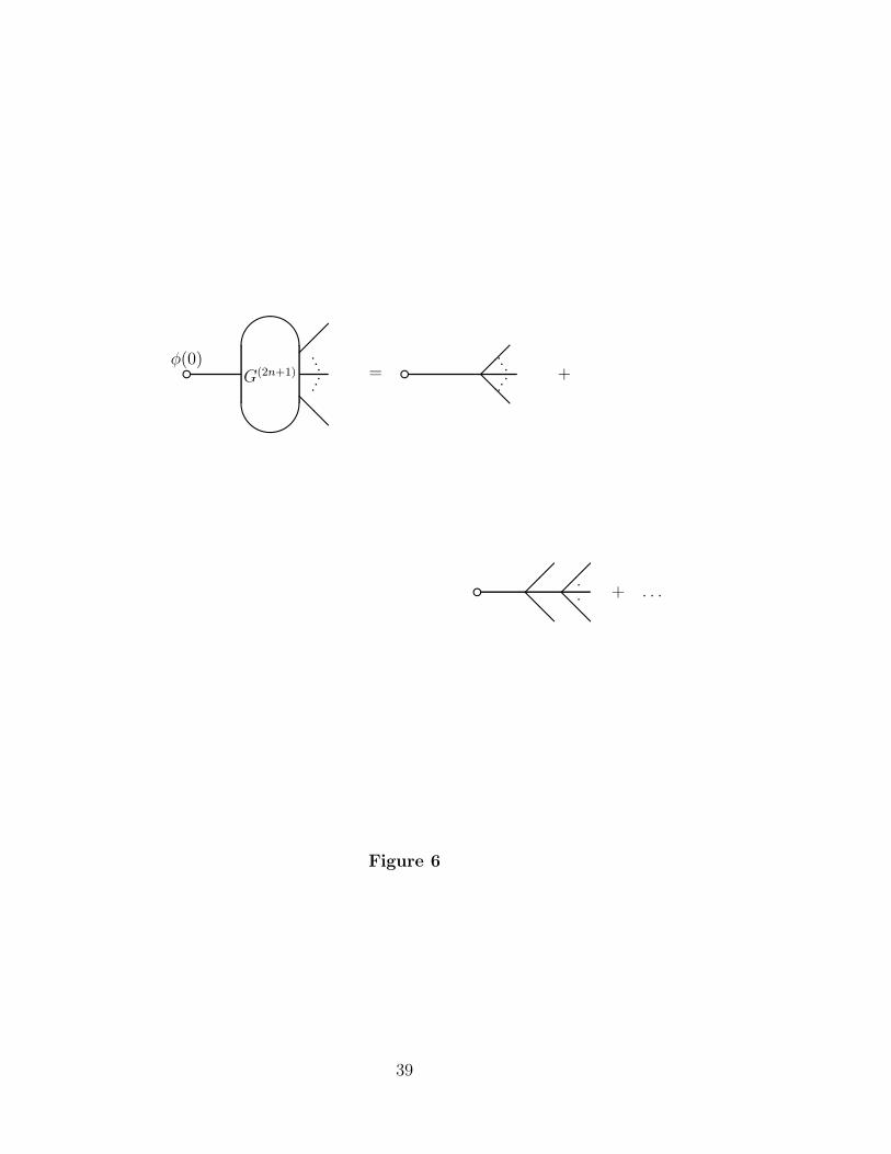
F2n+1(β1, β2, . . . , β2n+1) → 0 as βi → +∞ βj 6=i fixed. (4.54)

In fact, the propagator (4.52) goes to zero in this limit whereas the remaining

expression of the Feynman graphs entering F2n+1 is a perturbative series which

starts from the tree level vertex diagram shown in fig. 6, which is a constant. Other

tree level contributions at the lowest order and higher order corrections are either

finite or they vanish in the limit (4.54). In fact, by dimensional analysis they must

have external momenta in the denominator in order to compensate the increasing

power of the mass in the coupling constants.

In order to prove the factorization (4.45) for the form factors FΘ2n of the trace

of the stress-energy tensor, let us consider the conservation laws satisfied by this

operator

∂zT (z, z) + ∂zΘ(z, z) = 0 , ∂zT (z, z) + ∂zΘ(z, z) = 0 (4.55)

where T (T ) is the component of the stress-energy tensor which in the conformal

limit becomes holomorphic (anti-holomorphic). Using eq. (2.14), the identities (4.25

20

together with (4.55), we obtain

σ(2n)1 σ

(2n)2n F T

2n(β1, . . . , β2n) = σ(2n)2n−1F

Θ2n(β1, . . . , β2n) (4.56)

σ(2n)2n−1F

T2n(β1, . . . , β2n) = σ

(2n)1 σ

(2n)2n FΘ

2n(β1, . . . , β2n). (4.57)

Since F T2n, F T

2n and FΘ2n are expected to have the same analytic structure, we conclude

that FΘ2n(β1, . . . , β2n) is proportional to the product σ

(2n)1 σ

(2n)2n−1 for n > 2.

4.4 Solutions of the Recursive Equations

Let us summarize the analysis carried out in the previous sections. The form factors

F φ2n+1 (n > 0) of the elementary field φ(x) are given by

F φ2n+1(β1, . . . , β2n+1) =

1√2

(

4 sin(πB/2)

Fmin(iπ, B)

)n

σ(2n+1)2n+1 P2n+1(x1, . . . , x2n+1)

∏

i<j

Fmin(βij)

xi + xj

(4.58)

and the normalization of the field is fixed by

F φ1 =

1√2

. (4.59)

The form factors FΘ2n (n > 1) of the trace of the stress-energy tensor Θ(x) are given

by

FΘ2n(β1, . . . , β2n) =

2πm2

Fmin(iπ)

(

4 sin(πB/2)

Fmin(iπ)

)n−1

σ(2n)1 σ

(2n)2n−1P2n(x1, . . . , x2n)

∏

i<j

Fmin(βij)

xi + xj

(4.60)

where the normalization is fixed by the matrix element of Θ(0) between the two-

particle state and the vacuum

FΘ2 (β12) = 2πm2Fmin(β12)

Fmin(iπ). (4.61)

Notice that (4.60) for n = 0 leads to the expectation value of Θ on the vacuum

< 0|Θ(0)|0 > =πm2

2 sin(πB/2). (4.62)

21

Using the recursive equations (4.47) and the transformation property of the elemen-

tary symmetric polynomials (4.46), the explicit expressions of the first polynomials

Pn(x1, . . . , xn) are given by‡

P3(x1, . . . , x3) = 1

P4(x1, . . . , x4) = σ2

P5(x1, . . . , x5) = σ2σ3 − c21σ5 (4.63)

P6(x1, . . . , x6) = σ3(σ2σ4 − σ6) − c21(σ4σ5 + σ1σ2σ6)

P7(x1, . . . , x7) = σ2σ3σ4σ5 − c21(σ4σ

25 + σ1σ2σ5σ6 + σ2

2σ3 − c21σ2σ5) +

−c2(σ1σ6σ7 + σ1σ2σ4σ7 + σ3σ5σ6) + c1c22σ

27

where c1 = 2 cos(πB/2) and c2 = 1 − c21. Expression of the higher Pn are eas-

ily computed by an iterative use of eqs. (4.40). For practical application the first

representatives of Pn are sufficient to compute with a high degree of accuracy the

correlation functions of the fields. In fact, the n-particle term appearing in the

correlation function of the fields (2.28) behaves as e−n(mr) and for quite large values

of mr the correlator is dominated by the lowest number of particle terms. This

conclusion is also confirmed by an application of the c-theorem which is discussed

in sect. 6. Nevertheless, it is interesting to notice that closed expressions for Pn can

be found for particular values of the coupling constant, as we demonstrate in the

next subsections.

4.4.1 The Self-Dual Point

The self-dual point in the coupling constant manifold has the special value

B(√

8π)

= 1 . (4.64)

‡The upper index of the elementary symmetric polynomials entering Pn is equal to n and we

suppress it, in order to simplify the notation.

22

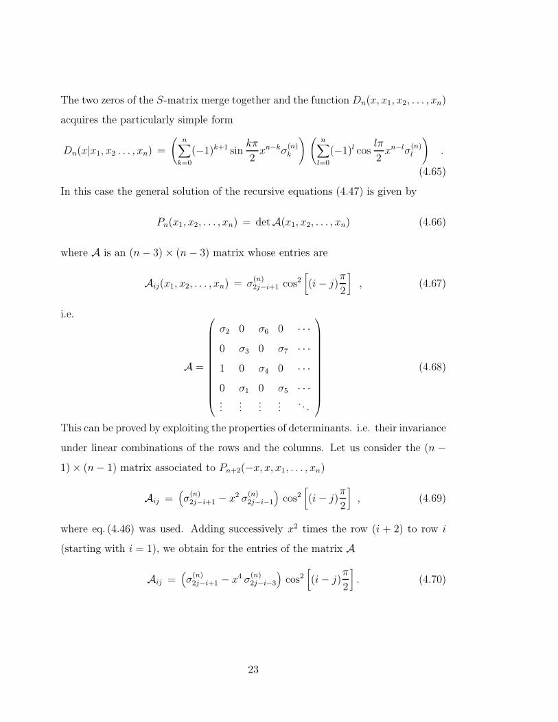
The two zeros of the S-matrix merge together and the function Dn(x, x1, x2, . . . , xn)

acquires the particularly simple form

Dn(x|x1, x2 . . . , xn) =

(

n∑

k=0

(−1)k+1 sinkπ

2xn−kσ

(n)k

) (

n∑

l=0

(−1)l coslπ

2xn−lσ

(n)l

)

.

(4.65)

In this case the general solution of the recursive equations (4.47) is given by

Pn(x1, x2, . . . , xn) = detA(x1, x2, . . . , xn) (4.66)

where A is an (n − 3) × (n − 3) matrix whose entries are

Aij(x1, x2, . . . , xn) = σ(n)2j−i+1 cos2

[

(i − j)π

2

]

, (4.67)

i.e.

A =

σ2 0 σ6 0 · · ·0 σ3 0 σ7 · · ·1 0 σ4 0 · · ·0 σ1 0 σ5 · · ·...

......

.... . .

(4.68)

This can be proved by exploiting the properties of determinants. i.e. their invariance

under linear combinations of the rows and the columns. Let us consider the (n −1) × (n − 1) matrix associated to Pn+2(−x, x, x1, . . . , xn)

Aij =(

σ(n)2j−i+1 − x2 σ

(n)2j−i−1

)

cos2[

(i − j)π

2

]

, (4.69)

where eq. (4.46) was used. Adding successively x2 times the row (i + 2) to row i

(starting with i = 1), we obtain for the entries of the matrix A

Aij =(

σ(n)2j−i+1 − x4 σ

(n)2j−i−3

)

cos2[

(i − j)π

2

]

. (4.70)

23

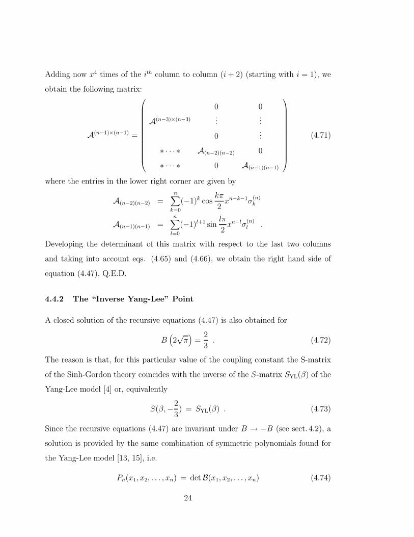
Adding now x4 times of the ith column to column (i + 2) (starting with i = 1), we

obtain the following matrix:

A(n−1)×(n−1) =

0 0

A(n−3)×(n−3) ......

0...

∗ · · · ∗ A(n−2)(n−2) 0

∗ · · · ∗ 0 A(n−1)(n−1)

(4.71)

where the entries in the lower right corner are given by

A(n−2)(n−2) =n∑

k=0

(−1)k coskπ

2xn−k−1σ

(n)k

A(n−1)(n−1) =n∑

l=0

(−1)l+1 sinlπ

2xn−lσ

(n)l .

Developing the determinant of this matrix with respect to the last two columns

and taking into account eqs. (4.65) and (4.66), we obtain the right hand side of

equation (4.47), Q.E.D.

4.4.2 The “Inverse Yang-Lee” Point

A closed solution of the recursive equations (4.47) is also obtained for

B(

2√

π)

=2

3. (4.72)

The reason is that, for this particular value of the coupling constant the S-matrix

of the Sinh-Gordon theory coincides with the inverse of the S-matrix SYL(β) of the

Yang-Lee model [4] or, equivalently

S(β,−2

3) = SYL(β) . (4.73)

Since the recursive equations (4.47) are invariant under B → −B (see sect. 4.2), a

solution is provided by the same combination of symmetric polynomials found for

the Yang-Lee model [13, 15], i.e.

Pn(x1, x2, . . . , xn) = detB(x1, x2, . . . , xn) (4.74)

24

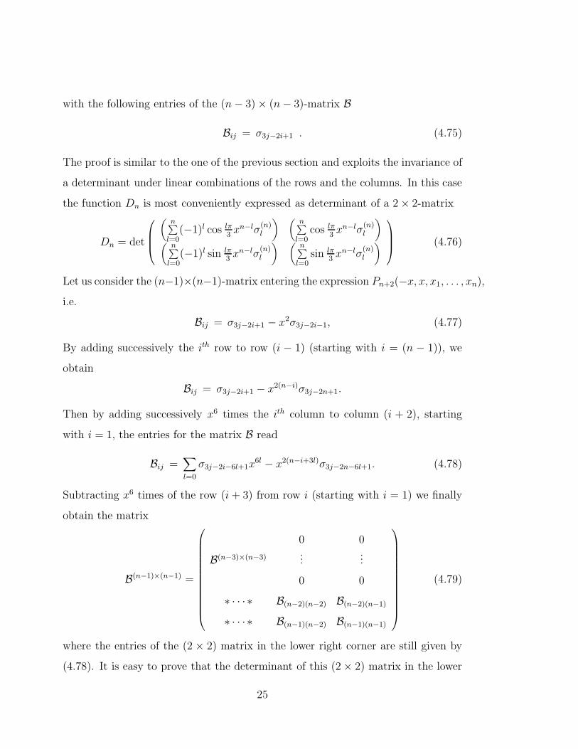
with the following entries of the (n − 3) × (n − 3)-matrix B

Bij = σ3j−2i+1 . (4.75)

The proof is similar to the one of the previous section and exploits the invariance of

a determinant under linear combinations of the rows and the columns. In this case

the function Dn is most conveniently expressed as determinant of a 2 × 2-matrix

Dn = det

(

n∑

l=0(−1)l cos lπ

3xn−lσ

(n)l

) (

n∑

l=0cos lπ

3xn−lσ

(n)l

)

(

n∑

l=0(−1)l sin lπ

3xn−lσ

(n)l

) (

n∑

l=0sin lπ

3xn−lσ

(n)l

)

(4.76)

Let us consider the (n−1)×(n−1)-matrix entering the expression Pn+2(−x, x, x1, . . . , xn),

i.e.

Bij = σ3j−2i+1 − x2σ3j−2i−1, (4.77)

By adding successively the ith row to row (i − 1) (starting with i = (n − 1)), we

obtain

Bij = σ3j−2i+1 − x2(n−i)σ3j−2n+1.

Then by adding successively x6 times the ith column to column (i + 2), starting

with i = 1, the entries for the matrix B read

Bij =∑

l=0

σ3j−2i−6l+1x6l − x2(n−i+3l)σ3j−2n−6l+1. (4.78)

Subtracting x6 times of the row (i + 3) from row i (starting with i = 1) we finally

obtain the matrix

B(n−1)×(n−1) =

0 0

B(n−3)×(n−3) ......

0 0

∗ · · · ∗ B(n−2)(n−2) B(n−2)(n−1)

∗ · · · ∗ B(n−1)(n−2) B(n−1)(n−1)

(4.79)

where the entries of the (2 × 2) matrix in the lower right corner are still given by

(4.78). It is easy to prove that the determinant of this (2 × 2) matrix in the lower

25

right corner is equal to (4.76). Therefore, with the definition (4.74), the determinant

of B(n−1)×(n−1) gives rise the right hand side of (4.47). Q.E.D.

5 Form Factors for Descendent Operators

In this section we investigate the effect of the Lorentz transformation on the space of

solutions for all form factors denoted by P. This problem has been firstly addressed

by Cardy and Mussardo [16] for the space of descendant operators of the Ising model.

The space of the form factors P can be decomposed as

P =⊕

s

Ps , (5.80)

meaning that FOn ∈ Ps if O has spin s. On the rapidity variables a Lorentz trans-

formation is realized by βi → βi +ε, i.e. xi → eεxi. Since the elementary symmetric

polynomials are homogeneous functions of xi, under a Lorentz transformation they

transform as

σn(x1, ..., xn) → enεσn(x1, ..., xn). (5.81)

Hence, given a form factor FOn of an operator O with spin s which satisfies Watson’s

equations, a new function in Ps+s′ which still satisfies Watson’s equations can be

defined by

FO′

n (x1, . . . , xn) = Is′

n (x1, . . . , xn)FOn (x1, . . . , xn), (5.82)

provided that Isn is composed out of elementary symmetric polynomials. Additional

constraints on the Isn are imposed by their invariance under the kinematic residue

equation

Isn+2(−x, x, x1, . . . , xn) = Is

n(x1, . . . , xn) . (5.83)

A basis in the space of solutions of eq. (5.83) is given by symmetric polynomials Isn

satisfying the recursion relations [16]

σ(n)2k+1 = I2k+1

n + σ(n)2 I2k−1

n + σ(n)4 I2k−3

n + . . . + σ(n)2k I1

n , (5.84)

26

where s is equal to the spin of the conserved charges (3.12). A closed expression of

Isn as been obtained in [17]

I2s−1n = (−1)s+1 det I (5.85)

where the entries of the (s × s)-matrix I for j = 1, . . . , s and i = 2, . . . , s are

I1j = σ2j−1 Iij = σ2j−2i+2 (5.86)

i.e.

I =

σ1 σ3 σ5 σ7 . . . σ2s−1

1 σ2 σ4 σ6 . . . σ2s−2

0 1 σ2 σ4 . . . σ2s−4

0 0 1 σ2 . . . σ2s−2

......

......

. . ....

(5.87)

The determinant of I will always be of order 2s − 1 as required.

As it was first noticed in [4], eqs. (5.82) naturally provides a grading in the

space of matrix elements of local operators in an integrable massive field theory. In

fact, given an invariant polynomial Isn, eq. (5.82) defines form factors of an operator

O′s which, borrowing the terminology of Conformal Field Theories [26], is natural

to call descendant operator of the spinless field O. In particular, choosing O to

be the trace of the stress-energy tensor, the form factors defined by eq. (5.82) are

related to the matrix elements of the higher conserved currents, as can be easily

seen by eq. (3.13) and by the fact that the symmetric polynomials which appear as

eigenvalues of the conserved charges Qs

sk = xk1 + xk

2 + . . . + xkn , (5.88)

can be expressed in terms of the invariant polynomials Isn. Indeed they satisfy the

recursive relation

sk − sk−1σ1 + sk−2σ2 − . . . + (−1)k−1s1σk−1 + (−1)kkσk = 0 , (5.89)

27

that, together with eq. (5.84), permits to express sk in terms of the invariant poly-

nomials Isn.

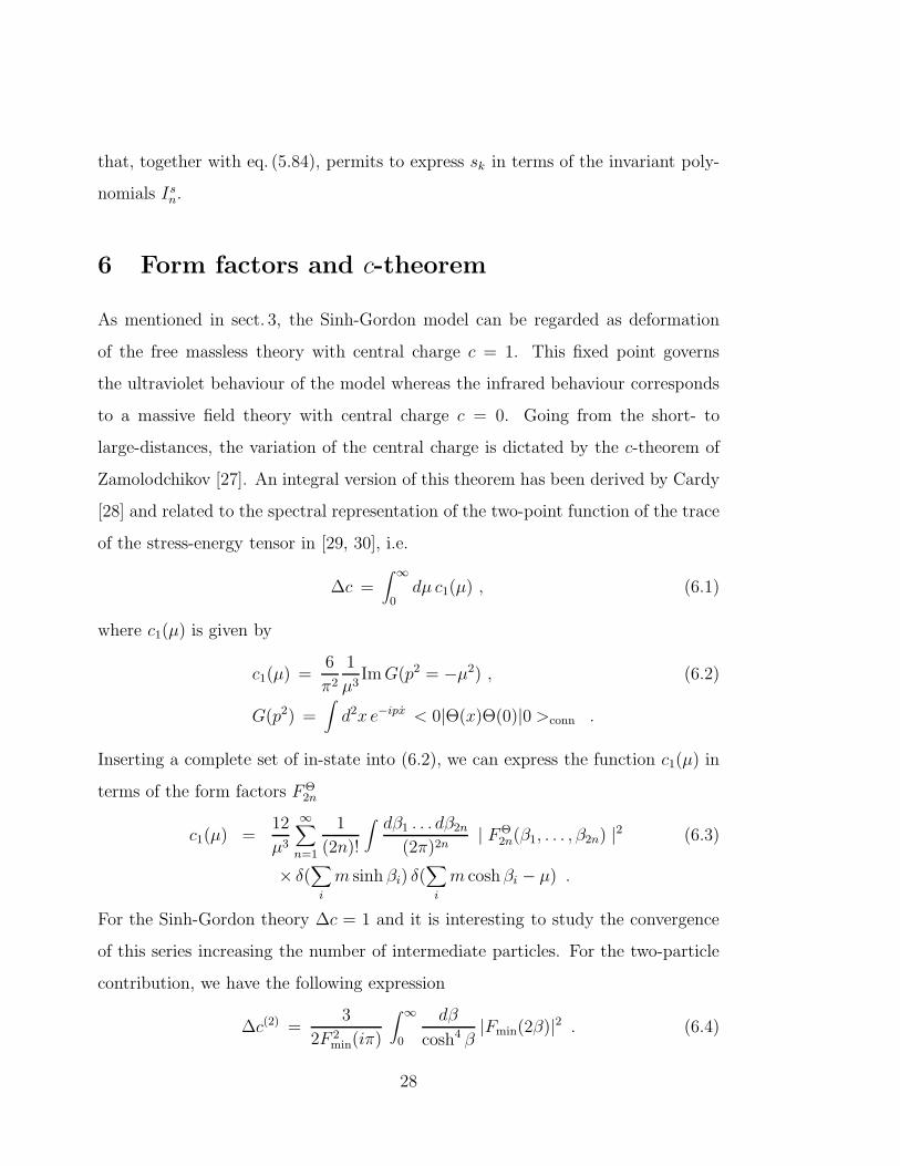
6 Form factors and c-theorem

As mentioned in sect. 3, the Sinh-Gordon model can be regarded as deformation

of the free massless theory with central charge c = 1. This fixed point governs

the ultraviolet behaviour of the model whereas the infrared behaviour corresponds

to a massive field theory with central charge c = 0. Going from the short- to

large-distances, the variation of the central charge is dictated by the c-theorem of

Zamolodchikov [27]. An integral version of this theorem has been derived by Cardy

[28] and related to the spectral representation of the two-point function of the trace

of the stress-energy tensor in [29, 30], i.e.

∆c =∫ ∞

0dµ c1(µ) , (6.1)

where c1(µ) is given by

c1(µ) =6

π2

1

µ3Im G(p2 = −µ2) , (6.2)

G(p2) =∫

d2x e−ipx < 0|Θ(x)Θ(0)|0 >conn .

Inserting a complete set of in-state into (6.2), we can express the function c1(µ) in

terms of the form factors FΘ2n

c1(µ) =12

µ3

∞∑

n=1

1

(2n)!

∫

dβ1 . . . dβ2n

(2π)2n| FΘ

2n(β1, . . . , β2n) |2 (6.3)

× δ(∑

i

m sinh βi) δ(∑

i

m cosh βi − µ) .

For the Sinh-Gordon theory ∆c = 1 and it is interesting to study the convergence

of this series increasing the number of intermediate particles. For the two-particle

contribution, we have the following expression

∆c(2) =3

2F 2min(iπ)

∫ ∞

0

dβ

cosh4 β|Fmin(2β)|2 . (6.4)

28

The numerical results for different values of the coupling constant g2/4π are listed

in Table 1. It is evident that the sum rule is saturated by the two-particle form

factor also for large values of the coupling constant. Hence, the expansion in the

number of intermediate particles results in a fast convergent series, as it is confirmed

by the computation of the next terms involving the form factor with four and six

particles.

7 Conclusions

The computation of the Green functions is a central problem in a Quantum Field

Theory. For integrable models, a promising approach to this question is given

by the bootstrap principle applied to the computation of the matrix elements of

local operators. In this paper we have investigated the form factors of the most

representative fields of the Z2 sectors of the Sinh-Gordon model, i.e. the field φ(x)

and the trace of the stress-energy tensor Θ(x). The simplicity of the Sinh-Gordon

model permits clarification of the basic properties of the local operators and their

matrix elements in a QFT, without being masked by algebraic complexities due to

the structure of the bound states. Compared to the usual method of computing

correlation functions in terms of a perturbative series in the coupling constant,

the form factor approach is extremely advantageous for two reasons. Firstly, the

coupling constant dependence of the correlation functions is encoded (to all orders

in g) into the expression of Fmin(b, B), eq. (4.31), and into the solutions of the

recursive equations (2.25) for the pre-factors Kn entering the form factors, eq. (2.20).

Secondly, even for not large values of the distances, the resulting expressions of the

correlation functions as an infinite series over the multi-particle form factors are

actually dominated by the lowest number of particle terms and therefore present a

very fast rate of convergence.

29

Acknowledgments

A.F. and G.M. are grateful for the hospitality at the International School for Ad-

vanced Studies and Imperial College, respectively. We are grateful to S. Cecotti, F.

Colomo, S. Elitzur, M. Nolasco, D. Olive, I. Pesando and A. Schwimmer for useful

discussions.

References

[1] A.B. Zamolodchikov, Al.B. Zamolodchikov, Ann.Phys. 120 (1979), 253.

[2] A.B. Zamolodchikov, in Advanced Studies in Pure Mathematics 19 (1989), 641;

Int. J. Mod. Phys.A3 (1988), 743.

[3] R. Koberle and J.A. Swieca, Phys. Lett. 86B (1979), 209; A.B. Zamolodchikov,

Int. J. Mod. Phys. A3 (1988), 743; V. A. Fateev and A.B. Zamolodchikov, Int.

J. Mod. Phys. A5 (1990), 1025.

[4] J.L. Cardy, G. Mussardo, Phys. Lett. B225 (1989) , 275.

[5] G. Mussardo, Off-critical Statistical Models: Factorized Scattering Theories

and Bootstrap Program, ISAS/92/37, to appear on Phys. Reports.

[6] A.E. Arinshtein, V.A. Fateev and A.B. Zamolodchikov, Phys. Lett. 87B (1979),

389.

[7] P. Christe and G. Mussardo, Nucl.Phys. B B330 (1990), 465; P. Christe and G.

Mussardo Int. J. Mod. Phys. A5 (1990), 1025; H. W. Braden, E. Corrigan, P.

E. Dorey, R. Sasaki, Nucl. Phys. B338 (1990), 689; H. W. Braden, E. Corrigan,

P. E. Dorey, R. Sasaki, Nucl. Phys. B356 (1991), 469.

[8] H.W. Braden and R. Sasaki, Phys. Lett B255(1991) 343.

30

[9] K.M. Watson, Phys. Rev. 95 (1954), 228.

[10] B. Berg, M. Karowski, P. Weisz, Phys. Rev. D19 (1979), 2477; M. Karowski,

P. Weisz, Nucl. Phys. B139 (1978), 445; M. Karowski, Phys. Rep. 49 (1979),

229;

[11] F. A. Smirnov, in Introduction to Quantum Group and Integrable Massive Mod-

els of Quantum Field Theory, Nankai Lectures on Mathematical Physics, World

Scientific 1990.

[12] F.A. Smirnov, J. Phys. A17 (1984), L873; F.A. Smirnov, J. Phys. A19 (1984),

L575; A.N. Kirillov and F.A. Smirnov, Phys. Lett. B198 (1987), 506; A.N.

Kirillov and F.A. Smirnov, Int. J. Mod. Phys. A3 (1988), 731.

[13] F.A. Smirnov, Nucl. Phys. B337 (1989), 156; Int. J. Mod. Phys. A4 (1989),

4213.

[14] V.P. Yurov and Al. B. Zamolodchikov, Int. J. Mod. Phys. A6 (1991), 3419.

[15] Al.B. Zamolodchikov, Nucl. Phys. B348 (1991), 619.

[16] J.L. Cardy and G. Mussardo, Nucl. Phys. B340 (1990), 387.

[17] P. Christe, Int. J. Mod. Phys. A6 (1991), 5271.

[18] E.K. Sklyanin, Nucl. Phys. B326 (1989), 719.

[19] A.V. Mikhailov, M.A. Olshanetsky and A.M. Perelomov, Comm. Math. Phys.

79 (1981), 473.

[20] O. Babelon and L. Bonora, Phys. Lett. B244 (1990), 220.

[21] P. Mansfield, Nucl. Phys. B222 (1983), 419.

[22] R. Sasaki and I. Yamanaka, in Advanced Studies in Pure Mathematics 16

(1988), 271.

31

[23] L.D. Faddev and L.A. Takhtajan, Hamiltonian Method in the Theory of Soli-

tons, (Springer, N.Y., 1987).

[24] P.E. Dorey, Nucl. Phys B358 (1991) 654; A. Fring, H.C. Liao and D.I. Olive,

Phys. Lett. B266 (1991) 82; A. Fring and D.I. Olive, Nucl. Phys. B379 (1992),

429.

[25] I.G. MacDonald, Symmetric Functions and Hall Polynomials (Clarendon Press,

Oxford, 1979).

[26] A.A. Belavin, A.M. Polyakov, A.B. Zamolodchikov, Nucl. Phys. B241 (1984),

333.

[27] A.B. Zamolodchikov, JEPT Lett. 43 (1986), 730.

[28] J.L. Cardy, Phys. Rev. Lett. 60 (1988), 2709.

[29] A. Cappelli, D. Friedan and J.L. Latorre, Nucl. Phys. B352 (1991), 616.

[30] D.Z. Freedman, J.I. Latorre and X. Vilasis, Mod. Phys. Lett. A6 (1991), 531.

32

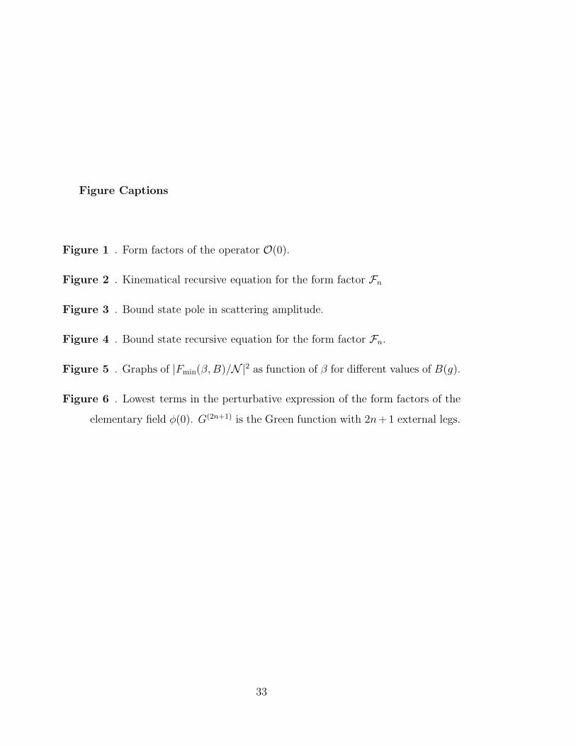
Figure Captions

Figure 1 . Form factors of the operator O(0).

Figure 2 . Kinematical recursive equation for the form factor Fn

Figure 3 . Bound state pole in scattering amplitude.

Figure 4 . Bound state recursive equation for the form factor Fn.

Figure 5 . Graphs of |Fmin(β, B)/N|2 as function of β for different values of B(g).

Figure 6 . Lowest terms in the perturbative expression of the form factors of the

elementary field φ(0). G(2n+1) is the Green function with 2n+1 external legs.

33

Table Caption

Table 1 . The first two-particle term entering the sum rule of the c-theorem.

34

&%'$O(0)

@@

@ β1

β3��

�

βn

βn−1

...β2

���

@@@

Figure 1

35

&%'$

Fn

@@

@

��

�

...

���

@@@

- &%'$Fn−2

@@@

...

@@@

���

i@@

@

@@

@

Figure 2

36

����

Γkij

��

@@

����

Γkij

��

@@

Ai

AjAi

Aj

Ak

Figure 3

37

&%'$

Fn

@@

@ βi

��

�

βn

βn−1

...

βj

���

@@@

- &%'$Fn−1

@@@

...

@@@

���

����

Γkij

��

@@

βi

βj

Figure 4

38

dφ(0)

'

&

$

%G(2n+1)

��......

@@

= d ��

@@

......

+

d ��

@@

��

@@

.

. + . . .

Figure 6

39

B g2

4π∆ c(2)

1500

2999

0.9999995

1100

2199

0.9999878

110

219

0.9989538

310

617

0.9931954

25

12

0.9897087

12

23

0.9863354

23

1 0.9815944

710

1413

0.9808312

45

43

0.9789824

1 2 0.9774634

Table 1

40