arX

iv:h

ep-t

h/06

0512

1v1

11

May

200

6

Preprint typeset in JHEP style. - HYPER VERSION SHEP 06-17

Structure of the MHV-rules Lagrangian

James H. Ettle and Tim R. Morris

School of Physics and Astronomy, University of Southampton, Highfield,

Southampton SO17 1BJ, U.K.

E-mails: jhe@phys.soton.ac.uk, T.R.Morris@soton.ac.uk

Abstract: Recently, a canonical change of field variables was proposed that converts

the Yang-Mills Lagrangian into an MHV-rules Lagrangian, i.e. one whose tree level

Feynman diagram expansion generates CSW rules. We solve the relations defining

the canonical transformation, to all orders of expansion in the new fields, yielding

simple explicit holomorphic expressions for the expansion coefficients. We use these

to confirm explicitly that the three, four and five point vertices are proportional to

MHV amplitudes with the correct coefficient, as expected. We point out several

consequences of this framework, and initiate a study of its implications for MHV

rules at the quantum level. In particular, we investigate the wavefunction matching

factors implied by the Equivalence Theorem at one loop, and show that they may

be taken to vanish in dimensional regularisation.

Contents

1. Introduction 1

2. Notation and Transformation 4

2.1 Preliminaries 4

2.2 The transformation 5

2.3 The precise correspondence 7

3. Explicit Expansion 9

3.1 A expansion coefficients to all orders 9

3.2 A expansion coefficients to all orders 11

3.3 Three-point vertex 13

3.4 Four-point vertices 13

3.5 Five-point vertices 14

4. Equivalence Theorem Matching Factors 15

5. Conclusions 18

A. Off-shell matching factors 20

1. Introduction

The standard approach to computing perturbative scattering amplitudes is to de-

velop a Feynman diagram expansion using Feynman rules, which in turn follow di-

rectly from a bare Lagrangian. While this procedure is very well understood [1], the

complexity of the calculation grows so rapidly with increasing order that it seriously

challenges our ability, especially at one loop and higher, to compute background pro-

cesses to the accuracy that must be known if we are to exploit fully the new physics

potential of the LHC [2].

Stemming from two remarkable papers [3, 4], dramatically simpler methods have

been developed which could help solve this problem. These so far apply mostly to

scattering amplitudes in gauge theories at tree level [5, 6] but also to some one-loop

amplitudes [7–10].

The starting point is the set of maximally helicity-violating (MHV) amplitudes:

the tree-level colour-ordered partial amplitudes for n− = 2 negative helicity gluons

1

and any number n+ ≥ 1 of positive helicity gluons.1 Despite the factorial growth in

complexity of the underlying Feynman diagrams for increasing n+, when these are

written in terms of some associated two-component spinors, the amplitudes collapse

to a single simple ratio [11]. As if this were not astonishing enough, considerations

of topological string theory in twistor space [3] led Cachazo, Svrcek and Witten to

conjecture that arbitrary (n+, n−) tree-level amplitudes of gluons may be calculated

by sowing together certain off-shell continuations of these MHV amplitudes with

scalar propagators, using colour-ordered Feynman rules [4]. These “MHV-rules”

(a.k.a. CSW rules) result in much simpler expressions for generic small n−, growing

in complexity only polynomially with increasing n+. Under parity, we can exchange

n+ ↔ n−, resulting in an alternative expansion via MHV-rules.

The MHV rules were proven indirectly as a consequence of another development

[12]: the BCFW recursion, an expansion of colour-ordered amplitudes involving si-

multaneously both MHV and MHV sub-amplitudes, which in some cases leads to

even more compact expressions albeit at the expense of introducing unphysical poles

in intermediate terms. The recursion equation results from using Cauchy’s theorem

on a carefully chosen complex continuation, to reconstruct the amplitude from its

poles. This idea has been generalised to provide a direct proof of the MHV rules

[13], and applied and extended at tree-level to both Yang-Mills and other theories [6].

It has also been generalised to one-loop amplitudes [7, 9], although the appearance

of physical cuts, spurious cuts, higher poles in complex momenta, and the need for

regularisation in general, limits the power of this idea.

In a separate and initially unexpected development, the MHV rules have been

applied successfully at one loop [9, 10, 14] by again tying together the same off-shell

continuation of the MHV amplitudes with scalar propagators. This is meant to

provide the cut-constructible parts of one-loop amplitudes (which is the whole one-

loop amplitude in theories with unbroken supersymmetry). Although much evidence

supports this contention, a full proof has been missing [15] — until now (see below).

The cut-constructible parts of one-loop amplitudes are specified because these

are directly related to tree amplitudes via their cuts. No claim is made therefore

to generate the full one-loop amplitude in non-supersymmetric theories from MHV

rules. Indeed, it is known that certain non-constructible (parts of) one-loop am-

plitudes are not generated by MHV rules [16], a fact that we will return to in the

conclusions.

As can be gleaned even from this short survey, a feature of these new develop-

ments is that they lie outside the Lagrangian framework, proceeding by a combination

of inspired conjecture and varying levels of proof.

All this potentially changes with Mansfield’s paper however [17]. According to

this paper, a change of field variables satisfying certain specific properties trans-

1Throughout the paper we label all external momenta as out-going.

2

forms the standard Lagrangian into an equivalent MHV-rules Lagrangian, i.e. one

involving effectively a complex scalar whose vertices are proportional to the CSW

off-shell continuation of the MHV amplitudes, so that it directly generates at tree

level the CSW rules. (For a different approach to such a Lagrangian, see ref. [18].

For approaches via (ambi)twistor space see ref. [19].)

Assuming the validity of this proposal, we can apply at once the well developed

quantum field theory framework [1] to confirm and extend these methods. For ex-

ample, if we side-step for the moment the issue of regularisation, by concentrating

on the cut-constructible parts of one-loop amplitudes at non-exceptional momenta,

the existence of the MHV-rules Lagrangian shows immediately that the program of

refs. [9, 10, 14, 15] is correct because the application of MHV rules at one loop sim-

ply means in this framework that one constructs the one loop amplitudes by using

this equivalent Lagrangian. (Actually, we need to take into account ‘ET match-

ing factors’, certain wave function renormalization matching factors that arise from

applying the equivalence theorem [1, 20], however we will see later that they vanish.)

It also means that, up to modifications which are necessary to provide a full

regularisation (which is also much easier to figure out within standard quantum

field theory) and the ET matching factors, the MHV rules must work for the full

amplitudes at any number of loops. In particular we can expect that MHV rules

supply the full amplitude at any loop in finite supersymmetric theories (e.g. N = 4

Yang-Mills).

We make further comments about this framework in the conclusions.

The structure of the rest of the paper is as follows. In the next section we briefly

review Mansfield’s construction [17], which is based on light-cone quantization, and

state precisely the form the MHV-rules Lagrangian should take, paying attention to

conventions. We note in passing that the arbitrary null vector introduced by Cachazo,

Svrcek and Witten to define off-shell continuations is exactly the one defining light-

cone time.

In sec. 3, we give the transformation explicitly to all orders by deriving recur-

rence relations, which we then solve. We find that the expansion coefficients take

simple forms and are in particular already holomorphic. From Mansfield’s arguments

it follows that the resulting vertices yield the MHV-rules Lagrangian, however we

nevertheless check explicitly that the required three, four and five point vertices are

obtained.

In sec. 4, we investigate the one-loop ET matching factors. These are examples

of terms that could not be anticipated using the earlier methods. In the massless case

however (as here) it is easy to argue that they vanish in dimensional regularisation.

Although we are missing the full regularisation, the leading divergent pieces should

be able to be trusted. We check explicitly and find indeed that they are forced to

vanish.

Finally, in section sec. 5, we draw our conclusions.

3

2. Notation and Transformation

In this section we review the form of the transformation to an MHV-rules Lagrangian

as proposed in ref. [17]. We define closely allied notation, but pin down several factors

involved in comparison with the MHV rules.

2.1 Preliminaries

Mansfield maps from the Minkowski coordinates (t, x1, x2, x3) using a (+,−,−,−)

signature metric to ones appropriate for light-front quantization i.e. quantization

surfaces of constant x0 = µ · x, where µν is some constant null-vector. Defining

Minkowski coordinates so that µν = (1, 0, 0, 1), the map is

x0 = t − x3, x0 = t + x3, z = x1 + ix2, z = x1 − ix2. (2.1)

In these coordinates, the metric has covariant components g00 = g00 = −gzz =

−gzz = 1/2, all others being zero.

We will mostly deal with covariant vectors (1-forms) for which it is useful to

introduce a more compact notation, thus we write (p0, p0, pz, pz) ≡ (p, p, p, p). This

allows us, in sympathy with the literature, to write components of external momenta

simply by the number of the leg with the appropriate decoration, thus the nth mo-

mentum pµn will simply be written as (n, n, n, n). Note that we put a tilde over the

z component in this case, so that n will not be confused with a numerical factor of

n [see e.g. (2.4,2.5)].

We can write any 4-vector in the form of a bispinor with components pαα as

(pαα) =(pt δαα + p · σαα

)= 2

(p −p

−p p

), (2.2)

where σ is the usual 3-vector formed of the Pauli matrices. If pµ is null, pp = pp

and the bispinor factorises: pαα = λαλα. For real (pt,p), λα and λα are related by

complex conjugation. For momenta, it is helpful to make the choice:

λ =√

2

(−p/√

p√p

)and λ =

√2

(−p/√

p√p

). (2.3)

Of particular importance for MHV rules is the ‘angle bracket’ invariant, which we

can now express as

〈1 2〉 := ǫαβλ1αλ2β = 2(1 2)√

12, (2.4)

where the two-dimensional alternating tensor has ǫ12 = 1, and we have introduced

(1 2) ≡ (p1 p2) := 12 − 21. (2.5)

4

We can similarly express the contragredient invariant [λ1 λ2] := ǫαβλ1αλ2β in terms

of the complex conjugate 2{1 2}/√

12, where

{1 2} := (1 2)∗ = 12 − 21. (2.6)

Choice (2.3) is not suitable for µαα = νανα, since the only non-zero covariant com-

ponent is µ = 1. Thus from (2.2) we take instead

ν = ν =

(√2

0

).

The standard polarisations for a massless on-shell vector boson of momentum p,

E+ =ν λ

〈ν λ〉 and E− =λ ν

[λ ν],

then have non-zero components

E+ = −1

2, E− =

1

2. (2.7)

There are also E+ = −p/2p and E− = p/2p, although these time-like components

will not be needed. (The remaining components vanish.)

Importantly, (2.3) contains no reference to p and makes sense even for non-null

momenta. In this case, the spinors factor the bispinor associated to the null momen-

tum p+aµ, where a = pp/p−p. This definition is equivalent to the CSW prescription

for taking the spinors off-shell [4, 17], providing the CSW spinor is identified (pro-

jectively) with ν. Indeed, the CSW prescription is to introduce a fixed spinor η and

take the off-shell momentum spinor to be proportional to

ǫαβpααηβ = λα[λ η] − aνα[ν η],

so the two definitions coincide when η ∝ ν. We thus arrive at the satisfying conclusion

that the arbitrary null vector ηαηα is just µαα, the vector defining light-cone time

and the quantization surface.

2.2 The transformation

We take the Yang-Mills action written as [17]

S =1

2g2

∫dt dx1dx2dx3 trF λρFλρ, (2.8)

where

Fλρ = [Dλ, Dρ], Dµ = ∂µ + Aµ, Aµ = AaµT

a, (2.9)

5

and the generators of the internal group have been taken as anti-Hermitian:

[T a, T b] = fabcT c, tr (T aT b) = −1

2δab. (2.10)

We choose light-cone gauge A = 0, discarding the non-interacting Fadeev-Popov

ghosts, and integrate out the longitudinal field A (which appears quadratically and

is not dynamical, in the sense that the Lagrangian has no terms ∂A).

The resulting action takes the form

S =4

g2

∫dx0L, (2.11)

where L is the light-cone Lagrangian defined as an integral d3x = dx0 dz dz over

surfaces Σ of constant x0. From (2.7), A (A) has only positive (negative) helicity

on-shell states. Labelling the parts by the participating helicities L = L−+ +L++− +

L−−+ + L′−−++, where

L−+[A] = tr

∫

Σ

d3x A (∂∂ − ∂∂) A (2.12)

L++−[A] = −tr

∫

Σ

d3x (∂∂−1A) [A, ∂A] (2.13)

L−−+[A] = −tr

∫

Σ

d3x [A, ∂A] (∂∂−1A) (2.14)

L′−−++[A] = −tr

∫

Σ

d3x [A, ∂A] ∂−2 [A, ∂A]. (2.15)

Now we define a canonical change of variables from A to B to absorb the un-

wanted term L++− into the kinetic term:

L−+[A] + L++−[A] = L−+[B]. (2.16)

This means that the transformation is performed on the quantization surface Σ with

all fields having the same time dependence x0 (which henceforth we suppress). It

induces the following transformation for the canonical momenta:

∂Aa(y) =

∫

Σ

d3xδBb(x)

δAa(y)∂Bb(x). (2.17)

Substituting this back into (2.16) yields the defining relation between A and B:

∫

Σ

d3y

[D,

∂

∂A

]a

(y)δBb(x)

δAa(y)=

∂∂

∂Bb(x). (2.18)

It follows that A is a power series in B, of the form A = B + O(B2) (at least for

general momenta: see further comments in sec. 3) and thus from (2.17), A is a power

series in B each term containing also a single B, of the form A = B + O(BB).

6

Thus it follows from the equivalence theorem that we can equally well use B (B)

as the positive (negative) helicity field in place of A (A) [1, 17]. The canonical nature

of the transformations ensures that the change of variables in the functional integral

has unit jacobian [17], whilst substituting the transformations into L results, from

(2.16) and (2.14,2.15), in a Lagrangian with an infinite number of interactions each

containing just two B fields and an increasing number of B fields:

L = L−+[B] + L−−+[B] + L−−++[B] + L−−+++[B] + · · · . (2.19)

This has precisely the structure required to be identified with the MHV-rules La-

grangian, in the sense that its tree level perturbation theory generates CSW rules

with the Feynman rules following from these vertices. It follows immediately that

these vertices when taken on-shell must be proportional to the corresponding MHV

amplitude since only one vertex is used to construct the tree-level amplitude with the

right helicity assignment of two negative and any number positive helicities. (Using

two or more vertices results in “NnMHV” amplitudes with more than two negative

helicities.)

It remains to show that when off-shell, these vertices must give the CSW contin-

uations of the MHV amplitudes. Mansfield argues that this would follow from the

fact that the vertices contain no explicit x0 dependence (or ∂) if one can show that

the vertices are also holomorphic in the sense that they contain no ∂ derivatives. We

will see that this is true at least for general momenta. Mansfield argues that this

holomorphy follows from considering the homogeneous transformations:

δA = [A, θ] and δA = [A, θ], (2.20)

where θ is a function of z only. He uses the fact that this corresponds to the shift

δ∂A = [A, ∂θ] when acting on (2.16), the equation defining the expansion, and does

not leave it invariant, whereas (2.20) does leave invariant the sum of the two terms

(2.14,2.15) which generates all the vertices in (2.19). From this viewpoint however,

it is a surprise to find that the coefficients of the series for A (A) themselves are

already holomorphic. Furthermore, we will show that they take a very simple form.

2.3 The precise correspondence

Clearly, it would be very welcome to investigate explicitly the transformation (2.17,2.18)

and its effect on the vertices. In order to do this, we write the general n-point term

in (2.19) in 3-momentum space as

1

2

n∑

s=2

∫

12···n

V s12···n tr[B1B2 · · · Bs · · ·Bn], (2.21)

where the bar on the indices indicates that the 3-momentum dependence is Bk ≡B(−pk) (we continue to suppress their common x0 dependence, which is not Fourier

7

transformed), the missing fields in the trace being Bks. The components of p are

expressed, as always, as (p, p, p). The integral shorthand means, here and later,∫

12···n

≡n∏

k=1

∫dpk dpk dpk

(2π)3,

and the vertex is expressed as

V s12···n = (2π)3δ3(p1 + p2 + · · ·+ pn) V s(p1,p2, · · · ,pn). (2.22)

Throughout the paper, expansion coefficients, vertices and amplitudes carry these

momentum conserving delta-functions; they will be factored off in this manner and

thus not written explicitly. We often simply write V s(12 · · ·n) ≡ V s(p1,p2, · · · ,pn).

It should be borne in mind that from (2.22) such coefficients are only defined when

their momentum arguments sum to zero.

Note that, by using (2.10), we can always express the group theory factors as

traces of products of the Bs and Bs valued in the Lie algebra, as in (2.21). This

form leads to the required colour-ordered Feynman rules. We will express group

theory factors throughout by absorbing them in the fields, including for the expansion

coefficients of sec. 3.

By the cyclicity of the trace, we can always arrange for the first field in (2.21) to

be a B. Since we have a choice of two Bs, we could have restricted the sum in (2.21)

to r ≤ ⌊n/2 + 1⌋, however by writing it as a full sum over r and dividing the result

by two, we get the same thing except that the ⌊n/2 + 1⌋th vertex is accompanied by

a factor 12

when n is even, consistent with the fact that it alone has a Z2 symmetry

under exchange of the Bs.

We would like to compare V s1···n to the MHV amplitude [11]:

An = gn−2 〈r s〉4〈1 2〉〈2 3〉 · · · 〈n − 1, n〉〈n 1〉 , (2.23)

r and s being the negative helicity legs, itself a component of the full tree-level

amplitude: ∑

σ

tr (T aσ(1) · · ·T a

σ(n)) (2π)4i δ4(p1 + · · · + pn) Aσn, (2.24)

the sum being over distinct cyclic orderings σ. However this is written with different

conventions.

There are many ways to perform the translation. Perhaps the following is sim-

plest. The normalization for the generators in (2.23,2.24) is such that tr (T aT b) = δab

and [T a, T b] = i√

2fabcT c [21]. Comparing with (2.10) we see we need to replace

T a 7→ −iT a/√

2. To form the momentum space Feynman rule from (2.21) and

(2.22), we Fourier transform the x0 dependence also, obtaining a four-dimensional

delta-function as in (2.24), however in our case it is defined via (2.1) to be

(2π)4δ4(p) =

∫dx0dx0dz dz e i(p x0 + p x0 + p z + p z).

8

As can be seen by computing the jacobian or√−g, this is four times the one in

(2.24). Noting that pµpµ = 4(pp − pp), we see that (2.11) and (2.12) yield the

propagator 2ig2δab/p2. To bring this to canonical normalization requires absorbing

2g2 by B 7→ Bg√

2 (similarly B). Combining all these with the prefactor from (2.11),

we see that the r = 1 MHV amplitude should be given by

16

g2(−ig)n V s(12 · · ·n) (E+)n−2 (E−)2.

Of course the factor 12

for the even-n ⌊n/2+1⌋th vertex in (2.21) is cancelled here by

the two ways to form this amplitude. Finally, from (2.7), (2.23) and (2.4) we thus

expect to find

V s(12 · · ·n) = (2i)n−4 〈1 s〉4〈1 2〉〈2 3〉 · · · 〈n − 1, n〉〈n 1〉

= in2 · · · n (1 s)4

1s2(1 2)(2 3) · · · (n − 1, n)(n 1). (2.25)

3. Explicit Expansion

In this section we derive recursion relations for the expansions satisfying (2.18) and

(2.17) in the case that A and B have support only on general momenta. We then

solve these and use the results to confirm (2.25) for the three point, the two four-point

and the two five-point vertices.

3.1 A expansion coefficients to all orders

Rearranging (2.18) and transforming to 3-momentum space yields

ω1A1 − i

∫

23

ζ3[A2, A3] (2π)3δ3(p1 − p2 − p3) =

∫

p

ωpBbp

δA1

δBbp

, (3.1)

using the notation set up in subsec. 2.3, and introducing ζp ≡ ζ(p) = p/p and

ωp = pp/p.

From this one would be tempted to conclude that at lowest order Ap = Bp

and thus in general, absorbing the group theory generators into the fields, A has an

expansion in B of the form

A1 =

∞∑

n=2

∫

2···n

Υ12···n B2 · · ·Bn, (3.2)

where Υ(p,−p) = 1. However we have to divide through by ωp to conclude that Ap =

Bp to lowest order, and since ωp vanishes when p = 0 or p = 0, more general solutions

exist where Ap has a piece not containing Bp but with delta-function support, viz.

δ(p) and/or δ(p).

9

It is tempting to ignore these terms, however we cannot do so and also implement

some expected residual gauge invariances: the light cone action (2.11) is arrived at

by fixing the gauge µ · A ∝ A = 0. This leaves gauge transformations δAµ = [Dµ, θ]

unfixed providing θ does not depend on z. If θ depends on x0, we can expect the form

of the gauge transformation to be modified as a result of A being integrated out. On

the other hand, it is easy to check that (2.11) is invariant under holomorphic gauge

transformations θ(z), providing we interpret2 ∂∂−1θ := ∂−1(∂θ) = 0. Similarly (by

symmetry) we also have antiholomorphic gauge invariance generated by θ(z).

Now, the left hand side of (2.16) is actually invariant under holomorphic gauge

transformations which indicates that B and B must also be invariant. Indeed this

ensures that the defining transformations (2.17,2.18) transform covariantly. However,

(3.2) only transforms covariantly if we allow for an extra term independent of B and

proportional to δ(p1) to absorb the gauge transformation. This indicates one should

really interpret (3.2) as amounting to further gauge fixing. For the present we will

simply declare that (3.2) is to be applied only for generic momenta in particular such

that p1 and p1 are non-zero.

Substituting (3.2) in (3.1), comparing coefficients and stripping off momentum

conserving delta functions as in (2.22), yields the recurrence relation:

Υ(1 · · ·n) =i

ω1 + · · ·+ ωn

n−1∑

j=2

(ζj+1,n − ζ2,j)Υ(−, 2, · · · , j)Υ(−, j+1, · · · , n), (3.3)

where the arguments labelled “−” are minus the sum of the remaining arguments

(as follows from momentum conservation) and we have defined ζj,k = ζ(Pj,k) with

Pj,k =∑k

i=j pi (similarly for ωj,k below). The next two coefficients are thus

Υ(123) = iζ3 − ζ2

ω1 + ω2 + ω3, (3.4)

Υ(1234) =1

ω1 + ω2 + ω3 + ω4

[(ζ4 − ζ3)(ζ3,4 − ζ2)

ω3,4 − ω3 − ω4+

(ζ4 − ζ2,3)(ζ3 − ζ2)

ω2,3 − ω2 − ω3

]. (3.5)

Although apparently not holomorphic, once they are expressed in terms of indepen-

dent momenta and simplified, all pk dependence drops out, resulting in very compact

expressions:

Υ(123) = −i1

(2 3),

Υ(1234) =13

(2 3)(3 4),

Υ(12345) = i134

(2 3)(3 4)(4 5).

2We note that this is consistent with the Mandelstam-Leibbrandt prescription [22].

10

We have displayed the four-point coefficient which we also checked explicitly. Now

we prove by induction that the general coefficient takes the form

Υ(1 · · ·n) = in134 · · · n − 1

(2 3)(3 4) · · · (n−1, n), (3.6)

where n ≥ 4. It is sufficient to show that substituting (3.6) into the right hand side

of (3.3) yields the left hand side. Substituting (3.6) into the right hand side yields

− Υ(1 · · ·n)

1(ω1 + · · ·+ ωn)

n−1∑

j=2

(j, j+1)

j j+1{P2,j Pj+1,n},

after due care with the ends of the sum. Expanding the (j, j+1) term and relabelling

so that both halves are indexed by j converts the sum ton∑

j=2

j

j({P2,j−1 Pj,n} − {P2,j Pj+1,n}) ,

where contributions at the end of the sum are correctly incorporated by defining

Pj,k = 0 when j > k. Writing P2,j = P2,j−1 +pj and Pj+1,n = −P2,j−1 −p1 −pj, and

using the antisymmetry of (2.6), the sum collapses to −1(ω1 + · · ·+ωn), proving the

assertion (3.6).

3.2 A expansion coefficients to all orders

Differentiating (3.2) with respect to B and substituting the inverse into (2.17) yields

an expansion for A of the form

1A1 =∞∑

m=2

m∑

s=2

∫

2···m

s Ξs−112···m

B2 · · · Bs · · ·Bm, (3.7)

where the superscript on Ξ labels the relative position (not momentum) of the B

field and the missing fields are Bks. We use the invariant

tr

∫

Σ

d3x ∂A∂A = tr

∫

Σ

d3x ∂B∂B

to extract a recurrence relation. Recalling that all fields have the same x0 dependence,

we have from (3.2),

∂A1 =

∞∑

n=2

n∑

r=2

∫

2···n

Υ12···n B2 · · · ∂Br · · ·Bn.

Substituting this and (3.7) into the above, using cyclicity of the trace and several

careful relabellings we find:

Ξl(1 · · ·n) = −n+1−l∑

r=2

r+l−1∑

m=max(r,3)

Υ(−, n−r+3, · · · , m−r+1)×

Ξl+r−m(−, m−r+2, · · · , n−r+2), (3.8)

11

where l = 1, · · · , n − 1, the momentum indices on the right hand side must be

interpreted cyclically, i.e. mod n, and Ξ1(p,−p) = 1. [Note that m is the number

of arguments in Υ. The inner sum should be interpreted as zero when r = 2 and

l = 1, alternatively the lower limit in r can be given as max(2, 4− l).] From this, or

directly, one can readily compute the first few coefficients:

Ξ1(123) = −Υ(231),

Ξ2(123) = −Υ(312),

Ξ1(1234) = −Υ(2+3, 4, 1) Ξ1(1+4, 2, 3)− Υ(2341),

Ξ2(1234) = −Υ(3+4, 1, 2) Ξ1(1+2, 3, 4)− Υ(2+3, 4, 1) Ξ2(1+4, 2, 3)− Υ(3412),

Ξ3(1234) = −Υ(3+4, 1, 2) Ξ2(1+2, 3, 4)− Υ(4123).

Clearly, since the Υ coefficients are already holomorphic, the Ξs will turn out to be

also. In fact they take a very simple form when expressed in terms of Υ:

Ξs−1(1 · · ·n) = − s

1Υ(1 · · ·n), (3.9)

(s = 2, · · · , n and n ≥ 2).

Let us now prove this assertion. Again, it is sufficient to show that substituting

(3.9) into the right hand side of (3.8) yields its left hand side. Substituting (3.9) into

the right hand side and using (3.6), we find we can extract a factor of Ξl(1 · · ·n) and

thus learn that proving (3.9) is equivalent to proving that

n+1−l∑

r=2

r+l−1∑

m=max(r,3)

(m−r+1, m−r+2)(n−r+2, n−r+3)Pn−r+3,m−r+1

m−r+1 m−r+2 n−r+2 n−r+3

equals

−(1 2)(n 1)

12n(3.10)

In a similar way to the proof of (3.6), we now expand the factor (m−r+1, m−r+2)

and relabel so that both halves are collected. (However since here momentum labels

are treated mod n, Pj,k means summing from j increasing to k, going through 1 when

k < j.) This allows us to perform the inner sum with the result displayed in braces:

n+1−l∑

r=2

(n−r+2, n−r+3)

n−r+2 n−r+3

{−Pq+2,l +

l + 1

l + 1Pn−r+3,l −

q + 1

q + 1Pn−r+3, q+1

}. (3.11)

Here q = 1 if r = 2 otherwise q = 0. We note that the term in curly brackets vanishes

when r = 2 and l = 1, as required, cf. below (3.9). At this stage it proves useful to

consider the case l = n − 1 separately. Substituting this into (3.11) gives

(n 1)

1n

{n + 1 + 2 − n − 2

2P1,2

},

12

where we have used momentum conservation on the first two terms in curly brackets.

It is immediate to see that this gives (3.10) as required. For l < n − 1, we expand

(n−r+2, n−r+3) and collect both halves. This gives

P1,l+1

(1

1− l + 1

l + 1

)+

n

n

(12

2− 1

)+

1

1

(−P3,l +

l + 1

l + 1P1,l − 2 − 12

2

)

+l + 1

l + 1

(P2,l + l + 1 +

1

1Pl+2,1

).

Using momentum conservation and cancelling terms, this expression collapses to

(3.10), and thus (3.9) is proved.

Recall that to obtain the vertices (2.21,2.22) in (2.19), we substitute the series

(3.2) and (3.7), which we have seen are holomorphic, into (2.14) and (2.15), which are

also holomorphic. Thus we have proven that the vertices in (2.19) are holomorphic.

It follows by Mansfield’s arguments [17] that these vertices when off-shell give the

CSW continuations of the MHV amplitudes, i.e. are the ones in (2.25). Nevertheless

it is instructive to verify that this really does work out in practice.

3.3 Three-point vertex

Since A (A) is, to lowest order, linear in B (B), the three-point vertex is simply the

light-cone gauge vertex (2.14). Transforming to 3-momentum space and casting in

the form (2.21), we have

V 2(123) = i3

12(2 1). (3.12)

On the other hand, from (2.25) we expect

−i3

12

(1 2)3

(2 3)(3 1).

Substituting p3 = −p1 −p2 in the denominator, we readily see that these equations

are the same and thus simply verify that the light-cone gauge three-point vertex

satisfies the general formula (2.25) as expected:

V 2(123) =1

2i

〈1 2〉3〈2 3〉〈3 1〉 .

3.4 Four-point vertices

The four-point vertices receive contributions from (2.14) and the first non-trivial

terms in (3.2,3.7), and also directly from (2.15), and thus are more exacting tests.

We write (2.15) in the same form as (2.21):

L′−−++ =

∫

1234

{W 2

1234 tr[A1A2A3A4] +1

2W 3

1234 tr[A1A2A3A4]

},

13

where

W 2(1234) = − 13 + 24

(1 + 4)2and W 3(1234) =

14 + 23

(1 + 2)2+

12 + 34

(1 + 4)2

(after symmetrization). Therefore,

V 2(1234) =1

5V 2(523) Ξ2(541) +

2

5V 2(154) Ξ1(523) + V 2(125)Υ(534) + W 2(1234),

(3.13)

where the momentum p5 is determined by conservation in each term (thus e.g. in the

first term p5 = p1 + p4). To compare this formula to the expected result (2.25) we

map both to unique functions of independent momenta. For example, we substitute

for the last momentum: p4 = −p1 − p2 − p3. It is then straightforward using

computer algebra to show that this coincides with the right hand side of (2.25), and

thus:

V 2(1234) =〈1 2〉3

〈2 3〉〈3 4〉〈4 1〉 .

For example, simplifying by partial fractions, both (2.25) and (3.13) give:

(1 + 2)2(12 − 21)

12 [(1 + 2)3 − 31 − 32]− 2(1 + 2 + 3)(12 − 21)

1(2 + 3)(23 − 32)− 13(12 − 21)

2(2 + 3)(12 + 13 − 21 − 31).

Similarly, after symmetrization,

V 3(1234) =1

5V 2(352) Ξ2(541) +

3

5V 2(512) Ξ1(534)

+3

5V 2(154) Ξ2(523) +

1

5V 2(534) Ξ1(512) + W 3(1234),

and it is straightforward to confirm as above that this agrees with (2.25):

V 3(1234) =24

13

(1 3)4

(1 2)(2 3)(3 4)(4 1).

3.5 Five-point vertices

The five-point vertices leave no doubt that the off-shell MHV vertices are produced:

they involve substituting up to the first three terms in the expansions (3.2,3.7) into

14

both original vertices (2.14,2.15). We find

V 2(12345) =3

6V 2(612) Ξ1(6345) +

1

7V 2(726)Υ(634) Ξ2(751) + V 2(126)Υ(6345)

+2

6

1

7V 2(764) Ξ1(623) Ξ2(751) +

2

6V 2(167) Ξ1(623)Υ(745)

+2

6V 2(165) Ξ1(6234) + W 2(1236)Υ(645) + W 2(1265)Υ(634)

+2

6W 2(1645) Ξ1(623) +

1

6W 2(6234) Ξ2(651),

V 3(12345) =3

6V 2(612) Ξ1(6345) +

1

6V 2(634) Ξ2(6512) +

1

6V 2(637) Ξ1(612)Υ(745)

+1

6

3

7V 2(675) Ξ1(612) Ξ1(734) +

1

7

3

6V 2(672) Ξ1(634) Ξ2(751)

+1

6

3

7V 2(674) Ξ2(651) Ξ2(723) +

3

6V 2(167) Ξ2(623)Υ(745)

+3

6V 2(165) Ξ2(6234) +

1

6V 2(362) Ξ3(6451) +

3

6W 2(1645) Ξ2(623)

+1

6W 2(6345) Ξ1(612) +

3

6W 3(1265) Ξ2(634) +

1

6W 3(3462) Ξ2(651)

+ W 3(1236)Υ(645)

(where, like before, indices 6 and 7 label momenta that are uniquely determined in

terms of the first five by momentum conservation). Again, eliminating p5 in favour

of the first four momenta and doing likewise for the corresponding right hand sides

in (2.25), we find the expressions agree, and thus confirm that

V 2(12345) = 2i〈1 2〉3

〈2 3〉〈3 4〉〈4 5〉〈5 1〉 , and

V 3(12345) = 2i〈1 3〉4

〈1 2〉〈2 3〉〈3 4〉〈4 5〉〈5 1〉 .

4. Equivalence Theorem Matching Factors

Even if a change of field variables from A to B turns the light-cone gauge Lagrangian

into an MHV-rules Lagrangian, this does not mean necessarily that one-loop and

higher contributions are obtained purely by using the CSW rules. We have to re-

member that wavefunction renormalization terms, which we have already referred to

as ET matching factors, are also generated [1, 20].

Let us recall that an S-matrix element is obtained by computing the amputated

Green function (the LSZ procedure). Thus to the action (2.11), we should add the

15

source terms ∫d4x JaAa + JaAa, (4.1)

where, after amputating propagators 〈A A〉(p), by multiplying by −ip2 and taking

the on-shell limit p2 → 0, we see that J acts as a source for positive helicity A legs

in the amputated Green function (and likewise J for negative helicity A legs).

Now, substituting the series (3.2) and (3.7) into (4.1), we see that at tree-level

the process of multiplying by −ip2 and taking the on-shell limit, kills all terms but

the first, which survives because these generate cancelling poles via the propagators

〈B B〉(p). Therefore, we can effectively write the source terms as∫

d4x JaBa + JaBa.

This is the tree-level content of the Equivalence Theorem.

At one loop and higher, the only change to this conclusion is that we can use the

vertices in the expansions (3.2,3.7) and those of the Lagrangian, viz. (2.21), to form

self-energy-like diagrams, cf. fig. 1. Since these again attach to propagators carrying

the external momentum pµ, they survive the process of amputation.

These ET matching factors are not explicitly Lorentz invariant, a consequence

of both the light-cone axial gauge and the change to B fields. However, if everything

is defined correctly, Lorentz invariance should be recovered in the process of forming

S-matrix elements. Therefore we should find that these matching factors depend

only on p2, which is sent to zero. Since these self-energy-like diagrams then depend

on no scale at all, in dimensional regularisation we must set them to zero.

+ ++

+

−

−p

(a)

− −−

+

+

−p+

− −+

−

−

+p

(b)

Figure 1: Topology of the one-loop ET matching factors, with (a) the contribution to

negative helicity B legs; and (b) the contribution to positive helicity B legs. Wavy lines

denote A and A fields, straight lines B and B.

We now confirm these conclusions at one loop. The terms in fig. 1 contribute by

multiplying the legs of the corresponding tree-level amplitude (computed using the

CSW rules). The diagrams in fig. 1 contain both ultraviolet and infrared divergences.

We derived the vertices (3.2,3.7) and (2.21) without using any regularisation. Strictly

speaking, we should therefore wait until a corresponding Lagrangian is supplied

incorporating sufficient regularisation. However, if we proceed with the calculation,

16

naıvely applying dimensional regularisation where needed, we can expect to get right

the most divergent pieces.

From the diagram fig. 1(a), using (3.2) and (3.12), we obtain

−1

2g2CA

∫d4q

(2π)4

Υ(−p, p + q,−q)V 2(q,−p − q, p)

q2(p + q)2= −ip g2CA

∫d4q

(2π)4

1

q2(p + q)2q(4.2)

where a factor 4g2 arises from the multiplier in (2.11), a factor 1/4 arises for con-

verting dq dq dq dq to the dqtdq1dq2dq3 taken above, and CA/2 arises from evaluating

the trace over the various products of generators, CA being the adjoint Casimir [so

CA = N for SU(N)]. The right hand side follows after using partial fractions and

shifts in loop momentum. We can write it in Lorentz invariant fashion using µ, and

furthermore map it to D = 4 − 2ǫ dimensions:

−ig2CA µ·p∫

dDq

(2π)D

1

q2(p + q)2µ·q . (4.3)

In order to evaluate the integral we need to keep p off-shell and let p2 → 0 at the end.

This is consistent with the way this contribution arises through the LSZ procedure.

The integral has already been evaluated in ref. [23] and we reproduce the result

in the appendix. However we can see that it vanishes in the p2 → 0 limit without

calculation. By Lorentz invariance, the result can only depend on p2 and µ ·p (µ2

being zero). However since the expression is independent of r when scaled as µ 7→ rµ,

we see that the result does not in fact depend on µ ·p. We thus confirm that the

integral depends only on the scale p2 → 0 and thus must be set to zero, as required

in dimensional regularisation.3

Now we turn to the two diagrams of fig. 1(b). Using (3.7) and (3.12), we obtain

1

2g2CA

∫d4q

(2π)4

1

q2(p + q)2

(1 +

q

p

)Υ(p + q,−q,−p)V 2(p, q,−p − q)

− 1

2g2CA

∫d4q

(2π)4

1

q2(p + q)2

q

pΥ(−q,−p, p + q)V 2(−p − q, p, q),

which simplifies to

−ig2CA

∫d4q

(2π)4

1

q2(p + q)2

(p + q)3

qp2. (4.4)

Writing this in a Lorentz invariant way in D dimensions gives

−ig2CA

∫dDq

(2π)D

1

q2(p + q)2

(µ·p + µ·q)3

µ·q(µ·p)2. (4.5)

3In more detail, by dimensions the integral depends only on p2 through the factor (−p2)−ǫ. The

vanishing of the integral is then fully justified if we keep ǫ < 0 as p → 0.

17

This integral is also evaluated off shell in the appendix, however again we see that

this expression is independent of µ·p and thus depends only on the scale p2, forcing

the integral to vanish on shell, in dimensional regularisation.

Finally we would like to note that in this case the contribution contains the term

11

6

g2CA

(4π)2

1

ǫ(−p2)−ǫ,

arising from an ultraviolet divergence. It is tempting to try and interpret this in the

case where p2 is small but non-zero, since if we add the divergence to the B tree-level

matching factor (which is just Z+ = 1), it is precisely of the correct form to be

cancelled by renormalizing a factor of the bare coupling constant g0, such as appears

in the tree-level MHV-rules amplitude. The left-over ln(−p2) would be expected to

cancel such a term in tree-level bremsstrahlung from off-shell positive helicity gluons.

However this cannot be the whole story. In particular we expect other divergences

in the one-loop amplitudes obtained using MHV-rules.

5. Conclusions

We have seen that the direct series solution of the transformation proposed in ref. [17]

does indeed yield the vertices (2.25) necessary to reproduce the CSW rules at tree

level.

A key step in making the expansions manageable was to recognize that all the

group theory factors could be absorbed into the fields, allowing also the derivation

of compact recurrence relations (3.3,3.8). We were able to solve these and thus

discovered very simple expressions (3.6,3.9) for the coefficients of the expansion of

A and A, in terms of the “MHV-frame” B field to all orders. We expect that

these explicit expressions will be useful for further developments in the subject. Of

particular note is that the expansion coefficients are purely holomorphic — a property

we would like to understand on a more profound basis than we do at present. It

follows that all the Lagrangian vertices (2.21) are also holomorphic. We can then

use the arguments as given in ref. [17] to prove that all these vertices must correspond

to the CSW off-shell extension of MHV-rules vertices.

We would like to mention that the comparison between the explicitly derived

vertices that come out of the expansion and MHV vertices was very straightforward

to do algebraically once the spinors were converted into momentum components us-

ing (2.3) and (2.4). This is because it is then straightforward to eliminate one of

the momentum arguments by using momentum conservation and from there obtain

a unique representation of the vertex function. It is surely the case that such a pro-

cedure would allow verification of algebraic (rather than just numerical) equivalence

for different representations of other amplitudes in the literature.

18

In the light of what we have learned, it is obvious that lying behind the CSW

rules is light-cone quantization. The fixed spinor η introduced in ref. [4] defines a

preferred null direction which we have seen is the same direction as the null direction

µ defining light-cone time in light-cone quantization. We note that it is the locality

of the resulting vertices in light-cone time which is actually exploited when applying

the Feynman Tree Theorem in ref. [15].

It is difficult to overstress the potential importance of the program started by

ref. [17]. The spinor/twistor methods have been very successful at tree level and for

cut-constructible pieces at one loop. This is the natural domain for methods inher-

ently tied to the structure of tree-level four-dimensional on-shell scattering processes.

Progress has been limited beyond this domain (see however ref. [25]).

However, since it transpires that these methods are a direct consequence of a

change of field variables, extending these methods simply means applying well un-

derstood techniques from quantum field theory. For example, it is now obvious that

the CSW rules apply to fully off-shell amplitudes, the external spinors being contin-

ued off-shell using the CSW prescription.

It also can no longer be in doubt that these methods can be appropriately reg-

ularised (for computing general quantum corrections): we can simply apply our

favourite method to the Yang-Mills Lagrangian and trace through the consequences

for the change of variables. The real question is whether a regularisation can be

applied (hopefully dimensional regularisation appropriately adapted) in such a way

as to preserve sufficiently the simplifying power of these methods.

These regularised CSW methods will then apply to the whole amplitude to any

number of loops, excepting only that we must multiply by the correct ET matching

factors. Of course, as is well known, we cannot compute the n-point one-loop all “+”

amplitude or the n-point amplitude with just one negative helicity leg, using only

MHV rules [16]. These amplitudes are non-vanishing but finite [26] and of course

contain no cut-constructible part. It is thus a reasonable assumption that these

amplitudes are missing simply because the extra regularisation structure is missing.

Another possible extension is to develop mixed representations for computing

amplitudes, where gluonic parts can be computed in the “MHV frame” by performing

the relevant change of variables, while particles’ interactions that do not benefit from

this (e.g. involving massive particles) can be computed in the normal “Feynman

rules frame”. It is even possible to consider mixed representations for amplitudes

containing the same field.

In sec. 4, we investigated the quantum contributions to the ET matching factors,

which are Z+ = Z− = 1 at tree level, and which multiply S-matrix elements computed

using CSW rules. These are two-point contributions formed from the expansion

coefficients (3.6,3.9) and the MHV-rules vertices (2.25). Although Lorentz invariance

has been broken by the light-cone gauge and the change of field variables, it should

be recovered when computing S-matrix elements. Therefore the matching factors

19

can only depend on the external momentum squared of the scattered particle, so

providing we are dealing with only massless particles, the one-loop and higher-loop

contributions depend on no scale at all and must be set to zero in dimensional

regularisation. We verified this argument for the divergent parts at one loop, giving

also explicit off-shell expressions for these factors. We note that in general certain

on-shell contributions to the ET matching factors could prove to be non-zero when

massive particles are included in the theory.

Acknowledgments

It is a pleasure to thank Andi Brandhuber, Nick Evans, Nigel Glover, Valya Khoze,

Paul Mansfield, Simon McNamara, Douglas Ross, Olly Rosten, Bill Spence and

Gabriele Travaglini for discussions, and PPARC for financial support. Special thanks

to Andi, Bill and Gabriele for bringing to our attention ref. [23], correcting an error

in an earlier version of this paper.

A. Off-shell matching factors

We confirm the result [23]1

ǫ2g2CA cΓ(−p2)−ǫ (A.1)

for integral (4.3), where the standard one-loop factor cΓ is

cΓ =Γ(1 + ǫ)Γ2(1 − ǫ)

(4π)2−ǫΓ(1 − 2ǫ).

Temporarily ignoring −ig2CA and combining denominators in (4.3) using Feynman

parameters we have

4µ·p∫

dDq

(2π)Ddα dβ dγ δ(1 − α − β − γ)

1

[αq2 + β(p + q)2 + 2γµ·q]3.

We note in passing that this has only infrared divergences. Performing the momen-

tum integral, the α integral, and substituting β = ρ(1 − ω) and γ = ρω, yields

−2iµ·p Γ(1 + ǫ)

(4π)2−ǫ

∫ 1

0

dρ

∫ 1

0

dω ρ−ǫ(1 − ω)−1−ǫ(1 − ρω)−1+2ǫ{2ρωµ·p− (1 − ρ)p2

}−1−ǫ

.

As noted below (4.3), this integral does not in fact depend on µ ·p. Exploiting this

[23], we set µ·p > 0, substitute ω 7→ ω/µ·p and then let µ·p → ∞. The result,

−2iΓ(1 + ǫ)

(4π)2−ǫ

∫ 1

0

dρ

∫∞

0

dω ρ−ǫ{2ρω − (1 − ρ)p2

}−1−ǫ

,

is readily evaluated and gives (A.1) on reinstating −ig2CA.

20

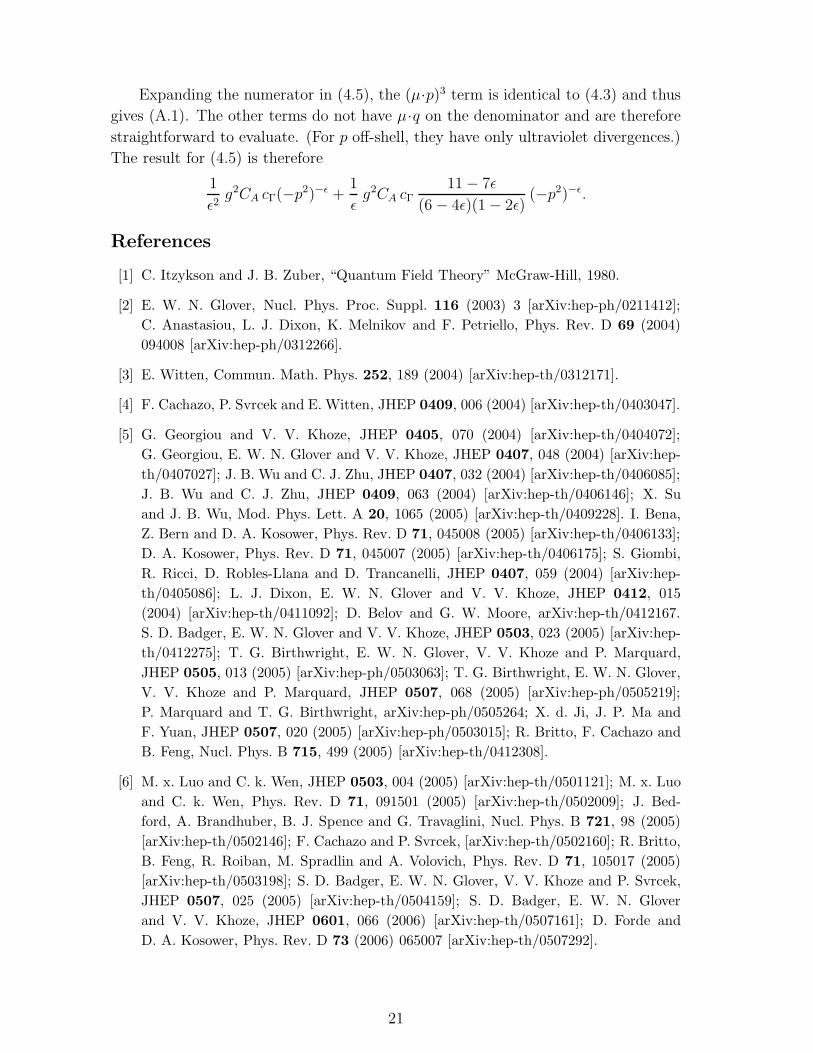
Expanding the numerator in (4.5), the (µ·p)3 term is identical to (4.3) and thus

gives (A.1). The other terms do not have µ·q on the denominator and are therefore

straightforward to evaluate. (For p off-shell, they have only ultraviolet divergences.)

The result for (4.5) is therefore

1

ǫ2g2CA cΓ(−p2)−ǫ +

1

ǫg2CA cΓ

11 − 7ǫ

(6 − 4ǫ)(1 − 2ǫ)(−p2)−ǫ.

References

[1] C. Itzykson and J. B. Zuber, “Quantum Field Theory” McGraw-Hill, 1980.

[2] E. W. N. Glover, Nucl. Phys. Proc. Suppl. 116 (2003) 3 [arXiv:hep-ph/0211412];

C. Anastasiou, L. J. Dixon, K. Melnikov and F. Petriello, Phys. Rev. D 69 (2004)

094008 [arXiv:hep-ph/0312266].

[3] E. Witten, Commun. Math. Phys. 252, 189 (2004) [arXiv:hep-th/0312171].

[4] F. Cachazo, P. Svrcek and E. Witten, JHEP 0409, 006 (2004) [arXiv:hep-th/0403047].

[5] G. Georgiou and V. V. Khoze, JHEP 0405, 070 (2004) [arXiv:hep-th/0404072];

G. Georgiou, E. W. N. Glover and V. V. Khoze, JHEP 0407, 048 (2004) [arXiv:hep-

th/0407027]; J. B. Wu and C. J. Zhu, JHEP 0407, 032 (2004) [arXiv:hep-th/0406085];

J. B. Wu and C. J. Zhu, JHEP 0409, 063 (2004) [arXiv:hep-th/0406146]; X. Su

and J. B. Wu, Mod. Phys. Lett. A 20, 1065 (2005) [arXiv:hep-th/0409228]. I. Bena,

Z. Bern and D. A. Kosower, Phys. Rev. D 71, 045008 (2005) [arXiv:hep-th/0406133];

D. A. Kosower, Phys. Rev. D 71, 045007 (2005) [arXiv:hep-th/0406175]; S. Giombi,

R. Ricci, D. Robles-Llana and D. Trancanelli, JHEP 0407, 059 (2004) [arXiv:hep-

th/0405086]; L. J. Dixon, E. W. N. Glover and V. V. Khoze, JHEP 0412, 015

(2004) [arXiv:hep-th/0411092]; D. Belov and G. W. Moore, arXiv:hep-th/0412167.

S. D. Badger, E. W. N. Glover and V. V. Khoze, JHEP 0503, 023 (2005) [arXiv:hep-

th/0412275]; T. G. Birthwright, E. W. N. Glover, V. V. Khoze and P. Marquard,

JHEP 0505, 013 (2005) [arXiv:hep-ph/0503063]; T. G. Birthwright, E. W. N. Glover,

V. V. Khoze and P. Marquard, JHEP 0507, 068 (2005) [arXiv:hep-ph/0505219];

P. Marquard and T. G. Birthwright, arXiv:hep-ph/0505264; X. d. Ji, J. P. Ma and

F. Yuan, JHEP 0507, 020 (2005) [arXiv:hep-ph/0503015]; R. Britto, F. Cachazo and

B. Feng, Nucl. Phys. B 715, 499 (2005) [arXiv:hep-th/0412308].

[6] M. x. Luo and C. k. Wen, JHEP 0503, 004 (2005) [arXiv:hep-th/0501121]; M. x. Luo

and C. k. Wen, Phys. Rev. D 71, 091501 (2005) [arXiv:hep-th/0502009]; J. Bed-

ford, A. Brandhuber, B. J. Spence and G. Travaglini, Nucl. Phys. B 721, 98 (2005)

[arXiv:hep-th/0502146]; F. Cachazo and P. Svrcek, [arXiv:hep-th/0502160]; R. Britto,

B. Feng, R. Roiban, M. Spradlin and A. Volovich, Phys. Rev. D 71, 105017 (2005)

[arXiv:hep-th/0503198]; S. D. Badger, E. W. N. Glover, V. V. Khoze and P. Svrcek,

JHEP 0507, 025 (2005) [arXiv:hep-th/0504159]; S. D. Badger, E. W. N. Glover

and V. V. Khoze, JHEP 0601, 066 (2006) [arXiv:hep-th/0507161]; D. Forde and

D. A. Kosower, Phys. Rev. D 73 (2006) 065007 [arXiv:hep-th/0507292].

21

[7] Z. Bern, L. J. Dixon and D. A. Kosower, Phys. Rev. D 71, 105013 (2005) [arXiv:hep-

th/0501240; M. Bertolini, F. Bigazzi and A. L. Cotrone, Phys. Rev. D 72, 061902

(2005) [arXiv:hep-th/0505055]; M. Bertolini, F. Bigazzi and A. L. Cotrone, Phys.

Rev. D 72, 061902 (2005) [arXiv:hep-th/0505055]; Z. Bern, N. E. J. Bjerrum-Bohr,

D. C. Dunbar and H. Ita, JHEP 0511 (2005) 027 [arXiv:hep-ph/0507019].

[8] R. Britto, F. Cachazo and B. Feng, Nucl. Phys. B 725, 275 (2005) [arXiv:hep-

th/0412103]; S. J. Bidder, N. E. J. Bjerrum-Bohr, D. C. Dunbar and W. B. Perkins,

Phys. Lett. B 612, 75 (2005) [arXiv:hep-th/0502028]; A. Brandhuber, S. McNamara,

B. J. Spence and G. Travaglini, JHEP 0510, 011 (2005) [arXiv:hep-th/0506068];

E. I. Buchbinder and F. Cachazo, JHEP 0511, 036 (2005) [arXiv:hep-th/0506126];

K. Risager, S. J. Bidder and W. B. Perkins, JHEP 0510, 003 (2005) [arXiv:hep-

th/0507170]; Z. Bern, V. Del Duca, L. J. Dixon and D. A. Kosower, Phys. Rev. D

71, 045006 (2005) [arXiv:hep-th/0410224]; R. Roiban, M. Spradlin and A. Volovich,

Phys. Rev. Lett. 94, 102002 (2005) [arXiv:hep-th/0412265].

[9] Z. Bern, L. J. Dixon and D. A. Kosower, Phys. Rev. D 72, 045014 (2005) [arXiv:hep-

th/0412210].

[10] A. Brandhuber, B. J. Spence and G. Travaglini, Nucl. Phys. B 706, 150 (2005)

[arXiv:hep-th/0407214]; C. Quigley and M. Rozali, JHEP 0501, 053 (2005)

[arXiv:hep-th/0410278]; J. Bedford, A. Brandhuber, B. J. Spence and G. Travaglini,

Nucl. Phys. B 706, 100 (2005) [arXiv:hep-th/0410280]; J. Bedford, A. Brandhuber,

B. J. Spence and G. Travaglini, Nucl. Phys. B 712, 59 (2005) [arXiv:hep-th/0412108];

[11] S. J. Parke and T. R. Taylor, Phys. Rev. Lett. 56, 2459 (1986); F. A. Berends and

W. T. Giele, Nucl. Phys. B 306, 759 (1988).

[12] R. Britto, F. Cachazo, B. Feng and E. Witten, Phys. Rev. Lett. 94 (2005) 181602

[arXiv:hep-th/0501052].

[13] K. Risager, JHEP 0512 (2005) 003 [arXiv:hep-th/0508206].

[14] F. Cachazo, P. Svrcek and E. Witten, JHEP 0410, 077 (2004) [arXiv:hep-th/0409245].

[15] A. Brandhuber, B. Spence and G. Travaglini, JHEP 0601 (2006) 142 [arXiv:hep-

th/0510253].

[16] F. Cachazo, P. Svrcek and E. Witten, JHEP 0410 (2004) 074 [arXiv:hep-th/0406177].

[17] P. Mansfield, JHEP 0603, 037 (2006) [arXiv:hep-th/0511264].

[18] A. Gorsky and A. Rosly, JHEP 0601, 101 (2006) [arXiv:hep-th/0510111].

[19] L. J. Mason, JHEP 0510, 009 (2005) [arXiv:hep-th/0507269]; L. J. Mason and D. Skin-

ner, Phys. Lett. B 636, 60 (2006) [arXiv:hep-th/0510262]; R. Boels, L. Mason and

D. Skinner, arXiv:hep-th/0604040.

[20] M. C. Bergere and Y. M. Lam, Phys. Rev. D 13 (1976) 3247.

22

[21] L. J. Dixon, lectures published in Boulder TASI 95:539–584 [arXiv:hep-ph/9601359].

[22] S. Mandelstam, Nucl. Phys. B 213 (1983) 149; G. Leibbrandt, Phys. Rev. D 29 (1984)

1699.

[23] D. A. Kosower and P. Uwer, Nucl. Phys. B 563 (1999) 477 [arXiv:hep-ph/9903515].

[24] Z. Bern, L. J. Dixon, D. C. Dunbar and D. A. Kosower, Nucl. Phys. B 425, 217 (1994)

[arXiv:hep-ph/9403226].

[25] Z. Bern, L. J. Dixon and D. A. Kosower, Phys. Rev. D 71, 105013 (2005) [arXiv:hep-

th/0501240]; C. F. Berger, Z. Bern, L. J. Dixon, D. Forde and D. A. Kosower,

arXiv:hep-ph/0604195.

[26] Z. Bern, G. Chalmers, L. J. Dixon and D. A. Kosower, Phys. Rev. Lett. 72, 2134

(1994) [arXiv:hep-ph/9312333]; Z. Bern, L. J. Dixon and D. A. Kosower, arXiv:hep-

th/9311026.

23