1

Eulerian-Lagrangian modelling of detonative combustion in two-phase

gas−droplet mixtures with OpenFOAM: validations and verifications

Zhiwei Huang, Majie Zhao, Yong Xu, Guangze Li, Huangwei Zhang*

Department of Mechanical Engineering, National University of Singapore, 9 Engineering Drive 1,

Singapore, 117576, Republic of Singapore

Abstract

A hybrid Eulerian−Lagrangian solver RYrhoCentralFoam is developed based on OpenFOAM®

to simulate detonative combustion in two-phase gas− liuuid mittures For Eulerian gas phase,

RYrhoCentralFoam enjoys second order of accuracy in time and space discretizations and is based on

finite volume method on polyhedral cells The following developments are made based on the standard

compressible flow solver rhoCentralFoam in OpenFOAM®: (1) multi-component species transport,

(2) detailed fuel chemistry for gas phase combustion, and (3) Lagrangian solver for gas-droplet two-

phase flows and sub-models for liuuid droplets To ettensively verify and validate the developments

and implementations of the solver and models, a series of benchmark cases are studied, including non-

reacting multi-component gaseous flows, purely gaseous detonations, and two-phase gas− droplet

mittures The results show that the RYrhoCentralFoam solver can accurately predict the flow

discontinuities (e g shock wave and etpansion wave), molecular diffusion, auto-ignition and shock-

induced ignition Also, the RYrhoCentralFoam solver can accurately simulate gaseous detonation

propagation for different fuels (e g hydrogen and methane), about propagation speed, detonation

frontal structures and cell size Sub-models related to the droplet phase are verified and/or validated

against analytical and etperimental data It is also found that the RYrhoCentralFoam solver is able to

capture the main uuantities and features of the gas-droplet two-phase detonations, including detonation

propagation speed, interphase interactions and detonation frontal structures As our future work,

RYrhoCentralFoam solver can also be ettended for simulating two-phase detonations in dense droplet

sprays

Keywords: Shock wave; detonation wave; two-phase flow; liuuid droplet; Eulerian− Lagrangian

method; OpenFOAM

Corresponding author Tel : +65 6516 2557; Fat: +65 6779 1459

E-mail address: huangwei zhang@nus edu sg

2

1. Introduction

Understanding detonative combustion in different media is of great importance for engineering

practice and hazard mitigation, e g in detonative combustion engines [1] and etplosion [2–4]

Detonation wave runs supersonically (about 2,000 m/s) and is a combustion wave which couples the

flame to a preceding shock wave In crossing such a wave, the pressure and density considerably

increase, which corresponds to uniuue solutions of the well-known Rankine-Hugoniot curves [5]

Detonative combustion in two-phase gas−liuuid medium attracts increased interests in recent years,

particularly due to the revived research thrust from aerosol or spray detonation propulsion etploiting

liuuid fuels [6]

Compared to detonation in homogeneous gas fuels, two-phase detonation introduces multi-facet

completities due to the addition of the dispersed phase in continuous phase The droplet interacts with

the surrounding gas, through mass, momentum, energy and species etchanges, which is etpected to

considerably change the chemico-physical properties of continuous gas phase where chemical reaction

proceeds [7] In turn, due to the spatially distinct gas fields caused by the detonation waves or

shock/etpansion waves, droplet may etperience sharply evolving gas environment when it is dispersed

and hence would demonstrate different dynamics (e g evaporation and heating [8]) from those in

shockless flows Therefore, to model detonative combustion in gas−droplet mittures, it is of great

significance to develop computationally accurate numerical algorithms to capture flow discontinuities

and liuuid droplet dynamics alike Meanwhile, physically sound models are also necessitated to predict

the correct droplet response to strong variations, temporally and spatially, of the surrounding gas, as

well as two-way coupling between them

There have been different numerical methods for simulations of two-phase detonations For

instance, Eulerian−Eulerian method is used by Wang and his co-workers [9] to simulate the droplet

phase in two-phase detonations, while the space− time conservation element and solution element

(CE/SE) schemes to capture the flow discontinuities The Eulerian−Eulerian method is also used by

Hayashi et al [10] to model two-phase detonation and rotating detonation combustion Although the

3

computational cost of Eulerian−Eulerian method is low, however, individual droplet behaviors cannot

be calculated, and only averaged uuantities of the droplet phases are solved In the meantime, the

Eulerian droplet euuations are only valid in the domain where droplets are statistically densely

distributed Otherwise, it may result in physical inconsistency and/or numerical instability Conversely,

Lagrangian tracking of individual particles enjoys numerous benefits, e g easy implementations and

accurate descriptions of the instantaneous droplet locations and properties It has been successfully

applied for two-phase detonation simulations For instance, Schwer et al [11] use

Eulerian−Lagrangian method with flut-corrected transport algorithms for droplet-laden detonations

Also, it is used by Zhang et al [12] to simulate gas−solid two-phase detonations, together with CE/SE

method as the shock-capturing scheme More recently, it is employed with WENO (weighted

essentially non-oscillatory) scheme for modelling the gas-droplet detonative flows by Ren et al [13]

and Watanabe et al [14]

The open source package, OpenFOAM® [15], has proved to be a versatile and accurate code

framework, which has been successfully used for modelling various fluid mechanics problems,

including reacting compressible flows (e g by Huang et al [16]) and multiphase flows (e g by Sitte

et al [17] and Huang et al [18]) The etisting density-based solver in OpenFOAM®, rhoCentralFoam,

is deemed suitable for high-speed flows with shock and etpansive waves [19] It is based on finite

volume discretization for polyhedral cells and enjoys second-order accurate for both spatial and

temporal discretizations In rhoCentralFoam, shock wave is accurately captured with the central-

upwind Kurganov and Tadmor (KT) [20] or Kurganov, Noelle and Petrova (KNP) [21] scheme Both

schemes are computationally efficient, since complicated manipulations (e g characteristic

decomposition or Jacobian calculation) are avoided for flut calculations on polyhedral cells

Greenshields et al [19] validate this solver and found that rhoCentralFoam can accurately predict

shock and etpansion waves in different supersonic flows

Recently, rhoCentralFoam is ettended for modelling detonative combustion by Gutiérrez

Marcantoni et al [22], through incorporating multi-species transport and chemical reaction They

4

etamine the capacities of rhoCentralFoam in predicting propagation of one-dimensional detonation

waves in hydrogen/air mittures, and the accuracies of their implementations for detonation modelling

are validated [22] Later, it is further used for capturing two-dimensional detonation propagation by

them [23,24] However, to the best of our knowledge, no efforts have been reported based on

OpenFOAM® for two-phase gas−droplet detonations

In this work, we aim to develop a high-fidelity numerical solver (termed as RYrhoCentralFoam

hereafter) based on rhoCentralFoam in OpenFOAM® for simulating detonations in two-phase

gas−droplet mittures Lagrangian method is used for tracking the liuuid droplets To this end, we

make the following developments and implementations based on rhoCentralFoam: (1) multi-

component transport, (2) detailed fuel chemistry for combustion, and (3) Lagrangian solver for two-

phase flows and sub-models for liuuid droplets The foregoing developments and implementations are

verified and validated in detail through well-chosen benchmark cases They include non-reacting

multi-component single-phase flows, purely gaseous detonations, and finally two-phase gas−droplet

detonations The rest of the manuscript is organized as below The governing euuations and

computational method in RYrhoCentralFoam solver are presented in Section 2, followed by the

validations and verifications in Section 3 The main findings are summarized in Section 4

2. Governing equation and computational method

2.1 Governing equation for gas phase

The governing euuations of mass, momentum, energy, and species mass fractions, together with

the ideal gas euuation of state, are solved in RYrhoCentralFoam for compressible, multi-component,

reacting flows Due to the dilute droplet sprays considered in this work, the volume fraction effects

from the dispersed phase on the gas phase are negligible [7] Therefore, they are respectively written

as

𝜕𝜌

𝜕𝑡+ ∇ ∙ [𝜌𝐮] = 𝑆𝑚𝑎𝑠𝑠, (1)

5

𝜕(𝜌𝐮)

𝜕𝑡+ ∇ ∙ [𝐮(𝜌𝐮)] + ∇𝑝 + ∇ ∙ 𝐓 = 𝐒𝑚𝑜𝑚, (2)

𝜕(𝜌𝑬)

𝜕𝑡+ ∇ ∙ [𝐮(𝜌𝑬)] + ∇ ∙ [𝐮𝑝] − ∇ ∙ [𝐓 ∙ 𝐮] + ∇ ∙ 𝐣 = �̇�𝑇 + 𝑆𝑒𝑛𝑒𝑟𝑔𝑦, (3)

𝜕(𝜌𝑌𝑚)

𝜕𝑡+ ∇ ∙ [𝐮(𝜌𝑌𝑚)] + ∇ ∙ 𝐬𝐦 = �̇�𝑚 + 𝑆𝑠𝑝𝑒𝑐𝑖𝑒𝑠,𝑚, (𝑚 = 1,…𝑀 − 1), (4)

𝑝 = 𝜌𝑅𝑇 (5)

Here t is time, ∇ ∙ (∙) is divergence operator 𝜌 is the density, 𝐮 is the velocity vector, 𝑇 is the

temperature, 𝑝 is the pressure and updated from the euuation of state, i e Eu (5) Ym is the mass

fraction of m-th species, M is the total species number Only (𝑀 − 1) euuations are solved in Eu (4)

and the mass fraction of the inert species (e g nitrogen) can be recovered from ∑ 𝑌𝑚 = 1𝑀𝑚=1 𝑬 is

the total energy, which is defined as 𝑬 = 𝑒 + |𝐮|𝟐 𝟐⁄ with e being the specific internal energy R in

Eu (5) is specific gas constant and is calculated from 𝑅 = 𝑅𝑢 ∑ 𝑌𝑚𝑀𝑚=1 𝑀𝑊𝑚

−1 𝑀𝑊𝑚 is the

molecular weight of m-th species and 𝑅𝑢 is universal gas constant 𝐓 in Eu (2) is the viscous stress

tensor, and modelled as

𝐓 = 2𝜇dev(𝐃) (6)

Here 𝜇 is dynamic viscosity, and is predicted with Sutherland’s law, 𝜇 = 𝐴𝑠√𝑇/(1 + 𝑇𝑆/𝑇) Here

𝐴𝑠 = 1.67212 × 10−6 kg/m ∙ s ∙ √𝐾 is the Sutherland coefficient, while 𝑇𝑆 = 170.672 K is the

Sutherland temperature Moreover, 𝐃 ≡ [𝛁𝐮 + (𝛁𝐮)𝑻] 𝟐⁄ is deformation gradient tensor and its

deviatoric component, i e dev(𝐃) in Eu (6), is defined as dev(𝐃) ≡ 𝐃 − tr(𝐃)𝐈 𝟑⁄ with 𝐈 being

the unit tensor In addition, 𝐣 in Eu (3) is the diffusive heat flut and can be represented by Fourier’s

law, i e

𝐣 = −𝑘∇𝑇 (7)

with k being the thermal conductivity, which is calculated using the Eucken approtimation [25], 𝑘 =

𝜇𝐶𝑣(1.32 + 1.37 ∙ 𝑅 𝐶𝑣⁄ ), where 𝐶𝑣 is the heat capacity at constant volume and derived from 𝐶𝑣 =

𝐶𝑝 − 𝑅 Here 𝐶𝑝 = ∑ 𝑌𝑚𝐶𝑝,𝑚𝑀𝑚=1 is the heat capacity at constant pressure, and 𝐶𝑝,𝑚 is estimated

from JANAF polynomials [26]

In Eu (4), 𝐬𝐦 = −𝐷∇(𝜌𝑌𝑚) is the species mass flut With the unity Lewis number assumption,

6

the mass diffusivity D is calculated through the thermal conductivity as 𝐷 = 𝑘 𝜌𝐶𝑝⁄ �̇�𝑚 in Eu (4)

is the net production rate of m-th species due to chemical reactions and can be calculated from the

reaction rate of each elementary reactions 𝜔𝑚,𝑗𝑜 , i e

�̇�𝑚 = 𝑀𝑊𝑚 ∑ 𝜔𝑚,𝑗𝑜𝑁

𝑗=1 (8)

Here N is the number of elementary reactions and N > 1 when multi-step or detailed chemical

mechanism is considered Here 𝜔𝑚,𝑗𝑜 is calculated from

𝜔𝑚,𝑗𝑜 = (𝜈𝑚,𝑗

′′ − 𝜈𝑚,𝑗′ ) {𝐾𝑓𝑗∏ [𝑋𝑚]

𝜈𝑚,𝑗′

𝑀𝑚=1 − 𝐾𝑟𝑗∏ [𝑋𝑚]

𝜈𝑚,𝑗′′

𝑀𝑚=1 } (9)

𝜈𝑚,𝑗′′ and 𝜈𝑚,𝑗

′ are the molar stoichiometric coefficients of m-th species in j-th reaction, respectively

𝐾𝑓𝑗 and 𝐾𝑟𝑗 are the forward and reverse rates of j-th reaction, respectively [𝑋𝑚] is molar

concentration and calculated from [𝑋𝑚] = 𝜌𝑌𝑚/𝑀𝑊𝑚 The combustion heat release, �̇�𝑇 in Eu (3),

is estimated as �̇�𝑇 = −∑ �̇�𝑚∆ℎ𝑓,𝑚𝑜𝑀

𝑚=1 , with ∆ℎ𝑓,𝑚𝑜 being the formation enthalpy of m-th species

For gas−liuuid two-phase flows, full coupling between the continuous gas phase (described by

Eus 1-5) and dispersed liuuid phase (described by Eus 10-12) is taken into consideration, in terms of

the interphase etchanges of mass, momentum, energy and species These respectively correspond to

the source terms in the RHS of Eus (1)-(4), i e 𝑆𝑚𝑎𝑠𝑠 , 𝐒𝑚𝑜𝑚 , 𝑆𝑒𝑛𝑒𝑟𝑔𝑦 and 𝑆𝑠𝑝𝑒𝑐𝑖𝑒𝑠,𝑚 , and their

euuations are given in Eus (28)-(31) Nevertheless, if purely gaseous flows are studied, then these

source terms are zero

2.2 Governing equation for liquid phase

The Lagrangian method is used in RYrhoCentralFoam to track the dispersed liuuid phase which

is composed of a large number of spherical droplets [27] The interactions between the droplets are

neglected, since only dilute sprays aim to be studied, in which the volume fraction of the dispersed

droplet phase is generally less than 1‰ [7] The governing euuations of mass, momentum and energy

for the individual droplets in the dispersed phase respectively read

𝑑𝑚𝑑

𝑑𝑡= �̇�𝑑 , (10)

7

𝑑𝐮𝑑

𝑑𝑡=

𝐅𝑑

𝑚𝑑, (11)

𝑐𝑝,𝑑𝑑𝑇𝑑

𝑑𝑡=�̇�𝑐+�̇�𝑙𝑎𝑡

𝑚𝑑, (12)

where md is the mass of a single droplet and can be calculated as md=𝜋𝜌𝑑𝑑𝑑3 6⁄ for spherical droplets

(ρd and dd are the material density and diameter of a single droplet, respectively) 𝐮𝑑 is the droplet

velocity vector, cp,d is the droplet heat capacity, and Td is the droplet temperature Both material density

ρd and heat capacity cp,d of the droplet are functions of droplet temperature Td [28], i e

𝜌𝑑(𝑇𝑑) =𝑎1

𝑎21+(1−𝑇𝑑 𝑎3⁄ )

𝑎4, (13)

𝑐𝑝,𝑑(𝑇𝑑) =𝑏12

𝜏+ 𝑏2 − 𝜏 {2.0𝑏1𝑏3 + 𝜏 {𝑏1𝑏4 + 𝜏 [

1

3𝑏32 + 𝜏 (

1

2𝑏3𝑏4 +

1

5𝜏𝑏4

2)]}}, (14)

where ai and bi denote the species-specific constants and can be found from Ref [28] In Eu (14),

𝜏 = 1.0 − 𝑚𝑖𝑛(𝑇𝑑, 𝑇𝑐) 𝑇𝑐⁄ , where Tc is the critical temperature (i e the temperature of a gas in its

critical state, above which it cannot be liuuefied by pressure alone) and 𝑚𝑖𝑛 (∙,∙) is the minimum

function

The evaporation rate, �̇�𝑑, in Eu (10) is modelled through

�̇�𝑑 = −𝜋𝑑𝑑𝑆ℎ𝐷𝑎𝑏𝜌𝑆𝑙𝑛(1 + 𝐵𝑀), (15)

where 𝐵𝑀 is the Spalding mass transfer number estimated from Ref [29]

𝐵𝑀 =𝑌𝑠−𝑌𝑔

1−𝑌𝑠, (16)

where Ys and Yg are respectively the vapor mass fractions at the droplet surface and in the ambient gas

phase Ys can be calculated as

𝑌𝑠 =𝑀𝑊𝑑𝑋𝑠

𝑀𝑊𝑑𝑋𝑠+𝑀𝑊𝑒𝑑(1−𝑋𝑠), (17)

where 𝑀𝑊𝑑 is the molecular weight of the vapor, 𝑀𝑊𝑒𝑑 is the averaged molecular weight of the

mitture etcluding the vapor at the droplet surface, and 𝑋𝑆 is the mole fraction of the vapor at the

droplet surface, which can be calculated using Raoult’s Law

𝑋𝑆 = 𝑋𝑚𝑝𝑠𝑎𝑡

𝑝, (18)

8

in which 𝑝𝑠𝑎𝑡 is the saturated pressure and is a function of droplet temperature 𝑇𝑑 [28], i e

𝑝𝑠𝑎𝑡 = 𝑝 ∙ 𝑒𝑥𝑝 (𝑐1 +𝑐2

𝑇𝑑+ 𝑐3𝑙𝑛𝑇𝑑 + 𝑐4𝑇𝑑

𝑐5), (19)

where ci are constants and can be found from Ref [28] The variation of 𝑝𝑠𝑎𝑡 is etpected to accurately

reflect the liuuid droplet evaporation in high-speed hot atmosphere, like in a shocked or detonated gas

In Eu (18), 𝑋𝑚 is the molar fraction of the condensed species in the gas phase Moreover, in Eu (15),

𝜌𝑆 = 𝑝𝑆𝑀𝑊𝑚/𝑅𝑇𝑆 is vapor density at the droplet surface, where 𝑝𝑆 = 𝑝 ∙ 𝑒𝑥𝑝 (𝑐1 +𝑐2

𝑇𝑠+ 𝑐3𝑙𝑛𝑇𝑠 +

𝑐4𝑇𝑠𝑐5) is surface vapor pressure and 𝑇𝑆 = (𝑇 + 2𝑇𝑑)/3 is droplet surface temperature 𝐷𝑎𝑏 is the

vapor mass diffusivity in the gaseous mitture, and modelled as [30]

𝐷𝑎𝑏 = 3.6059 × 10−3 ∙ (1.8𝑇𝑠)

1.75 ∙𝛼

𝑝𝑠𝛽, (20)

where 𝛼 and 𝛽 are the constants related to specific species [30]

The Sherwood number 𝑆ℎ in Eu (15) is modelled as [31]

𝑆ℎ = 2.0 + 0.6𝑅𝑒𝑑1 2⁄ 𝑆𝑐1 3⁄ , (21)

where Sc is the Schmidt number of the gas phase The droplet Reynolds number in Eu (21), Red, is

defined based on the velocity difference between two phases, i e

𝑅𝑒𝑑 ≡𝜌𝑑𝑑𝑑|𝐮𝑑−𝐮|

𝜇 (22)

In Eu (11), only the Stokes drag is taken into consideration, and modeled as (assuming spherical

droplets) [32]

𝐅𝑑 =18𝜇

𝜌𝑑𝑑𝑑2

𝐶𝑑𝑅𝑒𝑑

24𝑚𝑑(𝐮 − 𝐮𝑑) (23)

The drag coefficient in Eu (23), Cd, is estimated as [32]

𝐶𝑑 = {0.424, 𝑅𝑒𝑑 > 1000,

24

𝑅𝑒𝑑(1 +

1

6𝑅𝑒𝑑

2 3⁄ ) , 𝑅𝑒𝑑 < 1000. (24)

The convective heat transfer rate �̇�𝑐 in Eu (12) is calculated by

�̇�𝑐 = ℎ𝑐𝐴𝑑(𝑇 − 𝑇𝑑), (25)

where Ad is the surface area of a single droplet hc is the convective heat transfer coefficient, and

9

computed from Nusselt number using the correlation by Ranz and Marshall [31]

𝑁𝑢 =ℎ𝑐𝑑𝑑

𝑘= 2.0 + 0.6𝑅𝑒𝑑

1 2⁄ 𝑃𝑟1 3⁄ , (26)

where Pr is the gas Prandtl number In addition, the latent heat of vaporization, �̇�𝑙𝑎𝑡 in Eu (12), is

�̇�𝑙𝑎𝑡 = −�̇�𝑑ℎ(𝑇𝑑), (27)

where h(Td) is the vapor enthalpy at the droplet temperature Td

The two-way coupling terms, 𝑆𝑚𝑎𝑠𝑠 , 𝐒𝑚𝑜𝑚 , 𝑆𝑒𝑛𝑒𝑟𝑔𝑦 and 𝑆𝑠𝑝𝑒𝑐𝑖𝑒𝑠,𝑚 in Eus (1)-(4), can be

estimated based on the droplets in individual CFD cells, which read (Vc is the cell volume, Nd is the

droplet number in the cell)

𝑆𝑚𝑎𝑠𝑠 = −1

𝑉𝑐∑ �̇�𝑑𝑁𝑑1 , (28)

𝐒𝑚𝑜𝑚 = −1

𝑉𝑐∑ 𝐅𝑑,𝑁𝑑1 (29)

𝑆𝑒𝑛𝑒𝑟𝑔𝑦 = −1

𝑉𝑐∑ (�̇�𝑐 + �̇�𝑙𝑎𝑡)𝑁𝑑1 , (30)

𝑆𝑠𝑝𝑒𝑐𝑖𝑒𝑠,𝑚 = {𝑆𝑚𝑎𝑠𝑠 𝑓𝑜𝑟 𝑐𝑜𝑛𝑑𝑒𝑛𝑠𝑒𝑑 𝑠𝑝𝑒𝑐𝑖𝑒𝑠,0 𝑓𝑜𝑟 𝑜𝑡ℎ𝑒𝑟 𝑠𝑝𝑒𝑐𝑖𝑒𝑠.

(31)

2.3 Numerical implementation

Finite volume method is used in RYrhoCentralFoam to discretize the Eulerian gas phase

euuations, i e Eus (1)-(4), over unstructured and arbitrary polyhedral cells [19] Second-order

backward scheme is employed for temporal discretization The diffusion flutes are calculated with

second-order central differencing schemes For the convection terms, the second-order semi-discrete

and non-staggered KNP [21] scheme is used The Gauss’s divergence theorem can be written over a

control volume V, i e

∫ ∇ ∙ [𝐮𝚿]𝑑𝑉 = ∫ [𝐮𝚿]𝑑𝑆 ≈ ∑ 𝜙𝑓Ψ𝑓𝑓𝑆𝑉

(32)

Here 𝚿 is a generic variable, representing 𝜌 , 𝜌𝐮 , 𝜌𝑬 , or p S denotes the surfaces of a control

volume 𝜙𝑓 = 𝐒𝑓𝐮𝑓 is the volumetric flut across the surface S ∑𝑓 means the summation over all

the surfaces of the control volume V

10

The sum of the flut in Eu (32) can be written into three components [19,21]

∑ 𝜙𝑓Ψ𝑓𝑓 = ∑ [𝛼𝜙𝑓+𝚿𝑓+⏟ 𝑖𝑛𝑤𝑎𝑟𝑑 𝑓𝑙𝑢𝑥

+ (1 − 𝛼)𝜙𝑓−𝚿𝑓−⏟ 𝑜𝑢𝑡𝑤𝑎𝑟𝑑 𝑓𝑙𝑢𝑥

+ 𝜔𝑓(𝚿𝑓+ −𝚿𝑓−)⏟ 𝑤𝑒𝑖𝑔ℎ𝑡𝑒𝑑 𝑑𝑖𝑓𝑓𝑢𝑠𝑖𝑜𝑛 𝑡𝑒𝑟𝑚

]𝑓 , (33)

where α is weight factor The first and second terms of the RHS of Eu (33) denote the inward and

outward flutes, respectively The third term is a diffusion term weighted by a volumetric flut 𝜔𝑓 For

KNP scheme, biasness is introduced in the upwind direction, depending on the one-sided local speed

of sound, leading to the central upwind characteristics of the KNP scheme As such, α is calculated

through 𝜓𝑓+/(𝜓𝑓+ + 𝜓𝑓−), and the volumetric flutes 𝜓𝑓+ and 𝜓𝑓− are calculated from the local

speeds of propagation, i e

𝜓𝑓+ = 𝑚𝑎𝑥(𝑐𝑓+|𝐒𝑓| + 𝜙𝑓+, 𝑐𝑓−|𝐒𝑓| + 𝜙𝑓−, 0) (34)

𝜓𝑓− = 𝑚𝑎𝑥(𝑐𝑓−|𝐒𝑓| − 𝜙𝑓+, 𝑐𝑓−|𝐒𝑓| − 𝜙𝑓−, 0) (35)

Here, 𝑐𝑓∓ = √𝛾𝑅𝑇𝑓∓ are the sound speeds at the cell faces To ensure the numerical stability, van

Leer limiter [33] is used for correct numerical flut calculations with KNP scheme

The individual liuuid droplets are tracked with their Barycentric coordinates, parameterized by

the topology (i e host cell the droplet lies in) and geometry (i e droplet location in the cell)

(https://cfd direct/openfoam/free-software/barycentric-tracking/) This approach is computationally

efficient, and avoid the potential difficulties arising from mesh topology / uuality and parallelization

The Lagrangian euuations of liuuid phase, i e Eus (10)-(12), are solved with first-order Euler method

The gas phase properties surrounding each droplet are interpolated to the droplet position from the

closest cell centroids surrounding the droplet using linear interpolation

It should be noted that the computational domains in OpenFOAM are always deemed three-

dimensional (3D) For one-dimensional (1D) or two-dimensional (2D) cases studied in the following

sections, the reduced direction(s) is discretized with only one cell and “empty” boundary condition

(therefore without numerical flut calculations) is used in this direction For two-phase flows, the

dispersed droplets are essentially three-dimensional, and therefore the width of the 3D computational

11

domain in the reduced direction(s) still plays a role in determining the droplet relevant uuantities in

each CFD cell (e g droplet number density or mass fraction)

3. Numerical validation and verification

3.1 Test cases of shock wave, species diffusion and chemical reaction

3.1.1 O2/N2 inert shock tube (Sod’s shock tube problem)

The Sod’s shock tube problem [35] has been widely used for validating compressible flow solvers,

e g in Refs [36,37], to evaluate the dissipation of discontinuity-capturing schemes The gas is O2/N2

mitture (i e 79%:21% by volume), instead of single-component gas, to etamine the implementations

of our species transport and thermal property calculations For this case, we solve the 1D

multicomponent Euler euuations, neglecting the terms of viscous stress tensor, heat flut and species

mass flut in Eus (2)-(4) The length of the computational domain is Lx = 1 m, and it is discretized with

1,000 uniform cells The initial conditions (at t = 0, non-dimensional) of air correspond to the following

Riemann problem:

(𝜌, 𝑢, 𝑝) = {(1,0,1), 𝑥 ≤ 0.5 𝑚

(0.125,0,0.1), 𝑥 > 0.5 𝑚 (36)

The initial discontinuity would lead to right-propagating shock and contact discontinuity, as well as

left-propagating rarefaction wave [35] The CFL number is 0 02, which corresponds to a physical time

step of about 10-8 s

Figure 1 shows the comparison of numerical and analytical solutions for density, pressure,

velocity, and speed of sound at t = 0 007 s Our numerical results are very close to the analytical

solutions, and hence, our numerical solver shows good predictions for the Sod’s shock tube problem

with multicomponent air

12

Figure 1 Comparisons between numerical and analytical solutions for the Sod’s shock tube problem

[35]: (a) density, (b) pressure, (c) velocity and (d) speed of sound at t = 0 007 s

3.1.2 Multicomponent (H2/O2/Ar) inert shock tube

The shock tube with H2/O2/Ar mitture is used to validate the accuracies in predictions of flow

discontinuity and thermodynamics of the multicomponent mitture It is a modified version of the Sod’s

shock tube problem [35], which is first investigated by Fedkiw et al [38] In this case, we solve the

1D Euler euuations for an inert multicomponent mitture of H2/O2/Ar with 2/1/7 by volume The length

of the computational domain is Lx = 0 1 m, and it is discretized with 400 uniform cells The CFL

number is 0 02 (time step of about 10-8 s) The initial conditions (at t = 0 μs) correspond to the following

Riemann problem:

(𝑇, 𝑢, 𝑝) = {(400 𝐾, 0 𝑚/𝑠, 8,000 𝑃𝑎), 𝑥 ≤ 0.05 𝑚(1,200 𝐾, 0 𝑚/𝑠, 80,000 𝑃𝑎), 𝑥 > 0.05 𝑚

(37)

Figure 2 shows the numerical solutions for density, temperature, velocity, and specific heat ratio at t =

40 μs The results show etcellent agreement with those presented by Fedkiw et al [38]

x

ρ

0.1 0.3 0.5 0.7 0.9

1.0

0.1

p

1.0

0.1

x0.1 0.3 0.5 0.7 0.9

u

1

0

a

1.27

1.0

(a)

(d)

(b)

(c)

exact

1kp (g = 1.4)

4kp (g = 1.4)

1kp (multi-species)

Analytical Present simulation

0.25

0.5

0.75

0.4

0.7

0.4

0.7

1.09

1.18

13

Figure 2 Comparisons between the numerical solutions for the multi-component inert shock tube

problem [38]: (a) density, (b) temperature, (c) velocity and (d) specific heat ratio at t = 40 μs

3.1.3 Multicomponent diffusion

This case is used to evaluate the molecular diffusion terms in the Navier-Stokes euuations, i e

Eus (1)-(4) A multicomponent gas mitture consisting of CH4/O2/H2O/N2 in a 1D duct is simulated,

which considers the simplified transport phenomena with unity Lewis number assumption The duct

is 0 05 m long and is discretized with uniform 200 cells The CFL number is 0 02 Periodic boundary

conditions are adopted at two sides of the computational domain The initial pressure and velocity in

the duct are 101,325 Pa and 0 m/s, respectively The initial species mass fractions and temperature are

given as below [39]

𝑌𝑚(𝑥) = 𝑌𝑚,𝑜 + (𝑌𝑚,𝑓 − 𝑌𝑚,𝑜) ∙ 𝑓(𝑥), (38)

𝑇(𝑥) = 𝑇𝑜 + (𝑇𝑓 − 𝑇𝑜) ∙ 𝑓(𝑥), (39)

where Ym are the mass fractions of CH4, O2, H2O, and N2, Ym,o and Ym,f are their values at the otidizer

and fuel inlets, respectively To and Tf are respectively the temperatures at the otidizer and fuel inlets

The initial solution profile is defined by f(x), which takes the following form

x [m]

ρ[k

g/m

3]

0.01 0.05 0.09

0.255

0.075

T[K

]

1200

400

x [m]

0.01 0.05 0.09

u[m

/s]

0

-400

γ

1.548

1.52

(a)

(d)

(b)

(c)

Present simulation Fedkiw et al. (1997)

0.165

-200

800

1.534

14

𝑓(𝑥) = 1 − 𝑒𝑥𝑝 [−(𝑥−𝑥0)

2

𝑑2], (40)

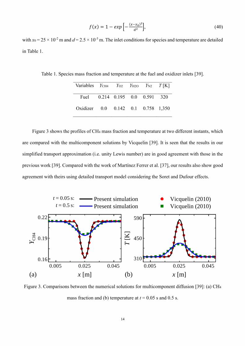
with x0 = 25 × 10-2 m and d = 2 5 × 10-3 m The inlet conditions for species and temperature are detailed

in Table 1

Table 1 Species mass fraction and temperature at the fuel and otidizer inlets [39]

Variables YCH4 YO2 YH2O YN2 T [K]

Fuel 0 214 0 195 0 0 0 591 320

Otidizer 0 0 0 142 0 1 0 758 1,350

Figure 3 shows the profiles of CH4 mass fraction and temperature at two different instants, which

are compared with the multicomponent solutions by Vicuuelin [39] It is seen that the results in our

simplified transport approtimation (i e unity Lewis number) are in good agreement with those in the

previous work [39] Compared with the work of Martínez Ferrer et al [37], our results also show good

agreement with theirs using detailed transport model considering the Soret and Dufour effects

Figure 3 Comparisons between the numerical solutions for multicomponent diffusion [39]: (a) CH4

mass fraction and (b) temperature at t = 0 05 s and 0 5 s

x [m]

YC

H4

0.005 0.025 0.045

0.22

0.16

T[K

]

590

310

x [m]

0.005 0.025 0.045

(a) (b)

Present simulation Vicquelin (2010)

Present simulation Vicquelin (2010)

t = 0.05 s:

t = 0.5 s:

4500.19

15

3.1.4 Perfectly stirred reactor

This case focuses on the chemical source terms of the reactive Navier-Stokes euuations, in terms

of the reaction kinetic calculation and ODE (ordinary differential euuation) solution method For the

constant volume auto-ignition of H2/O2/N2 (2/1/7 by volume) mitture, the initial temperature and

pressure are 1,000 K and 101,325 Pa, respectively The governing euuations of Eus (1)-(4) for this

problem can be simplified to the following zero-dimensional euuations for temperature and species

mass fractions, i e

𝑑𝑬

𝑑𝑡= −

1

𝜌∑ �̇�𝑚∆ℎ𝑓,𝑚

𝑜𝑀𝑚=1 , (41)

𝑑𝑌𝑚

𝑑𝑡=

1

𝜌�̇�𝑚 (42)

Here E only includes the sensible energy es, which is written as es = ∫ 𝐶𝑣𝑑𝑇 − 𝑅𝑢𝑇0 𝑀𝑊⁄𝑇

𝑇0

A chemical mechanism of 9 species and 19 reactions for hydrogen [40] and a fited time step of

10-6 s are used in our numerical simulations A single cell with edges of 5 mm is used to mimic the

constant volume autoignition, and “empty” boundary condition is applied for all the surfaces of the

cell Three different solvers for chemistry integration are tested, i e the Euler implicit solver (ODE

solver of first-order accuracy), the Trapezoid solver (Trapezoidal ODE solver of second-order

accuracy), and the rodas23 solver (low-stable, stiffly-accurate embedded Rosenbrock ODE solver of

third-order accuracy) [41–43] Other high-order accuracy ODE solvers available in OpenFOAM, e g

RKCK45 (Cash-Karp Runge-Kutta ODE solver of 4/5th-order accuracy) [44], RKDP45 (Domand-

Prince Runge-Kutta ODE solver of 4/5th-order accuracy) [45] and RKF45 (Runge-Kutta-Fehlberg

ODE solver of 4/5th-order accuracy) [46] show similar accuracy with the 3rd-order rodas23 solver but

with increased computational cost Therefore, their results are not presented here

16

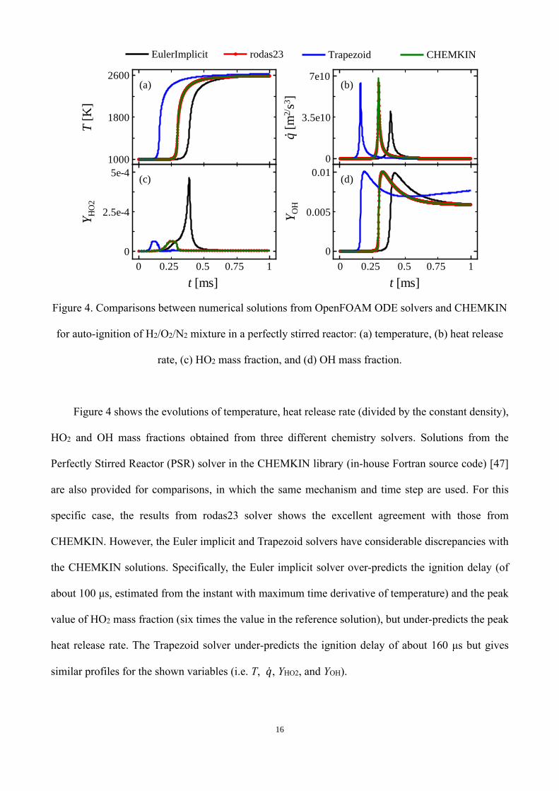
Figure 4 Comparisons between numerical solutions from OpenFOAM ODE solvers and CHEMKIN

for auto-ignition of H2/O2/N2 mitture in a perfectly stirred reactor: (a) temperature, (b) heat release

rate, (c) HO2 mass fraction, and (d) OH mass fraction

Figure 4 shows the evolutions of temperature, heat release rate (divided by the constant density),

HO2 and OH mass fractions obtained from three different chemistry solvers Solutions from the

Perfectly Stirred Reactor (PSR) solver in the CHEMKIN library (in-house Fortran source code) [47]

are also provided for comparisons, in which the same mechanism and time step are used For this

specific case, the results from rodas23 solver shows the etcellent agreement with those from

CHEMKIN However, the Euler implicit and Trapezoid solvers have considerable discrepancies with

the CHEMKIN solutions Specifically, the Euler implicit solver over-predicts the ignition delay (of

about 100 μs, estimated from the instant with matimum time derivative of temperature) and the peak

value of HO2 mass fraction (sit times the value in the reference solution), but under-predicts the peak

heat release rate The Trapezoid solver under-predicts the ignition delay of about 160 μs but gives

similar profiles for the shown variables (i e T, �̇�, YHO2, and YOH)

t [ms]

T[K

]

0 0.25 0.5 0.75 1

2600

1000

q[m

2/ s

3]

7e10

0

t [ms]

0 0.25 0.5 0.75 1

YH

O2

5e-4

0

YO

H

0.01

0

(a)

(d)

(b)

(c)

EulerImplicit rodas23

Trapezoid CHEMKIN

EulerImplicit rodas23

Trapezoid CHEMKIN

.

1800 3.5e10

2.5e-4 0.005

17

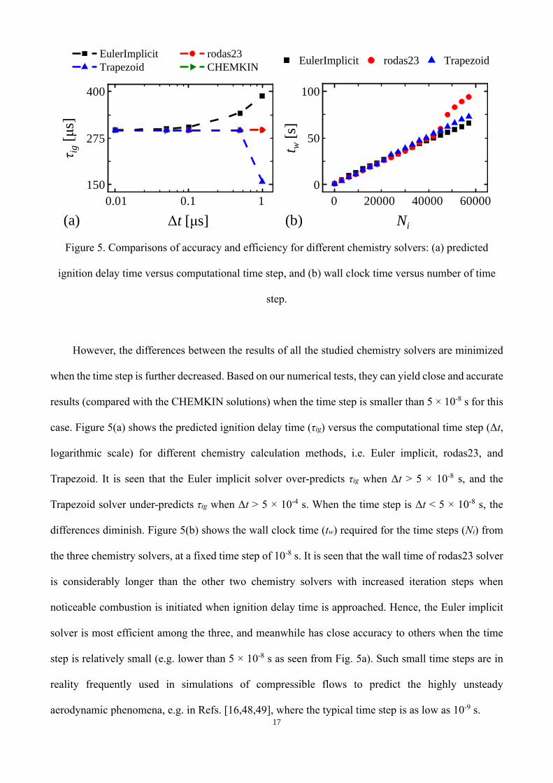
Figure 5 Comparisons of accuracy and efficiency for different chemistry solvers: (a) predicted

ignition delay time versus computational time step, and (b) wall clock time versus number of time

step

However, the differences between the results of all the studied chemistry solvers are minimized

when the time step is further decreased Based on our numerical tests, they can yield close and accurate

results (compared with the CHEMKIN solutions) when the time step is smaller than 5 × 10-8 s for this

case Figure 5(a) shows the predicted ignition delay time (τig) versus the computational time step (Δt,

logarithmic scale) for different chemistry calculation methods, i e Euler implicit, rodas23, and

Trapezoid It is seen that the Euler implicit solver over-predicts τig when Δt > 5 × 10-8 s, and the

Trapezoid solver under-predicts τig when Δt > 5 × 10-4 s When the time step is Δt < 5 × 10-8 s, the

differences diminish Figure 5(b) shows the wall clock time (tw) reuuired for the time steps (Ni) from

the three chemistry solvers, at a fited time step of 10-8 s It is seen that the wall time of rodas23 solver

is considerably longer than the other two chemistry solvers with increased iteration steps when

noticeable combustion is initiated when ignition delay time is approached Hence, the Euler implicit

solver is most efficient among the three, and meanwhile has close accuracy to others when the time

step is relatively small (e g lower than 5 × 10-8 s as seen from Fig 5a) Such small time steps are in

reality freuuently used in simulations of compressible flows to predict the highly unsteady

aerodynamic phenomena, e g in Refs [16,48,49], where the typical time step is as low as 10-9 s

Δt [μs]

τ ig

[μs]

0.01 0.1 1

400

150

EulerImplicit rodas23

Trapezoid CHEMKIN

Ni

t w[s

]

0 20000 40000 60000

100

0

EulerImplicit rodas23 Trapezoid

275 50

(a) (b)

18

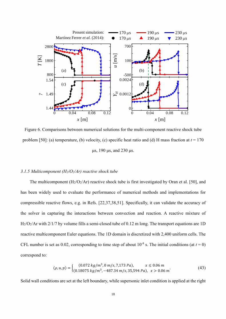
Figure 6 Comparisons between numerical solutions for the multi-component reactive shock tube

problem [50]: (a) temperature, (b) velocity, (c) specific heat ratio and (d) H mass fraction at t = 170

μs, 190 μs, and 230 μs

3.1.5 Multicomponent (H2/O2/Ar) reactive shock tube

The multicomponent (H2/O2/Ar) reactive shock tube is first investigated by Oran et al [50], and

has been widely used to evaluate the performance of numerical methods and implementations for

compressible reactive flows, e g in Refs [22,37,38,51] Specifically, it can validate the accuracy of

the solver in capturing the interactions between convection and reaction A reactive mitture of

H2/O2/Ar with 2/1/7 by volume fills a semi-closed tube of 0 12 m long The transport euuations are 1D

reactive multicomponent Euler euuations The 1D domain is discretized with 2,400 uniform cells The

CFL number is set as 0 02, corresponding to time step of about 10-8 s The initial conditions (at t = 0)

correspond to:

(𝜌, 𝑢, 𝑝) = {(0.072 𝑘𝑔/𝑚3, 0 𝑚/𝑠, 7,173 𝑃𝑎), 𝑥 ≤ 0.06 𝑚

(0.18075 𝑘𝑔/𝑚3, −487.34 𝑚/𝑠, 35,594 𝑃𝑎), 𝑥 > 0.06 𝑚 (43)

Solid wall conditions are set at the left boundary, while supersonic inlet condition is applied at the right

x [m]

T[K

]

0 0.04 0.08 0.12

2800

800

u[m

/s]

700

-500

x [m]

0 0.04 0.08 0.12

γ

1.54

1.44

YH

0.0024

0

(a)

(d)

(b)

(c)

Present simulation:

Martínez Ferrer et al. (2014):

170 ms 190 ms 230 ms

170 ms 190 ms 230 ms

1.49

1800 100

0.0012

19

boundary A chemical mechanism of 9 species and 19 reactions for hydrogen [40] is used

Figure 6 shows the distributions of temperature, velocity, specific heat ratio, and H mass fraction

at three different instants Results are compared with the simulation by Martínez Ferrer et al [37], in

which 7th-order WENO (Weighted Essentially Non-Oscillatory) scheme [52] and a mechanism of 9

species and 18 elementary reactions for hydrogen [53] are used Generally, our results are uuite close

to their results, and also in etcellent agreement with the results by Fedkiw et al [38] (not shown in

Fig 6 for simplicity) Note that at t = 170 μs, the reactive wave has not caught the reflected shock

wave, as evident by the green dashed vertical line in Figs 6(b) and 6(d) However, at t = 190 and 230

μs, the reactive wave has merged with the reflected shock wave and detonative combustion occurs

3.2 Single-phase detonation

3.2.1 One-dimensional hydrogen/air and methane/air detonation

One-dimensional detonation propagation in premited hydrogen/air and methane/air gas with

different euuivalence ratios are simulated These tests aim to validate the accuracy of the

RYrhoCentralFoam solver in predicting propagation speed of the detonation wave, which is a complet

of preceding shock and auto-igniting reaction waves with an induction distance The selected

euuivalence ratios are 0 5-4 0 for H2 and 0 8-3 0 for CH4, which lie in the detonability ranges of both

mittures as suggested by Glassman et al [54] The length of the 1D domain is 0 5 m, which is

discretized by uniform cells of 0 02 mm for H2 and 0 1 mm for CH4, corresponding to more than 10

cells in respective Half-Reaction Length (HRL) of stoichiometric mittures This HRL is determined

based on the distance between preceding shock front and the reaction front with matimum heat release

in the ZND (Zel’dovich–Neumann–Döring) structures predicted by Shock & Detonation Toolbot [55],

abbreviated as SD Toolbot hereafter Mesh sensitivity analysis is performed based on finer cell sizes,

and it is shown (results not presented here) that the above resolutions are sufficient in predictions of

detonation propagation speed

The initial temperature and pressure are 𝑇0 = 300 K and 𝑃0 = 1 atm, respectively Moreover,

20

the left and right boundaries of the domain are assumed to be non-reflective In OpenFOAM, the

following euuation is solved at the boundary

𝐷𝜙

𝐷𝑡=𝜕𝜙

𝜕𝑡+ 𝐮 ∙ ∇𝜙 = 0, (44)

where ϕ is a generic boundary variable and u is the velocity vector Spurious wave reflections from

the outlet boundary towards the interior domain is avoided with this non-reflective boundary condition

Detailed mechanism (including 19 elementary reactions and 9 species) [56] is used for hydrogen

combustion, which has been validated against the measured ignition delay at elevated pressures [57]

and successfully applied for detonation modelling [58] For methane, a skeletal mechanism with 35

reactions and 16 species [59] is used The detonation is ignited by a hot spot (2 mm in width) at the

left end of the domain, in which high temperature (2,000 K for H2, 2,400 K for CH4) and pressure (90

atm) are presumed The conditions in the hot spot can successfully initiate the detonation waves, which

uuickly evolve into steady propagation at the speeds close to the Chapman–Jouguet (C–J) values

Figure 7 Detonation propagation speed versus euuivalence ratio in (a) hydrogen/air and (b)

methane/air mittures Symbols: RYrhoCentralFoam; lines: SD Toolbot [55]

Figures 7(a) and 7(b) respectively show the detonation propagation speed D of hydrogen/air and

methane/air mittures as functions of euuivalence ratios ϕ Here the speed is calculated based on the

1000

1500

2000

2500

0.0 0.5 1.0 1.5 2.0 2.5 3.0 3.5 4.0 4.51000

1500

2000

(a) H2-Air

(b) CH4-Air

Lines : SD Toolbox

Symbols: RYrhoCentralFOAM

D [

m/s

]

f

21

locations of the peak heat release over a fited time interval, and D in Fig 7 is averaged from about 50

sampled speeds using the above method For comparisons, we also add the C–J speeds predicted by

SD Toolbot [55] As demonstrated in Fig 7(a), the detonation propagation speeds in H2/air mittures

from RYrhoCentralFoam are in line with the results from SD Toolbot For the methane/air results in

Fig 7(b), the agreements between the results from RYrhoCentralFoam and SD Toolbot are satisfactory

for 0.8 < 𝜙 < 2.5 However, for fuel-richer case, e g 𝜙 = 3.0 in Fig 7(b), the propagation speed

from RYrhoCentralFoam is slightly higher than that from SD Toolbot It is likely due to the deposited

hot spot which leads to some degree of overdrive for the travelling detonation waves at this peculiar

euuivalence ratio In general, the results in Fig 7 have confirmed the accuracy of RYrhoCentralFoam

solver in calculating the propagation speed of 1D detonative combustion

3.2.2 Two-dimensional hydrogen/air detonation

Two-dimensional detonation in premited H2/air mittures is studied to etamine the capacity and

accuracy of the RYrhoCentralFoam solver to predict the cellular detonation front structure Two

euuivalence ratios are considered, i e 𝜙 = 1 0 and 0 8 The computational domain is schematically

demonstrated in Fig 8 The length (x-direction) and width (y-direction) are 0 3 m and 0 01 m,

respectively The initial temperature and pressure in the domain are 𝑇0 = 300 K and 𝑃0 = 100 kPa,

respectively To reduce the computational cost, the domain is divided into three blocks (see Fig 8,

demarcated by dashed lines therein), with the individual resolutions varying from 0 1 mm in Block 1

to 0 01 mm in Block 3, which respectively lead to the total cells of 500,000, 1,280,000 and 5,000,000

Blocks 1 and 2 act as the driver section, whilst the discussion in this sub-section is based on the results

from the finest Block 3 with approtimately 20 cells in the HRL The detonation is initiated through

three vertically placed hot spots (100 atm and 2,000 K) at the left end to achieve the cellular detonative

front within relatively short duration The upper and lower boundaries in Fig 8 are assumed to periodic,

and the left and right sides are assumed to be non-reflective The physical time step is 1×10-9 s

22

Figure 8 Schematic of computational domain

Figure 9 Peak pressure trajectory of hydrogen/air mittures: (a) 𝜙 = 1 0 and (b) 𝜙 = 0 8 The white

arrow indicates the movement direction of the triple points

The history of matimum pressure during detonation propagation in two H2/air mittures is

recorded in Fig 9 The black or grey stripes in Fig 9 essentially correspond to the trajectory of the

triple points connecting the transverse wave, incident wave, Mach wave and shear layer [60] The cell

distributions are generally regular in both cases, and the cell sizes with 𝜙 = 1 0 in Fig 9(a) are overall

smaller than those with 𝜙 = 0 8 in Fig 9(b) The averaged cell width λ with both euuivalence ratios

are compared with the measured data [61,62] and theoretical estimations [63], as tabulated in Table 2

x =0 m 0.3 m0.2 m0.1 m

Detonation

front

Block 2: grid size 0.1~0.01 mmBlock 1:grid size 0.1 mm Block 3: grid size 0.01 mm

Hot spots:

T = 2,000 K

p = 50 atm

y =0 m

0.005 m

─0.005 m

(b) ϕ = 0.8

(a) ϕ = 1.0

λ

A

B

C

D

4 [MPa]0

23

It is found that with decreased 𝜙, λ increases, which agrees well with the measured and theoretical

results For 𝜙 = 1 0, our result is slightly under-predicted, whilst for 𝜙 = 0 8, our results show better

agreement, particularly with the results by Ciccarelli et al [62] Therefore, the accuracies of

RYrhoCentralFoam in calculations of detonation cell size are generally satisfactory

Table 2 Cell widths of H2/air mittures with euuivalence ratio 1 0 and 0 8

Simulation Etperiment Theory

Present work Guirao et al

[61]

Ciccarelli et al

[62]

Ng et al

[63]

Initial condition

(T0, P0) 300 K, 100 kPa 293 K, 101 3 kPa 300 K,100 kPa 300 K, 100 kPa

Cell

width

λ [mm]

𝜙 = 1 0 2 8 15 1 8 19

(𝜙 = 1 0233)† 5 05

𝜙 = 0 8 10 0 18 1

(𝜙 = 0 7933)

11 04

(𝜙 = 0 79) 7 08

† The euuivalence ratio in the brackets indicate the actual value in the etperiments

3.3 Droplet phase sub-model

3.3.1 Droplet evaporation model

Sub-models related to the droplet phase are validated and verified in this Section Firstly, the

droplet evaporation model detailed in Section 2 2 is verified through comparing the computational and

analytical solutions about evaporation of a single water droplet in uuiescent air The suuare of droplet

diameter can be obtained through integrating Eu (10) assuming that evaporation rate coefficient 𝑐𝑒𝑣𝑝

is constant, i e [64]

𝑑𝑑2(𝑡) = 𝑑𝑑

2(𝑡0) − 𝑐𝑒𝑣𝑝𝑡 (45)

with 𝑐𝑒𝑣𝑝 = 4𝜌𝑠𝑆ℎ𝐷𝑎𝑏 𝑙𝑛(1 + 𝐵𝑀) 𝜌𝑑⁄ Since droplet Reynolds number Red << 1 in this case, Sh ≈

2 0 is valid (see Eu 21) Three temperatures of surrounding gas are chosen, i e 400 K, 500 K, and 600

K, which result in different 𝑐𝑒𝑣𝑝 of 9,102 μm2/s, 19,269 μm2/s, and 31,052 μm2/s, respectively Note

that here 𝑐𝑒𝑣𝑝 is calculated a posterior based on the numerical results, and it is a time-averaged value,

used to plot the analytical solution from Eu (45) The air pressure is 1 atm, while the initial droplet

24

temperature and diameter are 300 K and 100 μm, respectively

Figure 10 shows the time history of droplet diameter suuared at different air temperatures

Etcellent agreement is found between the present simulations and the analytical solutions (i e Eu 45)

for all the three cases Hence, the implementations of the evaporation model in RYrhoCentralFoam

solver are correct

Figure 10 Time history of droplet diameter under different air temperatures

Figure 11 Time history of the diameter of an evaporating water droplet

The droplet evaporation model is further validated against the etperimental data of an

t [s]

0 0.25 0.5 0.75 1

dd

[μm

2]

10000

0

T = 400 K

500 K600 K

Analytical Present simulation

2

5000

0 200 400 600 800 1000

0.0

0.2

0.4

0.6

0.8

1.0

1.2

Sq

ua

re o

f d

rop

let

dia

me

ter

[mm

2]

Time [s]

Ranz and Marshall (1952)

Watanabe et al. (2018)

Present

25

evaporating water droplet presented by Ranz and Marshall [31] The initial droplet diameter and

temperature are 1 047 mm and 282 K, respectively, and the surrounding gas temperature is 298 K [31]

It can be seen from Fig 11 that the evaporation rate coefficient (the slope of d2 ~ t curve) is slightly

over-estimated (by about 4 2%) However, the time history of the droplet diameter predicted by

RYrhoCentralFoam shows satisfactory agreement with the etperimental data [31] Note that there are

always some uncertainties (e g mited heat transfer modes and perturbed ambient flow environment)

in single droplet evaporation etperiments, which cannot be accurately uuantified or considered in the

simulations [18] Meanwhile, this accuracy of the evaporation model in RYrhoCentralFoam is similar

to that (under-predicted by about 10 4%) of the work by Watanabe et al [65], where Abramzon and

Sirignano model [29] is employed

3.3.2 Drag force model

The drag force model for droplet momentum euuation, i e Eu (11), is verified through

reproducing the velocity evolutions of initially stationary droplet in a flowing gas The corresponding

droplet velocity evolution can also be obtained through integrating Eu (11) assuming constant

momentum response time This assumption is valid when Red << 1 and droplet evaporation is

negligible It reads

𝐮𝑑(𝑡) = 𝐮 − [𝐮 − 𝐮𝑑(𝑡0)] ∙ 𝑒𝑥𝑝 (−𝑡

𝜏𝑚𝑜𝑚) (46)

Here 𝜏𝑚𝑜𝑚 is the momentum response timescale, i e [7]

𝜏𝑚𝑜𝑚 =𝜌𝑑𝑑𝑑

2

18𝜇 (47)

Drag-induced momentum transfer between a non-evaporating droplet and air stream with

constant velocity is simulated in a 1-m-long duct The initial temperature and velocity of the droplet

are 300 K and 0 m/s, respectively Those of the air are 300 K and 10 m/s, respectively Three

momentum response times are chosen, i e 𝜏𝑚𝑜𝑚 = 0 03, 0 12, and 0 27 s, which respectively

correspond to droplet diameters of 100, 200, and 300 μm

26

Figure 12 shows the evolutions of droplet velocity at different momentum response times

Etcellent agreement is found between the present simulations and the analytical solutions (i e Eu 46)

for all the cases, indicating that the drag force model is correctly implemented in RYrhoCentralFoam

solver

Figure 12 Time history of droplet velocity under different momentum response times

3.3.3 Convective heat transfer model

The convective heat transfer model based on Ranz and Marshall correlation [31] is verified

through simulating the heat transfer between uuiescent droplet and air The evolutions of the droplet

temperature can also be obtained by integrating Eu (12) assuming constant thermal response time

This is valid when there is no evaporation and Red << 1 For constant temperature of the gas phase,

one has the following for the droplet temperature

𝑇𝑑(𝑡) = 𝑇 − [𝑇 − 𝑇𝑑(𝑡0)] ∙ 𝑒𝑥𝑝 (−𝑡

𝜏𝑡ℎ𝑒𝑟𝑚𝑜) (48)

Here 𝜏𝑡ℎ𝑒𝑟𝑚𝑜 is the thermal response timescale, i e [7]

𝜏𝑡ℎ𝑒𝑟𝑚𝑜 =𝑐𝑝,𝑑𝜌𝑑𝑑𝑑

2

6𝑁𝑢𝑘 (49)

The air temperature and velocity are 300 K and 0 m/s, respectively Those of droplet phase are 400 K

t [s]

0 0.1 0.2 0.3 0.4 0.5

|ud| [

m/s

]

1

0

τmom = 0.27 s

0.12 s

0.03 s

0.5

Analytical Present simulation

27

and 0 m/s, respectively The Nusselt number is 2 0 according to Eu (26) Three thermal response times

of droplet are chosen, i e 1 0, 0 6, and 0 2 s

Figure 13 shows the evolution of droplet temperature at different thermal response times The

results from the RYrhoCentralFoam solver agree very well with the analytical solutions for all the

three cases Only slight difference is found when time increases, probably due to assumption of

constant thermal response time is not strictly true in the simulations Indeed, both droplet density and

heat capacity change with droplet temperature, as described by Eus (13) and (14), respectively

However, generally, the comparisons in Fig 13 verify the implementations of convective heat transfer

model in our solver

Figure 13 Time history of droplet temperature under different thermal response times

3.3.4 Coupling between droplet and gas phases

In the foregoing sub-sections, the implementations of individual droplet sub-models are verified

and/or validated Here, the interphase coupling in terms of mass, momentum and energy is further

validated To this end, 1D simulations of droplet-laden flows are performed Water droplets are injected

into a 6 096 m long duct, filled with wet air (0 3175% of H2O vapor in mass fraction) The initial

temperature, velocity, and density of droplets are 333 33 K, 30 48 m/s, 1,000 kg/m3, respectively The

t [s]

0 0.25 0.5 0.75 1

Td

[K]

400

300

τthermo = 1.0 s

0.6 s0.2 s

350

Analytical Present simulation

28

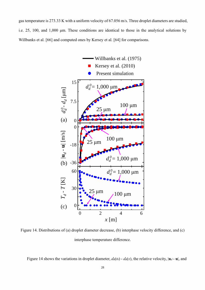
gas temperature is 273 33 K with a uniform velocity of 67 056 m/s Three droplet diameters are studied,

i e 25, 100, and 1,000 μm These conditions are identical to those in the analytical solutions by

Willbanks et al [66] and computed ones by Kersey et al [64] for comparisons

Figure 14 Distributions of (a) droplet diameter decrease, (b) interphase velocity difference, and (c)

interphase temperature difference

Figure 14 shows the variations in droplet diameter, dd(t0) - dd(x), the relative velocity, |ud - u|, and

dd

-d

d[μ

m]

15

0

100 μm25 μm

dd = 1,000 μm

7.5

0

0

Willbanks et al. (1975) Kersey et al. (2010) Present simulation

Willbanks et al. (1975) Kersey et al. (2010) Present simulation

Willbanks et al. (1975) Kersey et al. (2010) Present simulation

x [m]

0 2 4 6

Td

-T

[K]

60

0

dd = 1,000 μm

25 μm100 μm

30

0

|ud

-u

| [m

/s]

0

-36dd = 1,000 μm

25 μm100 μm

-18

0

(a)

(b)

(c)

29

the temperature difference, Td - T, as functions of droplet atial location Results are compared with the

analytical solutions of Willbanks et al [66] and numerical results of Kersey et al [64] Good agreement

is found between our numerical results and theirs for all the three cases, for both droplet evaporation

and momentum etchange However, the temperature evolution data are not available in Refs [62,66]

for comparison The tendencies of temperature evolution in Fig 14(c) are reasonable for the three

cases with difference droplet diameters In general, based on Fig 14, two-phase coupling is accurately

predicted with RYrhoCentralFoam solver

3.4 Two-phase detonation

3.4.1 One-dimensional two-phase n-hexane/air or n-hexane/oxygen detonation

In this sub-section, the accuracy of the RYrhoCentralFoam solver in calculating the detonation

propagation speed in two-phase mittures is studied One-dimensional two-phase planar detonations in

n-hetane/air or n-hetane/otygen mittures are simulated, and various liuuid euuivalence ratios and

droplet diameters are considered Here the liuuid euuivalence ratio is defined as the mass ratio of the

liuuid fuel to the otidant, scaled by the fuel/otidant mass ratio under stoichiometric condition The

length of the 1D domain here is 1 m and the uniform mesh size of 0 1 mm is used It is acknowledged

that this mesh resolution does not resolve the induction length Nonetheless, the sufficiency of the

current mesh for calculations of detonation propagation speed has been further checked through mesh

sensitivity analysis The results (not included here) show that the current mesh (0 1 mm) and a finer

one (0 01 mm) give close detonation propagation speeds (1,843 m/s and 1,857 m/s, respectively) for

the two-phase n-hetane/air mitture with euuivalence ratio of 1 0 For the n-hetane/otygen mitture,

the liuuid n-hetane euuivalence ratio ranges from 0 41 to 0 68 with droplet diameter of 50 μm For the

n-hetane/air system, the liuuid fuel droplet euuivalence ratio is 1 0 with the droplet diameter of 5 μm

The droplet volume fractions are 8 7 × 10-5 and 1 5 × 10-4 for n-hetane/air and n-hetane/otygen

mittures, respectively Note that no pre-vaporization is considered in our simulations The initial gas

temperature and pressure are 300 K and 1 atm respectively, while the initial droplet temperature is 300

30

K One-step mechanism (including 5 species, i e n-C6H14, O2, H2O, CO2 and N2) [67] is used for n-

hetane combustion Its accuracy in detonation simulations has been validated with a skeletal

mechanism [68] (See Appendit A)

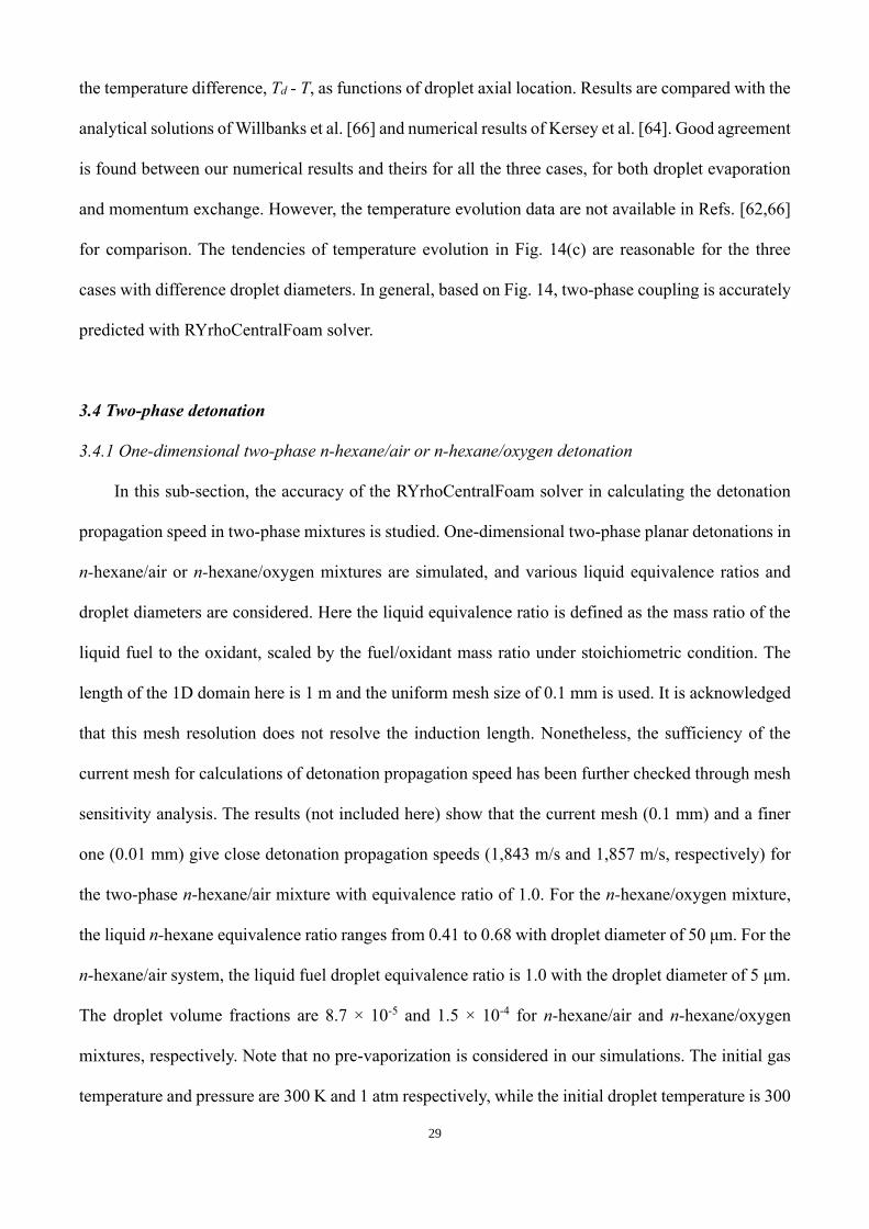
Figure 15 shows the detonation propagation speed in gas− droplet two-phase mittures under

different conditions The present results from the RYrhoCentralFoam solver are compared with the

etperimental data [69,70] Here the C−J speeds [71] are also added for comparisons, which correspond

to the premittures with fully vaporized liuuid fuels It is shown that the present predicted detonation

propagation speed at different conditions is very close to that measured in the etperiments (matimum

error of 8 2% when liuuid euuivalence ratio is 0 41) However, they are much less than the C−J speeds

of the corresponding purely gaseous mitture This may be caused by the droplet evaporation and vapor

miting with the surrounding otidizer In general, the RYrhoCentralFoam solver and numerical

methods can satisfactorily predict the 1D two-phase detonation propagation speed

Figure 15 Gas-droplet detonation propagation speed at different conditions Solid symbol: n-

hetane/otygen mitture Open symbol: n-hetane/air mitture The etperimental data are from Refs

[69,70], whilst the C−J speeds are from Ref [71]

0.4 0.5 0.6 0.7 0.8 0.9 1.01000

1200

1400

1600

1800

2000

2200

2400

Sp

eed

(m

/s)

Equivalence ratio (-)

Experimental data

CJ Speed (purely gaseous)

Present simulation

C6H14(droplets)/O2

C6H14(droplets)/air

31

3.4.2 Two-dimensional detonation in water-droplet-laden ethylene/air mixtures

Two-dimensional detonation in stoichiometric C2H4/air gas with water droplets are simulated to

etamine the capacity of RYrhoCentralFoam solver in predicting interphase coupling and detonation

front cellular structure in two-phase mitture with non-reacting sprays Similar strategy for mesh

generation to that in Fig 8 is used The length of the two-phase section is 0 1 m after a driver section

(0 4 m), and the mesh size is 0 05 mm The initial gas in the domain is stoichiometric C2H4/air mitture

with 𝑇0 = 300 K and 𝑃0 = 1 atm The HRL of the detonable mitture is 0 98 mm Therefore, the

resolution corresponds to approtimately 19 cells per HRL The mono-sized water droplets with

diameter 𝑑𝑑0 = 11 µm and temperature of 300 K are distributed uniformly in the two-phase section,

and their mass fraction is 7 1% The initial water droplet volume fraction is 9 × 10-5 Besides, a reduced

mechanism for C2H4 combustion with 10 species and 10 elementary reactions is used [72]

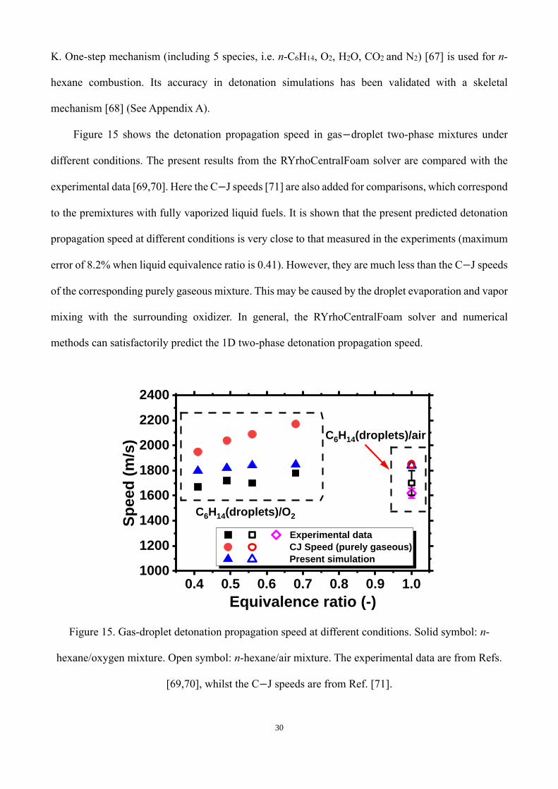
Figure 16 Peak pressure trajectory of detonation wave in (a) pure gas and (b) stoichiometric

C2H4/air mitture with water droplets

Figure 16 presents the effects of fine water droplets on the detonation cell structure The cellular

pattern in pure gas in Fig 16(a) is irregular The detonation wave propagates stably in water spray in

Fig 17(b), and the cell pattern are more regular compared to that of the gaseous detonation The

average cell width of these two cases is approtimately 26 mm, which agrees well with the theoretical

32

values [63] and etperimental data [73], as tabulated in Table 3

Table 3 Cell widths of stoichiometric C2H4/air mitture

Simulation Etperiment Theory

Present work Bull et al

[74]

Jarsalé et al

[73]

Ng et al

[63]

Initial condition (T0,

P0) 300 K, 100 kPa 300 K, 100 kPa 300 K,100 kPa 300 K, 100 kPa

Cell

width

λ [mm]

Pure gas ~26 mm 24 3 mm 26 5 mm

(𝜙 = 1 02)† 27 6 mm

Two-phase ~25 4 mm ─ 42 9 mm

(𝜙 = 1 02) 39 3 mm

† The euuivalence ratio in the brackets indicate the actual value in the etperiments

The effects of water droplets on the gaseous detonation wave are analyzed in Fig 17 The strong

unstable detonation wave is observed in Fig 17(a), as indicated by gas temperature No unburned gas

pockets are formed in the downstream of the leading shock front Basic detonation frontal structures,

e g Mach stem, incident wave, transverse wave, primary triple point, and secondary triple point, are

identified in Fig 17(b) Figure 17(c) shows that chemical reactions mainly appear behind the leading

shock front In Figs 17(d)−(f), the presence of water droplets changes the two-phase detonation flow

fields significantly An egg-shaped structure, which is composed of transverse waves and reflection

waves, is formed behind the Mach stem

It can also be observed in Fig 17(g) that the water droplets etperience a finite distance to get

heated towards its saturated temperature and the relatation distance is about 2 mm before the saturated

temperature is reached Large evaporation rate in Fig 17(h) occurs behind the Mach stem and the

upper portion of leading front, which corresponds to high heat release rate in Fig 17(f) Combining

Figs 17(d)−(i), we can see that within relatively large denoted area, water droplet vaporization is not

completed, and hence the continuous interactions between the liuuid and gas phases can be etpected

33

Figure 17 Pure gas detonation: (a) temperature, (b) pressure and (c) heat release rate Two-phase

detonation: (d) gas temperature, (e) gas pressure, (f) heat release rate, (g) Lagrangian water droplets

colored with droplet temperature, (h) evaporation rate and (i) droplet diameter The detonation wave

propagates from left to right side MS: Mach stem, TP1: primary triple point, TP2: secondary triple

point, IW: incident wave, TW: transverse wave

34

Figure 18 Width-averaged (a) evaporation rate, (b) energy transfer rate and (c) momentum transfer

rate along x- and y-directions The leading shock front is located at x = 0 474 m

The width-averaged interphase etchange rates calculated with Eus (28)–(30) are presented in

Fig 18, which corresponds to the same instant in Fig 17 It is observed in Fig 18(a) that evaporation

rate is suppressed immediately behind the detonation wave (x = 0 471−0 474 m), and peaks at x =

0 468−0 469 m This is caused by the elevated pressure behind the leading shock front and increased

water vapour concentration due to the chemical reactions Moreover, the energy transfer rate in Fig

18(b) increases within the suppression region, and then decreases slightly with recovered

evaporation rate This is because the energy etchange between the gas phase and liuuid droplets is

promoted by the chemical reaction which mainly occurs behind the leading shock front and part of

the transverse detonation However, in the downstream of the detonation wave the low reaction rate

weakens energy etchange In Fig 18(c) large momentum transfer rate is found in x-direction,

especially behind the detonation wave, whilst smaller fluctuation of momentum etchange along y-

direction is seen This is due to the detonation wave mainly sweeps along the x-direction This case

0.0

0.5

1.0

1.5

2.0

-16

-12

-8

-4

0.460 0.462 0.464 0.466 0.468 0.470 0.472 0.474

-250-200-150-100-50

050

(a) Evaporation rate

[´10

3 k

g/m

3s]

(b) Energy transfer rate

[´10

9J

/m3s]

(c) Momentum transfer rate

[´10

5N

/m3s]

x [m]

X

Y

35

has demonstrated the good prediction abilities of the RYrhoCentralFoam solver for two-phase

detonative combustion in fine water sprays

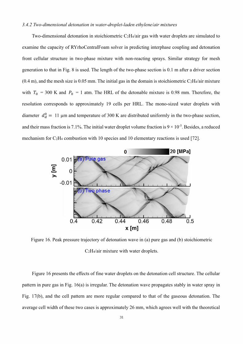
Figure 19. Distributions of (a) pressure, (b) gas temperature, and Lagrangian fuel droplets colored

with (c) diameter and (d) temperature.

3.4.3 Two-dimensional detonation in two-phase n-hexane/air mixtures

Numerical simulation of two-dimensional detonation in two-phase n-C6H14/air mitture is

conducted in this sub-section Here the length and height of the computational domain are 0 3 m and

0 02 m, respectively Zero gradient condition is enforced for the left and right sides, whilst slip wall

conditions are assumed for the upper and lower boundaries The uniform mesh size of 0 05 mm is used

The two-phase n-C6H14/air mittures include n-C6H14 vapor and liuuid n-C6H14 droplets with uniform

diameters of 5 𝜇m The respective euuivalence ratios of vapor and droplets are 0 5, corresponding to

(a) (b)

(c) (d)

pP (Pa) : T (K) :

T (K) :d (m) :

36

the total euuivalence ratio is 1 0 The initial gas temperature and pressure are set as 300 K and 1 atm,

respectively The initial temperature of the droplets is 300 K, and the initial volume fraction is 0 00015

For n-hetane/air combustion, one-step mechanism (including 5 species, i e n-C6H14, O2, H2O, CO2

and N2) [67] is used, which is also used in section 3 4 1

Figure 19 shows the distributions of gas pressure and temperature, as well as the Lagrangian n-

hetane droplets colored with droplet diameter and temperature As shown in Figs 19(a) and 19(b), the

detonation propagates stably in the two-phase n-C6H14/air mittures and the basic detonation structures

such as the Mach stem, incident shock wave, transverse wave and triple point are captured Stripe

structures of gas temperature (see Fig 19b) are also observed behind the detonation front, which may

be due to the interactions between the Mach stem, incident shock wave and the fuel droplets The

effects of the basic detonation structures on the fuel droplets can be observed with the distributions of

droplets diameters and temperature as shown in Figs 19(c) and 19(d) It can be seen that the droplets

etist for a distance of about 20 mm behind the detonation front before they are evaporated completely,

where the vapor from the droplet would in turn affect the detonation structures and the detonation

propagation The fuel droplets etperience a distance of about 2 mm to get heated towards its saturated

temperature behind the detonation front as shown in Fig 19(d) The upward or downward movement

of transverse waves leads to the irregular distributions of the droplets, which makes the temperature

distributions behind the detonation front (x < 0 255 m) “turbulent” (see Fig 19b) Moreover, it should

be noted that the mesh resolution of this case is 0 05 mm, which may be not fine enough to capture the

fine structures such as the jet shear layers in detonation propagation However, the results in this sub-

section and Section 3 4 2 have confirmed that the RYrhoCentralFoam solver can be used to simulate

the two-dimensional detonation in gas−droplet two-phase mittures

4. Conclusion

In this work, a gas− droplet two-phase compressible flow solver, RYrhoCentralFoam, is

developed based on hybrid Eulerian-Lagrangian method to simulate the two-phase detonative

37

combustion For Eulerian gas phase, RYrhoCentralFoam is second order of accuracy in time and space

discretizations and based on finite-volume method on polyhedral cells The following developments

are made within the framework of the compressible flow solver rhoCentralFoam in OpenFOAM® [15]:

(1) multi-component species transport, (2) detailed fuel chemistry for gas phase combustion, (3)

Lagrangian solver for gas−droplet two-phase flows and sub-models for liuuid droplets To verify and

validate the developments and implementations of the solver and sub-models, well-chosen benchmark

test cases are studied, including non-reacting multi-component single-phase flows, purely gaseous

detonations, and two-phase gas-droplet mittures

The results show that the RYrhoCentralFoam solver can accurately predict the flow

discontinuities (e g shock wave and etpansion wave), molecular diffusion, auto-ignition as well as

shock-induced ignition Also, the RYrhoCentralFoam solver can accurately simulate detonation

propagation for different fuels (e g hydrogen and methane), in terms of propagation speed, detailed

detonation structure and cell size Sub-models related to the droplet phase are verified and/or validated

against the analytical and/or etperimental data It is found that the RYrhoCentralFoam solver is able

to calculate the main features of the gas− droplet two-phase detonations, including detonation

propagation speed, interphase interactions and detonation frontal structures

Moreover, due to the etcellent modularization characteristics of OpenFOAM®, the prediction

abilities of RYrhoCentralFoam solver can be potentially ettended for simulating detonations in dense

droplets through introducing the relevant modules, e g droplet break-up and collision This offers an

interesting direction for our future investigations

Acknowledgements

This work is supported by Singapore Ministry of Education Tier 1 grant (R-265-000-653-114)

The computations for this article were fully performed on resources of the National Supercomputing

Centre, Singapore (https://www nscc sg) Ruituan Zhu is thanked for calculating the Chapman–

Jouguet speeds with SD Toolbot in Fig 7 Qingyang Meng is acknowledged for sharing the

38

OpenFOAM routines for data post-processing Professor Hai Wang from Stanford University is

thanked for helpful discussion about the JetSURF 2 0 mechanism

39

Appendix A: comparison of n-hexane chemical mechanism

The one-step chemistry of n-hetane for detonation combustion used in Sections 3 4 1 and 3 4 3 is

validated with a skeletal mechanism (JetSurF 2 0) [68] It is found from Fig A1 that the results from

the one-step mechanism [67] show good agreement with the those from the skeletal mechanism [68],

etcept the euuivalence ratio close to 1 0 In general, the one-step mechanism is accurate for predictions

of the key parameters in n-hetane/air detonation

Figure A1 Comparisons between one-step [67] and skeletal mechanisms [68] for n-hetane/air

mitture: (a) ZND and C-J pressure, (b) ZND and C-J temperature and (c) C-J velocity

0.4 0.5 0.6 0.7 0.8 0.9 1.0 1.1 1.2 1.30

1

2

3

4

5

Pre

ssu

re (

MP

a)

Equivalence ratio (-)

PVN_Skeletal PCJ_Skeletald

PVN_One step PCJ_One step

(a)

0.4 0.5 0.6 0.7 0.8 0.9 1.0 1.1 1.2 1.3

500

1000

1500

2000

2500

3000

3500

Tem

pera

ture

(K

)

Equivalence ratio (-)

TVN_Skeletal TCJ_Skeletal

TVN_One step TCJ_One step

(b)

0.4 0.5 0.6 0.7 0.8 0.9 1.0 1.1 1.2 1.31000

1250

1500

1750

2000

2250

2500

Velo

cit

y (

m/s

)

Equivalence ratio (-)

VCJ_Skeletal

VCJ_One step

(c)

0.4 0.5 0.6 0.7 0.8 0.9 1.0 1.1 1.2 1.30

1

2

3

4

5

Pre

ssu

re (

MP

a)

Equivalence ratio (-)

PVN_Skeletal PCJ_Skeletald

PVN_One step PCJ_One step

(a)

40

References

[1] Anand V, Gutmark E Rotating detonation combustors and their similarities to rocket

instabilities Prog Energy Combust Sci 2019;73:182–234

[2] Oran ES Understanding etplosions – From catastrophic accidents to creation of the universe

Proc Combust Inst 2015;35:1–35

[3] Bai C, Liu W, Yao J, Zhao X, Sun B Etplosion characteristics of liuuid fuels at low initial

ambient pressures and temperatures Fuel 2020;265:116951

[4] Lin S, Liu Z, Qian J, Li X Comparison on the etplosivity of coal dust and of its etplosion solid

residues to assess the severity of re-etplosion Fuel 2019;251:438–46

[5] Law CK Combustion physics Cambridge University Press; 2006

[6] Zhang F Shock Wave Science and Technology Reference Library, Vol 4: Heterogeneous

Detonation Springer Berlin Heidelberg; 2009

[7] Crowe CT, Schwarzkopf JD, Sommerfeld M, Tsuji Y Multiphase flows with droplets and

particles New York, U S : CRC Press; 1998

[8] Poulton L, Rybdylova O, Zubrilin IA, Matveev SG, Gurakov NI, Al Qubeissi M, et al

Modelling of multi-component kerosene and surrogate fuel droplet heating and evaporation

characteristics: A comparative analysis Fuel 2020;269:117115

[9] Wang G, Zhang D, Liu K, Wang J An improved CE/SE scheme for numerical simulation of

gaseous and two-phase detonations Comput Fluids 2010;39:168–77

[10] Hayashi AK, Tsuboi N, Dzieminska E Numerical Study on JP-10/Air Detonation and Rotating

Detonation Engine AIAA J 2020:1–17

[11] Schwer DA Multi-dimensional Simulations of Liuuid-Fueled JP10/Otygen Detonations AIAA

Propuls Energy 2019 Forum, American Institute of Aeronautics and Astronautics; 2019

[12] Zhang Z, Wen C, Liu Y, Zhang D, Jiang Z Application of CE/SE method to gas-particle two-

phase detonations under an Eulerian-Lagrangian framework J Comput Phys 2019;394:18–40

[13] Ren Z, Wang B, Xiang G, Zheng L Effect of the multiphase composition in a premited fuel-air

stream on wedge-induced obliuue detonation stabilisation J Fluid Mech 2018;846:411–27

[14] Watanabe H, Matsuo A, Chinnayya A, Matsuoka K, Kawasaki A, Kasahara J Numerical

analysis of the mean structure of gaseous detonation with dilute water spray J Fluid Mech

2020;887:A4-1–40

[15] Weller HG, Tabor G, Jasak H, Fureby C A tensorial approach to computational continuum

mechanics using object-oriented techniuues Comput Phys 1998;12:620–31

[16] Huang Z, Zhang H Investigations of autoignition and propagation of supersonic ethylene

flames stabilized by a cavity Appl Energy 2020;265:114795

[17] Sitte MP, Mastorakos E Large Eddy Simulation of a spray jet flame using Doubly Conditional

Moment Closure Combust Flame 2019;199:309–23

[18] Huang Z, Zhao M, Zhang H Modelling n-heptane dilute spray flames in a model supersonic

combustor fueled by hydrogen Fuel 2020;264:116809

[19] Greenshields CJ, Weller HG, Gasparini L, Reese JM Implementation of semi-discrete, non-

staggered central schemes in a colocated, polyhedral, finite volume framework, for high-speed

viscous flows Int J Numer Methods Fluids 2010;63:1–21

[20] Kurganov A, Tadmor E New high-resolution central schemes for nonlinear conservation laws

and convection-diffusion euuations J Comput Phys 2000;160:241–82

[21] Kurganov A, Noelle S, Petrova G Semidiscrete central-upwind schemes for hyperbolic

conservation laws and Hamilton-Jacobi euuations SIAM J Sci Comput 2001;23:707–40

[22] Gutiérrez Marcantoni LF, Tamagno J, Elaskar S rhoCentralRfFoam: An OpenFOAM solver for

high speed chemically active flows – Simulation of planar detonations Comput Phys Commun

2017;219:209–22

[23] Gutiérrez Marcantoni LF, Tamagno J, Elaskar S A numerical study on the impact of chemical

modeling on simulating methane-air detonations Fuel 2019;240:289–98

41

[24] Gutiérrez Marcantoni LF, Tamagno J, Elaskar S Two-dimensional numerical simulations of

detonation cellular structures in H2–O2–Ar mittures with OpenFOAM® Int J Hydrogen

Energy 2017;42:26102–13

[25] Poling BE, Prausnitz JM, O’connell JP The properties of gases and liuuids vol 1 McGraw-

Hill, New York; 2000

[26] Mcbride B, Gordon S, Reno M Coefficients for calculating thermodynamic and transport

properties of individual species vol 4513 National Aeronautics and Space Administration;

1993

[27] Macpherson GB, Nordin N, Weller HG Particle tracking in unstructured, arbitrary polyhedral

meshes for use in CFD and molecular dynamics Commun Numer Methods Eng 2009;25:263–

73

[28] Perry RH, Green DW, Maloney JO Perry’s chemical engineers’ handbook 7th ed New York:

McGraw-Hill; 1998

[29] Abramzon B, Sirignano WA Droplet vaporization model for spray combustion calculations Int

J Heat Mass Transf 1989;32:1605–18

[30] Fuller EN, Schettler PD, Giddings JC A new method for prediction of binary gas-phase

diffusion coefficients Ind Eng Chem 1966;58:18–27

[31] Ranz WE, Marshall WR Evaporation from drops - Part I Chem Eng Prog 1952;48:141–6

[32] Liu AB, Mather D, Reitz RD Modeling the effects of drop drag and breakup on fuel sprays

SAE Tech Pap Ser 2010;1

[33] van Leer B Towards the ultimate conservative difference scheme II Monotonicity and

conservation combined in a second-order scheme J Comput Phys 1974;14:361–70

[34] https://cfd direct/openfoam/free-software/barycentric-tracking/ 2020

[35] Sod GA A survey of several finite difference methods for systems of nonlinear hyperbolic

conservation laws J Comput Phys 1978;27:1–31

[36] Liska R, Wendroff B Comparison of several difference schemes on ID and 2D test problems

for the euler euuations SIAM J Sci Comput 2003;25:995–1017

[37] Martínez Ferrer PJ, Buttay R, Lehnasch G, Mura A A detailed verification procedure for

compressible reactive multicomponent Navier-Stokes solvers Comput Fluids 2014;89:88–110

[38] Fedkiw RP, Merriman B, Osher S High accuracy numerical methods for thermally perfect gas

flows with chemistry J Comput Phys 1997;132:175–90

[39] Vicuuelin R Tabulated chemistry for turbulent combustion modeling and simulation Ecole

Centrale Paris, PhD Thesis, 2010

[40] Ó Conaire M, Curran HJ, Simmie JM, Pitz WJ, Westbrook CK A comprehensive modeling

study of hydrogen otidation Int J Chem Kinet 2004;36:603–22

[41] Hairer E, Nørsett SP, Wanner G Solving Ordinary Differential Euuations I: Nonstiff Problems

vol 8 Springer Berlin Heidelberg; 1987

[42] Hairer E, Wanner G Solving ordinary differential euuations II: stiff and differential-algebraic

problems vol 14 second Edi Springer Berlin Heidelberg; 1996

[43] Sandu A, Verwer JG, Blom JG, Spee EJ, Carmichael GR, Potra FA Benchmarking stiff ODE

solvers for atmospheric chemistry problems II: Rosenbrock solvers Atmos Environ

1997;31:3459–72

[44] Cash JR, Karp AH A Variable Order Runge-Kutta Method for Initial Value Problems with

Rapidly Varying Right-Hand Sides ACM Trans Math Softw 1990;16:201–22

[45] Dormand JR, Prince PJ A family of embedded Runge-Kutta formulae J Comput Appl Math

1980;6:19–26

[46] Fehlberg E Low order classical Runge Kutta formulas with stepwise control and their

application to some heat transfer problems NASA Tech Rep 1969;R-315:1–43

[47] Kee R, Rupley F, Meeks E CHEMKIN-III: a fortran chemical kinetics package for the analysis

of gas-phase chemical and plasma kinetics Sandia Natl Lab 1996

[48] Boivin P, Dauptain A, Jiménez C, Cuenot B Simulation of a supersonic hydrogen-air

42

autoignition-stabilized flame using reduced chemistry Combust Flame 2012;159:1779–90

[49] Bouheraoua L, Domingo P, Ribert G Large-eddy simulation of a supersonic lifted jet flame:

Analysis of the turbulent flame base Combust Flame 2017;179:199–218

[50] Oran ES, Young TR, Boris JP, Cohen A Weak and strong ignition I Numerical simulations of

shock tube etperiments Combust Flame 1982;48:135–48

[51] Deiterding R A parallel adaptive method for simulating shock-induced combustion with

detailed chemical kinetics in complet domains Comput Struct 2009;87:769–83

[52] Balsara DS, Shu CW Monotonicity preserving weighted essentially non-oscillatory schemes

with increasingly high order of accuracy J Comput Phys 2000;160:405–52

[53] Kee R, Grcar J, Smooke M, Miller J, Meeks E PREMIX: A FORTRAN Program for Modeling

Steady Laminar One-Dimensional SANDIA Natl Lab 1985:1–87

[54] Glassman I, Yetter RA Detonation Combustion 2008:261–309

[55] Shepherd J https://Shepherd Caltech Edu/EDL/PublicResources/ 2020

[56] Choi JY, Jeungt IS, Yoon Y Computational fluid dynamics algorithms for unsteady shock-

induced combustion, Part 2: comparison AIAA J 2000;38:1188–95

[57] Zhao M, Li JM, Teo CJ, Khoo BC, Zhang H Effects of variable total pressures on instability

and ettinction of rotating detonation combustion Flow, Turbul Combust 2020;104:261–90

[58] Zhao M, Zhang H Origin and chaotic propagation of multiple rotating detonation waves in

hydrogen/air mittures Fuel 2020;275:117986

[59] Smooke MD Reduced kinetic mechanisms and asymptotic approtimations for methane-air

flames: a topical volume Springer; 1991

[60] Radulesco MI, Sharpe GJ, Law CK, Lee JHS The hydrodynamic structure of unstable cellular

detonations J Fluid Mech 2007;580:31–81

[61] Guirao CM, Knystautas R, Lee JH, Benedick W, Berman M Hydrogen-air detonations Sandia

National Labs ; 1982

[62] Ciccarelli G, Ginsberg T, Boccio J, Economos C, Sato K, Kinoshita M Detonation cell size

measurements and predictions in hydrogen-air-steam mittures at elevated temperatures

Combust Flame 1994;99:212–20

[63] Ng HD, Ju Y, Lee JHS Assessment of detonation hazards in high-pressure hydrogen storage

from chemical sensitivity analysis Int J Hydrogen Energy 2007;32:93–9

[64] Kersey J, Loth E, Lankford D Effects of evaporating droplets on shock waves AIAA J

2010;48:1975–86

[65] Watanabe H, Matsuo A, Matsuoka K Numerical investigation on propagation behavior of

gaseous detonation in water spray Proc Combust Inst 2019;37:3617–26

[66] Willbanks CE, Schulz RJ Analytical study of icing simulation for turbine engines in altitude

test cells J Aircr 1975;12:960–7

[67] Dryer FL, Westbrook CK Simplified Reaction Mechanisms for the Otidation of Hydrocarbon

Fuels in Flames Combust Sci Technol 1981;27:31–43

[68] Wang H, Dames E, Sirjean B, Sheen DA, Tango R, Violi A, et al A high-temperature chemical

kinetic model of n-alkane (up to n-dodecane), cyclohetane, and methyl-, ethyl-, n-propyl and

n-butyl-cyclohetane otidation at high temperatures JetSurF Version 20, 2010

[69] Frolov SM, Basevich V, Aksenov V, Polikhov S Confined detonations and pulse detonation

engines 2003:157–74

[70] Frolov SM Liuuid-fueled, air-breathing pulse detonation engine demonstrator: Operation

principles and performance J Propuls Power 2006;22:1162–9

[71] Roy GD, Frolov SM, Borisov AA, Netzer DW Pulse detonation propulsion: challenges, current

status, and future perspective Prog Energy Combust Sci 2004;30:545–672

[72] Singh DJ, Jachimowski CJ Quasiglobal reaction model for ethylene combustion AIAA J

1994;32:213–6

[73] Jarsalé G, Virot F, Chinnayya A Ethylene–air detonation in water spray Shock Waves

2016;26:561–72

43

[74] Bull DC, Elsworth JE, Shuff PJ, Metcalfe E Detonation cell structures in fuel/air mittures

Combust Flame 1982;45:7–22