ILASS Americas 21st Annual Conference on Liquid Atomization and Spray Systems, Orlando, FL, May 2008

A Hybrid Lagrangian-Eulerian Method (hLE) for Interface Tracking

Sourabh V. Apte∗

School of Mechanical, Industrial, and Manufacturing EngineeringOregon State University

204 Rogers Hall, Corvallis, OR 97331

AbstractA hybrid Lagrangian-Eulerian (hLE) scheme, combining a particle-based, mesh-free technique with a finite-volume flow solver, is developed for direct simulations of two-phase flows. The approach uses marker pointsaround the interface and advects the signed distance to the interface in a Lagrangian frame. The kernel–basedderivative calculations typical of particle methods are used to extract the interface normal and curvaturefrom unordered marker points. Connectivity between the marker points is not necessary. The fluid flowequations are solved on a background, fixed mesh using a co-located grid finite volume solver together withbalanced force algorithm (Francois et al. JCP, 2006, Herrmann JCP, 2007) for surface tension force. Thenumerical scheme is first validated for standard test cases: (i) parasitic currents in a stationary sphericaldrop, (ii) small amplitude damped surface waves, (iii) capillary waves on droplet surface, (iv) Rayleigh-Taylor instability, and (v) gravity-driven bubble/droplet in a stationary fluid. Extension of the approachto three-dimensions is conceptually straight forward, however, poses challenges for parallel implementation.A domain-decomposition based on balancing the number of grid points per processor gives rise to load–imbalance due to uneven distribution of the marker points and advanced domain partitioning methods areneeded for improved efficiency of the approach.

∗Corresponding Author: sva@engr.orst.edu

IntroductionNumerical methods to accurately track/capture

the interface between two fluids have been an area ofresearch for decades. Tryggvason et al. [1] providea detailed review on various methods used for di-rect simulation of multiphase flows. Broadly, theseschemes can be classified into two categories: (a)front tracking and (b) front capturing methods.

Front tracking methods are Lagrangian in na-ture [2, 3, 4, 5], and the interface is tracked by a setof connected [1] or unconnected [6] marker pointson the interface and the Navier-Stokes equations aresolved on a fixed grid in an Eulerian frame. An-other class of Lagrangian methods include mesh-free algorithms such as moving particle-methods [7],vortex-in cell methods [8, 9], and smoothed-particlehydrodynamics [10], where the interface is repre-sented by Lagrangian points (LPs) and the flow-field is also evaluated on these points. Pure La-grangian methods are promising as they avoid enor-mous memory requirements for a three-dimensionalmesh. These methods automatically provide adap-tive resolution in the high-curvature region [8] andhave been applied successfully to many two-phaseflow problems [11, 12, 13]. However, they exhibitother difficulties such as high cost of finding nearestneighbors in the zone of influence of a Lagrangianpoint, true enforcement of continuity (or incompress-ibility) conditions, and problems associated with ac-curate one-sided interpolations near boundaries [8].

In capturing methods the interface is not ex-plicitly tracked, but captured using a characteristicfunction, which evolves using the advection equa-tion. Representative capturing methods are: vol-ume tracking [14, 15], level set [16, 17, 18] andphase field models. Both approaches (the VoF andlevel set) are straightforward to implement, how-ever, level-set approach does not preserve volumeof the fluids on either side of the interface. TheVOF formulation on the other hand, conserves thefluid volume but lacks in the sharpness of the in-terface. Several improvements to these methods in-volving combination of the two [19], adaptive mesh-refinement [20, 21], particle-level sets [22], refinedlevel-set grid scheme [23, 24, 25] have been proposedfor improved accuracy.

In the present work, some of the limitationsof the above schemes are addressed by combiningthe two broad approaches mentioned above. Thebasic idea is to merge the locally ‘adaptive’ mesh-free particle-based methods with the relative ‘ease’of Eulerian finite-volume formulation in order toinherit the advantages offered by individual ap-proaches. The interface between two fluids is rep-

resented and tracked using Lagrangian points orfictitious particles [13]. Unlike particle level setmethod [22] or the semi-Lagrangian methods [26],in the present approach the interface is representedby Lagrangian points (LPs) (or particles1) that areadvanced in a Lagrangian frame. The motion of theinterface is determined by a velocity field (interpo-lated to the particle locations) obtained by solvingthe Navier-Stokes equations on a fixed backgroundmesh in an Eulerian frame. The interface location,once determined, identifies the region of the meshto apply jump-conditions in fluid properties. In thissense, it is in the realm of Arbitrary Lagrangian-Eulerian (ALE) [27] schemes, wherein the compu-tational grid deforms to conform to the shape ofthe dispersed phase. The potential advantage of thepresent hybrid method is that the background meshcould be of any kind: structured, body-fitted, or ar-bitrary shaped unstructured (hex, pyramids, tetrahe-drons, prisms) and may be stationary or changingin time (adaptive refinement). Here, we use a co-located grid, incompressible flow solver based on theenergy conserving finite-volume algorithm developedby Mahesh et al. [28, 29].

The Lagrangian points (LPs) in our interfacecalculations, are particles distributed in a narrowband around the interface [30]. These LPs are ini-tially uniformly spaced and carry information suchas the signed distance to the interface (SDF) alongthe characteristic paths. Variations in flow veloci-ties leads to an irregular distribution of the initiallyuniform LPs. Regularization of the particles areperformed by mapping the particles on a uniformlyspaced lattice [13]. Values for particle properties atnew LP locations are obtained through kernel molli-fication as done in Smoothed Particle Hydrodynam-ics [10] and remeshed-SPH [12]. The novelty in ourapproach is that this mesh-free interface representa-tion is integrated with a finite-volume solver wherethe governing equations for flow evolution are solved.The Lagrangian points provide sub-grid resolutionand in this respect the method is similar to the Re-fined Level Set Grid (RLSG) approach [24, 25, 31].However, here the LPs move in space with the flowvelocity and different discretizations are necessaryand we use high-order schemes based on mollifica-tion kernels.

The paper is arranged as follows. The gov-erning equations and mathematical formulation isdescribed followed by description of the numericalscheme. The numerical approach is then applied tostandard test cases to evaluate the accuracy of the

1In this paper, the term ‘particles’ means Lagrangianpoints (LPs) that are used to represent the interface.

scheme compared to other approaches. Finally, somepreliminary results on rising bubble in a quiescentfluid are presented.

Mathematical Formulation and GoverningEquations

Consider two immiscible fluids labeled as ‘1’ and‘2’ forming an interface. The regions occupied bythe two fluids can be represented by an indicatorfunction Ψ which can be zero or unity representingone of the fluids. In a front tracking scheme [1],connected marker points are used to represent theinterface surface. The marker points are embeddedin a background computational mesh. Knowing thelocation of the marker points, a smoothly varyingindicator function (or color function) is constructedon the computational mesh (Ψcv, where cv standsfor the grid control volume). Torres and Brackbill [6]developed a point-set method where the connectivitybetween the marker points was not necessary. Thepresent work is motivated by the point-set method.Instead of using marker points on the interface only,a uniformly distributed set of points (termed here asLagrangian points, LP) are placed in a small bandsurrounding the interface. These marker points areassigned a signed distance function (SDF, Φ) to theinterface, and thus represent the interface implicitly.

The main advantage of this approach is thatthe color function can be easily constructed fromthe marker points (as discussed in the following sec-tions) and does not require a solution of the Laplaceequation (52Ψ = 0) as in the point-set method [6].However, as the marker points are moved by the un-derlying flow, the flow strain can cluster the LPs insome region and spread them apart in other regions.Such non-uniform distribution may affect the inter-face representation (and interface properties such assurface normals, curvature etc.) and the LPs areperiodically re-arranged to a uniform distributionthrough a systematic remeshing or reconfigurationprocedure [13] typically used in remeshed SmoothParticle Hydrodynamics [8]. The formulation thusrepresents a combination of marker points, level setmethods, and smooth particle hydrodynamics andis termed as hybrid Lagrangian Eulerian (hLE) ap-proach. Note that this approach is different fromthe particle-level set method [22] where the levelset function was advanced in an Eulerian frame andlater corrected by subgrid particles. In the presentwork, the advection of the interface is performedsolely in the Lagrangian frame using the motion ofthe LPs.

Hybrid Lagrangian-Eulerian (hLE) SchemeFollowing Hieber & Koumoutsakos [13], the in-

terface between two fluids is represented using uni-formly spaced Lagrangian points (LPs) or fictitiousparticles in a narrow band around the interface.Each LP is associated with position xp, velocity up,volume Vp and a scalar function Φp which repre-sents the signed distance to the interface. The av-erage spacing (h between the uniformly spaced LPsis related to the volume Vp. In this work, we usecubic elements (h = V1/3

p ). As the LPs move, theycarry the SDF value along the characteristic pathsand implicitly represent the motion of the interface.The evolution of the interface is calculated by solv-ing level set equations in the Lagrangian form:

DΦpDt

= 0;DVpDt

= 〈∇ · u〉p Vp;DxpDt

= up, (1)

where p denotes the Lagrangian point or particle.For incompressible fluids, the velocity field is diver-gence free and theoretically, the change in volume ofthe LPs (DVp/Dt) is zero.

As is done in Smoothed Particle Hydrodynamics(SPH) and mesh-free methods, smoothed approxi-mation of the level set function and its derivativescan be obtained by using a mollification operatorwith LPs as quadrature points. The localized mol-lification kernel ξε generates a smooth continuousapproximation of Φ around the particle at locationxp using SDF of other particles at locations xq:

Φq =N∑p=1

VpΦpξε(xq − xp) (2)

where Φq = Φ(xq) and∑Np=1 ξεVp = 1. Differ-

ent mollification kernels have been proposed such asquartic spline and Mn splines [10]. In this paper, weuse the quartic spline function given as:

ξε(x) =

s4

4 −5s2

8 + 115192 , 0 ≤ s < 1

2

− s4

6 + 5s3

6 −5s2

4 + 5s24 + 55

9612 ≤ s <

32

(2.5−s)424 , 3

2 ≤ s <52

0 s ≥ 52

where s = |x|/ε. Here, ε is the radius of influ-ence around the particle (or LP) and depends onthe spacing between the LPs and the width of themollification kernel. For all calculations in this workε is set equal to the uniform spacing between theLPs. The surface normal and curvature calculationsrequire derivatives of the scalar function Φ on theparticles. These are approximated in a conservative

form by using derivatives of the mollification ker-nel [32]:

〈∇Φ〉q =∑p

Vp (Φp − Φq)∇ξε(xq − xp), (3)

〈∇2Φ〉q =∑p

Vp (Φp − Φq)∇2ξε(xq − xp). (4)

In the above equations, kernel (ξε) and its first andsecond derivatives should be properly normalizedsuch that corresponding non-zero moment condi-tions are satisfied (details are given in [32]).

Once the location of the LPs and the associ-ated Φp values are obtained, a color function Ψ(x)can be constructed. Following the definition of colorfunction, finding Ψ on the LPs is straightforward:Ψ = 0 when Φ ≥ 0 and Ψ = 1 for Φ < 0. Thenthe color function field can also be obtained on thebackground computational mesh by interpolating Ψfrom the LPs. In order to obtain a smooth function,the M ′4 kernel interpolation is used:

M ′4 =

1− 5/2s2 + 3/2s3

1/2(1− s)(2− s)2

0

0 ≤ s < 11 ≤ s < 22 ≤ s

(5)

where s = x in one-dimension. The higher-dimensional interpolations are obtained by takingtensorial products of their one-dimensional counter-parts.

Once the color function Ψ is obtained at a con-trol volume (cv), the density and viscosity are givenas:

ρcv = ρ1 + (ρ2 − ρ1)Ψcv (6)µcv = µ1 + (µ2 − µ1)Ψcv (7)

Then the flow field is computed on a backgroundmesh (which could be structured or unstructured) bysolving the Navier-Stokes equations for the two-fluidsystem:

∇ · u = 0 (8)

∂u∂t

+u·∇u = −1ρ∇p+

1ρ∇·(µ(∇u+∇Tu))+g+

1ρFσ

(9)where u is velocity vector of fluid, p is pressure, ρ andµ are fluid density and viscosity (uniform inside eachfluid), g body force, and Fσ is the surface tensionforce which is non-zero only at the interface location(Φ = 0). Following Brackbill et al. [33], the surfacetension force is modeled as a continuum surface force(CSF):

FCSFσ = σκnδ(Φ) (10)

where σ is the surface tension coefficient (assumedconstant in the present work), κ is the curvature, n

the interface normal, and δ(Φ) a dirac-delta func-tion. A common issue with numerical simulationsinvolving surface tension force, is the development ofspurious currents (unphysical velocity field) [1, 20]due to inaccuracies in the discrete approximations tothe surface-tension forces (equation 9). In order toobtain a consistent coupling of the surface tensionforce with the pressure gradient forces in a finite-volume approach, Francois et al. [34] indicated thatthe surface tension force must be evaluated at thefaces of the control volumes as:

FCSFσ,f = σκf (∇Ψ)f (11)

where the subscript f stands for the face of the con-trol volume. The surface tension force at the cv-centers can be obtained through reconstruction fromthe faces of each cv.

To compute the surface tension force, accurateestimation of the curvature of the interface is nec-essary. Any errors in the curvature calculation andsurface tension force representation give rise to non-physical velocity fields that could be detrimental tothe accuracy of the numerical solution [1, 6]. Her-rmann [25, 35] developed a procedure to computethe curvature accurately in the level-set framework.Here we follow a similar procedure for curvatureevaluations:

• The curvature at a point on the interface isgiven as:

κ = ∇ · ∇Φ|∇Φ|

; n =∇Φ|∇Φ|

. (12)

First the curvature and normal are evaluatedat the LPs close to the interface (|Φ| ≤ 2∆LP ,where ∆LP is the spacing between the LPs. Thegradients in the curvature and surface normalcomputations are evaluated using using equa-tions 4.

• For each of these LPs (with |Φ| ≤ 2∆LP ) , apoint on the interface is obtained by projectingnormals onto the interface [25]:

xinterface = xLP −Φ|∇Φ|

n (13)

• Curvature on the interface point xinterface isevaluated by using curvature values on LPs inits neighborhood through M ′4-kernel based in-terpolation (equation 5).

• Once curvatures on all interface points are eval-uated, these values are assigned to the corre-sponding LPs from which these interface pointswere obtained.

• Curvature at the background control volume cvis then computed by simply adding the curva-tures of LPs that lie inside the control volume.

• Curvature at the faces of the control volumeare evaluated by arithmetic average of the twocontrol volumes associated with the face. Here,the average is taken only if the both cvs containthe interface, i.e. color function 0 < Ψcv < 1,else κf is assigned the value of κcv containingthe interface.

Finally, the motion of the LPs is determined bya velocity field obtained by solving the Navier Stokesequations on a fixed background mesh. The velocityof each LP is obtained through interpolation fromthe background mesh. The motion of the LPs, maydistort the initially uniformly spaced particles anda reconfiguration step is necessary wherein the dis-torted LPs are mapped to a uniformly spaced Carte-sian lattice as described below.

Particle Map Distortion, Reconfiguration and Reini-tialization

For the present particle-based method of inter-face representation, the LPs should overlap in orderto obtain an accurate solution and interface prop-erties such as normals and curvature. If the par-ticle map gets highly distorted, the color functionobtained from the LPs will no longer be smoothand continuous. This is overcome by performinga consistent re-configuration of the LP locations,termed as remeshing, around the interface. Herethe Lagrangian points are redistributed on a Carte-sian lattice with uniform spacing. After new setsof Lagrangian points are generated the values ofthe signed-distance function are obtained from theold ones by using higher order interpolations [8].Remeshing removes any unphysical kinks in the in-terface and gives the ‘entropy-satisfying viscous so-lution’ [13]. It also eliminates unnecessary pointsaway from the interface. For remeshing, we usethe M ′4 kernel to obtain the interpolated SDF val-ues. Although the reconfiguration procedure pro-vides the entropy solution, it does not guaranteethat Φ remains a signed-distance to the interface,which is crucial to obtain accurate curvature andinterface normals. In this work, reinitialization isimplemented according to the method suggested bySussman et al. [36, 37] in which the following equa-tion is solved on uniformly spaced LPs:

∂Φ∂τ

= sign(Φ0)(1− |∇Φ|) (14)

where Φ(x, 0) = Φ0 and sign(Φ0) ≡ 2(Hε(Φ)− 1/2)and Hε(Φ) is the Heaviside function. We apply re-

distancing in a two-layer narrow band around the in-terface and using the procedure described in Gomezet al. [31].

Numerical AlgorithmThe governing equations are solved using a co-

located grid finite-volume algorithm [28, 29]. Ac-cordingly, all variables are stored at the control vol-ume (cv) centers with the exception of a face-normalvelocity, located at the face centers, and used to en-force the divergence-free constraint. The variablesare staggered in time so that they are located mostconveniently for the time advancement scheme. De-noting the time level by a superscript index, the ve-locities are located at time level tn and tn+1, andpressure, density, viscosity, the signed distance func-tion, and the color function at time levels tn−1/2 andtn+1/2. A balanced force algorithm [34, 35] is usedfor discrete balance of surface tension force and pres-sure gradient in the absence of any flow and otherexternal forces. The basic steps are summarized be-low:

1. Advance the LPs (from tn−1/2 to tn+1/2)according to equations (1) and using a velocityfield interpolated to the LP location from the back-ground mesh. In this work, we use the M ′4-kernelbased interpolation. We use third-order Runge-Kutta scheme to solve the ordinary differential equa-tions for each LP.

2. Remesh and reinitialize the particle-map ifnecessary. Remeshing of LPs is necessary only ifthe particles cease to overlap as they adapt to theflow map. This is indicated by the distortion index(DI) [13]:

DI =1N

∑p

|Hp(t)−Hp(0)|Hp(0)

, (15)

where Hp(t) =∑q vq(t)ξε(xp(t) − xq(t)), N is the

number of Lagrangian points, vq the volume of eachLP, and ξε the quartic spline mollification kernel. Byselecting a proper threshold for DI the remeshingprocedure can be triggered. Reinitialization is onlynecessary after a few remeshing steps, thus makingthe hybrid approach attractive. Reinitialization isdone on remeshed LPs so that standard 5th-orderWENO scheme [38] can be used.

3. Once the LPs are advanced, curvature κLPis evaluated using the procedure outlined in the pre-vious section. M ′4-kernel based interpolations areperformed from the LPs to the background meshto obtain curvature (κn+1/2

cv ). Similarly, Ψn+1/2cv

is obtained through interpolations and ρn+1/2cv , and

µn+1/2cv are calculated from equations (7). The face-

based surface tension force is then obtained as:

Fn+1/2σ,f = σκ

n+1/2f

Ψn+1/2icv2 −Ψn+1/2

icv1

|sn|(16)

where sn is the vector joining the control volumesicv1 to icv2.

4. The remaining steps are a variant of the co-located fractional step method as described by Ham& Young [20]. We present the semi-descretizationhere for completeness. First, a projected velocityfield ui at the cv-centers is calculated:

ui − uni∆t

= gi +1

ρn+1/2cv

(− ∂p

∂xi

n−1/2

+

Fn+1/2v,i + F

n+1/2σ,i )

where Fv,i represents the viscous, Fσ,i the surfacetension, and gi the gravitational forces at the cv cen-troids. The viscous terms are treated implicitly us-ing second order symmetric discretizations and thesurface tension force is treated explicitly. The cv-based surface tension force is obtained from Fσ,f us-ing area weighted least-squares interpolation consis-tent with the pressure reconstruction scheme devel-oped by Mahesh et al. [28]. This is the essence ofthe balanced force algorithm [20, 34, 25].

5. Subtract the old pressure gradient:

u∗n+1i = ui + ∆t

1

ρn+1/2cv

δp

δxi

n−1/2

(17)

6. Obtain an approximation for the face-basedvelocity:

U∗n+1f = u∗n+1

i −∆t

Fn+1/2i

ρn+1/2cv

−Fn+1/2σ,f

ρn+1/2f

(18)

where ρn+1/2f = (ρn+1/2

icv1 + ρn+1/2icv2 )/2 and the inter-

polation operator, η = ni,f [ηicv1 + ηicv2]/2, yields aface-normal component from the adjacent cvs asso-ciated with the face and the normal ni,f .

7. Solve the variable coefficient Poisson equa-tion to obtain pressure:

1∆t

∑faces of cv

U∗n+1f Af =

∑faces of cv

1

ρn+1/2f

Afδp

δn

n+1/2

(19)where Af is the face area.

8. Update the face-normal velocities by impos-ing a divergence free constraint and update the cv-based velocities from the reconstructed pressure gra-dient at the cv-centers:

Un+1f − U∗n+1

f

∆t= − 1

ρn+1/2f

∂p

∂n

n+1/2

un+1i − u∗n+1

i

∆t= − 1

ρn+1/2cv

∂p

∂xi

n+1/2

where the pressure gradient at the cv-centers(∂p/∂xi)n+1/2is obtained from the face-normal gra-dient using the same area-weighted least-squaresminimization approach [28] used for the surface ten-sion force above.

9. Interpolate the velocity field un+1/2i,cv to the

LP locations and advance the LPs to the next timelevel.

ResultsIn this section, some numerical examples of stan-

dard test cases using the hLE scheme are presented.First, the accuracy of the pure Lagrangian advec-tion approach is evaluated by performing standardtest cases such as the Zalesak disc rotation and theevolution of a circular interface in a deformationfield [39]. These showed comparable results withpublished data [13] and are not shown here. Theaccuracy of the surface normal and curvature evalu-ation procedure for a circular interface is comparedwith analytical solution to show second-order con-vergence. Next, we test the balanced-force algorithmand curvature evaluations on a stationary bubble ina quiescent, zero-gravity environment to investigatethe level of spurious currents obtained due to errorsin surface tension force representation. A systematicgrid-refinement study is performed. Test cases suchas damped surface waves, oscillating liquid column,Rayleigh Taylor instability, and rise (or fall) of bub-bles (or droplets) under gravity are also simulatedto show good accuracy.

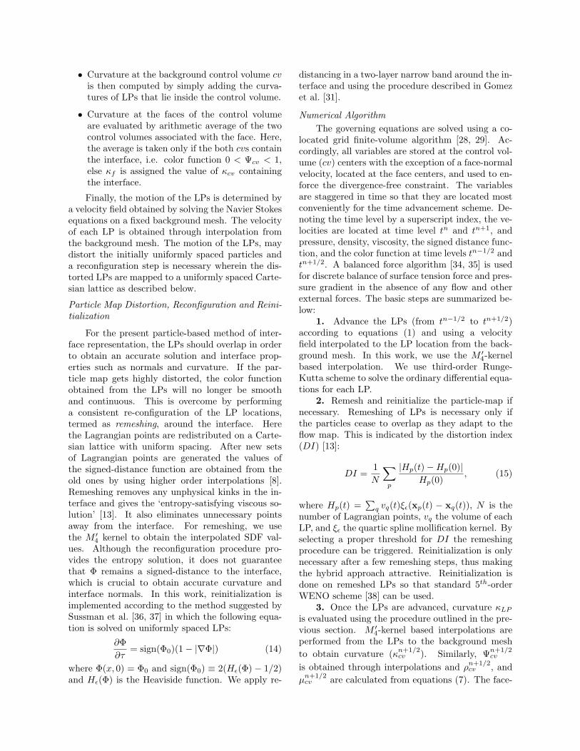
Estimation of Surface Normal and CurvatureThe accuracy of the surface normal and curva-

ture calculation by using the procedure described be-fore is tested on a circular interface. The Lagrangianpoints (LPs) are uniformly distributed in a narrowband around the interface and initialized by exactsigned distance function. The surface normals andcurvatures are first calculated on the LPs using theequations (4). Only those LPs are considered where|Φ| ≤ 2∆LP , where ∆LP is the LP-spacing. Theaverage relative error in surface normal calculationis shown in Figure 1 indicating second order con-vergence. For all these LPs, corresponding pointson the interface are calculated using the normalsand signed distance function (Φ) (equation 13). Theinterface-projected curvature values at the interfacepoints are evaluated using the M ′4-kernel based in-terpolation from the neighboring LP values. Thesecurvatures are then compared with the exact curva-ture κexact = 1/R for a two-dimensional interface.

R/h

Ave

rage

Rel

ativ

eE

rror

50 100 150 20010-6

10-5

10-4

10-3

10-2

2nd order

1st order

Figure 1: Average relative error (L2) in surface nor-mal for a circular interface.

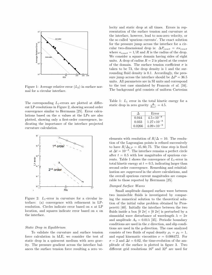
The corresponding L1-errors are plotted at differ-ent LP-resolutions in Figure 2, showing second orderconvergence similar to Herrmann [25]. Error calcu-lations based on the κ values at the LPs are alsoplotted, showing only a first-order convergence, in-dicating the importance of the interface projectedcurvature calculation.

Figure 2: L1-error in curvature for a circular in-terface: (a) convergence with refinement in LP-resolution. Circles indicate error based on κ at LPlocation, and squares indicate error based on κ onthe interface.

Static Drop in EquilibriumTo validate the curvature and surface tension

force calculation in hLE, we consider the test ofstatic drop in a quiescent medium with zero grav-ity. The pressure gradient across the interface bal-ances the surface tension force resulting a zero ve-

locity and static drop at all times. Errors in rep-resentation of the surface tension and curvature atthe interface, however, lead to non-zero velocity, orthe so called ‘spurious currents’. The exact solutionfor the pressure jump across the interface for a cir-cular two-dimensional drop is: ∆Pexact = σκexactwhere κexact = 1/R and R is the radius of the drop.We consider a square domain having sides of eightunits. A drop of radius R = 2 is placed at the centerof the domain. The surface tension coefficient σ istaken to be 73, the drop density is 1 and the sur-rounding fluid density is 0.1. Accordingly, the pres-sure jump across the interface should be ∆P = 36.5units. All parameters are in SI units and correspondto the test case simulated by Francois et al. [34].The background grid consists of uniform Cartesian

Table 1: L1 error in the total kinetic energy for astatic drop in zero gravity ∆

∆LP= 4.5.

∆ Error0.044 4.5×10−8

0.033 1.27×10−8

0.0266 4.09×10−9

elements with resolution of R/∆ = 10. The resolu-tion of the Lagrangian points is refined successivelyto have R/∆LP = 45, 60, 75. The time step is fixedat ∆t = 10−3. The interface remains a perfect circleafter t = 0.5 with low magnitudes of spurious cur-rents. Table 1 shows the convergence of L1-error intotal kinetic energy at t = 0.5, indicating larger thansecond order convergence. Remeshing and reinitial-ization are suppressed in the above calculations, andthe overall spurious current magnitudes are compa-rable to those reported by Herrmann [25].

Damped Surface WavesSmall amplitude damped surface wave between

two immiscible fluids is investigated by compar-ing the numerical solution to the theoretical solu-tion of the initial value problem obtained by Pros-peretti [40]. Initially the interface between the twofluids inside a box [0 2π] × [0 2π] is perturbed by asinusoidal wave disturbance of wavelength λ = 2πand amplitude A0 = 0.01λ [35]. Periodic boundaryconditions are used in the x direction, and slip condi-tions are used in the y-direction. The case analyzedconsists of two fluids of equal density ρ1 = ρ2 = 1,and equal kinematic viscosities ν = 0.006472. Forσ = 2 and ∆t = 0.02, the time-evolution of the am-plitude of the surface is plotted in figure 3. Twodifferent grid resolutions 162 and 322 are used for

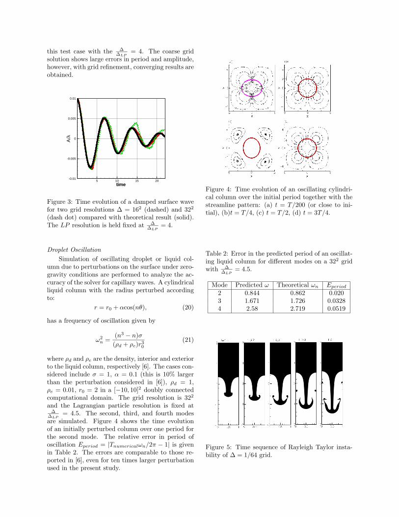
this test case with the ∆∆LP

= 4. The coarse gridsolution shows large errors in period and amplitude,however, with grid refinement, converging results areobtained.

time

Α/λ

5 10 15 20-0.01

-0.005

0

0.005

0.01

Figure 3: Time evolution of a damped surface wavefor two grid resolutions ∆ = 162 (dashed) and 322

(dash dot) compared with theoretical result (solid).The LP resolution is held fixed at ∆

∆LP= 4.

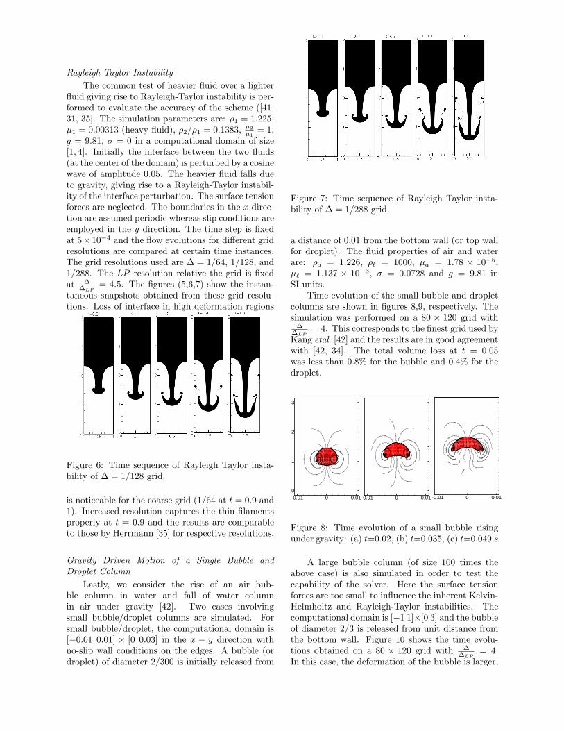
Droplet OscillationSimulation of oscillating droplet or liquid col-

umn due to perturbations on the surface under zero-gravity conditions are performed to analyze the ac-curacy of the solver for capillary waves. A cylindricalliquid column with the radius perturbed accordingto:

r = r0 + αcos(nθ), (20)

has a frequency of oscillation given by

ω2n =

(n3 − n)σ(ρd + ρe)r3

0

(21)

where ρd and ρe are the density, interior and exteriorto the liquid column, respectively [6]. The cases con-sidered include σ = 1, α = 0.1 (this is 10% largerthan the perturbation considered in [6]), ρd = 1,ρe = 0.01, r0 = 2 in a [−10, 10]2 doubly connectedcomputational domain. The grid resolution is 322

and the Lagrangian particle resolution is fixed at∆

∆LP= 4.5. The second, third, and fourth modes

are simulated. Figure 4 shows the time evolutionof an initially perturbed column over one period forthe second mode. The relative error in period ofoscillation Eperiod = |Tnumericalωn/2π − 1| is givenin Table 2. The errors are comparable to those re-ported in [6], even for ten times larger perturbationused in the present study.

Figure 4: Time evolution of an oscillating cylindri-cal column over the initial period together with thestreamline pattern: (a) t = T/200 (or close to ini-tial), (b)t = T/4, (c) t = T/2, (d) t = 3T/4.

Table 2: Error in the predicted period of an oscillat-ing liquid column for different modes on a 322 gridwith ∆

∆LP= 4.5.

Mode Predicted ω Theoretical ωn Eperiod2 0.844 0.862 0.0203 1.671 1.726 0.03284 2.58 2.719 0.0519

Figure 5: Time sequence of Rayleigh Taylor insta-bility of ∆ = 1/64 grid.

Rayleigh Taylor InstabilityThe common test of heavier fluid over a lighter

fluid giving rise to Rayleigh-Taylor instability is per-formed to evaluate the accuracy of the scheme ([41,31, 35]. The simulation parameters are: ρ1 = 1.225,µ1 = 0.00313 (heavy fluid), ρ2/ρ1 = 0.1383, µ2

µ1= 1,

g = 9.81, σ = 0 in a computational domain of size[1, 4]. Initially the interface between the two fluids(at the center of the domain) is perturbed by a cosinewave of amplitude 0.05. The heavier fluid falls dueto gravity, giving rise to a Rayleigh-Taylor instabil-ity of the interface perturbation. The surface tensionforces are neglected. The boundaries in the x direc-tion are assumed periodic whereas slip conditions areemployed in the y direction. The time step is fixedat 5×10−4 and the flow evolutions for different gridresolutions are compared at certain time instances.The grid resolutions used are ∆ = 1/64, 1/128, and1/288. The LP resolution relative the grid is fixedat ∆

∆LP= 4.5. The figures (5,6,7) show the instan-

taneous snapshots obtained from these grid resolu-tions. Loss of interface in high deformation regions

Figure 6: Time sequence of Rayleigh Taylor insta-bility of ∆ = 1/128 grid.

is noticeable for the coarse grid (1/64 at t = 0.9 and1). Increased resolution captures the thin filamentsproperly at t = 0.9 and the results are comparableto those by Herrmann [35] for respective resolutions.

Gravity Driven Motion of a Single Bubble andDroplet Column

Lastly, we consider the rise of an air bub-ble column in water and fall of water columnin air under gravity [42]. Two cases involvingsmall bubble/droplet columns are simulated. Forsmall bubble/droplet, the computational domain is[−0.01 0.01] × [0 0.03] in the x − y direction withno-slip wall conditions on the edges. A bubble (ordroplet) of diameter 2/300 is initially released from

Figure 7: Time sequence of Rayleigh Taylor insta-bility of ∆ = 1/288 grid.

a distance of 0.01 from the bottom wall (or top wallfor droplet). The fluid properties of air and waterare: ρa = 1.226, ρ` = 1000, µa = 1.78 × 10−5,µ` = 1.137 × 10−3, σ = 0.0728 and g = 9.81 inSI units.

Time evolution of the small bubble and dropletcolumns are shown in figures 8,9, respectively. Thesimulation was performed on a 80 × 120 grid with

∆∆LP

= 4. This corresponds to the finest grid used byKang etal. [42] and the results are in good agreementwith [42, 34]. The total volume loss at t = 0.05was less than 0.8% for the bubble and 0.4% for thedroplet.

-0.01 0 0.01-0.01 0 0.01-0.01 0 0.010

.01

.02

.03

Figure 8: Time evolution of a small bubble risingunder gravity: (a) t=0.02, (b) t=0.035, (c) t=0.049 s

A large bubble column (of size 100 times theabove case) is also simulated in order to test thecapability of the solver. Here the surface tensionforces are too small to influence the inherent Kelvin-Helmholtz and Rayleigh-Taylor instabilities. Thecomputational domain is [−1 1]×[0 3] and the bubbleof diameter 2/3 is released from unit distance fromthe bottom wall. Figure 10 shows the time evolu-tions obtained on a 80 × 120 grid with ∆

∆LP= 4.

In this case, the deformation of the bubble is larger,

-0.01 0 0.010

.01

.02

.03

-0.01 0 0.01 -0.01 0 0.01

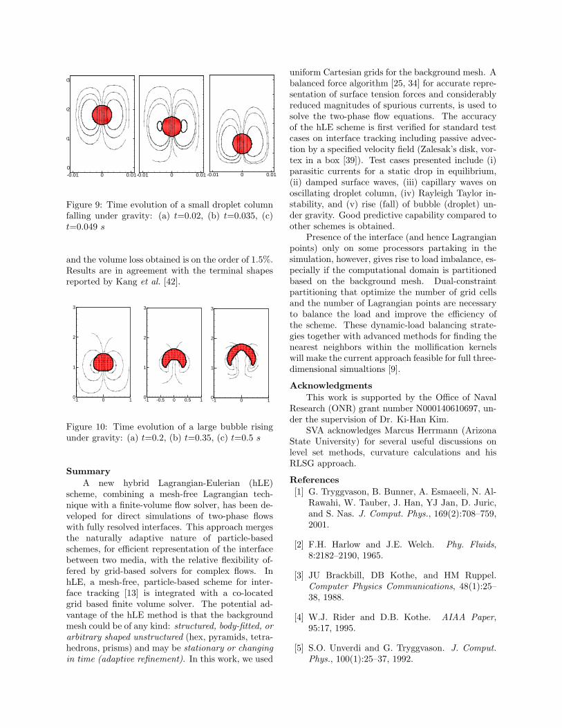
Figure 9: Time evolution of a small droplet columnfalling under gravity: (a) t=0.02, (b) t=0.035, (c)t=0.049 s

and the volume loss obtained is on the order of 1.5%.Results are in agreement with the terminal shapesreported by Kang et al. [42].

-1 0 10

1

2

3

-1 -0.5 0 0.5 10

1

2

3

-1 0 10

1

2

3

Figure 10: Time evolution of a large bubble risingunder gravity: (a) t=0.2, (b) t=0.35, (c) t=0.5 s

SummaryA new hybrid Lagrangian-Eulerian (hLE)

scheme, combining a mesh-free Lagrangian tech-nique with a finite-volume flow solver, has been de-veloped for direct simulations of two-phase flowswith fully resolved interfaces. This approach mergesthe naturally adaptive nature of particle-basedschemes, for efficient representation of the interfacebetween two media, with the relative flexibility of-fered by grid-based solvers for complex flows. InhLE, a mesh-free, particle-based scheme for inter-face tracking [13] is integrated with a co-locatedgrid based finite volume solver. The potential ad-vantage of the hLE method is that the backgroundmesh could be of any kind: structured, body-fitted, orarbitrary shaped unstructured (hex, pyramids, tetra-hedrons, prisms) and may be stationary or changingin time (adaptive refinement). In this work, we used

uniform Cartesian grids for the background mesh. Abalanced force algorithm [25, 34] for accurate repre-sentation of surface tension forces and considerablyreduced magnitudes of spurious currents, is used tosolve the two-phase flow equations. The accuracyof the hLE scheme is first verified for standard testcases on interface tracking including passive advec-tion by a specified velocity field (Zalesak’s disk, vor-tex in a box [39]). Test cases presented include (i)parasitic currents for a static drop in equilibrium,(ii) damped surface waves, (iii) capillary waves onoscillating droplet column, (iv) Rayleigh Taylor in-stability, and (v) rise (fall) of bubble (droplet) un-der gravity. Good predictive capability compared toother schemes is obtained.

Presence of the interface (and hence Lagrangianpoints) only on some processors partaking in thesimulation, however, gives rise to load imbalance, es-pecially if the computational domain is partitionedbased on the background mesh. Dual-constraintpartitioning that optimize the number of grid cellsand the number of Lagrangian points are necessaryto balance the load and improve the efficiency ofthe scheme. These dynamic-load balancing strate-gies together with advanced methods for finding thenearest neighbors within the mollification kernelswill make the current approach feasible for full three-dimensional simualtions [9].

AcknowledgmentsThis work is supported by the Office of Naval

Research (ONR) grant number N000140610697, un-der the supervision of Dr. Ki-Han Kim.

SVA acknowledges Marcus Herrmann (ArizonaState University) for several useful discussions onlevel set methods, curvature calculations and hisRLSG approach.

References[1] G. Tryggvason, B. Bunner, A. Esmaeeli, N. Al-

Rawahi, W. Tauber, J. Han, YJ Jan, D. Juric,and S. Nas. J. Comput. Phys., 169(2):708–759,2001.

[2] F.H. Harlow and J.E. Welch. Phy. Fluids,8:2182–2190, 1965.

[3] JU Brackbill, DB Kothe, and HM Ruppel.Computer Physics Communications, 48(1):25–38, 1988.

[4] W.J. Rider and D.B. Kothe. AIAA Paper,95:17, 1995.

[5] S.O. Unverdi and G. Tryggvason. J. Comput.Phys., 100(1):25–37, 1992.

[6] Torres D.J. and J.U. Brackbill. J. Comp.Physics, 165(2):620–644, 2000.

[7] S. Koshizuka, A. Nobe, and Y. Oka. Int. J.Numer. Meth. Fluids, 26(7):751–769, 1998.

[8] P. Koumoutsakos. Annu. Rev. Fluid Mech.,37(1):457–487, 2005.

[9] IF Sbalzarini, JH Walther, M. Bergdorf,SE Hieber, EM Kotsalis, and P. Koumoutsakos.J. Comput. Phys., 215(2):566–588, 2006.

[10] JJ Monaghan. Reports on Progress in Physics,68(8):1703–1759, 2005.

[11] HY Yoon, S. Koshizuka, and Y. Oka. Int. J.Multiphase Flow, 27(2):277–298, 2001.

[12] JH Walther, T. Werder, RL Jaffe, andP. Koumoutsakos. Physical Review E,69(6):62201, 2004.

[13] S.E. Hieber and P. Koumoutsakos. J. Comput.Phys., 210(1):342–367, 2005.

[14] R. Scardovelli and S. Zaleski. Annu. Rev. FluidMech., 31(1):567–603, 1999.

[15] WF Noh and P. Woodward. Int. Conf. Numer.Meth. Fluid Dynamics, 5th, Enschede, Nether-lands, June 28-July 2, 1976,, 1976.

[16] JA Sethian. J. Comput. Phys., 169(2):503–555,2001.

[17] S. Osher and R.P. Fedkiw. J. Comput. Phys.,169(2):463–502, 2001.

[18] M. Sussman, P. Smereka, and S. Osher. J. Com-put. Phys., 114(1):146–159, 1994.

[19] M. Sussman. J. Comput. Phys., 187(1):110–136, 2003.

[20] F. Ham and YN. Young. Annu. ResearchBriefs, 2003: Center for Turbulence Research,2003.

[21] F. Ham, Y.N. Young, S. Apte, and M. Her-rmann. 2 nd Int. Conf. Comput. Meth. Mul-tiphase Flow, pp. 313–322, 2003.

[22] D. Enright, R. Fedkiw, J. Ferziger, andI. Mitchell. J. Comput. Phys., 183(1):83–116,2002.

[23] M. Herrmann. Annu. Research Briefs, 2004:Center for Turbulence Research, pp. 15–29,2004.

[24] M. Herrmann. Annu. Research Briefs, 2005:Center for Turbulence Research, 2005.

[25] M. Herrmann. Annu. Research Briefs, 2004:Center for Turbulence Research, 2006.

[26] J. Strain. J. Comp. Phy., 170:373–394, 2001.

[27] CW Hirt, AA Amsden, and JL COOK. J. Com-put. Phys., 14(3):227–253, 1974.

[28] K. Mahesh, G. Constantinescu, and P. Moin. J.Comput. Phys., 197(1):215–240, 2004.

[29] K. Mahesh, G. Constantinescu, S. Apte, G. Iac-carino, F. Ham, and P. Moin. J. Applied Mech.,73:374, 2006.

[30] D. Peng, B. Merriman, S. Osher, H. Zhao, andM. Kang. J. Comput. Phys., 155(2):410–438,1999.

[31] P. Gomez, J. Hernandez, and J. Lopez. Int. J.Numer. Meth. Eng., 2005.

[32] Jeff D. Eldredge, Anthony Leonard, and TimColonius. J. Comput. Phys., 180(2):686–709,2002.

[33] JU Brackbill, DB Kothe, and C. Zemach. J.Comput. Phys., 100(2):335–354, 1992.

[34] M.M. Francois, S.J. Cummins, E.D. Dendy,D.B. Kothe, J.M. Sicilian, and M.W. Williams.J. Comput. Phys., 213(1):141–173, 2006.

[35] M. Herrmann. J. Comp. Physics, 227(4):2674–2706, 2008.

[36] E. Fatemi and M. Sussman. SIAM J. Sci. Com-put., 158(1):36–58, 1995.

[37] M. Sussman, E. Fatemi, P. Smereka, and S. Os-her. Computers & Fluids, 27(5):663–680, 1998.

[38] GS Jiang and D. Peng. SIAM J. Sci. Comput.,21(6):2126–2143, 2000.

[39] Shams E. and Apte S.V. ILASS America’s20th Annual Conference on Liquid Atomizationand Spray Systems, Chicago, IL, May 2007, 30,2007.

[40] A. Prosperetti. Phy. Fluids, 24(7):1217–1223,1981.

[41] Popinet S. and S. Zaleski. Int. J. Numer. Meth-ods Fluids, 30:775–793, 1999.

[42] M. Kang, R.P. Fedkiw, and X.D. Liu. J. Sci.Comput., 15(3):323–360, 2000.