A Coupled Lagrangian-Eulerian Framework to model droplet ...
300
A Coupled Lagrangian-Eulerian Framework to model droplet to film interaction with Heat Transfer Akinola A. Adeniyi B.Eng.(Ilorin), M.Sc.(London), R.Eng.(COREN) Thesis submitted to The University of Nottingham for the degree of Doctor of Philosophy July 2015
-
Upload
khangminh22 -
Category
Documents
-
view
1 -
download
0
Transcript of A Coupled Lagrangian-Eulerian Framework to model droplet ...

A Coupled Lagrangian-Eulerian
Framework to model droplet to film
interaction with Heat Transfer
Akinola A. Adeniyi
B.Eng.(Ilorin), M.Sc.(London), R.Eng.(COREN)
Thesis submitted to The University of Nottingham
for the degree of Doctor of Philosophy
July 2015

To my family for their wonderful support as ever.

Abstract
In aeroengine applications, oil is used lubricate and cool the bearings as well as cool
the structural parts. The high operational speeds break the oil up forming ligaments and
droplets. To contain the oil, the bearings are located inside sealed bearing chambers and
a positive pressure across the seals is used to contain the oil within the system. The highly
rotational flow in the chamber is laden with droplets emanating from the bearings. The
droplets travel to the outer bearing chamber walls and form cooling oil films that rotate
in the direction of the shaft spin. The used oil is scavenged out via the sump for recycling.
The multiphase flow in aeroengine bearing chambers includes strong interactions
between the gas and the liquid, where the liquid can exist in the form of droplets and
continuous film. There are other applications, such as spray cooling, that create similar
modelling challenges. In spray cooling nozzle atomisation of the coolant creates high
speed droplets that eventually form a film on the hot surface being cooled. To model
this type of flows, with computational fluid dynamics (CFD), there is a need to be able
to account for the multiple impacting droplets and the resulting cooling films. Volume-
of-Fluid (VoF) based CFD techniques have been used by researchers to model droplet-film
impacts by applying an extremely fine computational mesh to resolve the flow around the
droplets and the film. Such methods, because of the computing cost are, however, not
practical for applications of interest in this work.
i

In this work, droplets are not explicitly resolved to a computational mesh, they are
represented as point source terms in an unsteady Lagrangian formulation. Represent-
ing droplets in Lagrangian formulation, as done here, is not new but the coupling with
the continuous phase to form flowing film from user defined source terms and onward
tracking of splashing droplets using published correlations are novel. The mass and mo-
mentum of the Lagrangian particle are transferred into VoF by adding the source term as a
“handover” of mass from the discrete phase to VoF film, in the continuity and momentum
equations after interface tracking is done. Heat transfer is achieved by mass averaging
of the temperatures in the spread zone equivalent to the spherical droplet. The particle
tracking is then stopped and the particle is subsequently removed from the simulation.
The method is developed using the ANSYS-Fluent CFD software and formulated using an
enhanced VoF technique. The developed technique is validated using a series of simple
numerical checks on single Lagrangian droplet-to-film to more complex spray-to-film test
cases to check for mass, momentum and heat transfer with reasonably good performance.
The developed sub-model was also tested on two different aeroengine bearing cham-
ber geometries; one representative of a bearing chamber in the AE3007 aeroengine and
one representative of a bearing chamber test rig at Karlsruhe Institute of Technology. The
AE3007 geometry was used in the experiments of Chandra et al. [1, 2] and the KIT ge-
ometry by Gorse et al. [3]. The AE3007 bearing chamber geometry is somewhat similar
to that of the high-pressure/intermediate-pressure (HP-IP) bearing chamber of a 3-spool
large civil aircraft. The film thickness results predicted for the AE3007 geometry are over-
predicted but similar in trend when compared with experimental measurements. The
simulations show film formation and pooling as observed in the experiments. The top
ii
parts of the bearing chamber, generally, show higher heat transfer coefficient results than
the lower parts of the chamber where films are typically somewhat thicker.
For the KIT chamber application, there is a good prediction of the film thickness
when compared with the experiment. A parametric study of the flow shows that the film
thickness increases with the flow rate. At a fixed liquid flowrate, film thickness decreases
with increasing shaft speed. The average film temperature increases with a reducing flow
rate and increases with shaft speed. This current work presents the development of a
useful tool applicable to bearing chamber modelling.
iii

List Of Publications
Published
[1] Akinola A. Adeniyi, Hervé P. Morvan & Kathy A. Simmons, A transient CFD simu-
lation of the flow in a test rig of an aeroengine bearing chamber, GT2014-26399,
Proceedings of the ASME Turbo Expo 2014, D’usseldorf, Germany, 2014.
[2] Akinola Adeniyi, Hervé Morvan & Kathy Simmons, A Coupled 3-Phase CFD Approach
to model Droplets to Film Interaction with Heat Transfer, 2014 UoN High Performance
Computing (HPC) user conference, University of Nottingham, 2014.
[3] Adeniyi, A.A., Morvan, H. & Simmons, K., Droplet-Film Impact Modelling Using a
Coupled DPM-VoF Approach, ISABE-2013-1419, Proceedings of XXI Intl. Symp. on
Air Breathing Engines (ISABE 2013), American Inst. of Aeronautics and Astronautics
(AIAA), Busan, South Korea, 2013.
Pending/In review
[1] Akinola A. Adeniyi, Hervé P. Morvan & Kathy Simmons, A DPM-VoF approach for
the formation of film from Lagrangian droplets spray with heat transfer in the non-
boiling regime, Int. J. of Heat and Fluid Flow, XXXX.
iv

[2] Akinola A. Adeniyi, Hervé P. Morvan & Kathy A. Simmons, A COUPLED EULER –LA-
GRANGE CFD MODELLING OF DROPLETS-TO-FILM, Int. J. Multph., XXXX.
[3] Akinola A. Adeniyi, Hervé P. Morvan & Kathy A. Simmons, Splashing of droplets
on an arbitrary free film surface using a coupled Lagrangian-Eulerian (DPM-VoF)
technique, AIP Phy. Rev., XXXX.
Posters and Presentations
[1] A.A. Adeniyi, H.P. Morvan & K. Simmons, Bearing Chamber modelling with a DPM-
VOF technique, Nottingham-Surrey UTCs Workshop, Institute for Aerospace Technolo-
gies, (IAT), Nottingham, 13 Mar. 2014.
[2] A.A. Adeniyi, H.P. Morvan & K. Simmons, Progress on a coupled Lagrangian-VOF
approach for oil systems applications, Rolls-Royce UTC QTR, Derby, 28 Nov. 2013.
[3] Akinola A. Adeniyi, Hervé Morvan & Kathy Simmons, Modelling Heat Transfer within
Aero-Engine Bearing Chambers, Rolls-Royce PhD Day, 12-13 June 2013.
[4] Akinola A. Adeniyi, Hervé P. Morvan & Kathy A. Simmons, A Coupled Lagrangian
- Volume of Fluid Approach to Simulate Aero-engine Bearing Chambers, Energy &
Sustainability Poster Competition, University of Nottingham, Jan. 2013.
v

Acknowledgements
I acknowledge God the Almighty for making this a possibility.
This research was carried out at the University Technology Centre (UTC) in Gas Tur-
bine Transmissions Systems at the University of Nottingham with financial support from
University of Ilorin ETF/AST&D 2009 award for my tuition and maintenance.
I must also mention financial supports from Rolls-Royce plc, Aerospace Group, Energy
& Sustainability Division of The Faculty of Engineering, University of Nottingham, and of
course, mainly, by the UTC group. The fundings cover all expenses for my conference at-
tendance in Busan, South-Korea. I was also sponsored on ICEM meshing software training
at the ANSYS UK Office in Sheffield. I also wish to say thank you for the provision of the
powerful computing resources.
I sincerely acknowledge the contributions, supervision, mentoring, motivation and
the many supports from my supervisors, Prof. Hervé Morvan and Dr. Kathy Simmons. I
benefited a great deal from their skills, industrial links and experience. Contributions from
Prof. Henry Power, my internal examiner, during my first and second year review were
very helpful in preparing this thesis. This thesis would not have been complete without
the thorough reading and constructive criticism by Prof. John Chew. I got inspirations
from Prof. Seamus Garvey.
The UTC has a fantastic team of researchers. I especially acknowledge discussions and
contributions from Al Baydu, Piotr Tkaczyk, Turner Adam, De Carvalho Thiago, Natarajan
vi

Arun Prakash, Peduto Davide (KIT), Torsten Sonner (KIT) and Roberto Ovando Martinez
(Instituto Tecnológico de la Laguna, Mexico).
The Graduate School is a place to look out for when studying in University of Notting-
ham. I received a number of useful training from the Grad. school. I was even sponsored
for a 3-day Engineering Young Entrepreneur Scheme (Engineering YES) competition in
Loughborough, for which my team won “Best Team Work Award” in 2011.
I cannot forget the constant “how many percent more?” reminder from Lawal Bashir
and Komolafe Biola. I must acknowledge Prof. A.A. Adedeji, Prof. Y.A. Jimoh, Prof. J.S.
Olorunmaiye, Prof. H.D. Olusegun, Dr. K.R. Ajao, Dr. A.S. Aremu, Dr. Wahab Salami, Dr.
T.K. Ajiboye for their wonderful contributions towards making my PhD a possibility. All
my friends were very supportive; I want to specially mention Ibrahim Olojoku, Abubakar
Mohammed, Muntaka Sirina, Nurudeen Almustapha, Ajibi Michael, Akanmu Olalekan,
Oba Abdullahi and others so numerous to list for their support.
I want to acknowledge my family members for their support and solid confidence
in me. My parents, Alhaji Mohammed Baba (dad) and Mrs. Idiayat Adunni (mom) are
inspirational. My brothers Dr. Suleiman, Ghaly, Abdul-Jeleel, Abdul-Rasaq, Lawyer Ahmed
and others.
Finally, I want to specially mention the kind support and understanding of my wife
Mrs. Temitope Mariam Adeniyi. Our children Miss Ayomide Azizat, Miss Farida Oyinkan-
sola and Miss Adeola Amira Elizabeth “the PhD baby” born in Nottingham and named
after the Queen.
vii

Contents
Abstract i
Table of contents ix
List of Figures xiv
List of Tables xix
Nomenclature xix
1 Introduction 1
1.1 Background . . . . . . . . . . . . . . . . . . . . . . . . . . . . . . . . . . . . 1
1.2 The Challenge . . . . . . . . . . . . . . . . . . . . . . . . . . . . . . . . . . . 4
1.3 Applications . . . . . . . . . . . . . . . . . . . . . . . . . . . . . . . . . . . . 6
1.3.1 Aero Engine Bearing Chambers . . . . . . . . . . . . . . . . . . . . . 7
1.3.2 Other Applications . . . . . . . . . . . . . . . . . . . . . . . . . . . . 9
1.4 The Thesis . . . . . . . . . . . . . . . . . . . . . . . . . . . . . . . . . . . . . 10
1.4.1 Specific Objectives . . . . . . . . . . . . . . . . . . . . . . . . . . . . 11
1.4.2 Thesis Overview . . . . . . . . . . . . . . . . . . . . . . . . . . . . . 12
viii

2 Literature Overview 15
2.1 Overview . . . . . . . . . . . . . . . . . . . . . . . . . . . . . . . . . . . . . 15
2.2 Free-Surface modelling . . . . . . . . . . . . . . . . . . . . . . . . . . . . . . 16
2.2.1 Stratified flows . . . . . . . . . . . . . . . . . . . . . . . . . . . . . . 22
2.2.2 Inter-facial heat transfer . . . . . . . . . . . . . . . . . . . . . . . . . 26
2.3 Droplet impact outcome . . . . . . . . . . . . . . . . . . . . . . . . . . . . . 27
2.4 Bearing Chamber flow . . . . . . . . . . . . . . . . . . . . . . . . . . . . . . 33
2.5 Summary . . . . . . . . . . . . . . . . . . . . . . . . . . . . . . . . . . . . . 38
3 Existing Multiphase Modelling Framework 40
3.1 Overview . . . . . . . . . . . . . . . . . . . . . . . . . . . . . . . . . . . . . 40
3.2 Eulerian Phase . . . . . . . . . . . . . . . . . . . . . . . . . . . . . . . . . . 41
3.2.1 Continuity Equation . . . . . . . . . . . . . . . . . . . . . . . . . . . 42
3.2.2 Navier-Stokes Equation . . . . . . . . . . . . . . . . . . . . . . . . . 43
3.2.3 Energy Equation . . . . . . . . . . . . . . . . . . . . . . . . . . . . . 44
3.2.4 Free-surface tracking . . . . . . . . . . . . . . . . . . . . . . . . . . . 44
3.3 Modelling Turbulent flows . . . . . . . . . . . . . . . . . . . . . . . . . . . . 49
3.3.1 Standard κ - ε turbulence model . . . . . . . . . . . . . . . . . . . . 52
3.3.2 Standard κ - ω turbulence model . . . . . . . . . . . . . . . . . . . . 54
3.3.3 SST κ - ω turbulence model . . . . . . . . . . . . . . . . . . . . . . . 57
3.3.4 Turbulence Damping . . . . . . . . . . . . . . . . . . . . . . . . . . . 61
3.3.5 Wall treatment . . . . . . . . . . . . . . . . . . . . . . . . . . . . . . 63
3.4 Lagrangian Phase - Discrete Phase Model (DPM) . . . . . . . . . . . . . . . 65
3.4.1 Eulerian-Phase Coupling . . . . . . . . . . . . . . . . . . . . . . . . . 68
ix

3.5 Numerical Method . . . . . . . . . . . . . . . . . . . . . . . . . . . . . . . . 68
3.5.1 Discretisation . . . . . . . . . . . . . . . . . . . . . . . . . . . . . . . 69
3.5.2 Solvers . . . . . . . . . . . . . . . . . . . . . . . . . . . . . . . . . . . 74
3.6 Adopted Modelling Strategy . . . . . . . . . . . . . . . . . . . . . . . . . . . 77
3.7 Summary . . . . . . . . . . . . . . . . . . . . . . . . . . . . . . . . . . . . . 77
4 The DPM-VoF Model 79
4.1 Overview . . . . . . . . . . . . . . . . . . . . . . . . . . . . . . . . . . . . . 79
4.2 DPM-VoF Gas phase drag . . . . . . . . . . . . . . . . . . . . . . . . . . . . . 83
4.3 DPM-VoF Mass Transfer . . . . . . . . . . . . . . . . . . . . . . . . . . . . . 83
4.4 DPM-VoF Momentum Transfer . . . . . . . . . . . . . . . . . . . . . . . . . . 88
4.5 DPM-VoF Heat Transfer . . . . . . . . . . . . . . . . . . . . . . . . . . . . . . 88
4.6 Interface Tracking & Splashing . . . . . . . . . . . . . . . . . . . . . . . . . 89
4.6.1 Splashing . . . . . . . . . . . . . . . . . . . . . . . . . . . . . . . . . 89
4.6.2 Film depth search . . . . . . . . . . . . . . . . . . . . . . . . . . . . . 97
4.7 Implementation Algorithm . . . . . . . . . . . . . . . . . . . . . . . . . . . . 99
4.8 Summary . . . . . . . . . . . . . . . . . . . . . . . . . . . . . . . . . . . . . 104
5 Validating the DPM-VoF Model 107
5.1 Overview . . . . . . . . . . . . . . . . . . . . . . . . . . . . . . . . . . . . . 107
5.2 Single droplet: DPM droplet turns VoF droplet . . . . . . . . . . . . . . . . . 108
5.3 Simple box fill with a Single Droplet Train . . . . . . . . . . . . . . . . . . . 111
5.4 Simple box fill with Multiple Droplet Trains . . . . . . . . . . . . . . . . . . 114
5.5 Crater dynamics (Momentum conservation) . . . . . . . . . . . . . . . . . . 118
x

5.5.1 Normal Impacts . . . . . . . . . . . . . . . . . . . . . . . . . . . . . . 118
5.5.2 Oblique impacts . . . . . . . . . . . . . . . . . . . . . . . . . . . . . 121
5.5.3 Crown splashing . . . . . . . . . . . . . . . . . . . . . . . . . . . . . 123
5.6 Simple Heat Transfer Checks . . . . . . . . . . . . . . . . . . . . . . . . . . . 125
5.6.1 Single droplet: Core Temperature as DPM turns VoF . . . . . . . . . 125
5.6.2 Single droplet: Impact on a hot wall . . . . . . . . . . . . . . . . . . 126
5.6.3 Simple Adiabatic box fill . . . . . . . . . . . . . . . . . . . . . . . . . 128
5.7 DPM-VoF: Spray Film Cooling Test Case . . . . . . . . . . . . . . . . . . . . 129
5.7.1 Spray-Film: DPM-VoF setup . . . . . . . . . . . . . . . . . . . . . . . 131
5.7.2 Spray-Film: Results . . . . . . . . . . . . . . . . . . . . . . . . . . . . 137
5.8 Splashing demonstration . . . . . . . . . . . . . . . . . . . . . . . . . . . . . 142
5.9 Summary . . . . . . . . . . . . . . . . . . . . . . . . . . . . . . . . . . . . . 144
6 Application to Aero-Engine Bearing Geometry 147
6.1 Overview . . . . . . . . . . . . . . . . . . . . . . . . . . . . . . . . . . . . . 147
6.2 CASE 1: The AE3007 Bearing Chamber . . . . . . . . . . . . . . . . . . . . . 149
6.2.1 Film Generation . . . . . . . . . . . . . . . . . . . . . . . . . . . . . 151
6.2.2 The AE3007 Bearing Chamber Geometry . . . . . . . . . . . . . . . . 157
6.2.3 AE3007 Bearing Chamber Mesh . . . . . . . . . . . . . . . . . . . . . 159
6.2.4 Boundary conditions . . . . . . . . . . . . . . . . . . . . . . . . . . . 161
6.2.5 AE3007 bearing chamber reference orientation . . . . . . . . . . . . 162
6.2.6 The Solution method . . . . . . . . . . . . . . . . . . . . . . . . . . . 163
6.2.7 CASE 1: Results and Discussions . . . . . . . . . . . . . . . . . . . . 164
6.3 CASE 2: The KIT Bearing Chamber . . . . . . . . . . . . . . . . . . . . . . . 174
xi

6.3.1 The KIT Bearing Chamber Geometry . . . . . . . . . . . . . . . . . . 176
6.3.2 KIT Mesh . . . . . . . . . . . . . . . . . . . . . . . . . . . . . . . . . 176
6.3.3 Boundary conditions . . . . . . . . . . . . . . . . . . . . . . . . . . . 178
6.3.4 The bearing chamber reference/notation . . . . . . . . . . . . . . . . 179
6.3.5 CASE 2: Results and Discussions . . . . . . . . . . . . . . . . . . . . 179
6.4 Summary . . . . . . . . . . . . . . . . . . . . . . . . . . . . . . . . . . . . . 188
7 Conclusion 191
7.1 Main Achievements . . . . . . . . . . . . . . . . . . . . . . . . . . . . . . . . 191
7.2 Contributions to knowledge . . . . . . . . . . . . . . . . . . . . . . . . . . . 195
7.3 Future Work . . . . . . . . . . . . . . . . . . . . . . . . . . . . . . . . . . . . 196
References 198
A DPM-VoF Code 218
A.1 .h files . . . . . . . . . . . . . . . . . . . . . . . . . . . . . . . . . . . . . . . 218
A.2 .c file . . . . . . . . . . . . . . . . . . . . . . . . . . . . . . . . . . . . . . . . 241
xii

List of Figures
1.1 Aero-Engine Oil System & Engine Mounting illustrations . . . . . . . . . . . 2
1.2 Air sealing in the HP-IP hub . . . . . . . . . . . . . . . . . . . . . . . . . . . 3
1.3 Rolls-Royce Trent 1000 engine . . . . . . . . . . . . . . . . . . . . . . . . . . 7
1.4 Rolls-Royce Trent engine sectional view . . . . . . . . . . . . . . . . . . . . . 8
1.5 A schematic representation of the HP-IP bearing chamber . . . . . . . . . . . 9
2.1 An SPH simulation of Rayleigh-Taylor Instability . . . . . . . . . . . . . . . . 18
2.2 Particle in Cell surface markers . . . . . . . . . . . . . . . . . . . . . . . . . 19
2.3 VoF free-surface construction . . . . . . . . . . . . . . . . . . . . . . . . . . 21
2.4 Stratified flows . . . . . . . . . . . . . . . . . . . . . . . . . . . . . . . . . . 23
2.5 Film separation from a sharp bend . . . . . . . . . . . . . . . . . . . . . . . 25
2.6 Droplets deforming in a shear-driven flow . . . . . . . . . . . . . . . . . . . 26
2.7 Droplet impact outcome . . . . . . . . . . . . . . . . . . . . . . . . . . . . . 28
3.1 CLSVoF Flow chart . . . . . . . . . . . . . . . . . . . . . . . . . . . . . . . . 49
3.2 Turbulence damping effect . . . . . . . . . . . . . . . . . . . . . . . . . . . . 62
3.3 Log law . . . . . . . . . . . . . . . . . . . . . . . . . . . . . . . . . . . . . . 63
xiii

3.4 Near wall treatment . . . . . . . . . . . . . . . . . . . . . . . . . . . . . . . 64
3.5 DPM in a 3D Space . . . . . . . . . . . . . . . . . . . . . . . . . . . . . . . . 66
3.6 Control volume for Scalar Transport Equation . . . . . . . . . . . . . . . . . 71
3.7 CFD Solvers . . . . . . . . . . . . . . . . . . . . . . . . . . . . . . . . . . . . 76
4.1 DPM-VoF Concept . . . . . . . . . . . . . . . . . . . . . . . . . . . . . . . . . 80
4.2 Impacting droplet photograph . . . . . . . . . . . . . . . . . . . . . . . . . . 81
4.3 Droplet impact and tracking: DPM-VoF Concept . . . . . . . . . . . . . . . . 82
4.4 Mass source spread sphere . . . . . . . . . . . . . . . . . . . . . . . . . . . . 85
4.5 Scan zone: Centroids . . . . . . . . . . . . . . . . . . . . . . . . . . . . . . . 86
4.6 Interior and Wall bounded cells faces . . . . . . . . . . . . . . . . . . . . . . 89
4.7 Normal & Oblique Splash experiment . . . . . . . . . . . . . . . . . . . . . . 90
4.8 Normal & Oblique Splash detailed VoF . . . . . . . . . . . . . . . . . . . . . 90
4.9 DPM-VoF Splash Model . . . . . . . . . . . . . . . . . . . . . . . . . . . . . . 92
4.10 DPM-VoF secondary droplet initiation plane . . . . . . . . . . . . . . . . . . 94
4.11 DPM-VoF splash plane circle . . . . . . . . . . . . . . . . . . . . . . . . . . . 95
4.12 Alternative secondary droplets distribution . . . . . . . . . . . . . . . . . . . 97
4.13 DPM-VoF film thickness scan . . . . . . . . . . . . . . . . . . . . . . . . . . . 98
4.14 DPM-VoF Implementation . . . . . . . . . . . . . . . . . . . . . . . . . . . . 99
4.15 DPM setup in ANSYS-Fluent (GUI) . . . . . . . . . . . . . . . . . . . . . . . 100
5.1 DPM-VoF: Single DPM Mesh . . . . . . . . . . . . . . . . . . . . . . . . . . . 108
5.2 Single DPM droplet turns VOF . . . . . . . . . . . . . . . . . . . . . . . . . . 109
5.3 DPM-VoF Single droplet: Mesh resolution/mass conservation . . . . . . . . . 110
xiv

5.4 DPM-VoF: Simple box fill setup . . . . . . . . . . . . . . . . . . . . . . . . . 111
5.5 DPM-VoF: Simple box fill results 800µm diameter droplet . . . . . . . . . . 113
5.6 DPM-VoF: Schematic of a Train of Multiple Droplets . . . . . . . . . . . . . . 114
5.7 Mesh for the Multiple Droplet Train Setup . . . . . . . . . . . . . . . . . . . 115
5.8 DPM-VoF: Simple multiple droplet box fill results . . . . . . . . . . . . . . . 117
5.9 DPM-VoF: Crater dynamics test . . . . . . . . . . . . . . . . . . . . . . . . . 118
5.10 Crater evolution . . . . . . . . . . . . . . . . . . . . . . . . . . . . . . . . . . 120
5.11 DPM-VoF: Oblique angle droplet impact on film . . . . . . . . . . . . . . . . 122
5.12 A visual impression of crater evolution . . . . . . . . . . . . . . . . . . . . . 123
5.13 Highly resolved and DPM-VoF normal impact . . . . . . . . . . . . . . . . . 124
5.14 Single DPM droplet turns VoF - Core Temperature . . . . . . . . . . . . . . . 126
5.15 Single droplet impact boundedness test . . . . . . . . . . . . . . . . . . . . . 127
5.16 Cold droplet injection into an adiabatic box . . . . . . . . . . . . . . . . . . 129
5.17 Schematic of a nozzle spray with DPM-VoF . . . . . . . . . . . . . . . . . . . 132
5.18 Spray film Experiment Setup . . . . . . . . . . . . . . . . . . . . . . . . . . . 133
5.19 Experimental estimation of Heat Flux and Wall Surface Temperature . . . . 134
5.20 DPM-VoF: Spray-film Geometry and Mesh . . . . . . . . . . . . . . . . . . . 135
5.21 DPM-VoF: Spray-film Showing DPM and VoF Film . . . . . . . . . . . . . . . 138
5.22 DPM-VoF: Spray-film thickness . . . . . . . . . . . . . . . . . . . . . . . . . 139
5.23 DPM-VoF: Spray-film Heat Flux . . . . . . . . . . . . . . . . . . . . . . . . . 140
5.24 DPM-VoF: Spray-film Heat Transfer Coefficient . . . . . . . . . . . . . . . . . 141
5.25 DPM-VoF: Normal splashing . . . . . . . . . . . . . . . . . . . . . . . . . . . 142
5.26 DPM-VoF: Normal splashing evolution . . . . . . . . . . . . . . . . . . . . . 143
xv

5.27 DPM-VoF: Oblique splashing on an arbitrary film interface . . . . . . . . . . 144
6.1 Bearing chamber experimental rig . . . . . . . . . . . . . . . . . . . . . . . . 148
6.2 Bearing chamber with Perspex see-through wall . . . . . . . . . . . . . . . . 150
6.3 Film Generator . . . . . . . . . . . . . . . . . . . . . . . . . . . . . . . . . . 152
6.4 Rotating Inlet Distributor . . . . . . . . . . . . . . . . . . . . . . . . . . . . . 153
6.5 RID droplet formation schematic . . . . . . . . . . . . . . . . . . . . . . . . 154
6.6 RID injector motion . . . . . . . . . . . . . . . . . . . . . . . . . . . . . . . . 155
6.7 Simulated bearing chamber geometry . . . . . . . . . . . . . . . . . . . . . . 157
6.8 CFD Pump Model . . . . . . . . . . . . . . . . . . . . . . . . . . . . . . . . . 158
6.9 Simulated AE3007 bearing chamber hexahedral mesh . . . . . . . . . . . . 159
6.10 Mesh quality histogram . . . . . . . . . . . . . . . . . . . . . . . . . . . . . 159
6.11 Hexa-blocking layout for the bearing chamber . . . . . . . . . . . . . . . . . 160
6.12 Boundary conditions for the AE3007 bearing chamber geometry . . . . . . . 162
6.13 AE3007 bearing chamber reference orientation . . . . . . . . . . . . . . . . 163
6.14 An instantaneous loading of droplets in the chamber . . . . . . . . . . . . . 165
6.15 Droplets emanating from four random holes of the RID . . . . . . . . . . . . 166
6.16 Transient film formation for 10, 000RPM . . . . . . . . . . . . . . . . . . . . 167
6.17 3D film pooling at 10, 000RPM shaft speed . . . . . . . . . . . . . . . . . . 169
6.18 Transient film formation for 15, 000RPM . . . . . . . . . . . . . . . . . . . . 170
6.19 Average wall film thickness at angular positions . . . . . . . . . . . . . . . . 171
6.20 Surface HTC on the bearing wall . . . . . . . . . . . . . . . . . . . . . . . . 173
6.21 Time averaged heat transfer coefficient . . . . . . . . . . . . . . . . . . . . . 174
6.22 The KIT Bearing Chamber Test rig . . . . . . . . . . . . . . . . . . . . . . . 175
xvi

6.23 The KIT Chamber I - Schematic . . . . . . . . . . . . . . . . . . . . . . . . . 176
6.24 The KIT Chamber Mesh . . . . . . . . . . . . . . . . . . . . . . . . . . . . . 177
6.25 The KIT Chamber Hexa-blocking . . . . . . . . . . . . . . . . . . . . . . . . 177
6.26 KIT bearing reference orientation . . . . . . . . . . . . . . . . . . . . . . . . 179
6.27 KIT bearing chamber droplet-film formation . . . . . . . . . . . . . . . . . . 180
6.28 Effect of flow rate on film thickness (16,000 RPM) . . . . . . . . . . . . . . 181
6.29 Effect of shaft speed on film thickness (100 l/hr) . . . . . . . . . . . . . . . 182
6.30 Average film temperature . . . . . . . . . . . . . . . . . . . . . . . . . . . . 184
6.31 Average film velocity . . . . . . . . . . . . . . . . . . . . . . . . . . . . . . . 185
6.32 KIT bearing chamber wall heat transfer coefficient . . . . . . . . . . . . . . . 186
6.33 Average wall heat transfer coefficient . . . . . . . . . . . . . . . . . . . . . . 187
xvii

List of Tables
2.1 Description of droplet impact surfaces . . . . . . . . . . . . . . . . . . . . . 29
2.4 Published criteria for droplet impact outcome -III . . . . . . . . . . . . . . . 30
2.2 Published criteria for droplet impact outcome -I . . . . . . . . . . . . . . . . 31
2.3 Published criteria for droplet impact outcome -II . . . . . . . . . . . . . . . . 32
4.1 Selected Correlations Employed in Splashing . . . . . . . . . . . . . . . . . . 91
4.2 The DPM-VoF modules and their functions . . . . . . . . . . . . . . . . . . . 103
5.1 Box mesh dependence case setup . . . . . . . . . . . . . . . . . . . . . . . . 112
5.2 Box case setup . . . . . . . . . . . . . . . . . . . . . . . . . . . . . . . . . . 112
5.3 Train of multiple droplets case setup . . . . . . . . . . . . . . . . . . . . . . 116
5.4 Crater dynamics setup details. . . . . . . . . . . . . . . . . . . . . . . . . . . 119
5.5 Single droplet: DPM to VoF Droplet’s Temperature . . . . . . . . . . . . . . 125
5.6 Spray film setup: DPM-VoF . . . . . . . . . . . . . . . . . . . . . . . . . . . . 136
6.1 Water and air properties for simulation . . . . . . . . . . . . . . . . . . . . . 150
6.2 AE3007 Geometry case setup . . . . . . . . . . . . . . . . . . . . . . . . . . 161
6.3 Oil and air properties for simulation . . . . . . . . . . . . . . . . . . . . . . 175
6.4 RID Boundary Condition for the KIT Configuration . . . . . . . . . . . . . . 178
xviii

Nomenclature
A : Area:
: Acell : of a 2D cell ,
: Aliq : of liquid phase in a 2D cell , [m2]
: An arbitrary vector,−→A
B : Turbulence damping constant [ ]
: An arbitrary vector,−→B
C1ε, C2ε, C1ε : Constants in the turbulence models
C0, C1 : Cell centroids
c, Cg : Speed of sound [m/s]
CD : Coefficient of drag [ ]
cp : Specific heat[J/kgK]
Do : Droplet diameter just before impact [m]
Dp : Diameter of Langrangian droplet [m]
Dω, D+ω : Cross-diffusion terms in the κ-ω model
d32 : Sauter mean diameter [m]
E : Total enthalpy [J/m2K]
F1, F2 : Blending function in the κ-ω model
Fd : Drag force per unit mass on a particle [N/kg]
Fs : Surface tension force [N/m3]
f : Frequency of droplet train [Hz]
fn : Nozzle atomisation frequency [Hz]
g, gi : Gravity [m/s2]
Gκ : Production of turbulence kinetic energy
Gb : Bouyancy driven production of turbulence kinetic energy
(film thickness with respect to droplet diameter)
xix

Nomenclature ...
Hε : Heaviside function
H∗, h∗ : Relative film thickness,
hf : Mean spray film thickness [m]
h : Grid spacing [m]
Convective heat transfer coefficient [J/m2K]
hb : Bulk heat tranfer coefficient [W/m2K]
hf , hfilm : Film thickness [m]
: [subscritical (hsub), supercritical(hsup), free flow (h0)] [m]
hfg : Latent heat of vaporisation [J/kg]
ht, HTC : Heat tranfer coefficient [W/m2K]
i : Index or item number (similar for j, k & n)
JL : Jet length [m]
k : Thermal conductivity [W/mK]
K : Splash factor
KB : Boltzmann constant [W/m2K4]
kt : Turbulent thermal conductivity [W/mK]
m : mass [kg]
∆mp, mp : Mass of a droplet [kg]
Mfn : Lagrangian equivalent of a continuous mass flow rate [kg]
Mf : Mass of bulk of liquid in a cell [kg]
: Mass of ejected droplets/film [kg]
Mg : Gas molecular weights [kg/mol]
ms : Mass of ejected (secondary droplets) [kg]xx

Nomenclature ...
N ,N1,N2 : Interface normals (vectors)
: Count of items (or n)
∆n : Cell spacing (m)
Nf : Number of splashing droplet fingers
Ns : Number of splashing droplets
Nx, Ny, Nz, N : Number of nodes
Npb : Number of particles released from a nozzle per timestep
N1sec : Number of droplets in 1 sec.
P, p : Pressure [Pa]
Droplet impact planar vector [−→P ]
q : Cell wall heat flux, [W/m2]
qa : Time and area-averaged wall heat flux, [W/m2]
Q : Flow rate of water, Ql & air Qa [kg/s]
−→r : Displacement vector
R : Universal gas constant [Jkg−1K−1]
Rb : Radius of bearing chamber [m]
S : Source term
SR : Scavenge ratio
SRin,SRout : Region inside/outside a sphere
S1, S2 : A plane or a surface
xxi

Nomenclature ...
S∗ : Relative grid spacing to resolve a DPM droplet to a
VoF droplet, Dp/h
Sρ, Sαi : Mass source term [kgm−3s−1]
Sij : Mean strain rate [1/s]
Sω, Sκ, Sω : Source terms in the turbulence models
Sm : Momentum source term [kgm−2s−2]
T : Temperature [K, oC], (Ts, T1, T2, T3, Ti, Td)
Tspray : Temperature of spray [K, oC]
Yκ, Yε, Yω : Dissipation of κ, ε or ω
−→U , −→u : Velocity of continuous phase (similar for V, v,W,w) [m/s]
Uo : Velocity of droplet particle at impact on a film [m/s]
Ut : Threshold velocity to determine splash [m/s]
Uf : Mean film velocity of a spray [m/s]
Up, Vp, ~Vd0 : Velocity of a droplet particle in the gas phase [m/s]
vs : Superficial velocity [m/s]
Vwj : Water jet velocity at the exit of the RID device [m/s]
Xi, Xc, Xp : 3D spatial locations/centroids within the domain
xxii

Greek symbols
α : Volume fraction
αp : Angle of attack of droplet on a surface [o]
α∗ : Low Reynolds number correction coefficient
in the κ - ω models
α∗∞ : Turbulence models constants, and similary for :
α0, α∗0, α∞, βi1, βi2, βi,β∗∞, ζ, Rβ, Rω
β : Mass fraction of liquid absorbed [%]
: Coefficient of thermal expansion [K−1]
βmax : Ratio of maximum to primary droplet diameter
ρ : Density [kg/m3]
σ : Surface tension [N/m]
σκ, σε, σω : Turbulent Prandtl number (for κ, ε & ω)
Γκ,Γε,Γω : Effective diffusivity of κ, ε or ω
Λ : Material property, mass diffusivity [m2/s]
ν : Kinematic viscosity [m2/s]
µ : Dynamic viscosity [Pa.s]
xxiii

Greek symbols ...
γ : Specific heat ratio
κ : Surface curvature [m−1]
κ : Turbulent kinetic energy per unit mass [m2/s2]
ε : Turbulence dissipation rate of κ [m2/s3]
ε : A small distance [m]
θ : Mean ejection angle of secondary droplets [o]
: Contact angle [o]
τ : Wall shear stress [Pa]
ω : Inverse time scale of turbulence
Ω : Shaft speed [RPM]
Ωij : Mean rate of rotation of a tensor [1/s]
Φ : Angular rotation/displacement [rad]
φ : Level set function
Orientation/angles [o]
Ψ(t) : Transient transport variable of a fluid (properties)
Ψ : Mean transport variable of a fluid (properties)
ψ′(t) : Stochastic component of Ψ(t)
λd : Droplet spacing length scale [m],
λ∗ : Relative droplet spacing length scale [],
δ, δε, δo : Delta function
xxiv

Subscripts/Superscripts
o,0 : Before impact
a : Air
g : Gas
l : Liquid, oil or water
s : Secondary droplet
d, p : Droplet (Primary droplet)
w : Wall
∗ : Non-dimensional
xxv

Table 0: Useful non-dimensional numbers
Number Expression Showing/Describing
Bond Bo = ρgD2oσ Bouyancy to surface tension effect (Same as
Eötvös number).
Craterdiameter
D∗ = DDp
A measure of the diameter, D, of the craterformed by a droplet of diameter Dp on a film.
Drop im-pact fre-quency
f∗ = f doUo Frequency of the train of droplets.
Film thick-ness
H∗ =hfdo
Relative film thickness at impact point.
Froude Fr = U2o
gdo= We
Bo Inertia to gravitational forces.
Laplace La = ρσDoµ2l
= Re2
We Surface tension to momentum transport ratio.
Nusselt Nu = hLkeff
Ratio of convective to conductive heat transfercoefficients.
Ohnesorge Oh = µl√ρσDo
=√WeRe Viscous to inertia and surface tension.
Prandtl Pr =cpµk Viscous diffusion rate to thermal diffusion rate.
Reynolds Re = ρDoUoµl
Inertia to viscous forces.
Schmidt µρΛ Viscous momentum diffusivity to mass diffusiv-
ity.
Surfaceroughness
R∗ = RaDo
Surface roughness of the walls, wall roughness,Ra, is often expressed in microns.
Time t∗ = τ = tDoUo Flow time.
Weber We = ρDoU2o
σ Inertia to surface tension.
xxvi

Glossary
Abbreviation Full meaning
BC Boundary ConditionCCFL Counter-Current Flow LimitationCFD Computational Fluid DynamicsCFL Courant-Lewy-FriedrichCV Control VolumeCLSVoF Coupled Level Set Volume of FluidDLL Dynamic Linked LibraryDNS Direct Numerical SimulationDPM Discrete Phase ModelFG Film GeneratorFBH Front Bearing HousingFSM Fractional-Step MethodFVM Finite Volume MethodGUI Graphical User InterfaceHI-IP High-Pressure Intermediate PressureHP High-PressureHPC High Performance Computing; High Performance ComputersHTC Heat Transfer CoefficientIAT Institute for Aerospace TechnologyIGB Internal Gear BoxIP Intermediate PressureKIT Karlsruhe Institute for TechnologyKIT Karlsruhe Institut für TechnologieLP Low PressureLP-IP-HP Low Pressure-Intermediate Pressure-High PressureLS Level SetMAC Marker-and-CellPIC Particle-In-CellPISO Pressure-Implicit with Splitting of OperatorsPLIC Piecewise Linear Interface Calculation/ConstructionRANS Reynolds-Averaged Navier-StokesRID Rotating Inlet DistributorSILOET Strategic Investment in Low-carbon Engine TechnologySIMPLE Semi-Implicit Method for Pressure-Linked EquationsSIMPLEC Semi-Implicit Method for Pressure-Linked Equations ConsistentSPH Spherical Particle HydrodynamicsSR Scavenge RatioTBH Tail Bearing HousingUDF User-Defined FunctionUTC University Technology CentreVoF Volume of Fluid
xxvii

Chapter 1
Introduction
1.1 Background
Oil finds useful applications in engineering. In aeroengine applications, for example, it
is often relied upon to provide lubrication and cooling for the transmissions system. The
transmissions system consists of moving parts, such as the bearings, shafts, gears, and
static parts of the engine core. In an aero engine, the oil is used in a cycle. From the
colder tank, it is pumped to where it is needed for lubrication and cooling, the used oil
is scavenged out for filtering, cooling, and further re-use. It is desired that the oil goes
through this loop with no part of the oil residing longer than necessary. Longer than nec-
essary residence time will degrade the oil faster and potentially increase chance of coking
as a result of the high temperatures. It is known that higher operational temperatures can
allow for better efficiencies in aeroengines.
1

1.1. BACKGROUND 2
(a) Oil system schematic[4]
(b) Main support structures & engine mounts on a Trent Engine[5]
Figure 1.1: Aero-Engine Oil System & Engine Mounting illustrations
The aeroengine oil system for a 3-shaft civil aeroengine is schematically illustrated
in Figure 1.1a. The shafts are supported on bearings and these bearings are housed in

3 1.1. BACKGROUND
bearing chambers. For a 3-shaft Trent-style aeroengine, shown in Figure 1.1b, there are
typically 4 bearing chambers: the front bearing housing (FBH) at the front of the engine;
the internal gearbox (IGB), towards the centre of the engine; the HP-IP1 bearing chamber
also towards the centre of the engine and the tail bearing house (TBH) towards the rear of
the engine. Of these the two hottest chambers are those in the middle of the engine. The
HP-IP chamber is the smallest and hottest. The IGB is also a hot region and it contains the
spiral bevel gear pair used for the auxiliary power offtake, adding additional complexity
to the heat management challenge. The oil loop is designed to recycle the oil and as
much as possible and the bearing chamber allows the containment and capture of the oil
shed. These chambers are typically pressurised to guarantee the oil containment from the
bearings.
Figure 1.2: Air sealing in the HP-IP hub [5]
1HP: High Pressure, LP: Low Pressure, IP: Intermediate Pressure.

1.2. THE CHALLENGE 4
Figure 1.2 shows a representation of the HP-IP air/oil sealing structure. To prevent oil
escaping from the bearing chambers, air pressurised seals such as labyrinth seals are used
to provide a positive pressure into the chamber and thus contain the oil. The oil mainly
exits the bearing chamber via the sump but some of the oil exits with the air through vents.
The oil that exits through such vent needs to be separated from the air, before it can be
reused.
In the bearing chambers, the oil can be found in various forms. It can be found as films
flowing on the hot wall structures or as fast moving filaments, bubbles (trapped air within
a film) and droplets. The oil plays an important role as a coolant for the bearings. It is
obvious that an aeroengine oil system is a complex two-phase flow of air and oil. Progress
in engineering material technology to support very high temperatures is also pushing the
limits for aeroengine design, thus understanding the oil system is critical to the overall
engine performance.
1.2 The Challenge
The capability to model fully an aeroengine bearing chamber is highly desirable for an
engine designer. Aeroengine bearing chambers present a particular challenge because of
the multiphase flow. When doing multiphase flow simulations, there is a difficult challenge
deciding how to model the way the fluids interact whilst interchanging mass, momentum
and heat. It is not reasonable to assume one representation only for the different fluid
phases present. The oil/liquid exists as a continuum when it is a either a flowing film

5 1.2. THE CHALLENGE
or as ligaments before eventually breaking up into droplets. The oil droplets in the gas
space are another form of existence. Bubbles of gas/air trapped within the oil continuum
or the bulk air over the film surface is another form. The film interface is not static and
its locations cannot be predetermined. The interface deforms as it moves over arbitrary
shapes dictated by properties such as the viscosity, surface tension and density. The various
forms of existence of these fluids interchange mass and momentum and sometimes heat.
For example, an impingement of a cold droplet into a pool of hot liquid will add mass
by mixing and transfer of momentum into the pool the result of which may result into a
splash. Also, there will be a local cooling of the film at the impact region. A holistic model
of these phenomenon is as complex as it sounds.
The use of CFD techniques, in fluid systems analysis, play a very important role in
understanding the problem and making engineering design decisions. Understanding the
multiphase flow and heat transfer process within the aeroengine bearing chambers has
been a challenge for several years. Most of the bearing chamber related studies have
been carried out by experiments, mathematical analyses and CFD simulations. Many of
the bearing chamber simulations have been limited to single phase, two-dimensional and
mostly isothermal. Some of the studies involve very detailed simulation of specific phe-
nomena, such as a single droplet splashing. Despite having very powerful multi-thread
High Performance Computing (HPC) facilities, the detailed simulation of the full flow in
the bearing chambers is still not computationally feasible.
High speed droplets forming cooling film over hot surfaces exist in many engineering
applications, for example in spray-film cooling. The flow in the bearing chambers is even

1.3. APPLICATIONS 6
more complex because of the geometry and the sealing air dynamics.
1.3 Applications
There are a number of applications in which liquid and gas flow together and sometimes
with droplet entrainment into the liquid or gas phase. The multiphase scenario of interest
in this work involve segregated fluids for which the capture of the gas-liquid interface is
key. A significant body of work devoted to this area, both experimentally and numerically,
exist. There are a number of research based techniques available to individually describe
some of the aforementioned interactions between various forms of the liquid, some of the
techniques even at an atomic level of resolution. There is still, however, a gap between
what can be achieved through detailed simulation of events or phenomena and what can
be used practically. The detailed analysis of a droplet impinging on a film creating a splash,
for example, shows it is a highly complex process. As complex as the process is, there are
models that can be used to simulate it.
A detailed, multiphase and transient simulation of a representative bearing chamber
is not currently feasible with available techniques because of the computational overhead.
In particular there is a need to bring together developed computational models; this is
addressed and presented in the work.

7 1.3. APPLICATIONS
1.3.1 Aero Engine Bearing Chambers
The bearing chamber of an aeroengine can be described simply as a cylinder encasing a
portion of a high speed shaft, bearings and other static parts. A major source of heat-
to-oil comes from the bearing ball friction; there is also a secondary contribution from
the compressor as well as the combustion chamber [6]. Figure 1.3 shows the Rolls-Royce
Trent 1000 engine used on the Dreamliner™ (Boeing 787) commercial aircraft. One of
the bearing chamber locations, the HP-IP2 bearing chamber, is indicated in the figure. The
surrounding parts of the chamber carry load through the HP turbine exit airflow. This
chamber is located in one of the hottest parts of the engine [5]. A section through a Trent
engine is shown in Figure 1.4 indicating the rotors and the bearings.
Figure 1.3: A cutaway view of the Rolls-Royce Trent 1000 engine [7]
2HP-IP: High-Pressure, Intermediate Pressure.

1.3. APPLICATIONS 8
The closed loop oil system basically consists of the pressure feed & distribution sys-
tem, a scavenge system and a venting system. The pressure feed & distribution system
supply oil to the components. An external gearbox, powered by the HP shaft, drives the
oil feed pump, the centrifugal breather and scavenge pumps. The design also includes
the oil filter and fuel oil heat exchanger. A complete description of the Rolls-Royce Trent
engine oil system can be found in Rolls-Royce publications[5].
Figure 1.4: Rolls-Royce Trent engine sectional view [4]
The design and modelling of the HP-IP bearing chambers is a challenging feat. This
involves a need to understand the oil history in the bearing chamber; the oil feed, film
formation and its thickness at the walls, and the heat convection from the hot chamber
walls. If the oil does not reach some parts of the chamber it can potentially result in
coking of bearing walls; and if the oil is resident longer than necessary, it could lead to

9 1.3. APPLICATIONS
a quicker oil degradation. Figure 1.5 shows a schematic representation of the flow in a
representative sector of an HP-IP bearing chamber. The oil breaks up as it lubricates the
bearings and travels to the walls to cool the walls. The used oil goes through the scavenge
for re-use.
Figure 1.5: A schematic representation of the HP-IP bearing chamber
1.3.2 Other Applications
Spray film cooling is an example of where a sheet of liquid is atomised into tiny droplets
that cool a hot surface. In the spray film cooling process, the atomised droplets exit the
nozzle and form a thin wall film that convects heat away from the hot surface.
The transport of liquid and gas in pipes is another application where the interaction of

1.4. THE THESIS 10
phases is important. Authors, for example, Weisman et al. [8] and Coleman [9], classified
flow patterns observed in pipes/ducts as stratified wavy flow, bubbly flow, plug flow, and
annular flow among others. These classifications were based on the superficial or average
velocities3 of the gas and liquid phases. Of these, the stratified flow pattern [§2.2.1] is of
interest in this work.
1.4 The Thesis
Multiphase interaction of fluids is a complex phenomenon. There has been significant
progress in Finite Volume Computational Fluid Dynamics (CFD) to model multiphase
interaction as a Eulerian mixture of phases. There is also good progress to model dis-
crete phase but little or no work exist to couple the discrete liquid phase with the Eule-
rian/continuum phase. This thesis focuses on the integration and extension of available
CFD models for the interaction of droplets and a film with heat transfer, for which the HP-
IP aeroengine bearing chamber is the primary target. In the bearing chamber, the injected
oil is thought to break up into high speed droplets that coat the bearing walls in a film
that provides cooling to the entire structure. The high speed droplets impact on the film
and can splash to produce even smaller droplets. It is possible to model the droplet to film
impact process. In finite volume CFD techniques, the fluids are resolved and discretised
around a computational mesh and solved with the continuity and Navier-Stokes equations.
This is the so called Eulerian approach. This ultimately means that an extremely fine mesh
will be required to resolve the flow to the droplet level in the simulations. A heavy com-3Superficial velocity of a given phase of fluid, vs [m/s], is described as the ratio of the volumetric flow
rate of the phase, Q [m3/s] to the cross-sectional area, A [m2], vs = Q/A.

11 1.4. THE THESIS
putational overhead is involved to an impractical level as the mesh density increases in a
CFD simulation.
In this work, the droplets are not discretised to the computational mesh, but taken as
Lagrangian particles. The flowing/continuous oil and gas phase representations are de-
scribed in the Eulerian frameworks. There is a need to couple the Eulerian and Lagrangian
phases. The mesh density is focused around the liquid regions and the wall regions of the
control volume (domain), based on a technique from the in-house SILOET4 project of the
Nottingham University Technology Centre (UTC) in Gas Turbine Research. This technique,
pro-actively, reduces the computational mesh in the domain and thus potentially reduces
computational time. The use of a combination of fine and coarse mesh in such a multi-
phase flow has a price. Detailed physics, such as jetting and splashing, is lost in the coarse
regions. The method uses published experimental correlations to predict the splashing
droplets and continues to track them as Lagrangian particles.
1.4.1 Specific Objectives
The aim of this work is to develop a technique to model the complex multiphase flow of
air and oil flow in the bearing chambers of aeroengines. The specific objectives of the
work presented in this thesis are:
• extend existing modelling capabilities by coupling the Lagrangian representation
and Eulerian representations of the interacting fluids.
4SILOET: Strategic Investment in Low-carbon Engine Technology funded by the Technology StrategyBoard.

1.4. THE THESIS 12
• validate the developed model against appropriate experimental data from the liter-
ature.
• implement the developed model on realistic 3D and non-isothermal aeroengine bear-
ing chamber geometry.
1.4.2 Thesis Overview
This chapter introduces the background to the thesis. The modelling challenges involved
were also discussed. There are a number of potential applications for the modelling
methodology developed and presented in this thesis. The primary focus of application
is the modelling of an aeroengine bearing chamber, but spray-to-film, and oil/gas trans-
port were also introduced as likely immediate applications. This introductory chapter also
gives the specific objectives of the work.
In Chapter 2, an overview of relevant literature is presented. There is relevance in
free-surface modelling and droplet to film impact research. As the identified primary
application of this work is the bearing chamber, a short review of past research work in
this area is also presented.
The basic multiphase framework is presented in Chapter 3. This chapter describes
the models, the methods and the strategies used to apply these models. It describes the
techniques to model turbulent immiscible two-phase flows. The techniques to capture the
free interface and interface correction to effect the correct inter-facial momentum transfer
are presented.

13 1.4. THE THESIS
Chapter 4 presents an extension to the basic multiphase framework discussed in Chap-
ter 3. This extension enables the coupling of the two phases and the two liquid compo-
nents as discretised in this work. The chapter discusses the coupling, which exists as a
result of the so called “source terms” contribution into the Eulerian (continuum) phases.
The droplets-film interface tracking algorithm is presented. The Lagrangian droplets can
“identify” the arbitrarily shaped film surfaces and the walls in this technique. The splash-
ing model, which is based partly on correlations, is presented.
Whereas Chapter 4 presents the proposal and methodology for modelling droplet
interaction of the continuous phases, Chapter 5, presents a number of numerical verifica-
tions and validations of the methods. A simple Lagrangian droplet turning to an Eulerian
droplet, and a simple box fill test demonstrates the conservation of mass between the
model. Detailed modelling of crater dynamics demonstrates momentum transfer and data
obtained is compared with correlations [10–13]. Basic heat transfer is demonstrated by
filling an adiabatic box and compared with an analytical expectations. The complex case
of multiple droplets (spray) impacting on a hot wall forming film, is modelled using data
from the experiments by Yaqing et al. [14]. The capability to create splashing droplets on
normal and arbitrary surfaces is also presented. This chapter shows the developed mod-
elling technique to be sufficiently robust and accurate that it can be applied to a bearing
chamber geometry with confidence and thus leading into the work of Chapter 6.
In Chapter 6, the developed technique is applied to the geometry of an experimen-
tal/research rig (AE3007 geometry) as used by Chandra et al. [1, 2]. This test rig com-
prises an outer stationary cylindrical chamber housing a single rotating shaft from which

1.4. THE THESIS 14
droplets are flung via a bespoke rotating inlet distributor (RID) system. The experimental
test rig is Perspex and uses water as the working fluid, droplets travel from the RID to, the
chamber walls where they form a film that travels under the combined influences of gravity
and shear towards the scavenge region. Although the experiment was performed isother-
mally, some arbitrary temperature boundary conditions were set in the simulation to give
some initial non-isothermal results on the three dimensional bearing chamber model. The
bearing chamber model also included the pump outlet boundary condition [15] so that
scavenge ratios comparable to those investigated experimentally could be applied. A sec-
ond bearing chamber application is modelled and results compared with the film thickness
measurement experiments on the KIT bearing chamber by Gorse et al. [3]. Unlike in the
simulation of the AE3007 geometry, the boundary conditions for the droplets in KIT ge-
ometry are obtained from the experimental measurements from the work of Glahn et al.
[16] for the same bearing chamber geometry.
A summary and conclusion of the work is presented in Chapter 7. This chapter also
includes some recommendations for future work and has a section where the unique con-
tribution to knowledge of this work is clearly summarised. The Appendix sections contain
among other things, a documentation (readme file) [A.1.0.5] on how to make the de-
veloped code available in ANSYS-Fluent otherwise called “hooking” of the user defined
functions (UDF). The source code [A.2] is also included.

Chapter 2
Literature Overview
2.1 Overview
This work is concerned with the multiphase flow of liquid and gas for engineering applica-
tions. In the target applications, the liquid phase exists as a continuous flowing film and as
filaments and droplets impacting or shedding off the free interface of the liquid and gas.
This chapter presents a survey into the literature for relevant research work in liquid-gas
interface modelling, droplet to film impact dynamics, and in aeroengine bearing chamber
applications, the main focus of the developments proposed in this work.
15

2.2. FREE-SURFACE MODELLING 16
2.2 Free-Surface modelling
Free-surface modelling involves numerically describing the hydrodynamic fields of the gas
phase, the liquid phase and the liquid-gas interface [17]. The interface between the gas
and the liquid phases is known as a free-surface. The abrupt change of physical properties
at the free surface makes the modelling more involved. Several simplifications to flows
with sharp interfaces exist; the simplifications often depend on the application of interest.
A simplification is that both the gas and the liquid phases are incompressible; another
is that only the gas phase is compressible. Many of the formulations solve the momentum
balance by decomposing the flow into bulk phases and implementing numerical jump
conditions at the free surface [17]. Navti et al. [18] & Caboussat [19], for example,
assume that the gas phase is compressible. The pressure in the gas phase is taken to be
constant and can be solved with the ideal gas equation. The Navier-Stokes equations [see
§3.2.2] are solved in the liquid phase. This method has been shown to perform quite well
for low Reynolds number and highly viscous flows such as in molten metals [18]. In the
two methods mentioned here, the surface tension force is simply balanced at the free-
surface with the pressure drop (∆P ) across the interface using the Laplace formulation
[20] (∆P = σκ, where σ is the surface tension and κ is the interface curvature).
A generalised analytical solution of free-surface flow is not possible. The techniques
developed have all been based on solving a set of non-linear partial differential equations
(PDEs). Flows can be solved using the Lagrangian or Eulerian frameworks [21]. These
describe the viewpoints or the observer reference frame.

17 2.2. FREE-SURFACE MODELLING
In the Lagrangian formulations, the local reference frame moves with the fluid flow.
In the Eulerian approaches, the reference frame observes the fluid system as it goes
through it, otherwise known as a grid based method. For the purpose of this thesis, the
Lagrangian framework can be considered as imaginary points (observers) or particles em-
bedded within the flow. These two frameworks can be used alone or in combination.
In flows of interest in this work, the approaches can be categorised into Lagrangian,
Eulerian-Eulerian and Eulerian-Lagrangian techniques depending on how each phase is
treated. In all of these techniques, the fluid system is discretised into representative units
or local reference frames. In Euler-Lagrange techniques, both moving and fixed reference
frames can be used.
A prominent Lagrangian technique is the so called Smooth Particle Hydrodynamics
(SPH) which was originally developed in 1977 by Lucy, and Gingold & Monaghan for
nonaxisymetric phenomena in astrophysics [22, 23]. The fluid system is discretised into N
interacting spherical particles separated by a smoothing length/kernel; a general equation
modelling pressure interactions is used to model their evolution [24–26]. The SPH tech-
nique has developed over the years and is getting more attention in multiphase simulation
of free-surface applications, such as the air entrapment work of Colagrossi & Landrini [26].
Handling realistic fluid properties and complex boundary conditions as well as the com-
putational overhead are still a challenge for the SPH method, it is however, a promising
tool for engineering applications; for example, Figure 2.1 shows an SPH simulation of the
classical Rayleigh Taylor instability owing to inertia and body forces of two fluids. The
heavier fluid (Phase -A) is above and the arrow indicates the free-surface separating the

2.2. FREE-SURFACE MODELLING 18
fluids. The model captures instability at the interface that results in the interpenetration
of the two fluids.
Figure 2.1: An SPH simulation of Rayleigh-Taylor Instability [27]
The Euler-Lagrange technique has been used by a number of authors for modelling
free-surface flows [28], such as large bubbles [29, 30] rising in a liquid column. The clas-
sical particle in cell (PIC) method of Harlow & Welch [31], where marked (Lagrangian)
particles are tracked with the (Eulerian) fluid to determine the free-surface is an Euler-
Lagrange technique. In this PIC based method, the Navier-Stokes equations are written
in iterative finite-difference form around the fixed grid. The inert/massless particles are
placed inside cells with fluid present; the local velocities move the particles and by some

19 2.2. FREE-SURFACE MODELLING
linear interpolation, the coordinates are determined. The free-surface is determined where
there are no marker cells. An improved particle marker tracking algorithm to include ef-
fects of the surface tension was developed by Popinet & Zaleski [32]. The technique uses
a bilinear interpolation scheme for the particle advection and a set of connected cubic
polynomials of the particle coordinates to describe the free-surface. Surface marking,
like this, makes them particularly good for films forming vortices (Figure 2.2A) or thin
bridge(Figure 2.2B) structures [17].
Figure 2.2: Particle in Cell surface markers [17]
The requirement to represent the interface clearly makes free-surface modelling dif-
ficult. Fixed grid and moving (deformable) grids are the two types of methods used to
treat incompressible/immiscible fluids [32–34]. Boundary discretisation and volume dis-
cretisation techniques are generally the two numerical techniques to simulate non-linear
free-surface flows [35, 36]. Although all numerical techniques are developed around a
mathematical basis, it is worth noting that it is difficult to have a general technique that is
all inclusive. The finite volume discretisation techniques are quite robust to handle both
inviscid and viscous flows [17, 35]. The finite volume implementation of the governing
equations is used by the main commercial solvers (ANSYS-Fluent, ANSYS-CFX, FLOW3D,

2.2. FREE-SURFACE MODELLING 20
STAR-CD and others) [37, 38] and is also available with the major open source codes
(OpenFoam [39] and its variants such as CAE Linux™[40]). Finite volume methods per-
form well for simulations that require high memory or processing on parallel machines
[41, 42]. ANSYS-Fluent is Rolls-Royce’s choice for two-phase flow applications and the
work presented in this thesis was conducted using it.
The Volume of Fluid (VoF) method is a homogeneous Eulerian-Eulerian based method
used in two-phase simulation of incompressible and immiscible fluids flows with free-
surface. The VoF methods trace back to the works of Noh & Woodward [43] and Hirt &
Nichols [44]. The VoF technique is rather a “cheap” way to deal with segregated flows.
It is known to be more memory efficient than the Harlow & Welch [31] marker-and-
cell (MAC) approach, although unphysical results might result with poor choice of spatial
discretisation [44]. VoF is a homogeneous approach that assumes a single fluid continuum
of varying properties defined by the so called “colour” functions typically defined with the
representative phase volume fractions. In the 2D representation, illustrated in Figure 2.3,
the volume fraction of the phases present is the ratio of the area integral of the liquid
present, Aliq, to the cell area, Acell as given in Equation 2.1.
α =Aliq
Acell(2.1)
Therefore, cells filled with the liquid phase have a volume fraction, α equal to 1 and
cells filled with the gaseous phase have a volume fraction of zero such that free-surface
is somewhere in 0 < α < 1. In the free-surface regions α has values not exactly 1 nor 0.

21 2.2. FREE-SURFACE MODELLING
Therefore, there is still a desire to reconstruct the interface. In early VoF models interface
reconstruction was based on a first-order or simple line interface calculations [17, 44] as
shown in Figure 2.3B.
Figure 2.3: VoF free-surface construction
Advancement of the VoF technique to improve the free-surface prediction has been
researched over the years. The Piecewise Linear Interface Calculation (PLIC) method,
Figure 2.3C was intended to smooth the interface using a joined train of segments [45, 46].
It is known that VoF based methods have good mass conservation properties [34, 47] but
the difficulties of interface normal and curvature prediction remain following that surface
tension models rely on the local curvature for example. The coupling of the Level Set (LS)
function with the VoF method was proposed by Bourlioux [48] in 1995 and was further
developed by Sussman & Puckett [34]. The level set function is a signed, smooth and
continuous function [§3.2.4.2] advected similarly to the volume fraction equation. Osher
& Sethian [49] defined the free-surface at a zero LS iso-surface. Level Set does not on its
own have good mass conservation properties [47], the coupling combines the interface

2.2. FREE-SURFACE MODELLING 22
capturing ability of level set and the good mass conservation ability of the VoF method.
The surface tension force can be predicted using the continuum surface force models
such as the Brackbill model [50]; this model depends on properly capturing the interface
curvature. Without properly capturing the interface curvature, the VoF only technique
has been noted to over-predict the surface tension force, and this can lead to, undesirable
calculation outcomes such as the prediction of unphysical dry out in flows where surface
tension forces are important [15].
A promising approach for the extension of the VoF method to compressible multiphase
flows is given by Saurel & Abgrall [51]. They employed a system of equations that ensures
the closure of partial pressures, surface tension, interface velocity relaxation, and mass
transfer with volume fraction evolution (a technique similar to VoF). They presented good
results for some supersonic test regimes; these regimes are, however, not relevant to this
work. In the kind of applications of interest in this work, the incompressible assumptions
will suffice. Free-surface prediction plays a very important role in modelling the flow in
the bearing chamber.
2.2.1 Stratified flows
Stratified flows are a special class of free-surface flow resulting from the vertical variation
in density of the fluids systems [52]. A flow consisting of layers of two or more fluids with
different densities is hereby considered a stratified flow. Figure 2.4 shows a schematic
representation of a sectional side view of a horizontal duct where liquid and gas exhibit a
stratified flow. In Figure 2.4A, both phases flow in the same direction and this is therefore

23 2.2. FREE-SURFACE MODELLING
known as co-current but in Figure 2.4B, a counter-current stratified flow, the gas phase
flows in the opposite direction to the liquid. Figure 2.4C illustrates a phenomenon known
as the hydraulic jump.
At a minimal energy level, the liquid will flow out of the channel with a mean thick-
ness h0, assuming the flow is steady. The behaviour of the liquid depends on the local
Froude number, Fr, where Fr = Ul/√ghf and hf is the local film thickness. The flow
is supercritical when Fr > 1 and subcritical when Fr < 1. The flow of the liquid from a
supercritical flow zone into a sub-critical zone creates a hydraulic jump [52]. A high veloc-
ity liquid flowing into a region of slower or stationary pool will create a hydraulic jump.
This is seen to occur in the sump region of bearing chamber geometries tested experi-
mentally in the UTC. Counter-current stratified flows are inevitable in some engineering
applications for example in a nuclear reactor core cooling process. Counter-current flows
are only stable within certain flow regimes known as the counter current flow limitation
(CCFL) [53, 54].
Figure 2.4: Stratified flows
The flow in the bearing chamber is both co-current and shear-driven. Shear driven

2.2. FREE-SURFACE MODELLING 24
flows have the gas phase exerting a shear stress over the surface of the film and the
shear may even drive the film flow. For turbulent flows [see §3.3], the VoF method needs
correction for momentum exchange at the free-surface [53, 55]. There is a huge difference
in physical properties and a high velocity gradient at the interface results in numerical
noise; very high turbulence is generated in the higher velocity gas phase than in the slower
liquid phase. There is a need for correction at the interface in the turbulence model.
An approach consists in approximating the interface as if it were a wall and creating a
near wall damping effect such as proposed by Egorov et al. [56]. Vallée et al. [53]
conducted both experimental and CFD simulation studies of the stratified flow using a
VoF technique using the interface damping correction [see §3.3.4] with good prediction of
the slug pattern as compared with the experiments. Tkaczyk & Morvan [55] investigated
and established the validity of this correction for bearing chamber flow regimes.
A stratified flow can be extremely complex. For example, stratified flow past sharp
edges may break up into liquid jets and create droplets [57]. Film separation and breakup
phenomenon could happen when the film flows past obstacles such as close to sharp angles
that may be found in the scavenge offtake or in regions of the bearing chamber where the
geometry changes abruptly such as in the recesses. Figure 2.5, shows film separation
occurring as a film flow encounters a sharp edge. A number of works exists on flow past
sharp bends; Owen & Ryley [58] conducted experiment and numerical analysis of radial
stress distribution within a thin film flow around sharp and fixed bend radius and observed
that thick films1, H∗ > 1.06, are more likely to separate than thin films and the point of
separation is at a boundary wall. They defined the non-dimensional film thickness as the
1see Table 2.1 for description/notations of film thickness.

25 2.2. FREE-SURFACE MODELLING
ratio of the film thickness to the curvature (H∗ = hf/R).
Figure 2.5: Film separation from a sharp bend [57]
In Maroteaux et al. [59], film of given thickness separates only after reaching a critical
angle defined as a function of the amplitude of film surface perturbation and perturbation
growth frequency. Friedrich et al.[61] observed that about 90% of the film is separated
about corners; but the onset of separation for a thin film attached to a wall [see Fig. 2.5]
begins at a force ratio of 1, with about 5% of the film separated. The force ratio described
as the ratio of the inertia film force to restoring force; this ratio is defined in a complex
equation relating the local Weber, Froude, Reynold numbers and the corner angle. The
characteristics or sizes of the droplets stripped from the film are, however, not reported
and the results limited to rectangular ducts.
An investigation of deforming droplets to film impact in a shear driven flow was
reported by Alghoul et al. [62] and is schematically represented in Figure 2.6. Both 2D
and 3D surface wave patterns were observed. A transition between 2D (rolling) and 3D
wave patterns was not distinct but a low film loading creates 2D wave patterns and a high
loading creates 3D surface patterns which create secondary droplets. The experiments
were performed at low Weber numbers using large droplets, with diameters larger than

2.2. FREE-SURFACE MODELLING 26
2, 400µm. The results showed that the impact process on a static film is different from
that of a shear driven film, but the outcome of the impact of spherical droplets in a shear-
driven flow is similar to those on static film [62]. In a similar experiment, by Samenfink
et al. [63], the criteria2 leading to splashing or deposition was given.
Figure 2.6: Droplets deforming in a shear-driven flow [62]
2.2.2 Inter-facial heat transfer
The gas and the liquid phases are in contact and exchange heat. Inter-facial heat transfer
modelling will be important if interphase mass transfer can occur at the free-surface in
the form of either condensation or evaporation [64–66]. The VoF technique in its original
form cannot handle such mass and heat exchange at the free-surface. There are no simple
correlations for inter-phase momentum and heat transfer at the free-surface. Davidson &
Rudman [66] presented a VoF based algorithm for inter-facial heat and mass transfer of a
droplet rising in a liquid column by partitioning the cells. The energy equation is solved
for both phases in the computational cell and properties mass averaged. The technique2Please refer to Table 2.2.

27 2.3. DROPLET IMPACT OUTCOME
is, however, limited by the its inability to compute highly deformable free-surfaces and
lack of validation data. In a similar work by Yang & Mao [67], a 2D Level Set together
with mass transport equations across the phases were solved for laminar and buoyancy
driven droplet rising in a column. The concentrations of mass compare well with the
experimental data [68] of which the model constants were calibrated against.
ANSYS-Fluent offers a mass averaged energy equation without mass transfer at the
cells within the free-surface zone for VoF [69]. The conditions at the interface are assumed
to be at equilibrium conditions so that simple mass averaging applies. Mass transfer from
one phase to the other in the form of evaporation or condensation can be treated as source
terms in the transport equations. These source terms can be added or subtracted from the
energy equation provided that the mass transfer rate is known [65]. Interphase mass
transfer, such as oil vaporisation, has not be implemented in this work.
2.3 Droplet impact outcome
The outcome of droplet impact has been a subject of intensive research for more than
a century. Splashing studies date as far back as the 1908 work of Worthington [70].
Splashing is one of the possible outcomes of the impact of a droplet on a surface; it
has been observed at high Reynolds and high Weber number impact conditions [13, 71,
72]. Droplet film interaction is a complex phenomenon and depends on a wide range of
parameters such as the inertia, surface tension, thermal properties of the impacting liquid
and the surface of impact. Yarin [73] generalised the outcomes of the impact of a droplet

2.3. DROPLET IMPACT OUTCOME 28
on surfaces (dry or free-surface) as stick, spread, rebound or splash. These scenarios are
relevant in this work and are depicted in Figure 2.7.
Figure 2.7: Droplet impact outcome (A - Stick, B - Spread, C - Bounce, D - Splash)
In Figure 2.7A, the droplet sticks to the surface. A surface can be a dry wall or a
gas-film interface. Figure 2.7B is a case where the droplets spreads [74] on impact to
the surface; in Figure 2.7C, the droplet bounces [75]. The droplet impact in Figure 2.7D
creates child droplets in the form of a splash as a result of the impact and accompanied
with crater formation. The droplet approaching a surface is regarded as the primary
droplet and the splashing droplets are referred to as a child droplets or secondary droplets.
This identification is conventionally used in this work; that is, a child droplet becomes a
primary droplet as it approaches the film or a wall.
There is a wide body of work on droplet-film studies at different flow regimes. Of the
various possible outcomes of droplet impact on films, splashing and sticking are of partic-
ular interest to this work because of the high impact energy regime. Bouncing, such as ob-
served on super-hydrophobic surfaces [75] is very unlikely. Bisighini [76] observed other

29 2.3. DROPLET IMPACT OUTCOME
complex phenomena at selected impact Weber number, such as the trampoline bounce and
toroidal bubble regime; but these are not relevant to the present work. The interest in
splashing is not limited to experiments, there are also bodies of work on theoretical and
numerical prediction of droplet impact outcome. A number of authors [11, 12, 77] have
tried to use direct numerical simulation (DNS) or detailed VoF techniques to study the
first few timestep after impact.
Experimental observations in droplet to film impact studies have been based majorly
on normal impact and only a few on oblique impact. A normal droplet impact happens
when the primary droplet hits a flat surface along a normal vector to the surface. An
oblique droplet impact happens when the droplet impacts at a shallow angle relative to
the surface. A droplet can impact on a wet or a dry surface. It is common to refer to a film
as thin or thick. In droplet film impact studies, relative film thickness or the ratio of film
thickness to droplet diameter, H∗, (H∗ = hf/D0, where hf is the film thickness and D0 is
the droplet diameter at the point of impact.) have been used to characterise the film and
impact outcomes. Table 2.1 gives the description of film thickness by authors [12, 13, 71].
Table 2.1: Description of droplet impact surfaces
Film type Expression Wall type
Dry wall H∗ = 0 Dry wall by definition
Thin-film H∗ 1 Pre-wetted wall
Intermediate film H∗ = 1 Pre-wetted wall
Thick film/Deep pool H∗ 1 Deep pool/pre-wetted wall
This non-dimensional film thickness is conventionally used in this work. This con-

2.3. DROPLET IMPACT OUTCOME 30
vention is useful as a matter of convenience in programming the droplet interaction with
film, for example when checking the droplet impact outcome from published correlations
[see §4.6.1]. In this work, it is not intended to “finely” resolve the flow physics such as the
splashing droplets. To compensate for the lost details such as the splashing droplets, the
secondary droplets are determined from published correlations in the relevant or closest
regimes. Tables 2.2 & 2.3 give published correlations for different scenarios that could
result in droplets sticking or splashing. Table 2.4 gives correlations useful to predict sec-
ondary droplets.
Table 2.4: Published criteria for droplet impact outcome -III
Author Correlation NoteOkawa et al.
[84]Ns = 7.84·10−6 ·K1.8 (H∗)−0.3 Experiment range:
0.0275 < H∗ < 68Ns = number of secondary droplets.
Mehdizadeh et
al. [85]Nf = 1.14We
12 Impact on flat plat, range:
753 < We < 44, 5205, 500 < Re < 65, 000Dp > 550µmNf = number of fingers.
Peduto et al.
[12]θ = 0.015K + 12 θ = mean ejection angle;
K = 2100 + 5880(H∗)1.44 Vs/Vp = mean ratio ofVsVp
= 0.52; & Mf = 0.04 impact to ejection velocity;Mf = mean mass fractionejected (oblique impact).
Okawa et al.
[84]Mf = 0.00158e0.000486K Experiment range:
0.0275 < H∗ < 680 < α < 10o
K < 1.3 · 104
Droplet impact outcomes depend on the inertia effects and thermal conditions of the
droplets and the film pool; most of the experiments in the open literature and in the

31 2.3. DROPLET IMPACT OUTCOME
Tabl
e2.
2:Pu
blis
hed
crit
eria
for
drop
let
impa
ctou
tcom
e-I
Cit
atio
nPa
ram
eter
sa
Poss
ible
outc
ome
Not
esb
Yari
n[73
]Ut
=18 σ ρ l1 4
×υ
1 8f
3 8
ifUo<Ut
On
dry
wal
l,w
here
Ut
isa
thre
shol
dve
loci
tyan
dUo
isth
eim
pact
velo
city
.-S
PREA
DS
ifUo>Ut
-SPL
ASH
ESSa
men
fink
etal
.[63
]hf'
210µm
ifScd<
1O
bliq
ueim
-pa
ct,
wav
yflo
win
gfil
m( 0.5
6cm
2/s)
0.5<H∗<
1.8
-CO
ALE
SCEN
CE.
Scd
=1 24Re×La−
0.4
189
ifScd
=1
-Sec
onda
rydr
ople
tsin
itia
lisat
ion.
ifScd>
1-S
PLA
SHES
Ran
dyet
al.[
78]
d0
=2.
00mm
Thic
kfil
ms
inhi
bit
dela
yed
spla
sh-
ing,
high
surf
ace
tens
ion
inhi
bits
spla
shin
gfo
rth
infil
ms
ordr
ysu
r-fa
ce.
Thin
film
sge
nera
teei
ther
prom
ptor
dela
yed
spla
shin
g.
(con
stan
t)0.1≤H∗≤
1.0
Cos
sali
etal
.[71
]Y
=We·Oh−0.4
2100+
5880·(H∗)1.44
ifY<
1-S
TIC
KS
ifY>
1-S
PLA
SHES
0.1<H∗<
1.0
&Oh>
7·1
0−3
-Not
valid
for
pure
wat
erw
here
:H∗>
0.2
Smoo
ther
surf
aces
orH∗<
0.0
2fo
rmm
ore
sec-
onda
rydr
ople
ts.
ahf
=m
ean
film
heig
ht,La
=La
plac
e’s
num
ber,Oh
=O
hnes
orge
num
ber,Scd
=Sc
hmid
tnu
mbe
ran
dWe
=W
eber
num
ber.
b Plea
sere
fer
toTa
ble
0on
the
Nom
encl
atur
epa
gefo
rde
scri
ptio
nof
non-
dim
ensi
onal
num
bers
.

2.3. DROPLET IMPACT OUTCOME 32
Table2.3:
Publishedcriteria
fordroplet
impact
outcome
-II
Citation
Parameters
aPossible
outcom
eN
otes
Yarin[73]
if0.1<H∗<
1.0
&A
pre-wetted
surface.Oh>
7·10−
3
K=We·Oh−
25-SPLA
SHES
Surfaceroughness:
K=
2100
+588
0(H∗)
1.4
4if
0.08≤H∗≤
0.14&
R∗
=5·10−
5
K'
400,
0.1<H∗<
1.0
-SPREA
DS
Impact
EnergyifE
2>
57.72
Filmthickness
<500µ
mA
NSYS
Fluent
E2
=ρU
2od0
σ× [
1
min
(H∗,1
)+δbl
d0 ]
-SPLASH
ESN
umber
ofsecondarydroplets
ispre-set
byuser.
[69,79,80]
boundarylayer
thickness,δbl
=d
0 / √Re
E2
= (We
min
(H∗,1
)+Re −
0.5 )
d0
=700µ
m,α
p=
50.50
Vladim
ir&
ifE
2>
57.72,
U0
=60.6m
/s
Heister[81]
-SPLASH
ESNs
= (msm ) (
dd32 )
3
Geom
etrylike
theR
olls-Royce
AE3007
engine.
Xu
etal.[82]
Aerodynam
icstress
ratio: bif ∑
g∑l>
0.45,d
0=
3.4±
0.1mm
-SPLASH
ESPressure,P
,range:0<P<
80kPa,
∑g
∑l
= √γMg ·P· √
d0 ·U
04KBT·√υσ
2<U
0<
8m/s
& ∑g
∑l
=12Cg
U0
ρgρWe·Re −
0.5
Mundo
etal.[83]
Ohc ∼ √
3(1−
cos(θ
)β2max −
12)
Re2−
4.5β4maxRe
ifOh>Ohc
-SPLASH
ES60<d
0<
150µm
ifOh<Ohc
-STICK
S4
0<αp<
650µm
aKB
=B
oltzmann
constant,γ
=ratio
ofspecific
heats,Mg
=gas
molecular
weights,
Cg
=speed
ofsound
ingas,
T=
Temperature,
f=
droplettrain
frequency,d0
=droplet
impact
diameter,
d32
=Sauter-m
eandiam
eter,αp
=prim
arydroplet
impact
angle,ms
=m
assof
ejecteddroplet,
m=
mass
ofthe
primary
droplet,βmax
=ratio
ofmaxim
umto
primary
dropletdiam
eter,υ
=viscosity,
σ=
surfacetension
andθ
=contact
angle.
bThey
concludedthat
ifsplashing
isrequired,
eitheror
bothof
pressureand
gasproperties
beincreased.
Inthe
reviewby
Marengo
etal.
[72]the
Xu
etal.’s[82]
approachis
saidto
contradictthe
hydrodynamic
approach.

33 2.4. BEARING CHAMBER FLOW
regimes relevant to this work, however, have been mostly based on inertia effects. There
is still much to know about splashing despite the long term study, interest and practical
applications of it. For example, there are hardly any published results on the thermal
effects of splashing at high speed/energy impact or at oblique angle impact as most of
the work has been done at a normal impact angle. The data in Tables 2.2 to 2.4 identify
possible outcomes of droplet impact at high Weber and Reynolds number that can be used
in combination in a splashing model. The limitation of the experiments to basic impact
scenarios limits the splashing model.
2.4 Bearing Chamber flow
Research into multiphase flow for aeroengine bearing chamber applications is an area
where the Nottingham UTC, KIT and Rolls-Royce are well experienced and there are a
number of outstanding analytical, numerical simulation and experimental works done in
this area.
The bearing chamber flow can, in a very simple form, be represented as the flow
inside two cylinders (an annular geometry). Flow in annular geometries is not a new
field of study, it has been a problem of interest for over a century. Rayleigh for example,
in 1916, was interested in the stability of inviscid flow inside concentric layers with no-
slip wall conditions [86]. Taylor [86] proposed the conditions for the onset of instability
in laminar annular geometry flow, using approximations based on the thinness of the
fluid in the annulus gap. There is a vast amount of literature on single phase laminar

2.4. BEARING CHAMBER FLOW 34
[87] or turbulent [88] flows within co-axial cylinders with/without eccentricity3 [88, 89],
inner/outer wall rotations [90], axial flow [91, 92] and even heat transfer from the wall
[93], although not all are in regimes relevant or similar to bearing chamber applications;
moreso, flow in the bearing chambers is multiphase.
There are a number of fundamental and fairly mathematical works [94–96] on ide-
alised cases and others that are more application specific ones [55, 97, 98] like this cur-
rent work. In accounting for the two phases, there are generally the thick and the thin
film approximations. In the thin-film assumptions (classical lubrication theory), the film
thickness is very small compared to the length scale of the geometry; the wall film is gen-
erally taken as boundary layer with a prescribed profile and the core flow taken as a single
phase flow; while thick film models attempt to resolve both phases. An integral method
with an assumed boundary layer profile (thin-film) was proposed by Chew [99] to anal-
yse the flow in a drum partially filled with oil and rotated horizontally forming a rimming
flow. Although it was a simplistic 2D thin-film model, there was consideration for surface
friction, swirl of the oil at the inlet and heat transfer from the film to the drum. The model
was simplified by assuming that axial variations and air-oil interaction are all negligible.
The model was validated with experimental data from Wittig et al. [100]; although there
was no agreement with the level of sensitivity of heat transfer coefficient with speed of
rotation but there was a good agreement with film thickness and the mean heat transfer
coefficient.
Baxter [94] developed 3D mathematical models for low Reynolds number thin-film
3Eccentricity here means whether or not the centers of the annular cyclinders are aligned.

35 2.4. BEARING CHAMBER FLOW
profile for flows over and around cylindrical obstacles as may obtain in specific regions
of the bearing chamber; this work provided a good insight to the challenges and physics
involved around awkward obstacles such as bolts & nuts, it however still needs consider-
ation for important effects such as surface air shear. Williams [95] assumed the bearing
chamber system to be isothermal and made of a horizontal cylinder with the inside coated
with a film of fluid. The simplified model accounts for surface tension, gravity, rotation
and Marangoni forces and formulated dilute distribution of droplets carried in an invis-
cid airflow. Kay et al. [96, 101] is similar, but an improvement, to the work of Williams
[95]. It accounted for air-shear and thermal effects as well as the mass flux of the film
driving droplets. Quadratic profiles for both velocity and temperature fields in the film
depth were assumed. The work is a significant improvement but still limited to thin film
rimming flows.
The flow in the bearing is not simply that of oil on the wall and core air; the core flow
also contain of oil mostly in the form of droplets. Authors have considered the droplets as
discrete particles in motion with the air using Lagrangian formulations [102, 103]. The
Lagrangian droplet formulation helps to study gas phase interaction with the droplets.
Farrall et al. [102] modelled the chamber isothermally and as consisting of three compo-
nents, the core-air, the oil droplets and the oil film. The vent and scavenge ports were
accounted for using an extension of their previously validated 2D film model [98] and re-
ported sensitivity of film thickness and associated bulk-velocities to their choice of bound-
ary conditions. The 2D model [98] describes a continuous, shear driven film in an annular
geometry profile. Maqableh [103] worked on simplified bearing chamber geometries in
2D, extending the work of Farrall [98]. The studies included turbulent single phase gas

2.4. BEARING CHAMBER FLOW 36
flow in an annular cylinder. In the work, the ANSYS-CFX Eulerian multiphase technique
was employed. The oil and air phases were considered but there was no consideration for
the mass of the droplets impacting on the oil film.
The Volume of Fluid (VoF) technique has been used for bearing chamber related stud-
ies. Unlike in the thin-film models, the film is not taken as a boundary layer but explicitly
resolved as a true film. Young & Chew [104] simplified the flow as a that of a laminar 2D
partially filled rotating horizontal drum, at a speed of less than 250 rpm. The simulation
was more of a demonstration of the VoF technique for aeroengine applications. The pro-
posed model under-predicted the speed for the film to collapse by around 12% relative to
the observations of White & Higgins [105] but interestingly captures the relevant rimming
flow. VoF with enhancement has been used in recent studies to study flows in sections of
the bearing chamber. Krug [97] recently evaluated the VoF method for application to the
KIT aeroengine bearing chamber test rig and concluded it is suitable for the two-phase
flow found in the chamber but it is still computationally expensive. The flow of film on
the outer wall into the sump of a sector of the AE3007 styled bearing chamber was studied
by Tkaczyk & Morvan [55].
One of the challenges of numerical simulation of the aeroengine bearing chamber is
boundary conditions for the oil and air inlets. A mass flow inlet into a small sector of
the bearing chamber was setup by Krug [97] using a very fine mesh to observe the oil
behaviour as it enters the chamber. An adaptive mesh technique to study the oil breakup
process as it enters the bearing chamber on a full chamber geometry was illustrated by
Crouchez-Pillot & Morvan [106]; there is however a high memory requirement challenge.

37 2.4. BEARING CHAMBER FLOW
The inlet oil boundary condition did not capture the breakup of oil from the ball bearings,
for the demonstration purposes it was taken as a continuum of oil breaking up as a result
of the air turbulence inside the bearing chamber rather than as being shed off the ball
bearings.
Bearing chambers studies have not been limited to theoretical or numerical modelling
works. A number of bearing chamber related experiments [16, 100, 107–109] have been
performed over 20 years. It is known that the highly rotational environment creates very
tiny droplets that escape through the vents. The separation of the tiny droplets, as low as
0.55µm, from the air as observed by Gorse et al. [107] was carried out using an experimen-
tal breather by Willenborg et al. [110]. The experimental rig of Busam et al. [108] and
the visualisation rigs by Chandra et al. [1, 111] have been used to measure a number of
parameters, including but not limited to, film thickness, oil residence volume and droplet
motion. Pooling was reported on the lower half of the bearing chamber for which gravity
was thought to be mostly responsible for the phenomenon [1, 102]. Experiments for shaft
speeds ranging from 10,000 to 19,000 revolutions per minute, similar to cruise speeds of
commercial aircraft, were carried out. Observation of the flow in the bearing chamber in
regimes similar to aero-engine real time operations, were made by Busam et al. [108] to
describe the bearing chamber flow field. It was described as rotating film of oil which is
interspersed with some gas bubbles and oil droplets in the turbulent regime driving the film
circumferentially. A more recent attempt was made by Kurz & Bauer [112] to predict flow
regimes in bearing chambers. Consistent with other authors [1], two major regimes were
identified, first of which is at low shaft speeds where gravity dominates the oil driving;
and the second regime is where the shaft speed creates enough momentum in the air to

2.5. SUMMARY 38
sufficiently drive the film around the chamber. A momentum correlation dependent on the
chamber goemetry, shaft speed and oil viscosity was proposed. The critical momentum for
regime change could be identified but it does not account for the contributions from the
impacting droplets shed from the bearings.
There has not been, to date, any full and transient aero-engine bearing chamber
simulation which includes the droplet to film interaction. This is partly because of the
memory need of detailed techniques, for example, a detailed simulation of a single droplet
splash required over 3 million computation cells [12] but the bearing chamber is laden
with thousands of droplets in any single “camera-exposure”. In this work, a technique
based on simplifying the computational overhead need in the droplet representation of
the oil phase is presented. The VoF technique is used in predicting the flowing film and a
coupling method is used to account for the interaction of the droplet with the walls and
the free-surface.
2.5 Summary
The turbulent flow of gas and liquid is complex to numerically simulate because of the
need to account for several features of the flow. The complexity arises from the need
to predict the clear separation of the interfaces or resolving the flow to droplets level
phase interaction on top of the other flow field parameters. The practical applications of
these fluid interaction is found in oil and gas applications, spray-film cooling application,
bearing chamber cooling applications among other possibilities.

39 2.5. SUMMARY
A number of techniques for predicting free-surface flows and droplet to film impact
works have been reviewed in this chapter. A number of authors have measured the out-
comes of droplet impact on films and proposed correlations for the outcomes. These
existing data sets do not, however, cover all possible impact scenarios likely to occur in
an aeroengine bearing chamber, e.g. shallow impacts on fast moving films. In the later
part of this thesis, selected correlations in the regimes relevant to the flow are used, as a
reference, to predict impact outcomes such as splashing or sticking of the droplets to the
film.
Several attempts have been made as reported in the literature, to study the flow
in the HP-IP bearing chamber and other similar bearing chambers. To account for the
multiphase, annular and highly rotational, flow of air and oil, different models are utilised.
Thick/thin film assumptions as well as discrete representation of the droplets in core-air,
in different numerical formulations and with their different challenges, have been used
over the years. There is, however, still a need to bring many of the proposals together for
a practical modelling of the complex flow of the bearing chamber.

Chapter 3
Existing Multiphase Modelling
Framework
3.1 Overview
The flow of interest in this work consists of liquid-gas interaction, gas-droplet interac-
tion and droplet-liquid film interaction in a turbulent environment. These individual flow
modelling techniques have come of age and have been used as standards in most commer-
cial codes. This work builds around ANSYS-Fluent and the descriptions following apply
largely around this commercial code. In this chapter, the basic and relevant models, upon
which the next chapter [see §4] builds are described. The continuum phases (liquid and
gas interaction) are modelled in the Eulerian framework but the droplet representation is
made in the Lagrangian framework.
40

41 3.2. EULERIAN PHASE
3.2 Eulerian Phase
The multiphase flow of continous fluids can be modelled using a number of techniques.
In ANSYS-Fluent, Volume of Fluid (VoF), Mixture and Eulerian models are available. In
these approaches, the phases are mathematically represented as continua. This approach
for representing the fluids is referred to as the Euler-Euler approach.
The choice of model is determined by the nature of the problem to be solved and
the capability of the model. In the Eulerian model, each of the phases share a single
pressure but individual momentum and continuity equations are solved for all the phases.
The phases are treated as inter penetrating continua. Inter-phase drag coefficients are
implemented to couple the phases. This model is used in both fluid-solid and fluid-fluid
flow applications. Risers, bubble columns and particle suspensions are typically modelled
with this model.
In the Mixture model, similar to the Eulerian model, the phases are treated as inter-
penetrating continua. The Mixture model, however and unlike the Eulerian model, con-
siders the two phases to be a single fluid and solves a single momentum equation. It
prescribes the relative velocities for the disperse phases. Like the Eulerian model, it can
also be applied to liquid-solid flow applications. It is typically used for modelling applica-
tions such as cyclones, bubbly flows and sedimentation.
The VoF technique uses a colour function to represent the phases as volume fraction.
VoF assumes a single continuum and solves only one momentum equation [see §3.2.4].
VoF is a free-surface tracking technique applied on fixed Eulerian mesh. It is particularly

3.2. EULERIAN PHASE 42
useful for applications where the position of the free-surface is important, such as in dam
break, sloshing, stratified flows and transient bubble tracking.
The three models can handle only one of the phases as compressible, but this can
be extended using User Defined Functions (UDFs). In the Eulerian model, Lagrangian
particles interact only with the primary phase. This will not be suitable for the problem
described in this work.
The finite volume numerical technique described in §3.5.1 is used to solve the govern-
ing equations by discretising the fluid domain into finite computational cells [37, 38, 42].
The governing equations as used within ANSYS-Fluent to solve the fluid flow are
described in §3.2.1 to §3.4.1. For the work presented in this thesis, the Volume of Fluid
technique is considered the most suitable. This work effectively extends the Volume of
Fluid technique as an Euler-Euler-Lagrange technique.
3.2.1 Continuity Equation
The continuity equation, Equation (3.1), is a statement of mass conservation within a
control volume.
∂ρ
∂t+∇· (ρ−→u ) = 0 (3.1)
The flow velocity is −→u . This can be expressed in index or Cartesian vector representations.
In the index notation, −→u = (u1, u2, u3)T and in the Cartesian vector representation, −→u =

43 3.2. EULERIAN PHASE
u1i + u2j + u3k. The vector components are u1, u2 and u3. i, j and k are the Cartesian
unit vector components.
The incompressible assumption has been taken in this work, and so Equation (3.1)
reduces to Equation (3.2).
∇·−→u = 0 (3.2)
This assumption is because of the low fluid velocities, the Mach number1, Ma, is by far
less than 1. Therefore, no part of the mass of the continuum is compressed or expands.
3.2.2 Navier-Stokes Equation
The Navier-Stokes equations are given in Equation (3.3). These represent the force bal-
ance at each point in the domain. The inertial terms are balanced with the divergence of
stress, body forces and other contributory source terms such as−→Sm.
Inertial terms︷ ︸︸ ︷ρ
unsteady acceleration︷︸︸︷
∂−→u∂t
+ ∇ · (−→u−→u )︸ ︷︷ ︸convective acceleration
=
Divergence of stress terms︷ ︸︸ ︷− ∇p︸︷︷︸
pressure gradient
+∇ · µ[∇−→u + (∇−→u )
T]
︸ ︷︷ ︸viscous forces
−
body forces︷ ︸︸ ︷Fs + ρ−→g︸︷︷︸
gravity
+−→Sm︸︷︷︸
source term
(3.3)
1Ma = uc
, ratio of fluid speed, u, to speed of sound, c. A flow is supersonic if Ma > 1; subsonic ifMa < 1.

3.2. EULERIAN PHASE 44
where Fs is the surface tension force added as a spatially varying body force and only near
the free surface [see §3.2.4].
3.2.3 Energy Equation
The energy equation for the multiphase flow is computed as given in Equation (3.4a) and,
also, for the VoF technique, mass averaging is done for the energy and temperature as
given, respectively, in Equations (3.4b) and (3.4c). Ei for each phase, i to phase n, is
based on the specific heat of that phase and the shared temperature. k is the thermal
conductivity and Sh is the source term.
∂
∂t(ρE) +∇ · (u (ρE + p)) = ∇ · (k∇T ) + Sh (3.4a)
E =
∑ni=1 αiρiEi∑ni=1 αiρi
(3.4b)
T =
∑ni=1 αiρiTi∑ni=1 αiρi
(3.4c)
3.2.4 Free-surface tracking
The concept of interface tracking was earlier introduced in §2.2. The computation of the
“colour-functions”, or volume fraction, α is given in Equation (3.5). From the compu-
tation, a volume fraction isosurface with value in the region 0 < α < 1 identifies the
free-surface. The VoF technique alone is not sufficient to describe the free-surface, thus
the coupling of VoF with Level Set was introduced [34, 48]. The Level Set method clearly
defines the free-surface at a zero isosurface [see §3.2.4.2].
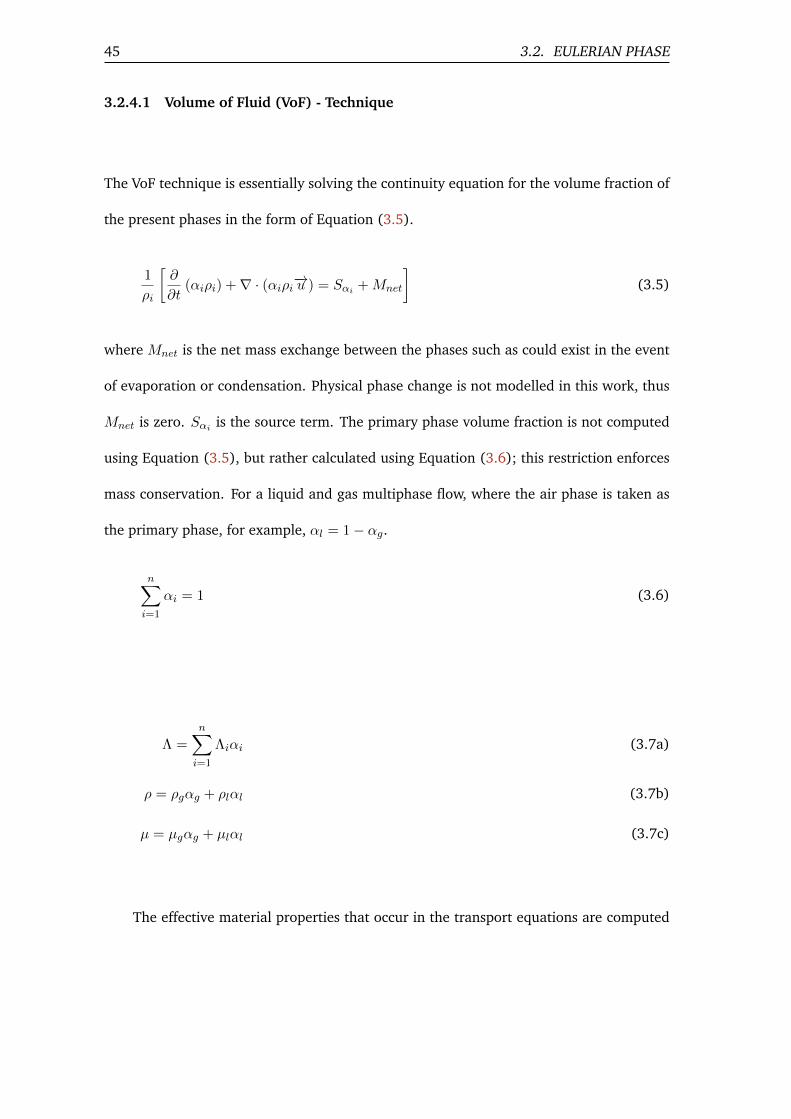
45 3.2. EULERIAN PHASE
3.2.4.1 Volume of Fluid (VoF) - Technique
The VoF technique is essentially solving the continuity equation for the volume fraction of
the present phases in the form of Equation (3.5).
1
ρi
[∂
∂t(αiρi) +∇ · (αiρi−→u ) = Sαi +Mnet
](3.5)
where Mnet is the net mass exchange between the phases such as could exist in the event
of evaporation or condensation. Physical phase change is not modelled in this work, thus
Mnet is zero. Sαi is the source term. The primary phase volume fraction is not computed
using Equation (3.5), but rather calculated using Equation (3.6); this restriction enforces
mass conservation. For a liquid and gas multiphase flow, where the air phase is taken as
the primary phase, for example, αl = 1− αg.
n∑i=1
αi = 1 (3.6)
Λ =n∑i=1
Λiαi (3.7a)
ρ = ρgαg + ρlαl (3.7b)
µ = µgαg + µlαl (3.7c)
The effective material properties that occur in the transport equations are computed

3.2. EULERIAN PHASE 46
using the volume fraction average Equation (3.7a) for a given material property Λ in
an n-phase system. The density and viscosity, for example, are computed respectively in
Equations (3.7b) & (3.7c).
3.2.4.2 Coupled Level Set Volume of Fluid (CLSVoF)
The Level Set (LS) function, φ, is advected using Equation (3.8). The Level Set function,
φ, can take positive and negative values; the interface is described at the zero Level Set
and the liquid phase is described with positive Level Set values.
∂φ
∂t+−→u · ∇φ = 0 (3.8)
The equation will move the zero Level Set exactly as the free-surface motion from the
initially known position of the film. The Level Set function is smooth and continuous; this
makes it possible to accurately compute the spatial gradients. This capability of the Level
Set method provides a good estimation of the interface curvature, Equation (3.9) and in
turn the surface tension force, Equation (3.10), required in the Navier-Stokes Equation
(3.3).
κ (φ) = ∇ · ∇φ|∇φ|
∣∣∣∣φ=0
(3.9)

47 3.2. EULERIAN PHASE
Fs = σκ∇φδε (φ) (3.10)
where δε [Eqn. 3.11] is a delta function, smoothed over a distance ε, this is by
assuming that the interface can be considered as a “thin” fluid region with a thickness ε.
δε (φ) =
12ε
(1 + cos
(πφε
))if |φ| < ε
0 otherwise
(3.11)
where ε is taken as 1.5 times the grid spacing.
In Level Set method [34], the effective density and viscosity of the fluid are calculated
using Equations (3.12a) & (3.12b) respectively.
ρ = ρg + (ρl − ρg)Hε (φ) (3.12a)
µ = µg + (µl − µg)Hε (φ) (3.12b)

3.2. EULERIAN PHASE 48
where Hε (φ) is a smoothed Heaviside function.
Hε (φ) =
0 if φ < −ε
(φ+ε)(2ε) + 1
(2π)sin(πφε ) if |φ| ≤ ε
1 if φ > ε
(3.13)
Level Set alone is, however, not mass conservative. In the VoF formulation on the
other hand, there is discontinuity at the free-surface posing a weakness for the method to
compute the spatial gradients. A major strength of the VoF method is its mass conservation
ability however. The coupling of both Level Set and the volume of fluid (CLSVoF) meth-
ods ensures mass conservation and the ability to capture the free-surface and correctly
compute surface tension force.
In Coupled Level Set Volume of Fluid (CLSVoF) method, both the Level Set and vol-
ume fractions are used to reconstruct the free-surface using the concept of piecewise linear
interface construction (PLIC) [69]. The algorithmic implementation is shown in Figure
3.1, adapted from Nichita [113]. The nature2 of Equation (3.8) does not guarantee that
|∇φ| = 1 is always maintained after the solution thus resulting in errors accumulating
during the iteration process. The re-initialisation of φ every time step is necessary as a
result of the errors that will accumulate during the iteration process.
2The interface deforms and has uneven profile with a thickness across the interface.

49 3.3. MODELLING TURBULENT FLOWS
Figure 3.1: Algorithm for implementing CLSVoF [113]
3.3 Modelling Turbulent flows
In turbulent fluid flow, the flow fields fluctuate in a stochastic manner. An approach to
“model” the stochastic flow fields, ψ(t), properties is done by decomposing them into
two components [37], the mean, Ψ and the stochastic component, ψ′(t). In other words,
ψ(t) = Ψ+ψ′(t). For example, the velocity field will be represented as u = u(t) = U+u′(t).
Although this is intended to simplify to averaging of flow fields, it introduces further terms
to be solved in the continuity, Navier-Stokes equations and any transport equations that
may be involved.
The mathematical or algorithmic closure of mean flow equations in a control vol-

3.3. MODELLING TURBULENT FLOWS 50
ume leads to the turbulence models class known as the Reynolds Average Navier-Stokes
(RANS). The RANS technique can be found well discussed in books [37, 42, 69]. The
compact index form of the continuity and Reynolds-averaged Navier-Stokes equations are
shown, respectively, in Equations (3.14) and (3.15).
∂(ρUi)
∂xi= Sρ (3.14)
[∂(ρUi)
∂t+∂(ρUiUj)
∂xj
]= − ∂P
∂xi+
∂
∂xj
µ∂Ui∂xj− ρu
′iu′j︸ ︷︷ ︸
Reynolds stress tensor
+ Sm (3.15)
where Sρ and Sm are source terms.
Reynolds stress tensor is the new set of unknown introduced. The 1877 Boussinesq
hypothesis that Reynolds stresses are proportional to the rate of deformation forms the
basis for many of the turbulence models [114, 115]. The proportionality constant or
the turbulent viscosity, µt is another variable introduced by this simplification, Equation
(3.16). The kinematic turbulent viscosity also follows as υt = µt/ρ.
−ρu′iu′j = µt
(∂Ui∂xj
+∂Uj∂xi
)(3.16)
In an attempt to predict the turbulent viscosity, several “standard” models have been

51 3.3. MODELLING TURBULENT FLOWS
developed. Such models like the Prandtl‘ mixing length model, Spalart-Allmaras model
and the variants of the κ − ε and κ − ω models exist. The mixing length model assumes
that υt is proportional to the length scale. This model can be fine for simple flows where
the mixing length scales are known and/or not changing. The Spalart-Allmaras model
solves a single conservation equation containing convective and diffusive terms for the
production and dissipation of kinematic turbulent viscosity. It is generally known to be
good for flows with mild separation or with simple recirculation but not reliable for flows
with decaying turbulence or free shear flows.
The κ− ε model was proposed by Launder & Spalding [116] in 1974 and it is one of
the most used models in industrial applications. It essentially models kinematic turbulent
viscosity as proportional to κ2/ε. Where, the flow fields, κ and ε are, respectively, the
turbulence kinetic energy per mass and dissipation rate of κ. This model further introduces
two more equations to be solved for κ and ε. The performance is, however, not reliable in
flows with large extra strains [37]. The κ− ω models can be thought of, also, as variants
of the standard κ− ε model. They model turbulent viscosity as µt = ρ · (κ/ω), where ω is
an inverse time scale measure of turbulence.
For RANS κ − ε based turbulence models, the energy equation is modelled using the

3.3. MODELLING TURBULENT FLOWS 52
form in Equation (3.17a).
∂
∂t(ρE) +
∂
∂xiUi (ρE + p) =
∂
∂xj
(keff
∂T
∂xj
)+ Sh (3.17a)
keff = k + cpµt/Prt (3.17b)
where E is the total energy, keff is the effective thermal conductivity and Prt is the tur-
bulent Prandtl number.
In this work, the (shear-stress transport) SST k−ω model described in §3.3.3 has been
used. For completeness, the standard κ-ε and κ − ω models are respectively described in
§3.3.1 and §3.3.2.
3.3.1 Standard κ - ε turbulence model
The Standard κ-ε turbulence model [69, 116] is basically the transport equation for the
turbulence kinetic energy, κ, and ε, its rate of dissipation. These are expressed in the form,
respectively, given in Equations (3.18) and (3.19). ANSYS-Fluent allows user defined
functions to describe source terms Sκ and Sε.
∂
∂t(ρκ) +
∂
∂xi(ρκUi) =
∂
∂xj
(Γκ
∂κ
∂xj
)+Gκ +Gb − ρε− YM + Sκ (3.18)

53 3.3. MODELLING TURBULENT FLOWS
∂
∂t(ρε) +
∂
∂xi(ρεUi) =
∂
∂xj
(Γε
∂ε
∂xj
)+ C1ε
ε
κ(Gκ + C3εGb)− C2ερ
ε2
κ+ Sε (3.19)
where Γκ =(µ+ µt
σκ
)and Γε =
(µ+ µt
σε
). The turbulent viscosity is modelled as
given in Equation (3.20a). Gκ is the production of turbulence kinetic energy modelled
using Equation (3.20b). The buoyancy driven generation of the turbulence kinetic energy,
Gb, is modelled using Equation (3.20c) and the coefficient of thermal expansion β is given
by Equation (3.20d).
µt = ρCµκ2
ε(3.20a)
Gκ = −ρu′iu′j
∂Uj∂xi
= µt
(∂Ui∂xj
+∂Uj∂xi
)2
(3.20b)
Gb = βgiµtPrt
∂T
∂xi(3.20c)
β = −1
ρ
(∂ρ
∂T
)p
(3.20d)
YM = 2ρMa2t (3.20e)
For high turbulent Mach3 number flows, the effect of compressibility, YM , on turbu-
lence is modelled using Equation (3.20e); in incompressible flows this is negligible.
The default model constants [69] are given as C1ε = 1.44, C2ε = 1.92, Cµ = 0.09,
3Mat =√κ/c2; c =
√γRT is the speed of sound.

3.3. MODELLING TURBULENT FLOWS 54
σκ = 1.0, σε = 1.3, Prt = 0.85 and gi is the gravity component in the ith direction.
3.3.2 Standard κ - ω turbulence model
In ANSYS-Fluent, the standard κ-ω model is based on the work of Wilcox [115]. This
model employs modification for low-Reynolds number effects, compressibility and shear
flow spreading [69]. It is an empirical model for the transport of κ and ω as given,
respectively, in Equations (3.21) & (3.22) similar to the κ-ε model described in §3.3.1
with the ability to define user defined source terms Sκ and Sω.
∂
∂t(ρκ) +
∂
∂xi(ρκUi) =
∂
∂xj
(Γκ
∂κ
∂xj
)+Gκ − Yκ + Sκ (3.21)
∂
∂t(ρω) +
∂
∂xi(ρωUi) =
∂
∂xj
(Γω
∂ε
∂xj
)+Gω − Yω + Sω (3.22)
where the effective diffusivities, Γκ & Γω, are respectively defined by Equations (3.23a)
& (3.23b). The turbulent viscosity, µt, is a blend of both κ and ω as given by Equation

55 3.3. MODELLING TURBULENT FLOWS
(3.24a).
Γκ =
(µ+
µtσκ
)(3.23a)
Γω =
(µ+
µtσω
)(3.23b)
To correct for low-Reynolds number, the coefficient α∗, Equation (3.24b), damps the
turbulent viscosity as a function of the turbulent Reynolds number, Ret, given by Equation
(3.24c). It is easy to see from Equation (3.24d) that this correction approaches unity for
high Reynolds numbers.
µt = α∗ρκ
ω(3.24a)
α∗ = α∗∞
(α∗0 + Ret
Rκ
1 + RetRκ
)(3.24b)
Ret =ρκ
µω(3.24c)
limRet→∞
[α∗∞
(α∗0 + Ret
Rκ
1 + RetRκ
)]= α∗∞ = 1 (3.24d)
The modelling of the production of κ, Gκ is same as given in Equation (3.20b). The
production of ω, Gω is given by Equation (3.25a). The coefficient α is given Equation

3.3. MODELLING TURBULENT FLOWS 56
(3.25b).
Gω = αω
κGκ (3.25a)
α =α∗∞α∗
(α0 + Ret
Rω
1 + RetRω
)(3.25b)
The dissipation of κ and ω are modelled using Equations (3.26a) & (3.26b).
Yκ = ρβ∗fβ1 · κω (3.26a)
Yω = ρβ∗fβ2 · ω2 (3.26b)
where the coefficients in Equations (3.26a) & (3.26b) are expressed in Equations (3.27a)
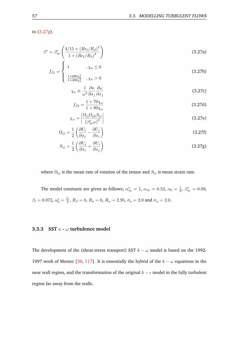
57 3.3. MODELLING TURBULENT FLOWS
to (3.27g).
β∗ = β∗∞
(4/15 + (Ret/Rβ)4
1 + (Ret/Rβ)4
)(3.27a)
fβ1 =
1 , χκ ≤ 0
1+680χ2κ
1+400χ2κ
, χκ > 0
(3.27b)
χκ ≡1
ω3
∂κ
∂xj
∂ω
∂xj(3.27c)
fβ2 =1 + 70χω1 + 80χω
(3.27d)
χω =
∣∣∣∣ΩijΩjkSij
(β∗∞ω)3
∣∣∣∣ (3.27e)
Ωij =1
2
(∂Ui∂xj− ∂Uj∂xi
)(3.27f)
Sij =1
2
(∂Uj∂xi
+∂Ui∂xj
)(3.27g)
where Ωij is the mean rate of rotation of the tensor and Sij is mean strain rate.
The model constants are given as follows; α∗∞ = 1, α∞ = 0.52, α0 = 19 , β∗∞ = 0.09,
βi = 0.072, α∗0 = βi3 , Rβ = 8, Rκ = 6, Rω = 2.95, σκ = 2.0 and σω = 2.0.
3.3.3 SST κ - ω turbulence model
The development of the (shear-stress transport) SST k − ω model is based on the 1992-
1997 work of Menter [38, 117]. It is essentially the hybrid of the k − ω equations in the
near wall region, and the transformation of the original k − ε model in the fully turbulent
region far away from the walls.

3.3. MODELLING TURBULENT FLOWS 58
The transport equations solved in the SST k − ω model for κ and ω are respectively
given in Equations (3.28) & (3.29). Although the transport equations are expressed sim-
ilarly to the standard κ − ω model further refinements were introduced in ANSYS-Fluent
[69]. In the implementation, a “blending” function is used such that it activates the k − ω
close to the surface and k − ε is activated away from the wall. The model constants are
different and a damped cross-diffusion derivative term, Equation (3.32), is introduced to
the ω equation blending the κ− ε and κ−ω models together. A modification of the turbu-
lent viscosity is done to account for turbulent shear stress. The constants are also different
from the standard equations.
∂
∂t(ρκ) +
∂
∂xi(ρκUi) =
∂
∂xj
(Γκ
∂κ
∂xj
)+ Gκ − Yκ + Sκ (3.28)
∂
∂t(ρω) +
∂
∂xi(ρωUi) =
∂
∂xj
(Γω
∂ω
∂xj
)+Gω − Yω +Dω + Sω (3.29)
The effective diffusivities are defined using Equations (3.23a) & (3.23b), but the tur-
bulent viscosity, µt, turbulent Prandtl numbers for κ and ω are, respectively, described in
Equations (3.30a) to (3.30c). The coefficients of these equations are described in Equa-

59 3.3. MODELLING TURBULENT FLOWS
tions (3.31a) to (3.31e).
µt =ρκ
ω
1
max(
1α∗ ,
SF2α1ω
) (3.30a)
σκ =1
F1/σκ1 + (1− F1) /σκ2(3.30b)
σω =1
F1/σω1 + (1− F1) /σω2(3.30c)
F1 = tanh(Φ4
1
)(3.31a)
F2 = tanh(Φ2
2
)(3.31b)
Φ1 = min
[max
( √κ
0.09ωy,
500µ
ρy2ω
),
4ρκ
σω2D+ω y2
](3.31c)
D+ω = max
[2ρ
1
σω21ω∂κ∂xj
∂ω∂xj
, 10−10
](3.31d)
Φ2 = max
[2
√κ
0.09ωy,
500µ
ρy2ω
](3.31e)
where S is the strain manitude (Eqn. (3.27g)), F1 and F2 are blending functions and
y is the distance to the next surface and D+ω is the positive portion of the cross-diffusion
term, Dω, described in Equation (3.32).
Dω = 2 (1− F1) ρ1
ωσω2
∂κ
∂xj
∂ω
∂xj(3.32)

3.3. MODELLING TURBULENT FLOWS 60
The production of the turbulence kinetic energy, Gκ and the production of ω, Gω are
given by Equations (3.33a) & (3.33b). This formulation is different4 from the standard
κ− ω as seen in the coefficients Equations (3.34a) to (3.34c).
Gκ = min (Gκ, 10ρβ∗κω) (3.33a)
Gω =α
νtGκ (3.33b)
α∞ = F1α∞1 + (1− F1)α∞2 (3.34a)
α∞1 =βi1β∗∞− ζ2
σω1
√β∗∞
(3.34b)
α∞2 =βi2β∗∞− ζ2
σω2
√β∗∞
(3.34c)
The modelling of the turbulence dissipation term, Yκ, is modelled using Equation
(3.35a) and the dissipation of ω given by (3.35b).
Yκ = ρβ∗κω (3.35a)
Yω = ρβω2 (3.35b)
where β∗ = 1 and β = F1βi1 + (1− F1)βi2.
The model constants are σκ1 = 1.176, σω1 = 2.0, σκ2 = 1.0, σω2 = 1.168, α1 = 0.31,
4Unless otherwise described in this section, the terms are the same as those of the standard κ− ω.

61 3.3. MODELLING TURBULENT FLOWS
βi1 = 0.075, βi2 = 0.0828 and ζ = 0.41.
Although the κ − ω model is isotropic, the attractiveness of the SST k − ω model to
this work is because it combines the good near-wall behaviour of the k − ω model with
the robustness and numerical stability of the k − ε models far from the walls. The κ − ω
model performs better than κ − ε models in modelling stratified flows as a result of the
turbulence damping correction introduced by Egorov et al. [56] described later in §3.3.4.
3.3.4 Turbulence Damping
The need for the damping correction arises from the fact that there is a big difference
in the physical properties of the fluids across the free-surface. The difference manifests
as a high difference in turbulence level in the gas and the liquid phases. The damping
correction model has been validated by authors ( Valle et al. [118], Amir et al. [119] &
Tkaczyk and Morvan [55] ) and is only available in the SST k − ω model for free-surface
flows in ANSYS-Fluent 14.5 and subsequent versions. Numerical turbulence damping is
introduced by Egorov et al. [56] as source term in the ω [Eqn. 3.29] equation. This is
expressed as Sω in Equation (3.36).
Sω = Ai∆nβρi
(6 ·Bµiβρi∆n2
)2
(3.36)
where B is a damping constant that can take values from 0 − 100. The default value
in ANSYS-Fluent is 10 and is rather a calibration factor. Ai is the inter-facial area while
ρi is the density for the phase i. From Egorov et al. [56] and the ANSYS-Fluent [69]

3.3. MODELLING TURBULENT FLOWS 62
implementation, the area is computed as a function of the volume fraction, αi, as Ai =
2 · αi |∆αi|. The cell height normal to the free-surface is ∆n. β is the model closure
coefficient (β = 0.075).
Figure 3.2: Turbulence damping effect [55]
Figure 3.2 shows result from Tkaczyk & Morvan’s [55] implementation of the tur-
bulence damping correction. The velocities are measured on a plane downstream of a
rectangular duct carrying water film and air in a stratified flow. The film depth is about
40mm and flowing at about 10% of the air velocity.
The value B = 0 in the figure is equivalent to the κ− ε model implementation. It can
be seen that without the correction, there is a numerical “error” at the interface region
that propagates into the core flow in the air phase as compared with the experimental
data. The value B can therefore be seen as a calibration to the experiment.

63 3.3. MODELLING TURBULENT FLOWS
3.3.5 Wall treatment
Although a flow may be turbulent, the flow behaviour at the walls is laminar. The flow
magnitude increases gradually through the viscous sub-layer, closer to the wall, into the
core turbulent regime. For completeness, this section describes the standard treatment of
walls in ANSYS-Fluent [69]. y+ is a non-dimensional distance from the wall boundary as
given by Equation (3.37a).
y+ =ρuτµy (3.37a)
uτ =
√τwρ
(3.37b)
where y is a distance measured from the wall, τw is the wall shear stress. The viscous
sub-layer[69] is in the region where y+ is below 30.
Figure 3.3: Log law [120]

3.3. MODELLING TURBULENT FLOWS 64
Figure 3.3 shows non-dimensional velocity (U+) plot against y+ for flow close to a
smooth wall with a no-slip boundary condition. This velocity is normalised with the wall
shear stress, τw and density (U+ = U/ (τw/ρ)). The circles are experimental points and
the solid lines are by curve fitting. The logarithmic law fits well away from the viscous
sub-layer.
Figure 3.4: Near wall treatment
In ANSYS-Fluent [69], special treatment is used for ω at the walls depending on the
mesh. Given the flow in Figure 3.4 where either Mesh A or B is used. Mesh - A is fine and
able to resolve flow in the laminar sub-layer to the wall but Mesh -B is not fine enough
to resolve it. The viscous layer/region is bridged using wall functions instead of resolving
the flow. For fine meshes, the low-Reynolds number boundary conditions apply [see §3.3.2
& Equation (3.24b)]. The analytical function approach is used with coarser mesh, where
the mesh is not able to resolve the laminar sub-layer and otherwise the appropriate low-
Reynolds number boundary conditions apply. The value of ω at the wall or ωw is given in

65 3.4. LAGRANGIAN PHASE - DISCRETE PHASE MODEL (DPM)
Equation (3.38).
ωw =ρ (u∗)2
µ×
6
βi(y+)2Analytical, y+ < 30
1√β∗∞
du+turbdy+
Logarithmic region, y+ > 30
(3.38)
where β∗∞ = 0.09, βi = 0.072 and u∗ is the non-dimensional friction velocity.
3.4 Lagrangian Phase - Discrete Phase Model (DPM)
A model of a cold droplet moving in a hot stream of high velocity gas needs treatment for
aerodynamics, mass transfer and heat transfer. A droplet can be considered as spherical
liquid volume held together by surface tension force. The interaction of the droplet with
the gas phase, for example, causes deformation as a result of the aerodynamic drag and
some liquid may evaporate, thus transferring mass as vapour. The droplet can also cool
down in the gas stream if the gas is colder than the droplets. The droplets in the target
applications are small (around 50 − 1500 µm). The shape deformation of the droplets is
considered negligible and it may be reasonable to assume they maintain a spherical shape
because they are small. This non-deformation assumption of the droplets is only for sim-
plicity and could be modified in future development. For a disperse droplet concentration
in the fluid domain, the Lagrangian representation could be used, this is the Discrete Phase
Model (DPM) in ANSYS Fluent.
Figure 3.5 shows a single droplet in a 3D space moving with a velocity Up. The actual
diameter is given as Dp. A Lagrangian representation, shown as the centre dark dot, of

3.4. LAGRANGIAN PHASE - DISCRETE PHASE MODEL (DPM) 66
the whole droplet considers the droplet as a single point, regardless of the actual space
occupied by the droplet. The coordinates, P(x,y,z) are obtained from the integration of
force per unit mass balance, Equation (3.39).
Figure 3.5: DPM in a 3D space
d−→Updt
=−→FD︸︷︷︸drag
+−→F otherforces︸ ︷︷ ︸
pressure, virtual mass, bouyancy
(3.39)
The drag force per unit particle mass,−→FD, is given in Equation (3.40). The Reynolds
number of the particle, Re, is estimated as Re ' ρlµDp
∣∣∣−→U p −−→u∣∣∣. The coefficient of drag,
CD, is computed depending on the scenario and can be implemented as a User Defined
Function (UDF) in ANSYS-Fluent.
−→FD =
18µ
ρlD2p
CDRe
24(−→U p −−→u ) (3.40)

67 3.4. LAGRANGIAN PHASE - DISCRETE PHASE MODEL (DPM)
The droplets are assumed to be non-deforming and behave like hard spheres, an as-
sumption made because of the small sizes of the droplets. The drag coefficient is computed
based on the Reynolds number using the Schiller & Naumann [121] correlations as given
in Equation (3.41).
CD =
24 1Re , Re ≤ 1
24 1Re
(1 + 0.15Re0.68
)1 < Re < 1000,
0.45, 1000 ≤ Re ≤ 3500
(3.41)
The energy equation for the Lagrangian particle in the continuous phase whose tem-
perature is T∞ is given in Equation (3.42).
mpCpdTpdt
= hAp (T∞ − Tp)︸ ︷︷ ︸convective heat
+dmp
dthfg︸ ︷︷ ︸
evaporative heat
+Apεσ(T 4∞ − T 4
p
)︸ ︷︷ ︸radiative heat
(3.42)
where the latent heat of evaporation is hfg, σ is the Stefan-Boltzmann constant and ε
is the emissivity of the surface. In this work, the droplets are non-volatile, travel at very
high speeds and travel short distances from shedding to impact, thus limiting the effect
of evaporation. Also, considering that the temperature difference between the droplets
and the fluids is not extremely wide, or mathematically, limTp→T∞ T4∞
1−
(TpT∞
)4
= 0.
Therefore, both the radiative and evaporative components of Equation (3.42) are assumed
negligible.

3.5. NUMERICAL METHOD 68
3.4.1 Eulerian-Phase Coupling
In the implementation of the Lagrangian phase representation of the droplet, when the
Lagrangian droplets (DPM particles) do not affect the Eulerian phase but the continu-
ous Eulerian flow fields do affect the DPM particles, it is known as “One-Way Coupling”.
“Two-way Coupling” is achieved when both the DPM and the Eulerian phases affect each
other. In the Two-way Coupling approach, the DPM solution iteration alternates between
the Eulerian phase solution iteration until convergence is reached. When coupled, the
momentum transfer into the Eulerian phase5 is expressed in the form given in Equation
(3.43).
−→F =
∑18
24
µCDRe
ρlD2p
(−→U p −−→u
)+
−→F other︸ ︷︷ ︸
other interaction forces
mp∆t (3.43)
where mp is the mass flow rate of the particulate phase and ∆t is the time step.
3.5 Numerical Method
Although a full review of the numerical techniques available to implement CFD techniques
is beyond the scope of this thesis, it is worth briefly summarising what is used here. A
detailed description of solvers and techniques have been published widely in books [37,
69]. Moreover, the solution methods and the solution algorithms (solvers) are available
for implementation in commercial and major open source solvers.
5This can be expressed as Sm in Equation (3.15).

69 3.5. NUMERICAL METHOD
3.5.1 Discretisation
The transport equations can be expressed in the generic form given in Equation (3.44). It
obeys generalised conservation principle in the transport of the variable φ.
∂ρφ
∂t+∇ · (ρφ−→u ) = ∇ · (Γφ∇φ) + Sφ (3.44)
where Γφ is the diffusion coefficient and the source term per unit volume is Sφ.
In Equation (3.44), the temporal term, ∂ (ρφ) /∂t, accounts for the accumulation of φ
in the control volume of interest;∇·(ρφ−→u ), the convective term, accounts for the transport
of φ owing to the existence of the velocity field in it. The diffusion term, ∇ · (Γφ∇φ),
accounts for the transport of the variable φ owing to the gradients while Sφ is a source (or
sink) term that creates (or destroys) φ.
The transport equations are difficult to solve analytically but different kinds of numer-
ical discretisation techniques, such as Finite Difference Method, Finite Element Method,
Boundary Element Method, Finite Volume Method, etc could be used [42, 122]. The ob-
jective of numerical discretisation is to simplify the governing equations into a system of
algebraic equations. Generally, the system of equations obtained by the numerical method
can then be applied over the control volume mesh generating a set of linear equations to
be solved for the variables.
In Finite Volume Method (FVM) used in ANSYS-Fluent, the transport equation is

3.5. NUMERICAL METHOD 70
integrated about the control volume. The Gauss’ divergence theorem is used to reduce the
volume integrals of the spatial terms [Eqn. 3.45a] to the surface integrals in the resulting
system of equation [Eqn. 3.45b].
∫V
∂ρφ
∂tdV +
∫V∇ · (ρφ−→u ) dV =
∫V∇ · (Γφ∇φ) dV +
∫VSφdV (3.45a)∫
V
∂ρφ
∂tdV +
∮ρφu · d
−→A =
∮Γφ∇φ · d
−→A +
∫VSφdV (3.45b)
where−→A is the surface area vector, V is the cell volume.
The equivalent numerical discretisation of Equation (3.45b), for a two-dimensional
computational cell with N faces is given in Equation (3.46).
∂ρφ
∂tV +
N∑i
ρiφi−→u i ·
−→A i =
N∑i
Γφ∇φi · d−→A i + SφV (3.46)
where φi is the value of φ convected through face i, ∇φi is the gradient of φ at face i and,
for example, this can be expressed as ∇φ = (∂φ/∂x) i+ (∂φ/∂y) j + (∂φ/∂z) k. The mass
flux through face i is given by ρi−→u i ·−→A i.
Both spatial and temporal discretisation are required for transient solutions as dis-
cussed in §3.5.1.1 and §3.5.1.2.

71 3.5. NUMERICAL METHOD
3.5.1.1 Spatial discretisation
In ANSYS Fluent, the values of the scalar φ are stored in memory locations corresponding
to the centroids C0 and C1 shown in Figure 3.6. The figure shows the arbitrary control
volume used to illustrate the transport of a scalar quantity φ given by Equation (3.45b).
Figure 3.6: Control volume for Scalar Transport Equation [69]
Upwind scheme is used to interpolate for the face values of φi in Equation (3.46).
This implies deriving the scalar from values in the cells upstream/upwind relative to the
direction of the normal velocity. There are several spatial upwinding techniques available
in ANSYS-Fluent [69]. In this work, the second order upwind has been used for the spatial
parts of the transport equations. The second order accurate upwind method is used for the
continuity, VoF, momentum, and energy equations. The second-order upwind scheme for
the cell-centred solution, φi,2, about the centroid of the cell as given by Equation (3.47).
φi,2 = φ+∇φ · −→r (3.47)
where and −→r is the displacement vector from the upstream cell centroid to the face cen-

3.5. NUMERICAL METHOD 72
troid.
3.5.1.2 Temporal discretisation
The temporal part, (∂ρφ/∂t)V , of Equation (3.46), is solved using a numerical integration
technique over a time step ∆t. The generic temporal PDE in Equation (3.48), can be
discretised using backward differencing scheme. Its first order accurate discretisation is
given by Equation (3.49a) and a second order accurate discretisation is given by Equation
(3.49b).
∂φ
∂t= F (φ) (3.48)
φ(t+∆t) − φ(t)
∆t= F (φ) (3.49a)
3φ(t+∆t) − 4φ(t) + φ(t−∆t)
2∆t= F (φ) (3.49b)
The right hand function, F (φ), of this discretisation also depends on φ which can be
evaluated at a time now, t, otherwise referred to as “Explicit time integration” as given
by Equation (3.50a). When evaluated in a “future” time, t + ∆t, as given by Equation

73 3.5. NUMERICAL METHOD
(3.50b), it is referred to as “Implicit time integration”.
φ(t+∆t) − φ(t)
∆t= F
(φ(t)
)(3.50a)
φ(t+∆t) − φ(t)
∆t= F
(φ(t+∆t)
)(3.50b)
For solution stability in explicit time integration, the choice of time step (∆t), Equa-
tion 3.51b should be made to satisfy the Courant−Friedrichs−Lewy (CFL) number given
in Equation 3.51a considering a computational cell with characteristic length ∆X with
fluid moving with a velocity −→u .
CFL =|−→u |(∆X∆t
) (3.51a)
∆t ≤ ∆X
|−→u |(3.51b)
The implicit time integration is unconditionally stable with the choice of time step. As
shown above, for the explicit time integration, the time step is restrictive but it is useful in
capturing transient behaviours. It is also less computationally expensive than the implicit
time integration [69].

3.5. NUMERICAL METHOD 74
3.5.2 Solution Algorithm
The numerical solution algorithms for the governing equations in ANSYS-Fluent are often
referred to as “Solvers”. There are basically two solvers available, the “Pressure-Based
Solver” and “Density-Based Solver”. The density based solver was originally intended
for compressible flows while the pressure based solver was for low-speed incompressible
flows [69]. The density based solver, Figure 3.7A, solves for all the flow fields, pressure,
velocity & temperature, in a coupled way in all the computational cells at the same time.
The velocity field is obtained from the momentum equations while the density is obtained
from the continuity equation, but the equation of state is used to determine the pressure.
In the discretised scalar transport equation, [Eqn. 3.46], the scalar variable φ is
unknown at the cell center and at those of the surrounding neighbour cells. The mesh
topology will determine the number of neighbour cells. This is a non-linear system in
general and can be expressed in the linear form given by Equation (3.52). For the whole
cells in the mesh, this will result in a sparse coefficient matrix system. The linear system
is solved using Gauss-Seidel technique in conjunction with an algebraic multigrid (AMG)
solver.
aiφ =∑j
ajφj + b (3.52)
where the subscripts j point to the neighbour cells and ai & aj are the linearised coeffi-
cients for φ and φj .

75 3.5. NUMERICAL METHOD
The pressure based solver uses either a segregated algorithm, Figure 3.7B or the
coupled algorithm, Figure 3.7C. In these solvers, a manipulation of the continuity and
Navier-Stokes equations is used to solve or “correct” for the pressure field and similar to
the density based method, the solution is discretised into computational grids and the sys-
tem of equations linearised appropriately. In the segregated solver, the flow field variables
are solved for one at a time in a sequence. The coupled algorithm solves the same set
of variables in a simultaneous manner. The segregated algorithm is known to be more
memory efficient although it is slower. It is favoured in this work for its memory efficiency
bearing in mind that the volume of computational nodes in a typical geometry can be in
order of millions.
The algorithms available in ANSYS-Fluent to couple pressure and velocity are the
SIMPLE, SIMPLEC, PISO, Coupled and FSM algorithms. These algorithms are well dis-
cussed in books [37, 38, 42, 69]. SIMPLE means Semi-Implicit Method for Pressure-Linked
Equations, SIMPLEC, an extension of SIMPLE, means SIMPLE -Consistent. PISO, extends
on SIMPLE and SIMPLEC, means Pressure-Implicit with Splitting of Operators. FSM, used
in non-iterative time advancement, means Fractional-Step Method. The PISO algorithm is
favoured in this thesis, over both SIMPLE and SIMPLEC, because it provides better sta-
bility to the simulations than the other two. Although the stability issue is not critical
with either SIMPLE or SIMPLEC, it is thought to be related with new velocity and fluxes
computation in the iteration. They fail to satisfy the momentum balance after the pressure
correction equation is solved. The PISO algorithm performs extra corrections [37, 69].

3.5. NUMERICAL METHOD 76
Figure 3.7: CFD Solvers [69]

77 3.6. ADOPTED MODELLING STRATEGY
3.6 Adopted Modelling Strategy
A combination of the modelling techniques is required for the kind of problem described in
this thesis. The Volume of Fluid (VoF) with the Level Set enhancement is considered most
suitable. This is because it can handle deforming complex free-surface. The combination
of the enhanced VoF technique with the turbulence damping strategy provides the oppor-
tunity to handle shear driven and turbulent stratified flow. The two-way coupling tracking
ability of Lagrangian droplets (DPM) makes its combination with the Eulerian CLSVoF at-
tractive. The stability of the combined model is good with the PISO solver. A second order
discretisation for the spatial terms and first order accurate explicit time integration for the
temporal terms are required for numerical stability of the solution. The solution of tran-
sient partial differential equations is also limited by the Courant−Friedrichs− Lewy (CFL)
condition [see Eqn. 3.51a]. This requirement means the small time steps are required for
stability. The possibility of combining or further enhancing the models is described in the
next chapter [§4].
3.7 Summary
In this chapter the mathematical and computational basics for doing multiphase flow sim-
ulations have been discussed.
The fluid system in a multiphase system can be represented as separate mixtures
coupled mathematically or can be represented numerically as a single fluid identified using

3.7. SUMMARY 78
colour function. The free-surface can be tracked using the volume fraction of the fluids
present. To solve for the flow fields, the continuity and Navier-Stokes equations are solved.
For turbulent flows, the averaged Reynolds equations can be used to simplify the equation
systems. The simplification further introduces more complications that need development
of turbulent models. For stratified type flows, corrections are required, and available,
to compute more accurate propagation of momentum at the free-surface. For disperse
droplets, the Lagrangian technique is available to model droplet to gas interaction.
In ANSYS-Fluent, there are robust numerical techniques available and the relevant so-
lution strategies have been identified. The enhanced free-surface Volume of Fluid method
combined with the Lagrangian droplet tracking are the identified candidates, and further
work will be based them in this thesis.

Chapter 4
The DPM-VoF Model : A Coupled
Framework for Gas-Droplet-Film
Interaction with Heat Transfer
4.1 Overview
The modelling of droplet interaction with the gas and the liquid film using a coupled
Lagrangian-Eulerian approach is proposed in this chapter. This is new, in particular in the
context of an aeroengine application where it enables a better description of the oil flow
in the bearing chamber. In the bearing chamber, the flow consists of high speed filaments
and disperse oil droplets interacting with the gas and flowing film, with the latter formed
as a result of oil droplets accumulating on the chamber outer wall. Although the oil
79

4.1. OVERVIEW 80
is introduced into the chamber in a continuous form, the highly rotational environment
breaks some of it up into high speed droplets and probably many of the droplets are shed
by the bearings. The oil is fed at a lower temperature than the chamber and so provides
cooling.
In Chapter 3, the basic modelling approaches applicable individually for the inter-
action of the air and oil phases were presented. The coupling of the Lagrangian droplet
representation (DPM, in ANSYS-Fluent) with the gas phase was also presented. A novel
extension of the DPM coupling accounting for the droplet to liquid (film) interaction is
proposed here. There are significant limitations associated with the droplet-liquid in-
teraction as currently formulated in commercially available codes when the droplets are
represented by the discrete phase model and the work presented in this thesis provides a
formulation where the interaction is far closer to that found in the physical situation.
Figure 4.1: The DPM-VoF Concept

81 4.1. OVERVIEW
The proposal in this work is schematically shown in Figure 4.1. The primary droplet,
mass Md, approaches the gas-liquid interface (dashed line) with a velocity, Vd, the impact
of which can lead to splashing (formation of secondary drops). In the model formulation
the droplets are still treated as DPM particles (all the mass and momentum located at a
single point) but the interaction with the liquid phase is far more physically representative.
In the physical situation, when a droplet impacts on a film, mass and momentum are
added to the film and if there is a temperature difference then energy is transferred and a
new equilibrium is established. Over some impact parameter ranges the impact event can
result in smaller droplets being splashed back into the gaseous phase.
Figure 4.2: Impacting droplet photograph [123]
An example of this type of droplet-film impact is shown in Figure 4.2 where the
droplet impact results in a crown being formed and smaller droplets being shed from
the crown. Here a fraction of the mass of the impacting droplet goes into the splashing
droplets with the remainder (from mass conservation) going into the film. In the model
developed and presented in this thesis droplets travel through the gas phase are repre-
sented using a Lagrangian framework (DPM). At the point of interaction with the film
interface the impact conditions are used to generate an impact outcome including the

4.1. OVERVIEW 82
mass fraction that splashes, the size(s) of the droplets splashed and their velocities. These
splashed droplets, as they move through the gas phase, are represented using a discrete
phase model.
Figure 4.3 shows how the DPM-VoF concept of Figure 4.1 is implemented. The dashed
boxes represent different computational modules.
Figure 4.3: Droplet impact and tracking: DPM-VoF Concept

83 4.2. DPM-VOF GAS PHASE DRAG
4.2 DPM-VoF Gas phase drag
The coupling of Lagrangian droplet with the gas phase implementation, [see §3.4], is done
through a User Defined Function (UDF). The effects of interference drag experienced by
a droplet trailing behind another droplet are assumed neglible. Kaka & Zhi-yong [124]
did numerical simulation to compare drag coefficient of two close spheres with that of a
single sphere each of diameter Ds. Their results shows that the drag coefficient ratio of
two spheres to that of only one sphere is between about ±5%; for Re > 500 and when
spaced over 5 × Ds. It is, therefore, considered safe to do no further calibration on the
ANSYS-Fluent standard drag coefficient in the implementation of this work.
4.3 DPM-VoF Mass Transfer
The transfer of mass from the DPM to the VoF phase is achieved by managing source
terms into the VoF Equation (3.5) and simultaneously interrupting the particle tracking.
Exchange of mass from the Lagrangian droplet particle, mass Mp, (in kg), to the Eulerian
VoF phase takes effect when one of two things happens:
(a)
the DPM particles passes into a liquid region. The test for this is related to cell
volume fraction and typically the droplet will be said to be interacting with the film
interface when the liquid volume fraction in the cell is greater than or equal to 0.51.
1In ANSYS Fluent 14.5 used in this work, the LS “macro” is not available; this dictates the use of C_V OFas a guage instead of LS.

4.3. DPM-VOF MASS TRANSFER 84
(b)
when the droplet interacts with a solid surface in such a way that the outcome leaves
some or all of the droplet liquid on the surface. In this case a film can be initiated
from droplet impacts.
The interface tracking implementation ensures the model works for any arbitrary
surfaces [see §4.6]. The mass source term (in kg/sm3) created by this “handover” of DPM
to VoF is given in Equation (4.1). This novel exchange of droplets from its Lagrangian
representation is responsible for film formation, as seen in the next chapters.
Sρ =ρiρl
Mp
∆t
1
Vcellδo (4.1)
with the phase source determined using:
ρi =
−ρg for gas phase
+ρl for liquid source(4.2)
where the current computational cell volume is Vcell in m3 and δo is a top hat function as
given in Equation (4.4).
DPM tracking was originally intended for scenarios where the particle sizes are low
in concentration and relatively smaller than the cell. It is common to employ fine mesh
density at the interface and sometimes throughout the film to better resolve the film and
the interface. It was also shown by Tkaczyk & Morvan [55] that there is a minimum
requirement for the number of cells required in the film to achieve a given resolution in

85 4.3. DPM-VOF MASS TRANSFER
the profile in the interface region. With the technique developed and presented in this
thesis, it is possible for the mesh size and particle size to become comparable in size
especially close to the walls.
Figure 4.4: Mass source spread sphere
Figure 4.4 shows a schematic representation of a DPM particle, given as the small
darker dot, in a cell where the liquid volume fraction is just above 0.5; the level set zero
isosurface can be used to identify the interface location within this interface region.
As the droplet travels in the solution domain, it is even possible that the droplet vol-
ume becomes, on some occasions, larger than the current cell volume. This therefore
implies that the mass of the droplet will not “fit” the cell, violating the DPM basic assump-
tions and the incompressibilty principle. In situations where the droplet size is bigger
than the cell, the mass source term is distributed to a “Spread Radius” zone, as indicated
in Figure 4.4. This zone represents the actual spherical volume an actual droplet will
occupy and as shown for that instance is larger than the current cell. The liquid source

4.3. DPM-VOF MASS TRANSFER 86
term represents the mass of liquid phase that is supposed to be occupied in the zone if the
droplet were not a DPM particle. It should be noted that a mass of an equal volume of the
gas should be taken out from that zone, this is achieved as indicated by Equation (4.2).
If the whole mass source is added into only the central cell (without spreading the source
terms), large residuals are observed because the incompressibility assumptions is clearly
violated, thereby causing unphysical velocity and pressure jump. On the other hand, ex-
perience has shown that, instability issues might be experienced if the mass is spread over
too many cells.
Figure 4.5: Scan zone: from impact point to the centroids
The proposed algorithm involves locating and marking the neigbour cells of the cell
where the DPM particle is currently located before distributing the source terms. The
centroids, Xc(x, y, z), of the cells in domain are used as reference for each cell while the
current position, Xp(x, y, z), of the particle is known. These are, respectively, represented
as position vectors−→X c and
−→X p. The distances from the particle positions to the cell cen-

87 4.3. DPM-VOF MASS TRANSFER
troids, RSR given by Equation (4.3), determine if the cell falls inside or outside of the
region where source terms are required. The white crosses in Figure 4.5 represent the cell
centroids and the current particle position is represented with the dark dot.
RSR =∣∣∣−→X c −
−→X p
∣∣∣ (4.3)
Inside SRin, source terms are added; outside of the zone, SRout, no source term is
added. A cell is considered to be in SRout when RSR > 0.5Dp. This is used to describe the
top hat function δo, Equation (4.4), used to determine where the source terms are to be
added.
δo =
1 if RSR
0.5Dp≤ 1
0 Out of range(4.4)
It should be noted that real droplets are not spherical all the times as assumed in
DPM formulations; upon the DPM turning into VoF film, it is expected to start to deform.
There is no special consideration for the curvature of the droplets, the CLSVoF function
[see 3.2.4.2] and surface tension is relied upon to handle the shape. The marking ensures
the correct mass source is added to enforce mass conservation.

4.4. DPM-VOF MOMENTUM TRANSFER 88
4.4 DPM-VoF Momentum Transfer
The momentum of the DPM particle is transferred into the VoF film based on the La-
grangian solution of the particle velocity vector,−→U p and the mass source term, Sρ, earlier
described [see §4.3]. In Figure 4.1, the fraction of mass splashed is taken off before adding
the source terms, if any. The momentum source is transferred into the Navier-Stokes equa-
tions and follows simply as given in Equation (4.5).
−→SM = Sρ
−→U pδo (4.5)
4.5 DPM-VoF Heat Transfer
The energy equation solution of the DPM particle gives the temperature of a droplet. The
droplet is assumed to mix adiabatically and instantly at the impact and the splashing
droplets assume the temperature of the film. The temperature, Ti, in each of the VoF cells
at the impact locations are approximated as a mass average of the DPM temperature, Td,
and the temperature, Tf , of the fluid. The representative mass of the fluid in the current
cell during the scan described in §4.3, Mf , is obtained from the product of the volume
fraction, density and the current cell volume, Mf = αρVcell. Equation (4.6) gives the
temperature of the cell at the impact zone.
Ti =MfTf +MdTdMf +Md
(4.6)

89 4.6. INTERFACE TRACKING & SPLASHING
4.6 Interface Tracking & Splashing
An important aspect of the DPM-VoF technique is identifying the free-surface. This is
interface tracking. The droplet-position requires interface tracking to continually identify
the film or walls. The position,Xp, of the DPM droplet and the computational cell volume’s
liquid volume fraction, α, is used. Where a droplet crosses into any isosurface with α >
0.5, for example, the droplet is taken to be at the free-surface; and the source term modules
are initiated once these conditions are met. A UDF code scans the cell faces and determines
if a cell volume has a wall bounded face, Figure 4.6. DPM-VoF is initiated in any cell that
has a wall-bounded face. The interface normal on the isosurface relative to the incoming
primary droplet will determine the splashing direction.
Figure 4.6: Interior and Wall bounded cells faces
4.6.1 Splashing
The droplet-film impact experiment from Roisman & Tropea [125] shown in Figure 4.7
illustrates a normal and an oblique splash. The image in Figure 4.7(A) is for a normal
droplet impact and Figure 4.7(B) is for a primary droplet impact at an oblique angle to
the impact surface. A corresponding detailed numerical resolution of the primary and

4.6. INTERFACE TRACKING & SPLASHING 90
secondary droplets as undertaken by Peduto et al. [12] is shown in Figure 4.8. These
simulations required computational grids of the order of 3 million cells.
Figure 4.7: Splash from normal, (A) and oblique (B) droplets impact [125]
Figure 4.8: Detailed VoF Simulation for Normal (A) & Oblique (B) impacts [12]
The work of Peduto et al. [12], illustrated in Figure 4.8, shows that it is possible to
model droplet-film impact directly if a very large number of cells is used. However, for
modelling a practical flow situation in which there are many droplets impacts, such meshes
are extremely impractical. In the currently developed DPM-VoF model, the simplification
of the splash is obtained by assuming that at impact the free-surface is momentarily “hard”
and “flat” at the point of impact serving as a “bouncing” plane for the computation of the
direction cosines and position vector of the centre of the secondary droplets’ distribution.
The position vector of the splash ring centre makes it possible to compute the spatial ori-
entation of the secondary droplets (droplets A). Figure 4.9 shows the geometric technique
applied to model the emerging secondary droplets as Lagrangian particles. The velocity
of impact, Vp, and the mean velocity, Vs, of the secondary droplets are obtainable from
published correlations. For example, Table 2.2 lists possible outcomes for different impact

91 4.6. INTERFACE TRACKING & SPLASHING
conditions.
In the code implementation in this work and based on relavant regimes, the correla-
tions in Table 4.1 have been used.
Table 4.1: Selected Correlations Employed in Splashing
Parameter
/Action
Correlation/Criteria Notes
K K1 = We ·Oh−2/5
K = 20100 + 5880 (H∗)1.44 Definitions from Yarin [73].
SPLASH 0.08 ≤ H∗ & K ≈ 400 Yarin [73]
SPLASH H∗ < 0.08 & K ≥ 400 If K < 400 droplet STICKS
SPLASH H∗ ≥ 0.14 & K1/K > 1 If K1/K ≤ 1 droplet STICKS,Cossali et al. [71].
Ns 7.84× 10⁻⁶K1.8 (H∗)−0.3 Experiment tested in the range:0.0275 < H∗ < 68; 0 < αp < 10o,Okawa et al. [84].
θ 0.015K + 12 Mean angle of secondary dropletsejected from theimpact plane [12, 126, 127],with evenly spaced cusps.
β ≈ 0.04 Mass fraction absorbed [126].β = 0.00156e0.000486K Experiment range:
0.0275 < H∗ < 68; 0 < α < 10o,not valid when K > 1.3×10⁴ [84].
Vs 0.52× Vp Mean speed of ejected secondarydroplets [126].
JL ≈ 0.57Dp2 Jet length [73].

4.6. INTERFACE TRACKING & SPLASHING 92
Although these are limited, for example, there are no known correlations for droplets
splashing in moving films, where the film flow is turbulent or a moving film on a curved
surface. Thus the closest correlation that matches would be used from data where the
relative film thickness and other parameters are similar. Column 2, in Table 4.1, shows
the criteria calculated or checked against at impact points to determine the action taken
in column 1 based on the definitions in column 3. If an impact is determined to create
secondary droplets, the number of secondary droplets, Ns, the mean ejection angle, θ,
the mass fraction absorbed from the primary droplet, β as well as the mean speed of the
splashing droplets, Vs and the jet length, JL are calculated using column 2.
Figure 4.9: DPM-VoF Splash Model

93 4.6. INTERFACE TRACKING & SPLASHING
The secondary droplets are created at the end of the impact time step. The position
above the free-surface for the creation of the secondary droplets is defined here as the jet
length, JL.
In Figure 4.9, the primary droplet impacts at the free-surface, C, at a point B to create
secondary droplets at A. The distribution of the secondary droplets follows an almost
elliptical distribution in an oblique impact as shown by the work of Peduto et al. [12] &
Roisman and Tropea [125] and illustrated by Figures 4.7 & 4.8.
The generation of secondary droplets in the VoF to DPM model occurs a few micro
seconds earlier than what the reality is. The start points are also only approximate as well,
but from a practical point of view, it is not unrealistic to make such an approximation in
the development stages of the model. Layers of complexity can be added as the modelling
approach is refined and developed. In the model presented here, the secondary droplets’
spatial positions can be represented as a circular ring with a diameter equal to the crown
diameter2 at a chosen time step further down the simulation flow time.
To create a plane of splashing droplet particles, consider a primary droplet impacting
on a free surface S1 at a point P1 as shown in Figure 4.10. The side and top views are
shown. The normal of the splash plane, N2, is considered to be parallel to the impact
normal3, N1.
2Crown diameter-time evolution curve (Figure 5.10) or equation (Equation 5.2) can be used to estimatethis diameter.
3The normal, Equation 4.7a, is computed from the level set function based on the Brackbill et al. [50]continuum surface force model, Equation 4.7b. An alternative proposal for the improvement of the normalcomputation technique is proposed by Bohacek [128].

4.6. INTERFACE TRACKING & SPLASHING 94
Figure 4.10: Secondary droplet initiation plane
The spatial locations,Xi[j], of the secondary droplets are predicted from the geometric
equation of the plane S2 whose centre is a position vector, P2 [Eqn. 4.7d]. Plane S2 on
Figure 4.11, is a great circle on a sphere whose diameter, (2× r), is the same as the crown
diameter of the splash.

95 4.6. INTERFACE TRACKING & SPLASHING
Equations(4.7a) - (4.7f) are obtained using simple vector manipulations4 of Figure
4.10.
‖−→N ‖=‖
−→N1 ‖=‖
−→N2 ‖
= n1i+ n2j + n3k (4.7a)
=‖ ∇φ ‖ (4.7b)
−→Vs =‖
−→Vp − 2
(−→Vp ·−→N1
)−→N1 ‖ (4.7c)
−→P2 =
−→P1 + JL
(−→Vs
)(4.7d)
−→A =
−→Vs× ‖
−→N1 ‖ (4.7e)
−→B =
−→A× ‖
−→N1 ‖ (4.7f)
Figure 4.11: DPM-VoF splash plane circle
4The double modulus sign operator on a vector here is used to mean computing the unit vector of thevector.

4.6. INTERFACE TRACKING & SPLASHING 96
The initiation jet length5, JL is taken as 1.5 × Dp, as a first approximation. The
interface normal is computed in the cell where the DPM particle crosses into the free
surface or wall boundary. The magnitude of the velocity vector of the secondary particles
is taken from correlations but the directions are obtained from the unit vector of the
reflection vector Vs in Equation 4.7c.−→A and
−→B (Equations (4.7e) & (4.7f) respectively)
are any two perpendicular unit vectors in the plane of the splash. The radial distribution
of the droplet is clearly stochastic and not known a priori. This stochastic distribution can
be implemented into Equation (4.8) which is a parametric equation of a ring on a sphere.
Xi[j] = P2[j] + rcos (θi)A[j] + rsin (θi)B[j] (4.8)
The number of droplets are spread evenly on the ring, but the start point, θs, uses
a random angle from 0 to π4 . The values of θi from θs to 2π + θs, are put into Equation
(4.8), to get the spatial orientations, Xi[j], for a secondary droplet number i of a total of N
splashed children. The ring radius, r, is fixed here, but can be adjusted to give an elliptical
children ring shape as is seen in Figure 4.9B. Here, j represents the jth component of the
n Cartesian coordinates.
It should be noted that the droplets can be randomly distributed on an area within
two concentric circles rather than exactly on the ring described. This is schematically
illustrated in Figure 4.12. The region can be obtained by manipulating the radius, r, to be
between radii of the two concentric dashed circles. This is subject to availability of data;
5Yarin [73] shows a linear growth rate for the jet length, h, with the crown diameter, r as dh/dr = 0.57.

97 4.6. INTERFACE TRACKING & SPLASHING
the turbulent nature of the target application makes this an “unnecessary complication”.
Figure 4.12: Alternative secondary droplets distribution
4.6.2 Film depth search
Most of the correlations depend on the relative film depth, H∗, at the impact point [see
Table 2.2]. For a simple experiment setup, the film thickness and the droplet diameter can
be pre-planned. In a real application environment, the average droplet sizes, Dp, might be
known but the film thickness and structure at the impact point are not known a priori. A
simple algorithm for computing a “false film depth” is proposed here. A scan is made for
the presence of film about an imaginary scan sphere whose maximum radius is equivalent
to a “thick film” depth relative to the droplet as shown in Figure 4.13. The scan radius
(Rs) is based on the distance from the DPM impact position vector, P , on a free surface to
the cell centroids, C.
The Lagrangian particle is represented with the dark dot at the centre of the concen-

4.6. INTERFACE TRACKING & SPLASHING 98
Figure 4.13: DPM-VoF film thickness scan
tric circles shown. The actual droplet diameter is the first (solid) circle. For deep pools,
there is no need for scanning the whole film depth, thereby potentially saving computa-
tional time. A maximum scan radius is set to, say, 2 × Dp. If film is found and there is
no wall boundary in the zone, the film is presumed to be a thick film and the thick film
correlations apply. If a wall boundary is reached during the scanning, the “scan loop”6
is stopped and the relative film thickness is computed as the distance from the impact to
the point where the wall BC is found. The film depth therefore gets a new definition,
H∗ = Dp/PC, to be used as the relative film thickness in place of H∗ = hfilm/Dp in de-
termining the impact outcome. The closest correlation match from data where the relative
film thickness is similar is used along side other parameters.
6In ANSYS-Fluent, there is a provision to identify each cell during iteration loop with a begin_c_loop. UDF.This loop is used to do the scan on top the solution iteration loop.

99 4.7. IMPLEMENTATION ALGORITHM
4.7 Implementation Algorithm
The numerical implementation described in this chapter is built in ANSYS-Fluent as shown
in Figure 4.14. The DPM-VoF code is attached/“hooked” as a compiled UDF7 and runs as
shown in the flowchart. Table 4.2 gives the different modules [see Appendix §A.2 - §A.1]
and where to “hook” them in the ANSYS-Fluent GUI(graphical user interface).
Figure 4.14: The DPM-VoF Implementation
4.7.0.1 Setting up DPM Injection
Droplet injection in the developed model uses the ANSYS-Fluent DPM model. In the
ANSYS-Fluent DPM model, injectors are used to inject droplets into the control volume
7In ANSYS-Fluent, UDF codes can be compiled and the modules will be available dynamically (dll) byloading libudf.

4.7. IMPLEMENTATION ALGORITHM 100
based on the initial conditions defined by the user. There are several possible injectors
in ANSYS-Fluent; such as single, group, cone, file, etc. These are standardised and set
up in the graphical user interface to help the user describe the initial conditions of the
particles as shown in Figure 4.15. The UDF tab can be used to perform extra user define
routines. This is, for example, used to implement the splashing model described in §4.6.1
and the RID model described in §6.2.1.3. The “file injector” gives the description of each
individual droplet giving the user a good flexibility to manipulate the droplets.
Figure 4.15: DPM setup in ANSYS-Fluent (GUI)
In ANSYS-Fluent, the injection file is created as a plain text file. The format and
heading of the injection file is: ((x y z u v w diameter temperature mass-flow) name);

101 4.7. IMPLEMENTATION ALGORITHM
for example the lines below, saved as text file, say try.inj, will inject into the domain, 2
droplets each of 50µm diameter with velocities of 0.5m/s from the two different locations
(-0.5,0,0)mm and (0.5,0,0)mm at a flow rate of 3g/s and 340K.
- - - - - - - Save as try.inj and attach to the DPM panel((x y z u v w diameter temperature mass-flow) name)((-0.5E-3 0.0 0.0 0.5 0.0 0.0 50.E-6 340.0 3.0E-3) injector1)(( 0.5E-3 0.0 0.0 -0.5 0.0 0.0 50.E-6 340.0 3.0E-3) injector2)- - - - - - - - - This is the end of the injection file
In the DPM-VoF model, the droplets are tracked at the VoF timestep but the droplets
are not injected every VoF timestep. By default in ANSYS-Fluent, the flow rate specified
gives the mass of DPM injected every timestep. For example, by the default settings, if a
mass flow rate of 10−3kg/s is specified and the timestep is 1ms, the mass of DPM injected
will be 10−3×10⁻³kg or 1µg every timestep if tracking at the VoF timestep. Therefore, the
mass flow rate to specify is the ratio of the mass of the droplet to the VoF timestep.
Other than for a single injector that injects only one DPM particle at a time, the stan-
dard ANSYS-Fluent injectors (cone, group, file etc) can and typically will inject more than
one DPM particle at a time. The droplets are injected at the beginning of each DPM
timestep. A droplet injector injects Nd (Nd ≥ 1) number of droplets at a time, otherwise
called a batch of droplets in this thesis. This batch release of DPM droplets/particles is
a standard practice in ANSYS Fluent and the number of DPM particle/parcels is released
every timestep specified. In this work, although the DPM particles are tracked at the VoF
timestep the release frequency is changed in the UDF so as not to release droplets every
VoF timestep but based on an artificial atomisation frequency, Fn. Atomisation frequency,

4.7. IMPLEMENTATION ALGORITHM 102
as used throughout in this thesis, refers to the frequency at which DPM droplets are in-
jected into the domain. For example, the injectors wait to inject after every 1/ (Fn∆t) of
the VoF timestep (∆t). For injectors where the number of droplets in a batch to inject are
specified, such as from a surface injector, the DPM mass flow rate, Mp, to specify in the
GUI is Mp = Nd ×Md × Fn; where Md is mass of one droplet and Nd is the number of
droplets in that batch.
In the standard DPM model setup the injectors are set up manually. This is a problem
for tracking the secondary droplets since the locations of the secondary droplets cannot be
predetermined until there is an impact. Therefore, a set of dummy DPM injectors are used.
The dummy injectors are blank injectors and do not inject anything into the domain. They
“wait” for a splash to occur, after the splash, their initial conditions are set corresponding
to those of the splashing droplets. It should be noted that injectors are not droplets,
they only serve as a way to create droplets in the domain. Once the droplets are in the
domain they can interact as if they are from the same source; the injectors can be placed
at different locations as desired and based on the problem.
These dummy injectors serve as “waiters” expecting to inject at any moment. To
distinguish among them, the primary droplet injectors are called “mother injectors” and
the dummy injectors are called “children injectors”. About 10 children injectors are setup
to inject inside the domain8. As a rule of thumb, the number of injectors will be more
than the number of process threads, for example when running on 8-cores, 10 or more
dummy injectors will suffice. A memory location is set to hold the initial conditions of
8If the injection positions (coordinates) are outside of the fluid domain, ANSYS-Fluent will not track thedroplets not even by using a UDF to set the desired positions.

103 4.7. IMPLEMENTATION ALGORITHM
Tabl
e4.
2:Th
eD
PM-V
oFm
odul
esan
dth
eir
func
tion
s
Mod
ule
nam
eA
NSY
S-Fl
uent
Tab
Func
tion
dpm
_dra
g_vi
rtua
lD
rag
Law
Com
pute
sth
edr
agco
effie
ntof
the
part
icle
s
vof_
drag
_tra
pD
PM.
Bou
ndar
yC
ond.
Func
tion
(For
wal
ls)
Cre
ates
film
atw
alls
/Spl
ash
vof_
dpm
_Z_m
omen
tum
Cel
l-zo
neSo
urce
Term
s.
Z-M
omen
tum
Mom
entu
mso
urce
inZ-
dire
ctio
n
vof_
dpm
_Y_m
omen
tum
Cel
l-zo
neSo
urce
Term
s.
Y-M
omen
tum
Mom
entu
mso
urce
inY-
dire
ctio
n
vof_
dpm
_X_m
omen
tum
Cel
l-zo
neSo
urce
Term
s.
X-M
omen
tum
Mom
entu
mso
urce
inX-
dire
ctio
n
vof_
dpm
_Ene
rgy
Cel
l-zo
neSo
urce
Term
s.
Ener
gyM
ixin
gte
mpe
ratu
re
vof_
liqui
d_sr
cC
ell-
zone
Sour
ceTe
rms.
liqui
dph
ase.
Mas
sso
urce
Cre
ates
VoF
film
vof_
gas_
src
Cel
l-zo
neSo
urce
Term
s.
gas
phas
e.
Mas
sso
urce
Rem
oves
gas
befo
read
ding
liqui
d
dpm
CHIL
DRE
NSe
tInj
ecti
onPr
oper
ties.
UD
F.
Init
ializ
a-ti
onC
reat
essp
lash
ing
drop
lets
,rot
ates
drop
lets
wit
hR
IDpo
siti
on[§
6.2.
1.2]
Clea
nup_
DPM
UD
FFu
ncti
onho
oks.
Adj
ust
Rem
oves
drop
lets
not
requ
ired
befo
rene
xtit
er-
atio
nst
arts
Init
_Chi
ld_I
njec
tors
UD
FFu
ncti
onho
oks.
Init
ializ
atio
nC
reat
esth
edr
ople
tsfo
rtr
acki
ng
Inte
rfac
eNor
mal
sU
DF
Func
tion
hook
s.
Adj
ust
Com
pute
sin
terf
ace
norm
alfo
rin
terf
ace
trac
k-in
g
src_
rese
ter
UD
FFu
ncti
onho
oks.
Exec
ute
atEn
dFr
ees
upm
emor
y
New
Case
Rese
tInj
ecto
rsU
DF
Func
tion
hook
s.
Rea
dC
ase
Res
ets
the
inje
ctor
sba
sed
ona
new
case
file
New
Dat
aRes
etIn
ject
ors
UD
FFu
ncti
onho
oks.
Rea
dda
taR
eset
sth
ein
ject
ors
base
don
ane
wda
tafil
elo
aded

4.8. SUMMARY 104
the splashing droplets. These override the initial conditions of the children injectors, thus
creating the new “boundary conditions”. The memory location is checked every iteration
to ensure that all the splashed droplets are tracked. With this technique, even the splashed
droplets can end up creating further children. A limit is created for the maximum number
of splash per impact in the UDF, to prevent memory leak tracking too many droplets.
For example, it is assumed that any single droplet impact should not create more than
50 droplets9. Once the DPM is in the control volume, the tracking ensues following the
standard tracking.
4.8 Summary
In this chapter, a modelling approach is described that represents a considerable enhance-
ment to existing coupled Lagarangian-Eulerian modelling techniques. Using the developed
approach it is possible to model a two-phase flow consisting of liquid film, liquid droplets
and a gas phase. The oil droplets are represented as Lagrangian particles behaving as
if they are disperse solid spheres travelling in air. The two phase flow is therefore repre-
sented as a gas phase and two components in the liquid phase each with its own numerical
representation. This will from here onwards be referred to as “three-numerical phases”.
Upon the droplets crossing into any part of the control volume with flowing film or a wall
boundary condition, the droplets are transferred into the Eulerian VoF film as source terms
in the continuity and Navier-Stokes equations.
9The limiting constant ID is MAX_NO_OF_DROPS_PER_SPLASH and this can be increased if necessary.

105 4.8. SUMMARY
The standard energy equation solutions are relied upon to provide the temperatures
of the film and the droplets at the impact point. The impact is assumed to be adiabatic
with mixing occurring instantly such that the mass averaging of the temperatures of the
droplet and representative fluids present is solved at the impact point.
Consideration was also given to the geometric size of the impacting droplet relative to
the computational cells. A spreading of the source terms is made across a “Spread Zone”
determined by the actual diameter of the droplet.
A method to enable the modelling of splashing of a primary droplet to form sec-
ondary droplets was also proposed and developed. The initial conditions for the splashing
droplets, such as the velocity magnitude, number of drops and diameters of the secondary
droplets are based on the predictions from published correlations. The impact conditions
are compared to the available published criteria. The orientations of the splashing droplets
are computed using the impact normals and some geometric and vector manipulations.
The temperature of the splashing droplets was assumed to be the temperature of the film
before mixing.
Since experimental correlations cannot cover the whole range of possibilities, it is
reasonable to use the most similar correlations for the experimental conditions that are
available. For example, there are no known correlations for droplets splashing in moving
film, where the film flow is turbulent or a moving film on a curved surface. It is suggested
that the closest correlation match would be from data where the relative film thickness
and other parameters are similar.

4.8. SUMMARY 106
The implemented code is found to be stable in spite of the “extra load” of these
novel contributions on top of the standard Lagrangian-Eulerian formulation. The DPM-
VoF method developed and presented in this chapter has been applied and the results can
be seen in Chapters §5 & §6.

Chapter 5
Validating the DPM-VoF Model
5.1 Overview
In this chapter the validity and performance of the proposed sub-models is investigated
through their application in a number of simplified test cases. This is regarded as a nec-
essary step before moving to the target application of an aeroengine bearing chamber.
The tests involve exchange/transfer of mass, momentum and energy (heat) from the La-
grangian droplet representation (i.e. DPM particle) with the film which is represented with
the Eulerian VoF formulation. They also provide the opportunity for qualitative validation.
107

5.2. SINGLE DROPLET: DPM DROPLET TURNS VOF DROPLET 108
5.2 Single droplet: Conversion of DPM droplet representation
into VoF droplet representation
In this basic set up, a single DPM droplet is injected at the centre of an empty box. The
diameter, Dp, of the droplet is 1000µm. The box is a cube with a width 15 × Dp. In this
test, four different mesh resolution setups are used. The meshes resolve the droplet by a
spacing S∗ (= Dp/h) in the zones indicated on Figure 5.1 with the mesh becoming coarser
away from the droplet as shown; where h is the grid spacing in the droplet zone. The S∗
cases tested are respectively 50, 25, 10 and 5.
Figure 5.1: Mesh used for single droplet DPM-VoF test case
Figure 5.1 shows that the mesh is only fine in the zone of interest; the expansion
of the mesh into the coarse regions increase in a geometric progression ratio of 1.2, a

109 5.2. SINGLE DROPLET: DPM DROPLET TURNS VOF DROPLET
recommended practice for mesh growth rate when variable mesh spacing is used [69].
Resolving1 everywhere with equal grid spacing as obtained in the droplet zone is not
necessary for this test. The zero level set iso-surfaces in Figures 5.2a to 5.2d show the
conversions to the VoF droplets for the four levels of refinements.
(a) S∗ = 50, DPM turns VoF (b) S∗ = 25, DPM turns VoF
(c) S∗ = 10, DPM turns VoF (d) S∗ = 5, DPM turns VoF
Figure 5.2: Single DPM droplet turns VOF
1The case S∗ = 50, for example, will require about (15Dp/h)3 = (15Dp/ (Dp/S∗))3 = (15× 50)3 =
421, 875, 000 cells!

5.2. SINGLE DROPLET: DPM DROPLET TURNS VOF DROPLET 110
Figure 5.3: DPM-VoF Single droplet: Mesh resolution/mass conservation
Figure 5.3 shows the efficacy of conversion from the DPM droplet to the VoF droplet
against the mesh resolution of the droplets. This shows that the “loss in mass” is a result
of the inability to resolve the droplet to a mesh by a coarser mesh. The finer the mesh, the
better the resolution of the droplet free-surface; it is, however, worth remembering that
the number of cells required to resolve the droplet is actually (S∗)3. The “mass loss” can
be estimated from 100(
1− (R/Re)3)
, where R is the radius of the iso-surface and Re is
the expected radius of the resulting VoF droplet. A resolution, S∗, higher than 10 yields
mass conservation over 99.6% in this single droplet test. From this simple test, a rule of
thumb can be prescribed for mesh spacing in the wall regions to be of the order S∗ > 10;
i.e. the mesh spacing to be a tenth of the mean droplet sizes, so that the first sets of DPM
droplets landing on a dry wall can be resolved.

111 5.3. SIMPLE BOX FILL WITH A SINGLE DROPLET TRAIN
5.3 Simple box fill with a Single Droplet Train
(Mass conservation check)
In this basic test, a train of DPM droplets is injected into a box, as schematically shown in
Figure 5.4a. The flow rate is specified for the Lagrangian droplet stream and expected to
fill the box to a height, h.
(a) Box fill setup schematic
(b) Schematic of mesh setup for the box
Figure 5.4: DPM-VoF: Simple box fill setup
Particles with a density of 1000kg/m3 are injected into an initially dry box of volume
12 × 12 × 20mm. The mesh setup is such that it is refined close to where the film is

5.3. SIMPLE BOX FILL WITH A SINGLE DROPLET TRAIN 112
expected, Figure 5.4b.
The number of nodes (Nx, Ny, Nz) used for mesh dependence studies is shown in
Table 5.1. The number of nodes in the film region, Nf , and in the gas, Ng, and those
of the box dimensions are varied. The number of nodes in the region where the film
is expected are chosen to be able to resolve the film when filled to the height but not
sufficient to resolve each droplet as previously done in §5.2 because it is not practical to
do so.
Table 5.1: Box mesh dependence case setup
CASE Nf Total number of nodes Nx Ny Nz
MSH − 1 15 14, 625 15 50 15MSH − 2 25 104, 125 35 60 35MSH − 3 40 300, 000 50 80 50
The target fill level, h, is 1.2mm for all the cases described in Table 5.2. The mass of
the liquid expected is 172.8mg in 1sec. The droplets are injected at a spacing of 5 × Dp
between each injection2. In this simulation, the VoF timestep, ∆T , is 1µsec to limit the
Courant number to less than 1. The convergence criteria set for all the equations is 10−4.
Table 5.2: Box case setup
Dp, [µm] H∗x H∗f Number ofdroplets
Droplet injec-tion frequencya,Fd[Hz]
150 80 8.0 97, 785 1, 333500 24 2.4 2, 641 400800 15 1.5 645 250
aPlease refer to §4.7.0.1 for more on setting up DPM injection.H∗x and H∗f are respectively the box width and target film depth relative to the droplet diameter, Dp
A mesh dependence study is done by comparing the volume of the film in the geome-
2Injection frequency, Fd, can be determined from V = Fdλ, where λ = 5×Dp and V = 1m/s.

113 5.3. SIMPLE BOX FILL WITH A SINGLE DROPLET TRAIN
try after it settles down with the expected volume of water (17.3×10⁻⁶m3) in the box after
1sec. The results for Meshes MSH − 1, MSH − 2, MSH − 3 given in Table 5.1, for the
800µm droplet, are smaller than the correct value by 8.5%, 1.6% and 1.49% respectively.
With VoF, the finer the mesh, the better the ability to capture the film.
(a) The droplet train and film
(b) 800µm, 0.5sec. (c) 800µm, 0.75sec. (d) 800µm, 2.0sec.
Figure 5.5: DPM-VoF: Simple box fill results 800µm diameter droplet
As the box was initially dry, there was some error capturing the first set of droplets
landing but this gets better as the film accumulates to a level where the mesh can resolve
the film. This is demonstrated in §5.4 where the film can already be resolved before the
droplets are injected. The film grew from no-film at all to relative thicknesses, H∗f , 1.5,
2.4 and 8.0 in the 3 cases, where H∗f = h/Dp . The qualitative film formation is shown
in Figure 5.5 for a stream of 800µm droplets filling the box to the marked level. As the

5.4. SIMPLE BOX FILL WITH MULTIPLE DROPLET TRAINS 114
film continues to form in the box (Fig. 5.5b), they collect together under the influence of
surface tension and move about in the box from one side to the other.
5.4 Simple box fill with Multiple Droplet Trains
(Mass conservation check)
This is a simple extension of the previous case [§5.3] to test capability for multiple droplets
in a domain. In this case, batches of droplets with equal diameters of 260µm are released
into a box already partially filled with water. This physically represents a box being filled
from a spray.
Figure 5.6 shows the schematic of the box, H0 is the initial level of the film before
injection starts, the filling is done by the DPM droplets with the simulation duration and fill
rate such that at the end of the simulation there should be liquid in the VoF representation
up to a level of 2×H0; Figure 5.7 shows the mesh setup for this case.
Figure 5.6: DPM-VoF: Schematic of a Train of Multiple Droplets

115 5.4. SIMPLE BOX FILL WITH MULTIPLE DROPLET TRAINS
Figure 5.7: Mesh for the Multiple Droplet Train Setup
By the setup given in Table 5.3, the film is expected to fill to 2 × H0 after 1.3sec.
The number of nodes in the region where the film is expected, is higher than those in the
gas region and two mesh densities are evaluated. In the film region there are 25 and 35
nodes in the vertical direction; these correspond to grid spacing3, S∗, of about 2.0 and 2.5.
According to the criteria set down in [55] both these meshes are fine enough to resolve
the film. The finer and coarser meshes contain 30,625 cells and 260,130 cells respectively.
The volume4 of the liquid present in the domain is computed using Equation (5.1).
3The grid spacing described in terms of the approaching droplet, S∗ = Dp/h. S∗ > 1 means the dropletis larger than the current cell.
4This is the built-in ANSYS CFD-POST function V olume_Int.

5.4. SIMPLE BOX FILL WITH MULTIPLE DROPLET TRAINS 116
The starting volume is 86.260×10⁻⁹m3 and the expected final volume is 172.520×10⁻⁹m3;
the final volume computed using the finer mesh is 172.544× 10⁻⁹m3, representing 0.013%
difference; the coarser mesh with 25 nodes in the film gave a difference of 0.025%.
Vint =
∫α dV =
N∑i
α[i]V[i]
cell (5.1)
where α[i] and V[i]
cell are respectively the volume fraction (α) and the computational cell
volume of cell number i of the total of N cells in the domain.
Table 5.3: Train of multiple droplets case setup
Item Value
Diameter of DPM droplets, Dp 260µmRelease frequency of droplet batch, Fn 76.9HzDroplet speed 0.1m/sGUI Mass rate 920.28µg/sBox (square) base width, Hx 50×Dp
Box height, Hy 75×Dp
Initial film level, H0 1.089mmDroplets spacing in a batch 4×Dp
Height from the base with fine mesh 3.5mmNumber of droplets in 1 batch 100 (10× 10)Total number of batches of droplets 10
Figure 5.8 shows the transient film formation. The two red marks show the level to
fill from and to fill to. This qualitatively shows the mass conversion; with only Figure 5.8c
showing the droplets forming the film.

117 5.4. SIMPLE BOX FILL WITH MULTIPLE DROPLET TRAINS
(a) Start (b) Patched (c) 0.10045s
(d) 0.20045s (e) 0.30045s (f) 0.40045s
(g) 0.50045s (h) 0.60045s (i) 0.70045s
(j) 0.80045s (k) 0.90045s (l) 1.00045s
(m) 1.10045s (n) 1.20045s (o) 1.30045s
Figure 5.8: DPM-VoF: Simple multiple droplet box fill results

5.5. CRATER DYNAMICS (MOMENTUM CONSERVATION) 118
5.5 Crater dynamics (Momentum conservation)
After impact of droplets on a free-surface, a crater is formed depending on the impinging
impact parameters. Capturing the crater diameter evolution in the early evolution times
provides a test of the model’s momentum transfer abilities. With a fine mesh that is capable
of resolving the droplets, it is possible to capture the full crater dynamics [11, 12]. The
work of Rieber & Frohn[11] and Peduto et al.[12] illustrates this but such simulations are
very costly however, and currently not really viable for a full bearing chamber simulation.
5.5.1 Normal Impacts
If the DPM-VoF technique is applied on a normal impact and is able to capture crater
diameter evolution well, it will validate mass and momentum transfer from DPM to VoF
and this is investigated in the following test case. The setup, schematically represented in
Figure 5.9, is a box with a square base, Hx. The setup shows the DPM particle approaching
a film of thickness h, the white crater shapes give an impression of the evolution.
Figure 5.9: DPM-VoF: Crater dynamics test
The crater diameter is measured from the point of impact. The geometry sizes and

119 5.5. CRATER DYNAMICS (MOMENTUM CONSERVATION)
the fluid properties are the same as the ones in Peduto et al. [12]. The setup details are
given in Table 5.4. The dimensionless film thickness parameters used are based on Rieber
& Frohn [11], Peduto et al. [12] and Cossali et al. [13].
Table 5.4: Crater dynamics setup details.
H∗ We Oha K Re Uo(m/s) Hx/Dp ρl/ρg µl/µg
0.116 250 0.00141 3,454 11,216 2.70 8.0 997 401 328 0.00218 3,806 8,806 2.87 12.1 997 662 345 0.00218 4,003 9,469 2.95 12.1 997 664.5 737 0.00218 8,552 12,450 4.31 12.1 997 66
aPlease refer to Nomenclature for the non-dimensional numbers.
A generalisation of the crown rim evolution, as suggested by Cossali et al. [13], is
given in Equation 5.2 where n is approximately 0.5. The constant C as proposed in Yarin &
Weiss [10] is such that it is dependent on the initial film thickness, with C = (2/3H∗)0.25.
X is the crater width and the droplet diameter at impact is Dp. T ∗ (= tUo/Dp) is the
non-dimensional time and T ∗o is a time shifting constant.
D∗ =X
Dp= C (T ∗ − T ∗o )n (5.2)
The crater dynamics experiments for a normal impact of a single droplet on a known
film thickness are presented in Figure 5.10 using the previous mesh structure in §5.3 and
350, 000 cells in total. The film thicknesses fall into thin and thick categories (as defined
in terms of the droplet and film height relative sizes in Table 2.1). The thin film results
(H∗ = 0.116), are from detailed simulations work of Rieber & Frohn [11], and the thick
film experimental data is that of Cossali et al. [13], as used in Peduto et al. [12].

5.5. CRATER DYNAMICS (MOMENTUM CONSERVATION) 120
The experimental points are not connected with curves. The correlations, from Yarin
& Weiss [10] and Equation 5.2, are given with the dashed lines. The solid lines are
results from the developed DPM-VoF model (matched in colours with the corresponding
experimental data points).
Neither the published correlations nor the DPM-VoF model exactly match the experi-
mental data points for all conditions, but follow a similar pattern. It can be seen that the
thin film crater growth rate is higher than those of the thick films.
Figure 5.10: Crater evolution
The mean deviations of the simulated D∗ from the corresponding reference exper-
imental data points are estimated using Equation 5.3. The deviations are estimated as

121 5.5. CRATER DYNAMICS (MOMENTUM CONSERVATION)
4.3%, 15.0% and 8.1% respectively for the relative thickness values of 0.116, 1 and 2.
L2 = 100×
√√√√∑Ni
D∗ei −D
∗i
2∑Ni (D∗ei)
2(5.3)
where D∗ei is the experimental D∗ measured at a point i and D∗i is corresponding CFD data
and N is the total number of points.
5.5.2 Oblique impacts
After normal impacts oblique impacts should also be considered as many of the droplet-
film impacts in a bearing chamber are likely to be oblique. A qualitative result of an
oblique impact is shown in Figure 5.11c based on the setup of Figure 5.11a. The impact
angle is 41o to the impact surface for the droplet impacting at a Weber number of 283 and
the image can be compared directly to the corresponding experimenatal one from the ex-
perimental work of Okawa et al. [84], Figure 5.11b. The “ship’s prow” structure observed
at 0.5ms and 1.0ms are shown for the experiment and the DPM-VoF simulation. Figures
5.11d & 5.11e show sectional views, of the DPM-VoF results in Figure 5.11c, through the
impact point and showing the formation of the “ship’s prow” shape.

5.5. CRATER DYNAMICS (MOMENTUM CONSERVATION) 122
(a) Oblique angle impact: The setup
(b) Oblique impact, Okawa et al. [84] (c) DPM-VoF result
(d) Sectional view of 0.5ms (see Fig. 5.11c) (e) Sectional view of 1ms (see Fig. 5.11c)
Figure 5.11: DPM-VoF: Oblique angle droplet impact on film

123 5.5. CRATER DYNAMICS (MOMENTUM CONSERVATION)
5.5.3 Crown splashing
Figure 5.12 shows a visual for a normal droplet impact on a film. The DPM-VoF technique
is of course not able to “resolve” the splashing droplets and other fine details such as the
lamella. This is because the mesh is only fine in the film region.
Figure 5.12: A visual impression of a normal crater evolution

5.5. CRATER DYNAMICS (MOMENTUM CONSERVATION) 124
Figure 5.13a shows a highly resolved droplet impact at a Weber number of 737, from
Peduto et al. [12], on a thick film and the DPM-VoF equivalent, Figure 5.13b.
(a) Normal impact [12]: We 737
(b) DPM-VoF normal impact: We 737
Figure 5.13: Highly resolved and DPM-VoF normal impact
It can be argued that it is a rather unfair comparison as the DPM-VoF used about
350,000 computational cells here, or about a 10th of the 3 million cells used by Peduto et
al. [12]. It is, however, not the intention of the DPM-VoF technique to resolve to very fine
details, as it is intended that splashing droplets are specified by correlations and computed
as Lagrangian droplets for onward tracking after the impact(see §5.8).

125 5.6. SIMPLE HEAT TRANSFER CHECKS
5.6 Simple Heat Transfer Checks
5.6.1 Single droplet: Core Temperature as DPM turns VoF
In this section, a very basic test is carried out to check energy exchange from DPM droplet
to the VoF droplet. The single droplet case in §5.2 is revisited but now as an adiabatic
box. The air temperature before injection is 300K and the 1000µm diameter droplet has a
temperature of 350K.
The core temperature of the VoF droplet at conversion is expected to be the same as
the DPM droplet’s temperature. Figures 5.14a to 5.14d show the core temperatures of the
different mesh resolutions. The droplet iso-surface is given as mesh and the contour is on
a plane through the centre of the droplet.
Table 5.5: Single droplet: DPM to VoF Droplet’s Temperature
Droplet zone meshresolution, S∗
VoF droplet CoreTemperature, K
% of Expected
50 349.8 99.9525 349.8 99.9310 347.4 99.255 344.8 98.50
The mean core temperatures and the accuracy of conversion are given in Table 5.5.
This table shows that with a resolution of S∗ > 10, a conversion of 99.25% is achieved. The
accuracies are of the same trend as the ability to resolve the free-surface of the droplets.

5.6. SIMPLE HEAT TRANSFER CHECKS 126
(a) S∗ = 50, Temperature (b) S∗ = 25, Temperature
(c) S∗ = 10, Temperature (d) S∗ = 5, Temperature
Figure 5.14: Single DPM droplet turns VoF - Core Temperature
5.6.2 Single droplet: Impact on a hot wall
A numerical test involving a single droplet impacting on a hot dry wall is used to check
for boundedness of the thermal solution using the mesh setup in 5.3. Figure 5.15 shows a
cold droplet injected at a temperature Tdrop to impact on a hot surface in the spread regime

127 5.6. SIMPLE HEAT TRANSFER CHECKS
[see Table 2.2]. At the instance of hitting the wall, the DPM to VoF module vof_drag_trap5
is activated at the wall boundary condition.
The DPM turns to Eulerian VoF liquid and spreads over the wall which is at a wall
temperature, Twall. The droplet is naturally expected to heat-up or cool down towards the
wall temperature. The DPM-VoF is bounded within Tdrop and Twall as expected. Figure
5.15b shows the evolution result of a 500µm droplet at a temperature of 320K hitting the
wall at 400K. The temperature does not fall below the initial droplet temperature, 320K,
and did not exceed the wall temperature of 400K.
(a) Single droplet setup
(b) Temperature evolution
Figure 5.15: Single droplet impact boundedness test
5see Table 4.2.

5.6. SIMPLE HEAT TRANSFER CHECKS 128
5.6.3 Simple Adiabatic box fill
The box-fill simulation [§5.3] is revisited from an energy perspective. The boundary con-
ditions, now, were set as an adiabatic wall and the film level was 1.5mm and the internal
temperature of both the air and liquid inside were at 500K. The DPM droplet injection is
setup to fill the level to 2.5mm similar to §5.3 but with the temperature of DPM droplets
injected at 300K.
An asymptotic (by a first approximation) solution to the described setup can be found
by assuming that all the energy from the incoming droplet stream is absorbed by the initial
film; so that after a very long time (10sec say), the film cools down to the mass averaged
temperatures of the droplets and the original film in the box. From the setup, the ratio
of the mass of the film in the box to the injected droplets, Mf/Md, is 1.5 given that the
density of the droplets is the same as that of the film originally in the box before injection
of the droplets. Equation 5.4 gives the final temperature a long time after mixing. In this
simplified equation, there is no consideration for other types of energy transfer such as
radiation or convection with the gas.
T∞ = limt→∞
Mf
MdTf (t) + Td
1 +Mf
Md
' 420K (5.4)
The box wall temperature after 18s is given in Figure 5.16. This is long after steady
state is reached. The mass averaged temperature of the domain is about 416K (0.95%

129 5.7. DPM-VOF: SPRAY FILM COOLING TEST CASE
Figure 5.16: Cold droplet injection into an adiabatic box containing hot fluid
off). It is expected to be lower than 420K because the gas phase was not considered
in Equation 5.4 but this was solved in the energy equation. The results are therefore
considered physically acceptable.
5.7 DPM-VoF: Spray Film Cooling Test Case
A spray from a nozzle may consist of hundreds of thousands of small droplets of liquid.
The droplets are formed (or atomised) by an interaction of the gas and a sheet of the
liquid continuum in the nozzle. Atomisation of a liquid creates a high surface to volume
ratio which serves to provide a better cooling on the hot surfaces. Results from the spray
cooling experiments of Oliphant et al. [129] show that sprays can provide the same heat
transfer rate at lower mass flux as a continuum jet of liquid impingement. With a nozzle,
the droplet diameters are not equal as is found with a mono-disperse droplet generator.
Experimental measurements [130, 131] show that the droplet diameters from a pneumatic
nozzle follow some statistical distribution with a wide range of droplet sizes. This range is

5.7. DPM-VOF: SPRAY FILM COOLING TEST CASE 130
often represented using the Sauter mean diameter [132, 133]. The Sauter mean diameter,
d32, represents the diameter with the same volume to surface area as the whole spray.
The process of heat transfer in spray cooling is complex because of the several possi-
ble mechanisms involved. The droplets interact with the surrounding gas and neighbour
droplets before impact on the free-surface or on the hot wall. Some of the droplets may
even vaporise before impact. The atomised droplets may form a continuum of film after
impact on the wall or mix with the flowing liquid film. Depending on the fluid impact
properties and the wall temperature, nucleate boiling and evaporation of the wall film
might also occur.
The film thickness and its distribution are very important variables of interest to re-
searchers [134–136] in spray-film studies, but not all their findings and setup are neces-
sarily consistent. It is difficult to measure film thickness and temperature experimentally
under a spray. The differences in experimental conditions or parameters such as wall
roughness, working fluid’s wettability [137], nozzle setup [134, 135] to achieve stag-
nation or to avoid film pooling might also be responsible for the inconsistency in film
thickness distributions under their sprays. Most of the published works have considered
spray film cooling in the boiling regime [138] or with sub-cooling [134]. In this thesis the
work of Yaqing et al. [14] is chosen for comparison because it was done in the non-boiling
regime and there are velocity measurements suitable for the DPM-VoF model.
Film formation simulation is important because the film is primarily responsible for
conveying the heat away from the hot surface. To apply the DPM-VoF technique, the
sprayed droplets are considered as Lagrangian particles in the gas phase; upon the droplets

131 5.7. DPM-VOF: SPRAY FILM COOLING TEST CASE
hitting a wall or a film surface, the model creates the film from source terms informed
from the Lagrangian phase as described in §4.3. The data of Yaqing et al. [14] present
a simpler validation case also for the DPM-VoF technique. This is because of the reduced
complexity of the spray mechanism in the non-boiling regime. Although film thickness was
not measured in the experiment, the heat flux measurements provide a good validation
data for this work. Evaporation is still bound to occur in the non-boiling regime but to a
lesser extent. This work does not provide the complete solution to spray film modelling but
it will provide a better insight for application to multiple droplets to film impact research.
5.7.1 Spray-Film: DPM-VoF setup
Figure 5.17 shows the DPM-VoF schematic representation of spray-film characteristics of
a nozzle. A review of nozzle atomisation process by Schmidt [139] shows it is a very
complex process and the outcome depends on several parameters. For simplicity, it is
assumed that the droplets are fully atomised at the nozzle exit and that a “batch” of
droplets are released at a time from the nozzle. It is assumed that there are N number
droplets in a batch. It has been considered that the frequency of release of a batch of
droplets from the nozzle is fn. In other words, every 1/fn sec., N number droplets of
mass Mfn are released from the nozzle consistently over the spray time [see §4.7.0.1].
The spacing length scale, λd, of each batch is expressed as an integer multiple of the
mean droplet diameter, Dp. A relative droplet spacing, λ∗ (= λd/Dp), of 10 is considered
reasonable and has been used in this work.

5.7. DPM-VOF: SPRAY FILM COOLING TEST CASE 132
(a) The nozzle film
(b) Closeup at the wall
Figure 5.17: Schematic of a nozzle spray with DPM-VoF

133 5.7. DPM-VOF: SPRAY FILM COOLING TEST CASE
The mean velocity, Vd, frequency, fn and spacing, λ∗ can be mathematically balanced
to suit the nozzle continuum mass flow rate such that the mass of a batch of N droplets,
Mfn, is met as given in Equation 5.5.
Mfn =π
6ρ
N∑i=1
D3pi (5.5)
An open loop flow system at atmospheric pressure was used in the experimental setup
of Yaqing et al. [14] as shown in Figure 5.18. The data acquisition system records the
thermal measurements. The characteristics of the droplets were measured using a Dantec
Phase Doppler Particle Analyser (PDPA).
Figure 5.18: Spray-film Experiment Setup, Yaqing et al. [14]
The PDPA readings give the Sauter mean diameters and the velocities of the droplets.
Water is used as the working fluid and it is supplied to the 60o cone-spray nozzle from the
low temperature heat sink which cools the working fluid in the loop. The working fluid is

5.7. DPM-VOF: SPRAY FILM COOLING TEST CASE 134
pumped through the filter to ensure that there are no impurities in it. The heater surface
or hot plate is made of a 10mm × 10mm copper block with a thermal conductivity (k) of
401W/mK.
The one dimensional Fourier law of heat conduction was used with the temperature
measurements from the equispaced thermocouples placed under the hot plate and above
the cartridge heaters to predict the surface temperature, Ts, and heat flux. From Figure
5.19, the heat flux and surface temperature can be estimated by solving Equation (5.6).
Figure 5.19: Experimental estimation of Heat Flux and Wall Surface Temperature
q = k · T1 − Ts∆L
= k · T2 − T1
∆L= k · T3 − T2
∆L(5.6)
where q is the estimated heat flux, ∆L is the spacing between the thermocouples and T1,
T2 and T3 are the mean temperatures recorded at the separations between the thermocou-

135 5.7. DPM-VOF: SPRAY FILM COOLING TEST CASE
ples put inside the heated block.
(a) DPM-VoF: Spray-film setup (with the boundary conditions)
(b) DPM-VoF: Spray-film mesh (mirrored to show fully)
Figure 5.20: DPM-VoF: Spray-film Geometry and Mesh
The schematic representation in Figure 5.20a shows the CFD setup used. A quarter
of the geometry is modelled as the geometry is symmetric about x and z axes. In the

5.7. DPM-VOF: SPRAY FILM COOLING TEST CASE 136
simulation, the characteristics, such as the Sauter mean diameters and the mean velocities,
of the spray at a height, (hi), of 4.8mm above the heater surface from the experiment are
used as the boundary condition for the DPM droplets.
The hexahedral mesh used is given in Figure 5.20b. Computational meshes of about
25, 000 cells were used. The mesh density is finer closer to the hot surface and the wall y+
is about 12 and there is a minimum of 10 cells in the film region. With this mesh, the S∗ is
between about 1.12 and 1.25.
Table 5.6: Spray film setup: DPM-VoF
Case TwoC a Dp (µm) Mass
flux(kg/m2s
) Vn (m/s)b Fn (kHz) c Ndp N1secd ×106
249a 40249b 64 90 24.9 13.0 14 453 6.54249c 85181a 40 95 18.1 12.0 13 320 4.04181b 64157a 40 100 15.7 11.0 11 273 3.00
aTw, is the wall temperature.bVn is the nozzle mean velocity.cFn is the nozzle atomisation frequency.dN1sec is the number of droplets in 1 sec.
The mass fluxes indicated in Table6 5.6 are based on the hot plate area. The tempera-
ture of the droplets when they leave the nozzle is 19.9oC or 293.1K and the temperatures
of the wall takes different values for the different cases as given in Table 5.6. The densi-
ties of water (ρw) and air (ρa) are, respectively, 998kg/m3 and 1.25kg/m3 and the surface
tension is 72.8mN/m. The viscosities for water (µw) and air (µa) are, respectively, taken
as 10−3Pa.s and 10−5Pa.s . The mass flux, based on the area of the hot plate is used
6Note: case names are appended with alphabets a, b and c which, respectively, refer to the temperatures40, 64 and 85oC.

137 5.7. DPM-VOF: SPRAY FILM COOLING TEST CASE
to obtain the mass flow rate for each case. The number of droplets in a batch of nozzle
release, given in Table 5.6, is estimated by balancing the mass flow rate, the expected
number of droplets as given by Equation (5.7).
Npb =Mf ×A(ρπ6D
3p
)Fn
(5.7)
where Npb is the number of droplets released in an atomisation, Mf is the mass flux
(kg/m2s) and A is the hot plate surface area and Fn is the frequency of release of a batch
of DPM particles (nozzle atomisation frequency).
The Reynolds numbers at the nozzle region(Re = ρaVdNpbDp/µa
)are between (3.76
−6.62) ×104. The overall massflow and energy imbalances are have not been monitored
in this simulation. The convergence criteria for the residuals are of the order of 10−4 and
the solution method follows from §3.5.
5.7.2 Spray-Film: Results
In the simulations, the DPM droplets hit the hot plate and form the VoF film as shown in
Figure 5.21. The simulated mean film thicknesses for the three different mass fluxes are
shown in Figure 5.22 with the error bars showing the deviation from the means.

5.7. DPM-VOF: SPRAY FILM COOLING TEST CASE 138
Figure 5.21: DPM-VoF: Spray-film Showing DPM and VoF Film on the hot plate
These are the timed averaged values of the film thickness taken at five planar loca-
tions, X from the centre of the plate after steady state has been reached. In this simula-
tion, the film thickness values range from about 180µm to 226µm. It is seen that the film
is generally thicker at the centre of the hot plate. The film thickness increases with an
increasing mass flux and the film thickness is more uniformly distributed at the highest
spray flux of 24.9kg/m2s. The film flow Reynolds numbers7, (Ref ), are about 450, 470,
and 480, respectively for the fluxes 24.9, 18.1 and 15.7kg/m2s.
7 Ref = ρwHf Uf/µw , where Hf is the film mean thickness and U is the mean film speed.

139 5.7. DPM-VOF: SPRAY FILM COOLING TEST CASE
Figure 5.22: DPM-VoF: Spray-film thickness
For a fixed wall temperature, Tw, the wall heat flux, q, is calculated in ANSYS-Fluent
using Equation (5.8). The heat transfer coefficient ht is calculated based on the local
flow field condition as described by the law of the wall for temperature using the analogy
between heat and momentum transfer [69]. The average heat flux over the hot plate
surface is plotted in Figure 5.23 as a function of time.
q = ht · (Tw − Tsf ) (5.8)
where Tsf is the local fluid temperature, computed in the first cell next to the wall.

5.7. DPM-VOF: SPRAY FILM COOLING TEST CASE 140
Figure 5.23: DPM-VoF: Spray-film Heat FluxNote: case names are appended with alphabets a, b and c which, respectively,refer to the temperatures 40, 64 and 85oC; the names also show the spray fluxes;249, 181 and 157 correspond, respectively, to the fluxes 24.9, 18.1 and 15.7kg/m2s.
In order to compare to the experimental data a bulk heat transfer coefficient for heat
transfer between spray and the hot wall is calculated. This is given by Equation (5.9)
where qa is the area-averaged flux over the surface, averaged over the time period shown
in Figure 5.23.
hb =qa
(Tw − Tspray)(5.9)

141 5.7. DPM-VOF: SPRAY FILM COOLING TEST CASE
Figure 5.24: DPM-VoF: Spray-film Heat Transfer Coefficient
The wall heat fluxes for the six different cases (given in Table 5.6) are shown in Figure
5.23. This figure shows that for higher spray mass flux and higher wall temperature there
is a higher heat flux. These observations are consistent with the experimental observation.
The 157a and 181a cases are similar in flux and wall temperature and are also similar in
wall heat fluxes.
Yaqing et al. [14] estimated the instrumentation error contribution to the experimen-
tal values for the HTC as ±6%. In the DPM-VoF simulations, the mean deviations of the
HTC from the experimental measurements is 12.2%. The error range is between 6.8% and
16.8%. The results show a good average prediction with the DPM-VoF technique.

5.8. SPLASHING DEMONSTRATION 142
5.8 Splashing demonstration
The impact of a droplet at a high momentum may create lots of even smaller droplets. In
practical applications of droplet to film impact, the splashing droplets are also important.
This section demonstrates the splashing technique proposed in §4.6.1. Figure 5.25 shows
results from the detailed simulation of Rieber & Frohn [11], A and the DPM-VoF splashing,
B. The droplet impact Weber number is 598 on the film with a thickness, h∗, of 0.116.
The droplet at A1/B1 is just before impact on the free-surface. The detailed simulation
required about 32.8 million computational cells while the DPM-VoF has been done on
only about 0.5 million computational cells. The detailed simulation is able to capture lots
of details and a wide distribution of droplet sizes. The DPM-VoF technique, with that
small number of cells, is not able to capture the full cusp and filament disintegration to
droplets but the experimental correlations were used to predict the number and diameters
of droplets in the splash.
Figure 5.25: Normal impact: A: Detailed simulation [11] B: DPM-VoF

143 5.8. SPLASHING DEMONSTRATION
Mean diameter from correlations has been used for the splashing droplets. The im-
pacting droplet, at B1, is seen as a Lagrangian particle. The crater is formed as a result of
the impact momentum source. A close up look at the DPM-VoF impact is shown in Figure
5.26.
Figure 5.26: DPM-VoF: Normal splashing evolution -frozen in timesteps
The droplets have been shown in a time-frozen frame to give an impression of the
relative locations. The primary droplet impacts at B0 and the splashing crown starts at B1.
The crown and the secondary droplets positions grow radially outwards. To demonstrate
splashing, the secondary droplets are generated using the splashing technique described
in §4.6.1; the interface position is detected and the number of secondary droplets are
estimated based on the Weber and the Ohnesorge numbers. The film cross section is also
shown, after source term exchanges.
Of key interest to this work is the ability of the droplets to track/identify the free film
interface and identify wall boundaries. The (large) primary droplet in Figure 5.27 impacts
at an oblique angle on an arbitrary curved film interface.

5.9. SUMMARY 144
Figure 5.27: DPM-VoF: Oblique splashing on an arbitrary film interface
Experimental correlations do not exist for splashing of droplets on impact on films
on curved walls. The algorithm detects the interface normal at the point of impact and
generates the secondary droplets based on correlations for impact on flat film surfaces. For
the shown case, Figure 5.27, the impact Weber number is 350 and the Reynolds number is
6, 175 and Ohnesorge number is 0.00303. For a similar impact parameter but impacting on
a thick flat film, the correlations will predict about 16 droplets. The film depth searched
“sees” a thick film. The film deformation forms the ship’s prow structure [84] and deforms
in the expected direction.
5.9 Summary
This chapter presented a number of simple to more complex, and application type tests
and results for the DPM-VoF technique proposed in chapter 4 for the simulation of droplet
to film interaction. The methods exploit the Lagrangian DPM framework to track the

145 5.9. SUMMARY
droplets without resolving explicitly the droplets because of their relatively small sizes,
often less than 1000µm diameter in the target applications. To test the proposed model,
several basic to more complex cases were used.
A very basic mass conservation test was done by checking a single Lagrangian droplet
turning into an Eulerian VoF droplet. To resolve the droplets in VoF, mesh resolutions
spaced a fraction of the droplet diameter were used. To resolve a single droplet, a 10th of
the droplet diameter, in grid spacing, or lower gives a mass conservation over 99.6%. This
sort of resolution in the whole domain is obviously too computationally expensive; but for
the DPM-VoF model, such spacings in the wall/film regions provide guidance on the mesh
resolutions likely to be required at the wall regions.
The simple box fill test was used to demonstrate mass conservation by injecting a single
stream of droplets in the Lagrangian form to fill the box to a given level in the VoF form
at less than 1.5% error. A further stream of multiple droplets stream were injected into a
partially filled box to double the initial volume. By using a mesh that could sufficiently
resolve the film in regions where film is expected, the DPM-VoF technique captures mass
to less than 0.1% error. The momentum conservation of the technique was checked with
crater evolution and compared with published correlations. Momentum transfer capability
was found to be within 10% of published correlations (on the basis of crater evolution).
The thermal boundedness of the solution proposed was tested using the single droplet
turning into a VoF droplet. With mesh resolution of a 10th of the droplet diameter and
better, the computation returned a droplet temperature within 0.8% of the expected tem-
perature. Further, a test of a droplet impacting on a hot wall was done and the temperature
5.9. SUMMARY 146
of the film formed did not go beyond bounds. A further simple test was done by repeating
the box fill test as a problem of cold and hot fluids mixing in an adiabatic box.
A more application type test was done using spray-film heat transfer setup in the non-
boiling regime without consideration for evaporation. The deviation of the heat transfer
coefficient from published experimentally measured value is about 12.2%. Splashing after
the impact of a primary droplet onto an arbitrary film surface was also demonstrated.
The sparsely distributed droplets forming film on some walls is a challenge from the
CFD modelling point of view. The ability to track the free-surface regardless of the impact
location is particular useful for an environment like the bearing chamber as will be shown
next in chapter 6. A major contribution of this thesis is that in a problem with multiple
droplets and film interaction, mesh density can be finer at the walls and the film regions
of the domain and potentially reducing computational overhead needed to fully resolve
the entire flow. The DPM-VoF model is, therefore, a very practical method for droplet to
film interaction. However, it does not attempt to replace detailed simulations in droplet
to film interactions.

Chapter 6
Application to Aero-Engine Bearing
Geometry
6.1 Overview
A brief description of the bearing chamber flow problem, in §1.1 & §1.3.1, has illustrated
the challenges that could be faced in attempting to model such a complex system. The
oil enters the chamber from the bearing in the form of sheets, filaments and droplets
shedding off the bearings; but these droplets are also formed from the breakup of the film
caused by surface instability. These droplets travel and eventually impact on walls and
other structures. As this happens mass, momentum and energy (heat) are exchanged with
wall films. To study the bearing chamber phenomenon, experimental rigs are used. A
visualisation rig that attempts to simulate the flow inside the bearing, such as shown in
147

6.1. OVERVIEW 148
Figure 6.1, can be used to study inside the bearing chamber.
Figure 6.1: Bearing chamber experimental rig [140]
In this chapter, the developed DPM-VoF methodology is applied to two different bear-
ing chamber configurations [CASE 1: §6.2 & CASE 2: §6.3]; the first of which is a visuali-
sation rig and the other is a more engine realistic rig. The visualisation rig uses water as its
working fluid and does not have bearings that break the working fluid up; rather the film

149 6.2. CASE 1: THE AE3007 BEARING CHAMBER
is generated to simulate what happens to the oil as it enters into the chamber, as seen later
in §6.2.1. The second configuration operates like an engine and has bearings lubricated
with engine oil and has bearing chambers of different geometric configurations.
6.2 CASE 1: The AE3007 Bearing Chamber
The Nottingham Transmissions UTC conducts experimental and modelling work to under-
stand the complex flow in aeroengine bearing chambers. As part of this work Chandra
et al. [1, 2] developed an experimental test facility that could be used to investigate test
geometries representative of elements of aeroengine bearing chambers. Figure 6.2 shows
one test geometry mounted on the rig, which operates at ambient conditions and shaft
speeds up to 15,000 rpm. The rig has good visual access and in addition numerical exper-
imental data for residence volume and film thickness has also been obtained. One of the
configurations investigated on the rig, the “curved wall deep sump” was investigated over
a number of geometric variants, as reported in [141, 142]. The baseline curved wall deep
sump is similar to that found on the AE3007 geometry.
Experiments were conducted on the rig to investigate liquid/gas removal from the
bearing chamber for a variety of liquid flowrates, shaft speeds and scavenge ratios (scav-
enge ratio is the ratio of total volume at chamber exit to volume of supplied liquid and is
typically around 4 in normal engine operation).
Water was used as the working fluid in the experiments because of its similar proper-
ties, such as density and viscosity, at room temperature with the properties of aeroengine

6.2. CASE 1: THE AE3007 BEARING CHAMBER 150
Figure 6.2: Bearing chamber with Perspex see-through wall
bearing chamber oil (see Mobil Jet Oil II) at operating conditions.
The baseline AE3007 geometry as tested on the Nottingham UTC test rig was mod-
elled using the capability developed in this thesis. The properties used in the simulation
are given in Table 6.1.
Table 6.1: Water and air properties for simulation
Description Values
Density (water) [kg/m3] 1,000(air)[kg/m3] 1.24
Dynamic viscosity (water)[kg/ms] 100.30× 10⁻⁵
(air)[kg/ms] 2.21× 10⁻⁵
Surface tension [N/m] 0.0728
The experimental test chamber included a vent on the front face that maintained the
pressure in the chamber at approximately atmospheric. The scavenging of water from the

151 6.2. CASE 1: THE AE3007 BEARING CHAMBER
chamber is achieved by connecting a gear pump to the offtake region. The scavenge ratio
(SR) given by Equation 6.1, defines the ratio of the total exit volume flow rate to the inlet
water flow rate.
SR =Qo +QaQo
(6.1)
where Qo is the flow rate (kg/s) of water and Qa is the flow rate (kg/s) of air.
6.2.1 Film Generation
To experimentally replicate the bearing chamber flow such that the wall film can be stud-
ied, there is a need to be able to introduce the working fluid into the bearing chamber.
Chandra et al. [1, 2] attempted to reduce the complexity by using two different inlet de-
vices. The devices are the Film Generator (FG) and the Rotating Inlet Distributor (RID).
Either the FG or the RID is used at a time, they are not combined in these experiments.
Only the RID is of interest in this work but the FG is described for completeness.
6.2.1.1 Film Generator -FG
The Film Generator experimentally simulates film formation at the walls of the bearing
chamber by directly creating film at the wall.

6.2. CASE 1: THE AE3007 BEARING CHAMBER 152
(a) FG Device [140]
(b) FG Schematic(Showing it injecting water at the bearing wall)
Figure 6.3: Film Generator
Figure 6.3 shows a representation of a film generator. The CFD simulation of the
flow with a Film Generator was done by Tkaczyk & Morvan [55]. It can be immediately
seen that this technique is limited to forming film on only one section of the wall. This
technique can however create film of uniform thickness at the walls.
6.2.1.2 Rotating Inlet Distributor - RID
The RID can be thought of as a rotating cylinder with a number of holes on its outer
surface, Figure 6.4b.

153 6.2. CASE 1: THE AE3007 BEARING CHAMBER
(a) Rotating Inlet Distributor - RID [140]
(b) RID wall schematic showing P1 in Figure 6.4a
Figure 6.4: Rotating Inlet Distributor setup
Pumping water inside the cavity formed by the cylinder (shown in Figure 6.4a) forces
the liquid to exit into the chamber via the outer holes in the form of atomised droplets.
The cylinder outer wall rotates and represents the shaft going through the engine chamber.
Figure 6.4a shows the RID together with details of its internal parts, and in particular jets
A,B,C, and D that bring the water into the RID cavity.
The 1mm diameter holes are randomly distributed in the axial direction, one per
section, on the rotating cylinder wall1 of the RID, but uniformly spaced 40o, Figure 6.4b.
With the RID, water is introduced into the bearing chamber in the form of droplets, as if1The photograph inset in Figure 6.4a does not show the cover with the holes.

6.2. CASE 1: THE AE3007 BEARING CHAMBER 154
shedding off the high speed shaft. This working fluid introduction approach results in a
film which forms along the entire wall of the test chamber, unlike with the FG approach
which only leads to a film upstream of the deeper sump.
6.2.1.3 DPM-VoF Model of the RID
To create the DPM-VoF boundary condition for the RID, the schematic shown in Figure 6.5
is used. The RID encases the shaft. Water is fed into the volume between the shaft and
walls of the RID. The random holes behave like nozzles to generating droplets of water as
it exits the device. The radial component of velocity of the droplets exiting from the holes
can be estimated from the continuity for a continuous feed of water into the RID chamber.
The tangential component is estimated to be a fraction of the shaft linear speed.
Figure 6.5: RID droplet formation schematic
If the shaft is stationary, the radial component of velocity at which the pumped water
leaves the holes can be obtained from Equation 6.2; where MRID is the feed rate, in kg/s,

155 6.2. CASE 1: THE AE3007 BEARING CHAMBER
of the water into the RID chamber and Ah is the area of each of the N holes.
Vwj =1
N
MRID
ρAh(6.2)
The droplets initial velocities, ~Vd0 , can be estimated from the vector components of the
shaft tangential components (Vs) and the water jet velocity (Vwj). There can be an axial
component to the droplet velocity, Equation 6.3, for example if there is significant axial
air flow but; although this is possible, no axial movement of the shaft has been considered
here.
~Vd0 = Vwj i+ Vsj + 0k (6.3)
In the DPM-VoF injection setup, the droplets are not injected directly from the surface of
the shaft. The droplets are injected from about 5×Dp as shown in Figure 6.6 and spread2
every 5 droplet diameters(5×Dp), between injection.
Figure 6.6: RID injector motion
2The interference drag between particles is considered negligible with this spacing [143], thus considereda reasonable guide to the arbitrary spacing.

6.2. CASE 1: THE AE3007 BEARING CHAMBER 156
The injectors move with the rotation of the shaft as it will in the experiment, using
Equations 6.4a to 6.4e.
Φ =2π
60× Ω to − tc (6.4a)
x = xo cos(Φ) + yo sin(Φ) (6.4b)
y = yo cos(Φ)− xo sin(Φ) (6.4c)
U = Uo cos(Φ) + Vo sin(Φ) (6.4d)
V = −Uo sin(Φ) + Vo cos(Φ) (6.4e)
where Ω is the shaft speed in RPM, to is the starting time for injection based on the
specified frequency of injection and tc is the current time step in seconds, Φ is the angular
rotation of the shaft in radians. The previous location of the particle is at (xo,yo,zo) and
(x,y,z) is the location the injector is moved to. The velocity vector is also rotated from
(Uo,Vo,Wo) to (U ,V ,W ) but the magnitude of the vector remains the same as in the initial
condition.
There was no experimental measurement of droplet properties in Chandra et al. [1,
2]. Glahn et al. [144] studied the disintegration of droplets from a similarly rotating rim
arrangement. From the work, it can be seen that there is a rapid reduction in Vd0 , in the
radial direction outward from the shaft. An attempt was made by Glahn et al. [144] to
correlate the relative droplet velocity to the rim speed as a logarithmic function of the
droplet Weber number. The speed of the droplets was less than 50% of the rim speed.
Therefore a reduction factor is required in the velocities of the droplet initialisation.

157 6.2. CASE 1: THE AE3007 BEARING CHAMBER
6.2.2 The AE3007 Bearing Chamber Geometry
The representative CFD geometry3 of the AE3007 test geometry used by Chandra et al
[1, 2] is shown in Figure 6.7. The CFD geometry has a shaft diameter of 100mm, the
outer wall diameter is 200mm and the length of the shaft section is 100mm. The diameter
of the offtake pipe is 10mm and its center is 25mm from the wall. The breadth of the
sump is 27.4mm and of the same width as the shaft [2]. The pump diameter is 30mm and
100mm long.
Figure 6.7: Simulated bearing chamber geometry
3Please refer to Figure 6.12 for the boundary conditions.

6.2. CASE 1: THE AE3007 BEARING CHAMBER 158
A mixture of water and air goes through the offtake pipe as implied in the definition
of scavenge ratio. In ANSYS-Fluent it is possible to specify a mass flow rate boundary
for a mixture of air and water. It is, however, not possible to know how much of each
of the phases are present at the offtake every time. This, therefore, means that the mass
flow boundary condition will not be suitable. To simulate the effect of pumping at a given
scavenge ratio, a larger diameter cylinder is attached at the end of the off-take port, an
idea from the work reported in Robinson [15].
Figure 6.8: CFD Pump Model
To achieve the pumping, the pump part is preset with an initial amount of water and
the mass flow rate is set using Equation 6.1. A schematic representation of the pump
model is shown in Figure 6.8. This is similar to “priming” before starting a centrifugal
water pump. Krug [97] validated the pump technique for bearing chamber applications.

159 6.2. CASE 1: THE AE3007 BEARING CHAMBER
6.2.3 AE3007 Bearing Chamber Mesh
Figure 6.9 shows the mesh used in the simulations. It is a structured/hexahedral mesh
of about 1 million computational nodes. This builds on the guidelines for meshing the
bearing chamber from the work by Tkaczyk & Morvan [55] and Sonner et al. [145]. The
mesh density is higher closer to the walls to be able to resolve the film.
Figure 6.9: Simulated bearing chamber hexahedral mesh
Figure 6.10: Mesh quality histogram [146]

6.2. CASE 1: THE AE3007 BEARING CHAMBER 160
The mesh quality calculated in ANSYS-ICEM is given in Figure 6.10. Mesh regions
with quality close to 1 are of high quality and those with quality less than 0.5 are not
recommended; for good results, mesh quality should be above 0.5 [146].
A mesh growth factor of 1.2 is used at the walls. At the walls, y+ is ensured to satisfy
y+ < 30 [see 3.3.5]. To make the structured mesh, the control volume is split into logical
building blocks, Figure 6.11 in ANSYS-ICEM. The O-grid meshing technique [146] is used
for the cylindrical parts such as the pump exit, offtake pipe and the shaft.
Figure 6.11: Hexa-blocking layout for the bearing chamber

161 6.2. CASE 1: THE AE3007 BEARING CHAMBER
6.2.4 Boundary conditions
The boundary conditions are summarised in Figure 6.12. The vent is kept at 0 bar relative
pressure. The pump exit is a mass flow outlet and everywhere else is a wall. All walls are
stationary except for the shaft which is a rotating wall boundary. The water inflow into the
chamber is achieved using droplets in the DPM representation injected inside the domain
from the shaft surface as described in §6.2.1.3. The simulations were carried out at 10, 000
and 15, 000RPM for selected scavenge ratios of 1.1, 2.0 and 4.0 as given in Table 6.2. The
droplets diameters, Dp, although arbitrary, are chosen to be similar in size to the RID exit
holes. The mean velocities of the droplets are taken as 60% of the shaft speeds; these are,
respectively, 31.45m/s and 47.21m/s for the 10, 000 and 15, 000 rpm shaft speeds. For the
thermal boundary conditions, water droplets are injected at 60oC and the wall is kept at
the 120oC. Again, these are arbitrary as the experiments [1, 2] were done isothermally.
The offtake region is assumed to be exposed to the atmosphere and wall heat transfer
coefficient of 10W/m2K is assumed.
Table 6.2: AE3007 Geometry case setup
Case Name Shaft speed,[RPM]
SR Dp [µm] Water flowrate [l/min]
Droplet injec-tion frequency,Fd[kHz]
10KSR1.1 10, 000 1.1 800 8 4010KSR4.0 10, 000 4.0 800 12 2615KSR2 15, 000 2.0 600 16 110

6.2. CASE 1: THE AE3007 BEARING CHAMBER 162
Figure 6.12: Boundary conditions for the AE3007 bearing chamber geometry
6.2.5 AE3007 bearing chamber reference orientation
The orientation used here, as in Chandra et al. [2] and Tkaczyk & Morvan [55], to refer
to the bearing chamber wall locations follows as shown in Figure 6.13. The shaft speed is
clockwise and 3 o‘clock is the reference angle zero. The angular positions are taken in a
counter-clockwise orientation. Angles 330o, 0o, 30o and 60o, respectively, fall on the “right
side” while angles 120o, 150o, 180o and 210o fall on the “left side” of the chamber. The
axial positions, Z∗ = Z/Zw, of the chamber is from −0.5 to 0.5 such that the “middle” of
the chamber falls on Z∗ = 0, where Zw is the width of the chamber.

163 6.2. CASE 1: THE AE3007 BEARING CHAMBER
Figure 6.13: AE3007 bearing chamber reference orientation
6.2.6 The Solution method
The boundary conditions, solution method and convergence criteria are set in ANSYS-
Fluent. The solution method builds on the existing solution strategy for a bearing chamber
[55]. The κ − ω (SST ) turbulence model [§3.3.3] is used. The Volume of Fluid (VoF)
method is used as the multiphase model. The time step is of the order of 1µs to ensure
the CFL [§3.5.1] is maintained below 1. The convergence criteria for all the equations is
10−4 or lower for the iteration residuals.
The developed method was implemented using user defined functions (UDF4) imple-
4see Appendix §A.2 - §A.1 for the codes.

6.2. CASE 1: THE AE3007 BEARING CHAMBER 164
mented in ANSYS-Fluent version 14.5 [69]. The UDFs codes are compiled, loaded and
implemented based on the algorithm described in §4.7. The simulations were carried out
with computational nodes of the order of 1 million. The S∗ are in the range 1.6 to 2.2
for the cases. The parallel solver on the University of Nottingham HPC [147] with 24
cores per simulation used. The run time is approximately 30ms of the flow per week (of
computation), involving up to 120, 000 droplets at a time.
6.2.7 CASE 1: Results and Discussions
Results of the application of the model to the selected bearing chamber are presented here
for film formation, film thickness and heat transfer coefficient at the bearing walls for the
10, 000 and 15, 000RPM shaft speeds setup for comparison against Chandra et al [2].
6.2.7.1 Droplets loading pattern
There are a total of 36 “injection” locations on the RID. An instantaneous full droplet
loading in the chamber is shown in Figure 6.14 consisting of about 120, 000 droplets.

165 6.2. CASE 1: THE AE3007 BEARING CHAMBER
Figure 6.14: An instantaneous loading of droplets in the chamber
Figures 6.15a to 6.15d show an instantaneous droplets’ pattern from four randomly
selected holes/injectors at 10, 000 rpm. The concentric circles represent the shaft and the
outer bearing wall. The small circles represent the droplets’ positions. The solid blue
droplets, in each of the figures, close to the shaft region are the droplets injected that
instance. The red solid droplets (close to the outer bearing walls) have stayed the longest
time in the chamber at the instance. The 3D windage (or air motion) affects the pattern
of the droplets stochastically. The patterns can be seen to be a roughly spiral following
behind the high speed shaft.

6.2. CASE 1: THE AE3007 BEARING CHAMBER 166
(a) Injector #1 (b) Injector #2
(c) Injector #3 (d) Injector #4
Figure 6.15: Droplets emanating from four random holes of the RID
6.2.7.2 Qualitative chamber film formation
The simulations start by running air only (single phase) for some time to ensure stability of
the solution. The pump model is then initialised with water similar to what would happen
when an engine is started from rest. At about 5ms in Figure 6.16, the arrow shows the
initialised water level in the sump area of the initially dry chamber. The pump part is
filled with the liquid phase below the indicated level; the isosurface shows the liquid-gas
free-surface.

167 6.2. CASE 1: THE AE3007 BEARING CHAMBER
Figure 6.16: Transient formation of film at a shaft speed of 10, 000RPM , inflow rate of12l/min, scavenge ratio of 4, 0.2 volume fraction isosurface
The VoF film that is formed on the bearing chamber outer wall is the result of the
DPM collection into the VoF model. The film grows and plunges into the sump creating
a bulk splash that is noticed after 25ms. This bulk of film travels along the bearing walls
in the windage direction and evens out with the wall film. The offtake pipe can be seen

6.2. CASE 1: THE AE3007 BEARING CHAMBER 168
to be injesting some air as expected. This is indicated by the presence of the isosurface in
the offtake and pump regions from 30ms of the flow. It should be noted that the droplets
(DPM) are not shown in Figure 6.16, only the continuous phases have been shown; the
droplet loading has been previously shown in Figure 6.14.
The film distribution is clearly a three dimensional problem. Figure 6.17 shows a
cutaway view of the 10, 000RPM shaft speed at a flow rate of 12l/min. It shows quali-
tatively the film surface wave pattern inside the bearing chamber. There is a pooling of
the film in the sump region similar to experimental observations in Chandra et al. [2].
The rotation and sloshing of the film at the walls makes it look thicker at the walls. The
sloshing is, although, less pronounced for the 15, 000RPM shaft speed. The film can be
seen to be occasionally reaching back to the shaft region as a result of the sloshing. The
oblique cutaway view at 140 − 144ms in Figure 6.17 shows that the film can look very
thick at the walls but towards the middle of the chamber, the wall film is thin. The film on
the bearing walls is more uniformly distributed in the 15, 000RPM case as seen in Figure
6.18 but thinner than the 10, 000RPM shaft speeds.

169 6.2. CASE 1: THE AE3007 BEARING CHAMBER
Figure 6.17: Sectional view of the sump region showing 3D pooling for the 10, 000RPMshaft speed, inflow rate of 12l/min, scavenge ratio of 4.0 and 0.2 isosurface

6.2. CASE 1: THE AE3007 BEARING CHAMBER 170
Figure 6.18: Transient formation of film at a shaft speed of 15, 000RPM , inflow rate of16l/min, scavenge ratio of 2, and 0.2 volume fraction isosurface
6.2.7.3 Film thickness measurement
The film thickness measurements are taken on a plane across the chamber width at the
angular locations described in §6.2.5. The film thickness fluctuates over any given mea-
surement plane. The measurement of the relative film thickness5, H∗, is taken between
5Film thickness, Hfilm , is normalised with the bearing chamber radius, Rb, as done in Chandra et al.[140] such that
(H∗ = 1
RbHfilm
)

171 6.2. CASE 1: THE AE3007 BEARING CHAMBER
−0.45 and 0.45 on the Z∗ plane [see Fig. 6.13]. This represents a 90% coverage of the
chamber width, Zw. A time averaged film thickness, H∗, against the angular positions are
shown in Figure 6.19 for the DPM-VoF computations for the cases given in Table 6.2.
Figure 6.19: Average wall film thickness at angular positions
The fluctuations of the time averaged film thickness about the mean is about ±0.0005.
It is clear that film is relatively thinner for the 15, 000RPM shaft overall, as expected. The
film thickness pattern is similar for the 10, 000RPM shaft speeds. The “right side” (or
gravity side) of the bearing is generally thicker than the “left side” of the bearing too.
There is no strong link of the scavenge ratio variation on the film thickness.
The experimental, relative film thickness, measurements in Chandra et al. [2] gave
a mean value of H∗ = 0.0030 ± 0.0007. The trends and pattern of the film thickness
observed in the simulations are similar to the experiments of Chandra et al. [1, 2] but the

6.2. CASE 1: THE AE3007 BEARING CHAMBER 172
thickness is being over predicted by the simulation. This may be caused by the uncertainty
of the droplet sizes as used in the RID boundary condition for this bearing chamber. There
has not been any measurement of the droplet size or distribution for this chamber setup
with the RID. The guessed mean droplet diameter values have been chosen to be close the
diameters of the holes of the RID. An experimental investigation of the droplet breakup
from the RID will therefore form a good dataset. This motivates the simulations in section
§6.3 which uses measurements from experimental measurements of droplet sizes.
6.2.7.4 Heat Transfer Coefficient
For the constant wall temperature, Tw, boundary condition specified, the local heat trans-
fer coefficient, ht, is calculated by solving Equation6 (5.8).
The heat transfer coefficient calculated at the walls (in ANSYS CFD Post) of the bear-
ing chamber is shown at randomly selected times in Figure 6.20. The heat transfer coef-
ficient is generally higher towards the top region of the chamber. The variation of heat
transfer coefficient on the bearing chamber wall surface is as a result of the transient film
thickness variation on the wall as the film rotates with the shaft speed. The variation in
magnitude of the heat transfer coefficient on the surface is large and also transient. This
variation is captured with the error bars in the time averaged result of the surface average
heat transfer coefficients in Figure 6.21.
6 Equation (5.8) is q = ht · (Tw − Tsf )where Tsf is the local fluid temperature in the first cell next to the bearing chamber wall.

173 6.2. CASE 1: THE AE3007 BEARING CHAMBER
(a) 10, 000RPM @SR1.1
(b) 10, 000RPM @SR4.0
(c) 15, 000RPM @SR4.0
Figure 6.20: Surface heat transfer coefficient on the bearing walls.

6.3. CASE 2: THE KIT BEARING CHAMBER 174
Figure 6.21: Time averaged heat transfer coefficient
The time averaged heat transfer coefficient on the bearing walls is given in Figure
6.21. The average heat transfer coefficient is similar for the 15, 000RPM , 16l/min, SR 2.0
and 10, 000RPM , 8l/min, SR 4.0. The gaps in the averages of the heat transfer coefficient
is as a result of the fluctuating wall film thickness since local film temperatures will vary
with film thickness.
6.3 CASE 2: The KIT Bearing Chamber
This section presents the application and results of the proposed DPM-VoF method to the
bearing chamber experiments of Gorse et al. [3]. The roller bearings generate the oil
droplets from the lubricant supply. Table 6.3 gives the properties of the fluid used in the
simulation. The characteristic of the droplets were measured in the experiment of Glahn

175 6.3. CASE 2: THE KIT BEARING CHAMBER
et al. [16, 144].
Table 6.3: Oila and air properties for simulation
Description Values
Density (oil) [kg/m3] 929.5(air)[kg/m3] 1.24
Dynamic viscosity (oil)[kg/ms] 4.83 × 10⁻³
(air)[kg/ms] 0.0221× 10⁻³
Surface tension [mN/m] 24.5
aMobil Oil II [97]
Figure 6.22 shows the experimental rig. It is showing a co-axial sectional view. The
oil droplets from the bearings go into both the vented chamber I and II. The simulation
reported here applies to Chamber I.
Figure 6.22: The KIT Bearing Chamber Test rig [3]

6.3. CASE 2: THE KIT BEARING CHAMBER 176
6.3.1 The KIT Bearing Chamber Geometry
The chamber is simplified to Figure 6.23 for the CFD simulations. The shaft diameter
is 128mm. The width and height of this chamber are, respectively, 15 and 10mm. The
labyrinth seals are 2.5mm wide. The diameters of the top and bottom vents are both
10mm. The vents are aligned axially in the middle. The vent pipes are 15mm long and
extend to the atmosphere.
Figure 6.23: The KIT Chamber I - Schematic
6.3.2 KIT Mesh
Figure 6.24 shows the structured/hexahedral mesh used. It consists of about 1.2 million
cells. This builds on the suggested mesh requirements at the walls [§5] for film and the
mesh dependence studies by Sonner et al. [145]; such that y+ satisfies y+ < 30 and the
near wall mesh blocking has a minimum of 10 vertices. The S∗are between 1.9 and 2.1.

177 6.3. CASE 2: THE KIT BEARING CHAMBER
Figure 6.24: The KIT Bearing Chamber Mesh
These conditions ensures film resolution and good heat transfer capture. The cylin-
drical shapes require using the O-grid technique [146]. The Hexa-blocking strategy for
the mesh is given in Figure 6.25. O-grid can be seen in the pipes. The solid shaft O-ring is
subtracted to get the cylindrical orientation shown.
Figure 6.25: The KIT Chamber Hexa-blocking

6.3. CASE 2: THE KIT BEARING CHAMBER 178
6.3.3 Boundary conditions
In all the cases, the mass flow rate of air into the chamber through the labyrinth seals is
5g/s. The droplets with a mean diameter, Dp, are injected as Lagrangian/DPM particles at
radial locations Rs + 5× Dp from the center of shaft with radius Rs. The injection follows
the rotating RID technique earlier described [§6.2.1.3]. The mean droplet sizes given in
Table 6.4 are based on the experiments of Glahn et al. [16]. The measured diameters
range from about 50 to 500µm. The RID injection positions move with the shaft speed and
time as given in the developed UDF.
The injection file [see §4.7.0.1] is created for each case to match the flow rates. The
vents are open to the atmosphere. The shaft temperature is taken to be the same as those
of the droplets.
Table 6.4: RID Boundary Condition for the KIT Configuration
CASE Ref. Shaft speed(RPM)
Oil flowrate (L/hr)
Dp µm Oil dropletsspeed(m/s)
DPM Frequency(kHz)a
N16Q150 16, 000 150 180 12.04 13N16Q100 16, 000 100 150 12.04 16N16Q050 16, 000 50 150 14.04 19N08Q100 8, 000 100 180 7.16 8N04Q100 4, 000 100 200 4.27 4
aThis is the frequency of injection of the DPM particles into the domain.
The no-slip stationary walls of the chamber are initially dry and at 433K. The droplets
are injected at a temperature of 373K and run until steady results are reached. The
thermal values are arbitrary but are used to demonstrate and study heat transfer effects
not done in the experiment of Gorse et al. [3]. Table 6.4 gives the cases simulated for this

179 6.3. CASE 2: THE KIT BEARING CHAMBER
chamber configuration.
6.3.4 The bearing chamber reference/notation
To refer to the measurements made in the bearing chamber, the geometric orientation
follows from Figure 6.26. The shaft rotates clockwise and 6 o‘clock is the reference angle
zero.
Figure 6.26: KIT bearing chamber reference orientation
The angular positions are taken in a clockwise orientation. Angles, φ, between 0o and
180o are on the “left side” of the bearing chamber. Angles between 180o and 360o fall on
the “right side” while angles 0o and 180o are, respectively, at the bottom and top vents.
The axial positions, Z∗ = Z/Zw, of the chamber is from −0.5 to 0.5 such that the “middle”
of the chamber falls on Z∗ = 0, where Zw is the width of the chamber.
6.3.5 CASE 2: Results and Discussions
The results presented are for the film thickness measurements for the different shaft speeds
and oil flow rates. The average film velocities, temperatures and heat transfer coefficients
at the bearing walls are also presented.

6.3. CASE 2: THE KIT BEARING CHAMBER 180
(a) An instantaneous droplet loading (b) Wall film: 4, 000RPM , @ 100l/hr
(c) Wall film: 8, 000RPM , @ 100l/hr (d) Wall film: 16, 000RPM , @ 50l/hr
(e) Wall film: 16, 000RPM , @ 100l/hr (f) Wall film: 16, 000RPM , @ 150l/hr
Figure 6.27: KIT bearing chamber droplet-film formation

181 6.3. CASE 2: THE KIT BEARING CHAMBER
6.3.5.1 Film formation
An instantaneous droplet loading in the domain is shown in Figure 6.27a. There are
about 25, 000-40, 000 droplets in the domain in an instance. The droplets form the films
qualitatively shown in Figures 6.27b to 6.27f. Parametric analyses of the film for the
different setup are given in the next section [§6.3.5.2].
6.3.5.2 Film thickness measurements
The film thickness predictions from the DPM-VoF model application to the KIT bearing
chamber are plotted along the bearing chamber walls and compared with the experiment
of Gorse et al. [3] in Figures 6.28 & 6.29.
Figure 6.28: Effect of flow rate on film thickness (16,000 RPM)

6.3. CASE 2: THE KIT BEARING CHAMBER 182
There are vents at positions 0, 180 and 360o; the vent position 360o is the same as
0o. There are no measurements at these exact positions, the values are only taken as zero
at the vents. The solid lines and solid markers are the results from the simulation. The
equivalent dashed lines and the hollow markers are of the experiment.
Figure 6.28 shows the effect of flow rate on film thickness. The film thickess gener-
ally increases with the flow rate in the bearing chamber. As in the experiment, the film
thickness measurements are below 1, 500µm. Hydraulic jump can be noticed before the
film reaches the vents. The film exits both vents and the thickness is highest before the
exits, in the 90− 180o & 270− 360o quadrants of the chamber.
Figure 6.29: Effect of shaft speed on film thickness (100 l/hr)
Figure 6.29 shows the effect of shaft speed at the same flow rate on film thickness at

183 6.3. CASE 2: THE KIT BEARING CHAMBER
oil flow rate of 100 l/hr. The film thickness at 16, 000RPM and 150l/hr are similar to the
thickness at 4, 000RPM and 100l/hr.
Film pooling before the vents occurs at all the shaft speeds. The effect of gravity is
pronounced even at 16, 000RPM ; the film is thinner in the top right corner of the chamber
before getting thicker at bottom vent exit. The results also show that the film thickness is
not symmetric about the center of the chamber. Over-prediction of twice in magnitudes
can be seen close to the vents. However, the results are generally comparable with the
experiment of Gorse et al. [3] with about 8.7% over-prediction in the mean film thickness.
6.3.5.3 Average film temperature
For easy reading of Figures 6.30, 6.31 and 6.33, the case name convention are such that
the shaft RPM and the flow rates are given; for example, “N04Q100” means 4,000 RPM at
100 litre/hour oil flow rate. Note also the arrangement in increasing orders of shaft speed
and by flow rates.
The average film temperatures in the bearing chamber from the computational model
are shown in Figure 6.30. The wall temperature is at 433K and the liquid temperature is
373K. The 50l/hr, increased the highest, at 1.9% rise in the cooling liquid temperature.
The lowest temperature rise of 0.05% is at 4, 000RPM . The liquid temperature rose 0.2%
and 0.6%, respectively at 8, 000RPM and 16, 000RPM at a flow rate of 100l/hr. The
temperature rise of the liquid is 0.4% at 16, 000RPM at a flow rate of 150l/hr.
It can be seen that the highest film temperature was obtained at the lowest flow rate,

6.3. CASE 2: THE KIT BEARING CHAMBER 184
50l/hr. At a fixed flow rate the film temperature increases with an increasing shaft speed.
At a fixed shaft speed, the film temperature reduces with an increasing flow rate.
Figure 6.30: Average film temperature
The average film velocities are shown in Figure 6.31. The film velocities increase
with the shaft speed and the volumetric flow rates and consequently have effect on the
wall heat transfer coefficient.

185 6.3. CASE 2: THE KIT BEARING CHAMBER
Figure 6.31: Average film velocity
6.3.5.4 Average wall heat transfer coefficient
The surface heat transfer coefficient [see §6.2.7.4] distribution on the bearing wall for
the different cases are shown in Figures 6.32a-6.32e. The region of low heat transfer
coefficients have thinner film coverage. The distribution of the heat transfer coefficient,
as seen in the contours, is well spread across the bearing surface. The time averaged
values of the surface average heat transfer coefficient (HTC) at the bearing wall for the
different cases are shown in Figure 6.33. The wall heat transfer coefficient reduces with
an increasing shaft speed at the same flow rate. For a fixed shaft speed, the heat transfer
coefficient increase with the flow rate.

6.3. CASE 2: THE KIT BEARING CHAMBER 186
(a) HTC: 16, 000RPM @ 50l/hr (b) HTC: 16, 000RPM @ 100l/hr
(c) HTC: 16, 000RPM @ 50l/hr
(d) HTC: 8, 000RPM @ 100l/hr (e) HTC: 4, 000RPM @ 100l/hr
Figure 6.32: KIT bearing chamber wall heat transfer coefficient

187 6.3. CASE 2: THE KIT BEARING CHAMBER
Figure 6.33: Average wall heat transfer coefficient
From these simulations, it can be seen that a higher flow rate is desirable for better
heat transfer at high shaft speeds. Since shaft speeds depend on the engine operating
conditions and higher lubricant pumping rate has a negative signature on the overall
efficiency of the engine, there is a need for an optimal analysis for selecting the appropriate
flow rate to match an engine speed. Comparing the flow rate at 150l/hr with that at
100l/hr (33% flow rate reduction) and at 50l/hr (67% flow rate reduction), the heat
transfer coefficients reduced, respectively, by about 13% and 40%; the film temperatures
consequently increased, respectively, by about 1K and 6K.

6.4. SUMMARY 188
6.4 Summary
In this chapter, the validated DPM-VoF methodology was applied [see §5] to the flow
in two different aeroengine bearing chamber rigs. The Nottingham UTC experimental
rig uses water and air as the working fluids and is operated at atmospheric conditions.
In the test rig investigating a chamber geometry relevant to the AE3007 aeroengine the
rig simulates the droplet breakup from the roller bearings by using the Rotating Inlet
Distributor (RID). The chamber has a curved wall deep sump design for the collection of
the lubricant. The KIT bearing chamber has oil-lubricated roller bearings that breakup
the lubricant continuum to droplets and other forms before entering the bearing chamber
areas. The chamber flow is complex to model because of the combined interactions, and
the mathematical representation of the present multiphase fluids.
The simulations were carried out using 24 cores per simulation on the University of
Nottingham HPC at an average rate of about 30ms per week and may involve up to 100
thousand droplets at a time. This is still a significant computational time, however, for
this order of simulation, it is a significant progress compared to a computing approach
where individual droplets are fully resolved using a VoF approach. The overall massflow
and energy imbalances were not monitored in the simulations.
For the first bearing chamber case (AE3007 geometry), the diameters of the droplets
released from RID were not measured in the experiment. The values used were taken to
be similar in magnitudes with the hole diameter. The film thickness pattern in the bearing
is similar for the shaft speeds and delivery volume rates investigated. The film is thicker as

189 6.4. SUMMARY
it approaches the scavenge compared to after the scavenge. The film thickness is similar
for the same flow rate even at different scavenge ratios. Pooling was observed in the
sump regions. The film thickness computed were ten times out in magnitude compared
with the experimental measurements. The droplet diameters used in the simulation of the
second bearing chamber (KIT geometry) are employed from the experimental observation
of the same chamber from an earlier experiment. In this test and at locations close to
the vents, the film thickness were over-predicted in magnitudes twice the experimental
values. The mean film thickness values are over by around 8.7%; the many uncertainties
in the choice of boundary conditions for the RID model as the droplet diameters is thought
to be responsible for these.
A parametric study of the flow shows that the film thickness increases with the flow
rate. The film thickness increases with reducing shaft speed for same flow rate. The film
thickness increases as the film approaches the top and bottom vents. Although the ex-
periment was done isothermal, the thermal boundary conditions given in the simulations
show that average film temperature increases with reducing flow rate and increases with
shaft speed. The heat transfer coefficient results show that higher flow rates provide bet-
ter heat transfer at higher shaft speeds. The simulations show that reducing flow rates by
33% and 67% resulted respectively in 13% and 40% reductions in heat transfer coefficients
and amounted to average film temperature rise of 1K and 6K.
It is clear that the developed DPM-VoF methodology provides a method for meaning-
ful computations to be carried out on bearing chamber geometries. With good boundary
condition data representative results can be obtained providing insight beyond what can

6.4. SUMMARY 190
readily be experimentally measured/observed. This approach provides engine designers
with a computational design tool that will yield useful data in a timeframe perhaps longer
than desired but not inconsistent with engine design timeframes.

Chapter 7
Conclusion
7.1 Main Achievements
In this thesis, a framework was developed for modelling of droplet to film interaction. The
focus applications are such as those involving multiple droplets and a continuum of film
and gas in a turbulent environment. There are no comprehensive or practical models that
can handle this class of multiphase flows in the open literature. An overview of literature
in Chapter 2 reveals that the modelling challenge comes majorly from the mathematical
representation of the interacting fluids. A close up look at the fluids shows an interaction
of gas and liquid; however, it will immediately be clear that the liquid phase presents
itself in two forms; as droplets and a continuum of film or ligaments. The problem is
further complicated with heat transfer phenomena. In the Finite Volume CFD Method,
a computational mesh is required to capture the fluid flow; obviously a very fine mesh
191

7.1. MAIN ACHIEVEMENTS 192
would be required if the full details of the flow at the droplet level were to be resolved
given that the diameters of the droplets in such flows are typically far less than 2000µm
and that they are present in hundreds of thousands in number. This is computationally
expensive and the state of the art CFD modelling techniques are currently not feasible
for target applications like bearing chamber flows or spray-film cooling because of the
computational overhead.
In this work, existing multiphase modelling techniques were combined, linked and
developed in a novel way leading to a low cost CFD solution for realistic applications
that involve droplet-film formation with heat transfer. The “building block” modelling ap-
proaches of discrete phase modelling and volume-of-fluid are presented and described in
Chapter 3. In Chapter 4 the new methodology for combining and linking these two mod-
els is developed and presented. The droplets are tracked as Lagrangian point particles
“holding” the droplet history in the gas phase. The Lagrangian droplet representation is
otherwise called the DPM phase. The DPM phase is essentially a third numerical phase.
This technique, however, creates a challenge of transporting conservatively the mass, mo-
mentum and energy between the two numerical liquid phases. Upon the impact of the
DPM droplets on a free film surface or a wall boundary, they are coupled into the Eule-
rian phase using source terms. With this method, fine mesh density is only used close
to the walls and the free interface regions; relatively coarse mesh density is used in the
gas phase thus significantly reducing the computational overhead. An algorithm was also
developed to track droplets at a free-surface and correspondingly determine and track
splashing droplets. The algorithm uses published correlation to determine splashing com-
ponents and the absorbed components based on the balance of mass of the splashing

193 7.1. MAIN ACHIEVEMENTS
droplets.
The developed model was tested using simple validations for mass, momentum and
heat transfer and this is presented in Chapter 5. Several basic tests were done for mass
conservation check for the Lagrangian droplets turning to Eulerian VoF film and the ac-
curacy ranged around 0.1 & 1.5% depending on how the film region is resolved. When a
droplet impacts on a film, the consequence of momentum transfer is the crater evolution
that follows it. This indirect check for momentum conservation is impressive when com-
pared with published crater evolution results. The crater evolution simulations compare
well with published correlations and this is within 9.4%. A validation of the work with
the spray cooling experimental work of Yaqing et al. [14], in Chapter 5, shows good re-
sults. The deviation of the heat transfer coefficient from experimental averages is about
12.2%. For good results, the aim should be that the region where the film is most ex-
pected in the domain should be refined sufficiently to capture the film; 10 cells or more
are recommended in the film region.
An application of the model to two realistic bearing chamber geometries (test rig
at Nottingham representative of a chamber in the AE3007 engine and a test rig at KIT
representative of a chamber on a BR7 series engine: AE3007 [2] & KIT [3] geometries)
was done. In an engine, the bearings are lubricated with oil; the bearing motion breaks the
lubricant up into sheets and droplets. The droplets travel to the bearing chamber walls and
provide cooling of the structures before collection of the oil via the sumps. The AE3007
rig setup simulated droplets formation from a Rotating Inlet Distributor (RID). The RID
is a cylinder with randomly distributed holes. Pumping water into the RID cavity and
7.1. MAIN ACHIEVEMENTS 194
rotating it at the shaft speed simulates droplet breakup from the bearings/shaft region.
In the DPM-VoF simulations of the AE3007 geometry, the mean droplet size was taken to
be close to the diameter of the holes in the RID. The KIT bearing chamber has a roller
bearing with under-race feed and the oil is ejected into the chamber as film and droplets.
The KIT bearing chamber has vents where the oil and air exit. The droplet diameters for
the DPM-VoF simulations are based on a previous published experiment [16] on the same
geometry.
For the AE3007 geometry, the simulations show film formation and pooling as ob-
served in the experiments. Heat transfer coefficients (HTCs), based on an estimated but
representative choice of thermal boundary conditions, were calculated. The top parts of
the bearing chamber, generally, show higher HTC results than the lower parts of the cham-
ber. The film thickness results are overpredicted but similar in trend when compared with
experimental measurements. A parametric study of the flow shows that the film thickness
increases with the flow rate. The film thickness increase with reducing shaft speed for
same flow rate. The film thickness increases as the film approaches the top and bottom
vents. The average film temperature increases with reducing flow rate and increases with
shaft speed. The heat transfer coefficient results show that higher flow rates provide better
heat tranfer at higher shaft speeds.
Initial boundary conditions for the DPM-VoF model may be obtained from experi-
ments measuring the mean temperatures, droplet distributions and velocities of the droplets.
These boundary conditions can be similarly obtained from detailed simulations, for exam-
ple, a detailed simulation of droplet breakup from the bearings or the RID can serve as

195 7.2. CONTRIBUTIONS TO KNOWLEDGE
input for the model for a bearing chamber application.
This model can also find potential application in simulating the flow past the blades
of a micro wind turbine in the rain or any such similar application where the effect of the
film on the surface might be of interest. The model is, however, at best an approximation
because fine details are lost to coarse grid, but results in the “region” of interest are quite
good and can be useful for taking engineering decisions. The stability of the method
is good considering the high Reynolds and/or Weber numbers that can be involved in
a bearing chamber flow for example. The spreading of source terms can help prevent
divergence during iteration. The extent of spreading source term should be limited as the
solution can become unstable; for example spreading source terms over more than 20 cells
is not recommended.
7.2 Contributions to knowledge
The work presented in this thesis makes a significant contribution to modelling capabil-
ity for situations where there is droplet-film interaction arising from large numbers of
droplets. Examples include modelling aeroengine bearing chambers and spray cooling sit-
uations. It is posible to model such situations using VoF alone but only at the expense of
huge computational meshes. The developed approach linking DPM to VoF provides a vi-
able approach of adequate accuracy for bearing chamber design. The work demonstrates
the ability to couple Lagrangian and Eulerian phases. The presented work develops and
implements an approach to use also employed existing correlations to recreate splashing

7.3. FUTURE WORK 196
droplets from high Reynolds and Weber number impact and creates splashing components
in a Lagrangian representation. As future experimental or computational correlations be-
come available they can easily be added into the existing capability.
Prior to the work presented in this thesis, there has never been a full simulation of
the complex flow in a bearing chamber, this work has been able to show flow in a bearing
chamber and gave insight into the heat transfer coefficient. The presented work also
shows clearly the way data from the developed model can be used to provide insight into
bearing chamber design.
7.3 Future Work
For a bearing chamber application, there is a need to do a detailed simulation of the
droplet breakup process from the shaft. The detailed simulation will give the droplet
size distribution, velocities and perhaps the thermal properties. This will be useful to
inform more correctly the boundary conditions for the developed Lagrangian-Eulerian
model. This simplified model has not considered the effect of physical phase changes like
evaporation which is worth consideration in a future work. The fluid properties such as
density and viscosity have been assumed to be constant, although it is clearly possible to
include non-constant properties in future models.
There is need to develop a more efficient cell zone scanning macro in ANSYS-Fluent.
Currently, scanning relies on the built-in “begin_c_loop” macro that actually scans through
the control volume instead of a marked region. Such a macro would be used at impact

197 7.3. FUTURE WORK
points and the diameter to scan would simply be passed as value to such macro.
Algorithms that can reduce simulation time are definitely important, an investiga-
tion into the possibility of using different timesteps per phase might potentially improve
simulation time.

References
[1] B. Chandra, K. Simmons, and S. Pickering, “Parametric Study of Shallow AE3007
Sump,” tech. rep., UTC in Gas Turbine Transmission, The University of Nottingham,
UK, 2012. JF24/BC/04.
[2] B. Chandra, K. Simmons, and S. Pickering, “Experimental Bearing Chamber Scav-
enge: Comparison of Sump Designs - AE3007 (INDY), BR725, TP400,” tech.
rep., UTC in Gas Turbine Transmission, The University of Nottingham, UK, 2012.
JF24/BC/03.
[3] P. Gorse, S. Busam, and K. Dullenkopf, “Influence of Operating Condition and Ge-
ometry on the Oil Film Thickness in Aeroengine Bearing Chambers,” Journal of
Engineering for Gas Turbines and Power, vol. 128, pp. 103–110, 2006.
[4] Airliners.NET, “Trent engine.” www.airliners.net Accessed: Jul, 2014.
[5] Rolls-Royce, The Jet Engine. Rolls-Royce plc, London, 2005.
[6] H. Streifinger, “Fuel/oil system thermal management in aircraft turbine engines,”
198

199 REFERENCES
RTO AVT Symposium on Design Principles and Methods for Aircraft Gas Turbine En-
gines, Toulouse, France, vol. 15, May 11 1998.
[7] Rolls Royce Plc, “Trent-1000 engine.” www.rolls-royce.com Accessed: Jul, 2013.
[8] J. Weisman, D. Duncan, J. Gibson, and T. Crawford, “Effects of fluid properties and
pipe diameter on two-phase flow patterns in horizontal lines,” International Journal
of Multiphase Flow, pp. 437–462, 1979.
[9] W. John and C. S. Garimella, “Characterization of two-phase flow patterns in small
diameter round and rectangular tubes,” International Journal of Heat and Mass
Transfer, vol. 42, no. 15, pp. 2869–2881, 1999.
[10] A. Yarin and D. Weiss, “Impact of drops on solid surfaces: self-similar capillary
waves, and splashing as a new type of kinematic discontinuity,” Journal of Fluid
Mechanics, vol. 283, pp. 141–173, 1995.
[11] M. Rieber and A. Frohn, “A numerical study on the mechanism of splashing,” Inter-
national Journal of Heat and Fluid Flow, vol. 20, pp. 455–461, 1999.
[12] D. Peduto, R. Koch, H. Morvan, K. Dullenkopf, and H.-J. Bauer, “Numerical studies
of single drop impact onto a plane shallow and deep liquid pool,” in ILASS -Europe
2011, 24th Annual Conference on Liquid Atomization and Spray Systems, Estoril,
Portugal, 2011.
[13] G. Cossali, M. Marengo, A. Coghe, and S. Zhdanov, “The role of time in single drop
splash on thin film,” Experiments in Fluids, vol. 36, pp. 888–900, 2004.

REFERENCES 200
[14] W. Yaqing, L. Minghou, L. Dong, K. X., and C. Yiliang, “Experimental study on
the effects of spray inclination on water spray cooling performance in non-boiling
regime,” Experimental Thermal and Fluid Science, vol. 34, no. 7, pp. 933–942, 2010.
[15] A. Robinson, Computational investigation into offtake flows with application to gas
turbine bearing chambers. PhD thesis, The University of Nottingham, 2010.
[16] A. Glahn, M. Kurreck, M. Willmann, and S. Wittig, “Feasibility Study on Oil Droplet
Flow Investigations Inside Aero Engine Bearing Chambers - PDPA Techniques in
Combination With Numerical Approaches,” Journal of engineering for gas turbines
and power, vol. 118, pp. 749–755, 1996.
[17] R. Scardovelli and S. Zaleski, “Direct Numerical Simulation of Free-Surface and
Interfacial Flow,” Annu. Rev. Fluid Mech., vol. 31, no. 567-603, 1999.
[18] S. Navti, K. Ravindran, C. Taylor, and R. Lewis, “Finite element modelling of sur-
face tension effects using a Lagrangian-Eulerian kinematic description,” Computer
methods in applied mechanics and engineering, vol. 147, pp. 41–60, 1997.
[19] A. Caboussat, “A numerical method for the simulation of free surface flows with
surface tension,” Computers & fluids, vol. 35, no. 10, pp. 1205–1216, 2006.
[20] L. Landau and E. Lifshitz, Fluid Mechanics. Pergamon, New York, 1959.
[21] I. Malcevic and O. Ghattas, “Dynamic-mesh finite element method for lagrangian
computational fluid dynamics,” Finite Elements in Analysis and Design, vol. 38,
no. 10, pp. 965–982, 2002.

201 REFERENCES
[22] J. Monaghan, “SMOOTHED PARTICLE HYDRODYNAMICS,” Annual review of as-
tronomy and astrophysics, vol. 30, pp. 543–74, 1992.
[23] R. Gingold and J. Monaghan, “Smoothed particle hydrodynamics: theory and ap-
plication to non-spherical stars,” Monthly notices of the royal astronomical society,
vol. 181, pp. 375–89, 1977.
[24] S. Idelsohna, M. Stortia, and E. Oñateb, “Lagrangian formulations to solve free
surface incompressible inviscid fluid flows,” Computational Methods in Applied Me-
chanics and Engineering, vol. 191, no. 6-7, pp. 583–593, 2001.
[25] C. Hirt, J. Cook, and T. Butler, “A Lagrangian method for calculating the dynamics
of an incompressible fluid with free surface,” Journal of Computational Physics,
vol. 5, no. 1, pp. 103–124, 1970.
[26] A. Colagrossi and M. Landrini, “Numerical simulation of interfacial flows by
smoothed particle hydrodynamics,” Journal of Computational Physics, vol. 1, no. 2,
pp. 448–475, 2003.
[27] T. Yue, F. Pearce, A. Kruisbrink, H. Morvan, and A. Cliffe, “Numerical Simulation
of single and multi-mode Rayleigh Taylor Instability using weakly-compressible
Smoothed Particle Hydrodynamics,” Computer & Fluids, vol. in press.
[28] H. Braess and P. Wriggers, “Arbitrary Lagrangian Eulerian finite element analy-
sis of free surface flow,” Computer Methods in Applied Mechanics and Engineering,
vol. 190, pp. 95–109, 2000.
[29] V. Buwa, D. Deo, and V. Ranade, “Eulerian-Lagrangian simulations of unsteady gas-

REFERENCES 202
liquid flows in bubble columns,” International Journal of Multphase Flow, vol. 32,
pp. 864–885, 2006.
[30] S. Laín, D. Bröder, M. Sommerfeld, and M. Göz, “Modelling hydrodynamics and
turbulence in a bubble column using the Euler-Lagrange procedure,” International
Journal of Multiphase Flow, vol. 28, pp. 1381–1407, 2002.
[31] F. Harlow and J. Welch, “Numerical Calculation of Time-Dependent Viscous Incom-
pressible Flow of Fluid with Free Surface,” The Physics of Fluids, vol. 8, no. 12,
pp. 2182–2189, 1965.
[32] S. Popinet and S. Zaleski, “A Front-Tracking Algorithm for Accurate Representation
of Surface Tension,” International Journal for Numerical Methods in Fluids, vol. 30,
pp. 775–793, 1999.
[33] D. Gueyffier, J. Li, A. Nadim, R. Scardovelli, and S. Zaleski, “Volume-of-Fluid In-
terface Tracking with Smoothed Surface Stress Methods for Three-Dimensional
Flows,” Journal of Computational Physics, vol. 152, pp. 423–456, 1999.
[34] M. Sussman and E. Puckett, “A Coupled Level Set and Volume-of-Fluid Method
for Computing 3D and Axisymmetric Incompressible Two-Phase Flows,” Journal of
Computational Physics, vol. 162, pp. 301–337, 2000.
[35] W.-t. Tsai and D. K. Yue, “COMPUTATION OF NONLINEAR FREE-SURFACE
FLOWS,” Annual review of fluid mechanics, vol. 28, pp. 249–278, 1996.
[36] H. Power and D. Ingham, “Special issue: application of the BEM to interfacial

203 REFERENCES
phenomena,” Engineering Analysis with Boundary Elements, vol. 28, no. 4, pp. 293
–, 2004. Application of the BEM to interfacial phenomena.
[37] H. Versteeg and W. Malalasekera, An introduction to Computational Fluid Dyanmics:
The Finite Volume Method. Pearson Education Limited, 1995.
[38] H. Versteeg and W. Malalasekera, An introduction to Computational Fluid Dynamics
-The Finite Volume Method Second Edition. Essex, England: Pearson Prentice Hall,
2007.
[39] OpenFOAM®, “The open source CFD toolbox.” www.openfoam.com Accessed: Jan,
2011.
[40] CAELinux®, “CAE Linux.” www.caelinux.com Accessed: Jan, 2013.
[41] J. Shang, D. Calahan, and B. Vikstrom, “Performance of a finite volume CEM code
on multicomputers,” Computing Systems in Engineering, vol. 6, no. 3, pp. 241–250,
1995.
[42] S. Patankar, Numerical heat transfer and fluid flow. New York:Hemisphere, 1980.
[43] W. Noh and P. Woodward, “SLIC (Simple Line Interface Calculation),” in Proceed-
ings of the Fifth International Conference on Numerical Methods in Fluid Dynamics
June 28 - July 2, 1976 Twente University, Enschede (A. Vooren and P. Zandbergen,
eds.), vol. 59 of Lecture Notes in Physics, pp. 330–340, Springer Berlin Heidelberg,
1976.
[44] C. Hirt and B. Nichols, “Volume of Fluid (VoF) Method for the Dynamics of free
Boundaries,” Journal of Computational Physics, vol. 39, pp. 201–225, 1981.

REFERENCES 204
[45] G. Son and N. Hur, “A Coupled level set and Volume-of-Fluid method for the
Buoyancy-Driven motion of fluid particles,” Numerical Heat Transfer: Part B: Fun-
damentals, vol. 42, no. 6, pp. 523–542, 2002.
[46] M. Meier, G. Yadigaroglu, and B. Smith, “A novel technique for including surface
tension in PLIC-VOF methods,” European Journal of Mechanics-B/Fluids, vol. 21,
pp. 61–73, 2002.
[47] Z. Wang, J. Yang, and F. Stern, “Comparison of Particle Level Set and CLSVOF
Methods for Interfacial Flows,” 46th AIAA Aerospace Sciences Meeting and Exhibit,
7-10 Jan. 2008, Reno, Nevada.
[48] A. Bourlioux, “A coupled level-set volume of fluid algorithm for tracking material
interfaces, Proceedings of the 6th International Symposium on Computational Fluid
Dynamics, Lake Tahoe, USA.,” 1995.
[49] S. Osher and J. Sethian, “Fronts propagating with curvature-dependent speed:
algorithms based on Hamilton-Jacobi formulations,” Journal of Computational
Physics, vol. 79, pp. 12–49, 1988.
[50] J. Brackbill, D. Kothe, and C. Zemach, “A continuum method for modeling surface
tension,” Journal of Computational Physics, vol. 100, no. 2, pp. 335–354, 1992.
[51] R. Saurel and R. Abgrall, “A Multiphase Godunov Method for Compressible Multi-
lfuid and Multiphase Flows,” Journal of Computational Physics, vol. 150, pp. 425–
467, 1999.

205 REFERENCES
[52] R. R. Long, Film Notes for Stratified Flow. Educationa Development Center, National
Committee for Fluid Mechanics Films, No. 21618, 1970.
[53] C. Vallée, T. Höhne, H.-M. Prasser, and T. Sühnel, “Experimental investigation and
CFD simulation of horizontal stratified two-phase flow phenomena,” Nuclear Engi-
neering & Design, vol. 238, pp. 637–646, 2008.
[54] M. Gargallo, T. Schulenberg, L. Meyer, and E. Laurien, “Counter-current flow limi-
tations during hot leg injection in pressurized water reactors,” Nuclear Engineering
and Design, vol. 235, pp. 785–804, 2005.
[55] P. Tkaczyk and H. Morvan, “SILOET: CFD Modelling Guidelines of Engine Sumps
- Oil and Air Flows Simulation of Bearing Chambers & Sumps using an Enhaced
Volume of Fluid (VOF) Method, Technical report JF82/PT/06, UTC in Gas Turbine
Transmission Systems, The University of Nottingham, UK.,” tech. rep., 2012.
[56] Y. Egorov, M. Boucker, A. Martin, S. Pigny, M. Scheuerer, and S. Willemsen, “Vali-
dation of CFD codes with PTS-relevant test cases,” in 5th Euratom Framework Pro-
gramme ECORA project, CONTRACT No FIKS-CT-2001-00154, pp. 91–116, 2004.
[57] M. A. Friedrich, A Seperation Criterion and Non-Intrusive Thickness Measurement
Technique for Shear-Driven Films. PhD thesis, Missouri University of Science and
Technology, 2008.
[58] I. Owen and D. Ryley, “The flow of thin liquid films around corners,” International
Journal of Multiphase Flow, vol. 11, no. 1, pp. 51–62, 1984.
[59] F. Maroteaux, D. Llory, J.-F. Coz, and C. Habchi, “Liquid Film Atomization of Wall

REFERENCES 206
Edges - Separation Criterion and Droplets Formation Model,” Journal of Fluid Engi-
neering, vol. 124, pp. 565–575, 2002.
[60] P. Tkaczyk and H. Morvan, “Film thickness prediction in an annular two-phase flow
around c-shaped bend,” Journal of Computational Multiphase Flows, vol. 3, no. 1,
pp. 27–40, 2011.
[61] M. A. Friedrich, H. Lan, J. Wegener, J. Drallmeier, and B. F. Armaly, “A separation
criterion with experimental validation for shear-driven films in separated flows,”
Journal of Fluids Engineering, vol. 130, no. 5, p. 051301, 2008.
[62] S. Alghoul, C. Eastwick, and D. Hann, “Experimental investigation of a Single
Droplet Interaction with Shear Driven Film,” in ILASS, 23rd Annu. Conf. on Liq-
uid Atomization and Spray Systems, Brno, Czech Republic, 2010.
[63] W. Samenfink, A. Elsaβer, K. Dullenkopf, and S. Wittig, “Droplet interaction with
shear-driven liquid films: analysis of deposition and secondary droplet characteris-
tics,” International Journal of Heat and Fluid Flow, vol. 20, pp. 462–469, 1999.
[64] I. Chen and G. Kocamustafaogullari, “Condensation heat transfer studies for strat-
ified, cocurrent two-phase flow in horizontal tubes,” International Journal of Heat
and Mass Transfer, vol. 30, no. 6, pp. 1133–1148, 1987.
[65] M. Scheuerer, M. Heitsch, F. Menter, Y. Egorov, I. Toth, et al., “Evaluation of com-
putational fluid dynamic methods for reactor safety analysis (ECORA),” Nuclear
Engrg & Design, vol. 235, p. 9, 2005.
[66] M. Davidson and M. Rudman, “Volume-of-Fluid Calculation of Heat or Mass Trans-

207 REFERENCES
fer Across Deforming Interfaces in Two-Fluid flow,” Numerical Heat Transfer: Part
B: Fundamentals, vol. 41, no. 3, pp. 291–308, 2002.
[67] C. Yang and Z.-S. Mao, “Numerical simulation of interphase mass transfer with the
level set approach,” Chemical Engineering Science, vol. 60, pp. 2643–2660, 2005.
[68] T. Li, Z. Mao, J. Chen, and W. Fei, “Experimental and numerical investigation of sin-
gle drop mass transfer in solvent extraction systems with resistance in both phases,”
Chinese Journal of Chemical Engineering, vol. 10, no. 1, pp. 1–14, 2002.
[69] ANSYS, Fluent 14.5-User Manual. ANSYS Inc., 2013.
[70] A. Worthington, A Study of Splashes. London: Longmans, Green & Co.,
1908. http://www.gutenberg.org/files/39831/39831-h/39831-h.htm, Accessed:
Jul. 2011.
[71] G. Cossali, A. Coghe, and M. Marengo, “The impact of a single drop on a wetted
solid surface,” Experiments in Fluids, vol. 11, pp. 463–472, 1997.
[72] M. Marengo, A. Carlo, R. Llia V, and T. Cameron, “Drop Collisions with simple and
complex surfaces,” Current Opinion in Colloid & Interface Science, vol. 16, pp. 292–
302, 2011.
[73] A. Yarin, “Drop Impact Dynamics: Splashing, Spreading, Receding, Bouncing ...,”
The Annual Review of Fluid Mech., vol. 38, pp. 159–92, 2006.
[74] S. Schiaffino and A. A. Sonin, “Molten droplet deposition and solidification at low
Weber numbers,” Physics of Fluids, vol. 9, no. 11, pp. 3172–3187, 1997.

REFERENCES 208
[75] R. Riobo, C. Tropea, and M. Marengo, “Outcomes from a drop impact on solid
surfaces,” Atomization and Sprays, vol. 11, no. 2, pp. 155–165, 2001.
[76] A. Bisighini, Single and Double Drop Impacts onto a Deep and Thick liquid layers.
PhD thesis, Universitá degli Studi di Bergamo, 2009.
[77] B. Edin, P. v. H. Nils, J. Suad, V. R. Llia, and C. Tropea, “Drop impact onto a liq-
uid layer of finite thickness: Dynamics of the cavity evolution,” Physical Review E,
vol. vol 79/036306, pp. pp 1 – 15, 2009.
[78] L. Randy, W. Vander, M. B. Gordon, and D. M. Steven, “Droplets splashing upon
films of the same fluid of various depths,” Experiments in Fluids, vol. vol. 40, pp. pp
33–52, 2006.
[79] C. Bai and A. Gosman, “Mathematical Modelling of Wall Films Formed by Impinging
Sprays,” SAE TECHNICAL PAPER SERIES 960626, 1996.
[80] P. O’Rourke and A. Amsden, “A Spray/Wall Interaction Submodel for the KIVA-3
Wall Film Model,” SAE TECHNICAL PAPER SERIES 2000-01-0271, 1996.
[81] D. Vladimir and S. D. Heister, “Modeling Oil Flows in Engine Sumps: Drop Dynam-
ics and Wall Impact Simulation,” Journal of Engineering for Gas Turbines and Power,
vol. 128, pp. pp 163–172, 2004.
[82] L. Xu, W. Z. Wendy, and R. N. Sidney, “Drop splashing on a dry smooth surface,”
Physical review letters (APS J.), vol. 94, no. 18, 2005.
[83] C. Mundo, M. Sommerfeld, and C. Tropea, “Droplet-Wall Collisions: Experimental

209 REFERENCES
Studies of the Deformation and Breakup Process,” International Journal of Multi-
phase Flow, vol. 21, no. 2, pp. 151–173, 1995.
[84] T. Okawa, T. Shiraishi, and T. Mori, “Effect of impingement angle on the outcome
of single water drop impact onto a plane water surface,” Experiments in Fluids,
vol. 44, pp. 331–339, 2008.
[85] Z. Mehdizadeh, Navid, S. Chandra, and J. Mostaghimi, “Formation of fingers
around the edges of a drop hitting a metal plate with high velocity,” Journal of
Fluid Mechanics, vol. 510, pp. 353–373, 2004.
[86] G. Taylor, “Stability of a viscous liquid contained between two rotating cylinders,”
Philosophical Transactions of the Royal Society of London. Series A, Containing Papers
of a Mathematical or Physical Character, vol. 223, pp. 289–349, 1923.
[87] T. Kuehn and R. Goldstein, “An experimental and theoretical study of natural con-
vection in the annulus between horizontal concentric cylinders,” Journal of Fluid
mechanics, vol. 74, no. 04, pp. 695–719, 1976.
[88] T. Kuehn and R. Goldstein, “Correlating equations for natural convection heat
transfer between horizontal circular cylinders,” International Journal of Heat and
Mass Transfer, vol. 19, no. 10, pp. 1127–1134, 1976.
[89] M. Escudier, P. Oliveira, and F. Pinho, “Fully developed laminar flow of purely
viscous non-newtonian liquids through annuli, including the effects of eccentricity
and inner-cylinder rotation,” International Journal of Heat and Fluid Flow, vol. 23,
no. 1, pp. 52–73, 2002.

REFERENCES 210
[90] C. Nouar, C. Desaubry, and H. Zenaidi, “Numerical and experimental investigation
of thermal convection for a thermodependent herschel-bulkley fluid in an annular
duct with rotating inner cylinder,” European Journal of Mechanics-B/Fluids, vol. 17,
no. 6, pp. 875–900, 1998.
[91] S. Gardiner and R. Sabersky, “Heat transfer in an annular gap,” International Jour-
nal of Heat and Mass Transfer, vol. 21, no. 12, pp. 1459 – 1466, 1978.
[92] K. M. Becker and J. Kaye, “Measurements of diabatic flow in an annulus with an
inner rotating cylinder,” Journal of Heat Transfer, vol. 84, no. 2, pp. 97–104, 1962.
[93] A. Quarmby and R. Anand, “Turbulent heat transfer in the thermal entrance region
of concentric annuli with uniform wall heat flux,” International Journal of Heat and
Mass Transfer, vol. 13, no. 2, pp. 395–411, 1970.
[94] S. J. Baxter, Numerical Simulation Of Three-Dimensional Free Surface Film Flow Over
Or Around Obstacles On An Inclined Plane. PhD thesis, The University of Notting-
ham, 2010.
[95] J. Williams, Thin film rimming flow subject to droplet impact at the surface. PhD
thesis, The University of Nottingham, 2008.
[96] E. D. Kay, A depth-averaged model for non-isothermal rimming flow driven at the
surface by droplet impact. PhD thesis, The University of Nottingham, 2013.
[97] M. Krug, Evaluation of the Volume of Fluid Method for the Numerical Modelling of an
Aero Engine Bearing Chamber. PhD thesis, Karlsruhe Institut für Technologie, 2012.

211 REFERENCES
[98] M. Farrall, Numerical modelling of two-phase flow in a simplified bearing chmaber.
PhD thesis, The University of Nottingham, 2000.
[99] J. W. Chew, “Analysis of the oil film on the inside surface of an aero-engine bear-
ing chamber housing, 96-GT-300,” Presented at the International Gas Turbine and
Aeroengine Congress & Exhibition, Birmingham, UK - June 10-13, 1996.
[100] S. Wittig, A. Glahn, and J. Himmelsbach, “Influence of high rotational speeds on
heat transfer and oil film thickness in aero-engine bearing chambers,” Journal of
engineering for gas turbines and power, vol. 116, no. 2, pp. 395–401, 1994.
[101] E. Kay, S. Hibberd, and H. Power, “A depth-averaged model for non-isothermal
thin-film rimming flow,” International Journal of Heat and Mass Transfer, vol. 70,
no. Complete, pp. 1003–1015, 2014.
[102] M. Farrall, S. Hibberd, K. Simmons, and D. Giddings, “Prediction of air/oil exit
flows in a commercial aero-engine bearing chamber.,” Proceedings of the Institution
of Mechanical Engineers Part G - Journal of Aerospace Engineering, 220(G3):197-202,
2006.
[103] A. M. Maqableh, Computational Study of Multi-Phase Air/Oil Heat Transfer in Aero-
Engine Bearing Chambers. PhD thesis, The University of Nottingham, 2005.
[104] C. Young and J. W. Chew, “Evaluation of the volume of fluid modelling approach
for simulation of oil/air system flows,” in ASME Turbo Expo 2005: Power for Land,
Sea, and Air, pp. 1249–1257, American Society of Mechanical Engineers, 2005.

REFERENCES 212
[105] R. White and T. Higgins, “Effect of the fluid properties on condensate behavior,”
TAPPI Journal, vol. 41, no. 2, pp. 71–76, 1958.
[106] A. Crouchez-Pillot and H. Morvan, “CFD Simulation of an Aeroengine Bearing
Chamber using an Enhanced Volume of Fluid (VoF) Method, GT2014-26405,”
ASME Turbo Expo 2014.
[107] D. K. Gorse, P. and H.-J. Bauer, “The effect of airflow across aero-engine roller
bearing on oil droplet generation , AIAA Paper No. 2005-1208,” Proceedings of the
XVII Symposium on Air Breathing Engines, ISABE 2005.
[108] S. Busam, A. Glahn, and S. Wittig, “Internal Bearing Chamber Wall Heat Transfer
as a Function of Operating Condition and Chamber Geometry,” ASME Journal of
Engineering for Gas Turbines and Power, vol. 122, pp. 314–320, 2000.
[109] P. Gorse, K. Willenborg, S. Busam, J. Ebner, K. Dullenkopf, and S. Wittig, “3d-
lda measurements in an aero-engine bearing chamber,” in ASME Turbo Expo 2003,
collocated with the 2003 International Joint Power Generation Conference, pp. 257–
265, American Society of Mechanical Engineers, 2003.
[110] K. Willenborg, M. Klingsporn, S. Tebby, T. Ratcliffe, P. Gorse, K. Dullenkopf, and
S. Wittig, “Experimental analysis of air/ oil separator performance,” Journal of En-
gineering for Gas Turbines and Power, vol. 130, no. 6, p. 062503, 2008.
[111] B. W. Chandra, Flow in turbine engine oil sumps. PhD thesis, Purdue University,
Indiana, 2006.
[112] W. Kurz and H.-J. Bauer, “An approach for predicting the flow regime in an aero

213 REFERENCES
engine bearing chamber,” in ASME Turbo Expo 2014: Turbine Technical Conference
and Exposition, American Society of Mechanical Engineers, 2014.
[113] B. A. Nichita, An Improved CFD Tool to Simulate Adiabatic and Diabatic Two-Phase
Flows. PhD thesis, ÉCOLE POLYTECHNIQUE FÉDÉRALE DE LAUSANNE, 2010.
[114] J. Boussinesq, “Théorie de l’Écoulement tourbillat,” Mem. Prés. Acad. Sci, vol. 46,
no. 23, 1877.
[115] D. Wilcox, Turbulence Modeling for CFD. DCW Industries, Inc., 1993.
[116] B. E. Launder and D. B. Spalding, “The numerical computation of turbulent flows,”
Computer Methods in Applied Mechanics and Engineering, vol. 3, no. 2, pp. 269–289,
1974.
[117] F. R. Menter, “Two-Equation Eddy-Viscosity Turbulence Models for Engineering Ap-
plications,” AIAA Journal, vol. 32, no. 8, pp. 1598–1605, 1994.
[118] C. Valle, T. Hohne, Horst-Michael, and T. Suhnel, “Experimental Investigation and
CFD simulation of horizontal stratified two-phase flow phenomena,” Nuclear Engi-
neering and Design 238, pp. 637–646, 2008.
[119] A. H. Amir, K. Dullenkopf, R. Koch, and H.-J. Bauer, “CFD Methods for Shear Driven
Liquid Wall Films,” vol. PGT201-23532, Proceedings of ASME Turbo Expo 2010:
Power for land, Sea and Air GT2010.
[120] T. Craft, Near-Wall Modelling. Online Teaching Materials, School of Mech.
Aerospace & Civil Engineering, University of Manchester., 2010.
[121] L. Schiller and Z. Naumann, “Z. Ver. Deustsch. Ing.77. 318.,” 1935.

REFERENCES 214
[122] Y. Liu, An Introduction to the Boundary Element Method (BEM) and Its Applications
in Engineering. University of Cincinnati, Ohio, 2013.
[123] Alexi Thomas, “A droplet splash.” http://mylightpaintings.com Accessed: Jul,
2012.
[124] M. Kaka and L. Zhi-yong, “Numerical Study on the Drag Coefficients of Sphere and
Double Spheres,” Comput. Aided Draft. Des. and Manuf., vol. 19, no. 1, pp. 26–35,
2009.
[125] I. Roisman and C. Tropea, “Fluctuating flow in a liquid layer and secondary spray
created by an impacting spray,” International Journal of Multiphase Flow, vol. 31,
pp. 179–200, 2005.
[126] D. Peduto, R. Koch, H. Morvan, and J. Banner, H, “Splashing products during single
water drop impact onto a deep liquid pool using highspeed shadowgraphy and ptv
technique,” UTC/Karlsruhe Institute of Technology (KIT), Germany, 2012.
[127] D. Kalantari and T. Cameron, “Spray impact onto flat and rigid walls: Empirical
characterization and modelling,” International Journal of Multiphase Flow, vol. 33,
pp. 525–544, 2007.
[128] J. Bohacek, “Surface Tension Model for High Viscosity Ratios Implemented in VOF
Model,” in ILASS, 23rd Annual Conference on Liquid Atomization and Spray Systems,
Brno, Czech Republic, 2010.
[129] K. Oliphant, B. Webb, and M. McQuay, “An experimental comparison of liquid jet ar-

215 REFERENCES
ray and spray impingement cooling in the non-boiling regime,” Experimental Ther-
mal and Fluid Science, vol. 18, pp. 1–10, 1998.
[130] J. Gretzinger and W. R. Marshall, “Characteristics of pneumatic atomization,”
AIChE Journal, vol. 7, no. 2, pp. 312–318, 1961.
[131] K. Y. Kim and W. R. Marshall, “Drop-size distributions from pneumatic atomizers,”
AIChE Journal, vol. 17, no. 3, pp. 575–584, 1971.
[132] K. A. Estes and I. Mudawar, “Correlation of sauter mean diameter and critical heat
flux for spray cooling of small surfaces,” International Journal of Heat and Mass
Transfer, vol. 38, no. 16, pp. 2985–2996, 1995.
[133] J. Kim, “Spray cooling heat transfer: The state of the art,” International Journal of
Heat and Fluid Flow, vol. 28, pp. 753–767, 2006.
[134] B. Horacek, K. T. Kiger, and J. Kim, “Single nozzle spray cooling heat transfer
mechanisms,” International Journal of Heat and Mass Transfer, vol. 48, pp. 1425–
1438, 2004.
[135] E. A. Silk, J. Kim, and K. Kiger, “Spray cooling of enhanced surfaces: Impact of
structured surface geometry and spray axis inclination,” International Journal of
Heat and Mass Transfer, vol. 49, no. 25, pp. 4910–4920, 2006.
[136] J. Yang, L. Chow, M. R. Pais, and A. Ito, “Liquid film thickness and topography
determination using fresnel diffraction and holography,” Experimental Heat Trans-
fer: A Journal of Thermal Energy Generation, Transport, Storage, and Conversion,
vol. 5:4, pp. 239–252, 1992.

REFERENCES 216
[137] J. yuan Jia, Y. xian Guo, W. dong Wang, and S. rong Zhou, “Modeling and ex-
perimental research on spray cooling,” in Semiconductor Thermal Measurement
and Management Symposium, 2008. Semi-Therm 2008. Twenty-fourth Annual IEEE,
pp. 118–123, 2008.
[138] W. Jia and H. H. Qua, “Experimental investigation of droplet dynamics and heat
transfer in spray cooling,” Experimental Thermal and Fluid Science, vol. 27, pp. 829–
838, 2003.
[139] P. D. Schmidt, Cavitation in Diesel Fuel Injector Nozzles. PhD thesis, University of
Wisconsin - Madison, 1997.
[140] B. Chandra, K. Simmons, S. Pickering, S. Colliocot, and N. Wiedemann, “Study
of gas/liquid behaviour within an aeroengine bearing chamber, GT2012-68753,”
ASME Expo 2012.
[141] B. Chandra, K. Simmons, and B. Keeler, “Parametric study into the effect of geomet-
ric and operational factors on the performance of an idealized aeroengine sump,
ISABE Paper No. 2005-1208, 2005,”
[142] K. Simmons and B. Chandra, “Experimental investigation into the performance of
shallow aeroengine off-takes,” in ASME Turbo Expo 2014: Turbine Technical Confer-
ence and Exposition, American Society of Mechanical Engineers, 2014.
[143] A. Cheung, B. Tan, K. Hourigan, and M. Thompson, “Interference Drag Between
Spherical and Cylinderical Particles in Stokes Flow,” 2001.
[144] A. Glahn, M. F. Blair, K. L. Allard, S. Busam, O. Schäfer, and S. Wittig, “Disinte-

217 REFERENCES
gration of oil films emerging from radial holes in a rotating cylinder,” Journal of
engineering for gas turbines and power, vol. 125, no. 4, pp. 1011–1020, 2003.
[145] T. Sonner, P. Davide, A. Adeniyi, and H. Morvan, “Verification and Validation of
an Euler-Lagrange method for the Modelling of Drop-to-Film interaction, Technical
report UF72/TS/01, UTC in Gas Turbine Transmission Systems, The University of
Nottingham, UK.,” tech. rep., 2013.
[146] ANSYS, ICEM 14.5-User Guide. ANSYS Inc., 2013.
[147] The University of Nottingham, High Performance Computing(HPC) Service, “HPC.”
https://workspace.nottingham.ac.uk/display/HPC/, Accessed: Feb, 2010.

Appendix A
DPM-VoF Code
A.1 .h files
The following built-in ANSYS-Fluent header files are required.
1. “udf.h”
2. “vof_surf.h”
3. “rp_defined.h”
4. “surface_facet.h”
5. “vof_dpm_capture.h”
The next list of header files are developed in this work.
218

219 A.1. .H FILES
1. [see §A.1.0.6] “sourceterms.h”
2. [see §A.1.0.7] “globarvars.h”
3. [see §A.1.0.8] “otherfunctions.h”
4. [see §A.1.0.5] “readme.h”
The main c file is also appendended: “dpmvof.c”[see §A.2].

A.1. .H FILES 220
A.1.0.5 readme.h
The readme file shows how to implement the code.

/readme.h 1
1 /*
2 READ ME or ADVANCED USER GUIDE
3 1.)
4 You must define memory locations
5 Define>User-Defined>User-Defined Memory
6 20
7 8
8 ---------------------------------------------------------
9 2.)
10 Compile the code:
11 1 source file .c file:
12 Header files
13 readme.h
14 vof_dpm_capture.h
15 surface_facet.h
16 sourceterms.h
17 rp_defined.h
18 otherfunctions.h
19 globalvars.h
20 vof_surf.h
21 Library Name:
22 libudf
23 ----------------------------------------------------------
24 3.)
25 Attaching the source terms:
26 Cell Zone Conditions:
27 (a) Mixture:
28 edit>select source terms>Source Terms>
29 X momentum source:udf vof_dpm_X_momentum::libudf
30 Y momentum source:udf vof_dpm_Y_momentum::libudf
31 Z momentum source:udf vof_dpm_Z_momentum::libudf
32 Energy source: udf vof_dpm_Energy::libudf
33 (b) Liquid phase:
34 edit>source terms>Source Terms>
35 Mass source:udf vof_liquid_src::libudf
36 (c) Gas phase: ?not required for 1 cell impact?
37 edit>source terms>Source Terms>
38 Mass source:udf vof_gas_src::libudf
39
40 Function Hooks:
41 Initialization:
42 Init_Child_Injectors::libudf
43 Adjust:
44 interfaceNormals::libudf
45 Cleanup_DPM::libudf
46 Execute at End:
47 src_reseter::libudf
48 4)
49 DPM Model:
50 Interaction wiht Continous Phase, Update DPM Source Every Flow Iteration
51 Drag Parameters
52 Drag Law:
53 udf dpm_drag_virtual::libudf
54
55 injection names:
56 mother-01, mother-02....etc These are the primary injectors eg use
221 A.1. .H FILES

/readme.h 2
mother-01 to mother-05
57 child-01, child-02.....etc Splash created here...eg use child-01 to
child-15
58 for each injection set the UDF code:
59 UDF>Initialization>
60 dpmCHILDREN::libudf
61
62 change DPM material to same as the Liquid phase after set up
63 Mass rate = mass of 1 dpm /vof time step, if more than 1kg/s expect
crash! Choose carefully
64
65
66 -----------------------------------------------------------
67 Start injection far off the start of the simulation and after film is introduced
68
69
70
71
72
73
74
75
76
77
78
79
80
81
82
83
84
85
86
87
88
89
90
91 */
A.1. .H FILES 222

223 A.1. .H FILES
A.1.0.6 sourceterms.h
See following pages for the code ...

/sourceterms.h 1
1 #ifndef _SOURCETERMS_H_
2 #define _SOURCETERMS_H_
3 #include "mem.h"
4 #include "sg.h"
5 #include "vof_dpm_capture.h"
6 #include "surface_facet.h"
7 #include "random.h"
8 #include "rp_defined.h"
9 #include "surf.h"
10 #include "dpm.h"
11 #include "globalvars.h"
12 #include "otherfunctions.h"
13 /*
14 (c)2012
15 A.A. Adeniyi, H.P. Morvan, K.A. Simmons
16 Rolls-Royce UTC Centre for Gas Turbine Research
17 University of Nottingham
18 Nottingham, UK
19
20 */
21
22 /*Change when headers updated*/
23
24 #endif
25
A.1. .H FILES 224

225 A.1. .H FILES
A.1.0.7 globarvars.h
See following pages for the code ...

/globalvars.h 1
1 /*
2 -------------------------------------------------
3 (c) 2012 A.A. Adeniyi, H.P. Morvan, K.A. Simmons
4 Rolls-Royce UTC in Gas Turbine Research
5 University of Nottingham, Nottingham, UK
6 ---------------------------------------------------
7 */
8
9 /*You can change any of the following */
10
11 /* DPM Droplets */
12 #define VOF_FLOW_TIME_STEPS 1.E-6 /* Recommended Flow time step,
13 If you change in the GUI, change this to match*/
14 #define MAX_NO_OF_DROPS_PER_SPLASH 50 /*If there are more they are ignored */
15 #define RELEASE_STEP 60.0E-6 /* seconds but use micro-seconds order
16 eg 10.E-6 instead of 1.E-5 note the dot
17 This is the time between droplet injections
1/Frequency
18 mass rate of DPM=mass of dpm/vof time step
19 tracking is done at VoF time step
20 */
21
22
23 #define SHAFT_SPEED 16000. /*eg 5000 RPM */
24
25
26
27 #define MAX_DROPLET_SPEED 50. /* 50 m/s is the limit, higher is removed! */
28
29 /*Some VoF */
30 /* The Properties of the Fluid should be same on the GUI and below
31 todo: Debug and read from GUI interface values better I think?
32
33 User To do: Use the Correct properties if this line is still present */
34 #define LIQ_RHO 1000.0 /*Liquid or oil phase density */
35
36 #define surf_ten 0.001 /*Surface tension */
37 #define GAS_MU 1.5e-5 /*Gas phase only, viscosity */
38 #define LIQ_MU 0.001 /*Liquid phase viscosity */
39
40
41 /*PLEASE DO NOT CHANGE BELOW, unless you are sure of what you are doing */
42 #define interface_vof1 0.5
43 #define interface_vof 0.35 /*Exchange at the interface or just before it */
44 #define drywall_vof 0.0000001 /*This is not far from dry */
45
46 /* Depth search size: as DPM approaches a film,
47 determine the pool type by searching a to h*<=SR_star_max
48 h*<1 is a thin film
49 h*>1 is a thick film eg h*=1.2 is a thick film relative to the droplet
50 SR_star is how much into the film to scan
51 */
52 #define SR_STAR_MAX 1.8 /* default h/dp to be called a thick film when
fixing needed */
53 #define hstar_THIN_FILM 0.4 /* Used as the thin film default value, it is
calculated,
A.1. .H FILES 226

/globalvars.h 2
54 no need to change*/
55
56
57
58
59
60
61
62
63
64
65 #define ForceTrap 0 /* THIS SHOULD BE 0
66 unless you know what you are doing
67 you can change it to 1 */
68 /* Further notes:
69 This is 0 or 1:
70 For correct simulation, it should be 0
71 For the test of DPM turning to VoF it is 1 at x,y,z_dpmTrap
72
73 When testing the Momentum source transfer,
74 basic transfer of DPM to VoF without crossing any interface
75 is allowed. This happens when DPM crosses the position x,y,z_dpmTrap
below
76 */
77
78 /*The position (x,y,z) below is a point where the DPM crosses
79 and turns to VoF without impacting on a film
80 It is assumed you are testing a droplet
81 moving towards the negative axis of your axis system. This works only if
82 ForceTrap 1
83 (see above), it will not if
84 ForceTrap 0
85 */
86 #define x_dpmTrap 0.
87 #define y_dpmTrap -2.5e-6
88 #define z_dpmTrap 0.
89
90
91
92
93
94
95
96 /*DO NOT CHANGE BELOW AT ALL */
97 #define LIQUID_PHASE_ID 3
98 #define SMALLEST_NUMBER 1.e-15
99 #define LARGEST_NUMBER 1.e9
100 #define SRC_CONST 0.001
101 #define Axis_x 0
102 #define Axis_y 1
103 #define Axis_z 2
104 #define No 0
105 #define Yes 1
106 #define DROP_DEAD -1
107 #define DROP_SPLASHES 1
108 #define DROP_SPREADS 2
227 A.1. .H FILES

/globalvars.h 3
109 #define DROP_STICKS 3
110 #define DROP_BOUNCES 4
111 #define DROP_SPLASHES_NON_WALL 5
112 #define DROP_SPREADS_NON_WALL 6
113 #define DROP_STICKS_NON_WALL 7
114 #define DROP_BOUNCES_NON_WALL 8
115 #define PI 3.14159
116 #define DPM_THROWN_TO_X 0.13
117 #define DPM_THROWN_TO_Y 0.05
118 #define DPM_THROWN_TO_Z 0.
119
120
121
122 /* DO NOT CHANGE ANYTHING BELOW! */
123 enum
124 R=Axis_z+1,
125 M,
126 xVel,yVel,zVel,
127 Cp,TEMP2,RE,
128 RHO,
129
130 DIM_SPHERE,
131 ;
132 enum
133 /*xVel,yVel,zVel,*/
134 Rscan=zVel+1,
135 itsWall,
136
137 DIM_SCANNER;
A.1. .H FILES 228

229 A.1. .H FILES
A.1.0.8 otherfunctions.h
See following pages for the code ...

/otherfunctions.h 1
1 #ifndef _OTHERFUNCTIONS_H_
2 #define _OTHERFUNCTIONS_H_
3 /*
4 -------------------------------------------------
5 (c) 2012 A.A. Adeniyi, H.P. Morvan, K.A. Simmons
6 Rolls-Royce UTC in Gas Turbine Research
7 University of Nottingham, Nottingham, UK
8 ---------------------------------------------------
9 */
10
11 int Number_of_Children(real);
12 real Ejection_Angle(real);
13 real Secondary_Drop_Size(real);
14 real Jet_Length(real);
15 real Secondary_Drop_Mean_Velocity(real);
16 real Mass_Fraction_Ejected(real, real,int);
17 real Mass_Fraction_Ejected_2(real,real);
18 real Ohnesorg(real);
19 real ScanRange(real*,real*);
20
21 real getCrownWeber(real,real);
22 real getWeber(real,real,real,real);
23 real getReynolds(real,real,real,real,real);
24 real signOf(real);
25 int IsPositive(real);
26 int IsNegative(real);
27 real getMIN(real,real);
28 real getMAX(real,real);
29 real getMAXIMUM(real,real);
30 real getGoodNumber(real);
31 real getMINIMUM(real,real);
32 real getMAXIMUM_3Nos(real,real,real);
33 real getNode_Y1 (cell_t,Thread*);
34 real getNode_Y2 (cell_t,Thread*);
35 real getNode_X1 (cell_t,Thread*);
36 real getNode_X2 (cell_t,Thread*);
37 real getNode_Z1 (cell_t,Thread*);
38 real getNode_Z2 (cell_t,Thread*);
39 real getCell_height_X(cell_t,Thread*);
40 real getCell_height_Y(cell_t,Thread*);
41 real getCell_height_Z(cell_t,Thread*);
42 real getFilmThickness(real*);
43 real getMagnitude(real*);
44 real create_splashed_drops_old(Tracked_Particle*,real);
45 int Not_A_Number(real);
46 int approximately_equal_to(real,real);
47 int IsMyNeighbour(cell_t,Thread*,cell_t*,Thread**,int);
48 /* others July 2012 edited: 26 Nov 2012*/
49 void computeNormal(cell_t, Thread*, real*);
50
51
52 real childrenInjectionStarts;
53 #define MAX_NUMBER_OF_CHILD_INJECTORS 500
54 /*This is a store for secondary droplets at one
55 instance in an iteration/timestep
56 It is not the same as the number of
A.1. .H FILES 230

/otherfunctions.h 2
57 dummy Injectors child-0 to child-10 eg attached
58 from the GUI
59 child-0 to n injects physically but its fate is
60 determined by the stored childinjector ie can be
61 killed at birth or set to inject..therefore we can
62 track any secondary drop. The algorithm is such that
63 the childinjector goes in a cycle and marked
64 appropriately for use or not.
65
66 Change LIQ_RHO=997.05; edit 26/Nov/2012 Made a constant in global vars .h */
67 int counter,counter_erg;
68 real energy_source(real);
69 real gas_source(real);
70 real liq_source(real);
71 void freeup_Injector(int);
72 void freeup_All_Injectors();
73 real within_360(real);
74 int radial_pointer(real,int);
75 int find_substring(char *, char *);
76 real create_splashed_drops(Tracked_Particle*, real);
77
78 void Kill_DPM(Tracked_Particle*,Thread*,real);
79 int add_tracked_particle_to_vof(Tracked_Particle*,face_t,Thread*,int,real);
80 int drop_impact_outcome(real,real,real,real);
81 void SpreadMassSource(real*);
82 real SphericalRange(real *,real *);
83 real getSpreadRadiusCorrelation(real);
84 void echo(char[]);
85 struct child_injector_t
86 int ID; int MotherID;
87 char *injector_name;
88 int injection_kind;
89 /* INJECTION_SURFACE=0,_SINGLE=1,_GROUP=2,_CONE=3 */
90 int free; int number_of_droplets;
91 real x; real y; real z;
92 real u; real v; real w; real Rho;
93 real diam; real mass_flow_rate; real Temp;
94 child_injector[MAX_NUMBER_OF_CHILD_INJECTORS];
95
96 int Not_A_Number(real foo)
97 real f=0.;f=foo;
98 if (f+0.==f) return No; else return Yes;
99
100 void Kill_DPM(Tracked_Particle *p, Thread *ct, real massadded)
101
102
103 if(P_FLOW_RATE(p)<=0.)
104 CX_Message("****KILL a dead PARTICLE: Continue (Yes/No)? Yes selected \n\n");
105 /* Kill DPM Rountine */
106 MARK_PARTICLE(p, P_FL_REMOVED);
107 /* Mark Identity of this particle for Splash Details
108 DEBUG */
109 p->state.liquid_fraction = SMALLEST_NUMBER; /*Dead Particles*/
110 p->state.temp=-999;
111 p->stream_index = -1;
112 P_FLOW_RATE(p) = 0.;
231 A.1. .H FILES

/otherfunctions.h 3
113 P_MASS(p) = 0.;
114 NV_S(P_VEL(p),=,0.);
115 /*if(massadded>=0) =-1.0 when not the regular call */
116 add_to_dpm_summary(p,FATE_ESCAPED,ct);
117
118 /*
119 if(counter<200)*/
120 CX_Message("\n****DPM Killed (Mass source-%E)\n\n",massadded);
121
122
123
124 /* */
125 real getCrownWeber(real Re,real We)
126
127 /* The impact of a droplet on film creates as sheet of liquid
128 called crown, the Crown's Weber number is determined as obtained from
129 Zi-Niu W. (2003) -Prediction of the size distribution of secondary ejected
droplets
130 by crown splashing od droplets impinging on a solid wall
131 We_CrownSheet=2(We+12)/[sqrt(9+[2*We(We+12)/Re])+3]
132 */
133 real D;
134 D=SMALLEST_NUMBER;
135 if (Re<=0.)
136 D=SMALLEST_NUMBER; /*No Division by 0 */
137 else
138
139 D=2*We*(We+12.);
140 D/=Re;
141 D+=9.;
142 D=3.+pow(D,0.5);
143 D=2*(We+12.)/D;
144
145 return D;
146
147
148 real getWeber(real Rho, real Vel, real L, real surface_tension)
149 /*########################################*/
150 real v2,weber;
151 /*End variables*/
152 v2=Vel*Vel;
153 weber = Rho * v2 * L/ surface_tension;
154 return weber;
155
156 real getReynolds(real Rho, real Vp, real v_cont, real L, real Miu)
157 /*########################################*/
158 /*########################################*/
159 real Re;
160 /* v_cont = Velocity of the continous fluid
161 Vp = Velocity of particle*/
162 Re=Rho*fabs(Vp-v_cont)*L/Miu;
163 /*CX_Message("Particle Vel=%E VOF Vel.=%E Re=%E\n", V,v_cont,Re);*/
164 return Re;
165
166 real signOf(real N)
167 if(N>=0.) return 1.; else return -1.;
A.1. .H FILES 232

/otherfunctions.h 4
168
169 int IsPositive(real N)
170 if (N>=0.) return Yes; else return No;
171
172 int IsNegative(real N)
173 if (N<=0.) return Yes; else return No;
174
175 real getMIN(real x, real y)
176 /*Like Overiding getMINIMUM */
177 real foo;
178 foo=getMINIMUM(x,y);
179 return foo;
180
181 real getMAX(real x, real y)
182 /*Like Overiding getMAXIMIM */
183 real foo;
184 foo=getMAXIMUM(x,y);
185 return foo;
186
187 real getMAXIMUM(real x, real y)
188 if (x>y) return x; else return y;
189
190 real getGoodNumber(real x)
191 /*If number is too big, it must be some internal bug so return some very small
number*/
192 if (fabs(x)>=LARGEST_NUMBER) return SMALLEST_NUMBER; else return x;
193
194 real getMINIMUM(real x, real y)
195 if (x<y) return x; else return y;
196
197 real getMAXIMUM_3Nos(real x, real y,real z)
198 if (z>getMAXIMUM(x,y)) return z; else return getMAXIMUM(x,y);
199
200 /* ########################################################
201 DEBUG THESE ----Use Centroid or Gausian Transformation */
202 real getNode_Y1 (cell_t c, Thread *ct)
203 /* Y1= The Y coordinate of current cell
204 |----------|y2
205 | CELL |
206 |----------|y1
207 */
208 int n, i; real h1,h2;Node *node; i=0;
209 h1=h2=0.;
210 c_node_loop(c, ct, n)
211 node = C_NODE(c,ct,n);
212 if (i==0) h1=NODE_Y(node);
213 if (h1!=NODE_Y(node)) h2=NODE_Y(node);
214 i++;
215
216 return getMINIMUM(h2,h1);
217
218 real getNode_Y2 (cell_t c, Thread *ct)
219 /* Y2 =The Y coordinate of current cell
220 |----------|y2
221 | CELL |
222 |----------|y1 */
233 A.1. .H FILES

/otherfunctions.h 5
223 int n, i; real h1,h2;Node *node; i=0;
224 h1=h2=0.;
225 c_node_loop(c, ct, n)
226 node = C_NODE(c,ct,n);
227 if (i==0) h1=NODE_Y(node);
228 if (h1!=NODE_Y(node)) h2=NODE_Y(node);
229 i++;
230
231 return getMAXIMUM(h2,h1);
232
233
234 /* X Coord */
235 real getNode_X1 (cell_t c, Thread *ct)
236 /* X1= The Y coordinate of current cell
237 |----------|x2
238 | CELL |
239 |----------|x1
240 */
241 int n, i; real h1,h2;Node *node; i=0;
242 h1=h2=0.;
243 c_node_loop(c, ct, n)
244 node = C_NODE(c,ct,n);
245 if (i==0) h1=NODE_X(node);
246 if (h1!=NODE_X(node)) h2=NODE_X(node);
247 i++;
248
249 return getMINIMUM(h2,h1);
250
251 real getNode_X2 (cell_t c, Thread *ct)
252 /* X2 =The X coordinate of current cell
253 |----------|X2
254 | CELL |
255 |----------|X1 */
256 int n, i; real h1,h2;Node *node; i=0;
257 h1=h2=0.;
258 c_node_loop(c, ct, n)
259 node = C_NODE(c,ct,n);
260 if (i==0) h1=NODE_X(node);
261 if (h1!=NODE_X(node)) h2=NODE_X(node);
262 i++;
263
264 return getMAXIMUM(h2,h1);
265
266
267 /* Z Coord*/
268 real getNode_Z1 (cell_t c, Thread *ct)
269 /* Z1= The Z coordinate of current cell
270 |----------|z2
271 | CELL |
272 |----------|z1
273 */
274 int n, i; real h1,h2;Node *node; i=0;
275 h1=h2=0.;
276 c_node_loop(c, ct, n)
277 node = C_NODE(c,ct,n);
278 if (i==0) h1=NODE_Z(node);
A.1. .H FILES 234

/otherfunctions.h 6
279 if (h1!=NODE_Z(node)) h2=NODE_Z(node);
280 i++;
281
282 return getMINIMUM(h2,h1);
283
284 real getNode_Z2 (cell_t c, Thread *ct)
285 /* Z2 =The Z coordinate of current cell
286 |----------|Z2
287 | CELL |
288 |----------|Z1 */
289 int n, i; real h1,h2;Node *node; i=0;
290 h1=h2=0.;
291 c_node_loop(c, ct, n)
292 node = C_NODE(c,ct,n);
293 if (i==0) h1=NODE_Z(node);
294 if (h1!=NODE_Z(node)) h2=NODE_Z(node);
295 i++;
296
297 return getMAXIMUM(h2,h1);
298
299
300 /* ################################### */
301 real getCell_height_X(cell_t c, Thread *ct)
302 /*For Hexa-Mesh*/
303 int n, i; real height, h1,h2;
304 Node *node;
305 i=0;
306 h1=h2=0.;
307 c_node_loop(c, ct, n)
308 node = C_NODE(c,ct,n);
309 if (i==0) h1=NODE_X(node);
310 if (h1!=NODE_X(node)) h2=NODE_X(node);
311 /*Looping through all the nodes in an order am not sure of
312 Avoid a situation where the two nodes will be on the same x
313 Only two (different) points make a straight line
314 */
315 i++;
316
317 height=fabs(h2-h1);
318 return getGoodNumber(height);
319
320 real getCell_height_Y(cell_t c, Thread *ct)
321 /*For Hexa-Mesh*/
322 int n, i; real height, h1,h2;
323 Node *node;
324 i=0;
325 h1=h2=0.;
326 c_node_loop(c, ct, n)
327 node = C_NODE(c,ct,n);
328 if (i==0) h1=NODE_Y(node);
329 if (h1!=NODE_Y(node)) h2=NODE_Y(node);
330 /*Looping through all the nodes in an order am not sure of
331 Avoid a situation where the two nodes will be on the same x
332 Only two (different) points make a straight line
333 */
334 i++;
235 A.1. .H FILES

/otherfunctions.h 7
335
336 height=fabs(h2-h1);
337 return getGoodNumber(height);
338
339
340 real getCell_height_Z(cell_t c, Thread *ct)
341 /*For Hexa-Mesh*/
342 int n, i; real height, h1,h2;
343 Node *node;
344 i=0;
345 h1=h2=0.;
346 c_node_loop(c, ct, n)
347 node = C_NODE(c,ct,n);
348 if (i==0) h1=NODE_Z(node);
349 if (h1!=NODE_Z(node)) h2=NODE_Z(node);
350 /*Looping through all the nodes in an order am not sure of
351 Avoid a situation where the two nodes will be on the same x
352 Only two (different) points make a straight line
353 */
354 i++;
355
356 height=fabs(h2-h1);
357 return getGoodNumber(height);
358
359
360 /* function taken to .c file 22/01/2013 to scan instead of using constant h
361 real getFilmThickness()
362
363 */ /*########################################*/
364
365 /*########################################*/
366 /*This is film thickness relative to the impacting droplet h*=h/d
367 Assumming h*=0.8 for test case...read film thickness and divide by droplet dia
368 */
369 /*
370 return 800./1000.;
371
372 */
373 real getMagnitude(real *V)
374
375 return pow(V[0]*V[0]+V[1]*V[1]+V[2]*V[2],0.5);
376
377
378 int approximately_equal_to(real number1, real number2)
379 /* Checking if specified number1 is close to number2
380 eg 400.1 is close to 399 or 401
381 */
382 int result; real max_margin_percent=1./100.;
383 result=No;
384 if ((number1-number2)>0.)if ((number1-number2)<=max_margin_percent*number1)
result=Yes;
385 if ((number1-number2)<0.)if ((number2-number1)<=max_margin_percent*number2)
result=Yes;
386 if (number1==number2) result=Yes;
387 return result;
388
A.1. .H FILES 236

/otherfunctions.h 8
389
390 int IsMyNeighbour(cell_t c, Thread *ct, cell_t *c_n, Thread **ct_n, int num)
391 /* IsMyNeighbour(c,ct,c_n,ct_n,num)
392 c,ct is me, c_n,ct_n is the neighbour num is the face number
393 */
394 face_t f; Thread *tf;
395 f = C_FACE(c,ct,num);
396 tf = C_FACE_THREAD(c,ct,num);
397 if (THREAD_TYPE(tf) != THREAD_F_WALL) /*!BOUNDARY_FACE_THREAD_P(tf))*/
398 (*c_n) = F_C0(f,tf);
399 if((*c_n) == c)
400 (*c_n) = F_C1(f,tf);
401 (*ct_n) = F_C1_THREAD(f,tf);
402
403 else
404
405 (*ct_n) = F_C0_THREAD(f,tf);
406 return Yes;
407 return No;
408
409 /* *************************July 2012******************************************/
410 real within_360(real theta)
411 return theta-360.*floor(theta/360.);
412
413 int radial_pointer(real theta,int V_axis)
414
415 /*Creates a radial pointing vector...
416 DEBUG: outwards from impact center */
417
418 int outward_sign=0;
419 theta=within_360(theta);
420
421 if (V_axis==Axis_x) /* V_x-axis*/
422
423 if(theta> 0. && theta< 90. ) outward_sign= 1;
424 if(theta> 90. && theta<270. ) outward_sign=-1;
425 if(theta>270. && theta<360. ) outward_sign= 1;
426 if(theta== 0. || theta==360.) outward_sign= 1;
427 if(theta== 90. || theta==270.) outward_sign= 0;
428
429 if (V_axis==Axis_y)
430
431 outward_sign=1;
432
433 if (V_axis==Axis_z)
434
435 if(theta> 0. && theta< 180. ) outward_sign= 1;
436 if(theta>180. && theta< 360. ) outward_sign=-1;
437 if(theta== 0. || theta==180. || theta==360.) outward_sign= 0;
438
439 return outward_sign;
440
441 int find_substring(char *needle, char *haystack)
442 int h_index,n_index,matched_counts,ret; /*char *p, *p2;*/
443 matched_counts=0; ret=No;
444 for(h_index=0; h_index<sizeof(haystack); h_index++)
237 A.1. .H FILES

/otherfunctions.h 9
445 for(n_index=0; n_index<sizeof(needle); n_index++)
446 if(needle[n_index]==haystack[h_index+n_index])
447 matched_counts++;
448
449 if (matched_counts==sizeof(needle))
450 ret=Yes;
451 /* CX_Message("Needle=%s Hay=%s\n", needle,haystack);*/
452
453 matched_counts=0;
454
455
456 return ret;
457
458
459 void echo(char texts[100])
460 /*
461 CX_Message("*-*-*-*-*-*-*-*-*---::::::: >> ");
462 CX_Message(texts);
463 CX_Message("\n");*/
464
465 void freeup_All_Injectors()
466 int i;
467 /*LIQ_RHO=999.;debug */
468
469 /* Set the children injection start to 1 micro seconds after current timestep */
470 childrenInjectionStarts=CURRENT_TIME+VOF_FLOW_TIME_STEPS;
471
472 CX_Message("INFO. ONLY: Children injection can only start after %g
micro-seconds\n"
473 ,1000000.*childrenInjectionStarts);
474
475 for (i=0;i<MAX_NUMBER_OF_CHILD_INJECTORS;i++)
476 child_injector[i].ID=i;
477 child_injector[i].MotherID=-1;
478 child_injector[i].free=Yes;
479 child_injector[i].number_of_droplets=1;
480 child_injector[i].mass_flow_rate=SMALLEST_NUMBER;
481 child_injector[i].diam=1.;
482 child_injector[i].u=0.;
483 child_injector[i].v=0.;
484 child_injector[i].w=0.;
485 child_injector[i].x=0.;
486 child_injector[i].y=0.;
487 child_injector[i].z=0.;
488 child_injector[i].Temp=300.;
489 child_injector[i].Rho=LIQ_RHO;
490
491
492 void freeup_Injector(int ID)
493 if(ID>-1)
494 child_injector[ID].free=Yes;
495 child_injector[ID].MotherID=-1;
496 child_injector[ID].number_of_droplets=1;
497 child_injector[ID].mass_flow_rate=SMALLEST_NUMBER;
498 child_injector[ID].diam=1.;
499 child_injector[ID].u=0.;
A.1. .H FILES 238

/otherfunctions.h 10
500 child_injector[ID].v=0.;
501 child_injector[ID].w=0.;
502 child_injector[ID].x=0.;
503 child_injector[ID].y=0.;
504 child_injector[ID].z=0.;
505
506
507 int get_Injector_ID_Waiting()
508 int ID,i;
509 ID=-1;
510 /* Search for the next DPM waiting to inject */
511 for (i=0;i<MAX_NUMBER_OF_CHILD_INJECTORS;i++)
512 if(child_injector[i].free==No)
513 /*A child injection found waiting*/
514 return i;
515
516
517 return ID;
518
519
520 int NextInjectorID()
521 int ID,i;
522 ID=-1;
523 for (i=0;i<MAX_NUMBER_OF_CHILD_INJECTORS;i++)
524 if(child_injector[i].free==Yes)
525 /*A child injection free for use*/
526 return i;
527
528
529 return ID;
530
531
532 void initInjectors()
533 /* int i;*/
534 freeup_All_Injectors();
535 CX_Message ("\n\n WARNING: Liquid Phase Density= %g kg/m3\nChange in
globalvars.h\n!----Initialisation Complete\n\n",LIQ_RHO);
536
537
538 real liq_source(real foo)
539 if(counter<200 && foo!=0.)
540 /* Print Source Terms on screen 200X only */
541 CX_Message("--***Run Water MASS Source %E\n", foo);counter++;
542 if (Not_A_Number(foo)==Yes) /*IF NOT A NUMBER eg INFINITY*/
543 foo=0.;
544 if(counter<20) echo("WARNING:NAN Zeroed LiquidSrce");
545
546 if (foo>9.*pow(10,18)) /*Bound Input*/
547 if (foo!=0.) CX_Message("WARNING: Mass Source %E>9e+018 IGNORED\n\n",foo);
548 foo=0.;
549
550 return foo;
551
552
553 real gas_source(real foo)
554 real LiqPhaseRho;
239 A.1. .H FILES

/otherfunctions.h 11
555 LiqPhaseRho =LIQ_RHO; /* DEBUG: Do not Hardcode*/
556 foo = foo/LiqPhaseRho;
557 if(counter<20 && foo!=0.)
558 CX_Message("--***Run Air MASS Source %E\n", -foo);counter++;
559 if (Not_A_Number(foo)==Yes) /*IF NOT A NUMBER eg INFINITY*/
560 foo=0.;
561 if(counter<20) echo("WARNING:NAN Zeroed GasSource");
562
563
564 /* if(foo!=0.) CX_Message("*-*-*- Mass Source: %E\n",foo);counter++;*/
565 if (foo>9.*pow(10,18)) /*Bound Input*/
566 if (foo!=0.)
567 if(counter<20) CX_Message("!!WARNING Air MASS Source %E >-9e+018
IGNORED\n\n",-foo);
568 foo=0.;
569
570 return -foo;
571
572 real energy_source(real foo)
573 if(foo!=0. && counter_erg<2000)
574 CX_Message(" *-*-*-Mass Averaged Temp: %g\n",foo);counter_erg++;
575 /* edit 26/Nov/2012
576 Energy source used to be passed: Now Mass Averaged temp is set
577 if (foo>9.*pow(10,18))
578 if (foo!=0.)CX_Message("----->>> ENERGY Source %E > 9e18 is Ignored\n",foo);
579 foo=0.;
580 */
581 return 0.; /* foo;*/
582
583
584 /*Functions 27/Nov/2012 */
585 void computeNormal(cell_t c, Thread *ct, real *Normal_N)
586 /* Normal=gradPhi/|gradPhi| by definition */
587 real dot;
588 /* Reconstructed VoF Grad :use either better use this*/
589 Normal_N[Axis_x] =C_UDMI(c,ct,VOF_R_GRADIENT_x);
590 Normal_N[Axis_y] =C_UDMI(c,ct,VOF_R_GRADIENT_y);
591 Normal_N[Axis_z] =C_UDMI(c,ct,VOF_R_GRADIENT_z);
592 dot = NV_MAG(Normal_N);
593 if(dot<=0.) dot=1.;
594 /*Compute Normal in the cell*/
595 Normal_N[Axis_x]/=dot; Normal_N[Axis_y]/=dot; Normal_N[
Axis_z]/=dot;
596 if (counter!=250)CX_Message("\n-----------------\nImpact Normal:
(%gi+%gj+%gk)\n"
597 ,Normal_N[Axis_x],Normal_N[Axis_y],Normal_N[Axis_z]);
counter++;
598
599
600 #endif
601
A.1. .H FILES 240

241 A.2. .C FILE
A.2 .c file

/dpmvof.c 1
1 #include "udf.h"
2 #include "sourceterms.h"
3
4 /* Prototypes */
5 /* moved to otherfunctions.h */
6 /*Global variables
7 child_injector_t */
8 int ndrops=0;
9 real xVelocityRelaxation =1.;
10 real yVelocityRelaxation =1.;
11 real zVelocityRelaxation =1.;
12 int MotherIDUsed=-1;
13 int counter,K; real sums;
14 real sum_mass; /*DEBUG: Remove these later*/
15 real dry_wall_vof_after_impact;
16 int once=1;
17 /* -=-=-=-=-=-=-=-=-=-=-=-=-=-=-=-=-=-=-=-=-=-=-=-=-=-=-=-
18 END DECLARATIONS AND PROTOTYPING
19 -=-=-=-=-=-=-=-=-=-=-=-=-=-=-=-=-=-=-=-=-=-=-=-=-=-=-=-
20 */
21 real getFilmThickness(real *ScanZONE)
22 /*########################################*/
23
24 real SR_Max; /* Max. region to scan hstar=1.1 */
25 real hstar,R_new_scan_distance;
26 int dummy;
27 real dp;
28 real xc[ND_ND];
29 int n; cell_t c; Thread *ct,*f_thread; /* face_t face; */
30 Domain *subdomain;
31
32
33 /*Scan around the spread sphere range for film
34 if impact is at a wall, it is a dry wall
35 if it is at a free surface, it is a thin film...but scan further till h*=1,
36 if there is film within h*>1, it is a droplet approaching a thick film
37
38 if (VERBOSE==1) CX_Message("ScanZONE x%E,y%E,z%E, R%E,wall%d \n",
39 ScanZONE[Axis_x],
40 ScanZONE[Axis_y],
41 ScanZONE[Axis_z],
42 ScanZONE[Rscan],
43 ScanZONE[itsWall]
44
45 );*/
46 subdomain =Get_Domain(LIQUID_PHASE_ID);
47 dummy=1;
48 dp =ScanZONE[Rscan]*2.; /*Rscan comes with particle radius */
49
50 if(ScanZONE[itsWall]==Yes)
51 hstar=0.; /* This is a dry wall: Call from Wall BC enables is_wall=Yes*/
52
53 else
54 /* */
55 SR_Max=dp*SR_STAR_MAX;
56 hstar=SMALLEST_NUMBER;
A.2. .C FILE 242

/dpmvof.c 2
57
58 thread_loop_c(ct,subdomain)
59 begin_c_loop (c,ct)
60 C_CENTROID(xc,c,ct);
61 /* The Spherical SCAN range */
62 R_new_scan_distance=ScanRange(xc,ScanZONE);
63 if (R_new_scan_distance<=SR_Max)
64 /*If any cell has vof>0,5 it has fluid */
65 if(C_VOF(c,ct)>=interface_vof1)
66 /*still in thin film */
67 hstar=getMAXIMUM(R_new_scan_distance,hstar);
68 /* if (VERBOSE==1) CX_Message("Current depth Scan Radius
=%3.2f mm VoF =%3.2f\n",1000*hstar,C_VOF(c,ct));
69 */
70 /*If any wall BC is found when R<SR_Max it is a thin film */
71 /*Check face thread only in the film range */
72 c_face_loop(c,ct,n)
73 /* face = C_FACE(c,ct,n);*/
74 f_thread = C_FACE_THREAD(c,ct,n);
75 if (THREAD_TYPE(f_thread) == THREAD_F_WALL)
76 /*This cell is at a wall*/
77 dummy=0;
78
79
80
81
82 end_c_loop(c,ct)
83
84
85 /* if (VERBOSE==1) CX_Message("h* =%E SR_Max =%E
dummy=%d\n",hstar,SR_Max,dummy); */
86 if(dp<0.) dp=1.;hstar=0.; /*dont crash */
87 hstar/=dp; /*relative film thickness */
88 /*if(dummy==0) hstar=hstar_THIN_FILM; */
89
90 if(dummy>0)
91 /*Did not hit a wall*/
92 if(hstar>SMALLEST_NUMBER)
93 /*Film is still away..must be a thick film
94 If mesh is coarse, it might not be able to scan far
95 thus predicting a thin film in error
96 */
97 if(hstar<1) /*Correct this*/
98 hstar=SR_STAR_MAX;
99
100
101
102 if(hstar<1.)
103 /*if(dummy==0)
104 echo("Droplet hits dry wall");
105 else*/
106 echo("Droplet approaching THIN film");
107
108 else
109 echo("Droplet approaching THICK film");
110
243 A.2. .C FILE

/dpmvof.c 3
111 return hstar;
112
113 real ScanRange(real *xc,real *ScanZONE)
114
115 return sqrt(ND_SUM(pow(xc[Axis_x] - ScanZONE[Axis_x],2.),
116 pow(xc[Axis_y] - ScanZONE[Axis_y],2.),
117 pow(xc[Axis_z] - ScanZONE[Axis_z],2.)
118 ));
119
120 real SphericalRange(real *xc,real *SpreadSphere)
121 /*Returns the Length of two Points
122 This is used to know if the points
123 lie in the spherical domain to mark
124 xc is the Centroid of the Cell
125 SpreadSphere is the point marked*/
126 return sqrt(ND_SUM(pow(xc[Axis_x] - SpreadSphere[Axis_x],2.),
127 pow(xc[Axis_y] - SpreadSphere[Axis_y],2.),
128 pow(xc[Axis_z] - SpreadSphere[Axis_z],2.)
129 ));
130 /* return sqrt(ND_SUM(pow(xc[Axis_x] - SpreadSphere[Axis_x],2.),
131 pow(xc[Axis_y] -
132 (SpreadSphere[Axis_y]+0.1*SpreadSphere[Axis_z+1]),2.),
133 pow(xc[Axis_z] - SpreadSphere[Axis_z],2.)
134 )); 0.1*SpreadSphere[Axis_z+1] =10% Spread Radius?
135 */
136
137 void SpreadMassSource(real *SpreadSphere )
138 /*SpreadSphere (x,y,z,R,M)
139 Centre (x,y,z): R= Radius: M= Total Mass Source:kg/m3s */
140 /*Declaring Variables*/
141 int i,phase_domain_index;
142 int CentreChecked;
143 /* n,real Prant; real NU_selt;
144 real Ap; real mp;
145 real Dp; real HTC;
146 real tcond, Miu; */
147 cell_t c,c_home;
148 Thread *ct,*ct_home;
149 real R_range,xc[ND_ND],massadded;
150 real R_range_smallest;
151 real Rmin,RminNew,dummy,massadded_toThisCell;
152 real countCells;
153 real Tf;
154 /*face_t f; Thread *ft;*/
155 Domain *mixture_domain,*subdomain;
156
157 /*End Variable Declarations*/
158 phase_domain_index =0;
159 countCells =0.;
160 Rmin =LARGEST_NUMBER;
161 RminNew =0.;
162 R_range_smallest =LARGEST_NUMBER;
163 mixture_domain =Get_Domain(1);
164 subdomain =Get_Domain(LIQUID_PHASE_ID);
165 /* Loop to Mark the Cell Thread for Mass Source */
166
A.2. .C FILE 244

/dpmvof.c 4
167 /*
168 MARKING:
169 The Spherical Droplet is enclosed within a Box
170 (1) Loop over all cells in the domain
171 and Mark Cells in the Sphere
172 -Slow? Note: The call to this loop is from
173 DPM drag (Memory can cause issues?)
174 (2) Alternative using CX_Find_Cell_With_Point()
175 not working but looks nice
176 (3) Loop over cell Neighbours radially outwards
177 to get cell within the box.
178 Problem is the complex structure and
179 multiple marking of same cell
180
181 Clip to the Box Inside
182 */
183 i =0;
184 massadded =SpreadSphere[M];
185 dummy =0.;
186 CentreChecked =No;
187 /*Spread the Mass sources
188 in ratio of volume of cell
189 to total sphere vol
190 VolSphere=PI*pow(2.*SpreadSphere[R],3.)/6.;*/
191 /*Is Counting first Not EFFICIENT??
192 No. It is better, as cells to be spread to might be wall
193 bounded and less than the diam to spread to.
194 COUNT: How many cells to add */
195 if (SpreadSphere[M]>0)
196
197 thread_loop_c(ct,subdomain)
198 /*if (VERBOSE==1) CX_Message("*********Thread Counter %d\n", i+10000);*/
199 begin_c_loop (c,ct)
200 C_CENTROID(xc,c,ct);
201 /* The Spherical Domain range to mark */
202 R_range=SphericalRange(xc,SpreadSphere);
203 if (R_range<=R_range_smallest)
204 R_range_smallest=R_range;
205 c_home=c; ct_home=ct;
206
207
208 if (R_range<=SpreadSphere[R])countCells+=1.;
209 end_c_loop(c,ct)
210
211 /* if countCells<=0, the DPM is so small
212 that it can pass inside the cell and not close to the centroid
213 in this case, check this cell and dump the mass there
214 :The Current Cell has the closest range
215 */
216 if(countCells<=0 && R_range_smallest!=LARGEST_NUMBER)
217 /*Dump in current cell */
218 c = c_home; ct = ct_home; countCells=1;
219 echo("DPM dumped in the current cell ONLY, NO SPREADING REQUIRED");
220 massadded_toThisCell = SpreadSphere[M]/(C_VOLUME(c,ct));
221 C_VOF_DPM_M_SRC(c,ct) = massadded_toThisCell;
222 C_VOF_DPM_MOM_SRC_X(c,ct) = massadded_toThisCell*SpreadSphere[
245 A.2. .C FILE

/dpmvof.c 5
xVel];
223 C_VOF_DPM_MOM_SRC_Y(c,ct) = massadded_toThisCell*SpreadSphere[
yVel];
224 C_VOF_DPM_MOM_SRC_Z(c,ct) = massadded_toThisCell*SpreadSphere[
zVel];
225 if(fabs(C_VOF_DPM_H_SRC(c,ct))<=0.) /* Mass average once on 1 dpm
impact*/
226 Tf=C_T(c,ct); dummy=C_VOF(c,ct);
227 if (Tf>=MIN_TEMPERATURE || Tf<=MAX_TEMPERATURE)Tf=
MIN_TEMPERATURE;
228 if (dummy<0.1) dummy=0.5; dummy*=LIQ_RHO;
229 /* Mass Averaged expected temperature */
230 C_VOF_DPM_H_SRC(c,ct) = ( dummy*Tf+massadded_toThisCell*SpreadSphere
[TEMP2])
231 /(dummy+massadded_toThisCell);
232
233 if (once<20)if (VERBOSE==1) CX_Message("*********Source Mass %g MomY
%g Temp=%g \n",
234 C_VOF_DPM_M_SRC(c,ct) ,C_VOF_DPM_MOM_SRC_Y(c,ct),C_VOF_DPM_H_SRC(c,ct));
235 once++;
236
237 /*end Dump in current cell */
238 else
239
240 /* Spread Mass Source EQUALLY in the Cell */
241 thread_loop_c(ct,subdomain)
242 /*if (VERBOSE==1) CX_Message("*********Mass Sphere %E \n",
SpreadSphere[M]); */
243 begin_c_loop (c,ct)
244 /*if (VERBOSE==1) CX_Message("Count Domain Loop: %d\n",i++);*/
245 C_CENTROID(xc,c,ct);
246 /* The Spherical Domain range to mark */
247 R_range=SphericalRange(xc,SpreadSphere);
248 if (R_range<=SpreadSphere[R])
249 /* This means the DPM is bigger than the cell!
250 The Distribution of Mass/Momentum and HT
251 goes to the cells in the R_range region */
252 /* MASS SOURCE C_VOF(c,ct)=interface_vof;*/
253 /* Keep the Left over mass for the centre*/
254 massadded_toThisCell = SpreadSphere[M]/(C_VOLUME(c,ct)*countCells
);
255 C_VOF_DPM_M_SRC(c,ct) = massadded_toThisCell;
256 C_VOF_DPM_MOM_SRC_X(c,ct) = massadded_toThisCell*SpreadSphere[
xVel];
257 C_VOF_DPM_MOM_SRC_Y(c,ct) = massadded_toThisCell*SpreadSphere[
yVel];
258 C_VOF_DPM_MOM_SRC_Z(c,ct) = massadded_toThisCell*SpreadSphere[
zVel];
259
260 if(fabs(C_VOF_DPM_H_SRC(c,ct))<=0.) /* Mass average once on 1 dpm
impact*/
261 Tf=C_T(c,ct); dummy=C_VOF(c,ct);
262 if (Tf>=MIN_TEMPERATURE || Tf<=MAX_TEMPERATURE)Tf=
MIN_TEMPERATURE;
263 if (dummy<0.1) dummy=0.5; dummy*=LIQ_RHO;
264
A.2. .C FILE 246

/dpmvof.c 6
265 /* Mass Averaged expected temperature */
266 C_VOF_DPM_H_SRC(c,ct) =
267 ( dummy*Tf+massadded_toThisCell*SpreadSphere
[TEMP2])
268 /(dummy+massadded_toThisCell);
269
270
271 if (once<20)
272 if (VERBOSE==1)
273 CX_Message("*********Source Mass %g MomY %g Temp=%g \n",
274 C_VOF_DPM_M_SRC(c,ct) ,C_VOF_DPM_MOM_SRC_Y(c,ct),
C_VOF_DPM_H_SRC(c,ct));
275 once++;
276
277
278
279 end_c_loop(c,ct)
280
281 once=0;
282
283
284
285 if (VERBOSE==1) CX_Message ("****Mass of Droplet Sphere=%E\n Spread to %g
Cells\n\n",
286 SpreadSphere[M],countCells);
287 /*return void;*/
288
289
290 int add_tracked_particle_to_vof(Tracked_Particle *p, face_t c, Thread *ct,int
is_wall,real VOF)
291 /*########################################*/
292 /*########################################*/
293 /*Declaring Variables */
294 /*
295 cell_t c_n; Thread *ct_n; */
296 /*Neighbour cells*/
297 /* face_t f; Thread *tf; */
298 real foo,We,Re,film_thickness; real l_scale;/*mass_src_increment,*/
299 real Miu, Rho,surface_tension, L,Vp,V_fluid; /*,x,y, JetLength;*/
300 real Vel[3],v_cont[3]; int droplet_impact_outcome,no_faces,no_cells_to_add;
301 real massadded,mass_fraction_absorbed,dry_wall_factor;
302 real Dp,Oh; real mass_vof_patch;
303 real Beta,percent_others,percent;
304 real WeCrown,Vcrown;
305 real SpreadSphere[8+2];
306 real ScanZONE[DIM_SCANNER]; /*Droplet impact point */
307 real secondary_drop_temp;
308 int R,M;
309 int xVel,yVel,zVel,Cp,TEMP;
310 /* unused variables to be removed DEBUG
311 int i,
312 real ds;
313 */ /* Diam. and no. of secondary droplets*/
314 /*Ending Variable Declarations*/
315 /*Don't do anything for a Dead particle */
316 droplet_impact_outcome=DROP_STICKS; /* Default */
247 A.2. .C FILE

/dpmvof.c 7
317 WeCrown=Vcrown=0.; no_cells_to_add =0;
318 no_faces=0; percent_others=percent=0.;
319 Beta=1;R=Axis_z+1;M=R+1;xVel=M+1;yVel=M+2;zVel=M+3;Cp=zVel+1;TEMP=Cp+1;
320 foo=1.;
321 if(P_FLOW_RATE(p)<=SMALLEST_NUMBER)
322 foo=0.;if (VERBOSE==1) CX_Message("\n\n----Droplet Dead---Continue(Yes/No?)
Yes Selected \n");
323 /*return DROP_DEAD; */
324
325 /* #################### */
326 massadded=0.;mass_vof_patch=0.;dry_wall_factor=1.;
327 mass_fraction_absorbed=1.;
328 /* Since Stick is default: 100% absorbed*/
329 /*Velocity of DPM particles*/
330 Vel[Axis_x]= P_VEL(p)[Axis_x]; Vel[Axis_y]= P_VEL(p)[Axis_y]; Vel[Axis_z]=
P_VEL(p)[Axis_z];
331 /*Velocity of Eulerian Phase*/ v_cont[Axis_x]=C_U(c,ct); v_cont[Axis_y]=C_V(c
,ct); v_cont[Axis_z]=getGoodNumber(C_W(c,ct));
332 Vp = getMagnitude(Vel);
333 surface_tension=getMAXIMUM(DPM_SURFTEN(p),surf_ten);
334 Rho=P_RHO(p);
335 Dp= L=P_DIAM(p);
336
337 /*Miu= getMAXIMUM (SMALLEST_NUMBER,C_MU_EFF(c,ct));*/
338 Miu= getMAXIMUM (SMALLEST_NUMBER,LIQ_MU);
339 V_fluid=getMagnitude(v_cont);
340
341
342 ScanZONE[Axis_x]=p->state.pos[Axis_x];
343 ScanZONE[Axis_y]=p->state.pos[Axis_y];
344 ScanZONE[Axis_z]=p->state.pos[Axis_z];
345 ScanZONE[Rscan]=0.5*Dp;
346 ScanZONE[itsWall]=is_wall;
347
348
349 film_thickness=getFilmThickness(ScanZONE);
350 l_scale=getCell_height_Y(c,ct);
351 /*################## Mass Source ######################*/
352 P_MASS(p)= massadded= (Rho*M_PI*pow(Dp,3)/6.);
353 massadded = foo*massadded/CURRENT_TIMESTEP;
354 /*
355 foo*P_MASS(p)/CURRENT_TIMESTEP;
356 P_MASS(p)/CURRENT_TIMESTEP same as P_FLOW_RATE(p); but better for
variable time step*/ /*/(C_VOLUME(c,ct));*/
357
358 /* -------------------------- */
359 We=foo*getMAXIMUM(getWeber(Rho,Vp,L,surface_tension),
SMALLEST_NUMBER );
360 Re=foo*getReynolds(Rho,Vp,V_fluid,L,Miu);
361 Oh=Ohnesorg(Dp);
362 if (VERBOSE==DEBUG)
363 CX_Message("=+=+We=%E Re=%E Vp=%g V_fluid=%g Miu=%E\n",We,Re
,Vp,V_fluid,Miu);
364 /* ########################################*/
365 /*Debug Here*/
366 if (massadded!=0. && Re>0.)
A.2. .C FILE 248

/dpmvof.c 8
367 if (is_wall!=Yes)
368 droplet_impact_outcome=drop_impact_outcome(We,Re,film_thickness,Oh);
369 /*DEBUG: Testing Mass Transfer...DO NOT SPLASH...Just STICK ALL
370 droplet_impact_outcome=DROP_STICKS;
371 End Debug
372
373 Crown Velocity */ /* WeCrown=getCrownWeber(Re,We);
374 Vcrown=pow(WeCrown*surface_tension/(Rho*L),0.5); Vp x 0.55; 55 percent
*/
375 /* ds=4.23*2*L/WeCrown; second. drop diam Rayleigh Taylor*/
376 if (is_wall==Yes)
377 droplet_impact_outcome=drop_impact_outcome(We,Re,0.,Oh);
378 /* Film is at a wall bounded Cell*/
379 if (VERBOSE==1) CX_Message("\n**-*-*-Droplet Impacting Cell Wall -DPM-VOF\n"
);
380 switch (droplet_impact_outcome)
381 case DROP_STICKS:
382 /* Stop Particle tracking */
383 echo("Droplet STICKS to WALL x89779854f");
384 mass_fraction_absorbed=1.; /* 100% absorbed */
385 /*Create Source Terms
386 :Distribute to Neighbour Cells
387 within the
388 1. One Cell ONLY?
389 2. Spherical/Hemispherical range
390 Using Petudo/Marengo/Tropea
correlations?
391
392 CreateSourceTerms(SpreadRadius);
393 dD*\dT* =+xVelocityRelaxation=zVelocityRelaxation
394 dY*\dT* =+zVelocityRelaxation
395 */
396 SpreadSphere[Axis_x]=p->state.pos[Axis_x];
397 SpreadSphere[Axis_y]=p->state.pos[Axis_y];
398 SpreadSphere[Axis_z]=p->state.pos[Axis_z];
399
400 SpreadSphere[xVel]=xVelocityRelaxation=1.;
401 SpreadSphere[yVel]=yVelocityRelaxation=1.;
402 SpreadSphere[zVel]=zVelocityRelaxation=1.;
403 SpreadSphere[xVel]*=p->state.V[Axis_x];
404 SpreadSphere[yVel]*=p->state.V[Axis_y];
405 SpreadSphere[zVel]*=p->state.V[Axis_z];
406
407 SpreadSphere[R]=getSpreadRadiusCorrelation(0.5*P_DIAM(p));
408 SpreadSphere[M]=massadded;
409 SpreadSphere[Cp]=DPM_SPECIFIC_HEAT(p,p->state.temp);
410 SpreadSphere[TEMP2]=p->state.temp;
411 if (VERBOSE==1) CX_Message(">>>>>>>Sp. Heat Capacity of DPM: %E
Ave. Temp %3.4f\n"
412 ,SpreadSphere[Cp],SpreadSphere[TEMP2]);
413
414 SpreadMassSource(SpreadSphere);
415 Kill_DPM(p,ct,massadded);
416
417
418 break;
249 A.2. .C FILE

/dpmvof.c 9
419
420 case DROP_SPLASHES:
421 /*Make a splash:: Debug and create correct splash*/
422 /* 0.65; DEBUG HERE: Assuming the droplet creates a
splash 35% of its size*/
423 /*secondary_drop_temp=420.; Debug:
424 mass_fraction_absorbed
425 =create_splashed_drops_old(p,secondary_drop_temp);*/
426 echo("====Drop Splashing WALL...xg08887hf");
427 /*-----------------SPLASH HANDLE*/
428 /*Make a splash:: Debug and create correct splash
429 0.65;*/
430 secondary_drop_temp=C_T(c,ct); /*Debug: */
431
432 /* Reduce momentum */
433 SpreadSphere[Axis_x]=p->state.pos[Axis_x];
434 SpreadSphere[Axis_y]=p->state.pos[Axis_y];
435 SpreadSphere[Axis_z]=p->state.pos[Axis_z];
436 /*DEBUG reducing impact momentum*/
437 /*reduce by normal component*/
438 xVelocityRelaxation=1.;
439 yVelocityRelaxation=1.-Secondary_Drop_Mean_Velocity(1.);
440 zVelocityRelaxation=1.;
441 SpreadSphere[xVel]=xVelocityRelaxation;
442 SpreadSphere[yVel]=yVelocityRelaxation;
443 SpreadSphere[zVel]=zVelocityRelaxation;
444
445 SpreadSphere[xVel]*=p->state.V[Axis_x];
446 SpreadSphere[yVel]*=p->state.V[Axis_y];
447 SpreadSphere[zVel]*=p->state.V[Axis_z];
448 /*DEBUG reduce spread now*/
449 SpreadSphere[R]=getSpreadRadiusCorrelation(0.5*P_DIAM(p));
450 SpreadSphere[M]=mass_fraction_absorbed*massadded;
451 SpreadSphere[Cp]=DPM_SPECIFIC_HEAT(p,p->state.temp);
452 SpreadSphere[TEMP2]= p->state.temp;
453 mass_fraction_absorbed
454 =create_splashed_drops_old(p,secondary_drop_temp);
455 SpreadMassSource(SpreadSphere);
456 Kill_DPM(p,ct,massadded);
457
458
459 break;
460
461 case DROP_BOUNCES:
462 echo("Droplet bounces xh8999056");
463 mass_fraction_absorbed=0.; /* 100% absorbed*/
464 break;
465
466 case DROP_SPREADS:
467 echo("Droplet sticks xhh08909h");
468 mass_fraction_absorbed=1.; /* 100% absorbed*/
469 break;
470
471
472 /*end switch*/
473 /*end if is_wall*/
A.2. .C FILE 250

/dpmvof.c 10
474 /*ELSE---> Film is not attached to a wall FILM IS FLOATING IN SPACE
---DEBUG*/
475 /* else
476
477 switch (droplet_impact_outcome)
478
479 case DROP_STICKS_NON_WALL:
480 */
481 /* Stop Particle tracking */
482 /*if (Beta<=0) Kill_DPM(p,ct);*/
483 /*if (VERBOSE==1) CX_Message("DPM killed and
sticked as vof to NON-WALL-FILM \n");
484 */
485 /*
486 break;
487
488 case DROP_SPLASHES_NON_WALL:
489 break;
490 case DROP_BOUNCES_NON_WALL:
491 break;
492 case DROP_SPREADS_NON_WALL:
493 break;
494
495
496 */
497 /* The code below should run at film interface Not at the wall Cell
498 ...Need to put in the if iswall case above
499 ...this is just simplified now to forge ahead and fast
500 -------------------------------------FILM INTERFACE -------------
501 */
502 if (is_wall==No)
503
504 if (droplet_impact_outcome==DROP_SPLASHES)
505 /*Running Splashing Action */
506 echo("====Drop Splashing...xh00988");
507 /*-----------------SPLASH HANDLE*/
508 /*Make a splash:: Debug and create correct splash
509 0.65;*/
510 secondary_drop_temp=C_T(c,ct); /*Debug: */
511
512 /* Reduce momentum */
513 SpreadSphere[Axis_x]=p->state.pos[Axis_x];
514 SpreadSphere[Axis_y]=p->state.pos[Axis_y];
515 SpreadSphere[Axis_z]=p->state.pos[Axis_z];
516 /*DEBUG reducing impact momentum*/
517 /*reduce by normal component*/
518 xVelocityRelaxation=1.;
519 yVelocityRelaxation=1.-Secondary_Drop_Mean_Velocity(1.);
520 zVelocityRelaxation=1.;
521 SpreadSphere[xVel]=xVelocityRelaxation;
522 SpreadSphere[yVel]=yVelocityRelaxation;
523 SpreadSphere[zVel]=zVelocityRelaxation;
524
525 SpreadSphere[xVel]*=p->state.V[Axis_x];
526 SpreadSphere[yVel]*=p->state.V[Axis_y];
527 SpreadSphere[zVel]*=p->state.V[Axis_z];
251 A.2. .C FILE

/dpmvof.c 11
528 /*DEBUG reduce spread now*/
529 SpreadSphere[R]=getSpreadRadiusCorrelation(0.5*P_DIAM(p));
530 SpreadSphere[M]=mass_fraction_absorbed*massadded;
531 SpreadSphere[Cp]=DPM_SPECIFIC_HEAT(p,p->state.temp);
532 SpreadSphere[TEMP2]= p->state.temp ;
533 mass_fraction_absorbed
534 =create_splashed_drops_old(p,secondary_drop_temp);
535 SpreadMassSource(SpreadSphere);
536 Kill_DPM(p,ct,massadded);
537
538 /*-----------------End Splash Handle*/
539 if (droplet_impact_outcome==DROP_SPREADS)
540 /*Running Spreading Action*/
541 mass_fraction_absorbed=1.; /* 100% absorbed*/
542 echo("=========Droplet Spreading x0000f");
543 /*if (Beta<=0) Kill_DPM(p,ct);*/
544
545 if (droplet_impact_outcome==DROP_STICKS)
546 /*Running Droplet Sticking*/
547 echo("Droplet sticks xx8900077");
548 /*if (VERBOSE==1) CX_Message("\n---------Drop Sticks
Non-Wall CELL\n");*/
549 mass_fraction_absorbed=1.;
550 /* 100% absorbed
551 CreateSourceTerms(SpreadRadius);*/
552 SpreadSphere[Axis_x]=p->state.pos[Axis_x];
553 SpreadSphere[Axis_y]=p->state.pos[Axis_y];
554 SpreadSphere[Axis_z]=p->state.pos[Axis_z];
555
556 /* CreateSourceTerms(SpreadRadius);
557 dD*\dT* =+xVelocityRelaxation=zVelocityRelaxation
558 dY*\dT* =+zVelocityRelaxation
559 */
560 SpreadSphere[xVel]=xVelocityRelaxation;
561 SpreadSphere[yVel]=yVelocityRelaxation;
562 SpreadSphere[zVel]=zVelocityRelaxation;
563
564 SpreadSphere[xVel]*=p->state.V[Axis_x];
565 SpreadSphere[yVel]*=p->state.V[Axis_y];
566 SpreadSphere[zVel]*=p->state.V[Axis_z];
567
568 SpreadSphere[R]=getSpreadRadiusCorrelation(0.5*P_DIAM(p));
569 SpreadSphere[M]=massadded;
570 SpreadSphere[Cp]=DPM_SPECIFIC_HEAT(p,p->state.temp);
571 SpreadSphere[TEMP2]= p->state.temp ;
572
573 if (VERBOSE==1) CX_Message(">>>>>>>Sp.Heat Capacity of DPM: %E Average
Temp %3.4f\n"
574 ,SpreadSphere[Cp],SpreadSphere[TEMP2]);
575
576 SpreadMassSource(SpreadSphere);
577 Kill_DPM(p,ct,massadded);
578
579
580 /*End of no is wall*/
581
A.2. .C FILE 252

/dpmvof.c 12
582 /*End if mass added*/
583
584 return droplet_impact_outcome;
585
586 int drop_impact_outcome(real We, real Re, real film_thickness, real Oh)
587 /*########################################*/
588 int outcome; real K;
589 /*outcome=DROP_SPLASHES;*/
590 outcome=DROP_STICKS;
591 /*return DROP_SPLASHES;*/
592
593 /*return outcome;
594 Default Droplet outcome is STICK
595
596 outcome=DROP_STICKS;
597 return outcome; STICK ALL DROPS - DEBUG HERE*/
598 /*
599 There are 4 Ranges based on h*=h/d
600 Source/Author
601 0.00-0.08 Assumed to Splash/May depend on Wall Roughness not included in this
work
602 0.08-0.14 Yarin et al 2006
603 0.14-1.00 Cossali et al 1997
604 1.00++ Assumed based on K
605 */
606 /*if (Re!=0)Oh=pow(We,0.5)/Re; else Oh=0.;Division by zero not allowed*/
607
608 K=We * pow(Oh,-2./5.);
609 if (film_thickness<0.08)
610 /*Very Very Thin film AND Dry walls
611 if (VERBOSE==1) CX_Message("*-*-*-> h=%E K=%E/n",film_thickness,K);*/
612 if (K<400) outcome=DROP_STICKS; else outcome=DROP_SPLASHES;
613
614
615 if (film_thickness>=0.08 && film_thickness<0.14)
616 /* Yarin 2006 : Very Thin film*/
617 if(approximately_equal_to(400.,K)==Yes) outcome=DROP_SPLASHES;
618 else outcome=DROP_STICKS;
619
620 if (film_thickness>=0.14 && film_thickness<1.0)
621 /* Cossali 1997 :Thin film*/
622 K=(We * pow(Oh,-.4))/(2100. +5880. * pow(film_thickness,1.44));
623 if (K<=1.) outcome=DROP_STICKS; else outcome=DROP_SPLASHES;
624
625
626 if (film_thickness>=1.0)
627 /*Assumed :Thick film, No correlations */
628 K=(2100. +5880. * pow(film_thickness,1.44));
629 if (K<5000.) outcome=DROP_STICKS; else outcome=DROP_SPLASHES;
630
631
632
633 /*if (VERBOSE==1) CX_Message("*-*-*-> h=%E K=%E\n",film_thickness,K);*/
634 return outcome;
635
636
253 A.2. .C FILE

/dpmvof.c 13
637
638 real create_splashed_drops_old(Tracked_Particle *p,real secondary_drop_temp )
639 /*Splash is created as new DPM Particle*/
640 /* Signature: film_mass = Mass of film turning to droplets */
641
642 cell_t c; Thread *ct;
643 /*Node *node;*/
644
645 /*real x[ND_ND];*/
646
647 int i,ID,MotherID,N_Children;
648 int isThisANormalSplash, AxisNormal;
649 real JetLength,K,mass_fraction_absorbed;
650 real secondary_drop_diam; /*n,real secondary_drop_temp;*/
651 real secondary_drop_x,secondary_drop_y,secondary_drop_z; /*Each drop position */
652 real NV_VEC(A),NV_VEC(B);
653
654 /*real NV_VEC(Phi);,NV_VEC(gradPhi) Level Set Variable */
655
656
657 real NV_VEC(secondary_drop_Pos);/*Position vector holding center of children
crown, P2 */
658 real NV_VEC(impact_point); /*Position vector holding impact location P1 */
659 /*P2=P1-|JetLength|UnitVector(Vsecondary) */
660
661 real NV_VEC(Vsecondary); /*Velocity vector of children crown center=Vs */
662 real NV_VEC(VsecondaryBar); /*Unit Vector of Vsecondary Vsbar*/
663
664 real NV_VEC(Vprimary); /*Velocity vector of the impact droplet=Vp*/
665
666 real NV_VEC(VprimaryBar);/* Unit vector of Vp*/
667 real NV_VEC(Normal_1); /*Normal at the impact surface*/
668 real secondary_drop_Vx , secondary_drop_Vy, secondary_drop_Vz;
669 /*Individual secondary droplet */
670 real dot,foo;
671 real secondary_drop_velocity_magnitude,impact_magnitude;
672 real secondary_drop_mass_flow_rate; real CrownDiam;
673
674 real ring_start_angle, ring_theta,ring_theta_rad;
675 real theta_exit,sin_theta_exit, cos_theta_exit;
676
677 real ds,Oh,We;
678 /*-------------------------------------------------------------*/
679 isThisANormalSplash=No; /* Default */
680 AxisNormal =-20;
681 /*&& once<=1*/
682 if(LIQ_RHO<=0.) initInjectors(); /*DEBUG */
683 MotherID=p->part_id;
684 if(MotherID<=-1) return 1.;
685 /*Returns mass fraction absorbed =100% as there was no Droplet to splash*/
686
687 NV_D(A,=,0.,0.,0.); NV_D(B,=,0.,0.,0.);
688 ring_start_angle =getMIN(90,cheap_uniform_random()*90);
689 /* The children are ejected as a ring
690 The angle between each child drop is ring_theta,
691 The start is randomised from 0-90 deg*/
A.2. .C FILE 254

/dpmvof.c 14
692
693 Vprimary[Axis_x] =p->state.V[Axis_x];
694 Vprimary[Axis_y] =p->state.V[Axis_y];
695 Vprimary[Axis_z] =p->state.V[Axis_z];
696 impact_magnitude = NV_MAG(Vprimary);
697 if(impact_magnitude<=0. || impact_magnitude>MAX_DROPLET_SPEED)
698 return 1.; /*NO IMPACT? impact_magnitude=1.;*/
699 VprimaryBar[Axis_x]=Vprimary[Axis_x]/impact_magnitude;
700 VprimaryBar[Axis_y]=Vprimary[Axis_y]/impact_magnitude;
701 VprimaryBar[Axis_z]=Vprimary[Axis_z]/impact_magnitude;
702
703
704 impact_point[Axis_x] = p->state.pos[Axis_x];
705 impact_point[Axis_y] = p->state.pos[Axis_y];
706 impact_point[Axis_z] = p->state.pos[Axis_z];
707 /*Compute surface normal at the impact point */
708
709 c = P_CELL(p);
710 ct = THREAD_SUB_THREAD(P_CELL_THREAD(p), PHASE_DOMAIN_INDEX(Get_Domain(
LIQUID_PHASE_ID)));
711 computeNormal(c,ct,Normal_1);
712 /*if (VERBOSE==1) CX_Message ("\n\n*****Normal =%gi +%gj+ %gk \n",
713 Normal_1[Axis_x],Normal_1[Axis_y],Normal_1[Axis_z]
714 );
715 */
716
717 i=0;
718
719 /*Vector Vs Vsecondary=Vprimary-2.*dot*Normal_1;*/
720 dot=NV_DOT(Vprimary,Normal_1);
721 Vsecondary[Axis_x]=Vprimary[Axis_x]-2.*dot*Normal_1[Axis_x];
722 Vsecondary[Axis_y]=Vprimary[Axis_y]-2.*dot*Normal_1[Axis_y];
723 Vsecondary[Axis_z]=Vprimary[Axis_z]-2.*dot*Normal_1[Axis_z];
724 secondary_drop_velocity_magnitude=NV_MAG(Vsecondary);
725 /*Dont crash by dividing zero! */
726 if(secondary_drop_velocity_magnitude<=0.)secondary_drop_velocity_magnitude=1.;
727 VsecondaryBar[Axis_x]=Vsecondary[Axis_x]/secondary_drop_velocity_magnitude;
728 VsecondaryBar[Axis_y]=Vsecondary[Axis_y]/secondary_drop_velocity_magnitude;
729 VsecondaryBar[Axis_z]=Vsecondary[Axis_z]/secondary_drop_velocity_magnitude;
730 if(secondary_drop_velocity_magnitude>MAX_DROPLET_SPEED)
731 echo ("Ballistic overshoot of sec. droplet, ignored"); return 1.;
732 CrownDiam =5.*P_DIAM(p) ; /*DEBUG:*/
733 JetLength =CrownDiam*0.57; /*Yarin */
734 /*Jet_Length(CrownDiam); JetLength=2./4.; */
735
736 secondary_drop_Pos[Axis_x]=impact_point[Axis_x]+JetLength*VsecondaryBar[Axis_x];
737 secondary_drop_Pos[Axis_y]=impact_point[Axis_y]+JetLength*VsecondaryBar[Axis_y];
738 secondary_drop_Pos[Axis_z]=impact_point[Axis_z]+JetLength*VsecondaryBar[Axis_z];
739
740
741
742
743
744
745 /* Using correlations */
746 ds=Oh=P_DIAM(p)+0.; ds =Secondary_Drop_Size(ds);
255 A.2. .C FILE

/dpmvof.c 15
747 Oh =Ohnesorg(Oh);
748 We =getMAXIMUM(getWeber(LIQ_RHO,impact_magnitude,
749 P_DIAM(p),surf_ten),SMALLEST_NUMBER );
750 K =We*pow(Oh,-0.4);
751 N_Children =Number_of_Children(K);
752 /* Quit if bad splash */
753 if(N_Children<=0||N_Children>MAX_NO_OF_DROPS_PER_SPLASH)
754 echo("Bad Splash! Ignored: Trapped all mass"); return 1.;
755
756 theta_exit =Ejection_Angle(K);/*DEBUG: Why not a distribution */
757 if(theta_exit<=0||theta_exit>90.)
758 echo("Bad Splash angle! Continue (Y/N)? Yes selected"); theta_exit=0.;
759
760 cos_theta_exit =cos(theta_exit*M_PI/180.);
761 sin_theta_exit =sin(theta_exit*M_PI/180.);
762 secondary_drop_velocity_magnitude=Secondary_Drop_Mean_Velocity(impact_magnitude
);
763 mass_fraction_absorbed=1.-Mass_Fraction_Ejected(P_DIAM(p),ds,N_Children);
764
765 if (VERBOSE==1) CX_Message("Impact created %d secondary drops\n",N_Children);
766 if (VERBOSE==1) CX_Message("We = %E Impact=%gm/s d=%Emicrons\n",We,
impact_magnitude,1000000.*ds);/* */
767 if (VERBOSE==1) CX_Message("K = %E\n\n",K);/**/
768 if (VERBOSE==1) CX_Message("P1= %3.4fi+%3.4fj+%3.4fk\n",
769 impact_point[Axis_x],impact_point[Axis_y],
770 impact_point[Axis_z]);
771 if (VERBOSE==1) CX_Message("Vp= %3.4fi+%3.4fj+%3.4fk\n",
772 Vprimary[Axis_x],Vprimary[Axis_y]
773 ,Vprimary[Axis_z]);
774
775 if (VERBOSE==1) CX_Message("...Ps= %3.4fi+%3.4fj+%3.4fk\n",secondary_drop_Pos[
Axis_x],
776 secondary_drop_Pos[Axis_y],
777 secondary_drop_Pos[Axis_z]);
778 if (VERBOSE==1) CX_Message("...Vs= %3.4fi+%3.4fj+%3.4fk\n",
779 Vsecondary[Axis_x],Vsecondary[Axis_y]
780 ,Vsecondary[Axis_z]);
781
782 if (VERBOSE==1) CX_Message("\n\nJetLength =%gmicrons\n",
783 JetLength*1000000.);
784 /*Parametric definition of a 3D circle in X,Y,Z cordinates
785 X(thetha)=C1+Radius(A1*cos(thetha)+B1*sin(thetha))
786 Y(thetha)=C2+Radius(A2*cos(thetha)+B2*sin(thetha))
787 Z(thetha)=C3+Radius(A3*cos(thetha)+B3*sin(thetha))
788 C=secondary_drop_Pos, A=Vsbar cross N1, B=A cross N1
789 */
790 NV_CROSS(A,Vsecondary,Normal_1);
791 foo=NV_MAG(A); if (foo<=0.)foo=1.;
792 A[Axis_x]/=foo;A[Axis_y]/=foo;A[Axis_z]/=foo;
793 /*Projected Radius on Unit vector*/
794 NV_CROSS(B,Normal_1,A);
795 foo=NV_MAG(B); if (foo<=0.)foo=1.;
796 B[Axis_x]/=foo;B[Axis_y]/=foo;B[Axis_z]/=foo;
797 /*Projected Radius on Unit vector*/
798 /*
799 if (VERBOSE==1) CX_Message("A= %3.4fi+%3.4fj+%3.4fk\n",
A.2. .C FILE 256

/dpmvof.c 16
800 A[Axis_x],A[Axis_y],A[Axis_z]);
801 if (VERBOSE==1) CX_Message("B= %3.4fi+%3.4fj+%3.4fk\n",
802 B[Axis_x],B[Axis_y],B[Axis_z]);
803 if (VERBOSE==1) CX_Message("Impact Created %d Droplets\nMother ID =%d Used
=%d\n"
804 ,N_Children,MotherID,MotherIDUsed);*/
805
806
807 if(impact_magnitude>0. && MotherID>MotherIDUsed)
808 /*There is a droplet impacting*/
809 MotherIDUsed=MotherID;
810 /*ASSUMPTIONS:
811 All secondary droplets have roughly the same flow rate
812 Secondary droplets may have a distribution (Assumed LINEAR HERE)
813 */
814 secondary_drop_diam = ds;
815 secondary_drop_mass_flow_rate = P_FLOW_RATE(p);
816 secondary_drop_mass_flow_rate *=(1.0-mass_fraction_absorbed);
817 secondary_drop_mass_flow_rate /= N_Children;
818
819 if (VERBOSE==1) CX_Message("@@@********** Mass Rate Sec=%g kg/s\n",
secondary_drop_mass_flow_rate);
820
821 ring_theta=0.+ring_start_angle;
822 for(i=0;i<N_Children;i++)
823
824 /* The mother Particle ID should be checked
825 if this is a case of iteration and only over-write
826 instead of getting a new injection*/
827 ID =NextInjectorID();
828 if (ID==-1)
829 echo ("WARNING!!! Too many secondary droplets...Ignoring this 1");
830 else
831
832 /*DEBUG: Use Normals to compute */
833 ring_theta+=(360./N_Children);
834 ring_theta_rad=within_360(ring_theta);
835 /* if (VERBOSE==1) CX_Message("*******Ring %d =%g\n",i,ring_theta_rad);*/
836 ring_theta_rad=M_PI*ring_theta_rad/180.;
837 /*
838 secondary_drop_x =impact_point[Axis_x]+0.5*CrownDiam*cos(ring_theta_rad);
839 secondary_drop_y =impact_point[Axis_y]+ JetLength;
840 secondary_drop_z =impact_point[Axis_z]+0.5*CrownDiam*sin(ring_theta_rad);;
841 */
842 secondary_drop_x = secondary_drop_Pos[Axis_x]
843 + 0.5*CrownDiam
844 *( A[Axis_x]*cos(ring_theta_rad)
845 +B[Axis_x]*sin(ring_theta_rad)
846 );
847
848 secondary_drop_y = secondary_drop_Pos[Axis_y]
849 + 0.5*CrownDiam
850 *( A[Axis_y]*cos(ring_theta_rad)
851 +B[Axis_y]*sin(ring_theta_rad)
852 );
853
257 A.2. .C FILE

/dpmvof.c 17
854 secondary_drop_z = secondary_drop_Pos[Axis_z]
855 + 0.5*CrownDiam
856 *( A[Axis_z]*cos(ring_theta_rad)
857 +B[Axis_z]*sin(ring_theta_rad)
858 );
859
860
861 if (VERBOSE==1) CX_Message("Droplet ID=%d Marked @ X(%g,%g,%g)mm\n",
862 child_injector[i].injector_name,
863 1000.*secondary_drop_x,
864 1000.*secondary_drop_y,
865 1000.*secondary_drop_z);
866 /*DEBUG Direction cosine of Normal pointing out */
867 /*Treat the Normal splash velocity differently */
868
869
870 /* ACADEMIC TESTS for single droplet on plane film */
871 if( fabs(Normal_1[Axis_x]) >=0.99
872 && fabs(VprimaryBar[Axis_x])>=0.99
873 )
874 AxisNormal=Axis_x; isThisANormalSplash=Yes;
875
876 if( fabs(Normal_1[Axis_y]) >=0.99
877 && fabs(VprimaryBar[Axis_y])>=0.99
878 )
879 AxisNormal=Axis_y; isThisANormalSplash=Yes;
880
881 if( fabs(Normal_1[Axis_z]) >=0.99
882 && fabs(VprimaryBar[Axis_z])>=0.99
883 )
884 AxisNormal=Axis_z; isThisANormalSplash=Yes;
885 /*if (VERBOSE==1) CX_Message ("\n\n*****Normal =%gi +%gj+ %gk \n VpBar =%gi
+%gj+ %gk \n",
886 Normal_1[Axis_x],Normal_1[Axis_y],Normal_1[Axis_z],
887 VprimaryBar[Axis_z],VprimaryBar[Axis_y],VprimaryBar[Axis_z]
888 ); */
889
890
891
892 if(isThisANormalSplash==Yes)
893 echo ("Splash on a plane x-y, x-z or y-z");
894 /* Use reflection as default */
895 secondary_drop_Vx = VsecondaryBar[Axis_x]*secondary_drop_velocity_magnitude;
896 secondary_drop_Vy =VsecondaryBar[Axis_y]*secondary_drop_velocity_magnitude;
897 secondary_drop_Vz=VsecondaryBar[Axis_z]*secondary_drop_velocity_magnitude;
898 switch (AxisNormal)
899 case Axis_x:
900 secondary_drop_Vy = fabs(secondary_drop_velocity_magnitude*
cos_theta_exit*cos(ring_theta_rad))
901 *radial_pointer(ring_theta,Axis_x);
902
903 secondary_drop_Vz =fabs(secondary_drop_velocity_magnitude*
cos_theta_exit*sin(ring_theta_rad))
904 *radial_pointer(ring_theta,Axis_z);
905
906 secondary_drop_Vx= -1.*secondary_drop_velocity_magnitude
A.2. .C FILE 258

/dpmvof.c 18
907 *signOf(Vprimary[Axis_x])
908 *sin_theta_exit;
909
910
911 break;
912
913 case Axis_y:
914
915
916 secondary_drop_Vx = 0.-fabs(secondary_drop_velocity_magnitude*
cos_theta_exit*cos(ring_theta_rad))
917 *radial_pointer(ring_theta,Axis_x);
918
919 secondary_drop_Vz = fabs(secondary_drop_velocity_magnitude*
cos_theta_exit*sin(ring_theta_rad))
920 *radial_pointer(ring_theta,Axis_z);
921
922 secondary_drop_Vy= -1.*secondary_drop_velocity_magnitude
923 *signOf(Vprimary[Axis_y])
924 *sin_theta_exit;
925
926
927 break;
928
929 case Axis_z:
930
931 secondary_drop_Vx = fabs(secondary_drop_velocity_magnitude*
cos_theta_exit*cos(ring_theta_rad))
932 *radial_pointer(ring_theta,Axis_x);
933
934 secondary_drop_Vy =fabs(secondary_drop_velocity_magnitude*
cos_theta_exit*sin(ring_theta_rad))
935 *radial_pointer(ring_theta,Axis_z);
936
937 secondary_drop_Vz= -1.*secondary_drop_velocity_magnitude
938 *signOf(Vprimary[Axis_z])
939 *sin_theta_exit;
940
941 break;
942
943
944
945
946
947
948 else
949 secondary_drop_Vx = VsecondaryBar[Axis_x]*
secondary_drop_velocity_magnitude;
950 /* *cos_theta_exit*fabs(cos(ring_theta_rad))*
951 radial_pointer(ring_theta,Axis_x); */
952
953 secondary_drop_Vy =VsecondaryBar[Axis_y]*
secondary_drop_velocity_magnitude;
954 /*secondary_drop_velocity_magnitude*
955 cos_theta_exit*fabs(sin(ring_theta_rad))*
956 radial_pointer(ring_theta,Axis_z);*/
259 A.2. .C FILE

/dpmvof.c 19
957
958 secondary_drop_Vz=VsecondaryBar[Axis_z]*secondary_drop_velocity_magnitude;
959 /* -1.*signOf(impact_direction_cosine[Axis_y]);
960 secondary_drop_Vy *=secondary_drop_velocity_magnitude*sin_theta_exit; */
961
962
963 child_injector[ID].number_of_droplets =1; /* Single Injector Used*/
964 child_injector[ID].free =No; /*Assigned a droplet */
965 child_injector[ID].injection_kind =1; /*INJECTOR_SINGLE */
966 child_injector[ID].Rho =LIQ_RHO;
967 child_injector[ID].mass_flow_rate =secondary_drop_mass_flow_rate;
968 child_injector[ID].diam =secondary_drop_diam;
969 child_injector[ID].u =secondary_drop_Vx;
970 child_injector[ID].v =secondary_drop_Vy;
971 child_injector[ID].w =secondary_drop_Vz;
972 child_injector[ID].x =secondary_drop_x;
973 child_injector[ID].y =secondary_drop_y;
974 child_injector[ID].z =secondary_drop_z;
975 child_injector[ID].Temp =secondary_drop_temp;
976
977 if (VERBOSE==1) CX_Message("**AXES=%d Vel. of particle %d %g %g
%g \ncos_theta_exit=%g stX %g rth %g \n",
978 AxisNormal,i,secondary_drop_Vx,secondary_drop_Vy,
secondary_drop_Vz,
979 cos_theta_exit,sin_theta_exit,ring_theta);
980
981
982
983
984
985
986 return mass_fraction_absorbed;
987
988 /*=====================DRAG===============================================*/
989 DEFINE_DPM_DRAG(dpm_drag_virtual,Re,p)
990 cell_t c; Thread *ct;
991 real Cd,drag,k;
992 real NV_VEC(Vp);
993 int outcome; int is_wall=No;
994 /*Particle is in this cell*/
995 c = P_CELL(p);
996 ct = THREAD_SUB_THREAD(P_CELL_THREAD(p),
997 PHASE_DOMAIN_INDEX
998 (Get_Domain(LIQUID_PHASE_ID)));
999
1000 Vp[Axis_x]=p->state.V[Axis_x];
1001 Vp[Axis_y]=p->state.V[Axis_y];
1002 Vp[Axis_z]=p->state.V[Axis_z];
1003 k =Cd =1.;
1004 /* Stop balistic overshoot of droplets */
1005 if( fabs(Vp[Axis_x])>MAX_DROPLET_SPEED
1006 ||fabs(Vp[Axis_y])>MAX_DROPLET_SPEED
1007 ||fabs(Vp[Axis_z])>MAX_DROPLET_SPEED)
1008
1009 echo ("Ballistic Overshoot of Droplet---Removed!!");
1010 if (VERBOSE==1) CX_Message("Velocity=%3.3fi +%3.3fj +%3.3fk\n",p->state.V[
A.2. .C FILE 260

/dpmvof.c 20
Axis_x],p->state.V[Axis_y],p->state.V[Axis_z]);
1011 Kill_DPM(p,ct,0.);
1012 return 1E-30;
1013
1014
1015 if(P_FLOW_RATE(p)<=SMALLEST_NUMBER||P_MASS(p)<=SMALLEST_NUMBER ||Re<=0.)
1016 /*
1017 if (VERBOSE==1) CX_Message("\n\nDead particle in DRAG--Re %E %Ekg %Ekg/s
%Em %gm/s\n\n",
1018 Re,P_MASS(p),P_FLOW_RATE(p),P_DIAM(p),p->state.V[Axis_y]);*/
1019 Kill_DPM(p,ct,0.);
1020 return 1E-30;
1021
1022 /*
1023 if(Cd==1)
1024
Re=getReynolds(P_RHO(p),getMagnitude(Vp),getMagnitude(v_cont),P_DIAM(p),GAS_
MU);
1025 if (VERBOSE==1) CX_Message("Re=%g D=%g Vp=%g
Vy=%g\n",Re,P_DIAM(p),p->state.V[Axis_y],C_V(c,ct));
1026 --------------------------------*/
1027 /*Compute Drag Coefficient
1028 *********************************
1029 Schiller-Naumann 1933 and Newton Drag Correlations
1030 *********************************
1031 if (Re <= 1000.)
1032 Cd=(24./Re)*(1.+0.15*pow(Re,0.687));
1033 else
1034 Cd= 0.44;
1035
1036 ********************************
1037 from Mingjun et al 2011
1038 *********************************
1039 */
1040 /*Compute Drag everywhere but only exchange mass at interface and Boundary*/
1041 if (Re>0. && Re <= 1.)
1042 Cd=(24./Re);
1043 else if (Re > 1. && Re < 1000.)
1044 Cd=(24./Re)*(1.+ 0.15*pow(Re,0.68));
1045 else if (Re >= 1000. && Re < 350000.)
1046 Cd = 0.45;
1047 /* Special Case Re=0*/
1048 if (Re<=0.) Cd=0.;
1049 drag=18.0*Cd*Re/24.0;
1050
1051
1052
1053 /*At the interface */
1054 if(ForceTrap==No)
1055
1056 if (((C_VOF(c,ct) >=interface_vof)||is_wall==Yes) && (P_FLOW_RATE(p)>
SMALLEST_NUMBER))
1057 outcome = add_tracked_particle_to_vof(p, c, ct,is_wall,C_VOF(c,ct));
1058 drag=SMALLEST_NUMBER; k=SMALLEST_NUMBER;
1059 Re=SMALLEST_NUMBER;
1060
261 A.2. .C FILE

/dpmvof.c 21
1061
1062
1063 else
1064
1065 if (p->state.pos[Axis_x]<=x_dpmTrap &&
1066 p->state.pos[Axis_y]<=y_dpmTrap &&
1067 p->state.pos[Axis_z]<=z_dpmTrap
1068 )
1069 outcome = add_tracked_particle_to_vof(p, c, ct,is_wall,C_VOF(c,
ct));
1070 drag=SMALLEST_NUMBER; k=SMALLEST_NUMBER;
1071 Re=SMALLEST_NUMBER;
1072
1073
1074
1075
1076 /*Caping Momentum Exchange */
1077 if (drag>1E18 || (Not_A_Number(drag)==Yes))
1078 if (VERBOSE==1) CX_Message ("*****WARNING:Drag=%E IGNORED\n",drag); drag=
SMALLEST_NUMBER;
1079 return (drag*k);
1080
1081
1082 /* ************************************************************************** */
1083 /*=====================BOUNDARY CONDITION
DPM===============================================*/
1084 DEFINE_DPM_BC(vof_dpm_trap, p, ft, f, norm, dim)
1085 cell_t c; Thread *ct; int vfo,is_wall=Yes;
1086 c = P_CELL(p); /*Particle is in this cell*/
1087 ct = THREAD_SUB_THREAD(P_CELL_THREAD(p), PHASE_DOMAIN_INDEX(Get_Domain(
LIQUID_PHASE_ID)));
1088 if (VERBOSE==1) CX_Message("*************Running Wall DPM_BC\n\n");
1089 vfo=add_tracked_particle_to_vof(p, c, ct,is_wall,0.99); /* returns impact
outcome */
1090 switch (vfo)
1091 case DROP_BOUNCES:
1092 /*Do not kill/end this path for this one */
1093 if (VERBOSE==1) CX_Message("*************Droplet BOUNCED >>>Running
Wall DPM_BC\n");
1094 return PATH_ACTIVE;
1095 break;
1096
1097 case DROP_DEAD:
1098 /*Dead Particle: Do what?*/
1099 if (VERBOSE==1) CX_Message("----Dead Particle running BC\n");
1100 return PATH_END;
1101 break;
1102
1103
1104 /* Kill_DPM(p,ct,0.); */ /* test exit
1105 P_DIAM(p)*=5.6; This Particles are not really DEAD--So I set Diam to zero at
death!
1106 if (VERBOSE==1) CX_Message("This particle is supposed to be DEAD!
Diam:%E\n", P_DIAM(p));
1107 */
1108 /* Case else eg STICK, SPREAD etc*/
A.2. .C FILE 262

/dpmvof.c 22
1109 if (!dpm_par.unsteady_tracking) add_to_dpm_summary(p,FATE_ESCAPED,ft);
1110 return PATH_END;
1111 /* PATH_ACTIVE PATH_END,,, Was PATH_ABORT but that is for emergencies
(lost particles) */
1112
1113
1114 /* ************************************************************************** */
1115 /*=====================MOMENTUM===============================================*/
1116 /*=====================z-MOMENTUM===============================================*
/
1117 DEFINE_SOURCE(vof_dpm_Z_momentum, c, ct, dS, eqn)
1118 real foo=C_VOF_DPM_MOM_SRC_Z(c,ct);
1119 if(foo!=0. && counter<20) if (VERBOSE==1) CX_Message("*-*-*- Mom z Source:
%E\n",foo);counter++;
1120 if (foo>9.*pow(10,18))
1121 if (foo!=0.)if (VERBOSE==1) CX_Message("-*-* * -->>> Z-Momentum Source %E >
9e18 is Ignored\n",foo);
1122 foo=0.;
1123
1124 dS[eqn]=0.;
1125 return foo;
1126
1127 /* ************************************************************************** */
1128 /*=====================x-MOMENTUM===============================================*
/
1129 DEFINE_SOURCE(vof_dpm_X_momentum, c, ct, dS, eqn)
1130 real foo=C_VOF_DPM_MOM_SRC_X(c,ct);
1131 if(foo!=0. && counter<20) if (VERBOSE==1) CX_Message("*-*-*- Mom x: %E\n",foo);
counter++;
1132 if (foo>9.*pow(10,18))
1133 if (foo!=0.)if (VERBOSE==1) CX_Message("-*-* * -->>> X-Momentum Source %E >
9e18 is Ignored\n",foo);
1134 foo=0.;
1135
1136 dS[eqn]=0.;
1137 return foo;
1138
1139 /* ************************************************************************** */
1140 /*=====================y-MOMENTUM===============================================*
/
1141 DEFINE_SOURCE(vof_dpm_Y_momentum, c, ct, dS, eqn)
1142 real foo=C_VOF_DPM_MOM_SRC_Y(c,ct);
1143 if(foo!=0. && counter<500) if (VERBOSE==1) CX_Message("*-*-*- Mom y Source:
%E\n",foo);counter++;
1144 if (foo>9.*pow(10,18))
1145 if (foo!=0.)if (VERBOSE==1) CX_Message("----->>> Y-Momentum Source %E >
9e18 is Ignored\n",foo);
1146 foo=0.;
1147
1148 dS[eqn]=0.;
1149 return foo;
1150
1151 /* ======================ENERGY SOURCE==================================*/
1152 DEFINE_SOURCE(vof_dpm_Energy, c, ct, dS, eqn)
1153 real foo=C_VOF_DPM_H_SRC(c,ct);
1154 dS[eqn]=0.;
263 A.2. .C FILE

/dpmvof.c 23
1155 return energy_source(foo);
1156
1157 /* ************************************************************************** */
1158 /*=====================MASS
SOURCES===============================================*/
1159 DEFINE_SOURCE(vof_liquid_src, c, ct, dS, eqn)
1160 real foo=fabs(C_VOF_DPM_M_SRC(c,ct));
1161 dS[eqn]=0.;
1162 return liq_source(foo);
1163
1164 /*=====================AIR MASS
SOURCES===============================================*/
1165 DEFINE_SOURCE(vof_gas_src, c, ct, dS, eqn)
1166 real foo = fabs(C_VOF_DPM_M_SRC(c,ct));
1167 dS[eqn]=0.;
1168 return gas_source(foo);
1169
1170 /*=====================PROPERTIES===============================================*
/
1171 DEFINE_DPM_PROPERTY(dpm_surface_tension,c,t,p)
1172 /*Debug here for correct surface tension characteristics*/
1173 return surf_ten;
1174
1175
1176
1177 /* DROPLET INSTANTANEOUS INJECTION */
1178 DEFINE_DPM_INJECTION_INIT(dpmCHILDREN,I)
1179 /* Variables */
1180 int remove,ID;
1181 real theta,x,y,Vx,Vy;
1182 Particle *p;
1183 /*real dummy; real t;
1184 ,N_To_Inject
1185 ,N_Injectors,N_Max_Droplets,N_InjectedDrops
1186 */
1187
1188 /*unused variables to be removed DEBUG
1189 Thread *ct;cell_t c; i,
1190 */
1191 /*End variables
1192 t=CURRENT_TIME;*/
1193 ID=-1;remove=Yes; theta=0.;
1194 x=y=Vx=Vy=0;
1195 /*echo("Attempting to Inject Droplet");
1196 Single Injections from the Injectors
1197 Number of Injectors = N_Injectors =20 eg
1198 Number of Injections = N_Injections =5 droplets
1199 N_Injections <= N_Injectors
1200 Injector Names:
1201 child-01
1202 child-02
1203 ...
1204 child-99
1205 FLUENT is set to inject from all injectors every time step
1206 The CleanUp Module in this UDF removes unwanted injections
1207 */
A.2. .C FILE 264

/dpmvof.c 24
1208 /*For the Mother Injector ONLY =Can use "injection" or "mother" in the names */
1209 /*RELEASE_STEP=5000.e-6;55.e-6;*/
1210 /*if(find_substring("mother",I->name)==Yes)*/
1211 if(memcmp("mother",I->name,5)== 0 || memcmp("injection",I->name,8)== 0)
1212 I->unsteady_start += RELEASE_STEP;
1213 if (VERBOSE==1) CX_Message("************\n %s Attempting in %g sec of the
FLOW\n",I->name,I->unsteady_start);
1214
1215 else
1216 I->unsteady_start = childrenInjectionStarts;
1217 /*Secondary droplets can be waiting
1218 every timestep so try inject always*/
1219
1220
1221 if (VERBOSE==1) CX_Message("%s \n",I->name);
1222
1223 /* Model of the RID injector */
1224 if (SHAFT_SPEED>0.)
1225 if(memcmp("mother",I->name,5)== 0 || memcmp("injection",I->name,8)== 0)
1226
1227 loop(p,I->p_init)
1228
1229 /* Move the injector position with the RID injector shaft */
1230 theta= 2.*M_PI*SHAFT_SPEED*(childrenInjectionStarts-CURRENT_TIME)/60.;
/*Injector moves with shaft speed*/
1231
1232 /*Initial position as defined in the injection file*/
1233 x= p->state.pos[Axis_x] ;
1234 y= p->state.pos[Axis_y] ;
1235 /* p->state.pos[Axis_z] ; The Axial axis is Z */
1236
1237 Vx=p->state.V[Axis_x] ;
1238 Vy=p->state.V[Axis_y] ;
1239 /* p->state.V[Axis_z] */
1240 p->state.pos[Axis_x] =x*cos(theta)+y*sin(theta);
1241 p->state.pos[Axis_y] =y*cos(theta)-x*sin(theta);
1242
1243 /*Rotation vector */
1244 p->state.V[Axis_x] =(Vx*cos(theta)+Vy*sin(theta));
1245 p->state.V[Axis_y] =(0.-Vx*sin(theta)+Vy*cos(theta));
1246 if (VERBOSE==1) CX_Message ("Po(%3.2g,%3.2g) \n...Pn(%3.2g,%3.2g)
Vo(%3.2g,%3.2g) \n...Vn(%3.2g,%3.2g) \n",
1247 x,p->state.pos[Axis_x],
1248 y,p->state.pos[Axis_y],
1249 Vx,p->state.V[Axis_x],
1250 Vy,p->state.V[Axis_y]);
1251
1252
1253
1254
1255
1256
1257
1258 if(memcmp("child",I->name,5)== 0)
1259
1260 loop(p,I->p_init)
265 A.2. .C FILE

/dpmvof.c 25
1261 /*Loop thru the say 10 "child" injectors only*/
1262 remove =Yes; ID =get_Injector_ID_Waiting();
1263 /*Returns ID of Injector Store Next() */
1264
1265 if(ID>-1) /* Inject the Child */
1266 if (VERBOSE==1) CX_Message("sec. drop-> %d waiting\n",ID);
1267 if(child_injector[ID].diam<1. && child_injector[ID].diam>0.)
1268 remove=No;
1269 echo("CHILD DROPLET INITIALISING");
1270 /*Load Properties*/
1271 p->state.pos[Axis_x]=child_injector[ID].x;
1272 p->state.pos[Axis_y]=child_injector[ID].y;
1273 p->state.pos[Axis_z]=child_injector[ID].z;
1274 p->state.V[Axis_x] =child_injector[ID].u;
1275 p->state.V[Axis_y] =child_injector[ID].v;
1276 p->state.V[Axis_z] =child_injector[ID].w;
1277 P_T(p) =child_injector[ID].Temp;
1278 P_DIAM(p) =child_injector[ID].diam;
1279 P_RHO(p) =child_injector[ID].Rho;
1280 P_MASS(p) =P_RHO(p)*M_PI*pow(P_DIAM(p),3.0)/6.0;
1281 P_FLOW_RATE(p) =P_MASS(p)/CURRENT_TIMESTEP;
1282
1283 if (VERBOSE==1) CX_Message("%s\n %E(m) %Ekg\n %Ekg/s\n",I->name,
1284 P_DIAM(p),
1285 P_MASS(p),
1286 P_FLOW_RATE(p)
1287 );
1288 freeup_Injector(ID);
1289
1290
1291 else
1292
1293 P_RHO(p)=1.;P_DIAM(p)=SMALLEST_NUMBER; P_FLOW_RATE(p) =SMALLEST_NUMBER;
1294
1295 MARK_PARTICLE(p, P_FL_REMOVED);
1296 /*p->stream_index = -1; */
1297 P_MASS(p) = 0.; NV_S(P_VEL(p),=,0.);
1298 /* add_to_dpm_summary(p,FATE_ESCAPED,ct);*/
1299 echo("Blank Injection -For CLEAN UP");
1300
1301
1302
1303
1304
1305 if (VERBOSE==1) CX_Message("End Drop Injection attempt @%s\n-----\n", I->name);
1306
1307
1308
1309 DEFINE_ADJUST(Cleanup_DPM,d)
1310
1311
1312 /*-----------------------------INITIALISE SOLUTION----------------- */
1313 DEFINE_INIT(Init_Child_Injectors,d)
1314 initInjectors();
1315
1316
A.2. .C FILE 266

/dpmvof.c 26
1317 /*--------------- Create Gradients to use for Interface Normal Computation
-------*/
1318 DEFINE_ADJUST(interfaceNormals, domain)
1319 Thread *ct; Thread **pt; cell_t c;
1320 int phase_domain_index = 0.;
1321 Domain *pDomain = DOMAIN_SUB_DOMAIN(domain,phase_domain_index);
1322 Alloc_Storage_Vars(pDomain,SV_VOF_RG,SV_VOF_G,SV_NULL);
1323 Scalar_Reconstruction(pDomain, SV_VOF,-1,SV_VOF_RG,NULL);
1324 Scalar_Derivatives(pDomain,SV_VOF,-1,SV_VOF_G,SV_VOF_RG,
Vof_Deriv_Accumulate);
1325
1326 mp_thread_loop_c (ct,domain,pt)
1327 if (FLUID_THREAD_P(ct))
1328 Thread *ppt = pt[phase_domain_index];
1329 begin_c_loop (c,ct)
1330 /*Can use VoF Grad */
1331 C_UDMI(c,ct,VOF_GRADIENT_x) = C_VOF_G(c,ppt)[Axis_x];
1332 C_UDMI(c,ct,VOF_GRADIENT_y) = C_VOF_G(c,ppt)[Axis_y];
1333 C_UDMI(c,ct,VOF_GRADIENT_z) = C_VOF_G(c,ppt)[Axis_z];
1334 /*or Reconstructed VoF Grad */
1335 C_UDMI(c,ct,VOF_R_GRADIENT_x) = C_VOF_RG(c,ppt)[Axis_x];
1336 C_UDMI(c,ct,VOF_R_GRADIENT_y) = C_VOF_RG(c,ppt)[Axis_y];
1337 C_UDMI(c,ct,VOF_R_GRADIENT_z) = C_VOF_RG(c,ppt)[Axis_z];
1338 /* Level Set Grad Function
1339 C_UDMI(c,ct,LS_GRADIENT_x) = NODE_PHI_G(c,ppt)[Axis_x];
1340 C_UDMI(c,ct,LS_GRADIENT_y) = NODE_PHI_G(c,ppt)[Axis_y];
1341 C_UDMI(c,ct,LS_GRADIENT_z) = NODE_PHI_G(c,ppt)[Axis_z];*/
1342
1343
1344 end_c_loop (c,ct)
1345
1346 Free_Storage_Vars(pDomain,SV_VOF_RG,SV_VOF_G,SV_NULL);
1347
1348
1349
1350 /* ------------------------------------ RESET THE
VARIABLES-------------------- */
1351 DEFINE_EXECUTE_AT_END(src_reseter)
1352 Domain *d; Thread *ct; cell_t c;
1353 int noDPM;
1354 int i=0;
1355 /*unused variables to be removed DEBUG
1356 Tracked_Particle *tp;real t; Particle *p;
1357 Injection *I;, *IList
1358 */
1359 d = Get_Domain(1);
1360 noDPM=0;
1361 thread_loop_c(ct,d)
1362 begin_c_loop (c,ct)
1363
1364 /* Reset Source Terms */
1365 C_VOF_DPM_M_SRC(c,ct)=0.;
1366 C_VOF_DPM_MOM_SRC_X(c,ct)=0.;
1367 C_VOF_DPM_MOM_SRC_Y(c,ct)=0.;
1368 C_VOF_DPM_MOM_SRC_Z(c,ct)=0.;
1369
267 A.2. .C FILE

/dpmvof.c 27
1370
1371 /*Dont set the cell temp to zero ie no DPM-VoF action*/
1372 if(fabs(C_VOF_DPM_H_SRC(c,ct))>0.)
1373
1374 if (VERBOSE==1)
1375 CX_Message (" Cell Temp. was : %3.2f now: %3.2f K\n", C_T(c,ct), C_VOF_DPM_H_SRC
(c,ct));
1376 C_T(c,ct) = C_VOF_DPM_H_SRC(c,ct);
1377 C_VOF_DPM_H_SRC(c,ct)=0.;
1378
1379
1380 /* C_UDMI(c,ct,VOF_GRADIENT_x) = 0.;
1381 C_UDMI(c,ct,VOF_GRADIENT_y) = 0.;
1382 C_UDMI(c,ct,VOF_GRADIENT_z) = 0.;
1383 or Reconstructed VoF Grad
1384 C_UDMI(c,ct,VOF_R_GRADIENT_x) = 0.;
1385 C_UDMI(c,ct,VOF_R_GRADIENT_y) = 0.;
1386 C_UDMI(c,ct,VOF_R_GRADIENT_z) = 0.;*/
1387
1388 end_c_loop (c,ct)
1389 /* How many outstanding carried over to next timestep? */
1390 for (i=0;i<MAX_NUMBER_OF_CHILD_INJECTORS;i++)
1391 if(child_injector[i].free==No && child_injector[i].diam<1.) noDPM++;
1392 if (VERBOSE==1) CX_Message("*-*->>%d Injections leftover till Next
Timestep\n",noDPM);
1393 if (VERBOSE==1) CX_Message("\n*****************End of Time Step T=%E\n",
CURRENT_TIME);
1394
1395
1396
1397
1398
1399
1400
1401
1402 /*Reset Injectors every time a case is read or new data is read */
1403 DEFINE_EXECUTE_AFTER_CASE(NewCaseResetInjectors,libraryname)
1404
1405 initInjectors();
1406 echo ("READ CASE and Prepared the Children Injectors: Complete");
1407
1408
1409 DEFINE_EXECUTE_AFTER_DATA(NewDataResetInjectors,libraryname)
1410
1411 initInjectors();
1412 echo ("READ DATA and Prepared the Children Injectors: Complete");
1413
1414
1415
1416
1417
1418
1419
1420
1421
1422
A.2. .C FILE 268

/dpmvof.c 28
1423
1424
1425
1426 /* ************************************************************************** */
1427 /* CORRELATIONS */
1428 real Ohnesorg(real Dp)
1429 /*Oh (K=We*Oh-0.4) */
1430 if (VERBOSE==1) CX_Message("Oh=%E, rho:%E st=%E Mu=%E dp=%E\n",
1431 LIQ_MU/pow(surf_ten*LIQ_RHO*Dp,0.5),
1432 LIQ_RHO,surf_ten,LIQ_MU,Dp
1433 );
1434 if(Dp<0)
1435 return 1.;
1436 else
1437 return LIQ_MU/pow(surf_ten*LIQ_RHO*Dp,0.5);
1438
1439 int Number_of_Children(real K)
1440 /*Experiment: Davide et al(2012), Okawa 2006, ?????
1441 K=We*Oh^-0.4 N=0.0085246*K-14.02 */
1442 if (K<=14.02/0.0085246)
1443 return 0;
1444 else
1445 return getMIN(0.0085246*K-14.02,MAX_NO_OF_DROPS_PER_SPLASH);
1446
1447 real Ejection_Angle(real K)
1448 /*Experiment: Davide et al(2012)
1449 Alpha=0.0015*K+12 (K=We*Oh-0.4)
1450 */
1451 real ang=0.0015*K+12;
1452 if (ang<0.||ang>90.) ang=12.;
1453 /*Bound unphysical result when K diverging eg K>52,000 */
1454 return ang;
1455
1456 real Mass_Fraction_Ejected_2(real Oh, real We)
1457 /* Experiment showing Em=0.02 to 0.1 */
1458 return 0.04;
1459
1460 real Mass_Fraction_Ejected(real dp, real ds, int N_Drops)
1461 /*The total mass of droplets ejected
1462 as a fraction of the impacting droplet.
1463 Mass Conservation
1464 Mass_sec = N_Drops*LIQ_RHO*M_PI*pow(ds,3.0)/6.0;
1465 Mass_prim = LIQ_RHO*M_PI*pow(dp,3.0)/6.0; */
1466 real mf=N_Drops*pow(ds/dp,3.0);
1467 /*if (VERBOSE==1) CX_Message("**********Ns=%d ds=%E dp=%E
M.Ejected=%E\n",N_Drops,ds,dp,mf);*/
1468 return mf;
1469
1470 real Secondary_Drop_Size(real Primary_Drop_Size)
1471 /* Okawa et al 2006, Davide et al 2012
1472 Ds=0.1*Dp constant 0<K<12000 for Water
1473 Some distribution exists for high viscous
1474 fluid like Water-Glycerine and dependent on K
1475 if (VERBOSE==1) CX_Message("Prim. drop size %E\n",Primary_Drop_Size);*/
1476 return 0.1*Primary_Drop_Size;
1477
269 A.2. .C FILE

/dpmvof.c 29
1478 real Jet_Length(real CrownDiam)
1479 real foo;/*dhc/drc=0.57 Yarin & Weiss 1995 by A.L. Yarin 2006*/
1480 foo=0.57*CrownDiam*0.5;
1481 if (VERBOSE==1) CX_Message("Sec. drop Jet Length. %E\n",foo);
1482 return foo;
1483
1484 real Secondary_Drop_Mean_Velocity(real Impact_Velocity)
1485 /*Davide et al (2012) Vol. mean, Okawa et al (2006)
1486 based on 80% distribution
1487 if (VERBOSE==1) CX_Message("Sec. drop Vel. %E\n", 0.52*Impact_Velocity);*/
1488 return 0.52*Impact_Velocity;
1489
1490 real getSpreadRadiusCorrelation(real foo)
1491 /* The Crown Dynamics corretion from Published Articles
1492 to determine the source term coordinates
1493 DEBUG: Now using Radius of DPM (foo)
1494 Spread Mass source to the Radius*/
1495 /*if (VERBOSE==1) CX_Message("Radius: Corr. %E\n",foo);*/
1496 if(foo>=LARGEST_NUMBER)
1497 return SMALLEST_NUMBER;
1498 else
1499 return foo;
1500
1501
A.2. .C FILE 270

271 A.2. .C FILE
/* End of UDF codes */