3

Lagrangian Flows in Complex Eulerian Current Fields

Herman Ridderinkhof

Abstract

A framework which was developed originally to analyse nonlinear dynamical systems is used to obtain insight in the Lagrangian flows in complex 2D stationary and time- periodic current fields. The method involves the identification of hyperbolic fixed points in the Lagrangian displacement field and of the curves along which particles move from and to these points. In a stationary current field these curves are identical to the outermost streamline of the mass transport streamfunction surrounding an eddy and form the boundary between circulation cells and areas of throughflow. In a time-periodic current field these curves are either regular and similar to the flows in a stationary current field or, if chaotic advection occurs, show wild oscillations. These wild oscillations indicate a strong sensitivity of trajectories to their initial position and a quasi-random spreading of particles. An application of these methods to analyse the Lagrangian flows in tidal models of the Gulf of Maine and the Dutch Wadden Sea is discussed and compared. The stationary current fields in both models are qualitatively similar whereas the Lagrangian flows in the time-dependent current fields in both areas completely differ. In the Gulf of Maine no chaotic advection occurs and the displacement of particles is qualitatively similar to the displacement in the stationary current field. In the Wadden Sea chaotic advection occurs causing a quasi-random spreading of particles.

Introduction

For long term calculations it is common practice to decompose the time-dependent current field into stationary (residual) and time-periodic (tidal) components (e.g. Prandle, 1984). Subsequently the stationary component of the Eulerian current field is used for the

Quantitative Skill Assessment for Coastal Ocean Models Coastal and Estuarine Studies Volume 47, Pages 31-48 Copyright 1995 by the American Geophysical Union

31

32 Lagrangian Flows

prediction of the material's centre of mass while the spreading about this centre of mass is modelled as a diffusive process. Turbulent shear-dispersion (Fischer et al, 1979) due to the interaction of turbulent motions with the tidal currents is traditionally assumed to cause the diffusive spreading and the value of the applied dispersion coefficient is mostly based on this concept. However, especially in areas where due to the irregularity of the Eulerian current field the Euler-Lagrange transformation is very complicated, it is a priori questionable whether the Eulerian residual current field can be used for the prediction of the advective component of the long term spreading (see e.g. Loder, 1980, Cheng and Casulli, 1982, Ridderinkhof and Zimmerman, 1990) and whether the turbulent shear dispersion concept can be applied to determine the diffusive component (Pasmanter, 1988, Zimmerman, 1986).

In recent years, starting with Aref's (1984) paper, it has been recognised that the basic equations governing the trajectory of a particle in a 2D current field can be interpreted as a nonlinear dynamical system. Solutions of such a system can be chaotic which, applied to our application, implies that particle trajectories are very sensitive to their initial position. A large number of studies have used this framework for the study of Lagrangian flows in relatively simple current fields (see Aref, 1991 for a review). Most of these studies concentrate on the mixing of fluid due to this so-called chaotic advection or Lagrangian chaos. Insight in this process is obtained through the identification of the position and character of fixed points in the Lagrangian displacement field. In general this technique serves to obtain a global description of the Lagrangian flows in complex Eulerian current fields (e.g. Perry and Chong, 1987). Recently these techniques have been applied to analyse the Lagrangian flows in tidal current fields (Ridderinkhof and Zimmerman, 1992, Ridderinkhof and Loder, 1994).

First the approach and methodology is briefly discussed followed by a review of the application of this framework to 2D tidal models for the Gulf of Maine and the Wadden Sea. Then both applications are compared and discussed, followed by a summary and conclusions in the last section.

Techniques to derive Lagrangian information from 2D Eulerian current models

In this section techniques which have been developed originally to analyze (nonlinear) dynamical systems are introduced briefly. Different textbooks (e.g. Hirsch and Smale, 1974, Ottino, 1989, Tabor, 1989, Wiggings, 1990) are available in which these techniques are discussed in more detail. Here those parts of the theory and methodology are discussed which are of importance for the analyses of Lagrangian flows in 2D stationary and 2D time periodic current fields.

Ridderinkhof 33

Stationary current fields

The stationary or residual current field in a tidal area can be derived from the results of a time-periodic model by averaging the results in each grid point over the basic period or by directly solving the governing equations for the residual motion. Averaging the equations for the conservation of mass results in a divergence free mass transport field, q(x, y):

c)q +c)q = O, q(x) = u(H +• ) q(y) = v(H +• ) (1)

in which q(x,y) is the residual mass transport per unit width, (u,v) the current velocity in (x,y) direction, H the mean waterdepth, • the fluctuating waterlevel and the overbar means averaging over a tidal period. The mass transport field, q(x,y), can be used to define a mass stransport streamfunction •(x,y):

c)l/r c)l/r (2) q(x)=---•- q(Y)= •xx In the terminology of dynamical systems theory these equations are interpreted as a Hamiltonian dynamical system with one degree of freedom which is integrable (e.g. Aref, 1984). Then particle trajectories, which in a 2D current field can be interpreted as moving watercolumns, follow regular paths along the streamlines of the streamfunction. Thus an overall picture of the Lagrangian flow in a 2D stationary current field can be obtained from the streamlines belonging to the residual transport streamfunction. Streamlines for a divergence free residual mass transport field are either closed within the model domain or enter and leave the domain at the open boundaries. Closed streamlines indicate the presence of eddies or circulation cells where particles remain trapped and are separated from areas with throughflow. In general both circulation cells and throughflow are present. Then two types of fixed points, i.e. positions where the current velocity and mass transport is exactly zero, can be identified, e.g. elliptic fixed points in the center of the cells and hyperbolic fixed points (or saddle points) at the transition between adjacent cells. Streamlines connected to an hyperbolic fixed point form the boundary between the throughflow and the circulation cell. Therefore these are often referred to as separation lines. Thus the identification of saddle points and the separation lines along which particles move to and from these points can be used to discriminate between eddies and throughflow, which are the two basic components of a 2D steady current field.

The streamlines give an overall picture of the Lagrangian flows. A local measure of the Lagrangian flow in each grid point of the model is obtained from the residual transport velocity field (u•,vr), (Zimmerman, 1979):

34 Lagrangian Flows

u(H+•) v(H+•) ur = vr = (3)

(H+•') (H+•')

which includes the Stokes drift contribution from the local time-dependent surface elevation.

Both measures give the advective component of the spreading of material in a stationary current field. In most transport models a dispersive component for the spreading of material is added. Then streamlines and the residual transport velocity are a measure for the displacement of the center of mass along the streamlines whereas the magnitude of the dispersive component gives a measure for the spreading about this centre of mass.

Time-periodic current fields

In time periodic current fields the transport streamfunction is time periodic. In dynamical systems theory this means that the system, eq. (2), has 'one and a half degrees of freedom' and becomes non-integrable. Particles do not necessarily follow regular paths but chaotic advection may occur which causes a stirring of particles. The consequence is that long term particle trajectories in time-periodic current fields can be completely different from particle trajectories in the residual current field of the same model. Thus the streamlines of the residual mass transport streamfunction can not a priori be used to obtain an overall picture of the Lagrangian flows. The stirring of particles in a chaotic regime has much similarities with a spreading due to random motions. Thus a 2D time periodic deterministic Eulerian current field allows the occurence of quasi-random particle trajectories while the underlying current field does not contain any random components. This means that, in contrast to a 2D stationary current field, such a time periodic current field can have dispersive properties in a Lagrangian sense.

In a variety of studies kinematical models with a relatively simple current field have been used to study the occurrence and mixing properties of chaotic advection in detail (e.g. Aref, 1984, Ottino et al, 1988, Rom Kedar et al, 1990, Camassa and Wiggins, 1991, Weiss and Knobloch, 1989, Pierrehumbert, 1991). For tidal systems such simple kinematical models were applied by Pasmanter (1988), Ridderinkhof and Zimmerman (1992) and Beerens et al (1994). All of these studies stress that insight in the Lagrangian flows can be obtained through the identification of fixed points, i.e. those positions where a particle returns exactly after one period, and the trajectories of particles around these points. Similar to the situation in a 2D stationary current field, the positon of the curves along which particles move to and from hyperbolic fixed points plays a key role. The character of the curve (in dynamical systems terminology referred to as the stable and unstable manifold if particles move to and from the hyperbolic fixed points along these curves respectively) indicates whether, and in which subregion, chaotic advection occurs.

Ridderinkhof 35

Then intersections between these curves are present causing 'wild' oscillations which is indicative for the extreme sensitivity of particle trajectories to their initial position. Such 'wild oscillations' are not present in a regular, non-chaotic, regime. The lobe of fluid which is surrounded by such intersecting curves in between two successive intersection points is involved in the mixing between the (former) circulation cell and the rest of the area. The identification of these lobes and their magnitude allows a quantification of the stirring by chaotic advection (see e.g. Rom Kedar et al, 1992, Beerens et al, 1994).

In summary these studies with relatively simple current fields show that the identification of the position of the hyperbolic fixed points and associated stable and unstable manifolds is a powerful tool in order to obtain insight in the Lagrangian flows. The position of these fixed points and associated manifolds is evaluated on the basis of the Lagrangian residual displacement field, %, which is defined as:

x(T)-x(o) = (4) ut' T

where x(o) is the original position of a particle and x(T) the position after one tidal period, T. Note that in contrast to the Eulerian residual transport velocity field no streamlines can be attributed to this Lagrangian residual displacement field since particle trajectories can cross.

Application to the Wadden Sea and the Gulf of Maine

Description of the areas

Wadden Sea

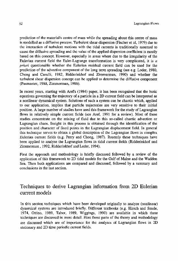
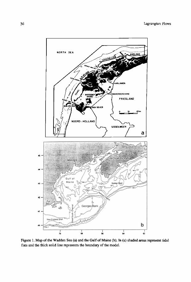
The Dutch Wadden Sea consists of a series of shallow, well mixed tidal basins to the north of the Dutch mainland. Each tidal basin consists of a system of tidal channels surrounded by intertidal flats which is connected to the adjacent North Sea by a relatively narrow and deep tidal inlet between the islands. Here we discuss the Lagrangian flows in the southernmost basin, the Marsdiep basin. The main channel in this basin has a length of some 40 km and a depth of some 10-20 m (see Fig. l a). The topography within the channel is irregular. A typical length scale of the topographical irregularities (e.g. channel bends and sand banks) is some 5-10 km. The amplitude of the dominant semi- diurnal barotropic tidal current is some 1 m/s in the deeper parts of the channels which corresponds with a tidal excursion length of some 10-15 km (Ridderinkhof, 1988).

36 Lagrangian Flows

Gulf of

New England Shelf

I I I I 70 68 66 64 62

Figure 1. Map of the Wadden Sea (a) and the Gulf of Maine (b). In (a) shaded areas represent tidal flats and the thick solid line represents the boundary of the model.

Ridderinkhof 37

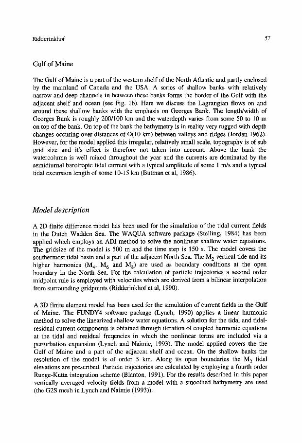
Gulf of Maine

The Gulf of Maine is a part of the western shelf of the North Atlantic and partly enclosed by the mainland of Canada and the USA. A series of shallow banks with relatively narrow and deep channels in between these banks forms the border of the Gulf with the adjacent shelf and ocean (see Fig. lb). Here we discuss the Lagrangian flows on and around these shallow banks with the emphasis on Georges Bank. The length/width of Georges Bank is roughly 200/100 km and the waterdepth varies from some 50 to 10 m on top of the bank. On top of the bank the bathymetry is in reality very rugged with depth changes occuring over distances of O(10 km) between valleys and ridges (Jordan 1962). However, for the model applied this irregular, relatively small scale, topography is of sub grid size and it's effect is therefore not taken into account. Above the bank the watercolumn is well mixed throughout the year and the currents are dominated by the semidiurnal barotropic tidal current with a typical amplitude of some 1 m/s and a typical tidal excursion length of some 10-15 km (Burman et al, 1986).

Model description

A 2D finite difference model has been used for the simulation of the tidal current fields

in the Dutch Wadden Sea. The WAQUA software package (Stelling, 1984) has been applied which employs an ADI method to solve the nonlinear shallow water equations. The gridsize of the model is 500 rn and the time step is 150 s. The model covers the southermost tidal basin and a part of the adjacent North Sea. The M 2 vertical tide and its higher harmonics (M 4, M 6 and M8) are used as boundary conditions at the open boundary in the North Sea. For the calculation of particle trajectories a second order midpoint rule is employed with velocities which are derived from a bilinear interpolation from surrounding gridpoints (Ridderinkhof et al, 1990).

A 3D finite element model has been used for the simulation of current fields in the Gulf

of Maine. The FUNDY4 software package (Lynch, 1990) applies a linear harmonic method to solve the linearized shallow water equations. A solution for the tidal and tidal- residual current components is obtained through iteration of coupled harmonic equations at the tidal and residual freqencies in which the nonlinear terms are included via a perturbation expansion (Lynch and Naimie, 1993). The model applied covers the the Gulf of Maine and a part of the adjacent shelf and ocean. On the shallow banks the resolution of the model is of order 5 km. Along its open boundaries the M 2 tidal elevations are prescribed. Particle trajectories are calculated by employing a fourth order Runge-Kutta integration scheme (Blanton, 1991). For the results described in this paper vertically averaged velocity fields from a model with a smoothed bathymetry are used (the G2S mesh in Lynch and Naimie (1993)).

38 Lagrangian Flows

5kin I !

I I

Figure 2. The residual mass transport streamfunction in the Marsdiep basin (a) and the Gulf of Maine (b). In (a) the interval between successive isolines is .2.106 m3/s and in (b) .03-106 m3/s . Dashed lines indicate the region which is studied in more detail in the next figures. Thick solid lines indicate the coastlines.

Ridderinkhof 39

b

... e.-- /

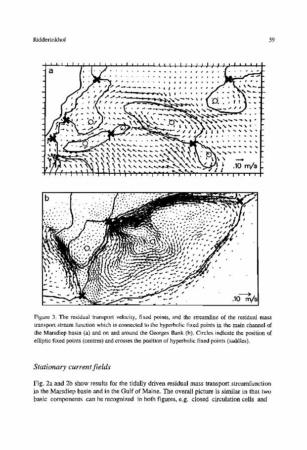
Figure 3. The residual transport velocity, fixed points, and the streamline of the residual mass transport stream function which is connected to the hyperbolic fixed points in the main channel of the Marsdiep basin (a) and on and around the Georges Bank (b). Circles indicate the position of elliptic fixed points (centres) and crosses the position of hyperbolic fixed points (saddles).

Stationary current fields

Fig. 2a and 2b show results for the tidally driven residual mass transport streamfunction in the Marsdiep basin and in the Gulf of Maine. The overall picture is similar in that two basic components can be recognized in both figures, e.g. closed circulation cells and

40 Lagrangian Flows

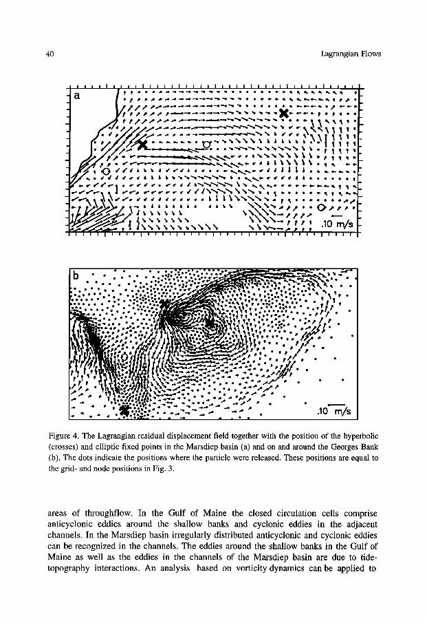
Figure 4. The Lagrangian residual displacement field together with the position of the hyperbolic (crosses) and elliptic fixed points in the Marsdiep basin (a) and on and around the Georges Bank (b). The dots indicate the positions where the particle were released. These positions are equal to the grid- and node positions in Fig. 3.

areas of throughflow. In the Gulf of Maine the closed circulation cells comprise anticyclonic eddies around the shallow banks and cyclonic eddies in the adjacent channels. In the Marsdiep basin irregularly distributed anticyclonic and cyclonic eddies can be recognized in the channels. The eddies around the shallow banks in the Gulf of Maine as well as the eddies in the channels of the Marsdiep basin are due to tide- topography interactions. An analysis based on vorticity dynamics can be applied to

Ridderinkhof 41

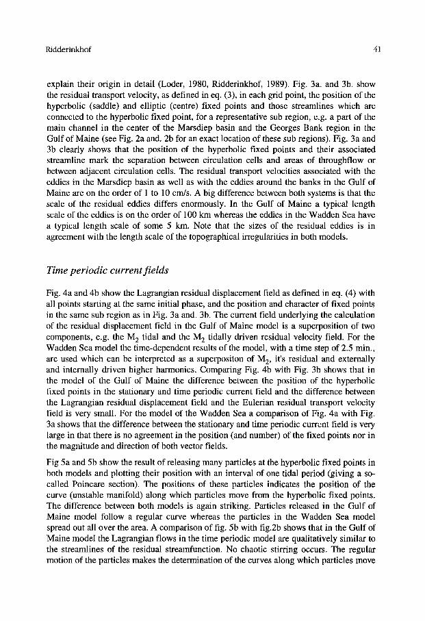
explain their origin in detail (Loder, 1980, Ridderinkhof, 1989). Fig. 3a. and 3b. show the residual transport velocity, as defined in eq. (3), in each grid point, the position of the hyperbolic (saddle) and elliptic (centre) fixed points and those streamlines which are connected to the hyperbolic fixed point, for a representative sub region, e.g. a part of the main channel in the center of the Marsdiep basin and the Georges Bank region in the Gulf of Maine (see Fig. 2a and. 2b for an exact location of these sub regions). Fig. 3a and 3b clearly shows that the position of the hyperbolic fixed points and their associated streamline mark the separation between circulation cells and areas of throughflow or between adjacent circulation cells. The residual transport velocities associated with the eddies in the Marsdiep basin as well as with the eddies around the banks in the Gulf of Maine are on the order of 1 to 10 cm/s. A big difference between both systems is that the scale of the residual eddies differs enormously. In the Gulf of Maine a typical length scale of the eddies is on the order of 100 km whereas the eddies in the Wadden Sea have

a typical length scale of some 5 km. Note that the sizes of the residual eddies is in agreement with the length scale of the topographical irregularities in both models.

Time periodic current fields

Fig. 4a and 4b show the Lagrangian residual displacement field as defined in eq. (4) with all points starting at the same initial phase, and the position and character of fixed points in the same sub region as in Fig. 3a and. 3b. The current field underlying the calculation of the residual displacement field in the Gulf of Maine model is a superposition of two components, e.g. the M 2 tidal and the M 2 tidally driven residual velocity field. For the Wadden Sea model the time-dependent results of the model, with a time step of 2.5 min., are used which can be interpreted as a superpositon of M 2, it's residual and externally and internally driven higher harmonics. Comparing Fig. 4b with Fig. 3b shows that in the model of the Gulf of Maine the difference between the position of the hyperbolic fixed points in the stationary and time periodic current field and the difference between the Lagrangian residual displacement field and the Eulerian residual transport velocity field is very small. For the model of the Wadden Sea a comparison of Fig. 4a with Fig. 3a shows that the difference between the stationary and time periodic current field is very large in that there is no agreement in the position (and number) of the fixed points nor in the magnitude and direction of both vector fields.

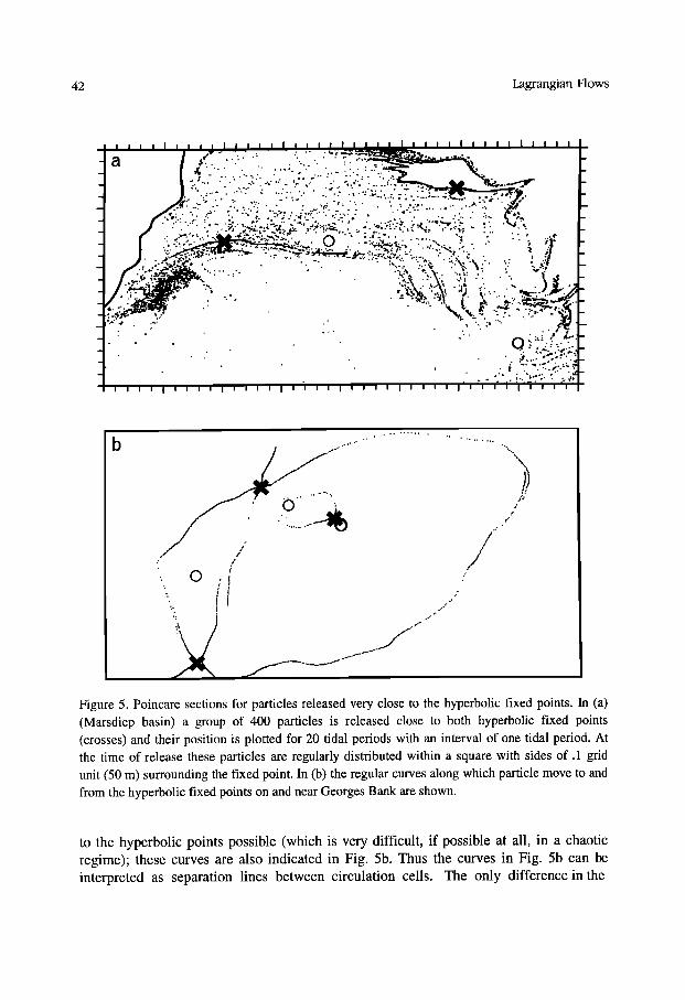
Fig 5a and 5b show the result of releasing many particles at the hyperbolic fixed points in both models and plotting their position with an interval of one tidal period (giving a so- called Poincare section). The positions of these particles indicates the position of the curve (unstable manifold) along which particles move from the hyperbolic fixed points. The difference between both models is again striking. Particles released in the Gulf of Maine model follow a regular curve whereas the particles in the Wadden Sea model spread out all over the area. A comparison of fig. 5b with fig.2b shows that in the Gulf of Maine model the Lagrangian flows in the time periodic model are qualitatively similar to the streamlines of the residual streamfunction. No chaotic stirring occurs. The regular motion of the particles makes the determination of the curves along which particles move

42 Lagrangian Flows

..,,/

Figure 5. Poincare sections for particles released very close to the hyperbolic fixed points. In (a) (Marsdiep basin) a group of 400 particles is released close to both hyperbolic fixed points (crosses) and their position is plotted for 20 tidal periods with an interval of one tidal period. At the time of release these particles are regularly distributed within a square with sides of .1 grid unit (50 m) surrounding the fixed point. In (b) the regular curves along which particle move to and from the hyperbolic fixed points on and near Georges Bank are shown.

to the hyperbolic points possible (which is very difficult, if possible at all, in a chaotic regime); these curves are also indicated in Fig. 5b. Thus the curves in Fig. 5b can be interpreted as separation lines between circulation cells. The only difference in the

Ridderinkhof 43

I I I I I I I I I I I I J I i I I J I J J I I I I J I I I I I I I I I I I I I !

t

..

.

ß ß •

ß . .

ß

I i i • I I I I I I I I i • I I • I I I • I I I I I I I I i I I I I • • i •

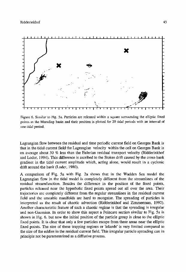
Figure 6. Similar to Fig. 5a. Particles are released within a square surrounding the elliptic fixed points in the Marsdiep basin and their position is plotted for 20 tidal periods with an interval of one tidal period.

Lagrangian flow between the residual and time periodic current field on Georges Bank is that in the tidal current field the Lagrangian velocity within the cell on Georges Bank is on average about 30 % less than the Eulerian residual transport velocity (Ridderinkhof and Loder, 1994). This difference is ascribed to the Stokes drift caused by the cross-bank gradient in the tidal current amplitude which, acting alone, would result in a cyclonic drift around the bank (Loder, 1980).

A comparison of Fig. 5a with Fig. 2a shows that in the Wadden Sea model the Lagrangian flow in the tidal model is completely different from the streamlines of the residual streamfunction. Besides the difference in the position of the fixed points, particles released near the hyperbolic fixed points spread out all over the area. Their trajectories are completely different from the regular streamlines in the residual current field and the unstable manifolds are hard to recognise. The spreading of particles is interpreted as the result of chaotic advection (Ridderinkhof and Zimmerman, 1992). Another characteristic feature of such a chaotic regime is that the spreading is irregular and non-Gaussian. In order to show this aspect a Poincare section similar to Fig. 5a is shown in Fig. 6. but now the initial position of the particle group is close to the elliptic fixed points. It is clear that only a few particles escape from these areas near the elliptic fixed points. The size of these trapping regions or 'islands' is very limited compared to the size of the eddies in the residual current field. This irregular particle spreading can in principle not be parameterized as a diffusive process.

44 Lagrangian Flows

Releasing particle groups covering different initial sizes and evaluating their spatial variance after one tidal period shows that the results are sensitive to the initial position and size of the particle group (Ridderinkhof and Zimmerman, 1990). Ascribing a diffusion coefficient to the variance growth, while realizing that the spreading can formally not be described as a diffusive process, gives a value of order 100 m2/s. This value falls in the range of observations with dye experiments in similar tidal areas (Talbot & Talbot, 1974). Adding random motions to the particle trajectories, as a parameterization of turbulent motions, does not change the results significantly in that the spreading remains non-Gaussian with the existence of multiple maxima in the horizontal distribution of particles. Moreover the variance growth remains about the same.

Thus, in summary, in the Gulf of Maine model Lagrangian flows in the tidal model are similar to the Lagrangian flows in the stationary model of the tidally driven residual currents. The addition of the tidal current does not change the presence and size of closed circulation cells since no chaotic advection is present. In contrast to this, chaotic advection occurs in the tidal model of the Wadden Sea. Here the addition of time-

periodic currents destroys the closed circulation cells and a stirring of particles occurs with an extreme sensitivity of particle trajectories to their initial position. Thus the Lagrangian displacement of a particle can not be predicted from the streamlines of the residual mass transport nor from the presence of separation lines in the Lagrangian residual displacement field.

Discussion

The Lagrangian flow in a stationary model is along the streamlines of the residual mass transport streamfunction which, in both models, is based on the tidally driven resiudal transport current field. This tidally driven residual current field is caused by tide- topography interactions which result in tidally driven residual eddies. These eddies are the main component of the residual streamfunction in both areas. Therefore closed circulation cells are dominantly present in both stationary models. The circulation cells in both models differ in size due to the differences in underlying bathymetry.

A large qualitative difference occurs in the Lagrangian flows in the time periodic current fields in both models in that the Lagrangian flows in the Gulf of Maine model only marginally differ from the flows in the stationary current field whereas in the Wadden Sea model chaotic advection of particles in the tidal current field gives a completely different picture from the stationary current field. This difference is ascribed to the difference in the irregularities in both the tidal and residual current fields in both areas. Both spatial and temporal components of the current field contribute to these irregularities.

With respect to the temporal variability both models differ in that the time periodic current field in the Gulf of Maine model consists of two temporal modes (the total

Ridderinkhof 45

current field is composed by a superposition of the residual (zero) and tidal frequency) whereas in the Wadden Sea model more temporal modes are present since the underlying current field is the outcome of a full nonlinear simulation in which the basic M 2 frequency not only contributes to the residual current field but also to higher harmonics (e.g. M4,M6,M 8 etc.).

With respect to the spatial variability both models differ in that the dominant length scale of the irregularities in the current field of the Wadden Sea model are from the same order as the tidal excursion length whereas the dominant length scale in the Gulf of Maine model far exceeds the tidal excursion length. This difference is clearly expressed in the difference between the sizes of the dominant residual eddies in both areas (see Fig. 2.). Thus over the scale of the excursion length of the particles the current field in the Gulf of Maine model is much more uniform than in the Wadden Sea model. These differences in

the length scale of the irregularities in the current field are caused firsfly by the different scales of bathymetric variations in both areas and secondly by the resolution of this bathymetry in both models. In order to be able to simulate irregularities in a current field over the excursion length of the particles it is necessary to represent the bathymetric variations on this length scale in a model. This means that at least a few gridpoints per tidal excursion length have to be present. Interestingly a simulation with a non-smoothed version of the bathymetry on top of Georges Bank, where the distance between nodes is on the order of 2 to 3 km, gives a chaotic spreading of particles in this area (Ridderinkhof and Loder, 1994). These results indicate that the tendency towards a chaotic regime of particle spreading will increase with increasing reality of the underlying velocity fields.

The sensitivity of the Lagrangian flows to the length scale of the irregularities in the underlying Eulerian current field is in agreement with the analyses of particle trajectories in a simple kinematical model (Ridderinkhof and Zimmerman, 1992, Beerens et al, 1994). In these studies it is shown show that in a current field consisting of uniform periodic tidal currents superimposed on a regular lattice of residual eddies the size of the chaotic region and the intensity of the particle spreading depends heavily on the ratio between the tidal excursion length and the diameter of the topographical eddies. For small values of this ratio Beerens et al (1994) predict a small region which is influenced by chaotic advection (having a size of some .5 to 1% of the size of the topographical eddy). Such a region was not detected in the model of the Gulf of Maine. The cause of this is as yet unclear but might have to do with inevatible numerical approximations in the computation of both the current field and the Lagrangian trajectories. For values representative for the current field in the Wadden Sea model, the kinematical model predicts a substantial region which is influenced by chaotic advection (some 30% of the total area). This underestimation compared to the realistic model of the Wadden Sea is most presumably due to the (over)simplification of the current field in the kinematical model. However, it clearly shows the importance of the presence of irregularities in the Eulerian current field over the length scale of the tidal excursion for widespread chaotic advection to occur.

46 Lagrangian Flows

Summary and conclusions

Techniques originally devised for analyzing (nonlinear) dynamical systems are a powerful tool for analyzing Lagrangian flows in complex 2D stationary and time- periodic current fields. The identification of hyperbolic fixed points and the curves along which particles proceed to or receed from these points provides insight in the global Lagrangian circulation.

In a stationary current field this method is equal to selecting the streamlines of the residual mass transport streamfunction which are connected to the hyperbolic points. These streamlines indicate the position of the outermost streamline surrounding an eddy and are useful for delineating closed circulation cells and areas of throughflow in the Lagrangian flow.

In a time-periodic current field the position and character of the curves along which particles move to and from hyperbolic fixed points are either similar to the regular streamlines of the stationary current field or, in a chaotic regime, differ substantially and show 'wild' oscillations. In the first situation the Lagrangian flows are qualitatively similar to the Lagrangian flows in the stationary current field. In the chaotic regime an irregular stirring of particles occurs which is most intense near the hyperbolic fixed points and less intense near the elliptic fixed points where 'islands' of trapped particles can exist. Although the underlying current field does not contain any random components the spreading of particles is quasi-random. This, combined with the insensitivity of the results to the addition of random motions, means that in such areas the classical shear dispersion concept as a framework for mixing is not valid (Ridderinkhof and Zimmerman, 1992).

An application of this methodology to study the Lagrangian flows in tidal models of the Gulf of Maine and the Wadden Sea shows that the results with respect to the occurrence of chaotic advection are sensitive to length scale over which irregularities are present in the Eulerian current field. If this length scale is on the order of the tidal excursion length widespread chaotic advection appears to occur whereas the Lagrangian flows are regular and qualititatively similar to the flows in the stationary current field if this length scale is much larger than the tidal excursion length. Both applications show that the stationary residual current field can not be used to predict the advective component of the spreading of material. On Georges Bank the direction of the residual transport velocity is similar to the the Lagrangian residual displacement but it's magnitude is on average some 30% too high. In the Wadden Sea there is no agreement at all between the residual transport velocity field and the Lagrangian residual displament field. Thus for a realistic simulation of the transport of material the time-periodic current field has to be used.

The importance of the irregularities in a tidal current field within the length scale of a tidal excursion for a realistic simulation of Lagrangian flows stresses the importance of the inclusion of topographical detail on this length scale in a model since these iregularities are mainly caused by tide-topography interactions. These interactions also result in the presence of higher harmonics in the current field which contribute to the

Ridderinkhof 47

irregularity of the current field. In order to simulate all of these aspects a full nonlinear model is needed which resolves the bathymetry in sufficient detail.

Acknowledgements. The studies with the Gulf of Maine model were performed during a stay at the Bedford Institute of Oceanography which was supported by the (Canadian) Interdepartemental Panel for Energy, Research and Development and by the US GLOBEC program, sponsored jointly by the US NSF and NOAA. Dan Lynch and co- workers provided the modelling software and John Loder stimulated the model application strategy for the Gulf of Maine. The studies with the Wadden Sea model were performed with the WAQUA software package which is supported by Rijkswaterstaat and ICIM. This is BEWON contribution 79.

References

Aref, H., 1984. Stirring by chaotic advection. J. Fluid Mech. 143: 1-21. Aref, H., 1991. Chaotic advection of fluid particles. Philos. Trans. Roy. Soc. A 333: 273-288. Beerens, S. P., H. Ridderinkhof & J. T. F. Zimmerman, 1994. An Analytical Study of Chaotic

stirring in Tidal Areas. Chaos, Solitons and Fractals. in press B lanton, B., 1991. Drogues.f and Drogdt.f: User's manual for 2-dimensional drogue tracking on a

finite element grid with linear finite elements. Skidaway Institute of Oceanography. Butman, B., J. W. Loder, & R. C. Beardsley 1986. The seasonal mean circulation on Georges

Bank: observation and theory. Georges Bank. Boston, MIT Press. 125-138. Camassa, R. and S. Wiggins, 1991. Transport of a passive tracer in time-dependent Rayleigh-

Benard convection. Physica D 51: 472-482. Cheng, R. T. and V. Casulli, 1982. On Lagrangian residual currents with applications in South San

Fransisco Bay, California. Wat. Res. Res. 18:1652-1662. Fischer, H. B., E.J. List, R.C.Y. Koh, J. Imberger & N.H. Brooks, 1979. Mixing in inland and

coastal waters. Acad. Press, New York: 1-483

Hirsch, M. W. and S. Smale, 1974. Differential equations, dynamical systems, and linear algebra. New York, Academic Press.

Jordan, G. F., 1962. Large submarine sandwaves. Science 136: 839-848. Loder, J. W., 1980. Topographic rectification of tidal currents on the sides of Georges Bank. J.

Phys. Oceanogr. 10: 1399-1416. Lynch, D. R., 1990. Three-dimensional diagnostic model for baroclinic, wind-driven and tidal

circulation in shallow seas; FUNDY4 user's manual. Thayer School of Engineering. Lynch, D. R. and C. E. Naimie, 1993. The M2 Tide and Its Residual on the Outer Banks of the

Gulf of Maine. J. Phys. Oceanogr. 23(10): 2222-2253. Ottino, J. M., 1989. The kinematics of mixing: stretching, chaos and transport. Cambridge,

Cambridge University Press. Ottino, J. M., C. W. Leong, H. Rising & P.D.Swanson, 1988. Morphological structures produced

by mixing in chaotic flows. Nature 333: 419-425. Pasmanter, R., 1988. Anamalous diffusion and anamalous stretching in vortical flows. Fluid Dyn.

Res. 3: 320-326.

48 Lagrangian Flows

Perry, A. E. and M. S. Chong, 1987. A description of eddying motions and flow patterns using critical-point concepts. Ann. Rev. Fluid Mech. 19: 125-155.

Pierrehumbert, R. T., 1991. Chaotic mixing of tracer and vorticity by modulated travelling Rossby waves. Geophys. Astrophys. Fluid Dyn. 58: 285-319.

Prandle, D., 1984. A modelling study of the mixing of Cs 137 in the seas of the European continental shelf. Phil. Trans. Roy. Soc. (A) 310: 407-436.

Ridderinkhof, H. and J. W. Loder, 1994. Lagrangian Characterization of Circulation over Submarine Banks with Application to the Outer Gulf of Maine. J. Phys. Oceanogr. 24 (6): 1184- 2000

Ridderinkhof, H., 1988. Tidal and residual flows in the Western Dutch Wadden Sea, I: Numerical model results. Neth. J. Sea Res. 22: 1-22.

Ridderinkhof, H., 1989. Tidal and residual flows in the Western Dutch Wadden Sea, lIl: Vorticity balances. Neth. J. Sea Res. 24: 9-26.

Ridderinkhof, H., J. T. F. Zimmerman & M. Philippart, 1990. Tidal exchange between the North Sea and the Wadden Sea and mixing time scales of the tidal basins. Neth. J. Sea Res. 25:331- 350.

Ridderinkhof, H. and J. T. F. Zimmerman, 1990. Mixing processes in a numerical model of the Western Dutch Wadden Sea. in: Residual currents and Long Term Transport, Coastal and Estuarine Studies 38, R.T. Cheng (ed.), Springer-Verlag. New York: 93-104

Ridderinkhof, H. and J. T. F. Zimmerman, 1992. Chaotic stirring in a tidal system. Science 258:1107-1111.

Rom-Kedar, V., A. Leonard & S. Wiggins, 1990. An analytical study of transport, mixing and chaos in an unsteady vortical flow. J. Fluid Mech. 214: 347-394.

Stelling, G. S., 1984. On the construction of computational methods for shallow water flow problems. The Netherlands, Rijkswaterstaat.

Tabor, M., 1989. Chaos and integrability in Nonlinear Dynamics: An Introduction. New York, John Wiley & Sons.

Talbot, J. W. and G.A. Talbot, 1974. Diffusion in shallow seas and in English coastal and estuarine waters. Rapp. P. v. Reun. Cons. perm. int. Explor. Mer 167:93-110

Weiss, J. B. and E. Knobloch, 1989. Mass transport and mixing by modulated travelling waves. Phys. Rev. A 40: 2579-2589.

Wiggins, S., 1990. Introduction to Applied Nonlinear Dynamical Systems and Chaos. New York, Springer.

Zimmerman, J. T. F., 1978. Topographic generation of residual circulation by oscillatory (tidal) currents. Geophys. Astrophys. Fluid Dyn. 11:35-47

Zimmerman, J. T. F., 1979. On the Euler-Lagrang transformation and the Stokes drif in the presence of oscillatory and residual currents. Deep Sea Res 26: 505-520.

Zimmerman, J. T. F., 1986. The tidal whirlpool: A review of horizontal dispersion by tidal and residual currents. Neth. J. Sea Res. 20: 133-154.