Signalized Flows
184
Signalized Flows Optimizing Traffic Signals and Guideposts and Related Network Flow Problems Von der Fakult¨at f¨ ur Mathematik, Naturwissenschaften und Informatik der Brandenburgischen Technischen Universit¨at Cottbus zur Erlangung des akademischen Grades Doktor der Naturwissenschaften (Dr. rer. nat.) genehmigte Dissertation von Diplom-Mathematiker Martin Strehler geboren am 24.06.1982 in Karl-Marx-Stadt Gutachter: Prof. Dr. rer. nat. Ekkehard K¨ohler Gutachter: Prof. Dr. rer. nat. Thomas Erlebach Gutachter: Prof. Dr. rer. nat. Kai Nagel Tag der m¨ undlichen Pr¨ ufung: 2. Februar 2012
-
Upload
khangminh22 -
Category
Documents
-
view
0 -
download
0
Transcript of Signalized Flows

Signalized Flows
Optimizing Traffic Signals and Guideposts
and Related Network Flow Problems
Von der Fakultat fur Mathematik, Naturwissenschaften und Informatik
der Brandenburgischen Technischen Universitat Cottbus
zur Erlangung des akademischen Grades
Doktor der Naturwissenschaften(Dr. rer. nat.)
genehmigte Dissertation
von
Diplom-Mathematiker
Martin Strehlergeboren am 24.06.1982 in Karl-Marx-Stadt
Gutachter: Prof. Dr. rer. nat. Ekkehard Kohler
Gutachter: Prof. Dr. rer. nat. Thomas Erlebach
Gutachter: Prof. Dr. rer. nat. Kai Nagel
Tag der mundlichen Prufung: 2. Februar 2012


Abstract
Guideposts and traffic signals are important devices for controlling inner-city traf-fic and their optimized operation is essential for efficient traffic flow without con-gestion. In this thesis, we develop a mathematical model for guideposts and trafficsignals in the context of network flow theory. Guideposts lead to confluent flowswhere each node in the network may have at most one outgoing flow-carrying arc.The complexity of finding maximum confluent flows is studied and several poly-nomial time algorithms for special graph classes are developed. For traffic signaloptimization, a cyclically time-expanded model is suggested which provides the pos-sibility of the simultaneous optimization of offsets and traffic assignment. Thus, theinfluence of offsets on travel times can be accounted directly. The potential of thepresented approach is demonstrated by simulation of real-world instances.
Zusammenfassung
Vorwegweiser und Lichtsignalanlagen sind wichtige Elemente zur Steuerung in-nerstadtischen Verkehrs und ihre optimale Nutzung ist von entscheidender Bedeu-tung fur einen staufreien Verkehrsfluss. In dieser Arbeit werden Vorwegweiser undLichtsignalanlagen mittels der Netzwerkflusstheorie mathematisch modelliert. Vor-wegweiser fuhren dabei zu konfluenten Flussen, bei denen Fluss einen Knoten desNetzwerks nur gebundelt auf einer einzigen Kante verlassen darf. Diese konfluentenFlusse werden hinsichtlich ihrer Komplexitat untersucht und es werden Polynomial-zeitalgorithmen fur das Finden maximaler Flusse auf ausgewahlten Graphenklassenvorgestellt. Fur die Versatzzeitoptimierung von Lichtsignalanlagen wird ein zyklischzeitexpandiertes Modell entwickelt, das die gleichzeitige Optimierung der Verkehrs-umlegung ermoglicht. So kann der Einfluss geanderter Versatzzeiten auf die Fahr-zeiten direkt berucksichtigt werden. Die Leistungsfahigkeit dieses Ansatzes wird mitHilfe von Simulationen realistischer Szenarien nachgewiesen.


3
Acknowledgments
So many people were involved in the development of this thesis. I wish to thank every-body who supported me.
First of all, I thank my supervisor Ekkehard Kohler. I am grateful for his support andencouragement.
Next, I wish to thank Thomas Erlebach and Kai Nagel for taking the assessments ofthis thesis.
I am indebted to my math teacher Stephan Lamm who encouraged my mathemati-cal interests and prepared me well for mathematical competitions. I thank ChristophHelmberg for raising my interest in applied discrete mathematics during my years as un-dergraduate and graduate student even though I was not faithful to the ‘matrix magic’of semidefinite programming.
I would like to thank Christian Liebchen and Gregor Wunsch who were involved inthe first ideas of the cyclically time-expanded network for traffic signal coordination.I also thank Klaus Nokel from ptv AG in Karlsruhe. He and ptv AG supported ourproject, provided the VISSIM tool for simulation, and gave good hints and suggestionsto understand the traffic engineer’s point of view. Likewise, I thank Kai Nagel andhis group from TU Berlin, who equipped us with MATSim and its traffic signal plug-in. Additionally, I thank Klaus Nokel, Gregor Wunsch, Sandor Fekete, Kai Nagel, andDominik Grether for providing real-world scenario data and stimulating ideas on trafficmodels involving traffic signals.
Furthermore, I thank my coauthors Daniel Dressler and Ekkehard Kohler. I amespecially indebted to Daniel, who supplied me with good ideas and good coffee. Ourjoint work on confluent flows filled several dozen black boards.
I also want to thank all members of the research group of Ekkehard Kohler. AlexanderReich and Harald Schulzke provided an excellent working atmosphere. I enjoyed ourdiscussions about discrete mathematics, mathematical riddles and everything under thesun. Moreover, I would like to thank Alex for his careful proofreading of the manuscript.I thank our students Erik Panzer and Rene Schneider who helped me coding thousandsof lines. Diana Hubner was my sure help in cutting through the red tape.
Last, but surely not least, I am grateful to my friends (not necessarily disjoint frompersons mentioned above) and my family.
Cottbus, November 2011 Martin Strehler


Contents 5
Contents
Introduction 9
1 Basic Definitions and Notation 13
1.1 Graphs . . . . . . . . . . . . . . . . . . . . . . . . . . . . . . . . . . . . . . 13
1.2 Flows and Networks . . . . . . . . . . . . . . . . . . . . . . . . . . . . . . 14
1.2.1 Definitions . . . . . . . . . . . . . . . . . . . . . . . . . . . . . . . 14
1.2.2 Important results . . . . . . . . . . . . . . . . . . . . . . . . . . . . 16
1.3 Algorithms and Complexity . . . . . . . . . . . . . . . . . . . . . . . . . . 17
1.3.1 Polynomial-time algorithms . . . . . . . . . . . . . . . . . . . . . . 18
1.3.2 P, NP, and co-NP . . . . . . . . . . . . . . . . . . . . . . . . . . 18
1.3.3 NP-complete problems . . . . . . . . . . . . . . . . . . . . . . . . 19
1.3.4 Complexity of optimization problems . . . . . . . . . . . . . . . . . 19
1.3.5 Approximation . . . . . . . . . . . . . . . . . . . . . . . . . . . . . 20
1.4 Linear Programming and Integer Programming . . . . . . . . . . . . . . . 20
1.4.1 Linear programs . . . . . . . . . . . . . . . . . . . . . . . . . . . . 20
1.4.2 Integer programs . . . . . . . . . . . . . . . . . . . . . . . . . . . . 22
2 Destination-based Routing and Confluent Flows 25
2.1 Guideposts, destination-based routing, and confluent flows . . . . . . . . . 25
2.1.1 Guideposts . . . . . . . . . . . . . . . . . . . . . . . . . . . . . . . 25
2.1.2 Destination-based Routing . . . . . . . . . . . . . . . . . . . . . . 25
2.1.3 Applications . . . . . . . . . . . . . . . . . . . . . . . . . . . . . . 26
2.1.4 Intuitive description of confluent flows . . . . . . . . . . . . . . . . 27
2.2 Preliminaries . . . . . . . . . . . . . . . . . . . . . . . . . . . . . . . . . . 28
2.3 Related problems . . . . . . . . . . . . . . . . . . . . . . . . . . . . . . . . 31
2.3.1 Bottleneck paths . . . . . . . . . . . . . . . . . . . . . . . . . . . . 31
2.3.2 Unsplittable and k-splittable flow . . . . . . . . . . . . . . . . . . . 32
2.3.3 Disjoint paths . . . . . . . . . . . . . . . . . . . . . . . . . . . . . . 32
2.3.4 Confluent flows with uniform arc capacities and congestion . . . . 33
2.3.5 Mixed integer programming and confluent flows . . . . . . . . . . . 34
2.3.6 Confluent flows over time on trees . . . . . . . . . . . . . . . . . . 35
2.3.7 Spanning trees, minimum cost flows and setup costs . . . . . . . . 35
2.4 Complexity . . . . . . . . . . . . . . . . . . . . . . . . . . . . . . . . . . . 36
2.5 A mixed integer programming formulation . . . . . . . . . . . . . . . . . . 39
2.6 A max-flow min-cut theorem . . . . . . . . . . . . . . . . . . . . . . . . . 41
2.7 Arc-confluent flows . . . . . . . . . . . . . . . . . . . . . . . . . . . . . . . 45
2.7.1 Definition of arc-confluent flow . . . . . . . . . . . . . . . . . . . . 45
2.7.2 Complexity results for arc-confluent flows . . . . . . . . . . . . . . 47

6 Contents
3 Algorithms for Confluent Flows 51
3.1 Confluent flows on trees . . . . . . . . . . . . . . . . . . . . . . . . . . . . 51
3.1.1 Maximum Confluent Flows on trees with a single sink . . . . . . . 513.1.2 Confluent transshipments on trees . . . . . . . . . . . . . . . . . . 52
3.2 Confluent flows on graphs with small treewidth . . . . . . . . . . . . . . . 53
3.2.1 Treewidth . . . . . . . . . . . . . . . . . . . . . . . . . . . . . . . . 543.2.2 The dynamic programming approach . . . . . . . . . . . . . . . . . 57
3.2.3 Computing the tables . . . . . . . . . . . . . . . . . . . . . . . . . 593.2.4 Putting it all together . . . . . . . . . . . . . . . . . . . . . . . . . 683.2.5 Constructing an FPTAS . . . . . . . . . . . . . . . . . . . . . . . . 70
3.3 Confluent flows on outerplanar graphs . . . . . . . . . . . . . . . . . . . . 713.3.1 Outerplanar graphs . . . . . . . . . . . . . . . . . . . . . . . . . . 71
3.3.2 Solving confluent flows on outerplanar graphs . . . . . . . . . . . . 713.3.3 Dynamic programming . . . . . . . . . . . . . . . . . . . . . . . . . 763.3.4 Simple functions . . . . . . . . . . . . . . . . . . . . . . . . . . . . 78
3.3.5 Runtime analysis . . . . . . . . . . . . . . . . . . . . . . . . . . . . 803.3.6 Confluent flows and minors . . . . . . . . . . . . . . . . . . . . . . 80
3.4 Planar graphs with all terminals on the boundary . . . . . . . . . . . . . . 83
3.4.1 Boundary instances . . . . . . . . . . . . . . . . . . . . . . . . . . 833.4.2 Preliminaries . . . . . . . . . . . . . . . . . . . . . . . . . . . . . . 84
3.4.3 An algorithm for boundary instances . . . . . . . . . . . . . . . . . 893.5 Conclusion and open problems . . . . . . . . . . . . . . . . . . . . . . . . 93
4 Traffic Signal Coordination 95
4.1 Introduction to traffic signals . . . . . . . . . . . . . . . . . . . . . . . . . 954.1.1 A brief history of traffic signals . . . . . . . . . . . . . . . . . . . . 954.1.2 The language of traffic signals . . . . . . . . . . . . . . . . . . . . . 97
4.1.3 Safety constraints . . . . . . . . . . . . . . . . . . . . . . . . . . . 1004.1.4 Controlling traffic signals . . . . . . . . . . . . . . . . . . . . . . . 101
4.2 Traffic assignment . . . . . . . . . . . . . . . . . . . . . . . . . . . . . . . 1014.2.1 Motivation . . . . . . . . . . . . . . . . . . . . . . . . . . . . . . . 1024.2.2 System optimal flows . . . . . . . . . . . . . . . . . . . . . . . . . . 102
4.2.3 User equilibria and Wardrop’s principles . . . . . . . . . . . . . . . 1034.2.4 Dynamic Flows . . . . . . . . . . . . . . . . . . . . . . . . . . . . . 105
4.2.5 Dynamic traffic assignment . . . . . . . . . . . . . . . . . . . . . . 1074.2.6 Computing assignments . . . . . . . . . . . . . . . . . . . . . . . . 108
4.3 Optimizing traffic signals . . . . . . . . . . . . . . . . . . . . . . . . . . . 109
4.3.1 Measures of performance . . . . . . . . . . . . . . . . . . . . . . . 1104.3.2 Optimization of pretimed signals . . . . . . . . . . . . . . . . . . . 1104.3.3 Adaptive traffic signals . . . . . . . . . . . . . . . . . . . . . . . . . 112
4.3.4 Simultaneous coordination and assignment . . . . . . . . . . . . . 1144.3.5 Tools . . . . . . . . . . . . . . . . . . . . . . . . . . . . . . . . . . 114
4.3.6 Conclusions . . . . . . . . . . . . . . . . . . . . . . . . . . . . . . . 1154.4 Complexity of signal coordination . . . . . . . . . . . . . . . . . . . . . . . 116

Contents 7
5 A New Model 119
5.1 Motivation . . . . . . . . . . . . . . . . . . . . . . . . . . . . . . . . . . . 1195.2 The new model . . . . . . . . . . . . . . . . . . . . . . . . . . . . . . . . . 121
5.2.1 Cyclically time-expansion . . . . . . . . . . . . . . . . . . . . . . . 1215.2.2 Expanded intersections . . . . . . . . . . . . . . . . . . . . . . . . 1225.2.3 Modeling traffic signals . . . . . . . . . . . . . . . . . . . . . . . . 1235.2.4 Modeling traffic assignment . . . . . . . . . . . . . . . . . . . . . . 124
5.3 Mixed integer programming formulation . . . . . . . . . . . . . . . . . . . 1245.4 Properties of the model . . . . . . . . . . . . . . . . . . . . . . . . . . . . 1255.5 Analyzing link performance . . . . . . . . . . . . . . . . . . . . . . . . . . 126
5.5.1 Link performance of a single road . . . . . . . . . . . . . . . . . . . 1275.5.2 Link performance for platoons of cars . . . . . . . . . . . . . . . . 1285.5.3 Link performance in networks and user equilibria . . . . . . . . . . 130
5.6 Model improvements . . . . . . . . . . . . . . . . . . . . . . . . . . . . . . 1345.6.1 Split and phase optimization . . . . . . . . . . . . . . . . . . . . . 1345.6.2 Multiple signal plans . . . . . . . . . . . . . . . . . . . . . . . . . . 1375.6.3 Flow dependent travel times with fan graphs . . . . . . . . . . . . 1375.6.4 Queues . . . . . . . . . . . . . . . . . . . . . . . . . . . . . . . . . 1385.6.5 First-in first-out . . . . . . . . . . . . . . . . . . . . . . . . . . . . 1385.6.6 Intersections without signals . . . . . . . . . . . . . . . . . . . . . 140
6 Experiments 141
6.1 Scenarios . . . . . . . . . . . . . . . . . . . . . . . . . . . . . . . . . . . . 1416.1.1 Portland and Denver . . . . . . . . . . . . . . . . . . . . . . . . . . 1416.1.2 Braunschweig and Cottbus . . . . . . . . . . . . . . . . . . . . . . 142
6.2 Test procedure . . . . . . . . . . . . . . . . . . . . . . . . . . . . . . . . . 1446.2.1 Data processing . . . . . . . . . . . . . . . . . . . . . . . . . . . . . 1456.2.2 Simulation . . . . . . . . . . . . . . . . . . . . . . . . . . . . . . . 146
6.3 Installing green waves . . . . . . . . . . . . . . . . . . . . . . . . . . . . . 1476.4 Comparison to established approaches . . . . . . . . . . . . . . . . . . . . 1496.5 Advantages of simultaneous assignment . . . . . . . . . . . . . . . . . . . 1506.6 Solving the MIP . . . . . . . . . . . . . . . . . . . . . . . . . . . . . . . . 157
6.6.1 Influence of granularity . . . . . . . . . . . . . . . . . . . . . . . . 1586.6.2 Column generation . . . . . . . . . . . . . . . . . . . . . . . . . . . 1596.6.3 Relaxation and Branch&Cut. . . . . . . . . . . . . . . . . . . . . . 160
6.7 Conclusion . . . . . . . . . . . . . . . . . . . . . . . . . . . . . . . . . . . 161
Bibliography 165
List of figures 177
Index 179


0 INTRODUCTION 9
Introduction
Urban traffic congestion is increasing day by day. Examples can be found around theworld. Growing cities and increasing population doubled the traffic volume in the last twodecades in Europe and North America and an even higher rise has to be expected for theurban regions in Asia or South America in the next years. In Germany, the populationtravels about 1000 billion kilometers every year, and 85 percent of this distance is coveredby individual motor car traffic [25, 56]. The city of Sao Paulo, Brazil, is famous for itsrecord-breaking traffic jams. The 20 million inhabitants own about six million vehicles.On an evening in June 2009, the traffic congestion the city reached a new record of293 kilometers in total [47]. In August 2010, there was a 60-mile, nine-day traffic jamnear Beijing, China, that even made headlines in Europe.
Traffic congestion causes delays which add up to huge costs for society and business.The urban mobility report 2009 [136] states a total loss of 4.2 billion hours and87.2 billion dollars for the 439 urban areas in the United States in only one year.Wasted fuel of 2.8 billion gallons, noise, and pollution accumulate. A huge problem hasto be solved.
But what can mathematics do to support the quest for stress-free, environment-friendly,and safe traveling? In this thesis we will have a close look at two familiar systemsfor traffic control–guideposts and traffic signals. If you do not like traffic jams you areinvited to read on and find out how an optimization of guideposts and traffic signals canbe used to direct and improve inner-city traffic flow.
Guideposts. Guideposts have been used for a long time. They provide guidance, es-pecially in unfamiliar regions. With increasing mobility, we cannot imagine travelingwithout guideposts and we can find them everywhere. Even modern GPS-based satellitenavigation systems can be seen as small, virtual guideposts inside our cars. Everythingseems clear–just follow the guideposts!
But we missed an important question. Where should we install these guideposts? Andwhat consequences arise from our choice?
Assume we want to find a certain point of interest in an unfamiliar network. Fortu-nately, this network is equipped with guidepost pointing towards our destination wher-ever a routing decision has to be made. Further, we may assume that these guidepostspoint in an unique direction, i.e. they exclude all but one road at each intersection.Nothing would be more confusing than two guidepost naming the same destination butpointing in two different directions. Most likely, other traffic participants with the samedestination will follow these guideposts, too. If we meet one of them, she will makethe same routing decisions just like us. Thus, we will travel on the same route until wereach our destination. Consequently, a group of road users starting at the same originwill share the same path, even if there would exist several alternatives. The capacity ofthis path limits the amount of traffic participants that can reach the common destina-tion. With road users starting all over the network, a bad choice of guideposts may leadto congestion, although the traffic flow in the network is far away from the network’s

10
capacity at free route choice.
Traffic signals. With increasing car traffic, traffic signals managing the right of way atintersections became more and more important. However, the red traffic light seems tobe dominant. But sometimes, we arrive at a traffic signal and it switches to green justin time, so that we can go on without stopping. And once in a blue moon1, we get evenfour or five green lights in a row.
Such a traffic signal coordination is a difficult task. Of course, coordinating one roadin one direction is rather easy, but with traffic in the opposite direction or traffic in awhole street network it becomes considerably harder.
Even more, changing the coordination also means changing travel times. After awhile road users will learn about the fastest routes in the network and they will switchto these routes. This new distribution of traffic in the network may completely disturbour fine-tuned coordination.
Obviously, guideposts and traffic signals are important tools for controlling traffic andtraffic control is the backbone in the management of traffic flows in our cities. Theoptimal use of these signals is essential when we are going to resolve traffic congestion.However, it is sometimes not even clear what ‘optimal’ means in this context. Guide-posts are often installed with respect to the shortest distance towards the destination.Their influence on congestion is poorly studied. In contrast, traffic signal coordinationhas been investigated for a long time and many approaches and models have been pro-posed. But these models also recommend various definitions of optimality. The twomost common objectives are minimizing the delay/waiting time of vehicles facing redlights and minimizing the number of stops. Furthermore, the majority of the approachesreveal some deficits like unrealistic modeling of inner-city traffic flows or no guaranteefor an optimal solution.
Contribution
In this thesis, we tackle traffic congestion with the help of network flow theory fromtwo sides. First, we advance guideposts from a theoretical point of view and introduceconfluent flows. A flow is called confluent if the flow uses at most one outgoing arc ateach node. Unlike previous results we consider heterogeneous arc capacities. We willfocus on NP-hardness results for maximum confluent flows, an approximation algorithmfor graphs with treewidth bounded by a constant k, and polynomial time-algorithms forspecial graph classes.
Second, we advance traffic signals. Since this discussion is actually a practical one –most results presented in this part are an outcome of the ADVEST project that emerged
1A blue moon refers to the third full moon in a season with four full moons. A season with four fullmoons is very rare, this happens only once every 2 or 3 years.

0 INTRODUCTION 11
between BTU Cottbus, TU Berlin, TU Braunschweig, and PTV AG2 – we start ourcontribution with a new model for the simultaneous optimization of traffic signal coordi-nation and traffic assignment. This combined approach accounts the feedback betweenred lights and route choices. We answer the time dependance of traffic signals by acyclically time-expanded network. This time expansion will also allow capturing severalother characteristics of inner-city traffic like platoons of cars and exact arrival times ofthese platoons at the intersections. Still, viewing inner-city traffic as a periodic processlimits the time horizon of the expansion and leads to a compact formulation of the prob-lem as a mixed-integer program. Solving the MIP yields a guarantee or at least boundsfor the optimal solution. We investigate our approach with the help of real-world dataand state-of-the-art simulation tools.
Outline of the thesis
In Chapter 1 we will fix the notation and terminology and present basic definitions.We assume the reader to be familiar with the basic concepts in graph theory, complexitytheory as well as linear programming. However, for later reference and as a short refresh-ing of knowledge we recall some of the most important facts. For additional informationwe refer to [2, 66, 100, 122, 147].
In Chapter 2 we will derive the concept for flows in networks with guideposts. Forthat, we will introduce confluent flows and conclude some basic properties, e.g. theunderlying tree structure. We will study complexity result for both the transshipmentand the maximum flow variant. We also present arc-confluent flows and discuss cuts forconfluent flows.
Afterwards, we present polynomial time algorithms for restricted graph classes,e.g. trees, planar graphs with at most k terminals on the boundary, and graphs with-out K2,3 as a minor in Chapter 3. The relation between confluent flows and trees willlead to a pseudo-polynomial time solution for maximum confluent flows on graphs withtreewidth bounded by a constant k. We use this result to develop a fully polynomial timeapproximation scheme (FPTAS) for confluent flows on this kind of graphs.
Due to the various approaches for traffic signal optimization we start with a shortsurvey on this topic in Chapter 4. We will use this survey to make the reader familiarwith concepts in traffic engineering and with terms related to traffic signals. We willalso discuss the advantages and disadvantages of the considered approaches to motivateour new model. Herewith, the ground for the next two chapters should be prepared.Additional information can be found, e.g., in [69, 141].
In Chapter 5 we use the concept of dynamic flows and the periodicity of traffic signalsto develop a cyclically time-expanded network. The model is completed by modelingintersections, traffic signals and traffic assignment. As a main result of this chapterwe show how this model can be used to optimize traffic signal coordination and trafficassignment simultaneously. Aiming for a realistic modeling we also discuss the conse-
2PTV AG is a traffic planning company from Karlsruhe, Germany. It is well known for its trafficplanning and simulation software VISUM and VISSIM.

12
quences of our approach to travel times and link performance in detail and derive furtherproperties of the model.
Finally, Chapter 6 is designated for the simulation of inner-city traffic and the practi-cal evaluation of the proposed model. We introduce the reader to two traffic simulationtools, namely VISSIM and MATSim. In detail, we consider the real-world inner-citynetworks of Cottbus, Braunschweig, Portland, and Denver. In particular, we empha-size the advantages of our simultaneous optimization of signal coordination and trafficassignment by comparing to a decomposed successive version of our approach.
About this thesis
A lot of results in this thesis were obtained during the ADVEST project, grantedby the German ministry of education and research (BMBF). This also reflects in thethesis. First, some results were already published, see [52, 53, 96, 97, 98]. Second, theaims of the project lead to different kinds of results. On the one hand confluent flowswere studied theoretically and are better understood now. But due to the combinatorialcomplexity practical applicability is – in the moment – poor. One the other hand, in amore experimental approach, a new model for simultaneous traffic signal coordinationand traffic assignment was created, implemented, improved and tested with help ofsimulation tools. Hereby, a model of high practicability was developed, but it is difficultto prove the impact of the model also mathematically. Hence, the first part of the thesiswill perhaps be more interesting for readers who focus on combinatorial optimization.The second part may more appeal to readers who are interested in the modeling of realworld problems.

1 BASIC DEFINITIONS AND NOTATION 13
1 Basic Definitions and Notation
In this chapter we introduce and fix the basic notation for this thesis. Many fields ofdiscrete mathematics are touched. First, we introduce the graph notation and we presentsome classical graph problems that we will refer to later. Due to the wide area of graphtheory this description cannot be complete. For an introduction to graph theory wesuggest, e.g., [152] or [49]. A good textbook on network flows is, for example, [2]. Goodtextbooks, covering network flows and other combinatorial optimization strategies, are[36, 100, 138]
Furthermore, we fix the notations for algorithms, complexity and approximation.Again, we can only give a short overview. For additional information, we refer to [66]and [9].
Linear Programming and Integer Programming are two basic approaches to solvenetwork flow problems and combinatorial optimization problems. We will introduceboth techniques in section 1.4 and suggest [147, 153] for further reading.
Please note that the following chapters also provide their own introductions and termsspecific to these chapters are defined there.
1.1 Graphs
In this work we consider finite graphs G = (V,E) where V = V (G) is the vertex setand elements v ∈ V are called vertices or nodes. E = E(G) is the edge set of G. Weconsider both undirected and directed graphs (digraphs). In the case of undirected, loopfree graphs the edge set is a subset of V 2, i.e. E ⊆ {{u, v} : u, v ∈ V, u 6= v}.
To denote directed edges, we also call them arcs. E is termed arc set A. A consistsof ordered pairs of nodes, i.e. A ⊆ V × V = {(u, v) : u, v ∈ V }. Therefore, each arca ∈ A, a = (u, v) is directed from its tail(a) = u to its head(a) = v. For v ∈ V , we useδ−(v) = {a ∈ A : v = head(a)} for the set of incoming arcs and δ+(v) = {a ∈ A : v =tail(a)} for the set of outgoing arcs. A graph is called bi-directed if it contains for eacharc a = (u, v) also the arc in the opposite direction a′ = (v, u). A directed graph can bemade undirected by simply deleting the directions of the arcs. To make an (undirected)graph a bi-directed one we add both directions for each edge/arc.
The cardinalities of the node and edge sets are denoted by n = |V | and m = |E|. Agraph with n vertices that contains all possible edges, is called a complete graph anddenoted by Kn. Obviously, the complete graph has m =
(
n2
)
= n(n−1)2 edges. Sometimes,
a graph is allowed to contain multi-edges, i.e., parallel edges. Hence, E, or A respectively,is defined as a multi-set in this case and G is called multi-graph. The induced subgraphon a vertex set V ′ ⊆ V is denoted by G[V ′]. The induced arc set of G[V ′] is denoted byA[V ′].
A sequence W = (a1, . . . , ak), ai ∈ A, of arcs is called a walk if it fits head to tail,i.e. head(ai) = tail(ai+1) ∀i ∈ {1, . . . , k − 1}. For short, we will use tail(W ) := tail(a1)and head(W ) := head(ak). V [W ] is used for the set of vertices that occur in the arcsof W . To simplify matters, we use a ∈ W to denote that the arc a is contained in thesequence of arcs in walk W . A path P is a walk which passes through every vertex at

14 1.2 Flows and Networks
most once. A walk/path where the tail of the first arc and the head of the last arccoincide is called cycle/circuit . For u, v ∈ V , Pu,v denotes the set of all paths with tail uand head v. The length of a path (with respect to unit edge lengths) is the number of arcsin its sequence. Two paths P1 and P2 are (arc) disjoint if A[V [P1]]∩A[V [P2]] = ∅. Theyare node disjoint if V [P1] ∩ V [P2] = ∅. The composition of two paths P1 = (a1, . . . , ak)and P2 = (b1, . . . , bl) is defined as P1 ◦ P2 = (a1, . . . , ak, b1, . . . , bl).
Similarly, walks, paths, cycles, and circuits can be defined for undirected graphs.
A graph is strongly connected if for each pair of vertices (u, v) there exists a path Pfrom u to v, i.e. tail(P ) = u and head(P ) = v. A graph is weakly connected if its corre-sponding bi-directed graph is strongly connected. A node set U ⊆ V is (strongly/weakly)connected if the induced graph G[U ] is (strongly/weakly) connected. The inclusion max-imal (strongly/weakly) connected subgraphs of G are called (strongly/weakly) connectedcomponents.
A cut in G is an arc set C such that G\C = (V,A\C) has at least one connectedcomponent more than G. The value of a cut is simply the number of arcs in the cut.An s-t-cut is defined as a partition of V into two subsets C1 and C2, such that s ∈ C1
and t ∈ C2. Let C = {a ∈ A : tail(a) ∈ C1 ∧ head(a) ∈ C2} then there exists no directedpath from s to t in G\C. The value of the s-t-cut is |C|, i.e. the number of forward arcsfrom C1 to C2.
1.2 Flows and Networks
Flows have been a major planning tool for many applications ever since Ford and Fulk-erson [58] studied them. Before considering flows with additional routing constraints inthe following sections, standard flow is introduced here.
1.2.1 Definitions
Although there is consens what a flow in a network should be, we will use a slightlydifferent and modular approach for defining flows3.
A flow function is a non-negative function on the arc set x : A → R+0 . In most
practical applications the maximal flow on each arc is limited by a capacity bound, i.e.,a maximal flow value that cannot be exceeded on this arc. The capacities are given bya function u : A → R+
0 ∪ {∞}. A flow is feasible if 0 ≤ x(e) ≤ u(e) ∀e ∈ A holds.A graph together with capacities is called a network G = (V,A, u). For some resultsin this thesis, we will limit the capacity function to integer values, i.e., u : A → N0.This is no restriction for most applications, since rational values can simply be scaled tointeger values and irrational numbers cannot exactly be represented in our computersanyway4.Furthermore, a flow function is integral if it has only integral values.
3In some of the algorithms especially in Section 3, we will not be able to fulfill all requirements of aflow at once. A modular definition admits step-by-step procedures. For example, we will define andderive preflows with a slightly different flow conservation constraint.
4Irrational input may yield a unexpected behavior, the algorithm of Ford and Fulkerson is a primeexample.

1 BASIC DEFINITIONS AND NOTATION 15
The inflow and outflow of a flow function x at a given node v are
inflowx(v) :=∑
a∈δ−(v)
x(a)
outflowx(v) :=∑
a∈δ+(v)
x(a)
and the balance of a flow function x at a node v is defined as net flow out of this node
balx(v) := outflowx(v)− inflowx(v).
We can now distinguish between three kinds of nodes. At some nodes v ∈ V flow mayenter into the network, i.e., the outflow is higher than the inflow. Therefore, these nodeshave positive balance and we call them sources. The set of all sources is denoted S+.At other nodes, the balance may be negative and flow may leave the network. Thesenodes are called sinks and the set of all sinks is accordingly denoted S−. All nodes inS+ and S− are also called terminals and we demand S+ ∩ S− = ∅. For all other nodesv we require that x satisfies the flow conservation constraint, i.e., balx(v) = 0.
Definition 1.1 (Flow). A flow in a network G = (V,A, u) with sources S+ and sinksS− is a feasible flow function x : A→ R+
0 that
1. satisfies the flow conservation at all non-terminals,
2. has non-negative balance at all sources,
3. has non-positive balance at all sinks.
An s-t-flow is a flow with a single source s ∈ V and a single sink t ∈ V . A circulationis a flow where balx(v) = 0 holds for all v ∈ V and thus, there are no sources or sinks.
The value of a flow x is the amount of flow reaching the sinks, i.e.,
val(x) = −∑
v∈S−
balx(v).
This is equal to val(x) =∑
v∈S+ balx(v) due to flow conservation at the non-terminals.For most applications we need to restrict the balances of the terminals. We use asupply/demand function d : V → R. All sources have positive values d(v) > 0, whileall sinks have negative values d(v) < 0. For non-terminals we require d(v) = 0. Whenwe talk about the supply of a source or the demand of a sink this refers to the absolutevalues of the supply/demand function.
We can now study two variants of flow problems. In the case of a transshipment thesupplies and demands should exactly be satisfied. This means balx(v) = d(v) ∀v ∈ V .Of course, this can only be achieved if
∑
v∈V d(v) = 0. In a weaker variant a source smay send up to d(s) and a sink t can accept up to d(t) units of flow. A flow obeys thesupply/demand function if 0 ≤ balx(v)d(v) ≤ d(v)2 ∀v ∈ V .
These two variants lead to two problems.

16 1.2 Flows and Networks
Problem 1.2. Consider a network G = (V,A, u) with sources S+, sinks S−, and amatching supply/demand function d.
1. Is there a flow x that satisfies d? (Transshipment Problem)
2. What is the maximum value of a flow x obeying d? (Max Flow)
Note that both problems can also be formulated as a circulation problem. In manyproblems one can typically add a supersource s∗ and a supersink t∗ without changing theproblem. More precisely, one connects the supersource with all sources, i.e., one addsthe arcs (s∗, s) ∀s ∈ S+ with capacities u((s∗, s)) = d(s). Respectively, the same is donefor the supersink with arcs (s, t∗) ∀s ∈ S− with capacities u((s, t∗) = −d(s). Connectingsupersink and supersource as well, we require x((t∗, s∗)) =
∑
v∈S+ d(v) for the transship-ment or we try to maximize x((t∗, s∗)) for a maximum circulation. Furthermore, flowconservation applies in every node.
This general definition of flows can be extended by adding costs to each arc, i.e., thereis another function c : A → R+
0 . These arc costs can be interpreted as the length ofan arc or a toll that has to be paid for using this arc. The total cost of flow on an arce is f(e)c(e) and the total cost of a flow in a network is given by
∑
e∈A c(e)f(e). Wecan now vary the above flow problems by adding an additional constraint, which limitsthe overall costs of a flow. Or we can look for the cheapest flow among all flows withmaximum flow value.
Problem 1.3. Consider a network G = (V,A, u) with sources S+, sinks S−, a matchingsupply/demand function d, and a cost function c.
1. What is the minimum cost of a transshipment? (Min Cost Transshipment)
2. What is the minimum cost of a maximum flow? (Min Cost Flow)
One can also think of negative costs, i.e., getting money for using an arc. But thiscomplicates the computation of shortest paths and Min Cost Flow. Shortest pathscan have negative infinite length if the graph contains a cycle with negative cost sum.On the other hand a minimum circulation can be used to calculate a Max Flow.Just add supersource and supersink as above with c((t∗, s∗)) = −1, and all other costsc(e) = 0, e 6= (t∗, s∗).
Up to now, we considered only homogeneous flows. In many applications one hasto deal with several goods with different origins and destinations in the same network.This can be modeled by multicommodity flows. For each commodity i, i ∈ {1, . . . , N}we implement a separate flow function xi : A → R+
0 . We require flow conservationas above for each flow xi. The capacity of an arc is shared among the commodities,∑N
i=1 xi(e) ≤ u(e) ∀e ∈ A. All problems given above can be formulated in a multi-commodity variant [2].
1.2.2 Important results
In 1927, Menger presented his famous result which shows the relationship between dis-joint paths and cuts.

1 BASIC DEFINITIONS AND NOTATION 17
Theorem 1.4 (Menger, 1927). Let G = (V,A) be a graph and s, t ∈ V . The maximumnumber of edge disjoint paths from s to t is equal to the minimum value of an s-t-cut.
Introducing arc weights, i.e. arc capacities, this result can be extended to flows.Hereby, the capacity of an s-t-cut is
∑
e∈C ue where C is the set of forward arcs fromC1 ∋ s to C2 ∋ t.
Theorem 1.5 (Maximum-flow Minimum-cut). The maximum value of an s-t-flowis equal to the minimum capacity of an s-t-cut.
This theorem was proven by P. Elias, A. Feinstein, and C.E. Shannon in 1956, andindependently also by L.R. Ford, Jr. and D.R. Fulkerson in the same year.
Several algorithms for finding a maximum s-t-flow have been developed since the1950s. To name a few approaches, Ford and Fulkerson constructed an algorithm thatis related to their constructive proof of the maximum-flow minimum-cut theorem. Thisalgorithm uses augmenting paths and was improved by Dinic and by Edmonds and Karp.Goldberg and Tarjan presented a push-relabel-algorithm, which was improved by Ahujaand Orlin. Note that, despite the bunch of combinatorial algorithms for s-t-flows, noexact combinatorial algorithm is known for multicommodity flows, yet.
The successively increasing flow value in the algorithm of Ford and Fulkerson alsoleads to an important observation.
Corollary 1.6 (Integrality theorem). If the capacity function u is integral, thereexists an integral maximum flow.
Note that this result is not true for multicommodity flows.
There is also another important link between flows and paths. Let x be an s-t-flowin a network G = (V,A, u) with s, t ∈ V . Then there exists up to m = |A| s-t-pathsor cycles, such that x can be represented as a nonnegative linear combination of thesepaths or cycles. Moreover, if x is integral, the linear combination can be realized withintegral coefficients. This result is also known as path decomposition.
1.3 Algorithms and Complexity
In the previous section we just mentioned some algorithms for maximum flows and manymore algorithms for restricted flows will follow in this thesis. But when talking aboutalgorithms, we have to discuss running times and complexity . Again, we can only providean overview.
An algorithm is a finite list of instructions. These instructions perform operations onthe given data, but they need not be performed in linear order. Each instruction alsodetermines which instruction is next or may even stop the algorithm. Therefore, thealgorithm itself is fixed, but the input data may vary.
Obviously, the running time of an algorithm may depend on the size of the input.We will not discuss memory models or machine models here. For a detailed survey ondeterministic Turing machines see [66].

18 1.3 Algorithms and Complexity
For short, we measure the size of the input data as its lengths in some binary encoding.The running time of an algorithm is measured in the number of elementary arithmeticoperations (addition, subtraction, multiplication, division, comparison), that are per-formed until the algorithm stops. Even inputs of the same size may lead to differentbehavior of the algorithm. Considering the worst case, the time complexity function foran algorithm is the largest amount of time for each possible input length, that is neededby the algorithm to solve an instance of this size.
1.3.1 Polynomial-time algorithms
If the number of elementary operations is bounded by a polynomial in the input size, thealgorithm is called polynomial-time algorithm or efficient algorithm. We can describethe running time of an algorithm with help of the O-notation. A function f(n) is inO(g(n)) if there exists a constant factor c and n0 ∈ N such that |f(n)| ≤ c|g(n)| ∀n ≥ n0.Therefore, an algorithm is efficient, if its time complexity function is in O(p(n)) for apolynomial p and input length n.
To simplify matters we do not measure the size of a graph or network in some binaryencoding. The size of a graph depends on the number n of nodes and the number m ofedges/arcs. Therefore, the input size for graph related problems is in most cases n + m.
With help of this notation, we can now compare algorithms. For example, the algo-rithm for Max Flow from Edmonds and Karp with shortest augmenting paths has atime complexity of O(nm2), while the algorithm from Goldberg and Tarjan has timecomplexity O(nm log(n2/m)). Remember that m < n2.
Note that huge constant factors are maybe ignored in this run time analysis. Also,the running time may depend on some additional implementation tricks. The popularDijkstra’s algorithm for shortest path calculation (cf. [50]) can simply be implementedwith a time complexity of O(n2). Using a more sophisticated data structure, namelyFibonacci heaps, the time complexity can be reduced to O(n log n + m) [2].
Sometimes, an input value itself appears in the running time of an algorithm insteadof its logarithm (its size). If the complexity bound is also a polynomial of this parameter,the algorithm is called pseudo-polynomial .
For other problems, it is useful to describe the input with several parameters. Thisallows a finer analysis of their inherent complexity. Not only the size of the input datainfluences the running time of the algorithm, but the structure of the data may beimportant as well. Therefore, for some hard problems one can compute an answer ina time that is polynomial in the size of the input and exponential in a parameter k.If k is small and fixed, then such problems can still be considered manageable. Thecorresponding algorithms are called fixed-parameter tractable.
1.3.2 P, NP, and co-NP
For some problems one has not found polynomial time algorithms yet. This leads to thequestion whether some problems are harder than other problems. The classes P, NP,and co-NP are collections of decision problems. A decision problem is a problem that

1 BASIC DEFINITIONS AND NOTATION 19
can be answered by Yes or No. More precisely, we consider a finite alphabet Σ and theset Σ∗ of all finite words of letters from Σ. A problem Π is an arbitrary subset of Σ∗.For a given x ∈ Σ∗ we have to decide whether x ∈ Π.
Problems in P are considered to be ‘easy’ problems, because they can be solved on adeterministic Turing machine in polynomial time with respect to the length of the input.
A problem is in NP when it can be answered on a nondeterministic Turing machinein polynomial time. Clearly, P ⊆ NP. An equivalent definition for NP requires thata given certificate (Yes-solution) can be verified on a deterministic Turing machinein polynomial time. For example, it is hard to decide whether a graph contains aHamiltonian circuit, i.e., a cycle that visits all nodes exactly once. But when a cycle isgiven, it is easy to check, whether it is a Hamiltonian circuit.
A problem is in co-NP when its complement is in NP. It holds P ⊆ NP ∩ co-NP.But it is an open problem whether P = NP or P 6= NP. Assuming the second caseholds, NP-hard problems are not solvable in an acceptable time.
1.3.3 NP-complete problems
A problem in NP is said to be NP-complete if each problem in NP can be reducedto this problem. Hereby, a reduction is a polynomial time algorithm that transforms aproblem into another problem such that both problems have the same answer. Hence,NP-complete problems are also referred as the hardest problems in NP. A problem isNP-hard if and only if there is an NP-complete problem that is reducible in polynomialtime to this problem. In other words, a problem is NP-hard when it is at least as hardas the hardest problems in NP. Note that an NP-hard problem needs not to be inNP. It could be even harder, undecidable or it may not even be a decision problem.This notation dates back to Cook, who proved that there exists a formal languagewith NP-complete problems [35]. Building on that, Karp [85] showed for 21 popularcombinatorial problems (e.g. the Travelling Salesman Problem (TSP)) that theyare NP-complete.
1.3.4 Complexity of optimization problems
We defined complexity for decision problems, i.e., problems with a Yes or No answer.But in most problems introduced up to now like Max Flow or Min Cost Flow, weare looking for a minimum or maximum of some objective.
Assume, we minimize a function f(x) over x ∈ X. We consider the following decisionproblem:
Given a value v, is there an x ∈ X with f(x) < v?
We perform a binary search to find the optimal value v. If we have an upper boundon the size of the optimal solution and a polynomial time algorithm for the decisionproblem, this usually yields a polynomial time algorithm for the optimization problem.On the other hand, if an optimization problem has an NP-complete decision version,then it is NP-hard.

20 1.4 Linear Programming and Integer Programming
1.3.5 Approximation
Many practical optimization problems are NP-hard problems. Theory states that mostreal world instances of such problems cannot be solved exactly in an acceptable time,assuming P 6= NP. But on the other hand, this is not necessary for a lot of applicationsand an exact solution is of limited use when, e.g., the input data is noisy. In this case areasonable good solution near to the optimum is sufficient.
A p-approximation algorithm is an algorithm that runs in polynomial time and cal-culates a solution that is at most a factor p away from the optimum. The factor pis called the performance ratio of the approximation. Obviously, to performance ratiofor a maximization algorithm is less than 1, while it is greater than 1 for minimizationproblems.
If we can find polynomial time approximation algorithms with a performance ratio ofp = (1 + ǫ) for minimization problems or p = (1 − ǫ) for maximization problems ∀ǫ ∈(0, 1), we call the family {Aǫ}0<ǫ<1 a polynomial time approximation scheme (PTAS).Furthermore, when each algorithm Aǫ in this family has a running time polynomial inthe input size and polynomial in 1/ǫ we call the family {Aǫ}0<ǫ<1 a fully polynomialtime approximation scheme (FPTAS).
Approximation algorithms are not only used for hard problems. For example, thereexist combinatorial approximation algorithms for Multicommodity Flow (see, e.g.,[67]).
1.4 Linear Programming and Integer Programming
1.4.1 Linear programs
Linear programming (LP) is a powerful optimization tool, which we will also use in thisthesis. Again, we can only sketch the main ideas here. Fortunately, there exist verygood text books and we recommend, e.g., [147, 153].
Whenever we can formulate a problem in the form
min cTx
s. t. Ax ≤ b
x ∈ Qn
with the objective cTx (c ∈ Qn), and some constraints Ax ≤ b (A ∈ Qm×n, b ∈ Qm)linear programming is an alternative option to solve this problem. For example, theMax Flow problem can be formulated as a linear program. For simplicity, we assumea single source s and a single sink t with infinite capacities:

1 BASIC DEFINITIONS AND NOTATION 21
max∑
e=(s,v)
x(e)−∑
e=(v,s)
x(e) (1)
s. t. u(e)− x(e) ≥ 0 ∀e ∈ A (2)∑
e=(u,v)
x(e)−∑
e=(v,w)
x(e) = 0 ∀v ∈ V \{s, t} (3)
x(e) ≥ 0 (4)
Hereby, the objective (1) is the outgoing flow of the source. The constraints (2) ensurethe capacity bounds. The flow conservation is formulated in (3), i.e., the balance is equalto zero. Of course, all flow values have to be non-negative (4).
Linear programs can be solved by the simplex algorithm, presented by Dantzig [44] in1947. Despite the simplex algorithm has no polynomial running time in theory, it workswell in practice.
In 1979, Khachiyan proved that linear programs can be solved in polynomial time withthe ellipsoid method [87]. Therefore, whenever we can formulate a problem Π as a linearprogram, and this formulation is polynomial in time and size of the original problem,this proves that Π is in P. For example, no combinatorial algorithm is known for theMulticommodity Flow problem. But it is easy to formulate this problem as a linearprogram similar to the formulation of Max Flow above. Hence, Multicommodity
Flow is in P.
Interestingly, the ellipsoid method is inefficient in practice. Today, most solvers forLP also use interior points methods, introduced by Karmarkar [84] in 1984, which areefficient in theory and practice.
The existence of a dual program is an important property of linear programs. Asa consequence of Farkas’ lemma, each linear program has a dual linear programmingformulation and both problems have the same optimal objective value [147]. For example,the path based Max Flow can be formulated as linear program as follows:
max∑
P∈Ps,t
xP
s. t.∑
P :e∈P
xP ≤ u(e) ∀e ∈ A
xp ≥ 0 ∀P ∈ P
Note that the set Ps,t is very large in general. It is not a good idea to list all pathsbetween two nodes. However, this formulation is very useful when only considering arather small set of active paths. This can be achieved, e.g., by a column generationapproach. The dual formulation is:

22 1.4 Linear Programming and Integer Programming
min∑
e∈A
yeu(e)
s. t.∑
e∈P
ye ≥ 1 ∀P ∈ P
ye ≥ 0 ∀e ∈ E
It is not obvious that this dual linear program always has an optimal solution withinteger values for ye. One will need a result concerning total unimodular matrices toprove this. So, assume, we have found this integer solution. This optimal solution ofthe dual determines a minimum s-t-cut in the graph, i.e., the set of arcs in the cutis {e : ye = 1}. All paths between s and t are cancelled by deleting this set of arcs.Furthermore, the objective is the weighted sum over this set of arcs.
Solving primal and dual LP simultaneously yields bounds for the optimal solution.Furthermore, if both solutions have equal value, then optimality is proved.
1.4.2 Integer programs
If some of the variables have to be integral, finding an optimal solution is much harder.Simply dropping the integrality constraints and rounding does not need to yield goodsolutions in general. In fact, a special case, the decision version of an integer programwith binary variables, is one of Karp’s 21 NP-complete problems.
Integer Programming and Mixed Integer Programming are based on linear program-ming, but they use various strategies to handle integrality constraints. Typically, onesolves the relaxation of the problem, i.e., the integrality constraints are dropped. Ifthe solution is not integral, the problem is modified and solved again. These modifica-tions include adding new constraints or splitting the problem. Two strategies are brieflyintroduced here. For further reading, we recommend [153].
Cutting plane methods This method was first used by Dantzig et al. [45] to solve aninstance of the Travelling Salesman Problem, containing 49 major cities in theUnited States. Gomory [70] generalized this approach to arbitrary integer programs.A cutting plane is an additional constraint that refines the relaxation of an integerprogram. If the optimal solution of the relaxation is not integral, then there exists alinear inequality separating the optimum from the integer feasible set. This inequalitycan be added to the relaxation. Obviously, the current optimum is no longer feasible.This process is repeated until an optimal integer solution is found.
Branch&Bound The branch&bound method was introduced by Land and Doig [104].This enhanced enumeration method consists of two steps. In the branching step theproblem is split into two smaller problems. For example, assume the value of a variablex is not integral in the optimal solution, i.e. x = r and r 6∈ Z. We may now considertwo new problems:

1 BASIC DEFINITIONS AND NOTATION 23
• one with the additional constraint x ≤ ⌊r⌋
• the other one with the additional constraint x ≥ ⌈r⌉
Obviously, the union of these two sub-problems is the original problem. Now, a recursivebranching is executed. In each step, a new variable and a new threshold is chosen,depending on the branch in the last step. In the bounding step upper and lower boundsfor each sub-problem are calculated. If we consider a minimization problem and a lowerbound of some sub-problem X is greater than the upper bound of another sub-problemY , then X can be safely discarded from the branching (pruning), since Y will alwaysyield better solutions. Again, this is repeated until an optimal integer solution is found.


2 DESTINATION-BASED ROUTING AND CONFLUENT FLOWS 25
2 Destination-based Routing and Confluent Flows
2.1 Guideposts, destination-based routing, and confluent flows
2.1.1 Guideposts
Guideposts provide orientation for travelers in unfamiliar regions. The oldest knownguideposts which can still be found are probably the milestones of the Roman Empireall over Southern Europe. When visiting Rome and the forum romanum one can takea look at the basement of the Milliarium Aureum (golden milestone). All milestones inthe Roman Empire provided the distance and direction to this central point. Most likely,this is the origin of the saying ‘all roads lead to Rome’. Another kind of guideposts stillused today are fingerposts. Such fingerposts dating back to the 17th century can still befound in England, but they have surely been used much earlier.
Today, modern guideposts, e.g. the one in Figure 1, can be found nearly everywhere.There are 3.5 million traffic guideposts only in Germany, equating to one guidepost every160 metres in average. But guideposts are not only used for traffic guidance. Some otherapplications, e.g. designing emergency exit plans, are discussed in Section 2.1.3.
Figure 1: Guidepost near Kelvedon Hatch, North-east of London.
2.1.2 Destination-based Routing
The guidepost in Figure 1 is confusing in a funny way. But there is an even simplerscenario for confusing guideposts: two guideposts at the same intersection, naming thesame destination, but pointing in different directions. Thinking of emergency exit routesthis could be dangerous as a person fleeing in panic may not act logically.
Of course, we want to avoid confusing guideposts. Therefore, we make the followingassumption. Whenever representing a street network or a building as a graph, we allowat most one guidepost for every destination per node. This implies that the chosenpath only depends on the destination. This also provides a very easy routing protocolfor flow units representing traffic participants. Whenever two flow units with the samedestination meet they will stay together for the remaining journey. If the guideposts arealready installed, routing itself is very easy. Placing the guideposts is the main task.
Before we are delving into theory we will take a closer look at some applications.

26 2.1 Guideposts, destination-based routing, and confluent flows
2.1.3 Applications
Besides common road traffic, destination-based routing is used in a variety of otherapplications. In practice, a simple routing protocol is often desired for various reasons.Sometimes, the demand distribution in the network is not known a priori and the routingdecision has to be made locally. In other cases, there is not enough time for calculatinganother routing protocol which is optimal with respect to a more sophisticated objectivefunction.
Evacuation. Most of the time, we do not pay much attention to these green pictogramswith the little stick figure fleeing from danger: emergency exit signs. Creating evacuationplans means, besides lots of other tasks, choosing the escape routes. And here a crucialpoint arises. Two persons arriving at the same evacuation sign will follow the sameroute.
Herd behavior has been observed in many species. When panicked individuals canchoose between two equal exits of a room, most of them tend to stay together. Themajority will use one of the exits and only a minority will favor the other exit. Thisimplies that a group of humans fleeing in panic cannot be splitted equally among twoescape routes. There is no use to put up two signs pointing in different directions.
On the other hand, people should be partitioned evenly among the different emergencyexits of a building. One has to avoid congestion since people pushing through a narrowdoor can be even more dangerous than the actual emergency. This application alsoshows a relation between destination based routing and a partitioning problem.
Internet routing. Internet routing is based on packet forwarding. The overwhelmingmajority of Internet traffic is routed by unicast forwarding5. Routing decisions are solelybased on the destination IP (Internet Protocol) address found in IP packets.
But with a network that big and with so many queries every second, there is a needfor very fast routing algorithms. Hence, one relies on local routing strategies instead ofa global optimum solution controlled by a central unit.
Routing protocols are defined in the Internet Protocol Suite. The two most importantprotocols in this suite are the Transmission Control Protocol and the Internet Protocol.Therefore, this suite is often referred as TCP/IP. TCP provides the service of exchangingdata directly between two hosts on the same network, whereas IP handles addressingand routing messages across one or more networks.
IP again contains several different protocols for routing. In most protocols the topologyof the network determines the routing table. One can distinguish between Distance-vector routing protocols and Link-state routing protocols. For example, Open ShortestPath First (OSPF) is a most widely-used protocol based on Dijkstra’s algorithm.
Speaking in terms of the Internet, guideposts are Next Hop Forwarding Tables, whichmay also contain distance metric information. In this context, the guideposts are notstatic – an important part of these protocols is the detection of link failures and the
5Of course, there are also other routing strategies like multicast or broadcasting which are essential forservices like WLAN (wireless local area network).

2 DESTINATION-BASED ROUTING AND CONFLUENT FLOWS 27
recalculation of the forwarding tables [17]. On the one hand, the network topology ofthe Internet changes quickly. On the other hand, exchange of information is very fastand latencies are small. Therefore, for short amounts of time, we can consider Internetrouting as a destination-based routing. Furthermore, certain virtual private network(VPN) design problems always admit a flow-carrying tree as the optimum solution [71].
Logistics. There are also some applications for destination based routing in logistics.Many shipping companies prefer that cargo with the same destination is transportedtogether. However, destination based routing seems to be an artificial constraint inmost of these cases. It is used to keep the routing simple and it appears plausible for thedispatcher on-site. But it is probably not optimal with respect to total time or costs.
An example is described in [65]. The authors study railway cargo routing with freighttrains that are recombined at large marshalling yards. Wagons with the some destinationshould be grouped together and they stay together until they reach their destination.However, the authors do not explicitly study the destination based routing. It is justone of many subconstraints in an integer program.
2.1.4 Intuitive description of confluent flows
Now, we are going to send flow through a network with guideposts. We will concentrateon the core of the applications presented above: the destination based routing. Therefore,we make two assumptions. First, we will only consider single commodity flows. Second,we assume that all flow units are following the guideposts.
Given sources and sinks, we choose a unique arc for outgoing flow at each node of thenetwork. All flow particles will follow these guideposts. This additional constraint willsignificantly change the flow distribution. Therefore, we will introduce confluent flowsin the next section to describe the corresponding flow pattern mathematically.
The word confluent originates from the Latin confluo (con- ‘with; together’ and fluo‘flow’). A flow in a network G = (V,A, u) is called confluent if the flow uses at mostone outgoing arc at each node. Intuitively, one can think of creeks and rivers. Thus,confluent flows can be seen as the ‘most natural’ flows.
Furthermore, we demand that sinks have no outgoing flow carrying arcs at all. Anoutgoing flow carrying arc out of a sink may imply that the flow is splitted inside thesink and only some flow is absorbed. Nevertheless, all-or-nothing sinks can be modeledas follows. For each sink t add a new sink t∗ with the same capacity, an arc (t, t∗) andtransform t to a normal node.
These restrictions have far-reaching consequences: flow carrying paths may not crossor split, and every source is assigned to exactly one sink. The total view shows the flow-carrying arcs forming an oriented sub-forest of the graph, pointing towards the sinks.There may still occur cycles. But since these cycles cannot consist of any sources orsinks, they do not contribute to the flow value and they can be ignored.
When the sub-forest of flow carrying arcs is fixed a priori, it is very easy to calculate thevalue of a maximum confluent flow on this forest by a preflow-push-algorithm. Startingat the sources flow is simply pushed along the arcs of the sub-forest with respect to the

28 2.2 Preliminaries
capacities until it reaches the sinks. Surplus flow units can be cancelled by tracing theflow back to the sources. Hence, the combined problem of finding the optimal sub-forest,i.e. putting up the guideposts, and calculating the maximum flow on this forest is thetask addressed in this chapter.
From an alternative point of view, confluent flows are also linked to graph partitioning,since every source is assigned to exactly one sink. Nonsurprisingly, we will mostly facecombinatorial decision problems in this chapter.
2.2 Preliminaries
After this motivation from applications, we would like to turn to a more formal descrip-tion of the problem. From now on, the road network is represented by a graph-theoreticalnetwork, based on a directed graph G = (V,A) without multiple arcs or loops and a ca-pacity function u. Given a demand function d, flow units are to be sent from the sourcesto the sinks obeying the capacities on the arcs. Of course, we do not install guidepostsin our network. Instead, we choose a unique outgoing arc at each node. None but thesearcs may carry flow.
More formally, let F(V ′) be the family of sets F ⊆ A[V ′] such that |F ∩ δ+(v)| ≤ 1for all v ∈ V ′ ⊆ V .
Definition 2.1 (Instance). An instance of a flow problem consists of a directed graphG = (V,A), a capacity function u : A → N0, a set of sinks T ⊆ V with sink capacitiesc : T → N0∪{∞}, and supplies d : V → N0∪{∞}. The vertices S := {v ∈ V : d(v) > 0}are called sources and we assume S ∩ T = ∅.Definition 2.2 (Flow). Given an instance, a flow is a function x : A → R with0 ≤ x(a) ≤ u(a) for all a ∈ A. A flow is called integral if it has only integral values.The inflow and outflow of a flow x at a given node v are inflowx(v) :=
∑
a∈δ−(v) x(a) andoutflowx(v) :=
∑
a∈δ+(v) x(a). Let balx(v) := outflowx(v) − inflowx(v) be the balanceof a node. A flow x is an S-T -flow if it satisfies the flow conservation constraint 0 ≤bal(v) ≤ d(v) for all v ∈ V \T and −balx(t) ≤ c(t) for all t ∈ T . The value of anS-T -flow is val(x) := −∑
t∈T bal(t) (as we assume d(t) = 0 ∀t ∈ T ).
Definition 2.3 (Confluent flow). Given an instance and a flow x, let Fx := {(v,w) ∈A : x(v,w) > 0} be the set of flow-carrying arcs. A flow x is called nearly confluentif Fx ∈ F(V ) and Fx ∩ δ+(t) = ∅ for all t ∈ T . A nearly confluent flow x is calledconfluent if Fx contains no directed cycle. The value of a confluent S-T -flow is val(x) :=−∑
t∈T bal(t).
The subgraph G′ = (V, Fx) of flow-carrying arcs is also called support graph of x. Forthe sake of brevity, we will also simply use Fx to address this subgraph. In a confluentflow x, there is no undirected cycle in Fx. This undirected cycle would be a directedcycle as well, because it cannot contain a vertex with two outgoing arcs, which is notallowed in Fx. Fx is also an in-forest in this case.
Definition 2.4 (In-forest). A directed forest with a unique sink per tree where all arcsare pointing towards a sink is called an in-forest.

2 DESTINATION-BASED ROUTING AND CONFLUENT FLOWS 29
Given a graph with supplies, every support graph of a confluent flow on this graphis an in-forest, but not every in-forest is a support graph of a confluent flow. An in-forest may contain a leaf that is neither source nor sink. Thus, it cannot be reachedby a confluent flow. Nevertheless, we will consider all subgraphs of G with the in-forestproperty as feasible set for confluent flows since unused nodes and arcs can be deleted.
An in-forest is closely related to arborescences, i.e. directed, rooted trees in which allarcs point away from the root. Thus, a re-orientation of the arcs in the opposite directiontransforms an arborescence to an in-forest.
Furthermore, a confluent flow can never use an arc a = (u, v) and the arc in theopposite direction a′ = (v, u) at the same time. Keeping this in mind, all definitions andresults in this chapter carry over to undirected networks by considering the correspondingbi-directed graph, i.e. each edge is substituted by two opposing arcs. The positions ofthe sinks always imply which of the two arcs has to be used.
We can now formally define Maximum Confluent Flow and Confluent Trans-
shipment.
Problem 2.5 (Confluent Transshipment). Input: An instance G, u, d, S, and T .Output: Yes if and only if there is a confluent S-T -flow of value
∑
s∈S d(s).
Problem 2.6 (Maximum Confluent Flow). Input: An instance G, u, d, S, and T .Output: The maximum flow value over all confluent S-T -flows.
Clearly, an algorithm for solving Maximum Confluent Flow can solve Confluent
Transshipment as well by comparing the flow value to∑
s∈S d(s). In contrast, wecannot use Confluent Transshipment directly, e.g. with a binary search, to computea solution of Maximum Confluent Flow since every source and their demands haveto be considered separately.
A helpful way to view confluent flows and the associated Maximum Confluent
Flow and Confluent Transshipment is to break the flow computation into twoparts. The first step is to determine the set of arcs that actually carry flow, in otherwords the in-forest Fx. Once Fx is fixed, one can use any maximum (standard) flowalgorithm to compute an optimal confluent S-T -flow on Fx in a second step. (Since Fx
is a forest, this subproblem is even easier than a standard flow computation.) Thus,solving any confluent flow problem essentially reduces to picking the optimum in-forest.Of course it is not clear whether this is the right point of view to handle confluent flows.However, the complexity result in Section 2.4 implies that this is at least not the worstapproach.
We have already defined all capacity functions to be integral. This is not a strongrestriction, since all results carry over to rational inputs after scaling and irrational inputscan be approximated. Furthermore, we assumed a loop free graph without multiple arcs.Again, this is no restriction. Loops may never contribute to the flow value and all butthe one parallel arc with the highest capacity are redundant.
One important consequence is that maximum confluent S-T -flows can always be cho-sen integral if the input, i.e. capacities and demands, is integral, because they can becomputed as maximum flows on the in-forests Fx, which are well-known to have integralsolutions under this assumption.

30 2.2 Preliminaries
Observation 2.7. Maximum confluent S-T -flows can always be chosen integral, if theinput is integral.
We will now derive some more implications of the above definitions. Since we areworking on a restricted arc set, the following observation is obvious.
Observation 2.8. Given an instance, the value of Maximum Confluent Flow isless than or equal to the value of Max Flow.
Another observation (easily understandable on trees) is that one can always dropexcess units of flow in a confluent flow and trace this back to some source in the treewhere the outflow can be adjusted downwards. Similar to a preflow-push-algorithmon a tree, the sources try to send their complete demand along the in-forest. Flow thatwould exceed the capacity constraint of an arc is temporarily stored in the tail of this arc.Thus, we primarily derive the amount of flow units that can reach the sinks. Afterwards,we compute the corresponding flow pattern by sending the overhead flow back to thesources. So flow conservation is not really needed, as long as no additional flow unitsappear out of nowhere. We will sometimes use this weaker variant of flow conservation,i.e. inflow(v) + d(v) ≥ outflow(v) ∀v ∈ V , implicitly. For example, some algorithms inChapter 3 will store overhead flow units.
Furthermore, we have seen that cycles do not contribute to the flow value. Some ofthe following algorithms will not explicitly exclude cycles, but a backtracking step fromthe sinks will eliminate them. The optimal flow value is already calculated without thispost-processing step.
Observation 2.9. Given an instance, the value of Maximum Confluent Flow isequal to the value of a maximum nearly confluent S-T -flow.
We will finish this section with an estimate on the number of feasible in-forests fora given graph. Since Maximum Confluent Flow depends on finding the optimalin-forest, this number gives a hint on the complexity of Maximum Confluent Flow.Assume, that all nodes but the sink are sources. To determine all possible in-forests forthe single sink t, we have to consider all spanning trees with root t in the network.
Since the sink determines the orientation of all arcs in the tree, we can use a resultfrom undirected graphs. The number of labeled spanning trees of the complete graph Kn
with labeled vertices is nn−2. This famous result is called Cayley’s formula, named afterArthur Cayley. The formula was discovered by Borchardt and proven via a determinant.A very elegant proof was given by Prufer. He introduced the Prufer code and showedthat there is a bijection between the set of labeled trees with n nodes and the set ofsequences over the set {1, . . . , n} of length n− 2.
For short, the Prufer code of a tree can be constructed as follows. Remove the leafwith the smallest label and set the next element of the Prufer code to be the label of thisleaf’s neighbor. Stop, when only two nodes are left. Similar, a tree can be constructedout of the code. The degree of each node is equal to the number of occurrences of thelabel in the sequence increased by one. The proof of the Prufer code and other proofsfor Cayley’s formula can be found in [3].

2 DESTINATION-BASED ROUTING AND CONFLUENT FLOWS 31
For multiple sinks, we are interested in the number of spanning forests, where eachsink is the root of exactly one sub-tree.
Proposition 2.10 ([3]). The number of labeled spanning forests on the complete graphKn with k roots is knn−k−1.
Proof. The formula can be proved very similar the Cayley’s formula via a modified Prufercode and we only present the main idea. Without loss of generality, we assume that theroots have the highest labels, i.e. label n− k + 1 up to label n.
The sinks/roots are not connected in the desired spanning forests, but we connectthem temporarily with k − 1 arbitrary edges. Now, we are counting the number ofspanning trees on the graph which are using these k − 1 edges.
We calculate the Prufer code as described above, but we stop when k + 1 vertices areleft. This yields nn−k−1 codes. It is easy to see that there exists always a leaf with alabel smaller than n − k + 1, hence none of the roots is deleted up to now and there isonly one other node left. Since we have fixed the edges between the roots, the last partof the Prufer code is redundant. We only need to know which root is the neighbor ofthe last node, yielding another k possibilities.
Two other proofs for the formula in Proposition 2.10 can be found in [3]. They areparts of proofs for Cayley’s formula (k = 1) using recursion and induction or doublecounting respectively. However, since the author did not find the above proof in theliterature, its main idea was presented here.
Concluding, an arbitrary graph may have an exponential number of in-forests. Thus,it is not a good idea to enumerate all possible in-forests and compute a maximum flowon them if we want to solve Maximum Confluent Flow.
2.3 Related problems
Several graph theoretical problems are related to confluent flows. Despite the variousapplications, pure confluent flows are rarely studied in literature. In this section, wecollect the main insights about confluent flows and similar problems from the literature.
2.3.1 Bottleneck paths
Given a graph G = (V,E, u) with integral edge weights u(e) and two special nodes s, t,the bottleneck bP of an s-t-path P is defined as bP = mine∈P u(e). The bottleneckbetween s and t is defined as maxP∈Ps,t bP . Each path P realizing the maximum iscalled a bottleneck path.
In other words, a bottleneck path is the thickest path between a source s and a sinkt allowing to send as much flow as possible on a single path. Hence, for a single sourceand a single sink, the confluent flow problem is equivalent to a bottleneck path.
A bottleneck path can be found with a modified Dijkstra’s algorithm. Instead ofpushing the smallest label and adding lengths, one pushes the highest label first anddecreases the label whenever the corresponding capacity is not sufficient. Therefore, thebottleneck path problem is solvable in polynomial time.

32 2.3 Related problems
Another possibility is a binary search on the bottleneck capacity. One deletes all edgeswith a smaller capacity than the supposed capacity and checks whether s and t are stillconnected.
Since the bottleneck path problem is a subroutine in some algorithms for higher levelproblems, e.g. Max Flow, some efforts have been made to develop fast algorithms(e.g. [83]).
2.3.2 Unsplittable and k-splittable flow
An unsplittable flow ships the demands along a single path between a source s and asink t. Hence, for a single commodity, a maximum unsplittable flow is equivalent toa bottleneck path or a confluent flow. Unsplittable flow becomes challenging, whenmultiple commodities are considered [89]. In this case, a source and a sink is given foreach commodity.
However, confluent flows can be seen as taking the idea of unsplittable flows a littlebit further. Still, only one path between source and sink is allowed, but additionally,paths may not cross each other. If we assume that all commodities of an unsplittableflow use the same sink, the following observation is obvious.
Observation 2.11. For a unique sink, every confluent flow is an unsplittable flow.Thus, for a given instance, the maximum value of an unsplittable flow is an upper boundfor the value of a confluent flow.
A generalization of unsplittable flows are k-splittable flows. In such a flow, up to kpaths between a source and a sink can be used. This problem is already hard for thecase of a single source and a single sink as shown by Baier et al. [10, 11, 12]. Even worse,it is also hard to approximate a maximum k-splittable flow with arbitrary precision, i.e.there does not exist a polynomial time approximation scheme. Baier et al. present a2k -approximation and they prove that it is NP-hard to achieve a better performanceratio for k = 3. Further, the authors restrict the problem to uniform exactly-k-splittableflows where exactly k paths have to be used and each path has to carry the same amountof flow. In this case, a maximum s-t-flow can be found in O(km log n).
2.3.3 Disjoint paths
Many variants of disjoint paths can be found in the literature. Given a graph G = (V,E)and a set of pairs (si, ti) of terminals, the disjoint path problems asks for pairwise disjointpaths Pi from si to ti. One may consider node-disjoint or edge-disjoint paths as well asdirected or undirected graphs. This decision problem is extendable to the Maximum
Edge Disjoint Paths problem. Given a set of pairs of terminals, the goal is to connectas many pairs as possible with edge disjoint paths.
Consider a network with uniform arc capacities. A maximum confluent flow may havea path decomposition with many node disjoint paths. However, in confluent flows sourcescan be assigned to arbitrary sinks in contrast to disjoint paths where this assignment isusually fixed. Similarly, there is a relation between edge-disjoint paths and arc-confluentflows (cf. Section 2.7). Note that node disjoint paths are also edge disjoint.

2 DESTINATION-BASED ROUTING AND CONFLUENT FLOWS 33
Arbitrary graphs. For arbitrary directed graphs, Fortune et al. show that the Di-
rected Vertex Disjoint Paths problem is NP-complete even for only two pairsof terminals [62]. We will use this result for a complexity analysis of confluent flows inSection 2.4.
On undirected graphs, Robertson and Seymour [129] show that k node disjoint paths(if they exist) can be found in polynomial time for every constant k. However, when thenumber of terminals is not bounded by a constant, Lynch [107] proves the problem tobe NP-complete via a reduction from the satisfiability problem (SAT).
Consequently, the Maximum Edge Disjoint Paths (MEDP) problem is also hardon general graphs. Further, an approximation scheme for MEDP would contradict thehardness of the 2-Directed Vertex Disjoint Paths. In fact, this approach can beused to derive an O(
√m) in-approximability result. There exist a few approximation
algorithms with a matching ratio. A easily comprehensible survey of MEDP relatedresults is provided by Erlebach [54].
Planar graphs. Planar graphs are of special interest for the disjoint path problemfor example due to its application in Very-large-scale integration (VLSI), i.e. designingintegrated circuits.
Schrijver [137] proves, that the problem of finding k pairwise vertex-disjoint directedpaths in a directed planar graph is solvable in polynomial time for each fixed k. Fur-thermore, Reed et al. [127] show that for undirected planar graphs the k disjoint pathsproblem can be solved even in linear time for any fixed k.
Several other restricted variants of disjoint path problems are directly related to wirerouting. For example, Kramer and van Leeuwen [101] show that the disjoint path prob-lem is NP-complete on rectangular grids, i.e. finding crossing-free connections on aconductor board is difficult.
Other authors consider planar graphs where all terminals are placed on the boundaryof the graph. Edge disjoint paths can quickly be found on undirected graphs with anevenness condition [13, 86, 148]. A graph G = (V,E) with pairs (si, ti) of terminals onthe boundary fulfills the evenness condition if G′ = (V,E ∪⋃
i{(si, ti)}) is Eulerian.
The maximization problem MEDP is also hard on several restricted graph classes.For chain graphs, i.e. the graph consists of a single path, this problem is equivalentto finding a maximum number of pairwise disjoint intervals on the number line. Thisproblem is solvable in linear time. For undirected trees, the problem is still in P, butfor bi-directed trees, MEDP is already APX -hard, i.e. there does not exist a polynomialtime approximation scheme [55].
2.3.4 Confluent flows with uniform arc capacities and congestion
Chen et al. [29, 30] introduce confluent flows in a different setting as considered in thisthesis. Instead of obeying arc capacities, they are interested in a transshipment witha minimum node congestion, i.e. they are minimizing the maximum flow arriving atone of the sinks. Using unit demands in each node, this problem resembles a partitionproblem of a graph into disjoint trees of almost equal size. It is shown that there exists

34 2.3 Related problems
a congestion gap of Θ(log n) compared to common flows, i.e. a significant amount ofnetwork capacity is lost due to the confluent flow condition. They derive some powerfulinapproximability result and also derive an almost matching approximation algorithm.For example, they show that it is NP-hard to approximate the congestion of an optimalconfluent flow to within a factor of 1
2 lg k, where k is the number of sinks in a graph G.When G admits a splittable flow with congestion at most 1, their proposed algorithmcan compute a confluent flow with congestion at most 1 + ln k in polynomial time.
On the one hand, one can use the Confluent Transshipment to model the decisionversion of their problem using sink capacities and sufficient arc capacities. On the otherhand, by scaling congestion to 1, their problem can be seen as a maximum flow problemwith uniform capacities. How much flow can be sent without exceeding the congestion?This problem is quite different from Maximum Confluent Flow and their inapprox-imability within a factor of 1
2 lg k − ε does not carry over to our problem. The crucialproblem is that in the congestion case all demands are satisfied proportionally. As longas this proportion is 1, i.e. all flow must arrive at the sinks, the Maximum Confluent
Flow problem behaves the same. For lower values, Maximum Confluent Flow doesnot enforce any proportion at all.
Furthermore, the authors of [30] study their confluent congestion minimization prob-lem on trees and present a polynomial time algorithm for this case. We adapt someideas of this algorithm in Section 3.1 for the Confluent Transshipment problemwith heterogeneous arc capacities. Chen et al. [29] also study a demand maximizationvariant, where each vertex must send either nothing or its full supply, and give a 13.29-approximation for this problem. Again, this result can be seen as a maximum flowwith uniform arc capacities. The authors list heterogeneous capacities among their openproblems.
As a generalization, Donovan et al. [51] study d-furcated flows with node congestion,that is the graph of flow carrying arcs has at most outdegree d. Surprisingly, they present
a(
1 + 1d−1
)
-approximation for d ≥ 2. Additionally, the congestion gap is bounded by the
same ratio. Thus, increasing the maximum outdegree from one to two almost eliminatesthe congestion gap of Θ(log n) of confluent flows.
2.3.5 Mixed integer programming and confluent flows
To the best of our knowledge, there are no combinatorial approaches to solve confluentflows with heterogeneous arc capacities on non-trivial graph classes up to now. Never-theless, confluent flows appear in some applications and most authors addressed themby mixed integer programming.
As mentioned in the introduction, Fugenschuh et al. [65] integrate confluent flow con-straints into their mixed integer programming formulation for a railway routing problem.Due to the many other integral constraints in their application, integer programming isrecommended.
A more detailed analysis of mixed integer formulations for confluent flows is statedby Achterberg [125]. Under the name of arboricity flows, he studies an improved linear

2 DESTINATION-BASED ROUTING AND CONFLUENT FLOWS 35
programming relaxation and derives classes of cutting planes. Under certain conditions,these inequalities can describe facets of the flow polytope.
2.3.6 Confluent flows over time on trees
In a series of papers Fujishige et al. [108, 109, 110, 111] consider confluent flows over time(cf. Section 4.2.4) with multiple sinks but restricted to trees. The routing decisions arereduced to a sink location problem in this case. Further, the authors study evacuationas an application.
In Section 2.4, we will see that confluent flows are hard to compute even on trees.Somewhat surprising, this time-dependent problem can be solved in polynomial timeeven though the related static Maximum Confluent Flow problem cannot. Onekey difference is that arc capacities in flows over time limit the flow rate and not thetotal flow on an arc as in the static version. Therefore, additional flow can be sent overeach link in the network at the expense of more time. Thus, more flow can always beachieved with patience, whereas a static flow problem simply becomes infeasible if thegiven capacities are insufficient. Finally, Fujishige et al. present an O(n log n) algorithmfor their sink location problem in dynamic tree networks.
2.3.7 Spanning trees, minimum cost flows and setup costs
Given a connected, undirected graph G, a spanning tree of G is a subgraph that is a treeand contains all vertices of G. Given edge weights, one may ask for spanning tree withminimum or maximum overall weight. There exist several polynomial time algorithmsfor find minimum spanning trees, e.g. the algorithm of Prim and Kruskal’s algorithm.Both are greedy algorithms.
The k-minimum/maximum spanning tree, which is the tree that spans some subsetof k vertices in G with minimum/maximum weight, seems to be closely related to theproblem above. In contrast, this problem is NP-hard [9]. Another related problem isthe Steiner tree problem on graphs. Given a subset S ⊆ V a Steiner tree is a tree inG that spans all vertices of S. It may contain vertices of V \S. Again, one may askfor minimum Steiner trees. The corresponding decision problem is one of Karp’s 21NP-complete problems.
As seen above, there are several problems where a tree or a subtree of a graph issearched for. For confluent flows, we are also looking for a subtree with high capacitieson the arcs. However, the above problems do not consider any additive behavior of aconfluent flow towards the sink. For confluent flows the highest capacity is needed nextto the sink. Hence, on the one hand, the above problems seem to be rather looselyrelated to confluent flows.
On the other hand, consider minimum cost flows as introduced in Problem 1.3. A somewhat challenging variation of minimum cost flows are flows with setup costs. Hereby,a certain setup cost or toll has to be paid if an arc is going to be used. This toll isindependent of the flow value on this arc. Now, the objective is to ship a certain amountof flow at minimum cost. For infinite capacities, a minimum cost Steiner tree is the

36 2.4 Complexity
optimal solution for the flow carrying arcs. Thus, the minimum cost flow is confluent.
2.4 Complexity
In Section 2.2, we gave an estimation on the number of feasible in-forests for confluentflows. However, a high number of possible routings does not imply the hardness ofconfluent flows. Thus, we will now have a closer look at the complexity of confluentflows.
First, let us fix the decision version of Maximum Confluent Flow to discuss itshardness: “Given an instance G, u, d, S, T and c, is there a confluent S-T -flow withvalue at least f?”.
We start with a result for general directed graphs. In Section 2.3 we presented theDirected Vertex Disjoint Path Problem. We will use its relationship to confluentflows for a reduction. One main difficulty of disjoint paths is the assignment of thesources to the corresponding sink. We will use arc capacities to model this assignmentwith confluent flows. The setting is also displayed in Figure 2.
Theorem 2.12. Approximating Maximum Confluent Flow on general directedgraphs within a factor of 2/3 + ε is NP-hard.
Proof. Consider the k-Directed Vertex Disjoint Path Problem: Given a directedgraph G with k terminal pairs (s1, t1), . . . , (sk, tk), are there k node-disjoint paths thatconnect the corresponding terminals? Even for k = 2, this problem is strongly NP-complete [62].
This can be transformed to a Maximum Confluent Flow on the same graph witharc capacities u ≡ 2. Each source si, i ∈ {1, 2}, has supply d(si) := i and each sinkti has capacity c(ti) := i. The maximum flow value is 3 if and only if the two disjointpaths exist.
When using the disjoint paths, a confluent flow value of 3 is obvious. Otherwise, ifthere are no disjoint paths, one of the following is true:
• The paths of the confluent flow meet, one sink cannot be used at all.
• The terminals are mismatched, i.e. s1 is connected to t2 and s2 is connected to t1.
• One pair of terminals is not connected at all.
However, the optimum value of a single commodity confluent flow is at most 2. Hence,any confluent flow with a flow value of 2 + ǫ would imply that two disjoint paths havebeen found. Thus, it is NP-hard to approximate Maximum Confluent Flow ongeneral directed graphs within a factor of 2/3 + ε.
Note that the capacities are chosen in a well-considered way, that is all of the threecases above imply the same value of a maximum confluent flow. Furthermore, the valueof a maximum confluent flow on a fixed in-forest can easily be computed. Thus, wehave a polynomial-time checkable certificate for the Yes-answer of the decision version

2 DESTINATION-BASED ROUTING AND CONFLUENT FLOWS 37
c(t1) = 1d(s2) = 2
?
c(t2) = 2d(s1) = 1
t2
t1
s1
s2
G = (V,A)
Figure 2: Graph with two pairs of terminals, all arc capacities are 2. If we canfind node disjoint paths connecting s1 with t1 and s2 with t2, then we can use thesepaths to ship 3 units of flow confluently. If no such paths exist, then we may onlysend 2 flow units.
of the confluent flow problem. A non-deterministic algorithm just guesses the right in-forest, everything else can be computed in polynomial time. Hence, NP-hardness resultsfor confluent flows presented in this thesis imply NP-completeness of the consideredproblems.
With our practical application in mind, the NP-completeness of the Maximum Con-
fluent Flow is discouraging but not surprising at all. We will now consider confluentflows on several graph classes. We will start with the most restrictive graph class forconfluent flows. If G is a tree, it should be easy to determine the optimal in-forest.Hence, the following result is surprising.
Theorem 2.13. Maximum Confluent Flow is NP-hard if G is a directed tree andall demands and supplies are infinite.
Proof. We reduce the weakly NP-complete Partition problem [66] to the decisionversion of Maximum Confluent Flow. An instance of Partition consists of npositive integers d1, . . . , dn with D :=
∑ni=1 di and the question is, whether there is a
subset P ⊆ {1, . . . , n} such that∑
i∈P di = D/2.
To model this as a Maximum Confluent Flow, consider a graph with vertex setV = T ′∪S∪{v, t∗} where S = {s1, . . . , sn} is the set of sources, T ′ = {t1, . . . , tn} and t∗
are sinks, and v is a normal vertex. The arc set is E = {(si, ti), (si, v) : i = 1, . . . , n} ∪{(v, t∗)}, that is the sources can either go to “their own” sink or through v to a commonsink t∗. The arc capacities are u(si, ti) = di, u(si, vi) = 2di, and u(v, t∗) = D. All sourceand sink capacities are infinite. See Figure 3 for the construction.

38 2.4 Complexity
t∗ vD
t1
t2
··tn
s12d1
d1
s22d2
d2
··
sn2dn
dn
Figure 3: This tree models a Partition instance using n sources {si}, and D =∑n
i=1 di. Labels at arcs refer to capacities. The optimum confluent flow value is32
∑ni=1 di if and only if partitioning {2di : 1 ≤ i ≤ n} into two sets of equal sum is
possible.
Seen locally, a source si may send twice as much flow to t∗ than to ti. From a globalperspective, flow sent to t∗ could be wasted if the capacity of (v, t∗) is already utilized.
We claim that the solution to Maximum Confluent Flow is at least f := 32D if
and only if the Partition instance is a Yes-instance.
If there is a solution P to the Partition instance, we direct the flow from each si withi ∈ P to v, and si with i 6∈ P to ti. Of course, v should direct its flow to t∗. The flow valueof this solution is di for i 6∈ P and 2di for i ∈ P , noting that
∑
i∈P 2di = D = u(v, t∗).This yields a flow of value 3
2D as claimed.
Suppose a flow x with value at least 32D is given. Let P contain those indices i such
that si tries to send flow to t∗ and let z :=∑
i∈P di. With respect to the capacities,min{2z,D} flow units can reach t∗. Consequently, the remaining sources si, i 6∈ P , cansend a total amount of D − z flow units to T ′. If z > D/2, then the value of the flow isat most D + (D − z) < 3
2D, a contradiction. If z < D/2, then the flow value is at most2z + (D − z) < 3
2D, again a contradiction. So z =∑
i∈P di = D/2 must hold, and thePartition instance is a Yes-instance.
On the one hand, it follows that, although confluent flows are closely linked to trees,the Maximum Confluent Flow problem is hard on trees. This result implies hardnessfor several other graph classes, even when using only a single sink.
Corollary 2.14. Maximum Confluent Flow with a single sink is NP-hard on planargraphs with treewidth 2 (cf. Section 3.2 for the definition of treewidth).
Proof. Note that in the proof of Theorem 2.13 we can identify all of T = T ′ ∪ {t∗} witht∗. This yields a planar graph that has treewidth 2 with only one sink. Another modifiedinstance with treewidth 2 is presented in Figure 4.
On the other hand, the Maximum Confluent Flow is very easy on a tree with asingle sink, since the routing is completely fixed in this case. Thus, the border of easy

2 DESTINATION-BASED ROUTING AND CONFLUENT FLOWS 39
t
D
D
s1
2d1
2d1
s2
2d2
2d2
· · sn
2dn
2dn
Figure 4: The modified Partition instance with a single sink. This instanceimplies that Maximum Confluent Flow with one sink is at least weakly NP-hard on 3 × n grids, series-parallel graphs (or graphs with treewidth 2) and 2-outerplanar graphs, all of which are planar in particular.
and hard problems is somewhere in between. We will investigate special graph classesand restrictions to the number of terminals in Chapter 3.
2.5 A mixed integer programming formulation
In Section 1.4.1, we introduced a linear program for the Max Flow problem. We willextend this LP to confluent flows, now. Obviously, we will need some integral variablesto restrict the number of outgoing arcs. Given an instance G = (V,A), u, d, S, t andc(t) =∞, we formulate the following mixed integer program (MIP).
max∑
e=(v,t)
x(e) (5)
s. t. u(e)b(e) − x(e) ≥ 0 ∀e ∈ A (6)
0 ≤∑
e=(u,v)
x(e)−∑
e=(v,w)
x(e) ≤ d(v) ∀v ∈ V \{t} (7)
∑
e∈δ+(v)
b(e) ≤ 1− δvt ∀v ∈ V (8)
x(e) ≥ 0 ∀e ∈ A (9)
b(e) ∈ {0, 1} ∀e ∈ A (10)
The objective (5) is the sum over the incoming flow into the sink t. In constraint (6),the capacity of each arc is multiplied with the corresponding binary decision variable.Thus, the binary variable switches the arc on or off. Flow conservation and demandsare handled in constraint (7). The next constraint limits the number of flow-carryingoutgoing arcs of each node. For short, we use Kronecker’s delta δvt to forbid outgoingarcs out of the sink, i.e. δvt = 1 if v = t and 0 otherwise.
Observation 2.15. Solving the mixed integer program (5)–(10) yields a maximum con-fluent S-T -flow for the underlying network.

40 2.5 A mixed integer programming formulation
This mixed integer formulation can also be extended to multicommodity confluentS-T -flows.
max∑
i∈I
∑
e=(v,ti)
xi(e) (11)
s. t. u(e)bi(e) − xi(e) ≥ 0 ∀e ∈ A ∀i ∈ I (12)
u(e)−∑
i∈I
xi(e) ≥ 0 ∀e ∈ A (13)
0 ≤∑
e=(u,v)
xi(e)−∑
e=(v,w)
xi(e) ≤ di(v) ∀v ∈ V \{ti} ∀i ∈ I (14)
∑
e∈δ+(v)
bi(e) ≤ 1− δvti ∀v ∈ V ∀i ∈ I (15)
xi(e) ≥ 0 ∀e ∈ A ∀i ∈ I (16)
bi(e) ∈ {0, 1} ∀e ∈ A ∀i ∈ I (17)
Assuming that each commodity has its own destination, we use separate flow functionsfor each commodity. There are two capacity contraints, now. The first constraint (12)models the binary switches for each commodity. The second constraint (13) guaranteesthat the capacity of an arc is shared among all commodities. All other constraints applyfor each commodity.
But there is also another important observation. For many related flow problems,e.g. standard Max Flow or k-splittable flow, one can find a practicable path basedformulation (cf. Section 1.4.1). Such a formulation admits a column generation approach.The columns correspond to shortest paths, calculated iteratively to improve the flowvalue. A similar path based approach for confluent flows does not seem to exist, becausea crucial problem occurs. Consider two paths in the MIP formulation. We need anadditional constraint that permits flow on both paths only if they do not cross eachother. Such constraints can be formulated, but there seems to be no way around binarydecision variables for each path. Much more binary variables are needed than in thearc based formulation. Furthermore, thinking of column generation for solving the MIP,adding a new path to the MIP may conflict with all other paths found so far.
Consequently, one may think of a tree based mixed integer formulation, now. Similarly,listing all in-trees is not a good idea due to their high number. In contrast to paths, onlyone in-tree is used for a confluent flow with a single sink. Thus, in a column generationapproach, only one column can be used. An algorithm that computes a new columnwould actually compute a better in-tree. Such an algorithm would nearly solve theMaximum Confluent Flow problem by itself.

2 DESTINATION-BASED ROUTING AND CONFLUENT FLOWS 41
2.6 A max-flow min-cut theorem
The Maximum Flow Minimum Cut theorem (cf. Section 1.2.2) is one of the most im-portant results in network flow theory. In this section, we will have a closer look at‘confluent’ cuts and we will try to derive a result similar to Max Flow-Min Cut.
In this section, we assume that all sources and sinks have infinite demand or capacityrespectively. That is not a strong restriction. If a source s has finite demand d(s) > 0, weintroduce a new source s and an arc a = (s, s) with capacity u(a) = d(s). Finally, we setd(s) = 0 and d(s) =∞. Obviously, the maximum flow value remains unchanged. How-ever, we may consider a in the computation of a cut. One can use a similar constructionfor the sinks or one may add a supersink.
Non-surprisingly, the capacity of a standard cut is an upper bound on the value of theMaximum Confluent Flow. But a standard cut will in most cases overestimate aconfluent S-T -flow, since only one outgoing arc can be used at each node. That is, theoutflow of each node is obviously bounded by the highest capacity of the outgoing arcs.But there is no guarantee that an arc with the highest capacity is used at all. Thus, weneed a more sophisticated cut definition. On the other hand, confluent S-T -flows arehard to compute. Hence, an associated cut – which marks the critical arcs – is also nottrivial to derive.
t
v10
v11
v12
v13
v14
v55
v65
v75
v85
v95
v3
v4
v110
v210
s1
s2
s3
Figure 5: What is an appropriate cut definition for confluent flows? The arcs arelabeled with their capacities. Unlabeled arcs have infinite capacity. If we considerthe pair of parallel arcs, 20 flow units may reach the sink. This would be a minimumcut for standard flows. The five parallel arcs itself can carry 25 flow units. However,the maximum value of a confluent flow is 10.
The evidential quality of a standard cut is limited since we have no informationwhether flow was merged before the cut or not. Figure 5 suggests the following def-inition.
Definition 2.16 (Confluent cut). A confluent cut consists of two node sets C1, C2
with C1 ⊆ C2 ⊆ V such that S ⊆ C1 and T ⊆ V \C2.
A confluent cut defines two consecutive frontiers between the set of sources and theset of sinks. Note that C1 ⊆ C2, i.e. flow that was already merged inside C1 has to leaveC2 on a single arc, too. If x flow units are going to be sent out of C1 on a single arc, then

42 2.6 A max-flow min-cut theorem
we need an outgoing arc of C2 which provides at least the same capacity. Unaffectedthereof, flow can be merged after it left C1 and before it leaves C2.
This behavior resembles bin packing. Here, a set of items with weights wi should beassigned to bins of size bj , such that the total weight of items assigned to a bin doesnot exceed the size of this bin. Items must not be splitted, but several items may beassigned to a single bin. With bin packing in mind, the capacity of a confluent cut isderived as follows.
Definition 2.17 (Capacity of a confluent cut). For i = 1, 2 let Ai be the set ofoutgoing arcs of Ci, i.e. Ai = {a ∈ A : tail(a) ∈ Ci, head(a) 6∈ Ci}. Let A′
i be anarbitrary subset of Ai such that each node in Ci is incident to at most one arc in A′
i.Now consider a bin packing of items of size u(a) ∀a ∈ A′
1 into bins of size u(a) ∀a ∈ A′2.
The volume of a bin may be exceeded, but at most the size of the bin is accounted. Thatis, the value of such a packing is the filled volume of the bins.
The capacity of a confluent cut is the maximum value of such a bin packing.
Since the capacity of a confluent cut is defined as a maximum, one has to choose thearcs with the largest capacities in Ai to obtain optimal subsets A′
i.Applying this definition to the graph in Figure 5, we choose C1 = {s1, s2, s3, v1, v2}
and C2 = {s1, s2, s3, v1, . . . , v9}. We have to assign two packets of size 10 to five bins ofsize 5. Hence, the capacity of this confluent cut is 10.
Theorem 2.18. Given an instance, the capacity of a confluent cut is greater than orequal to the value of a confluent S-T -flow.
Proof. Confluent flow may leave a node only on one outgoing arc. On the one hand, atmost
∑
a∈A′iu(a) flow units may leave Ci for i = 1, 2. Flow that leaves C1 on a single
arc is not allowed to split. Hence, this flow has to leave C2 on a single arc, too. This ismodeled by the bin packing.
On the other hand, given a confluent S-T -flow, we may restrict Ai to the in-forest offlow carrying arcs. This yields another bin packing instance. The number of packetsand bins is less than or equal to the number of packets and bins in the original instance.Since the in-forest may not take the arcs with the largest capacities packets and binsmay be even smaller. Thus, the maximum value of this new bin packing is less than orequal to the maximum value of the original packing.
If we consider the flow values f(a) instead of the capacities u(a) for defining thebin packing, this yields a bin packing instance with even smaller value. However, thisinstance has a solution where all bins are filled exactly due to flow conservation and theunderlying tree structure. Obviously, this value is equal to the value of the confluentflow.
Unfortunately, the minimum value of a confluent cut is not equal to the maximumvalue of a confluent S-T -flow in general. We may assign items to arbitrary bins. In con-trast, node disjoint paths between the corresponding arcs may not exist in the network,i.e. this assignment cannot be realized in a confluent flow. The example in Figure 6shows that the gap between flow value and cut capacity can be at least 3
2 .
2 DESTINATION-BASED ROUTING AND CONFLUENT FLOWS 43
t2
1
1
2
s1
s2
Figure 6: In the presented graph, the minimum value of a confluent cut is 3.However, a flow of value 3 cannot be established without crossing or splitting paths.Thus, the value of a maximum confluent S-T -flow is 2.
Nevertheless, equality holds in some cases.
Proposition 2.19. For a single source and a single sink, the value of maximum con-fluent S-T -flow is equal to the value of a minimum confluent cut.
Proof. For a single source s and a single sink t, a maximum confluent S-T -flow becomesa bottleneck path problem (cf. Section 2.3). Given an instance, we choose C1 = {s}.Thus, A′
1 contains a single arc. W.l.o.g. this arc has infinite capacity. Let C2 be anarbitrary subset of V \{t}. The bin packing identifies the arc with the highest capacityin A′
2, since only one packet (of infinite size) can be assigned to a bin. Thus, the confluentcut definition is equal to finding the classical cut where the maximum arc capacity isminimum.
The identified arc is the bottleneck arc. Since it is the arc with the highest capacityin the cut, deleting all arcs with this capacity or any lower capacity disconnects sourceand sink. Thus, the capacity of this arc is equal to the capacity of the bottleneck pathand, consequently, it is equal to the value of a confluent flow in this instance.
Proposition 2.20. For uniform capacities and uniform demands, the value of maximumconfluent S-T -flow is equal to the value of a minimum confluent cut.
Proof. For uniform capacities and uniform demands, the problem is reduced to nodedisjoint paths between S and T . There exists an integral solution, thus we may use eachflow carrying path P with f(P ) = 1. Consequently, no flow carrying paths meet, sincethey cannot be merged. Hence, there exists an optimal confluent flow which uses nodedisjoint paths. The maximum number of such paths between S and T is equal to theminimum number of nodes in a separator of S and T (Menger’s Theorem).
Choose arbitrary sets C1 and C2 with S ⊆ C1 ⊆ C2 ⊆ V \ T . Ci = {v ∈ Ci : ∃(v, u) ∈A,u 6∈ Ci} defines a node separator of S and T . For u ≡ 1, the capacity of a confluentcut simple counts the minimum number of nodes in both separators Ci, since only oneoutgoing arc per node is considered. Obviously, the minimum capacity of a confluentcut is equal to the minimum number of nodes in a separator. Thus, Menger’s theoremproves the claim.
The following proposition limits the gap between the minimum capacity of a confluentcut and the maximum value of a confluent S-T -flow.

44 2.6 A max-flow min-cut theorem
Proposition 2.21. Given an instance with k sources, the value of a minimum confluentcut is at most k times the value of a maximum confluent S-T -flow.
Proof. Let s1, . . . , sk be the k sources. We insert a supersink t that is reachable fromall sinks via an arc with infinite capacity. We consider the k bottleneck paths fromeach source to the sink t. Obviously, we cannot send more flow than the sum over thecapacities of these k paths, but we can send at least flow on the path with the highestcapacity. Let P be this path with the maximum bottleneck uP .
We choose C1 = {si : i = 1, . . . , k}, i.e. A′1 contains at most k arcs. C2 is chosen as in
the proof of Proposition 2.19 to be the bottleneck cut for P . Thus, A′2 consists of arcs
with capacity at most uP . Therefore, the value of the bin packing can reach at mostkuP .
That is, the maximum confluent flow value is at least uP and the minimum confluentcut capacity is at most kuP .
Unfortunately, the presented confluent cut definition is not very strong. On the onehand, it is difficult to keep track of crossing paths when considering only a small setof arcs. On the other hand, confluent flows are hard to compute. Thus, we should nothope for an easy definition of a confluent cut that is easy to compute at all. Closing thissection, we will suggest some ideas for an improvement of confluent cuts.
For arbitrary graphs, the bin packing idea can be applied consecutively. Instead ofonly two sets C1 and C2, we can consider a cascade of node sets Ci, i = 1, . . . , N ,with S ⊆ Ci ⊂ Ci+1 ⊆ V \T ∀i ∈ {1, . . . , N}. The filled bins corresponding to Ci areconsidered as items, i.e. the filled volume is accounted as item size, and these itemsare assigned to bins representing the outgoing arcs of Ci+1. Obviously, the bin packinginstances are not independent from each other. Thus, it is already difficult to computean optimal consecutive packing for a given cascade. Nevertheless, an appropriate cascademay help to reduce the capacity of a confluent cut significantly.
For planar graphs, we can use an embedding of the graph to define an ordered binpacking. Items, i.e. arcs corresponding to items, cannot be assigned to arbitrary bins,since an embedding would imply crossing paths. An example is presented in Figure 7.Here, the embedding implies an ordering of items and bins. If we assign an item to abin, no item with a higher index may be assigned to a bin with a lower index. However,we have to be very careful, since it is not clear whether another embedding of the samegraph may yield a different capacity of the confluent cut. Furthermore, the example inFigure 7 also demonstrates that the gap is not closed completely.
Finally, the presented confluent cuts provide quite useful bounds in practice. Theestimation in Proposition 2.21 seems to be poor and can probably be improved. Basedon Theorem 2.12, one may conjecture that the ratio between a minimum confluent cutand a maximum confluent flow in a network with two sources is at most 1.5.
Summarizing, the definition of a confluent cut and its implications can certainly beimproved. Thus, we list confluent cuts as one of the most interesting open problemsrelated to confluent flows in the outlook in Section 3.5.

2 DESTINATION-BASED ROUTING AND CONFLUENT FLOWS 45
t1
2
3
s13
s22
s31
Figure 7: The embedding implies the sequence (3, 2, 1) of item weights and thesequence (1, 2, 3) of bin sizes. If we assign the ith item to the jth bin, the mappingi 7→ j has to be non-decreasing, since paths must not cross. Here, the maximumconfluent flow is 4 (cf. Section 3.4). The value of a confluent cut is 6. Consideringplanarity, the upper bound on the flow value is reduced the 5 (1 7→ 2, 2 7→ 3, 3 7→ 3),but the gap is not closed.
2.7 Arc-confluent flows
With the above definitions the routing decision is made in the nodes of the network. Flowunits that meet in a node are merged. In contrast, one may also consider a variant of theproblem where only flow that meets on a common arc has to stay together. Speakingin the terms of guideposts, the guidepost is located at the road before arriving at theintersection. We will call such a flow arc-confluent .
2.7.1 Definition of arc-confluent flow
To simplify matters, we assume that each source has exactly one outgoing arc. This isno restriction. For each source s ∈ S in the original network, we introduce a new sources and an arc a = (s, s) with capacity u(a) = d(s). Source demands are adjusted tod(s) = 0 and d(s) =∞, i.e. s is no source anymore (c.f. Section 2.6).
Definition 2.22 (Nearly arc-confluent flow). Given an instance and an S-T -flowx, this S-T -flow x is called nearly arc-confluent if there exists a mapping Mv : δ−(v)→δ+(v) for each node v ∈ V \(S ∪ T ) such that
∑
a∈M−1v (a) x(a) = x(a) ∀a ∈ δ+(v),
|δ+(s)| = 1 ∀s ∈ S, and δ+(t) = ∅ ∀t ∈ T .
A nearly arc-confluent S-T -flow may use several outgoing arcs at each node. Note thatthe above definition also ensures flow conservation. Additionally, the graph induced bythe flow carrying arcs may contain several directed cycles. Neither these cycles cansimply be ignored nor can they be cancelled like cycles in standard flows. Figure 8shows an example that cancelling cycles may violate the nearly arc-confluent condition.
The following definitions deal more carefully with forbidden cycles. There are threekinds of cycles. In the first case, there exists a mapping, where flow units actuallycirculate, i.e. no flow particles enter or leave this cycle. The flow on this cycle can bereduced by an arbitrary value. In the second case, there exists a mapping which impliesa path decomposition of the flow, where a path passes a node twice. This loop can bedeleted. Both cases are displayed in Figure 9. Before we look at cycles of the third

46 2.7 Arc-confluent flows
t1
t3
t2
v21
v1
3
1
v32
3 2
s11
s3
3
s22
t1
t3
t2
v21
v1
3
0
v32
2 1
s11
s3
3
s22
Figure 8: Cycles in nearly arc-confluent S-T -flows cannot simply be cancelled.The labels at the arcs correspond to the flow values. Obviously, the flow on the leftside is nearly arc-confluent. We may try to cancel the cycle by pushing one unitof flow backwards. This yields the flow on the right side. This flow is not nearlyarc-confluent, because there is a node with one incoming and two outgoing flowcarrying arcs.
kind, we exclude arc-confluent flows which contain cycles of category 1 and 2 from ourconsiderations with help of Definition 2.23.
Definition 2.23 (Weakly arc-confluent flow). Given an instance and a nearly arc-confluent S-T -flow x, this S-T -flow x is called weakly arc-confluent if for all feasi-ble mappings Mv : δ−(v) → δ+(v) as in Definition 2.22 there does not exist a cycle(a1, . . . , ak) such that ai+1 = Mhead(ai)(ai) ∀i ∈ {1, . . . , k − 1}.
The support graph of a weakly confluent flow may still contain a directed cycle ofthe third kind. Flow on these cycles cannot be reduced by simply turning it back. Are-routing of several flow carrying paths is necessary to delete these cycles. An exampleof this third case is shown in Figure 10.
The following definition also excludes the third kind of cycles.
Definition 2.24 (Arc-confluent flow). Given an instance and a weakly arc-confluentS-T -flow x, this S-T -flow x is called arc-confluent if for any value r > 0 there exists
no cycle C = (a1, . . . , ak) such that the flow x :=
{
x(a) = x(a)− r : a ∈ Cx(a) = x(a) : a 6∈ C
is
weakly arc-confluent.
Arc-confluent flows can be seen as the less restrictive variant of confluent flows. Flowon a common arc also uses a common node which implies Observation 2.25.
Observation 2.25. Every confluent S-T -flow is also arc-confluent.
Thus, confluent flows and arc-confluent flows have a similar relation as arc disjointpaths and node disjoint paths. Observation 2.25 leads directly to the following observa-tion.

2 DESTINATION-BASED ROUTING AND CONFLUENT FLOWS 47
t1
t3
t2
v22
v1
1
5
v33
5 5
s11
s3
3
s22
t1
t3
t2
v20
v1
3
1
v30
3 2
s11
s3
1
s21
Figure 9: A nearly arc-confluent S-T -flow can contain several kinds of cycles. Onthe left side, there is a circulation that can be deleted. On the right side, a flowparticle from s1 is send to t3 via v1, v2, v3, and v1 again. Thus, flow on the innercycle can be reduced by exactly one flow unit by sending flow from (s1, v1) directlyto (v1, t3).
t1
t3
v1
2
v21
v3
2
2
v4
2
1
s11
s2
1
s31
s4
1
t1
t3
v1
2
v20
v3
2
1
v4
1
0
s11
s2
1
s31
s4
1
Figure 10: The flow in the left network is weakly arc-confluent. In contrast to theflows in Figure 9, the inner cycle is build up by various paths. Nevertheless, flow onthis cycle can be reduced by several re-routings as demonstrated on the right side.
Observation 2.26. Given an instance, the value of a maximum arc-confluent S-T -flowis greater than or equal to the value of a maximum confluent S-T -flow.
2.7.2 Complexity results for arc-confluent flows
In the previous section, we introduced arc-confluent flows with fewer restrictions on therouting than confluent flows. We will now present two (polynomial-time) reductionsto transform an arc-confluent flow problem on a directed graph into a confluent flowproblem and vice versa. Thus, the main complexity result from confluent flows carriesover to arc-confluent flows.

48 2.7 Arc-confluent flows
Theorem 2.27. It is NP-complete to decide whether an instance G, u, d, S, T and callows an arc-confluent flow of value f .
Proof. ⇒: Assume, we have an instance G, u, d, S, T and c and we want to computea confluent flow. We construct a graph G′ as follows. For each vertex v ∈ V we addtwo vertices vin and vout to G′, demands are transmitted to vin. These vertices areconnected via arcs (vin, vout) with infinite capacity. For each arc a = (v, u) in G weadd the arc (vout, uin) with the same capacity to G′. In other words, each node is splitinto an incoming and an outgoing node. Obviously, an arc-confluent flow on G′ alsosolves the original problem on G. All incoming flow of a node is forced on a commonarc, where the arc-confluent flow condition applies. Now, only one outgoing arc of theoutgoing node can be used. The construction is depicted in Figure 11.
v
u
vout
uin uout
vin
Figure 11: Transformation of an instance of confluent flow into a correspondingarc-confluent flow problem. We observed that a confluent flow may never use anarc and its backward arc at the same time, because this would induce a cycle. Thiscarries over to arc-confluent flows on graphs obtained with the construction in theproof of Theorem 2.27. The nodes for incoming flow have only one outgoing arcand the corresponding cycle consists of four arcs.
⇐: Now, assume, we want to compute an arc-confluent flow for an instance G, u, d, S,T and c. Arc-confluent flow may bypass in a node. This can be modeled by a confluentflow on the line graph of G. For our purpose, the line graph G′ of G is constructedas follows. For each arc a in G, add a node va to G′. For each pair (a1, a2) of arcs inG with head(a1) = tail(a2) the arc (va1
, va2) is added to G′. For each arc a in G the
capacity of a is assigned to all outgoing arcs of va in G′. Since only one outgoing arccan be used in the confluent flow, we have not to care about capacity sharing. Sourceand sink demands cannot directly be added to G′, since the original terminal is splittedinto its several route choice possibilities, so to say. Instead, we add a new node with thesame demand to G′ and connect it to all nodes which correspond to the outgoing arcs orincoming arcs of the original terminal respectively. Likewise as above, a confluent flowon G′ also solves the original problem on G. All arc-confluent flow which would have

2 DESTINATION-BASED ROUTING AND CONFLUENT FLOWS 49
met on a is merged in va now.Obviously, the transformation of the problem can be done in polynomial time in both
cases. Reconstructing the solution of the original problem is also straightforward.
Thus, confluent flow and arc-confluent flow are very similar. Note that the reduc-tion is not applicable for special graph classes, since G′ may not belong to the sameclass anymore. Furthermore, this transformation applies only to directed graphs, butundirected graphs can be processed by making them bi-directed. From now on, we willmainly consider confluent flows on directed graphs.


3 ALGORITHMS FOR CONFLUENT FLOWS 51
3 Algorithms for Confluent Flows
Up to now, we have seen that Maximum Confluent Flow is a challenging problemon arbitrary graphs. This discouraging (complexity) result motivates to study confluentflows on special graph classes. However, even on planar graphs Maximum Confluent
Flow is NP-hard (see Theorem 2.13). In this chapter, we will examine confluent flowson more restrictive graph classes. We start with the easiest graph class for confluentflows, namely trees. Hereby, a directed graph is a tree if its underlying undirected graphis a tree. Afterwards, we will extend this result to graphs with treewidth bounded by aconstant k and derive an approximation scheme for this class. We will also discover thatit is easy to compute maximum confluent flows on outerplanar graphs and planar graphswith all terminals on the boundary. Several algorithms in this chapter are a result ofjoint work with Daniel Dressler and have already been published [53].
3.1 Confluent flows on trees
3.1.1 Maximum Confluent Flows on trees with a single sink
We have already seen that a maximum confluent S-T -flow on a tree with a single sinkcan be computed easily by a preflow-push algorithm (cf. Section 2.1.4). Still, there aresome degrees of freedom in the choice of the next vertex to push. Since we will needa similar idea in Section 3.4, we properly specify Algorithm 3.1 for confluent S-T -flowson trees for later reference. For simplicity, we assume that the single sink has infinitecapacity and that the tree is bi-directed.
Algorithm 3.1: ConfluentFlowTree
Input: bi-directed tree G = (V,A), supplies d : V → N0, capacities u : A→ N0, asink t ∈ V with d(t) = 0 and infinite capacity
Output: Maximum value of a confluent flowSet S := {v ∈ V : d(v) > 0};1
Initialize f ≡ 0;2
while S 6= ∅ do3
choose s ∈ S arbitrarily;4
find the unique path P from s to t;5
find bottleneck capacity of P , i.e. b = mine∈P u(e)− f(e);6
increase f(e) along P by min{b, d(s)};7
S := S \ {s};8
return∑
e∈δ−(t) f(e)9
Lemma 3.1. Algorithm 3.1 is correct and has polynomial runtime.
Proof. Since G is a tree, the flow is confluent and there is a unique path from each sources to t. A (confluent) S-T -flow has to use this path if s should be used. The algorithmsends as much flow as possible from each source. A path may only be blocked by flow

52 3.1 Confluent flows on trees
units from other sources considered earlier. However, their route choices were withoutalternative. Hence, the algorithm obviously determines the maximum flow value.
Furthermore, exploiting the tree structure of G, all steps of the algorithm can beperformed in linear time.
Algorithm 3.1 is obvious, one should keep in mind that the order of the sources hasno influence on the flow value itself. But the flow distribution may change significantlywhen starting with another source.
Next, we show the existence of polynomial time algorithms for Maximum Confluent
Flow on trees if either the number of sources or sinks is bounded by a constant k. Recallthat Maximum Confluent Flow on trees with an unlimited number of sources andsinks is NP-hard in general (see Theorem 2.13).
Theorem 3.2. Maximum Confluent Flow on trees can be solved in polynomial timeif either the number of sinks or the number of sources is bounded by a constant.
Proof. Let the number of sources or sinks be bounded by a constant k. In a confluentflow, the flow from each source travels along a path that eventually ends at one sink. Asthere are at most |V |k assignments of the sources to the sinks, and the paths taken bythe flow units are uniquely determined, all possibilities can simply be enumerated andchecked in polynomial time.
As a simple extension, instances where the underlying undirected graph only differsfrom a tree by a constant number of edges can be reduced to a tree by “guessing” asuitable tree, i.e. with brute force.
3.1.2 Confluent transshipments on trees
Maximum Confluent Flow on a tree with a single sink is an easy problem, becausethe optimal in-forest is obvious. But as shown in Section 2.4, Maximum Confluent
Flow with multiple sinks is weakly NP-hard even on trees. Surprisingly, this does nothold for Confluent Transshipment on trees, which can be solved in polynomial time,and we will use a finding of Chen et al. [30] to prove this.
Chen et al. studied confluent flows on trees with congestion and uniform capacities.They present a polynomial time algorithm which can be extended to an algorithm forConfluent Transshipment with arbitrary capacities by slight modifications. Themain idea is to resolve the confluent flow constraints at the leaves of the tree. Forexample, if there is a leaf that is a source node, its supply must leave along the only arcto the neighbor vertex.
Theorem 3.3. There exists a polynomial time algorithm for Confluent Transship-
ment on bidirected trees (with arbitrarily many sources and sinks).
Proof. We assume that the tree is rooted at an arbitrary vertex. The algorithm proceedsto delete leaf after leaf, each time yielding a smaller equivalent instance of Confluent
Transshipment, until only a single vertex remains. The instance is a Yes-instance ifand only if this vertex has non-positive supply.

3 ALGORITHMS FOR CONFLUENT FLOWS 53
Suppose there is a leaf v which is not a sink. Let w denote the parent of v. All flowof v must be routed to w. If u(v,w) < d(v), the flow cannot be routed and the instanceis a No-instance. Otherwise, if w is not a sink we can increase d(w) by d(v) and deletev. If w is a sink, we decrease c(w) by d(v) and delete v. The instance is a No-instanceif w does not provide enough capacity to do so.
In the remaining case, all leaves are sinks. We want to consider a vertex w in thesecond-lowest layer of the tree. All its children are leaves and therefore sinks. If w isa sink itself, we delete all of its children because by Definition 2.3 flow cannot leave asink. Flow trying to reach them is absorbed in w. Otherwise, let v∗ be a leaf below wthat maximizes min{u(w, v), c(v)}, i.e., v∗ is a best sink among the children of w. Itseffective capacity is c∗ := min{u(w, v), c(v∗)} ≥ 0.
If d(w) ≤ c∗, there is no need to route flow from w out of its subtree, so we cancontract the arc (w, v). In terms of the algorithm, we set c(w) := c∗ − d(w) ≥ 0, i.e. wbecomes a sink, and delete all the children of w. On the other hand, if d(w) > c∗, thereis no possibility to route all the flow from w except upwards, so we leave d(w) unchangedbut again delete all children of w.
The Proof of Theorem 3.3 suggests a polynomial time algorithm for Confluent
Transshipment on trees. It is very important to choose a node from the second-lowestlayer if all leaves are sinks. Otherwise, one can accidently push a sink into a path andby that block flow. See Figure 12 for an example.
t1c = 1
t2c = 2
t3c = 1
s1
d = 2
Figure 12: Instance of the Confluent Transshipment on a tree. The algorithmrecursively resolves the leaves. Sink t3 cannot be processed, because it would blockthe path from s1 to t2. Indeed, its parent node is also not on the second-lowestlayer of the tree, whatever root was chosen. Thus, the algorithm continues with t1or t2 in the next step.
3.2 Confluent flows on graphs with small treewidth
In the previous sections we have seen that confluent flows and trees go together. We willextend this result to graphs with treewidth bounded by a constant k. Treewidth can beconsidered to be a measure for how close a graph is to a tree. Trees are exactly thosegraphs with treewidth 1. Treewidth increases with the number of disjoint paths betweennodes. The complete graph Kn has treewidth n − 1. A precise definition will follow inthe next Section 3.2.1.

54 3.2 Confluent flows on graphs with small treewidth
t
s
Figure 13: On a tree confluent flow always moves towards the sink. On a graphwith bounded treewidth (in particular, the displayed graph has treewidth 2) flowmay also move “away” from the sink taking a detour through the branches.
Treewidth is a prime example of parametrized complexity in graph theory. Normally,graphs with bounded treewidth are considered in the context of combinatorial problemslike graph coloring or dominating set. In particular, each graph theoretical problemthat can be expressed in terms of monadic second order logic can be parametrized bytreewidth. This result was proven by Courcelle and Mosbah [38]. An alternative proofwas presented by Arnborg, Lagergren, and Seese [8] at the same time.
Considering flow problems and bounded treewidth together is rather uncommon. Onlya few examples can be found in the literature, e.g. an approach by Koch, Skutella, andSpenke to tackle k-splittable flows [92]. Approximation algorithms for multicommodityflows and treewidth were examined by Chekuri et al. [28]. Hagerup et al. study multi-terminal flows and external flow patterns [74]. Additionally, some problems like disjointpaths which are related to confluent flows were studied on those graphs [88, 134].
Recalling Corollary 2.14 Maximum Confluent Flow is at least weakly NP-hardon graphs with treewidth 2. Therefore, we can only hope for a pseudo-polynomial timealgorithm which leads to a polynomial time approximation scheme. Hence, we fall backto dynamic programming . Dynamic programming works well on graphs with boundedtreewidth by exploiting the special structure of the underlying tree structure [18].
We will show that one can solve the Maximum Confluent Flow problem in abottom-up strategy from the “leaves” to the “root”. However, the algorithm is much morecomplicated than the corresponding algorithm for confluent flows on trees. Figure 13illustrates one of the main difficulties.
3.2.1 Treewidth
For defining treewidth, we follow Bodlaender [19, 21]. For our purposes, the treewidthof a directed graph only depends on the underlying undirected graph with edge setE := {{v,w} : (v,w) ∈ A}, so the following definitions deal with undirected graphs.Johnson et al. [82] also give a generalization of treewidth to directed graphs, but it leadsto the same results in the case that all reverse arcs are assumed to be in G as well.
Definition 3.4 (Tree decomposition). Let G = (V,E) be an undirected graph. A

3 ALGORITHMS FOR CONFLUENT FLOWS 55
tree decomposition of G is a tree (I,T ) on some new node set I with edges T , and afamily of sets Bi ⊆ V for i ∈ I. The following three properties must hold:
1.⋃
i∈I Bi = V ;
2. for every edge {u, v} ∈ E, there is an i ∈ I with {u, v} ⊆ Bi;
3. for all i, j, k ∈ I, if j lies on the unique path between i and k in (I,T ), thenBi ∩Bk ⊆ Bj .
Each Bi is called a bag. The width of a tree decomposition is maxi∈I |Bi| − 1. Thetreewidth of G is the minimum k such that G has a tree decomposition of width k.
The following additional requirements reduce the number of cases that have to beconsidered by the algorithm. Similar conditions are often used, e.g. [121]. In essence,they enforce that the bags change only slowly while traversing the tree.
Definition 3.5 (Nice tree decomposition). Let (I,T ) with {Bi : i ∈ I} be a treedecomposition of G = (V,E) and let t be a vertex of V . Then this tree decomposition iscalled nice if (I,T ) is a binary tree for some root r, satisfying the following additionalproperties:
4. If a node i ∈ I has two children j, k ∈ I, then Bi = Bj = Bk. In this case, i iscalled a Join node.
5. If a node i ∈ I has one child j, then one of the following must hold:
a) |Bi| = |Bj | − 1 and Bi ⊆ Bj . Then i is called a Forget node.
b) |Bi| = |Bj |+ 1 and Bj ⊆ Bi. Then i is called an Introduce node.
6. |Bi| = 1 holds for all leaves i of (I,T ). Such an i is called a Leaf node.
7. Br = {t} holds.
Note that refinement 7 is a variation from the common definition in the literature,which further eases the construction of the algorithm. The root r can be chosen tocontain an arbitrary vertex. We will use Br = {t}, the (super-)sink. Consequently,we will follow Niedermeier [121] to prove the existence of a nice tree decomposition inLemma 3.6.
Determining the treewidth of a graph is NP-hard [7]. However, if the treewidth isbounded by a constant k, many related problems can be solved in polynomial or evenlinear time. In particular, one can check in linear time whether a graph has treewidthat most k. One can also construct a tree decomposition with width k in linear time, ifit exists [20]. However, in all cases the hidden factors are large and grow quickly withk. See [21] for an overview of fast algorithms.
Lemma 3.6. Let G = (V,E) be a graph of treewidth k and t ∈ V an arbitrary node.Then G has a nice tree decomposition (I,T ) of width k with root r such that Br = {t}and it can be constructed in linear time, assuming that k is constant. Furthermore, thenumber of nodes in I is polynomially bounded in the size of G.

56 3.2 Confluent flows on graphs with small treewidth
Proof. We assume a tree decomposition of polynomial size is given and make it “nice”.Showing that the result remains a tree decomposition of G mostly revolves around con-dition 3 from above. Note that there is an equivalent formulation of condition 3, itrequires that the nodes containing a given vertex v in their bags must form a connectedcomponent of (I,T ). This condition can be easily checked because we will only modifythe tree locally.
First, we choose an arbitrary node r′ with t ∈ Br′ and orient the tree towards r′. If|Br′ | > 1, we introduce a new node r above r′ that becomes the real root with Br = {t}.If |Br′ | = 1, no such additional step is needed. Next we want to obtain a binary tree.We replace any node i ∈ I with p > 2 children by a binary tree (I ′,T ′) with p leavesand all nodes i′ ∈ I ′ are associated with the vertex set Bi. The p children of i are thenconnected to the p children of the new binary tree (I ′,T ′). Note that the replacementbinary tree can be chosen such that |I ′| ≤ 2p− 1. Thus, all such replacements can onlydouble the size of the entire tree.
It is easy to see that leaves with empty bags may be deleted. Now consider a leaf iwith |Bi| > 1. We simply add a new child node to it with a bag containing only onevertex out of Bi.
Notice that a single edge {i, k} in the tree (I,T ) can be subdivided easily as long asthe new node j between i and k has a bag satisfying Bi∩Bk ⊆ Bj ⊆ Bi∪Bk. So if i is afather of k that does not satisfy the bag size restrictions of a nice tree decomposition, thisallows us to first introduce a node j with Bj = Bi ∩Bk inbetween, and then “forget” allvertices in Bi \Bj one by one in further subdivisions of the edge {i, j}. Proceeding fromj downwards, we can then “introduce” all vertices in Bk \ Bj in subdivisions of {j, k}.For a Join node i it might actually be necessary to introduce one more subdivision tofirst obtain a child with the exact same bag Bi. The number of steps needed for eachsequence of subdivisions is clearly bounded in |V |, giving a tree decomposition still witha polynomial number of nodes. Since we never use a bag larger than max{|Bi|, |Bk|},the treewidth does not increase. It only remains to contract edges where both ends haveoutdegree one and identical associated bags.
Additionally, we address the subgraph that is separated from t by the nodes in Bi asbagend Gi.
Definition 3.7 (Bagend). Given a nice tree decomposition (I,T ) and i ∈ I, the bagendGi is the subgraph of G induced by the union of Bi and all Bj for j in the subtree rootedat i.
Let us establish some properties of nice tree decompositions that we will use in theproofs.
Lemma 3.8. Let (I,T ) be a nice tree decomposition of G = (V,E) with root r.
1. For a vertex v ∈ V , the set {i ∈ I : v ∈ Bi} forms a connected component of (I,T ).
2. For a vertex v ∈ V \ Br, there is a unique Forget node i ∈ I with child j ∈ Isuch that Bj = Bi ∪ {v}. There is no such Forget node for v ∈ Br.

3 ALGORITHMS FOR CONFLUENT FLOWS 57
3. For a Join node i with children j and k, it holds Bi = V (Gj) ∩ V (Gk).
4. For an Introduce node i with child j, let v be the unique vertex in Bi \Bj . Thenthere are no edges between v and V (Gj) \Bj.
Proof. 1. This follows directly from Definition 3.4.3.
2. The unique Forget node for v ∈ V \ Br is the node i ∈ I that contains v and isclosest to the root r of (I,T ). If there was a Forget node for v ∈ Br, that wouldcontradict the connectedness of {i ∈ I : v ∈ Bi}.
3. Since Bi = Bj = Bk, we have Bi ⊆ V (Gj) ∩ V (Gk). Suppose there is a vertexv ∈ V (Gj)∩V (Gk)\Bi. Thus v is contained in some nodes j′ and k′ of the subtreesrooted at j and k, respectively, and so in any node on the path from j′ to k′. Inparticular, v ∈ Bi, a contradiction.
4. Suppose there is an edge {v,w} for some w ∈ V (Gj) \ Bj . This edge must becontained in some Bk, k ∈ I. Thus, v and w are in Bk, in particular k 6= i, k 6=j. If k is in the subtree of (I,T ) rooted j, then v ∈ V (Gj), a contradiction.Otherwise the path from j to k passes through i. Then w ∈ Bi must hold, againa contradiction.
3.2.2 The dynamic programming approach
We now explain the overall structure of our dynamic program for solving the Maximum
Confluent Flow problem on graphs with treewidth bounded by a constant k. First,one pre-processes the instance of Maximum Confluent Flow to obtain one withfinite supplies d and a single uncapacitated sink t. Then one determines a nice treedecomposition with t in the root bag. Such a tree decomposition has the useful propertythat each bag Bi of a node i separates the sink from the subgraph of G induced byall bags Bj of nodes j in the subtree of i, i.e. the bagend Gi. One can then computesuitable representations of all possible flows on each bagend, starting at the Leaf nodesand working towards the root. Having done so, it just remains to read off the maximumflow value at the root node.
The bags and bagends of a nice tree decomposition change towards the sink in anorderly fashion, so this really suggests a dynamic programming approach. However, onehas to carefully choose representatives for the flows on each bagend Gi, while keepingenough information to develop the values for the next bag from these.
The main trick to make such a representation work is the following: The moment avertex is first considered, one fixes the amount of flow that this vertex sends out. Thisis what we will call the estimated outflow d+(v). Of course, in a dynamic program wecan try all possible integer values for each vertex up to a reasonable bound U and lateron delete those combinations that turn out to be infeasible. For U we can take everyupper bound on the flow value, the smaller the better. For example, one can choose the

58 3.2 Confluent flows on graphs with small treewidth
sum over all demands (U =∑
v∈V d(v)) or the sum over the capacities of the incomingarcs of t (U =
∑
e=(v,t) u(e)).
Flow conservation requires that a vertex cannot send more flow than it receives (in-cluding its own supply), but when a vertex is first examined, it is not clear how muchflow will eventually enter this vertex. Thus, flow conservation cannot be establishedimmediately. Instead, we track how much more flow must reach a vertex in its balancedeficit, which we denote by d−(v). The supply d(v) does not come into play until thevery last moment when a vertex leaves the currently considered bag.
The main advantage of fixing the estimated outflow is that we can locally manipulatethe set of flow-carrying arcs. For example, if a vertex v uses no outgoing arc so farand we want to send the flow along (v,w), we can simply do so without triggering achain reaction of increasing flow along the path that these flow units take. Indeed, sucha path could lead into “uncharted territory” of the graph, which would make trackingthe changes even harder. Instead, we simply update the balance deficit d−(w) of thereceiving vertex. Its estimated outflow d+(w) remains unchanged, and therefore no othersteps need to be taken.
We also need to keep track of some structural information for each Bi, the most obviousbeing the set of used arcs F ⊆ A[Bi], which coupled with d+ implies the actual flow onA[Bi]. On a very abstract level, one could misleadingly think of the following idea: atree-like flow on a tree-like graph structure pointing towards the sink should only flow inthe same direction as the underlying tree decomposition. However, this turns out to bewrong, and the optimum flow may send flow back and forth between Bi, the rest of thebagend Gi \Bi and the part with the sink G\Gi (cf. Figure 13). The implication is thatwe have to remember whether a vertex has an outgoing arc at all, because this mightnot be clear from F , if a flow-carrying outgoing arc points to an already “forgotten”vertex (an already processed vertex in Gi \Bi). For this, each vertex v ∈ Bi is assignedone of two states: z(v) ∈ {free,nonfree}. The state nonfree denotes a vertex thatalready has an outgoing arc and satisfies the balance condition as if it had supply equalto its balance deficit d−(v). Vertices in the other state free resemble sinks, which iswhy they must have no outgoing arcs yet. These free vertices act as temporary storage.The estimated outflow d+(v) for a free vertex v means how much flow it could possiblysend.
As can be expected for a problem of this complexity, the flow values that are possibleat a single vertex are not independent of the flow values at a different vertex. Thus, thedynamic program will always consider tuples of these values as one entry of the dynamicprogram. All of this culminates in the following table for each bag Bi:
Definition 3.9 (Table). Let G = (V,A) be a graph with arc capacities u : A → N0,supplies d : V → N0 and an uncapacitated sink t. Assume that δ+(t) = ∅ and thatU ∈ N0 is an upper bound on Maximum Confluent Flow for this instance. Let(I,T ) and (Bi)i∈I be a nice tree decomposition of G.
For i ∈ I, let TABLE(i) be defined as the set containing exactly these elements(F, z, d−, d+) with F ∈ F(Bi), z ∈ {free,nonfree}Bi , d− ∈ {0, 1, . . . , U}Bi , d+ ∈{0, 1, . . . , U}Bi for which there is an integral nearly confluent flow x in Gi with the

3 ALGORITHMS FOR CONFLUENT FLOWS 59
following properties:
1. a ∈ F ⇐⇒ x(a) > 0 ∀a ∈ A[Bi]
2. d+(v) = inflowx(v) + d−(v) ∀v ∈ Bi
3. outflowx(v) = 0 ⇐⇒ z(v) = free ∀v ∈ Bi
4. d+(v) = outflowx(v) ∀v ∈ Bi : z(v) = nonfree
5. 0 ≤ bal(v) ≤ d(v) ∀v ∈ Gi \Bi.
For brevity, SET (i) := F(Bi)×{free,nonfree}Bi×{0, 1, . . . , U}Bi× {0, 1, . . . , U}Bi
denotes the domain of TABLE(i).
Please note that given a nearly confluent flow x on the bagend Gi and some tableelement (F, z, d−, d+), it is easy to check whether they match. However, x does notnecessarily determine a unique entry in TABLE(i). For a free vertex v, the flow onlydetermines the difference d+(v) − d−(v) = inflowx(v) by condition 2, not the absolutevalues. For a nonfree vertex, condition 4 eliminates any ambiguity.
A detailed view of this definition reveals that for a vertex v not all possible flow valuesin Gi are considered as d+(v) because the bound U on the overall flow value affectsd+(v) ∈ {0, 1, . . . , U} in any bag. Even if v could send or receive much more flow in Gi,this amount of flow could never reach the sink by the definition of U .
3.2.3 Computing the tables
For computing the entries of the TABLE(i) out of the tables of the children of i,algorithms that address the four classes of nodes Leaf, Introduce, Join, and Forget
are needed. One has to ensure that the flow values are calculated correctly and to proofthat all entries can be derived in this way.
All of the following lemmata establish that certain entries are in TABLE(i) based onthe existence of a different entry in either TABLE(i) or the table of the child or thechildren of i. Thus, we need to construct nearly confluent flows that match these newentries, starting with a flow for the old entry. Once a suitable flow has been chosen, itremains to check the conditions of Definition 3.9. Remember that flow just refers to afunction without flow conservation. Flow conservation and demands are realized at thevery end to turn a confluent flow into a confluent S-T -flow. Furthermore, we do notcare about cycles, since the optimal value of a nearly confluent S-T -flow is equal to thevalue of a confluent S-T -flow (see Observation 2.9).
In these lemmata, we often modify vectors or functions and use a special notation forthis. For example, if x is a flow, a an arc and f ∈ R, we write x ← (a : f) to denotea flow x almost like x except that x(a) = f . Similarly, for a subset A′ of arcs we usex ← (A′ : f) to set x(a) = f for all a ∈ A′. Note that this may extend the domain aswell.

60 3.2 Confluent flows on graphs with small treewidth
Leaf node. First, we present the easiest case of calculating TABLE(i) of a Leaf nodewhich only contains one vertex and cannot contain any arcs at all.
Lemma 3.10. Let i ∈ I be a Leaf node.Then TABLE(i) = {(∅, (free), (f), (f)) : 0 ≤ f ≤ U}.
Proof. If i is a Leaf in T , then Bi = {v} by definition. Since Gi is just a single vertex,A(Gi) is empty. We show the equality by showing both inclusions.
“⊇”: Let 0 ≤ f ≤ U . To show that (∅, (free), (f), (f)) is in TABLE(i) we have toconsider some nearly confluent flow x and then check the conditions for TABLE(i)given in Definition 3.9. Since A(Gi) = ∅, this flow x is a function on an empty setand thus there is no choice to be made. It is also trivially a nearly confluent flow.Note that ∅ is the set of flow-carrying arcs of A(Gi), as required by condition 1.Also, d+(v) = f = d−(v) and inflowx(v) = 0, so condition 2 is satisfied. Sinceoutflowx(v) = 0, we set z(v) = free in accordance with condition 3. Finally, thereare no nonfree vertices in this bag and no vertices in the empty set Gi\Bi, either,so conditions 4 and 5 are trivially satisfied.
“⊆”: Now let (F, z, d−, d+) ∈ TABLE(i) and let x be a corresponding nearly confluentflow on Gi. (Again, x is defined on the empty set A(Gi).) Since F ⊆ A(Gi) = ∅,we know F = ∅. Also, inflowx(v) = 0 which, combined with condition 2, impliesd+(v) = d−(v) =: f ∈ {0, 1, . . . , U}. Finally, condition 3 implies z(v) = free.Thus, every entry must have the form (∅, (free), (f), (f)) as claimed and thisconcludes the proof.
Introduce node. The remaining types of nodes require a much more complex handling.Therefore, we sketch the basic ideas first. Introduce nodes are algorithmically handledin two steps. First, the new vertex v is added to the bag as a free vertex withoutany flow entering or leaving it. Afterwards we can designate some of the arcs incidentto v to carry flow to or from v, say along (w,w′), i.e. either w or w′ is identical tov. This must change the state of w to nonfree and it affects the balance of thereceiving vertex w′. Of course, one needs to ensure that the arc capacity is not exceededand that the receiving vertex actually requires that much additional incoming flow, i.e.d+(w) ≤ min{u(w,w′), d−(w′)} must hold.
Lemma 3.11. Consider an Introduce node i ∈ I with child j and v the uniquevertex in Bi \ Bj . Let (F, z, d−, d+) ∈ SET (j). Choose some f ∈ {0, . . . , U}. Then(F, z, d−, d+) ∈ TABLE(j) if and only if(F, z ← (v : free), d− ← (v : f), d+ ← (v : f)) ∈ TABLE(i).
Proof. ⇒ Let x be a flow corresponding to (F, z, d−, d+) ∈ TABLE(j). Let x bethe extension of x to A(Gi) with flow value 0. We claim that x matches the newentry of TABLE(i) and show that the conditions of Definition 3.9 are met. Note

3 ALGORITHMS FOR CONFLUENT FLOWS 61
that x is a nearly confluent flow. Also, F contains exactly those arcs of A[Bi] thathave non-zero flow (condition 1), because this was true for A[Bj ] and all arcs inA[Bi] \ A[Bj ] carry no flow. Condition 2 is still satisfied for w ∈ Bj and, becauseinflowx(v) = 0 also for v by construction. Similarly, condition 3 is met by v, sincev is set to be free. Conditions 4 and 5 are unaffected. Therefore, the claim holds.
⇐ Let x be a flow for (F, z ← (v : free), d− ← (v : f), d+ ← (v : f)) ∈ TABLE(i)with F ⊆ A[Bj ] as this was implied by (F, z, d−, d+) ∈ SET (j). Since {a ∈ A[Bi] :x(a) > 0} = F ⊆ A[Bj ], no flow can leave or enter v from Bj . By Lemma 3.8.4,there is no arc between v and V (Gi) \Bi either. Therefore, restricting x to A(Gj)only removes arcs with flow 0 and thus, it results in a nearly-confluent flow again.Since the conditions for TABLE(j) are a subset of those in TABLE(i) and x isunchanged for the vertices in Bj , we can conclude (F, z, d−, d+) ∈ TABLE(j).
Once the vertex is added, one can designate arcs that carry flow to v or away fromv as follows. We will call sending flow across an arc like this a “push operation”. Notethat it applies to any kind of node, but we only use it for Introduce nodes.
Lemma 3.12. Let i ∈ I and (F, z, d−, d+) ∈ SET (i). Let v ∈ Bi with z(v) = free andconsider some arc (v,w) ∈ A(Bi) \ F such that F := F ∪ {(v,w)} is in F(Bi). Suppose0 < d+(v) ≤ min{u(v,w), d−(w)}.
Then (F, z, d−, d+) ∈ TABLE(i) if and only if(F , z ← (v : nonfree), d− ← (w : d−(w)− d+(v)), d+) ∈ TABLE(i).
Proof. For brevity, let z := z ← (v : nonfree) and d− := d− ← (w : d−(w)− d+(v)).
⇒ Let x be a flow on Gi that corresponds to (F, z, d−, d+) ∈ TABLE(i). Let x :=x ← ((v,w) : d+(v)). We claim that x is a nearly-confluent flow that shows(F , z, d−, d+) ∈ TABLE(i). Assuming 0 < d+(v) ≤ u(v,w), the function x is aflow and F are the arcs of A[Bi] that carry flow. Also, since z(v) = free, therewas no outgoing arc of v that carried flow before (v,w) was used, so x is a nearlyconfluent flow.The conditions in Definition 3.9 on all vertices but v and w are unchanged, soit remains to check these two vertices. Condition 3 and outflowx(v) = x(v,w) =d+(v) > 0 forces z(v) = nonfree, while outflowx(w) is unchanged. In fact, onlyoutflowx(v) and inflowx(w) are changed. The change from outflowx(v) = 0 tooutflowx(v) = d+(v) matches condition 4. And inflowx(w)+ d−(w) = inflowx(w)+d+(v) + d−(w)− d+(v) = d+(w) satisfies condition 2. Note that d−(w) = d−(w)−d+(v) is non-negative by the assumption on d+(v).
⇐ Let x be the flow on Gi corresponding to (F , z, d−, d+) ∈ TABLE(i). We will setthe flow on (v,w) to 0, i.e., let x := x← ((v,w) : 0), and claim that x correspondsto (F, z, d−, d+). Clearly, x is a nearly confluent flow and F satisfies condition 1of Definition 3.9. All vertices but v and w are again unaffected. For v, there is

62 3.2 Confluent flows on graphs with small treewidth
no outgoing edge anymore and thus, outflowx(v) = 0 matches z(v) = free. Con-dition 4 does not apply to v anymore and none of the values in condition 2 werechanged for v, so it remains valid.For w, most values are unaffected by the loss of the incoming edge, exceptinflowx(w). Also, the only entry of the table changed is d−(w). Since inflowx(w)+d+(v) = inflowx(w)−x(v,w)+d+(v) = inflowx(w) by condition 4, we have d+(w) =inflowx(w)+d−(w) = (inflowx(w)+d+(v))+(d−(w)−d+(v)) = inflowx(w)+d−(w),satisfying condition 2.
It remains to show that we can always construct all entries for an Introduce nodewith these two constructions.
Lemma 3.13. Consider an Introduce node i ∈ I with child j and v the unique vertexin Bi \Bj. Let (F, z, d−, d+) ∈ SET (i).
Then (F, z, d−, d+) ∈ TABLE(i) if and only if it can be produced by a sequence of pushoperations from some entry (F , z, d−, d+) ∈ TABLE(i) with F ∈ F(Bj), z(v) = free
and d−(v) = d+(v).
Proof. ⇐ First note that if (F, z, d−, d+) is the result of such a sequence of pushoperations, then Lemma 3.12 applied repeatedly implies that it is an entry ofTABLE(i).
⇒ Let (F, z, d−, d+) ∈ TABLE(i) and x be a corresponding flow. We use induction on|F \A[Bj ]|. If |F \A[Bj ]| = 0, then F ∈ F(Bj) and z(v) must be free. Furthermore,by condition 2 in Definition 3.9, we have d+(v) = d−(v) + inflowx(v) = d−(v),because no arcs incident to v carry flow. Thus, (F, z, d−, d+) is itself the desiredentry.Now assume |F \A[Bj ]| > 0. Pick an arc in F \A[Bj ]. This is either an arc (v,w) or(w, v), but we can treat it all the same as some (w,w′). Note that z(w) = nonfree
must hold, which implies d+(w) = x(w,w′) and 0 < x(w,w′) ≤ u(w,w′), because(w,w′) ∈ F and x is a flow. Let x := x ← ((w,w′) : 0). Then x is again a nearlyconfluent flow. Let F := F \ {(w,w′)}, z = z ← (w : free) and d− ← (w′ :d−(w′)+d+(w)). We claim that x justifies (F , z, d−, d+) ∈ TABLE(i). Clearly, Fmatches x and w must be free as its outflow is now 0. The only values affectedby the change from x to x are outflowx(w) and inflowx(w′). Since z(w) = free,condition 4 does not matter for w anymore.Note that inflowx(w′) = inflowx(w′) − x(w,w′) = inflowx(w′) − d+(w) and, thus,d+(w′) = inflowx(w′) + d−(w′) = inflowx(w′) + d+(w) + d−(w) = inflowx(w′) +d−(w′), satisfying condition 2 for w′ again. Finally, d−(w′) ≥ d−(w′) ≥ 0 andd−(w′) = d−(w′) + d+(w) = d+(w′) − inflowx(w
′) + d+(w) ≤ d+(w′)− x(w,w′) +d+(w) = d+(w) ≤ U , thus the only changed value still obeys the boundaries.Therefore, we know (F , z, d−, d+) ∈ TABLE(i).We want to apply Lemma 3.12 to the new entry (F , z, d−, d+), which will resultin (F, z, d−, d+) again. However, we still need to check the conditions for this

3 ALGORITHMS FOR CONFLUENT FLOWS 63
push operation on (w,w′) to finish the induction. We know z(w) = free and(w,w′) ∈ A(Bi) \ F and that F ∪ {(w,w′)} = F is in F(Bi). Also, d+(w) =x(w,w′) ∈ {1, . . . , u(w,w′)} holds, as well as d+(w) ≤ d+(w) + d−(w) = d−(w′),so we are allowed to use the push operation.
This finally concludes the handling of Introduce nodes. Algorithm 3.2 presents asample implementation.
Algorithm 3.2: INTRODUCE
Input: i ∈ IOutput: Array TABLE(i)
Set j := child of i;1
Set v to the unique vertex in Bi \Bj;2
foreach (F, z, d−, d+) ∈ TABLE(j) do3
foreach f ∈ {0, 1, . . . , U} do4
z := z ← (v : free);5
d− := d− ← (v : f);6
d+ := d+ ← (v : f);7
TABLE(i) := TABLE(i) ∪ (F, z, d−, d+);8
Initialize queue Q = ∅;9
foreach (F, z, d−, d+) ∈ TABLE(i) do10
append (F, z, d−, d+) to Q;11
while Q 6= ∅ do12
(F, z, d−, d+) :=pop(Q);13
foreach w ∈ Bi with z(w) = free do14
foreach (w,w′) ∈ A[Bi] do15
F := F ∪ {(w,w′)};16
z := z ← (w : nonfree);17
d− := d− ← (w′ : d−(w′)− d+(w));18
if 0 < d+(w) ≤ u(w,w′) ∧ d−(w′) ≥ 0 then19
if (F , z, d−, d+) 6∈ TABLE(i) then20
append (F , z, d−, d+) to Q;21
TABLE(i) := TABLE(i) ∪ (F , z, d−, d+);22
return TABLE(i);23
Join node. For a Join node i with children j and k, we “sum” selected entries ofTABLE(j) and TABLE(k) in such a way, that one of the children carries no flow atall on the bag Bi = Bj = Bk. Note that the bagends Gj and Gk are disjoint elsewhere.

64 3.2 Confluent flows on graphs with small treewidth
Thus, we do not have to worry about exceeding capacities there, or changing the alreadyfixed value d+.
Lemma 3.14. Let i ∈ I be a Join node with children j, k ∈ I. Let (F , z, d−, d+) ∈SET (i).
Then (F , z, d−, d+) ∈ TABLE(i) if and only if there are entries (F, z, d−, d+) ∈TABLE(j) and (F ′, z′, d′−, d′+) ∈ TABLE(k) satisfying
a) F = F and F ′ = ∅,
b) z(v) = free or z′(v) = free ∀v ∈ Bi,
c) z(v) = free ⇐⇒ z(v) = z′(v) = free ∀v ∈ Bi,
d) d+ = d+ = d′+
e) d− = d− + d′− − d+.
Proof. ⇐ Let x and x′ be the flows on Gj and Gk, respectively, corresponding tothe entries in TABLE(j) and TABLE(k). Note that Gj and Gk are subgraphsof Gi and extend those flows to Gi with 0. Let x := x + x′. We claim that x isthe desired flow. First of all note that by Lemma 3.8 part 3 the bagends Gj andGk share only the vertices of Bi and in particular they can only share the edgesA[Bi]. Since F ′ = ∅, all of x′ is 0 on A[Bi]. Thus, each edge of Gi can only carrypositive flow in one of x and x′, so x obeys the capacity constraints. Similarly,x is nearly confluent. If it was not, some vertex in Bi would have two outgoingarcs carrying flow. This cannot happen with just the edges from x or x′, so thevertex was nonfree in both flows. This contradicts the condition of the lemmathat z(v) = free or z′(v) = free for all vertices.It remains to show that x matches (F, z, d−, d+), i.e. the conditions of Defini-tion 3.9. (Note that F = F and d+ = d+, so this is the desired entry.) Onlyx contributes flow on A[Bi] to x and F is also derived entirely from x, so con-dition 1 is satisfied. Since outflowx(v) = outflowx(v) + outflowx′(v), this is 0 iffz(v) = z′(v) = free and in exactly this case z(v) = free as well, as demandedby condition 3. Also, outflowx(v) > 0 implies z(v) = nonfree, thus z′(v) = free
leading to outflowx′(v) = 0 and vice versa. So for a vertex with z(v) = nonfree,we obtain d+(v) = outflowx(v) + outflowx′(v) = outflowx(v) as required in condi-tion 4. Now consider condition 2 for some v ∈ Bi: d+(v) is equal for both tableentries and also for the new entry. Then inflowx(v) = inflowx(v) + inflowx′(v) =d+(v) − d−(v) + d′+(v) − d+(v) = d+(v) − d−(v). So this condition is satisfied aswell. Finally, the balance conditions for the vertices in Gi \ Bi are carried overfrom the two separate flows.
⇒ Let x be the flow on Gi corresponding to (F , z, d−, d+) ∈ TABLE(i). We need toconstruct appropriate flows x and x′ on Gj and Gk. Choose x := x|A(Gj ) as therestriction of x to the arc set of Gj . Similarly, choose x′ := x|A(Gk) ← (A[Bi] : 0)as the restriction of x to Gk, but set to 0 on all arcs in Bi. Note that x = x + x′

3 ALGORITHMS FOR CONFLUENT FLOWS 65
if x and x′ are extended with 0 to the entire arc set of Gi, because Lemma 3.8.3shows that Gj and Gk have exactly the vertices of Bi and in particular the arcsin A[Bi] in common.
Clearly, x and x′ are nearly confluent flows satisfying the capacity conditions,and so they correspond to some entries in (F, z, d−, d+) ∈ TABLE(j) and(F ′, z′, d′−, d′+) ∈ TABLE(k). Actually, there are many choices for theseentries, as a flow does not determine d+ and d− for a free vertex, but onlytheir difference. We can assume that d+(v) = d+(v) for all v ∈ Bi withz(v) = free, as long as we ensure that d+(v) and d−(v) stay within 0, 1, . . . , U .If we increase d+(v), there is no problem because d−(v) ≤ d+(v) = d+(v) ≤ U .If we had to decrease d+(v), note that then for the new values we haved−(v) = d+(v) − inflowx(v) ≥ d+(v) − inflowx(v) = d−(v) ≥ 0, so this is alsounproblematic. Similarly, we can assume d′+(v) = d+(v) for all v ∈ Bi withz′(v) = free.
We can now show that entries chosen like this satisfy the conditions claimed in thelemma.
a) x equals x on A[Bi] and so F = F holds. The flow x′ is 0 on A[Bi], implyingF ′ = ∅.
b) Suppose for some v ∈ Bi, z(v) = z′(v) = nonfree. Since z(v) = nonfree,there is some arc (v,w) that carries flow in Gj . The same arc (v,w) carriesflow in x. Similarly, z′(v) = nonfree implies the existence of an arc (v,w′)that carries flow in Gk and Gi. However, this cannot be the same arc as (v,w)because A(Gj)∩A(Gk) = A[Bi], but x′ is 0 on A[Bi]. But then flow leaves vvia two arcs in x, a contradiction.
c) Note that z(v) = free iff there is no flow-carrying arc leaving v in x. Sincex = x + x′, this is equivalent to neither x nor x′ having flow-carrying arcsleaving v. By the definition of TABLE, this holds iff z(v) = z′(v) = free.
d) For a vertex v with z(v) = free, we have d+(v) = d+(v) by construction,and similarly z′ = free implies that we chose d′+(v) = d+(v). Now supposez(v) = nonfree, which implies z′(v) = free and z(v) = nonfree as wejust proved. Then x must have a flow carrying arc (v,w), while x′(v,w) = 0.Thus, d+(v) = x(v,w) = x(v,w) + x′(v,w) = x(v,w) = d+(v). Analogously,z′(v) = nonfree implies z(v) = free and z(v) = nonfree, and againd+(v) = x(v,w) = x′(v,w) = d′+(v).
e) By definition of TABLE(i), d−(v) = d+(v) − inflowx(v), which decomposesinto d−(v) = d+(v) − inflowx(v) − inflowx′(v) = d−(v) − (d+(v) − d−(v))as claimed, using the definition of TABLE(j) and TABLE(k) and the justproven property d+ = d+ = d′+.

66 3.2 Confluent flows on graphs with small treewidth
Again, we present a sample implementation in Algorithm 3.3.
Algorithm 3.3: JOIN
Input: i ∈ IOutput: Array TABLE(i)
Set j := first child of i;1
Set k := second child of i;2
foreach (F, z, d−, d+) ∈ TABLE(j) do3
foreach (∅, z′, d′−, d+) ∈ TABLE(k) do4
Set ok := true;5
foreach v ∈ Bi do6
if z(v) = free ∧ z′(v) = free then7
z(v) := free;8
else if z(v) = free ∨ z′(v) = free then9
z(v) := nonfree;10
else11
ok := false;12
d−(v) := d−(v) + d′−(v)− d+(v);13
if d−(v) < 0 then14
ok := false;15
if ok = true then16
TABLE(i) := TABLE(i) ∪ {(F, z, d−, d+)};17
return TABLE(i);18
Forget node. It remains to describe the process for Forget nodes. In this case, thevertex v that leaves the bag suddenly needs to satisfy any remaining imbalance d−(v)with its own supply d(v), if it uses an outgoing arc at all. Otherwise, it should not tryto send any flow.
Fortunately, Forget nodes are easy to handle. As long as the vertex that left thebag satisfies the flow conservation constraint, either by using its own supply d(v) or bynot being part of the flow at all, everything works out fine.
Lemma 3.15. Let i ∈ I be a Forget node and j ∈ I its unique child. Let Bj\Bi = {v}.Let (F, z, d−, d+) ∈ SET (i).
Then (F, z, d−, d+) ∈ TABLE(i) if and only if there is an entry (F , z, d−, d+) ∈TABLE(j) with F = F ∩ A[Bi], z = z|Bi
, d− = d|−Biand d+ = d|+Bi
, satisfying one ofthe following conditions:
(i) z(v) = free and d+(v) = 0 or
(ii) z(v) = nonfree and d−(v) ≤ d(v).

3 ALGORITHMS FOR CONFLUENT FLOWS 67
Proof. ⇐ Let x be a flow in Gj corresponding to (F , z, d−, d+) ∈ TABLE(j) andsatisfying the assumptions of the lemma. Note that Gi = Gj , even though v is notin Bi. Then x can also be considered as a nearly confluent flow on Gi. It remains toshow that it matches the entry of TABLE(i) as claimed. However, x is not changedand the conditions of TABLE(i) are a subset of the conditions of TABLE(j), theonly exception being the flow conservation constraint for v. First suppose z(v) =free, i.e., no flow leaves v, and d+(v) = 0. Then inflowx(v)+d−(v) = d+(v) = 0, sothere is no flow entering v either. Thus, v satisfies the flow conservation constraintwith balx(v) = 0. Otherwise, the lemma assumed z(v) = nonfree and d−(v) ≤d(v). This implies outflowx(v) = d+(v) = inflowx(v) + d−(v) ≤ inflowx(v) + d(v).So outflowx(v) − inflowx(v) ≤ d(v). Also, outflowx(v) = inflowx(v) + d−(v) ≥inflowx(v) shows the other side of the flow conservation constraint.
⇒ Let x be a flow on Gi corresponding to (F, z, d−, d+) ∈ TABLE(i). Using Gi = Gj
again, we consider x on Gj and claim that it is the desired flow. Choose F ⊆ A[Bj ]according to x. All entries of z, d−, d+ can be chosen for w ∈ Bi exactly asin z, d−, d+ as they only depend on x. Note that this already satisfies all theproperties claimed in the lemma except those for v, where we have not fixed anyvalues yet.
If inflowx(v) = outflowx(v) = 0, let z(v) := free and d+(v) := d−(v) := 0. Thisalso satisfies the conditions of TABLE(j) for v. Otherwise, let z(v) := nonfree
and d+(v) := outflowx(v) and d−(v) := balx(v) = outflowx(v) − inflowx(v). Sincex satisfied 0 ≤ balx(v) ≤ d(v), this satisfies condition 2 and 4 of Definition 3.9.Furthermore, this yields an entry as claimed in the lemma.
We also present an implementation in Algorithm 3.4.
Algorithm 3.4: FORGET
Input: i ∈ IOutput: Array TABLE(i)
Set j := child of i;1
Set v to the unique vertex in Bj \Bi;2
foreach (F, z, d−, d+) ∈ TABLE(j) do3
if z(v) = free ∧ d+(v) = 0 then4
TABLE(i) := TABLE(i) ∪ {(F ∩A[Bi]), z|Bi, d−Bi
, d+Bi};5
else if z(v) = nonfree ∧ d−(v) ≤ d(v) then6
TABLE(i) := TABLE(i) ∪ {(F ∩A[Bi]), z|Bi, d−Bi
, d+Bi};7
return TABLE(i);8

68 3.2 Confluent flows on graphs with small treewidth
3.2.4 Putting it all together
Well-equipped with algorithms for the four node classes, one can then formulate a dy-namic program that computes all tables, represented as arrays containing |SET (i)| ∈O(2(k+1)22k+1U2(k+1)) = O(U2k+2) bits. Thus, we obtain the following theorem.
Theorem 3.16. There is an algorithm that given a nice tree decomposition (I,T ) com-putes all tables correctly and runs in time polynomial in |I| and U , assuming that thewidth k of (I,T ) is constant.
Proof. It is clear that computing the tables bottom-up will result in |I| calls to thesubroutines handling the different cases of nodes in the tree decomposition. It justremains to show that the running time is as claimed. We will represent each table as abinary array of size |SET (i)|, which is polynomial in |U | if k is a constant.
1. For a Leaf node, Lemma 3.10 gives an explicit statement of TABLE(i). Thisrequires O(|U |) insertions.
2. For an Introduce node, an algorithm would first have to insert the new vertexas a free vertex for any entry of the existing table (Lemma 3.11). This requiresO(|SET (j)||U |) insertions. Starting from this table, a breadth-first search can beemployed to produce all combinations of pushing flow across arcs as in Lemma 3.12.Every entry has to be considered only once in the BFS, and can produce at most|A[Bi]| ≤ k(k + 1) new entries. Lemma 3.13 shows that this creates all entries.
3. For a Join node, the algorithm can simply loop over all combinations of pairsfrom the tables of the children that match the conditions of Lemma 3.14. Onlyif they are all satisfied, the entry is inserted into TABLE(i). This requiresO(|SET (j)||SET (k)|) checks. Additionally, Lemma 3.14 also states that suchtwo entries always exist to create an entry of TABLE(i).
4. For a Forget node, the algorithm applies the rules from Lemma 3.15 to produceonly valid entries. The same lemma also shows that these are all entries that needto be considered. This is a simple projection for O(|SET (j)|) entries.
Thus, the algorithm computes each table in time polynomial in |U |, proving the overallrunning time to be polynomial in |I| and |U |.
Algorithm 3.5 is a sample implementation for the process described in Theorem 3.16.
We can now apply the previous theorem to solve the Maximum Confluent Flow
problem as follows.
Theorem 3.17. Maximum Confluent Flow on graphs with an arbitrary number ofsinks and with treewidth bounded by some constant k can be solved in pseudo-polynomialtime.

3 ALGORITHMS FOR CONFLUENT FLOWS 69
Algorithm 3.5: MaximumConfluentFlowBoundedTreewidth
Input: G = (V,A), supplies d : V → N0, capacities u : A→ N0, a sink t ∈ V withδ+(t) = ∅, a bound on the maximum confluent flow value U , a nice treedecomposition (I,T ) with bags Bi of G, root r and Br = {t}
Output: TABLE(i) for each i ∈ I according to Definition 3.9Initialize empty arrays TABLE(i) for all i ∈ I;1
Set J := I;2
while J 6= ∅ do3
Choose i ∈ J such that all children of i are not in J ;4
if i has 0 children then5
TABLE(i) := {(∅, (free), (f), (f)) : 0 ≤ f ≤ U};6
else if i has 1 child j and |Bi| = |Bj |+ 1 then7
TABLE(i) := INTRODUCE(i);8
else if i has 1 child j and |Bi| = |Bj | − 1 then9
TABLE(i) := FORGET(i);10
else if i has 2 children then11
TABLE(i) := JOIN(i);12
J := J \ {i};13
return TABLE(i) for each i ∈ I14
Proof. Consider an instance G = (V,A), u, d, S, T and c. It is assumed that thetreewidth of G is at most k. W.l.o.g. we can assume that no vertex has larger supplythan it could send to a sink by itself. This can be assured in polynomial time by solvingthe BottleneckShortestPath problem, e.g., with a modified Dijkstra’s algorithm(cf. [83]). In particular, these values are finite.
First we preprocess the instance to obtain a graph G′ with a single supersink t∗:Remove all arcs leaving the sinks. Then add a supersink t∗ and connect each old sinkt to it by an arc (t, t∗) with capacity min{c(t),∑(v,t)∈A u(v, t)}. The supersink hasinfinite sink capacity and no supply, while the old sinks T now become normal vertices,i.e. T ′ = {t∗}. Notice that this preprocessing does not change the solution of Maximum
Confluent Flow since sinks are not allowed to send out flow to any other vertex.Also, the treewidth of this new instance is at most k + 1 because a tree decompositionof G can be turned into a tree decomposition of G′ by simply adding t∗ to every bag.
Next we compute a nice tree decomposition of G′ with width at most k + 1 and withpolynomially many nodes, as described in Lemma 3.6. Finally, we run the dynamicprogram from Theorem 3.16 on the modified instance with U :=
∑
v∈V d(v) to computeTABLE(r) for Br = {t∗}. Note that the overall running time is pseudo-polynomial inthe size of G and its demands and capacities.
Now, we claim that the solution is the maximum value f ∈ {0, 1, . . . , U} such that(∅, (free), (0), (f)) ∈ TABLE(r). This value can be extracted from the table easily. Tosee that it is indeed the solution, first recall that the maximum value of a nearly confluentS-T ′-flow is the same as the maximum value of a confluent S-T ′-flow (Observation 2.9).

70 3.2 Confluent flows on graphs with small treewidth
Note that Gr = G and that every nearly confluent S-T ′-flow x induces an entry inTABLE(r) of the form (∅, (free), (0), (balx(t∗))). On the other hand, all table entriesof this kind correspond to a nearly confluent flow x which satisfies the flow conservationconstraint in every vertex except t∗. Since d−(t∗) = 0, we have d+(t∗) = inflowx(t∗)and outflowx(t∗) = 0 because z(t∗) = free, so the value of the flow must be equal tod+(t∗).
3.2.5 Constructing an FPTAS
The previous results can be extended to an FPTAS for Maximum Confluent Flow.
Theorem 3.18. Maximum Confluent Flow on graphs with |V | nodes and treewidthbounded by some constant k can be approximated within a factor of (1− ε) for any ε > 0in time polynomial in |V | and 1/ε.
Proof. Again the input is G = (V,A), u, d, T and c and we assume that the supplies dare all individually routable. We first have to bound the value f∗ of an optimal solution.With dmax := maxv∈V d(v), we obtain dmax ≤ f∗ ≤∑
v∈V d(v) ≤ |V |dmax =: U .We will use a simple rounding scheme to obtain the approximation. Let ε′ := ε/|V |2
and round down all numerical values to multiples of ε′U . Call these new values u, d
and c. For example, u(a) :=⌊
u(a)ε′U
⌋
ε′U . If we further scale the instance by (ε′U)−1, we
obtain integral values between 0 and ⌊1/ε′⌋. We run the algorithm to solve this scaleddown integral instance. Theorem 3.17 shows that the running time is polynomial in thesize of the graph and U := (ε′U)−1
∑
v∈V d(v) ∈ O(|V |/ε′) = O(|V |3/ε). Thus, this is apolynomial time algorithm overall.
Let f denote the optimum value of the rounded instance scaled back to the originalrange by a factor of ε′U . (The optimum value scales with the parameters.) We need toshow f ≥ (1− ε)f∗ to conclude this proof.
Consider a confluent S-T -flow x with value f∗ for the original instance. Standardflow theory tells us that we can decompose it into at most |Fx| ≤ |V | paths P ∈ Pcarrying flow from the sources to the sinks. Cycles do not occur in Fx by definition. Wedenote the flow on each path with x(P ), and
∑
P∈P x(P ) = f∗ must hold. Rounding
the flow on each path to x(P ) :=⌊
x(P )ε′U
⌋
ε′U yields a path decomposition of a new flow
x where all flow values are multiples of ε′U . Rounding down individual paths resultsin a larger loss due to rounding than for d, u or c, so x obeys all rounded capacities.Thus, x is a confluent S-T -flow that is feasible in the rounded instance and has value∑
P∈P x(P ) ≥ ε′U∑
P∈P(x(P )ε′U − 1) = f∗ − |V |ε′U . Since f is the optimum value of a
feasible flow in the rounded instance, it follows that f ≥ val(x) ≥ f∗ − |V |ε′U .Recalling the bounds on f∗, we obtain f ≥ f∗ − |V |ε′U = f∗ − |V |2ε′dmax = f∗ −
εdmax ≥ f∗ − εf∗ = (1− ε)f∗ as claimed.
As usual in dynamic programming, backtracking provides the solution, i.e. the actualS-T -flow, for both algorithms. Note that it is also possible to modify the exact dynamicprogram in order to handle, e.g., lower capacities on arcs or all-or-nothing flows. How-ever, since the accuracy of the rounded instance is limited, these conditions only carry

3 ALGORITHMS FOR CONFLUENT FLOWS 71
over in an O(ε)-precise way to the approximation algorithm, i.e. lower bounds may beviolated by at most ε′U since all numerical values are rounded down.
3.3 Confluent flows on outerplanar graphs
One observation encourages to reconsider the gap between easy and hard confluent flowproblems despite the hardness results on trees: On cycles with a single sink Maximum
Confluent Flow can be solved efficiently. There are only |V | possibilities to split theflow – the flow on one side of this split point reaches the sink clockwise, the flow on theother side moves counterclockwise.
We will now extend this approach to outerplanar graphs, which look “somewhat likecycles” but are complex enough to foil a brute force approach. The ideas presented inthis section fall into two groups. First, we explore the hierarchy of a certain class ofself-contained induced subgraphs to enable dynamic programming. Second, we analyzeand exploit the properties of the dynamic programming solutions to achieve polynomialrunning times by expressing the data in a compressed way.
3.3.1 Outerplanar graphs
Definition 3.19 (Outerplanar graph). An undirected graph G = (V,E) is calledouterplanar, if it has an embedding in the plane such that all vertices lie on the outerface. We will call a digraph outerplanar if the underlying undirected graph is outerplanar.
Outerplanar graphs are exactly those graphs that do not have K4 or K2,3 as minor [27]and they can be recognized in linear time [114]. The usual drawing of an outerplanargraph places all vertices on a circle and all edges are embedded within that circle (Fig-ure 14). A fascinating result [72] shows that given any outerplanar graph G = (V,E)and any set of points P in the plane in general position (i.e., no 3 points lie on the samestraight line) with |P | = |V |, one can find an embedding of G such that the vertices aremapped to P and all edges are represented by straight lines. Actually, with this resultouterplanar graphs can be easily seen to be the largest graph class that admits such anembedding for every given point set. There is an O(|V | log3 |V |) algorithm to find suchan embedding, and a simpler O(|V |2) algorithm exists as well [22]. We will use thisresults and always embed the outerplanar graph on a (regular) n-gon.
3.3.2 Solving confluent flows on outerplanar graphs
In this section we will explore the intrinsic structure of outerplanar graphs that limitsthe number of choices for the single sink case of Maximum Confluent Flow thatneed to be considered by a dynamic program.
We start with a high-level description of the algorithm. As mentioned above we canassume that we are given a straight-line embedding of a bidirected outerplanar graphG = (V,A) on the regular n-gon, and that the vertices are labelled clockwise v0 to vn−1.We may also assume that the entire outer cycle is part of the graph in both directions.Adding these arcs with capacity 0 cannot lead to any crossings by simple geometric

72 3.3 Confluent flows on outerplanar graphs
t
v1
v2
v3
v4 v5
v6
v7
v8
Figure 14: A maximal outerplanar graph and a possible spanning in-tree. Anouterplanar graph consists of up to 2|V | − 3 edges (or 4|V | − 6 arcs respectively)and therefore contains an exponential number of spanning in-trees. The chordsadmit zigzag paths for flow units.
arguments. An arc (vi, vj) with |i − j| > 1 is called chord . Since we only consider thesingle sink case, let the (unlimited) sink be v0, located at the bottom of the cycle. Forthe sake of brevity, we think of vertices with low indices as being left of vertices withhigher indices instead of saying “in counterclockwise direction”.
Our dynamic program works on “slices” cut out of the cycle. More precisely, for i < j,we consider the graph induced by {vi, vi+1, . . . , vj}, which we denote by Gi,j. This isagain an outerplanar graph (with the same embedding as in G). We will only considersubgraphs Gi,j that are self-contained, i.e. no vertex vk with i < k < j is adjacent to avertex outside of Gi,j.
Definition 3.20. Gi,j denotes the self-contained induced subgraph G[{vi, vi+1, . . . , vj}].
We want to capture all the relevant information about the flow inside of Gi,j in thedynamic program. Since Gi,j is self-contained, we only need to know the balance atvi and vj . Once this information is available, we will join consecutive Gi,j and Gj,k toobtain the values for Gi,k.
Recalling treewidth and tree decompositions (cf. Definition 3.4), the subgraphs Gi,j
also have another interpretation. Outerplanar graphs are 2-trees and therefore theyhave treewidth at most 2 [24]. Let (vi, vj) be a chord in our embedding. Since everyarc has to be contained in a bag by definition of treewidth, {vi, vj} is a bag of everynice tree-decomposition of width 2 of the outerplanar graph. Remember, that bags onlychange slowly due to Introduce and Forget nodes. Therefore, the subgraph Gi,j isequal to the bagend induced by {vi, vj}. However, we want to develop a polynomialtime algorithm. Hence, the pseudo-polynomial dynamic program in Section 3.2.2 is notpowerful enough. Furthermore, we have seen a graph with treewidth 2 in Figure 3,that was used in the NP-hardness proof. That is, there is something special aboutouterplanar graphs that we have to exploit. This will be uncovered in Lemma 3.23.Hence, a tree decomposition and the results of Section 3.2 are of minor use here.

3 ALGORITHMS FOR CONFLUENT FLOWS 73
To determine the balance balx(vi) and balx(vj) for the dynamic program, consider anoptimum confluent S-T -flow x on G. The flow-carrying arcs induce an in-tree pointingtowards the sink which we can greedily extend to a spanning in-tree. The path from anyvertex in Gi,j to v0 must either travel through vi or vj . This gives rise to three cases.
1. The support graph of a confluent flow could induce two trees on Gi,j which mustthen be rooted at vi and vj . That is, flow is splitted into two components andsome flow units leave Gi,j at vi and the other leave at vj. We denote this case bySPLITi,j. To compute the corresponding entries in the dynamic program, we cantreat vi and vj as sinks in a smaller confluent flow instance consisting only of Gi,j.Since this instance would have two sinks, we may connect them to a supersink, atleast in mind.
2. Otherwise, the tree of flow carrying arcs induces only one component in Gi,j whichis either rooted at vi or vj. If it is rooted at vi, then we say the flow is routed leftand treat vi as a sink. This is the case LEFTi,j. But it may be that additionalflow enters Gi,j at vj in an optimum solution. Therefore we have to treat vj as asource with undetermined supply. For a dynamic program, we therefore have toknow the flow value at vi for all possible supplies of vj .
3. In the other case, called RIGHTi,j, the flow leaves Gi,j through vj , which acts assink, while vi is a variable source.
The dynamic program needs a separate table for each of the three cases. For SPLITi,j,all dominating pairs (in terms of Pareto maximal) of flow values arriving at vi and vj arecomputed. We will show that there can be only (j − i) such values, as these situationscan be characterized by a split point between vi and vj .
For LEFTi,j (and analogously for RIGHTi,j), the desired table is a function describingthe maximum flow that can reach the temporary sink vi for each possible amount ofsupply at vj, and not just for d(vj). Without further effort, these tables would have apseudo-polynomial size. However, this function is what we want to call simple: For everyunit of additional supply at vj , the output at vi can increase by 1 or remain unchanged.We will show that the number of times this behavior changes is bounded by (j − i)2.If we additionally perform the entire computations with such a piecewise description ofthe tables in mind, we obtain a polynomial running time. Corresponding lemmata andproofs will follow in the next section.
To have a more symmetric notation, we actually want to split up the single uncapaci-tated sink v0 into two sinks: We introduce a new node vn between v0 and vn−1 and makeit a second sink. The capacities between vn−1 and vn are inherited from the former arcs(vn−1, v0) and (v0, vn−1), but there is no arc added between v0 and vn. All the chordsto and from v0 remain at v0. Both sinks again have infinite capacity. One can easily seethat the original instance has the same Maximum Confluent Flow value as the newinstance, because capacities did not change. We will further assume that these sinks useno outgoing arc because they have infinite demands. These preparations allows us tofocus on the following kind of instances:

74 3.3 Confluent flows on outerplanar graphs
Definition 3.21 (Outerplanar instance). An outerplanar instance consists of anouterplanar graph G = (V,A) with the vertices V = {v0, . . . , vn} embedded on the regular(n + 1)-gon and labelled clockwise, arc capcities u, supplies d, and sinks v0 and vn withinfinite demand. Furthermore, all arcs along the outer cycle except (v0, vn) and (vn, v0)must be in A.
The following definitions formalize the dynamic programming tables.
Definition 3.22. Consider an outerplanar instance and i, j ∈ N0 with 0 ≤ i < j ≤ n.
• Let Gi,j := G[{vi, vi+1, . . . , vj}].
• Let LEFTi,j(z) : N0 → N0 be the maximum value of a confluent S-T -flow in Gi,j
with capacities u, supplies d except d(vi) := 0, d(vj) := z, and c(vi) :=∞.
• Let LEFTi,i(z) := 0 for all z ∈ N0.
• Let RIGHTi,j(z) : N0 → N0 be the maximum value of a confluent S-T -flow in Gi,j
with capacities u, supplies d except d(vi) := z, d(vj) := 0 and c(vj) :=∞.
• Let RIGHTi,i(z) := 0 for all z ∈ N0.
• Let SPLITi,j ⊆ N20 contain exactly those pairs (lk, rk) with lk = LEFTi,k(dk) and
rk = RIGHTk+1,j(dk+1) for k ∈ {i, . . . , j − 1}.Figure 15 shows an example why the RIGHT functions for larger subgraphs are not
trivial. The crucial observation is that more flow entering on the left does not increasethe output on the right immediately, but at some point the optimal solution mightswitch to an in-tree that allows for more capacity on the chord, but routes less of theflow originating inside Gi,j to the right, still resulting in a net gain. In contrast, if thechord is not needed to route anything past Gi,j , then it is usually more effective to routethe flow from vertices on the left through the chord instead of along the outer cycle.Finding the right balance between capacity on the chord and sending flow from insideto the outside is the trick. Note that this leads to optimal solutions that send flow in azigzag path (see Figure 14) to the sink, which is quite unlike the flow in a cycle.
We now show the reasoning behind the definition of SPLITi,j and how we can computethe optimum Maximum Confluent Flow value from SPLIT0,n. The key property ofthe outerplanar embedding is that if we consider two undirected chords {vi, vj} and{vk, vl} with i < j and i < k < l, these chords would cross if and only if i < k < j < l.This can be extended to paths: If there is a path from vj to vi (going left) and from vl
to vk, then these paths must have a vertex in common if i < k < j < l. But neitherchords in an outerplanar graph nor flow carrying paths in a confluent flow are crossingeach other. Thus, there always is a vertex vm with the highest index that sends flow tov0 in an optimum solution and no flow is sent between G0,m and Gm+1,n. This yieldsthe next lemma.
Lemma 3.23. Consider an outerplanar instance. Let x be a confluent S-T -flow for thisinstance. W.l.o.g., assume v0 and vn use no outgoing arc. Then there exists some m ∈{0, . . . , n−1} such that all flow-carrying arcs Fx lie in the arc set A(G0,m)∪A(Gm+1,n).

3 ALGORITHMS FOR CONFLUENT FLOWS 75
v0 = v7
v1
5/7
v2
0/4
v34/4
v42/4
v5
0/2
v6
7/7
0/1
1/1
9/105
4
1 2
2
1
(a)
1
4
5
6
7
8
9
1 2 3 4 5 6 7 8 9 10z
RIGHT3,6(z)
(b)
Figure 15: Confluent flow on a bagend: (a) The supplies d are underlined and theoptimal solution is written as x/u on the arcs. (b) The plot of RIGHT3,6 and thedefining in-trees below.
Proof. For i ∈ {0, 1, . . . , n}, let Pi be the path from vi to either v0 or vn in Fx, or Pi = ∅if there is no path from vi to the sinks in Fx. Let m := max{i : 0 ≤ i ≤ n − 1 ∧ ∅ 6=V (Pi) ⊆ {v0, v1, . . . , vi}}. Since i = 0 is always admissible, m is properly defined. Weclaim that this is the desired index.
Suppose there exists an arc in Fx \ A(G0,m) ∪ A(Gm+1,n). We need to treat the twodirections of this arc slightly differently.
If there is an arc (vi, vj) from G0,m to Gm+1,n, then Pm cannot contain vi, which wouldimply containing vj as well, because Pm does not contain any vertex with a larger indexthan m. Then there must be a chord (vk, vl) in Pm with l < i < k ≤ m < j that enablesPm to bypass vi. However, (vk, vl) would cross the chord (vi, vj).
Now that we have established that no chord carries flow from G0,m to Gm+1,n, weconsider the case that there is a chord (vj , vi) carrying flow in the other direction. Sincevn has no outgoing flow, j < n must hold. This implies V (Pj) = V (Pi) ∪ {vj} and Pi
cannot use any chord going back to Gm+1,n as just shown. This makes j > m eligiblefor the choice of m, a contradiction.
Given SPLIT0,n, it is now trivial to find the optimum Maximum Confluent Flow
value.
Lemma 3.24. The optimum Maximum Confluent Flow value of an outerplanarinstance is
max(l,r)∈SPLIT0,n
(l + r).
Proof. Choose (l, r) that attains the maximum. By definition of SPLIT0,n, this impliesthe existence of two confluent flows on the disjoint subgraphs G0,k and Gk+1,n with sinks

76 3.3 Confluent flows on outerplanar graphs
v0 and vn, respectively, and with the original demands. Thus, we can easily combinethem to obtain a feasible solution. (Note that for k = 0 or k = n − 1, one of thesubgraphs consists of a single vertex and no arc. Thus, the flow is actually an emptyfunction. This is not a problem, though, as LEFTi,i and RIGHTi,i are always 0.)
On the other hand, Lemma 3.23 shows that for any confluent S-T -flow x there alwaysis an index m where the outerplanar graph is split by Fx. Plugging m into the definitionof SPLIT0,n, we see that the optimum solution gives an entry (l∗, r∗) ∈ SPLIT0,n withl∗ and r∗ being the amount of flow sent to the two sinks. Then l + r ≥ l∗ + r∗ must betrue, but the latter is the optimum value.
3.3.3 Dynamic programming
We will now show how one can compute the functions LEFT and RIGHT efficiently ina dynamic program, which immediately implies the computation for SPLIT as well. Asmentioned above, we compute the values for Gi,j from self-contained subgraphs Gi,m
and Gm,j . For this we need to ensure that this is always possible.
Lemma 3.25. Consider an outerplanar instance. For j − i ≥ 2, 0 ≤ i < j ≤ n, therealways exist m ∈ {i+ 1, . . . , j − 1} such that there is no arc in G between {vi, . . . , vm−1}and {vm+1, . . . , vj} besides maybe (vi, vj) and (vj , vi).
Proof. Let j − i ≥ 2. If vi has no incoming arc from or outgoing arc to {vi+2, . . . , vj−1},then simply choose m := i + 1. This already fulfills the statement of the lemma.
Otherwise let m := max{m′ : i < m′ < j∧ ((vi, vm′) ∈ A∨ (vm′ , vi) ∈ A)}. This is nowwell-defined. Any arc between a vertex in {vi+1, . . . , vm−1} and a vertex in {vm+1, . . . , vj}would be a chord, because it bypasses vm. Then such a chord would also cross the chord(i,m) or (m, i), which is a contradiction to the assumed embedding of G. Any other arcwhich the lemma forbids would have to be incident to vi. Then it either contradicts thechoice of m or is actually a chord between vi and vj , which is allowed.
Lemma 3.26. Consider an outerplanar instance. Let 0 ≤ i < m < j ≤ n be as inLemma 3.25, that is, Gi,m and Gm,j are self-contained. Assume the chords (vi, vj) and(vj , vi) exist but maybe with capacity 0.
1. Then LEFTi,i+1(z) = min{u(vi+1, vi), z} holds.
2. Then RIGHTi,i+1(z) = min{u(vi, vi+1), z} holds.
3. Define
CHORDLEFTi,j(z) := max(l,r)∈SPLITi,j
l + min{u(vj , vi), z + r}.
Then
LEFTi,j(z) = max{LEFTi,m (LEFTm,j(z) + d(m)) ,
CHORDLEFTi,j(z)}
holds.

3 ALGORITHMS FOR CONFLUENT FLOWS 77
4. Define
CHORDRIGHTi,j(z) := max(l,r)∈SPLITi,j
r + min{u(vi, vj), z + l}.
Then
RIGHTi,j(z) = max{RIGHTm,j (RIGHTi,m(z) + d(m)) ,
CHORDRIGHTi,j(z)}
holds.
Proof. 1. The value LEFTi,i+1(z) is the maximum value of a confluent flow over thesingle arc (vi+1, vi) with supplies d(vi) = −∞ and d(vi+1) = z. The claim followsobviously.
2. Similarly for RIGHTi,i+1.
3. For a fixed z, LEFTi,j(z) is defined to be the maximum confluent flow value inGi,j that can leave vi if the supply of vj is z and the intermediate vertices havetheir usual supply, but vi has no supply of its own. Let x be such an optimalconfluent flow and consider Fx. Since the single sink cannot use an outgoing arc,(vi, vj) 6∈ Fx holds. First consider the case (vj , vi) 6∈ Fx: Then any flow originatingin {vm, . . . , vj} must be routed through vm to reach vi, by the choice of m. Thus,we can see this as additional supply on vm. The maximum supply available at vm
is then LEFTm,j(z) + d(m). So the maximum flow reaching vi if (vj , vi) 6∈ Fx isLEFTi,m(LEFTm,j(z) + d(m)), which constitutes the first part of the maximumthat defines LEFTi,j(z).
Now suppose that (vj , vi) ∈ Fx. Then x can be interpreted as a flow on Gi,j butwith sinks vi and vj and ignoring the flow on the chord. (It may not be the optimalconfluent flow for this instance, though.) We can apply Lemma 3.23 to this smallerinstance, yielding a k ∈ {i, . . . , j− 1} such that the two trees pointing towards thesinks in Fx are contained in {vi, . . . , vk} and {vk+1, . . . , vj}, respectively. Then theflow value of x in this new instance is at most LEFTi,k(dk) + RIGHTk+1,j(dk+1).Note that if k = i or k = j, the special case definitions of LEFTi,i ≡ 0 andRIGHTj,j ≡ 0 ensure that these sinks by themselves do not contribute any flowvalue.
Since vj is not really a sink, but has supply z and uses the chord (vj , vi) to sendto vi, the flow value of the contribution from vj is increased by z and bounded byu(vj , vi). So assuming x is the optimal confluent flow, we then obtain LEFTi,j(z) =LEFTi,k(dk) + min{u(vj , vi),RIGHTk+1,j(dk+1) + z}.Since we do not know if (vj , vi) is used (if it is available at all) and which vertexvk is the splitting point, we have to try all combinations and take the maximumvalue. The function CHORDLEFTi,j(z) summarizes all cases where (vj , vi) ∈ Fx,and is therefore the only other option that needs to be considered for the maximumdefining LEFTi,j(z).

78 3.3 Confluent flows on outerplanar graphs
4. As for LEFTi,j.
3.3.4 Simple functions
Using the formulae developed in the previous section to evaluate the functions at certainvalues of z is not advisable in a polynomial algorithm. Computing LEFTi,j or RIGHTi,j
in the interesting case where there is a chord (i, j) or (j, i) with positive capacity relieson SPLITi,j. This again relies on LEFT and RIGHT evaluations for j − i subgraphs,which can be computed recursively. In particular, the same pair of indices might oc-cur in different subtrees of the recursion. So we want to use a dynamic programmingapproach instead, which computes the required values in a bottom-up way. There isone big problem, though, compared to the recursion: We do not know for which valuesof z we need to evaluate the LEFT and RIGHT functions, so we will compute the en-tire functions! Done naıvely, this only yields a pseudo-polynomial algorithm because zmay take pseudo-polynomially many values. However, we can describe these functionsefficiently, making use of their simple “stair-case” form as seen in Figure 15(b). Evenbetter, we can carry out the computations in Lemma 3.26 on these efficient descriptionsmuch faster than for all values of z by themselves.
Definition 3.27 (Simple function). Let f : N0 → N0 be a function such that f(z+1) ∈{f(z), f(z) + 1} for all z ∈ N0. Then we call f a simple function. Such a function canbe described by f(0) and the (inclusion maximal) intervals on which f increases. Wedenote the size of this set of intervals by 〈f〉.
For example, for the simple function in Figure 15(b) we store f(0) = 4 and the setof increasing intervals {[0, 3], [4, 5], [6, 7]}. Note that it is easy to store the 〈f〉 intervalsdescribing f in a linked list. This trivially allows the evaluation of f(z) in O(〈f〉).
Lemma 3.28. LEFTi,j and RIGHTi,j are simple.
Proof. As LEFTi,j describes a maximum flow value, LEFTi,j(z + 1) ≥ LEFTi,j(z),because the flow cannot become worse with higher supply by using the same in-forest Fx
of flow carrying arcs. Also LEFTi,j(z +1) ≤ LEFTi,j(z)+1 holds, because any in-forestused for LEFTi,j(z + 1) could have been used for LEFTi,j(z), losing at most one unit offlow. RIGHTi,j is simple by the same arguments.
We can operate on simple functions as follows:
Lemma 3.29. Let f1 and f2 be two simple functions.
1. g(z) := f1(f2(z)) is simple and 〈g〉 ≤ 〈f1〉+ 〈f2〉.
2. g(z) := max{f1(z), f2(z)} is simple and 〈g〉 ≤ 〈f1〉+ 〈f2〉.
3. For c ∈ N0, g(z) := f1(z) + c is simple and 〈g〉 = 〈f1〉.
4. For c ∈ N0, g(z) := f1(z + c) is simple and 〈g〉 ≤ 〈f1〉.

3 ALGORITHMS FOR CONFLUENT FLOWS 79
In all cases, g can be computed in time linear in 〈f1〉 and 〈f2〉, where applicable.
Proof. 1. The definitions immediately imply f1(f2(z + 1)) ≤ f1(f2(z) + 1) ≤f1(f2(z))+1 and f1(f2(z+1)) ≥ f1(f2(z)). So, g(z) is simple. Whenever f1(f2(z))changes between increasing and constant behavior there has to be a change in thebehavior of f1 or f2. Therefore f1(f2(z)) can have at most 〈f1〉 + 〈f2〉 intervalson which it increases. The computation can be carried out by a scan throughthe interval list of f2, pushing another pointer in f1 forward whenever f2(z) hasincreased enough.
2. g(z + 1) ≥ f1(z + 1) ≥ f1(z) and g(z + 1) ≥ f2(z + 1) ≥ f2(z), so g(z + 1) ≥max{f1(z), f1(z)} = g(z). On the other hand, if g(z + 1) = f1(z + 1), theng(z+1) ≤ f1(z)+1 ≤ g(z)+1, and analogously for the case g(z+1) = f2(z+1). So,g(z) is simple. Any increasing interval of g(z) must be contained in an increasinginterval of f1(z) or f2(z). However, the same increasing interval of f1(z) or f2(z)cannot cause more than one increasing interval in g(z): If it did, the endpoints ofthe subintervals would still have the same values and distances as in the originalfunction, so the slope in between must always be 1 for g(z), meaning that theincreasing interval in g(z) was uninterrupted.The computation is a scan along both functions simultaneously.
3. This only shifts the constant f1(0).
4. This shifts the entire function to the left by c. All intervals ending before c haveto be deleted, and f1(0) adjusted accordingly.
We can now apply these considerations to the recursive definitions in Lemma 3.26.
Lemma 3.30. For all 0 ≤ i ≤ j ≤ n the following holds:
1. |SPLITi,j| ≤ j − i (assuming i < j).
2. 〈LEFTi,j〉 ≤ (j − i)2.
3. 〈RIGHTi,j〉 ≤ (j − i)2.
Proof. 1. All the entries in SPLITi,j are determined by one of the values of k ∈{i, . . . , j − 1}.
2. We use induction on j− i. For j− i = 0, the claim holds because LEFTi,i ≡ 0 and〈LEFTi,i〉 = 0. Similarly elemental, for j − i = 1, we note 〈min{uvj ,vi
, z}〉 ≤ 1.
Induction and Lemma 3.29 yield 〈LEFTi,m(LEFTm,j(z) + d(m))〉 ≤ (j − m)2 +(m− i)2.
Now consider CHORDLEFTi,j. It is the maximum over |SPLITi,j | ≤ j − i simplefunctions of size at most 1. So 〈CHORDLEFTi,j〉 ≤ j − i. This plus the size ofLEFTi,m(LEFTm,j(z)+ d(m)) bounds the size of LEFTi,j due to the computationby a maximum over the two. But (j −m)2 + (m− i)2 + j − i ≤ (j −m)2 + (m−i)2 + 2(j −m)(m− i) because i < m < j, and the latter is simply (j − i)2.

80 3.3 Confluent flows on outerplanar graphs
3. As above.
Now all the pieces for a polynomial algorithm for Maximum Confluent Flow onouterplanar graphs with one sink are set up.
Theorem 3.31. Maximum Confluent Flow on an outerplanar graph G with a singlesink can be solved in polynomial time.
Proof. First, find an embedding of G and transform the input into an outerplanar in-stance. Then, starting with j − i = 0 and proceeding towards j − i = n, compute allSPLITi,j, then LEFTi,j and RIGHTi,j inductively in a dynamic program. For each ofthese pairs (i, j), SPLITi,j can be computed from various LEFTi,k and RIGHTk+1,j,with k − i < j − i and j − (k + 1) < j − i. Having done so, compute LEFTi,j fromSPLITi,j, LEFTi,m and LEFTm,j with i < m < j, and similarly for RIGHTi,j. Impor-tantly, all of these calculations are performed on the interval representation of the simplefunctions.
3.3.5 Runtime analysis
Lemma 3.30 shows that at no time the size of SPLIT can be larger than j − i, whileLEFT and RIGHT need at most (j − i)2 entries to describe them. Computing eachSPLITi,j requires O(n) evaluations of LEFT and RIGHT functions, each of which canbe done in O(〈LEFT〉) = O(n2). So for each SPLITi,j we need at most time O(n3).Computing LEFT requires 2 evaluations of LEFT and the maximum over O(n) entriesin SPLIT. So this takes O(n2) time. Note that we can find the splitting point m witha simple greedy strategy by checking the existence of O(n) arcs, as shown the proof ofLemma 3.26. Clearly, this is dominated by O(n3). So for each pair (i, j) we can find allnecessary functions in O(n3), and the entire table is computed in O(n5). Finally, themaximum value can be found in O(n) from SPLIT0,n, as noted in Lemma 3.24.
While the running time might not seem too good, here are a few things to consider:So far, we do not know of any instance, where LEFT and RIGHT actually have morethan linearly many intervals. Maybe one can tighten the analysis of Lemma 3.30, whichwould immediately imply a faster running time. Furthermore, a better algorithm isalready possible because not all pairs (i, j) are actually required to compute SPLIT0,n.Indeed, the costly computation of SPLITi,j is only needed if there is a chord (vi, vj) or(vj , vi) because otherwise CHORDLEFT is not a good option. But there are only O(n)chords in an outerplanar graph (actually, any planar graph has only O(n) edges), so animproved algorithm would need to construct SPLITi,j only for O(n) pairs of indices. Tokeep it simple, we ignored this matter of fact in the construction of our algorithm, buta running time of O(n4) could already be realized by a proper implementation.
3.3.6 Confluent flows and minors
A minor M of an undirected graph G is a graph that can be obtained out of a subgraphof G by zero or more edge contractions. Outerplanar graphs are exactly those graphs

3 ALGORITHMS FOR CONFLUENT FLOWS 81
that do not contain a K4 nor a K2,3 as a minor [27]. They are in particular series-parallelgraphs, which are exactly those graphs that are K4-free [24]. But we cannot hope tosolve Maximum Confluent Flow on this larger class of K4-free graphs in polynomialtime because the NP-hard problem with treewidth 2 (see Section 2.4, Figure 4) isseries-parallel. In this section we will try to identify the K2,n as the key minor for thecomplexity of confluent flows. We start with the following lemmata.
Lemma 3.32. Let G be a (undirected) graph which does not contain the complete bipar-tite graph K2,3 as a minor. If G contains the complete graph K4 as a minor, then theK4 is an induced subgraph G.
Proof. Assume, that G contains the K4 as minor, but G is K4-free. Thus, there isa sequence of edge contractions on a subgraph G′ of G, which lead to the K4. Let(G′, G1, G2, . . . , Gk = K4) be the sequence of the resulting graphs. There exists a min-imum index i such that Gi contains a K4 as induced subgraph. W.l.o.g. i = k, i.e. theK4 is created in the last step for the first time. All redundant nodes and vertices canbe deleted before. Gk−1 has 5 nodes and at least 7 edges (since the resulting K4 has 4nodes and 6 edges). Thus, Gk−1 is a K5 with up to three deleted edges. These threemissing edges cannot be incident to the same node, because this implies a K4 on theother 4 nodes. With the same argument, at least two edges have to be missing. On theother hand, 6 vertices are involved in three edges. Hence, at least one vertex is incidentto at least two missing edges by the pigeonhole principle in this case.
Now, it is easy to check the remaining cases for Gk−1. In fact, there is only one casewhere Gk−1 contains only 7 edges and can be transformed to a K4. The graph and itsinduced K2,3 are presented in Figure 16. Each case with 8 edges also contains a inducedK2,3. Hence, we have a contradiction.
A
B
A
A
B
Figure 16: Minimum example for a graph which contains a K4 as a minor but notas an induced subgraph. Nevertheless, it contains a K2,3 as an induced subgraph.The both partitions of the bipartite subgraph are labeled with A and B.
Lemma 3.33. Let G be a (undirected) graph which does not contain the complete bipar-tite graph K2,3 as a minor. Furthermore, let G contain the K4 as an induced subgraph.

82 3.3 Confluent flows on outerplanar graphs
Let v and w be two arbitrary vertices of this induced K4, then there is no path betweenv and w which contains any other vertices than the nodes of the K4.
Proof. Assume there exists a path P which contains a vertex not belonging to the K4.W.l.o.g. P starts at v, ends at w and contains no other vertices of the K4. Delete allnodes and edges which do not belong to the K4 or P . Contract the edges of P until onlytwo edges remains. The resulting graph has a K2,3 as an induced subgraph (Figure 17),a contradiction.
A
B
A
A
B
Figure 17: Two nodes of a K4 connected via a path always induces a K2,3.
With these two lemmata, it is easy to understand the structure of a graph that containsno K2,3 as a minor. The graph may contain some induced K4 subgraphs. Deleting alledges of these K4 the graph decomposes in some outerplanar components. Lemma 3.33ensures that two induced K4 or an induced K4 and an induced outerplanar subgraphhave at most one common vertex. Furthermore, it guarantees a tree structure of thesecomponents, since there are no paths connecting two nodes of a K4. The underlyingtree H can be constructed easily. For each induced K4 and each induced maximal out-erplanar component add one vertex. Connect two nodes if and only if the correspondingcomponents have a common vertex. H is similar to the block graph of G. Note that twonodes corresponding to outerplanar components are never connected directly since weconsider only maximal outerplanar components. Thus, each cycle in H would contain atleast one node corresponding to a K4. Therefore, a cycle would induce a forbidden pathbetween two nodes of the K4. Hence, H contains no cycles. We can use this underlyingtree structure to solve Maximum Confluent Flow on graphs without K2,3 minor.
Corollary 3.34. If G contains no K2,3 as a minor, then Maximum Confluent Flow
with a single sink can be solved in polynomial time.
Proof. We exploit the underlying tree structure. First, construct H by decomposingG into maximal outerplanar components and K4 components. H is a tree, thus thedirection of flow is well defined on H and therefore on each component. W.l.o.g. thesink is contained in only one component, which corresponds to the root of H (add a

3 ALGORITHMS FOR CONFLUENT FLOWS 83
new sink and connect it to the old one via one arc). The components have at mostone common vertex. These vertices act as temporary sources or sinks and we computea maximum confluent S-T -flow for each component starting at the leaves of H. Theincoming flow of a temporary sink defines the maximum demand of the correspondingsource in the parent component. This implies that the maximum value of a confluent flowin G is equal to the maximum value of a confluent flow in the root component. Maximumvalues of confluent flows on outerplanar components are processed as in Theorem 3.31.K4 components have fixed size, therefore a maximum confluent flow can be found inO(1). Obviously, the number of components is bounded by the size of G. Thus, theclaim follows.
Note that there is no polynomial time algorithm for the class of K3,3-free graphs(unless P = NP), as this allows a K2,k, which can again model a Partition instance(cf. Section 2.4, Figure 4). However, there is room for one stronger conjecture:
Conjecture 3.35. For any constant k ∈ N, Maximum Confluent Flow on K2,k-freegraphs can be solved in polynomial time.
A graph that is K2,k-free is probably too restrictive to contain arbitrarily large NP-hard subproblems like Partition. In particular, this weaker requirement could alsoallow outerplanar graphs with up to k − 1 sinks modeled by a supersink. However, analgorithm for this problem might be quite involved.
3.4 Planar graphs with all terminals on the boundary
3.4.1 Boundary instances
The class of outerplanar graphs is a very restricted graph class. In this section, we relaxthe restrictions by allowing some additional nodes and arcs inside the cycle. In otherwords, we consider planar graphs with all terminals on a common face. For clearness,we choose an embedding such that this face is the outer face, i.e. all sources and thesink are placed on the boundary. Unfortunately, the results in this section do not holdfor an arbitrary number of sources. Instead, we always have to assume the number ofsources to be bounded by a constant k.
This section is motivated by related disjoint path problems. Okamura and Sey-mour [123] studied edge disjoint paths in the above-mentioned setting. They provedan existence theorem under a certain evenness condition (cf. Section 2.3.3). Several fastalgorithms for edge disjoint paths in this so-called Okamura-Seymour-case were devel-oped [13, 86, 148]. Furthermore, this was also generalized to multicommodity flows onsuch graphs, e.g. [151].
Definition 3.36 (Boundary instance). A boundary instance consists of an embeddedplanar graph G = (V,A), where the set of k sources {s1, . . . , sk} and a single sink t lieon the boundary of this embedding. The sources are labeled counterclockwise such thatt is placed between sk and s1. Furthermore, arc capacities u, infinite supplies d at thesources, and an infinite sink capacity are given.

84 3.4 Planar graphs with all terminals on the boundary
For brevity, we use infinite demands here. This is no restriction for Maximum Con-
fluent Flow. As always, limited demands can be simulated by adding new sourceswith infinite demand and arcs with the desired capacity ahead of the original sources.
Again, we start with a high-level description. The algorithm is based on recursivebottleneck path computations. However, we cannot take the first bottleneck path thatcomes along, since a bad choice may block other paths.
At this point, we will exploit the special properties of the boundary instance. Itprovides an orientation between paths, i.e. we can define whether a path is left or rightof another path. This also defines a partial ordering of arbitrary paths. For paths of aconfluent flow which must not cross, we obtain a total ordering. Therefore, for a certainsource sl and a capacity z, we will define a left most transshipment , i.e. the path fromsl to t that is left of every other path among all sl-t-paths which provide a capacity ofat least z flow units.
Furthermore, Algorithm 3.1 for trees tells us that we can process the sources in anyorder, when the in-tree is given. Consequently, we will process them in their naturalordering, that is from s1 to sk. We will start with exploring all critical left most trans-shipments from s1 to t. This leaves a residual network for each path and we will continuewith the next source recursively.
Lemma 3.37. Given two paths from si to t and from sj to t in a boundary instance,let i < j. If both paths meet in a node v in a confluent flow, then flow from sl, i < l < jalso passes through v.
Proof. The claim is obvious. Since the graph is planar and all terminals are on theboundary, there is no possibility that any paths bypass each other.
3.4.2 Preliminaries
Let us start with the definitions for left of and left most transshipment . On the onehand, left and right are very intuitive. On the other hand, a robust definition is rathertechnical. Figure 18 explains left and right in a simple way.
Given a boundary instance with sources ordered counterclockwise and a path P fromsl to t, we add the arc (t, sl) crossing the outer face. Now, we consider the dual graphG of G = (V,A ∪ {(t, sl)}), i.e. each face of the graph is identified by a vertex and twovertices are connected if the corresponding faces share a common arc. Let vl of the dualgraph be the node corresponding to the face adjacent to t and s1, . . . , sl. Similarly, vr
is the node corresponding to the face adjacent to t and sl, . . . , sk. The cycle P ∪ (t, sl)defines a cut in the dual graph. Furthermore, it splits G in exactly two connectedcomponents. Let Vl be the node set of the component which contains vl and Vr is thenode set of the component which contains vr. Now, Vl ⊆ V is the node set of all verticesadjacent to faces which correspond to nodes in Vl. Vl is the node set left of P . Similarly,Vr is defined as the node set right of P . Vl ∩ Vr is exactly the node set visited by P .
Definition 3.38 (Left of, right of). Given a boundary instance and a path P from si
to t. P separates the vertices into two sets Vl and Vr as above. A path P ′ from sj is left

3 ALGORITHMS FOR CONFLUENT FLOWS 85
tsl P
left of
right of
(t, sl)
· · ·
· · ·
s1
sk
Figure 18: A path P in a boundary instance with the node sets left and right ofP .
of P if it only visits vertices of Vl. Similarly, a path is right of P , if it only visits nodesof Vr.
Obviously, there exist paths that are neither left nor right of P . Thus, left of definesa partial ordering. Note that this relation is reflexive, i.e. each path is left of itself.
Definition 3.39 (Left most transshipment). Given a boundary instance with sinkt, a specified source s and a value z, a left most transshipment lmt(s, z) is a path Ps,z
from s to t and a flow on this path with value equal to z, such that z ≤ mina∈Ps,z u(a)and z > mina∈P ′ u(a) for all paths P ′ left of Ps,z.
Obviously, a left most transshipment is well-defined, i.e. it is unique. Furthermore, itis easy to compute if the embedding is given. If we have found such a path we may alsouse it at full capacity, that is its bottleneck capacity. The following definition increasesthe flow value of a left most transshipment up to its bottleneck.
Definition 3.40 (Left most flow). Given a boundary instance with sink t, a specifiedsource s and a value z, a left most flow lmf(s, z) is a path Ps,z from s to t and a flow withflow value equal to z on this path, such that z ≤ z = mina∈Ps,z u(a) and z > mina∈P ′ u(a)for all paths P ′ left of Ps,z.
The intention of a left most flow is the following. Assume we want to send at leastz units of flow from s1. We should send these flow units in a way such that we do notblock confluent flow from other sources. Ps1,z seems to be a good choice. However, thisis not completely true.
On the one hand, Ps1,z is optimal before it reaches its bottleneck. We cannot use anyother path left of Ps1,z, because there is none. Thinking of Ps1,z as part of an in-tree, it isused at full capacity, which is also desired. Furthermore, there is no use that additionalflow from other sources is routed to this first part of the path, since the bottleneck is

86 3.4 Planar graphs with all terminals on the boundary
still ahead. On the other hand, it is easy to see that Ps1,z can be a bad choice after itsbottleneck. Maybe, flow from s2 has to meet Ps1,z directly after the bottleneck arc. Now,the confluent condition forces this flow to follow Ps1,z which may limit the additionalcapacity drastically (cf. Figure 19).
t
s1
s2
v10/30/1
v2
2/4
v30/4
v42/2
0/4
v5
2/3
2/5
v6
0/7
0/5
s3
0/5 0/1
Figure 19: Boundary instance with a left most transshipment of 2 flow units froms1 to t. The arc labels denote arc flow and arc capacity in the form flow/capacity.Assume, we are going to send flow from s2 to t. There is a path which providesa capacity of 4. Unfortunately, this path meets the previous path at v4, thus, wehave to pick up these two flow units. Consequently, we may only send 3 flow unitsfrom s2 via v3, v4, and v6 to t. However, we should also consider sending onlyone additional flow unit via v5, since this may provide additional capacity for floworiginating at s3.
Nevertheless, we maintain the idea of a left most flow for the remaining section. For asource sl, we will first choose the flow value that should be shipped at least. Afterwards,we search for a path on the left side of the network, which provides enough capacity.Finally, we increase flow on this path up to its bottleneck capacity and continue withthe next source sl+1.
However, if we meet the path from the previous source sl−1, then we will usually haveto re-route flow. That is, we should look for a new left most flow with respect to thesum of the flow values starting at the meeting point. We prepare this computation bydefining a residual network .
Definition 3.41 (Residual network). A residual network is a boundary instance withan additional label q : V → N0. For the original instance, q ≡ 0.
The label is used to keep track how much flow already passes a certain node v. Thelabels can also be seen as a temporary storage. If a path from another source meets thisnode v, both the stored flow and the new flow have to be routed together to the sink.

3 ALGORITHMS FOR CONFLUENT FLOWS 87
Otherwise, we would break the confluent flow condition in v. For small amounts of flow,the previous sl−1-t-path may provide enough capacity such that the new path P cansimply follow the previous path. For higher flow values, we have to re-route the storedflow q(v).
For determining the capacity of such a new path P which meets a node with labelgreater than 0, the capacities of the remaining arcs have to be reduced by the amountof collected stored flow units. Assume, all sources from s1 to sl−1 are already processedand we are going to send z flow units along a sl-t-path P = ((v1, v2), . . . , (vr−1, vr)),i.e. s = v1 and t = vr. First, we have to check, whether this path provides enoughcapacity for sending z units of flow. This is true, if u((vj , vj+1)) ≥ z + max1≤i≤j q(vi)∀j = 1, . . . , r − 1. Note that labels are not additive, since we may follow the previouspath or meet it twice, thus, a label indicating the same flow units may appear severaltimes. Afterwards, we use P at its bottleneck capacity z > z and update the residualnetwork as follows.
Procedure 3.42 (Update of the residual network). If flow is sent on a pathP = ((v1, v2), . . . , (vr−1, vr)) with bottleneck capacity z, then the residual instance isupdated as follows:
1. Delete all nodes and incident arcs of V \Vr, that is all nodes left of P besides thepath itself.
2. Update the labels along P : q(vj) = q′(vj) + z with q′(vj) = max1≤i≤j q(vi).
3. Delete all outgoing arcs of all vertices that P visits before it reaches its last bottle-neck arc.
4. Delete all remaining nodes that are in the same connected component as the sink.
The embedding of the remaining nodes and arcs is not changed.
This procedure is reasonable. Since we are going to process the sources in ascendingorder, the left part of the network in the residual instance contains no more sources.Furthermore, the confluent flow condition permits crossing the path P . Thus, the leftside of the network is not accessible for the remaining sources and the first update ruledeletes it. The second update rule collects all flow values stored along P and propagatesthem. Thus, the labels are set to the current confluent flow that arrives at these nodes.Update rule 3 ensures the confluent flow condition on the first part of P before itsbottleneck arc by deleting all alternative arcs. Note that each node with label greaterthan 0 is on the boundary of the updated residual instance. Furthermore, starting nextto the sink, the labels are decreasing in counterclockwise direction.
Summarizing, the labels provide an interface to the current flow pattern of flow sentfrom s1, . . . , sl to t in the part of the network which was already deleted. Originally,the flow stored in the labels was sent to the sink via these paths, it is equivalent to thecurrent outflow of the nodes along the sl-t-path. With help of the labels, we keep trackof the flow for re-routing purposes.

88 3.4 Planar graphs with all terminals on the boundary
Now, we are prepared to discuss the choice of the next flow-carrying path P in detail.Assume we have already processed all sources from s1 to sl, we proceed with sl+1 and weare going to send z flow units. Following the mantra of this section we try to stay as leftas possible. If the new flow-carrying path P arrives at a node v on the boundary withlabel greater than 0, then it has to carry along this stored flow for the remaining wayto the sink or it would break the confluent condition. Unfortunately, a path providingenough capacity for the summed flow value may imply a long detour on the right side ofthe instance. Consequently, it could be better to avoid picking up flow in this node v.
Further, we cannot directly apply the left of relation if the flow value changes on apath. Assume, we may choose between two possibilities P ′ and P ′′ for the next path.P ′ is a path leading directly to the sink t without hitting the boundary, its bottleneckcapacity is z′. On path P ′′ we are going to send only z′′ < z′ flow units. Thus, P ′′
can start left of P ′, but it may arrive at a node v on the boundary. If z′′ + q(v) > z′,then the re-routing could force the P ′′ to the right side of P ′. An example is depictedin Figure 20.
ts
4
0/5
2
2/2
0/3
0
0/5
0
4/5
4/5
0
4/5
0/1
0/3
0/3
4/5
0/3ts
4
0/5
2
0/2
0/3
0
0/5
0
0/5
0/5
0
0/5
0/1
0/3
2 + 1/3
0/5
2 + 1/3
Figure 20: Assume we are trying to send 2 units of flow from s to t in the residualinstance. The node labels are depicted inside the nodes. The arc labels denote arcflow and arc capacity as in Figure 19. On the left side, the 2 flow units are sentto a node on the boundary, where another 2 flow units are stored. Now, 4 unitshave to be shipped and the capacity constraints force the path to the right side. Inthe residual instance on the right side, the path also stays as left as possible, but itavoids the boundary except for t. Furthermore, this path provides capacity for onemore flow unit. Thus, it is very important, where the new path hits the boundary.
We will use a workaround to avoid these difficulties. The update procedure has deletedall nodes left of the sl-t-path, thus, only nodes on the boundary between t and sl havea label with value greater than 0. We number the nodes on the boundary with a label

3 ALGORITHMS FOR CONFLUENT FLOWS 89
greater than 0 in counterclockwise order from w0 = t to wh. Hence, the index alsoprovides a distance measure along the boundary. Furthermore, we set w∞ := sl+1.
Given a path P , it may visit several nodes wi. We use P i,j to denote the part of Pbetween wi and wj which must not visit any other vertex wr. Thus, there is a uniquedecomposition of P into paths P∞,ri ◦ P ri,ri−1 ◦ · · · ◦ P r1,0. Now, we consider paths,which use P∞,r as first part for an arbitrary r ∈ {0, . . . , h− 1}.
Definition 3.43 (Left most flow in a residual network). Given a residual networkwith a specified source s = w∞ and nodes with label greater than 0 on the boundarylabeled counterclockwise from w0 = t to wh, a value z ∈ R≥0, and a number r ∈ N0, aleft most flow in the residual network lmf(s, z, r) is a path P = P∞,ri ◦P ri,ri−1 ◦· · ·◦P r1,0
and a flow on this path with flow value equal to z such that
1. z ≥ z is the remaining capacity of P with respect to the capacities in the residualinstance,
2. P does not visit wj for any j > r, i.e. ri = r,
3. P rj ,rj−1 is the path of a left most transshipment from wrjto wrj−1
with flow valuez + q(wj) ∀j ∈ {1, . . . , i}.
In easier words, we are looking for a path from s to t which provides capacity z. Westrictly avoid the nodes with stored flow on the boundary near to the source, but we haveto visit wr. Whenever we visit a node on the boundary, we pick up the flow stored in thelabel. For the remaining journey, we try to stay as left as possible until we visit anothernode on the boundary. This influence of the parameter r is depicted in Figure 21.
Please note that such a left most flow in a residual network may not exist, even if thereis a path with capacity at least z. If we pick up too much flow in the boundary nodes, wemay not find a way without exceeding an arc capacity. Nevertheless, computing a leftmost flow in the residual network for given values z and r is very easy, e.g. by a simpledepth-first-search strategy using the embedding. At each node, the left most outgoingarc with respect to the incoming arc is tried first. We do not use an arc, if it does notprovide enough capacity or if it leads to a forbidden node on the boundary.
3.4.3 An algorithm for boundary instances
Now, we can give an algorithm for Maximum Confluent Flow on boundary instances.The (planar) graph contains m arcs, thus, there are at most O(m) = O(n) reasonablechoices for bottleneck capacities z. These capacities are reduced by at most k differentvalues of flow on previous paths. Algorithm 3.6 simply enumerates all O(kn) possibilitiesof flow values sent out by the k sources in the residual network. Furthermore, there areat most n nodes on the boundary and the algorithm enumerates all choices of r for theleft most flow in the residual network. That is, we use brute force to guess the optimalvalues of z and r for each source.
Lemma 3.44. Algorithm 3.6 is correct.

90 3.4 Planar graphs with all terminals on the boundary
t
s1
s2
v10/30/1
v2
2/4
v30/4
v42/20/4
v5
2/3
2/5
v6
0/7
0/2 0/5
s3
0/5 0/1
t
s1
s2
v1
v2
04
24
2
3
5
0
7
2 5
s3
5 1
Figure 21: Nearly the same boundary instance as in Figure 19 with an additionalarc from v3 to v6. On the right side, the corresponding residual network with nodelabels is depicted. We may route 3 flow units from s2 via v4, but this will pull 2additional flow units to the arc (v6, t), which attains its maximum capacity. Hence,v3 may only send one flow unit directly to t. More flow can be reached, if we considerlmf(s2, 2, 0), i.e. r = 0. Now, we are not allowed to visit v4 = w2. Thus, we do notpick up any flow, the path with the arc (v3, v6) is chosen and the arc (v6, t) is onlyloaded with two units of flow. Therefore, s3 can send 3 additional flow units viav6. However, choosing lmf(s2, 1, 2) and lmf(s3, 5, 0) will yield the optimal solutionof 8 flow units for this choice of the first path. Still, one more flow unit could bereached, if we had considered the upper path for s1.
Proof. First, we prove that the algorithm computes a feasible confluent flow and returnsits flow value. For each source, the algorithm computes a single path which is a necessarycondition. Thus, we have at most k paths. We have to show how these paths are mergedcorrectly when they meet. We process the sources in strict cyclic order, thus it sufficesto show that a new path is merged with the path computed in the previous recursionstep. It cannot meet any other path computed so far without meeting the previous one,cf. Lemma 3.37. This is realized by the Update Procedure 3.42.
The new path cannot meet the previous path before its last bottleneck. With alloutgoing arcs deleted this is a dead end. The path after the bottleneck arc is markedwith the labels. If the path arrives at a node with a label q(v) > 0 for the first time,all further arc capacities are reduced by this value (cf. Definition 3.40). This conformsto re-routing this stored flow and finding a common bottleneck for the combined flow.Remember that labels are not additive. Furthermore, the previous path was computedby a left most flow. The update rule already deleted the left part of the network.Therefore, the new path will be right of the previous path.
Additionally, if we find an increased label, this implies that the previous path wasmerged with its predecessor path. Thus, the maximum label is propagated to route all

3 ALGORITHMS FOR CONFLUENT FLOWS 91
Algorithm 3.6: ConfluentBoundary
Input: residual instance IOutput: maximum confluent flow value
if residual network contains no sources then1
return 0;2
Set L := sorted list of all residual capacities (u(a) − q(v)) ∀a ∈ A ∀v ∈ V ;3
Determine h such that s1 = wh;4
Initialize M as an empty list;5
foreach z ∈ L do6
foreach r ∈ {0, . . . , h} do7
compute (P, z) := lmf(s1, z, r);8
if there exists a left most flow for z then9
Compute residual instance I (Procedure 3.42);10
Rename sources of I (decrease index by 1);11
z′ := ConfluentBoundary(I);12
Insert z + z′ in M ;13
return max M ;14
stored flow in a confluent manner. Note that labels appear in ascending order due tothe properties of the boundary instance. Finally, the update rule sets the labels to thecurrent flow values along the path.
In summary, the computed paths never cross and are merged correctly. A confluentflow can be constructed by backtracking in the recursive Algorithm 3.6. Furthermore,the algorithm returns a value for the remaining instance plus the flow from the currentsource. Hence, also the flow value is calculated correctly.
Second, we show that our algorithm calculates a solution that is at least as good as anoptimal solution. Given a boundary instance, let T be an in-tree of an optimal solution.First, compute a maximum confluent flow on T by the help of Algorithm 3.1. Choosethe sources in ascending order, i.e. s1, . . . , sk. This does not change the value of theoptimal solution, but it may change the flow distribution on the tree. Now, we comparethis optimal solution source by source with the solution computed by Algorithm 3.6.
We start with s1. Let si send zi flow units in the optimal solution computed by Algo-rithm 3.1. We denote the unique paths in the in-tree T from si to t by Pi. Furthermore,this algorithm uses P1 at its bottleneck capacity.
For s = s1 and z = z1 Algorithm 3.6 now computes (P 1, z) = lmf(s1, z1, h) withz1 ≥ z1. Obviously, this path is left of P1. Remember, that each path is left of itself.Hence, both paths can be identical.
Now, we continue with s2. Consider P2 in the residual instance and determine itsbottleneck capacity b2. Furthermore, let w be the node where P 1 and P2 meet eachother. Of course, we do not know P2 in the algorithm, but since we also enumerate overr, there is a value r′ with w = wr′ . We consider two cases:

92 3.4 Planar graphs with all terminals on the boundary
1. If z1 = z1, then b2 ≥ z2 holds. Furthermore, our algorithm will compute (P 2, z2) =lmf(s2, b, r
′). By definition of the left most flow in a residual network, this pathP 2 is left of P2, since both parts of P 2 (before and after wr′) are left of thecorresponding parts of P2. Additionally, z2 ≥ z2.
2. If z1 > z1, then b2 < z2 is possible. However, our algorithms again computes(P 2, z2) = lmf(s2, b2, r
′). Similarly, the computed path is left of P2. Furthermore,any gap of z2 to z2 is compensated by the overachievement of s1 with z1 flow units.To be more precise, z1 + z2 ≤ z1 + z2 holds.
For k = 2, this already yields the optimal solution. For the succeeding sources, wecontinue iteratively with the same procedure. For a suitable choice of wr, we compute apath P i which does not meet P i−1 before the path Pi from the optimal solution wouldmeet it. Thus, among many sequences of values r, the algorithm also considers a certainsequence (r1, . . . , rk) and a certain sequence (z1, . . . , zk) such that P i meets P j in thesame node where Pi would meet P j ∀j < i. Furthermore,
∑ij=1 zj ≤
∑ij=1 zj holds.
Since Pi provides enough capacity – it is a path in the optimal solution and P i does notcollect more flow on the boundary than Pi would do – it follows that P i is left of Pi.
Thus, among many other solutions, our algorithm computes a sequence of paths P i
with bottleneck capacities zi such that P l−1 is left of P l and∑l
i=1 zi ≤∑l
i=1 zi ∀l ∈N, l ≤ k. Whenever a source si does not send zi units of flow like in the consideredoptimal solution, this missing flow was already compensated by the preceding sources.Therefore, for l = k, we have a solution that provides at least the optimal value.
In easier words, Algorithm 3.6 enumerates over two parameters. The parameter rdescribes the topology of the in-forest of the confluent flow, i.e. it chooses the distancefrom the sink, where two neighboring paths P i and P i+1 should meet. Simultaneously,the parameter z considers all reasonable flow values on these paths. Both parametersinfluence the actual in-forest that is computed. Among all optimal in-forests the one ‘asleft as possible’ is chosen.
Theorem 3.45. Let G be a planar graph with all terminals on the boundary and asingle sink. If the number of sources is bounded by a constant k, then the Maximum
Confluent Flow can be solved efficiently.
Proof. We have already provided Algorithm 3.6 and its proof of correctness (seeLemma 3.44). Thus, we only need to discuss its running time. Obviously, the algo-rithm has a recursion depth of k, since one source is eliminated in every recursion step.At each function call, we have to compute up to O(kn2) left most flows in the resid-ual network. One left most flow computation can be done in polynomial time, e.g. bya simple depth-first-search strategy using the embedding. Assume, we have a counter-clockwise ordering of the incoming and outgoing arcs of each node, this can be calculatedeven in linear time. Furthermore, we use a sorted list of all arc capacities. This list hasto be sorted only once and can be updated accordingly.
Hence, the running time of an algorithm following this approach contains at most afactor (kn)2k, i.e. Maximum Confluent Flow can be solved in O(n2k).

3 ALGORITHMS FOR CONFLUENT FLOWS 93
Note that the presented running time is a very rough estimation. Furthermore, Al-gorithm 3.6 can be accelerated in various parts. For example, the computation of leftmost flows in the residual network will fail very often for higher values of z and severalvalues of r. Furthermore, we can skip all values of z in the loop, that are smaller thanor equal to z computed in the last iteration.
3.5 Conclusion and open problems
In the previous chapter and in this one, we have studied various aspects of confluent flows.We presented some complexity results and tried to tackle the dual problem via confluentcuts. We have demonstrated an exact pseudo-polynomial time algorithm and an FPTASfor Maximum Confluent Flow on graphs with bounded tree-width which matchedwith our hardness results. Furthermore, we presented algorithms for outerplanar graphsand graphs with all sources on the boundary, both restricted to a single sink. However,some questions remain unresolved.
Future research should look into approximation algorithms (not schemes, as thosecannot exist) for Maximum Confluent Flow on general graphs or improve the in-approximation bound from Theorem 2.12. Maybe one can even show that Maximum
Confluent Flow cannot be approximated within a constant factor. Restricted to uni-form capacities, this is unlikely because of the 13.29-approximation by Chen et al. [29]for the All-or-Nothing variant of Maximum Confluent Flow.
Furthermore, improving the cut definition is an attractive challenge. Of course, com-puting the minimum capacity of such a matching cut is at least as hard as computingthe maximum value of a confluent flow. Nevertheless, a confluent cut at least for planargraphs with strict duality would be very interesting. The gap of Proposition 2.21 cancertainly be reduced.
Finally, one may shorten or even close the gap between easy and hard confluent flowproblems. One could start with a proof of Conjecture 3.35. It could also be worthwhileto study intersection graphs (cf. [24]). For paths, the intersection graph H of a graph Gcan be defined as follows: for each path in G add a vertex to H. Two nodes in H areconnected if and only if the corresponding paths cross each other. Since such paths haveto be avoided in confluent flows, it is conceivable that an analysis of the properties ofintersection graphs may also provide deeper insight in confluent flow related problems.


4 TRAFFIC SIGNAL COORDINATION 95
4 Traffic Signal Coordination
A reduction of traffic jams will certainly improve the quality of life in the cities. How-ever, simply expanding the infrastructure is often impossible due to space limitations.Besides strengthening public transport an increase of network performance seems to bea suitable way to cope with the boosting traffic. While the roads themselves do notallow much control of the traffic flow, signalized intersections provide a lot of traffic sig-nal parameters ready to be optimized. Especially the coordination of numerous trafficsignals at different intersections in a network seems worthwhile. The main concept of aso-called ‘green wave’, i.e. the coordination of traffic signals along an arterial road, wasalready introduced by Adolph [1] in 1925.
In this chapter we present a short survey on traffic signal optimization. We start withfixing the notation, introduce basic optimization concepts afterwards and build a bridgeto traffic assignment. We close with a discussion of the computational complexity ofoffset optimization.
As a main intention of this chapter the reader should gain insight in the differentconcepts of traffic signal optimization. Each solution has advantages and disadvantagesand is affected by the different approaches of traffic engineers or mathematicians. Finally,this should enable the reader to classify a new model for traffic signal optimization thatwill be presented in Chapter 5.
4.1 Introduction to traffic signals
4.1.1 A brief history of traffic signals
The traffic signal is much older than the automobile. On December 10, 1868, the World’sfirst traffic signal was installed near the British Houses of Parliament in London at theintersection of George and Bridge Street. This traffic signal was invented by the railwayengineer J. P. Knight and with its semaphore arms it also resembled railway signals. Fornight use red and green gas lamps were installed. The signal was manually operated bya policeman, who could turn the latern with a lever. Unfortunately, the gas poweredlight exploded on January 2, 1869.
Surprisingly, this first traffic signal was already equipped with the typical red andgreen light representing stop and go. Why these colors are used is not completely clear.Most likely they were derived from those in maritime navigation. Navigation lightson ships are nearly as old as seafaring itself. The oldest known law was enacted byByzantine Emperor Leo III the Isaurian in 740. It ordered a white light on anchoredships6. During the centuries several rules and systems coexisted, but with the upcomingfast steam ships at the beginning of the 19th century a uniform system had to be created.In 1847, the leading seafaring nation Great Britain took the initiative and establisheda green light for the starboard (right) side, a red light for the port (left) side of a shipand a white masthead light, all to be shown between sunset and sunrise and at poorvisibility. Why the attendant admirals and commanders decided this way is not told,
6This rule is still in effect.

96 4.1 Introduction to traffic signals
but it gathered worldwide acceptance and changed only little since then [81]. With therule priority to right this choice of lights has the following implication. A ship comingfrom the right side has the right of way, a ship coming from the left has to give way. Atnight, seeing a red light means seeing the left side of a ship. Hence, this ship is comingfrom the right side, i.e. one has to stop. Seeing a green light means seeing the right sideof a ship, which is therefore coming from the left and one may go ahead.
The modern electric traffic signal was invented in 1912 by the policeman Lester Wirefrom Salt Lake City, Utah. The next red-green electric traffic light followed in 1914in Cleveland, Ohio. While the early traffic signals were operated manually, the firstautomatic signal got a US patent in 1917. The first traffic signal with a third color toprovide a warning for color changes was also invented by a police officer. This design byWilliam Potts was first installed in Detroit, Michigan in 1920.
In Europe, traffic signals were first established in Paris, France and Hamburg, Ger-many in 1922. A famous traffic signal is the traffic signal tower at the Potsdamer Platz,Berlin, Germany, installed on October 21, 1924 (see Figure 22). It was a five sided towerwith a cabin for a policeman on its top. On each side there were a clock and four trafficlights: red, blue (instead of amber), green and white. The white light allowed crossingfor pedestrians. The traffic signal even increased congestion due to curious onlookers inthe first weeks in operation.
Figure 22: Traffic signal tower at Potsdamer Platz, Berlin, 1925. (Source: Bun-desarchiv, Bild 102-01702)
Traffic signals in other metropolises followed, e.g. Milan in 1925, London and Viennain 1926, Munich and Prague in 1927, Bremen and Nuremberg in 1928, Barcelona in

4 TRAFFIC SIGNAL COORDINATION 97
1929 and Moscow, Leningrad and Tokyo in 1930. Smaller cities like Helsinki or Baselobtained their first traffic signals in the 1950s.
In Europe the first traffic signals especially for pedestrians were established in Copen-hagen, Denmark in 1933. But these traffic lights still resembled small sized traffic signalsfor automobiles. On February 5th, 1952 the first automatic pedestrian lights display-ing the famous ‘Walk’ / ‘Don’t Walk’ were set up in New York City. Meanwhile, KarlPeglau, Chief Psychologist of German Democratic Republic’s Traffic Authority, thoughtof pedestrian lights suitable for children. On October 13th, 1961, he presented the firstAmpelmannchen pictograms (see Figure 23). The traffic lights were upgraded with amask that shows the silhouette of a man. The red man with his outstretched armslooks like a crossing guard, the green man is walking energetically. Starting from Berlin,the Ampelmannchen spread over the GDR. In 1982, it became a TV star in the reg-ularly broadcasted children’s bedtime television program Unser Sandmannchen. Oncein a month, Stiefelchen and Kompasskalle entertained with stories about road safety.At the Czech festival for road safety education film in 1984, this series won the SpecialAward by the Jury and the Main Prize for Overall Accomplishments [77]. Four decadesafter its introduction, Daniel Meuren of the German weekly Der Spiegel described theAmpelmannchen as uniting ‘beauty with efficiency, charm with utility, sociability withfulfilment of duties’ [113]. Although the Ampelmannchen was the best pedestrian sig-nal from a psychological point of view, it did not become a worldwide standard. Yet,optically poorer pictograms can be found in a lot of cities around the world.
Figure 23: The Ampelmannchen.
4.1.2 The language of traffic signals
There is no unified terminology in the field of traffic engineering. Even when consideringtraffic signals there is no unified notation. John Q. Public is speaking of traffic lights,stoplights, traffic lamps, traffic signals, stop-and-go lights or even semaphores. But alsothe notation used by traffic scientists varies from country to country. Touching otherscientific fields like mathematics, physics or psychology the number of terms used intraffic theory increases further. Fortunately, following this thesis only requires basicknowledge of traffic terms and we fix the notation in this section.
For further information, we refer to official handbooks, in particular the HighwayCapacity Manual for the United States of America [146] and the Handbuch fur die Be-messung von Straßenverkehrsanlagen (HBS) [60] as well as the Richtlinien fur Lichtsig-

98 4.1 Introduction to traffic signals
nalanlagen (RiLSA) [61] for Germany. There are also several good textbooks on trafficand traffic signals, e.g. [46, 69, 76, 130, 141]. More compactly, Warberg et al. [149] andPapageorgiou et al. [124] present surveys on traffic signal optimization.
Mathematically, we model the road network of a city as a directed graph G = (V,A).The nodes v ∈ V represent the intersections. The arcs e ∈ A correspond to the connect-ing roads. Each arc e has a capacity u(e) and a transit time t(e) which is derived fromits length and the speed limit.
Traffic signals are signaling devices positioned at road intersections (or other locations,e.g. pedestrian crossings) to control competing flows of traffic and to regulate the rightof way.
Traffic signals at intersections are characterized by various parameters. The mostimportant ones are cycle time, red-green split , order of the phases and the offset betweentraffic signals at adjacent intersections. Each single traffic light has a characteristicsequence of red and green that appears periodically with cycle time Γ. The proportionbetween red and green is called red-green split. All traffic lights at an intersection aregrouped together to signal groups which again are grouped together to a traffic signal.The (interior) offset of their sequences is fixed to avoid collisions. These parameters aredepicted in Figure 24.
Despite amber phases are depicted in the diagram, we do not use them further toavoid unnecessary complications. For our models we add this safety relevant times tothe red phase.
W
X Y
Z
WXYZ
ΨY/Z
cycle time Γ
Figure 24: Signal plan for an intersection. Each of the four directions has its ownsignal group W,X, Y, and Z. Each group can consist of several traffic lights, e.g. alight for each lane. This signal has cycle time Γ. Green and red times are depictedin the diagram. At phase shifts there is also a short time of amber. The green phaseof Z is extended, for example to enable left-turning. Time is measured relatively toa fixed point during one cycle. Ψ denotes the interior offset of a traffic light, i.e. therelative point in time this signal turns green. Thus, ΨW = ΨX = 0 and ΨY = ΨZ .
If all traffic signals in a network have the same cycle time, one can also look at theoffsets of the intersections with respect to a global system time. That means, given afixed signal plan for an intersection, the offset of this intersection is the time span thatthe start of this plan is shifted with respect to the global system time. Let a car need t

4 TRAFFIC SIGNAL COORDINATION 99
units of time to bridge the distance between two consecutive intersections. If the greenphase of the second traffic signal group starts exactly t time units after the green phaseof the first one, the car experiences a green wave.
W1
X1
Y1
Z1
W2
X2
Y2
ρ1
ρ2
(node) offset
(link) offset φY2,Z1
Figure 25: Signal plans for two traffic signals. The signals have offsets of ρ1 andρ2 relative to a global system time. Therefore, the signal group W2 at signal 2turns green exactly ρ2 − ρ1 time units after the signal group W1 at signal 1 does.Furthermore, it is assumed that one may travel from intersection 2 facing signalgroup Y2 on link e to intersection 1 facing signal group Z1. When the differenceφY2,Z1
= φe is near to the travel time modulo Γ on the corresponding link we havea progressive signal setting.
The offset parameters for our study are depicted in the signal plans in Figure 25. Todetermine all points in time a signal turns green, one has to add the (node) offset ofthe intersection, the (interior) offset of the signal group and an integer multiple of thecycle time. The link offset φX,Y denotes the relative difference between offsets of twoconsecutive traffic lights along a road (link).
All of these parameters can be used for traffic signal optimization. In this thesis wewill concentrate on optimizing the offsets of all traffic signals in a network and we assumeall other parameters to be fixed.
Additionally, we assume a unified cycle time at each traffic signal. Note that this isnot a hard restriction; if traffic signals in the network have different cycle times, thenthe least common multiple of all cycle times can be used as a unified cycle time instead,which, on the other hand, may significantly increase the size of the model.
Let the street network be represented by a directed graph G = (V,A) with node setV and arc set A. We will use the notation in Table 1. We also refer to the sequence ofred and green lights as operating sequence of a traffic signal.

100 4.1 Introduction to traffic signals
n ∈ V = {1, . . . , N} intersection indicese ∈ A = {1, . . . , M} link indicesΓ cycle timeρn (node) offset of intersection nφe edge offset on link eX, Y, Z, . . . signal groupsΨn
A interior node offset of signal A at intersection nΘ = {θ1, . . . , θk} a set of commodities with source node, sink node, and
demand, i.e. θ = (sθ, zθ, dθ) ∈ V 2 × R+
fθ(e) link flow for commodity θ ∈ Θ on a link efe total link flow on link e, i.e. fe =
∑
θ∈Θ fθ(e)ue capacity of link ete free speed travel time on link e
Table 1: Notation for traffic lights and signals in a network model.
4.1.3 Safety constraints
The main intention of traffic signals is the safe guidance of road users at busy intersec-tions. To avoid collisions at crossing streets several constraints have to be considered.Obviously, two crossing directions should never have green at the same time. Further-more, there has to be enough time to clear the intersection at phase shifts (clearancetime). The signal plan in Figure 24 takes this into account by a short time of red for alldirections. In practice there are further simple rules for signal plans, e.g. each directionhas to get green during one cycle. Other constraints are not that familiar, for exampleif a light switches to green there is also a minimum time before it may switch back tored.
Thinking of left-turners or pedestrians, one could write books about traffic signalsat a single intersection. Actually, there are some books, e.g. [61, 146]. Furthermore,several rules are country-specific. Therefore, we leave the safety aspect to experts in thisengineering aspect. With all interior parameters fixed by a traffic engineer, a safe crossingof an intersection can be guaranteed. Changing only offsets between consecutive signalsis non-hazardous. In this thesis we will concentrate on this and mainly shift completesignal plans.
Additionally, this approach is also compatible to the infrastructure, commissioning,and traffic guiding principle of many cities. Due to their complexity, most intersectionsare designed independently. That is a few signal plans are developed for each intersectionbased on local traffic information. For safety reasons, the signal plans are encoded inread-only memory and the signal is operated by a micro-controller. Most signals areconnected to a central server. Among other things, this server monitors the trafficsignals and sends the global time signal. Therefore, it is easy to change (node) offsets.Changing other parameters will involve a complete, expensive analysis and evaluationof the affected intersection.
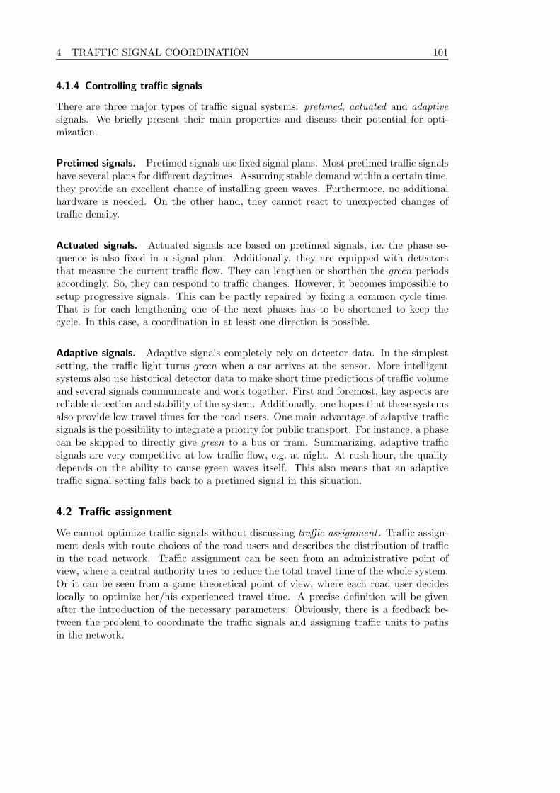
4 TRAFFIC SIGNAL COORDINATION 101
4.1.4 Controlling traffic signals
There are three major types of traffic signal systems: pretimed, actuated and adaptivesignals. We briefly present their main properties and discuss their potential for opti-mization.
Pretimed signals. Pretimed signals use fixed signal plans. Most pretimed traffic signalshave several plans for different daytimes. Assuming stable demand within a certain time,they provide an excellent chance of installing green waves. Furthermore, no additionalhardware is needed. On the other hand, they cannot react to unexpected changes oftraffic density.
Actuated signals. Actuated signals are based on pretimed signals, i.e. the phase se-quence is also fixed in a signal plan. Additionally, they are equipped with detectorsthat measure the current traffic flow. They can lengthen or shorthen the green periodsaccordingly. So, they can respond to traffic changes. However, it becomes impossible tosetup progressive signals. This can be partly repaired by fixing a common cycle time.That is for each lengthening one of the next phases has to be shortened to keep thecycle. In this case, a coordination in at least one direction is possible.
Adaptive signals. Adaptive signals completely rely on detector data. In the simplestsetting, the traffic light turns green when a car arrives at the sensor. More intelligentsystems also use historical detector data to make short time predictions of traffic volumeand several signals communicate and work together. First and foremost, key aspects arereliable detection and stability of the system. Additionally, one hopes that these systemsalso provide low travel times for the road users. One main advantage of adaptive trafficsignals is the possibility to integrate a priority for public transport. For instance, a phasecan be skipped to directly give green to a bus or tram. Summarizing, adaptive trafficsignals are very competitive at low traffic flow, e.g. at night. At rush-hour, the qualitydepends on the ability to cause green waves itself. This also means that an adaptivetraffic signal setting falls back to a pretimed signal in this situation.
4.2 Traffic assignment
We cannot optimize traffic signals without discussing traffic assignment . Traffic assign-ment deals with route choices of the road users and describes the distribution of trafficin the road network. Traffic assignment can be seen from an administrative point ofview, where a central authority tries to reduce the total travel time of the whole system.Or it can be seen from a game theoretical point of view, where each road user decideslocally to optimize her/his experienced travel time. A precise definition will be givenafter the introduction of the necessary parameters. Obviously, there is a feedback be-tween the problem to coordinate the traffic signals and assigning traffic units to pathsin the network.

102 4.2 Traffic assignment
4.2.1 Motivation
Most road users are interested in the fastest route to their destination. Locals often knowall the shortcuts in their home town. Assume, you have two routes to your destinationof equal length when traveling with free speed. Obviously, your route choice will dependon the traffic volume on the particular route and the coordination of traffic signals alongthis route. If one of the routes provides a green wave, you will probably arrive muchearlier. Consequently, every change of pretimed signal plans may influence the traveltimes in the road network and thus, it may also influence the road choice of the users.
The associated aging of pretimed traffic signal plans [15] is very important but oftenunappreciated in the optimization of traffic signals: It can be observed that some trafficsignal coordinations, once having been very efficient, become worse over time. Increasingtraffic in general and road users changing to optimized arterial roads lead to higherwaiting times and may disturb the fine-tuned coordination.
Therefore traffic signal coordination and the traffic assignment should be consideredas one single optimization problem. Hereby, traffic signal coordination means an opti-mal choice of the parameters of the traffic signals such that the road users reach theirdestinations as fast as possible. Traffic assignment describes the corresponding trafficpattern.
4.2.2 System optimal flows
We use flow and multicommodity flow to define traffic assignment. In the notation ofTable 1, a flow is a function f : A → R≥0 that has to fulfill capacity bounds and flowconservation constraints. We also require that the demands of all the commodities θ ∈ Θhave to be satisfied. In the multicommodity case capacities are shared by the differentcommodities, i.e.
∑
θ∈Θ fθ(e) = f(e) ≤ ue. Furthermore, a travel time function te isgiven for each link.
A traffic assignment problem is the distribution of traffic flow in a street network satis-fying demands of flow between origin and destination pairs of nodes. Assignment meth-ods are looking for an optimal way to distribute the traffic flow in the network accordingto different objective functions. One option for this objective function is to minimizethe total transit time spent by all flow particles in the network,
∑
e∈A f(e)t(f(e)).
In the following, we address the real-world application by using the notation road user,traffic participant, and traffic flow. These terms correspond to flow unit, flow particle,and flow in the theoretic model, respectively.
It matches to our experience that the travel time on a road is not independent of thetraffic flow on this road. The more cars are on the road, the more time we need. Thus,te(f(e)) : R+
0 → R+0 is the travel time function describing the time a flow particle needs
to traverse arc e in dependence of the amount of flow f(e) on arc e.
In the literature, these travel time functions are also called link performance functionor latency function [46, 69, 141]. Commonly, they are assumed to be non-linear, convexe,increasing functions (cf. Figure 26). Assume, we are equipped with link performancefunctions for each link. An assignment of flow to arcs, that minimizes the total travel time

4 TRAFFIC SIGNAL COORDINATION 103
of all road users with respect to these travel time functions, is called system optimum.
free
spe
ed
maximum capacity
Ave
rage
tran
sit t
ime
Link flow
Figure 26: A typical link performance function. Starting at the free speed traveltime, the average travel time increases with increasing flow. Sometimes the capacitybound on the link is implicitly forced by a pole at f(e) = ue. Note that the linkperformance function does not capture traffic signal coordination or variation offlow values over time.
4.2.3 User equilibria and Wardrop’s principles
While the system optimal solution is good for the system as a whole, it might be unfairto single users that could improve their own travel time by changing to a faster path.However, they will disturb traffic flow there and thus, the total travel time would increase.
In 1952, Wardrop [150] characterized the difference between a system optimum andan user equilibrium for a fixed origin-destination pair with two simple principles. Hisfirst principle reads as follows:
The journey times on all the routes actually used are equal, and less thanthose which would be experienced by a single vehicle on any unused route.
A flow which fulfills this principle for each commodity is called user equilibrium flow.Please note that Wardrop considered uncapacitated networks. In contrast, Wardrop’ssecond principle characterizes the system optimum.
The average journey time is a minimum.
This concept of user equilibria is often used for modeling the behavior of traffic instreet networks, where experienced users adjust their paths to minimize their own traveltimes until a stable situation is reached. A similar concept was developed by Nash atthe same time [120]. Obviously, there is a gap between the value of the ‘selfish’ userequilibrium and the system optimum. This gap is sometimes called price of anarchy . Adetailed survey on selfish routing can be found in [132].

104 4.2 Traffic assignment
A famous example for the impact of selfish routing is Braess’s Paradox [23]. Braessconstructed a small network with load dependent travel times. Surprisingly, adding anew link to this network increased the average travel time. Even more surprisingly, thiseffect was also observed in real world traffic, e.g. in Stuttgart, New York, and Seoul [99].We present a version of Braess’s Paradox in Figure 27.
s
v1t = f
v2t = 1
t = 0 z
t = 1
t = f
Figure 27: Example for Braess’s Paradox. The additional road is dashed. Traveltimes are displayed at the links. Each road has capacity ue = 1 and we send oneflow unit from s to z, i.e. Θ = {(s, z, 1)}. Without the new road we should send 0.5flow units on the upper and on the lower road each. This yields a total travel timeof 2 · (0.52 + 1 · 0.5) = 1.5. With the new road, every flow particle can improve itsown travel time from f + 1 to 2f by switching to the route (s, v1, v2, z). However,this will slow down the other particles on the links (s, v1) and (v2, z). Finally, allflow particles choose the new road, i.e. f = 1, yielding a total travel time of 2. Thus,the price of anarchy is 4
3 .
The problem of finding the user equilibrium is referred to as equilibrium traffic as-signment problem. Due to the properties of the link performance functions (e.g. non-linearity), the traffic assignment problem cannot be solved by simply applying standardnetwork flow algorithms but requires more involved approaches. For continuous, non-decreasing latency functions in uncapacitated networks, Roughgarden and Tardos [133]provide an existence theorem. Moreover, it can be shown, that a flow is at a Nashequilibrium if it solves the following convex optimization problem.
min∑
e∈A
∫ f(e)
0te(x)dx
s. t.∑
e∈δ−(v)
fθ(e)−∑
e∈δ+(v)
fθ(e) = 0 ∀θ ∈ Θ, ∀v ∈ V \{sθ, zθ}
∑
e∈δ+(sθ)
fθ(e) = dθ ∀θ ∈ Θ
∑
e∈δ−(zθ)
fθ(e) = dθ ∀θ ∈ Θ
fθ(e) ≥ 0 ∀e ∈ A
For non-decreasing link performance functions the objective is obviously convex.Roughgarden and Tardos [133] also provide bounds for the price of anarchy. Surprisingly,

4 TRAFFIC SIGNAL COORDINATION 105
these bounds are independent of the network topology [131]. For affine linear travel timefunctions the gap between system optimum and user equilibrium is at most 4
3 .
Correa, Schulz, and Stier-Moses [37] extend the results of Roughgarden and Tardosto capacitated networks. Whereas flow values are often bounded implicitly by a polein the travel time function in the former approach, we now consider a strict capacitybound. Consequently, Wardrop’s first principle is no longer valid, since the capacityof the shortest paths may be reached first. Remaining flow particles have to chooselonger paths. Even in the case of linear travel time functions, the value of capacitateduser equilibria is no longer unique and the price of anarchy, i.e. the ratio of cost ofthe worst user equilibrium to that of the system optimum, jumps to infinity. Correaet al. characterize capacitated user equilibria by the non-existence of unsaturated pathsthat are shorter than any path actually used. They focus on a special convex sub-classof equilibria, based on a mathematical programming approach by Beckmann, McGuireand Winsten [14].
Please note that the described static traffic model does not capture any time-dependentbehavior. For example, (static) link performance functions cannot handle platoons oftraffic arriving at different points in time. All flow particles on a particular road are as-sumed to experience the same travel time. Thus, these static link performance functionsare also not capable of capturing the dynamic properties of coordinated traffic signals.
4.2.4 Dynamic Flows
So far, the presented static assignment techniques conflict with the dynamics of trafficsignals. Therefore, models are needed that can capture the development of flow in atimely fashion. One approach are dynamic flows or flows over time. Already Ford andFulkerson [59] considered flows with a time component. An excellent survey on dynamicflows is presented by Skutella [142].
Now, a flow over time f with time horizon T is a (Lebesgue-integrable in the secondparameter t) function f : A × [0, T ) → R+
0 . f(e, t) is the rate of flow or load enteringlink e at time t. Flow particles entering e at time t arrive at the head of e at time t + te.The amount of flow that passes a link e can be calculated as
∫ T0 f(e, t)dt.
We now have two possibilities to introduce a capacity for dynamic flows. We maysimply restrict the flow rate, i.e. f(e, t) ≤ u(e). On the other hand, we may restrict
the amount of flow that enters a link during a certain period of time, i.e.∫ t+τe
t f(e, t)dt∀t ∈ [0, T − τe). Thus, there can occur peaks in the flow rate which balance over time.Dynamic flows with such a capacity constraint are also called bridge flows.
Furthermore, flow conservation has to ensure that flow cannot leave a node beforeit arrives there. Additionally, one assumes that flow can be stored in a node for some
time. In detail, for a non-terminal v ∈ V ,∑
e∈δ−(v)
∫ t−te0 f(e, t)dt ≥∑
e∈δ+(v)
∫ t0 f(e, t)dt
∀t ∈ [0, T ). If we require a strict equation, then flow must not be stored at intermediatenodes. Demands are handled similarly.
If the flow is induced by a static flow, i.e. it uses only s-z-paths Ps,z with a constantflow rate in the time interval [0, T − t(Ps,z)), then the dynamic flow is called temporallyrepeated flow .

106 4.2 Traffic assignment
In this setting, various interesting problems appear. In the Maximum Flow over
Time problem, we want to send as much flow as possible from a source s to a sink zuntil the time horizon T is reached. This problem can be solved with the Ford-Fulkersonalgorithm for static maximum flows. In detail, one computes a path decomposition of amaximum flow on a slightly modified network and derives a temporally repeated flow.
Earliest arrival flows are a variant of this problem. The goal is to find a single s-z-flowover time that simultaneously maximizes the amount of flow reaching the sink z up toany time t ≥ 0. Surprisingly, such flows exist. However, it seems unlikely that they canbe computed in polynomial time [142].
The Quickest Flow problem corresponds to a transshipment in minimum time. Fora single source and a single sink, it can be computed efficiently by maximum flows overtime and a Megiddo search of the time horizon [26]. Surprisingly, for multiple sourcesor sinks, this problem is not equivalent to a maximum flow over time. However, Hoppeand Tardos present an efficient algorithm [78, 79].
Minimum cost flows over time are NP-hard [90]. Considering multiple commodities,Maximum Flow over Time is also hard [75]. Klinz and Woeginger [91] study a slightlymodified integral version of dynamic flows. Here, arcs are called dedicated if flow blocksan arc as long as the transmission continues. This also yields NP-hard problems.
Many dynamic flow problems can be solved using time-expanded networks. AlreadyFord and Fulkerson introduced time-expanded networks in their seminal work on networkflow theory [59]. In this expanded network, for every node, several copies of this node areadded to the graph, one for each desired time step. These nodes are connected by arcs,where the various copies of the vertices are connected accordingly to the travel timesof the original arcs. Additionally, arcs connecting consecutive copies of the same nodemay allow waiting. We give a precise definition and Figure 32 shows a simple networktogether with its time-expanded network.
Definition 4.1 (Time-expanded network). Let G = (V,A) be a network with ca-pacities u : A → N and non-negative integral transit times tl. For a given time horizonT ∈ N, the corresponding time-expanded network GT = (V T , AT ) is constructed as fol-lows.
1. For each node v ∈ V , we create T copies v0, v1, . . . , vT−1, thus V T = {vt|v ∈ V, t ∈{0, 1, . . . , T − 1}}.
2. For each arc e = (v,w) ∈ A, we create T − te copies l0, e1, . . . , eT−te−1 where arcet connects node vt to node wt+te . Arc et has capacity u(et) = u(e).
3. Additionally, there are waiting arcs from vt to vt+1 ∀v ∈ V and ∀t ∈ {0, 1, . . . , T −2}.
The big advantage of flows over time compared to static flows is the opportunity tocapture the complete time-dependent behavior of the journey of a flow unit in a givennetwork. In contrast, a static flow can only describe the time-independent behavior ofthis journey. This yields a very powerful approach and it was already suggested to useflows over time in traffic networks [94] or logistics [57]. Our new model for traffic signal

4 TRAFFIC SIGNAL COORDINATION 107
x
y
t
x
y
tl3 = 3
tl1 = 3tl2 = 2
tl4 = 1
0
1
2
3
4
5
6
7
Figure 28: Simple example of a 4-vertex graph together with its time-expandednetwork for time horizon T = 8. The network is presented in a perspective view.The graph itself is embedded in the xy-plane. The time is displayed along thevertical t-axis. Corresponding arcs have the same color. Waiting arcs (black) allowbuffering of flow units in a node for some time.
coordination in Chapter 5 will be based on this concept. Unfortunately, the model fordynamic flows quickly becomes very large and a different input (e.g. dynamic demand)is needed. Thus, we cannot apply this approach one-to-one to traffic signals.
4.2.5 Dynamic traffic assignment
Dynamic traffic assignment model (DTA; see, e.g., [34, 144] for surveys) is a generalterm for several similar approaches which try to extend traffic assignment with staticlink performance functions to a dynamic model with a time component. The travel timewhich a road user experiences on a road now depends on the arrival time of this trafficparticipant at the road and the actual traffic flow on this road at this time. Consequently,a road user chooses its route and a departure time.
DTA models have in common that they try to compute a user equilibrium with aniterative approach. However, the methodologies are quite different, but they share asimilar overall model structure. One may identify three major steps [34]. Firstly, givena set of route choices, the resulting travel times are computed. Various network loadingmodels including both analytical and simulation-based approaches are used in this step.For example, several queueing models are tested [144]. Secondly, the new shortest routesare computed for each origin-destination pair and each departure interval with respectto the new link travel times. Thirdly, given the updated route sets, vehicles are assignedto new routes. If the stopping criterion is not met, then one returns to the first step.
Summarizing, these models focus on varying demand over time, but they still usestandard travel time functions. Unfortunately, as pointed out in [144], the queueingmodels lead to non-monotone and non-differentiable route travel times. Hence, solutions,

108 4.2 Traffic assignment
if they exist at all, are hard to find, non-unique, and heuristic solution methods aresuggested. Furthermore, some DTA models cannot ensure that a user on a link whoenters the link earlier than another user will also leave it sooner than the second user.
Additionally, these approaches do not–to the best of our knowledge–capture changingcoordinations of traffic signals. Some of them do not provide the accuracy to handle thevery fast changes in traffic density caused by traffic signals. But traffic signals and theircoordination are the main reason for platoons of cars in inner-city traffic. Thus, thereis a time-dependent change of flow on an even finer level. It seems to be essential thata model for traffic signal coordination also captures these platoons.
4.2.6 Computing assignments
As already mentioned in the introduction (Section 1.2.2), several combinatorial algo-rithms are known for the single commodity maximum flow problem. Similar approachescan be used to solve assignments with linear cost functions, but additional difficultiesoccur. In the style of Ford and Fulkerson, one may use a residual network and aug-menting paths. Here, cycles with negative total cost are a crucial problem. These cyclescan be canceled by pushing flow backwards on them. Always augmenting flow on cycleswith minimum mean cost yields a polynomial running time. Alternatively, negative costcycles can be avoided by using the successive shortest paths algorithm which yields apseudo-polynomial running time. Using capacity scaling, this algorithm can be usedto compute minimum cost flows efficiently. A detailed presentation of the algorithmsmentioned in this section can be found in [2].
Minimum cost flows are easily formulated as a linear program and thus, they can becomputed with the simplex method. This approach can be accelerated significantly byexploiting the special structure of the underlying network problem [2]. Given a flowx, an arc e is called restricted arc if x(e) = 0 or x(e) = u(e). A flow x is a spanningtree solution if there exists a spanning tree such that every non-tree arc is a restrictedarc. One can show that the problem always has an optimal spanning tree solution. Thenetwork simplex algorithm (see, e.g., [2]) starts with a feasible spanning tree solution andimproves it iteratively maintaining this property until it becomes optimal. Besides linearprogramming multicommodity instances can be solved with approximation algorithms,e.g. [67].
Convex cost functions can be approximated with piecewise linear functions. Subse-quently, an arc with a piecewise linear cost function can be transformed to a set ofparallel arcs with different linear cost functions. For each linear piece of the originalfunction, an arc with a linear cost function with the same slope is used. The capacityis adjusted to the length of the interval of the linear segment. If a small amount of flowis assigned to these arcs, only the cheapest arc, i.e. the one with the lowest slope, isused. If the flow value is increased, then the arcs with higher cost functions have tobe used, too. Combining both steps with an algorithm of the first passage of this sec-tion yields a combinatorial approximation algorithm for the minimum cost flow problemwith convex cost functions. Due to the substantially increased network size, the runningtime of this algorithm is not polynomial in the input size. A generalization of the ca-

4 TRAFFIC SIGNAL COORDINATION 109
pacity scaling algorithm with successive shortest paths solves the convex flow problemefficiently [2]. Alternatively, convex programming can be used to handle convex costfunctions exactly [122].
Besides these combinatorial and mathematical programming approaches, there existvarious heuristic methods using, e.g., simulation and genetic programming for deter-mining traffic assignment solutions. The agent-based simulation tool MATSim (cf. Sec-tion 4.3.5) is an example for one of these strategies, where assignment is realized by aniterative simulation and replanning. On the one hand, the traffic assignment approachin MATSim is similar to some DTA models. On the other hand, MATSim providesfeatures like public transport, traffic signals and many more. Thus, although we onlysummarize the assignment approach here, MATSim should not be reduced to a pureassignment model.
Actually, the non-cooperative road users (also known as agents) of MATSim play agame on the underlying network to find user equilibria. In the simplest case, each linkhas a constant travel time and it is modeled by a queue. An agent is directly assignedto this queue when it enters the link and it has to stay in the queue until the travel timehas expired. Further, the storage of a queue and the number of agents that can leave aqueue in a certain time interval are limited. The queue also guarantees the first in firstout property. Hence, agents can move through the network in a timely fashion. Themodel is extended with lanes, intersections and traffic signals.
Each agent is equipped with a set of plans. Each plan consists of activities, i.e. adestination in the network and a duration, and a route connecting these activities. Inevery iteration step, each agent chooses one plan with respect to a score for execution.All chosen plans are evaluated simultaneously in a simulation run. The experiencedtravel time is used to update the scores of the plans. Afterwards, a fixed amount of roadusers may change their plans by varying the departure time or computing an alternativeroute. This process is repeated until a convergence criterion is reached.
Summarizing, MATSim is built-up around an evolutionary algorithm and the assign-ments computed by MATSim can be interpreted as stochastic user equilibria [117].
This concept admits to compute user equilibria for very complex systems where not allrelations are known in terms of a closed mathematical formulation. However, discussingthese approaches more detailed we would slightly drift away from a strict mathematicalmodeling of traffic flow and simulation issues would come into play.
4.3 Optimizing traffic signals
The idea of coordinating traffic signals is nearly as old as the traffic signal itself. Asmentioned in the introduction of this chapter, Adolph [1] patented his concept of ‘greenwaves’ in 1925. But it was not before 1964, when Morgan and Little [116] started abroad analysis and presented a graphical solution for calculating maximal time slots andbandwidths for a single road.
By now there exist various models to transform the concept of a ‘green wave’ to a wholenetwork of roads. It is impossible to discuss all of them here. However, we will give asurvey on the–to the best of our knowledge–most important and pioneering approaches.

110 4.3 Optimizing traffic signals
In the last decades, a number of models were presented, allowing for different phenom-ena of urban traffic. The concepts in this section can be distinguished by various pointsof view. We will present heuristic approaches as well as strict mathematical program-ming approaches. Other models use direct search techniques. The models will addressdifferent parameters (offset, red-green split, cycle length and combinations thereof), sce-narios (single intersections, arterial roads, networks), and signals (pretimed, actuated,adaptive). They try to optimize different objectives (minimizing travel time, delay,number of stops, fuel consumption, and combinations thereof; maximizing greenbands).Furthermore, we have to distinguish between theoretical and practical approaches.
4.3.1 Measures of performance
The performance of traffic signal optimization can be measured by different parameters.One of the first measures used in the literature is the bandwidth of greenbands (cf. Fig-ure 29). A greenband consists of several consecutive intersections on a certain route anda time interval such that all road users arriving at the first signal during this time slotexperience a green wave on this route. Bandwidth is the width of the greenband, i.e. thetime span in which the green wave is available. However, it is difficult to apply thisconcept on networks. Nowadays, the most common measure is the average delay or thenumber of stoppages. A weighted combination of those has also been used.
When considering the traffic assignment problem and an optimal traffic signal coor-dination simultaneously, however, measuring delays and stoppages is not a good choice.Traffic participants may now choose arbitrary routes. Thus, taking only stops and delayinto account, a road user may choose a very long detour through the network just toavoid stopping or waiting in front of a red traffic light. This is rather unrealistic as mostroad users are interested in the fastest way to their destination. Therefore, one maychoose the total or average travel time (transit time + delay) as the measure of qualityof the solution. However, this measure is rarely used in the literature.
Furthermore, Sun et al. [143] have shown that the number of stops and delays are verysensitive to changes of the cycle time. Long cycle times minimize stops while short cycletimes lead to less delay. Thus, if combining these two measures in an objective function,slight changes in the weighting may lead to very different coordinations.
There are also several other measures of performance, e.g. preferences for public trans-port and pedestrians or fuel consumption, that are not discussed in this thesis.
4.3.2 Optimization of pretimed signals
Assuming fairly stable demands within certain divisions of time, the usage of pretimedtraffic signals appears reasonable. All approaches presented in this section introduce asimplified traffic model and suggest a solution method. However, they vary significantlyin the model assumptions and the optimization techniques.
In 1964, Morgan and Little [116] presented MAXBAND, a graphical method for max-imizing bandwidth. The concept of bandwidth is displayed in Figure 29.
Little [106] developed this approach further, using mixed-integer programming. This

4 TRAFFIC SIGNAL COORDINATION 111
t
x
Figure 29: Time-space-diagram showing the coordination of four consecutive traf-fic lights. Many traffic planning tools visualize signal coordination in this way. Thedistance is displayed on the horizontal axis, the time moves on in vertical direction.Cars in the light blue area arrived at all predecessing signals at green. But onlyin the dark blue zone, there is a green wave through all four signals. This area isthe greenband. Its width is called bandwidth. Some optimization approaches likeMAXBAND try to maximize this parameter.
program adjusts optimal values for offsets and a common cycle time for a bi-directionalroad. Two years later, a graph-theoretical model for minimizing delay was developed byAllsop [4]. Hereby, the solution is successively extended from a solution of a sub-network.
Shortly after, Robertson [128] presented his theoretical work on the optimization ofoffsets. He uses a simplified simulation approach and a genetic algorithm to optimizethis traffic signal parameter. These results led to the development of TRANSYT7, untilnow a most widely used tool for inner-city traffic optimization. TRANSYT providesmainly two different heuristic techniques to improve a so-called performance index. Itis presented more detailed in Section 4.3.5.
Gartner et al. [68] presented a mixed integer programming approach for network co-ordination in the mid-1970s. They developed MITROP8, which was one of the firstapproaches for networks that used integer programming. Gartner et al. introduce sat-uration deterrence functions to capture the influence of offsets. Further, they proposea piecewise linear approximation of these functions such that a mixed integer linearprogram can be formulated. The integer programming formulation also contains cycleconstraints for each cycle in the network, i.e. the algebraic sum of the edge offsets alongthis cycle has to be an integral multiple of the cycle time. The importance of theseequations is easy to understand. Assume to go for a round trip on an arbitrary cycle.Let φi be the ith edge offset on this cycle, i.e. the second signal turns to green exactly
7TRAffic Network StudY Tool8Mixed Integer TRaffic OPtimization

112 4.3 Optimizing traffic signals
φ1 time units after the first signal. The third traffic signal turns to green φ2 time unitsafter the second signal and thus, φ1 + φ2 time units after the first signal. On the onehand, if the round trip is finished and we are standing in front of the first traffic signal,then all edge offsets have summed up. On the other hand, the first traffic signal is stillin cycle with itself, i.e. if it turns green, then a certain number periods have passed by.Hence, cycle constraints ensure the consistency of edge offsets. As a consequence, anintegral variable is needed for every cycle in the network.
In 1977, Allsop and Charlesworth [5] presented an example that coordination andassignment interact. They suggest an iterative approach for optimizing both problems.
Serafini and Ukovich [139] studied the scheduling of periodic events. As an outcome,they also presented an involved mathematical model for the coordination of pretimedtraffic signals [140] in 1989. In their context, phase changes of traffic signals are events.The authors define several kinds of constraints for signals, conflicts, coordination, andcycles. More precisely, they introduce a lower and an upper bound for the link offset oneach road. Thus, their approach is a feasibility problem.
Recently, Wunsch et al. [95, 115] presented a further development of the approach ofGartner et al. [68]. They replace the saturation deterrence functions by a more realisticplatoon model. In their model flow units are bundled during the red phase of a trafficlight. When the signal switches to green, the flow particles resume their journey togetheras a platoon. Hence, they will also arrive at the next intersection as a platoon. Thisapproach admits a very realistic estimation of waiting times at traffic signals which arederived as the integral over the queue length. For a fixed assignment, i.e. the waitingtime only depends on the offsets, a piecewise linear approximation of these offset induceddelays is used to turn the problem formulation into a mixed integer program. Here,Wunsch [154] also focusses on the cycle constraints introduced by Gartner et al. [68].Cycle constraints apply to every cycle in a network and street networks constists of ahuge number of cycles. Wunsch proves that it is sufficient to demand cycle constraintson a subset of cycles which span all other cycles in the network. To accelerate the mixedinteger programming, he searches for minimal cycle bases which reduce the number ofinteger variables.
4.3.3 Adaptive traffic signals
It is often seen as a handicap that pretimed traffic signals cannot react to fluctuationsin traffic flow, whereas traffic itself is seen as a stochastic process. Consequently, in thelast decades, big efforts have been made on developing highly adaptive traffic signalswhich are able to react on changes in traffic volume immediately. The approaches differsignificantly from those of pretimed signals.
On the one hand, adaptive signal control can be seen as a problem of interdisciplinarycontrol theory. The usual objective of control theory is stability of the dynamical system.A controller reacts on the input and tries to manipulate the system such that it follows areference without oscillating. The same is true for adaptive signal control. Primarily, thesystem tries to avoid building up congestion. Furthermore, even a single road user shouldget green within a certain amount of time. Optimization is more or less a secondary

4 TRAFFIC SIGNAL COORDINATION 113
goal. Furthermore, real-time feasibility is a critical aspect for the applicability of thesetechniques in practice.
On the other hand, one can also account the problem to online optimization. Thus,all adaptive control strategies are heuristic techniques based on limited information.However, hardly any analysis concerning this point of view can be found in the literature.It would be very interesting to compare the heuristic solutions to optimal offline solutions.
Most solutions consist of a traffic model and a complex system of detectors and trafficsignals. They focus on the following questions:
• Which detectors are used?
• Where are these detectors placed?
• Which traffic signal gets which information?
• How does the signal react on the information?
These questions also include that information on traffic is propagated in the trafficnetwork in space and in time. Some systems also use historical data to predict futuretraffic. Adaptive signal control techniques are often evaluated with the help of micro-simulations which yields very realistic results.
There are several competing approaches for optimizing adaptive traffic signals. Asurvey of common approaches is, e.g., presented by Friedrich [63, 64]. Representatively,we discuss two recently published systems.
The first model is based on a cell transmission model for networks developed byDaganzo in a series of papers [39, 40, 41, 42, 43]. The underlying cellular automatonmodel was qualified for traffic theory by Nagel and Schreckenberg. In their famouspaper [119], the authors explain spontaneous congestions on freeways with help of themodified one-dimensional binary cellular automaton rule 184. The name of the rule is aWolfram code. It defines the evolution of the states of the cellular automaton (cf. [105]).Daganzo extends this approach to traffic networks with intersections. Further, he studiesgridlocks in this system. Almasri and Friedrich [6] extend this model with an adaptivesignal control. A genetic algorithm is used for optimization. Due to the high computationtime the limit for practical applicability is already reached for the comparatively smalltest network with six intersections.
The second approach was recently presented by Lammer [102]. The three basic com-ponents are a local prediction of future traffic, a local optimization with a priority indexfor the next phase, and a local stabilization to force an average and a maximal period.This system is going to be tested in reality at seven intersections in Dresden, Germany.Lammer states stability as one of the main problems of adaptive systems. He suggestsan underlying pretimed signal coordination as a guideline to stabilize the system. Fur-ther, he states that an adaptive system has to be runned below saturated traffic demandto prevent degeneracy [103]. Therefore, offset optimization is also important for theoperation of adaptive traffic signals

114 4.3 Optimizing traffic signals
4.3.4 Simultaneous coordination and assignment
Most of the approaches presented so far did not consider assignment. But each changeof a traffic signal parameter will also change travel times for at least a few road users.Allsop and Charlesworth recognized the feedback between an optimized coordination andtraffic assignment [5]. In 1977, they proposed an iterative approach. Signal timings areoptimized with TRANSYT. Afterwards, an equilibrium traffic assignment is computed.These steps are repeated until no change in the coordination occurs. Obviously, usingheuristic methods iteratively, one may only hope to derive a local optimum. Even worse,this approach may lead to a decline of network performance as shown by Dickson [48].
Despite the interaction of signal coordination and traffic assignment, only few researchwas spent in the combined optimization. For example, Chiou [31, 32] presented a bilevelformulation based on the approach of Allsop and Charlesworth. She uses a gradientprojecting method for calculating local optima. Further, she presents a subgradientmethod for a non-smooth single-level formulation of the problem [33]. Recent results werealso made by Bell and Ceylan [16] as well as Teklu et al. [145] using genetic programming.
4.3.5 Tools
So far, we have seen several (theoretical) approaches for traffic signal optimization. Inthis section, we will present some tools and software kits, that are actually used by trafficengineers to optimize and control traffic signal systems.
Optimization. TRANSYT is a widely accepted software tool for modeling, analyzing,and optimizing traffic signal settings. It is based on an approach by Robertson [128].It is developed by the Transport Research Laboratory. TRANSYT supports severalsophisticated traffic models, including the Cell Transmission Model and the PlatoonDispersal Model, to derive a so-called performance index (PI). Normally, this indexis a parametrized sum over stoppages and delays in the network. TRANSYT usesoptionally a genetic programming approach or a gradient search technique for improvingthis performance index. On the one hand, the detailed objective function is seen as abig advantage of TRANSYT since also other aspects like fuel consumption can be takeninto account. On the other hand, the obtained solution significantly depends on theparameter choice of the user.
Another widely used traffic planning tool is VISUM, developed by ptv AG in Karls-ruhe, Germany. It provides several tools for all kinds of inner-city traffic from a singleintersection up to a whole town. VISUM features various state-of-the-art static trafficassignment techniques. The tool also supports the optimization of traffic signals, e.g. bya plug-in based on the approach of Wunsch. Further, VISUM provides tools for planningpublic transport or for estimating pollution.
Signal control. Of course, an offline optimization of traffic signals is not sufficient, thesignal have to be operated in practice. We briefly discuss two tools that are actuallyused to control traffic signals. Both of them fall into the category of actuated signals.

4 TRAFFIC SIGNAL COORDINATION 115
Since both systems are based on pretimed signals this also emphasizes the need for wellcoordinated signals.
SCOOT9 was primarily developed by Bretherton et al. [80] and presented in 1981. Ituses TRANSYT to optimize green splits, offsets and cycle length in real time. Basedon prevailing traffic conditions SCOOT modifies those parameters in small steps to keeptrack with changing traffic conditions. SCOOT is used all over the world and is stillenhanced.
A similar system mainly used in Germany is Sylvia+ [135]. This method is also basedon a coordinated pretimed signal coordination. Depending on the recent traffic, Sylvia+can extend or shorten a single phase of the traffic signal. However, changing phasedurations in an arbitrary manner will completely disturb the underlying coordination.Therefore, Sylvia+ uses a recovery algorithm to restore the common cycle. Whenever aphase is extended, another phase in the same period has to be shortened by the sameamount of time. Thus, at least for one direction, a green wave can be maintained.
Simulation. Micro-simulation is essential in the development of new traffic signal coor-dination methods. Not every coordination can be tested in practice. We briefly presenttwo simulation tools, namely MATSim and VISSIM, that we will also use to evaluateour approach for signal coordination in Chapter 6.
The software MATSim is mainly developed at TU Berlin and ETH Zurich and isa multi-agent transport simulation tool based on queue models. MATSim is a multi-purpose simulation tool. Among others, it can be used for a traffic microsimulation ininner-cities. It provides lanes, queues and traffic signals, but the dynamics of agents arereduced to their bare essentials. It is capable of simulating large scale traffic networksand computing traffic assignment using an iterative approach. See [112] for more detailson this software.
The tool VISSIM from ptv AG provides a microscopic traffic simulation with state-of-the-art longitudinal dynamics and lane change models [126]. VISSIM is widely acceptedto produce very realistic results. It also supports several additional features like pedes-trians and public transport which are far beyond our purposes. VISUM and TRANSYTprovide a link to VISSIM.
Despite their different simulation approaches, both tools provide measured travel timesfor the commodities and they visualize congestion. Thus, we can use at least theseparameters to evaluate signal coordinations and to compare both tools.
4.3.6 Conclusions
There are many reasons for the usage of coordinated pretimed traffic signals. Consideringrush hour situations with high demand at every road, also adaptive coordinations willfall back to fixed time coordinations. Furthermore, pretimed signal settings are the basisfor widely used actuated signal systems. Additionally, due to the high costs of sensortechnologies and a lacking acceptance of car-to-car or car-to-traffic-signal communication
9Split Cycle and Offset Optimization Technique

116 4.4 Complexity of signal coordination
for data privacy reasons, a complete adaptive control is out of range for many cities.Thus, the importance of well coordinated pretimed signals will persist the next years.
On the one hand, most approaches for traffic signal coordination use heuristic methodsto improve the signal settings. This is especially true for the combined optimization ofsignal coordination and traffic assignment. These models are somewhat unsatisfyingfrom a mathematician’s point of view. Despite the solutions operate well in practice,one has no guarantee of optimality. On the other hand, models designed for exactsolution methods often make inaccurate assumptions on the traffic flow model. Thus,one can perhaps solve the model exactly, but the applicability is sometimes disputable.
4.4 Complexity of signal coordination
Closing the short survey on traffic signal optimization, we discuss the complexity of thesignal coordination problem in this section. The formulation and analysis essentiallydepends on the chosen model. Various proofs of complexity for different approaches canbe found in the literature. All of them have in common that the offset optimizationproblem for traffic signal coordination is NP-hard. Network coordination is closelyrelated to the Periodic Event Scheduling Problem (PESP). Serafini and Ukovich [139]proved NP-completeness for the PESP by reducing the Hamiltonian Cycle Problem.Wunsch [154] provides a reduction from PESP to his formulation of the Network SignalCoordination problem.
In the following we show that traffic signal coordination is an NP-hard problem alsoin our traffic model. This result is presented before the introduction of our model, sinceit also applies to more general models and it is not restricted to our approach. Moreprecisely, we consider traffic signal coordination in a general dynamic network flowssetting with constant transit times. The network contains traffic signals where waitingis possible. Building up on this assumption we define the signal coordination problemas follows.
Problem 4.2 (Signal Coordination Problem).Input: Network G = (V,A) with arc capacities u(e) and travel times consisting of aconstant transit time t(e) per arc plus waiting time at the intersection; a set of trafficsignals with arbitrary but fixed operating sequences at some of the intersections vn ∈ V ,n ∈ {1, . . . , N}; a cycle time Γ that is the same for all traffic signals; commodities θ ∈ Θ,θ = (sθ, zθ, dθ) with origin sθ, destination zθ, demand dθ and fixed routes.Output: A dynamic flow on the fixed routes and a set of offsets {ρ1, . . . , ρN} whichminimize the total travel time, i.e. the sum over the travel times of all road users.
Theorem 4.3. Offset optimization of traffic signals is NP-hard, even with travel timesconsisting of constant transit time per arc plus waiting time at the intersection.
Proof. First, let us fix the decision version of the Signal Coordination Problem:Given a network G = (V,A) with capacities, travel times, commodities and traffic signalsas in Definition 4.2 and a value t∗, is there a coordination (set of offsets) that induces atotal travel time equal to or less than t∗.

4 TRAFFIC SIGNAL COORDINATION 117
We reduce the Signal Coordination Problem from the 3-Partition Problem
which is NP-complete [66]. The problem is to decide whether 3m integers can bepartitioned into m sets of 3 integers of equal sum. More formally:
3-Partition Problem:
Input: multiset S = {x1, . . . , x3m} of 3m integersQuestion: Is there a partition of S into disjoint triples S1, . . . , Sm that allhave the same sum C = 1
m
∑3mi=1 xi?
The 3-Partition Problem remains NP-complete when C4 < xi < C
2 ∀i ∈{1, . . . , 3m}.
Given an arbitrary instance S = {x1, . . . , x3m} of 3-Partition we show how thisinstance is used to build an instance of the the Signal Coordination Problem suchthat the Signal Coordination instance has a solution if and only if the 3-Partition
instance has a solution.
Figure 30 shows the network used for the reduction. We create 3m roads with ademand of xi, (i = 1, . . . , 3m) flow units in each road (C = 1
m
∑3mi=1 xi and C
4 < xi <C2 ∀i ∈ {1, . . . , 3m} as above). There is only one path to the destination for eachcommodity, thus route choice is fixed. Each road has a transit time of zero time unitsand there is a traffic signal at the end of each road that has a cycle time of m time unitsand is green for exactly one time unit in each period. Waiting is only allowed at thetraffic signals. The capacity of these m roads is not bounded, thus all demands maypass the signal during one period.
However, all roads lead to a narrow road e, which starts after the signals and ends atthe destination. This road has a capacity of u(e) = C flow units per time unit.
...
x1
traffic signals
destination
demands
x2
x3u(e) = 1
m
P
xi
x3m
Figure 30: Traffic network for reduction from 3-Partitioning. The narrow roadat the exits forces perfect coordination.
As the capacity of the narrow road cannot be exceeded, flow units will have to waitin front of the traffic signals when this small road at the exit is congested. If too muchtraffic signals turn green at the same time, flow units will even have to wait in front ofgreen signals. More precisely, each signal is green for only one time step within the timehorizon m. To make sure that no more than m time steps are needed for getting all flowunits to the destination this one time step has to be used for sending all flow units of acommodity at once through the signal. Since xi > C
4 , no more than three commodities

118 4.4 Complexity of signal coordination
can be sent at once. Hence, exactly three signals have to be green at the same time stepsuch that the capacity of the narrow road is exhausted.
Thus, if the related 3-Partition Problem has a Yes answer, we can use the exitroad at maximum capacity all the time and we need m time units to empty the network.If the 3-partitioning has no Yes solution, then there will be congestion in the networkand flow units will have to wait for the next green cycle yielding a higher total traveltime. Consequently, the Signal Coordination Problem is at least as hard as the3-Partition Problem.
When allowing route choice and by considering related hard problems like Partition
or Numerical 3-Dimensional Matching [66] even more realistic traffic networks thanthe one in the proof of Theorem 4.3 can be constructed and be used for the hardnessproof. For example, one can find a planar network with node degree at most three formodeling partition by the help of signals and traffic (Figure 31). The main idea of theconstructions is using traffic signals for sorting, assigning and splitting traffic. Yet, itshould be pointed out that Partition (in contrast to 3-Partition) is weakly NP-hard.
...x2x1 x3 xn
destination
demands
traffic signals
u = 12
P
xi
Figure 31: Traffic network for reduction from Partition. All road users at origink start at time t = k. For each road, a free speed travel time of one time unitis assumed. All traffic lights have the same signal plan and four phases of equallength as follows: green for right turners→ red → green for left turners→ red. Thenarrow roads at the right end of the network limit the traffic to u = 1
2
∑ki=1 xi per
time unit. If there is a partition of the demands into two sets of equal size, we canfind a coordination which allows the road users to switch to the upper or lower roadaccording to the partition without waiting at the traffic signals.

5 A NEW MODEL 119
5 A New Model
5.1 Motivation
In this chapter, we will develop our combined model for traffic signal coordination andtraffic assignment. We have already seen several models for at least one of these problemsin Chapter 4. With these insights of advantages and disadvantages, we fix the key pointsthat our model should provide, first.
The time-dependent behavior of traffic signals is one of the most important propertiesof our problem. Thus, our model has to capture this dynamic behavior. Flows over timeare an adequate mathematical model that can be extended with traffic signals. Fur-thermore, this will allow mathematical programming techniques. Most practitioners donot concentrate on sound mathematical models, but they are mainly interested in goodresults that are applicable in practice. Most established models for signal coordinationuse genetic programming or other heuristic approaches. From a mathematician’s pointof view, this is not satisfying. For us, the guarantee of optimality or at least a measureof the quality of a solution is of the same importance as the solution value itself. Severalapproaches presented in Section 4.3 do not fulfill this requirement. Actually, none of theknown models for simultaneous optimization of coordination and assignment provides adual bound. Our model should improve this, i.e. it should be suitable for applying anexact mathematical programming approach.
In Section 4.3.1, we have discussed several possibilities for measuring the performanceof coordinated signals and came to the conclusion that only total travel time which con-sists of transit times and delay, seem reasonable for the assignment problem. Thus, ourobjective is to minimize the total travel time in our combined model. Given a networkG = (V,A) with fixed capacities, transit times, commodities and traffic signals withfixed signal plans, we define the Traffic Signal Coordination Traffic Assign-
ment Problem (TSCTAP) to be the problem of finding a set of offsets and a trafficassignment, such that the total travel time is minimized.
Most likely, a traffic engineer would have to be convinced of a model without flowdependent travel times. The more cars are on a road, the more the average traveltime increases. Classical link performance functions have this property, but they donot capture any time-dependent behavior like traffic signals or fluctuating flow values.Hence, some traffic experts think that link performance functions are not sufficient tomodel inner-city traffic [118]. Our model should capture such typical effects of trafficlike platoons of cars. Further, we need a handy concept for travel times that doesnot disturb our exact mathematical programming approach. Therefore, we make thefollowing simplifying assumption in our traffic model. The travel time on a link in thenetwork splits into two components: the free speed travel time that is needed to bridgethe distance of the link, and the waiting time in front of the intersection, i.e. in front of atraffic signal. In particular, we assume the free speed travel time to be independent of theload of the street. Although this assumption is not justified on highways or in rural areas,it is appropriate in inner-cities, where the distance between consecutive intersections iscomparably small and a strict speed limit is present. The speed of a single car does not

120 5.1 Motivation
differ much from the speed of a platoon of cars. The waiting time mainly depends onthe offsets of the subsequent traffic signals. This assumption will allow the formulationof flow dependent travel times in an implicit manner. We will thoroughly discuss theconsequences of this assumption and its influence on system optima and user equilibriain this chapter.
Based on these assumptions, we properly define our problem:
Problem 5.1 (Traffic Signal Coordination Traffic Assignment Problem).Input: Network G = (V,A, u) with capacities u : A→ N0 and travel times consisting ofa constant transit time per arc, i.e. t : A → N0, plus waiting time at the intersection;a set of traffic signals with arbitrary but fixed operating sequences at some of the inter-sections vn ∈ V , n ∈ {1, . . . , N}; a cycle time Γ that is the same for all traffic signals;commodities θ ∈ Θ, θ = (sθ, zθ, dθ) with origin sθ, destination zθ and demand dθ.Output: A dynamic flow and a set of offsets {ρ1, . . . , ρN} which minimize the totaltravel time, i.e. the sum over the travel times of all road users.
Now we have stated the basics of our input and output and can state the aims andanticipated properties of a model that we would like to get:
• Develop a model for simultaneous optimization of traffic signal coordination andtraffic assignment. Consider feedback between coordination and assignment.
• Capture time-dependence:
– dynamic travel times without static link performance functions,
– traffic signals, and
– fluctuating traffic, e.g. platoons.
• Objective: total travel time (transit time + delay).
• Realize flow dependent travel times via constant travel times plus flow dependentwaiting times.
• If possible, approximate user equilibria with system optimal solutions.
• Solvability with mathematical programming. Provide dual bounds.
• Compute solutions of practical relevance, i.e. demonstrate applicability of themodel with simulation results.
We will show that most of these aims and properties can infact be achieved by our newmodel. In the following, we first describe the various parts of this new model that arecombined to solve the TSCTAP. These parts cover the cyclic time-expansion, expansionof intersections, and implementation of traffic signals. Building on these notions, wewill give a mixed integer programming formulation, study basic properties, and discussvarious subsequent improvements of the model. Afterwards, Chapter 6 is dedicated tothe evaluation of our model with help of simulation tools.
Please note that some of the results were already presented at conferences [96, 97, 98].

5 A NEW MODEL 121
5.2 The new model
5.2.1 Cyclically time-expansion
As explained earlier, for traffic signals and their coordination, a time-dependent model,capable of describing the time-offset between consecutive intersections, is a vital in-gredient. Hence, flows over time and time-expanded networks seem to be the suitablemathematical model.
Yet, time-expanded networks are rather inefficient if the time horizon is large, sincethe number of time steps determines the number of network copies that have to beprovided. However, since traffic signals have a periodical behavior it is not necessary touse a full time horizon expansion. Instead, we suggest a cyclic time-expansion where weexpand only a time interval of size of the cycle time Γ and use only k ∈ N time steps ofsize t = Γ
k .
...
x
y
t
x
yt = 3
t = 2
t = 1
6
5
4
3
2
1
0
5
4
3
2
1
00
1
2
3
4
5
t = 3
Figure 32: Simple example of a 4-vertex graph together with its time-expandedgraph similar to the example in Figure 28 in Section 4.2.4. Again, the graph isembedded in the 2-dimensional Euclidean plane and the expansion is displayedalong the third axis. In our model this time expansion is reduced to a cyclic timeexpansion with finitely many time steps. Waiting arcs allow buffering of flow unitsin a node for some time.
Furthermore, we add the arcs according to transit times modulo k with adjustedcapacities. Of course, this treatment only applies to the indices of the incident nodes,the original transit time of an arc is preserved for further calculations. To model theability to wait in front of an intersection, all copies of one node v are cyclically connectedin chronological order with waiting arcs (vi, vi+1). Again, vk−1 is connected to v0 whichyields a cyclically rolling horizon (see Figure 32 and 34). A cost of one time unit is

122 5.2 The new model
assigned to each waiting arc.
Please note that there is almost no difference between transit arcs and waiting arcs inthe model. On waiting arcs one only moves in time whereas on regular arcs one movesin space and time. On all arcs the cost is the travel time on this arc. Thus, waitingtime is travel time on waiting arcs. Hence, both kinds of arcs are treated in the sameway and we do not need to explicitly distinguish between them in the modeling of trafficassignment.
5.2.2 Expanded intersections
To model intersections with different lanes, turning directions, and interior traffic signaloffsets, we use a standard approach from traffic networks. Before the time expansionis employed, every intersection node is split up into several nodes for incoming andoutgoing traffic; interior arcs connect the lanes (see Figure 33). Each of these arcs isassigned to one traffic light.
Figure 33: Expanded intersection with arcs for each turning alternative. Theincoming nodes of the horizontal road are subdivided into three nodes to modeldifferent lanes and queues for the turning directions. The vertical road is smaller,thus, all cars are waiting in the same queue.
We will refer to the set of all interior arcs of intersections by E ⊂ A. By choosingappropriate capacities u(e) and transit times t(e), e ∈ E, these interior links formdifferent queues, i.e. flow on the waiting arcs, for the several turning directions, becausethey limit the outgoing flow of the waiting arcs.
5 A NEW MODEL 123
5.2.3 Modeling traffic signals
The traffic signals themselves can be modeled by binary decision variables that switchthe capacities of the interior arcs at an intersection on or off, depending on the signalplan and the corresponding time step (see Figure 34). For each traffic light a matrixQe ∈ {0, 1}k×k is given; here Qe
ij = 1 means that the particular traffic light is green attime step j when using offset iΓ
k . So each row stands for a certain offset and determinesthe operating sequence of the traffic light for this specific offset. For each interior arc eof the not time-expanded graph we create such a matrix. The signal plan is completelyencoded in these matrices.
Qe =
0 0 1 1 · · · 0 00 0 0 1 1 · · · 0. . . . . . . . . . . . . . . . . . . . . . . .. . . . . . . . . . . . . . . . . . . . . . . .
For each intersection n we introduce k binary variables bn = (bn1 , . . . , bn
k) ∈ {0, 1}kwith constraint
∑ki=1 bn
i = 1 that describe the chosen offset at the intersection. Moreprecisely, bn
i = 1 is equivalent to offset ρn = iΓk at intersection n. By multiplying this
characteristic vector bn with Qe and the capacity u(e) of a lane, we can switch thecapacities of the links on or off and thus, represent the green and red lights.
Using f(e) ≤ bnQeu(e) for all interior lanes of an intersection (where u(e) is chosenin correspondence to the granularity of the time-expansion) we can map the completedynamic behavior of traffic signals in our model.
t = 3‘road’ arc ‘interior’ arc
t = 1
Figure 34: Cyclic time-expansion of a traffic signal. The gray arcs starting at thered phase of the signal are switched off and thus have zero capacity.
Putting together the various parts of the model we get the following definition ofcyclically time-expanded networks.

124 5.3 Mixed integer programming formulation
Definition 5.2 (Cyclically time-expanded traffic network). A cyclically time-expanded traffic network is a network, that is obtained from a traffic network G = (V,A)by
(i) expanding the intersections with arcs for turning alternatives and lanes,
(ii) cyclic time-expansion with respect to the cycle time, and
(iii) expanding signal plans.
5.2.4 Modeling traffic assignment
Building up on the cyclically time-expanded network, we can now consider the trafficassignment problem within this framework. Although flow can be considered to travelin a time-dependent manner through the cyclically time-expanded network, one shouldrather see this model as a static model that just captures some time-dependent aspectsof traffic flow. Due to the cyclic repetition of the vertex and arc copies, a flow particletraveling through this network can be seen as a representative of a whole set of temporallyrepeated particles at every multiple of the cycle time.
On the other hand, there is a closely related interpretation of static network flow fortraffic networks. In this interpretation one considers a flow-carrying path in the staticnetwork as a mapping of a corresponding amount of flow particles traveling over timethrough the traffic network at the corresponding flow rate. In other words, a flow-carrying path in the static network represents a constant rate of flow on this path in the‘real’ time-dependent traffic network.
This interpretation suggests how to put together the two models, the cyclically time-expanded network on the one hand and the static traffic assignment model on the otherhand. Basically, the demands for the different commodities have to be subdivided tothe number of layers/time steps in the cyclically time-expanded network. The preciseconstruction is given in the following.
Given (static) commodities θ ∈ Θ, θ = (sθ, zθ, dθ) in the original (static) network(sending dθ units of flow from node sθ to node zθ), one has to extend them to thecyclically expanded network. Each demand has to be scaled to time Γ and can bedivided uniformly among all copies of sθ. The constraints for the sink nodes should beless restrictive, i.e., no uniform distribution is required. We propose to use a super-sourceand a super-sink, connected by a backward arc, as shown in Figure 35.
5.3 Mixed integer programming formulation
Let G = (V,A) be a cyclically time-expanded traffic network and commodities θ ∈ Θ,θ = (sθ, zθ, dθ), capacities u : A → N, a set E ⊂ A of interior arcs at intersectionswith associated matrices Qe for each e ∈ E, travel times t(e) for each link e ∈ A andflow functions fθ : A → R for each commodity. Now we can formulate a mixed integerprogram for TSCTAP.
We extend a common multicommodity min-cost circulation program for the cyclicallytime-expanded network by adding the binary variables and capacity constraints above.

5 A NEW MODEL 125
... ...expandednetwork
cyclically
v0
u = dθ
copies of v = sθ
sθ
vk−1
u = dθ/k
copies of w = zθ
zθ
wk−1
fθ((zθ, sθ)) = dθ
w0
Figure 35: Demand splitting for commodities.
min∑
e∈A
∑
θ∈Θ
t(e)fθ(e)
s. t. 0 ≤∑
θ∈Θ
fθ(e) = f(e) ≤ u(e) ∀ e ∈ A \ E (18)
∑
e∈δ+(v)
fθ(e) =∑
e∈δ−(v)
fθ(e) ∀ θ ∈ Θ ∀ v ∈ V (19)
fθ((zθ, sθ)) = dθ ∀ θ ∈ Θ (20)
k∑
i=1
bni = 1 ∀ n ∈ {1, . . . , N} (21)
f(e) ≤ bnQeu(e) ∀ e ∈ E (22)
f(e) ≥ 0, bn ∈ {0, 1}k
The constraints of type (18) fix the capacity bounds, type (19) implements the flowconservation and the constraints (20) force the circulation. Equation (21) ensures thatexactly one offset is chosen at each intersection, and (22) permits flow only on arcs thatare switched on with respect to the chosen offsets.
5.4 Properties of the model
First, we examine the assignment problem for fixed traffic signals.
Theorem 5.3. Using the cyclically time-expanded network the traffic assignment prob-lem for a fixed traffic signal coordination and for a fixed time granularity can be solvedefficiently.
Proof. If the traffic signal coordination is fixed, then all binary decision variables in ourmodel are also fixed. Therefore, we obtain a standard linear program (LP) for the traffic

126 5.5 Analyzing link performance
assignment problem. Since the LP has polynomial size with respect to the input, i.e. thecyclically time-expanded network, it can be solved in polynomial time, e.g. by using theellipsoid method [73].
Instead of using a standard LP solver for the assignment problem, one can exploitthe network structure of the problem: as explained in Section 5.2.4, for each commodityartificial source and sink nodes can be added to create a circulation problem for thesecommodities with the help of a backward arc. One can apply this to all commoditiesand finally remove all arcs that are switched off by the decision variables. Now, anyalgorithm for the Minimum Cost Multicommodity Circulation problem can beused. Thus, we can also take advantage of fast combinatorial approximation algorithms(e.g. [67]) to solve the assignment even faster.
We can also observe an interesting property of the optimal solution, even for arbitrarysignal coordinations.
Observation 5.4. An optimal solution (system optimum) of the proposed multicom-modity min cost flow problem is also a user equilibrium.
Proof. Consider a flow with minimum total travel time, i.e. a system optimal flow. Alltransit times of arcs in the model are independent of the flow on that particular arc.Therefore, any route change of a single road user has no influence on the transit timesof the arcs. By the optimality of the flow the new route cannot be shorter than the oldone, since this would imply an improved system optimal solution, a contradiction.
By Wardrop’s principle, a flow is in a user equilibrium, if the route choice of a singleuser does not improve on its travel time. Consequently, a system optimal solution of ourmodel is also an user equilibrium.
We confirm that this result holds if the cyclically time-expanded model is seen as acommon static network. We compute a static assignment in a – although time is encodedindirectly – static network and we apply a result from static network flows. Furthermore,using a network with capacities user equilibria are not unique [37]. Thus, Observation 5.4does not provide any statement about the relevance of this user equilibrium. In general, itis not guaranteed that this specific traffic assignment can be achieved in reality. Beforewe get back to the implications of Observation 5.4 in Section 5.5.3 and a dynamicinterpretation, we have to study travel times in the cyclically time-expanded networkfirst.
5.5 Analyzing link performance
So far, we have introduced a model with constant, flow independent transit times onlinks. This might seem too restrictive for a lot of practitioners in the first moment. How-ever, there is infact a time-dependent behavior and it is captured in the time expansion.We will now try to uncover this time dependency by an analysis of our model on a singlelink with a traffic signal. Furthermore, we support the observations by a simulation oftraffic on this link.

5 A NEW MODEL 127
We will see that travel time on a link depends on numerous parameters, e.g. the dis-tribution of incoming flow values over time. Furthermore, flow particles on the same linkat different times will experience different travel times. We use link performance to termthe average travel time on a link. We will not present a closed function for computingtravel times. Nevertheless, we use the term inherent link performance function accordingto related traffic assignment models with flow dependent travel times. In the following,we fix most of the parameters and restrict the inherent link performance function to asmall subset of its domain to at least demonstrate the most important properties of thisimplicit link performance in the cyclically time-expanded model.
5.5.1 Link performance of a single road
We consider a very small network which consists of a single road with a traffic signal inthe middle similar to the network in Figure 34. Assume a set of flow values assigned tothe network and a fixed coordination to be given. The total waiting time in this smallnetwork can be determined by multiplying flow value and transit time and summing overall waiting arcs. Increasing flow will increase the waiting time, because more flow willbe assigned to the waiting arcs. Furthermore, due to the bounded capacities, the flowunits on the waiting arcs may not leave completely on the first green outgoing arc if thearc does not provide enough capacity. Instead, the flow will have to use more waitingarcs until the accumulated flow is drained off. This relation is illustrated in Figure 36.Therefore, if the incoming flow is raised linearly on all copies of an arc, then the growthof the waiting time will be not linear but rather quadratic. More precisely, the obtainedfunction is piecewise linear, but converges to a quadratic function if the length of thetimesteps in the expansion converges to zero.
In Figure 37 we present the relation between flow and average waiting time on a singlelink in the cyclically expanded network, i.e. our network consists of only one road witha traffic signal. The traffic is equally distributed on all copies of this link, a traffic signalwith a cycle time of 60 seconds and a red time of 20 seconds is put at the end of theroad and a free speed travel time of 10 seconds is assumed. Additionally, a capacityreduction from two lanes to one lane at the traffic signal was used. We now computethe average travel time on this link with respect to the flow value. The obtained traveltime in Figure 37 demonstrates the capability of our waiting arc model: although usingonly constant travel times the inherent, implicit link performance functions of the modelare not linear. Even better, they seem to resemble common standard link performancefunctions (cf. Figure 26).
Please note that Figure 37 visualizes the average travel time. The individual traveltime of a single flow particle depends on its arrival time at the traffic signal. It rangesfrom 10 seconds for flow units arriving at green with no waiting queue at the signal upto 30 seconds for particles arriving at the beginning of the red phase. Further, we canalso compute the expected free speed transit time. With a probability of 2
3 we arrive atthe traffic signal at green. Thus, we arrive at red with a chance of 1
3 and the waitingtime is equally distributed between 0 and 20 seconds in this case. Thus, the expectedfree speed travel time is 10 + 1
6 · 20 = 1313 seconds.

128 5.5 Analyzing link performance
Figure 36: Accumulation of waiting time. The thickness of the arcs depicts theflow value. On the left side, incoming flow is low. All flow accumulated duringthe red phase can leave the signal directly when it becomes green. On the rightside, the flow is tripled. Thus, much more flow is accumulated on the waiting arcs.Furthermore, due to the capacity bound of the outgoing street, more waiting arcshave to be used. Waiting time increases in this scenario by a factor of 4.8.
This analysis suggests that our model can capture flow dependent travel times similarto standard link performance functions. However, we assumed traffic to be equallydistributed over time. This is rather unrealistic for inner-city traffic. In particular,traffic signals create platoons of cars. Thus, we extend our analysis to flows with quicklychanging traffic density.
5.5.2 Link performance for platoons of cars
In the cyclically time-expanded network platoons can be modeled by different flow valueson the copies of each particular arc. Some arcs may be used at full capacity, otherarcs may not be used at all. Varying flow values can be interpreted as platoons ofdifferent lengths and densities. Thus, our model is capable of creating, splitting, merging,compressing and stretching these platoons.
Let us return to the single road from above. Even in this small example, a platooncan change the characteristics of the average waiting time dramatically. A platoon ofcars can be described by its length and its density. For simplicity, we fix the density tobe constant, thus the platoon length can be considered to be proportional to the averagelink flow.
To visualize the occurring effects even better, we change the green time to 30 secondsand the capacity of the outgoing road is set to twice the capacity of the incoming road.The average travel time now depends on two parameters: the length of the platoonand the arrival time of the head of the platoon at the traffic signal. In Figure 38, thecalculated average travel time is plotted versus the platoon length. On the left side, the

5 A NEW MODEL 129
max capacity13
14
15
16
17
18
19
20
Flow
Ave
rage
trav
el ti
me
Figure 37: Computed average travel time with respect to flow on a single link inthe cyclically time-expanded network. Incoming traffic is equally distributed overtime.
first flow unit arrives at the intersection 10 seconds before the signal turns green. Onthe right side, the first flow particle arrives 20 seconds after the signal turned green. Thedifferent characteristics show the influence of these two offsets on our travel times.
0 10 20 30 40 50 600
5
10
15
20
25
30
Platoon length (proportional to flow)
Ave
rage
trav
el ti
me
0 10 20 30 40 50 600
5
10
15
20
25
30
Platoon length (proportional to flow)
Ave
rage
trav
el ti
me
Figure 38: Inherent link performance function for a platoon of cars in the cyclicallytime-expanded model. On the left side, the platoon is arriving 10 seconds before thesignal turns green. Due to the higher capacity of the outgoing road the traffic signalcan be used to densify the platoon, e.g., the cars may leave on parallel lanes. Thefirst car of the platoon has to wait for the longest time, the last cars may pass thesignal without stopping. On the right side, the first flow particle arrives 20 secondsafter the signal turned green. Thus, small platoons can pass without stopping, longplatoons are splitted by the traffic signal which turns red 10 seconds after the headof the platoon has passed.
Obviously, the implicit travel times in our model are quite different from standard

130 5.5 Analyzing link performance
static link performance functions found in traffic literature [46, 69]. There, link perfor-mance functions are assumed to be convex and monotonically increasing. This simplifiesthe analysis of user equilibria considerably. In contrast, the inherent link performancefunctions in the cyclic time-expanded model may be decreasing or concave on some in-tervals (see Figure 38). However, this is no inaccuracy or disadvantage of our model.Anticipating the simulation results in Chapter 6, these characteristics of travel timefunctions can be reproduced by state-of-the-art traffic simulation tools (see Figure 39)which supports our model.
0 10 20 30 40 50 600
5
10
15
20
25
30
Platoon length (proportional to flow)
Ave
rage
trav
el ti
me
0 10 20 30 40 50 600
5
10
15
20
25
30
Platoon length (proportional to flow)A
vera
ge tr
avel
tim
e
Figure 39: Link performance for the same scenario as in Figure 38, but nowsimulated and measured with VISSIM. Note that only the average travel time isdisplayed. The actual time depends on the position of the car within the platoon.Comparing to Figure 38, the predicted travel times fit remarkably well to the sim-ulated travel times even without a careful calibration of our model.
Finally, the average travel time of a flow particle on a link in the cyclically time-expanded model is depicted in Figure 40 with respect to both parameters platoon length(i.e. traffic flow) and arrival time (i.e. offset of the signal). Hence, one can conclude thatthe common assumptions on static link performance functions may be realistic in ruralareas or on highways. But they are not accurate enough for signalized inner-city traffic.Further, it can be concluded that the cyclic time expansion is able to model both classicallink performance and link performance for traffic signal coordination and platoons.
5.5.3 Link performance in networks and user equilibria
We have seen that the inherent link performance of the cyclically time-expanded modelis flow-dependent. On the one hand, this is not really surprising. Even in minimumcost flows the average cost per unit shipped from the source to the sink increases withincreasing demand. When the capacity of the cheapest path is reached, more expensivepaths have to be used for the remaining flow.
On the other hand, applying Wardrop’s principles and classical game theory, we canconclude that the system optimum of our cyclically time-expanded model is also a user

5 A NEW MODEL 131
0
10
20
30
40
50
60
30
20
10
0
50
40
3010
15
20
25
30
35
40
Platoon lengthArrival time
Ave
rage
trav
el ti
me
Figure 40: Calculated average travel time for a road user in a platoon with respectto platoon length and arrival time at the traffic signal. The signal turns green att = 0 and red at t = 30. The inherent link performance functions of Figure 38 areobtained as profile for t = 50 and t = 20. Note that for fixed platoon length oneobtains waiting time functions very similar to those used by Wunsch et al. [95, 115].
equilibrium (Observation 5.4). Does this result allow for effects, e.g. Braess’s paradox,that are linked to flow dependent travel times?
First of all, Observation 5.4 is not a contradiction to classical game-theoretic results.As shown by Correa et al. [37], the value of user equilibria in a network with capacities isnot unique. Thus, several equilibria may occur in the cyclically time-expanded network.
In the classical assignment with static link performance function, each flow particleon a link experiences the same travel time on this link. If an additional flow unit isassigned to a path containing this link, then this increases the travel time of all flowparticles, including the new one, by the same amount. In the case of capacitated links,the saturation of some arcs restricts the route choice of the remaining flow units. Thisis the main reason for the existence of multiple equilibria. According to the definitionof capacitated user equilbria (cf. [37]), only unsaturated paths are considered for analternative routing. A flow particle can only change its path through the network ifall links of the new path have sufficient remaining capacity. Thus, two flow particlescrossing twice may both improve by swapping the intermediate part of their routes.Unfortunately, co-operation is not allowed and they may block each other.
132 5.5 Analyzing link performance
Considered statically, this applies one-to-one to the arcs and waiting arcs of the cycli-cally time-expanded network. In contrast, the dynamic point of view in the cyclicallytime-expanded model provides a new concept and interesting questions arise. Consider-ing all copies of an arc in the cyclically time-expanded network together with the waitingarcs as a single link, flow particles may experience quite different travel times dependingon their arrival time at the origin node. Further, we may apply the saying first come firstserve. Assume an additional particle is assigned to a link. If the flow particle arrivesearlier at the link than other flow units, it may simply jump the queue and push in atthe first position. Thus, it experiences the smallest travel time among all flow units andall other particles are slowed down.
Now, we can also interpret the user equilibrium of Observation 5.4. In our systemoptimum no road user can switch to another road to improve its travel time withoutjumping into any queue. Using an unsatured path corresponds to always being thelast car in each queue on this path. Thus, we may think of our road users as friendlyor pessimistic10. They are friendly, because they join the queue at the end and theydo not push into queues. On the other hand, it seems they calculate the travel timeof an alternative route pessimistically by assuming to be always the last car in eachqueue. Unfortunately, this interpretation also implies that this user equilibrium is ofminor practical relevance. Due to the traffic signals, road users are pushed right intothe queues and traffic is getting mixed up. The pessimistic point of view over-estimatesthe travel times on alternative routes.
Concluding, for any user equilibrium we have to analyze whether there is a flow particlethat could improve its travel time by switching to another path with jumping into queuespermitted. We may speak of a fair or realistic user equilibrium if no such flow particlesexist. Such an equilibrium is most likely hard to compute exactly. It would imply anassignment where a chronological ordering of the paths is defined. However, some flowunits may arrive at a certain node at the same time. One would still need a policy tohandle these situations. Even more complicating, we have dissolved the temporal orderin the cyclically time-expansion. There is no chance to determine, whether any eventhappens before or after any other event. The concept of user equilibria in dynamic trafficassignment is not applicable. Thus, we have to leave the evaluation of user equilibria asan open question here. Fortunately, referring to the simulation results in Chapter 6, thesystem optimum solution already provides improved coordinations of practical relevance.
Finally, we support the explanations above by a small example. The scenario issimilar to the Braess’s paradox in Section 4.2.3 and the underlying graph is displayedin Figure 41. The network consists of 4 nodes and 5 arcs. Each link has a capacity ofu ≡ 1. The links (v1, v2), (v2, v3), and (v3, v4) have a transit time of 0 seconds, whereasthe other links have a transit time of 20 seconds. Traffic signals are installed in the nodesv2, v3 and v4 with a cycle time of 60 seconds and a green time of 30 seconds for eachtraffic light. All intersections have two turning directions and we choose interior offsetsof 0 and 30 seconds for the beginning of the green phases, respectively. Additionally,there is one commodity from v1 to v4 with a demand of d units of flow per second.
10This decision is left to the reader.

5 A NEW MODEL 133
v1
v2t = 0
v3t = 20
t = 0 v4
t = 20
t = 0
Figure 41: Small example of link performance in a network. Arc labels correspondto the free speed travel time on the links in seconds. All links have the same capacityu ≡ 1. All traffic signals are green for 30 seconds.
Braess’s paradox is originally a static network flow. If we consider the above scenario ina static setting without capacities and disregarding the traffic signals, nothing surprisingwill happen. With constant travel times, all flow particles choose the fastest path via v2
and v3. However, flow will use the paths ((v1, v2), (v2, v4)) and ((v1, v3), (v3, v4)) if weintroduce capacities and the capacity of the shortest path is exceeded.
Now consider a dynamic flow with capacities, still without traffic signals. Assume acertain demand of flow units, all of them willing to start at time 0. In the first 20 seconds,the path via v2 and v3 is used at full capacity, since there is no faster possibility to reachv3. After this initial time, route choice depends on the right of way in node v3. Ifthe road users arriving from v2 have the right of way, then they will block the path((v1, v3), (v3, v4)). All flow particles will use the fastest route, but some of them willhave to wait at v1 for a long time. If traffic participants coming from v1 have the right ofway in v3, then this path will be used. A flow unit could wait for more than 20 secondsat v1 to use the fastest path or it could start directly traveling to v3. With the right ofway, this will be its fastest connection. For symmetry reasons, path ((v1, v2), (v2, v4)) isalso used with the same flow henceforward. Both possibilities are user equilibria in theterms of Wardrop. Pushing other flow particles to other paths is not allowed. However,only the second equilibrium is indeed system optimal.
With traffic signals, the right of way at v3 changes periodically. Each of the twoequilibria is given preference alternately. Consequently, the assignment may switchbetween both solutions. In Figure 42 we present the system optimal flow pattern for a50 % utilized capacity, i.e. d = 0.5, and incoming traffic equally distributed over time.The model suggests a perfect coordination for the fast path via v2 and v3. However,half of the flow particles arrive at v1 at red at the corresponding lane. Those who arriveshortly after the beginning of the red phase choose the alternative route to avoid waiting.The other flow units queue up for using the fast route.
The cyclically time-expanded model suggests a quite different solution when trafficincreases. For d = 1, both paths ((v1, v2), (v2, v4)) and ((v1, v3), (v3, v4)) are used, whichis indeed the sole possibility to handle the demand without exceeding capacities. Sur-prisingly, the former quick connection via (v2, v3) is assigned a ‘red wave’ automatically.Now, this is the slowest path between v1 and v4 and the system optimum is a stable userequilibrium in this case.
With an appropriate choice of traffic signal plans and fixed offsets, we may also con-

134 5.6 Model improvements
v1
v20.42
v30.08
0.36 v4
0.06
0.44
Figure 42: Optimal solution for the small example of Figure 41 with 50 % load.The arc labels correspond to the total flow on the link copies in the cyclically time-expanded model. The fastest road via v2 and v3 is given an additional preferenceby a perfect coordination.
struct system optimum assignments that are not stable user equilibria. Let us splitv1 into two nodes which admits two commodities with a fixed ratio of demands. Ifwe choose the parameters such that the path via v2 and v3 is only slightly faster than((v1, v2), (v2, v3)), selfish flow particles of the first commodity will switch to this route.However, they will block the second commodity traveling via v3 at the signal at v4, ifwaiting is necessary there. A system optimal solution would prefer the upper path forthe first commodity.
Nevertheless, the example provides another observation. Metaphorically speaking, ourroad users are very clever and they use the coordination at its limit. A driver knowswhether she will miss the green phase at a traffic signal several intersection in advanceand her route choice depends on this knowledge. In our small example, already thearrival time at the first traffic signal provides enough information for a qualified choicebetween three routes. This seems unrealistic for real world problems, since traffic isnever completely constant and depends on several stochastic influences. This effect maybe reduced by a proper calibration of the model, e.g. by decreasing capacities or greentimes. Furthermore, flow particles can wait everywhere in the network, even in front ofgreen traffic lights. Additionally, they may wait such that other particles can overtake.This happens when flow has to wait somewhere on its path anyway, but the passingparticle has to keep in time with a green wave on its path. We discuss this first-infirst-out property in Section 5.6.5.
5.6 Model improvements
In this section we propose some refinements and extensions of our model that allow foran even more realistic modeling of road traffic in signalized networks.
5.6.1 Split and phase optimization
The first extension of the cyclically time-expanded model addresses split times and phaseorder. Until now, we only considered offset optimization and assignment. However,changes in assignment lead to different demands at single traffic lights. Thus, adjustingsplit times could improve the capacity of an intersection. Optimizing the phase order oflarge junctions with many lanes may also improve the coordination significantly.

5 A NEW MODEL 135
In contrast, the fixed interior offsets and split times of the present model are animportant advantage. The signal plans in the matrices Qe can be designed by a trafficengineer who takes all safety aspects into account. If we try to optimize split timesand phase sequences, we have to take care of these rules. Hence, we will need muchmore variables and constraints to ensure the interior logic of traffic lights at a singleintersection. We concentrate on the following constraints:
• Crossing directions must not have green at the same time.
• Some directions must have green at the same time.
• There has to be enough time to clear the intersection at phase changes before otherany other direction gets green.
• There has to be a minimum duration of each green and red phase.
In reality, many more constraints can occur, e.g. due to pedestrians. For simplicity,we only discuss a small standard intersection with 2 phases as depicted in Figure 43.The common cycle time is Γ and we use a cyclical expansion with k time steps. Thus,in the following, all indices apply modulo k.
W
XY
Z
Figure 43: Simple intersection with four signal groups W,X, Y and Z.
The intersection n is expanded as usual. In contrast to the present model, we introducek binary variables bn
W = (bnW,1, . . . , b
nW,k) for each signal group that represent the status
of the signal directly. We refer to these variables as status variables. bnW,i = 1 implies
that signal group W at intersection n is green at time step i. Otherwise, the signal is red.These binary variables switch the capacities of the corresponding interior lanes directly,i.e. we introduce constraints f(ei) ≤ bn
W,iu(ei) for each interior arc of the cyclically time-expanded intersection. To keep the variables in a readable format, we will omit the indexn in the following.
Thus, we bypass the matrices Qe, but the signal can change in arbitrary sequences.Therefore, we demand that the signal W switches from red to green and from green tored only once during one cycle. Again, we use 2k binary variables bon
W = (bonW,1, . . . , b
onW,k)

136 5.6 Model improvements
and boffW = (boff
W,1, . . . , boffW,k), respectively. This variables act like the decision variables for
the offset in the present model and we refer to them as decision variables. Thus, bonW,i = 1
means that signal group W switches from red to green at time step i. The followingconstraints fix the number of switching operations per cycle to 1.
k∑
i=1
bonW,i = 1 and
k∑
i=1
boffW,i = 1
Now, we link the decision variables to the status variables. Remember to regard timemodulo k.
bW,i − bW,i−1 ≤ bonW,i ∀i ∈ {0, . . . , k − 1}
Thus, if bonW,i = 1, then the signal may switch to green, i.e. bW,i−1 = 0 and bW,i = 1. If
bonn,W,i = 0, then bW,i−1 = bW,i, that is the status is not changed. Similarly, we formulate
the constraints for switching the signal to red.
bW,i − bW,i−1 ≥ −boffW,i ∀i ∈ {0, . . . , k − 1}
However, it is not guaranteed that the signal switches at all. We combine this with aconstraint for minimum green and red times. If the signal should be green for at least gtime steps, we require:
k∑
i=1
bW,i ≥ g.
If the signal should be red for at least r time steps, we require:
k∑
i=1
bW,i ≤ k − r.
Therefore, if the signal is green for at least one time step and it is red for at least onetime step, two switching operations are forced.
So far, we can switch traffic lights and we can control capacities. We continue with thesafety constraints. Crossing directions must not have green at the same time. However,red for both directions is possible. Obviously, the following constraints ensure safecrossing for two signal groups W and X (cf. Figure 43).
bW,i + bX,i ≤ 1 ∀i ∈ {0, . . . , k − 1}Furthermore, we have to guarantee a clearance time. Together with the previous
inequality, a clearance time of at least one time step is forced by the following constraint.
boffW,i + bon
X,i + bonX,i+1 ≤ 1 ∀i ∈ {0, . . . , k − 1}
Thus, if signal group W switches to red in time step i, then X cannot switch to greenat the same time step or at time step i + 1. Longer clearance times are possible. One

5 A NEW MODEL 137
may even insert another phase. Hence, clearance time constraints have to be formulatedfor each pair of traffic lights. In contrast, we may also fix the clearance time and thephase order with the next equation if desired.
boffW,i = bon
X,i−2 ∀i ∈ {0, . . . , k − 1}
Finally, if two signals should switch to green at the same time, e.g. group W and Yin Figure 43, we may use the following constraints.
bonW,i = bon
Y,i ∀i ∈ {0, . . . , k − 1}
Summarizing, we have introduced several linear equations or inequalities for the mostimportant safety constraints at a traffic signal. Their mode of action is mostly obvious.Furthermore, it is easy to create a mixed integer program similar to the MIP presentedin Section 5.3 for a complete cyclically time-expanded network.
This MIP enables to optimize the signal plans and the traffic assignment simultane-ously. Thus, offsets are optimized implicitly, since they are encoded in the new decisionvariables.
Instead of k binary offset variables per intersection, we have 3k binary variables pertraffic light/lane. Hence, the MIP becomes large in practice and it is probably moredifficult to compute an exact solution.
5.6.2 Multiple signal plans
Traffic signals are often capable of switching between different programs or modes, e.g.,different red-green splits. Our model can be extended to the case of several programsor modes by adding these programs to the matrices Qe. Thus, the binary variables notonly choose the offset but also the operating sequence. This provides a trade-off betweenthe present model and the extension in Section 5.6.1.
5.6.3 Flow dependent travel times with fan graphs
As pointed out above, waiting arcs are a very useful tool to model flow dependent transittimes at traffic signals. In the literature, flow dependent travel times on long roads arealso motivated by the interaction between moving cars. So far, this is not captured byour model, since we assume constant transit times on a link. For more realistic flow-dependent travel times we can make use of a model used for flows over time. In [93]a fan-like time-expanded network is suggested that models different travel times fordifferent flow-rates on a given arc. Consider two intersections v and u with free-speedtravel time τ on a = (v, u). Instead of only adding one arc at = (vt, ut+τ ) for eachtime step of the expansion, several additional arcs at,i = (vt, ut+τ+i) are added and thecapacity is split among those copies. See Figure 44 for a visualization of such a fan.Therefore, in a situation with low load the original arc at provides enough capacity andall road users can be routed with the free speed travel time. Considering a rush-hourscenario some flow units are assigned to the ‘slower’ copies at,i yielding an increasing

138 5.6 Model improvements
average travel time. Note that this flow dependency does not touch the conclusion ofProposition 5.4.
v1
v2
v3
v4
w1
w2
u = 12
w3
u = 13
w4
u = 16
Figure 44: A fan-like expansion to model time-dependent travel times. Note thatthe capacities are not equally distributed.
5.6.4 Queues
Earlier, we introduced waiting arcs (vi, vi+1) between consecutive copies of a node v,but up to now the capacities of these arcs have not been discussed. For modeling therestriction of small streets, we propose choosing the capacity with respect to the lengthof the street. This bounds the queue at a traffic signal and allows backing-up of trafficover several consecutive intersections.
In particular, this may lead to traffic users waiting in front of green traffic signals.Flow conservation propagates the limited capacity of the outgoing link and its waitingarc to the incoming links of an intersection automatically. Thus, cars cannot pass asignal when the outgoing road is blocked and green time elapses unused.
Furthermore, we introduced waiting arcs at all nodes in the network. However, a queuedirectly behind the intersection is unrealistic. In the following, we set the capacity ofwaiting arcs between nodes for outgoing traffic to zero. The capacity of waiting arcsbetween nodes for incoming traffic is limited as above.
5.6.5 First-in first-out
Up to now, the queues of our model do not provide the first-in first-out property. Thus,road users may overtake each other.
Overtaking in the queues can be reduced with help of confluent flows. Flow carryingpath of a confluent flow cannot cross each other (cf. Chapter 2). This can be used on the

5 A NEW MODEL 139
waiting arcs to disable passing. To achieve this, waiting arcs are expanded to a confluentwaiting net.
In detail, we also expand a node, where waiting is possible, in direction of the queue.Let v ∈ V be a node in the unexpanded network. In the time expansion with k timesteps, we create copies v1, . . . , vk. Now, each node vi is split into k copies vi,1, . . . , vi,k.We add arcs:
• from vi,j to vi,j+1 ∀i ∈ {1, . . . , k − 1} ∀j ∈ {1, . . . , k − 1},
• from vi,j to vi+1,j+1 ∀i ∈ {1, . . . , k − 1} ∀j ∈ {1, . . . , k − 1},
• from vi,j to vi+1,j ∀i ∈ {1, . . . , k − 1} ∀j ∈ {2, . . . , k − 1}.
Indices i apply modulo k. This yields the cyclically time-expanded waiting net. Onthis part of the network, we demand confluent routing at all nodes vi,j , i = 1, . . . , k andj = 2, . . . , k for all commodities concurrently. This confluent waiting net is connected tothe remaining cyclically time-expanded network. Arcs for incoming flow end in vi,1 withtravel times analogically to the cyclical time expansion. Similarly, arcs for outgoing flowstart in vi,k. The construction is displayed in Figure 45.
v1,1
vk,k
incoming outgoing
confluent routing
Figure 45: Example for a confluent waiting net for k = 4 time steps. We do notneed a capacity constraint for single arcs of the waiting net, since flow is bounded bythe outgoing arcs and the confluent conditions. The length of the queue (compareSection 5.6.4) can be limited by bundle constraints on the total flow at a certaintime step.
Flow on the arcs is bounded by the capacity of the outgoing arcs and the confluentrouting conditions. Since flow cannot split, the capacity constraints of the outgoing arcsautomatically assign to every arc in the confluent waiting net. Confluent routing alsopermits crossing of flow. Note that incoming flow may split once before the confluentrouting starts. Thus, flow can be grouped to fulfill the capacity constraint of the outgoingroad exactly, but cars cannot overtake each other. The order is preserved, a first-in first-out queue is achieved.

140 5.6 Model improvements
On the other hand, this is only a theoretical approach. Most confluent flows problemsare NP-hard. Thus, we cannot hope to solve the coordination problem with a confluentsubproblem efficiently.
5.6.6 Intersections without signals
Not all intersections in an urban area are equipped with traffic signals. We handle thesejunctions as follows.
The intersection is expanded as usual. There exist no binary variables for switchingcapacities on or off. Instead, we use bundle constraints for the capacity bound, i.e. thecapacity is shared between crossing lanes. In detail, if e1 and e2 cross each other, wedemand f(e1)+f(e2) ≤ max{c(e1), c(e2)} ∀i ∈ {0, . . . , k−1}. This reduces the capacityof the intersection significantly. Furthermore, if there is a lane with right of way, wedelete the waiting edges for this direction. Thus, the corresponding traffic participantscannot wait. Consequently, road users in the other direction have to give way.

6 EXPERIMENTS 141
6 Experiments
In this chapter we evaluate the applicability of the presented model by discussing varioussimulation results. We apply two well-established microscopic traffic simulation tools:MATSim (TU Berlin) and VISSIM (ptv AG) for our studies on four different scenarios.
Furthermore, we analyze runtimes for solving the mixed integer program of our modelwith CPLEX. We discuss the influence of several parameters and try to improve theperformance.
6.1 Scenarios
Real-world data for offset optimization is always hard to get. One needs detailed infor-mation on the network, the traffic flow, and the signalization. Furthermore, we do notjust need load or usage information on the roads, but rather commodities with origin-destination information. Additionally, we need geometric information about the positionof traffic lights, lanes etc. as input for the simulation tools.
Fortunately, we were able to collect the detailed data for four real-world scenarios withhelp of several research partners.
• Braunschweig, Germany, 10 signalized intersections
• Cottbus, Germany, 32 intersections
• Denver, Colorado, 36 intersections
• Portland, Oregon, 16 intersections
6.1.1 Portland and Denver
Our research partner ptv AG kindly provided us with VISSIM-models for Portlandand Denver. We could extract the relevant data out of these models. Furthermore,Wunsch [154] also uses parts of the inner-city networks of these two North Americancities to evaluate his platoon model. The author would like to thank Gregor Wunsch forproviding his results which admit the opportunity of benchmarks.
With a population of about 570,000 (2007), the city of Portland is the largest city inthe state of Oregon and one of the largest cities in the Pacific Northwest. However, weonly consider a small part of downtown Portland which is depicted in Figure 46. The16 intersections of the chosen network between Broadway and 4th Avenue and betweenTaylor Street and Madison Street are equipped with pretimed signals with a cycle lengthof 54 seconds. Green times reach from 17 up to 31 seconds. All streets are one-way witha varying number of lanes. Wunsch [154] identified 13 commodities.
We will use the Portland scenario to compare our model with the present coordination,a coordination obtained with TRANSYT, and the platoon model of Wunsch. Restric-tively, route choice is nonrelevant in this scenario. Most of the given commodities willuse the shortest paths to their destinations. The one-way streets lead to long detours

142 6.1 Scenarios
1
2
3
4
5
6
7
8
9
10
11
12
13
14
15
16
Taylor Street
Madison Street
Broadway
4th Avenue
Figure 46: Network of downtown Portland, Oregon. The square between Broad-way and 4th Avenue and between Taylor Street and Madison Street consists of 16intersections with pretimed traffic signals and alternating one-way streets.
if one decides to leave the direct path. Thus, our model will not be able to show itscapability of simultaneous traffic signal optimization and traffic assignment.
As a similar example we investigate the inner-city of Denver. Located in the foothillsof the Rocky Mountains, Denver has about 600,000 inhabitants (2010) and is the capitalof the U.S. state of Colorado. We consider a 6 × 6-grid between Larimer Street andStout Street and between 15th Steet and 20th Street. Again, the signal settings of the 36intersections could be extracted from a VISSIM-scenario. All traffic signals are pretimedsignals with a cycle time of 75 seconds. The network is presented in Figure 47.
These two scenarios show a typical North-American inner-city grid consisting of reg-ularly arranged one-way streets. For better evaluating the interplay between our trafficassignment and the signal coordination we were interested in a more complex streetnetwork. Thus, we chose the German cities of Braunschweig and Cottbus to test ourmodel on a more European shaped city.
6.1.2 Braunschweig and Cottbus
The city of Braunschweig with its 250,000 inhabitants is located in the German federal-state of Lower Saxony and its founding dates back in the 9th century. The presentedscenario was proposed by Sandor Fekete and his working group, who also provided mostof the data. The Bohlweg road leads from the Technical University of Braunschweigto the main station. Due to a–most likely–bad coordination of several traffic signals for

6 EXPERIMENTS 143
1
2
3
4
5
6
7
8
9
10
11
12
13
14
15
16
17
18
19
20
21
22
23
24
25
26
27
28
29
30
31
32
33
34
35
36
15th Street
20th Street
Larimer Street
Stout Street
Figure 47: Network of downtown Denver, Colorado. The square between LarimerStreet and Stout Street and between 15th Steet and 20th Street consists of 36 inter-sections with pretimed traffic signals.
pedestrians, the road is completely congested during rush-hour. The network is depictedin Figure 48.
The 10 traffic signals in the Braunschweig scenario have a cycle time of 84 seconds.With 7 signals in a row the network is ideal to test whether our model creates greenwaves. For simulation, we also created a model of this network for MATSim and VISSIM.
The most complex network in our experiments represents the inner-city of Cottbus(Figure 49). Located in the federal state of Brandenburg and about 75 miles south ofBerlin, it is the largest city in the district of Upper and Lower Lusatia with a populationof slightly more than 100,000. The settlement was founded by Sorbs in the 10th centuryon a sandy island in the River Spree. The name ‘Chotibuz’ was first mentioned in recordsin 1156.
The scenario consists of the whole inner-city between Bahnhofstraße, Stadtring, andNordring. The Brandenburg University of Technology is located in the Northwest nearintersection 19. The historical city-center can be found near intersections 26 – 29. Thenetwork was created with data of the OpenStreetMap project. All intersections but oneare equipped with actuated traffic signals. The signal settings were measured by theauthor. Most signals are also influenced by a priority for public transport. Nevertheless,we will use the base plans without changes of phase durations. Commodities wereestimated with the traffic observed everyday in mind.

144 6.2 Test procedure
1
2
3
4
Bohlweg
5
6
7
8
9
10
Ritterbrunnen
Steinweg
Figure 48: Graph of the inner-city of Braunschweig. The Bohlweg leads from toUniversity in the North to the main station in the South. Arcs denote one-waystreets. Links with no arrow can be used in both directions. The traffic signals at2, 4, 5, 8, and 9 enable crossing for pedestrians. They connect tram stations andtwo shopping malls. Some minor roads are not displayed.
6.2 Test procedure
It takes more than real-world data to evaluate our cyclically time-expanded model. Inthis section, we specify the remaining test procedure and highlight some essential factors.For each scenario, our modus operandi consists of the following steps.
1. acquisition of data
2. creation of the corresponding cyclically time-expanded model
3. solving of the mixed integer program with CPLEX
4. construction of simulation models in MATSim and VISSIM
5. transfer of assignment and coordination from MIP solution to simulation
6. simulation runs with present coordination, optimized coordination, and randomcoordinations
7. evaluation of the simulation runs

6 EXPERIMENTS 145
01 2 3
45
6
7
8
9
10
11
1213
14
15
16
17
18
19
20 21
22 23
24
25
262728
29
30
31
Nordring
Stadtring
Bahnhofstraße
River Spree
Figure 49: Network of the inner-city of Cottbus with an area of about 7.5 km2.Only main streets are considered. Most traffic signals are actuated signals. Incontrast, traffic signals 8, 11, 30, and 31 are adaptive. Intersection 29 is not equippedwith a traffic signal. Meanwhile, intersection 6 is transformed to a roundabout.
6.2.1 Data processing
The scenarios and their generation were already presented in the previous section. How-ever, two important sets of parameters are still missing. We decided to determine transittimes and capacities in an easy and documented manner for every scenario. Further-more, these parameters are not adjusted afterwards to improve the performance of asingle instance. Parameter tuning always contains in itself the danger of a harmoniza-tion with other coordination or simulation models on a special problem instance insteadof providing an independent approach. This concern is also addressed by using two dif-ferent simulation tools for evaluation. Thus, the transit time of a single road is simplycalculated by (geometrical length of the road)/(speed limit on this road). Traffic liter-ature specifies a capacity of 1,800 to 2,000 cars per hour on a single lane. For ease ofuse, we apply a maximum capacity of one car every two seconds on each lane in our net-works. Therefore, the capacity of a road is determined by multiplying the lane capacityof 0.5 cars per second with the number of lanes of a road.
Given a network, the time expansion and the formulation of the mixed integer pro-

146 6.2 Test procedure
gram is straightforward. We developed our own data format for storing cyclically time-expanded networks with traffic signals. A C++-script expands the networks, generatesthe MIPs and addresses them to CPLEX.
In contrast, transferring the network data and solution to the simulation tools is byno means easy to accomplish. First, the simulation models for MATSim and VISSIMhad to be created. Especially VISSIM needs additional geometric information on lanes,traffic signals etc. Thus, the simulation models can hardly be generated from the purenetwork data automatically and a lot of time consuming manual work was necessary.
Furthermore, the solution of our model has to be transferred to the simulation models.Traffic signals are excellently supported in both simulation tools. With the help of asuitable naming convention, it is easy to copy offset values with a script. However, thisis complicated by the fact that we also optimize the assignment. Both simulation toolshandle route choice in different ways.
In VISSIM, each commodity has a source, a sink, and a prescribed and fixed route.Hence, we calculate a path decomposition of our assignment. Afterwards, we createnew commodities in VISSIM with a one-to-one correspondence to the paths of the pathdecomposition. The demands are adjusted to the flow values on the paths.
MATSim is based on agents. Each agents has a set of plans and it executes one ofthem. Each plan consists of a source, a sink, and a route as well as a departure time.Thus, each agent has a limited route choice. Furthermore, MATSim can generate newplans for agents by shortest path calculations. An executed plan is evaluated and the setof plans of an agent is updated similar to a genetic programming approach. Therefore,we create basic plans for each path in the path decomposition. To transfer the demand,we copy these basic plans in proportion to the flow and adjust the departure timesaccordingly. Now, each agent is equipped with a unique plan. In the simulation process,replanning is disabled.
6.2.2 Simulation
As mentioned before, for verifying and comparing our solutions to solutions of otheroptimization techniques we use two different simulation software tools. We alreadypresented MATSim and VISSIM in Section 4.3.5.
Despite their different simulation approaches, both MATSim and VISSIM providemeasured travel times for the commodities and they visualize delays and congestion.Additionally, we can also use our cyclically time expanded model to predict travel timesand delays, where delay corresponds to the accumulated waiting time at a certain trafficlight. Thus, we can compare the solutions of the two simulation tools and our modelin terms of these characteristic numbers. However, we have to be careful comparingthe optimized solution to the present coordination. Since we also optimize the trafficassignment, delays are of limited information. Instead, we will consider traffic inducedcosts. Assume, each road user travels on the fastest path in an empty network withouttraffic signals. Summing these free speed transit times for all traffic participants yieldsa lower bound on the travel time in the network. This trivial bound cannot be underbidand we can only hope to minimize the additional travel time caused by signals and traffic.

6 EXPERIMENTS 147
The difference to the measured total travel time is called traffic induced cost (TIC) andwe will measure the improvement of a coordination by means of this term.
Furthermore, the simulation in VISSIM is influenced by stochastical variations,e.g. small changes in speed. Hence, each scenario was simulated at least 20 times andwe always present average values in the following. Moreover, each simulation run startswith an empty network. Thus, the travel times of the first cars in a run provide little in-formation. Therefore, we use an initial phase of one hour of simulated time. Afterwards,we measure travel times of all cars in the network for a period of 5 hours of simulatedtime. Additionally, every scenario was examined with different flow values reaching fromnearly empty streets to nose-to-tail traffic by scaling of demands.
Since we do not have coordination data of all of the considered cities or since somesignals are influenced by public transport, we also compare the optimized set of offsets tosets of randomly chosen offsets. Although we are aware of the limited informative valueof random coordinations, the best random solution gives an impression of what can beobtained by blind guessing. For every scenario, we also randomized 100 sets of randomoffsets. For each set we used the cyclically time-expanded model to predict congestion.Afterwards, the most promising offsets were simulated with the present assignment aswell as the optimized assignment obtained with our model.
6.3 Installing green waves
We start our case studies with the Braunschweig scenario (cf. Figure 48). With sev-eral consecutive traffic signals, this scenario admits to test whether the cyclically time-expanded model creates green waves. We consider three commodities. The first com-modity (300 cars per hour) starts at intersection 1 and travels to intersection 7. Thesecond commodity with 150 cars per hour origins at Steinweg (intersection 10) and joinsthe first commodity at intersection 3. It also ends at intersection 7. The third commod-ity (300 cars per hour) travels in opposite direction from intersection 7 to 10. Table 2and Figure 50 depict the improvement of the present coordination.
2
3
4
5
6
7
1
Figure 50: Present (left) and optimzed coordination (right) for the Bohlweg inBraunschweig. The signal plans from intersection 1 to intersection 7 are depicted.They are shifted in time with respect to the offsets in Table 2.

148 6.3 Installing green waves
intersection transit time present optimized
1 0 6710
2 48 6917
3 0 012
4 6 767
5 15 818
6 54 398
7 (62) 47
Table 2: Present and optimized offsets for the Bohlweg in the Braunschweig sce-nario. The cycle time is 84 seconds. Furthermore, free speed transit times betweenconsecutive intersections are presented in the second column. Note that the presentoffset of intersection 7 could not be extracted from the data. Thus, the relativeoffset of the optimized solution was used in the simulation for both coordinations.
Figure 50 demonstrates that a green wave is created by the cyclically time-expandedmodel. The present coordination also appears suitable. However, these offsets do notmatch to the transit times. The differences in performance are clearly visible, when wecompare the simulated travel times in Table 3.
commodity present optimized free speed
1 145 98 642 86 85 473 63 63 44
avg. 100 81 52
Table 3: Average travel times in seconds simulated by VISSIM in the Braunschweigscenario for the three commodities.
The optimized coordination reduces the average traffic induced costs per road userfrom 47.8 seconds to 28.8 seconds. Thus, about 40 % less delay is realized. Even forhigher demands, a significant reduction of traffic induced cost is possible with the samecoordination (see Table 4).
The improvement is not only visible in the tables above. The good performance ofour coordination is also observable directly in the simulation. Figure 51 shows details ofscreenshots made in VISSIM.

6 EXPERIMENTS 149
commodity present optimized
1 163 1042 90 963 65 65
avg. 109 87
Table 4: Average travel times in seconds for the Braunschweig scenario with dou-bled demands. Now, 1500 cars per hour enter the network. The travel time ofcommodity 1 improves considerably compared to the present coordination. How-ever, cars of commodity 2 need slightly more time.
Figure 51: Details of screenshots made in VISSIM (ptv AG). Traffic signals atintersection 4 and 5 are shown. In the present coordination on the left side, ared signal blocks the traffic such that cars have to wait in front of a green signalat intersection 4. In the coordination optimized with the cyclically time-expandednetwork and shown on the right side, traffic signal 5 turns green just in time whenthe platoon of cars is arriving.
6.4 Comparison to established approaches
To compare our model to previous approaches we use the results of Wunsch [154] forthe Portland scenario and a part of the Denver scenario. Network data and simulationresults were kindly provided by the author of [154]. The benchmark is set by TRANSYT(TRAffic Network StudY Tool, version Transyt-7F 10.1) and compared to Wunsch’splatoon model (cf. Section 4.3.2).
As a reference, we also compare our solution to the present coordination. Unfortu-nately, it is not known how this coordination was obtained. Most likely, it was designed

150 6.5 Advantages of simultaneous assignment
by a traffic engineer by hand. Further, we include random offsets in our experiment.Since all benchmark scenarios use prescribed routes, we disabled route choice in our
cyclically time-expanded model, i.e., we compare only the performance of coordination.Due to the one-way streets, route choice has no big influence anyway.
Table 5 summarizes the simulation results for the Portland scenario. The runningtime of the particular algorithm which calculated the coordination is given in brackets.
coordination delay
average random 30.1best random 21.9present 16.6CYC. TIME-EXPANSION (10 s) 16.4PLATOON MODEL (1 s) 16.1TRANSYT (10 s) 22.2TRANSYT (800 s) 15.9
Table 5: Simulation results for Portland (VISSIM).
For coordination without the assignment our approach yields competitive solutions.The differences between the solutions most likely result from the differences of the trafficmodel. TRANSYT uses a model with dynamics similar to the model in the simulationtool VISSIM; the platoon approach and our approach make much more simplifyingassumptions. Furthermore, we did not use a fine-tuned calibration of travel times in ourmodel, yet. This will probably yield even less delay.
A similar result is obtained for the Denver scenario. This scenario has already a verygood coordination. Still, the solution of our cyclically time-expanded model slightlyreduces the average travel time from 117 to 113 seconds. A MATSim screenshot showingdelays is depicted in Figure 52. However, the present coordination applies to a largernetwork. Thus, our coordination omits maybe some constraints of surrounding trafficsignals. More seriously, again only little rerouting occurs due the network structure withone-way roads.
6.5 Advantages of simultaneous assignment
One of the main intentions of our model is feedback between traffic assignment andcoordination during the optimization process. We demonstrate the impact of our ap-proach by the help of a small, idealized example. Given two parallel routes between twointersections A and B with two additional intersections on each route (Figure 53, weaim to find an optimal assignment for two commodities (A to B and B to A) and anoptimal coordination for the six traffic signals. We assume identical operating sequencesfor each traffic signal (cycle time 60 s, green for 27 s) and a travel time of 20 secondsbetween consecutive intersections.
For initially computing a static traffic assignment we assume that the same strictlyconvex link-performance function is given for each link in the network. A conventionalapproach would first determine the assignment by the help of these functions. Convexity

6 EXPERIMENTS 151
Figure 52: Visualisation of delays in the Denver scenario in MATSim. White linksindicate a perfect coordination. On green links a small amount of waiting time isaccumulated. Only a few roads show significant congestion (orange).
A v1
v2
v3
v4t = 20
v5
v6 B
Figure 53: Idealized example for demonstrating the impact of simultaneous routingand offset optimization.
yields a fifty-fifty split for each commodity between upper and lower path in this simplenetwork. Therefore, we fix this split and optimize the coordination with our model andcompare this to the results of the simultaneous optimization.
For the fifty-fifty split there are many conflicts of traffic in opposite directions. Thesimulation yields an average waiting time of 25.2 seconds for the best coordination.
In contrast, the computed solution of the simultaneous optimization with our modelis very different. The commodity from A to B is completely assigned to the lower path,while the commodity from B to A is completely assigned to the upper path. This avoidsall conflicts with opposite traffic and allows perfect ‘green waves’. The average waitingtime is reduced to 6.1 seconds and occurs only at the first traffic signal where cars are

152 6.5 Advantages of simultaneous assignment
assumed to appear randomly. The simultaneous assignment and coordination reduceswaiting time by 75 percent in this simple scenario.
Of course, the parameters in the example above were chosen ideally for maximumeffect. Furthermore, we did not consider any crossing traffic. However, the intendedadvantage of simultaneous optimization in contrast to a successive approach is clearlyvisible even in this very simple example. The same effect of separating traffic flows toforce ‘green waves’ is also observed in realistic scenarios like Cottbus, although the effecton the waiting times is not as dramatic as in the constructed network. To prove this wechose the following approach. First of all, determine a classical, static traffic assignmentwith VISUM. VISUM is a traffic planning tool from ptv AG linked with VISSIM andfeatures various state-of-the-art static traffic assignment techniques. Secondly, fix thisassignment in our model to the route choice proposed by VISUM and optimize the trafficsignal coordination. Note that it is not trivial to assign flow to a certain path, becauseit is not known which time slots will be chosen in the cyclically time-expanded network.Instead, a new commodity is introduced for each path of the path decomposition of theVISUM assignment. For each commodity, all arc capacities except those correspondingto the arcs of the path are set to zero such that the flow is fixed to the route but it canmove freely in time. Thirdly, optimize signals and assignment simultaneously for thesame demands with our model and compare both solutions.
We chose the Cottbus scenario with 17 origin-destination pairs for this experiment.The chosen demands correspond to 200 cars that enter the network during one cycle of90 seconds. Optimizing with both strategies we observed that free route choice yields11 % less additional traffic induced travel time (see Table 6 and Figures 54–57). Further-more, VISUM assigns most commodities to their shortest paths and therefore opposingcommodities to the same road. In contrast, the cyclically time-expanded network modelsuggests a circulation around the city center. More road users are assigned to the outercircular road, bypassing the center. Nearly two third of them use the outer road inclockwise direction, and only one third uses this road in counterclockwise manner.
total travel time traffic induced costs pure waiting timein seconds in seconds in seconds
fixed routes 36,736 8,967 8,528free assignment 35,729 7,960 4,821best random 40,345 12,576 -
free speed 27,769 - -
Table 6: The traffic-induced costs are reduced from 9,000 to about 8,000 seconds.These 1,000 seconds are saved every cycle, i.e. every 90 seconds. Remember thatthe traffic induced costs do not only consist of the overall waiting time. In the caseof free assignment they also include additional travel times for detours which areaccepted to avoid congested roads. The total waiting time is about 4,800 secondsper cycle.

6 EXPERIMENTS 153
These completely different but high-performance assignments characterize the pre-sented model. We believe that similar efficient results cannot be obtained without si-multaneously considering assignment and coordination, i.e., a highly-adaptive trafficsignal optimization will have problems to find a competitive solution. These results alsosuggest that traffic signal coordination could be used to actively route or redirect traffic.
01 2 3
45
6
7
8
9
10
11
1213
14
15
16
17
18
19
20 21
22 23
24
25
262728
29
30
31
River Spree
0
0 − 100
100 − 200
200 − 300
300 − 400
400 − 500
500 − 600
600 − 800
> 800
Figure 54: Traffic assignment calculated with VISUM for 17 commodities in theCottbus scenario. The color encodes the traffic density from dark green (up to100 cars per hour and lane) to dark red (more than 800 cars per hour and lane)separately for both directions. It is notable that the traffic is distributed fairlyequally in the network. Only a few commodities deviate from their shortest pathsdue to exhausted capacities. Some changes in traffic density are caused by capacitychanges, i.e. a varying number of lanes.

154 6.5 Advantages of simultaneous assignment
01 2 3
45
6
7
8
9
10
11
1213
14
15
16
17
18
19
20 21
22 23
24
25
262728
29
30
31
River Spree
0
0 − 100
100 − 200
200 − 300
300 − 400
400 − 500
500 − 600
600 − 800
> 800
Figure 55: Traffic assignment for the same scenario as in Figure 54, calculatedwith the cyclically time-expanded model. The traffic on the outer road is increasedin clockwise direction.

6 EXPERIMENTS 155
01 2 3
45
6
7
8
9
10
11
1213
14
15
16
17
18
19
20 21
22 23
24
25
262728
29
30
31
River Spree
Figure 56: Splitting of two commodities in the scenario of Figure 55. 400 roadusers per hour travel from a shopping mall in the North (intersection 3) to a housingarea in the South (intersection 12). Their paths are displayed in red. The sameamount of cars is traveling in the opposite direction (green paths). VISUM assignsall flow units to the shortest path which runs straight through the city center (notshown in the diagram). In our model more than 50% of the road users join thecirculation on the outer road. Here, the color brightness encodes the traffic density(dark means higher density).

156 6.5 Advantages of simultaneous assignment
01 2 3
45
6
7
8
9
10
11
1213
14
15
16
17
18
19
20 21
22 23
24
25
262728
29
30
31
River Spree
≤ 5
5 − 50
50 − 100
100 − 150
150 − 200
200 − 250
250 − 300
300 − 400
> 400
Figure 57: This diagram shows the waiting time integrated over all cars duringone cycle at each traffic signal after optimization with our model. Dark greenmeans total waiting time of less then 50 seconds, dark red stands for more than 400seconds at the specific traffic signal. With the assignment in Figure 55 in mind thewaiting time on streets with high traffic volume is rather low. A good coordinationis found. The highest waiting times occur at the feeder roads where traffic is equallydistributed over time.

6 EXPERIMENTS 157
6.6 Solving the MIP
For practical applications a model should be quickly solvable. Due to the time-expansionand the decision variables, the MIP-formulation of our model is rather large. Table 7shows the size of the Cottbus scenario with its 31 traffic signal controlled intersections,14 commodities, and a cyclic expansion with 90 time steps (Γ = 90 seconds) and thecorresponding mixed integer program (MIP). The offset of one traffic signal is fixed toreduce symmetry.
Number of
Network: nodes 15,570arcs 31,410decision variables 2,700
MIP: variables 80,211constraints 159,821non-zeroes 625,167
Table 7: Size of the expanded Cottbus network and its MIP.
Solving the mixed integer programs with CPLEX produces some expected and somesurprising effects. Optimal or near to optimal solutions are obtained very fast. For lowor medium traffic load, a good assignment and coordination for the regularly shapedcity of Portland is often calculated in less than 10 seconds and the optimal solution isobtained in less than 60 seconds. For high load, the convergence is slower, but goodsolutions are still computed quite fast. Unfortunately, it takes much longer to actuallyprove that these solutions are optimal or close to optimal, i.e. to close the gap to the dualbound. The dual bound increases slowly while the primal solution remains unchanged(see also Table 8).
In scenarios with many conflicts between commodities with opposite directions,e.g. Cottbus, and high load the gap cannot be closed at all by CPLEX. In some scenariosa gap of up to 30 % remains even after hours of computation. Still, the obtained primalsolutions show very good performance in the simulation. On the other hand, even slightdisturbances like changing the demand of a commodity or changing a signal plan a littlebit may yield a completely different behavior of the solver and may significantly influ-ence the running time. For example, changing the phase order of a single signal plan canchange the computation time by a factor of 10 and parameter tuning in CPLEX doesnot give a uniform picture. In this section, we will mainly focus on these hard instances.
The highest hurdle is the computation of good dual bounds. This observation issupported by data from the Cottbus scenario. The instance in Table 7 was solved usingCPLEX 12. We obtained a primal solution with objective function of value 44,100.The best dual bound stayed at 37,025 even after one day of computation. To ratethe relevance of this dual solution we compare it to two trivial bounds. Calculatingthe length of a shortest path for each commodity times the demand of this commodity

158 6.6 Solving the MIP
yields a dual bound of 33,390. Calculating an assignment without traffic signals in theunexpanded network yields a dual bound of about 35,180. Thus, the dual bound wasnot significantly increased by CPLEX.
In the following, we present our efforts on the improvement of the formulation of themixed integer program to speed up the computation of good lower bounds. Unfortu-nately, we had only little success so far. We will briefly summarize our experiences andthe occurring difficulties.
6.6.1 Influence of granularity
Up to now, we did not discuss granularity of our model in detail. From the practicalpoint of view, a granularity of one time step per second seems to be reasonable. Witha typical maximum flow rate of one car per 2 seconds and lane, we have to limit thecapacity of an arc in our model to 1/2 flow units per time unit. So, thinking of commondisturbances in real world traffic, this time expansion is fine enough.
In contrast, a rougher granularity yields fewer binary variables and the size of theMIP is significantly reduced. With rougher granularity, we have to adapt the matrixQ of the interior traffic signal plans, because the provided signal plans have a precisionof one second. This can be done by reducing or increasing green times. Therefore, thevalue of the optimal solution will increase due to worse coordination, but it may alsochange due to the inaccuracy of the matrix Q, i.e. increased green times. We study theinfluence of granularity in the Portland scenario. We choose a scenario with very highload and slow convergence. The results are presented in Table 8.
Granularity: 1s 3s 6s
initial 21,273/6,477 27,810/6,576 34,632/6,612after 10 s 11,532/6,479 10,995/6,621 10,692/7,314after 60 s 10,198/6,479 10,251/7,107 9,888/7,770after 300 s 9,300/6,479 9,504/7,260 9,888/8,334after 600 s 9,300/6,601 9,504/7,386 9,888/8,616after 1 h 9,180/6,610 9,504/7,779 9,888/9,144after 5 h 8,769/6,725 9,504/8,283 9,888/9,888
Table 8: Solution values (primal/dual) and calculation times for different choices ofgranularity for the Portland scenario with routing enabled and very high traffic load.For the finest granularity, the primal solution value stayed at 8,713 even after twodays of calculation, but the dual solution was slowly increasing to 7,049. Assuminga behavior as for the other granularities, the primal solution after 5 minutes seemsto be only 6 % off of the optimum. Hence, convergence is very poor, but an optimalor near to optimal solution is calculated rather fast.
A finer granularity slows down the convergence, but competitive solutions are stillobtained quite fast even for the finest cyclic time expansion. The primal solution after

6 EXPERIMENTS 159
60 seconds of this finest expansion is only 3 % away from the optimal solution of theroughest expansion. After five minutes, the solution with the finest granularity outper-forms all solutions for rougher time steps.
On the other hand, it is much harder to compute lower bounds and prove optimalityfor finer granularity. However, the dual bounds of the rougher cyclic time expansionscannot be used for the finer expansions.
From a practical point of view, the better solutions are obtained for finer expansions.From a theoretical perspective, optimality certificates – or at least good bounds – canbe obtained for rougher expansions. From an optimist’s point of view, the primal gapseems to be much smaller than the dual gap.
Nevertheless, one may use a successive refinement to find good solutions even faster.Given a solution for a rough granularity, we create the cyclically time-expanded networkfor a finer granularity, but we admit offsets only near the given solution, i.e. severalbinary decision variables are set to 0 a priori. With a successive refinement good solu-tions can be found faster. Table 9 shows computations times for this approach and theBraunschweig scenario. In this case, both solution values are also equal. This is not truefor arbitrary scenarios. Since we restrict our model to a subset of possible offsets, weloose the guarantee on the optimality of our solution. Thus, one of our main objectivesis not reached. In most applications the decreased running time should not compensatethis disadvantage.
Granularity computation time# of steps original refined
14 37 s 37 s28 160 s 2 s84 2,700 s 8 s
47 s
Table 9: Computation times for solving the MIP of the successively refined Braun-schweig scenario (CPLEX 12). In each refinement step only 10 offsets near the bestoffset of the previous solution are variable at each traffic signal. An optimal solutionfor the finest granularity was found in 47 seconds instead of 45 minutes.
6.6.2 Column generation
Column generation often yields significant improvements of running times. We discusstwo different approaches.
First, we considered a path based formulation of the traffic assignment problem. Thisformulation is exponential in size. But with column generation, i.e. increasing the setof active path iteratively, min-cost-flow problems on large networks can often be solvedquickly [2].
For our model, we also implemented this approach, but we faced the following problem:

160 6.6 Solving the MIP
changing one offset may turn the complete set of active paths infeasible. At this moment,one loses all information and the iterative approach fails. One may now think of a slightlyrelaxed path generation. We do not fix the paths in the cyclically time-expanded networkbut in the original network. For example, consider a path in the original network withten traffic signals. With a cyclic time expansion of 60 steps (e.g. a cycle time of 60seconds and one step per second), this implies a set of 6010 paths. Instead of this largeset, we fix the corresponding path in the original network. However, the set of reasonablepaths in the original inner-city network is small. For most commodities, not more than10 paths have to be taken into account. Furthermore, even with each commodity fixedto one such path, the problem is still very hard to solve. Thus, no time saving could beachieved.
Second, one may think of a pattern generation approach for the binary offset variables.Pattern generation is very helpful in many problems, e.g. cutting stock, to tackle thecombinatorial variety. Therefore, one may interpret the binary decision variables as apattern. But in our model, exactly one offset per intersection has to be fixed and eachcombination of offsets for several intersections is feasible in principle. Thus, our patternshave a very easy structure. Even more restricting, we are only allowed to choose exactlyone pattern in the solution. Hence, the relation to other pattern generation problemsis very poor and we can stop following this approach even without discussing how togenerate new patterns out of old ones.
6.6.3 Relaxation and Branch&Cut.
Relaxation and Branch&Cut are two standard techniques for solving mixed integer pro-grams.
First, we consider the relaxation of our model, i.e., the binary conditions for thedecision variables bn
t are dropped and we add the constraint 0 ≤ bnt ≤ 1 instead. Choosing
one offset out of a set of k offsets is still a tight constraint, i.e.∑k
t=1 bnt = 1 itself provides
integer feasible solutions. Hence, the difficulties occur in the inequalities for the capacitybounds that are multiplied with the decision variables.
When solving this relaxed formulation one obtains shared offsets. Several of the de-cision variables range in between 0 and 1. So to say, each traffic light is a little bitgreen and a little bit red at the same time. Thus, this relaxation itself has no practicalmeaning. Not surprising, the solution value is exactly the same value of the first dualbound computed by CPLEX.
Therefore, we have to re-introduce the binary conditions via a Branch&Cut technique.However, we did not succeed in developing a good branching strategy up to now. Wetried a blockwise branching, i.e. we shrank the interval of possible offsets in the styleof a binary search. For example, the whole set of consecutive offsets from bn
1 to bnk/2 is
fixed to zero. Hence, the offset has to be somewhere in the interval (k/2, k]. The biggestdifficulty is computing good bounds for such a strategy.
The cyclically time-expanded model has a lot of very good solutions that are near tooptimal. Some of these solutions differ only slightly, other solutions imply quite differentroutings and coordinations. Symmetries in the network tighten the problem. This also

6 EXPERIMENTS 161
makes it very difficult to calculate good bounds, i.e. estimations on the traffic inducedcosts. For each fixed decision, there are various re-routings and changes in the otheroffset variables such that the optimal value does not change significantly. Hence, thebranching tree becomes very large and pruning is hardly possible.
This observation is also supported by the results presented in Figure 58. We tooka near to optimal solution from the Cottbus scenario. All but one offset are fixed andwe calculate the objective value with respect to the free offset. There occur three localminima for quite different choices of the free offset. Furthermore, Figure 58 suggeststhat there are various local optima in general. Thus, a local search strategy will alsofail.
0 20 40 60 805.5
5.55
5.6
5.65
5.7
5.75x 10
4
Figure 58: Objective values for the Cottbus scenario. In a random coordination,all but one offsets are fixed. The free offset (Intersection 15) is varied in steps of5 seconds and optimal assignments are calculated. The corresponding total traveltime is displayed in the diagram.
6.7 Conclusion
The cyclically time-expaned model represents a perfect trade-off between static anddynamic models. It provides enough dynamic behavior to capture traffic signals, but itdoes not carry time dependency to excess.
Another main advantage of the presented cyclically time-expanded model is the simul-taneous description of the traffic assignment problem and the traffic signal coordinationproblem in an uncomplicated linear mixed integer programming formulation. The in-teractions between road users and the traffic signal coordination are taken into accountand provide considerable potential for better solutions. Furthermore, our model allowsfor an efficient solution of the traffic assignment problem when the signal coordinationis fixed.
The simulation results with MATSim and VISSIM suggest the applicability of ourmodel in real-world traffic optimization frameworks. In spite of the size of the MIP-formulation good solutions are obtained quickly. In our solutions green waves, i.e.,

162 6.7 Conclusion
progressive signal systems, are indeed created and traffic is assigned to well coordi-nated arterial roads. The optimized coordination features lower travel times and lesscongestion. The traffic induced costs are usually reduced by 10 to 75 % compared toconventional two-step approaches for assignment and coordination.
Furthermore, our model assumptions of flow independent transit times are not toosimplifying. The link performance predicted by the cyclically time-expanded modelcan be reproduced with the microscopic traffic simulation VISSIM. Quite surprisingly,both simulation tools VISSIM and MATSim, despite their different approaches, producevery similar results. Average travel times vary less than 5 % and the overall pictureof congestion is nearly identical. As a consequence, the coordinations obtained by ouroptimization seem to be robust with respect to disturbances as both simulations ratethem equally; in particular, our optimization is not fine-tuned to fit the special propertiesof a special simulation tool.
Summarizing, our model yields competitive solutions in a competitive time. Theadvantage of a simultaneous optimization of traffic assignment and traffic signal coordi-nation is clearly visible. Solving this mixed integer program with a common solver alsoyields a dual bound for the solution. This guaranteed maximal gap to optimality allowsto evaluate the quality of the found solution and, thus, this is an advantage over heuristicapproaches like genetic programming or neural networks. Most state-of-the-art trafficsignal optimization tools like TRANSYT are very vulnerable to local optima and do notprovide any dual bound or any guarantee on the optimal solution at all. To the bestof our knowledge, there are no other models for a simultaneous optimization of trafficassignment and traffic signal coordination, that use strict mathematical programmingand that do not drop significant properties of inner-city traffic.
Nevertheless, there remain some open tasks. The extension of the model to splitoptimization as presented in Section 5.6.1 is very fascinating from the author’s pointof view. This will involve mainly two questions. Much more data will be needed tomodel a single intersection. All safety constraints have to be formulated and integratedinto the mixed integer program. Building a scenario like Cottbus will be even moretime consuming. Further, the number of decision variables will increase significantly. Itwill be much harder to compute good solutions, but this approach also provides greatpotential for better traffic signal coordinations.
With overload, the cyclically time-expanded model simply turns infeasible. Especiallyin a dynamic setting, one would expect that overload could be handled by extending thetime horizon, but the cyclic expansion provides no possibility to expand the time horizon.Thus, other strategies for handling overload or scaling demands are needed. We have alsodiscussed the difficulty of determining stable user equilibria in Section 5.5.3. A conceptof equilibria that consider ‘pushing’ even without time as an indicator for causality,is an interesting challenge. In the present model, road users of a commodity couldintentionally block other traffic participants to reduce traffic flow on their remainingpath which would reduce travel times for this commodity. Thus, user equilibria involvemany aspects and they are also linked to the handling of overload.
Combining both topics of this thesis also yields an interesting question. Most likely,there will always be some road users that are unfamiliar with the network. These users

6 EXPERIMENTS 163
will follow guideposts to their destination. A small percentage of the traffic can be routedexplicitly on a fixed route by a proper installation of these traffic signs. The influenceof some commodities routed confluently on the network capacity could be much greater.This reminds of Stackelberg routing in game-theoretic approaches for traffic assignment.Furthermore, one may study whether traffic signal coordination can be used to affectassignments systematically. Urban planners may be interested in calming traffic nearschools or hospitals. ‘Red waves’ are certainly not the best idea, but providing well-coordinated alternative routes is a reasonable possibility.
Expanding the model directly leads to another open question. The differences in theperformance of the solver even for very similar scenarios are not well understood, yet.A good idea for a branch&cut strategy with a clever estimation of traffic induced costswill directly lead to decreased computation times. Additionally, one may include othersolvers in the experiments.
The investigations of our cyclically time-expanded model can be extended to othercriteria like robustness. What happens with the system if one signal loses contact to themain server and therefore its cycle. Furthermore, more accurate information and datafor other cities would enhance our portfolio of scenarios and improve the practical valueof our solutions.
Eventually, let us return to the question from the beginning of this thesis. What canmathematics do to support the quest for stress-free, environment-friendly, and safe trav-eling? For example, guideposts and traffic signals can be optimized with the help ofnetwork flow theory to reduce congestion. We presented two new concepts concerningconfluent flows and offset optimization. Now, improving guideposts in a real applicationor testing one of our optimized coordinations in reality would cap it all.


Bibliography 165
Bibliography
[1] J. Adolph. Regelung des Wagenverkehrs in Straßen mittels elektrischer Signallam-pen. Reichspatentamt, 1925. Patent DE 439255 A.
[2] R. K. Ahuja, T. L. Magnanti, and J. B. Orlin. Network Flows: Theory, Algorithms,and Applications. Prentice Hall, Englewood Cliffs, 1993.
[3] M. Aigner and G. M. Ziegler. Proofs from THE BOOK. Springer, Berlin, 1998.
[4] R. E. Allsop. Selection of offsets to minimize delay to traffic in a network controlledby fixed-time signals. Transportation Science, pages 1–13, 1968.
[5] R. E. Allsop and J. A. Charlesworth. Traffic in a signal-controlled road network:An example of different signal timings inducing different routeings. Traffic Eng.Control, 18(5):262–265, 1977.
[6] E. Almasri and B. Friedrich. Online offset optimisation in urban networks based oncell transmission model. In Proceedings of the 5th European Congress on IntelligentTransport Systems and Services (ITS), Hannover, Germany, 2005.
[7] S. Arnborg, D. Corneil, and A. Proskurowski. Complexity of finding embeddingsin a k-tree. SIAM Journal on Matrix Analysis and Applications, 8(2):277–284,1987.
[8] S. Arnborg, J. Lagergren, and D. Seese. Easy problems for tree-decomposablegraphs. Journal Algorithms, 12:308–340, 1991.
[9] G. Ausiello, P. Crescenzi, G. Gambosi, V. Kann, A. Marchetti-Spaccamela, andM. Protasi. Complexity and approximation. Combinatorial optimization problemsand their approximability properties. Springer, Berlin, 1999.
[10] G. Baier. Flows with Path Restrictions. PhD thesis, TU Berlin, 2003.
[11] G. Baier, E. Kohler, and M. Skutella. On the k-splittable flow problem. InR. Mohring et al., editors, Proceedings of the 10th annual European Symposium onAlgorithms, number 2461 in LNCS, pages 101–113. Springer, 2002.
[12] G. Baier, E. Kohler, and M. Skutella. The k-splittable flow problem. Algorithmica,42(3-4):231–248, 2005.
[13] M. Becker and K. Mehlhorn. Algorithms for routing in planar graphs. ActaInformatica, 23:163–176, 1986.
[14] M. Beckmann, C. McGuire, and C. Winston. Studies in the Economics of Trans-portation. Yale University Press, New Haven, 1956.
[15] M. C. Bell and R. D. Bretherton. Ageing of fixed-time traffic signal plans. In 2ndInternational Conference on Road Traffic Control, London, 1986.

166 Bibliography
[16] M. G. H. Bell and H. Ceylan. Traffic signal timing optimization based on geneticalgorithm approach, including drivers’ routing. Transportation Research Part B,38:329–342, 2004.
[17] A. Bley. Routing and Capacity Optimization for IP Networks. PhD thesis, TUBerlin, 2007.
[18] H. L. Bodlaender. Dynamic programming on graphs of bounded treewidth. InProceedings of the 15th International Colloquium on Automata, Languages andProgramming, LNCS 317, pages 105–118, Berlin, 1988. Springer.
[19] H. L. Bodlaender. A Tourist Guide through Treewidth. Acta Cybernetica, 11:1–23,1993.
[20] H. L. Bodlaender. A linear time algorithm for finding tree-decompositions of smalltreewidth. SIAM J. Comput., 25:1305–1317, 1996.
[21] H. L. Bodlaender. Treewidth: Algorithmic techniques and results. In 22nd In-ternational Symposium on Mathematical Foundations of Computer Science, pages29–36. Springer, 1997.
[22] P. Bose. On embedding an outer-planar graph in a point set. ComputationalGeometry, 23(3):303–312, 2002.
[23] D. Braess. Uber ein Paradoxon aus der Verkehrsplanung. Unternehmensforschung,12:258–268, 1968.
[24] A. Brandstadt, V. B. Le, and J. P. Spinrad. Special Graph Classes — A Survey.SIAM Monographs on Discete Mathematics and Applications. SIAM, 1999.
[25] Bundesministerium fur Verkehr, Bau- und Wohnungswesen, editor. Verkehr inZahlen 2003/2004. Deutscher Verkehrs-Verlag, Hamburg, 2003.
[26] R. Burkard, K. Dlaska, and B. Klinz. The quickest flow problem. Zeitschrift furOperations Research, 37:31–58, 1993.
[27] G. Chartrand and F. Harary. Planar permutation graphs. Ann. Inst. H. Poincare(section B), 3(4):433–438, 1967.
[28] C. Chekuri, S. Khanna, and B. F. Shepherd. A note on multiflows and treewidth.Algorithmica, 54:400–412, May 2009.
[29] J. Chen, R. D. Kleinberg, L. Lovasz, R. Rajaraman, R. Sundaram, and A. Vetta.(Almost) tight bounds and existence theorems for single-commodity confluentflows. Journal of the ACM, 54(4), 2007.
[30] J. Chen, R. Rajaraman, and R. Sundaram. Meet and merge: approximation algo-rithms for confluent flows. Journal of Computer and System Sciences, 72(3):468–489, 2006.

Bibliography 167
[31] S.-W. Chiou. Optimization of Area Traffic Control for Equilibrium Network Flows.PhD thesis, University College London, 1999.
[32] S.-W. Chiou. Joint optimization for area traffic control and network flow. Com-puters and Operations Research, 32:2821–2841, 2005.
[33] S.-W. Chiou. Optimization for signal setting problems using non-smooth tech-niques. Information Sciences, pages 2985–2996, 2009.
[34] Y.-C. Chiu, J. Bottom, M. Mahut, A. Paz, R. Balakrishna, T. Waller, and J. Hicks.A primer for dynamic traffic assignment. Technical report, ADB30 TransportationNetwork Modeling Committee of the Transportation Research Board, 2010.
[35] S. Cook. The complexity of theorem proving procedures. In Proceedings of thethird Annual ACM Symposium on Theory of Computing, pages 151–158, 1971.
[36] W. J. Cook, W. H. Cunningham, W. R. Pulleyblank, and A. Schrijver. Combina-torial Optimization. Wiley, New York, 1998.
[37] J. R. Correa, A. S. Schulz, and N. E. Stier-Moses. Selfish routing in capacitatednetworks. Mathematics of Operations Research, 29(4):961–976, 2004.
[38] B. Courcelle and M. Mosbah. Monadic second-order evaluations on tree-decomposable graphs. Theor. Comp. Sc., 109:49–82, 1993.
[39] C. F. Daganzo. The cell transmission model: A dynamic representation of high-way traffic consistent with the hydrodynamic theory. Transportation Research B,28(4):269–287, 1994.
[40] C. F. Daganzo. The cell transmission model. part ii: Network traffic. Transporta-tion Research B, 29(2):79–93, 1995.
[41] C. F. Daganzo. The nature of freeway gridlock and how to prevent it. InJ. Lesort, editor, Traffic and Transportation Theory, pages 629–646. Pergamon-Elsevier, 1996.
[42] C. F. Daganzo. In traffic flow, cellular automata = kinematic waves. TransportationResearch B, 40(5):396–403, 2006.
[43] C. F. Daganzo. Urban gridlock: macroscopic modeling and mitigation approaches.Transportation Research part B, 41:49–62, 2007.
[44] G. B. Dantzig. Linear Programming and Extensions. RAND Corporation, SantaMonica, CA, 1963.
[45] G. B. Dantzig, D. R. Fulkerson, and S. M. Johnson. Solution of a large-scaletraveling-salesman problem. Operations Research 2, pages 393–410, 1954.
[46] J. de Dios Ortuzar and L. G. Willumsen. Modelling Transport. Wiley, Chichester,2006.

168 Bibliography
[47] Deutsche Presse-Agentur. News report June 11th, 2009.
[48] T. J. Dickson. A note on traffic assignment and signal timings in a signal-controlledroad network. Transportation Research B, 15B(4):267–271, 1981.
[49] R. Diestel. Graph Theory. Springer, Heidelberg, 4th edition, 2010.
[50] E. W. Dijkstra. A note on two problems in connexion with graphs. NumerischeMathematik, 1:269–271, 1959.
[51] P. Donovan, B. Shepherd, A. Vetta, and G. Wilfong. Degree-constrained networkflows. In Proceedings of the thirty-ninth annual ACM symposium on Theory ofcomputing, STOC ’07, pages 681–688, New York, NY, USA, 2007. ACM.
[52] D. Dressler and M. Strehler. Polynomial-time algorithms for special cases of themaximum confluent flow problem. Submitted.
[53] D. Dressler and M. Strehler. Capacitated confluent flows: Complexity and al-gorithms. In Proceedings of the 7th International Conference on Algorithms andComplexity (CIAC 2010), 2010.
[54] T. Erlebach. Approximation algorithms for edge-disjoint paths and unsplittableflow. In E. Bampis et al., editors, Efficient Approximation and Online Algorithms,LNCS 3484, pages 97–134. Springer, 2006.
[55] T. Erlebach and K. Jansen. The maximum edge-disjoint paths problem in bidi-rected trees. SIAM Journal on Discrete Mathematics, 14(3):326–355, 2001.
[56] Eurostat. http://epp.eurostat.ec.europa.eu/portal/page/portal/transport/
data/database. Last accessed July 28th, 2011.
[57] F. Fischer and C. Helmberg. Dynamic graph generation and dynamic rolling hori-zon techniques in large scale train timetabling. In T. Erlebach and M. Lubbecke,editors, Proceedings of the 10th Workshop on Algorithmic Approaches for Trans-portation Modelling, Optimization, and Systems, volume 14 of OpenAccess Seriesin Informatics (OASIcs), pages 45–60, Dagstuhl, Germany, 2010.
[58] L. R. Ford and D. R. Fulkerson. Maximal flow through a network. CanadianJournal of Mathematics, 8:399–404, 1956.
[59] L. R. Ford and D. R. Fulkerson. Flow in Networks. Princeton University Press,Princeton, 1962.
[60] Forschungsgesellschaft fur Straßen- und Verkehrswesen, Koln. Handbuch fur dieBemessung von Straßenverkehrsanlagen, 2009.
[61] Forschungsgesellschaft fur Straßen- und Verkehrswesen, Koln. Richtlinien furLichtsignalanlagen, 2010.

Bibliography 169
[62] S. Fortune, J. Hopcroft, and J. Wyllie. The directed subgraph homeomorphismproblem. Theoretical Computer Science, 10:111–121, 1980.
[63] B. Friedrich. Adaptive signal control: an overview. In Proceedings of the 9thMeeting of the Euro Working Group Transportation, Bari, 2002.
[64] B. Friedrich. Verkehrsadaptive Steuerung von Lichtsignalanlagen – ein Uberblick.Technical report, Institut fur Verkehrswirtschaft, Straßenwesen und Stadtebau,Universitat Hannover, 2002.
[65] A. Fugenschuh, H. Homfeld, and H. Schuelldorf. Routing cars in rail freight service.In Dagstuhl Seminar Proceedings, 09261, Dagstuhl, Germany, 2009.
[66] M. R. Garey and D. S. Johnson. Computers and Intractability; A Guide to theTheory of NP-Completeness. W. H. Freeman & Co., New York, 1979.
[67] N. Garg and J. Konemann. Faster and simpler algorithms for multicommodityflow and other fractional packing problems. Research Report MPI-I-97-1-025,Max-Planck-Institut fur Informatik, Saarbrucken, Germany, November 1997.
[68] N. H. Gartner, J. D. C. Little, and H. Gabbay. Optimization of traffic signalsettings by mixed-integer linear programming, Part I: The network coordinationproblem. Transportation Sciences, 9:321–343, 1966.
[69] N. H. Gartner, C. J. Messer, and A. K. Rathi, editors. Revised Monograph onTraffic Flow Theory: A State-of-the-Art Report. Turner-Fairbank Highway Re-search Center, Federal Highway Administration, U.S. Dept. of Transportation,2005. Available at http://www.tfhrc.gov/its/tft/tft.htm.
[70] R. Gomory. Outline of an algorithm for integer solutions to linear programs.Bulletin of the American Mathematical Society 64, pages 275–278, 1958.
[71] N. Goyal, N. Olver, and F. B. Shepherd. The VPN conjecture is true. In STOC’08: Proceedings of the 40th annual ACM symposium on Theory of computing,pages 443–450, New York, NY, USA, 2008. ACM.
[72] P. Gritzmann, B. Mohar, J. Pach, and R. Pollack. Embedding a planar triangula-tion with vertices at specified points (solution to problem E3341). The AmericanMathematical Monthly, 98(2):165–166, 1991.
[73] M. Grotschel, L. Lovasz, and A. Schrijver. The ellipsoid method and its conse-quences in combinatorial optimization. Combinatorica, 1:169–197, 1981.
[74] T. Hagerup, J. Katajainen, N. Nishimura, and P. Ragde. Characterizing multiter-minal flow networks and computing flows in networks of small treewidth. Journalof Computer and System Sciences, 57:366–375, December 1998.
[75] A. Hall, S. Hippler, and M. Skutella. Multicommodity flows over time: Efficientalgorithms and complexity. Theor. Comput. Sci., 379(3):387–404, 2007.

170 Bibliography
[76] R. W. Hall, editor. Handbook of Transportation Science. Kluwer Academic Pub-lishers, Boston, Dordrecht, London, 2nd edition, 2003.
[77] M. Heckhausen. Das Buch vom Ampelmannchen. Eulenspiegel, 1997.
[78] B. Hoppe. Efficient dynamic network flow algorithms. PhD thesis, Cornell Uni-versity, 1995.
[79] B. Hoppe and E. Tardos. The quickest transshipment problem. Mathematics ofOperations Research, 25:36–62, 2000.
[80] P. Hunt, D. Robertson, R. Bretherton, and R. Winton. Scoot – a traffic responsivemethod of co-ordinating signals. Technical report, Traffic Reasearch Laboratory,1981. Laboratory Report 1014.
[81] International Maritime Organization. Convention on the International Regulationsfor Preventing Collisions at Sea, 1972.
[82] T. Johnson, N. Robertson, P. D. Seymour, and R. Thomas. Directed tree-width.Journal of Combinatorial Theory, Series B, 82(1):138–154, 2001.
[83] V. Kaibel and M. A. F. Peinhardt. On the bottleneck shortest path problem.Technical Report 06-22, Konrad-Zuse-Zentrum f. Informationstechnik Berlin, 2006.
[84] N. K. Karmarkar. A new polynomial-time algorithm for linear programming. Com-binatorica, 4:373–395, 1984.
[85] R. M. Karp. Reducibility among combinatorial problems. In R. E. Miller andJ. W. Thatcher, editors, Complexity of Computer Computations, pages 85–103,New York, 1972.
[86] M. Kaufmann and G. Klar. A faster algorithm for edge-disjoint paths in planargraphs. In W.-L. Hsu and R. Lee, editors, ISA’91 Algorithms, volume 557 ofLecture Notes in Computer Science, pages 336–348. Springer Berlin / Heidelberg,1991.
[87] L. G. Khachiyan. A polynomial algorithm in linear programming. Sov. Math.,Dokl., 20:191–194, 1979.
[88] J. Kleinberg. Approximation algorithms for disjoint paths problems. PhD thesis,MIT, 1996.
[89] J. M. Kleinberg. Single-source unsplittable flow. In 37th Annual Symposium onFoundations of Computer Science, pages 68–77, 1996.
[90] B. Klinz and G. Woeginger. Minimum-cost dynamic flows: The series-parallel case.Networks, 43:153–162, 2004.

Bibliography 171
[91] B. Klinz and G. J. Woeginger. One, two, three, many, or: Complexity aspects ofdynamic network flows with dedicated arcs. Operation Research Letters, 22:119–127, 1998.
[92] R. Koch, M. Skutella, and I. Spenke. Maximum k-splittable s,t-flows. Theory ofComputing Systems, 43:56–66, 2008.
[93] E. Kohler, K. Langkau, and M. Skutella. Time-expanded graphs with flow-dependent transit times. In R. H. Mohring and R. Raman, editors, ProceedingsESA 2002, LNCS 2461, pages 599–611. Springer, 2002.
[94] E. Kohler, R. H. Mohring, and M. Skutella. Traffic networks and flows over time.In J. Lerner, D. Wagner, and K. A. Zweig, editors, Algorithmics of Large andComplex Networks, LNCS 5515, pages 166–196. Springer, 2009.
[95] E. Kohler, R. H. Mohring, and G. Wunsch. Minimizing total delay in fixed-timecontrolled traffic networks. In Proceedings of Operations Research (OR), 2004.
[96] E. Kohler and M. Strehler. Traffic signal optimization using cyclically expandednetworks. Journal submission.
[97] E. Kohler and M. Strehler. Traffic signal optimization using cyclically expandednetworks. In T. Erlebach and M. Lubbecke, editors, Proceedings of the 10th Work-shop on Algorithmic Approaches for Transportation Modelling, Optimization, andSystems, OpenAccess Series in Informatics (OASIcs), 2010.
[98] E. Kohler and M. Strehler. Signalanlagenoptimierung mit zyklisch expandiertenNetzwerken. In Proceedings of HEUREKA 11, pages 314–333, Koln, 2011. FGSVVerlag.
[99] G. Kolata. What if they closed 42d street and nobody noticed? New York Times,December 25th 1990.
[100] B. Korte and J. Vygen. Combinatorial Optimization – Theory and Algorithms.Springer, Berlin, 4th edition, 2007.
[101] M. R. Kramer and J. van Leeuwen. Wire-routing is NP-complete. Technical report,Rijksuniversiteit Utrecht, 1982.
[102] S. Lammer. Reglerentwurf zur dezentralen Online-Steuerung von Lichtsignalanla-gen in Straßennetzwerken. PhD thesis, Technische Universitat Dresden, 2007.
[103] S. Lammer. Stabilitatsprobleme vollverkehrsabhangiger Lichtsignalsteuerungen.Technical report, Technische Universitat Dresden, 2009. Diskussionsbeitrag.
[104] A. H. Land and A. G. Doig. An automatic method of solving discrete programmingproblems. Econometrica, 28(3):497–520, 1960.

172 Bibliography
[105] W. Li. Power spectra of regular languages and cellular automata. Complex Sys-tems, 1:107–130, 1987.
[106] J. D. C. Little. The synchronizing of traffic signals by mixed-integer linear pro-gramming. Operations Research 14, pages 568–594, 1966.
[107] J. Lynch. The equivalence of theorem proving and the interconnection problem.SIGDA Newsletter, 5(3):31–36, 1975.
[108] S. Mamada, K. Makino, and S. Fujishige. Optimal sink location problem fordynamic flows in a tree network. IEICE Trans. Fundamentals, E85-A:1020–1025,2002.
[109] S. Mamada, K. Makino, and S. Fujishige. An evacuation problem in tree dynamicnetworks with multiple exits. In Proceedings of International Symposium on Sys-tems & Human Science for Safety, Security, and Dependability, pages 347–351,2003.
[110] S. Mamada, T. Uno, K. Makino, and S. Fujishige. A tree partitioning problemarising from an evacuation problem in tree dynamic networks. Journal of theOperations Research Society of Japan, 48(3):196–206, 2005.
[111] S. Mamada, T. Uno, K. Makino, and S. Fujishige. An O(n log2 n) algorithm forthe optimal sink location problem in dynamic tree networks. Discrete Appl. Math.,154(16):2387–2401, 2006.
[112] MATSim Homepage. http://www.matsim.org/. Last accessed October 17th, 2011.
[113] D. Meuren. Die rot-grune Koalition. Der Spiegel, 2001. Available online http:
//www.spiegel.de/kultur/gesellschaft/0,1518,159072,00.html.
[114] S. L. Mitchell. Linear algorithms to recognize outerplanar and maximal outerplanargraphs. Information Processing Letters, 9:229–232, 1979.
[115] R. H. Mohring, K. Nokel, and G. Wunsch. A model and fast optimization methodfor signal coordination in a network. In H. van Zuylen and F. Middelham, editors,Proceedings of the 11th IFAC Symposium on Control in Transportation Systems -CTS 2006, pages 73–78, Delft, The Netherlands, 2006.
[116] J. T. Morgan and J. D. C. Little. Synchronizing traffic signals for maximal band-width. Journal of the Operations Research Society of America, 12(6):896–912,1964.
[117] K. Nagel and G. Flotterod. Agent-based traffic assignment: Going from trips tobehavioral travelers. In Proceedings of the 12th Conference of the InternationalAssociation for Travel Behaviour Research (IATBR), Jaipur, India, 2009.
[118] K. Nagel and D. Grether. Personal communication, 2010.

Bibliography 173
[119] K. Nagel and M. Schreckenberg. A cellular automaton model for freeway traffic.J. Phys. I France 2, pages 2221–2229, 1992.
[120] J. Nash. Non-cooperative games. The Annals of Mathematics, 54(2):286–295,1951.
[121] R. Niedermeier. Invitation to fixed-parameter algorithms. Oxford University Press,Oxford, 2006.
[122] J. Nocedal and S. J. Wright. Numerical optimization. Springer, New York, 2ndedition, 2006.
[123] H. Okamura and P. D. Seymour. Multicommodity flows in planar graphs. Journalof Combinatorial Theory, 31:75–81, 1981.
[124] M. Papageorgiou, C. Diakaki, V. Dinopoulou, A. Kotsialos, and Y. Wang. Reviewof road traffic control strategies. In Proceedings of the IEEE, volume 91 (12), pages2043–2067, 2003.
[125] T. Pfender. Arboreszenz-Flusse in Graphen: polyedrische Untersuchungen.Diploma thesis, Technische Universitat Berlin, 2001.
[126] ptv AG. VISSIM manual. Last accessed September 6th, 2011.
[127] B. Reed, N. Robertson, A. Schrijver, and P. Seymour. Finding disjoint trees inplanar graphs in linear time. In N. Robertson et al., editors, Graph structuretheory. Proceedings of the AMS-IMS-SIAM joint summer research conference ongraph minors, pages 295–301. American Mathematical Society, 1993.
[128] D. I. Robertson. TRANSYT method for area traffic control. Traffic Engineering& Control, 10:276 – 281, 1969.
[129] N. Robertson and P. Seymour. Graph minors. xiii: The disjoint paths problem. J.Comb. Theory, Ser. B, 63(1):65–110, 1995.
[130] R. P. Roess and W. R. McShane. Traffic Engineering. Prentice Hall, EnglewoodCliff, New Jersey, 1999.
[131] T. Roughgarden. The price of anarchy is independent of the network topology.Journal of Computer and System Sciences, 67:341–364, September 2003.
[132] T. Roughgarden. Selfish Routing and the Price of Anarchy. MIT Press, Cambridge,2005.
[133] T. Roughgarden and E. Tardos. How bad is selfish routing? Journal of the ACM,49(2):236–259, 2002.
[134] P. Scheffler. A practical linear time algorithm for disjoint paths in graphs withbounded treewidth. Technical Report 396, Technische Universitat Berlin, 1994.

174 Bibliography
[135] Schlothauer & Wauer Ingenieurgesellschaft fur Straßenverkehr. Sylvia+ –Kurzbeschreibung, 2010.
[136] D. Schrank and T. Lomax. 2009 Urban Mobility Report. Texas Transportation In-stitut, 2009. Available at http://tti.tamu.edu/documents/mobility report 2009
wappx.pdf.
[137] A. Schrijver. Finding k disjoint paths in a directed planar graph. SIAM J. Comput.,23(4):780–788, 1994.
[138] A. Schrijver. Combinatorial Optimization – Polyhedra and Efficiency. Springer,Berlin, 2003.
[139] P. Serafini and W. Ukovich. A mathematical model for periodic scheduling prob-lems. SIAM Journal on Discrete Mathematics, 2(4):550–581, 1989.
[140] P. Serafini and W. Ukovich. A mathematical model for the fixed-time traffic controlproblem. European Journal of Operational Research, 42(2):152–165, 1989.
[141] Y. Sheffi. Urban Transportation Networks: Equilibrium Analysis with Mathemati-cal Programming Methods. Prentice Hall, 1984.
[142] M. Skutella. An introduction to network flows over time. In W. Cook, L. Lovasz,and J. Vygen, editors, Research Trends in Combinatorial Optimization, pages 451–482. Springer Berlin Heidelberg, 2009.
[143] D. Sun, R. F. Benekohal, and S. T. Waller. Multiobjective traffic signal tim-ing optimizing using non-dominated sorting genetic algorithm. In IEEE IV2003Intelligent Vehicles Symposium, 2003.
[144] W. Y. Szeto and H. K. Lo. Dynamic traffic assignment: Properties and extensions.Transportmetrica, 2(1):31–52, 2006.
[145] F. Teklu, A. Sumalee, and D. Watling. A genetic algorithm approach for optimizingtraffic control signals considering routing. Computer-Aided Civil and InfrastructureEngineering, 22:31–43, 2007.
[146] Transportation Research Board, Washington, D.C. Highway Capacity Manual, 4thedition, 2000.
[147] R. J. Vanderbei. Linear Programming. Springer, New York, 3rd edition, 2008.
[148] D. Wagner and K. Weihe. A linear-time algorithm for edge-disjoint paths in planargraphs. Combinatorica, 15(1):135–150, 1995.
[149] A. Warberg, J. Larsen, and R. M. Jørgensen. Green Wave Traffic Optimization –A Survey, 2008.
[150] J. G. Wardrop. Some theoretical aspects of road traffic research. In Institute ofCivil Engineers, PART II, volume 1, pages 325–378, 1952.
Bibliography 175
[151] K. Weihe. Multicommodity flows in even, planar networks. In K. Ng, P. Raghavan,N. Balasubramanian, and F. Chin, editors, Algorithms and Computation, volume762 of Lecture Notes in Computer Science, pages 333–342. Springer Berlin / Hei-delberg, 1993.
[152] D. B. West. Introduction to Graph Theory. Prentice Hall, Upper Saddle River,2nd edition, 2001.
[153] L. A. Wolsey. Integer programming. Wiley, Chichester, 1998.
[154] G. Wunsch. Coordination of Traffic Signals in Networks. PhD thesis, TechnischeUniversitat Berlin, 2008.


List of Figures 177
List of Figures
1 Guidepost (Copyright: Neil Rickards, CC by 2.0) . . . . . . . . . . . . . . 252 Disjoint paths and confluent flow . . . . . . . . . . . . . . . . . . . . . . . 373 A tree to model a Partition instance . . . . . . . . . . . . . . . . . . . . 38
4 Modified Partition instance with a single sink . . . . . . . . . . . . . . . 395 Examples of cuts for confluent flows . . . . . . . . . . . . . . . . . . . . . 41
6 Gap between confluent cut and flow . . . . . . . . . . . . . . . . . . . . . 437 Planar instance of a confluent cut . . . . . . . . . . . . . . . . . . . . . . . 458 Cycles in nearly arc-confluent flows . . . . . . . . . . . . . . . . . . . . . . 46
9 Removable cycles in nearly arc-confluent flows . . . . . . . . . . . . . . . . 4710 Cycles in weakly arc-confluent flows . . . . . . . . . . . . . . . . . . . . . 47
11 Transformation of confluent and arc-confluent flows . . . . . . . . . . . . . 4812 Confluent transshipment . . . . . . . . . . . . . . . . . . . . . . . . . . . . 5313 Confluent flows on graphs with bounded treewidth . . . . . . . . . . . . . 54
14 A maximal outerplanar graph and a possible spanning in-tree . . . . . . . 7215 Confluent flow on a bagend . . . . . . . . . . . . . . . . . . . . . . . . . . 75
16 Graph with induced K2,3 . . . . . . . . . . . . . . . . . . . . . . . . . . . 8117 Another graph with induced K2,3 . . . . . . . . . . . . . . . . . . . . . . . 8218 Left and right in boundary instances . . . . . . . . . . . . . . . . . . . . . 85
19 Left most transshipment . . . . . . . . . . . . . . . . . . . . . . . . . . . . 8620 Left most paths in a residual instance . . . . . . . . . . . . . . . . . . . . 88
21 Left most flow in a boundary instance . . . . . . . . . . . . . . . . . . . . 9022 Traffic signal tower in Berlin (Bundesarchiv, Bild 102-01702) . . . . . . . 9623 Ampelmannchen (License: public domain) . . . . . . . . . . . . . . . . . . 97
24 Signal plan for an intersection . . . . . . . . . . . . . . . . . . . . . . . . . 9825 Signal plans for two traffic signals . . . . . . . . . . . . . . . . . . . . . . . 99
26 A typical link performance function . . . . . . . . . . . . . . . . . . . . . 10327 Example for Braess’s Paradox . . . . . . . . . . . . . . . . . . . . . . . . . 10428 Time-expanded network . . . . . . . . . . . . . . . . . . . . . . . . . . . . 107
29 Greenband and bandwidth . . . . . . . . . . . . . . . . . . . . . . . . . . . 11130 Traffic network for reduction from 3-Partitioning . . . . . . . . . . . . . 117
31 Traffic network for reduction from Partition . . . . . . . . . . . . . . . . 11832 Cyclically time-expanded network . . . . . . . . . . . . . . . . . . . . . . . 12133 Expanded intersection . . . . . . . . . . . . . . . . . . . . . . . . . . . . . 122
34 Cyclic time-expansion of a traffic signal . . . . . . . . . . . . . . . . . . . 12335 Demand splitting for commodities . . . . . . . . . . . . . . . . . . . . . . 125
36 Accumulation of waiting time . . . . . . . . . . . . . . . . . . . . . . . . . 12837 Computed average travel time . . . . . . . . . . . . . . . . . . . . . . . . . 12938 Inherent link performance . . . . . . . . . . . . . . . . . . . . . . . . . . . 129
39 Measured link performance . . . . . . . . . . . . . . . . . . . . . . . . . . 13040 Link performance for a platoon . . . . . . . . . . . . . . . . . . . . . . . . 131
41 Small example of link performance in a network . . . . . . . . . . . . . . . 13342 Optimal solution of the small example . . . . . . . . . . . . . . . . . . . . 134

178 List of Figures
43 Simple intersection . . . . . . . . . . . . . . . . . . . . . . . . . . . . . . . 13544 Fan graph . . . . . . . . . . . . . . . . . . . . . . . . . . . . . . . . . . . . 13845 Confluent waiting net . . . . . . . . . . . . . . . . . . . . . . . . . . . . . 13946 Portland . . . . . . . . . . . . . . . . . . . . . . . . . . . . . . . . . . . . . 14247 Denver . . . . . . . . . . . . . . . . . . . . . . . . . . . . . . . . . . . . . . 14348 Braunschweig . . . . . . . . . . . . . . . . . . . . . . . . . . . . . . . . . . 14449 Cottbus . . . . . . . . . . . . . . . . . . . . . . . . . . . . . . . . . . . . . 14550 Coordination in Braunschweig . . . . . . . . . . . . . . . . . . . . . . . . . 14751 Simulation in VISSIM . . . . . . . . . . . . . . . . . . . . . . . . . . . . . 14952 Simulation in MATSim . . . . . . . . . . . . . . . . . . . . . . . . . . . . . 15153 Example for simultaneous optimization . . . . . . . . . . . . . . . . . . . . 15154 Traffic assignment in Cottbus with VISUM . . . . . . . . . . . . . . . . . 15355 Optimized traffic assignment for Cottbus . . . . . . . . . . . . . . . . . . . 15456 Path decomposition for a commodity in the Cottbus scenario . . . . . . . 15557 Waiting times after optimization . . . . . . . . . . . . . . . . . . . . . . . 15658 Local optima of the objective . . . . . . . . . . . . . . . . . . . . . . . . . 161

Index
algorithm, 17efficient, 18running time, 17
approximation, 20fully polynomial time approxima-
tion scheme, 20performance ratio, 20
arborescences, 29arc, 13
cost, 16head, 13tail, 13
balance, 15boundary instance, 83
left most transshipment, 84left of, 84, 85residual network, 86
capacity, 14circuit, 14circulation, 15commodity, 16complexity, 17NP, 18NP-complete, 19NP-hard, 19O-notation, 18P, 18Maximum Confluent Flow, 363-Partition, 117Directed Vertex Disjoint
Paths, 32, 36Partition, 37, 118Signal Coordination Problem,
116co-NP, 18fixed-parameter tractable, 18pseudo-polynomial, 18time complexity function, 18
confluent cut, 41confluent flow, 28
arc-confluent, 45, 46
complexity, 47
complexity, 36
congestion, 33
cut, 41
in-forest, 28
instance, 28
integral, 28, 29
maximum flow, 29
mixed integer program, 39
nearly arc-confluent, 45
nearly confluent, 28
preflow-push-algorithm, 30
support graph, 28
transshipment, 29
value, 28
weakly arc-confluent, 46
connected, 14
strongly, 14
weakly, 14
CPLEX, 146, 157
cut, 14
s-t-cut, 14
capacity, 17
confluent, 41
value, 14
cycle, 14
dynamic flow, 105
bridge flow, 105
dedicated arc, 106
earliest arrival flow, 106
flow conservation, 105
load, 105
quickest flow, 106
temporally repeated flow, 105
time-expanded network, see time-expanded network
dynamic programming, 54
edge, 13
179

180 Index
flow, 14, 15
k-splittable, 32capacity, 14
circulation, 15
commodity, 16
confluent, see confluent flowconservation, 15
cost, 16
dynamic, 105feasible, 14
function, 14
inflow, 15
integral, 14maximum flow, 16
minimum cost, 16
multicommodity, 16
outflow, 15path decomposition, 17
sink, 15
source, 15supersink, 16
supersource, 16
transshipment, 15, 16
unsplittable, 32value, 15
flow over time, see dynamic flow
graph, 13
connected components, 14
bi-directed, 13
boundary instance, see boundary in-stance
complete, 13
digraph, 13
directed, 13outerplanar, 71
treewidth, see treewidth
undirected, 13
green wave, 95
in-forest, 28
induced subgraph, 13inflow, 15
integer programming, 22, 124, 157
branch&bound, 22branch&cut, 160column generation, 159confluent flow, 39cutting plane, 22granularity, 158
intersection, 122
line graph, 48linear programming, 20
MATSim, 115, 141, 146, 151
network, 14time expansion, see time-expanded
networknode, 13
balance, 15inflow, 15outflow, 15sink, 15source, 15terminal, 15
outerplanar graph, 71LEFT, 73RIGHT, 73SPLIT, 73chord, 72instance, 74
outflow, 15
path, 13disjoint, 14, 32node disjoint, 14bottleneck, 31bottleneck path, 31, 84disjoint, 46length, 14
road network, 98
scenario, 141Braunschweig, 142, 147Cottbus, 143, 152Denver, 142, 150

Index 181
Portland, 141, 150SCOOT, 115
signal coordination problem, 116complexity, 116
simulation, 146sink, 15
source, 15spanning tree, 30, 35
Cayley’s formula, 30
Prufer code, 30supply/demand function, 15
support graph, 28
terminal, 15time-expanded network, 106
Braess’s paradox, 132circulation, 124
cyclic time-expansion, 121cyclically, 121
cyclically rolling horizon, 121granularity, 158inherent link performance function,
127
intersection, 122link performance, 126, 128
platoon, 128, 149queue, 122, 138
traffic assignment, 124traffic signal, 123waiting arc, 106, 122
traffic assignment, 101Braess’s Paradox, 104, 132
capacitated user equilibria, 105capacitated user equilibrium, 126,
131
first-in first-out, 138flow, 102latency function, 102
link performance function, 102, 130multicommodity flow, 102
Nash equilibrium, 104price of anarchy, 103
selfish routing, 103system optimum, 102
traffic induced cost, 147user equilibrium, 103Wardrop’s principle, 103
traffic signal, 95, 98control
actuated, 101adaptive, 101pretimed, 101
coordination, 95aging, 102bandwidth, 110complexity, 116greenband, 110
cycle time, 98cyclically time-expanded, 123green wave, 95, 99, 109, 147interior offset, 98link offset, 99offset, 98operating sequence, 99optimization, 109
delay, 110performance, 110stoppages, 110
phase order, 98, 134red-green split, 98, 134signal group, 98signal plan, 99, 123traffic light, 98
amber, 98green, 98red, 98
waiting time, 119transshipment, 15TRANSYT, 111, 114, 149treewidth, 53
Forget node, 55Introduce node, 55Join node, 55Leaf node, 55bag, 55bagend, 56bottom-up strategy, 54dynamic programming, 57

182 Index
nice tree decomposition, 55table, 58tree decomposition, 54width, 55
vertex, see nodeVISSIM, 115, 130, 141, 146, 149VISUM, 114, 152
walk, 13