WAVE INTERACTIONS AND FLUID FLOWS
334
CAMBRIDGE MONOGRAPHS ON MECHANICS AND APPLIED MATHEMATICS General Editors G. K. BATCHELOR, F.R.S. University of Cambridge CARL WUNSCH Massachusetts Institute of Technology J. RICE Harvard University WAVE INTERACTIONS AND FLUID FLOWS
-
Upload
khangminh22 -
Category
Documents
-
view
0 -
download
0
Transcript of WAVE INTERACTIONS AND FLUID FLOWS

CAMBRIDGE MONOGRAPHS ON
MECHANICS AND APPLIED MATHEMATICS
General EditorsG. K. BATCHELOR, F.R.S.University of CambridgeCARL WUNSCHMassachusetts Institute of TechnologyJ. RICEHarvard University
WAVE INTERACTIONS AND FLUID FLOWS
Downloaded from University Publishing Online. This is copyrighted materialIP139.153.14.250 on Tue Jan 24 02:27:19 GMT 2012.
http://ebooks.cambridge.org//ebook.jsf?bid=CBO9780511569548

Downloaded from University Publishing Online. This is copyrighted materialIP139.153.14.250 on Tue Jan 24 02:27:19 GMT 2012.
http://ebooks.cambridge.org//ebook.jsf?bid=CBO9780511569548

Wave interactions andfluid/lows
ALEX D.D.CRAIKProfessor in Applied Mathematics, St Andrews University,St Andrews, Fife, Scotland
i.i.l
I 1
, s l
tnfi ti
i i
* *
The right of theUniversity of Cambridge
to print ami selfall manner of books
was granted byHenry Vllt in 1534,
The University has printedand published continuously
since 1584.
CAMBRIDGE UNIVERSITY PRESS
Cambridge
New York Port Chester
Melbourne Sydney
Downloaded from University Publishing Online. This is copyrighted materialIP139.153.14.250 on Tue Jan 24 02:27:19 GMT 2012.
http://ebooks.cambridge.org//ebook.jsf?bid=CBO9780511569548

CAMBRIDGE u n i v e r s i t y p r e s sCambridge, New York, Melbourne, Madrid, Cape Town, Singapore,São Paulo, Delhi, Dubai, Tokyo, Mexico City
Cambridge University PressThe Edinburgh Building, Cambridge CB2 8RU, UK
Published in the United States of America byCambridge University Press, New York
www.cambridge.orgInformation on this title: www.cambridge.org/9780521368292
© Cambridge University Press 1985
This publication is in copyright. Subject to statutory exceptionand to the provisions of relevant collective licensing agreements,no reproduction of any part may take place without the writtenpermission of Cambridge University Press.
First published 1985First paperback edition 1988
Reprinted 1990
A catalogue record for this publication is available from the British Library
Library of Congress Cataloguing in Publication Data
Craik, Alex D. D.Wave interactions and fluid flows.(Cambridge monographs on mechanics and applied mathematics)Bibliography: p.Includes index.1. Fluid dynamics. 2. Wave-motion, Theory of.I. Title. II. Series.TA357.C73 1985 532-'-593 85-7803ISBN 978-0-521-26740-3 HardbackISBN 978-0-521-36829-2 Paperback
Cambridge University Press has no responsibility for the persistence oraccuracy of URLs for external or third-party internet websites referred to inthis publication, and does not guarantee that any content on such websites is,or will remain, accurate or appropriate. Information regarding prices, traveltimetables, and other factual information given in this work is correct atthe time of first printing but Cambridge University Press does not guaranteethe accuracy of such information thereafter.
Downloaded from University Publishing Online. This is copyrighted materialIP139.153.14.250 on Tue Jan 24 02:27:19 GMT 2012.
http://ebooks.cambridge.org//ebook.jsf?bid=CBO9780511569548

'A wave is never found alone, but is mingled with as many other wavesas there are uneven places in the object where the said wave is produced.At one and the same time there will be moving over the greatest wave ofa sea innumerable other waves proceeding in different directions.'
Leonardo da Vinci, Codice Atlantico, c. 1500. (Translation by E. MacCurdy, TheNotebooks of Leonardo da Vinci.)
'Since a general solution must be judged impossible from want of analysis,we must be content with the knowledge of some special cases, and thatall the more, since the development of various cases seems to be the onlyway of bringing us at last to a more perfect knowledge.'
Leonhard Euler, Principes generaux du mouvement desfluides, 1755.
'Notwithstanding that...the theory is often not a little suspect amongpractical men, since nevertheless it rests upon the most certain principlesof mechanics, its truth is in no way weakened by this disagreement, butrather one must seek the cause of the difference in the circumstances whichare not properly considered in the theory.'
Leonhard Euler, Tentamen theoriae de frictione fluidorum, 1756/7.(Translations by C. A. Truesdell, Leonhardi Euleri Opera Omnia, Ser. 2, vol. 12.)
Downloaded from University Publishing Online. This is copyrighted materialIP139.153.14.250 on Tue Jan 24 02:27:19 GMT 2012.
http://ebooks.cambridge.org//ebook.jsf?bid=CBO9780511569548

Downloaded from University Publishing Online. This is copyrighted materialIP139.153.14.250 on Tue Jan 24 02:27:19 GMT 2012.
http://ebooks.cambridge.org//ebook.jsf?bid=CBO9780511569548

CONTENTS
Preface page xi
1 Introduction 11 Introduction 1
2 Linear wave interactions 102 Flows with piecewise-constant density and velocity 10
2.1 Stability of an interface 102.2 A three-layer model 142.3 An energy criterion 172.4 Viscous dissipation 19
3 Flows with constant density and continuous velocityprofile 21
3.1 Stability of constant-density flows 213.2 Critical layers and wall layers 23
4 Flows with density stratification and piecewise-constantvelocity 274.1 Continuously-stratified flows 274.2 Vortex sheet with stratification 294.3 Over-reflection and energy flux 314.4 The influence of boundaries 33
5 Flows with continuous profiles of density and velocity 355.1 Unbounded shear layers 355.2 Bounded shear layers 375.3 The critical layer in inviscid stratified flow 415.4 Diffusive effects 44
vn
Downloaded from University Publishing Online. This is copyrighted materialIP139.153.14.250 on Tue Jan 24 02:27:18 GMT 2012.
http://ebooks.cambridge.org//ebook.jsf?bid=CBO9780511569548

viii Contents
6 Models of mode coupling 456.1 Model dispersion relations 456.2 Mode conversion in inhomogeneous media 49
7 Eigenvalue spectra and localized disturbances 517.1 The temporal eigenvalue spectrum 517.2 The spatial eigenvalue spectrum 587.3 Evolution of localized disturbances 59
3 Introduction to nonlinear theory 658 Introduction to nonlinear theory 65
8.1 Introductory remarks 658.2 Description of a general disturbance 668.3 Review of special cases 69
4 Waves and mean flows 759 Spatially-periodic waves in channel flows 75
9.1 The mean-flow equations 759.2 Particular solutions 779.3 The viscous wall layer 78
10 Spatially-periodic waves on deformable boundaries 8110.1 The Eulerian drift velocity of water waves 8110.2 'Swimming' of a wavy sheet 84
11 Modulated wave-packets 8711.1 Waves in viscous channel flows 8711.2 Waves on a free surface 9011.3 Wave propagation in inhomogeneous media 9511.4 Wave action and energy 9811.5 Waves in inviscid stratified flow 10011.6 Mean flow oscillations due to dissipation 104
12 Generalized Lagrangian mean (GLM) formulation 10512.1 The GLM equations 10512.2 Pseudomomentum and pseudoenergy 10812.3 Surface gravity waves 10912.4 Inviscid shear-flow instability 111
13 Spatially-periodic mean flows 11313.1 Forced motions 11313.2 Wave-driven longitudinal-vortex instability 120
Downloaded from University Publishing Online. This is copyrighted materialIP139.153.14.250 on Tue Jan 24 02:27:18 GMT 2012.
http://ebooks.cambridge.org//ebook.jsf?bid=CBO9780511569548

Contents ix
Three-wave resonance 12314 Conservative wave interactions 123
14.1 Conditions for resonance 12314.2 Resonance of capillary-gravity waves 12514.3 Some properties of the interaction equations 12914.4 Wave-interaction experiments 132
15 Solutions of the conservative interaction equations 13615.1 The one-dimensional solutions 13615.2 Inverse-scattering solution in two dimensions 13915.3 Solutions in three and four dimensions 14715.4 Long wave-short wave interactions 150
16 Linearly damped waves 15116.1 One wave heavily damped 15116.2 Waves dependent on t only 15216.3 Higher-order effects 159
17 Non-conservative wave interactions 16117.1 Resonant triads in shear flows 16117.2 The interaction equations 16617.3 Some particular solutions 170
Evolution of a nonlinear wave-train 17218 Heuristic derivation of the evolution equations 17219 Weakly nonlinear waves in inviscid fluids 176
19.1 Surface and interfacial waves 17619.2 Internal waves 18219.3 Baroclinic waves 184
20 Weakly nonlinear waves in shear flows 18820.1 Waves in inviscid shear flows 18820.2 Near-critical plane Poiseuille flow 19020.3 Non-critical (nearly) parallel flows 193
21 Properties of the evolution equations 19921.1 Nonlinear Schrodinger equation with real
coefficients 19921.2 Davey-Stewartson equations with real coefficients 20421.3 Nonlinear Schrodinger equation with complex
coefficients 20621.4 Korteweg-de Vries equation and its relatives 209
22 Waves of larger amplitude 21222.1 Large-amplitude surface waves 21222.2 Higher-order instability of wave-trains 215
Downloaded from University Publishing Online. This is copyrighted materialIP139.153.14.250 on Tue Jan 24 02:27:18 GMT 2012.
http://ebooks.cambridge.org//ebook.jsf?bid=CBO9780511569548

x Contents
22.3 Numerical work on shear-flow instability 21922.4 The nonlinear critical layer 22622.5 Taylor-Couette flow and Rayleigh-Benard
convection 229
7 Cubic three- and four-wave interactions 23123 Conservative four-wave interactions 231
23.1 The resonance condition 23123.2 The temporal evolution equations 23323.3 Properties of the evolution equations 23523.4 Zakharov's equation for gravity waves 23723.5 Properties of Zakharov's equation 241
24 Mode interactions in Taylor-Couette flow 24424.1 Axisymmetric flow 24424.2 Periodic wavy vortices 24624.3 Effects of finite length 24924.4 Doubly-periodic and'chaotic'flow 253
25 Rayleigh-Benard convection 25825.1 Introduction 25825.2 Instabilities of rolls 25925.3 Rolls in finite containers 26425.4 Three-roll interactions 268
26 Wave interactions in planar shear flows 27226.1 Three dominant waves 27226.2 Analysis of four-wave interactions 27526.3 Direct computational approach 279
8 Strong interactions, local instabilities and turbulence: apostscript 28227 Strong interactions, local instabilities and turbulence: a
postscript 28227.1 Short waves and long waves 28227.2 Local transition in shear flows 28327.3 Some thoughts on transition and turbulence 286
References 289Index 319
Downloaded from University Publishing Online. This is copyrighted materialIP139.153.14.250 on Tue Jan 24 02:27:18 GMT 2012.
http://ebooks.cambridge.org//ebook.jsf?bid=CBO9780511569548
PREFACE
When, over four years ago, I began writing on nonlinear wave interactionsand stability, I envisaged a work encompassing a wider variety of physicalsystems than those treated here. Many ideas and phenomena recur in suchapparently diverse fields as rigid-body and fluid mechanics, plasmaphysics, optics and population dynamics. But it soon became plain thatfull justice could not be done to all these areas - certainly by me andperhaps by anyone.
Accordingly, I chose to restrict attention to incompressible fluid mech-anics, the field that I know best; but I hope that this work will be of interestto those in other disciplines, where similar mathematical problems andanalogous physical processes arise.
I owe thanks to many. Philip Drazin and Michael Mclntyre showed mepartial drafts of their own monographs prior to publication, so enablingme to avoid undue overlap with their work. My colleague Alan Cairns hasinstructed me in related matters in plasma physics, which have influencedmy views. General advice and encouragement were gratefully receivedfrom Brooke Benjamin and the series Editor, George Batchelor.
Various people kindly supplied photographs and drawings and freelygave permission to use their work: all are acknowledged in the text. Otherillustrations were prepared by Mr Peter Adamson and colleagues of StAndrews University Photographic Unit and by Mr Robin Gibb, UniversityCartographer. The bulk of the typing, from pencil manuscript of dubiouslegibility, was impeccably carried out by Miss Sheila Wilson, with assistancefrom Miss Pat Dunne.
My wife Liz, who well knows the traumas of authorship, deserves specialthanks for all her understanding and tolerance; as do our children Peterand Katie, for their welcome distractions.
xi
Downloaded from University Publishing Online. This is copyrighted materialIP139.153.14.250 on Tue Jan 24 02:27:20 GMT 2012.
http://dx.doi.org/10.1017/CBO9780511569548.001

xii Preface
Many have instructed and stimulated me by their writing, lecturing andconversation: I hope that this book may do the same for others. I hope,too, that errors and serious omissions are few. But selection of materialis a subjective process, and I do not expect to please everyone!
Such writing as this must often be set aside because of other commitments.But for two terms of study leave, granted me by the University of StAndrews, this book would have taken longer to complete. Things were everso: in 1738, Colin Maclaurin wrote to James Stirling as follows -
' . . . it is my misfortune to get only starts for minding those thingsand to be often interrupted in the midst of a pursuit. The enquiry,as you say, is rugged and laborious.'
St Andrews, September 1984
Downloaded from University Publishing Online. This is copyrighted materialIP139.153.14.250 on Tue Jan 24 02:27:20 GMT 2012.
http://dx.doi.org/10.1017/CBO9780511569548.001
Chapter one
INTRODUCTION
1 IntroductionWaves occur throughout Nature in an astonishing diversity of
physical, chemical and biological systems. During the late nineteenth andthe early twentieth century, the linear theory of wave motion wasdeveloped to a high degree of sophistication, particularly in acoustics,elasticity and hydrodynamics. Much of this 'classical' theory is expoundedin the famous treatises of Rayleigh (1896), Love (1927) and Lamb (1932).
The classical theory concerns situations which, under suitable simplifyingassumptions, reduce to linear partial differential equations, usually thewave equation or Laplace's equation, together with linear boundaryconditions. Then, the principle of superposition of solutions permitsfruitful employment of Fourier-series and integral-transform techniques;also, for Laplace's equation, the added power of complex-variable methodsis available.
Since the governing equations and boundary conditions of mechanicalsystems are rarely strictly linear and those of fluid mechanics and elasticityalmost never so, the linearized approximation restricts attention tosufficiently small displacements from some known state of equilibrium orsteady motion. Precisely how small these displacements must be dependson circumstances. Gravity waves in deep water need only have wave-slopessmall compared with unity; but shallow-water waves and waves in shearflows must meet other, more stringent, requirements. Violation of theserequirements forces abandonment of the powerful and attractive mathe-matical machinery of linear analysis, which has reaped such rich harvests.Yet, even during the nineteenth century, considerable progress was madein understanding aspects of weakly-nonlinear wave propagation, the mostnotable theoretical accomplishments being those of Rayleigh in acousticsand Stokes for water waves.
1
Downloaded from University Publishing Online. This is copyrighted materialIP139.153.14.250 on Tue Jan 24 02:27:20 GMT 2012.
http://dx.doi.org/10.1017/CBO9780511569548.002

2 Introduction
Throughout the present century, development of the linear theory ofwave motion in fluids and of hydrodynamic stability has been steady andsubstantial: much of this is described in the books of Lin (1955), Stoker(1957), Chandrasekhar (1961), Lighthill (1978) and Drazin & Reid (1981).In contrast, the present vigorous interest in nonlinear waves and stabilityin fluids dates mainly from the 1960s. Particularly deserving of mentionare the monographs of Eckhaus (1965), Whitham (1974), Phillips (1977)and Joseph (1976) and the collections edited by Leibovich & Seebass (1974)and Swinney & Gollub (1981). Related works by Weiland & Wilhelmsson(1977) on waves in plasmas and Nayfeh (1973) on perturbation methodsare also of interest to fluid dynamicists.
The great scope, and even greater volume, of recent work on nonlinearwaves and stability pose a daunting task for any student entering the fieldand a continuing, time-consuming challenge to all who try to keep abreastof recent developments. Comprehensive, yet broad, surveys of research inthis area become increasingly difficult to write as the subject expands. Butcollections of more narrowly-focused reviews by groups of specialistsoften fail to emphasize the many similarities which exist between relatedareas; similarities which can reveal fresh insights and generate new ideas.
The underlying theme of the present work is that of wave interactions,primarily in incompressible fluid dynamics. But similar mathematicalproblems arise in a variety of other disciplines, especially plasma physics,optics, electronics and population dynamics: accordingly, some of thework cited derives from the latter fields of study.
Many fascinating and unexpected wave-related phenomena occur influids. For instance, water-wave theory has experienced a revolution in thelast two decades: solutions are now available, for waves modulated in spaceas well as time, which exhibit properties as diverse as solitons, side-bandmodulations, resonant excitation, higher-order instabilities and wave-breaking. Recent progress has been no less dramatic in nonlinear hydro-dynamic stability: the role of mode interactions in the processes leadingtowards fully-developed turbulence in shear flows is now fairly wellunderstood, and the discovery of low-dimensional 'chaos' in certain fluidflows and in corresponding differential equations is of great currentinterest. Throughout the history of mathematical analysis, fluid mechanicshas provided a challenge and source of inspiration for new theoreticaldevelopments: there is every indication that this situation will persist forgenerations to come.
Chapter 2 is devoted to linear wave interactions, but the remainder ofthis work concerns aspects of nonlinearity. The underlying assumptions
Downloaded from University Publishing Online. This is copyrighted materialIP139.153.14.250 on Tue Jan 24 02:27:20 GMT 2012.
http://dx.doi.org/10.1017/CBO9780511569548.002

1 Introduction 3
are usually those necessary for development of a weakly nonlinear theory:that is to say, linear theory is considered to provide a good starting pointin the search for better, higher-order, approximations. However, thenonlinear evolution equations which result from such approximations aresometimes amenable to exact solution: when this is so, an account of theirproperties is given.
Nonlinear problems are treated in broad categories, on the basis ofmathematical rather than physical similarity. Chapter 3 provides a generaltheoretical introduction; then Chapter 4 treats wave-driven mean flowsand waves modified by weak mean flows. Chapter 5 deals with cases ofthree-wave resonance driven by nonlinearities which are quadratic in waveamplitudes; Chapter 6 concerns nonlinear evolution of a single dominantwave-mode which experiences cubic nonlinearities and Chapter 7 mainlyconsiders interaction of several (typically three or four) wave-modescoupled by cubic nonlinearities. Chapter 8 briefly considers local secondaryinstabilities and aspects of turbulence. Included in most categories areproblems concerning surface waves, internal waves in stratified or rotatingfluids and wave-modes in thermal convection and shear flows. Inviscid,and so in some sense conservative, systems are treated side by side withdissipative ones, in order to demonstrate similarities and differences.Typically, the resulting nonlinear evolution equations are soluble analyti-cally in conservative cases, but have rarely been solved other thannumerically in dissipative ones. Numerical work which attempts toencompass high-order nonlinearities beyond the range of present analyticaltechniques is discussed where appropriate.
The use of non-rigorous, sometimes non-rational, procedures - mostnotably series truncation - is a feature of much work of undoubted interestand value. Unlike Joseph (1976), I have not scrupled to give a full accountof the 'state of the art': but it must firmly be borne in mind that theconnection between a theoretical model so derived and physical reality isoften unclear and perhaps less close than the original author's enthusiasmled him to believe. It is also true that many of the physical configurationsso readily envisaged by theoreticians can be rather intractable for experi-mentalists: even the most obvious restriction to channels of finite length,width and depth immediately causes difficulties! The tendency to makecomparisons between theories and experiments which are not strictlycomparable is natural and widespread. Theories which are rationallydeduced, for some limiting case, have restricted domains of validity whichmay not overlap with available experimental evidence: comparisons madeoutwith this range of validity are no more rational - indeed may be less
Downloaded from University Publishing Online. This is copyrighted materialIP139.153.14.250 on Tue Jan 24 02:27:20 GMT 2012.
http://dx.doi.org/10.1017/CBO9780511569548.002

4 Introduction
so - than those based on less rigorous theories. Throughout this work, theexisting experimental evidence is discussed.
Mechanical systems normally vibrate when displacements from equilib-rium are resisted by restoring forces. Examples in fluid mechanics aresound waves, surface gravity and capillary waves, and internal wavessustained by density-stratification, uniform rotation or electromagneticfields. Such waves may exist in fluid otherwise at rest and they are usuallydamped by diffusive processes associated with viscosity, thermal orelectromagnetic conductivity. But doubly or triply diffusive systems areknown to support other instabilities, such as 'salt fingering'.
Relative motion of parts of the fluid, maintained by moving boundariesor applied stresses, modifies wave properties and admits new, possiblyunstable, modes. The (Kelvin-Helmholtz) instability of waves at a velocitydiscontinuity and the centrifugal (Rayleigh-Taylor) instability of differen-tially rotating flows were among the first to be successfully analysed bylinear theory. In unstable rotating flows, the centrifugal force is analogousto the destabilizing body force due to buoyancy in fluid layers heated frombelow: the latter causes convective (Benard) instability.
Surface tension provides a restoring force on plane surface waves; butit causes instability of cylindrical columns or jets of liquid. This occurs forgeometrical reasons related to the total curvature of the deformed surface,and is analogous to certain instabilities of magnetic flux tubes. Variationsin surface tension, due to gradients of temperature or concentration ofadsorbed contaminants, may also enhance or inhibit instabilities.
The linear instability of parallel and nearly-parallel flows in channels,boundary layers, unbounded jets and wakes is profoundly influenced bythe presence of one or more 'critical layers' where the local flow velocityis close to the phase velocity of a wavelike perturbation. When the primaryvelocity profile has no inflection point, there are no unstable inviscidmodes. But viscosity plays a dual role: as well as providing dissipation,it can also admit new unstable modes which continually absorb energyfrom the primary flow at the critical layer. Such viscous instability hassimilarities with Landau damping of plasmas.
Density stratification and the presence of boundaries also play dualroles. A gravitationally-stable density distribution may suppress shear-flowinstability; but it can also admit new modes which may interact linearlyor nonlinearly to give instability. Likewise, a boundary may enhanceviscous dissipation, largely due to the intense oscillatory boundary layerin its vicinity; but it can also reflect wave energy generated elsewhere withinthe flow and so encourage wave growth.
Downloaded from University Publishing Online. This is copyrighted materialIP139.153.14.250 on Tue Jan 24 02:27:20 GMT 2012.
http://dx.doi.org/10.1017/CBO9780511569548.002
/ Introduction 5
These few examples serve to illustrate the variety and subtlety ofinstability mechanisms in fluids. Excellent detailed accounts of linearstability theory are presently available, which it is pointless to duplicatehere. The existence of linear instability of a particular flow indicates thatthis flow cannot normally persist, but will evolve into another type ofmotion if given an arbitrary small disturbance. However, it is sometimespossible to stabilize a flow by eliminating potentially unstable modes: theparty trick of inverting a gauze-covered glass of water is an example, forthe gauze prevents growth of the longer wavelength gravitationally-unstablemodes not already stabilized by surface tension. Of more practical interestare recent attempts to suppress boundary-layer instability by artificiallycreating a wave with phase such as to 'cancel' the spontaneously-growingmode. Such stabilization by controlled vibration is effective in dynamicalsystems with just a few degrees of freedom - for instance the invertedpendulum - but may also induce new parametric instabilities.
If interest is restricted to a finite region of space, say the surface of anaeroplane wing or turbine blade, the mere existence of instability is notthe only important aspect. One needs to know whether a disturbance ofcertain size initiated at some location, say part of the leading edge, willattain significant amplitudes within the region of interest; and, if so, wherethe greatest amplitudes will occur. Hence, consideration of spatial, as wellas temporal, growth is important.
Though linear theory may successfully yield criteria for onset ofinstability to small disturbances (and sometimes may not!) a finitedisturbance can assume a form remote from that of the most unstablelinear mode. It may happen that nonlinear effects stabilize the disturbanceat some small fixed amplitude and that its form broadly resembles the singlelinear mode from which it evolved.
An instance of this is the toroidal-vortex motion in Taylor-Couette flowbetween concentric rotating cylinders, at Taylor numbers marginally abovethe critical one for onset of linearinstability.Otherexamples are near-criticalBenard convection and wind-generated ripples in rather shallow water atjust above the critical wind speed. In all such cases, there is a stable solutionof the nonlinear equations in the immediate vicinity of the criticalconditions for onset of linear instability: this solution bifurcates at thecritical point from the trivial zero-amplitude solution.
But, when nonlinear terms have a destabilizing influence, there is nostable small-amplitude solution near the critical point and large enoughdisturbances typically evolve to more complex states. As one moves furtherfrom the linear critical conditions, even those constant-amplitude solutions
Downloaded from University Publishing Online. This is copyrighted materialIP139.153.14.250 on Tue Jan 24 02:27:20 GMT 2012.
http://dx.doi.org/10.1017/CBO9780511569548.002

6 Introduction
which were stable may lose their stability and support spontaneous growthof other modes. In a similar way, water waves, which are neutrally-stableaccording to linear theory, exhibit nonlinear instability and modulation.
When a flow becomes very irregular, it is normally described as beingturbulent. In fully-developed turbulence, there is no discernible regularityof spatial or temporal structure: Fourier spectra in both space and timeare then continuous and broadband, without distinct peaks. When notfully developed, turbulence may be intermittent, confined to localizedregions which propagate within an otherwise laminar (though disturbed)flow. A weaker sort of turbulence is found in certain flows which retaina dominant periodic structure amid the broadband 'noise': an exampleis Taylor-Couette flow at very large Taylor numbers, where spatially-periodic toroidal vortices persist.
Still weaker apparently chaotic motions may occur due to the mutualinteraction of a small number of modes: though the temporal structuremay be broadband, usually with a few dominant peaks, the spatialstructure remains highly organized. Behaviour of this kind, indicative ofa ' strange attractor' in the solution space of the governing equations, hasdeservedly received much recent attention. Both Benard convection andTaylor-Couette flow can exhibit such behaviour. However, frequent useof the word ' turbulence' in this connection seems misplaced: although themotion is certainly 'chaotic' in time, it remains highly organized in space.
Sometimes, instability and subsequent nonlinear growth have noconnection whatever with turbulence. The capillary instability of liquid jetsleads to breaking into discrete droplets, usually of regular size; otherinterfacial instabilities also lead to droplet formation and entrainment.Low Reynolds-number flow of thin liquid films, down an incline undergravity or horizontally under an airflow, may support large-amplitude butstill periodic waves or may break up to form dry patches.
Throughout most of this work, the governing equations are the incom-pressible Navier-Stokes equations,
(d/dt + u • V) u = -po l Vp + f + v V2u,'
V u = 0.
Here, u(x, t) and p(\, t) respectively denote the velocity vector and pressureat each point x and instant / and f is a body force per unit mass. The fluiddensity p0 is taken to be constant, though this constant may differ indifferent fluid layers; also, continuous changes in density, assumed smallcompared with p0, may be incorporated into the gravitational body force(the so-called Boussinesq approximation). The kinematic viscosity v is also
Downloaded from University Publishing Online. This is copyrighted materialIP139.153.14.250 on Tue Jan 24 02:27:20 GMT 2012.
http://dx.doi.org/10.1017/CBO9780511569548.002

/ Introduction 7
assumed constant and is related to the dynamic viscosity coefficient /i byv = fi/p0. Equation (1.1a) yields three scalar momentum equations, onefor each co-ordinate direction, and (1.1b) is the continuity equation.
Equations (1.1) are frequently expressed in dimensionless form, relativeto characteristic scales of mass, length and time. If the latter are definedby a length L, velocity V and the density p0, dimensionless counterpartsof (1.1) are
vr.i, .wwT__w » ^ M * " 1 (Ua,b)'
with the new variables related to the old by U = a/ V, P = p/p0 V2,
F = fL/ Vz. The new space co-ordinates, if Cartesian, and dimensionlesstime T are respectively(X,Y,Z) = (x/L,y/L,z/L), V, s (3/3 ,3/3Y,d/dZ), T=tV/L.
Viscosity is now represented by the Reynolds number R = VL/v. In thefollowing chapters, lower-case symbols are sometimes used to denote thesedimensionless variables: there should be no risk of confusion.
The choice of scales for non-dimensionalization is to some extentarbitrary, but strong conventions exist. For example, plane Poiseuille flowthrough a plane channel is usually characterized by the half-width of thechannel and the maximum flow velocity at mid-channel, yielding thedimensionless velocity profile
( 7 ( Z ) = 1 - Z 2 ( - 1 < Z < 1 ) . (1.2)
Similarly, boundary-layer flows may be non-dimensionalized relative tothe (local) free-stream velocity and displacement thickness.
When there occur variations of temperature 6, and so of density, (1.1)must be supplemented by the thermal equation and by an equation of stateexpressing variation of density with 0. In the Boussinesq approximation,the former becomes
(3/3/ + u-V)<9 = KV26 (1.3)
where K is thermal diffusivity, and consequent density variations from p0
are considered sufficiently small to be retained only in the gravitationalbody force pg per unit volume. The dimensionless counterpart of (1.3) hasK replaced by Pr~*R~l where Pr = V/K is the Prandtl number.
A steady state u = uo(x), p = po(x) which satisfies (1.1) may experiencea perturbation to
u = u0 + eu'(x, t), p = po + e/>'(x, /),
Downloaded from University Publishing Online. This is copyrighted materialIP139.153.14.250 on Tue Jan 24 02:27:20 GMT 2012.
http://dx.doi.org/10.1017/CBO9780511569548.002

8 Introduction
where e is a small parameter characteristic of the initial magnitude of theperturbation. From (1.1),
(6/6f + uo-V)u' + (u'-V)u0 = — pzl Vp' + f' + vV2u' — e(u'-V)u',l
Vu' = 0, } ( L 4 a ' b )
where ef' denotes any perturbation of the body force from its steady-statevalue. When the disturbance is sufficiently small, it may be justifiable toneglect the term e(u'v")u' in (1.4a): if so, the resultant set of equationsfor the disturbance is linear and may be solved to find a first approximationto the true perturbed solution. Weakly-nonlinear theory then builds on thisby constructing the solution as a series in ascending powers of e.
When viscosity is negligible, equations (1.1) reduce to Euler's equations.If the body force f is conservative (say f = — VQ), these greatly simplifyfor irrotational flows: for then the vorticity V x u remains zero at all timesif zero initially. Accordingly, the velocity is expressible as u = V<}> in termsof a scalar velocity potential ^(x, i) and (1.1b) immediately yields Laplace'sequation. Integration of (1.1 a) along any line element within the fluid gives
(1.5a, b)
and the arbitrary function/(/) may be absorbed into <f> without loss. Here,the nonlinear Euler's equations have reduced exactly to the linear Laplace'sequation, without restriction on any disturbance amplitude, and/> is givendirectly by (1.5a) once $ is known. However, in many cases to be discussed,the boundary conditions remain nonlinear and so solution is notstraightforward.
The physical condition at solid boundaries is that the velocity of the fluidimmediately adjacent to the boundary equals that of the boundary: i.e.u(x, t) = ub(x, i) on the boundary surface B(\, t) = 0. Here, ub denotes thevelocity of material particles of the boundary. The boundary itself mustsatisfy a kinematic condition connecting ub with the boundary positionB = 0. However, for inviscid flows, the 'no-slip' boundary condition mustbe discarded and only the velocity component normal to the boundary isprescribed: i.e. (u — ub)-ft = 0 where ft is the unit normal to the boundary.
At free surfaces and fluid interfaces, there are both kinematic anddynamical boundary conditions. Continuity of velocity (or, for inviscidflows, the normal component of velocity) across interfaces is required; alsothe location of the interface is related to the velocity of particles comprisingit by a kinematic condition. In addition, dynamical boundary conditionsexpress the force balance at the interface. In Cartesian form, the stress
Downloaded from University Publishing Online. This is copyrighted materialIP139.153.14.250 on Tue Jan 24 02:27:20 GMT 2012.
http://dx.doi.org/10.1017/CBO9780511569548.002

/ Introduction 9
tensor <rti (i, j — 1,2,3) within either fluid (designated by superscripts1, 2) and the unit normal ft = n at the interface satisfy
(<$>-«$>) A, = Tt ( i = l , 2 , 3 ) (1.6)
with summation over/ Here, Tt = T represents interfacial forces per unitarea; when these derive solely from surface tension, T equals y(V-ft)ftwhere y is the coefficient of interfacial surface tension. The stress tensor<ri} is related to u = ut and p by
arv - -pSt] +/i(dut/dx} + dUj/dxt) (1.7)
where x = xt denote Cartesian co-ordinates and Si} is the Kronecker delta.At a free surface, <ry is zero for the absent fluid.
Since these boundary conditions apply at the moving interface, theposition of which may be unknown, approximations valid for smalldisplacements from some known location are usually employed. Theboundary conditions applicable to inviscid water-wave theory are set outin §§11 and 14. Both the kinematic equation and the pressure boundarycondition are inherently nonlinear; further nonlinearities result fromconstructing the approximate boundary conditions at the mean level of thewater surface.
On nomenclature, note that Figures are numbered by Chapter butequations by section. For instance, Figure 6.1 is in Chapter 6 and equation(6.1) is in §6, Chapter 2.
Downloaded from University Publishing Online. This is copyrighted materialIP139.153.14.250 on Tue Jan 24 02:27:20 GMT 2012.
http://dx.doi.org/10.1017/CBO9780511569548.002

Chapter two
LINEAR WAVE INTERACTIONS
2 Flows with piecewise-constant density and velocity2.1 Stability of an interface
We begin by considering the flow shown in Figure 2.1. Twoinviscid incompressible fluids of effectively unlimited extent have respectiveconstant densities px, p2 and horizontal velocities U, 0. Their commoninterface is situated at z = 0. Gravitational acceleration g acts downwards,in the — z direction, and there may be an interfacial surface tension y.
Figure 2.1. Kelvin-Helmholtz flow configuration.z
[ )
» I-> p.
»
10
Downloaded from University Publishing Online. This is copyrighted materialIP139.153.14.250 on Tue Jan 24 02:27:20 GMT 2012.
http://dx.doi.org/10.1017/CBO9780511569548.003

2 Piecewise-constant density and velocity 11
We envisage that, superimposed on this flow, there is an irrotationaldisturbance such that the interface is displaced to z = r/(x, y, t) where / istime and y the horizontal co-ordinate perpendicular to the flow U. Theassociated velocity perturbations have the form u = V0 where ^ is avelocity potential satisfying Laplace's equation in either fluid. The dis-turbances are assumed to decay to zero as |z|->oo. The pressure p isknown, in terms of the velocity field, from equation (1.5a).
At the interface, kinematic boundary conditions relate the velocity ineither fluid to the displacement r/(x, y, t). There is also a dynamicalboundary condition expressing the force balance across the interface,between pressure, gravity and surface tension. These relationships yieldthree nonlinear boundary conditions, in <f> and rj, to be satisfied at theinterface.
For sufficiently small disturbances, these nonlinear boundary conditionsmay be replaced by linear approximations applied at the undisturbedsurface-level, z = 0. A typical Fourier component of the displacement7]{x, y, t) has the form
z = ti(x, y,t) = e Re [exp i(kx+ly — o)f)\
where k, I are horizontal wavenumber components, assumed real, and<o(k, I) is a possibly complex frequency. The associated velocity potentialwhich decays as | z | ->oo is
u)t)] (z > 0)
expi(jbc + ly-&>/)] (z < 0)
where m = (k2 + I2)l denotes the modulus of the wavenumber vector (it, /).The kinematic conditions at z = 0 yield
Ax — \m "'(w — kU), A2 = — im"'w
and the dynamical boundary condition yields the linearized eigenvaluerelationship for w = (o(k, /) as
(Pi-pjgm + ym3 = pzatt+Piiaj-kU)2. (2.1)
Full details of the derivation of these results are given in Lamb (1932 art.232) (see also Drazin & Reid 1981 and §11.2 following).
This quadratic equation for u> has either two real roots or a complex-conjugate pair. For real roots, there are two wave-modes which propagatewith constant amplitude. For complex-conjugate roots, w = wr±iwi(WJ > 0) subscripts ' r ' and ' i ' indicating real and imaginary, the modewith the positive imaginary part grows exponentially with time / whilethat with negative imaginary part decays. When there exists such an
Downloaded from University Publishing Online. This is copyrighted materialIP139.153.14.250 on Tue Jan 24 02:27:20 GMT 2012.
http://dx.doi.org/10.1017/CBO9780511569548.003

12 Linear wave interactions
exponentially-growing mode for some wavenumber pair (k, /), the primaryflow is unstable. If there is no such mode for any (k, I), the flow is regardedas stable to linearized disturbances. Note that stability, in this sense, doesnot imply the decay of all disturbances as r->oo, but merely the absenceof growing modes with the chosen form: modes with real w are neutrallystable. Formal definitions of stability in the sense of Liapunov arediscussed, for example, by Drazin & Reid (1981, p. 9) and Knops & Wilkes(1966) but these need not be considered here.
On defining the horizontal co-ordinate x' s m~\kx+ly) in the directionof the wavenumber vector (k, I) (i.e perpendicular to wave crests), it is seenthat waves propagate in the direction of increasing x' with phase speed(i)r/m. The value of (o/m, as given by (2.1), is dependent on k and /: thewaves are therefore dispersive and (2.1) is called the (complex) dispersionrelation for w(k, I). Various special cases deserve attention.
When U — 0, the primary state is one of rest and
which are real roots whenever (p2—p1)g+ym2 is positive. When p2 > py,they represent interfacial capillary-gravity waves. When p2 < pu theheavier fluid is on top and there is gravitational instability of all wave-numbers with m2 < (p1—p2)g/y. that is, sufficiently long waves areunstable but short waves are stabilized by surface tension if present. Anidentical instability exists when g is replaced by an acceleration in thedirection of increasing density. This is usually known as Rayleigh-Taylorinstability.
When px = p2, y = 0 and U * 0,
2((o/kU)2 - 2{w/kU) + 1 = 0 (2.3)
giving roots
Here, there exists an unstable mode for all non-zero values of k, withexponential growth rate &>j = \\kU\. This is the well-known Helmholtzinstability of a vortex sheet.
For p2 > px and non-zero y and g, the combined restoring forces ofgravity and surface tension prevent this instability whenever the discrimi-nant of the quadratic equation (2.1) is positive. The condition forinstability, with given k and /, is therefore
p P (2-4)
Downloaded from University Publishing Online. This is copyrighted materialIP139.153.14.250 on Tue Jan 24 02:27:20 GMT 2012.
http://dx.doi.org/10.1017/CBO9780511569548.003

2 Piecewise-constant density and velocity
There exists instability, for some k and /, if and only if
13
As \U\ is progressively increased from zero, the first unstable modeappears on exceeding the critical value Ue, this mode having wavenumbercomponents (&c,0) with kc = \g(p2-pi)/y$. The instability criterion foroblique wave-modes with wavenumber vector (k, /) is the same as that fortwo-dimensional modes (m, 0) but with the reduced velocity k U/m replacingU. This is just the component U cos 6 of the primary flow in the directionof the wavenumber vector (k, I), 6 being the angle between (k, I) and theflow direction (1,0). This instability is known as Kelvin-Helmholtzinstability.
The energy associated with a mode with real frequency w is transmittedwith the horizontal group velocity
Figure 2.2. Typical dispersion curves u> vs. k of Kelvin-Helmholtz flow, (a) U = 0,(b) U < Uc, (c) U > Uc. Complex conjugate roots occur along the dashed portionof(c).
(c)
Downloaded from University Publishing Online. This is copyrighted materialIP139.153.14.250 on Tue Jan 24 02:27:20 GMT 2012.
http://dx.doi.org/10.1017/CBO9780511569548.003
14 Linear wave interactions
This is also the velocity of propagation of the envelope of a slowly-modulated 'almost periodic' wave-train (see §11). When U is zero, cg isparallel to the wavenumber vector; but this is not so in the presence ofa primary flow. When U = 0, the dispersion relation describes capillary-gravity waves. For sufficiently short waves, | ee \ then exceeds the phasespeed | a>/m |; but long waves dominated by gravity have | cg | < | w/m \.Equality of | cg | and (o/m occurs at the wavenumber m = kc defined above,where the phase speed is a minimum. When w is complex, so also is thegroup velocity and its close connection with energy propagation is lost.
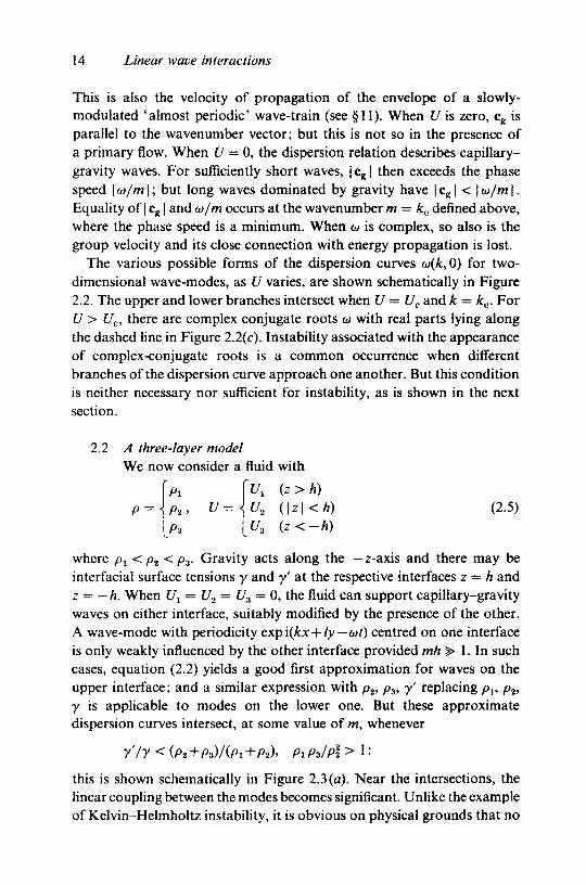
The various possible forms of the dispersion curves co(k, 0) for two-dimensional wave-modes, as U varies, are shown schematically in Figure2.2. The upper and lower branches intersect when U = Uc and k = kc. ForU > Uc, there are complex conjugate roots w with real parts lying alongthe dashed line in Figure 2.2(c). Instability associated with the appearanceof complex-conjugate roots is a common occurrence when differentbranches of the dispersion curve approach one another. But this conditionis neither necessary nor sufficient for instability, as is shown in the nextsection.
2.2 A three-layer modelWe now consider a fluid with
'px \UX (z>h),, U=\u2 {\z\<h) (2.5)
[p3 [U3 (z<-h)
where px < p2 < p3. Gravity acts along the — z-axis and there may beinterfacial surface tensions y and y' at the respective interfaces z — h andz — —h. When U1 — U2 = U3~ 0, the fluid can support capillary-gravitywaves on either interface, suitably modified by the presence of the other.A wave-mode with periodicity expi(kx+ly—<ot) centred on one interfaceis only weakly influenced by the other interface provided mh > 1. In suchcases, equation (2.2) yields a good first approximation for waves on theupper interface; and a similar expression with p2, p3, y' replacing ply p2,7 is applicable to modes on the lower one. But these approximatedispersion curves intersect, at some value of m, whenever
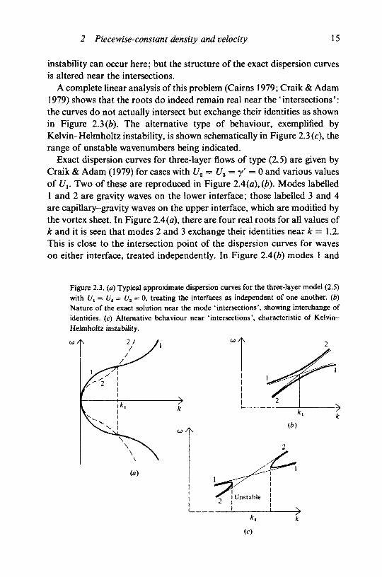
this is shown schematically in Figure 2.3 (a). Near the intersections, thelinear coupling between the modes becomes significant. Unlike the exampleof Kelvin-Helmholtz instability, it is obvious on physical grounds that no
Downloaded from University Publishing Online. This is copyrighted materialIP139.153.14.250 on Tue Jan 24 02:27:20 GMT 2012.
http://dx.doi.org/10.1017/CBO9780511569548.003
2 Piecewise-constant density and velocity 15
instability can occur here; but the structure of the exact dispersion curvesis altered near the intersections.
A complete linear analysis of this problem (Cairns 1979; Craik & Adam1979) shows that the roots do indeed remain real near the 'intersections':the curves do not actually intersect but exchange their identities as shownin Figure 2.3(6). The alternative type of behaviour, exemplified byKelvin-Helmholtz instability, is shown schematically in Figure 2.3 (c), therange of unstable wavenumbers being indicated.
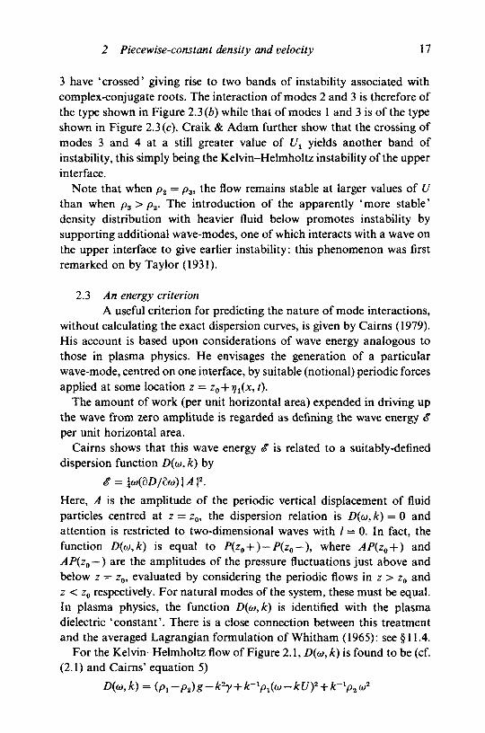
Exact dispersion curves for three-layer flows of type (2.5) are given byCraik & Adam (1979) for cases with U2 — U3 = y' = 0 and various valuesof Uv Two of these are reproduced in Figure 2A(a),(b). Modes labelled1 and 2 are gravity waves on the lower interface; those labelled 3 and 4are capillary-gravity waves on the upper interface, which are modified bythe vortex sheet. In Figure 2.4 (a), there are four real roots for all values ofk and it is seen that modes 2 and 3 exchange their identities near k = 1.2.This is close to the intersection point of the dispersion curves for waveson either interface, treated independently. In Figure 2.4(6) modes 1 and
Figure 2.3. (a) Typical approximate dispersion curves for the three-layer model (2.5)with U, = Ut = U3 = 0, treating the interfaces as independent of one another, (b)Nature of the exact solution near the mode 'intersections', showing interchange ofidentities, (c) Alternative behaviour near 'intersections', characteristic of Kelvin-Helmholtz instability.
Downloaded from University Publishing Online. This is copyrighted materialIP139.153.14.250 on Tue Jan 24 02:27:20 GMT 2012.
http://dx.doi.org/10.1017/CBO9780511569548.003

16 Linear wave interactions, 4
OJ 0
co 0
-1 -
Figure 2.4. Frequency vs. wavenumber dispersion curves for the three-layer flow (2.5),with £/2 = U3 = / = 0, y = 74gs-2, h = 8 cm, g = 981 cms"1, p, = 1.015,p3= 1.020, p 3 = 1.026gcnr3. Case (a) shows 1^ = 8.0cms"1 and case (b)[/, = 8.7 cm s"1 (from Craik & Adam 1979).
Downloaded from University Publishing Online. This is copyrighted materialIP139.153.14.250 on Tue Jan 24 02:27:20 GMT 2012.
http://dx.doi.org/10.1017/CBO9780511569548.003
2 Piecewise-constant density and velocity 17
3 have 'crossed' giving rise to two bands of instability associated withcomplex-conjugate roots. The interaction of modes 2 and 3 is therefore ofthe type shown in Figure 2.3 (b) while that of modes 1 and 3 is of the typeshown in Figure 2.3 (c). Craik & Adam further show that the crossing ofmodes 3 and 4 at a still greater value of Ul yields another band ofinstability, this simply being the Kelvin-Helmholtz instability of the upperinterface.
Note that when p2 = p3, the flow remains stable at larger values of Uthan when ps>p2- The introduction of the apparently 'more stable'density distribution with heavier fluid below promotes instability bysupporting additional wave-modes, one of which interacts with a wave onthe upper interface to give earlier instability: this phenomenon was firstremarked on by Taylor (1931).
2.3 An energy criterionA useful criterion for predicting the nature of mode interactions,
without calculating the exact dispersion curves, is given by Cairns (1979).His account is based upon considerations of wave energy analogous tothose in plasma physics. He envisages the generation of a particularwave-mode, centred on one interface, by suitable (notional) periodic forcesapplied at some location z = Zg+r/^x, t).
The amount of work (per unit horizontal area) expended in driving upthe wave from zero amplitude is regarded as defining the wave energy £per unit horizontal area.
Cairns shows that this wave energy <f is related to a suitably-defineddispersion function D(a>, k) by
Here, A is the amplitude of the periodic vertical displacement of fluidparticles centred at z = z0, the dispersion relation is Z)(w, k) = 0 andattention is restricted to two-dimensional waves with / = 0. In fact, thefunction D(o),k) is equal to P(zg +) — P(z0 —), where AP(zo + ) andAP(z0 —) are the amplitudes of the pressure fluctuations just above andbelow z = z0, evaluated by considering the periodic flows in z > z0 andz < z0 respectively. For natural modes of the system, these must be equal.In plasma physics, the function D((o,k) is identified with the plasmadielectric 'constant'. There is a close connection between this treatmentand the averaged Lagrangian formulation of Whitham (1965): see § 11.4.
For the Kelvin-Helmholtz flow of Figure 2.1, Z>(w, k) is found to be (cf.(2.1) and Cairns' equation 5)
D(cj,k) = (pi-pjg
Downloaded from University Publishing Online. This is copyrighted materialIP139.153.14.250 on Tue Jan 24 02:27:20 GMT 2012.
http://dx.doi.org/10.1017/CBO9780511569548.003

18 Linear wave interactions
when z0 is chosen to be just below the interface z — 0. It follows that
g = \\A\*k^u>[(pl+p,)u>-plkU] (2.6)
where A is the interfacial wave amplitude. Substitution from the dispersionrelation Z)(w, k) = 0 yields
the + and — signs corresponding to the greater and lesser roots wrespectively and the positive square root being taken. Kelvin-Helmholtzinstability occurs when the expression in square brackets is negative, inagreement with the result found above: here we suppose that thisexpression is positive.
When U > 0, the greater root of w is positive for all k > 0 and the energyg of this mode is therefore positive. The lesser root to is certainly negativefor sufficiently small positive values of U and then carries positive energyg. But this root a> may become positive, for some k, at large values of U.An instance of this is shown in Figure 2.2(6) with kx < k < k2; anotheris shown in Figure 2.4(a) for mode 3 with 0.1 < k < 0.8. In such cases,the wave energy g is negative.
The realization that waves may possess either positive or negative energyg is the key to understanding the two types of mode interaction near'intersection points' of the approximate dispersion curves obtained byregarding the interfaces as uncoupled. When two approximate dispersioncurves cross, and the respective modes have energies of the same sign, thenthe exact dispersion curves 'exchange identities' when they approach oneanother and both roots remain real. But when two modes cross and haveenergies of opposite sign, the coupling causes complex conjugate roots toappear when the modes are sufficiently close. The form of the dispersioncurves is then as shown in Figure 2.3(c), with instability near the'intersection' point.
The reason for this behaviour is easily demonstrated. The exactdispersion relation for the three-layer flow (2.5) with U2 = U3 = 0 has theform (cf. Cairns 1979)
Z)j(w, k) £>2(w, k) = (pi oj*/k2) cosech2 2kh (2.7)
where D1 = 0 and D2 = 0 are the respective dispersion relations for waveson either interface, with the other replaced by a plane rigid wall. Theright-hand side, an exponentially-small quantity when kh is large, represents
Downloaded from University Publishing Online. This is copyrighted materialIP139.153.14.250 on Tue Jan 24 02:27:20 GMT 2012.
http://dx.doi.org/10.1017/CBO9780511569548.003

2 Piecewise-constant density and velocity 19
the coupling between the modes. This has negligible effect except when theroots of Z>! = 0 and D2 = 0 are close. In this case, let
for some k where w2—w, = 8, a real quantity with | S/^ | small. On settingto = wx + A in (2.7) one obtains the leading-order approximation
This has the form
with K positive if the energies S of the waves have the same sign and Knegative if the signs of S differ. In the former case, the roots A are realand no instability occurs. In the latter, they are complex conjugateswhenever | S/K | < 2: instability then occurs whenever the roots a)1 and w2
are sufficiently close.Application of the above energy criterion remains valid for all multi-
layered flows with piecewise-constant density and velocity. For continuousvelocity and density profiles, though, the situation is complicated by theoccurrence of critical layers within the flow where energy may be exchangedbetween waves and mean flow. The situation is then somewhat analogousto Landau damping in plasmas (Briggs, Daugherty & Levy 1970).
2.4 Viscous dissipationThe above consideration of wave energy also provides some
insight into the dissipative role of viscosity. We illustrate this for thevortex-sheet configuration (Figure 2.1), following Cairns (1979): (see alsoLandahl 1962; Benjamin 1963; Ostrovsky & Stepanyants 1983). Let thelower fluid have kinematic viscosity v, while the upper fluid remainsinviscid. Since the lower fluid is at rest apart from the periodic disturbance,viscosity must continuously extract energy from the system. In this case,a positive-energy wave must gradually decay as its energy diminishes. Incontrast, a negative-energy wave must grow to accommodate the gradualdecrease in energy!
For example, in Figure 2.2(6) which has a flow velocity below that forKelvin-Helmholtz instability, mode 2 has negative energy for kt < k < k2.Such wavenumbers must therefore be destabilized by the viscosity of thelower fluid, while all other waves are damped. The dispersion relation thenhas the form
(2.8)
Downloaded from University Publishing Online. This is copyrighted materialIP139.153.14.250 on Tue Jan 24 02:27:20 GMT 2012.
http://dx.doi.org/10.1017/CBO9780511569548.003

20 Linear wave interactions
where D(<u, k) = 0 for inviscid flow. When wo(A:) is a root of the latterequation, a good approximation to the solution of (2.8), when v issufficiently small, is <o = oi0 + SOJ where
Since 8u> is imaginary, this approximation denotes growth or decayaccording as the sign of the wave energy, given by (2.6), is negative orpositive.
This instability is of a different sort from the Kelvin-Helmholtz type.In the language of plasma physics (e.g. Bekefi 1966) the latter is a 'reactive'instability where one mode reacts on another to produce complex conjugateroots, while the present type is an example of' resistive' instability. Growthrates of the resistive instability are typically much smaller than for thereactive.
The effect of dissipation by viscosity within a particular layer of fluidpossessing uniform velocity U may be inferred by determining the sign ofthe wave energy in the reference frame moving with this velocity U. If thewave appears in this frame to have positive energy, then the local viscousdissipation tends to diminish the wave amplitude; if negative, the amplitudewill tend to increase. Of course, the envisaged flow is a rather artificial one;and one cannot normally regard viscosity as zero in one part of the flowand non-zero in another. For instance, in the rest frame of the upper fluidof the Kelvin-Helmholtz flow of Figure 2.1, the wave which the lower fluidperceived as having negative energy appears to have positive energy:viscosity in the upper fluid therefore tends to cause this mode to decay andthe influences of the upper and lower fluid viscosities are in conflict.
Furthermore, the above treatment assumes that the major part of theviscous dissipation is accomplished by the straining of the irrotational flowfield. While this is so for wave motion with interfaces which are virtuallyfree from tangential stress and in the absence of (or with sufficientlydistant) rigid horizontal boundaries, this is not always the case. A nearbyupper or lower rigid boundary, or an interface between two viscous fluids,usually has a rather strong periodic viscous boundary layer in its vicinityand this may account for the bulk of the dissipation (see §3.2 below),thereby contradicting result (2.9). Nevertheless, the present account servesto demonstrate the rather unexpected, but frequent, destabilizing role ofviscosity. A further example of resistive instability is that of a uniform shearflow with free surface above and rigid boundary below (Miles 1960; Smith& Davis 1982).
Downloaded from University Publishing Online. This is copyrighted materialIP139.153.14.250 on Tue Jan 24 02:27:20 GMT 2012.
http://dx.doi.org/10.1017/CBO9780511569548.003

3 Constant density, continuous velocity profile 21
Benjamin (1963) proposed a three-fold classification of unstable disturb-ances. His class C instability is of the Kelvin-Helmholtz, or reactive, type.His class A instability is the resistive type in which negative-energy wavesgrow by a net extraction of energy from the system by dissipation. His classB instability corresponds to the instability of a wave of positive energy bythe net addition of energy from an external source. However, categoriesA and B are not entirely distinct: the choice of a different reference framemay change the energy sign of a disturbance and so the category to whichit belongs. Unfortunately, this classification is not particularly helpful forshear flows with critical layers, where energy may be transferred betweenmean flow and wave.
Finally, we observe that bounded flows of homogeneous viscous fluid,with prescribed velocities at the boundaries, are globally stable at sufficientlysmall Reynolds numbers (Synge 1938; Joseph 1976). But this is notnecessarily so for flows with free surfaces or internal interfaces. Examplesof small-/? instability are those of Benjamin (1957), Craik (1966,1969), Yih(1967) and Hooper & Boyd (1983). Variable tangential stresses at the meaninterface level typically play an important role in causing such instabilityat small dimensionless wavenumbers.
3 Flows with constant density and continuous velocity profile3.1 Stability of constant-density flows
Vortex-sheet profiles cannot persist, being eroded by viscosity intocontinuously-varying shear layers. The study of such discontinuous profilesis therefore based on the expectation that they retain characteristic featuresof continuous shear-layer profiles, while allowing simpler mathematicaltreatment. This is indeed so, but care is required in interpreting the results.
A fundamental difference between vortex-sheet profiles and continuousones is the appearance, in the latter, of one or more critical layers wheneverthe phase velocity of the wave lies between the maximum and minimumflow velocities. In the linear inviscid approximation, the governing equationis singular at such locations. For a primary parallel shear flow U(z) ofconstant-density fluid with kinematic viscosity v, a small two-dimensionalwavelike disturbance has velocity perturbations
u' = dfr/dz, W = —dijf/cix,
i/r = e Re {<f>(z) exp [ik(x—ct)]}, c = cT+ici.
This dependence of u' and w' on the perturbation stream function i/rensures that the continuity equation (1.1b) is identically satisfied. Theeigenfunction <p(z) may be shown to satisfy the Orr-Sommerfeld equation
(3.1a)
Downloaded from University Publishing Online. This is copyrighted materialIP139.153.14.250 on Tue Jan 24 02:27:20 GMT 2012.
http://dx.doi.org/10.1017/CBO9780511569548.003

22 Linear wave interactions
where the prime denotes d/dz. This is just the vorticity equation, obtainedby eliminating the pressure p from the momentum equations (1.1a).
The complex frequency (o(k) equals kc and the wavenumber k is real forpurely temporal growth or decay. At rigid plane boundaries, say at z = zx
and z2, the appropriate boundary conditions are
0 = 0, 0' = O {2 = 2^2^. (3.2a, b)
The latter of these must be ignored for inviscid flows, v = 0, when the orderof the equation (3.1) is reduced from four to two. Equation (3.1a) withv = 0,
(U-c)(<f>"-k2<P)-U"<?> = 0, (3.3a)
is known as Rayleigh's equation. When U" = 0, Rayleigh's equation in turnreduces to 0" = k?<j>, which is equivalent to Laplace's equation for \jr.
The customary introduction of dimensionless variables, relative tochosen velocity and length scales V and h, leads to a similar equation withU, c, k, 2 replaced by their dimensionless counterparts and v~l replacedby the Reynolds number R = Vh/v. The dimensionless wavenumber kh iscustomarily denoted by a and the dimensionless form of (3.1a) is
( t / - c ) ( 0 " - a 2 0 ) - ^ Y = (ia/?)-1(^iv-2a2^"+aV) (3.1b)where U, c and z now represent dimensionless quantities. Similarly, thedimensionless form of Rayleigh's equation for inviscid flow is
(t/-c)(0"-aV)-tr0 = O. (3.3b)
The eigenvalue problem for c = c(a.,R), posed by (3.1b) and (3.2) oralternative boundary conditions, with C/(z) given, has received muchattention, the most up-to-date account being that of Drazin & Reid (1981).When acR is sufficiently large, the general solution of Rayleigh's equation(3.3) for inviscid flow gives good approximations, over most but not allof the flow domain, to two of the four independent solutions of (3.1). Theremaining two solutions depend explicitly on the Reynolds number R. Theinviscid solutions normally have singular derivatives at locations z = zc
where t/(zc) = c, and they do not satisfy the no-slip condition (3.2b) at rigidboundaries. Accordingly, modification of the inviscid solutions takes placenear critical layers and walls.
Much effort has been devoted to the development of asymptotictechniques, incorporating the viscous terms, to obtain acceptable approxi-mations for 0(z) and c. Indeed, this was for long the only means ofprogress; but the development of high-speed computers and improvementsin numerical techniques now provide a ready means of solving (3.1)directly. A comprehensive account of the asymptotic theory, includingrecent successes in achieving uniformly-valid representations, is given by
Downloaded from University Publishing Online. This is copyrighted materialIP139.153.14.250 on Tue Jan 24 02:27:20 GMT 2012.
http://dx.doi.org/10.1017/CBO9780511569548.003

3 Constant density, continuous velocity profile 23
Drazin & Reid (1981), who also review the better-known computationalmethods.
For the present, we confine attention to results for the particulardimensionless shear-layer profile
U - tanhz,which illustrate the connection with the vortex-sheet model. The inviscidproblem, with unbounded flow, was studied by Gotoh (1965). He foundtwo modes with imaginary parts cx of c which approach + 1 as thedimensionless wavenumber a approaches zero. The real parts cr of bothmodes approach zero as a-*0. This long-wave limit is in complete accordwith result (2.3) for the vortex sheet, on taking account of the changeof reference frame. However, as a increases, the imaginary parts ct ofboth roots decrease, approaching asymptotes q / a = —0.376 and —2.22respectively as <x->oo (Drazin & Reid p. 238). The mode which is unstableat small a has Cj = 0 at a = 1 and is damped for all a > 1. The shearprofile therefore exerts a stabilizing influence on the flow in the absenceof viscosity.
The corresponding viscous problem was treated by Betchov & Szewczyk(1963) who found the curve of neutral stability in the a-R plane. At everyReynolds number, no matter how small, there exist unstable modes withsufficiently small wavenumbers a, the band of unstable wavenumbersbecoming ever smaller as R decreases (Drazin & Reid p. 239). Indimensional terms, the Helmholtz instability persists for waves longcompared with both the shear-layer thickness h and the viscous length-scale(p/
3.2 Critical layers and wall layersThe critical layer plays an important role in the instability of
parallel flows of homogeneous fluid: see §9 and, for a fuller account,Drazin & Reid (1981). Inviscid flows satisfy the Rayleigh equation (3.3)and the presence of lateral boundaries at z = zl,zi requires0(zx) = $J(z2) = 0; alternatively, for unbounded and' semi-bounded' flows,{i->0asz->-oo or +oo. For a neutrally-stable wave (c, = 0), the meandimensionless Reynolds stress T = — (u'w') = — \a Im{0'0*} is constantexcept at any critical layer z = zc, where it has a discontinuity
r(zc + ) - T(ZC - ) = \om{U'U U'c) \<pc\\
the subscript c denoting evaluation at zc. Here, * denotes complex con-jugate and the overbar an x-average. But the above boundary conditionsrequire that T vanishes at zx and z2. If there is just one critical layer,neutral and amplified disturbances may exist if and only if U" vanishessomewhere in the flow domain. This and other general theorems are
Downloaded from University Publishing Online. This is copyrighted materialIP139.153.14.250 on Tue Jan 24 02:27:20 GMT 2012.
http://dx.doi.org/10.1017/CBO9780511569548.003

24 Linear wave interactions
reviewed by Drazin & Reid. If there is more than one critical layer, thesum of all the discontinuities in T must vanish for neutral disturbances.
For continuous, monotonically increasing profiles of boundary-layerform, there is one critical layer when Umin < c < f/max. For planeCouette-Poiseuille channel flows, there may be one or two. If U" does notchange sign, there can be no unstable or neutrally-stable inviscid modes.However, viscosity admits additional modes, the Tollmien-Schlichtingwaves, some of which may be unstable. The mathematical reason for theappearance of these additional modes is the increased order of thegoverning equation, from the two of Rayleigh's equation to the four ofthe Orr-Sommerfeld equation. In physical terms, when aR > 1 and c is0(1), there are thin oscillatory viscous boundary layers with thickness0[{a.R)~^] adjacent to the wall; also viscous modifications in a layer ofthickness 0[(aR)~§ about z = zc. These may permit neutral or growingwaves with finite values of r in the inviscid region between critical layerand wall, since T is able to decrease rapidly to zero within the viscous walllayer.
Near the walls, the viscous modes resemble the flow induced byoscillating a rigid boundary in its own plane, the wavelength 2n/a typicallybeing large compared with the O[(aR)~%\ wall-layer thickness within whichthe viscous modes rapidly decay. In place of an oscillating boundary, itis the inviscid flow just beyond the wall layer which oscillates: the inviscidand viscous modes must combine to satisfy the no-slip condition at thestationary wall. Similar viscous modes also occur at deformable boundarieswhere different boundary conditions must be met (see §§9-10).
For the Blasius boundary layer on a flat plate, unstable modes exist forall R = Uo S(x)/v greater than the critical value Rc = 520 (Jordinson 1970).Here Uo is the free-stream velocity and S(x) the displacement thickness.This result was obtained by solving the Orr-Sommerfeld equation,neglecting the weak non-parallelism of the flow. The pioneering experimentsof Schubauer & Skramstad (1947, but first issued in 1943) revealed at leastapproximate agreement with quasi-parallel linear theory and more completedata were obtained by Ross, Barnes, Burns & Ross (1970). Despite someas yet unresolved points of detail concerning non-parallelism, the agreementbetween linear theory and experiment is gratifyingly good.
The influence of flow divergence has been variously treated. Bouthier(1973), Gaster (1974) and Saric & Nayfeh (1975) developed approximateprocedures for flow at near-critical Reynolds numbers. Their results showsome reduction of Rc due to non-parallelism and agree even better withexperiment than do those of quasi-parallel theory. Rational asymptoticanalyses of Smith (1979a) and Bodonyi & Smith (1981) determine the
Downloaded from University Publishing Online. This is copyrighted materialIP139.153.14.250 on Tue Jan 24 02:27:20 GMT 2012.
http://dx.doi.org/10.1017/CBO9780511569548.003

3 Constant density, continuous velocity profile 25
asymptotes to the lower and upper branches of the neutral stability curveas R -> oo. The influence of non-parallelism then leads to rather complicatedflow structures. Extrapolation of their results to lower 0(1O2) Reynoldsnumbers at which experimental data are available again yields quitesatisfactory agreement. However, such extrapolation is 'non-rational', forthe respective analyses employ R~^ and R~& as small parameters and thelatter equals 0.7 when R — 103, for instance.
For plane Poiseuille flow, satisfactory agreement between linear theoryand experiment was only recently achieved, by the experimental work ofNishioka, Iida & Ichikawa (1975). The critical Reynolds number for thisflow is Rc = 5772 and, at such high Reynolds numbers, great care isnecessary to achieve conditions free from nonlinearity and the influenceof side walls and entry region. Without such care, subcritical instabilityand transition to turbulence occurs for all R > 103 or so. In fact, as Rincreases, the range of validity of linear theory is confined to ever-smallerwave amplitudes. The neutral curve in the a-R plane, which separatesregions of stability and instability, is shown in Figure 6.3 of §20.
For plane Couette flow (Romanov 1973) and for Poiseuille flow in a pipeof circular cross-section, linear theory indicates no normal mode instability;but a rigorous proof for the latter flow is still lacking. In practical terms,nonlinear mechanisms will govern the stability of these flows.
The role of the critical layer is also crucial in the generation of waterwaves by wind. This was first elucidated by Miles (1957a). There is a criticallayer in the airflow above downwind-propagating water waves providedtheir phase velocity does not exceed the maximum wind speed. Onassuming the airflow to be 'quasi-laminar' (though, in fact, turbulentfluctuations ought not to be ignored), Miles showed that this induces amean Reynolds stress T much as described above. In the absence of suchReynolds stress, the pressure fluctuation p' at the air-water interface is inexact antiphase with the upwards surface displacement i\ and the onlypossible instability mechanism is the Kelvin-Helmholtz one discussed in§2.1. A non-zero Reynolds stress is associated with a phase-shift of p'relative to i/, and this phase-shift is responsible for instability at windspeeds far smaller than those required for Kelvin-Helmholtz instability.The rate of working of p' on a neutrally-stable wave is
W = —p' 9i//0/ = \ck Imp'rj*
per unit area, which is positive when p' has a component in phase with_the wave-slope dij/dx. Instability, and so wave generation, occurs when Wexceeds the rate of energy dissipation by viscosity within the water.
Miles' original inviscid theory was extended by Miles (1959), Benjamin
Downloaded from University Publishing Online. This is copyrighted materialIP139.153.14.250 on Tue Jan 24 02:27:20 GMT 2012.
http://dx.doi.org/10.1017/CBO9780511569548.003

26 Linear wave interactions
(1959) and others to viscous airflows. Agreement is good with subsequentdirect computations (Caponi, Fornberg et al. 1982) of the airflow oversmall-amplitude waves. However, as expected, the calculated airflow overlarger waves, and the corresponding pressure distribution, are ratherdifferent from linear estimates: then, separation eddies form in the troughsof the waves.
The linear quasi-laminar theory has also been integrated with another,complementary, theory of Phillips (1957) which dealt with waves generatedin response to imposed (turbulent) pressure variations convected by theairflow (Phillips 1977; Barnett & Kenyon 1975). The influence of small-scaleturbulence in the vicinity of the critical layer was discussed heuristicallyby Lighthill (1962) and a more comprehensive theory of turbulent airflowwas developed by Davis (1972, 1974). However, such theories remain farfrom complete.
Experiments in laboratory channels by Cohen & Hanratty (1965) andPlant & Wright (1977) - see also the reviews by Barnett & Kenyon (1975)and Hanratty (1983) - show satisfactory agreement with the quasi-laminartheory only for rather short waves. In thin layers of water, the energytransfer is insufficient to overcome increased viscous dissipation: in this
Figure 2.5. Experimental results of Craik (1966) on onset of wind-generated wavesin thin horizontal films of water.
600
$ 400
I 20°
-1 1 ' I004 008 012
Film thickness (cm)0-16
Downloaded from University Publishing Online. This is copyrighted materialIP139.153.14.250 on Tue Jan 24 02:27:20 GMT 2012.
http://dx.doi.org/10.1017/CBO9780511569548.003

4 Variable density, piecewise-constant velocity 27
case, there is a range of depths for which the interface is stable. But a newtype of instability appears in sufficiently thin films (typically, with depthsd of order 0.3 mm or less) with small Reynolds numbers. In this, wavesgrow because the restoring forces of gravity and surface tension areovercome by a combination of normal and tangential stresses at theinterface, the latter becoming increasingly important as kd-+0 where k isthe dimensional wavenumber (Craik 1966): see Figure 2.5.
Of less practical concern, but of interest in the context of modeinteractions, is a possible coupling between Tollmien-Schlichting waves ofa laminar airflow and the water-wave mode. Under appropriate circum-stances, the real phase velocities cr of the two modes may nearly coincidefor a range of wavenumbers k. This leads to a rather abrupt increase inthe growth rates of the surface-wave (Miles 1962; Blennerhassett 1980;Akylas 1982).
Many surface additives, particularly oils and detergents, have a remark-able capacity to inhibit wave generation by wind and to damp out wavesalready present. Varying surface concentrations of such additives producechanges in surface tension and the interface acquires elastic or elastico-viscous properties whereby it resists local extension or contraction (see, forexample, Miles 1967; Smith & Craik 1971). In effect, the interface nowpossesses additional natural modes of oscillation, comprising periodicextensions and compressions of the free surface. These are stronglycoupled to the underlying watermotion, through modified surface boundaryconditions. The strength of the viscous boundary layer, and so the rate ofdissipation, just beneath the surface is greatly enhanced (see § 10.1 below).The limiting case of an inextensible surface is particularly easy to treatmathematically. In this case, the damping rate of deep-water gravity wavesis just half the maximum possible damping rate when the extensional modeand water wave are most strongly coupled, and much greater than for aclean surface. Scott (1979) gives a comprehensive bibliography of suchwork.
4 Flows with density stratification and piecewise-constant velocity4.1 Continuously-stratified flows
Flows in which the density varies continuously with height areof particular interest in meteorology and oceanography. For these, itis customary to simplify matters by making the so-called Boussinesqapproximation. In this, the influence of density variations upon thegravitational force is retained but such variations are ignored in the fluidinertia. This is an acceptable procedure whenever the maximum density
Downloaded from University Publishing Online. This is copyrighted materialIP139.153.14.250 on Tue Jan 24 02:27:20 GMT 2012.
http://dx.doi.org/10.1017/CBO9780511569548.003

28 Linear wave interactions
variation is small compared with the mean density: this is certainly so inthe ocean and is often, but not always, a satisfactory approximation in theatmosphere.
In these circumstances, a small two-dimensional wavelike disturbancehas the form
u' = iijr/dz, w' = — di/r/dx,
xjr = e Re {<j>(z) exp [ik(x - ct)]} (4.1)
where e is small and the eigenfunction <j>{z) satisfies the equation
(U-c)(<f>"-k20)-U"tj) + N*(f>/(U-c) = 0 (4.2)
for inviscid flow. This was first derived by Taylor (1931), Goldstein (1931)and Haurwitz (1931) and is normally named after the first two authors.Here N(z) s (—gp^1dp0/dz)^ is the buoyancy (Brunt-Vaisala) frequency;po(z) is the density distribution in the undisturbed state, stably-stratifiedso that dpo/dz < 0 everywhere, with z measured vertically upwards; g isgravitational acceleration and U(z) is the primary velocity-profile in thehorizontal x-direction.
On setting C/(z) = 0 and 0(z) = constant, it is seen that there existsolutions corresponding to vertical oscillations with frequencies ± N. Moregenerally, in regions where U(z) and N(z) are constant, there existpropagating internal-gravity waves with <f> oc exp (+ im z) where m is realand non-negative. The possible phase speeds are
c = U±N(k2 + m2)-i
(where signs need not correspond to those in the exponent of $), whichare respectively faster and slower than the free stream U. The correspondingfrequency is <o = kc and the group velocity of the modes <}> oc exp(+iwz)has horizontal (in the x-direction) and vertical components
(wg, wg) = (9w/8fc, do)/dm).
This gives
(«g - U, we) = ± Nm(k* + w2)-? (m, - A:),
showing that, relative to the free stream U, the group velocity is perpen-dicular to the wavenumber vector (k, m) and so parallel to the wave crests.Since energy is transmitted with the group velocity, it is clear that waveenergy is transported upwards by the mode with c < U and downwardsby the mode with c> U. Similarly, the modes <j> oc exp(—imz) havewg ^ 0 according as c $ U.
Downloaded from University Publishing Online. This is copyrighted materialIP139.153.14.250 on Tue Jan 24 02:27:20 GMT 2012.
http://dx.doi.org/10.1017/CBO9780511569548.003

4 Variable density, piecewise-constant velocity 29
4.2 Vortex sheet with stratificationAs an illustrative example, we consider the Helmholtz profile
with constant positive TV and U. The corresponding density distribution/90(z) decreases exponentially with height z. As boundary conditions, werelax the requirement that i/r^O as |z|->-oo in order to admit thepropagating modes, and require instead that rjr remains finite as |z|->oo.We let 0(z) equal ^ (z ) and <j>2(z) in the respective regions z > 0 and z < 0and denote the disturbed interface by z = TJ(X, t) where
T)(X, t) = e Re{expik(x—ct)}
and k is known.Appropriate solutions are
m^ (z > 0) "m** (z < 0)
the positive roots for m, and m2 being taken. Also A,B,C and D are relatedby the kinematic conditions
A + B _ C+Dc-U~ c
while a further boundary condition is furnished by the pressure-balanceacross the interface. When m1 and m2 are real, <p remains bounded atinfinity and these three boundary conditions are clearly insufficient todetermine the four constants A, B,C, D and the phase-speed c(k); in fact,two of these constants may be assigned arbitrary values.
In the region z < 0, the wave modes have frequencies
(o=
Suppose that w, as well as k, is a given positive quantity: then m2 is uniquelydetermined. When m2 is real, the terms of <fi2 in C and D then representwaves with downwards and upwards-propagating energies respectively.Then C may be regarded as a reflected wave. Likewise, in z > 0, A andB represent waves whose energy propagates downwards and upwardsrespectively whenever c> U and ml is real; but these directions arereversed when c < U.
If the frequency w is such that w2 > iV2, m2 is imaginary. Since <f>2 remainsbounded at infinity, it is then necessary to set C = 0: the resultant wave
Downloaded from University Publishing Online. This is copyrighted materialIP139.153.14.250 on Tue Jan 24 02:27:20 GMT 2012.
http://dx.doi.org/10.1017/CBO9780511569548.003

30 Linear wave interactions
amplitude <f>% decays exponentially as exp (| m2 \ z) away from the interfaceand the wave is said to be 'evanescent' in z < 0. Likewise, in z > 0, mt
is imaginary whenever (w — Uk)2 > N*; in this case one must set B = 0 and<px decays as exp (— | mx \ z) as z increases. Both ^>1 and <j52 are evanescentwhen w < — N, N < u> < Uk — N or to > N+Uk. The three interfacialconditions determine whether there are permissible eigenvalues (o(k) inthese ranges.
When (o(k) is such that both w, and m2 are real and c = u>/k > U > 0,we may consider a given wave D, incident on the vortex sheet fromz = — co, as giving rise to reflected and transmitted waves C and B. Thewave A incident from z = + oo is meantime chosen to be zero. Thereflection and transmission coefficents | C/D | and | B/D \ are determinedby the interfacial conditions to be (cf. Lindzen 1973; Acheson 1976)
C 1 G Bl^U)v
D l+Q D c(\+Q)where
Q_m1(c-Uym2c
2
Since | C/D | < 1 for all Q > 0, partial reflection occurs. When Q—\, thereis no reflection and the transmission coefficient attains its greatest value(m.i/ml)i. Qualitatively similar results are obtained for propagating modeswith c < 0.
A rather different picture emerges for propagating modes with0 < c < U. Then, the transmitted wave in z > 0 is A, while B may be chosenas zero. The reflection and transmission coefficients (with A replacing B)have the same form as (4.5), but now Q is minus the above expression. Thismeans that the reflection coefficient always exceeds unity in such cases.Moreover, a singularity occurs at Q = — 1, when both the reflection andtransmission coefficients become infinite. This phenomenon has becomeknown as over-reflection, the singular case being called resonant over-reflection. The latter case arises when the system can support outgoing' reflected' and' transmitted' waves in the absence of an incident wave. Thisintriguing phenomenon was first noted by Miles (1957b) and Ribner (1957)in the context of acoustics, but was not recognized for internal gravitywaves until the work of Jones (1968).
In the absence of incoming wave energy, the only possible neutral modesare those which correspond to resonant over-reflection. For these,
Downloaded from University Publishing Online. This is copyrighted materialIP139.153.14.250 on Tue Jan 24 02:27:20 GMT 2012.
http://dx.doi.org/10.1017/CBO9780511569548.003

4 Variable density, piecewise-constant velocity 31
where 0 < c < U and mx, mz are as defined above. Substitution for wt andw2 yields a cubic equation for c,
(c-\U)[c2-Uc + \(U2-N2/k2)] = 0 (4.6)
with the three roots
\\U, m1 = mt = (—-k*) >0,c =
ck (U-c)k
The first of these roots exists only for A;2 < 47V2/ U2, there being no solutionwith pure imaginary wx and m2 which remains bounded at infinity. Thelatter pair of roots exists provided k2 > N2/U2, since c must lie in the range0 < c < U for over-reflection. They are real for N2/U* < k2 < 2N2/U2
and become complex conjugates when k2 > 2N2/U2. The appearance ofconjugate roots signals the onset of a Kelvin-Helmholtz instability:sufficiently short waves are always unstable, however strong thestratification.
4.3 Over-reflection and energy fluxAn understanding of over-reflection is acquired by examining the
energy flux. Unlike the evanescent wave-modes in homogeneous fluidlayers, internal waves which propagate vertically to infinity have infinitewave energy per unit horizontal area. One must calculate the rate of workdone in maintaining such a wave, as it continuously transmits energy toinfinity. To do this, consider just half the flow, either above or below theinterface z = i](x, /), and suppose that an applied periodic pressuredistribution/?^, t) at the interface maintains an outgoing wave of constantamplitude. The rate of working W by p is just
W= f/roftds
where s denotes arc-length along the interface, h is the unit normal directedinto the region considered and u is the fluid velocity vector at the interface.For the upper region, we have the linear approximations
7/ = e Re {exp [ik(x - c/)]}, ds = dx, h = ( - dij/dx, 1),
u = (U, 0) + e Re {iK(m, -k) exp i(kx+mz-kct)} (z > 0)
where K — c— U by virtue of the kinematic boundary condition.For an outgoing wave, m = — m, for c > U and + m1 for c < U, where
Downloaded from University Publishing Online. This is copyrighted materialIP139.153.14.250 on Tue Jan 24 02:27:20 GMT 2012.
http://dx.doi.org/10.1017/CBO9780511569548.003

32 Linear wave interactions
It follows that
pwdx\
where w is the O(e) z-velocity component evaluated at z = 0. The averageof W, per unit length of the interface, is therefore
W = (-^~j)pw = pocW^ = -|eVo(c-Uf c Re{m*k} (4.7)
where * denotes complex conjugate and the overbar signifies an x-average.Here, we have used the result relating p to the O(e) x-velocity u' (cf.Acheson 1976), that
p = po(c -U)u'
which follows directly from the .x-momentum equation.When c < 0 or c> U and m is real, W is positive for an outgoing wave.
The positive upwards component of group velocity w-then transmitspositive wave energy to z = + oo. But, when 0 < c < U, W is negative; inwhich case there is a flux of negative wave energy towards z = + oo.
For the lower fluid z < 0, where there is no primary flow,
where m — m2 (> 0) for c > 0 and —m% for c < 0 for outwards wavepropagation towards z = — oo. Since W is positive in both cases, thesewaves transmit positive energy towards z = — oo.
During over-reflection, a positive-energy wave incident on the vortexsheet from z = — oo with wave speed c either less than zero or greater thanV can only generate transmitted and reflected waves with positive energy.Partial reflection therefore takes place. But an incident wave with0 < c < U necessarily generates a transmitted wave with negative energy,and the negative energy carried off to +oo can only be offset by areflected positive-energy wave with amplitude greater than that of theincident wave.
Resonant over-reflection occurs when the interfacial conditions admitoutgoing-wave solutions with equal and opposite energy flux in theupwards and downwards directions. That is, the upward-propagatingnegative-energy wave and the downward-propagating positive-energywave together yield zero total energy flux away from the interface. Wavesradiate away from the vortex sheet and there is a constant-amplitudeinterfacial disturbance.
The addition of a jump in density at the interface admits interfacial
Downloaded from University Publishing Online. This is copyrighted materialIP139.153.14.250 on Tue Jan 24 02:27:20 GMT 2012.
http://dx.doi.org/10.1017/CBO9780511569548.003

4 Variable density, piecewise-constant velocity 33
gravity waves. Then, it is possible for waves to grow by radiative instability;for, when an interfacial wave resonates linearly with an outward propa-gating internal wave-mode, both grow if their respective energies haveopposite signs. Examples of such instability are given by Ostrovsky &Tsimring (1981) and Ostrovsky, Stepanyants & Tsimring (1983).
They discuss a Kelvin-Helmholtz configuration with homogeneousupper fluid of density Pl and uniformly (but weakly) stratified lower fluidwith constant Brunt-Vaisala frequency N and reference density p2. Whenthe upper fluid has depth h and the lower fluid is unbounded, the lineardispersion relation is then
Pl(c- Uf cothkh+P2c[c2-(N/k)*]l-(Pi-Pl)g/k = 0
if surface tension is ignored. Note that this is consistent with (2.1) as N->Qand kh ->oo.
At sufficiently large wavenumbers k, Kelvin-Helmholtz instabilityoccurs (though this may be inhibited by surface tension); also, there is aseparate unstable range of smaller wavenumbers, owing to downwardsradiation of positive-energy internal waves with the same real frequencyas negative-energy interfacial waves. This takes place when the slower ofthe two interfacial modes has 0 < cr < N/k, the condition cr > 0 ensuringthat this mode has negative energy (see §2) while downward-radiatinginternal waves must have cT < N/k.
It should be noted that not all the O(e2) energy resides in the O(e)periodic fluctuations, but that an O(e2) mean-flow modification alsocontributes. This fact, and also the relationship between energy and ' waveaction', are demonstrated in §11.
4.4 The influence of boundariesFor the simple Kelvin-Helmholtz flow of Figure 2.1, but with
plane rigid boundaries at z = a and z = —b (a,b > 0), the instabilitycriterion differs from (2.4) by the replacement of the factor Pl p2(Pl +p2)~
1
of the left-hand side by Pl P2{Pl tanh (mb)+p2 tanh (ma)}'1 (Rayleigh 1896,vol. 2, p. 378). Since this factor is always greater than that for unboundedflow, the boundaries have a destabilizing effect on all wavenumbers. Thephase speed of capillary-gravity waves with U = 0 is reduced by thepresence of the boundaries and so a lower value of Ucan cause coalescenceof the two modes.
However, in another sense, the presence of boundaries is stabilizing, inthat the growth rate of unstable modes is usually decreased. This is
Downloaded from University Publishing Online. This is copyrighted materialIP139.153.14.250 on Tue Jan 24 02:27:20 GMT 2012.
http://dx.doi.org/10.1017/CBO9780511569548.003
34 Linear wave interactions
exemplified by the Kelvin-Helmholtz profile with pl = p2 and y = 0 withboundaries at z = a and — b. For this, the eigenvalue relation (2.3) isaltered to
\kU)
for which the unstable root has \m{<i)/kU} < \ for all non-equal value ofa and b.
For continuously-stratified flows, the presence of boundaries has a moredramatic effect. This is most simply demonstrated for the Helmholtz profile
ft/ (z>0), 1U{z>-\0 ( - / / < z < 0 ) I (4.8)
N2 = constant ( — H < z < oo)J
with a rigid plane boundary at z = — H. Since the vertical velocity at theboundary must vanish, the stream function in — H < z < 0 has the formgiven in (4.4), but with
C- = - e .
The solution in this region therefore comprises both upwards- anddownwards-propagating components. It follows directly from (4.5a) that
Q = +^!i£ L = j c o t (m2 H) (4.9)
when no wave is incident from z = + 00. The dispersion relation definedby (4.4) and (4.9) is a special case of that examined by Lalas, Einaudi &Fua(1976).
This relation yields an infinite number of modes, for given k, many ofwhich are unstable. A comprehensive discussion and computed dispersioncurves for some of these modes are given by Lalas et al. These new modesappear because the region between boundary and interface acts as an(imperfect) waveguide. A wave-component incident on the interface frombelow may be either partially reflected or over-reflected, while a waveincident on the boundary is totally reflected. A 'trapped' mode suffersrepeated reflections, its amplitude increasing or decreasing with eachreflection at the interface. Over-reflected waves are therefore unstable andpartially-reflected waves are damped.
This instability due to repeated reflections is quite distinct from theradiative instability mentioned in §4.3. Flows which can admit bothmechanisms together deserve study.
Downloaded from University Publishing Online. This is copyrighted materialIP139.153.14.250 on Tue Jan 24 02:27:20 GMT 2012.
http://dx.doi.org/10.1017/CBO9780511569548.003

5 Continuous density and velocity profiles 35
5 Flows with continuous profiles of density and velocity5.1 Unbounded shear layers
For inviscid flows with continuous velocity profiles U(z), thepresence of a critical layer significantly modifies the above results. A fulldiscussion of the various classes of disturbance is given by Banks, Drazin& Zaturska (1976) and Drazin, Zaturska & Banks (1979). The former dealwith flows between lateral boundaries and unbounded flows such thatiV2(z)->0 as | z | ->oo: for these, no modes propagate at infinity. The latterconsider flows with N2(z) -* N% (constants) as z -> + oo for which suchpropagating modes exist.
Any unstable mode of the inviscid velocity profile with N\z) = 0 ismodified by buoyancy and all instabilities disappear if the local Richardsonnumber J{z) s N2(dU/dz)~2 is nowhere less than \. This is the 'Miles-Howard theorem' (Drazin & Howard 1966). But buoyancy sometimes hasa destabilizing effect when J(z) < £ somewhere within the flow (Howard& Maslowe 1973). In addition to any unstable, or marginally-stable, modesthere are exponentially-damped modes, all having phase velocities with^min < cr < ^max- There also exist classes of constant-amplitude internalgravity waves with cr > £/max and cT < Umin and a continuous spectrumof singular neutral modes associated with algebraic, rather than expo-nential, decay of disturbances. If N2 < 0 anywhere, gravitationally-unstable modes of course occur.
Many general results, together with those for particular profiles of l/(z)and N2(z), are described by Drazin & Howard (1966), Hazel (1972) andin the above-mentioned papers. Typical of unbounded shear layers is thehyperbolic-tangent velocity profile with constant Brunt-Vaisala frequency,discussed in detail by Drazin, Zaturska & Banks (1979). In dimensionlessvariables, this is
l / = t a n h r , iV2 = J (constant) ( - o o < z < o o ) . (5.1)
If a = kh denotes the corresponding dimensionless wavenumber where his the length-scale which characterizes the shear-layer thickness, theTaylor-Goldstein equation (4.2) yields neutrally stable solutions
y = a 2 ( l - a 2 ) , c = 0 (5.2)
and unstable solutions exist at all points of the ct-J plane enclosed by thiscurve and the axis 7 = 0.
In the unstratified case, 7 = 0, all sufficiently-short waves (a > 1) aredamped, as described previously. Now buoyancy provides a furtherrestoring force which acts to inhibit Kelvin-Helmholtz instability, especiallyat longer wavelengths. It is readily seen that instability disappears for allJ > I in agreement with the general Richardson-number criterion.
Downloaded from University Publishing Online. This is copyrighted materialIP139.153.14.250 on Tue Jan 24 02:27:20 GMT 2012.
http://dx.doi.org/10.1017/CBO9780511569548.003

36 Linear wave interactions
In addition to this mode with cr = 0, Drazin, Zaturska & Banks foundtwo other unstable modes with equal and opposite non-zero phasevelocities cr. These exist for 0 < / < 0.13 approximately and have valuesof a somewhat less than the smaller root of (5.2). These modes resemblethe propagating neutral modes of (4.6) associated with resonant over-reflection at a vortex sheet, but now have ct > 0 for a range of a on accountof the role played by the critical layer.
Among the various limiting cases discussed by Drazin et al. is that witha2 ~> 0 and J/a.2 -> 2, for which the dispersion relation simplifies to
c3 + ( l - i / / a 2 ) c = ia. (5.3)
If the right-hand side were zero, this equation would have roots c = 0,c = ±{\J/a2 — 1) which precisely correspond to the roots (4.6) for the
Figure 2.6. Dispersion curves of cr and c, vs. a for the stratified shear layer U = tanh z,N2 = J (constant): c{ is shown by a continuous line when cT =t= 0 and a dashed linewhen cr = 0. Case (a) corresponds to J/a2 = 0.91, case (6) to J/a2 = 0.95 (fromDrazin, Zaturska & Banks 1979).
(a)0-4
0-3
0-2
0-1
0-1 0-2 0-3
0-4
0-3
01 0-2
01
(6)
0-4 0-5 0-6 0-7 0-8
0-22
a 0-20
018
0 001 002 003
0-1 0-2 0-3 0-4 0-5 0-6 0-7 0-8
Downloaded from University Publishing Online. This is copyrighted materialIP139.153.14.250 on Tue Jan 24 02:27:20 GMT 2012.
http://dx.doi.org/10.1017/CBO9780511569548.003

5 Continuous density and velocity profiles 37
vortex sheet when account is taken of the change of origin. The right-handside derives from the critical layer and this provides a coupling betweenthe three modes which is absent for the vortex sheet. Unstable roots existat values of J/a2 greater than 2, for which the vortex-sheet modes arestable.
Computed dispersion curves of cr and cs versus a at various fixed valuesof J/a2 are given by Drazin et al. Two of these are reproduced in Figure2.6(a),(b). In Figure 2.6(a) for J/a2 = 0.91, the dashed line denotes theunstable (Kelvin-Helmholtz) mode with cr = 0. Conjugate modes withcr 4= 0 are unstable for a range of a near that of the neutrally-stable modewith cr = 0. In contrast, Figure 2.6(b) for J/a2 = 0.95 shows a doublebifurcation of the modes. At J/a2 = 1.5 Drazin et al. find a singlebifurcation. At J/a.2 — 3, there is no bifurcation and no unstable mode withcT = 0. At this last value of J/a2, the eigenvalues of the correspondingvortex sheet are c = 0, c = + 2~* and there is no Kelvin-Helmholtzinstability. Drazin et al. find modes with cr close to the latter values butwith small growth rates (q > 0) for 0 < a < 0.1. Presumably, a third modewith cT x 0 is now damped.
In fact, this rather complicated behaviour may be modelled qualitativelyby the root locus of simple cubic equations (see §6 below). Possible formsof the dispersion curves for the three roots are sketched in Figure2.7 (a), (b),(c).
Figure 2.7(a) shows no bifurcation and corresponds to Figure 2.6(a);two conjugate modes with cT 4= 0 pass on either side of the mode withcr = 0. Figure 2.1 {b) shows a double bifurcation, as in Figure 2.6{b), themodes with zero, positive and negative cT now being connected. Figure2.7(c) shows a single bifurcation, such as occurs for J/a.2 = 1.5, the modeswith cr 4= 0 having disappeared at small a to be replaced by two moremodes with cr = 0. The solid lines denote unstable modes (q > 0), thedashed curves damped ones.
5.2 Bounded shear layersIt was seen above that the presence of boundaries introduces
additional unstable modes of the stratified Helmholtz profile (4.3). Notsurprisingly, this is also the case for continuous profiles. Einaudi & Lalas(1976) have examined the ' tanh' profile (5.1) with rigid walls situated atz = a and z = — b (a, b > 0). Lalas & Einaudi (1976) considered the sameprofile bounded below at z — — b but unbounded above, thereby allowingupwards wave-propagation towards z = oo. These authors take accounto f non-Boussinesq' inertial terms associated with the variation with height
Downloaded from University Publishing Online. This is copyrighted materialIP139.153.14.250 on Tue Jan 24 02:27:20 GMT 2012.
http://dx.doi.org/10.1017/CBO9780511569548.003

38 Linear wave interactions
Figure 2.7. Sketches of possible forms of three-mode dispersion curves in
space.
/ \
/ \
(a)
(b)
(O
Downloaded from University Publishing Online. This is copyrighted materialIP139.153.14.250 on Tue Jan 24 02:27:20 GMT 2012.
http://dx.doi.org/10.1017/CBO9780511569548.003

5 Continuous density and velocity profiles 39
of the mean density profile, such terms being neglected in the Taylor-Goldstein equation (4.2). The effect of these is represented, in their work,by a parameter cr which denotes the ratio of shear-layer thickness to avertical length-scale of the density profile. The value of cr is typically smalland the inclusion (or neglect) of such terms does not then inducesubstantial changes in the results.
Figure 2.8, from Lalas & Einaudi (1976), shows the stability boundariesof four modes in the J-a plane and Figures 2.9 (a), (b), (c) give correspond-ing growth rates <xci and phase velocities cr versus a for various J. Mode Iis close to result (5.2) except at small a, the phase velocity rather rapidlydecreasing from 0 to —1 as a->0 and the region of instability beingsomewhat greater. This destabilization of long waves accords with theeffect of boundaries, noted earlier, upon Kelvin-Helmholtz instability ofthe vortex sheet. The unstable over-reflecting modes II and III are typicallymuch less strongly amplified than the Kelvin-Helmholtz mode I and areconfined to smaller wavenumbers. The boundary in these cases is situatedat z = —10, which is quite distant from the region of strong shear.Naturally, for smaller values of b, the influence of the boundary on modeI is more pronounced. For given values of / and a, there is a finite rangeof b within which each of the higher modes is unstable. For instance, mode
Figure 2.8. J vs. a stability boundaries of the first four modes, for stratified flowU = tanhz, N* = J (constant), <r = 0.1, with a rigid wall at z = - 1 0 but unboundedas z-»-+ oo (from Lalas & Einaudi 1976).
1.0
Downloaded from University Publishing Online. This is copyrighted materialIP139.153.14.250 on Tue Jan 24 02:27:20 GMT 2012.
http://dx.doi.org/10.1017/CBO9780511569548.003

40 Linear wave interactions
III with a = 0.01, J= 0.1 and a = 0.1 is unstable only for 2.5 < b < 7.5approximately. Unstable modes, apart from mode I, are always 'propa-gating' (i.e. the local vertical wavenumber m is real) for large z. Nearer theboundary, to quote Lalas & Einaudi,' they are either mostly propagatingor mostly evanescent dependent on the actual value of/'.
With both upper and lower boundaries, there can be no energy flux toinfinity, wave components being reflected at both walls. Trapped wavesimpinging on a vortex-sheet profile from either side may be partially- orover-reflected and the possibilities for instability are enhanced, but thispicture is modified by the shear for continuous profiles. Einaudi & Lalas(1976) have studied the first three modes of the profile (5.1) in such cases.
Figure 2.9. Growth rates ac, and phase velocities cr versus a for various J. The flowis as for Figure 2.8: (a), {b) and (c) show modes I, II and III respectively (from Lalas& Einaudi 1976).
-I 0.5
0.0
-0.5
-1.00.0 0.2 0.4 0.6 0.8 1.0
(a)
0.03
0.02
0.01J = 0.06
— c,ate.
0.0 0.02 •
0.0 0.2 0.4 0.6a
(b)
-0.5 0.01 -
0.5
0.0
-0.5
0.0 0.2
(c)
Downloaded from University Publishing Online. This is copyrighted materialIP139.153.14.250 on Tue Jan 24 02:27:20 GMT 2012.
http://dx.doi.org/10.1017/CBO9780511569548.003

5 Continuous density and velocity profiles 41
For mode I and moderate values of a and b, shorter waves are more stableand longer waves less stable than in unbounded flow. The additionalunstable modes appear at smaller wavenumbers than those of mode I,certainly when the boundaries are not too close; but some, and eventuallyall, of these modes disappear as a and b are reduced. For instance, modesII and III are not unstable for a = b < 5.3 and the instability of mode Iis itself suppressed for a and b less than about 1.2. The presence ofboundaries therefore plays a dual role. Their reflection of waves encouragesinstability by over-reflection at the shear layer; but they also rule outpropagating wave solutions with vertical wavelengths 2n/m, long comparedwith the channel width a+b. As a+b decreases, more such modes arerendered inadmissible until, for sufficiently small values, no instability ispossible.
The case of a partially-reflecting, partially-transmitting upper boundary,associated with a sudden increase in N2, has also been considered by Lalas& Einaudi (1976). For this, they find that the distinct mode structuredisappears and there are no longer separate stability boundaries for eachmode, as in Figure 2.8. Instead, the transition from one mode to anotheris continuous, and the neutral curve in the J-a plane is also a continuousone. But the shape of this curve clearly indicates the vestiges of a three-modestructure.
In flows with several layers, separated by partially- or over-reflectinginterfaces, a mode may be over-reflected at one interface but only partiallyreflected at the next. With the added complications of critical layers andreflections from other, more distant, interfaces, some effort would berequired to discover whether repeated reflections increase or decrease thewave amplitude.
5.3 The critical layer in inviscid stratified flowThe mean Reynolds stress T = —p^tTw and rate of work done W
in maintaining a wave are related, from (4.7), by W = —cr. SinceT = 2P0 I m {0'0*} where * denotes complex conjugate, it follows from (4.2)that dr/dz = 0 when ci = 0, except possibly at any_ critical layers z = zc
where U(zc) = c. The Reynolds stress, and hence W, are constant exceptnear such critical layers, where they may suffer discontinuities. In regionswhere W is constant, so also is the vertical energy flux wg E, where E isthe net energy density of the disturbance (see § 11.5) and wg the verticalgroup-velocity component.
The structure of solutions of (4.2) near the critical layer was discussedby Booker & Bretherton (1967) for cases with local Richardson number
Downloaded from University Publishing Online. This is copyrighted materialIP139.153.14.250 on Tue Jan 24 02:27:20 GMT 2012.
http://dx.doi.org/10.1017/CBO9780511569548.003

42 Linear wave interactions
J'= N2(zc)[U'(zc)]-* greater than \. Cases with J < \ were examined byEltayeb & McKenzie (1975). Near zc, a Frobenius series solution of (4.2)has leading-order terms
lzc-z)h~^ (z<zc)A2 zc) \z > zc)
A — __ | D f±7ffi A — \ R f* — if ft
where /t s (J—$ is real and positive when J > \. When J < \, identicalresults hold with ju = iv where v is positive.
For J > \, let z = z1+S where Zj is close enough to zc for the aboveapproximation to hold and suppose that | S/(z1 — zc) | < 1. We may thenwrite
where miz^) may be interpreted as a local vertical wavenumber. Wavecomponents with exponent \ + i/i have positive vertical group velocityWgizj) and those with exponent \—i/i have negative w^z^. For the former,mizy) is negative below and positive above the critical layer; for the latter,vice versa. Since m{z^) -> ± oo as z1 -> zc, waves are strongly refracted nearthe critical layer and the group velocity cg(zt) of each component becomesmore nearly horizontal. The wave energy density increases without limitas zx-->zc. An approximate 'ray-theory' analysis (Bretherton 1966; cf.§11.5) shows that an incident wave-packet takes an infinite time to reachzc and so becomes 'trapped' in the critical layer. The critical layer maytherefore act as an absorber of wave energy which is either dissipated byviscosity or transferred to the mean flow near zc. The wave componentAx incident from below yields a 'transmitted' component Bx with|B1/A11 = exp( — n/i). The transmitted component has much smalleramplitude, since exp (— n/i) is very small except for / close to \. Equivalentresults hold for downwards-travelling components. Van Duin & Kelder(1982) give some exact solutions for the reflection and transmissioncoefficients of internal waves incident on the shear layer (5.1). Thesmallness of waves penetrating a critical level was confirmed experimentallyby Thorpe (1981).
The vertical energy flux of a wave incident from below is
and that of the ' transmitted' wave is
Clearly, the energy of the incident wave is positive and that of the
Downloaded from University Publishing Online. This is copyrighted materialIP139.153.14.250 on Tue Jan 24 02:27:20 GMT 2012.
http://dx.doi.org/10.1017/CBO9780511569548.003

5 Continuous density and velocity profiles 43
transmitted wave is negative. The net rate of accumulation of (positive)wave energy near the critical layer is therefore
the outgoing wave being associated with increased, not decreased, absorp-tion of positive energy. The positive-energy wave is totally absorbed andthe negative-energy wave is emitted, rather than transmitted, at the criticallayer.
Eltayeb & McKenzie (1975) considered a wave incident on the shearlayer ro (*<<»
U = \ Uoz/L (OsSzsSZ,), N2 constant. (5.4)[u0 (z>L)
When c < 0 or c> Uo there is no critical layer. The vertical energy fluxH^is therefore constant, the wave components all have positive energy andpartial reflections occur at the interfaces z = 0, L. When 0 < c < Uo, Wis constant on either side of the critical layer zc = cL/U0. WhenJ = N2L2/Ul> \, the critical layer absorbs energy and a reduced-amplitude negative-energy component is emitted. In addition there arereflections from the interfaces. That from the first interface encounteredis of greatest importance, all others being attenuated on each passagethrough the critical layer. There is no over-reflection for J >\.
For J <\, the above identification of positive and negative-energy wavesbreaks down. Near zc, the local vertical structure of the wave componentsis exponential, as exp(±/i#) where n = v(z1 — zc,)
-1 and v = (\ — J)l. Therespective energy fluxes W_, W+ below and above z(. are then
W_ = pQ v Im {A* A2}, W+ = -Po v Im {** Bt} = -/>„ v Im {A* A2 c*™}.
A wave incident from z = — oo with 0 < c < Ux and J < \ suffers partialreflection at z = 0. The transmitted wave is no longer a propagating modethroughout the shear layer, but decomposes into exponentially growingand decaying parts as it approaches z in order to maintain the constantvalue of W_. The values of Ax and A2 are known, in terms of the incidentwave amplitude^ from _the matching conditions at z = 0. The respectiveenergy fluxes Wi and WT of incident and reflected waves in z < 0 mustsatisfy
accordingly, over-reflection takes place in z < 0 whenever W_ is negative.In such cases, the critical layer acts as a source of positive energy for theregion z < 0. For the flow (5.4), Eltayeb & McKenzie show this occurswhen J < 0.1129. For the region z > L, the critical layer acts as a source
Downloaded from University Publishing Online. This is copyrighted materialIP139.153.14.250 on Tue Jan 24 02:27:20 GMT 2012.
http://dx.doi.org/10.1017/CBO9780511569548.003
44 Linear wave interactions
of negative energy whenever W+ < 0, the net rate of accumulation _of(positive) energy near zc being W_ — W+. In the limit v -> \ {J -> 0), W+^-lV_and over-reflection from the shear layer takes place with no absorptionat the critical layer, just as for the vortex sheet (4.8). Instability due toresonant over-reflection may occur with cr = |f/0.
Other such flows are discussed by Lindzen & Barker (1985).
5.4 Diffusive effectsThe influence of viscosity upon the stability of stratified flows has
received comparatively little attention. One might reasonably expect thatthe eigenfunctions <j> satisfy an equation with left-hand side as in theTaylor-Goldstein equation (4.2) and right-hand side as in the Orr-Sommerfeld equation (3.1). This is broadly true, except near the criticallayer, where such an equation remains singular though the Orr-Sommerfeldequation does not. This singularity persists because, in deriving (4.2), useis made of an equation for the density distribution p(x, z, f) in the formDp/Dt = 0. This states that the density of particular fluid particles remainsunchanged throughout their motion.
Withp(x,z, t) = Po(z)+e Re{/5(z) e"**-""},
this gives(U-c)p = (dpJdz)<t> (5.5)
and it is this approximation for p which yields the singular term of (4.2)containing N2. In order to remove this singularity, it is necessary toincorporate diffusive effects. These arise from thermal conductivity,diffusivity of solutes or both. Such terms are significant within thecritical-layer region, but are unimportant near isothermal (and iso-solutal)walls where the boundary condition p = 0 is automatically satisfied by(5.5). For other boundary conditions, diffusive effects may be significantin thermal (solutal) boundary layers near the walls. The structure of thesolutions in the vicinity of the critical layer was analysed by Baldwin &Roberts (1970) and is essentially the same as for compressible shear flows,studied long before by Lees & Lin (1946).
For the modes presently under discussion, the influence of viscosity andother diffusive agents is broadly similar to the unstratified case. Inparticular, the rapid change in Reynolds stress across the critical layerpersists, still spread over a layer of thickness 0[(aR)~i] when the ratio ofthermal diffusivity to kinematic viscosity is O{\). The jump in T is the sameas that given by inviscid theory on indenting below the singularity zc inthe complex z-plane. However, we note that there are other, essentially
Downloaded from University Publishing Online. This is copyrighted materialIP139.153.14.250 on Tue Jan 24 02:27:20 GMT 2012.
http://dx.doi.org/10.1017/CBO9780511569548.003

6 Models of mock coupling 45
diffusive, modes which can lead to instability of a rather different kind (see
§6).Following the discussion of §4.3, it might appear that the negative-energy
wave components of over-reflection at a vortex sheet would be susceptibleto resistive instability associated with viscous dissipation. However, thisdoes not occur for these propagating modes since, as z-> + oo, they alwayshave positive energy in the rest frame of the fluid. Their amplitude istherefore diminished by viscous dissipation over most of the flow region.Accordingly, no such resistive instability precedes the Kelvin-Helmholtzinstability of an unbounded vortex sheet with constant A'2. But thepresence of a density discontinuity at the interface can support interfacialmodes which are resistively unstable at velocities U below that forKelvin-Helmholtz instability. This is also likely to be so for stablecontinuous density distributions such that N*(z)>0 as z-> + oo. There isthen no energy propagation to z = ± oo and the energy of bound modes,evanescent as |z|-*oo, may be treated as in §2. Detailed calculations ofsuch cases have yet to be carried out, and it may well turn out that thisdestabilizing mechanism is normally offset by the stabilizing role of theinterfacial viscous boundary layers (cf. §2.4).
6 Models of mode coupling6.1 Model dispersion relations
When several modes interact, the dispersion relations exhibitbehaviour of seemingly bewildering complexity: the cases discussed abovewell illustrate this diversity. Nevertheless, the local characteristics of suchdispersion relations are frequently well represented by the roots of simplealgebraic equations. Examination of simple models provides an aid tobetter understanding of many exact dispersion relations.
We first consider the quadratic dispersion relationship
D((o, p) = [(o- m^p)] [w - a)2(p)] = €&* (e 3s 0, - n < <j> s? n),
(6.1)
where p is a variable real parameter and e, 0 are real constants. Forinstance, the parameter p may represent wavenumber a at fixed R orReynolds number R at fixed a. When e is sufficiently small, goodapproximations to the two roots are
where ( )} denotes evaluation at w = <Oj. But this approximation breaksdown at any values of p such that \(o1—w2| ^ O{&). For instance, the
Downloaded from University Publishing Online. This is copyrighted materialIP139.153.14.250 on Tue Jan 24 02:27:20 GMT 2012.
http://dx.doi.org/10.1017/CBO9780511569548.003

46 Linear wave interactions
resistive instability (2.8) has co1 and w2 real, (f> = — \ir and e proportionalto viscosity. The O(e) contribution (2.9) then yields the growth rate OJ^P).
More generally, the complex roots <<>(/?) = wr + iw, of (6.1) followcontinuous curves in three-dimensional (wr, co^ p) space. If | w, — w21 > O(e^)everywhere, roots 1 and 2 retain their identities as separate curves.Locally-strong interaction takes place where | wx — w21 is O(a) or less andthis may or may not lead to interchange of mode identities. Suppose that| Wj— o)2\ has a minimum at/) = pm and that \o)1—(o2\
2 > e except near pm.Then the modes interchange identities near/?m if and only if the two curves
O(p) = (w, - w2)2, A(/>) = (w, - w2)
2 + 4e e1^
traced out in the complex plane as p varies enclose a region containing theorigin. Note that A{p) is the discriminant of the quadratic equation (6.1).There is bifurcation only if A = 0 for some p: if | A | becomes very smalllocally, but does not vanish, there will be 'near bifurcations' where thecurves almost meet.
Such local behaviour is displayed by the exact (computed) dispersionrelations of many flows. Good examples are plane Poiseuille flow (Grosch& Salwen 1968), the Blasius boundary layer (Mack 1976; Antar & Benek1978), Poiseuille pipe flow (Salwen & Grosch 1972; Salwen, Cotton &Grosch 1980) and stratified plane Couette flows (Davey & Reid 1977a, b;Gustavsson & Hultgren 1980).
Figures 2.10 (a), (b) reproduce the results of Salwen, Cotton & Grosch(1980) for the first azimuthal harmonic with periodicity exp \[6+<z(x — ct)\,when a = 1.0 and R varies. At R = 61 there is an almost exact bifurcationof modes 2 and 3. At slightly lower values of a, this bifurcation is lessperfect. Modes 2 and 4 also experience near-bifurcation around R = 240,with identity interchange. In contrast, modes 1 and 2 do not exchangeidentity: however, they do so at a = 1.0 for the third and fourth azimuthalharmonics (Grosch & Salwen 1968).
In Davey & Reid's (1977a, b) results, precise bifurcations occur becauseof the symmetry of the problem, damped modes having cr = 0 andpropagating ones equal positive and negative values cT. Some of the lattermodes have cr outwith the range of U(z) and so may be identified asinternal gravity-wave modes: these are absent in constant-density flow.Others, with Umin < cT < f/max, exist also for constant density and havecrH>- Umin or f/max asa^->oo. At small R, the eigenvalues a q match thedecay rates of viscous or thermal (density) diffusion. Along any onecontinuous curve, the physical character of the mode may change from,say, a gravitational to a diffusive mode.
Downloaded from University Publishing Online. This is copyrighted materialIP139.153.14.250 on Tue Jan 24 02:27:20 GMT 2012.
http://dx.doi.org/10.1017/CBO9780511569548.003

6 Models of mode coupling 47
Figure 2.10. Real and imaginary parts cr, c, of the complex phase velocity c vs. R ata = 1.00 for four modes of the first azimuthal harmonic ocexpi(0+jc-c/) inPoiseuille pipe flow (from Salwen, Cotton & Grosch 1980). Note the' near-bifurcations'at R * 61 and 240. These are the four least damped modes as R-+0; but at R = 10«they are 1st, 19th, 2nd and 15th respectively.
ft
4 ^ £ ~ -3 ^J^>,1
i i i i 11 I I i i i i 1111 i i i 11111
^ * •r"111—
2i i i i 11 II
4
1 1 I I 111110 102 103 104
Reynolds number,/?
(b)
Downloaded from University Publishing Online. This is copyrighted materialIP139.153.14.250 on Tue Jan 24 02:27:20 GMT 2012.
http://dx.doi.org/10.1017/CBO9780511569548.003
48 Linear wave interactions
Eigenvalues often group into separate families (see §7.1). Also, thenature of the discrete spectrum may change with R. For boundary-layerflows, there are few discrete modes at low R, but these increase in numberas R increases. Discrete modes of the Orr-Sommerfeld equation, as R >co,need not correspond to discrete modes of the inviscid Rayleigh equation.Such matters are examined in the following section.
A model of thermal instability in horizontal layers of viscous fluid heatedfrom below (see Drazin & Reid 1981 or Chandrasekhar 1961 for a fullaccount) is given by the algebraic equation
(to + ia-j)(w + i<x2) = S
for real constants «r,, er2 and S. In the absence of buoyancy, a1 and <r2 reduceto the decay rates of dynamical and thermal modes, respectively due toviscosity and thermal conductivity. The mode-coupling provided bybuoyancy is denoted by S. Unstable roots exist if and only if S < — crl <r2,a result equivalent to the critical Rayleigh-number criterion for onset ofconvection.
For 'doubly-diffusive' instability with, say, thermal and solutal diffus-ivities operating in addition to viscosity, the corresponding model has acubic left-hand side, the additional factor (w+io-3) being associated withdecay of variations in solute concentration (cf. Turner 1973, Chapter 8;Huppert & Turner 1981).
Acheson (1980), among others, has noted that the introduction of astatically-stable density distribution may render a flow unstable by intro-ducing new dynamical modes to the system. Most simply, suppose that asystem supports only a decaying mode, w = i<r0, associated with somedissipative process. The introduction of a statically-stable density distri-bution admits a new dynamical mode, which in the absence of dissipationwould be unattenuated; say w = w0 with w0 real. Weak coupling betweenthe modes gives a dispersion relation of the form
(w-io-0)(w-w0) = ee1«i
and the dynamical mode is approximately
If <j> = \v, this mode has a positive growth rate
toj = -
which is a maximum when w0 = o-0. This is a variant of the resistiveinstability discussed in §2.4. Similar magnetohydrodynamic instabilities
Downloaded from University Publishing Online. This is copyrighted materialIP139.153.14.250 on Tue Jan 24 02:27:20 GMT 2012.
http://dx.doi.org/10.1017/CBO9780511569548.003
6 Models of mode coupling 49
occur, with the propagating mode sustained by the magnetic field ratherthan buoyancy.
Another example of destabilization by mode coupling is given by thecubic equation (5.3), which has the form
c(c2 — c%) = ia
when / / a 2 > 2, with approximate roots
c = - iacp2 + 0(a2), c = ± c0+^iac^2 + O(a2)
when a is small. Here the propagating modes are destabilized and thestationary mode stabilized. For J/a.2 < 2, the corresponding equation is
c(c2+ cr2) = ia
for which the stationary mode c x 0 is destabilized when a is small.
6.2 Mode conversion in inhomogeneous mediaRecently, Cairns & Lashmore-Davies (1983a, b) have proposed an
interesting model for mode coupling in inhomogeneous media. Let (o^k, x),o)2(k,x) be the approximate dispersion relations of two modes, whenregarded as uncoupled. These vary slowly with x on account of theinhomogeneity. Suppose that there is a 'mode-crossing point' x = x0 atfrequency w0 where these modes coalesce. Near x0, the (coupled) dispersionrelation may be approximated by
(to — Wj) (to — to2) = S. (6.3)
Here, S is a small number, taken as real, and wt(A;0, x0) = (o2(k0, x0) = w0
say, for some wavenumber k0. The frequencies w of the coupled modes arewell approximated by w, and w2 far from x0.
A disturbance comprising both modes is regarded as having constantfrequency w0 and two slowly-varying wavenumbers k = k^x), k2(x) whichcoalesce into k0 near JC = x0. As the waves pass through the linearresonance region, their interaction causes substantial changes in theamplitudes. Outside the resonance region near x0, slower amplitudemodulations take place owing to the inhomogeneity: the latter, but notthe former, are described by Whitham's theory of slowly-varying waves(see §11.3).
At fixed frequency w0, let k = k0 + S, x = x0 + £ where 8, £ are small inthe resonance region. Expanding Wj, w2 about (A:o, xa) gives the leading-orderapproximation
where a, b,f, g denote the appropriate partial derivatives of wl5 w2 at (k0, x0).
Downloaded from University Publishing Online. This is copyrighted materialIP139.153.14.250 on Tue Jan 24 02:27:20 GMT 2012.
http://dx.doi.org/10.1017/CBO9780511569548.003
50 Linear wave interactions
The relation (6.3) then yields
8o (6.4)
where 80 is 8 at (ko,xa).The local dispersion relation (6.4) may be associated with a differential
equation for the disturbance amplitude, with k identified with the operator— id/d£; but straightforward replacement of k in (6.4) to yield a second-order equation is both ambiguous and unjustified as the latter is incom-patible with energy conservation. Instead, (6.4) must be converted to a pairof coupled differential equations for two wave amplitudes Ax and A2,namely
where A = (#0/a/)i It is readily verified that this satisfies energyconservation,
when af> 0, the amplitudes being normalized so that the \A}\2 denote
energy flux. When af < 0, the respective group velocities differ in sign andiA is real in (6.5): in this case, the energy equation is
On eliminating A2 from (6.5) and making the substitutions
AM) = exp [i*0 g-J i (
one obtains Weber's equation
d hfr/d? + [ido(ag - bf)-1 + {- K8] f = 0
provided gf~l > bar1. Its solution is a parabolic cylinder function .£>„(£)which has known properties. Accordingly, the asymptotic solutions for Alt
and hence A2, are known as £•->•—oo and g-^+oo.These asymptotic solutions may be employed to find the changes in wave
amplitude which take place on crossing the resonance region. A wave Al
incident from g < 0 is partly transmitted into £ > 0 and partly convertedinto wave A2. The energy transmission coefficient is
and that for the converted wave is 1 — T. Conversion of A2 to Ax is of coursesimilar. These remarkably simple results hold for waves with both like anddiffering signs in the energy equation, and they agree with detailed analysesof particular problems in plasma physics.
Downloaded from University Publishing Online. This is copyrighted materialIP139.153.14.250 on Tue Jan 24 02:27:20 GMT 2012.
http://dx.doi.org/10.1017/CBO9780511569548.003

7 Eigenvalue spectra and localized disturbances 51
This method extends Whitham's theory of slowly-varing waves toencompass direct, linear resonance. Though rigorous justification is stilllacking, this may reasonably be expected, perhaps via an averagedLagrangian. Extension to include effects of damping and temporal variationseems feasible, but equations equivalent to (6.5) would not then conserveenergy flux.
7 Eigenvalue spectra and localized disturbances7.1 The temporal eigenvalue spectrum
A plane parallel flow u° = [t/(z),0,0] of homogeneous fluid,supporting small (linearized) wavelike disturbances, has the formu = u°+u' where
iw<]}, ( / = 1,2,3).The complex frequency, w = wr + iwt, depends on the wavenumbers a, /?,the Reynolds number R and any other flow parameters. For spatially-periodic wave-modes, a and /? must be real.
The velocity components wy of a given initial disturbance may berepresented as a double Fourier integral
u ; (x , 0) = f r £/,(«, /?; z) exp [i(ax+fiy)] d a d/?, 0 = 1 , 2 , 3 ) .J J —00
The subsequent evolution of the disturbance with time t is determined bythe decomposition of the U}{ct, /?; z) into a set of eigenfunctions, each ofwhich has its own exponential time-variation, exp (—iwt). For a given flowand given real wavenumber components (a,/?), there may be manyeigenvalues w for which the flow disturbance satisfies prescribed homo-geneous boundary conditions. The possible complex values of w comprisethe temporal eigenvalue spectrum.
On restricting attention to the transverse velocity component u3 = w,one obtains the linearized equation
R-1V*w. (7.1)
When w(x, y,z, t) consists of a single mode w oc Re{0(z) exp[ia(x—ct)]}with (D = ac, this reduces to the Orr-Sommerfeld equation (3.1) for 0(z).On applying to (7.1) a double Fourier transform in x and y,
J{a, p; z, t) = ^ j j °° exp [- i(ax+fiy)] fix, y, z, t) dx d^
and a Laplace transform in time,poo
g{s\z)=\ e-«g(z,Jo
Downloaded from University Publishing Online. This is copyrighted materialIP139.153.14.250 on Tue Jan 24 02:27:20 GMT 2012.
http://dx.doi.org/10.1017/CBO9780511569548.003

52 Linear wave interactions
the resultant transformed equation is (cf. Case 1961; Gustavsson 1979)
)t_0,(7.2)
The left-hand side is just the Orr-Sommerfeld operator for obliquewave-modes and the right-hand side is determined by the initial disturbance.With boundary conditions w = dw/dz = 0 on plane boundaries z = 0,z = H, the corresponding conditions on <b are <l> = <I>' = 0 o n z = 0 andH. The homogeneous equation (7.2), with zero right-hand side, clearly hasfour linearly-independent solutions in 0 < z < H; from these, the solutionof the inhomogeneous equation and given boundary conditions for <I> maybe constructed by the method of variation of parameters. Inversion of theLaplace transform yields
| °Jp—io
w(a, ft;z,t) = (2m)-1 | est <D dsJp—ioo
where the constant p is chosen to give a path of integration to the rightof all singularities of <J> in the complex s-plane. This integral may beevaluated by the method of residues on choosing a contour T whichencloses all singularities. A line Re {p} = constant and a semi-circular arcat infinity would suffice provided there is no branch cut associated witha branch point of <I>. The poles of $ then yield a discrete spectrum ofeigenvalues. For viscous flows in finite domains 0^z^H(H=l withoutloss of generality), the number of discrete eigenvalues is infinite and thereis no continuous spectrum. The associated eigenfunctions then form acomplete set (Lin 1961; DiPrima & Habetler 1969). On the other hand,inviscid flows (R = oo) with finite H have a continuous spectrum (Dikii1960a, b; Case 1961) and the relationship between the inviscid spectrumand the viscous spectrum as R->co is a matter of some subtlety.
For unbounded viscous flows, such as jets and shear layers, and forboundary-layer flows with just one wall, the discrete spectrum of theOrr-Sommerfeld operator contains only a finite number of modes. In suchcases, the associated eigenfunctions cannot comprise a complete set andthere must be a continuous spectrum. Gustavsson (1979) has identified thecontribution of this continuous spectrum to the contour integral aroundF as due to the appearance of a branch point of O, the contour beingdeformed to pass around the branch cut. The continuous spectrum mayalso be found directly from the Orr-Sommerfeld operator by relaxing theboundary condition O-»0 as z^oo to require only boundedness as z->oo.
Downloaded from University Publishing Online. This is copyrighted materialIP139.153.14.250 on Tue Jan 24 02:27:20 GMT 2012.
http://dx.doi.org/10.1017/CBO9780511569548.003
7 Eigenvalue spectra and localized disturbances 53
The following simple example, given by Grosch & Salwen (1978), dispelsany air of mystery surrounding the appearance of the continuous spectrumfor H = QO. The wave equation
has solutions of the form u =J{x) eiwt where
With boundary conditions M(0, /) = w(l, i) = 0, there is an infinite set ofdiscrete eigenvalues wn = nn with corresponding orthonormal eigenfunc-tions / „ = 2~i sin(nnx) (n = 1,2,3, ...)• But for the infinite domain0 < x < oo with boundary conditions
u(O,t) = O, u(x,t)->0 as x->oo,
there is a finite number of discrete eigenvalues: in fact, none! With therelaxed boundary condition
u(x, t) bounded as JC->OO,
the spectrum is continuous, with 'improper' eigenfunctions
f{x; (D) = (2n)~% sinwx
for all real non-negative values of w. In the finite case, an arbitrarydisturbance may be represented by a Fourier sine series, summed over thediscrete spectrum, while in the infinite case a Fourier integral over thecontinuous spectrum is required.
In the free stream, where U{z) -> (^(constant) as z->oo, the Orr-Sommerfeld equation (3.1) reduces to
(Z>2 - A2) (Z>2 - k2) <D = 0, A2 = ia.R( Ut-c) + k2, D = d/dz,
with four independent solutions
0, «exp (A ,z ) ( /= 1,2,3,4), A ^ - A , A2 = A, A3 = - a , A4 = a.
Here, (f>u 02 are 'viscous' solutions and 03, $J4 are 'inviscid' solutions. Onchoosing Aj and A2 to have negative and positive real parts respectively,it is seen that only 0X and (j>3 decay to zero as z->oo. The discreteeigenvalues c are those for which a linear combination of $x and (j>z canbe found which satisfies the two boundary conditions at the wall z = 0.
Additionally, there are solutions which remain bounded as z->oo. Thesearise when A2 is real and negative; that is, when
cr=Ult Ci=-(k* + P)/ocR
where / is an arbitrary real and non-zero number. There are then threepermissible solutions ^ x exp(A;z), with Ax = — i/, A2 = +i/, A3 = —a,bounded as z -> oo. Clearly, it is always possible to find a linear combination
Downloaded from University Publishing Online. This is copyrighted materialIP139.153.14.250 on Tue Jan 24 02:27:20 GMT 2012.
http://dx.doi.org/10.1017/CBO9780511569548.003

54 Linear wave interactions
of these which satisfies the two boundary conditions at z = 0. Thesesolutions make up the continuous spectrum of the temporal stabilityproblem. They all travel with the free-stream velocity Ul and have dampingrates no smaller than k2/a.R. Their form is
as 2^00. The first two terms represent waves propagating towards andaway from the wall respectively (though without energy flux in thez-direction); the third is a 'wall mode' which decays exponentially with z.Grosch & Salwen (1978) find 'reflection coefficients' \B\ which are lessthan unity for a Blasius boundary-layer flow, but which may be as great
Figure 2.11. Real and imaginary parts cT, c, of the complex phase velocity c vs. R ata = 0.179 for the first 15 modes of Blasius flow. The continuous spectrum lies alongcr = 1 with q < -a/R (from Mack 1976).
10r—
001
10
1 inv.
(n)
(6)
10'
Downloaded from University Publishing Online. This is copyrighted materialIP139.153.14.250 on Tue Jan 24 02:27:20 GMT 2012.
http://dx.doi.org/10.1017/CBO9780511569548.003

7 Eigenvalue spectra and localized disturbances 55
Figure 2.12. Eigenvalues of Blasius flow in the cT-Ci plane at a = 0.179 and fourReynolds numbers R: (a) 1000, (b) 2000, (c) 5000, (d) 10000 (from Mack 1976).
0-2 n 04 0-6 0-8 10
cf - 0 2
-0-4
-0-2
-0-4
0 0 2 04 0-6 0 8 10
Downloaded from University Publishing Online. This is copyrighted materialIP139.153.14.250 on Tue Jan 24 02:27:20 GMT 2012.
http://dx.doi.org/10.1017/CBO9780511569548.003

56 Linear wave interactions
as O(103) for a jet profile. The explanation of such large values of | B | isunknown.
Jordinson (1971), Mack (1976), Grosch & Salwen (1978) and Antar &Benek (1978) have examined, numerically, the temporal eigenvaluespectrum of the Blasius boundary layer. The results of Antar & Beneknicely demonstrate how part of the discrete spectrum for a finite domainbecomes increasingly dense and close to the continuous spectrum for aninfinite domain as the size of the domain is increased. Mack (1976) hasshown that there are just seven modes in the discrete spectrum for R = 580,a = 0.179, p = 0; of these, only the first is unstable. As R increases, moremodes emerge from the continuous spectrum: at the same wavenumberand R = 5000, there are at least fifteen and probably more, all damped.Such modes are shown in Figures 2.11 (a), (b) and 2.\2{a)-{d); apart frommode 1, they fall on two distinct curves in the cr-Cj plane at each fixed R.The continuous spectrum lies along the line cr = 1, ct < —ac/R. Salwen& Grosch (1981) established that, for temporal evolution of two-dimen-sional disturbances in unbounded parallel flow, the discrete eigenmodesand continuous eigenfunctions form a complete set: this generalizes the
Figure 2.13. Distribution of eigenvalues of antisymmetric disturbances for planePoiseuille flow at a = 1.0, / ? = 104. O /^-family, V P-family, • S-family (from Mack1976).
Downloaded from University Publishing Online. This is copyrighted materialIP139.153.14.250 on Tue Jan 24 02:27:20 GMT 2012.
http://dx.doi.org/10.1017/CBO9780511569548.003

7 Eigenvalue spectra and localized disturbances 57
work of DiPrima & Habetler (1969), who proved the completeness of thediscrete eigenfunctions in bounded flow. The nature of the continuousspectrum for non-parallel unbounded flows was briefly considered byBouthier (1983).
Grosch & Salwen (1968), Orszag (1971) and Mack (1976) computed thetemporal eigenvalue spectrum of plane Poiseuille flow. The eigenvalues arediscrete and infinite in number, divided into three families: see Figure 2.13.The y4-family is finite in number and qualitatively resembles the discretespectrum of Blasius flow; the P- and S-families resemble results found byAn tar & Benek (1978) for Blasius flow infinite domains, which correspondto the continuous spectrum of the unbounded case.
So far, we have considered only the transverse velocity component w,governed by (7.1). For two-dimensional disturbances independent ofy, thisis sufficient; but there also exist j-dependent modes for which w isidentically zero. To see this, we need only consider the equation for thetransverse vorticity component, <DZ = dv/dx—du/dy. This is
=-u'%> ( 7-3 )
with w given by (7.1). A j-dependent w therefore acts as a source of verticalvorticity, by tilting the spanwise vortex lines associated with the primaryflow U(z). But the homogeneous equation for w2, with zero right-hand side,has its own eigenvalue spectrum, which must be taken into account in acomplete description of three-dimensional disturbances. The spectrum isjust that of the equation
D^xjf - i*R(U- c') \lr = 0, c' = c + ik*/aR (7.4)
where c is the complex phase speed of wavelike disturbances of the formo)z oc r[r(z) exp [i(ax+fty — act)]. The appropriate boundary conditions are\]/ = 0 on z = 0, H, or i/r finite as | z | -»oo in the unbounded case.
This eigenvalue problem is identical with that for two-dimensionaltemperature (or density) modes in plane stratified flows, examined byDavey & Reid (1977a, b) and already discussed in §6 above. Gustavsson& Hultgren (1980) and Gustavsson (1981 )consider the interesting possibilityof linear resonance, when an eigenvalue c of (7.2) coincides with one of(7.4). They find such resonant cases for plane Couette and plane Poiseuilleflow and it is likely that they exist for most flows. The solution of (7.3)then contains a term in t exp (— iotct). Although all modes have ct < 0 forplane Couette flow, this term grows to a maximum amplitude beforedecaying. The largest amplitudes are apparently attained for modes with|/?/a| > 1, which are highly-elongated in the streamwise direction.
Downloaded from University Publishing Online. This is copyrighted materialIP139.153.14.250 on Tue Jan 24 02:27:20 GMT 2012.
http://dx.doi.org/10.1017/CBO9780511569548.003

58 Linear wave interactions
The eigenvalue problem (7.4) has been considered analytically byMurdock & Stewartson (1977) for the discontinuous velocity profile U = 0(0 < z < 1), U = 1 (1 < z < oo). The structure of the spectrum is believedto resemble, qualitatively, that of the Orr-Sommerfeld equation. Murdock& Stewartson point out that the continuous temporal spectrum may bereinterpreted as a discrete spectrum of modes of heat conduction type, withz replaced, in z > 1, by the similarity variable z/$ rk
For inviscid flows between plane parallel walls at z = 0 and z = H,exponentially-growing modes may occur only if U" = 0 somewhere in0 < z < H. However, even when U" =f= 0 everywhere, there exist invisciddisturbances which grow algebraically with time t (Shnol' 1974; Landahl1980). These are essentially three-dimensional, being associated withlongitudinal stretching and tilting of vortex lines. The total kinetic energyof an initially-localized disturbance may indeed increase at least as fast aslinearly with time /, largely because the stream wise extent of the disturbancegrows in proportion to t. The presence of viscosity would lead to theeventual decay of such linear disturbances (Gustavsson & Hultgren1980; Hultgren & Gustavsson 1981). Corresponding two-dimensionaldisturbances always decay algebraically in time, in stratified as well ashomogeneous flows (see, most recently, Brown & Stewartson 1980; alsoBlumen 1971 for a discussion of three-dimensional disturbances). All suchdisturbances may of course be represented in terms of the eigenfunctionsof the complete three-dimensional temporal eigenvalue spectrum.
7.2 The spatial eigenvalue spectrumAs an alternative to specifying initial disturbances at t = 0, we now
consider disturbances which are known, for all times t, at a particularlocation, say on x = 0. Such situations frequently arise in experimentalconfigurations, where a known disturbance may be continuously drivenby a wave-maker or vibrating ribbon. The spatial evolution of thedisturbance, with x, is then required. For disturbances of fixed (real)frequency w and (real) spanwise wavenumber /?, it is necessaryto find the complex eigenvalues of the downstream wavenumber,a(/?, &>, R) = ar+i<Xi. The spectrum of a for the Orr-Sommerfeld equationhas been investigated for Blasius flow by Jordinson (1971), Corner,Houston & Ross (1976), Grosch & Salwen (1978) and Salwen & Grosch(1981). As well as a finite discrete spectrum, there is a continuous spectrumwith four branches. Two of these branches represent waves travellingupstream into the region x < 0; the other two describe downstream
Downloaded from University Publishing Online. This is copyrighted materialIP139.153.14.250 on Tue Jan 24 02:27:20 GMT 2012.
http://dx.doi.org/10.1017/CBO9780511569548.003

7 Eigenvalue spectra and localized disturbances 59
propagation into x > 0. All modes of the continuous spectrum decayexponentially with distance away from the source at x — 0.
Murdock & Stewartson (1977) also studied the structure of the spatialeigenvalue spectrum of equation (7.1) with real frequency w = ac. Theyfound that the continuous spectrum may be re-expressed as an infinite butdiscrete spectrum of modes of diffraction type.
For bounded viscous flows, there is an infinite discrete spectrum. Theleast stable spatial mode of plane Poiseuille flow has been calculated byItoh (1974a, b) and agrees satisfactorily with the experiments of Nishiokaet al. (1975).
An exact, but complicated, linear solution with specified localizedperiodic forcing is given by Jones & Morgan (1972): they consider aninviscid compressible fluid with Helmholtz vortex-sheet velocity profilesubjected to acoustic radiation from a fixed, pulsating, line source. Suchare the analytical complexities, even for this simple idealized flow, thatmodelling of more realistic flows demands approximation, via numericaland asymptotic methods. Mack & Kendall (1983) recently made such astudy of the motion downstream of oscillatory point and line sources ofdisturbance in the Blasius boundary layer. Their theoretical results agreewell with their own experiments and also those of Gilev, Kachanov &Kozlov (1982).
7.3 Evolution of localized disturbancesAs discussed above, the evolution of a prescribed initial disturbance
may be described by Fourier-Laplace transforms. In practice, a completesolution is rarely available in simple form; but good approximations maybe obtained on making certain assumptions.
For each given real wavenumber pair (a, /?), it is reasonable to retainonly the contribution from the least-damped (most unstable) eigenvaluea>(a, /?), since this must eventually dominate the higher eigenmodes - andusually does so after just a few wave periods. Also, the contribution fromthe continuous spectrum may be neglected, when there exist unstable (orless-heavily damped) discrete modes for some range of (a, /?).
In such cases, the disturbance is well-represented by a double Fourierintegral over a and /?,
M;.(X, 0 ~ I ] tfy(ct,/?;z)exp[i(ax+/?y-au)]dad/?, (7.5)
where w = occ(<x, /?) is the complex dispersion relation for the least-damped
Downloaded from University Publishing Online. This is copyrighted materialIP139.153.14.250 on Tue Jan 24 02:27:20 GMT 2012.
http://dx.doi.org/10.1017/CBO9780511569548.003

60 Linear wave interactions
discrete mode at each (a, (5) and U} is the contribution of this mode to up
determined by the initial conditions.It often happens that the most unstable mode is two-dimensional, with
wavenumber components (a, fi) = (a0,0) say. Then, a satisfactoryapproximation to w(a, /?) in the vicinity of (a0,0) at fixed Reynolds numberR is given by a truncated power series in (a—a0) and /?2; viz. w =where
/3wr\ , 1 /32wr\ . x, 1 /32wr\ m
\ 3 a / 0 2V3a2/0 2\3/?2yo
(7.6)
2\3a2/0 2\CfPJa
Here, wi0 is the maximum temporal growth rate and both (32Wi/3a2)0 and(32Wi/3/?2)0 are negative. Also (3wr/3a)0 is the group velocity of the mostunstable mode.
Employing such a representation, both Benjamin (1961) and Criminale& Kovasznay (1962) derived the asymptotic behaviour of the integral (7.5).For disturbances initially localized near the origin x = y = 0 (i.e. when thephases of Uj(a, /?; z) are strongly correlated) they found solutions of theform
Uj(x,t) a 17/00,0; z)rl exp(w(7.7)
X = x—(3wr/3a)0 /, / -> oo
where stf and 08 are complex constants with $2r, &T > 0. Contours ofconstant amplitude at each time t and on each plane of constant z aretherefore ellipses. This result is apparently supported by Benjamin'sexperiment of an unstable film of water on an inclined plane, which showsa nearly circular wave-envelope. The centre of disturbance X = y = 0propagates downstream with the group velocity (3wr/3a)0 and no waveamplification occurs outside the ellipse ^/rA"2+^r y
% = wl0/2. Also, the
wave amplitude within the packet satisfies a nearly Gaussian distribution,with characteristic widths (t/s/r)i, (t/@r)l in the respective X and ydirections. Accordingly, the linear dimensions of the unstable wave-packetvary as t, but most of the disturbance is concentrated within a distanceof order O(&) from the centre. Since X/t and y/t are O(w|0) within theunstable region, the visible wave crests deviate only slightly from a planetwo-dimensional wave-train whenever wi0 is small.
Gaster (1968, 1979) and Gaster & Davey (1968) observed that a moreappropriate expansion procedure than (7.6) is that about the saddle point
Downloaded from University Publishing Online. This is copyrighted materialIP139.153.14.250 on Tue Jan 24 02:27:20 GMT 2012.
http://dx.doi.org/10.1017/CBO9780511569548.003
7 Eigenvalue spectra and localized disturbances 61
(a*,/?*) of the integral (7.5), where a* and /?* are complex quantitiesdefined by
The resultant solution differs from the above elliptical patch, but coincideswith it near the centre of disturbance. Gaster's (1968) results incorporatedan incorrect assumption which led to a spurious caustic, but this iscorrected in Gaster (1979).
Gaster (1975) and Gaster & Grant (1975) undertook a detailed compu-tational and experimental study of localized disturbances in the Blasiusboundary layer. In their computations, the continuous Fourier represen-tation (7.3) was replaced by a superposition of many discrete wave-modes.Their well-known results (see Figure 2.14) show rather crescent-shapedwave-packets with curved wave crests, which are very different from theelliptical patch predicted by Benjamin and Criminale & Kovasznay. Fortwo-dimensional disturbances only, but including the effect of boundary-layer growth, Gaster's (1982a, b) critical comparison of approximatemethods shows that direct computation and the saddle-point method arein good agreement.
An analytical approach by Craik (1981, 1982a) employed a modeldispersion relation which coincides with (7.6) close to (ao,O) but betterrepresents the directional properties of three-dimensional wave-modes.Simple solutions for various limitingcases were obtained by the saddle-pointmethod. These represent curved wave-packets and successfully reconcile(7.7) with Gaster's computed results. For much of the parameter range,the wave-envelopes and wave crests are curved concavely in the upstreamor downstream direction respectively, according as the group velocity(3wr/3a)0 is greater or less than the phase velocity (or0/a.0. But there arealso solutions with roughly circular wave-envelopes, which typically occurwhen the group velocity and phase velocity are nearly equal: the lattersituation may correspond to Benjamin's experiment.
A rather different method, based on ideas of ray theory, was used byItoh (1980a) to study two-dimensional wave-packets in plane Poiseuilleflow and is readily extended to three-dimensional packets (N. Itoh, privatecommunication).* His method correctly yields the neutral wave-envelope -beyond which no unstable waves are observed - but may not accurately
* and pp. 59-64, Turbulence and Chaotic Phenomena in Fluids (ed. T. Tatsumi),IUTAM, Elsevier (1984).
Downloaded from University Publishing Online. This is copyrighted materialIP139.153.14.250 on Tue Jan 24 02:27:20 GMT 2012.
http://dx.doi.org/10.1017/CBO9780511569548.003

62 Linear wave interactions
describe growing wave-modes. Craik (1982a) obtains good agreement withItoh's curved wave-envelope and also draws attention to cases o f splitting'wave-packets with two maxima, one on either side of the centre line. Thelatter may arise when the most unstable waves are oblique modes withnon-zero y#, as often occurs at Reynolds numbers substantially above thecritical one for onset of instability. Oblique modes are also prominent in
Figure 2.14. Comparison of experimental and computational results for a wave-packet 76 cm downstream of the excitation point (from Gaster 1975). Flow is fromtop right to bottom left.
(a) Experiment
(b) Theory
Downloaded from University Publishing Online. This is copyrighted materialIP139.153.14.250 on Tue Jan 24 02:27:20 GMT 2012.
http://dx.doi.org/10.1017/CBO9780511569548.003

7 Eigenvalue spectra and localized disturbances 63
Spooner & Criminale's (1982) computational study of localized disturbancesin an Ekman boundary layer.
Yet another approach employs multiple scales, where the complex waveamplitude A(x, y, t) of a nearly-monochromatic wave-train withwavenumbers (a0,0) is assumed to vary only slowly with respect to x, yand t. One may then formally replace u>, a. and /? in the dispersion relationw = w(a, /?) by differential operators
w + ie/S/, cc-id/dx, fi-id/dy
respectively, acting on the amplitude A(x, y, t) (Newell & Whitehead 1969;Hocking, Stewartson & Stuart 1972). The co-ordinate scaling
T = et, £, = e\x — al t), n) = eiy,
where ax = (8w/8a)0 and e is a small parameter which characterizes theamplitude modulation, leads to a linear Schrodinger equation
HA' h S € Wl0> ( 7 ' 8 )
at leading order in e. Here the amplification rate w10 is assumed to be O(e).Among the solutions of this equation is the elliptical packet (7.7). Differentco-ordinate scalings are required to recover differential equations withcurved wave-packets as solutions (Craik 1981). Though the saddle-pointseems simplest and most natural for linear wave-packets, a multiple-scalesapproach is obligatory for weakly nonlinear problems (see Chapter 6).
When the instability arises from the coalescence of neutral inviscidmodes, with resultant complex-conjugate frequencies, the form of localizedwave-packets is rather different from that just described. The partialdifferential equation governing an almost two-dimensional wave-packet isthen no longer (7.8), but a linear Klein-Gordon or telegraph equation,
d2A/dt2-ad2A/dx2-bd2A/dy2-dA =0, (7.9)
in an appropriately-chosen reference frame (see Weissman 1979 and § 18).The approximate linear dispersion relation in this frame is just
(w - w0)2 = a(k - k0)2 + bl2 - d,
where w is frequency and k = (k, I) is the wavenumber vector. The termdis small and denotes a small departure from the critical conditions co = w0,(k, I) = (k0,0) for onset of instability. In the unstable case, a, b and d maybe normalized to unity without loss.
Then, w = wo + w', (k,l) = (ko,0) + (k',l) where u'2 = k'2 + l2-l and awave-packet evolves as
Re N
Downloaded from University Publishing Online. This is copyrighted materialIP139.153.14.250 on Tue Jan 24 02:27:20 GMT 2012.
http://dx.doi.org/10.1017/CBO9780511569548.003

64 Linear wave interactions
where D denotes the unstable portion of wavenumber space, k'2 + l2 ^ 1.The saddle-point method may be applied much as above to determine
the asymptotic form of solutions as /->oc. Note, also, that the generalsolution of the telegraph equation is known (Copson 1975, p. 86).Weissman (1979) gave an asymptotic approximation independent ofy andwith | x | < t. A more general asymptotic representation is given by Craik& Adam (1978), who found that the saddle-point method fails at x/t — ± 1,where the saddle-points go off to infinity. Even in the absence of instability,the large-time linear evolution of arbitrary localized disturbances may bedominated by the contribution from Fourier modes near points of direct(linear) resonance (Akylas & Benney 1982).
This chapter ends with a cautionary note on the use of discontinuousvelocity profiles, when arbitrary initial disturbances are permitted. Theeigenvalues (2.4) of Helmholtz instability imply that growth rates approachinfinity as k ->oo: Craik (1983) has observed that in such cases linear theorypredicts that some, though not all, initial disturbances attain infiniteamplitudes after a finite time. Moreover, some bounded initial disturbancesexhibit this singularity at all times, however small, after initiation! Ofcourse, the discontinuous profile ceases to be a realistic approximation forwaves with length comparable to the shear-layer thickness: such wavescannot have indefinitely-large growth rates.
Downloaded from University Publishing Online. This is copyrighted materialIP139.153.14.250 on Tue Jan 24 02:27:20 GMT 2012.
http://dx.doi.org/10.1017/CBO9780511569548.003

Chapter three
INTRODUCTION TO NONLINEAR THEORY
8 Introduction to nonlinear theory8.1 Introductory remarks
Nonlinear theories are of three more or less distinct kinds. In one,properties of arbitrarily-large disturbances are deduced directly from thefull Navier-Stokes equations. Consideration of integral inequalities yieldsbounds on flow quantities, such as the energy of disturbances, which givestability criteria in the form of necessary or sufficient conditions for growthor decay with time. An admirable account of such theories is given byJoseph (1976). They have the advantage of supplying mathematicallyrigorous results while incorporating very few assumptions regarding thesize or nature of the disturbances. Sometimes, these criteria correspondquite closely to observed stability boundaries. The bounds for onset ofthermal (Benard) instability and centrifugal (Rayleigh-Taylor) instabilityin concentric rotating cylinders are particularly notable successes. Often,however, the bounds are rather weak: this is especially so for shear-flowinstabilities, where local details of the flow typically play an important rolewhich cannot be (or, at least, has not been) incorporated into the globaltheory.
The second class of theories relies on the idea that linearized equationsprovide a satisfactory first approximation for those finite-amplitudedisturbances which are, in some sense, sufficiently small. Successiveapproximations may then be developed by expansion in ascending powersof a characteristic dimensionless wave amplitude. These are known asweakly nonlinear theories, and they have proved successful in revealingmany important physical processes. Some of these theories have beendeveloped with full regard to mathematical rigour, yielding firm results forparticular limiting cases. Others rely on more heuristic methods in whichquestions of convergence of amplitude expansions, or the validity of their
65
Downloaded from University Publishing Online. This is copyrighted materialIP139.153.14.250 on Tue Jan 24 02:27:22 GMT 2012.
http://dx.doi.org/10.1017/CBO9780511569548.004
66 Introduction to nonlinear theory
truncation at some chosen order, are left unresolved. The justification foradopting an unrigorous approach must rest on its success in modellingsituations of real scientific interest which are not yet amenable to exactmathematical representation. In practice, many important theoreticalideas, eventually formulated with full rigour, have grown from heuristicmodels; and many apparently 'irrational' theories have stimulatedvaluable new experiments and provided new insights into old ones.
The third class may be called numerical simulations, which attempt tofollow the development of some initial disturbance by direct computation.Recently, considerable successes have been achieved in this area andfurther rapid advances may confidently be predicted, despite the complexityand sensitivity of the numerical procedures. Since the present work hasmode interactions as its theme, it is primarily concerned with theories ofthe second and, to lesser extent, the third class, which have been mostsuccessful in describing the evolution and interaction of wavelikedisturbances.
8.2 Description of a general disturbanceFor definiteness, we first consider finite-amplitude disturbances to
a parallel shear flow U(z) of constant-density fluid, between plane rigidboundaries at z = 0, H. The exact equations of motion are the Navier-Stokes equations (1.1)'. Since the boundary conditions are here linear andhomogeneous, all nonlinearities are contained in the convective term(u-V)u. For other flow configurations, particularly those with fluidinterfaces or free surfaces, nonlinearities may also appear in the boundaryconditions. For instance, irrotational, inviscid water waves exactly satisfyLaplace's equation within the fluid, but the free-surface boundary con-ditions are nonlinear.
When the disturbance is independent of the spanwise co-ordinate y, theflow may be represented by
u(x, z, 0 = [U(z) + V¥/cSz, 0, -e*/3jc]
where *?(*, z, t) is a disturbance stream function. The nonlinear equationfor *P, deduced from the Navier-Stokes equations, is (cf. Eckhaus 1965;Itoh 1977a)
(L - M 3/30 *¥ = JNPF, «P] (8.1)
where the operators L, M and N are defined as
L = R-lMi-(UU-U")i!/Zx, M =
,<D ] s — - — — — M0> + ( — - — _ _\ 6z 6x dx dzj \ dz dx dx dz
Downloaded from University Publishing Online. This is copyrighted materialIP139.153.14.250 on Tue Jan 24 02:27:22 GMT 2012.
http://dx.doi.org/10.1017/CBO9780511569548.004

8 Introduction to nonlinear theory 67
and R is the Reynolds number. The boundary conditions areS4*/Sx = 3*F/8z = 0 on z = 0, H. A treatment of three-dimensional dis-turbances would follow similar lines, but is omitted for simplicity.
The temporal eigenvalue spectrum of the linear operator L — M d/dt,which is just that of (7.1), was discussed in §7.1. For each Fouriercomponent i/r(a; z, t) exp(iajc) of *P at fixed R and finite H, there existsa complete set of discrete eigenfunctions ^ ( n )(a, z) and eigenvalues (on(a)(n = 1,2,..., oo). Accordingly, any ^-independent disturbance of finiteamplitude may be expressed formally as an eigenfunction expansion
V(x,z,t)=\ I, A<n\a.,t)^(a,z)eiaxda.. (8.2)Ja~ — oo n—1
For// = oo, thecorrespondingrepresentationmustincludethecontributionof the continuous spectrum.
Adjoint linear eigenfunctions 0(n)(a, z) are found from
(L'-M8/8/)<D = 0,
L / s i r 1 M 2 - (MC/- t / " )a /3x , a*/8;c = cXD/dz = 0 (z = 0,//).
Each 0(n)(a, z) satisfies the adjoint Orr-Sommerfeld equation
[({/-wn/a)(D2-a2) + 2f/'D-(ia/?)-1(D4-2a2D2-(-a4)]^<") = 0
and boundary conditions
fin) = D0<"> = 0 (z = 0, H)
with D = d/dz and the same eigenvalues wn(a.) as above. The functions5^(n)(z), <f>(n\z) may be orthonormalized so that
f" 0<»»(D2-a2)^<n>dz = SmnJo
for each wavenumber a (cf. Eckhaus 1965, Chapter 6), together with anyconvenient normalization of the functions \jr{n).
At this stage, it is convenient to confine attention to flows which areperiodic in x, thereby replacing the Fourier integral (8.2) by a Fourierseries. Solutions of (8.1) which are strictly periodic in x at some instant/ remain so at all times. Such solutions may, but need not, possess a singledominant Fourier mode. In general, all Fourier components of the formexp(ikax) are present, as
*V(x,zj)= £ «P t(z,/)e i*" ( * = 0 , ± l , ± 2 , . . . ) (8.3)
where a is a fixed wavenumber. Also, each component Tfr(r, /) may bedecomposed into a sum of linear eigenfunctions,
r), (8.4)
Downloaded from University Publishing Online. This is copyrighted materialIP139.153.14.250 on Tue Jan 24 02:27:22 GMT 2012.
http://dx.doi.org/10.1017/CBO9780511569548.004

68 Introduction to nonlinear theory
where \jfkn){z) is the nth Orr-Sommerfeld eigenfunction with wavenumber
ka. To ensure a real physical disturbance, it is necessary that A(J%> — [Akm)]*
where * denotes complex conjugation.Separation of the Fourier components of (8.1) gives
1 l—x.
(8.5)
where the operators Lk, Mk and N are obtained from L, M and N onreplacing 5 ^ / c x by (iotqjVg.
On substituting (8.4) in (8.5), multiplying by the corresponding adjointeigenfunction &k
n)(z) and integrating over z from 0 to //, an infinite setof coupled nonlinear equations is found for the unknown amplitudefunctions Ak
n)(t), namely
Jo
m,p,q = 1,2,3,.../
(8.6b)
where w "1' = <>Jm(koi) is the wth eigenvalue at wavenumber ka andiw'T = [iwjtm)]*. Also, since ^Lr4 = ^%* and ^<r^ = <{><£*, it follows that
rr'". r>, «) = [o-fm .P.*)]*.
The nonlinear interaction between eigenmodes is expressed exactly onthe right-hand side of (8.6a). The interaction of any two modes withwavenumbers (k — l)x and la. influences a third mode with wavenumberka. The strength of each interaction is determined by the interactioncoefficients <T^-""-U) defined in (8.6b). Results similar to (8.5), (8.6a) and(8.6b) may be derived for a continuous wave spectrum, with summationover k and / replaced by integrations (cf. Ikeda 1977). Unfortunately, butpredictably, little progress can be made in solving these equations withoutthe introduction of further assumptions.
For other physical configurations, the theory may be similarly con-structed. Ripa (1981) has formulated the problem of general nonlinearwave-interactions for two geophysical systems, inviscid barotropic Rossbywaves and internal gravity waves without primary flow. The generalinteraction equations for a continuous spectrum of inviscid surface gravitywaves are comprehensively discussed by Yuen & Lake (1982) and West(1981). For these, the eigenmodes are just solutions of Laplace's equation
Downloaded from University Publishing Online. This is copyrighted materialIP139.153.14.250 on Tue Jan 24 02:27:22 GMT 2012.
http://dx.doi.org/10.1017/CBO9780511569548.004

8 Introduction to nonlinear theory 69
and the free-surface boundary conditions supply the nonlinearity. In thiscase, amplitude equations equivalent to (8.6a) may be deduced withoutintegrating over the flow domain (see Chapters 6 and 7).
8.3 Review of special cases(0 All modes dampedThe simplest - and least interesting - case is that where all eigen-
modes are damped. This is certainly so if each initial mode amplitudeAjn)(O) is sufficiently small that
00 00
I—oo p, q—1
for every k and m. Then, every wave component decays to zero as r-»-oo,tending asymptotically to the linear approximation
A^"\t) = Cjtm) exp(—i<4m> t), Cjfcm) constant.
(if) Single dominant neutral modeIf all free linear modes, except one, are damped and the exceptional
mode is maintained at a constant amplitude a with frequency Q, eithernaturally or driven by suitable applied forces, there exists a non-zerotime-periodic equilibrium state containing all harmonics. On choosing theforced mode to have k = + 1, m = \ and setting A[l} = \a exp( — \Qt),A(*l = \a exp (iQ/) where a is small and real, each A^m) may be ordered as
| A<1\ | = O(a); | A^ \, | AW \ < O(a2); "1
provided each \o-^f>p^)((o[m} — fcQ)"11 has magnitude of order 0(1) or lessrelative to a. Successive approximations may then be constructed, asascending power series in a. The first few terms are
The first term represents the fundamental forced mode, the second groupof terms an O(a2) mean flow induced by the self-interaction of the forcedmode, and the third group the various components of a second harmonic.The higher harmonics are absent at O(a2), but the procedure may becontinued to any desired order. The series may be expected to convergefor sufficiently small values of a, but an appreciation of the actual radiusof convergence requires detailed knowledge of all interaction coefficients.
Downloaded from University Publishing Online. This is copyrighted materialIP139.153.14.250 on Tue Jan 24 02:27:22 GMT 2012.
http://dx.doi.org/10.1017/CBO9780511569548.004

70 Introduction to nonlinear theory
If the higher eigenstates ^jtm)(z) (m > 1) are heavily damped comparedwith the first eigenstate fttfKz) at each k, satisfactory approximations maysometimes be obtained on retaining only the modes with m = 1. This willbe so whenever
(all m > 1)
at the value of z considered.In the same way, a single dominant mode which is damped according
to linear theory as r/r1 = aijr^iz) e~at exp[i(ax — Sit)], where Cl = Re(w^')anda- = Im( — to^Xwilldrivemean-flowandsecond-harmoniccomponentsproportional to a2e~2at and a2 e~2<rt exp[2i(ax — Qt)] respectively. Ifonly the >Jr\l) mode is present initially, the requirement that there isno mean flow or second harmonic at t — 0 necessitates the presence,for all t^O, of O(a2) free modes of the form ^<,m) exp(-iw</"> t),i/r(
2m) exp[i(2ax — &4m)/)]. Only if the respective damping rates of these
modes exceed 2a do the forced components dominate them after asufficient time has elapsed.
When the fundamental O(a) wave is amplified according to linear theory(a- < 0) and |<r| is 0(1) relative to a, the convergence of the amplitudeexpansion is certain to break down at sufficiently large times: this is clearsince successive terms behave as O{qn e"|orl()-
(Hi) The Landau equationIf the dominant mode is not maintained at constant amplitude and
its linear growth or damping rate a is very small, of order a2, the analysisrequires modification to account for changes in amplitude. Then, O(a3)terms on the right-hand side of (8.6a), for k — 1, are of the same orderas the linear term crA^K The linear approximation for the temporalevolution is inadequate and the appropriate evolution equation for thewave amplitude is found to have the form (see § 18)
(8.8)
This is generally known as the Landau equation (Landau 1944) andA = Ar + iAj as the Landau constant, a complex number which is determinedby the linear eigenfunction ^ i 1 ' and its adjoint (pf. The cubic nonlinearityarises through interaction of the fundamental O(a) mode with O(a2)mean-flow and second-harmonic components which it drives. This non-linear term is stabilizing or destabilizing according as Ar < 0 or Ar > 0.
Provided higher-order terms may be ignored, a linearly-damped mode
Downloaded from University Publishing Online. This is copyrighted materialIP139.153.14.250 on Tue Jan 24 02:27:22 GMT 2012.
http://dx.doi.org/10.1017/CBO9780511569548.004

8 Introduction to nonlinear theory 71
(cr > 0) will grow, if Ar is positive, whenever its amplitude | A{1} | exceeds(<rA~x)2. Similarly, a linearly unstable mode (<r < 0) decays if Ar < 0 and| A^ | exceeds (aA'1)^. In both cases, an equilibrium ' threshold' amplitude\A[l)\ — (o-A~1)^ separates growing and decaying solutions. When <r andAr have opposing signs, the nonlinear term reinforces the linear growth ordecay rate and there is no equilibrium solution of the truncated equation.
As a flow parameter, typically the Reynolds number R, varies, sodo the constants cr and A. At Reynolds numbers very near the criticalvalue Rc for onset of linear instability, we may write
At R = /?c, there is a bifurcation of equilibrium solutions of (8.6). Thetrivial solution | A^ |2 = 0 and the non-trivial solution
intersect at R = Rc. The latter solution curve lies in the region R ^ Rc if(do-/di?)o/A<.c) is positive and in R ^ Re if it is negative. Since a is normallynegative (i.e. linear wave growth) for R> Rc and positive (linear wavedecay) for R < Rc, the bifurcating solution (8.9) is said to be supercriticalwhen A{.e> < 0 and subcritical when A£c) > 0. These cases are shownschematically in figures 3.1 (a), (b), where the regions of growth and decaypredicted by (8.8) are indicated by arrows (cf. Stuart 1963; Drazin & Reid1981).
In the supercritical case, all waves decay when R < Rc but initially-smallwave amplitudes A^ grow to the equilibrium amplitude of (8.9) whenR > Rc. In the subcritical case, all amplitudes grow when R > Rc, and onlythose with amplitudes less than (8.9) decay to zero when R < Rc. Of course,
Figure 3.1. Schematic representation of bifurcating equilibrium solutions near Rc ofLandau equation (8.8): (a) supercritical case Aj.c) < 0, (b) subcritical case Mr
c) > 0.Solid lines denote stable solutions and dashed lines unstable ones; arrows indicateregions of growth or decay.
^ (a) T (*)l^i i2] I /4I2 !
V
Downloaded from University Publishing Online. This is copyrighted materialIP139.153.14.250 on Tue Jan 24 02:27:22 GMT 2012.
http://dx.doi.org/10.1017/CBO9780511569548.004

72 Introduction to nonlinear theory
equation (8.8) is only a local approximation, formally justifiable in the limit
Waves cannot grow to indefinitely large amplitudes. There may beequilibrium solutions at larger | A {x) | beyond the range of the approximation(8.8). More likely, other wave-modes attain magnitudes comparable withA[V and a more complicated quasi-equilibrium state may be reached. Whenthis state contains a continuum of strongly interacting modes in bothwavenumber and frequency space, it is one of turbulence.
After Landau (1944), the nonlinear theory of hydrodynamic stability ofshear flows was advanced by Stuart (1958,1960) and Watson (1960). Stuart(1960) derived (8.8) together with an expression for A by amplitude-expansion techniques. A subsequent rigorous derivation of the bifurcatingperiodic solutions also leads to result (8.9) (Joseph & Carmi 1969). Morerecently, higher-order amplitude expansions have been carried out in thequest for greater accuracy and wider range of validity (see §22).
(iv) Modulation in space and timeFor nearly uniform wave-trains with amplitudes which vary
slowly with both x and t, Stewartson & Stuart (1971) developed a rationalnonlinear theory which is formally valid as R^ R(r The complex amplitudeBj(x, 0 = eA then satisfies a nonlinear Schrodinger equation
dA d2A• a2 ~^f — hA+A I A 12A (8.10)
(see Zakharov 1968; Taniuti & Washimi 1968; Watanabe 1969; DiPrima,Eckhaus & Segel 1971 for earlier related work). The scaled space and timevariables £, T are g = e(x — cgt), T = e2t and the small parameter e is chosenproportional to | R— Rc \i; the O(l) scaled growth rate h is just —e~'V andcg = 6Q/8a is the dimensionless group velocity. An account of this theoryand various extensions is given in Chapter 6. The case A = 0 reduces tothe equation for a linearized wave-packet noted in §7.3.
(v) Three- and four-wave resonanceWhen several dominant wave-modes are present, their mutual
interaction is significant. This is especially so when some of these modesresonate. The simplest and most important case is three-wave resonance.
Suppose that three dominant linear modes have the form
Re {a;(0 exp [i(k,- x - Re w, t)]} 0 = 1 , 2 , 3 )
with small respective amplitudes a}. Interaction of any two such modes,say ; = / ) and q, yields O(a2) quadratic te rms-of (8.1) or any other
Downloaded from University Publishing Online. This is copyrighted materialIP139.153.14.250 on Tue Jan 24 02:27:22 GMT 2012.
http://dx.doi.org/10.1017/CBO9780511569548.004

8 Introduction to nonlinear theory 73
nonlinear equation or boundary condition - with periodicities
exp {i[ ± (kp • x - Re <op t) ± (kQ • x - Re <oq t)]}.
Three-wave resonance occurs when any of these terms has the same(x,/)-periodicity as that of the third wave-mode: i.e. when
k , ± k 2 ± k 3 = 0, Re{bjl±(l)2±oj3} = 0 (8.1 la, b)
with corresponding signs being chosen.A satisfactory O(a2) approximation to (8.6a) when k, + k2 = k3 and
= Re{w3} is
r1a1 = A, a* a3 + O(a3) ]
a2 = A2af a3 + O{a3) I (8.12)
a3 = A3 ax a2 + O(a3) J
where
These equations for three-wave resonance, and their extension to waveamplitudes with spatial as well as temporal variation, have many interestingproperties, discussed in Chapter 5. Note that whenever the linear growthrates — vi are O(a) or less, the linearized approximation is unacceptable.
Not all systems exhibit three-wave resonance. Ironically, one of the firstsearches for such resonance (Phillips 1960, 1961), among inviscid surfacegravity waves, yielded negative results and Phillips bravely continued hisanalysis to third order in a, to determine the cubic interaction coefficientsof resonant quartets with
k ! - | - k 2 -k 3 -k 4 = 0 , w , + w 2 - w 3 - w 4 = 0. (8.13)
The resultant equations then have the form
4
da,/d/ = ia, £ glk \ak\2 + iJf(ox at a3 a4 + O(a%
(8-14)
da2/d; = ia2 £ g2k | ak |2 + iJfoj2 at a3 a4 + O(a*),
da 3 /d / = \a3 £ g3lc\ak\2 + i J fw 3 a ,a 2 a* + O(a4),
* r - l
4
da4/d/ = ifl4 £ gik\ak\i + iXw4a,a2o* + O{a%
k-\
where grs (r,s = 1,2,3,4) and JT are known real constants and the (real)linear wave freqencies wj equal (g \k}\)l where g is gravitational acceleration.The properties of this system of coupled equations, and similar systemswhich arise in other contexts, are discussed in Chapter 7.
Downloaded from University Publishing Online. This is copyrighted materialIP139.153.14.250 on Tue Jan 24 02:27:22 GMT 2012.
http://dx.doi.org/10.1017/CBO9780511569548.004

74 Introduction to nonlinear theory
When the amplitudes of resonant wave-modes vary slowly in space xas well as in time, the derivatives d/dt must be replaced by partial-differential operators d/dt + c<,J) • V where c > denotes the (possibly complex)group velocity of each mode and V is the gradient operator in the propa-gation space of one, two or three dimensions.
Three important subclasses of three- and four-wave interactions deservespecial attention. These are (a) degenerate classes of three-wave resonancesuch as kl = k2 = 2k3, iox = w2 = Jw3; (b) four-wave interactions among'sidebands', k, = k2 = k3 — 3 = kt+S where 8 is small; (c) three- andfour-wave interactions between wave-modes of very different length scales,(e.g. k2 = kj — 6 and k3 = S where | <S | < | k, |) or very different frequencies(e.g. w2 = w, — A, <o3 = A with |A|<^|w, | ) . Such cases are discussedbelow, mainly in Chapters 5 and 7.
(vi) Wave-driven mean flowsSmall-amplitude wave-trains usually have the capacity to induce
mean flows and to modify pre-existing ones by their O(a2) self-interaction.Not only do such flows contribute at O(a3) to the evolution of the wave:they are frequently very important in their own right, as agents for thetransport of mass and momentum. Such flows are subject to both inviscidand viscous effects and the outcome often depends rather sensitively ontheir relative magnitudes. For flows with a free surface, nonlinear boundaryconditions are important as well as nonlinearities within the fluid. Amplitudemodulations in space also induce mean flows. In the presence of apre-existing primary flow or a free surface, wave-driven O(a2) mean flowsmake a significant contribution to the total energy of the disturbance. Suchconsiderations are among those addressed in the following chapter.
Downloaded from University Publishing Online. This is copyrighted materialIP139.153.14.250 on Tue Jan 24 02:27:22 GMT 2012.
http://dx.doi.org/10.1017/CBO9780511569548.004

Chapter four
WA VES AND MEAN FLO WS
9 Spatially-periodic waves in channel flows9.1 The mean-flow equations
Incompressible flows comprising a primary unidirectional shearflow and a small-amplitude two-dimensional wave-train have the dimen-sionless form
u = (u, v, w) = [U(z) + 9^/3z, 0, - ^ / ]
fix, z, 0 = e Re (0(z) exp [iot(x - ct)]} + f s(x, z,t).J
Here, ^ is the disturbance stream function, e is a small real constantcharacteristic of the wave amplitude and f2 denotes contributions to \jrwhich are O(e2) or smaller. The flow is confined between rigid walls at z = 0and z = H, where / /may be normalized to unity except for boundary-layerflows. For the latter, H = oo and the normalized boundary-layer thicknessmay be taken as unity.
The complex wave velocity c = cr+iCj is an eigenvalue and 0(z) is thecorresponding eigenfunction of the dimensionless Orr-Sommerfeldequation (3.1b).
As indicated in the preceding chapter, the only O(e2) contributions to5 2 are a mean-flow component independent of x and a second-harmonicproportional to exp(±2iax). The equations for the O(e2) mean flow[w(2),0, w(2)] and pressure pl2) are found from (1.1)' to be
cz
w<2> = - M
Downloaded from University Publishing Online. This is copyrighted materialIP139.153.14.250 on Tue Jan 24 02:27:27 GMT 2012.
http://dx.doi.org/10.1017/CBO9780511569548.005

76 Waves and mean flows
the overbar denoting an x-average. By continuity, the boundary conditionsw(2) = 0 at z = 0, H require H>(2) and so 3/?(2)/3z to be zero everywhere.Accordingly, 3/J ( 2 ) /3X must be a function of t only, since M(2) is independentof x. This pressure gradient may be externally and arbitrarily imposed.Two choices are commonly made: either dp^/dx = 0, giving a constantimposed pressure gradient independent of e, or the amplitude-dependentpressure gradient yielding constant mass flux at each instant t. The latterchoice requires that
fJo
(9.3)
The nonlinear term on the right of (9.2a) is just —3(w>v)/3z, the <9(e2)mean Reynolds stress gradient. For inviscid flows, and in regions whereviscosity may be neglected when <xR is large, this term becomes
3z(9 4)
where <j>(z) satisfies Rayleigh's equation (3.3). As q-^0+ , expression (9.4)approaches zero except at any critical levels z = zc where U(zc) = c.
For neutral waves, the inviscid solution <j>'{z) normally has a logarithmicsingularity at such critical levels (see e.g. Drazin & Reid 1981) and theReynolds stress — uw there has a discontinuity of magnitude|7ra(U"J\ {/cl)l0cl2> where the subscript ' c ' denotes evaluation at zc. Astudy of the asymptotic structure, near zc, of solutions of the Orr-Sommerfeld equation reveals the same jump in Reynolds stress, but spreadby viscosity over a layer of thickness O[(aR)~i]. The inviscid approximationfor the Reynolds stress is valid, outside this thin layer, wheneverI ci I O[(ctR)~k] and e is sufficiently small to permit linearization. Also,it is valid everywhere along the real z-axis, except close to the walls, foramplified waves with ct §> O[(aR)~i]. In contrast, for damped waves, thereis a finite interval around zc within which the inviscid estimate is invalid(Lin 1955; Drazin & Reid 1981).
Near the walls, the linear eigenfunction <j>(z) has a boundary-layerstructure, with viscous effects confined to regions of thickness O[(aR)~^\.These viscous boundary layers remain distinct from any O[(aR)~i] criticallayer centred on zc unless cT is close to the flow velocity U at either wall.We assume in the following that this is so: when not, a different asymptotictheory as a.R-+co or a direct numerical approach is required.
Though methods for numerical solution of the Orr-Sommerfeld equationare well established, the use of asymptotic approximations is justified on
Downloaded from University Publishing Online. This is copyrighted materialIP139.153.14.250 on Tue Jan 24 02:27:27 GMT 2012.
http://dx.doi.org/10.1017/CBO9780511569548.005

9 Spatially-periodic waves in channel flows 77
two grounds: they yield firm results in limiting cases, where numericalsolutions are usually least reliable, and help provide valuable physicalinsight into the processes of instability. It is true, however, that asymptotictheories now play a less central role than previously. Very full discussionsof the asymptotic solutions of the Orr-Sommerfeld equation are given byReid (1965) and Drazin & Reid (1981).
9.2 Particular solutionsIf the mean pressure gradient is held constant, /?<2> = 0 and
solutions of (9.2a) which vary as exp (2<ZCJ /) are
sinh [/t(z - Zj)] (dZ/dZi) dzt
+ A cosh fiz+B sinh /iz> (9.5)
where
fi = (2aCiR)K J{z) = i<x(<f>'<p* - $$'*).
The solution which satisfies M<2) = 0 on z = 0 and z = H has A = 0 and
B = -cosech/ t i / sinh {(i(H-zx)} (df/dzj dz,. (9.6)Jo
For a,cxR P 1, (9.5), (9.6) and Rayleigh's equation (3.3) together yieldthe inviscid approximation
. U" I <h I2uS*) = je e «.——r—^ (9.7)
a result most easily obtained from (9.2a) by ignoring the term inR~l
62H(2)/C3Z2. As q ->0+, this solution develops a singularity at the criti-cal layer zc where U(zc) = cT unless U" or <j> vanishes there. Result (9.5)shows how viscosity modifies this singular solution, the singularity asCi~>0+ being replaced by a narrow jet-like profile of width O[(aciR)'^\.Note that the thickness of this jet greatly exceeds that of the oscillatoryviscous critical layer for <j>{z) when O[{<xR)~l] <^cx< O[(a/?)"^].
When acj R < 0(1), the inviscid expression (9.7) for the mean flow M<2)
is never a good approximation, even though the linear eigenfunction 0(z)may be well-represented by inviscid theory over most of the flow domain.For the mean flow, viscous diffusion operates on a time-scale which is O(R)whereas the nonlinear forcing terms evolve with time-scale ^[(acj)"1]: theformer must greatly exceed the latter for the inviscid approximation (9.7)to hold.
Downloaded from University Publishing Online. This is copyrighted materialIP139.153.14.250 on Tue Jan 24 02:27:27 GMT 2012.
http://dx.doi.org/10.1017/CBO9780511569548.005

78 Waves and mean flows
If a q R <^ 1 but <fi(z) remains well-approximated by the inviscid linearsolution, M<2) approaches the 'quasi-steady' approximation
r _ 7 Yl e2ac, ( (V <- z \• Zc->J c ' ^ z ^ z c / ,n o\
on either side of any critical layer. However, the constants Kx and K2 cannotimmediately be evaluated by applying the no-slip boundary conditions atz = 0 and z = // , because the inviscid approximation to <j>(z) is invalid inthe viscous wall layers of thickness O[(aR)~i]. The effect of these boundarylayers is considered below.
If one imposes a constant-mass-flux condition (9.3) in place ofp(2) — 0,there is normally an additional O(e2) pressure gradient P which inducesa further contribution to M<2). The inviscid approximation (9.7) is anexception, for it already satisfies (9.3). To the quasi-steady approximation(9.8) a term in \RPz(z — H) must be added, with appropriate P. Forboundary-layer flows (H = oo), there can be no such pressure gradient and(9.3) cannot normally be satisfied for x-periodic wave-trains. Furthermore,the quasi-steady solution can become established throughout the infiniteflow domain only when Kx = Kz = 0.
Since the complete solution «<2)(z, /) must correspond to some giveninitial state M(2)(Z, 0), the above particular solutions which vary as exp (2aCj f)must be supplemented by a complementary function comprising the freemodes of the diffusion equation. When H is finite, these are
£ Cne-»<sin[(/fcrn)M (9-9)
with eigenvalues crn — R'^nn/H)2 determined by the no-slip boundaryconditions M<2>(0) = u(2)(H) = 0. The constants Cn may be found in termsof the initial distribution «<2)(z,0) and particular solution (9.5). Since allthese modes decay with time, (9.5) eventually dominates when the wavesare neutrally-stable or amplified. But this is not necessarily so when thewaves decay with time. Solution (9.5) then dominates, as f->oo, only if theslowest damping rate at
1 = R~1(n/H)2 of the free modes exceeds 2a | Cj |.The corresponding diffusive solution for boundary-layer flows with H = oois readily constructed.
9.3 The viscous wall layerIn a thin oscillating boundary-layer of thickness O[(aR)~i] adjacent
to each wall, the Orr-Sommerfeld equation (3.1) for the wave motion may
Downloaded from University Publishing Online. This is copyrighted materialIP139.153.14.250 on Tue Jan 24 02:27:27 GMT 2012.
http://dx.doi.org/10.1017/CBO9780511569548.005
9 Spatially-periodic waves in channel flows 79
be approximated by
\aR( Uw-c)<t>"-0iv = O, (9.10)
where C/w is the value of U(z) at the wall. This approximation is validprovided acR\Uw — c\ is sufficiently large (Drazin & Reid 1981, Chapter4). Its general solution is
f^Ae-^+B^+C+Dz, A = [ia/?(t/w-c)]i, (9.11)
the terms in C and D being vestiges of the inviscid solution. Of the twoindependent viscous solutions, one grows and the other decays withdistance from the wall. Only the latter may be retained, in order to matchwith the inviscid solution in the region beyond the wall layer.
For the wall layer adjacent to z = 0, the solution which satisfies theboundary conditions 0(0) = 0'(O) = 0 has B = 0, C = -A and D = AA.On substituting this approximation for <j>(z) into (9.2a), the solution for«<2) which varies as exp (2aCj t) in the wall layer may be found. Providedak i l 4 1,
in this layer and so the time-derivative may be ignored. Also, any O(e2)pressure gradient has negligible effect. The appropriate quasi-steadyapproximation follows by direct integration, on using the boundarycondition M(2)(0) = 0. Just beyond the wall layer, at z — 8 say, where| A18 > 1 but 8 < 1 still, M(2> is found to equal
«<>>(*,O = ie>e '" e . t|^
i )J_ ' c | (9.12)
at leading order. Moreover, D is just the value of <j>\0) given by the inviscidouter solution.
Result (9.12), together with a similar one at z = H, supply the missingconditions required to determine the arbitrary constants of the quasi-steadyapproximation (9.8). Note that (9.12) is independent of Reynolds numberR (provided this is large). The induced velocity (9.12) just outside the walllayer therefore persists even as R^-co, provided (9.10) remains a validapproximation within the wall layer.
The above result is also applicable to the flow induced near the bottomof an open water channel along which propagates a train of constant-amplitude surface gravity waves (Longuet-Higgins 1953; Phillips 1977).Experiments by Collins (1963) and others show satisfactory agreementwith (9.12), which then gives a corresponding dimensional velocity
(9.13)
Downloaded from University Publishing Online. This is copyrighted materialIP139.153.14.250 on Tue Jan 24 02:27:27 GMT 2012.
http://dx.doi.org/10.1017/CBO9780511569548.005

80 Waves and mean flows
Figure 4.1. Wave-driven mean flow correction uw for critical plane Poiseuille flow:(a) with constant mass flux (from Reynolds & Potter 1967), (b) with constant pressuregradient. The normalized coordinate z equals 0 at the channel centre and 1 at the wall.Approximate widths of viscous critical layer and wall layer are denoted by i—i.
10
0
-10
in
01
- (a)
-
i
0.2I
i
1
i
0.41
\\
i
1
\
i
0.61
\
\
1
1
\\
I
0.81
/
1
1
/
/
/
i
1.
-
-
0 -
-10 -
1/(2)
-20 -
0 0.2
Downloaded from University Publishing Online. This is copyrighted materialIP139.153.14.250 on Tue Jan 24 02:27:27 GMT 2012.
http://dx.doi.org/10.1017/CBO9780511569548.005
10 Periodic waves on deformable boundaries 81
where a is the wave elevation at the free surface, k the dimensionalwavenumber, h the mean water depth and <o the wave-frequency. A muchearlier example, in acoustics, of a mean flow driven by an oscillatoryboundary layer was given by Rayleigh (1896, p. 340). Further examplesare discussed by Stuart (1966), Riley (1967) and Kelly (1970).
Wave-driven mean flows in closed channels have been calculatednumerically, from (9.2) and the Orr-Sommerfeld equation, by Reynolds& Potter (1967), Pekeris & Shkoller (1967) and others. Figure 4.1 (a)shows Reynolds & Potter's steady-state velocity profile u(2)(z) for planePoiseuille flow at the critical point for neutral stability: a =1.02,R = 5772, c - 0.264 in the usual normalization.
Since Reynolds & Potter employed the constant mass-flux condition(9.3), their profile (a) is nearly parabolic in the region between the twocritical layers. The lower curve (/>) shows the corresponding mean flow withzero mean pressure gradient. The location and approximate width of theviscous critical layer and wall layer are indicated. This curve is in broadagreement with the asymptotic result (9.8), despite the fact that the criticallayer is rather close to the wall in this example.
10 Spatially-periodic waves on deformable boundaries10.1 The Eulerian drift velocity of water waves
When a bounding surface of the flow is deformable, the boundaryconditions adopted above are inappropriate. For surface capillary-gravitywaves with no primary flow U, the presence of viscosity, however small,modifies the linearized inviscid flow near the free surface. This modificationtakes the form of a thin oscillatory boundary layer of (dimensional)thickness O[(v/u)fi\, adjacent to the curved free surface, where v iskinematic viscosity and w is the wave frequency. In the presence of aprimary shear flow, a similar boundary layer occurs, with equivalentdimensionless thickness 0{[a,R(Us — cr)]~*} where US is the (dimensionless)flow velocity at the mean free surface. This boundary layer is rather similarin structure to that at a plane rigid wall discussed above, but it is bestdescribed in curvilinear co-ordinates which follow the deformed surface(Longuet-Higgins 1953; Craik 1982b).
If the surface is truly free, supporting no tangential stress, this oscillatoryboundary layer is rather weak, having vorticity which is O(aka>), where akis the maximum wave-slope at the surface. By proceeding to O[(ak)2], onemay find the mean flow induced within this weak boundary layer. Whenthe deformable surface is free of stress, there is found to be a non-zero
Downloaded from University Publishing Online. This is copyrighted materialIP139.153.14.250 on Tue Jan 24 02:27:27 GMT 2012.
http://dx.doi.org/10.1017/CBO9780511569548.005

82 Waves and mean flows
velocity gradient just beyond the viscous layer. For free-surface waves inwater of depth h which is otherwise at rest, this is
d«<2Vdz, = -2a2k*aj cothkh (z, = 0+) (10.1)
where w<2> is now the dimensional mean horizontal velocity just beyondthe oscillatory boundary layer and zx is dimensional distance measuredvertically downwards from the mean surface level.
For waves on an interface between viscous fluids of differing densities,the oscillatory boundary layers on either side of the interface are stronger,with vorticity which is O[ak(i)J^,]. Here, Rw = u)/k2v g> 1 is a 'waveReynolds number'. Such boundary layers induce mean flow gradientsstronger than (10.1), of magnitude O[a2/c2w/?i] when the viscosities of thetwo fluids are comparable. Details are given by Dore (1970,1978a, b), whopoints out that, even at an air-water interface, result (10.1) ceases to bea good approximation for waves more than a few metres in length.
A similar increase in the strength of the oscillatory boundary layer,particularly important for short waves, may be brought about by contami-nation of an otherwise free surface by oil, detergents or other organicsubstances. Such contaminants impart to the surface an elasticity due tolocal changes in surface tension associated with their varying surfaceconcentrations. Scott (1979) gives a comprehensive bibliography of workon surface-contamination effects. Such contamination greatly enhances theattenuation rate of short waves by viscosity, because of the increasedvigour of the shearing oscillations within the boundary layer. It also givesrise to an enhanced mean flow gradient. In the limiting case of aninextensible surface which supports no mean concentration gradient ofcontaminant, Craik (1982b) has shown that (10.1) is replaced by
dM<2)/dzj = -2~ia2k2(o coth2khJ^,. (10.2)
This is likely to be a satisfactory approximation for sufficiently shortcapillary-gravity waves with a contaminated surface. Indeed, it seems that(10.1) may never be a good approximation at a contaminated air-waterinterface!
For water waves with no primary mean flow, there is no critical layer.Accordingly, the predicted quasi-steady second-order Eulerian velocityoutside the oscillatory boundary layers at z1 = 0 and h is just
M<2, = (du<2>/dz l)o(zI-/0 + (w(2))A (0+ < z, < *_) (10.3)
when /><2> = 0. Here, (u<2\ is given by (9.13) and (dM<2>/dz1)0 by (10.1),(10.2) or similar result. For waves in channels closed at the downstream
Downloaded from University Publishing Online. This is copyrighted materialIP139.153.14.250 on Tue Jan 24 02:27:27 GMT 2012.
http://dx.doi.org/10.1017/CBO9780511569548.005

10 Periodic waves on deformable boundaries 83
end, the zero-mass-flux condition must apply instead of p(2) = 0. The meansurface would then adjust itself to incline at a slight angle to the horizontal,so that gravity can supply the necessary small pressure gradient6/>(2)/3x = pF. The velocity profile (10.3) is then augmented by a term\v~lPzl (z1-h), with P chosen to satisfy (9.3).
As the depth h increases, so does the time necessary to establish aquasi-steady mean flow. At shorter times, the solution u(2)(z, t) has aboundary-layer structure. The thickness of the boundary layers at thesurface and the bottom increases with time and the quasi-steady flow iseventually established, unless other factors intervene. If the wave-train isnot effectively infinite in length, but is generated by a wavemaker at somefixed location, the quasi-steady mean flow retains a boundary-layerstructure near the wavemaker: the boundary layers then grow in thicknesswith downstream distance, rather than time. Such problems have beentreated by Dore (1977) and Dore & Al-Zanaidi (1979). In infinitely deepwater, an ever-deepening boundary layer would occur; but Madsen (1978)has shown that inclusion of the Coriolis force again permits a steady-statesolution.
If a spatially-periodic wave-train decays with time under viscousaction - as it must unless externally maintained - the quasi-steadysolution (10.3) dominates the diffusive modes (cf. equation 9.9) only if thedecay rate is sufficiently small. This was overlooked by Liu & Davis (1977)whose particular solution was generalized by Craik (1982b). Coriolisterms were included by Weber (1983).
Craik (1982b) also gives a physical explanation of the mean flowboundary condition for du(2)/dzl. In an Eulerian representation, all themean momentum
J( = ipcoa2 coth kh (10.4)
per unit horizontal area within the fluctuating motion is concentratedbetween the horizontal planes containing the crests and troughs of thewaves (Phillips 1977, p. 40). A decaying wave loses this momentum at arate 2aM where cr is the exponential decay rate of the waves. This rateof momentum loss induces a stress just below the level of the troughs. Partof this is a constant Reynolds stress —puw transmitted to the bottomboundary layer: this part equals 2&J( where
<r = \k(2(i)vfi cosech 2kh
is the decay rate due to bottom friction alone. The remainder, 2(«r—CT)J(,equals the mean Eulerian stress ppdu^/dz^ Since the presence of surface
Downloaded from University Publishing Online. This is copyrighted materialIP139.153.14.250 on Tue Jan 24 02:27:27 GMT 2012.
http://dx.doi.org/10.1017/CBO9780511569548.005
84 Waves and mean flows
contamination or a superposed viscous fluid increases the decay rate crabove that for a truly free surface, it naturally causes an increase in(iu{2)/dzx. For waves maintained at constant amplitude by externally-imposed spatially-periodic normal stresses at the surface, similar meanvelocity gradients are induced, the momentum of the fluctuating motionthen being continuously replenished by the imposed stresses.
The second-order mean Eulerian velocity w<2) differs from the meanvelocity of individual fluid particles. The latter is a Lagrangian mean, sayw^', and the difference i42) = u^ — u(2) is known as the Stokes drift. Fora truly inviscid fluid, M<2) would be identically zero, since there would beno boundary layers to drive the flow; but a second-order Stokes drift «42)
remains, as Stokes (1847) first showed. However, for real fluids, results like(10.1) and (10.2) demonstrate that the induced Eulerian velocity M(2) cannever be ignored, as it does not vanish when the viscosity approaches zero.The Lagrangian velocity gradient dw^/dzj just below a clean free surfaceis precisely twice that given by (10.1), because of the contribution fromthe Stokes drift. For interfacial waves, and for waves at a contaminatedsurface, the Stokes-drift contribution to du^/dz is normally a small partof the whole.
Various measurements of drift-current profiles M^2> have been made,most notably by Russell & Osorio (1958), but none shows satisfactoryagreement with theory over the whole water depth. There are formidableexperimental difficulties in controlling surface contamination and ineliminating end and side-wall effects. Also, the unidirectional drift-currentprofiles calculated above are almost certainly unstable to spanwise-varyingdisturbances for all but the smallest of wave amplitudes (see Craik 1982band §13.2 below).
Mean flows generated by standing surface gravity waves and interfacialwaves may be calculated rather similarly; see Longuet-Higgins (1953),Dore (1976), Crampin & Dore (1979).
10.2 'Swimming' of a wavy sheetIn a pioneering study of the propulsive mechanisms of micro-
organisms, Taylor (1951) considered the idealized model of an almost planeinfinite sheet which undergoes small wave-like distortions. If w and k arethe frequency and wavenumber of such undulations of periodicityexp [i(kx — cut)], in a reference frame fixed relative to the unperturbed sheet,a characteristic Reynolds number is R = io/vk2 where v is the kinematicviscosity of the surrounding fluid. Taylor considered R to be sufficiently
Downloaded from University Publishing Online. This is copyrighted materialIP139.153.14.250 on Tue Jan 24 02:27:27 GMT 2012.
http://dx.doi.org/10.1017/CBO9780511569548.005

10 Periodic waves on deformable boundaries 85
small to allow the Stokes approximation: in this case, the streamfunction\jr satisfies the biharmonic equation in x and z,
V2( V V ) = 0, V2 = 82/6x2+82/9z2,
u = dfr/dz, w = — dft/dx.
Here, (u, W) are the Cartesian velocity components along and normal tothe plane z = 0 denoting the unperturbed sheet position.
Since the biharmonic equation is linear, nonlinearity enters the problemonly through the kinematic boundary conditions on the sheet, that
u(xs, z9, t) = - j ^ , w(xs, zs, t) = ~ , (10.5)
where [xs(t), zs(t)] denote the position co-ordinates of material points ofthe sheet. For plane waves,
xs = x+acos(kx—u)t—<j>), zs = bsin(kx—(ot) (10.6)
at leading order in wave amplitude, where the real constants a, b and $depend on the nature of the distortion of the sheet. For instance, whena 4= 0 and 6 = 0, the sheet remains plane and performs purely tangentialoscillations involving extension and compression, while, if b 4= 0 and a = 0,the leading-order displacement is purely perpendicular to the sheet and anyextension or contraction enters only at O(b2).
A small-amplitude expansion of ft may be developed in ascendingpowers of ak and bk, together with a Taylor expansion of the boundaryconditions (10.5) about (JC, 0, t). Imposition of the remaining far-fieldboundary conditions 9M/9Z, n>->-0asz->-±oo leads to a non-zero second-order mean velocity, as z^-+ oo, of
u=Us = frk(b* + 2abcos<}>-ai). (10.7)
Clearly Us is the (right-to-left) swimming speed of the sheet relative to theundisturbed fluid at infinity. The magnitude and sign of Us depend onthe values a, b and <j> (see Childress 1981, for further details).
Taylor (1951) continued this analysis to higher order in wave amplitudefor the case of a strictly inextensible sheet; for this, a — 0 and the kinematicconditions (10.5) yield
u = \a)kb* cos[2(foc -ti)i)] + O(b*),
w = —(t>b cos (kx — u>t) + O(b3)
on the surface z = b sin (kx — ojt). The resultant second-order mean velocityas z->-+ oo is found to be
u = Us = &kb\l -$b2k2) + O[(bk)6]. (10.8)
Downloaded from University Publishing Online. This is copyrighted materialIP139.153.14.250 on Tue Jan 24 02:27:27 GMT 2012.
http://dx.doi.org/10.1017/CBO9780511569548.005

86 Waves and mean flows
Taylor's analysis was generalized to all finite Reynolds numbers R byTuck (1968) and Brennen (1974) (see also Childress 1981). In thisextension, nonlinear inertia terms contribute to the solution, the biharmonicequation being replaced by the full two-dimensional vorticity equation.Nevertheless, it must be assumed that the wave amplitude b is such thatnonlinear convective terms remain small compared with viscous ones: thatis, R is finite but bkR < 1 as well as (bk)2 <^ 1. Tuck found that
Us = \ojkb2
2F(R)+o[(kby. (10.9)
which is consistent with (10.7) as R^*0 and yields precisely one half ofTaylor's value as R^cc and kb-^-0.
Quite clearly, the wavy sheet is not an acceptable model for flagellarpropulsion o f long-tailed' micro-organisms like spermatozoa. But, despitethe obvious idealizations, this model is believed to be relevant to certaintypes of ciliary propulsion, with the wave-envelope describing thepositions of the tips of closely-spaced beating cilia (Brennen 1974;Blake & Sleigh 1975).
The above solutions have the property that no net force is exerted onany portion of the sheet. Suppose, on the other hand, that a long but finitewavy sheet must develop a net thrust in order to overcome the viscous dragon a 'head' or other inactive portion of the body. This can only beaccomplished by the exertion of an equal and opposite force on thesurrounding fluid through a mean tangential stress. But, in this event, thereis no quasi-steady x-independent solution when the surrounding fluid isunbounded. Instead, a boundary-layer structure must develop, growingeither with x or /.
As a simple example, consider the configuration of Figure 4.2. In this,an infinitely long slender body has a plane lower boundary situated a
Figure 4.2. Slender-body configuration which cannot support constant progressivemotion by means of undulations.
Downloaded from University Publishing Online. This is copyrighted materialIP139.153.14.250 on Tue Jan 24 02:27:27 GMT 2012.
http://dx.doi.org/10.1017/CBO9780511569548.005

11 Modulated wave-packets 87
distance h from a plane stationary wall, the upper boundary undulates withconstant amplitude and the surrounding fluid extends to z = oo. TheStokes approximation is assumed to hold. To sustain a constant swimmingspeed — Us, the upper boundary must provide a net thrust —pvUJh perunit area to counteract the viscous drag on the inert lower boundary: butthis is impossible! If released from rest, the body would at first accelerate;but as the viscous boundary layer above the upper surface deepens, theswimming speed must eventually decay to zero. The best swimmingstrategy in this instance is one of' stop-go': thrust is provided with leastdiminution in speed when the upper boundary layer is thin. In contrast,if the lower boundary undulates and the upper is inert, a uniformswimming speed can be maintained.
11 Modulated wave-packets11.1 Waves in viscous channel flows
Suppose that a primary unidirectional shear flow U(z) is modifiedby a slowly-modulated, almost two-dimensional wave-train, with horizontallocal (downstream) wavenumber everywhere close to a0. The velocity fieldhas the form
u = U(z) + e dijrjdz + O(e2), v = O(e2),
where
i/r, = Re {A(x, y, t) <j>{z) exp [icco(x - ct))}; (11.1)
e is a small parameter which characterizes the wavemotion and A(x, y, t)is a complex amplitude function which varies slowly in space and time.When the mode with wavenumber a0 is neutrally stable (c; = 0), the slowmodulation is best described by new co-ordinates
E, = e(x-cgt), i} = ey, T = e2t (11.2)
where cg = d(acT)/da is the real part of the wave's group velocity.Obviously, in the linear approximation, all weak amplitude modulationsof a neutrally stable wave-train are carried along with the group velocitycg. Evolution on the slow time-scale T is associated with cubic nonlinearitiesstudied in Chapter 6, and plays no part in the analysis at this stage.
As in Davey, Hocking & Stewartson (1974), the quasi-steady mean-flowand pressure modifications may be expressed as
= e2[w2, v2, w2] + e3[u3, v3, w3] +... 1
Downloaded from University Publishing Online. This is copyrighted materialIP139.153.14.250 on Tue Jan 24 02:27:27 GMT 2012.
http://dx.doi.org/10.1017/CBO9780511569548.005

88 Waves and mean flows
where u2, v2, w2, u3, v3, w3 are functions of z, £, ij and T. The resultant 0(e2)mean-flow equations are (cf. equations 9.2)
= \icc0R\A \*D[W-W], 1
I (11.4a,b,c)
Dw2 = 0, (D = d/dz). J
The first two are just the momentum equations in the x and y directionsand the third is the equation of continuity. Also, at O(e3), the continuityequation is
8M2/8£ + dvjdrj + Dw3 = 0. (11.4d)
For definiteness, we follow Davey et al. (1974) and confine attention tothe critical neutral mode of plane Poiseuille flow between parallel walls atz = + 1. For this,
t / ( z ) = l - z 2 ( - 1 < Z < 1 ) , R = 5112, a o =1 .02 (11.5)
and (j>(z) is an even function of z. The boundary conditions areu = v = w = 0onz=±l and a solution of (11.4a-c) is
u2 = - K1 - z2) R e/\/8g + \A |« S(z),
h (ii.6)
where 5(z) is an even function of z defined by
5(z) = -{ia.R f (<{>*<?>'-<f><p*')dz (0 < z < 1).
Also, from (11.4d),
and so32P:
For a given amplitude distribution /!(£, J/,T), the 6>(e) pressure field maybe found from (11.7) and the O(e2) mean flow determined from (11.6).
For modulations independent of the spanwise co-ordinate ij,
3P,/3£ = 3/?"11-4 I2 fs(z)dz (11.8)Jo
there being no O(e2) pressure gradient when | A | = 0. Accordingly, v2 = 0and
f (11.9)
Downloaded from University Publishing Online. This is copyrighted materialIP139.153.14.250 on Tue Jan 24 02:27:27 GMT 2012.
http://dx.doi.org/10.1017/CBO9780511569548.005

r
11 Modulated wave-packets 89
which satisfies the constant-mass-flux condition (9.3) at each station £.Numerical computation, employing the eigenfunction <f){z) of the criticalneutral mode of plane Poiseuille flow normalized so that 0(0) = 2,f yields
S(z)dz = -87.2. (11.10)Jo
Here, R~* dS/dz is just the wave Reynolds stress, which is virtually zeroin the inviscid region \z\< zc- between the two critical layers. The term| A |2 S(z) of M2 is therefore nearly constant in this region and it varies almostlinearly with z between critical layer and wall layer in accord with theasymptotic result (9.8). Result (11.9) is precisely that of Reynolds & Potter(1967), shown in Figure 4.1 (a).
For ^-dependent modulations, the spanwise pressure gradient cannot beignored and one first must solve the Poisson equation (11.7) beforedetermining the velocity components (11.6).
The above quasi-steady theory also holds for small linear growth ordecay rates, such that \acci\R-4 1, on retaining exponential factors inexp (2aq t). However, the quasi-steady state is attained only if sufficienttime is available for the effect of viscous diffusion to penetrate throughoutthe mean flow. Since this viscous time scale is O(R) and variations in | A |2,convected past a fixed observer, occur on a time scale which isOicg11 AidA/dx)"1|}, the quasi-steady solution is attained only when themodulations are sufficiently weak that
|ctcj|, lA^dA/dxKR-1. ( l l . l la ,b)
Of course, this is tacitly assumed by the scaling (11.2), for e is an over-ridingsmall parameter which approaches zero and R is a fixed, though fairlylarge, finite constant. But (11.1 lb) is a very stringent condition requiring,when R is O(103), that the wave amplitude changes little over as many asa thousand wavelengths.
An unsteady, inviscid alternative to the above quasi-steady approxi-mation may be developed when the dimensionless ^(e"1) length scale| AidA/dx)'11 of the modulation, or the amplification time scale {ac^1,is small compared with R. Such an approximation led to result (9.7) in thecase of spatially-uniform waves. When the modulated wave amplitude hasthe form A = B(g, rj) eaei*, the viscous terms D2u2 and D2v2 of (11.4) arereplaced by respective acceleration terms
— eR{2aci — cg 9/9£) u2, — ei?(2aCj — cg 9/9£) W2> ^i = e""1^
t This normalization accords with Davey et al.\ 0(0) = 1 as their definition of fl
differs from (11.1) by a factor of 2.
Downloaded from University Publishing Online. This is copyrighted materialIP139.153.14.250 on Tue Jan 24 02:27:27 GMT 2012.
http://dx.doi.org/10.1017/CBO9780511569548.005
90 Waves and mean flows
for solutions which vary in time as exp (2ac11). It readily follows that P1 = 0everywhere for localized wave-packets with P1->0 as |g | and |i/|->ce.Accordingly, the required particular solution is
ioce2acit , f00
w2 = - D[(j>*(p'— <j>(j)*'\ exp[2acj(§ — E,^)/Cg\ \ B(E,, if) | 2 d£ , ,4ecg jg
v2 = 0, (11.12)
which generalizes the inviscid approximation (9.7) to cover modulatedwaves.
For modulated wave-packets in boundary-layer flows of unboundedextent as z -» oo, a quasi-steady approximation can never be valid throughoutthe flow domain, even when q = 0, unless M2 is identically zero above thecritical layer. If the x-dependence of the boundary-layer profile can beneglected - and this is not justified in general - an outer, inviscid solutionwith i \ = u2 = 0 may have to be matched to a time-dependent viscoussolution with non-zero M2, valid in a layer of ever-growing thickness. Forthe asymptotic suction boundary-layer, which is independent of x, theconstant velocity component normal to the wall is responsible for extraconvective effects, which limit the extent of the viscous region and so permita quasi-steady flow. This case has been studied by Hocking (1975).
11.2 Waves on a free surfaceConsiderable modifications are necessary to deal with weakly
nonlinear modulated waves on a free surface. This is because of thenonlinear kinematic and stress boundary conditions at the deformableboundary. The role of these boundary conditions is most simply demon-strated for a modulated train of gravity waves in strictly inviscid fluid andit is this which is first discussed. But it should not be forgotten thatsecond-order flows driven by viscous, oscillatory boundary-layers do notgenerally vanish in real fluids as R^oo.
A rather general treatment of slowly-varying non-dissipative wave-trainsis that pioneered by Whitham (1965 et seq.) and extended by Hayes (1973)(who lists relevent articles to that date). This employs a locally-averagedLagrangian or Hamiltonian representation. In skilled hands, this powerfultool copes successfully not only with small local variations in wavenumberand frequency about fixed real values, but also with substantial overallchanges, such as occur in fluid of varying depth, provided these changestake place sufficiently gradually. This theory is fully described in Whitham'sown monograph (1974) and elsewhere (e.g. Leibovich & Seebass 1974) and
Downloaded from University Publishing Online. This is copyrighted materialIP139.153.14.250 on Tue Jan 24 02:27:27 GMT 2012.
http://dx.doi.org/10.1017/CBO9780511569548.005

11 Modulated wave-packets 91
so is not systematically expounded here; but several aspects are discussedlater (§§11.4-11.5).
Unfortunately, Whitham's formulation lacks any definite measure of the'slowness' of the modulation required for the theory to remain valid, forno small parameter is explicitly introduced (but see Whitham 1970). AsDavey & Stewartson (1974) point out, 'since the rigorous theory of suchequations is in its infancy many students feel a certain unease in usingtheir solutions widely, particularly as the leading term of some asymptoticexpansion': though further advances have been achieved since thisstatement was made, it remains broadly true.
For the moment, we continue to employ a multiple-scales approach,following that developed by Hasimoto & Ono (1972) and Davey &Stewartson (1974). This yields results in agreement with Whitham's whileproviding an explicit scheme of approximation. In one sense, a multiple-scales analysis is more restricted than an averaged-Lagrangian method inthat it necessarily deals with weak modulations about a fixed frequencyand wavenumber; in another, it is more general, for extension to dissipativeflows is relatively straightforward in principle, whereas no Lagrangian thenexists. Attempts to extend Whitham's variational method to dissipativeflows (Usher & Craik 1974; Jimenez & Whitham 1976; Itoh 1981) havehad some limited success.
Following Davey & Stewartson (1974), we consider an in viscid liquidof depth h with lower rigid boundary z = —h and undisturbed free surfaceat z = 0. There is no (3(1) primary flow and the surface supports amodulated wave-train with elevation z — Qx, y, t) given by
£ = vettg-^Ad, 7/, T) exp [\{kx -cot)]+c.c. + O(e2),
where ' c . c ' denotes complex conjugate. Here, k, w are the dimensionalwavenumber and frequency of the wave-train, g, rj, T are the dimensionalcounterparts of (11.2), e is a small parameter which characterizes thewave-slope and g is gravitational acceleration. The dispersion relation forgravity waves is
a) = (gkoj*, <r = tanh kh
and the group velocity cg is Aw/dk.The liquid motion is described by a velocity potential <f>(x, y, z, t), with
u = V<}>, which satisfies Laplace's equation in — h < z < £. The bottomboundary condition is just d<f>/dz = 0 on z — — h. The nonlinearities arisein the two surface boundary conditions, namely the kinematic and pressure
Downloaded from University Publishing Online. This is copyrighted materialIP139.153.14.250 on Tue Jan 24 02:27:27 GMT 2012.
http://dx.doi.org/10.1017/CBO9780511569548.005

92 Waves and mean flows
conditions at z = f:
6z 3* 3x6* dydy' U JJ
^ gf. (11.14)
The O(e) wave motion is
0u = eA ^ exp [i(fcx - <at)] + c.c. (11.15)
Because of the modulations, one must include an O(e) aperiodic functionei>oM<V'T) m t n e velocity potential and an 0{e2) aperiodic surfacedisplacement e2£02(£, r/, T) in the expansions of <fi and £in powers of e. From(11.14),
*£oi = c g ( 3 9 i 0 1 / 3 | ) - ^ ( l - ^ ) M | 2 . (11.16)
Also, on integrating Laplace's equation over the depth h and using (11.13)and (11.16) one obtains
This coupled system may be integrated to yield <j>n and £02 subject toappropriate boundary conditions: e.g. the 'far-field' boundary conditionsV<fi01->0 as £,2 + i)2^*oo, for a localized wave-packet with amplitude Awhich decays to zero sufficiently far from its centre.
The O(e2) horizontal mean flow e2[3^01/3^, 3^0 1 /3J/] is independent ofdepth 2 and, to preserve continuity, there is a consequent O(e3) depth-dependent vertical velocity component
-e3(z+/?)(3V3^ + 32/3i/2)^01. (11.18)
When the modulation is independent of the spanwise variable y, thehorizontal mean O(e2) velocity is solely in the x-direction, of magnitude
and the O(e2) mean surface displacement e2£O2 is
(11.20)
The constant is chosen to conserve the total volume of fluid: for a localizedwave-packet, with \A\2 < o(|x| -1) ad |JC|->OO, it approaches zero.
For waves in deep water (kh ^ 1), w and cg are independent of h anda- = 1: accordingly both mean flow and surface displacement approach
Downloaded from University Publishing Online. This is copyrighted materialIP139.153.14.250 on Tue Jan 24 02:27:27 GMT 2012.
http://dx.doi.org/10.1017/CBO9780511569548.005

11 Modulated wave-packets 93
zero as kh -oo (provided the wave-packet remains long compared with thedepth: ekh < 1). However, the local x-momentum of the mean flow,integrated over the depth, remains finite, as
JK1*s-2p<*k*u-1\A\* = -tfwcP (M->oo) (11.21)
per unit area of surface, where a is the modulated surface-wave amplitude.This exactly cancels the local mean momentum (10.4) associated with thefluctuating motion of deep-water waves. The cancelling of these contribu-tions implies that, although work must be done, no net impulse need beexerted in order to generate a wave-packet in deep water. But, for finitedepths h, the mean-flow momentum and that of (10.4) do not exactly canceland the wave-packet possesses a finite net momentum. If, in creating alocalized disturbance, an excess (or defect) of momentum is supplied overthat required by the wave-packet, additional small changes in surface levelare produced which eventually propagate far away from the maindisturbance with the speed ± (gh)i of long surface waves. A comprehensivediscussion of questions relating to 'wave momentum' is given by Mclntyre(1981 and forthcoming monograph).
Results (11.19) and (11.20) establish that when a localized inviscid,two-dimensional wave-packet propagates through otherwise undisturbedwater, the induced mean flow which accompanies the packet is usually inthe direction opposite to that of the packet's progress and the mean surfacelevel is depressed below its equilibrium value. This is so provided cg < (ghfi,which is generally satisfied for gravity waves. Since cg->(gh)l as £/?->-0, theeffect is most pronounced in relatively shallow water. Observational andexperimental evidence support these conclusions for waves of smallamplitude (Longuet-Higgins & Stewart 1962; Leblond & Mysak 1978) butone must guard against unwarranted extrapolation beyond the range ofvalidity of the theory. In particular, breaking waves exhibit an oppositeeffect.
Results (11.19) and (11.20) may be derived rather more simply, ifsomewhat less rigorously, by introducing the concept of' radiation stress'(Longuet-Higgins & Stewart 1960,1962). In the present context, this is thedepth-integrated quantity
511(g,r)=f (p+pu*)dz~\ pg(£-z)dz (11.22)
where u = 3^/3x and overbars denote local horizontal or time averages,taken over the fundamental wavelength or wave period. The first integralrepresents the total averaged x-momentum flux across each vertical plane£ = constant and the second denotes that part of the flux attributable to
Downloaded from University Publishing Online. This is copyrighted materialIP139.153.14.250 on Tue Jan 24 02:27:27 GMT 2012.
http://dx.doi.org/10.1017/CBO9780511569548.005

94 Waves and mean flows
hydrostatic pressure alone. At leading order in e, d/dt = — cg 8/3x and thedepth-integrated equations of continuity of mass and momentum reduceto
g = 0,g = — 8 S U / 9 J C
where
(cf. Longuet-Higgins & Stewart 1962). Here, M is the total mean horizontalmomentum, defined as
Ma
= pudzJ-ft
and £ is the O(e2) mean surface displacement. The termderives from the horizontal hydrostatic pressure gradient associated withthe mean surface slope. The solution corresponding to (11.19) and (11.20)is just
— Su
which yields the O(e2) depth-averaged mean velocity
where Jt is the momentum (10.4) within the fluctuating motion only. Sincethe mean flow is irrotational, M2 cannot vary with z and this expressionreduces to (11.19).
Of course, the above inviscid results are modified by viscosity, becauseboundary conditions similar to (9.13) and (10.1) or (10.2) must be appliedjust outside the viscous boundary layers at the bottom and the free surface.If, in contrast to (11.11b), \A~xAAjAx\ f> i?~\ the influence of viscosityis confined to thin, but growing, boundary layers as the wave-packet goesby. For example, a wave-packet of finite length L would leave behind itboundary layers of thickness O[(vtL)l], where tL — L/cg is the time takenfor the wave-packet to pass. Subsequently, these boundary-layer flowsfurther spread and decay by viscous diffusion. Inevitably, analysis of suchproblems is rather involved: the most comprehensive treatment so far isthat of Grimshaw (1981b). Grimshaw (1977,1979a, 1982) has also studiedthe mean flows generated by internal-wave-packets, both with and withoutviscous dissipation and primary shear flow. The internal-wave problem isfurther complicated by possible resonances involving the modulated meanflow and long internal-wave-modes (see also §19).
Downloaded from University Publishing Online. This is copyrighted materialIP139.153.14.250 on Tue Jan 24 02:27:27 GMT 2012.
http://dx.doi.org/10.1017/CBO9780511569548.005

11 Modulated wave-packets 95
11.3 Wave propagation in inhomogeneous mediaLonguet-Higgins & Stewart (1961, 1962) employed a 'radiation
stress tensor' Sa/} to determine the evolution of water waves in inhomo-geneous environments with variable depth or horizontal current (see alsoPhillips 1977; Leblond & Mysak 1978). The local 0(e2) depth-integratedmean energy density E associated with O(e) fluctuations u' only is
roE = p \ u'2 dz = \pga2
J-ftfor gravity waves with local amplitude a. (Recall that kinetic and potentialenergies are equal for such conservative oscillations.) Suppose that suchwaves propagate through a known slowly-varying, depth-independent,horizontal current U(x, y, t) and that the depth h also varies slowly.
When the imposed current variations are large compared with any O(e2)induced mean flow, the former may be retained while disregarding thelatter and it may be shown that E evolves subject to
0,1
tat 0(e2), with summation over repeated indices. Here, Vx = (3/3x, d/dy),cg is the group velocity observed in a frame moving with the local meanflow U, k = {kx,k^ denotes the horizontal wavenumber vector and w thelocal frequency as seen by an observer moving with the current velocityU. Accordingly,
cg = 3w/3k, w2 = gIkI tanh \kh\.
Note that Sa/3 is determined, at O(e2), from the O(e) wave field and thatequation (11.23) is linear in E.
The wave-train is assumed to remain 'coherent': that is, it may alwaysbe described, locally, in terms of a single wave-mode of wavenumber k.Its frequency relative to the fixed reference frame is w' = w + U k , whereo) satisfies the usual linear dispersion relation given above. The periodicitymay be written as exp(i#), with x = k-x—&/r+A, where A is some phaseshift. The quantities k, w, A may vary slowly in space and time and linesof constant phase carry constant values of x- To define k and wunambiguously, one chooses k = V#, « ' = —3^/3/. It follows that
V x k = 0, 3k/3f+V(w + U-k) = 0. (11.24a,b)
The latter is sometimes called the equation of 'conservation of wavecrests'. For given U(x, y, t) and h(x, y, t), the variations in k, w and /sinay
Downloaded from University Publishing Online. This is copyrighted materialIP139.153.14.250 on Tue Jan 24 02:27:27 GMT 2012.
http://dx.doi.org/10.1017/CBO9780511569548.005

96 Waves and mean flows
be calculated from the above equations. The approximate equations out-lined above constitute' ray theory', so named by analogy with geometricaloptics. They remain valid provided the wave-train is coherent, slowly-varying and of sufficiently small amplitude to permit linearization. We hereconsider just two illustrative examples, others being given by Longuet-Higgins & Stewart (1961, 1962); Peregrine (1976), Phillips (1977) andLeblond & Mysak (1978).
Case (a): U = 0. With variable depth h(x, y) but no 0(1) mean flow,solutions with time-independent k must have constant frequency w, from(11.24b). For simplicity, we restrict attention to the shallow-water case| kh | -4 1; then, the dispersion relation is w = (gh)% | k |, on choosing thepositive root, and cg = (gh$k/\k |. Also from (11.24a), dkjdx = dkjdy,where k = (£x, k2).
A solution of (11.23) and (11.24) for which h, kt and E depend on x only
Ux) mo+kio)ho -i*Ki\x) — h(x) ' ~
E{x)~W)Hxy ( }
where kx, k2, is and h take the constant values fc10, kw, Eo and h0 respectivelyat x = 0. The wavenumber component k1 remains real for all x if and only
1
everywhere. If h{x) increases towards the value
at some x = x*, kx-^Q and E^oo there. Although the 'slowly-varying'approximation breaks down before this point is reached, relatively largeamplitudes must nevertheless arise as waves approach this depth.
Wave refraction occurs because the phase speed increases with depth.The x-component of group velocity falls to zero at x* and wave energycan penetrate no further in this direction. In this event, a caustic formsat x* and elementary ray theory breaks down. A more complete analysis(Leblond & Mysak 1978, pp. 337-41; Lighthill 1978, §4.11), but still basedon the linear approximation, resolves the singularity and finds the solutionnear x* to have the form of an Airy function. The waves are turned backas a reflected wave-train with equal and opposite magnitude to theincoming one and the solution beyond x* decays rapidly to zero. If thedepth approaches a constant value h^ > h* beyond x*, this decayingsolution is an 'edge wave' with amplitude proportional to exp( — Kx) asx-^oo, where K=
Downloaded from University Publishing Online. This is copyrighted materialIP139.153.14.250 on Tue Jan 24 02:27:27 GMT 2012.
http://dx.doi.org/10.1017/CBO9780511569548.005

/ / Modulated wave-packets 97
Figure 4.3 shows ray trajectories for trapped waves which suffer totalreflection at a vertical barrier x = 0 and which are 'turned back' byrefraction at the caustic x*. Trapped waves and edge waves are known tooccur near coastlines.
Case (b): h constant. With constant depth but variable mean flow,U = [U^x, y), U2(x, y), 0], it is necessary that
However, this condition may be relaxed if a small depth-dependentupwelling component U3 is introduced (cf. Phillips 1977, Ch. 3). Forsimplicity, we consider a unidirectional shear flow Ux = U^y), U2 = 0 anddeep-water waves (/i->oo) for which w2 = g \ k |.
Time-independent solutions have
a)' = w+U-k = w0 (constant), Vxk = 0:
those also independent of x have constant kx = k10 say, with k2(y) andU^y) related by
S2(£?o+*D = K - ^ i o ) 4 - (11.26)
Also, from (11.23b),
Ek2
for deep-water waves and (11.23a) reduces to
= constant. (11.27)t-2 4.J-2
If Ux(y) is a shear-layer profile with t / ^ 0 as y^— 00, and waves withk = (klo,k3o) as y^— 00 propagate towards it, the changes in k2 and Ewithin the shear layer are given by (11.26) and (11.27). However, (11.26)has real roots k2 only when
K - tfi *io I > I sKo I*,
Figure 4.3. Ray trajectories showing wave trapping by reflection at a barrier x = 0and 'turning' at a caustic x = x*.
h(x)
Downloaded from University Publishing Online. This is copyrighted materialIP139.153.14.250 on Tue Jan 24 02:27:27 GMT 2012.
http://dx.doi.org/10.1017/CBO9780511569548.005

98 Waves and mean flows
Consequently, when k10 > 0 and max U1 = V > 0, the waves can propa-gate right through the shear layer only if
Otherwise, they cannot pass the value y* where U(y*) — V*, at which bothk2 and cg2 become zero and E^ao.
In the latter case, the wave is totally reflected and there is an evanescentwave beyond y*. This reflection does not occur at the critical layer where<o'/kw = U, but before it is reached: this contrasts with the situationdiscussed in §5.3 for internal waves. The linear solution near the causticmay be constructed, by the WKB method, in terms of the Airy functionas mentioned above. However, if the local wave amplitude near such acaustic becomes too large, nonlinear effects may interfere with thepredicted total reflection and local dissipation of energy by wave breakingmay occur.
With little modification, the above theory may be applied to study theeffect of large-scale internal waves on relatively short ocean surface waves(see §14). Gargett & Hughes (1972) have drawn attention to short-wavemodulation and apparent caustic formation, with local wave breaking, inthis context. Internal waves are normally rendered visible at the oceansurface by such changes in the surface-wave field.
11.4 Wave action and energyBecause the radiation-stress tensor Sa/3 enters equation (11.23a),
the energy E within the fluctuating motion is not conserved as the waveevolves, even in the absence of dissipation. This is because E is just a partof the total O(e2) energy associated with the disturbance; the remaindercoming from any O(e2) mean flow. However, (11.23) may be recast as aconservation law, not of E, but of the wave action si = E/a>, as
i>s//to + V1-[(U+cJj*] = 0. (11.28)
This was first introduced by Whitham (1965) and its derivation was furthergeneralized by Bretherton & Garrett (1968) and Hayes (1970). In Cases(a) and (b) above, results (11.25) and (11.27) follow directly from (11.28).
A compact derivation of this result comes from considering a suitably-chosen averaged Lagrangian density ££(k, &>', a; x, t). The average is takenover the phase x °f the waves and the explicit dependence on the spacevariables x and t is weak. With 'modal waves' for which spatial variationin one or more co-ordinate directions is not periodic — for instance thedepth-dependence of water waves - ,5? takes the form of an integral oversuch co-ordinates and x denotes the remaining 'propagation space'
Downloaded from University Publishing Online. This is copyrighted materialIP139.153.14.250 on Tue Jan 24 02:27:27 GMT 2012.
http://dx.doi.org/10.1017/CBO9780511569548.005

/ / Modulated wave-packets 99
co-ordinates (e.g. x, y above). The parameter a characterizes the localwave amplitude.
For coherent wave-trains, the function i£ satisfies a variational principlewith respect to variations in amplitude a and phase x — k x —ca't+A,namely
— = 0, — ( )+Vx- = 0. (11.29a, b)
Because of the averaging, SC is independent of x- Also, by definition,Xt — — <*>' and Vx = k and so the latter equation is
= O, A- • - £ .ow ok
The equation d^C/da = 0 yields a nonlinear dispersion relation and thelinear one is recovered on letting a^O. In the presence of a slowly-varyingmean flow U(x, t), the latter dispersion relation has the form« ' = U-k+Q(k) relating k to w'. Accordingly,
8k
where cg = oQ/ok, and a result of the form (11.28) is established.It remains to show that A may be identified with s4 = E/(o, with
w = Q(k). In a reference frame moving with velocity V, A is conserved andB is altered by the addition of the quantity A\ (Hayes 1970). Accordingly,A may be evaluated by constructing S£ in any reference frame and the mostconvenient choice has V exactly equal to the local mean flow U. In thisframe, 3if/flw' equals 3r/3w, where T is the kinetic energy. Also, T isproportional to (wa)2 and so 3r/3w = 2T/o). For linear waves, IT = E inthis frame, and the result follows. In any other frame, with observed meanflow U, the frequency is w' = w+U-k, and the O(e2) energy density E'associated with the fluctuations is
E' = E+p I U-u'dzJ-h
= E+ (U • k) (pa*a>/2k tanh kh)
0)
Accordingly,
A = E/o) = E'/oj'. (11.30)
Notice that E' is the energy density directly associated with the O(e)fluctuations only. It does not take into account contributions to the total
Downloaded from University Publishing Online. This is copyrighted materialIP139.153.14.250 on Tue Jan 24 02:27:27 GMT 2012.
http://dx.doi.org/10.1017/CBO9780511569548.005

100 Waves and mean flows
energy density associated with O(e2) mean changes ^2' in surface level orany wave-induced mean flows u ^ additional to the given U, though thesecontributions are typically of comparable magnitude. It should also benoted that, although a conservation equation for A exists for fullynonlinear waves (see § 12.2), the wave action A may be identified with E/u>only in the weakly-nonlinear limit.
For surface waves, the total O(e2) disturbance energy density, relativeto that when no wave is present, is
S = E'+\pU*&!>+pytuP> (11.31)
when the fixed level of zero potential energy is chosen at the undisturbedfree surface. If, say, the channel bottom were chosen instead, an additionalterm pghQ® must be added. In view of this arbitrariness of definition, nosimple relationship between S and A should be expected here. In particular,S does not satisfy a conservation law of the form (11.28). In contrast, anexample is given in the next section for which the total disturbance energyand wave action density are so connected.
11.5 Waves in inviscid stratified flowConsider a train of small-amplitude internal gravity waves propa-
gating through a stably stratified fluid which supports a primary shearflow [U(z), 0,0]. For simplicity, the Boussinesq approximation is assumedto hold and wavelengths are supposed small compared with the length-scaleof variations of U(z) and the density p(z). Consistent with (11.24a, b),we further suppose that the frequency «/ and horizontal wavenumbercomponents kx, k2 are constant and we set k2 = 0, though the latter is notan essential restriction. Also, there is now a vertical wavenumber componentk3 which is a function of z only, and the local wave amplitude is assumedto depend only on z and t.
The linear dispersion relation yields the 'ray-theory approximation' (cf.§4.1)
a/ = to+k, U(z), <w» = N\z) k\/{k\+k%z))where N2(z) is the local Brunt-Vaisala frequency (—gp^1dp/dz% Therequirement that to' is constant yields
Uz) = +fc1[iV2(W'-/c1 U)--l$. (11.32)
The horizontally-averaged energy equation for such disturbances is, at
Uu'w')/dz (11.33)
at each level z. Here, primes denote O(e) fluctuations, M(2) is the wave-induced
Downloaded from University Publishing Online. This is copyrighted materialIP139.153.14.250 on Tue Jan 24 02:27:27 GMT 2012.
http://dx.doi.org/10.1017/CBO9780511569548.005

11 Modulated wave-packets 101
O(e2) mean flow correction, p0 is the constant reference density and E isthe horizontally-averaged energy density at each z associated with the O(e)fluctuations (cf. Acheson 1976).
Now, for plane waves,
w = {-Uz)/KWby continuity, and
E(z, i) = \p£F+tf*+N<£*) = Po^ft!+ *©/*!where g denotes the O(e) vertical displacement of fluid particles. Clearly,E is positive definite: unlike the depth-integrated result (11.30), no term inU here occurs in E, whatever the reference frame.
Equation (11.33) may be rewritten as
d^/dt + d^/dz = 0, (11.34)
5 = E+p0 Uu(2\ & = WW+po UWW,
where $ is the total O(e2) mean energy density of the disturbance. Clearly,$ may take either positive or negative values. This expression is simplerthan the depth-integrated gravity-wave result (11.31) owing to the absenceof free-surface terms.
Integration of the linearized x-momentum equation yields
p' = Po(c- U) u'-podU/dz r w' dx
and so
p'w' = po(c — U) u'w'
where c = w'/^i is the constant horizontal phase velocity of the waves.Accordingly,
6 = p0 aJTw'.
Also, the mean O(e2) x-momentum equation is
Podu<»/dt = -,0o3O7F)/8z. (11.35)
Result (11.34) turns out to be the wave-action equation
8.s//9*+e(wgj/)/ez = 0 (11.36)
multiplied by the constant &>', where wg = da>/dks is the vertical componentof group velocity and
rf = S/u)' = E/a>. (11.37)
Here, wave action and total disturbance energy $ are directly related. Itfollows that
' = Po fc-i TTw7 = wgs/
Downloaded from University Publishing Online. This is copyrighted materialIP139.153.14.250 on Tue Jan 24 02:27:27 GMT 2012.
http://dx.doi.org/10.1017/CBO9780511569548.005

102 Waves and mean flows
and, from (11.35) and (11.36), that
pou™ = kxsi = c~^S (11.38)
since w(2) = 0 when si = 0.This remarkably simple result for the induced mean flow u<2) has no
counterpart in the superficially-similar case of surface gravity wavestreated in §11.3(b): in the latter, the matter is complicated by variationsof mean surface level.
The particular case of over-reflection in uniformly stratified Helmholtzflow (4.8) has already been discussed in §4.4. As a packet of incidentx-periodic internal waves with local energy density ET travels upwardsthrough the lower fluid in which U = 0, it induces an O(e2) horizontal meanflow w<2) = El{p0 c)~\ in accordance with (11.38). This disappears after thewave-packet has passed. A reflected wave induces a similar mean flow. Inthe upper fluid, where U = U^ the mean flow modification w<2) is positiveor negative in accordance with the sign of the transmitted disturbanceenergy $ — ST. When &T is negative, the local reduction —pu(i)Ux of meankinetic energy is
- U-L <ST/c = C/^f/j - c)"1 £ T
which exceeds the local energy density ET of the fluctuations. Theupwards-transmitted disturbance then carries a net energy defect, while thereflected disturbance transmits positive net energy downwards. It is for thisreason that the amplitude of the reflected wave must exceed that of theincident wave. The mean flows induced during over-reflection of such awave-packet are illustrated schematically in Figure 4.4 (a). In most respects,the above discussion follows Acheson (1976), who also incorporateshydromagnetic effects.
In resonant over-reflection, there is no incident wave but 'transmitted'and ' reflected' waves of opposite energies radiate away from the vortexsheet. In this case, the mean-flow modification is as indicated in Figure4.4 (b). It is of interest to note that the radiating waves do not continuouslyerode the velocity discontinuity: it is merely decreased from its originalvalue by a fixed O(e2) amount. In contrast, a Kelvin-Helmholtz instabilityleads to the eventual (in fact, rapid) smoothing of the discontinuity, as inFigure 4.4 (c). In the former case, the vortex sheet acts as a continuoustransmitter of waves; in the latter, it produces an intense disturbance offinite duration.
Resonant over-reflection, without instability, provides a means ofredistributing energy without greatly disrupting the primary shear flowwhich supports it. Lindzen (1974) has suggested this as a possible
Downloaded from University Publishing Online. This is copyrighted materialIP139.153.14.250 on Tue Jan 24 02:27:27 GMT 2012.
http://dx.doi.org/10.1017/CBO9780511569548.005
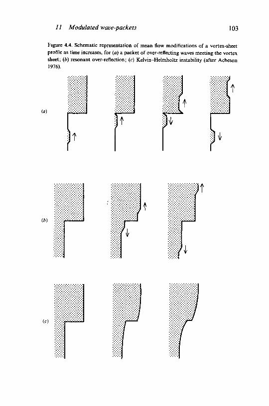
11 Modulated wave-packets 103
Figure 4.4. Schematic representation of mean flow modifications of a vortex-sheetprofile as time increases, for (a) a packet of over-reflecting waves meeting the vortexsheet; (b) resonant over-reflection; (c) Kelvin-Helmholtz instability (after Acheson1976).
(a)
It
t
}
(ft)
it
Downloaded from University Publishing Online. This is copyrighted materialIP139.153.14.250 on Tue Jan 24 02:27:27 GMT 2012.
http://dx.doi.org/10.1017/CBO9780511569548.005
104 Waves and mean flows
mechanism for generating clear-air turbulence at large altitudes. However,there are few known cases of resonant over-reflection for which the velocityprofile is not unstable to other wavenumbers (see Acheson 1976, for amagnetohydrodynamic case) and, for most of these, instability reappearswhen more realistic velocity profiles are employed (Drazin, Zaturska &Banks 1979). The true importance of over-reflection in meteorology andoceanography has yet to be established: see Fritts' (1984) survey ofatmospheric wave-phenomena.
11.6 Mean flow oscillations due to dissipationIn the preceding section, changes in mean flow are driven by a
vertical gradient of Reynolds stress, which occurs only when the local waveamplitude is changing with time. However, when dissipation is taken intoaccount, such stress gradients may be supported by time-independent waveamplitudes. For water waves, this was shown in §10.1: here we considera related internal-wave phenomenon.
As an internal wave, maintained at constant amplitude at some levelz = 0, propagates upwards, it is progressively attenuated by viscous andother dissipative processes. Because the wave amplitude diminishes withheight z, there is an associated Reynolds stress gradient 9T/9Z whichcontributes to the governing equation
8M 62M _ 1 3T
cit 6z2 p0 6z
for the mean horizontal flow u. In equilibrium,
"zu{z) = -(vp0)-
1 rdz + Az + BJo
where A and B are constants which vanish identically if u remains boundedas z-»oo and w(0) = 0.
Holton & Lindzen (1972), Plumb (1977) and Plumb & McEwan (1978)have investigated the mutual interaction of waves and mean flow in suchcircumstances. Not only do the waves drive the mean flow: the presenceof the mean flow slightly modifies the attenuation rate of the waves. Witha single train of internal waves, generated at z = 0, Plumb (1977) concludedthat a steady state is always established after a sufficient time has elapsed.
A much more interesting situation exists when two wave-trains arepresent. Plumb (1977) and Plumb & McEwan (1978) considered suchwave-trains as having equal and opposite horizontal phase velocities: thiscorresponds to a standing wave maintained at z = 0. By symmetry, thereis an equilibrium solution with zero mean flow, since mean-flow contri-
Downloaded from University Publishing Online. This is copyrighted materialIP139.153.14.250 on Tue Jan 24 02:27:27 GMT 2012.
http://dx.doi.org/10.1017/CBO9780511569548.005

12 Generalized Lagrangian mean formulation 105
butions from the respective wave-trains cancel. But this solution some-times turns out to be unstable. The presence of a weak mean flow breaksthe symmetry and alters the local attenuation rate of one wave componentrelative to the other. This, in turn, produces a Reynolds stress gradientwhich acts on the mean flow. Computations by Plumb (1977), both fora 'fully' nonlinear model and a weakly nonlinear approximation, revealedtime-periodic oscillations of the mean flow. Experiments were conductedby Plumb & McEwan (1978), in an annular channel with flexible bottommade to perform standing-wave oscillations. Mean-flow reversals, ofroughly one-hour period, were observed in the salt-stratified water withinthe channel. A similar mechanism is believed to be responsible for observedreversals, every 26 months or so, of the mean wind in the lower equatorialstratosphere.
Such phenomena deserve further theoretical and experimental investi-gation. The importance of dissipative processes, with sometimes un-expected manifestations, is all too easily overlooked.
12 Generalized Lagrangian mean (GLM) formulation12.1 The GLM equations
It has long been recognized that the second-order Eulerian meanflow is not usually identical to the second-order averaged drift velocity ofindividual fluid particles. As mentioned in §10.1, the O(e2) Eulerianvelocity is zero for constant amplitude inviscid water waves, but fluidparticles travel with a non-zero Stokes drift velocity ws(z) which diminisheswith depth. In a Lagrangian (particle) formulation, the Stokes driftcontains all the mean momentum. In contrast, the Eulerian representation,with time-averages at fixed points in space, yields zero mean momentumexcept above the level of wave troughs. Only at those points, which aresometimes in the water and sometimes not, is there a non-zero average.
Rather different, but complementary, views of the flow are given by theEulerian and Lagrangian representations. Traditionally, the former haspredominated, but recent work has shown that a Lagrangian approach isoften helpful. The stimulus for the latter work has come from thederivation of exact equations for Lagrangian-mean flows, by Andrews &Mclntyre (1978a, b) following earlier attempts by Bretherton (1971) andothers. The' generalized Lagrangian mean' (or' GLM') equations connecta Lagrangian velocity uL(x, t) and density /3(x, t) to a ' pseudomomentum'vector p(x, t), per unit mass. For weakly nonlinear waves, the pseudo-momentum p may be evaluated, at order C(e2), directly from the linearwave solution and so the O(e2) Lagrangian velocity uL may be found. The
Downloaded from University Publishing Online. This is copyrighted materialIP139.153.14.250 on Tue Jan 24 02:27:27 GMT 2012.
http://dx.doi.org/10.1017/CBO9780511569548.005

106 Waves and mean flows
O(e2) Eulerian velocity may be recovered from the Lagrangian velocity onsubtracting the 'generalized Stokes drift' us(x, t) which can also beevaluated at O(e2) from the linear solution. For many systems whichsupport waves and weak mean flows, the GLM equations yield the meanflows more readily than would an Eulerian analysis, particularly wherenonlinear free-surface boundary conditions are involved. We here give abrief outline of the GLM theory and some applications.
The GLM description is a hybrid Eulerian-Lagrangian one in which theGLM flow is described by equations in Eulerian form, with spatial positionx and time / as independent variables rather than initial particle positionand time. Let the particle displacement associated with the waves be £(x, i)where the (suitably-defined) Lagrangian mean of £ is zero. The GLMoperator ( ) entails averaging over particles at the displaced positionsx+£: i.e.
j4(x, tf = ^(x, t), 0£(x, 0 = 0(x+{, 0, (12. la, b)where ( ) denotes a corresponding Eulerian average over positions inspace. Averaging may be carried out over time t for time-periodic flowsor over a single space co-ordinate x4 for flows which are spatially-periodicin xt; alternatively, an ensemble average may be taken over some othersuitable label, such as the phase of waves at some fixed position and time.The best choice of average depends on the problem to be examined.
Associated with any Eulerian velocity vector field u(x, i), there is auniquely defined ' related velocity field' v(x, t) such that, when the actualfluid particle at x+£ moves with its velocity u(x+^, i); a notional particleat x may be regarded as moving with velocity v(x, /). Here, v(x, t) satisfies
(3/8*+T-V) [x+«(x, 0] = u(x+£, 0;
|(x, t) has zero Eulerian mean, £(x, t) = 0, and v(x, t) is a mean quantitysuch that v(x, 0 = v(x, i). So defined, v(x, t) is the required Lagrangian-meanvelocity, uL(x, t). The Lagrangian means of all other flow quantities aresimilarly defined but it proves convenient to treat the density ratherdifferently.
From the compressible Navier-Stokes equations, Andrews & Mclntyre(1978a, b) derived the exact equations of GLM motion. For homentropicflows, the GLM momentum and continuity equations simplify to
x aL)i + Ef = -Xf-J^n,(12.2)
D ls9/3(+flL-V. (12.3)
Downloaded from University Publishing Online. This is copyrighted materialIP139.153.14.250 on Tue Jan 24 02:27:27 GMT 2012.
http://dx.doi.org/10.1017/CBO9780511569548.005

12 Generalized Lagrangian mean formulation 107
Here, Ft denotes all external body forces per unit mass except the GLMCoriolis force per unit mass £2xuL, where ft is the constant angularvelocity of a rotating reference frame; the vector field p = pt(x, i) is thepseudomomentum per unit mass defined as
m (i2-4)(not to be confused with pressure p) and X = XL + X' is a function whichrepresents all dissipative terms. Symbols identified by the label ( )l are'wave quantities' with zero mean, such that
Also, the 'wave fields' £(x, t) and u!(x, t) are related by the kinematiccondition
u' = D\ (12.5)
Cartesian tensor notation is used throughout, with ( )j = d/dxp( ),t — 3/9' a n d summation of repeated indices over the values 1, 2,3.
The density p(x, i) of the' related flow' 0L(x, t) is defined so as to satisfy
(12.3), and is connected to the actual fluid density p£(x, i) = p(x+£, t) by
p = pfJ, / s d e t {*„+&,,} (12.6)
where / i s the Jacobian of the mapping x->x+£. We note that constant-density flows, p£ = constant, do not usually give rise to a constant densityp of the related flow field. But this definition has the major advantage thatp is a mean quantity, p(x, i) = p(x, t).
In general, equations (12.2) and (12.3) must be supplemented by anequation of state linking pressure and density. The GLM equations arethen complete if the wave field is known and may in principle be solvedto find the GLM flow associated with any specified wave field §(x, t). Ofcourse, the wave field is itself usually dependent on the mean state: in thissense, the above equations are not complete. But, for weakly nonlinearsystems, the O(e) wave field is frequently known and equations (12.2) and(12.3) are then sufficient to yield the O(e2) mean flow supported by thewaves.
For small-amplitude waves but 0(1) mean state, a Taylor expansion of(12.1b) gives
where ^(x, t) = $ x , t)+<f>'(ji,t) and <?>'(x,t) denotes the Eulerian wavefield. Accordingly,
and the mean fields ^L(x, /), ^(x, t) differ by the 'Stokes correction'
, 0 = $^-$= Irfj+hW*l K + O(e3). (12.7)
Downloaded from University Publishing Online. This is copyrighted materialIP139.153.14.250 on Tue Jan 24 02:27:27 GMT 2012.
http://dx.doi.org/10.1017/CBO9780511569548.005

108 Waves and mean flows
In particular, result (12.7) yields the'generalized Stokes drift' us = uL —a.For incompressible (Boussinesq) flows, such that V • u' = 0 and the
density p£ of each fluid particle is constant,
Accordingly,
and the Lagrangian-mean velocity field is not usually divergence-free.Fortunately, it often happens that the O(e2) variations of p drop out ofthe O(e2) equations for nL.
When the mean flow u is also weak, of order O(e2), (j>1 = <j>' + O(e2) and0 s = £] <t>'] + O(e3). If the Coriolis force is absent, one then has, from (12.4),(12.5) and (12.7),
When the wave field E,} is time-periodic, this gives pt = uf + O(e3); a resultwhich establishes the equality at 0(e2) of the pseudomomentum ppt perunit volume and the O(e2) mean momentum per unit volume, psf. Ingeneral, physical momentum and the pseudomomentum pi are not equalbut Pi and u\ are exactly related by
V x ( u L - p ) = 0
whenever the wave fluid is irrotational.
12.2 Pseudomomentum andpseudoenergyThe wave action stf defined in § 11.4 was originally introduced to
describe an 0(e2) property of weakly nonlinear waves. But the concept ofwave action has been powerfully generalized by Andrews & Mclntyre(1978b), who derived an exact equation of the form
DL/1+/5~1V-B = jf . (12.9)
The right-hand side J f is zero for conservative motions and is heredisregarded. The generalized wave action density A is defined as
£J7| (12.10)
where fi is the label over which averages are taken. The non-advective fluxof wave action B is
and Ky is the (i, y)th cofactor of the Jacobian /defined in (12.6). For wavesperiodic in xu (I may be chosen as — xx; then A is identical to the^-component of pseudomomentum, A = pv
Downloaded from University Publishing Online. This is copyrighted materialIP139.153.14.250 on Tue Jan 24 02:27:27 GMT 2012.
http://dx.doi.org/10.1017/CBO9780511569548.005

12 Generalized Lagrangian mean formulation 109
For plane-periodic, small-amplitude waves of frequency w' in a (locally)constant mean flow U, u* = u' = D § and £ oc expi(k-x—w't—8) correctto O(e). On choosing fi as the phase S varied over (0,2v), we have£,/? = w~xD ^ = w~lu'wherew = w'—k-U is the intrinsic wave frequencyobserved in the local rest frame of the fluid. From (12.10),
A 111''"/1
which establishes that the integral of A over depth coincides with stf of(11.28) at O(e2) when £1 = 0. General relationships between A and otherGLM quantities, such as the flux of pseudomomentum and the 'pseudo-energy' are discussed by Andrews & Mclntyre (1978b), within an energy-momentum-tensor formalism. Also, the O(e2) concept of 'radiationstresses' is connected to the exact GLM formulation by Andrews &Mclntyre (1978a).
Briefly, for inviscid flows, a tensor T^, where /*, v stand for xt (i = 1,2,3)or t, satisfies a set of conservation relations
^ = 0. (12.11)
The component Ttt is thepseudoenergy per unit volume and the componentsTtj (J = 1,2,3) denote its flux. These are defined (see Andrews & Mclntyre1978b, §5) as
Ttt=pe-L-L0,
Tt} = uf pe+p££mrtKmj (12.12)
where
L is the total Lagrangian density and Lo the 'undisturbed' Lagrangianobtained from L by retaining all mean and ignoring all fluctuatingquantities.
12.3 Surface gravity wavesAs a first simple example, we consider the linear wave field
u' = V$,
**.*,0 = "Tsthfc/^3 «k<**-«O+0(*) (-*<*< 0)(12.13)
of inviscid surface capillary-gravity waves with frequency w given by
W2 = (gk+p-'Lyk*) tanhkh
(cf. §11.2 above). The associated periodic particle displacements £,t(i =1 ,2 ,3 ) satisfy g M = u't + O(e2), where e = ka, and the Stokes drift
Downloaded from University Publishing Online. This is copyrighted materialIP139.153.14.250 on Tue Jan 24 02:27:27 GMT 2012.
http://dx.doi.org/10.1017/CBO9780511569548.005
110 Waves and mean flows
velocity wf = (tfi, 0,0),
(1)ka2cosh[2k(zs_ 2sinh2A:/!
is immediately given by (12.7). The corresponding 0(e2) solution of (12.2)is uf — Pi = uf. It immediately follows that the O(ez) Eulerian mean flowu{ is zero. Also, at 0(e2), (12.6) gives
plp-\= -\{kdf cosh2[k(z+h)]/sinh2kh.
The reduction in mean density p of the related velocity field may beexplained, physically, in terms of a mean O(e2) change in level of anaveraged set of fluid particles, as compared with that when no wave ispresent. This is most readily understood by considering a marked set ofparticles which, in the absence of waves, lie at equal intervals in x alonga given line, say z = z0. In a reference frame moving with the wave, theseparticles are observed to be more closely spaced at wave crests than at wavetroughs. Their average height therefore exceeds z0 by an 0(e2) amount. Asimilar line of particles initially situated on z = z0 + 8 experiences a slightlygreater or lesser O(e2) mean displacement according as 8 > 0 or < 0,because the local wave amplitude increases with height. As a result, theapparent mean density p associated with the slab of fluid initially betweenz = ZQ and z = zo + 8 decreases in order to conserve mass. It must beemphasized that this 'divergence effect' of the related velocity field uL isa property of the averaging procedure: the physical density of the fluid ofcourse remains constant.
With averages taken over —x, the wave action density A and pseudo-momentum component px are the same. Integrating over the liquid depth,we here have
j / = f p1dz = -[° (8g,/8x)ii;dzJ - f t J - f t
andCC fo Q ro
(V • B) dz = (QBJdx) dz = - — p' 8&/3JC dzJ-h J-ft OX J-h
at O(e2). Since the latter integral is just 3(cg s/)/dx, where cg = dw/dk, andD L j ^ = djtf/dt at O(e2), result (11.28) with U = 0 is recovered from (12.9).A similar equivalence between (11.28) and (12.9) for small-amplitudewaves is readily verified for other examples discussed above.
Downloaded from University Publishing Online. This is copyrighted materialIP139.153.14.250 on Tue Jan 24 02:27:27 GMT 2012.
http://dx.doi.org/10.1017/CBO9780511569548.005

12 Generalized Lagrangian mean formulation 111
12.4 Inviscid shear-flow instabilityThe GLM formulation was used by Craik (1982c) to describe
growing waves in unstable shear flows [ U(z), 0,0] between plane boundariesat z = zx and z = z2. In a reference frame moving with the wave velocitycT, the disturbance stream function of a small-amplitude two-dimensionalwave-train is (cf. §9.1)
f{x,z, i) = e eaci* Re{0(z) eiaxi} + O(e2)
where x1 = x—cTt. We assume that ct ^ 0. The corresponding linearizedvelocity components (u[, 0, u3) and displacements (£x, 0, £3) aref
u[ = e eaci * Re {0'(z) etex»}, "!, = e eaci« Re {- ia^(z) e iazi},
g3 = e eaci* Re
u — 'icj ia(u — u
\, a=u-cT.
(12.14)
From (12.7), the generalized Stokes drift us = («f, 0, M|) is found to be
— + C.C. +
/ •
(12.15a,b)
As aq->0, wf^-O and
except near the critical layer where u vanishes. This singularity exists evenfor viscous flows, since it derives from the linearized kinematic conditionD £ = u'(x+§, 0- The linear approximation there breaks down and thereis a region of closed streamlines - the Kelvin 'cats' eyes' - centred on thecritical layer for which the chosen averaging procedure is invalid.
The pseudomomentum p = (px, 0, p3) has
— — Ip2 P2ac, t
(12.16a, b)
As aCi->0, p3->0 for inviscid disturbances but not for viscous ones.The O(e2) Eulerian mean flow M<2) for inviscid disturbances was found
to satisfy (9.7). This may also be derived from the GLM equations (12.2),
t Recall that primes denote d/dz only when applied to functions of z only.
Downloaded from University Publishing Online. This is copyrighted materialIP139.153.14.250 on Tue Jan 24 02:27:27 GMT 2012.
http://dx.doi.org/10.1017/CBO9780511569548.005

112 Waves and mean flows
(12.3) and (12.6), which reduce to
when there is no 0(e2) pressure gradient. The last of these equations is anidentity and the other two yield
Substitution from (12.14), (12.15) and (12.16) gives
M<2> = M^-Kf-M = !S"3 (12.17)
for the O(e2) Eulerian velocity. This is just result (9.7).Since the net Eulerian mass flux must remain constant in the absence
of any pressure gradient,
2 u<2> dz = P 2 s"Ifdz = 0. (12.18)i Jz1
The inflexion-point criterion that u" must change sign in [zt,z2] is animmediate consequence.
For inviscid flow with averages taken over —xlt the conservation law(12.9) yields
Qt = p dA/dt = - 8(/?' 8£3/8x)/8zat O(e2) where p' is the O(e) Eulerian pressure fluctuation. Integrationacross the flow between rigid boundaries at z = zt and z2 immediatelyyields
ptAz = constant:
net pseudomomentum in the Xj-direction is conserved. Moreover, theconstant is zero since px = 0 at / = — oo. From (12.16a) this implies that
= 0, (12.19)
from which follows the well-known result that the wave velocity cr lieswithin the range of the flow velocity.
In the present case, the pseudoenergy density satisfies
from (12.11), and net pseudoenergy is conserved,
fJz,
Downloaded from University Publishing Online. This is copyrighted materialIP139.153.14.250 on Tue Jan 24 02:27:27 GMT 2012.
http://dx.doi.org/10.1017/CBO9780511569548.005

13 Spatially-periodic mean flows 113
since Tt3 vanishes on plane boundaries z = zx and z2 and Ttt is zero att = — oo. But Ttt here reduces to
at O(e2) (see Craik 1982c) and so
z = 0. (12.20)fJ*lEquations (12.19) and (12.20) together imply that w2 — C\+A« changes
sign within [zls z2] for all constants A: a result which leads immediately toHoward's (1961) semicircle theorem (cf. Eckart 1963).
The total energy is
f2*1 = E+p «<%dzJz,Jz,
where
Jz,£• = Je2/) e2ac.« (| 95' |2 + a21 ^ |2) dz
Jis the energy within the fluctuations. Substitution for w(2) from (12.17) anduse of (12.14) and Rayleigh's equation (3.3) yields $ = 0. Also, becauseof (12.18), $ remains zero in any parallel reference frame with u replacedby U—cT. Accordingly, spontaneously-growing disturbances in inviscidunstratified flows have zero total energy as well as zero net pseudo-momentum and pseudoenergy.
Applications of GLM theory to stratified shear flows are reviewed byGrimshaw (1984).
13 Spatially-periodic mean flows13.1 Forced motions
The quadratic interaction of two O(e) wave-modes with amplitudesai and periodicities exp[i(ky-x —Wy/)] + c.c. where j = 1, 2, \ = (x,y)and k = (a, /?) yields O(e2) forcing terms of the formb± expti(k1±k2)-x—i(w1±w2)?]+c.c. when ft* are proportional to axa2
and ax a* respectively. When kx = k2 and to1 = w2, the given wave-modescoincide and the forcing terms drive a spatially-uniform mean flow anda second harmonic.
More generally, on writing kf = k1±k2 , the respective Fourier com-ponents in k£ satisfy equations of the form
(L± 8/8f+M±)953± = 6±¥ l i ± 2 (z) e(wii+w«>* e - ^ r t ^ r ) * , (13.1)
where L*, M± are known linear operators in 8/9z, and "F^ ± 2 may be
found in terms of the linear eigenfunctions of the given wave-modes. The
Downloaded from University Publishing Online. This is copyrighted materialIP139.153.14.250 on Tue Jan 24 02:27:27 GMT 2012.
http://dx.doi.org/10.1017/CBO9780511569548.005

114 Waves and mean flows
corresponding homogeneous equation, with zero right-hand side, togetherwith appropriate homogeneous boundary conditions, defines an eigenvalueproblem for the frequency. This yields a set of discrete eigenvalues w±3
(« = 1,2,...) and sometimes a continuous spectrum. In particular, fortwo-dimensional modes with k, = {a}, 0), the appropriate homogeneousequation is just the Orr-Sommerfeld equation for wavenumbers o^io^.
Any solution of (13.1) may be expressed as a sum (or integral) over acomplete set of the linear eigenfunctions of the homogeneous problem withtime-dependent coefficients. If a>1 ± w2 coincides, or nearly coincides, withan eigenvalue «±g, a three-wave resonance occurs. In this case, the thirdmode need not remain small compared with the two original modes.Consideration of such resonance is deferred to the next chapter. Here, weassume that wx± w2 are not close to any linear eigenvalue «±3 and that thesolution 03± remains of order O(e2) at all times. We also assume that thegrowth rates Im{w±3} of all linear eigenmodes of (13.1) are less than<oli±(u2i, so that <j>£ is eventually dominated by a particular integral of theform Q>£ exp[—i(<olr±<o2T)t] exp[((ou±(oii)t] where
[-i(Wl±W2)L±+M±]<D3± = b±V1,±2(z).
When two wavenumbers kl5 k2 have identical real frequencies wlr = w2r,and <i>u = w2l = 0, the forcing terms in exp[ + i(k1 —k2)-x] and the corre-sponding particular integral are independent of time t. This gives rise toa spatially-periodic mean flow. Such flows may result from symmetry ofthe wave fields, as with two equal oblique waves exp [i(ax+fly—o)t)] withreal frequency w in a parallel flow [U(z), 0,0]. More generally, if twowavenumbers kx, k2 have nearly equal frequencies, | (<O1 — OJ2)/OJ1 \< I, theforced solution fa varies slowly in time.
The best-known observations of wave-induced spatially-periodic meanflows are those in Klebanoff, Tidstrom & Sargent's (1962) study ofthree-dimensional disturbances in the unstable Blasius boundary layer. Asmall-amplitude, nearly two-dimensional, Tollmien-Schlichting wave wasgenerated by a ribbon which vibrated with fixed frequency. As the waveprogressed downstream, growing in amplitude, marked spanwise variationsin amplitude spontaneously appeared. To control the spanwise wavelengthand phase of these variations, small strips of adhesive tape were placedat equal intervals on the plate, beneath the vibrating ribbon. The local waveamplitude at fixed x and z then varied almost periodically with spanwisedistance y, about a non-zero mean. Also, a spanwise-periodic mean flowdeveloped, in the form of'longitudinal vortices' which varied only slowlywith x. A somewhat similar development of three-dimensionality was
Downloaded from University Publishing Online. This is copyrighted materialIP139.153.14.250 on Tue Jan 24 02:27:27 GMT 2012.
http://dx.doi.org/10.1017/CBO9780511569548.005

13 Spatially-periodic mean flows 115
found by Nishioka, Iida & Ichikawa (1975), in plane Poiseuille flow. Thelongitudinal-vortex structure is generally believed to play an importantpart in inducing transition to turbulence (e.g. Tani 1969). Certainly,turbulent 'spots' are observed to develop first at spanwise ('peak')locations where the local wave amplitude is greatest (see §27.2).
Benney & Lin (1960) first proposed a theoretical model of the develop-ment of such longitudinal vortices, which was subsequently extended byBenney (1961, 1964). They considered a wave field comprising O(e)two-dimensional and span wise-periodic modes - say, a exp(iax—iwf) andb exp(iax±ifly~ iu>'t) plus complex conjugates - with wr = u>'r and smallamplification rates «j, <o{. They then calculated the resultant mean flowcomponents in ab* exp (+ i/ly) and | b |2 exp (+ 2i/?_y) plus conjugates. Theformer derive from the interaction of the two-dimensional mode with anoblique mode; the latter from the interaction of the two oblique modes.In addition, there are j-independent mean flow components in | a |2 and| b |2 from the self-interaction of each mode. The resultant mean flows werefound to have a longitudinal-vortex structure qualitatively similar to thatobserved by Klebanoff et al. However, this theoretical model postulates,rather than explains, the existence of a strongly j-periodic wave fielddownstream of a nearly uniformly-vibrating ribbon. In addition, the modelhas been criticised by Stuart (1962a) and others on the grounds that thelinear frequencies wr, <D'T in fact differ by around 15% at wavenumberscorresponding to the experimental data.
Antar & Collins (1975) improved upon Benney's model analyses bothby relaxing the assumption wr = o)'T to account for the actual frequencymismatch Awr = wr—a>'T and by computing second-order flows for actualBlasius and Falkner-Skan velocity profiles. The component of mean-flowdistortion with spanwise wavenumber fi then oscillates in time withfrequency Aw while that with wavenumber 2fl does not. An alternativemodel, proposed by Nelson & Craik (1977), concerns waves of equalfrequency, but with a mismatch Act in downstream wavenumber. Meanflow components then have wavenumbers (Aa, /?) and (0,2/1). The lattermodel seems closer to Klebanoff et al.'s experimental situation anddeserves a more detailed study. It is also possible that higher-ordernonlinearities, especially those at O(e3), may lead to synchronization ofwave-modes with the same downstream wavenumber (see §26). Examplesof Antar & Collins' calculated mean-flow structure are shown in Figure4.5, while Figure 4.6 reproduces some of Klebanoff et al.'s experimentaldata. Fuller discussions of mean-flow distortion in unstable boundarylayers are given by Tani (1980) and Craik (1980).
Downloaded from University Publishing Online. This is copyrighted materialIP139.153.14.250 on Tue Jan 24 02:27:27 GMT 2012.
http://dx.doi.org/10.1017/CBO9780511569548.005
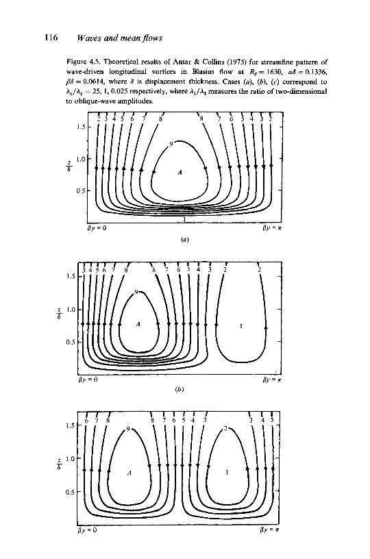
116 Waves and mean flows
Figure 4.5. Theoretical results of Antar & Collins (1975) for streamline pattern ofwave-driven longitudinal vortices in Blasius flow at Rs = 1630, a8 = 0.1336,p& = 0.0614, where S is displacement thickness. Cases (a), (b), (c) correspond toAl/A2 = 25, 1, 0.025 respectively, where ^/^ measures the ratio of two-dimensionalto oblique-wave amplitudes.
1.5
z 1.0T
0.5
I I I I I3 4 5 6 7
(a)
(b)
1.5
z 1.0J
0.5
Downloaded from University Publishing Online. This is copyrighted materialIP139.153.14.250 on Tue Jan 24 02:27:27 GMT 2012.
http://dx.doi.org/10.1017/CBO9780511569548.005

13 Spatially-periodic mean flows 117
Figure 4.6. Experimental results of Klebanoff, Tidstrom & Sargent (1962) showing'peak-valley' and longitudinal-vortex structure in the Blasius boundary layer, (a)shows spanwise variations of mean (U,V) and r.m.s. fluctuating (u',v') velocitycomponents in the downstream and spanwise directions, at a fixed downstreamlocation and fixed distance z from the wall: circles denote measurements at z = 0.31 S,crosses at 0.11 S. (b), overleaf, shows z-distributions of mean velocity Fat two span-wise locations separated by 0.4 in. and two downstream locations: those markedby O> V correspond to the position further downstream.
-001 -
-00206
05
04
004 r
zBlasius
05 0y (in)
Downloaded from University Publishing Online. This is copyrighted materialIP139.153.14.250 on Tue Jan 24 02:27:27 GMT 2012.
http://dx.doi.org/10.1017/CBO9780511569548.005

118 Waves and mean flows
A rather similar model was proposed by Craik (1970) in an early attemptto describe the phenomenon of 'Langmuir circulations'. These arestructures of longitudinal-vortex type which commonly develop in bodiesof water subjected to moderate winds. Craik (1970) calculated the O(e2)spanwise-periodic flows associated with a pair of equal surface gravitywaves with periodicities e exp(iocx±ifiy~\iot) propagating through aninviscid 0(1) primary shear flow u = [Kz, 0,0]. Without shear, there is noEulerian mean flow; but when K is non-zero there is a spanwise-periodicdistortion of the mean vorticity field. Leibovich & Ulrich (1972) gave aneat physical interpretation of this process in cases of weak O(e2) meanshear. Then the linear wave field is irrotational and has a Stokes drift whichcontains a spanwise-periodic component. Since vortex lines and fluidparticles coincide in inviscid flows, the Stokes drift must induce spanwise-periodic distortions of an initially-uniform vorticity field. The spanwise-periodic x-component of vorticity at first grows linearly with time t, andthis induces a further distortion of the mean flow to give a spanwise-periodic
Fig. 4.6b. For caption see previous page.
002 "
001 -
-001 -
-002 -
Downloaded from University Publishing Online. This is copyrighted materialIP139.153.14.250 on Tue Jan 24 02:27:27 GMT 2012.
http://dx.doi.org/10.1017/CBO9780511569548.005

13 Spatially-periodic mean flows 119
x-velocity component which grows initially as t2. Viscous diffusion mustinhibit the growth of the vortices and lead to an ultimate steady state.
Craik & Leibovich (1976) and Leibovich (1977a) subsequently derivedthe general equations governing weak O(e2) mean flows in the presence ofarbitrary O(e) fluctuations. The mean vorticity equation was found to be
(e /aT-^V 2 ) to = (e>-V)(u + u s ) - ( u + us)-V«J (13.2)
at leading order. Here, the mean Eulerian velocity, vorticity and generalizedStokes drift are e2u, e2e» and e2us respectively, while T = e1t and vt = e~ VThe viscosity v is supposed small, of order O(e2), where e characterizes thewave-slope. The average ( ) is taken over a time-scale large compared withthe periods of the O(e) wave-components but small compared with the slowO(e~2) time-scale of the mean flow evolution. Note that the influence ofthe waves in (13.2) is entirely represented by the Stokes drift us, in line withthe convective processes described above. This, and the associatedmomentum equations, were initially derived using an Eulerian formulation,and entailed considerable effort, since the Stokes drift us does not arisenaturally in such a representation. Subsequently, Leibovich (1980) derivedthese equations much more simply from the GLM equations (12.2) and(12.3). Craik (1982d) similarly showed that stronger mean flows, with anO(e) downstream component, satisfy nearly identical equations whichdiffer only by scaling factors in the definitions of u, e>, vx and T. Forinstance, if the mean flow is initially given as e[u(z), 0,0] and the knownO(e) wave-field provides a spanwise-periodic Stokes drift e2[«s(j/, z), 0,0],the inviscid GLM equations (12.2) and (12.3) yield
bu1/&r = -(du/dz)u3,
d{MJdz-duJdy)/dr = -(du/dz)(difi/dy), L (13.3)
Jat leading order for the O(e2) Eulerian mean flow modification e 2 ^ , M2, M3).(Note that the pseudomomentum here equals the Stokes drift at O(e2).)At first, the spanwise-periodic longitudinal vorticity, and hence u2 and «3,grow linearly with time T while the downstream component Mj developsas T-2.
For weak mean flows, Leibovich (1977a) and Leibovich & Radhakrish-nan (1977) have computed the developing longitudinal vortex systemdriven by a pair of oblique waves, with viscous terms included. Laboratoryexperiments of this configuration by Faller & Caponi (1978) and Faller& Cartwright (1982) confirm the appearance of such vortices.
For strong 0(1) primary shear flows, the GLM equations are normally
Downloaded from University Publishing Online. This is copyrighted materialIP139.153.14.250 on Tue Jan 24 02:27:27 GMT 2012.
http://dx.doi.org/10.1017/CBO9780511569548.005

120 Waves and mean flows
insufficient to determine the developing vortices, because distortions of theinitial Stokes drift and pseudomomentum cannot be neglected as in (13.3)(the case studied by Craik (1970) is an exception). The GLM equationsmust then be complemented by those governing the evolution of the wavefield.
13.2 Wave-driven longitudinal-vortex instabilityCraik (1977, 1982d) and, for stratified flows, Leibovich (1977b)
and Leibovich & Paolucci (1981) have considered the stability of unidirec-tional shear flows in the presence of O(e) two-dimensional surface gravitywaves independent of the spanwise direction. The disturbances are regardedas x-independent, of longitudinal-vortex form.
When the primary flow is weak, of magnitude O(e2), let
u = [0(e)wave &eld] + e2[u0(z) + Sii1, Sdftfiz, -8dft/dy] + O(e3,e282)
where ux and ijr depend on y, z and T = e2t, and 8 is sufficiently small topermit linearization. The mean-flow equations then reduce to
(3 /3T - vx V2) ux = (du°/dz)
(3/Sr - v1 V2) V2^ = (dws/dz)
where the primary flow e2u°(z) and Stokes drift e2t^(z) are known (cf. Craik1977).
These equations bear a close similarity to those governing thermal(Benard) and centrifugal (Rayleigh-Taylor) instability. Boundary con-ditions ux = 0, Vijr = 0 hold at a rigid bottom z = — H (or ux, V^->0 asz -+ — oo). At the mean free surface, z = 0, the kinematic and tangential-stressboundary conditions give
dujdz = 0, dxjr/dy = (32 /3j 2 -3V3z2)^ = 0.
It is readily shown that instability occurs, unless inhibited by viscosity,whenever the gradients of w° and MS have the same sign in some part ofthe flow domain. Leibovich & Paolucci (1981) comprehensively discusssuch instability of time-dependent mean flows induced by a constantsurface stress: such flows are unstable for all but exceedingly-small waveamplitudes. For stronger, but still weak, primary flows of magnitude O(e),the stability analysis is virtually identical. Treatment of strong 0(1) shearflows with O{e) plane waves is necessarily more complex, but a rathersimilar instability mechanism is still likely to operate in such flows (Craik1982d), with pseudomomentum rather than Stokes drift playing a centralrole.
Downloaded from University Publishing Online. This is copyrighted materialIP139.153.14.250 on Tue Jan 24 02:27:27 GMT 2012.
http://dx.doi.org/10.1017/CBO9780511569548.005

13 Spatially-periodic mean flows 121
Langmuir circulations are certainly responsible for the parallel'windrows' often observed in lakes (see Figure 4.7) and similar longi-tudinal-vortex structures are an important ingredient of all turbulent shearflows. Such longitudinal vortices provide an efficient mixing mechanismwhich is believed to play a part in determining the location and structureof the thermocline in lakes and oceans (see Leibovich's (1983) review); butother factors such as temperature 'fronts' or 'ramps' (Thorpe & Hall1982) and intermittent Kelvin-Helmholtz instability of internal-wavemodes (Thorpe 1971, 1973) also contribute.
Even without the wind to supply a constant surface stress, surfacegravity waves induce an O(e2) Eulerian drift velocity by viscous action (see§ 10.1). It would appear that unidirectional drift-velocity profiles like (10.3)are inherently unstable to spanwise-periodic perturbations.
The physical mechanism for instability of weak primary flows is readilyunderstood in terms of vortex-line deformation. An initially-unidirectionalshear flow w° has vortex lines extending uniformly in the -direction whilethe Stokes drift ws of a plane-wave field depends only on depth z. A smallspanwise-periodic x-velocity perturbation ut provides a small periodic
Figure 4.7. Photograph of windrows (Banana River). Those normally observed arerather less regular than this. (Photograph by A. Woodcock, published in Stommel1951.)
mmm
Downloaded from University Publishing Online. This is copyrighted materialIP139.153.14.250 on Tue Jan 24 02:27:27 GMT 2012.
http://dx.doi.org/10.1017/CBO9780511569548.005
122 Waves and mean flows
component of vertical vorticity: the resultant vortex lines are 'wavy' andlie in vertical planes. In the absence of viscosity, vortex lines travel withthe fluid particles: accordingly, they are tilted by the Stokes drift gradientdifi/dz to yield a periodic component of longitudinal (x-) vorticity.This induces periodic upwelling and downwelling which convects thex-momentum of the primary flow w°(z). When difi/dz and du°/dz have thesame sign, this momentum supplements the perturbation ux and leads toinstability: when the signs are opposite, ux is diminished and the flow isstable.
An alternative, complementary, physical interpretation is given by Craik(1982d). In this, the forcing term is identified with that of centrifugalTaylor-Gortler instability on curved walls, a mean O(e2) curvaturederiving from the x-averaged curvature of streamlines in the wavy flow.These equivalent kinematical and dynamical explanations typify thedifferent insights provided by Lagrangian and Eulerian viewpoints.
A rather different physical model for generation of Langmuir circulationswas proposed by Garrett (1976). The amplitudes of short gravity wavesare modified by their interaction with variable horizontal currents associatedwith large-scale longitudinal vortices. Garrett envisages enhanced viscousor turbulent dissipation where the wave amplitudes are greatest and aresultant radiation stress acting to maintain the spanwise-periodic meanflow. Though Garrett's physical hypotheses are less secure than those ofthe Craik-Leibovich theory, it is reassuring that this alternative mechanismacts to reinforce the circulations.
The longitudinal-vortex instability is quite distinct from the Lin-Benneytype of mechanism, in which vortices are forced by a pre-existing spanwisestructure of the wave field. In contrast, the instability mechanism operateswith two-dimensional waves independent of the spanwise co-ordinate.Further work is necessary to assess the importance of such instability instrong shear flows such as boundary layers. A recent theory developed inthe latter context by Benney (1984) has similarities with that of Craik(1982d): see §20.3.
Downloaded from University Publishing Online. This is copyrighted materialIP139.153.14.250 on Tue Jan 24 02:27:27 GMT 2012.
http://dx.doi.org/10.1017/CBO9780511569548.005

Chapter five
THREE-WAVE RESONANCE
A derivation of the three-wave resonance equations (8.12) was outlined in§8, for wave amplitudes a}(J = 1,2,3) depending only on time t. Here, afuller account is given of such resonance, including cases where the waveamplitudes a;- vary slowly in both time and space.
Many investigations of resonance followed Phillips' (1960, 1961) pion-eering studies: Phillips (1981a) himself gives an interesting overview.Inviscid surface gravity waves in still water do not exhibit three-waveresonance with quadratic interactions. The lowest-order resonance theninvolves quartets of waves, with cubic nonlinearities. Discussion of suchhigher-order terms is mostly deferred to Chapters 6 and 7. Three-waveresonance in conservative systems is examined in § 14 and §15; systems withlinear growth or damping are treated in § 16; non-conservative interactions,such as arise in shear flows, are considered in § 17.
14 Conservative wave interactions14.1 Conditions for resonance
McGoldrick (1965) showed that three capillary-gravity wavesmay interact resonantly, although gravity waves cannot. The frequenciesof three two-dimensional waves with periodicities a}exp(ik}x—i(o}t)(7 =1,2,3) are
for positive wavenumbers kj. Here, y denotes the coefficient of surfacetension. If k3 is chosen to equal &1+fc2, the resonance conditionWj + w2 = o)3 is met when kt and k2 satisfy
(l+r) + (l +r)(l + 7r+rftr(9+14r+9r2) ' ( }
T = ykl/2pg, r^kJK
123
Downloaded from University Publishing Online. This is copyrighted materialIP139.153.14.250 on Tue Jan 24 02:27:28 GMT 2012.
http://dx.doi.org/10.1017/CBO9780511569548.006

124 Three-wave resonance
This may be rearranged as a cubic equation in r, with coefficientsdepending on T.
For waves propagating in different horizontal directions,
aj exp (ik} • x — \mi t), k3 = k t+k a , x = (x, y),
the frequencies o>} are as above, with k} replaced by |k^|. Roots ofw3 = w/l+w2 are then best located by computation or graphical construc-tion: see Simmons (1969) for the latter.
In stratified fluid, three-wave resonance exists among internal gravitywaves and between two surface gravity waves and one internal wave (Ball1964; Thorpe 1966). In the latter case, the wavenumber kx and frequencya>1 of the internal wave are typically much smaller than those of the surfacewaves. Accordingly, let
u)1 = <i>3 — w2 = Aw, kj = k3 — k2 = Ak
at resonance, where Aw and |Ak| are small. Since the frequencies andwavenumbers of the surface waves are nearly equal,
w 3 «w 2 + (3w/3k)2-Ak.
But 3w/3k is the group velocity cg of the surface waves and so the resonancecondition becomes
Aw « cg • Ak.
This means that the horizontal phase velocity of the internal wave,
AwAk
equals the component of cg in the direction of Ak. When all three wavestravel in the same direction, resonance occurs when cln = cg.
In most regions of the ocean, lowest-mode internal waves on thethermocline cannot have | cin | greater than about 50 cm s~\ and | cg | is assmall as this only for rather short surface waves, of under 60 cmwavelength. But when the directions of k2 and Ak differ, the internal waveresonates with longer surface waves. One should therefore expect aperiodic surface-wave field to generate internal waves which propagate ata considerable angle to that of k2.
Internal waves on the thermocline are frequently visible in aerialphotographs as periodic light and dark bands. These bands indicateregions of differing' surface roughness', brought about by modification ofthe surface waves by the long internal waves. Such interactions of long andshort waves may conveniently be treated by regarding the short waves as
Downloaded from University Publishing Online. This is copyrighted materialIP139.153.14.250 on Tue Jan 24 02:27:28 GMT 2012.
http://dx.doi.org/10.1017/CBO9780511569548.006
14 Conservative wave interactions 125
propagating in a slowly-varying current: variations of the short-wave fieldmay then be found as described in § 11.
Internal waves in stratified fluid of finite depth have a denumerable setof frequencies w(n> (n = 1,2,...) for every horizontal wavenumber k. Eachyields a separate surface in w-k space and these surfaces characterizefamilies of modes with differing vertical mode-structures. For three-waveresonance to occur among these, Thorpe (1966) showed that the wavescannot belong to the same family. Longuet-Higgins & Gill (1967) and Ripa(1981) consider resonance in various other systems of geophysical interest.
14.2 Resonance of capillary—gravity wavesMcGoldrick's (1965) derivation of the three-wave resonance
equations was generalized by Simmons (1969) and Case and Chiu (1977)to waves with amplitudes varying slowly in both space and time. Beforedescribing Simmons' variational method, we outline Case & Chiu'sperturbation analysis.
The in viscid equations and boundary conditions for deep-water capillary-gravity waves are
= 0 ' u = - ' -oo < * < £ ( * , * / ) ;
(14.2a-e)
P = -yi((x, y, i)
Here, 4> is the velocity potential, £(x, y, i) the free:surface elevation, y thecoefficient of surface tension and K(X, y, t) the surface curvature. SinceK = V • n where n is the unit outwards normal to the free surfacez = £(*, y, t),
For small-amplitude waves, the kinematic and pressure boundaryconditions at the deformed free surface may be approximated by conditionsat the mean level z = 0, through Taylor expansions about this value. AtO(a2), where a is a dimensionless measure of wave-slope, these are
the terms on the left-hand sides being O(a) and those on the right O(a2).Subscripts t and z denote partial differentiation.
Downloaded from University Publishing Online. This is copyrighted materialIP139.153.14.250 on Tue Jan 24 02:27:28 GMT 2012.
http://dx.doi.org/10.1017/CBO9780511569548.006

126 Three-wave resonance
At leading order, O(a), let
<p = I ^(x, z, i) eV, £ = I tyx, 0,
^- = iw;- kjx{P}{x, z, t) exp [i(k;- • x + w;- /)]
- g3(x, z, 0 exp [i(k; • x - w3- 0]} + c.c,[ (14-5)
Aj = Pj(x, 0,0 exp [i(k3- • x + w} 0]+ gy(x, z, 0 exp [i(ky • x - w;- 0] + c.c. ,
with x = (x, j>), kj = | k | and k3-, w- chosen so that
k2 = k1+k3 , o)2 = u)1 + o)s. (14.6)
The functions Pj, Qj are O(a) and slowly-varying in x, z and /, withderivatives which are O(a2). From (14.2a), Pj and g;- approximately satisfy
8/»y/9z = -i*71(k,-V^) ) 62J/9z = - i ^ - 1 ( k ; - V ^ ) . (14.7)
Substitution of (14.5)—(14.7) in the boundary conditions (14.4) andisolation of Fourier components eventually yields
along with similar equations for the Pj with v;- and y replaced by — v;- and— jj. In these, the v3 = (8w/3k)3 denote the linear group velocities of thewaves. But the v; do not arise ' naturally' in this derivation and must bereconstituted from the linear dispersion relation. The coupling coefficientsjj are found to be
y1 = \{kx u>il(u>l + 0)1) + (w3 k3 -oj2k2- kx w^1 w2 w3)
+k 2 • k3[w2 kz1 - co3 ks1 — o)2 u)3 kt{k2 k3 OJ^1]},
y2 = \{k2 <i>2\(i)\ + col) — (<t)1 fej + (o3 k3 — k2 o)^1 Wj w3)
3 k ^ k3 a)^1]},
2ki- k3 w^1 wx w2)
+ kx • k2[w2 /c^1 - wj A; 1 - wx o>2 k3(kr k2 o)^"1]}.
Here, two independent resonant wave triads are present, since the Qj andPj modes have equal and opposite frequencies ±u>j. When |P^| = Ig^l.these may be viewed as a resonant triad of standing waves.
The variational approach of Simmons (1969) gives the same resultsrather more quickly. This was inspired by Whitham's (1965, 1967)variational method, with local averaging of a suitable Lagrangian i ? over
Downloaded from University Publishing Online. This is copyrighted materialIP139.153.14.250 on Tue Jan 24 02:27:28 GMT 2012.
http://dx.doi.org/10.1017/CBO9780511569548.006

14 Conservative wave interactions 127
the 'short' length scales and 'fast' time-scales of waves. But Whitham'smethod was not directly applicable to resonant triads, for it allowed slowvariations in frequency and wavenumber incompatible with (14.6).Modifying a previous Lagrangian formulation by Luke (1967), Simmonschose
L(<?>,Qdxdydt,allx, y
J
Variation of Z£ is subject to constraints 8<f> = 0 at times t0 and t1 for allx, y, z. Variation of <f> alone, by 8<f>(x, y, z, i) yields
r nxw*^ dKd/+r \\along with two other integrals which vanish if 8<j> is restricted to bezero at x = + oo and y — ± oo. The volume integral is taken over thedomain V comprising — oo < z ^ £(x, y, i) and the horizontal planeS — { — oo < x < oo, — oo<_y<oo}. Since the variation 8<f> is arbitrary,each term in square brackets must vanish. The volume integral yields thefield equation (14.2a) and the two surface integrals the boundary con-ditions (14.2c) and (14.2e). Similarly, variation 8£ of £(x, y, i), subject tothe restriction that 8£ — 0 at x = ± oo and y — ± oo, gives the dynamicalboundary condition (14.2d) with/j eliminated through (14.2b).
The next step is to substitute into Z£ expressions equivalent to (14.5),(14.6) for resonant waves, and then to construct the averaged Lagrangian3? taken over horizontal distances and times large compared with thewavelengths and wave periods but short compared with the modulationsin wave amplitude. The algebra at this stage is rather tedious, but less sothan in Case & Chiu's method. One then postulates arbitrary variations8Qj of each complex wave amplitude Q} and constructs the associatedEuler-Lagrange equations
) +\ (
\d(c>q/dt)) + dx \d(dq/dx)) + dy \d(dq/dy)
= Q} 0 = 1 , 2 , 3 ) .At O(a2) these simply yield the linear dispersion relation for each wave-mode; but at next order they give the interaction equations (14.8). A
Downloaded from University Publishing Online. This is copyrighted materialIP139.153.14.250 on Tue Jan 24 02:27:28 GMT 2012.
http://dx.doi.org/10.1017/CBO9780511569548.006

128 Three-wave resonance
similar Lagrangian formulation of three- and four-wave resonance inplasmas is given by Turner & Boyd (1978).
Simmons actually considered independent variations of real amplitudesbt and phases of wave components of the form
hj = b} cos(kj-x-ojj t+ijj) (j = 1,2,3)
withk1+k2+k3 = (O1+CO2+OJ3 = 0. These lead to the equivalent interactionequations
fi b\)\ = Oj b2 b^Jki/tJi) sin ij,
bf{dVi/St+V • (v4 Vt)} = ^ fe2 b^Jkt/uJ cos 9 (i = 1,2,3)
4/ = - £ o^+1(l+fc,-t,+1) (fc^stj, (-04.9)
where k- are unit vectors along the directions of wave propagation. Thevariational approach leads naturally to the simple form /fej/w^ for theinteraction coefficients, which was obscured in the 'direct' perturbationanalysis. This form was confirmed by Hasselmann (1967a) for moregeneral conservative systems.
Equations (14.9) hold for all resonant triads with non-equal wavenumbers k . If, say, kx = k2 = — |k3, further terms which normally havezero spatial averages must be retained, for the wavenumber kt is then inresonance with its own second harmonic. This case was separately dealtwith by Simmons and has also been considered, using perturbation theory,by Nayfeh (1970). The phenomenon of second-harmonic resonance ofcapillary-gravity waves in deep water was first encountered by Wilton(1915), who found that a Stokes expansion in powers of wave amplitudebecame singular at certain wavenumbers (see §22.1). The greatest of theseis kx = 2~i(pg/y)i, which is just result (14.1) with r = 1. This correspondsto ripples of wavelength 2.44 cm in clean water. Wilton's other singularitiesrelate to higher-order resonances; the next, at k = 3~^(pg/y)K is a 'four-wave ' resonance between k and its third harmonic.
The form of (14.8) may be inferred from a simple, but general, heuristicanalysis. If the linear dispersion relation is Z>(w, k) = 0, slow modulationsof each complex wave amplitude Qj satisfy
Downloaded from University Publishing Online. This is copyrighted materialIP139.153.14.250 on Tue Jan 24 02:27:28 GMT 2012.
http://dx.doi.org/10.1017/CBO9780511569548.006
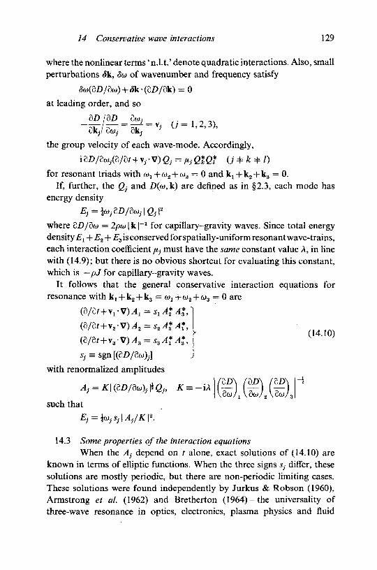
14 Conservative wave interactions 129
where the nonlinear terms' n.l.t.' denote quadratic interactions. Also, smallperturbations <5k, 8u> of wavenumber and frequency satisfy
fe(6Z)/Sw) + 5k-(eZ)/9k) = 0
at leading order, and so
3Z>/3Z>_6W,"ei^/a^-e^-^ 0-1,2,3),
the group velocity of each wave-mode. Accordingly,
iaZ>/3wy(8/a/+vV)g, = HjQtQt 0 : * k * /)
for resonant triads with Wj+Wg+Wg = 0 and kj+kg+kg = 0.If, further, the Q} and Z)(w,k) are defined as in §2.3, each mode has
energy density
where 3D/3w = 2pco | k |~* for capillary-gravity waves. Since total energydensity E1 + E2 + E3 is conserved for spatially-uniform resonant wave-trains,each interaction coefficient /t; must have the same constant value A, in linewith (14.9); but there is no obvious shortcut for evaluating this constant,which is — pj for capillary-gravity waves.
It follows that the general conservative interaction equations forresonance with kj+kjj+kg = Wj+Wj + Wg = 0 are
s} =
with renormalized amplitudes
such that
- I
14.3 Some properties of the interaction equationsWhen the Aj depend on / alone, exact solutions of (14.10) are
known in terms of elliptic functions. When the three signs s} differ, thesesolutions are mostly periodic, but there are non-periodic limiting cases.These solutions were found independently by Jurkus & Robson (1960),Armstrong et al. (1962) and Bretherton (1964) - the universality ofthree-wave resonance in optics, electronics, plasma physics and fluid
Downloaded from University Publishing Online. This is copyrighted materialIP139.153.14.250 on Tue Jan 24 02:27:28 GMT 2012.
http://dx.doi.org/10.1017/CBO9780511569548.006

130 Three-wave resonance
mechanics not being matched, then as now, by rapid communication!When the three signs Sj are the same, a singularity may, or may not, developat a particular value of /: such a singularity signifies an 'explosive'breakdown of the equations after a finite time. Such solutions were givenby Coppi, Rosenbluth & Sudan (1969). All these are described below in§15.1. Long before, the case with Aj(t) real and differing signs s} was solvedby Euler (1765): the equations are then Euler's equations for free rotationof a rigid body about a fixed point.
An 'explosion', in which all three wave amplitudes simultaneouslybecome infinitely large, does not violate energy conservation: Ex + E2 + E3
remains constant, with the participating waves having energies E, ofdiffering sign. For most waves in fluid at rest, including surface, interfacialand internal waves, 9£>/9&i is necessarily proportional to w | k I"1: therefore,such resonant waves with wr + w2 + w3 = 0 must have (9D/3w)y of differingsign, positive definite energies E}, and bounded periodic modulations.
Interactions among waves of differing energy sign need not lead tobreakdown: this only occurs when the wave of greatest absolute frequency|w| has energy of different sign from the other two. In other words,breakdown occurs only if the wave actions Ej/o)j have the same sign.Examples where this occurs are frequent in plasma physics (see, forexample, Weiland & Wilhelmsson 1977). Craik & Adam (1979) have shownthat the three-layer Kelvin-Helmholtz flow (2.5) supports resonant triadsof both the explosive and periodic types, even when the flow is linearlystable. In contrast, the resonant triads identified by Ma (1984a) in simpleKelvin-Helmholtz flow (cf. §2.1) exist only when the flow is linearlyunstable.
In addition to energy conservation, there are three other conservedquantities of (14.10), expressed by the Manley-Rowe relations
= ^[s3\A3\*-s1\A1\*] = 0. (14.11)
From these, it is obvious that the Aj remain bounded whenever the signsSj differ. Equivalently, each st \ Aj |2 may be replaced by the wave actionsEj/ojj.
When the Aj of (14.10) depend on a single variable, £ = erx+/?r (a, /?constant), similar solutions are easily constructed (Armstrong, Sudhanshu& Shiren 1970). For near-resonance, with kj-|-k2-|-k3 = 0 but smallfrequency mismatch Aw = &>1 + w2 + w3, equations analogous to (14.10)have additional exponential factors exp(—i Aw?) on the right-hand side.
Downloaded from University Publishing Online. This is copyrighted materialIP139.153.14.250 on Tue Jan 24 02:27:28 GMT 2012.
http://dx.doi.org/10.1017/CBO9780511569548.006

14 Conservative wave interactions 131
These, too, yield Jacobi elliptic function solutions (Armstrong et al. 1962),though Ex+E2+E3 is no longer constant.
When two of the waves, say A2 and A3, are much smaller than the third,Alt and each depends on t alone, (14.10) yield the linearized approximation
dAJdt = 0, dAJdt = s2 A* A*, dAJdt = s3 A* A*or
AX = A\ (constant), dMfc/d;2 = s2 s3 \ A\ |2 Ak (k = 2,3).
Obviously, A% and A% are periodic, with frequency \A\ | if the signs s2, s3
are opposite; and exponential, with growth and decay rates ±|-4J| ifs2 s3 = 1. For waves in fluid at rest, s} = sgn oij and the waves A2, A3 remainsmall compared with Ax except when Ax corresponds to the wave ofgreatest absolute frequency. When | w21 is largest, the wave Ax is unstableto wave-modes A2, A3 (Hasselmann 1967b). In plasma physics, Ax is calleda 'pump wave' when it can pump up A2 and A3 from infinitesimal levels;and the instability of the latter is usually described as 'parametric-reso-nance' instability. When all three signs Sj are the same, growth of A2 andA3 is limited by the depletion of Ax at larger amplitudes; periodicmodulations occur as described by the elliptic-function solutions.
A 'pump-wave approximation' may also be applied to (14.10) todescribe modulations in both time and space, when one wave is dominant(Craik & Adam 1978), but this inevitably breaks down if the magnitudesof the Aj become comparable, unless the 'pump wave' is artificiallymaintained at constant amplitude. The governing equations may then becombined as a linear Klein-Gordon (or telegraph) equation (7.9) whichis easily solved.
General conservation laws of (14.9), derived by Simmons (1969) forcapillary-gravity waves, are
E (6/8f+vV)£i = 0, 2 (3/3f+v(-V)Mi = 0,
Here, Mt denotes the momentum (per unit horizontal area) of the ith mode.Corresponding conservation laws of (14.10) are
(14.12)
These yield energy conservation and the Manley-Rowe relations (14.11)when the At depend on / only. When the A( depend on the two variables
Downloaded from University Publishing Online. This is copyrighted materialIP139.153.14.250 on Tue Jan 24 02:27:28 GMT 2012.
http://dx.doi.org/10.1017/CBO9780511569548.006
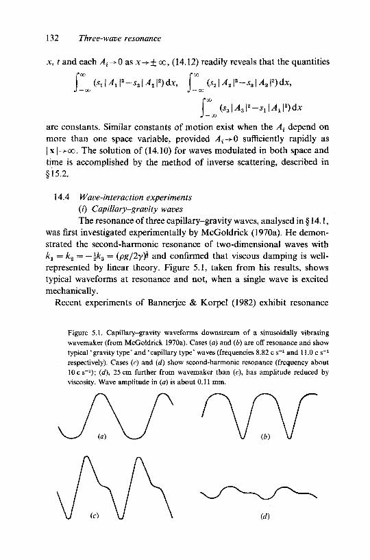
132 Three-wave resonance
x, t and each as ;t-s*+ oo, (14.12) readily reveals that the quantities/*oo p
(s.lA^-sJA^dx,J — 00 J
(s2\A2\*-s3\A3\*)dx,
are constants. Similar constants of motion exist when the At depend onmore than one space variable, provided A^O sufficiently rapidly as|x|->oo. The solution of (14.10) for waves modulated in both space andtime is accomplished by the method of inverse scattering, described in§15.2.
14.4 Wave-interaction experiments(i) Capillary-gravity wavesThe resonance of three capillary-gravity waves, analysed in § 14.1,
was first investigated experimentally by McGoldrick (1970a). He demon-strated the second-harmonic resonance of two-dimensional waves withfej = k2 = — §&3 = {pg/2y)t and confirmed that viscous damping is well-represented by linear theory. Figure 5.1, taken from his results, showstypical waveforms at resonance and not, when a single wave is excitedmechanically.
Recent experiments of Bannerjee & Korpel (1982) exhibit resonance
Figure 5.1. Capillary-gravity waveforms downstream of a sinusoidally vibratingwavemaker (from McGoldrick 1970a). Cases (a) and (b) are off resonance and showtypical'gravity type' and 'capillary type' waves (frequencies 8.82 cs"1 and 11.0c s"1
respectively). Cases (c) and (d) show second-harmonic resonance (frequency about10 c s"1); (d), 25 cm further from wavemaker than (c), has amplitude reduced byviscosity. Wave amplitude in (a) is about 0.11 mm.
(d)
Downloaded from University Publishing Online. This is copyrighted materialIP139.153.14.250 on Tue Jan 24 02:27:28 GMT 2012.
http://dx.doi.org/10.1017/CBO9780511569548.006

14 Conservative wave interactions 133
among waves with differing directions of propagation. A mechanicallygenerated wave k3 = (k, 0) gave rise to obliquely-propagating subharmonicskx 2 = (%k, ± I) with half the fundamental frequency. As reinterpreted byHogan (1984b), their results show satisfactory agreement with theory. Onedifficulty, which must be accounted for, is that viscous damping of thewaves induces a significant second-order mean flow and this, in turn, causesa frequency shift of the waves.
Kim & Hanratty (1971) also demonstrated second-harmonic resonanceof capillary-gravity waves in shallow liquid layers and found evidence ofhigher-harmonic generation. These higher harmonics were further investi-gated by McGoldrick (1972), who attributed them to higher-ordernear-resonances of the form k2 = Arfc1,w2 x N^ (integer N 5= 2):cf.§22.2.Clearly, the Mh harmonic must have phase speed close to that of thefundamental: it is then generated as a parametric instability by Mh ordernonlinearities and the resultant wave profiles typically have N crests perperiod. In contrast, Kim & Hanratty attempted to explain their higher-harmonic generation by quadratic interactions among four waves withwavenumbers nk (n = 1,2,3,4): this would be effective only if the waveswere weakly dispersive, with nearly equal phase speeds.
The onset of three-dimensionality in wind-generated ripples, reportedby Craik (1966)-see Figure 2 .5-may also be due to three-waveresonance.
(if) Internal gravity wavesDavis & Acrivos (1967) showed that an internal wave, propagating
along a diffuse stratified layer between fluids of different densities, maybecome distorted from its original sinusoidal shape by the growth of athree-wave resonance. This was revealed by use of neutrally-buoyant dyeddroplets which showed surfaces of constant density: their photographs arereproduced in Figure 5.2(a),(b),(c). The 'lumps' which develop in thestratified layer give rise to local turbulent mixing.
McEwan (1971), McEwan, Mander & Smith (1972) and McEwan &Robinson (1975) investigated standing internal gravity waves in fluid withlinear density variation with depth. The first and second of these studiesconcern the degeneration of a single forced mode into more complexstructures through three-wave resonances. The third deals with parametricinstability of waves due to periodic oscillations of the container; this maybe viewed as a limiting case of three-wave resonance where one wave,represented by the moving container, is much longer than the other two.When, because of geometrical constraints of the apparatus, the given
Downloaded from University Publishing Online. This is copyrighted materialIP139.153.14.250 on Tue Jan 24 02:27:28 GMT 2012.
http://dx.doi.org/10.1017/CBO9780511569548.006

134 Three-wave resonance
Figure 5.2. Progressive * disintegration' of an internal wave due to three-waveresonance (from Davis & Acrivos 1967).
(a)
(b)
(c)
Downloaded from University Publishing Online. This is copyrighted materialIP139.153.14.250 on Tue Jan 24 02:27:28 GMT 2012.
http://dx.doi.org/10.1017/CBO9780511569548.006

14 Conservative wave interactions 135
fundamental wave can participate in only one resonant triad, the resultantmotion is easily understood in terms of the growth of two other modes;but when several participating triads co-exist the behaviour is much morecomplex. Similar effects were demonstrated, for progressive internal waves,by Martin, Simmons & Wunsch (1972), who considered up to five triadswith a member in common. Such cases are analysed in §16.2 (v) and (vi).
(Hi) Surface and internal wavesWith two interfaces, or with a free surface above continuously
stratified fluid, resonant interactions occur between surface and internalwaves. There are many oceanographic observations of such interactingmodes - see, for example, Gargett & Hughes (1972) - but few quantitativeinvestigations in the ocean. Experiments in a large tank were conductedby Lewis, Lake & Ko (1974) and Koop & Redekopp (1981). In the former,a layer of water was bounded above by a free surface and below by a denserfreon-kerosene mixture. Since the density difference across the lowerinterface was quite small, resonant triads comprised relatively shortsurface gravity waves and a long wave at the lower interface. Both surfaceand internal waves were generated mechanically with the same directionof propagation. It was confirmed that the strongest modulations of theformer occurred when their group velocity was close to the phase velocityof the interfacial wave, in agreement with theory (see §14.1). The studyof Koop & Redekopp concerned similar interaction of long and shortwaves on the two interfaces of a three-layer configuration (see § 19.1).
A novel application of three-wave interaction theory is that examinedby Davies (1982), Davies & Heathershaw (1984) and Mei (1984): theyconsider propagation of a wave-train over fixed periodic sandbars on thebottom. When the incident waves have wavenumber and frequency (k, w)and the zero-frequency bottom undulations have wavenumber 2k, theirinteraction produces resonant reflected waves with wavenumber andfrequency (—k,(o). Because the undulations have fixed amplitude, the'pump-wave approximation' then applies and solutions are readily con-structed. Predicted reflection coefficients in resonant and non-resonantcases agree quite well with the experimental results of Davies & Heathershaw(1984). Such partial reflection can induce second-order drift currents whichact to maintain or enhance the sandbars by sediment transport. Thisresonant excitation of reflected waves is similar to Bragg reflection of X-raysby crystal lattices (see e.g. Pinsker 1978).
As yet, no experiment has been undertaken, in fluid mechanics, todemonstrate the potentially explosive conservative interactions among
Downloaded from University Publishing Online. This is copyrighted materialIP139.153.14.250 on Tue Jan 24 02:27:28 GMT 2012.
http://dx.doi.org/10.1017/CBO9780511569548.006
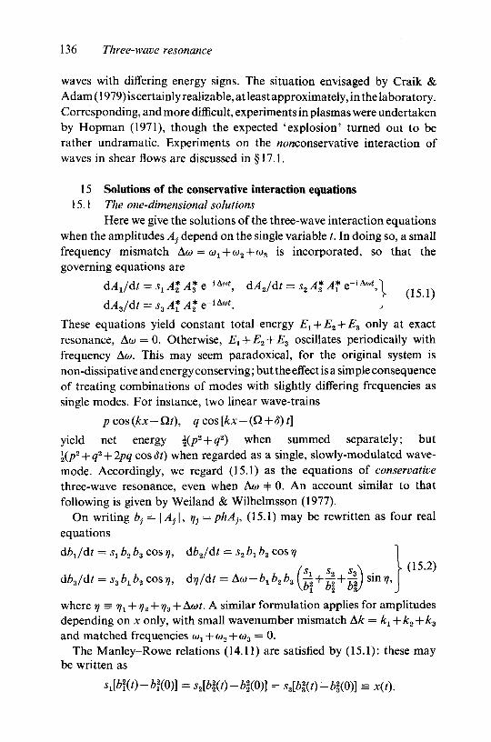
136 Three-wave resonance
waves with differing energy signs. The situation envisaged by Craik &Adam (1979) is certainly realizable, at least approximately, in the laboratory.Corresponding, and more difficult, experiments in plasmas were undertakenby Hopman (1971), though the expected 'explosion' turned out to berather undramatic. Experiments on the wonconservative interaction ofwaves in shear flows are discussed in §17.1.
15 Solutions of the conservative interaction equations15.1 The one-dimensional solutions
Here we give the solutions of the three-wave interaction equationswhen the amplitudes A} depend on the single variable t. In doing so, a smallfrequency mismatch Aw = w1 + w2 + w3 is incorporated, so that thegoverning equations are
dAJdt = sx A* A* e~iAat, dAJdt = s2A* A* e-1 A*VO5-1)
These equations yield constant total energy E1 + E2 + E3 only at exactresonance, Aw = 0. Otherwise, E1 + E2 + E3 oscillates periodically withfrequency Aw. This may seem paradoxical, for the original system isnon-dissipative and energy conserving; but the effect is a simple consequenceof treating combinations of modes with slightly differing frequencies assingle modes. For instance, two linear wave-trains
pcos(kx-Qt), qcos[kx-(Q + S)t]
yield net energy i(p2 + q2) when summed separately; buti(/>2 + 1 2 + 2/><7 cos 8t) when regarded as a single, slowly-modulated wave-mode. Accordingly, we regard (15.1) as the equations of conservativethree-wave resonance, even when Aw + 0. An account similar to thatfollowing is given by Weiland & Wilhelmsson (1977).
On writing bj — \A}\,ri} =phAp (15.1) may be rewritten as four real
equations
db1/dt = s1 b2 b3 cos y, db2/dt = s2 bx b3 cos y
dbz/dt — s3 bx b2 cos rj, drj/dt = Aw — I
where ?; = 1/1 + 2 + 3 + Awf. A similar formulation applies for amplitudesdepending on x only, with small wavenumber mismatch AA: = k1 + k2 + k3
and matched frequencies wx + a>2 + w3 = 0.The Manley-Rowe relations (14.11) are satisfied by (15.1): these may
be written as
sJLbl(t)-bl(O)] = s2[bt(t)-bl(O)] = sM(t)-bl(0)] = *(t).
Downloaded from University Publishing Online. This is copyrighted materialIP139.153.14.250 on Tue Jan 24 02:27:28 GMT 2012.
http://dx.doi.org/10.1017/CBO9780511569548.006
75 Solutions of the interaction equations 137
A further constant of motion is
T = blb2 b3 sin r/ — \ AOJSJ bj,
for any choice of j = 1, 2, 3.On using these, (15.2) reduces to a single equation for x{i),
dx/dt = ± 2{[Sl x + b\ (0)] [s2 x + bl(0)] [ss x
= ±{-2TT(X)}1, (15.3)
where the + signs indicate that of cos?;. Since at least two of the s}
Figure 5.3. Typical potential function n(x) when Aw = F = 0: (a)
oscillates between — 6|(0) and b\(0); (b) sl = 1, x grows without bound.= - 1 , x
-61(0)
(a)
_ \
Downloaded from University Publishing Online. This is copyrighted materialIP139.153.14.250 on Tue Jan 24 02:27:28 GMT 2012.
http://dx.doi.org/10.1017/CBO9780511569548.006

138 Three-wave resonance
(j = 1,2,3) are equal, there is no loss in setting s2 = s3 = 1 and in takingthe term s}bj(O) as bl(0).
Equation (15.3) has the form
\(dx/dtf + n{x) = Q (15.3)'
where n(x) is a cubic function, negative in cases of interest. Clearly, n(x)may be thought of as a potential. If Aw = F = 0, n(x) is typically as inFigure 5.3 (a) when ^ = — 1 and as in Figure 5.3 (b) when st = 1. In theformer, the wave actions EJ/CJ^ have differing signs; in the latter they havethe same sign and the signs of the energies E} differ. For s1 = — 1, thesolution x(t) must oscillate in the potential well. For sx = 1, x(t) mustalways become infinite: in fact, it does so 'explosively', in a finite time.
This explosive growth is inhibited, but not eliminated, by non-zerofrequency mismatch Aw which changes the location of the roots of n(x).Explosive growth then occurs only with sufficiently large initial amplitudes.The constant of motion F is related to the initial phases of the waves andthe coupling is strongest when Aw = F = 0. When F 4= 0, the roots of n(x)remain real when st = — 1 but two may be complex conjugates when s1 = 1.Solutions for F =t= 0, s1 = — 1 remain periodic and those with F =)= 0, s1 = 1,Aw = 0 remain explosive for all initial amplitudes.
The solution of (15.3) may be given explicitly as an elliptic integral,
t=±\ [Jo
which gives x{i) in terms of ' sn ' and 'en' Jacobi elliptic functions(Abramowitz & Stegun 1964). Corresponding solutions for the amplitudesbj are as follows (cf. Weiland & Wilhelmsson 1977; Coppi, Rosenbluth &Sudan 1969).
bx = [bt(O)-x(t)f, bk = [b%(0)+x(t)f (* = 2,3),
x(t) = (a2-ax) sn2[(a1-
where x1 > a2 > a3 are the three real roots of the cubic n(x) = 0. Casesof equal roots are simpler but require separate treatment. Solutions haveperiod
|*2TT
(l-A:sin2M)Jo
Downloaded from University Publishing Online. This is copyrighted materialIP139.153.14.250 on Tue Jan 24 02:27:28 GMT 2012.
http://dx.doi.org/10.1017/CBO9780511569548.006

15 Solutions of the interaction equations 139
(ii) s1 = 1; real roots 0 > ax > a2 > a3.
6, = [ftJ(O)+ *(/)]* (7=1,2 ,3) ,
x(r) = (a t - a3) {sn2 [(f „ - t) (a± - a3)*, fc']}'* + a3,
Here, t^ denotes the time of explosion.
(Hi) st= 1; real non-positive ax, complex conjugate a2, a3.0=1,2,3),
These also explode at finite time.
(iv) s1 = 1; real roots with ax < 0 < a2 < a3.Solutions oscillate in the potential well at < x < <x2. These periodic
solutions resemble (i) and arise when the initial amplitudes bj(O) lie belowthe threshold for explosion imposed by frequency mismatch Aw.
When F = Aw = 0, there are particularly simple solutions of (15.2) whentwo or more wave amplitudes are initially equal. These are
(a) bx = b tanh (bt), b2 = b3 = b sech (bt), cos tj = — 1,
[st = - 1 , bt(0) = 0, b2(0) = b3(0) = b];
(b) b1 = b tan (bt), b2 = b3 = b sec (bt), cosij — 1,
[$i = 1, bt(0) = 0, b2(0) = 63(0) = 6];
(c, d) bj = (Zr1 - 0"1 O = 1,2,3), cos v = 1and
^ = (ft-1 + 0"1 0 = 1 , 2 , 3 ) , cos r, = - 1 ,
[ $ i = l , &i(0) = b2(0) = 63(0) = b].
Note that (b) and (c) explode at t = n/2b and t = \/b respectively.
15.2 Inverse-scattering solution in two dimensionsFor modulations in one space dimension and time, or in two space
dimensions only, Zakharov & Manakov (1973, 1975) and Kaup (1976)have obtained solutions of (14.10) by the method of inverse scattering.Subsequently, solutions for modulation in two space dimensions and time(or three space dimensions alone) were given by Zakharov (1976), Cornille(1979) and Kaup (1980). This work is admirably reviewed by Kaup,
Downloaded from University Publishing Online. This is copyrighted materialIP139.153.14.250 on Tue Jan 24 02:27:28 GMT 2012.
http://dx.doi.org/10.1017/CBO9780511569548.006

140 Three-wave resonance
Reiman & Bers (1979) and Kaup (1981b) (frequent misprints in the formerare mercifully corrected in the reprints). Here, a brief account is given ofthe two-dimensional case, with A} depending on x and t.
First, let the indices 1, 2, 3 be ordered such that c1< c2< c3 where ct
denotes the x-component of v}. The strategy, as in all inverse-scatteringproblems, is to find an associated linear eigenvalue problem which helpstowards constructing the solutions of the nonlinear equations (14.10).
The eigenvalue problem of Zakharov & Manakov is
( i d / d r - c 1 0 « i = K11iiI + K1,!i,,1
( id /dx-c 2 g)u 2 = V2lUl+V23u3, I (15.4)
<id/dx-c,Qut=Vnu1+V»ut,\
where u = (uu u2, u3) is an eigevector, £ the eigenvalue and Fy are sixunknown 'potentials' related to the unknown amplitudes Aj(x, t) by
—\Ai i/ _ „ „ is*V —
V - (15.5)
The amplitudes A} are assumed to be localized in x so that Vtj-+0 as|x|->oo.
Suppose that u<TC) = wjn) (n = 1,2,3) are three linearly-independentsolutions, each associated with an eigenvalue £, which satisfy respectiveboundary conditions
wjn) « *;„ exp (—ic^ x), x -> — oo,
(» =7)
Note that these are consistent with (15.4). Each solution may be thoughtof (loosely) as a different wave-mode incoming from x = — oo.Asx->+oo,Vfj -> 0 and each solution must behave as
ujn) « an](£, t) exp ( - \ct gx), x -> + oo.
The anj may be viewed as a 'scattering matrix' which relates the outgoingto the incoming wave field. On using (14.10) and, in particular, theinvariant properties (14.12), it may be shown - with some effort - that theeigenvalue £ is independent of t and that the time-dependence of ai}(£, t) isexponential, as
««(& 0 = ««(£, 0) exp Wcx c2 c3(cji - cri)]. (15.6)
Downloaded from University Publishing Online. This is copyrighted materialIP139.153.14.250 on Tue Jan 24 02:27:28 GMT 2012.
http://dx.doi.org/10.1017/CBO9780511569548.006
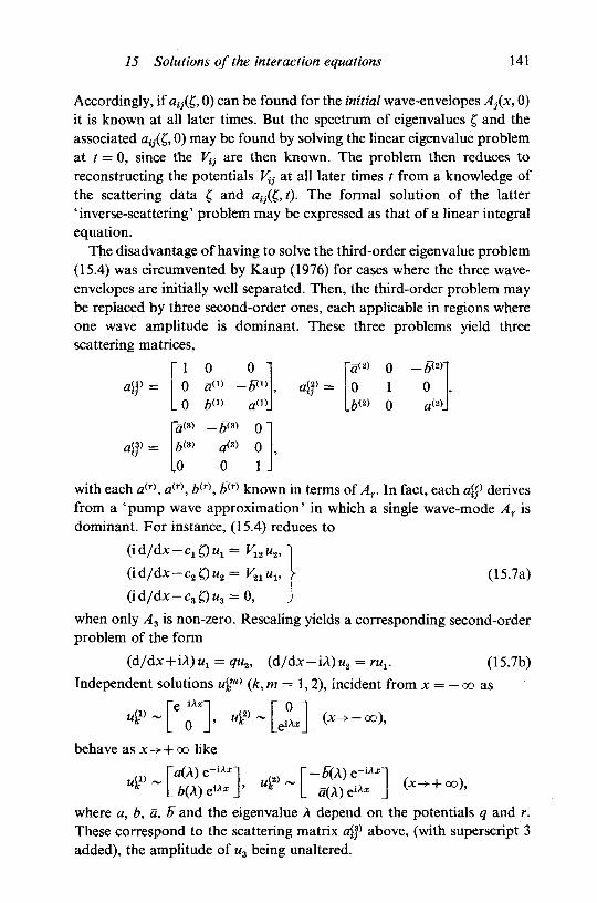
75 Solutions of the interaction equations 141
Accordingly, if ay(£, 0) can be found for the initial wave-envelopes A}(x, 0)it is known at all later times. But the spectrum of eigenvalues £ and theassociated ay(f, 0) may be found by solving the linear eigenvalue problemat t = 0, since the Vti are then known. The problem then reduces toreconstructing the potentials Vi} at all later times / from a knowledge ofthe scattering data £ and ay(£, t). The formal solution of the latter'inverse-scattering' problem may be expressed as that of a linear integralequation.
The disadvantage of having to solve the third-order eigenvalue problem(15.4) was circumvented by Kaup (1976) for cases where the three wave-envelopes are initially well separated. Then, the third-order problem maybe replaced by three second-order ones, each applicable in regions whereone wave amplitude is dominant. These three problems yield threescattering matrices,
d$ =
af =
10
. 0
s<3>1,(3)
.0
0i) _
i )
b(3)
a(3)
0
0
a d )
0"01.
0J,(2)
010
0a< 2 ) .
with each a(r), a(r), /><r), Z>(r) known in terms of Ar. In fact, each a<p derivesfrom a 'pump wave approximation' in which a single wave-mode Ar isdominant. For instance, (15.4) reduces to
( id /dx-c 1 O"i= V12 Kg,(id/dx-c2£)w2= V21ut, I (15.7a)
Jwhen only ,43 is non-zero. Rescaling yields a corresponding second-orderproblem of the form
= qu2, (d/dx-iA)«2 = rux. (15.7b)Independent solutions t4m) (k, m= 1,2), incident from x = - oo as
behave as x->+ oo like
fc L a(A)e l A a : J (x-^+oo),
where a, b, a, 5 and the eigenvalue A depend on the potentials q and r.These correspond to the scattering matrix a\f above, (with superscript 3added), the amplitude of u3 being unaltered.
Downloaded from University Publishing Online. This is copyrighted materialIP139.153.14.250 on Tue Jan 24 02:27:28 GMT 2012.
http://dx.doi.org/10.1017/CBO9780511569548.006

142 Three-wave resonance
With the separate envelopes initially ordered 3, 2, 1 from left to right,the overall scattering matrix at t = 0 is just
If the envelopes again separate at sufficiently large times, say tt, (which doesnot always happen!) the final scattering matrices affl(£,tt) have similarform and
) = a®a®alf (t = tt), (15.8)the relative positions of the envelopes being reversed in accordance withc1< c2 < c3. Results analogous to (15.6) relate each initial and finalscattering matrix ajp. Inversion of the scattering data yields the respectivewave amplitudes after interaction has been completed: but this simplertreatment does not yield the solution during interaction.
The complete formal solution of the inverse-scattering problem, in termsof a linear integral equation, is not usually amenable to further analyticreduction. Nevertheless, a class of closed-form w-soliton solutions isavailable. These are associated with a discrete 'bound-state' spectrum ofeigenvalues £ (or A) which corresponds to poles of the ratios b(r)/air) andwhich exists only when the signs s} differ. Each a(r) may be thought of(loosely) as a wave incident from x = + oo which yields a transmitted waveof unit amplitude as x ->—oo and a ' reflected' wave of amplitude £(r)
(actually, 6<r) is 'converted', not reflected, into another member of theresonant triad). The bound-state spectrum of £ arises, analogously withresonant over-reflection, when 'transmitted' and 'reflected' waves occurin the absence of an incident mode.
In addition to these bound-state soliton solutions, there is a continuousspectrum of £ with non-singular b(r) /aSr\ Since (14.10) are non-dispersivein the linear limit, the contribution from this continuous spectrum doesnot decay with time (as it does for the Korteweg-de Vries equation, forexample) but remains on an equal footing with the solitons. Nevertheless,investigation of the properties of the soliton solutions provides valuableinsight.
For a given eigenvalue £, a ratio b(r)/aSr) may be singular at t = 0 butnot at the final time tt, or vice versa. Precisely, zeros of a(r> and a(r> presentat t = 0 persist at t = tt for the fast and slow envelopes r = 1 and 3, butall zeros of a(2) present at / = 0 are absent at t = tt. This means that themiddle envelope always loses any solitons it may originally possess, butthat solitons are not usually lost from the fast and slow envelopes. Amiddle-envelope soliton with eigenvalue £(2) is converted to solitons of theslow and fast envelopes with respective eigenvalues £W, £® with
Downloaded from University Publishing Online. This is copyrighted materialIP139.153.14.250 on Tue Jan 24 02:27:28 GMT 2012.
http://dx.doi.org/10.1017/CBO9780511569548.006

15 Solutions of the interaction equations 143
Figure 5.4. Soliton exchange interactions, computed by Kaup, Reiman & Bers (1979).Mode flj (with intermediate group velocity) dominates at t = 0 but mode a^ (smallestgroup velocity) is also present. Subsequently, one, two or more pulses of a3- and thethird mode ak are emitted. Reference frame chosen with vt — 0, fs = ~yk. (a)|ay /oj | = 0.02 and pulse length L/Lc = 3.25 initially; (A) |Oj/Of | = 0.002 andL/Lc = 6.4 initially. (Courtesy of Amer. Phys. Soc).
(or y)
Downloaded from University Publishing Online. This is copyrighted materialIP139.153.14.250 on Tue Jan 24 02:27:28 GMT 2012.
http://dx.doi.org/10.1017/CBO9780511569548.006

144 Three-wave resonance
g(i) 4. g(3) _ g(2) jhese three solitons therefore form a resonant triad. If,exceptionally, the initial data provides fast and slow envelopes withsolitons at such eigenvalues gW, £<3) and with appropriate phases, theseannihilate one another to produce a £(2) -soliton in the middle envelope,but this would subsequently disintegrate back into £(1) and £(3) solitons ifit met any other disturbance. Such 'soliton exchange interaction' bynonlinear resonance is not confined to (14.10): it arises also for solutionsof the Korteweg-de Vries and nonlinear Schrodinger equations (Miles1977a,b;Kaup 1981b).
Soli ton exchange interactions occur for (14.10) when the wave ofgreatest frequency has the middle group velocity and the signs s}
(J = 1,2,3) differ. Examples of such interaction, obtained numerically byKaup et al. (1979), are shown in Figure 5.4. But soliton exchange isprohibited in other cases.
One such is 'stimulated back-scattering', where the highest-frequencywave has fastest or slowest group velocity and all three wave energies havethe same sign (e.g. sl = s2 = 1, ss = — 1). Then, neither the high-frequencywave nor the middle envelope can ever possess solitons. Interaction of alaser and ion acoustic wave, to produce a backscattered (i.e. slower) laserpulse, is of this kind.
The assumed separation of the wave-envelopes at t > tt breaks downin 'explosive' cases. These occur when the high-frequency envelope hasenergy of opposite sign to the other two waves (i.e. the signs s} are the same)and travels with the middle group velocity. Solutions may then developa singularity after a finite time, or may not, depending on the initial data.Numerical examples, from Kaup et al., are shown in Figures 5.5(a),(b):the latter explodes but the former does not. In Kaup's (1976) formulation,an earlier 'explosion' is indicated by inconsistencies in the scattering dataat tt: neither the fast nor slow envelope can ever contain solitons in thiscase, but neither can the middle envelope retain its solitons at ?,. Solutionsbounded for all t exist only when the middle envelope contains no solitonsat t - 0.
The n-soliton solution, for Sj of differing signs, has the following formfor each (non-overlapping) envelope (Kaup et al., Appendix B):
(15.9)
^ (T= 1,2,3),
A, = it,,, Sv =
N = Nfj = D^(?/4 + q}) 1 exp [ — (r,t + rjj) x'], x' = x — cr t—xr
(xr constant),.
Downloaded from University Publishing Online. This is copyrighted materialIP139.153.14.250 on Tue Jan 24 02:27:28 GMT 2012.
http://dx.doi.org/10.1017/CBO9780511569548.006

15 Solutions of the interaction equations 145
Figure 5.5. Collision of initially rectangular pulses in potentially explosive cases: (a)non-explosive, with | aj/at | = 0.25 at t = 0; (b) explosive, with | cij/a( | = 0.35 at / = 0(from Kaup, Reiman & Bers 1979, courtesy of Amer. Phys. Soc).
Downloaded from University Publishing Online. This is copyrighted materialIP139.153.14.250 on Tue Jan 24 02:27:28 GMT 2012.
http://dx.doi.org/10.1017/CBO9780511569548.006

146 Three-wave resonance
where a, = af1, bj = &<r) (r = 1,2,3) are elements of the three scatteringmatrices a$ corresponding to the 7th eigenvalue-pair A = + A . Thesebound-state positive and negative eigenvalue pairs are pure imaginary andthe summation yields two terms for eachy, k. The scaled eigenvalues A arerelated to the original eigenvalue £ by
A« = &(c, - c2), A<2) = J£(c, - C l), AW = &(c, - cj
for the respective envelopes (cf. equation 15.7a, b). Also, from (15.5) and(15.7), the amplitudes Ar are related to qir) by
a(X) = S2S»A1 (2) _
9 [(CcMccdf q
< 7 ( 3 ) = ;
Each soliton travels with its linear group velocity cr in the non-interactingregion but ap bj and so D3- take different values before and after interaction.Fuller details are given by Kaup et al.
The trivial one-soliton solution (J = k = n = 1) is
?w = -2Vl sgn(-D1) seci[2iil(x'-x0)]
with x0 defined by
IDJI = 2i;1exp(2i/1x0).
The collision of two single envelope solitons is the next simplest solution(see Kaup et al.). At t->-— 00 this is
?<D ~ 21/j sech (2Vl zx) e \ q™ ~ 0,
q^ ~ 2Vs sech(2Vaz3) &**, z} = x-Cjt-xoj
where xop <pi are constants. Provided the eigenvalues A = i^1; ii/3 are suchthat the corresponding values £l5 g3 of £ are not equal, these solitons arenon-resonant. They collide when t « (x10 — x30)(c3 — c^)"1 and for a timeproduce a ^(2> soliton. But, as /-> 00, the qf(2> soliton decays, replenishingthe r(1) and q(3) solitons to
qM ~ 2^ sech (2^ zx - 8) e^+d\ q™ ~ 0,
q™ „ 2% sech(2r,3z3 * « >
(the eigenvalues A being assumed imaginary).When £j = ^3, the two solitons are resonant with a third, for then
A(D + A(3) = ^ ( c g - q ) = A<2>. In this case,
qm „ g») ~ 0, qM ~ - 2V2 sech (2^2 z2) tfa
Downloaded from University Publishing Online. This is copyrighted materialIP139.153.14.250 on Tue Jan 24 02:27:28 GMT 2012.
http://dx.doi.org/10.1017/CBO9780511569548.006

15 Solutions of the interaction equations 147
as /->oo, where z2 = x—c21—x20 and
Clearly, the qm and ^<3) solitons have been converted to a <7<2) soliton whichcompletes the resonant triad.
The latter resonance occurs only in exceptional cases for which the initialdata yield equal eigenvalues £x and £3. Usually, the conversion processoperates in reverse: a given middle envelope qi2) soliton interacting withan arbitrary small disturbance decays into fast and slow solitons which areresonant with it. This is normally referred to as a 'decay instability'.
Similar inverse scattering solutions have been found for three-waveinteractions in inhomogeneous media. Then, a small wavenumber mis-match, say Ak denoting imperfect resonance, varies linearly with distancex; but the governing equations may still be transformed into (14.10)(Reiman 1979). Inverse-scattering and Backlund-transformation solutionsfor three-wave interaction with constant frequency or wavenumber mis-match were earlier given by Chu & Scott (1975) and Chu (1975a): theserelate to cases where two of the three group velocities ci are equal.
15.3 Solutions in three and four dimensionsFor propagation in two or three space dimensions and time, the
inverse scattering theory has been developed, along somewhat similar lines,by Zakharov (1976), Cornille (1979) and Kaup (1980). Zakharov firstnoted a broad class of explicit solutions, independently discovered usingelementary analysis by Craik (1978). These and further classes of solutionshave also been constructed, using a Backlund transformation, by Kaup(1981a, b).
With three, or four, independent variables x, t available, it is possibleto choose characteristic co-ordinates Xi (' = 1,2,3) such that
6/8*, = 9 / 3 / + v V f a * v2 4= v3):
these are clearly linear combinations of x, t. If there is dependence on three,rather than two, space co-ordinates and t, the fourth characteristicco-ordinate Xt is chosen so that
(a/8/ + y , - V ) ^ = 0 (1=1,2,3).
In the amplitude equations, XiIS just a 'dummy variable' which acts likea fixed parameter and so is ignorable. The three amplitude equations(14.10) are then just
dAi/dXi = siAfAZ (15.10)
with i,j, k taken in cyclic order, equal to 1, 2 or 3.
Downloaded from University Publishing Online. This is copyrighted materialIP139.153.14.250 on Tue Jan 24 02:27:28 GMT 2012.
http://dx.doi.org/10.1017/CBO9780511569548.006

148 Three-wave resonance
Surprisingly, the inverse-scattering analysis reveals that the associatedlinear eigenvalue problem yields no discrete bound states. Accordingly,there are no three-dimensional n-solitons and the complete solution derivesfrom the continuous spectrum.
On introducing moduli b( and phases 6t, where At = bt exp (i6t), (15.10)becomes
+ 8Z). jSolutions with constant phases Bt = Q\ have
= 2(-l)N\s1s2s3—,— T — — -——- (1512)
where F(xv x%, #3) is a n v r e a l solution of the last equation which yields
positive values for each b\. The problem lies in finding such functions F.That given by Craik (1978) is
F= —s1s2s3 In\fi(xi) +/2CV2) +-/sOfo)] (15.13)
with (— 1)^ = — sls2s9, thef((xt) being three not quite arbitrary differenti-able functions. This class of explicit solutions also emerged as a specialcase of Zakharov's (1976) inverse-scattering representation and a somewhatsimilar solution, for propagation in x and t only, was given by Wilhelmsson,Watanabe & Nishikawa (1977).
For initially-bounded envelopes, the functions ftixd at * = 0 must havenon-zero sum / t + / 2 + / s at all points of space. Some further restrictionsare necessary to ensure that the amplitudes bj are real, but the class ofsolutions remains large. Initially-bounded envelopes 'explode' at a latertime if/i +f2 +f3 becomes zero at any point in space. Craik (1978) showedthis to be possible only when the three signs s} are the same, as expected.He and also Kaup (1981a, b) give some particular examples of interactinglocalized wave-envelopes. They also give a 'bursting criterion', in termsof the available' energies' of initial wave-envelopes. A typical configurationof interacting envelopes is shown in Figure 5.6. When one wave-mode islocally dominant, a ' pump-wave' approximation suffices (Craik & Adam1978), but this cannot represent the explosive instability.
More general solutions were derived by Kaup (1981a), using a Backlundtransformation. First, the linear scattering problem
(i,j,k= 1,2,3) (15.14)
Downloaded from University Publishing Online. This is copyrighted materialIP139.153.14.250 on Tue Jan 24 02:27:28 GMT 2012.
http://dx.doi.org/10.1017/CBO9780511569548.006

75 Solutions of the interaction equations 149
is defined, where i,j, k are cyclic. This comprises six equations for the threefunctions fafa, #2> Xs)- These have three conservation laws,
3(^ I fa \2)/dx* = 9fe I f* \2)/dXi («" * *)and so there exists a function -D(#15 #2> #3) wi*h
3 D / 3 ^ = - j f | ^ ( | * (1 = 1,2,3). (15.15)If A] (J = 1,2,3) is any known solution of (15.10), the correspondingfunctions fa and D may be found from these equations.
The Backlund transformation is
(15.16)with D real and cyclic i, j , k. It is readily verified that A} is then also asolution of (15.10)! The transformation therefore generates new solutionsfrom old.
The trivial solution A} = 0 yields
Aj = ijr* xjr^/D,/ fan \
(w)|2dM)+constant°=k<\:where each fa is an arbitrary, differentiable, complex function of thecorresponding single variable Xi- This class of solutions, called' one-lump'solutions, is precisely that of (15.12)—(15.13). 'Two-lump' solutions A} arenext constructed by using the one-lump solution for A} in (15.14) and(15.16) and calculating new functions ^ and D. Continuation of thisprocess generates an arbitrary number of W-lump' solutions. Kaup
Figure 5.6. Configuration of localized disturbances (a) before and (b) after interaction.Each mode is contained within the domain Dj(j= 1,2,3) which moves in the directionindicated.
(a)
Downloaded from University Publishing Online. This is copyrighted materialIP139.153.14.250 on Tue Jan 24 02:27:28 GMT 2012.
http://dx.doi.org/10.1017/CBO9780511569548.006

150 Three-wave resonance
(1981a) gives only the one-lump and two-lump solutions explicitly, thelatter containing six arbitrary functions compared with the one-lumpsolution's three. Kaup conjectures that the two-lump solution may besufficiently general to describe the behaviour of all initially-localized wave-envelopes, but this has yet to be shown.
In one sense, the three-dimensional TV-lump solutions may be regardedas counterparts of the two dimensional N-solitons: in inverse scatteringtheory, both derive from separable kernels of integral equations. Inanother, these solutions are very different, for the three-dimensionalproblem yields no discrete bound-state eigenvalues, such as give rise tojV-solitons. A feature reminiscent of resonant soliton interactions is the'decay instability' exhibited by some one-lump solutions: particularA1 envelopes have been shown to convert completely into A2 and A3
envelopes on meeting a small amount of A2 and A3 (Case & Chiu 1977;Kaup 1981b).
15.4 Long wave-short wave interactionsInteractions among short waves and long waves are resonant when
the group velocity cg of the short-wave envelope equals the phase velocitycp of the long waves. This is just the condition
Ak = kt, Aw = cg Ak = (ol
where (kh, o)h) are the wavenumber and frequency of the long wave and(Ak, Aw) are the limits (k-k',(o—w') as (&', w') approaches the short-wavewavenumber and frequency {k, w). Obviously, this is a special case ofthree-wave resonance.
With short-wave envelope At(X, T) and long-wave envelope B(X, T), thegoverning equations in many cases take the form
Here, X - e§ (x -c g 0andr = e*/(cf. 19.2a, b). Equality of cg and cp allowsthe dispersive term PXAXXX to be included in (15.17a), though this wouldotherwise be of higher order (see § 19). Equations of this form were derivedby Grimshaw (1977) for resonant interaction of a packet of short surfacewaves with a long internal wave. These were solved by Ma (1978) and Ma& Redekopp (1979), using inverse scattering, for real coefficients.
With two short-wave envelopes Ax(X,i), A2(X,T) with differing wave-
Downloaded from University Publishing Online. This is copyrighted materialIP139.153.14.250 on Tue Jan 24 02:27:28 GMT 2012.
http://dx.doi.org/10.1017/CBO9780511569548.006

16 Linearly damped waves 151
numbers and frequencies but with equal group velocities cgl = cg2 = cp,the corresponding equations are
(15.18)
These are discussed by Ma (1981), who gives their solution by inversescattering for real coefficients with f$x = /?2, yx = y2 and sgn A1A2 = 1. Suchcases are conservative, with waves of like energy sign. There are, in effect,two degenerate resonant triads with the long wave in common. Therestriction cgl = cg2 constrains the choice of modes.
With rescaled co-ordinates, (15.18) transform to
and boundary conditions Sk, L^-0 as | X | ->oo are imposed. The methodof inverse scattering applies, in principle, also to interactions with N shortwaves (k — 1,2, ...,N). The linear eigenvalue problem associated with(15.19) is a fourth-order one, with complex eigenvalues £ = — £+i?/ say,where g, ij > 0. The one-soliton solution is
(15.20)L = - 2V* sech2 MX- Xo) + 2gr,r], c\ + c\ = 1, J
where Xo and the 'polarization vector' c = (c^c^) are known constants.All such solitons travel to the left, with velocity — 2g, without change inform.
Interaction of two such solitons, with different eigenvalues £ls £2 yieldssolutions like (15.20) for both, as t->—oo and t^>+ oo. But the respectivevalues of xy> and cW) (j = 1,2) differ before and after interaction. Thecentres of the two envelope solitons are shifted and the polarization vectorsc0 ) are changed because of redistribution of energy among the Sx and S3
wave-modes in either soliton. Nevertheless, the total energy of each mode,
poo poo poo
\S^dX, \S2\*dX, LdX,J —00 J —OO J —OO
remains unchanged - a property not shared by other models of longwave-short wave interaction (Ma 1978; Newell 1978).
Downloaded from University Publishing Online. This is copyrighted materialIP139.153.14.250 on Tue Jan 24 02:27:28 GMT 2012.
http://dx.doi.org/10.1017/CBO9780511569548.006

152 Three-wave resonance
16 Linearly damped waves16.1 One wave heavily damped
When the nonlinear interaction remains of conservative type, butthe waves are linearly damped or amplified, the normalized amplitudeequations resemble (14.10) but have an additional term o-jAj (j = 1,2,3)added to each left-hand side. A uniform wave-train, for giveny, would thendecay with exponential rate <Xy in the absence of the other two modes. (Asbefore, the resonant triad is taken to have the form k j + k a + k ^ O ,0)1 + (O2+C03 = 0.)
The inverse-scattering solution exists only for cr,- = 0 and very fewsolutions incorporating damping are known, for amplitudes varying inboth space and time. One relates to the case cr1 = a2 — 0 and <r3 very large.Then, the equation for A3 yields the approximate solution
A3 = <r3 S3A± A2
and those for Ax and A2 yield
hh, (3/Sr+v2-V)/2 = IJ2,(16.1)
= 2s2s3o-3-1\A1\
2, I2s=2sls3<r31\A2"~
Solutions of these are given by Hasimoto (1974), Chu (1975b) andWilhelmsson, Watanabe & Nishikawa (1977) for amplitude variations inx and t. Chu & Karney (1977) consider variations in x, y and t: thisextension derives from a straightforward change of reference frame sincederivatives of A3 are negligible compared with the large damping term.When Ix, I2 depend on x and t, introduction of characteristic co-ordinatesreduces (16.1) to
a = i.2),li f _x-c2t \ (16.2)
> 62 -cc1 — c2 c2 c1
where ct is the x-component of v . The known class of solutions has
This is reminiscent of the one-lump solutions of (15.10) in threedimensions.
16.2 Waves dependent on t only(i) Equal damping ratesWhen the amplitudes depend on t only and each damping rate cr}
is the same, say <r, the governing equations may be reduced to the
Downloaded from University Publishing Online. This is copyrighted materialIP139.153.14.250 on Tue Jan 24 02:27:28 GMT 2012.
http://dx.doi.org/10.1017/CBO9780511569548.006
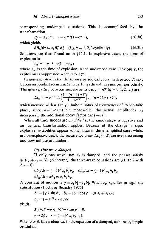
16 Linearly clamped waves 153
corresponding undamped equations. This is accomplished by thetransformation
B} = A} eat, T = o - ^ l -e - 0 *) , (16.3a)
which yieldsdBt/dr = st Bf Bt (i, j , k = 1,2,3 cyclically). (16.3b)
Solutions are then found as in §15.1. In explosive cases, the time ofexplosion is
; 0 0 = - o - 1 l n ( l - o - T 0 0 )where r^ is the time of explosion in the undamped case. Obviously, theexplosion is suppressed when a > T"1 .
In non-explosive cases, the Bt vary periodically in T, with period T, say;but corresponding recurrences in real time t do not have uniform periodicity.The intervals Atn between successive values r = nT (n = 0,1,2,...) are
which increase with n. Only a finite number of recurrences of Bt can takeplace, since n+1 < (crT)*1; meanwhile, the actual amplitudes At
incorporate the additional decay factor exp (— cri).When all three modes are amplified at the same rate, a- is negative and
an identical transformation applies. Because of the change in sign,explosive instabilities appear sooner than in the unamplified case; while,in non-explosive cases, the recurrence times Atn of Bt are ever-decreasingand now infinite in number.
00 One wave dampedIf only one wave, say As is damped, and the phases satisfy
?/1 + ??2 + 7/3 = Nn {N integer), the three-wave equations are (cf. 15.2 withAw = 0)
dbJdt = {-\)N Sl b2 b3, dbjdt = ( - 1 ) N s2 bx b3,
dba/dt + <rb3 = s3b1b2.
A constant of motion is y s s-^bf — s2b\. When sx, s2 differ in sign, thesubstitution (Fuchs & Beaudry 1975)
b-i = 171« sin yS% b2 = \ y |i cos rjr (0 < ifr < \n)
yieldssiny = 0,
y l 13yWhen r > 0, this is identical to the equation of a damped, nonlinear, simplependulum.
Downloaded from University Publishing Online. This is copyrighted materialIP139.153.14.250 on Tue Jan 24 02:27:28 GMT 2012.
http://dx.doi.org/10.1017/CBO9780511569548.006

154 Three-wave resonance
(Hi) Three different damping ratesThe general case is more difficult to handle. Weiland & Wilhelmsson
(1977) describe analytical approximations and numerical solutions bothfor equal and differing signs Sj. Miles (1976b) also does so for thedegenerate case of two-mode interaction (A1 = A2 say).
(iv) Three-wave strange attractorWhen the wave of greatest frequency is linearly amplified and the
other two are linearly damped, the temporal evolution of near-resonanttriads with k 1 = k 2 + k3, (o2 + w3 — o)1 = d is described by normalizedequations
d^/dt = bx + b2 b3 exp (\St), "1
dbjdt = -(r2b2-b1b*exp(-i8t), \ (16.4)
dbjdt = - o-3 b3 - bt bt exp (- \St), J
(corresponding to s2 = s3 = —Sj). The normalized damping rates cr2, a3 arepositive.
Wersinger, Finn & Ott (1980a, b) discovered that these equations havea surprisingly rich structure, with solutions which exhibit bifurcations tosuccessively more complex periodic orbits and also the 'chaotic' behaviourof a 'strange attractor'. On setting
bx = a, exp ( i^ ) , bk = ak exp (i0fc - \ASt) (k = 2,3)
and restricting attention to the special case a2 = a3, cr2 = <T3 = cr, (16.4)become
da1/dt = flj + a\ cos <j>, dajdt = — a2(cr + ax cos <j>),
d(j>/dt = -S+a^ilal-al) sincf>, <f> = fi-fa-fa.
These depend on just two parameters, S and ar. Wersinger et al. undertooka numerical study for 8 = 2 and 1 < tr 25. When the initial phase <j> waschosen in the range 0 < $ < n, it remained so at all subsequent times.Wersinger et al. recorded their results by plotting a1 against a2 each timethe solution orbit crossed (f>(t) = \TT with d^/d/ < 0.
For small damping rates, 1 < cr < 3, ay and a3 grow without bound;while, for 3 < cr < 8.5, all solutions approach a simple limit cycle abouta single fixed-point solution. At ar « 8.5, bifurcation occurs from the singlefixed point to one unstable and two stable fixed points: solutions thenapproach a 2-point periodic limit cycle at large t. Further bifurcations, tostable 4-point, 8-point, 16-point and 32-point limit cycles occur at<r« 11.9, 12.8, 13.15 and 13.16 respectively. For 13.16 < o- < 13.20 and13.20 < cr < 16.8, solutions had no observable periodicity and showed the
Downloaded from University Publishing Online. This is copyrighted materialIP139.153.14.250 on Tue Jan 24 02:27:28 GMT 2012.
http://dx.doi.org/10.1017/CBO9780511569548.006

16 Linearly damped waves 155
typical chaotic behaviour of a strange attractor, but a stable 48-pointperiodic cycle was observed at a = 13.20. For 16.8 < a < 17.4, periodicityreappeared as a stable 3-point limit cycle, but at a x 17.4 this bifurcatedto a 6-point cycle. Apparently chaotic behaviour resumed at a « 18.5 andpersisted to a = 25.
(t>) Equilibrium solutions with external forcingWith three damped waves and external forcing, equations for the
moduli and phases of the amplitudes are (cf. 14.9)
\ d(b\)/dt = b, b2 b2(Jkt/ut) sin v-<rt b\ + bt Ft cos (yt - i/,),
— blb263(A4/wt) cos^ + btFt sin(yt —1/4)3
y='LVi ('= 1.2,3).i-1
Here, the damping rates are <r4 and Ft, yt represent the respectivemagnitudes and phases of the external forcing. If Ft and yi are constants,steady-state solutions exist with i/4 = yi when yx+y2+y3 = (N—§n(N integer). The amplitudes bt then satisfy
<rt b\ - Ft bt = ( - 1 )N b, b2 b^JkJiod (i = 1,2,3),
and the number of permissible solutions varies. They have the form
b, = b?(K) l^F^iajFI + KBrfU
where AT is a root of
McEwan, Mander & Smith (1972) examined such triads of standinginternal waves in stratified fluid, both experimentally and theoretically,when only the wave of greatest absolute frequency is forced. Then,F2 = F3 = 0 and the only steady-state solutions are
t)2, i/3 arbitrary,and
Vi = 7i> bx = b10 = (B2 B3)~i, rj2 = (N— 2)n — yx —i)3, ~)
b2( - Bt B3)i = b3( - B, B2)i = ( - 1 + F, 071 b$$, y3 arbitrary. J " a>
The latter solution exists only if B2 B3 > 0 - when Bx B2 and B^ B3 are bothnegative by (16.5) - and if cr^1 Fx > (B2 B3)~^. With weaker forcing thanthis, only the former solution occurs.
As F1 is increased from zero, at first only the single wave bx appears,
Downloaded from University Publishing Online. This is copyrighted materialIP139.153.14.250 on Tue Jan 24 02:27:28 GMT 2012.
http://dx.doi.org/10.1017/CBO9780511569548.006

156 Three-wave resonance
but this solution is unstable for Ft ^ <ri(fl2 B3)~l and resonating waves b2
and b3 appear. As F1 increases beyond the critical value, the amplitudesof b2 and b3 increase while that of the driven wave remains constant at(B2 B3)~l. This behaviour was confirmed experimentally by McEwan et al.Figure 5.7 shows an example of their experimental and theoretical results.A single standing-wave mode was first produced and then a paddle, whichdirectly excited a second mode, was turned on. The results showestablishment of a three-wave equilibrium solution, comprising these anda third, resonating, mode.
Chester (1968) and Miles (1976b) have analysed resonant oscillations ofwater waves in closed containers subjected to periodic forcing, and relatedexperiments are described by Chester & Bones (1968). When the forcingfrequency w and the frequencies w,, w2 of standing-wave modes satisfy
Figure 5.7. Forced triad interaction among standing internal waves (from McEwan,
Mander & Smith 1972). Mode (1,2) was present initially and mode (3,1) was driven
by an oscillatory paddle. Three-wave equilibrium, with these and mode (2, — 1), was
eventually established. Q denotes amplitudes, N the number of paddle cycles; • . •
show measurements and solid lines theoretical results.
1.5
200 300
N (cycles)
Downloaded from University Publishing Online. This is copyrighted materialIP139.153.14.250 on Tue Jan 24 02:27:28 GMT 2012.
http://dx.doi.org/10.1017/CBO9780511569548.006

16 Linearly damped waves 157
W « o>! x \u)2, and when the wavenumbers satisfy k1 = \k2, Miles' coupledamplitude equations are
This is a degenerate case of three-wave resonance with damping andperiodic forcing. Similar resonances of elastic structures containing aliquid, under periodic forcing, were investigated both theoretically andexperimentally by Ibrahim & Barr (1975a, b). For harmonic two-modeinteractions, equations like Miles' were recovered; while three-modeinteractions satisfied equations like those of McEwan, Mander & Smith.
Waves in oscillating containers were also studied theoretically byMahony & Smith (1972) and Huntley & Smith (1973), but with imposedvibrations of much higher frequency Q than those of standing water waves.The latter are driven unstable by a limiting form of three-wave resonance,W3 = wt—w2 say, where w, « <D2 « Cl > w3. The modulations of forcedcomponents with frequencies &>„ w2 may then occur on the same O^1)timescale as the standing-wave oscillations. Huntley's (1972) experimentson waves in a rapidly-vibrated glass beaker and Franklin, Price &Williams' (1973) acoustically-excited water waves gave dramatic demon-strations of the phenomenon. With cubic nonlinearities retained in theamplitude equations, the theoretical model successfully reproducedobserved features of hysteresis and nonlinear detuning.
It is appropriate also to mention parallel work on resonance and forcedoscillations in mechanical systems with just a few degrees of freedom:Rott's (1970) multiple pendulum and Barr & Ashworth's (1977) weightedelastic beams provide particularly elegant demonstrations of parametricand internal resonances.
(pi) Coupled triadsWhen there exist two resonant triads with one member in common,
say
k, + k 4+k 5 = 0, to1+toi+ojb = 0,
there are five coupled amplitude equations, each with quadratic nonlineari-ties. Undamped cases are discussed by Wilhelmsson & Pavlenko (1973)(see also Weiland & Wilhelmsson 1977) for potentially explosive inter-actions. Analytic solutions are found, in particular cases, in terms ofelliptic functions.
Downloaded from University Publishing Online. This is copyrighted materialIP139.153.14.250 on Tue Jan 24 02:27:28 GMT 2012.
http://dx.doi.org/10.1017/CBO9780511569548.006

(a)
(b)
Figure 5.8. Shadographs of dyed layers showing resonance among standing internal waves (from McEwan, Mander & Smith 1972).(a) shows initial single-mode state with dimensionless wavenumber (4, 2). (b) shows state after 430 cycles of paddle driving the (5, 1)mode. This mode resonates both with (4, 2), (1, - 1 ) and with (3, 3), (8, 4), the latter of which have grown to prominence.
Downloaded from University Publishing Online. This is copyrighted materialIP139.153.14.250 on Tue Jan 24 02:27:28 GMT 2012.
http://dx.doi.org/10.1017/CBO9780511569548.006

16 Linearly damped waves 159
McEwan, Mander & Smith (1972) considered five damped internalwaves, with the common wave bx externally forced and having the greatestabsolute frequency. They showed that the steady state bx = 071 Fl5 b} = 0(j = 2,3,4,5) is stable when 071 Fx is below the threshold value for bothtriads, regarded separately. Otherwise, the only stable equilibrium statecorresponds to (16.6b) for the triad with lowest threshold, the remainingtwo waves having zero amplitude.
Figure 5.8, from McEwan, Mander & Smith (1972), shows just such acase. The initial configuration (a) is a single standing-wave mode, say k2.Direct forcing of mode k t at first led to growth of this and the resonantk3 component; but, after sufficient time, modes k4 and k6 grew toprominence as shown in (b).
Explosive instability of triads and coupled pairs of triads of baroclinicwaves was recently discussed by Merkine & Shtilman (1984): their modelequations incorporate linear growth or damping and also cubic nonlineari-ties. The mutual interaction of many coupled resonant triads wasinvestigated numerically by Loesch & Domaracki (1977); see also §19.3.
16.3 Higher-order effectsThe influence of higher-order terms on three-wave resonance is
described, in part, by Weiland & Wilhelmsson (1977); see also Goncharov(1981). Their equations have the general form
3*-iA1 I xlk\Ak\
2,fc-i
dA2/dt+a-2A2 = cX3A3A%-\A2 £ cc2k\Ak\2,
= c*2A1A2-iA3
(16.7a, b,c)
for resonance with k3 = kj + ka, w3 = e^+Wa. In addition to the threesecond-order coupling coefficients, there are nine third-order coefficientsa « (hj= 1,2,3). The real parts of a.^ contribute amplitude-dependentfrequency shifts and the imaginary parts yield extra growth or dampingterms.
For conservative systems, o - = Im {<*„•} = 0 and (16.7) transform toscaled equations like (15.2), namely
dbjdt = st bj bk cos y (i, j , k cyclic),3
drj/dt = Aw — bx b2 b3 sin rj "£ Sj bj2.
Downloaded from University Publishing Online. This is copyrighted materialIP139.153.14.250 on Tue Jan 24 02:27:28 GMT 2012.
http://dx.doi.org/10.1017/CBO9780511569548.006

160 Three-wave resonance
But the frequency shift Aw is now an additional variable,
j f, p} = Re {a,, - an - a,,}.
A solution with all three waves equal and each st = 1 is
b} = b(t) = [y* + (t, - tf]-i 0 = 1 , 2 , 3 ) ,
sin r, = -
When y = 0, this is the explosive solution iv{c) of § 15.1; but, for finite y,bj(t) reach a maximum of y"1 before decaying to zero. The explosion issuppressed by nonlinear detuning of the resonance.
More generally, the conservative equations (16.8) may be cast in theform (15.3)' since they, like (15.2), have constants of motion. But thefunction n(x) is now a fourth, not third, degree polynomial. This againyields solutions in terms of elliptic functions: the sn function when all fourroots of n(x) are real and the en function when two are real and twocomplex. Since n{x) ~ 2y2x4 > 0 as | x \ ->oo, unbounded solutions cannotoccur. Except for a few limiting cases, like that above, the solutions areperiodic. Cases which are explosive in the absence of third-order termsnormally exhibit 'repeated stabilized explosions' as shown schematicallyin Figure 5.9.
In non-conservative cases, only approximate analytic solutions areknown when c{j are non-zero; but it is a simple matter to solve any given
Figure 5.9. Repeated stabilized explosions (after Weiland & Wilhelmsson 1977).
Downloaded from University Publishing Online. This is copyrighted materialIP139.153.14.250 on Tue Jan 24 02:27:28 GMT 2012.
http://dx.doi.org/10.1017/CBO9780511569548.006

17 Non-conservative wave interactions 161
initial-value problem numerically. These, too, are discussed by Weiland &Wilhelmsson. Bifurcating equilibrium solutions of (16.7) were consideredby Craik (1975): when only one wave, A3, is present, (16.7c) reduces toa Landau-type equation (cf. equation 8.8),
This may have an equilibrium-amplitude solution with
| A31 = [Re or Jim oc33]\ = a(R) (R > Rc)
where R denotes a variable flow parameter which yields a(Rc) = 0 at thecritical value Rc. As R and a{R) increase away from Rc, initially-infinitesi-mal, linearly-damped, wave modes At and A2 may eventually be drivenunstable by terms containing Aa in (16.7a, b).
A fuller discussion of three-mode interactions with cubic nonlinearitiesis postponed until §§25-26, where examples of thermal convection andshear-flow instability are treated.
17 Non-conservative wave interactions17.1 Resonant triads in shear flows
Until now, we have mostly considered energy-conserving inter-actions: even for the linearly-damped modes of §§16.1 and 16.2, theinteraction coefficients were of conservative form. For waves in shear flows,
Figure 5.10. Curves of constant cr and ct for three-dimensional disturbances withwavenumber components (a, /?) in Blasius flow at R = 882. The curves of constantCj are shown only for /? ^ 0 and those of constant cr for /? > 0. Both curvesare symmetrical about /? = 0. The arrows designate resonant triads (from Craik 1971).
<*c, = 0-095etc, = 0-095
Downloaded from University Publishing Online. This is copyrighted materialIP139.153.14.250 on Tue Jan 24 02:27:28 GMT 2012.
http://dx.doi.org/10.1017/CBO9780511569548.006

162 Three-wave resonance
Figure 5.11. Smoke-streak flow visualization photographs, by Saric and co-workers,of growing disturbances in the Blasius boundary layer in air. Photographs (a), (b) and(c) show the same location, for U^ = 6.8 m s"1 and disturbances of differingamplitudes but same frequency (39 Hz) introduced upstream by a vibrating ribbon.Case (a) with 11/ l / l /^ = 2.5 x 10~3 at onset of linear instability, shows two-dimensionalwaves. Case (b), with |M'|/£/OO = 5.0 x 10~3 shows three-dimensional disturbanceswith 'staggered peak-valley' arrangement characteristic of oblique-wave resonance.
Downloaded from University Publishing Online. This is copyrighted materialIP139.153.14.250 on Tue Jan 24 02:27:28 GMT 2012.
http://dx.doi.org/10.1017/CBO9780511569548.006

17 Non-conservative wave interactions 163
Case (c), with | u' l/U^ = 9.0 x 10~3 shows coexisting' staggered' and * aligned' peak-valley structures. Case (d) shows a typical 'aligned' configuration with * A-vortices'such as was observed by Klebanoff et al. (1962). Flow is from left to right.(Photographs kindly supplied by Professor Saric.)
id)
Downloaded from University Publishing Online. This is copyrighted materialIP139.153.14.250 on Tue Jan 24 02:27:28 GMT 2012.
http://dx.doi.org/10.1017/CBO9780511569548.006

164 Three-wave resonance
this is not usually so and nonlinearity may be responsible for additionalenergy transfer to or from the primary flow.
A weak shear flow may participate in three- or four-wave resonance justas if it were a 'wave' with zero frequency (cf. Phillips 1966). But thisapproach is unsuitable for strong shear flows. Raetz (1959, 1964) andStuart (1962b) first showed that resonant triads of Tollmien-Schlichtingwaves can occur in boundary-layer flows and Kelly (1967, 1968) examinedsubharmonic and three-wave resonance of inviscid modes for jet andshear-layer profiles. In all this work, attention was confined to wave-modeswhich are neutrally stable according to linear theory, although linearlyunstable modes also exist in these flows.
Craik (1968) showed that resonant triads of surface gravity waves andinterfacial gravity waves exist in sufficiently strong uniformly shearedflows. When such waves share a common critical layer, there is asurprisingly large O(R) viscous contribution to the quadratic interactioncoefficients, where R is the Reynolds number. The same was found to betrue for waves in general parallel shear flows, provided the critical layeris far from boundaries (Craik 1971, Usher & Craik 1974). These triadsconsist of one two-dimensional and two oblique wave-modes withperiodicities
exp [ia(x -cTt)}, exp [i{\ax ±fiy—\a.c'T t)\
which are in resonance provided cr = c'T. These are best located from curvesof constant cr plotted in the a-/? wavenumber plane at given Reynoldsnumbers R. Such curves may be deduced from the Orr-Sommerfeldeigenvalues cT+ic± = c(x,R) by using Squire's transformation. Examples,from Craik (1971), are shown in Figure 5.10 for Blasius flow at R = 882.Since cr and q are even functions of /? they are shown only for f$ 5= 0 and/? ^ 0 respectively. The arrows denote two separate resonant triads. Thatwith a = 0.254 has the linearly-most-unstable mode as its two-dimensionalcomponent; that with a = 0.46 has linearly-unstable oblique waves withfrequency equal to that of the linearly-most-unstable mode. Such resonanttriads can cause preferential amplification of particular oblique modes.
The classic boundary-layer experiments of Klebanoff, Tidstrom &Sargent (1962) and the plane Poiseuille flow experiments of Nishioka, Iida& Ichikawa (1975) showed the spontaneous growth of oblique modes withfrequency close to that of the fundamental, but provided no evidence ofthe generation of subharmonic oblique waves with half that frequency. Thefirst such evidence in boundary layers was found by Kachanov, Kozlov& Levchenko (1977) and this was later substantiated by Thomas & Saric(1981), Kachanov & Levchenko (1984) and Saric & Thomas (1984). Saric
Downloaded from University Publishing Online. This is copyrighted materialIP139.153.14.250 on Tue Jan 24 02:27:28 GMT 2012.
http://dx.doi.org/10.1017/CBO9780511569548.006

17 Non-conservative wave interactions 165
& Thomas' work employed an ingenious smoke-wire technique for flowvisualization; typical results are shown in Figure 5.11 where the develop-ment of spanwise-periodic oblique disturbances is clear. Kozlov &Ramazanov's (1984) similar study of plane Poiseuille flow showsstructures as in Figure 5.\\(d).
The work of Levchenko and co-workers records the evolution down-stream of a vibrating ribbon, of the complete frequency spectrum ofdisturbances. At low excitation amplitudes, the development of a broadband of rather low frequencies was noticed. When the ribbon was excitedwith two frequencies <o0, cul simultaneously, sum and difference frequenciesWo+Wj could be observed along with other higher-order combinations.Judicious variation of the ribbon amplitudes and frequencies providedclear evidence of three-wave resonance at downstream positions: seeFigure 5.12. When a^ = jw0, the oblique wave resonance is symmetric;
Figure 5.12. Measured frequency spectra of Kachanov & Levchenko (1984), at a fixedlocation with R = 633 and fixed primary (&>„) oscillation frequency 120 Hz, for varioussecondary excitation frequencies («,) detuned from symmetric resonance at jw0.Curves labelled 1 to 5 correspond to detuning of - 3 0 , —10, —5, 0, +10 Hzrespectively. The twin low-frequency peaks of 2,3,5 are associated with non-symmetricresonance, the single peak of 4 with symmetric resonance. Note contributions of higherharmonics and of broadband low-frequency components deriving from resonantlyamplified non-controlled disturbances.
•a
-20 -
-40 -
100 200/(Hz)
Downloaded from University Publishing Online. This is copyrighted materialIP139.153.14.250 on Tue Jan 24 02:27:28 GMT 2012.
http://dx.doi.org/10.1017/CBO9780511569548.006
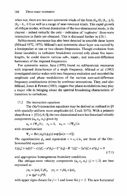
166 Three-wave resonance
when not, there are two non-symmetric triads of the form {kQ, 0), (ku ± I),(ko—kv + / ) as well as a range of near-resonant triads. This rapid growthof oblique modes, without diminution of the two-dimensional mode, is theclearest - indeed virtually the only - indication of' explosive' three-waveinteraction in fluids yet obtained. This is discussed further in §26.1.
Subharmonic resonance has also been detected in unstable shear layers(Miksad 1972, 1973). Miksad's anti-symmetric shear layer was excited bya loudspeaker at one or two chosen frequencies. Though evolution fromlinear instability to turbulent breakdown covered only about five wave-lengths, he could discern various sub-, super-, and sum-and-differenceharmonics of the imposed frequencies.
For symmetric wakes, Sato (1970) found no subharmonic resonancewith imposed disturbances of a single frequency. Miksad et al. (1982)investigated similar wakes with two-frequency excitation and recorded theamplitude and phase modulations of the various sum-and-differencefrequency combinations driven by nonlinear interactions. They, and alsoMiksad, Jones & Powers (1983), suggest that phase modulations may playa major role in bringing about the spectral broadening characteristic oftransition to turbulence.
17.2 The interaction equationsThe O(a2) interaction equations may be derived as outlined in §8
with spatially-uniform wave amplitudes (cf. Craik 1971). With a primaryshear flow u = [U(z), 0,0], the two-dimensional wave has linearized velocitycomponents (u3, v3, w3) given by
u3 = dVJdz, vs = 0, H>3 = -e*F3/8x
with streamfunction
¥3 = Re{A3(t)<f>3(z) exp[ia(x-c?)]}.
The eigenfunction <f>3 and eigenvalue c = cr + iq are those of the Orr-Sommerfeld equation
(17.1)and appropriate homogeneous boundary conditions.
The oblique-wave velocity components (u},V},w}) (J = 1,2) are bestexpressed as
yUj = laciij + fiVj, yv} = ± fiu} + \av},
with upper signs chosen for7 = 1 and lower fory = 2. The new horizontal
Downloaded from University Publishing Online. This is copyrighted materialIP139.153.14.250 on Tue Jan 24 02:27:28 GMT 2012.
http://dx.doi.org/10.1017/CBO9780511569548.006

17 Non-conservative wave interactions 167
velocity components up v} are those perpendicular and parallel to therespective wave crests. Accordingly,
dx 0=1,2),
where fa{z), c — cr+icj are eigenfunction and eigenvalue of the modifiedOrr-Sommerfeld equation
= 0(17.2)
and given homogeneous boundary conditions. At resonance, the eigenvaluesc and c have equal real parts and this requirement selects a particular valueof p. The remaining velocity components v} satisfy
fa(U-Z)e,-lt-H%-y*6i) = TiU'flh (17.3)
(cf. equation 7.3).On retaining terms of order O(a2) in the vorticity equations for each
Fourier component, one finds that
A2(t) L'[<j>2] = - (dAJdt) {<j>'2 -y*fc) + A3A*
M*) Ufa] = - (dAJdt) (& - a V.) 4-^x^
The functions G((z) (i= 1,2,3), which are omitted for brevity, involveproducts of the <j>k, Vj and their derivatives and so may be evaluated fromlinear theory. When ( ^ d j and (&2,v2) satisfy the same boundaryconditions - as is usual - Gx and G2 are identical, by symmetry.
The orthogonality conditions necessary for the existence of solutions ofthese equations are obtained on multiplication by the respective adjointfunctions ifrt(z) (i= 1,2,3) and integration across the flow from boundariesat, say, zx and z2. That is,
dAJdt
dAJdt \ f2{<j>l-y^2)dz = ASA* eaci' \ G2f2dz,
dAJdt
where rjrt are eigenfunctions of linear equations and boundary conditionsadjoint to those of <f>t. The functions fa, i/rt may be normalized in anyconvenient manner. (Note that the notation differs from that of §8.2.)
Downloaded from University Publishing Online. This is copyrighted materialIP139.153.14.250 on Tue Jan 24 02:27:28 GMT 2012.
http://dx.doi.org/10.1017/CBO9780511569548.006

168 Three-wave resonance
In terms of the amplitudes a1 2 = Ax 2 exp (faq 0, «3 = Aa exp (aq t),these are
flj/d? = |aq aj + At a3 a*,
I (17.4)
where each A4 is a ratio of the above integrals and terms of O(aa) areomitted. Normally, At = A2 by symmetry. The omission of the higher-orderterms is formally justified only in the limit a->0 where a is a measure ofthe wave amplitudes. The O(a2) nonlinear terms are then comparable withthe linear growth terms if | {acJX^ 21 and | a,cJX31 are O(a). But it is onlyin exceptional cases that all three waves of a resonant triad are neutrallystable, as the formal limit a^O requires. However, typical linear growthrates are numerically small, and the At may be quite large. Accordingly,it is reasonable to hope that the truncated equations (17.4) may yieldsatisfactory approximations at sufficiently small but finite wave amplitudes;but formal justification for omitting higher-order terms is lacking. The nextorder O(a3) terms were considered by Usher & Craik (1975); these havethe form of those in (16.7) (see also §26.1).
Consideration of the asymptotic structure of the linear eigenfunctionsallows approximate evaluation of the interaction coefficients A4 for arbi-trary primary flows U(z) at large Reynolds numbers R. When the criticallayer is located far from the boundaries zx and z2 and the wavenumber a.is 0(1) - which is not usually so as R^ao but may nevertheless be trueat fairly large R - Craik (1968, 1971) found that |A 1 2 | is O(R) and |A3|is O{\) relative to R for near-neutral waves and standard normalizationsof the <f>}. The rather unexpected O(R) contributions derive from theimmediate vicinity of the common critical layer, and depend crucially onthree-dimensionality through the velocity components 6}. Large interactioncoefficients for the next order O(a3) terms were also predicted by Usher& Craik (1975). Though lacking validity in the formal limit R~>oo, theseresults provided an early indication of the remarkable strength of nonlinearinteractions in shear flows at fairly large, finite, Reynolds numbers.
Large interaction coefficients for oblique waves may lead to enhancedgrowth of three-dimensional modes, even when these are linearly damped.The coefficients A4 were evaluated explicitly by Craik (1971) for boundarylayers approximated by straight-line profiles, but computer evaluation isnormally necessary. Computations by Hendricks, reported in Usher &Craik (1975), give values of At for Blasius flow at R = 882 and various a.The ratio of | Aj 2/A31 increases rapidly with a, from near 1 at a = 0.1 (whenthe asymptotic theory is certainly invalid) to about 30 at a — 0.5.
Downloaded from University Publishing Online. This is copyrighted materialIP139.153.14.250 on Tue Jan 24 02:27:28 GMT 2012.
http://dx.doi.org/10.1017/CBO9780511569548.006

17 Non-conservative wave interactions 169
Later, Volodin & Zel'man (1979) calculated the At for R ranging from650 to 1300 and confirmed that the ratio |A12/A3| remains fairly large.Their analysis of three-wave resonance in Blasius flow considers spatial,rather than temporal, wave evolution and attempts to incorporate theeffects of downstream variation of the primary flow. Then, spatialderivatives are associated with the respective group velocities v of eachwave, as in (14.10), but each v may be complex.
An alternative derivation of (17.4) is given by Usher & Craik (1974).In this, they extend to viscous flows the variational approach used bySimmons (1969, see § 14.2 above) for inviscid water waves. To do this, theyemployed a little-used variational formulation of the Navier-Stokesequations, given by Dryden, Murnahan & Bateman (1956). Since theNavier-Stokes equations are not self-adjoint, this variational formulationinvolves additional functions, of no direct physical significance, which maybe regarded as a 'pseudo-velocity vector' and 'pseudo pressure'. In thelinear approximation, these extra functions are identified as the solutionsof the adjoint Orr-Sommerfeld problems. Apart from this additionalcomplexity, the derivation of the interaction equations proceeds much asin Simmons' case and it entails rather less algebraic manipulation than doesthe direct method described above.
Exceptionally, for plane Poiseuille flow between rigid boundaries, theinteraction coefficients Af are identically zero, by symmetry, when the threeparticipating waves have eigenfunctions ${ which are all even with respectto the centre of the channel. Accordingly, the least damped modes do notinteract resonantly at this order: see §26.1. Resonant interactions in atwo-layer channel flow, with fluids of differing viscosity but the samedensity, were considered by Hame & Muller (1975). Lekoudis (1980) hasexamined the boundary layer on a swept wing for similar resonance.
Wave interactions in Blasius boundary-layer flows were further analysedby Nayfeh & Bozatli (1979a, b, 1980). The first and third of these studiesconfirm that exact resonance does not occur between two-dimensionalwaves with frequencies wt and wa = Wj and that the spatial mismatchA = kr — 2k2 is normally sufficiently large to suppress parametric instabilityof this subharmonic. Moreover, because the primary flow develops withdownstream distance, modes which are resonant at one downstreamlocation become progressively detuned with distance from it. Their 1979bpaper concerns oblique interactions rather like those above, but with theadditional ingredient that the two-dimensional second harmonic withperodicity exp[2ia(x—cTt)] lies close to a linear mode. In effect, theyconsider two coupled near-resonant triads, one comprising the two-dimensional wave and its harmonic with wavenumbers (a, 0), (2a, 0), the
Downloaded from University Publishing Online. This is copyrighted materialIP139.153.14.250 on Tue Jan 24 02:27:28 GMT 2012.
http://dx.doi.org/10.1017/CBO9780511569548.006

170 Three-wave resonance
other consisting of the wave (2a, 0) and the oblique waves (a, (}), (a, — fi).These oblique waves have downstream wavenumbers and frequencies closeto that of the two-dimensional wave (a, 0) - cf. Figure 5.10.
17.3 Some particular solutionsAlthough numerical solutions of (17.4) are easily obtained, no
general analytic solutions, like those for conservative interactions, areknown. When A1 = A2 = A, the change of variables
£3 = ^a3, t>i, 2 = (^3 Xft ai, 2yields dbjdt = a^ + b3 b%, dbjdt = ab2 + b3 fc?,l
dbs/dt = (rb3 + b1b2, e1*5 = A3 A/\ A3 A |, \ (17.5)
<r = aq, & = ^aq. J
Conservative interactions with d(\b1\2+\bi\
s±\bz\i)/dt = 0 exist when
expi^ = ± 1 but not otherwise. With arbitrary tfr, Craik (1971) gives twoparticular solutions of the system (17.5).* The first is periodic, with
bl2 = [<r5-/cos 6 cos(0 - 6)f exp [i((91> 2 - at tan 0)],
b3 = ( - (r/cos 8) exp [i(03 - 2frt tan 8)]
where the real phases 0} (j = 1,2,3) satisfy 83—62 — 61 = 6 and
tan(0-0)co t0 = 2<r/<r.
This solution exists provided (<r + 2o-)2 cot20 + 8cr<T > 0; in particular,when all three waves are damped or amplified according to linear theory.
When & = <r, a transformation like (16.3a) may be used. Equations like(16.3b) are obtained, namely
dBJdr = BzB*, dBJdr = B3B*, dBt/*r = &B1Bt (17.6)
with Bj = bj e-<*, r = cr~\e* -1 ) .
A further class of solutions of (17.6) is then
Bt = B e \ B2 = B e1^, B3 = B3 e \
K e e e e
where K is an arbitrary positive constant, 0 is a root of
tan(0-0)co t0 = 2
and any two of the phases 0}(J = U 2,3) may be assigned arbitrarily.
Roots with cos 0 < 0 yield solutions B} which decay algebraically withT. When cr > 0, the corresponding b} approach equilibrium values
* See also Stenflo, L. (1971) Z. Physik 243, 341-5.
Downloaded from University Publishing Online. This is copyrighted materialIP139.153.14.250 on Tue Jan 24 02:27:28 GMT 2012.
http://dx.doi.org/10.1017/CBO9780511569548.006

17 Non-conservative wave interactions 171
bk = - <r[cos 6 cos (<p -0)]-l eie* (k = 1,2), bz = ( - o-/cos 0) e10*
as t^-cc; when tr < 0 they decay to zero. Roots with cos6 > 0 yieldexplosive growth of Bt with a singularity appearing at T = (.Kcosfl)"1.Provided exp \j> # — 1, initial phases 0} may always be found which leadto this singularity. Corresponding singularities of b} are attained at thefinite real time
t = or-1 log(l+o-/Kcosd)
provided <r > —Kcosd, but sufficient linear damping causes the bi todecay. Such explosive growth may often be expected in shear flows, forthe interaction coefficients are then complex, with no simple phase-relationbetween their arguments.* Of course, the assumptions underlying thetruncated equation (17.5) must fail before the singularity is reached.
Wang (1972) has derived upper and lower bounds for the solutions ofthree-wave interacting systems with linear damping and frequency mismatchand arbitrary coupling coefficients. These yield a sufficient condition forthe non-existence of explosive instability. Weiland & Wilhelmsson (1977)also discuss the qualitative nature of solutions, with particular regard tothe presence, or not, of explosive growth and phase locking.
It seems that no exact solutions of the corresponding equations withboth spatial and temporal amplitude variations have yet been published,for non-conservative interactions. The 'pump-wave' approximation wasdeveloped by Craik & Adam (1978) in such cases with amplitudes that varyin x, y and t. The system may then be transformed into the telegraphequation, valid in regions where a single mode is dominant.
However, very recently, Craik (1985, to be published)! has re-examinedequations of the form (cf. 15.10)
QAJdxi = siA* A* (»> h k = 1,2,3 cyclically)
where the st are complex coupling coefficients s4 = exp (i^j). A new classof solutions has been found which closely resembles the class of' one-lump'solutions described in §15.3. These, like the conservative 'one-lump'solutions, are phase-locked, with constant values of 6 = dx + d2+63 wheredt = ph At. But now 6 must be a root of
tan (0! - 6)+tan (0a - 6)+tan (03 - 0) = 0.
Such roots always exist and solutions for A( may exhibit explosiveinstability after a finite time much as already described.
* See also Wilhelmsson, H., Stenflo, L. & Engelmann, F. (1970) / . Math, Phys. 11,1738^12.
f Proc. Roy. Soc. Lond. A406, 1-12 (1986) and Proc. Roy. Soc. Edin. 106A, 205-7(1987).
Downloaded from University Publishing Online. This is copyrighted materialIP139.153.14.250 on Tue Jan 24 02:27:28 GMT 2012.
http://dx.doi.org/10.1017/CBO9780511569548.006

Chapter six
EVOLUTION OF A NONLINEAR
WAVE-TRAIN
18 Heuristic derivation of the evolution equationsEvolution equations for linear wave-packets were discussed in
§7.3 above. The form of such equations is determined by the lineardispersion relation. For weakly nonlinear wave-packets centred on a singlewavenumber and frequency, the appropriate governing equations may beinferred heuristically by similar means.
Let a wave-packet have the form Re{A(x,t)expi(ko-x—a>ot)} where(i) = d)0 is a real root of the linear dispersion relation
F(<v,k, V) = 0 (18.1)
when k = k0 and V = Vo. Fis some flow parameter, typically the Reynoldsnumber R or, for inviscid flows, a dimensionless measure of the velocityscale. When the spatial and temporal modulations in wave amplitudeA(\, t) are slow compared with the characteristic wavelength 2n/\ k01 andwave period 2TT/W0, the linearized evolution equation for A is found byreplacing w, k, Kin (18.1) by
wo+i8/9f, £0-i8/8x, Vo+V (18.2)
and applying the resultant partial differential operator to A(\, i). Here, xdenotes only the propagation space of the waves; non-periodic dependenceof the linear eigenmode on any other co-ordinate direction, such as thedepth for gravity waves, is removable from a suitably-defined amplitudeequation. The replacement (18.2), suggested by the work of Whitham(1965), is not a strictly rigorous procedure, but it is both instructive andfruitful. An early application was given by Benney & Newell (1967) andthe method was subsequently developed by Whitham (1974), Davey (1972),Benney & Maslowe (1975), Weissman (1979) and others.
172
Downloaded from University Publishing Online. This is copyrighted materialIP139.153.14.250 on Tue Jan 24 02:27:34 GMT 2012.
http://dx.doi.org/10.1017/CBO9780511569548.007

18 Heuristic derivation of evolution equations 173
WhenF(w,k, V) = 0 takes the simple form w—fi(k, V) = 0 characteristicof a single wave-mode, the amplitude equation is readily found to be
+ i^V'A = 0. (18.3)
Here, kt denote the Cartesian components of the wavenumber vector k,x{ the propagation space co-ordinates and summation over repeated indicesis implied. All partial derivatives of £2(k, V) are evaluated at k = k0 andV=V0.
For weakly nonlinear wave-packets, the same linear operator must arise,but the right-hand side is no longer zero. If | A(x, i) | is O(e), the O(e2)self-interaction of the wave normally yields a second harmonic inA2 exp2i(kox—w01) and a mean flow contribution such as was found inChapter 4. Sometimes, as for inviscid surface gravity waves in deep water,the O(e2) mean flow is identically zero (cf. § 11.2). In other cases, typicallythose with two-dimensional modulations where A depends on t and onlythat space co-ordinate parallel to k0, the mean flow is directly proportionalto | A |2. In both these situations, the interaction of the fundamental wavewith its own second harmonic and mean flow (if present) yields O(e3) termswith the same periodicity as the fundamental, which are directlyproportional to \A\2A.
Such terms are of magnitude comparable with those of (18.3) when weakmodulations of A = eA are appropriately described by the scalings
T = e2t, £, = e[x-(8Q/6k) t], V = e2f\ (18.4)
At leading order, O(e2), (18.3) then shows that the wave-packet propagatesas a whole with the group velocity cg = 8Q/9k; while, at O(e3), it evolvesaccording to
~A. (18.5)
The usually complex constant A must be determined by detailed study ofeach particular case. Clearly, it is the Landau constant and (18.5) reducesto Landau's equation (8.8) in cases of purely temporal modulation, with— i(dQ/dV)"T identified as the linear growth rate. Equation (18.5) is anonlinear Schrodinger equation, the properties of which are discussed in §21below.
For three-dimensional wave-packets, the O(e2) mean flow is not usuallydirectly proportional to | A \2. For instance, with A — A(^x, g2, T), the 0{e2)
Downloaded from University Publishing Online. This is copyrighted materialIP139.153.14.250 on Tue Jan 24 02:27:34 GMT 2012.
http://dx.doi.org/10.1017/CBO9780511569548.007

174 Evolution of a nonlinear wave-train
mean flow K(2) associated with inviscid water waves satisfies an equationof the form (11.17); that is,
32 \ 32
where a, K are constants. The nonlinear equation for A then resembles(18.5) but has a right-hand side (A1\A\2+A2 B)A with suitable constantsA15 A2. This and (18.6) form a coupled system, the Davey-Stewartsonequations.
The equation for A may also be deduced from the nonlinear dispersionrelation, w = fi(k, V, \ A |2, fi) say, where B - e^B, if this is known. It isreadily seen that Aj = -id£l/d\A |2 and A2 = -i9Q/9JB with partialderivatives evaluated at | A |2 = B = 0.
When the linear dispersion relation has the more general form (18.1),similar arguments normally apply. The linear group velocity cg is then
and no difficulties arise unless 8F/9w = 0 at (k0, &„, Vo). But the latter caseis of genuine interest, for dF/dco vanishes whenever modes coalesce: forinstance, this is so at every point of the stability boundary of inviscidKelvin-Helmholtz instability. At the critical point for instability, dF/Skalso vanishes but at other points of the stability boundary it does not. Theevolution equation then differs from those given above.
Following Weissman (1979), we set k-(k,l) and let ko = (fcc,0),Vo — vc denote the critical wavenumber and flow velocity for onset of aKelvin-Helmholtz type instability. The linear dispersion relation and thesubstitution (18.2) then yields an evolution equation
+i~ * c - i — , - i T - , Vc + V')A(x,y,t) = n.lt.at ox oy /
where the right-hand side comprises appropriate nonlinear terms. When9F/9w = 9F/3£ = 3F/9/ = 0 at (we, kc, 0, Fc) and 92F/3w 9/ = d2F/dk 9/ = 0also, by symmetry, this becomes
the subscripts denoting partial derivatives evaluated at the critical point.The nonlinear terms are typically similar to those described above. Forunbounded Kelvin-Helmholtz flows, there is no mean-flow distortion and
Downloaded from University Publishing Online. This is copyrighted materialIP139.153.14.250 on Tue Jan 24 02:27:34 GMT 2012.
http://dx.doi.org/10.1017/CBO9780511569548.007
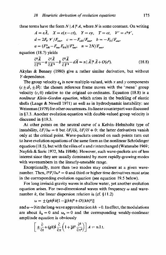
18 Heuristic derivation of evolution equations 175
these terms have the form N \ A |2 A, where N is some constant. On writing
A=eA, X=e(x-ct), F = ej, T = et,
d=2Fvr/F<M1, c = -Fwt/Flltt, b^-Fa/
a = {F%k - F^ F^/Fl,, n =
equation (18.7) yields
Akylas & Benney (1980) give a rather similar derivation, but withoutF-dependence.
The group velocity cg is now multiple-valued, with x and y components(c±O2, ±bi): the chosen reference frame moves with the 'mean' groupvelocity (c, 0) relative to the original co-ordinates. Equation (18.8) is anonlinear Klein-Gordon equation, which arises in the buckling of elasticshells (Lange & Newell 1971) as well as in hydrodynamic instability: seeWeissman (1979) for other occurrences. Its linear counterpart was discussedin §7.3. Another evolution equation with double-valued group velocity isdiscussed in §19.3.
At other points on the neutral curve of a Kelvin-Helmholtz type ofinstability, 3F/3w = 0 but dF/dk, dF/dl * 0: the latter derivatives vanishonly at the critical point. Wave-packets centred on such points turn outto have evolution equations of the same form as the nonlinear Schrodingerequation (18.5), but with the roles of x and t interchanged (Watanabe 1969;Nayfeh & Saric 1972, Ma 1984b). However, such wave-packets are of lessinterest since they are usually dominated by more rapidly-growing modeswith wavenumbers in the linearly-unstable range.
Exceptionally, more than two modes may coalesce at a given wave-number. Then, 32F/3«2 = 0 and third or higher time derivatives must arisein the corresponding evolution equation (see equation 19.5 below).
For long inviscid gravity waves in shallow water, yet another evolutionequation arises. For two-dimensional waves with frequency w and wave-number k, the linear dispersion relation is (cf. §11.2)
and (o ->• 0 in the long-wave approximation kh ->• 0. In effect, the modulationsare about &0 = 0 and w0 = 0 and the corresponding weakly-nonlinearamplitude equation is obviously
Downloaded from University Publishing Online. This is copyrighted materialIP139.153.14.250 on Tue Jan 24 02:27:34 GMT 2012.
http://dx.doi.org/10.1017/CBO9780511569548.007

176 Evolution of a nonlinear wave-train
Here, A is the actual surface-wave elevation, not the modulated amplitude.Moreover, the nonlinear terms are found to be quadratic in A, namely—%AdA/dx with suitably denned A (see e.g. Peregrine 1972). This isbecause the nonlinearities 'felt by the wave' need no longer match itsperiodicity: the second-harmonic and mean flow are themselves 'longwaves' like the fundamental. The resultant equation
is the celebrated Korteweg-de Vries equation, more simply expressed inrescaled form as
SA AdA Q3A n
-^ + <rA—+-~ = 0. (18.9b)
OT 9 | eg3
A generalization of (18.9b) is
3,4 , 8A d*A d3A 6M+ A + + f i + 0 ( 1 8 1 0 )
The corresponding linear dispersion relation for small-amplitude waveswith periodicity exp[i(£g—WT)] is
this gives instability for 0 < k < (a/y)* when a, /?, y are real and a, y > 0.Equations of the form (18.10) have arisen in a variety of physical contexts.For fluids, cases with /? = 0 approximate long waves in thin viscous layersflowing down an incline (Benney 1966) and on the interface between twoviscous layers (Hooper & Grimshaw 1985). In the former case, thedestabilizing a-term derives from gravity or downstream pressure gradient,but in the latter it may also be due to differing viscosities (cf. Yih 1967).The stabilizing y-term represents the effect of surface tension. Whenft = y = 0, (18.10) reduces to a form of Burgers' equation, first proposedas a model of turbulence (Burgers 1946). This may be transformed intothe heat equation and solved for arbitrary initial conditions (see e.g.Whitham 1974). A three-dimensional counterpart of (18.10) withA — A(£, 7), T) is considered by Lin & Krishna (1977).
19 Weakly nonlinear waves in inviscid fluids19.1 Surface and inter facial waves
The evolution of weakly nonlinear surface waves in inviscid fluidhas been much studied. Hasimoto & Ono (1972) considered gravity waveswith slow amplitude variations in x and t; Benney & Roskes (1969) andDavey & Stewartson (1974) incorporated modulations in x, y and t;
Downloaded from University Publishing Online. This is copyrighted materialIP139.153.14.250 on Tue Jan 24 02:27:34 GMT 2012.
http://dx.doi.org/10.1017/CBO9780511569548.007
19 Weakly nonlinear waves in inviscid fluids 177
Djordjevic & Redekopp (1977) and Ablowitz & Segur (1979) added surfacetension effects. All employed perturbation theory but a parallel developmentusing Whitham's method is practicable (Yuen & Lake 1975, 1982). Forlinearly-stable interfacial waves in inviscid Kelvin-Helmholtz flow, theanalysis follows similar lines; but differences occur for modes located nearthe stability boundary, for reasons outlined above.
For gravity waves on a free surface, the velocity potential satisfiesLaplace's equation within the fluid, together with the surface conditions(11.13), (11.14) and the bottom boundary condition d<f>/dz = Q. Onlya brief outline of the perturbation analysis need be given here. The wave-train has the same form as in §11.2, with fundamental periodicityE = exp i(kx—u)i) and amplitude modulations described by the scaled co-ordinates (11.2). The velocity potential <f> and free surface displacement £are expanded in ascending powers of the wave-slope parameter e. AnyO(e2) mean flow driven by amplitude modulations is precisely as givenin (11.17). In the series expansions for 0 and £, there are also 0(e2)terms with periodicity E, forced by the modulation of the fundamental.
A second harmonic is driven by the self-interaction of the fundamental:this is O(e2) and proportional to A2E2 + c.c. except when 2w is close to thenatural frequency of a linear mode with wavenumber 2k. This exceptionalcase is one of second-harmonic resonance, first identified by Wilton (1915)and later elucidated by Nayfeh (1970) and McGoldrick (1970a, b, 1972)for capillary-gravity waves and by Nayfeh & Saric (1972) and Weissman(1979) for unbounded Kelvin-Helmholtz flows. This degenerate exampleof three-wave resonance was discussed in §14.2 above; here we considernon-resonant cases.
The perturbation analysis leads to a set of equations for the variousterms proportional to epE« (p = 1,2,3,..., q = 0, ± 1 , ±2 , ± . . . ) , andthese may be solved seriatim. The interaction of the fundamental O(e) wavewith the O(e2) mean flow and second harmonic yields O(e3) terms in thenonlinear boundary conditions (11.13) and (11.14), some of which havethe same periodicity E*1 as the fundamental wave-train. Such terms causeslow amplitude modulations of the fundamental waves, on the time scaleT = e2t. Once the solutions for the mean flow and second harmonic havebeen found, evaluation of these terms is a straightforward, but rathertedious task. Third-harmonic terms in e3E±3 are also present but play nopart in modifying the fundamental at this order. These may be disregardedexcept in special cases of resonance between the third harmonic andfundamental: for the latter, see Nayfeh (1970) and §22.2.
The expansions of <j> and £ contain respective terms in e3£$13(z) and
Downloaded from University Publishing Online. This is copyrighted materialIP139.153.14.250 on Tue Jan 24 02:27:34 GMT 2012.
http://dx.doi.org/10.1017/CBO9780511569548.007

178 Evolution of a nonlinear wave-train
e3.Ef13. These enter linearly into the boundary conditions at O(e3). Termsin e3E may then be extracted from (11.13) and (11.14), evaluated at themean surface z — 0 by a Taylor expansion. These yield two algebraicequations for ^13(0) and £13, in the form
where A is a known 2 x 2 matrix. The right-hand side contains all nonlinearinteraction terms with periodicity E, also linear terms involving partialderivatives of A{£,, i\, r) which arise from the modulation of the wave-train.Since the linear approximation is /\{<j>, Qtr = 0, the linear dispersionrelation is just det A = 0. The quantities bl and b2 must therefore satisfya compatibility condition in order that a solution (<j>13, £13) exists. It is thiscompatibility condition which yields the governing equation for theevolution of the amplitude modulations.
For surface capillary-gravity waves and stable waves in Kelvin-Hehnholtz flow, this amplitude evolution equation and the O(e2) mean-flowequation take the form derived heuristically above:
(19.1a, b)
where O = 4>01(E,, i\, T), subscripts £, rj, r denote partial differentiation and
Figure 6.1. Dependence of a, A, x and v on kh and T (from Ablowitz & Segur1979). Curves indicate where the various coefficients change sign.
4 r ~
kh
X< 0
0.25 0.S 0.75
f=k2y/pg
1.0
a<0, v>0
c > 0
1.25 1.5
Downloaded from University Publishing Online. This is copyrighted materialIP139.153.14.250 on Tue Jan 24 02:27:34 GMT 2012.
http://dx.doi.org/10.1017/CBO9780511569548.007
19 Weakly nonlinear waves in inviscid fluids 179
A, /i, x, Xi> a a n d /? a r e known real constants. These equations were firstderived by Davey & Stewartson (1974). For capillary-gravity waves,expressions for the various constants are given by Djordjevic & Redekopp(1977) and Ablowitz & Segur (1979). In particular, we note that
a=\-(c\/gh),
that [i, Xi and /? are non-negative and bounded, and that a, A, x a n dv = x~Xi(fi/a) change sign as shown in Figure 6.1. The two axes representdimensionless wavenumber kh and the surface tension parameterT = k2y/pg. Each line denotes a simple zero of the designated coefficientexcept those bounding region F, which denote singularities of v and x-These singularities arise where
T= <r2(3 — cr2)"1, <r = \aahkh;
this is the condition for second-harmonic resonance, for which the presentperturbation expansion breaks down.
Cases where a = 0 are also singular. For these, cg = ± (gh)i and thegroup velocity of the fundamental waves coincides with the phase speedof much longer shallow water waves. This is also a degenerate three-waveinteraction: a long wave with small wavenumber K -4 k and frequencyQ = K(gh)* resonates with the fundamental wave of wavenumber andfrequency (k, w), and either of its ' sidebands' (k ± K, W + Q). This long-waveresonance has been treated by Djordjevic & Redekopp (1977) for amplitudemodulations in x and t only. A new co-ordinate scaling
| = e%(x — cg f), T = dt
is required and the surface displacement and x-velocity associated with thelong wave are taken to be O(et). The governing equations are then
(19.2a, b)
with A as above and
<*i = - 2^2 cosech2 kh, S = k[l+^cg fc/w) (1 + T) cosech2 kh]
for capillary-gravity waves. Here, e^O(g,r) is the leading-order velocitypotential of the long wave.
A similar pair of coupled equations was derived by Grimshaw (1977)and Koop & Redekopp (1981) for the resonant interaction of a packet ofinternal gravity waves and a long internal wave-mode in stratified fluid.Grimshaw also covers the case of near resonance, when an extra term in<!>££ enters equation (19.2b). Such equations are likely to arise in many otherconfigurations where the group velocity of a modulated wave-train
Downloaded from University Publishing Online. This is copyrighted materialIP139.153.14.250 on Tue Jan 24 02:27:34 GMT 2012.
http://dx.doi.org/10.1017/CBO9780511569548.007

180 Evolution of a nonlinear wave-train
matches the phase velocity of a much longer wave. However, in water ofinfinite depth, the equations governing such interaction of short and longcapillary-gravity waves do not take this form (Benney 1976): this isbecause the second-order mean flow generated by self-interaction of theshort waves vanishes in the deep-water limit.
Solution of (19.2a, b) by the method of inverse-scattering is given by Ma(1978) and Ma & Redekopp (1979) as mentioned in § 15.4. Complementarynumerical work is described by Bryant (1982). Newell (1978) proposed adifferent model of long-wave/short-wave interactions,
Bt-\BXX = -AxB+iA2B-2io-\B\2B
in scaled form, for which exact solutions can also be found.The interesting experiments of Koop & Redekopp (1981) concern
interacting waves on the two interfaces of a three-layer configuration. Inthese, packets of relatively short gravity waves on the upper interfaceresonate with long waves on the lower interface. Examples of their resultsare shown in Figure 6.2, the long wave being generated by the short-wavemodulations. Their results are generally in fair agreement with theoreticalestimates which (somewhat empirically) incorporate viscous effects. How-ever, long time-scale recurrent modulations predicted by inviscid theorycould not be confirmed in their apparatus.
For stable waves in Kelvin-Helmholtz flow of unbounded extent in z,and for waves in water of infinite depth, the constants Xi and /? of (19.1)are zero. The vanishing of/? is shown by (11.17), there being no O(e2) meanflow in infinitely deep inviscid fluid. The wave-packet is then governed bythe nonlinear Schrodinger equation
iAT + AAu+/iAn = x\A\tA, (19.3)
the coefficient x resulting solely from the interaction of the fundamentaland the second harmonic. For unbounded Kelvin-Helmholtz flow,Weissman (1979) gives x explicitly, in the form
where F(w, k, I, U) is the dispersion function. The value of x may bepositive or negative and it is singular, due to the vanishing of dF/da>, onthe neutral curve of Kelvin-Helmholtz instability.
Weakly nonlinear marginally-unstable waves near the critical point forKelvin-Helmholtz instability were first examined by Drazin (1970), forpurely temporal modulation. Spatial and temporal evolution of such wavesis discussed by Nayfeh & Saric (1972) and Weissman (1979), the latter ofwhom gives the governing equation (18.8).
Downloaded from University Publishing Online. This is copyrighted materialIP139.153.14.250 on Tue Jan 24 02:27:34 GMT 2012.
http://dx.doi.org/10.1017/CBO9780511569548.007

19 Weakly nonlinear waves in inviscid fluids 181
Figure 6.2. Examples of resonant long-wave/short-wave interaction, from experimentsof Koop & Redekopp (1981). Modulated short waves generated at upper interfacecause long waves at lower interface of a three layer fluid, (a) periodic modulations;(b) single wave packet; (c) 'dark-pulse' modulation.
LOW PASS OFLOWER INTERFACESIGNAL
LOWERINTERFACEDISPLACEMENT(LONGWAVE)
UPPER INTERFACEDISPLACEMENT(SHORTWAVE)
SHORT WAVEGENERATORDISPLACEMENT
TIME INCREASING
(a)
WAVEMAKERDISPLACEMENT
UPPER INTERFACEDISPLACEMENT
LOWER INTERFACEDISPLACEMENT
LOWER INTERFACESIGNAL LOW PASSFILTERED ANDAMPLIFIED
i
. vMlT
i
I<
i11
i i i i i i1 1
,.1\w
T- •
11
•
_Li
i \
rftW"I tf
j jtj(V7r
f .::
-
"TrT n• ;
1
_
t — • INCREASING
(b)
t — INCREASING
(c)
Downloaded from University Publishing Online. This is copyrighted materialIP139.153.14.250 on Tue Jan 24 02:27:34 GMT 2012.
http://dx.doi.org/10.1017/CBO9780511569548.007

182 Evolution of a nonlinear wave-train
For wave-packets with amplitude-dependence on g and T only, theappropriate mean-flow solution of (19.1b) is just
The system (19.1a, b) then also reduces to a nonlinear Schrodingerequation for A of the form (19.3), but with x replaced by
For deep-water gravity-wave packets, Dysthe (1979), Janssen (1983) andLo & Mei (1985) consider a higher-order approximation to the evolutionequation. In this, the nonlinear Schrodinger equation is replaced byanother containing additional terms which, under the scaling (11.2), wouldbe vanishingly small. For water of finite depth, Prasad & Krishnan (1978)propose a generalization of the Davey-Stewartson equations (19. la, b) toaccount for more strongly curved wavefronts.
Further discussion of the properties of these various governing equationsand of related experiments is deferred till §21.
19.2 Internal wavesGrimshaw's (1977) investigation of internal gravity waves in
stratified fluid at rest also led to a modification of the Davey-Stewartsonequations. A further nonlinear term SA must then be added to theright-hand side of (19.1a). S denotes the contribution from a discretespectrum of extremely long-wavelength internal-wave modes which areexcited by the amplitude modulations of the shorter waves. It has the form
S= *L3 - 1
with known constants Sp and each W} relates to a single long-wavelengthmode. The functions W} satisfy a set of equations
[l-(C g /^)2]82^/9£2 + 92^/a?/2 = Vi&\A\*/?»i* (7= 1,2,...)
where cg is the group velocity of the fundamental packet, c} is the phasevelocity of the yth long-wave mode and each v} a known constant. Theresonant case Cj = cg requires separate treatment and was mentionedabove.
The linear theory of over-reflecting internal gravity waves was discussedin §4.2, for continuous density stratification with constant N and the dis-continuous Helmholtz velocity profile (4.3). For resonant over-reflection,the linear dispersion relation (4.6) gives three modes, with Kelvin-Helm-holtz instability at wavenumbers k2 > 2N2/U2. Grimshaw (1976, 1979b)
Downloaded from University Publishing Online. This is copyrighted materialIP139.153.14.250 on Tue Jan 24 02:27:34 GMT 2012.
http://dx.doi.org/10.1017/CBO9780511569548.007

19 Weakly nonlinear waves in inviscidfluids 183
has developed a weakly nonlinear analysis of such cases, for temporal, butnot spatial, amplitude modulation.
At wavenumbers below the cutoff value for linear instability, hisamplitude equation is
dA/dT = /3\A\2A + I (19.4)
where /is a known forcing term representing waves incident from z = + oo.For the symmetric mode with c = \U, /? is found to be zero. Though thismode and its harmonic are in resonance when k2 < N2/U2, the resonantcoupling is so weak that the harmonic remains O(e2). The vanishing of /?suggests that unforced steady waves may indeed exist at the interface, withinternal waves radiating off to z = + oo in accordance with linear theory.
For the other pair of modes, /? 4= 0 and Re /? > 0, indicating a destabil-izing effect. The interaction of the fundamental wave and the 0(e2) meanflow is found to contribute only to Im/?: accordingly, the destabilizationof these linearly stable modes derives solely from the interaction of thefundamental with its second harmonic. If the velocity discontinuity isreplaced by a very thin shear layer, equation (19.4) is modified only byaddition of a linear term yA to the right-hand side. The value of y isnegative for the symmetric mode and positive for the asymmetric modes(Grimshaw 1981a).
At the cutoff value kc = 2%N/U for onset of linear instability, all threemodes of the vortex-sheet profile coalesce. Close to this value, withk = fcc(l +e2K), the dispersion relation has the renormalized form
and the heuristic replacement (18.2) is just to' = id/dt. The correspondingnonlinear equation for A(T), where T = et, is
dA QA]Al
with no forcing. Grimshaw (1976) derives this equation and discusses someof its properties.
The value of investigating such stable or marginally unstable modes isopen to question when, as here, other strongly-unstable linear modes arepresent. On the other hand, it is instructive to know what influence weaknonlinearities may have on over-reflection, even though the modelincorporates unrealistic features.
Downloaded from University Publishing Online. This is copyrighted materialIP139.153.14.250 on Tue Jan 24 02:27:34 GMT 2012.
http://dx.doi.org/10.1017/CBO9780511569548.007

184 Evolution of a nonlinear wave-train
19.3 Baroclinic wavesBaroclinic waves occur in rotating, stratified systems: they are
important in large-scale atmospheric and other geophysical flows and havebeen studied in many laboratory experiments. They derive from the factthat equilibrium states in rotating systems have non-coincident surfacesof constant gravitational potential and constant density. Mathematicalmodels of baroclinic phenomena have been developed both for superposedlayers of immiscible fluids with differing densities and for fluid withcontinuous density stratification. Baroclinic waves are linearly unstable inthe presence of sufficiently strong mean-flow variations. Weakly-nonlinearanalyses have been carried out for conditions close to those for onset oflinear instability. Reviews of baroclinic flow phenomena are given by Hide& Mason (1975), Drazin (1978) and Hart (1979).
Spatial and temporal evolution of marginally unstable finite-amplitudewaves was studied by Pedlosky (1970, 1971, 1972) for a two-layer modeland corresponding analyses of continuously-stratified shear flows wereundertaken by Drazin (1972), Pedlosky (1979) and Moroz & Brindley(1981, 1984).
At the critical point of linear inviscid instability, the group velocity cg
becomes double-valued, as in (18.8); but the form of the nonlinear termsnow involves wave-driven variations of the mean flow. As in the Davey-Stewartson equations (19.1), a pair of coupled equations arises for the waveamplitude A and mean-flow modification B. For modulations in x and tonly, these turn out to have the form
with suitably scaled variables. Here, cx, c2 are the two group velocities, ± ais the (small) linear growth or decay rate and /? a real coupling coefficient.Pedlosky (1972) gave solutions depending on a single variable, X-VT, withconstant V.
A derivation of these equations from a more general standpoint is givenby Gibbon & McGuinness (1981): the coefficients a, /? may then becomplex. These equations are solvable by inverse scattering (Gibbon,James & Moroz 1979) and have soliton-type solutions. If A (and so a, /?)is restricted to be real, the substitutions
A = (2/*)-* Qf+c2 A W B= ±(a//?)(l -cos«D)
Downloaded from University Publishing Online. This is copyrighted materialIP139.153.14.250 on Tue Jan 24 02:27:34 GMT 2012.
http://dx.doi.org/10.1017/CBO9780511569548.007

19 Weakly nonlinear waves in inviscidfluids 185
transform (19.6) into the sine-Gordon equation
3
which has well-known properties (see, e.g., Dodd et al. 1982).In the purely time-dependent case, Gibbon & McGuinness (1982) have
argued that the counterparts of (19.6) in the presence of weak viscosityshould be
dM/dr+A1d^t/dr ±*A/SAB,\dB/dT+ A2 B = d \A |*/dr+ A8 \A \\ J
the new A^-terms representing viscous damping. (But care is necessary:Af/a must remain small as a->0 if the neutral curve is to be only slightlyaffected - cf. Newell 1972.) With a, A1 allowed to be complex, but withthe other parameters real, the transformation
r = fir, fi = Re(A1)-|A3,
3C = (2fif£l-xA, & = 2/Jfi-1 A3-x B
enables (19.7) to be rewritten as
(19.8)
d37dr = - 6iF + f(<F *<W + %<&*)]where
<r = ^ - ^ 3 , 6 = 0 - ^ 2 , a =
When a and A1 (and so a and r) are real, so also may be A and B (and so9£ and <&). Equations (19.8) then reduce to the Lorenz equations (Lorenz1963; Yorke & Yorke 1981), which constitute the first studied strange-attractor system. Properties of the complex system (19.8) are discussed byFowler, Gibbon & McGuinness (1983).
With stronger dissipation, equations (19.7) are inappropriate. Linearinstability is then no longer due to a coalescence of two neutral modes,but to the crossing of a single previously-damped mode into the amplifiedregime. Accordingly, second-order time derivatives should not arise in thenonlinear evolution equations (cf. §18). The weakly-nonlinear evolutionof such viscous baroclinic waves was treated by Pedlosky (1976), allowingfor cross-stream variations in y as well as time t. His coupled equationsfor (scaled) wave and mean-flow components <fi, u have the form
d<f>/dt-d*<f>/dy2 = 5^(1+") (s constant) 1
du/cst - Wu/dy* = d2\(t>\2/dy\ J
Downloaded from University Publishing Online. This is copyrighted materialIP139.153.14.250 on Tue Jan 24 02:27:34 GMT 2012.
http://dx.doi.org/10.1017/CBO9780511569548.007

186 Evolution of a nonlinear wave-train
where <j> is associated with the periodicity exp [ik(x—ct)]. Pedlosky imposed'sidewall' boundary conditions M = ^ = 0 a t j = 0 and 1, which restrictthe cross-stream structure: there is then a discrete set of linear modes, as$, w~>0, given by
</>m = A exp (<rm 0 sin (nary), <rm=s2- (mi?
where m is integer. The mth mode is unstable if s > nm.When the first mode is slightly supercritical, s2 = n2+S say, its weakly-
nonlinear evolution is found from (19.9) to be given by
96 = $A(T) sin ny + smaller harmonics,
u = -\4>\2, r = 8t ( 0 < < M l ) ,
dA/dr = A - (3n2/4) \A\2 A.
This evolves to a finite-amplitude equilibrium, \A\ = 2(2>*-n)~l.For arbitrarily large s, (19.9) admits time-independent solutions with
u(y) = -<f>*(y), d2<f>/dy2-s2<f>(l-<f>2) = 0, 0 real.
Those satisfying <f>(0) = 0 are Jacobian elliptic functions
<f»(y) = asn[^, v], 7) = asy/2w, a = 2h(v2+ l)~i
with modulus v. The remaining boundary condition </>(l) — 0 is satisfiedfor values v such that asjl^v coincides with a zero of the elliptic function.Pedlosky showed that, when jn < s < (j+ l)n with integer j , there areexactly j such steady states. He also undertook a numerical investigationof the temporal evolution of finite-amplitude disturbances, based uponequations (19.9), and employing truncated Fourier-series representation iny. The results indicated eventual equilibration at the steady state withlargest available amplitude, usually after an interval of decaying oscillations.On the other hand, with weaker dissipation, Hart (1973) and Pedlosky(1977) found finite-amplitude permanent oscillations and so the issueremains unresolved. It is also worth remarking that, for s substantiallyabove n, it seems unduly restrictive to admit just a single Fourier modein x, but several in y.
Resonant triads of inviscid baroclinic waves were studied by Loesch(1974) and Pedlosky (1975), for cases where one of the three waves ismarginally unstable. The governing equations for temporal evolution arenot then of the standard form (15.1) since the linear inviscid instability isdue to coalescence of modes. Rather, they have the (scaled) form
d^AJdT2-*^ = N, A^N, I At \2 + N21A2 \2 + N3 \A3 \
dAJdT=\N2A*A*, \ (19.10a,b,c)
Downloaded from University Publishing Online. This is copyrighted materialIP139.153.14.250 on Tue Jan 24 02:27:34 GMT 2012.
http://dx.doi.org/10.1017/CBO9780511569548.007

19 Weakly nonlinear waves in inviscidfluids 187
when w1+w2+wa = O, k!+k2+k3 = 0 and subscripts 1 designate themarginally unstable mode. Here, a is related to the linear growth rate andthe constants N} are real. Loesch gave several numerical solutions whilePedlosky made analytical progress in cases with No — 0. The lattercorrespond to waves Ax having no meridional (north-south) wavenumbercomponent: these are of particular interest because, when A2 = A3 = 0,there are no cubic terms to suppress the linear wave growth. In such cases,Nx < 0 while N2, N3 > 0.
A further scaling
T = r/a, A, = *(N2NJ*rx e \ A2 = <r(-N,N3)^r2 e J \
A^ai-N.N^r,^
then yields three real equations
d2rjdr2 = rx(l - r\ - rj), dr2/dr = rt r3, drs/dr = rx r2,
provided dx-srd7,-\-dz is chosen to equal |TT. Pedlosky showed that the
solutions are oscillatory, with r\ — r\ constant. His rather cumbersomeaccount is simplified by the transformation
r2 — Acoshu, rs = Asinhu, r\ — r% = A2^0.
This readily leads to
rx = dw/dr = ±(u* + au+b-\Ai cosh 2K)*,
where a and b are constants determined by the initial data. The solutionis obviously periodic, with period
2 \u2 + au+b-lA2 cosh 2u)~i dw,J«i
where ut and u2 are the values of u for which rx = 0.Loesch & Domaracki (1977) extended this work to investigate the effect
of several co-existing resonant triads on a marginally unstable mode Av
Their numerical results for 5, 9 then 13 participating modes showincreasingly complex modulations; but these apparently remain quasi-periodic, with two or three superposed periods. In contrast, Merkine &Shtilman (1984) found instances of explosive growth among (three-wave)triads and coupled (five-wave) triads, in the presence of weak viscouseffects: since their marginally unstable mode satisfies a first-order equation,their systems resemble those discussed in Chapter 5.
Downloaded from University Publishing Online. This is copyrighted materialIP139.153.14.250 on Tue Jan 24 02:27:34 GMT 2012.
http://dx.doi.org/10.1017/CBO9780511569548.007

188 Evolution of a nonlinear wave-train
20 Weakly nonlinear waves in shear flows20.1 Waves in inviscid shear flows
The simplest such flows to handle are constant-density flows withbroken-line velocity profiles, which yield explicit expressions for the hneardispersion relation and eigenfunctions. The absence of curvature of thevelocity profile, except at 'joins' between layers of differing vorticity,means that the linear eigenfunctions of two-dimensional waves are non-singular at any critical layer.
Benney & Maslowe (1975) investigate weakly nonlinear waves in thepresence of the primary velocity profiles
u =
the former of which has a plane rigid boundary at z — 0. For profile (20. la),inviscid linear modes with periodicity exp[ik(x—ct)] have (cf. Tietjens
c=l-Ar1e~*sinhJfc.A perturbation analysis, similar to that of § 19.1, again leads to result (19.3),with the Landau constant x given by
In deriving this result, Benney & Maslowe ignored any contribution dueto modifications of the mean flow at 0(e2). This is apparently justified* fortheir unbounded constant-density flows, but it would not normally be sofor bounded fluid layers of differing densities, under gravity. Then, meanflow modifications are driven by spatial modulation of the wave-train andcoupled equations of the form (19.1a, b) must result.
Benney & Maslowe (1975) restrict their study of profile (20.1b) towave-modes with c — 0. By symmetry, this case corresponds to coalescenceof right and left propagating modes centred on the respective interfaces(cf. §2). This is an instance of marginal stability, with neighbouringunstable modes, and the governing amplitude equation is then
3 M / 3 T 2 = 0.201 i (dA/dX+2.ll KM*) (20.2)
with suitably scaled variables X, T. This has the form typical of wave-modesnear the neutral curve of Kelvin-Helmholtz instability, but not at thecritical wavenumber (see §18). Again, mean flow modifications may be
* Not so: see Balagondar, P. M., Maslowe, S. A. & Melkonian, S. (1987) Stud. Appl.Math. 76, 169-85.
Downloaded from University Publishing Online. This is copyrighted materialIP139.153.14.250 on Tue Jan 24 02:27:34 GMT 2012.
http://dx.doi.org/10.1017/CBO9780511569548.007
20 Weakly nonlinear waves in shear flows 189
ignored in deriving this result since gravitational effects are absent. Thesecond time derivative also arises, for similar reasons, in the evolutionequation derived by Engevik (1982) for waves in some stratified shearflows.
The linear stability of the inviscid shear-layer profile
w = tanhz ( - o o < z < o o ) (20.3)
was described in §3.1. The behaviour of weakly-nonlinear marginallyunstable modes was treated by Schade (1964) and Stuart (1967). Schadeconsidered purely temporal wave growth and Stuart confined attentionfrom the outset to nonlinear constant-amplitude disturbances. Any meanflow modification was ignored. This is obviously permissible for constant-amplitude waves in any inviscid parallel flow: the mean flow may be chosenas (20.3) in the presence of such waves, without regard to the originalvelocity profile in their absence. But the neglect of mean flow variationsrequires justification when temporal or spatial amplitude changes areadmitted. The perturbation solutions are valid for sufficiently small lineargrowth rates a,c% or, equivalently, for wavenumbers sufficiently close to thatof the linear neutral mode, here a— I. Stuart continued his analysis ofequilibrium disturbances to higher order, finding that disturbances withthe streamfunction (cf. §3.1)
f - e sech z cos [a(x - ct)\ + O(e2), c - 0,have
a2 = 1 - | e a + f (1 + | In2)e* + 0(e6). (20.4)
Correspondingly, the equilibrium amplitude e is
the leading-order approximation of which agrees with Schade's result.Benney & Maslowe (1975) show that the latter generalizes, with spatial
and temporal variation, to the amplitude equation
J^pA <20.5)or n \dX 3 /
the linear group velocity 3w/9a = — 2i/n being purely imaginary andderiving from the influence of the linear (viscous) critical layer. In contrast,for the piecewise-linear profile (20.1 b), there is no critical layer contributionand the linear group velocity is infinite for waves with c = 0, so leadingto (20.2). Benney & Maslowe further show that, for a nonlinear critical layer(see §22.4), which sustains no jump in Reynolds stress, the tanhz profileleads to an equation similar to (20.2). Attempts to incorporate viscouseffects for the profile (20.3) are discussed in §20.3 below.
Downloaded from University Publishing Online. This is copyrighted materialIP139.153.14.250 on Tue Jan 24 02:27:34 GMT 2012.
http://dx.doi.org/10.1017/CBO9780511569548.007
190 Evolution of a nonlinear wave-train
20.2 Near-critical plane Poiseuille flowWe here outline the derivation of the amplitude equation of a
weakly nonlinear wave-packet in plane Poiseuille flow (11.5), taking intoaccount amplitude modulations in x, y and t. The treatment broadlyfollows that of Davey, Hocking and Stewartson (1974): this incorporatesas special cases the work of Stuart (1960), Watson (1960, 1962) and Chen& Joseph (1973) on purely temporal and purely spatial growth and alsothat of Stewartson & Stuart (1971) for modulations in x and t. Weinstein(1981) has demonstrated that some differences of method in these papersdo not affect the results.
The flow is taken to be marginally unstable, at a Reynolds number Rjust above the critical value Rc = 5772 for onset of linear instability. Alocalized small disturbance initially centred on x = y — t = 0 at firstevolves according to linear theory, as discussed in § 7.3, into a slowly-varyingwave-train with streamfunction
f = Re {eA{g, v, r) ^ ( z ) exp [iao(x- c0 0] + O(e2)}. (20.6)
Here, a0 and c0 are the real wavenumber and phase speed of the neutralmode at R = Rc and ^ ( z ) its corresponding (normalized) eigenfunction.The scaled co-ordinates £,, rj,T are as denned in (11.2) where e is a smallparameter and A is regarded as 0(1).
Since R is close to Rc, we setc,
and denote the precise linear eigenvalue c at this value of R with ac — a0
byc = cT + iq = c0 + eHd^d^ a0) ~ \ d% = d1T+idxi
for suitable 0(1) real constants dlT, du. This choice fixes e2 as the smalllinear growth rate oio q. (This differs from Davey, Hocking & Stewartson'schoice of e = a0 q : throughout, their e* is our e.)
Successive approximations are constructed by expressing the velocitycomponents (u, v, w) and pressure p as
u = MO(£, r/, T, z, e) + Re [Eu^i, i),r,z,e)
and similar expressions. Each function um may be expanded in powers ofe as
w0 = I - z2 + e2w02(£, 7),r,z
"i = eH11(£,97,T,z) + e2w12(g,i?,T,z
«2 = e2i/22(g, 1?» T, z)+
Downloaded from University Publishing Online. This is copyrighted materialIP139.153.14.250 on Tue Jan 24 02:27:34 GMT 2012.
http://dx.doi.org/10.1017/CBO9780511569548.007

20 Weakly nonlinear waves in shear flows 191
together with similar expansions for the corresponding components of v,w and p. Those for v0 and w0 contain no 0(1) term in 1 — z2; also,
p0 = - 2Rrxx+constant+eP01+e2P02 +...,
the leading-order pressure gradient — 2R"1 being that which maintains theprimary flow.
The various coefficients of enEm (n,m — 0,1,2,...) which arise in thegoverning Navier-Stokes equations (1.1 a, b)' must then be equated to zero.That in eE yields the linear solution
Mn = A(g, t), T) Df^z), vn - 0, wn=- iac0 Ai/r^z),
where D = d/dz and ftt(z) is the Orr-Sommerfeld eigenfunction atwavenumber a0 and R = Rc. For definiteness, the normalization i/r^O) = 2may be adopted (this accords with Davey et al.'s normalization).
The O{e%) mean flow components (M02, V02, W02) are just as found in § 11.1on applying the condition of constant mass flux: these are given by (11.6)and (11.7). The other O(e2) components in E and E2 are also readily found(see Davey et al., §2).
The evolution equation for A{E,,JI,T) is deduced from the O(e3E)equations. These are three momentum equations and the equation ofcontinuity, connecting M13, V13, w13, Pl3 and lower-order functions. Byelimination of w13, v13 and P13, these reduce to a single equation for w13
of the form
where £C is just the Orr-Sommerfeld operator of (3.1b) and & is knownin terms of A, its partial derivatives, and the lower-order functions alreadyfound. As described in §8.2, the function & must be orthogonal to theadjoint function <&(z) of if. Accordingly, multiplication by <t(z) andintegration across the flow domain yields
This gives the equation for A in the form
^ ^---^^—^-^A + k AfA + qAB, (20.7)OT at,2 oi)2 d1T
as already indicated in §18. Here,
and the O(e2) mean flow modification «02 is related to B by
u02 = | A |2S(z)+l(l - z 2 ) f1 S(z)dz(B-\ A I2)Jo
Downloaded from University Publishing Online. This is copyrighted materialIP139.153.14.250 on Tue Jan 24 02:27:34 GMT 2012.
http://dx.doi.org/10.1017/CBO9780511569548.007

192 Evolution of a nonlinear wave-train
in agreement with (11.6). Also, from (11.7),
VBVBJ2111 (20 8)
(The substitution 8 = K(B+\A\2) in (18.5) and (18.6) yields equations ofthe same form.)
In agreement with (18.5), the complex constants a2, b2 of (20.7) are|i 82w/9a2, |i 62w/3/?2 respectively, evaluated at a = a0, j3 = 0, /? = i?c,where w(a, /?, i?) = ac is the complex frequency of oblique linear modeswith periodicity expi(ax±fiy—u>t). The constants d1T, cln may also bededuced from the linear dispersion relation, while
The Landau constant k is an integral of a rather lengthy expression whichneed not be reproduced here.
Numerical integration at the neutral point for plane Poiseuille flow gives
Rc = 5772.22, a0 = 1.02055, c0 = 0.264, cg = 0.383
a2 = 0.187+0.0275 i, 62 = 0.004 66+0.0808 i,
^ = (0.168+0.811 i) 10"5, q = -1 .27 + 29.1 i, jfc = 30.8-173 i.
These values for k and q may be deduced from results of Reynolds & Potter(1967); the others were computed by Davey et al.
For amplitude modulations independent of rj, M02 is directly proportionalto | A |2 and B is identically zero. The coupled system (20.7), (20.8) thenreduces to a nonlinear Schrodinger equation, with Landau constant k.Since the real part of k is positive, the nonlinear terms exert a destabilizinginfluence upon spatially-uniform waves. Periodic solutions with a = a0
therefore bifurcate subcritically from R — Re.Ikeda (1977, 1978) has developed a higher order approximation to the
evolution equation for waves in plane Poiseuille flow. For wave amplitudesindependent of rj, the nonlinear Schrodinger equation is replaced by
where 6X, d2 are complex constants. This equation is simpler than Dysthe's(1979) higher-order equation for deep-water waves, the latter beinginfluenced by the free-surface boundary conditions. Ikeda's higher-orderequations for wave amplitudes dependent on £, i\ and T form a coupledsystem substantially more complex than (20.7) and (20.8).
Downloaded from University Publishing Online. This is copyrighted materialIP139.153.14.250 on Tue Jan 24 02:27:34 GMT 2012.
http://dx.doi.org/10.1017/CBO9780511569548.007

20 Weakly nonlinear waves in shear flows 193
20.3 Non-critical (nearly) parallel flowsFor wave-modes at other values of (a, R) sufficiently close to the
neutral curve for linear stability, the governing equations are similar to(20.7) and (20.8), but with different numerical coefficients. For thesemodes, the linear growth or decay rate may again be characterized by anarbitrarily small parameter e. But such cases are of less interest than thecritical one because of the presence of neighbouring more-strongly amplifiedmodes.
One might hope that similar equations would give acceptable approxi-mations at values of (a, R) some distance from the neutral curve, providedthe linear growth or decay rate remains numerically small; but such hopesappear to be unduly optimistic. There is an inherent difficulty: for, if thelinear eigenvalue is c —q+iq, with finite q, one cannot consistentlychoose aq to be O(e) since c — cT is not an eigenvalue of the linear problem.But retention of q at 0(1) negates the assumption that the linear growthor decay is of no greater importance than the nonlinear contribution.
Certainly, a self-consistent series expansion may be constructed withwave amplitude A, but not aq, characterized by a small parameter, as wasindicated in §8.3(ii). But truncation after a few terms is unlikely to succeedat amplitudes Q large enough that | Q |2 is O(aq).
Reynolds & Potter (1967) and Pekeris & Shkoller (1967) sought toovercome this dilemma by including ci in the linear Orr-Sommerfeldequation but omitting it elsewhere. Reynolds & Potter omitted it from bothlinear operators arising in the O(ea) harmonic and mean-flow equations;Pekeris & Shkoller omitted it only from the latter. Reynolds & Potterargued that their procedure should yield correct results for finite amplitudeequilibrium states, for then the O(e2) forcing terms are of constantamplitude. With truncation at O(\ Q |3), the resulting Landau equation forpurely temporal growth is (cf. 8.8) dQ/dt—aciQ = k\Q\2Q. Many valuesof the Landau constant k were computed, for a range of a and R, both forplane Poiseuille flow and for plane Couette-Poiseuille flows with relativemotion of the channel walls. Since both authors considered only temporalmodulations, they were free to impose either constant mass flux orconstant pressure gradient; Reynolds & Potter chose the former andPekeris & Shkoller the latter. Despite these differences, their results for kare in quite close agreement. Figure 6.3, from Pekeris & Shkoller, showsthe curve on which Re k — kT — 0, together with the neutral curve of lineartheory, for plane Poiseuille flow. Sub-critical equilibrium may be expectedonly when q < 0 and kr > 0 and supercritical equilibrium when q > 0 andkT < 0. When both kT and q are negative, both terms cause the wave to
Downloaded from University Publishing Online. This is copyrighted materialIP139.153.14.250 on Tue Jan 24 02:27:34 GMT 2012.
http://dx.doi.org/10.1017/CBO9780511569548.007

194 Evolution of a nonlinear wave-train
decay; while, when both are positive, they promote wave growth.Corresponding results for two superposed horizontal layers of fluid withdiffering densities and viscosities, flowing between parallel walls, have beenobtained by Blennerhassett (1980).
Figure 6.4 shows, for the first time, a direct comparison of predictionsof the subcritical equilibrium amplitude in plane Poiseuille flow. Theseresults, obtained by the methods of Reynolds & Potter and of Pekeris &Shkoller, were kindly provided by A. Davey. Clearly, substantial discrep-ancies result from the differing treatments of growth terms. Series trunca-tion is a further source of error at larger \Q\.
The omission (or inclusion) of the growth terms from the harmonic andmean-flow equations is of no consequence provided | act \ is sufficientlysmall. But the necessary restriction on | a q | is severe and only those resultsfor (a, R) close to the linear neutral curve should be trusted. For a SJ 1.0the magnitude of k increases rather rapidly with both a and R, reachingseveral thousands at a = 1.2 and JR = 2.4 x 10* for example. This is inrough accord with an asymptotic result of Usher & Craik (1975), that | k |should vary as R§ for large JR, provided a and cT remain 0(1) and| acx | R < 0(1). Unfortunately, the latter restrictions are not normally metfor channel flows as 7?->oo; but suitably compliant walls would admit suchbehaviour. The increasing magnitude of | k | with R suggests that the radiusof convergence of the amplitude expansion decreases as R increases, as
Figure 6.3. Curves kr = 0 and q = 0 in a-R plane for plane Poiseuille flow (fromPekeris & Shkoller 1967).
1.0
0.8
0.6
- ~ " • _ _ ,
" I c, > 0
\ \ . —"""
- S s C ^ ^ ^ ^ *,<o
l 1 i 1 i i
. q
— - L .
•^ ,
i
= 0
- 0
i i
12 16 20 24RX 10"
Downloaded from University Publishing Online. This is copyrighted materialIP139.153.14.250 on Tue Jan 24 02:27:34 GMT 2012.
http://dx.doi.org/10.1017/CBO9780511569548.007

20 Weakly nonlinear waves in shear flows 195
some inverse power of R. This partly explains the great sensitivity tononlinear effects of those flows which remain linearly stable up to fairlylarge values of R.
A formally-valid asymptotic theory for i?->oo has been constructed byHall & Smith (1982) for wave-modes situated indefinitely close to the lowerbranch of the neutral curve of plane Poiseuille and boundary-layer flows.
Figure 6.4. Subcritical equilibrium amplitude \Q\ = (-acj/fc,.)' versus frequency occT
for plane Poiseuille flow at R = 5000. Solid line, Pekeris & Shkoller's method(constant pressure gradient). Dashed line, Reynolds & Potter's method (constant massflux). • , Reynolds & Potter's method but with constant pressure gradient. (Resultsof A. Davey.) A and V are 3rd and 4th order results of Zhou (1982).
120 r
100
80
60
40
20
0.1 0.2 0.3 0.4
Downloaded from University Publishing Online. This is copyrighted materialIP139.153.14.250 on Tue Jan 24 02:27:34 GMT 2012.
http://dx.doi.org/10.1017/CBO9780511569548.007

196 Evolution of a nonlinear wave-train
Since a->-0 and c->0 as R^co on both branches, attention is therebyconfined to very long waves. Near the lower branch (but not the upper),the critical layer and viscous wall layer merge into one. The Landauconstant k is then found to vary as J$. Surprisingly, for plane Poiseuilleflow, the lower branch of the curve kT = 0 does not remain below that ofq = 0, as suggested by Figure 6.3: consequently, linearly neutral modeson the lower branch are destabilized by nonlinearity at sufficiently largeR. In contrast, kr is stabilizing for boundary layers. Hall & Smith alsoconsider the influence of forced wavelike distortions of a boundary wall.Unfortunately, enormous Reynolds numbers seem to be required for thevalidity of their asymptotic analysis, since /?~* must be small comparedwith unity.
From Figure 6.3, it is seen that both aq and kT vanish at a point onthe neutral curve with a « 0.91, R « 6600. Struminskii & Skobelev (1980)develop a higher-order approximation for waves in the neighbourhood ofthis point, finding two equilibrium solutions (in addition to A — 0) for anamplitude evolution equation of the form
dA/dt = A(*Ci + a1\A\2+a2\A\i).
Attempts to treat the nonlinear stability of flows which have no linearneutral curve were made by Ellingsen, Gjevik & Palm (1970) and Coffee(1977), who examined plane Couette flow, and Davey & Nguyen (1971),Itoh (1977a, b) and Davey (1978), who considered Poiseuille pipe flow.Ellingsen et al. and Coffee predicted finite-amplitude equilibrium solutionsfor plane Couette flow, but recent computations by Orszag & Kells (1980)suggest otherwise. Contradictory results were also obtained by Davey &Nguyen, who followed the method of Reynolds & Potter, and by Itoh, whotreated the troublesome growth terms somewhat differently. Davey (1978)examined the reasons for the latter discrepancy, interpreting the differenceas due to a rearrangement of terms of an infinite series. When the radiiof convergence of the respective series are unknown, there is no apparentreason for favouring one rather than the other. Davey pragmaticallysuggests that only when the two methods give results in close agreementshould either be trusted. Cowley & Smith (1985) have recently developedan asymptotic theory for such flows, valid as R^ao.
Herbert (1983a) and Sen & Venkateswarlu (1983) recently re-examinedthe question of convergence with a view to constructing valid high-orderamplitude expansions at finite R. The latter authors, like Davey & Nguyen,found finite-amplitude equilibrium states for Poiseuille pipe flow. However,direct numerical solution of the Navier-Stokes equations by Patera &
Downloaded from University Publishing Online. This is copyrighted materialIP139.153.14.250 on Tue Jan 24 02:27:34 GMT 2012.
http://dx.doi.org/10.1017/CBO9780511569548.007

20 Weakly nonlinear waves in shear flows 197
Orszag (1981) yielded only damped disturbances at values of a and R forwhich equilibrium solutions are predicted by amplitude-expansion methods.The issue is accordingly unresolved.
Weakly nonlinear, spatially-varying waves are discussed by Watson(1962) and Itoh (1974b, c) for plane Poiseuille flow and for the Blasiusboundary layer. Linear modes are then spatially amplified or damped asexp (—a? x) where x denotes distance downstream of a continuous sourceof disturbance, such as a vibrating ribbon. Itoh finds coupled equationsfor the complex wave amplitude A{x) and a measure B(x) of the mean-flowmodulation, in the form
(2*<>+AB+ti\A\*)A (20.9a, b)
higher-order terms in | A | and B having been neglected. Here, A, /i, K and7 are real constants. These yield constant-amplitude solutions
fiK — Ay fiK—Ay
which agree with those of Watson (1962) as a.\ -> 0. But the range of validityof the truncated equations (20.9) remains unclear for finite a?.
A further recent attempt to resolve the difficulties associated with finitegrowth rates was made by Zhou (1982). In this, the primary flow isregarded as perturbed from its actual form to another notional one whichyields a linearly-neutral mode. The (hopefully) small O(e) modification ofthe primary flow then reappears at higher order in the perturbationexpansion. Zhou claims better agreement with the experiments of Nishiokaet al. (1975) than that hitherto obtained for the amplitudes of equilibriumsolutions. Some of Zhou's results are shown on Figure 6.4: agreement withprevious computations of k is not good. Furthermore, the data of Nishiokaet al. at larger acT - with which better agreement was claimed - are nowthought to be influenced by three-dimensional effects (see Figure 6.13).
Despite the fact that the 'tanh' shear-layer velocity profile (20.3) is nota solution of the Navier-Stokes equations, the nonlinear stability of aviscous fluid with this profile has been studied by various authors.Maslowe (1977a, b) investigated both constant-density and stratified flows,neglecting any mean flow distortion as the wave amplitude changes; butthis omission is hardly justifiable. Huerre (1980) avoided some of thedifficulties of dealing with the mean flow modification by incorporatingan artificial, unphysical, body force which keeps the mean flow parallel.In any case, a homogeneous fluid with profile (20.3) is linearly unstable
Downloaded from University Publishing Online. This is copyrighted materialIP139.153.14.250 on Tue Jan 24 02:27:34 GMT 2012.
http://dx.doi.org/10.1017/CBO9780511569548.007

198 Evolution of a nonlinear wave-train
at all moderately large values of R, having a range of wavenumbers with0(1) growth rates. The study of weakly nonlinear marginally unstablemodes is therefore of reduced physical interest.
The experiments of Miksad (1972) on an unstable free shear layerreinforce this view. The complete process, from spatial amplification ofsmall wavelike disturbances to ultimate transition to turbulence takes placewithin a short downstream distance of around five fundamentalwavelengths. Within this distance, Miksad discerns no fewer than sixdistinct regions of behaviour, including linear growth, generation ofharmonics and subharmonics, development of three-dimensional longi-tudinal vortices, secondary instability and breakdown into turbulence.Though Miksad compares his results with those of various weakly-nonlineartheories, any agreement can only be qualitative for such rapidly growingdisturbances (cf. Ho & Huerre 1984).
Brown, Rosen & Maslowe (1981) give a more satisfactory treatment ofstratified shear flows. Inclusion of stratification permits the study of amarginally unstable mode that is also the least stable of all availablewavenumbers. Weakly nonlinear theory, with purely temporal modulations,leads to a Landau-Stuart equation of the type (8.8).
Brown et al. find that, when R > 1, the Landau constant k is real andO(R) (except when the Prandtl number Pr is unity). They also presentnumerical results at several values of R showing that k changes sign as Prvaries: the disturbance is supercritically stable (k < 0) at smaller values ofPr, and unstable (k > 0) at larger. At larger amplitudes, nonlinear termswithin the critical layer greatly modify the evolution equation. This isdiscussed in §22.4 below. In all the above mentioned work, the critical layerregion is dominated by viscosity, rather than nonlinearity.
Further difficulties are met in treating nearly, but not quite, parallel flowssuch as jets, wakes and boundary layers. Liu's (1969) early treatment ofa plane compressible jet ignored these by assuming parallel flow andneglecting the mean flow distortion; but Itoh (1974c), Herbert (1975),Corner, Barry & Ross (1974), Smith (1979b) and others have variouslytreated non-parallelism and mean flow distortion in discussing the Blasiusboundary layer.
The asymptotic suction boundary layer is simpler to treat, beingindependent of x and t with primary flow
u = {U0[l - e x p ( - Wo z/v)], 0, - Wa}
where WQ is a constant suction velocity. For this, Hocking (1975) has shownthat marginally stable weakly nonlinear waves of the form (20.6) obey a
Downloaded from University Publishing Online. This is copyrighted materialIP139.153.14.250 on Tue Jan 24 02:27:34 GMT 2012.
http://dx.doi.org/10.1017/CBO9780511569548.007
21 Properties of the evolution equations 199
nonlinear Schrodinger equation, like (20.7) but with q = 0). He givesnumerical values for the coefficients at a = 0.1555 and R — 54370, thesebeing the values at the critical point of linear instability. The real part ofk is then positive, indicating that nonlinearity has a destabilizing effect.
Benney (1984) has recently proposed a yet-incomplete in viscid theoryfor the development of three-dimensional disturbances in shear flows.Consider an initially parallel shear flow «0(z) which sustains O{e) two-dimensional constant-amplitude waves with periodicity exp [iac(x—ct)]. Letthis be given an infinitesimal spanwise-periodic disturbance comprisingmean-flow components
[u'o, v'o, w'o] = S eiK(x-cT) [Ug cos#y, ev0 s in^j , ew0 cos/?j],
X = ex, T=et, S « 1
and a corresponding O(8e) perturbation of the wave field. Here, u0, V0, W0
depend only on the normal-to-wall co-ordinate z. The governing equationsfor the O(Se) wave field involve a term due to coupling of the original O(e)waves and the O(S) mean-flow perturbation u'o; and the equations governingthe mean flow contain terms which represent the interaction, at O(e28), ofthe original and perturbed wave fields. This set of equations is linear in§ and, together with appropriate boundary conditions, defines an eigenvalueproblem for C = C(K, a, /?). Spanwise-periodic disturbances are unstable,for a given real wavenumber a, if there exist roots with Im (C) > 0 for anyreal values K and /?. Benney speculates that such instability may explainthe experimental observations of Klebanoff, Tidstrom & Sargent (1962):but see also §26.2. Though developed from an entirely different standpoint,Benney's theory is similar in essence to that earlier described by Craik(1982d): see §13.2.
21 Properties of the evolution equations21.1 Nonlinear Schrodinger equation with real coefficients
Equation (19.3), which has real coefficients A, /i, #, describesamplitude modulations in time T and two space co-ordinates £ and i\. It isnot amenable to solution by inverse scattering, except in degenerate caseswhere only one space co-ordinate is relevant. For this reason, no exactthree-dimensional solutions are known.
When modulations depend on a single space co-ordinate, sayix — g cos 0+1/ sin 95 where $ is a fixed angle of orientation, (19.3) reducesto
U r + A x ^ £ l = X M | M (21.1)
where Ar = A cos20+/t sin2^. In similar circumstances, the Davey-
Downloaded from University Publishing Online. This is copyrighted materialIP139.153.14.250 on Tue Jan 24 02:27:34 GMT 2012.
http://dx.doi.org/10.1017/CBO9780511569548.007
200 Evolution of a nonlinear wave-train
Stewartson equations (19.1a,b) also reduce to this form. This equation issolvable by inverse scattering (Zakharov & Shabat 1972). With Atx < 0,initially localized wave-packets evolve into discrete 'envelope solitons' anda dispersive 'tail'. Each soliton propagates with unchanged form andsurvives intact any interactions with other solitons. Such solitons are alsounaffected by non-resonant interaction with wave-packets centred on otherwavenumbers and frequencies. Recent accounts of the inverse scatteringtheory for this equation are given by Ablowitz & Segur (1981) and Doddet al. (1982).
The simplest, one-soliton, solution for At x < 0 is
A = a\2AJx\* sechtafe-2^)] exp[i^x + U1(O*-A»)T], (21.2)where b denotes a small arbitrary shift in fundamental wavenumber. Thewidth of the envelope is O{a~x) and so decreases with increasing amplitudea. The actual number of solitons which emerge from an initial disturbanceincreases with the ' strength' of that disturbance.
In contrast, there are no localized soliton solutions when Aj x > 0.Smooth, initially-localized disturbances are then completely described bythe remaining dispersive part of the solution: the amplitude decays as r~ias the disturbance spreads in space.
Hui & Hamilton (1979) give exact solutions of (21.1), for gravity wavesin deep water, which elucidate the directional properties of the envelopemodulations. For such waves with wavenumber components (klt fc2), thefrequency is Q — gi(kf + kf^. Accordingly, from (18.5), wave-trains with
A = -Renormalization of A and T allows the choice A = — §, ii — \, x~\ of Hui& Hamilton. Clearly, Ax x passes through zero when tan^J = +2~£ and sosolitary-wave solutions exist only for \<fi\ or 1180° — 01 less than 35°.Within these sectors, there are also periodic solutions in the form of enand dn elliptic functions. Solutions of permanent form - but not localizedones-also exist outside these sectors: these are periodic sn ellipticfunctions and solitary tanh solutions. The latter wave-envelopes have asingle depression, with A = 0 at its centre, and a finite constant waveamplitude as Zx^ + cc. Hui & Hamilton also discuss wave groupspropagating along the characteristic directions with | tan <j> | = 2~*, withapplication to Kelvin ship waves. These and other solutions of (21.1) areusefully reviewed by Peregrine (1983). Modifications which take accountof slowly-varying depth or current are discussed by Turpin, Benmoussa& Mei (1983).
Downloaded from University Publishing Online. This is copyrighted materialIP139.153.14.250 on Tue Jan 24 02:27:34 GMT 2012.
http://dx.doi.org/10.1017/CBO9780511569548.007

21 Properties of the evolution equations 201
Good experimental agreement with the 'sech' soliton (21.2) was foundby Hammack, reported in Ablowitz & Segur (1979), for the envelope ofdeep-water gravity waves in a narrow channel. Results at two distancesdownstream of a suitably modulated wavemaker are reproduced in
Figure 6.5. Measured surface displacements, by Hammack, of envelope soliton at twodownstream locations in a narrow channel. Dashed curves show theoretical envelopeshapes (from Ablowitz & Segur 1979).
0.12 -
0.08 -
0.04 -
-0.04 -
-0.08 -
-0.12 -
0.12 r
0.08 -
0.04 -
-0.04 -
-0.08 -
-0.12
/ ft
- N'
flJ\l u
\
1AA7V7T———
(b)
Downloaded from University Publishing Online. This is copyrighted materialIP139.153.14.250 on Tue Jan 24 02:27:34 GMT 2012.
http://dx.doi.org/10.1017/CBO9780511569548.007
202 Evolution of a nonlinear wave-train
Figure 6.5. Owing to viscous dissipation, the wave heights slowly decreasewith distance. The theoretical envelope breadth consequently increases inaccord with (21.2), but the experimental data display less broadening.Further experiments on the evolution of localized disturbances in narrowchannels and on the interaction of envelope solitons are described by Yuen& Lake (1975, 1982): again, agreement with the solutions of (21.1) issatisfactory.
Another interesting feature described by (21.1) is the instability andsubsequent modulation of initially-uniform wave-trains, known asBenjamin-Feir instability. Benjamin & Feir (1967) demonstrated theprogressive disintegration of initially-uniform waves as they propagatedownstream from a wavemaker performing sinusoidal oscillations.Benjamin (1967) showed theoretically that energy passes from thefundamental wave into 'sidebands' with slightly different wavenumber.Though he did not employ (21.1), this equation leads to the same result,as the more general analysis of Zakharov (1968) showed. The result is alsoin agreement with somewhat earlier analyses by Lighthill (1965), whoemployed Whitham's method, and by Zakharov (1966).
Let
A = [a + b+ exp (\K£X + \QT) + b_ exp ( - \Kgl - iQ*r)] exp ( - ia^r)
where Q, with its conjugate Q*, is an eigenvalue to be determined and ± eKdenote perturbations of the fundamental wavenumber. The finalexponential factor is just the Stokes frequency correction for finite-amplitude waves. Substitute this into (21.1) and consider b + to be smallenough compared with the real constant a to permit linearization. Twohomogeneous equations for b+ and b_ result and these yield the eigenvaluerelation
(21.3a)
Imaginary, and so unstable, roots arise whenever
0<^ 2 <(-2 A ; /A 1 )a 2 ; (21.3b)
that is to say, there is a range of unstable wavenumbers ATor all amplitudesa, provided A, # < 0. In particular, gravity waves are unstable to sidebandmodulations with orientation of £, within ±35° of the fundamentalwavenumber vector. Maximum growth occurs at AT = ( — /A^a; thisis Im Q = x"2 and the corresponding dimensional growth rate isI frequency x (wave-slope)2.
Computations of Lake et al. (1977) based on (21.1) indicated that thewave and sidebands ultimately evolve into a periodic modulation-
Downloaded from University Publishing Online. This is copyrighted materialIP139.153.14.250 on Tue Jan 24 02:27:34 GMT 2012.
http://dx.doi.org/10.1017/CBO9780511569548.007

21 Properties of the evolution equations 203
demodulation cycle with repeated recurrence of a virtually 'pure' wave-train. Such behaviour, known as Fermi-Pasta-Ulam recurrence, was firstdiscovered in lattice dynamics (Fermi et al. 1955) but was unexpected forwater waves. Experiments by Lake et al. provided some evidence for thisphenomenon, but results were restricted to just one cycle by the length oftheir wave tank. They also found a reduction in carrier frequency ratherthan true recurrence. A fuller discussion is given by Yuen & Lake (1982)and Thyagaraja (1983). When more than one pair of sidebands is admitted,the temporal evolution may become much more complicated (Caponi,Saffman & Yuen 1982; see also §23.5).
Also important are three-dimensional modulations of the form
A - [a+b+ exp(iAg+iLi/+iQT)
+£>_ exy(-iKg-iLti -iQ*r)] exp(-uz2xr) (21.4)
where A satisfies the three-dimensional nonlinear Schrodinger equation(19.3). Here, e(±K, ±L) denote prescribed wavenumber perturbations inthe | and if directions. Linearization with respect to b± yields theeigenvalue relation
Q2 = (MP+pL*)(*K*+ttL*+2xeP), (21.5a)
which reveals instability whenever
0<K*<(-fi/A)L2 + (-2x/A)a*. (21.5b)
For gravity waves, — ji/A — 2 and A# < 0. Then, unlike result (21.3b),unstable modes are not confined within narrow sidebands of the funda-mental, since both L and Kmay be large while satisfying (21.5b). Further,the maximum growth rate is attained everywhere along a curve withL/K = tan $ — ± 2 ^ as asymptote. Of course, when eK and eL are of thesame order as the fundamental wavenumber kQ, the Schrodinger equation(19.3) is no longer a valid approximation. Because such modes can grow,disturbances initially confined to a narrow wavenumber band near(k0,0) - and so well represented by (19.3) - eventually pass out of its rangeof validity. Wave-trains in wide tanks are susceptible to these and otherthree-dimensional modulations, as shown by Melville (1982) and Su et al.(1982). Crawford et al. (1981) describe a more general theory of suchthree-dimensional instabilities, based on that of Zakharov (1968), whichpermits the interacting modes to have widely differing wavenumbers. Ineffect, this is a four-wave interaction problem and so is deferred to thefollowing chapter.
The stability of spatially-varying solutions of (21.1) has also receivedattention. Vakhitov & Kolokolov (1973) first showed that the envelope
Downloaded from University Publishing Online. This is copyrighted materialIP139.153.14.250 on Tue Jan 24 02:27:34 GMT 2012.
http://dx.doi.org/10.1017/CBO9780511569548.007

204 Evolution of a nonlinear wave-train
soliton (21.2) is stable to small perturbations which depend on gt and Tonly: that is, the Benjamin-Feir instability of uniform wave-trains issuppressed by the spatial variation. But spanwise-periodic perturbationsakin to (21.4) yield instability (Zakharov & Rubenchik 1974, Martin et al.1980, Yuen & Lake 1982), for (21.2) and also for periodic 'dn' solutionsof (21.1). A more general discussion of the transverse instability of solitons,for governing equations other than (19.3), is given by Ablowitz & Segur(1981, §3.8). Unpublished observations of Hammack, briefly reported byAblowitz & Segur (1981, §4.3), show evidence of the transverse instabilityof water wave-packets. Only when the channel is sufficiently narrow aresuch instabilities suppressed and permanent two-dimensional envelopesattained.
More dramatically, the three-dimensional nonlinear Schrodinger equa-tion (19.3) may exhibit focusing at a finite time, when singularitiesdevelop: this occurs when A, /* are both positive and x is negative. Theseconditions are met for gravity waves (cf. Ablowitz & Segur 1979, equation2.25 and note misprint in their 2.24d). In finite depth, the correspondingequations are (19. la, b), which exhibit similar behaviour mentioned below.
The breakdown of localized solutions with radial symmetry was elegantlydemonstrated by Zakharov (1972). Then, (19.3) rescales to
where p denotes the radial co-ordinate. This has constants of motion
Ix = r p* \A |* dp, /2 = I"" (| %pA)/dp I2 + 2 \A |2 - | p 2 1 A I") dpJo Jo
and it is readily shown that
Accordingly,"00
/?* | A |2 dp < 3/212 + Cx t+C2 (Q, C2 constant)
fe
JoJoand solutions exist only for a finite time if the initial envelope A(p, 0) issufficiently large that /2 < 0. Zakharov extends this argument to moregeneral disturbances.
21.2 Davey-Stewartson equations with real coefficientsThe three-dimensional Davey-Stewartson equations (19.1a,b)
have not been solved by inverse scattering for general real values of the
Downloaded from University Publishing Online. This is copyrighted materialIP139.153.14.250 on Tue Jan 24 02:27:34 GMT 2012.
http://dx.doi.org/10.1017/CBO9780511569548.007
21 Properties of the evolution equations 205
coefficients. But for capillary-gravity waves in the shallow-water limitkh->Q,e4 (M)2 they rescale toiAT—sAxx + AYY = s IA I2 A + A<&x,",
(21.6)
These latter are of inverse-scattering type and various two- and three-dimensional soli ton solutions are given by Ablowitz & Haberman (1975),Anker & Freeman (1978a) and Satsuma & Ablowitz (1979). Particularsolutions for intermediate depth are noted by Kirby & Dalrymple (1983).
The stability of uniform wave-trains in finite depth is governed by(19. la, b), in place of (19.3) for infinite depth. Disturbances A representingweak envelope modulations may be taken in similar form to (21.4), butwith a modified frequency correction which (by a change of referenceframe) incorporates any uniform part <D0 = BE, of the mean flow. Modifi-cations to the mean flow take the corresponding form
Substitution in (19.1a,b) and linearization with respect to b± and/yields
Q2 = (AK^+ziL^iAK^+fin + l^lx-fyi^iocK^+L2)-1]}. (21.7)
This reveals the possibility of unstable modes at some (K, L) whenever
(A*2+fiL*) \x -fiXi K%ocK2 + L2)-1] < 0:
this result, derived by Davey & Stewartson (1974), was earlier deduced byHayes (1973) using Whitham's formulation.
For gravity waves, such unstable wavenumbers (K, L) always exist. Forcapillary-gravity waves, the kh, k2y/pg parameter space divides intoregions shown in Figure 6.1 (cf. Djordjevic & Redekopp 1977; Ablowitz& Segur 1979). Instability is present in all but region E. For planemodulations with L — 0, the instability criterion reduces to (21.3) with Al5
X replaced by A, v = X~Xi(.fi/oc)- ^n regions A and D (where A/* < 0) andin regions B and C (where a. < 0) the unstable domain extends to largevalues of (K, L): in these, the developing disturbance presumably departsfrom the range of validity of (19.1a, b) at large enough times r, just ashappens with (19.3). In region F, unstable wavenumbers are restricted tosidebands with K, L of order a.
In region F, breakdown of equations (19. la, b) can take a different form:some solutions are 'self-focusing', with initially-smooth modulationsdeveloping a singularity after a finite time (Ablowitz & Segur 1979). Noexperimental demonstration of this has yet been given for water waves;but a similar phenomenon has been observed in nonlinear optics, where
Downloaded from University Publishing Online. This is copyrighted materialIP139.153.14.250 on Tue Jan 24 02:27:34 GMT 2012.
http://dx.doi.org/10.1017/CBO9780511569548.007

206 Evolution of a nonlinear wave-train
the nonlinear Schrodinger equation (19.3) applies (Vlasov, Petrishchev &Talanov 1974).
21.3 Nonlinear Schrodinger equation with complex coefficientsFor two-dimensional wave-packets with A — A(E,, r), the coupled
system (20.7), (20.8) reduces to the nonlinear Schrodinger equation
dA/dT-a2d*A/d£2 = {dJdlt)A + k\A\2 A (21.8)
with complex coefficients a2, dJd1T and k. An equation of similar formresults when A depends on just one spatial direction, £x = £ cos fi+y sin0say. In this form, the wave-mode is taken to be linearly unstable, since
If aiT is also positive, (21.8) rescales without loss to
dA/dr-il+iaJd^A/di2 = A + (8r + i8i)\A\2A, (21.9)
where 8T = 1, 0 or — 1 according as the nonlinear term is destabilizing,neutral or stabilizing. A particular exact solution, independent of §, has
< 2 U 0 )
where A = Ao at r = 0 (Hocking & Stewartson 1972). Result (21.10) isindependent of 8t and ' bursts' at a finite time whenever 8r > 0. Exactsolutions with periodicity exp iKE, behave similarly provided K2 < 1.
(i) Soliton solutionsWhen£r < 0, bursting of spatially-uniform solutions cannot occur
because the nonlinear term is stabilizing. Equilibrium of | A | is thenpossible, with \A\ = \Ae\ = ( -£ r )~ i Also, Pereira & Stenflo (1977) givean equilibrium solution localized in £, in the form
A = />(sech qg)1+ir e~iST (21.11)
for particular real constants p, q, r, s determined by the coefficients of(21.8). This yields the soliton solution (21.2, with b = 0) as a special case;but, unlike the latter, (21.11) normally represents a single solution, not afamily with an arbitrary amplitude parameter.
Interesting special cases of (21.8) are
A = 0, "1\*A = 0,j (21.12a,b)
obtainable from (21.9) on rescaling when <5r = 0. Both represent decayingwaves when e > 0. When 0 < e -4 1, approximate solutions may bedeveloped by perturbation of the conservative equation (21.1), in an
Downloaded from University Publishing Online. This is copyrighted materialIP139.153.14.250 on Tue Jan 24 02:27:34 GMT 2012.
http://dx.doi.org/10.1017/CBO9780511569548.007

21 Properties of the evolution equations 207
alliance of inverse-scattering theory and 'two-timing' (Kaup 1976; Keener& McLaughlin 1977). Numerical solutions of (21.12a, b) by Pereira (1977)and Pereira & Chu (1979) display damped single and double solitons.
Segur (1981) investigated the viscous decay rate of a gravity-wave packetinitially of envelope soliton form. He assumed that the solution remainedclose to (21.2) as the amplitude decreased, a supposition supported atleading order in e by Pereira (1977) and also by experiment. Segur's result,that the exponential decay rate of A{X, T) is twice as great as for uniformwave-trains, is readily understood. The breadth of the envelope soliton isof order [Maxx | A(X, T) I]"1 = a~l(T) and so the total energy E within theenvelope is 0{a) rather than O(a2) as for uniform wave-trains. With energydissipated at the same rate A = E~ldE/dT, one immediately obtainsarx da/dT'— A for the soliton and ar1 da/dT — |A for the uniform train.In other words, exactly half the rate of reduction in amplitude of the solitonis attributable to spreading of the packet.
(if) Sideband modulationsEquations (21.8) or (20.7) and (20.8) may be employed, as were
(21.1) and (19.1a,b) above, to investigate the modulational stability ofuniform wave-trains. Stuart & DiPrima (1978) did so for (21.8), taking
where Ao is constant and the small disturbance B has the form
B{£,T) = a{r) s^^+
/it+fi2 = 2/t0, y1 + 7i = 2y0.
For equilibrium,
The linearized equations for a(r), b(j) admit exponential growth, and soinstability, when an explicit but algebraically complex criterion involvinga%, dJd1T and k is met. Stuart & DiPrima investigated several special cases,including those of Taylor-vortex and Benard flows: a relationship withearlier work of Eckhaus (1963) is made clear.
Equation (21.9) (under the alias of the 'Ginzburg-Landau equation')has been investigated numerically by Moon, Huerre & Redekopp (1983).They examined cases with 8T — — \, ai = Si = c^1 where c0 is a variableparameter, and chose initial conditions
A(x,0)= 1+0.2 cos qg
representative of a uniform wave-train modulated by a sideband. They
Downloaded from University Publishing Online. This is copyrighted materialIP139.153.14.250 on Tue Jan 24 02:27:34 GMT 2012.
http://dx.doi.org/10.1017/CBO9780511569548.007

208 Evolution of a nonlinear wave-train
imposed periodic boundary conditions at x = +.n/q (which inhibit thedevelopment of subharmonics \q etc.) and investigated a range of q withvarious fixed c0 but mainly c0 = \. Note that ) >4 j = 1 is the equilibriumamplitude of temporal oscillations with no ^-dependence and that infini-tesimal sidebands oc exp (± iq£) are unstable for a range of q. The followingwas observed for c0 = f as q was decreased.
Motion was simply periodic, with a single frequency u>1 and harmonics,for q above 0.60 (though more complex motion apparently sets in nearq — 1); doubly periodic, with independent frequencies u,, w2 and combi-nations, for 0.52 < q < 0.60; triply periodic for 0.49 < q < 0.52. Phaselocking into a limit cycle solution was found at q = 0.49, followed by achaotic regime in 0.41 < q < 0.49. A two-frequency state returned for0.38 < q < 0.41, with all sideband energy transferred to 2q and Aqwavenumber modes: this reflects the fact that the ±2q sidebands havegreatest linear amplification rate at q = 0.41. A further bifurcation set inat q — 0.38, with modes q and 3q returning to prominence; chaoticbehaviour resumed in the range 0.20 < q < 0.377.
Analogous computations, for the conservative nonlinear Schrodingerequation (c0 = 0) and Zakharov equation for deep-water waves, and fornon-conservative mode interactions in Taylor-Couette flow and Benardconvection, are discussed in §§ 23.5,24.4 and 25.2: rather similar transitionswere found.
(Hi) Bursting solutionsWhen 8T > 0 in (21.9), solutions A(£., T) may, or may not, develop
singularities at a single value of £ after a finite time. Such singularities areno longer entirely due to focusing of a fixed amount of available energy,as for (19.3): now, the available energy in the disturbance also increaseswith time.
By judicious choice of similarity variables, Hocking & Stewartson (1971,1972) investigated the structure of such localized bursting solutions, whichthey found to be of two distinct types. One or both types may occurthroughout most of the at, Sx parameter space; but there are tworegions - broadly, with 13 \ and | a^1 | both large enough - where burstingis impossible. Haberman (1973a, 1977) has considered how burstingevolves from initial linear disturbances of the form (7.7). His analyticalresults mostly agree with computations, for similar initial packets, byHocking, Stewartson & Stuart (1972) and Hocking & Stewartson (1972);but he found only one type of singularity.
For linearly-damped cases, dJd1T in (21.8) is replaced by a constant with
Downloaded from University Publishing Online. This is copyrighted materialIP139.153.14.250 on Tue Jan 24 02:27:34 GMT 2012.
http://dx.doi.org/10.1017/CBO9780511569548.007
21 Properties of the evolution equations 209
negative real part. Then, with sufficiently large initial amplitudes andk > 0, Hocking et al. (1972) found that bursts also occur. The three-dimensional counterpart
a b A + k U \ A (21 13)
of (21.8) was also investigated by Hocking et al. (1972) and Hocking &Stewartson (1971), who found some three-dimensional bursting solutions.
Marginally unstable disturbances in plane Poiseuille flow satisfy (20.7)and (20.8), not (21.13); but plane modulations of the form A^T),E,x = E,cos<j> + rj sm(f>, satisfy an equation like (21.8). Davey, Hocking &Stewartson (1974), correcting Hocking & Stewartson (1972), show thatmodulations skewed at angles | $ | > 57.3° to the flow direction may burstbut that those with | ^ | < 57.3° cannot. It is worth mentioning that, thoughthese envelopes are skewed at a considerable angle, the actual wavesmust remain virtually straight-crested for the governing equations to hold.Little is known yet about three-dimensional solutions of (20.7)-(20.8) withcomplex coefficients, but bursting is sure to occur over much of theparameter range.
Despite claims to the contrary, such bursting is not directly connectedwith the development of turbulent spots in unstable shear flows. The theoryoutlined above is confined to disturbances centred on a single wavenumberand frequency, whereas turbulent spots are characterized by wavenumbersand frequencies much greater than those of the fundamental wave. Ofcourse, since the 'burst' arises when the fundamental wave is modified sorapidly that weakly-nonlinear theory breaks down, subsequent events suchas local secondary instabilities are liable to proceed rapidly.
21.4 Korteweg-de Vries equation and its relativesComprehensive accounts of the derivation and solution of the
Korteweg-de Vries equation (18.9) and of Benjamin's (1967) analogouslong-wave approximation for internal waves may be found elsewhere,particularly Miles (1980), Ablowitz & Segur (1981) and Dodd et al. (1982).The powerful method of inverse scattering, first developed for the Korteweg-de Vries equation, has greatly advanced the understanding of nonlinearwavemotion. It would be superfluous to add another account of themethod here: instead, only a few remarks are made with the aim of relatingthe long-wave Korteweg-de Vries approximation to general water-wavetheory.
Packets of long surface gravity waves in water of finite depth h may be
Downloaded from University Publishing Online. This is copyrighted materialIP139.153.14.250 on Tue Jan 24 02:27:34 GMT 2012.
http://dx.doi.org/10.1017/CBO9780511569548.007

210 Evolution of a nonlinear wave-train
characterized by two dimensionless parameters: a depth-related amplitudea/h and wavenumber kh. The limits a/h-+0 and kh-^O are non-uniform,the result depending on the order in which these limits are taken. ButFreeman & Davey (1975) showed that introduction of A = (a/h)(kh)~* inplace of a/h leads to a uniform double limit A->0, kh^Q. They derive ageneralization of the Korteweg-de Vries equation, with spatial variationin both i and TJ, which is valid as kh-^0 with A finite. This is
1V (21.14a, b)
as earlier proposed by Kadomtsev & Petviashvilli (1970). Here, £ is the(dimensionless) surface elevation and O the leading-order approximationto the velocity potential. If, for small A, one sets
where A, O0 depend on scaled variables
the long-wave limit (21.6) of the Davey-Stewartson equations (19.1) isrecovered at 0(A) after a further slight rescaling (cf. Freeman & Davey).
Solutions of (21.14a, b) which represent obliquely interacting solitonshave been found (Miles 1977a, b, 1980). Resonant interaction of three suchsolitons, reminiscent of three-wave resonance, occurs when conditions
k3 = k2±k1, ws = w2±w1
are met. However, k and (Oj no longer represent wavenumbers andfrequencies. Instead, |1^ | represents the spatial 'length' of the/th soliton,with the direction of k normal to the wave crest; and o)} equals | k; | c} whereCj is the speed of the/th soliton. The existence of such resonant triads ofsolitons has important implications for reflection of solitary waves at arigid wall. At sufficiently small angles of incidence, regular reflection isreplaced by Mach reflection similar to that of shock waves, with threeresonant solitons meeting at a single point (Miles 1977a, b; Melville 1980).Higher-order resonances are discussed by Anker & Freeman (1978b).
The range of validity of the Korteweg-de Vries equation, for wavepropagation in one space dimension, was recently clarified by Fenton &Rienecker (1982). They obtained computer solutions of the full water-waveequations, by means of truncated Fourier series, both for solitary waveswhich overtake one another and for colliding solitary waves travelling in
Downloaded from University Publishing Online. This is copyrighted materialIP139.153.14.250 on Tue Jan 24 02:27:34 GMT 2012.
http://dx.doi.org/10.1017/CBO9780511569548.007

21 Properties of the evolution equations 211
opposite directions. For the former, some deviations from the Korteweg-deVries solutions were noted, but agreement was quite good. For the latter,the Korteweg-de Vries equation is inadequate since the direction ofpropagation is assumed a priori in its derivation.
Experimental confirmation of the Korteweg-de Vries model and demon-stration of the properties of solitary wave interactions are given byvarious workers, notably Hammack & Segur (1974, 1978), Weidman &Maxworthy (1978), Koop & Butler (1981) and Segur & Hammack (1982).
The more general equation (18.10), which admits linear instability of arange of wavenumbers, has been investigated analytically and numericallyby Cohen et al. (1976), Kawahara (1983) and Hooper & Grimshaw (1985).A modal decomposition
A = £ An{r) exp(i«££), A^n = A*— 00
is appropriate for spatially-periodic solutions and Ao may be taken to bezero without loss of generality. The various An then satisfy
/ n n-1 \
dAn/dr = anAn — inkrri 2 A*Ar+n+\ E ArAn_r),Vr-l r -1 /
With only a few linearly-unstable modes available, this set of equationsmay justifiably be truncated at some n. In particular, if only n = ± 1 arelinearly amplified, a reasonable approximation may be the two-modeequations
dAJdr = ax A1 — ikcrAz A\, Re ax = alr > 0,
d^42/dr = a2 A2 — iko-Al, Re a2 — a2r < 0.
This has the equilibrium solution
for real a. A three-mode model (n = ± 1, ±2, ±3) was considered byCohen et al.; Lin & Krishna (1977) investigated similar interactions oftwo- and three-dimensional wave-modes in thin viscous films, using ageneralization of (18.10).
If k is reduced so that the n = ±2 modes enter the unstable waveband,another two-mode equilibrium state becomes available, with A2 and Ai asdominant components. Obviously, further reduction of k admits stillhigher modes and more possible equilibrium states. Solutions may equi-librate to one such state or may exhibit continual modulations, regular or
Downloaded from University Publishing Online. This is copyrighted materialIP139.153.14.250 on Tue Jan 24 02:27:34 GMT 2012.
http://dx.doi.org/10.1017/CBO9780511569548.007

212 Evolution of a nonlinear wave-train
irregular, with energy exchange among several modes. Kawahara'snumerical solutions for /? = 0 developed no regular pattern, but non-zerodispersion led to formation of rows of'solitary-wave'-like pulses of equalamplitude. No general analytic solution of equation (18.10) is available.Consideration of (18.10) as a perturbation of the Korteweg-de Vriesequation, or of Burger's equation, might prove fruitful.
Though interesting in its own right, little weight should be attached to(18.10) as a model of observable waves in thin viscous layers: these usuallyhave amplitudes a comparable with the mean depth h whereas (18.10) isvalid only for a/h <§ 1.
22 Waves of larger amplit ide22.1 Large-amplitude surface waves
Nonlinear theory must be pursued to higher order if it is todescribe steep waves. For a uniform train of progressive, inviscid, surfacegravity waves of a given wavenumber k and amplitude a, Stokes (1847)developed a perturbation expansion to third order in the wave-slopeparameter ka. The vertical surface displacement has sharper peaks andbroader troughs than a sine-wave, and the frequency exceeds that of lineartheory (see e.g. Lamb 1932; Kinsman 1969). Stokes (1880b) also introduceda conformal mapping which transformed the free boundary problem tothat of finding the space co-ordinates as functions of velocity potential andstreamfunction. Wilton's (1915) extension of Stokes' analysis to capillary-gravity waves encountered singularities now known to be due to resonanceof the wave with its harmonic (see §14 above).
Both the perturbation-expansion and conformal-transformationmethods have recently been allied with powerful computation to yieldsolutions of high accuracy. A useful recent review is given by Schwartz &Fen ton (1982). Schwartz (1974) and Cokelet (1977) carried the perturbationseries to around a hundred terms and used Pade approximants to sum theseries. The surface displacement and phase speed, the mass, momentum,energy and their fluxes were all found for waves of various heights in waterof various depths. Particular attention was paid to determining theproperties of the highest and nearly-highest waves. The highest has apointed crest, with 120° included angle, as originally conjectured by Stokes(1880a) and calculated by Michell (1893). But Longuet-Higgins (1975) andLonguet-Higgins & Cokelet (1976) found that this wave does not havegreatest energy per wavelength, the wave of maximum energy having aslightly lower, rounded, crest. Williams (1981) obtained similar results, viaan integral equation method, and showed that in the shallow-water limit
Downloaded from University Publishing Online. This is copyrighted materialIP139.153.14.250 on Tue Jan 24 02:27:34 GMT 2012.
http://dx.doi.org/10.1017/CBO9780511569548.007

22 Waves of larger amplitude 213
kh^O his results agree with the solitary-wave solutions of the Korteweg-deVries equation; so also do those of Fenton & Rienecker (1982).
The nature of wave breaking was clarified by Longuet-Higgins &Cokelet (1978) and Longuet-Higgins (1981). Large-amplitude waves aresubject to normal-mode instabilities which destroy the upstream-downstream symmetry and lead to plunging or spilling breakers (seebelow). The 120° limiting solution is normally bypassed and this solutionwould be very difficult to realize experimentally.
Exact solutions for finite-amplitude capillary waves were obtained byCrapper (1957), Kinnersley (1976) and Vanden-Broeck & Keller (1980).The wave troughs are then sharper than the peaks and the solution oflargest amplitude has 'bubbles' trapped in the troughs. The near-surfaceparticle displacements and associated mean drift velocity turn out to besurprisingly large (Hogan 1984a). Schwartz & Vanden-Broeck (1979),Rottman & Olfe (1979), Hogan (1980, 1981) and Chen & Saffman (1980b)give numerical solutions for capillary-gravity waves.
For progressive gravity waves on an interface between fluids of differingdensities, pn and px, a sharp-crested wave cannot occur since this wouldnecessitate infinite velocity in the upper field. Interfacial waves wereexamined by Holyer (1979), using similar numerical techniques, for fluidsof infinite depth. The highest wave has points on the interface withlongitudinal velocity equal to the phase speed. For free-surface waves,these points occur at the peak of the 120° crests; but, as the density ratiopu/pi increases from zero, they move away from the top of the crests andapproach the half-way points between crests and troughs as pu/pi tendstowards 1 —. For air over water, the maximum phase speed, momentumand energy still occur at amplitudes below the highest possible; but forPu/Pi ^ 0-1 these properties were all found to increase monotonically withamplitude. The maximum possible wave height increases with pn/p^: thatfor air-water is just 2% greater than for a free surface, but it reaches 2|times the free-surface value as pjp\ -> 1 — - Experiments of Thorpe (1968a)show reasonable agreement with the results of third-order theory but theobservations are confined to relatively small amplitudes. Solutions foundby Meiron & Saffman (1983), which represent overhanging large-amplitudeinterfacial waves, are certainly strongly unstable and so physicallyunrealizable.
Finite-amplitude waves on the (stable) interface between fluids ofdiffering densities and velocities - i.e. the Kelvin-Helmholtz configurationof §2.1 - were recently studied both analytically and computationally bySaffman & Yuen (1982).
Downloaded from University Publishing Online. This is copyrighted materialIP139.153.14.250 on Tue Jan 24 02:27:34 GMT 2012.
http://dx.doi.org/10.1017/CBO9780511569548.007
214 Evolution of a nonlinear wave-train
For standing waves on the free surface of infinitely deep liquid, Schwartz& Whitney (1981) carried out an expansion to 25th order. Earlier, Penney& Price (1952) had suggested that the free-surface standing wave ofmaximum height experiences a downwards acceleration of g at the crest,when this is at its highest point; in which case, the crest should form a 90°corner. Schwartz & Whitney's results support this conclusion, as do thoseof Rottman (1982), but Saffman & Yuen (1979) disagree. Meiron, Saffman& Yuen (1982) note a lack of uniqueness inherent in all such solutions forstanding waves, which makes their physical significance uncertain.Nevertheless, experiments of Taylor (1953) and Edge & Walters (1964)show that the highest wave certainly attains a crest angle close to 90°, forair-water interfaces. For standing waves in water of finite depth, expansionsto third order are given by Tadjbaksh & Keller (1960) and Chabert-d'Hieres (1960).
Standing gravity waves at an interface between infinite fluids arediscussed by Rottman (1982), who carried the series expansion to 21storder, with Pade summation. A corner cannot occur at the highest crestunless the density ratio pjpi is precisely zero. For other values, the waveof maximum amplitude has a vertical tangent at some point: higher waveswould break by overturning. Though experiments by Thorpe (1968b) showbreaking, this takes place at smaller amplitudes and is thought to be dueto an instability associated with the shear layers induced by viscosity nearthe interface.
Formal convergence of Stokes' expansion was proved by Levi-Civita(1925) for progressive free-surface waves of sufficiently small amplitude.Corresponding proofs for interfacial and for standing waves are lacking.Convergence at large amplitudes has not been rigorously established forany configuration, but the circumstantial evidence of the high-orderapproximations appears strong. Proofs of the existence of large-amplitudesolutions are given by Keady & Norbury (1978) and Toland (1978). Butwe shall see below that such uniform wave-trains are invariably unstable!
Other steady solutions, representing non-uniform and three-dimensionalwave-trains, are given by Chen & Saffman (1980a), Olfe & Rottman (1980),Meiron, Saffman & Yuen (1982) and Roberts (1983). The first two papersconcern two-dimensional modulated wave patterns with successive crestsof differing heights, such that every alternate, or every third, crest is thesame. Meiron et al. give corresponding three-dimensional solutions, bothsymmetric and skew-symmetric, which agree quite well with observationsof Su (1982), made in a wide outdoor basin (see Figure 6.8).
Downloaded from University Publishing Online. This is copyrighted materialIP139.153.14.250 on Tue Jan 24 02:27:34 GMT 2012.
http://dx.doi.org/10.1017/CBO9780511569548.007

22 Waves of larger amplitude 215
22.2 Higher-order instability of wave-trainsLonguet-Higgins (1978a, b), McLean et al. (1981) and McLean
(1982a, b) have reported a new type of instability for finite-amplitudegravity waves, the existence of which was conjectured by Zakharov (1968).Its discovery by Longuet-Higgins came from computations based onStokes' (1880b) conformal mapping representation of two-dimensionalgravity waves in deep water. McLean et al. and McLean (1982a, b)considered a wider class of three-dimensional disturbances, for gravitywaves in both infinite and finite depths. Their computational method,based on the exact (inviscid) equations, employed Stokes' perturbationexpansion.
Thus, the surface displacement of a finite-amplitude wave-train ofwavelength 2TT/& is represented as
£= I Ancosn(x-Ct)»—0
with normalized x, t co-ordinates and with known Fourier coefficients An
and phase speed C depending on the wave-slope parameter ka. This waveis perturbed by an infinitesimal three-dimensional disturbance
00
£' = exp \[p(x - Ct)+qy- £lt] I an exp in(x - Ct)+c.c.n—oo
where Q = Cl(p, q, H) is an eigenvalue to be found. Instability arises whenIm Q #= 0, with roots Q occurring in complex-conjugate pairs.
McLean et a/.'s computations were accomplished by truncating theexpansions at high order, | n | < 20 or 50. They found two distinct regionsof instability in the p-q plane for various values of ka. Examples are shownin Figure 6.6. The region nearer the origin (Type I instability) reduces tothat for modulational instability of the three-dimensional Schrodingerequation (19.3) when | /> | , | ? | and ka are sufficiently small. It alsocoincides, at larger p, q but small ka, with Phillips' (1960) four-waveresonance (see §23.1, Figure 7.2). Yuen (1983) also reports on Type I andII instabilities of linearly-stable waves in Kelvin-Helmholtz flow.
The outer region of (Type II) instability may be interpreted, at small ka,as a degenerate five-wave resonance of the form
kt-(-k2 = k 3 +k 4 +k 5 , , l
where, in normalized form,
ks = k4 = k6 = (1,0), (x>3 — w4 = w5 = C — 1
Downloaded from University Publishing Online. This is copyrighted materialIP139.153.14.250 on Tue Jan 24 02:27:34 GMT 2012.
http://dx.doi.org/10.1017/CBO9780511569548.007

216 Evolution of a nonlinear wave-train
represent the fundamental wave-train and
k1 = (l+p,q), k2 = (2-/7,-9)
the perturbation. The linear dispersion relation
w = g*(** + /*)i, k = (*,/)
and (22.1b) yield
f p)2 + q2f = 3.
The highest growth rate occurs withp = f, when kj and k2 have the same^-component, k = | : their x-phase velocity then coincides with C. At othervalues of p, there are two distinct pairs kx, k2 corresponding to positiveand negative roots q.
Clearly, an acceptable description of the latter instability for small kacould be given by weakly-nonlinear analysis of three discrete wave-modes,pursued to fourth-order in the amplitudes. But this hardly seems worthwhilein view of the available computational results for the exact equations.
These two types of instability are probably the first two members of an
Figure 6.6. Type I and Type II instability of finite-amplitude gravity waves in deepwater (from McLean et al. 1981). Cases (a)-(d) correspond to ka/n = 0.064, 0.095,0.111,0.127 respectively.
2 r , , 2( a ) ,5 X 10-3
1/ I 2 X 10~2
(6)
2 r
q 1-
(c)
4X 10'2
|2X 10"
(d)
1 9 X 10"2
0 0.5 1 2P
3 0 0.5 1 2P
Downloaded from University Publishing Online. This is copyrighted materialIP139.153.14.250 on Tue Jan 24 02:27:34 GMT 2012.
http://dx.doi.org/10.1017/CBO9780511569548.007

22 Waves of larger amplitude 217
infinite class of higher-order resonances among three discrete (linear)wave-modes, as suggested by Zakharov (1968). These satisfy
where k0 = (1,0), w0 = 1 denote the fundamental wave-train and N is anypositive integer greater than 1. Since the characteristic growth rates of k}
and k2 are O[(ka)N] and ka < 0.443 even for the highest gravity waves,instability at sufficiently large N is likely to be suppressed by viscosity.
Longuet-Higgins' (1978a, b) earlier investigations (also Hasselmann,1979) were confined to two-dimensional sub- and super-harmonic modesindependent of y. His results agree with those of McLean et al. for q — 0.For q = 0 and at small ka there is no Type I instability of the discretewavenumbers p = M/% (M = 1,2,..., 16) and p = ± M (M = 1,2,..., 7)studied by Longuet-Higgins (though there is such instability at other valuesofp, notably Benjamin-Feir instability as/>->0). But, as ka was increased,Longuet-Higgins found Type I instability among wavenumbers kx, k2
satisfying
kt+k2 = 2the fundamental wavenumber and frequency being normalized to unity.The corresponding frequency condition for four-wave resonance is
(i)1-\rd)i = 2
but this cannot be satisfied as ka-+0 for Longuet-Higgins' chosen wave-numbers. Onset of Type I instability, as ka increases, is due to nonlinearmodification of the frequencies o>v w2 which causes the resonance conditionto be nearly satisfied over a finite range of ka. For large and small ka, thewaves are 'detuned' and no instability takes place. The domain of Type Iinstability of two-dimensional disturbances is shown in Figure 6.7. Themost unstable Type I instability, at given ka, is two-dimensional.
At large values of ka, not far short of that for the highest wave,Longuet-Higgins encountered Type II instability of the mode with k1 = §.Owing to nonlinearity, this attains the same phase speed as the fundamental(i.e. 2&i — 3, 2wj = 3) when ka « 0.41: this is the degenerate five-waveresonance condition. These results clearly demonstrate the role of non-linearity in tuning and detuning the resonance. But restriction to discretetwo-dimensional modes conceals McLean et a/.'s wider class ofinstabilities.
The onset of Type II instability of two-dimensional modes almostcoincides with the attainment of the greatest possible amplitude of the firstFourier component of the fundamental wave (not quite the highest wave).The view that this instability is directly associated with wave breaking is
Downloaded from University Publishing Online. This is copyrighted materialIP139.153.14.250 on Tue Jan 24 02:27:34 GMT 2012.
http://dx.doi.org/10.1017/CBO9780511569548.007

218 Evolution of a nonlinear wave-train
Figure 6.7. Stability boundary for growth of two-dimensional perturbations ofuniform finite-amplitude gravity waves: o, results of Longuet-Higgins (1978); thesolid line is approximation (23.16) derived from Zakharov's equation (from Crawfordet al. 1981).
0-5
0-4
0-3
I 0-2
c 01o
£
5
Longuet-Higgins (1978)
0 1 0-2 0-3 0-4
Wave steepness, koao
0-5
Figure 6.8. Three-dimensional wave configuration resulting from oblique Type IIinstability, for ok = 0.33 (from Su 1982).
Downloaded from University Publishing Online. This is copyrighted materialIP139.153.14.250 on Tue Jan 24 02:27:34 GMT 2012.
http://dx.doi.org/10.1017/CBO9780511569548.007
22 Waves of larger amplitude 219
supported by computations of Longuet-Higgins & Cokelet (1978). How-ever, Type II instability of oblique modes is present at all fundamental waveamplitudes. It may be that breaking is associated with the near-coalescenceof many members of the class of higher-order resonances noted above.
Experimental evidence of three-dimensional Type I and Type II insta-bilities is reported by Melville (1982), Su et al. (1982) and Su (1982). Atrelatively small wave-slopes, ak < 0.3, the Type I instability is stronger thanType II and the most rapid growth is associated with two-dimensionalsubharmonics of the fundamental. But oblique Type II instability isdominant for 0.3 <ak < 0.44. The latter leads to three-dimensionalwaves: see Figure 6.8. Steady-state solutions corresponding to these aregiven by Ma (1982) and Meiron et al. (1982).
22.3 Numerical work on shear-flow instabilityTruncation of the amplitude equation to exclude powers of | A \
higher than the third is justifiable only for rather small amplitudes. Ahigher-order expansion scheme was developed by Herbert (1980), whocalculated the first seven coefficients a} of a series expansion
dA/dt = A 2 a,-Ml2'J'-O
for temporal evolution in plane Poiseuille flow, both at the critical pointof linear theory and at R = 5000, a = 1.12. He found that the a3 increaserapidly in magnitude withy" rather faster than R?, and that the signs of Re a}
alternate. The radius of convergence is therefore sure to be small.Calculation of the first three a} by Gertsenshtein & Shtempler (1977)yielded similarly large values. Since the disturbance is considered to evolveunder a constant mean pressure gradient, dP/dx = — G say, the Reynoldsnumber is best re-expressed as R — Rp = \Ghz/pv% where 2h is the channelwidth. Herbert (1982) gives a useful review of theory and experimentrelating to the stability of plane Poiseuille flow.
Herbert (1983a) and Sen & Venkateswarlu (1983) re-examined thequestion of convergence and provided the expansion procedure with amore rational basis. The latter authors computed up to nineteen coefficientsof the series expansion and used Shanks' method to sum the infinite serieseven when it diverges. Thereby, they calculated equilibrium amplitudes atvarious a and R, employing extensions of both Reynolds & Potter's (1967)and Watson's (1960) formulations. Convergence of the former was themore satisfactory: at a - 1.15 and R - 5000,4000 and 3500 it successfullyyielded the equilibrium amplitudes, but below R — 3500 (at this a) a
Downloaded from University Publishing Online. This is copyrighted materialIP139.153.14.250 on Tue Jan 24 02:27:34 GMT 2012.
http://dx.doi.org/10.1017/CBO9780511569548.007

220 Evolution of a nonlinear wave-train
singularity of the series prevented this. These and other results suggest thatthe | aj | increase rapidly with j , roughly in proportion to (3a/?y for therange of a, R considered, with the usual normalization that $^(0) = 2.
Alternative methods, employing truncated Fourier series representationsof a constant-amplitude disturbance, were employed by George, Heliums& Martin (1974), Zahn, Toomre, Spiegel & Gough (1974) and Herbert(1977) to seek equilibrium solutions of the Navier-Stokes equations.Figure 6.9 shows Herbert's results, with rather severe truncation after justtwo harmonics, of the neutral surface in (R-oc-E) space, where J? is ameasure of the kinetic energy of a two-dimensional wavelike disturbance.This surface intersects the plane E = 0 in the linear neutral curve, withcritical point at R = 5772, a = 1.02. A minimum critical Reynolds numberRe « 2702 for finite-amplitude equilibrium is attained at ae = 1.313, aresult which agrees closely with that of Zahn et al. A constant pressuregradient was imposed in both sets of computations. Retention of moreFourier modes causes some modification of the neutral surface: with four,Re increases to 2935 at the wavenumber ae = 1.323.
Note that, for a range of wavenumbers a at each R, there are twoequilibrium values of E. The smaller value denotes the threshold amplitudefor subcritical nonlinear instability at prescribed a, R and this correspondsto unstable equilibrium: a small increase in amplitude leads to growth anda small decrease leads to decay. In contrast, the larger equilibrium valueof iiis stable to small amplitude changes; but this is a very restricted type
Figure 6.9. Herbert's (1977) results for the neutral surface in R-a-E space, withtruncation after two harmonics.
12000
2.0 a
Downloaded from University Publishing Online. This is copyrighted materialIP139.153.14.250 on Tue Jan 24 02:27:34 GMT 2012.
http://dx.doi.org/10.1017/CBO9780511569548.007

22 Waves of larger amplitude 221
of stability which excludes disturbances of different wavenumber from thatassociated with E. It seems likely that instability of real flows to disturbancesof the latter sort will prevent the attainment of these large amplitudetwo-dimensional periodic states (see §26).
With even more powerful computational facilities, Orszag& Kells (1980)and Orszag & Patera (1981) could retain up to 16 Fourier modes in x, and16 in the spanwise direction y, while representing z-variations in terms of33 Chebyshev polynomials. Thereby, they studied the temporal evolutionof various initial disturbances, reporting satisfactory convergence of thetruncated series and quite good agreement with Herbert's most accurateequilibrium solution for two-dimensional waves. They concluded that thethreshold for finite-amplitude temporal instability of plane Poiseuille flowis near Re — 2800, for initial disturbances with the form of a singleOrr-Sommerfeld eigenmode. But these, and Herbert's conclusions are atvariance with recent results of Rozhdestvensky & Simakin (1984), whichat first agree with those of Orszag & Kells but are continued to muchgreater times.
Rozhdestvensky & Simakin carefully distinguish the Reynolds numbersjRp based on pressure gradient, denned above, and i?a based on mass fluxQ, which equals SQ/3/ih. In the absence of any disturbance, these bothequal Vh/v where Fis the centreline velocity, but they take differing valueswhen a disturbance is present. Rozhdestvensky & Simakin claim that alltwo-dimensional wavelike initial disturbances with a > 1 eventually decayto zero if Rp < 3250. They found an equilibrium solution at Rv — 3250(J?Q = 2855) for a = 1.25 and various other equilibria at higher Rp andother values of a. It seems that Orszag & Kells allowed insufficient timefor true equilibration of their solutions: Rozhdestvensky & Simakin'scomputations continued for dimensionless times T — 0(1O3), which corre-spond to hundreds of wave periods, as compared with Orszag & Kells'T = 150.
Rozhdestvensky & Simakin also report two-dimensional equilibriumstates with longer spatial perodicities, a <, 0.34 at Reynolds numbers Rp
as low as 2700. However, these states comprise more than one dominantwave-mode, typically those with wavenumbers 3a and 4a which correspondto rather lightly-damped linear modes.
Orszag & Kells' and Rozhdestvensky & Simakin's results for finitethree-dimensional and doubly-periodic disturbances are discussed in §26below: meantime, we mention that such disturbances may grow at muchlower values of R than those for amplification of a single two-dimensionalwave-mode. In particular, for plane Couette flow, Orszag & Kells could
Downloaded from University Publishing Online. This is copyrighted materialIP139.153.14.250 on Tue Jan 24 02:27:34 GMT 2012.
http://dx.doi.org/10.1017/CBO9780511569548.007

222 Evolution of a nonlinear wave-train
find no undamped two-dimensional mode, but three-dimensional disturb-ances grew for R « 1000.
It appears that convergence of the Fourier-truncation method is morerapid than for the amplitude expansion technique (Herbert 1980). This maybe due mainly to the requirement of a critical layer dominated by viscosityin the latter, which needs | A \ R% <4 1 as shown in §22.4. Though the rangesof validity of both methods require further clarification, they seem destinedto play an important role in future developments.
Related experiments mostly concern the downstream evolution ofdisturbances introduced by a vibrating ribbon and such configurationshave also been treated numerically. Fasel (1976), Fasel, Bestek & Schefen-acker (1977) and Fasel & Bestek (1980) employed a finite-differencescheme to solve the full Navier-Stokes equations with dependence on x,
Figure 6.10. Instantaneous disturbance velocities u\ W and span wise vorticity Of forplane Poiseuille flow at R = 10000 and frequency <o = 0.2375, for (a) 3% and (b) 5%input amplitudes. Direct numerical computations of Fasel & Bestek (1980).
- 2 . 4 1
(a) (b)
Downloaded from University Publishing Online. This is copyrighted materialIP139.153.14.250 on Tue Jan 24 02:27:34 GMT 2012.
http://dx.doi.org/10.1017/CBO9780511569548.007

22 Waves of larger amplitude 223
z and t. They studied finite disturbances in both plane Poiseuille flow andthe Blasius boundary layer on a flat plate. Their domain of integrationextended downstream for several wavelengths (typically five), the inputdisturbance was chosen as a Tollmien-Schlichting wave described by thelinear Orr-Sommerfeld equation and the downstream boundary conditionspermitted 'free passage' of the disturbance. At sufficiently small inputamplitudes, good agreement was obtained with linear stability theory; atlarger amplitudes, nonlinearity normally had a destabilizing influence. ForBlasius flow, rather similar results were obtained by Murdock (1977) andMurdock & Taylor (1977) using a spectral method which employsChebyshev polynomials.
Figures 6.10 and 6.11 display some of Fasel & Bestek's results. Theseshow growing disturbances in plane Poiseuille flow at R = 10000 andfrequency w = 0.2375, the input disturbances having a maximum stream-wise velocity fluctuation which is 3% and 5% of the centre channel velocity.Figure 6.10 shows the disturbance velocity components u', W and spanwisevorticity O'. Considerable distortion from the virtually sinusoidal x-variation of linear theory is apparent. Fourier decomposition of the signalis shown in Figure 6.11: the second harmonic and mean flow distortionare substantial but higher harmonics are still insignificant.
Nishioka, Iida & Ichikawa (1975) attempted to measure the threshold
Figure 6.11. Fourier components of u' in Figure 6.9, for 3% disturbance amplitude;from Fasel & Bestek (1980). 0, mean flow distortion; 1, fundamental; 2, secondharmonic; 3, third harmonic.
0.06
0.06
2. AMPL 3.AMPL.
Downloaded from University Publishing Online. This is copyrighted materialIP139.153.14.250 on Tue Jan 24 02:27:34 GMT 2012.
http://dx.doi.org/10.1017/CBO9780511569548.007

224 Evolution of a nonlinear wave-train
amplitude for subcritical instability of plane Poiseuille flow. Disturbancesof prescribed amplitude, introduced by a vibrating ribbon, either grow ordecay sufficiently far downstream (Figure 6.12). Measurements of thethreshold amplitude at R = 4000, 5000 and 6000 are shown in Figure6.13 (a). The surprising decrease in threshold amplitude observed at largerID is believed to be due to three-dimensional effects. Herbert's theoreticalestimates, on retaining just two harmonics, are given in Figure 6.13(6) forcomparison. However, in view of the large time, or the correspondinglylarge downstream distance, which is apparently necessary for true equi-librium states to emerge, it is arguable that accurate experimental deter-mination of these two-dimensional threshold equilibria is unattainable inany apparatus yet constructed.
An earlier numerical study by Zabusky & Deem (1971) concerns rapidlygrowing disturbances to velocity profiles representative of symmetric
Figure 6.12. Amplitude variations, with downstream distance x — x0, in plane Poiseuilleflow at R = 5000 and o> = 0.323. Experimental data of Nishioka et al. (1975). Noteeventual decay of small initial amplitudes and subcritical instability of larger ones.
denotes Herbert's (1977) theoretical threshold amplitude. ATS is the wavelength(from Herbert 1982).
Downloaded from University Publishing Online. This is copyrighted materialIP139.153.14.250 on Tue Jan 24 02:27:34 GMT 2012.
http://dx.doi.org/10.1017/CBO9780511569548.007
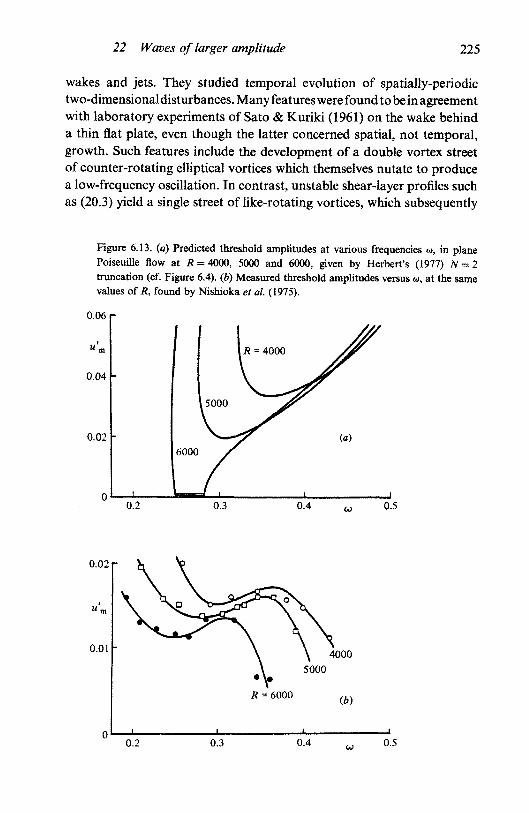
22 Waves of larger amplitude 225
wakes and jets. They studied temporal evolution of spatially-periodictwo-dimensional disturbances. Many features were found to be in agreementwith laboratory experiments of Sato & Kuriki (1961) on the wake behinda thin flat plate, even though the latter concerned spatial, not temporal,growth. Such features include the development of a double vortex streetof counter-rotating elliptical vortices which themselves nutate to producea low-frequency oscillation. In contrast, unstable shear-layer profiles suchas (20.3) yield a single street of like-rotating vortices, which subsequently
Figure 6.13. (a) Predicted threshold amplitudes at various frequencies w, in planePoiseuille flow at R = 4000, 5000 and 6000, given by Herbert's (1977) JV" = 2truncation (cf. Figure 6.4). (b) Measured threshold amplitudes versus <o, at the samevalues of R, found by Nishioka et al. (1975).
0.06 r
0.04 -
0.02 -
o.O2 r
o.oi 4000
0.2 0.3 0.4 0.5
Downloaded from University Publishing Online. This is copyrighted materialIP139.153.14.250 on Tue Jan 24 02:27:34 GMT 2012.
http://dx.doi.org/10.1017/CBO9780511569548.007

226 Evolution of a nonlinear wave-train
interact in pairs (Winant & Browand 1974). Similar structures have beenreproduced in the numerical studies of Patnaik, Sherman & Corcos (1976)and Peltier, Halle & Clark (1978). An example is shown in Figure 6.14.
The successes of these various numerical studies give confidence in theircapacity to represent finite disturbances accurately beyond the range ofweakly nonlinear analysis. Nevertheless, weakly nonlinear theories willlong have a part to play in aiding physical understanding of nonlinearprocesses, in supplying a check on numerical results and, hopefully, inproviding a source of fresh ideas for future progress.
22.4 The nonlinear critical layerObviously, weakly nonlinear theory cannot cope with strong
nonlinearities. For waves in shear flows, these first appear in the vicinityof the critical layer z = zc. The linear theory for waves of constantamplitude, outlined in §3.2, led to a jump in Reynolds stress across thiscritical layer. A logarithmic singularity of inviscid theory was resolved by
Figure 6.14. Computed constant-density contours at various times of development ofKelvin-Helmholtz instability of a viscous stratified shear layer. Dimensionless timesT in {dyif) are 0,0.5,1.0, 1.5, 2.0 and 2.42 (from Patnaik, Sherman & Corcos 1976).
(a)
Downloaded from University Publishing Online. This is copyrighted materialIP139.153.14.250 on Tue Jan 24 02:27:34 GMT 2012.
http://dx.doi.org/10.1017/CBO9780511569548.007

22 Waves of larger amplitude 227
viscosity, at large R, a phase shift of n from the logarithmic term occurringacross a viscous critical layer of width O[(aR)~i].
The width of the Kelvin 'cat's eyes' within the critical layer is O(ei)where e is the wave amplitude at some distance from zc (Drazin & Reid1981, p. 141). Neglected nonlinear terms are unimportant only if theviscous critical layer thickness far exceeds the width of the cat's eyes: thatis to say, A = /J"1e~2 must be large compared with unity for linear andweakly nonlinear theories to remain applicable.
The contrary assumption, that both A ^ 0(1) and e <4 1, underlies thetheory of the nonlinear critical layer. This was first developed independentlyby Benney & Bergeron (1969) and Davis (1969), for A -> 0, and subsequentlyimproved and extended by Haberman (1972, 1976). A weakly nonlineartheory still suffices outside the critical layer region of thickness O(p) butstrong nonlinearities are present within it. For A = 0 the logarithmic phaseshift <f>, and consequently the jump in Reynolds stress, is zero, whereas thelinear phase shift is n. Haberman's (1972) computations show how <j>increases from 0 to n as A increases from zero to large values. For largeA, Haberman (1976) has shown analytically that
An analogous theory, differing in details, has been developed by Kelly &Maslowe (1970) and Haberman (1973b) for weakly stratified flows; whilestronger stratification was investigated numerically by Maslowe (1972).Benney & Maslowe (1975) and Huerre & Scott (1980) incorporatenonlinear critical layers in their studies of marginally unstable waves inshear layers.
The critical-layer solutions exhibit closed-streamline 'cat's eyes', which,by virtue of the Prandtl-Batchelor theorem (Batchelor 1956), encloseregions of constant vorticity. Towards the edges of these cat's eyes, it ispostulated that there are thin viscous layers across which the vorticity (and,in the stratified case, density) changes, in order to match with the flow inthe outer regions. Though some doubts remained regarding the detailedflow within these layers, these studies made an important contribution tothe analysis of nonlinear waves. A useful summary of the analytical detailsis given by Maslowe (1981).
Since then, Smith (1979b), Smith & Bodonyi (1982a) and Bodonyi,Smith & Gajjar (1983) have further elucidated the complex mathematicalstructure of finite neutrally-stable disturbances in boundary layers asR^-oo. Separate detailed analyses are necessary in various parameterranges; as the amplitude increases, the character of the critical layer
Downloaded from University Publishing Online. This is copyrighted materialIP139.153.14.250 on Tue Jan 24 02:27:34 GMT 2012.
http://dx.doi.org/10.1017/CBO9780511569548.007

228 Evolution of a nonlinear wave-train
changes from a nonlinear viscous one, like Haberman's (1972), to astrongly nonlinear, primarily inviscid, sort. Corresponding amplitude-dependent neutral disturbances in Poiseuille pipe flow were studied bySmith & Bodonyi (1982b).
Precisely how, and whether, a linearly unstable mode or a finite initialdisturbance evolves in time towards such an equilibrium state is a matterof some complexity. It is unlikely that such equilibrium states could persistin real boundary-layer flows at the very large Reynolds numbers neededfor the validity of the asymptotic theory. These solutions certainly existand have an interest of their own; but their stability to other wave-modes - and so their practical significance - remains unknown.
There have been some related studies of the temporal evolution offinite-amplitude disturbances. For the shear-layer profile (20.3), Robinson(1974) developed a nonlinear inviscid analysis for rapidly growing waveswhich do not equilibrate. Later, Warn & Warn (1978), Stewartson (1978)and Brown & Stewartson (1978a, b) provided much insight into thedevelopment of marginally unstable Rossby waves and those in stratifiedshear layers. This work is conveniently reviewed by Stewartson (1981). Arecent analysis by Gajjar & Smith (1985) considers unsteady nonlinearcritical layers in channel and boundary-layer flows.
Brown & Stewartson (1978b) give an inviscid analysis of the marginallyunstable stratified shear flow (5.1) with Richardson number J very closeto \. They demonstrate how nonlinear critical-layer effects develop on thetime scale / = 0{e~*), the wave amplitude A = eA(t) then satisfying anevolution equation
dA/dt = ( ! - / ) i+<x 4 f 6 | I | 4 A
where a4 is a small positive constant, approximately 10~6. The unexpectedappearance of the factor t is at variance with Maslowe's (1977a) analysisfor a viscous shear layer, which led to a more conventional Landau-Stuartequation of the form (8.8). This apparent discrepancy was reconciled byBrown, Rosen & Maslowe (1981). The details are complex, being sensitiveto the relative strengths of viscous and thermal diffusion and of nonlineareffects, on various evolutionary time scales. Depending on circumstances,Maslowe's (1977a) cubic nonlinearity or Brown & Stewartson's quintic onemay dominate in the viscous problem.
Numerical studies by Beland (1976, 1978) of forced nonlinear Rossbywaves display their development and near-equilibration. The logarithmicphase shift ^ is found to agree with Haberman's (1972) prediction: initialabsorption of the incident wave at the critical layer is later replaced by
Downloaded from University Publishing Online. This is copyrighted materialIP139.153.14.250 on Tue Jan 24 02:27:34 GMT 2012.
http://dx.doi.org/10.1017/CBO9780511569548.007

22 Waves of larger amplitude 229
reflection but virtually no transmission. The flow structure in the vicinityof the critical layer resembles that of Figure 6.14.
Similarly, with strong stratification, an internal gravity wave approachingthe critical level where U= cT initially undergoes absorption, along withjust a little reflection and transmission. The linear theory of Booker &Bretherton (1967) and others was described in § 5.3: their transmission andreflection coefficients are O(e~m), where v = (/—|)i and these are smallfor all moderately large values of / . In the absence of dissipation,nonlinearity must eventually become important within the critical layer,since wave energy steadily accumulates in its vicinity.
Brown & Stewartson (1980,1982a, b) and Burke (1983) have shown thatthe linear results remain valid on the time scale 1 < t <£ e~i; but that, whent is O(e~%), nonlinear modification of the critical layer causes the reflectionand transmission coefficients to develop with time. When v P 1, leading-order corrections are found: the transmission coefficient remains expo-nentially small, O(e~"w), but the reflection coefficient increases to O^"1).Accordingly, the critical layer begins to restore wave energy to the outerflow by reflection, while continuing to act as an absorber and a very weaktransmitter. These results are in qualitative agreement with the numericalstudies of Breeding (1971, 1972) and of Jones & Houghton (1972).Experiments of Thorpe (1981) and Koop (1981) confirm that there is littletransmission through the critical layer, but show no clear evidence of theabove nonlinear effects.
The nonlinear critical theory has been developed only for a singledominant two-dimensional wave-mode. Though linear superposition ofsolutions remains permissible at leading order outside the critical layerregion, this is not so within it. With two or more modes present, there mustbe strong nonlinear coupling within critical layers: as yet, no attempt hasbeen made to construct a theory for such cases. Similarly, the stability ofthe nonlinear critical layer deserves attention: its similarity to a row ofequally-spaced vortices suggests that instability and subsequent 'vortexpairing' may occur.
22.5 Taylor-Couette flow and Rayleigh—Benard convectionThese two are among the most fascinating of fluid flows, despite
their deceptively simple geometry. In Taylor-Couette flow, the fluid isconfined to the gap between concentric, differentially-rotating cylinders;in Benard convection, fluid is confined between plane horizontal walls, andwould be at rest were the temperature of the lower wall not higher thanthat of the upper.
Downloaded from University Publishing Online. This is copyrighted materialIP139.153.14.250 on Tue Jan 24 02:27:34 GMT 2012.
http://dx.doi.org/10.1017/CBO9780511569548.007

230 Evolution of a nonlinear wave-train
In the simplest theoretical formulations, the cylinder lengths and thehorizontal walls are regarded as infinite. If, also, the gap between thecylinders is small compared with the radii of the cylinders, the linear theoryfor small disturbances in the two flows takes identical form (see e.g.Chandrasekhar 1961; Drazin & Reid 1981). Instability gives rise to astationary array of counter-rotating toroidal cells between cylinders, andto parallel roll cells between horizontal heated walls, the former driven bycentrifugal forces and the latter by buoyancy. Since the roll cells of thermalconvection have no preferred direction of orientation, composite cellscomprising more than one Fourier mode in space commonly arise. Theconfiguration of the side walls of the apparatus, together with weaknonlinearities, influences the type of convection cell, rectangular andhexagonal ones being most common.
For these flows, the prediction of onset of instability, by linear theory,agrees remarkably well with experiment. This is so largely because, nearthe critical point of linear theory, weak nonlinear terms have a stabilizingeffect: the nonlinear equilibrium solution bifurcates supercritically fromthe linear critical point because the Landau constant Ar (cf. §8) is negative.
A plethora of recent reviews describes the large quantity of analytical,computational and experimental work concerning these two flow configur-ations: see Palm (1975), Normand, Pomeau & Velarde (1977), Busse(1978,1981a, b), DiPrima & Swinney (1981), DiPrima (1981) and Benjamin(1981). Further details are given in §§24-25 of the following chapter.
Downloaded from University Publishing Online. This is copyrighted materialIP139.153.14.250 on Tue Jan 24 02:27:34 GMT 2012.
http://dx.doi.org/10.1017/CBO9780511569548.007

Chapter seven
CUBIC THREE- AND FOUR-WAVE
INTERACTIONS
23 Conservative four-wave interactions23.1 The resonance condition
For some systems, no three-wave resonance is possible and thestrongest interactions take place among resonant quartets of waves. Thedominant nonlinearities are then of cubic order in wave amplitude and soare much weaker than the quadratic nonlinearities of three-wave resonance.But even in systems which admit three-wave resonance, phenomenaassociated with four-wave resonances may be significant. For example, asingle capillary-gravity wave resonating with its own third harmonic,mentioned in §14.2, is a degenerate four-wave resonance. So, too, is theself-modulation of nearly uniform wave-trains examined in the previouschapter, for then the 'four' participating modes are all identical, orvirtually so.
The general conditions for four-wave resonance are, of course,
k!±k2±k,±k4 = 0,(23.1)
i i W2 i 0Js i W4 = "»
with corresponding signs, for participating modes with periodicitiesexp + i(k3- • x — i»j t) (j — 1,2,3,4) and x = {x, y). The most studied reso-nance is that among deep-water gravity waves. Since these do not admitthree-wave resonance, four-wave interactions provide the dominantcoupling between modes. This plays an important role in establishing thespectrum of ocean waves, for direct wave-generation by wind operateseffectively only at rather short wavelengths (Phillips 1977). Three- andfour-wave resonance is also important in linking modes of differentphysical types, especially in plasma physics, where a great diversity ofwaves is available (see, e.g. Davidson 1972).
231
Downloaded from University Publishing Online. This is copyrighted materialIP139.153.14.250 on Tue Jan 24 02:27:40 GMT 2012.
http://dx.doi.org/10.1017/CBO9780511569548.008

232 Cubic three- and four-wave interactions
Phillips (1960, 1961) was the first to study four-wave resonance amonggravity waves, and he has since given several accounts of the subject: see,especially, his monograph (Phillips 1977) and retrospective article (Phillips1981a). Other early work was that of Longuet-Higgins (1962), Benney(1962) and Hasselman (1962, 1963).
The dispersion relation for deep-water gravity waves is w = ± (g | k |)*,which defines an axisymmetric double trumpet-shaped surface in u>-k-lspace, where k = (k, I). If a similar surface is constructed, with differentorigin O' as in Figure 7.1, they intersect in some curve. Any two points onthis curve define four wavenumbers k3- (those shown in the figure having/ = 0) which satisfy the resonance condition
(23.2a, b)
Movement of O' parallel to the w-axis yields a family of such curves. Their
Figure 7.1. Diagram in <o-k plane, with / = 0, which determines a resonant quartetof surface gravity waves. The corresponding intersecting axisymmetric surfaces in (a-k-lspace are readily envisaged (from Phillips 1974).
Downloaded from University Publishing Online. This is copyrighted materialIP139.153.14.250 on Tue Jan 24 02:27:40 GMT 2012.
http://dx.doi.org/10.1017/CBO9780511569548.008

23 Conservative four-wave interactions 233
projection on the k-l plane is shown in Figure 7.2 and this denotes thecomplete family of resonance curves if its scale and orientation is regardedas arbitrary. This is because the dispersion relation for gravity waves hasno preferred direction and <o is proportional to a single power of | k |. Forother dispersion relations, as for capillary-gravity waves or (stable)Kelvin-Helmholtz flow (see §2.1), variations with scale or direction occurand so all possible origins O' must be considered in analogous graphicalconstructions. The latter flows also admit stronger three-wave resonances.
23.2 The temporal evolution equationsFor progressive gravity waves with wavenumbers satisfying con-
dition (23.2a), let A}{i) (j = 1,2,3,4) denote the complex amplitudes of thefree-surface displacements associated with each wave. The evolutionequations are found to have the form (Benney 1962; Bretherton 1964)
dA1/dt = iA1
dAJdt = \At
dAJdt =
(23.3)
Figure 7.2. Curves in k-l wavenumber plane given by resonance condition (23.2). Linesfrom A and B to any pair of points on one such curve determine a resonant quartetas shown (after Phillips 1977).
Downloaded from University Publishing Online. This is copyrighted materialIP139.153.14.250 on Tue Jan 24 02:27:40 GMT 2012.
http://dx.doi.org/10.1017/CBO9780511569548.008

234 Cubic three- and four-wave interactions
when interactions of higher than cubic order are ignored. If the resonancecondition (23.2b) is not nearly met, the terms in h contain rapidly-oscillatingexponential factors and these average to zero over the modulationtimescale. Only if the mismatch Aw from resonance is small need theseterms be retained.
The sixteen elements of the matrix atj are real and so also is h. Theirvalues depend on the wavenumber configuration and determination ofthese is algebraically tedious. The terms in ai} modify the phases but notthe magnitudes of the amplitudes At: that is, they provide a nonlinearmodification to the phase velocities. The diagonal terms ati representStokes' (1847) frequency shift due to self-interaction. Only the h terms actto transfer energy between modes.
Benney's (1962) derivation employs techniques of perturbation theorywhich are now standard. The governing equations are as (14.2), but withsurface tension y set equal to zero. The two free-surface boundaryconditions are just (11.13) and (11.14), which contain all nonlinearities.These may be replaced by Taylor expansions about the mean surface z = 0,namely,
(2 = 0) (23.4a, b)
correct to cubic order in wave amplitude. Elimination of £ then yields asingle boundary condition for <j>.
A velocity potential, satisfying Laplace's equation and the boundarycondition at z = — oo,
4> = e Re 2 Pt(t) el k ; r e^s + e2P0 0(t)
i
+ e 2 R e S Pt ra(Oe1<k!+km>-fel
ki+kmlz
l,m
+ e3Re S /);,ro)n(Oe i(ki+km+kn)-re^+km+
I, m, n
describes a discrete set of wave-modes with wavenumbers k, ( /= 1,2,...)in propagation space r = (x, y). Substitution into the nonlinear boundarycondition at z = 0 enables the various /"-functions to be found. Theparameter e characterizes the wave amplitudes.
In the linear approximation, (23.4a, b) reduces to
and so
Downloaded from University Publishing Online. This is copyrighted materialIP139.153.14.250 on Tue Jan 24 02:27:40 GMT 2012.
http://dx.doi.org/10.1017/CBO9780511569548.008
23 Conservative four-wave interactions 235
which yields two primary-wave frequencies ±(g\kt|)i For propagatingwave-trains, one or other value is selected, say wl for each k?: for standingwaves, both must be retained as in §14.2. At O(e2),
^ ^ + g | k , + k m | P , i m = 2(k ! -k m - |k , | |k m | )^(P i P m ) . (23.5)
Here, both sums and differences of the primary wavenumbers are retainedby allowing m to take both positive and negative values, with k_m = — km,w_m = -wffl and P_m — P^, the complex conjugate of Pm. Sinceno three-wave resonance is possible, free modes with frequencies+ (gjkz+km|)2, for which the left-hand side of (23.5) vanishes, may bedisregarded. The remaining, forced, solution for Pt m has periodicityo)l+(om and is proportional to PiPm: this is readily found from (23.5).
On proceeding to O(e3), terms in exp (ikz • r) may be extracted from thenonlinear boundary conditions. The corresponding equation for Pt has theform
dVj/d/'+wfP^i^e-1"!*/?, (/=1,2,...) (23.6)for each primary wave amplitude. The nonlinear interaction terms repre-sented by Ft derive from various sources. Those proportional to | Pk |
2 Pt
and Pi,-kPk automatically have the correct periodicity; others, proportionalto PrPmPn and PrPmn, have periodicity
e i (k r +k m +k n -k , ) • r e-i<«v+fc>m +un-a>l) t
and these terms match the periodicity of Pj only if the resonance conditions(23.1) are satisfied. With eP}(t) re-expressed as (-iwylk,^1)^/?) e"1^',where the A} denote slowly-varying complex amplitudes of the free-surfacedisplacements, (23.6) yield
<Lyd/ = - i « ^ J 5 0=1,2,3,4) .With four wavenumbers satisfying (23.2a), these are just the evolutionequations (23.3) above. The complicated expressions for the coefficientsay and h are given by Benney (1962).
23.3 Properties of the evolution equationsEquations (23.3) satisfy the conservation relations
d (\Adt\ w2 / dt\ <i>3 J dt
(23.7)
which connect the wave actions of the modes. It follows that total waveaction is conserved,
«,•
Downloaded from University Publishing Online. This is copyrighted materialIP139.153.14.250 on Tue Jan 24 02:27:40 GMT 2012.
http://dx.doi.org/10.1017/CBO9780511569548.008
236 Cubic three- and four-wave interactions
SL result which is not true of three-wave resonance. Also, the energyequation is
and this also vanishes by virtue of the resonance condition (23.2). As forthe three-wave case, £ t o t is not constant when there is a small detuningAw = feij+Wj—w3 —w4 from exact resonance, despite the fact that thesystem is non-dissipative.
Because of (23.7), the four evolution equations (23.3) may be reducedto an equation for a single variable x{t) just as in §15.1. Completeanalytical solutions may then be given in terms of Jacobian ellipticfunctions (Bretherton 1964; Turner & Boyd 1978).
The extension to spatial, as well as temporal, modulations is accomplishedon replacing dAj/dt by {d/dt-\-\fV)Aj in (23.3), where v,- denote therespective group velocities d(Oj/Skj: but this is justified only for waves indeep water. With finite depth, spatial modulations in amplitude drive anO(e2) mean flow as described in § 11.2 and this must be taken into accountwhen deriving the O(e3) interaction equations. Apparently, little work hasbeen done on this problem. In the deep-water case, uniformly-propagatingmodulations which depend on a single variable, say T S t — ax—by withconstant a and b, obey equations of similar form to (23.3) and so may besolved. Likewise, waves with equal linear damping rates may be treatedby transforming to a new 'time' co-ordinate, as in §16.2, which recoversequations of undamped form (Bingham & Lashmore-Davies 1979).
Initial scepticism of the importance of resonances among gravity waveswas dispelled by the experiments of Longuet-Higgins & Smith (1966) andMcGoldrick, Phillips, Huang & Hodgson (1966). Two wave-trains, withmutually perpendicular wavenumbers k1; k2 and corresponding frequenciesWj, <o2 were generated mechanically from adjacent sides of a square wavetank. When these were chosen to satisfy the resonance conditions
2kx = k2+k3 , 2wj = wa+ws,
the oblique mode k3 was seen to grow spontaneously with distance acrossthe tank. Quite good agreement was obtained with the theoretical initialgrowth rate of k3 but the tank was not large enough to confirm theexistence of periodic modulations. At other, non-resonant, choices of kx
and k2, no significant k3 component was generated. Figure 7.3, fromMcGoldrick et ah, shows measured frequency spectra for resonant andnon-resonant cases.
Downloaded from University Publishing Online. This is copyrighted materialIP139.153.14.250 on Tue Jan 24 02:27:40 GMT 2012.
http://dx.doi.org/10.1017/CBO9780511569548.008

23 Conservative four-wave interactions 237
Subsequent experiments on the modulational instabilities of initiallyuniform wave-trains, already described in §21, demonstrated the resonantgrowth of sidebands. At the other extreme, measurements of the evolutionof ocean-wave frequency spectra (see e.g. Phillips 1977) support the viewthat resonance is responsible for broadening the spectrum to low frequencieswhich cannot be generated directly by wind.
23.4 Zakharov's equation for gravity wavesHasselmann (1962,1963) was first to consider resonant interactions
within a continuous spectrum of gravity waves. Later, in an important but
Figure 7.3. Gravity-wave frequency spectra measured by McGoldrick et at. (1966),with two forced components/,,/,. Four-wave resonance occurs with/,//, = 1.775 atcomponent with frequency 2/,—f2. This component is not prominent in the non-resonant case/,//,, = 1.600.
-, 1 0
0.1 =
Frequency (c.p.s.)
Downloaded from University Publishing Online. This is copyrighted materialIP139.153.14.250 on Tue Jan 24 02:27:40 GMT 2012.
http://dx.doi.org/10.1017/CBO9780511569548.008

238 Cubic three- and four-wave interactions
terse paper, Zakharov (1968) gave a rather different formulation. Onlyrecently has Zakharov's work gained deserved recognition through itsfuller rederivation by Crawford, Saffman & Yuen (1980), also describedin Yuen & Lake (1982).
Instead of referring the surface boundary conditions to the mean levelz = 0, Zakharov introduced the potential </>s at the free surface as adependent variable,
0-(M) = 0(r.£(r,O,O,
where r denotes (x, y), z — £(r, t) is the free surface and 0(r, z, t) the usualvelocity potential. It follows that
Vr <f>*(r, t) = Vr 0(r, £(r, r), 0 + &(r, £(r, 0, 0 Vr £(r,where Vr = (8/6x, 6/8y).
The boundary conditions (14.2c, d) yield
and it remains to express $z in terms of <ps and ^. Zakharov showed thatthese boundary conditions may be rewritten in the elegant Hamiltonianform
£t = 8E/8<f>*, ft = -SE/9£ (23.9)
where E is the total energy and S/8<frs, 8/S£ denote variational derivatives;but this reformulation was not used by Crawford et al.
The (double) Fourier transforms of the velocity potential <j> and surfacedisplacement f are defined as
1 f00$(k, z,t) — — 4>(t, z, t) exp ( - ik • r) dr,
£n J_oo
£(k, 0 = i - T g(r, 0 exp ( - ik • r) dr,
where
by virtue of Laplace's equation (14.2a). The corresponding surface potentialis
^s(r, 0 = ^ j°° <t>(k, 0 exp [| k | §(r, 0] exp (ik • r) dk.
The convenient shorthand of dr and dk is used to denote dxdy and d&d/respectively, where k = (k, I). For sufficiently small surface displacements,
Downloaded from University Publishing Online. This is copyrighted materialIP139.153.14.250 on Tue Jan 24 02:27:40 GMT 2012.
http://dx.doi.org/10.1017/CBO9780511569548.008
23 Conservative four-wave interactions 239
the exponential in |k |£ may be expanded by Taylor series. With gexpressed in terms of £, this yields
$«(*, 0 = T - f0 $00 exp (ik • r) dk
«Pl»(k+k1+k1)T]dkdk1dk t
with the time-dependence of <& and £ implied.The Fourier transform $s(k, t) of <j>*(j, i) is therefore found as a series
of integrals involving <f> and £. This may be inverted iteratively, giving$ in terms of $s and £ as
where d( ) denotes the delta function
It follows that ^ may be constructed as a convergent series in terms of$s and £: accordingly, in the boundary conditions (23.8a, b), 4>z is nowknown in terms of 08(r, t) and £(r, t).
These boundary conditions may be combined into a single equation bydefining the complex variable
b(k, t) = frKk) | k |"l)1/2£(k, 0+ i ( | | k | a r W V (k, 0- (23.10)
The free surface £ and potential 0 are recovered as a sum and difference,respectively, of the inverse Fourier transforms of b and its conjugate b*.The equation for b(k, t) is
bt(k)+iw(k)b(k)+i
f f° 1; k2) 6*(k,) 6*(k2) 5(k+k t+k2) dkj dk2(ot;er)
Downloaded from University Publishing Online. This is copyrighted materialIP139.153.14.250 on Tue Jan 24 02:27:40 GMT 2012.
http://dx.doi.org/10.1017/CBO9780511569548.008

240 Cubic three- and four-wave interactions
k, k l t k2, k3) b(kt) b(k2) b(k3) d(k - k, - k2 - k3) dkx dk2 dk3
k, k1; k2, k3) b*{kx) b(k2) b(ks) ^ k + k ! - k 2 - k 3 ) dkx dk2 dk3
W^(k,k1,k2,k3)b*(k0b*(k2)b(k3)S(k+k1+k2-ki)dk1dk2dl
W^(k,k1,k2,k3)b*(k1)b*(k2)b*(k3)S(k+k1+k2+k3)dk1dk26
+ . . . = 0 , (23.11)
where the real interaction coefficients V(i), W(i) are known, but lengthy,functions of the wavenumbers k, and frequencies w^Qq). These coefficientsare stated by Crawford et al. (1980) (also Crawford et al. 1981 and Yuen& Lake 1982) who correct minor errors in Zakharov's account.
Zakharov (1968) derived this result rather differently. He first showedthat Hamilton's equations (23.9) are equivalent to
then calculated the right-hand side from the energy functional E.The leading-order approximation bt = — \u>b yields the linear result. The
three double integrals in VU) represent quadratic interactions amongFourier components. If we set
b(kp i) = eBjikj, t) exp [-ia>(k;) t]
where e is a measure of the small wave-slope | k | £, (23.11) yields
e X B2 S(k - k, - k2) exp [i(w - wx - wa) /] dkj dk2Gt UJ
) (23.12)
at quadratic order, where I2 and /3 denote corresponding integrals in F(2>
and F (3). If no three-wave resonance is possible, the right-hand side is arapidly-varying function of t, and B may be decomposed into a dominant0(1) slowly-varying part with O(e2) time derivative and a small 0{e)rapidly-varying part, eB' say. The latter may be found by integrating(23.12) directly with respect to t; for, only the dominant parts of Bx, B2
need be retained in the integrals, and they are constant on the 0(1)timescale /. If three-wave resonance occurs, direct integration of (23.12)is impossible: the integrals have slowly-varying parts and B evolves on thetimescale et.
With no three-wave resonance, the slow evolution of B on the timescaleeH is found by retaining the 0(e3) terms of (23.11). Some of these derive
Downloaded from University Publishing Online. This is copyrighted materialIP139.153.14.250 on Tue Jan 24 02:27:40 GMT 2012.
http://dx.doi.org/10.1017/CBO9780511569548.008

23 Conservative four-wave interactions 241
from the FW) integrals through products of the dominant O(e) part of band the known rapidly-varying part e2JS'; others come from the WU)
integrals and are of cubic order in the dominant part of b. Again, manyof these terms are rapidly-varying and may be 'filtered out' since theydo not contribute to the slow modulation of B. In particular, theonly resonances among deep-water gravity waves are those withw + W! —w2 —w3 = 0 (where the w's are constrained to be positive withoutloss of generality) and so the integrals in W{1), W(3) and WH) may besuppressed. The final result has the form
, klf k2, k3) B* fi2 B3 S(k+kx - k2 - k3)
x exp [i(w 4- (D1—<o2—w3) t] dkx dk2 dk3, (23.13)
where Tis known in terms of the V(i) and W(2). This is Zakharov's integralequation for the slow evolution of a weakly nonlinear wave field. Onlythose modes for which \o)+o)1—o)2—(t)a\is O(e2w) or less need be retainedin the integral.
23.5 Properties of Zakharov's equationSuppose that the Fourier spectrum B(k, t) comprises just four
discrete resonant modes,4
I3\JS.y Ij — J£J Jj ylj Oyjfk — *^M/» - l
with conditions (23.2) satisfied by the wavenumbers Kn and frequencies con.It is readily confirmed that (23.13) then yields results (23.3).
Alternatively, for a narrow spectrum closely centred around a singlewavenumber k0 and frequency w(k0), the dispersion relation isapproximately
where a, b, c are constants, Kx is the component of k—k0 parallel tok0 and K2 that perpendicular to k0. Obviously, a is the group velocityof k0. In (23.13), r(k, k15 k2, k3) may be replaced by the constant,To = r(k0, k0, k0, k0), which equals | k0 \
3/4n2. Also, 5(k, /) may be rewrittenas
B(k, t) = i ( k , i) exp [{{a^ + bK\ + cK\ + ...)t] (23.14)
to incorporate the frequency shift. Equation (23.13) then gives
<Kf + cK2+...)A
A* i 2 As <5(k+kx - k2 - k3) dkj dk2 dk3. (23.15)
Downloaded from University Publishing Online. This is copyrighted materialIP139.153.14.250 on Tue Jan 24 02:27:40 GMT 2012.
http://dx.doi.org/10.1017/CBO9780511569548.008

242 Cubic three- and four-wave interactions
The inverse Fourier transform of A is
A(T, t) = ^ Jj°° i(k, 0 exp [i(^ x + K2 y)] d ^ dK2
to leading order, with x measured along k0. Correspondingly, (23.15) gives
dt dx 2 V dx2 dy2
which is just the nonlinear Schrodinger equation (19.3). This derivation
was originally given by Zakharov.Zakharov also examined the stability of periodic wave-trains (see §21.1)
and this work was extended by Crawford et al. (1981). A solution of(23.13), which represents a uniform wave-train with wavenumber
'Boexp(-iToBlt), k = k0
k 4= k0.
The amplitude a0 of the wave is given, from (23.10), by
If this wave-train is perturbed by two modes with wavenumbers k0 ± Kand small amplitudes B±{t), the equations for B± are found from (23.13)to be
i dBJdt = T1+ B2 Bt exp [ - i(Q + 2T0 Bl) t] + 2T2+Bl B+,
i dB_/dt = 71_ Bl B* exp [- i(Q + 2T0 Bl) t]+272_ Bl 5_,T — 7Yk + K I I K I k l T — TCk 4-K k k k 4-K\
Q = 2«(k0) - w(k0+K) - w(k0 - K).
The substitution
B+ = B+ exp [ - iQ£2 + To Bl) t - \<rt],
Bl = B*_ exp [i(|Q + To B2.) t - iat]
leads to an eigenvalue problem with eigenvalues <r given by
(23.16)
This result is correct to O(klal) for all wavenumbers K such that thefrequency mismatch Q from exact resonance is O(T0 Bl) or less. In contrast,the corresponding results (21.3) and (21.5), derived from the two- andthree-dimensional nonlinear Schrodinger equations (21.1) and (19.3), arevalid only for wavenumbers K small compared with k0: in particular, (21.5)incorrectly predicts instability for all L/K close to +2~i Result (23.16)
Downloaded from University Publishing Online. This is copyrighted materialIP139.153.14.250 on Tue Jan 24 02:27:40 GMT 2012.
http://dx.doi.org/10.1017/CBO9780511569548.008

23 Conservative four-wave interactions 243
may also be derived from (23.3), with frequency mismatch Aw = Q,A1=A2 = B and A3, At = B+, B_.
Crawford et al. (1981), also Yuen & Lake (1982), compare the stabilityboundary Im{o-} = 0 with those of (21.3) and (21.5) and also withLonguet-Higgins' (1978a, b) computations from the full nonlinear equations(see §22.2). For two-dimensional disturbances, this comparison is shownin Figure 6.7: result (23.16) is a clear improvement on the Benjamin-Feirresult (21.3) and gives reasonable agreement with the full nonlinearcomputations even at quite large wave-slopes.
For three-dimensional disturbances, the unstable region given by (23.16)is shown in Figure 7.4 for various wave-slopes: the fundamental wave-number is k0 = (ko,0) and the perturbations have k+ = (ko±Kx, +Ky).As k0 a0 approaches zero, the region of instability is situated narrowlyaround Phillips' figure-of-eight curve for four-wave resonance with2k0—k+ — k_ =0 . For fairly small koao, the unstable region resembles apair of touching' horseshoes' and, as k0 a0 further increases, the' horseshoes'move apart due to stabilization of modes with small | K |. The unstableregion becomes increasingly concentrated near K = +0.78 k0 and finallydisappears when koao x 0.5. This reproduces, at least qualitatively, thestabilization of Type I instability at large wave-slopes found by McLeanet al. (1981) and already discussed in §22.2. However, the Zakharovequation (23.13) is no longer a rational approximation at such largewave-slopes. Moreover, the Zakharov equation is incapable of predictingthe higher-order Type II instability which corresponds to five-waveresonance. However, Zakharov's analysis has recently been extended byStiassnie & Shemer (1984) to incorporate the next-order five-wave
Figure 7.4. Regions of instability in Kx-Ky space as given by (23.16), for various valuesof wave-slope koao: /coao = 0, &0a0 = 0.01,kaa0 = 0.4, fcoa0 = 0.48 (from Crawford et al. 1981).
-0-25
-0-4
Downloaded from University Publishing Online. This is copyrighted materialIP139.153.14.250 on Tue Jan 24 02:27:40 GMT 2012.
http://dx.doi.org/10.1017/CBO9780511569548.008

244 Cubic three- and four-wave interactions
resonances in water of both infinite and finite depth: their extendedequation represents Type II instability fairly satisfactorily.
In principle, the evolution of any finite number of discrete modes maybe studied numerically, using Zakharov's equation. Caponi, Saffman &Yuen (1982) - repeated in Yuen & Lake (1982) - have done so for a sevenmode system of two-dimensional waves, comprising a fundamentalk = (fco,0) and six sidebands k = (fc±,0), /c±=£0±nA/c (n = 1,2,3):Ak/k0 was chosen to be 0.2. Initially, a uniform wave-train with wavenumberk0 and amplitude a0 was prescribed, together with small 0(lO~6ao)perturbations at the other wavenumbers. At sufficiently small koao
(= 0.05), the motion was periodic and the sidebands remained small; butat k0 a0 = 0.1 quasi-periodic (Fermi-Pasta-Ulam) modulations occurredas a consequence of Benjamin-Feir instability of the kf sidebands. Atkoao = 0.2, both kf and k£ lie in the unstable domain of Figure 6.7 andthe modulations were found to be chaotically irregular. At k0 a0 = 0.45,the sidebands kf, k£ are stable but kf now lies in the unstable domain:then, seemingly periodic modulations at first occurred, but the kf and kfmodes later grew to prominence (because of their resonance with k0 andkf) and chaotic behaviour ensued. At k0a0 = 0.5, all the sidebands arestable and the periodic wave-train remained unmodulated - but Type IIinstabilities may then be expected. In accord with expectations, corre-sponding calculations based on the nonlinear Schrodinger equation (21.1)showed similar quasi-periodic and chaotic modulations, but no restabil-ization at large koao where (21.1) is not a good approximation.
Of much oceanographic interest is the evolution of a field of randomgravity waves. Following on from Hasselmann's (1962, 1963) work,Longuet-Higgins (1976) and Alber (1978) considered the limiting case ofa narrow-band spectrum, for which the nonlinear Schrodinger equationprovides an acceptable starting point. In contrast, Crawford et al. (1980)employed Zakharov's equation to investigate a narrow-band randomspectrum. All agree that Benjamin-Feir instability is suppressed bysufficient randomness, but a homogeneous spectrum remains modulation-ally unstable if the bandwidth is sufficiently narrow. Discussion of randomwave spectra is outside the scope of this work: recent accounts may befound in Phillips (1977), Yuen & Lake (1982) and West (1981).
24 Mode interactions in Taylor-Couette flow24.1 Axisymmetric flow
Finite-amplitude axisymmetric Taylor-vortex flow was first calcu-lated by Davey (1962), by an amplitude-expansion method similar to that
Downloaded from University Publishing Online. This is copyrighted materialIP139.153.14.250 on Tue Jan 24 02:27:40 GMT 2012.
http://dx.doi.org/10.1017/CBO9780511569548.008

24 Mode interactions in Taylor-Couette flow 245
of Stuart (1960) and Watson (1960). Velocity perturbations have the form
u(r, z, t) = Re {A(t) u^r) exp (iaz)} + h.o.t.
where higher-order terms include harmonics, mean-flow distortion andmodifications of the leading-order eigenmode. Here, z and r denotedistances along and perpendicular to the axis of the cylinders, which(meantime) are taken to have infinite length.
The amplitude equation has the typical Landau form (cf. §22.3)
dA/dt = a-A-axA \A \2 + a2A \A | 4 +. . . ,
where a{T, a) is the real eigenvalue of the corresponding linear stabilityproblem. The Taylor number Tis a dimensionless measure of the strengthof the rotation, proportional to the square of a Reynolds numberR = Q1r1 djv. Other parameters are the gap to inner radius ratio d/rt andthe ratio of outer- to inner-cylinder rotation speeds QJQV which may beregarded as constants: the case Q2/Q1 = 0 and the small-gap approximationd/r^O have received most attention. The Taylor number is usuallydefined as
T=^4where r2 = rx + d is the outer radius.
At the critical Taylor number To for onset of linear instability, <x changessign; also, Davey (1962) found ax to be real and positive near To.Accordingly, there is a super-critical finite-amplitude equilibrium state
\A\**cr/a1 (T>T0)
with axial wavenumber a = a0 equal to that of the least stable linear mode.Subsequently, DiPrima & Eagles (1977) calculated a2, and several higher-order coefficients have been computed by Herbert (1981).
At each T> To, there is a finite bandwidth of linearly unstable wave-numbers a, centred on a0, each of which may yield a finite-amplitudeequilibrium state. For Tonly slightly greater than To, when the bandwidthis narrow, the stability of these states to 'sideband' disturbances withwavenumbers a ± S has been investigated. This was first done by Kogelman& DiPrima (1970), following an earlier general approach of Eckhaus (1963,1965). Stuart & DiPrima (1978) have noted the similarity of Eckhaus'mechanism to that of Benjamin & Feir (1967) already discussed in §21.1.It was found that wavenumbers sufficiently close to a0 are stable equilibriumstates, but that those outside a band of width 3 ^ times that of thelinearly-unstable bandwidth are not. A later analysis by Nakaya (1974),taken to higher order, found a slightly narrower bandwidth of stable vortex
Downloaded from University Publishing Online. This is copyrighted materialIP139.153.14.250 on Tue Jan 24 02:27:40 GMT 2012.
http://dx.doi.org/10.1017/CBO9780511569548.008

246 Cubic three- and four-wave interactions
flows. The nonlinear coupling between the modes a., a.+ 8 and a — S isessentially a four-wave resonance with kx = k2 = a and all four frequencieszero.
24.2 Periodic wavy vorticesThe transition from axisymmetric Taylor vortices to wavy vortex
flow (see Figure 7.5) is also a four-wave interaction phenomenon. Davey,DiPrima & Stuart (1968) considered the interaction of axisymmetric modeswith azimuthal velocity components
v = vc0(r, t) cos ocz, vs0(r, i) sin ocz
and two non-axisymmetric modes with
v = Re {vcl(r, t) cos az e1"?4}, Re {vsl(r, i) sin acz e1"*6}.
Here, vc0, vs0 are real and vcl, vsl are complex functions, n is an integerand <j> is the azimuthal angle. To leading order, the ^-functions may bewritten as
"co ~ Ac(i)f0(r), vs0 ~ As(t)f0(r),
vcl » Bc(t) ho(r), vsl at Bs(t) ho(r)
where Ac, As are real and Bc, Bs are complex functions with complexconjugates B*, B*. Higher-order expansions may then be developed inascending powers and products of the A's, 5's and fi*'s. In this way, thethird-order amplitude equations were found to be
dAJdt = a0 Ac + a, AC{A\ + AD + Ac(a3 \ Bc |2 + a41 Bs |
2
+ Ke{2atABBeB*},
(24.1a-d)
+ (b3 - b4) Bs Ac As + (bt - b2) B* Bl
dBJdt = b0
+ (b3 - bj Bc As Ac + (b, -
with known real a- and complex Z>-coefHcients. Real and imaginary partsof the latter will be identified by subscripts r and i respectively.
The real Ae and As equations may be combined as a single complexequation for A = Ac + iAs. Also, B+ = Bc — iBs and B_ = B* — iB* may beidentified as the respective complex amplitudes of modes with periodicities
Downloaded from University Publishing Online. This is copyrighted materialIP139.153.14.250 on Tue Jan 24 02:27:40 GMT 2012.
http://dx.doi.org/10.1017/CBO9780511569548.008

24 Mode interactions in Taylor-Couette flow 247
exp(iaz+i«0), exp(iaz—in</>). Equations (24.1) might therefore be recastas
dA/dt =(24.1)'
with the c- and ^-constants known in terms of the cfs and Z>'s.
Figure 7.5. Taylor-vortex flows at various values of R/Rc where Rc is the linear criticalReynolds number, (a) R/Rc =1 .1 , steady axisymmetric Taylor vortices; (£)i?/^ c = 6.0 and (c) R/Rc = 16.0, wavy vortices; (d) R/Rc = 23.5, waves havedisappeared (from Fenstermacher et al 1979).
Downloaded from University Publishing Online. This is copyrighted materialIP139.153.14.250 on Tue Jan 24 02:27:40 GMT 2012.
http://dx.doi.org/10.1017/CBO9780511569548.008

248 Cubic three- and four-wave interactions
This demonstrates the connection with the four-wave resonance equa-tions (23.3) with two modes identical; but now the coupling coefficientsare no longer real and the modes experience linear growth or damping.Note that the linear frequencies of the modes A, B+ and B_ are0, boi, —bQi respectively and so satisfy (23.2b). A similar analysis byNakaya (1975) allowed the axial wavenumber of the A- and fi-modesto differ: the interaction criterion
8,n)-(<x-8,-n) = 0
is met and this includes both the axisymmetric sideband instability (n = 0,8 4= 0) and wavy-vortex instability (8 = 0, n 4= 0).
From (24.1), it is easily seen that axisymmetric Taylor vortices haveBc = Bs = 0, As = CAC and
A\ + A2S = Ka0 e
2a»'(l -Kax e2(M)-i
for arbitrary constants C, K. The constant a1 is known to be negative andthere is a supercritical equilibrium state for a0 > 0 (T > To). Similarly, asimple non-axisymmetric mode has Ac = As = 0 and
Bc = Ace elw(<-'o>, Bs = /?Be e-«-V,
Pie + Ale = P% /?e = ( - *or/*lr)*, « = *>oi - (6U V / M -
The stability of the axisymmetric equilibrium state to infinitesimalnon-axisymmetric disturbances is established by linearizing (24.1) withrespect to B+ and B_. Since Ac and As are then constant, with
As = CAC, A\ + A\ = -aja, > 0,
Bc and Bs may be taken as proportional to exp(A0 and A satisfies theeigenvalue relationship
provided (24.1) may be truncated after the cubic terms. The largest growthrate Ar occurs with C zero or infinity; that is, when As = Bc = 0 orAc = Bs = 0. For these cases, the non-axisymmetric mode grows whenever
( - ao/flj) sup (b3T, bir) >-bor. (24.2)
The right-hand side is the linear damping rate of this mode, and is positivenear 7 ,. The coefficients b0, b3, bi depend on the azimuthal mode numbern. As T increases above To, the equilibrium amplitude (— ao/a1)i of theTaylor vortices increases from zero. The criterion (24.2) therefore yieldsa set of critical Taylor numbers Tn{n= 1,2,3,...) for onset of instabilitywith azimuthal periodicity exp( + i«0).
In the small gap approximation, the azimuthal wavenumber is n/rt sinceazimuthal arc length equals rx <j>. Also, the critical axial wavenumber a0
Downloaded from University Publishing Online. This is copyrighted materialIP139.153.14.250 on Tue Jan 24 02:27:40 GMT 2012.
http://dx.doi.org/10.1017/CBO9780511569548.008

24 Mode interactions in Taylor-Couette flow 249
equals 3.127/d and this is much larger than n/r^ for many integers n.Consequently, the wavenumber vectors (a0, + n/rt) of the lowest non-axisymmetric modes remain close to that of the fundamental and it comesas no surprise that the first few critical Taylor numbers Tn lie close to ro.
Improved estimates of the Tn, based on retaining quintic terms in (24.1)and relaxing the small gap approximation, were given by Eagles (1971):his first few values, with Davey et al.'s (1968) added in parentheses, areTo = 3506 (3390), Tx = 3892 (3670), T2 = 3902 (3676), T4 = 3962 (3710),for QJQ1 = 0, d/rx = 0.05 and a = a0 = 3.127/rf. Herbert (1981) laterdeveloped a computational amplitude-expansion approach (similar to thatdescribed in §22.3) which retained terms of up to 15th order for thesmall-gap limit. Jones (1981) employed an amplitude and Galerkinexpansion to compute Tn for various gap ratios d/rv Their results are inreasonable agreement with those just quoted and are probably moreaccurate.
Transition to the lowest n = 1 mode was observed by Schwartz,Springett & Donnelly (1964), but the first unstable non-axisymmetric modefound by Coles (1965) and others was that with « = 4: the apparentpreference for the n = 4 mode is not understood. Measurements by Kinget al. (1984) of the azimuthal wave speeds of non-axisymmetric modesagree well with theory.
24.3 Effects of finite lengthExperiments are necessarily conducted with finite, not infinite,
cylinders; but when the ratio of length to radius is sufficiently large,reasonable agreement is normally obtained with theoretical results for theinfinite case. Coles (1965) studied the formation and destruction of stablenon-axisymmetric flows by very gradually increasing and decreasing therotation speed of his inner cylinder with the outer cylinder held fixed. Arepeatable sequence of events was recorded, with sharp transitions betweenvarious states having/? Taylor vortices and n azimuthal waves, each stablefor some range of T. The transitions displayed marked hysteresis, accordingto whether the rotation was increasing or decreasing: different (p, n) statescould be maintained indefinitely at the same rotation speed, that presentbeing dependent on the history of the motion. For no other flowconfiguration has the non-uniqueness of stable solutions been demonstratedso dramatically: all who solve boundary-value problems by computationalmethods should ponder this work.
An even greater variety of flows was recently observed by Andereck,Dickman & Swinney (1983), using an apparatus in which both cylindersrotated. They describe' twisted' and' braided' Taylor vortices and vortices
Downloaded from University Publishing Online. This is copyrighted materialIP139.153.14.250 on Tue Jan 24 02:27:40 GMT 2012.
http://dx.doi.org/10.1017/CBO9780511569548.008
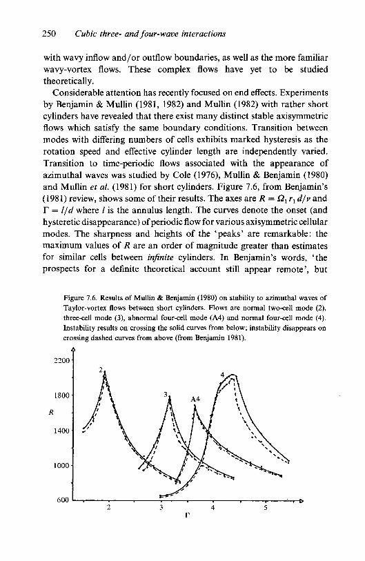
250 Cubic three- and four-wave interactions
with wavy inflow and/or outflow boundaries, as well as the more familiarwavy-vortex flows. These complex flows have yet to be studiedtheoretically.
Considerable attention has recently focused on end effects. Experimentsby Benjamin & Mullin (1981, 1982) and Mullin (1982) with rather shortcylinders have revealed that there exist many distinct stable axisymmetricflows which satisfy the same boundary conditions. Transition betweenmodes with differing numbers of cells exhibits marked hysteresis as therotation speed and effective cylinder length are independently varied.Transition to time-periodic flows associated with the appearance ofazimuthal waves was studied by Cole (1976), Mullin & Benjamin (1980)and Mullin et al. (1981) for short cylinders. Figure 7.6, from Benjamin's(1981) review, shows some of their results. The axes are R = Q1r1 d/v andF = l/d where / is the annulus length. The curves denote the onset (andhysteretic disappearance) of periodic flow for various axisymmetric cellularmodes. The sharpness and heights of the 'peaks' are remarkable: themaximum values of R are an order of magnitude greater than estimatesfor similar cells between infinite cylinders. In Benjamin's words, 'theprospects for a definite theoretical account still appear remote', but
Figure 7.6. Results of Mullin & Benjamin (1980) on stability to azimuthal waves ofTaylor-vortex flows between short cylinders. Flows are normal two-cell mode (2),three-cell mode (3), abnormal four-cell mode (A4) and normal four-cell mode (4).Instability results on crossing the solid curves from below; instability disappears oncrossing dashed curves from above (from Benjamin 1981).
22002,
1800
1400
1000
600
Downloaded from University Publishing Online. This is copyrighted materialIP139.153.14.250 on Tue Jan 24 02:27:40 GMT 2012.
http://dx.doi.org/10.1017/CBO9780511569548.008

24 Mode interactions in Taylor-Couette flow 251
(24.3)
qualitative insights are gained by approaches employing abstract mathe-matics (e.g. Benjamin 1978).
End effects are more easily modelled for long, but finite, cylinders withends at z = +/. This was done by Hall (1980a,b, 1982) and Stuart &DiPrima (1980). Axisymmetric modes denoted by Ac = A and As = B areeven and odd, respectively, in z and may then satisfy
dA/dt = <TA A+a20 A2+a02 W + a30 A3+a12
dBjdt = aBB+a11AB+a03B3+a21A
2B+...,
far from the ends. As /->oo, crA/<rB-^-1, a20, a02 and a n approach zero anda30, a12, a03, a21 become equal: these equations then resemble (24.1a,b)without the Bs and Bc modes.
Small, but non-zero, quadratic coefficients a20, a02 and an, along withslightly different linear growth rates and cubic coefficients, destroy symmetryand indicate a preference for one or other mode. Odd equilibriumsolutions, in addition to the trivial 5 = 0, are
A=0 (T>TB),
which resemble the supercritical equilibrium states described above. As <rB
increases from zero at T = TB with a03 negative, these give the ' pitchfork'bifurcation from B = 0 shown in Figure 7.7(a). Even solutions are inequilibrium when
<TAA + awAi+a3()A3 + O{Ai) = Q, 5 = 0,
where a20 is numerically small; the two non-trivial solutions show asym-metric 'transcriticaP bifurcation from A = 0 as in Figure U(Jb). Onesolution branch now extends to subcritical Taylor numbers.
The supercritical, dashed, portion of the curve is known to be unstablewith respect to small changes in A (see e.g. Joseph 1976). The solution withA < 0 is stable to small changes in A; but it would be unstable to phase
Figure 7.7. Typical (a) 'pitchfork' and (b) 'transcritical' bifurcations. Solid portionsdenote equilibrium solutions stable to amplitude perturbations, dashed portionsdenote unstable solutions.
B
(b)
Downloaded from University Publishing Online. This is copyrighted materialIP139.153.14.250 on Tue Jan 24 02:27:40 GMT 2012.
http://dx.doi.org/10.1017/CBO9780511569548.008

252 Cubic three- and four-wave interactions
variations, and so evolve towards the solution with A > 0, if such phasevariations were compatible with the end-wall boundary conditions.
But equations (24.3) are appropriate only for end-wall boundaryconditions at z = + / which admit a purely azimuthal primary flow. Infact, realistic end conditions drive flows with some axial and radialdependence at all rotation speeds of the inner cylinder (cf. Benjamin &Mullin 1981). Fourier decomposition shows that additional constant termseA, eB must then be added to the right-hand sides of (24.3): these constantsapproach zero as /^oo, and eA or eB is zero if the boundary conditionsare respectively symmetric or antisymmetric. With non-zero values eA, eB,the bifurcations are 'imperfect' and single-mode equilibrium solutions areas shown schematically in Figure 7.8(a), (b), (c).
The dashed portions of the curves are unstable to small amplitudechanges. Some curves, but not others, admit a smooth transition betweenthe primary flow and Taylor-vortex flow as T is increased. Imperfectbifurcations of similar kind were first analysed, for thermal convection infinite containers, by Kelly & Pal (1976, 1978), Hall & Walton (1977) andDaniels (1977). Mixed modes, with both A and B present, are discussedby Hall (1980b, 1982) for Taylor-vortex flow and by Hall & Walton (1979)for Benard convection. Benjamin (1978), Schaefler (1980) and Joseph(1981) have demonstrated the generic nature of such solutions and clarifiedtheir relationship to Thorn's (1975) catastrophe theory.
Figure 7.8. Equilibrium solutions with imperfect bifurcation, (a) B(T) for eB > 0(inverted for eB < 0); (2>) A(T) for eA > 0; (c) A(T) for eA < 0.
A
(*)
(c)
Downloaded from University Publishing Online. This is copyrighted materialIP139.153.14.250 on Tue Jan 24 02:27:40 GMT 2012.
http://dx.doi.org/10.1017/CBO9780511569548.008

24 Mode interactions in Taylor-Couette flow 253
24.4 Doubly-periodic and' chaotic' flowWavy-vortex flow remains strictly periodic, with a dominant
frequency (ox and its harmonics, until the Reynolds number R is an orderof magnitude larger than its value Rc at onset of Taylor instability.Fenstermacher, Swinney & Gollub (1979), employing a laser-Dopplertechnique to measure the flow at a single point, found rather sudden onsetof a second, incommensurate frequency w3t at R/Rc = 10.1: see Figure7.9. (Strictly, 'incommensurate' means that w3/wj is irrational; but, forpresent purposes, it is taken to mean that no small integers m, n, less than10 say, exist with m/n = (o^/io^). Gorman & Swinney (1982) identified w3
with a modulation of the wavy vortices, which was usually spatial as wellas temporal. Their visual observations showed a periodic 'flattening' ofone or more wavelengths around the annulus. The evolution with azimuthalangle <j> and time t took various forms, characterized by a pair of integers(n\k): here, n denotes the azimuthal mode number of the waves and k thatof the modulation. Gorman & Swinney's schematic representation ofseveral of these forms is reproduced in Figure 7.10.
The purely temporal modulations (cases «|0) might be thought tocorrespond to periodic solutions of (24.1), with continuous energy exchangeamong the modes A, Bc and Bs: after all, the rather similar four-waveresonance equations (23.3) display periodic modulations. DiPrima (1981)has noted that Eagles' (1971) calculated coefficients do not admit thispossibility, but these results relate to fairly small values of (R — Re)/Re.Also, these truncated equations are formally valid only as the linear growthrates a0, b0 simultaneously approach zero: and this is never so for n 4= 0!The practical range of approximate validity of (24.1) is unknown, but isunlikely to extend to R/Rc > 10.
Gorman & Swinney found their results to be qualitatively consistentwith a rather abstract but general theory of Rand (1981). They also seemto be consistent with the growth of modes with azimuthal mode numbersdiffering from that of the fundamental wavy vortices. In particular,azimuthal modes n + l , n ± 2 , . . . interact resonantly with the n-mode (aswell as with the primary Taylor vortices) since their azimuthal phase speedsare known to be the same: the growth of such modes might well induceazimuthal modulations like those of Figure 7.10. Modes with slightlydifferent axial wavenumbers a could also play a part. Further computationalwork may be expected to clarify the issue.
Shortly after the appearance of two incommensurate frequencies,
t Subscript 3 is used to accord with Fenstermacher et al.'s notation.
Downloaded from University Publishing Online. This is copyrighted materialIP139.153.14.250 on Tue Jan 24 02:27:40 GMT 2012.
http://dx.doi.org/10.1017/CBO9780511569548.008

254 Cubic three- and four-wave interactions
Figure 7.9. Measured time-dependence of radial velocity component and correspond-ing frequency power spectra at various R/Rc (from Fenstermacher et at. 1979).Values of R/Ro in (a)-{h) are 9.6, 10.1, 11.0, 15.1, 18.9, 21.7, 23.0, 43.9 respectively.
1 i-o
<
II113 2
(a)
IlllIffl4 t
(b)
R/Rc
IIIw6 {
= 9.6
f3a.
= 10.1
102
10°
10'2
10"4
«1
Ik Mid n^lUiw
J - ' i o '
2CJ3-CJ!u2
3O)3—CO!
% ^
">3
Downloaded from University Publishing Online. This is copyrighted materialIP139.153.14.250 on Tue Jan 24 02:27:40 GMT 2012.
http://dx.doi.org/10.1017/CBO9780511569548.008

24 Mode interactions in Taylor—Couette flow 255
Fenstermacher et al. (1979) observed the development, at aboutR/Rc =12, of a weak broadband contribution to the frequency spectrummeasured at a single point. As R/Rc further increased, so too did theintensity of this broadband 'peak' and also the background noise. Thesharp modulation-frequency peak w « w3 disappeared at R/Rc = 19.3 and
Figure 7.9(e-h). For legend see opposite.(e) R/Rc = 18.9
10'
^. 10°o
l l O " 2
cu
10"4
•
LJ
Downloaded from University Publishing Online. This is copyrighted materialIP139.153.14.250 on Tue Jan 24 02:27:40 GMT 2012.
http://dx.doi.org/10.1017/CBO9780511569548.008

256 Cubic three- and four-wave interactions
the wavy-vortex frequency peak itself vanished at R/Rc = 21.9. Thespectrum then appeared to be continuous and so suggestive of fully-developed turbulence. However, after similar events in a different apparatus,Walden & Donnelly (1979) witnessed the surprising re-emergence of asharp spectral peak for 28 < R/Rc < 36.
Koschmieder (1980), DiPrima (1981), DiPrima & Swinney (1981) andL'vov, Predtechensky & Chernykh (1983) review these and other relatedstudies. A notable feature of flows at large R/Rc is the persistence of astrong Taylor-vortex configuration along with the 'turbulence'. The
Figure 7.10. Gorman & Swinney's (1982) schematic representation of periodictemporal modulations, in reference frame rotating with the waves. Each diagramrepresents evolution in time of a single vortex outflow boundary (not a stack of vorticesat fixed time). Heavy lines denote greatest 'flattening'. Corresponding values of (n \k)are noted.
4/1
4/2
Downloaded from University Publishing Online. This is copyrighted materialIP139.153.14.250 on Tue Jan 24 02:27:40 GMT 2012.
http://dx.doi.org/10.1017/CBO9780511569548.008

24 Mode interactions in Taylor-Couette flow 257
robustness of these axisymmetric vortices is remarkable. So, too, is the factthat the observed number of cells, even in 'turbulent' flow, is determinedby the past history of the flow and not just the operational value of R. Sucha 'memory' is inconsistent with most notions of strong turbulence.
Much attention has recently focused on theoretical analyses of modelsystems of low dimension which display' strange attractor' behaviour: see,e.g. Swinney & Gollub (1981). One such model, for three-wave interactions,was described in § 16.2. The first, and most celebrated, was that of Lorenz(1963), whose three-variable analogue of Rayleigh-Benard convectionexhibited apparently chaotic behaviour. Ruelle & Takens (1971) laterproposed that a generic feature of low-dimensional strange-attractormodels is the emergence of two incommensurate frequencies followed by'chaotic' motion with a broadband frequency spectrum. With this workand the experiments of Fenstermacher et al. (1979) in mind, Sherman &McLaughlin (1978) investigated a set of five amplitude equations withquadratic coupling. These exhibited transition from sharply-peaked tobroadband frequency spectra as a growth-rate parameter was varied, buttheir model is not strictly applicable to the experiments. It may beconjectured that equations (24.1) would display qualitatively similarproperties for some ranges of the parameters. There are obvious similarities,too, with the computations of Yuen & Lake (1982) described above, onsideband modulations of gravity waves.
More elaborate computational models have been constructed by Yahata(1981, 1983a), who employed a Galerkin representation of axisymmetricand « = 4 modes comprising 56 separate functions. Essentially, hisconfiguration represents four-wave interaction among modes (a,0),(2a, 0), (a, 4), (a , -4) and mean flow (0,0). The results exhibit theappearance and then disappearance of two and three dominant frequencies(plus sum and difference harmonics) and the onset of chaotic motion. Thesemay have a bearing on Gorman & Swinney's modulated wavy (n | A:)-vorticeswith k = 0, but the computations do not allow for azimuthal modulations.Finally, it should be remembered that these chaotic motions take place ina low-dimensional system comprising just a few spatially-periodic modes(C'est chaotique, mais ce n'est pas la turbulence!). In contrast, much ofthe 'noise' which comes to dominate turbulent flow at large R seems tobe associated with small spatial scales: these are evident in Figure 7.5 evenat the fairly low values R/Rc — 16 and 23.5. Recent overviews of 'orderin chaos' are given in Campbell & Rose (1983) and Barenblatt, Iooss &Joseph (1983).
Downloaded from University Publishing Online. This is copyrighted materialIP139.153.14.250 on Tue Jan 24 02:27:40 GMT 2012.
http://dx.doi.org/10.1017/CBO9780511569548.008
258 Cubic three- and four-wave interactions
25 Rayleigh-Benard convection25.1 Introduction
Thermally-driven convective instabilities in horizontal fluid layersheated uniformly from below have many similarities with Taylor-Couetteflow. But there are also important differences: while the latter are stronglyanisotropic, with well-defined axial, azimuthal and radial dependence,convective flows are usually much less so. Convection cells in layers ofinfinite lateral extent have no preferred horizontal orientation and hori-zontal anisotropy is weak in layers of large aspect ratio where thehorizontal dimensions greatly exceed the depth.
Convective instabilities may lead to stable rolls, with well-definedwavenumber k, which are very similar to steady axisymmetric Taylorvortices, both mathematically and physically. Governing dimensionlessparameters are the Rayleigh number R and the Prandtl number P, definedas
y1gATd3 vR =VK K
(Note that, in this section, R no longer denotes Reynolds number.) Here,v and K are kinematic viscosity and thermal diffusivity, d the layer depth,g gravitational acceleration, y1 the coefficient of thermal expansion andAT the temperature difference between bottom and top boundaries.
Instability first sets in at a particular value kc of | k | when the Rayleighnumber R (a dimensionless measure of the importance of buoyancy overdiffusive processes) exceeds a critical value Rc. The value Rc depends onthe boundary conditions but not on the Prandtl number P of the fluid. Withrigid horizontal boundaries, Rc = 1708 for layers of infinite lateral extentand the orientation of k is immaterial. In practice, however, lateralboundaries play an important part in selecting a preferred mode, especiallywhen the aspect ratio is not large. For instance, rectangular side wallsusually favour rolls aligned parallel to the shorter side and circular wallsmay give rise to concentric circular cells. Nevertheless, a marked lack ofuniqueness remains and many stable convective flows may satisfy identicalboundary conditions.
Cellular convection was first systematically examined by Benard (1900,1901) in a shallow liquid layer with free upper surface, but there are manyearlier reports of the phenomenon (see Normand, Pomeau & Velarde1977). The hexagonal cells observed by Benard correspond to threesuperposed roll patterns, with wavenumbers kj- (J = 1,2,3) of equalmagnitude but differing in orientation by 120°. Motion may be eitherupwards or downwards at the centres of cells depending on small vertical
Downloaded from University Publishing Online. This is copyrighted materialIP139.153.14.250 on Tue Jan 24 02:27:40 GMT 2012.
http://dx.doi.org/10.1017/CBO9780511569548.008
25 Rayleigh-Benard convection 259
asymmetries, such as the temperature dependence of fluid viscosity, andon surface tension effects. In shallow layers like Benard's, horizontaltemperature-induced gradients in surface tension are more powerful thanbuoyancy in driving the flow (Pearson 1958). Here, attention is mainlyfocused on buoyancy-driven convection in layers confined by rigid topand bottom boundaries. Previous reviews of theory and experimentinclude those of Palm (1975), Normand, Pomeau & Velarde (1977) andBusse (1978, 1981a, b). A rigorous approach to theoretical aspects is givenby Joseph (1976).
25.2 Instabilities of rollsA weakly nonlinear amplitude-expansion analysis by Schluter,
Lortz & Busse (1965) extended earlier work of Gor'kov (1957) and Malkus& Veronis (1958). This elucidated the properties of steady finite-amplitudeconvection in horizontally-infinite layers between rigid parallel boundariesat small positive values of R — Rc. They found that the only stable flowsare longitudinal rolls with a range of | k | centred on kc that is narrowerthan the bandwidth for linear instabilities. (In contrast, configurations withvertical asymmetry are subcritically unstable (R < Rc) to finite-amplitudedisturbances and hexagonal cells are preferred near Rc: see below.)
Near Rc, the instability of rolls with wavenumbers outwith this rangeis due to growth of modes with wavenumbers closer to kc. For instance,when k = (k, 0) and k is too small, an instability bends the roll axis intoa sinusoid, thereby exciting (resonant) modes (k, ± I) with greaterwavenumber (k2 + l2)*: both conditions (23.1) are satisfied since the rollshave zero frequency. This is the 'zig-zag instability' observed by Busse &Whitehead (1971) with angles of about 40° and 140° between the new andoriginal rolls. In contrast, rolls with k too far above kc - but still withinthe linearly-unstable bandwidth - are normally replaced, through 'cross-roll instability', by rolls at right angles with wavenumber close to (0, ke).Both types of instability are shown in Figure 7.11 taken from Busse &Whitehead (1971). Also possible is a two-dimensional Eckhaus instability(Stuart & DiPrima 1978) of sidebands (k ±8,0) with the same orientationas the original rolls.
Newell & Whitehead (1969) analysed roll cells with wavenumberk = (kc, 0) and slowly-varying amplitude eA(x, y, t) at R just above Rc.With suitably-scaled variables, the amplitude equation may be written inthe form
Downloaded from University Publishing Online. This is copyrighted materialIP139.153.14.250 on Tue Jan 24 02:27:40 GMT 2012.
http://dx.doi.org/10.1017/CBO9780511569548.008

(a)
Figure 7.11. Temporal development of (a) 'cross-roll' instability and (b) 'zig-zag' instability of convection rolls (from Busse & Whitehead 1971).In (a), R = 3000, depth = 5 mm, k = 2n/\.64; times between successive photographs are 10, 4, 3, 7, 24min respectively. In (b), R = 3600,depth = 5 mm, k = 2TT/2.8; times between photographs are 9, 10, 10, 26, 72 min.
Downloaded from University Publishing Online. This is copyrighted materialIP139.153.14.250 on Tue Jan 24 02:27:40 GMT 2012.
http://dx.doi.org/10.1017/CBO9780511569548.008

(b)
Figure 7.11 (b). For legend see opposite.
Downloaded from University Publishing Online. This is copyrighted materialIP139.153.14.250 on Tue Jan 24 02:27:40 GMT 2012.
http://dx.doi.org/10.1017/CBO9780511569548.008

262 Cubic three- and four-wave interactions
The Eckhaus instability, and similar sideband instability of oblique modesk = (&„ + #!, ±S2) with \3j/kc \<\, may be deduced from this equationmuch as outlined in §21.1 for gravity waves. The form of the linearoperator on the left-hand side is a consequence of the linear growth-raterelation,
near (Rc,ke). Setting k = (kc+K,L) where K, L are small, gives
and transformations K^~ i 6/6JST, L^—ik\ 8/3 Y yield the required form.(In contrast, the nonlinear Schrodinger equation results from dispersionrelations with a leading-order L-term proportional to L2.)
At larger R, a 'skewed varicose instability' affects even those rolls with| k | x kc. This is apparently associated with the growth of 'subharmonic'modes (\k, ± I) and so may be an instance of three-wave resonance.
A further type of instability differs from the above-mentioned (quasi-)steady flows in being time-periodic. This oscillatory instability of steadyrolls sets in close to Rc if the Prandtl number P is very small and if bothupper and lower boundaries are stress-free: but transition is delayed tolarger R for rigid boundaries. For P%\, the rolls are sinusoidallydistorted as in the 'zig-zag' instability, but they also oscillate in time, eitheras travelling or standing waves.
For onset of oscillatory instability, there is qualitative agreementbetween calculations (Clever & Busse 1974; Lipps 1976) and experimentfor P < 2 (Krishnamurti 1970; Busse & Whitehead 1974), but observedand theoretical frequencies differ somewhat. The similarity with onset ofwavy vortices in Taylor-Couette flow is striking, though oscillatorystanding waves have not been observed in the latter flow. At larger P, onsetof oscillatory instability is delayed to higher values of R, and other typesof instability (notably cross rolls) may appear first. The observed perioddecreases as R increases.
Krishnamurti (1973) describes the periodicity, for large P and R, as dueto the orbiting of local hot or cold spots (with associated high shear)around the roll-cell, rather than distortions of the cell axis. Behaviour ofthis sort was reproduced in computations of Moore & Weiss (1973), forfree boundaries and with the motion artificially restricted to be two-dimensional: with P = 6.8, as for water, their oscillations set in at aroundR/Rc = 50. Lipps (1976) undertook a three-dimensional direct numerical
Downloaded from University Publishing Online. This is copyrighted materialIP139.153.14.250 on Tue Jan 24 02:27:40 GMT 2012.
http://dx.doi.org/10.1017/CBO9780511569548.008

25 Rayleigh-Benard convection 263
simulation for air (P = 0.7) between rigid upper and lower boundariesand stress-free 'sidewalls' which admitted spatially-periodic solutions.Previously two-dimensional rolls became wavy and time-periodic atR « 6500 (R/Rc ~ 3.8); more complex spatial and time dependence setin for R ^ 9000. Though the sidewall conditions admit only discrete cellsizes, these results are convincing.
The current theoretical situation is more fully set out by Busse (1981a, b).His map of the predicted region of stable finite-amplitude two-dimensionalrolls in k-R-P parameter space is reproduced in Figure 7.12. This regionis bounded by onset of various kinds of instability and summarizes results
Figure 7.12. Region of stable two-dimensional convection rolls in k-R-P space. Thisis bounded by various types of instability: oscillatory (OS), skewed varicose (SV),cross-roll (CR), knot (KN) and zig-zag (ZZ) (Busse 1981a, b).
CR
2.0/ 3.0 4.0 5.0
Downloaded from University Publishing Online. This is copyrighted materialIP139.153.14.250 on Tue Jan 24 02:27:40 GMT 2012.
http://dx.doi.org/10.1017/CBO9780511569548.008

264 Cubic three- and four-wave interactions
of several earlier numerical studies by Busse and Clever. These studies allemployed Galerkin representations of the rolls, as truncated series oforthogonal functions; the imposition of small disturbances of the requiredform led to linear eigenvalue problems which determined their stability.Though these results are probably quite accurate, the range of validity ofsuch series-truncation methods is difficult to establish, other thanempirically.
25.3 Rolls infinite containersThe influence of aspect ratio modifes the picture. With large aspect
ratios, the multi-roll pattern which first emerges from random backgrounddisturbances is patchy, with each patch containing rolls of differingorientation. Dislocations at patch boundaries, where different cell structuresmeet, move with time, causing some patches to shrink and others to grow.An experimental study of the merging, or 'pinching', of artificially createdroll cells with the same orientation but differing wavenumber was madeby Whitehead (1976). Gollub, McCarriar & Steinman (1982) have recentlyexamined evolving convection patterns in layers of large aspect ratio.
In contrast, the theoretical configurations analysed by Kelly & Pal (1976,1978), Daniels (1977) and Hall & Walton (1977, 1979) are strictlytwo-dimensional, consisting of parallel rolls with fixed orientation. Theseaccounts of secondary and imperfect bifurcations, already mentioned in§24.3 above, apply only rather close to the critical Rayleigh number Rc
for onset of convection.For convection in a box of small aspect ratio, only a limited number
of flow configurations are possible and rather sharp transitions from oneto the other may be observed. For this reason, recent experiments haveconcentrated on high-precision measurements in small-aspect-ratio appar-atus of small scale. For instance, Gollub & Benson (1980) used laser-Doppler measurement to study convection in a rectangular box about 1 cmdeep and less than 3 cm long, which typically contained only two or threeroll cells. Ahlers & Behringer (1978) employed cryogenic techniques tostudy heat transfer in (normal) liquid helium *He. This was contained insmall cylinders of about 1 or 2.5 cm diameter and various aspect ratios(r = radius/depth) from 2 to 57.
Though the above-mentioned instabilities are suppressed or delayed bythe proximity of sidewalls, the evolution of theflow as R is gradually raisedremains complex. The influence of Prandtl number, aspect ratio andsidewall configuration are all important. Gollub & Benson (1980) describedfour quite separate 'routes to turbulent convection' (by which they mean
Downloaded from University Publishing Online. This is copyrighted materialIP139.153.14.250 on Tue Jan 24 02:27:40 GMT 2012.
http://dx.doi.org/10.1017/CBO9780511569548.008

25 Rayleigh-Benard convection 265
the development of temporally-periodic flows into flows with broadbandfrequency spectrum).
In the first, a two-cell configuration at P = 5.0 became oscillatory, withsome frequency wx, at R/Re = 27.2 (Re being the value of R for onset ofconvection in an infinite layer, not in their apparatus); a second apparentlyunrelated frequency w2 appeared at R/Rc = 32; then, at aboutR/Rc — 44.4, these frequencies 'phase-locked' at w1/w2 « 7/3; next,substantial broadband noise developed at the slightly higher R/Re = 46.0and this increased while (D1/(D2 decreased as R/Rc was made larger;ultimately, the peaks at wx and w2 became submerged in the broadbandspectrum.
In the second, a similar two-cell configuration at the lower Prandtlnumber P = 2.5 became oscillatory at R/Rc = 17; sharp spectral peaks at(o1 and its harmonics were observed until, at /J/i?c = 21.5, a period-doublingsubharmonic component |w2 appeared; by R/Rc = 26.5, the l ^ componenthad dominated the fundamental, and a second subharmonic bifurcation,to Jwj, set in; the flow became non-periodic at about R/Rc = 28 and thepeaks of the frequency spectrum merged with the broadband contributionat about R/Rc = 40.
Three-cell configurations behaved very differently. At P = 2.5, forexample, period flow set in at R/Rc « 30 and apparently independentfrequencies w2, w3 appeared at 39.5 and 41.5; broadband noise began togrow at R/Ro — 43. At higher P, similar behaviour was found, but onsetof a>2 and w3 was delayed to larger R/Rc.
Finally, instances were found where a)2/ct)1 was rather small, such thatthe velocity records showed slow periodic modulations in the amplitudeof (^-oscillations. In a three-cell case with P — 5.0, the w2 modulationsappeared at R/Rc = 95 and intermittent noise of irregular duration set inat R/Rc — 102; at greater R/Rc, a featureless broadband spectrum wasobtained.
Ahlers & Behringer (1978) reported onset of aperiodic 'turbulent' flowsat R/Rc close to 1 for their largest aspect ratio of F = 57; the value of R/Rc
at onset increased as F was reduced, reaching about 11 when F = 2.08.Rather similar results were found by Libchaber & Maurer (1978). Theadditional effect of a magnetic field on convection in mercury was exploredby Libchaber, Fauve & Laroche (1983).
Gollub & Benson could discern 'no simple rules for predicting whichsequence will occur for a given aspect ratio, Prandtl number, and meanflow' but each of their observed sequences is characterized by modeinteractions. The route through two incommensurate frequencies to
Downloaded from University Publishing Online. This is copyrighted materialIP139.153.14.250 on Tue Jan 24 02:27:40 GMT 2012.
http://dx.doi.org/10.1017/CBO9780511569548.008

266 Cubic three- and four-wave interactions
broadband spectrum parallels the behaviour of Taylor vortices. Thesubharmonic bifurcations are reminiscent of quadratic three-wave reso-nance, but lack of information about the spatial structure precludes firmidentification. For the same reason, emergence of three distinct frequenciesdefies precise interpretation: no direct connection with the theory of Ruelle& Takens (1971) has yet been established, though qualitative similaritiesexist. As to intermittent noise, it is tempting to draw parallels with the onsetof intermittent, spatially-localized, patches of turbulence in parallel shearflows (see §27.2) but here, again, data on the spatial structure is lacking.
A 14-mode Lorenz-attractor model investigated by Curry (1978) and asystem of several modes solved numerically by Yahata (1982, 1983b)reproduce various of the observed features, including period-doublingbifurcations and transition to 'chaotic' time-dependence. However, thesemode-truncated models should not be regarded as precise representationsof the flow. An interesting example of an experiment which apparently doescorrespond exactly to a known strange-attractor system of ordinarydifferential equations is that described by Roux, Simoyi & Swinney (1983):this concerns the remarkable Belousov-Zhabotinskii reaction of chemicalkinetics.
In a numerical study of doubly-diffusive thermosolutal convection,Huppert & Moore (1976) solved the governing partial differential equa-tions by finite differences and found transitions from time-periodic tochaotic motion. Further work by Da Costa, Knobloch & Weiss (1981) andby Moore et al. (1983) has revealed further details of the solution structure,for two-dimensional convection with fixed roll spacing and stress-freehorizontal boundaries. As the thermal Rayleigh number RT was increased,with other flow parameters assigned constant values, finite-amplitudeoscillatory rolls gave way to chaotic motion through a sequence ofperiod-doubling bifurcations. As RT was further increased, a narrow'window' was found which yielded oscillatory solutions with three timesthe original dimensionless period T = 1; these then passed through moreperiod-doubling bifurcations till chaotic motion was re-established. Solu-tions at still larger RT yielded 'an inverse cascade of period-halvingbifurcations leading to solutions with period 1, followed by anothertransition back to chaos through a period-doubling sequence'. Figure7.13 (a)-(ti) shows examples of phase-plane trajectories and frequencypower spectra of the total kinetic energy. Cases (a, b) and (g, h) are the 2Tand 3T periodic limit cycles while (c, d) and (e, / ) describe 'semi-periodic'chaotic motion.
A recent review by Swinney (1983), of order and chaos in nonlinear
Downloaded from University Publishing Online. This is copyrighted materialIP139.153.14.250 on Tue Jan 24 02:27:40 GMT 2012.
http://dx.doi.org/10.1017/CBO9780511569548.008
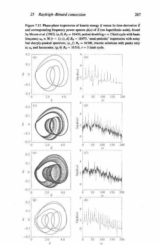
25 Rayleigh-Benard convection 267
Figure 7.13. Phase-plane trajectories of kinetic energy E versus its time-derivative isand corresponding frequency power spectra <j>((o) of E (on logarithmic scale), foundby Moore et al. (1983). (a, b) RT = 10450, period-doubling r = 2 limit cycle with basicfrequency w0 « 30 (r = 1); (c,<f) i?T = 10475, 'semi-periodic' trajectories with noisybut sharply-peaked spectrum; (e,f) RT = 10500, chaotic solutions with peaks onlyat <o0 and harmonics; (g,h) RT= 10510, T = 3 limit cycle.
0.2 r
0.2
0.1
E 0
-0.1
-0.2
2.0 4.0
2.0
(b)
n
50 100 150 20000
E
> )
frnWm
4.0 50 100 150 200CO
Downloaded from University Publishing Online. This is copyrighted materialIP139.153.14.250 on Tue Jan 24 02:27:40 GMT 2012.
http://dx.doi.org/10.1017/CBO9780511569548.008

268 Cubic three- and four-wave interactions
systems, mentions many other related experiments and recent theoreticaldevelopments which cannot be discussed here: the richness of structurerevealed in recent years is both remarkable and bewildering.
25.4 Three-roll interactionsAn interesting case of three-mode interaction for convection in
infinite rotating layers was studied by (Clippers & Lortz (1969) and Busse& Clever (1979) (also reported by Busse 1981a). The latter's perturbationanalysis relates to three sets of rolls, each with the same wavenumbermodulus |k | , but orientations differing by 120°. Accordingly,
k1 + k2 + k3 = 0
and, since the corresponding frequencies are zero, quadratic resonancemight be expected. In layers of fluid otherwise at rest, each set of rolls isstable provided R/Rc is not too far above unity, and one possibility isfinite-amplitude hexagonal cells. However, the mode-interactions are nothere of quadratic order: though the governing evolution equations havethe form of (16.7), the quadratic coefficients are identically zero (by reasonof vertical symmetry) and the dominant interactions are cubic. Also, thelinear-growth rates — <Tj are equal and the cubic coupling coefficients ai}-are found to be imaginary with iccjjc > 0.
By means of symmetry arguments and the transformationsGi = I % / ° > 11 Aj I2> r= - o-j t,
the governing equations may be recast as
(25.1)= G,(l-G,-aG1-/?Ga)J
where a and /? are positive constants. For convection in layers at rest, a = /?and possible finite-amplitude equilibrium states are the individual-rollconfigurations
G,= l, G} = 0 ( / * » = 1.2 or 3),
and the hexagons
Gi = ( l + 2 a ) " 1 (z= 1,2 and 3).
Differing positive values of a and /? arise when the layer is rotating abouta vertical axis: then, individual rolls remain possible equilibrium solutions,but these are unstable whenever one of a, /? is less than unity. Theequilibrium combined-mode solution is
0 '= 1,2,3)
Downloaded from University Publishing Online. This is copyrighted materialIP139.153.14.250 on Tue Jan 24 02:27:40 GMT 2012.
http://dx.doi.org/10.1017/CBO9780511569548.008

25 Rayleigh-Benard convection 269
and this is stable to small perturbations of the Gt if and only if a+/? < 2.Accordingly, in the two regions of parameter space
R1 = {a,fi: 0 < a < 1, a+/3 > 2}, R2 = {a,/1: 0<@< l , a + / ? > 2 } ,
no equilibrium solution is stable.Surprisingly, this absence of stable equilibrium solutions does not signal
transition to time-periodic flow: such oscillatory solutions cannot exist, atleast near Rc, when P > 1. Instead, solutions of (25.1) rapidly approachthe plane G1 + G2 + Gs= 1 and then wander around seeking, but neverattaining, one or other of the single-roll fixed points Gi = 1 (i = 1, 2 or3). The solutions are neither periodic nor' chaotic' but spend ever-increasingtimes in the vicinity of each fixed point. This behaviour was first describedby May & Leonard (1975), who investigated (25.1) as a model ofthree-species competition in biological population dynamics. A similar'period lengthening' was noted in §16.2 for damped three-waveinteractions.
Both May & Leonard (1975) and Busse (1981a) reject continued periodlengthening as unphysical, since the minimum value of each G; for eachcycle is ever-decreasing. In practice, random low-level disturbances inevi-tably affect the temporal and spatial evolution, as apparently found inexperiments by Busse & Heikes (1980): the 'period' is then an irregular,stochastic function.
Segel (1962) examined the interaction of two sets of roll cells withparallel wavenumbers ku k2 of differing magnitude. The governingequations, with vertical symmetry, are then as (25.1), but with one mode,say G3, equal to zero. When rolls with wavenumbers k1 + k2 are not toostrongly damped, one would expect these to be driven unstable by the cubicinteraction.
In earlier theoretical investigations of hexagonal convection, Palm(1960), Segel & Stuart (1962) and Segel (1965) incorporated verticalasymmetry due to weak temperature dependence of the fluid viscosity;
v{T) = v0 + Av cos [n(T- ro)/(7; - To)], Av/v0 < 1,
say, where Tu To are the temperatures at stress-free lower and upperboundaries respectively. At leading order, perturbation quantities may bewritten in the form
<p = A1cos {ay + 6J + A2 cos [£a( y - 3h) - 02] + A3 cos [\a,(y + 3h) - d3].
Here, the A] and 6} depend on t only and are the (real) amplitudes and
Downloaded from University Publishing Online. This is copyrighted materialIP139.153.14.250 on Tue Jan 24 02:27:40 GMT 2012.
http://dx.doi.org/10.1017/CBO9780511569548.008

270 Cubic three- and four-wave interactions
phases of three roles inclined at angles of 60° to one another. Aperturbation analysis, taken to cubic order in A}, leads to equations of theform
(25.2)A2 = <rA2 — aAy A3 cos (6l + d2
A3 = aA3 — aA1A2 cos(0! + 02
A\ &1 = A\ 62 = A\ d3 = aAx A2A3 sin (0 t+
with terms of higher than cubic order omitted. These are equivalent to thethree complex amplitude equations (16.7) with real coupling coefficients.Segel & Stuart (1962) retain terms in the second time derivatives, A}, butthese are negligible when At are small. The constant coefficients a-, p andr are just those obtained by neglecting the temperature variations of v, buta is proportional to Av. In other words, vertical asymmetry is responsiblefor quadratic coupling which is absent in the symmetric case.
Below Rc, a- < 0 and there are no non-trivial equilibrium states if a = 0,since p and r are positive. But quadratic coupling admits a class ofsubcritical hexagonal cells,
Ax = A2 = A3 = A, dl-\-d2 + 03 = n,with
A = \(r + ipY1 {a ± [a2+4<r(r + 2p)% a > 0,
Figure 7.14. Schematic representation of finite equilibrium states corresponding tohexagons and rolls. A denotes amplitude, R the Rayleigh number; linear instability(a- > 0) occurs for R > Rc. Solid curves are stable, dashed curves unstable, toamplitude perturbations.
Downloaded from University Publishing Online. This is copyrighted materialIP139.153.14.250 on Tue Jan 24 02:27:40 GMT 2012.
http://dx.doi.org/10.1017/CBO9780511569548.008

25 Rayleigh-Benard convection 271
Figure 7.15. Hexagonal convection with a free surface: (a) R < Re, (b) R > Rc,from Koschmieder (1967).
Downloaded from University Publishing Online. This is copyrighted materialIP139.153.14.250 on Tue Jan 24 02:27:40 GMT 2012.
http://dx.doi.org/10.1017/CBO9780511569548.008
272 Cubic three- and four-wave interactions
whenever c > — \a\r + 2p)~l. These are indicated schematically in Figure7.14: the lower branch, with negative sign, is unstable to perturbations ofA and the upper branch is stable. Corresponding solutions, with the signof A reversed, are obtained for 61 + 62 + 8s = 0 and also for a < 0.
Above Rc, equilibrium solutions include the hexagons just described andalso individual rolls. Other equilibrium solutions of' mixed' type also exist,but these are always unstable (Segel 1965). The regions of stability ofhexagons and rolls are indicated qualitatively in Figure 7.14. The hexagonsshown with A > 0 have upwards motion at the cell centres when Av < 0and downwards motion when Av > 0; those shown with A < 0 (orequivalently, A > 0 with 01 + 62 + 6S = 0) have opposite directions ofmotion and are unstable to phase perturbations. It must be rememberedthat the truncated equations (25.2) give valid approximations for theequilbrium solutions only when a, a (and so A) are sufficiently small topermit the omission of higher-order terms.
Palm, Ellingsen & Gjevik (1967) derived corresponding results for morerealistic rigid-rigid and rigid-free boundary conditions at the bottom andtop. Busse (1967) included temperature variations of thermal diffusivity Kand the coefficient of expansion yx. Busse's general formulation allowedfor interactions among a large number of discrete modes and bears a closeresemblance to the discretized form of Zakharov's formulation (23.11).Scanlon & Segel (1967) discussed surface-tension driven hexagonal con-vection. In all cases, stable hexagons were found in some parameter rangenear Rc. Such hexagons were realized experimentally by Koschmieder(1967) and others, for both R < Rc and R > Rc: see Figure 7.15. Time-dependent interaction of differing hexagonal configurations has beenmodelled numerically, at rather large R, by Toomre, Gough & Spiegel(1982). Mode interactions of hexagonal configuration in baroclinic insta-bility were studied by Newell (1972) and, more generally, by Loesch &Domaracki (1977).
26 Wave interactions in planar shear flows26.1 Three dominant waves
Cubic nonlinearities influencing three-wave resonant interactionsin parallel shear flows were already mentioned in §16.3: for temporalmodulations, the governing equations have the form (16.7). Non-resonantthree-wave interactions among arbitrary wavenumbers kt give rise tosimilar cubic terms, without significant quadratic coupling; but thenfurther 'sum and difference' wavenumber components may grow toprominence unless these experience stronger linear damping than the threewaves chosen.
Downloaded from University Publishing Online. This is copyrighted materialIP139.153.14.250 on Tue Jan 24 02:27:40 GMT 2012.
http://dx.doi.org/10.1017/CBO9780511569548.008

26 Wave interactions in planar shear flows 273
Both resonant and non-resonant cases were considered by Usher &Craik (1975), who suggested, on the basis of asymptotic estimates for largeR, that particularly large cubic interaction coefficients may usually influencethe growth of symmetric oblique-mode configurations like those of §17.2.These coefficients may be largest when interaction is resonant, for all threemodes then have the same critical layer.
The parametric excitation of resonant oblique-wave modes by a two-dimensional wave was briefly discussed in §14.3, where only quadraticnonlinearities were retained. With the configuration of § 17.2, the resonancecondition selects a particular value of the spanwise wavenumber /? whichmight be expected to lie close to that of the most strongly excited mode.But cubic (and higher) nonlinearities also act to modify the frequencies andto enhance or suppress oblique modes: accordingly, these may shift thepreferred value of /? away from that at resonance. Moreover, in the specialcase of plane Poiseuille flow, the quadratic coupling coefficients are zeroby reason of symmetry, for interactions among lowest, even, Orr-Sommerfeld eigenmodes: obviously, there is then less reason for the'resonant' value of/? to be strongly excited.
Experiments of Saric & Thomas (1984) and Kachanov & Levchenko(1984) on the Blasius boundary layer all found evidence of subharmonicoblique-wave growth roughly as predicted by Craik (1971): but observedspanwise wavenumbers did not always agree closely with those predictedby the resonance criterion. Also, subharmonic oblique waves in planePoiseuille flow are reported by Ramazanov (1985).
In an attempt to clarify the situation, Herbert (1983b,c; 1984) recentlymade several computational studies. All of these concern the temporaleigenvalues of infinitesimal, symmetric, oblique-wave pairs in the presenceof a finite-amplitude two-dimensional wave. His results of (1983b) forplane Poiseuille flow appear to be inaccurate, though they, like those of(1984), show the expected parametric growth of subharmonic obliquewaves at subcritical Reynolds numbers and a preferred /? with maximumgrowth rate. Results of (1983c) for the Blasius boundary layer (neglectingnon-parallelism) display some interesting features which may be interpretedas follows.
The evolution equations of near-resonant, infinitesimal, oblique modesAlf A2 in the presence of a finite two-dimensional wave with supposedconstant amplitude Ao have the form (cf. 16.7 and Craik 1975)
Ax = a-A1 +fiA0 A * + A | Ao \*AU', (26.1)
A 2 = A A A f + A \ A \ 2 Awith truncation after cubic terms. In a reference frame moving with the
Downloaded from University Publishing Online. This is copyrighted materialIP139.153.14.250 on Tue Jan 24 02:27:40 GMT 2012.
http://dx.doi.org/10.1017/CBO9780511569548.008
274 Cubic three- and four-wave interactions
phase speed w/a of the two-dimensional wave, <r (and so A1 2) incorporatesthe effect of detuning from resonance. Setting A1 oc expst, A2 oc exps*tyields eigenvalues
When | Ao | is sufficiently small, these are complex conjugates.As | 401 is increased, the two roots become real whenever \/i\2 > 4^Aj :
modes Ax and A2 are then phase-locked to the fundamental wave Ao. Atstill larger \A0\, the roots become complex conjugates again. The wavesare driven unstable if, for some | Ao |, Re s > 0. Behaviour of this sort wasfound by Herbert (1983c), but it must be noted that his series truncation,like (26.1), is invalid for large \A0\.
Herbert (1983c) also discovered that higher eigenstates with the samex-y periodicity as the Orr-Sommerfeld eigenmodes Ax, A2 may grow toprominence. These new modes originate from the least damped modes ofthe 'Squire equation' (7.4). If these are represented by A3 and Ax, thelinearized system (26.1) must be replaced by the four-mode equations
A3 = a'A3 + A0(fi'A* + v'A*) + \A^ (A'A1 + K'A3),
A, = i/
Here, ar' is the least-damped eigenvalue |ia(cr — c) of the homogeneousform of (17.3), in a reference frame moving with the phase speed cr of thewave Ao, and several additional quadratic and cubic coupling coefficientsarise. With Alt Aa oc expst and A%, At oc exp.?*J, the eigenvalues s arefound as roots of a fourth-degree polynomial. Two of Herbert's examplesshow that as \A0\ increases, one of the two new roots coalesces with thesmaller of two real roots associated with Ax and A2: the resultantcomplex-conjugate pair may, or may not, become unstable (Re s > 0)depending on the chosen a, fi and R. In another example, the A1 and A2
modes are sufficiently detuned from resonance that their roots remaincomplex conjugates as \A0\ is increased and a real root originating as a'Squire mode' is the first to become unstable. Saric & Thomas (1984) haveinvoked' Squire modes' to explain some of their experimental observations.But this seems unconvincing since true 'Squire modes' have no velocitycomponent normal to the wall: it must be remembered that modes canexchange their physical identities when dispersion curves pass closetogether (cf. §§2.2, 6.1).
The experiments of Kachanov & Levchenko (1984) merit further
Downloaded from University Publishing Online. This is copyrighted materialIP139.153.14.250 on Tue Jan 24 02:27:40 GMT 2012.
http://dx.doi.org/10.1017/CBO9780511569548.008
26 Wave interactions in planar shear flows 275
description. By a vibrating ribbon, they excited modes with two frequencies,&>! and w2 = |«1+Aw, the latter at first having much smaller amplitudesthan a two-dimensional mode with frequency w1 and wavenumber (<zlf 0).Because of the frequency mismatch Aw, symmetric wavenumber pairs(lai» +/?) with frequency w2 are not exactly resonant with the mode (a1; 0).However, there are modes Qaj+£,/?), (|ax—$, —ft) for appropriate S and/? with respective frequencies ^wt + Aw and fwj—Aw and these formasymmetric resonant triads with (al5 0). The results of Kachanov &Levchenko show the emergence of a frequency peak at |wj —Aw andamplitude modulations consistent with the growth of asymmetric resonantmodes (Figure 5.12). In contrast with these quantitative experiments, thoseof Saric & Thomas (1984) are flow-visualization studies, using an ingenioussmoke-wire technique. These show a characteristic 'staggered peak-valleystructure' with A-shaped corrugations of streaklines when subharmonicmodes are prominent; otherwise, a' regular peak-valley structure' emerges,as in the earlier experiments of Klebanoff, Tidstrom & Sargent (1962).Examples of these distinctive patterns are reproduced in Figure 5.11.
For plane Poiseuille flow, recent experiments of Kozlov & Ramazanov(1984) and Nishioka& Asai (1985) concern the growth of three-dimensionalmodes in the presence of a finite-amplitude two-dimensional Tollmien-Schlichting wave: The latter find agreement with some of Herbert's results.
26.2 Analysis of four-wave interactionsThe experiments of Klebanoff et al. showed clear evidence of
spanwise-periodic longitudinal vortices maintained by the wave motion.This led Benney & Lin (1960) and Benney (1961, 1964) to examinethe quadratic interaction of a two-dimensional wave with periodicityAexpi(a.x—<of) and an oblique-wave combination of the form5cos/?y expi(ax—wO- As already described in §13.1, this gave rise tolongitudinal vortices like those observed: their assumption that two- andthree-dimensional modes had equal x-wavenumbers and frequencies isunjustified, but this was later relaxed by Antar & Collins (1975). Benney& Lin did not continue their analysis to calculate the effect of cubicnonlinearities on the waves and gave no means of estimating the preferredspanwise wavenumber ft.
Stuart (1962b) first set out the analytical formalism leading to equationsfor the temporal evolution of the complex amplitudes A and B, namely
Downloaded from University Publishing Online. This is copyrighted materialIP139.153.14.250 on Tue Jan 24 02:27:40 GMT 2012.
http://dx.doi.org/10.1017/CBO9780511569548.008

276 Cubic three- and four-wave interactions
Omitted terms are of higher than cubic order and hopefully negligible forsmall but finite amplitudes. The coefficients a0, b0 arise from linear theory.If (o is chosen to be the real frequency of the mode with wavenumber (a, 0),a0 is real and denotes the linear growth rate act; b0 is then complex, withreal part equal to the growth rate of oblique modes (a, +/?) and imaginarypart given by the frequency difference between these and the two-dimensional mode. The connection between (26.3) and the four-waveinteraction equations (24.1)' with | B+ \ = | fi_ | is clear. The wavenumberconfiguration satisfies
2(a,0)-(a , /?)-(a,-/?) = 0
but the frequencies are somewhat detuned from resonance.The main task lies in determining the interaction coefficients a}, bj
(J = 1,2,3) by the method of amplitude expansion. Second-order terms inA2, AB and B2 have x-t periodicity exp2i(ax — a>t), the AB and some ofthe B2 terms also being ^-dependent. Others in | A \2, AB* and | B |2
represent mean-flow modification and include Lin—Benney longitudinalvortices with spanwise wavenumbers /? and 2/?. These quadratic terms inturn interact with the A and B waves (and conjugates) to yield cubicnonlinearities, some with the same periodicity as the original waves. Muchas for the single-wave equation of §20, compatibility conditions for theexistence of solutions at this order yield the temporal evolution equations(26.3). The various interaction coefficients are found as integrals over theflow domain involving eigenfunctions of the linear and second-orderproblems. Clearly, ax is the Landau constant for the two-dimensionalmode, but numerical determination of the other coefficients was notcarried out until Itoh (1980b) did so for plane Poiseuille flow. As in thesingle-wave case, treatment of the growth-rate terms poses a dilemma (cf.§20.3): Itoh supposed that mean flow and harmonic terms are inequilibrium.
Itoh chose to re-express (26.3) in the real form
(26.4a, b,c)d = 2 ph B- 2 ph A, 6X = ph (ia3), 62 = ph (ib3).
Neither for plane Poiseuille nor Blasius flow can exact resonance (boi — 0)occur with the chosen wavenumber configuration. When detuning is
Downloaded from University Publishing Online. This is copyrighted materialIP139.153.14.250 on Tue Jan 24 02:27:40 GMT 2012.
http://dx.doi.org/10.1017/CBO9780511569548.008

26 Wave interactions in planar shear flows 277
sufficiently large that | boi | is by far the largest term on the right of (26.4c),6 « 2boi t+0(O). Then, the 0-terms may be eliminated from (26.4a, b) byaveraging over the period n/boi of' fast' oscillations. Equilibrium solutionsare then possible when
\A\*{ao + a1T\A\* + a2I\B\*} = \B\*{b0r + b1T\A\* + b2r\B\*} = 0.
Corresponding equilibrium states in boundary-layer flows were earlierconsidered by Volodin & Zel'man (1977).
If | B | is zero, the solution | A |2 = — ao/a1T denotes subcritical equilibrium(cf. §8.3). As R is reduced below the critical Reynolds number for thechosen a (where a0 = 0 but b0 < 0), the equilibrium value of | A \ increasesfrom zero and infinitesimal three-dimensional modes B are driven unstablewhen | A |2 exceeds — bOT/blr = A\. Itoh has calculated this thresholdamplitude AT for onset of three-dimensional growth over a range ofspanwise wavenumbers fi at R = 5500, 5000 and 4500 and a. = 1. Thelowest threshold is attained at ft « 0.3 in each case. Itoh also found thethreshold amplitudes | A | for temporary growth of infinitesimal modes \B\by considering sin(0+#2) to equal unity in (26.4b): these are of coursesmaller than AT and would replace the former time-average threshold ifboi were sufficiently small to permit phase-locking of A and B modes with
A more general phase-locked criterion for sustained growth of (infini-tesimal) |J?|is
cos (6 + 62) = (bu \A\- + ba- ^ \b,\~\
Equations (26.4a, b, c) may also be employed to examine finite-amplitudesolutions with \B\ = OQA |), but the equations are certainly invalid whenamplitudes are large. An erroneous symmetry argument advanced byOrszag & Patera (1983) purports to show that two- and three-dimensionalmodes are necessarily locked in phase: this physically absurd result is dueto an incorrect Fourier representation of the disturbance (which fortunatelydoes not invalidate their numerical results).
When a = 1, the amplitude \A\ denotes the magnitude of velocityfluctuations normal to the wall at the channel centre, with the free-streamvelocity taken as unity. The least value, \A\ = AT, which can supportsustained three-dimensional growth is very small: Itoh's values are about0.0031, 0.0047 and 0.0063 for ac = 1 and R = 5500, 5000 and 4500respectively. These fall well below the corresponding equilibrium values\A\ = (—ao/a1T)i of the two-dimensional mode. But whether neglectedhigher-order terms are in fact negligible, even at such small amplitudes,
Downloaded from University Publishing Online. This is copyrighted materialIP139.153.14.250 on Tue Jan 24 02:27:40 GMT 2012.
http://dx.doi.org/10.1017/CBO9780511569548.008

278 Cubic three- and four-wave interactions
remains an open question; this could, and should, be answered byextending to three-dimensional modes the methods employed by Sen &Venkateswarlu (1983).
Hall & Smith (1984) recently carried out an asymptotic analysis, validas R ->• oo, of the weakly-nonlinear interaction of two or more non-resonantoblique modes, each having wavenumbers close to the lower branch of theneutral curve for linear stability. Of course, the choice of such wavenumbers,when other linearly-unstable modes are available, is artificial; but this isimposed by the requirements of rational asymptotic development inpowers of the small parameter R"k For two modes, Hall & Smith'sequations for downstream spatial evolution take the form
dA/dX = qt(X-Xt) A + {a1 \ A |2 + a2 \ B |2) A
dB/dX=qi(X-X2)B+(b1\A\2 + b2\B\2)B,
where Xu X2 are real and qp a}, bj complex constants. Dependence of therespective linear-growth terms on scaled distance X derives from non-parallelism of their boundary-layer flow. Hall & Smith emphasize thatnon-parallelism can play a crucial role in determining the ultimate stateachieved from given initial (i.e. upstream) conditions: solutions may reacha stable finite amplitude or terminate in a singularity. The calculatedconstants yield ratios | a2T/alr | and | blr/b2T | (where r denotes real part)which are typically rather large: that is to say, the mutual interaction ofeven non-resonant modes is usually stronger than their self-interaction, asUsher & Craik (1975) earlier inferred in less rigorous fashion.
Benney & Gustavsson (1981) have examined the nonlinear interactionof an oblique Orr-Sommerfeld mode (A) and an eigenmode (B) of thevertical-vorticity equation (7.4). As described in Gustavsson & Hultgren's(1980) linear analysis (see §7.1), these two modes are envisaged to be closeto direct (linear) resonance and so have nearly the same periodicityexp[i(ax+/?y — Git)]. Weakly-nonlinear evolution of the amplitudes A andB then satisfies equations like (26.3), with a2 = a3 = b2 = 0 but with anadditional term c0A added to the expression for dB/dt. The imaginaryparts of a0 and bB describe the slight detuning of either mode from thefrequency w. Solutions may be examined much as for (26.3). Benney &Gustavsson also consider interaction of several such modes. The practicalimportance, or otherwise, of vertical-vorticity modes in hydrodynamicstability needs further clarification.
Downloaded from University Publishing Online. This is copyrighted materialIP139.153.14.250 on Tue Jan 24 02:27:40 GMT 2012.
http://dx.doi.org/10.1017/CBO9780511569548.008

26 Wave interactions in planar shear flows 279
26.3 Direct computational approachDirect numerical solution of the three-dimensional, time-depen-
dent Navier-Stokes equations has been accomplished by Orszag & Kells(1980), Orszag & Patera (1983) and Rozhdestvensky & Simakin (1984).Their spectral method was briefly discussed in §22.3, along with thetwo-dimensional solutions. A two-dimensional disturbance consists of thefundamental Fourier wavenumber component (a, 0), higher harmonics(noc, 0) and mean-flow distortion; three-dimensional Fourier componentsare chosen as («a, m/?) with integer n, m and some fixed /?. Accordingly,subharmonic disturbances like those discussed in §17 and §26.1 are ex-cluded. Earlier, rougher, computations by Maseev (1968) examined similarconfigurations.
A particular solution, for plane Poiseuille flow at R = 2935 witha = 1.3231 and /? = 1, is described by Orszag & Kells. A two-dimensionalwave was imposed with quite large initial amplitude close to that forsubcritical equilibrium; three-dimensional modes were then found to growexponentially with time from very small amplitudes, in accord withexpectations from (26.4). Figure 7.16, from Orszag & Patera, shows a seriesof similar calculations with a = /? = 1.25 and various subcritical Reynolds
Figure 7.16. Evolution of three-dimensional modes in presence of an initiallydominant two-dimensional wave, for plane Poiseuille flow at a = /? = 1.25 andvarious Reynolds numbers R; from Orszag & Patera (1983).
i
0 75
R= 1500
Downloaded from University Publishing Online. This is copyrighted materialIP139.153.14.250 on Tue Jan 24 02:27:40 GMT 2012.
http://dx.doi.org/10.1017/CBO9780511569548.008

280 Cubic three- and four-wave interactions
numbers. The chosen two-dimensional wave (a, 0) is initially large comparedwith the imposed three-dimensional modes (a, +/?) but the Reynoldsnumbers are too low to permit self-supporting finite-amplitude two-dimensional disturbances. Though the two-dimensional wave decays, thesmall-amplitude oblique modes grow rapidly for all R #5 1000. Of course,truly infinitesimal oblique modes must ultimately decay again to zero, sincethe wave which forces them itself decays: but initially-small, finite, obliquemodes might attain sufficient amplitude to support self-sustaining disturb-ances. Orszag & Kells give such examples, the one reproduced in Figure7.17 showing apparently chaotic modulations at R = Rp = 1250,a = p = 1. (See p. 221 for definitions of Rp, R^).
The same authors have carried out corresponding computations forplane Couette flow and pipe Poiseuille flow, neither of which sustains linearinstability. They found that 'with moderate two-dimensional amplitudes,the critical Reynolds numbers for substantial three-dimensional growth areabout 1000 in plane Poiseuille and Couette flows and several thousandin pipe Poiseuille flow'. They go on to conjecture that turbulence, onceestablished, might be sustained at somewhat lower Reynolds numbers thanthis.
Rozhdestvensky & Simakin (1984) carried out similar computations of
Figure 7.17. Temporal evolution of mixed two- and three-dimensional disturbancesat R = 1250, a = p = 1 in plane Poiseuille flow; from Orszag & Kells (1980).
01
005 -
150
Downloaded from University Publishing Online. This is copyrighted materialIP139.153.14.250 on Tue Jan 24 02:27:40 GMT 2012.
http://dx.doi.org/10.1017/CBO9780511569548.008
26 Wave interactions in planar shear flows 281
plane channel flows for much longer times. At Rp = 1250, a. = /? = 1, theyfound that their disturbance eventually decayed to zero; but they foundself-sustaining disturbances for /?p ^ 2100 (/?q ^ 1313), the lowest valuesof i?p and i?q corresponding to a. = 1.25 and /? = 2.0. The value of i?q isin broad agreement with various experiments (e.g. Patel & Head 1969)which found transition to turbulence in plane channels for i?q :> 1000.More surprising is the quite good agreement between the observed(turbulent) mean-velocity profiles and those computed. Is it too much tohope that this approach may lead to a satisfactory representation ofturbulent shear flows, despite the restriction to just a few three-dimensionalFourier modes? Other numerical studies specifically related to turbulencemodelling are reviewed by Deissler (1984).
Orszag & Kells emphasize the computational difficulties of correctlydescribing these flows. 'One disturbing feature is the high resolution inboth space and time that seems to be necessary';' low horizontal resolutioncan give spurious predictions of transition [which] must be consideredcarefully in future work... '
The importance of three-dimensional disturbances in promoting sub-critical instability and transition to turbulence in shear flows is clear: atwo-dimensional viewpoint is seldom tenable. Three-dimensionality maymanifest itself by the four-wave interactions (with higher-order modifi-cations) here discussed or a subharmonic three-wave mechanism of §§ 17.2and 26.1. Possible alternative routes are interaction with pre-existingspan wise variations of the mean flow or boundary walls (Komoda 1967;Nayfeh 1981; Dhanak 1983) and spanwise-vortex instability of the meanflow in the presence of two-dimensional waves (Craik 1982d; Herbert &Morkovin 1980; cf. §13.2). The roles of weak free-stream turbulence andsurface roughness in promoting subcritical instability in boundary layersare well known but difficult to model mathematically (cf. Reshotko 1976;Tani 1969, 1981). Other, more exotic, mechanisms are doubtless possible.
Further theoretical and experimental work on three- and four-waveinteractions is currently in progress: accounts presented at the SecondIUTAM Symposium on Laminar-Turbulent Transition (Novosibirsk,1984) have just been published (Kozlov 1985). A long-awaited monographby Morkovin (1986?) will also discuss experiments on instability andtransition to turbulence.
Downloaded from University Publishing Online. This is copyrighted materialIP139.153.14.250 on Tue Jan 24 02:27:40 GMT 2012.
http://dx.doi.org/10.1017/CBO9780511569548.008

Chapter eight
STRONG INTERACTIONS, LOCAL
INSTABILITIES AND TURBULENCE:
A POSTSCRIPT
27 Strong interactions, local instabilities and turbulence: a postscript27.1 Short waves and long waves
Small-wavelength disturbances may ride on large-amplitude longgravity waves. The orbital velocities of fluid particles due to the long wavesprovide a variable surface current through which the short waves propagate.When this current is comparable with the propagation velocity of the shortwaves relative to the long ones, their interaction is no longer weak.Nevertheless, the characteristics of the short waves may still be described,at least in part, by Whitham's theory of slowly-varying wave-trains in aninhomogeneous medium (see §11.3). Phillips (1981b) deduced from waveaction conservation that capillary waves are likely to be 'blocked' by steepgravity waves. In much the same way, Gargett & Hughes (1972) earliershowed that short gravity waves may be trapped by long internal waves,so leading to caustic formation and local wave breaking. Untrapped modesalso undergo amplitude modulations by the straining of the dominant wavefield.
Computations of Longuet-Higgins (1978a, b) and McLean et al. (1981),already described in §22.2, display generation of short waves by high-orderinstability of steep gravity waves. In addition, finite-amplitude wave-trainsnecessarily contain bound harmonics, which travel with the fundamentalFourier component. Weakly-nonlinear interaction of neighbouring fre-quency components may also give rise to phase-locking of modes.
For these reasons, and doubtless others besides, measurements of thephase speeds of Fourier components of wave fields often reveal significantdepartures from the linear dispersion relation, even after allowance is madefor wave-induced mean currents. Ramamonjiarisoa & Coantic (1976),Ramamonjiarisoa & Giovanangeli (1978) and others have observed a
282
Downloaded from University Publishing Online. This is copyrighted materialIP139.153.14.250 on Tue Jan 24 02:27:43 GMT 2012.
http://dx.doi.org/10.1017/CBO9780511569548.009
27 Postscript: strong interactions, turbulence 283
strong tendency for short waves to move with the phase speed of dominantlonger waves (see also Yuen & Lake 1982).
Waves on a sharp density interface produce an oscillatory shear layersince the (inviscid) tangential velocity fluctuations on either side of theinterface are of opposing sign. When the wave amplitude is large, this shearlayer may exhibit Kelvin-Helmholtz-like instability, with billows of muchsmaller scale than the fundamental wavelength. Thorpe (1968b) observedsuch local instability induced by standing internal waves. This instabilitycauses mixing of denser and lighter fluid and may contribute significantly,though intermittently, to thermocline erosion in sea and lakes.
Airflow over large-amplitude water waves is known to separate fromnear the crests, with consequent eddy formation. If a 'trapped' eddy formson the downwind side of the crest, there is enhanced energy transfer fromwind to wave. Jeffreys' (1925) old 'sheltering hypothesis', originallyadvanced to explain the generation of infinitesimal waves, is then morerelevant. However, the mutual interaction of finite-amplitude water wavesand a turbulent wind remains the most intractable of problems.
27.2 Local transition in shear flowsGrowing disturbances in unstable shear flows induce increasingly
strongdistortionsof the instantaneous velocityprofile. Local, instantaneousprofiles are likely to develop one or more inflection points and so maysupport a secondary inviscid instability like that of §3.1. When the primarydisturbance contains appreciable oblique-wave components, the strongestinflectional, enhanced-shear profiles arise at 'peak' locations where thewaves are largest. The subsequent instability may be regarded as ashort-wave 'wrinkling' of this shear layer. Klebanoff, Tidstrom & Sargent(1962) detected this, for the flat-plate boundary layer, first as a rapid one-,two- or three-spike fluctuation in the hot-wire signal recording downstreamvelocity at 'peak' positions; further downstream, more spikes appearedand the small-scale disturbance soon evolved into a localized, but growing,turbulent spot (Figure 8.1).
Instantaneous velocity profiles were measured by Kovasznay, Komoda& Vasudeva (1962) for boundary layers and by Nishioka, Asai & Iida(1980) for plane Poiseuille flow. Their results are qualitatively very similar:viewed in a reference frame travelling downstream with the wave speed,their sequences of velocity profiles at peak locations display a region ofenhanced shear inclined at an angle to the wall (Figure 8.2). On either sideof peak positions, the maximum intensity of shear diminishes.
The enhanced shear layer was for long attributed mainly to distortion
Downloaded from University Publishing Online. This is copyrighted materialIP139.153.14.250 on Tue Jan 24 02:27:43 GMT 2012.
http://dx.doi.org/10.1017/CBO9780511569548.009

284 Postscript: strong interactions, turbulence
Figure 8.1. Oscillograms of Klebanoff et al. (1962), of downstream velocity fluctu-ations, showing progress of' breakdown' at various downstream distances xx from thevibrating ribbon (JJ^/v = 3.1 x 105 ft"1, frequency 145 c s"1). The lower trace is asinusoidal reference signal.
z- 0.12 in. y = -0 .2 in.
! =8.00 in.
9.75 in.
11.00 in.
9.00 in.
10.00 in.
12.00 in.
9.25 in.
10.25 in.
13.00 in.
9.50 in.
10.50 in.
15.00 in.
Figure 8.2. Instantaneous downstream velocity profiles measured during passage of9.4 % disturbance in plane Poiseuille flow (i.e. just before formation of the first * spike').Note inclination to wall of enhanced shear region. From Nishioka et al. (1980).
t T
(U+u)/Uc
0.51.0
z/h
0.5
Downloaded from University Publishing Online. This is copyrighted materialIP139.153.14.250 on Tue Jan 24 02:27:43 GMT 2012.
http://dx.doi.org/10.1017/CBO9780511569548.009

27 Postscript: strong interactions, turbulence 285
of the primary velocity profile by the spanwise-periodic Lin-Benneyvortices with accompanying oblique waves (cf. Tani, 1969). However,instantaneous profiles are most strongly influenced by the waves themselves,oblique waves being particularly effective because of the contribution ofthe velocity component parallel to wave crests. It is the latter contributionwhich explains the inclination to the wall of the high-shear layer (cf. Craik1980).
Nishioka, Asai & Iida (1980) investigated the local secondary instabilityof the high-shear layer by introducing artificial small-scale disturbancesand measuring their spatial growth rates for a range of imposed frequenciesmuch higher than that of the primary waves. Growth rates much largerthan that of Tollmien-Schlichting waves were recorded.
The secondary instability is strongly three-dimensional, the 'wrinkle' ofthe high-shear layer being rapidly swept back on either side of the peaklocation. Klebanoff et al. interpreted this as the origin of the discrete'hairpin-eddy' structure known to develop further downstream. A similarsecondary instability, occurring within a localized packet of primarywaves, was described by Gaster (1978): this appears as a smaller-scale'packet within a packet' which later manifests a tertiary instability to evensmaller scales. Flow-visualization experiments of Wortmann (1977) giveyet another view of these complex events. It seems that the secondaryinstability at first comprises a small number of swept-back short waves;but these quickly roll up, like Kelvin-Helmholtz billows, into discretevortices with strongly three-dimensional structure.
Attempts to develop a theoretical description of the secondary transitionhave had only limited success. Greenspan & Benney (1963) tried to modelit by considering the linear stability of a set of two-dimensional inviscidparallel flows. With a profile chosen to represent that just prior tobreakdown, they found rapid instability with a preferred wavenumberabout five times that of the primary wave: an encouraging result from anover-crude model.
Later, Landahl (1972) and Itoh (1981) attempted to extend Whitham'skinematic-wave theory to dissipative waves in a slowly-varying shear flow.Landahl's formulation proved controversial and was strongly criticized byStewartson (1975), Tani (1980,1981) and others on grounds of mathematicalinconsistency. Itoh's attempt to resolve these was only partly successfuland the matter was re-examined by Landahl (1982). Though a totallyconvincing theory is still lacking, the underlying idea, that short secondarywaves grow not only through local instability but also by focusing of waveenergy at particular locations, remains an attractive one. Such focusing
Downloaded from University Publishing Online. This is copyrighted materialIP139.153.14.250 on Tue Jan 24 02:27:43 GMT 2012.
http://dx.doi.org/10.1017/CBO9780511569548.009

286 Postscript: strong interactions, turbulence
can certainly take place when capillary waves ride on longer gravity waves,for instance; however, secondary transition in shear flows is not onlydissipative but strongly three-dimensional. The Landahl-Itoh theoryconfronted, without entirely resolving, the difficulties of handling dissi-pation, but three-dimensionality was ignored.
The strength, and distance from the wall, of this high-shear layerdepends both on downstream distance x' = x — cT t and spanwise distancez. Furthermore, its orientation does not normally coincide with that ofstreamlines (viewed relative to the wave). Accordingly, it is doubtfulwhether a quasi-parallel approximation is justified, even though thewavelength of the secondary instability is rather small. Craik (1980)conjectured that secondary instability may be most likely when the primarywaves are large enough to nearly 'match' streamlines and high-shear layerover a substantial part of the primary wavelength: only in this event doindividual fluid particles 'see' a slowly-varying inflectional profile. Perhapsthe best hope of success lies in refining the resolution of full-scale numericalmodels, like those developed by Orszag and Herbert for the growth of theprimary waves: at present, these cannot cope with the small spatial scalesof secondary transition.
The secondary transition is an important precursor of the developmentof turbulence: the local 'spikes' or 'wrinkles' of the high-shear layer inturn lead to local turbulent spots which grow and eventually merge to yielda fully-turbulent state. Conversely, an artificially-introduced turbulentspot generates oblique Tollmien-Schlichting waves somewhat analogousto ship waves (Wygnanski, Haritonidis & Kaplan 1979). For reports ofother current work, see Kozlov (1985): especially the view of Kachanovet al. (1985) that high-frequency 'spikes' indicate rapid deterministicgrowth of high harmonics of oblique modes, rather than local secondaryinstability.
27.3 Some thoughts on transition and turbulenceMuch attention and effort has recently centred on the investigation
of 'coherent structures' in fully-developed turbulent flows. These arewave-like or billow-like features which resemble laminar-flow phenomena:they may persist amid the 'incoherent' turbulence for some time andsimilar structures continually appear and then decay. Hussain (1983) hasrecently reviewed much of the experimental literature and current quasi-theoretical speculations in this area.
It has been repeatedly conjectured that these large-scale coherentmotions within turbulent flows may originate from linear instability of the
Downloaded from University Publishing Online. This is copyrighted materialIP139.153.14.250 on Tue Jan 24 02:27:43 GMT 2012.
http://dx.doi.org/10.1017/CBO9780511569548.009
27 Postscript: strong interactions, turbulence 287
mean velocity profile. Though the mean velocity profile doubtless plays apart in the development of such disturbances, it is inconceivable to thepresent writer that strong, large-scale turbulent fluctuations should notalso do so: to restrict attention to linear instability of the mean-flow profileseems naive.
Apparently even more naive is the customary 'engineering approxima-tion' for prediction of transition to turbulence in boundary-layer flows.According to conventional lore, disturbances introduced at an upstreamlocation (typically the leading edge of an aircraft wing or turbine blade),trigger transition to turbulence when their amplitude is increased inaccordance with linear theory by a factor of e^: the value of N is usually,but not always, taken to be 9. This criterion pays no heed to the size ofthe initial disturbance nor to any nonlinear mechanism. Nevertheless, itis a firmly-established, simple, empirical criterion which would not havesurvived in use were it totally unreliable (see e.g. Mack 1977). It may bedefended on two main grounds: firstly, the level of background disturbancesis often much the same for a variety of flow conditions; and secondly, thetime (and distance) of linear amplification of Tollmien-Schlichting wavesis much longer than the interval between onset of significant nonlinearityand breakdown to turbulence. The latter view is supported by the knownrapid growth of weakly nonlinear three-dimensional disturbances and theshort timescale of local secondary transition. Ironically, it is the verystrength and rapidity of nonlinear growth mechanisms which enables themto be neglected in the empirical e^ criterion!
A recent growth area is the development of computer codes fordescribing fully turbulent flows, usually offered as a service to industry.Almost all involve empirical modelling of small-scale ' sub-grid' motionsand so lack secure theoretical support: claims to accuracy, in a competitivecommercial market, may owe more to salesmanship than scholarship.Notable and promising exceptions are the works of Patera & Orszag (1981)and Rozhdestvensky & Simakin (1984) which simulate turbulent channelflows at Reynolds numbers up to 5000 (see also Deissler 1984).
Parametrization of turbulent mixing processes is incorporated intoincreasingly-elaborate large-scale computer models of atmospheric andocean dynamics. Employment of empirical 'eddy diffusion coefficients' tomodel turbulence is widespread but defensible only faute de mieux. Modelsof global weather patterns, for example, contain many free parameters, andthese may be adjusted to reproduce known realistic features withconsiderable success. But the use of such models as predictive tools, toestimate, say, the effect of melting the polar icecap, is fraught with dangers.
Downloaded from University Publishing Online. This is copyrighted materialIP139.153.14.250 on Tue Jan 24 02:27:43 GMT 2012.
http://dx.doi.org/10.1017/CBO9780511569548.009

288 Postscript: strong interactions, turbulence
They are very likely to have been constructed to be 'robust', producingsmall responses to small perturbations; but the real environment is notnecessarily so resilient. Various mechanisms, which have been describedin previous chapters, produce large responses to small disturbances inrelatively simple dynamical systems; is it reasonable to expect complexsystems to behave otherwise?
Undoubtedly, the next decade will see a further increase in the use andpower of computational methods and a likely decline in the applicationof analytical, particularly asymptotic, techniques. However, the verysuccess of a direct computational approach carries its own dangers. Theuser of a 'package' for solving the Navier-Stokes equations need not beso conversant with underlying mathematical structure, nor develop asmuch physical insight, as one whose work is analytically based. At present,the best numerical work has grown naturally from the (relatively) firmground of weakly-nonlinear theory, and its practitioners are themselveswell-versed in analytical methods. Emphasis on adequate spatial andtemporal resolution has enabled reproduction and extension of knownresults of linear and weakly-nonlinear theory. Inadequate resolution mayyield spectacular failures or, worse, results which are plausible butincorrect. The development of 'computational fluid dynamics' as aseparate, self-contained, discipline must be resisted.
That the past twenty years have witnessed important theoretical advancesshould be evident. But they have also seen extravagant claims, engenderedby over-enthusiasm for an attractive idea, which mislead the ill-informedand are detrimental to science. The irrational temptation to extrapolateresults of rational theories beyond their range of validity is ever-present:so too is uncritical belief in over-crude empirical modelling. The 'key' tounderstanding nonlinear wave motion and transition to turbulence is notany one of solitons, bifurcation theory, catastrophe theory, strangeattractors, period-doubling cascades, et cetera. Fashionable, and fasci-nating, theoretical bandwagons add momentum to scientific progress butcan also carry the unwary up blind alleys. The richness of fluid mechanicsis such that many new surprises and insights still await discovery.
Downloaded from University Publishing Online. This is copyrighted materialIP139.153.14.250 on Tue Jan 24 02:27:43 GMT 2012.
http://dx.doi.org/10.1017/CBO9780511569548.009

REFERENCES
Ablowitz, M. J. & Haberman, R. (1975) Phys. Rev. Lett. 35, 1185-1188. Nonlinearevolution equations - two and three dimensions.
Ablowitz, M. J. & Segur, H. (1979) J. Fluid Mech. 92, 691-715. On the evolution ofpackets of water waves.
Ablowitz, M. J. & Segur, H. (1981) Solitons and the Inverse Scattering Transform.S.I.A.M. Philadelphia.
Abramowitz, M. & Stegun, I. A. (eds) (1964) Handbook of Mathematical Functions. U.S.Govt. Printing Office, Washington, D.C. [also Dover, 1965].
Acheson, D. J. (1976) J. Fluid Mech. 11, 433-472. On over-reflexion.Acheson, D. J. (1980) J. Fluid Mech. 96, 723-733. 'Stable' density stratification as a
catalyst for instability.Ahlers, G. & Behringer, R. P. (1978) Phys. Rev. Lett. 40, 712-719. Evolution of
turbulence for the Rayleigh-Benard instability.Akylas, T. R. (1982) Stud. Appl. Math. 67, 1-24. A nonlinear theory for the generation of
water waves by wind.Akylas, T. R. & Benney, D. J. (1980) Stud. Appl. Math. 63, 209-226. Direct resonance in
nonlinear wave systems.Akylas, T. R. & Benney, D. J. (1982) Stud. Appl. Math. 67, 107-123. The evolution of
waves near direct-resonance conditions.Alber, I. E. (1978) Proc. Roy. Soc. Lond. A363, 525-546. The effects of randomness on
the stability of two-dimensional surface wavetrains.Andereck, C. D., Dickman, R. & Swinney, H. L. (1983) Phys. Fluids 26, 1395-1401. New
flows in a circular Couette system with co-rotating cylinders.Andrews, D. G. & Mclntyre, M. E. (1978a) J. Fluid Mech. 89, 609-646. An exact theory
of nonlinear waves on a Lagrangian-mean flow.Andrews, D. G. & Mclntyre, M. E. (1978b) J. Fluid Mech. 89, 647-664 (Corrigendum 95,
796). On wave-action and its relatives.Anker, D. & Freeman, N. C. (1978a) Proc. Roy. Soc. Lond. A360, 529-540. On the
soliton solutions of the Davey-Stewartson equation for long waves.Anker, D. & Freeman, N. C. (1978b) J. Fluid Mech. 87, 17-31. Interpretation of
three-soliton interactions in terms of resonant triads.Antar, B. N. & Benek, J. A. (1978) Phys. Fluids 21, 183-189. Temporal eigenvalue
spectrum of the Orr-Sommerfeld equation for the Blasius boundary layer.Antar, B. N. & Collins, F. G. (1975) Phys. Fluids 18, 289-297. Numerical calculation of
finite amplitude effects in unstable laminar boundary layers.
289
Downloaded from University Publishing Online. This is copyrighted materialIP139.153.14.250 on Tue Jan 24 02:27:49 GMT 2012.
http://dx.doi.org/10.1017/CBO9780511569548.010

290 References
Armstrong, J. A., Bloembergen, N., Ducuing, J. & Pershan, P, S. (1962) Phys. Rev. 127,1918-1939. Interactions between light waves in a nonlinear dielectric.
Armstrong, J. A., Sudhanshu, S. J. & Shiren, N. S. (1970) IEEE J. Quantum ElectronicsQE-6, 123-129. Some effects of group-velocity dispersion on parametric interactions.
Baldwin, P. & Roberts, P. H. (1970) Mathematika 17, 102-119. The critical layer instratified shear flow.
Ball, F. K. (1964) / . Fluid Mech. 20, 465^78. Energy transfer between external andinternal gravity waves.
Banks, W. H. H., Drazin, P. G. & Zaturska, M. B. (1976) J. Fluid Mech. 75, 149-171. Onthe normal modes of parallel flow of inviscid stratified fluid.
Bannerjee, P. P. & Korpel, A. (1982) Phys. Fluids 25, 1938-1943. Subharmonic generationby resonant three-wave interaction of deep-water capillary waves.
Barenblatt, G. I., Iooss, G. & Joseph, D. D. (eds) (1983) Nonlinear Dynamics andTurbulence, Pitman.
Barnett, T. P. & Kenyon, K. E. (1975) Rep. Prog. Phys. 38, 667-729. Recent advances inthe study of wind waves.
Barr, A. D. S. & Ashworth, R. P. (1977) U.S. Air Force Off. Sci. Res. Rep. 74-2723.Parametric and nonlinear mode interaction behaviour in the dynamics of structures.
Batchelor, G. K. (1956) J. Fluid Mech. 1, 177-190. On steady laminar flow with closedstreamlines at large Reynolds number.
Bekefi, G. (1966) Radiation processes in plasmas, Wiley.Beland, M. (1976) J. Atmos. Sci. 33, 2066-2078. Numerical study of the nonlinear Rossby
wave critical level development in a barotropic zonal flow.Beland, M. (1978) / . Atmos. Sci. 35, 1802-1815. The evolution of a nonlinear Rossby
wave critical level: effects of viscosity.Benard, H. (1900) Revue Gen. Sci. Pur. Appl. 11, 1261-1271, 1309-1328. Les tourbillons
cellulaires dans une nappe liquide.Benard, H. (1901) Ann. Chim. Phys. 7, Ser 23, 62-144. Les tourbillons cellulaires dans une
nappe liquid transportant de la chaleur par convection en regime permanent.Benjamin, T. Brooke (1957) J. Fluid Mech. 2, 554-574 (and Corrigendum, 3, (1958) 657).
Wave formation in laminar flow down an inclined plane.Benjamin, T. Brooke (1959) J. Fluid Mech. 6, 161-205. Shearing flow over a wavy
boundary.Benjamin, T. Brooke (1961) J. Fluid Mech. 10, 401^tl9. The development of
three-dimensional disturbances in an unstable film of liquid flowing down an inclinedplane.
Benjamin, T. Brooke (1963) / . Fluid Mech. 16, 436^t50. The threefold classification ofunstable disturbances in flexible surfaces bounding inviscid flows.
Benjamin, T. Brooke (1967) Proc. Roy. Soc. Land. A299, 59-75. Instability of periodicwavetrains in nonlinear dispersive systems.
Benjamin, T. Brooke (1978) Proc. Roy. Soc. Land. A359, 1-26. Bifurcation phenomena insteady flows of a viscous fluid. I. Theory.
Benjamin, T. Brooke (1981) In Transition and Turbulence (ed. R. E. Meyer), pp. 25-41.Academic. New observations in the Taylor experiment.
Benjamin, T. Brooke & Feir, J. E. (1967) J. Fluid Mech. 27, 417-^30. The disintegrationof wavetrains on deep water. Part 1. Theory.
Benjamin, T. Brooke & Mullin, T. (1981) Proc. Roy. Soc. Lond. A377, 221-249.Anomalous modes in the Taylor experiment.
Benjamin, T. Brooke & Mullin, T. (1982) J. Fluid Mech. Ill, 219-230. Notes on themultiplicity of flows in the Taylor experiment.
Benney, D. J. (1961) / . Fluid Mech. 10, 209-236. A non-linear theory for oscillations in aparallel flow.
Downloaded from University Publishing Online. This is copyrighted materialIP139.153.14.250 on Tue Jan 24 02:27:49 GMT 2012.
http://dx.doi.org/10.1017/CBO9780511569548.010

References 291
Benney, D. J. (1962) J. Fluid Mech. 14, 577-584. Non-linear gravity wave interactions.Benney, D. J. (1964) Phys. Fluids 7, 319-326. Finite amplitude effects in an unstable
laminar boundary layer.Benney, D. J. (1966) / . Math, and Phys. 45, 150-155. Long waves on liquid films.Benney, D. J. (1976) Stud. Appl. Math. 55, 93-106. Significant interactions between small
and large scale surface waves.Benney, D. J. (1984) Stud. Appl. Math. 70, 1-19. The evolution of disturbances in shear
flows at high Reynolds numbers.Benney, D. J. & Bergeron, R. F. (1969) Stud. Appl. Math. 48, 181-204. A new class of
nonlinear waves in parallel flows.Benney, D. J. & Gustavsson, L. H. (1981) Stud. Appl. Math. 64, 185-209. A new
mechanism for linear and nonlinear hydrodynamic instability.Benney, D. J. & Lin, C. C. (1960) Phys. Fluids 3, 656-657. On the secondary motion
induced by oscillations in a shear flow.Benney, D. J. & Maslowe, S. A. (1975) Stud. Appl. Math. 54, 181-205. The evolution in
space and time of nonlinear waves in parallel shear flows.Benney, D. J. & Newell, A. C. (1967) J. Math, and Phys. 46, 133-139. The propagation of
nonlinear wave envelopes.Benney, D. J. & Roskes, G. (1969) Stud. Appl. Math. 48, 377-385. Wave instabilities.Betchov, R. & Szewczyk, A. (1963) Phys. Fluids 6, 1391-1396. Stability of a shear layer
between parallel streams.Bingham, R. & Lashmore-Davies, C. N. (1979) J. Plasma Phys. 21, 51-59. On the
nonlinear development of the Langmuir modulational instability.Blake, J. R. & Sleigh, M. A. (1975) Swimming and Flying in Nature vol. 1, (ed. Wu,
T. Y-T., Brokaw, C. J. & Brennen, C.) Plenum, New York. Hydromechanical aspectsof ciliary propulsion.
Blennerhassett, P. J. (1980) Phil. Trans. Roy. Soc. Land. A298, 451-494. On thegeneration of waves by wind.
Blumen, W. (1971) Geophys. Fluid Dyn. 2, 189-200. On the stability of plane flow withhorizontal shear to three-dimensional nondivergent disturbances.
Bodonyi, R. J. & Smith, F. T. (1981) Proc. Roy. Soc. Lond. A375, 65-92. The upperbranch stability of the Blasius boundary layer, including non-parallel flow effects.
Bodonyi, R. J., Smith, F. T. & Gajjar, J. (1983) I.M.A. J. Appl. Math. 30, 1-19.Amplitude-dependent stability of boundary-layer flow with a strongly nonlinear criticallayer.
Booker, J. R. & Bretherton, F. P. (1967) J. Fluid Mech. 27, 513-539. The critical layer forinternal gravity waves in a shear flow.
Bouthier, M. (1973) J. de Mecanique 12, 75-95. Stabilite lineaire des ecoulements presqueparalleles, II. La couche limite de Blasius.
Bouthier, M. (1983) Comptes rendus Acad. Sci. Paris 296, Ser II, 593-596. Sur la stabilitedes ecoulements non paralleles et le spectre continu.
Breeding, R. J. (1971) J. Fluid Mech. 50, 545-563. A nonlinear investigation of criticallevels for internal atmospheric gravity waves.
Breeding, R. J. (1972) J. Geophys. Res. 77, 2681-2692. A nonlinear model of the break-upof internal gravity waves due to their exponential growth with height.
Brennen, C. (1974) / . Fluid Mech. 65, 799-824. An oscillating boundary-layer theory forciliary propulsion.
Bretherton, F. P. (1964) J. Fluid Mech. 20, 457-479. Resonant interactions betweenwaves. The case of discrete oscillations.
Bretherton, F. P. (1966) Quart. J. Roy. Met. Soc. 92, 466-480. The propagation of groupsof internal waves in a shear flow.
Downloaded from University Publishing Online. This is copyrighted materialIP139.153.14.250 on Tue Jan 24 02:27:49 GMT 2012.
http://dx.doi.org/10.1017/CBO9780511569548.010

292 References
Bretherton, F. P. (1971) Lectures Appl. Math. 13, 61-102, Am. Math. Soc. The generallinear theory of wave propagation.
Bretherton, F. P. & Garrett, C. J. R. (1968) Proc. Roy. Soc. Lond. A302, 529-554.Wavetrains in inhomogeneous moving media.
Briggs, R. J., Daugherty, J. D. & Levy, R. H. (1970) Phys. Fluids 13, 421-432. Role ofLandau damping in crossed-field electron beams and inviscid shear flow.
Brown, S. N., Rosen, A. S. & Maslowe, S. A. (1981) Proc. Roy. Soc. Lond. A375,271-293. The evolution of a quasi-steady critical layer in a stratified viscous shear layer.
Brown, S. N. & Stewartson, K. (1978a) Geophys. Astrophys. Fluid Dyn. 10, 1-24. Theevolution of the critical layer of a Rossby wave. Part II.
Brown, S. N. & Stewartson, K. (1978b) Proc. Roy. Soc. Lond. A363, 175-194. Theevolution of a small inviscid disturbance to a marginally unstable stratified shear flow;stage two.
Brown, S. N. & Stewartson, K. (1980) J. Fluid Mech. 100, 811-816. The algebraic decayof disturbances in a stratified linear shear flow.
Brown, S. N. & Stewartson, K. (1982a) J. Fluid Mech. 115, 217-230. On the nonlinearreflection of a gravity wave at a critical level. Part 2.
Brown, S. N. & Stewartson, K. (1982b) J. Fluid Mech. 115, 231-250. On the nonlinearreflection of a gravity wave at a critical level. Part 3.
Bryant, P. J. (1982) J. Fluid Mech. 114, 443-466. Modulation by swell of waves and wavegroups on the ocean.
Burgers, J. M. (1946) Adv. Appl. Mech. 1, 171-196. A mathematical model illustrating thetheory of turbulence.
Burke, A. T. (1983) 'On gravity induced critical layers'. Ph.D. Thesis, University ofLondon.
Busse, F. H. (1967) J. Fluid Mech. 30, 625-649. The stability of finite amplitude cellularconvection and its relation to an extremum principle.
Busse, F. H. (1978) Rep. Prog. Phys. 41, 1930-1967. Non-linear properties of thermalconvection.
Busse, F. H. (1981a) In Transition and Turbulence (ed. R. E. Meyer), pp. 43-61,Academic. Transition to turbulence in thermal convection with and without rotation.
Busse, F. H. (1981b) In Hydrodynamic Instabilities and the Transition to Turbulence (edsH. L. Swinney & J. P. Gollub), pp. 97-137, Springer. Transition to turbulence inRayleigh-Benard convection.
Busse, F. H. & Clever, R. M. (1979) In Recent Developments in Theoretical andExperimental Fluid Mechanics (eds U. Miiller, K. G. Roesner & B. Schmidt),pp. 376-385, Springer. Nonstationary convection in a rotating system.
Busse, F. H. & Heikes, K. E. (1980) Science 208, 173-175. Convection in a rotating layer:a simple case of turbulence.
Busse, F. H. & Whitehead, J. A. (1971) J. Fluid Mech. 47, 305-320. Instabilities ofconvection rolls in a high Prandtl number fluid.
Busse, F. H. & Whitehead, J. A. (1974) J. Fluid Mech. 66, 67-79. Oscillatory andconvective instabilities in large Prandtl number convection.
Cairns, R. A. (1979) / . Fluid Mech. 92, 1-14. The role of negative energy waves in someinstabilities of parallel flows.
Cairns, R. A. & Lashmore-Davies, C. N. (1983a) Proc. 3rd Joint Varenna-GrenobleInternat. Symp. on Heating in Toroidal Plasmas, Grenoble 1982, Vol. 2, 755-760. Amode conversion interpretation of the absorption of electron cyclotron radiation forperpendicular propagation.
Cairns, R. A. & Lashmore-Davies, C. N. (1983b) Phys. Fluids 26, 1268-1274. A unifiedtheory of a class of mode conversion problems.
Downloaded from University Publishing Online. This is copyrighted materialIP139.153.14.250 on Tue Jan 24 02:27:49 GMT 2012.
http://dx.doi.org/10.1017/CBO9780511569548.010

References 293
Campbell, D. & Rose, H. (eds) (1983) Physica 7D. 'Order in Chaos': Proc. Internal.Conf., Los Alamos (1982).
Caponi, E. A., Fornberg, B., Knight, D. D., McLean, J. W., Saffman, P. G. & Yuen,H. C. (1982) J. Fluid Mech. 124, 347-362. Calculations of laminar viscous flow over amoving wavy surface.
Caponi, E. A., Saffman, P. G. & Yuen, H. C. (1982) Phys. Fluids 25, 2159-2166.Instability and confined chaos in a nonlinear dispersive wave system.
Case, K. M. (1961) J. Fluid Mech. 10, 420-429. Hydrodynamic stability and the inviscidlimit.
Case, K. M. & Chiu, S. C. (1977) Phys. Fluids 20, 742-745. Three-wave resonantinteractions of gravity-capillary waves.
Chabert-d'Hieres, G. (1960) Houille Blanche 15, 153-163. Etude du clapotis.Chandrasekhar, S. (1961) Hydrodynamic and Hydromagnetic Stability, Clarendon, Oxford.Chen, B. & Saffman, P. G. (1980a) Stud. Appl. Math. 62, 1-21. Numerical evidence for
the existence of new types of gravity waves of permanent form on deep water.Chen, B. & Saffman, P. G. (1980b) Stud. Appl. Math. 62, 95-111. Steady gravity-capillary
waves on deep water. II Numerical results for finite amplitude.Chen, T. S. & Joseph, D. D. (1973) J. Fluid Mech. 58, 337-351. Subcritical bifurcation of
plane Poiseuille flow.Chester, W. (1968) Proc. Roy. Soc. Lond. A306, 5-22. Resonant oscillations of water
waves. I. Theory.Chester, W. & Bones, J. A. (1968) Proc. Roy. Soc. Lond. A306, 23-39. Resonant
oscillations of water waves. II. Experiment.Childress, S. (1981) Mechanics of Swimming and Flying, Cambridge Univ. Press.Chu, F. Y. F. (1975a) Phys. Lett. 51A, 129-130. Special solutions for nonlinear
wave-particle interaction.Chu, F. Y. F. (1975b) Phys. Rev. A12, 2065-2067. Backlund transformation for the
wave-wave scattering equations.Chu, F. Y. F. & Karney, C. F. F. (1977) Phys. Fluids 20, 1728-1732. Solution of the
three-wave resonant equations with one wave heavily damped.Chu, F. Y. F. & Scott, A. C. (1975) Phys. Rev. A12, 2060-2067. Inverse scattering
transform for wave-wave scattering.Clever, R. M. & Busse, F. H. (1974) J. Fluid Mech. 65, 625-645. Transition to
time-dependent convection.Coffee, T. (1977) J. Fluid Mech. 83, 401^13 (and Corrigendum, 88, 798 (1978)). Finite
amplitude stability of plane Couette flow.Cohen, B. I., Krommes, J. A., Tang, W. M. & Rosenbluth, M. N. (1976) Nuclear Fusion
16, 971-992. Nonlinear saturation of the dissipative trapped-ion mode by modecoupling.
Cohen, L. S. & Hanratty, T. J. (1965) A.I.Ch.E.J. 11, 138-144. Generation of waves inthe concurrent flow of air and a liquid.
Cokelet, E. D. (1977) Phil. Trans. Roy. Soc. Lond. A286, 183-230. Steep gravity waves inwater of arbitrary uniform depth.
Cole, J. A. (1976) / . Fluid Mech. 75, 1-15. Taylor-vortex instability and annulus-lengtheffects.
Coles, D. (1965) / . Fluid Mech. 21, 385^125. Transition in circular Couette flow.Collins, J. I. (1963) J. Geophys. Res. 68, 6007-6014. Inception of turbulence at the bed
under periodic gravity waves.Coppi, B., Rosenbluth, M. N. & Sudan, R. N. (1969) Annals of Phys. 55, 207-247.
Nonlinear interactions of positive and negative energy modes in rarified plasmas (I).Copson, E. T. (1975) Partial Differential Equations, Cambridge Univ. Press.
Downloaded from University Publishing Online. This is copyrighted materialIP139.153.14.250 on Tue Jan 24 02:27:49 GMT 2012.
http://dx.doi.org/10.1017/CBO9780511569548.010

294 References
Corner, D., Barry, M. D. J. & Ross, M. A. S. (1974) Aero. Res. Counc. Rep. C.P. 1296,London. Nonlinear stability theory of the flat plate boundary layer.
Corner, D., Houston, D. J. R. & Ross, M. A. S. (1976) J. Fluid Mech. 11, 81-103. Highereigenstates in boundary-layer stability theory.
Cornille, H. (1979) J. Math. Phys. 20, 1653-1666. Solutions of the nonlinear three-waveequations in three spatial dimensions.
Cowley, S. J. & Smith, F. T. (1985) J. Fluid Mech. 156, 83-100. On the stability ofPoiseuille-Couette flow: a bifurcation from infinity.
Craik, A. D. D. (1966) J. Fluid Mech. 26, 369-392. Wind-generated waves in thin liquidfilms.
Craik, A. D. D. (1968) J. Fluid Mech. 34, 531-549. Resonant gravity-wave interactions ina shear flow.
Craik, A. D. D. (1969) J. Fluid Mech. 36, 685-693. The stability of plane Couette flowwith viscosity stratification.
Craik, A. D. D. (1970) J. Fluid Mech. 41, 801-821. A wave-interaction model for thegeneration of windrows.
Craik, A. D. D. (1971) / . Fluid Mech. 50, 393-413. Nonlinear resonant instability inboundary layers.
Craik, A. D. D. (1975) Proc. Roy. Soc. Land. A343, 351-362. Second order resonance andsubcritical instability.
Craik, A. D. D. (1977) J. Fluid Mech. 81, 209-223. The generation of Langmuircirculations by an instability mechanism.
Craik, A. D. D. (1978) Proc. Roy. Soc. Lond. A363, 257-269. Evolution in space and timeof resonant wave triads. II. A class of exact solutions.
Craik, A. D. D. (1980) J. Fluid Mech. 99, 247-265. Nonlinear evolution and breakdownin unstable boundary layers.
Craik, A. D. D. (1981) Proc. Roy. Soc. Lond. A373, 457-476. The development of wavepackets in unstable flows.
Craik, A. D. D. (1982a) Trans. A.S.M.E. Jour. Appl. Mech. 49, 284-290. The growth oflocalized disturbances in unstable flows.
Craik, A. D. D. (1982b) J. Fluid Mech. 116, 187-205. The drift velocity of water waves.Craik, A. D. D. (1982c) J. Fluid Mech. 125, 27-35. The generalized Lagrangian-mean
equations and hydrodynamic stability.Craik, A. D. D. (1982d) J. Fluid Mech. 125, 37-52. Wave-induced longitudinal-vortex
instability in shear flows.Craik, A. D. D. (1983) Proc. Roy. Soc. Edin. 94A, 85-88. Growth of localized
disturbances on a vortex sheet.Craik, A. D. D. & Adam, J. A. (1978) Proc. Roy. Soc. Lond. A363, 243-255. Evolution in
space and time of resonant wave triads. I. The 'pump-wave approximation'.Craik, A. D. D. & Adam, J. A. (1979) J. Fluid Mech. 92, 15-33. 'Explosive' resonant
wave interactions in a three-layer fluid flow.Craik, A. D. D. & Leibovich, S. (1976) J. Fluid Mech. 73, 401^26. A rational model for
Langmuir circulations.Crampin, D. J. & Dore, B. D. (1979) Mathematika 26, 224-235. Mass transport induced
by standing interfacial waves.Crapper, G. D. (1957) J. Fluid Mech. 2, 532-540. An exact solution for progressive
capillary waves of arbitrary amplitude.Crapper, G. D. (1970) J. Fluid Mech. 40, 149-159. Nonlinear capillary waves generated
by steep gravity waves.Crawford, D. R., Saffman, P. G. & Yuen, H. C. (1980) Wave Motion 2, 1-16. Evolution
of a random inhomogeneous field of nonlinear deep-water gravity waves.
Downloaded from University Publishing Online. This is copyrighted materialIP139.153.14.250 on Tue Jan 24 02:27:49 GMT 2012.
http://dx.doi.org/10.1017/CBO9780511569548.010

References 295
Crawford, D. R., Lake, B. N., Saffman, P. G. & Yuen, H. C. (1981) J. Fluid Mech. 105,177-191. Stability of weakly nonlinear deep-water waves in two and three dimensions.
Criminale, W. O. & Kovasznay, L. S. G. (1962) / . Fluid Mech. 14, 59-80. The growth oflocalized disturbances in a laminar boundary layer.
Curry, J. H. (1978) Comm. Math. Phys. 60, 193-204. A generalized Lorenz system.Da Costa, L. N., Knobloch, E. & Weiss, N. O. (1981) J. Fluid Mech. 109, 25-43.
Oscillations in double-diffusive convection.-Daniels, P. (1977) Proc. Roy. Soc. Lond. A358, 173-197. The effect of distant side walls
on the transition to finite amplitude Benard convection.Davey, A. (1962) / . Fluid Mech. 14, 336-368. The growth of Taylor vortices in flow
between rotating cylinders.Davey, A. (1972) / . Fluid Mech. 53, 769-781. The propagation of a weak nonlinear wave.Davey, A. (1978) J. Fluid Mech. 86, 695-703. On Itoh's finite amplitude stability theory
for pipe flow.Davey, A., DiPrima, R. C. & Stuart, J. T. (1968) J. Fluid Mech. 31, 17-52. On the
instability of Taylor vortices.Davey, A., Hocking, L. M. & Stewartson, K. (1974) J. Fluid Mech. 63, 529-536. On the
nonlinear evolution of three-dimensional disturbances in plane Poiseuille flow.Davey, A. & Nguyen, H. P. F. (1971) J. Fluid Mech. 45, 701-720. Finite-amplitude
stability of pipe flow.Davey, A. & Reid, W. H. (1977a) J. Fluid Mech. 80, 509-525. On the stability of stratified
viscous plane Couette flow. Part 1: Constant buoyancy frequency.Davey, A. & Reid, W. H. (1977b) J. Fluid Mech. 80, 527-534. On the stability of stratified
viscous plane Couette flow. Part 2: Variable buoyancy frequency.Davey, A. & Stewartson, K. (1974) Proc. Roy. Soc. Lond. A338, 101-110. On
three-dimensional packets of surface waves.Davidson, R. C. (1972) Methods in Nonlinear Plasma Theory, Academic, New York.Davies, A. G. (1982) Dyn. of Atmos. and Oceans 6, 207-232. The reflection of wave
energy by modulations on a seabed.Davies, A. G. & Heathershaw, A. D. (1984) / . Fluid Mech. 144, 419-443. Surface wave
propagation over sinusoidally varying topography.Davis, R. E. (1969) J. Fluid Mech. 36, 337-346. On the high Reynolds number flow over a
wavy boundary.Davis, R. E. (1972) J. Fluid Mech. 52, 287-306. On prediction of the turbulent flow over a
wavy boundary.Davis, R. E. (1974) J. Fluid Mech. 63, 673-693. Perturbed turbulent flow, eddy viscosity
and the generation of turbulent stresses.Davis, R. E. & Acrivos, A. (1967) / . Fluid Mech. 30, 723-736. The stability of oscillatory
internal waves.Deissler, R. G. (1984) Rev. Mod. Phys. 56, 223-254. Turbulent solutions of the equations
of fluid motion.Dhanak, M. R. (1983) Proc. Roy. Soc. Lond. A385, 53-84. On certain aspects of
three-dimensional instability of parallel flows.Dikii, L. A. (1960a) J. Appl. Math. Mech. 24, 357-369. [trs. of Prikl. Mat. Mekh. 24,
249-259.] On the stability of plane parallel flows of an inhomogeneous fluid.Dikii, L. A. (1960b) Sov. Phys. Doklady 5, 1179-1182. [trs. of Dokl. Akad. Nauk, SSSR
135, 1068-1071.] The stability of plane-parallel flows of an ideal fluid.DiPrima, R. C. (1981) In Transition and Turbulence (ed. R. E. Meyer), pp. 1-23,
Academic. Transition in flow between rotating concentric cylinders.DiPrima, R. C. & Eagles, P. M. (1977) Phys. Fluids 20, 171-175. Amplification rates and
torques for Taylor-vortex flows between rotating cylinders.
Downloaded from University Publishing Online. This is copyrighted materialIP139.153.14.250 on Tue Jan 24 02:27:49 GMT 2012.
http://dx.doi.org/10.1017/CBO9780511569548.010

296 References
DiPrima, R. C , Eckhaus, W. & Segel, L. A. (1971) J. Fluid Mech. 49, 705-744. Nonlinearwave-number interaction in near-critical two-dimensional flows.
DiPrima, R. C. & Habetler, G. J. (1969) Arch. Rat. Mech. Anal. 34, 218-227. Acompleteness theorem for non-selfadjoint eigenvalue problems in hydrodynamicstability.
DiPrima, R. C. & Swinney, H. L. (1981) In Hydrodynamic Instabilities and the Transitionto Turbulence (eds H. L. Swinney & J. P. Gollub), pp. 139-180, Springer. Instabilitiesand transition in flow between concentric rotating cylinders.
Djordjevic, V. D. & Redekopp, L. G. (1977) J. Fluid Mech. 79, 703-714. Ontwo-dimensional packets of capillary-gravity waves.
Dodd, R. K., Eilbeck, J. C , Gibbon, J. D. & Morris, H. C. (1982) Solitons and NonlinearWave Equations, Academic.
Dore, B. D. (1970) J. Fluid Mech. 40, 113-126. Mass transport in layered fluid systems.Dore, B. D. (1976) / . Fluid Mech. 74, 819-828. Double boundary layers in standing
interfacial waves.Dore, B. D. (1977) Quart. J. Mech. Appl. Math. 30, 157-173. On mass transport velocity
due to progressive waves.Dore, B. D. (1978a) Geophys. Astrophys. Fluid Dyn. 10, 215-230. Some effects of the
air-water interface on gravity waves.Dore, B. D. (1978b) J. Engng. Math. 12, 289-301. A double boundary-layer model of
mass transport in progressive interfacial waves.Dore, B. D. & Al Zanaidi, M. A. (1979) Quart. Appl. Math. 37, 35-50. On secondary
vorticity in internal waves.Drazin, P. G. (1970) J. Fluid Mech. 42, 321-335. Kelvin-Helmholtz instability of finite
amplitude.Drazin, P. G. (1972) J. Fluid Mech. 55, 577-587. Nonlinear baroclinic instability of a
continuous zonal flow of viscous fluid.Drazin, P. G. (1978) In Rotating Fluids in Geophysics (eds P. H. Roberts &
A. M. Soward), pp. 139-169, Academic. Variations on a theme of Eady.Drazin, P. G. & Howard, L. N. (1966) Advances in Appl. Mech. 9, 1-89. Hydrodynamic
stability of parallel flow of inviscid fluid.Drazin, P. G. & Reid, W. H. (1981) Hydrodynamic Stability, Cambridge Univ. Press.Drazin, P. G., Zaturska, M. B. & Banks, W. H. H. (1979) J. Fluid Mech. 95, 681-705. On
the normal modes of parallel flow of inviscid stratified fluid. Part 2: Unbounded flowwith propagation at infinity.
Dryden, H. L., Murnahan, F. P. & Bateman, H. (1956) Hydrodynamics, Dover, New York.Dysthe, K. B. (1979) Proc. Roy. Soc. Lond. A369, 105-114. Note on a modification to the
nonlinear Schrodinger equation for application to deep water waves.Eagles, P. M. (1971) X Fluid Mech. 49, 529-550. On the stability of Taylor vortices by
fifth-order amplitude expansions.Eckart, C. (1963) Phys. Fluids 6, 1042-1047. Extension of Howard's circle theorem to
adiabatic jets.Eckhaus, W. (1963) J. Mecanique 2, 153-172. Problemes non-lineaires de stabilite dans un
espace a deux dimensions. Deuxieme partie: Stabilite des solutions periodiques.Eckhaus, W. (1965) Studies in Nonlinear Stability Theory, Springer, Berlin.Edge, R. D. & Walters, G. (1964) J. Geophys. Res. 69, 1674-1675. The period of standing
gravity waves of largest amplitude on water.Einaudi, F. & Lalas, D. P. (1976) Trans. A.S.M.E. J. Appl. Mech. E98, 243-248. The
effect of boundaries on the stability of inviscid stratified shear flows.Ellingsen, T., Gjevik, B. & Palm, E. (1970) J. Fluid Mech. 40, 97-112. On the nonlinear
stability of plane Couette flow.
Downloaded from University Publishing Online. This is copyrighted materialIP139.153.14.250 on Tue Jan 24 02:27:49 GMT 2012.
http://dx.doi.org/10.1017/CBO9780511569548.010
References 297
Eltayeb, I. A. & McKenzie, J. F. (1975) J. Fluid Mech. 72, 661-671. Critical-levelbehaviour and wave amplification of a gravity wave incident upon a shear layer.
Engevik, L. (1982) J. Fluid Mech. 117, 457-471. An amplitude-evolution equation forlinearly unstable modes in stratified shear flows.
Euler, L. (1765) Theoria Motus Corporum Solidorum seu Rigidorum, Griefswald. [L. EuleriOpera Omnia Ser. 2, Vols 3-4.]
Faller, A. J. & Caponi, E. A. (1978) J. Geophys. Res. 83, 3617-3633. Laboratory studiesof wind-driven Langmuir circulations.
Faller, A. J. & Cartwright, R. W. (1982) (University of Maryland, Technical Rep.BN-985). Laboratory studies of Langmuir circulations.
Fasel, H. (1976) / . Fluid Mech. 78, 355-383. Investigation of the stability of boundarylayers by a finite-difference model of the Navier-Stokes equations.
Fasel, H., Bestek, H. & Schefenacker, R. (1977) Laminar-Turbulent Transition: Proc.AGARD Conf. No. 224, Lyngby, 1977, paper 14. Numerical simulation studies oftransition phenomena in incompressible, two-dimensional flows.
Fasel, H. & Bestek, H. (1980) In Laminar-Turbulent Transition: Proc. IUTAM Symp.Stuttgart 1979 (eds R. Eppler & H. Fasel), pp. 173-185. Investigation of nonlinear,spatial disturbance amplification in plane Poiseuille flow.
Fenstermacher, P. R., Swinney, H. L. & Gollub, J. P. (1979) J. Fluid Mech. 94, 103-128.Dynamical instabilities and the transition to chaotic Taylor vortex flow.
Fenton, J. D. & Rienecker, M. M. (1982) J. Fluid Mech. 118, 411-442. A Fourier methodfor solving nonlinear water-wave problems: application to solitary wave interactions.
Fermi, E., Pasta, J. & Ulam, S. (1955) Studies of nonlinear problems. Collected Papers ofEnrico Fermi, Vol. 2, 978-988. Chicago.
Fowler, A. C , Gibbon, J. D. & McGuinness, M. J. (1983) Physica 7D, 126-134. The realand complex Lorenz equations and their relevance to physical systems.
Franklin, R. E., Price, M. & Williams, D. C. (1973) J. Fluid Mech. 57, 257-268.Acoustically driven water waves.
Freeman, N. C. & Davey, A. (1975) Proc. Roy. Soc. Lond. A344, 427-433. On theevolution of packets of long surface waves.
Fritts, D. C. (1984) Rev. Geophys. Space Phys. 22, 275-308. Gravity wave saturation inthe middle atmosphere: a review of theory and observations.
Fuchs, V. & Beaudry, G. (1975) J. Math. Phys. 16, 616-619. Effects of damping onnonlinear three-wave interaction.
Gajjar, J. & Smith, F. T. (1985) J. Fluid Mech. 157, 53-77. On the global instability offree disturbances with a time-dependent nonlinear viscous critical layer.
Gargett, A. E. & Hughes, B. A. (1972) J. Fluid Mech. 52, 179-191. On the interaction ofsurface and internal waves.
Garrett, C. J. R. (1976) / . Mar. Res. 34, 117-130. Generation of Langmuir circulations bysurface waves - a feedback mechanism.
Gaster, M. (1968) J. Fluid Mech. 32, 173-184. The development of three-dimensionalwave packets in a boundary layer.
Gaster, M. (1974) J. Fluid Mech. 66, 465-480. On the effects of boundary-layer growth onflow stability.
Gaster, M. (1975) Proc. Roy. Soc. Lond. A347, 271-289. A theoretical model of a wavepacket in the boundary layer on a flat plate.
Gaster, M. (1978) Proc. 12th Symp. Naval Hydrodyn., Washington. The physical processescausing breakdown to turbulence.
Gaster, M. (1979) A.I.A.A. Paper 79-1492 (presented at AIAA 12th Fluid and PlasmaDyn. Conf., Williamsburg, Va.). The propagation of linear wave packets in laminarboundary layers. Asymptotic theory for nonconservative wave systems.
Downloaded from University Publishing Online. This is copyrighted materialIP139.153.14.250 on Tue Jan 24 02:27:49 GMT 2012.
http://dx.doi.org/10.1017/CBO9780511569548.010

298 References
Gaster, M. (1982a) J. Fluid Mech. 121, 365-377. Estimates of the errors incurred invarious asymptotic representations of wave packets.
Gaster, M. (1982b) Proc. Roy. Soc. Land. A384, 317-332. The development of atwo-dimensional wavepacket in a growing boundary layer.
Gaster, M. & Davey, A. (1968) J. Fluid Mech. 32, 801-808. The development ofthree-dimensional wave packets in unbounded parallel flows.
Gaster, M. & Grant, I. (1975) Proc. Roy. Soc. Lond. A347, 253-269. An experimentalinvestigation of the formation and development of a wave packet in a laminarboundary layer.
George, W. D., Heliums, J. D. & Martin, B. (1974) / . Fluid Mech. 63, 765-771.Finite-amplitude neutral disturbances in plane Poiseuille flow.
Gertsenshtein, S. Y. & Shtempler, Y. M. (1977) Sov. Phys. Dokl. 22, 300-302. Nonlineargrowth of perturbations in boundary layers and their stability.
Gibbon, J. D., James, I. N. & Moroz, I. M. (1979) Proc. Roy. Soc. Lond. A367, 219-237.An example of soliton behaviour in a rotating baroclinic fluid.
Gibbon, J. D. & McGuinness, M. J. (1981) Proc. Roy. Soc. Lond. A377, 185-219.Amplitude equations at the critical points of unstable dispersive physical systems.
Gibbon, J. D. & McGuinness, M. J. (1982) Physica 5D, 108-122. The real and complexLorenz equations in rotating fluids and lasers.
Gilev, V. M., Kachanov, Y. S. & Kozlov, V. V. (1982) Development of three-dimensionalwave packets in a boundary layer (in Russian); Publication of Institute of Theoreticaland Applied Mechanics, Novosibirsk.
Goldstein, S. (1931) Proc. Roy. Soc. Lond. A132, 524-548. On the stability of superposedstreams of fluid of different densities.
Gollub, J. P. & Benson, S. V. (1980) J. Fluid Mech. 100, 449^70. Many routes toturbulent convection.
Gollub, J. P., McCarriar, A. R. & Steinman, J. F. (1982) J. Fluid Mech. 125, 259-281.Convective pattern evolution and secondary instabilities.
Goncharov, V. V. (1981) Izv., Atmos. & Oceanic Phys. 17, 65-69. (trs. of Izv. Akad. Nauk.SSSR Fiz. Atmos. i Okeana). The influence of high-order nonlinearity on three-waveresonance processes.
Gor'kov, L. P. (1957) Sou. Phys. J.E.T.P. 6, 311-315 (1958). [trs. of/. Eksp. Tear. Fiz. 33,402-407.] Stationary convection in a plane liquid layer near the critical heat transferpoint.
Gorman, M. & Swinney, H. L. (1982) J. Fluid Mech. 117, 123-142. Spatial and temporalcharacteristics of modulated waves in the circular Couette flow.
Gotoh, K. (1965) J. Phys. Soc. Japan 20, 164-169. The damping of the large wavenumberdisturbances in a free boundary layer flow.
Greenspan, H. P. & Benney, D. J. (1963) J. Fluid Mech. 15, 133-153. On shear-layerinstability, breakdown and transition.
Grimshaw, R. H. J. (1976) J. Fluid Mech. 76, 65-83. Nonlinear aspects of an internalgravity wave co-existing with an unstable mode associated with a Helmholtz velocityprofile.
Grimshaw, R. H. J. (1977) Stud. Appl. Math. 56, 241-266. The modulation of an internalgravity-wave packet and the resonance with the mean motion.
Grimshaw, R. H. J. (1979a) Phil. Trans. Roy. Soc. Lond. A292, 391^*17. Mean flowsinduced by internal gravity wave packets propagating in a shear flow.
Grimshaw, R. H. J. (1979b) J. Fluid Mech. 90, 161-178. On resonant over-reflexion ofinternal gravity waves from a Helmholtz velocity profile.
Grimshaw, R. H. J. (1981a) / . Fluid Mech. 109, 349-365. Resonant over-reflection ofinternal gravity waves from a thin shear layer.
Downloaded from University Publishing Online. This is copyrighted materialIP139.153.14.250 on Tue Jan 24 02:27:49 GMT 2012.
http://dx.doi.org/10.1017/CBO9780511569548.010

References 299
Grimshaw, R. H. J. (1981b) J. Austr. Math. Soc. B22, 318-347. Mean flow generated by aprogressing water wave packet.
Grimshaw, R. H. J. (1982) /. Fluid Mech. 115, 347-377. The effect of dissipative processeson mean flows induced by internal gravity-wave packets.
Grimshaw, R. H. J. (1984) Ann. Rev. Fluid Mech. 16, 11-44. Wave action and wave-meanflow interaction, with application to stratified shear flows.
Grosch, C. E. & Salwen, H. (1968) J. Fluid Mech. 34, 177-205. The stability of steady andtime-dependent plane Poiseuille flow.
Grosch, C. E. & Salwen, H. (1978) J. Fluid Mech. 87, 33-54. The continuous spectrum ofthe Orr-Sommerfeld equation. Part 1. The spectrum and the eigenfunctions.
Gustavsson, L. H. (1979) Phys. Fluids 22, 1602-1605. Initial value problem for boundarylayer flows.
Gustavsson, L. H. (1981) J. Fluid Mech. 112, 253-264. Resonant growth ofthree-dimensional disturbances in plane Poiseuille flow.
Gustavsson, L. H. & Hultgren, L. S. (1980) J. Fluid Mech. 98, 149-159. A resonancemechanism in plane Couette flow.
Haberman, R. (1972) Stud. Appl. Math. 51, 139-161. Critical layers in parallel flows.Haberman, R. (1973a) J. Fluid Mech. 58, 129-142. (and Corrigendum, 61, 829.) Note on
slightly unstable nonlinear wave systems.Haberman, R. (1973b) /. Fluid Mech. 58, 727-735. Wave-induced distortions of a slightly
stratified shear flow: a nonlinear critical layer effect.Haberman, R. (1976) S.I.A.M. J. Math. Anal. 7, 70-81. Nonlinear perturbations of the
Orr-Sommerfeld equation - asymptotic expansion of the logarithmic phase shift acrossthe critical layer.
Haberman, R. (1977) S.I.A.M. J. Appl. Math. 32, 154-163. On the singular behaviour ofspatially dependent nonlinear wave envelopes.
Hall, P. (1980a) Proc. Roy. Soc. hond. A372, 317-356. Centrifugal instabilities ofcircumferential flow in finite cylinders: nonlinear theory.
Hall, P. (1980b) /. Fluid Mech. 99, 575-596. Centrifugal instabilities in finite containers: aperiodic model.
Hall, P. (1982) Proc. Roy. Soc. Lond. A384, 359-379. Centrifugal instabilities ofcircumferential flows in finite cylinders: the wide gap problem.
Hall, P. & Smith, F. T. (1982) Stud. Appl. Math. 66, 241-265. A suggested mechanism fornonlinear wall roughness effects on high Reynolds number flow stability.
Hall, P. & Smith, F. T. (1984) Stud. Appl. Math. 70, 91-120. On the effects ofnonparallelism, three-dimensionality, and mode interaction in nonlinear boundary-layerstability.
Hall, P. & Walton, I. C. (1977) Proc. Roy. Soc. Lond. A358, 199-221. The smoothtransition to a convective regime in a two dimensional box.
Hall, P. & Walton, I. C. (1979) J. Fluid Mech. 90, 377-395. Benard convection in a finitebox: secondary and imperfect bifurcations.
Hame, W. & Muller, U. (1975) Ada Mechanica 23, 75-89. Uber die Stabilitat einerebenen Zweischichten Poiseuille Stromung.
Hammack, J. L. & Segur, H. (1974) J. Fluid Mech. 65, 289-314. The Korteweg-de Vriesequation and water waves. Part 2. Comparison with experiments.
Hammack, J. L. & Segur, H. (1978) J. Fluid Mech. 84, 337-358. The Korteweg-de Vriesequation and water waves. Part 3. Oscillatory waves.
Hanratty, T. J. (1983) In Waves on Fluid Interfaces (ed. R. E. Meyer), Academic,pp. 221-259. Interfacial instabilities caused by air flow over a thin liquid layer.
Hart, J. E. (1973) /. Atmos. Sci. 30, 1017-1034. On the behaviour of large-amplitudebaroclinic waves.
Downloaded from University Publishing Online. This is copyrighted materialIP139.153.14.250 on Tue Jan 24 02:27:49 GMT 2012.
http://dx.doi.org/10.1017/CBO9780511569548.010
300 References
Hart, J. E. (1979) Ann. Rev. Fluid Mech. 11, 147-172. Finite amplitude baroclinicinstability.
Hasimoto, H. (1974) Proc. Japan Acad. 50, 623-627. Exact solution of a certainsemi-linear system of partial differential equations related to a migrating predationproblem.
Hasimoto, H. & Ono, H. (1972) J. Phys. Soc. Japan 33, 805-811. Nonlinear modulationof gravity waves.
Hasselmann, D. E. (1979) J. Fluid Mech. 93, 491-500. The high wavenumber instabilitiesof a Stokes wave.
Hasselmann, K. (1962) J. Fluid Mech. 12, 481-500. On the nonlinear energy transfer in agravity wave spectrum. Part 1: General theory.
Hasselmann, K. (1963) J. Fluid Mech. 15, 273-281. On the nonlinear energy transfer in agravity wave spectrum. Part 2: Conservation theorems, wave-particle analogy,irreversibility.
Hasselmann, K. (1967a) Proc. Roy. Soc. Land. A299, 77-100. Nonlinear interactionstreated by the methods of theoretical physics (with application to the generation ofwaves by wind).
Hasselmann, K. (1967b) J. Fluid Mech. 30, 737-739. A criterion for nonlinear wavestability.
Haurwitz, B. (1931) Veroff. Geophys. Inst. Univ. Leipzig 6, No. 1. Zur Theorie derWellenbewegungen in Luft und Wasser.
Hayes, W. D. (1970) Proc. Roy. Soc. Land. A320, 187-208. Conservation of action andmodal wave action.
Hayes, W. D. (1973) Proc. Roy. Soc. Lond. A332, 199-221. Group velocity and nonlineardispersive wave propagation.
Hazel, P. (1972) J. Fluid Mech. 51, 39-61. Numerical studies of the stability of inviscidstratified shear flows.
Herbert, T. (1975) Proc. 4th Internal. Conf. Num. Methods in Fluid Dyn. (ed.R. D. Richtmyer), 212-217. Springer Lecture Notes in Physics 35. On finite amplitudesof periodic disturbances of the boundary layer along a flat plate.
Herbert, T. (1977) Laminar-Turbulent Transition: Proc. AGARD Conf. No. 224, Lyngby,paper 3. Finite amplitude stability of plane parallel flows.
Herbert, T. (1980) AIAA Jour. 18, 243-248. Nonlinear stability of parallel flows byhigh-order amplitude expansions.
Herbert, T. (1981) In Proc. 7th Internal. Conf. Num. Methods in Fluid Dyn. (edsW. C. Reynolds & R. W. MacCormack). Springer Lecture Notes in Physics, 141, p. 200.Numerical studies on nonlinear hydrodynamic stability by computer extendedperturbation series
Herbert, T. (1982) Polish Acad. Sci. Fluid Dynamics Trans. 11, 77-126. Stability of planePoiseuille flow - theory and experiment.
Herbert, T. (1983a) J. Fluid Mech. 126, 167-186. On perturbation methods in nonlinearstability theory.
Herbert, T. (1983b) Phys. Fluids 26, 871-874. Secondary instability of plane channel flowto subharmonic three-dimensional disturbances.
Herbert, T. (1983c) AIAA Paper 83-1759 (Presented at 16th Fluid and Plasma Dyn.Conf.; Danvers, Mass.) Subharmonic three-dimensional disturbances in unstable planeshear flows.
Herbert, T. (1984) In Turbulence and Chaotic Phenomena in Fluids. Proc. IUTAM Symp.,Kyoto (ed. T. Tatsumi); North Holland. Modes of secondary instability in planePoiseuille flow.
Herbert, T. & Morkovin, M. V. (1980) In Laminar-Turbulent Transition: Proc. IUTAM
Downloaded from University Publishing Online. This is copyrighted materialIP139.153.14.250 on Tue Jan 24 02:27:49 GMT 2012.
http://dx.doi.org/10.1017/CBO9780511569548.010

References 301
Symp., Stuttgart (ed. R. Eppler & H. Fasel); Springer, pp. 47-72. Dialogue on bridgingsome gaps in stability and transition research.
Hide, R. & Mason, P. J. (1975) Adv. Phys. 24, 47-100. Sloping convection in a rotatingfluid.
Ho, C.-H. & Huerre, P. (1984). Ann. Rev. Fluid Mech. 16, 365-424. Perturbed free shearlayers.
Hocking, L. M. (1975) Quart. J. Mech. Appl. Math. 28, 341-353. Nonlinear instability ofthe asymptotic suction velocity profile.
Hocking, L. M. & Stewartson, K. (1971) Mathematika 18, 219-239. On the nonlinearresponse of a marginally unstable plane parallel flow to a three-dimensionaldisturbance.
Hocking, L. M. & Stewartson, K. (1972) Proc. Roy. Soc. Lond. A326, 289-313. On thenonlinear response of a marginally unstable plane parallel flow to a two-dimensionaldisturbance.
Hocking, L. M., Stewartson, K. & Stuart, J. T. (1972) / . Fluid Mech. 51, 707-735. Anonlinear instability burst in plane parallel flow.
Hogan, S. J. (1980) J. Fluid Mech. 96, 417-445. Some effects of surface tension on steepwater waves. Part 2.
Hogan, S. J. (1981) J. Fluid Mech. 110, 381-410. Some effects of surface tension on steepwater waves. Part 3.
Hogan, S. J. (1984a) / . Fluid Mech. 143, 243-252. Particle trajectories in nonlinearcapillary waves.
Hogan, S. J. (1984b) Phys. Fluids 27, 42-45. Subharmonic generation of deep-watercapillary waves.
Holton, J. R. & Lindzen, R. S. (1972) J. Atmos. Sci. 29, 1076-1080. An updated theoryfor the quasi-biennial oscillation of the tropical stratosphere.
Holyer, J. Y. (1979) J. Fluid Mech. 93, 433-448. Large amplitude progressive interfacialwaves.
Hooper, A. P. & Boyd, W. G. C. (1983) J. Fluid Mech. 128, 507-529. Shear-flowinstability at the interface between two viscous fluids.
Hooper, A. P. & Grimshaw, R. (1985) Phys. Fluids 28, 37-45. Nonlinear instability at theinterface between two viscous fluids.
Hopman, H. J. (1971) Proc. 10th Internat. Conf. Phenomena in Ionized Gases, Oxford.Evidence for explosive three-wave interaction.
Howard, L. N. (1961) J. Fluid Mech. 10, 509-512. Note on a paper of John W. Miles.Howard, L. N. & Maslowe, S. A. (1973) Boundary-Layer Meteorol. 4, 511-523. Stability
of stratified shear flows.Huerre, P. (1980) Phil. Trans. Roy. Soc. Lond. A293, 643-675. The nonlinear stability of a
free shear layer in the viscous critical layer regime.Huerre, P. & Scott, J. F. (1980) Proc. Roy. Soc. Lond. A371, 509-524. Effects of critical
layer structure on the nonlinear evolution of waves in free shear layers.Hui, W. H. & Hamilton, J. (1979) J. Fluid Mech. 93, 117-134. Exact solutions of a
three-dimensional nonlinear Schrodinger equation applied to gravity waves.Hultgren, L. S. & Gustavsson, L. H. (1981) Phys. Fluids 24, 1000-1004. Algebraic growth
of disturbances in a laminar boundary layer.Huntley, I. (1972) J. Fluid Mech. 53, 209-216. Observations on a spatial-resonance
phenomenon.Huntley, I. & Smith, R. (1973) J. Fluid Mech. 61, 401-413. Hysteresis and nonlinear
detuning in a spatial-resonance phenomenon.Huppert, H. E. & Moore, D. R. (1976) J. Fluid Mech. 78, 821-854. Nonlinear
double-diffusive convection.
Downloaded from University Publishing Online. This is copyrighted materialIP139.153.14.250 on Tue Jan 24 02:27:49 GMT 2012.
http://dx.doi.org/10.1017/CBO9780511569548.010
302 References
Huppert, H. E. & Turner, J. S. (1981) J. Fluid Mech. 106, 299-329. Double-diffusiveconvection.
Hussain, A. K. M. F. (1983) Phys. Fluids 26, 2816-2850. Coherent structures - reality andmyth.
Ibrahim, R. A. & Barr, A. D. S. (1975a) J. Sound and Vibration 42, 159-179.Autoparametric resonance in a structure containing a liquid. Part I: two modeinteraction.
Ibrahim, R. A. & Barr, A. D. S. (1975b) J. Sound and Vibration 42, 181-200.Autoparametric resonance in a structure containing a liquid. Part II: three modeinteraction.
Ikeda, M. (1977) J. Phys. Soc. Japan 42, 1764-1771. Nonlinearity and non-periodicity ofa two-dimensional disturbance in plane Poiseuille flow.
Ikeda, M. (1978) / . Phys. Soc. Japan 44, 667-675. Instability of plane Poiseuille flowcaused by a nonlinear, nonperiodic and three-dimensional disturbance.
Itoh, N. (1974a) Trans. Japan Soc. Aero. Space Sci. 17, 65-75. A power series method forthe numerical treatment of the Orr-Sommerfeld equation.
Itoh, N. (1974b) Trans. Japan Soc. Aero. Space Sci. 17, 160-174. Spatial growth of finitewave disturbances in parallel and nearly parallel flows. Part 1. The theoretical analysisand the numerical results for plane Poiseuille flow.
Itoh, N. (1974c) Trans. Japan Soc. Aero. Space Sci. 17, 175-186. Spatial growth of finitewave disturbances in parallel and nearly parallel flows. Part 2. The numerical results forthe flatplate boundary layer.
Itoh, N. (1977a) J. Fluid Mech. 82, 455-467. Nonlinear stability of parallel flows withsubcritical Reynolds numbers. Part 1. An asymptotic theory valid for small amplitudedisturbances.
Itoh, N. (1977b) J. Fluid Mech. 82, 469^479. Nonlinear stability of parallel flows withsubcritical Reynolds numbers. Part 2. Stability of pipe Poiseuille flow to finiteaxisymmetric disturbances.
Itoh, N. (1980a) In Laminar-Turbulent Transition: Proc. IUTAM Symp. Stuttgart (ed.R. Eppler & H. Fasel), pp. 86-95. Springer. Linear stability theory for wave packetdisturbances in parallel and nearly parallel flows.
Itoh, N. (1980b) Trans. Japan Soc. Aero. Space Sci. 23, 91-103. Three-dimensionalgrowth of finite wave disturbances in plane Poiseuille flow.
Itoh, N. (1981) Proc. Roy. Soc. Lond. A375, 565-578. Secondary instability of laminar flow.Janssen, P. A. E. M. (1983) J. Fluid Mech. 126, 1-11. On a fourth-order envelope
equation for deep-water waves.Jeffreys, H. (1925) Proc. Roy. Soc. Lond. A107, 189-206. On the formation of water
waves by wind.Jimenez, J. & Whitham, G. B. (1976) Proc. Roy. Soc. Lond. A349, 277-287. An averaged
Lagrangian method for dissipative wavetrains.Jones, C. S. (1981) J. Fluid Mech. 102, 249-261. Nonlinear Taylor vortices and their
stability.Jones, D. S. & Morgan, J. D. (1972) Proc. Camb. Phil. Soc. 72, 465-488. The instability
of a vortex sheet on a subsonic stream under acoustic radiation.Jones, W. L. (1968) J. Fluid Mech. 34, 609-624. Reflexion and stability of waves in stably
stratified fluids with shear flow: a numerical study.Jones, W. L. & Houghton, D. D. (1972) J. Atmos. Sci. 29, 844-849. The self-destructing
internal gravity wave.Jordinson, R. (1970) J. Fluid Mech. 43, 801-811. The flat-plate boundary layer. Part 1.
Numerical integration of the Orr-Sommerfeld equation.Jordinson, R. (1971) Phys. Fluids 14, 2535-2537. Spectrum of eigenvalues of the
Orr-Sommerfeld equation for Blasius flow.
Downloaded from University Publishing Online. This is copyrighted materialIP139.153.14.250 on Tue Jan 24 02:27:49 GMT 2012.
http://dx.doi.org/10.1017/CBO9780511569548.010

References 303
Joseph, D. D. (1976) Stability of Fluid Motions. 2 vols. Springer Tracts in NaturalPhilosophy, vols 27 and 28. Springer, Berlin.
Joseph, D. D. (1981) In Hydrodynamic Instabilities and the Transition to Turbulence (edsH. L. Swinney & J. P. Gollub), pp. 27-76. Academic. Hydrodynamic stability andbifurcation.
Joseph, D. D. & Carmi, S. (1969) Quart. Appl. Math. 26, 575-599. Stability of Poiseuilleflow in pipes, annuli and channels.
Jurkus, A. & Robson, P. N. (1960) Proc. I.E.E. 107b, 119-122. Saturation effects in atravelling-wave parametric amplifier.
Kachanov, Yu. S., Kozlov, V. V. & Levchenko, V. Ya. (1977) Fluid Dyn. 3, 383-390. [trs.of Mekh. Zhid. i Gaza 3, 49-53.] Nonlinear development of a wave in a boundarylayer.
Kachanov, Yu. S., Kozlov, V. V., Levchenko, V. Ya. & Ramazanov, M. P. (1985) InLaminar-Turbulent Transition: Proc. IUTAM Symp. Novosibirsk (ed. V. V. Kozlov),pp. 61-73. On the nature of ^C-breakdown of a laminar boundary layer. Newexperimental data.
Kachanov, Yu. S. & Levchenko, V. Ya. (1984) J. Fluid Mech. 138, 209-247. The resonantinteraction of disturbances at laminar-turbulent transition in a boundary layer.
Kadomtsev, B. B. & Petviashvilli, V. I. (1970) Sov. Phys. Dokl. 15, 539-541 (Engl. trs.).On the stability of solitary waves in weakly dispersive media.
Karpman, V. I. & Maslov, E. M. (1977) Sov. Phys. - JETP 46, 281-291, [trs. of Zh. Eksp.Teor. Fiz. 73, 537-559]. Perturbation theory for solitons.
Kaup, D. J. (1976) S.I.A.M. J. Appl. Math. 31, 121-133. A perturbation expansion forthe Zakharov-Shabat inverse scattering transform.
Kaup, D. J. (1980) Stud. Appl. Math. 62, 75-83. A method for solving the separableinitial value problem of the full three-dimensional three-wave interaction.
Kaup, D. J. (1981a) /. Math. Phys. 22, 1176-1181. The lump solutions and the Backlundtransformation for the three-dimensional three-wave resonant interaction.
Kaup, D. J. (1981b) Nonlinear phenomena inphysics and biology. Proc. NATO AdvancedStudy Institute, 1980, Banff, Canada, Plenum, pp. 95-123. The linearity of nonlinearsoliton equations and the three wave resonance interaction.
Kaup, D. J., Reiman, A. & Bers, A. (1979) Rev. Mod. Phys. 51, 275-310. [Errata, in Rev.Mod. Phys. 51, 915, are corrected in reprints.] Space-time evolution of nonlinearthree-wave interactions. I. Interactions in a homogeneous medium.
Kawahara, T. (1983) Phys. Rev. Lett. 51, 381-383. Formation of saturated solutions in anonlinear dispersive system with instability and dissipation.
Keady, G. & Norbury, J. (1978) Math. Proc. Camb. Phil. Soc. 83, 137-157. On theexistence theory for irrotational water waves.
Keener, T. P. & McLaughlin, D. W. (1977) Phys. Rev. A16, 777-790. Solitons underperturbations.
Kelly, R. E. (1967) J. Fluid Mech. 27, 657-689. On the stability of an inviscid shear layerwhich is periodic in space and time.
Kelly, R. E. (1968) /. Fluid Mech. 31, 789-799. On the resonant interaction of neutraldisturbances in two inviscid shear flows.
Kelly, R. E. (1970) J. Fluid Mech. 42, 139-150. Wave-induced boundary layers in astratified fluid.
Kelly, R. E. & Maslowe, S. A. (1970) Stud. Appl. Math. 49, 301-326. The nonlinearcritical layer in a slightly stratified shear flow.
Kelly, R. E. & Pal, D. (1976) Proc. Heat Transf. Fluid Mech. Inst. 1-17. Thermalconvection induced between non-uniformly heated horizontal surfaces.
Kelly, R. E. & Pal, D. (1978) /. Fluid Mech. 86, 433^t56. Thermal convection withspatially periodic boundary conditions: resonant wavelength excitation.
Downloaded from University Publishing Online. This is copyrighted materialIP139.153.14.250 on Tue Jan 24 02:27:49 GMT 2012.
http://dx.doi.org/10.1017/CBO9780511569548.010

304 References
Kim, Y. Y. & Hanratty, T. J. (1971) / . Fluid Mech. 50, 107-132. Weak quadraticinteractions of two-dimensional waves.
King, G. P., Li, Y., Lee, W. & Swinney, H. L. (1984) J. Fluid Mech. 141, 365-390. Wavespeeds in wavy Taylor-vortex flow.
Kinnersley, W. (1976) J. Fluid Mech. 77, 229-241. Exact large amplitude capillary waveson sheets of fluid.
Kinsman, B. (1969) Wind Waves: Their Generation and Propagation on the Ocean Surface.Prentice-Hall, Englewood Cliffs, N.J.
Kirby, J. T. & Dalrymple, R. A. (1983) Phys. Fluids 26, 2916-2918. Oblique envelopesolutions of the Davey-Stewartson equations in intermediate water depth.
Klebanoff, P. S., Tidstrom, K. D. & Sargent, L. M. (1962) J. Fluid Mech. 12, 1-34. Thethree-dimensional nature of boundary-layer instability.
Knops, R. J. & Wilkes, E. W. (1966) Internal. J. Engng. Sci. 4, 303-329. On Movchan'stheorems for stability of continuous systems.
Kogelman, S. & DiPrima, R. C. (1970) Phys. Fluids 13, 1-11. Stability of spatiallyperiodic supercritical flows in hydrodynamics.
Komoda, H. (1967) Phys. Fluids Suppl. 10, 587-594. Nonlinear development ofdisturbances in a laminar boundary layer.
Koop, C. G. (1981) / . Fluid Mech. 113, 347-386. A preliminary investigation of theinteraction of internal gravity waves with a steady shearing motion.
Koop, C. G. & Butler, G. (1981) J. Fluid Mech. 112, 225-251. An investigation of internalsolitary waves in a two-fluid system.
Koop, C. G. & Redekopp, L. G. (1981) J. Fluid Mech. I l l , 367-409. The interaction oflong and short internal gravity waves: theory and experiment.
Koschmieder, E. L. (1967) / . Fluid Mech. 30, 9—15. On convection under an air surface.Koschmieder, E. L. (1980) In Laminar-Turbulent Transition: Proc. IUTAM Symp.,
Stuttgart, (ed. R. Eppler & H. Fasel), pp. 396-404. Springer. Transition from laminarto turbulent Taylor vortex flow.
Kovasznay, L. S. G., Komoda, H. & Vasudeva, B. R. (1962) Proc. 1962 Heat Transf. &Fluid Mech. Inst., 1-26. Detailed flow field in transition.
Kozlov, V. V. (ed.) (1985) Laminar-Turbulent Transition: Proc. IUTAM Symp.Novosibirsk, Springer.
Kozlov, V. V. & Ramazanov, M. P. (1984) J. Fluid Mech. 147, 149-157. Development offinite-amplitude disturbances in Poiseuille flow.
Krishnamurti, R. (1970) J. Fluid Mech. 42, 309-320. On the transition to turbulentconvection. Part 2. The transition to time-dependent flow.
Krishnamurti, R. (1973) J. Fluid Mech. 60, 285-303. Some further studies on thetransition to turbulent convection.
Kuppers, G. & Lortz, D. (1969) J. Fluid Mech. 35, 609-620. Transition from laminarconvection to thermal turbulence in a rotating fluid layer.
Lake, B. M., Yuen, H. C , Rungalder, H. & Ferguson, W. E. Jr. (1977) J. Fluid Mech. 83,49-74. Nonlinear deep-water waves: Theory and experiment. Part 2, Evolution of acontinuous wave train.
Lalas, D. P. & Einaudi, F. (1976) J. Atmos. Sci. 33, 1248-1259. On the characteristics ofgravity waves generated by atmospheric shear layers.
Lalas, D. P., Einaudi, F. & Fua, D. (1976) J. Atmos. Sci. 33, 59-69. The destabilizingeffect of the ground on Kelvin-Helmholtz waves in the atmosphere.
Lamb. H. (1932) Hydrodynamics 6th edn., Cambridge Univ. Press.Landahl, M. T. (1962) J. Fluid Mech. 13, 609-632. On the stability of a laminar
incompressible boundary layer over a flexible surface.Landahl, M. T. (1972) J. Fluid Mech. 56, 775-802. Wave mechanics of breakdown.
Downloaded from University Publishing Online. This is copyrighted materialIP139.153.14.250 on Tue Jan 24 02:27:49 GMT 2012.
http://dx.doi.org/10.1017/CBO9780511569548.010

References 305
Landahl, M. T. (1980) / . Fluid Mech. 98, 243-251. A note on an algebraic instability ofinviscid parallel shear flows.
Landahl, M. T. (1982) Phys. Fluids 25, 1512-1516. The application of kinematic wavetheory to wave trains and packets with small dissipation.
Landau, L. (1944) C.R. Acad. Sci. U.R.S.S. 44, 311-314. (Also Collected Papers (1965),pp. 387-391.) On the problem of turbulence.
Lange, C. G. & Newell, A. C. (1971) S.I.A.M. J. Appl. Math. 21, 605-629. Thepost-buckling problem for thin elastic shells.
Leblond, P. H. & Mysak, L. A. (1978) Waves in the Ocean, Elsevier; Amsterdam.Lees, L. & Lin, C. C. (1946) N.A.C.A. Tech. Note TN 1115. Investigation of the stability
of the laminar boundary layer in a compressible fluid.Leibovich, S. (1977a) J. Fluid Mech. 79, 715-743. On the evolution of the system of wind
drift currents and Langmuir circulations in the ocean. Part 1. Theory and averagedcurrent.
Leibovich, S. (1977b) J. Fluid Mech. 82, 561-585. Convective instability of stablystratified water in the ocean.
Leibovich, S. (1980) J. Fluid Mech. 99, 715-724. On wave-current interaction theories ofLangmuir circulations.
Leibovich, S. (1983) Ann. Rev. Fluid Mech. 15, 391-427. On wave-current interactiontheories of Langmuir circulations.
Leibovich, S. & Paolucci, S. (1981) / . Fluid Mech. 102, 141-167. The instability of theocean to Langmuir circulation.
Leibovich, S. & Radhakrishnan, K. (1977) / . Fluid Mech. 80, 481-507. On the evolutionof the system of wind drift currents and Langmuir circulations in the ocean. Part 2.Structure of the Langmuir vortices.
Leibovich, S. & Seebass, A. R. (eds) (1974) Nonlinear Waves, Cornell Univ. Press.Leibovich, S. & Ulrich, D. (1972) J. Geophys. Res. 77, 1683-1688. A note on the growth
of small-scale Langmuir circulations.Lekoudis, S. G. (1980) AIAA J. 18, 122-124. Resonant wave interactions on a swept wing.Levi-Civita, T. (1925) Math. Ann. 93, 264-314. Determination rigoureuse des ondes
permanentes d'ampleur finie.Lewis, J. E., Lake, B. M. & Ko, D. R. S. (1974) / . Fluid Mech. 63, 773-800. On the
interaction of internal waves and surface gravity waves.Libchaber, A. & Maurer, J. (1978) J. Phys. Lett. (Paris) 39, L369. Local probe in a
Rayleigh-Benard experiment in liquid helium.Libchaber, A., Fauve, S. & Laroche, C. (1983) Physica 7D, 73-84. Two-parameter study
of the routes to chaos.Lighthill, M. J. (1962) / . Fluid Mech. 14, 385-398. Physical interpretation of the
mathematical theory of wave generation by wind.Lighthill, M. J. (1965) J. Inst. Math. Applic. 1, 269-306. Contributions to the theory of
waves in nonlinear dispersive systems.Lighthill, M. J. (1978) Waves in Fluids, Cambridge Univ. Press.Lin, C. C. (1955) The Theory of Hydrodynamic Stability, Cambridge Univ. Press.Lin, C. C. (1961) J. Fluid Mech. 10, 430-438. Some mathematical problems in the theory
of the stability of parallel flows.Lin, S. P. & Krishna, M. V. G. (1977) Phys. Fluids 20, 2005-2011. Stability of a liquid
film with respect to initially finite three-dimensional disturbances.Lindzen, R. S. (1973) Boundary-layer Meteor. 4, 327-343. Wave-mean flow interactions in
the upper atmosphere.Lindzen, R. S. (1974) J. Attnos. Sci. 31, 1507-1514. Stability of a Helmholtz velocity profile
in a continuously stratified infinite Boussinesq fluid - Applications to clear-air turbulence.
Downloaded from University Publishing Online. This is copyrighted materialIP139.153.14.250 on Tue Jan 24 02:27:49 GMT 2012.
http://dx.doi.org/10.1017/CBO9780511569548.010

306 References
Lindzen, R. S. & Barker, J. W. (1985) / . Fluid Mech. 151, 189-217. Instability and waveover-reflection in stably stratified shear flow.
Lipps, F. B. (1976) J. Fluid Mech. 75, 113-148. Numerical simulation ofthree-dimensional Benard convection in air.
Liu, J. T. C. (1969) Phys. Fluids 12, 1763-1774. Finite-amplitude instability of thecompressible laminar wake. Weakly nonlinear theory.
Liu, A-K. & Davis, S. H. (1977) J. Fluid Mech. 81, 63-84. Viscous attenuation of meandrift in water waves.
Lo, E. & Mei, C. C. (1985) J. Fluid Mech. 150, 395-416. A numberical study ofwater-wave modulation based on a higher-order nonlinear Schrddinger equation.
Loesch, A. Z. (1974) J. Almos. Sci. 31, 1177-1217. Resonant interactions betweenunstable and neutral baroclinic waves. Parts I & II.
Loesch, A. Z. & Domaracki, A. (1977) J. Atmos. Sci. 34, 22-35. Dynamics of Nresonantly interacting baroclinic waves.
Longuet-Higgins, M. S. (1953) Phil. Trans. Roy. Soc. Lond. A245, 535-581. Masstransport in water waves.
Longuet-Higgins, M. S. (1962) / . Fluid Mech. 12, 321-332. Resonant interactions betweentwo trains of gravity waves.
Longuet-Higgins, M. S. (1975) Proc. Roy. Soc. Lond. A342, 157-174. Integral propertiesof periodic gravity waves of finite amplitude.
Longuet-Higgins, M. S. (1976) Proc. Roy. Soc. Lond. A347, 311-328. On the nonlineartransfer of energy in the peak of a gravity wave spectrum: a simplified model.
Longuet-Higgins, M. S. (1978a) Proc. Roy. Soc. Lond. A360, 471-^88. The instabilities ofgravity waves of finite amplitude in deep water. I. Superharmonics.
Longuet-Higgins, M. S. (1978b) Proc. Roy. Soc. Lond. A360, 489-505. The instabilities ofgravity waves of finite amplitude in deep water. II. Subharmonics.
Longuet-Higgins, M. S. (1981) Proc. Roy. Soc. Lond. A376, 377-400. On the overturningof gravity waves.
Longuet-Higgins, M. S. & Cokelet, E. D. (1976) Proc. Roy. Soc. Lond. A350, 1-26. Thedeformation of steep surface waves on water. I: A numerical method of computation.
Longuet-Higgins, M. S. & Cokelet, E. D. (1978) Proc. Roy. Soc. Lond. A364, 1-28. Thedeformation of steep surface waves on water. II: Growth of normal-mode instabilities.
Longuet-Higgins, M. S. & Gill, A. E. (1967) Proc. Roy. Soc. Lond. A299, 120-140.Resonant interactions between planetary waves.
Longuet-Higgins, M. S. & Smith, N. D. (1966) / . Fluid Mech. 25, 417-435. An experimenton third order resonant wave interactions.
Longuet-Higgins, M. S. & Stewart, R. W. (1960) J. Fluid Mech. 8, 565-583. Changes inthe form of short gravity waves on long waves and tidal currents.
Longuet-Higgins, M. S. & Stewart, R. W. (1961) J. Fluid Mech. 10, 529-549. The changesin amplitude of short gravity waves on steady non-uniform currents.
Longuet-Higgins, M. S. & Stewart, R. W. (1962) J. Fluid Mech. 13, 481-504. Radiationstress and mass transport in gravity waves, with application to 'surf beats'.
Lorenz, E. N. (1963) J. Atmos. Sci. 20, 130-141. Deterministic non-periodic flow.Love, A. E. H. (1927) A Treatise on the Mathematical Theory of Elasticity 4th edn.
Cambridge. [Reprinted Dover, New York, 1944.]Luke, J. C. (1967) J. Fluid Mech. 11, 395-397. A variational principle for a fluid with a
free surface.L'vov, V. S., Predtechensky, A. A. & Chernykh, A. I. (1983) In Nonlinear Dynamics and
Turbulence (eds G. I. Barenblatt, G. Iooss & D. D. Joseph), pp. 238-280, Pitman.Bifurcations and chaos in the system of Taylor vortices - laboratory and numericalexperiment.
Downloaded from University Publishing Online. This is copyrighted materialIP139.153.14.250 on Tue Jan 24 02:27:49 GMT 2012.
http://dx.doi.org/10.1017/CBO9780511569548.010

References 307
McEwan, A. D. (1971) J. Fluid Mech. 50, 431^48. Degeneration of resonantly-excitedstanding internal gravity waves.
McEwan, A. D., Mander, D. W. & Smith, R. K. (1972) J. Fluid Mech. 55, 589-608.Forced resonant second-order interactions between damped internal waves.
McEwan, A. D. & Robinson, R. M. (1975) J. Fluid Mech, 67, 667-687. Parametricinstability of internal gravity waves.
McGoldrick, L. F. (1965) J. Fluid Mech. 21, 305-331. Resonant interactions amongcapillary-gravity waves.
McGoldrick, L. F. (1970a) /. Fluid Mech. 40, 251-271. An experiment on second-ordercapillary-gravity resonant wave interactions.
McGoldrick, L. F. (1970b) J. Fluid Mech. 42, 193-200. On Wilton's ripples: a special caseof resonant interactions.
McGoldrick, L. F. (1972) /. Fluid Mech. 52, 725-751. On the rippling of small waves: aharmonic nonlinear nearly resonant interaction.
McGoldrick, L. F., Phillips, O. M., Huang, N. & Hodgson, T. (1966) J. Fluid Mech. 25,437-456. Measurements on resonant wave interactions.
Mclntyre, M. E. (1981) J. Fluid Mech. 106, 331-347. On the 'wave momentum' myth.McLean, J. W. (1982a) J. Fluid Mech. 114, 315-330. Instabilities of finite-amplitude water
waves.McLean, J. W. (1982b) J. Fluid Mech. 114, 331-341. Instabilities of finite-amplitude
gravity waves on water of finite depth.McLean, J. W., Ma, Y. C, Martin, D. U., Saffman, P. G. & Yuen, H. C. (1981) Phys.
Rev. Lett. 46, 817-820. Three-dimensional instability of finite-amplitude water waves.Ma, Y.-C. (1978) Stud. Appl. Math. 59, 201-221. The complete solution of the
long-wave-short-wave resonance equations.Ma, Y.-C. (1981) Wave Motion 3, 257-267. The resonant interaction among long and
short waves.Ma, Y.-C. (1982) Wave Motion 4, 113-125. On steady three-dimensional deep water
weakly nonlinear gravity waves.Ma, Y.-C. (1984a) Phys. Fluids 27, 571-578. Resonant triads and direct resonance for
Kelvin-Helmholtz waves.Ma, Y.-C. (1984b) Stud. Appl. Math. 70, 201-213. On nonlinear Kelvin-Helmholtz waves
near direct resonance.Ma, Y.-C. & Redekopp, L. G. (1979) Phys. Fluids 22, 1872-1876. Some solutions
pertaining to the resonant interaction of long and short waves.Mack, L. M. (1976) J. Fluid Mech. 73, 497-520. A numerical study of the temporal
eigenvalue spectrum of the Blasius boundary layer.Mack, L. M. (1977) In Laminar-Turbulent Transition. Proc. AGARD Conf. No. 224,
Lyngby, Denmark, Paper 1. Transition prediction and linear stability theory.Mack, L. M. & Kendall, J. M. (1983) AIAA Paper 83-0046. Wave patterns produced by a
localized harmonic source in a Blasius boundary layer.Madsen, O. S. (1978) J. Phys. Oceanog. 8, 1009-1015. Mass transport in deep-water
waves.Mahony, J. J. & Smith, R. (1972) /. Fluid Mech. 53, 193-208. On a model representation
for certain spatial-resonance phenomena.Malkus, W. V. R. & Veronis, G. (1958) J. Fluid Mech. 4, 225-260. Finite amplitude
cellular convection.Martin, S., Simmons, W. & Wunsch, C. (1972) J. Fluid Mech. 53, 17-44. The excitation
of resonant triads by single internal waves.Martin, D. U., Saffman, P. G. & Yuen, H. C. (1980) Wave Motion 2, 215-229. Stability of
plane wave solutions of the two-space-dimensional nonlinear Schrodinger equation.
Downloaded from University Publishing Online. This is copyrighted materialIP139.153.14.250 on Tue Jan 24 02:27:49 GMT 2012.
http://dx.doi.org/10.1017/CBO9780511569548.010

308 References
Maseev, L. M. (1968) Fluid Dyn. 3, No. 6, 23-24. [trs. of Mekh. Zhid. i Gaza 3, No. 6,42-45.] Occurrence of three-dimensional perturbations in a boundary layer.
Maslowe, S. A. (1972) Stud. Appl. Math. 51, 1-16. The generation of clear-air turbulenceby nonlinear waves.
Maslowe, S. A. (1977a) J. Fluid Mech. 79, 689-702. Weakly nonlinear stability of aviscous free shear layer.
Maslowe, S. A. (1977b) Quart J. Roy. Met. Soc. 103, 769-783. Weakly nonlinear stabilitytheory of stratified shear flows.
Maslowe, S. A. (1981) In Hydrodynamic Instabilities and the Transition to Turbulence (edsH. L. Swinney & J. P. Gollub), pp. 181-228. Springer. Shear flow instabilities andtransition.
May, R. M. & Leonard, W. J. (1975) S.I.A.M. J. Appl. Math. 29, 243-253. Nonlinearaspects of competition between three species.
Mei, C. C. (1985) J. Fluid Mech. 152, 315-335. Resonant reflection of surface water wavesby periodic sandbars.
Meiron, D. I., Saffman, P. G. & Yuen, H. C. (1982) / . Fluid Mech. 124, 109-121.Calculation of steady three-dimensional deep-water waves.
Meiron, D. I. & SafTman, P. G. (1983) J. Fluid Mech. 129, 213-218. Overhanginginterfacial gravity waves of large amplitude.
Melville, W. K. (1980) J. Fluid Mech. 98, 285-297. On the Mach reflexion of a solitarywave.
Melville, W. K. (1982) J. Fluid Mech. 115, 165-185. The instability and breaking ofdeep-water waves.
Merkine, L.-O. & Shtilman, L. (1984) Proc. Roy. Soc. Land. A395, 313-340. Explosiveinstability of baroclinic waves.
Meyer, R. E. (ed.) (1981) Transition and Turbulence. Academic.Michell, J. H. (1893) Philos. Mag. [5] 36, 430-437. The highest waves in water.Miksad, R. W. (1972) J. Fluid Mech. 56, 695-719. Experiments on the nonlinear stages of
free-shear-layer transition.Miksad, R. W. (1973) J. Fluid Mech. 59, 1-21. Experiments on nonlinear interactions in
the transition of a free shear layer.Miksad, R. W., Jones, F. L., Powers, E. J., Kim, Y. C. & Khadra, L. (1982) J. Fluid
Mech. 123, 1-29. Experiments on the role of amplitude and phase modulation duringtransition to turbulence.
Miksad, R. W., Jones, F. L. & Powers, E. J. (1983) Phys. Fluids 26, 1402-1409.Measurements of nonlinear interactions during natural transition of a symmetric wake.
Miles, J. W. (1957a) J. Fluid Mech. 3, 185-204 (and Corrigenda, 6, (1959) 582). On thegeneration of surface waves by shear flows.
Miles, J. W. (1957b) / . Acoust. Soc. Am. 29, 226-228. On the reflection of sound at aninterface of relative motion.
Miles, J. W. (1959) J. Fluid Mech. 6, 583-598. On the generation of surface waves byshear flows. Part 3: Kelvin-Helmholtz instability.
Miles, J. W. (1960) J. Fluid Mech. 8, 593-610. The hydrodynamic stability of a thin filmof liquid in uniform shearing motion.
Miles, J. W. (1962) / . Fluid Mech. 13, 433-448. On the generation of surface waves byshear flows, Part 4.
Miles, J. W. (1967) Proc. Roy. Soc. Lond. A297, 459-475. Surface wave damping in closedbasins.
Miles, J. W. (1976a) J. Fluid Mech. 75, 419-448. Nonlinear surface waves in closed basins.Miles, J. W. (1976b) Stud. Appl. Math. 55, 351-359. On internal resonance of two
damped oscillators.Miles, J. W. (1977a) J. Fluid Mech. 79, 157-169. Obliquely interacting solitary waves.
Downloaded from University Publishing Online. This is copyrighted materialIP139.153.14.250 on Tue Jan 24 02:27:49 GMT 2012.
http://dx.doi.org/10.1017/CBO9780511569548.010

References 309
Miles, J. W. (1977b) J. Fluid Mech. 79, 171-179. Resonantly interacting solitary waves.Miles, J. W. (1980) Ann. Rev. Fluid Mech. 12, 11-43. Solitary waves.Moon, H. T., Huerre, P. & Redekopp, L. G. (1983) Physica 7D, 135-150. Transitions to
chaos in the Ginzburg-Landau equation.Moore, D. R., Toomre, J., Knobloch, E. & Weiss, N. O. (1983) Nature 303, 663-667.
Period doubling and chaos in partial differential equations for thermosolutalconvection.
Moore, D. R. & Weiss, N. O. (1973) J. Fluid Mech. 58, 289-312. Two-dimensionalRayleigh—Benard convection.
Morkovin, M. (1986?) Guide to Experiments on Instabilities and Laminar TurbulentTransition in Shear Layers. AIAA, New York, (forthcoming).
Moroz, I. M. & Brindley, J. (1981) Proc. Roy. Soc. Lond. A377, 379-404. Evolution ofbaroclinic wave packets in a flow with continuous shear and stratification.
Moroz, I. M. & Brindley, J. (1984) Stud. Appl. Math. 70, 21-61. Nonlinear amplitudeevolution of baroclinic wave trains and wave packets.
Mullin, T. (1982) J. Fluid Mech. 121, 207-218. Mutations of steady cellular flows in theTaylor experiment.
Mullin, T. & Benjamin, T. Brooke (1980) Nature 288, 567-569. Transition to oscillatorymotion in the Taylor experiment.
Mullin, T., Benjamin T. Brooke, Schatzel, K. & Pike, E. R. (1981) Phys. Lett. 83A,333-336. New aspects of unsteady Couette flow.
Murdock, J. W. (1977) AIAA Jour. 15, 1167-1173. A numerical study of nonlinear effectson boundary-layer stability.
Murdock, J. W. & Stewartson, K. (1977). Phys. Fluids 20, 1404-1411. Spectrum of theOrr-Sommerfeld equation.
Murdock, J. W. & Taylor, T. D. (1977) Laminar-Turbulent Transition: Proc. AGARDConf. No. 224, Lyngby, 1977, paper 4. Numerical investigation of nonlinear waveinteraction in a two-dimensional boundary layer.
Nakaya, C. (1974) J. Phys. Soc. Japan 36, 1164-1173. Domain of stable periodic vortexflows in a viscous fluid between concentric circular cylinders.
Nakaya, C. (1975) J. Phys. Soc. Japan 38, 576-585. The second stability boundary forcircular Couette flow.
Nayfeh, A. H. (1970) J. Fluid Mech. 40, 671-684. Finite amplitude surface waves in aliquid layer.
Nayfeh, A. H. (1973) Perturbation Methods. Wiley-Interscience.Nayfeh, A. H. (1981) J. Fluid Mech. 107, 441^53. Effect of strearflwise vortices on
Tollmien-Schlichting waves.Nayfeh, A. H. & Bozatli, A. N. (1979a) Phys. Fluids 22, 805-813. Secondary instability in
boundary-layer flows.Nayfeh, A. H. & Bozatli, A. N. (1979b) Proc. AIAA 12th Fluid & Plasma Dyn. Conf.
Williamsburg, Va.: AIAA Paper 79-1456. Nonlinear wave interactions in boundarylayers.
Nayfeh, A. H. & Bozatli, A. N. (1980) Phys. Fluids 23, 448-458. Nonlinear interaction oftwo waves in boundary-layer flows.
Nayfeh, A. H. & Saric, W. S. (1972) / . Fluid Mech. 55, 311-327. Nonlinear waves in aKelvin-Helmholtz flow.
Nelson, G. & Craik, A. D. D. (1977) Phys. Fluids 20, 698-700. Growth of streamwisevorticity in unstable boundary layers.
Newell, A. C. (1972) J. Atmos. Sci. 29, 64-76. The post bifurcation stage of baroclinicinstability.
Newell, A. C. (1978) S.I.A.M. J. Appl. Math. 35, 650-664. Long waves-short waves; asolvable model.
Downloaded from University Publishing Online. This is copyrighted materialIP139.153.14.250 on Tue Jan 24 02:27:49 GMT 2012.
http://dx.doi.org/10.1017/CBO9780511569548.010

310 References
Newell, A. C. & Whitehead, J. A. (1969) J. Fluid Mech. 38, 279-304. Finite bandwidth,finite amplitude convection.
Nishioka, M., Asai, M. & Iida, S. (1980) In Laminar-Turbulent Transition: Proc. IUTAMSymp. Stuttgart (eds R. Eppler & H. Fasel), pp. 37-46, Springer. An experimentalinvestigation of the secondary instability.
Nishioka, M. & Asai, M. (1985) In Laminar-Turbulent Transition: Proc. IUTAM Symp.Novosibirsk (ed. V. V. Kozlov) pp. 173-182. Three-dimensional wave-disturbances inplane Poiseuille flow.
Nishioka, M., Iida, S. & Ichikawa, Y. (1975) J. Fluid Mech. 72, 731-751. An experimentalinvestigation of the stability of plane Poiseuille flow.
Normand, C , Pomeau, Y. & Velarde, M. G. (1977) Rev. Mod. Phys. 49, 581-624.Convective instability: a physicist's approach.
Olfe, D. B. & Rottman, J. W. (1980) J. Fluid Mech. 100, 801-810. Some new highest-wavesolutions for deep-water waves of permanent form.
Orszag, S. A. (1971) J. Fluid Mech. 50, 689-703. Accurate solution of theOrr-Sommerfeld stability equation.
Orszag, S. A. & Kells, L. C. (1980) J. Fluid Mech. 96, 159-205. Transition to turbulencein plane Poiseuille and plane Couette flow.
Orszag, S. A. & Patera, A. T. (1981) In Transition and Turbulence (ed. R. E. Meyer),pp. 127-146. Academic. Subcritical transition to turbulence in planar shear flows.
Orszag, S. A. & Patera, A. T. (1983) J. Fluid Mech. 128, 347-385. Secondary instability ofwall-bounded shear flows.
Ostrovsky, L. A. & Stepanyants, Yu. A. (1983) Fluid Dyn. 17, 540-546. [trs. of Izv. Akad.Nauk. SSSR Mekh. Zhidk. i Gaza.] Nonlinear stage of the shearing instability in astratified liquid of finite depth.
Ostrovsky, L. A., Stepanyants, Yu. A. & Tsimring, L. Sh. (1983) Int. J. Nonlinear Mech.19, 151-161. Radiation instability in a stratified shear flow.
Ostrovsky, L. A. & Tsimring, L. Sh. (1981) Atmos. Ocean Phys. 17, 564-565. [trs. of Izv.Akad. Nauk. SSSR Fiz. Atmos. i Okeana, 17, 766.] Radiation instability of shear flowsin a stratified fluid.
Palm, E. (1960) J. Fluid Mech. 8, 183-192. On the tendency towards hexagonal cells insteady convection.
Palm, E. (1975) Ann. Rev. Fluid Mech. 77, 39-61. Nonlinear thermal convection.Palm, E., Ellingsen, T. & Gjevik, B. (1967) / . Fluid Mech. 30, 651-661. On the occurrence
of cellular motion in Benard convection.Patel, V. C. & Head, M. R. (1969) J. Fluid Mech. 38, 181-201. Some observations on skin
friction and velocity profiles in fully developed pipe and channel flows.Patera, A. T. & Orszag, S. A. (1981) J. Fluid Mech. 112, 467-474. Finite-amplitude
stability of axisymmetric pipe flow.Patera, A. T. & Orszag, S. A. (1981) In Proc. 7th Internal. Conf. on Numerical Methods in
Fluid Dynamics (eds R. W. MacCormack & W. C. Reynolds); Springer. Transition andturbulence in planar channel flows.
Patnaik, P. C , Sherman, F. S. & Corcos, G. M. (1976) J. Fluid Mech. 73, 215-240. Anumerical simulation of Kelvin-Helmholtz waves of finite amplitude.
Pearson, J. R. A. (1958) J. Fluid Mech. 4, 489-500. On convection cells induced bysurface tension.
Pedlosky, J. (1970) J. Atmos. Sci. 11, 15-30. Finite-amplitude baroclinic waves.Pedlosky, J. (1971) J. Atmos. Sci. 28, 587-597. Finite-amplitude baroclinic waves with
small dissipation.Pedlosky, J. (1972) J. Atmos. Sci. 29, 680-686. Finite-amplitude baroclinic wave packets.Pedlosky, J. (1975) J. Phys. Oceanog. 5, 608-614. The amplitude of baroclinic wave triads
and mesoscale motion in the ocean.
Downloaded from University Publishing Online. This is copyrighted materialIP139.153.14.250 on Tue Jan 24 02:27:49 GMT 2012.
http://dx.doi.org/10.1017/CBO9780511569548.010

References 311
Pedlosky, J. (1976) J. Fluid Mech. 78, 621-637. On the dynamics of finite amplitudebaroclinic waves as a function of supercriticality.
Pedlosky, J. (1977) J. Atmos. Sci. 34, 1898-1912. A model of wave-amplitude vacillation.Pedlosky, J. (1979) J. Atmos. Sci. 36, 1908-1924. Finite-amplitude baroclinic waves in a
continuous model of the atmosphere.Pekeris, C. L. & Shkoller, B. (1967) / . Fluid Mech. 29, 31-38. Stability of plane Poiseuille
flow to periodic disturbances of finite amplitude in the vicinity of the neutral curve.Peltier, W. R., Halle, J. & Clark, T. L. (1978) Geophys. Astrophys. Fluid Dyn. 10, 53-87.
The evolution of finite amplitude Kelvin-Helmholtz billows.Penney, W. G. & Price, A. T. (1952) Phil. Trans. Roy. Soc. Lond. A244, 251-284. Some
gravity wave problems in the motion of perfect liquids. Part II. Finite periodicstationary gravity waves in a perfect fluid.
Peregrine, D. H. (1972) In Waves on Beaches and Resulting Sediment Transport (ed.R. E. Meyer), pp. 95-121. Academic. Equations for water waves and theapproximations behind them.
Peregrine, D. H. (1976) Advances in Appl. Mech. 16, 9-117. Interaction of water wavesand currents.
Peregrine, D. H. (1983) / . Austral. Math. Soc. B25, 16-43. Water waves, nonlinearSchrddinger equations and their solutions.
Pereira, N. R. (1977) Phys. Fluids 20, 1735-1743. Solitons in the damped nonlinearSchrodinger equation.
Pereira, N. R. & Chu, F. Y. F. (1979) Phys. Fluids 22, 874-881. Damped double solitonsin the nonlinear Schrodinger equation.
Pereira, N. R. & Stenflo, L. (1977) Phys. Fluids 20, 1733-1734. Nonlinear Schrodingerequation including growth and damping.
Phillips, O. M. (1957) X Fluid Mech. 2, 417-445. On the generation of waves by turbulentwind.
Phillips, O. M. (1960) J. Fluid Mech. 9, 193-217. On the dynamics of unsteady gravitywaves of finite amplitude. Part 1. The elementary interactions.
Phillips, O. M. (1961) J. Fluid Mech. 11, 143-155. On the dynamics of unsteady gravitywaves of finite amplitude. Part 2. Local properties of a random wave field.
Phillips, O. M. (1966) Proc. 6th Naval Hydrodyn. Symp., Washington D.C., Paper 21. Oninternal wave interactions.
Phillips, O. M. (1974) In Nonlinear Waves (ed. S. Leibovich & A. R. Seebass), CornellUniv. Press, pp. 186-211. Wave interactions.
Phillips, O. M. (1977) The Dynamics of the Upper Ocean, 2nd edn. Cambridge Univ. Press.Phillips, O. M. (1981a) J. Fluid Mech. 106, 215-227. Wave interactions - the evolution of
an idea.Phillips, O. M. (1981b) J. Fluid Mech. 107, 465-485. The dispersion of short wavelets in
the presence of a dominant long wave.Pinsker, Z. G. (1978) Dynamical scattering of X-rays in crystals. Springer.Plant, W. J. & Wright, J. W. (1977) J. Fluid Mech. 82, 767-793. Growth and equilibrium
of short gravity waves in a wind-wave tank.Plumb, R. A. (1977) J. Atmos. Sci. 34, 1847-1858. The interaction of two internal waves
with the mean flow: implications for the theory of the quasi-biennial oscillation.Plumb, R. A. & McEwan, A. D. (1978) J. Atmos. Sci. 35, 1827-1839. The instability of a
forced standing wave in a viscous stratified fluid: a laboratory analogue of thequasi-biennial oscillation.
Prasad, P. & Krishnan, E. V. (1978) J. Phys. Soc. Japan 1028-1032. On multi-dimensional packets of surface waves.
Raetz, G. S. (1959) Norair Rep, NOR-59-383. Hawthorne, Calif. A new theory of thecause of transition in fluid flows.
Downloaded from University Publishing Online. This is copyrighted materialIP139.153.14.250 on Tue Jan 24 02:27:49 GMT 2012.
http://dx.doi.org/10.1017/CBO9780511569548.010

312 References
Raetz, G. S. (1964) Norair Rep. NOR-64-111. Hawthorne, Calif. Current status ofresonance theory of transition.
Ramamonjiarisoa, A. & Coantic, M. (1976) C.R. Acad. Sci. Paris B282, 111-113. Loiexperimental de dispersion des vagues produites par le vent sur une faible longueurd'action.
Ramamonjiarisoa, A. & Giovanangeli, J.-P. (1978) C.R. Acad. Sci. Paris B287, 133-136.Observations de la vitesse de propagation des vagues engendrees par le vent au large.
Ramazanov, M. P. (1985) In Laminar-Turbulent Transition: Proc. IUTAM Symp.Novosibirsk (ed. V. V. Kozlov) pp. 183-190. Development of finite-amplitudedisturbances in Poiseuille flow.
Rand, D. (1981) Arch. Rat. Mech. Anal. 79, 1-37. Dynamics and symmetry. Predictionsfor modulated waves in rotating fluids.
Rayleigh, Lord (J. W. Strutt) (1896) The Theory of Sound 2 vols. 2nd edn. Macmillan,London, (reprinted Dover, New York, 1945).
Reid, W. H. (1965) Basic Developments in Fluid Dynamics 1, (ed. M. Holt), pp. 249-307.Academic, New York. The stability of parallel flows.
Reiman, A. (1979) Rev. Mod. Phys. 51, 311-330. Space-time evolution of nonlinearthree-wave interactions. II: Interactions in an inhomogeneous medium.
Reshotko, E. (1976) Ann. Rev. Fluid Mech. 8, 311-349. Boundary-layer stability andtransition.
Reynolds, W. C. & Potter, M. C. (1967) J. Fluid Mech. 27, 465^(92. Finite amplitudeinstability of parallel shear flows.
Ribner, H. S. (1957) J. Acoust. Soc. Amer. 29, 435-441. Reflection, transmission andamplification of sound by a moving medium.
Riley, N. (1967) J. Inst. Math. Applic. 3, 419-434. Oscillatory viscous flows. Review andextension.
Ripa, P. (1981) / . Fluid Mech. 103, 87-115. On the theory of nonlinear wave-waveinteractions among geophysical waves.
Roberts, A. J. (1983) / . Fluid Mech. 135, 301-321. Highly nonlinear short-crested waterwaves.
Robinson, J. L. (1974) J. Fluid Mech. 63, 723-752. The inviscid nonlinear instability ofparallel shear flows.
Romanov, V. A. (1973) Functional Anal. & its Applies. 7, 137-146. [trs. of Funkc. Anal, iProlozen 7, (2), 62-73.] Stability of plane-parallel Couette flow.
Ross, J. A., Barnes, F. H., Burns, J. G. & Ross, M. A. S. (1970) J. Fluid Mech. 43,819-832. The flat plate boundary layer. Part 3. Comparison of theory with experiment.
Rott, N. (1970) Z.A.M.P. 21, 570-582. A multiple pendulum for the demonstration ofnonlinear coupling.
Rottman, J. W. (1982) J. Fluid Mech. 124, 283-306. Steep standing waves at a fluidinterface.
Rottman, J. W. & Olfe, D. B. (1979) J. Fluid Mech. 94, 777-793. Numerical calculationsof steady gravity-capillary waves using an integro-differential formulation.
Roux, J.-C, Simoyi, R. H. & Swinney, H. L. (1983) Physica 8D, 257-266. Observationsof a strange attractor.
Rowlands, G. (1974) J. Inst. Math. Applic. 13, 367-377. On the stability of solutions ofthe nonlinear Schrodinger equation.
Rozhdestvensky, B. L. & Simakin, I. N. (1984) J. Fluid Mech. 147, 261-289. Secondaryflows in a plane channel: their relationship and comparison with turbulent flows.
Ruelle, D. & Takens, F. (1971) Comm. Math. Phys. 20, 167-192. On the nature of astrange attractor.
Russell, R. C. H. & Osorio, J. D. C. (1958) Proc. 6th Conf. Coastal Engng. {Miami 1957)
Downloaded from University Publishing Online. This is copyrighted materialIP139.153.14.250 on Tue Jan 24 02:27:49 GMT 2012.
http://dx.doi.org/10.1017/CBO9780511569548.010

References 313
pp. 171-193, Counc. Wave Res., Univ. California, Berkeley. An experimentalinvestigation of drift profiles in closed channels.
Saffman, P. G. & Yuen, H. C. (1978) Phys. Fluids 21, 1450-1451. Stability of a planesoliton to infinitesimal two-dimensional perturbations.
Saffman, P. G. & Yuen, H. C. (1979) J. Fluid Mech. 95, 707-715. A note on numericalcomputations of large amplitude standing waves.
Saffman, P. G. & Yuen, H. C. (1982) J. Fluid Mech. 123, 459-476. Finite-amplitudeinterfacial waves in the presence of a current.
Salwen, H., Cotton, F. W. & Grosch, C. E. (1980) J. Fluid Mech. 98, 273-284. Linearstability of Poiseuille flow in a circular pipe.
Salwen, H. & Grosch, C. E. (1972) / . Fluid Mech. 54, 93-112. The stability of Poiseuilleflow in a pipe of circular cross-section.
Salwen, H. & Grosch, C. E. (1981) J. Fluid Mech. 104, 445-465. The continuous spectrumof the Orr-Sommerfeld equation. Part 2. Eigenfunction expansions.
Saric, W. S. & Nayfeh, A. H. (1975) Phys. Fluids 18, 945-950. Non-parallel stability ofboundary layer flows.
Saric, W. S. & Thomas, A. S. W. (1984) In Turbulence and Chaotic Phenomena in Fluids,Proc. IUTAM Symp., Kyoto (ed. T. Tatsumi). North Holland. Experiments on thesubharmonic route to turbulence in boundary layers.
Sato, H. (1970) / . Fluid Mech. 44, 741-765. An experimental study of nonlinearinteraction of velocity fluctuations in the transition region of a two-dimensional wake.
Sato, H. & Kuriki, K. (1961) / . Fluid Mech. 11, 321-352. The mechanism of transition inthe wake of a thin flat plate placed parallel to a uniform flow.
Satsuma, J. & Ablowitz, M. J. (1979) J. Math. Phys. 20, 1496-1503. Two dimensionallumps in nonlinear dispersive systems.
Scanlon, J. W. & Segel, L. A. (1967) /. Fluid Mech. 30, 149-162. Finite amplitude cellularconvection induced by surface tension.
Schade, H. (1964) Phys. Fluids 7, 623-628. Contribution to the nonlinear stability theoryof inviscid shear layers.
Schaeffer, D. G. (1980) Math. Proc. Comb. Philos. Soc. 87, 307-337. Qualitative analysisof a model for boundary effects in the Taylor problem.
Schluter, A., Lortz, D. & Busse, F. (1965) /. Fluid Mech. 23, 129-144. On the stability ofsteady finite amplitude convection.
Schubauer, G. B. & Skramstad, H. K. (1947) J. Res. Nat. Bur. Stand. 38, 251-292.Laminar boundary-layer oscillations and transition on a flat plate.
Schwartz, L. W. (1974) J. Fluid Mech. 62, 553-578. Computer extension and analyticcontinuation of Stokes' expansion for gravity waves.
Schwartz, L. W., Springett, B. E. & Donnelly, R. J. (1964) J. Fluid Mech. 20, 281-289.Modes of instability in spiral flow between rotating cylinders.
Schwartz, L. W. & Fenton, J. D. (1982) Ann. Rev. Fluid Mech. 14, 39-60. Stronglynonlinear waves.
Schwartz, L. W. & Vanden-Broeck, J.-M. (1979) J. Fluid Mech. 95, 119-139. Numericalsolution of the exact equations for capillary-gravity waves.
Schwartz, L. W. & Whitney, A. K. (1981) J. Fluid Mech. 107, 147-171. A semianalyticsolution for nonlinear standing waves in deep water.
Scott, J. C. (1979) Oil on Troubled Waters. A bibliography on the effects of surface-activefilms on surface-wave motions. Multiscience Publ. Co., London.
Scott, J. C. (1981) J. Fluid Mech. 108, 127-131. The propagation of capillary-gravitywaves on a clean water surface.
Segel, L. A. (1962) J. Fluid Mech. 14, 97-114. The nonlinear interaction of twodisturbances in the thermal convection problem.
Downloaded from University Publishing Online. This is copyrighted materialIP139.153.14.250 on Tue Jan 24 02:27:49 GMT 2012.
http://dx.doi.org/10.1017/CBO9780511569548.010

314 References
Segel, L. A. (1965) J. Fluid Mech. 21, 359-384. The nonlinear interaction of a finitenumber of disturbances to a layer of fluid heated from below.
Segel, L. A. & Stuart, J. T. (1962) J. Fluid Mech. 13, 289-306. On the question of thepreferred mode in cellular thermal convection.
Segur, H. (1981) Phys. Fluids 24, 2372-2374. Viscous decay of envelope solitons in waterwaves.
Segur, H. & Hammack, J. L. (1982) / . Fluid Mech. 118, 285-304. Soliton models of longwaves.
Sen, P. K. & Venkateswarlu, D. (1983) J. Fluid Mech. 133, 179-206. On the stability ofplane Poiseuille flow to finite-amplitude disturbances, considering the higher-orderLandau constants.
Shen, S. F. (1964) In Theory of Laminar Flows (ed. F. K. Moore), pp. 719-853, Princeton.Stability of laminar flows.
Sherman, J. & McLaughlin, J. B. (1978) Comm. Math. Phys. 58, 9-17. Power spectra ofnonlinearly coupled waves.
Shnol', E. E. (1974) J. Appl. Math. Mech. 38, 464-468. [trs. of Prikl. Mat. Mekh. 38,502-506.] On the instability of plane-parallel flows of perfect fluid.
Simmons, W. F. (1969) Proc. Roy. Soc. Lond. A309, 551-575. A variational method forweak resonant wave interactions.
Smith, F. I. P. & Craik, A. D. D. (1971) J. Fluid Mech. 45, 527-544. Wind-generatedwaves in thin liquid films with soluble contaminant.
Smith. F. T. (1979a) Proc. Roy. Soc. Lond. A366, 91-109. On the non-parallel flowstability of the Blasius boundary layer.
Smith, F. T. (1979b) Proc. Roy. Soc. Lond. A368, 573-589 (and Corrigenda: A371, (1980)439-440). Nonlinear stability of boundary layers for disturbances of various sires.
Smith, F. T. & Bodonyi, R. J. (1982a) / . Fluid Mech. 118, 165-185. Nonlinear criticallayers and their development in streaming-flow stability.
Smith, F. T. & Bodonyi, R. J. (1982b) Proc. Roy. Soc. Lond. A384, 463^89.Amplitude-dependent neutral modes in the Hagen-Poiseuille flow through a circularpipe.
Smith, M. K. & Davis, S. H. (1982) J. Fluid Mech. 121, 187-206. The instability ofsheared liquid layers.
Spooner, G. F. & Criminale, W. O. (1982) J. Fluid Mech. 115, 327-346. The evolution ofdisturbances in an Ekman boundary layer.
Stewartson, K. (1975) Polish Acad. Sci. Fluid Dyn. Trans. 7, 101-128. Some aspects ofnonlinear stability theory.
Stewartson, K. (1978) Geophys. Astrophys. Fluid Dyn. 9, 185-200. The evolution of thecritical layer of a Rossby wave.
Stewartson, K. (1981) IMA Jour. Appl. Math. 27, 133-175. Marginally stable inviscidflows with critical layers.
Stewartson, K. & Stuart, J. T. (1971) J. Fluid Mech. 48, 529-545. A nonlinear instabilitytheory for a wave system in plane Poiseuille flow.
Stiassnie, M. & Shemer, L. (1984) J. Fluid Mech. 143, 47-67. On modifications of theZakharov equation for surface gravity waves.
Stoker, J. J. (1957) Water Waves. Interscience, New York.Stokes, G. G. (1847) Trans. Carnb. Phil. Soc. 8, 441^55. (Reprinted in Math. Phys.
Papers 1, 197-219.) On the theory of oscillatory waves.Stokes, G. G. (1880a) Mathematical and Physical Papers, Vol. 1, 219-229. Appendix to
'On the theory of oscillatory waves'.Stokes, G. G. (1880b) Mathematical and Physical Papers, Vol. 1, 314-326. Cambridge.
Supplement to a paper on the theory of oscillatory waves.Stommel, H. (1951) Weather, 6, 72-74. Streaks on natural water surfaces.
Downloaded from University Publishing Online. This is copyrighted materialIP139.153.14.250 on Tue Jan 24 02:27:49 GMT 2012.
http://dx.doi.org/10.1017/CBO9780511569548.010

References 315
Struminskii, V. V. & Skobelev, B. Yu. (1980) Sov. Phys. Doklady. 25, 345-347. [trs.of Dokl. Akad. Nauk. SSSR 252, 566-570.] Nonlinear neutral curve for Poiseuilleflow.
Stuart, J. T. (1958) J. Fluid Mech. 4, 1-21. On the nonlinear mechanics of hydrodynamicstability.
Stuart, J. T. (1960) J. Fluid Mech. 9, 353-370. On the nonlinear mechanics of wavedisturbances in stable and unstable parallel flows, Part 1. The basic behaviour in planePoiseuille flow.
Stuart, J. T. (1962a) Proc. 10th Internal. Congr. Appl. Mech. Stresa, Italy 1960, (edsF. Rolla & W. T. Koiter), pp. 63-97. Elsevier, Amsterdam. Nonlinear effects inhydrodynamic stability.
Stuart, J. T. (1962b) Adv. Aero. Sci. 3-4, 121-142. On three-dimensional nonlinear effectsin the stability of parallel flows.
Stuart, J. T. (1963) In Laminar Boundary Layers (ed. L. Rosenhead), pp. 492-579. OxfordUniversity Press. Hydrodynamic stability.
Stuart, J. T. (1966) J. Fluid Mech. 24, 673-687. Double boundary layers in oscillatoryviscous flow.
Stuart, J. T. (1967) J. Fluid Mech. 29, 417-440. On finite amplitude oscillations in laminarmixing layers.
Stuart, J. T. & DiPrima, R. C. (1978) Proc. Roy. Soc. Lond. A362, 27-41. The Eckhausand Benjamin-Feir resonance mechanisms.
Stuart, J. T. & DiPrima, R. C. (1980) Proc. Roy. Soc. Lond. A372, 357-365. On themathematics of Taylor-vortex flows in cylinders of finite length.
Su, M.-Y. (1982) J. Fluid Mech. 124, 73-108. Three-dimensional deep-water waves.Part 1. Experimental measurement of skew and symmetric wave patterns.
Su, M.-Y., Bergin, M., Marler, P. & Myrick, R. (1982) J. Fluid Mech. 124, 45-72.Experiments on nonlinear instabilities and evolution of steep gravity wave trains.
Swinney, H. L. (1983) Physica 7D, 3-15. Observations of order and chaos in nonlinearsystems.
Swinney, H. L. & Gollub, J. P. (eds) (1981) Hydrodynamic Instabilities and the Transitionto Turbulence. Springer.
Synge, J. L. (1938) Semicentenn. Publ. Amer. Math. Soc. 2, 227-269. Hydrodynamicalstability.
Tadjbaksh, I. & Keller, J. B. (1960) J. Fluid Mech. 8, 442-451. Standing surface waves offinite amplitude.
Taneda, S. (1983) Phys. Fluids 26, 2801-2806. Visual observations on the amplification ofartificial disturbances in turbulent shear flows.
Tani, I. (1969) Ann. Rev. Fluid Mech. 1, 169-196. Boundary-layer transition.Tani, I. (1980) In Laminar-Turbulent Transition: Proc. IUTAM Symp. Stuttgart (eds.
R. Eppler & H. Fasel). Springer, pp. 263-276. Some thoughts on boundary layertransition.
Tani, I. (1981) Proc. Indian Acad. Sci. (Engg. Sci.) 4, 219-238. Three-dimensional aspectsof boundary layer transition.
Taniuti, T. & Washimi, H. (1968) Phys. Rev. Lett. 21, 209-212. Self-trapping andinstability of hydromagnetic waves along the magnetic field in a cold plasma.
Taylor, G. I. (1931) Proc. Roy. Soc. Lond. A132, 499-523. [Reprinted in Scientific Papers(1960), Vol. II, 219-239.] Effect of variation in density on the stability of superposedstreams of fluid.
Taylor, G. I. (1951) Proc. Roy. Soc. Lond. A209, 447-461. [Reprinted in Scientific Papers,IV, 147-162.] Analysis of the swimming of microscopic organisms.
Taylor, G. I. (1953) Proc. Roy. Soc. Lond. A218, 44-59. An experimental study ofstanding waves.
Downloaded from University Publishing Online. This is copyrighted materialIP139.153.14.250 on Tue Jan 24 02:27:49 GMT 2012.
http://dx.doi.org/10.1017/CBO9780511569548.010

316 References
Thom, R. (1975) Structural Stability and Morphogenesis, Benjamin; Reading, Mass.Thomas, A. S. W. & Saric, W. S. (1981) Bull. Amer. Phys. Soc. 26, 1252. Harmonic and
subharmonic waves during boundary-layer transition. (Abstract.)Thorpe, S. A. (1966) / . Fluid Mech. 24, 737-751. On wave interactions in a stratified fluid.Thorpe, S. A. (1968a) Phil. Trans. Roy. Soc. Lond. A263, 563-614. On the shape of
progressive internal waves.Thorpe, S. A. (1968b) J. Fluid Mech. 32, 489-528. On standing internal gravity waves of
finite amplitude.Thorpe, S. A. (1971) J. Fluid Mech. 46, 299-319. Experiments on the instability of
stratified shear flows: miscible fluids.Thorpe, S. A. (1973) J. Fluid Mech. 61, 731-751. Experiments on instability and
turbulence in a stratified shear flow.Thorpe, S. A. (1981) / . Fluid Mech. 103, 321-344. An experimental study of critical layers.
Thorpe, S. A. & Hall, A. J. (1982) / . Fluid Mech. 114, 237-250. Observations of thethermal structure of Langmuir circulation.
Thyagaraja, A. (1983) In Nonlinear Waves (ed. L. Debnath) pp. 308-325, Cambridge.Recurrence phenomena and the number of effective degrees of freedom in nonlinearwave motions.
Tietjens, O. (1925) Z. angew. Math. Mech. 5, 200-217. Beitrage zur Entstehung derTurbulenz.
Toland, J. F. (1978) Proc. Roy. Soc. Lond. A363, 469-485. On the existence of a wave ofgreatest height and Stokes' conjecture.
Toomre, J., Gough, D. O. & Spiegel, E. A. (1982) / . Fluid Mech. 125, 99-122.Time-dependent solutions of multimode convection equations.
Tuck, E. O. (1968) J. Fluid Mech. 31, 305-308. A note on a swimming problem.Turner, J. S. (1973) Buoyancy Effects in Fluids, Cambridge Univ. Press.Turner, J. G. & Boyd, T. J. M. (1978) / . Math. Phys. 19, 1403-1413. Three- and
four-wave interactions in plasmas.Turpin, F.-M., Benmoussa, C. & Mei, C. C. (1983) / . Fluid Mech. 132, 1-23. Effects of
slowly varying depth and current on the evolution of a Stokes wave packet.Usher, J. R. & Craik, A. D. D. (1974) J. Fluid Mech. 66, 209-221. Nonlinear wave
interactions in shear flows. Part 1. A variational formulation.Usher, J. R. & Craik, A. D. D. (1975) J. Fluid Mech. 70, 437-461. Nonlinear wave
interactions in shear flows. Part 2. Third-order theory.Vakhitov, N. G. & Kolokolov, A. A. (1973) Radiophys. Quant. Electr. 16, 745-753. [trs.
of Izv. Vys. Uch. Zav. Radiofiz. 16, 1020-1028.] Stationary solutions of the waveequation in the medium with nonlinearity saturation.
Vanden-Broeck, J. M. & Keller, J. B. (1980) / . Fluid Mech. 98, 161-169. A new family ofcapillary waves.
Van Duin, C. A. & Kelder, H. (1982) J. Fluid Mech. 120, 505-521. Reflection propertiesof internal gravity waves incident upon a hyperbolic tangent shear layer.
Vlasov, V. N., Petrishchev, I. A. & Talanov, V. I. (1974) Quant. Electron. Radiophys. 14,1002. ;
Volodin, A. G. & Zel'man, M. B. (1977) Fluid Dyn. 12, 192-196. [trs. of Izb. Akad. Nauk.SSSR Mekh. Zhid. i Gaza.] Pairwise nonlinear interactions of Tollmien-Schlichtingwaves in flows of the boundary-layer type.
Volodin, A. G. & Zel'man, M. B. (1979) Fluid Dyn. 13, 698-703 [trs. of Mekh. Zhid. iGaza 5, 78-84.] Three-wave resonance interaction of disturbances in a boundary layer.
Walden, R. W. & Donnelly, R. J. (1979) Phys. Rev. Lett. 42, 301-304. Re-emergent orderof chaotic circular Couette flow.
Wang, P. K. C. (1972) J. Math. Phys. 13, 943-947. Bounds for solution of nonlinearwave—wave interacting systems with well-defined phase description.
Downloaded from University Publishing Online. This is copyrighted materialIP139.153.14.250 on Tue Jan 24 02:27:49 GMT 2012.
http://dx.doi.org/10.1017/CBO9780511569548.010

References 317
Warn, T. & Warn, H. (1978) Stud. Appl. Math. 59, 37-71. The evolution of a nonlinearcritical level.
Watanabe, T. (1969) J. Phys. Soc. Japan 27, 1341-1350. A nonlinear theory oftwo-stream instability.
Watson, J. (1960) J. Fluid Mech. 9, 371-389. On the nonlinear mechanics of wavedisturbances in stable and unstable parallel flows. Part 2. The development of asolution for plane Poiseuille and for plane Couette flow.
Watson, J. (1962) J. Fluid Mech. 14, 211-221. On spatially-growing finite disturbances inplane Poiseuille flow.
Weber, J. E. (1983) J. Fluid Mech. 137, 115-129. Attenuated wave-induced drift in aviscous rotating ocean.
Weidman, P. D. & Maxworthy, T. (1978) J. Fluid Mech. 85, 417-431. Experiments onstrong interactions between solitary waves.
Weiland, J. & Wilhelmsson, H. (1977) Coherent Nonlinear Interaction of Waves inPlasmas. Oxford: Pergamon.
Weinstein, M. (1981) Proc. Roy. Soc. Lond. A375, 155-167. Nonlinear instability in planePoiseuille flow: a quantitative comparison between the method of amplitudeexpansions and the method of multiple scales.
Weissman, M. A. (1979) Phil. Trans. Roy. Soc. Lond. A290, 639-685. Nonlinear wavepackets in the Kelvin-Helmholtz instability.
Wersinger, J-M., Finn, J. M. & Ott, E. (1980a) Phys. Rev. Lett. 44, 453-456. Bifurcationsand strange behaviour in instability saturation by nonlinear mode coupling.
Wersinger, J-M., Finn, J. M. & Ott, E. (1980b) Phys. Fluids 23, 1142-1154. Bifurcationand 'strange' behaviour in instability saturation by nonlinear three wave modecoupling.
West, B. J. (1981) Deep Water Gravity Waves. Lecture Notes in Physics No.146, Springer.Whitehead, J. A. (1976) J. Fluid Mech. 75, 715-720. The propagation of dislocations in
Rayleigh-Benard rolls and bimodal flow.Whitham, G. B. (1962) J. Fluid Mech. 12, 135-147. Mass, momentum and energy flux in
water waves.Whitham, G. B. (1965) J. Fluid Mech. 22, 273-283. A general approach to linear and
nonlinear dispersive waves using a Lagrangian.Whitham, G. B. (1967) J. Fluid Mech. 27, 399-412. Nonlinear dispersion of water waves.Whitham, G. B. (1970) J. Fluid Mech. 44, 373-395. Two-timing, variational principles and
waves.Whitham, G. B. (1974) Linear and Nonlinear Waves. Wiley, New York.Wilhelmsson, H. & Pavlenko, V. P. (1973) Physica Scripta 7, 213-216. Five wave
interaction - a possibility for enhancement of optical or microwave radiation bynonlinear coupling of explosively unstable plasma waves.
Wilhelmsson, H., Watanabe, M. & Nishikawa, K. (1977) Phys. Lett. 60A, 311-313.Theory for space-time evolution of explosive-type instability.
Williams, J. M. (1981) Phil. Trans. Roy. Soc. Lond. 302, 139-188. Limiting gravity wavesin water of finite depth.
Wilton, J. R. (1913) Phil. Mag. 26, (Ser. 6) 1053-1058. On the highest wave in deep water.Wilton, J. R. (1915) Phil. Mag. 29, (Ser. 6) 688-700. On ripples.Winant, C. D. & Browand, F. K. (1974) J. Fluid Mech. 63, 237-255. Vortex pairing: the
mechanism of turbulent mixing-layer growth at moderate Reynolds number.Wortmann, F. X. (1977) In Laminar-Turbulent Transition: Proc. AGARD Conf. No. 224,
Lyngby, Denmark, Paper 12. The incompressible fluid motion downstream oftwo-dimensional Tollmien-Schlichting waves.
Wygnanski, I., Haritonidis, J. H. & Kaplan, R. E. (1979) J. Fluid Mech. 92, 505-528. Ona Tollmien—Schlichting wave packet produced by a turbulent spot.
Downloaded from University Publishing Online. This is copyrighted materialIP139.153.14.250 on Tue Jan 24 02:27:49 GMT 2012.
http://dx.doi.org/10.1017/CBO9780511569548.010

318 References
Yahata, H. (1981) Prog. Theor. Phys. 66, 879-891. Temporal development of the Taylorvortices in a rotating fluid: IV.
Yahata, H. (1982) Prog. Theor. Phys. 68, 1070-1081. Transition to turbulence in theRayleigh-Benard convection.
Yahata, H. (1983a) Prog. Theor. Phys. 69, 396-402. Temporal development of the Taylorvortices in a rotating fluid: V.
Yahata, H. (1983b) Prog. Theor. Phys. 69, 1802-1805. Period-doubling cascade in theRayleigh-Benard convection.
Yih, C.-S. (1967) J. Fluid Mech. 27, 337-352. Instability due to viscosity stratification.Yorke, J. A. & Yorke, E. D. (1981) In Hydrodynamic Instabilities and the Transition to
Turbulence (eds H. L. Swinney & J. P. Gollub), Springer, pp. 77-95. Chaotic behaviourand fluid dynamics.
Yuen, H. C. (1983) In Waves on Fluid Interfaces (ed. R. E. Meyer) Academic, pp. 17-40.Instability of finite-amplitude interfacial waves.
Yuen, H. C. & Lake, B. M. (1975) Phys. Fluids. 18, 956-960. Nonlinear deep waterwaves: theory and experiment.
Yuen, H. C. & Lake, B. M. (1980) Ann. Rev. Fluid Mech. 12, 303-334. Instabilities ofwaves on deep water.
Yuen, H. C. & Lake, B. M. (1982) Advances in Appl. Mech. 22, 67-229. Nonlineardynamics of deep-water gravity waves.
Zabusky, N. J. & Deem, G. S. (1971) J. Fluid Mech. 47, 353-379. Dynamical evolution oftwo-dimensional unstable shear flows.
Zahn, J.-P., Toomre, J., Spiegel, E. A. & Gough, D. O. (1974) J. Fluid Mech. 64,319-345. Nonlinear cellular motions in Poiseuille channel flow.
Zakharov, V. E. (1966) Sov. Phys.-J.E.T.P. 24, 740-744. [trs. of Zh. Eksp. Teor. Fiz. 51,1107-1114.] The instability of waves in nonlinear dispersive media.
Zakharov, V. E. (1968) / . Appl. Mech. Tech. Phys. 2, 190-194. [trs. of Zh. Prikl. Mekh.Tekh. Fiz. 9 (2), 86-94.] Stability of periodic waves of finite amplitude on the surface ofa deep fluid.
Zakharov, V. E. (1972) Sov. Phys. - J.E.T.P. 35, 908-914. [trs. of Zh. Eksp. Teor. Fiz. 62,1745-1751.] Collapse of Langmuir waves.
Zakharov, V. E. (1976) Soviet Phys. Dokl. 21, 322-323. [trs. of Dokl. Akad. Nauk.S.S.S.R. 228, 1314-1316.] Exact solutions to the problem of the parametric interactionof three-dimensional wave packets.
Zakharov, V. E. & Manakov, S. V. (1973) Soviet Phys. - J.E.T.P. Lett. 18, 243-247. [trs.of Zh. Eksp. Teor. Fiz. Pis'ma Red. 18, 413-417.] Resonant interaction of wave packetsin nonlinear media.
Zakharov, V. E. & Manakov, S. V. (1975) Soviet Phys. - J.E.T.P. 42, 842-850 (1976). [trs.of Zh. Eksp. Teor. Fiz. 69, 1654-1673.] The theory of resonance interaction of wavepackets in nonlinear media.
Zakharov, V. E. & Rubenchik, A. M. (1974) Sov. Phys. - J.E.T.P. 38, 494-500. [trs. ofZh. Eksp. Teor. Fiz. 65, 997-1011.] Instability of waveguides and solitons in nonlinearmedia.
Zakharov, V. E. & Shabat, A. B. (1972) Sov. Phys.-J.E.T.P. 34, 62-69. [trs. of Zh. Eksp.Teor. Fiz. 61, 118-134.] Exact theory of two-dimensional self-focusing andone-dimensional self-modulating waves in nonlinear media.
Zhou, H. (1982) Proc. Roy. Soc. Lond. A381, 407-418. On the nonlinear theory ofstability of plane Poiseuille flow in the subcritical range.
Downloaded from University Publishing Online. This is copyrighted materialIP139.153.14.250 on Tue Jan 24 02:27:49 GMT 2012.
http://dx.doi.org/10.1017/CBO9780511569548.010

Subject index
adjoint eigenfunctions, 67, 167, 191amplitude-expansions, high-order, 72, 196,
212-26averaged-Lagrangian formulation, 17,
90-1, 98-9, 126-7
Backlund transformation, 146-50baroclinic waves, 159, 184-7, 272Benard convection, 48, 65, 120, 207-8,
229-30, 252, 257-72Benjamin-Feir instability, 74, 202-6,
217-18, 243-5bifurcation of eigenvalues, 37, 46-50
of equilibrium solutions, 71, 155-6, 161,230, 249-52, 264
of periodic orbits, 154-5, 208, 265-6,288
Blasius boundary layer, 24, 46, 54-9, 61-2,114-18, 162-9, 197-8, 223, 273-7
boundaries, effect on stability of, 33-4,37-^1, 249-52, 264-8
boundary-layer flow, 63, 90, 115, 198, 227,281
see also Blasius boundary layerBoussinesq approximation, 6, 27, 100Brunt-Vaisala frequency, 28, 33, 100Burger's equation, 176, 212'bursting' solutions, 130, 135-9, 144-5,
148, 204-6, 208-9, 285
capillary-gravity waves, 12-21, 82-4, 205,212-14
resonance among, 123-9, 132-3, 177-9,231-3
catastrophe theory, 252, 288caustic formation, 61, 96-8, 282centrifugal instability, see Rayleigh-Taylor
instability
chaotic motion, 154-5, 208, 244, 253-7,264-8, 280
conservation of energy, 130-2of wave action, 98-104, 130-2, 235of wave crests, 95
Coriolis force, 83, 107critical layer, nonlinear, 189, 226-8
in stratified flow, 35-45viscous, 19, 23-7, 76-81, 161, 168, 189
Davey-Stewartson equations, 174, 179,182, 199-200, 204-6, 210
diffusive effects, double-, 48, 266solutal, 44thermal, 44viscous, 19-21, 24, 44, 81-2, 89, 104-5,
227doubly-periodic flows, 253-7, 265-6drift velocity, Eulerian, 81-7, 105-13
Lagrangian, 84, 105-12, 213Stokes, 84, 105-12, 118-22
edge waves, 97eigenvalue spectrum, inverse-scattering,
140-6spatial, 58-9temporal, 35, 48, 51-8, 67
Ekman boundary layer, 63energy of waves, 17-21, 28, 31-3, 42,
95-102, 236flux of, 31-3, 41-4
exchange of mode-identity, 15, 18, 46-50experim;nts: Benard convection, 258-68
boun iary-layer flows, 24, 59, 61-2,162-6,273-5,281,283-7
char nel flows, 25, 162-6, 197, 223-5,2 3, 281, 283-5
ela.' ic structures, 157
319
Downloaded from University Publishing Online. This is copyrighted materialIP139.153.14.250 on Tue Jan 24 02:27:48 GMT 2012.
http://ebooks.cambridge.org//ebook.jsf?bid=CBO9780511569548

320 Index
(continued)flow down incline, 60internal waves, 133-6, 156-9plasma waves, 136shear layers, jets and wakes, 166, 225-6surface and interfacial waves, 79, 84,
132, 135, 156-7, 180-1, 201-4, 211,213-14, 218-19, 236-7
Taylor-Couette flow, 230, 247-57wind-generated waves, 26-7, 133
'explosive' resonance, 130, 135-9, 144-5,148, 153, 160, 171
Fermi-Pasta-Ulam recurrence, 203, 244frequency mismatch, 136, 160, 217, 234-6,
242, 276spectra, 165, 236-7, 253-7, 265-7
generalized Lagrangian-mean formulation105-13
Ginzburg-Landau equation, 207gravity waves, continuous spectrum of,
231, 236-42, 244damping of, see viscosityin inhomogeneous media, 90-103instability of, 202-8, 213-19, 236-7, 242internal, 27-45, 68, 98, 124-5, 133-5,
179mean flows driven by, 79-84, 90-4,
100-10resonance among, 123-5, 133-5, 231-44surface and interfacial, 10-19, 25-6, 68,
73, 90-100, 109-10, 123, 176-82,180-2, 209-19, 231-44
group velocity, 13, 28, 42, 60, 74, 87, 96,124, 144, 189
Helmholtz flow, stratified, 29, 34, 102-4,182-3
Helmholtz instability, 12, 64heuristic derivation of evolution equations,
50, 63, 128-9, 172-6Howard's semicircle theorem, 113
inflexion-point criterion, 112inhomogeneous media, waves in, 49-51,
95-8, 147, 198, 200see also non-parallel flow
instability, baroclinic, 159, 184-7, 272convective, 258-72see also Benarddue to double diffusion, 48, 266due to mode coupling, 15-19, 45-9due to repeated reflections, 34due to resonant over-reflection, 30, 44due to 'stable' density, 17due to three-wave resonance, 133-4
Eckhaus, 207, 245, 259, 262local secondary, 282-6longitudinal-vortex, 120-2of gravity waves, 202-9, 215-19, 242of Taylor vortices, 244-57parametric, 131-3, 242, 273^1, 277radiative, 33reactive, 20resistive, 20, 45, 48sideband, 202-8, 237, 244-5, 262subcritical, 25, 71, 193-6, 220-6, 251Taylor-Gortler, 122see also Benjamin-Feir, Benard,
Helmholtz, Kelvin-Helmholtz,Rayleigh—Taylor, shear-flow
internal waves, see gravity waves,inverse-scattering, method of, 132, 139-47,
150-1, 180, 184, 200, 205, 207, 209
Jacobi elliptic function solutions, 129-31,138-9, 160, 186, 236
Kelvin 'cat's eyes', 111, 227Kelvin-Helmholtz flow, 10-19, 130, 174,
177-80, 213, 215, 233stratified, 33three-layer, 14, 18, 130
Kelvin-Helmholtz instability, 10-19, 25,31-3, 35, 39, 45, 102, 121, 172, 180,283, 285
Klein-Gordon equation, 63, 131, 175Korteweg-de Vries equation, 144, 176,
209-12
Landau constant, 70-2, 173, 188, 192-9,230, 276
Landau (or Landau-Stuart) equation,70-2, 161, 173, 228, 245
Langmuir circulations, 118-22Laplace's equation, 8, 66, 234localized disturbances, linear evolution of,
59-64longitudinal vortices, wave-induced,
113-22, 199,275,285Lorenz equations, 185, 257'lump' solutions for three-wave resonance,
149-50, 152, 171
Manley-Rowe relations, 130, 136mean flow, wave-induced, 69-70, 74-122,
177, 191spatially-periodic, 113-22, 199
mode conversion in inhomogeneous media,49-51
mode-coupling, linear, 15-19, 27, 45-51model dispersion relations, 37—8, 45—9momentum, of wave motion, 83, 93-4
Downloaded from University Publishing Online. This is copyrighted materialIP139.153.14.250 on Tue Jan 24 02:27:48 GMT 2012.
http://ebooks.cambridge.org//ebook.jsf?bid=CBO9780511569548

Index 321
Navier-Stokes equations, 6, 66, 169numerical solutions of, 220-6, 279-81,
288negative-energy waves, 18-21, 32, 42, 130non-parallel flow, 24, 57, 198, 278
Orr-Sommerfeld equation, 21-2, 44, 48,51-9, 75-81, 114, 166, 191, 223
adjoint, 67, 167, 191modified, 167
over-reflection, 30-4, 40, 102-4resonant, 30, 32, 36, 44, 102, 142, 182
peak-valley structure, 114-18, 162-5, 275phase-locking, 115, 171, 265, 274, 277,
282-3plane Couette flow, 25, 46, 57, 196, 221,
280plane Poiseuille flow, 7, 25, 46, 57-9, 61,
80-1, 87-90, 162, 165, 190-7, 219-26,273-81
Poiseuille pipe flow, 25, 46, 196, 228, 280Prandtl number, 7, 258pseudoenergy, 108-13pseudomomentum, 105-13, 119-20pump-wave approximation, 131, 135, 141,
171
radiation stress, 93-8, 109Rayleigh number, 258Rayleigh's equation, 22, 48, 76-8Rayleigh-Taylor instability, 12, 65, 120
see also Taylor-Couette flowray theory, 42, 61, 96, 100reflection, coefficient of, 30, 54, 135, 229
over-, 30-3, 40-1, 44, 102-4, 142, 182partial, 30, 40, 43, 135, 229
refraction, 96-8resonance, explosive, 130, 135-9, 144-5,
148five-wave, 215-19, 2 4 3 ^four-wave, 72-4, 231-49, 275-81high-order, 215-19linear (direct), 15-18, 27, 45-51, 57, 64,
278long-wave short-wave, 98, 124, 135,
150-1, 179-82, 282multiple-triad, 135, 157-9, 187, 274second- and sub-harmonic, 74, 128,
132-3, 161-70, 177, 179, 211, 273-5sideband-, 74, 179, 202-3, 237, 244-5,
262soliton-, 142-4, 210three-wave, 72-4, 114, 123-71, 240,
268-75third-harmonic, 177within wave spectrum, 237-44
Reynolds number, 7, 22, 245critical, 25, 71, 190, 220, 277wave-, 82
Reynolds stress, 23, 41, 76, 83, 89, 189,226-7
Richardson number, 35, 41Rossby waves, 68, 228
saddle-point method, 61-4salesmanship, 287Schrodinger equation, nonlinear, 72, 144,
173-5, 180, 182, 192, 199-209, 215,242, 262
second-harmonic flow, 69-70, 75, 113shear-flow instability, 10-49, 75-81, 87-90,
111-13, 161-70, 188-99, 219-29,272-81
shear-layer, hyperbolic tangent, 23, 189,197, 228
stratified, 35-45, 197sine-Gordon equation, 185soliton interactions, 142-7, 210, 288
solutions, 146, 151, 184, 200-1, 204-7splitting of wave packets, 61—3Squire modes, 57, 274Stokes drift, 84, 105-12, 118-22strange attractor, 154-5, 185, 257, 266, 288surface contamination, effect on water
waves, 27, 82surface tension, 9, 27, 82, 259, 272
see also capillary-gravity wavesswimming of wavy sheet, 84-7 *
Taylor-Couette flow, 12, 65, 120, 207-8,229-30, 244-58, 262
Taylor-Goldstein equation, 28, 35, 39, 44Taylor number, 245telegraph equation, 63, 131, 171thermal convection, see Benard convectionthermocline, 121, 124, 283threshold amplitude, 71, 193-7, 219-25,
277Tollmien-Schlichting waves, 21-5, 27,
51-62, 75-81, 87-90, 161-70, 219-26,272-81, 283-7
transmission coefficient, 30, 50, 229trapped waves, 34, 40, 42, 97, 282turbulence, 72, 256-7, 281, 286-8
transition to, 25, 72, 209, 257, 281-8
variational principle, 91, 99, 125-9, 169,238-40
viscosity, damping due to, 19-20, 27, 82,104, 151-76, 185-6, 202, 207, 236
destablizing role of, 19-21, 24, 45,104-5
temperature-dependent, 269
Downloaded from University Publishing Online. This is copyrighted materialIP139.153.14.250 on Tue Jan 24 02:27:48 GMT 2012.
http://ebooks.cambridge.org//ebook.jsf?bid=CBO9780511569548

322 Index
vortex-sheet profiles, 10-21, 29-34, 58, Weber's equation, 50102-4, 130, 182-3 Whitham's method, 17, 51, 90-1, 98-9,
126-7, 177, 202, 285wall layer, viscous, 23-7, 76-81 Wilton's ripples, 128, 177wave action, 33, 98-102, 108-10, 130, 138, windrows, 121
235breaking, 213, 217-19, 282 Zakharov equation, 208, 218, 237-44, 272focusing,' 204^6, 208-9, 285generation by wind, 25-7, 133, 237, 283
Downloaded from University Publishing Online. This is copyrighted materialIP139.153.14.250 on Tue Jan 24 02:27:48 GMT 2012.
http://ebooks.cambridge.org//ebook.jsf?bid=CBO9780511569548