Peristaltic flow of a micropolar fluid in a channel with different wave forms

Physics Letters A 370 (2007) 331–344

www.elsevier.com/locate/pla

Peristaltic flow of a micropolar fluid in a channel with different wave forms

Tasawar Hayat, Nasir Ali ∗, Zaheer Abbas

Department of Mathematics, Quaid-i-Azam University, 45320 Islamabad 44000, Pakistan

Received 12 April 2007; received in revised form 25 May 2007; accepted 28 May 2007

Available online 6 June 2007

Communicated by F. Porcelli

Abstract

This Letter looks at the peristaltic flow of a micropolar fluid in a channel. Five illustrative wave forms are considered. Exact analytic solutionsof the flow quantities are developed under long wavelength and low Reynolds number assumptions. Besides that the phenomena of pumping andtrapping are analyzed. The comparison of the various considered wave forms on the flow is delineated.© 2007 Elsevier B.V. All rights reserved.

Keywords: Peristalsis; Micropolar fluid; Channel flow; Wave forms

1. Introduction

Nature is abundant with examples of flows dealing with the non-linear phenomena. The analytic solutions to the non-linearequations are of fundamental importance. Even the approximate analytic solutions are important in the sense that they provide astandard for checking the accuracies of many numerical methods. The approximate solutions give the solutions for each point withinthe domain of interest, unlike the numerical solutions, which are available, for a particular run, only for a set of discrete points inthe domain. The benefit of an (semi) analytic solution is that it can act as a benchmark for the numerical solutions. Therefore, inthe past few decades, both mathematicians and physicists have made significant progress in this direction. Mention may be made tosome recent investigations [1–12] that deal with the analytic solutions involving non-Newtonian fluids.

Over a years various models of non-Newtonian fluids have been suggested. This is due to their different rheological character-istics. Amongst the several fluid models, the micropolar fluid model has acquired the special status recently. Eringen [13–15] hasformulated the theory of micropolar fluids. This theory includes the effects of local rotary inertia and couple stresses and is expectedto provide a mathematical model for the non-Newtonian behavior observed in certain man-made liquids such as polymers and alsoliquids such as blood. Very recent works on the micropolar fluids have been made in the investigations [16,17].

It is well known that peristalsis is an important mechanism for mixing and transporting fluids, which is induced by a progressivewave of contraction or expansion moving on the wall of a channel/tube. Such mechanism occurs in the urine transport from kidneyto the bladder, food mixing and chyme movement in the intestine, lymph transport in the lymphatic vessel and in vasomotion ofsmall blood vessels, transport of spermatozoa in cervical canal, movement of eggs in the female fallopian tube and many others.Recently, several investigators [18–31] are engaged to discuss the peristaltic mechanism theoretically under various approximations.The main object of the present study is to provide an exact solution for the peristaltic flow of a non-Newtonian fluid under longwavelength and low Reynolds number considerations. Constitutive equations of a micropolar fluid are used in the flow modelling.The flow is generated through five wave forms of the channel walls. Literature survey indicates that only one [32] such attempt isavailable for a power law fluid. Therefore, the present analysis is fundamental and is a second attempt in this direction. Here theproblem is formulated in Section 2. The analytic expressions of velocity, microrotation, axial pressure gradient and stream function

* Corresponding author.E-mail address: [email protected] (N. Ali).

0375-9601/$ – see front matter © 2007 Elsevier B.V. All rights reserved.doi:10.1016/j.physleta.2007.05.099

http://www.elsevier.com/locate/pla

mailto:[email protected]

http://dx.doi.org/10.1016/j.physleta.2007.05.099

332 T. Hayat et al. / Physics Letters A 370 (2007) 331–344

are constructed in Section 3. The non-dimensional expressions for the considered wave forms are given in Section 4. In Section 5,the pumping and trapping phenomena have been analyzed in detail. The comparison among the five wave forms is also carefullymade in this section. The main conclusions are summarized in Section 6.

2. Mathematical modelling

We consider the peristaltic transport of an incompressible micropolar fluid in a two-dimensional channel of width 2a. The flowis induced by periodic peristaltic wave of wavelength λ and amplitude b propagating with constant speed c along the channel walls.Its instantaneous height at any axial station X′ is

(2.1)Y ′ = H

(X′ − ct ′

λ

).

Five possible wave forms namely sinusoidal (s), multisinusoidal (ms), triangular (t), square (sq) and trapezoidal (tr) waves areconsidered in the present analysis.

In the laboratory frame (X′, Y ′) the flow is unsteady. However if observed in a coordinate system moving at the wave speed c

(wave frame) (x′, y′) it can be treated as steady. The coordinates and velocities in the two frames are related by

(2.2)x′ = X′ − ct ′, y′ = Y ′,(2.3)u′(x′, y′) = U ′ − c, v′(x′, y′) = V ′,

where u′ and v′ indicate the velocity components in the wave frame.In the absence of body force and body couple, the equations which govern the steady flow of an incompressible micropolar fluid

are

(2.4)∇.v = 0,

(2.5)ρ(v · ∇v) = −∇p′ + k∇ × w + (μ + k)∇2v,

(2.6)ρj ′(v · ∇w) = −2kw + k∇ × v − γ (∇ × ∇ × w) + (α + β + γ )∇(∇ · w).

Here v is the velocity vector, w is the microrotation vector, p is the fluid pressure, ρ and j are the fluid density and microgyrationparameter. The material constants μ,k,α,β and γ satisfy [15]:

(2.7)2μ + k � 0, k � 0, 3α + β + γ � 0, γ � |β|.We write the velocity field v = (u, v,0) and microrotation vector w = (0,0, w). We introduce the non-dimensional variables, theReynolds number (Re) and the wave number (δ) as follows:

x = x′

λ, y = y′

a, u = u′

c, v = v′

δc, w = aw′

c, t = c

λt ′,

(2.8)j = j ′

a2, h = H

a, δ = a

λ, Re = ρca

μ, p = a2

cλμp′, φ = b

a.

The dimensionless equations which govern the flow are:

(2.9)∂u

∂x+ ∂v

∂y= 0,

(2.10)Re δ

(u

∂

∂x+ v

∂

∂y

)u = −∂p

∂x+ 1

1 − N

(N

∂w

∂y+ δ2 ∂2u

∂x2+ ∂2u

∂y2

),

(2.11)Re δ3(

u∂

∂x+ v

∂

∂y

)v = −∂p

∂y+ δ2

1 − N

(−N

∂w

∂x+ δ2 ∂2v

∂x2+ ∂2v

∂y2

),

(2.12)Re jδ(1 − N)

N

(u

∂

∂x+ v

∂

∂y

)w = −2w +

(δ2 ∂v

∂x− ∂u

∂y

)+ 2 − N

M2

(δ2 ∂2w

∂x2+ ∂2w

∂y2

),

in which N = k/(μ+ k) is the coupling number (0 � N � 1), M2 = a2k(2μ+ k)/(γ (μ+ k)) is the micropolar parameter and α,β

do not appear in the governing equation as the microrotation vector is solenoidal. It is noted that for k → 0 we get the classicalNavier–Stokes equations.

Like several previous attempts [18,21,22,25–29,32], we employ the long wavelength and low Reynolds number approximationsand thus Eqs. (2.9)–(2.12) reduce to

(2.13)N∂w + ∂2u

2= (1 − N)

∂p,

∂y ∂y ∂x

T. Hayat et al. / Physics Letters A 370 (2007) 331–344 333

(2.14)∂p

∂y= 0,

(2.15)−2w − ∂u

∂y+

(2 − N

M2

)∂2w

∂y2= 0,

where Eq. (2.14) shows that p �= p(y).In laboratory frame, the dimensional volume flow rate is defined by

(2.16)Q =H∫

0

U ′(X′, Y ′, t ′) dY ′,

where H = H(X′, t ′). The above equation in wave frame becomes

(2.17)q =h∫

0

u′(x′, y′) dy′

in which h = h(x′). From Eqs. (2.3), (2.16) and (2.17) we can write

(2.18)Q = q + ch.

The time-averaged flow over a period T at a fixed position X′ is

(2.19)Q′ = 1

T

T∫0

Qdt.

Invoking Eq. (2.18) into Eq. (2.19) and then integrating one obtains

(2.20)Q′ = q + ac.

If we define the dimensionless mean flows Θ in the laboratory frame and F , in the wave frame as

(2.21)Θ = Q′

cd1, F = q

cd1,

then Eq. (2.20) gives

(2.22)Θ = F + 1,

where

(2.23)F =h∫

0

udy.

In the wave frame, the appropriate boundary conditions are:

(2.24)∂u

∂y= 0, w = 0, at y = 0,

(2.25)u = −1, w = 0, at y = h.

3. Exact solution

Keeping in mind Eq. (2.14) one can rewrite Eq. (2.13) in the following form:

(3.1)∂2u

∂y2= ∂

∂y

[(1 − N)

dp

dxy − Nw

].

Integration of above equation yields

(3.2)∂u

∂y= (1 − N)

dp

dxy − Nw + C1.


Fig. 1. Plot showing �Pλ versus flow rate Θ . Here φ = 0.4, M = 2 (panel (a)) and φ = 0.4, N = 0.4 (panel (b)).

Fig. 2. Plot showing �Pλ versus flow rate Θ . Here φ = 0.4, n = 2, M = 2 (panel (a)) and φ = 0.4, n = 2, N = 0.4 (panel (b)).

Fig. 3. Plot showing �Pλ versus flow rate Θ . Here φ = 0.4, n = 5, M = 2 (panel (a)) and φ = 0.4, n = 5, N = 0.4 (panel (b)).


Fig. 7. Plot showing �P(max)λ (pressure rise required to produce zero mean flow rate) versus amplitude ratio φ. Here N = 0.4 and M = 2.

Fig. 8. Streamlines for four different coupling number values N = 0 (panel (a)), N = 0.4 (panel (b)), N = 0.6 (panel (c)), and N = 0.8 (panel (d)). The otherparameters chosen are φ = 0.4, M = 2 and Θ = 0.53.

From Eqs. (2.15) and (3.2) one can write

(3.3)∂2w

∂y2− M2w = χ2C1 + χ2(1 − N)

dp

dxy.


Fig. 9. Streamlines for four different coupling number values M = 0.001 (panel (a)), M = 2 (panel (b)), M = 5 (panel (c)), and M = 8 (panel (d)). The otherparameters chosen are φ = 0.4, N = 0.4 and Θ = 0.53.

The general solution of the above equation can be written as

(3.4)w = −C1χ2

M2− χ2

M2

dp

dx(1 − N)y + C2 coshMy + C3 sinhMy.

Making us of above equations into Eq. (3.2) one obtains

(3.5)u = 1

2

(1 + Nχ2

M2

)(1 − N)

dp

dxy2 + C1

(1 + Nχ2

M2

)y − C2N

MsinhMy − C3N

McoshMy + C4,

in which C1−4 are the functions of integration and χ2 = M/(2 − N).In order to obtain the arbitrary constants involved in Eq. (3.5), we use the boundary conditions (2.24) and (2.25) and thus the

resulting solutions are given by

(3.6)u =(

1 − N

2 − N

)dp

dxy2 − h(N − 1)

M(N − 2) sinhMh

dp

dx

[N(coshMy − coshMh) + Mh sinhMh

] − 1,

(3.7)w = dp

dx

(1 − N

2 − N

)[h sinhMy

sinhMh− y

].

Using Eq. (2.23) we find that

(3.8)dp

dx= F + h( 1−N

2−N

)h3

3 − (N−1)hM(N−2) sinhMh

[NM

sinhMh − (N coshMh − Mh sinhMh)h] .


Fig. 10. Streamlines for four different flow rate values Θ = 0.53 (panel (a)), Θ = 0.7 (panel (b)), Θ = 0.9 (panel (c)) and Θ = 1.1 (panel (d)). The other parameterschosen are φ = 0.4, N = 0.4 and M = 2.

The stream function is of the following form

(3.9)ψ = dp

dx

[(1 − N

2 − N

)y3

3− (N − 1)h

M(N − 2) sinhMh

(N

MsinhMy − (N coshMh − Mh sinhMh)y

)].

The non-dimensional expression for the pressure rise per wavelength �Pλ is

(3.10)�Pλ =1∫

0

(dp

dx

)dx.

4. Expression for wave shape

The non-dimensional expressions for the five considered wave forms are given by the following equations:

(1) Sinusoidal wave

h(x, t) = 1 + φ sin 2πx.

(2) Multisinusoidal wave

h(x, t) = 1 + φ sin 2nπx.



(3) Triangular wave

h(x, t) = 1 + φ

[8

π3

∞∑m=1

(−1)m+1

(2m − 1)2sin

{2(2m − 1)πx

}].

(4) Square wave

h(x, t) = 1 + φ

[4

π

∞∑m=1

(−1)m+1

(2m − 1)cos

{2(2m − 1)πx

}].

(5) Trapezoidal wave

h(x, t) = 1 + φ

[32

π2

∞∑m=1

sin π8 (2m − 1)

(2m − 1)2sin

{2(2m − 1)πx

}].

The total number of terms in the series that are incorporated in the analysis is 50. Note that the expression for the triangular, squareand trapezoidal wave are derived from the Fourier series.

5. Numerical results and discussion

5.1. Pumping characteristics

The expression for pressure rise per wavelength is evaluated numerically for the five considered wave forms and the results arepresented graphically. When pressure difference �Pλ = 0 which is the case of free pumping, the corresponding time mean flow



rate is denoted by Θ0. The maximum pressure against which the peristalsis works as a pump, i.e., �Pλ corresponding to Θ = 0 isdenoted by P0. When �Pλ < 0, the pressure assists the flow and it is known as copumping. Figs. 1(a) and 1(b) show the variationof �Pλ with flow rate Θ for various values of coupling number N and micropolar parameter M , respectively for sinusoidal waveform. We observed that peristaltic pumping rate Θ increases (for the same �Pλ) by increasing N and N = 0 corresponds to thecase of Newtonian fluid. In the free pumping, larger values of N increases the time mean flow rate Θ0 (also evident more clearlyfrom Table 1). While in copumping for an appropriately chosen �Pλ, Θ decreases by increasing N . Fig. 1(b) shows that peristalticpumping rate Θ decreases (for the same �Pλ) by increasing M . For the free pumping, Θ0 increases up to a certain limit andthen start decreasing as M increases (Table 2 presents more clear picture). In the copumping for an appropriately chosen �Pλ, Θ

increases by increasing M . Figs. 2(a) and 2(b) present the variation of �Pλ with Θ for various values of coupling number N andmicropolar parameter M , respectively for multisinusoidal waveform. Here in these figures value of n is taken to be 2. We observethat there in no difference between Figs. 1 and 2. But when n is equal to 5, the difference is pronounced which is evident fromFig. 3. We note that there is no peristaltic pumping and retrograde pumping occurs for very small value of adverse pressure gradient.For free pumping the value of flow rate is zero (Tables 1 and 2). The observation regarding the effects of N and M in copumping aresimilar as in Figs. 1 and 2. It is interesting to note that when the wave type is chosen to be of triangular form (Fig. 4), the pumpingcharacteristics are seen to be similar to that in the case of multisinusoidal wave with n = 5. But a more closer examination showsthat peristaltic pumping occurs for triangular wave and pumping rate increases by increasing N but it is very low as compared toother wave forms (Table 1). The effects of N and M on �Pλ with Θ for square wave can be seen through Figs. 5(a) and 5(b),respectively. Fig. 5(a) elucidates that similar to the case of sinusoidal wave, peristaltic pumping rate increases (for same �Pλ)as N increases. Also in free pumping and copumping we have similar observation as in Fig. 1(a). Fig. 5(b) depicts similar effecton �Pλ as in the case of Fig. 1(b). Figs. 6(a) and 6(b) illustrate the variation of N and M on �Pλ with Θ for trapezoidal waverespectively. These figures show that the effects of trapezoidal wave on pumping rate are similar to those for sinusoidal and squarewaves. A closer examination of these figures show that the peristaltic pumping rate Θ for square wave is greater when compared


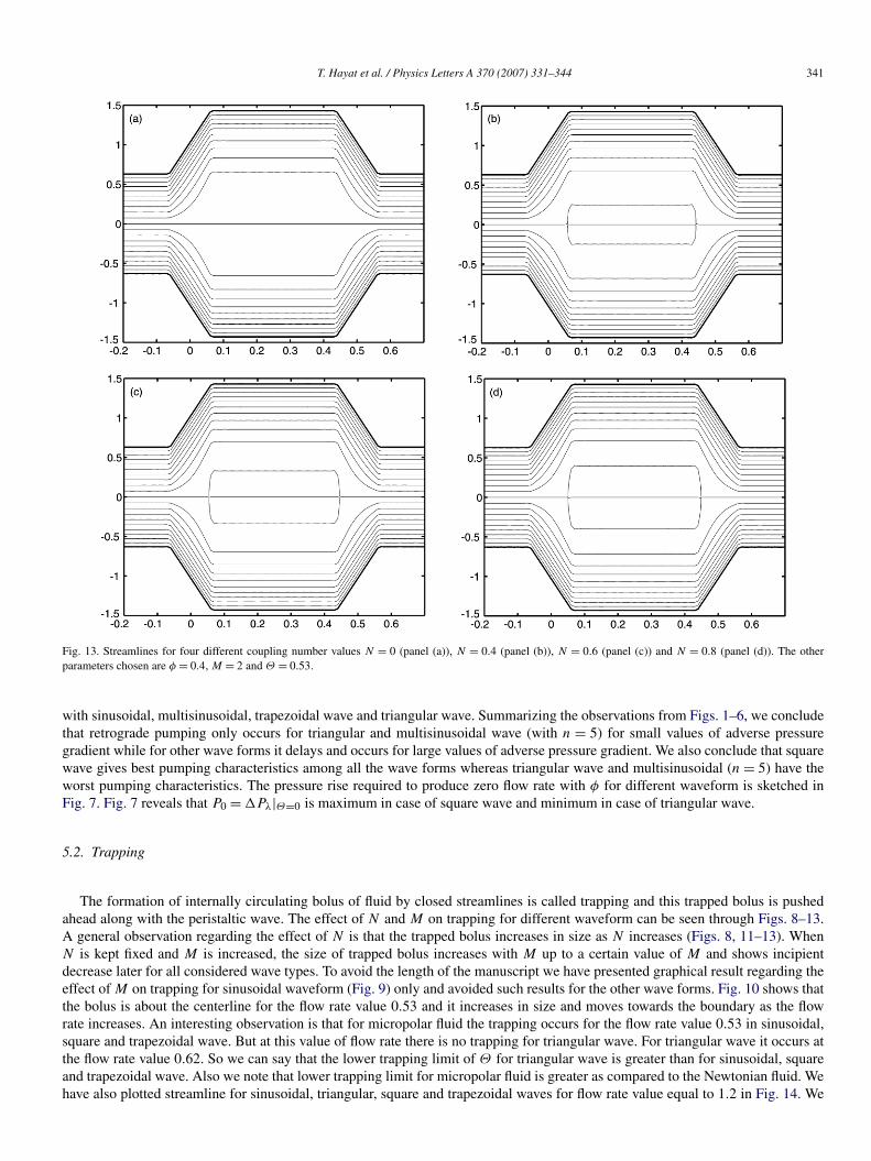
Fig. 13. Streamlines for four different coupling number values N = 0 (panel (a)), N = 0.4 (panel (b)), N = 0.6 (panel (c)) and N = 0.8 (panel (d)). The otherparameters chosen are φ = 0.4, M = 2 and Θ = 0.53.

with sinusoidal, multisinusoidal, trapezoidal wave and triangular wave. Summarizing the observations from Figs. 1–6, we concludethat retrograde pumping only occurs for triangular and multisinusoidal wave (with n = 5) for small values of adverse pressuregradient while for other wave forms it delays and occurs for large values of adverse pressure gradient. We also conclude that squarewave gives best pumping characteristics among all the wave forms whereas triangular wave and multisinusoidal (n = 5) have theworst pumping characteristics. The pressure rise required to produce zero flow rate with φ for different waveform is sketched inFig. 7. Fig. 7 reveals that P0 = �Pλ|Θ=0 is maximum in case of square wave and minimum in case of triangular wave.

5.2. Trapping

The formation of internally circulating bolus of fluid by closed streamlines is called trapping and this trapped bolus is pushedahead along with the peristaltic wave. The effect of N and M on trapping for different waveform can be seen through Figs. 8–13.A general observation regarding the effect of N is that the trapped bolus increases in size as N increases (Figs. 8, 11–13). WhenN is kept fixed and M is increased, the size of trapped bolus increases with M up to a certain value of M and shows incipientdecrease later for all considered wave types. To avoid the length of the manuscript we have presented graphical result regarding theeffect of M on trapping for sinusoidal waveform (Fig. 9) only and avoided such results for the other wave forms. Fig. 10 shows thatthe bolus is about the centerline for the flow rate value 0.53 and it increases in size and moves towards the boundary as the flowrate increases. An interesting observation is that for micropolar fluid the trapping occurs for the flow rate value 0.53 in sinusoidal,square and trapezoidal wave. But at this value of flow rate there is no trapping for triangular wave. For triangular wave it occurs atthe flow rate value 0.62. So we can say that the lower trapping limit of Θ for triangular wave is greater than for sinusoidal, squareand trapezoidal wave. Also we note that lower trapping limit for micropolar fluid is greater as compared to the Newtonian fluid. Wehave also plotted streamline for sinusoidal, triangular, square and trapezoidal waves for flow rate value equal to 1.2 in Fig. 14. We


Fig. 14. Streamlines for four different wave forms sinusoidal wave (panel (a)), triangular wave (panel (b)), square wave (panel (c)), and trapezoidal wave (panel (d)).The other parameters chosen are φ = 0.4, N = 0.4, M = 2 and Θ = 1.2.

found that in all considered wave forms trapped bolus increases in size and moves towards the boundary wall but its size is smallerin case of triangular wave when compared with other three wave forms.

6. Concluding remarks

The peristaltic flow of a mircopolar fluid in a two-dimensional channel in studied under long wavelength and low Reynoldsnumber approximation through different wave forms namely sinusoidal, multisinusoidal, triangular, square and trapezoidal. Theexpressions of velocity vector, microrotation, axial pressure gradient and stream function are developed. Numerical integrationis used to analyze the pumping characteristics. Stream line are plotted to discuss the phenomena of trapping. The present studydiscloses some important findings. These are:

(1) An increase in N causes an increase in peristaltic pumping Θ for sinusoidal, multisinusoidal (with n = 2), square and trape-zoidal wave. However this increase is maximum for square wave and minimum for triangular wave. For multisinusoidal with(n = 5) wave there is no peristaltic pumping.

(2) Retrograde pumping can occur in cases of multisinusoidal (with n = 5) and triangular waves for smaller values of adversepressure gradient when compared to sinusoidal, square and trapezoidal waves.

(3) The size of trapped bolus increases with N for all the considered wave forms. However, by increasing M it first increases andthen starts decreasing.

(4) The lower limit of Θ for trapping is same for all the considered wave forms except triangular wave. In triangular wave it is lessthan the lower trapping limit for all other considered wave forms.

(5) The results for Newtonian fluid can be obtained as a limiting case of our analysis by taking N → 0.


Table 1Values of flow rate Θ in the free pumping for different values of N . Theother parameters chosen are φ = 0.4 and M = 2

Parameter (N) Wave type Θ0

Newtonian s wave 0.2224ms wave (n = 2) 0.2224ms wave (n = 5) 0.0002t wave 0.0156sq wave 0.3396tr wave 0.3110

N = 0.4 s wave 0.2255ms wave (n = 2) 0.2255ms wave (n = 5) 0.0002t wave 0.0156sq wave 0.3423tr wave 0.3141



Table 2Values of flow rate Θ in the free pumping for different values of M . Theother parameters chosen are φ = 0.4 and N = 0.4

Parameter (N) Wave type Θ0

M = 0.001 s wave 0.2224ms wave (n = 2) 0.2224ms wave (n = 5) 0.0002t wave 0.0156sq wave 0.3396tr wave 0.3110

M = 2 s wave 0.2255ms wave (n = 2) 0.2255ms wave (n = 5) 0.0002t wave 0.0156sq wave 0.3423tr wave 0.3141



Acknowledgements

We are grateful to the Higher Education Commission (HEC) for the financial assistance. We further thank the referees for theiruseful suggestions.

References

[1] T. Hayat, A.H. Kara, E. Momoniat, Int. J. Non-Linear Mech. 38 (2003) 1533.[2] T. Hayat, A.H. Kara, Math. Comput. Modell. 43 (2006) 132.[3] T. Hayat, S.B. Khan, M. Khan, Non-Linear Dynam., in press.[4] M. Sajid, T. Hayat, S. Asghar, Phys. Lett. A 355 (2006) 18.[5] Z. Abbas, T. Hayat, M. Sajid, Theor. Comput. Fluid Dyn. 20 (2006) 229.[6] C. Fetecau, C. Fetecau, Int. J. Eng. Sci. 44 (2006) 788.[7] C. Fetecau, C. Fetecau, Int. J. Non-Linear Mech. 38 (2005) 1214.[8] C. Fetecau, C. Fetecau, Z. Angew. Math. Phys. 56 (2005) 1098.[9] C. Fetecau, C. Fetecau, Int. J. Eng. Sci. 43 (2005) 781.

[10] W.C. Tan, T. Masuoka, Int. J. Non-Linear Mech. 40 (2005) 515.[11] W.C. Tan, T. Masuoka, Phys. Fluid 17 (2005) 023101.[12] S. Liao, J. Fluid Mech. 488 (2003) 189.[13] A.C. Eringen, Int. J. Eng. Sci. 2 (1964) 189.[14] A.C. Eringen, Int. J. Eng. Sci. 2 (1964) 205.[15] A.C. Eringen, J. Math. Mech. 16 (1966) 1.[16] R. Nazar, N. Amin, D. Filip, I. Pop, Int. J. Non-Linear Mech. 39 (2004) 1227.[17] A. Ishak, R. Nazar, I. Pop, Fluid Dyn. Res. 38 (2006) 489.[18] T. Hayat, Y. Wang, A.M. Siddiqui, K. Hutter, Math. Problems Eng. 1 (2003) 1.[19] T. Hayat, Y. Wang, K. Hutter, S. Asghar, A.M. Siddiqui, Math. Problems Eng. 4 (2004) 347.[20] A.M. Siddiqui, T. Hayat, M. Khan, J. Phys. Soc. Jpn. 73 (2004) 2142.[21] T. Hayat, F.M. Mahomed, S. Asghar, Non-Linear Dynam. 40 (2005) 375.[22] T. Hayat, N. Ali, Physica A 370 (2006) 225.[23] T. Hayat, N. Ali, S. Asghar, Phys. Lett. A 363 (2007) 397.[24] T. Hayat, M. Khan, S. Asghar, A.M. Siddiqui, J. Porous Media 9 (2006) 55.[25] D. Srinivasacharya, M. Mishra, A.R. Rao, Acta Mech. 161 (2003) 165.[26] Kh.S. Mekheimer, J. Porous Media 6 (2003) 189.[27] Kh.S. Mekheimer, Arab. J. Sci. Eng. 28 (2003) 183.


[28] Kh.S. Mekheimer, Appl. Math. Comput. 153 (2004) 763.[29] Kh.S. Mekheimer, Biorheol. 39 (2002) 755.[30] M. El-Shahed, Appl. Math. Comput. 138 (2003) 479.[31] M. Elshahed, M.H. Haroun, Math. Problems Eng. 6 (2005) 663.[32] P. Hariharan, Peristaltic pressure-flow relationship of non-Newtonian fluids in distensible tubes with limiting wave forms, MS thesis, University of Cincinnati,

2005.

Peristaltic flow of a micropolar fluid in a channel with different wave forms

Documents

Transcript of Peristaltic flow of a micropolar fluid in a channel with different wave forms