APPLIED STOCHASTIC MODELS AND DATA ANALYSIS, VOL. 8 , 283-302 (1992)

PRODUCT FORMS FOR AVAILABILITY MODELS

ERIC SMEITINK PTT Research, St Paulusstraat 4, 2264 XZ Leidschendam, The Netherlands

NICO M . VAN DIJK Faculteit Econometrie, Universiteit van Amsterdam, Roeterstraat 11, 1018 WB Amsterdam, The Nethertands

AND

BOUDEWIJN R . HAVERKORT Faculteit der Informatica, Universiteit Twente, Postbus 217, 7500 A E Enschede, The Netherlands

SUMMARY

This paper shows and illustrates that product form expressions for the steady state distribution, as known for queueing networks, can also be extended to a class of availability models. This class allows breakdown and repair rates from one component to depend on the status of other components. Common resource capacities and repair priorities, for example, are included. Conditions for the models to have a product form are stated explicitly. This product form is shown to be insensitive to the distributions of the underlying random variables, i.e. to depend only on their means. Further it is briefly indicated how queueing for repair can be incorporated. Novel product form examples are presented of a simple serieslparallel configuration, a fault tolerant database system and a multi-stage interconnection network.

KEY WORDS Availability modelling Product form Insensitivity

1. INTRODUCTION

The measures commonly used to quantify the functioning of a system are reliability and availability. The reliability function is typically of interest for systems that must remain operational during their whole (limited) mission length, such as air or spacecraft systems. If components can be repaired and if some down time can be tolerated, then availability is the more appropriate concept. There are several availability measures. An overview of numerical methods for calculating transient measures such as point- and interval-availability is given in Reference 1.

In this paper we focus on the steady state availability of repairable computer systems. We consider a system consisting of Ncomponents that are alternatively up and down. The simplest case occurs when all components have independent up times and down times with mean X i ' respectively p;' for component h. In this case note that ph = p h / ( p t l + XA) corresponds to the marginal steady state probability that component h is up, so that the steady state probability a ( H ) that the components in the set H are down while the others are up is easily concluded to be given by

(1.1) T ( H ) = n Ph n ( 1 - P h ) h f H h t H

87 5 5 -00241 92/ 04028 3 -20$15.00 01992 by John Wiley & Sons, Ltd.

Received 5 December 1991 Revised 19 May 1992

284 E. SMEITINK, N. M. VAN DlJK AND B. R. HAVERKORT

The asymptotic properties of this model, which is often used in reliability studies of (large) communication networks, are extensively studied in, for example, Reference 2. A typical measure of interest in this context is the steady state probability that two nodes can communicate via a network of links that are subject to failure. This probability can in principle be calculated from the steady state distribution ?r (cf. References 3,4,5,6).

Fault tolerant computer systems often exhibit state dependencies, by which the breakdown or repair rate of one component can be accelerated or slowed down depending on the up or down status of other (neighbouring) components. For example, if all components share a common resource for repair, the down times will most likely increase with an increasing number of components that are down. Under exponential assumptions, such systems can be analysed using continuous time Markov models. In that case, the steady state distribution can in principle be obtained by numerically solving a system of linear equations. This can be computationally expensive, however, and if the cardinality of the state space is large special techniques have to be used, such as sparse matrix storage and successive overrelaxation (cf. Reference 7). In Reference 8 a bounding technique based on state space aggregation is presented for obtaining the steady state availability of highly reliable systems.

The primary purpose of this paper is to illustrate that product form expressions for steady state distributions, which have been extensively studied for queueing networks, also apply to a class of availability models. This class is characterized by imposing conditions on the state dependent breakdown and repair rates. Although from a mathematical point of view the product form expression is not new, as it is based on the notion of reversibility (cf. References 9 and lo), its recognition for the present purpose appears to be new. In particular, as state dependent breakdown and repair rates arise naturally, the interpretation of the actual transition rates is different. If in some configuration H a certain transition is prohibited, for example the breakdown of component h @ H , the corresponding transition rate is zero, i.e. the repair of that component is stopped. This situation occurs, for example, in the model of a series system considered in Reference 11 (pp. 194-201). As the system is a pure series configuration, system failure coincides with component failure and it is therefore natural to assume that, while a failed component undergoes repair, all other components remain in ‘suspended operation’. When the repair of the failed component is complete, the remaining components resume operation. At that instant they are not ‘as good as new’, but rather as good as they were when the system stopped operating. The steady state results obtained in Reference 1 1 turn out to be insensitive, i.e. to depend only on the means of the underlying random variables.

By introducing speed functions, i.e. state dependent breakdown and repair rates, we can generalize the above model of a series system and consider arbitrary systems. We then state sufficient conditions on the speed functions that guarantee a product form steady state distribution. These so-called product form conditions impose a special structure on the stochastic process of components going up and down. Loosely put, we require that in the steady state the system exhibits a certain local balance property. Local balance properties are closely connected to insensitivity. 12*13,14

This paper is organized as follows. In Section 2 we formulate the model and illustrate how the speed functions can be used to model failure and repair dependencies between the components. In Section 3 we first formulate the product form conditions. Then, under exponential assumptions, we show how these conditions naturally arise when requiring local balance and obtain the steady state probabilities n ( H ) that the system is in configuration H. In Section 4 we consider a slight extension of our original model and illustrate, again under exponential assumptions, how queueing for repair can be incorporated. In Section 5 we show

PRODUCT FORMS FOR AVAlLABILlTY MODELS 285

that the steady state probabilities ?r (H) are insensitive. In Section 6 we give three examples to illustrate how various systems can be modelled and how the product form conditions can be verified. Section 7 concludes the paper.

2. MODEL

We consider a system consisting of N components where each component is alternatively up (being able to work) and down (not able to work and needing repair). The set of all components is denoted by C and a configuration H c C denotes that the components in the set Hare down while the other components are up. The configuration in which all components are up (none is down) is denoted by 0.

At time t = 0 all components start their first up period. During its ith up period, component h performs a random amiunt of work w h , i before going down. When component h goes down for the ith time it requires a random amount of repair Rh,i. Upon completion of its repair a component immediately returns to the up mode. We assume that all these random variables [ Wh,r]f 2 I and 1 R h , i ] l > 1 are mutually independent and that, for each fixed h E C, the random variables [ Wh,r)r 2 I respectively ( R h , i ] i 2 1 are identically distributed. Consequently, [ Wh,r] I 2 1

and [ R h , r ) r 2 1 are renewal sequences. We denote the distribution functions of the generic variables wh and Rh by Fh, respectively Gh.

The speed at which a component h E H i s repaired is denoted by d(h I H ) , i.e. the remaining amount of repair that component h requires before going up again is provided at the configuration dependent rate b(h I H ) . Likewise, the speed at which a component h $ H works when the system is in configuration H i s given by P(h I H ) . We will refer to /3 and 6 as the speed functions. Further, if we write /3(h I H ) (6(h I H)) we implicitly assume that h f H ( h € H ) .

We denote by .XC 2' the set of configurations, including 0, which can be reached from 0 by components going up and down (2= denotes the power set of C ) . For convenience, we will denote by H + h the configuration in which, apart from the components in H , an additional component h p His down. Similarly, H - h denotes the configuration in which the components in H are down except for component h E H .

Apart from the renewal assumptions above we will require the following regularity conditions for all components h E C.

R1 The speed functions P(h I a ) and 6(h I .) are bounded.

R2 0 < E[Whl, E[Rh] < * R3 The distribution functions Fh and Gh are continuously differentiable. We denote the

probability densities by f h , respectively g h . Furthermore, these densities are bounded.

Note that R2 directly implies R3 if Fh and Gh are exponentially distributed. In this case we also have that Rl and R2 together imply that

HEreandP(hIH)>O-- .H+hE.re (2.1)

and

H E 2 and 6 ( h I H ) > 0 --. H - h E X'

Condition R3 ensures that (2.1) and (2.2) also hold in the general case, i.e. that the set of configurations .Yfthat can be reached in the general case is the same as the set of configurations that can be reached under exponential assumptions.

286 E. SMEITINK, N. M. VAN DIJK AND B. R. HAVERKORT

Interpretation of the speed functions

The actual time that component h remains up depends on the random amount of work, wh,

that it performs before going down and on the varying speed(s) P(h I a ) with which it works, i.e. on the configurations that the system visits during the up time of component h . In the same way the time that a component h remains down depends on the amount of repair, R h , that it needs and on the speed(s) 6(h I a) with which it is repaired. Below we give some examples of how the functions /3 and 6 can be used as delay or acceleration factors to model failure and repair dependencies between the components.

(a) P(h 1 H ) = 0 reflects that component h, although it is up, does not work (cannot be used) if the components in the set H are down. Consequently, component h cannot go down if the system is in configuration H. Note that our model is not applicable to circumstances where the ‘ageing process’ continues while a component is unused.

(b) P(h I H + h ’ ) > P(h I H ) indicates that component h works faster if the additional component h’ has failed. This can be used to model situations where work is shared between components that are up.

(c) 6(h I H + h + h ‘ ) < 6(h I H + h ) indicates that the repair of component h is slowed down if an additional component h’ has failed. This situation occurs when components share a common repair facility.

(d) 6(h I ( h , h ‘ ] ) > 6(h’ I ( h , h ’ ) ) = 0 models the (pre-emptive) priority of the repair of component h over that of component h ’ .

Steady state behaviour

We are interested in the steady state behaviour of the stochastic process 2?= (k(t), t 2 0) on X, defined by letting k(t) = H if at time t the configuration of the system is H . It will be clear that, in general, the process k is not a Markov process, as the future evolution of the system depends on the residual amounts of work and repair. In order to imbed the process in a Markov process X we define for a given configuration H the vector s = ( ~ 1 , ..., S,V) E Y= RY by

the residual amount of work for component h, if h f H the residual amount of repair for component h, if h E H s h = [

Owing to the independence assumptions on the random variables ( R h , i } i 1 and { w h , i ) i 2 I the state of the system is then completely determined by a pair ( H , s) E X x 9 and, defining X ( t ) = ( H , s) if at time t 2 0 the system is in state ( H J ) , it is easily verified that the stochastic process X = ( X ( t ) , t 2 0) on X X B has the desired Markov property. The regularity conditions R1-3 ensure that X has a limiting probability density function p (see, for example, Reference 15), which we will obtain in Section 5. For all H E X t h e steady state probability T ( H ) that the system is in configuration H is then given by

T ( H ) = lim P(J?(t) = H ) = lim P ( X ( t ) E ( H , 9)) = p ( H , s) d s (2.3) [-a t-m 9

3. PRODUCT FORM CONDITIONS

It will be convenient to define for an arbitrary state H = ( h l , ..., hn) E y: (1, ..., n) +- (h l , ..., h,] the sets H z for k 2 0 by H: = 0 and

(H # 0) and bijection

H : = ( r ( l ) , ..., y ( k ) ) , k = 1, ... ) n

PRODUCT FORMS FOR AVAILABILITY MODELS 287

The bijection y indicates a possible ordering of the components of H , which might indicate, for example, that component y(i) went down before component y ( j ) if i < j .

Definition 3.1

An ordering y of H = ( h l , ..., h,) is called a breakdown path if

/3 (y(k) Iff;-,) > 0, k = 1, ..., n and a repair path if

6 ( y ( k ) I H ; ) > O , k = 1, ..., n The set of all possible breakdown paths for state H is denoted by I'p(H) and the set of all repair paths is denoted by I'a(H).

Note that H E sfdoes not necessarily imply that HZ E s fand that in principle &?may contain states for which no breakdown path and/or repair path exists. However, this pathological case will be excluded by the conditions PFC 1 and PFC 2 below. The product form conditions are the following.

PFC 1

For any state HE sf (H # 0) we must have that

i.e at least one component is being repaired and as a result I '&(H) f 0.

PFC 2

For any state H € sf ( H # 0) we must have that

6(h 1 H ) = 0 /3(h 1 H - h ) = 0 for all h E H such that H- h E 2

i.e. if component h cannot be repaired in configuration H it cannot break down in configuration H - h, and vice versa. As a result we have that r s ( H ) = I'a(H).

PFC 3

For any state H = (hl , ..., h,) E s f ( H # 0) and repair path yEra(H) we must have that

where K ( H ) is some strictly positive value depending on H only. We define K ( 0 ) = 1. This key condition is related to the well-known Kolmogorov criterion for a Markov chain to be reversible (cf. Reference 10, pp. 21-25]). A further discussion of this condition and an interpretation are given in Section 3.2.

The speed functions 0 and 6 often suggest a form for the function K ( * ) , in which case PFC 3 can be checked using the equivalent condition PFC 3' stated below.

288 E. SMEITINK, N. M. VAN DlJK AND B. R. HAVERKORT

PFC 3'

For all states h E A? ( H # 0 ) and all components h c H such that 6(h I H ) > 0 we have that

Remark 3.2

As we will frequently use PFC 3' let us briefly show that the two are indeed equivalent. First observe that for H = ( h l , ..., h,) 6 %(H # 0 ) and h E H such that 6(h I H ) > 0 there exists a repair path y E Fa(H) with y ( n ) = h, i.e. the repair of component h is completed first. Using this path in (3.1) we obtain

Thus PFC 3 implies PFC 3 ' . Repeatedly using PFC 3' in (3.2) yields that

K ( H ) = K(0)

for each repair path y E ra(H). Noting that PFC 3.

we defined K(0) = 1 it follows that PFC 3'implies

Source balance

In order to illustrate the role of the conditions PFC 1-3 let us first assume that wh and Rh are exponentially distributed with mean E [ wh] = A;' and E[Rh] = p;' respectively. Owing to the memoryless property of the exponential distribution, the process 2 = (*(t), t 2 0) defined in Section 2 is a Markov process at X, for which a unique steady state distribution T exists if ,f is irreducible. This is guaranteed by condition PFC 1, as the existence of a repair path for each state H E &guarantees that all states communicate with the state 0.

The steady state distribution ?r can be found as the unique solution (up to normalization) of the global balance equations, which require that for every state H ~ % t h e 'total rate of change' is equal to zero, i.e.

where we used the observation that 6(h 1 H ) > 0 * H - h E &and P(h I H ) > 0 * H + h E M. In order to find a closed-form solution to the global balance equations we require the stronger source balance property to hold, which in our model requires that for every state HE &:

the probability flow into state H due to the breakdown of component h equals the probability flow out of that same state H due to the repair of component h, and vice versa

(3.4)

This notion of source balance is related to job-local balance as introduced in Reference 12 and local balance as introduced in Reference 13, which are known to be responsible for insensitive

PRODUCT FORMS FOR AVAILABILITY MODELS 289

product form results. It is readily verified that the global balance equations (3.3) are satisfied if the source balance property (3.4) holds, i.e. if we can find a probability distribution r such that for every state HE &, H # 0

r ( H ) 6 ( h I H)Ph=?r(H-h)P(hIH-h)Xh (3.5) for every component h E H such that H- h E %. In Theorem 3.3 below we will see that this is possible provided conditions PFC 1-3 are satisfied. In Section 5 we will show that the same result holds true for generally distributed quantities of work and repair, i.e. that the steady state probabilities r ( H ) given in (3.6) below are insensitive.

Theorem 3.3

Provided that PFC 1 holds, the conditions PFC 2 and PFC 3 are both necessary and sufficient for source balance. Further, if the conditions PFC 1-3 are satisfied, the steady state distribution r of 2 is given by

(3.6) Ah

h c H Ph r ( H ) = c K ( H ) n: -

with c a normalizing constant and K ( H ) given by (3.1).

Pro0 f That PFC 2 is a necessary condition for source balance follows directly from the

irreducibility of R and the regularity conditions R1-2, which imply r ( H ) > 0 for all HE X. Let H = (hl , ..., h,) (H # 0) and let y c I’a(H) denote an arbitrary repair path for state H. By repeatedly using (3 3) it readily follows that source balance implies

As the ratio between r ( H ) and r (0 ) must be constant, we conclude that PFC 3 is also necessary for source balance.

All that remains to verify is that ?r given by (3.6) satisfies the source balance equations ( 3 . 9 , as these imply that each separate term between brackets in (3.3) equals zero. Owing to PFC 2 we need only consider states HE %and components h E H with 6(h 1 H) > 0. As for any such state we also have H- h E % with P(h I H - h ) > 0 we obtain from (3.6) and PFC 3‘ that

r ( H ) = K(H)Xh -P(hIH-h)Xh - a(H- h ) K ( H - h ) P h 6(h I H ) P h

which completes the proof.

Remark 3.4

The interpretation of PFC 3 is that given the starting point 0 E Z a n y path in the state space which ultimately returns to 0 must have the same probability whether this path is traced in one direction or the other.

Remark 3.5

The equations (3.5) are also called detailed bahnce equations, l4 a term reserved to express balance between any pair of states, in this example that is between states H and H- h. When

290 E. SMEITINK, N. M. VAN DIJK AND B. R. HAVERKORT

applied to the same state description, detailed balance implies source balance, but in Section 4.2 (Equation (4.4)) we will see that source balance does not necessarily imply detailed balance

4. QUEUEING FOR REPAIR

The model described in Section 2 above is primarily suited for systems with a hierarchic structure. As the breakdown and repair speeds depend only on the set of components that are down and not on the order in which they broke down, product form results for systems with an FIFO queue of failed components in front of a limited number of repair facilities, for example, cannot be directly concluded using this model.

4.1. Identical components

The simplest such case is the following basic machine interference model (see Reference 10, p. loo), where all components h E C are assumed to be identical and where wh and Rh are exponentially distributed, each with the same mean E[Wh] = A-' respectively E[Rh] = p - * . The state of the system is now completely determined by the number of components that are down. We denote by $(n), n = 0, ..., N - 1, and $(n), n = 1, ..., N , the total work, respectively repair speed, when n components are down. For example, $(n) = 1 models an FIFO queue for repair, whereas $(n) = n models independent repairs, The situation that only one component is actually working with the others in cold standby (not working) can be modelled by letting 4 ( n ) = 1, reflecting an 'FIFO queue for breakdowns'.

We define nmax as the maximum number of components that can be down at the same time. As initially all components are up nmax = min (n: $(n) = 0) . We assume that + and $ are bounded and that $(n) > 0, n = 1, ..., nmax. These conditions are the equivalent of R 1 and PFC 1. Then, denoting by d(t) = n the event that n components are down at time t 2 0, it can easily be verified that the steady state distribution if of the Markov chain d= [x(t), t 2 0) (a birth-death process) is given by

with c a normalizing constant. Thus d has a product form steady state distribution, even though conditions PFC 2 and PFC 3 are not necessarily satisfied. Instead, however, we have assumed that all components are identical with exponentially distributed quantities of work wh

and repair Rh.

Remark 4.1

The steady state distribution ii satisfies the detailed balance equations ( 3 3 , if we only specify the total number of components, n, that are down. This seems to conflict with Remark 3.5, since the source balance property (3.4) does not generally hold. Note, however, that here we work with a different, aggregated, state description.

4.2. Non-identical components

In relation with queueing the conditions of Section 4.1 may be relaxed. Let us illustrate this by considering one concrete situation in which the components of some subset

PRODUCT FORMS FOR AVAILABILITY MODELS 29 1

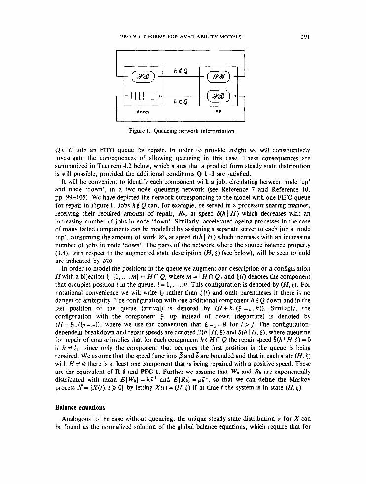
down UP

Figure 1. Queueing network interpretation

Q C C join an FIFO queue for repair. In order to provide insight we will constructively investigate the consequences of allowing queueing in this case. These consequences are summarized in Theorem 4.2 below, which states that a product form steady state distribution is still possible, provided the additional conditions Q 1-3 are satisfied.

It will be convenient to identify each component with a job, circulating between node ‘up’ and node ‘down’, in a two-node queueing network (see Reference 7 and Reference 10, pp. 99-105). We have depicted the network corresponding to the model with one FIFO queue for repair in Figure 1. Jobs h j! Q can, for example, be served in a processor sharing manner, receiving their required amount of repair, R h , at speed 6(h I H ) which decreases with an increasing number of jobs in node ‘down’. Similarly, accelerated ageing processes in the case of many failed components can be modelled by assigning a separate server to each job at node ‘up’, consuming the amount of work wh at speed /3(h I H ) which increases with an increasing number of jobs in node ‘down’. The parts of the network where the source balance property (3.4), with respect to the augmented state description (H, [) (see below), will be seen to hold are indicated by yigg.

In order to model the positions in the queue we augment our description of a configuration H with a bijection [: ( 1, . . . , m) - H n Q, where m = I H f l Q I and [(i) denotes the component that occupies position i in the queue, i = 1, ..., m. This configuration is denoted by (H, [). For notational convenience we will write [i rather than [(i) and omit parentheses if there is no danger of ambiguity. The configuration with one additional component h € Q down and in the last position of the queue (arrival) is denoted by ( H + h , ( E ~ - m , h ) ) . Similarly, the configuration with the component up instead of down (departure) is denoted by ( H - [I, ( E 2 - m ) ) , where we use the convention that j = 0 for i > j . The configuration- dependent breakdown and repair speeds are denoted B(h I H, [) and 8(h I H, [), where queueing for repair of course implies that for each component h € H n Q the repair speed 8(h 1 H , 5) = 0 if h # El , since only the component that occupies the first position in the queue is being repaired. We assume that the speed functions 6 and 6 are bounded and that in each state (H, E) with H # 0 there is at least one component that is being repaired with a positive speed. These are the equivalent of R 1 and PFC 1. Further we assume that wh and Rh are exponentially distributed with mean E[Wh] = X i ‘ and E[Rh] = p i ‘ , so that we can define the Markov process x= ( f ( t ) , t 2 0) by letting R(t) = (H, [) if at time t the system is in state (H, E ) .

Balance equations

Analogous to the case without queueing, the unique steady state distribution ii for 2 can be found as the normalized solution of the global balance equations, which require that for

292 E. SMEITINK, N. M. VAN DIJK AND B. R. HAVERKORT

all states (H, E)

+ [F(H, E ) ~ ( E I 1 H , Opt1 - % ( H - Em, (El + m - l ) )D(Em 1 H - Em, ( 4 1 - + m - 1 ) ) & ~ 1 = O (4.2)

It will be clear that source balance cannot be satisfied at the queue, corresponding to the last term of (4.2): the state ( H , [) can be entered due to the breakdown of component Em, but since Em is the last component in the queue, state ( H , E) can in general not be left due to the repair of component Em (the only exception being the case m = 1).

However, we can still try to solve the global balance equations in a local manner, i.e. by requiring that each separate term between brackets in (4.2) above equals zero. As in the case without queueing, the terms corresponding to components h p Q are equal to zero, provided that for all components h E H n QC

* ( H , t ) z ( h I H , E)Ph = * ( H - h, E)B(h 1 ff- h, [ ) A h (4.3)

reflecting source balance for all components h p Q, both in node ‘up’ and node ‘down’ (see Figure 1). By considering the rate of change in state ( H - [ I , ( E 2 - m ) ) rather than (H , t ) , we see that the terms in the third sum all equal zero, provided that

(4.4)

This equation reflects that the probability flow into state (H - El, (,5 - m ) ) due to the repair of component El must equal the probability flow out of that same state due to the breakdown of component [ I , corresponding to source balance for components h E Q in node ‘up’. Note that (4.4) is not a detailed balance equation (see Remark 3.5). The last equation is just the last term of (4.2) corresponding to the queue (no source balance),

(4.5)

f W , E P ( E l I H , t ) P € l = f ( H - E19(t2-m>>BcEl I H - El,(E2-+rn))XEI

+(H,E)~(EI I H , t ) f i ~ , = * ( H - E m l ( E 1 - m - l ) ) B ( E m l H - E m y ( E 1 - m - ~ ) ) & m

Conditions and result

As in Section 3 (see Equation (3.7)) we can repeatedly use the equations (4.3)-(4.5) to obtain the (fixed) ratio between the steady state probabilities F(H, E) and ii(0,0). However, if 8(& 1 H, 4 ) > 0 we can either use (4.4) or (4.5) to proceed with. If both 8(& I H, E) > 0 and 6(h 1 H , [) > 0 for some h p Q we may even use any of the three equations. These observations lead to the conjecture that the global balance equations (4.2) can only be solved in this local manner if the conditions Q 1-3 below are satisfied.

Q 1 All components h € Q require an exponentially distributed amount of repair R with the same mean I l p .

Q 2 The speed functions

-

and 8 are of the form

i.e. apart from modelling the queue, the order 5 does not influence the speeds.

PRODUCT FORMS FOR AVAILABILITY MODELS 293

Q 3 For all states (H, () and for all components h, h’ E Q we must have that

6(h I H ) = S(h’ I H ) (4.7)

i.e. all components h E Q are repaired in exactly the same manner.

With these conditions we are almost back in the setting of our original model. Although 0 and 6 are not the real speed functions in the model with queueing, we can still use the notion of (now fictitious) breakdown and repair paths as introduced in Definition 3.1 and formulate the conditions PFC 1-3. We then have the following result.

Theorem 4.2

/3 and 6 that satisfy PFC 1-3 and Q 3, the steady state distribution ?r of R is given by If condition Q 1 holds and the speed functions 6 and 8 are given by (4.6) for some functions

%(H, t ) = c K ( H ) (4.8)

with c a normalizing constant and K ( H ) given by (3.1).

Pro0 f Using (4.6) and condition PFC 3‘ the source balance equations (4.3) and (4.4) can be directly

verified in the same manner as was done in the proof of Theorem 3.3. Equation (4.5) can be verified by first using (4.6) and the conditions Q1 and Q2 to write $(tl 1 H , =

0 &(ti I H)Ph = &(Ern I W P .

Remark 4.3

We have already hinted at the connection between insensitivity and source balance as related to job-local balance. l 2 Without proof we state that the steady state probabilities %(H, t ) depend on the distributions of wb for h t C and R h for h Q only through their means. These distributions correspond to the parts of the network in Figure 1 where source balance is satisfied, indicated by 98. This partial insensitivity can be proven along the same lines as will be done for the case without queueing in Section 5 .

Remark 4.4

The above extension of our model to incorporate queueing reflects only one of the many possibilities. However, we considered FIFO queueing for repair as it seems to be one of the most natural cases. Further, Theorem 4.2 can easily be extended to model several different queues. Note that components in cold standby can also be modelled by an ‘FIFO queue for breakdowns’.

5 . INSENSITIVITY

in Section 4 we extended our model to incorporate queueing for repair, and saw that in order to obtain a product form steady state distribution exponential assumptions are needed. In this section we consider the model as stated in Section 2 and concentrate on insensitivity. The main

294 E. SMEITINK, N. M. VAN DIJK AND B. R. HAVERKORT

results is the technical Theorem 5.2, yielding a product form limiting probability density function p : YZ'x 8+ R+ for the Markov process X defined in Section 2. The more practical insensitive product form expression for the steady state probabilities n ( H ) , h E YZ, given in Corollary 5.3, is an immediate consequence.

Although this insensitivity result can in principle be concluded from Reference 13, we prefer to give a direct proof, both for completeness and because it clearly illustrates the role of the regularity- and product form conditions. Extensions of Theorem 5.2 and Corollary 5.3 so as to include queueing for repair under appropriate conditions can be obtained by combining the results from this section and Section 4.

Remark 5.1

In the proof of Theorem 5.2 we will assume that a limiting probability density function p of X exists. That this is indeed the case can be argued under the sufficient regularity conditions R 1-3, which further imply that p can be found as the unique continuously differentiable solution of the stationary forward infinitesimal Kolmogorov equations (see, for example, Reference 15, Theorems 1.9 and 2.3). This solution is called the stationary probability density function of X .

Theorem 5.2

Under conditions PFC 1-3 and R 1-3 the limiting probability density function p of X is given by

with c a normalizing constant and K ( H ) given by (3.1).

Pro0 f First we derive the forward infinitesimal Kolomogorov equations (5 .2) , which express the

distribution of X at some arbitrary epoch t in terms of the distribution of X at t - A . Then, using the fact that a unique stationary probability density p for X exists which is continuously differentiable w.r.t. the residual amounts of work/repair s h , we obtain the stationary forward infinitesimal Kolmogorov (or global balance) equations (5.6). The proof is completed by verifying that the density p given in (5.1) is indeed continuously differentiable and satisfies these global balance equations.

In order to derive the forward infinitesimal Kolmogorov equations we define for any configuration HE X a n d for any A > 0 the vectors A H , - A H and A H in P b y

zip = A f l ( h I H ) , i f h P H Ah"= A , if A ? = O { A b ( h , H ) , i f h E H - [o , i f A ? > o

and A H = A H + A H . Further we denote by e h the hth N-dimensional unit vector. The interpretation of the vector A H is that in an infinitesimal time A a component h 6 H performs an amount of work Ah" and a component h E H receives an amount of repair a?. The additional vectors AH and A H are introduced in order to define infinitesimal elements (s - A H , s) C Y with positive volume. Consider an arbitrary state (H, s) E YZx 9 with sh > 0 for all h E C. As all speeds p and 6 are finite we can choose A small enough such that Sh - Ah" > 0 for all h E C and thus (H, (s - A H , s)) C S x % Conditioning upon the epoch

PRODUCT FORMS FOR AVAILABILITY MODELS 295

t - A there are three possibilities for the event X ( t ) € (H, (s - A H , s)) to occur:

The configuration does not change in the time interval (t - A , t ) , i.e.

X ( t - A ) € (H, (S - A H , s + A H ) )

The configuration changes from H + h to H in (t - A , t ) due to the repair of some component h with a residual amount of repair r < A6(h I H + h ) at time t - A . In this case the change in configuration occurs at time t - A + r/b(h I H + h ) . In order to account for the change of speeds in the interval ( t - A , t ) we define the vector a(h, 7) E 8 by

h ’ = h P

Note that, for example,

is the amount of repair received by component h‘ E If in the interval ( t - A , t ) . Thus, given some 7 E (0, A6(h I H + h ) ) we must have that

and the amount of work that component h can perform after its repair must be in the interval

The configuration changes from H - h to H in ( t - A , t ) due to the breakdown of some component h with a residual quantity of work 7 < AP(h 1 H - h ) at time t - A . Defining the vector b(h, r ) E Yanalogous to the vector a(h, r ) in the previous case, we must have that

X ( t - A ) E ( H - h, (b(h, T ) - A H , b(h, T ) + A H - A f e h ) )

and the amount of repair that component h needs after its breakdown must be in some interval with width Ah” around Sh.

All other contributions would require two or more components to change status in the interval ( t - A , t ) . Owing to the regularity assumptions, these contributions will become negligible as A 10 and can thus be omitted. From the above observations and using the Markov

296 E. SMEITINK, N. M. VAN DIJK AND B. R. HAVERKORT

property it follows that

P ( X ( t ) E (H, s - AH, s))) = P ( X ( t - A ) E (H , (S - A H , s + A H ) ) )

( S ( h I h - h ) > 0 )

E ( H - h, (b(h, 7) - - A H - 7 e h , b(h, 7 ) + A H - A f e h ) ) ) (5.2) where we have used the assumption that the random variables wh and R h have densities fh respectively g h and o( -) denotes any function with the property that o(x) /x -+ 0 as x 10.

Now, without loss of generality, assume that a unique stationary probability density p exists which is continuously differentiable in its residual amounts of work/repair s h . Then, using the mean value theorem we obtain

P ( X ( t ) E (H, (S - AH, s))) - P ( X ( t - A ) E (H, (S - AH, s + A H ) ) )

= S a E @,aH' [ p ( H , s - AH + a ) - p ( H , s - A H + a)] da

= p ( H , s - AH + 0') - p ( H , s - AH + a ' )

for some vector a' E (0, A H ) . Note that s - AH + a' -+ s along some trajectory in the interior of 9 as A 10. Again using the mean value theorem, for each separate integral in the second term of the r.h.s. of (5.2) we obtain (apart from the factor f h ( s h ) A h H + o ( A f ) )

A8(h I H + h ) dP(X( t - A ) E ( H + h, (a (h , 7 ) - AH - 7 e h , a(h , 7 ) + A H - Z h H e h ) ) ) -

- - p ( H + h, ~ ( h , 7 ) - A H + a) du d7 uC (O.AH - AhHet,)

p ( H + h , a(h, 7 ' ) - A H + a2)A6(h I H + h ) (5.4) = ( , h * , C h ' # h l

for some value T~ E (0, A6(h I H + h ) ) and vector a2 E (0, AH - A h H e h ) . In a similar manner we obtain for each integral in the third term of the r.h.s. of (5 .2) (apart from the factor g h ( & )A f + o(A hH))

A\B(h I H - h ) dP(X( t - A ) E (ff- h, (b(h, 7 ) - AH - T e h , b(h, 7 ) + A H - X h H e h ) ) )

for some value 73 E (0, Ap(h I H - h ) ) and vector a3 E (0, AH - A h H e h ) . Note that both a(h, 72) - + a2 -+ s - s h e h and b(h, 73) - 4 H + a3 -+ s - s h e h along some trajectory

PRODUCT FORMS FOR AVAILABILITY MODELS 297

in the interior of <Yas A 10. Finally, eliminating the common factor n h ' EC A$ in (5.3)-(5.5), dividing by A and letting A LO we obtain the stationary forward infinitesimal Kolmogorov equations

= O (5 .6)

All that remains is to verify that the probability density p as given in (5.1) above satisfies these equations. Consider some component h f H with P(h I H ) > 0. First note that the regularity condition R 3 and PFC 2 imply that H + h E *and 6(h 1 H + h ) > 0. Differentiating (5.1) yields

and using lim.rh10 [l - F h ( X h ) ] = 1 we obtain

lim p ( H + h , X ) = C K ( H + h ) fl [ I - F h ( s h ) ] fl [ I - G h ( . S h ) ] (5 .8) I - s - sheh h f H t h h c H

With condition PFC 3 ' it follows that all contributions due to components h f! H in (5.6) are equal to zero. In a similar manner it can be shown that all contributions due to components

1 LJ h E H are equal to zero also.

Using Theorem 5.2 the steady state probability ?r(H) that the system is in configuration H can be readily obtained by integrating the limiting probability density function p over all possible residual amounts S h of work (if h e H ) or repair (if h € H ) .

Corollary 5.3

Under conditions PFC 1--3 and R 1-3 we have for all H E 9 that

(5.9)

with C a normalizing constant and K ( H ) given by (3.1).

Pro0 f The change of order of integration and taking products below is justified by the fact that

all integration variables occur in exactly one separate factor in the product form (5.1). Thus, m m

T(H)= [ p ( H , S) d s = C K ( H ) [ I - F h ( s h ) ] d.Sh fl [ - G h ( S h ) ] d S h h f H 0 h t H 0

(5.10)

298 E. SMEITINK, N . M. VAN DlJK AND B. R. HAVERKORT

6 . EXAMPLES

In this section we give a number of examples that illustrate the kind of systems that can be modelled, i.e. for which the speed functions satisfy the product form conditions.

6.1. Simple series-parallel system

Consider a system consisting of one critical component, a, and a set B = (61, ..., bMM) of M secondary components (see Figure 2). The system is operational if the critical component and at least M - k of the secondary components are up. We assume that none of the components can be used if the system is not operational, so that the set of possible configurations is given by

S v = ( H C C : I H j < k + l )

Further we assume that there is a single repair unit giving pre-emptive priority to the critical component and that the secondary components are repaired in a processor sharing manner. Defining n e ( H ) = I H n BI as the number of secondary components that are down in configuration H , the breakdown and repair speeds for the secondary components b E B are given by

and for the critical component a we have

It can easily be seen that PFC 1 and PFC 2 are satisfied. In order to check PFC 3’, the equivalent of PFC 3, observe that if a E H all repair paths y E r s ( H ) have y(1) = a, i.e. the critical component is repaired first. Thus, the only conditions for the function K are

Figure 2. Series-parallel system

PRODUCT FORMS FOR AVAILABILITY MODELS

As a consequence K is given by K ( H ) = ~ B ( H ) ! and from Corollary 5.3 we conclude that

299

processor

switch memory

processor

with c a normalizing constant.

--,

Remark 6.1

From Section 4.2 it can be concluded that instead of a processor sharing discipline, also an FIFO queue for the repair of the secondary components (Q= B ) leads to a product form steady state solution provided that for all A € B the required quantity of repair Rh is exponentially distributed with mean p - ’ . The corresponding function 6 for b € B in (4.6) is given by

Otherwise the functions 0 and 6 are as given above. It can easily be verified that conditions Q 1-3 and PFC 1-3 are satisfied, now with K ( H ) = I , so that from Theorem 4.2 we conclude that the steady state probabilities i i(H, [) are given by

with c a normalizing constant. Noting that s(H, [) does not depend on 4‘ and that there are ~ B ( H ) ! possible orderings 4 we see that the steady state probability that the set of components H is down is still given by (6.1), of course with E[Rh] = p - l for h C B.

6.2. Fault tolerant database system

Consider a database system consisting of a front-end, two processing subsystems and a database. Each subsystem consists of a switch, a memory and two processors and is operational if the switch, the memory and at least one of its processors are up. The system as a whole is operational if the front-end and the database are up and at least one of the processing subsystems is operational. The system can be interpreted as a nested series-parallel system (see Figure 3).

!-

Figure 3. Nested series-parallel system

300 E. SMEITINK. N. M. VAN DIJK AND B. R . HAVERKORT

We assume that the components in a subsystem cannot be used if that subsystem is down and if the whole system is down none of the components can be used. In order to define the speed functions and the set of all possible configurations we define for each component h € C its direct dependability set D ( h ) as the set of components, other than h, that can only be used if component h is up. For example, if h denotes a processor D ( h ) = 0 and if h denotes a switch, D ( h ) contains all the component of the subsystem, except for the switch itself. Further, from Figure 3 it is apparent that the system has four different path sets Pi C C, i = 1, ..., 4, where a path set is defined as a minimal set of components that must be up for the system as a whole to be operational. Let us label the four processors by PI, ..., p4 such that pI E Pi, i = 1, ..., 4. The set of all possible configurations M i s given by

i

i.e. each component was contained in at least one path set with all components up just before it broke down. For the breakdown speeds, we have for all HE

P(h 1 H ) = 0 * 3h' E H: h E D ( h ' ) (6.2)

and all h # H

As PFC 2 requires that for all HE X a n d all h E H

6 ( h / H ) = O o 3h'EH: hED(h') (6.3)

we must assume a hierarchic repair strategy, which we model as follows. Each subsystem has its own repair unit, giving pre-emptive priority to the memory and the switch. (Note that, within a subsystem, the memory and the switch cannot be down at the same time.) If the database goes down then both repair units are assigned to repair the database immediately. The same holds for the front end. Thus, the database and the front end have pre-emptive priority at system level. The repair units resume the work they were doing as soon as they finish the repair of a component with higher priority, i.e. the priority disciplines are work conserving.

Having modelled the hierarchy, i.e. when speeds equal zero, we have the freedom to assign the positive speeds in an arbitrary manner. Suppose that the repair speed for a processor is equal to 1 if it is the only processor that is down in its subsystem but that, if the other one goes down too, this speed drops to q for both processors. Further, if in a subsystem both processors are up then they both work at speed 1 and if only one of them is up then it works at speed p. The speeds of all other components take the values 0 or 1 only.

Again, it is easy to see that PFC 1 is satisfied. That PFC 2 is satisfied follows from (6.2) and (6.3). In order to check PFC 3, consider a configuration H # 0 and an arbitrary repair path y E I'&(H). The only factors

that matter in (3.1) are those for which ~ ( k ) denotes a processor, all other factors P/S being equal to 1. From this observation it follows that the function

if in both subsystems at most one processor is down

if all four processors are down K ( H ) = [:/q, if in one subsystem both processors are down

( p / ~ ) ~ ,

satisfies PFC 3. As in Remark 6.1 it can be verified that the steady state distribution x is still of product form

if the processors in each subsystem join a FIFO queue for repair (one separate queue for each

PRODUCT FORMS FOR AVAILABILITY MODELS 301

subsystem), provided that they require exponentially distributed amounts of repair with means p a and p.bl for subsystem a and b, respectively. Note that the case where all four processors join the same queue would violate condition Q 3.

- I

6.3. Multi-stage interconnection network

Consider a multi-stage interconnection network (MIN) connecting K inputs to K outputs. We assume that K is a power of two. When using 2 x 2 internal switches to build up the MIN, there are M = 'log K stages required. The number of switches per stage is N = K12. In Figure 4 an 8 x 8 MIN is depicted.

Assume that under normal operation all switches that are up work at speed 0 = 1. Switches that are down are repaired in a processor sharing manner. However, there is a critical number B;, 1 < B; < N, associated with each stage, i = 1, ..., M. As soon as B; switches of stage i are down the network abandons normal operation. Stage i is now critical and all switches that are up stop working. The repair of all switches that are not in the critical stage is also stopped in favour of the B; switches that are down in the critical stage i. These are repaired in a processor sharing manner. As soon as one of the switches in the critical stage is repaired the system resumes normal operation again.

Let C, denote the set of switches in stage i and let n ; ( H ) = I H n Ci I denote the number of switches that are down in stage i if the system is in configuration H,i= 1, ..., M .

The set .@of all possible configurations is given by

.rP= ( H C C : ( 3 j E { I , . . . ,MJ)( n j ( H ) < B j a n d n ; ( H ) < B ; , i # j ) J

For all states H and switches h E C the speeds 0 and 6 are given by

1, if n ; ( H ) < B;, i = 1, ..., M 1 H ) = [o, else

and

i f n j ( H ) = B , f o r s o m e j E ( l , . . . ,A4 a n d h € S j i f n j ( H ) = B j f o r s o m e j € ( l , ...,MJ a n d h f S j

stage 1 stage 2 stage 3

Figure 4. Multi-stage interconnection network

302 E . SMEITINK, N. M. VAN DIJK AND B. R. HAVERKORT

From this, it is not difficult to see that PFC 1 and PFC 2 are satisfied. Finally, in the same manner as was done in Example 6.1, it can be verified that the function K ( H ) given by

satisfies PFC 3 ‘ .

7. CONCLUSION

In this paper we have characterized a class of availability models that exhibit a product form steady state solution. The conditions that have to be fulfilled for a model to fall in this class (the product form conditions) have been stated and examples are given that show how these conditions can be verified. Further research is conducted on using the product form results to obtain bounds for non-product-form models. This can be done by making proper adjustments in the speed functions 8 and 6 .

ACKNOWLEDGEMENT

The authors are very grateful for the helpful comments of the referees.

REFERENCES

1. A. L. Reibman, R. M. Smith and K. S. Trivedi, ‘Markov and Markov reward model transient analysis: an

2. S. M. Ross, ‘On the calculation of asymptotic system reliability characteristics’, in Reliability and Fault Tree

3. R. Addie and R. Taylor, ‘An Algorithm for calculating the availability and mean time to repair for

4. A. Agrawal and R. E. Barlow, ‘A survey of network reliability and domination theory’, Operations Research,

5. T. B. Brecht and C. J . Colbourn, ‘Lower bounds on two-terminal network reliability’, Discrete Applied

6. V. 0. K. Li and J . A. Silvester, ‘Performance analysis of networks with unreliable components’, IEEE Trans.

7. A. Goyal, S. S. Lavenberg and K . S. Trivedi, ’Probabilistic modeling of computer systems availability’, Ann.

8. R. R. Muntz, E. de Souza e Silva and A. Goyal, ‘Bounding availability of repairable computer systems’, IEEE

9. N. M. van Dijk and J . P. Veltkamp, ‘Product forms for interference systems’, Probability Eng. I f . Sciences,

overview of numerical approaches’, Europ. J. Operafions Research, 40, 257-267 (1989).

Analysis, SIAM, Philadelphia, 1975.

communication through a network’, in ITC Specialisf Seminar, Adelaide, Paper No. 10.5, 1989.

32, 478-492 (1984).

Mathemarics, 21, 185-198 (1988).

Commun., 32(10), 1105-1110 (1984).

Operations Research, 8, 285-306 (1987).

Trans. Comput., 38(12), 1714-1723 (1989).

355-376 (1988). 10. F. P. Kelly, Reversibility and Stochastic Networks, Wiley, 1979. 11. R. E. Barlow and F. Proschan, Statistical Theory of Reliability and Life Testing, Holt, Rinehart and Winston,

12. A. Hordijk and N. M. van Dijk, ‘Adjoint processes, job local balance and insensitivity for stochastic networks’,

13. R. Schassberger, ‘Insensitivity of steady-state distributions of generalised semi-Markov processes with speeds’,

14. P. Whittle, Systems in Stochastic Equilibrium, Wiley, 1986. 15. E. B. Dynkin, Markov Processes I , Springer-Verlag, Berlin, 1965. 16. F. Baskett, K. M. Chandy, R. R. Muntz and F. G. Palacios, ‘Open, closed and mixed networks of queues with

1975.

Bull. 44th Session Int. Stat. Inst., Vol. 50, 1983, pp. 716-788.

Adv. Appl. Probability, 10, 836-851 (1978).

different classes of customers’, Journal of the ACM, 22(2), 248-260 (1975).