Computers and Mathematics with Applications 55 (2008) 589–608www.elsevier.com/locate/camwa

Peristaltic flow of a micropolar fluid in an asymmetric channel

Nasir Ali∗, Tasawar Hayat

Department of Mathematics, Quaid-i-Azam University, 45320, Islamabad-44000, Pakistan

Received 15 October 2006; received in revised form 18 May 2007; accepted 7 June 2007

Abstract

In this paper, we carry out a study of peristaltic motion of an incompressible micropolar fluid in an asymmetric channel. The flowanalysis has been developed for low Reynolds number and long wavelength case. Exact analytic solutions have been establishedfor the axial velocity, microrotation component and stream function. Expression for the shear stresses are also obtained. The effectsof pertinent parameters on the pressure rise per wavelength are investigated by means of numerical integration. The phenomena oftrapping is further discussed. The results for micropolar fluid are compared with those for Newtonian fluid.c© 2007 Elsevier Ltd. All rights reserved.

Keywords: Peristaltic motion; Micropolar fluid; Asymmetric channel; Trapping

1. Introduction

It is well known that peristaltic flows can be generated by the propagation of waves along the flexible walls of achannel. Such flows occur in urine transport from kidney to the bladder through the ureter, chyme transport in thegastro-intestinal tract, movement of spermatozoa in the ductus efferentes of the male reproductive tract, movement ofovum in the female fallopian tube and vasomotion of small blood vessels. Peristaltic flows also play indispensable rolein some biomedical instruments, such as heart–lung machines. Due to complexity of fluids, several models have beenproposed in the literature. Amongst the several models of real fluids, the simplest one is the Newtonian. Equationswhich govern the flow of Newtonian fluids are the Navier–Stokes equations. But there are many fluids whose behaviorcannot be described by the classical Navier–Stokes model. The inadequacy of the theory of Newtonian fluids inpredicting the behavior of some fluids, especially those of high molecular weight leads to the development of non-Newtonian fluid mechanics. Undoubtedly, the governing equations for non-Newtonian fluids are of higher order,much more complicated and subtle in comparison with Newtonian fluids. These equations present special challengesto engineers, mathematicians, numerical simulists and physicists alike. Even then, several investigators [1–12] haverecently engaged in making progress in flows of non-Newtonian fluids.

Although there is extensive literature available on peristaltic flows of Newtonian fluids, very limited attention hasbeen given to peristaltic flows of non-Newtonian fluids. Some recent studies relevant to peristaltic flows may bementioned, such as the references [13–28]. Furthermore, it is worth mentioning that there is not a single constitutive

∗ Corresponding author.E-mail address: nasirali qau@yahoo.com (N. Ali).

0898-1221/$ - see front matter c© 2007 Elsevier Ltd. All rights reserved.doi:10.1016/j.camwa.2007.06.003

590 N. Ali, T. Hayat / Computers and Mathematics with Applications 55 (2008) 589–608

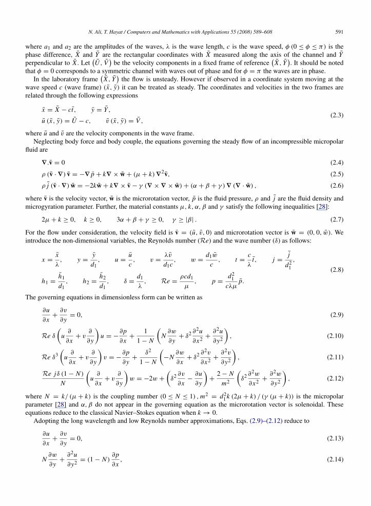
Fig. 1. Schematic diagram of the problem.

equation which exhibits all properties of non-Newtonian fluids. For this reason, many non-Newtonian models orconstitutive equations have been proposed and most of them are empirical or semi-empirical. Amongst these modelsthere is a micropolar fluid for which one can hope to obtain an approximate solution. In fact Eringen [29,30]originated the theory of micropolar fluids. Such a fluid can support coupled stresses, body couples and exhibitmicrorotational and microinertial effects. This theory is expected to provide a mathematical model for the rheologicalbehavior in certain man-made liquids such as polymers and also liquids such as blood. The theory of micropolarfluids is a special case of the theory of simple microfluids [31] introduced by Eringen himself. A detailed surveyof microcontinum fluid mechanics with various applications in physiological fluid flows has been given by Arimanet al. [32]. Lukasazewicz [33] in his recent book discussed many interesting aspects of the theory and applications ofmicropolar fluids.

Ever since the theory of the micropolar fluid appeared, a few workers have attempted peristaltic flow problemsconcerning these fluids. For example, Devi and Devanathan [34] studied the peristaltic motion of a micropolar fluidin a cylindrical tube with sinusoidal waves of small amplitude travelling down its flexible wall for the case of lowReynolds number. Srinivasacharya et al. [35] recently discussed the peristaltic transport of a micropolar fluid in acircular tube using low Reynolds number and long wavelength assumptions.

In the present paper, our concern is to investigate the peristaltic transport of a micropolar fluid in an asymmetricchannel. Now it has been noted by physiologists [36] that the intra-uterine fluid flow due to myometrial contractionsexhibits peristalsis and myometrial contractions may occur in both symmetric and asymmetric directions. It is also wellknown that blood is a non-Newtonian fluid in microcirculation [37,38]. Therefore, such consideration of peristaltictransport may be used to evaluate intra-uterine fluid flow in a non-pregnant uterus [39]. Also the main advantageof using a micropolar fluid model over the other non-Newtonian fluid models is that it takes care of the rotation offluid particles by means of an independent kinematic vector called the microrotation vector. The present analysis ofperistaltic flow is confined to large wavelength and low Reynolds number assumptions. Closed form solutions aredeveloped for axial velocity, axial pressure gradient, stream function and microrotation component. The numericaldiscussion of the pressure rise per wavelength, shear stresses and trapping is presented.

2. Mathematical formulation

Consider the peristaltic transport of an incompressible micropolar fluid in a two dimensional channel (Fig. 1) ofwidth d1 + d2. The flow is induced by sinusoidal wave trains propagating with constant speed c along the channelwalls. The geometry of the wall surfaces is

h1(X , t

)= d1 + a1 cos

[2πλ

(X − ct

)], ......upper wall (2.1)

h2(X , t

)= −d2 − a2 cos

[2πλ

(X − ct

)+ φ

], ......lower wall (2.2)

N. Ali, T. Hayat / Computers and Mathematics with Applications 55 (2008) 589–608 591

where a1 and a2 are the amplitudes of the waves, λ is the wave length, c is the wave speed, φ (0 ≤ φ ≤ π) is thephase difference, X and Y are the rectangular coordinates with X measured along the axis of the channel and Yperpendicular to X . Let

(U , V

)be the velocity components in a fixed frame of reference

(X , Y

). It should be noted

that φ = 0 corresponds to a symmetric channel with waves out of phase and for φ = π the waves are in phase.In the laboratory frame

(X , Y

)the flow is unsteady. However if observed in a coordinate system moving at the

wave speed c (wave frame) (x, y) it can be treated as steady. The coordinates and velocities in the two frames arerelated through the following expressions

x = X − ct, y = Y ,

u (x, y) = U − c, v (x, y) = V ,(2.3)

where u and v are the velocity components in the wave frame.Neglecting body force and body couple, the equations governing the steady flow of an incompressible micropolar

fluid are

∇.v = 0 (2.4)

ρ (v · ∇) v = −∇ p + k∇ × w + (µ+ k)∇2v, (2.5)

ρ j (v · ∇) w = −2kw + k∇ × v − γ (∇ × ∇ × w)+ (α + β + γ )∇ (∇ · w) , (2.6)

where v is the velocity vector, w is the microrotation vector, p is the fluid pressure, ρ and j are the fluid density andmicrogyration parameter. Further, the material constants µ, k, α, β and γ satisfy the following inequalities [28]:

2µ+ k ≥ 0, k ≥ 0, 3α + β + γ ≥ 0, γ ≥ |β| . (2.7)

For the flow under consideration, the velocity field is v = (u, v, 0) and microrotation vector is w = (0, 0, w). Weintroduce the non-dimensional variables, the Reynolds number (Re) and the wave number (δ) as follows:

x =x

λ, y =

y

d1, u =

u

c, v =

λv

d1c, w =

d1w

c, t =

c

λt, j =

j

d21

,

h1 =h1

d1, h2 =

h2

d1, δ =

d1

λ, Re =

ρcd1

µ, p =

d21

cλµp.

(2.8)

The governing equations in dimensionless form can be written as

∂u

∂x+∂v

∂y= 0, (2.9)

Re δ

(u∂

∂x+ v

∂

∂y

)u = −

∂p

∂x+

11 − N

(N∂w

∂y+ δ2 ∂

2u

∂x2 +∂2u

∂y2

), (2.10)

Re δ3(

u∂

∂x+ v

∂

∂y

)v = −

∂p

∂y+

δ2

1 − N

(−N

∂w

∂x+ δ2 ∂

2v

∂x2 +∂2v

∂y2

), (2.11)

Re jδ (1 − N )

N

(u∂

∂x+ v

∂

∂y

)w = −2w +

(δ2 ∂v

∂x−∂u

∂y

)+

2 − N

m2

(δ2 ∂

2w

∂x2 +∂2w

∂y2

), (2.12)

where N = k/ (µ+ k) is the coupling number (0 ≤ N ≤ 1) ,m2= d2

1 k (2µ+ k) / (γ (µ+ k)) is the micropolarparameter [28] and α, β do not appear in the governing equation as the microrotation vector is solenoidal. Theseequations reduce to the classical Navier–Stokes equation when k → 0.

Adopting the long wavelength and low Reynolds number approximations, Eqs. (2.9)–(2.12) reduce to

∂u

∂x+∂v

∂y= 0, (2.13)

N∂w

∂y+∂2u

∂y2 = (1 − N )∂p

∂x, (2.14)

592 N. Ali, T. Hayat / Computers and Mathematics with Applications 55 (2008) 589–608

∂p

∂y= 0, (2.15)

−2w −∂u

∂y+

(2 − N

m2

)∂2w

∂y2 = 0. (2.16)

The dimensional volume flow rate in the laboratory frame is

Q =

∫ h1(X ,t)

h2(X ,t)U

(X , Y , t

)dY . (2.17)

In the above equation h1 and h2 are functions of X and t . In the wave frame the above equation reduces to

q =

∫ h1(x)

h2(x)u (x, y) dy (2.18)

in which h1 and h2 are functions of x alone. From Eqs. (2.3), (2.17) and (2.18) we have

Q = q + ch1 (x)− ch2 (x) . (2.19)

The time-averaged flow over a period T at a fixed position X is

Q =1T

∫ T

0Qdt. (2.20)

Invoking Eq. (2.19) into Eq. (2.20) and then integrating one can write

Q = q + cd1 + cd2. (2.21)

Defining the dimensionless mean flows θ in the laboratory frame and F in the wave frame as

θ =Q

cd1, F =

q

cd1, (2.22)

Eq. (2.21) can be written as

θ = F + 1 + d (2.23)

in which

F =

∫ h1

h2

udy. (2.24)

The dimensionless form of the surfaces of the peristaltic walls is

h1 (x) = 1 + a cos 2πx, h2 (x) = −d − b cos (2πx + φ) , (2.25)

where a = a1/d1, b = a2/d1 and d = d2/d1.In the wave frame, the boundary conditions are

u = −1, at y = h1 (x) , y = h2 (x) , (2.26)

w = 0, at y = h1 (x) , y = h2 (x) . (2.27)

3. Exact solution

With the help of Eq. (2.15), Eq. (2.14) can be written in the following form

∂2u

∂y2 =∂

∂y

[(1 − N )

dp

dxy − Nw

]. (3.1)

N. Ali, T. Hayat / Computers and Mathematics with Applications 55 (2008) 589–608 593

Integration of the above equation yields

∂u

∂y= (1 − N )

dp

dxy − Nw + C1. (3.2)

Upon making use of above equation in Eq. (2.16) we get

∂2w

∂y2 − m2w = χ2C1 + χ2 (1 − N )dp

dxy. (3.3)

The general solution of Eq. (3.3) is

w = −C1χ

2

m2 −χ2

m2

dp

dx(1 − N ) y + C2 cosh my + C3 sinh my. (3.4)

Inserting above value of w into Eq. (3.2) we can write

u =12

(1 +

Nχ2

m2

)(1 − N )

dp

dxy2

+ C1

(1 +

Nχ2

m2

)y −

C2 N

msinh my −

C3 N

mcosh my + C4, (3.5)

in which C1−4 are the constants of integration and χ2= m2/ (2 − N ).

The arbitrary constants involved in Eq. (3.5) can be found with the help of boundary conditions (2.26) and(2.27) and are given by

C1 =L7

2L6

dp

dx, C2 =

L8

4L6

dp

dx, C3 =

L9

−4L6

dp

dx, C4 =

L10

4L6

dp

dx+

L11

4L6. (3.6)

Using Eq. (2.24) we find that

dp

dx=

F −L114L6

(h1 − h2)

η, (3.7)

where

η =L2

3

(h3

1 − h32

)+

L1L7

2L6

(h2

1 − h22

)+

L3L8

4mL6(cosh mh1 − cosh mh2)

−L9L3

4mL6(sinh mh1 − sinh mh2)+

L10

4L6(h1 − h2) .

The corresponding stream function is

ψ =L11

4L6y +

dp

dx

[L2

y3

3+

L1L7

L6

y2

2+

L3L8

4mL6cosh my −

L9L3

4mL6sinh my +

L10

4L6y

], (3.8)

where the values of L1–L11 are given in the Appendix.The non-dimensional expression for the pressure rise per wavelength 1Pλ is

1Pλ =

∫ 1

0

(dp

dx

)dx . (3.9)

4. Shear stress distribution at the walls

An interesting property of the micropolar fluid is that the stress tensor is not symmetric. The non-dimensional shearstresses in the problem under consideration are given by

τxy =∂u

∂y−

N

1 − Nw, (4.1)

τyx =1

1 − N

∂u

∂y+

N

1 − Nw. (4.2)

594 N. Ali, T. Hayat / Computers and Mathematics with Applications 55 (2008) 589–608

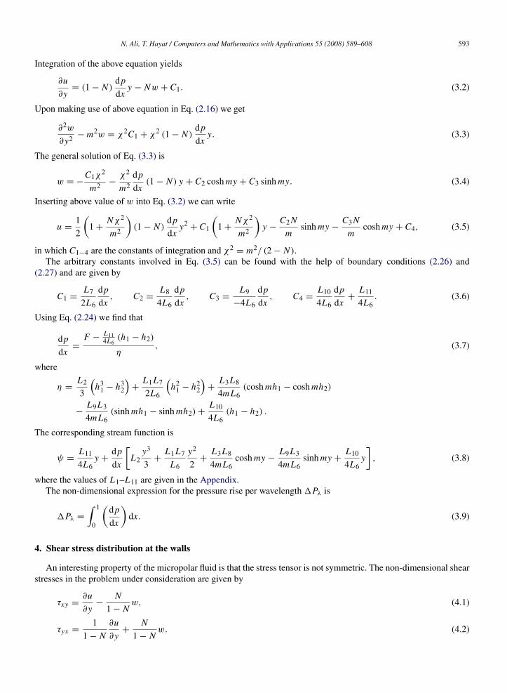
Fig. 2a. Plot showing 1Pλ versus flow rate θ . Here a = 0.5, b = 0.5, d = 1.5, φ = 0 and N = 0.4.

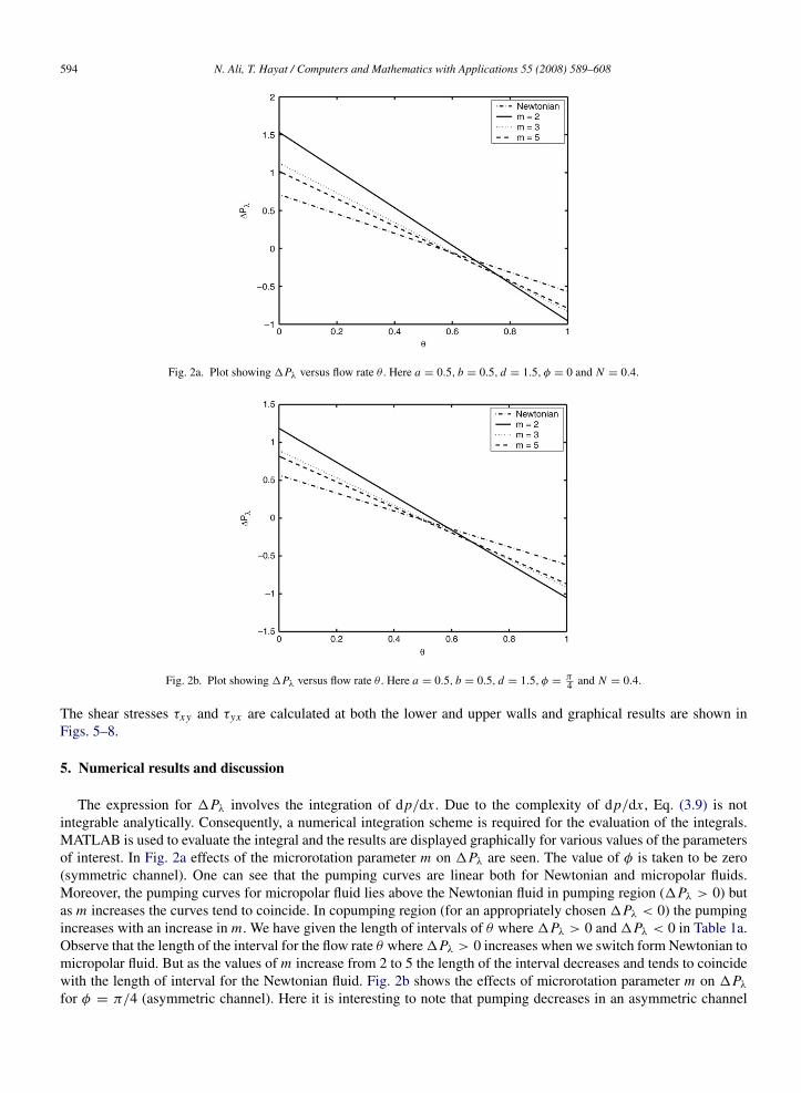
Fig. 2b. Plot showing 1Pλ versus flow rate θ . Here a = 0.5, b = 0.5, d = 1.5, φ =π4 and N = 0.4.

The shear stresses τxy and τyx are calculated at both the lower and upper walls and graphical results are shown inFigs. 5–8.

5. Numerical results and discussion

The expression for 1Pλ involves the integration of dp/dx . Due to the complexity of dp/dx , Eq. (3.9) is notintegrable analytically. Consequently, a numerical integration scheme is required for the evaluation of the integrals.MATLAB is used to evaluate the integral and the results are displayed graphically for various values of the parametersof interest. In Fig. 2a effects of the microrotation parameter m on 1Pλ are seen. The value of φ is taken to be zero(symmetric channel). One can see that the pumping curves are linear both for Newtonian and micropolar fluids.Moreover, the pumping curves for micropolar fluid lies above the Newtonian fluid in pumping region (1Pλ > 0) butas m increases the curves tend to coincide. In copumping region (for an appropriately chosen 1Pλ < 0) the pumpingincreases with an increase in m. We have given the length of intervals of θ where 1Pλ > 0 and 1Pλ < 0 in Table 1a.Observe that the length of the interval for the flow rate θ where1Pλ > 0 increases when we switch form Newtonian tomicropolar fluid. But as the values of m increase from 2 to 5 the length of the interval decreases and tends to coincidewith the length of interval for the Newtonian fluid. Fig. 2b shows the effects of microrotation parameter m on 1Pλfor φ = π/4 (asymmetric channel). Here it is interesting to note that pumping decreases in an asymmetric channel

N. Ali, T. Hayat / Computers and Mathematics with Applications 55 (2008) 589–608 595

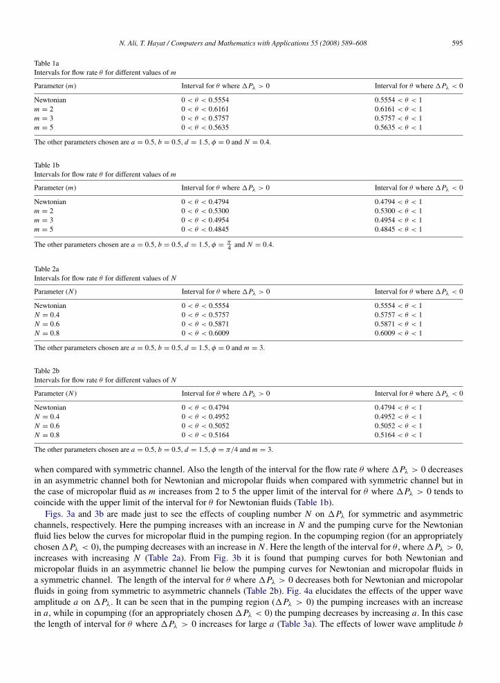
Table 1aIntervals for flow rate θ for different values of m

Parameter (m) Interval for θ where 1Pλ > 0 Interval for θ where 1Pλ < 0

Newtonian 0 < θ < 0.5554 0.5554 < θ < 1m = 2 0 < θ < 0.6161 0.6161 < θ < 1m = 3 0 < θ < 0.5757 0.5757 < θ < 1m = 5 0 < θ < 0.5635 0.5635 < θ < 1

The other parameters chosen are a = 0.5, b = 0.5, d = 1.5, φ = 0 and N = 0.4.

Table 1bIntervals for flow rate θ for different values of m

Parameter (m) Interval for θ where 1Pλ > 0 Interval for θ where 1Pλ < 0

Newtonian 0 < θ < 0.4794 0.4794 < θ < 1m = 2 0 < θ < 0.5300 0.5300 < θ < 1m = 3 0 < θ < 0.4954 0.4954 < θ < 1m = 5 0 < θ < 0.4845 0.4845 < θ < 1

The other parameters chosen are a = 0.5, b = 0.5, d = 1.5, φ =π4 and N = 0.4.

Table 2aIntervals for flow rate θ for different values of N

Parameter (N ) Interval for θ where 1Pλ > 0 Interval for θ where 1Pλ < 0

Newtonian 0 < θ < 0.5554 0.5554 < θ < 1N = 0.4 0 < θ < 0.5757 0.5757 < θ < 1N = 0.6 0 < θ < 0.5871 0.5871 < θ < 1N = 0.8 0 < θ < 0.6009 0.6009 < θ < 1

The other parameters chosen are a = 0.5, b = 0.5, d = 1.5, φ = 0 and m = 3.

Table 2bIntervals for flow rate θ for different values of N

Parameter (N ) Interval for θ where 1Pλ > 0 Interval for θ where 1Pλ < 0

Newtonian 0 < θ < 0.4794 0.4794 < θ < 1N = 0.4 0 < θ < 0.4952 0.4952 < θ < 1N = 0.6 0 < θ < 0.5052 0.5052 < θ < 1N = 0.8 0 < θ < 0.5164 0.5164 < θ < 1

The other parameters chosen are a = 0.5, b = 0.5, d = 1.5, φ = π/4 and m = 3.

when compared with symmetric channel. Also the length of the interval for the flow rate θ where 1Pλ > 0 decreasesin an asymmetric channel both for Newtonian and micropolar fluids when compared with symmetric channel but inthe case of micropolar fluid as m increases from 2 to 5 the upper limit of the interval for θ where 1Pλ > 0 tends tocoincide with the upper limit of the interval for θ for Newtonian fluids (Table 1b).

Figs. 3a and 3b are made just to see the effects of coupling number N on 1Pλ for symmetric and asymmetricchannels, respectively. Here the pumping increases with an increase in N and the pumping curve for the Newtonianfluid lies below the curves for micropolar fluid in the pumping region. In the copumping region (for an appropriatelychosen1Pλ < 0), the pumping decreases with an increase in N . Here the length of the interval for θ , where1Pλ > 0,increases with increasing N (Table 2a). From Fig. 3b it is found that pumping curves for both Newtonian andmicropolar fluids in an asymmetric channel lie below the pumping curves for Newtonian and micropolar fluids ina symmetric channel. The length of the interval for θ where 1Pλ > 0 decreases both for Newtonian and micropolarfluids in going from symmetric to asymmetric channels (Table 2b). Fig. 4a elucidates the effects of the upper waveamplitude a on 1Pλ. It can be seen that in the pumping region (1Pλ > 0) the pumping increases with an increasein a, while in copumping (for an appropriately chosen 1Pλ < 0) the pumping decreases by increasing a. In this casethe length of interval for θ where 1Pλ > 0 increases for large a (Table 3a). The effects of lower wave amplitude b

596 N. Ali, T. Hayat / Computers and Mathematics with Applications 55 (2008) 589–608

Fig. 3a. Plot showing 1Pλ versus flow rate θ . Here a = 0.5, b = 0.5, d = 1.5, φ = 0 and m = 3.

Fig. 3b. Plot showing 1Pλ versus flow rate θ . Here a = 0.5, b = 0.5, d = 1.5, φ =π4 and m = 3.

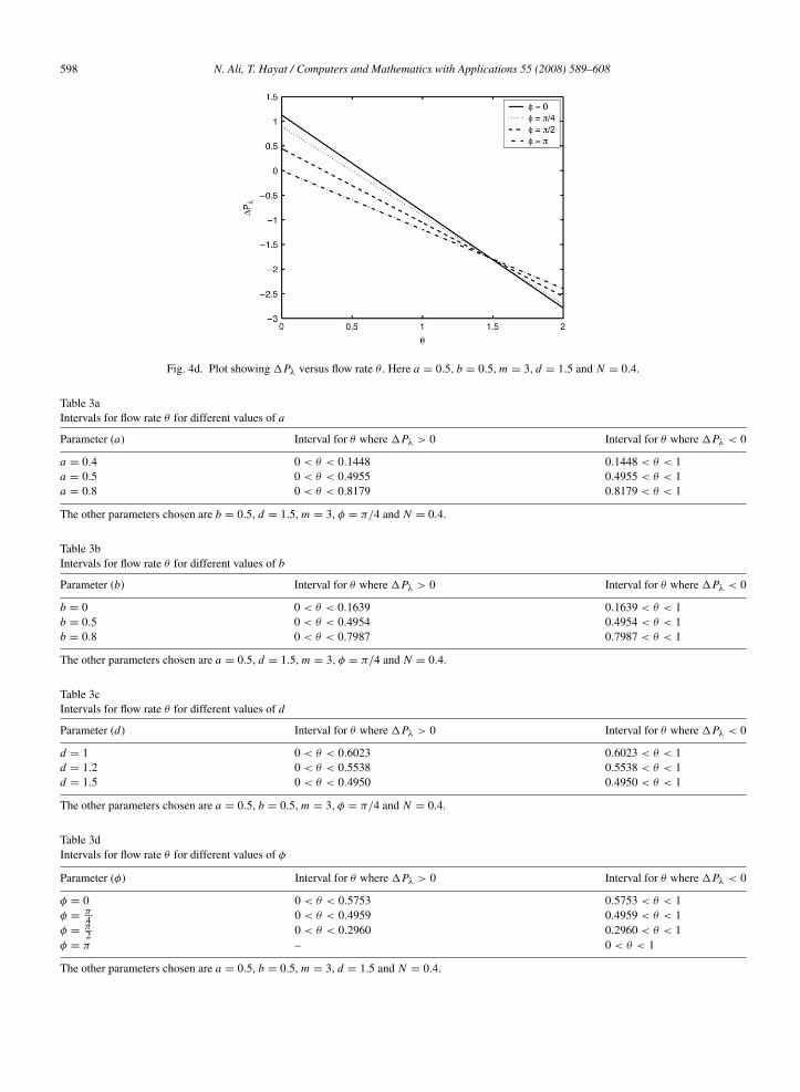
on 1Pλ are similar to that of a (Fig. 4b and Table 3b). We have sketched Fig. 4c for the effects of channel width don 1Pλ. Note that the pumping decreases for large d (in pumping region) while in copumping (for an appropriatelychosen1Pλ < 0) the pumping increases with increasing d. The length of the interval for θ where1Pλ < 0 decreaseswith an increase in d which is evident from Table 3c. Fig. 4d depicts the effects of phase difference φ on 1Pλ. Theeffects are similar to that of d on 1Pλ. Here as in the previous case the length of interval for θ where 1Pλ > 0decreases with an increase in φ (Table 3d).

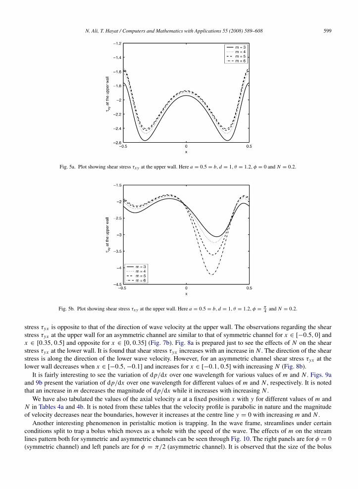
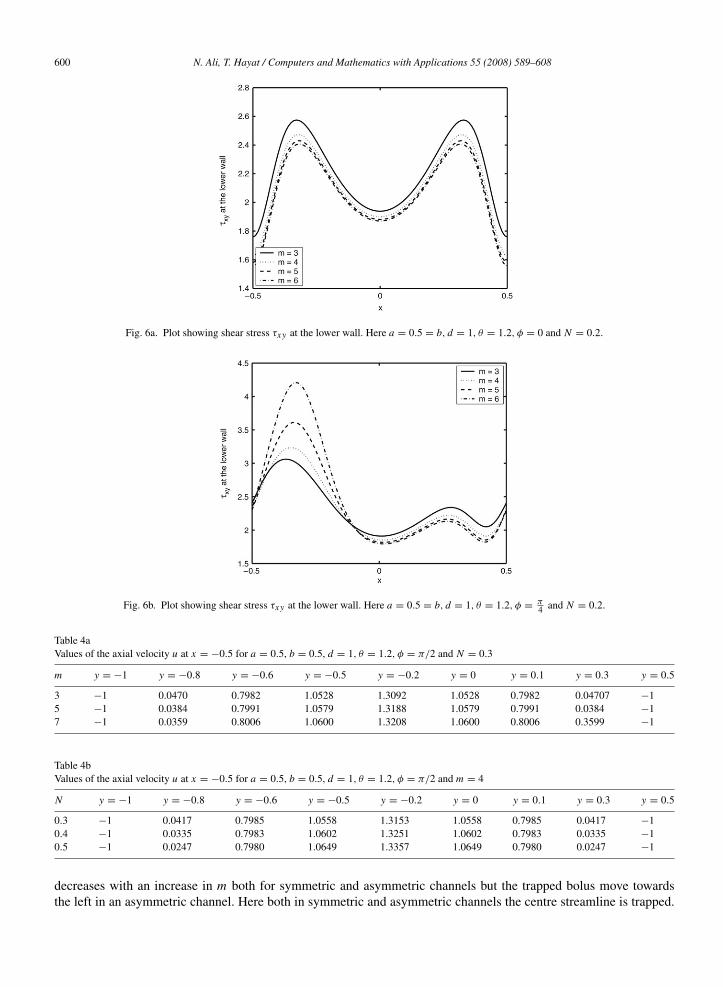
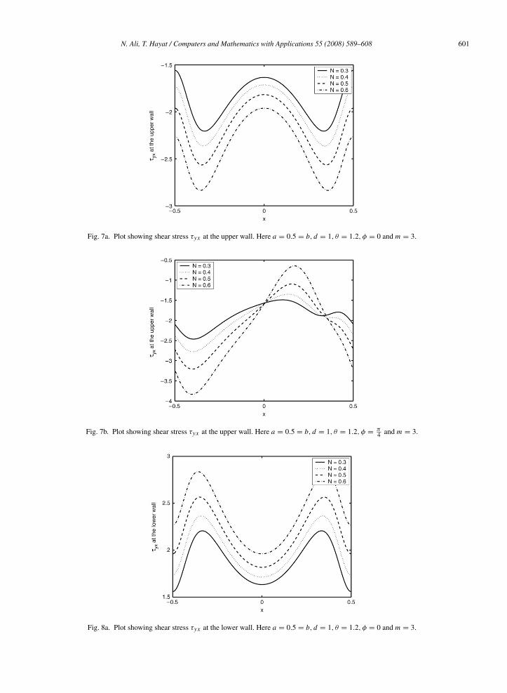
It is known that stress tensor is not symmetric in micropolar fluid. That is why the expressions for τxy and τyxare different. We have plotted the shear stress τxy at the upper wall for various values of m in Fig. 5a when φ = 0(symmetric channel). It can be seen that shear stress is symmetric about the line x = 0. However, it decreases withan increase in m. Moreover, the shear stress has direction opposite to the upper wave velocity. For an asymmetricchannel (Fig. 5b) shear stress decreases for x ∈ [−0.5, 0] and x ∈ [0.35, 0.5] while it increases for x ∈ [0, 0.35]when m is increased. The shear stress τxy at the lower wall is plotted for various values of m in Fig. 6a for symmetricchannels. The shear stress here decreases with increasing m and also the shear stress has its direction along the lowerwave velocity. The effects of m on the shear stress τxy at the lower wall for an asymmetric channel are opposite tothat in symmetric channels for x ∈ [−0.5,−0.1] and similar for x ∈ [−0.1, 0.5] (Fig. 6b). Further the direction ofshear stress is also along the lower wave velocity as in (Fig. 6a). Fig. 7a depicts the effects of N on the shear stressτyx at the upper wall. It is obvious from Fig. 7a that an increase in N increases the shear stress. The direction of shear

N. Ali, T. Hayat / Computers and Mathematics with Applications 55 (2008) 589–608 597

Fig. 4a. Plot showing 1Pλ versus flow rate θ . Here b = 0.5, d = 1.5, φ =π4 ,m = 3 and N = 0.4.

Fig. 4b. Plot showing 1Pλ versus flow rate θ . Here a = 0.5, d = 1.5,m = 3, φ =π4 and N = 0.4.

Fig. 4c. Plot showing 1Pλ versus flow rate θ . Here a = 0.5, b = 0.5,m = 3, φ =π4 and N = 0.4.

598 N. Ali, T. Hayat / Computers and Mathematics with Applications 55 (2008) 589–608

Fig. 4d. Plot showing 1Pλ versus flow rate θ . Here a = 0.5, b = 0.5,m = 3, d = 1.5 and N = 0.4.

Table 3aIntervals for flow rate θ for different values of a

Parameter (a) Interval for θ where 1Pλ > 0 Interval for θ where 1Pλ < 0

a = 0.4 0 < θ < 0.1448 0.1448 < θ < 1a = 0.5 0 < θ < 0.4955 0.4955 < θ < 1a = 0.8 0 < θ < 0.8179 0.8179 < θ < 1

The other parameters chosen are b = 0.5, d = 1.5, m = 3, φ = π/4 and N = 0.4.

Table 3bIntervals for flow rate θ for different values of b

Parameter (b) Interval for θ where 1Pλ > 0 Interval for θ where 1Pλ < 0

b = 0 0 < θ < 0.1639 0.1639 < θ < 1b = 0.5 0 < θ < 0.4954 0.4954 < θ < 1b = 0.8 0 < θ < 0.7987 0.7987 < θ < 1

The other parameters chosen are a = 0.5, d = 1.5, m = 3, φ = π/4 and N = 0.4.

Table 3cIntervals for flow rate θ for different values of d

Parameter (d) Interval for θ where 1Pλ > 0 Interval for θ where 1Pλ < 0

d = 1 0 < θ < 0.6023 0.6023 < θ < 1d = 1.2 0 < θ < 0.5538 0.5538 < θ < 1d = 1.5 0 < θ < 0.4950 0.4950 < θ < 1

The other parameters chosen are a = 0.5, b = 0.5, m = 3, φ = π/4 and N = 0.4.

Table 3dIntervals for flow rate θ for different values of φ

Parameter (φ) Interval for θ where 1Pλ > 0 Interval for θ where 1Pλ < 0

φ = 0 0 < θ < 0.5753 0.5753 < θ < 1φ =

π4 0 < θ < 0.4959 0.4959 < θ < 1

φ =π2 0 < θ < 0.2960 0.2960 < θ < 1

φ = π – 0 < θ < 1

The other parameters chosen are a = 0.5, b = 0.5, m = 3, d = 1.5 and N = 0.4.

N. Ali, T. Hayat / Computers and Mathematics with Applications 55 (2008) 589–608 599

Fig. 5a. Plot showing shear stress τxy at the upper wall. Here a = 0.5 = b, d = 1, θ = 1.2, φ = 0 and N = 0.2.

Fig. 5b. Plot showing shear stress τxy at the upper wall. Here a = 0.5 = b, d = 1, θ = 1.2, φ =π4 and N = 0.2.

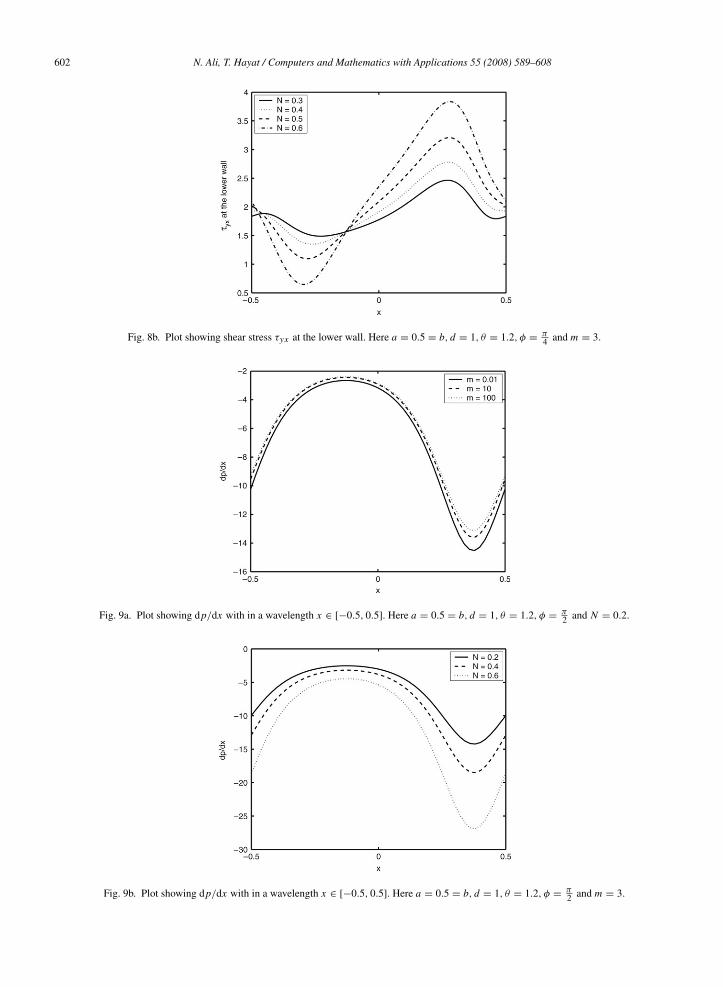
stress τyx is opposite to that of the direction of wave velocity at the upper wall. The observations regarding the shearstress τyx at the upper wall for an asymmetric channel are similar to that of symmetric channel for x ∈ [−0.5, 0] andx ∈ [0.35, 0.5] and opposite for x ∈ [0, 0.35] (Fig. 7b). Fig. 8a is prepared just to see the effects of N on the shearstress τyx at the lower wall. It is found that shear stress τyx increases with an increase in N . The direction of the shearstress is along the direction of the lower wave velocity. However, for an asymmetric channel shear stress τyx at thelower wall decreases when x ∈ [−0.5,−0.1] and increases for x ∈ [−0.1, 0.5] with increasing N (Fig. 8b).

It is fairly interesting to see the variation of dp/dx over one wavelength for various values of m and N . Figs. 9aand 9b present the variation of dp/dx over one wavelength for different values of m and N , respectively. It is notedthat an increase in m decreases the magnitude of dp/dx while it increases with increasing N .

We have also tabulated the values of the axial velocity u at a fixed position x with y for different values of m andN in Tables 4a and 4b. It is noted from these tables that the velocity profile is parabolic in nature and the magnitudeof velocity decreases near the boundaries, however it increases at the centre line y = 0 with increasing m and N .

Another interesting phenomenon in peristaltic motion is trapping. In the wave frame, streamlines under certainconditions split to trap a bolus which moves as a whole with the speed of the wave. The effects of m on the streamlines pattern both for symmetric and asymmetric channels can be seen through Fig. 10. The right panels are for φ = 0(symmetric channel) and left panels are for φ = π/2 (asymmetric channel). It is observed that the size of the bolus

600 N. Ali, T. Hayat / Computers and Mathematics with Applications 55 (2008) 589–608

Fig. 6a. Plot showing shear stress τxy at the lower wall. Here a = 0.5 = b, d = 1, θ = 1.2, φ = 0 and N = 0.2.

Fig. 6b. Plot showing shear stress τxy at the lower wall. Here a = 0.5 = b, d = 1, θ = 1.2, φ =π4 and N = 0.2.

Table 4aValues of the axial velocity u at x = −0.5 for a = 0.5, b = 0.5, d = 1, θ = 1.2, φ = π/2 and N = 0.3

m y = −1 y = −0.8 y = −0.6 y = −0.5 y = −0.2 y = 0 y = 0.1 y = 0.3 y = 0.5

3 −1 0.0470 0.7982 1.0528 1.3092 1.0528 0.7982 0.04707 −15 −1 0.0384 0.7991 1.0579 1.3188 1.0579 0.7991 0.0384 −17 −1 0.0359 0.8006 1.0600 1.3208 1.0600 0.8006 0.3599 −1

Table 4bValues of the axial velocity u at x = −0.5 for a = 0.5, b = 0.5, d = 1, θ = 1.2, φ = π/2 and m = 4

N y = −1 y = −0.8 y = −0.6 y = −0.5 y = −0.2 y = 0 y = 0.1 y = 0.3 y = 0.5

0.3 −1 0.0417 0.7985 1.0558 1.3153 1.0558 0.7985 0.0417 −10.4 −1 0.0335 0.7983 1.0602 1.3251 1.0602 0.7983 0.0335 −10.5 −1 0.0247 0.7980 1.0649 1.3357 1.0649 0.7980 0.0247 −1

decreases with an increase in m both for symmetric and asymmetric channels but the trapped bolus move towardsthe left in an asymmetric channel. Here both in symmetric and asymmetric channels the centre streamline is trapped.

N. Ali, T. Hayat / Computers and Mathematics with Applications 55 (2008) 589–608 601

Fig. 7a. Plot showing shear stress τyx at the upper wall. Here a = 0.5 = b, d = 1, θ = 1.2, φ = 0 and m = 3.

Fig. 7b. Plot showing shear stress τyx at the upper wall. Here a = 0.5 = b, d = 1, θ = 1.2, φ =π4 and m = 3.

Fig. 8a. Plot showing shear stress τyx at the lower wall. Here a = 0.5 = b, d = 1, θ = 1.2, φ = 0 and m = 3.

602 N. Ali, T. Hayat / Computers and Mathematics with Applications 55 (2008) 589–608

Fig. 8b. Plot showing shear stress τyx at the lower wall. Here a = 0.5 = b, d = 1, θ = 1.2, φ =π4 and m = 3.

Fig. 9a. Plot showing dp/dx with in a wavelength x ∈ [−0.5, 0.5]. Here a = 0.5 = b, d = 1, θ = 1.2, φ =π2 and N = 0.2.

Fig. 9b. Plot showing dp/dx with in a wavelength x ∈ [−0.5, 0.5]. Here a = 0.5 = b, d = 1, θ = 1.2, φ =π2 and m = 3.

N. Ali, T. Hayat / Computers and Mathematics with Applications 55 (2008) 589–608 603

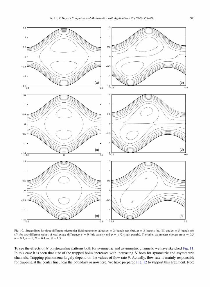
Fig. 10. Streamlines for three different micropolar fluid parameter values m = 2 (panels (a), (b)), m = 3 (panels (c), (d)) and m = 5 (panels (e),(f)) for two different values of wall phase difference φ = 0 (left panels) and φ = π/2 (right panels). The other parameters chosen are a = 0.5,b = 0.5, d = 1, N = 0.4 and θ = 1.3.

To see the effects of N on streamline patterns both for symmetric and asymmetric channels, we have sketched Fig. 11.In this case it is seen that size of the trapped bolus increases with increasing N both for symmetric and asymmetricchannels. Trapping phenomena largely depend on the values of flow rate θ . Actually, flow rate is mainly responsiblefor trapping at the center line, near the boundary or nowhere. We have prepared Fig. 12 to support this argument. Note

604 N. Ali, T. Hayat / Computers and Mathematics with Applications 55 (2008) 589–608

Fig. 11. Streamlines for three different coupling parameter values N = 0.4 (panels (a), (b)), N = 0.6 (panels (c), (d)) and N = 0.8 (panels (e),(f)) for two different values of wall phase difference φ = 0 (left panels) and φ = π/2 (right panels). The other parameters chosen are a = 0.5,b = 0.5, d = 1,m = 3 and θ = 1.3.

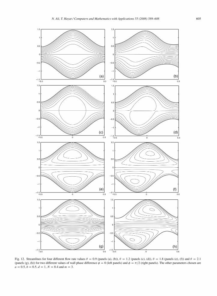
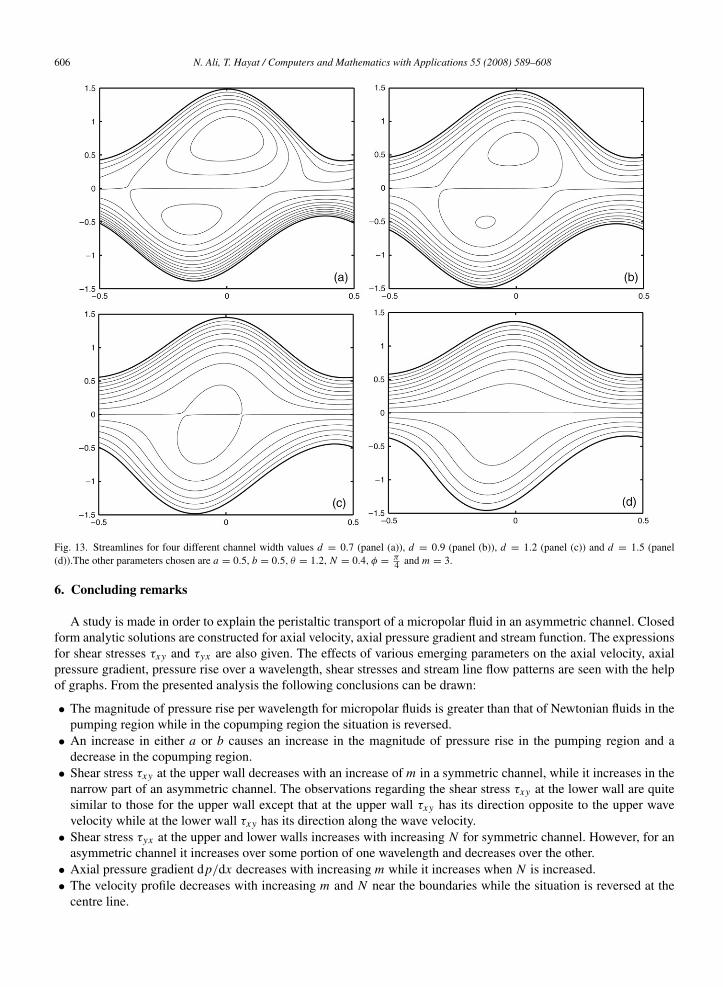
that for θ = 0.9 there is no trapping phenomenon. For θ = 1.2 center streamline is trapped and trapping move towardsthe boundary for the flow rate value θ = 1.8. Moreover, for θ = 2.1 trapping is at the boundary. The effects of thechannel width d on the trapping can be seen through Fig. 13. It is found that for small values of d trapping exists andthe size of the trapped bolus is large and decreases in size when d increases and vanishes for d = 1.5.

N. Ali, T. Hayat / Computers and Mathematics with Applications 55 (2008) 589–608 605

Fig. 12. Streamlines for four different flow rate values θ = 0.9 (panels (a), (b)), θ = 1.2 (panels (c), (d)), θ = 1.8 (panels (e), (f)) and θ = 2.1(panels (g), (h)) for two different values of wall phase difference φ = 0 (left panels) and φ = π/2 (right panels). The other parameters chosen area = 0.5, b = 0.5, d = 1, N = 0.4 and m = 3.

606 N. Ali, T. Hayat / Computers and Mathematics with Applications 55 (2008) 589–608

Fig. 13. Streamlines for four different channel width values d = 0.7 (panel (a)), d = 0.9 (panel (b)), d = 1.2 (panel (c)) and d = 1.5 (panel(d)).The other parameters chosen are a = 0.5, b = 0.5, θ = 1.2, N = 0.4, φ =

π4 and m = 3.

6. Concluding remarks

A study is made in order to explain the peristaltic transport of a micropolar fluid in an asymmetric channel. Closedform analytic solutions are constructed for axial velocity, axial pressure gradient and stream function. The expressionsfor shear stresses τxy and τyx are also given. The effects of various emerging parameters on the axial velocity, axialpressure gradient, pressure rise over a wavelength, shear stresses and stream line flow patterns are seen with the helpof graphs. From the presented analysis the following conclusions can be drawn:

• The magnitude of pressure rise per wavelength for micropolar fluids is greater than that of Newtonian fluids in thepumping region while in the copumping region the situation is reversed.

• An increase in either a or b causes an increase in the magnitude of pressure rise in the pumping region and adecrease in the copumping region.

• Shear stress τxy at the upper wall decreases with an increase of m in a symmetric channel, while it increases in thenarrow part of an asymmetric channel. The observations regarding the shear stress τxy at the lower wall are quitesimilar to those for the upper wall except that at the upper wall τxy has its direction opposite to the upper wavevelocity while at the lower wall τxy has its direction along the wave velocity.

• Shear stress τyx at the upper and lower walls increases with increasing N for symmetric channel. However, for anasymmetric channel it increases over some portion of one wavelength and decreases over the other.

• Axial pressure gradient dp/dx decreases with increasing m while it increases when N is increased.• The velocity profile decreases with increasing m and N near the boundaries while the situation is reversed at the

centre line.

N. Ali, T. Hayat / Computers and Mathematics with Applications 55 (2008) 589–608 607

• The size of a trapped bolus decreases with an increase in m while it increases with an increase in N .• The trapping phenomenon is largely dependent upon the values of the flow rate θ .

Acknowledgements

We are grateful to the Higher Education Commission (HEC) for financial assistance. We further thank the reviewersfor their valuable suggestions.

Appendix

Here we provide the values of the constants appearing in Eqs. (3.6)–(3.9). These are

L1 =12

(1 +

Nχ2

m2

),

L2 = L1 (1 − N ) ,

L3 = −N

m, L4 = −

χ2

m2 , L5 = (1 − N ) L4,

L6 = (h1 − h2) L1 cosh(

h1 − h2

2

)m − L3L4 sinh

(h1 − h2

2

)m,

L7 = − (h1 + h2)

[(h1 − h2) L2 cosh

(h1 − h2

2

)m − L3L5 sinh

(h1 − h2

2

)m

],

L8 = (h1 − h2) csc h

(h1 − h2

2

)m [L3L4L5 (cosh mh2 − cosh mh1)+ (h1 + h2) L2L4 sinh mh1

+ 2L1L5 (h1 sinh mh2 − h2 sinh mh1)− (h1 − h2) L2L4 sinh mh2] ,

L9 = (h1 − h2) csc h

(h1 − h2

2

)m [(h1 + h2) L2L4 (cosh mh1 − cosh mh2)

+ 2L1L5 (h2 cosh mh1 − h1 cosh mh2)+ L3L4L5 (sinh mh2 − sinh mh1)] ,

L10 = csc h

(h1 − h2

2

)m

[−L2L3L5

(h2

1 + h22

) (L2L3L4

(h2

1 + h22

)− 4h1h2L1L3L5

)× cosh (h1 − h2)m + 2L1L3L5

(h2

1 + h22

)+ (h1 − h2) sinh (h1 − h2)m

(2h1h2L1L2 − L2

3L4L5

)],

L11 = csc h

(h1 − h2

2

)m [2L3L4 (cosh (h1 − h2)m − 1)− 2 (h1 − h2) L1 sinh (h1 − h2)m] .

References

[1] T. Hayat, A.H. Kara, E. Momoniat, Exact flow of a third grade fluid on a porous wall, Internat. J. Non-linear Mech. 38 (2003) 1533–1537.[2] T. Hayat, A.H. Kara, Couette flow of a third grade fluid with variable magnetic field, Math. Comput. Modelling 43 (2006) 132–137.[3] T. Hayat, S.B. Khan, M. Khan, The influence of Hall current on the rotating oscillating flows of an Oldroyd-B fluid in a porous medium,

Non-Linear Dynam. 47 (2007) 353–362.[4] C. Fetecau, C. Fetecau, Decay of a potential vortex in an Oldroyd-B fluid, Internat. J. Engrg. Sci. 43 (2005) 340–351.[5] C. Fetecau, C. Fetecau, Unsteady flows of Oldroyd-B fluids in a channel of rectangular cross-section, Internat. J. Non-Linear Mech. 38 (2005)

1214–1219.[6] C. Fetecau, C. Fetecau, On some axial Couette flows of non-Newtonian fluids, Z. Angew. Math. Phys. 56 (2005) 1098–1106.[7] C. Fetecau, C. Fetecau, Starting solutions for some unsteady unidirectional flows of a second grade fluid, Internat. J. Engrg. Sci. 43 (2005)

781–789.[8] W.C. Tan, T. Masuoka, Stokes first poroblem for second grade fluid in a porous half space with heated boundary, Internat. J. Non-Linear

Mech. 40 (2005) 515–522.[9] W.C. Tan, T. Masuoka, Stokes first problem for an Oldroyd-B fluid in a porous half space, Phys. Fluids 17 (2005) 023101–023107.

[10] S. Liao, On analytic solution of magnetohydrodynamic flows of non-Newtonian fluids over a stretching sheet, J. Fluid Mech. 488 (2003)189–212.

608 N. Ali, T. Hayat / Computers and Mathematics with Applications 55 (2008) 589–608

[11] C.I. Chen, C.K. Chen, Y.T. Yang, Unsteady unidirectional flow of an Oldroyd-B fluid in a circular duct with different given volume flow rateconditions, Heat Mass Transfer 40 (2004) 203–209.

[12] C.I. Chen, C.K. Chen, Y.T. Yang, Unsteady unidirectional flow of a second grade fluid between the parallel plates with different given volumeflow rate conditions, Appl. Math. Comput. 137 (2) (2003) 437–450.

[13] T. Hayat, Y. Wang, A.M. Siddiqui, K. Hutter, S. Asghar, Peristaltic transport of a third order fluid in a circular cylindrical tube, Math. ModelsMethods Appl. Sci. 12 (2002) 1691–1706.

[14] T. Hayat, Y. Wang, A.M. Siddiqui, K. Hutter, Peristaltic motion of Johnson–Segalman fluid in a planar channel, Math. Probl. Eng. 1 (2003)1–23.

[15] T. Hayat, Y. Wang, K. Hutter, S. Asghar, A.M Siddiqui, Peristaltic transport of an Oldroyd-B fluid in a planar channel, Math. Probl. Eng. 4(2004) 347–376.

[16] A.M. Siddiqui, T. Hayat, M. Khan, Magnetic fluid model induced by peristaltic waves, J. Phy. Soc. Japan 73 (2004) 2142–2147.[17] T. Hayat, F.M. Mahomed, S. Asghar, Peristaltic flow of magnetohydrodynamic Johnson–Segalman fluid, Nonlinear Dynam. 40 (2005)

375–385.[18] T. Hayat, M. Khan, S. Asghar, A.M. Siddiqui, A mathematical model of peristalsis in tubes through a porous medium, J. Porous Media 9

(2006) 55–67.[19] Kh.S. Mekheimer, Nonlinear peristaltic transport through a porous medium in an inclined planar channel, J. Porous Media 6 (2003) 189–201.[20] Kh.S. Mekheimer, Nonlinear peristaltic transport of magneto-hydrodynamic flow in an inclined planar channel, Arab J. Sci. Eng. 28 (2003)

183–201.[21] Kh.S. Mekheimer, Peristaltic flow of blood under effect of a magnetic field in a non uniform channels, Appl. Math. Comput. 153 (2004)

763–777.[22] Kh.S. Mekheimer, Peristaltic transport of a couple-stress fluid in a uniform and non-uniform channels, Biorheology 39 (2002) 755–765.[23] M. El-Shahed, Pulsatile flow of blood through a stenosed porous medium under periodic body acceleration, Appl. Math. Comput. 138 (2003)

479–488.[24] M. Elshahed, M.H. Haroun, Peristaltic transport of Johnson–Segalman fluid under effect of a magnetic field, Math. Probl. Eng. 6 (2005)

663–677.[25] M.H. Haroun, Effect of wall compliance on peristaltic transport of a Newtonian fluid in an asymmetric channel, Math. Probl. Eng. 2006

(2006) 1–19.[26] M.H. Haroun, Non-linear peristaltic flow of a fourth grade fluid in an inclined asymmetric channel, Comput. Mater. Sci. 39 (2007) 324–333.[27] M.H. Haroun, Effect of Deborah number and phase difference on peristaltic transport of a third-order fluid in an asymmetric channel, Commun.

Nonlinear Sci. Numer Simul. 12 (2007) 1464–1480.[28] M. Mishra, A.R. Rao, Peristaltic transport of a Newtonian fluid in an asymmetric channel, Z. Angew. Math. Phys. 54 (2004) 532–550.[29] A.C. Eringen, Non-linear theory of simple micro-elastic solids-I, Internat. J. Engrg. Sci. 2 (1964) 189–203.[30] A.C. Eringen, Some micro fluids, Internat. J. Engrg. Sci. 2 (1964) 205–217.[31] A.C. Eringen, Theory of micropolar fluids, J. Math. Mech. 16 (1966) 1–16.[32] T. Ariman, M.A. Turk, N. Sylvester, Application of microcontinum fluid mechanics, Internat J. Engrg. Sci. 12 (1974) 273–293.[33] G. Lukasazewicz, Micropolar Fluid-Theory and Applications, Birkhausr, Boston, 1999.[34] G. Devi, R. Devanathan, Peristaltic motion of a micropolar fluid, Proc. Indian Acad. Sci. 81 (A) (1975) 149–163.[35] D. Srinivasacharya, M. Mishra, A.R. Rao, Peristaltic pumping of a micropolar fluid in a tube, Acta Mech. 161 (2003) 165–178.[36] K. De Vries, E.A. Lyons, J. Ballard, C.S. Levi, D.J. Lindsay, Contractions of the inner third of the myometrium, Amer. J. Obstetrics Gynecol.

162 (1990) 679–682.[37] C.Y. Fung, C.S. Yih, Peristaltic transport, Trans. ASME J. Appl. Mech. 35 (1968) 669–675.[38] L.K. Antanovskii, H. Ramkissoon, Long-wave peristaltic transport of a compressible viscous fluid in a finite pipe subject to a time-dependent

pressure drop, Fluid Dynam. Res. 19 (1997) 115–123.[39] O. Eytan, D. Elad, Analysis of intra-uterine fluid motion induced by uterine contractions, Bull. Math. Biol. 61 (1999) 221–238.