Asymmetric stochastic Tau theory in car-following

Transportation Research Part F 18 (2013) 21–33

Contents lists available at SciVerse ScienceDirect

Transportation Research Part F

journal homepage: www.elsevier .com/locate / t r f

Asymmetric stochastic Tau Theory in car-following

1369-8478/$ - see front matter � 2012 Elsevier Ltd. All rights reserved.http://dx.doi.org/10.1016/j.trf.2012.12.002

⇑ Corresponding author. Address: #806, Central Main Building, Tsinghua University, Beijing 100084, China. Tel.: +86 (10) 62782071.E-mail address: [email protected] (L. Li).

Li Li a,⇑, Xiqun Chen b, Zhiheng Li a

a Department of Automation, Tsinghua University, Beijing 100084, Chinab Department of Civil Engineering, Tsinghua University, Beijing 100084, China

a r t i c l e i n f o

Article history:Received 18 April 2010Received in revised form 27 September2012Accepted 5 December 2012

Keywords:Tau TheoryWeber–Fechner LawCar-followingHeadway distribution

a b s t r a c t

In this paper, we examine the distribution of headways collected from Next GenerationSIMulation (NGSIM) datasets. Statistics show that the observed headways follow a certainlog-normal type distribution within each preselected velocity range. To explain this phe-nomenon, an asymmetric stochastic extension of the Tau Theory is proposed. This novelapproach assumes that the observed headway distributions are due to drivers’ continuousheadway adjustment behaviours, and that the intensity of headway change is proportionalto headway magnitude. The agreement between the model predictions and the empiricalobservations indicates that driving behaviours may be implicitly governed by the physio-logical Tau characteristics of drivers.

� 2012 Elsevier Ltd. All rights reserved.

1. Introduction

Time headway is defined as the amount of time that elapses between the rears of two successive vehicles passing thesame point on a road. The statistics of time headway have gained a lot of attention in the field of transportation engineeringfor its significant impacts on behavioural studies, traffic signal timing (Highway Capacity Manual, 2010) and traffic flowphysics. It is often viewed as a reflection of the implicit forces that govern human driving (see Brackstone & McDonald,2007; Brackstone, Waterson, & McDonald, 2009; Ranney, 1999; Van Winsum, 1999).

In recent years, a number of experiments have been conducted in an effort to examine headway adjustment behaviour incar-following (Banks, 2003; Brackstone & McDonald, 2003; Chen, Li, & Zhang, 2010, Taieb-Maimon & Shinar, 2001). The resultsindicate that drivers tend to maintain a generally consistent headway while within a single specific driving scenario. However,it is impossible for a driver to maintain a fixed headway, because of the unpredictability of leading vehicle movements and theinaccuracy of human perceptions, which lead to errors in decision making and action. Drivers have to constantly adjust theirbehaviour in an attempt to maintain their preferred headways. This process, which depends on the physiological response ofdrivers, yields a log-normal type headway distribution (or more generally, a C distribution) within each preselected velocityrange (Chen, Li, Jiang, Yang, 2010; Chen, Li, & Zhang, 2010; Jin, Su, Zhang, Wei, & Li, 2009; Jin, Zhang et al., 2009).

Since the early 1950s, many models have been proposed in order to explain headway distribution patterns (e.g. Abul-Magd, 2007; Chen et al., 2010; HCM, 2010; Jin et al., 2009; Krbalek, Šeba, & Wagner, 2001; Li, Wang, Jiang, Hu, & Ji, 2010;Nishinari, Treiber, & Helbing, 2003; Wang et al., 2009; Yan, Lorv, Li, & Sun, 2011). In most of these stochastic models, theproposed virtual forces that control vehicle movements are difficult to interpret from our daily driving experiences.

Thus, a question naturally arises: Is there a driver-centric factor behind such log-normal distributions? By further examiningempirical headway distributions, we recently realized that this phenomenon can be physiologically explained by extendingthe Tau Theory on perception and action.

http://crossmark.dyndns.org/dialog/?doi=10.1016/j.trf.2012.12.002&domain=pdf

http://dx.doi.org/10.1016/j.trf.2012.12.002

mailto:[email protected]

http://dx.doi.org/10.1016/j.trf.2012.12.002

http://www.sciencedirect.com/science/journal/13698478

http://www.elsevier.com/locate/trf

22 L. Li et al. / Transportation Research Part F 18 (2013) 21–33

The Tau Theory originates from the study of optical variable Tau (s), which is defined as the projected angular size h of anobject divided by the relative change rate Dh/Dt. In other words, it describes the change of the incoming object’s image onthe retina (Lee, 1976; Lee, 2009), i.e. s = h/(Dh/Dt). Tau (s) is often regarded as an invariant. It is veridical and independent ofother variables, such as the distance and velocity of the incoming object (Yan et al., 2011).

In this paper, we study the ratio s between the current headway and the change in headway in the next time interval.Although different values of s can be observed in each iteration of the headway adjustment process due to the randomnessof human behaviour, we found that the values can generally be represented as s� and s+ for acceleration and deceleration,respectively. It is also widely accepted that the coexistence of s� and s+ is caused by asymmetric driving behaviours (Edie,1965; Foote, 1965; Forbes, 1963; Yeo, 2008; Yeo & Skabardonis, 2009).

The above findings indicate that microscopic driving behaviours influence macroscopic traffic flow dynamics in a latentand stochastic way. More importantly, we can identify intrinsic common physiological characteristics of driving behaviourvia the extrinsic measurements (e.g. headways).

To provide a detailed discussion of our research, the rest of this paper is structured as follows: First, the Tau Theory, whichforms the fundamental background of this research, is presented. Then, an asymmetric stochastic extension of the Tau The-ory is proposed as a novel explanation for the log-normal type headway distributions observed in empirical car-followingprocesses. Finally, we will discuss statistics based on Next Generation SIMulation (NGSIM, 2006) datasets and whether ornot the results validate the asserted asymmetric headway adjustment behaviour.

2. Asymmetric stochastic extension of the Tau Theory

2.1. The original Tau Theory model

There are several measures of driving behaviour characteristics. For example, Time-To-Collision (TTC) is a frequentlymentioned one. It is defined as the time at which two vehicles would collide if both vehicles maintained their independentspeeds and trajectories (Brackstone & McDonald, 2007; Brackstone et al., 2009). That is, TTC is the ratio of the relative spacegap divided by the relative speed Dv (a positive value represents a higher following vehicle speed), i.e. TTC = Dx/Dv = (hv � l)/Dv if Dv > 0, where Dx is the following gap, h is the time headway, v is the following velocity, l is the vehiclelength.

Similarly but differently, Tau theory studies time headway h instead of TTC. The initial Tau Theory, which was developedby Lee (1976), states that drivers focus on visual information (such as time-to-collision) instead of other types of information(such as space gap, speed, or ac/deceleration). More recently, Frost (2009) showed that all purposeful actions entail control-ling s, which is the time-to-collision between the current position and the expected post-adjustment position. Lee (2009)pointed out that it is possible to build various s models depending on how the movements and states are defined.

From a neurophysiology perspective (see Farrow, Haag, & Borst, 2006; Frost, 2009; Schrater, Knill, & Simoncelli, 2001; Sun& Frost, 1998), time headway change caused by driver actions is controlled by a parameter s as

s ¼ hðtÞDhðtÞ=T

¼ hðtÞ � Thðt þ TÞ � hðtÞ ð1Þ

where h(t) is the time headway at time t, and Dh(t) = h(t + T) � h(t) is the change of h(t) within a defined time interval T,which is the time interval between two consecutive driver reactions.

If s is a constant, Eq. (1) indicates that the intensity of headway magnitude is proportional to headway change in T. Basedon the Weber–Fechner Law (Deco, Scarano, & Soto-Faraco, 2007; Shen, 2003; Weber, 1834), Eq. (1) can also be explained as alinear function between visual stimulus (headway) and driver response (headway change) within a certain time interval T.This is in accordance with previous assumptions from most psychophysical car-following models (Boer, 1999; Brackstone &McDonald, 1999; Michaels, 1963; Van Winsum, 1999). The difference is that previous psychophysical models aim to directlydepict the visual angle subtended by the leading vehicle; while Eq. (1) attempts to incorporate perceptual reactions intoheadway change and provide an indirect measure for human visual control.

However, we cannot directly fit Tau-theory model (1) with empirical observations. As discussed by Michaels (1963) andBoer (1999), the perceptions and actions of drivers are generally limited and inaccurate. In other words, s is not a constant inthe real world.

2.2. Extended Tau Theory model in car-following

The randomness explicitly embedded in the evolution of headway can be explained as the unconscious and inaccurateperceptions of time interval and space that humans perform. If a driver is observed for a long enough time period, wecan characterize the driver’s car-following behaviour by examining the statistical features of this stochastic process. Anadvantage of this approach is that the steady-state distribution of this stochastic process can be directly calculated, and com-pared with empirical headway distributions as a way to validate the model.

To model the randomness in driving behaviour, a special stochastic process was proposed in Jin et al. (2009) and Li et al.(2010) as follows:

L. Li et al. / Transportation Research Part F 18 (2013) 21–33 23

hðt þ TÞhðtÞ ¼

b with prob: p1=b with prob: 1� p

�ð2Þ

where b e (0, 1) is the scaling coefficient and p e (0, 0.5] denotes the tendency for the driver to reach a smaller headway thanpreferred at time t + T. Analogously, 1 � p is the tendency to reach a larger headway than preferred at time t + T. Specifically,the situation T = 1.0 s is considered in Jin et al. (2009) and Li et al. (2010).

As such, Eq. (2) can be viewed as a modified Tau Theory model, which can be rewritten as

DhðtÞhðtÞ ¼

Ts� ¼ b� 1 with prob: p

Tsþ ¼ 1=b� 1 with prob: 1� p

(ð3Þ

or equivalently

s ¼ hðtÞDhðtÞ=T

¼s� < 0 if hðt þ TÞ < hðtÞ;with prob: p

sþ > 0 if hðt þ TÞ > hðtÞ;with prob: 1� p

�ð4Þ

where s� and s+ are the Tau factors, given that Ts� þ 1� �

Tsþ þ 1� �

¼ 1.Eq. (4) extends Eq. (1), the original Tau Theory model, in two ways:

(1) Asymmetric behaviour: a driver’s behaviour varies according to whether he/she is accelerating or decelerating. Duringacceleration, a driver will be more cautious and make smaller changes in headway. On the contrary, during deceler-ation, he/she will be less sensitive to headway change. This asymmetry in vehicle acceleration and deceleration hasbeen observed by many researchers (see Edie, 1965; Foote, 1965; Forbes, 1963). There are different ways to considersuch asymmetry in car following models. For example, Forbes (1963) explained this asymmetry as a difference in dri-ver response time, which is slower during acceleration than deceleration. However, in this paper, we consider morethan just driver response time when addressing the asymmetric property of s. Eq. (4) does not indicate whetherthe Tau factors s� and s+ are constant or velocity-dependent. This will be determined using field data in a later section.

(2) Stochastic behaviours: as reported in numerous literature (e.g. Banks, 2003; Brackstone & McDonald, 2003; Chen, Li &Jiang, et al., 2010; Taieb-Maimon & Shinar, 2001), drivers try to maintain a consistent headway; but in reality, driversmaintain a stochastic headway that fluctuates around an expected value. In order to model this uncertainty, the prob-ability p is introduced to characterize the tendency of reaching headway h(t + T), which is smaller than the currentheadway h(t).

The first part of Eq. (4) asserts that, on average, drivers have a tendency/probability p to reach a smaller headway thanpreferred. However, Eq. (4) does not assert that drivers will adjust headway exactly as Dh(t) = h(t)T/s� < 0 or Dh(t) = h(t)T/s+ > 0 for each t. Indeed, if the statistical mean of Dh(t) is calculated over a relatively long period, the adjustment behaviourwill lead to a headway change of D�hðtÞ ¼ hðtÞT=s�. Similarly, we can interpret the second part of Eq. (4) as the tendency toreach a larger headway than preferred. In this case, the headway change can be expressed as D�hðtÞ ¼ hðtÞT=sþ.

As proven in numerous literature (Jin et al., 2009; Li et al., 2010; Limpert, Stahel, & Abbt, 2001), a stochastic process char-acterized by Eq. (4) would generate velocity-dependent log-normal headway distributions during simulations. However, dif-fering from the previous physical analysis (Jin et al., 2009; Li et al., 2010), the extended Tau Theory is a more penetrative andintrinsic explanation because it is built on the assumption that the limits of driver perceptions and actions will allow for a cer-tain s-type proportional law between the headway and its increments (Lee, 2009).

Eq. (4) has not been previously validated by empirical flow data. In Section 3, we will test the validity of the above asser-tions based on the observed headway data.

2.3. Testing method for extended Tau Theory model

To verify Eq. (4), we need to prove two assertions for h(t) ? h(t + T).

(1) Drivers have a relatively constant tendency p to reach a smaller headway than preferred at different velocities. If this istrue, then

(2) Drivers have relatively constant s� and s+ at different velocities and ð Ts� þ 1Þð T

sþ þ 1Þ ¼ 1.

Notice that h(t) is a continuous value. In order to accurately verify Eq. (4), it is necessary to estimate a transferring kernelof the proposed stochastic process (Kallenberg, 1997). However, this can be quite complicated and time consuming. In addi-tion, we may not have enough data to obtain acceptable results.

In this paper, we use the aggregation method to estimate the statistics in the two assertions. More precisely, these ob-served triples (vi(t), hi(t), hi(t + T)) will be first divided into several distinct groups according to vi(t). Within each velocitygroup, the observed triples will be further divided into distinct subsets based on Dhi(t) = hi(t + T) � hi(t), where i denotesthe sampling index. Finally, we examine the transferring frequency among these subsets for each velocity group. The de-tailed Tau value estimation algorithm will be presented in Section 3.2.


The headway adjustment time may be variable but we cannot determine the exact adjustment time for each driver. So,we choose several discrete values of sampling time interval T to check its effects on the distributions of Tau values. Besides,we also need to further consider two dominant factors that may influence the estimation and validation of the extended Tautheory model: headway division strategies (N, i.e. headway domain is uniformly divided into N groups in order to specifyheadway change) and velocity change threshold (e). Related discussions will be presented in Sections 3.3–3.5, respectively.

To find appropriate values for these factors, we choose the best parameter set from the following alternatives, i.e.T = 0.5 s, 1.0 s, 2.0 s, 5.0 s, N = 5, 6, . . . , 15, and e = 0.25 m/s, 0.5 m/s, 1.0 m/s, 1.0 m/s. Though we can neither enumerate allthe possible values of these factors nor analytically derive their optimal solutions, we believe that these empirical analysisand comparisons would reveal the variation trend of the statistical results of p and T

s� þ 1� �

Tsþ þ 1� �

.To select the best values from the empirical alternatives, we propose two criteria: mean criterion and variance criterion.

(1) Mean criterion: we compare the F statistic and p-value based on the analysis of variance (ANOVA) for each value of theaforementioned influencing factors. The smaller F statistic and the corresponding larger p-value indicate the hypoth-esis that the means of several populations are equal.

(2) Variance criterion: we further compare the statistical features of p and Ts� þ 1� �

Tsþ þ 1� �

by using box-and-whisker dia-gram through five statistics, i.e. the lower quartile (25th percentile, Q1), median (Q2), upper quartile (75th percentile,Q3), the smallest and largest observations within the interquartile ranges (i.e. 1.5 � |Q1 � Q3|). A smaller statisticalrange of p and T

s� þ 1� �

Tsþ þ 1� �

indicates a better concentration for the influencing factor and thus a better parameterset.

How these criteria are used in statistical test results will be presented in Sections 3.3–3.5.

3. Testing results on the extended Tau Model based on NGSIM dataset

3.1. Data preparation

To test the two assertions aforementioned, we studied a typical trajectory dataset provided by NGSIM (2006), which wascollected on a segment of US Highway 101 (Hollywood Freeway) in Los Angeles, California between 7:50 a.m. and 8:35 a.m.on June 15, 2005. The road segment contains eight total lanes, consisting of five through lanes, an auxiliary lane, an on-ramp,and an off-ramp. The sampling time interval for vehicle trajectory is set as 0.1 s. Due to the high costs of extracting trajec-tories from video cameras, the dataset only contained a 45-min long video and overall 6101 vehicles were recorded.

Since the NGSIM dataset only monitors a 640-m freeway segment, we could not collect enough headway adjustment dataon individual drivers from the available trajectory dataset. In this paper, we examined the headway adjustment processes ofthe aggregate driver population. As such, the following statistics reflect the common characteristics of the aggregate driverpopulation. This is also in accordance with the headway distribution measurements collected on the driver population, in-stead of individuals.

In this paper, we conduct three data filtering procedures for the NGSIM Highway 101 dataset:

(1) In order to minimize the data correlation caused by extracting samples from the full trajectory dataset, we set up 12stationary virtual detectors, one at every 50 m, as shown in Fig. 1. All data associated with lane changing maneuverswere discarded. The velocity and headway for each vehicle were recorded as the vehicle passed each virtual detectorand at four later discrete points in time (i.e. 0.5 s, 1.0 s, 2.0 s, 5.0 s). Further discussions on this will be presented inSection 3.3.

(2) We filter out the samples whose headways are larger than 10 s or spacings are larger than 50 m to retain car-followingstates. Data that showed velocities lower than 3 m/s were also filtered out to avoid error caused by vehicles that werefully stopped or travelling in a stop-and-go flow. When spacing is larger than 50 m, the vehicle will be running in freeflow and drivers will pursuit maximum velocity instead of safe headways.

(3) We use velocity of the following vehicle and velocity change of the leading vehicle to further filter the data. Thosesamples in which the leading vehicle velocity changes are larger than the threshold e will also be discarded.

Virtual Detectors

12

34

5

0 50 100 150 200 250 300 350 400 450 500 m550 600

67 8

Ventura Blvd Cahuenga Blvd

Fig. 1. The schematic of virtual detectors.


Table 1 shows the filtered samples of NGSIM Highway 101 dataset with the parameters N = 10 and e = 1.0 m/s as an exam-ple. After the three-step procedures of data filtering, we believe finally remaining samples reflect representative normal car-following behaviours.

In this paper, headway measurements are organized into 12 groups based on the recorded velocity, which ranges from3 m/s to 15 m/s. Each 1 m/s increase in velocity is considered as an individual velocity range group (i.e. 3–3.99 m/s; 4–4.99 m/s). Later, the headway is further divided into separate categories using a series of discrete values from 5 to 15.The effects of different division strategies will be discussed in Section 3.4.

Let SK :¼ fðv jðtÞ;hjðtÞ;hjðt þ TÞÞ; j ¼ 1; . . . ; JKg denote the set of triples (vi(t), hi(t), hi(t + T)) where all vi(t) belong to thesame K th group, K = 1, . . . ,12. The number of records in the K th group is JK. Here, T denotes the sampling time interval.

Fig. 2a shows the smoothed empirical joint probability density function of 56,481 filtered velocity-headway pairs fromthe NGSIM dataset. The obtained spacing data are unbiased because the measurement errors of space travelled is negligible.A more detailed discussion on the analysis of speed measurement errors, acceleration, headway and spacing during data pro-cessing and vehicle trajectory reconstruction can be found in Punzo, Borzacchiello, and Ciuffo (2011). The measurement er-rors of velocities and corresponding headways will not affect our analysis significantly as a result of the previously describedfiltering efforts.

Fig. 2b shows the empirical headway distributions within each velocity range. It indicates that the mean headway willapproach a limit (about 2 s) as velocity increase. Results from the Kolmogorov–Smirnov (K–S) test show that all headwaydistributions follow a family of log-normal distributions. The detailed statistics can be found in Chen et al. (2010).

Suppose that within the K th velocity group, the collected headway hi(t) follows a log-normal type velocity-dependentdistribution CK. This can be expressed as:

Table 1Headwa

T (s)

0.5

1.0

2.0

5.0

Fig. 2.trajectodata as

hiðtÞ � Log �NðlK ;r2KÞ;v iðtÞ 2 SK ð5Þ

where lK is the location parameter and rK is the scale parameter of log-normal distributions.The probability density function (PDF) of hi(t) can be written as

y adjustment data extracted from NGSIM Highway 101 dataset.

Data filtering Sample size Headway decrease Headway increase Percentage of headway adjustment (%)

Step 1&2 16,206 2252 2148 27Step 3 13,827 1890 1789 27

Step 1&2 56,481 10,444 10,154 36Step 3 42,199 7614 7207 35

Step 1&2 15,998 3647 4031 48Step 3 8465 1941 1930 46

Step 1&2 15,675 4737 5206 63Step 3 4566 1507 1270 61

0 1 2 3 4 5 6 7 8 9 100

0.1

0.2

0.3

0.4

0.5

0.6

Headway (s)

Prob

abili

ty d

ensi

ty

0 ~ 3 m/s3 ~ 4 m/s4 ~ 5 m/s5 ~ 6 m/s6 ~ 7 m/s7 ~ 8 m/s8 ~ 9 m/s9 ~ 10 m/s10 ~ 11 m/s11 ~ 12 m/s12 ~ 13 m/s13 ~ 14 m/s14 ~ 15 m/s

(a) (b)(a) The joint probability distributions of headway-velocity (hi, vi) and (b) the marginal headway distributions hi that were taken from the NGSIMry data collected on US Highway 101. (The records associated with spacing larger than 50 m or velocity larger than 15 m/s were discarded to removesociated with free-driving flows.)


f ðhiðtÞÞ ¼1ffiffiffiffiffiffiffi

2pp

rK hiðtÞexp �ðlog hiðtÞ � lKÞ

2

2r2K

" #; hiðtÞ > 0;v iðtÞ 2 SK ð6Þ

where the expectation is

E½hiðtÞ� ¼ expðlK þ r2K=2Þ ð7aÞ

and the variance is

Var½hiðtÞ� ¼ exp 2lK þ r2K

� �exp r2

K

� �� 1

� �ð7bÞ

The cumulative distribution function (CDF) of hi(t) is

CK ¼ Ulog hiðtÞ � lK

rK

� �; v iðtÞ 2 SK ð8Þ

where U is the standard normal distribution function.The a/2 quantile of the log-normal distribution can be calculated from the inverse CDF of hi(t) as follows

C�Ka=2 ¼ exp½rKU�1ða=2Þ þ lK �; v iðtÞ 2 SK ð9Þ

where C�Ka=2 is the a/2 quantile of CK with respect to the Kth velocity range; and U�1 is the inverse function of the standard

normal distribution.To discard abnormal distribution patterns, we only focused on headways within a confidence interval at the significance

level of a as ½C�Ka=2;C

�K1�a=2�, where C�K

a=2 and C�K1�a=2 denote the inverse function of the CDF at a/2 and 1 � a/2, respectively.

We estimated the parameters of the log-normal distributions for each velocity range based on the filtered NGSIM trajec-tory data. Fig. 3 shows the mean lK and standard deviation rK of the headways’ natural logarithm. From this, we determinedthe confidence intervals of headway ½C�K

a=2;C�K1�a=2� at the significance level of a = 0.05. The mean headway values indicate that

the lower and upper bounds of headway decrease monotonically as velocity increases, which is in accordance with Fig. 2b.

3.2. Tau value estimation algorithm

In this paper, we discretize ½C�Ka=2;C

�K1�a=2� into N subsets uniformly, each of which occupies a headway range of

½C�K1�a=2 � C�K

a=2�=N. We will only study effective headway adjustment behaviours where hj(t) belongs to the mth subset andhj(t + T) belongs to a different nth subset. This method filters out data that was collected during periods of zero action, allow-ing us to isolate and focus on headway adjustment data.

Furthermore, we screened out data from headway changes caused by the ac/deceleration of leading vehicles. That is, (vj(-t), hj(t), hj(t + T)) is a valid sample, if and only if the velocity change of the leading vehicle is less than the threshold of e (i.e.jv j�1ðt þ TÞ � v j�1ðtÞj 6 e). We will discuss using different velocity change thresholds in Section 3.5 (i.e. e = 0.25 m/s forT = 0.5 s; e = 0.5 m/s for T = 1.0 s; e = 1.0 m/s for T = 2.0 s and T = 5.0 s).

As a result, SK is divided into four groups:

(1) if hj(t) and hj(t + T) are part of the same subset, the triple (vj(t), hj(t), hj(t + T)) is categorized as part of S�K , which is thegroup that did not show significant adjustment behaviours;

2 4 6 8 10 12 14 160

0.2

0.4

0.6

0.8

1

1.2

1.4

1.6

1.8

2

Velocity (m/s)

Log

-nor

mal

Par

amet

ers

μK

σK

2 4 6 8 10 12 14 160

2

4

6

8

Velocity (m/s)

Hea

dway

Mean Headway

Fig. 3. The estimated location and scale coefficients of log-normal distributions.


(2) if hj(t) ? hj(t + T) is an effective headway adjustment, and hj(t) > hj(t + T), the triple is categorized as part of S�K , which isthe group that accelerated during headway adjustment;

(3) Similar to 2), if hj(t) < hj(t + T), the triple is categorized into the SþK group;(4) if vi(t) ? vi(t + T) is not an effective headway adjustment, the triple is categorized as part of the SD

K group, where thevelocity change of the leading vehicle is larger than e, which equals 1 m/s in this paper.

Then, S�K[�K [ SþK [ SDK ¼ SK , and S�K \ S�K \ SþK \ SD

K ¼ Ø. The numbers of triples within each subset are denoted as J�K , J�K , JþK andJDK , respectively, satisfying J�K þ J�K þ JþK þ JDK ¼ JK . Thus, s�K is calculated as

s�K ¼1J�K

XJ�Kj¼1

hjðtÞ � Thjðt þ TÞ � hjðtÞ

ð10Þ

similarly, we can calculate sþK .And pK is calculated as

pK ¼J�K

J�K þ JþKð11Þ

3.3. The influence of sampling time interval

Choosing an appropriate sampling time interval is a difficult problem. Generally, the chosen T needs to be long enough toallow the driver to react. Therefore, it cannot be less than 0.5 s. A smaller sampling time interval will result in the inability tosmooth out the measurement noise generated by vision-based vehicle trajectory retrieval, which may lead to incorrect con-clusions. On the other hand, headway adjustment actions can be viewed as a series of temporally discrete ac/decelerations,where the driver rapidly makes one decision/action after another. If the sampling time interval is larger than 5 s, we may beunable to capture many of the driver’s actions.

In this paper, we compare four sampling time intervals: 0.5 s, 1.0 s, 2.0 s and 5.0 s based on the mean criterion and variance

criterion in Section 2.3. Fig. 4 compares the variations of Ts�Kþ 1

� TsþKþ 1

� and pK , K = 1, . . . , 12, with respect to the subset

number, N (N = 5, 6, . . . , 15), and the sampling time interval, T (T = 0.5 s, 1.0 s, 2.0 s, 5.0 s).To further explain these results, we incorporated ANOVA to determine whether or not the mean Tau values are equal for

different headway groups (each value of N represents one division strategy). Same as many typical applications of ANOVA,we define the null hypothesis as all groups are simply random samples of the same population. So, large differences betweenthe central lines of the boxes correspond to a small p-value derived from the large values of the F statistic. In addition, a smallp-value usually indicates significant differences between column means.

As shown in Fig. 4, the p-value is just 0.40 for the means of Ts�Kþ 1

� TsþKþ 1

� calculated under T = 0.5 s. This indicates sig-

nificant differences among these estimated means.The p-values are close to 1.00 for all N division strategies at T = 1.0 s, T = 2.0 s and T = 5.0 s. This indicates that the means of

Ts�

Kþ 1

� TsþKþ 1

� for each group are equal. Since we do not know the exact distributions or have a priori knowledge of s�K , sþK

and pK , it is difficult to accurately conduct the hypothesis test to compare Ts�Kþ 1

� TsþKþ 1

� and 1.0, and pK and 0.5, respec-

tively. Therefore, in this paper, we will focus on the empirical statistical properties based on the field data.It is interesting to note that the variation range of T

s�Kþ 1

� TsþKþ 1

� stays within (1.0, 1.1) when T 6 1:0 s; but significantly

increases with T when T P 2:0 s. This might be caused by the growing omissions of driver actions due to larger T values. In

short, based on the statistics of Ts�Kþ 1

� TsþKþ 1

� and pK , T = 1.0 s is the best sampling time interval.

In addition, pK for all N can be generally viewed as the same at T = 0.5 s, T = 1.0 s, T = 2.0 and T = 5.0 s. This is because the p-values for all four cases are close to 1.0.

From the statistics in Fig. 4, the box-and-whisker diagram graphically depicts the lower quartile, median, and upper quar-

tile. We find that when T = 1.0 s, the ranges between the upper and lower quartiles for both Ts�Kþ 1

� TsþKþ 1

� and pK are the

lowest. This empirical observation validates that T = 1.0 s is the most reasonable sampling time interval for an asymmetricalbehavioural analysis.

3.4. The influence of division strategies

Whether the division strategies (N) for headway change affect our tests on the Tau values also requires carefulexamination.

Table 2 shows the variations of the average probability for reaching a smaller headway p, and the average asserting indexTs� þ 1� �

Tsþ þ 1� �

weighted by the number of samples, with respect to different N values (from 5 to 15). The sampling time

interval is chosen as T = 1.0 s. Here p and Ts� þ 1� �

Tsþ þ 1� �

are calculated as

Fig. 4. Variation of the two behavioural statistics Ts�

Kþ 1

� Tsþ

Kþ 1

� and pK .


Table 2Estimated parameters with respect to N, the number of headway division groups, where T = 1.0 s, and

PKJK = 56436.

NP

K J�KP

K JþKP

K ðJ�K þ JþK Þ=

PK ðJK � JDK Þ (%) p ð T

s� þ 1Þð Tsþ þ 1Þ

5 3859 3723 18 0.51 1.036 4590 4484 22 0.51 1.037 5401 5239 25 0.51 1.038 6268 6010 29 0.51 1.029 7025 6722 33 0.51 1.02

10 7614 7207 35 0.51 1.0211 8226 7822 38 0.51 1.0212 8842 8367 41 0.51 1.0213 9260 8912 43 0.51 1.0214 9984 9476 46 0.51 1.0215 10,379 9886 48 0.51 1.02


p ¼

XK

½ðJ�K þ JþK ÞpK �XK

ðJ�K þ JþK Þ¼

XK

J�KXK

ðJ�K þ JþK Þð12Þ

Ts�þ 1

� �Tsþþ 1

� �¼

XK

J�K þ JþK� �

Ts�

Kþ 1

� Tsþ

Kþ 1

� h iX

K

ðJ�K þ JþK Þð13Þ

Results indicate that p stays consistently at 0.51, and Ts� þ 1� �

Tsþ þ 1� �

is approximately 1 for all headway divisionstrategies.

Fig. 5 presents the distributions of Ts� þ 1� �

Tsþ þ 1� �

and p with respect to both the number N of headway division groupsand the sampling time interval T under the same velocity change threshold of e = 1.0 m/s. The obtained p-values are approx-

imately 0.00, strongly indicating that the means of Ts� þ 1� �

Tsþ þ 1� �

and p at different time sampling intervals are not the

same. This is consistent with the results shown in Fig. 4, where we concluded the same means for Ts�Kþ 1

� TsþKþ 1

� and

pK , K = 1, . . . , 12 for different headway division strategies N (5, 6,. . ., 15) at each T. However, the comparison indicates thatthe headway division strategies have no significant influence on the statistical tests; while the sampling time intervals willsignificantly impact statistical tests.

3.5. The influence of velocity change threshold

As mentioned in the third step of the data filtering, whether the velocity change threshold of the leading vehicle affect ourtests on the Tau values is worthy for investigations.

In the above discussions, the velocity change threshold is kept as e = 1.0 m/s, below which changes in velocity of the leadingvehicle are minor. If we estimate the approximate ac/deceleration rates for a large sampling time interval T, these maximal ac/decelerations rates within one sampling time interval would be reasonable for the aforementioned assumption of the stableleading vehicle. For example, we have maximal deceleration rated as �e/T = �0.2 m/s2 for T = 5.0 s and �0.5 m/s2 for T = 2.0 s.

Fig. 5. Variations of the two behavioural statistics with respect to T (e = 1.0 m/s): (a) ð Ts� þ 1Þð T

sþ þ 1Þ; (b) p.


However, if we estimate ac/deceleration rates for a small sampling time interval T, the obtained values may infer to strongbraking maneuvers. For example, when we choose e = 1.0 m/s, we may have the maximum deceleration rate as �2.0 m/s2 forT = 0.5 s.

In order to solve this problem, we choose smaller velocity change thresholds for T = 0.5 s and T = 1.0 s, respectively, andcheck whether the above conclusions will be violated. After the new filtering, the samples in steady car-following states be-come fewer. Recall Table 1, for T = 0.5 s, the sample size reduces from 13,827 to 7503 (46% reduction); for T = 1.0 s, the sam-ple size reduces from 42,199 to 30,376 (28% reduction).

Though the remaining sample sizes decrease notably, as shown in Fig. 6, the two behavioural statistics ð Ts� þ 1Þð T

sþ þ 1Þ and

p do not perform differently with respect to both the number N of headway division groups and the sampling time interval Tunder the various velocity change thresholds. Using the mean and variance criteria to check the best sampling time intervalout of the four alternatives, we see that the interquartile ranges of T = 0.5 s is also the smallest. The corresponding mean val-

ues are ð Ts� þ 1Þð T

sþ þ 1Þ ¼ 1:02 and p ¼ 0:51, which are almost the same as Table 2 and Fig. 6. This consistency indicates thatthe velocity change threshold has no significant influence on the Tau Theory statistics.

3.6. Test results on Tau values

In the beginning of this paper, we argue that Tau values are potentially governing psychological factors for drivers duringcar-following. Next, in Sections 3.3–3.5, we had identified that sample time interval is the major influencing factor for Tauvalue estimations; while headway division strategies and velocity change threshold have no significant influence on the TauTheory statistics. Finally in this section, we will study Tau values by choosing N = 10 and e = 1.0 m/s.

Fig. 7 shows the mean values between the 25th and 75th percentile of sþK and s�K , which were estimated from Eq. (10)using the K th velocity range with four discrete sampling time intervals of T = 0.5 s, 1.0 s, 2.0 s and 5.0 s. We divided the head-way confidence interval into 10 subgroups (i.e. N = 10). The mean values of sþK and js�K jwere roughly increased as the velocity

Fig. 6. Variations of the two behavioural statistics with respect to T (various e): (a) ð Ts� þ 1Þð T

sþ þ 1Þ; (b) p.

2 4 6 8 10 12 14 16-20

-15

-10

-5

0

5

10

15

20

Velocity (m/s)

τ (s

)

τK+

τK-

Fig. 7. The estimated Tau values (T = 1.0 s, N = 10).

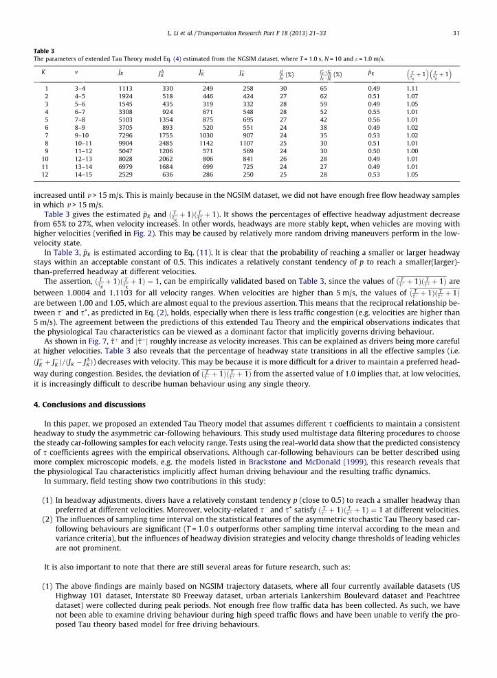
Table 3The parameters of extended Tau Theory model Eq. (4) estimated from the NGSIM dataset, where T = 1.0 s, N = 10 and e = 1.0 m/s.

K v JK JDK J�K JþK JDKJK

(%) JþKþJ�KJK�JDK

(%) pK Ts�Kþ 1

� TsþKþ 1

� 1 3–4 1113 330 249 258 30 65 0.49 1.112 4–5 1924 518 446 424 27 62 0.51 1.073 5–6 1545 435 319 332 28 59 0.49 1.054 6–7 3308 924 671 548 28 52 0.55 1.015 7–8 5103 1354 875 695 27 42 0.56 1.016 8–9 3705 893 520 551 24 38 0.49 1.027 9–10 7296 1755 1030 907 24 35 0.53 1.028 10–11 9904 2485 1142 1107 25 30 0.51 1.019 11–12 5047 1206 571 569 24 30 0.50 1.00

10 12–13 8028 2062 806 841 26 28 0.49 1.0111 13–14 6979 1684 699 725 24 27 0.49 1.0112 14–15 2529 636 286 250 25 28 0.53 1.05


increased until v > 15 m/s. This is mainly because in the NGSIM dataset, we did not have enough free flow headway samplesin which v > 15 m/s.

Table 3 gives the estimated pK and ð Ts�Kþ 1Þð T

sþKþ 1Þ. It shows the percentages of effective headway adjustment decrease

from 65% to 27%, when velocity increases. In other words, headways are more stably kept, when vehicles are moving withhigher velocities (verified in Fig. 2). This may be caused by relatively more random driving maneuvers perform in the low-velocity state.

In Table 3, pK is estimated according to Eq. (11). It is clear that the probability of reaching a smaller or larger headwaystays within an acceptable constant of 0.5. This indicates a relatively constant tendency of p to reach a smaller(larger)-than-preferred headway at different velocities.

The assertion, ð Ts�Kþ 1Þð T

sþKþ 1Þ ¼ 1, can be empirically validated based on Table 3, since the values of ð T

s� þ 1Þð Tsþ þ 1Þ are

between 1.0004 and 1.1103 for all velocity ranges. When velocities are higher than 5 m/s, the values of ð Ts� þ 1Þð T

sþ þ 1Þare between 1.00 and 1.05, which are almost equal to the previous assertion. This means that the reciprocal relationship be-tween s- and s+, as predicted in Eq. (2), holds, especially when there is less traffic congestion (e.g. velocities are higher than5 m/s). The agreement between the predictions of this extended Tau Theory and the empirical observations indicates thatthe physiological Tau characteristics can be viewed as a dominant factor that implicitly governs driving behaviour.

As shown in Fig. 7, sþ and js�j roughly increase as velocity increases. This can be explained as drivers being more carefulat higher velocities. Table 3 also reveals that the percentage of headway state transitions in all the effective samples (i.e.ðJþK þ J�K Þ=ðJK � JDKÞ) decreases with velocity. This may be because it is more difficult for a driver to maintain a preferred head-

way during congestion. Besides, the deviation of ð Ts� þ 1Þð T

sþ þ 1Þ from the asserted value of 1.0 implies that, at low velocities,it is increasingly difficult to describe human behaviour using any single theory.

4. Conclusions and discussions

In this paper, we proposed an extended Tau Theory model that assumes different s coefficients to maintain a consistentheadway to study the asymmetric car-following behaviours. This study used multistage data filtering procedures to choosethe steady car-following samples for each velocity range. Tests using the real-world data show that the predicted consistencyof s coefficients agrees with the empirical observations. Although car-following behaviours can be better described usingmore complex microscopic models, e.g. the models listed in Brackstone and McDonald (1999), this research reveals thatthe physiological Tau characteristics implicitly affect human driving behaviour and the resulting traffic dynamics.

In summary, field testing show two contributions in this study:

(1) In headway adjustments, divers have a relatively constant tendency p (close to 0.5) to reach a smaller headway thanpreferred at different velocities. Moreover, velocity-related s� and s+ satisfy ð T

s� þ 1Þð Tsþ þ 1Þ ¼ 1 at different velocities.

(2) The influences of sampling time interval on the statistical features of the asymmetric stochastic Tau Theory based car-following behaviours are significant (T = 1.0 s outperforms other sampling time interval according to the mean andvariance criteria), but the influences of headway division strategies and velocity change thresholds of leading vehiclesare not prominent.

It is also important to note that there are still several areas for future research, such as:

(1) The above findings are mainly based on NGSIM trajectory datasets, where all four currently available datasets (USHighway 101 dataset, Interstate 80 Freeway dataset, urban arterials Lankershim Boulevard dataset and Peachtreedataset) were collected during peak periods. Not enough free flow traffic data has been collected. As such, we havenot been able to examine driving behaviour during high speed traffic flows and have been unable to verify the pro-posed Tau theory based model for free driving behaviours.


(2) Our research only used headway records collected from a single driving scenario. As proven in previous research, driv-ers are inconsistent in their headway choice across different driving scenarios (Michael, Leeming, & Dwyer, 2000). Forexample, Brackstone et al. (2009) showed that the road type (motorway versus urban dual carriageway) did not seemto affect headway choice but the type of leading vehicle (truck/vans or cars) did influence the following headway.Broughton, Switzer, and Scott (2007) illustrated drivers’ velocity variability increased under conditions of reduced vis-ibility. However, we believe that all these headway adjustment processes will still be governed by the extended Tautheory, even though the observed s may vary with respect to certain other factors, including heterogeneity of differentkinds of drivers (aggressive versus passive), different vehicle types (cars versus trucks, buses), various visibility con-ditions. We will collect more data to validate our conjectures.

(3) Another question is how far the s coefficients for an individual driver can deviate from the common values in a pop-ulation. In NGSIM datasets, we monitored one only 640-m long road segment. As a result, we were unable to collectdriver action data for a long enough time period, or develop effective statistical tests on s coefficients for individualdrivers.

On the other hand, the main concern of this study is to address the close following actions of drivers when they are tryingto maintain a certain preferred distance. During free flow traffic, the interactions between vehicles are relatively weak andthe dominant task of a driver is to maintain the highest possible speed. Therefore, we argue that such driving behavioursshould be described by another model type. We will collect more data in order to validate our argument in the near future.

To solve this problem, we can use laser or radar sensors to accurately and diligently measure the relative speed and thespace gap between vehicles. With the aid of inertial navigation systems (INS) and global positioning systems (GPS), we canalso measure the positions of vehicles (Grewal, Weil, & Andrews, 2007; Li & Wang, 2007; Skog & Handel, 2009) at all times.These emerging technologies and fast developing in-vehicle equipment can help us collect long term leading vehicle trackingdata on individual drivers that cannot be obtained via video-based traffic monitoring methods. We will collect more data andtry to answer these questions in our forthcoming studies.

Acknowledgements

This work was supported in part by Hi-Tech Research and Development Program of China (863 Project) 2011AA110301,National Natural Science Foundation of China 51278280, 51138003, and National Science and Technology Major Project2012ZX03005016002.

The authors would like to thank the anonymous reviewers and the Editors for their valuable suggestions and commentsthat helped to improve this paper.

References

Abul-Magd, A. Y. (2007). Modeling highway-traffic headway distributions using superstatistics. Physical Review E, 76, 057101.Banks, J. H. (2003). Average time gaps in congested freeway flow. Transportation Research Part A, 37(6), 539–554.Boer, E. R. (1999). Car following from the driver’s perspective. Transportation Research Part F, 2(4), 201–206.Brackstone, M., & McDonald, M. (2003). Driver behavior and traffic modeling: Are we looking at the right issues? In Proceedings of IEEE intelligent vehicles,

symposium (pp. 517–521).Brackstone, M., & McDonald, M. (1999). Car following: A historical review. Transportation Research Part F, 2(4), 181–196.Brackstone, M., & McDonald, M. (2007). Driver headway: How close is too close on a motorway? Ergonomics, 50(8), 1183–1195.Brackstone, M., Waterson, B., & McDonald, M. (2009). Determinants of following headway in congested traffic. Transportation Research Part F, 12(2),

131–142.Broughton, K. L. M., Switzer, F., & Scott, D. (2007). Car following decisions under three visibility conditions and two speeds tested with a driving simulator.

Accident Analysis and Prevention, 39(1), 106–116.Chen, X., Li, L., Jiang, R., & Yang, X. (2010a). On the intrinsic concordance between the wide scattering feature of synchronized flow and the empirical spacing

distributions. Chinese Physics Letters, 27(7), 074501.Chen, X., Li, L., & Zhang, Y. (2010). A Markov model for headway/spacing distribution of road traffic. IEEE Transactions on Intelligent Transportation Systems,

11(4), 773–785.Deco, G., Scarano, L., & Soto-Faraco, S. (2007). Weber’s law in decision making: Integrating behavioral data in humans with a neurophysiological model. The

Journal of Neuroscience, 17, 11192–11200.Edie, L. C. (1965). Discussion of traffic stream measurements and definitions. In Proceedings of the second international symposium on the theory of road traffic

flow (pp. 139–154). London.Farrow, K., Haag, J., & Borst, A. (2006). Nonlinear, binocular interactions underlying flow field selectivity of a motion-sensitive neuron. Nature Neuroscience,

9, 1312–1320.Foote, R. S. (1965). Single lane traffic flow control. In Proceedings of the second international symposium on the theory of road traffic flow (pp. 84–103). London.Forbes, T. W. (1963). Human factor consideration in traffic flow theory. Highway Research Record, 15, 60–66.Frost, B. J. (2009). Lee’s Tau operator. Perception, 38, 852–853.Grewal, M. S., Weil, L. R., & Andrews, A. P. (2007). Global positioning systems, inertial navigation, and integration. New York: John Wiley & Sons.Highway Capacity Manual (2010). Transportation Research Board. Washington, DC: National Research Council.Jin, X., Su, Y., Zhang, Y., Wei, Z., & Li, L. (2009). Modeling of spacing distribution of queuing vehicles at signalized junctions using random-matrix theory.

Tsinghua Science & Technology, 14(2), 252–254.Jin, X., Zhang, Y., Wang, F., Li, L., Yao, D., Su, Y., et al (2009). Departure headways at signalized intersections: A log-normal distribution model approach.

Transportation Research Part C, 17(3), 318–327.Kallenberg, O. (1997). Foundations of modern probability. New York: Springer-Verlag.Krbalek, M., Šeba, P., & Wagner, P. (2001). Headways in traffic flow: Remarks from a physical perspective. Physical Review E, 64, 066119.Lee, D. N. (1976). A theory of visual control of braking based on information about time-to-collision. Perception, 5(4), 437–459.Lee, D. N. (2009). General Tau Theory: Evolution to date. Perception, 38, 837–850.


Li, L., & Wang, F.-Y. (2007). Advanced motion control and sensing for intelligent vehicles. New York: Springer-Verlag.Li, L., Wang, F., Jiang, R., Hu, J., & Ji, Y. (2010). A new car-following model yielding log-normal type headways distributions. Chinese Physics B, 19(2), 020513.Limpert, E., Stahel, W. A., & Abbt, M. (2001). Lognormal distributions across the sciences: Keys and clues. Bioscience, 51(5), 341–352.Michael, P. G., Leeming, F. C., & Dwyer, W. O. (2000). Headway on urban street: observational data and an intervention to decrease tailgating. Transportation

Research Part F, 3(3), 54–64.Michaels, R. M. (1963). Perceptual factors in car following. In Proceedings of international symposium on the theory of road traffic flow (pp. 44–59).NGSIM (2006). Next Generation SIMulation. <http://ngsim.fhwa.dot.gov/>.Nishinari, K., Treiber, M., & Helbing, D. (2003). Interpreting the wide scattering of synchronized traffic data by time gap statistics. Physical Review E, 68(6),

067101.Punzo, V., Borzacchiello, M. T., & Ciuffo, B. (2011). On the assessment of vehicle trajectory data accuracy and application to the Next Generation SIMulation

(NGSIM) program data. Transportation Research Part C, 19(6), 1243–1262.Ranney, T. A. (1999). Psychological factors that influence car-following and car-following model development. Transportation Research Part F, 2(4), 213–219.Schrater, P. R., Knill, D. C., & Simoncelli, E. P. (2001). Perceiving visual expansion without optic flow. Nature, 410, 816–819.Shen, J. (2003). On the foundations of vision modeling: I. Weber’s law and Weberized TV restoration. Physica D, 175, 241–251.Skog, I., & Handel, P. (2009). In-car positioning and navigation technologies – A survey. IEEE Transactions on Intelligent Transportation Systems, 10(1), 4–21.Sun, H., & Frost, B. J. (1998). Computation of different optical variables of looming objects in pigeon nucleus rotundus neurons. Nature Neuroscience, 1(4),

296–303.Taieb-Maimon, M., & Shinar, D. (2001). Minimum and comfortable driving headways: Reality versus perception. Human Factors, 43(1), 159–172.Van Winsum, W. (1999). The human element in car following models. Transportation Research Part F, 2(4), 207–211.Wang, F., Li, L., Hu, J., Ji, Y., Ma, R., & Jiang, R. (2009). A Markov process inspired CA model of highway traffic. International Journal of Modern Physics C, 20(1),

117–131.Weber, E. H. (1834). De pulsu, resorptione, audita et tactu. In H. E. Ross (Trans.) (1978), Annotationes Anatomicae et Physiologicae. New York: Academic Press.Yan, J.-J., Lorv, B., Li, H., & Sun, H.-J. (2011). Visual processing of the impending collision of a looming object: Time to collision revisited. Journal of Vision,

11(12), 1–25.Yeo, H. (2008). Asymmetric microscopic driving behavior theory. Doctoral dissertation. Dept. of Civil and Environmental Engineering, University of California,

Berkeley, U.S.A.Yeo, H., & Skabardonis, A. (2009). Understanding stop-and-go traffic in view of asymmetric traffic theory. In W. Lam, S. C. Wong & H. K. Lo (Eds.), Proceedings

of the 18th international symposium on traffic and transportation theory (pp. 99–116). Springer.

http://ngsim.fhwa.dot.gov/

Asymmetric stochastic Tau theory in car-following

Documents

Transcript of Asymmetric stochastic Tau theory in car-following