Mathematical and Computer Modelling 47 (2008) 380–400www.elsevier.com/locate/mcm

Peristaltic transport of a Johnson–Segalman fluid in anasymmetric channel

Tasawar Hayat, Ambreen Afsar, Nasir Ali∗

Mathematics Department, Quaid-i-Azam University 45320, Islamabad, Pakistan

Received 31 March 2006; received in revised form 10 March 2007; accepted 5 April 2007

Abstract

This paper deals with peristaltic flow of a Johnson–Segalman fluid in an asymmetric channel under long-wavelength and low-Reynolds number considerations. The channel asymmetry is caused due to the peristaltic wave train on the walls having differentamplitudes and phase. A series solution for small Weissenberg number is obtained for the stream function, axial velocity, axialpressure gradient and pressure drop over a wavelength. The effects of various emerging parameters on the flow characteristics areshown and discussed with the help of graphs.c© 2007 Elsevier Ltd. All rights reserved.

Keywords: Johnson–Segalman fluid; Peristalsis; Asymmetric channel

1. Introduction

Peristalsis is defined as a wave of relaxation contraction imparted to the walls of a flexible conduit effecting thepumping of enclosed material. Intense research on peristalsis has been attempted and is still demanded due to itspractical applications especially in physiology. Examples include urine transport from kidney to bladder through theureter, chyme movement inside the gastro-intestinal tract, transport of spermatozoa in the ductus efferentes of the malereproductive tracts, in the cervical canal, movement of ovum in the female fallopian tube, transport of lymph in thelymphatic vessels, vasomotion of small blood vessels such as arterioles, venules and capillaries and so on.

During the last 40 years researchers have extensively focused on the peristaltic flow of Newtonian fluids (see forexample [1–13] and several references therein). Especially, peristaltic pumping occurs in many practical applicationsinvolving biomechanical systems such as roller and finger pumps. In particular, the peristaltic pumping of corrosivefluids and slurries could be useful as it is desirable to prevent their contact with mechanical parts of the pump. Inthese investigations, solutions for peristaltic flow with various considerations of the nature of the fluid, the geometryof the channel and the propagating waves were obtained for various degree of approximation. Much attention hasbeen confined to symmetric channels or tubes, but there exist also flow situations where the channel flow may notbe symmetric. Mishra and Rao [14] studied the peristaltic flow of a Newtonian fluid in an asymmetric channel in arecent research. In another attempt, Rao and Mishra [15] discussed the non-linear and curvature effects on peristaltic

∗ Corresponding author.E-mail address: nasirali qau@yahoo.com (N. Ali).

0895-7177/$ - see front matter c© 2007 Elsevier Ltd. All rights reserved.doi:10.1016/j.mcm.2007.04.012

T. Hayat et al. / Mathematical and Computer Modelling 47 (2008) 380–400 381

flow of a Newtonian fluid in an asymmetric channel when the ratio of channel width to the wavelength is small. Veryrecently, Haroun [16] extended the analysis of reference [14] for a third order fluid. An example for a peristaltic typemotion is the intra–uterine fluid flow due to myometrial contraction, where the myometrial contractions may occurin both symmetric and asymmetric directions. An interesting study was made by Eytan and Elad [17] whose resultshave been used to analyze the fluid flow pattern in a non-pregnant uterus. In another paper, Eytan et al. [18] discussedthe characterization of non-pregnant women uterine contractions as they are composed of variable amplitudes and arange of different wavelengths.

Although most prior studies of peristaltic motion have focused on Newtonian fluids, there are also studies involvingnon-Newtonian fluids [19–29], i.e. fluids in which the relation between shear stress and shear rate is not linear. As aresult the viscosity of a non-Newtonian fluid is not constant at a given temperature and pressure, but depends on therate of shear or on the previous kinematic history of the fluid [30]. In this way, a single constitutive relation is notable to describe and predict all non-Newtonian behavior that can occur. One of the models developed to predict non-Newtonian effects is the Johnson–Segalman fluid model. This was used by Hayat et al. [25] for peristaltic mechanismsand was extended by Elshahed and Haroun [31] to magnetohydrodynamic fluids. The Johnson–Segalman model is aviscoelastic fluid model which is developed to allow for non-affine deformations [32]. Various investigators [33–35]have employed this model to explain the “spurt” phenomenon. The term “spurt” is used to describe the large increasein the volume throughput for a small increase in the driving pressure gradient [36,37] at a critical value of the pressuregradient that is observed in the flow of many non-linear fluids. Some experiments [38–43] relevant to this issue havealso been carried out. Experimentalists usually associate “spurt” with slip at the wall. Rao and Rajagopal [44] alsostudied three distinct flows of a Johnson–Segalman fluid. Unlike most other fluid models, the Johnson–Segalman (JS)fluid allows for a non-monotonic relationship between the shear stress and the rate of share in a shear flow for certainvalues of the material parameter. While the JS model offers a very interesting means for explaining “spurt”, it seemsmore likely that the phenomenon is because of the “stick-slip” that takes place at the boundary [45]. This fluid modelhas the capacity to describe “shear layers” [46], wherein the mechanism of “stick-slip” in the interior of the domainmay not be natural.

Until now no attempt was made to model peristaltic motion of Johnson–Segalman fluid in an asymmetric channel.This paper presents a first study in this field. We introduce the model by deducing the governing equations andreporting the boundary conditions in Section 2. Section 3 derives the perturbation solution for small Weissenbergnumber. Numerical results, discussion and comparison are given in Section 4. Finally concluding remarks are includedin Section 5.

2. The mathematical model

2.1. Governing equations

Consider an incompressible, Johnson–Segalman fluid confined in a two-dimensional infinite asymmetricchannel [14–16] of width d1 + d2 (see Fig. 1). We employ a rectangular coordinate system with X parallel to andY normal to the channel walls. Moreover, we consider an infinite wave train travelling with velocity c along thechannel walls. The asymmetry in the channel is induced by assuming the peristaltic wave train on the walls to havedifferent amplitudes and phases. The resulting asymmetric channel walls are defined as [14–16]

h1(X , t) = d1 + a1 sin[

2π

λ(X − ct)

], upperwall, (1)

h2(X , t) = −d2 − a2 sin[

2π

λ(X − ct) + φ

], lowerwall. (2)

Here a1 and a2 are the amplitudes of the waves, λ is the wavelength and φε [0, π] is the phase difference. Note thatφ = 0 corresponds to an asymmetric channel with waves out of phase and φ = π describes the case where waves arein phase. Moreover a1, a2, d1, d2 and φ satisfy the following inequality [14–16]

a21 + a2

2 + 2a1a2 cos φ ≤ (d1 + d2)2. (3)

382 T. Hayat et al. / Mathematical and Computer Modelling 47 (2008) 380–400

Fig. 1. Schematic diagram of the problem.

The equations governing the flow of an incompressible fluid are

div V = 0, div σ + ρ f = ρdVdt

, (4)

where V is the velocity, f is the body force per unit mass, ρ is the fluid density, d/dt is the material derivative and σ

is the Cauchy stress tensor given by [32]

σ = −pI+T, (5)

T = 2µD + S, (6)

S + m

[dSdt

+ S(W − eD

)+(W − eD

)TS

]= 2ηD, (7)

D =12[L + L

T], W =

12[L − L

T], L = grad V (8)

and bars indicate the quantities in the dimensional coordinates. The equations above include the scalar pressure p,the identity tensor I, the dynamic viscosities µ and η, the relaxation time m, the slip parameter e and the respectivesymmetric and skew symmetric part of the velocity gradient, D and W. Note, that model (5) reduces to the Maxwellfluid model for e = 1 and µ = 0, and for m = 0 = µ we receive the classical Navier–Stokes fluid model.

The velocity for unsteady two-dimensional flows is defined as

V =[U (X , Y , t), V

(X , Y , t

), 0]. (9)

From Eqs. (4)–(9) we obtain, when body forces are absent,

∂U

∂ X+

∂ V

∂Y= 0, (10)

ρ

(∂

∂ t+ U

∂

∂ X+ V

∂

∂Y

)U = −

∂ p

∂ X+ µ

(∂2

∂ X2+

∂2

∂Y 2

)U +

∂ SX X

∂ X+

∂ SX Y

∂Y, (11)

ρ

(∂

∂ t+ U

∂

∂ X+ V

∂

∂Y

)V = −

∂ p

∂Y+ µ

(∂2

∂ X2+

∂2

∂Y 2

)V +

∂ SX Y

∂ X+

∂ SY Y

∂Y, (12)

2η∂U

∂ X= SX X + m

[∂

∂t+ U

∂

∂ X+ V

∂

∂Y

]SX X − 2emSX X

∂U

∂ X+ m

[(1 − e)

∂ V

∂ X− (1 + e)

∂U

∂Y

]SX Y , (13)

T. Hayat et al. / Mathematical and Computer Modelling 47 (2008) 380–400 383

η

(∂U

∂Y+

∂ V

∂ X

)= SX Y + m

[∂

∂t+ U

∂

∂ X+ V

∂

∂Y

]SX Y +

m

2

[(1 − e)

∂U

∂Y− (1 + e)

∂ V

∂ X

]SX X

+m

2

[(1 − e)

∂ V

∂ X− (1 + e)

∂U

∂Y

]SY Y , (14)

2η∂ V

∂Y= SY Y + m

[∂

∂t+ U

∂

∂ X+ V

∂

∂Y

]SY Y − 2emSY Y

∂ V

∂Y+ m

[(1 − e)

∂U

∂Y− (1 + e)

∂ V

∂ X

]SX Y . (15)

In the fixed frame(X , Y

)the motion is unsteady, while it becomes steady in the wave frame (x, y) given by

x = X − ct, y = Y , u = U − c, v = V , (16)

when moving away in direction of the wave from the fixed frame(X , Y

)with speed c. Here u, v and U , V are the

velocity components in the wave frame and in the fixed frame, respectively. We put Eq. (16) into Eqs. (10)–(15) andfollowing Ref. [16]

x =2π x

λ, y =

y

d1, u =

u

c, v =

v

c, h1 =

h1

d1,

S =d1

µcS(x), p =

2πd21

λ (µ + η) cp(x), h2 =

h2

d1,

δ =2πd1

λ, Re =

ρcd1

µ, Wi =

mc

d1, (17)

we have

δ∂u

∂x+

∂v

∂y= 0, (18)

Re

(δu

∂

∂x+ v

∂

∂y

)u = −

(µ + η

µ

)∂p

∂x+

(δ2 ∂2

∂x2 +∂2

∂y2

)u + δ

∂Sxx

∂x+

∂Sxy

∂y, (19)

δRe

(δu

∂

∂x+ v

∂

∂y

)v = −

(µ + η

µ

)∂p

∂y+ δ

(δ2 ∂2

∂x2 +∂2

∂y2

)v + δ2 ∂Sxy

∂x+ δ

∂Syy

∂y, (20)

δ

(2η

µ

)∂u

∂x= Sxx + Wi

(δu

∂

∂x+ v

∂

∂y

)Sxx − 2eδWi Sxx

∂u

∂x+ Wi

[δ(1 − e)

∂v

∂x− (1 + e)

∂u

∂y

]Sxy, (21)

η

µ

(∂u

∂y+ δ

∂v

∂x

)= Sxy + Wi

(δu

∂

∂x+ v

∂

∂y

)Sxy +

Wi

2

[(1 − e)

∂u

∂y− δ(1 + e)

∂v

∂x

]Sxx

+Wi

2

[δ(1 − e)

∂v

∂x− (1 + e)

∂u

∂y

]Syy, (22)(

2η

µ

)∂v

∂y= Syy + Wi

(δu

∂

∂x+ v

∂

∂y

)Syy − 2eWi Syy

∂v

∂y+ Wi

[(1 − e)

∂u

∂y− δ(1 + e)

∂v

∂x

]Sxy . (23)

Writing Eqs. (18)–(23) in terms of the stream function Ψ(x, y) defined by

u =∂Ψ∂y

, v = −δ∂Ψ∂x

, (24)

we get

δRe

[(∂Ψ∂y

∂

∂x−

∂Ψ∂x

∂

∂y

)∂Ψ∂y

]= −

(µ + η

µ

)∂p

∂x+ δ

∂Sxx

∂x+

∂Sxy

∂y+

(δ2 ∂3Ψ

∂x2∂y+

∂3Ψ∂y3

), (25)

−δ3Re

[(∂Ψ∂y

∂

∂x−

∂Ψ∂x

∂

∂y

)∂Ψ∂x

]= −

(µ + η

µ

)∂p

∂y+ δ2 ∂Sxy

∂x+ δ

∂Syy

∂y− δ2

(δ2 ∂3Ψ

∂x3 +∂3Ψ

∂x∂y2

), (26)

384 T. Hayat et al. / Mathematical and Computer Modelling 47 (2008) 380–400(2ηδ

µ

)∂2Ψ∂x∂y

= Sxx + Wi δ

[∂Ψ∂y

∂

∂x−

∂Ψ∂x

∂

∂y

]Sxx − 2eWi δ

∂2Ψ∂x∂y

− Wi

[δ2(1 − e)

∂2Ψ∂x2 + (1 + e)

∂2Ψ∂y2

]Sxy, (27)

η

µ

(∂2Ψ∂y2 − δ2 ∂2Ψ

∂x2

)= Sxy + Wi δ

[∂Ψ∂y

∂

∂x−

∂Ψ∂x

∂

∂y

]Sxy +

Wi

2

[(1 − e)

∂2Ψ∂y2 + δ2(1 + e)

∂2Ψ∂x2

]Sxx

−Wi

2

[δ2(1 − e)

∂2Ψ∂x2 + (1 + e)

∂2Ψ∂y2

]Syy, (28)

−

(2ηδ

µ

)∂2Ψ∂x∂y

= Syy + Wi δ

[∂Ψ∂y

∂

∂x−

∂Ψ∂x

∂

∂y

]Syy + 2eWi δSyy

∂2Ψ∂x∂y

+ Wi

[(1 − e)

∂2Ψ

∂y2 + (1 + e)δ2 ∂2Ψ∂x2

]Sxy, (29)

where δ is wave number, Re is the Reynolds number and Wi is the Weissenberg number. The continuity equation isidentically satisfied.

2.2. Rate of volume flow and boundary conditions

The dimensional rate of fluid flow in the fixed frame (X , Y ) is

Q =

∫ h2(X)

h1(X)U (X , Y , t)dY . (30)

In the wave frame (x, y) Eq. (30) reduces to

q =

∫ h2(x)

h1(x)

u(x, y)dy. (31)

By Eq. (16), the above rates are related in the following expression

Q = q + ch1 − ch2. (32)

Applying the averaged flow

Q =1T

∫ T

0Qdt (33)

over a period T at a fixed position X , we receive

Q = q + cd1 + cd2. (34)

With the definition of the dimensionless time averaged flows

θ ≡Q

cd1, F ≡

q

cd1, (35)

in the fixed and moving frames, respectively, we can write Eq. (34) as

θ = F + 1 + d, (36)

where

F =

∫ h2(x)

h1(x)

∂Ψ∂y

dy = Ψ(h1) − Ψ(h2) (37)

T. Hayat et al. / Mathematical and Computer Modelling 47 (2008) 380–400 385

and the dimensionless surface of the peristaltic walls are

h1 (x) = 1 + a sin (x) , h2 (x) = −d − b sin (x + φ) , (38)

with a = a1/d1, b = a2/d1 and d = d2/d1 and where the inequality [15–17]

a2+ b2

+ 2ab cos φ ≤ (1 + d)2 (39)

holds. The dimensionless boundary conditions in the wave frame are [15–17]

Ψ =F

2,

∂Ψ∂y

= −1 at y = h1 (x) , (40)

Ψ = −F

2,

∂Ψ∂y

= −1 at y = h2 (x) . (41)

Here it is pointed out that the conditions on Ψ satisfy Eq. (37) and the conditions on ∂Ψ/∂y are no-slip.

2.3. Model equations

We note that the Eqs. (25)–(29) are highly non-linear differential equations. Analytic solutions valid for allarbitrary parameters appearing in these equations seem to be impossible to find. Even in the case of Newtonian fluids[1–13], all existing solutions are based on assumptions that one or some of the parameters are zero or small. Mostof the studies in the literature use asymptotic expansion with small Reynolds number, wave number, amplitude ratioas the perturbation parameters. Some existing attempts have been discussed by using long wavelength approximation[3,4,9–13]. Therefore employing the long wavelength approximation here, it follows from Eqs. (25)–(29) that theappropriate equations describing the flow are of the form(

µ + η

µ

)∂p

∂x=

∂Sxy

∂y+

∂3Ψ∂y3 , (42)

∂p

∂y= 0, (43)

Sxx = Wi(1 + e)∂2Ψ∂y2 Sxy, (44)(

η

µ

)∂2Ψ∂y2 = Sxy +

Wi

2(1 − e)

∂2Ψ∂y2 Sxx −

Wi

2(1 + e)

∂2Ψ∂y2 Syy, (45)

Syy = −Wi(1 − e)∂2Ψ∂y2 Sxy . (46)

We note that similar to various previous attempts [3,4,9–13], the term having Reynolds number disappears under longwavelength approximation. Also under this approximation, Eq. (43) indicates that p 6= p (y). Elimination of p fromEqs. (42) and (43) yields

∂2

∂y2 Sxy +∂4Ψ∂y4 = 0. (47)

Substituting Eqs. (44) and (46) into Eq. (45) we have

Sxy =

(ηµ)(

∂2Ψ∂y2

)1 + Wi2(1 − e2)

(∂2Ψ∂y2

)2 . (48)

386 T. Hayat et al. / Mathematical and Computer Modelling 47 (2008) 380–400

Fig. 2(a). Effect of the Weissenberg number Wi on variation of ∆P(2) with θ (2) for e = 0.8, a = 0.2, b = 0.5, d = 0.7, η = 1, µ = 1 and φ =π2 .

Fig. 2(b). Effect of the Weissenberg number Wi on variation of ∆P(2) with θ (2) for e = 0.8, a = 0.2, b = 0.5, d = 0.7, η = 1, µ = 1 and φ =π2 .

Upon making use of Eq. (48) in Eq. (42) and (47) we can write

∂2

∂y2

(

ηµ

+ 1) (

∂2Ψ∂y2

)+ Wi2(1 − e2)( ∂2Ψ

∂y2 )3

1 + Wi2(1 − e2)( ∂2Ψ∂y2 )2

= 0, (49)

(µ + η

µ

)∂p

∂x=

∂

∂y

(ηµ)(

∂2Ψ∂y2

)1 + Wi2(1 − e2)

(∂2Ψ∂y2

)2

+∂3Ψ∂y3 . (50)

3. Perturbed systems and perturbation solutions

After using binomial expansion for small Wi2, Eqs. (49) and (50) may be simplified to

∂2

∂y2

[∂2Ψ∂y2 + Wi2α1

(∂2Ψ∂y2

)3

+ Wi4α2

(∂2Ψ∂y2

)5]= 0, (51)

T. Hayat et al. / Mathematical and Computer Modelling 47 (2008) 380–400 387

Fig. 3. Effect of the width of the channel d on variation of ∆P(2) with θ (2) for e = 0.8, a = 0.1, b = 0.3, η = 1, µ = 1, φ =π6 , and Wi = 0.01.

Fig. 4. Effect of the phase difference φ on variation of ∆P(2) with θ (2) for e = 0.8, a = 0.7, b = 1.2, η = 1, µ = 1, d = 2, and Wi = 0.01.

Fig. 5. Effect of the upper wave amplitude a on variation of ∆P(2) with θ (2) for b = 0.3, d = 2, e = 0.8, η = 1, µ = 1, φ =π6 , and Wi = 0.05.

388 T. Hayat et al. / Mathematical and Computer Modelling 47 (2008) 380–400

Fig. 6. Effect of the lower wave amplitude b on variation of ∆P(2) with θ (2)for e = 0.8, d = 2, a = 0.5, η = 1, µ = 1, φ =π6 , and Wi = 0.05.

Fig. 7. Effect of the dimensionless flow rate θ (2) on variation of ∆P(2)(max)

with d for e = 0.8, a = 0.2, b = 0.4, η = 1, µ = 1, φ =π4 , and

Wi = 0.01.

∂p

∂x=

∂3Ψ∂y3 + Wi2α1

∂

∂y

[(∂2Ψ∂y2

)3]+ Wi4α2

∂

∂y

[(∂2Ψ∂y2

)5], (52)

where

α1 =(e2

− 1)η

(η + µ), α2 = (e2

− 1)α1. (53)

In order to solve the present problem, we expand the flow quantities in a power series of Wi2 as follows

Ψ = Ψ0 + Wi2Ψ1 + Wi4Ψ2 + · · · ,

p = p0 + Wi2 p1 + Wi4 p2 · · · ,

F = F0 + Wi2 F1 + Wi4 F2 · · · .

(54)

Substituting Eq. (54) into Eqs. (51) and (52) and boundary conditions (40) and (41) and then equating the like powersof Wi2 we get:

T. Hayat et al. / Mathematical and Computer Modelling 47 (2008) 380–400 389

Fig. 8. Effect of the Weissenberg number Wi on variation of ∆P(2)(max)

with d for e = 0.8, a = 0.2, b = 0.2, η = 1, µ = 1, and φ =π4 .

Fig. 9. Effect of the upper wave amplitude a on variation of ∆P(2)(max)

with b for e = 0.8, d = 2, η = 1, µ = 1, and φ =π4 , Wi = 0.07.

Fig. 10. Effect of the phase difference φ on variation of ∆P(2)(max)

with a for e = 0.8, d = 2, b = 0.4, η = 1, µ = 1, and Wi = 0.1.

390 T. Hayat et al. / Mathematical and Computer Modelling 47 (2008) 380–400

3.1. Perturbed systems

3.1.1. Zeroth-order system

∂4Ψ0

∂y4 = 0,∂p0

∂x=

∂3Ψ0

∂y3 ,∂p0

∂y= 0, (55)

Ψ0 =F0

2,

∂Ψ0

∂y= −1 on y = h1 (x) ,

Ψ0 = −F0

2,

∂Ψ0

∂y= −1 on y = h2 (x) . (56)

3.1.2. System of order Wi2

∂4Ψ1

∂y4 = −α1∂2

∂y2

[(∂2Ψ0

∂y2

)3],

∂p1

∂x=

∂3Ψ1

∂y3 + α1∂

∂y

[(∂2Ψ0

∂y2

)3], (57)

∂p1

∂y= 0,

Ψ1 =F1

2,

∂Ψ1

∂y= 0 on y = h1 (x) ,

Ψ1 = −F1

2,

∂Ψ1

∂y= 0 on y = h2 (x) . (58)

3.1.3. System of order Wi4

∂4Ψ2

∂y4 = −3α1∂2

∂y2

[(∂2Ψ0

∂y2

)2∂2Ψ1

∂y2

]− α2

∂2

∂y2

[(∂2Ψ0

∂y2

)5],

∂p2

∂x=

∂3Ψ2

∂y3 + 3α1∂

∂y

[(∂2Ψ0

∂y2

)2∂2Ψ1

∂y2

]+ α2

∂

∂y

[(∂2Ψ0

∂y2

)5], (59)

∂p2

∂y= 0,

Ψ2 =F2

2,

∂Ψ2

∂y= 0 on y = h1 (x) ,

Ψ2 = −F2

2,

∂Ψ2

∂y= 0 on y = h2 (x) . (60)

3.2. Perturbation solutions

3.2.1. Zeroth-order solutionWe point out that the problem at this order is the same as for Newtonian fluids. Thus solution expressions at this

order are similar to [14–16] and are given by

Ψ0 =(h1 − h2 + F0)(2y3

− 3 (h1 + h2) y2+ 6h1h2 y)

(h2 − h1)3 − y

+(h2−h1)

3 (2h1 + F0) + 2h21 (h1−3h2) (h1 − h2 + F0)

2 (h2 − h1)3 , (61)

T. Hayat et al. / Mathematical and Computer Modelling 47 (2008) 380–400 391

u0 =6(h1 − h2 + F0)(y2

− (h1 + h2) y + h1h2)

(h2 − h1)3 − 1,

dp0

dx= −12

[1

(h1 − h2)2 +

F0

(h1−h2)3

]. (62)

Furthermore, the non-dimensionless pressure rise per wavelength, which has already be given in [14–16], is

∆P0 =

∫ 2π

0

dp0

dxdx = −

12π

(1 + d)2 (1 − M)32

[2 +

(2 + M) F0

(1 + d) (1 − M)

], (63)

where

M =a2

+ b2+ 2ab cos φ

(1 + d)2 . (64)

3.2.2. First-order solution

Substituting the zeroth-order solution (61) into Eq. (57) and then solving the resulting system with thecorresponding boundary conditions, we get

Ψ1 =α1

2

[−

110

(dp0

dx

)3

y5+

(h1 + h2)

4

(dp0

dx

)3

y4+

(B1

6−

(h1 + h2)2

4

(dp0

dx

)3)

y3

−(h1 + h2)

8

[2B1 − (h1 + h2)

2(

dp0

dx

)3]

y2+

[h1h2 B1

2− S3

]y

+12

[h2

1 (h1 − 3h2) B1

6− 2S1 + 2h1S3

]]−

(2F1

(h1 − h2)3

)y3

+

(3 (h1 + h2) F1

(h1 − h2)3

)y2

−

(6h1h2 F1

(h1 − h2)3

)y +

F1

2−

h21 (h1 − 3h2) F1

(h1 − h2)3 , (65)

u1 =α1

2

[−

12

(dp0

dx

)3

y4+ (h1 + h2)

(dp0

dx

)3

y3+

(B1

2−

3 (h1 + h2)2

4

(dp0

dx

)3)

y2

−(h1 + h2)

4

[2B1 − (h1 + h2)

2(

dp0

dx

)3]

y +

[h1h2 B1

2− S3

]]−

(6F1

(h1 − h2)3

)y2

+

(6 (h1 + h2) F1

(h1 − h2)3

)y −

(6h1h2 F1

(h1 − h2)3

)dp1

dx= −

12F1

(h1 − h2)3 +

3α1

20(h1 − h2) 2

(dp0

dx

)3

, (66)

where

B1 =12 (S1 − S2)

(h1 − h2)3 −

12S3

(h1 − h2)2 ,

S1 =h2

1(h31 + 5h2(h2

1 + h1h2 + h22))

40

(dp0

dx

)3

,

S2 =h2

2

(h3

2 + 5h1h22 + 5h2

1h2 + 5h31

)40

(dp0

dx

)3

,

S3 =h1h2

(h2

1 + h22

)4

(dp0

dx

)3

.

392 T. Hayat et al. / Mathematical and Computer Modelling 47 (2008) 380–400

The non-dimensional pressure slope per wavelength at this order is

∆P1 =

∫ 2π

0

dp1

dxdx = −12F1 I3 −

1296α1

5[I4 + 3F0 I5 + 3F2

0 I6 + F30 I7], (67)

with

I3 =π (2 + M)

(1 + d)3 (1 − M)52

, I4 =π (2 + 3M)

(1 + d)4 (1 − M) 72

(68)

and for n > 4,

In =1

(1 + d) (1 − M)

[(2n − 3)

(n − 1)In−1 −

(n − 2)

(1 + d) (n − 1)In−2

]. (69)

3.2.3. Second-order solutionBy inserting the zeroth-order and first-order solutions into Eq. (59) and then solving the resulting problems, we

obtain

Ψ2 =3α2

1

2

(K1 y7

+ K2 y6+ K3 y5

+ K4 y4+ K30 y3

+ K33 y2+ K36 y + K39

)+

3α1

2

(K5 y5

+ K6 y4+ K31 y3

+ K34 y2+ K37 y + K40

)− α2

(K7 y7

+ K8 y6+ K9 y5

+ K10 y4+ K32 y3

+ K35 y2+ K38 y + K41

)−

(2F2

(h1 − h2)3

)y3

+

(3 (h1 + h2) F2

(h1 − h2)3

)y2

−

(6h1h2 F2

(h1 − h2)3

)y +

F2

2−

h21 (h1 − 3h2) F2

(h1 − h2)3 , (70)

u2 =3α2

1

2

(7K1 y6

+ 6K2 y5+ 5K3 y4

+ 4K4 y3+ 3K30 y2

+ 2K33 y + K36

)+

3α1

2

(5K5 y4

+ 4K6 y3+ 3K31 y2

+ 2K34 y + K37

)− α2

(7K7 y6

+ 6K8 y5+ 5K9 y4

+ 4K10 y3+ 3K32 y2

+ 2K35 y + K38

)−

(6F2

(h1 − h2)3

)y2

+

(6 (h1 + h2) F2

(h1 − h2)3

)y −

(6h1h2 F2

(h1 − h2)3

),

dp2

dx= −

3α21

2

(dp0

dx

)5 ( 3350

(h1 − h2)4)

−3α1

2

(dp0

dx

)2 ( 185 (h1 − h2)

)+

3α2

112

(dp0

dx

)5

(h1 − h2)4−

12F2

(h1 − h2)3 . (71)

where the functions Ki,i = 1, . . . , 41 are

K1 =1

21

(dp0

dx

)5

, K2 = −(h1 + h2)

6

(dp0

dx

)5

,

K3 =

(dp0

dx

)5((

47h21 + 106h1h2 + 47h2

2

)3200

),

K4 = −(h1 + h2)

2

(dp0

dx

)5((

41h21 + 118h1h2 + 41h2

2

)120

),

K5 =

(dp0

dx

)2 6F1

5 (h1 − h2)3 , K6 = −

(dp0

dx

)2 3 (h1 + h2) F1

(h1 − h2)3 ,

K7 =1

42

(dp0

dx

)5

, K8 = −(h1 + h2)

12

(dp0

dx

)5

,

T. Hayat et al. / Mathematical and Computer Modelling 47 (2008) 380–400 393

K9 =(h1 + h2)

8

(dp0

dx

)5

, K10 = −

(dp0

dx

)5 5 (h1 + h2)3

48,

K11 = −h71 K1 − h6

1 K2 − h51 K3 − h4

1 K4,

K12 = −h72 K1 − h6

2 K 2 − h52 K3 − h4

2 K4,

K13 = −7h61 K1 − 6h5

1 K2 − 5h41 K3 − 4h3

1 K4,

K14 = −7h62 K1 − 6h5

2 K2 − 5h42k3 − 4h3

2 K4,

K15 = −h51 K5 − h4

1 K6, K16 = −h52k5 − h4

2 K6,

K17 = −5h41k5 − 4h3

2 K6, K18 = −5h42 K5 − 4h3

2 K6,

K19 = −h71 K7 − h6

1 K8 − h51 K9 − h4

1 K10,

K20 = −h72 K7 − h6

2 K8 − h52 K9 − h4

2 K10,

K21 = −7h61 K7 − 6h5

1 K8 − 5h41 K9 + 4h3

1 K10,

K22 = −7h62 K7 − 6h5

2 K8 − 5h42 K9 − 4h3

2 K10,

K30 =

(−2 (K11 − K12) + (h1 − h2) (K13 + K14)

(h1 − h2)3

),

K31 =

(−2 (K15 − K16) + (h1−h2) (K17−K18)

(h1−h2)3

),

K32 =

(−2 (K19−K20) + (h1−h2) (K21−K22)

(h1−h2)3

),

K33 =

(3 (h1 + h2) (K11 − K12) − (h1−h2) ((h1 + 2h2) K13 + (2h1 + h2) K14)

(h1 − h2)3

),

K34 =

(3 (h1 + h2) (K15 − K16) − (h1−h2) ((h1 + 2h2) K17 + (2h1 + h2) K18)

(h1 − h2)3

),

K35 =

(3 (h1 + h2) (K19 − K20) − (h1−h2) ((h1 + 2h2) K21 + (2h1 + h2) K22)

(h1 − h2)3

),

K36 =

(K14 − 3h2

2 K30 − 2h2 K33

), K37 =

(K18 − 3h2

2 K31 − 2h2 K34

),

K38 =

(K22 − 3h2

2 K32 − 2h2 K35

),

K39 =

(K11 − h1 K14 − h1 (h1 − 2h2) K33 − h1

(h2

1 − 3h22

)K30

),

K40 =

(K15 − h1 K20 − h1 (h1 − 2h2) K34 − h1

(h2

1 − 3h22

)K31

),

K41 =

(K17 − h1 K22 − h1 (h1 − 2h2) K35 − h1

(h2

1 − 3h22

)K32

).

The non-dimensionless pressure rise per wavelength is defined as

∆P2 =

∫ 2π

0

dp2

dxdx =

(559 872α2

1

175−

4665α2

7

)(I11 F5

0 + 5F40 I10 + 10F3

0 I9 + 10F20 I8 + 5F0 I7 + I6

)−

3888α1 F1

5

(F2

0 I7 + 2F0 I6 + I5

)− 12F2 I3. (72)

Summing up the perturbation results, we find that the pressure rise per wavelength up to o(Wi4) is

∆P = −12π

(1 + d)2 (1 − M)32

(2 +

(2 + M) F0

(1 + d) (1 − M)

)

394 T. Hayat et al. / Mathematical and Computer Modelling 47 (2008) 380–400

Fig. 11. Streamlines for φ = 0, a = 0.5, b = 0.5, d = 1, e = 0.8, θ (2)= 1.3, µ = 1, η = 1 and for different Wi; (a) Wi = 0, (b) Wi = 0.3,

(c) Wi = 0.6.

+ Wi2[

12F1 I3 −1296α1

5

(I4 + 3F0 I5 + 3F2

0 I6 + F30 I7

)]+ Wi4

[(559 872α2

1

175−

46 656α2

7

)(I11 F5

0 + 5F40 I10 + 10F3

0 I9 + 10F20 I8 + 5F0 I7 + I6

)

−3888α1

5α1 F1

(F2

0 I7 + 2F0 I6 + I5

)− 12F2 I3

]. (73)

Defining

F (2)= F0 + Wi2 F1 + Wi4 F2,

we get the equations

F0 = F (2)− Wi2 F1 − Wi4 F2,

Wi2 F1 = F (2)− F0 − Wi4 F2,

Wi4 F2 = F (2)− F0 − Wi2 F1, (74)

and substituting the expressions above into Eq. (73) while retaining only terms up to order Wi4, we obtain

∆P(2)=

−24π

(1 + d)2 (1 − M)32

− 12F (2) I3 + Wi2[−

1296α1

5

(I4 + 3F (2) I5 + 3F (2)2

I6 + F (2)3I7

)]

T. Hayat et al. / Mathematical and Computer Modelling 47 (2008) 380–400 395

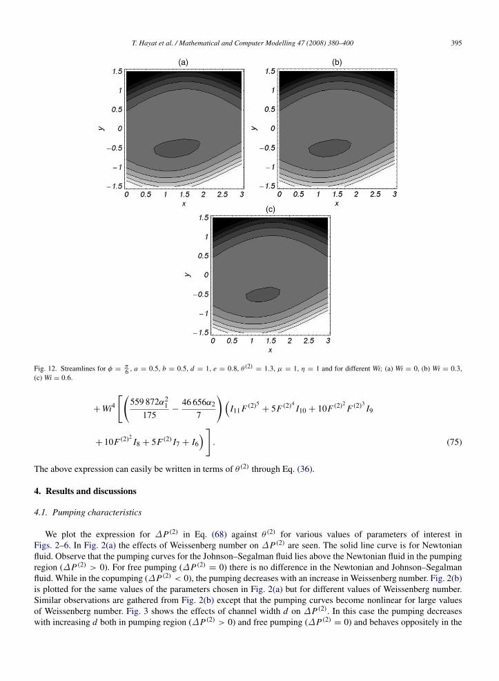
Fig. 12. Streamlines for φ =π6 , a = 0.5, b = 0.5, d = 1, e = 0.8, θ (2)

= 1.3, µ = 1, η = 1 and for different Wi; (a) Wi = 0, (b) Wi = 0.3,(c) Wi = 0.6.

+ Wi4[(

559 872α21

175−

46 656α2

7

)(I11 F (2)5

+ 5F (2)4I10 + 10F (2)2

F (2)3I9

+ 10F (2)2I8 + 5F (2) I7 + I6

)]. (75)

The above expression can easily be written in terms of θ (2) through Eq. (36).

4. Results and discussions

4.1. Pumping characteristics

We plot the expression for ∆P(2) in Eq. (68) against θ (2) for various values of parameters of interest inFigs. 2–6. In Fig. 2(a) the effects of Weissenberg number on ∆P(2) are seen. The solid line curve is for Newtonianfluid. Observe that the pumping curves for the Johnson–Segalman fluid lies above the Newtonian fluid in the pumpingregion (∆P(2) > 0). For free pumping (∆P(2) = 0) there is no difference in the Newtonian and Johnson–Segalmanfluid. While in the copumping (∆P(2) < 0), the pumping decreases with an increase in Weissenberg number. Fig. 2(b)is plotted for the same values of the parameters chosen in Fig. 2(a) but for different values of Weissenberg number.Similar observations are gathered from Fig. 2(b) except that the pumping curves become nonlinear for large valuesof Weissenberg number. Fig. 3 shows the effects of channel width d on ∆P(2). In this case the pumping decreaseswith increasing d both in pumping region (∆P(2) > 0) and free pumping (∆P(2)

= 0) and behaves oppositely in the

396 T. Hayat et al. / Mathematical and Computer Modelling 47 (2008) 380–400

Fig. 13. Streamlines for Wi = 0.1, a = 0.7, b = 0.7, d = 1, e = 0.8, θ (2)= 1.3, µ = 1, η = 1, and for different φ; (a) φ = 0, (b) φ =

π4 ,

(c) φ =π2 .

copumping region. Fig. 4 illustrate the effects of phase difference φ on ∆P(2). Observe that an increase in φ causesa decrease in pumping in the pumping region (∆P(2) > 0) and free pumping. It is also noted from Fig. 4 that incopumping (for an appropriately chosen ∆P(2) < 0) θ (2) increases with an increase in φ. The observations regardingthe effects of upper and lower wave amplitudes a and b, respectively on ∆P(2) are quite opposite to those in the caseof φ (Figs. 5 and 6). Fig. 7 depicts the effects of varying θ (2) on ∆P(2) with d. On the one hand for small valuesof d there is a noticeable change in the behavior of ∆P(2) i.e. with an increase in θ (2), ∆P(2) decreases. On theother hand the effects become negligible when large values of d are taken into account. Fig. 8 elucidates the effectsof Weissenberg number on ∆P(2)

(max) (pressure rise required to produce zero flow rate) with channel width d. We can

see that ∆P(2)(max) increases with an increase in Wi for small values of d and the curves coincide (i.e. ∆P(2)

(max) forNewtonian and Johnson–Segalman fluid become equal in magnitude) for large d. In order to obtain the effects of a, band φ on ∆P(2)

(max) we sketched Figs. 9 and 10. We see that the ∆P(2)(max) increases with an increase of a and b while it

decreases with an increase of φ. Table 1 shows the variation of ∆P(2) with flow rate θ (2) for different values of slipparameter e. It is noted that an increase in e causes a decrease in ∆P(2).

4.2. Trapping

Another interesting phenomenon in peristaltic motion is trapping. In the wave frame, streamlines under certainconditions split to trap a bolus which moves as a whole with the speed of the wave. The effects of Weissenbergnumber Wi on trapping can be seen through Fig. 11 for a symmetric channel. Furthermore, Fig. 11 shows that thebolus is symmetric about the centre line and its size decreases with an increase in Wi. Similar effects on the size of

T. Hayat et al. / Mathematical and Computer Modelling 47 (2008) 380–400 397

Fig. 14. Streamlines for Wi = 0.1, φ =π6 , b = 0.7, d = 1, e = 0.8, θ (2)

= 1.3, µ = 1, η = 1 and for different a; (a) a = 0, (b) a = 0.2,(c) a = 0.7.

bolus are observed for asymmetric channels, while differences in bolus motion occur: the bolus move towards the leftside of the channel (Fig. 12). Fig. 13 is made in order to see the effects of φ on trapping. Observe that for φ = 0the bolus is symmetric about the centre line while it move towards the left and decreases in size for φ = π/4 andvanishes for φ = π/2. In Fig. 14 the effect of varying the upper wave amplitude a on trapping is seen. Note that fora = 0 (when there is no wave on the upper wall) a trapped bolus does not exists. The trapping occurs when a = 0.2and bolus size increases with an increase in a. The effects of lower wave amplitude on trapping can be seen throughFig. 15. Similar to the previous case for b = 0 (when there is no wave on the lower wall), a trapped bolus does notexist, the trapping occurs for b = 0.4 and bolus size increases with an increase in b. Fig. 16 depicts the effects ofchannel width, d , on trapping. The trapped bolus exists for small values of d, its size decreases and it disappears withtaking into account large values of d .

5. Concluding remarks

In this paper we succeeded in presenting a mathematical model to study the peristaltic transport of a non-Newtonianfluid inside an asymmetric channel. A regular perturbation method is employed to obtain the expression for the streamfunction, axial velocity, axial pressure gradient and pressure rise over a wavelength. The interaction of the rheologicalparameters of the fluid with peristaltic flow is discussed. The main results can be summarized as follows:

• The pressure rise over a wavelength ∆P(2) increases with an increase in Weissenberg number Wi in the pumpingregion, while the situation is reversed in the copumping region (Fig. 2).

• The pressure rise over a wavelength ∆P(2) decreases with an increase in φ in the pumping region, while in thecopumping region (for an appropriately chosen ∆P(2) < 0) θ (2) increases with an increase in φ (Fig. 4).

398 T. Hayat et al. / Mathematical and Computer Modelling 47 (2008) 380–400

Fig. 15. Streamlines for Wi = 0.1, φ =π6 , a = 0.7, d = 1, e = 0.8, θ (2)

= 1.3, µ = 1, η = 1 and for different b; (a) b = 0, (b) b = 0.2,(c) b = 0.7.

Table 1

Variation of ∆P(2) with θ (2) for different values of slip parameter e

e θ (2)= 0 θ (2)

= 0.2 θ (2)= 0.4 θ (2)

= 0.6 θ (2)= 0.8 θ (2)

= 1

0.1 24.0528 15.2916 7.7276 0.9177 −5.5084 −11.87820.2 24.0270 15.2844 7.7263 0.9176 −5.5083 −11.87820.3 23.9857 15.2728 7.7242 0.9174 −5.5083 −11.87800.4 23.9317 15.2576 7.7214 0.9172 −5.5083 −11.87790.5 23.8685 15.2398 7.7182 0.9170 −5.5082 −11.7770.6 23.8010 15.2941 7.7147 0.9167 −5.5081 −11.87740.7 23.7350 15.2023 7.7113 0.9165 −5.5081 −11.87720.8 23.6774 15.1861 7.7083 0.9163 −5.5080 −11.87710.9 23.6361 15.1745 7.7062 0.9161 −5.5080 −11.87691 23.6202 15.1700 7.7054 0.9161 −5.5080 −11.9769

The other parameters chosen are a = 0.6, d = 0.8, b = 0.7, η = 1, µ = 1, and Wi = 0.1.

• The size of the trapped bolus decreases with an increase in Wi and φ (Figs. 11–13).

• Pressure rise per wavelength decreases by increasing e (Table 1).

• The present analysis is more general and the results for Newtonian and Maxwell fluids can be obtained as specialcases.

T. Hayat et al. / Mathematical and Computer Modelling 47 (2008) 380–400 399

Fig. 16. Streamlines for Wi = 0.1, a = 0.7, b = 0.7, e = 0.8, φ =π6 , θ (2)

= 1.3, µ = 1, η = 1 and for different d; (a) d = 0.8, (b) d = 1,(c) d = 1.5.

Acknowledgments

We are grateful to a reviewer for constructive and valuable suggestions. The suggestions made undoubtedlyimproved the earlier version of this manuscript. We are also grateful to the Higher Education Commission of Pakistanfor financial support.

References

[1] J.C. Burns, T. Parkes, Peristaltic motion, J. Fluid Mech. 29 (1967) 731–743.[2] Y.C. Fung, C.S. Yih, Peristaltic transport, J. Appl. Mech. 35 (1968) 669–675.[3] M. Hanin, The flow through a channel due to transversly oscillating walls, Israel J. Tech. 6 (1968) 67–71.[4] A.H. Shapiro, M.Y. Jaffrin, S.L. Weinberg, Peristaltic pumping with long wavelengths at low Reynolds number, J. Fluid Mech. 37 (1969)

799–825.[5] T.S. Chow, Peristaltic transport in a circular cylindrical pipe, J. Appl. Mech. 37 (1970) 901–905.[6] M.Y. Jaffrin, A.H. Shapiro, Peristaltic pumping, Annu. Rev. Fluid Mech. 3 (1971) 13–36.[7] S.K. Guha, H. Kaur, A.M. Ahmad, Mechanism of spermatic flow in the vas deferens, Med. Biol. Eng. 13 (1975) 518–522.[8] K. Ayukawa, T. Kawa, M. Kimura, Streamlines and pathlines in peristaltic flows at high Reynolds numbers, Bull. Japan Soc. Mech. Eng. 24

(1981) 948–955.[9] S. Takabatake, K. Ayukawa, A. Mori, Peristaltic pumping in circular cylindrical tubes: A numerical study of fluid transport and its efficiency,

J. Fluid Mech. 193 (1988) 269–283.[10] S. Takabataka, K. Ayukawa, Numerical study of two-dimensional peristaltic flows, J. Fluid Mech. 122 (1982) 439–465.[11] Kh.S. Mekheimer, Nonlinear peristaltic transport through a porous medium in an inclined planar channel, J. Porous Media 6 (2003) 189–201.[12] Kh.S. Mekheimer, Nonlinear peristaltic transport of magneto-hydrodynamic flow in an inclined planar channel, Arab J. Sci. Eng. 28 (2003)

183–201.[13] A.M. Siddiqui, T. Hayat, M. Khan, Magnetic fluid model induced by peristaltic waves, J. Phy. Soc. Japan. 73 (2004) 2142–2147.

400 T. Hayat et al. / Mathematical and Computer Modelling 47 (2008) 380–400

[14] M. Mishra, A.R. Rao, Peristaltic transport of a Newtonian fluid in an asymmetrical channel, Z. Angew. Math. Phys. 54 (2003) 532–550.[15] A.R. Rao, M. Mishra, Nonlinear and curvature effects on peristaltic flow of a viscous fluid in an asymmetric channel, Acta Mech. 168 (2004)

35–59.[16] M.H. Haroun, Effect of Deborah number and phase difference on peristaltic transport of a third-order fluid in an asymmetric channel, Comm.

Nonlinear Sci. Numer. Simul. 12 (2007) 1464–1480.[17] O. Eytan, D. Elad, Analysis of intra-uterine fluid motion induced by uterine contractions, Bull. Math. Biol. 61 (1999) 221–228.[18] O. Eytan, A.J. Jaffa, J. Har-Toor, E. Dalach, D. Elad, Dynamics of the intrauterine fluid-wall interface, Ann. Biomed. Eng. 27 (1999) 372–379.[19] L.M. Srivastava, V.P. Srivastava, Peristaltic transport of blood; Casson model-II, J. Biomech. 17 (1984) 821–829.[20] Kh.S. Mekheimer, E.F. El Shehawey, A.M. Elaw, Peristaltic motion of a particle-fluid suspension in a planar channel, Internat. J. Theoret.

Phys. 37 (1998) 2895–2919.[21] T. Hayat, Y. Wang, A.M. Siddiqui, S. Asghar, A mathematical model for study of gliding motion of becteria on a layer of non-Newtonian

slime, Math. Models Methods Appl. Sci. 27 (2004) 1447–1468.[22] T. Hayat, E. Momoniat, F.M. Mahomed, Effects of an endoscope and an electrically conducting third grade fluid on peristaltic motion. Internat.

J. Modern Phys. B (in press).[23] Kh.S. Mekheimer, Peristaltic flow of blood under effect of a magnetic field in a non-uniform channels, Appl. Math. Comput. 153 (2004)

763–777.[24] G. Radhakrishnamacharya, Long wavelength approximation to peristaltic motion of power law fluid, Rheol Acta. 21 (1982) 30–35.[25] T. Hayat, Y. Wang, A.M. Siddiqui, K. Hutter, Peristaltic motion of a Johnson–Segalman fluid in a planar channel, Math. Probl. Eng. 1 (2003)

1–23.[26] T. Hayat, Y. Wang, A.M. Siddiqui, K. Hutter, S. Asghar, Peristaltic transport of a third order fluid in a circular cylindrical tube, Math. Models

Methods Appl. Sci. 12 (2002) 1691–1706.[27] T. Hayat, F.M. Mahomed, S. Asghar, Peristaltic flow of a magnetohydrodynamic Johnson–Segalman fluid, Nonlinear Dynam. 40 (2005)

375–385.[28] M.H. Haroun, Effect of relaxation and retardation time on peristaltic transport of the Oldroydian viscoelastic fluid, J. Appl. Tech. Phys. 46

(2005) 842–850.[29] T. Hayat, E. Momoniat, F.M. Mahomed, Endoscope effects on MHD peristaltic flow of a power-law fluid. Math. Probl. Eng. (in press).[30] R.I. Tanner, Engineering Rheology, Oxford University Press, Oxford, 1992.[31] M. Elshahed, M. Haroun, Peristaltic transport of a Johnson–Segalman fluid under effect of a magnetic field, Math. Probl. Eng. 6 (2005)

663–667.[32] M.W. Johnson Jr., D. Segalman, A model for viscoelastic fluid behavior which allows nonaffine deformation, J. Non-Newton. Fluid Mech. 2

(1977) 255–270.[33] R.W. Kolkka, D.S. Malkus, M.G. Hansen, G.R. IerIy, A.R. Worthing, Spurt phenomenon of the Johnson–Segalman fluid and related models,

J. Non-Newton. Fluid Mech. 29 (1988) 303–335.[34] D.S. Malkus, J.A. Nohel, B.J. Plohr, Dynamics of shear flows of non-Newtonian fluids, J. Comput. Phys. 87 (1990) 464–497.[35] T.C.B. McLeish, R.C. Ball, A molecular approach to the spurt effect in polymer melt flow, J. Polym. Sci. (B) 24 (1986) 1735–1745.[36] G.V. Vinogardov, A.Ya. Malkin, G.Yu. Yanovskii, E.K. Borisenkova, B.V. Yarlykov, G.V. Brezhnava, Viscoelastic properties and flow of

narrow distribution polybutadienes and polyisopropenes, J. Polym. Sci. Part A-2 10 (1972) 1061–1084.[37] M.M. Denn, Issues in viscoelastic fluid mechanics, Annu. Rev. Fluid Mech. 22 (1990) 13–34.[38] A.M. Kraynik, W.R. Schowalter, Slip at the wall and extrudate roughness with aqueous solutions of polyvinyl alcohol and sodium borate,

J. Rheol. 25 (1981) 95–114.[39] F.J. Lim, W.R. Schowalter, Wall slip of narrow molecular weight distribution polybutadienes, J. Rheol. 33 (8) (1989) 1359–1382.[40] D.S. Malkus, J.A. Nohel, B.J. Plohr, Analysis of new phenomena in shear flows of non-Newtonian fluid, J. Comput. Phys. 87 (2) (1990)

464–487.[41] K.B. Migler, H. Hervert, L. Leger, Slip transition of a polymer melt under shear stress, Phys. Rev. Lett. 70 (3) (1990) 287–290.[42] K.B. Migler, G. Massey, H. Hervert, L. Leger, The slip transition of the polymer-solid interface, J. Phys. Condens. Matter 6 (1994)

A301–A304.[43] A.V. Ramamurthy, Wall slip in viscous fluid and influence of materials of construction, J. Rheol. 30 (2) (1986) 337–357.[44] I.J. Rao, K.R. Rajagopal, Some simple flows of a Johnson–Segalman fluid, Acta Mech. 132 (1999) 209–219.[45] I.J. Rao, K.R. Rajagopal, The effects of the slip boundary condition on the flow of fluids in a channel, Acta Mech. 135 (1999) 113–126.[46] A. Sirivat, A.Z. Szeri, K.R. Rajagopal, An experimental investigation of the flow of non-Newtonian fluids between rotating disks, J. Fluid

Mech. 186 (1988) 243–256.