Available online at www.sciencedirect.com

Applied Mathematical Modelling 32 (2008) 761–774

www.elsevier.com/locate/apm

Effect of variable viscosity on the peristaltic transportof a Newtonian fluid in an asymmetric channel

Tasawar Hayat, Nasir Ali *

Department of Mathematics, Quaid-I-Azam University 45320, Islamabad 44000, Pakistan

Received 12 October 2006; received in revised form 9 February 2007; accepted 19 February 2007Available online 25 February 2007

Abstract

The effect of variable viscosity on the peristaltic flow of a Newtonian fluid in an asymmetric channel has been discussed.Asymmetry in the flow is induced due to travelling waves of different phase and amplitude which propagate along the chan-nel walls. A long wavelength approximation is used in the flow analysis. Closed form analytic solutions for velocity com-ponents and longitudinal pressure gradient are obtained. The study also shows that, in addition to the effect of mean flowparameter, the wave amplitude also effect the peristaltic flow. This effect is noticeable in the pressure rise and frictionalforces per wavelength through numerical integration.� 2007 Elsevier Inc. All rights reserved.

Keywords: Peristaltic flow; Newtonian fluid; Asymmetric channel; Variable viscosity

1. Introduction

Peristaltic transport is a form of fluid transport generated by a progressive wave of area contraction orexpansion along the length of a distensible tube containing fluid. The studies of peristaltic flows of Newtonianand non-Newtonian fluids have become important, not only because of biomedical and engineering sciencesbut also in view of the interesting mathematical features presented by the equations governing the flow. Suchstudies have considerable practical relevance, for example in urine transport from kidney to bladder, move-ment of chyme in the gastrointestinal tract, transport of spermatozoa in the ductus efferentes of the malereproductive tracts, and, in cervical canal, in movement of ovum in the female fallopian tube, transport oflymph in the lymphatic vessels, and in the vasomotion of small blood vessels such as arterioles, venulesand capillaries. The roller and finger pumps also operate under this principle. Moreover, some biomechanicalinstruments e.g., heart lung machine, has been fabricated using the principle of peristalsis.

There are many fluids whose behavior cannot be described by the Navier–Stokes model with constantviscosity. Also the inadequacy of the classical Navier–Stokes theory of Newtonian fluids in predicting the

0307-904X/$ - see front matter � 2007 Elsevier Inc. All rights reserved.

doi:10.1016/j.apm.2007.02.010

* Corresponding author.E-mail address: nasirali_qau@yahoo.com (N. Ali).

762 T. Hayat, N. Ali / Applied Mathematical Modelling 32 (2008) 761–774

behavior of some fluids, especially those with high molecular weight, leads to the developments of non-New-tonian fluid mechanics. The governing equations for such fluids are of higher order, much more complicatedand subtle than the Newtonian fluids. The governing equations present various challenges to engineers, math-ematicians, numerical simulists and pyhsicists alike. But even then, several investigators [1–10] are presentlyengaged in obtaining analytic solutions for flows of such fluids. Furthermore, the analysis of the mechanismresponsible for peristaltic transport have been studied by various workers. Latham’s investigation [11] is thefirst study in this field. After that extensive literature is available on the topic that deals with the peristalsis ofNewtonian and non-Newtonian fluid. Recent contributions in this direction may be mentioned in the refer-ences [12–26]. Literature survey indicates that no attempt is available yet for effects of variable viscosity onthe peristaltic flow in an asymmetric channel. The importance of the peristaltic transport in an asymmetricchannel has been brought out by Eytan and Elad [27] with an application in intra-uterine fluid flow in anon-pregnant uterus. Also, the consideration of physiological fluids with constant viscosity fails to give betterunderstanding when peristaltic mechanism involved in small blood vessels, lymphatic vessel, intestine, ductusefferentes of the male reproductive tracts and in transport of spermatozoa in the cervical canal has been takeninto account. In these body organs, viscosity of the fluid varies across the thickness of the duct [28–31]. Theseorgans are generally observed to be non-uniform ducts [32,33], for example vas deferens. The vas deferens inrhesus monkey is in the form of a diverging tube with a ratio of exit to inlet dimensions of approximately 4[34]. Thus, the peristaltic mechanism of a constant viscosity fluid cannot be applied to explain the peristalsis inthese organs.

In the current study we have considered the peristaltic transport of a Newtonian fluid with variable viscos-ity in an asymmetric channel. The mathematical modelling of the problem is developed using the two popularapproaches to study the problems of peristaltic transport, one in the wave frame and other in the fixed or lab-oratory frame. The procedure adopted in this study is as follows: in Section 2, we develop the mathematicalanalysis for physical and mathematical formulation of the problem. The solution for velocity components,longitudinal pressure gradient and expression for pressure rise and frictional forces have also been given inthe same section. In Section 3, we present the numerical results and discussion, while in Section 4 we includethe concluding remarks.

2. Mathematical analysis

Consider peristaltic transport of an incompressible Newtonian fluid with variable viscosity in an asymmet-ric channel of width d1 + d2. Sinusoidal wave trains propagate with constant speed c along the channel wallsand propel the fluid along the walls. In a Cartesian coordinate system ðX ; Y Þ the shape of the walls are

�h1ðX ;�tÞ ¼ d1 þ a1 cos2pkðX � c�tÞ

� �; � � � upper wall; ð2:1Þ

�h2ðX ;�tÞ ¼ �d2 � a2 cos2pkðX � c�tÞ þ /

� �; � � � lower wall: ð2:2Þ

In above equation a1 and a2 are the amplitudes of the waves, k is the wave length, c is the wave speed and/ ð0 6 / 6 pÞ is the phase difference. Let ðU ; �V Þ be the velocity components in fixed frame of referenceðX ; Y Þ. It should be noted that / ¼ 0 corresponds to symmetric channel with waves out of phase and for/ ¼ p the waves are in phase, and further a1; a2; d1; d2 and / satisfies the condition a2

1 þ a22 þ 2a1a2

cos / 6 ðd1 þ d2Þ2.In the laboratory frame ðX ; Y Þ the flow is unsteady. However if observed in a coordinate system moving at

the wave speed c (wave frame) ð�x; �yÞ it can be treated as steady. The coordinate frames are related in thefollowing

�x ¼ X � c�t; �y ¼ Y ;

�uð�x; �yÞ ¼ U � c; �vð�x; �yÞ ¼ �V ;ð2:3Þ

in which �u and �v are the velocity components in the wave frame.

T. Hayat, N. Ali / Applied Mathematical Modelling 32 (2008) 761–774 763

Using the continuity and momentum equations, the following differential equations hold:

o�uo�xþ o�v

o�y¼ 0; ð2:4Þ

q �uo

o�xþ �v

o

o�y

� ��u ¼ � o�p

o�xþ 2

o

o�x�lð�yÞ o�u

o�x

� �þ o

o�y�lð�yÞ o�v

o�xþ o�u

o�y

� �� �; ð2:5Þ

q �uo

o�xþ �v

o

o�y

� ��v ¼ � o�p

o�yþ 2

o

o�y�l �yð Þ o�v

o�y

� �þ o

o�x�lð�yÞ o�u

o�yþ o�v

o�x

� �� �; ð2:6Þ

where �p is the pressure and �lð�yÞ is the viscosity function.The boundary conditions in the wave frame are

�u ¼ �c at �y ¼ �h1; y ¼ �h2; ð2:7Þ

�v ¼ �cdh1

dxat �y ¼ �h1 and �v ¼ �c

dh2

dxat �y ¼ �h2: ð2:8Þ

The Eqs. (2.4)–(2.8) are non-dimensionalized with the following scales

x ¼ �xk; y ¼ �y

d1

; u ¼ �uc; v ¼ �v

cd; t ¼ c�t

k; a ¼ a1

d1

; d ¼ d2

d1

; b ¼ b1

d1

;

h1 ¼�h1

d1

; h2 ¼�h2

d1

; p ¼ d21�p

ckl0

; S ¼ d1�S

l0c; d ¼ d1

k; lðyÞ ¼ �lð�yÞ

l0

; Re ¼ qcd1

l

ð2:9Þ

in which Re is the Reynolds number, d is the wave number and l0 is the viscosity.In terms of the non-dimensional quantities, the Eqs. (2.4)–(2.8) read

ouoxþ ov

oy¼ 0; ð2:10Þ

qd uo

oxþ v

o

oy

� �u ¼ � op

oxþ 2d2 o

oxlðyÞ ou

ox

� �þ o

oylðyÞ d2 ov

oxþ ou

oy

� �� �; ð2:11Þ

qd3 uo

oxþ v

o

oy

� �v ¼ � op

oyþ 2d2 o

o�y�lð�yÞ o�v

o�y

� �þ d2 o

o�x�lð�yÞ o�u

o�yþ d2 o�v

o�x

� �� �; ð2:12Þ

u ¼ �1 at y ¼ h1 ¼ 1þ a cos 2px and �y ¼ h2 ¼ �d � b cosð2pxþ /Þ; ð2:13Þ

v ¼ � dh1

dxat y ¼ h1 and v ¼ � dh2

dxat y ¼ h2: ð2:14Þ

Based upon long wavelength d� 1 and low Reynolds number assumptions [12,13,15–17,24,25] Eqs. (2.11)and (2.12) become as follows:

0 ¼ � opoxþ o

oylðyÞ ou

oy

� �; ð2:15Þ

0 ¼ � opoy; ð2:16Þ

The dimensional volume flow rate in the laboratory frame is

Q ¼Z �h1ðX ;�tÞ

�h2ðX ;�tÞUðX ; Y ;�tÞdY ð2:17Þ

where �h1 and �h2 are functions of X and �t. The above expression in the wave frame can be expressed as

q ¼Z �h1ð�xÞ

�h2ð�xÞ�uð�x; �yÞd�y ð2:18Þ

764 T. Hayat, N. Ali / Applied Mathematical Modelling 32 (2008) 761–774

in which �h1 and �h2 are functions of �x alone. Through Eqs. (2.3), (2.17) and (2.18) we have

Q ¼ qþ c�h1ð�xÞ � c�h2ð�xÞ: ð2:19Þ

The time-averaged flow over a period T at a fixed position X is

Q ¼ 1

T

Z T

0

Qdt: ð2:20Þ

Invoking Eq. (2.19) into Eq. (2.20) and then integrating one can write

Q ¼ qþ cd1 þ cd2: ð2:21Þ

Defining the dimensionless mean flows h in the laboratory frame and F, in the wave frame as

h ¼ Qcd1

; F ¼ qcd1

; ð2:22Þ

Eq. (2.21) can be written as

h ¼ F þ 1þ d: ð2:23Þ

The solution of the problem consisting of Eqs. (2.13)–(2.15) is given by

u ¼ dpdxðI1ðyÞ � I1ðh1ÞÞ þ

I1ðh2Þ � I1ðh1ÞI0ðh1Þ � I0ðh2Þ

� �ðI0ðyÞ � I0ðh1ÞÞ

� �� 1; ð2:24Þ

in which

I0ðyÞ ¼Z

1

lðyÞ dy; I1ðyÞ ¼Z

ylðyÞ dy: ð2:25Þ

Using the dimensionless form of Eq. (2.18)

F ¼Z h1

h2

udy;

we find that

F ¼ � dpdx

I2 �I1ðh1Þ � I1ðh2Þf g2

I0ðh1Þ � I0ðh2Þ

" #� ðh1 � h2Þ ð2:26Þ

and thus

dpdx¼ � F þ h1 � h2

I2 � I1ðh1Þ�I1ðh2Þf g2

I0ðh1Þ�I0ðh2Þ

; ð2:27Þ

where

I2 ¼Z h1

h2

y2

lðyÞ dy:

From Eqs. (2.10), (2.24) and boundary condition (2.14) we can write

v ¼ L01 I3ðh1Þ � I3ðyÞ½ � þ L02 I2ðh1Þ � I2ðyÞ½ � � L03ðh1 � yÞ � h01; ð2:28Þ

where

L1 ¼dpdx; L2 ¼ L1

I1ðh2Þ � I1ðh1ÞI0ðh1Þ � I0ðh2Þ

� �; L3 ¼ �L2I0ðh1Þ � L1I1ðh1Þ � 1;

h01 ¼dh1

dx; I3ðyÞ ¼

ZI1ðyÞdy; I2ðyÞ ¼

ZI0ðyÞdy;

T. Hayat, N. Ali / Applied Mathematical Modelling 32 (2008) 761–774 765

and prime indicates the differentiation with respect to x. The non-dimensional expressions for the pressure riseper wavelength DPk, frictional forces on the upper and lower walls F ðuÞk and F ðlÞk are respectively given asfollows:

DP k ¼Z 1

0

dpdx

� �dx; ð2:29Þ

F ðuÞk ¼Z 1

0

h21 �

dpdx

� �dx; ð2:30Þ

F ðlÞk ¼Z 1

0

h22 �

dpdx

� �dx: ð2:31Þ

Obviously the influence of viscosity variation on the flow characteristics can be analyzed through I0, I1 and I2

for any given lðyÞ. Moreover, it has now been accepted that the cases of a two-dimensional channel and anaxisymmetric tube yield qualitatively similar results. Therefore, following [25,26,31] the non-dimensional vis-cosity variation here is of the following form

lðyÞ ¼ e�ay ; ð2:32Þ

or

lðyÞ ¼ 1� ay for a� 1; ð2:33Þ

where a is the viscosity parameter. The choice of l here is reasonable physiologically because normal person oranimal of similar size takes 1–2 L of fluid every day. Also 6–7 L of fluid is received by the small intestine assecretions from salivary glands, stomach, pancreas, liver and small intestine itself. This indicate the depen-dence of fluid concentration upon y and hence the choice of l in the present analysis is appropriate. Substi-tuting the above value of lðyÞ in Eq. (2.27) we finally get

dpdx¼ � 12ðF þ h1 � h2Þ

ðh1 � h2Þ31� a

2

6ðh41 � h4

2Þ � 8ðh1 þ h2Þðh31 � h3

2Þ þ 3ðh21 � h2

2Þðh1 þ h2Þ2

ðh1 � h2Þ3

( )" #þOða2Þ:

ð2:34Þ

It is worth mentioning here that results for the flow with constant viscosity can be recovered as a special caseby taking lðyÞ ¼ 1 [24]. Also if we put a ¼ b; d ¼ 1 and / ¼ 0 the results for symmetric channel can be ob-tained. The expressions for DP k; F ðuÞk and F ðlÞk involve the integration of dp=dx. Due to the complexity ofdp=dx, the Eqs. (2.28)–(2.30) are not integrable analytically. Consequently, a numerical integration schemeis required for the evaluation of the integrals. MATLAB is used to evaluate the integrals and later to generateall the plots.

3. Numerical results and discussion

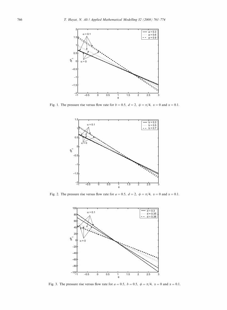
Here the flow quantities DP k; F ðuÞk and F ðlÞk are evaluated numerically for different values of a, b, d, / andresults are displayed graphically. The values of a are taken to be 0 and 0.1 [31]. Fig. 1 is plotted in order to seethe effects of upper wave amplitude a on DPk. It is observed that with an increase in a pumping increases in thepumping region ðDP k > 0Þ, copumping region ðDP k < 0Þ and free pumping ðDP k ¼ 0Þ. Also note that for anappropriately chosen DP k < 0, h decreases with an increase in a. Moreover the pumping curves for a ¼ 0:1 lieabove the curves for a ¼ 0 in pumping region, free pumping and copumping region for all three values of a.The effects of lower wave amplitude b on DPk are similar to that of a (Fig. 2). Fig. 3 presents the effects ofchannel width d on DPk. It can be seen that in pumping region ðDP k > 0Þ pumping decreases by increasingd. For free pumping there is no difference in the pumping curves while in copumping region ðDP k < 0Þ pump-ing increases for large d. It is also noted that for a ¼ 0:1 pumping curves lie above the curves for a ¼ 0 in thepumping region while situation is reversed in the case of copumping region. Fig. 4 shows the effects of phasedifference / on DPk. Similar effects are seen in the pumping and copumping region while in the free pumping,the pumping decreases with an increase in /.

—1 —0.5 0 0.5 1 1.5 2 2.5 3—2

—1.5

—1

—0.5

0

0.5

1

1.5

2

θ

ΔPλ

a = 0.3a = 0.6a = 0.9

α = 0.1

α = 0

Fig. 1. The pressure rise versus flow rate for b ¼ 0:5; d ¼ 2; / ¼ p=4; a ¼ 0 and a ¼ 0:1.

—1 —0.5 0 0.5 1 1.5 2 2.5 3—2

—1.5

—1

—0.5

0

0.5

1

1.5

θ

ΔPλ

b = 0.3b = 0.5b = 0.7

α = 0.1

α = 0

Fig. 2. The pressure rise versus flow rate for a ¼ 0:5; d ¼ 2; / ¼ p=4; a ¼ 0 and a ¼ 0:1.

—1 —0.5 0 0.5 1 1.5 2 2.5 3—100

—80

—60

—40

—20

0

20

40

60

80

100

θ

ΔPλ

d = 0.3d = 0.35d = 0.38

α = 0.1

α = 0

Fig. 3. The pressure rise versus flow rate for a ¼ 0:5; b ¼ 0:5; / ¼ p=4; a ¼ 0 and a ¼ 0:1.

766 T. Hayat, N. Ali / Applied Mathematical Modelling 32 (2008) 761–774

—1 —0.5 0 0.5 1 1.5 2 2.5 3—250

—200

—150

—100

—50

0

50

100

150

200

θ

ΔPλ

φ = 0φ = π/4φ = π/3

α = 0.1

α = 0

Fig. 4. The pressure rise versus flow rate for a ¼ 0:5; b ¼ 0:5; d ¼ 0:3; a ¼ 0 and a ¼ 0:1.

T. Hayat, N. Ali / Applied Mathematical Modelling 32 (2008) 761–774 767

The above discussion regarding the effects of a, b, d and / on DPk is in qualitative sense. To discuss theeffects quantitatively we will give the intervals for h where DP k < 0 and DP k > 0. Observe that as a increasesthe length of the interval for DP k > 0 increases (Table 1). Similar observation is for the case when viscosityincreases from 0 to 0.1 and a fixed (Table 1). This means that the interval for h in which pressure resiststhe flow increases in length as a and a increase. The lower wave amplitude b has similar effects on the lengthof the interval as that of a (Table 2). It is interesting to note that an increase in the channel width d causes adecrease in the length of the interval where DP k > 0 for both values of a ð¼ 0; 0:1Þ (Table 3). The observationsregarding the effects of / on DPk are similar to that of d (Table 4).

Figs. 5 and 6 are made to see the effects of / on the frictional forces F ðuÞk and F ðlÞk respectively. Qualitativelyfrictional forces decrease in magnitude by increasing / and increase by increasing a. Also frictional forces on

Table 1Intervals for flow rate h for different values of a

Parameter (a) Interval for h where DP k > 0 Interval for h where DP k < 0

0.3 a ¼ 0; �1 < h < 0:2674 a ¼ 0; 0:2674 < h < 3a ¼ 0:1; �1 < h < 0:2723 a ¼ 0:1; 0:2723 < h < 3

0.6 a ¼ 0; �1 < h < 0:4890 a ¼ 0; 0:4890 < h < 3a ¼ 0:1; �1 < h < 0:5031 a ¼ 0:1; 0:5031 < h < 3

0.9 a ¼ 0; �1 < h < 0:7747 a ¼ 0; 0:7747 < h < 3a ¼ 0:1; �1 < h < 0:7938 a ¼ 0:1; 0:7938 < h < 3

The other parameters chosen are b ¼ 0:5; d ¼ 2 and / ¼ p=4.

Table 2Intervals for flow rate h for different values of b

Parameter (b) Interval for h where DP k > 0 Interval for h where DP k < 0

0.3 a ¼ 0; �1 < h < 0:2675 a ¼ 0; 0:2675 < h < 3a ¼ 0:1; �1 < h < 0:2781 a ¼ 0:1; 0:2781 < h < 3

0.5 a ¼ 0; �1 < h < 0:4075 a ¼ 0; 0:4075 < h < 3a ¼ 0:1; �1 < h < 0:4188 a ¼ 0:1; 0:4188 < h < 3

0.7 a ¼ 0; �1 < h < 0:5776 a ¼ 0; 0:5776 < h < 3a ¼ 0:1; �1 < h < 0:5889 a ¼ 0:1; 0:5889 < h < 3

The other parameters chosen are a ¼ 0:5; d ¼ 2 and / ¼ p=4.

Table 3Intervals for flow rate h for different values of d

Parameter (d) Interval for h where DP k > 0 Interval for h where DP k < 0

0.3 a ¼ 0; �1 < h < 0:7838 a ¼ 0; 0:7838 < h < 3a ¼ 0:1; �1 < h < 0:8023 a ¼ 0:1; 0:8023 < h < 3

0.35 a ¼ 0; �1 < h < 0:7811 a ¼ 0; 0:7811 < h < 3a ¼ 0:1; �1 < h < 0:7666 a ¼ 0:1; 0:7666 < h < 3

0.38 a ¼ 0; �1 < h < 0:7690 a ¼ 0; 0:7690 < h < 3a ¼ 0:1; �1 < h < 0:7564 a ¼ 0:1; 0:7564 < h < 3

The other parameters chosen are a ¼ 0:5; b ¼ 0:5 and / ¼ p=4.

Table 4Intervals for flow rate h for different values of /

Parameter (/) Interval for h where DP k > 0 Interval for h where DP k < 0

0 a ¼ 0; �1 < h < 0:8975 a ¼ 0; 0:8975 < h < 3a ¼ 0:1; �1 < h < 0:9267 a ¼ 0:1; 0:9267 < h < 3

p4

a ¼ 0; �1 < h < 0:7837 a ¼ 0; 0:7837 < h < 3a ¼ 0:1; �1 < h < 0:8024 a ¼ 0:1; 0:8024 < h < 3

p3

a ¼ 0; �1 < h < 0:7092 a ¼ 0; 0:7092 < h < 3a ¼ 0:1; �1 < h < 0:7268 a ¼ 0:1; 0:7268 < h < 3

The other parameters chosen are a ¼ 0:5; b ¼ 0:5 and d ¼ 0:3.

—1 —0.5 0 0.5 1 1.5 2 2.5 3—60

—40

—20

0

20

40

60

80

θ

F λ(u)

φ = 0φ = π/4φ = π/2

α = 0

α = 0.1

Fig. 5. The friction force at the upper wall versus flow rate for a ¼ 0:5; b ¼ 0:5; d ¼ 0:3; a ¼ 0 and a ¼ 0:1.

768 T. Hayat, N. Ali / Applied Mathematical Modelling 32 (2008) 761–774

the lower wall is less than that of on the upper wall. Quantitatively with an increase in / the length of theinterval for h in which frictional forces F ðuÞk and F ðlÞk have direction opposite to the wave velocity decrease whilekeeping / fixed the length of interval increases by increasing a (Table 5). In Figs. 7 and 8 frictional forces F ðuÞk

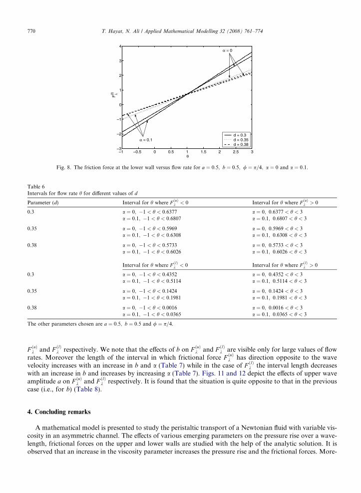
and F ðlÞk are plotted against h for different values of d. The effects of d on F ðuÞk and F ðlÞk are quite similar to thatof / qualitatively. But the length of the interval in which F ðuÞk has direction opposite to the peristaltic wave islarger than the interval length where F ðlÞk has direction opposite to the peristaltic wave in all three cases(d = 0.3,0.35 and 0.38) with a ð¼ 0; 0:1Þ (Table 6). Further it is seen while plotting graphs that variation inthe curves for frictional forces (F ðuÞk and F ðlÞk ) is only for small values of d and these effects vanish and thecurves coincide as d takes larger values. Figs. 9 and 10 illustrate the effects of lower wave amplitude b on

—1 —0.5 0 0.5 1 1.5 2 2.5 3—8

—6

—4

—2

0

2

4

6

8

θ

F λ(l)

φ = 0φ = π/4φ = π/2

α = 0

α = 0.1

Fig. 6. The friction force at the lower wall versus flow rate for a ¼ 0:5; b ¼ 0:5; d ¼ 0:3; a ¼ 0 and a ¼ 0:1.

Table 5Intervals for flow rate h for different values of /

Parameter (/) Interval for h where F ðuÞk < 0 Interval for h where F ðuÞk > 0

0 a ¼ 0; �1 < h < 0:7706 a ¼ 0; 0:7706 < h < 3a ¼ 0:1; �1 < h < 0:8336 a ¼ 0:1; 0:8336 < h < 3

p4 a ¼ 0; �1 < h < 0:6376 a ¼ 0; 0:6376 < h < 3

a ¼ 0:1; �1 < h < 0:6809 a ¼ 0:1; 0:6809 < h < 3

p2 a ¼ 0; �1 < h < 0:0612 a ¼ 0; 0:0612 < h < 3

a ¼ 0:1; �1 < h < 0:0676 a ¼ 0:1; 0:0676 < h < 3

Interval for h where F ðlÞk < 0 Interval for h where F ðlÞk > 0

0 a ¼ 0; �1 < h < 0:7498 a ¼ 0; 0:7498 < h < 3a ¼ 0:1; �1 < h < 0:8415 a ¼ 0:1; 0:8415 < h < 3

p4 a ¼ 0; �1 < h < 0:4350 a ¼ 0; 0:4350 < h < 3

a ¼ 0:1; �1 < h < 0:5121 a ¼ 0:1; 0:5121 < h < 3

p2 a ¼ 0; �1 < h < 0:0621 a ¼ 0; 0:0621 < h < 3

a ¼ 0:1; �1 < h < 0:0685 a ¼ 0:1; 0:0685 < h < 3

The other parameters chosen are a ¼ 0:5; b ¼ 0:5 and d ¼ 0:3.

—1 —0.5 0 0.5 1 1.5 2 2.5 3—30

—20

—10

0

10

20

30

40

θ

F λ(u)

d = 0.3d = 0.35d = 0.38

α = 0

α = 0.1

Fig. 7. The friction force at the upper wall versus flow rate for a ¼ 0:5; b ¼ 0:5; / ¼ p=4; a ¼ 0 and a ¼ 0:1.

T. Hayat, N. Ali / Applied Mathematical Modelling 32 (2008) 761–774 769

–1 –0.5 0 0.5 1 1.5 2 2.5 3–3

–2

–1

0

1

2

3

4

θ

Fλ(l)

d = 0.3d = 0.35d = 0.38

α = 0.1

α = 0

Fig. 8. The friction force at the lower wall versus flow rate for a ¼ 0:5; b ¼ 0:5; / ¼ p=4; a ¼ 0 and a ¼ 0:1.

Table 6Intervals for flow rate h for different values of d

Parameter (d) Interval for h where F ðuÞk < 0 Interval for h where F ðuÞk > 0

0.3 a ¼ 0; �1 < h < 0:6377 a ¼ 0; 0:6377 < h < 3a ¼ 0:1; �1 < h < 0:6807 a ¼ 0:1; 0:6807 < h < 3

0.35 a ¼ 0; �1 < h < 0:5969 a ¼ 0; 0:5969 < h < 3a ¼ 0:1; �1 < h < 0:6308 a ¼ 0:1; 0:6308 < h < 3

0.38 a ¼ 0; �1 < h < 0:5733 a ¼ 0; 0:5733 < h < 3a ¼ 0:1; �1 < h < 0:6026 a ¼ 0:1; 0:6026 < h < 3

Interval for h where F ðlÞk < 0 Interval for h where F ðlÞk > 0

0.3 a ¼ 0; �1 < h < 0:4352 a ¼ 0; 0:4352 < h < 3a ¼ 0:1; �1 < h < 0:5114 a ¼ 0:1; 0:5114 < h < 3

0.35 a ¼ 0; �1 < h < 0:1424 a ¼ 0; 0:1424 < h < 3a ¼ 0:1; �1 < h < 0:1981 a ¼ 0:1; 0:1981 < h < 3

0.38 a ¼ 0; �1 < h < 0:0016 a ¼ 0; 0:0016 < h < 3a ¼ 0:1; �1 < h < 0:0365 a ¼ 0:1; 0:0365 < h < 3

The other parameters chosen are a ¼ 0:5; b ¼ 0:5 and / ¼ p=4.

770 T. Hayat, N. Ali / Applied Mathematical Modelling 32 (2008) 761–774

F ðuÞk and F ðlÞk respectively. We note that the effects of b on F ðuÞk and F ðlÞk are visible only for large values of flowrates. Moreover the length of the interval in which frictional force F ðuÞk has direction opposite to the wavevelocity increases with an increase in b and a (Table 7) while in the case of F ðlÞk the interval length decreaseswith an increase in b and increases by increasing a (Table 7). Figs. 11 and 12 depict the effects of upper waveamplitude a on F ðuÞk and F ðlÞk respectively. It is found that the situation is quite opposite to that in the previouscase (i.e., for b) (Table 8).

4. Concluding remarks

A mathematical model is presented to study the peristaltic transport of a Newtonian fluid with variable vis-cosity in an asymmetric channel. The effects of various emerging parameters on the pressure rise over a wave-length, frictional forces on the upper and lower walls are studied with the help of the analytic solution. It isobserved that an increase in the viscosity parameter increases the pressure rise and the frictional forces. More-

Table 7Intervals for flow rate h for different values of b

Parameter (b) Interval for h where F ðuÞk < 0 Interval for h where F ðuÞk > 0

0.3 a ¼ 0; �1 < h < 0:1349 a ¼ 0; 0:1349 < h < 3a ¼ 0:1; �1 < h < 0:1512 a ¼ 0:1; 0:1512 < h < 3

0.5 a ¼ 0; �1 < h < 0:3643 a ¼ 0; 0:3643 < h < 3a ¼ 0:1; �1 < h < 0:3770 a ¼ 0:1; 0:3770 < h < 3

0.7 a ¼ 0; �1 < h < 0:6726 a ¼ 0; 0:6726 < h < 3a ¼ 0:1; �1 < h < 0:6860 a ¼ 0:1; 0:6860 < h < 3

Interval for h where F ðlÞk < 0 Interval for h where F ðlÞk > 0

0.3 a ¼ 0; �1 < h < 0:2220 a ¼ 0; 0:2220 < h < 3a ¼ 0:1; �1 < h < 0:2364 a ¼ 0:1; 0:2364 < h < 3

0.5 a ¼ 0; �1 < h < 0:1369 a ¼ 0; 0:1369 < h < 3a ¼ 0:1; �1 < h < 0:1500 a ¼ 0:1; 0:1500 < h < 3

0.7 a ¼ 0; �1 < h < �0:0878 a ¼ 0; �0:0878 < h < 3a ¼ 0:1; �1 < h < �0:0762 a ¼ 0:1; �0:0762 < h < 3

The other parameters chosen are a ¼ 0:5; d ¼ 0:7 and / ¼ p=4.

—1 —0.5 0 0.5 1 1.5 2 2.5 3—2

—1

0

1

2

3

4

5

θ

F λ(l)

b = 0.3b = 0.5b = 0.7

α = 0

α = 0.1

Fig. 10. The friction force at the lower wall versus flow rate for a ¼ 0:5; d ¼ 0:7; / ¼ p=4; a ¼ 0 and a ¼ 0:1.

—1 —0.5 0 0.5 1 1.5 2 2.5 3—10

—5

0

5

10

15

θ

F λ(u)

b = 0.3b = 0.5b = 0.7

α = 0

α = 0.1

Fig. 9. The friction force at the upper wall versus flow rate for a ¼ 0:5; d ¼ 0:7; / ¼ p=4; a ¼ 0 and a ¼ 0:1.

T. Hayat, N. Ali / Applied Mathematical Modelling 32 (2008) 761–774 771

—1 —0.5 0 0.5 1 1.5 2 2.5 3—3

—2

—1

0

1

2

3

4

5

θ

F λ(u)

a = 0.3a = 0.6a = 0.9

α = 0.1

α = 0

Fig. 11. The friction force at the upper wall versus flow rate for b ¼ 0:5; d ¼ 1; / ¼ p=4; a ¼ 0 and a ¼ 0:1.

—1 —0.5 0 0.5 1 1.5 2 2.5 3—10

—8

—6

—4

—2

0

2

4

6

8

10

θ

F λ(l)

a = 0.7a = 0.9a = 1

α = 0

α = 0.1

Fig. 12. The friction force at the lower wall versus flow rate for b ¼ 0:5; d ¼ 1; / ¼ p=4; a ¼ 0 and a ¼ 0:1.

Table 8Intervals for flow rate h for different values of a

Parameter (a) Interval for h where F ðuÞk < 0 Interval for h where F ðuÞk > 0

0.3 a ¼ 0; �1 < h < 0:2274 a ¼ 0; 0:2274 < h < 3a ¼ 0:1; �1 < h < 0:2274 a ¼ 0:1; 0:2274 < h < 3

0.6 a ¼ 0; �1 < h < 0:2126 a ¼ 0; 0:2126 < h < 3a ¼ 0:1; �1 < h < 0:2317 a ¼ 0:1; 0:2317 < h < 3

0.9 a ¼ 0; �1 < h < 0:0213 a ¼ 0; 0:0213 < h < 3a ¼ 0:1; �1 < h < 0:0667 a ¼ 0:1; 0:0667 < h < 3

Interval for h where F ðlÞk < 0 Interval for h where F ðlÞk > 0

0.3 a ¼ 0; �1 < h < 0:0513 a ¼ 0; 0:0513 < h < 3a ¼ 0:1; �1 < h < 0:0513 a ¼ 0:1; 0:513 < h < 3

0.6 a ¼ 0; �1 < h < 0:3452 a ¼ 0; 0:3452 < h < 3a ¼ 0:1; �1 < h < 0:3624 a ¼ 0:1; 0:3624 < h < 3

0.9 a ¼ 0; �1 < h < 0:7925 a ¼ 0; 0:7925 < h < 3a ¼ 0:1; �1 < h < 0:8233 a ¼ 0:1; 0:8233 < h < 3

The other parameters chosen are b ¼ 0:5; d ¼ 1 and / ¼ p=4.

772 T. Hayat, N. Ali / Applied Mathematical Modelling 32 (2008) 761–774

T. Hayat, N. Ali / Applied Mathematical Modelling 32 (2008) 761–774 773

over, the interval for the flow rate h where DP k > 0 increases with an increase in the viscosity parameter. Theresults of Newtonian fluid with constant viscosity [24] can be recovered as a special case of our analysis.

Acknowledgement

The authors are grateful to the anonymous referees for the valuable suggestions which undoubtedly im-proved the earlier version of this manuscript. We are further grateful to the Higher Education Commissionfor the financial support.

References

[1] T. Hayat, A.H. Kara, E. Momoniat, Exact flow of a third grade fluid on a porous wall, Int. J. Non-linear Mech. 38 (2003) 1533–1537.[2] T. Hayat, A.H. Kara, Couette flow of a third grade fluid with variable magnetic field, Math. Comput. Modell. 43 (2006) 132–137.[3] T. Hayat, S.B. Khan, M. Khan, The influence of Hall current on the rotating oscillating flows of an Oldroyd-B fluid in a porous

medium, Non-Linear Dyn. 47 (2007) 353–362.[4] C. Fetecau, C. Fetecau, Decay of a potential vortex in an Oldroyd-B fluid, Int. J. Eng. Sci. 43 (2005) 340–351.[5] C. Fetecau, C. Fetecau, Unsteady flows of Oldroyd-B fluids in a channel of rectangular cross-section, Int. J. Non-linear Mech. 38

(2005) 1214–1219.[6] C. Fetecau, C. Fetecau, On some axial Couette flows of non-Newtonian fluids, Z. Angew. Math. Phys. 56 (2005) 1098–1106.[7] C. Fetecau, C. Fetecau, Starting solutions for some unsteady unidirectional flows of a second grade fluid, Int. J. Eng. Sci. 43 (2005)

781–789.[8] W.C. Tan, T. Masuoka, Stokes first problem for second grade fluid in a porous half space with heated boundary, Int. J. Non-Linear

Mech. 40 (2005) 515–522.[9] W.C. Tan, T. Masuoka, Stokes first problem for an Oldroyd-B fluid in a porous half space, Phys. Fluid 17 (2005) 023101–023107.

[10] S. Liao, On analytic solution of magnetohydrodynamic flows of non-Newtonian fluids over a stretching sheet, J. Fluid Mech. 488(2003) 189–212.

[11] T.W. Latham, Fluid motion in a peristaltic pump, M.S. Thesis, Massachusetts Institute of Technology Cambridge, Massachusetts,1966.

[12] T. Hayat, Y. Wang, A.M. Siddiqui, K. Hutter, S. Asghar, Peristaltic transport of a third order fluid in a circular cylindrical tube,Math. Models Methods Appl. Sci. 12 (2002) 1691–1706.

[13] T. Hayat, Y. Wang, A.M. Siddiqui, K. Hutter, Peristaltic motion of Johnson–Segalman fluid in a planar channel, Math. Probl. Eng. 1(2003) 1–23.

[14] T. Hayat, Y. Wang, K. Hutter, S. Asghar, A. M Siddiqui, Peristaltic transport of an Oldroyd-B fluid in a planar channel, Math.Probl. Eng. 4 (2004) 347–376.

[15] A.M. Siddiqui, T. Hayat, M. Khan, Magnetic fluid model induced by peristaltic waves, J. Phys. Soc. Jpn. 73 (2004) 2142–2147.[16] T. Hayat, F.M. Mahomed, S. Asghar, Peristaltic flow of magnetohydrodynamic Johnson–Segalman fluid, Nonlinear Dyn. 40 (2005)

375–385.[17] T. Hayat, M. Khan, S. Asghar, A.M. Siddiqui, A mathematical model of peristalsis in tubes through a porous medium, J. Porous

Media 9 (2006) 55–67.[18] Kh.S. Mekheimer, Nonlinear peristaltic transport through a porous medium in an inclined planar channel, J. Porous Media 6 (2003)

189–201.[19] Kh.S. Mekheimer, Nonlinear peristaltic transport of magneto-hydrodynamic flow in an inclined planar channel, Arab J. Sci. Eng. 28

(2003) 183–201.[20] Kh.S. Mekheimer, Peristaltic flow of blood under effect of a magnetic field in a non uniform channels, Appl. Math. Comput. 153

(2004) 763–777.[21] Kh.S. Mekheimer, Peristaltic transport of a couple-stress fluid in a uniform and non-uniform channels, Biorheology 39 (2002) 755–

765.[22] M. El-Shahed, Pulsatile flow of blood through a stenosed porous medium under periodic body acceleration, Appl. Math. Comput.

138 (2003) 479–488.[23] M. Elshahed, M.H. Haroun, Peristaltic transport of Johnson–Segalman fluid under effect of a magnetic field, Math. Probl. Eng. 6

(2005) 663–677.[24] M. Mishra, A.R. Rao, Peristaltic transport of a Newtonian fluid in an asymmetric channel, Z. Angew. Math. Phys. 54 (2004) 532–550.[25] A.M. El Misery, Abd El Hakeem, Abd El Naby, Abd Hameed El Nagar, Effects of a fluid with variable viscosity and an endoscope

on peristaltic motion, J. Phys. Soc. Jpn. 72 (2003) 89–93.[26] Abd El Hakeem, Abd El Naby, A.M. El Misery, I.I. El Shamy, Effects of an endoscope and fluid with variable viscosity on peristaltic

motion, Appl. Math. Comput. 158 (2004) 497–511.[27] O. Eytan, D. Elad, Analysis of intra-uterine motion induced by uterine contractions, Bull. Math. Biol. 61 (1999) 221–238.[28] H.R. Haynes, Physical basis of the dependence of blood viscosity on tube radius, Am. J. Physiol. 198 (1960) 1193–1200.[29] G. Bugliarello, J. Sevilla, Velocity distribution and other characteristics of steady and pulsatile blood flow in fine glass tubes,

Biorheology 7 (1970) 85–107.

774 T. Hayat, N. Ali / Applied Mathematical Modelling 32 (2008) 761–774

[30] H.L. Gold smith, R. Skalak, Hemodynamics, in: M. Van Dyke (Ed.), Annual Review of Fluid Mech, vol. 7, Annual Review Inc. PaloAlto Publ., California, 1975, pp. 231–247.

[31] L.M. Srivastava, V.P. Srivastava, S.N. Sinha, Peristaltic transport of a physiological fluid Part-I: Flow in non-uniform geometry,Biorheology 20 (1983) 153–166.

[32] M.P. Wiedeman, Dimensions of blood vessels from distributing artery to collecting vein, Circ. Res. 12 (1963) 375–381.[33] J.S. Lee, Y.C. Fung, Flow in non-uniform small blood vessels, Microvasc. Res. 3 (1971) 272–279.[34] S.K. Guha, H. Kaur, A.M. Ahmed, Mechanism of spermatic fluid transport in the vas deferens, Med. Biol. Eng. 13 (1975) 518–522.