Mathematical and Computational Methods of non-Newtonian ...
212
CRANFIELD UNIVERSITY Robert Sawko Mathematical and Computational Methods of non-Newtonian, Multiphase Flows School of Engineering PhD Thesis Academic year 2011/2012 Supervisor: Prof. Chris Thompson In partial fulfillment of the requirements for the degree of Philosophiae Doctor (PhD) c Cranfield University, 2012. All rights reserved. No part of this publication may be reproduced without the written permission of the copyright holder.
-
Upload
khangminh22 -
Category
Documents
-
view
1 -
download
0
Transcript of Mathematical and Computational Methods of non-Newtonian ...

CRANFIELD UNIVERSITY
Robert Sawko
Mathematical and Computational
Methods of non-Newtonian, Multiphase
Flows
School of Engineering
PhD Thesis
Academic year 2011/2012
Supervisor:
Prof. Chris Thompson
In partial fulfillment of the requirements for the degree of
Philosophiae Doctor (PhD)
c©Cranfield University, 2012. All rights reserved. No part of this publication may be
reproduced without the written permission of the copyright holder.

Abstract
The research presented in this thesis is concerned with the development of
numerical techniques and mathematical models for non-Newtonian fluids
and two-phase flows in pipes and channels.
Single phase, turbulent flow calculations of non-Newtonian fluids were per-
formed initially. Based on the literature a revised approach to wall mod-
elling is proposed and implemented. The approach uses analytical and
experimental analyses of the turbulent boundary layer structure. A com-
parison with the standard approach is presented.
The interaction between turbulence and non-Newtonian behaviour is stud-
ied by examining the rate of strain induced by fluctuating components of
velocity. The statistical analysis of published DNS data is performed. Fi-
nally, a model is proposed where the turbulent rate of strain is determined
from turbulence quantities used by the Reynolds-averaged Navier–Stokes
model and used in the calculation of molecular viscosity.
For two-phase flow, the solution procedure using periodic boundary condi-
tions was developed under an assumption of a flat interface. The numerical
technique was verified by comparing to an analytical result obtained for
laminar flow in a channel. An extension to three dimensional flow is per-
formed.
With periodic boundary conditions standard turbulence models are applied
to two-phase stratified flow. Several models and their corrections for two-
phase flow are assessed and a new model is proposed. The numerical studies
were carried out primiarily in the open-source code OpenFOAM, but initial
attempts were made in commercial packages such as STAR-CD and FLU-
ENT. Experimental data collected from the literature are used to verify the
results showing good agreement in pressure drops and phase fractions.

Acknowledgements
It is a pleasant duty to express gratitude to all those who have contributed
to the completion of the presented work. I would like to acknowledge the
work of my supervisor Professor Chris Thompson who offered many stimu-
lating discussions and introduced me to this fascinating field. It is also my
privilege to acknowledge Professor Ray Chhabra, Doctor Fernando Pinho,
Doctor Robert Poole and Doctor Murray Rudman for supplying me with
experimental data and for many comments. Many thanks to Doctor Dag
Biberg for providing his own code, consultancy and many useful hints and
to Doctor Mustapha Gourma for his critical remarks. I am also immensely
grateful to Sarah Jones for offering an engineering perspective in numerous
discussions and for invaluable assistance in language matters. Last, but def-
initely not least I would like to thank my closest family for their constant
support.

ii

Contents
List of Figures vii
List of Tables xi
List of Symbols xiii
1 Introduction 1
1.1 Modelling in computational fluid dynamics . . . . . . . . . . . . . . . . 3
1.2 Non-Newtonian flows . . . . . . . . . . . . . . . . . . . . . . . . . . . . . 4
1.3 Computational multiphase fluid dynamics . . . . . . . . . . . . . . . . . 6
1.4 Areas of application . . . . . . . . . . . . . . . . . . . . . . . . . . . . . 7
1.5 Objectives . . . . . . . . . . . . . . . . . . . . . . . . . . . . . . . . . . . 9
1.6 Presented contributions . . . . . . . . . . . . . . . . . . . . . . . . . . . 9
1.7 Outline . . . . . . . . . . . . . . . . . . . . . . . . . . . . . . . . . . . . 10
2 Finite volume method 13
2.1 Domain discretisation . . . . . . . . . . . . . . . . . . . . . . . . . . . . 14
2.2 Equations discretisation . . . . . . . . . . . . . . . . . . . . . . . . . . . 15
2.2.1 Face interpolation . . . . . . . . . . . . . . . . . . . . . . . . . . 16
2.2.2 Discretisation of transport equation terms . . . . . . . . . . . . . 21
2.3 Boundary conditions . . . . . . . . . . . . . . . . . . . . . . . . . . . . . 22
2.4 The system of linear equations . . . . . . . . . . . . . . . . . . . . . . . 24
2.4.1 Under-relaxation . . . . . . . . . . . . . . . . . . . . . . . . . . . 26
3 Volume of fluid method with periodic boundaries 27
3.1 Governing equations . . . . . . . . . . . . . . . . . . . . . . . . . . . . . 27
3.1.1 Phase fraction . . . . . . . . . . . . . . . . . . . . . . . . . . . . 29
iii

CONTENTS
3.1.2 Continuity and momentum Equations . . . . . . . . . . . . . . . 34
3.1.3 Turbulence equations . . . . . . . . . . . . . . . . . . . . . . . . 35
3.1.4 Additional constraints . . . . . . . . . . . . . . . . . . . . . . . . 36
3.2 Pressure-velocity coupling . . . . . . . . . . . . . . . . . . . . . . . . . . 37
3.2.1 SIMPLE . . . . . . . . . . . . . . . . . . . . . . . . . . . . . . . . 40
3.2.2 PISO . . . . . . . . . . . . . . . . . . . . . . . . . . . . . . . . . 40
3.2.3 Additional discretisation considerations . . . . . . . . . . . . . . 41
3.3 Periodic boundary conditions . . . . . . . . . . . . . . . . . . . . . . . . 42
3.3.1 Notation . . . . . . . . . . . . . . . . . . . . . . . . . . . . . . . . 43
3.3.2 Single-phase pressure-correction . . . . . . . . . . . . . . . . . . . 43
3.3.3 Two-phase pressure-correction . . . . . . . . . . . . . . . . . . . 45
3.3.4 Liquid height correction . . . . . . . . . . . . . . . . . . . . . . . 45
3.3.5 Other approaches . . . . . . . . . . . . . . . . . . . . . . . . . . . 47
3.3.6 Preliminary results . . . . . . . . . . . . . . . . . . . . . . . . . . 48
3.4 Concluding remarks . . . . . . . . . . . . . . . . . . . . . . . . . . . . . 48
4 Non-Newtonian properties in turbulence modelling 51
4.1 Newtonian turbulence in channels and pipes . . . . . . . . . . . . . . . . 52
4.1.1 Logarithmic law of the wall . . . . . . . . . . . . . . . . . . . . . 53
4.1.2 Friction factors for pipelines . . . . . . . . . . . . . . . . . . . . . 55
4.1.3 Relevant quantities and their order of magnitude analysis . . . . 56
4.1.4 Near-wall treatments . . . . . . . . . . . . . . . . . . . . . . . . . 57
4.2 Constitutive laws . . . . . . . . . . . . . . . . . . . . . . . . . . . . . . . 61
4.2.1 Reiner–Rivlin fluids . . . . . . . . . . . . . . . . . . . . . . . . . 62
4.2.2 Generalised Newtonian fluids . . . . . . . . . . . . . . . . . . . . 63
4.2.3 Viscoplasitc fluids . . . . . . . . . . . . . . . . . . . . . . . . . . 64
4.2.4 Viscoelastic fluids . . . . . . . . . . . . . . . . . . . . . . . . . . 64
4.2.5 Non-dimensional parameters . . . . . . . . . . . . . . . . . . . . 66
4.3 Friction factors . . . . . . . . . . . . . . . . . . . . . . . . . . . . . . . . 67
4.3.1 Dodge and Metzner . . . . . . . . . . . . . . . . . . . . . . . . . 67
4.3.2 Clapp . . . . . . . . . . . . . . . . . . . . . . . . . . . . . . . . . 68
4.3.3 BNS equation . . . . . . . . . . . . . . . . . . . . . . . . . . . . . 68
4.3.4 Other friction factor correlations and some comparisons . . . . . 69
iv

CONTENTS
4.4 Non-Newtonian wall function . . . . . . . . . . . . . . . . . . . . . . . . 70
4.5 Concluding remarks . . . . . . . . . . . . . . . . . . . . . . . . . . . . . 76
5 Rate of strain in turbulent flow 79
5.1 Theory . . . . . . . . . . . . . . . . . . . . . . . . . . . . . . . . . . . . . 80
5.1.1 Relation to vorticity . . . . . . . . . . . . . . . . . . . . . . . . . 82
5.2 Probabilisitc information . . . . . . . . . . . . . . . . . . . . . . . . . . . 84
5.3 Analysis of DNS data . . . . . . . . . . . . . . . . . . . . . . . . . . . . 86
5.3.1 Comparison of viscosity fields . . . . . . . . . . . . . . . . . . . . 87
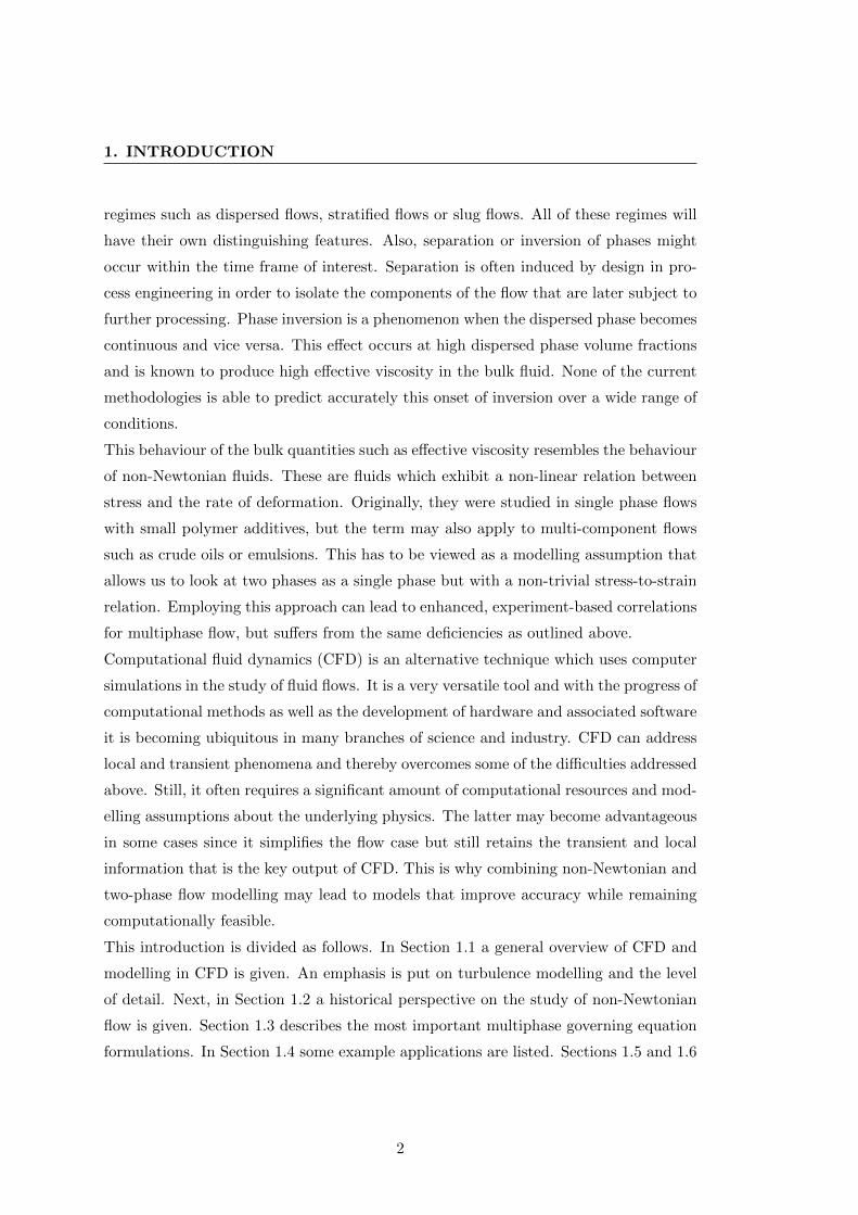
5.3.2 Rate of strain magnitude . . . . . . . . . . . . . . . . . . . . . . 88
5.3.3 Yield stress and unyielded regions . . . . . . . . . . . . . . . . . 90
5.3.4 Statistical hypothesis testing . . . . . . . . . . . . . . . . . . . . 91
5.4 CFD two-equation models . . . . . . . . . . . . . . . . . . . . . . . . . . 98
5.4.1 Results . . . . . . . . . . . . . . . . . . . . . . . . . . . . . . . . 100
5.5 Concluding remarks . . . . . . . . . . . . . . . . . . . . . . . . . . . . . 104
6 Modelling stratified flow 107
6.1 Empirical pressure drop correlations . . . . . . . . . . . . . . . . . . . . 108
6.1.1 Stratified gas/Newtonian liquid . . . . . . . . . . . . . . . . . . . 108
6.1.2 Stratified gas/non-Newtonian liquid . . . . . . . . . . . . . . . . 110
6.1.3 Farrooqi and Richardson . . . . . . . . . . . . . . . . . . . . . . . 111
6.1.4 Dziubinski . . . . . . . . . . . . . . . . . . . . . . . . . . . . . . . 112
6.2 Analytical velocity profiles . . . . . . . . . . . . . . . . . . . . . . . . . . 113
6.2.1 Laminar profiles . . . . . . . . . . . . . . . . . . . . . . . . . . . 114
6.2.2 Turbulent profiles . . . . . . . . . . . . . . . . . . . . . . . . . . 116
6.3 Comparison against CFD . . . . . . . . . . . . . . . . . . . . . . . . . . 122
6.3.1 Laminar profiles . . . . . . . . . . . . . . . . . . . . . . . . . . . 123
6.3.2 Turbulent profile . . . . . . . . . . . . . . . . . . . . . . . . . . . 126
6.4 Non-Newtonian fluid and two-phase flow . . . . . . . . . . . . . . . . . . 134
6.5 Recent DNS and LES results . . . . . . . . . . . . . . . . . . . . . . . . 138
6.6 Concluding remarks . . . . . . . . . . . . . . . . . . . . . . . . . . . . . 141
v

CONTENTS
7 Summary 143
7.1 Conclusions . . . . . . . . . . . . . . . . . . . . . . . . . . . . . . . . . . 143
7.2 Suggestions for future work . . . . . . . . . . . . . . . . . . . . . . . . . 145
References 149
A Low-Re models test 161
B Holdup and pressure drop correlations 169
B.1 Laminar flow in a channel . . . . . . . . . . . . . . . . . . . . . . . . . . 170
B.2 Pipe flow with Taitel–Dukler correlation . . . . . . . . . . . . . . . . . . 171
B.3 Biberg model . . . . . . . . . . . . . . . . . . . . . . . . . . . . . . . . . 173
C Heat transfer modelling 177
C.1 Temperature effect on viscosity . . . . . . . . . . . . . . . . . . . . . . . 179
C.1.1 Governing equations . . . . . . . . . . . . . . . . . . . . . . . . . 180
C.1.2 Reference scale . . . . . . . . . . . . . . . . . . . . . . . . . . . . 182
C.1.3 Main analytical results . . . . . . . . . . . . . . . . . . . . . . . . 182
C.2 Periodicity in heat transfer . . . . . . . . . . . . . . . . . . . . . . . . . 184
C.3 Results . . . . . . . . . . . . . . . . . . . . . . . . . . . . . . . . . . . . . 186
D Data collected from the literature review 189
vi

List of Figures
1.1 Flow patterns in horizontal flows. Picture taken from Brennen (2005) . 8
1.2 Flow map in a horizontal pipe of diameter 5.1cm Picture taken from
Brennen (2005) . . . . . . . . . . . . . . . . . . . . . . . . . . . . . . . . 8
1.3 The outline of the thesis . . . . . . . . . . . . . . . . . . . . . . . . . . . 11
2.1 Finite volume notation. . . . . . . . . . . . . . . . . . . . . . . . . . . . 14
2.2 Normalised value diagrams for HRIC. The shaded area represents schemes
satisfying convective boundedness criteria. . . . . . . . . . . . . . . . . . 18
2.3 The NVD diagram for Superbee scheme. . . . . . . . . . . . . . . . . . . 20
2.4 Dirichlet and Neuman boundary conditions. . . . . . . . . . . . . . . . . 23
2.5 Robin and periodic boundary conditions. . . . . . . . . . . . . . . . . . . 23
3.1 Quartic scheme for two neighboring cells and its iso-surfaces. . . . . . . 30
3.2 Capturing the interface at the front of a displaced phase region. The
velocities in each cell are equal and the values of phase fraction were
chosen arbitrarily to create a two-cell wide interface. Note the lack of
treatment on the first face. . . . . . . . . . . . . . . . . . . . . . . . . . 31
3.3 Capturing the interface at the back of displaced field. Note the increased
diffusion from the last cell. Velocities in each cell are equal and the values
of phase fraction were chosen arbitrary to create a two-cell wide interface. 32
3.4 The comparison of different interpolation schemes for Riemann problem.
Courant number equals to 0.1. . . . . . . . . . . . . . . . . . . . . . . . 33
3.5 The structure of a segregated solver. . . . . . . . . . . . . . . . . . . . . 38
3.6 Intuitive idea for the phase correction algorithm. . . . . . . . . . . . . . 46
3.7 Typical results from a 3D periodic simulation of a stratified flow. . . . . 49
vii

LIST OF FIGURES
4.1 Channel flow: stress and velocity profile sketch. . . . . . . . . . . . . . . 52
4.2 Turbulent boundary layer structure with respect to the first computa-
tional cell. High and low Reynolds number approaches i.e. wall function
against fine grid (possibly with damping functions). . . . . . . . . . . . 58
4.3 Various classes of genaralised Newtonian fluids. . . . . . . . . . . . . . . 64
4.4 Prediction of non-Newtonian friction factors with standard wall functions. 73
4.5 Prediction of non-Newtonian friction factors with Dodge and Metzner
(1959) using only the profile constants. . . . . . . . . . . . . . . . . . . . 73
4.6 Prediction of non-Newtonian friction factors with Clapp (1961) using
only the profile constants. . . . . . . . . . . . . . . . . . . . . . . . . . . 74
4.7 Prediction of non-Newtonian friction factors with Dodge and Metzner
(1959) using wall distance calculation. . . . . . . . . . . . . . . . . . . . 74
4.8 Prediction of non-Newtonian friction factors with Clapp (1961) using
wall distance calculation. . . . . . . . . . . . . . . . . . . . . . . . . . . 75
4.9 Velocity profiles for n = 0.7 and ReMR = 106. . . . . . . . . . . . . . . . 77
4.10 Laminar and turbulent viscosity profiles for n = 0.7 and ReMR = 106. . . 77
5.1 Vortex stretching phenomena that occurs in the in the presence of shear. 82
5.2 DNS grid by Rudman et al. (2004). . . . . . . . . . . . . . . . . . . . . . 87
5.3 The radial interpolation of viscosity field. . . . . . . . . . . . . . . . . . 88
5.4 Top: rate of strain based on mean (left) and rate of strain based on
instantaneous velocity (right). Bottom: the ratio of instantaneous to
mean rate of strain. Reg regions show signficant differences between
shear rate caused by mean and fluctuating components. . . . . . . . . . 89
5.5 Ratios of instantaneous to mean rate of strain for τY = 0.28 (Left)
τY = 0.85 (Right). . . . . . . . . . . . . . . . . . . . . . . . . . . . . . . 89
5.6 The logarithm of shear-stress normalised by yield stress for τY = 0.28
(Left) τY = 0.85 (Right). . . . . . . . . . . . . . . . . . . . . . . . . . . . 90
5.7 The difference between the rate of strain (RoS) calculated from the mean
velocity and instantaneous velocity, averaged over all radial points. . . . 92
5.8 p-values for the equal mean hypothesis. . . . . . . . . . . . . . . . . . . 92
5.9 Skewness (left) and kurtosis (right) of the probability distribution. . . . 94
viii

LIST OF FIGURES
5.10 The p–values associated with hypothesis of log-normality of instanta-
neous rate of strain (H2) and normality of mean rate of strain (H2’). . . 96
5.11 The p–values associated with hypothesis of log-normality of the fluctu-
ating rate of strain H2’. . . . . . . . . . . . . . . . . . . . . . . . . . . . 96
5.12 The QQ plot for the one of the fitted histograms. . . . . . . . . . . . . . 97
5.13 Probability density functions of strain rates of mean (left) and instanta-
neous (right) fields. (Rudman et al. (2004)). . . . . . . . . . . . . . . . 98
5.14 Left: Cross model with parameters fitted for 0.09% solution of CMC in
water. Right: Laminar, steady calculation. . . . . . . . . . . . . . . . . . 101
5.15 Left: Turbulent velocity profile in physical coordinates. Right: Turbu-
lence intensity. The error of the turbulent intensity prediction was less
than 5%. . . . . . . . . . . . . . . . . . . . . . . . . . . . . . . . . . . . . 102
5.16 Viscosity profiles in FLUENT for Rudman et al. (2004) cases. . . . . . . 103
5.17 Viscosity profiles for ReW = 7000 τY = 0.24 (left) τY = 0.85 (right).
The viscosity of the flow is closely reproduced. . . . . . . . . . . . . . . 105
6.1 Sketch of the physical problem. . . . . . . . . . . . . . . . . . . . . . . . 113
6.2 Turbulent profiles in steady state fully developed channel flow: shear
stress (left), eddy viscosity (centre), mean velocity (right). . . . . . . . . 116
6.3 The behaviour of liquid height and pressure gradient with respect to
Reynolds number in laminar flow. . . . . . . . . . . . . . . . . . . . . . . 124
6.4 Typical velocity profiles obtained with OpenFOAM: Profiles on the left
have ReG = 150 on the right ReG = 1500. Profiles at the top have
ReL = 150 and at the bottom: ReL = 1500. . . . . . . . . . . . . . . . . 124
6.5 Top: the grid employed, Bottom: The normal velocity distribution and
the phase fraction distribution. . . . . . . . . . . . . . . . . . . . . . . . 125
6.6 FLUENT results for turbulent quantities from top to bottom: turbulence
intensity, turbulence dissipation and effective viscosity. . . . . . . . . . . 127
6.7 Standard turbulence models against Akai et al. (1981). Velocity profiles
on the gas (left) and liquid (right) sides. Top: ReG = 2.34× 10³ Centre:
ReG = 6.52× 10³, Bottom: ReG = 1.32× 10⁴. . . . . . . . . . . . . . . . 128
6.8 a) Curvilinear mesh (Issa (1988)) b) Single phase with moving wall
(Holmas and Biberg (2007)). . . . . . . . . . . . . . . . . . . . . . . . . 129
ix

LIST OF FIGURES
6.9 Egorov (2004) type correction: pressure gradient predictions. Smooth
and wavy lines are plotted according to Biberg (2007) model. Top:
ReL = 255 Centre ReL = 745, Bottom: ReL = 255 but with constant
B = 1. . . . . . . . . . . . . . . . . . . . . . . . . . . . . . . . . . . . . . 131
6.10 Modified turbulence models against Akai et al. (1981). Velocity profiles
on the gas (left) and liquid (right) sides. Top: ReG = 2.34× 10³ Centre:
ReG = 6.52× 10³, Bottom: ReG = 1.32× 10⁴. . . . . . . . . . . . . . . . 135
6.11 Estimated against experimental pressure gradients and liquid height. . . 136
6.12 Biberg model against Akai et al. (1981). Velocity profiles on the gas (left)
and liquid (right) sides. Top: ReG = 2.34×10³ Centre: ReG = 6.52×10³,
Bottom: ReG = 1.32× 10⁴. . . . . . . . . . . . . . . . . . . . . . . . . . 137
6.13 The influence of non-Newtonian property on the velocity profile of the
two-phase flow. . . . . . . . . . . . . . . . . . . . . . . . . . . . . . . . . 138
A.1 Laminar profiles. Coarse mesh Re = 100 . . . . . . . . . . . . . . . . . . 163
A.2 Laminar profiles. Fine mesh Re = 100 . . . . . . . . . . . . . . . . . . . 164
A.3 Transitional profiles: fine mesh Re = 1000 . . . . . . . . . . . . . . . . . 165
A.4 Turbulent profiles. Fine mesh Re = 5000 . . . . . . . . . . . . . . . . . . 166
B.1 Notation required for Taitel–Dukler method of calculating pressure gra-
dients . . . . . . . . . . . . . . . . . . . . . . . . . . . . . . . . . . . . . 171
B.2 Non-dimensional height as a function of Lockhard–Martinelli parameter. 174
B.3 Non-dimensional gas pressure gradient as a function of Lockhard–Martinelli
parameter. . . . . . . . . . . . . . . . . . . . . . . . . . . . . . . . . . . . 174
C.1 Top: temperature variation in a 10 diameter long channel section. Bot-
tom left: laminar velocity profile. Bottom right: temperature at the
outlet and the inlet of the section. Self-similar solution was obtained. . . 187
C.2 Comparison of maximum temperature for different inlet bulk temperatures.187
x

List of Tables
5.1 Flow-rate predictions showing improvements in accuracy for selected cases.105
6.1 VOF turbulence interface damping mechanisms. . . . . . . . . . . . . . . 133
B.1 File list for laminar two-phase calculation profile and pressure drop cal-
culation. . . . . . . . . . . . . . . . . . . . . . . . . . . . . . . . . . . . . 170
B.2 File list for Taitel–Dukler scripts. . . . . . . . . . . . . . . . . . . . . . . 173
B.3 File list for Taitel–Dukler scripts. . . . . . . . . . . . . . . . . . . . . . . 175
D.1 Form and content of obtained data sets . . . . . . . . . . . . . . . . . . 190
D.2 Bruno (1988) 1“ channel data . . . . . . . . . . . . . . . . . . . . . . . . 193
D.3 Flow values and rheology of used data sets . . . . . . . . . . . . . . . . . 194
xi

LIST OF TABLES
xii

List of Symbols
Abbreviations
CFD Computational fluid dynamics
CICSAM Compressive interface capturing scheme for arbitrary meshes
DNS Direct numerical simulations
FDM Finite difference method
FEM Finite element method
FVM Finite volume method
GNF Generalised Newtonian fluids
HRIC High resolution interface capturing
LES Large eddy simulation
NVD Normalised value diagram
PCG Preconditioned conjugate gradient
PDF Probability density function
PISO Pressure-implicit split-operators method
RANS Reynolds-averaged Navier–Stokes
SIMPLE Semi-implicit method for pressure-linked equations
STACS Switching technique for advection and capturing of surfaces
xiii

LIST OF TABLES
URF Under-relaxation factor
VOF Volume of fluid
Greek Symbols
ε Turbulence dissipation [m2/s3]
Γ Scalar diffusivity coefficient
µ Molecular viscosity [Pa s]
µt Eddy viscosity [Pa s]
ν Kinematic viscosity [m2/s]
νt Eddy kinematic viscosity [m2/s]
ω Specific dissipation [s−1]
φ Scalar quantity
ρ Denisty [kg2/m3]
τi Interface shear stress [Pa]
τw Wall shear stress [Pa]
εijk Levi-Civita symbol
ζi Vorticity component [1/s]
Roman Symbols
Sij Mean rate of strain [1/s]
sij Fluctuating rate of strain [1/s]
sij Instantaneous rate of strain [1/s]
Usg Superficial gas velocity [m/s]
Usl Superficial liquid velocity [m/s]
xiv

LIST OF TABLES
d Distance between centres of two cells
S Surface area vector
x Spatial position vector
aij Matrix coefficient
R Source term or in the context of the Biberg model the ratio of shear stresses
Sφ Source term
Ui the i’th coordinate of the velocity vector U. In the context of turbulent flow
the symbol denotes mean velocity.
ui the i’th coordinate of the fluctuating component of velocity m/s
V Volume
xi the i’th coordinate of the position vector x
Subscripts
Qf Q at a face
QN Q of a neighbouring cell
QP Q of a cell
xv

LIST OF TABLES
xvi

Chapter 1
Introduction
With the progress of science and technology, the study of flows with more than one
phase receives increasing attention among practitioners. Currently, there are many
branches of industry where multi-component flows are commonplace. The natural
world also abounds in phenomena that are inherently multiphase giving an incentive
and opportunities to study multiphase fluid dynamics. Equipment such as coolant
systems, long pipelines and separators interact with at least two component flow. The
optimal design, maintenance and control of these devices require a better understanding
of the complex flow phenomena that are involved. Therefore, the development of current
predictive techniques must include the modelling of multiple phases and the interactions
that occur between them.
Experimental studies and the resulting empirical correlations are still the most common
approaches in investigations of multiphase flows and the design processes. In some cases
these techniques proved to be successful but in general multiphase flows encompass
many complex mechanisms of mass, momentum and heat transfer that take place inside
and between phases e.g. turbulence, surface tension, buoyancy. This, in turn, gives rise
to many non-dimensional numbers parameterising the flow and the lack of universally
established scaling laws makes it difficult to design efficient and meaningful experiments.
An additional difficulty is intrusiveness of most measurement devices. The empirical
correlations that come from these experiments are usually of limited applicability.
Moreover, empirical correlations are usually of a global character whereas fluid flows
often exhibit transient or local phenomena that can significantly affect the bulk quan-
tities. The local distribution of volume phase fractions can lead to many different flow
1
1. INTRODUCTION
regimes such as dispersed flows, stratified flows or slug flows. All of these regimes will
have their own distinguishing features. Also, separation or inversion of phases might
occur within the time frame of interest. Separation is often induced by design in pro-
cess engineering in order to isolate the components of the flow that are later subject to
further processing. Phase inversion is a phenomenon when the dispersed phase becomes
continuous and vice versa. This effect occurs at high dispersed phase volume fractions
and is known to produce high effective viscosity in the bulk fluid. None of the current
methodologies is able to predict accurately this onset of inversion over a wide range of
conditions.
This behaviour of the bulk quantities such as effective viscosity resembles the behaviour
of non-Newtonian fluids. These are fluids which exhibit a non-linear relation between
stress and the rate of deformation. Originally, they were studied in single phase flows
with small polymer additives, but the term may also apply to multi-component flows
such as crude oils or emulsions. This has to be viewed as a modelling assumption that
allows us to look at two phases as a single phase but with a non-trivial stress-to-strain
relation. Employing this approach can lead to enhanced, experiment-based correlations
for multiphase flow, but suffers from the same deficiencies as outlined above.
Computational fluid dynamics (CFD) is an alternative technique which uses computer
simulations in the study of fluid flows. It is a very versatile tool and with the progress of
computational methods as well as the development of hardware and associated software
it is becoming ubiquitous in many branches of science and industry. CFD can address
local and transient phenomena and thereby overcomes some of the difficulties addressed
above. Still, it often requires a significant amount of computational resources and mod-
elling assumptions about the underlying physics. The latter may become advantageous
in some cases since it simplifies the flow case but still retains the transient and local
information that is the key output of CFD. This is why combining non-Newtonian and
two-phase flow modelling may lead to models that improve accuracy while remaining
computationally feasible.
This introduction is divided as follows. In Section 1.1 a general overview of CFD and
modelling in CFD is given. An emphasis is put on turbulence modelling and the level
of detail. Next, in Section 1.2 a historical perspective on the study of non-Newtonian
flow is given. Section 1.3 describes the most important multiphase governing equation
formulations. In Section 1.4 some example applications are listed. Sections 1.5 and 1.6
2

1.1 Modelling in computational fluid dynamics
give the initial objectives and the contributions of this study. Section 1.7 serves as an
outline for the remaining part of this thesis.
1.1 Modelling in computational fluid dynamics
CFD is an important tool in the study of complex flows. It relies on the numerical
solution of the partial differential equations that govern the motion of the fluids. Until
recent CFD was mostly applied to single phase flow. This proved surprisingly diffi-
cult due to the high computational requirements when dealing with turbulent flow.
Nevertheless, the progress in numerical techniques, modelling and computer hardware
allowed the incorporation of CFD as an industry standard in the development of many
products. Multiphase CFD attempts to build on this success by extending the current
techniques.
Many challenges have to be overcome. Firstly, there is still much uncertainty in the
formulation of the governing equations that capture the essential physics of the flow in
question. Currently there is no universal approach and different multiphase flows will
require a different set of equations. Furthermore the equations might pose additional
numerical difficulties such as in stability or excessive numerical diffusion.
Single phase CFD encountered significant problems when dealing with turbulence. The
source of these problems is the energy cascade that can be described as large scale mo-
tions giving rise to small scale motions. The small scale motion in turn affect the large
scale structures, giving rise to a multi-scale phenomenon. The computational resources
required to capture this energy cascade grow rapidly with the Reynolds number of the
flow.
Direct numerical simulation (DNS) addresses the problem by resolving all the motions
that contribute to the energy spectrum of the fluid. This approach requires the im-
plementation of high accuracy numerical schemes leading also to high computational
effort. For scientific purposes DNS is a preferred method if it can be applied since it is
equivalent to experimental data but it benefits from the non-intrusiveness of the mea-
surement technique. For engineering applications the results are usually not directly
applicable and additional post-processing is required in order to obtain bulk quantities
or quantities averaged over time.
3

1. INTRODUCTION
On the other end of the spectrum we have the Reynolds-averaged Navier–Stokes (RANS)
equations framework. This approach expresses the governing equations in terms of first
and second order statistical quantities i.e. mean flow and variance (second central mo-
ment). The results from this approach must be understood as an ensemble average of
a collection of experiments. In practice, since the whole turbulent energy spectrum is
modelled, the modelling assumptions might give a completely distorted picture of the
flow. Nevertheless, this approach usually produces results that are directly applicable
for engineering purposes and in comparison with other approaches it has the lowest
computational requirements. It became a standard in industrial applications where
large or complex geometries are involved.
Large eddy simulation (LES) tries to combine the best of both worlds by only modelling
a portion of the energy spectrum (usually ≤ 20%). This makes the various statisti-
cal assumptions more applicable since it is known that turbulent structures at small
scales are independent of the large scale motions and exhibit properties like isotropy
or homogeneity. Despite the progress in LES, these calculations still require signifi-
cant computational times and common models of turbulence have to be altered when
inter-phase effects become important.
1.2 Non-Newtonian flows
Chhabra (2006) discerns three stages in the development of fluid mechanics. At the first
stage, studies were focused on ideal fluids i.e. fluids without viscosity, compressibility,
elasticity and with all the remaining material properties kept constant. Those kind of
fluids are purely imaginary concepts1 and were used mainly for the purpose of analysis.
Despite the seemingly crude approximations, inviscid and incompressible theories led
to ground-breaking results in many areas of science and engineering (e.g. accurate
prediction of lift force, which paradoxically is a viscous effect).
The next step was to introduce viscous effects. This was pioneered by Ludwig Prandtl
who assumed that viscosity becomes important only in the boundary layer, formed in
the direct vicinity of a solid surface. Hence, the flow domain was decomposed into
region of ideal fluid (far from the surface) and a viscous fluid (close to the surface).
This approach is the basis for classical fluid dynamics.
1Except for some unusual situations like superfluidity.
4

1.2 Non-Newtonian flows
Finally, the third stage, which is still an active area of research, addresses the departure
from Newton’s linear law of viscosity. Its importance was appreciated at the beginning
of the last century as many industrial materials could not be accurately described with
this simple relation. Two sources of non-Newtonian behaviour can be distinguished. On
a microscopic level, it is the molecular structure of fluid particles. Spherical and roughly
spherical particles produce a Newtonian behaviour whilst the addition of long chains
of particles might cause Newton’s approximation to become invalid. On a macroscopic
level, mixtures such as emulsions or slurries may become Non-Newtonian despite the
fact that the components are Newtonian. The discipline which deals with flow of matter
is called rheology.
Doraiswamy (2002) gave a very precise date for the foundation of the science of rhe-
ology as the 29 April 1929, which is the date of the Third Plasticity Symposium and
the formation of the first permanent organisation keeping watch over the emerging dis-
cipline. Among the participants of the Society of Rheology we can mention Eugene
Bingham, Winslow Herschel, Wolfgang Ostwald, Markus Reiner and Ludwig Prandtl.
Doraiswamy (2002) also reviews the roots of fluid dynamics and surveys with regard to
rheology to eventually present modern issues in this discipline. According to this survey
problems of elastic solids were studied in the 17th century by Hooke, Young and Cauchy.
The empirical law of viscosity was given by Newton in 1687 but it took almost two
centuries to incorporate viscosity in to the governing equations by Claude-Louis Navier
and George Gabriel Stokes. The conjunction of the two empirical laws of viscosity and
elasticity led in mid 19th century to linear viscoelasticity and a Maxwell model. In the
20th century Arthur Metzner was one of the first to introduce generalized Newtonian
fluids in industrial applications on a wide scale and popularised these concepts outside
of scientific society.
A more mathematical view of non-Newtonian fluids is due to James Oldroyd who
introduced convected derivatives and constitutive law admissibility conditions. This
allowed a more qualitative understanding of fluid behaviour although it was at the
expense of quantitative accuracy.
Toms (1949) description of drag reduction in polymers has been a source of increased
interest in non-Newtonian turbulence. To this day it is still an area of active research
including experimental studies, DNS and modelling of these fluids.
5

1. INTRODUCTION
1.3 Computational multiphase fluid dynamics
Multiphase computational fluid dynamics deals with the formulation and solutions of
fluid flow equations where the flow under investigation has more than one component.
Three models have gained particular recognition and are commonly used in academic
and industrial applications: volume of fluid (VOF), Eulerian–Lagrangian and Eulerian–
Eulerian formulations. All of these models possess different benefits and limitations
making them applicable to different, usually exclusive, flow regimes. All of these ap-
proaches take the Eulerian approach as its base i.e. they solve the governing equations
on fixed control volumes.
VOF, also known as the “one fluid” method, comprises one set of momentum equations,
the continuity equation and a scalar transport equation that represents the distribution
of the second phase. The material constants are calculated using weighted averages of
the components. This approach works when there is clear separation between phases
e.g. in stratified flows or for bubbles that are much larger than the mesh size.
The Eulerian–Lagrangian (EL) approach distinguishes between the carrier and the
dispersed phases. The carrier phase is treated as a continuous medium and its evolution
is modelled via a set of momentum equations and continuity equations. These equations
contain special source terms that represent the influence of the dispersed phase such
as the drag that a particle exerts. The dispersed phase is modelled as a set of discrete
particles with specified position and velocity. The velocity is calculated based on the
forces acting on a particle. Then the position is advanced and the forces recalculated
again using the continuous phase equations. For turbulent dispersions a random walk
algorithm may be invoked. If this is the case several trajectories for a given particle are
calculated and then averaged over realisations. Phase coupling in EL can be a one-way
or a two-way coupling. The latter is usually more accurate than the former but may
encounter significant numerical stability problems. Two-way coupling will face similar
problems to those encountered in pressure-velocity coupling in single phase CFD. The
solution of one set of equations might give a large residual in the second set of equations.
Therefore, care must be exercised in the coupled (both sets solve simultaneously) or
the segregated (iterative alternating solution) approach.
Finally, the Eulerian–Eulerian (EE) approach uses two sets of momentum equations,
continuity and phase fraction equations. Again, various source terms are used to model
6

1.4 Areas of application
phase interactions which can take the form of mass, momentum or energy transfer. EE
does not intrinsically assume that the phase is dispersed or continuous but the choice
of source terms may limit the scope of applicability to a given flow regime.
Solving additional equations is not the only complication when dealing with multiphase
flows. The behaviour of the fluid is related to the pattern of the phase distribution that
is dominant at a given time. Many one dimensional computer codes will utilise some
modelling expressions that are specific to a given pattern, thereby increasing the ac-
curacy at the expense of applicability. Three dimensional CFD has the potential to
address a wider range of flow patterns accurately but might demand more computa-
tional resources.
One of the ways to catalogue these patterns are so called flow maps. See Figure 1.2
for an example. The problem with composing such a chart is the dependency on the
composition of phases, volume fractions and geometry and inclination of the bounding
surface. The validity of a particular flow map is usually confined to specific values of
above properties.
1.4 Areas of application
Non-Newtonian and multiphase flow appear often in industrial processes or everyday
life phenomena. This study will focus mainly on transportation in horizontal conduits
that is typical in the petroleum industry, but other areas of application suggested by
Chhabra (2008) may involve:
Biology: animal waste, blood.
Chemistry: pharmaceutical products, polymer melts and solutions.
Engineering: fire fighting foams, viscous coupling unit in four wheel drive.
Food processing: diary products, fruit or vegetable purees, ice creams.
Geo-sciences: drilling muds, magmas, molten lava.
Transportation: waxy crude oil, sewage sludge, coal slurries, drilling muds, mine
tailings, mineral suspensions.
7

1. INTRODUCTION
Figure 1.1: Flow patterns in horizontal flows. Picture taken from Brennen (2005)
Figure 1.2: Flow map in a horizontal pipe of diameter 5.1cm Picture taken from Brennen
(2005)
8

1.5 Objectives
1.5 Objectives
The main objective of this study was to improve CFD methods for predicting stratified
gas/liquid flows in long horizontal conduits. Speed and robustness were the key features
that were targeted. Additionally, the models of the flow were to take non-Newtonian
properties of the liquid phase into account. Several tasks were identified and studied
separately:
1. Modelling of turbulent flow. A RANS approach was employed in order to give
directly applicable information quickly.
2. The model must allow the specification of effective viscosity in laminar and turbu-
lent flow of the fluid. In the context of turbulence modelling, turbulent boundary
layer modelling is required.
3. Effective methods for solving the equations in large or repetitive domains. Current
multidimensional CFD for multiphase flows limits the computational domain size.
4. Modelling of turbulent flow in the vicinity of the gas/liquid interface. Standard
RANS methods overpredict turbulent momentum transfer at the interface.
1.6 Presented contributions
1. Non-Newtonian wall functions. Based on the literature review, four different wall
functions i.e. the models for turbulent boundary layer behaviour were proposed
and assessed. The advantage of using rheology aware wall functions was demon-
strated and some of the functions exhibited good predictive capabilities against
empirical friction factor curves. The advantage of having an accurate wall func-
tions is decreased demand for computational resources. On the other hand, the
solution becomes sensitive to wall mesh refinement since the empirical correlations
hold only within a certain range of values.
2. Statistical analysis of non-Newtonian DNS data. The data collected through the
literature review and private communication was subject to rigorous statistical
analysis in order to test the two hypotheses proposed. The first conjectured that
the average rate of strain calculated from the instantaneous velocity is larger
9

1. INTRODUCTION
than the rate of strain calculated from the averaged velocity. This statement was
not falsified by the data. The second one assumed a form of distribution of the
turbulent rate of strain, but this hypothesis was largely disproved.
3. Effective molecular viscosity model for the bulk flow. This represents the effect of
turbulence on non-Newtonian rheology in the bulk of the turbulent flow. In the
turbulent core region modeled by the RANS equations the effective turbulence
viscosity should dominate. A model linking rheological and turbulent quantities
is proposed and compared against experimental data.
4. Periodic boundary conditions for two-phase flow. The implementation of periodic
boundary conditions is extended to encompass stratified two-phase flow of two
incompressible fluids under specified mass fluxes. Two and three-dimensional
extensions are given and in case of two-dimensional flow the results are compared
against the analytical solution.
5. Models for effective viscosity at the interface of two-phase stratified flow. RANS
modelling of stratified flow is compared against experimental data and against
other flow models obtained from the literature. Various corrections of turbu-
lence at the interface are subsequently reviewed and assessed. A new method is
proposed and tested.
1.7 Outline
The structure of the remaining part of the document and its relation to the objectives
listed in Section 1.5 are given in Figure 1.3. Chapter 2 begins the dissertation by
explaining the principles of the discretisation with the finite volume method. This is
the first chapter because it all the subsequent chapters solve the equations obtained
by this method. Chapter 3 describes the VOF method in detail and introduces pe-
riodic boundary conditions for multiphase flows. Next, in Chapter 4, non-Newtonian
fluids are described and the special wall functions are presented. Chapter 5 focuses
on the theoretical formulation of effective viscosity models and contains the statistical
analysis of DNS data. CFD simulations using effective viscosity models are also shown
there. Modelling of turbulent and laminar flow in the stratified regime is presented in
Chapter 6.
10

1.7 Outline
Chapter 1
Chapter 2
Chapter 3
Chapter 4
Chapter 5
Chapter 6
Chapter 7
Obj. 3
Obj. 1 & 2
Obj. 4
Figure 1.3: The outline of the thesis
Chapters 4 and 5 consider only single phase flows whereas Chapters 3 and 6 consider
multiphase flows. This is justified, since periodicity for multiphase is an extension of
single phase flow and all of the single phase solutions use this periodicity in order to
focus on the behaviour of turbulence models in long conduits.
Finally, the conclusion and the outline of possible extensions to this work are outlined
in Chapter 7.
11

1. INTRODUCTION
12

Chapter 2
Finite volume method
Discretisation of partial differential equations allows the transformation of a problem
from a continuous to a discrete domain. There are many methods that achieve this goal
e.g. finite difference (FDM), finite volume (FVM) or finite element methods (FEM). In
general these methods can lead to systems of algebraic equations which give solutions
that do not correspond to the original continuous system.
FVM can be seen as a special case of FEM (see Chung (2002)) where the basis function
is a linear combination of Dirac deltas and the test functions are indicator functions
for each control volume. The test functions do not appear explicitly in the formulation
making the method easier to implement in a computer code. Although not as general
as FEM, FVM has proven to be reliable and it is in use in many commercial and
open-source CFD codes. Its properties and behaviour are often more intuitive and the
solutions less diffusive since the quantities are located in a single point within a cell.
There is abundant literature on FVM (Patankar (1980), Ferziger and Peric (2002),
Chung (2002), Rusche (2002)) and Toro (2009)). The aim of this chapter is to recall
the fundamentals that are required for the exposition of a solver that uses periodic
boundary conditions and conserves mass flux constraints. In this chapter the discreti-
sation techniques are covered with particular emphasis on difference schemes used in
multiphase calculations.
13

2. FINITE VOLUME METHOD
fb
P
bN
d
S
Figure 2.1: Finite volume notation.
2.1 Domain discretisation
The solution of a system of partial differential equations is a function that varies in time
and space. We will proceed with a description of the temporal and spatial discretisation
of the solution domain.
Time discretisation breaks the time interval into time steps of length ∆t. These can have
uniform length or vary in a predefined manner, usually according to some simulation
parameters. Most of the modern methods will automatically decrease the time step if
higher accuracy is required.
The spatial discretisation requires the division of the space into non-overlapping control
volumes with adjacent faces. In this study only flat faces will be considered although
it is generally possible to accommodate curved faces as well.
A pair of cells is depicted in Figure 2.1. It is common to denote a cell of interest as P ,
a face as f and a neighbouring cell with common face f as N(f), Sf as a vector normal
to the surface with a magnitude equal to the area of the surface. Since, in general, the
shapes of faces and control volumes are arbitrary the definition of face centre xf and
cell centres xP are as follows: ∫S
(x− xf ) dS = 0 (2.1)∫VP
(x− xP ) dV = 0 (2.2)
14

2.2 Equations discretisation
If d = xN − xP satisfies d · Sf = |d||Sf | then we say that the grid is orthogonal.
Otherwise the grid is called non-orthogonal and will require special treatment during
a further discretisation process.
Furthermore the grids can be divided into structured and unstructured. Structured
grids consist of cuboids i.e. control volumes are quadrilateral polyhedrons isomorphic
to a cube. In unstructured grids the only requirements is that the control volume
remain convex. When implementing solvers for unstructured girds additional care must
be taken to account for connectivity.
There is also a choice of the location where the independent and dependant quantities
are calculated. If all the data are estimated at cell centres than such arrangement is
called a collocated grid. However, due to some numerical effects, it can be beneficial to
store some quantities at the face centres. Such arrangement is called a staggered grid.
2.2 Equations discretisation
After discretising the domain the next step is to discretise the equations describing the
phenomenon under study. This procedure transforms continuous differential equations
to a system of discrete algebraic equations where the vector of unknowns represents
field values in every point in the grid and for each time step. The equations solved
in fluid dynamics problems are all based on conservation laws and take the form of a
general scalar transport equation:
∂ρφ
∂t︸︷︷︸Transient term
+ ∇ · (ρUφ)︸ ︷︷ ︸Convective term
= ∇ · (Γ∇φ)︸ ︷︷ ︸Diffusion term
+ Sφ(φ)︸ ︷︷ ︸Source term
,
where φ is a scalar, ρ density, U velocity, Γ diffusion rate and Sφ a source term. In
FVM the algebraic equations are formed by taking an integral over volume and over
time of the above equation. This leads to:∫ t+∆t
t
[∫VP
∂ρφ
∂tdV +
∫VP
∇ · (ρUφ) dV
]dt =∫ t+∆t
t
[∫VP
∇ · (Γ∇φ) dV +
∫VP
Sφ(φ) dV
]dt. (2.3)
The next step is to apply the divergence theorem to turn some of the spatial integrals
into surface integrals. If F is a vector field then the divergence theorem states:∫VP
(∇ · F ) dV =
∮SP
F dS, (2.4)
15

2. FINITE VOLUME METHOD
where SP is the surface encompassing the cell containing point P . In a collocated
arrangement the appearance of surface integrals and therefore surface values forces
us to approximate them from the values at cell centres. The collocated arrangement
admits certain oscillating solutions that are unrealistic from the physics point of view
and would not appear in the originally continuous system. Techniques to alleviate this
problem will be discussed later.
The next subsection will be devoted to face interpolation schemes. Then we will proceed
to the discretisation of particular terms that appear in Equation (2.3).
2.2.1 Face interpolation
The choice of a face interpolation method has been an active area of research since the
emergence of FVM. There seems to be a frustrating lack of universality and schemes
that perform better under one set of circumstances will manifest deficiencies under a
different set of conditions. It is perhaps worth mentioning that a simple 1D, advection
equation still remains a benchmark problem (see Toro (2009), Leonard (1991)).
If there exist regions where the flow characteristics change sharply (e.g. the interface
in stratified flow) the choice of an appropriate interpolation scheme can significantly
affect the result. For scalar convection problems the scheme should exhibit the required
accuracy whilst minimising numerical diffusivity and satisfying boundedness.
Fields describing real-life phenomena often have to satisfy certain boundedness criteria
e.g. temperature in K must be positive, phase indicator function must be between
0 and 1 etc. Certain choice of interpolation may lead to schemes that violate these
bounds giving unrealistic solutions. A canonical example is given in Patankar (1980).
The choice of central differencing as the discretisation of spatial derivative in heat
convection/diffusion problem gives a scheme that admits solutions with values that
exceed given bounds.
The central difference scheme corresponds to an interpolation based on piecewise linear
functions that connect the values at central points. It takes the form of:
φf,CD = fxφP + (1− fx)φN , (2.5)
fx =|xf − xN |
|xf − xN |+ |xf − xP |. (2.6)
16

2.2 Equations discretisation
This is a second-order accurate scheme, which stems from the fact that we match the
second term in the Taylor series. It can be shown that even for simple, 1D, heat transfer
this method can give unbounded, unrealistic solutions (see e.g. Patankar (1980)).
To address these difficulties an upwind scheme is often used. It can be formulated as
follows:
φf,UD =
φP U · Sf > 0φN U · Sf < 0
, (2.7)
This scheme is only first-order accurate, is diffusive, but is bounded.
These two extreme approaches show the typical dilemma one faces in the choice of
an appropriate scheme: improving some properties usually proves detrimental in other
areas. To tackle this, a hybrid method can be proposed by introducing a blending
factor.
φf,BD = γφf,UD + (1− γ)φf,CD, (2.8)
where 0 < γ < 1.
Numerical diffusion is especially detrimental in keeping a sharp interface between
phases. The problem can be addressed to some extent with increased grid resolution.
However in industrial-scale, multiphase, VOF models this can lead to high computa-
tional cost. On the other hand, coarser meshes will lead to significant loss of accuracy
and therefore the so-called interface capturing schemes became an important compo-
nent of these simulations.
Some of the first developments in this area were DAS (Donor–acceptor scheme) by
Hirt and Nichols (1981), SLIC (Simple line interface capturing) by Noh and Woodward
(1976) and PLIC (Piecewise linear interface capturing) by Youngs (1982). More re-
cently, activities involved extension of these ideas into spline fitting, e.g. Lopez et al.
(2004), or fitting with least squares method as in Pilliod (2004).
The above methods take the mesh structure into account making them less versatile
under changing geometries. Also the computational cost can be prohibitive in large-
scale calculations. Three widely recognised schemes, applicable to both structured and
unstructured meshes, are (according to Darwish (2010)):
• CICSAM (Compressive interface capturing scheme for arbitrary meshes),
• HRIC (High resolution interface capturing),
17

2. FINITE VOLUME METHOD
0
1.0
0 1.0
0.3 ≤ Co < 0.7
Co = 0.7
Co = 0.3
φC
φ∗f
0
1.0
0 1
Co < 0.3
φC
φ∗f
0
1.0
0 1.0
0.7 ≤ Co
φC
φ∗f
Figure 2.2: Normalised value diagrams for HRIC. The shaded area represents schemes
satisfying convective boundedness criteria.
• STACS (Switching technique for advection and capturing of surfaces).
All of these methods can be described using a normalised value diagram (NVD). Here,
only the second one will be briefly presented. More detailed descriptions as well as
comparative surveys can be found in: Muzaferija et al. (1999); Ozkan et al. (2007);
Ubbink and Issa (1999). First the cell value φC is normalised with respect to upwind
φU and downwind φD values:
φC =φC − φUφD − φU
. (2.9)
Gaskell and Lau (1988) formulated so-called convective boundedness criteria (CBC) as:
φf = φC φC < 0 or 1 ≤ φC , (2.10)
φC ≤ φf ≤ 1 0 ≤ φC < 1. (2.11)
The objective of HRIC is to minimise diffusion while simultaneously satisfying CBC.
Next the normalised value at the face is calculated. This procedure can be seen as a
hybrid between downwind and upwind:
φf =
φC φC < 0 or φC > 1
2φC 0 < φC < 0.5
1 0.5 ≤ φC ≤ 1
, (2.12)
18

2.2 Equations discretisation
So far the switching between downwind and upwind depends only on spatial distribution
of φ. It is known that this can produce stability problems and therefore the following
correction is introduced to enable switching according to the dynamics of the process
(see Figure 2.2 ):
φ∗f =
φf Co < 0.3
φC + 0.7−Co0.7−0.3
(φf − φC
)0.3 ≤ Co < 0.7
φC 0.7 ≤ Co
, (2.13)
here Co =U·Sfd·Sf ∆t is a local Courant number. Since a downwind scheme can cause
alignment of the interface with the mesh there is need of a correction that takes the
grid alignment into account. This is performed in the following way:
cos(θ) =∇φ · d|∇φ||d|
, (2.14)
φ∗∗f = φ∗f√
cos(θ) + φC√
1− cos(θ). (2.15)
θ is simply the angle between the grid alignment and the normal to the interface.
Eventually the scheme is just a blending between downwind and upwind schemes.
γ =(1− φ∗∗f )(φD − φU )
φD − φC(2.16)
φf = γφC + (1− γ)φD (2.17)
Two features that appear in the above description are common to all the interface
capturing schemes. They are all a combination of compressive and high resolution
schemes, and the blending is a function of the angle between the grid orientation and
the interface direction.
Another scheme that was used in this study was developed by Roe (1985) and is called
Superbee. Superbee is really a limiter function that can be used together with a class
of flux-limited numerical schemes. The idea originates from the piecewise constant
approximation (Godunov scheme) that is extended into piecewise linear interpolation
i.e. values are assumed to be changing linearly between the nodes. Based on this subgrid
scale model an average flux is calculated. The only unknown of this model are the slopes
of the linear functions that are used for interpolation. The flux equations are closed
using various expressions involving the node values e.g. central difference (Fromm’s
method), upwind difference (Beam–Warming method) or downwind difference (Lax–
Wendroff method).
19

2. FINITE VOLUME METHOD
0
1.0
0 1.0
Co = 1
Co = 0
φC
φ f
Figure 2.3: The NVD diagram for Superbee scheme.
The piecewise linear approximation can, however, introduce unphysical oscillations in
the vicinity of a sharp discontinuity and this is where flux-limiters are used. The idea
of using a flux limiter is to remove these oscillations at discontinuities but retain high
accuracy at smoothly varying regions.
To detect the regions in which discontunity might occur a ratio of gradients of the form:
r =φC − φUφD − φC
(2.18)
is introduced. Based on this ratio a limiting function, denoted here by φl, can be
defined. For Superbee it is given by:
φl(r) = max 0,min 2r, 1 ,min r, 2 . (2.19)
Finally the approximation of the value is:
φf = φC +1
2(1− Co)φl(r)(φD − φC), (2.20)
which is shown on the NVD diagram in Figure 2.3. Superbee is known for being
highly compressive and therefore it is useful in the context of preserving the interface
discontinuity.
20

2.2 Equations discretisation
2.2.2 Discretisation of transport equation terms
Now we shall proceed to the discretisation of each term in Equation (2.3). To discretise
the time derivative of the form ∂ρφ∂t a simple backward Euler scheme is used and then
integrated over the cell volume:∫V
∂ρφ
∂tdV =
ρnPφnP − ρ0
Pφ0P
∆tVP (2.21)
where φn = φ(t+ ∆t) and φ0 = φ(t).
The next term is the convective term which as remarked earlier is first turned into the
surface integral:∫VP
∇ · (ρUφ) dV =
∮SP
(ρUφ) · dS ≈∑f
Sf · (ρU)fφf =∑f
Ffφf , (2.22)
where Ff = Sf · (ρU)f is the mass flux and φf is a face value that can be evaluated in
a way described in Section 2.2.1.
Similarly we treat the diffusion term:∫VP
∇ · (Γ∇φ) dV =
∮SP
(Γ∇φ)f · dS ≈∑f
Γf · ∇fφ, (2.23)
where the only additional difficulty is the gradient term. On orthogonal meshes, the
above approximation is second order accurate, but for non-orthogonal meshes further
corrections are required. Since this study uses only orthogonal meshes the issue will
not be discussed.
Finally, we arrive at source terms of Equation (2.3). The spatial discretisation proceeds
with the linearisation and then integration of these terms:∫VP
Sφ(φ) dV ≈∫VP
SIφ+ SE dV = SIVPφP + SEVP . (2.24)
Additional care has to be taken in the temporal discretisation. Two options are to use
the value of φP from the current or from the previous step. These two treatments are
called respectively implicit and explicit discretisations. Since eventually the discretisa-
tion process will lead to a system of algebraic equations it is important to think about
the resulting matrix of the system and a vector of coefficients. The general strategy
is to increase the diagonal dominance of the corresponding linear equation system and
therefore whenever the SI is negative an implicit treatment is advised. Contrariwise
when SI is positive an explicit formulation is better.
21

2. FINITE VOLUME METHOD
2.3 Boundary conditions
All the control volumes inside the domain are discretised in the same manner. The
fluxes are expressed in terms of values of neighbouring cells as described in Section 2.2.1.
The problem of estimating fluxes arises only at the boundaries where no neighbouring
cells exist and hence an extrapolation is required.
For differential equations three types of boundaries are usually possible:
1. Dirichlet boundary conditions, where the value at the boundary points are spec-
ified.
2. Neuman boundary conditions, where the normal gradients at the boundary points
are specified.
3. Robin or mixed boundary conditions where a combination of the above boundaries
is specified.
4. Periodic boundary conditions.
Now a review of these four primitive boundary types is presented. But it is worth noting
that in a multidimensional flow there is a number of possible boundaries reflecting
various physical situations e.g. free surfaces, far-field boundaries, inlets, outlets, etc.
These conditions express the influence of the surrounding that is not captured by the
equations defined at interior points. Since this study focuses on internal flows, only the
boundaries specific to this class will be reviewed.
In the finite volume approach we seek to evaluate the fluxes at the boundaries of each
control volume. We can distinguish two types of fluxes: convective fluxes and diffusive
fluxes. The former will usually be prescribed at the inflow boundaries and vanish at
impermeable walls. The diffusive fluxes may be specified at a wall where the difference
is used to approximate the normal gradient.
Dirichlet A specification of a value φb is provided at the boundary. This means that
the equation for a control volume adjacent to this boundary will have φf = φb. If
the equation contains a gradient then a an approximation of the following form
can be used
S · ∇fφ = |S|φb − φP|dB|
. (2.25)
22

2.3 Boundary conditions
φe = φb b
P
db SeSw
Sn
Ss
b b
Pbdb SeSw
Sn
Ss
∂φ∂n = gb
Figure 2.4: Dirichlet and Neuman boundary conditions.
Pdb SeSw
Sn
Ss
b
b ∂φ∂n =
hg(φ∞ − φn)
b
P
SeSw
Sn
Ss
b
P′
Figure 2.5: Robin and periodic boundary conditions.
Often inlet boundaries are treated this way.
Neuman The fixed gradient at the boundary is known and given as gb = ∇fφ. Now
it is the value at the face which is unknown but can be obtained by for example:
φf = φP + db∇fφ = φP + dbgb. (2.26)
This treatment is often employed in outlet boundary conditions or at a wall in
heat transfer where the normal gradient denotes the prescribed heat flux through
the wall (if gb = 0 than an adiabatic wall is obtained).
Robin boundaries fix only the linear combination of the normal gradient and the value.
This is often conveniently expressed as:
∂φ
∂n= h(φ∞ − φb), (2.27)
where h is the diffusion rate at the wall and φb is the value of the scalar in the
environment surrounding the boundary. This can be explicitly expressed through
23

2. FINITE VOLUME METHOD
centroid values after approximating the gradient with a finite difference:
φP − φb|d|
= hb(φ∞ − φb), (2.28)
which after rearrangement gives:
φb =φP + |d|hbφ∞
1 + |d|hb, (2.29)
that eventually leads to an estimate of the value at the face in the transport
equation for the boundary control volume.
This condition determines the medium “impedance” it can be used in heat transfer
problems where it models the heat exchange between the environment and the
material behind the wall.
Periodic boundaries consist of two sets of faces often referred to as periodic zone and
shadow zone. Each face on the periodic boundary requires a specification of the
corresponding face in the shadow zone. Then the regions are matched and behave
as if they were adjacent. The cells which are adjacent through a periodic zone are
considered neighbours adjusting appropriately the fluxes in the control volume
transport equation. Essentially, the equations for the boundary cells are now
exactly the same as for internal cells.
2.4 The system of linear equations
The final form of the linear equations is obtained by substituting the discretised and
linearised terms back into Equation (2.3). The most compact way of expressing the
resulting system of linear equations takes the form:
aPφP +∑N
aNφN = RP , (2.30)
where aP , aN s are coefficients which depend on the choice of discretisation method.
Equation (2.30) expressed in matrix notation is:
Aφφ = R. (2.31)
Matrix Aφ contains aP coefficients on the diagonal and aN outside of it. φ is a vector
of unknowns and R a source vector. This equation can be fed into a linear equation
solver.
24

2.4 The system of linear equations
Now Equation (2.31) has to be solved with respect to φ using a viable numerical tech-
nique. Linear equation solvers can be broadly split into two groups: iterative and direct
methods. The latter ones usually give an exact answer in a finite number of steps how-
ever the number of steps usually grows as a cube of the number of unknowns, making
the total cost prohibitively high for large scale computations. Iterative methods begin
with an initial guess and at each step attempt to improve the solution. Convergence of
these methods depends on the form of the matrix and will usually require satisfaction
of some additional criteria.
For the estimate of computational resources required to solve Equation (2.31) it is
important to note that Aφ is usually a sparse matrix i.e. only a relatively small subset
of coefficients has non-zero values. Choosing a solver that preserves this property will
limit memory requirements. It is also important to notice that discretisation errors
are usually an order of magnitude higher than the errors coming from the solution of
Equation (2.31) and therefore there is no need for a high accuracy solution of the linear
equation.
In the discretisation every term treated explicitly will contribute to the source vector R
whilst implicit terms might contribute to both A and R (c.f. Subsection Section 2.2.2)
A matrix is said to be diagonally dominant if for all P it satisfies∑
N |aN | ≤ |aP |.For Jacobi and Gauss–Seidel methods diagonal dominance is a sufficient condition for
the convergence of the algorithm. Therefore, increasing the diagonal dominance will
enhance the performance of the linear solver.
A solver used in this study for symmetric matrices is a preconditioned conjugate gra-
dient (PCG). The original method was proposed by Hestens and Stiefel (1952). It
converges in a number of steps less than or equal to the number of equations. The
exact number of steps depends on the dispersion of eigenvalues characterised by so
called condition number. In general condition number is a property of the problem
that measures how much the output values change with small perturbations of input
values. If the change is large than the problem is said to be ill-conditioned and if the
change is small it is said to be well-conditioned.
For an arbitrary matrix the condition number is the ratio of the highest to the lowest
singular value from the matrix singular value decomposition. For real, square matri-
ces this simplifies to the ratio of the maximal eigenvalue to the minimal eigenvalue.
Preconditioner is a method of preprocessing of the matrix in order to decrease this
25

2. FINITE VOLUME METHOD
value. The preconditioner used in this study is diagonal incomplete Cholesky (DIC).
For asymmetric matrices the solver used was the Preconditioned Bi-Conjugate Gradient
(PBiCG) with a Diagonal Incomplete LU (DILU) as a preconditioner.
2.4.1 Under-relaxation
For steady state calculations, which are often undertaken in this study, the time deriva-
tive is neglected which significantly decreases the diagonal dominance of matrix A. In
the absence of implicit source terms the matrix can be at best diagonally equal mak-
ing it unsuitable for iterative linear solvers (see Rusche (2002)). To enhance diagonal
dominance an artificial term is introduced
aPφnP +
1− λλ
aPφnP +
∑N
aNφN = RP +1− λλ
aPφ0P , (2.32)
where 0 < λ ≤ 1 is an under-relaxation factor (URF), and φn,φ0 are the current and
the previous iteration values of the solution respectively. If we rewrite this equation to
a form:1
λaPφ
nP +
∑N
aNφnN = RP +
1− λλ
aPφ0P , (2.33)
where it is clear that decreasing λ increase the diagonal dominance of the left hand side.
With this modification the simulation is considered converged when φn approaches φ0.
26

Chapter 3
Volume of fluid method with
periodic boundaries
A single scalar transport equation of the form presented in the previous chapter is in-
sufficient to describe the governing equations of fluid dynamics. The equations derived
from the conservation of momentum form a vector transport equation. The first im-
portant difference is that the convection term now ties together the values of all vector
components creating a coupling between equations. This vector equation is further
coupled with a continuity equation through the pressure field. The pressure term in
momentum equations can be treated as a source term which leads to a non-conservative
formulation or as a surface force which leads to a conservative formulation (see Ferziger
and Peric (2002)).
In this chapter we present the standard equations solved by computational methods
and then we review the techniques commonly employed to resolve with the pressure-
velocity coupling. Then we move to a special treatment of periodic boundary conditions
for single phase and multiphase flows. Validation against an analytical result is also
presented.
3.1 Governing equations
In the community of multiphase flows, the methodology presented here is called as “one
fluid” approach (see Prosperatti and Tryggvason (2006)) since only one set of momen-
tum equations and one continuity equation will be solved. If we are to take account
27

3. VOLUME OF FLUID METHOD WITH PERIODIC BOUNDARIES
of the different properties of the fluids it is necessary to account for varying material
constants i.e. density, viscosity or thermal properties as well as to add appropriate
terms to the momentum equations to account for interfacial phenomena (e.g. surface
tension).
For a two-phase flow, the constituent fluids can be identified with an indicator function
H(x). We assume that the fluids are immiscible and therefore only one phase can
occupy point x and consequently the indicator will take only two possible values: 1 if
area is occupied by the denoted phase and 0 otherwise. For two-phase flow only one
indicator is necessary.
If both of the fluids are incompressible the density is given by
ρ(x) = H(x)ρ1 + (1−H(x))ρ2. (3.1)
Similar equations can be derived for other material properties, but it is important to
note that the constants appearing in the diffusion terms might be further related to the
position of the interface. In these cases the relation between the direction of diffusion
and the position of the interface might significantly affect the rates of diffusion.
To account for interfacial effects in the momentum equations it is necessary to localise
the interface in the spatial domain. The interface is marked by a non-zero gradient of
the indicator function. Therefore we need to calculate the gradient of H. The indicator
function can be re-expressed in terms of delta functions as follows:
H =
∫Aδ(x1 − x1)δ(x2 − x2) dx, (3.2)
where A corresponds to an area occupied by the phase denoted by H. The gradient
can be expressed as
∇H =∇x
∫Aδ(x1 − x1)δ(x2 − x2) dx
=
∫A∇xδ(x1 − x1)δ(x2 − x2) dx
=−∫A∇xδ(x1 − x1)δ(x2 − x2) dx
=−∮Sδ(x1 − x1)δ(x2 − x2)n′ ds′, (3.3)
where S is the bounding surface of A. The transformation of the variables in the
gradient was possible because δ is antisymmetric with the integration of the variable.
28

3.1 Governing equations
Now we introduce a new coordinate system. The first coordinate will be the distance
s along the bounding surface. The second coordinate is the length of a vector normal
to the surface S. This is denoted by n. With the new coordinate system it is possible
to write:
δ(x1 − x1)δ(x2 − x2) = δ(n)δ(s). (3.4)
And eventually the Heaviside function is expressed:
∇H = −∮Sδ(s′)δ(n′)n ds′ = −δ(n)n. (3.5)
For the sake of brevity the above derivation has been written for two-dimensional flow.
A generalisation to three dimensions is possible and will be used subsequently. This
allows us to write down the momentum equations
∂ρU
∂t+∇ ·
(ρUUT
)=−∇p+∇ · τ + g + σκδ(n)n, (3.6)
where κ is the curvature of the interface, ρ density, µ viscosity, and σ surface tension
coefficient.
The above equations contain discontinuities over the material interfaces and therefore
cannot be solved with the FDM. However, the finite volume method can obtain a
solution to an equivalent integral form, which admits discontinuous solutions.
In the discretisation process the indicator function will be turned into a scalar field.
The corresponding scalar transport equation must be added to the system.
3.1.1 Phase fraction
In the VOF approach the indicator function becomes another scalar field which enters
the system of governing equations as an unknown. Let α denote a volume fraction
occupied by the first phase within a given control volume. This study adopts the
following equation to capture the evolution of the phase distribution:
∂α
∂t+∇ · (αU) + ∇· (α(1− α)Uc)︸ ︷︷ ︸
interface compression
= 0, (3.7)
where Uc is an additional velocity field required to compress the interface. This equa-
tion differs from an ordinary scalar transport equation ( Equation (2.3)). The third
term on the left hand side has no physical meaning and it has been artificially added in
29

3. VOLUME OF FLUID METHOD WITH PERIODIC BOUNDARIES
wf(0.25,0.5)
Quartic 0.8 0.6
0.4 0.2
0 0.2
0.4 0.6
0.8 1
αP
0 0.2
0.4 0.6
0.8 1
αN
0
0.2
0.4
0.6
0.8
1
wf
0
0.2
0.4
0.6
0.8
1
0 0.2 0.4 0.6 0.8 1
x
1-(1-2x)4
αP =1
4αN =
1
2
Figure 3.1: Quartic scheme for two neighboring cells and its iso-surfaces.
order to counteract numerical diffusion and keep the interface between phases sharp.
Note that the weighting α(1 − α) ensures that the whole term is effective only in the
region where both phases coexist.
After discretisation with FVM Equation (3.7) will take the form:
αP − αoldP
∆t+∑f
Ffαf +∑f
F cfwf (α)wf (1− α) = 0, (3.8)
where F = U ·S is the flux surface field and αf is a face value of α estimated according
to a chosen interpolation scheme. Fcf , appearing in the third term, is the compressive
flux and w(·) is quartic weighting which is described below in greater detail.
The additional flux F c is designed to keep the interface sharp. The approach adopted
in this study, calculates it as a flux equal in magnitude to the original flux, but pointing
in the direction of the phase fraction gradient. The flux direction is expressed by:
n =∇α
|∇α|+ δ, (3.9)
where δ is the smallest positive number available in a given digital representation,
included to prevent numerical instabilities.
Fc = |F |(
n ·Sf|Sf |
). (3.10)
The special weighting wf (·), employed in Equation (3.8), is calculated in the following
way:
30

3.1 Governing equations
Flow direction
α = 1 α = 2
3α = 1
3α = 0
Compressive fluxes |Fc| = |F|
FcFcFc
Phase fraction weights
w f = 0w f = 0 w f =8081w f =8081
w f = 0w f = 0
Anti-diffusion fluxes
b0.9Fc
b
Diffusion
Figure 3.2: Capturing the interface at the front of a displaced phase region. The velocities
in each cell are equal and the values of phase fraction were chosen arbitrarily to create a
two-cell wide interface. Note the lack of treatment on the first face.
w∗f (αN , αP ) = 1−max
(1− 2αP )4, (1− 2αN )4, (3.11)
wf (αN , αP ) =
0 w∗f (αN , αP ) < 0
w∗f (αN , αP ) otherwise. (3.12)
The interface compression weighting scheme is based on the quartic scheme and is
depicted in Figure 3.1. The values are obtained for each face based on two neighbouring
cells. Also, the function in Equation (3.11) is symmetric with respect to a point (0.5, 0.5)
and therefore for 0 ≤ α ≤ 1
wf (αN , αP ) = wf (1− αN , 1− αP ). (3.13)
The interface compression term is inactive if the there are less than two layers of cells
with phase fraction between zero and one. For wider interfaces the treatment is not
symmetric with respect to the side of the front: the method behaves differently in
the case of a phase entering the control volume and for the phase leaving the control
volume. The first example is depicted in Figure 3.2. The method is inactive if any
of the neighboring cells is 1 or 0. This means that numerical diffusion is counteracted
only in the region between transition cells and not in the first cell of the interface.
If the phase is leaving the control volume (see Figure 3.3) then the non-zero compressive
flux is positioned between the last cell containing the phase and its upwind neighbour.
This time the compressive treatment increases the transport rate of the phase and
therefore keeps a sharper gradient at the phase boundary.
31

3. VOLUME OF FLUID METHOD WITH PERIODIC BOUNDARIES
Flow direction
α = 0 α = 1
3α = 2
3 α = 1
Compressive fluxes |Fc| = |F|
FcFcFc
Phase fraction weights
w f = 0w f = 0 w f =8081w f =8081
w f = 0w f = 0
Anti-diffusion fluxes
b0.9Fc
b
Enhanced diffusion
Figure 3.3: Capturing the interface at the back of displaced field. Note the increased
diffusion from the last cell. Velocities in each cell are equal and the values of phase fraction
were chosen arbitrary to create a two-cell wide interface.
To summarise, in front of the displaced phase a rarefaction wave will be formed, which
connects continuously regions of two phases. This effect will decay fairly quickly since
subsequent cells will receive an anti-diffusion treatment which hinder an increased scalar
spreading. At the back of the bubble the discontinuity will remain sharp due to en-
hanced diffusion. Simple tests show an exponentially decaying region at the front of a
displaced phase and a sharp interface on its back. This result is in contradiction with
a weak solution of a Riemann problem for Burgers equation where an exactly opposite
picture emerges (i.e. a discontinuity at the front and a rarefaction at the back of the
displaced phase).
A comparison between various interpolation schemes of the kind presented in Chapter 2
with the method presented in this section is shown in Figure 3.4. The test is the result of
advancing a 1D linear advection equation on a uniformly spaced grid with the Courant
number equal to 0.1. This demonstration serves to show that the artificial flux method
presented in this section can perform the task of advecting a discontinuity in a similar
way to the more established methods.
The definition of a phase fraction indicator, α, allows the calculation of material con-
stants as averages where α takes the role of weighting function:
ρ = αρG + (1− α)ρL, µ = αµG + (1− α)µL (3.14)
and similar relationships for thermodynamical properties. Again we point out that in
32

3.1 Governing equations
0
0.2
0.4
0.6
0.8
1
0 20 40 60 80 100
Va
lue
Position
Artifical flux
0
0.2
0.4
0.6
0.8
1
0 20 40 60 80 100V
alu
e
Position
Superbee
0
0.2
0.4
0.6
0.8
1
0 20 40 60 80 100
Va
lue
Position
Gamma 0.1
0
0.2
0.4
0.6
0.8
1
0 20 40 60 80 100
Va
lue
Position
Upwind
0
0.2
0.4
0.6
0.8
1
0 20 40 60 80 100
Va
lue
Position
Self-filtered CD
0
0.2
0.4
0.6
0.8
1
0 20 40 60 80 100
Va
lue
Position
van Leer
Figure 3.4: The comparison of different interpolation schemes for Riemann problem.
Courant number equals to 0.1.
33

3. VOLUME OF FLUID METHOD WITH PERIODIC BOUNDARIES
some cases the orientation of the interface with respect to diffusion should be taken
into account.
3.1.2 Continuity and momentum Equations
The material properties calculated in the previous stage allow us to obtain coefficients
for momentum equations properly accounting for the differences between phases. This
leads to a single set of governing equations with varying coefficients which represent
averages over control volumes. The equations for a single phase flow with varying
coefficients have been derived by many authors (see e.g. Batchelor (1967), Landau
and Lifshitz (1987), Anderson (1995), Panton (1996)). The form that is relevant to
two-phase flows needs additional terms that model phase interactions e.g. gravity force
or surface tension.
To simplify the specification of pressure at the boundary a modified pressure is usually
introduced. The equations are then solved with the modified pressure as an independent
variable.
p = p− ρg · x. (3.15)
This also eliminates the constant gravity source term that appears on the right hand
side of Equation (3.6) since the gradient of pressure is now expressed by:
∇p = ∇p+ g · x∇ρ+ ρg. (3.16)
To include the effects of surface tension the curvature coefficient κ has to be calculated.
In the interface capturing methodology there is no explicit interface and κ has to be
extracted from the phase fraction distribution. Using the interface normal vector n
obtained in the previous section, the curvature can be obtained as:
κ = ∇ · n. (3.17)
The form of the stress tensor is derived based on the following assumptions. The
tensor must be related to the local deformation of the fluid, which can be expressed
by velocity gradients. If we assume that the deformations are small, we can postulate
that the stress depends only on the first derivative of velocity and the dependency is
linear. Also, there can be no terms which are independent of velocity derivatives, since
34

3.1 Governing equations
the tensor has to vanish for a constant velocity field. The most general tensor of rank
two satisfying these condition is (see Landau and Lifshitz (1987)):
τ = µ
(∇U + (∇U)T − 2
3Itr∇ ·U
)+ ζItr∇ ·U, (3.18)
where I is the identity tensor, µ is the shear viscosity and ζ is the extensional viscosity.
In incompressible flows the term containing extensional viscosity vanishes and therefore
this constant will not be taken into account. In some cases, relevant to multiphase flow
it is important to introduce it, e.g. Batchelor (1967) studies the extensional viscosity
of bubbly liquids.
With these relations the general equations of momentum transfer are:
∂ρU
∂t+∇ ·
(ρUUT
)= −∇p+∇ · µ(∇U + (∇U)T )︸ ︷︷ ︸
viscous stresses
+
− g · x∇ρ︸ ︷︷ ︸gravity
+ σκ∇α︸ ︷︷ ︸surface tension
, (3.19)
where the stress tensor has been further expanded taking into account that viscosity
now varies spatially.
Apart from the conservation of momentum, the overall mass conservation must be
satisfied.
∂ρ
∂t+∇ · (ρU) = 0 (3.20)
3.1.3 Turbulence equations
If Equation (3.19) was solved for high Reynolds number flow than a very fine mesh
would have to be adopted in order to resolve all the scales of turbulence. This equation
would constitute the core of DNS approach. In this study turbulence modelling is
adopted and therefore the above equations are derived for averaged velocities. This
procedure gives an additional term on the right hand side:
∂ρU
∂t+∇ ·
(ρUUT
)= −∇p+∇ · µ(∇U + (∇U)T )+
− g · x∇ρ+ σκ∇α+ ∇ · ρuu︸ ︷︷ ︸Reynolds stress
, (3.21)
where U has a meaning of average velocity and there is an additional term which
needs to be modelled. The modelling assumption usually adopted is called Boussinesq
35

3. VOLUME OF FLUID METHOD WITH PERIODIC BOUNDARIES
eddy viscosity assumption. It expresses the unknown correlations in terms of averaged
velocities and turbulent viscosity that is derived from scaling arguments.
ρuu = µt
(∇U + (∇U)T
)− 2
3ρIk, (3.22)
Turbulence and turbulence modelling are described in more detail in Chapter 4. Here it
is only important to mention that apart from momentum and mass balance equations,
a set of scalar transport equations is also solved. As an example a Wilcox (1988) k–ω
turbulence model equations are presented here. The two additional quantities and their
corresponding transport equations are.
µT = ρk
ω(3.23)
∂
∂xi(ρuik) = µT
(∂ui∂xj
)2
− ρCkkω +∂
∂xj
[(µ+ σkµt)
∂k
∂xj
](3.24)
∂
∂xi(ρuiω) = µTC1ω
(∂ui∂xj
)2 ω
k− ρC2ωω
2 +∂
∂xj
[(µ+ σωµt)
∂ω
∂xj
](3.25)
The constants in the above equations are Ck = 0.09, C1ω = 59 , C2ω = 3
40 , σk = 12 ,
σω = 12 .
3.1.4 Additional constraints
Equations (3.7), (3.21), (3.24) and (3.25) are solved inside every control volume. For
the control volumes that do not border with any boundaries the fluxes are expressed
using the values in neighbouring cells. For the control volumes on the border of the
domain, the fluxes need to be specified. Here, we use no-slip boundary condition for
every solid wall i.e. the convective flux over the patch is equal to zero. The diffusive
fluxes are approximated using the value of wall velocity.
The velocity inlet and the pressure outlet can be used for inlet/outlet modelling, how-
ever, this study focuses on periodic boundary conditions. Neighborhood list of the
control volumes adjacent to the inlet now includes the control volumes adjacent to the
outlet.
Furthermore a mass flux over the periodic surface is imposed. Because each of the
phases is incompressible, this is conveniently expressed through superficial velocities,
36

3.2 Pressure-velocity coupling
which are bulk velocities of a given phase if the phase were to occupy the whole cross-
section. If the periodic cross-section is denoted by S, then
1
|S|
∫SαU · dS = Usg
1
|S|
∫S
(1− α)U · dS = Usl (3.26)
where Usg and Usl are known superficial velocities. The imposition of these mass fluxes
completes the specification of the problem.
3.2 Pressure-velocity coupling
The governing equations presented in Section 3.1 are a system of coupled, non-linear
equations. If the coupling between these equations is weak then an efficient strategy of
obtaining a solution is to solve these equations sequentially. In this approach we begin
with an initial guess and correct each unknown field assuming that the remaining fields
do not change.
In general, the governing equations have to be solved in both time and space. During
the calculation various coefficients in these equations might change. Therefore there
is a need to distinguish between inner and outer iterations. The solution procedure
can be repeated several times taking the previous solution as an initial guess. These
repetitions are called inner iterations and the series of inner iterations coupled with a
stopping criterion is an outer iteration. For example an inner iterations might be run
for a given time step and then every execution of inner iterations leads to an improved
solution for a given time step. When the stopping criterion has been met, the equation
is advanced in time and another series of inner iterations is performed.
Convergence criteria can be specified in many ways. For transient simulations it is
necessary to prescribe the end time of the simulation. For inner iterations of transient
calculations or for steady state calculation a relative residual is usually given.
Rn < εR0, (3.27)
where ε is a specified number. In this study ε = 10−6 is used. Figure 3.5 summarises
the above algorithm for the governing equations presented in Section 3.1.
The momentum equations, Equation (3.19), are discretised according with the FVM
which leads to the following form
ADU∗ = AH −∇p∗ − g · x∇ρ+ σκ∇α, (3.28)
37

3. VOLUME OF FLUID METHOD WITH PERIODIC BOUNDARIES
No Yes
Update properties
Solve for α
Solve for U
Solve for pressure-velocity coupling
Update fluxes
Solve for remainingscalars:h, k, ω etc.
Converged? Stop
b
b
b
b
Figure 3.5: The structure of a segregated solver.
where U∗ and p∗ are vectors of unknowns corresponding to values at cell centres. AD
is a matrix of diagonal generated from time derivatives and the implicit source terms.
The matrix AH is:
AH = AR −ANUold (3.29)
where AR is a term derived from the discretisation of the explicit source vector and AN
is a matrix of off-diagonal coefficients coming from the convective and viscous terms,
Uold is a velocity vector from the previous iteration. We can re-express Equation (3.28)
as:
U∗ =AH
AD− 1
AD∇p∗ − 1
ADg · x∇ρ+
1
ADσκ∇α (3.30)
since division is well-defined for non-singular, diagonal matrices. Now if we express this
in terms of volumetric fluxes for each of the cell bounding surfaces we get:
φ = φold −(
1
AD
)f
|S|∇⊥f p∗ (3.31)
where S is the surface vector and subscript f denotes the quantity interpolated at the
surface. φold is:
φold =AH
AD· S− 1
AD(g · x)f |S|∇
⊥f ρ+
1
AD(σκ)f ∇
⊥f α. (3.32)
38

3.2 Pressure-velocity coupling
Equation (3.31) substituted in the continuity equation gives a Poisson equation:
∇ ·
[(1
AD
)f
|S|∇⊥f p∗]
= ∇ · φold. (3.33)
Solving the above equation will give a velocity and pressure field that satisfy the conti-
nuity equation but might not satisfy the momentum equation. At this point we execute
the next inner iteration by using the new values for velocity and pressure. We continue
until convergence is reached.
The above is a classical example of so called projection methods, which projects out the
divergence producing part. Other commonly used methods rely on a decomposition of
velocity and pressure into a provisional value and a correction required to satisfy the
original set of equations. The decomposition is denoted by:
U∗ = Uold + U′, p∗ = pold + p′, (3.34)
It is assumed that the equation pold and Uold satisfy the momentum equation although
they do not have to satisfy the continuity equations. Subtracting the momentum equa-
tions with the old values from the current iteration values gives:
U′ = −ANU′
AD−(
1
AD
)∇p′, (3.35)
which ties the correction of velocity to the correction of pressure. By expressing this
correction in terms of volumetric fluxes this can be substituted back in the continuity
equation:
φ′ = (φ′)old −
(1
AD
)f
|S|∇⊥f p′, (3.36)
(φ′)old
= −ANU′
AD· S, (3.37)
∇ ·
[(1
AD
)f
|S|∇⊥f p′]
= ∇ · φold +∇ · (φ′)old, (3.38)
which must be implicitly solved for p′ and U′. Many methods have been proposed based
on the treatment of the last term on the right hand side. Two extreme approaches will
be presented here.
39

3. VOLUME OF FLUID METHOD WITH PERIODIC BOUNDARIES
3.2.1 SIMPLE
In the semi-implicit method for pressure-linked equations the effect of the last term
on the right hand side of Equation (3.38) is neglected and the correction of velocity is
expressed by:
U′ = −(
1
AD
)∇p′. (3.39)
There is no formal justification for this step. However, if the method converges, then
the values of p′ and U′ are small in comparison with pold,Uold and therefore the coupling
term will have little effect, vanishing if the exact solution is recovered.
The price paid for this simplification is that the method is known to converge slowly
(see Ferziger and Peric (2002)) and often does not converge at all. Under-relaxation
factors have to be used to control the convergence rate.
3.2.2 PISO
Pressure-implicit split-operators method performs a series of corrections to velocity and
pressure. The first iteration, similarly to SIMPLE, neglects the correction coupling
term. However, subsequent iterations use the velocity corrections calculated in the
previous stage giving an explicit estimate of the last term in Equation (3.38):
U′′ = −ANU′
AD−(
1
AD
)∇p′′. (3.40)
Since the velocity field U′ obtained in the previous stage from Equation (3.39) al-
ready satisfies continuity conditions now only the velocity of U′′ is substituted back to
continuity giving:
∇ ·
[(1
AD
)f
|S|∇⊥f p′′]
= ∇ ·(φ′)old
. (3.41)
This procedure can be repeated several times giving many interim estimates of pressure
and velocity fields. There is no need to use to the under-relaxation factors in this
approach.
40

3.2 Pressure-velocity coupling
3.2.3 Additional discretisation considerations
As mentioned in Chapter 2 collocated grid may introduce solution that do not have a
meaningful physical interpretation. This is caused by the fact that after discretisation
of pressure term in the momentum equation with simple linear interpolation the central
value of pressure for each control volume vanishes.
This leads various spurious solutions e.g. for 1D and 2D are respectively the so called
zigzag solution and the checkerboard solution. These solutions use an interchanging
pattern of values e.g. for 2D p2i = 100 and p2i+1 = 500 (example from Patankar (1980).
Since the central value is not accounted in the control volume discretised momentum
equation, pressure will be solved on the twice as coarse grid as every other quantity
interchanging values will be perceived by the method as a uniform pressure field. This
is sometimes called odd-even decoupling.
In structured grids a remedy to this problem is to adopt the staggered arrangement:
pressure is solved for the points in the centre of the control volume whilst velocity is
solved for the points that lie on the faces of control volumes. Staggered grid, however,
becomes more difficult to implement in complex geometries when unstructured grids
need to be used.
Rhie–Chow interpolation alleviates this problem by including such a correction term in
convective velocities that the central value of pressure does not vanish from the pressure
correction equation and an odd-even decoupling does not take place.
aPUiP + [∇p]P = HP , (3.42)
aNUiN + [∇p]N = HN , (3.43)
where i denotes the direction, aP , aN denote corresponding coeffcients in matrix AD
and H denotes remaining terms after discretisation. Now we write the same equation
for the face value:
afUif + [∇p]f = Hf . (3.44)
Rhie–Chow interpolation assumes that the value for the face can be described as a
weighted average of HN and HB, which after simple algebraic transformations leads to
Uif = U if +1
af
(∇ip −∇ip
), (3.45)
41

3. VOLUME OF FLUID METHOD WITH PERIODIC BOUNDARIES
where an overbar denotes the weighted average. The key benefit from this formulation
is that the values included in the weighted average come from the centres and the
gradients from the centres will use face values which in turn will use the central values
again. As a result more values will be used and most importantly the central values
will be retained (they will not simplify).
The methods presented in preceding subsections circumvent these difficulties by calcu-
lating flux with face values of pressure in Equation (3.31) and then solving for centroid
values in Equation (3.33). This can be termed as a correction in the spirit of the Rhie–
Chow interpolation since approximation in Equation (3.45) never appears explicitly.
3.3 Periodic boundary conditions
Periodic boundary conditions alter the solution procedure at the level of pressure-
velocity coupling. Firstly, observe that the constraint expressed by Equation (3.26) has
a global character and involves two independent quantities, namely velocity and phase
fraction. This is different from a single phase, incompressible flow case, where velocity
was the only independent quantity.
On its own, the multiphase equivalent of the problem will have many solutions. How-
ever, if we confine ourselves to stratified flows only, then the we expect the steady state
solution to have the liquid at the bottom and gas at the top of the channel. This limits
the number of solutions and allows the development of effective procedures.
The assumption of having a heavier phase at the bottom simplifies the goal of calculat-
ing the height and the pressure gradient. At each step three quantities will be modified:
pressure, velocity and phase fraction. Many approaches have been attempted in this
study. Eventually a three step method has been proposed. In the first step we account
for continuity using the PISO algorithm to resolve pressure-velocity coupling. This is
a standard procedure in segregated solvers. In the second step streamwise pressure
gradient and velocity are corrected for gas and liquid separately. This generalises the
procedures described in Murthy and Mathur (1997), Patankar and Spalding (1972),
Beale (2007). Note, that these correction are performed separately.
The next step compares the pressure gradients in liquid and gas phases and performs a
local correction to the phase fraction distribution that moves the interface in the normal
direction in such a manner that the streamwise pressure gradients in each phase become
42

3.3 Periodic boundary conditions
equal. The idea behind the local correction was guided by an attempt to keep the shape
of the interface intact. This would allow us to obtain the shape of interface from the
solution of VOF equation and then move it in the normal direction to account for
constraint of Equation (3.26). The simulation is said to converge when the pressure
gradients in both phase are sufficiently close to each other.
This method is applied here for steady state calculations only. However, it is possible to
incorporate it as an inner loop of an unsteady simulation. In this case the modification
would work only on the periodic patch, whilst the internal control volumes would solve
the full unsteady form of the governing equations. The shape of the interface would
appear due to modifications caused by gravity and surface tension, whilst its exact
position would be calculated using the above procedure.
3.3.1 Notation
Consider the domain of length L, with a periodic patch applied at both ends. This
should represent a repeatable segment of the original flow problem. Let e be a normal
to the periodic patch. Then, similarly to Murthy and Mathur (1997), periodicity can
be described as follows:
U(x) = U(x + eL), (3.46)
p(x + eL)− p(x)
L=p(x + 2eL)− p(x + eL)
L. (3.47)
As opposed to the velocity field, the pressure field is not strictly periodic, since there is
a jump of constant height between the outlet and the inlet of each segment. To perform
periodic calculations we must include the jump of pressure at the periodic patch.
p(x) = p∗(x) + (x · e)β (3.48)
where β will designate a constant, streamwise pressure gradient and p will be the
periodic pressure field.
3.3.2 Single-phase pressure-correction
Some of the first publications on periodic boundary conditions in three-dimensional
flows were those by Patankar and Spalding (1972), Patankar et al. (1977). In the
former one the FDM was used to solve continuity, momentum equation and a general
43

3. VOLUME OF FLUID METHOD WITH PERIODIC BOUNDARIES
scalar transport equation. To run a 3D calculation with a speed comparable to 2D
a Tri-Diagonal Matrix Algorithm in y and z is employed. When sweep in one of the
direction is performed the values in the other transverse direction are held constant.
In the latter temperature equation is also considered with a special consideration of
wall-boundary conditions as the choice of these, alter the form of the resulting periodic
equations.
Murthy and Mathur (1997) reports a development of a FVM code on unstructured
meshes, generalising the previous results. Using this technique they study triangular
ducts, serrated channel and pipe bundles. Application to offset-fin heat exchangers was
presented by Beale (2007).
Using periodic boundary conditions Kawamura (1998), Tiselj et al. (2001), Kozuka
et al. (2009) performed a series of direct numerical simulations that allow the study
of the turbulent heat flux budget, temperature variation, heat dissipation and other
statistical quantities related to thermal fields of a turbulent flow.
In a single phase flow only one equation for the mass flux is necessary. In the in-
compressible case we can use constant volumetric flux or average velocity instead of
constant mass flux. The average velocity at a discretised periodic face is given by:
1
|S|∑f
Uf · Sf = Ub, (3.49)
where Ub is a given bulk velocity that has to be specified as an input to the procedure.
We decompose velocity according to Equation (3.34) and reorganise the terms to get
the corrections on the left hand side.
1
|S|∑f
(U′f ) · Sf = Ub − Uoldb , (3.50)
Similarly to pressure, the pressure drop across the periodic patch has to be decomposed
into the current value and the correction:
β = βold + β′. (3.51)
Now in case of the SIMPLE algorithm we can express the velocity correction in terms
of a pressure correction according to Equation (3.39), a discretisation of the gradient
and the decomposition of pressure in Equation (3.48) and we obtain:
β′ = −Ub − Uold
b∑f d−1f
, (3.52)
44

3.3 Periodic boundary conditions
where df is a diagonal value of matrix AD. Ultimately, the calculation using periodic
boundaries with a specified mass flux requires us to solve the momentum equations for
the points inside the domain and subsequently apply the correction for β which leads
to a correction of the values on the boundary of the domain.
3.3.3 Two-phase pressure-correction
As described at the beginning of this section, for two-phase flow we solve two periodic
problems separately. First we decompose β in the following way:
β = αβG + (1− α)βL, (3.53)
where βG and βL are streamwise pressure drops across the periodic boundary for gas
and liquid respectively. This effectively makes β a function dependant on spatial coor-
dinates. Now our task is to calculate the constants βP , where P=G,L. Again, we can
decompose these phase values into the current value and the correction:
βP = βoldP + β
′P . (3.54)
The discretised form of Equation (3.26) is given by:
1
|S|∑f∈B
αfUf · Sf = UsP (3.55)
where B is the periodic streamwise boundary through which the net mass flux is im-
posed. Using specified superficial velocities and pressure-velocity coupling we can derive
a correction for βP similarly to Murthy and Mathur (1997):
β′P = −
UsP − UoldsP∑
f αfd−1f
. (3.56)
After correcting the respective βP the rest of the correction to velocity proceeds in the
same manner as in single phase flow.
3.3.4 Liquid height correction
Correction of the velocity completes the second step. Now Equation (3.26) is satisfied
but βL and βG might differ. The problem we face now is to adjust the phase distribution
in such a way that will be closer to equilibrium in the next iteration. The intuitive idea
45

3. VOLUME OF FLUID METHOD WITH PERIODIC BOUNDARIES
Liquid
Gas
Small∂p∂x Large
∂p∂x
Liquid
Gas
Small∂p∂x Large
∂p∂x
Figure 3.6: Intuitive idea for the phase correction algorithm.
for this scheme is presented in Figure 3.6. If the streamwise gradient is lower on the
liquid side than the interface is moved down which increased gas phase width, decreasing
the pressure gradient and decreases liquid phase width, increasing the pressure gradient
there. If the pressure gradient is lower on the gas side the correction is performed in
the opposite direction with an analogous effect.
The realisation of this idea can be performed via the iteration of the advection equation
for the values of phase fraction at the patch:
∂α
∂t+∇(Ucorrα) = 0 (3.57)
where Ucorr is an artificial velocity that is specified to secure the direction for the
correction according to the above logic. Its specification is a part of an algorithm and
in this study the following formula proved to be sufficient:
Ucorr =(|βG| − |βL|)υ
max |βL| , |βG|. (3.58)
where υ is a constant with the dimension of velocity.
Finally, the procedure is said to converge when the difference between streamwise pres-
sure gradients in both phases is longer small than a given tolerance:
|βG − βL| < ε (3.59)
This modification is performed only for the cells at the periodic patch. The time step
in Equation (3.57) is a fractional time step for unsteady simulation and the number
46

3.3 Periodic boundary conditions
of iterations is another parameter of the solution procedure. A simple explicit scheme
was adopted to solve Equation (3.57) with the Superbee interpolation scheme for the
divergence term. Superbee is renowned for its ability to keep discontinuities compressed
and was therefore suitable for a task of moving the interface.
3.3.5 Other approaches
The above approach includes artificial flux that acts only as a way to impose mass flux
constraints. Provided the method converges, the artificial flux vanishes and therefore
the resulting field is a solution to the problem posed at the beginning of this chap-
ter. Since the indicator function is directly translated this may cause smearing of the
interface which will deteriorate the quality of the results.
A way to address this problem would be to keep the value of interface height explicitly
in the code, modify it at every step of the procedure and then invoke a reinitialisation
to keep the interface compressed. This approach has been successfully implemented in
the progress of this study in FLUENT and STAR-CD commercial packages, however
the results are not presented here, since the method does not generalise easily to three
dimensions. In three dimensions concave and convex or irregular interfaces are possible,
which would require further parametrization and suitable corrections.
A use of geometrical interface reconstruction could alleviate some of the problems but
this approach is not followed here.
A completely different approach would be to formulate the problem where the pressure
gradient is known and the mass fluxes are to be calculated. Such approaches have been
already presented in the literature for instance Lombardi et al. (1996) or Fulgosi et al.
(2003). Specifying the pressure gradient alone leads to a strong dependency on initial
solution since the dependency on the distribution of the phase fraction will determine
different velocity fields under the same pressure gradient. An otter algorithm could be
then implemented which would perform a search for a pressure gradient and an initial
phase fraction distribution that satisfy given mass fluxes. Although this procedure is
essentially equivalent to the one proposed above, it is argued that in practical terms
it will incur a higher computational cost. This is caused by the fact that every time
the CFD calculation is executed the initial condition might vary significantly leading
to decreased convergence rate or even convergence problems.
47

3. VOLUME OF FLUID METHOD WITH PERIODIC BOUNDARIES
3.3.6 Preliminary results
Figure 3.7 show a typical result of a periodic calculation. Phase fraction and velocity
field are obtained. It was discovered that incorporating additional layers in the stream-
wise direction enhanced the stability of the procedure. More results follow in the
Chapter 6 where for simpler cases a comparison with analytical solution is presented.
For turbulent flows a comparison with experimental data is carried out.
3.4 Concluding remarks
The novel approach to periodic boundary for two-phase calculations is presented here.
The solution procedure combines single phase periodicity in such a way as to assure
the fluxes over the periodic face remain constant and equal to a specified number. In
the following chapter VOF method is used with inlet and outlet boundary conditions.
The periodic boundary condition is used only with flat interface assumption. However,
there is no contraindication for this procedure to work with VOF, provided that the
modification is limited to the cells adjacent to the periodic boundary. The compatibility
with VOF method is achieved by defining corrections for phase indicator function.
A simpler version would be to apply periodicity with specified pressure drop across
the periodic face, a given initial condition and evolve the state of the system with the
governing equations. Unfortunately, this method has no way of preserving the relative
mass fluxes and the physical Reynolds number characterising the flow, might change
over time. The periodic boundary method presented here is used in the following
chapters as a tool for assessing turbulence model and preserving the physical Reynolds
number is an important feature.
48

3.4 Concluding remarks
Figure 3.7: Typical results from a 3D periodic simulation of a stratified flow.
49

3. VOLUME OF FLUID METHOD WITH PERIODIC BOUNDARIES
50

Chapter 4
Non-Newtonian properties in
turbulence modelling
Despite being more than a hundred years since the pioneering work of Boussinesq and
Reynolds on the statistical nature of turbulent flow, turbulence modelling remains a
very active area of both science and engineering. The lack of universally applicable
models on one side, and numerous applications and the ubiquitousness of turbulence
on the other, proved to be extremely motivating factors and led to multiple specialised
branches. One of them is turbulent flow of non-Newtonian fluids with turbulent drag
reduction in polymeric solutions appearing as an important and distinguishing feature.
The chapter begins with recalling one of the main results in the Newtonian case, namely
the logarithmic law of the wall and corresponding friction factors that were obtained
for channel and pipe flows. These formulae assist engineers in calculating pressure
gradients and therefore are useful for pipe design purposes. Then we move to results
in rheology that have been pioneered by Dodge and Metzner (1959), who observed a
necessity of introducing power-law viscosity equations to describe some fluids of interest
to industry. We follow the results that have been obtained in this context and eventually
we arrive at the recent turbulence models of non-Newtonian fluids.
In this chapter a new approach to calculating turbulent flows of power-law and yield
stress fluids is proposed. Emphasis is put on correcting the near wall modelling which
in standard approaches does not take the fluid rheology into account. In the spirit of
the RANS wall function modelling several possible corrections are proposed and tested
on a wide range of experimental conditions.
51

4. NON-NEWTONIAN PROPERTIES IN TURBULENCE MODELLING
x1
x2
U1
−τw
τw
τ
Figure 4.1: Channel flow: stress and velocity profile sketch.
4.1 Newtonian turbulence in channels and pipes
Consider the flow presented on Figure 4.1. Consider the flow is steady and fully de-
veloped so that all streamwise and time derivatives vanish. If additionally the flow is
incompressible than the simplified single phase momentum equations are as follows:
∂Ui∂xi
= 0, (4.1)
0 = −1
ρ
∂p
∂x1− ∂
∂x2u1u2 + ν
∂2U1
∂x22
, (4.2)
0 = −1
ρ
∂p
∂x2− ∂
∂x2u2
2 , (4.3)
where uiuj is the Reynolds stress i.e. correlation between fluctuating velocities. The
second momentum equation can be readily integrated giving:
p
ρ+ u2
2 =pwρ, (4.4)
where pw = p(x1, 0, 0) is a pressure at the wall and therefore is a function of the axial
coordinate only. Upon substitution of this equation into the first momentum equation,
recalling that velocity statistics are independent of the axial coordinate (fully developed
flow) and with subsequent integration along x2 we obtain:
0 = −x2
ρ
∂pw∂x1− u1u2 + ν
∂U1
∂x2− u2
τ (4.5)
52

4.1 Newtonian turbulence in channels and pipes
where uτ =√
τwρ relating it to shear stress at the wall. At this stage Equation (4.5) still
has many solutions. There are two unknown functions: Reynolds stress and velocity.
By applying a symmetry condition of the form u1u2 + ν ∂U1∂x2
= 0 at H/2 we observe
that the balance between remaining terms gives:
−δρ
∂pw∂x1
= u2τ , (4.6)
where 2δ = H. After substitution to Equation (4.5) we arrive with:
−u1u2 + ν∂U1
∂x2= u2
τ
(1− x2
δ
). (4.7)
With these simplifications, further analysis will just be an exercise in coordinate per-
turbation coupled with dimensional analysis. The reasoning is based on Tennekes and
Lumley (1972).
The xmomentum balance equation may written in the following non-dimensional forms:
−u1u2
u2τ
+ Re−1τ
∂
∂η
U1
uτ= 1− η (4.8)
−u1u2
u2τ
+∂
∂y+
U1
uτ= 1− Re−1
τ y+ (4.9)
scaled by η = x2/δ, y+ = x2uτ/ν and with Reynolds number as Reτ = uτδ/ν.
Lastly, from the purely mathematical standpoint the symmetry condition does not have
to hold. Also the point where the stress is equal to zero does not have to coincide with
the centre of the channel. This assumption was introduced on empirical grounds only.
A plausible justification is that steady state, fully developed flow without Reynolds
decomposition has the zero stress point exactly in the centre. It is the introduction of
a new function, namely Reynolds stress, which distorts the symmetry that is contained
in the original equations.
4.1.1 Logarithmic law of the wall
In the large Reynolds number limit Equation (4.9) the Reynolds number effect on the
RHS becomes negligible. Therefore, the left hand side terms have to be functions of
y+ only:
u1u2
u2τ
= g(y+) (4.10)
U1
uτ= f(y+) (4.11)
53

4. NON-NEWTONIAN PROPERTIES IN TURBULENCE MODELLING
Function f will play the role of an inner expansion. After neglecting Reynolds stress,
which vanishes at the wall anyway, we can integrate Equation (4.9) and obtain a linear
profile which is valid close to the wall.
U1
uτ∼ y+ (4.12)
Unfortunately the asymptotic form of the momentum equations will reveal nothing
more. To obtain proper scaling relations we have to turn to the turbulent kinetic
energy equation. For this case it takes the form:
u1u2∂U1
∂x2= − ∂
∂x2
(1
ρpu2 +
1
2uiuiu2
)− ε. (4.13)
From Equation (4.8) we know that u1u2 scales as u2τ . Based on this, an argument can
be constructed for pure shear flows (see Tennekes and Lumley (1972)) that the RHS of
the above scales as u3τ/δ. With this estimate1 the velocity gradient scales as:
∂U1
∂y=uτδ
∂F
∂η, (4.14)
where F is an unknown function that will play the role of an outer expansion.
Having defined inner and outer expansions the third step is to match the functions in
the limits where one coordinate begin to overlap the other (coordinate perturbation).
Instead of matching the functions themselves it is better to perform matching on the
functions’ derivatives. Using the inner expansion the velocity gradient can be expressed
as:
∂U1
∂y=u2τ
ν
∂f
∂y+, (4.15)
and the matching condition is:
uτδ
∂F
∂η=u2τ
ν
∂f
∂y+, (4.16)
which upon multiplication by y gives:
η∂F
∂η= y+ ∂f
∂y+. (4.17)
1To obtain it a set of equations describing the evolution equation of u2i for each i have to be derived
and compared the dissipation term that is known to scale as u3τ/δ. The lack of production terms in
equations for components normal to the mean flow suggests that the energy is redistributed through
pressure interaction terms which have to sum up to zero due to incompressibility. Note that the flow
is not isotropic.
54

4.1 Newtonian turbulence in channels and pipes
Now assuming that η and y+ are independent quantities, we may conclude that the left
and right side of Equation (4.17) has to be equal to a constant:
η∂F
∂η=
1
κ(4.18)
The outer solution might not be valid close to the wall and therefore the integration
has to be conducted from the centre of the channel leading to:
Uc − U1
uτ= F (η) (4.19)
where Uc = U1(δ) is the mean velocity at the centre. After integration we obtain:
Uc − U1
uτ= F (η) =
1
κln η + C1, (4.20)
U1
uτ= f(y+) =
1
κln y+ + C2, (4.21)
which is the well-known logarithmic law of the wall. The above analysis can be repeated
for pipelines which will also result in a logarithmic velocity profile (see Pope (2000);
Tennekes and Lumley (1972)).
4.1.2 Friction factors for pipelines
There are numerous laws relating, pressure gradient, flow rates and other problem
parameters. For pipeline design and also for validation of turbulence models the Darcy–
Weisbach friction factor expression is commonly used:
f =∆pD
12ρU
2b L
, (4.22)
where L is pipe length, D pipe diameter, ρ density, Ub is the stream-wise velocity
averaged over crossection. Averaged values must be understood in a sense appropriate
for a given flow problem e.g. in the context of pipelines the bulk velocity which is given
by:
Ub =1
πR2
∫ R
02U1(r)πr dr (4.23)
Writing down the equations of motion in cylindrical coordinates (convenient for a
pipeline) and with the above definitions it is already possible to draw several relations
(see Pope (2000)):
uτUb
=
√1
f(4.24)
55

4. NON-NEWTONIAN PROPERTIES IN TURBULENCE MODELLING
An analysis similar to Section 4.1.1 but performed in cylindrical coordinates can be
now applied to yield an estimate of bulk velocity.
Moreover the so called “friction law of smooth pipes” can be obtained which explicitly
captures the Reynolds number effect. The law may be obtained by simply adding
Equations (4.20) and (4.21) which eliminates dependency on the y+ coordinate leading
to:
U0
uτ=
1
κln
(Re
(U0
uτ
)−1)
+ C1. (4.25)
This result with appropriate constants which have to be given empirically is:
1√f
= 2.0 log10
(√fRe
)− 0.8 (4.26)
where the empirical constants have been chosen to fit Nikuradse (1932) data who per-
formed a number of experiments for turbulent flows in pipes.
The above law performs well for smooth pipes. In practice, the internal surface might
not be smooth. Nikuradse (1933) presents friction factor data for rough pipes.
f =1(
2 log Rkr
+ 1.74)2 , (4.27)
where R = D/2 and kr is the roughness parameter.
Smooth and fully rough pipes represent two extreme cases for friction factors. The
experimental data reveal also an existence of a transition region. To account for it in
a friction factor expression Colebrook (1939) proposed:
1√f
= 1.74− 2.0 log10
(krR
+18.7√fRe
). (4.28)
This formula reduces to Prandtl law of smooth pipes if kr is set to zero. The von
Karman law, which captures the rough pipe data, is recovered if Re→∞.
4.1.3 Relevant quantities and their order of magnitude analysis
For the purpose of developing turbulence models, especially low-Reynolds number tur-
bulence models, it is necessary to secure so called asymptotic consistency with the wall
behaviour. To gain into insights about the variation of Reynolds stresses in the vicinity
56

4.1 Newtonian turbulence in channels and pipes
of a solid wall a Taylor expansion of fluctuating components is carried out:
u1 = a11 + a12x2 + . . . , (4.29)
u2 = a21 + a22x2 + . . . , (4.30)
u3 = a31 + a32x2 + . . . . (4.31)
By applying a no slip boundary condition we observe that the first terms of each equa-
tion ai1 vanish. Moreover substituting these expansions into the continuity equation
results in a22 = 0. With these relations we can estimate the Reynolds stresses and
consequently terms in the equations of turbulent kinetic energy. The equation for fully
developed flows is the following:
∂
∂x2
(1
2uiuiu2 +
1
ρu2p′ − ν
∂
∂x2
(k + u2
2
))= P − ε (4.32)
where p′ denotes fluctuating pressure. With
P = O(x32) ε = O(1), (4.33)
νd2k
dx22
= O(1), νd2u2
2
dx22
= O(x22) (4.34)
∂
∂x2
(1
2u2uiui
)= O(x3
2)∂
∂x2
(u2p′
ρ
)= O(x2) (4.35)
The above estimates are important as they provide the desirable asymptotic behaviour
of low-Reynolds number models.
4.1.4 Near-wall treatments
The structure of a turbulent boundary layer exhibits large gradients of velocity and
quantities characterising turbulence, compared with the flow in the core region. In a
collocated grid these gradients will be approximated using discretisation procedures
which are not suitable for such high variation since they usually assume linear interpo-
lation of values between cell centres.
Moreover, the additional quantities appearing in the two-equation models that were
briefly presented in Chapter 3 require specification of their boundary conditions that
from purely physical grounds cannot be specified a priori.
This situation gave rise to a plethora of near-wall treatments. Two approaches can be
distinguished:
57

4. NON-NEWTONIAN PROPERTIES IN TURBULENCE MODELLING
Log-law
Buffer region
Viscous sublayer
bP1 b
Figure 4.2: Turbulent boundary layer structure with respect to the first computational
cell. High and low Reynolds number approaches i.e. wall function against fine grid (possibly
with damping functions).
• Low Reynolds number treatment (LRN) integrates every equation up to the vis-
cous sublayer and therefore the first computational cell must have its centroid at
y+ ∼ 1. This results in very fine meshes close to the wall. Additionally, for some
models additional treatment (damping functions) of the equations is required to
guarantee asymptotic consistency with the turbulent boundary layer behaviour.
This often makes the equations stiff and further increases computation time.
• High Reynolds number treatment (HRN) also known as the wall functions ap-
proach relies on a log-law velocity profile and therefore the first computational cell
must have its centroid in the log-layer. Use of HRN often enhances convergence
rate and numerical stability.
Interestingly, neither of the current approaches can deal with buffer layer i.e. the layer
in which both viscous and Reynolds stresses are significant. The first computational cell
should be either in viscous sublayer or in log-layer – not in-between. Automatic wall
treatments, available in some codes, are an ad hoc solution but the blending techniques
employed there are usually arbitrary and though they can achieve the switching between
HRN and LRN treatments they cannot be regarded as the correct representation of the
buffer layer.
58

4.1 Newtonian turbulence in channels and pipes
4.1.4.1 Low Reynolds-number treatment
Low Reynolds approaches employ fine grids to resolve the turbulent boundary layer.
Some models require additional care in order to guarantee consistency with the known
asymptotic behaviour at the wall. In particular in a standard k-ε model eddy viscosity
vanishes as y4 at the wall, whereas from the considerations presented in Section 4.1.3
it is supposed to vanish as y3.
To deal with the problem many low Reynolds-number corrections have been proposed.
These models use additional functions that dampen some terms in model equations.
As an example and also for future reference Lam and Bremhorst (1981) k-ε model
equations are:
νt = Cµfµk2/ε, (4.36)
∂k
∂t+∂Uik
∂xi=
∂
∂xi
[(ν + νt/σk)
∂k
∂xi
]+ P − ε, (4.37)
∂ε
∂t+∂Uiε
∂xi=
∂
∂xi
[(ν + νt/σε)
∂ε
∂xi
]+ C1εf1Pε/k − C2εf2ε
2/k, (4.38)
with the damping functions:
fµ = [1− exp(−0.0165Rew)]2/(1 + 20.5/Ret), (4.39)
f1 = 1 + (0.05/fµ)3 (4.40)
f2 = 1− exp(−Re2t ) (4.41)
where Rew =√kyw/ν is a wall Reynolds number with yw being the wall distance.
Finally, Ret = k2/(εν) is a turbulent Reynolds number. A Taylor expansion around
the wall will show that νt now vanishes as y3. Unlike HRN approaches, LRN can
reproduce classical laminar solutions e.g. a parabolic velocity profile in a channel or
a pipeline. This is demonstrated in Appendix A where it is also compared with other
commercially available LRN models and with laminar model for a range of Reynolds
numbers and meshes.
4.1.4.2 High-Reynolds number treatment
There are two possible ways of implementing wall functions in a finite volume code:
• Additional source term in the momentum equations.
59

4. NON-NEWTONIAN PROPERTIES IN TURBULENCE MODELLING
• Modification of turbulent viscosity in cells adjacent to solid walls.
The source term in the first approach is simply the difference between the logarithmic
and linear interpolation of velocity gradient multiplied by viscosity (the difference be-
tween a shear stress using linear interpolation and the shear stress from logarithmic
interpolation). The second approach does not attempt to reproduce the correct veloc-
ity gradient. Instead, turbulent viscosity is modified in such a way as to guarantee the
correct shear stress. After reorganising Equation (4.21) and using τw = ρu2τ we obtain:
τw =ρuτκU
lnEy+, (4.42)
where E = 9.8 is equivalent to additive constants. On the other hand, the linear
interpolation for shear stress U∣∣y=0
= 0 we have:
τw = ρ(νt + ν)Upyp. (4.43)
Comparing Equations (4.42) and (4.43) an expression for turbulent viscosity can be
obtained:
νt = ν
(y+κ
lnEy+− 1
). (4.44)
Note that uτ has been been incorporated in y+. The latter remains the only unknown
in the equation and has to be estimated for the current velocity field. In the standard
approach this cannot be done explicitly and instead an implicit way of obtaining y+
has to be employed.
After multiplying Equation (4.21) by yp/ν we obtain a compact version
κUpypν
= y+ lnEy+, (4.45)
This equation can be solved numerically with respect to y+ for example via root search-
ing algorithms e.g. Newton’s method for specified Up, yp and ν. One iteration in a
Newton’s method for Equation (4.45) is
y+n+1 =
κUpypν + y+
n
1 + lnEy+n. (4.46)
Thus obtained y+ is then substituted to Equation (4.44). Eventually the estimated uτ
serves also to define the values of turbulent quantities in the cell adjacent to the wall:
kp =u2τ√Cµ
, ωp =
√kp
C1/4µ κyp
, (4.47)
60

4.2 Constitutive laws
which are the values for k and ω according to Wilcox (2006) asymptotic analysis of log
layer. These wall functions for k and ω are a results of a solution of model equation
for the logarithmic layer.
The above methodology is known in the literature as Standard Wall Functions. It has
been shown that this approach has many limitations, especially in separated flows like
backward facing step, where uτ becomes zero by definition in separation and reattach-
ment points. A different approach is to use the relation uτ = C1/4µ
√k in both y+ and
Equation (4.42) leading to:
νt = ν
(y∗κ
lnEy∗− 1
), (4.48)
where
y∗ =ypC
1/4µ
√k
ν(4.49)
To guarantee the correct behaviour of k in the first cell the production term is adjusted:
Pp = −u1u2∂U1
∂x2= (νt + ν)
∂U1
∂x2︸ ︷︷ ︸Boussinesq assumption
C1/4µ
√kp
κyp︸ ︷︷ ︸Logarithmic velocity
(4.50)
and ωp is specified as in Equation (4.47).
This enhancement has been proposed by Launder and Spalding (1974). For rough
surfaces a different form of log law velocity has to be used to derive the correct wall
functions.
4.2 Constitutive laws
From a mathematical point of view a non-Newtonian rheology changes the stress term
in the Navier–Stokes equation. The modifications may come under various forms in-
cluding the introduction of viscometric functions or a new differential equation relating
stress tensor to the rate of strain tensor. Viscometric functions introduce a variation
of viscosity with relation to the scalar invariants of the rate of strain tensor. The dif-
ferential equation can account for history and can capture effects like viscoelasticity.
The former is usually applied for robust engineering calculations of steady state flow
whereas the latter is used primarily for scientific purposes to understand the impact of
non-Newtonian behaviour in transient and complex flow simulations.
61

4. NON-NEWTONIAN PROPERTIES IN TURBULENCE MODELLING
4.2.1 Reiner–Rivlin fluids
Reiner–Rivlin fluids arise by applying principles of material isotropy and homogeneity
(see Astarita and Marrucci (1974)) to an equation of the form:
τ = g(S), (4.51)
where
S = [sij ]ij , sij =1
2
(∂ui∂xj
+∂uj∂xi
), (4.52)
where ui is an instantaneous velocity. The hat symbol was introduced to distinguish
between instantaneous and fluctuating values. By homogeneity we mean that the ma-
terial function g does not change with respect to translation of the frame of reference.
Isotropy states that any rotation of the frame of reference leaves the form of the function
g intact. The latter can be formally rewritten as:
Q · g(S) ·QT = g(Q · S ·QT ), (4.53)
where Q is an orthogonal tensor. Isotropic and symmetric tensor function can only be
of the following form:
g(S) = φ01 + φ1S + φ2S2. (4.54)
The scalar coefficients can depend only on the tensor scalar invariants IS , IIS , IIIS
defined as:
IS = trS, (4.55)
IIS = trS2 − trS
2, (4.56)
IIIS = detS, (4.57)
where tr is the trace. The first invariant, denoted IS vanishes for incompressible flows.
The first term in Equation (4.54) can also be neglected since we expect the stress to
be zero if no deformation occurs. Therefore we have:
τ = φ1 (IIS , IIIS) S + φ2 (IIS , IIIS) S2. (4.58)
A fluid that satisfies above equation is called Reiner-Rivlin fluid and the functions φ1,
φ2 are often referred to as material functions. Newtonian case is reconstructed by
taking φ1 = 2µ, φ2 = 0. The main drawback of this model is its inability to account
for normal-stress effects.
62

4.2 Constitutive laws
4.2.2 Generalised Newtonian fluids
An important subclass of Reiner–Rivlin fluids is a group called generalised Newtonian
fluids (GNF). This class is obtained by taking:
φ1(IIS , IIIS) = µ(IIS), (4.59)
φ2(IIS , IIIS) = 0. (4.60)
The literature usually denotes
γ =√
2IIS , (4.61)
and defines viscosity models with respect to this parameter.
The most popular is the Ostwald–de Waele model (see Chhabra (2006)), also known
as power-law model. It aims to describe a log-linear relation that commonly observed
in many industrial processes.
µ = K (γ)n−1 (4.62)
where K is a so called consistency index and n is a power-law index, both chosen
empirically. Based on the latter one we can introduce the following distinction:
1. n < 1 is called shear-thinning fluid,
2. n > 1 is a shear-thickening fluid,
3. n = 1 is a Newtonian fluid.
It should be emphasized that the power-law is applicable on finite shear intervals only.
Also it exhibits a singularity close to γ = 0 which can cause numerical solvers to
complain. This is why various regularisation are considered, of which the most common
is:
µ =
K (γ)n−1 µ0 6 K (γ)n−1 6 µ∞µ0 K (γ)n−1 < µ0
µ∞ K (γ)n−1 > µ∞
, (4.63)
where limiting viscosities µ0, µ∞ have been imposed somewhat brutally.
A more elegant solution is the Cross model which is defined on a single interval and
guarantees a smooth1 transition between limiting viscosities.
µ = µ∞ +µ0 − µ∞
1 + (λγ)1−n . (4.64)
1The function is in C∞ i.e. having continuous derivatives
63

4. NON-NEWTONIAN PROPERTIES IN TURBULENCE MODELLING
γ
τ
NewtonianShe
ar-thickenningShe
ar-thinn
ing
Bingham
Figure 4.3: Various classes of genaralised Newtonian fluids.
4.2.3 Viscoplasitc fluids
Another class of fluids are fluids that do not yield if the stress does not exceed certain
critical value called yield stress. The Herschel–Bulkey fluid is a constitutive law that
models this behaviour:
Kγn =
0 τ < τYτ − τY otherwise
, (4.65)
where τy is the yield stress, K is a consistency index, n is a power law index, τY is a
yield stress. For τy = 0 the model reduces to power-law model of Ostwald–de Waele
and for n = 1 Bingham plastic behaviour is reproduced.
Two regularisations used in the literature and computational codes are
µ =
µy γ < τy/µyτyγ +Kγn−1 otherwise
(4.66)
and the exponential one suggested by Papanastasiou (1987):
µ =(1− e−mγ
) (τy +Kγn)
γ. (4.67)
These regularised forms can be also considered as examples of Reiner–Rivlin fluids
4.2.4 Viscoelastic fluids
A viscoelastic fluid is a one which combines viscosity and elasticity. The link between
these behaviours can be postulated by equation:
τ21 +µ
G
∂τ21
∂t= −µγ21. (4.68)
64

4.2 Constitutive laws
In steady state the second term on the left hand side is small and the equation reduced
to the well-known Newtonian relation between strain rate and stress.
If the first term is neglected the integration of both sides gives Hooke’s law:
τ21 = −Gγ (4.69)
where γ is the infnitesimal strain (as opposed to strain rate). A more general equation
is given by:
τ + λ1∂τ
∂t= −µγ (4.70)
We can easily solve this equation obtaining
τ (t) = e−t/λ1(∫ t
−∞− µ
λ1γ(t′)et
′/λ dt′ + C
)(4.71)
which shows the most important aspect of this model, namely the relationship between
the stress and the history of strain.
Further generalisation of this model is the so called Jeffreys model which relates stress
to the strain rate time derivative.
τ + λ1∂τ
∂t= −µ
(γ + λ2
∂γ
∂t
)(4.72)
The experiments reported by Toms (1949) gave rise to research into a phenomenon
called polymeric turbulence drag reduction. The work that has been undertaken since
then had shown that it is possible to reduce the friction factor in a turbulent flow by
up to 80% by adding just a few tens of parts per million (ppm) of long chain polymers.
As Lumley (1964) points out this effect cannot be tied to purely viscous non-Newtonian
effects and therefore has to rely on elastic effects. The DNS work by De Angelis et al.
(2002); Sureshkumar et al. (1997); Vaithianathan (2003) shows, that the phenomenon
can be explained by the higher extensional viscosity which inhibits vortex dynamics.
This qualitative picture is yet to be furnished with quantitative predictions that relate
rheology of the fluid to the actual flow as in Pinho et al. (2008).
Interestingly, a similar phenomenon can be observed in liquid with a fiber suspensions.
Even more surprising is the fact that underlying mechanism of drag reduction in this
case, despite some similarities with polymer solutions, is actually different. The most
convincing demonstration of this fact is a mixture of polymer solutions with a fiber
suspension which exhibits drag reduction greater than the sum of drag reduction of
components alone.
65

4. NON-NEWTONIAN PROPERTIES IN TURBULENCE MODELLING
4.2.5 Non-dimensional parameters
A common procedure when describing fluid dynamics problems is to non-dimensionalise
the equations and then work only with non-dimensional groups e.g. Reynolds or Prandtl
number to capture the relative contribution of various terms. Such ratios are useful in
estimating the impact of corresponding effects.
In the context of viscoelastic fluids an important role is played by the Deborah1 number
which is a ratio of elastic to viscous forces and is given by:
De =λ
tf(4.73)
where λ is a time scale describing the slowest molecular motion or a time constant
stemming from linear viscoelasticity (Bird et al. (1987)) while tf is a problem related
time scale related to the longest path a fluid element is traveling e.g. L/U for steady
state flows, where U is the magnitude of velocity and L length along velocity direction.
As proposed by Reiner, the purpose is to measure the solid-like response of the fluid
(see Phan-Thien (2008)) in the following sense: for De→∞ the material behaves like
a solid and for De = 0 we have a liquid behaviour.
The other non-dimensional number, the Weissenberg number, measures the ratio of
elastic effects to viscous effects by relating fluid relaxation time to strain rate:
We = λκ (4.74)
where κ is characteristic strain rate e.g. U/D for steady state flow, whereD is the length
along the directions associated with the largest velocity gradient. The Weissenberg
number can be only defined for flows with constant stretch history2.
Finally the definition of known Newtonian dimensional numbers is slightly altered for
above models. The first approximation of non-Newtonian turbulence might rely on the
calculation of a Newtonian fluid with a viscosity equal to the wall-viscosity of non-
Newtonian fluid. The estimate of non-Newtonian fluid wall viscosity can be expressed
1Deborah was a female prophetess of the Old Testament. The quantity was introduced by Reiner
and the name refers to the following passage of Deborah’s song: “Even the mountains will flow before
the Lord”. The Lord as a being with an infinite amount of time can indeed observe the viscous
behaviour of mountains visible only on a sufficiently large time scale.2Flows where the history of stretch does not depend on the time instant t but only on the time lag
t2 − t1.
66

4.3 Friction factors
in terms of wall shear-stress:
µw = K1n τ
n−1n
w , (4.75)
µw =K
1n τw
(τw − τy)1n
(4.76)
for power-law and Herschel–Bulkley fluids respectively. This allows us to define a wall
Reynolds number:
Rew =ρUbD
µW, (4.77)
where Ub is the bulk velocity, D is the diameter and ρ the density of the fluid. We can
combine these expressions now and couple them with friction factor expressions.
4.3 Friction factors
Recent review papers such as El-Emam et al. (2003) report more than 14 friction factors
for non-Newtonian fluids in pipes. Most of them are accompanied by an analysis of
the logarithmic region behaviour. This section briefly presents the results from the
literature with some remarks about their applicability and derivation.
For laminar flows Metzner and Reed (1955) suggested a correlation utilising a gener-
alised Reynolds number called henceforth Metzner–Reed (M–R) Reynolds number.
f =64
ReMR
(4.78)
ReMR =U2−nb Dn
8n−1K(4.79)
where D = 2R is a pipe diameter.
4.3.1 Dodge and Metzner
The first theoretical analysis of turbulent non-Newtonian pipe-flows is ascribed to
Dodge and Metzner (1959). They divided a flow in a pipe into three regions: lam-
inar, transition and turbulent core. By applying dimensional analysis arguments and
performing an asymptotic matching in the transition region they obtained velocity pro-
files in the transition and turbulent core regions. The velocity profile in the core region
was then integrated yielding eventually an estimate of average velocity.
67

4. NON-NEWTONIAN PROPERTIES IN TURBULENCE MODELLING
The formulae they obtained are the following:
Uc − U1
uτ= −nA ln
( yR
)n(turbulent core region), (4.80)√
1
f=
2
n0.75log[ReMRf
1−n/2]− 0.2
n1.2(friction factor). (4.81)
4.3.2 Clapp
A similar relation for channel flow was derived by Clapp (1961) who applied the Prandtl
mixing length hypothesis to close the channel flow Reynolds-averaged Navier–Stokes
equations. The asymptotic analysis for laminar, transition and turbulent core region
gave the following relations:
u+ = (y+)1/n (laminar region), (4.82)
u+ =5.0
nln y+ − 3.05 (transition region), (4.83)
u+ =C1
nln y+ +
C2
n(turbulent core) (4.84)
where u+ = U1/uτ , y+ = ρu2−nτ yn/K, and the friction factor:
1√f
=√
2
((C2
2− 3C1
4
)log ReMR(
√f)2−n + 0.174C1
(5n− 8
n
)). (4.85)
The integration constants C1 and C2 were obtained as a result of experiment.
4.3.3 BNS equation
Szilas, Bobok and Navratil (1981) collected all the known friction factors at the time
and derived a new one from the pipe flow momentum balance equation written in
cylindrical coordinates. They approximated Reynolds stress using a closure by von
Karman who derived it from similarity considerations:
u1u2 = −κ2
(∂U1
∂r
)4(∂2U1
∂r2
)−2
. (4.86)
where r is the radial coordinate. The rest of the analysis was conducted in a usual
manner. An additional difficulty was the need to estimate the viscous sublayer width.
68

4.3 Friction factors
The resulting velocity profiles and friction factors are given below:
U1
uτ=Ucuτ
+1
κ
(√r
R+ ln
(1− r
R
))(turbulent core), (4.87)
umax
uτ=
1
nκln
[ReMR
(uτu 2
)2−n]−
1
κ
(1 +
lnα
n
)+(α
8
)1/n 6n− 2
n(maximum velocity), (4.88)
1√f
=0.8141
nκlog ReMRf
1−n/2 + 0.7532n− 2
2nκ−
0.3535
[1
κ
(2.238 +
lnα
n
)+(α
8
)1/n 6n− 2
n
](friction factor). (4.89)
The M–R Reynolds number used in the above formulae has the following form:
ReMR =U2−nb Dnρ
K8
(6n+2n
)n . (4.90)
4.3.4 Other friction factor correlations and some comparisons
Of course there are other non-Newtonian friction factor correlations. See El-Emam
et al. (2003) for a more complete review. Worth noting are Tommita and Shaver–
Merril (S–M). Shaver and Merrill extended the Blasius formula for pseudoplastic fluids
while Tommitta got approached it from a similarity consideration. The latter confirmed
the resulting predictions with experiments on lime slurries.
f =0.316
n5RemMR
(Shaver–Merrill) (4.91)
m =2.63
1.05n(4.92)
1√f
= 2 log
(Re
√f
2
)− 0.2 (Tommita’s) (4.93)
Comparisons of the accuracy of friction factors have been conducted by Szilas et al.
(1981) and El-Emam et al. (2003). In the first review four out of five of the above equa-
tions were compared with experimental data gathered on the Algyo-Szazhalombatta
crude oll pipeline. The pipeline is 161.3 km long and 305 mm in diameter. Five series
of measurements were taken at seven test points at Reynolds numbers varying for 104
to105. The best mean relative error of 0.39% was been obtained for the BNS equation.
The next two were Clapp and Dodge–Metzner formulae with -1.75% and 1.96% relative
errors. Tommita and S–M resulted in errors around 20%.
69

4. NON-NEWTONIAN PROPERTIES IN TURBULENCE MODELLING
In the second review carried out by El-Emam et al. (2003) the friction factor data have
been gathered from four different sets available in the literature. Ten friction factor
formulae have been compared. According to the presented results the most accurate
description, in a sense of mean deviation, was provided by a model using a regression
analysis carried out by the authors in the same papers. Other equations performed
reasonably well only on data for which they were calibrated. On average S–M and
BNS equations were the second and third best, giving a percentage relative mean error
below 10%, while D–M and Clapp were low in the ranking, scoring mean errors close
to 20%.
4.4 Non-Newtonian wall function
Two ways of modifying wall functions are proposed here. The first one uses only
the altered constants from Clapp (1961) and Dodge and Metzner (1959). The second
one uses also an altered way of calculating wall distance based on the non-Newtonian
definition of y+.
The alteration of wall distance procedure based on Clapp (1961) and Dodge and Met-
zner (1959) formulae for the logarithmic layer is proposed here. The stage that has to
be adjusted is the solution of y+ from law of the wall. We assume that logarithmic law
describes correctly the wall behaviour. For a non-Newtonian fluid the general form is
given as:U1
uτ= An ln y+ +Bn, (4.94)
where An and Bn are coefficients derived from experimental data and depend on the
power-law index n. For Dodge and Metzner (1959) these coefficients are:
An =5.66
n0.75 ln 10, (4.95)
Bn = − 0.4
n0.75+
2.458
n0.75
(1.96 + 1.255n− 1.628n log10
(3 +
1
n
)). (4.96)
And for Clapp (1961) we have
An =2.78
n, (4.97)
Bn =3.8
n. (4.98)
70

4.4 Non-Newtonian wall function
This can be expressed in a more compact form by:
U1 =uτκn
lnEny+ (4.99)
where En = exp(Bn/An) and κn = 1/An. Currently Equation (4.94) has two unknowns,
y+ and uτ and two experimental coefficients, En and κn. Using simple algebraic trans-
formations it is possible to remove one of the unknowns.
κ2−nn U2−n
1 = u2−nτ
(lnEny
+)2−n
. (4.100)
Now multiplying by yn/K the left hand side can be expressed as a non-Newtonian
Reynolds number and on the right hand side non-Newtonian y+ emerges.
κnU2−n
1 yn
K= y+
(lnEny
+)2−n
. (4.101)
Now for a given velocity field the left hand side is known. The procedure of calculating
y+ is derived based on one iteration of Newton’s method of the function:
F (y+) = Reκ − y+(lnEny
+)2−n
. (4.102)
The derivative of F with respect to y+ is:
F ′(y+) = − ln(Eny
+)2−n − (2− n) ln
(Eny
+)1−n
. (4.103)
In Newton’s method we start with an initial guess for y+ which we will denote as y+0 .
This is always initialised with the laminar value y+ = 11. Then the procedure iterates
using the following equations:
y+n+1 = y+
n −F (y+)
F ′(y+), (4.104)
y+n+1 =
lnn−1 (Eny+) Reκ + (2− n)y+
ln(Eny+) + (2− n), (4.105)
which is a generalisation of Equation (4.46).
Wall functions that automatically calculate the coefficients for a given power-law index
n have been implemented in OpenFOAM. Moreover the altered way of calculating wall
distance has been implemented as an optional modification. Equation (4.105) is iterated
no more than ten times and the tolerance is set statically in the code to 10−2. The
static set up is justified by the universality of the log-law behaviour and by the fact
71

4. NON-NEWTONIAN PROPERTIES IN TURBULENCE MODELLING
that the procedure is executed as an inner iteration of the iteration of the main solver.
A simple cross-check with FLUENT was also run to ensure that the wall functions from
OpenFOAM give the same results. The test was successful and serves as validation of
standard wall function in OpenFOAM.
A series of simulations was run to reproduce friction factor curves from Clapp (1961).
Clapp (1961) is preferred to Dodge and Metzner (1959) because the final friction factor
equation was correlated on the wider range of Reynolds numbers. All of these friction
factor expressions are actually Fanning friction factors so they had to be additionally
transformed into the Darcy–Weisbach formulation. The values of the parameters were
non-dimensionalised and the simulated segment had a length of 10 diameters. Periodic
boundary conditions were used at each end and the mass flux was specified using mean
velocity. Axial symmetry was utilised. Because OpenFOAM is a three dimensional
code only a circular sector instead of a 2D mesh was used. The sector had an angle of
1 and there was only one layer of cells in the angular direction. The number of cells in
radial direction depended on y+. For each case two meshes were used. The fine mesh
kept y+ ∼ 100 whilst the coarse mesh had y+ ∼ 300. The streamwise direction was set
to 300.
Power-law fluid with a cut-off was used for this test because the original log-law was
derived for this case. The cut-off values are set up so that the lowest viscosity is never
reached. This causes the power-law behaviour to affect the whole boundary layer. Also,
the choice of a classical power-law makes the above methodology directly applicable.
For Cross or Carreau–Yasuda, a suitable relationship between power-law indices would
have to be used.
The error of the prediction is calculated in the following way:
e =|fClapp − fCFD|
fClapp100% (4.106)
where fClapp is the friction factor corresponding to Clapp friction factor curve and the
fCFD is the friction factor obtained from the calculation.
Figures 4.4 to 4.7 show the friction factors predicted with standard and modified wall
functions. The continuous lines represent experimental curves from Clapp (1961) .
The results agree well for flows with high Reynolds number but depart from the the
experimental curves as Reynolds number decreases. Despite the proposed methodology
72

4.4 Non-Newtonian wall function
0.01
0.02
0.03
0.04
0.05
0.06
0.07
0.08
103
104
105
Frictio
n f
acto
r
Reynolds number
Clapp n=1.0Clapp n=0.9Clapp n=0.8Clapp n=0.7
CFD n=1.0CFD n=0.9CFD n=0.8CFD n=0.7
Figure 4.4: Prediction of non-Newtonian friction factors with standard wall functions.
0.01
0.02
0.03
0.04
0.05
0.06
0.07
0.08
103
104
105
Frictio
n f
acto
r
Reynolds number
Clapp n=1.0Clapp n=0.9Clapp n=0.8Clapp n=0.7
CFD n=1.0CFD n=0.9CFD n=0.8CFD n=0.7
Figure 4.5: Prediction of non-Newtonian friction factors with Dodge and Metzner (1959)
using only the profile constants.
73

4. NON-NEWTONIAN PROPERTIES IN TURBULENCE MODELLING
0.01
0.02
0.03
0.04
0.05
0.06
0.07
0.08
103
104
105
Frictio
n f
acto
r
Reynolds number
Clapp n=1.0Clapp n=0.9Clapp n=0.8Clapp n=0.7
CFD n=1.0CFD n=0.9CFD n=0.8CFD n=0.7
Figure 4.6: Prediction of non-Newtonian friction factors with Clapp (1961) using only
the profile constants.
0
0.01
0.02
0.03
0.04
0.05
0.06
0.07
0.08
103
104
105
Frictio
n f
acto
r
Reynolds number
Clapp n=1.0Clapp n=0.9Clapp n=0.8Clapp n=0.7
CFD n=1.0CFD n=0.9CFD n=0.8CFD n=0.7
Figure 4.7: Prediction of non-Newtonian friction factors with Dodge and Metzner (1959)
using wall distance calculation.
74

4.4 Non-Newtonian wall function
0
0.01
0.02
0.03
0.04
0.05
0.06
0.07
0.08
0.09
0.1
103
104
105
Frictio
n f
acto
r
Reynolds number
Clapp n=1.0Clapp n=0.9Clapp n=0.8Clapp n=0.7
CFD n=1.0CFD n=0.9CFD n=0.8CFD n=0.7
Figure 4.8: Prediction of non-Newtonian friction factors with Clapp (1961) using wall
distance calculation.
it was impossible to keep y+ above buffer layer values and the cell point was entering
the buffer layer in the low Reynolds number cases.
The standard wall function is largely insensitive to fluid rheology and gives similar
friction factor estimates for different values of power law index. Small discrepancies are
the result of the wall viscosity entering the expression for y+ in Equation (4.46). This
is, however, not enough to account for the effect of the power-law index. Eventually,
this results in errors of the order of 10% for Newtonian case but increasing to 35% with
increasing the power-law index.
Non-Newtonian wall functions are rheology-aware and correctly predict the translation
of the friction factor curve. As remarked on above the results deteriorate due to overly
low y+ values for the low Reynolds number cases. The main advantage is the modelling
of the turbulent boundary layer for high Reynolds number.
The Newtonian behaviour is represented by the curve n = 1 and is reproduced correctly
by all formulations of wall functions. The modified wall function correctly captures the
Newtonian behaviour. A small discrepancy is caused by the difference in the exper-
imental parameters used by Dodge and Metzner (1959) and Clapp (1961) which do
75

4. NON-NEWTONIAN PROPERTIES IN TURBULENCE MODELLING
not coincide exactly with values from Nikuradse (1932). The best result was achieved
with Dodge formulation where the error for high Reynolds numbers and most non-
Newtonian fluid was reduced to within 1%. For the low Reynolds number the error of
prediction remained at the level of 10%.
Moreover, Figure 4.10 compares the prediction of velocity and viscosity (both laminar
and turbulent) profiles for the modified and unmodified function for the cases with the
lowest n considered, which represents the furthest departure from Newtonian behaviour.
We can see that the laminar viscosity changes across the pipe radius, which means that
the cut-off values are not used and therefore should have no influence on the results.
Turbulent viscosity shows the same trend but is altered due to different wall shear stress
estimates imposed by the wall function. Moreover the values of turbulent viscosity
compared with laminar viscosity are much larger which means that the rheology does
not have significant impact far away from the wall.
4.5 Concluding remarks
Analytical investigation of the boundary layer can significantly improve the predictions
of bulk quantities. Two benefits can be distinguished. Firstly, a friction factor expres-
sion can be derived based on the boundary layer analysis. This can lead to a robust
method that can be of direct use to engineers designing pipelines. Secondly a model of
near wall behaviour can be supplied for the purpose of CFD solvers, which which leads
to a diminished demand for wall refinement and a more stable method.
As outlined in the literature review non-Newtonian properties alter the structure of
the boundary layer by changing the coefficients in the universal laws for velocity. This
leads to different expressions from those used in Newtonian flows and it is clear that
the power-law index can affect the friction factor curve by translating it up or down
depending on the power-law index.
In this chapter several modifications of standard wall functions have been proposed and
tested against known friction factor expressions. The maximum improvement achieved
was 35%. The result is promising but its practical application in situations relevant
to engineering might pose serious difficulties. On one hand, the correct estimates for
high Reynolds number are crucial since the friction factor is multiplied by the velocity
squared which for high Reynolds number will be typically very large. But on the
76

4.5 Concluding remarks
0.3
0.4
0.5
0.6
0.7
0.8
0.9
1
1.1
1.2
0 0.005 0.01 0.015 0.02 0.025 0.03 0.035 0.04 0.045 0.05
U/U
b
r/R
Standard
Modified
Figure 4.9: Velocity profiles for n = 0.7 and ReMR = 106.
0
2e-05
4e-05
6e-05
8e-05
0.0001
0.00012
0 0.005 0.01 0.015 0.02 0.025 0.03 0.035 0.04 0.045 0.05
ν [
m2/s
]
r/R
StandardModified
0
0.0005
0.001
0.0015
0.002
0.0025
0 0.005 0.01 0.015 0.02 0.025 0.03 0.035 0.04 0.045 0.05
νt [m
2/s
]
r/R
StandardModified
Figure 4.10: Laminar and turbulent viscosity profiles for n = 0.7 and ReMR = 106.
77

4. NON-NEWTONIAN PROPERTIES IN TURBULENCE MODELLING
other hand for high Reynolds number the Colebrook-White equation suggests that
pipe roughness might have a more important effect. This might further diminish the
effect of fluid properties in the formation of the boundary layer.
A two layer model wall function could further explore possible advantages of the known
rheology. Also, it is important to mention that only the constants in the νt wall function
have been changed. To make these changes compatible with the whole wall function
approach we also need to change the ε wall function. Still the presented results are
a demonstration of the significance of including the power law index in the near wall
modelling. The modification of ε wall function appears straightforward and is proposed
as a further refinement of the method.
78

Chapter 5
Rate of strain in turbulent flow
The review of generalized Newtonian fluid (GNF) presented in Chapter 4 shows that all
rheology models commonly used in the industry express viscosity in terms of the rate of
strain. For RANS based CFD this means that both molecular and turbulent viscosity
are functions of the flow field. Turbulent viscosity is expressed via the Boussinesq
approximation, whereas molecular viscosity is expressed by a constitutive law.
In this chapter a relation between turbulent flow and the estimate of the rate of strain
is studied. The issue of correct rate of strain and subsequently the correct viscosity
estimation arose after running well known models against available experimental data.
For some cases the predicted flow would have a laminar profile. The postulated reason
for this behaviour was the flat velocity profile, characteristic for turbulent flow, and
consequently molecular viscosity being large compared to eddy viscosity. This caused
viscous effects to manifest themselves unnaturally far from the viscous sublayer, where
one would normally expect them to be located.
Two hypotheses are proposed and examined.
1. The magnitude of the rate of strain of the instantaneous velocity field is an order
of magnitude higher than the magnitude of the mean velocity field.
2. The instantaneous rate of strain follows a log-normal distribution.
The theoretical basis for these hypotheses is discussed in Section 5.1. Its verification
is then presented in Section 5.3, where we look at DNS data that have been published
in the literature. MATLAB has been used to construct histograms and best fit curves
to collect other statistics of the relevant flow quantities. The chapter concludes with
79

5. RATE OF STRAIN IN TURBULENT FLOW
Section 5.4 where the model is proposed and subsequently compared against other
approaches in a set of new CFD calculations.
5.1 Theory
In a physical system that contains a GNF fluid, viscosity depends on the instantaneous
rate of strain. However, in the RANS approach we are restricted to expected values
of random variables and their second moments. The standard formulation of the k-ε
turbulence model gives the rate of strain as the symmetric part of the mean velocity
field gradient. This neglects any additional variation due to the fluctuating field. In
the context of shear-thinning and yield stress fluids this leads to increased values of
viscosity.
The following heuristic analysis provides some insight as to the significance of the
neglected fluctuating terms. To examine the behaviour of rate of strain we decompose
strain into mean and fluctuating parts:
sij = Sij + sij (5.1)
and therefore the magnitude is:
γ =√
2sij sji =√
2SijSji + 4Sijsji + 2sijsji. (5.2)
By invoking Jensen’s inequality we have
√2SijSji 6 γ 6
√2sij sji =
√2SijSji + 2sijsji (5.3)
For homogeneous, isotropic, fully developed turbulence in a pure shear flow the trans-
port equation for turbulence kinetic energy reduces to:
−uiuj Sij = 2νsijsij (5.4)
which comes from the assumption that production equals dissipation (see Tennekes
and Lumley (1972)). Now assuming that turbulence is shear-generated with only one
length scale l and one velocity scale u we can transform the above to:
ulSijSij ∼ νsijsij . (5.5)
80

5.1 Theory
And now dividing both sides by ν will cause Reynolds number to appear on the left
hand side:
ReSijSij ∼ sijsij . (5.6)
Since we assume Reynolds number to be large the following relation must hold:
SijSji sijsji . (5.7)
Therefore, in any self-maintained turbulence the correlation of fluctuating rates of strain
must be at least an order of magnitude higher than the squared mean rate of strain. Ne-
glecting the fluctuating term will lead then to a significant underestimation of the rate
of strain values which for shear-thinning and yield stress fluids correspond to increased
values of viscosity. For turbulence simulation it means increased values of dissipa-
tion, lower Reynolds numbers and possibly the flow becoming laminar. Subsequently,
the values of laminar viscosity will be incorrect in homogeneous region. Moreover the
constitutive relationship will have a direct effect on the mean flow far away from the
wall.
By examining the behaviour close to the wall we can further develop Equation (5.3).
First recall that applying a no slip condition and the continuity equation leads in a fully
developed flow to the following asymptotic behaviour of velocities close to the wall:
u1 ∼ x2, u2 ∼ x22, u3 ∼ x2. (5.8)
These approximations lead to sijsij ∼ O(1). Which remains in contradiction with the
observation that in the vicinity of the wall fluctuating components vanish and only the
mean flow contributes to the rate of strain. It is therefore concluded that the inequality
in Equation (5.3) must be strict.
Furthermore, the expansion of the expression for the rate of strain magnitude variance
sijsij :
2sijsij =∂ui∂xj
∂ui∂xj
− ∂2uiuj∂xi∂xj
. (5.9)
shows that we are dealing with two quantities that are not known a priori. We are
facing here a problem similar to the problem of the closure of the RANS equations. If
we adopt a turbulence model for Reynolds stress the second term on the right hand
side of Equation (5.9) becomes known, since it is the second derivative of the Reynolds
stress. However the first term remains an unknown and requires further investigation.
81

5. RATE OF STRAIN IN TURBULENT FLOW
ω1
ω′1
U1
Figure 5.1: Vortex stretching phenomena that occurs in the in the presence of shear.
5.1.1 Relation to vorticity
Let us introduce fluctuating vorticity as:
ζi = εijk∂uk∂xj
, (5.10)
where εijk is a Levi-Civita symbol and ζi is the i’th component of vorticity and should
not be confused with specific disspation ω known from the k-ω model.
One of the characteristic features of turbulence is a phenomenon called vortex stretch-
ing. In the language of statistical turbulence it can be expressed in the following way:
the contribution to the Reynolds stress terms is highest in the regions of the flow that
have the vorticity aligned with the mean strain rate. This effect can be tentatively
explained by the conservation of angular momentum. Imagine a rotating filament of
fluid. If the axis of the filament is aligned with positive shear rate then the filament will
stretch in the direction normal to the basis and with the radius of the basis decreasing.
To preserve the angular momentum the vorticity must increase. Similarly, the vorticity
will decrease if the axis is aligned with negative shear rate. A sketch is provided on
Figure 5.1.
For isotropic turbulence Tennekes and Lumley (1972) show:
ε = 2νsijsij = 15ν
(∂u1
∂x1
)2
. (5.11)
82

5.1 Theory
For this flow the Taylor microscale can be defined1 as:(∂u1
∂x1
)2
=u2
λ2. (5.12)
Moreover, according to Hinze (1959) we can write the following relationship for turbu-
lent dissipation:
ε = 15νu2
λ2. (5.13)
Through a simplified energy budget expressed by Equation (5.4) and with the scaling
assumptions Sij ∼ u/l and ui ∼ u, we can relate the Taylor microscale to the integral
scale l:
Au3
l= 15ν
u2
λ2. (5.14)
And then the ratio of these two lengthscales is:
λ
l=
(15
A
) 12
Re−1/2l =
15
ARe−1
λ (5.15)
Where Reynolds number the subscript denotes the length scale that the number is
based on.
Defining the rotation tensor as the anti-symmetric part of the velocity gradient:
rij =1
2
(∂uj∂xi− ∂ui∂xj
), (5.16)
the vorticity magnitude and strain rate magnitude can be linked with following rela-
tions:
ζiζi = 2rijrij , (5.17)
sijsij − rijrij =∂2
∂xi∂xj(uiuj ) . (5.18)
Now we will use the scaling properties in Equations (5.11) and (5.12). The first term
on the left hand side of Equation (5.18) is of the order O(u2/λ2). The term on the right
hand side of the same equation is of the order O(u2/l2). According to Equation (5.15)
this means that sijsij dominates in Equation (5.18) and therefore rijrij must be of the
same order. Together with Equation (5.17) this means that:
ζjζj ∼ 2sijsij . (5.19)
1The general definition of Taylor lengthscale is given as the reciprocal of the square root of the
second derivative of the longitudinal integral length-scale at the origin.
83

5. RATE OF STRAIN IN TURBULENT FLOW
Which means that for large Reynolds number and for isotropic turbulence the unknown
shear rates in Equation (5.3) scale as fluctuating vorticity magnitude.
5.2 Probabilisitc information
Even if the above considerations give an accurate model of the rate of strain it does
not necessarily lead to an accurate estimate of mean viscosity. This is caused by the
non-linear relationship between rate of strain and viscosity.
Mathematically the problem can be stated as follows: if one random variable is a func-
tion of the other, what is the probability distribution of the former if the distribution of
the latter as well as the function itself are known. This problem has no definite answer
in general, but many specific results have been proven.
Monin and Yaglom (1975) argue that under certain self-similarity assumptions of a
high-Reynolds number flow, turbulence dissipation in an inertial region is a random
variable with a log-normal distribution. Their reasoning applies for any non-negative
quantity related to small-scale and locally isotropic motions of turbulent flow.
If the rate of strain was a random variable with a log-normal distribution then its
probability density function would be expressed as follows:
fP(γ) =1
γσ√
2πexp
1
2
(ln γ −M
σ
)2, (5.20)
where M and σ are parameters of the distribution. It can be verified that for each real
valued power m, the following holds true:∫ ∞0
γmfP(γ) dγ = exp
(mM +
m2σ2
2
). (5.21)
In other words, every moment can be expressed in terms of M and σ. The former can
be factored out and expressed in terms of the first moment. In the case of Herschel–
Bulkley mean viscosity one can observe that all the components are powers of rate of
strain magnitude giving us:
ν =
∫ ∞0
ν(γ)fP(γ) dγ =
∫ ∞0
τY γ +K (γ)(n−1) dγ =
=τY γ−1 +Kγ (n−1) exp
(σ2
2(n− 2)(n− 1)
)(5.22)
84

5.2 Probabilisitc information
The result in Equation (5.22) is valid only when we assume that the logarithm of γ has
a normal distribution. This section sketches a proof supporting this assertion.
To prove the assertion expressed by Equation (5.20) let us assume that the flow in
question can be enclosed in volume V0 which has a length-scale of L0. Let γ be a
random variable defined for each point in space and for any volume V let us introduce
the following spatial average:
γV =1
|V |
∫Vγ dV. (5.23)
Note that this average is itself a random variable that depends upon the position in
space.
Let us denote two volumes V ′ and V ′′. Both volumes have corresponding length-
scales: L′ and L′′. Moreover, the volumes and length-scales must satisfy V ′ ⊃ V ′′,
L L′ > L′′ η, where η is the Kolmogorov scale and L is a characteristic length
of the whole domain. In other words one volume contains the other and their length-
scales are much larger than Kolmogorov scale but much smaller than the scale of the
problem. For such volumes the assumption, which is often called the condition of scale
similarity of turbulent fields (see Gurvich (1967); Novikov (1969)), states that if the
Reynolds number is large the following holds true:
fP
(γV ′
γV
)∼ L′
L(5.24)
fP
(γV ′′
γV ′
γV ′
γV
)= fP
(γV ′′
γV ′
)fP
(γV ′
γV
). (5.25)
In other words the distribution of the ratio depends only on the ratio of scales and the
ratios are independent. From these assumptions one can easily arrive at:
fP
(γV ′′
γV ′
)∼ L′′
L′. (5.26)
Now let us take a sequence of volumes such that V0 ⊃ V1 ⊃ . . . ⊃ Vm ⊃ . . . with corre-
sponding length-scales L0 > L1 > . . . > Lm > . . . and adopt the following notation:
γm = γVm Rm =γm/γm−1 (5.27)
First, observe that the ratios of averages Rm are independently distributed. Using the
above hypothesis we can write:
Rm+1Rm ∼Lm+1
Lm
LmLm−1
=Lm+1
Lm
LmLm−1
∼ Rm+1Rm (5.28)
85

5. RATE OF STRAIN IN TURBULENT FLOW
which proves the independence of Rm and Rm+1. The central equality is trivial since
the length scale ratios are simply constants.
The next step is to observe that each average can be expressed in terms of ratios:
γm = γ0R1R2 . . . Rm−1 (5.29)
Taking the logarithm of the above expression, setting each Li/Li−1 = const we get
lnγmγ0
= lnR1 + lnR2 + . . . lnRm−1. (5.30)
The sum on the right hand side according to our hypothesis comprises mostly terms
that are independently, identically distributed random variables. Now the central limit
theorem can be invoked and leads to:
lnγmγ0∼ N(Mm, σm). (5.31)
The relation is only approximate since there are terms in the sum of the right hand
side of Equation (5.30) for which the conditions of the similarity hypothesis do not
hold. The influence of these terms is assumed to be confined to the parameters of the
distribution since they are either very small or constant in a given volume.
5.3 Analysis of DNS data
The DNS data from Rudman et al. (2004) have been chosen for investigation of the
relative magnitude and the hypothesis about the log-normal distribution. The data
has been obtained through a private communication. The level of detail that can be
achieved in DNS flow was the main reason for choosing this data set. The typical data
set contained 384 cross-sections with each cross-section comprising 12705 grid points
refined near the wall. The grid is presented on Figure 5.2.
Moreover, the Rudman et al. data consists of shear-thinning as well as yield stress fluids.
The investigation of the former has been undertaken by Pinho (2003) and resulted in a
development of a zeroth order model for power-law fluids. This study extends his work
into yield stress fluids.
All the values were normalised by bulk velocity, density and pipe diameter of the
pipe. The data were transformed to polar coordinates and interpolated to a radial
grid to facilitate the construction of radial statistics. The interpolation was performed
86

5.3 Analysis of DNS data
Figure 5.2: DNS grid by Rudman et al. (2004).
using a Delaunay triangulation (de Berg et al. (2000)). Delaunay triangulation is
a triangulation in which every triangle circumscribed circle does not contain in its
interior any other point of the triangulation. This allows the interpolation of values
within each triangle as a convex combination. This procedure is implemented in the
MATLAB in-built functions.
After data transformations the rates of strain have been obtained from velocity field.
Two types of this quantity are used here: rate of strain based on mean velocity field
and rate of strain based on instantaneous velocity field. In polar coordinates the rate
of strain tensor has the following form:
S =
∂U1∂r
12
(r ∂U2/r
∂r + 1r∂U1∂θ
)12
(∂U3∂r + ∂U1
∂z
)12
(r ∂U2/r
∂r + 1r∂U1∂θ
)1r∂U2∂θ + U2
r12
(∂U2∂z + 1
r∂U3∂θ
)12
(∂U3∂r + ∂U1
∂z
)12
(∂U2∂z + 1
r∂U3∂θ
)∂U3∂z
(5.32)
5.3.1 Comparison of viscosity fields
The viscosity field was computed by estimating the rate of strain from the velocity field
and substituting it into the Herschel–Bulkley fluid constitutive law with rheological
parameters taken from Rudman et al. (2004). Subsequently, it was compared with the
viscosity field supplied with the data. The field has been averaged over all angles and
over all cross-sections to obtain the graph presented in Figure 5.3. It can be seen that
the viscosity field obtained from interpolation agrees with the data close to the wall. A
87

5. RATE OF STRAIN IN TURBULENT FLOW
0 0.1 0.2 0.3 0.4 0.50
0.2
0.4
0.6
0.8
1
1.2x 10
−3
r/D
ν
DNS Rudman et al.
Interpolation
Figure 5.3: The radial interpolation of viscosity field.
small discrepancy is observed towards the centre of the pipeline. It is stipulated that
the agreement is correlated to the grid structure which is coarser at the centre. Also,
close to the wall the mesh from Rudman et al. (2004) resembles a radial grid whilst
further away from the wall it changes into rectangular blocks.
5.3.2 Rate of strain magnitude
Figure 5.4 presents a typical cross-section showing magnitudes of the rate of strain.
Obviously, the values based on instantaneous rates show much bigger variation. To
compare these two data sets a third snapshot was constructed showing the ratio of in-
stantaneous to mean velocity based rate of strain. The simulations reveal the existence
of regions where the rate of strain of instantaneous velocity field is at least an order
of magnitude higher than the rate of strain of mean velocity field. These regions are
formed at the distance from the wall that corresponds to a peak turbulence intensity
region. Then the region moves towards the centre of the pipeline where it remains for
a short time until it dissipates completely. These results present only the snapshots for
yield stress fluids, but for shear-thinning fluids similar behaviour was observed.
This picture shows a qualitative similarity to the vortex stretching phenomena depicted
in Figure 5.1. The vortices that are formed in the presence of the mean velocity gra-
dient travel towards the pipe centre, expanding and diminishing in magnitude. This
additional motion causes the local rate of strain to increase, showing that in the in-
stantaneous picture the mean rate of strain can be increased by coherent structures of
88
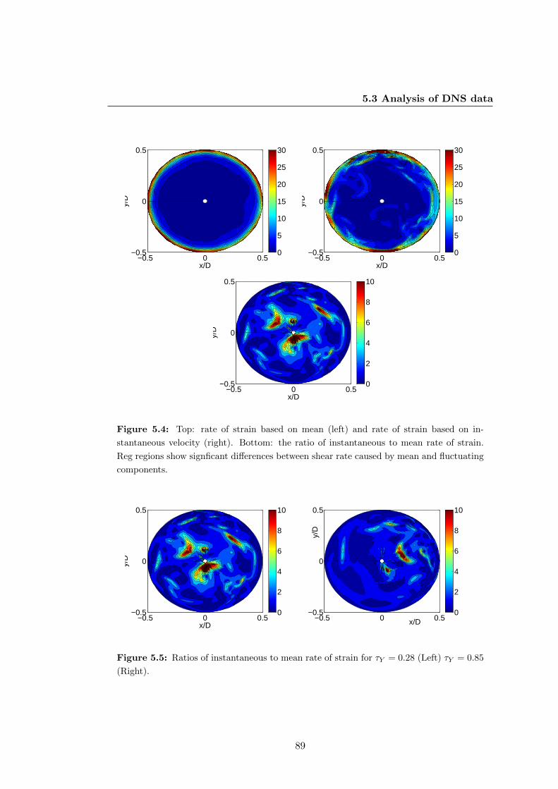
5.3 Analysis of DNS data
x/D
y/D
−0.5 0 0.5−0.5
0
0.5
0
5
10
15
20
25
30
x/D
y/D
−0.5 0 0.5−0.5
0
0.5
0
5
10
15
20
25
30
x/D
y/D
−0.5 0 0.5−0.5
0
0.5
0
2
4
6
8
10
Figure 5.4: Top: rate of strain based on mean (left) and rate of strain based on in-
stantaneous velocity (right). Bottom: the ratio of instantaneous to mean rate of strain.
Reg regions show signficant differences between shear rate caused by mean and fluctuating
components.
x/D
y/D
−0.5 0 0.5−0.5
0
0.5
0
2
4
6
8
10
x/D
y/D
−0.5 0 0.5−0.5
0
0.5
0
2
4
6
8
10
Figure 5.5: Ratios of instantaneous to mean rate of strain for τY = 0.28 (Left) τY = 0.85
(Right).
89
5. RATE OF STRAIN IN TURBULENT FLOW
x/R
y/R
−0.5 0 0.5−0.5
0
0.5
0.5
1
1.5
2
2.5
x/Ry/R
−0.5 0 0.5−0.5
0
0.5
0.2
0.4
0.6
0.8
1
1.2
Figure 5.6: The logarithm of shear-stress normalised by yield stress for τY = 0.28 (Left)
τY = 0.85 (Right).
turbulence.
To investigate the matter further we decided to gauge the effect of yield stress. A second
dataset with a yield stress four times larger has been examined and the resulting ratios
are compared on Figure 5.5. The evolution of shear regions at a higher rate is greatly
attenuated by a much faster dissipation away from the wall, which is in agreement with
Rudman et al. (2004). The frequency of occurrence of these regions is of the same
magnitude which suggests that turbulence in a non-Newtonian fluid remains a wall
phenomenon.
5.3.3 Yield stress and unyielded regions
As outlined above the higher yield stress attenuates turbulence in the core flow. More-
over, shear stress decreases towards the centre of the pipe. This means that at a certain
point it will pass the yield threshold and unyielded regions may form. In GNF the vis-
cosity is a function of shear rate tensor invariants. Since the viscosity and rate of strain
fields have been already calculated it was straightforward to calculate shear stress.
Figure 5.6 presents a typical snapshot of shear-stress in a cross-section. The shear-stress
has been normalised with yield stress so the value of one corresponds to an unyielded
region. We can observe a significant difference between the two presented cases. When
the yield stress is higher there is a large region of shear stress values close or exactly
equal to one. For lower values of yield threshold the regions tend to be smaller and are
90

5.3 Analysis of DNS data
confined only to the centre of the pipeline, appearing and disappearing in a transient
fashion.
5.3.4 Statistical hypothesis testing
Rigorous hypothesis testing requires tools of statistical inference. In particular a null
hypothesis must be identified and tested with an arbitrary significance level. This
methodology leads to four possible situations:
1. Failing to reject a true null hypothesis.
2. Rejecting a true null hypothesis – this is called Type I error or false positive.
3. Failing to reject a false null hypothesis – this is called Type II error or false
negative.
4. Rejecting a false null hypothesis.
With this distinction, statistical inference becomes a particular type of constrained
optimization problem. We want to minimize the probability of Type II error with a
specified probability of Type I error. The specification of the probability of Type I
error is the choice of significance level:
Pr(A|H0) = 1− α (5.33)
where Pr(·|·) is the conditional probability, A is the event observed, H0 is the null
hypothesis and α ∈ [0, 1] is the level of significance. We will adopt here α = 0.05.
Therefore, the test will treat as extraordinary all the values that under the null hy-
pothesis comprise the 5% of possible realisations. If such a value appears in the test the
null hypothesis is rejected. Increasing the level of significance is equivalent to reducing
the probability that the result occurred by chance.
A closely related concept is the confidence interval. The confidence interval is an
interval which contains the values of the random variable with a specified probability
given the null hypothesis is true.
Firstly, we investigate the hypothesis about the difference of means calculated from
mean rate of strain and from instantaneous rate of strain. To this end we adopt the
91

5. RATE OF STRAIN IN TURBULENT FLOW
0
5
10
15
20
25
0 0.1 0.2 0.3 0.4 0.5
Ra
te o
f str
ain
[1
/s]
r[m]
Mean RoS from mean velocityMean RoS from instantaneous velocity
Figure 5.7: The difference between the rate of strain (RoS) calculated from the mean
velocity and instantaneous velocity, averaged over all radial points.
0
0.2
0.4
0.6
0.8
1
0 0.1 0.2 0.3 0.4 0.5
Pro
ba
bili
ty
r[m]
H1Confidence level
Figure 5.8: p-values for the equal mean hypothesis.
92

5.3 Analysis of DNS data
equality of means as the null hypothesis. To establish the equality of means in two
samples a modified t-Student test is used.
t =X 1 −X 2√
1n (Var(X1) + Var(X2))
, (5.34)
where X is the sample mean, n is the population size and Var(·) is the variance.
Under the null hypothesis this statistic will have a t-distribution with the degrees of
freedom equal to 2n − 2. Subsequently a two tailed test is performed. A two tailed
tests calculates:
p = Pr(|T | > t), (5.35)
where T is the random variable following the t-distribution as described above. If p is
below the level of significance the null hypothesis is rejected.
Figure 5.7 shows the means calculated from the instantaneous rate of strain and mean
rate of strain, for the power-law fluid in Rudman et al. (2004). The estimates exhibit a
discrepancy that is especially pronounced around the centre of the pipe but decreases as
the wall is approached. It important to observe that the systematic difference remains
close to the wall, although it is decreased in magnitude. The p-value calculated from
Equation (5.35) and displayed on Figure 5.8 confirms this visual observation as the
value never surpasses the 0.05 significance level. The large population size allows us to
detect even the small discrepancy close to the wall.
The second hypothesis was the log normality of the rate of strain calculated from
instantaneous data. Therefore, the logarithm of the values should have approximately
normal distributions. This hypothesis is adopted directly as the null hypothesis. In the
literature many tests of data normality were proposed. The test used in this study was
proposed by D’Agostino et al. (1990) and it uses the fact that the sample skewness and
sample kurtosis must have values of zero and three respectively for normally distributed
populations.
More specifically, the skewness and kurtosis are defined in terms of central moments:
γ1 =E (X − EX)3(
E (X − EX)2)3/2
, (5.36)
γ2 =E (X − EX)4
(E (X − EX)2)2, (5.37)
93

5. RATE OF STRAIN IN TURBULENT FLOW
0
0.2
0.4
0.6
0.8
1
-3 -2 -1 0 1 2 3
PD
F
X
γ1 = 0
γ1 > 0
γ1 < 0
0
0.2
0.4
0.6
0.8
1
-3 -2 -1 0 1 2 3
PD
F
X
γ2 = 3
γ2 > 3
γ2 < 3
Figure 5.9: Skewness (left) and kurtosis (right) of the probability distribution.
where E denotes expected value. The geometrical representations of these concepts are
shown on Figure 5.9. If X is normally distributed then we have:
γ1 = 0, γ2 = 3. (5.38)
The sample equivalents are:
g1 =m3
m3/22
, (5.39)
g2 =m4
m22
, (5.40)
mk =1
n
n∑i=1
(Xi −X
)k(5.41)
Both, g1 and g2 are asymptotically normal. Therefore, it is possible to construct the
confidence interval for these values and compare it against the values obtained exper-
imentally. Unfortunately in practice the rate of convergence is very slow and conse-
quently requires a prohibitively large population size.
D’Agostino (1970) and Anscombe and Glynn (1983) propose transformations of these
sample quantities in such a way that the transformed quantities have an increased rate
of convergence to the normal distribution. These formulae are a good approximation
for sample sizes larger than twenty. Using these formulae the test for skewness can be
94

5.3 Analysis of DNS data
expressed as follows:
Y =√g1
((n+ 1) (n+ 3)
6 (n− 2)
) 12
, (5.42)
γ2(√g1) =
3(n2 + 27n− 70)(n+ 1)(n+ 3)
(n− 2)(n+ 5)(n+ 7)(n+ 9), (5.43)
W2 = −1 + (2 (γ2(√g1)− 1))
12 , (5.44)
X =
(2
W2 − 1
) 12
, (5.45)
Z(g1) = δ ln
(Y
X+
((Y
X
)2
+ 1
)), (5.46)
where Z(g1) has a normal distribution. The test for kurtosis is expressed by:
E(g2) =3 (n− 1)
n+ 1, (5.47)
Var(g2) =24n (n− 2) (n− 3)
(n+ 1)2 (n+ 3) (n+ 5), (5.48)
√γ1(g2) =
6(n2 − 5n+ 2)
(n+ 7)(n+ 9)
√6(n+ 3)(n+ 5)
n(n− 2)(n− 3), (5.49)
A = 6 +8√γ1(g2)
(2√γ1(g2)
+
√(1 +
4
γ1(g2)
)), (5.50)
Z(g2) =
√9A
2
(1− 2
9A
)−
1− 2/A
1 + g2−E(g2)√Var(g2)
√2/ (A− 4)
1/3 . (5.51)
Finally, we construct an omnibus test i.e. a test which simultaneously verifies skewness
and kurtosis:
K2 = Z2 (g1) + Z2 (g2) . (5.52)
Since both components have a normal distribution the sum have has a χ-squared dis-
tribution with two degrees of freedom. This allows us to construct a simple one sided
test that gives the probability of being simultaneously away from normal distribution
skewness and kurtosis.
Figure 5.10 shows the p-values for the log normality hypothesis. It can be seen that
the data fails this test for most of the radial points. This leads to rejection of the null
95

5. RATE OF STRAIN IN TURBULENT FLOW
0
0.2
0.4
0.6
0.8
1
0 0.1 0.2 0.3 0.4 0.5
Pro
ba
bili
ty
r[m]
H2H2’
Confidence level
Figure 5.10: The p–values associated with hypothesis of log-normality of instantaneous
rate of strain (H2) and normality of mean rate of strain (H2’).
0
0.2
0.4
0.6
0.8
1
0 0.1 0.2 0.3 0.4 0.5
Pro
ba
bili
ty
r[m]
H1’Confidence level
Figure 5.11: The p–values associated with hypothesis of log-normality of the fluctuating
rate of strain H2’.
96

5.3 Analysis of DNS data
-4
-3
-2
-1
0
1
2
3
4
-4 -3 -2 -1 0 1 2 3 4
Qu
an
tile
s
Standard normal distribution quantiles
ExperimentalTheoretical
Figure 5.12: The QQ plot for the one of the fitted histograms.
hypothesis. Moreover the normality of mean strain rate has been also assessed and is
denoted on the diagram as H2’. The normal distribution of the mean estimate fails in
an even larger regions and therefore must be deemed as coincidental. The log-normality
does not fail in some region, but this result is not repeated with the Herschel–Bulkley
data where log-normality assumption failed for every radial point.
If the hypothesis H1 was modified to pertain only to the fluctuating part of the rate of
strain then the similar analysis would lead to Figure 5.11. The fluctuating part of the
rate of strain does not fail the log-normality hypothesis in a large region away from the
wall and this region was reproduced for both Herschel–Bulkley fluids. This shows that
there may be a region where the log-normality of the fluctuating strain is an accurate
description of the flow.
For the radial points that did not fail the test histograms, QQ plots were constructed.
QQ plots are visual tests of normality which plot the quantiles of the standard normal
distribution against the sample quantiles. QQ plots are a more general tool since
they allow us to compare any two distributions and the equivalence of quantiles is the
equivalence of distributions. If the distributions are the same, the values should align
on the line.
97
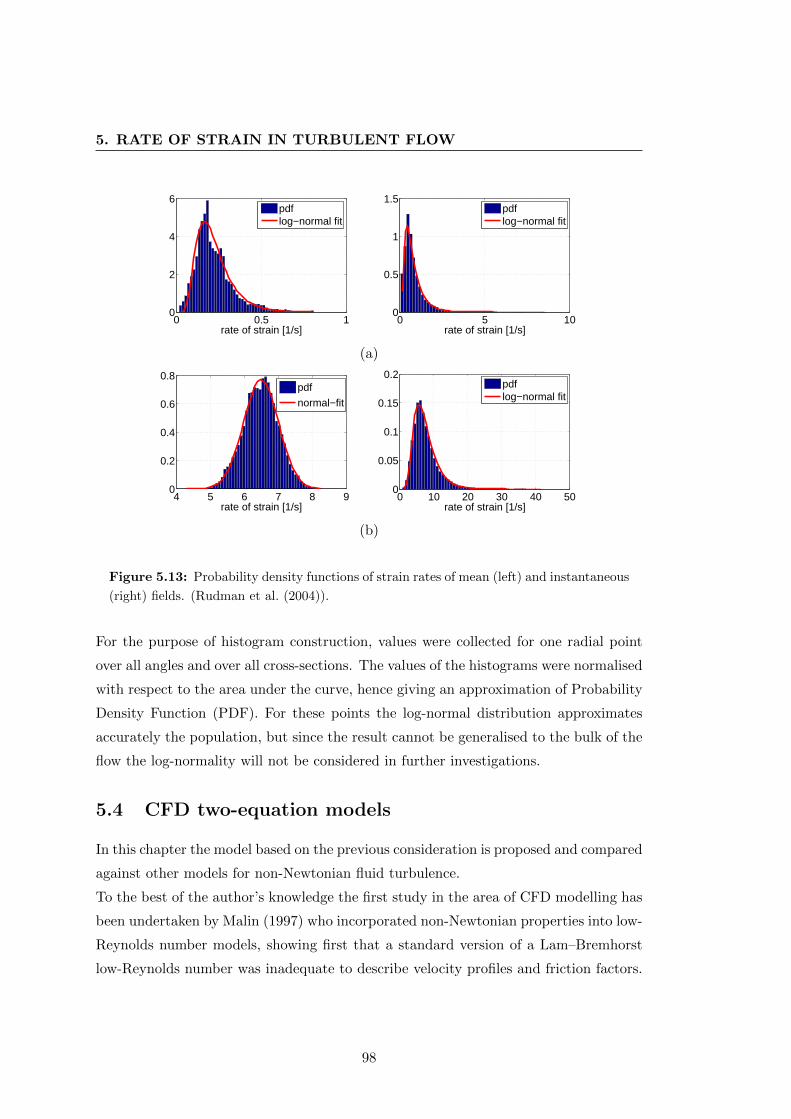
5. RATE OF STRAIN IN TURBULENT FLOW
0 0.5 10
2
4
6
rate of strain [1/s]
pdflog−normal fit
0 5 100
0.5
1
1.5
rate of strain [1/s]
pdflog−normal fit
(a)
4 5 6 7 8 90
0.2
0.4
0.6
0.8
rate of strain [1/s]
normal−fit
0 10 20 30 40 500
0.05
0.1
0.15
0.2
rate of strain [1/s]
pdflog−normal fit
(b)
Figure 5.13: Probability density functions of strain rates of mean (left) and instantaneous
(right) fields. (Rudman et al. (2004)).
For the purpose of histogram construction, values were collected for one radial point
over all angles and over all cross-sections. The values of the histograms were normalised
with respect to the area under the curve, hence giving an approximation of Probability
Density Function (PDF). For these points the log-normal distribution approximates
accurately the population, but since the result cannot be generalised to the bulk of the
flow the log-normality will not be considered in further investigations.
5.4 CFD two-equation models
In this chapter the model based on the previous consideration is proposed and compared
against other models for non-Newtonian fluid turbulence.
To the best of the author’s knowledge the first study in the area of CFD modelling has
been undertaken by Malin (1997) who incorporated non-Newtonian properties into low-
Reynolds number models, showing first that a standard version of a Lam–Bremhorst
low-Reynolds number was inadequate to describe velocity profiles and friction factors.
98

5.4 CFD two-equation models
He introduced a simple modification of the damping function
fµ = [1− exp(−0.0165Rew)/n1/4]2/(1 + 20.5/Ret). (5.53)
where n corresponds to power-law index in the consitutive law of Ostwald–de Waele
fluid. Compare this form with Equation (4.39).
The model has been shown to improve friction factor and velocity profiles predictions
although in the latter case the accuracy of the velocity profile result cannot be estab-
lished easily because the results are plotted in physical coordinates and therefore the
thin boundary layer is not visible clearly. As expected the model was able to reproduce
laminar power-law velocity profiles for sufficiently low Reynolds numbers. The model
was also tested against Herschel–Bulkley fluids. The runs reported in Malin (1998)
prove to be sufficiently accurate in a number of flow cases. This model is unable to
predict any of the elastic, unsteady effects and therefore it will not exhibit turbulent
drag reduction.
Pinho (2003) develops a k − ε model by introducing a decomposition of viscosity into
mean and fluctuating component in the same manner as turbulence theory decomposes
velocities:
ν = ν + ν ′. (5.54)
With this assumption the derivation of kinetic energy equation is conducted. Then,
based on a constitutive equation that is a modification of a GNF fluid to incorpo-
rate elastic effects an estimate for mean viscosity is given. Subsequently, an order of
magnitude analysis eliminates most of the equation terms and the eventual transport
equation for k and ε, based on low Reynolds number from Nagano and Hishida (1987)
simplified to a channel flow, is given by:
0 =∂
∂x2
[νTσk
∂k
∂x2+ ν
∂k
∂x2
]− u1u2
∂u
∂x2− ε (5.55)
0 =∂
∂x2
[(ν +
νTσε
)∂ε
∂x2
]+ f1Cε1
ε
kCνk2
ε
(∂u
∂x2
)2
+ Cε3ε
ν
∂ν
∂t+
+ Cε4νTσεν
∂ε
∂x2
∂ν
∂x2(5.56)
Moreover the classical turbulent viscosity damping function fµ is decomposed into
viscometric damping and elongation viscosity damping:
fµ = fµvfµe (5.57)
99

5. RATE OF STRAIN IN TURBULENT FLOW
The damping functions are derived in a similar way to Van Driest function and are
given by:
fµv = 1−[1 +
∣∣∣∣1− n1 + ny+
∣∣∣∣]|(1+n)/(1−n)|(1/A+)
(5.58)
fµe = 1−[1 +
∣∣∣∣p− 1
3− py+
∣∣∣∣C(1−p)/(2−p)]−|(3−p)/(p−1)|(1/A+)
(5.59)
(5.60)
where p is a power index that accounts for elongation viscosity properties in the GNF
constitutive equation
Friction factors and velocity profiles correlate favourably with experimental and previ-
ous computational data. However kinetic energy and dissipation are not quantitatively
correct. Only the qualitative shift of turbulence production peak value was observed.
The model has been recommended for low values of turbulence intensities.
A Finitely Extensive Nonlinear Elastic with Peterlin’s approximation (FENE-P) is a
molecular model that results in a constitutive equation of the Metzner–White type. So
far it has been mostly used in DNS simulations but recently an attempt by Pinho et al.
(2008) has proved to be successful for a low turbulent Reynold numbers. The model
is based on and validated against recent DNS data. A similar derivation of damping
function and model equations has been conducted but its presentation will be omitted
since this study does not deal with drag reducing fluids.
5.4.1 Results
The main aim of the computational studies undertaken here was to predict the flow
rate given the pressure gradient. For the experimental and DNS data presented here
the latter is not readily available and has to be estimated from the wall shear-stress
that is either reported Escudier et al. (2005) or can be extracted from the data Pinho
(2003); Rudman et al. (2004).
Since the rate of strain at the wall and the rheological properties were given, it was
possible to calculate the pressure gradient (see Pope (2000)):
∂p
∂x= − 2
Rτw. (5.61)
Two types of meshes were generated in GAMBIT. Both of them were 2D with axisym-
metric boundary conditions imposed. The first mesh had dimensions corresponding to
100

5.4 CFD two-equation models
10−2
10−1
100
101
102
103
10−3
10−2
10−1
100
log γ
µ
0 0.2 0.4 0.6 0.8 10
0.5
1
1.5
2
r/R
u/u b
Escudier et al.(2005)FLUENT Laminar
Figure 5.14: Left: Cross model with parameters fitted for 0.09% solution of CMC in
water. Right: Laminar, steady calculation.
a 14m long pipe of with 105mm ID (compare Escudier et al. (2005)), whilst the other
was a shorter section with a length equal to 4π diameters (compare Rudman et al.
(2004)). In case of the former inlet/outlet boundary conditions were imposed. In case
of the latter periodic boundary conditions were used.
In the vicinity of the wall a laminar sublayer will develop regardless of the constitutive
law of the fluid. This stems from the fact that the inertial terms in the Navier-Stokes
equation become negligible there. If we are to take full account of non-Newtonian
rheology we have to solve the equation close to the wall up to the laminar sublayer.
The wall Reynolds number was known a priori and hence it was possible to specify the
mesh size and refinement. The number of radial points varied from 64 to 128. All of
the meshes were refined towards the wall with a growth ratio varying between 1.05 and
1.15. Since for experimental data the pressure gradient and therefore the wall shear-
stress was known, it was possible to calculate wall viscosity and subsequently the wall
coordinates. Wall coordinates allow us to establish the resolution required to capture
the laminar sublayer.
In FLUENT we can choose between six k-ε low-Reynolds turbulence models. When a
Lam–Bremohorst (LB) model is chosen a non-Newtonian turbulence modification ap-
pears in the Text User Interface. For the k-ω model, low-Reynolds number corrections
can be also switched on.
Initially, the Lam–Bremhorst model with non-Newtonian modification was chosen. The
fluid used for validation was a 0.09% aqueous solution of CMC from Escudier et al.
101

5. RATE OF STRAIN IN TURBULENT FLOW
0 0.2 0.4 0.6 0.8 10
0.2
0.4
0.6
0.8
1
1.2
1.4
r/R
u/u b
Escudier et al.(2005)FLUENT LB
0 2 4 6 8 10 120
0.2
0.4
0.6
0.8
1
x[m]
k[m
2 /s2 ]
Figure 5.15: Left: Turbulent velocity profile in physical coordinates. Right: Turbulence
intensity. The error of the turbulent intensity prediction was less than 5%.
(2005). This fluid was well described by the Cross model which is described in Sec-
tion 4.2.2.
The results presented in Figure 5.15 show good agreement with the experimental data.
The velocity profile in wall and physical coordinates as well as the ultimate estimate of
the flow rate were within 5% of experimental data. Observe also that the specification
of turbulent quantities did not much affect the flow field downstream. After two metres
the turbulence intensity seems to stabilise around a value that is within 5% of the values
reported in the experiment.
This positive agreement was also repeated for all of the shear-thinning fluids from
Escudier et al. (2005). It is important to note that these fluids were well described by
Carreau–Yasuda or Cross rheologies. These constitutive laws remove the singularity
occurring in a classical power-law through limiting viscosities. The variation of viscosity
occurs only close to the wall whilst in the rest of the pipe the low-shear limit is reached.
The simulation of a yield-stress fluid was more complicated due to the fact that the low-
shear viscosities were not given in the Escudier experiment and therefore they became
subject to arbitrary choice. Following Rudman and Blackburn (2006) the choice of cut-
off parameters was such that the cut-off values were used only when the local strain
rate was 104 times lower than the average. The straightforward application of the
low Reynolds-number model on the full pipe mesh was completely unsuccessful. The
turbulence intensity was vanishing downstream from the inlet and the resulting velocity
profiles became laminar. The pressure drops were consequently underestimated. These
102

5.4 CFD two-equation models
0 0.1 0.2 0.3 0.4 0.50
0.01
0.02
0.03
0.04
0.05
r/D
ν
FLUENTFLUENT+mod.DNS (Rudman et al.)
Figure 5.16: Viscosity profiles in FLUENT for Rudman et al. (2004) cases.
negative results gave rise to the theoretical studies presented at the beginning of this
chapter.
5.4.1.1 Models with Turbulent Rate of Strain
We assume then that the rate of strain has the form:
γ =√
2SijSij + γt (5.62)
where the γt represents the effect of turbulence on the rate of strain. The form of this
term is established based on dimensional analysis and the preceding considerations.
Depending on the choice of the two-equation model, there are two pairs of quantities
describing turbulence in the flow: k and ε or k and ω. Using these scales it it possible
to construct a quantity with dimensions equal to the dimension of sij .
γt = fε(k, ε) = hε (Ret)ε2
k2, (5.63)
γt = fω(k, ω) = hω (Ret)ω2, (5.64)
where an additional damping function was added. In the above expressions Ret is the
turbulent Reynolds number i.e. the Reynolds number based on turbulence quantities.
This is to counteract the asymptotic behaviour of the wall of turbulence quantities. As
outlined in Section 4.1.3 k tends to x22 as we approach the wall whilst ε is of the order
of 1. Therefore, if no damping is used than the above expressions will tend to infinity
at the wall. This is why a damping function of the following form is used:
hε (Ret) = hω (Ret) = 1− exp (Ret) . (5.65)
103

5. RATE OF STRAIN IN TURBULENT FLOW
The turbulence Reynolds number is expressed in the k-ε model for a power-law fluid
as:
Ret =k2
εν, (5.66)
where the viscosity is taken from the previous iteration of the algorithm.
Simulations have been run for all available cases. Periodic boundary conditions have
been adopted to simulate fully developed flow. When necessary a pressure drop has been
calculated from the profile and given data. An initial guess was that of a Newtonian
fluid with viscosity equal to the wall viscosity reported in corresponding publications.
The results of these calculations are presented in Table 5.1. The simulations utilising
DNS viscosity profiles show clearly the benefit of an accurate estimation of this quantity,
both results were significantly improved with respect to the unmodified model. For the
Pinho (2003) data most of the results were giving similar and accurate results and
for the experimental Herschel–Bulkley data from Escudier et al. (2005) the results
from the original model were much better. Two conclusions can be drawn from this
result. Firstly, estimating the average velocity in the bulk of the fluid matters but only
when the values of viscosity reach the low-shear cut-off and only if the cut-off value
is comparable to the turbulent viscosity achieved at the centre. An accurate model
of turbulent strain in the bulk of the fluid will not on its own improve the result. To
suppose otherwise would be equivalent to believing that the viscous effects manifest
themselves far from the boundary layer and although such a supposition would not be
entirely unjustified for non-Newtonian fluids, the conclusion would further contradict
the significance of convective terms that should dominate outside the boundary layer.
A further investigation of viscosity profiles calculated from the proposed models shows
that k-ω gave the closest approximation (see Figure 5.17). The viscosity profiles show
good agreement with those obtained with DNS. These were the results for which the
highest in pressure gradient prediction accuracy was obtained.
5.5 Concluding remarks
The analysis presented in this chapter establishes that the mean rate of strain can be as
much as seven times higher than the mean velocity strain in some regions of the flow.
For the instantaneous rate of strain this value can be even larger. Both, power-law and
104

5.5 Concluding remarks
Table 5.1: Flow-rate predictions showing improvements in accuracy for selected cases.
SourceUnmodified Model
Predicted
flow-rate
[m/s]
Error
Predicted
flow-rate
[m/s]
Error
Pinho (2003)
3.16 0.06 3.18 0.06
1.48 0.06 1.49 0.04
1.3 0.03 1.31 0.02
Rudman et al. (2004)0.7 0.3 0.88 0.12
0.84 0.16 0.97 0.02
Escudier et al. (2005) 2.18 0.07 2.39 0.17
0 0.1 0.2 0.3 0.40
0.5
1
1.5x 10
−3
r/D
µ
model
Rudman et al.
0 0.1 0.2 0.3 0.40
0.01
0.02
0.03
r/D
µ
model
Rudman et al.
Figure 5.17: Viscosity profiles for ReW = 7000 τY = 0.24 (left) τY = 0.85 (right). The
viscosity of the flow is closely reproduced.
105

5. RATE OF STRAIN IN TURBULENT FLOW
Herschel–Bulkley fluid exhibit this different, but in case of the latter the difference is
more vital as it controls the yielded and unyielded regions that can appear throughout
cross-section.
The investigations of the probabilistic information of the rate of strain conclude that
the log-normality cannot be regarded as an accurate description. For the fluctuating
rate of strain, however, there seems to be a fairly good match in some regions and
this effect appears in both: power-law and Herschel–Bukley fluids. This finding is
potentially useful for developing an effective molecular viscosity model.
The applicability of these findings in CFD calculations depends on the regularisation
of the constitutive law. If the regularisation limits the maximum value of viscosity to
be an order of magnitude smaller than the effective eddy viscosity than the proposed
corrections will not take place. Otherwise, for the cases were regularisation does not
play a leading role, this study shows that the predictions can be improved by as much
as 18%.
106

Chapter 6
Modelling stratified flow
Stratified flow is one of the most common patterns in multiphase flows. The pattern
forms when gravity dominates and leads to segregation. This occurs, when one fluid
has a much larger density than the other.
Initial research in this area was focused on empirical correlations that allow the predic-
tion of bulk quantities such as gas hold-up or pressure drops in long pipelines with or
without inclination. This chapter surveys some of these correlations, concluding that
none of them is universal, which shows that there is still some unknown dependency
that affects the models.
This chapter also presents derivations of two velocity profiles. Similarly, to single phase
flow, the laminar profile can be derived analytically without any additional closures.
The interfacial shear-stress appears as an integration constant and it can be expressed
in terms of known parameters. The resulting relationship between mass-flow-rate and
pressure is not given explicitly. The turbulent profile has been proposed by Biberg
(2007) and here even the interfacial-shear stress is not given explicitly. The mass-flow-
rate to pressure relation can be extracted after solving the model equations in terms of
the liquid height and shear-stress ratios.
With the correlations and analytical velocity profiles we can study the accuracy of CFD
results. We employ the periodic boundary conditions described earlier and compare
the results with unsteady simulations. It is argued that CFD-turbulence models are
inadequate if they do not contain models of interfacial turbulence. DNS data supply
additional evidence that the phase coupling, as well as turbulent effects, have a major
107

6. MODELLING STRATIFIED FLOW
impact on bulk quantities and are required for scientific understanding and robust
engineering predictions.
6.1 Empirical pressure drop correlations
The empirical correlations surveyed here were developed to solve a common engineering
problem: estimate the gas phase volumetric fraction and the pressure drop in the pipe,
if the superficial velocities of gas and liquid phases are known. The superficial velocity
of phase P is the volumetric flow rate of phase P divided by cross-sectional area i.e.
UsP =1
|A|
∫AαPU · dS, (6.1)
where αP is the phase fraction and A is the cross-sectional area. This quantity takes
into account the phase distribution and therefore it does not reflect the actual average
velocity with which the phase is moving. The superficial velocity of phase P is the
average velocity as if P were the only phase present in the cross-section. Superficial
velocity can be directly computed from mass flow rate, which is often known a priori.
The actual average velocity of the phase can be calculated only if the phase distribution
is known. Then it can be calculated as the velocity averaged over a cross-sectional phase
fraction.
Two situations are surveyed here:
1. Co-current, stratified flow: gas/Newtonian liquid.
2. Co-current, Stratified flow: gas/non-Newtonian liquid.
6.1.1 Stratified gas/Newtonian liquid
The first attempts to understand and predict friction factors in two-phase flows were
undertaken by Lockhart and Martinelli (1949) and Martinelli and Nelson (1949). Both
approaches begin with a friction factor correlation and assume that that the pressure
drops computed from the parameters of both phases are equal.
dp
dx=
2ρfPU2P
µP(6.2)
where P denotes the phase. The second assumption is the steady state for phase
fraction: the flow under consideration comprises two co-current streams and the volume
108

6.1 Empirical pressure drop correlations
fraction remains constant throughout the pipe. The relaxation of the second assumption
was addressed by Martinelli and Nelson (1949). By defining hydraulic diameters as dG
and dL certain area ratios were defined:
κP =4APπd2
P
(6.3)
where AP = αPA. To predict friction factors the empirical formulae were utilised
fP = CP (ReP )−mP (6.4)
The parameter mP adopts a value 1/4 or 1 if the phase P is respectively in the turbulent
or laminar regime. The pressure is non-dimensionalised with the pressure drop that
would occur if only one phase was transported through a pipe.
φ2P =
(dpdx
)TP(
dpdx
)P
(6.5)
Simple algebraic transformations lead to
αG = 1− κ(3−mL)/(mL−5)L φ
4/(mL−5)L = κ
(3−mG)/(mG−5)G φ
4/(mG−5)G (6.6)
which can be solved giving the pressure drops results. Usually for the sake of data
presentation a Martinelli parameter is introduced.
X2 =φ2g
φ2l
=
(dpdx
)g(
dpdx
)l
(6.7)
Comparison with experiments shows that the derived equations overestimate the real
value of pressure drops. This over-prediction is due to the assumption of constant
wall shear stress which is definitely an overly pessimistic approximation. Normally the
phases will interact with each other and the stress on the smooth interface will be lower
than the wall stress thus leading to friction reduction. Conversely a rough interface
will lead to increased friction.
A modification worth mentioning taking the above issues into account is the one per-
formed by Chisholm (1967), who applied some geometrical considerations to evaluate
the effective wall shear stress. For a stratified flow he obtained:
α1−0.5mLL
(A
A−AL
)1−0.5mG
=X2
Z
(d′G)0.5(1+mG)
(d′L)0.5(1+mL)
(6.8)
φ2L =
1
d′G
(1 +
AGAL
)1−mL ( AGALZ2
+ 1
)(6.9)
109

6. MODELLING STRATIFIED FLOW
where d′P are phase hydraulic diameters non-dimensionalised with the hydraulic radius
of a single phase flow and Z is another non-dimensional quantity defined by:
Z =
(1 + τ
′AG/AL
1− τ ′
)(6.10)
where τ′
is a non-dimensional stress.
Comparisons with more recent procedures presented by Brennen (2005) reveals that
the above approaches can provide a robust engineering approximation.
6.1.1.1 Taitel and Dukler
The approach proposed by Taitel and Dukler (1976) begins with assuming stratified
flow in a pipeline and then writing the momentum balance equations for both phases:
−Aldp
dx− Slτwl + τiSi = 0 (6.11)
−Agdp
dx− Sgτwg − τiSi = 0, (6.12)
where AP is the phase cross-sectional area, SP is the phase wetted perimeter, Si is the
interface cross-sectional length, τwP is the wall shear-stress and τi is the shear-stress at
the interface.
Now assuming that the pressure drop is constant and the same for both phases this
can be simplified to one equation.
τwgSgAg− τwl
SlAl
+ τiSi
(1
AL+
1
AG
)= 0 (6.13)
Subsequently friction factors are used to estimate wall shear stresses. Eventaully an
implict procedure is developed that chooses the gas phase fraction so as to minimise
the residuum of Equation (6.13).
Further details of the derivation and the MATLAB scripts developed to calculate the
gas phase fraction and corresponding pressure drop can be found in Appendix B.
6.1.2 Stratified gas/non-Newtonian liquid
There is extensive literature on two-phase, non-Newtonian fluid friction factors. This
interest can be explained by the fact that non-Newtonian fluids are typically fluids of
high viscosities and their transport can pose serious engineering difficulties. Moreover,
110

6.1 Empirical pressure drop correlations
certain mixtures of phases can exhibit non-Newtonian properties of their bulk quanti-
tites e.g. bulk viscosity of slurries has yield stress and power-law behaviour. Treating
one of the phases as non-Newtonian in stratified flow, allows us to study flows that can
comprise more than two phases.
It is not entirely true that only high viscosity fluids can have non-Newtonian proper-
ties. Even water has its own non-trivial rheology which Newtonian behaviour merely
approximates. However, in a highly viscous fluids these changes are easier to observe
and are more significant from an engineering design standpoint.
6.1.2.1 Heywood
The analysis of non-Newtonian liquid–gas flows in horizontal pipes has been first con-
ducted by Heywood and Charles (1979) as an extension of Newtonian liquid–gas case.
The analysis was limited and did not encompass liquid turbulent flow. The liquid as-
sumed to behave as in an open channel and gas as in a closed duct giving well-defined
concepts of hydraulic diameters and friction factors.
The algebra eventually leads to:
φ2L =
unLD1+n
, (6.14)
where D is the hydraulic diameter non-dimensionalised with respect to pipe diameter
and u is a velocity non-dimensionalised by a single phase liquid velocity under the same
condition.
One of the main advantages of the formula shown is that it predicts drag reduction
due to decreased wetted perimeter which is not the case with Martinelli correlations.
Validation of the results was performed by comparison with computational results.
6.1.3 Farrooqi and Richardson
Farooqi and Richardson (1982) considered three-phase gas/liquid flows where, the liquid
was additionally a mixture of a Newtonian and non-Newtonian fluid. The Lockhart–
Martinelli predictions were, as usual, overestimating the results but were still within
+/- 30%.
Their studies included the drag reduction phenomenon in shear thinning suspensions
which has been reported to occur when air was injected into a laminar flow of liquid
111

6. MODELLING STRATIFIED FLOW
suspension. The maximum drag reduction has been correlated with a ratio of the
apparent viscosity to the apparent viscosity at ReMR = 2000. An empirical correlation
of this maximum drag reduction has been obtained and is the following
minφ2L =
λ0.205 if 0.6 < λ < 11− 0.0315λ if 0.35 < λ < 0.61.9λ if 0.05 < λ < 0.35
, (6.15)
where λ = (u1/utr)1−n which according to power-law model is the same as mentioned
above viscosity ratio.
The accuracy of the Heywood and Charles (1979) prediction has been also validated
for power-law indices in the interval from 0.14 to 0.326 but inaccurate for greater n
where it was over-predicting the actual values.
6.1.4 Dziubinski
Dziubinski (1995) attempted to develop a general correlation for intermittent two-phase
flows in a pipe where one phase had non-Newtonian properties. His analysis was based
on a loss coefficient which is of the form:
Λ =τwρD
2
µ2=
τwρu1
2Re2 =
f
8Re2, (6.16)
for Newtonian fluids and:
Λ = K(4n
3n+ 1)Re2
MR, (6.17)
for non-Newtonian fluids. By performing analogous steps as in the Newtonian case and
by substituting friction factor correlations for laminar (Equation (4.78)) and turbulent
flow:
f = 0.3164Re−1/4MR , (6.18)
Dziubinski reports the resulting formulae for loss coefficient which have a form:
Λ = 8αLCLReTP (laminar) (6.19)
CL =1 + 1.036 10−4Re1.235
TP
1 + 1.036 10−4Re1.235L
(6.20)
Λ = 0.0131αL
(3n+ 1
4n
)−5
exp 1.7453n+ 1
4n− 0.634αLRe
7/4TP (turbulent) (6.21)
112

6.2 Analytical velocity profiles
Liquid
Gas
interface
x2
x1H
h
U1
Figure 6.1: Sketch of the physical problem.
agree quite well with extensive experimental data giving an error of +/ − 15% and
+/− 30%
Xu, Wu, Shi, Lao and Li (2007) extended the analysis of Heywood and Charles (1979)
to inclined pipes. Two flow patterns were considered: stratified flow, which is more
common in downward inclined pipe and slug flow which appears more often in upward
sloped pipes. In the first case liquid, due to its high viscosity has been assumed to be
laminar while in the second case both possibilities were considered. The analysis begins
with a force balance equation accounting for buoyancy effects and interfacial stresses.
Typical correlations relating Reynolds number and friction factors were substituted
into the equations. Formulae for pressure drops for stratified and slug flow in inclined
pipes were obtained. Comparison with experimental data has shown that proposed
equations deviated 20% and 30% in case of stratified and slug flow respectively.
6.2 Analytical velocity profiles
In this section we present the derivations of velocity profiles for channel flow. These
profiles are further considered in the solution of the pressure drop and holdup predic-
tions.
It is often assumed that the origin of the coordinate system is at the interface. In some
cases it can significantly simplify the analysis.
113

6. MODELLING STRATIFIED FLOW
6.2.1 Laminar profiles
Laminar profiles have been derived by Bird et al. (1960), Biberg and Halvorsen (2000)
and Sim (2006). Bird et al. derives the profiles for rectangular channel flow but
under the assumption that the liquid pool height is known. This eliminates one of the
unknowns. Subsequently they obtain explicit expressions for the physical velocities of
both phases. Biberg and Halvorsen focuses on pipeline flow. Sim derives the profiles for
channel flow with stationary and oscillating walls. However, he deals with the inverse
problem i.e. he assumes the pressure drop and the liquid height to be known and
obtains the formulas for average velocities which are than compared with results from
numerical simulations.
In this section we deal with channel flow and we assume that only phase mass fluxes
or superficial velocities are given. The problem under consideration is depicted in
Figure 6.1. It involves two incompressible, Newtonian fluids, further denoted as g and
l, flowing between two flat plates set H apart. At a distance h from the lower plate there
is a phase interface over which fluid density and viscosity change but with velocity and
shear-stresses assumed to be continuous. Gravity acts in −x2 direction. The problem
is essentially two-dimensional.
We adopt the assumption that the flow is fully developed which means that the velocity
and the phase fraction profiles do not change with the axial coordinate x. Material
properties of both phases are assumed to be constant. The equations of motion for
case simplify to:
∂p
∂x=
∂
∂y
(µ∂U
∂y
)(6.22)
∂p
∂y= ρg. (6.23)
The assumption of fully developed flow also means that the RHS of Equation (6.22)
and RHS of Equation (6.23) depend only on the coordinate y. Integrating the latter
between 0 and y gives:
p(x, y) = ρgy + p(x, 0), (6.24)
which leads to a conclusion that ∂p∂x is a function of x only. Since the LHS of Equa-
tion (6.22) is a function of x and the RHS is a function of y, we conclude that both
114

6.2 Analytical velocity profiles
sides of this equation must be constant. Therefore, the streamwise pressure gradient
does not change with the axial coordinate:
∂p
∂x= const. (6.25)
To solve this equation with respect to the pressure gradient and interface height h we
assume that the velocity profiles are continuous over the interface:
limy→h+
U(y) = limy→h−
U(y) = ui (6.26)
and that viscosity can be expressed as
µ =
µg y > hµl y < h
. (6.27)
Solving this with the assumption that the interface is at level h and that the velocity
profile is continuous gives a concatenation of two “mirror” Couette flows:
U =
∂p∂x
12µg
(y2 − (H + h)y +Hh
)+ ui
H−h(H − y) y > h∂p∂x
12µl
(y2 − hy
)+ y
hui y < h, (6.28)
where ui is the velocity at the interface. We further assume that the stress at the
interface is also continuous so that we can put an equality between the left and right
side limits:
limy→h+
τ = limy→h−
τ (6.29)
and therefore
limy→h+
µg∂U
∂y= lim
y→h−µl∂U
∂y, (6.30)
which after substituting Equation (6.28) gives the interface velocity in terms of height
and pressure gradient:
ui = −∂p∂x
H
2µl
11h +
µgµl
1H−h
= −∂p∂x
H
2
h(H − h)
µgh+ µl(H − h)(6.31)
We have now expressed the velocity profile in terms of pressure gradient and height.
These are the unknowns which can be calculated only if additional conditions are
imposed on the system. One way is to specify phase mass fluxes:
1
H
H∫h
U(y) dy = Usg1
H
h∫0
U(y) dy = Usl. (6.32)
115

6. MODELLING STRATIFIED FLOW
Liquid
Gas
U
τwg
τwl
τi
τ µT/µ
Figure 6.2: Turbulent profiles in steady state fully developed channel flow: shear stress
(left), eddy viscosity (centre), mean velocity (right).
Substituting the velocity profile and subsequent integration gives a system of two non-
linear equations(∂p∂x
12µg
(y3/3− (H + h)y2/2 +Hhy
)+ ui
H−h(Hy − y2/2)) ∣∣∣∣H
h
= Usg
∂p∂x
12µl
(−1/6h3
)+ h
2ui = Usl
, (6.33)
where the first equation has only been written symbolically for the sake of brevity. This
system of equations can be ultimately solved numerically. The roots of these rational
expressions will give ∂p∂x and h, satisfying the constraints in Equation (6.32).
To solve this problem numerically a set of MATLAB scripts were written. The script use
Newton’s method for finding roots of a differentiable function and are further described
in Appendix B.
6.2.2 Turbulent profiles
To investigate turbulent flow profiles we adopt the averaged Navier–Stokes equations.
The derivation begins with a decomposition of instantaneous velocities into their mean
and fluctuating components and applying the averaging operation to the system of
equations. This leads to equations for mean velocity profiles containing the Reynolds
stress term which has to be expressed in terms of known parameters. It is now conve-
nient to assume that the origin of the coordinate system is at the interface.
116

6.2 Analytical velocity profiles
Integration of Equation (6.22) will give a linear profile of shear-stress.
τxy =∂p
∂xy + τi. (6.34)
This is depicted on Figure 6.2. Let hP denotes the position of the wall wetted by phases
P . Then we can express the wall shear stress by:
τwP =∂p
∂xhP + τi. (6.35)
Combining the two above expressions gives:
τxy = τi − (τwP − τi)y
hP. (6.36)
The shear stress can now be expressed as a sum of Reynolds stress and the stress coming
from molecular viscosity:
τxy = µ∂U
∂y− ρuv. (6.37)
The Reynolds stress terms is expressed by:
−ρuv = µt∂U
∂y. (6.38)
Biberg (2007) proposes an algebraic model of turbulence that reproduces log-layers
at both wall regions. Both phases in the flow are analysed separetely and the the
coupling between phases is ensured through continuity conditions at the interface and
specification of turbulence levels. We will now focus on the model applicable within
one phase and because of this the indices denoting the phase are temporarily dropped.
The non-dimensional profile is expressed using two new parameters.
R =τiτw
Y =y
h. (6.39)
Additionally, there is a parameter measuring the level of turbulence at the interface.
For know we define the parameter as the rescaled interfacial eddy viscosity from Biberg
(2011)
K =µt∣∣Y=0
ρκhu∗i, (6.40)
where κ is the von Karman constant. Eddy viscosity at the interface, and therefore K,
is not known a priori. Therefore, the closure of K is the key element of the model and
will be discussed separately.
117

6. MODELLING STRATIFIED FLOW
First let us consider the mixing length model. Prandtl originally expressed the eddy
viscosity in the following way:
µt = ρlvt, (6.41)
where l is the mixing length and vt, considering the momentum transfer between flow
strata (see Schlichting (1955)), is further approximated by:
vt = l∂U
∂y. (6.42)
Substituting back into Equation (6.38) and then back into equation Equation (6.37)
and then neglecting the viscous term we arrive at:
vt =
√τxyρ
(6.43)
From this point onwards the derivation assumes that the profile at the wall follows the
logarithmic distribution with respect to wall proximity:
U =u∗
κln (1− Y ) + C1, (6.44)
where u∗ =√
τwρ and the constant C1 is:
C1 = sgn (τw)u∗
κ
(ln
(u∗h
ν
)+ κB
). (6.45)
If we substitute Equation (6.44) into Equation (6.41) and use the auxillary expression
in Equation (6.43) we arrive with
l = κh(1− Y )
√∣∣∣∣τxyτw∣∣∣∣ (6.46)
as Y approaches the wall. The conclusion from above derivation is that the mixing
length must be of the form in Equation (6.46) in the vinicity of the wall to reproduce a
logarithmic velocity profile. Using this intuition from mixing length theory the algebraic
model of viscosity is decomposed in the following way:
l = LF, (6.47)
where L is the turbulent length scale and F represents the effect of non-constant shear
stress. The postulate on F is the following:
limY→1
F (Y ) =
√∣∣∣∣τxyτw∣∣∣∣, lim
Y→0F (Y ) =
√∣∣∣∣τxyτi∣∣∣∣. (6.48)
118

6.2 Analytical velocity profiles
Note that for Y = 0 or Y = 1, F (Y ) = 1.
According to Equation (6.46) limY→1 L (Y ) = κh(1 − Y ). This enforces the following
set of conditions:
L(1) = 0∂L
∂Y(1) = −κh (6.49)
On the side of the interface L must be related to the interfacial turbulence level K.
The interface turbulence length scale li is obtained from K after rescaling by channel
height which is the only dimensional quantity containing unit length scale.
li = κhK (6.50)
The condition limY→0 L(Y ) = li is now imposed. In terms of non-dimensional param-
eters this is expressed by:
L (0) =µ∣∣Y=0
ρvt= κhK. (6.51)
The second order polynomial which satisfies the required condition has the following
form:
L = κh (1− Y ) (Y +K (1− Y )) . (6.52)
The remaining terms in Equation (6.41) and approximation proposed Equation (6.47)
can be treated together as one function:
U = Fvt (6.53)
and interpolated using the third order rational polynomial:
U =b1 + b2Y + b3Y
2 + b4Y3
1 + b5Y + b6Y 2. (6.54)
The conditions for U are derived from Equation (6.48)
U (Y → 1) =1
u∗|τxy|ρ
, U (Y → 1) =1
u∗i
|τxy|ρ
, (6.55)
where u∗i =√|τi|ρ is the interface friction velocity. Using the defined non-dimensional
parameters and expressions for shear-stress we obtain
τxy = sgn (τw) ρu∗2 (R (1− Y )− Y ) , (6.56)
119

6. MODELLING STRATIFIED FLOW
Now substituting back to Equation (6.55) and taking first and second order derivatives
it is possible to obtain six conditions.
U∣∣Y=1
= u∗ U,Y∣∣Y=1
= u∗(1 +R) U,Y Y∣∣Y=1
= 0 (6.57)
U∣∣Y=0
= u∗ U,Y∣∣Y=0
= −u∗(1 + 1/R) U,Y Y∣∣Y=0
= 0 (6.58)
Solving for the polynomial constants gives:
U =u∗(Y 3 + |R|5/2 (1− Y )3
)R2(1− Y )2 +R (1− Y )Y + Y 2
. (6.59)
Combining all the interpolated expressions, the final form of the Biberg (2007) algebraic
turbulence model is given by:
µtρhu∗
=κ (1− Y ) (Y +K (1− Y ))
(Y 3 + |R|5/2 (1− Y )3
)R2 (1− Y )2 +R (1− Y )Y + Y 2
(6.60)
With this algebraic viscosity model it is possible to obtain the velocity distribution by
integrating Equation (6.38)
U =
∫τxyµt
dy (6.61)
Using partial fractions the final velocity profile is given by
U = sgn(τw)u∗
κ∆ + C (6.62)
where
∆ = ln(1− Y ) +
(K3 +R3
)ln (Y +K (1− Y ))
|R|5/2 −K3
+(R+
√|R| 3√|R| ln(Y + |R|5/6(1− Y ))
3(K − |R|5/6
)−
(R+√|R|)(K + 2|R|5/6) 3
√|R| ln
(Y 2 − (1− Y )
(Y − (1− Y ) |R|5/6
)|R|5/6
)6(K2 + |R|5/6K + |R|5/3
)+
K(R+
√|R|)
3√|R
√3(K2 + |R|5/6K + |R|5/3
) arctan
(2 (Y − 1) |R|5/3 + (2Y − 1) |R|5/6 + 2Y√
3|R|5/6
)(6.63)
where C is a function of the Reynolds number and can be given explicitly by recalling
that at the wall the profile should reproduce Equation (6.44):
limY→1
U =u∗
κln (1− Y ) + C1. (6.64)
120

6.2 Analytical velocity profiles
Therefore the constant C is expressed by:
C = C1 +u∗
κΨ(R,K) (6.65)
where
Ψ = −K(R+
√|R|)
√3(K2 + |R|5/6K + |R|5/3
)tan−1
(1 + 2
|R|5/6√3
)(6.66)
Using these profiles the expression for average velocity can be derived. This can be tied
back to the original problem of predicting pressure drop and phase fraction, given su-
perficial velocities. Unfortunately the expression for interface friction will not be given
explicitly and has to be obtained numerically. An algorithm using a double bracket-
ing root search algorithm is proposed in Biberg (2007). Biberg gives an algorithm for
pipelines, but for the purpose of this thesis a channel version has been written.
The additional advantage with respect to the correlations given in the previous section
is the ability to investigate the details of the flow i.e. velocity and viscosity profile.
This can be used as a tool for the validation of CFD codes (this is pursued in the next
section).
The above derivation introduces two unknown quantities: the non-dimensional tur-
bulence levels at the interface Kg and Kl. Similarly to the laminar case, turbulent
viscosity is not necessarily continuous over the interface. There is common agreement
that the gas phase perceives the liquid phase as a moving wall. The eddies in the gas
phase will usually have insufficient energy to significantly deform the liquid. On the
liquid side, the interface fluctuations are inhibited by the stabilising presence of gravity
(see Hunt (1984)).
Eventually two types of interfaces are distinguished: smooth and wavy interfaces. This
classification mirrors closely the distinction between smooth and rough wall surfaces.
Smooth interfaces are considered when the there is no deformation or the deformations
are small in comparison with pipeline diameter. Wavy interfaces allow larger interface
oscillations but the waves must be beyond the point of breaking. The effect of the
perturbed interface is manifested by an increased roughness parameter in the flow
model.
Smooth interface closures are given by:
Kg =8νg
|Ug − Ul|hg, Kl =1. (6.67)
121

6. MODELLING STRATIFIED FLOW
The wavy interface closures are:
Kg = 0.065ρg(Ug − Ul)2
(ρl − ρg) ghg, Kl =10
√ρgρl
∣∣∣∣Ug − UlUl
∣∣∣∣ . (6.68)
The constants in these expressions have been adjusted to fit the experimental data of
Espedal (1998).
6.3 Comparison against CFD
Validation of the method proposed in the previous chapter has been conducted. Recall,
that the problem specifies mass fluxes or superficial velocities as the only input to the
calculation. Therefore, the height and actual velocities for the respective phases are
unknown a priori. To facilitate comparisons the Reynolds number employed is based
on superficial velocity.
ReG =UsgH
νGReL =
UslH
νL(6.69)
Two approaches have been compared: steady state calculations performed in Open-
FOAM and unsteady calculations run in FLUENT. The OpenFOAM model uses the
periodic boundary conditions described in the previous chapter whilst the FLUENT
model uses a full length channel 50 inlet diameters in length with split velocity inlet and
pressure outlet boundary conditions. The channel inlet was split using User Defined
Functions and constant velocities, reflecting the specified superficial velocity have been
imposed. In some cases the split has been moved down (towards the liquid side), to
decrease the initial change in liquid height. Because OpenFOAM is a three dimensional
finite volume code and the problem addressed here is two-dimensional, a periodic patch
is applied on the faces with a normal aligned with the third dimension.
Because FLUENT performs a full channel simulation, the computational times are not
comparable. Unsteady simulations are at a disadvantage as they need to solve the
problem in spatial and temporal domains until the steady state is reached. They also
require a finer mesh as they need to resolve the effect of the inlet and outlet boundary
conditions which constrains the choice of time steps in explicit VOF, since large time
steps in comparison with the width of spatial discretisation will results in a high Courant
number and unstable behaviour. The comparison aims only at reproducing the fully
developed flow conditions and comparing the profiles with analytical or experimental
122

6.3 Comparison against CFD
results. In principle, it can be expected that FLUENT full simulation will reproduce
the experimental data more faithfully since it resolves the inlet and outlet effects.
6.3.1 Laminar profiles
An implicit solution of equation Equation (6.33) was implemented in MATLAB in order
to calculate the profiles in Equation (6.28) and obtain the characteristics of the flow for
given superficial velocities. The code is documented and appended to this document.
To demonstrate the effects of both Reynolds numbers on the flow profiles, three different
liquid Reynolds number have been chosen and a range of gas Reynolds numbers have
been examined. First, a purely analytical examination have been carried out to gauge
the effects of Reynolds numbers on characteristics of the flow. The results are depicted
in Figure 6.3. Subsequently four typical velocity profiles have been chosen to compare
against CFD calculations. OpenFOAM calculations are compared against analytical
solutions. The number of outer loop iterations in periodic boundaries has been set to 3×10³. PISO algorithm was used to account for pressure velocity coupling and no solution
of momentum equation has been performed (no predictor step). Convergence in the
inner loops for the solution of the pressure equation was set to 10−10 residual tolerance.
PCG method was used to solve the pressure equation and Diagonal Incomplete Cholesky
was used as the preconditioner. The cell count in the transverse direction was set
initially to 20 and then was increased up to 60. On the last increase the difference in
estimated pressure gradients was less than 5% of the actual value and therefore further
refinement has been abandoned.
Discrepancy between pressure the calculated and analytical pressure gradient was less
than 5% and the profiles remain in close correspondence. The profiles were normalised
with physical gas velocity so that the area under the gas profile is one. This allows to
compare shapes rather than particular values. The number of outer iterations before
reaching convergence was an average less than 2× 10³ whilst the number of iterations
was on average 2.33.
From the solution of Equation (6.33) an asymptote at ReG = 0 is clearly visible. As
anticipated an increase in liquid Reynolds number is much more pronounced than the
increase in gas Reynolds number. Two profiles after rescaling with gas velocities are
actually identical.
123

6. MODELLING STRATIFIED FLOW
0
1e-05
2e-05
3e-05
0 500 1000 1500 2000
Pre
ssure
gra
die
nt |d
p/d
x|
ReG
ReL=15 ReL=150 ReL=1500
0
0.1
0.2
0.3
0.4
0.5
0.6
0.7
0.8
0 500 1000 1500 2000
Liq
uid
heig
ht h/H
ReG
ReL=15 ReL=150 ReL=1500
Figure 6.3: The behaviour of liquid height and pressure gradient with respect to Reynolds
number in laminar flow.
0
0.2
0.4
0.6
0.8
1
0 0.5 1 1.5 2 2.5
y/D
u1/Usg
ReL=150 ReG=150
NumericalAnalytical
0
0.2
0.4
0.6
0.8
1
0 0.5 1 1.5 2 2.5 3 3.5
y/D
u1/Usg
ReL=1500 ReG=150
NumericalAnalytical
0
0.2
0.4
0.6
0.8
1
0 0.5 1 1.5 2
y/D
u1/Usg
ReL=150 ReG=1500
NumericalAnalytical
0
0.2
0.4
0.6
0.8
1
0 0.5 1 1.5 2 2.5
y/D
u1/Usg
ReL=1500 ReG=1500
NumericalAnalytical
Figure 6.4: Typical velocity profiles obtained with OpenFOAM: Profiles on the left have
ReG = 150 on the right ReG = 1500. Profiles at the top have ReL = 150 and at the
bottom: ReL = 1500.
124

6.3 Comparison against CFD
Figure 6.5: Top: the grid employed, Bottom: The normal velocity distribution and the
phase fraction distribution.
The results obtained for the 3D model of a pipeline are shown in Figure 6.5. A script was
first developed in order to create meshes for the 3D problem. Note that in Figure 6.5
the grid is divided into three regions in the cross-section: the central quadrilateral and
an outer and inner circles. The script allows the specification all the dimensions of
the problem i.e. the diameter, the length of the section, the concaveness of the middle
section and the ratio of each cross-sectional section diameter to the diameter of the
whole pipe.
The results in Figure 6.5 are the results of for the laminar model with ReL = 1500
and ReG = 600. Other Reynolds number were covered as well and it was discovered
that the method correctly conserves the specified mass fluxes. The method creates a
“smeared” interface at the place where the interface connects with the wall. This may
be caused by the cells being rotated in such a way the surface normals are no longer
aligned with the direction of the consecutive corrections.
Both, the Superbee scheme and the artificial flux method (described in Section 3.1.1)
125

6. MODELLING STRATIFIED FLOW
were used. The differences between these approaches was small in comparison with the
cell size.
To obtain these results, the surface tension term in Equation (3.6) had to be suppressed.
The inclusion of this term renders the method unstable. The reason for this unstable
behaviour have not been investigated since the study was focusing on turbulent flow
where the surface tension is expected to play a very minor role. The validation of the
method for 3D cases would require further investigations.
6.3.2 Turbulent profile
The RANS equations as described in Section 3.1.3 are adopted as a model of turbu-
lent. Therefore, only the mean velocity field is calculated. The influence of fluctuating
components is modelled through Reynolds stresses that are closed by the Boussinesq
hypothesis and eddy viscosity is expressed by k and ω for which additional transport
equations are solved. For the results presented in this section a two-equation k-ω model
was used with various turbulence interface corrections. At the end of this section results
from the MATLAB code implementing the Biberg model are also presented.
Discretsation and the linear solvers are the same as in laminar cases. Additional trans-
port equations are solved with Preconditioned Biconjugate Gradient with Incomplete
LU decomposition. Mesh refinement was performed until the resulting pressure gradi-
ent difference was lower than 5%.
Results using a standard RANS turbulence model are shown in Figure 6.7. All of these
models consistently predict the pressure gradient to be higher than experiment e.g.
FLUENT calculations for ReG = 1.32×10⁴ and ReL = 8.04×10⁴ were giving an average
pressure gradient in the fully developed region of 741 Pa, whereas the experimental value
for this point was 285 Pa.
This effect is caused by an overly dissipative solution. The effective viscosity calculated
in these cases exhibits a maximum around the interface which results from the large
velocity gradient in the k-equation production term. Two-equation models are known
to produce artificially high effective viscosity in regions of large normal strain (see Pope
(2000)). This is shown in Figure 6.6. Qualitative and quantitatively similar results were
obtained with OpenFOAM which leads to a conclusion that the problem is related to
the model that is being used.
126

6.3 Comparison against CFD
0
0.002
0.004
0.006
0.008
0.01
0.012
0.014
0.016
0.018
0 0.5 1 1.5 2 2.5 3 3.5 4
y[m
]
Turbulence intensity
0
0.002
0.004
0.006
0.008
0.01
0.012
0.014
0.016
0.018
0 50000 100000 150000 200000 250000 300000
y[m
]
Dissipation [m2/s
3]
0
0.002
0.004
0.006
0.008
0.01
0.012
0.014
0.016
0.018
0 0.05 0.1 0.15 0.2 0.25
y[m
]
Effective viscosity [kg/(ms)]
Figure 6.6: FLUENT results for turbulent quantities from top to bottom: turbulence
intensity, turbulence dissipation and effective viscosity.
127

6. MODELLING STRATIFIED FLOW
ReG = 2.34× 10³
0 0.1 0.2 0.3 0.4 0.5 0.6 0.7 0.8 0.9
1
0 0.5 1
(y-h
)/(H
-h)
u1/u1max
Gas
Akai 1980k-ω no treatment
0 0.1 0.2 0.3 0.4 0.5 0.6 0.7 0.8 0.9
1
0 0.5 1 1.5
y/h
u1/u1(y=h/2)
Liquid
Akai 1980k-ω no treatment
ReG = 6.52× 10³
0 0.1 0.2 0.3 0.4 0.5 0.6 0.7 0.8 0.9
1
0 0.5 1
(y-h
)/(H
-h)
u1/u1max
Gas
Akai 1980k-ω no treatment
0 0.1 0.2 0.3 0.4 0.5 0.6 0.7 0.8 0.9
1
0 0.5 1 1.5
y/h
u1/u1(y=h/2)
Liquid
Akai 1980k-ω no treatment
ReG = 1.32× 10⁴
0 0.1 0.2 0.3 0.4 0.5 0.6 0.7 0.8 0.9
1
0 0.5 1
(y-h
)/(H
-h)
u1/u1max
Gas
Akai 1980k-ω no treatment
0 0.1 0.2 0.3 0.4 0.5 0.6 0.7 0.8 0.9
1
0 0.5 1 1.5
y/h
u1/u1(y=h/2)
Liquid
Akai 1980k-ω no treatment
Figure 6.7: Standard turbulence models against Akai et al. (1981). Velocity profiles on
the gas (left) and liquid (right) sides. Top: ReG = 2.34 × 10³ Centre: ReG = 6.52 × 10³,
Bottom: ReG = 1.32× 10⁴.
128

6.3 Comparison against CFD
a) b)
Figure 6.8: a) Curvilinear mesh (Issa (1988)) b) Single phase with moving wall (Holmas
and Biberg (2007)).
Various interface treatments are employed to attenuate this artificial dissipation of
RANS models. To date, there has been no effort to derive RANS models specifically
for VOF multiphase model. Instead, single phase models have been used with various
ad -hoc corrections.
Akai et al. (1981) use one of the low-Re k-ε models. The authors are using a finite
difference method where the coordinate system is so defined as to have one direction
normal to the interface and with the origin at the interface. This provides a clear dis-
tinction between liquid and gas phases and allows them to specify boundary conditions
for k and ε, where empirical correlations obtained from Akai et al. (1980) are used.
It also limits the solution to steady steady flows with flat interfaces in channels. The
liquid pool height is obtained via scaling of coordinates.
Issa (1988) uses low and high Re k-ε models. The liquid pool height is obtained by
fitting a special curvilinear mesh that fills the circular cross-section and has one chord
denoting the interface position (see Figure 6.8). Therefore only flat interfaces can be
obtained and only steady solutions can be considered. Subsequently, Issa imposes mass
fluxes and chooses the position of the chord as to minimise the residuals in mass flux
constraints.
In the VOF framework Egorov (2004) (ANSYS CFX) and Ghorai and Nigam (2006)
(FLUENT) both use high Reynolds number models to simulate long channels. It is
reported that the standard models in these commercial packages fail to predict the
experimental data correctly. Then, Ghorai and Nigam modified the profiles around the
interface by imposing log-layers. This is only of limited applicability as a logarithmic
129

6. MODELLING STRATIFIED FLOW
profile does not necessarily emerge at the interface (see Biberg (2007)). Holmas and
Biberg (2007) use the k-ω model. Only the gas phase is simulated - the liquid is
modelled as a moving wall. Egorov includes an additional dissipation term in the
equation for specific dissipation ω:
∂ρω
∂t+∇ ·Uρω =ρC1ω
ω
kuiuj
∂Ui∂xj− ρC2ωω
2 +∂
∂xj
[(µ+ σµT )
∂ω
∂xj
]+ ρ
|∇α|max |∇α|
C2ωω2i︸ ︷︷ ︸
interface treatment
(6.70)
where ωi has a form of the wall value for ω if viscous sublayer is resolved, that is:
ωi = BµP
ρPC2ω(∆n)2. (6.71)
In this formula ρP and µP are the density and viscosity respectively of a given phase,
∆n is width of the cell and B is an adjustable constant. The main difficulty with this
approach lies with the adjustable constant. Egorov argues that it is mesh dependent
but there can also exist an additional parametric dependency related to the specific
problem. Figure 6.9 shows only the pressure gradient predictions for Bruno (1988)
air/water cases. The same meshes are employed, but two different liquid Reynolds
numbers and a range of gas Reynolds number are investigated. Two different values of
B are required in order to obtain the estimates for pressure gradients that are close to
experimental values. This suggests that the slip velocity might be a relevant parameter
in the scaling of B. When the choice of B is lower than the optimal value for a given set
of experiments, then we clearly see a diverging behaviour as the slip velocity increases.
Physically, B might be tied to interface “roughness”. It increases the specific dissipation
at the interface.
Additional difficulty in estimating ωi is the width of the cell ∆n. In general, with an
unstructured mesh and with an arbitrary interface shape this may pose a significant
difficulty. In this study, advantage was taken of the fact that the flows are stratified,
with the normal to the interface parallel to the gravity direction. Moreover, a structured
rectangular shape grid is employed and therefore the spatial dimensions of each cell can
be calculated by iterating over all faces and taking a projection of the difference of cell
and surface centroids onto a unit vector of a specific axis.
130

6.3 Comparison against CFD
0
5
10
15
20
25
30
35
40
45
4000 5000 6000 7000 8000 9000 10000 11000 12000
Pre
ssure
gra
die
nt [P
a/m
]
ReG
WavySmooth
k-w B=10Bruno 1988
0
5
10
15
20
25
30
35
40
45
50
4000 5000 6000 7000 8000 9000 10000 11000 12000
Pre
ssure
gra
die
nt [P
a/m
]
ReG
WavySmoothk-w B=1
Bruno 1988
0
10
20
30
40
50
60
70
80
90
4000 5000 6000 7000 8000 9000 10000 11000 12000
Pre
ssure
gra
die
nt [P
a/m
]
ReG
CFDBruno 1988
Figure 6.9: Egorov (2004) type correction: pressure gradient predictions. Smooth and
wavy lines are plotted according to Biberg (2007) model. Top: ReL = 255 Centre ReL =
745, Bottom: ReL = 255 but with constant B = 1.
131

6. MODELLING STRATIFIED FLOW
In their LES work Lakehal and Liovic (2011); Liovic and Lakehal (2007) develop a
special treatment that dampens the sub grid scale effective eddy viscosity. Two algo-
rithms are developed that calculate the distance to the interface and the interface shear
velocity. With these two quantities an interface distance in shear-based units y+int can
be obtained. Subsequently a van Driest type formula is used with different coefficients
for the polynomial in the exponent. For the gas side the damping is given by:
f(y+int) = 1− exp
(a1Gy
+int + a2G(y+
int
)2+ a3G(y+
int)3), (6.72)
whereas on the liquid side:
f(y+int) = 1− exp
(a1Ly
+int + a2G(y+
int)2), (6.73)
where aiP are coefficients obtained from previous DNS studies (see the survey of recent
DNS in Section 6.5).
Finally, Lo and Tomasello (2010), working with RANS equations of the k–ω model,
review various approaches, including constant multiplicative damping of the effective
viscosity at the interface:
µ′T =
C′µT 0 < α < 1
µT otherwise(6.74)
where C′
is a constant and α is VOF indicator function.
Lo and Tomasello (2010) propose another correction which again requires the calcu-
lation of interface distance. The distance to the interface is estimated based on the
scaling laws of specific dissipation ω. It has been pointed out by Masson and Gleize
(2004) that according to asymptotic analysis the following scaling is approximately
correct for log-layers and the viscous sublayer:
1
ω
∂ω
∂y∼ 1
y. (6.75)
and therefore a reciprocate of the function
Fint(ω) = N1
ω
∂ω
∂y(6.76)
is proportional to the interface distance. N is an adjustable parameter. Using this
additional information that we obtain from solving turbulence transport equations it
is possible to define y+int as
y+int =
ρPuτFint(ω)µP
. (6.77)
132

6.3 Comparison against CFD
Source Mechanism Coefficients
Egorov (2004) Equations (6.70)
and (6.71)
B = 2500 (depends on
slip velocity)
Lo and Tomasello (2010) Equation (6.74) C′
= 0.01
Lo and Tomasello (2010) Equation (6.78) C′
= 0.1, A+ = 2500,
A+ = y+lim = 500
Lakehal and Liovic (2011) Equation (6.72),
Equation (6.73)
a1G = −0.00013,
a2G = −0.00036,
a3G = −1.08 × 10⁻⁵,
a1L = −0.0014,
a2L = −0.00064
Table 6.1: VOF turbulence interface damping mechanisms.
Moreover, this modification also allows switching between low and high Reynolds num-
ber formulations making the k-ω model insensitive to wall refinement. This approach
has some drawbacks and its further developed in Masson and Gleize (2004). For our
purposes it is also important to note that Lo and Tomasello (2010) conclude with simple
van Driest damping in the vicinity of the interface:
µ′T =
C′(
1− exp(y+intA+
))y+
int < y+lim
µT otherwise(6.78)
where coefficients C′, y+
lim and A+ are adjusted to fit the experimental data.
Interface treatments used in concatenation with VOF boundaries are summarised in
Table 6.1. Constant coefficients that have been reported in the original papers are also
shown there.
Another treatment that is proposed in the current study combines the approach of
Egorov with automatic switching between low and high Reynolds number approaches
proposed by Menter (1994) for k-ω model. The aim was to remove the sensitivity to
near wall refinement that appeared in RANS turbulence models. The motivation to
use this method in this study is to remove mesh-dependant constants in Egorov model.
Menter uses a composite value of ω expressed in the following form:
ωw =√ω2
Lam + ω2Log (6.79)
133

6. MODELLING STRATIFIED FLOW
where ωw is the value at the wall, ω2Lam ω2
Log are the values coming from an analytical
approximation of the logarithmic and the laminar sublayer in turbulent boundary layer
of the k-ω model:
ωLam =6νw
Cµ∆y2, ωLog =
√k
4√Cµκ∆y
, (6.80)
where ∆y is the distance from the wall.
In the laminar expression for turbulence we identify Equation (6.71) from Egorov model.
So eventually the model for the interface:
ωi = B√ω2
Lam + ω2Log (6.81)
where
ωLam =6νw
C2ω(∆n)2, ωLog =
√k
4√C2ωκ∆n
, (6.82)
and the parameteric dependency was retained due to unsatisfactory results of initial
attempts.
The results are shown in Figure 6.10, they were obtained with the value of B = 100
which in a much stronger damping of turbulence than in the case of Bruno (1988) cases.
This might be caused by the higher density ratio as in Akai et al. (1981) cases we are
dealing with mercury as opposed to water. The choice of the value was preceded b the
fine tunning process and within 20% variation of the mesh size the predictions were
consistent. Care must be taken in chooshing the mesh size since the limitations are
imposed not only by interface modelling but also by the wall function modelling.
Last but not least, the Biberg model is employed. The prediction of pressure gradient
and liquid height is shown on Figure 6.11 where pressure gradient prediction of a CFD
turbulence model is also depicted. Moreover, velocity profiles are plotted in Figure 6.12.
Only the wavy cases have been examined. The coefficients in Equation (6.68) is changed
to 0.013 (original value×1.5 ), to better reflect the data at large pressure gradients.
6.4 Non-Newtonian fluid and two-phase flow
The periodic boundary conditions together with the k-ω turbulence model presented in
the preceding section were used in order to analyse the velocity profile as a function of
the power-law index in the constitutive law describing the viscosity of the liquid phase.
134

6.4 Non-Newtonian fluid and two-phase flow
ReG = 2.34× 10³
0 0.1 0.2 0.3 0.4 0.5 0.6 0.7 0.8 0.9
1
0 0.5 1
(y-h
)/(H
-h)
u1/u1max
Gas
Akai 1980k-ω with treatment
0 0.1 0.2 0.3 0.4 0.5 0.6 0.7 0.8 0.9
1
0 0.5 1 1.5
y/h
u1/u1(y=h/2)
Liquid
Akai 1980k-ω with treatment
ReG = 6.52× 10³
0 0.1 0.2 0.3 0.4 0.5 0.6 0.7 0.8 0.9
1
0 0.5 1
(y-h
)/(H
-h)
u1/u1max
Gas
Akai 1980k-ω with treatment
0 0.1 0.2 0.3 0.4 0.5 0.6 0.7 0.8 0.9
1
0 0.5 1 1.5
y/h
u1/u1(y=h/2)
Liquid
Akai 1980k-ω with treatment
ReG = 1.32× 10⁴
0 0.1 0.2 0.3 0.4 0.5 0.6 0.7 0.8 0.9
1
0 0.5 1
(y-h
)/(H
-h)
u1/u1max
Gas
Akai 1980k-ω with treatment
0 0.1 0.2 0.3 0.4 0.5 0.6 0.7 0.8 0.9
1
0 0.5 1 1.5
y/h
u1/u1(y=h/2)
Liquid
Akai 1980k-ω with treatment
Figure 6.10: Modified turbulence models against Akai et al. (1981). Velocity profiles on
the gas (left) and liquid (right) sides. Top: ReG = 2.34 × 10³ Centre: ReG = 6.52 × 10³,
Bottom: ReG = 1.32× 10⁴.
.
135

6. MODELLING STRATIFIED FLOW
0
50
100
150
200
250
300
350
400
0 50 100 150 200 250 300 350 400
Experim
enta
l pre
ssure
gra
die
nt [P
a/m
]
Estimated pressure gradient [Pa/m]
+20%
-20%
Biberg modelCFD
0
0.2
0.4
0.6
0.8
1
0 0.2 0.4 0.6 0.8 1
Experim
enal liq
uid
heig
ht h/H
Estimated liquid height h/H
+20%
-20%
Biberg modelCFD
Figure 6.11: Estimated against experimental pressure gradients and liquid height.
136

6.4 Non-Newtonian fluid and two-phase flow
ReG = 2.34× 10³
0 0.1 0.2 0.3 0.4 0.5 0.6 0.7 0.8 0.9
1
0 0.5 1
(y-h
)/(H
-h)
u1/u1max
Gas
Akai 1980 Biberg 2007
0 0.1 0.2 0.3 0.4 0.5 0.6 0.7 0.8 0.9
1
0 0.5 1 1.5
y/h
u1/u1(y=h/2)
Liquid
Akai 1980 Biberg 2007
ReG = 6.52× 10³
0 0.1 0.2 0.3 0.4 0.5 0.6 0.7 0.8 0.9
1
0 0.5 1
(y-h
)/(H
-h)
u1/u1max
Gas
Akai 1980 Biberg 2007
0 0.1 0.2 0.3 0.4 0.5 0.6 0.7 0.8 0.9
1
0 0.5 1 1.5
y/h
u1/u1(y=h/2)
Liquid
Akai 1980 Biberg 2007
ReG = 1.32× 10⁴
0 0.1 0.2 0.3 0.4 0.5 0.6 0.7 0.8 0.9
1
0 0.5 1
(y-h
)/(H
-h)
u1/u1max
Gas
Akai 1980 Biberg 2007
0 0.1 0.2 0.3 0.4 0.5 0.6 0.7 0.8 0.9
1
0 0.5 1 1.5
y/h
u1/u1(y=h/2)
Liquid
Akai 1980 Biberg 2007
Figure 6.12: Biberg model against Akai et al. (1981). Velocity profiles on the gas (left)
and liquid (right) sides. Top: ReG = 2.34 × 10³ Centre: ReG = 6.52 × 10³, Bottom:
ReG = 1.32× 10⁴.
137

6. MODELLING STRATIFIED FLOW
0
0.005
0.01
0.015
0.02
0.025
0.03
0 0.5 1 1.5 2 2.5 3 3.5 4 4.5 5
y[m
]
Velocity[m/s]
Newtoniann=.25n=.50
Figure 6.13: The influence of non-Newtonian property on the velocity profile of the
two-phase flow.
The cases developed on Bruno (1988) were used as a base Newtonian fluid, since for
these cases it was possible to obtain a good approximation of pressure gradients. For
the non-Newtonian behaviour the Cross-model, described in Chapter 4, was used in
order to avoid problems with zero-shear singularity.
A typical change of the velocity profile is shown in Figure 6.13. Despite the effective
viscosity being dominated by the eddy viscosity (derived Boussinesq hypothesis) the
change is clearly visible. Liquid laminar viscosity at the interface decreases with de-
creasing n and the profile on the gas side becomes less skewed. Additionally, it should
be noted that with the increase of the power-law index the phase fraction of the gas
phase increased. Since the Lockhart–Martinelli parameter is positive for these flows the
correlations, developed through analysis and experimental investigations by Xu et al.
(2007), confirm this prediction.
6.5 Recent DNS and LES results
The numerical investigation of interface flows can be divided into simulations with
shear-free surfaces (free surface) and with sheared surfaces. The literature from the
138

6.5 Recent DNS and LES results
last two decades exhibits a steady progress in the numerical investigations of these
flows.
Lam and Banerjee (1992) apply no-slip and free-slip boundary conditions in their DNS.
They observed that the nature of the boundary was less significant compared with the
magnitude of shear applied on the boundary. Despite the fact that vortex structures
behave differently at each boundary i.e. vortices can attach to a free-slip boundary, but
they cannot attach to a no-slip boundary, turbulent streaks appear on both sides and
their characteristics are related to S = S|u1u3 |/ε. Lam and Banerjee conclude with a
criterion for turbulent streak formation based on S.
Handler et al. (1993); Nagaosa (1999); Pan and Banerjee (1995); Shen et al. (1999); Tsai
(1998) study free-surface flows numerically. These papers focus on coherent structures
on the liquid side, just below the interface. Two types of characteristic structures that
are identified to occur are splats/antisplats and swirls. Splats are structures deflected
by the interface, whilst swirls are attached vortices with vorticity aligned with the
normal to the interface. Various correlations between these events are examined. Most
importantly, the contribution to Reynolds stress is assessed through quadrant analysis.
It is found that swirls, if not disturbed by interface movement, are relatively long lived
and can interact with each other. Additionally, Nagaosa and Handler (2003) studied
heat flow at the phase boundary.
Subsequently, sheared interfaces between fluids of high density ratios have been studied
by Lombardi et al. (1996). Continuity of velocity profiles and shear stresses was adopted
as the interface boundary condition and free slip boundaries were imposed on the
domain boundaries parallel to the interface. Periodic boundaries have been applied on
other boundaries with the streamwise boundary having a specified pressure gradient.
Both the statistical and instantaneous structure of turbulence are reported in their
paper. The statistics of turbulence on the gas side, compared with wall bounded
flow, are not altered significantly whereas on the liquid side the mean velocity profile
normalised with interface friction velocity is markedly different from the Nikuradse log
law. Also the turbulent energy budget is different: the production peak is increased
and shifted towards the boundary. Turbulent diffusion has a completely different trend
(with the peak value at the interface): the dissipation rates are higher. Reynolds
stresses on the liquid side are non zero and show a positive trend as y+ decreases.
139

6. MODELLING STRATIFIED FLOW
Instantaneous coherent structures were studied as well. The objective was to evaluate
the robustness of the Lam and Banerjee (1992) criterion and to establish whether
turbulent events are correlated on both sides. It has been confirmed that at least
20% of events are correlated across the interface although this estimate might be overly
pessimistic due to the strict spatial coherence criterion that was adopted. The coupling
was dominated by gas ejection–liquid ejection type events, but also gas sweep–liquid
ejection had a significant contribution. Coupled events comprised 60% of the Reynolds
stress.
Gas turbulence over wavy walls and slightly deformable interfaces has been studied
by De Angelis et al. (1997), Fulgosi et al. (2003) and Lin et al. (2008) . In the first
paper two sine waves have been imposed using coordinate transformation, whilst in the
remaining two an advection equation for liquid elevation has been solved for Froude and
Weber numbers that secure a non-breaking interface. All these studies confirm that
the structure of turbulence is altered in the near-interface region. Particularly in the
case of a slightly deformable interface it has been observed that the turbulent as well as
dissipation at the interface are dampened, although, unlike the wall boundary, turbulent
kinetic energy has a non zero value at the interface. In the Reynolds stress budget it
can be seen that the redistribution of energy is mostly affected. The mean velocity
profile on the gas side differs from the flat interface case significantly. Similarly to the
flat interface case Reynolds stresses on the liquid side increase towards the interface.
Finally, breaking waves are studied with LES approach by Lakehal and Liovic (2011).
The authors use VOF method to track the interface. Subgrid scale turbulence is mod-
elled with Smagorinsky model and a van Driest type damping of eddy viscosity at the
interface is used. To this end an algorithm for interface distance reconstruction and
calculation of shear velocity is also employed, these data extraction algorithms are all
described in Liovic and Lakehal (2007). In the exponent the damping uses a third order
polynomial on the gas side and a second order polynomial on the liquid side with coef-
ficients extracted from Fulgosi et al. (2003). With this model the authors study wave
breaking events and its interactions with turbulence and mean flow. Averaged velocity
profiles are reported and the turbulent kinetic energy budget is plotted. Interestingly,
during wave breaking events pressure diffusion terms and turbulent transport terms
around become significant contributors to the turbulent kinetic energy budget.
140

6.6 Concluding remarks
All of these studies are of immense importance in the development of RANS models
as they provide relevant statistics such as: mean profiles, Reynolds stresses, turbulence
kinetic energy budget etc. Based on these data the constants in interpolation functions
or damping terms can be adjusted. The changes in turbulent kinetic energy budget,
especially the increased role of turbulent transport and pressure diffusion might mean
that the gradient diffusion hypothesis which approximates these terms in the standard
two-equation RANS formulation might no longer be valid.
6.6 Concluding remarks
The test cases performed show that the periodic CFD code based on the method pre-
sented in Chapter 3 can correctly predict stratified flows in laminar and turbulent
regime, although in the latter case significant modelling difficulties were encountered.
The development of better models is ongoing research.
From a commercial standpoint the CFD modelling of stratified flows in long pipelines is
long-term research. This is mainly because simpler models and 1D codes are available
that give robust estimates under these conditions e.g. the Biberg model. Therefore
there is no direct incentive to supply such models but in the long run the future CFD
modelling of multiphase flows must be able to predict these flows correctly. This would
justify the use of CFD in more complex flow regimes, unsteady and local modelling
of complex geometries cases where simpler models or 1D codes working with averaged
equations might not work.
This long term goal is being advanced in the research community through DNS and,
more recently, LES studies. The statistical structure of the boundary layer around
the interface has been recently revealed and hence the multiphase community is in an
analogous situation to the one formerly encountered in single phase research i.e. with
the new data available there is an opportunity to develop better turbulence models.
This avenue is explored in this study and leads to significant improvements
As for the method, the laminar results presented for two-dimensional flows are in agree-
ment with the theoretical result. The three-dimensional version still requires some
refinements in order to incorporate all the relevant physics.
On the turbulence modelling side, there is not enough evidence to stipulate that con-
stants in Egorov model and its variation introduced above are mesh-dependant. The
141

6. MODELLING STRATIFIED FLOW
most likely interpretation is a missing dependency on the physical parameters describ-
ing the flow. The situation seems to be analogous to wall modelling in RANS, where
it was crucial to understand the local behaviour and introduce an approximation that
captures the effect of it on the bulk flow. With the new contribution in DNS studies
it should be soon possible to develop an equivalent of a wall-function that would be
suitable for stratified flows in turbulent regimes.
142

Chapter 7
Summary
The research presented in this thesis addresses CFD modelling of single phase flow
of non-Newtonian fluid and two-phase flow of Newtonian fluids. The standard turbu-
lence models were examined and refined to account for non-Newtonian properties and
interphase momentum and turbulence transfers. Although initial efforts to combine
these sets of developments into a composite model, that is described in Chapter 1,
were carried out in Section 6.4 a justification of the RANS results is difficult due to
uncertainties with modelling the interfacial turbulence. The main contributions are
therefore the improved models for non-Newtonian fluids, the implementation of peri-
odic boundary conditions for two-phase flows and improved models of turbulence for
stratified flows.
The last chapter of this thesis is divided as follows. In Section 7.1 all the results are
collected and the main conclusions are drawn. Section 7.2 outlines possibilities for
further refinements and developments.
7.1 Conclusions
• The standard wall function approach is not rheology-sensitive and does not agree
well with the experimental friction factor curves available in the literature. To ac-
count for the non-Newtonian boundary layer different log-layer interpolation must
be imposed leading to development and implementation of new wall functions.
These non-Newtonian wall functions presented in this thesis can correctly repro-
duce the translation of friction factor curve and give more accurate predictions
143

7. SUMMARY
of friction factors. The maximum improvement achieved was 35
• The mean rate of strain of instantaneous velocity field is larger than the rate
of strain of the mean velocity field. This hypothesis was evaluated with the
use of statistical inference methods and successfully passed all the tests. The
analysis of DNS data shows that although the averaged rate of strain of the
instantaneous field and the rate of strain of the averaged velocity field can be twice
as large (and instantaneous values can be even 10 times larger), the corresponding
change in viscosity results in molecular viscosity that is still much smaller than
the effective viscosity caused by turbulent flow. Simple regularisations of the zero-
shear singularity are usually sufficient for the accurate prediction of pipe flows.
For some cases an improved model based on dimensional analysis and order of
magnitude estimates gives improved predictions for power-law fluids.
• A new analysis presented in Chapter 5 which tests the hypothesis that under
certain self-similarity assumptions the rate of strain of the fluctuating field has a
log-normal distribution. This could lead to accurate models for effective molecular
viscosity in turbulent flow. Statistical analysis of DNS data establishes that this
assumption is valid only in a narrow region of the flow.
• For stratified, two-phase flow in a pipeline or channel a simulation on a full
geometry can be approximated with a simulation of a pipe section. The geometry
must be periodic in the streamwise direction. The problem is closed by applying
periodic boundary conditions on both ends and by specifying mass fluxes for
both phases. A novel solution procedure for periodic boundary is proposed. The
procuedure gives correct liquid height, pressure gradient and velocity profiles for
fully developed laminar flow in a channel. For the purpose of this validation an
analytical expression for laminar case has been derived.
• The standard RANS models for two-phase flow become predict too high turbu-
lence viscosity in the vicinity of the interface. This results in the prediction of
pressure gradients are typically larger by around one order of magnitude than
those reported in experimental investigations. A similar phenomenon was ob-
served for LES models. DNS studies, on the other hand, reveal that turbulence
around a flat interface behaves like turbulence in the vicinity of a moving wall.
144

7.2 Suggestions for future work
Several corrections based on this observation are assessed in this study and a new
approach was proposed. Improved predictions of pressure gradients and liquid
heights were obtained.
• The Biberg model was implemented and applied for the cases obtained from
the literature review. With an adjustment of turbulence level at the interface
the Biberg model reproduced the pressure gradients, liquid heights and gave a
very close approximation of velocity profiles. This demonstrates the necessity of
modelling the turbulence level at the interface.
7.2 Suggestions for future work
• Low- and high-Reynolds number approaches to the turbulence level at the in-
terface. The research carried out shows that the modelling of turbulence in the
vicinity of the interface cannot be neglected and may lead to large discrepancies
if not addressed. Ultimately the goal is to develop and implement a two-equation
RANS model that would correctly predict the behaviour of turbulence statistics
for two-phase stratified flow. The main challenge here is to describe correctly
the behaviour of the flow at the interface. This would require advances in the
fundamental understanding of phase interactions and gives an opportunity for
original contributions in the theory of two-phase turbulence. Similarly to the
wall modelling, wall function and damping function will arise as modelling tools
which will act as mathematical models of local behaviour.
• Combine the presented approaches into a composite model. The composite model
must be validated against experimental data. This can be carried out only when
the uncertainties caused by the interface modelling are eliminated (in Newtonian
cases). If this condition is not met, it will not be clear whether the results are an
effect of the fluid rheology or the interface turbulence model.
• The development of a thermal boundary condition for two-phase flow. Inclusion
of thermal calculations would enable us to investigate important two-phase flow
scenarios that arise in long fluid conduits e.g. hydrate formation. Initial attempts
145

7. SUMMARY
have been performed and are reported in Appendix C. Different types of ther-
mal conditions necessitate different implementation of periodicity. A validation
against DNS or experimental data will provide further insights and direction of
development. It seems natural to expect similar difficulties in modelling the heat
transfer at the interface.
• A two-layer implementation of wall function for non-Newtonian fluids. A two-
layer wall function could further explore possible advantages of the known rheol-
ogy. This could potentially make the model more accurate on a wider range of
cases including complex flows.
• v2 -f model for non-Newtonian fluids. Turbulence models may be formulated
using different quantities characterising turbulence. The model based on the
variance of the normal velocity component i.e. v2 has gained some acceptance.
This model is described by quantities that have known and finite values at the
wall. Moreover, these quantities are of direct use for the purpose of turbulent
rate of strain estimates and could therefore be used to give an effective molecular
viscosity model that accounts for the strain caused by the turbulent flow.
• The Biberg model with non-Newtonian fluids. The Biberg model does not inte-
grate the momentum balance equations up to the laminar layer, but imposes a
logarithmic profile in the vicinity of the wall and used friction factor expresions
to obtain wall shear-stresses. It appears straightforward to change the logarith-
mic form to account for non-Newtonian behaviour and formulate a model for
two-phase stratified flow with the liquid component having non-Newtonian prop-
erties.
This study was focused on RANS models and numerical techniques for non-Newtonian
fluids and two-phase flows. Although many problems still remain open to further
investigation, the presented contributions bring us several steps forward in the search
for robust predictive tools and more accurate multiphase CFD. Due to diversity of the
flow phenomena involved, both, the numerical and physical models, suffer from certain
limitations and it is unlikely that any one methodology will prove to be applicable
within the whole range of physical parameters that is of practical use. In this respect,
146

7.2 Suggestions for future work
it is the author’s hope that the novel work presented here, as well as other findings,
will assist multiphase modellers in further development of this field.
147

7. SUMMARY
148

References
Akai, M., Inoue, A. and Aoki, S. (1981), ‘The prediction of stratified two-phase flow
with a two-equation model of turbulence’, International Journal of Multiphase Flow
7(1), 21–39. ix, x, 128, 129, 134, 135, 137
Akai, M., Inoue, A., Aoki, S. and K., E. (1980), ‘A co-current stratified air-mercury
flow with wavy interface’, International Journal of Multiphase Flow 6(3), 173–190.
129, 192
Anderson, J. (1995), Computational fluid dynamics: basics and applications, McGraw-
Hill Inc., US. 34
Anscombe, F. and Glynn, W. J. (1983), ‘Distribution of the kurtosis statistic b2 for
normal statistics’, Biometrika 70(1), 227–234. 94
Arafin, S., George, A. and R.N., S. (2006), ‘Equation of state of crude oil through
temperature dependent ultrasonic measurements’, Chemical Engineering Science
3(7), 307–313. 181
Astarita, G. and Marrucci, G. (1974), Principles of Non-Newtonian Fluid Mechanics,
McGraw-Hill Inc., US. 62
Batchelor, G. (1967), An Introduction to Fluid Mechanics. 34, 35
Beale, S. (2007), ‘Use of streamwise periodic boundary conditions for problems in heat
and mass transfer’, ASME Journal of Heat Transfer 129(4), 601–605. 42, 44
Biberg, D. (2007), ‘A Mathematical Model For Two-Phase Stratified Turbulent Duct
Flow’, Multiphase Science and Technology 19(1), 1–48. x, 107, 117, 120, 121, 130,
131
149

REFERENCES
Biberg, D. (2011), Remarks on interfacial turbulence level. Private communication.
117
Biberg, D. and Halvorsen, G. (2000), ‘Wall and interfacial shear stress in pressure
driven two-phase laminar stratified pipe flow.’, International Journal of Multiphase
Flow 26(10), 1645–1673. 114
Bird, B., Armstrong, R. and Hassager, O. (1987), Dynamic of Polymeric Liquids, John
Wiley and Sons, New York. 66, 179
Bird, R., Stewart, W. and Lightfoot, E. (1960), Transport Phenomena, John Wiley &
Sons. 114
Brennen, C. E. (2005), Fundamentals of Multiphase Flow, Cambridge University Press,
New York. vii, 8, 110
Bruno, A. (1988), A Study of Interfacial Waves in Gas-Liquid Flows, PhD thesis,
University of Notre Dame. xi, 130, 134, 138, 192, 193
Chhabra, R. P. (2006), Bubbles, Drops, and Particles in Non-Newtonian Fluids, CRC
Press, London. 4, 63
Chhabra, R.P. amd Richardson, J. (2008), Non-Newtonian Flow and Applied Rheology:
Engineering Applications, 2 edn, Butterworth-Heinemann, Oxford. 7
Chisholm, D. (1967), ‘A theoretical basis for the lockhart-martinelli correlation for two-
phase flow’, International Journal of Heat and Mass Transfer 10(12), 1767–1778. 109
Chung, B., Vaidya, A. and Wulandana, R. (2006), ‘Stability of steady flow in a chan-
nel with linear temperature dependent viscosity’, International Journal of Applied
Mathematics and Mechanics 2(7), 24–33. 181
Chung, T. J. (2002), Computational fluid dynamics, Cambridge University Press. 13
Clapp, R. (1961), Turbulent heat transfer in pseudoplastic non-newtonian fluids, in
‘International Development in Heat Transfer’, Vol. Part III, New York. viii, 68, 70,
72, 74, 75
150

REFERENCES
Colebrook, C. (1939), ‘Turbulent flow in pipes, with particular reference to the transi-
tion region between smooth and rough pipe laws’, Journal of the Institution of Civil
engineers 11(4), 133:156. 56
D’Agostino, R. B. (1970), ‘Transformation to normality of the null distribution of g1’,
Biometrika 57(3), 679–681. 94
D’Agostino, R. B., Belanger, A. and D’Agostino, Jr., R. B. (1990), ‘A suggestion
for using powerful and informative tests of normality’, The American Statistician
44(4), 316–321. 93
Darwish, M. (2010), Multphase Flows Numerics Workshop, in ‘International Conference
on Numerical Analysis and Applied Mathematics’, AIP. 17
De Angelis, E., Casciola, C. M., L’vov, V. S., Piva, R. and Procaccia, I. (2002), ‘Drag
Reduction by Polymers in Turbulent Channel Flows: Energy Redistribution Between
Invariant Empirical Modes’, Physical Review E - Statistical, Nonlinear and Soft Mat-
ter Physics 67(5 Pt 2), 056312. 65
De Angelis, V., Lombardi, P. and Banerjee, S. (1997), ‘Direct numerical simulation
of turbulent flow over a wavy wall’, Theoretical and Computational Fluid Dynamics
9(2), 2429. 140
de Berg, M., van Kreveld, M., Overmars, M. and Schwarzkopf, O. (2000), Computa-
tional Geometry: Algorithms and Applications, second edn, Springer-Verlag. 87
Dodge, D. and Metzner, A. (1959), ‘Turbulent flow of non-newtonian systems’, AIChE
Journal 5(2), 189–204. viii, 51, 67, 70, 72, 73, 74, 75
Doraiswamy, D. (2002), ‘The origins of rheology: a short historical excursion’, Rheol.
Bull. 71(7). 5
Dziubinski, M. (1995), ‘A general correlation for two-phase pressure drop in intermit-
tent flow of gas and non-newtonian liquid mixtures in a pipe’, Chemical Engineering
Research and Design 73(5), 528–534. 112
Egorov, Y. (2004), Contact condensation in stratified stream-water flow, Technical
report, ECORA. x, 129, 130, 131, 133
151

REFERENCES
El-Emam, N., Kamel, A., El-Shafei, A. and El-Batrawy, A. (2003), ‘New equation
calculates friction factor for turbulent flow on non-newtonian fluids’, Oil and Gas
Journal 101(36), 74. 67, 69, 70
Escudier, M. P., Poole, R. J., Presti, F., Dales, C., Nouar, C., Desaubry, C., Graham, L.
and Pullum, L. (2005), ‘Observations of asymmetrical flow behaviour in transitional
pipe flow of yield-stress and other shear-thinning liquids’, Journal of Non-Newtonian
Fluid Mechanics 127(2-3), 143–155. 100, 101, 102, 104, 105, 190, 191, 194
Escudier, M. and Presti, F.and Smith, S. (1999), ‘Drag reduction in the turbulent pipe
flow of polymers’, J. Non-Newtonian Fluid Mech 81, 197213. 191
Espedal, M. (1998), An Experimental Investigation of Stratified Two-Phase Pipe Flow
at Small Inclinations, PhD thesis. 122
Farooqi, S. I. and Richardson, J. F. (1982), ‘Horizontal flow of air and (liquid newto-
nian and non-newtonian)in a smooth pipe part ii: Average pressure drop’, ICHEME
60, 323–333. 111, 190
Ferziger, J. and Peric, M. (2002), Computational Methods for Fluid Dynamics, Springer.
13, 27, 40
Frantz, J. (2008), ‘g3data’, http://www.frantz.fi/software/g3data.php. 192
Fulgosi, M., Lakehal, D., Banerjee, S. and Angelis, V. (2003), ‘Direct numerical simu-
lation of turbulence in a sheared air-water with a deformable interface’, Journal of
Fluid Mechanics 482, 319–345. 47, 140
Gaskell, P. H. and Lau, A. K. C. (1988), ‘Curvature-compensated convective transport:
SMART, A new boundedness- preserving transport algorithm’, International Journal
for Numerical Methods in Fluids 8(6), 617–641. 18
Ghorai, S. and Nigam, K. (2006), ‘CFD modeling of flow profiles and interfacial phe-
nomena in two-phase flow in pipes’, Chemical Engineering and Processing 45(1), 55–
65. 129
Gurvich, A.S. adn Yaglom, A. (1967), ‘Breakdown of eddies and probability ditributions
for small-scale turbulence’, Physics of Fluids 10, 59–65. 85
152

REFERENCES
Handler, R. A., Swean, T. F., Leighton, R. I. and Swearingen, J. D. (1993), ‘Length
scales and the energy balance for turbulence near a free surface’, AIAA Journal
31(11), 1998–2007. 139
Hestens, M. and Stiefel, E. (1952), ‘Methods of conjugate gradients for solving linear
systems’, Journal of Research of the National Bureau of Standards 49(6), 409–436.
25
Heywood, N. I. and Charles, M. E. (1979), ‘The stratified flow of gas and non-newtonian
liquid in horizontal pipes’, International Journal of Multiphase Flow 5(5), 341–352.
111, 112, 113
Hinze, J. (1959), Turbulence: an introduction to its mechanism and theory, McGraw-
Hill series in mechanical engineering, McGraw-Hill. 83
Hirt, C. and Nichols, B. (1981), ‘Volume of fluid (VOF) method for the dynamics of
free boundaries1’, Journal of Computational Physics 39(1), 201–225. 17
Holmas, K. and Biberg, D. (2007), Comparison of the Biberg analytical depth-
integrated two-phase stratified flow model with CFD simulations, in ‘13th Inter-
national Conference on Multiphase Production Technology’. ix, 129, 130
Hrenya, C., Bolio, E., Chakrabarti, D. and Sinclair, J. (1995), ‘Comparison of low-
reynolds k–ε turbulence models in predicting fully developed pipe flow’, Chemical
Engineering Science 50(12), 1923–1941. 162
Hunt, J. (1984), Turbulence structure and turbulent diffusion near gas-liquid interfaces,
pp. 67–82. 121
Issa, R. I. (1988), ‘Prediction of turbulent, stratified, two-phase flow in inclined pipes
and channels’, International Journal of Multiphase Flow 14(2), 141–154. ix, 129
Kawamura, H. (1998), ‘DNS of turbulent heat transfer in channel flow with low to
medium-high Prandtl number fluid’, International Journal of Heat and Fluid Flow
19(5), 482–491. 44
Kozuka, M., Seki, Y. and Kawamura, H. (2009), ‘DNS of turbulent heat transfer in a
channel flow with a high spatial resolution’, International Journal of Heat and Fluid
Flow 30(3), 514–524. 44
153

REFERENCES
Lakehal, D. and Liovic, P. (2011), ‘Turbulence structure and interaction with steep
breaking waves’, Journal of Fluid Mechanics 674, 522–577. 132, 133, 140
Lam, C. K. G. and Bremhorst, K. (1981), ‘Modified form of the k- epsilon model
for predicting wall turbulence’, Journal of Fluids Engineering, Transactions of the
ASME 103(3), 456–460. Cited By (since 1996): 317. 59, 190
Lam, K. and Banerjee, S. (1992), ‘On the condition of streak formation in a bounded
turbulent flow’, Physics of Fluids A 4(2), 306–320. 139, 140
Landau, L. and Lifshitz, E. (1987), Fluid Mechanics, 2nd edn, Pergamon Press, Oxford.
34, 35, 178, 179
Launder, B. E. and Spalding, D. B. (1974), ‘The numerical computation of turbulent
flows’, Computer Methods in Applied Mechanics and Engineering 3(2), 269–289. 61
Leonard, B. (1991), ‘The ULTIMATE conservative difference scheme applied to un-
steady one-dimensional advection’, Computer Methods in Applied Mechanics and
Engineering 88(1), 17–74. 16
Lin, M.-Y., Moeng, C.-H., Tsai, W.-T., Sullivan, P. P. and Belcher, S. E. (2008),
‘Direct numerical simulation of wind-wave generation processes.’, Journal of Fluid
Mechanics 616(-1), 1–30. 140
Liovic, P. and Lakehal, D. (2007), ‘Multi-physics treatment in the vicinity of arbitrarily
deformable gas–liquid interfaces.’, Journal of Computational Physics 222, 504–535.
132, 140
Lo, S. and Tomasello, A. (2010), Recent progress in CFD modelling of multiphase flow
in horizontal and near-horizontal pipes, in ‘7th North America Multiphase Technol-
ogy’, Banff, Canada. 132, 133
Lockhart, R. and Martinelli, R. (1949), ‘Proposed correlation of data for isothermal
two phase two-compnent flow in pipes.’, Chem. Eng. Progress 47, 39–48. 108
Lombardi, P., De Angelis, V. and Banerjee, S. (1996), ‘Direct numerical simulation of
near-interface turbulence in coupled gas-liquid flow’, Physics of Fluids 8(6), 1643–
1665. 47, 139
154

REFERENCES
Lopez, J., Hernandez, J., Gomez, P. and Faura, F. (2004), ‘A volume of fluid method
based on multidimensional advection and spline interface reconstruction’, Journal of
Computational Physics 195(2), 718–742. 17
Lumley, J. (1964), ‘Turbulence in non-newtonian fluids’, Physics of Fluids 7(3), 335–
337. 65
Malin, M. (1997), ‘Turbulent pipe flow of power-law fluids’, International Communica-
tions in Heat and Mass Transfer 24(7), 977–988. 98, 190
Malin, M. (1998), ‘Turbulent pipe flow of herschel-bulkley fluids’, International Com-
munications in Heat and Mass Transfer 25(3), 321–330. 99, 190
Martinelli, R. and Nelson, D. (1949), ‘Prediction of pressure drop during forced circu-
lation boiling of water’, Trans. ASME 70, 695–702. 108, 109
Marusic-Paloka, E. and Pazanin, I. (2009), ‘Non-isothermal fluid flow through a thin
pipe with cooling’, Applicable Analysis ?(?), 1–21. (to appear). 182, 186
Masson, E. and Gleize, V. (2004), Wall-distance free k-w turbulence model for com-
pressible unsteady flows., in P. Neittaanmaki, T. Rossi, K. Majawa and O. Piron-
neau, eds, ‘European Congress on Computational Methods in Applied Sciences and
Engineering’, ECCOMAS, 2004. 132, 133
MATLAB (2010), version 7.10.0 (R2010a), The MathWorks Inc., Natick, Mas-
sachusetts. 171
Menter, F. (1994), ‘Two-equation eddy-viscosity turbulence models for engineering ap-
plications’, AIAA Journal 32, 269–289. 133
Metzner, A. and Reed, J. (1955), ‘Flow of non-newtonian fluids - correlation of the
laminar, transition, and turbulent-flow regions’, AIChE Journal 1(4), 434–440. 67
Monin, A. and Yaglom, A. (1975), Statistical Fluid Mechahnics, Vol. 2, MIT Press,
Cambridge. 84
Murthy, J. and Mathur, S. (1997), ‘Periodic Flow And Heat Transfer Using Unstruc-
tured Meshes’, International Journal for Numerical Methods in Fluids1 25(6), 659–
677. 42, 43, 44, 45
155

REFERENCES
Muzaferija, S., Peric, M., Sames, S. and Schellin, T. (1999), A Two-Fluid Navier-
Stokes Solver to Simulate Water Entry, in ‘Twenty-Second Symposium on Naval
Hydrodynamics’, pp. 638–634. 18
Nagano, Y. and Hishida, M. (1987), ‘Improved form of the k model for wall turbulent
shear flows’, J. Fluid Eng. p. 109156. 99, 191
Nagaosa, R. (1999), ‘Direct numerical simulation of vortex structures and turbulent
scalar transfer across a free surface in a fully developed turbulence’, Physics of Fluids
11(6), 1581. 139
Nagaosa, R. and Handler, R. A. (2003), ‘Statistical analysis of coherent vortices near a
free surface in a fully developed turbulence’, Physics of Fluids 15(2), 375–394. 139
Nikuradse, J. (1932), ‘Gesetzmaßigkeiten der turbulenten Stromung in glatten Rohren.
’, Forschungsheft-Arb. Ing.-Wessen 356. 56, 76
Nikuradse, J. (1933), ‘Stromungsgesetze in rauhen Rohren’, Forschungsheft-Arb. Ing.-
Wessen 361. 56
Noh, W. and Woodward, P. (1976), SLIC (simple line interface calculation), in ‘5th
International Conference on Numerical Methods in Fluid Dynamics’, pp. 330–340.
17
Novikov, E. (1969), Scale similarity for random field, in ‘Dokl. Akad. Nauk SSSR’, Vol.
184, pp. 1072–1075. 85
Ozkan, F., Wenka, A. and Soyhan, H. S. (2007), ‘Critical evaluation of CFD codes for
interfacial simulation of bubble-train flow in a narrow channel’, International Journal
for Numerical Methods in Fluids 55(6), 537–564. 18
Pan, Y. and Banerjee, S. (1995), ‘A numerical study of free-surface turbulence in chan-
nel flow’, Physics of Fluids 7(7), 1649. 139
Panton, R. (1996), Incompressible Flow, 2nd edn. 34
Papanastasiou, T. (1987), ‘Flows of materials with yield’, J. Rheol. 31, 385. 64
156

REFERENCES
Patankar, S. (1980), Numerical Heat Transfer and Fluid Flow, Taylor & Francis. 13,
16, 17, 41
Patankar, S., Liu, C. and Sparrow, E. (1977), ‘Fully Developed Flow and Heat Transfer
in Ducts Having Streamwise-Periodic Variations of Cross-Sectional Area.’, ASME
Journal of Heat Transfer 99(2), 180–186. 43
Patankar, S. and Spalding, D. (1972), ‘A Calculation Procedure For Heat, Mass A nd
Momentum Transfer In Three-Dimensional Parabolic Flows’, International Journal
of Heat and Mass Transfe 2(10), 1787–1806. 42, 43
Phan-Thien, G. (2008), Understanding Viscoelasticity: Basics of Rheology, Springer,
US. 66
Pilliod, J. (2004), ‘Second-order accurate volume-of-fluid algorithms for tracking ma-
terial interfaces*1’, Journal of Computational Physics 199(2), 465–502. 17
Pinho, F. T. (2003), ‘A gnf framework for turbulent flow models of drag reducing fluids
and proposal for a k-? type closure’, Journal of Non-Newtonian Fluid Mechanics
114(2-3), 149–184. 86, 99, 100, 104, 105, 190, 191, 194
Pinho, F. T., Li, C. F., Younis, B. A. and Sureshkumar, R. (2008), ‘A low reynolds
number turbulence closure for viscoelastic fluids’, Journal of Non-Newtonian Fluid
Mechanics 154(2-3), 89–108. 65, 100
Pope, S. B. (2000), Turbulent Flows, Cambridge Press. 55, 100, 126
Prosperatti, A. and Tryggvason, G. (2006), Computational Methods for Multiphase
Flow. 27
Rhyne, L. (2010), Personal communication. 190, 191
Rodi, W. and Mansour, N. (1993), ‘Low-reynolds number k–ε modelling with the aid
of direct simulation data’, Journal of Fluid Mechanics 250, 509–529. 162
Roe, P. (1985), Some contributions to the modelling of discontinuous flows, in B. En-
gquist, S. Osher and R. C. Somerville, eds, ‘Large Scale Computations in Fluid Me-
chanics’, Lectures in Applied Mathematics, American Mathematical Society, pp. 163–
193. 19
157

REFERENCES
Rudman, M. and Blackburn, H. M. (2006), ‘Direct numerical simulation of turbulent
non-newtonian flow using a spectral element method’, Applied mathematical mod-
elling 30(2006), 1229–1248. 102, 190, 191
Rudman, M., Blackburn, H. M., Graham, L. J. W. and Pullum, L. (2004), ‘Turbu-
lent pipe flow of shear-thinning fluids’, Journal of Non-Newtonian Fluid Mechanics
118(1), 33–48. viii, ix, 86, 87, 88, 90, 93, 98, 100, 101, 103, 105, 191, 194
Rusche, H. (2002), Computational Fluid Dynamics of Dispersed Two-Phase Flows at
High Phase Fractions, PhD thesis, Imperial College. 13, 26
Schlichting, H. (1955), Boundary-Layer Theory, McGraw-Hill, Inc., New York. 118
Shen, L., Zhang, X., Yue, D. K. P. and Triantafyllou, G. S. (1999), ‘The surface layer
for free-surface turbulent flows’, Journal of Fluid Mechanics 386, 167–212. 139
Sim, W.-G. (2006), ‘Stratified Steady and Unsteady Two-Phase Flows Between Two
Parallel Plates’, Journal of Mechanical Science and Technology 20(1), 125–132. 114
Smith, E., Robert, R. and McCready, M. (2010), Atomization of Stratified Turbulent
Flow, in ‘7th International Conference on Multiphase Flow’, Tampa. 192
Sureshkumar, R., Beris, A. N. and Handler, R. A. (1997), ‘Direct numerical simulation
of the turbulent channel flow of a polymer solution’, Physics of Fluids 9(3), 743–755.
65
Szilas, A., Bobok, E. and Navratil, L. (1981), ‘Determination of turbulent pressure loss
of non-newtonian oil flow in rough pipes’, Rheologica Acta 20(5), 487–496. 68, 69
Taitel, Y. and Dukler, A. (1976), ‘A theoretical approach to the Lockhart–Martinelli
correlation for stratified flow’, International Journal of Multiphase Flow 2(6), 591–
595. 110, 173
Tennekes, H. and Lumley, J. (1972), A First Course in Turbulence, The MIT Press,
USA, pp. 59–103. 53, 54, 55, 80, 82
Tiselj, I., Bergant, R., Mavko, B., Bajsic, I. and Hetsroni, G. (2001), ‘DNS of Turbulent
Heat Transfer in Channel Flow With Heat Conduction in the Solid Wall’, Journal of
Heat Transfer 123(5), 849. 44
158

REFERENCES
Toms, B. (1949), Some observations on the flow of linear polymer solutions through
straight tubes at large reynolds numbers, in ‘Proceedings of the International
Congress on Rheology’, Vol. 2, p. 135. 5, 65
Toro, E. (2009), Riemann Sovers and Numerical Methods for Fluids Dynamics,
Springer. 13, 16
Tsai, W. T. (1998), ‘A numerical study of the evolution and structure of a turbulent
shear layer under a free surface’, Journal of Fluid Mechanics 354, 239–276. 139
Ubbink, O. and Issa, R. (1999), ‘A Method for Capturing Sharp Fluid Interfaces on
Arbitrary Meshes’, Journal of Computational Physics 153(1), 26–50. 18
Vaithianathan, T. (2003), ‘Numerical approach to simulating turbulent flow of a vis-
coelastic polymer solution’, Journal of Computational Physics 187(1), 1–21. 65
Wilcox, D. (1988), ‘Re-assessment of the scale-determining equation for advanced tur-
bulence models’, AIAA Journal 26(11), 1299–1310. 36
Wilcox, D. (2006), Turbulence Modeling for CFD, Birmingham Press, San Diego, Cal-
ifornia. 61, 162
Xu, J., Wu, Y., Shi, Z., Lao, L. and Li, D. (2007), ‘Studies on two-phase co-current
air/non-newtonian shear-thinning fluid flows in inclined smooth pipes’, International
Journal of Multiphase Flow 33(9), 948–969. 113, 138
Youngs, D. L. (1982), Time-Dependent Multi-Material Flow with Large Fluid Distor-
tion, Academic Press, pp. 273–285. 17
159

Declaration
I herewith declare that I have produced this paper without the prohibited
assistance of third parties and without making use of aids other than those
specified; notions taken over directly or indirectly from other sources have
been identified as such. This paper has not previously been presented in
identical or similar form to any examination board.
The work was conducted from 2008 to 2012 under the supervision of Pro-
fessor Chris Thompson at Applied Mathematics and Computing Group.
Cranfield University,

Appendix A
Low-Re models test
161

A. LOW-RE MODELS TEST
Standard k-ε model uses special interpolation schemes at the wall, called wall functions.
These allow to perform the calculations on more coarse meshes, saving the computa-
tional time, but limiting the applicability of the model.
Low-Reynolds number models (for good survey papers see Rodi and Mansour (1993),
Hrenya et al. (1995), Wilcox (2006)) integrate turbulence equations up to the viscous
layer without the use of wall functions. Instead they use special damping terms in order
to secure the right asymptotic behaviour of turbulence quantites.
2D calculations in FLUENT have been performed using two meshes: 32x128, 64x128.
These meshes are rescaled so that the height of the mesh is 1m and the length is 10m.
Axis boundary conditions are applied on the bottom edge of the mesh. Velocity inlet
is used and the velocity is set to 1ms . Pressure boundary is used as outlet and wall bc
is set on the top edge of the mesh. Solver is set for axisymmetric problems.
Density is normalised to 1 and the Reynolds number is varied by changing the viscosiy.
Three different Reynolds numbers have been chosen for comparison:
1. Re = 100
2. Re = 1000
3. Re = 5000
All of the k-ε models are used in this study and compared against laminar viscosity
model. Results are presented on figures A.1, A.2, A.3, A.4.
162

0
0.2
0.4
0.6
0.8
1
1.2
1.4
1.6
1.8
2
0 0.5 1
U
y
LaminarAbid
0
0.2
0.4
0.6
0.8
1
1.2
1.4
1.6
1.8
2
0 0.5 1
Uy
LaminarLam-Bremhorst
0
0.2
0.4
0.6
0.8
1
1.2
1.4
1.6
1.8
2
0 0.5 1
U
y
LaminarLaunder-Sharma
0
0.2
0.4
0.6
0.8
1
1.2
1.4
1.6
1.8
2
0 0.5 1
U
y
LaminarYang-Shih
0
0.2
0.4
0.6
0.8
1
1.2
1.4
1.6
1.8
2
0 0.5 1
U
y
LaminarAbe-Kondoh-Nagano
0
0.2
0.4
0.6
0.8
1
1.2
1.4
1.6
1.8
2
0 0.5 1
U
y
LaminarChang-Hsieh-Chen
Figure A.1: Laminar profiles. Coarse mesh Re = 100
163

A. LOW-RE MODELS TEST
0
0.2
0.4
0.6
0.8
1
1.2
1.4
1.6
1.8
2
0 0.5 1
U
y
LaminarAbid
0
0.2
0.4
0.6
0.8
1
1.2
1.4
1.6
1.8
2
0 0.5 1
U
y
LaminarLam-Bremhorst
0
0.2
0.4
0.6
0.8
1
1.2
1.4
1.6
1.8
2
0 0.5 1
U
y
LaminarLaunder-Sharma
0
0.2
0.4
0.6
0.8
1
1.2
1.4
1.6
1.8
2
0 0.5 1
U
y
LaminarYang-Shih
0
0.2
0.4
0.6
0.8
1
1.2
1.4
1.6
1.8
2
0 0.5 1
U
y
LaminarAbe-Kondoh-Nagano
0
0.2
0.4
0.6
0.8
1
1.2
1.4
1.6
1.8
2
0 0.5 1
U
y
LaminarChang-Hsieh-Chen
Figure A.2: Laminar profiles. Fine mesh Re = 100
164

0
0.2
0.4
0.6
0.8
1
1.2
1.4
0 0.5 1
U
y
LaminarAbid
0
0.2
0.4
0.6
0.8
1
1.2
1.4
0 0.5 1
Uy
LaminarLam-Bremhorst
0
0.2
0.4
0.6
0.8
1
1.2
1.4
0 0.5 1
U
y
LaminarLaunder-Sharma
0
0.2
0.4
0.6
0.8
1
1.2
1.4
0 0.5 1
U
y
LaminarYang-Shih
0
0.2
0.4
0.6
0.8
1
1.2
1.4
0 0.5 1
U
y
LaminarAbe-Kondoh-Nagano
0
0.2
0.4
0.6
0.8
1
1.2
1.4
0 0.5 1
U
y
LaminarChang-Hsieh-Chen
Figure A.3: Transitional profiles: fine mesh Re = 1000
165

A. LOW-RE MODELS TEST
0
0.2
0.4
0.6
0.8
1
1.2
0 0.5 1
U
y
LaminarAbid
0
0.2
0.4
0.6
0.8
1
1.2
0 0.5 1
U
y
LaminarLam-Bremhorst
0
0.2
0.4
0.6
0.8
1
1.2
0 0.5 1
U
y
LaminarLaunder-Sharma
0
0.2
0.4
0.6
0.8
1
1.2
0 0.5 1
U
y
LaminarYang-Shih
0
0.2
0.4
0.6
0.8
1
1.2
0 0.5 1
U
y
LaminarAbe-Kondoh-Nagano
0
0.2
0.4
0.6
0.8
1
1.2
0 0.5 1
U
y
LaminarChang-Hsieh-Chen
Figure A.4: Turbulent profiles. Fine mesh Re = 5000
166

All of the models correctly predict laminar profiles for low Reynolds numbers. As we
go into transition laminar model “breaks” but low-Re still gives reasonable profiles.
Turbulent profiles are also correctly predicted.
Further mesh refinement studies could be performed and the detailed study of transition
region could be examined. This however has been covered by the existing literature
(see below) and will not be pursued here.
167

A. LOW-RE MODELS TEST
168

Appendix B
Holdup and pressure drop
correlations
169

B. HOLDUP AND PRESSURE DROP CORRELATIONS
File name Comment
eq1.m Gives a residual of Equation (6.33).
Uprofile.m Calculates the velocity profile from Equation (6.28).
interfaceVelocity.m Calculates the interface velocity from Equation (6.31)
getPD.m Was used to create Figure. It contains an example of usage.
Table B.1: File list for laminar two-phase calculation profile and pressure drop calculation.
B.1 Laminar flow in a channel
The derivation of the velocity profile in a stratified channel flow is shown in Sec-
tion 6.2.1. This section contains only a description of the files that are attached with
the dissertation.
The files are to be used with MATLAB. The standard procedure is to use MATLAB
in built functions for solving function handles. As for version 7.1 the default MAT-
LAB method for solving a set of non-linear equations is Trust-Region Dogleg Method.
Trust-Region Methods define a model function at each step and use the model func-
tion in order to choose the direction. Trust regions are introduced in order to limit
the search space performed on the model function. If the model function gives a good
approximation of the original function the trust region can be expanded. Contrariwise
if the model function does not give a good approximation then the region is contracted.
Simple thresholding is used in order to control this mechanism. The goal of this ap-
proach is to improve the robustness of the method, especially in cases where the initial
guess is far from optimum and in regions where Jacobian might might be singular.
Matlab uses quadratic function as a model function. Instead of iterating a standard
Newton method given by
F (xk + d) = F (x) + J(xk)d (B.1)
where F is the function, xk is the current search point, d is the direction and J is the
Jacobian, MATLAB minimizes
m(d) =1
2F (xk)
TF (xk) + dTJ(xk)TF (xk) +
1
2dTJ(xk)
TJ(xk)d (B.2)
170

B.2 Pipe flow with Taitel–Dukler correlation
D
h
Ag
Sg
Si
AlSl
Figure B.1: Notation required for Taitel–Dukler method of calculating pressure gradients
on a trust region given such that ‖Dd‖ < ∆, where D is the diagonal scaling and ∆ is
the region radius (nomenclature taken from MATLAB (2010)). Table B.1 is a list of
files that were used to calculate laminar profiles.
B.2 Pipe flow with Taitel–Dukler correlation
Figure B.1 explains the notation used in Taitel–Dukler methodology. For a fully devel-
oped pipeline flow the momentum balance simplifies to:
−Aldp
dx− Slτwl + τiSi = 0, (B.3)
−Agdp
dx− Sgτwg − τiSi = 0, (B.4)
where Ag is the area occupied by the gas, Al is the area occupied by the liquid, whilst
Sg and Sl are the wetted perimeters of gas and liquid respectively. Si is the interface
area. Since the pressure gradients is equal these two equations can be combined into
one
τwgSgAg− τwl
SlAl
+ τiSi
(1
AL+
1
AG
)= 0 (B.5)
The wall shear stresses are expressed in terms of friction factors:
τwg = flρlu
2l
2, τwl = fg
ρgu2l
2, τwi = fi
ρg(ug − ul)2
2. (B.6)
171

B. HOLDUP AND PRESSURE DROP CORRELATIONS
The additional assumption is that ug ul and that fg ∼ fi so the interface shear
stress becomes equal to gas wall shear-stress. The quantities describing the area are
normalised with D2 whilst the quantities described in length units are normalised with
D. With some simple algebraic transformation the following formula can be derived:
flfg
ρlu2l
ρgu2g
Sl
Alu2l +
(Sg
Ag+fifg
(Si
Al+Si
A g
))u2l = 0. (B.7)
The Blasius equation is used for friction factors. It is expressed by:
fg = Cg
(ugDg
νg
)−ngfg = Cl
(ulDl
νl
)−nl, (B.8)
where Dl and Dg are the hydraulic diameters. The parameters are chosen depending
on the regime in which the phases are flowing. For laminar flow we have CP = 16
and nP = 1, where P = g, l, whilst for turbulent flow CP = 0.046 and nP = 0.2. The
hydraulic diameters are expressed as Dl = 4Al/Sl and Dg = 4Ag/(Sg +Si). Subsisting
this to the Equation (B.7)
−X2 (ulDl)−nl
(ugDg)−ngSl
Alu2l +
(Sg
Ag+fifg
(Si
Al+Si
A g
))u2l = 0. (B.9)
where X is the Lockhart–Martinelli parameter. Using trigonometry all the quantities
can be expressed in terms of liquid height h.
Al =1
4
(π − arccos(2h− 1) + (2h− 1)
√1− (2h− 1)2
)(B.10)
Ag =1
4
((2h− 1)
√1− (2h− 1)2
)(B.11)
Sl = π − arccos(2h− 1) (B.12)
Sg = arccos(2h− 1) (B.13)
Si =
√1− (2h− 1)2 (B.14)
ul =A
Al(B.15)
ug =A
Ag(B.16)
These relations can be subsisted into Equation (B.9) and Equation (B.9) can be then
implicitly solved for h. Note that the Lockhart-Martinelli paramter is the only input
to this procedure.
172

B.3 Biberg model
File name Comment
getFrictionFactor.m Blasius expression for calculation of friction factors.
bisection.m The implementation of bisection method. This serves the
implicit solution of Equation (B.9)
getDimensionless.m Calculates all non dimensional parameters given by equa-
tions Equations (B.10) to (B.16)
dimensionlessPressureDrops.m Calculates the dimensionless pressure drop with Equa-
tion (B.17).
eq7.m This is the residual of Equation (B.9) for a given set of input
paramters. In Taitel and Dukler (1976) this equation was
references as Eq. 7.
circularSegmentArea.m Calculation of a circular segment area.
taitel.ods OpenOffice spreadsheet for calculating Lockhart–Martinelli
parameter for a give flow case.
Table B.2: File list for Taitel–Dukler scripts.
After the solution of Equation (B.9) the non-dimensional pressure gradient can be
recovered from
φ2g =
1
4u2g
(ugDg)−ng
Ag
(Sg +
fifgSi
). (B.17)
Figures B.2 and B.3 show the results for a range of Lockhart–Martinelli paramters cal-
culated from the Taitel–Dukler method that was implemented in MATLAB. Moreover,
a file list is given in Table B.2
B.3 Biberg model
Biberg model is described in section 6.2.2. To solve the equations of the model two
bisection algorithm is requires i.e. the root search algorithm invokes another root
search to evaluate the function. The model is solved in terms of Rg and h. Table B.3
gives a summary of the functions implemented. Apart from MATLAB scripts, Maxima
files have been written in order to cross-check the results of the functions that are
implemented at various stages of calculation procedure.
173

B. HOLDUP AND PRESSURE DROP CORRELATIONS
10−2
100
102
104
0
0.2
0.4
0.6
0.8
1
X
h/D
Gas Turb./Liq. Turb
Gas Turb./Liq. Lam
Gas Lam./Liq. Turb
Gas Lam./Liq. Lam
Figure B.2: Non-dimensional height as a function of Lockhard–Martinelli parameter.
10−2
10−1
100
101
102
100
101
102
X
φ G
Gas Turb./Liq. Turb
Gas Turb./Liq. Lam
Gas Lam./Liq. Turb
Gas Lam./Liq. Lam
Figure B.3: Non-dimensional gas pressure gradient as a function of Lockhard–Martinelli
parameter.
174

B.3 Biberg model
File name Comment
bisection.m Implementation of the bisection method.
calcKgKlRl.m Calculation of gas and liquid interface turbulence level, and
Rl.
Eq39.m The dimensionless eddy viscosity profile for a single fluid.
Eq48.m The dimensionless velocity profile for a single fluid.
Eq51.m The dimensionless velocity profile translation Ψ.
Eq59.m The dimensionless mean velocity for a single fluid.
lambdaWall.m Wall friction factor.
profiles.m The function calculating the profiles given liquid height and
Rg.
stratFlowFric.m OpenOffice spreadsheet for calculating Lockhart–Martinelli
parameter for a give flow case.
stratFlow.m The main function of this collection. It calculates the pro-
files, pressure gradient, liquid height, shear-stresses and
other flow parameters, given superficial velocities, fluid
properties and channel or pipeline dimensions.
test.m A script containing example usage.
Table B.3: File list for Taitel–Dukler scripts.
Both versions i.e. channel and pipeline were implemented.
175

B. HOLDUP AND PRESSURE DROP CORRELATIONS
176

Appendix C
Heat transfer modelling
177

C. HEAT TRANSFER MODELLING
The general equation of heat transfer for a single phase flow is given by Landau and
Lifshitz (1987):
∂
∂t
(1
2ρ|U|2 + ρe
)= ∇ ·
(ρU
(1
2ρ|U|2 + ρh
)− k∇T
), (C.1)
where e is internal energy per unit mass, h is specific enthalpy and k is a coefficient
of thermal conductivity. The terms on the right hand side represent respectively: the
convective and conductive heat transfer. Viscous heating effect has been neglected.
With the help of thermodynamic relations the continuity and momentum equations
Equation (C.1) can be expressed in terms of enthalpy alone. First, the left hand side
can be rewritten as follows:
∂
∂t
(1
2ρ|U|2 + ρe
)=
1
2|U|2∂ρ
∂t+ ρU · ∂U
∂t+∂ρ
∂te+ ρ
∂e
∂t. (C.2)
Now, some of the time derivatives can be expanded with the use of the momentum and
continuity equations:
∂
∂t
(1
2ρ|U|2 + ρe
)=− 1
2|U|2∇ · ρU− ρU · ∇1
2|U|2 −U · ∇p
+ e∇ · ρU + ρ∂e
∂t, (C.3)
where the stress tensor has been neglected under the assumption that it is small
compared with other terms. To remove time derivatives of e the relation de =
T ds− p/ρ2 dρ, where s stands for entropy, is used. This gives:
∂e
∂t= T
∂s
∂t+
p
ρ2
∂ρ
∂t= T
∂s
∂t+
p
ρ2∇ · ρU. (C.4)
Now, using the definition of enthalpy h = e + p/ρ, e can be removed from the above
equation to give:
∂
∂t
(1
2ρ|U|2 + ρe
)=−
(1
2|U|2 + h
)∇ · ρU− ρU · ∇1
2|U|2 −U · ∇p
+ ρT∂s
∂t. (C.5)
The entropy is removed with the aid of relation dh = T ds+ dp/ρ:
∂
∂t
(1
2ρ|U|2 + ρe
)=−
(1
2|U|2 + h
)∇ · ρU− ρU · ∇1
2|U|2 + ρ
∂h
∂t
− Dp
Dt, (C.6)
178

C.1 Temperature effect on viscosity
where a symbol of material derivative DDt has been used to simply the notation. Now
adding and subtracting ρU · ∇h the equation can be simplified to:
∂
∂t
(1
2ρ|U|2 + ρe
)=−∇ ·
(ρU
(1
2|U|2 + h
))+ ρ
∂h
∂t+ ρU · ∇h− Dp
Dt, (C.7)
which after substitution in Equation (C.1) gives:
ρ
(∂h
∂t+ U · ∇h
)= ∇ · k∇T +
Dp
Dt. (C.8)
For an incompressible fluid the energy equation can be simplified (see Landau and Lif-
shitz (1987) and solved for temperature only. At constant pressure the thermodynamic
relationship gives: (∂h
∂T
)p
= cp, (C.9)
where cp is the specific heat capacity. Using chain rule we obtain:
∂h
∂t=
(∂h
∂T
)p
∂T
∂t. (C.10)
This means that Equation (C.8) can be transformed to:
ρcp
(∂T
∂t+ U · ∇T
)= ∇ · k∇T (C.11)
which can be used in the context of two-phase flow if no phase transitions are expected.
C.1 Temperature effect on viscosity
The standard approach to fluid dynamic problem is to assume that all material param-
eters are constant. The discussion above relates the changes of viscosity in terms of
strain rate or more general the relation between stress and strain rates. In this section
we will look at variation of viscosity function with relation to temperature.
According to Bird et al. (1987) the variation of these density and viscosity is much
more pronounced pronounced than variation of any other. The literature supplies us
with several expressions relating temperature to viscosity. Most of them are purely
empirical however after exposition of the models of strain rate and stress it is obvious
that correlating temperature history would be also possible (and in fact was postulated
by Oldroyd!).
179
C. HEAT TRANSFER MODELLING
Piecewise-polynomial
for T ∈ [Tmin,1, Tmax,1] T = a1,1 + a1,2T + . . ....
for T ∈ [Tmin,k, Tmax,k] T = ak,1 + ak,2T + . . .
(C.12)
Power-lawµ
µ0= a
(T
T0
)b(C.13)
Exponential-lawµ
µ0= a exp
(bT
T0
)(C.14)
Sutherland’s law based on kinetic theory
µ =aT 3/2
T + b(C.15)
It is now worth spending a while to develop a non-dimensional governing equations of
flows with temperature related viscosity.
C.1.1 Governing equations
We confine our attention to steady flows. Variations of density are assumed to be
negligible with the exception of buoyancy term where we assume that temperature
variation can lead to small differences in density approximated by a first order Taylor
expansion (Boussinesq approximation).
We assume a temperature dependant viscosity. Possible constitutive laws relating tem-
perature to viscosity are given at the end of this section.
∂uj∂xj
= 0 (C.16)
ρuj∂ui∂xj
= − ∂p
∂xi+
∂
∂xj(µ(T )γij) + ρgiβ(T − T∞) (C.17)
ρCpuj∂T
∂xj=
∂
∂xjk∂T
∂xj+
1
2µ(T )
(∂ui∂xj
∂uj∂xi
)(C.18)
where ρ density, µ(T ) is a temperature dependant viscosity, k is a conductivity, Cp is
heat capacity, β is heat expansion coefficient and γij is strain rate given by:
γij =1
2
(∂uj∂xi
+∂ui∂xj
)(C.19)
180

C.1 Temperature effect on viscosity
The boundary conditions we would like to impose on this system are the following:
k∂T
∂n= h(T∞ − T ), u = 0 at the wall (C.20)
T = T0 at the inlet (C.21)
where h is the heat transfer coefficient and T∞ is the temperature of the surrounding
of the pipe. The form of this condition corresponds to so called Newton’s cooling law.
We assume that it is much lower than temperature of the pipe by imposing T∞ = O(ε).
Therefore we can say that Neumann boundary conditions were applied for the pipe wall
and Dirichlet boundary conditions at the inlet. For this problem formulation existence
and uniqueness of weak solution has been proved under certain circumstances (see e.g.
Chung et al. (2006)).
One of the possible non-diemnsionalisation can be given by:
ui =uiU0, xi =
xiR, p =
Rp
µ0U0, T =
T − T∞T0 − T∞
. (C.22)
With these variables and with a little bit of terms rearrangement to form non-dimensional
groups we obtain:
∂ui∂xi
= 0, (C.23)
Re uj∂ui∂xj
= − ∂p
∂xi+
∂
∂xj
(µ(T )
µ0
˙γij
)+
Gr
ReT , (C.24)
Pe uj∂T
∂xj=
∂T
∂xi∂xixi +
1
2Br
(µ(T )
µ0
)(∂ui∂xj
∂uj∂xi
), (C.25)
and the non-dimensional numbers are:
Re =ρU0R
µ0Gr =
gβR3(T∞ − T0)ρ2
µ20
, Pe =ρCpRU0
k, Br =
µ0U20
k(T∞ − T0), (C.26)
where reference scales denoted by subscript zero are chosen based on the problem or
information we are seeking. To describe the average behaviour in the cross-section we
take U0 as bulk velocity, µ0 as bulk viscosity and R the radius of a pipe.
It is clear from these equations that the buoyancy contribution compared to momentum
transport can be measured by the ratio:
Gr
Re2 =gβR(T∞ − T0)
U20
(C.27)
The value of temperature expansion coefficient was based on Arafin et al. (2006)
181

C. HEAT TRANSFER MODELLING
C.1.2 Reference scale
The presented equations pose several problems related to scaling. Because of the non-
trivial rheology of the fluid in question it is uncertain if reference scales should refer to
the process scales (e.g. wall temperature) or to rheology of the fluid (e.g. temperature
required to achieve reference viscosity).
The choice of temperature non-dimensionalization was arbitrary and related to the the
process values, but for completeness and perhaps future use let us also present other
possibilities:
∆T1 = T∞ − Tw, ∆T2 =∆p
ρCp
∆T3 =µU2
0
ρk, ∆T4 =
∣∣∣∣ µ
∂µ/∂T
∣∣∣∣T=T0
. (C.28)
∆T1 is the process temperature difference scale referring to boundary conditions. ∆T2
is an adiabatic temperature of the process. ∆T3 is the temperature required to balance
viscous heating and conduction terms and ∆T4 is a temperature difference required to
make a substantial change to viscosity. Notice that it still requires a value of reference
temperature.
C.1.3 Main analytical results
An asymptotic analysis for the above case for negligible viscous heating has been con-
ducted in Marusic-Paloka and Pazanin (2009). Additionally it has been assumed that
the temperature of the surrounding T∞ and conduction parameter k varies with axial
coordinate x1. The analysis has been performed in the limit of a thin pipe. The pa-
rameter ε of the expansion was the thickness of the pipe, while the length of the pipe
was assumed to be of the order of one. This result is equally valid for a long pipe with
small ratio of thickness to length. The variables have normalised in order to eliminate
pressure and heat capacity from the equation.
Tε(x) = θ0(x1) +B0
(x1
ε,x′
ε
)+H0
(x1 − lε
,x′
ε
)
ε
(θ1(x1) +B1
(x1
ε,x′
ε
)+H1
(x1 − lε
,x′
ε
))+ ε2θ2
(x1,
x′
ε
) (C.29)
182

C.1 Temperature effect on viscosity
where x′
= (x2, x3) are the cross-section coordinates of the pipe. Bn andHn are the n’th
order corrections to the boundary layer due to outlet and inlet boundary conditions.
and θn are the terms of the expansions which are the unique solutions of the boundary
value problems for the following ODEs:(kθ′0
)′− 2γθ0 = 0, γ = h
ε = O(1)
θ0(0) = 1π
∫B T∞(y
′), θ0(l) = 1
π
∫B T∞(y
′), y
′= x
′/ε)
(C.30)
(kθ′1
)′− 2γ(T∞ − γθ1) = 0,
θ1(0) = k′(0)
πk(0)
∫∞0 s
∫B∂B0
∂y′(s, ·) ds, θ0(l) k
′(l)
πk(l)
∫ 0−∞ s
∫B∂H0
∂y′(s, ·) ds,
(C.31)
where θ2 = −14
((k(x1)θ
′0
)′k(x1) |y′ |2. Prime denotes the derivative with respect to axial coor-
dinate x1. Parameter γ in Equation (C.30) confines our attention to the only non-trivial
case namely the one when the variation of temperature is present throughout the pipe.
If this condition is not satisfied the temperature is either dominated by inlet boundary
condition with almost no heat transfer through the wall or the liquid is cooled very
quickly so that no variation of temperature and therefore the viscosity gradient are not
negligible.
The approximation for velocity and pressure are given by:
uε(x) =1
2µ(θ0)
(1− |x
′ |2
ε2
)(f1(W )− P ′0
)e1 (C.32)
pε(x1) = −C1
∫ x1
0µ(θ0(ξ)) dξ +
∫ x1
0f1(W (ξ))dξ + q0 (C.33)
where W (x1) = θ0(x1)− 1l
∫ l0 θ0(ξ)dξ and
C1 =
(q0 − ql +
∫ x1
0f1(W (ξ)) dξ
)(∫ x1
0µ(θ0(ξ)) dξ
)−1
The error analysis of the above solution leads to the following results:
V −1/2‖T − Tε‖ = O(ε√ε) (C.34)
V −1/2‖ε−2u1 − uε‖ = O(ε), V −1/2‖ε−2p1 − pε‖ = O(ε) (C.35)
where V is the volume of the pipe and the symbol ‖ · ‖ should be understood as L2(R)
norm.
183

C. HEAT TRANSFER MODELLING
C.2 Periodicity in heat transfer
In a subsea pipeline we usually face a problem of transporting hot material in a cold
environment. The material transported cools down as it progresses through the pipe.
There are two types of heat transfer mechanism involved. One comes from convection
caused by the hot material moving through the domain. The second mechanism removes
the heat through the pipe wall releasing it to the environment. The third possible
mechanism would be viscous heating but in this case it is assumed to be negligible.
As the temperature of the material approaches ambient temperature less and less heat
is being released and therefore the assumption of constant heat flux is invalid. Impo-
sition of the wall temperature is also dubious since sufficiently close to the inlet the
temperature will be dominated by inlet fluid temperature and initial sections might not
contain any region where the temperature is equal to temperature of the environment.
For the momentum equations the periodic boundary conditions are specified as in
Chapter 3. Only the treatment of temperature will be considered here.
Obviously, the heat transfer does not admit a periodic solution. In the subsea pipeline
example we see that the surrounding will remove the heat from the pipeline. Each
adjacent cross-section will contain less thermal energy. However the evolution of the
thermal profile might still be periodic under suitable rescaling. In other words the
temperature will be different but the shape of temperature profile might be the same.
In order to examine this resemblance we need to introduce some local reference quantity.
For this purpose the mass averaged temperature is considered here. Depending on
the choice of wall boundary conditions, different rescaling have to be used. Three
posibilities for wall boundary conditions are:
• Fixed wall temperature or Dirichlet condition for temperature
T∣∣x=wall
= Tw, (C.36)
where Tw is a wall temperature that needs to be specified.
• Fixed wall heat flux or Neumann condition for temperature
k∂T
∂n= qw, (C.37)
where qw is the wall heat flux that needs to be specified.
184

C.2 Periodicity in heat transfer
• Newton’s Cooling law or Robin condition for temperature
k∂T
∂n= β(T − Ta), (C.38)
where Ta is an ambient temperature and β is a heat transfer coefficient that needs
to be specified.
Moreover, the mass averaged temperature at the cross-section is defined
Tb(x) =
∫B(x) Tρu · dS∫B(x) ρu · dS
, (C.39)
where B(x) is the set of points in the cross-section located at x, where x is the stream-
wise coordinate.
Only the fixed wall temperature will be considered here. The normalisation for this
case takes the form:
θ =T − Tw
Tb(x)− Tw. (C.40)
Introducing a non-dimensional bulk temperature streamwise gradient as:
λ(x) =1
Tb(x)− Tw∂Tb∂x
, (C.41)
the temperature equation can be recast into the non-dimensional form as follows:
u1∂θ
∂x+ u2
∂θ
∂y− α
(∂2θ
∂x2+∂2θ
∂y2
)= λ
(2α∂θ
∂x− u1θ
)+ αθ
(λ2 +
∂λ
∂x
), (C.42)
where α = k/(ρcp) is the thermal diffusivity coefficient.
The problem that now appears is the new variable i.e. function λ. To obtain λ Equa-
tion (C.42): is first solved for θ with a guessed λ. Next, the advantage is taken of the
fact that for every cross-section a quantity
Ω(x) =
∫B(x) ρu1θ dx∫B(x) ρu1 dx
(C.43)
should be exactly one. The solution of Equation (C.42) does not have to satisfy this
constraint. Therefore, after solving Equation (C.42) for θ, Ω is calculated for each
section and the following variable transformation is employed:
θ(x, y)∗ =θ(x, y)
Ω(x). (C.44)
Afterwards θ∗ is substituted into Equation (C.42) as θ and the same equation is solved
now for λ. The procedure iterates until the steady state is reached.
185

C. HEAT TRANSFER MODELLING
C.3 Results
The parameters of the momentum equation solver were set in the same way as in .
In this study a constant temperature wall was set to 277 K. The inlet bulk tempera-
ture is used as an additional constraint for the inlet temperature. Four different inlet
temperatures are set: 299 K, 307 K, 347 K.
Figure C.1 and Figure C.2 show the results that were obtained with the method de-
scribed above. The self-similarity of the solution, which was the underlying assumption
of the method, is clearly manifested in the temperature profiles. The magnitude of the
change between various inlet temperatures seems to be consistent, however the peak
temperature in the cross-section is much higher than expected. Further testing is re-
quired in order to prove the efficiency of the method or in order to identify possible
flaws in the methodology. The asymptotic solution by Marusic-Paloka and Pazanin
(2009) in previous section is a viable route for a thorough validation.
186

C.3 Results
Figure C.1: Top: temperature variation in a 10 diameter long channel section. Bottom
left: laminar velocity profile. Bottom right: temperature at the outlet and the inlet of the
section. Self-similar solution was obtained.
Figure C.2: Comparison of maximum temperature for different inlet bulk temperatures.
187

C. HEAT TRANSFER MODELLING
188

Appendix D
Data collected from the literature
review
189

D. DATA COLLECTED FROM THE LITERATURE REVIEW
Table D.1: Form and content of obtained data sets
Source Type Content
Farooqi and Richardson (1982) Tablesfriction factors, two-phase
flow
Pinho (2003) CSV1D velocity field, turbulence
scalar fields, wall coordinates
Rudman and Blackburn (2006) CSV
3D velocity field, 3D viscosity
field, 3D Reynolds stress field
for a given pressure drop
Rudman and Blackburn (2006) Graphs1D velocity field, turbulence
scalar fields
Escudier et al. (2005) xls rheology and 1d velocity fields
Rhyne (2010) Tables
two-phase flow, friction fac-
tors, superficial velocities, an-
imations
During the last year literature review a following set of relevant data has been identified.
1. Farooqi and Richardson (1982) has conducted an experimental investigation to
establish the effect of non-Newtonian rheology in liquid/gas flow. The flow in
stratified regime with gas being either laminar or turbulent and liquid remaining
only in laminar state. The data comprise fluids rheology, flow rates and corre-
sponding pressure drops.
2. Malin (1997) and Malin (1998) were, to the best of author’s knowledge, the
first simulations of turbulent flows taking non-Newtonian properties into account.
Malin uses power-law and Herschel–Bulkley fluids. Lam and Bremhorst (1981)
turbulence model was used as a base, low-Reynolds number model. The modifica-
tion he introduces power-law index in damping function. The data he published
comprises velocity profiles, in physical coordinates though, Moody diagrams and
190

turbulence kinetic energy profiles. The simulations incorporate axisymmetric
boundary conditions on the mesh with 120 radial cells.
3. Escudier and Presti (1999): these experimental data comprise viscoelastic drag
reducing fluid. In a laminar shear flow the fluids were well described by a
Cross model. The measurements of extensional viscosity have been performed.
Reynolds numbers 104 - 5 105 were achieved. Wall coordinate velocity profiles
have been published.
4. Pinho (2003): is a presentation of low Reynolds-number model for viscous and
viscoelastic non-Newtonian effects. The rheology model used in a study is based
on the assumption that viscous and elastic response are both power-law function
of shear rate magnitude and displacement magnitude respectively. Nagano and
Hishida (1987) model was used as a base. Profiles of velocity, turbulence kinetic
energy, dissipation and molecular viscosity were plotted in wall-coordinates.
5. Rudman et al. (2004), and Rudman and Blackburn (2006): direct numerical Sim-
ulations undertaken in these study used power-law and Herschel–Bulkley fluid.
To facilitate the development of transitionally invariant flow the periodic bound-
ary conditions were imposed on inlet and outlet. The Reynolds numbers, based
on wall viscosity, were around 5-7 104. DNS calculations allowed to publish an
extensive survey of various results spanning velocity/viscosity profiles, turbulence
kinetic energy, dissipation, Reynolds’s stresses etc.
6. Escudier et al. (2005): experimental data of reporting the profiles of fully devel-
oped turbulent flows. The pipeline cross-section had 100mm of internal diame-
ter. The measurements were taken 12m from the inlet. Flow regimes spanned
laminar, turbulent and transitional regimes. In case of the latter one the axisym-
metric velocity profiles have been reported. The kinds of fluids span Newtonian,
Carreau-Yasuda fluids, Herschel–Bulkley fluids.
7. Rhyne (2010): is a set of tables describing two-phase flows in a pipeline under
varying pressure drops and inclinations. Tables have been supplemented with
films showing the flow regimes.
191

D. DATA COLLECTED FROM THE LITERATURE REVIEW
8. Akai et al. (1980): experimental data describing the co-current flow of air and
mercury flow in a square channel. The channel was 18mm high and 48mm wide.
The distance between the inlet section and the measurement devices was 3m.
The reported results comprised flow rates and corresponding pressure gradients,
velocity profiles as well as the profiles of turbulent kinetic energy in both gas and
liquid phases.
9. Bruno (1988): the original thesis has not been obtained, but the data set extracted
from Smith et al. (2010) was used instead. It contains sixteen different pairs of
liquid and gas Reynolds number and their corresponding pressure gradients. This
is shown in Table D.2
Most of the above data have been obtained by the means of private correspondence or
directly from the publication through a specialised data extraction tools. Obviously,
when the private correspondence has been involved the data came in many different
forms (consult the Table D.1).
To extract the data from published graphs a program g3data (see Frantz (2008)) was
used. It is an open source software for Linux system that allows a user to import a
graph, define the frame of reference, read the coordinates of any point, and export
the values to a CSV file. Additionally a magnifying tool is provided to facilitate an
accurate extraction of points.
192

Table D.2: Bruno (1988) 1“ channel data
ReG ReL Pressure gradient [Pa/m]
11000 745 26.2
10050 745 20.5
9000 745 19.0
7670 745 13.9
6100 745 9.7
4750 745 6.4
11000 255 18.7
10050 255 16.3
9000 255 12.6
7670 255 9.1
6100 255 6.5
4750 255 4.3
193

D. DATA COLLECTED FROM THE LITERATURE REVIEW
Tab
leD
.3:
Flow
valu
esan
drh
eolo
gy
of
used
data
sets
Sou
rceP
ressure
gradi-
ent
[Pa/m
]
Bu
lkvelo
c-
ity[m
/s]
Con
sistency
ind
ex
[m2sn−
2]
Pow
er-law
ind
ex
Yield
stress
[Pa]
Pin
ho
(2003
)
0.993.38
2.5e-050.8
0.171.56
2.5e-050.6
-
0.091.35
5.0e-050.4
Ru
dm
an
etal.
(2004)
12.221.0
4.23e-010.6
0.28
10.0441.0
2.95e-010.6
0.85
12.8711.0
3.32e-010.75
-
Escu
dier
etal.
(2005)
-0.360
-0.61
0.0010
0
-0.0398
-
0.2580.0082
00
-0.53
-2.03
2.5e-050.53
4.42
-2.0
-3.34
2.310.51
9.8
-2.25
-8.58
3.640.423
2.39
194