Mathematical Physics Problems
82
Mathematical Physics Problems David J. Jeffery Department of Physics University of Idaho Moscow, Idaho ♠ ♠ ♠ ♠ ♠ ♠ ♠ ♠ ♠ ♠ Portpentagram Publishing (self-published) 2008 January 1
-
Upload
khangminh22 -
Category
Documents
-
view
3 -
download
0
Transcript of Mathematical Physics Problems

Mathematical Physics Problems
David J. Jeffery
Department of Physics
University of Idaho
Moscow, Idaho
♠
♠ ♠ ♠ ♠
♠ ♠
♠
♠ ♠
Portpentagram Publishing (self-published)
2008 January 1

Introduction
Mathematical Physics Problems (MPP) is a source book for a mathematical physics course. Thebook is available in electronic form to instructors by request to the author. It is free courseware andcan be freely used and distributed, but not used for commercial purposes.
The problems are grouped by topics in chapters: see Contents below. The chapters correspondto the chapters of Weber & Arfken (2004). For each chapter there are two classes of problems: inorder of appearance in a chapter they are: (1) multiple-choice problems and (2) full-answer problems.All the problems have will have complete suggested answers eventually. The answers may be thegreatest benefit of MPP. The questions and answers can be posted on the web in pdf format.
The problems have been suggested by mainy by Weber & Arfken (2004) and Arfken (1970),they all been written by me. Given that the ideas for problems are the common coin of the realm,I prefer to call my versions of the problems redactions.
At the end of the book are three appendices. The first is an equation sheet suitable to give tostudents as a test aid and a review sheet. The next is a table of integrals. The last one is a set ofanswer tables for multiple choice questions. The first two appendices need to be updated for themathematical physics course. They are still for an intro physics course.
MPP is currently under construction and whether it will grow to adequate size depends onwhether I have any chance to teach mathematical physics again.
Everything is written in plain TEX in my own idiosyncratic style. The questions are all havecodes and keywords for easy selection electronically or by hand. The keywords will be on the questioncode line with additional ones on the extra keyword line which may also have a reference for theproblem A fortran program for selecting the problems and outputting them in quiz, assignment, andtest formats is also available. Note the quiz, etc. creation procedure is a bit clonky, but it works.User instructors could easily construct their own programs for problem selection.
I would like to thank the Department of Physics the University of Idaho for its support for thiswork. Thanks also to the students who helped flight-test the problems.
Contents
Chapters
1 Vector Analysis2 Vector Analysis in Curved Coordinates and Tensors3
45 Infinite Series6 Functions of a Complex Variable I7 Functions of a Complex Variable II89 Sturm-Liouville Theory and Orthogonal Functions
1011 Legendre Polynomials and Spherical Harmonics
12 Calculus of Variations
Appendices
1 Introductory Physics Equation Sheet2 Table of Integrals
i

3 Multiple-Choice Problem Answer Tables
References
Adler, R., Bazin, M., & Schiffer, M. 1975, Introduction to General Relativity (New York:McGraw-Hill Book Company) (ABS)
Arfken, G. 1970, Mathematical Methods for Physicists (New York: Academic Press) (Ar)Arfken, G. 1985, Mathematical Methods for Physicists, 3rd edition (New York: Academic Press)
(Ar3)Bernstein, J., Fishbane, P. M., & Gasiorowicz, S. 2000, Modern Physics (Upper Saddle River,
New Jersey: Prentice Hall) (BFG)Cardwell, D. 1994, The Norton History of Technology (New York: W.W. Norton & Company)
(Ca)Clark, J. B., Aitken, A. C., & Connor, R. D. 1957, Physical and Mathematical Tables
(Edinburgh: Oliver and Boyd Ltd.) (CAC)French, A. P. 1971, Newtonian Mechanics (New York: W. W. Norton & Company, Inc.) (Fr)Goldstein, H., Poole, C. P., Jr., & Safko, J. L. 2002, Classical Mechanics, 3rd Edition (San
Francisco: Addison-Wesley Publishing Company) (Go3)Griffiths, D. J. 1995, Introduction to Quantum Mechanics (Upper Saddle River, New Jersey:
Prentice Hall) (Gr)Halliday, D., Resnick, R., & Walker, J. 2000, Fundamentals of Physics, Extended 6th Edition
(New York: Wiley) (HRW)Hecht, E., & Zajac, A. 1974, Optics (Menlo Park, California: Addison-Wesley Publishing
Company) (HZ)Jackson, D. J. 1975, Classical Electrodynamics 2th Edition (New York: Wiley) (Ja)Krauskopf, K. B., & Beiser, A. 2003 The Physical Universe (New York: McGraw-Hill) (KB)Lawden, D. F. 1975, An Introduction to Tensor Calculus and Relativity (London: Chapman
and Hall) (La)Jeffery, D. J. 2001, Mathematical Tables (Port Colborne, Canada: Portpentragam Publishing)
(MAT)Mermin, N. D. 1968, Space and Time in Special Relativity (New York: McGraw-Hill Book
Company) (Me)Shipman, J. T., Wilson, J. D., & Todd, A. W. 2000 An Introduction to Physical Science (Boston:
Houghton Mifflin Company) (SWT)Weber, H. J., & Arfken, G. B. 2004, Essential Mathematical Methods for Physicists (Amsterdam:
Elsevier Academic Press) (WA)Wolfson, R., & Pasachoff, J. M. 1990, Physics: Extended with Modern Physics (Glenview Illinois:
Scott, Foresman/Little, Brown Higher Education) (WP)
ii

Chapt. 1 Vector Analysis
Multiple-Choice Problems
001 qmult 00100 1 4 5 easy deducto-memory: seven samuraiExtra keywords: not a serious question
1. “Let’s play Jeopardy! For $100, the answer is: In Akira Kurosawa’s film The Seven Samurai inthe misremembering of popular memory, what the samurai leader said when one of the sevenasked why they were going to defend this miserable village from a horde of marauding bandits.”
What is “ ,” Alex?
a) For honor. b) It is the way of the samurai. c) It is the Tao. d) For a fewdollars more. e) For the fun of it.
001 qmult 00202 1 4 4 easy deducto-memory: Einstein summationExtra keywords: mathematical physics
2. “Let’s play Jeopardy! For $100, the answer is: The person who made the remark to his/herfriend Louis Kollros (1878–1959): ‘I made a great discovery in mathematics: I suppressed thesummation sign every time that the summation has to be done on an index which appears twicein the general term.’ ”
Who is , Alex?
a) Saint Gall (circa 550–646) b) Wilhelm Tell (fl. circa 1300)c) Henri Dunant (1828–1910) d) Albert Einstein (1879–1955)e) Friedrich Durrenmatt (1921–1990)
001 qmult 00350 1 4 2 easy deducto-memory: Levi-Civita symbol identityExtra keywords: WA-156-2.9.4 gives this identity
3. “Let’s play Jeopardy! For $100, the answer is:
δiℓδjm − δimδjℓ .
What is , Alex?
a) ~A × ( ~B × ~C) b) εkijεkℓm c) εijk d) the Levi-Civita symbol e) theSynge-Yeats symbol
001 qmult 00410 1 1 3 easy memory: triple scalar product4. The ABSOLUTE VALUE of the triple scalar product of three vectors has a geometrical
interpretation as:
a) the plane spanned by the three vectors.b) a fourth vector orthogonal to the other three.c) the volume of a parallelepiped defined by the three vectors.d) the area of a left-hand rule quadrilateral.e) the direction of steepest descent from the vector peak.
1

2 Chapt. 1 Vector Analysis
001 qmult 00530 1 4 1 easy deducto-memory: gradient does whatExtra keywords: mathematical physics
5. “Let’s play Jeopardy! For $100, the answer is: It is a vector field whose direction at every pointin space gives the direction of maximum space rate of increase of a scalar function f(~r ).”
What is the of f(~r ), Alex?
a) gradient b) divergence c) curl d) Gauss e) ceorl
001 qmult 00610 1 4 2 easy deducto-memory: divergenceExtra keywords: mathematical physics WA-46
6. “Let’s play Jeopardy! For $100, the answer is: For a current density vector field, it is the netoutflow rate per unit volume of whatever quantity makes up the current (e.g., mass or charge).”
What is the , Alex?
a) gradient b) divergence c) curl d) Laplacian e) Gaussian
001 qmult 01110 1 1 1 easy memory: Gauss’s theorem stated7. The formula
∮
S
~F · d~σ =
∫
V
∇ · ~F dV
(where ~F is a general vector field, the first integral is over a closed surface S, and the secondover the volume V enclosed by the closed surface) is
a) Gauss’s theorem. b) Green’s theorem. c) Stokes’s theorem.d) Gauss’s law. e) Noether’s theorem.
001 qmult 01220 2 1 5 mod memory: potential implications8. The expression
∇× ~F = 0
for vector field ~F , implies
a) ~F = −∇φ where φ is some scalar field.b)∮
C F · d~r = 0 for all closed contours C.
c)∫~b
~a F · d~r is independent of the path from ~a to ~b.
d) ~F is curlless or irrotational.e) all of the above.
001 qmult 01310 1 4 4 easy deducto-memory: Gauss’s law ingredient9. Gauss’s law in integral form is for electromagnetism
∮
S
~E · d~σ =q
ε0
(where S is a closed surface, ~E is the electric field, q is the charge enclosed inside the closedsurface, and ε0 is the vacuum permittivity or permittivity of free space) and for gravity is
∮
S
~g · d~σ = −4πGM
(where S is a closed surface, ~g is the gravitational field, M is the mass enclosed inside the closedsurface, and G is the gravitational constant). The key ingredient in deriving the integral formof Gauss’s law is:

Chapt. 1 Vector Analysis 3
a) the fact that the charge or mass is entirely contained inside the closed surface. Gauss’s lawdoes NOT apply in cases where there is charge or mass outside of the closed surface.
b) the fact that the closed surface has spherical, cylindrical, or planar symmetry.
c) the use of Stokes’s theorem.
d) the inverse-square-law nature of the electric and gravitational forces.
e) all of the above.
001 qmult 01320 1 4 5 easy deducto-memory: Gauss’s law symmetries
Extra keywords: three geometries
10. “Let’s play Jeopardy! For $100, the answer is: They are the three cases of high symmetry towhich the integral form of Gauss’s law can be applied to obtain directly analytic solutions forthe electric or gravitational field.”
What are symmetries, Alex?
a) cubic, cylindrical, planar b) simple cubic, faced-centered cubic, body-centered cubicc) tubular, muscular, jugular d) spherical, elliptical, hyperbolical e) spherical,cylindrical, planar
000 qmult 01430 1 4 2 easy deducto-memory: Dirac delta use
Extra keywords: mathematical physics
11. “Let’s play Jeopardy! For $100, the answer is: It can be considered as a means for modelingthe behavior inside of an integral of a normalized function whose characteristic width is smallcompared to all other physical scales in the system for which the integral is invoked.”
What is the , Alex?
a) Kronecker delta function b) Dirac delta function c) Gaussiand) Laurentzian e) Heaviside step function
Full-Answer Problems
001 qfull 00210 1 3 0 easy math: Schwarz inequality
Extra keywords: Schwarz inequality for simple vectors: WA-513
12. Given vectors ~A and ~B show that
| ~A · ~B| ≤ AB ,
where A and B are, respectively, the magnitudes of ~A and ~B. The inequality is the Schwarzinequality for the special case of simple vectors.
001 qfull 00220 1 3 0 easy math: Einstein summation rule
Extra keywords: and Kronecker delta
13. The Einstein summation rule (or Einstein summation) is to sum on a repeated dummy indexand suppress the explicit summation sign: e.g.,
AiBi means∑
i
AiBi .
This rule is very useful in compactifying vector and tensor expressions and it adds a great dealof mental clarity. Of course, in some cases it cannot be used. For instance if a dummy indexis repeated more than once for some reason (i.e., the dummy index appears 3 or more times in

4 Chapt. 1 Vector Analysis
a term). The Kronecker delta often turns up when using the Einstein summation rule and inother contexts. It has the definition
δij =
1 if i = j;0 if i 6= j.
The Kronecker delta is obviously symmetric under interchange of its indices: i.e., δij = δji. Inthis question, the Einstein summation rule is TURNED ON unless otherwise noted. NOTE:The indices run over 1, 2, and 3, unless otherwise noted.
a) Given that index runs over 1 and 2 (note this), expand AiBi and AiBiCjDj in the valuesof the indices. Verify that the latter expression is NOT the same as
∑
i
AiBiCiDi ,
where the Einstein summation rule has been turned off since the index is repeated morethan once.
b) Prove by inspection (i.e., by staring at it) that
Aijδij = Aii .
Verify this result explicitly for the indices running over 1, 2, and 3 (as goes without saying).This result shows that the Kronecker delta will kill a summation. Note that Aij could beBiCj .
c) What is δii equal to? HINT: This is so easy.
d) What is δijδij equal to?
e) What is δijδjk equal to? Give a word argument to prove the identity.
001 qfull 00302 1 3 0 easy math: general symmetry identityExtra keywords: Levi-Civita symbol general symmetry identity
14. Say you have a mathematical object whose components are identified by specifying two indicesand which is symmetric under the interchange of the index values: i.e.,
Hjk = Hkj ,
where the indices can take on three values which without loss of generality we can call 1, 2,and 3. Such an object may be a set of second partial derivatives (provided they are continuous[WA-55]): e.g.,
∂2φ
∂xj∂xk=
∂2φ
∂xk∂xj.
Or the object’s components could each be a product of two components of one vector multipliedwith each other: i.e.,
AjAk = AkAj ,
where the vector is ~A. Or the object could be a tensor symmetric in two indices. Note itis common practice to refer to such object, particularly tensors, by just specifying a typicalcomponent: e.g., tensor Hjk (WA-146).
Whatever the object is, show that
εijkHjk = 0 ,
Chapt. 1 Vector Analysis 5
where εijk is the Levi-Civita symbol and we have used the Einstein summation rule. Since thisidentity has no particular name it seems, I just call it the Levi-Civita symbol general symmetryidentity or the general symmetry identity for short.
001 qfull 00315 1 3 0 easy math: dot product identityExtra keywords: dot product of the same cross product (WA-28-1.3.6)
15. Do the following.
a) Using the Levi-Civita symbol and the Einstein summation rule prove
( ~A× ~B) · ( ~A× ~B) = (AB)2 − ( ~A · ~B)2 ,
where A and B are, respectively the magnitudes of ~A and ~B.
b) Prove that the last result implies
sin2 θ + cos2 θ = 1 ,
where θ is the angle between ~A and ~B.
001 qfull 00320 2 3 0 moderate math: law of sinesExtra keywords: based on WA-28-1.3.9
16. Prove the law of sines for a general triangle whose sides are composed of vectors ~A (opposite
angle α), ~B (opposite angle β), and ~C (opposite angle γ). With these labels the law of sines is
A
sinα=
B
sinβ=
C
sin γ,
where the italic letters are the magnitudes of the corresponding vectors. HINT: Draw a diagramand exploit the vector cross product and vector addition.
001 qfull 00390 3 3 0 tough math: Levi-Civita symbol identityExtra keywords: WA-156-2.9.4-2.9.3 proof, Wik says varepsilon
17. In this problem, we consider the identity
εkijεkℓm = δiℓδjm − δimδjℓ .
This identity seems to have no conventional name despite its great utility. The author just callsit the Levi-Civita symbol identity.
a) Show that a general component i of
~A× ( ~B × ~C)
is given by[
~A× ( ~B × ~C)]
i= εkijεkℓmAjBℓCm .
This expression shows why the entity εkijεkℓm is of great interest. It turns up whenever onehas successive cross products or successive curl operators or combinations of cross productsand curl operators.
b) Explicitly expand the k summation of εkijεkℓm: i.e., write the summation explicitly in 3terms.
c) Argue that εkijεkℓm is zero if the indices ijℓm span 1 value only: i.e., if i, j, ℓ, and m allhave the same value.

6 Chapt. 1 Vector Analysis
d) Argue that εkijεkℓm is zero if the indices ijℓm span 3 values: i.e., if all of 1, 2, and 3 occuramong i, j, ℓ, and m.
e) Having proven that εkijεkℓm is zero in the cases where ijℓm span 3 and 1 values, only thecase where ijℓm span 2 values is left as a possibility for a non-zero result. Say that p andq are the 2 distinct values that ijℓm span. How many possible ways are there to chooseijℓm for a non-zero result for εkijεkℓm? What are the non-zero results?
f) Now consider the Kronecker delta expression
δiℓδjm − δimδjℓ
in the case where the indices ijℓm span 2 values. Say that p and q are the 2 distinct valuesthat ijℓm span. There are clearly 24 − 2 = 16 − 2 = 14 ways of choosing ijℓm: the −2prevents overcounting from the all p and all q choices included in the 24 = 16 possibilities.But the situation is made simpler by proving that if either i = j or ℓ = m, the Kroneckerdelta expression is zero. Make that argument and find and evaluate the non-zero cases.
g) Show εkijεkℓm and the Kronecker delta expression δiℓδjm − δimδjℓ are equal in the casewhere ijℓm span 2 values.
h) Now argue that
εkijεkℓm = δiℓδjm − δimδjℓ
holds generally. This completes the proof of the Levi-Civita symbol identity.
i) Show that
εkijεkim = εkjiεkmi = εjkiεmki = 2δjm .
j) Show that
εkijεkij = 6 .
k) Show that
δjkεijk = 0 .
l) This last part is strictly voluntary and is unmarked on homeworks and tests. It isonly recommended for students whose obstinacy knows no bounds. There is actually analternative derivation of the Levi-Civita identity. One must turn the Einstein summationrule off for the whole derivation, except one turns it on for the last step to get the identityin standard form. Without the Einstein summation rule, note that the Levi-Civita identitybecomes
∑
k
εkijεkℓm = δiℓδjm − δimδjℓ .
First, one defines the cycle function
f(i) =
i for i = 1, 2, 3;1 for i = 4;2 for i = 5;3 for i = 6;mod(i− 1, 3) + 1 for integer i ≥ 1 in general.
Note that f(i+ 3) = f(i) and this identity (along with its versions f [i+ 2] = f [i− 1], etc.)must be used in the proof. Note that the mod function has the following property:
mod(kn+ j, k) = j for j = 0, 1, 2, . . . , k − 1 and integer n ≥ 0 .

Chapt. 1 Vector Analysis 7
If one wants a similar function that runs over the range j = 1, 2, 3, . . . , k, then somewhatclearly one needs
mod(kn+ j − 1, k) + 1 = j .
Now
mod(kn+ j − 1 + k, k) + 1 = mod[k(n+ 1) + j − 1, k] + 1 = mod(kn+ j − 1, k) + 1 .
Thus, our function f(i) has the properties we claim for it.Now after some head shaking, one sees that
εkij = δf(k+1)iδf(i+1)j − δf(k+2)iδf(i+2)j .
This is sort of clear. The Levi-Civita symbol gives 1 for cyclic ordering of indices and −1 foran anticyclic ordering of the indices. For a cyclic ordering, for each index i, f(i+ 1) equals thenext index in the ordering. For an anticyclic ordering, for each index i, f(i+ 2) equals the nextindex in the ordering. The expression is, indeed, equivalent to the Levi-Civita symbol. Nowcomplete the proof.
001 qfull 00392 1 3 0 hard math math: Levi-Civita symbol, epsilon identity18. The Levi-Civita symbol is defined
εijk =
1 for ijk cyclic;−1 for ijk anticyclic;0 for any pair of ijk having the same value,
where indicies ijk can take on values 1, 2, and 3. Note the Levi-Civita symbol indices in thisproblem are taken to span all values unless explicitly stated otherwise.
NOTE: There are parts a,b,c,d,e,f,g. The parts can all be done independently. So don’tstop if you can’t do a part.
a) Prove
εijkεlmn =
1 for ijk and lmn having the same cyclicity;−1 for ijk and lmn having the different cyclicity;0 for any pair of ijk or lmn having the same value.
HINT: Recall the phrase “by inspection.”
b) The epsilon identity isεijkεlmn = f(i, j, k; l,m, n) ,
where
f(i, j, k; l,m, n) = δilδjmδkn − δilδjnδkm + δimδjnδkl − δinδjmδkl + δinδjlδkm − δimδjlδkn
= δil(δjmδkn − δjnδkm) + δim(δjnδkl − δjlδkn) + δin(δjlδkm − δjmδkl) ,
where lmn run through all possible 3! = 6 permutations in the terms as one can see andthe δ’s are Kronecker deltas. Recall the Kronecker delta is 1 if the indices are equal andzero otherwise. Prove the epsilon identity for the special case that both index sets ijk andlmn have all distinct values. HINT: This is not hard.
c) Prove the epsilon identity when at least one pair of indices in ijk or in lmn have the samevalue. HINT: To be cogent and concise, exploit symmetries.
d) Now prove the epsilon identity in general. HINT: This is easy.
e) Prove the contracted epsilon identity
εijkεimn = δjmδkn − δjnδkm ,

8 Chapt. 1 Vector Analysis
where the Einstein sum rule for repeated indices is used: i.e., there is a sum over all valuesof i.
f) Prove the doubly contracted epsilon identity
εijkεijn = 2δkn ,
where the Einstein sum rule for repeated indices is used again.
g) Prove the triply contracted epsilon identity
εijkεijk = 6 ,
where the Einstein sum rule for repeated indices is used again.
001 qfull 00410 1 3 0 easy math: BAC-CAB rule (e.g., WA-32)Extra keywords: This is a better question than WA-33-1.4.1
19. Prove the BAC-CAB rule,
~A× ( ~B × ~C) = ~B( ~A · ~C) − ~C( ~A · ~B) ,
using the Levi-Civita symbol εijk and the Einstein summation rule.
001 qfull 00430 2 3 0 moderate math: ang. mon. and rotational inertiaExtra keywords: WA-33-1.4.3
20. A particle has angular momentum ~L = ~r× ~p = m~r×~v, where ~r is particle position, ~p is particlemomentum, m is the particle mass, and ~v is particle velocity. Now ~v = ~ω × ~r, where ~ω is theangular velocity.
a) Show using the Levi-Civita symbol that
~L = mr2[~ω − r(r · ~ω)] ,
where r is the unit vector in the direction of ~r and r is the magnitude of ~r.
b) If r · ~ω = 0, the expression for angular momentum in part (a) reduces to ~L = I~ω, whereI = mr2 is the moment of inertia or rotational inertia. Argue that the rotational inertia ofa rigid body rotating with ~ω is
I =
∫
body
ρr2 dV ,
where ρ is the density, r here is the cylindrical coordinate radius from the axis of rotation(i.e., the radius measured perpendicular from the axis of rotation), and V is volume.
001 qfull 00504 2 3 0 moderate math: undetermined Lagrange multipliersExtra keywords: WA-38-ex-1.5.3 Dull question.
21. Do the following problems:
a) The equation of an ellipse not aligned with the x-y coordinate system is:
x2 + y2 + xy = 1 .
To find the ellipse in an aligned coordinate system use the transformations
x = x′ cos θ + y′ sin θ
and
y = −x′ sin θ + y′ cos θ ,

Chapt. 1 Vector Analysis 9
where going from the primed to the unprimed coordinates rotates the systemcounterclockwise by an angle θ and going from the unprimed to the primed coordiantesrotates the system clockwise by θ (WA-137–138). In this case, θ = π/4 = 45. Find theequation of the ellipse in the primed system and determine its semimajor and semiminoraxes.
b) Consider the squared-distance-from-the-origin function
F (x, y) = x2 + y2 .
Find the locations of F ’s extrema and the extremal values subject to the constraintof x and y lying on the ellipse of part (a): i.e., subject to the constraint functionG(x, y) = x2 + y2 + xy − 1 = 0. Use (undetermined) Lagrange multipliers and determinethe values of the multipliers. What is the relation of the extremal values to the semimajorand semiminor axes?
001 qfull 00530 1 3 0 easy math: full derivative of a vector functionExtra keywords: WA-44-1.5.3
22. We are given ~F as an explicit function of position ~r and time t: i.e.,
~F = ~F (~r, t) .
Show that
d~F = (d~r · ∇)~F +∂ ~F
∂tdt ,
where we interpret ∇~F as a nine-component quantity consisting of the gradient of eachcomponent of ~F . How is (d~r · ∇)~F to be interpreted? HINT: This is really easy. All that
is needed is to show that ordinary scalar calculus operations on a component of ~F lead to thegiven expression with the right interpretation.
001 qfull 00540 2 3 0 moderate math: parallel gradientsExtra keywords: WA-44-1.5.4
23. Do the following:
a) Given differentiable scalar functions u(~r) and v(~r), show that
∇(uv) = v∇u+ u∇v .
The product-rule expression to be proven in this problem part looks pretty obviously true.But it does involve a vector operator, and thus one needs to prove that the ordinary scalarproduct rule leads to this vector product rule.
b) What does ∇u ×∇v = 0 imply geometrically speaking about u and v? Assume here andin subsequent parts of this question that ∇u and ∇v are non-zero.
c) Show that ∇u×∇v = 0 is a necessary condition for u and v to be related by some functionf(u, v) = 0. Translating the last sentence into plain English, show that f(u, v) = 0 implies∇u ×∇v = 0. Assume that f(u, v) is non-trivial: i.e., a variation in u implies a variationin v and vice versa.
d) Show that ∇u×∇v = 0 is a sufficient condition for u and v to be related by some functionf(u, v) = 0. In other words, show that ∇u×∇v = 0 implies f(u, v) = 0.
001 qfull 00620 1 3 0 easy math: vector identitiesExtra keywords: WA-47-1.6.2 which isn’t much about divergence

10 Chapt. 1 Vector Analysis
24. The product-rule expressions to be proven in this question look pretty obviously true. But theydo involve vector objects (i.e., vector quantities and operators), and thus one needs to provethat the ordinary scalar product rule leads to these vectorial product rules.
a) Show that
∇ · (f ~V ) = ∇f · ~V + f∇ · ~V ,
using the Einstein summation rule.
b) Show that
d( ~A · ~B)
dt=d ~A
dt· ~B + ~A · d
~B
dt,
using the Einstein summation rule.
c) Show that
d( ~A× ~B)
dt=d ~A
dt× ~B + ~A× d ~B
dt,
using the Einstein summation rule and the Levi-Civita symbol.
001 qfull 00709 2 3 0 moderate math: magnetic momentExtra keywords: WA-52-1.7.9
25. The force on a CONSTANT magnetic moment ~M (which the non-physics majors can just
regard as an arbitrary vector) in an external magnetic field ~B is
~F = ∇× ( ~B × ~M) .
From Maxwell’s equations, we have ∇ · ~B = 0 and for time constant fields (which we assume
here) ∇× ~B = 0 (e.g., WA-56).
a) Given ∇× ~B = 0, show that∂Bj
∂xi=∂Bi
∂xj,
where i and j are general indices. Remember to consider the case of i = j without anyEinstein summation being implied.
b) Now show that~F = ∇( ~B · ~M) ,
where recall that ~M is a constant. HINT: You need the part (a) result, but you don’thave to have done part (a) to be able use the part (a) result.
001 qfull 00712 3 3 0 tough math: QM ang. mom.Extra keywords: WA-53-1.7.12–13
26. Classical angular momentum is given by the dynamical variable expression
~L = ~r × ~p ,
where ~r is position and ~p is momentum. The same expression holds in quantum mechanics,except that the variables are replaced by the corresponding operators. The ~r operator is justthe displacement vector and the momentum operator is
~p =h−i∇ ,
where h− is Planck’s constant divided by 2π and i =√−1 is the imaginary unit.

Chapt. 1 Vector Analysis 11
a) What is the expression for a general component Lk of the angular momentum operatorin Cartesian components using the Einstein summation rule and the Levi-Civita symbol.Note that the index i and the imaginary unit i are not the same thing.
b) Given thatHℓpmq = Hpℓmq = Hℓpqm = Hpℓqm ,
or in other words that Hℓpmq is symmetric for the interchange of the 1st and 2nd indicesand for the 3rd and 4th indices, show that
εiℓmεjpqHℓpmq = εjℓmεipqHℓpmq .
The entity Hℓpmq is general except for the symmetry propertites we attribute to it. It couldbe a tensor or tensor operator for example.
c) Show thatǫkijεiℓmεjpqHℓpmq = 0 .
It might help to knote—er note—that εiℓmεjpqHℓpmq only depends on indices i and j: allthe other index dependences are eliminated by the summations. Thus, one could define
Gij ≡ εiℓmεjpqHℓpmq .
This definition may make the identity to be proven more identifiable.
d) Prove the operator expression~L× ~L = ih−~L
using the part (c) answer, the Einstein summation rule, and the Levi-Civita symbol.Remember that quantum mechanical operators are understood to act on everything tothe right including an understood invisible general function. Note again that the index iand the imaginary unit i are not the same thing.
e) Given the operator commutator formula
[Li, Lj] = LiLj − LjLi ,
show thatih−εijkLk = LiLj − LjLi = [Li, Lj ] .
HINT: Using the expressions from part (d) answer makes this rather easy.
001 qfull 00802 1 3 0 easy math: double curl identityExtra keywords: WA-58-1.8.2
27. Using the Einstein summation rule and the Levi-Civita symbol show that
∇× (∇× ~A) = ∇(∇ · ~A) − (∇ · ∇) ~A ,
where (∇·∇) ~A is a vector made up of the Laplacians of each component of ~A: i.e., for componenti, one has ∇ · ∇Ai = ∇2Ai.
001 qfull 00905 2 3 0 moderate math: surface integralExtra keywords: WA-64 surface integral of saddle shape.
28. Consider a surface in three-dimensional Euclidean space defined by
z = f(x, y) .

12 Chapt. 1 Vector Analysis
a) What is the formula for a vector field that is normal to the surface everywhere on thesurface and has a positive z-component?
b) What is the formula for a unit vector n normal to the surface with the normal vector havinga positive z-component?
c) Given that differential area in the x-y plane dx dy, what is the differential area dA (in termsof dx dy and the partial derivatives of the function f(x, y)) of the surface z = f(x, y) thatoverlies dx dy and projects onto it? HINT: It might be helpful to draw a diagram showingthe two differential areas and the normal vector to the surface and the vector z.
d) Consider the special case ofz = xy .
Describe this surface. HINT: Consider it along lines of y = 0 (i.e., the x-axis), x = 0 (i.e.,the y-axis), y = x, and y = −x.
e) Find the surface area of z = xy over the circular area defined by a radius R. HINT: Giventhe symmetry of the system, a conversion to polar coordinates looks expedient.
001 qfull 01010 1 3 0 easy math: closed surface B-field integralExtra keywords: WA-70-1.10.1
29. Given ~B = ∇× ~A, show that∮
~B · d~σ = 0 ,
where the integral is over a closed surface S with differential surface area vector d~σ. The surfacebounds volume V . The vector field ~B could be the magnetic field. In this case, ~A is the vectorpotential.
001 qfull 01110 2 3 0 moderate math: area in a planeExtra keywords: WA-75-1.11.1
30. The area bounded by a contour C on a plane is given by the line integral
A =1
2
∣
∣
∣
∣
∮
C
~r × d~r
∣
∣
∣
∣
,
where we are assuming that the contour does not cross itself and ~r is measured from an originthat could be inside or outside the contour. Take counterclockwise integration to be positive.This means that the z direction is the direction for positive contributions.
a) Argue that the area formula is correct using vectors and parallelograms and triangles forthe case where the origin is inside the contour and the contour shape is such that ~r sweepingaround the origin never crosses the contour. HINT: A diagram might help.
b) The area formula is more general than the argument of the part (a) answer implies. Thearea formula is valid for any contour shape that does not cross itself and for any origin.Give the argument for this. HINT: You might think of a long wormy bounded region.Consider any sub-region bounded by the contour and two rays radiating from the origin.The sub-region may be bounded by inner and outer contour pieces or there may just be anouter contour piece and the inner boundary of the sub-region just being the origin (whichwill happen sometimes if the origin is inside the contour). The whole bounded region canbe considered as made up of these sub-regions that are as small as you wish. Also rememberthat ~r × d~r is a vector.
c) The perimeter of an ellipse is described by
~r = xa cos η + yb sin η ,

Chapt. 1 Vector Analysis 13
where η is not the polar coordinate of ~r, but an angular path parameter, and a and b arepositive constants. Using the result from the parts (a) and (b) answers show that the areaof an ellipse is πab.
c) Verify that the contour equation of part (b) describes an ellipse and find the ellipse formulain x and y coordinates in standard form: i.e., x over one semi-axis all squared plus y over theother semi-axis all squared equal to 1. What are the semi-axes and which is the semimajoraxis and which the semiminor axis?
d) Find the relationship between η and polar coordinate θ.
001 qfull 01203 2 3 0 moderate math: cross-producted gradientsExtra keywords: WA-80-1.12.3
31. Vector ~B is given by~B = ∇u×∇v ,
where u and v are scalar functions. Recall the general symmetry identity for this problem:
εijkHjk = 0
if Hjk = Hkj .
a) Show that ~B is solenoidal (i.e., divergenceless).
b) Given
~A =1
2(u∇v − v∇u) ,
show that~B = ∇× ~A .
001 qfull 01302 2 3 0 moderate math: Gauss’s law with symmetryExtra keywords: WA-85, but the it resembles WA-67-1.91.
32. Gauss’s law for electrostatics is∮
S
~E · d~σ =q
ǫ0,
where ~E is the electric field, S is any simply-connected closed surface (i.e., one without holes),d~σ is the differential surface vector (which points outward from the surface), q is the total chargeenclosed, and ǫ0 is vacuum permittivity (or permittivity of free space).
a) Gauss’s law can be used directly to obtain simple, exact, analytic formulae for the electricfield and electric potential for three cases of very high symmetry. What are those symmetrycases?
b) What is the electric field everywhere outside of a spherically symmetric body of charge qand radius R? Use spherical coordinates with the origin centered on the center of symmetry.
c) For the electric field from the part (b) answer find the potential with the potential atinfinity set to zero. Recall
~E = −∇φ ,where φ is the potential and in spherical coordinates for a spherically symmetric scalar field
∇ = r∂
∂r.
d) What is the electric field everywhere outside of a cylindrically symmetric body of linearcharge density λ and radius R? Use cylindrical coordinates with the axis on the axis ofsymmetry.

14 Chapt. 1 Vector Analysis
e) For the electric field from the part (d) answer find the potential with zero potential at afiducial radius Rfid. Recall
~E = −∇φ ,
where φ is the potential and in cylindrical coordinates for a cylindrically symmetric scalarfield
∇ = r∂
∂r.
Why can’t the potential be set to zero at infinity in cylindrical symmetry?
f) What is the electric field everywhere outside of a planar symmetric body of area chargedensity η and thinkness Z? Use Cartesian coordinates with the z-axis perpendicular to theplane of symmetry and the origin on the central plane of the body.
g) For the electric field from the part (f) answer find the potential with zero potential at afiducial distance ±Zfid from the plane of symmetry. Recall
~E = −∇φ ,
where φ is the potential and in planar coordinates for a planar symmetric scalar field withthe plane of symmetry being the z = 0 plane
∇ = z∂
∂z.
Why can’t the potential be set to zero at infinity in planar symmetry?
001 qfull 01410 2 3 0 moderate math: Dirac delta functionExtra keywords: WA-90
33. The Dirac delta function δ(x) is incompletely defined by the following properties:
δ(x) = 0 for x 6= 0 and f(0) =
∫ ∞
−∞
f(x)δ(x) dx .
Note that the two properties imply
∫ B
−A
f(x)δ(x) dx =
f(0) for 0 ∈ (A,B);undefined for A = 0 or B = 0;0 otherwise.
The definition is incomplete because the Dirac delta function as defined is not a real functionbecause of the divergence at x = 0. The Dirac delta function is actually a short-hand for thelimit of a sequence of integrals with a sharply peaked normalized function δn(x) (with peak atx = 0 and parameter n controlling width and height) as a factor in the integrand. In the limit,as n → ∞, the width of δn(x) vanishes, but function does not really have a limit as n → ∞since all forms of δn(x) diverge at x = 0 in this limit. (At least all forms that are commonlycited.) The sequence of integrals has the limit
limn→∞
∫ ∞
−∞
f(x)δn(x) dx = f(0) .
Now having said enough to satisfy mathematical rigor, we note that in many cases inphysics, the Dirac delta function is used to model a real normalized function whose region ofsignificant non-zero behavior around its fiducial geometrical central point (which is characterizedby its characteristic width around its fiducial geometrical central point) is much smaller than theany other scale of variation in the system. This real normalized function has all the ordinary

Chapt. 1 Vector Analysis 15
mathematical properties. Thus, any proofs with the Dirac delta function treating it as anordinary function had better lead to correct results or else the Dirac delta function does nothave the behavior that is desired for many physical applications. In such proofs, one may needto use one of the sequence of integrals with functions δn(x) in all the steps for mental clarity orto remove any ambiguity about what is to be done and take the limit of sequence of integralsin the last step. One assumes in such proofs that δn(x)’s width is much smaller than the scaleof variation of anything else in the system.
NOTE: There are parts a,b,c. The parts can be done independently. So don’t stop at anypart that you can’t immediately solve.
a) The Heaviside step function has the following definition:
H(x) =
0 for x < 0;1/2 for x = 0;1 for x > 0,
where H(0) is sometimes left undefined. The Heaviside step function is a real function, butwith an undefined derivative at x = 0. In physics, the Heaviside step function is often usedto model functions that rise rapidly from zero to 1 over a scale small compared to anythingelse in a system. Prove that
dH
dx= δ(x)
is a reasonable way to define the derivative of the Heaviside step function (so that itcorrectly models functions that rise rapidly from zero to 1 . . .) when it occurs in integrals(e.g., after integration by parts) which do not include 0 as an endpoint. HINT: Start from
∫ b
a
f(x)H(x) dx =
∫ b
a
f(x)H(x) dx ,
where F is the antiderivative of f , and work left-hand side and right-hand side until youget the equality you want.
b) Show that∫ ∞
−∞
f(x)dδ(x)
dxdx = −f ′(0)
defines the derivative of δ(x) in the only way consistent with δ(x) acting like a real narrow-width normalized function. We assume f(x) is finite everywhere.
c) Say that g(x) has a set xi of simple zeros (i.e., zeros or roots where the derivative of g(x)is not zero and g(x) can be expanded in a Taylor’s series). Show that
δ[g(x)] =∑
i
δ(x− xi)
|g′i|,
where g′i ≡ g′(xi), is the reasonable model for the behavior of a narrow-width functionδn[g(x)] in an integral in the limit that n → ∞. We assume f(x) is finite everywhere.HINT: This is a case where working with the δn(x) functions and the limit of the sequencesof integrals helps give guidance to the steps and credibility to the result.

Chapt. 2 Vector Analysis in Curved Coordinates and Tensors
Multiple-Choice Problems
002 qmult 00100 1 4 5 easy deducto-memory: curvilinear coordinatesExtra keywords: mathematical physics
34. “Let’s play Jeopardy! For $100, the answer is: In these coordinate systems, unit vectors are notin general constant in direction as a function of position.”
What are coordinates, Alex?
a) Cartesian b) Galilean c) parallax d) appalling e) curvilinear
002 qmult 01002 1 1 2 easy memory: standard coordinate systems35. For 3-dimensional Euclidean space, the 3 most standard coordinate systems are the Cartesian,
spherical, and:
a) elliptical. b) cylindrical. c) hyperbolical. d) tetrahedral. e) cathedral.
002 qmult 03002 1 1 4 easy memory: orthogonal coordinates36. If the unit vectors of a coordinate system are perpendicular to each other, the coordinates are:
a) Cartesian and only Cartesian. b) spherical and only spherical.c) orthorhombic and only orthorhombic. d) orthogonal. e) orthodox.
002 qmult 05002 1 4 1 easy deducto-memory: spherical coord. scale factorsExtra keywords: mathematical physics
37. “Let’s play Jeopardy! For $100, the answer is:
hr = 1 , hθ = r , hφ = r sin θ .”
What are the , Alex?
a) spherical-coordinate scale factors b) cylindrical-coordinate scale factorsc) complex conjugates d) spherical-coordinate gradient componentse) spherical-coordinate unit vectors
Full-Answer Problems
002 qfull 03020 2 3 0 moderate math: spherical coord. scale factorsExtra keywords: WA-120-2.3.2
38. A fairly general expression for the metric elements for a Riemannian space is
gij =∂xk
∂qi
∂xk
∂qj,
16

Chapt. 2 Vector Analysis in Curved Coordinates and Tensors 17
where Einstein summation has been used and the xk are Cartesian coordinates and the qi aregeneral coordinates. The squared distance element in the qi coordinates is
ds2 = gij dqi dqj .
We now turn Einstein summation OFF for the rest of the problem since it turns out to bea notational burden in dealing the commonest orthogonal curvilinear coordinates: i.e., polar,spherical, and cylindrical coordinates. If we specialize to orthogonal coordinates, the expressionfor the metric elements becomes
gij = δij∑
k
∂xk
∂qi
∂xk
∂qi.
We define the orthogonal coordinate scale factors by
hi =√gii =
√
∑
k
∂xk
∂qi
∂xk
∂qi=
√
√
√
√
∑
k
(
∂xk
∂qi
)2
.
The squared distance elemtent in the qi coordinates is now
ds2 =∑
i
h2i dq
2i .
We recognize thatdsi = hi dqi ,
is a length in the ith direction in space space. (“Space space” makes sense. The first word isadjective meaning ordinary space and the second word is a noun meaning general mathematicalspace). It follows (with a bit of trepidation) that
d~r =∑
i
hi dqiqi ,∂~r
∂qi= hiqi , qi =
1
hi
∂~r
∂qi.
We see that
hi = |hiqi| =
∣
∣
∣
∣
∂~r
∂qi
∣
∣
∣
∣
=
√
√
√
√
∑
k
(
∂xk
∂qi
)2
which agrees with the general formula given above.The transformation equations, from spherical to Cartesian coordinates are
x = r sin θ cosφ , y = r sin θ sinφ , z = r cos θ ,
where r is the radial coordinate, θ the polar angle coordinate, and φ the azimuthal anglecoordinate. The position vector ~r expressed using Cartesian unit vectors and the componentsexpressed in spherical coordinates is
~r = r sin θ cosφx+ r sin θ sinφy + r cos θz .
a) Determine the scale factors hr, hθ, and hφ for spherical coordinates. How can the scalesfactors can be obtained less rigorously, but more concretely?
b) For orthogonal coordinates the differential vector areas are just given by the orthogonalcross product
d~σk = d~ri × d~rj = hi dqiqi × hj dqj qj = hihjdqidqj qk ,

18 Chapt. 2 Vector Analysis in Curved Coordinates and Tensors
where the ijk are in cyclic ordering (WA-119). Find the differential vector areas forspherical coordinates.
c) For orthogonal coordinates the differential volume element is just given by the orthogonaltriple scalar product
dV = d~ri · d~rj × d~rk = h1h2h3dq1dq2dq3 ,
where the ijk are in cyclic ordering (WA-119). Find the differential volume element forspherical coordinates.
d) For curvilinear coordinates, the unit vectors are functions of the coordinates. Find theformulae for the unit vectors for spherical coordinates in terms of the spherical coordinatesand the Cartesian unit vectors.
002 qfull 04010 1 3 0 easy math: curvilinear dot and cross product39. The dot and cross product formulae for orthogonal curvilinear coordinates involve no scale
factors and don’t look odd by comparison to the corresponding Cartesian coordinate formulae.Einstein summation is turned OFF for this problem.
a) Find the formula for the dot product of vectors
~A =∑
i
Aiqi and ~B =∑
i
Biqi
which are expressed in the orthogonal curvilinear coordinates qi. Note that
qi · qj = δij
since the coordinates are orthogonal.
b) Find the formula for the cross product of vectors
~A =∑
i
Aiqi and ~B =∑
i
Biqi
which are expressed in the orthogonal curvilinear coordinates qi. Note that
qi × qj = qk
(where ijk are in cyclic ordering) and
qi × qi = 0
since the coordinates are orthogonal. Does the Levi-Civita symbol formula for the cross-product components hold?
002 qfull 05060 2 3 0 moderate math: motion in a planeExtra keywords: WA-134-2.5.6,2.5.7
40. Motion under a central force is one of the key problems in physics and it is best analyzed in polarcoordinates or spherical coordinates limited to the θ = π/2 (or x-y) plane. Here we investigatethis motion.
a) The unit vectors in spherical coordinates are
r = sin θ cosφx+ sin θ sinφy + cos θz ,
θ = cos θ cosφx + cos θ sinφy − sin θz ,
φ = − sinφx + cosφy .

Chapt. 2 Vector Analysis in Curved Coordinates and Tensors 19
Specialize them to the θ = π/2 plane.
b) Now determine dr/dt and dφ/dt for motion CONFINED to the θ = π/2 plane (i.e., inthe case where θ = π/2) in terms of spherical coordinate quantities: i.e., elminate x and
y in favor of r and φ. Since it is traditional in this context, use Newton’s own dot-overnotation (e.g., WA-134) for the time derivatives of r and φ where they are needed here andbelow: i.e., use
r =dr
dtand φ =
dφ
dt
where needed. Note no particular motion is being specified yet other than motion confinedto the θ = π/2 plane.
c) In spherical coordinates for motion confined to the θ = π/2 plane obtain the expressionsfor velocity and acceleration: i.e., for
~v =d~r
dtand ~a =
d2~r
dt2.
Simplify the latter by expressing it in r and φ components. Note the expression for ~r is
~r = rr .
d) A central force has ~F (~r ) = F (r)r: i.e., the force is purely radial and its magnitude justdepends on r. Thus, the net torque on a body acted on by a central force alone is
~τnet = ~r × ~F (~r ) = ~r × F (r)r = 0 .
The rotational version of Newton’s 2nd law is
~τnet =d~L
dt,
where ~L is angular momentum of the body. So for a central force d~L/dt = 0 and ~L is a
constant. If ~L is a constant, its direction in space is a constant and we can define thatdirection as the z direction. All the motion in this case is confined to the θ = π/2 plane.
The expression for angular momemtum for a point mass is
~L = ~r × ~p = ~r ×m~v ,
where ~p is momentum and m is mass. For the central-force case outlined above, SHOWthat
~L = mr2φz = constant
making use of the results from the part (c) answer. The constancy, of course, just followsfrom the preamble of this part of the problem.
e) Evaluate d~L/dt from the second part (d) expression for ~L and show explicitly that d~L/dt
along with the condition of ~L constant implies ~a is purely radial using the ~a expressionfrom the part (c) answer.
f) Kepler’s 2nd law is that a planet sweeps out equal areas in equal times: i.e., the planet-Sunline sweeps over equal areas in equal times as the planet orbits the Sun. Kepler’s 2nd lawcan be expressed in the formula
dA
dt=
1
2r2φ = constant ,

20 Chapt. 2 Vector Analysis in Curved Coordinates and Tensors
where dA/dt is called the areal velocity (Go3-73). The integration of dA/dt over equaltimes gives equal areas since dA/dt is a constant. Note that
dA =1
2r2 dφ =
1
2r2φ dt
is the differential bit of area swept out in dt.Prove dA/dt is a constant (i.e., prove Kepler’s 2nd law) using the results developed in
this central-force problem. HINT: This is really easy.
002 qfull 05140 1 3 0 easy math: the spherical coord. Laplacian41. Consider the Laplacian formula for orthogonal curvilinear coordinates:
∇2 =1
h1h2h3
[
∂
∂q1
(
h2h3
h1
∂
∂q1
)
+∂
∂q2
(
h1h3
h2
∂
∂q2
)
+∂
∂q3
(
h1h2
h3
∂
∂q3
)]
.
a) Specialize the Laplacian formula to spherical coordinates and simplify the formula as muchas possible.
b) Specialize the part (a) answer to the case where the functions the Laplacian acts on haveonly radial dependence and expand the expression using the product rule.
c) Show that the part (b) answer can also be written
∇2 =1
r
∂2
∂r2r ,
where the operator is still understood to be acting on an unspecified function to the right.This version is actually of great use in quantum mechanics and probably elsewhere inreducing 3-dimensional systems to 1-dimensional systems. Say the operator acts ψ in 3-dimensional differential equation You define a new function rψ which in some cases isthen the solution of 1-dimensional differential equation. HINT: Leibniz’s formula for thederivative of a product (Ar-558; also called the biderivative theorem by me)
dn(fg)
dxn=
n∑
k=0
(
n
k
)
dkf
dxk
dn−kg
dxn−k
can be used albeit more for the sake of using it than for any great help in this case.
002 qfull 05142 2 5 0 moderate thinking: Leibniz formulaExtra keywords: also called by the biderivative theorem by
42. Leibniz’s formula for the derivative of a product (Ar-558; also called the biderivative theoremby me) is
dn(fg)
dxn=
n∑
k=0
(
n
k
)
dkf
dxk
dn−kg
dxn−k.
Leibniz’s formula is analogous in form to the binomial theorem.
a) Prove Leibniz’s formula by induction.
b) Prove the binomial theorem,
(a+ b)n =
n∑
k=0
(
n
k
)
akbn−k ,

Chapt. 2 Vector Analysis in Curved Coordinates and Tensors 21
starting from Leibniz’s formula. HINT: Note for any constant a that
ak =1
eax
dk(eax)
dxk.
c) One could also prove the binomial theorem by induction, but that proof is exactly analogousto the proof of the biderative theorem. But there is another proof making use of calculus.Fairly clearly
(x + y)n =
n∑
k=0
Cn,kxkyn−k ,
where Cn,k is a constant coefficient depending on n and k. We note when you expand(x + y)n, you will always get terms where the sum of the powers of x and y is n. Usemultiple differentiation to find Cn,k. The binomial theorem is then proven.
002 qfull 06002 2 3 0 moderate math: orthogonality relationExtra keywords: WA-140
43. Let us limit ourselves throughout this problem to orthogonal Cartesian coordinates where we donot need to make use of the contravariant-covariant index distinction and can use subscripts (asis conventional) for all coordinate indices. In these coordinates, the coordinate transformationcoefficients (or partial derivatives) obey the following inverse relation:
∂x′i∂xj
=∂xj
∂x′i
where the left-hand side is for transformation from an unprimed to primed system and theright-hand side for the reverse transformation and i and j are general indices (as is usuallyjust understood). The inverse relation relation is valid for rotations simply because thetransformation coefficients are just cosines of the angles between the axes and those are thesame for transformation and inverse transformation. The inverse relation is also clearly validfor coordinate inversions (or reflections), where
∂x′i∂xj
= ±δij ,
where the upper case is for no inversion and the lower case for inversion.The general formula for a tensor transformation of tensor Bi from unprimed to primed
coordinates is
B′...i... = . . .
∂x′i∂xj
. . . B...j... ,
where Einstein summation is used (as throughout this problem unless otherwise stated) and theellipses stand for all possible other tensor indices and transformation coefficients.
a) Prove orthogonality relations
∂x′i∂xj
∂x′i∂xk
= δjk and∂x′j∂xi
∂x′k∂xi
= δjk ,
where δjk is the Kronecker delta and recall that the coordinates of one coordinates systemare independent of each other. Do the orthogonality relations hold for inversions as well asrotations?
b) Prove that the scalar product is a scalar: i.e., an invariant under coordinatetransformations. (Here the proof is limited, of course, to orthogonal coordinate

22 Chapt. 2 Vector Analysis in Curved Coordinates and Tensors
transformations, but the result can be generalized.) HINT: Show that ~B · ~C transforms
like a scalar by relating the dot product in the primed system (i.e., ~B′ · ~C′) to its value in
the unprimed system. The vectors ~B and ~C are general.
c) Prove that the magnitude of a vector is a scalar.
d) There is a rather obscure identity that we need to prove for 3-dimensional space. Welimit the proof to orthogonal Cartesian coordinates, of course, but the identity probablygeneralizes to general coordinates somehow. The identity is
det(a)∂x′i∂xp
εpℓm = εijk
∂x′j∂xℓ
∂x′k∂xm
or det(a)aipεpℓm = εijkajℓakm ,
where the second form just uses a more compact notation for the transformation coefficientsand det(a) is the determinant of the matrix a made of coefficients aij . For a general vector~B, the transformation
B′i = aijBj
can also be written in explicit vector form with a matrix multiplication: i.e.,
~B′ = a ~B .
We will not prove this, but
det(a) = ±1 ,
where the upper case is for rotations and even inversions and lower case for odd inversions(WA-197; Ar-131). Odd inversions are when 1 or 3 coordinates are inverted: the case of 1inverted coordinate is a reflection. Such inversions change right-handed coordinate systemsinto left-handed coordinate systems. Even inversions are when 2 coordinates are invertedand the third is not. Even inversions are actually identical to a rotations when you thinkabout it. Think about it. Hereafter, we will just subsume even inversions under rotationsand when we say an inversion mean an odd inversion which cannot be created by a rotation.
Now from one general expression for determinants (WA-164,166; Ar-156), we know
±det(a) = εqjkapqaℓjamk = εqjkaqpajℓakm ,
where there are no repeated values among pℓm and the upper case is for pℓm cyclic andthe lower case is for pℓm anticyclic. The 2nd and 3rd members of the last equation arezero if there is a repeated value among pℓm and in this case the equality with first memberdoes not hold. The zeros follows from the general symmetry identity for the Levi-Civitasymbol: i.e.,
εijkGij = 0 ,
for Gij = Gji. Say p = ℓ, then apqaℓj and aqpajℓ are symmetric entities under theinterchange of q and j and the 2nd and 3rd members of the penultimate equation arezero.
Now prove the obscure identity using the penultimate equation. Show explicitly thatit holds for the case when ℓ = m. HINT: It’s easy. First find a new version of penultimateequation that holds in all cases without the ± sign.
e) In Cartesian coordinates, prove that the Levi-Civita symbol is an isotropic 3rd rankpseudovector: i.e., prove that it transforms according to the formula
ε′ijk = det(a)aiℓajmaknεℓmn

Chapt. 2 Vector Analysis in Curved Coordinates and Tensors 23
and that its components are the same in all coordinate systems (which is what isotropicmeans [WA-146, 154]). Probably the simplest way to do the proof is to define the Levi-Civita in the unprimed system by the usual prescription
εijk =
1 for ijk cyclic;−1 for ijk cyclic;0 for a repeated index,
and then simply define the Levi-Civita symbol as a 3rd rank pseudovector. With the latterdefinition, one already has the transformation rule
ε′ijk = det(a)aiℓajmaknεℓmn .
All that remains is to prove that the Levi-Civita symbol is isotropic: i.e., that
ε′ijk = εijk .
f) Find the transformation formula for the cross product by considering the general case
~T = ~R× ~S
in unprimed and primed coordinates, where ~R and ~S are general vectors. When does thecross product transform like a vector and when not? What do we call the cross product?
g) Say that we invert all three coordinates in 3-dimensional space. What are the
transformation relations for the general vectors ~R and ~S and the cross product
~T = ~R× ~S
of part (e)? Does ~T transform like a vector in this case? Is the result consistent with thegeneral cross product transformation rule of the part (e) answer?

Chapt. 3 Scalars and Vectors
Multiple-Choice Problems
Full-Answer Problems
24

Chapt. 4 Two- and Three-Dimensional Kinematics
Multiple-Choice Problems
Full-Answer Problems
25

Chapt. 5 Infinite Series
Multiple-Choice Problems
005 qmult 00100 1 4 5 easy deducto-memory: infinite series valueExtra keywords: mathematical physics
44. “Let’s play Jeopardy! For $100, the answer is:
limL→∞
L∑
ℓ=0
uℓ .”
What is the , Alex?
a) Leibniz criterion b) Weierstrass M test c) uniqueness of power series theoremd) mean value theorem e) definition of the value of an infinite series
005 qmult 00110 1 1 3 easy memory: necessary conditon for convergence45. A necessary, but not sufficient, condition for the convergence of an infinite series
∞∑
ℓ=0
uℓ
is:
a) uℓ ≥ 0. b) uℓ = 0 for ℓ sufficiently large. c) limℓ→∞ uℓ = 0. d) uℓ ≤ 0.e) limℓ→∞(1/uℓ) = 0.
005 qmult 00120 1 1 1 easy memory: geometric series46. The series
1
1 − r=
∞∑
ℓ=0
rℓ
which is absolutely convergent for |r| < 1 and otherwise divergent, is called the:
a) geometric series. b) harmonic series. c) alternating harmonic series.d) power series. e) Hamilton series.
005 qmult 00220 1 1 3 easy memory: ratio test47. For an infinite series
∞∑
ℓ=0
uℓ ,
the limiting procedure
limℓ→∞
∣
∣
∣
∣
uℓ+1
uℓ
∣
∣
∣
∣
= r =
r < 1 for convergence;r = 1 for indeterminate;r > 1 for divergence
is called the:
26

Chapt. 5 Infinite Series 27
a) square root test. b) root test. c) ratio test. d) Leibniz criterion test.e) final test.
005 qmult 00550 1 1 3 easy memory: absolute and uniform convergence48. Absolute and uniform convergence:
a) are the same thing. b) imply each other. c) do NOT imply each other.d) imply conditional convergence. e) do NOT apply to infinite series.
Full-Answer Problems
005 qfull 00130 1 3 0 easy math: limit of sum is sum of limits49. Say uℓ is a sequence of real numbers indexed by ℓ: i.e., u0, u1, u2, u3, . . . . The sequence has
a limit u as ℓ → ∞ if for general (or arbitrary or every) real number ǫ > 0, there exits L suchthen when ℓ > L, we have |uℓ − u| < ǫ (Wikipedia: Limit (mathematics)).
a) Before we make use of the limit definition to do an interesting proof, we need anotherresult. Prove the triangle inequality for 1-dimensional vectors: i.e., prove
|x+ y| ≤ |x| + |y|
for general real numbers x and y.
b) Provelim
ℓ→∞(uℓ + vℓ) = lim
ℓ→∞uℓ + lim
ℓ→∞vℓ
given the limitslim
ℓ→∞uℓ = u and lim
ℓ→∞vℓ = v .
HINT: Make use of the triangle inequality.
005 qfull 00146 2 3 0 moderate math: prove n! greater/less than 2**n50. Given n is an integer greater than OR equal to 0, prove that
n! ≤ 2n for n ≤ 3 and n! > 2n for n ≥ 4 .
HINT: Divide by 2n.
005 qfull 00156 2 3 0 mod. math: generalized Gauss trick51. The story, possibly true, is that the schoolboy Johann Carl Friedrich Gauss (1777–1855)
discovered formula for sum of integers in arithmetic progression (i.e., 1, 2, 3, . . . , n) withinseconds of being challenged with adding up the integers from 1 to 100. His insight to see that onecould add the arithmetic progression integers (starting from zero not 1) to their counterpartsin the reverse arithmetic progression which always gave the same sum then multiply by thenumber of pairs and divide by 2. Thus, the formula is
S1(n) =
n∑
ℓ=0
ℓ =n(n+ 1)
2,
where the last expression is the evaluation formula for the sum.One wonders if Gauss’s trick can be generalized to general sums of powers
Sp(n) =
n∑
ℓ=0
ℓp

28 Chapt. 5 Infinite Series
(where p is any integer greater than 0) to get evaluation formulae. Well maybe, but yours trulyhas found that it can only be done for odd powers p and one only gets a formula that is in termsof lower p formulae.
Find this formula. One starts from
Sp(n) =
n∑
ℓ=0
ℓp =
n∑
ℓ=0
(n− ℓ)p
and makes use of the binomial theorem.
005 qfull 00158 1 3 0 easy math: series of powers52. The general formula for a series of powers is
Sp(n) =
n∑
ℓ=0
ℓp ,
where p is any integer greater than 0. Simple evaluation formulae for Sp (whose number ofterms is independent of n) can be found though for how high a p value I don’t know. We willtry to find some simple evaluation formulae. Note that as usual “find” implies giving a proofof the result to be found.
NOTE: There are parts a,b,c,d.
a) Find the explicit evalution formula for p = 0.
b) For ODD powers p, the formula
Sp(n) =1
2
p−1∑
k=0
(
p
k
)
np−k(−1)kSk(n)
allows one to find simple evaluation formulae in terms of lower p formulae. Use this formulato find the simple evaluation formula for p = 1. Simplify your formula as much as possible.
c) Find the simple evaluation formula for p = 2. HINT: Convert each power of 2 into acolumn of numbers that you sum. Then instead of summing column by column, sum rowby row. Simplify your formula as much as possible.
d) For ODD powers p, the formula
Sp(n) =1
2
p−1∑
k=0
(
p
k
)
np−k(−1)kSk(n)
allows one to find simple evaluation formulae in terms of lower p formulae. Use this formulato find the simple evaluation formula for p = 3. Simplify your formula as much as possible.
005 qfull 00164 2 3 0 moderate math: harmonic series explored53. The harmonic series
S =
∞∑
ℓ=1
1
ℓ= 1 +
1
2+
1
3+
1
4+ . . .
is divergent.
a) Show that is very plausible that the harmonic series is divergent using an integral.
b) Using brackets group the terms of the harmonic series starting from the 2nd term intoadditive groups of pi = 2i terms where i is the group number that runs i = 0, 1, 2, 3, . . . .What is the largest and smallest term in any group i? What is the sum ∆S′
i for any groupi? What is the partial sum S′
I of the harmonic series up to group I.

Chapt. 5 Infinite Series 29
c) Using the results of the part (b) answer show that the harmonic series diverges. Does thedivergence depending on the grouping of terms? I.e., would one get different behavior ofpartial sums without the grouping?
d) First prove that∆S′
i−1 < ∆S′i
for all finite i. Second, prove that
limi→∞
∆S′i = ln(2) .
Third, prove∆S′
i ≤ ln(2)
where the equality only holds for i = ∞. These are not terribly important results, butthey are tedious to prove. HINT: For the first proof, a plausible proof using an integralapproximation rather than definitive proof may be the best that can be done in a reasonabletime. For the second proof, note that if the terms of a series uℓ = f(uℓ) for ℓ = L to ℓ = n,where f(x) is monotonic decreasing function of x, then
∫ n+1
L
f(x) dx ≤n∑
ℓ=L
uℓ ≤ uL +
∫ n
L
f(x) dx
which is an inequality we will prove later. One can use the inequality to find the limit bysqueeze.
e) Omit this part on tests. Write a computer code to evaluate the harmonic series partialsum to any index n. Evaluate the partial sum four ways: forward single precision, reversesingle precision, forward double precision, and reverse double precision. By “forward”, wemean add up the terms in their standard order largest to smallest and by reverse, we meanadd up the terms from smallest to largest. Also estimate the summations using the lowerand upper bound integrals given in the hint to part (d) and using the a priori best-guessintegral. Test the code for n = 10p with p = 0, 1, 2, 3, . . . , 9. Are the results for the fourevaluation methods consistent? How well do the integral approximations work?
005 qfull 00182 2 3 0 moderate math: inverse square-like sums54. Partial sums of the form
Sn =
n∑
ℓ=1
1
(aℓ+ b)(a′ℓ + b′)
can be rewritten given a certain condition as term-count-independent-of-n formula (shortformula for short)
Sn =1
a′a
(c− b)
(c−b)/a∑
ℓ=1
1
aℓ+ b−
n+(c−b)/a∑
ℓ=n+1
1
aℓ+ b
,
where c = (a/a′)b′ and where, without loss of generality, we take c > b. Note c > b implies
a
a′b′ > b or
b′
a′>b
a.
If it had turned out thatb′
a′<b
a,
then we simply exchange which letters we prime and we get c > b again.
30 Chapt. 5 Infinite Series
a) What happens to the short formula if c = b? Why does the short formula have this badcase?
b) What is the certain condition on a, b, and c is needed for the rewrite to the short formula?Why is this condition needed?
c) What is the short formula for the infinite series that results for setting n = ∞? Are theinfinite series always convergent?
d) Given
Sn =
n∑
ℓ=1
1
(ℓ+ 3/2)(2ℓ+ 5),
what is the simple partial sum evaluation formula and what is the infinite series limit?
005 qfull 00210 1 3 0 easy math: root test proof55. The ratio test (AKA the Cauchy ratio test) is the simplest and most memorable of all
convergence tests. Here we prove and investigate this test. Note that part (d) can be donewithout having done the other parts, but not without having looked them over.
a) The ratio test is proven using a comparison test to the geometric series whose convergenceproperties are known by being able to explicitly find the limit of the partial sums. Whenthe geometric series converges the explicit evaluation formula is
1
1 − r,
where r is the common ratio. Write down the geometric series say from memory (or byproof if you must) how the convergence depends on r.
b) Consider the general of all positive terms
S =
∞∑
ℓ=0
aℓ .
The ratio test is
limℓ→∞
=aℓ+1
aℓ= f =
f < 1 for convegence;f > 1 for divergence;f = 1 for indeterminate.
Prove the ratio test using the comparison test with the geometric series. HINT: Remember
limℓ→∞
aℓ+1
aℓ= f
means that for general small ǫ > 0, there exists an n such that for all ℓ ≥ n we have
aℓ+1
aℓ∈ [f − ǫ, f + ǫ] .
This means if for example f < 1 that
aℓ+1
aℓ≤ f + ǫ = r < 1
for sufficiently large ℓ where we define r = f + ǫ

Chapt. 5 Infinite Series 31
c) Consider the general of all positive terms
S =
∞∑
ℓ=0
aℓ .
The inverse ratio test is
limℓ→∞
=aℓ
aℓ+1= f =
f > 1 for convegence;f < 1 for divergence;f = 1 for indeterminate.
Prove the inverse ratio test. HINT: Just follow the path of the part (b) answer.
d) Consider the general power series
S =
∞∑
ℓ=0
aℓxℓ ,
where the coefficents are aℓ are general: i.e., they can be positive, negative, or zero. Theradius of convergence of the series R defined such that the series converges absolutely for|x| < R. Derive the formula for R. What can one say about the convergence properties for|x| ≥ R? HINT: Make use of the part (c) inverse ratio test.
005 qfull 00234 1 3 0 easy math: integral test of 1/(k*ln(k)**q) forms56. Test for the convergence of
S =∞∑
ℓ=2
1
ℓ[ln(ℓ)]q,
where q ≥ 0. HINT: Remember to test for all cases of q ≥ 0. Also remember the integral test.If series
∞∑
ℓ=L
aℓ
has monotonically decreasing terms with ℓ and aℓ = f(ℓ) where f(x) is a monotonicallydecreasing function of x, then the series converges/diverges if
∫ ∞
L
f(x) dx
converges/diverges.
001 qfull 00240 1 3 0 moderate math: elementary convergence tests of series57. Consider the following three infinite series
S =
∞∑
ℓ=0
ℓp , S =
∞∑
ℓ=0
rℓ , S =
∞∑
ℓ=0
1
ℓq,
where p is an integer greater than or equal to zero, r is a constant greater than or equal to zero,q is an integer greater than or equal to 1.
a) Apply the ratio test to the three series and report the results.
b) Apply the root test to the three series and report the results.
c) Apply the integral test to the three series and report the results.
005 qfull 00242 2 3 0 moderate math: limit test

32 Chapt. 5 Infinite Series
58. The limit test for a series∑
ℓ uℓ with all uℓ ≥ 0 is
limℓ→∞
ℓpuℓ =
A <∞ for p > 1 gives convergence;A = ∞ for p > 1 is indeterminate;A > 0 for p = 1 gives divergence;A = 0 for p = 1 is indeterminate.
Note that for the first two cases, that the bigger p is, the more likely an indeterminate resultsince bigger p gives a greater tendency for the limit to go to infinity. So p should be chosen assmall as one conveniently can. The limit test may not be all that useful in practice since othersimple tests (e.g., the ratio, root, and integral test) may be as good or better. But proving thelimit test is a good exercise for students.
Prove the limit test. HINT: One knows that
∑
ℓ=1
1
ℓp
converges for p > 1 and diverges for p = 1 by the integral test.
005 qfull 00280 2 3 0 easy math: a general intro infinite seriesExtra keywords: WA-267-5.2.3 and other material
59. Infinite series are summations of infinitely many real numbers. Of course, what we really meanby an infinite series is that it is the limit of a sequence of partial sums. Say we have partial sum
SN =
N∑
n=1
an .
The infinite series isS = lim
n→∞Sn
which we conventionally write
S =∞∑
n=1
an .
Note that the summation can also start from a zeroth term and does so in many cases.If a sequence of sums approaches a finite limit (i.e., a finite, single value including zero),
the series is convergent. The classic convergent series is the geometric series for |x| < 1: i.e.,
S =
∞∑
n=0
xn
(WA-258). The geometric series is a special case of power series which are defined by
S =∞∑
n=0
anxn
(WA-291).If a sequence of sums approaches an infinite limit or oscillates among finite or infinite values,
the series is divergent. The geometric series with |x| > 1 and x = 1 is divergent (WA-258). Theclassic divergent series is the harmonic series:
S =
∞∑
n=1
1
n= ∞

Chapt. 5 Infinite Series 33
(WA-259). However, it diverges very slowly:
SN=1,000,000 =
1,000,000∑
n=1
1
n= 14.392726 . . .
(WA-266). If a divergent series turns up in a physical analysis for a quantity that is actuallyfinite (which is always/almost always the case), then the divergent series is not the correctresult. Series that diverge to infinity have special uses. The most common one in physicalanalysis is to prove divergence of another series in the comparison test for convergence.
Oscillatory divergence is pretty common: e.g., the geometric series for x = −1:
S = 1 − 1 + 1 − 1 + 1 − . . .
(WA-261). Oscillatory series have some mathematical interest, but have don’t had muchapplication in the empirical sciences (WA-261): if they turn up, one probably has the wrongresult. There are what also what are called asymptotic or semiconvergent series which are veryuseful (WA-314).
If the absolute values of the terms of series converge, then the series is said to be absolutelyconvergent (WA-271). The terms of an absolutely convergent series can be summed in any orderwith the same result. A conditionally convergent series is one that is not absolutely convergent,but converges because there is a cancelation between positive and negative terms (WA-271).Unlike absolutely convergent series, conditionally convergent do not converge to a unique valueindependent of the order of summation. It can be shown that a conditionally convergent serieswill converge to any value desired or even diverge depending on the order of summation (WA-272). In this problem (which we are slowly converging to), we will not consider conditionalcovergence problems.
Con/divergence can be proven if one has an explicit formula for the partial sums of aninfinite series. One just evaluates the limit of the partial sums and one has convergence if itis a single finite number. Often one doesn’t have such an explicit formula and one must useconvergence tests. There are many tests for convergence. Four simple ones are comparison test(WA-262, which makes use of a comparison series of known convergence behavior), the ratiotest (WA-263), and the limit test (Ar-244). Actually, most convergence tests are derived fromthe comparison test or so WA-263 and Ar-243 imply.
There is is a necessary, but NOT sufficient, condition for convergence This condition isthat the
limn→∞
an = 0
(WA-259). If this limit is not obtained, clearly the series won’t sum to a single finite value.Any convergence test can fail: i.e., give an indeterminate or no-test answer. If a test fails,
one must look for a more sensitive test.Here we consider convergence tests only for the cases of series of all positive terms.The comparison test is just that given series of terms an and series of terms un, then if for
n > N where N is some finite integer
un
≤ an and series an converges, then series un converges;≥ an and series an diverges, then series un diverges;≤ an and series an diverges, then there is no test;≥ an and series an converges, then there is no test.
Remember we are only considering all-positive-term series. It can be shown that there is nomost slowly convergent and no mostly slowly divergent series (Ar-243). These means thatcomparison test can fail for any given comparison series.

34 Chapt. 5 Infinite Series
The ratio test is
limn→∞
an+1
an
< 1 for convergence;> 1 for divergence;= 1 for no test.
The ratio test is easy to remember and apply, but often fails (i.e., gives a no-test result).The limit test (or tests if you prefer) are as follows. If
limn→∞
nan =
A > 0 , then the series diverges.A = ∞ is allowed of course;
0 , then there is no test.
If for some p > 1
limn→∞
npan =
A <∞ , then the series converges.A = 0 is allowed of course;
∞ , then there is no test.
The limit test is actually quite sensitive, but it can fail. This happens when the first part givesA = 0 and in the second part, one fails to find a p > 0 that gives a finite A.
The ratio test is pretty easy to memorize and I suggest everyone do that The limit test isa bit trickier to remember since there is tendency to get the no-test cases confused: it’s zero forthe divergence version and infinity for the convergence version. Perhaps the best way is just tosay to oneself, how can zero NOT be a no-test case for divergence since zero is what one wouldget for a rapidly convergent series. Similarly just to say to oneself, how can infinity NOT be ano-test case for convergence since infinity is what one would get for a rapidly divergent series.
End of preamble.
a) Show that a partial sum for the geometric series evaluates to
SN =
N∑
n=0
xn =
1 − xN+1
1 − xfor x 6= 1 and most useful for |x| < 1;
xN+1 − 1
x− 1for x 6= 1 and most useful for |x| > 1;
N + 1 for x = 1.
b) Find the sum of the geometric series for |x| < 1. Is the geometric series convergent in thiscase?
c) Show that the geometric series is divergent or oscillatory for |x| ≥ 1.
d) Consider the general power series
S =∞∑
n=0
anxn .
In many cases of interest, one finds
limn→∞
∣
∣
∣
∣
an+1
an
∣
∣
∣
∣
=1
R,
where R ∈ [0,∞]. (There may be no single limit if the coefficients ocscillate somehow:e.g., they run 1, 2, 1, 2, 1, 2, . . ., but such cases pathological.) For what values of x does thepower series absolutely converge? For what values of x does the power series not absolutelyconverge? For what values of x can one not decide about absolute convergence?

Chapt. 5 Infinite Series 35
e) Test for the convergence behavior of the harmonic series
∞∑
n=1
1
n.
f) Test for the convergence behavior of the series
∞∑
n=1
1
nq,
where q ≥ 0.
g) Test for the convergence behavior of the series
∞∑
n=2
1
ln(n),
∞∑
n=1
n!
Anwith A > 0,
∞∑
n=1
1
2n(2n+ 1),
∞∑
n=1
1√
n(n+ 1),
∞∑
n=0
1
2n+ 1.
005 qfull 00330 2 3 0 moderate math: ideal 2-hemisphere capacitor problemExtra keywords: Ar-553
60. If you take an ideal, infinitely thin conducting spherical shell of radius a and divide into twohemispheres separated by an infinitely thin insulator, then you an ideal 2-hemisphere capacitor.Since the hemispheres are ideal conductors, in an electrostatic situation, they must each have aconstant potential. Say the top one is at potential V0 and the bottom one is at potential −V0.It can be shown that the potential outside the hemispheres is
V (r, θ) = V0
∞∑
ℓ=0
(−1)ℓ(4ℓ+ 3)(2ℓ− 1)!!
(2ℓ+ 2)!!
(a
r
)2ℓ+2
P2ℓ+1(cos θ) ,
where r is the radial coordinate measured from the sphere center, θ is the polar coordinatemeasure the symmetry axis that passes through the top hemisphere, and P2ℓ+1(cos θ) is theLegendre polynomial of order 2ℓ + 1. Note that |Pn(x) ≤ 1 for all x ∈ [−1, 1] (Ar-543). Oddlyenough there is a potential discontinuity at the surface, but that seems to be a feature of thesystem (Ar-553).The surface charge density is
σ(r, θ) =ǫ0V0
a
∞∑
ℓ=0
(−1)ℓ(4ℓ+ 3)(2ℓ− 1)!!
(2ℓ)!!P2ℓ+1(cos θ) .
The !! symbols indicate the double factorial function. The definitions for the even and odd casesof this function are, respectively,
(2n)!! = 2n · (2n− 2) · . . . · 6 · 4 · 2 and (2n+ 1)!! = (2n+ 1) · (2n− 1) · . . . · 5 · 3 · 1
(e.g., Ar-457).
a) Given that
limℓ→∞
(4ℓ+ 3)(2ℓ− 1)!!
(2ℓ+ 2)!!= 0 ,

36 Chapt. 5 Infinite Series
prove that the infinite series
∞∑
ℓ
(−1)ℓ(4ℓ+ 3)(2ℓ− 1)!!
(2ℓ+ 2)!!
is convergent.
b) Determine the convergence status of the infinite series
∞∑
ℓ=0
(−1)ℓ(4ℓ+ 3)(2ℓ− 1)!!
(2ℓ)!!.
005 qfull 00420 1 3 0 easy math: rearrangement of a double-sum series61. We are given the absolutely convergent double-sum infinite series
S =
∞∑
m=0
∞∑
n=0
un,m .
One can picture adding up the terms of this series on a 2-dimensional table of rows and columns.Say the m index runs over the columns and the n index over the rows. A straightforward addingprocedure is add up the terms in a row in an inner loop and then in an outer loop, add up thecolumns. Since the series is infinite, in numerical calculation one has to truncate each additionat a finite number of terms and check that the value obtained is close enough to the convergedvalue for your purposes. Usually one stops adding when the addition makes no change to withinsome tolerance. Of course, if one has a simple exact evaluation formulae, one could add part orall of the series exactly.
But adding straightforwardly along rows then columns may not be the fastest procedure ormay not be useful in some mathematical development. Since the series is absolutely convergent,the value is independent of the order of addition, and so any addition ordering can be done.An immediate possibility is add along diagonals—using the term diagonal in the loose sense ofsloping line.
a) Picture starting at column m and adding terms along a diagonal that runs to the left. Onestarts at row 0 and adds to row pup which is the upper limit on diagonal before going off thetable. At each new row one moves left by k columns. One then adds up all the diagonalsstarting from the m = 0 diagonal. A little thought with a diagram shows that all the termswill get added up. Write down the rearranged summation and determine pup.
b) The finite series
S =
M∑
m=0
N∑
n=0
un,m
can be rearranged similarly to the infinite series to add up along diagonals. The onlydifficulty is the extra problem of finding the limits on the indexes, except for the lowerlimit on m which is still zero. Find those limits and write the series formula with them.Note that as usual “find” implies giving a proof of the result to be found.
005 qfull 00640 2 5 0 moderate thinking: exponential function 162. Let’s define a function E(x) by the powers series:
E(x) =
∞∑
ℓ=0
xℓ
ℓ!.

Chapt. 5 Infinite Series 37
Note that the parts of this question are largely independent. So do NOT stop if you can’tdo a part.
a) Find the radius of convergence of the function using the power series radius of convergenceformula
R = limℓ→∞
∣
∣
∣
∣
aℓ
aℓ+1
∣
∣
∣
∣
,
where the aℓ is the coefficient of xℓ and the aℓ+1 is the coefficient of xℓ+1. What does theresulting radius imply about the convergence properties of the series?
The power series converges absolutely for any x ∈ (−R,R) and coverges uniformly forany interval [−S, S] where S < R and any sub-interval of [−S, S]. See Ar-267 for theseproperties.
A few more statements can be made that are needed to complete the rest of the partsof this problem rigorously.
Since all the functions in the series E(x) are continuous, the function E(x), whereuniformly convergent, is continuous and
∫ b
a
E(x) dx =
∞∑
ℓ=0
∫ b
a
xℓ
ℓ!dx ,
where the a and b limits are in the region of uniform convergence See Ar-258 for theseproperties.
Furthermore, we note that
∞∑
ℓ=0
(
d
dx
)
xℓ
ℓ!=
∞∑
ℓ=1
xℓ−1
(ℓ− 1)!=
∞∑
ℓ=0
xℓ
ℓ!= E(x) .
Thus, we see that all orders of derivatives of the series’s functions are continuous andwherever E(x) is uniformly convergent, the series formed from these derivatives areuniformly convergent since these series are all just E(x) itself. Therefore, wherever theseries E(x) is uniformly convergent
dnE(x)
dxn=
∞∑
ℓ=0
(
dn
dxn
)
xℓ
ℓ!
for any n. See Ar-258 for this property.
b) Evaluate E(1) to 4th order in ℓ. The value E(1) is assigned the special symbol e and isjust called e. HINT: You can do the evaluation by hand.
c) Prove that
E(x)E(y) = E(x+ y) ,
where x and y are general real numbers. You are NOT allowed to assume E(x) = ex.That is something we prove/define below.
d) Prove that E(−x) = 1/E(x) for general real number x. HINT: This is easy given theresult of the part (c) question.
e) Prove that E(x)m = E(mx) for general integer m and general real number x. HINT: DoNOT forget to consider the case of m ≤ 0.
f) Prove that E(x)1/n = E(x/n) for general integer n except n 6= 0 and general real numberx. HINT: Start from E(x/n)n.

38 Chapt. 5 Infinite Series
g) Prove that E(x)m/n = E(mx/n) for general integers m and n except n 6= 0 and generalreal number x.
h) Prove that em/n = E(m/n) for general integers m and n except n 6= 0.
i) From part (h) result, we know that
E(m/n) = em/n = E(m/n)
for general integers m and n except n 6= 0. Thus, ex = E(x) for general RATIONALNUMBER x. Argue that the only natural way to define ex for general real number x isby ex = E(x).
j) Given that ex = E(x) for all real numbers, find the derivatives of ex and eax, where a is ageneral real number. As usual “find” means prove the required result.
k) Prove that the derivative of ex is always greater than or equal to zero. Then describe thegeneral nature of the function ex: e.g., does is increase or decrease with x and does ithave any stationary points and what are their natures (i.e., are they maxima, minima, orinflexion points).
005 qfull 00642 1 3 0 easy math: exponential function 263. The exponential function is defined by the infinite power series
ex =
∞∑
z=0
xz
z!= 1 + x+
x2
2+x3
6+ . . . .
The series converges absolutely for any x ∈ (−∞,∞) and coverges uniformly for any interval[−S, S] where S <∞ and any sub-interval of [−S, S]. See Ar-267 for these properties.
In this problem, we will only consider x for the range [0,∞). Note that the parts can bedone nearly independently. So do NOT stop if you cannot do a part.
a) The summation for ex can pictured as adding up the the columns of a HISTOGRAMwhere the horizontal axis is a continuous z variable. Each column has width 1 and iscentered on an integer values of z: i.e., on z = 0, 1, 2, 3, . . . . The histogram will for x > 1rise from z = 0 to a maximum for some z and then decline as z goes to infinity. (For x inthe interval [0, 1] the histogram decreases monontonically with z.) Sketch this histogramfor a general x value. The sketch is meant to be just qualitatively acceptable. Add acontinuous curve that passes through the center of the top of each column. This curve isfunction
f(z) =xz
z!,
where z is regarded as a continuous variable. Note the factorial function does generalize toreal and complex variables.
b) Show that the maximum of the curve
f(z) =xz
z!
as a function of z for x ≥ 1 occurs for
z ≈ x− 1
2.
HINT: Start from the ratio of f(z)/f(z − 1) confining z to integer values. Think aboutwhat this ratio means for terms in the series for ex.

Chapt. 5 Infinite Series 39
c) Actually, we can find the maximum of
f(z) =xz
z!
from differentiation with respect to z as for any ordinary differentiable function if we havea differentiable expression for z!. No simple exact differentiable formula for z! exists. Butwe do have Stirling’s series
z! = exp
[
z ln(z) − z +1
2ln(z) +
1
2ln(2π) +O
(
1
z
)]
,
where O(1/z) stands for terms of order 1 and higher in 1/z: actually only terms with oddpowers of 1/z occur: i.e., 1/z, 1/z3, 1/z5, . . . (Ar-464). Sterling’s series is an asymptoticseries which means it is actually divergent, but if truncated to a finite number of termsgives a value whose accuracy increases as z increases and is exact in the limit z → ∞(Ar-293). The accuracy isn’t so bad even for rather small z. The Sterling’s series (omittingO(1/z)) is only about 8 % in error for z = 1 and improves rapidly as z increases. But as zdecreases below 1, Stirling’s series’s accuracy rapidly declines.
Determine the approximate maximum point z for f(z) using the Stirling’s seriesomitting O(1/z). HINT: Recall that
xz = ez ln(x)
and note that1
2z≈ ln
(
1 +1
2z
)
to 1st order in 1/(2z).
d) It is of some interest to know how much the maximum term in the series for ex contributesto the ex value. Find an approximate formula for relative contribution
g =f(zmax)
ex
in as simplified form as possible. Note the f(zmax) factor in the expression for g is multipliedby an implicit 1 in order to make the contribution of a histogram column to the value ofex. HINT: You will need to use the result of part (b) or (c) for maximum position zmax,the Stirling’s series again omitting O(1/z), and 1st order approximation
1
2z≈ ln
(
1 +1
2z
)
.
005 qfull 00650 1 3 0 easy math: natural logarithm function64. The exponential function can be defined by the power series
ex =
∞∑
ℓ=0
xℓ
ℓ!.
where
e =
∞∑
ℓ=0
1
ℓ!= 2.71828182845904523536 . . . .

40 Chapt. 5 Infinite Series
The radius of convergence for power series is
R = limℓ→∞
∣
∣
∣
∣
aℓ
aℓ+1
∣
∣
∣
∣
= limℓ→∞
∣
∣
∣
∣
1/ℓ!
1/(ℓ+ 1)!
∣
∣
∣
∣
= limℓ→∞
|ℓ+ 1| = ∞
which is good since the power series definition allows ex to be evaluated for the x interval(−∞,∞), and we know that e−∞ = 0 and e∞ = ∞ by the nature of positive number raised toa power.
The inverse of the exponential function is the natural logarithm function ln(x), where “ln”is often vocalized as “lawn”. So
ln(ex) = x
which implies
ln(e) = 1 .
Let’s investigate the natural logarithm function.
a) Say function f−1 is the inverse of function f : i.e.,
x = f−1[f(x)] ,
where x is a general real number. Prove that f is the inverse of f−1 over the range (orin more modern jargon the image) of f at least? The image of a function is the set of allpossible output values.
What is the image of ex? What does the above result imply for the value of eln(x)?
b) What are ln(0) and ln(∞)?
c) What is the derivative of ax, where a is a general real number greater than or equal to 0.
d) Prove that
ln(ab) = ln(a) + ln(b) ,
where a and b are general real numbers greater than or equal to 0. HINT: Let a = ex andb = ey.
e) Prove that
ln(ba) = a ln(b) ,
where a is a general real number and b is a general real numbers greater than or equal to0.
f) Starting from x = x, prove that the derivative of
d ln(x)
dx=
1
x.
Now describe the behavior of the function ln(x): i.e., where are its stationary points andwhat are they and how does it rise or fall with x?
Now prove thatdn ln(x)
dxn= (−1)n−1 (n− 1)!
xn.
g) The Mercator series is
ln(1 + x) =
∞∑
ℓ=1
(−1)ℓ−1xℓ
ℓ.

Chapt. 5 Infinite Series 41
This series can be derived from Taylor’s series—but I was unable to make the remainderterm vanish in all the relevant cases—it’s tricky. One can alternatively derive it from thefinite geometric series:
1 − (−x)n
1 − (−x) =
n−1∑
ℓ=0
(−1)ℓxℓ .
Do the derivation and determine the convergence properties. Remember it is a necessary,but not sufficient, condition for convergence that the remainder vanish. HINT: You willneed to do an integration and use the mean value theorem.
h) Show how the Mercator series can be used to evaluate ln(y) for any value of y > 0.
005 qfull 00652 1 3 0 easy math: numerical natural logarithm evaluation65. Numerically the natural logarithm function can be evaluated using the Mercator series
ln(1 + x) =
∞∑
ℓ=1
(−1)ℓ−1xℓ
ℓ
which is absolutely convergent for interval (−1, 1) and conditionally convergent for x = 1.Some tricks have to used for values of x+ 1 that are in not the interval (0, 2]. But in any caseevaluation using Mercator series is computationally inefficient compared to other methods. Oneof these methods is the Newton-Raphsom method which is an iteration method for evaluatingthe inverse of a known, evaluatable function.
a) In a Newton-Raphson method case, you have evaluatable function f(x) and know aparticular value y. What you want is the x input that yields y as an output. But there isno simple algebraic inverse function. The idea is that you expand f(x) in a Taylor’s seriesabout some (i− 1)th iteration value xi−1 to 1st order:
y = f(x) = f(xi−1) + (x − xi−1)f′(xi−1) .
You now solve for x:
x = xi−1 +y − f(xi−1)
f ′(xi−1).
If the function f(x) were exactly linear, then the x obtained will be the solution. If xi−1 isin the region around x where the function is approximately linear, then the obtained x isonly an approximate solution that we can call the ith iteration and denote xi. Thus, theiteration formula is
xi = xi−1 +y − f(xi−1)
f ′(xi−1).
In a Newton-Raphson method, you somehow obtain an initial iteration value x0 that is inthe linear region of the solution and then iterate until the iteration values stop changingto within some tolerance. Often one stops when the relative difference between iterationvalues is a numerical zero. The Newton-Raphson method converges very quickly if yourinitial iteration value is in the linear region.
Note that there is a problem if f ′(xi−1) = 0 since one gets an indefinite in the iterationprocess. Simple tricks can get around this. The Newton-Rapshon method will fail if solutionx gives f ′(x) = 0. Something else has to be done in this case.
Actually, the Newton-Raphson method (combined with some numerical trickery) isguaranteed to converge no matter what the initial iteration value is if the function has acertain common property. What is that property? Explain why it guarantees convergence(when combined with some numerical trickery: e.g., a binary search algorithm).
b) Write down an algorithm for determing the natural logarithm of y given the exponentialfunction y = ex. If you don’t know a programming language, use pseudo-code (i.e., a line

42 Chapt. 5 Infinite Series
by line set of steps in programmy jargon). If you know a programming language writethe algorithm in that language and use it to compute the natural logarithm of integers 1through 10.
001 qfull 00654 1 3 0 easy math: rule of 7066. The rule of 70 is simple approximate formula to calculate the doubling time of an amount that
increases by a fixed fraction per unit time. One simply divides 70 by the percentage changepercentage change and that gives the time in the time units. For example, say you owed 10trillion dollars at 2 % interest compounded yearly. You’d owe 20 trillion dollars in 70/2 = 35years.
Prove the rule of 70. HINT: Start from
2 = (1 + f)n ,
and note that ln(2) = 0.6931 . . . .
005 qfull 00750 1 3 0 easy math: Leibniz’s formula for piExtra keywords: From Ar-271, Need to tighten up the solution
67. One knows that∫ 1
0
1
1 + x2dx = tan−1(x)|10 =
π
4.
But what’s π? Something like 3. Expand the integrand in a series and determine the convergenceproperties of that integrand series. Then integrate the integrand series to get a result seriesexpression for π. Prove the series for π converges and evaluate to 4th order.

Chapt. 6 Functions of a Complex Variable I
Multiple-Choice Problems
006 qmult 00130 1 4 3 easy deducto-memory: complex numbersExtra keywords: mathematical physics
68. “Let’s play Jeopardy! For $100, the answer is: They are ordered pairs of real numbers (x, y)that in many respects are like 2-dimensional vectors, but they have a special multiplication law
(x1, y1) · (x2, y2) = (x1x2 − y1y2, x1y2 + y1x2) .”
What are , Alex?
a) integers b) real numbers c) complex numbers d) complex conjugatese) imaginary numbers
006 qmult 01004 1 1 3 easy memory: complex number magnitude69. The magnitude (or modulus) of a complex number z = x+ iy is:
a) tan−1(y/x). b) x2 + y2. c)√
x2 + y2. d) tan−1(x/y). e) tan(y/x).
Full-Answer Problems
006 qfull 10020 2 3 0 moderate math: complex numbers70. A complex number z is actually an ordered pair of real numbers:
z = (x, y) ,
where x is called the real part and y is called the imaginary part. The names are conventional:the real and imaginary parts are both real and both real numbers. Addition/subtractionof complex numbers is straightforwardly defined and no different from that of 2-dimensionalvectors. Given
z1 = (x1, y1) and z2 = (x2, y2) ,
we havez1 ± z2 = (x1 ± x2, y1 ± y2) .
Obviously, addition is commutative and associative given that it is for real numbers. Thekey distinction from 2-dimensional vectors is that a special complex number multiplication isdefined. Given
z1 = (x1, y1) and z2 = (x2, y2) ,
we definez1z2 = (x1x2 − y1y2, x1y2 + y1x2) .
Obviously, multiplication is commutative given that it is for real numbers.
43

44 Chapt. 6 Functions of a Complex Variable I
a) Prove that complex number multiplication has the distributive and associative propertiesusing the ordered pair definition of complex multiplication: i.e., prove
z1(z2 + z3) = z1z2 + z1z3 and z1(z2z3) = (z1z2)z3
for general complex numbers z1, Z2, and z3. HINT: This a bit tedious, but straightforward.Just grind out the proofs.
b) Say z1 is pure real (i.e z1 = (x1, 0)), what is z1z2 with z2 general? Now say that z1 is pureimaginary (i.e z1 = (0, y1)), what is z1z2 with z2 general?
c) From the part (a) answer, the product of a pure real complex number (c, 0) and a generalcomplex number (x, y) is (cx, cy). It makes perfect sense to use the notation c(x, y) for(cx, cy), and thus write
c(x, y) = (cx, cy) .
Thus using this notation, general complex numbers z = (x, y) can be written
z = (x, y) = (x, 0) + (0, y) = x(1, 0) + y(0, 1) ,
where (1, 0) is the real unit and (0, 1) is the imaginary unit. Find the rules for the coefficientsof the sum of two general complex numbers using the new notation. Find the rules for thecoefficients of the products of two general complex numbers using the new notation. Forthe latter, first find the all the possible products of two units? Are the rules what oneexpected?
d) Given the part (c) answer, one can write
z = rx+ iy ,
where r = (1, 0) and i = (0, 1). For sums with this representation, one can just sumthe coefficients of r and i like real numbers. The products of complex numbers in thisrepresentation are obtained by real-number-like multiplication and the terms collected intocoefficients of r and i. The products of r and i with themselves and each other follow fromthe rules established in the part (c) answer:
r2 = r , ri = i , , i2 = −r .
It makes sense to just replace r by an invisible 1 everywhere since r acts just like 1 in a real-number-like multiplication and since the i alone suffices to distinguish real and imaginaryparts of the complex number. Thus, we write
z = x+ iy
which is, in fact, conventional representation of a complex number. Show that z1z2 usingthe conventional representation agrees with our earlier multiplication rule for complexnumbers.
e) i = (0, 1) is evidently the square root of (−1, 0) which in the conventional notation is√−1.
But there is another square root for −1. What is it?
f) For several reasons, it turns out to be useful to be useful to define the complex conjugateof a complex number. The complex conjugate of z is symbolized z∗ and is defined by
z∗ = (x + iy)∗ = x− iy .
The ∗ symbol actually means a function that outputs the complex conjugate of the imputz. Now we define the magnitude (or modulus) of z (symbolized by |z| where the vertical

Chapt. 6 Functions of a Complex Variable I 45
lines are a generalization of the absolute value sign of real numbers) to be the positive realnumber given by
|z| =√zz∗
Find the expression for |z| in terms of the general x and y.
g) What about complex number division you ask? First, we define division of a generalcomplex number z1 by a general pure real number x2 to be given by
z1x2
=x1
x2+ i
y2x1
.
No other definition would make much sense: i.e., lead to useful developments as far as onecan see. Second, the only sensible definition for z/z is
z
z= 1 .
This is consistent with the real number definition which is certainly a sensible consistencyto maintain. Third, it also seems seems sensible to define
z1z2
z3z4
=z1z3z2z4
.
(Remember as Leopold Kronecker [1823–1891] said “God made integers, all else is the workof man.”) Given the above definitions, determine what z1/z2 equals in standard form: i.e.,in the form which clearly consists of a real part plus an imaginary part.
h) What is 1/i in standard format?
006 qfull 01030 1 3 0 easy math: complex conjugation proofs71. Using general complex numbers z = x+ iy, z1 = x1 + iy1, and z2 = x2 + iy2, do the following:
a) Prove (z∗)∗ = z. This result shows that the complex conjugation function is its own inverse.Give an example of another function that is its own inverse and an example of one that isnot.
b) Prove (z1 ± z2)∗ = z∗1 ± z∗2 .
c) Prove (z1z2)∗ = z∗1z
∗2 .
d) Prove (z1z∗2)∗ = z∗1z2.
e) Prove (1/z)∗ = 1/z∗ and then as a corollary that (z1/z2)∗ = z∗1/z
∗2 .
006 qfull 01020 3 3 0 hard math: triangle inequalitiesExtra keywords: WA-328-6.1.2
72. The triangle inequalities for complex numbers are
∣
∣|z1| − |z2|∣
∣ ≤ |z1 + z2| ≤ |z1| + |z2| ,
where z1 and z2 are general complex numbers.
a) Prove the inequalities. HINT: In their addition and magnitude properties, complex
numbers are just like 2-dimensional vectors. Let ~c stand for z1 + z2 and ~a and ~b for,respectively, z1 and z2. Find the dot product of ~c with itself and proceed as seems fit. Thereare at least two other ways to do the proof. The 2nd proof is to assume the inequalitiesare true and work toward obviously true statements and the proof is completed by just
46 Chapt. 6 Functions of a Complex Variable I
following in the steps in reverse (and this reversal of the steps can be left implicit). The3rd proof is to start from
|z1 + z2|2 = (z1 + z2)(z1 + z2)∗
and use explicitly complex number formalism.
b) Interpret the complex number triangle inequalities in terms of 2-dimensional vectors.
006 qfull 01210 1 3 0 moderate math: RLC loopExtra keywords: WA-331-6.1.21
73. In treating electrical circuits with potentials that are sinusoidal with time (i.e., AC circuits), itis expedient to use complex numbers. Say the potential drop across a single current loop is
V = V0 cos(ωt) ,
where V0 is a constant, ω is the angular frequency of the potential, and t is time. What onedoes is imagine an imaginary dual world in which Kirchoff’s voltage and current laws also holdand where
Vim = V0 sin(ωt)
is the imaginary potential. The original potential formula is now
Vre = V0 cos(ωt) ,
where the subscript “re” stands for real. The complex potential is
V = Vre + Vim = V0eiωt .
The advantage of using this complex potential along with the corresponding complex currentin the current loop is just that it is easier to deal with the function eiωt in solving the currentloop differential equation. One solves for a complex current and the real part is the solution tothe original problem.
Kirchoff’s voltage law states that the sum of emfs going around a current loop at one instantin time is zero. One often says “sum of potential changes” rather than “sum of emfs”, but Ithink this is correct only stretching the meaning of potential. One can apply Kirchhoff’s voltagewhen no potential can be defined in any normal meaning of the word as long as emfs are present.For example, consider a closed loop of wire with resistance only a Faraday law induced emf.No potential around the loop can be defined: there is only the Faraday law induced emf andthe resistance emf. Kirchoff’s law still works though when summing the emfs. Still potentialchanges trips off the tongue through long familiarity and as long as one knows what one meansits OK.
Kirchoff’s voltage law applies whenever two conditions hold I think. The first condition isthat the total macroscopic kinetic energy changes of the electrons are negligible compared toenergy inputs and outputs to the total macroscopic kinetic energy bank. In practice, I thinkthis means the total macroscopic kinetic energy of the electrons is negligible which turns outbe the case. The macroscopic kinetic energy is that associated with the drift velocity, not thatof the random electron motions. The second condition is that energy of charge separation (orcharge build-ups) in the circuit is negligible, except in capacitors which are treated externalsources/sinks of energy. This second condition is actually virtually equivalent to Kirchoff’scurrent law which states that charge build-ups never happen, except inside capacitors whichstay neutral overall. (One wonders how true this is the dangling ends of an AC source. Maybethe ends regarded as a capacitor just have negligible capacitance usually.) Given the twoconditions, Kirchoff’s voltage law can be derived the work-kinetic energy theorem applied atone instant in time.

Chapt. 6 Functions of a Complex Variable I 47
In simple circuit theory, we idealize a current loop as consisting of elements across whichpotential changes (really emfs) occur and ideal wires across which they don’t. Real wiresactually have some potential drops across them. In our case, V stands for a potential rise thatis due to the whole circuit external to the current loop in question: it could be immenselycomplex in general, but all we know is V . The potential drops are in the current loop are dueto the elements. The simplest are resistor (with resistance R), inductor (with inductance L),and capacitor (with capacitance C) which together in the current loop (which means they arein series in circuit jargon) form an RLC loop as it is called. The drops across them just addlinearly as is consistent with Kirchhoff’s voltage law. For a simple RLC circuit with one of eachof resistor, inductor, and capacitor in series, one has
LI ′ + IR+Q
C= V = V0e
iωt ,
where Q is the charge on the capacitor and is given by
Q =
∫ t
−∞
I(t′) dt′ +Q0 ,
where Q0 is value at time t = −∞. For a periodic sinusoidal solution, the charge on thecapacitor is periodic and averages to zero over a period.
a) Solve by inspection the given differential equation for the complex current I. The definitionof impedance for a device is Z = V/I, where V is the potential drop across and I is thecurrent through. From this definition obtain an explicit formula for Z in the present case.Write the solution for I in terms of Z.
b) What are the magnitude and argument (phase) θ of Z? What are the limits on the phaseθ? Write Z in the polar representation and use that to simplify the expression for I.
c) Determine the real current Ire. In this case, the real current is really real and not justmathematically real.
d) Describe the nature of the current amplitude as a function of ω. Is the function evenor odd? Is the region ω < 0 physically distinct? Where are the function’s maxima andminima and its stationary points? Are the maxima and minima global or local? HINT:The behavior at ω = 0 is tricky.
e) How would you characterize the maximum with respect to ω? Show how you know thischaracterization is correct. HINT: Set R and the driver term V to zero in the complexdifferential equation and solve for the current. At what angular frequency does it oscillate?You don’t have to bother with ω < 0 case as you should know from the part (d) answer.
f) What happens physically when C = 0 and C = ∞.
g) If you have multiple impedances Zi in series (i.e., on the same loop) what is the netimpedance Z of the loop? A proof is needed, not just the result. HINT: RememberKirchhoff’s voltage law. If you have multiple impedances Zi in parallel (i.e., on parallelloops with the same V across the loops), what is the net impedance of the parallel loopscollectively? HINT: Remember Kirchhoff’s current law: the sum currents into a node,equals the sum of currents out a node in a steady state situation. What are the specialcases for series and parallel for resistances, inductances, and capacitances alone?
006 qfull 02004 2 3 0 moderate math: complex derivative rules74. The derivative of a complex function (of a complex variable) f(z) is defined analogously to the
case of a real function (of real variable): i.e.,
df
dz= lim
δz→0
f(z + δz) − f(z)
δz.

48 Chapt. 6 Functions of a Complex Variable I
This being the case, there are many differentiation rules for complex functions that are analogousand analogously proven to those for real function. But there are two special points. First, onehas assume the theorem that the limit of a product of functions equals a product of the limitsof complex functions. Even for real functions, proving this rigorously is tricky I think and needscompact sets and the like: I could be wrong. Someone has to proven it for complex numberstoo. We will assume that has been done. Second, to complete the proofs one always has to saysomething like “since the factors and terms on the right-hand side are continuous, the left-handside which is the derivative is continuous and exists.”
a) Prove the chain rule for complex functions of a complex variable: i.e., prove
df [g(z)]
dz=df(g)
dg
dg(z)
dz.
Assume f and g are continuous and analytic: i.e., they have existing or continuousderivatives.
b) Prove the product rule for complex function of a complex variable: i.e.,
d(fg)
dz=df
dzg + f
dg
dz.
Assume f and g are continuous and analytic: i.e., they have existing or continuousderivatives.
c) The Cauchy-Riemann conditions for a general complex function
f(z) = u(x, y) + iv(x, y)
are∂u
∂x=∂v
∂yand
∂u
∂y= −∂v
∂x.
If these conditions hold, the partial are themselves continuous, and the function itself exists(e.g., is not infinite), then df(z)/dz exists (i.e., is continuous) and f(x) is said to be analytic.Conversely if df(z)/dz is continuous and f(x) exists, then the Cauchy-Riemann conditionshold. These last two statements are proven by WA-332–333 (with some awkwardness Imight add). Of course, a function is generally only analytic in some places and those arealso the places the Cauchy-Riemann conditions hold.
There three rather special function of the complex variable: z∗, Re(z) = x, andIm(z) = y. Show that these three functions are NOT analytic anywhere. It followsfrom the chain rule that functions of these functions will not be analytic either except inspecial (but maybe not especially interesting) cases: e.g.,
f(z) = Re(z) + iIm(z) = z .
d) Actually real functions f(x) generalize straightforwardly to being complex functions f(z).However, in many cases it is non-trivial to separate f(z) into real and imaginary parts:e.g.,
ez =∞∑
k=0
zk
k!,
where we take WA-334’s assurance that the series converges. Thus, applying the Cauchy-Riemann conditions to test for analyticity is NOT straightforward in many cases. On theother hand, a real function whose derivative exists at least somewhere on the real axis when

Chapt. 6 Functions of a Complex Variable I 49
generalized to a complex function will (at least in many interesting cases) have a derivativeat least somewhere in the complex plane. Argue why this is so.
Note a generalized function might not exist at some points in the complex plane: e.g.,
1
x2 + 1,
which is defined everywhere on the real axis, generalizes to
1
z2 + 1
which is undefined, and so non-analytic, at z = ±i.

Chapt. 7 Sturm-Liouville Theory and Orthogonal Functions
Multiple-Choice Problems
009 qmult 01004 1 4 5 easy deducto-memory: Hermitian operatorExtra keywords: mathematical physics
75. “Let’s play Jeopardy! For $100, the answer is: A mathematical operator A defined by thePROPERTY A = A†, where the A† in turn is defined by
〈α|A|β〉 = 〈β|A†|α〉∗ ,
where |α〉 and |β〉 are general vectors of a Hilbert (vector) space (which has, of course, an innerproduct defined for it).”
What is a/an , Alex?
a) self-adjoint operator b) adjoint operator c) Henrician operatord) Hermitian conjugate operator e) Hermitian operator
009 qmult 02002 1 1 5 easy memory: Hermitian operator properties76. A Sturm-Liouville self-adjoint Hermitian operator has the following property/properties:
a) real eigenvalues.b) orthogonal eigenfunctions, except for those eigenfunctions with degenerate eigenvalues. The
degenerate eigenfunctions (as they are called), however, can always be orthogonalized.c) a complete set of eigenfunctions.d) a continuum of eigenvalues.e) all of the above, except (d).
009 qmult 03002 1 4 2 easy deducto-memory: Gram-Schmidt procedureExtra keywords: mathematical physics
77. “Let’s play Jeopardy! For $100, the answer is: It is a PROCEDURE for orthonormalizinga set of linearly independent vectors where the vectors are of very general sort, but with theinner-product property among other things. More exactly one can say that the procedure takesa linearly independent, but not orthonormal, set of vectors and constructs a new orthonormalset of vectors by linear combinations of the old set.”
What is the procedure, Alex?
a) Sturm-Liouville b) Gram-Schmidt c) Hartree-Fock d) Euler-Lagrangee) Heimlich
009 qmult 04002 1 4 3 easy deducto-memory: completenessExtra keywords: mathematical physics
78. “Let’s play Jeopardy! For $100, the answer is: This PROPERTY possessed by a set of vectors|n〉 means that any vector |ψ〉 in the space of the set (which is called a Hilbert space whichmust have the inner-product property among other things) can be expanded in the set thusly
|ψ〉 =∑
n
|n〉〈n|ψ〉 ,
50

Chapt. 7 Sturm-Liouville Theory and Orthogonal Functions 51
where 〈n|ψ〉 is the inner product of |n〉 and |ψ〉 and we have also assumed the set |n〉 isorthonormalized (which can always be arranged).”
What is , Alex?
a) orthonormality b) cleanness c) completeness d) degeneracy e) depravity
Full-Answer Problems
009 qfull 00520 1 3 0 easy math: normalizable79. Say we have two general complex functions u and v that are normalizable (or square-integrable)
over the interval [a, b]. This means that inner product of each function with itself exists (i.e.,does not diverge). Expanding the bra-ket notation for the inner products for our function space,the self inner products are
〈u|u〉 =
∫ b
a
u∗u dx =
∫ b
a
|u|2 dx and 〈v|v〉 =
∫ b
a
v∗v dx =
∫ b
a
|v|2 dx .
Prove that the inner product
〈v|u〉 =
∫ b
a
v∗u dx
exists. HINT: Write the functions in complex number polar form
u = rueφu and u = rve
φv ,
where the r’s stand for the magnitudes and the φ’s for the phases of the functions. Bothmagnitudes and phases are functions of x in general.
009 qfull 01005 2 3 0 moderate math: Sturm-Liouville weight functionExtra keywords: WA-484–485
80. Recall the 2nd order linear operator
L = p0d2
dx2+ p1
d
dx+ p2 ,
where p0’s first two deratives are continuous, p1’s first deratives is continuous, and p0 cannotbe zero except at the boundaries of the x interval of interest (Ar-424). This operator can betransformed to the self-adjoint form
Lself−adjoint =d
dx
(
pd
dx
)
+ q(x)
by multiplying by a weight function
w =exp
[∫ xp1(t)/p0(t) dt
]
p0,
wherep = wp0 and q = wp2 ,
and where the lower boundary of the integral for w can be left undefined since it just gives aconstant scale factor and w can have any constant scale factor (e.g., 1 or some other value) onewants for whatever purpose (WA-484–485).
52 Chapt. 7 Sturm-Liouville Theory and Orthogonal Functions
a) What differential equation must w satisfy in order for it to give the transformation? Writethe differential equation out in terms of w and its derivative and known functions p0, p1,and p2—whichever of these are needed. HINT: Expand Lself−adjoint, compare to wL,and equate what needs to be equated for the two expressions consistent. Remember bothoperators are understood to be operating on an unspecified function to the right. And doNOT assume you know what w is since that is what you solve for in part (b).
b) Solve the differential equation from the part (a) answer for w. HINT: Get w and itsderivative alone on one side of the differential equation.
c) Show that the expression for w yields 1 if L is itself self-adjoint. HINT: What is p1 if Lis self-adjoint.
009 qfull 01010 3 3 0 tough math: Laguerre equationExtra keywords: WA-493-9.1.1
81. The Laguerre equationxy′′ + (1 − x)y′ + αy = 0
and is a special case of its big brother the associated Laguerre equation
xy′′ + (ν + 1 + −x)y′ + αy = 0 .
(where α and ν are constants) The associated Laguerre equation is immensely important sinceit turns up as a transformed version of the radial Schrodinger equation for the hydrogen atom(and other hydrogenic atoms too) in quantum mechanics. Oddly enough the Laguerre equationdoesn’t turn up in the hydrogen atom solution since ν ≥ 1 in the transformed radial Schrodingerequation. Nevertheless it is interesting to study the Laguerre equation as simpler warm-up forthe associated Laguerre equation.
We will restrict the x interval of interest to [0,∞], since this is the interval orver whichthe self-adjoint form of the Laguerre operator is a Hermitian operator for a set of its solutions.This set is the complete set for the Hilbert space of functions normalizable over [0,∞].
a) Find the asymptotic solution of the Laguerre equation equation for large x. HINT:Approximate the equation for very large x, solve, and then show that asymptotic solutionvalidates the approximations made.
b) The asymptotic solution of the Laguerre equation for large x has the nasty property that itgrows exponentially with x in magnitude. Solutions of the Laguerre equation that have thisasymptotic form cannot be normalized with the weight function that turns the Laguerreoperator into a self-adjoint operator, and so can’t form part of the complete set of solutionof solutions of the Laguerre equation for the Hilbert space defined by [0,∞]. Rememberfunctions in this Hilbert space are normalizable on this interval. But there are solutionsthat don’t grow exponentially in magnitude for certain values of α. These solutions arepolynomial solutions (i.e., finite power series solutions).
Find the α values that yield polynomial solutions by substituting the general powerseries
y =
∞∑
ℓ=0
cℓxℓ
into the Laguerre equation and finding the recurrence relation for the coefficients cℓ. Is ourasymptotic solution wrong for these values of α?
c) The polynomial solutions obtainable from the recurrence relation of the part (b) answerwith c0 = 1 are, in fact, the Laguerre polynomials. Calculate the first three Laguerrepolynomials. There are easier ways to generate the Laguerre polynomials (Ar-616, WA-653).
Chapt. 7 Sturm-Liouville Theory and Orthogonal Functions 53
d) Recall the 2nd order linear operator form
L = p0d2
dx2+ p1
d
dx+ p2
(where p0, p1, and p0 are general functions of x, except that p0 cannot be zero except atthe boundaries of the x interval of interest) can be transformed to the self-adjoint form
Lself−adjoint =d
dx
[
pd
dx
]
+ q(x)
by multiplying by a weight function
w =exp
[∫ xp1(x
′)/p0(x′) dx′
]
p0,
wherep = wp0 and q = wp2 ,
and where the lower boundary of the integral for w can be left undefined since it just givesa constant scale factor and w can have any constant scale factor (e.g., 1 or some othervalue) one wants for whatever purpose (Ar-425, WA-484–485). Find the explicit w for theLaguerre (equation) operator and put the Laguerre operator in self-adjoint form.
e) A self-adjoint operator
L =d
dxpd
dx+ q
(with p and q being functions in general) is a Hermitian operator for a Hilbert space ofnormalizable function vectors defined on interval [a, b] for its set of eigenfunctions ui thatsatisfy the boundary conditions
pu∗jduk
dx
∣
∣
∣
∣
∣
x=b
x=a
= 0 ,
where uj and uk are general eigenfunctions of the set ui (Ar-430). The eigenfunctionsare solutions of the eigen equation
Lu = λwu ,
where lambda is an eigenvalue and w is a weight function. We also require that all Hilbert-space functions including those eigenfunctions in the set ui be normalizable over theinterval where the normalization rule will in general include a weight function w: i.e., werequire for general Hilbert space function f that
∫ b
a
|f |2w dx
exist (i.e., be non-divergent). Show that only the polynomial solutions of Laguerre equation(and also the self-adjoint Laguerre equation) satisfy the boundary conditions for the interval[0,∞].
009 qfull 01012 3 3 0 tough math: associated Laguerre equationExtra keywords: WA-493-9.1.1
82. The associated Laguerre equation
xy′′ + (ν + 1 + −x)y′ + αy = 0

54 Chapt. 7 Sturm-Liouville Theory and Orthogonal Functions
(where α and ν are constants) is immensely important in the solution of the radial part of thewave function of the hydrogen atom (and other hydrogenic atoms too) in quantum mechanics.The associated Laguerre equation is, in fact, a transformed version of the radial part of theSchrodinger equation with x being dimensionless scaled radial coordinate. The hydrogen atomsolution is a solution for the behavior of an electron in the spherical symmetric potential wellprovided by the proton nucleus. Spherical polar coordinates are the natural coordinates for thesolution. Since x is a radial coordinate the interval of interest for it is [0,∞],
a) Find the asymptotic solution of the associated Laguerre equation equation for large x.HINT: Approximate the equation for very large x, solve, and then show that asymptoticsolution validates the approximations made.
b) The asymptotic solution of the associated Laguerre equation for large x has the nastyproperty that it grow exponentially with x in magnitude. The quantum mechanical wavefunction of which the associated Laguerre equation solution must be a factor must go tozero as x goes to infinity as a necessary, but not sufficient, condition to be normalizable.It turns out that the asymptotic solution grows too strongly with x in magnitude to beallowed (Gr-152). But there are solutions that don’t grow exponentially in magnitudefor certain values of α. These solutions are polynomial solutions (i.e., finite power seriessolutions).
Find the α values that yield polynomial solutions by substituting the general powerseries
y =
∞∑
j=0
cjxj
into the assciatedLaguerre equation and finding the recurrence relation for the coefficientscℓ. Is our asymptotic solution wrong for these values of α?

Chapt. 8 Legendre Polynomials and Spherical Harmonics
Multiple-Choice Problems
011 qmult 05531 1 4 2 easy deducto-memory: generating functionExtra keywords: mathematical physics
83. “Let’s play Jeopardy! For $100, the answer is: It is a function that in many important cases canbe used for relatively easily determining general properties of special sets of functions (whichare often complete sets of solutions of Sturm-Liouville Hermitian operator eigenvalue problems).There seems to be a bit of black magic though in finding the function for particular cases.”
What is a , Alex?
a) general function b) generating function c) generic functiond) genitive function e) genuine function
011 qmult 05551 1 1 3 easy memory: uniqueness theorem and Leg. poly.84. It using the generating function to determine properties of the Legendre polynomials, one
frequently makes use of the uniqueness theorem of:
a) the harmonic series. b) the geometric series. c) power series.d) the Legendre series. e) the world series.
011 qmult 05571 1 4 5 easy deducto-memory: [n/2] functionExtra keywords: Really one could just int(n/2) or floor(n).
85. “Let’s play Jeopardy! For $100, the answer is: It is an integer function used among other thingsin the general power series formula for the Legendre polynomials.”
What is , Alex?
a) (n) which equals (n− 1)/2. b) (n) which equals n/2. c) ceiling(n/2).d) [n/2] which equals n/2 for n even and (n + 1) for n odd. e) [n/2] which equalsn/2 for n even and (n− 1)/2 for n odd.
011 qmult 05631 1 3 1 easy math: Leg. poly. recurrence relation86. Given the Legendre polynomial recurrence relation
(n+ 1)Pn+1(x) = (2n+ 1)xPn(x) − nPn−1(x)
and P0 = 1, find P1(x) and P2(x).
a) P1 = x and P2(x) = (1/2)(3x2 − 1). b) P1 = 2x and P2(x) = 4x2 − 2.c) P1 = −x+ 1 and P2(x) = (1/2!)(x2 − 4x+ 2). d) P1 = x and P2(x) = x2.e) P1 = 1/x and P2(x) = 1/x2.
011 qmult 05651 1 1 5 easy memory: Leg. poly. properties87. As the non-degenerate solutions of the Sturm-Liouville Hermitian operator eigenvalue problem
for the interval [−1, 1], the Legendre polynomials:
a) form a complete set for [−1, 1]. b) are orthogonal for [−1, 1]. c) have realassociated eigenvalues. d) are normalized as obtained from the generating function.e) all of the above, except (d).
55

56 Chapt. 8 Legendre Polynomials and Spherical Harmonics
011 qmult 05791 1 4 4 easy deducto-memory: Rodriques’s formulaExtra keywords: mathematical physics
88. “Let’s play Jeopardy! For $100, the answer is: It is an altnerative definition of the Legendrepolynomials.”
What is , Alex?
a) Borracho’s formula b) Gomez’s formula c) Morales’s formulad) Rodrigues’s formula e) Ruiz’s formula
011 qmult 05841 1 4 2 easy deducto-memory: spherical harmonicsExtra keywords: mathematical physics
89. “Let’s play Jeopardy! For $100, the answer is: They form the standard complete orthonormalset for the 2-dimensional spherical surface subspace of the 3-dimensional Euclidean space.”
What are the , Alex?
a) harmonies of the spheres b) spherical harmonics c) Harmonices Mundid) associated Legendre functions e) Legendre polynomials
011 qmult 05851 1 1 1 easy memory: memorable spherical harmonic90. The one spherical harmonic that everyone can remember is
a) Y0,0 = 1/√
4π. b) Y0,0 = 4π. c) Y1,0 = cos θ. d) Y1,0 = sin θ.e) Y0,m = eimφ.
Full-Answer Problems
011 qfull 00110 2 3 0 moderate math: Legendre generating function91. The Legendre polynomial generating function is
g(x, t) = (1 − 2xt+ t2)−1/2 =
∞∑
n=0
Pn(x)tn ,
where the Legendre polynomials Pn(x) come from arranging the infinite sum as a power seriesin t (WA-553). The series is absolutely convergent for |t| < 1 provided the |Pn(x)| have a finiteupper bound which they do. This follows because the geometric series
∞∑
n=0
xn =1
1 − x
is absolutely convergent for |x| < 1 (WA-258). First, we note that if the terms un of a seriesobey |un| ≤ |an|, then the un series absolutely converges if the an series does (WA-262,271). IfU is the upper bound of the |Pn(x)|, then |Pnt
n| ≤ Utn and the generating function absolutelyconverges for |t| < 1 since the Utn is just the geometric series times a constant U . (ActuallyU = 1 [WA-566].) The absolute convergence of the generating function for |t| < 1 is usefulbecause it means the series converges for any ordering of the terms (WA-271) which is a propertyoften needed in making use of the generating function.
We will make use of the generating function to prove a number of general results about theLegendre polynomials.
a) Use the generating function to prove
Pn(±1) = (±1)n

Chapt. 8 Legendre Polynomials and Spherical Harmonics 57
orPn(1) = 1 and Pn(−1) = (−1)n .
HINT: Use the uniqueness of power series (WA-292).
b) ProvePn(−x) = (−1)nPn(x) :
i.e., prove that the even order Pn are even functions and the odd order Pn are odd functions.HINT: Consider g(−x,−t) and use the uniqueness of power series (WA-292).
c) Show that
(1 + x)−1/2 =
∞∑
n=0
(−1)n (2n)!
22n(n!)2xn .
HINT: It helps to make use of the double factorials:
(2n)!! ≡
2n · (2n− 2) · (2n− 4) · . . . · 4 · 2 for n ≥ 1;1 for n = 0 by convention if one wishes;2nn! in general,
(2n− 1)!! ≡
(2n− 1) · (2n− 3) · (2n− 5) · . . . · 3 · 1 for n ≥ 1;1 for n = 0 by convention if one wishes
(Ar-457).
d) Find the expressions for Pn(0). HINT: Use g(0, t), the part (c) identity, and the uniquenessof power series (WA-292).
011 qfull 00240 1 3 0 easy math: satisfying the Legendre equation92. Legendre’s differential equation is
(1 − x2)y′′ − 2xy′ + n(n+ 1)y = 0 .
a) Prove that the Legendre operator
L = (1 − x2)d2
dx2− 2x
d
dx
is a Sturm-Liouville self-adjoint operator for the interval [−1, 1].
b)
011 qfull 00250 2 3 0 moderate math: Legendre orthogonalityExtra keywords: Legendre inner product
93. Because the Legendre polynomials are the non-degenerate eigensolutions of a Sturm-LiouvilleHermitian operator eigenvalue problem for interval [−1, 1], they are guaranteed to have realeigenvalues, be orthogonal for [−1, 1], and form a complete set for [−1, 1] (WA-496). ButLegendre polynomials as obtained from the generating function
g(x, t) = (1 − 2xt+ t2)−1/2 =∞∑
n=0
Pn(x)tn
are not normalized for [−1, 1]. In expanding functions in the Legendre polynomials, normalizedversions are needed. Here we show how to use the generating function to find the generalnormalization constant.

58 Chapt. 8 Legendre Polynomials and Spherical Harmonics
a) Integrate the square of the generating function
g(x, t) = (1 − 2xt+ t2)−1/2
over [−1, 1].
b) Expand1
tln
(
1 + t
1 − t
)
in a Taylor’s series about t = 0. For what values of t is the series absolutely convergent?HINT: It is easier to expand ln(1 + t) and then obtain the required series.
c) Integrate the square of the generating function series
g(x, t) =
∞∑
n=0
Pn(x)tn
over [−1, 1] to obtain a series with coefficients that are the inner product 〈Pn|Pn〉.d) Using the uniqueness of power series theorem (WA-292), determine the values of 〈Pn|Pn〉
and thus the general normalization constant of the Legendre polynomials.
011 qfull 00650 1 3 0 easy math: sph. har. expansionExtra keywords: WA-588-11.5.10
94. Recall that the spherical harmonics form a complete set for 2-dimensional angular subspace ofthe Euclidean 3-dimensional space. This means that any piecewise continuous non-divergentangular function can be expanded in the spherical harmonics. Consider following functionexpanded in spherical harmonics:
f(r, θ, φ) =
∞∑
ℓ=0
ℓ∑
m=−ℓ
aℓ,mrℓYℓm .
Recall the definition of Yℓm:
Yℓm = (−1)m
√
2ℓ+ 1
4π
(ℓ−m)!
(ℓ+m)!Pm
ℓ (cos θ)eimφ ,
where Pmℓ (cos θ) is an associated Legendre function and eimφ is an azimuthal eigenfunction
(WA-584).
a) Find the azimuthal-angle averaged value of f(r, θ, φ): i.e., 〈f(r, θ, φ)〉φ. HINT: Make useof orthogonality.
b) Now find the full angle averaged value of f(r, θ, φ) i.e., 〈f(r, θ, φ)〉θ,φ. HINT: Make use oforthogonality. Recall the inner product relation for pairs of Legendre polynomials:
〈Pm|Pn〉 =
∫ 1
−1
Pm(x)Pn(x) dx =2δmn
2n+ 1.
c) What is f(0, θ, φ)?

Chapt. 9 Calculus of Variations
Multiple-Choice Problems
Full-Answer Problems
017 qfull 00680 1 3 0 easy math: Fermat’s principle and law of reflection/refractionExtra keywords: Lagrange multipliers
95. Fermat’s principle (in modern form) states that light going from point 1 to point 2 traverses astationary optical path length (HZ-68–69). Optical path length is the path integral of the indexof refraction:
ℓ =
∫
n(s) ds ,
where ℓ is the optical path length, n(s) is the index of refraction, and s is the path lengthvariable. From the wave point of view, Fermat’s principle is a consequence of the fact that lighttraveling along nearly along the stationary optical path adds coherently to give a finite signaland elsewhere adds incoherently to give virtually zero. Fermat’s principle can be used to provethe laws of reflection and refraction.
a) Draw a diagram with a horizontal interface between region/medium 1 andregion/medium 2, and then draw a normal to the interface where the intersection of thetwo lines is the origin. Put the light source at point 1 above the interface to the left ofthe normal and point 2 above/below the interface to the right of the normal. The incidentangle 1 and reflection/refraction angle 2 are measured from the normal.
b) From point 1 with coordinates (x1, y1) to point 2 with coordinates (x2, y2), the optical pathlength is
ℓ = n1
√
x21 + y2
1 + n2
√
x22 + y2
2 .
The angles 1 and 2 can be varied freely by varying x1 and x2 to find the stationary opticalpath length subject to the constraint
x = x1 + x2
is constant. Use Lagrange multipliers to find the stationary path and prove the laws ofreflection and refraction.
59

Appendix 1 Introductory Physics Equation Sheet
Note: This equation sheet is intended for students writing tests or reviewing material. Therefore itis neither intended to be complete nor completely explicit. There are fewer symbols than variables,and so some symbols must be used for different things: context must distinguish.
60

Appendix 1 Introductory Physics Equation Sheet 61
Equation Sheet for Physical Sciences Courses
The equations are mnemonic. Students are expected to understand how to interpret and use them.Usually, non-vector forms have been presented: i.e., forms suitable for one-dimensional calculations.
96 Geometry
Ccir = 2πr Acir = πr2 Asph = 4πr2 Vsph =4
3πr3
c2 = a2 + b2 Pyth.Thm.
97 Kinematics
d = vt vave =dfinal − dinitial
tv = at aave =
vfinal − vinitial
t
Amount = Constant Rate × time time =Amount
Constant Rateacentripetal =
v2
r
98 Dynamics
Fnet = ma 1 N ≈ 0.225 lb Fcentripetal =mv2
rp = mv
99 Gravity
F =Gm1m2
r2Fg = mg vcircular =
√
GM
rvescape =
√
2GM
r
G = 6.6742× 10⁻¹¹ MKS units (circa 2002)
g = 9.80 m/s2 (latitude range ∼ 9.78030–9.8322 m/s2 [CAC-72])
100 Energy and Work
W = Fd 1 J = 1 N · m P =W
tKE =
1
2mv2 PEgravity = mgy
c = 2.99792458× 10⁸ m/s ≈ 2.998× 10⁸ m/s ≈ 3 × 10⁸ m/s
E = mc2 Erest = mrestc2 ∆tproper = ∆t
√
1 − (v/c)2
101 Thermodynamics and Buoyancy
Tabsolute = TCelsius + 273.15 TFahrenheit =9
5TCelsius + 32 ∆Q = Cspecificm∆T
ρ =m
Vn =
N
Vp =
F
Ap = psurface + ρgy Fbuoyant = mdisg = ρfluidVdisg
ρfluidVdis = mfloating PV = NkT k = 1.3806505× 10⁻²³ J/K
ε =Wdone
Qabsorbedεupperlimit = 1 − Tcold
Thot
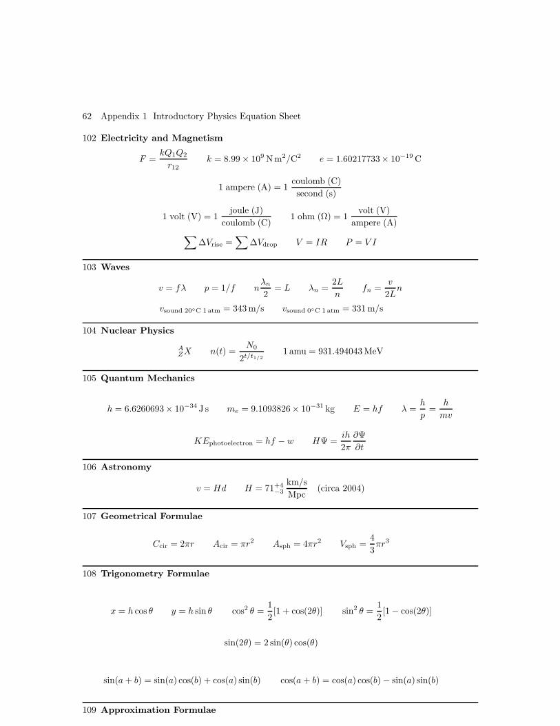
62 Appendix 1 Introductory Physics Equation Sheet
102 Electricity and Magnetism
F =kQ1Q2
r12k = 8.99 × 10⁹ Nm2/C2 e = 1.60217733× 10⁻¹⁹ C
1 ampere (A) = 1coulomb (C)
second (s)
1 volt (V) = 1joule (J)
coulomb (C)1 ohm (Ω) = 1
volt (V)
ampere (A)∑
∆Vrise =∑
∆Vdrop V = IR P = V I
103 Waves
v = fλ p = 1/f nλn
2= L λn =
2L
nfn =
v
2Ln
vsound 20C 1atm = 343 m/s vsound 0C 1 atm = 331 m/s
104 Nuclear Physics
AZX n(t) =
N0
2t/t1/2
1 amu = 931.494043 MeV
105 Quantum Mechanics
h = 6.6260693× 10⁻³⁴ J s me = 9.1093826× 10⁻³¹ kg E = hf λ =h
p=
h
mv
KEphotoelectron = hf − w HΨ =ih
2π
∂Ψ
∂t
106 Astronomy
v = Hd H = 71+4−3
km/s
Mpc(circa 2004)
107 Geometrical Formulae
Ccir = 2πr Acir = πr2 Asph = 4πr2 Vsph =4
3πr3
108 Trigonometry Formulae
x = h cos θ y = h sin θ cos2 θ =1
2[1 + cos(2θ)] sin2 θ =
1
2[1 − cos(2θ)]
sin(2θ) = 2 sin(θ) cos(θ)
sin(a+ b) = sin(a) cos(b) + cos(a) sin(b) cos(a+ b) = cos(a) cos(b) − sin(a) sin(b)
109 Approximation Formulae

Appendix 1 Introductory Physics Equation Sheet 63
∆f
∆x≈ df
dx
1
1 − x≈ 1 + x : (x << 1)
sin θ ≈ θ tan θ ≈ θ cos θ ≈ 1 − 1
2θ2 all for θ << 1
110 Quadratic Formula
If 0 = ax2 + bx+ c , then x =−b±
√b2 − 4ac
2a= − b
2a±
√
(
b
2a
)2
− c
a
111 Vector Formulae
~a+~b = (ax + bx, ay + by, az + bz) ~a ·~b = ab cos θ = axbx + ayby + azbz
~c = ~a×~b = ab sin(θ)c = (aybz − byaz, azbx − bzax, axby − bxay)
112 Differentiation and Integration Formulae
d(xn)
dx= nxn−1 except for n = 0;
d(x0)
dx= 0
d[ln(x)]
dx=
1
x
∫ b
a
f(x) dx = F (x)|ba = F (b) − F (a) wheredF (x)
dx= f(x)
∫
xn dx =xn+1
n+ 1except for n = −1;
∫
1
xdx = ln(x)
113 One-Dimensional Kinematics
vavg =∆x
∆tv =
dx
dtaavg =
∆v
∆ta =
dv
dt=d2x
dt2
v = v0 + at x = x0 + v0t+1
2at2
x = x0 +1
2(v0 + v)t v2 = v2
0 + 2a(x− x0) g = 9.8 m/s2
x′ = x− vframet v′ = v − vframe a′ = a
114 Two- and Three-Dimensional Kinematics: General
~vavg =∆~r
∆t~v =
d~r
dt~aavg =
∆~v
∆t~a =
d~v
dt=d2~r
dt2
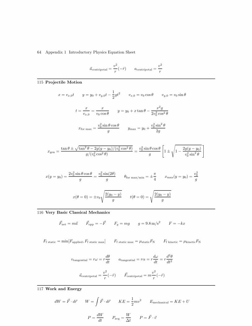
64 Appendix 1 Introductory Physics Equation Sheet
~acentripetal =v2
r(−r) acentripetal =
v2
r
115 Projectile Motion
x = vx,0t y = y0 + vy,0t−1
2gt2 vx,0 = v0 cos θ vy,0 = v0 sin θ
t =x
vx,0=
x
v0 cos θy = y0 + x tan θ − x2g
2v20 cos2 θ
xfor max =v20 sin θ cos θ
gymax = y0 +
v20 sin2 θ
2g
xgen =tan θ ±
√
tan2 θ − 2g(y − y0)/(v20 cos2 θ)
g/(v20 cos2 θ)
=v20 sin θ cos θ
g
[
1 ±√
1 − 2g(y − y0)
v20 sin2 θ
]
x(y = y0) =2v2
0 sin θ cos θ
g=v20 sin(2θ)
gθfor max/min = ±π
4xmax(y = y0) =
v20
g
x(θ = 0) = ±v0
√
2(y0 − y)
gt(θ = 0) =
√
2(y0 − y)
g
116 Very Basic Classical Mechanics
~Fnet = m~a ~Fopp = −~F Fg = mg g = 9.8 m/s2 F = −kx
Ff static = min[Fapplied, Ff static max] Ff static max = µstaticFN Ff kinetic = µkineticFN
vtangential = rω = rdθ
dtatangential = rα = r
dω
dt= r
d2θ
dt2
~acentripetal =v2
r(−r) ~Fcentripetal = m
v2
r(−r)
117 Work and Energy
dW = ~F · d~r W =
∫
~F · d~r KE =1
2mv2 Emechanical = KE + U
P =dW
dtPavg =
W
∆tP = ~F · ~v

Appendix 1 Introductory Physics Equation Sheet 65
KEf = KEi +Wnet ∆Uof a conservative force = −Wby a conservative force Ef = Ei +Wnonconservative
F = −dUdx
~F = −∇U U =1
2kx2 U = mgy
118 Systems of Particles
~rcm =
∑
imi~rimtotal
=
∑
submsub~rcm sub
mtotal~rcm =
∫
Vρ(~r )~r dV
mtotal
~Fnet ext = m~acm
~p = m~v ~Fnet = md~p
dt~Fnet ext = m
d~ptotal
dt
m~a = ~Fnet non-transferred + (~vtransferred − ~v)dm
dt= ~Fnet non-transferred + ~vrel
dm
dt
v = vi + vthrust ln(mi
m
)
rocket in free space
119 Collisions
~J =
∫ tf
ti
~F (t) dt ~Favg =~J
∆t~p1i + ~p2i = ~p1f + ~p2f ~vcm =
~p1 + ~p2
mtotal
KEtotal f = KEtotal i v1f =
(
m1 −m2
m1 +m2
)
v1i +
(
2m2
m1 +m2
)
v2i vrel f = −vrel i
1-d Elastic Expressions
Pperfect gas pressure =1
3
∫ ∞
0
pvn(v) dp Pideal gas pressure = nkT
120 Rotation
θ =s
rω =
dθ
dt=v
rα =
d2θ
dt2=dω
dt=a
rf =
ω
2πP = f−1 =
2π
ω
ω = ω0 + αt θ = θ0 + ω0t+1
2αt2 θ = θ0 +
1
2(ω0 + ω)t ω2 = ω2
0 + 2α(θ − θ0)
~τ = ~r × ~F ~τnet =d~L
dt~L = ~r × ~p
τ = rF sin θ τnet = Iα L = Iω

66 Appendix 1 Introductory Physics Equation Sheet
I =∑
i
mir2xy,i I =
∫
ρr2xy dV Ipar-axis = mr2xy,cm + Icm
a =g sin θ
1 + I/(mr2)
KErot =1
2Iω2 KEtotal = KEtrans +KErot =
1
2mv2 +
1
2Iω2 dW = τ dθ P = τω
∆KErot = Wnet =
∫
τnet dθ ∆U = −W = −∫
τ dθ Ef = Ei +Wnonconservative
121 Static Equilibrium in Two Dimensions
0 = Fnet x =∑
Fx 0 = Fnet y =∑
Fy 0 = τnet =∑
τ
122 Gravity
G = 6.67407× 10⁻¹¹ m3 kg−1 s−2 (2002 result) ~F1 on 2 =Gm1m2
r212(−r12)
~fg =GM
r2(−r)
∮
~fg · d ~A = −4πGM
U = −Gm1m2
r12V = −GM
rvescape =
√
2GM
rvorbit =
√
GM
r
P 2 =
(
4π2
GM
)
r3 P =
(
2π√GM
)
r3/2 dA
dt=
1
2r2ω =
L
2m= Constant
123 Fluids
ρ =∆m
∆Vp =
F
Ap = p0 + ρgddepth
Pascal’s principle p = pext − ρg(y − yext) ∆p = ∆pext
Archimedes principle Fbuoy = mfluid disg = Vfluid disρfluidg
equation of continuity for ideal fluid RV = Av = Constant
Bernoulli’s equation p+1
2ρv2 + ρgy = Constant
124 Simple Harmonic Oscillator

Appendix 1 Introductory Physics Equation Sheet 67
P = f−1 ω = 2πf F = −kx U =1
2kx2 a(t) = − k
mx(t) = −ω2x(t)
ω =
√
k
mP = 2π
√
m
kx(t) = A cos(ωt) + sin(ωt)
Emec total =1
2mv2
max =1
2kx2
max =1
2mv2 +
1
2kx2
P = 2π
√
I
mgℓP = 2π
√
ℓ
g
125 Waves
d2y
dx2=
1
v2
d2y
dt2v =
√
FT
µy = f(x∓ vt) y = ymax sin[k(x∓ vt)] = ymax sin(kx∓ ωt)
Period =1
fk =
2π
λv = fλ =
ω
kP ∝ y2
max
y = 2ymax sin(kx) cos(ωt) n =L
λ/2L = n
λ
2λ =
2L
nf = n
v
2L
v =
√
(
∂P
∂ρ
)
S
nλ = d sin(θ)
(
n+1
2
)
λ = d sin(θ)
I =P
4πr2β = (10 dB) × log
(
I
I0
)
f = nv
4L: n = 1, 3, 5, . . . fmedium =
f01 − v0/vmedium
126 Thermodynamics
TK = TC + 273.15 K TF = 1.8TC + 32 ∆L = Lα∆T ∆V = V β∆T β = 3α
Q = mc∆T = mc(Tf − Ti) Q =∑
k
mkck(Tf − Ti,k)
W =
∫ Vf
Vi
p dV dE = dQ− dW dE = T dS − p dV

68 Appendix 1 Introductory Physics Equation Sheet
Fcond = −kdTdx
Fsurface = ε1σT4surface Fenv = ε2σT
4env σ = 5.67 × 10⁻⁸ W m−2 K−4
pV = nRT = NkT R = 8.31 J mol−1 K−1 k = 1.38 × 10⁻²³ J/K
Wisothermal = nRT ln(Vf/Vi) E =f
2nRT = nCV T CV =
f
2R Cp = CV +R
PV γ = Constant γ =Cp
CV=CV +R
CV= 1 +
2
f
0 = ∆E = (Qh −Qc) −W ε =W
Qh= 1 − Qc
Qhη =
Qc
Qh= 1 − W
Qh
εCarnot = 1 − Tc
ThηCarnot =
Tc
Th= 1 − εCarnot εCarnot + ηCarnot = 1
∆S =
∫ f
i
dS =
∫ f
i
dQ
T∆S = nR ln
[
(
Tf
Ti
)f/2(Vf
Vi
)
]
127 Electrostatics
e = 1.602 × 10⁻¹⁹ C me = 9.109 × 10⁻³¹ kg
ε0 = 8.854 × 10⁻¹² C2/(N-m2) ≈ 10−11 k =1
4πε0= 8.99 × 10⁹ N-m2/C2 ≈ 1010
~F1 on 2 =kq1q2r21,2
r1,2~F = q ~E ~E(~r ) =
kq
r2r =
q
4πεr2r
∮
~E · d ~A =qenc
ε0
~E =σ
ε0n ~τ = ~p× ~E PE = −~p · ~E
∆U = q∆V ∆V = −∫ f
i
~E ·d~s V =kq
rV = k
∑
i
qiri
V = k
∫
dq
r~E = −∇V
C =q
VC =
ε0A
dCparallel =
∑
i
Ci1
Cseries=∑
i
1
Ci
UC =q2
2C=
1
2CV 2 Cdielectric = κCvacuum
~Emacroscopic charge = κ~Enet
∮
κ~E · d ~A =qenc
ε0

Appendix 1 Introductory Physics Equation Sheet 69
128 Current and Circuits
I =dq
dtI =
∫
~J · d ~A J =I
A~J = nq~vdrift
~J = σ ~E V = IR
σ =nq2τ
mρ =
1
σV = IR R = ρ
L
AP = IV P = I2R =
V 2
R
0 =
node∑
i
Ii 0 =
loop∑
i
∆Vi Rseries =∑
i
Ri1
Rparallel=∑
i
1
Ri
τ = RC I =∆Vinitial
Re−t/τ ∆V = ∆Vfinal
(
1 − e−t/τ)
129 Magnetic Fields and Forces
µ0 = 4π × 10−7 T-m/A 1 tesla (T) = 104 gauss (G)
~F = q~v × ~B ~dF = I d~ℓ × ~B
~rcyclotron =mv
qBωcyclotron =
qB
mfcyclotron =
qB
2πmP =
2πm
qB
~µ = NIAA τ = ~µ× ~B U = −~µ · ~B
d~B =µ0
4π
I d~s× r
r2Bwire =
µ0I
2πrBarc =
µ0Iθ
4πr~F1 on 2 =
µ0ℓI1I22πr
r2 to 1
Bsolenoid = µ0nI Btoroid =µ0NI
2πr~Bcirc. loop =
µ0IR2
2(R2 + z2)3/2z ~Bdipole =
µ0~µ
2πz3
∮
~B ·d~s = µ0I ΦB =
∫
linked area
~B ·d ~A Vemf =
∮
~E ·d~s = −dΦB
dt= − d
dt
∫
linked area
~B ·d ~A
L =ΦB
ILsolenoid = µ0n
2Vvol Vemf drop = LdI
dtUL =
1
2LI2 uB =
B2
2µ0
130 LR, LC, LRC Circuits and Alternating Current
τL =L
RI =
Vemf
R
(
1 − e−t/τL
)
I = I0e−t/τL

70 Appendix 1 Introductory Physics Equation Sheet
ω =1√LC
Imax =Vmax
√
R2 + [wdL− 1/(wdC)]2
131 Electromagnetic Waves and Radiation
c = 2.99792458× 10⁸ ≈ 3.00 × 10⁸ m/s Period =1
fc = fλ =
ω
kk =
2π
λc =
1√µ0ε0
~E = ~E0 sin(kx− wt) ~B = ~B0 sin(kx− wt)B
E=
1
c
Imonochr =1
2εE2
0 = εE2rms Ipoint =
L
4πr2
Ωsphere = 4π dΩ = sin θ dθ dφ
Itrans. polarized = Iinc cos2 θ Itrans. non-polarized =1
2Iinc
132 Geometrical Optics
θinc = θrefl n1 sin θ1 = n2 sin θ2 θ1,critical = sin−1
(
n2
n1
)
n =c
vnλn =
λvacuum
nf =
vnλn
=c
λvacuum
133 Interference and Diffraction
2-slit nλ = d sin θmax I =4I0r2
cos2(α) α = πd
λsin θ
single-slit nλ = a sin θzero I =I0r2
sin2(α)
α2α = π
a
λsin θ
grating nλ = d sin θmax X-ray nλ = 2d sin θmax
134 Special Relativity
c = 2.99792458× 10⁸ m/s ≈ 2.998 × 10⁸ m/s ≈ 3 × 10⁸ m/s ≈ 1 lyr/yr ≈ 1 ft/ns
β =v
cγ =
1√
1 − β2γ(β << 1) = 1 +
1
2β2 τ = ct
Galilean Transformations Lorentz Transformations
x′ = x− βτ x′ = γ(x− βτ)

Appendix 1 Introductory Physics Equation Sheet 71
y′ = y y′ = yz′ = z z′ = zτ ′ = τ τ ′ = γ(τ − βx)
β′obj = βobj − β β′
obj =βobj − β
1 − ββobj
ℓ = ℓproper
√
1 − β2 ∆τproper = ∆τ√
1 − β2
x′ =xintersection
γ= x′x scale
√
1 − β2
1 + β2τ ′ =
τintersection
γ= τ ′τ scale
√
1 − β2
1 + β2θMink = tan−1(β)
m = γm0 p = mv = γm0cβ E0 = m0c2 E = γE0 = γm0c
2 = mc2
E = mc2 E =√
(pc)2 + (m0c2)2 KE = E − E0 =√
(pc)2 + (m0c2)2 −m0c2 = (γ − 1)m0c
2
f = fproper
√
1 − β
1 + βfor source and detector separating f(β << 1) = fproper
(
1 − β +1
2β2
)
ftrans = fproper
√
1 − β2 ftrans(β << 1) = fproper
(
1 − 1
2β2
)
135 Quantum Mechanics
h− =h
2πE = hf p =
h
λ= h−k ∆λ =
h
mc(1 − cos θ)
− h−2
2m
∂2Ψ
∂x2+ VΨ = ih−∂Ψ
∂t− h−2
2m
∂2ψ
∂x2+ V ψ = Eψ Ψ(x, t) = ψ(x)e−iEt/h−
∆x∆p ≥ h−2
∫ ∞
−∞
|Ψ|2 dx = 1 En = −1
2mec
2α2Z2
n2= −Eryd
Z2
n2
Eryd = 13.6056981 eV α =e2
4πǫ0h−c=
1
137.0359895
aBohr = 0.529177249× 10−10 = 0.529177249 A
mamu = 1.6605402× 10⁻²⁷ kg = 931.49432 MeV me = 9.1093897× 10⁻³¹ kg = 0.510999906 MeV
mp = 1.6726231× 10⁻²⁷ kg = 938.27231 MeV mn = 1.6749286× 10⁻²⁷ kg = 939.56563 MeV

Appendix 2 Table of Integrals, Etc.
Note: There are no guarantees of accuracy with these integrals, etc. I include some derivatives atthe start, but they are such a minor component that they do not merit a change in title.
136. Derivatives
(1)d
dxsin−1 u =
1√1 − u2
du
dxfor sin−1 ∈
[
−π2,π
2
]
(2)d
dxcos−1 u =
−1√1 − u2
du
dxfor cos−1 ∈ [0, π]
137. Functions containing ax2 + b
(1)
∫
dx
ax2 + b=
1√ab
tan−1
(
x
√
a
b
)
a > 0 and b > 0;
1
2√−ab
ln
(
x√a−
√−b
x√a+
√−b
)
a > 0 and b < 0;
1
2√−ab
ln
(√b+ x
√−a√
b− x√−a
)
a < 0 and b > 0;
− 1
axb = 0;
x
ba = 0
(2)
∫
dx
(ax2 + b)2=
1
2b
x
(ax2 + b)+
1
2b
1√ab
tan−1
(
x
√
a
b
)
a > 0 and b > 0
(3)
∫
dx√ax2 + b
=1√−a sin−1
(
x
√
−ab
)
= − 1√−a cos−1
(
x
√
−ab
)
a < 0
138. Functions containing ax2 + bx+ c
(1)
∫
dx
(ax2 + bx+ c)3/2
= − 2(2ax+ b)
(b2 − 4ac)√ax2 + bx+ c
139. Functions containing sin(ax)
72

Appendix 2 Table of Integrals, Etc. 73
(1)
∫
sin3(ax) dx = −1
acos(ax) +
1
3acos3(ax)
(2)
∫
sin5(ax) dx = − 1
5asin4(ax) cos(ax) +
4
15acos3(ax) − 4
5acos(ax)
(3)
∫
sinn(ax) dx = − 1
nasinn−1(ax) cos(ax)
n− 1
n
∫
sinn−2(ax) dx
140. Inverse Trigonometric Functions
(1)
∫
sin−1(ax) dx = x sin−1(ax) +1
a
√
1 − a2x2
(2)
∫
cos−1(ax) dx = x cos−1(ax) − 1
a
√
1 − a2x2
141. Algebraic and Trigonometric Functions
(1)
∫
x sin(ax) dx =1
a2sin(ax) − x
acos(ax)
(2)
∫
x2 sin(ax) dx = −x2
acos(ax) +
2x
a2sin(ax) +
2
a3cos(ax)
(3)
∫
x cos(ax) dx =1
a2cos(ax) − x
asin(ax)
(4)
∫
x2 sin(ax) dx =x2
asin(ax) +
2x
a2cos(ax) − 2
a3sin(ax)
142. Gaussian Function and Factorial Integral
(1) G(x) =1
σ√
2πexp
[
− (x− µ)2
2σ2
]
standard form
(2)
∫ ∞
−∞
e−(a+ib)x2
dx =
√
π
a+ ib
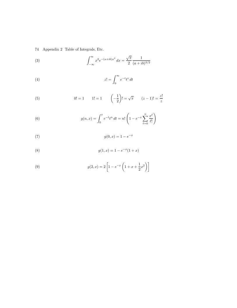
74 Appendix 2 Table of Integrals, Etc.
(3)
∫ ∞
−∞
x2e−(a+ib)x2
dx =
√π
2
1
(a+ ib)3/2
(4) z! =
∫ ∞
0
e−ttz dt
(5) 0! = 1 1! = 1
(
−1
2
)
! =√π (z − 1)! =
z!
z
(6) g(n, x) =
∫ x
0
e−ttn dt = n!
(
1 − e−xn∑
ℓ=0
xℓ
ℓ!
)
(7) g(0, x) = 1 − e−x
(8) g(1, x) = 1 − e−x(1 + x)
(9) g(2, x) = 2
[
1 − e−x
(
1 + x+1
2x2
)]

Appendix 3 Multiple-Choice Problem Answer Tables
Note: For those who find scantrons frequently inaccurate and prefer to have their own table andmarking template, the following are provided. I got the template trick from Neil Huffacker atUniversity of Oklahoma. One just punches out the right answer places on an answer table andoverlays it on student answer tables and quickly identifies and marks the wrong answers
Answer Table for the Multiple-Choice Questions
a b c d e a b c d e
143. O O O O O 6. O O O O O
144. O O O O O 7. O O O O O
145. O O O O O 8. O O O O O
146. O O O O O 9. O O O O O
147. O O O O O 10. O O O O O
75

76 Appendix 3 Multiple-Choice Problem Answer Tables
Answer Table for the Multiple-Choice Questions
a b c d e a b c d e
148. O O O O O 11. O O O O O
149. O O O O O 12. O O O O O
150. O O O O O 13. O O O O O
151. O O O O O 14. O O O O O
152. O O O O O 15. O O O O O
153. O O O O O 16. O O O O O
154. O O O O O 17. O O O O O
155. O O O O O 18. O O O O O
156. O O O O O 19. O O O O O
157. O O O O O 20. O O O O O

Appendix 3 Multiple-Choice Problem Answer Tables 77
Answer Table for the Multiple-Choice Questions
a b c d e a b c d e
158. O O O O O 16. O O O O O
159. O O O O O 17. O O O O O
160. O O O O O 18. O O O O O
161. O O O O O 19. O O O O O
162. O O O O O 20. O O O O O
163. O O O O O 21. O O O O O
164. O O O O O 22. O O O O O
165. O O O O O 23. O O O O O
166. O O O O O 24. O O O O O
167. O O O O O 25. O O O O O
168. O O O O O 26. O O O O O
169. O O O O O 27. O O O O O
170. O O O O O 28. O O O O O
171. O O O O O 29. O O O O O
172. O O O O O 30. O O O O O

78 Appendix 3 Multiple-Choice Problem Answer Tables
NAME:
Answer Table for the Multiple-Choice Questions
a b c d e a b c d e
173. O O O O O 26. O O O O O
174. O O O O O 27. O O O O O
175. O O O O O 28. O O O O O
176. O O O O O 29. O O O O O
177. O O O O O 30. O O O O O
178. O O O O O 31. O O O O O
179. O O O O O 32. O O O O O
180. O O O O O 33. O O O O O
181. O O O O O 34. O O O O O
182. O O O O O 35. O O O O O
183. O O O O O 36. O O O O O
184. O O O O O 37. O O O O O
185. O O O O O 38. O O O O O
186. O O O O O 39. O O O O O
187. O O O O O 40. O O O O O
188. O O O O O 41. O O O O O
189. O O O O O 42. O O O O O
190. O O O O O 43. O O O O O
191. O O O O O 44. O O O O O
192. O O O O O 45. O O O O O
193. O O O O O 46. O O O O O
194. O O O O O 47. O O O O O
195. O O O O O 48. O O O O O
196. O O O O O 49. O O O O O
197. O O O O O 50. O O O O O

Appendix 3 Multiple-Choice Problem Answer Tables 79
Answer Table Name:a b c d e a b c d e
198. O O O O O 31. O O O O O
199. O O O O O 32. O O O O O
200. O O O O O 33. O O O O O
201. O O O O O 34. O O O O O
202. O O O O O 35. O O O O O
203. O O O O O 36. O O O O O
204. O O O O O 37. O O O O O
205. O O O O O 38. O O O O O
206. O O O O O 39. O O O O O
207. O O O O O 40. O O O O O
208. O O O O O 41. O O O O O
209. O O O O O 42. O O O O O
210. O O O O O 43. O O O O O
211. O O O O O 44. O O O O O
212. O O O O O 45. O O O O O
213. O O O O O 46. O O O O O
214. O O O O O 47. O O O O O
215. O O O O O 48. O O O O O
216. O O O O O 49. O O O O O
217. O O O O O 50. O O O O O
218. O O O O O 51. O O O O O
219. O O O O O 52. O O O O O
220. O O O O O 53. O O O O O
221. O O O O O 54. O O O O O
222. O O O O O 55. O O O O O
223. O O O O O 56. O O O O O
224. O O O O O 57. O O O O O
225. O O O O O 58. O O O O O
226. O O O O O 59. O O O O O
227. O O O O O 60. O O O O O