Mathematical Appendix
47
Mathematical Appendix APPENDIX TO CHAPTER 4 Al Notional Case, Calculation of the Individual's Supply Func- tion of Hours and Demand Function of Goods (Equations 4.7 and 4.8) The analysis is based on the normalization of the time constraint, F t + H l = 1, equation (4.5') from the main text, and the FOCs of the household's problem (4.6), which are given by — = Xj p , \x — = X l w, and w - wF t + rK f = pC { . C, Ff We express C, by division of the second by the first FOC and reformulate to yield that C t = w^Hp- 1 /^ . Then we substitute for C, and for capital, given by equation (4.5'), into the budget constraint to calculate F } : — 1 w 1 — w-wF+^K.-p Fj = 0, => wFi+—wFj =w + t; K i9 fi p \x F r 1+/1 1 + «*/ Substitute by the time constraint to obtain the individual's notional supply function of working hours as H?>"=1 M l + /i 1 + «*/ (4.7) From the main text, we know that it has to be valid that p{l + p)~ x (l + E > k l lw)<l 9 = > / / + j U i-^<i + jU , =>£K<w/p We calculate F t from the first two FOCs, which yields that Fj =C /i u(/?/w), and substitute for F l and capital, given by equation (4.5'), into the budget constraint to obtain the notional individual's demand function for goods, C/M as w-w— L ^r + ^K i -pC lf =0, => pCifij+pCi =%K f +w 9 wp 145
-
Upload
khangminh22 -
Category
Documents
-
view
1 -
download
0
Transcript of Mathematical Appendix
Mathematical Appendix
APPENDIX TO CHAPTER 4
Al Notional Case, Calculation of the Individual's Supply Function of Hours and Demand Function of Goods (Equations 4.7 and 4.8)
The analysis is based on the normalization of the time constraint, Ft + Hl = 1, equation (4.5') from the main text, and the FOCs of the household's problem (4.6), which are given by
— = Xj p , \x — = Xl w, and w - wFt + rKf = pC{. C, Ff
We express C, by division of the second by the first FOC and reformulate to yield that Ct = w^Hp-1/^. Then we substitute for C, and for capital, given by equation (4.5'), into the budget constraint to calculate F}:
— 1 w 1 — w-wF+^K.-p Fj = 0, => wFi+—wFj =w + t; Ki9
fi p \x
Fr 1+/1 1 + « * /
Substitute by the time constraint to obtain the individual's notional supply function of working hours as
H?>"=1 M l + /i
1 + « * / (4.7)
From the main text, we know that it has to be valid that
p{l + p)~x(l + E>kllw)<l9 = > / / + j U i - ^ < i + jU , =>£K<w/p
We calculate Ft from the first two FOCs, which yields that Fj =C/iu(/?/w), and substitute for Fl and capital, given by equation (4.5'), into the budget constraint to obtain the notional individual's demand function for goods, C/M as
w-w—L^r + Ki-pClf = 0 , => pCifij+pCi =%Kf+w9 wp
145
146 Mathematical Appendix
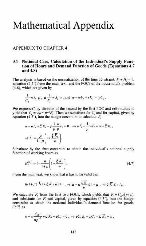
cD,n _ I %Kj+W
l + | i p (4.8)
A2 Notional Case, Calculation of the "Conditional" Factor Demand Functions (Equations 4.9 and 4.10)
The analysis is based on equations (4.1) and (4.2) from the main text. The cost minimization problem is given by
min TCj = min (rKj + whjLj),
sX:Yj=Kjtfr«Li7<*. (4.3)
Reformulate the production function to obtain that
1 l-<* 1 a Kj = Yf (hjLj) a , and hjLj = Y)~aKJ
l~a .
Substitution of Kt and hjLj9 respectively, into the cost minimization problem reduces the problem to
( J_ 1-a mm rYf(hjLj) « +whjLj , and min
K rKj+wYj-vKj1-"
We yield that:
1 l~a _ 1 ^ - = -^-rYfxh, a Li
a+wh1=09 dL< a J J J *
| ^ = lz£ryJl(*Ir)"i=wf dL, a J J
3/z,
l-a
a
1 _ 1 l~a
rYfhJaLJ
a +wLj=0,
dh; a J J ••w 9
30 -^—wY}-aK,l-a =0. l-a J J
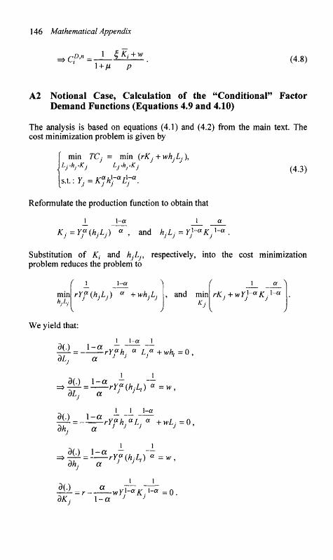
Mathematical Appendix 147
Hence the FOC for labor and working hours are identical. Reformulate for hjLj and Kh and use the rental price for capital as the numeraire to calculate the "conditional" demand functions for labor and capital:
X~^-Yf {hjLt)a =w, => (hjlif* = f - ^ - w
a ' J J 1-a (4.9)
a
l-a vYJ-aKjl-a = 1 , =>K]>" = •w l Yf.
l-a I ; (4.10)
A3 Notional Case, Calculation of the Cost Function of the Firm (Equation 4.11)
The analysis is based on equations (4.9) and (4.10), derived above, the cost-constraint from the main text (equation 4.2) and the use of the rental price of capital as the numeraire. We substitute equations (4.9) and (4.10) into equation (4.2) to obtain that:
TCj = / \\-a i a N
1-a -w Yj + w a 1-a
•a
H Yj>
1 - « V (r^-Q>l\ n\<*-\ir»-U( => TCj = wx-aYj(ax-a(l-a)a-x-ha-a(l-af),
=»TC7 = w 1 " a y / ( l - a ) a " 1 a ~ a ( a + l - a ) ,
=> TCJ={l-a)a~xa-awx-aYj. (4.11)
A4 Notional Case, Calculation of Equilibrium Output (Equation 4.13)
The analysis is based on equations (4.8'), (4.12'), (4.10') and (4.5") from the main text. Equilibrium on the goods markets directly yields that
.*,„__! C'" = $K+w
l + Ha-a{l-af-xwx~a
Equilibrium on the capital market leads to
!£. 1-a 1-a a
148 Mathematical Appendix
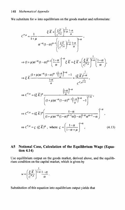
We substitute for w into equilibrium on the goods market and reformulate:
c*>" c *•" « \+n
a~a(\-af-x
c*,n I a
i-a
(l + yu)cra(l-a)a~1 l-a^a
v « y £ £ = £ * + [1-a 1-a
v « j
_(\ + p)a-a(l-af-xh-Ya -I A$K) l-a
1-a a c*-"'"a
• c - n = (|A:)'
•CJ"={^Kf
^r -a r« f(l + Hya-a(l-af-lh.)~a-l
1-a \l-a
=>C>" =q (%K)a 9 where $ =
(l + iu)«~a0-«)a_1«(l-«)1~a«o:"1 - a
1-a 1-a + u
(4.13)
A5 Notional Case, Calculation of the Equilibrium Wage (Equation 4.14)
Use equilibrium output on the goods market, derived above, and the equilibrium condition on the capital market, which is given by
,c*>" 1-a 1-a
Substitution of this equation into equilibrium output yields that
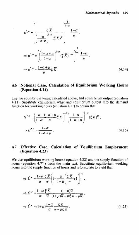
Mathematical Appendix 149
l-a+li )
1-a
1-a
a
l - a + /i
1-a
*jW _ 1-a + ju
\l-a ( $ * ) •
Fxl-a |l-a 1-a
a
a « * •
(4.14)
A6 Notional Case, Calculation of Equilibrium Working Hours (Equation 4.14)
Use the equilibrium wage, calculated above, and equilibrium output (equation 4.11). Substitute equilibrium wage and equilibrium output into the demand function for working hours (equation 4.8') to obtain that
//•'": a l-a + p
l-a a SK
•<v ,_„ >H* l-a + p
($K)a9
=>H*>"=-l-a
l-a + p (4.16)
A7 Effective Case, Calculation of Equilibrium Employment (Equation 4.23)
We use equilibrium working hours (equation 4.22) and the supply function of hours (equation 4.7") from the main text. Substitute equilibrium working hours into the supply function of hours and reformulate to yield that
=>fr=lz«UHl—lL a w 1 + A<
S* + 1
- l
*e_l-al;K (l + ju)w
• L •"=( ! + /!)•
a w (l + n)w-pl; K -jLiw '
1-q %K
a w-^K (4.23)
150 Mathematical Appendix
A P P E N D I X T O C H A P T E R 5
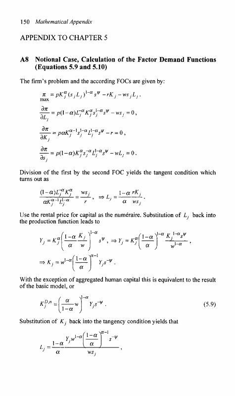
A8 Notional Case, Calculation of the Factor Demand Functions (Equations 5.9 and 5.10)
The firm's problem and the according FOCs are given by:
n = pIC" (s .LA1'" s¥ -rK , -ws iL.. max J J J J J J
^ = p(\-a)L-aKjsyasV-wSj=0,
dn — = paKj-V-al}-ras* - r = 0 , dK
| £ - = p(l-a)Kjs-aLXj-asV -wLj = 0.
Division of the first by the second FOC yields the tangent condition which turns out as
(l-a)L-aKj _wSj
aKj-lLx-a ~ ~
1-grKj
a ws;
Use the rental price for capital as the numeraire. Substitution of Lj back into the production function leads to
ry=*7
•Kj = W
l-a Kj a w
v J r 1 \a- l ' l - a N
Yj=KJ l-a
a
^l-ccK\-as¥
J-cc
l - a
V « J
YjS-V .
With the exception of aggregated human capital this is equivalent to the result of the basic model, or
vD,n KJ =
\ l -a
l - a YJSV . (5.9)
Substitution of Kj back into the tangency condition yields that
\cr-l
LJ = l-a
Y,w l-a l-a -¥
a
Mathematical Appendix 151
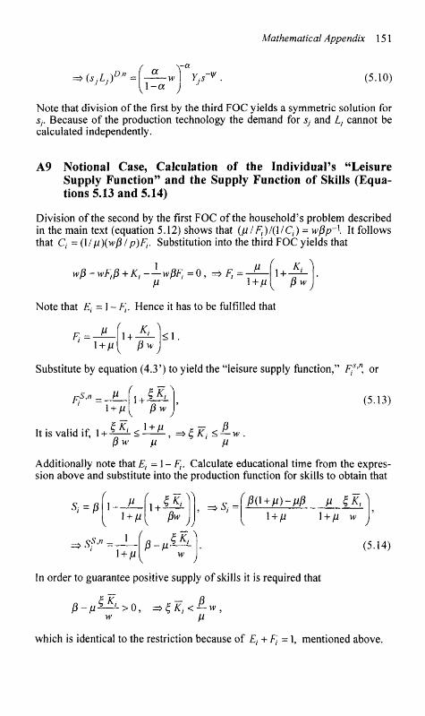
•w D.n , YjS-V . (5.10)
Note that division of the first by the third FOC yields a symmetric solution for Sj. Because of the production technology the demand for Sj and Lj cannot be calculated independently.
A9 Notional Case, Calculation of the Individual's "Leisure Supply Function" and the Supply Function of Skills (Equations 5.13 and 5.14)
Division of the second by the first FOC of the household's problem described in the main text (equation 5.12) shows that (p/F^/il/Cj) = wPp~\ It follows that C, = (l/jd)(wp/p)Fr Substitution into the third FOC yields that
wp-wFp + K^—wBF^O, =$F=-^— r K ^
V pw
Note that E,= 1 - F. Hence it has to be fulfilled that
F,=-1 + Ju
1 + K, pw)
<1.
Substitute by equation (4.3') to yield the "leisure supply function," Ff'" or
1 + p[ P w (5.13)
It is valid if, i + i ^ L < l ± ^ . , =*£Kl <^-w . Pw p ^ l p
Additionally note that E^l-Fj. Calculate educational time from the expression above and substitute into the production function for skills to obtain that
st=p 1 — l + p
1 + ML Pw
J)
, =>$ = 'j8(l + p)-pp ii $K^
l + p l + p w
<?S,n _ 1 p-n S*t (5.14)
In order to guarantee positive supply of skills it is required that
which is identical to the restriction because of Ej + F, = 1, mentioned above.
152 Mathematical Appendix
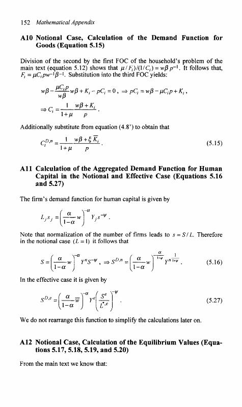
AlO Notional Case, Calculation of the Demand Function for Goods (Equation 5.15)
Division of the second by the first FOC of the household's problem of the main text (equation 5.12) shows that plFi)l(HCi) = wPp'1. It follows that, Ft = pCtpw-ip-l Substitution into the third FOC yields:
l wP + Kt
wp_12&Lwp + K pC Q9 ^pC^wp-pQp + K;, wP
l + p p
Additionally substitute from equation (4.8') to obtain that
cDjl= 1 wfi+SKj l + p p
(5.15)
A l l Calculation of the Aggregated Demand Function for Human Capital in the Notional and Effective Case (Equations 5.16 and 5.27)
The firm's demand function for human capital is given by
-a
LjSj = l-a ' J
Note that normalization of the number of firms leads to s -SI L. Therefore in the notional case (L = 1) it follows that
1 a x
w YnS-* 9 =* Su* = l-a
In the effective case it is given by
"T~ _L
1-a (5.16)
SD-e = a . -a fseTV
L>e
V J
(5.27)
We do not rearrange this function to simplify the calculations later on.
A12 Notional Case, Calculation of the Equilibrium Values (Equations 5.17, 5.18, 5.19, and 5.20)
From the main text we know that:
Mathematical Appendix 153
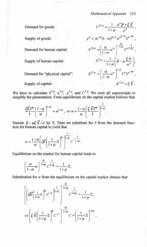
Demand for goods:
Supply of goods:
Demand for human capital:
Supply of human capital:
Demand for "physical capital":
Supply of capital:
C D , * = 1 wnP+£,K
1 + A< p n
p" = a-a(l-af-xw"l~aS"~¥ ,
,Djn _ a l-a
Ss>" =
\ wn
J
1 f
1+y yYl l+y/
\+H
l - a
4*A
xl-a Ynsn V |
KS*=$K.
We have to calculate 5 ,w, w*'w, p '" and C *w. We omit all superscripts to simplify the presentation. From equilibrium on the capital market follows that
rcV (\-„^~a
yes* l-a
a J-a l-a ZKS* l-a
Denote P-p^Klw by 3. Then we substitute for S from the demand function for human capital to yield that
l-a
a fr
\v
l + p
l-a C !""
Equilibrium on the market for human capital leads to
a l-a
— JL l+V £.l+v
l + p
Substitution for w from the equilibrium on the capital market obtains that
a
H&J c
l_\ 1-a
l+V i 1
SK \¥
l + p c
C 1 + ^ = _ i - 3 , l + p
a
l-a ( , <$+¥
C= -^—S l + p
1+li
-aty
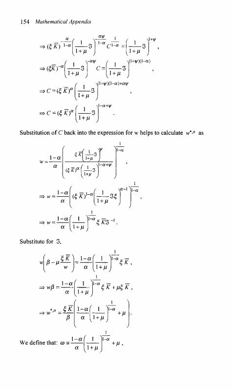
15 4 Mathematical Appendix
_ a r
=>C = (§*)"
~l^a
v1 + " , f
c =
cl-« =
1
1 xl+V
\ ( l+V)0-a
1 + /*
. 1 + < " \ ( l+yO(l-a)+ay
J \l~a+i/A
1 + Ai
Substitution of C back into the expression for w helps to calculate w*>n as
l
1-a
a
^ l - a
(£*? ,«[-L-3
l-a
a (ZK)] l-a
\a-l
l + p ^
1-a
l-a ( 1 \
a
l - a
v l ^ y
Z>KZ ~X.
Substitute for 3 ,
0-H « * 1-a ^ i A
a
l - a
v1 + " y ZK9
l-a f i A
a
/5
, ! + / « ,
1-a
l~°$K+tfK
1-a
Vl + M y + J"
We define that: co = 1-a l - a
^1 + M , + J " ,
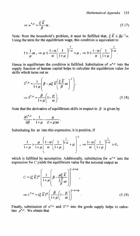
Mathematical Appendix 155
P (5.17)
Note: from the household's problem, it must be fulfilled that, £ K < pp V Using the term for the equilibrium wage, this condition is equivalent to
l<—co9 => p< p a v1 + " /
l-a 1 - ^ + p 9 = > 0 <
, 1 + J" ,
1__ 1-a
Hence in equilibrium the condition is fulfilled. Substitution of w*>" into the supply function of human capital helps to calculate the equilibrium value for skills which turns out as
S-n =- 1 l + p
p-pSK (O
V J
*-JL s<" = i+fi (5.18)
Note that the derivative of equilibrium skills in respect to /3 is given by
dS*-n _ 1 n
dfi \ + H (1 + ^)6)
Substituting for (0 into this expression, it is positive, if
-i-^ l + H \ + y.
1-a ( 1 ^ 1-a + M
1-a f i A l - a
v1 + " v >o,
which is fulfilled by assumption. Additionally, substitution for w*'" into the expression for C yields the equilibrium value for the notional output as
C = (SKf
r (
I l + p
V v
/ > - # «* (O
\}-a+y/
')
=> C*-n = (§ A-f ' PJl_lL^-a+V
l + p{ CO (5.19)
Finally, substitution of w*>n and S**n into the goods supply helps to calculate /?*'". We obtain that
156 Mathematical Appendix
p = a~a(l-a)t a-l — \l -a
\ H J 1-ii
1 + AH tf)
p*,n = a - « ( i _ a f - i /? a-Hr(l + j i y g W a i -F . ^ l - a i i"
co
-v (5.20)
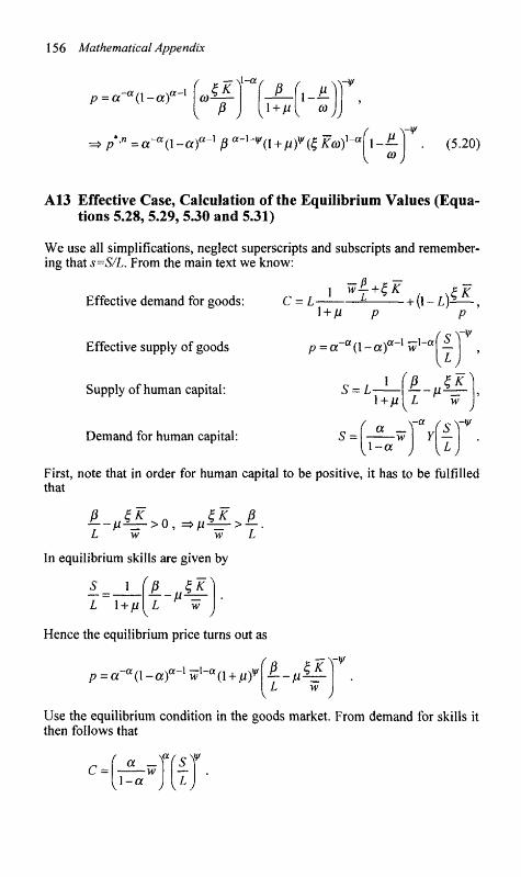
A13 Effective Case, Calculation of the Equilibrium Values (Equations 5.28, 5.29, 5.30 and 5.31)
We use all simplifications, neglect superscripts and subscripts and remembering that s=S/L. From the main text we know:
Effective demand for goods:
Effective supply of goods
Supply of human capital:
Demand for human capital:
c = i_i_fh££+(l_L)i£ 1+0 P P
p = oTa(l-a)a-1w1-af-l ,
S = L-1+|*
6 =| w 1-a
p L
x - a
/
**1 J
d*Y A — V)
First, note that in order for human capital to be positive, it has to be fulfilled that
P $1 A $K p
In equilibrium skills are given by
1 p 1;K L w L l + p
Hence the equilibrium price turns out as
p = a-a(l-a)a-xwx-a(l + pf P aX¥
L w
Use the equilibrium condition in the goods market. From demand for skills it then follows that
C-a _
w l-a
/ c f
KLJ
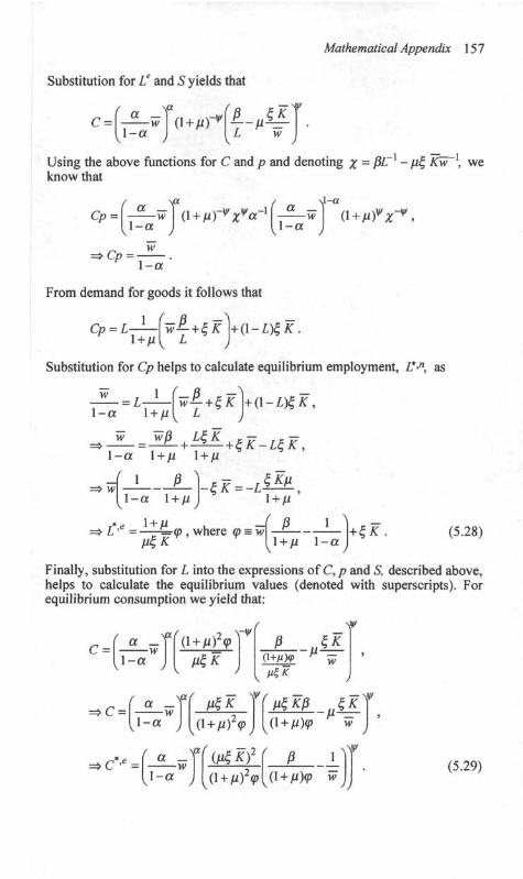
Mathematical Appendix 157
Substitution for Le and S yields that
C = ' a
1-a (l + p) -¥
f6 ^ L w
Using the above functions for C and p and denoting # = pL x - p^ Kw~\ we know that
CP: l - a
/ \ l -a ' a - >
l - a (l + nV*-* ,
=»Cp = 1-a
From demand for goods it follows that
Cp = L 1 l + p
w-P-+$K \+(l-L)£K.
Substitution for Cp helps to calculate equilibrium employment, L*>n9 as
w 1 1-a l + p
w£- + $K L *
+ (l-L)$K9
^-^+J£JL+tK-i4W9 l-a l + p l + p
1 P l-a l + p
-%K-
tfK
' l + / i
9,where cp = w -l + H 1-a
+ £ * . (5.28)
Finally, substitution for L into the expressions of C, /? and S, described above, helps to calculate the equilibrium values (denoted with superscripts). For equilibrium consumption we yield that:
- ( T ^ I T
/» „ « *
I — w l - a
M « * IT r
(i+pYv <PZKP IKJ
(l + p)(p w
C>e = a _ 1-a
F N 2
(/£*> (l + pYq>
P 1 (l + p)(p w
T
/> (5.29)
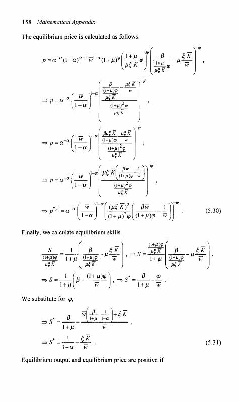
158 Mathematical Appendix
The equilibrium price is calculated as follows:
p = a - a ( l - a ) a - 1 w 1 - a ( l + ( u f ' l + Ai * —=<P
P %K - T - £ - jU~
=> p = a / — \ l -a
v l - a y
(1+A*)ff w
=> p = a
^ p = a~a
\ l - a
1-a (1+M)2<P rfK
r TT, \l~a
v l - a y
rt* pw 1
-V
p ' ° = a
v xl-a^
- a
iti Kf (l + p)z(p
Pw 1
(l + ju)<p w
\-v (530)
y
Finally, we calculate equilibrium skills.
p JK s i
1
~ 1 + ^ V
0+/0? ^ w
(l+AOy • _ jig*"
=>5=-1
1 + A*
We substitute for <p;
=>5 =-
O + AOv'l
l
l+/i l-a
,=>S =
+ ££
1 + jU
P <p
P JK V-
1 + // w
S =
l + p w
1 SK l-a w
Equilibrium output and equilibrium price are positive if
(5.31)
P <P u 4 P l ) J-—>-=z, where (p = w —*-l + p 1-a l + p w
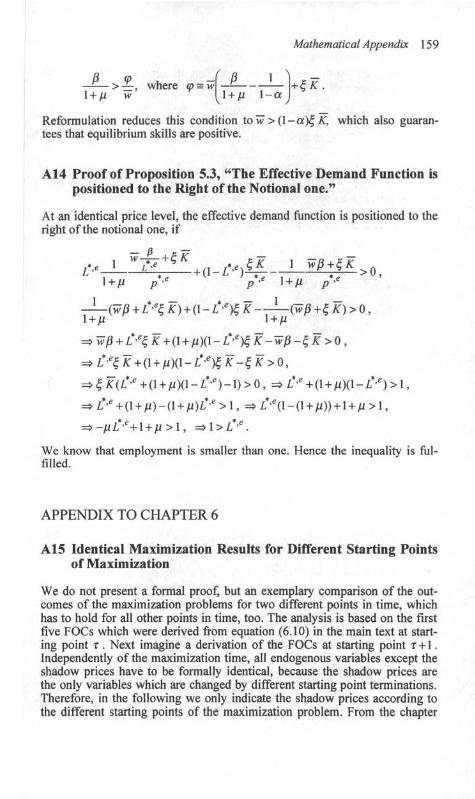
Mathematical Appendix 159
Reformulation reduces this condition to w > (1 - a)E, K, which also guarantees that equilibrium skills are positive.
A14 Proof of Proposition 5.3, "The Effective Demand Function is positioned to the Right of the Notional one."
At an identical price level, the effective demand function is positioned to the right of the notional one, if
l + A* / . « V * l + p />*
1 -(wp+L*>eZK) + (l-L*>e)£K l—(wP+%K)>09 l + p l + p
=>wP + L*^K+(l + p)(l-L*^K-wp-^K>09
=>L*>e£K+(l + p)(l-L*>e)%K-ZK>09
=*%K(L*>e+(l + p)(l-L*>e)-l)>09 =*L*>e+(l + p)(l-L*>e)>l9
=> L v + (l + p)-(l + p)L*>e >1, =>L*>e(l-(l + p)) + l + p>l9
=>-pl!'e+l + p>l9 =M>LV.
We know that employment is smaller than one. Hence the inequality is fulfilled.
APPENDIX TO CHAPTER 6
A15 Identical Maximization Results for Different Starting Points of Maximization
We do not present a formal proof, but an exemplary comparison of the outcomes of the maximization problems for two different points in time, which has to hold for all other points in time, too. The analysis is based on the first five FOCs which were derived from equation (6.10) in the main text at starting point T . Next imagine a derivation of the FOCs at starting point x + l. Independently of the maximization time, all endogenous variables except the shadow prices have to be formally identical, because the shadow prices are the only variables which are changed by different starting point terminations. Therefore, in the following we only indicate the shadow prices according to the different starting points of the maximization problem. From the chapter
160 Mathematical Appendix
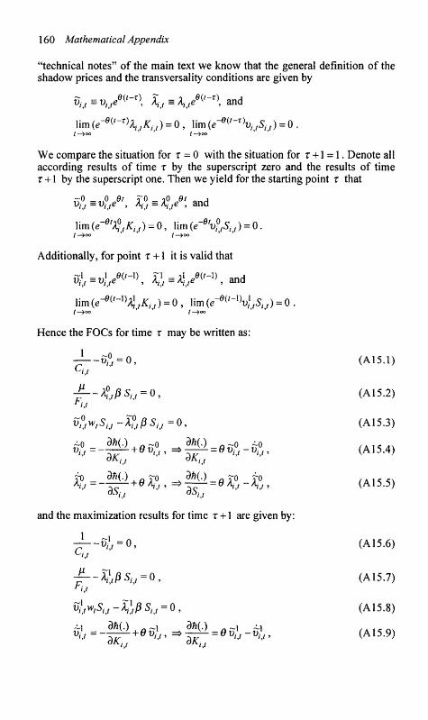
"technical notes" of the main text we know that the general definition of the shadow prices and the transversality conditions are given by
P,,, ^ , / ( ' " T ) , \ r s V * ( ' ~ T ) > and
lim(e^'-^Xt,K,,) = 0, lim(e"*('~r)u,-,Sit) = 0.
We compare the situation for r = 0 with the situation for r +1 = 1. Denote all according results of time r by the superscript zero and the results of time r + 1 by the superscript one. Then we yield for the starting point r that
vit = vite , Ajj = Aite , ana
lim(e~et^tKt,) = 0, lim(e'^v^Sit) = 0.
Additionally, for point T +1 it is valid that
lim(e~e{t~X)X]tKn) = 09 lim(e~e{t~%)tSit) = 0.
Hence the FOCs for time r may be written as:
- L - f i f t - o , (A15.1)
JL-flpSij-O, (A15.2)
vfjVtSij-tijPSu-O, (A15.3)
dKit 6Kit
fy'-^ + efy.^'Bfy-fy. (M5.5) ™i,t ™ij
and the maximization results for time r +1 are given by:
77—Vi!r = 0, (A15.6)
- £ - - ^ j9S l V = 0, (A15.7)
^ w ^ - ^ / 3 ^ - ^ 0 , (A15.8)
~1 ^ O , / ) ~ l _^ dft(-) /»~1 ~1 / A i c m d A : /7 d / c / , /
Mathematical Appendix 161
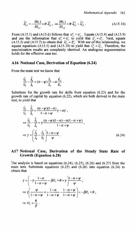
4 ) _ , r i j i Mu
(A15.10)
From (A 15.1) and (A 15.6) follows that vft =vj,. Equate (A 15.4) and (A 15.9) and use the information that v„=v)t to yield that i}t=vfr Next, equate (A15.2) and (A15.7) to obtain that Xjt = 4°. With use of this relationship, we equate equations (A15.5) and (A15.10) to yield that Xf4 = A ,. Therefore, the maximization results are completely identical. An analogous argumentation holds for the effective case too.
A16 Notional Case, Derivation of Equation (6.24)
From the main text we know that
-z---^ = (a~y/)—-a—
Substitute for the growth rate for skills from equation (6.23) and for the growth rate of capital by equation (6.22), which are both derived in the main text, to yield that
vt ^ _ (a-y/)(l-a) vt X] l-a+y/ Y-ccy,
^vt A] = (a-y/)(l-a)-a(l-a+y/) vt X] l-a+y/
f ~
'7 = \ % l-a + y/
¥ (6.24)
A17 Notional Case, Derivation of the Steady State Rate of Growth (Equation 6.28)
The analysis is based on equations (6.24), (6.25), (6.26) and (6.27) from the main text. Substitute equations (6.25) and (6.26) into equation (6.24) to obtain that
- 7 1-q
l-a + y/
¥ ^
-PHt+Q + y l-a + y/
¥
l-a l-a+y/
Ht =
l-a + y/ l-a+y/ l-a+y/
6
= -pvt+et
p
162 Mathematical Appendix
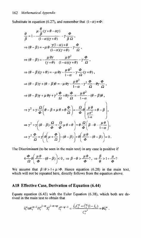
Substitute in equation (6.27), and remember that (1 - a ) = 0:
Q p—(y + 0-ay)
e j pyi f 0 P~ (l-a)(y + 0) J pa"
,* ^ n Y(l~a)+0 0 =>(0-p) = -pO— - y—,
( l - a ) (y + 0) Q
(0-P): pOy pO2
-Y-0
(y + 6) (l-a)(y + 9) Q '
,(9-P)(y + 0) = -peY-^—Y^-(Y + 0).. 1-a Q
(e-P)y+(e-p)e = -pey- V® 2 0 ^ 0 - yl 0y—, 1-a O Q
,(0-p)y + pey + y2 —+ey— = -Q Q l-a
(0-p)0,
Q 0 >yl+y—\9-p + p0+0—
0[ Q
r2+y
\ 2 0
•7 — + 7
( ^ - / 3 ) — + — i i O + e 0 0
Q — ( 0
0
j£+e-p l-a
p-e-pO
l-a
Q\p+±-\-(6-P) + 6 _p0_ 0 -0-P) = 0 .
The Discriminant (to be seen in the main text) in any case is positive if
0 4—0
a
JL6_
0 -(0-P)
pe <o, =*p-e>-£^-!9 => i l> l+^L? P v
0 e 0
We assume that piO>l + p/0. Hence equation (6.28) in the main text, which will not be repeated here, directly follows from the equation above.
A18 Effective Case, Derivation of Equation (6.44)
Equate equation (6.43) with the Euler Equation (6.38), which both are derived in the main text to obtain that
g/^ V-y-a+V*'-1 = L'c' +qa-M+mu
Mathematical Appendix 163
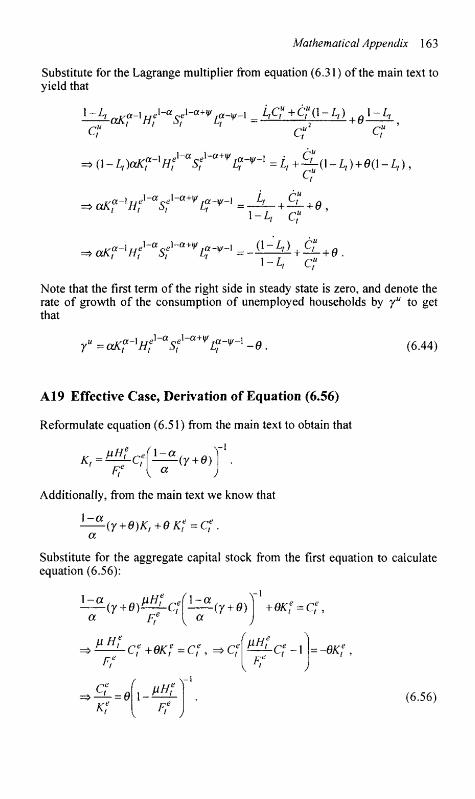
Substitute for the Lagrange multiplier from equation (6.31) of the main text to yield that
C? ' ' ' ' cf Cf '
=> (l-L,)C^rI^^f1"a+^^v'-, = A +4d- M+ea-4),
=*a/C ' i - A c,w
' ' ' l - A C,"
Note that the first term of the right side in steady state is zero, and denote the rate of growth of the consumption of unemployed households by yu to get that
7"=<VYa+YH-^ (6.44)
A19 Effective Case, Derivation of Equation (6.56)
Reformulate equation (6.51) from the main text to obtain that
Additionally, from the main text we know that
1-a
a '-(y + 0)K,+9Kf=Cf
Substitute for the aggregate capital stock from the first equation to calculate equation (6.56):
\-a a (7+0)
fiHf C
1-a - i
(7+0)1 +0Kf = Cf,
F,e
Kf
Cf+6K^=Cet, =>c; flHf Cf-l ••-6Kf
Ff (6.56)
164 Mathematical Appendix
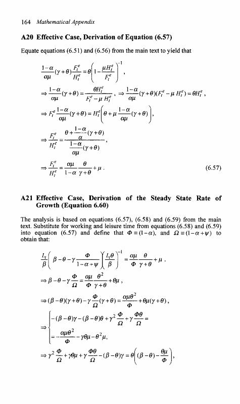
A20 Effective Case, Derivation of Equation (6.57)
Equate equations (6.51) and (6.56) from the main text to yield that
^ ( y + 0 ) 4 = 0 ap Hf
V^~' l-a, m OHf
=> (y + 0) = ——i-ap F?-»H<
r
e '
1-g ap
(y+0)(Fte-pHf) = 0H^9
Ftel—^(y+9) = H?
ap
l-a t 9 + p (y + 6)
ap
HI
* 0 + X—(y+0) t _ a * l-a
ap
Fte _ ap 0
-(7+0)
Het l-a y + 0
+ p. (6.57)
A21 Effective Case, Derivation of the Steady State Rate of Growth (Equation 6.60)
The analysis is based on equations (6.57), (6.58) and (6.59) from the main text. Substitute for working and leisure time from equations (6.58) and (6.59) into equation (6.57) and define that <Z> = ( l - a ) , and . Q = ( l - a + y O to obtain that:
p-o-r-±—W l-a + y/ I P
ap 0
0 y+e +p
Q „ 0 ap e2 . > P-0-y— = -£ • +0p ,
H a 0 y+e ^
>(P-0)(y + 0)-y^-(y + 0)--Q 0
apO2
+0p(y+0)9
20 &Q -(P-0)y-(P-0)0 + yz— + y — =
- °v°l-_7ep-e2p9 0
1 0 00
.r2- + ren + r — -(p-9)y = 9 03-0)-
0
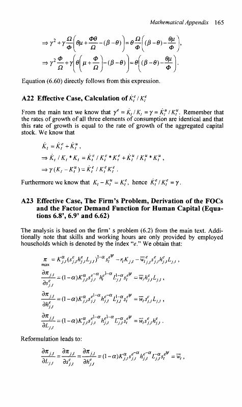
Mathematical Appendix 165
2 Q =*yl+y—
0 20
=>yz— + y
00 *+=£-V-e)U6- n
r r V + £2
-(P-9) = 9
(P-9)-^-0
W-9)-^ 0
Equation (6.60) directly follows from this expression.
A22 Effective Case, Calculation of k? IK?
From the main text we know that ye = K(IKt =y = K?IK?. Remember that the rates of growth of all three elements of consumption are identical and that this rate of growth is equal to the rate of growth of the aggregated capital stock. We know that
Kt-Kt +Kt ,
=> Kt IKt *Kt = K? IK? *K? + K? IK? *K? ,
=>y(Kt-K?) = K?IK?K?.
Furthermore we know that Kt - K? = K?9 hence K? IK? =y.
A23 Effective Case, The Firm's Problem, Derivation of the FOCs and the Factor Demand Function for Human Capital (Equations 6.8% 6.9' and 6.62)
The analysis is based on the firm' s problem (6.2) from the main text. Additionally note that skills and working hours are only provided by employed households which is denoted by the index "e" We obtain that:
max J J J J J J' J J J
" ^ / / n o-a J-a i n 0\u
dKj,t J-a, p-a 1-aeV-,
dLJJ
Reformulation leads to:
dftj t dKjt d7tjt aT~ ev -•-(\-a)K%sl, h)f L-a,sf=w,
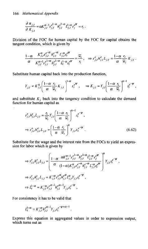
166 Mathematical Appendix
d KJJ -gKCc-l/^j/^jl-a eY _ jK -U^JJ sj,t nj,t ^j,t *j -n-
Division of the FOC for human capital by the FOC for capital obtains the tangent condition, which is given by
l - a KJJsj,t nj,t LjJst _wt
a va-l e^-auex~a A-a eV n
A y 7 sj,t nj,t h st
0e ue T _ l - a rt v
a w. 7^ J V ^ *
Substitute human capital back into the production function,
YJJ ~ KU l-a rt
x l - a
a wt
KU =>KJJ=YJ,< l-a rt
t a wt v t J
\a-l
and substitute Kj back into the tangency condition to calculate the demand function for human capital as
*e he r --1-Y l-a rt
a w,
\a-l
>shhhLjj = l-a rt
a wt
f Yjjsf (6.62)
Substitute for the wage and the interest rate from the FOCs to yield an expression for labor which is given by
aKa-xsel~ahel~aLx-ase¥
(l-a)KJytsJt hjt Ljtst
\a
Y se~¥
JJ t 9
c.e Ue T — V~a ve°{he<X' Ta Y ce ^ * sjjnjjLjjj — Ay,f sj,t nj,t 1^j,tIj,tst •>
jl-ct . Pa-l, Pa-\w
' Lt = KjJsjJ hj,t Yjjsi t >
For consistency it has to be valid that
Tl-a ir^Kfiifiyj.
a -1 e-y/+a-l
Express this equation in aggregated values in order to expression output, which turns out as
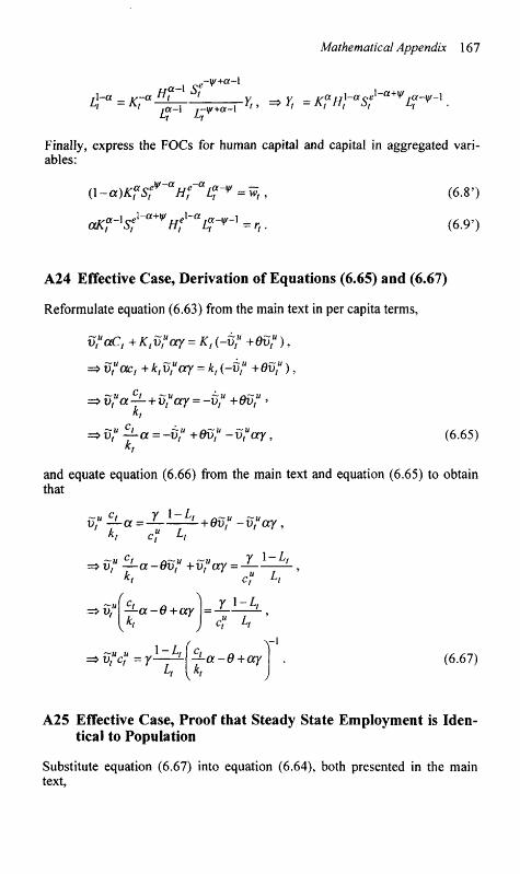
Mathematical Appendix 167
ir=/cr L „ _ , L7¥+a
e V+a-l
—Yt, =*y, =K?H)-aSf^vI%-V-x. rl-a _ ir-a **t f v _* v — F « U 1 - « C « ' a+V Ta-W-l
Finally, express the FOCs for human capital and capital in aggregated variables:
(l-a)^VV=^ aK?-xS?l-a+¥H?l-aLr^]=rt.
(6.8')
(6.9')
A24 Effective Case, Derivation of Equations (6.65) and (6.67)
Reformulate equation (6.63) from the main text in per capita terms,
vtuaCt + Ktvt
uay = Kt (-$? +0v?),
=> v?act + ktvtuay = kt (-ti? +0v?),
>vtua—+vt
uay = -v, + 0vtu >
K > vt
u —a = -0," +0vtu -vfay,
kt (6.65)
and equate equation (6.66) from the main text and equation (6.65) to obtain that
7 l -£/ 7 u* —
Kt Ct ^t vr —a = +0vt
u -v?ay,
^r« ct „ ck^u , „~H™, 7 * Lt >vr —a-Ovr +vray-Kt Ct
Lt
r i-A v,"
V,"
f \ ct •> —a-0+ay
„u_\~Lt \Ct
[K
Ct h
La-0+ay (6.67)
A25 Effective Case, Proof that Steady State Employment is Identical to Population
Substitute equation (6.67) into equation (6.64), both presented in the main text,
168 Mathematical Appendix
i,= ,lZ±L A
—a-9+ay -i r
+1
\ - l
Y(l-L,) + Lt ~a-9 + ay
^L,=
A y-a-9+ay
define that —a-9+ccy = t, to obtain that
=>!,= Al • 1 = £ -, =*rfl-A)+A«=5. y(l-A)+A<T ~y( i -A) + AS
y-yL,+L£=$, =>Y + L,($-7) = Z, => A(£-r)=£-r. L , = l .
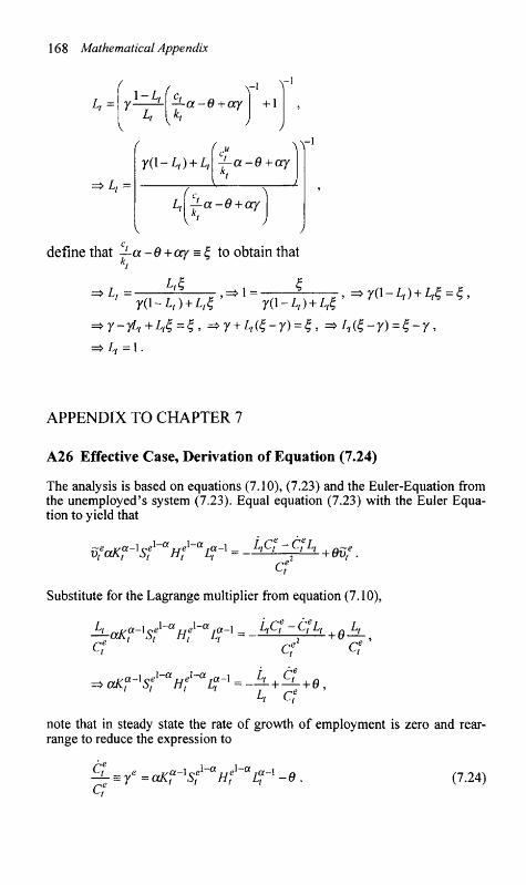
APPENDIX TO CHAPTER 7
A26 Effective Case, Derivation of Equation (7.24)
The analysis is based on equations (7.10), (7.23) and the Euler-Equation from the unemployed's system (7.23). Equal equation (7.23) with the Euler Equation to yield that
v,eaK?-lS?~aH?~aL?-'[ = -L'C>-C>L> +0v,e. ct
Substitute for the Lagrange multiplier from equation (7.10),
-Wafer's?"* H?-aLrl = _AQe-QeA+eJA_; cf cf cf
Lt Ct
note that in steady state the rate of growth of employment is zero and rearrange to reduce the expression to
^L EE f = aK?-lS?~aH?'<*1«-x -0 , (7.24)
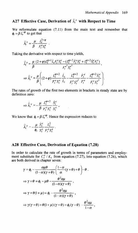
Mathematical Appendix 169
A27 Effective Case, Derivation of X,e with Respect to Time
We reformulate equation (7.11) from the main text and remember that 0,=pL^p to get that
V = M A 2 + * P F,eSf
Taking the derivative with respect to time yields,
fl (2 + <p)L^L,F,eSf - (Lf+2F,eSf + Lf+2SfF,e) V
• V P (2 + cp)
Ffsf r(p+2 j r(p+2 he r(jP+2Ae
Ut ^t Ut Ft Ut °f
F'Sf A F'Sf F' F,eSf
The rates of growth of the first two elements in brackets in steady state are by definition zero:
• V = -P LT1 S?
P FteS? S? '
We know that ^ =PL?P- Hence the expression reduces to
p _ I* Sf L2t
' 4>r S? FfS? '
A28 Effective Case, Derivation of Equation (7.28)
In order to calculate the rate of growth in terms of parameters and employment substitute for C? I Kt from equation (7.27), into equation (7.26), which are both derived in chapter seven:
y = (f)t apO
(l-a)(y + 0)
y+0 =<j)t-p0
l-a a
02ap
(y + 0) + 0 -0 .
.y + 0(l + fi) = 0,-
(l-a)(y + 0)
02ap ' (l-a)(y + 0)
^y(y + 0) + e(l + p)(y + e) = <j>t(y + 0) 02ap l-a
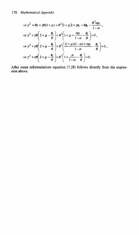
170 Mathematical Appendix
>y2+Oy + y0(l + p) + e2{l + p)) = ycl>t+e^-^L9
l-a
>y2+y0\2 + p-^ +e2\i+p+w--^ 1 ^ l-a 0
= 0,
^>y2+yO\2 + p-%- \+0 0
(l + p)(l-a) + ap h l-a 0 ' " '
>y2+y0 2 + p-?L * 0
\e>( 1 + V <t>t
l-a 0
After some reformulations equation (7.28) follows directly from the expression above.
Notes
1 Introduction
1. Even if claims on specific unemployment benefits are part of the wage negotiations, they depend solely on previous employment.
2. The formal description of the bargaining situations follows Oswald (1985) in a simplified and adapted form.
3. Manning (1987) showed that all three models may be regarded as special cases of a two-stage bargaining problem.
4. This is pointed out precisely by McDonald and Solow (1981). For a very short presentation and discussion see Blanchard and Fischer (1989), 442.
5. See Booth (1995) for a detailed discussion. 6. Compare the argumentation in chapter 2.2.2. 7. A discussion about this possibility has taken place in recent literature,
which was mainly based on the publications of Card and Krueger (1994 and 1995).
8. The examples follow Ragacs and Zagler (1998).
2 An Inquiry into the Theory of Minimum Wages
1. A very good presentation of the standard model can for instance be found in Fallon and Verry (1988).
2. For a short overview see Layard, Nickel und Jackman (1991). 3. Because of the existence of monopsony we are able to omit the index for
the number of firms. 4 These developments are best summarized by Boal and Ransom (1997). 5. For the description of the model see Zavodny (1998, 24). 6. Paragraphs one and two of this chapter are based on Zagler and Ragacs
(1999), paragraph three is based on Zagler and Ragacs (1998). 7. One of the basic ideas for endogenizing economic growth was contrib
uted much earlier by Arrow (1962). 8. Advisable books are: Barro and Sala-I-Martin (1995), Aghion and Howitt
(1998), Zagler (1999b), Solow (2000), Lucas (2002) Romer (2001 chapters 1-3); and on an introductory level: Jones (1997), and Gylfason (1999).
9. For an overview see Temple (1999). 10. The first to propose a correlation between unemployment and growth
was Arthur Okun (1970), but he described only an empirical correlation that was not theoretically founded.
11. For an overview of newer studies see Brown (1999). 12. See e.g. Card und Krueger (1995). 13. Meyer and Wise (1983). For the presentation see OECD (1998), 46. 14. For the discussion of elasticities see Ghellap (1998), 44-46 and 64 f., and
OECD (1998).
171
172 Notes
3 Minimum Wages and "General Equilibrium": Methodological Problems
1. A simple and recommendable introduction to Walrasian economics is provided by Katzner (1988).
2. A quick view of these theories can be found in Snowdown, Vane and Wynarczyk (1994), 109-23. Benassy (1982), Cuddington, Johansson and Lofgren (1984), and Dreze (1991) are also recommended.
3. Malinvaud first published his work in 1977. The second edition of his work (Malinvaud 1985, 16 ff.) serves as a basis for the illustration and the notation in this chapter. It has, however, been partly adapted. The assumptions that deviate from Malinvaud have been marked. The state sector was left out of the analysis completely.
4. The argumentation in this paragraph follows Rothschild (1981, 77 f.). 5. A7-A10 and A12 follow directly from Malinvaud (1985), 21 ff. 6. Endowment e.g. could be the maximum quantity of possible labor hours,
initial financial wealth or initial amount of goods.
4 Supporting the Partial Equilibrium Results
1. As will be shown later, the minimum wage has a positive effect on the price level of goods. It is, however, in such a small amount that in equilibrium the real minimum wage is also higher than the original real market wage, as will be explained later.
2. We have to use this unusual notation because in later models we will denote educational time by E and we will also introduce investment, then denoted by /.
3. The process introduced here corresponds with the standard solution for the problem described in several textbooks. Compare for instance Varian (1992, 54 f.), where the corresponding functions are generally derived for the Cobb-Douglas production function with unspecified scales of return and for the special case of constant returns.
4. Rearrange the utility function,
InC, =£/,(.)-/; lnF /?
and differentiate to yield,
dine,-, dlnFj |f/,.(.)=cr(.) ~
5. For a Lagrange representation of the Kuhn-Tucker Problem see for instance Chiang (1984), 724 ff.
6. See mathematical appendix, A1. 7. See mathematical appendix, Al. 8. See mathematical appendix, Al. 9. See mathematical appendix, A2.
10. See mathematical appendix, A3. 11. See mathematical appendix, A4.
Notes 173
12. See mathematical appendix, A5. 13. See mathematical appendix, A6. 14. See mathematical appendix, A7. 15. In the growth models presented later, investments are meaningful. Higher
total wages can lead to an increase in savings and hence in investment.
5 Minimum Wages, Unemployment and the Creation of Human Capital
1. Given the technical properties of the Cobb-Douglas production function, it is impossible for Z,V to become zero.
2. The technical properties of the consumption function are described in chapter four.
3. A similar assumption has to be implicitly set in any partial equilibrium micro model with labor-leisure choice.
4. See mathematical appendix, A8. 5. The calculation of the cost function follows the same methodology as the
calculation of the cost function in chapter four. See mathematical appendix, A3.
6. See mathematical appendix, A9. 7. See mathematical appendix, A9. The parameter restriction necessary to
guarantee a positive function is identical to the restriction necessary for the time constraint (see mathematical appendix). Note that for any deviation from the assumption of 1=1, we would yield the formulation piL instead of/?.
8. See mathematical appendix, AlO. 9. See mathematical appendix, All .
10. See mathematical appendix, A12. 11. See mathematical appendix, A12. 12. Of course, this expression could be easily reformulated as a function of
"physical labor" alone, but the used representation helps to simplify the analytical treatment. Note that
SeL\e = Se I L*,e * L*,e = Se.
13. See mathematical appendix, A13. 14. At first sight, there exist some other necessary restrictions, but they can
all be reduced to the two restrictions given above.
6 Minimum Wages, Human Capital and Growth
1. A good and short technical description of the basic Lucas model may be found in Sala-I-Martin (1990) or Barro and Sala-I-Martin (1995).
2. Remember that we use this unusual notation because we will denote educational time by Et.
3. Here we must anticipate the analysis presented later, where the behavior of the households is described precisely.
4. Due to the production technology presented later and the existence of perfect competition, economic profits must be zero.
174 Notes
5. Compare Barro and Sala-I-Martin (1995, 172) for the case without endogenous working time.
6. The felicity function fulfills the Inada conditions: z/Q-^ooas (.)->0, and u'(.)->0 as (.)-»«>.
7. The formal proof of the properties of a more broadly defined utility function, where the one used represents a subcase, was given by Barro and Sala-I-Martin (1995, 326 ff).
8. Compare Barro and Sala-I-Martin (1995, 172). 9. Of course, households do not care about average levels of skills and
working time, as firms do. 10. The argumentation of A15 is based on the derivation of the FOCs from
equation (6.10), which will be presented in the beginning of the next chapter. Hence we recommend reading this part of the text first.
11. A very good representation of Hamiltonian maximization can for example be found in Chiang (1992, 210 ff).
12. The derivation of the FOCs in the notional case follows the same methodology as the derivation in the effective case with the additional assumption that employment is normalized to one. See mathematical appendix, A23.
13. Substitute back into equation (6.21) to prove that this is one of the possible solutions.
14. See mathematical appendix, A16. 15. All remaining necessary mathematical derivations for the calculation of
the steady state rate of growth of the economy are presented in the mathematical appendix, A17.
16. Compare the presentations in Barro and Sala-I-Martin (1995, 65, and 182 ff).
17. The equilibrium wage w* at point zero is identical to the equilibrium wage of the notional system.
18. See mathematical appendix, A23. 19. Given the information about the maximization problems of employed
and unemployed households the equations presented in the chapter „mac-roeconomic relations" could be adapted easily for this model.
20. To see that this assumption is fulfilled, substitute by the rate of growth that will be derived later.
21. See mathematical appendix, A18. 22. To see that this assumption is fulfilled, substitute by the rate of growth
that will be derived later. 23. See mathematical appendix, A18. 24. See mathematical appendix, A22. 25. See mathematical appendix, A19. 26. Note, for the proof that shows that in steady state we will achieve full-
employment, this assumption and all results derived from it, are not necessary. We present the proof later to provide a structure of the model's presentation, which is mostly identical to that of the notional case.
27. See mathematical appendix, A20. 28. See mathematical appendix, A23. 29. See mathematical appendix, A23. 30. We do not have to change the shadow prices.

Notes 175
31. See mathematical appendix, A24. 32. See mathematical appendix, A24. 33. See mathematical appendix, A25. 34. Remember the standard properties of the utility function.
7 Minimum Wages, Unemployment and Growth
1. This formulation of the production function of skills is only used to simplify the presentation as much as possible. However, it induces an over-proportional reaction on unemployment. A linear reaction could for instance be expressed by, ^=p(l+cp(l-Lt))9 <p>0.
2. We do not simplify the rate of growth in order to show the connection to the result of chapter six, equation (6.28).
3. The solution of the firm's problem and the aggregation is obtained by using the same methodology as is presented in the mathematical appendix A23, with the exception that there exists no external effect in production.
4. Compare the derivation of equations (6.42) - (6.48) in chapter six. 5. See mathematical appendix, A26. 6. See mathematical appendix, A27. 7. Note, for the proof that shows that in steady state we will achieve full-
employment, this assumption and all results derived from this assumption are not necessary.
8. See mathematical appendix, A28.
8 Conclusions
1. The theory of the "Second Best" states that violating one Pareto-criterion also induces the violation of all other criteria, which is problematic for decision-finding.
Bibliography
1. In light of the importance of some specific publications on minimum wages which have not been available to the author, we must in some cases refer to the literature in which they have been cited.
Bibliography
Abowd, J. M., Kramarz, F., Lemieux, T. and Margolis, D. N. (1997) "Minimum Wages and Youth Employment in France and the United States," National Bureau of Economic Research, Working Paper, 6111.
Acemoglu, D. and Pischke, J. S. (1999) "Minimum Wages and On-The-Job Training," National Bureau of Economic Research, Working Paper, 7184.
Acemoglu, D., Pischke, J. S. (2002) "Minimum Wages and On-the-Job Training," Centre for Economic Performance, Discussion Papers, CEPDP0527 (http://cep.lse.ac.uk/pubs/download/DP0527.pdf).
Aghion, P. and Howitt, P. (1998) Endogenous Growth Theory (Cambridge: MIT Press).
Aghion, P., Caroli, E. and Garcia-Penalosa, C. (1999) "Inequality and Economic Growth: The Perspective of the New Growth Theories," Journal of Economic Literature, 37(4), December, 1615-60.
Albrecht, J. W. and Axell, B. (1984) "An Equilibrium Model of Search Unemployment," Journal of Political Economy, 92(5), 824-40.
Arrow, K. J. (1962) "The Economic Impact of Learning by Doing," Review of Economic Studies, 29, 155-73.
Arulampalam, W., Booth, A. L. and Bryan, M. L. (2002) "Work-related Training and the New National Minimum Wage in Britain," Institute for the Study of Labor (IZA), Discussion Paper, 595 (ftp://repec.iza.org/ Re-PEc/Discussionpaper/dp595.pdf).
Ashenfelter, O., Card, D., eds (1999) Handbook of Labor Economics, Volume 3B (Princeton: Princeton University Press).
Baker, M., Dwayne, B. and Stanger, S. (1997) "The Highs and Lows of the Minimum Wage Effect: A Time Series-Cross Section Study of the Canadian Law," Toronto University, mimeo; cited according to OECD (1998), Employment Outlook, 11 (Paris: OECD Publications).1
Baker, M., Benjamin, D. and Stanger, S. (1999) "The Highs and Lows of the Minimum Wage Effect: A Time-Series Cross-Section Study of the Canadian Law," Journal of Labor Economics, 17(2), 318-50.
Ball, L. and Mankiw, G. N. (1995) "What do Deficits do?," National Bureau of Economic Research, Working Paper, 5263.
Barro, R. J. and Sala-1-Martin, X. (1995) Economic Growth (New York: McGraw Hill).
Bazen, S. and Martin, J. P. (1991) "The Impact of the Minimum Wage on Earnings and Employment in France," OECD Economic Studies, 16, 199-221.
Bazen, S. and Marimoutou, V. (1997) "Looking for a Needle in a Haystack? A Re-examination of the Time Series Relationship Between Teenage Employment and Minimum Wages in the United States, " Universite Montesquieu Bordeaux IV, France, mimeo; cited according to OECD (1998), Employment Outlook, 11 (Paris: OECD Publications).
176
Bibliography 111
Bazen, S. and Skourias, N. (1997) "Is there a Negative Effect of Minimum Wages in France?," European Economic Review, 41, 723-32.
Bazen, S. and Marimoutou, V. (2002) "Looking for a Needle in a Haystack? A Re-examination of the Time Series Relationship between Teenage Employment and Minimum Wages in the United States," Oxford Bulletin of Economics and Statistics, 64/ Supplement, 699-725.
Bean, C. and Pissarides, C. (1993) "Unemployment, Consumption and Growth," European Economic Review, 37, 837-59.
Bell, L. A. (1995) "The Impact of Minimum Wages in Mexico and Columbia," The World Bank Policy Research, Working Paper, No. 1514; cited according to OECD (1998), Employment Outlook, 11 (Paris: OECD Publications).
Benassy, J. P. (1982) The Economics of Market Disequilibrium (New York: Academic Press).
Ben-David, D. (1996) "Trade and Convergence Among Countries," Journal of International Economics, 40(3/4), 279-98.
Benhabib, J. and Spiegel, M. (1994) "The Role of Human Capital in Economic Development: Evidence from Aggregate Cross-Country Data," Journal of Monetary Economics, 34, 143-74.
Benhayoun, G. (1994) "The Impact of Minimum Wages on Youth Employment in France Revisited: A Note on The Robustness of the Relationship," International Journal of Manpower, 15, 82-5.
Bhaskar, V. and To, T. (1998) "Minimum Wages for Ronald McDonald Monopsonies: A Theory of Monopsonistic Competition," Universities of Essex and Warwick, mimeo (http://econwpa.wustl.edu:8089/eps/lab/pa-pers/ 9603/960300 l.pdf).
Bhaskar, V. and To, T. (1999) "Minimum wages for Ronald McDonald monopsonies: a theory of monopsonistic competition, " Economic Journal, 109, pi90-203.
Black, D. A. and Loewenstein, M. A. (1991) "Self-enforcing Labor Contracts with Costly Mobility," in: Ehrenberg, R. G. (ed.), Research in Labor Economics. A Research Annual, 12, 3-83 (Greenwich: JAI Press).
Blanchard, O. J. and Fischer, S. (1989) Lectures on Macroeconomics (Cambridge and London: MIT-Press).
Boal, W. M. and Ransom, M. R. (1997) "Monopsony in the Labor Market," Journal of Economic Literature, 35(1), 86-112.
Booth, A. L. (1995) The Economics of the Trade Union (Cambridge: Cambridge University Press).
Brander, J. and Dowrick, S. (1994) "The Role of Fertility and Population in Economic Growth: Empirical Results from Aggregate Cross-national Data," Journal of Population Economics, 7(1), 1-25.
Brown C, Gilroy C. and Kohen, A. (1982) "The Effects of the Minimum Wage on Employment and Unemployment," Journal of Economic Literature, 20(2), 487-528.
Brown C, Gilroy C. and Kohen, A. (1983) "Time Series Evidence of the Effects of the Minimum Wage on Youth Employment and Unemployment," Journal of Human Resources, 18(1), 3-31.
Brown, C. (1988) "Minimum Wage Laws, Are They Overrated?," The Journal of Economic Perspectives, 2(3), 133-45.
178 Bibliography
Brown, C. (1999) "Minimum Wages, Employment and the Distribution of Income," in: Ashenfelter, O., Card, D., eds Handbook of Labor Economics, Volume 3B (Princeton: Princeton University Press).
Bruno, M. and Easterly, W. (1998) "Inflation Crises and Long-run Growth," Journal of Monetary Economics, 41(1), 3-26.
Burdett, K. and Mortenson, D. T. (1989) "Equilibrium Wage Differentials and Employer Size," Northwestern University, Working Paper, 860; cited according to Zavodny, M. (1998) "Why Minimum Wage Hikes May not Reduce Employment," Federal Reserve Bank of Atlanta Economic Review, Second Quarter, 18-28.
Burkhauser, R. V., Couch, K. A. and Wittenburg, D. (1977) "Who Minimum Wage Increases Bite: An Analysis Using Monthly Data from the SIPP and the CPS," Centre for Policy Research, Syracuse University, New York, mimeo; cited according to OECD (1998), Employment Outlook, 11 (Paris: OECD Publications).
Burkhauser, R. V., Couch, K. A and Wittenburg, D. C. (2000) "A Reassessment of the New Economics of the Minimum Wage Literature with Monthly Data from the Current Population Survey," Journal of Labor Economics, 18(4), 653-80.
Cahuc, P. and Michel, P. (1996) "Minimum Wage, Unemployment and Growth," European Economic Review, 40(7), 1463-82.
Calmfors, L. and Driffill, J. (1988) Bargaining Structure, Corporatism and Macroeconomic Performance, Economic Policy, 6, 13-61.
Calvo, G. A. and Wellisz, S. (1979) "Hierarchy, Ability, and Income Distribution," Journal of Political Economy, 87(5), Part 1, 991-1010.
Card, D. (1992) "Using Regional Variation in Wages to Measure the Effects of the Federal Minimum Wage," Industrial and Labor Relations Review, October, 38-54.
Card, D. and Krueger, A. B. (1994) "Minimum Wages and Employment: A Case Study of the Fast Food Industry in New York and Pennsylvania," American Economic Review, 84, 772-93.
Card, D. and Krueger, A. B. (1995) Myth und Measurement, The New Economics of the Minimum Wage (Princeton: Princeton University Press).
Card, D. and Krueger, A. B. (1998) "A Reanalysis of the Effect of the New Jersey Minimum Wage Increase on the Fast-Food Industry with Representative Payroll Data," Industrial Relations Section, Princeton University, Working Paper, 293, (http://netec.mimas.ac.uk/WoPEc/data/Papers/ nbrnberwo63 86.html).
Card, D. and Krueger, A., B. (2000) "Minimum Wages and Employment: A Case Study of the Fastfood Industry in New Jersey and Pennsylvania - Reply," American Economic Review, 90(5), 1397-420.
Carley, M. (2002) "Industrial Relations in the EU, Japan and USA, 2000," European Industrial Relations Observatory (http://www.eiro.eurofound.ie /2001/1 l/feature/tn0111148f.html, 1.4.2003, 2002).
Carley, M. (2003) "Industrial Relations in the EU, Japan and USA, 2001," European Industrial Relations Observatory (http://www.eiro.euro-found.ie/ 2002/12/feature/TN0212101F.html, 1.4.2003, 2003).
Bibliography 179
Carter, T. J. (1998) "Minimum Wage Laws: What does an Employment Increase imply about Output and Welfare?," Journal of Economic Behaviour & Organization, 36, 473-85.
Cass, D. (1965) "Optimum Growth in an Aggregative Model of Capital Accumulation," Review of Economic Studies, 32, 233-40.
Chappie, S. (1997) "Do Minimum Wages Have an Adverse Impact on Employment? Evidence from New Zealand," Labour Market Bulletin, 2; cited according to OECD (1998), Employment Outlook, 11 (Paris: OECD Publications).
Chiang, A. C. (1984) Fundamental Methods of Mathematical Economics, 3rd edn (Auckland: McGraw-Hill).
Chiang, A. C. (1992) Elements of Dynamic Optimization (New York et al.: McGraw-Hill).
Cooley, T. F., ed. (1995) Frontiers of Business Cycle Research (Princeton: Princeton University Press).
Cooley, T. F. and Prescott, E. C. (1995) "Economic Growth and Business Cycles," in: Cooley. T. F., ed. Frontiers of Business Cycle Research (Princeton: Princeton University Press), 1-38.
Crouch, C. and Traxler, F. (1995) Organized Industrial Relations in Europe: What Future? (Aldershot: Avebury).
Cuddington, J. T., Johansson, P. O. and Lofgren, K. G. (1984) Disequilibrium in Open Economies (Oxford: Basil Blackwell).
Currie, R. P. and Fallick, B. C. (1996) "The Minimum Wage and the Employment of Youth: Evidence from the NLSY," Journal of Human Resources, Spring 404-28.
Davidson, P. (1994) Post Keynesian Macroeconomic Theory (Brookfield: Edward Elgar).
Deere, D., Murphy, K. M. and Welch, F. (1995) "Reexamining Methods of Estimating Minimum Wage Effects: Employment and the 1990-91 Minimum Wage Hike," American Economic Review, Papers und Proceedings, May, 232-37.
Deininger, K. and Squire, L. (1997) "Economic Growth and Income Inequality: Reexamining the Links," Finance and Development, March, 38-41.
Dickens, R., Machin, S. and Manning, R. (1994) "Estimating the Effect of Minimum Wages on Employment from the Distribution of Wages: A Critical Review," Centre for Economic Performance, Discussion Paper, 203, (http:// netec.mimas.ac.uk/WoPEc/data/Papers/cepcepdps0203 .html).
Dickens, R. and Machin, S. (1999) "The Effects of Minimum Wages on Employment: Theory and Evidence from Britain," Journal of Labor Economics 17(1), 1-22.
Dolado, J., Kramarz, F., Machin, S., Manning, A., Margolis, D. and Teulings, C. (1996) "The Economic Impact of Minimum Wages in Europe," Economic Policy, October, 319-70.
Domar, E. D. (1946) "Capital Expansion, Rate of Growth, and Employment," Econometrica, 14, 137-47.
Dreze, J. H. (1991) Underemployment Equilibria. Essays in Theory, Econometrics and Policy (Cambridge: Cambridge University Press).
Ehrlich, I. and Lui, F. (1997) "The Problem of Population and Growth: A Review of the Literature from Malthus to Contemporary Models of En-
180 Bibliography
dogenous Population and Endogenous Growth," Journal of Economic Dynamics and Control, 21, 205-42.
Evans, G. W., Honkapohja, S. and Romer, P.M. (1998) "Growth Cycles," American Economic Review, 88(3), 495-515.
Fallon, P. and Verry, D. (1988) The Economics of Labour Markets (Oxford and New Jersey: Phillip Allan Publishers).
Ghellap, Y. (1998) "Minimum Wages and Youth Unemployment," International Labour Office, Employment and Training Department, Employment and Training Papers, 26.
Gramlich, E. (1976) "The Impact of Minimum Wages on Other Wages, Employment and Family Incomes," Brookings Papers of Economic Activity, 2,409-51.
Gregory, M. and Swaffield, J. K. (2002) "Preface: Evaluating the Impact of the UK National Minimum Wage," Oxford Bulletin of Economics and Statistics, 64/ Supplement, 565-66.
Grossman, J. B. (1983) "The Impact of the Minimum Wage on other Wages," Journal of Human Resources, 90, 359-78.
Grossman, G. M. and Helpman, E. (1991) Innovation and Growth in the Global Economy (Cambridge and London: The MIT Press).
Grossman, G. M. and Helpman, E. (1994) "Endogenous Innovations and the Theory of Growth," Journal of Economic Perspectives, 8, 23-44.
Gylfason, T. (1999) Principles of Economic Growth (Oxford: Oxford University Press).
Harrod, R. F. (1939) "An Essay in Dynamic Theory," The Economic Journal, 49, 14-39.
Huemer, G., Mesch, M., and Traxler, F., eds (1999) The Role of Employer Associations and Labour Unions in the EMU. Institutional Requirements for Europe and Economic Policies (Aldershot: Avebury).
Jones, C. I. (1997) An Introduction to Economic Growth (New York and London: W.W. Norton and Company)
Jones, S. R. G. (1987) "Minimum Wage Legislation in a Dual Labor Market," European Economic Review, 31, 1229-46.
Katzner, D. W. (1988) Walrasian Microeconomics. An Introduction to the Economic Theory of Market Behavior (New York: Addison-Wesley).
Koopmans, T. C. (1965) "On the Concept of Optimal Economic Growth," in: The Econometric Approach to Development Planning, (Amsterdam: North Holland).
Kosters, M. and Welch, F. (1972) "The Effects of Minimum Wage by Race, Sex, and Age," in: Pascall, A., ed. Racial Discrimination in Economic Life (Lexington: Heath) 103-18.
Koutsogeorgopoulou, V. (1994) "The Impact of Minimum Wages on Industrial Wages and Employment in Greece," International Journal of Manpower, 2/3, 86-99.
Lang, K. and Kahn, S. (1998) "The Effect of Minimum Wage Laws on the Distribution of Employment: Theory and Evidence," Journal of Public Economics, 69, 67-82.
Larcon, J. P., ed. (1998) Entrepreneurship and Economic Transition in Central Europe (Boston, Dortrecht and London: Kluwer Academic Publishers)
Bibliography 181
Layard, N., Nickel, S. and Jackman, R. (1991) Unemployment, Macroeconomic Performance and the Labour Market (Oxford: Oxford University Press).
Lindahl, M. and Krueger, A. B. (1998) "Education in Sweden and the World," Harvard University, mimeo (http://www.nuff.ox.ac.uk/Econom-ics/Growth/ refs/humanc.htm).
Lucas R. E., Jr. (1988) "On the Mechanics of Economic Development," Journal of Monetary Economy, 22(1), July, 3-42.
Lucas, R. E., Jr. (2002) Lectures on Economic Growth (Cambridge and London: Harvard University Press).
Machin, S. and Manning, A. (1994) "The Effects of Minimum Wages on Wage Dispersion and Employment: Evidence from the UK Wage Councils," Industrial and Labor Relations Review, January, 319-329.
Machin, S. and Manning, A. (1997) "Minimum Wages and Economic Outcomes in Europe," European Economic Review," 41, 733-742.
Malinvaud, E. (1985) The Theory of Unemployment Reconsidered, 2nd edn (Oxford and New York: Basil Blackwell).
Maloney, T. (1995) "Does the Adult Minimum Wage Affect Employment and Unemployment in New Zealand?," New Zealand Economic Papers, 1, 1-19; cited according to OECD (1998), Employment Outlook, 11 (Paris: OECD Publications).
Mankiw, G., N., Romer, D. and Weil, D. N. (1992) "A Contribution to the Empirics of Economic Growth," Quarterly Journal of Economics, 107 (2), 407-37.
Manning, A. (1987) An Integration of Trade Union Models in a Sequential Bargaining Framework, The Economic Journal, 97, 121-39.
Mare, D. (1995) "Comments on Maloney, T., Does the Adult Minimum Wage Affect Employment and Unemployment in New Zealand?," New Zealand Department of Labour, mimeo; cited according to OECD (1998), Employment Outlook, 11 (Paris: OECD Publications).
Marshall, A. (1890) Principles of Economics (London: Macmillan). McDonald, I. M. and Solow, R. M. (1981) "Wage Bargaining and Employ
ment," American Economic Review, 71(5), 896-908. Meyer, R. H. and Wise, D. A. (1983) "Discontinuous Distributions and
Missing Persons: The Minimum Wage and Unemployment Youth," Eco-nometrica, 51/6, 1677-98.
Mincer, J. (1976) "Unemployment Effects of Minimum Wages," Journal of Political Economy, 84, 87-104.
Murat, M. and Pigliaru, F. (1998) "International Trade and Uneven Growth: A Model with Intersectoral Spillovers of Knowledge," Journal of International Trade and Economic Development, 7, 221-36.
Neumark, D. and Wascher, W. (1992) "Employment Effects of Minimum and Sub-minimum Wages: Panel Data in State Minimum Wage Laws, Industrial and Labor Relations Review, October, 55-8.
Neumark, D. and Wascher, W. (1995) "Minimum Wage Effects on Employment and Enrolment: Evidence from Matched CPS Surveys," National Bureau of Economic Research, Working Paper, 5092.
182 Bibliography
Neumark, D. and Wascher, W. (2000) "Minimum Wages and Employment: A Case Study of the Fastfood Industry in New Jersey and Pennsylvania -Comment," American Economic Review, 90(5), 1397-420.
Neumark, D. and Wascher, W. (2003) "Minimum Wages, Labor market Institutions and Youth Employment: A Cross-National Analysis," Board of Governors of the Federal Reserve System, Finance and Economics Discussion Series, 2003-23 (http://www.federalreserve.gov/pubs/feds/2003/ 200323/ 200323pap.pdf).
Nickel S. J., and Andrews, M. (1983) "Unions, Real Wages and Employment in Britain 1951-79: The Minimum Wage and Unemployment Youth," Oxford Economic Papers, 35(0), Supplement 1983, 183-206.
OECD (1998) Employment Outlook, 77 (Paris: OECD Publications). Okun A. (1970) "Potential GDP: Its Measurement and Significance," re
printed in Okun, A., ed., The Political Economy of Prosperity (Washington, D.C: Brookings Institution).
Okun, A., ed. (1970), The Political Economy of Prosperity (Washington, D.C: Brookings Institution).
Orazem, P. F. and Mattila, P. J. (1998) "Minimum Wage Effects on Hours, Employment and Number of Firms: The Iowa Case," Iowa State University, mimeo (http://www.econ.iastate.edu/research/webpapers/ NDN0020.pdf).
Oswald, A. J. (1985) "The Economic Theory of Trade Unions: An Introductory Survey," Scandinavian Journal of Economics, 87(2), 160-93.
Pascall, A., ed., Racial Discrimination in Economic Life (Lexington: Heath). Penrod, J. H. (1995) "A Test for Monopsony in the Academic Labor Market,"
University of Michigan, Working Paper, Sept.; cited according to Boal, W. M. and Ransom, M. R. (1997) "Monopsony in the Labor Market," Journal of Economic Literature, 35(1), 86-112.
Ragacs, C. (1993a) "Minimum Wages in Austria: Estimation of Employment Functions," Vienna University of Economics and Business Administration, Department of Economics Working Paper Series, 20.
Ragacs, C. (1993b) "Employment, Productivity, Output and Minimum Wages in Austria: A Time Series Analysis," Vienna University of Economics and Business Administration, Department of Economics, Working Paper Series, 21.
Ragacs, C. and Zagler, M. (1998) "Wachstumsstrategien flir Osterreich in einem ver&nderten Mitteleuropa," in: Kompetenzzentrum Wien (Vienna: Service Verlag), 261-69.
Ramsey, F. (1928) "A Mathematical Theory of Saving," Economic Journal, 38 (December), 543-59.
Raven, M. O. and Sorenson, J. R. (1995) "Minimum Wages: Curse or Blessing," Centre for Economic Policy Research, Discussion Paper, 1212.
Raven, M. O. and Sorenson, J. R. (1999) "Schooling, Training, Growth and Minimum Wages," Scandinavian Journal of Economics, 101(3), 441-57.
Rebitzer, J. B. and Taylor, L. J. (1991) "The Consequences of Minimum Wage Laws, Some New Theoretical Ideas," National Bureau of Economic Research, Working Paper, 3S11'.
Rebitzer, J. B. and Taylor, L. J. (1995) "The Consequences of Minimum Wage Laws, Some New Theoretical Ideas," Journal of Public Economics, February, 245-55.
Bibliography 183
Romer, D. (2001) Advanced Macroeconomics, 2nd edn (Boston, Mass.: McGraw-Hill).
Romer, P. M. (1990) "Endogenous Technological Change," Journal of Political Economy, 98, 71-102.
Romer, P. M. (1986) "Increasing Returns and Long-Run Growth," Journal of Political Economy, 94, 1002-35.
Rosen, S. (1972) "Learning and Experience in the Labor Market," Journal of Human Resources, 7, 326-442.
Rothschild, K. W. (1981) Einfuhrung in die Ungleichgewichtstheorie (Berlin: Springer).
Sala-I-Martin, X. (1990) "Lecture Notes on Economic Growth (II), Five Prototype Models of Endogenous Growth," National Bureau of Economic Research, Working Paper, 3564.
Schumpeter, J. A. (1912) Theorie der wirtschaftliehen Entwicklung (Leipzig: Duncker & Humblot).
Shapiro, C. and Stiglitz, J. E. (1984) "Equilibrium Unemployment as a Workers Discipline Device," The American Economic Review, 74(3), 433-44.
Skinner, C, Stuttard, N., Beissel-Durrant, G., and Jenkins, J. (2002) "The Measurement of Low Pay in the UK Labour Force Survey," Oxford Bulletin of Economics and Statistics, 64/Supplement, 653-76.
Snowdown, B., Vane, H. and Wynarczyk, P. (1994) A Modern Guide to Macroeconomics. An Introduction to Competing Schools of Thought (Brookfield: Edward Elgar).
Solow, R. M. (1956) "A Contribution to the Theory of Economic Growth," Quarterly Journal of Economics, 71, 65-94.
Solow, R. M. (2000) Growth Theory: An Exposition, 2nd edn (Oxford: Oxford University Press).
Soskice, D. (1990), "Wage Determination: The Changing Role of Institutions in Advanced Industrialized Countries," Oxford Review of Economic Policy, 6/4,36-61.
Stewart, M. B. (2002) "Estimating the Impact of the Minimum Wage Using Geographical Wage Variation," Oxford Bulletin of Economics and Statistics, 64/Supplement, 583-605.
Stigler, G. (1946) "The Economics of Minimum Wage Legislation," American Economic Review, 36, 358-365.
Swinnerton, K. A. (1996) "Minimum Wages in an Equilibrium Search Model with Diminishing Returns to Labor in Production," Journal of Labor Economics, 2, 340-355.
Temple, J. R. W. (1999) "A Positive Effect of Human Capital on Growth," Economic Letters, 65(1), 131-34.
Temple, J. R. W. (1999) "The New Growth Evidence," Journal of Economic Literature, 18(1), 112-56.
Teulings, C. N. (1998) "Aggregation Bias in Elasticities of Substitution and the Minimum Wage Paradox," Tinbergen Institute, Discussion Papers, 98-118/3 (http://www.tinbergen.nl/discussionpapers/98118.pdf)
Topel, R. (1998) "Labor Markets and Economic Growth," University of Chicago, mimeo (http://gsbmxn.uchicago.edu/sole/topel.pdf).
184 Bibliography
Traxler, F. (1999) "Wage-Setting Institutions and European Monetary Union," in: Huemer, G., Mesch, M. and Traxler, F., eds, The Role of Employer Associations and Labour Unions in the EMU. Institutional Requirements for European Economic Policies (Aldershot: Avebury), 115-36.
Traxler, F. and Kittel, B. (2000) "The Bargaining System and Performance. A Comparison of 18 OECD Countries," Comparative Political Studies, 33/9, 1154-90.
Traxler, F., Blaschke, S. and Kittel, B. (2001) National Labour Relations in Internationalized Markets: A Comparative Study of Institutions, Change, and Performance (Oxford: Oxford University Press).
Traxler (2002) "Funktion und Wandel der Institutionen der Lohnregulierung," Wirtschaft und Gesellschaft," 28/4, 471-88.
Varian, H. G. (1992) Microeconomic Analysis, 3rd edn (New York: W. W. Norton and Company)
Walsh, F. (2003) "Comment on 'Minimum Wages for Ronald McDonald Monopsonies: A Theory of Monopsonistic Competition'," The Economic Journal, 113,718-22.
Welch, F. (1974) "Minimum Wage Legislation in the United States," Economic Inquiry, 12(3), 285-318.
WIFO (1999) Database of the (iAustrian Institute of Economic Research (Osterreichisches Institut fur Wirtschaftsforschung), restricted access.
Zagler, M. (1999a) "Endogenous Growth, Efficiency Wages, and Persistent Unemployment," Vienna University of Economics and Business Administration, Department of Economics, Working Paper Series, 66, (http://www.wu-wien.ac.at/inst/vw2/papers/wu-wp66.pdf).
Zagler, M. (1999b) Endogenous Growth, Market Failures, and Economic Policy (Basingstoke: Macmillan).
Zagler, M. and Ragacs, C. (1998) "Company Co-operations between Eastern and Western Europe: A Key Role in the Development of Eastern Europe," in: Larcon, J. P., ed., Entrepreneurship and Economic Transition in Central Europe (Boston, Dortrecht and London: Kluwer Academic Publishers), 163-75.
Zagler, M. and Ragacs, C. (1999) "Endogenous Growth, Division of Labour, and Fiscal Policy," in: Zagler, M., Endogenous Growth, Market Failures, and Economic Policy (Basingstoke: Macmillan), 27-45.
Zagler, M. (2004) Growth and Employment in Europe (Basingstoke: Pal-grave/Macmillan).
Zavodny, M. (1998) "Why Minimum Wage Hikes may not Reduce Employment," Federal Reserve Bank of Atlanta Economic Review, Second Quarter, 18-28.
Index of Names
Abowd,J.M. 34,176 Acemoglu, D. 29, 176 Aghion, P. 27,28, 171,176 Albrecht, J. W. 21, 176 Andrews M. 1,182 Arrow, K. J. 69, 171, 176 Arulampalam, W. 29, 176 Ashenfelter, O. 176, 178 Axell,B. 176
Baker, M. 33, 34, 176 Ball,L. 9,176 Barro, R. J. 10, 28, 171, 173, 174,
176 Bazen, S. 32,33,34,176, 177 Bean,C. 28,177 Beissel-Durrant, G. 183 Bell, L. A. 32,177 Benassy, J. P. 172, 177 Ben-David, D. 28, 177 Benhabib,J. 10,177 Benhayoun, G. 32,177 Benjamin, D. 176 Bhaskar, V. 26,177 Black, D. A. 21,177 Blanchard, O. J. 171,177 Blaschke, S. 184 Boal, W. M. 171, 177, 182 Booth, A. L. 29, 171, 176, 177 Brander, J. 28,177 Brown C. 16, 24, 31, 171, 177, 178 Bruno, M. 28, 178 Bryan, M. L. 29,176 Burdett,K. 26,178 Burkhauser, R. V. 34,35,178
Cahuc, P. 29,30,87, 117, 121, 178 Calmfors, L. 19,178 Calvo, G. A. 178 Card,D. 23, 31, 32, 33, 34, 35,
171, 176, 178 Carley, M. 7,178 Caroli,E. 27,176
Carter, T. J. 179 Cass,D. 27,179 Chappie, S. 35,179 Chiang, A. C. 172, 174, 179 Cooley, T. F. 64, 179 Couch, K. A. 178 Crouch, C. 19,179 Cuddington, J. T. 172, 179 Currie, R. P. 34, 179
Davidson, P. 41,179 Deere, D. 32,179 Deininger,K. 27, 179 Dickens, R. 33,179 Dolado, J. 4,7,31,34,179 Domar, E. D. 27,179 Dowrick, S. 28,177 Dreze,J.H. 40,179 Driffill,J. 178 Dwayne, B. 176
Easterly, W. 28,178 Ehrenberg, R. G. 177 Ehrlich,I. 28,179 Evans, G. W. 28,180
Fallick,B. C. 179 Fallon, P. 171,180 Fischer, S. 171, 177
Garcia-Penalosa, C. 27, 176 Ghellap, Y. 171, 180 Gilroy C. 24, 31, 177 Gramlich, E. 23,180 Gregory, M. 4,180 Grossman, G. M. 10, 27, 28, 180 Grossman, J. B. 24, 180 Gylfason,T. 171, 180
Harrod,R.F. 27,180 Helpman, E. 10,27,28, 180 Honkapohja, S. 28, 180 Howitt,P. 28, 171, 176
185
186 Index of Names
Holzl, W. xii Huemer,G. 180,184
Jackman,R. 171,181 Jenkins, J. 183 Johansson, P. O. 172, 179 Jones, C.I. 25,171,180 Jones, S. R. G 24
Kahn,S. 25,35,180 Katzner,D. W. 172,180 Kittel, B. 19,184 Klausinger, H. xii Kohen, A. 24,177 Koopmans, T. C. 27, 180 Kosters, M. 22,180 Koutsogeorgopoulou, V. 180 Kramarz,F. 176,179 Krueger, A. B. 10, 23, 31, 32, 33,
34,35,171,178,181
Lang,K. 25,35,180 Larcon,J. P. 180, 184 Layard,N. 171,181 Lemieux, T. 176 Lindahl,M. 10,181 Loewenstein, M. A. 21, 177 Lofgren,K. G. 172, 179 Lucas R.E., Jr. 9, 11, 12, 27, 68,
87, 91, 98, 102, 115, 120, 124, 134, 139, 140, 142, 171, 173, 181
Lui,F. 28,179
Machin S. 3,33,34,179,181 Malinvaud, E. 10, 40, 41, 43, 138,
172, 181 Maloney, T. 32,181 Mankiw,G.,N. 9, 10, 176, 181 Manning, R. 3, 33, 34, 171, 179,
181 Manning, A. 179 Mare,D. 32,181 Margolis, D. N. 176,179 Marimoutou, V. 33, 176, 177 Marshall, A. 26,27,181 Martin, J. P. xii, 32, 173, 176 MattilaP.J. 35,182
McDonald, I. M. 2, 171, 177, 181, 184
Mesch,M. 180,184 Meyer, R. H. 31, 171,181 Michel, P. 29, 30, 87, 117, 121,
178 Mincer, J. 23,181 Mortenson, D. T. 26, 178 Murat,M. 28,181 Murphy, K. M. 179
Neumark, D. 31, 34, 35, 181, 182 Nickel S.J. 171,181,182
Okun A. 171,182 Orazem,P. F. 35,182 Oswald, A. J. 2,171,182
Pascall,A. 180,182 Penrod, J. H. 21,182 Pigliaru,F. 28,181 Pischke, J. S. 29, 176 Pissarides, C. 28, 177 Prescott, E. C. 64,179
Ragacs, C. xii, 32, 171, 182, 184 Ragacs, U. xii Ramsey, F. 27, 95, 96, 104, 110,
116, 128,182 Ransom, M. R. 171,177,182 Raven, M. O. 29,69, 182 Rebitzer, J. B. 24, 182 Romer, P. M. 9, 27, 28, 171, 180,
183 Romer, D. 10,181 Rosen, S. 29,183 Rosner, P. xii Rothschild, K. W. 43, 172, 183
Sala-I-Martin, X. 10, 28, 171, 173, 174, 176, 183
Schumpeter, J. A. 26, 27, 183 Shapiro, C. 24,25, 183 Skinner, C. 33,183 Skourias, N. 34, 177 Snowdown,B. 172, 183 Solow, R.M. 2,27,171,181,183 Sorenson, J. R. 29,69, 182 Soskice,D. 19,183

Index of Names 187
Spiegel, M. 10,177 Squire, L. 27,179 Stanger, S. 176 Stewart, M. B., G. 35,183 Stiglitz, J. E. 24,25, 183 Stockhammer, E. xii Stuttard,N. 183 Swaffield, J. K. 4,180 Swinnerton, K. A. 25, 183
Taylor, L. J. 24,182 Temple, J. R. W. 10,171,183 Teulings, C. N. 33,179,183 To,T. 21,26,177 Topel, R. 10,183 Traxler, F. 19,179, 180, 184
Vane,H. 172,183 Varian,H.G. 57, 172, 184 Verry,D. 171,180
Walsh, F. 26,184 Walther, H. xii Wascher, W. 181, 182 Weil,D.N. 10,181 Welch, F. 22, 179, 180, 184 Wellisz, S. 178 Wise D. A. 31,171, 181 Wittenburg, D. C. 178 Wynarczyk,P. 172,183
Zagler, M. xii, 28, 171, 182, 184 Zavodny, M. 31, 171, 178, 184
Index of Subjects
accumulation 8-10, 27, 29, 30, 68, 87, 91, 92, 95, 102, 104, 112, 117-121, 124, 134, 140-141, 143
Austria 3-7, 137, 182 average learning efficiency 70
bargaining level 4, 5 bargaining power 1,2, 143 basic model viii, x, 51, 65, 68, 80,
87, 122 Belgium 3-5,6 budget constraint 17, 54, 56, 60,
71,73,74,87,93,138,145 business cycle 9, 28, 32
calibration 64, 65, 80, 83 classical unemployment 40, 47, 141 Cobb-Douglas 53, 57, 66, 67, 90,
142, 172, 173 comparative statics vii, ix, 16, 49,
139 conditional factor demand
functions 53 constant returns to scale 52, 53, 57,
58,66,69,90, 120 consumption 16, 17, 45, 51, 52, 54,
56, 60, 64, 65, 71-74, 77, 88-90, 92, 94-100, 103, 104, 107-111, 113, 116, 119, 129, 132, 157, 163, 165, 173, 193
contract curve 2 countries x, 4, 6, 32-34, 35, 177,
183,184 coverage xi, 7 creation of human capital 68,173 cross-sectional analysis x
demand curve for working hours 17, 18
Denmark 3 - 6 disequilibrium 39-41 dynamic analysis 29, 138
dynamics 3, 10, 28, 30, 68, 87, 93, 107, 118, 142
education 10-12, 68, 70, 91, 122, 134,140
educational decisions 11,68,139 educational time 11, 74, 87, 91,
102, 103, 118-120, 123, 134, 140,151, 172, 173, 193
effective case viii, 60, 76, 103, 124, 149, 152, 156, 162-165, 167-169
effective demand function 81,159 effective equilibrium price 81 efficiency wage models 21, 24, 28,
37, 137 efficient labor 24 elasticity of substitution xi elasticity of consumption with
respect to leisure time 54 empirical evidence vii, 10, 21, 28 empirical results 8, 10, 15, 16, 29,
31,36-38,137,143 employment x, xii, 28, 32, 34, 35,
37, 80, 115, 149, 167, 176-182, 184
employment elasticity of minimum wages 18, 23, 24, 32, 36, 82, 171, 193
equilibrium condition 18, 59, 63, 148, 156
equilibrium search models 21, 25, 26
external effect 9, 11, 12, 27, 29, 68 ,69 ,72 ,73 ,81-83 ,87 ,90 ,91 , 98, 102, 117, 122-125, 128, 133, 134, 139-141, 143, 175, 193
Finland 4-6 firms 1, 16-18, 21, 25, 26, 29, 30,
45, 47, 52, 53, 58, 62, 69, 72, 74, 88, 89, 94, 104, 115, 125, 136, 142, 152, 171, 174, 193
188
Index of Subjects 189
first order conditions xi, 17, 18, 20, 56, 57, 66, 72, 73, 93-96, 104-107, 109, 116-119, 125, 126, 145, 147, 150-152, 159, 160, 165-167, 174, 193
France 3-8, 32, 34, 37, 176, 177 full-employment 70, 89, 113, 117,
120, 132, 133, 135, 174, 175
general equilibrium vii, 39, 41, 172 Germany 3-6 Greece 3-6,32,180 Gross Domestic Product xi, 9, 182 growth vii, viii, ix, xii, 9, 26, 28,
85, 87, 96, 107, 122, 140, 161, 164, 173, 175-184
Hamiltonian 93, 94, 104, 105, 125, 174, 193
heterogeneous labor 22, 23, 37 high-skilled labor 23 homogenous labor 22, 37 households 11, 12, 16, 21, 23-25,
30, 40, 45, 47, 48, 52, 54, 56, 58, 60-62, 65, 68, 69-71, 73, 74, 76-79, 83, 87-89, 91-94, 96, 103-105, 108-111, 113, 115, 116, 118, 120, 122-125, 127-129, 132, 134, 138-140, 142, 163, 165, 173, 174, 193
human capital vii, viii, 9, 87, 152, 165, 173, 177, 183
imperfectly competitive markets 10,27
income distribution 24, 31 increasing returns to scale 70, 90,
120 interest rate 54, 88, 89, 101, 102,
104, 106, 110, 115, 116, 124, 125, 129, 166
investment 9, 27, 89, 116, 172, 173, 193
Ireland 3-6 isoprofit contour 2 Italy 3-7
Kaitz-Index xi, 5, 7 Keynes-Ramsey rule 95, 96, 104,
110, 116, 128 Kuhn-Tucker 55, 60, 73, 77, 172
labor costs 24 labor demand curve 2,18,136 labor market conditions 16 Lagrange multiplier 17, 55, 73, 93,
95-101, 107, 109, 110, 127, 128, 163,168
legally set minimum wages 2 leisure time 11, 16, 17, 54, 56, 57,
64 ,70 ,71 ,73 ,74 ,87 ,90 ,91 ,95 , 98, 102, 107, 111-115, 118-120, 134, 140, 151, 164, 173, 193
longitudinal approaches x, 34 low-skilled labor 23, 32, 34 Luxemburg 4-6
marginal costs 20, 53, 57, 62, 65, 67, 72, 73, 82
marginal product 17, 18, 20, 21, 23,69
marginal rate of substitution 17 market power 18, 21, 137, 143 maximization problem 2, 17, 18,
22-24, 48, 52, 54, 55, 60, 61, 71, 73, 76, 77, 88, 90, 92, 93, 105, 126, 138, 159, 174, 193
methodology vii, ix, 13, 137 micro-based 10, 11, 19, 27, 40, 41,
138, 140 minimum wage vii, viii, ix, x, 1,3,
5, 15, 16, 20, 26, 28, 35, 37, 39, 47, 49, 60, 65, 68, 76, 80, 85, 87, 103, 122, 124, 136, 139, 140, 171-173, 175, 176, 177-179, 180-184
minimum wage legislation 22, 24 minimum wage system 2-4,136 money wages 52 monopsonistic competition 21, 26,
137, 177 monopsony 8, 15, 16, 20, 21, 24,
26,36,37,143, 171,193 moving costs 21
Nash solution 1 national minimum wages 3, 5, 136 neoclassical 3, 18,27,28
190 Index of Subjects
Netherlands 3-6 Neumann-Morgenstern utility 30 non-decreasing returns 9, 27 non-union workers 3 Norway 4 ,6 notional case 60-64, 66, 70, 73,
74, 76-80, 104, 108, 110, 152, 174, 193
notional demand 42, 65 notional supply 145 numeraire 42, 51, 56, 57, 59-63,
67, 71, 72, 77, 78, 87, 89, 147, 150
OECD xi, 3, 31, 33, 35, 136, 171, 176-179, 181, 182, 184, 193
oligopsony 21 output 10, 11, 17, 22, 23, 25-27,
51-53, 55, 57-59, 63, 64-69, 76, 79,80-84,88,89, 107, 116, 127, 139, 141, 142, 148, 149, 155, 158, 166
output elasticity 53, 64, 69, 81, 90
partial equilibrium viii, 10, 16, 18, 19,38-40,51,67, 137, 139, 140, 172, 173, 193
perfect competition 2, 9, 16, 20, 21, 25, 27, 45, 52, 53, 57, 66, 69, 173, 193
physical capital 8, 51, 52, 64, 65, 69 ,71 ,75 ,77 ,81 ,87-89 ,91 ,92 , 94-96, 97, 107, 125, 128, 132, 153
pooled data, x, 34 Portugal 3-6 preferences 21 production function 17, 20, 53, 57,
62, 66-68, 70, 72, 74, 76, 81, 122, 142, 146, 150, 151, 166, 172, 173, 175, 193
production parameter 83 production technology 18, 52, 53,
59, 66, 67, 69, 73, 89, 120, 140, 151, 173, 193
productivity function 70, 123 profit 1, 2, 17, 18, 20, 21, 26, 45,
47, 51-53, 57,66, 70, 115, 173, 193
profit maximization 17, 20, 47, 53, 57,66,70, 115
purchases 42-44,46
quantity adj ustments 41,138
rationed economic actors 43, 44, 46
rationing rule 18,21 real effective equilibrium
output 52,66,81 real money effects. 11, 40, 138 real wage 1, 17, 18, 56, 64, 66, 67,
88 reference model viii, 55, 72, 94,
124 research and development xi reservation wage 1, 22, 26
sales 42, 43, 44 shadow price 17, 93, 95, 96, 98,
99, 103, 104, 107-110, 112, 113, 114, 119, 120, 129-131, 159, 174, 193
simulation results x, 64, 65, 80, 83 skills 11, 23, 29-31, 68-79, 81-83,
87-91, 93-104, 107, 108, 110, 112, 114, 115, 117-125, 128, 130, 131, 134, 139-141, 151, 155, 156, 158, 159, 161, 165, 174, 175, 193
Spain 3-7 static framework 8,15 steady state 11, 12, 27, 30, 87, 88,
91, 93, 97, 98, 100, 102, 105, 106, 107-118, 120-122, 127-134, 136, 140, 141, 163, 168, 169, 174, 175, 193
stylized facts vii, x, 4, 6 substitution effect 17 supply curve of working hours 16,
20,56,61 Switzerland 4 ,7
technological change 27 teenage employment 32, 33, 35 theory of endogenous growth 27 threat point 1 time constraint 17, 54, 56, 69, 71,
Index of Subjects 191
73, 91, 100, 103, 131, 134, 145, 173, 193
time series analysis x, 32, 182 training off the job 37 training on the job 37, 69 transaction costs 54 transactions 40-42, 47, 55, 138 transversality conditions 92, 94,
95, 160 two-sector models 16, 22, 24, 26
uncovered sector 23 unemployment viii, 11, 68, 122,
173, 175-178, 180-184 union 1-3, 5, 15, 19, 136, 137,
142, 143 union density 3, 4, 5, 136 United Kingdom xi, 8, 34, 35, 136 United States of America xi, 3, 4,
7-9, 29, 32-35, 37, 64, 136, 137 utility function 1, 16, 30, 54, 91,
92, 93, 95, 142, 172, 174, 175, 193
wage bargaining xi, 1-5, 15, 19, 36,37, 136, 143, 171, 181, 193
wagebill 64,82,142 wage floor 1 wage income 57, 61, 66, 67, 82 Walrasian economy viii, 55, 72,
117, 124 Walrasian equilibrium vii, viii, 10,
11,39-41,44-47,51,52,56,59, 88, 94, 106, 109, 113, 115, 116, 122, 124, 138, 139, 172, 180, 193
Walrasian model 11, 47, 51, 138, 139
working hours 16-18, 20, 22, 24, 52-54, 56, 58, 59, 63, 64, 69, 72, 97, 104, 111, 113, 141, 145, 147, 149, 165
working time 18, 56, 61, 63, 69, 89-91, 98-100, 103, 107, 108, 114, 115, 119, 120, 125, 129-132, 174, 193
youth employment 32, 34