Peristaltic transport and heat transfer of a MHD Newtonian fluid with variable viscosity

INTERNATIONAL JOURNAL FOR NUMERICAL METHODS IN FLUIDSInt. J. Numer. Meth. Fluids 2010; 63:1375–1393Published online 11 August 2009 in Wiley InterScience (www.interscience.wiley.com). DOI: 10.1002/fld.2134

Peristaltic transport and heat transfer of a MHD Newtonian fluidwith variable viscosity

S. Nadeem1,∗,†, Noreen Sher Akbar1 and M. Hameed2

1Department of Mathematics, Quaid-i-Azam University 45320, Islamabad 44000, Pakistan2Department of Mathematics and Computer Science, University of South Carolina Upstate, Spartanburg,

SC 29303, U.S.A.

SUMMARY

The influence of temperature-dependent viscosity and magnetic field on the peristaltic flow of an incom-pressible, viscous Newtonian fluid is investigated. The governing equations are derived under the assump-tions of long wavelength approximation. A regular perturbation expansion method is used to obtain theanalytical solutions for the velocity and temperature fields. The expressions for the pressure rise, frictionforce and the relation between the flow rate and pressure gradient are obtain. In addition to analytical solu-tions, numerical results are also computed and compared with the analytical results with good agreement.The results are plotted for different values of variable viscosity parameter �, Hartmann number M , andamplitude ratio �. It is found that the pressure rise decreases as the viscosity parameter � increases andit increases as the Hartmann number M increases. Finally, the maximum pressure rise (�=0) increasesas M increases and � decreases. Copyright q 2009 John Wiley & Sons, Ltd.

Received 28 February 2009; Revised 11 June 2009; Accepted 20 June 2009

KEY WORDS: peristaltic transport; heat transfer; variable viscosity; perturbation solution; numericalsolution; magnetic field

1. INTRODUCTION

Peristalsis is a well-known process of a fluid transport that is used by many systems in the livingbody to propel or to mix the contents of a tube. Such applications include urine transport fromkidney to bladder, swallowing food through the esophagus, chyme motion in the gastrointestinaltract, vasomotion of small blood vessels and movement of spermatozoa in the human reproductivetract. There are many engineering processes as well in which peristaltic pumps are used to handlea wide range of fluids particularly in chemical and pharmaceutical industries. This mechanism isalso used in the transport of slurries, sanitary fluids and noxious fluids in the nuclear industry [1].

∗Correspondence to: S. Nadeem, Department of Mathematics, Quaid-i-Azam University 45320, Islamabad 44000,Pakistan.

†E-mail: [email protected]

Copyright q 2009 John Wiley & Sons, Ltd.

1376 S. NADEEM, N. S. AKBAR AND M. HAMEED

Mathematical and computer modeling of the peristaltic motion has attracted the attention ofmany researchers starting with the work of Shapiro [2]. Later on, Pozrikidis [3] used boundaryintegral method to study the peristaltic flow in a channel for Stokes flow and studied the rela-tionship of molecular convective-transport to the mean pressure gradient. After the pioneeringwork of Shapiro and Pozrikidis, studies of peristaltic flows in different flow geometries havebeen reported analytically, numerically and experimentally by a number of researchers [4–10].Recently, Mecheimer and Abd-elmaboud [11] studied the peristaltic flow with heat transfer andconcluded that the heat transfer analysis may be used to obtain information about the propertiesof the tissues. Bio-heat transfer phenomena is common in many biological processes as well as insome biomedical applications, such as inhyperthermia treatment and RF ablation (radiofrequencyablation) [12]. Since most of the biochemical reactions in human body take place in a very narrowtemperature range and the reaction rate is largely dependent on the local temperature, the heattransfer plays a major role in many processes in living systems.

The study of heat transfer analysis in connection with peristaltic motion has industrial andbiological applications like sanitary fluid transport, blood pumps in heart lung machine and transportof corrosive fluids where the contact of the fluid with the machinery parts is prohibited. Theinteraction of peristalsis and heat transfer has been recognized and has received some attention[13–17] as it is thought to be relevant in some important processes such as hemodialysis andoxygenation. Vajravelu et al. [18] investigated the flow through vertical porous tube with peristalsisand heat transfer. They reported that the heat transfer at the wall is affected significantly by theamplitude of the peristaltic wave.

In most of the above-mentioned studies, the fluid viscosity is assumed to be constant. Thisassumption is not valid everywhere. In general, the coefficient of viscosity for real fluids arefunctions of temperature and pressure. For many liquids, such as water, oils and blood, thevariation in viscosity due to temperature change is more dominant than other effects. The pressuredependence of viscosity is usually very small and thus can be neglected [19, 20]. All of the above-mentioned studies adopt the assumption of constant viscosity in order to simplify the calculations.In fact, in many thermal transport processes, the temperature distribution within the flow fieldis never uniform, i.e. the fluid viscosity may change noticeably if a large temperature differenceexits in the system. Therefore, it is highly desirable to include the effect of temperature-dependentviscosity in momentum and thermal transport processes [21–26].

Considering the importance of heat transfer in peristalsis and keeping in mind the sensitivity ofliquid viscosity to temperature, an attempt is made to study the combined effect of magnetic fieldand heat transfer with variable viscosity on peristaltic flow in an axi-symmetric tube. We use anexponential form of viscosity–temperature relation, also known as the Reynolds model. The flow isconsidered to be axi-symmetric and a uniform magnetic field is applied in the transverse direction tothe flow. The non-dimensional problem is formulated in the wave frame under the long wavelengthand low Reynolds number approximations. By using perturbation expansion method, asymptoticsolutions for velocity and temperature fields are obtained. These results are compared with those thatemploy constant viscosity assumption. Furthermore, to check the validity of analytical solutions,long wave model equations are also solved numerically using finite difference scheme. Perturbationresults are found to be in good agreement with the numerical results. In order to study thequantitative effects, graphical results are presented and discussed for different physical quantities.We investigate the effect of variable viscosity and magnetic field on the behaviour of the pressuredrop, axial velocity and temperature profiles. The results are presented and analyzed for an adequaterange of influential parameters.

Copyright q 2009 John Wiley & Sons, Ltd. Int. J. Numer. Meth. Fluids 2010; 63:1375–1393DOI: 10.1002/fld

PERISTALTIC TRANSPORT AND HEAT TRANSFER 1377

2. FORMULATION OF THE PROBLEM

We consider MHD flow of an electrically conducting Newtonian fluid through an axi-symmetrictube of uniform cross-section with a sinusoidal wave traveling down its wall. The geometry ofthe problem is shown in Figure 1. We assume that the fluid is incompressible with uniformproperties, i.e. density and electrical conductivity are constant. The walls of the tube are set to agiven temperature at T =T1 and fluid viscosity is assumed to depend upon temperature given byReynolds model. We assume that the fluid is subject to a constant transverse magnetic field B.A very small magnetic Reynolds number is assumed and hence the induced magnetic field can beneglected. When fluid moves into the magnetic field, two major physical effects arise. The firstone is that an electric field E is induced in the flow. We will assume that there is no excess chargedensity and therefore, ∇ ·E=0. Neglecting the induced magnetic field implies that ∇×E=0 andtherefore the induced electric field is negligible. The second effect is dynamical in nature, i.e. aLorentz force (J×B) , where J is the current density, this force acts on the fluid and modifies itsmotion. This results in the transfer of energy from the electromagnetic field to the fluid. In presentstudy, the relativistic effects are neglected and the current density J is given by the Ohm’s law asJ =�(V ×B).A schematic diagram of the geometry of the problem under consideration is shown in Figure 1.

A sinusoidal peristaltic wave of small amplitude is traveling down its wall i.e.

h=a+bsin2�

�(Z−ct) (1)

Figure 1. Geometry of the problem.



where a is the radius of the tube at inlet, b is the wave amplitude, � is the wavelength, c is thepropagation velocity and t is the time. We are considering the cylindrical coordinate system (R, Z),where Z -axis lies along the centerline of the tube, and R is transverse to it. The upper wall ofthe tube is maintaining at temperature T1 and at the centre we have used symmetry condition ontemperature.

Introducing a wave frame (r , z) moving with velocity c away from the fixed frame (R, Z) bythe transformations

z= Z−ct, r = R (2)

w= W −c, u=U (3)

where U , W and u, w are the velocity components in the radial and axial directions in the fixedand moving coordinates, respectively.

Taking into account the magnetic Lorentz force and the energy transfer, the equations governingthe flow of a viscous, Newtonian, MHD fluid become

1

r

�(r u)

�r+ �w

�z=0 (4)

�P�r

= ��r

[[2�(T )

�u�r

]+ 2�(T )

r

(�u�r

− u

r

)+ �

�z

[�(T )

(�u�r

+ �w

�z

)]−�

[u

�u�r

+w�u�r

](5)

�P�z

= ��z

[2�(T )

�w

�z

]+ 1

r

��r

[�(T )r

(�u�r

+ �w

�z

)]

−��2mH2o w−�

[u

�w

�r+w

�w

�z

]+�g(T − T0) (6)

�cp

[u

�T�r

+w�T�z

]=k

[�2T�r2

+ 1

r

�T�r

+ �2T�z2

]+Q0 (7)

The corresponding boundary conditions are the symmetry at the centerline and no-slip at the walls

�w

�r=0, u=0 at r =0 (6a)

w=−c, u=−cdh

dzat r = h=a+b sin

2�

�(z) (6b)

�T�r

=0 at r =0 (7a)

T = T1 at r = h (7b)

where � is the density, P is the pressure, �(T ) is the variable viscosity, Q0 is the constant heataddition/absorption, T is the temperature, k denotes the thermal conductivity, cp is the specific heatat constant pressure. The viscous dissipation is assumed to be negligible in the energy equation.



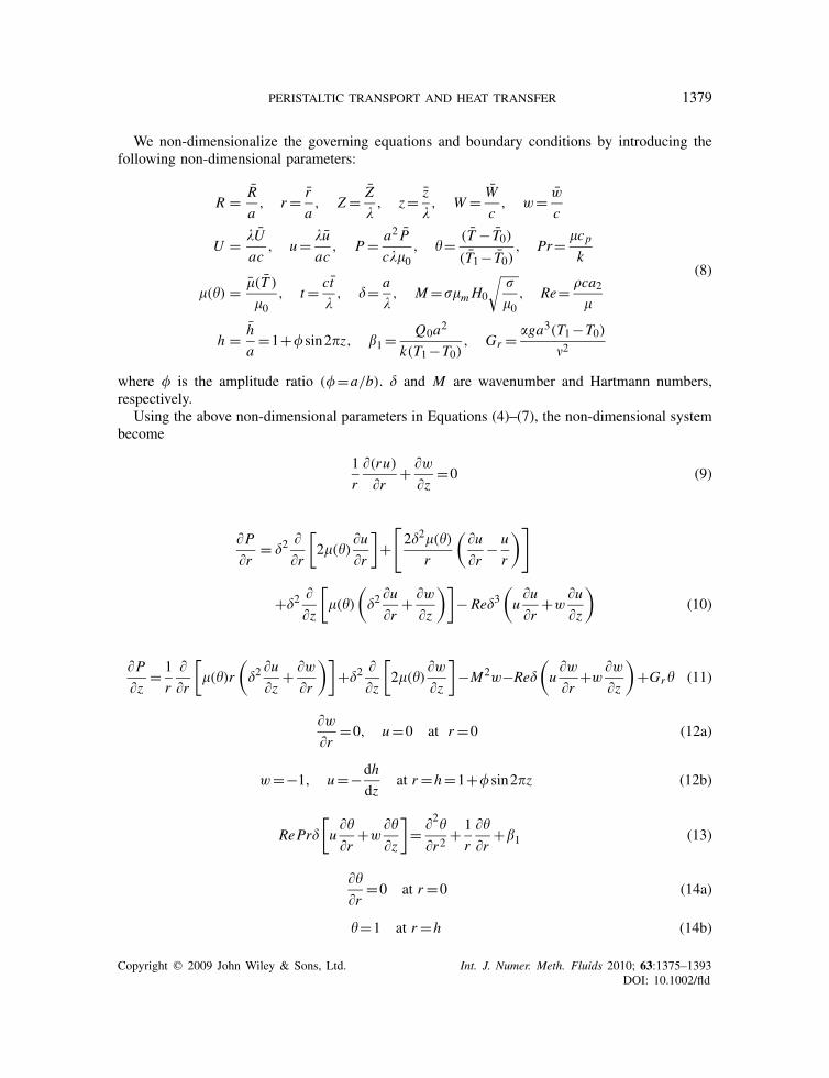
We non-dimensionalize the governing equations and boundary conditions by introducing thefollowing non-dimensional parameters:

R = R

a, r = r

a, Z = Z

�, z= z

�, W = W

c, w= w

c

U = �U

ac, u= �u

ac, P= a2 P

c��0, = (T − T0)

(T1− T0), Pr= �cp

k

�() = �(T )

�0, t= ct

�, �= a

�, M=��mH0

√�

�0, Re= �ca2

�

h = h

a=1+�sin2�z, �1= Q0a2

k(T1−T0), Gr = ga3(T1−T0)

�2

(8)

where � is the amplitude ratio (�=a/b). � and M are wavenumber and Hartmann numbers,respectively.

Using the above non-dimensional parameters in Equations (4)–(7), the non-dimensional systembecome

1

r

�(ru)

�r+ �w

�z=0 (9)

�P�r

= �2��r

[2�()

�u�r

]+[2�2�()

r

(�u�r

− u

r

)]

+�2��z

[�()

(�2

�u�r

+ �w

�z

)]− Re�3

(u

�u�r

+w�u�z

)(10)

�P�z

= 1

r

��r

[�()r

(�2

�u�z

+ �w

�r

)]+�2

��z

[2�()

�w

�z

]−M2w−Re�

(u

�w

�r+w

�w

�z

)+Gr (11)

�w

�r=0, u=0 at r =0 (12a)

w=−1, u=−dh

dzat r =h=1+�sin2�z (12b)

RePr�

[u

�

�r+w

��z

]= �2

�r2+ 1

r

�

�r+�1 (13)

�

�r=0 at r =0 (14a)

=1 at r =h (14b)



Using the long wavelength approximation (�→0) in Equations (10), (11) and (13), the appropriateequations describing the flow in the wave frame are

�2�r2

+ 1

r

�

�r+�1=0 (15)

�P�r

=0 (16)

�P�z

= 1

r

��r

[�()r

(�w

�r

)]−M2w+Gr (17)

Before we proceed towards finding the solutions of the above equations, note that in the longwavelength limit (�→0), the energy equation (15) is decoupled from the rest of the equations andthus can be solved independently. Also, from the radial component of the momentum equation, wefind that the pressure is independent of the radial direction. We will utilize these facts in findingthe analytical and numerical solutions.

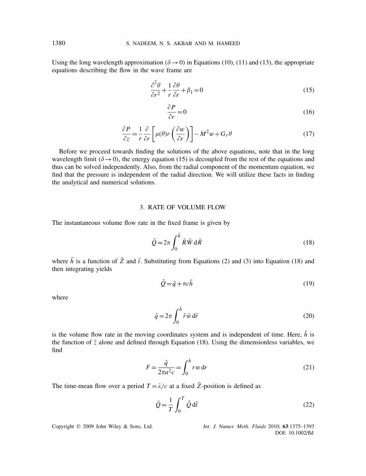
3. RATE OF VOLUME FLOW

The instantaneous volume flow rate in the fixed frame is given by

Q=2�∫ h

0RW dR (18)

where h is a function of Z and t . Substituting from Equations (2) and (3) into Equation (18) andthen integrating yields

Q= q+�ch (19)

where

q=2�∫ h

0rwdr (20)

is the volume flow rate in the moving coordinates system and is independent of time. Here, h isthe function of z alone and defined through Equation (18). Using the dimensionless variables, wefind

F= q

2�a2c=∫ h

0rwdr (21)

The time-mean flow over a period T =�/c at a fixed Z -position is defined as

Q= 1

T

∫ T

0Q dt (22)



Invoking Equation (18) into Equation (22) and integrating we obtain

Q= q+�c

(a2+ b2

2

)(23)

which may be written as

Q

2�a2c= q

2�a2c+ 1

2

(1+ �2

2

)(24)

The dimensionless time-mean flow can be defined as

�= Q

2�a2c(25)

we rewrite Equation (24) as

�=F+ 1

2

(1+ �2

2

)(26)

where F in the wave frame defined through (21).In the forthcoming analysis, we shall use

�()=e−�, �()=1−� for ��1 (27)

where � represents the Reynold model viscosity parameter. The choice of � is justified physiolog-ically because normal person or animal of similar size takes 1−2L of the fluid every day [5]. Also6−7L of the fluid is recurred by a small intestine as secretions from salivary glands, stomach,pancreas, liver and small intestine itself.

Thus, the viscosity of fluid is not constant in all phenomenon, in some typical situations viscositydepends upon temperature, here we have considered the well-known temperature-dependentviscosity model known as Reynold model of viscosity.

4. ANALYTICAL SOLUTION

In this section, we will present analytical solution of the system given in Equations (15)–(17) withboundary conditions (12), (14). We will use regular perturbation technique to find the solutions.The temperature Equation (15) with boundary conditions (14a), and (14b) yields

=1+ �14

(h2−r2) (28)

For the solution of Equations (16) and (17), we look for a regular perturbation in term of smallparameter � as follows:

w=w0+�w1+O(�)2 (29a)

u=u0+�u1+O(�)2 (29b)



dp

dz= dp0

dz+�

dp1dz

+O(�)2 (29c)

F=F0+�F1+O(�)2 (29d)

Substituting from Equations (29a)–(29c) in Equations (9), (16), and (17), and comparing the likepower of �, we have the following system of equations:

4.1. Zeroth-order system

1

r

�(ru0)

�r+ �w0

�z=0 (30)

�P0�r

=0 (31)

�P0�z

= 1

r

��r

[r

(�w0

�r

)]−M2w0+Gr (32)

with the boundary conditions are

�w0

�r=0, u0=0 at r =0 (33a)

w0=−1, u0=−dh

dzat r =h=1+�sin2�z (33b)

4.2. First-order system

1

r

�(ru1)

�r+ �w1

�z=0 (34)

�P1�r

=0 (35)

�P1�z

= 1

r

��r

[−r

(�w0

�r

)+r

(�w1

�r

)]−M2w1 (36)

with the corresponding boundary conditions are

�w1

�r=0, u1=0 at r =0 (36a)

w1=0, u1=0 at r =h=1+�sin2�z (36b)

4.3. Solution of zeroth-order system

With the help of temperature solution (28), the zeroth-order solution can be written as

w0= 1

I0(Mh)M2

(dp0dz

−M2+K8

)(I0(Mr)− I0(Mh))−1+ Gr�1

4M2(h2−r2) (37)



The volume flow rate F0 in the moving coordinates system is given by

F0=∫ h

0rw0 dr (38)

Substituting Equation (37) into Equation (38) and solving the result for dp0/dz, yields

dp0dz

= M4 I0(Mh)(2F0+h2+K5)

2MhI1(Mh)−M2h2 I0(Mh)+K6 (39)

4.4. Solution of the first-order system

w1 = dP1dz

1

I0(Mh)M2[(I0(Mr)− I0(Mh)+K1 I0(Mr))]+g(z)K2 I0(Mr)

+�2+�3r2+g(z)K3

∞∑k=0

ak(Mr)2k+4

2k+4+g(z)K4

∞∑k=0

ak(Mr)2k+2

2k+2(40)

The volume flow rate F1 in the moving coordinates system is defined as

F1=∫ h

0rw1 dr (41)

Substituting Equation (40) into Equation (41) and solving the result for dP1/dz, yields

dP1dz

= M4 I0(Mh)(2F1−K7)

2MhI1(Mh)−M2h2 I0(Mh)+ M6 I0(Mh)K77(2F0+h2)

(2MhI1(Mh)−M2h2 I0(Mh))2+K9 (42)

where

K1 = 1

I0(Mh)(−�2−�3h

2)

K2 = 1

I0(Mh)

(K3

∞∑k=0

ak(Mh)2k+4

2k+4−K4

∞∑k=0

ak(Mh)2k+2

2k+2

), K3=− �1

2M2

K4 = �1h2+4

2, K5=−Gr�1h

4

16M2, K6= Gr�1

M2+Gr +M2

K7 = 2K1h

MI1(Mh)+�2h

2+ �3h4

2

K8 = Gr�1M2

−Gr , K9= 2K8K77M2

(2MhI1(Mh)−M2h2 I0(Mh)), �3=−Gr�

21

2M4

K77 = − 1

M2

(K2(Mh)I1(Mh)+K3

∞∑k=0

ak(Mh)2k+6

(2k+4)(2k+6)+K4

∞∑k=0

ak(Mh)2k+4

(2k+2)(2k+4)

)



�2 = Gr�1M4

+ Gr�21h

2

4M4− 2Gr�

21

M6, g(z)= 1

I0(Mh)M2

(dp0dz

−M2+K8

)

a0 = 1

4, ak = bk

(2k+2)(k+2), bk = (k+1)

22k+1(k!)2

Substituting Equations (40) and (37) into Equation (29a) and using the relation

dP0dz

= dP

dz−�

dP1dz

neglecting terms greater than O (�), we get

w = 1

I0(Mh)M2

((dp

dz−M2

)+K8

)(I0(Mr)− I0(Mh))−1

+Gr�14M2

(h2−r2)+�

(K1 I0(Mr)+g(z)K2 I0(Mr)

+�2+�3r2+g(z)K3

∞∑k=0

ak(Mr)2k+4

2k+4+g(z)K4

∞∑k=0

ak(Mr)2k+2

2k+2

)(43)

Substituting Equations (42) and (39) into Equation (29c), using the relation F0=F−�F1,where F is defined in Equation (21), and neglecting the terms greater than O(�), we get

dP

dz=

M4 I0(Mh)(2− �2

2 −1+h2+K10

)2MhI1(Mh)−M2h2 I0(Mh)

+K6

+�

⎛⎜⎝2M6 I0(Mh)

(2− �2

2 −1+h2)K77

(2MhI1(Mh)−M2h2 I0(Mh))2+K9

⎞⎟⎠ (44)

where

K10=K5−�K7

The non-dimensional pressure rise per wavelength �P� and friction force F� (on the wall) inthe tube length � in their non-dimensional forms are given by

�P� =∫ 1

0

dP

dzdz (45)

F� =∫ 1

0h2(

−dP

dz

)dz (46)

where dP/dz is defined through Equation (44).The corresponding stream function(

u=−1

r

�

�rand w= 1

r

�

�r

)



0 0.2 0.4 0.6 0.8 1 1.2 1.4-1

-0.8

-0.6

-0.4

-0.2

0

0.2

0.4

0.6

r

w

Numerical SolAnalytic Sol

β = 0.0

0 0.2 0.4 0.6 0.8 1 1.2 1.4-1

-0.8

-0.6

-0.4

-0.2

0

0.2

0.4

0.6

r

w

Numerical SolAnalytical Sol

β = 0.1

Figure 2. Comparison of analytical and numerical velocity for dPdz =0.4,

M=3, Gr =2 and �1=5 for �=0,0.1.

0 0.1 0.2 0.3 0.4 0.5 0.6 0.7-40

-20

0

20

40

60

80

100

p

=0=0.1=0.2

A

Figure 3. Pressure rise versus flow rate at �=0.6, �1=5, �=3, Gr =3.

is

(r, z) = g(z)

2M2(2Mr I0(Mr)−(Mr)2 I0(Mh))− r2

2+ Gr�1r

2

16M2(2h2−r2)

+�

(1

M(K1r I1(Mr)+g(z)K2r I1(Mr))+ r2

4(2�2+�3r

2)

+ g(z)

M2

(K3

∞∑k=0

ak(Mr)2k+6

(2k+4)(2k+6)+K4

∞∑k=0

ak(Mr)2k+4

(2k+4)(2k+2)

))



M=2M=3M=4

B

0 0.1 0.2 0.3 0.4 0.5 0.6 0.7-40

-20

0

20

40

60

80

100

p

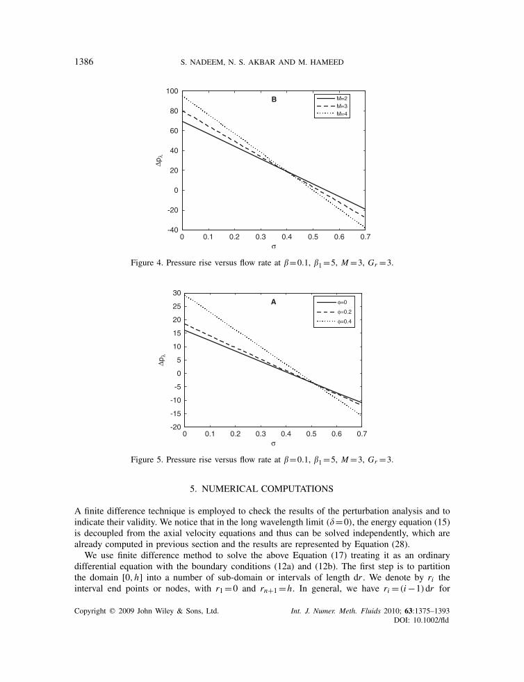
Figure 4. Pressure rise versus flow rate at �=0.1, �1=5, M=3, Gr =3.

0 0.1 0.2 0.3 0.4 0.5 0.6 0.7-20

-15

-10

-5

0

5

10

15

20

25

30

p

=0

=0.2

=0.4

A

Figure 5. Pressure rise versus flow rate at �=0.1, �1=5, M=3, Gr =3.

5. NUMERICAL COMPUTATIONS

A finite difference technique is employed to check the results of the perturbation analysis and toindicate their validity. We notice that in the long wavelength limit (�=0), the energy equation (15)is decoupled from the axial velocity equations and thus can be solved independently, which arealready computed in previous section and the results are represented by Equation (28).

We use finite difference method to solve the above Equation (17) treating it as an ordinarydifferential equation with the boundary conditions (12a) and (12b). The first step is to partitionthe domain [0,h] into a number of sub-domain or intervals of length dr . We denote by ri theinterval end points or nodes, with r1=0 and rn+1=h. In general, we have ri =(i−1)dr for



Fp

=0

=0.1=0.2

B

0 0.1 0.2 0.3 0.4 0.5 0.6 0.7-20

-15

-10

-5

0

5

10

15

Figure 6. Friction force versus flow rate at M=3, �1=5, �=0.2, Gr =3.

0 0.1 0.2 0.3 0.4 0.5 0.6 0.7-20

-15

-10

-5

0

5

10

15

20

25

σ

Fp λ

M=2M=3M=4

A

Figure 7. Friction force versus flow rate at �=0.4, �1=5, �=0.2, Gr =3.

i=1,2,3 . . .N . We represent the axial velocity w at the i th node by Wi . The second step is toexpress the differential operators in discrete form. This can be accomplished using finite differenceapproximations to the differential operators. In this problem we will use the central differenceapproximation and replaced the derivatives by their discrete approximations

w′′ = Wi+1−2Wi +Wi−1

(dr)2, w′ = Wi+1+Wi−1

2(dr)(47)



0 0.2 0.4 0.6 0.8 1-30

-20

-10

0

10

20

30

σ

Fp λ

φ=0φ=0.2

φ=0.6

B

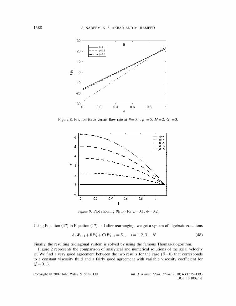
Figure 8. Friction force versus flow rate at �=0.4, �1=5, M=2, Gr =3.

Figure 9. Plot showing (r, z) for z=0.1, �=0.2.

Using Equation (47) in Equation (17) and after rearranging, we get a system of algebraic equations

AiWi+1+BWi +CiWi−1=Di , i=1,2,3 . . .N (48)

Finally, the resulting tridiagonal system is solved by using the famous Thomas-alogorithm.Figure 2 represents the comparison of analytical and numerical solutions of the axial velocity

w. We find a very good agreement between the two results for the case (�=0) that correspondsto a constant viscosity fluid and a fairly good agreement with variable viscosity coefficient for(�=0.1).



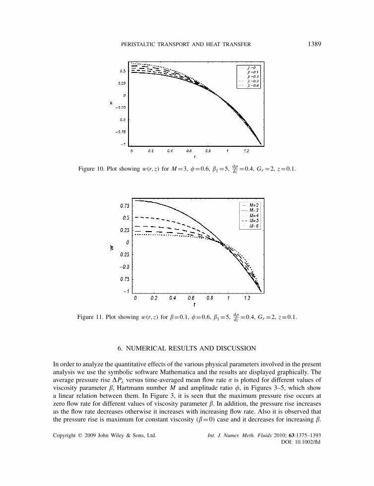
Figure 10. Plot showing w(r, z) for M=3, �=0.6, �1=5, dpdz =0.4, Gr =2, z=0.1.

Figure 11. Plot showing w(r, z) for �=0.1, �=0.6, �1=5, dpdz =0.4, Gr =2, z=0.1.

6. NUMERICAL RESULTS AND DISCUSSION

In order to analyze the quantitative effects of the various physical parameters involved in the presentanalysis we use the symbolic software Mathematica and the results are displayed graphically. Theaverage pressure rise �P� versus time-averaged mean flow rate � is plotted for different values ofviscosity parameter �, Hartmann number M and amplitude ratio �, in Figures 3–5, which showa linear relation between them. In Figure 3, it is seen that the maximum pressure rise occurs atzero flow rate for different values of viscosity parameter �. In addition, the pressure rise increasesas the flow rate decreases otherwise it increases with increasing flow rate. Also it is observed thatthe pressure rise is maximum for constant viscosity (�=0) case and it decreases for increasing �.



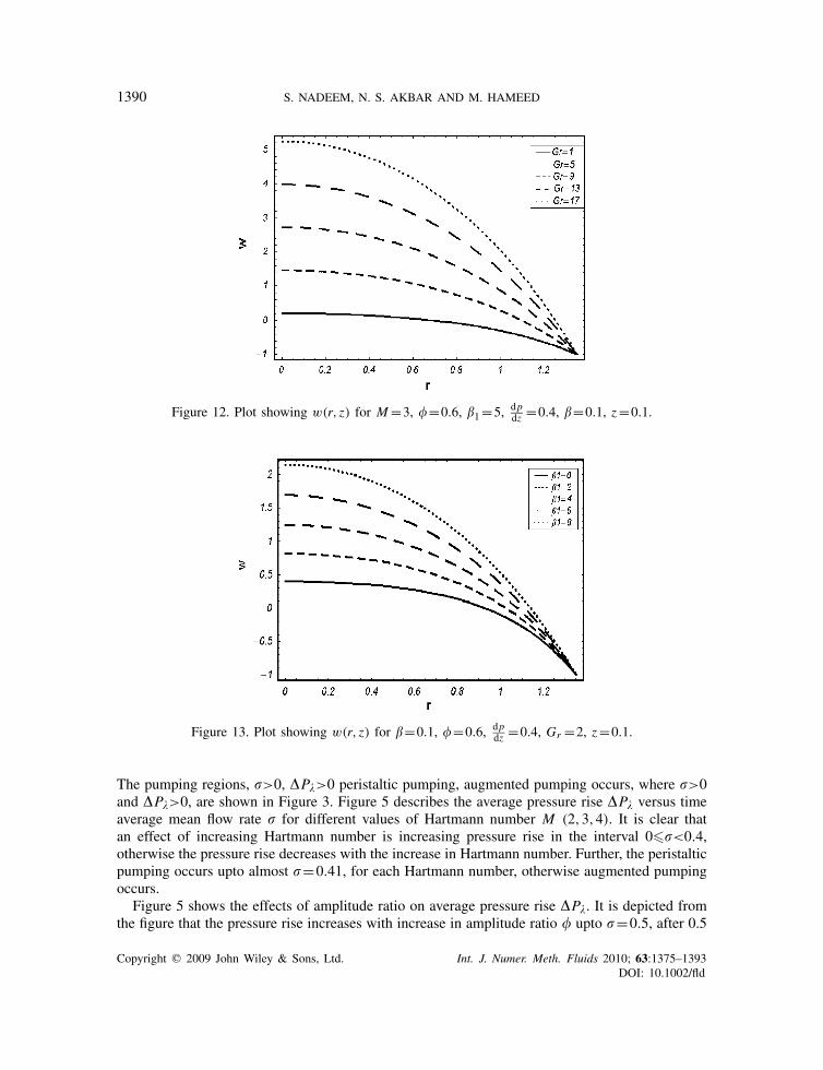
Figure 12. Plot showing w(r, z) for M=3, �=0.6, �1=5, dpdz =0.4, �=0.1, z=0.1.

Figure 13. Plot showing w(r, z) for �=0.1, �=0.6, dpdz =0.4, Gr =2, z=0.1.

The pumping regions, �>0, �P�>0 peristaltic pumping, augmented pumping occurs, where �>0and �P�>0, are shown in Figure 3. Figure 5 describes the average pressure rise �P� versus timeaverage mean flow rate � for different values of Hartmann number M (2,3,4). It is clear thatan effect of increasing Hartmann number is increasing pressure rise in the interval 0��<0.4,otherwise the pressure rise decreases with the increase in Hartmann number. Further, the peristalticpumping occurs upto almost �=0.41, for each Hartmann number, otherwise augmented pumpingoccurs.

Figure 5 shows the effects of amplitude ratio on average pressure rise �P�. It is depicted fromthe figure that the pressure rise increases with increase in amplitude ratio � upto �=0.5, after 0.5



-0.1 0 0.1 0.2 0.3 0.4 0.5 0.60.2

0.4

0.6

0.8

1

1.2

-0.1 0 0.1 0.2 0.3 0.4 0.5 0.60.2

0.4

0.6

0.8

1

1.2

(a) (b)

Figure 14. Streamlines for different values of �=0.8, 1, (panels (a) to (b)). The other parameters are�=0.4, �1=3, Gr =0.6, M=1.5, �=0.4.

-0.1 0 0.1 0.2 0.3 0.4 0.5 0.60.2

0.4

0.6

0.8

1

1.2

-0.1 0 0.1 0.2 0.3 0.4 0.5 0.60.2

0.4

0.6

0.8

1

1.2

(a) (b)

Figure 15. Streamlines for different values of �=0.2, 0.3 (panels (a) to (b)). The other parameters are�=0.9, �1=3, Gr =0.6, M=1.5, �=0.4.

the pressure rise decreases with the increase in amplitude ratio. Further the peristaltic pumpingoccurs in the region 0��<0.5, otherwise augmented pumping occurs. The frictionless force theFp� is plotted in Figures 6–8. we observe that frictionless force has the opposite behaviour ascompared with pressure rise. The temperature field versus r is plotted for different values ofheat absorption parameter �1 in Figure 9. It is depicted from the figure that with the increasing�1, the temperature field increases. Further the temperature field is maximum at (r =0).



-0.1 0 0.1 0.2 0.3 0.4 0.5 0.60.2

0.4

0.6

0.8

1

1.2

-0.1 0 0.1 0.2 0.3 0.4 0.5 0.60.2

0.4

0.6

0.8

1

1.2

(a) (b)

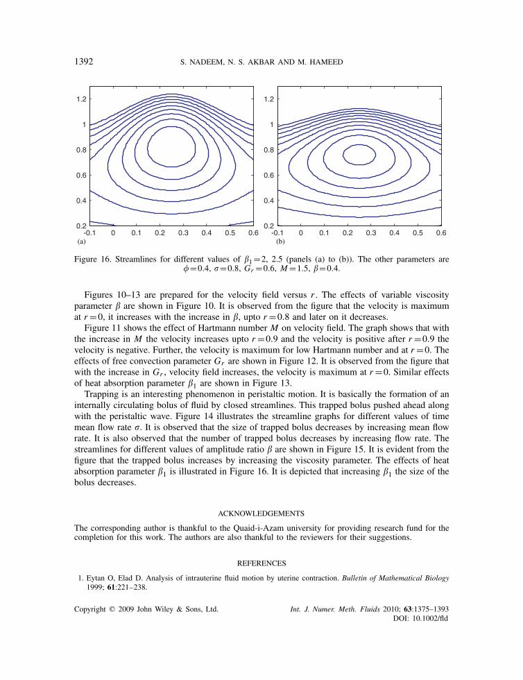
Figure 16. Streamlines for different values of �1=2, 2.5 (panels (a) to (b)). The other parameters are�=0.4, �=0.8, Gr =0.6, M=1.5, �=0.4.

Figures 10–13 are prepared for the velocity field versus r . The effects of variable viscosityparameter � are shown in Figure 10. It is observed from the figure that the velocity is maximumat r =0, it increases with the increase in �, upto r =0.8 and later on it decreases.

Figure 11 shows the effect of Hartmann number M on velocity field. The graph shows that withthe increase in M the velocity increases upto r =0.9 and the velocity is positive after r =0.9 thevelocity is negative. Further, the velocity is maximum for low Hartmann number and at r =0. Theeffects of free convection parameter Gr are shown in Figure 12. It is observed from the figure thatwith the increase in Gr , velocity field increases, the velocity is maximum at r =0. Similar effectsof heat absorption parameter �1 are shown in Figure 13.

Trapping is an interesting phenomenon in peristaltic motion. It is basically the formation of aninternally circulating bolus of fluid by closed streamlines. This trapped bolus pushed ahead alongwith the peristaltic wave. Figure 14 illustrates the streamline graphs for different values of timemean flow rate �. It is observed that the size of trapped bolus decreases by increasing mean flowrate. It is also observed that the number of trapped bolus decreases by increasing flow rate. Thestreamlines for different values of amplitude ratio � are shown in Figure 15. It is evident from thefigure that the trapped bolus increases by increasing the viscosity parameter. The effects of heatabsorption parameter �1 is illustrated in Figure 16. It is depicted that increasing �1 the size of thebolus decreases.

ACKNOWLEDGEMENTS

The corresponding author is thankful to the Quaid-i-Azam university for providing research fund for thecompletion for this work. The authors are also thankful to the reviewers for their suggestions.

REFERENCES

1. Eytan O, Elad D. Analysis of intrauterine fluid motion by uterine contraction. Bulletin of Mathematical Biology1999; 61:221–238.



2. Jaffrin MY, Shaprio AH. Peristaltic pumping. Annual Review of Fluid Mechanics 1971; 3:13–36.3. Pozrikidis CAC. A study of peristaltic flow. Journal of Fluid Mechanics 1987; 180:515–527.4. Elshehawey EF, Eladabe NT, Elghazy EM, Ebaid A. Peristaltic transport in an asymmetric channel through a

porous medium. Applied Mathematics and Computation 2006; 182:140–150.5. Abd El-Naby AH, El-Misiery AEM. Effects of an endoscope and generalized Newtonian fluid on peristaltic

motion. Applied Mathematics and Computation 2002; 128:19–35.6. Li M, Brasseur JGJG. Non-steady peristaltic transport in finite-length tubes. Journal of Fluid Mechanics 1993;

248:129–151.7. Misra JC, Pandey SK. A mathematical model for oesophageal swallowing of a food-bolus. Applied Mathematics

and Computation 2001; 33:997–1009.8. Hariharan P, Seshadri V, Banerjee RK. Peristaltic transport of non-Newtonian fluid in a diverging tube with

different wave forms. Mathematical and Computer Modelling 2008; 48:998–1017.9. Brasseur S, Lu NQ. The influence of a peripherical layer of different viscosity on peristaltic pumping with

Newtonian fluid. Journal of Fluid Mechanics 1987; 174:495–519.10. Nadeem S, Akram S. Peristaltic transport of a hyperbolic tangent fluid model in an asymmetric channel. Zeitschrift

fur Naturforschung A 2009; in press.11. Mekheimer KhS, Abd elmaboud Y. The influence of heat transfer and magnetic field on peristaltic transport of

a Newtonian fluid in a vertical annulus: application of an endoscope. Physics A 2008; 372:1657–1665.12. Eberhart RC, Shitzer A. Heat Transfer in Medicine and Biology (1st edn). Springer: Berlin, 1985.13. Radhakrishnamacharya G, Murthy VR. Heat transfer to peristaltic transport in a non-uniform channel. Defence

Science Journal 1993; 43:275–280.14. Radhakrishnamacharya G, Srinivasulu Ch. Influence of wall properties on peristaltic transport with heat transfer.

Comptes Rendus Mecanique 2007; 335:369–373.15. Hayat T, Qureshi MU, Hussain Q. Effect of heat transfer on the peristaltic flow of an electrically conducting

fluid in a porous space. Applied Mathematical Modelling 2008; 33:1657–1665.16. Nadeem S, Akram S. Heat transfer in a peristaltic flow of MHD fluid with partial slip. Communications in

Nonlinear Science and Numerical Simulation 2009; DOI: 10.1016/j.cnsns.2009.03.038.17. Nadeem S, Akbar NS. Influence of heat transfer on a peristaltic transport of Herschel Bulkley fluid in a

non-uniform inclined tube. Communications in Nonlinear Science and Numerical Simulation 2009; 14:4100–4113.18. Vajravelu K, Radhakrishnamacharya G, Radhakrishnamurty V. Peristaltic flow and heat transfer in a vertical

porous annulus with long wave approximation. International Journal of Non-Linear Mechanics 2007; 42:754–759.19. Herwig H, Wickern G. The effect of variable properties on laminar boundary layer flow. Wrme Stoffubert 1986;

20:45–57.20. Herwig H, Klemp K, Stinnesbeck J. Laminar entry flow in a pipe or channel. The effect of variable viscosity

due to heat transfer across the wall. Numerical Heat Transfer, Part A 1990; 18:51–70.21. El Hakeem A, El Naby A, El Misery AEM, El Shamy II. Hydromagnetic flow of fluid with variable viscosity

in a uniform tube with peristalsis. Journal of Physics A 2003; 368:8535–8547.22. El Hakeem A, El Naby A, El Misery AEM, El Shamy II. Effects of an endoscope and fluid with variable

viscosity on peristaltic motion. Applied Mathematics and Computation 2004; 158:497–511.23. Ali N, Hussain Q, Hayat T, Asghar S. Slip effects on the peristaltic transport of MHD fluid with variable

viscosity. Physics A 2007; 1.78:1–13.24. Nadeem S, Akbar NS. Effects of heat transfer on the peristaltic transport of MHD Newtonian fluid with variable

viscosity: application of Adomian decomposition method. Communications in Nonlinear Science and NumericalSimulation 2009; 14:3844–3855.

25. Ebaid A. A new numerical solution for the MHD peristaltic flow of a biofluid with variable viscosity in circularcylindrical tube via Adomian decomposition method. Physics A 2008; 372:5321–5328.

26. Eldabe NTM, El-Sayed MF, Ghaly AY, Sayed HM. Effect mixed convection heat and mass transfer in a non-Newtonian fluid at a peristaltic surface with temperature-dependent viscosity. Archive of Applied Mechanics 2008;78:599–624.


Peristaltic transport and heat transfer of a MHD Newtonian fluid with variable viscosity

Documents

Transcript of Peristaltic transport and heat transfer of a MHD Newtonian fluid with variable viscosity