Physics Letters A 372 (2008) 2653–2664

www.elsevier.com/locate/pla

The influence of slip on the peristaltic motionof a third order fluid in an asymmetric channel

T. Hayat ∗, M. Umar Qureshi, N. Ali

Department of Mathematics, Quaid-I-Azam University 45320, Islamabad 44000, Pakistan

Received 29 October 2007; received in revised form 12 December 2007; accepted 16 December 2007

Available online 3 January 2008

Communicated by F. Porcelli

Abstract

In this investigation, the peristaltic flow of a third order fluid in an asymmetric channel is considered in the presence of a slip condition. Theseries solution of the stream function and longitudinal pressure gradient is given under long wave length and low Reynolds number approximations.Pressure rise and frictional forces per wave length are analyzed through numerical integration. Pumping and trapping phenomena are examinedand the obtained results are compared with those of no-slip condition. Comparison is made with the results of no-slip and viscous fluid cases.© 2008 Published by Elsevier B.V.

PACS: 47.15.G-; 47.15.Rq; 47.27.nd; 47.45.Gx

Keywords: Slip condition; Asymmetric channel; Third-order fluid; Pumping and trapping

1. Introduction

Peristalsis is of great importance in many biological systems including the study of humans. It is relevant for the study of theureters, the intestines and the oviducts amongst others. The word peristalsis itself comes from a Greek word peristaltikos whichmeans clasping and compressing. It occurs when a progressive wave of area contraction or expansion propagates along the lengthof an extensible tube containing a liquid. Several theoretical and experimental investigations have been undertaken on the peristalticflow of a viscous fluid under various geometries and assumptions. Few such investigations are made for the nonNewtonian fluidsin a symmetric and non-uniform channels/tubes. Some recent representative studies in this direction may be mentioned throughthe works in Ref. [1–15]. Such investigations further narrowed down when non-Newtonian fluids in an asymmetric channel areconsidered. To the best of our knowledge, only Ali et al. [16] and Haroun [17] have made such studies for the couple stress and thirdorder fluids, respectively. However, no attention is given to explore the slip effects on the peristaltic flow of a non-Newtonian fluidin an asymmetric channel. Even such observations have not been yet reported for viscous fluid. In the literature, much attention hasbeen given to the flow problems with no-slip condition. This is not realistic in the case when thin films problems, problems involvingmultiple interfaces and the flow of rarefied fluids are considered. Many polymeric fluids slip or stick-slip on solid boundaries andhence no-slip condition is no-longer valid. Experimentalists usually associate “Spurt” with slip at the wall. A detailed discussion ofthe work relevant to the slip is given in Hayat et al. [18].

The main purpose of the present investigation is to analyze the peristaltic flow of a third order fluid in an asymmetric channel.The proposed non-linear slip condition here is dependent upon the shear stress. Computations of the mathematical formulationhas been fully developed. The present analysis has been carried out by employing a long wave length approximation. A regularperturbation method is used to solve the problem and the solutions are expanded in a power series of the Deborah number. The

* Corresponding author. Tel.: +92 51 90642172; fax: +92 51 2275341.E-mail address: t_pensy@hotmail.com (T. Hayat).

0375-9601/$ – see front matter © 2008 Published by Elsevier B.V.doi:10.1016/j.physleta.2007.12.049

2654 T. Hayat et al. / Physics Letters A 372 (2008) 2653–2664

Reynolds number is arbitrary. Closed form solutions for stream function, longitudinal velocity and pressure gradient are obtainedup to second order of the Deborah number. Numerical computations have been carried out for the pressure rise and frictional forcesat the channel walls. Finally, the graphical results are plotted and discussed in detail for various interesting phenomena.

2. Governing equations

The balance of linear momentum is

(1)ρdVdt

= −∇p + div S.

In above equation ρ is the fluid density, V is the velocity vector, p is the pressure, S is the extra stress tensor and d/dt is the materialtime derivative.

As the fluid is incompressible, it can undergo only isochoric motions and therefore

(2)div V = 0.

For two-dimensional flow of a third order fluid, we seek solutions for the velocity and extra stress S of the form [17]:

(3)V = (U (X, Y , t ), V (X, Y , t ),0

),

(4)S = (μ + β3 tr A2

1

)A1 + α1A2 + α2A2

1 + β1A3 + β2(A1A2 + A2A1),

where U and V are the velocities in the X and Y directions, respectively and t is the time. In Eq. (4), μ, αi(i = 1,2) and βi(i = 1–3)

are the material constants. The expressions of first three Rivlin–Ericksen tensors are

(5)A1 = L + L∗, An+1 = dAn

dt+ AnL + L∗An, n = 1,2,

where L = grad V and asterisk indicates the matrix transpose.

3. Development of the flow

We choose a Cartesian coordinate system with X axis along the centre line in the direction of wave propagation and Y transverseto it. A two-dimensional flow of a third order fluid in an infinite asymmetric channel having width d1 +d2 is considered. We assumean infinite sinusoidal wave train moving with velocity c along the flexible walls of the channel. The channel asymmetry is inducedby choosing peristaltic waves of different amplitudes and phases on the channel walls. The geometries of the walls are [17]

(6)H1(X, t ) = d1 + a1 sin

[2π

λ(X − ct )

], upper wall,

(7)H2(X, t ) = −d2 − a2 sin

[2π

λ(X − ct ) + φ

], lower wall,

where a1 and a2 are the wave amplitudes, λ is the wave length, t is the time and φ is the phase difference varying in the range0 � φ � π . It is noted that φ = 0 corresponds to symmetric channel with waves out of phase and for φ = π the waves are in phase.Moreover a1, a2, d1, d2 and φ satisfy the condition a2

1 + a22 + 2a1a2 cosφ � (d1 + d2)

2 [17]. We also assume the walls to have onlytransverse motion. The channel flow is unsteady in the laboratory frame (X, Y ) but the boundary shape is stationary and the flow issteady if we carry out the investigation in a coordinate system (x, y) moving with the wave speed in the positive X direction. Thecoordinates and velocities in the laboratory frame (X, Y ) and the wave frame (x, y) are related by the following transformations:

(8)x = X − ct, y = Y , u(x, y) = U (X, Y , t ) − c, v(x, y) = V (X, Y , t ),

in which (U , V ) and (u, v) are the velocity components in the laboratory and wave frames. In order to carry out the non-dimensionalanalysis, we define the following variables

x = 2πx

λ, y = y

d1, u = u

c, v = v

c, t = 2πt

λ,

p = 2πd21

λμcp, h1 = h1

d1, h2 = h2

d1, S = d1

μcS,

δ = 2πd1

λ, Re = ρcd1

μ, λ1 = α1c

μd1, λ2 = α2c

μd1, γ1 = β1c

2

μd21

, γ2 = β2c2

μd21

, γ3 = β3c2

μd21

,

T. Hayat et al. / Physics Letters A 372 (2008) 2653–2664 2655

where δ is the wave number, Re is the Reynolds number and incompressibility condition (2) is automatically satisfied if

(9)u = ∂ψ

∂y, v = −δ

∂ψ

∂x,

where ψ signifies the stream function.Since this is a sequel to our earlier work [19], therefore in order to make the Letter self-contained, we avoid the details of calcu-

lations for mathematical formulation. Following the same methodology of solution as in Ref. [19] and restricting the flow analysisto long wave length situation we can write the following expressions of compatibility, the pressure gradient and the boundaryconditions:

(10)∂2

∂y2Sxy = 0,

(11)∂p

∂x= ∂

∂ySxy,

where ∂p/∂y = 0 indicating that p �= p(y), hence ∂p/∂x = dp/dx and

(12)Sxy = ∂2ψ

∂y2+ 2Γ

(∂2ψ

∂y2

)3

,

in which Γ (= γ2 + γ3) is the Deborah number and the boundary conditions are

ψ = F

2,

∂ψ

∂y= −βSxy − 1 at y = h1(x),

(13)ψ = −F

2,

∂ψ

∂y= βSxy − 1 at y = h2(x),

where β(= L/d1) is the dimensionless slip parameter, L is the dimensional slip parameter and the dimensionless form of theperistaltic walls h1(x) and h2(x) are

(14)h1(x) = 1 + a sinx, h2(x) = −d − b sin(x + φ),

with

a = a1

d1, b = a2

d1, d = d2

d1,

which satisfy

(15)a2 + b2 + 2ab cosφ � (1 + d)2.

The respective dimensionless time mean flows θ and F in the laboratory and wave frames are related through the followingexpression:

(16)F = θ − 1 − d = ψ(h1) − ψ(h2).

4. Method of solution

Since the governing differential system is highly non-linear. Here the resulting system consists of non-linear differential equationand non-linear boundary conditions. Note that the corresponding boundary conditions for the no-slip case (i.e., β = 0) are linear.Exact analytical solution of the governing system is not possible and hence the attention is focused to the perturbation solution forsmall Deborah number Γ . For that we expand ψ , p and F as:

ψ = ψ0 + Γ ψ1 + Γ 2ψ2 + · · · ,p = p0 + Γp1 + Γ 2p2 + · · · ,

(17)F = F0 + Γ F1 + Γ 2F2 + · · · .Substitution of above equations into Eqs. (10), (11) and (13) and collection of terms with respect to like powers of Γ yields thefollowing systems:

2656 T. Hayat et al. / Physics Letters A 372 (2008) 2653–2664

4.1. Zeroth order system

(18)∂4ψ0

∂y4= 0,

(19)dp0

dx= ∂3ψ0

∂y3,

ψ0 = F0

2,

∂ψ0

∂y= −β

∂2ψ0

∂y2− 1, at y = h1(x),

(20)ψ0 = −F0

2,

∂ψ0

∂y= β

∂2ψ0

∂y2− 1, at y = h2(x).

4.2. First order system

(21)∂4ψ1

∂y4= −2

∂2

∂y2

[(∂2ψ0

∂y2

)3],

(22)dp1

dx= ∂3ψ1

∂y3+ 2

∂

∂y

[(∂2ψ0

∂y2

)3],

ψ1 = F1

2,

∂ψ1

∂y= −β

[∂2ψ1

∂y2+ 2

(∂2ψ0

∂y2

)3], at y = h1(x),

(23)ψ1 = −F1

2,

∂ψ1

∂y= β

[∂2ψ1

∂y2+ 2

(∂2ψ0

∂y2

)3], at y = h2(x).

4.3. Second order system

(24)∂4ψ2

∂y4= −6

∂2

∂y2

[∂2ψ1

∂y2

(∂2ψ0

∂y2

)2],

(25)dp2

dx= ∂3ψ2

∂y3+ 6

∂

∂y

[∂2ψ1

∂y2

(∂2ψ0

∂y2

)2],

ψ2 = F2

2,

∂ψ2

∂y= −β

[∂2ψ2

∂y2+ 6

∂2ψ1

∂y2

(∂2ψ0

∂y2

)2], at y = h1(x),

(26)ψ2 = −F2

2,

∂ψ2

∂y= β

[∂2ψ2

∂y2+ 6

∂2ψ1

∂y2

(∂2ψ0

∂y2

)2], at y = h2(x).

The solutions of the above systems are developed in the following subsections.

4.4. Zeroth order solution

The solution of Eq. (18) and boundary conditions (20) is

(27)ψ0 = S1y3 + S2y

2 + S3y + S4,

where

S1 = −2(F0 + h1 − h2)

(h1 − h2)2(h1 − h2 + 6β),

S2 = 3(F0 + h1 − h2)(h1 + h2)

(h1 − h2)2(h1 − h2 + 6β),

S3 = −h31 − 6F0h1h2 − 3h2

1h2 + 3h1h22 + h3

2 + 6F0(h1 − h2)β

(h1 − h2)2(h1 − h2 + 6β),

S4 = −(h1 + h2)(2h1h2(−h1 + h2) + F0(h21 − 4h1h2 + h2

2 + 6(h1 − h2)β))

2(h1 − h2)2(h1 − h2 + 6β).

T. Hayat et al. / Physics Letters A 372 (2008) 2653–2664 2657

The longitudinal velocity and pressure gradient are

(28)u0 = 3S1y2 + 2S2y + S3,

(29)dp0

dx= −12(F0 + h1 − h2)

(h1 − h2)2(h1 − h2 + 6β).

The non-dimensional pressure rise per wave length (�Pλ0) and frictional forces at the upper (Fλ01) and lower (Fλ02) walls arerespectively given by

(30)�Pλ0 =2π∫

0

dp0

dxdx,

(31)Fλ01 =2π∫

0

−h21

(dp0

dx

)dx, Fλ02 =

2π∫0

−h22

(dp0

dx

)dx.

We note that the solution expressions at this order are for the viscous fluid. These expressions coincide with no-slip case [17] whenβ = 0.

4.5. First order solution

Substituting Eq. (27) into Eqs. (21) and (22), solving and then applying the corresponding boundary conditions we get thesolutions for ψ1, u1 and dp1/dx in the form

(32)ψ1 = K1y5 + K2y

4 + K3y3 + K4y

2 + K5y + K6,

(33)u1 = 5K1y4 + 4K2y

3 + 3K3y2 + 2K4y + K5,

(34)dp1

dx= −60F1 + (dp0/dx)3L19 + (dp0/dx)2S2L20 + (dp0/dx)S2

2L21

5(h1 − h2)2(h1 − h2 + 6β),

where the quantities appearing in above equations are given in Appendix A.The pressure rise per wave length (�Pλ1) and frictional forces at the upper (Fλ11) and lower (Fλ12) walls are

(35)�Pλ1 =2π∫

0

dp1

dxdx,

(36)Fλ11 =2π∫

0

−h21

(dp1

dx

)dx, Fλ12 =

2π∫0

−h22

(dp1

dx

)dx.

4.6. Second-order solution

Employing the same methodology as for the first-order system we obtain

(37)ψ2 = R1y7 + R2y

6 + R3y5 + R4y

4 + R5y3 + R6y

2 + R7y + R8,

(38)u2 = 7R1y6 + 6R2y

5 + 5R3y4 + 4R4y

3 + 3R5y2 + 2R6y + R7,

(39)dp2

dx= −420F2 + (dp0/dx)2L37 + (dp0/dx)S2L38 + S2

2L39

35(h1 − h2)2(h1 − h2 + 6β).

The non-dimensional pressure rise per wave length (�Pλ2) is

(40)�Pλ2 =2π∫

0

dp2

dxdx

and the frictional forces at the upper (Fλ21) and lower (Fλ22) walls of the channel are

(41)Fλ21 =2π∫

0

−h21

(dp2

dx

)dx, Fλ22 =

2π∫0

−h22

(dp2

dx

)dx.

2658 T. Hayat et al. / Physics Letters A 372 (2008) 2653–2664

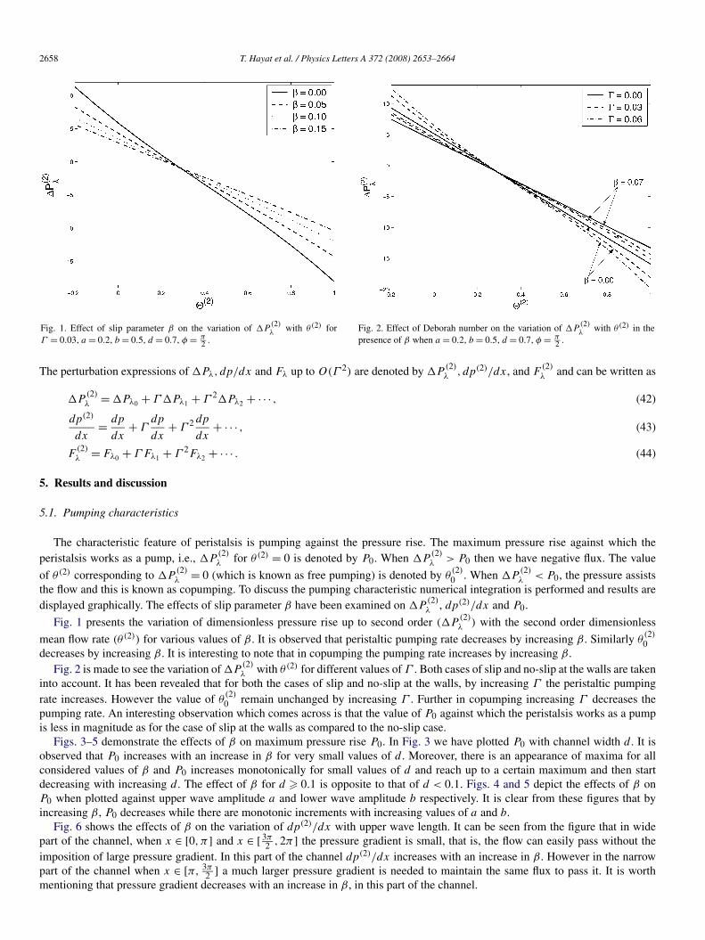
Fig. 1. Effect of slip parameter β on the variation of �P(2)λ with θ(2) for

Γ = 0.03, a = 0.2, b = 0.5, d = 0.7, φ = π2 .

Fig. 2. Effect of Deborah number on the variation of �P(2)λ with θ(2) in the

presence of β when a = 0.2, b = 0.5, d = 0.7, φ = π2 .

The perturbation expressions of �Pλ,dp/dx and Fλ up to O(Γ 2) are denoted by �P(2)λ , dp(2)/dx, and F

(2)λ and can be written as

(42)�P(2)λ = �Pλ0 + Γ �Pλ1 + Γ 2�Pλ2 + · · · ,

(43)dp(2)

dx= dp

dx+ Γ

dp

dx+ Γ 2 dp

dx+ · · · ,

(44)F(2)λ = Fλ0 + Γ Fλ1 + Γ 2Fλ2 + · · · .

5. Results and discussion

5.1. Pumping characteristics

The characteristic feature of peristalsis is pumping against the pressure rise. The maximum pressure rise against which theperistalsis works as a pump, i.e., �P

(2)λ for θ(2) = 0 is denoted by P0. When �P

(2)λ > P0 then we have negative flux. The value

of θ(2) corresponding to �P(2)λ = 0 (which is known as free pumping) is denoted by θ

(2)0 . When �P

(2)λ < P0, the pressure assists

the flow and this is known as copumping. To discuss the pumping characteristic numerical integration is performed and results aredisplayed graphically. The effects of slip parameter β have been examined on �P

(2)λ , dp(2)/dx and P0.

Fig. 1 presents the variation of dimensionless pressure rise up to second order (�P(2)λ ) with the second order dimensionless

mean flow rate (θ(2)) for various values of β . It is observed that peristaltic pumping rate decreases by increasing β . Similarly θ(2)0

decreases by increasing β . It is interesting to note that in copumping the pumping rate increases by increasing β .Fig. 2 is made to see the variation of �P

(2)λ with θ(2) for different values of Γ . Both cases of slip and no-slip at the walls are taken

into account. It has been revealed that for both the cases of slip and no-slip at the walls, by increasing Γ the peristaltic pumpingrate increases. However the value of θ

(2)0 remain unchanged by increasing Γ . Further in copumping increasing Γ decreases the

pumping rate. An interesting observation which comes across is that the value of P0 against which the peristalsis works as a pumpis less in magnitude as for the case of slip at the walls as compared to the no-slip case.

Figs. 3–5 demonstrate the effects of β on maximum pressure rise P0. In Fig. 3 we have plotted P0 with channel width d . It isobserved that P0 increases with an increase in β for very small values of d . Moreover, there is an appearance of maxima for allconsidered values of β and P0 increases monotonically for small values of d and reach up to a certain maximum and then startdecreasing with increasing d . The effect of β for d � 0.1 is opposite to that of d < 0.1. Figs. 4 and 5 depict the effects of β onP0 when plotted against upper wave amplitude a and lower wave amplitude b respectively. It is clear from these figures that byincreasing β , P0 decreases while there are monotonic increments with increasing values of a and b.

Fig. 6 shows the effects of β on the variation of dp(2)/dx with upper wave length. It can be seen from the figure that in widepart of the channel, when x ∈ [0,π] and x ∈ [ 3π

2 ,2π] the pressure gradient is small, that is, the flow can easily pass without theimposition of large pressure gradient. In this part of the channel dp(2)/dx increases with an increase in β . However in the narrowpart of the channel when x ∈ [π, 3π

2 ] a much larger pressure gradient is needed to maintain the same flux to pass it. It is worthmentioning that pressure gradient decreases with an increase in β , in this part of the channel.

T. Hayat et al. / Physics Letters A 372 (2008) 2653–2664 2659

Fig. 3. Effect of slip parameter β on the variation of P0 with channel width d

for Γ = 0.01, a = 0.2, b = 0.4, φ = π4 .

Fig. 4. Effect of slip parameter β on the variation of P0 with upper wave am-plitude a when Γ = 0.1, d = 2, b = 0.4, φ = π

4 .

Fig. 5. Effect of slip parameter β on the variation of P0 with lower wave am-plitude b for Γ = 0.1, a = 0.2, d = 2, φ = π

4 .Fig. 6. Effect of slip parameter β on the variation of dp(2)/dx with upper wavelength when Γ = 0.03, a = 0.2, b = 0.4, d = 2, φ = π

4 , θ = 0.1.

5.2. Frictional forces

Two figures have been made to see the behavior of frictional forces under the presence of slip, at the channel walls. For thispurpose numerical integration has been performed and graphical results are shown for various values of β .

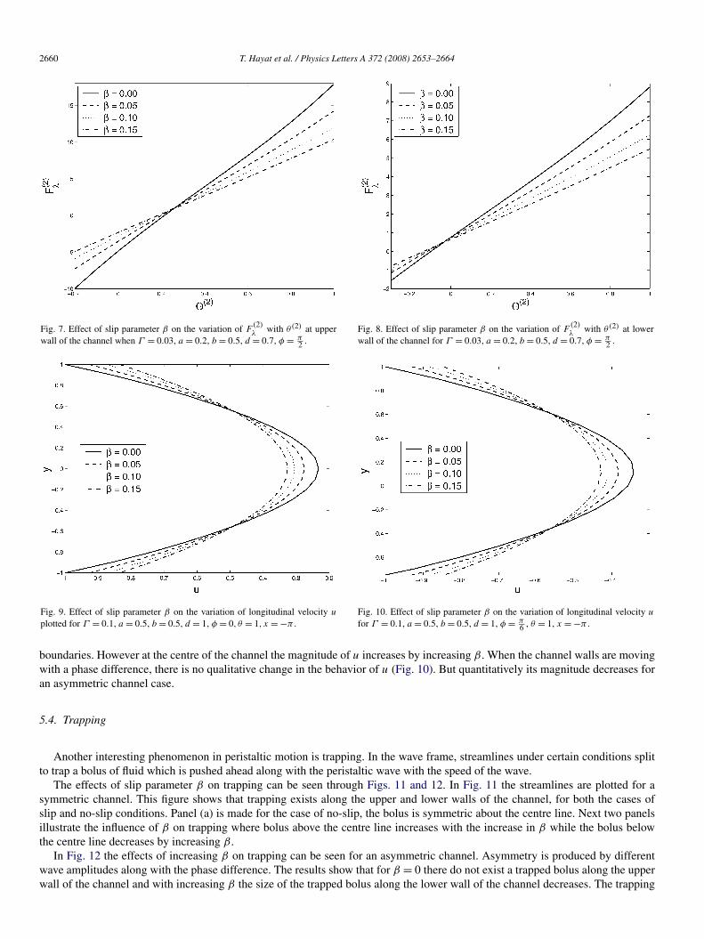
In Fig. 7 we have plotted the frictional force F(2)λ at the upper wall (y = h1(x)) of the channel with dimensionless time mean

flow θ(2). In this figure we observe that there exists a critical value of θ(2) below which F(2)λ resists the flow along the channel wall.

Here increase in β increases the frictional force. However, above this critical value of θ(2) the frictional force assist the flow and anincrease in β causes the decrease in F

(2)λ . Fig. 8 shows the influence of β on F

(2)λ at the lower wall (y = h2(x)) of the channel with

θ(2). We note that F(2)λ assists the flow for all θ(2) � 0 and β plays the similar role for variation of F

(2)λ at the lower and upper walls

of the channel.

5.3. Velocity behavior

It is fairly interesting to observe the effects of β on the longitudinal velocity u both for symmetric and asymmetric channels.The distributions of the longitudinal velocity u at the cross section x = −π are depicted for symmetric channel (φ = 0) and anasymmetric channel (φ = π/6) in Figs. 9 and 10. Fig. 9 shows that an increase in β causes a decrease in the magnitude of u at the

2660 T. Hayat et al. / Physics Letters A 372 (2008) 2653–2664

Fig. 7. Effect of slip parameter β on the variation of F(2)λ with θ(2) at upper

wall of the channel when Γ = 0.03, a = 0.2, b = 0.5, d = 0.7, φ = π2 .

Fig. 8. Effect of slip parameter β on the variation of F(2)λ with θ(2) at lower

wall of the channel for Γ = 0.03, a = 0.2, b = 0.5, d = 0.7, φ = π2 .

Fig. 9. Effect of slip parameter β on the variation of longitudinal velocity u

plotted for Γ = 0.1, a = 0.5, b = 0.5, d = 1, φ = 0, θ = 1, x = −π .Fig. 10. Effect of slip parameter β on the variation of longitudinal velocity u

for Γ = 0.1, a = 0.5, b = 0.5, d = 1, φ = π6 , θ = 1, x = −π .

boundaries. However at the centre of the channel the magnitude of u increases by increasing β . When the channel walls are movingwith a phase difference, there is no qualitative change in the behavior of u (Fig. 10). But quantitatively its magnitude decreases foran asymmetric channel case.

5.4. Trapping

Another interesting phenomenon in peristaltic motion is trapping. In the wave frame, streamlines under certain conditions splitto trap a bolus of fluid which is pushed ahead along with the peristaltic wave with the speed of the wave.

The effects of slip parameter β on trapping can be seen through Figs. 11 and 12. In Fig. 11 the streamlines are plotted for asymmetric channel. This figure shows that trapping exists along the upper and lower walls of the channel, for both the cases ofslip and no-slip conditions. Panel (a) is made for the case of no-slip, the bolus is symmetric about the centre line. Next two panelsillustrate the influence of β on trapping where bolus above the centre line increases with the increase in β while the bolus belowthe centre line decreases by increasing β .

In Fig. 12 the effects of increasing β on trapping can be seen for an asymmetric channel. Asymmetry is produced by differentwave amplitudes along with the phase difference. The results show that for β = 0 there do not exist a trapped bolus along the upperwall of the channel and with increasing β the size of the trapped bolus along the lower wall of the channel decreases. The trapping

T. Hayat et al. / Physics Letters A 372 (2008) 2653–2664 2661

(a) (b) (c)

Fig. 11. Streamlines for different values of β and Γ = 0.1, a = 0.7, b = 0.7, d = 1, φ = 0, (a) 0.00, (b) 0.03, (c) 0.05.

(a) (b) (c)

Fig. 12. Streamlines for values of β where Γ = 0.1, a = 0.7, b = 0.5, d = 1, φ = π6 , (a) 0.00, (b) 0.03, (c) 0.05.

occurs along the upper wall for β = 0.05 and the size of the trapped bolus increases by increasing slip coefficient β . However bothboluses tend to shift left side of the channel because of phase difference.

6. Concluding remarks

In this study the effects of slip condition on the peristaltic flow of a third order fluid in an asymmetric channel are ana-lyzed under long wave length and low Reynolds number situations. The effects of slip parameter β on pumping characteristics,frictional forces, longitudinal velocity and trapping are discussed in detail. The following points are made from the presentstudy:

• The peristaltic pumping rate and free pumping rate decreases by increasing β . However in copumping, the pumping rateincreases by increasing β .

• The maximum pressure against which the peristalsis work as a pump decreases by increasing β .• Axial pressure gradient dp(2)/dx increases by increasing β in the wider part of the channel. However, in the narrow part it

decreases for large values of β .• The size of trapped bolus above the centre line/below the centre line increases/decreases by increasing β .• The magnitude of the longitudinal velocity increases at the boundaries by increasing β . However, it decreases by increasing β

at the centre of the channel.

Acknowledgements

The authors wish to thank the Higher Education Commission for the financial support of this work.

2662 T. Hayat et al. / Physics Letters A 372 (2008) 2653–2664

Appendix A

Here we provide the quantities appearing in the flow analysis.

K1 = −1

10

(dp0

dx

)3

, K2 = −(

dp0

dx

)2

S2,

K3 = −20F1 + (dp0/dx)3L1 + (dp0/dx)2S2L2 + (dp0/dx)S22L3

10(h1 − h2)2(h1 − h2 + 6β),

K4 = L4 + (dp0/dx)S22L5 + (dp0/dx)3L6 + (dp0/dx)2S2

2L7 + S32L8

5(h1 − h2)2(h1 − h2 + 2β)(h1 − h2 + 6β),

K5 = L9 + S32L10 + (dp0/dx)2S2L11 + (dp0/dx)S2

2L12 + (dp0/dx)3L13

10(h1 − h2)2(h1 − h2 + 2β)(h1 − h2 + 6β),

K6 = L14 + (dp0/dx)S22L15 + S3

2L16 + (dp0/dx)3L17 + (dp0/dx)2S2L18

10(h1 − h2)2(h1 − h2 + 2β)(h1 − h2 + 6β).

L1 = (h1 − h2)3(3h2

1 + 4h1h2 + 3h22

),

L2 = 20(h1 − h2)3(h1 + h2),

L3 = −240(h1 − h2)2β,

L4 = 15F1(h1 + h2)(h1 − h2 + 2β),

L5 = 120(h1 − h2)3(h1 + h2)β,

L6 = −(h1 − h2)4(h1 + h2)

[h2

1 + 3h1(h2 − β) + h2(h2 + 3β)],

L7 = 5(h1 − h2)3[−(h1 − h2)

(h2

1 + 4h1h2 + h22

) + 6(h2

1 + h22

)β],

L8 = −80(h1 − h2)2β(h1 − h2 + 6β),

L9 = −60F1(h1 − h2 + 2β)[h1(h2 − β) + h2β

],

L10 = 160(h1 − h2)2(h1 + h2)β(h1 − h2 + 6β),

L11 = 20(h1 − h2)2(h1 + h2)

[h1h2(h1 − h2)

2 − (h1 − h2)(h1 + h2)2β + 6

(h2

1 + h22

)β2],

L12 = 240(h1 − h2)2β

[−h1h2(h1 − h2) + 2(h2

1 + h1h2 + h22

)β],

L13 = (h1 − h2)2[h1h2(h1 − h2)

2(4h21 + 7h1h2 + 4h2

2

) − 2(h1 − h2)(2h4

1 + 3h31h2 + 3h1h

32 + 2h4

2

)β

+ 12(h4

1 + h31h2 + h2

1h22 + h1h

32 + h4

2

)β2],

L14 = −5F1(h1 + h2)(h1 − h2 + 2β)[h2

1 − 4h1h2 + h22 + 6(h1 − h2)β

],

L15 = −480h1h2(h1 − h2)2(h1 + h2)β

2,

L16 = −160h1h2(h1 − h2)2β(h1 − h2 + 6β),

L17 = 2h1h2(h1 − h2)2[−h1h2(h1 − h2)

2(h1 + h2) + 2(h1 − h2)(h3

1 + h32

)β − 6(h1 + h2)

(h2

1 + h22

)β2],

L18 = 10h1h2(h1 − h2)2[−h1h2(h1 − h2)

2 + 2(h1 − h2)(h2

1 + h22

)β − 12

(h2

1 + h1h2 + h22

)β2],

L19 = 3(h1 − h2)3(3h2

1 + 4h1h2 + 3h22

),

L20 = 60(h1 − h2)3(h1 + h2),

L21 = 120(h1 − h2)3,

L22 = (h1 − h2)3[500h4

1K1 + 16h31(50h2K1 + 21K2) + 9h2

1

(100h2

2K1 + 56h2K2 + 21K3)

+ h2(500h3

2K1 + 336h22K2 + 189h2K3 + 70K4

) + h1(800h3

2K1 + 504h22K2 + 252h2K3 + 70K4

)],

L23 = 840(h1 − h2)2[(h1 − h2)

((3h2

1 + 4h1h2 + 3h22

)K1 + 2(h1 + h2)K2

) − 6K3β],

L24 = 56(h1 − h2)2[(h1 − h2)

(40K1

(h3

1 + h32

) + 60h1h2K1(h1 + h2) + 27K2(h2

1 + h22

)+ 36h1h2K1 + 15K3(h1 + h2)

) − 30K4β],

L25 = 105F2(h1 + h2)(h1 − h2 + 2β),

L26 = −84(h1 − h2)3[(h1 − h2)

(4(h2

1 + 3h1h2 + h22

)(5(h2

1 + h1h2 + h22

)K1 + 3(h1 + h2)K2

) + 5(h2

1 + 4h1h2 + h22

)K3

)− 2

(20h4K1 + h3(−40h2K1 + 18K2) − 3h2(20h2K1 + 6h2K2 − 5K3

) − 2h1(20h3K1 + 9h2K2 − 5K4

)

1 1 1 2 2 2

T. Hayat et al. / Physics Letters A 372 (2008) 2653–2664 2663

+ h2(20h3

2K1 + 18h22K2 + 15h2K3 + 10K4

))β],

L27 = −(h1 − h2)3[(h1 − h2)

(200(h1 + h2)

(2h4

1 + 6h31h2 + 5h2

1h22 + 6h1h3

2 + 2h42

)K1

+ 252(h2

1 + h1h2 + h22

)(h2

1 + 3h1h2 + h22

)K2 + 126(h1 + h2)

(h2

1 + 3h1h2 + h22

)K3 + 35

(h2

1 + 4h1h2 + h22

)K4

)− 6

(100h5

1K1 + h41(−300h2K1 + 84K2) − 3h1h

22

(100h2

2K1 + 56h2K2 + 21K3)

+ h31

(−4h2(125h2K1 + 42K2) + 63K3) − h2

1

(500h3

2K1 + 252h22K2 + 63h2K3 − 35K4

)+ h2

2

(100h3

2K1 + 84h22K2 + 63h2K3 + 35K4

))β],

L28 = 840(h1 − h2)2[−(h1 − h2)

2(2(h1 + h2)(h2

1 + 3h1h2 + h22

)K1 + (

h21 + 4h1h2 + h2

2

)K2

)+ 2(h1 − h2)

(3(h3

1K1 + h21(−h2K1 + K2) + h1

(−h22K1 + K3

) + h2(h2(h2K1 + K2) + K3

)) − K4)β − 12K4β

2],L29 = −210F2(h1 − h2 + 2β)

(h1(h2 − β) + h2β

),

L30 = 840(h1 − h2)2[h1h2(h1 − h2)

2((4h21 + 7h1h2 + 4h2

2

)K1 + 2(h1 + h2)K2

) − 2(h1 − h2)(2h4

1K1 + 3h21h2K2

+ h32(2h2K1 + K2) + h3

1(3h2K1 + K2) + 3h1h2(h2(h2K1 + K2) + K3

) − (h1 + h2)K4)β

+ 12(h4

1K1 + h31(h2K1 + K2) + h2

1

(h2(h2K1 + K2) + K3

) + (h1 + h2)(h2

(h2(h2K1 + K2) + K3

) + K4))

β2],L31 = 168(h1 − h2)

2[h1h2(h1 − h2)2(20h3

1K1 + 4h21(10h2K1 + 3K2) + h1

(40h2

2K1 + 21h2K2 + 5K3)

+ h2(4h2(5h2K1 + 3K2) + 5K3

)) − (h1 − h2)(20h5

1K1 + 4h41(5h2K1 + 3K2) + h3

1

(−20h22K1 + 18h2K2 + 5K3

)+ h3

2

(4h2(5h2K1 + 3K2) + 5K3

) − 5h21

(4h3

2K1 − 3h2K3) + h1h2

(20h3

2K1 + 18h22K2 + 15h2K3 + 10K4

))β

+ 2(20h5

1K1 + 2h41(10h2K1 + 9K2) + h3

1

(20h2

2K1 + 18h2K2 + 15K3) + (

h21 + h1h2 + h2

2

)× (

20h32K1 + 18h2

2K2 + 15h2K3 + 10K4))

β2],L32 = (h1 − h2)

2[h1h2(h1 − h2)2(800h4

1K1 + 4h31(425h2K1 + 126K2) + 4h2

1

(500h2

2K1 + 252h2K2 + 63K3)

+ 2h2(400h3

2K1 + 252h22K2 + 126h2K3 + 35K4

) + h1(h2

(4h2(425h2K1 + 252K2) + 441K3

) + 70K4))

− 2(h1 − h2)(400h6

1K1 + 12h51(25h2K1 + 21K2) + h4

1

(−600h22K1 + 252h2K2 + 126K3

)+ h3

1

(−9h2(4h2(25h2K1 + 7K2) − 21K3

) + 35K4) + 3h1h

22

(100h3

2K1 + 84h22K2 + 63h2K3 + 35K4

)+ h3

2

(400h3

2K1 + 252h22K2 + 126h2K3 + 35K4

) − 3h21

(200h4

2K1 + 84h32K2 − 35h2K4

))β

+ 12(100h16K1 + 4h5

1(25h2K1 + 21K2) + h41

(100h2

2K1 + 84h2K2 + 63K3) + (

h31 + h2

1h2 + h1h22 + h3

2

)× (

100h32K1 + 84h2

2K2 + 63h2K3 + 35K4))

β2],L33 = −35F2(h1 + h2)(h1 − h2 + 2β)

(h2

1 − 4h1h2 + h22 + 6(h1 − h2)β

),

L34 = 1680h1h2(h1 − h2)2[−h1h2(h1 − h2)

2(2(h1 + h2)K1 + K2) + 2(h1 − h2)

(2(h3

1 + h32

)K1

+ (h2

1 + h22

)K2 − K4

)β − 12

(h3

1K1 + h21(h2K1 + K2) + (

h1(h2(h2K1 + K2) + K3

)+ h2

(h2(h2K1 + K2) + K3

) + K4))

β2],L35 = 56h1h2(h1 − h2)

2[−h1h2(h1 − h2)2(20

(3h2

1 + 4h1h2 + 3h22

)K1 + 36(h1 + h2)K2 + 15K3

)+ 2(h1 − h2)

(20

(3h4

1 − h21h

22 + 3h4

2

)K1 + 36

(h3

1 + h32

)K2 + 15

(h2

1 + h22

)K3

)β

− 12(20h4

1K1 + 2h31(10h2K1 + 9K2) + h2

1

(20h2

2K1 + 18h2K2 + 15K3) + (h1 + h2)

× (20h3

2K1 + 18h22K2 + 15h2K3 + 10K4

))β2],

L36 = 2h1h2(h1 − h2)2[−h1h2(h1 − h2)

2(200(h1 + h2)(2h2

1 + h1h2 + 2h22

)K1 + 84

(3h2

1 + 4h1h2 + 3h22

)K2

+ 126(h1 + h2)K3 + 35K4) + 2(h1 − h2)

(200

(2h5

1 − h31h

22 − h2

1h32 + 2h5

2

)K1 + 84

(3h4

1 − h21h

22 + 3h4

2

)K2

+ 126(h3

1 + h32

)K3 + 35

(h2

1 + h22

)K4

)β − 12

(100h5

1K1 + 4h41(25h2K1 + 21K2)

+ h31

(100h2

2K1 + 84h2K2 + 63K3) + (

h21 + h1h2 + h2

2

)(100h3

2K1 + 84h22K2 + 63h2K3 + 35K4))β2],

L37 = 6(h1 − h2)3[500h4

1K1 + 16h31(50h2K1 + 21K2) + 9h2

1

(100h2

2K1 + 56h2K2 + 21K3)

+ h2(500h3

2K1 + 336h22K2 + 189h2K3 + 70K4

) + h1(800h3

2K1 + 504h22K2 + 252h2K3 + 70K4

)],

L38 = 336(h1 − h2)3[40K1

(h3

1 + h32

) + 60K1(h2

1h2 + h1h22

) + 9K2(3h2

1 + 4h1h2 + 3h22

) + 15(h1 + h2)K3 + 5K4],

L39 = 5040(h1 − h2)3[(3h2 + 4h1h2 + 3h2)K1 + 2(h1 + h2)K2 + K3

],

1 2

2664 T. Hayat et al. / Physics Letters A 372 (2008) 2653–2664

R1 = −20

7K1

(dp0

dx

)2

,

R2 = −4

5

dp0

dx

(3K2

dp0

dx+ 20K1S2

),

R3 = −3

5

(3K3

(dp0

dx

)2

+ 8S2

(3K2

dp0

dx+ 5K1S2

)),

R4 = −K4

(dp0

dx

)2

− 12S2

(K3

dp0

dx+ 2K2S2

),

R5 = −70F2 + (dp0/dx)2L22 + S22L23 + (dp0/dx)S2L24

35(h1 − h2)2(h1 − h2 + 6β),

R6 = L25 + (dp0/dx)S2L26 + (dp0/dx)2L27 + S22L28

35(h1 − h2)2(h1 − h2 + 2β)(h1 − h2 + 6β),

R7 = L29 + (dp0/dx)S2L31 + (dp0/dx)2L32 + S22L30

35(h1 − h2)2(h1 − h2 + 2β)(h1 − h2 + 6β),

R8 = L33 + (dp0/dx)S2L35 + (dp0/dx)2L36 + S22L34

70(h1 − h2)2(h1 − h2 + 2β)(h1 − h2 + 6β).

References

[1] M. Elshahed, M.H. Haroun, Math. Probl. Eng. 6 (2005) 663.[2] E.F. Elshehawey, Kh.S. Mekheimer, J. Phys. D: Appl. Phys. 27 (1994) 1163.[3] Kh.S. Mekheimer, Biorheology 39 (2002) 755.[4] Kh.S. Mekheimer, Appl. Math. Comput. 153 (2004) 763.[5] Kh.S. Mekheimer, E.F. Elshehawey, A.M. Elaw, Int. J. Theor. Phys. 37 (1998) 2895.[6] A.M. Siddiqui, A. Provost, W.H. Schwarz, Rheol. Acta 30 (1991) 249.[7] A.M. Siddiqui, W.H. Schwarz, J. Non-Newtonian Fluid Mech. 53 (1994) 257.[8] T. Hayat, Y. Wang, A.M. Siddiqui, K. Hutter, S. Asghar, Math. Mod. Methods Appl. Sci. 12 (2002) 1691.[9] T. Hayat, Y. Wang, A.M. Siddiqui, K. Hutter, Math. Probl. Eng. 1 (2003) 1.

[10] T. Hayat, Y. Wang, K. Hutter, S. Asghar, A.M. Siddiqui, Math. Probl. Eng. 4 (2004) 347.[11] T. Hayat, F.M. Mahomed, S. Asghar, Nonlinear Dynam. 40 (2005) 375.[12] T. Hayat, E. Momoniat, F.M. Mahomed, Int. J. Mod. Phys. B, in press.[13] T. Hayat, N. Ali, Appl. Math. Comput. 188 (2007) 1491.[14] T. Hayat, N. Ali, Physica A 371 (2006) 188.[15] T. Hayat, N. Ali, S. Asghar, Phys. Lett. A 363 (2007) 397.[16] N. Ali, T. Hayat, M. Sajid, Biorheology 44 (2007) 125.[17] M.H. Haroun, Commun. Nonlinear Sci. Numer. Simul. 12 (2007) 1464.[18] T. Hayat, M. Khan, M. Ayub, J. Comput. Appl. Math. 202 (2007) 402.[19] T. Hayat, A. Afsar, M. Khan, S. Asghar, Comput. Math. Appl. 53 (2007) 1074.