A discontinuous enrichment method for three-dimensional multiscale harmonic wave propagation...

INTERNATIONAL JOURNAL FOR NUMERICAL METHODS IN ENGINEERINGInt. J. Numer. Meth. Engng 2008; 76:400–425Published online 20 March 2008 in Wiley InterScience (www.interscience.wiley.com). DOI: 10.1002/nme.2334

A discontinuous enrichment method for three-dimensionalmultiscale harmonic wave propagation problems

in multi-fluid and fluid–solid media

Paolo Massimi∗,†, Radek Tezaur and Charbel Farhat

Department of Mechanical Engineering and Institute for Computational and Mathematical Engineering,Stanford University, Mail Code 3035, Stanford, CA 94305, U.S.A.

SUMMARY

An evanescent wave occurs when a propagating incident wave impinges on an interface between twofluid, solid, or fluid–solid media at a subcritical angle. Mathematical properties of such a wave make itdifficult to capture with standard finite element discretization schemes. For this reason, the discontinuousenrichment method (DEM) developed in (Comput. Methods Appl. Mech. Eng. 2001; 190:6455–6479;Comput. Methods Appl. Mech. Eng. 2003; 192:1389–1419; Comput. Methods Appl. Mech. Eng. 2003;192:3195–3210; Int. J. Numer. Meth. Engng 2004; 61:1938–1956; Wave Motion 2004; 39(4):307–317; Int.J. Numer. Meth. Engng 2006; 66:2086–2114; Int. J. Numer. Meth. Engng 2006; 66:796–815) is extendedhere to the solution of a class of three-dimensional evanescent wave problems in the frequency domain.To this effect, new DEM elements for three-dimensional elastodynamic problems are first proposed. Then,these and other DEM elements previously developed for the efficient solution of the Helmholtz problemare further enriched with free-space solutions of model evanescent wave problems, in order to achievehigh accuracy at practical mesh resolution for fluid–fluid and fluid–solid applications. The performanceof the extended DEM elements is reported to be better than that of its basic Helmholtz and Naviercounterparts and superior to that achieved by the classical high-order polynomial finite element method.Copyright q 2008 John Wiley & Sons, Ltd.

Received 21 December 2007; Revised 21 January 2008; Accepted 23 January 2008

KEY WORDS: discontinuous Galerkin; enrichment; evanescent waves; fluid–structure; Helmholtz;Lagrange multipliers; medium frequency; multiscale; wave propagation

∗Correspondence to: Paolo Massimi, Department of Mechanical Engineering and Institute for Computational andMathematical Engineering, Mail Code 3035, Stanford, CA 94305, U.S.A.

†E-mail: [email protected]

Contract/grant sponsor: Naval Research; contract/grant number: N00014-05-1-0204-1

Copyright q 2008 John Wiley & Sons, Ltd.

DEM FOR MULTISCALE WAVES 401

1. INTRODUCTION

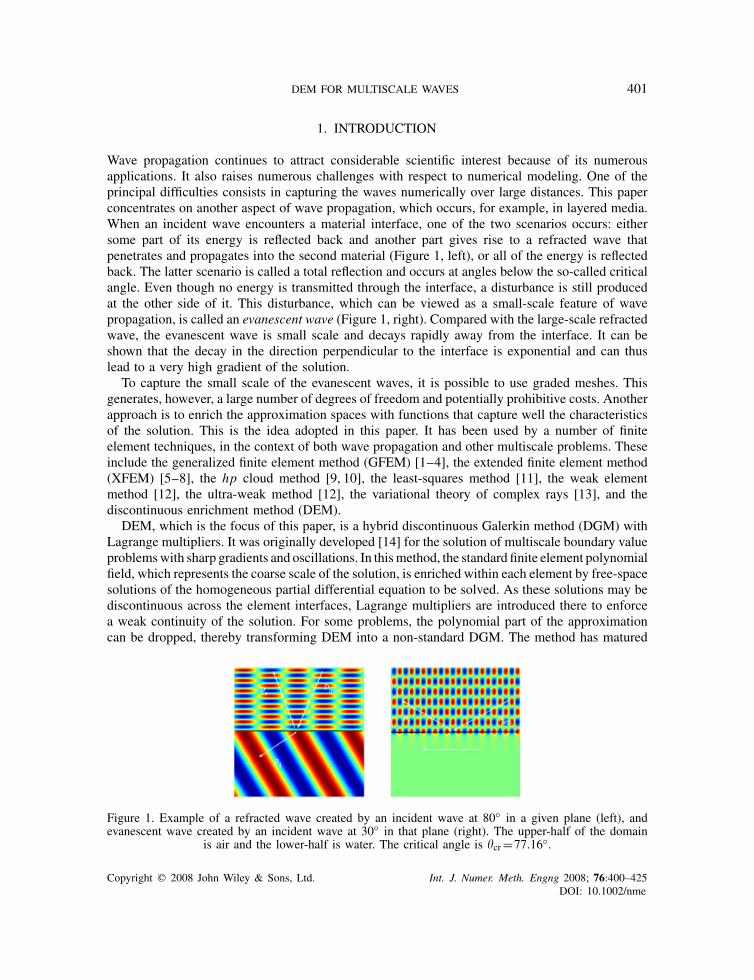
Wave propagation continues to attract considerable scientific interest because of its numerousapplications. It also raises numerous challenges with respect to numerical modeling. One of theprincipal difficulties consists in capturing the waves numerically over large distances. This paperconcentrates on another aspect of wave propagation, which occurs, for example, in layered media.When an incident wave encounters a material interface, one of the two scenarios occurs: eithersome part of its energy is reflected back and another part gives rise to a refracted wave thatpenetrates and propagates into the second material (Figure 1, left), or all of the energy is reflectedback. The latter scenario is called a total reflection and occurs at angles below the so-called criticalangle. Even though no energy is transmitted through the interface, a disturbance is still producedat the other side of it. This disturbance, which can be viewed as a small-scale feature of wavepropagation, is called an evanescent wave (Figure 1, right). Compared with the large-scale refractedwave, the evanescent wave is small scale and decays rapidly away from the interface. It can beshown that the decay in the direction perpendicular to the interface is exponential and can thuslead to a very high gradient of the solution.

To capture the small scale of the evanescent waves, it is possible to use graded meshes. Thisgenerates, however, a large number of degrees of freedom and potentially prohibitive costs. Anotherapproach is to enrich the approximation spaces with functions that capture well the characteristicsof the solution. This is the idea adopted in this paper. It has been used by a number of finiteelement techniques, in the context of both wave propagation and other multiscale problems. Theseinclude the generalized finite element method (GFEM) [1–4], the extended finite element method(XFEM) [5–8], the hp cloud method [9, 10], the least-squares method [11], the weak elementmethod [12], the ultra-weak method [12], the variational theory of complex rays [13], and thediscontinuous enrichment method (DEM).

DEM, which is the focus of this paper, is a hybrid discontinuous Galerkin method (DGM) withLagrange multipliers. It was originally developed [14] for the solution of multiscale boundary valueproblemswith sharp gradients and oscillations. In thismethod, the standard finite element polynomialfield, which represents the coarse scale of the solution, is enriched within each element by free-spacesolutions of the homogeneous partial differential equation to be solved. As these solutions may bediscontinuous across the element interfaces, Lagrange multipliers are introduced there to enforcea weak continuity of the solution. For some problems, the polynomial part of the approximationcan be dropped, thereby transforming DEM into a non-standard DGM. The method has matured

Figure 1. Example of a refracted wave created by an incident wave at 80◦ in a given plane (left), andevanescent wave created by an incident wave at 30◦ in that plane (right). The upper-half of the domain

is air and the lower-half is water. The critical angle is �cr=77.16◦.

Copyright q 2008 John Wiley & Sons, Ltd. Int. J. Numer. Meth. Engng 2008; 76:400–425DOI: 10.1002/nme

402 P. MASSIMI, R. TEZAUR AND C. FARHAT

since the initial development of two-dimensional elements for the Helmholtz equation on uniformmeshes [15]. High-order quadrilateral DGM elements have been developed, coupled with a suitableabsorbing boundary condition for scattering problems and shown to outperform classical polyno-mial approximations [16, 17]. The method has been extended to the three-dimensional Helmholtzequation [18] and to the two-dimensional elastodynamic harmonic problems [19]. A preliminarystudy of DEM in the context of two-dimensional evanescent waves has also been reported in [20].

The main objectives of this paper are to extend the concepts previously studied in two dimen-sions to three dimensions and demonstrate that they can be successfully applied to the efficientsolution of layered, multiscale, fluid–fluid, and fluid–solid problems. To this effect, this paper isorganized as follows. First, the mathematical formulation of DEM for a coupled three-dimensionalfluid–solid problem is presented in Section 2. After reviewing some key aspects of DEM andthe corresponding three-dimensional Helmholtz elements, new three-dimensional elastodynamic(Navier) DEM elements are proposed in Section 3. Then, new DEM elements with evanescentwaves are constructed based on analytical solutions near generic fluid/fluid and fluid/solid inter-faces. In Section 4, the performance of these new elements is evaluated for several benchmarkproblems. Finally, conclusions are presented in Section 5.

2. MATHEMATICAL FORMULATION OF ACOUSTIC PROBLEMS IN COMPRESSIBLEFLUIDS AND ELASTIC SOLIDS

A mathematical framework for acoustic fluid–solid interaction problems is presented here. Theformulation addresses the general heterogeneous problem and can be easily reduced to single- ormulti-layered problems for fluid or solid media. The associated hybrid variational formulation isalso addressed in order to establish the natural mathematical framework for the DEM method.

The wave propagation problem is formulated in a domain �=�f∪�s, where �f and �s are fluidand solid subdomains, respectively. For simplicity, the solid material is assumed to be isotropic andlinearly elastic. A time-harmonic elastic wave propagation is governed by Navier’s equations [21]

�L�u+(�L+�L)∇(∇ ·u)+�s�2u=− f (x) in �s (1)

Here, �s is the density of the elastic material, �L and �L are its Lame constants, � is the circularfrequency, f is the body force, and u≡u(x) is the displacement field in �s.

Let

M=

⎡⎢⎢⎢⎢⎢⎢⎢⎢⎢⎢⎣

�L+2�L �L �L 0 0 0

�L �L+2�L �L 0 0 0

�L �L �L+2�L 0 0 0

0 0 0 �L 0 0

0 0 0 0 �L 0

0 0 0 0 0 �L

⎤⎥⎥⎥⎥⎥⎥⎥⎥⎥⎥⎦

and D=

⎡⎢⎢⎢⎢⎢⎢⎢⎢⎢⎢⎢⎢⎢⎢⎢⎢⎢⎢⎣

��x

0 0

0��y

0

0 0��z

��y

��x

0

0��z

��y

��z

0��x

⎤⎥⎥⎥⎥⎥⎥⎥⎥⎥⎥⎥⎥⎥⎥⎥⎥⎥⎥⎦

(2)



Then, Navier’s equations (1) can also be expressed concisely as

DTMDu+�s�2u=− f in �s (3)

where the superscript ‘T’ designates the transpose operation. The wave propagation in the fluidsubdomain �f is governed by the Helmholtz equation

�p+k2f p=0 in �f (4)

where p≡ p(x ) is the pressure field,

kf= �

cf(5)

is the wave number in the fluid subdomain �f, and cf is the speed of sound in �f. Equilibriumand compatibility at the interface �0=��f∩��s yield the following transmission conditions:

�f�2u ·n = �p

�non �0 (6)

�(u)n ·n+ p = 0 on �0 (7)

where �f is the density of the fluid, n is the normal direction on the fluid/solid interface �0 fromthe solid side, and � is the stress tensor. Without any loss of generality, the following boundaryconditions are considered:

�(u)n = gs

on �s (8)

�p�n

− ikf p = gf on �f (9)

where �f=��f\�0, �s=��s\�0, gf is the excitation on �f, and gsis the specified traction on �s.

Let �f and �s be partitioned into nf and ns elements, respectively, i.e.

�f =nf⋃j=1

�fj , �fj ∩�fl =∅ if j �= l, j, l=1,2, . . . ,nf (10)

�s =ns⋃j=1

�sj , �sj ∩�sl =∅ if j �= l, j, l=1,2, . . . ,ns (11)

Let�fh ={�fj }nfj=1 and�s

h ={�sj }nsj=1 be the set of all elements in�f and�s, respectively. Furthermore,

let Uf, �f, Us, and �s denote the following spaces:

Uf = ∏�∈�f

h

H1(�), �f= ∏� j∈�f

h

∏�l∈�f

h , j<l

H−1/2(�� j ∩��l) (12)

Us = ∏�∈�s

h

(H1(�))3 (13)



�s =

⎧⎪⎪⎨⎪⎪⎩�∈ ∏

� j∈�sh

∏�l∈�s

hj<l

(H−1/2(�� j ∩��l))3 such that

∀�|�� j∩��l∃�∈ H(div;�s) s.t. �·n=� on �� j ∩��l

⎫⎪⎪⎬⎪⎪⎭ (14)

where H1 and H−1/2 are the usual Sobolev spaces [22], and

H(div;�s)=⎧⎨⎩�∈(L2(�s))

3×3 :� jl=�l j ,1� j, l�3,div�=(

3∑l=1

�� jl

�xl

)1� j�3

∈(L2(�s))3

⎫⎬⎭ (15)

Then, the hybrid weak form of the boundary value problem (3)–(9) can be expressed as follows:Find (p,�f)∈Uf×�f and (u,�s)∈Us×�s such that

af(p,q)+bf(�f,q)+�2c(u,q) = rf(q) ∀q∈Uf (16)

as(u,v)+bs(�s,v)+c(v, p) = rs(v) ∀v∈Us (17)

bf(�f, p) = 0 ∀�f∈�f (18)

bs(�s,u) = 0 ∀�s∈�s (19)

where af(·, ·) is the bilinear form defined on Uf×Uf as

af(p,q)= 1

�f

∑�∈�f

h

∫�(∇ p ·∇q−k2f pq)dx− 1

�f

∫�f

ikf pq ds (20)

bf(·, ·) is defined on �f×Uf as

bf(�f, p)= 1

�f

∑� j∈�f

h

∑�l∈�f

hj<l

∫�� j∩��l

�f(p|� j − p|�l )ds (21)

as(·, ·) and bs(·, ·) are defined on Us×Us and �s×Us, respectively, as

as(u,v) = ∑�∈�s

h

∫�(Dv)TM(Du)dx−�s�

2 ∑�∈�s

h

∫�u ·v dx (22)

bs(�,v) = ∑� j∈�s

h

∑�l∈�s

hj<l

∫�� j∩��l

�·(v|� j −v|�l )ds (23)



c(·, ·) is the coupling term defined on Us×Uf as

c(u, p)=∫

�0

p(u ·n)ds (24)

and the linear forms rf(·) and rs(·) are defined on Uf and Us, respectively, as

rf(q) = 1

�f

∫�f

gfq ds (25)

rs(v) =∫

�s

f ·v dx dy+∫

�s

gs·v ds (26)

Let Ufh , �f

h , Ush , and �s

h be finite-dimensional spaces satisfying

Ufh ⊂Uf, �f

h ⊂�f, Ush ⊂Us and �s

h ⊂�s (27)

Then, the discretization of the hybrid variational formulation described above is obtained in astandard manner by replacing the continuous spaces in (16)–(19) by their discrete subspaces (27).Problem (16)–(19) describes a general setting for a multi-phase heterogeneous problem for acousticwave propagation in solid and fluid media. If the coupling term c in Equations (16) and (17) isdropped, system (16) and (18) describes the propagation of acoustic waves in a fluid medium, andsystem (17) and (19) describes the elastodynamic problem associated with the propagation of anacoustic wave in an elastic medium.

3. DEM METHODOLOGY AND THREE-DIMENSIONAL DEM ELEMENTS

In general, DEM [14–19, 23] seeks an approximate solution to its hybrid variational problem inthe form of a locally enriched polynomial. For example, in the case of Navier’s elastodynamicequations (1), it approximates the solution u by

uh =uPh+uEh (28)

where uPh ∈UPh is based on the classical (low-order) finite element polynomials that are suitable for

representing the large scales of the solution [23], and uEh ∈UEh denotes the enrichment that should

be suitable for representing its small scales [23], so that

Uh =UPh⊕UE

h (29)

Note that in the above decomposition, the superscript ‘s’ has been dropped from Uh to indicateits suitability for fluid problems too. Usually, the enrichment field is constructed from the free-space solutions of the homogeneous part of the governing partial differential equations that arenot contained in UP

h . For a large class of Helmholtz problems such as those arising in acousticscattering, the exact solution can be well represented using only the free-space solutions of thegoverning partial differential equation. For such problems, DEM drops the polynomial field fromthe numerical approximation, in which case the enriched elements are labeled DGM (discontinuousGalerkin) elements instead of DEM elements. On the other hand, one can find in the solutionof elastodynamic problems non-oscillatory or slowly oscillatory components in space due to a



specific type of loading. For this reason, DEM can maintain the polynomial field in the numericalapproximation when applied to the solution of some elastodynamic problems, and the enrichedelements are labeled in this case as DEM elements.

As with every hybrid method, special attention needs to be paid to the choice of the Lagrangemultipliers in order to satisfy the inf–sup condition. To this effect, the following ‘limitation’criterion, which was justified in [15–17], is adopted here

n��nE

2(30)

where n� denotes the total number of Lagrange multiplier degrees of freedom per face, and nE

denotes the total number of enrichment functions per element—that is, the dimension of UEh .

The discontinuous enrichment finite element concept can be viewed as a p-type (polynomial)finite element method in the sense that increasing the number of enrichment functions is akin toincreasing the degree of a polynomial approximation. Both approaches are limited by numericalconditioning and computational complexity issues. In practical DEM/DGM computations, theenrichment degrees of freedom can be condensed out at the local (element) level. Hence, the overallcomputational complexity of a DEM/DGM discretization is determined mostly by the number ofLagrange multiplier and polynomial degrees of freedom.

Next, a family of three-dimensional elements for Helmholtz problems with an increasing numberof plane wave and Lagrange multiplier degrees of freedom previously developed in [18] is reviewedfor the sake of completeness.

3.1. DGM elements for three-dimensional Helmholtz problems

In this case, the space Uf,Eh is chosen as a superposition of planar waves. In the general case of nE

planar waves described by unitary directions of propagation �p, p=1, . . . ,nE, this discontinuousspace may be expressed as

Uf,Eh =

{pEh ∈L2(�f) : pEh

∣∣∣�=

nE∑p=1

ppeikf�

Tp ·x , x ∈R3, pp ∈C,

�p ∈R3, ||�p||=1, p=1, . . . ,nE,�p �=�q if p �=q

}(31)

The complex coefficients pp are the primal degrees of freedom in the element �.The other critical aspect of the DEM method is the choice of the Lagrange multipliers on the

element interfaces. It can be shown [15] that the exact solution p and the Lagrange multiplier � ofthe hybrid formulation for the Helmholtz problem are related on the interface between elements �and �′ by

�= �p�n

on ��∩��′ (32)



This suggests choosing �h as a good approximation of �p/�n and leads to the following space ofapproximation for the Lagrange multiplier field:

�fh =

{�h ∈�f :�h |��∩��′(t)=

n�∑p=1

�peikfcp�

Tpt , �p ∈C, p=1, . . . ,n�,

�p are given unitary directions inR2, cp ∈R are given coefficients,

t ∈R2 are local orthogonal coordinates on the face ��,�′ : x= x(t)

}(33)

where � and �′ are two neighboring elements and n� determines the dimension of �fh on each face.

Details about the choice of the directions of the enrichment field and those of the correspondingLagrange multipliers and various implementation details can be found in [18].

Figure 2 shows the directions of the plane waves included in the enrichment field and corre-sponding Lagrange multipliers for two elements that will play a role later in this paper. The firstone, DGM element H–26–4 employs 26 waves in the enrichment field and four Lagrange multi-pliers per face. It has a computational complexity that is similar to that of the classical quadraticelement Q2 but a significantly better performance. The second DGM element for Helmholtz appli-cations, H–56–8, utilizes 56 planar waves and eight Lagrange multipliers per face. It features acomputational complexity per element and a convergence rate that are similar to those of theclassical cubic element Q3. However, it delivers a significantly better performance. For example,it was shown in [18] that in the medium frequency regime, both DGM elements H–26–4 andH–56–8 reduce by one to two orders of magnitude the CPU time required by the standard p-type(polynomial) finite elements with comparable computational complexities and convergence rates,when applied to the solution of three-dimensional wave guide and acoustic scattering problems.

3.2. DEM elements for three-dimensional elastodynamic problems

The concepts underlying the construction of DEM elements for the solution of two-dimensionalelastodynamic problems were discussed in [19]. Here, these concepts are extended to three dimen-sions, and a new family of DEM elements for the solution of the Navier equations is proposed.For simplicity, the case of a homogeneous isotropic material is considered.

In general, free-space solutions of the homogeneous part of the partial differential equation ofinterest are used by DEM to construct an enrichment field for the approximation. In this case,

(a) (b)

Figure 2. Directions of the enrichment field inside the element (solution) and on its faces (Lagrangemultipliers) for elements H–26–4 (a) and H–56–8 (b).



three linearly independent solutions of Equation (3) in the form of planar waves can be found forany direction of propagation: a pressure (longitudinal) wave and two shear (transversal) waves.Hence, the enrichment space Us,E

h is chosen as

Us,Eh =

{uEh ∈(L2(�s))

3 :uEh∣∣∣�=

nE∑q=1

uEPq�qeikp�q ·x +

nE∑q=1

uE1,Sq�⊥q e

iks�q ·x

+nE∑q=1

uE2,Sq�⊥⊥q eiks�q ·x

}(34)

where uPq , u1,Sq , and u2,Sq are the qth pressure and shear amplitude vectors, and �q is the qthdirection of propagation of the elastic pressure and shear waves. The elastic wave numbers kp andks are given by

kp =�√

�

�L+2�Land ks=�

√�

�L(35)

As shown in [19], the exact solution u of the hybrid problem and the Lagrange multiplier � arerelated on the element interfaces by

�=�(u)n on ��∩��′ (36)

This indicates that the Lagrange multipliers should be chosen as approximations of the tractionsof the solution. Here, the traction of another carefully chosen set of pressure and shear waves isused:

�sh ={�h ∈�s :�h |��∩��′ }=

n�p∑j=1

pj �(�p

j eikp�

pj ·x )+

n�s∑j=1

sj�(�sj⊥eiks�

sj ·x ) (37)

where n�p and n�s denote the number of Lagrange multipliers arising from pressure and shearwaves on each face of the element, respectively, and p

j and sj are the dual degrees of freedom on

the edge ��∩��′. To compute the tractions, the following relationships can be conveniently usedfor pressure waves

�(�qeikp�q ·x )n= ikpe

ikp�q ·x [2�L(�q ⊗�q)+�Ln] (38)

and for shear waves

�(�⊥q e

iks�q ·x )n= ikseiks�q ·x�L[(�⊥

q ⊗�q)+(�q ⊗�⊥q )]n (39)

where ⊗ denotes the tensor product.When designing a particular DEM element, a balance must be struck between the quality of the

Lagrange multiplier approximation, which in general improves as their number is increased, andnumerical stability and cost concerns.

Next, two elastic wave propagation DEM elements of increasing order of accuracy are presentedas examples of the discretization methodology outlined above. For the sake of simplicity, onlyregular hexahedral geometries are considered. Generalizing these elements to the case of arbitraryhexahedral geometries is a straightforward task (for example, see [16]).



H–(26×3)–15: The directions �q , q=1, . . . ,26, of propagation of the pressure and shear wavesfor this element coincide with those of the Helmholtz DGM element H–26–4. They may beconcisely expressed as follows: Define

�=⎡⎢⎣1 0 0 1 1 1 −1 1 1 0 1 1 0

0 1 0 1 1 −1 1 1 0 1 −1 0 1

0 0 1 1 −1 1 1 0 1 1 0 −1 −1

⎤⎥⎦

and

�⊥ =⎡⎢⎣0 1 1 0 0 0 1 0 0 1 0 0 1

1 0 0 −1 1 1 1 0 1 0 0 1 0

0 0 0 1 1 1 −1 1 0 0 1 0 0

⎤⎥⎦

Let �qand �⊥

q, q=1, . . . ,26, denote the qth columns of the matrix [�,−�] and [�⊥,−�⊥],

respectively. Then, the directions and polarizations of the waves in (34) are for q=1, . . . ,26,

�q =�q

‖�q‖ , �⊥

q =�⊥q

‖�⊥q‖ , �⊥⊥

q =�q×�⊥

q(40)

In order to describe the Lagrange multipliers of this element, a local coordinate system is definedon each face in such a way that the x- and y-axes are aligned with the sides of the face, and thez-axis is normal to the face. Fifteen Lagrange multipliers per face are defined, of which one is ofpressure type and 14 are based on tractions of shear waves. Let n�p =1,n�s =14,

�pressure =

⎡⎢⎢⎣0

0

1

⎤⎥⎥⎦

�shear =

⎡⎢⎢⎣0 0 1 −1 1 −1 1 −1 1 −1 1 −1 1 −1

0 0 1 −1 −1 1 1 −1 −1 1 1 1 −1 −1

1 1√2

√2

√2

√2

√2

√2

√2

√2 0 0 0 0

⎤⎥⎥⎦

and

�⊥shear=

⎡⎢⎢⎣1 0 1 1 1 1

√2

√2

√2

√2 0 0 0 0

0 1 −1 −1 1 1√2

√2 −√

2 −√2 0 0 0 0

0 0 0 0 0 0 −2 2 −2 2 1 1 1 1

⎤⎥⎥⎦

Then, the explicit representation of the Lagrange multipliers is obtained by transforming eachcolumn of �pressure and corresponding columns of �shear and �⊥

shear into the global frame, normal-izing them to unity and using the relations (38) and (39), respectively. The pressure Lagrangemultiplier and the first two of the shear Lagrange multipliers are based on waves propagating in



the normal direction to the face and give rise to constant tractions. The last four of the Lagrangemultipliers are based on shear waves propagating in the plane of the face. The remaining eightmultipliers are based on waves directed at the face at a 45◦ cone angle (see Figure 3). This specificcone angle has a special importance as the corresponding tractions are invariant when the normalis flipped, which makes the element ‘symmetric’ without the need for adding multipliers in thedirections with the opposite z component.

H–(50×3)–28: This element uses 50 pressure waves and 100 shear waves in the enrichmentfield. The enrichment functions are defined as for the previous element and are based on thematrices

�=[1 0 0 1 1 1 −1 1 1 0 1 1 0 1 1 1 1 −1/2 −1/2 1/2 1/2 −1/2 −1/2 1/2 1/2

0 1 0 1 1 −1 1 1 0 1 −1 0 1 −1/2 −1/2 1/2 1/2 1 1 1 1 −1/2 1/2 −1/2 1/2

0 0 1 1 −1 1 1 0 1 1 0 −1 −1 −1/2 1/2 −1/2 1/2 −1/2 1/2 −1/2 1/2 1 1 1 1

]

and

�⊥ =⎡⎢⎣0 1 1 0 0 0 0 0 0 1 0 0 1 0 0 0 0 1 1 1 1 1 1 1 1

1 0 0 −1 1 1 1 0 1 0 0 1 0 1 1 1 1 0 0 0 0 −1 1 1 −1

0 0 0 1 1 1 −1 1 0 0 1 1 0 −1 1 1 −1 −1 1 1 −1 0 0 0 0

⎤⎥⎦

The Lagrange multipliers are constructed in a manner similar to that described for the previouselement. More specifically, there are eight Lagrange multipliers per face that are based on tractionsof pressure waves that propagate at an angle to the face

�pressure=⎡⎢⎣1 −1 0 0 1 −1 0 0

0 0 1 −1 0 0 1 −1

2 2 2 2 −2 −2 −2 −2

⎤⎥⎦

There are also 20 Lagrange multipliers per face that are based on tractions of shear waves.Compared with the case of the previous element, there are additional eight multipliers that are

Figure 3. DEM element H–(50×3)–28: directions of the enrichment field for the solution, and generatingwaves for the Lagrange multipliers.



based on 45◦ shear waves

�shear=

⎡⎢⎢⎣1 −1 0 0 1 −1 0 0 1 −1 1 −1 1 −1 1 −1 1 −1 1 −1

0 0 1 −1 0 0 1 −1 1 −1 −1 1 1 −1 −1 1 1 1 −1 −1

1 1 1 1 1 1 1 1√2

√2

√2

√2

√2

√2

√2

√2 0 0 0 0

⎤⎥⎥⎦

and

�⊥shear=

⎡⎢⎢⎣0 0 1 1 −1 1 0 0 1 1 1 1

√2

√2

√2

√2 0 0 0 0

1 1 0 0 0 0 −1 1 −1 −1 1 1√2

√2 −√

2 −√2 0 0 0 0

0 0 0 0 1 1 1 1 0 0 0 0 −2 2 −2 −2 1 1 1 1

⎤⎥⎥⎦

The aforementioned waves are graphically depicted in Figure 3.When required, the new H–(26×3)–15 and H–(50×3)–28 DEM elements described above

can also be equipped with a polynomial field. Without it, their sparsity pattern and number ofdegrees of freedom are such that, from a computational complexity viewpoint, they are equivalentto the quadratic and cubic p-type (polynomial) standard Galerkin elements, respectively. Theperformances of these new DEM elements are assessed in Section 5 for a coupled fluid–solidproblem.

Wave propagation problems with fluid/fluid, fluid/solid, or solid/solid interfaces give rise,however, to multiscale wave propagation problems with evanescent waves that have differentcharacteristics than the traveling waves on which the DGM/DEM elements covered so far arebased on. For this reason, the DEM/DGM elements outlined above, and summarily labeled hereH–X–Y, are further enriched in the following sections to improve their efficiency when appliedto the solution of wave propagation problems with evanescent waves. Similar ideas have beenpreviously explored in [20] in two dimensions. They are presented here in three dimensions. Theresulting elements are labeled H–X–Y ∗ and designed for usage in the vicinity of material interfaces.

3.3. DGM elements for fluid/fluid interface regions

Consider the case of two semi-infinite fluids with computational subdomains �f1 and �f2 separatedby a planar interface as illustrated in Figure 4(a). When an incident wave pinc impinges on theinterface from the �f1 side in an oblique direction and the two fluids have different speeds of sound,it produces a reflected wave pr in �f1 and a refracted wave pt in �f2 . The relationship between thealtitude angle of the incident wave �inc (see Figure 4), the altitude angle of the refracted wave �t(see Figure 4), and the speeds of sound in the two fluids, c1 and c2, is known as Snell’s law [24]and is recalled below.

cos�incc1

= cos�tc2

(41)

When c1<c2, Snell’s law predicts that the altitude angle of the refracted wave is smaller than thatof the incident wave, i.e. �t<�inc. As the altitude angle of incidence is decreased, the refracted



Figure 4. Incident, reflected, and refracted waves in fluid/fluid (a) and fluid/solid (b) media.

wave eventually becomes parallel to the interface. This occurs for one particular altitude angle ofincidence called the critical angle and is given by

�cr=cos−1(c1c2

)if c1<c2 (42)

If �inc<�cr, the refracted wave disappears, the incident wave undergoes total internal reflectionand an evanescent wave occurs in the second fluid, �f2 .

For simplicity, assume that the coordinate system is such that the interface is the x–y plane, �f1is the region z>0, and �f2 is the region z<0. Furthermore, assume that pinc, pr and pt are planewaves that satisfy the Helmholtz equation (4) in their respective domains. From the transmissionconditions

pinc+ pr= pt and1

�1

��n

(pinc+ pr)= 1

�2

�pt�n

it follows that these plane waves are of the form

pinc = Ainceik1[(x cos�+y sin�)cos�inc−z sin�inc] (43)

pr = Areik1[(x cos�+y sin�)cos�inc+z sin�inc] (44)

pt = Atezei

√k22+2(x cos�+y sin�) (45)

where =√k21 cos

2 �inc−k22 and the amplitudes Ainc, Ar, and At are given by

Ar =−�1+ ik1�2 sin�inc�1− ik1�2 sin�inc

Ainc, At=− 2ik1�2 sin�inc�1− ik1�2 sin�inc

Ainc (46)

Hence, is a real number if �inc<�cr, in which case the transmitted (refracted or evanescent) wavept is evanescent and decays exponentially in the negative z direction. Note also that the apparent



wave number of the evanescent wave pt along the interface is �∈[k2,k1], instead of the nativewave number k2.

Next, new DGM elements H–X–Y ∗ are constructed by further enriching the H–X–Y (seeSection 3.1) elements with evanescent waves. More specifically, the wave approximation of thesolution and its corresponding Lagrange multiplier field are rewritten, element by element and faceby face as

pEh (x)= pPWh (x)+ pEWh (x) and �h(x)=�h(x)PW+�h(x)

EW (47)

The superposition of planar waves pPWh (x) is given by (31). The enrichment field pEWh (x) is chosenas a superposition of evanescent waves that propagate along the fluid/fluid interface and decayaway from it. If the element is assumed—for the sake of simplicity of notation—to be a cubealigned with the coordinate system, then

pEWh (x)=nev∑j=1

p jeikevj ·x (48)

where nev is the number of evanescent enrichment waves and kevj =[�cos� j ,�sin� j , i]. The realconstants � and are given by

�=k1 cos�EW, =

√k21 cos

2 �EW−k22 (49)

where �EW is a subcritical altitude angle that is set a priori.Following the same approach adopted for the design of �PWh , the Lagrange multiplier field �EWh

is chosen as the following approximation of �pEWh /�n:

�EWh =

⎧⎪⎪⎨⎪⎪⎩

n�ev∑j=1

�EWj ei�(x cos� j+y sin� j ) on horizontal faces

�EW0 ez on vertical faces

(50)

Different choices of �EW and the number and values of the directions � j of the evanescentwaves (see Figures 5 and 6) lead to different elements with different computational efficiencies.Four possible choices leading to four new DGM elements are discussed below. These new elements

(a) (b)

Figure 5. Directions of the evanescent wave enrichment functions for the solution.



(a) (b) (c)

Figure 6. Directions of the evanescent wave functions for the Lagrange multipliers.

are labeled H–26–Y ∗ and H–56–Y ∗ because they are constructed by further enriching in differentways the DGM elements H–26–4 and H–56–8, respectively (Section 3.1).

H–26–4∗: Here, nev=4, n�ev =4 on the horizontal faces, and n�ev =1 on the vertical ones. Theevanescent enrichment waves are defined by (48) and the azimuthal angles

� j =�

4+( j−1)

�

2, j =1, . . . ,4

The evanescent Lagrange multipliers are constructed using the same angles and (50).H–26–4∗∗: For this element, nev=4, n�ev =4 on the horizontal faces, and n�ev =1 on the vertical

faces. The enrichment for evanescent wave problems is the same as in the previous element.However, the azimuthal angles for the multipliers are different and chosen as follows:

� j =( j−1)�

2, j =1, . . . ,4

H–26–8∗: Here, nev=8, n�ev =8 on the horizontal faces, and n�ev =1 on the vertical ones. ThisDGM element uses a set of eight directions for the evanescent enrichment. Its Lagrange multipliersare given by the following azimuthal angles:

� j =( j−1)�

4, j =1, . . . ,8

H–56–8∗: For this element, nev=8, n�ev =8 on the horizontal faces, and n�ev =1 on the verticalfaces. This DGM element uses the same enrichment for capturing evanescent waves as the previouselement but is based on the element H–56–8.

3.4. DEM elements for fluid/solid interface regions

When an incident wave pinc encounters a fluid/solid interface, it gives rise to two transmittedwaves in the solid: a pressure wave u p and a shear wave us , as shown in Figure 4(b). In thissituation, Snell’s law states that

cos�inccf

= cos�p

cp= cos�s

cs(51)



where �inc is the altitude angle of the incident wave, �p and �s are the altitude angles of therefracted pressure and shear waves, respectively, cf is the speed of sound in the fluid, and cp andcs are the elastic speeds of sound in the solid given by

cp = �

kp, cs = �

ks(52)

where kp and ks are given by (35).There are two critical angles: �cp for pressure waves and �cs for shear waves. These angles are

given by

�cp =cos−1(cfcp

)if cf<cp and �cs =cos−1

(cfcs

)if cf<cs (53)

Assume that the interface is aligned with the x–y plane, �f is the region z>0, �s is the regionz<0, and the incident, reflected, and transmitted waves are in the form of plane waves. In thiscase, using the transmission conditions (6) and (7), it can be shown that the transmitted pressurewave u p is evanescent if cf<cp and �inc<�cp , the transmitted shear wave us is evanescent if cf<csand �inc<�cs , and these waves are of the form

pinc = Ainceik[(x cos�+y sin�)cos�inc−z sin�inc] (54)

pr = Areik[(x cos�+y sin�)cos�inc+z sin�inc] (55)

u p = Ap

⎡⎢⎣

�cos�

�sin�

i

⎤⎥⎦ezei�(x cos�+y sin�) (56)

us = As

⎡⎢⎣

−ibcos�

−ib sin�

a

⎤⎥⎦ebzeia(x cos�+y sin�) (57)

where

�2 = 2+k2p, =√k2 cos2 �inc−k2p (58)

a2 = b2+k2s , b=√k2 cos2 �inc−k2s (59)

and the amplitudes are given by

As = − 2i�k sin�inc�f�2(2�a−a2+b2)− i2�k sin�inc

Ainc (60)

Ap = −a2−b2

2�As (61)

Ar = −i(k2p�L+22�L)Ap−2iab�LAs−Ainc (62)

Hence, the evanescent waves u p and us decay exponentially in the negative z direction.



Following the same procedure outlined previously for fluid-type (Helmholtz) DGM elements,the approximate solution in the solid-type (Navier) DEM elements for elastodynamic problemscan be further enriched for capturing evanescent waves as follows:

uEh =uPWh (x)+uEWh (x) (63)

where uPWh (x) is the same as in (34), and the evanescent enrichment is chosen as

uEWh (x) =nE∑j=1

u p j

⎡⎢⎢⎣

�cos� j

�sin� j

i

⎤⎥⎥⎦ezei�(x cos� j+y sin� j )

+nE∑j=1

us j

⎡⎢⎢⎣

−ibcos� j

−ib sin� j

a

⎤⎥⎥⎦ebzeia(x cos� j+y sin� j ) (64)

where

=√k2 cos2 �EW−k2p, �2=k2p+2 (65)

b =√k2 cos2 �EW−k2s , a2=k2s +b2 (66)

As in the case of a fluid/fluid interface, the Lagrange multiplier field is approximated by�h =�PWh +�EWh , where �PWh is chosen in the space �s

h specified in expression (37), and �EWh ischosen as the traction �(uEWh )n.

Evanescent waves can also potentially arise on the fluid side of a fluid/solid interface, dependingon the material properties. They can then be captured by the elements described in the previoussection with the wave number k1 in the fluid replaced by the pressure wave number kp and/or theshear wave number ks of the solid.

As an example, two new DEM elements are constructed below assuming again—for the sakeof simplicity of notation—that the element is a cube aligned with the coordinate system. Thenew elements are derived from the H–(26×3)–15 and H–(50×3)–28 elements, respectively, byadding a total of 16 evanescent waves to the enrichment field, eight of which are pressure wavesand eight of which are shear waves, using the definition (64) with nE=8 and the azimuthalangles

� j =( j−1)�

4, j =1, . . . ,8

In order not to over-constrain the final system and to avoid numerical instability, only four evanes-cent Lagrange multipliers are added on the horizontal faces. They are obtained by computing thetraction of the evanescent shear waves given by the directions � j =[0,�/2,�,3�/2]. Thus, for the



Lagrange multipliers on the horizontal faces, one obtains

�EW = �EW1

⎡⎢⎢⎣i(a2−b2)

0

2ab

⎤⎥⎥⎦eiax +�EW2

⎡⎢⎢⎣

0

i(a2−b2)

2ab

⎤⎥⎥⎦eiay

+�EW3

⎡⎢⎢⎣i(a2−b2)

0

−2ab

⎤⎥⎥⎦e−iax +�EW4

⎡⎢⎢⎣

0

i(a2−b2)

−2ab

⎤⎥⎥⎦e−iay

On the vertical faces aligned with the x–z plane and the y–z plane, the following multipliers witha decaying component are obtained:

�EW=�EW1

⎡⎢⎢⎣

2ab

0

i(a2−b2)

⎤⎥⎥⎦eiaxebz+�EW2

⎡⎢⎢⎣

−2ab

0

i(a2−b2)

⎤⎥⎥⎦e−iaxebz

and

�EW=�EW1

⎡⎢⎢⎣

0

2ab

i(a2−b2)

⎤⎥⎥⎦eiayebz+�EW2

⎡⎢⎢⎣

0

−2ab

i(a2−b2)

⎤⎥⎥⎦e−iayebz

4. NUMERICAL RESULTS

In this section, the performance of the newly constructed DGM elements with evanescent waveenrichment functions is assessed and compared with that of their counterparts without this addi-tional type of enrichment functions, and with the performance of comparable standard higher-orderpolynomial finite elements. For this purpose, fluid–fluid and fluid–solid wave propagation bench-mark problems with known analytical solutions, which furthermore justify dropping the polynomialfield from the enriched approximation, are considered.

It is recalled that in [18], it was shown that:

1. The DGM element H–26–4 has a computational complexity and a convergence rate thatare comparable to those of the standard quadratic Galerkin element Q2, but a significantlysmaller error constant and therefore a significantly better accuracy.

2. The DGM element H–56–8 has a computational complexity and a convergence rate that arecomparable to those of the standard cubic Galerkin element Q3, but a significantly smallererror constant and therefore a significantly better accuracy.

Hence, the performances compared here are those of the elements H–26–4, H–26–4∗, and Q2, andthose of the elements H–56–8, H–56–8∗, and Q3.

In the strict sense, the performance of a discretization method applied to the solution of thefamily of problems considered in this section depends on the direction of the incident wave. For



this reason, all benchmark problems discussed in this section are dealt with as follows. For eachspecified altitude angle of incidence �inc, five computations are performed for the following fivedifferent values of the azimuthal angle of incidence:

�inc=0◦, �inc=11.25◦, �inc=22.5◦, �inc=33.75◦ and �inc=45◦

The sampling in the interval [0◦,45◦] is due to the azimuthal symmetry of the considered benchmarkproblems. The five obtained relative errors are then simply averaged and the result is reported asthe relative error associated with the specified value of �inc.

For DGM, the degree of freedom count is based only on the total number of Lagrange multipliers,because of the static condensation property of these elements. As the internal degrees of freedomof the standard higher-order Galerkin elements can also be condensed out at the element level, theyare also not included in the degree of freedom count in order to provide meaningful performancecomparisons.

Because evanescent waves decay exponentially away from the interface, adding them to theapproximation space of the elements located far away from the interface may not be necessary.Therefore, the evanescent wave enrichment degrees of freedom and corresponding Lagrange multi-pliers are activated only in the two layers of elements that are closest to the interface, as shownin Figure 7. Also, due to the exponential decay of the function ez in the direction z<0, theinclusion of evanescent waves in a basis can result in nearly singular local stiffness matrices,particularly in the elements further away from the interface. To prevent this from happening, thescaling technique used for the evanescent waves in two dimensions [20] is adopted here—that is,the evanescent wave enrichment functions are scaled so that their maximum amplitude is equal toone in each element. The same scaling technique is applied to the corresponding approximationof the Lagrange multiplier field on each element face.

4.1. Acoustic evanescent waves

The domain �=[0,1]×[0,0.25]×[−0.25,0.25] is divided into two subdomains: �f1 =[0,1]×[0,0.25]×[−0.25,0] and �f2 =[0,1]×[0,0.25]×[0,0.25], which are assumed to be filled withwater (�1=1.29kg/m3, c1=343m/s) and air (�2=1000kg/m3,c2=1533m/s), respectively. TheRobin boundary condition (9) is applied on the boundaries �fm ,m=1,2, with gm =�pexm /�n−ikm pexm , where the two components of the exact solution pex1 = pinc+ pr in �f1 and pex2 = pt in �f2are shown in Figure 4. The incident wave pinc, the reflected wave pr, and the transmitted wavesare given by Equations (43)–(46). For this problem setup, the critical angle is �cr=77.16◦. The

Γ0

Γ0

Figure 7. Discretization of the computational subdomains associated with a fluid–fluidor fluid–solid problem: same mesh size scenario (left), and coarse-fine meshes scenario(right). Elements with evanescent wave enrichment functions are used only in the first two

layers of the bottom subdomain and colored in gray.



wave numbers k1=�/c1 and k2=�/c2 and the altitude angle of the incident wave �inc consideredfor this problem are specified later in this section.

The two computational subdomains are discretized uniformly (see Figure 7). For each assessednumerical solution method, the mesh size is varied in order to enable a mesh convergence numericalstudy. Since c1 is smaller than c2, a coarser mesh may be used in subdomain�f2 if a constant numberof elements per wavelength is adopted. Thus, two types of subdomain meshes are considered asshown in Figure 7: (a) same size meshes and (b) coarse-fine meshes where the mesh in �f2 istwice coarser than that in �f1 . Since by construction, the DGM elements incorporate Lagrangemultipliers on their interfaces in order to enforce there a weak continuity of the solution, theirusage on non-matching meshes as in the coarse-fine discretization scenario requires no specialattention. On the other hand, the eventual usage of standard Galerkin elements in the coarse-finediscretization scenario would require the introduction of mortar elements at the fluid–fluid interfaceand therefore is not considered here.

In all computations reported for this problem, �EW is set to

�EW= 12�cr=38.58◦

The discretization error is measured separately in each of the two computational subdomains�fm,m=1,2. The relative error associated with the classical FEM is measured by the discrete L2norm over all vertices in the subdomains—that is, by

‖pex− pFEMh ‖�fm

‖pex‖�fm

=√∑

V∈�mvert

|(pex− pFEMh )(V )|2√∑V∈�m

vertpex(V )2

(67)

where �mvert denotes the set of all vertices in the mesh �m

h ,m=1,2. The relative error associatedwith a DGM solution is measured using the same metric. However, as the DGM solution isdiscontinuous at the vertices, it is first averaged as follows:

pDGMh (V )= 1

nmvert

∑�∈�m

hV∈�

pDGMh |�(V ) (68)

where nmvert,m=1,2, denotes the number of elements in subdomain �fm sharing the vertex V .Then, the corresponding relative error is computed as follows:

‖pex− pDGMh ‖�fm

‖pex‖�fm

=√∑

V∈�mvert

|(pex− pDGMh )(V )|2√∑V∈�m

vertpex2

(69)

Figure 8 reports the convergence rates of the original DGM element H–26–4, its three versionsthat are enriched with evanescent wave functions H–26–Y∗, H–26–Y∗∗, and H–26–8∗, and thestandard Galerkin element Q2, in the medium frequency regimes k1=60 and k2=13.33 and forthe subcritical altitude angle of incidence �inc=25◦. This altitude angle of incidence gives rise toevanescent waves in �f2 . As expected, the results reported in this figure show that the selectiveinclusion of evanescent waves in the enrichment field of the DGM elements in the vicinity of



(a)

(c)

(b)

(d)

Figure 8. Fluid–fluid wave propagation model problem: comparison of the performances of theelements H–26–Y∗, H–26–4, and Q2 for k1=60, k2=13.33, and �inc=25◦: (a) domain �f1 ,matching meshes; (b) domain �f2 , matching meshes; (c) domain �f1 , coarse-fine meshes; and

(d) domain �f2 , coarse-fine meshes.

the fluid–fluid interface on the �f2 side (1) is a good strategy, (2) improves dramatically theperformance of the DGM elements in subdomain �f2 where evanescent waves are created, and (3)improves only a little the performance of the DGM elements in subdomain �f1 where the exactsolution does not contain any evanescent wave. More specifically, the DGM element H–26–4 isfound to improve the accuracy of the standard element Q2 in the subdomain �f1 by almost a fullorder of magnitude, which is consistent with the results previously established for a homogeneousfluid domain [18]. However, more importantly, portions (b) and (d) of Figure 8 show that insubdomain �f2 where evanescent waves arise, the DGM element H–26–4 fails even to match theperformance of the standard element Q2, which indicates that a basis of planar wave functions isnot quite able to capture the exponential decay of the solution there. On the other hand, all versionsof this DGM element that feature further enrichment by evanescent wave functions are reported tooutperform the standard quadratic element Q2. For example, the DGM element H–26–8∗ reachesthe 2% level of relative error in subdomain �f2 using five times fewer degrees of freedom than Q2for the matching meshes scenario. For the coarse-fine mesh scenario that is natural for the DGMtechnology, the DGM element H–26–8∗ reaches the same 2% level of relative error in �f2 using12 times fewer degrees of freedom than Q2.



Next, the two wave numbers are increased to k1=90 and k2=20.14. Accordingly, the DGMelements H–56–8 and H–56–8∗ and the standard Galerkin element Q3 are considered for thediscretization of the problem at hand. The results obtained for the scenario of matching meshesare reported in Figure 9. As in the previous case of lower frequency, the DGM element H–56–8 isfound to outperform the cubic element in �f1 ; more specifically it delivers the same accuracy usingseven times fewer degrees of freedom. However, in contrast to the previous case, the original DGMelement H–56–8 retains some of its advantages over the standard element Q3 even in subdomain �f2where the evanescent waves appear. The DGM element H–56–8∗, which contains the enrichmentby evanescent wave functions, re-establishes the complete performance superiority over the cubicelement Q3 in subdomain �f2 , almost to the same level achieved in subdomain �f1 . For thishigher-frequency problem, the performance gain delivered by the further enriched DGM elementH–56–8∗ over the original DGM element H–56–8 is, however, a little smaller than that delivered inthe lower-frequency case considered previously. This suggests that at higher frequencies, enrichingthe approximation by more than eight evanescent wave functions may be beneficial.

4.2. Elastodynamic evanescent waves

Here, the problem of interest is governed by the boundary value problem (3)–(9) and defined inthe domain �=[0,1]×[0,0.25]×[0,0.5]. The upper-half subdomain �f is assumed to be filledwith water, and the lower-half subdomain �s is assumed to be made of a steel characterized by theLame constants �L=9.24e+10 and �L=7.87e+10. The Robin boundary condition (9) is imposedon the boundary �f with gf=�pex/�n− ikpex, where pex= pinc+ pr is the exact pressure solutionin �f. The natural boundary condition (8) with g

s=�(uex)n is imposed on the boundary �s, where

the exact solution for the displacement field in �s is uex=u p+us and is shown in Figure 4.The incident wave pinc, the reflected wave pr, and the transmitted waves u p and us are given inEquations (54)–(60).

For this problem, the critical angles for the pressure and shear waves are

�cs =61.87◦, �cp =74.66◦ (70)

Figure 9. Fluid–fluid wave propagation model problem: comparison of the performances of the elementsH–56–8∗, H–56–8, and Q3 for k1=90, k2=20.14, and �inc=25◦.



(a) (b)

(c) (d)

Figure 10. Fluid–solid wave propagation model problem: comparison of the performances of the elementsH–(26×3)–15, H–(26×3)–15∗, and Q2 for k=40, ks=18.85, kp =10.58, and �inc=25◦: (a) fluid subdo-main, matching meshes; (b) solid subdomain, matching meshes; (c) fluid subdomain, coarse-fine meshes;

and (d) solid subdomain, coarse-fine meshes.

an evanescent wave can occur only in the solid subdomain, and the parameter �EW is set in allDGM elements enriched with evanescent wave functions to

�EW= 12�cs =30.94◦

As in the case of the fluid–fluid wave propagation model problem, two different uniformmesh scenarios are considered: one with matching size meshes and one with coarse-fine meshes(Figure 7). In the latter case, the mesh for the solid subdomain is twice coarser than that for thefluid subdomain. The evanescent wave degrees of freedom are activated in subdomain �s only, inthe two layers of elements closest to the fluid–solid interface. The discretization error is measuredseparately in the fluid and solid subdomains �f and �s. In �f, the relative errors are computedusing Equations (67)–(68). In �s, they are computed in a similar manner.

First, the altitude angle of the incident wave is set to �inc=25◦. From Equations (70), it followsthat �inc<�cs<�cp . Therefore, the exact solution in the solid subdomain is in this case a combinationof an evanescent pressure wave and an evanescent shear wave.



(a) (b)

(c) (d)

Figure 11. Fluid–solid model wave propagation problem: comparison of H–50×3–28, H–(50×3)–28∗, andQ3 for k=80, ks=37.71, kp =21.15: (a) fluid domain �inc=75◦; (b) solid domain �inc=75◦; (c) fluid

domain �inc=25◦; and (d) solid domain �inc=25◦.

Figure 10 reports the results obtained for the DGM elements H–(26×3)–15∗ and H–(26×3)–15and for the standard Galerkin element Q2 in the medium frequency regime defined by k=40,kp =10.58, and ks=18.86. The DGM element H–(26×3)–15∗, which is further enriched withevanescent wave functions, is found to improve the accuracy achievable by the DGM elementH–(26×3)–15 in both meshing scenarios. For the coarse-fine meshes scenario, this improvementis achieved even in the fluid subdomain where no evanescent wave appears, but where the effectof this wave is inherited from the solid subdomain via the fluid–solid interaction. Even whenintroducing up to 50 000 degrees of freedom, the solution of this problem by the Q2 element failsto reach a level of relative error as low as 1% in the solid subdomain. On the other hand, the DGMelement H–(26×3)–15∗ delivers this level of accuracy in �s with 10 000 degrees of freedom only.When the target relative error is relaxed to 10% in order to accommodate the performance of theelement Q2 for this problem, the DGM element H–(26×3)–15∗ achieves this objective in both thesolid subdomain using about 40 times fewer degrees of freedom than Q2.

Next, the frequency is increased so that the wave numbers become k=80, kp =21.15, andks=37.71. The higher-order elements H–(50×3)–28∗, H–(50×3)–28, and Q3 are then consideredfor the solution of the following fluid–solid interaction problems. First, �inc is set to �inc=75◦



so that no evanescent wave is produced in either subdomain. Figure 11(a)–(b) shows that in thiscase, both considered DGM elements yield virtually the same performance results and outperfomthe cubic element Q3 by more than one order of magnitude in the subdomain �s, while exhibitingapproximately the same rate of convergence. Next, �inc is set to �inc=25◦ so that two pressure andshear evanescent waves are created in the solid subdomain. In this case, the performance resultsdisplayed in Figure 11(c)–(d) show that the asymptotic convergence rate of the DGM elementH–(50×3)–28 is improved when evanescent wave functions are added to its set of enrichmentfunctions. In the solid subdomain, the discretization by the DGM element H–(50×3)–28∗ is foundto reach the 90% level of accuracy using approximately seven times fewer degrees of freedomthan that by the standard cubic Galerkin element Q3.

5. CONCLUSION

Evanescent waves occur in multi-material media when the altitude angle of an incident wave isbelow a critical value. When the different media are characterized by sufficiently different speedsof sound, these small-scale waves transform a wave propagation problem into a genuine multiscaleproblem that is difficult to solve numerically by standard approximation methods. Enrichment-based discretization approaches such as the DEM and its variant known as the discontinuousGalerkin method (DGM) with Lagrange multipliers can be well suited for solving such problems, ifappropriate enrichment fields are chosen. In this paper, it is shown that although plane wave shapefunctions can efficiently capture acoustic scattering fields in the absence of evanescent waves,including in the medium frequency regime, they sometimes do not perform significantly better thanhigher-order polynomial approximations in the presence of such waves. On the other hand, furtherenrichment of plane-wave-based elements with evanescent wave shape functions is shown to leadto high-performance multiscale elements that effectively capture all of the reflected and transmittedwaves in a multi-material problem. Numerical tests performed in three dimensions for various fluid–fluid and fluid–solid wave propagation model problems reveal that DGM elements with Lagrangemultipliers combining plane wave and evanescent wave shape functions can reduce the number ofdegrees of freedom required by either the DGM elements with plane wave shape functions onlyor the standard higher-order polynomial finite elements, by up to a factor larger than a full orderof magnitude.

ACKNOWLEDGEMENTS

The authors acknowledge the support by the Office of Naval Research under Grant N00014-05-1-0204-1.

REFERENCES

1. Melenk JM. On generalized finite element methods. Ph.D. Thesis, University of Maryland, College Park, MD,1995.

2. Strouboulis T, Copps K, Babuska I. The generalized finite element method. Computer Methods in AppliedMechanics and Engineering 2001; 190:4081–4193.

3. Strouboulis T, Zhang L, Babuska I. p-Version of the generalized FEM using mesh-based handbooks withapplications to multiscale problems. International Journal for Numerical Methods in Engineering 2004; 60:1639–1672.



4. Vitali E, Benson DJ. An extended finite element formulation for contact in multi-material arbitrary Lagrangian–Eulerian calculations. International Journal for Numerical Methods in Engineering 2006; 67:1420–1444.

5. Daux C, Moes N, Dolbow J, Sukumar N, Belytschko T. Arbitrary branched and intersecting cracks with theextended finite element method. International Journal for Numerical Methods in Engineering 2000; 48:1741–1760.

6. Belytschko T, Parimi C, Moes N, Sukumar N, Usui S. Structured extended finite element methods for soliddefined by implicit surfaces. International Journal for Numerical Methods in Engineering 2003; 56:609–635.

7. Ventura G. On the elimination of quadrature subcells for discontinuous functions in the extended finite elementmethod. International Journal for Numerical Methods in Engineering 2006; 66:761–795.

8. Gracie R, Ventura G, Belytschko T. A new fast finite element method for dislocations based on interiordiscontinuities. International Journal for Numerical Methods in Engineering 2007; 69:423–441.

9. Duarte CA, Oden JT. An hp adaptive method using clouds. Computer Methods in Applied Mechanics andEngineering 1996; 139:237–262.

10. Oden JR, Duarte CA, Zienkiewicz OC. A new cloud-based hp finite element method. Computer Methods inApplied Mechanics and Engineering 1998; 153:117–126.

11. Monk P, Wang DQ. A least-squares method for the Helmholtz equation. Computer Methods in Applied Mechanicsand Engineering 1999; 175:121–136.

12. Huttunen T, Monk P, Collino F, Kaipio JP. The ultra-weak variational formulation for elastic wave problems.SIAM Journal on Scientific Computing 2004; 25(5):1717–1742.

13. Ladeveze P, Riou H. Calculation of medium-frequency vibrations over a wide frequency range. Computer Methodsin Applied Mechanics and Engineering 2005; 94:3167–3191.

14. Farhat C, Harari I, Franca LP. The discontinuous enrichment method. Computer Methods in Applied Mechanicsand Engineering 2001; 190:6455–6479.

15. Farhat C, Harari I, Hetmaniuk U. A discontinuous Galerkin method with Lagrange multipliers for the solutionof Helmholtz problems in the mid-frequency regime. Computer Methods in Applied Mechanics and Engineering2003; 192:1389–1419.

16. Farhat C, Wiedemann-Goiran P, Tezaur R. A discontinuous Galerkin method with plane waves and Lagrangemultipliers for the solution of short wave exterior Helmholtz problems on unstructured meshes. New computationalmethods for wave propagation. Wave Motion 2004; 39(4):307–317.

17. Farhat C, Tezaur R, Weidemann-Goiran P. Higher-order extensions of a discontinuous Galerkin method formid-frequency Helmholtz problems. International Journal for Numerical Methods in Engineering 2004; 61:1938–1956.

18. Tezaur R, Farhat C. Three-dimensional discontinuous Galerkin elements with plane waves and Lagrangemultipliers for the solution of mid-frequency Helmholtz problems. International Journal for Numerical Methodsin Engineering 2006; 66:796–815.

19. Zhang L, Tezaur R, Farhat C. The discontinuous enrichment method for elastic wave propagation in themedium-frequency regime. International Journal for Numerical Methods in Engineering 2006; 66:2086–2114.

20. Tezaur R, Zhang L, Farhat C. A discontinuous enrichment method for capturing evanescent waves in multi-scale fluid and fluid/solid problems. Computer Methods in Applied Mechanics and Engineering 2007. DOI:10.1016/j.cma.2007.08.023.

21. Graff KF. Wave Motion in Elastic Solids. Dover: New York, 1991.22. Adams RA. Sobolev Spaces. Academic Press: New York, 1975.23. Farhat C, Harari I, Hetmaniuk U. The discontinuous enrichment method for multiscale analysis. Computer

Methods in Applied Mechanics and Engineering 2003; 192:3195–3210.24. DeSanto JA. Scalar Wave Theory. Springer: Berlin, 1992.


A discontinuous enrichment method for three-dimensional multiscale harmonic wave propagation...

Documents

Transcript of A discontinuous enrichment method for three-dimensional multiscale harmonic wave propagation...