Optimal sampling strategies for multiscale stochastic processes

arX

ivm

ath

0611

191v

1 [

mat

hST

] 7

Nov

200

6

IMS Lecture NotesndashMonograph Series

2nd Lehmann Symposium ndash Optimality

Vol 49 (2006) 266ndash290ccopy Institute of Mathematical Statistics 2006DOI 101214074921706000000509

Optimal sampling strategies for multiscale

stochastic processes

Vinay J Ribeiro1 Rudolf H Riedi1 and Richard G Baraniuk2lowast

Rice University

Abstract In this paper we determine which non-random sampling of fixedsize gives the best linear predictor of the sum of a finite spatial populationWe employ different multiscale superpopulation models and use the minimummean-squared error as our optimality criterion In multiscale superpopulationtree models the leaves represent the units of the population interior nodesrepresent partial sums of the population and the root node represents thetotal sum of the population We prove that the optimal sampling pattern variesdramatically with the correlation structure of the tree nodes While uniformsampling is optimal for trees with ldquopositive correlation progressionrdquo it providesthe worst possible sampling with ldquonegative correlation progressionrdquo As ananalysis tool we introduce and study a class of independent innovations treesthat are of interest in their own right We derive a fast water-filling algorithmto determine the optimal sampling of the leaves to estimate the root of anindependent innovations tree

1 Introduction

In this paper we design optimal sampling strategies for spatial populations underdifferent multiscale superpopulation models Spatial sampling plays an importantrole in a number of disciplines including geology ecology and environmental sci-ence See eg Cressie [5]

11 Optimal spatial sampling

Consider a finite population consisting of a rectangular grid of R times C units asdepicted in Fig 1(a) Associated with the unit in the ith row and jth column isan unknown value ℓij We treat the ℓij rsquos as one realization of a superpopulationmodel

Our goal is to determine which sample among all samples of size n gives thebest linear estimator of the population sum S =

sumij ℓij We abbreviate variance

covariance and expectation by ldquovarrdquo ldquocovrdquo and ldquoErdquo respectively Without loss ofgenerality we assume that E(ℓij) = 0 for all locations (i j)

1Department of Statistics 6100 Main Street MS-138 Rice University Houston TX 77005e-mail vinayriceedu riediriceedu

2Department of Electrical and Computer Engineering 6100 Main Street MS-380 Rice Uni-versity Houston TX 77005 e-mail richbriceedu url dspriceedu spinriceedu

lowastSupported by NSF Grants ANI-9979465 ANI-0099148 and ANI-0338856 DoE SciDAC GrantDE-FC02-01ER25462 DARPAAFRL Grant F30602-00-2-0557 Texas ATP Grant 003604-0036-2003 and the Texas Instruments Leadership University program

AMS 2000 subject classifications primary 94A20 62M30 60G18 secondary 62H11 62H1278M50

Keywords and phrases multiscale stochastic processes finite population spatial data net-works sampling convex concave optimization trees sensor networks

266

Optimal sampling strategies 267

i

j1

R

C

1

lij

leaves

21 22l

lll 1211

root

11 12 llll 21 22

(a) (b)

Fig 1 (a) Finite population on a spatial rectangular grid of size R times C units Associated withthe unit at position (i j) is an unknown value ℓij (b) Multiscale superpopulation model for afinite population Nodes at the bottom are called leaves and the topmost node the root Each leafnode corresponds to one value ℓij All nodes except for the leaves correspond to the sum of theirchildren at the next lower level

Denote an arbitrary sample of size n by L We consider linear estimators of Sthat take the form

(11) S(Lα) = αTL

where α is an arbitrary set of coefficients We measure the accuracy of S(Lα) interms of the mean-squared error (MSE)

(12) E(S|Lα) = E

(S minus S(Lα)

)2

and define the linear minimum mean-squared error (LMMSE) of estimating S fromL as

(13) E(S|L) = minαisinRn

E(S|Lα)

Restated our goal is to determine

(14) Llowast = argminL

E(S|L)

Our results are particularly applicable to Gaussian processes for which linear esti-mation is optimal in terms of mean-squared error We note that for certain multi-modal and discrete processes linear estimation may be sub-optimal

12 Multiscale superpopulation models

We assume that the population is one realization of a multiscale stochastic process(see Fig 1(b)) (see Willsky [20]) Such processes consist of random variables orga-nized on a tree Nodes at the bottom called leaves correspond to the populationℓij All nodes except for the leaves represent the sum total of their children atthe next lower level The topmost node the root hence represents the sum of theentire population The problem we address in this paper is thus equivalent to thefollowing Among all possible sets of leaves of size n which set provides the bestlinear estimator for the root in terms of MSE

Multiscale stochastic processes efficiently capture the correlation structure of awide range of phenomena from uncorrelated data to complex fractal data They

268 V J Ribeiro R H Riedi and R G Baraniuk

(a) (b)

OslashWOslashV

Oslash2V

Oslash1V

12 10

B(t)

(c)

Fig 2 (a) Binary tree for interpolation of Brownian motion B(t) (b) Form child nodes Vγ1

and Vγ2 by adding and subtracting an independent Gaussian random variable Wγ from Vγ2 (c)Mid-point displacement Set B(1) = Voslash and form B(12) = (B(1) minus B(0))2 + Woslash = Voslash1 ThenB(1) minus B(12) = Voslash2 minus Woslash = Voslash2 In general a node at scale j and position k from the left ofthe tree corresponds to B((k + 1)2minusj )minus B(k2minusj)

do so through a simple probabilistic relationship between each parent node and itschildren They also provide fast algorithms for analysis and synthesis of data andare often physically motivated As a result multiscale processes have been used ina number of fields including oceanography hydrology imaging physics computernetworks and sensor networks (see Willsky [20] and references therein Riedi et al[15] and Willett et al [19])

We illustrate the essentials of multiscale modeling through a tree-based inter-polation of one-dimensional standard Brownian motion Brownian motion B(t) isa zero-mean Gaussian process with B(0) = 0 and var(B(t)) = t Our goal is tobegin with B(t) specified only at t = 1 and then interpolate it at all time instantst = k2minusj k = 1 2 2j for any given value j

Consider a binary tree as shown in Fig 2(a) We denote the root by Voslash Eachnode Vγ is the parent of two nodes connected to it at the next lower level Vγ1and Vγ2 which are called its child nodes The address γ of any node Vγ is thus aconcatenation of the form oslashk1k2 kj where j is the nodersquos scale or depth in thetree

We begin by generating a zero-mean Gaussian random variable with unit varianceand assign this value to the root Voslash The root is now a realization of B(1) Wenext interpolate B(0) and B(1) to obtain B(12) using a ldquomid-point displacementrdquotechnique We generate independent innovation Woslash of variance var(Woslash) = 14 andset B(12) = Voslash2 +Woslash (see Fig 2(c))

Random variables of the form B((k+1)2minusj)minusB(k2minusj) are called increments ofBrownian motion at time-scale j We assign the increments of the Brownian motionat time-scale 1 to the children of Voslash That is we set

(15)Voslash1 = B(12)minusB(0) = Voslash2 +Woslash and

Voslash2 = B(1)minusB(12) = Voslash2minusWoslash


as depicted in Fig 2(c) We continue the interpolation by repeating the proceduredescribed above replacing Voslash by each of its children and reducing the variance ofthe innovations by half to obtain Voslash11 Voslash12 Voslash21 and Voslash22

Proceeding in this fashion we go down the tree assigning values to the differenttree nodes (see Fig 2(b)) It is easily shown that the nodes at scale j are nowrealizations of B((k + 1)2minusj)minusB(k2minusj) That is increments at time-scale j For agiven value of j we thus obtain the interpolated values of Brownian motion B(k2minusj)for k = 0 1 2j minus 1 by cumulatively summing up the nodes at scale j

By appropriately setting the variances of the innovations Wγ we can use theprocedure outlined above for Brownian motion interpolation to interpolate severalother Gaussian processes (Abry et al [1] Ma and Ji [12]) One of these is fractionalBrownian motion (fBm) BH(t) (0 lt H lt 1)) that has variance var(BH(t)) = t2H The parameter H is called the Hurst parameter Unlike the interpolation for Brow-nian motion which is exact however the interpolation for fBm is only approximateBy setting the variance of innovations at different scales appropriately we ensurethat nodes at scale j have the same variance as the increments of fBm at time-scalej However except for the special case when H = 12 the covariance betweenany two arbitrary nodes at scale j is not always identical to the covariance of thecorresponding increments of fBm at time-scale j Thus the tree-based interpolationcaptures the variance of the increments of fBm at all time-scales j but does notperfectly capture the entire covariance (second-order) structure

This approximate interpolation of fBm nevertheless suffices for several applica-tions including network traffic synthesis and queuing experiments (Ma and Ji [12])They provide fast O(N) algorithms for both synthesis and analysis of data sets ofsize N By assigning multivariate random variables to the tree nodes Vγ as well asinnovationsWγ the accuracy of the interpolations for fBm can be further improved(Willsky [20])

In this paper we restrict our attention to two types of multiscale stochasticprocesses covariance trees (Ma and Ji [12] Riedi et al [15]) and independent in-novations trees (Chou et al [3] Willsky [20]) In covariance trees the covariancebetween pairs of leaves is purely a function of their distance In independent innova-tions trees each node is related to its parent nodes through a unique independentadditive innovation One example of a covariance tree is the multiscale processdescribed above for the interpolation of Brownian motion (see Fig 2)

13 Summary of results and paper organization

We analyze covariance trees belonging to two broad classes those with positive cor-relation progression and those with negative correlation progression In trees withpositive correlation progression leaves closer together are more correlated thanleaves father apart The opposite is true for trees with negative correlation pro-gression While most spatial data sets are better modeled by trees with positivecorrelation progression there exist several phenomena in finance computer net-works and nature that exhibit anti-persistent behavior which is better modeledby a tree with negative correlation progression (Li and Mills [11] Kuchment andGelfan [9] Jamdee and Los [8])

For covariance trees with positive correlation progression we prove that uniformlyspaced leaves are optimal and that clustered leaf nodes provides the worst possibleMSE among all samples of fixed size The optimal solution can however changewith the correlation structure of the tree In fact for covariance trees with negative


correlation progression we prove that uniformly spaced leaf nodes give the worstpossible MSE

In order to prove optimality results for covariance trees we investigate the closelyrelated independent innovations trees In these trees a parent node cannot equalthe sum of its children As a result they cannot be used as superpopulation modelsin the scenario described in Section 11 Independent innovations trees are howeverof interest in their own right For independent innovations trees we describe anefficient algorithm to determine an optimal leaf set of size n called water-fillingNote that the general problem of determining which n random variables from agiven set provide the best linear estimate of another random variable that is not inthe same set is an NP-hard problem In contrast the water-filling algorithm solvesone problem of this type in polynomial-time

The paper is organized as follows Section 2 describes various multiscale stochas-tic processes used in the paper In Section 3 we describe the water-filling techniqueto obtain optimal solutions for independent innovations trees We then prove opti-mal and worst case solutions for covariance trees in Section 4 Through numericalexperiments in Section 5 we demonstrate that optimal solutions for multiscale pro-cesses can vary depending on their topology and correlation structure We describerelated work on optimal sampling in Section 6 We summarize the paper and discussfuture work in Section 7 The proofs can be found in the Appendix The pseudo-code and analysis of the computational complexity of the water-filling algorithmare available online (Ribeiro et al [14])

2 Multiscale stochastic processes

Trees occur naturally in many applications as an efficient data structure with asimple dependence structure Of particular interest are trees which arise from rep-resenting and analyzing stochastic processes and time series on different time scalesIn this section we describe various trees and related background material relevantto this paper

21 Terminology and notation

A tree is a special graph ie a set of nodes together with a list of pairs of nodeswhich can be pictured as directed edges pointing from one node to another withthe following special properties (see Fig 3) (1) There is a unique node called theroot to which no edge points to (2) There is exactly one edge pointing to any nodewith the exception of the root The starting node of the edge is called the parentof the ending node The ending node is called a child of its parent (3) The tree isconnected meaning that it is possible to reach any node from the root by followingedges

These simple rules imply that there are no cycles in the tree in particular thereis exactly one way to reach a node from the root Consequently unique addressescan be assigned to the nodes which also reflect the level of a node in the tree Thetopmost node is the root whose address we denote by oslash Given an arbitrary nodeγ its child nodes are said to be one level lower in the tree and are addressed by γk(k = 1 2 Pγ) where Pγ ge 0 The address of each node is thus a concatenationof the form oslashk1k2 kj or k1k2 kj for short where j is the nodersquos scale or depthin the tree The largest scale of any node in the tree is called the depth of the tree


LγL

γ

γ

γ2γ1 γPγ

Fig 3 Notation for multiscale stochastic processes

Nodes with no child nodes are termed leaves or leaf nodes As usual we denotethe number of elements of a set of leaf nodes L by |L| We define the operator uarrsuch that γk uarr= γ Thus the operator uarr takes us one level higher in the tree tothe parent of the current node Nodes that can be reached from γ by repeated uarroperations are called ancestors of γ We term γ a descendant of all of its ancestors

The set of nodes and edges formed by γ and all its descendants is termed thetree of γ Clearly it satisfies all rules of a tree Let Lγ denote the subset of L thatbelong to the tree of γ Let Nγ be the total number of leaves of the tree of γ

To every node γ we associate a single (univariate) random variable Vγ For thesake of brevity we often refer to Vγ as simply ldquothe node Vγrdquo rather than ldquotherandom variable associated with node γrdquo

22 Covariance trees

Covariance trees are multiscale stochastic processes defined on the basis of thecovariance between the leaf nodes which is purely a function of their proximityExamples of covariance trees are the Wavelet-domain Independent Gaussian model(WIG) and the Multifractal Wavelet Model (MWM) proposed for network traffic(Ma and Ji [12] Riedi et al [15]) Precise definitions follow

Definition 21 The proximity of two leaf nodes is the scale of their lowest commonancestor

Note that the larger the proximity of a pair of leaf nodes the closer the nodesare to each other in the tree

Definition 22 A covariance tree is a multiscale stochastic process with two prop-erties (1) The covariance of any two leaf nodes depends only on their proximity Inother words if the leaves γprime and γ have proximity k then cov(Vγ Vγprime) = ck (2) Allleaf nodes are at the same scale D and the root is equally correlated with all leaves

In this paper we consider covariance trees of two classes trees with positivecorrelation progression and trees with negative correlation progression

Definition 23 A covariance tree has a positive correlation progression if ck gtckminus1 gt 0 for k = 1 Dminus 1 A covariance tree has a negative correlation progres-sion if ck lt ckminus1 for k = 1 D minus 1


Intuitively in trees with positive correlation progression leaf nodes ldquocloserrdquo toeach other in the tree are more strongly correlated than leaf nodes ldquofarther apartrdquoOur results take on a special form for covariance trees that are also symmetric trees

Definition 24 A symmetric tree is a multiscale stochastic process in which Pγ the number of child nodes of Vγ is purely a function of the scale of γ

23 Independent innovations trees

Independent innovations trees are particular multiscale stochastic processes definedas follows

Definition 25 An independent innovations tree is a multiscale stochastic processin which each node Vγ excluding the root is defined through

(21) Vγ = γVγuarr +Wγ

Here γ is a scalar and Wγ is a random variable independent of Vγuarr as well as ofWγprime for all γprime 6= γ The root Voslash is independent of Wγ for all γ In addition γ 6= 0var(Wγ) gt 0 forallγ and var(Voslash) gt 0

Note that the above definition guarantees that var(Vγ) gt 0 forallγ as well as thelinear independence1 of any set of tree nodes

The fact that each node is the sum of a scaled version of its parent and anindependent random variable makes these trees amenable to analysis (Chou et al[3] Willsky [20]) We prove optimality results for independent innovations trees inSection 3 Our results take on a special form for scale-invariant trees defined below

Definition 26 A scale-invariant tree is an independent innovations tree whichis symmetric and where γ and the distribution of Wγ are purely functions of thescale of γ

While independent innovations trees are not covariance trees in general it is easyto see that scale-invariant trees are indeed covariance trees with positive correlationprogression

3 Optimal leaf sets for independent innovations trees

In this section we determine the optimal leaf sets of independent innovations treesto estimate the root We first describe the concept of water-filling which we lateruse to prove optimality results We also outline an efficient numerical method toobtain the optimal solutions

31 Water-filling

While obtaining optimal sets of leaves to estimate the root we maximize a sum ofconcave functions under certain constraints We now develop the tools to solve thisproblem

1A set of random variables is linearly independent if none of them can be written as a linearcombination of finitely many other random variables in the set


Definition 31 A real function ψ defined on the set of integers 0 1 M isdiscrete-concave if

(31) ψ(x+ 1)minus ψ(x) ge ψ(x+ 2)minus ψ(x+ 1) for x = 0 1 M minus 2

The optimization problem we are faced with can be cast as follows Given integersP ge 2 Mk gt 0 (k = 1 P ) and n le

sumPk=1Mk consider the discrete space

(32) ∆n(M1 MP ) =

X = [xk]

Pk=1

Psum

k=1

xk = nxk isin 0 1 Mk forallk

Given non-decreasing discrete-concave functions ψk (k = 1 P ) with domains0 Mk we are interested in

(33) h(n) = max

Psum

k=1

ψk(xk) X isin ∆n(M1 MP )

In the context of optimal estimation on a tree P will play the role of the number ofchildren that a parent node Vγ has Mk the total number of leaf node descendantsof the k-th child Vγk and ψk the reciprocal of the optimal LMMSE of estimatingVγ given xk leaf nodes in the tree of Vγk The quantity h(n) corresponds to thereciprocal of the optimal LMMSE of estimating node Vγ given n leaf nodes in itstree

The following iterative procedure solves the optimization problem (33) Form

vectors G(n) = [g(n)k ]Pk=1 n = 0

sumkMk as follows

Step (i) Set g(0)k = 0 forallk

Step (ii) Set

(34) g(n+1)k =

g(n)k + 1 k = m

g(n)k k 6= m

where

(35) m isin argmaxk

ψk

(g(n)k + 1

)minus ψk

(g(n)k

) g

(n)k lt Mk

The procedure described in Steps (i) and (ii) is termed water-filling because itresembles the solution to the problem of filling buckets with water to maximize thesum of the heights of the water levels These buckets are narrow at the bottomand monotonically widen towards the top Initially all buckets are empty (compareStep (i)) At each step we are allowed to pour one unit of water into any one bucketwith the goal of maximizing the sum of water levels Intuitively at any step wemust pour the water into that bucket which will give the maximum increase inwater level among all the buckets not yet full (compare Step (ii)) Variants of thiswater-filling procedure appear as solutions to different information theoretic andcommunication problems (Cover and Thomas [4])

Lemma 31 The function h(n) is non-decreasing and discrete-concave In addi-tion

(36) h(n) =sum

k

ψk

(g(n)k

)

where g(n)k is defined through water-filling


When all functions ψk in Lemma 31 are identical the maximum ofsumP

k=1 ψk(xk)is achieved by choosing the xkrsquos to be ldquonear-equalrdquo The following Corollary statesthis rigorously

Corollary 31 If ψk = ψ for all k = 1 2 P with ψ non-decreasing anddiscrete-concave then

(37) h(n)=(Pminus n+P

lfloor nP

rfloor)ψ(lfloor nP

rfloor)+(nminusP

lfloor nP

rfloor)ψ(lfloor nP

rfloor+1

)

The maximizing values of the xk are apparent from (37) In particular if n is amultiple of P then this reduces to

(38) h(n) = Pψ( nP

)

Corollary 31 is key to proving our results for scale-invariant trees

32 Optimal leaf sets through recursive water-filling

Our goal is to determine a choice of n leaf nodes that gives the smallest possibleLMMSE of the root Recall that the LMMSE of Vγ given Lγ is defined as

(39) E(Vγ |Lγ) = minα

E(Vγ minusαTLγ)

2

where in an abuse of notation αTLγ denotes a linear combination of the elementsof Lγ with coefficients α Crucial to our proofs is the fact that (Chou et al [3] andWillsky [20])

(310)1

E(Vγ |Lγ)+Pγ minus 1

var(Vγ)=

Pγsum

k=1

1

E(Vγ |Lγk)

Denote the set consisting of all subsets of leaves of the tree of γ of size n by Λγ(n)Motivated by (310) we introduce

(311) microγ(n) = maxLisinΛγ(n)

E(Vγ |L)minus1

and define

(312) Lγ(n) = L isin Λγ(n) E(Vγ |L)minus1

= microγ(n)

Restated our goal is to determine one element of Loslash(n) To allow a recursiveapproach through scale we generalize (311) and (312) by defining

microγγprime(n) = maxLisinΛγprime(n)

E(Vγ |L)minus1

and(313)

Lγγprime(n) = L isin Λγprime(n) E(Vγ |L)minus1

= microγγprime(n)(314)

Of course Lγ(n) = Lγγ(n) For the recursion we are mostly interested in Lγγk(n)ie the optimal estimation of a parent node from a sample of leaf nodes of one ofits children The following will be useful notation

(315) Xlowast = [xlowastk]Pγ

k=1 = arg maxXisin∆n(Nγ1NγPγ )

Pγsum

k=1

microγγk(xk)


Using (310) we can decompose the problem of determining L isin Lγ(n) intosmaller problems of determining elements of Lγγk(x

lowastk) for all k as stated in the

next theorem

Theorem 31 For an independent innovations tree let there be given one leaf set

L(k) belonging to Lγγk(xlowastk) for all k Then

⋃Pγ

k=1 L(k) isin Lγ(n) Moreover Lγk(n) =

Lγkγk(n) = Lγγk(n) Also microγγk(n) is a positive non-decreasing and discrete-concave function of n forallk γ

Theorem 31 gives us a two step procedure to obtain the best set of n leaves inthe tree of γ to estimate Vγ We first obtain the best set of xlowastk leaves in the tree ofγk to estimate Vγk for all children γk of γ We then take the union of these sets ofleaves to obtain the required optimal set

By sub-dividing the problem of obtaining optimal leaf nodes into smaller sub-problems we arrive at the following recursive technique to construct L isin Lγ(n)Starting at γ we move downward determining how many of the n leaf nodes ofL isin Lγ(n) lie in the trees of the different descendants of γ until we reach thebottom Assume for the moment that the functions microγγk(n) for all γ are given

Scale-Recursive Water-filling scheme γ rarr γk

Step (a) Split n leaf nodes between the trees of γk k = 1 2 Pγ First determine how to split the n leaf nodes between the trees of γk by maximizingsumPγ

k=1 microγγk(xk) over X isin ∆n(Nγ1 NγPγ) (see (315)) The split is given by

Xlowast which is easily obtained using the water-filling procedure for discrete-concavefunctions (defined in (34)) since microγγk(n) is discrete-concave for all k Determine

L(k) isin Lγγk(xlowastk) since L =

⋃Pγ

k=1 L(k) isin Lγ(n)

Step (b) Split xlowastk nodes between the trees of child nodes of γkIt turns out that L(k) isin Lγγk(x

lowastk) if and only if L(k) isin Lγk(x

lowastk) Thus repeat

Step (a) with γ = γk and n = xlowastk to construct L(k) Stop when we have reachedthe bottom of the tree

We outline an efficient implementation of the scale-recursive water-filling algo-rithm This implementation first computes L isin Lγ(n) for n = 1 and then in-ductively obtains the same for larger values of n Given L isin Lγ(n) we obtainL isin Lγ(n + 1) as follows Note from Step (a) above that we determine how tosplit the n leaves at γ We are now required to split n + 1 leaves at γ We easilyobtain this from the earlier split of n leaves using (34) The water-filling techniquemaintains the split of n leaf nodes at γ while adding just one leaf node to the treeof one of the child nodes (say γkprime) of γ We thus have to perform Step (b) onlyfor k = kprime In this way the new leaf node ldquopercolatesrdquo down the tree until we findits location at the bottom of the tree The pseudo-code for determining L isin Lγ(n)given var(Wγ) for all γ as well as the proof that the recursive water-filling algorithmcan be computed in polynomial-time are available online (Ribeiro et al [14])

33 Uniform leaf nodes are optimal for scale-invariant trees

The symmetry in scale-invariant trees forces the optimal solution to take a partic-ular form irrespective of the variances of the innovations Wγ We use the followingnotion of uniform split to prove that in a scale-invariant tree a more or less equalspread of sample leaf nodes across the tree gives the best linear estimate of theroot


Definition 32 Given a scale-invariant tree a vector of leaf nodes L has uniformsplit of size n at node γ if |Lγ | = n and |Lγk| is either lfloor n

Pγrfloor or lfloor n

Pγrfloor + 1 for all

values of k It follows that k |Lγk| = lfloor nPγ

rfloor+ 1 = nminus PγlfloornPγ

rfloor

Definition 33 Given a scale-invariant tree a vector of leaf nodes is called auniform leaf sample if it has a uniform split at all tree nodes

The next theorem gives the optimal leaf node set for scale-invariant trees

Theorem 32 Given a scale-invariant tree the uniform leaf sample of size n givesthe best LMMSE estimate of the tree-root among all possible choices of n leaf nodes

Proof For a scale-invariant tree microγγk(n) is identical for all k given any location γCorollary 31 and Theorem 31 then prove the theorem

4 Covariance trees

In this section we prove optimal and worst case solutions for covariance trees Forthe optimal solutions we leverage our results for independent innovations trees andfor the worst case solutions we employ eigenanalysis We begin by formulating theproblem

41 Problem formulation

Let us compute the LMMSE of estimating the root Voslash given a set of leaf nodes Lof size n Recall that for a covariance tree the correlation between any leaf nodeand the root node is identical We denote this correlation by ρ Denote an i times jmatrix with all elements equal to 1 by 1itimesj It is well known (Stark and Woods[17]) that the optimal linear estimate of Voslash given L (assuming zero-mean randomvariables) is given by ρ11timesnQ

minus1L L where QL is the covariance matrix of L and that

the resulting LMMSE is

E(Voslash|L) = var(Voslash)minus cov(L Voslash)TQminus1

L cov(L Voslash)(41)

= var(Voslash)minus ρ211timesnQminus1L 1ntimes1

Clearly obtaining the best and worst-case choices for L is equivalent to maximizingand minimizing the sum of the elements of Qminus1

L The exact value of ρ does notaffect the solution We assume that no element of L can be expressed as a linearcombination of the other elements of L which implies that QL is invertible

42 Optimal solutions

We use our results of Section 3 for independent innovations trees to determine theoptimal solutions for covariance trees Note from (42) that the estimation error fora covariance tree is a function only of the covariance between leaf nodes Exploitingthis fact we first construct an independent innovations tree whose leaf nodes havethe same correlation structure as that of the covariance tree and then prove thatboth trees must have the same optimal solution Previous results then provide theoptimal solution for the independent innovations tree which is also optimal for thecovariance tree


Definition 41 A matched innovations tree of a given covariance tree with pos-itive correlation progression is an independent innovations tree with the followingproperties It has (1) the same topology (2) and the same correlation structure be-tween leaf nodes as the covariance tree and (3) the root is equally correlated withall leaf nodes (though the exact value of the correlation between the root and a leafnode may differ from that of the covariance tree)

All covariance trees with positive correlation progression have correspondingmatched innovations trees We construct a matched innovations tree for a givencovariance tree as follows Consider an independent innovations tree with the sametopology as the covariance tree Set γ = 1 for all γ

(42) var(Voslash) = c0

and

(43) var(W (j)) = cj minus cjminus1 j = 1 2 D

where cj is the covariance of leaf nodes of the covariance tree with proximity jand var(W (j)) is the common variance of all innovations of the independent inno-vations tree at scale j Call cprimej the covariance of leaf nodes with proximity j in theindependent innovations tree From (21) we have

(44) cprimej = var(Voslash) +

jsum

k=1

var(W (k)

) j = 1 D

Thus cprimej = cj for all j and hence this independent innovations tree is the requiredmatched innovations tree

The next lemma relates the optimal solutions of a covariance tree and its matchedinnovations tree

Lemma 41 A covariance tree with positive correlation progression and its match-ed innovations tree have the same optimal leaf sets

Proof Note that (42) applies to any tree whose root is equally correlated withall its leaves This includes both the covariance tree and its matched innovationstree From (42) we see that the choice of L that maximizes the sum of elements ofQminus1

L is optimal Since Qminus1L is identical for both the covariance tree and its matched

innovations tree for any choice of L they must have the same optimal solution

For a symmetric covariance tree that has positive correlation progression the op-timal solution takes on a specific form irrespective of the actual covariance betweenleaf nodes

Theorem 41 Given a symmetric covariance tree that has positive correlationprogression the uniform leaf sample of size n gives the best LMMSE of the tree-root among all possible choices of n leaf nodes

Proof Form a matched innovations tree using the procedure outlined previouslyThis tree is by construction a scale-invariant tree The result then follows fromTheorem 32 and Lemma 41

While the uniform leaf sample is the optimal solution for a symmetric covariancetree with positive correlation progression it is surprisingly the worst case solutionfor certain trees with a different correlation structure which we prove next


43 Worst case solutions

The worst case solution is any choice of L isin Λoslash(n) that maximizes E(Voslash|L) We nowhighlight the fact that the best and worst case solutions can change dramaticallydepending on the correlation structure of the tree Of particular relevance to ourdiscussion is the set of clustered leaf nodes defined as follows

Definition 42 The set consisting of all leaf nodes of the tree of Vγ is called theset of clustered leaves of γ

We provide the worst case solutions for covariance trees in which every node(with the exception of the leaves) has the same number of child nodes The followingtheorem summarizes our results

Theorem 42 Consider a covariance tree of depth D in which every node (ex-cluding the leaves) has the same number of child nodes σ Then for leaf sets of sizeσp p = 0 1 D the worst case solution when the tree has positive correlationprogression is given by the sets of clustered leaves of γ where γ is any node at scaleD minus p The worst case solution is given by the sets of uniform leaf nodes when thetree has negative correlation progression

Theorem 42 gives us the intuition that ldquomore correlatedrdquo leaf nodes give worseestimates of the root In the case of covariance trees with positive correlation pro-gression clustered leaf nodes are strongly correlated when compared to uniform leafnodes The opposite is true in the negative correlation progression case Essentiallyif leaf nodes are highly correlated then they contain more redundant informationwhich leads to poor estimation of the root

While we have proved the optimal solution for covariance trees with positivecorrelation progression we have not yet proved the same for those with negativecorrelation progression Based on the intuition just gained we make the followingconjecture

Conjecture 41 Consider a covariance tree of depth D in which every node (ex-cluding the leaves) has the same number of child nodes σ Then for leaf sets ofsize σp p = 0 1 D the optimal solution when the tree has negative correlationprogression is given by the sets of clustered leaves of γ where γ is any node at scaleD minus p

Using numerical techniques we support this conjecture in the next section

5 Numerical results

In this section using the scale-recursive water-filling algorithm we evaluate theoptimal leaf sets for independent innovations trees that are not scale-invariant Inaddition we provide numerical support for Conjecture 41

51 Independent innovations trees scale-recursive water-filling

We consider trees with depth D = 3 and in which all nodes have at most two childnodes The results demonstrate that the optimal leaf sets are a function of thecorrelation structure and topology of the multiscale trees

In Fig 4(a) we plot the optimal leaf node sets of different sizes for a scale-invariant tree As expected the uniform leaf nodes sets are optimal


(leaf set size)

optimal

leaf sets

1

3

2

6

5

4

(leaf set size)

2

3

4

5

6

1

optimal

leaf sets

unbalancedvariance ofinnovations

(a) Scale-invariant tree (b) Tree with unbalanced variance

optimal

(leaf set size)

leaf sets

1

2

3

4

5

6

(c) Tree with missing leaves

Fig 4 Optimal leaf node sets for three different independent innovations trees (a) scale-invarianttree (b) symmetric tree with unbalanced variance of innovations at scale 1 and (c) tree withmissing leaves at the finest scale Observe that the uniform leaf node sets are optimal in (a) asexpected In (b) however the nodes on the left half of the tree are more preferable to those onthe right In (c) the solution is similar to (a) for optimal sets of size n = 5 or lower but changesfor n = 6 due to the missing nodes

We consider a symmetric tree in Fig 4(b) that is a tree in which all nodes havethe same number of children (excepting leaf nodes) All parameters are constantwithin each scale except for the variance of the innovations Wγ at scale 1 Thevariance of the innovation on the right side is five times larger than the varianceof the innovation on the left Observe that leaves on the left of the tree are nowpreferable to those on the right and hence dominate the optimal sets Comparingthis result to Fig 4(a) we see that the optimal sets are dependent on the correlationstructure of the tree

In Fig 4(c) we consider the same tree as in Fig 4(a) with two leaf nodes missingThese two leaves do not belong to the optimal leaf sets of size n = 1 to n = 5 inFig 4(a) but are elements of the optimal set for n = 6 As a result the optimal setsof size 1 to 5 in Fig 4(c) are identical to those in Fig 4(a) whereas that for n = 6differs This result suggests that the optimal sets depend on the tree topology

Our results have important implications for applications because situations arisewhere we must model physical processes using trees with different correlation struc-tures and topologies For example if the process to be measured is non-stationaryover space then the multiscale tree may be unbalanced as in Fig 4(b) In someapplications it may not be possible to sample at certain locations due to physicalconstraints We would thus have to exclude certain leaf nodes in our analysis as inFig 4(c)

The above experiments with tree-depth D = 3 are ldquotoy-examplesrdquo to illustratekey concepts In practice the water-filling algorithm can solve much larger real-


world problems with ease For example on a Pentium IV machine running Matlabthe water-filling algorithm takes 22 seconds to obtain the optimal leaf set of size100 to estimate the root of a binary tree with depth 11 that is a tree with 2048leaves

52 Covariance trees best and worst cases

This section provides numerical support for Conjecture 41 that states that theclustered leaf node sets are optimal for covariance trees with negative correlationprogression We employ the WIG tree a covariance tree in which each node has σ =2 child nodes (Ma and Ji [12]) We provide numerical support for our claim using aWIG model of depth D = 6 possessing a fractional Gaussian noise-like2 correlationstructure corresponding to H = 08 and H = 03 To be precise we choose theWIG model parameters such that the variance of nodes at scale j is proportionalto 2minus2jH (see Ma and Ji [12] for further details) Note that H gt 05 corresponds topositive correlation progression while H le 05 corresponds to negative correlationprogression

Fig 5 compares the LMMSE of the estimated root node (normalized by thevariance of the root) of the uniform and clustered sampling patterns Since anexhaustive search of all possible patterns is very computationally expensive (forexample there are over 1018 ways of choosing 32 leaf nodes from among 64) weinstead compute the LMMSE for 104 randomly selected patterns Observe that theclustered pattern gives the smallest LMMSE for the tree with negative correlationprogression in Fig 5(a) supporting our Conjecture 41 while the uniform patterngives the smallest LMMSE for the positively correlation progression one in Fig 5(b)as stated in Theorem 41 As proved in Theorem 42 the clustered and uniformpatterns give the worst LMMSE for the positive and negative correlation progressioncases respectively

100

1010

02

04

06

08

1

number of leaf nodes

norm

aliz

ed M

SE

clustereduniform10000 other selections

100

1010

02

04

06

08

1


norm

aliz

ed M

SE


(a) (b)

Fig 5 Comparison of sampling schemes for a WIG model with (a) negative correlation progressionand (b) positive correlation progression Observe that the clustered nodes are optimal in (a) whilethe uniform is optimal in (b) The uniform and the clustered leaf sets give the worst performancein (a) and (b) respectively as expected from our theoretical results

2Fractional Gaussian noise is the increments process of fBm (Mandelbrot and Ness [13])


6 Related work

Earlier work has studied the problem of designing optimal samples of size n tolinearly estimate the sum total of a process For a one dimensional process whichis wide-sense stationary with positive and convex correlation within a class ofunbiased estimators of the sum of the population it was shown that systematicsampling of the process (uniform patterns with random starting points) is optimal(Hajek [6])

For a two dimensional process on an n1 times n2 grid with positive and convex cor-relation it was shown that an optimal sampling scheme does not lie in the classof schemes that ensure equal inclusion probability of n(n1n2) for every point onthe grid (Bellhouse [2]) In Bellhouse [2] an ldquooptimal schemerdquo refers to a samplingscheme that achieves a particular lower bound on the error variance The require-ment of equal inclusion probability guarantees an unbiased estimator The optimalschemes within certain sub-classes of this larger ldquoequal inclusion probabilityrdquo classwere obtained using systematic sampling More recent analysis refines these resultsto show that optimal designs do exist in the equal inclusion probability class forcertain values of n n1 and n2 and are obtained by Latin square sampling (Lawryand Bellhouse [10] Salehi [16])

Our results differ from the above works in that we provide optimal solutions forthe entire class of linear estimators and study a different set of random processes

Other work on sampling fractional Brownian motion to estimate its Hurst pa-rameter demonstrated that geometric sampling is superior to uniform sampling(Vidacs and Virtamo [18])

Recent work compared different probing schemes for traffic estimation throughnumerical simulations (He and Hou [7]) It was shown that a scheme which useduniformly spaced probes outperformed other schemes that used clustered probesThese results are similar to our findings for independent innovation trees and co-variance trees with positive correlation progression

7 Conclusions

This paper has addressed the problem of obtaining optimal leaf sets to estimate theroot node of two types of multiscale stochastic processes independent innovationstrees and covariance trees Our findings are particularly useful for applicationswhich require the estimation of the sum total of a correlated population from afinite sample

We have proved for an independent innovations tree that the optimal solutioncan be obtained using an efficient water-filling algorithm Our results show thatthe optimal solutions can vary drastically depending on the correlation structure ofthe tree For covariance trees with positive correlation progression as well as scale-invariant trees we obtained that uniformly spaced leaf nodes are optimal Howeveruniform leaf nodes give the worst estimates for covariance trees with negative cor-relation progression Numerical experiments support our conjecture that clusterednodes provide the optimal solution for covariance trees with negative correlationprogression

This paper raises several interesting questions for future research The generalproblem of determining which n random variables from a given set provide the bestlinear estimate of another random variable that is not in the same set is an NP-hard problem We however devised a fast polynomial-time algorithm to solve one


problem of this type namely determining the optimal leaf set for an independentinnovations tree Clearly the structure of independent innovations trees was animportant factor that enabled a fast algorithm The question arises as to whetherthere are similar problems that have polynomial-time solutions

We have proved optimal results for covariance trees by reducing the problem toone for independent innovations trees Such techniques of reducing one optimizationproblem to another problem that has an efficient solution can be very powerful If aproblem can be reduced to one of determining optimal leaf sets for independent in-novations trees in polynomial-time then its solution is also polynomial-time Whichother problems are malleable to this reduction is an open question

Appendix

Proof of Lemma 31 We first prove the following statementClaim (1) If there exists Xlowast = [xlowastk] isin ∆n(M1 MP ) that has the followingproperty

(71) ψi(xlowasti )minus ψi(x

lowasti minus 1) ge ψj(x

lowastj + 1)minus ψj(x

lowastj )

foralli 6= j such that xlowasti gt 0 and xlowastj lt Mj then

(72) h(n) =Psum

k=1

ψk(xlowastk)

We then prove that such an Xlowast always exists and can be constructed using thewater-filling technique

Consider any X isin ∆n(M1 MP ) Using the following steps we transform the

vector X two elements at a time to obtain XlowastStep 1 (Initialization) Set X = X Step 2 If X 6= Xlowast then since the elements of both X and Xlowast sum up to n theremust exist a pair i j such that xi 6= xlowasti and xj 6= xlowastj Without loss of generalityassume that xi lt xlowasti and xj gt xlowastj This assumption implies that xlowasti gt 0 andxlowastj lt Mj Now form vector Y such that yi = xi + 1 yj = xj minus 1 and yk = xk fork 6= i j From (71) and the concavity of ψi and ψj we have

(73)ψi(yi)minus ψi(xi) = ψi(xi + 1)minus ψi(xi) ge ψi(x

lowasti )minus ψi(x

lowasti minus 1)

ge ψj(xlowastj + 1)minus ψj(x

lowastj ) ge ψj(xj)minus ψj(xj minus 1)

ge ψj(xj)minus ψj(yj)

As a consequence

(74)sum

k

(ψk(yk)minus ψk(xk)) = ψi(yi)minus ψi(xi) + ψj(yj)minus ψj(xj) ge 0

Step 3 If Y 6= Xlowast then set X = Y and repeat Step 2 otherwise stopAfter performing the above steps at most

sumkMk times Y = Xlowast and (74) gives

(75)sum

k

ψk(xlowastk) =

sum

k

ψk(yk) gesum

k

ψk(xk)

This proves Claim (1)

Indeed for any X 6= Xlowast satisfying (71) we must havesum

k ψk(xk) =sum

k ψk(xlowastk)

We now prove the following claim by induction


Claim (2) G(n) isin ∆n(M1 MP ) and G(n) satisfies (71)

(Initial Condition) The claim is trivial for n = 0(Induction Step) Clearly from (34) and (35)

(76)sum

k

g(n+1)k = 1 +

sum

k

g(n)k = n+ 1

and 0 le g(n+1)k le Mk Thus G

(n+1) isin ∆n+1(M1 MP ) We now prove thatG(n+1) satisfies property (71) We need to consider pairs i j as in (71) for whicheither i = m or j = m because all other cases directly follow from the fact thatG(n) satisfies (71)

Case (i) j = m where m is defined as in (35) Assuming that g(n+1)m lt Mm for

all i 6= m such that g(n+1)i gt 0 we have

ψi

(g(n+1)i

)minus ψi

(g(n+1)i minus 1

)= ψi

(g(n)i

)minus ψi

(g(n)i minus 1

)

ge ψm

(g(n)m + 1

)minus ψm

(g(n)m

)

(77)ge ψm

(g(n)m + 2

)minus ψm

(g(n)m + 1

)

= ψm

(g(n+1)m + 1

)minus ψm

(g(n+1)m

)

Case (ii) i = m Consider j 6= m such that g(n+1)j lt Mj We have from (35)

that

ψm

(g(n+1)m

)minus ψm

(g(n+1)m minus 1

)= ψm

(g(n)m + 1

)minus ψm

(g(n)m

)

ge ψj

(g(n)j + 1

)minus ψj

(g(n)j

)(78)

= ψj

(g(n+1)j + 1

)minus ψj

(g(n+1)j

)

Thus Claim (2) is proved

It only remains to prove the next claim

Claim (3) h(n) or equivalentlysum

k ψk(g(n)k ) is non-decreasing and discrete-

concaveSince ψk is non-decreasing for all k from (34) we have that

sumk ψk(g

(n)k ) is a

non-decreasing function of n We have from (35)

h(n+ 1)minus h(n) =sum

k

(ψk(g

(n+1)k )minus ψk(g

(n)k )

)

(79)= max

kg(n)

kltMk

ψk(g

(n)k + 1)minus ψk(g

(n)k )

From the concavity of ψk and the fact that g(n+1)k ge g

(n)k we have that

(710) ψk(g(n)k + 1)minus ψk(g

(n)k ) ge ψk(g

(n+1)k + 1)minus ψk(g

(n+1)k )

for all k Thus from (710) and (710) h(n) is discrete-concave

Proof of Corollary 31 Set xlowastk =lfloornP

rfloorfor 1 le k le P minusn+P

lfloornP

rfloorand xlowastk = 1+

lfloornP

rfloor

for all other k Then Xlowast = [xlowastk] isin ∆n(M1 MP ) and Xlowast satisfies (71) fromwhich the result follows

The following two lemmas are required to prove Theorem 31


Lemma 71 Given independent random variables AWF define Z and E throughZ = ζA+W and E = ηZ + F where ζ η are constants We then have the result

(711)var(A)

cov(AE)2middotcov(ZE)2

var(Z)=ζ2 + var(W )var(A)

ζ2ge 1

Proof Without loss of generality assume all random variables have zero mean Wehave

(712) cov(EZ) = E(ηZ2 + FZ) = ηvar(Z)

(713) cov(AE) = E((η(ζA +W ) + F )A)ζηvar(A)

and

(714) var(Z) = E(ζ2A2 +W 2 + 2ζAW ) = ζ2var(A) + var(W )

Thus from (712) (713) and (714)

(715)cov(ZE)2

var(Z)middot

var(A)

cov(AE)2=

η2var(Z)

ζ2η2var(A)=ζ2+var(W )var(A)

ζ2ge1

Lemma 72 Given a positive function zi i isin Z and constant α gt 0 such that

(716) ri =1

1minus αzi

is positive discrete-concave and non-decreasing we have that

(717) δi =1

1minus βzi

is also positive discrete-concave and non-decreasing for all β with 0 lt β le α

Proof Define κi = zi minus ziminus1 Since zi is positive and ri is positive and non-decreasing αzi lt 1 and zi must increase with i that is κi ge 0 This combined withthe fact that βzi le αzi lt 1 guarantees that δi must be positive and non-decreasing

It only remains to prove the concavity of δi From (716)

(718) ri+1 minus ri =α(zi+1 minus zi)

(1minus αzi+1)(1 minus αzi)= ακi+1ri+1ri

We are given that ri is discrete-concave that is

0 ge (ri+2 minus ri+1)minus (ri+1 minus ri)(719)

= αriri+1

[κi+2

(1minus αzi

1minus αzi+2

)minus κi+1

]

Since ri gt 0 foralli we must have

(720)

[κi+2

(1minus αzi

1minus αzi+2

)minus κi+1

]le 0

Similar to (720) we have that

(721) (δi+2 minus δi+1)minus (δi+1 minus δi) = βδiδi+1

[κi+2

(1minus βzi

1minus βzi+2

)minus κi+1

]


Since δi gt 0 foralli for the concavity of δi it suffices to show that

(722)

[κi+2

1minus βzi1minus βzi+2

minus κi+1

]le 0

Now

(723)1minus αzi

1minus αzi+2minus


=(αminus β)(zi+2 minus zi)

(1minus αzi+2)(1minus βzi+2)ge 0

Then (720) and (723) combined with the fact that κi ge 0 foralli proves (722)

Proof of Theorem 31 We split the theorem into three claims

Claim (1) Llowast = cupkL(k)(xlowastk) isin Lγ(n)

From (310) (311) and (313) we obtain

microγ(n) +Pγ minus 1

var(Vγ)= max

LisinΛγ(n)

Pγsum

k=1

E(Vγ |Lγk)minus1

(724)

le maxXisin∆n(Nγ1NγPγ )

Pγsum

k=1

microγγk(xk)

Clearly Llowast isin Λγ(n) We then have from (310) and (311) that


var(Vγ)ge E(Vγ |L

lowast)minus1

+Pγ minus 1

var(Vγ)=

Pγsum

k=1

E(Vγ |Llowastγk)

minus1

(725)

=

Pγsum

k=1

microγγk(xlowastk) = max

Xisin∆n(Nγ1NγPγ )

Pγsum

k=1

microγγk(xk)

Thus from (725) and (726) we have

(726) microγ(n) = E(Vγ |Llowast)minus1 = max


Pγsum

k=1

microγγk(xk)minusPγ minus 1

var(Vγ)

which proves Claim (1)

Claim (2) If L isin Lγk(n) then L isin Lγγk(n) and vice versaDenote an arbitrary leaf node of the tree of γk as E Then Vγ Vγk and E arerelated through

(727) Vγk = γkVγ +Wγk

and

(728) E = ηVγk + F

where η and γk are scalars andWγk F and Vγ are independent random variablesWe note that by definition var(Vγ) gt 0 forallγ (see Definition 25) From Lemma 71


we have

cov(Vγk E)

cov(Vγ E)=

(var(Vγk)

var(Vγ)

)122γk +

var(Wγk)var(Vγ)

2γk

12

(729)

= ξγk ge

(var(Vγk)

var(Vγ)

)12

From (730) we see that ξγk is not a function of EDenote the covariance between Vγ and leaf node vector L = [ℓi] isin Λγk(n) as

ΘγL = [cov(Vγ ℓi)]T Then (730) gives

(730) ΘγkL = ξγkΘγL

From (42) we have

(731) E(Vγ |L) = var(Vγ)minus ϕ(γ L)

where ϕ(γ L) = ΘTγLQ

minus1L ΘγL Note that ϕ(γ L) ge 0 since Qminus1

L is positive semi-definite Using (730) we similarly get

(732) E(Vγk|L) = var(Vγk)minusϕ(γ L)

ξ2γk

From (731) and (732) we see that E(Vγ |L) and E(Vγk|L) are both minimized overL isin Λγk(n) by the same leaf vector that maximizes ϕ(γ L) This proves Claim (2)

Claim (3) microγγk(n) is a positive non-decreasing and discrete-concave functionof n forallk γWe start at a node γ at one scale from the bottom of the tree and then move upthe treeInitial Condition Note that Vγk is a leaf node From (21) and () we obtain

(733) E(Vγ |Vγk) = var(Vγ)minus(γkvar(Vγ))

2

var(Vγk)le var(Vγ)

For our choice of γ microγγk(1) corresponds to E(Vγ |Vγk)minus1 and microγγk(0) correspondsto 1var(Vγ) Thus from (733) microγγk(n) is positive non-decreasing and discrete-concave (trivially since n takes only two values here)

Induction Step Given that microγγk(n) is a positive non-decreasing and discrete-concave function of n for k = 1 Pγ we prove the same when γ is replaced byγ uarr Without loss of generality choose k such that (γ uarr)k = γ From (311) (313)(731) (732) and Claim (2) we have for L isin Lγ(n)

microγ(n) =1

var(Vγ)middot

1

1minus ϕ(γL)var(Vγ)

and

(734)microγuarrk(n) =

1

var(Vγuarr)middot

1

1minus ϕ(γL)ξ2γuarrk

var(Vγuarr)

From (726) the assumption that microγγk(n) forallk is a positive non-decreasing anddiscrete-concave function of n and Lemma 31 we have that microγ(n) is a non-decreasing and discrete-concave function of n Note that by definition (see (311))


microγ(n) is positive This combined with (21) (735) (730) and Lemma 72 thenprove that microγuarrk(n) is also positive non-decreasing and discrete-concave

We now prove a lemma to be used to prove Theorem 42 As a first step wecompute the leaf arrangements L which maximize and minimize the sum of allelements of QL = [qij(L)] We restrict our analysis to a covariance tree with depthD and in which each node (excluding leaf nodes) has σ child nodes We introducesome notation Define

Γ(u)(p) = L L isin Λoslash(σp) and L is a uniform leaf node set and(735)

Γ(c)(p) = L L is a clustered leaf set of a node at scale D minus p(736)

for p = 0 1 D We number nodes at scale m in an arbitrary order from q =0 1 σm minus 1 and refer to a node by the pair (m q)

Lemma 73 Assume a positive correlation progression Thensum

ij qij(L) is min-

imized over L isin Λoslash(σp) by every L isin Γ(u)(p) and maximized by every L isin Γ(c)(p)

For a negative correlation progressionsum

ij qij(L) is maximized by every L isin

Γ(u)(p) and minimized by every L isin Γ(c)(p)

Proof Set p to be an arbitrary element in 1 D minus 1 The cases of p = 0 andp = D are trivial Let ϑm = qij(L) isin QL qij(L) = cm be the number ofelements of QL equal to cm Define am =

summk=0 ϑkm ge 0 and set aminus1 = 0 Then

sum

ij

qij =

Dsum

m=0

cmϑm =

Dminus1sum

m=0

cm(am minus amminus1) + cDϑD

=

Dminus1sum

m=0

cmam minusDminus2sum

m=minus1

cm+1am + cDϑD

(737)

=

Dminus2sum

m=0

(cm minus cm+1)am + cDminus1aDminus1 minus c0aminus1 + cDϑD

=

Dminus2sum

m=0

(cm minus cm+1)am + constant

where we used the fact that aDminus1 = aD minus ϑD is a constant independent of thechoice of L since ϑD = σp and aD = σ2p

We now show that L isin Γ(u)(p) maximizes am forallm while L isin Γ(c)(p) minimizesam forallm First we prove the results for L isin Γ(u)(p) Note that L has one element inthe tree of every node at scale pCase (i) m ge p Since every element of L has proximity at most pminus 1 with all otherelements am = σp which is the maximum value it can takeCase (ii) m lt p (assuming p gt 0) Consider an arbitrary ordering of nodes at scalem+ 1 We refer to the qth node in this ordering as ldquothe qth node at scale m+ 1rdquo

Let the number of elements of L belonging to the sub-tree of the qth node atscale m+ 1 be gq q = 0 σm+1 minus 1 We have

(738) am =σm+1minus1sum

q=0

gq(σp minus gq) =

σ2p+1+m

4minus

σm+1minus1sum

q=0

(gq minus σp2)2

since every element of L in the tree of the qth node at scale m + 1 must haveproximity at most m with all nodes not in the same tree but must have proximityat least m+ 1 with all nodes within the same tree


The choice of gqrsquos is constrained to lie on the hyperplanesum

q gq = σp Obviouslythe quadratic form of (738) is maximized by the point on this hyperplane closest tothe point (σp2 σp2) which is (σpminusmminus1 σpminusmminus1) This is clearly achievedby L isin Γ(u)(p)

Now we prove the results for L isin Γ(c)(p)

Case (i) m lt D minus p We have am = 0 the smallest value it can take

Case (ii) D minus p le m lt D Consider leaf node ℓi isin L which without any loss ofgenerality belongs to the tree of first node at scale m+1 Let am(ℓi) be the numberof elements of L to which ℓi has proximity less than or equal to m Now since ℓi hasproximity less than or equal to m only with those elements of L not in the sametree we must have am(ℓi) ge σp minus σDminusmminus1 Since L isin Γ(c)(p) achieves this lowerbound for am(ℓi) foralli and am =

sumi am(ℓi) L isin Γ(c) minimizes am in turn

We now study to what extent the above results transfer to the actual matrix ofinterest Qminus1

L We start with a useful lemma

Lemma 74 Denote the eigenvalues of QL by λj j = 1 σp Assume that noleaf node of the tree can be expressed as a linear combination of other leaf nodesimplying that λj gt 0 forallj Set DL = [dij ]σptimesσp = Qminus1

L Then there exist positivenumbers fi with f1 + + fp = 1 such that

σpsum

ij=1

qij = σpσpsum

j=1

fjλj and(739)

σpsum

ij=1

dij = σpσpsum

j=1

fjλj (740)

Furthermore for both special cases L isin Γ(u)(p) and L isin Γ(c)(p) we may choosethe weights fj such that only one is non-zero

Proof Since the matrix QL is real and symmetric there exists an orthonormaleigenvector matrix U = [uij ] that diagonalizes QL that is QL = UΞUT where Ξis diagonal with eigenvalues λj j = 1 σp Define wj =

sumi uij Then

sum

ij

qij = 11timesσpQL1σptimes1 = (11timesσpU)Ξ(11timesσpU)T

(741)= [w1 wσp ]Ξ[w1 wσp ]T =

sum

j

λjw2j

Further since UT = Uminus1 we have

(742)sum

j

w2j = (11timesσpU)(UT1σptimes1) = 11timesσpI1σptimes1 = σp

Setting fi = w2i σ

p establishes (739) Using the decomposition

(743) Qminus1L = (UT )minus1Ξminus1Uminus1 = UΞminus1UT

similarly gives (740)

Consider the case L isin Γ(u)(p) Since L = [ℓi] consists of a symmetrical set of leafnodes (the set of proximities between any element ℓi and the rest does not depend


on i) the sum of the covariances of a leaf node ℓi with its fellow leaf nodes does notdepend on i and we can set

(744) λ(u) =

σpsum

j=1

qij(L) = cD +

psum

m=1

σpminusmcm

With the sum of the elements of any row of QL being identical the vector 1σptimes1

is an eigenvector of QL with eigenvalue λ(u) equal to (744)Recall that we can always choose a basis of orthogonal eigenvectors that includes

1σptimes1 as the first basis vector It is well known that the rows of the correspondingbasis transformation matrix U will then be exactly these normalized eigenvectorsSince they are orthogonal to 1σptimes1 the sum of their coordinates wj (j = 2 σp)must be zero Thus all fi but f1 vanish (The last claim follows also from theobservation that the sum of coordinates of the normalized 1σptimes1 equals w1 =σpσminusp2 = σp2 due to (742) wj = 0 for all other j)

Consider the case L isin Γ(u)(p) The reasoning is similar to the above and we candefine

(745) λ(c) =

σpsum

j=1

qij(L) = cD +

psum

m=1

σmcDminusm

Proof of Theorem 42 Due to the special form of the covariance vector cov(L Voslash)=ρ11timesσk we observe from (42) that minimizing the LMMSE E(Voslash|L) over L isin Λoslash(n)is equivalent to maximizing

sumij dij(L) the sum of the elements of Qminus1

L Note that the weights fi and the eigenvalues λi of Lemma 74 depend on the

arrangement of the leaf nodes L To avoid confusion denote by λi the eigenvalues ofQL for an arbitrary fixed set of leaf nodes L and by λ(u) and λ(c) the only relevanteigenvalues of L isin Γ(u)(p) and L isin Γ(c)(p) according to (744) and (745)

Assume a positive correlation progression and let L be an arbitrary set of σp

leaf nodes Lemma 73 and Lemma 74 then imply that

λ(u) lesum

j

λjfj le λ(c)(746)

Since QL is positive definite we must have λj gt 0 We may then interpret the mid-dle expression as an expectation of the positive ldquorandom variablerdquo λ with discretelaw given by fi By Jensenrsquos inequality

(747)sum

j

(1λj)fj ge1sum

j λjfjge

1

λ(c)

Thussum

ij dij is minimized by L isin Γ(c)(p) that is clustering of nodes gives theworst LMMSE A similar argument holds for the negative correlation progressioncase which proves the Theorem

References

[1] Abry P Flandrin P Taqqu M and Veitch D (2000) Wavelets forthe analysis estimation and synthesis of scaling data In Self-similar NetworkTraffic and Performance Evaluation Wiley


[2] Bellhouse D R (1977) Some optimal designs for sampling in two dimen-sions Biometrika 64 3 (Dec) 605ndash611 MR0501475

[3] Chou K C Willsky A S and Benveniste A (1994) Multiscale re-cursive estimation data fusion and regularization IEEE Trans on AutomaticControl 39 3 464ndash478 MR1268283

[4] Cover T M and Thomas J A (1991) Information Theory Wiley In-terscience MR1122806

[5] Cressie N (1993) Statistics for Spatial Data Revised edition Wiley NewYork MR1239641

[6] Hajek J (1959) Optimum strategy and other problems in probability sam-pling Casopis Pest Mat 84 387ndash423 Also available in Collected Works ofJaroslav Hajek ndash With Commentary by M Huskova R Beran and V DupacWiley 1998 MR0121897

[7] He G and Hou J C (2003) On exploiting long-range dependency of net-work traffic in measuring cross-traffic on an end-to-end basis IEEE INFO-COM

[8] Jamdee S and Los C A (2004) Dynamic risk profile of the US termstructure by wavelet MRA Tech Rep 0409045 Economics Working PaperArchive at WUSTL

[9] Kuchment L S and Gelfan A N (2001) Statistical self-similarity ofspatial variations of snow cover verification of the hypothesis and applicationin the snowmelt runoff generation models Hydrological Processes 15 3343ndash3355

[10] Lawry K A and Bellhouse D R (1992) Relative efficiency of certianrandomization procedures in an ntimesn array when spatial correlation is presentJour Statist Plann Inference 32 385ndash399 MR1190205

[11] Li Q and Mills D L (1999) Investigating the scaling behavior crossoverand anti-persistence of Internet packet delay dynamics Proc IEEE GLOBE-COM Symposium 1843ndash1852

[12] Ma S and Ji C (1998) Modeling video traffic in the wavelet domain IEEEINFOCOM 201ndash208

[13] Mandelbrot B B and Ness J W V (1968) Fractional Brownian Mo-tions Fractional Noises and Applications SIAM Review 10 4 (Oct) 422ndash437MR0242239

[14] Ribeiro V J Riedi R H and Baraniuk R G Pseudo-code and com-putational complexity of water-filling algorithm for independent innovationstrees Available at httpwwwstatriceedu˜vinaywaterfilling pseudopdf

[15] Riedi R Crouse M S Ribeiro V and Baraniuk R G (1999)A multifractal wavelet model with application to TCP network traffic IEEETrans on Information Theory 45 3 992ndash1018 MR1682524

[16] Salehi M M (2004) Optimal sampling design under a spatial correlationmodel J of Statistical Planning and Inference 118 9ndash18 MR2015218

[17] Stark H and Woods J W (1986) Probability Random Processes andEstimation Theory for Engineers Prentice-Hall

[18] Vidacs A and Virtamo J T (1999) ML estimation of the parameters offBm traffic with geometrical sampling COST257 99 14

[19] Willett R Martin A and Nowak R (2004) Backcasting Adap-tive sampling for sensor networks Information Processing in Sensor Networks(IPSN)

[20] Willsky A (2002) Multiresolution Markov models for signal and imageprocessing Proceedings of the IEEE 90 8 1396ndash1458

Introduction

Optimal spatial sampling

Multiscale superpopulation models

Summary of results and paper organization

Multiscale stochastic processes

Terminology and notation

Covariance trees

Independent innovations trees

Optimal leaf sets for independent innovations trees

Water-filling

Optimal leaf sets through recursive water-filling

Uniform leaf nodes are optimal for scale-invariant trees

Covariance trees

Problem formulation

Optimal solutions

Worst case solutions

Numerical results

Independent innovations trees scale-recursive water-filling

Covariance trees best and worst cases

Related work

Conclusions

Appendix

References


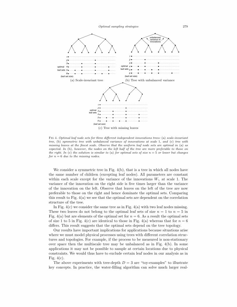i

j1

R

C

1

lij

leaves

21 22l

lll 1211

root

11 12 llll 21 22

(a) (b)

Fig 1 (a) Finite population on a spatial rectangular grid of size R times C units Associated withthe unit at position (i j) is an unknown value ℓij (b) Multiscale superpopulation model for afinite population Nodes at the bottom are called leaves and the topmost node the root Each leafnode corresponds to one value ℓij All nodes except for the leaves correspond to the sum of theirchildren at the next lower level

Denote an arbitrary sample of size n by L We consider linear estimators of Sthat take the form

(11) S(Lα) = αTL

where α is an arbitrary set of coefficients We measure the accuracy of S(Lα) interms of the mean-squared error (MSE)

(12) E(S|Lα) = E

(S minus S(Lα)

)2

and define the linear minimum mean-squared error (LMMSE) of estimating S fromL as

(13) E(S|L) = minαisinRn

E(S|Lα)

Restated our goal is to determine

(14) Llowast = argminL

E(S|L)

Our results are particularly applicable to Gaussian processes for which linear esti-mation is optimal in terms of mean-squared error We note that for certain multi-modal and discrete processes linear estimation may be sub-optimal

12 Multiscale superpopulation models

We assume that the population is one realization of a multiscale stochastic process(see Fig 1(b)) (see Willsky [20]) Such processes consist of random variables orga-nized on a tree Nodes at the bottom called leaves correspond to the populationℓij All nodes except for the leaves represent the sum total of their children atthe next lower level The topmost node the root hence represents the sum of theentire population The problem we address in this paper is thus equivalent to thefollowing Among all possible sets of leaves of size n which set provides the bestlinear estimator for the root in terms of MSE

Multiscale stochastic processes efficiently capture the correlation structure of awide range of phenomena from uncorrelated data to complex fractal data They


(a) (b)

OslashWOslashV

Oslash2V

Oslash1V

12 10

B(t)

(c)





























LγL

γ

γ

γ2γ1 γPγ





22 Covariance trees





















31 Water-filling








(32) ∆n(M1 MP ) =

X = [xk]

Pk=1

Psum

k=1



(33) h(n) = max

Psum

k=1





sumkMk as follows


Step (ii) Set

(34) g(n+1)k =

g(n)k + 1 k = m

g(n)k k 6= m

where

(35) m isin argmaxk

ψk

(g(n)k + 1

)minus ψk

(g(n)k

) g

(n)k lt Mk



(36) h(n) =sum

k

ψk

(g(n)k

)







lfloor nP

rfloor)ψ(lfloor nP

rfloor)+(nminusP

lfloor nP

rfloor)ψ(lfloor nP

rfloor+1

)


(38) h(n) = Pψ( nP

)





E(Vγ minusαTLγ)

2


(310)1


var(Vγ)=

Pγsum

k=1

1

E(Vγ |Lγk)



E(Vγ |L)minus1

and define


= microγ(n)



E(Vγ |L)minus1

and(313)






Pγsum

k=1

microγγk(xk)




next theorem



⋃Pγ










⋃Pγ















rfloor





4 Covariance trees

















and




jsum

k=1

var(W (k)

) j = 1 D





















5 Numerical results






(leaf set size)

optimal

leaf sets

1

3

2

6

5

4

(leaf set size)

2

3

4

5

6

1

optimal

leaf sets



optimal

(leaf set size)

leaf sets

1

2

3

4

5

6












100

1010

02

04

06

08

1


norm

aliz

ed M

SE


100

1010

02

04

06

08

1


norm

aliz

ed M

SE


(a) (b)




6 Related work






7 Conclusions







Appendix





lowastj )


(72) h(n) =Psum

k=1

ψk(xlowastk)






lowasti minus 1)




As a consequence

(74)sum

k




(75)sum

k

ψk(xlowastk) =

sum

k

ψk(yk) gesum

k

ψk(xk)



k ψk(xk) =sum

k ψk(xlowastk)





(76)sum

k

g(n+1)k = 1 +

sum

k

g(n)k = n+ 1





ψi

(g(n+1)i

)minus ψi

(g(n+1)i minus 1

)= ψi

(g(n)i

)minus ψi

(g(n)i minus 1

)

ge ψm

(g(n)m + 1

)minus ψm

(g(n)m

)

(77)ge ψm

(g(n)m + 2

)minus ψm

(g(n)m + 1

)

= ψm

(g(n+1)m + 1

)minus ψm

(g(n+1)m

)


that

ψm

(g(n+1)m

)minus ψm

(g(n+1)m minus 1

)= ψm

(g(n)m + 1

)minus ψm

(g(n)m

)

ge ψj

(g(n)j + 1

)minus ψj

(g(n)j

)(78)

= ψj

(g(n+1)j + 1

)minus ψj

(g(n+1)j

)






sumk ψk(g

(n)k ) is a



k

(ψk(g

(n+1)k )minus ψk(g

(n)k )

)

(79)= max

kg(n)

kltMk

ψk(g


(n)k )


(n)k we have that


(n)k ) ge ψk(g


(n+1)k )




lfloornP


lfloornP

rfloor





(711)var(A)



ζ2ge 1




and


Thus from (712) (713) and (714)

(715)cov(ZE)2

var(Z)middot

var(A)

cov(AE)2=

η2var(Z)


ζ2ge1


(716) ri =1

1minus αzi


(717) δi =1

1minus βzi








= αriri+1

[κi+2

(1minus αzi

1minus αzi+2

)minus κi+1

]


(720)

[κi+2

(1minus αzi

1minus αzi+2

)minus κi+1

]le 0



[κi+2

(1minus βzi

1minus βzi+2

)minus κi+1

]



(722)

[κi+2


minus κi+1

]le 0

Now

(723)1minus αzi

1minus αzi+2minus









var(Vγ)= max

LisinΛγ(n)

Pγsum

k=1

E(Vγ |Lγk)minus1

(724)


Pγsum

k=1

microγγk(xk)



var(Vγ)ge E(Vγ |L

lowast)minus1

+Pγ minus 1

var(Vγ)=

Pγsum

k=1

E(Vγ |Llowastγk)

minus1

(725)

=

Pγsum

k=1



Pγsum

k=1

microγγk(xk)




Pγsum

k=1


var(Vγ)




and

(728) E = ηVγk + F



we have

cov(Vγk E)

cov(Vγ E)=

(var(Vγk)

var(Vγ)

)122γk +

var(Wγk)var(Vγ)

2γk

12

(729)

= ξγk ge

(var(Vγk)

var(Vγ)

)12




From (42) we have






ξ2γk




2




microγ(n) =1

var(Vγ)middot

1


and


1

var(Vγuarr)middot

1


var(Vγuarr)









ij qij(L) is min-







sum

ij

qij =

Dsum

m=0

cmϑm =

Dminus1sum

m=0


=

Dminus1sum

m=0


m=minus1

cm+1am + cDϑD

(737)

=

Dminus2sum

m=0


=

Dminus2sum

m=0






q=0

gq(σp minus gq) =

σ2p+1+m

4minus

σm+1minus1sum

q=0

(gq minus σp2)2













σpsum

ij=1

qij = σpσpsum

j=1

fjλj and(739)

σpsum

ij=1

dij = σpσpsum

j=1

fjλj (740)



sumi uij Then

sum

ij


(741)= [w1 wσp ]Ξ[w1 wσp ]T =

sum

j

λjw2j


(742)sum

j


Setting fi = w2i σ







(744) λ(u) =

σpsum

j=1

qij(L) = cD +

psum

m=1

σpminusmcm





(745) λ(c) =

σpsum

j=1

qij(L) = cD +

psum

m=1

σmcDminusm







λ(u) lesum

j

λjfj le λ(c)(746)


(747)sum

j

(1λj)fj ge1sum

j λjfjge

1

λ(c)

Thussum


References






















Introduction






Covariance trees



Water-filling



Covariance trees

Problem formulation

Optimal solutions


Numerical results



Related work

Conclusions

Appendix

References


(a) (b)

OslashWOslashV

Oslash2V

Oslash1V

12 10

B(t)

(c)





























LγL

γ

γ

γ2γ1 γPγ





22 Covariance trees





















31 Water-filling








(32) ∆n(M1 MP ) =

X = [xk]

Pk=1

Psum

k=1



(33) h(n) = max

Psum

k=1





sumkMk as follows


Step (ii) Set

(34) g(n+1)k =

g(n)k + 1 k = m

g(n)k k 6= m

where

(35) m isin argmaxk

ψk

(g(n)k + 1

)minus ψk

(g(n)k

) g

(n)k lt Mk



(36) h(n) =sum

k

ψk

(g(n)k

)







lfloor nP

rfloor)ψ(lfloor nP

rfloor)+(nminusP

lfloor nP

rfloor)ψ(lfloor nP

rfloor+1

)


(38) h(n) = Pψ( nP

)





E(Vγ minusαTLγ)

2


(310)1


var(Vγ)=

Pγsum

k=1

1

E(Vγ |Lγk)



E(Vγ |L)minus1

and define


= microγ(n)



E(Vγ |L)minus1

and(313)






Pγsum

k=1

microγγk(xk)




next theorem



⋃Pγ










⋃Pγ















rfloor





4 Covariance trees

















and




jsum

k=1

var(W (k)

) j = 1 D





















5 Numerical results






(leaf set size)

optimal

leaf sets

1

3

2

6

5

4

(leaf set size)

2

3

4

5

6

1

optimal

leaf sets



optimal

(leaf set size)

leaf sets

1

2

3

4

5

6












100

1010

02

04

06

08

1


norm

aliz

ed M

SE


100

1010

02

04

06

08

1


norm

aliz

ed M

SE


(a) (b)




6 Related work






7 Conclusions







Appendix





lowastj )


(72) h(n) =Psum

k=1

ψk(xlowastk)






lowasti minus 1)




As a consequence

(74)sum

k




(75)sum

k

ψk(xlowastk) =

sum

k

ψk(yk) gesum

k

ψk(xk)



k ψk(xk) =sum

k ψk(xlowastk)





(76)sum

k

g(n+1)k = 1 +

sum

k

g(n)k = n+ 1





ψi

(g(n+1)i

)minus ψi

(g(n+1)i minus 1

)= ψi

(g(n)i

)minus ψi

(g(n)i minus 1

)

ge ψm

(g(n)m + 1

)minus ψm

(g(n)m

)

(77)ge ψm

(g(n)m + 2

)minus ψm

(g(n)m + 1

)

= ψm

(g(n+1)m + 1

)minus ψm

(g(n+1)m

)


that

ψm

(g(n+1)m

)minus ψm

(g(n+1)m minus 1

)= ψm

(g(n)m + 1

)minus ψm

(g(n)m

)

ge ψj

(g(n)j + 1

)minus ψj

(g(n)j

)(78)

= ψj

(g(n+1)j + 1

)minus ψj

(g(n+1)j

)






sumk ψk(g

(n)k ) is a



k

(ψk(g

(n+1)k )minus ψk(g

(n)k )

)

(79)= max

kg(n)

kltMk

ψk(g


(n)k )


(n)k we have that


(n)k ) ge ψk(g


(n+1)k )




lfloornP


lfloornP

rfloor





(711)var(A)



ζ2ge 1




and


Thus from (712) (713) and (714)

(715)cov(ZE)2

var(Z)middot

var(A)

cov(AE)2=

η2var(Z)


ζ2ge1


(716) ri =1

1minus αzi


(717) δi =1

1minus βzi








= αriri+1

[κi+2

(1minus αzi

1minus αzi+2

)minus κi+1

]


(720)

[κi+2

(1minus αzi

1minus αzi+2

)minus κi+1

]le 0



[κi+2

(1minus βzi

1minus βzi+2

)minus κi+1

]



(722)

[κi+2


minus κi+1

]le 0

Now

(723)1minus αzi

1minus αzi+2minus









var(Vγ)= max

LisinΛγ(n)

Pγsum

k=1

E(Vγ |Lγk)minus1

(724)


Pγsum

k=1

microγγk(xk)



var(Vγ)ge E(Vγ |L

lowast)minus1

+Pγ minus 1

var(Vγ)=

Pγsum

k=1

E(Vγ |Llowastγk)

minus1

(725)

=

Pγsum

k=1



Pγsum

k=1

microγγk(xk)




Pγsum

k=1


var(Vγ)




and

(728) E = ηVγk + F



we have

cov(Vγk E)

cov(Vγ E)=

(var(Vγk)

var(Vγ)

)122γk +

var(Wγk)var(Vγ)

2γk

12

(729)

= ξγk ge

(var(Vγk)

var(Vγ)

)12




From (42) we have






ξ2γk




2




microγ(n) =1

var(Vγ)middot

1


and


1

var(Vγuarr)middot

1


var(Vγuarr)









ij qij(L) is min-







sum

ij

qij =

Dsum

m=0

cmϑm =

Dminus1sum

m=0


=

Dminus1sum

m=0


m=minus1

cm+1am + cDϑD

(737)

=

Dminus2sum

m=0


=

Dminus2sum

m=0






q=0

gq(σp minus gq) =

σ2p+1+m

4minus

σm+1minus1sum

q=0

(gq minus σp2)2













σpsum

ij=1

qij = σpσpsum

j=1

fjλj and(739)

σpsum

ij=1

dij = σpσpsum

j=1

fjλj (740)



sumi uij Then

sum

ij


(741)= [w1 wσp ]Ξ[w1 wσp ]T =

sum

j

λjw2j


(742)sum

j


Setting fi = w2i σ







(744) λ(u) =

σpsum

j=1

qij(L) = cD +

psum

m=1

σpminusmcm





(745) λ(c) =

σpsum

j=1

qij(L) = cD +

psum

m=1

σmcDminusm







λ(u) lesum

j

λjfj le λ(c)(746)


(747)sum

j

(1λj)fj ge1sum

j λjfjge

1

λ(c)

Thussum


References






















Introduction






Covariance trees



Water-filling



Covariance trees

Problem formulation

Optimal solutions


Numerical results



Related work

Conclusions

Appendix

References




















LγL

γ

γ

γ2γ1 γPγ





22 Covariance trees





















31 Water-filling








(32) ∆n(M1 MP ) =

X = [xk]

Pk=1

Psum

k=1



(33) h(n) = max

Psum

k=1





sumkMk as follows


Step (ii) Set

(34) g(n+1)k =

g(n)k + 1 k = m

g(n)k k 6= m

where

(35) m isin argmaxk

ψk

(g(n)k + 1

)minus ψk

(g(n)k

) g

(n)k lt Mk



(36) h(n) =sum

k

ψk

(g(n)k

)







lfloor nP

rfloor)ψ(lfloor nP

rfloor)+(nminusP

lfloor nP

rfloor)ψ(lfloor nP

rfloor+1

)


(38) h(n) = Pψ( nP

)





E(Vγ minusαTLγ)

2


(310)1


var(Vγ)=

Pγsum

k=1

1

E(Vγ |Lγk)



E(Vγ |L)minus1

and define


= microγ(n)



E(Vγ |L)minus1

and(313)






Pγsum

k=1

microγγk(xk)




next theorem



⋃Pγ










⋃Pγ















rfloor





4 Covariance trees

















and




jsum

k=1

var(W (k)

) j = 1 D





















5 Numerical results






(leaf set size)

optimal

leaf sets

1

3

2

6

5

4

(leaf set size)

2

3

4

5

6

1

optimal

leaf sets



optimal

(leaf set size)

leaf sets

1

2

3

4

5

6












100

1010

02

04

06

08

1


norm

aliz

ed M

SE


100

1010

02

04

06

08

1


norm

aliz

ed M

SE


(a) (b)




6 Related work






7 Conclusions







Appendix





lowastj )


(72) h(n) =Psum

k=1

ψk(xlowastk)






lowasti minus 1)




As a consequence

(74)sum

k




(75)sum

k

ψk(xlowastk) =

sum

k

ψk(yk) gesum

k

ψk(xk)



k ψk(xk) =sum

k ψk(xlowastk)





(76)sum

k

g(n+1)k = 1 +

sum

k

g(n)k = n+ 1





ψi

(g(n+1)i

)minus ψi

(g(n+1)i minus 1

)= ψi

(g(n)i

)minus ψi

(g(n)i minus 1

)

ge ψm

(g(n)m + 1

)minus ψm

(g(n)m

)

(77)ge ψm

(g(n)m + 2

)minus ψm

(g(n)m + 1

)

= ψm

(g(n+1)m + 1

)minus ψm

(g(n+1)m

)


that

ψm

(g(n+1)m

)minus ψm

(g(n+1)m minus 1

)= ψm

(g(n)m + 1

)minus ψm

(g(n)m

)

ge ψj

(g(n)j + 1

)minus ψj

(g(n)j

)(78)

= ψj

(g(n+1)j + 1

)minus ψj

(g(n+1)j

)






sumk ψk(g

(n)k ) is a



k

(ψk(g

(n+1)k )minus ψk(g

(n)k )

)

(79)= max

kg(n)

kltMk

ψk(g


(n)k )


(n)k we have that


(n)k ) ge ψk(g


(n+1)k )




lfloornP


lfloornP

rfloor





(711)var(A)



ζ2ge 1




and


Thus from (712) (713) and (714)

(715)cov(ZE)2

var(Z)middot

var(A)

cov(AE)2=

η2var(Z)


ζ2ge1


(716) ri =1

1minus αzi


(717) δi =1

1minus βzi








= αriri+1

[κi+2

(1minus αzi

1minus αzi+2

)minus κi+1

]


(720)

[κi+2

(1minus αzi

1minus αzi+2

)minus κi+1

]le 0



[κi+2

(1minus βzi

1minus βzi+2

)minus κi+1

]



(722)

[κi+2


minus κi+1

]le 0

Now

(723)1minus αzi

1minus αzi+2minus









var(Vγ)= max

LisinΛγ(n)

Pγsum

k=1

E(Vγ |Lγk)minus1

(724)


Pγsum

k=1

microγγk(xk)



var(Vγ)ge E(Vγ |L

lowast)minus1

+Pγ minus 1

var(Vγ)=

Pγsum

k=1

E(Vγ |Llowastγk)

minus1

(725)

=

Pγsum

k=1



Pγsum

k=1

microγγk(xk)




Pγsum

k=1


var(Vγ)




and

(728) E = ηVγk + F



we have

cov(Vγk E)

cov(Vγ E)=

(var(Vγk)

var(Vγ)

)122γk +

var(Wγk)var(Vγ)

2γk

12

(729)

= ξγk ge

(var(Vγk)

var(Vγ)

)12




From (42) we have






ξ2γk




2




microγ(n) =1

var(Vγ)middot

1


and


1

var(Vγuarr)middot

1


var(Vγuarr)









ij qij(L) is min-







sum

ij

qij =

Dsum

m=0

cmϑm =

Dminus1sum

m=0


=

Dminus1sum

m=0


m=minus1

cm+1am + cDϑD

(737)

=

Dminus2sum

m=0


=

Dminus2sum

m=0






q=0

gq(σp minus gq) =

σ2p+1+m

4minus

σm+1minus1sum

q=0

(gq minus σp2)2













σpsum

ij=1

qij = σpσpsum

j=1

fjλj and(739)

σpsum

ij=1

dij = σpσpsum

j=1

fjλj (740)



sumi uij Then

sum

ij


(741)= [w1 wσp ]Ξ[w1 wσp ]T =

sum

j

λjw2j


(742)sum

j


Setting fi = w2i σ







(744) λ(u) =

σpsum

j=1

qij(L) = cD +

psum

m=1

σpminusmcm





(745) λ(c) =

σpsum

j=1

qij(L) = cD +

psum

m=1

σmcDminusm







λ(u) lesum

j

λjfj le λ(c)(746)


(747)sum

j

(1λj)fj ge1sum

j λjfjge

1

λ(c)

Thussum


References






















Introduction






Covariance trees



Water-filling



Covariance trees

Problem formulation

Optimal solutions


Numerical results



Related work

Conclusions

Appendix

References















31 Water-filling








(32) ∆n(M1 MP ) =

X = [xk]

Pk=1

Psum

k=1



(33) h(n) = max

Psum

k=1





sumkMk as follows


Step (ii) Set

(34) g(n+1)k =

g(n)k + 1 k = m

g(n)k k 6= m

where

(35) m isin argmaxk

ψk

(g(n)k + 1

)minus ψk

(g(n)k

) g

(n)k lt Mk



(36) h(n) =sum

k

ψk

(g(n)k

)







lfloor nP

rfloor)ψ(lfloor nP

rfloor)+(nminusP

lfloor nP

rfloor)ψ(lfloor nP

rfloor+1

)


(38) h(n) = Pψ( nP

)





E(Vγ minusαTLγ)

2


(310)1


var(Vγ)=

Pγsum

k=1

1

E(Vγ |Lγk)



E(Vγ |L)minus1

and define


= microγ(n)



E(Vγ |L)minus1

and(313)






Pγsum

k=1

microγγk(xk)




next theorem



⋃Pγ










⋃Pγ















rfloor





4 Covariance trees

















and




jsum

k=1

var(W (k)

) j = 1 D





















5 Numerical results






(leaf set size)

optimal

leaf sets

1

3

2

6

5

4

(leaf set size)

2

3

4

5

6

1

optimal

leaf sets



optimal

(leaf set size)

leaf sets

1

2

3

4

5

6












100

1010

02

04

06

08

1


norm

aliz

ed M

SE


100

1010

02

04

06

08

1


norm

aliz

ed M

SE


(a) (b)




6 Related work






7 Conclusions







Appendix





lowastj )


(72) h(n) =Psum

k=1

ψk(xlowastk)






lowasti minus 1)




As a consequence

(74)sum

k




(75)sum

k

ψk(xlowastk) =

sum

k

ψk(yk) gesum

k

ψk(xk)



k ψk(xk) =sum

k ψk(xlowastk)





(76)sum

k

g(n+1)k = 1 +

sum

k

g(n)k = n+ 1





ψi

(g(n+1)i

)minus ψi

(g(n+1)i minus 1

)= ψi

(g(n)i

)minus ψi

(g(n)i minus 1

)

ge ψm

(g(n)m + 1

)minus ψm

(g(n)m

)

(77)ge ψm

(g(n)m + 2

)minus ψm

(g(n)m + 1

)

= ψm

(g(n+1)m + 1

)minus ψm

(g(n+1)m

)


that

ψm

(g(n+1)m

)minus ψm

(g(n+1)m minus 1

)= ψm

(g(n)m + 1

)minus ψm

(g(n)m

)

ge ψj

(g(n)j + 1

)minus ψj

(g(n)j

)(78)

= ψj

(g(n+1)j + 1

)minus ψj

(g(n+1)j

)






sumk ψk(g

(n)k ) is a



k

(ψk(g

(n+1)k )minus ψk(g

(n)k )

)

(79)= max

kg(n)

kltMk

ψk(g


(n)k )


(n)k we have that


(n)k ) ge ψk(g


(n+1)k )




lfloornP


lfloornP

rfloor





(711)var(A)



ζ2ge 1




and


Thus from (712) (713) and (714)

(715)cov(ZE)2

var(Z)middot

var(A)

cov(AE)2=

η2var(Z)


ζ2ge1


(716) ri =1

1minus αzi


(717) δi =1

1minus βzi








= αriri+1

[κi+2

(1minus αzi

1minus αzi+2

)minus κi+1

]


(720)

[κi+2

(1minus αzi

1minus αzi+2

)minus κi+1

]le 0



[κi+2

(1minus βzi

1minus βzi+2

)minus κi+1

]



(722)

[κi+2


minus κi+1

]le 0

Now

(723)1minus αzi

1minus αzi+2minus









var(Vγ)= max

LisinΛγ(n)

Pγsum

k=1

E(Vγ |Lγk)minus1

(724)


Pγsum

k=1

microγγk(xk)



var(Vγ)ge E(Vγ |L

lowast)minus1

+Pγ minus 1

var(Vγ)=

Pγsum

k=1

E(Vγ |Llowastγk)

minus1

(725)

=

Pγsum

k=1



Pγsum

k=1

microγγk(xk)




Pγsum

k=1


var(Vγ)




and

(728) E = ηVγk + F



we have

cov(Vγk E)

cov(Vγ E)=

(var(Vγk)

var(Vγ)

)122γk +

var(Wγk)var(Vγ)

2γk

12

(729)

= ξγk ge

(var(Vγk)

var(Vγ)

)12




From (42) we have






ξ2γk




2




microγ(n) =1

var(Vγ)middot

1


and


1

var(Vγuarr)middot

1


var(Vγuarr)









ij qij(L) is min-







sum

ij

qij =

Dsum

m=0

cmϑm =

Dminus1sum

m=0


=

Dminus1sum

m=0


m=minus1

cm+1am + cDϑD

(737)

=

Dminus2sum

m=0


=

Dminus2sum

m=0






q=0

gq(σp minus gq) =

σ2p+1+m

4minus

σm+1minus1sum

q=0

(gq minus σp2)2













σpsum

ij=1

qij = σpσpsum

j=1

fjλj and(739)

σpsum

ij=1

dij = σpσpsum

j=1

fjλj (740)



sumi uij Then

sum

ij


(741)= [w1 wσp ]Ξ[w1 wσp ]T =

sum

j

λjw2j


(742)sum

j


Setting fi = w2i σ







(744) λ(u) =

σpsum

j=1

qij(L) = cD +

psum

m=1

σpminusmcm





(745) λ(c) =

σpsum

j=1

qij(L) = cD +

psum

m=1

σmcDminusm







λ(u) lesum

j

λjfj le λ(c)(746)


(747)sum

j

(1λj)fj ge1sum

j λjfjge

1

λ(c)

Thussum


References






















Introduction






Covariance trees



Water-filling



Covariance trees

Problem formulation

Optimal solutions


Numerical results



Related work

Conclusions

Appendix

References






(32) ∆n(M1 MP ) =

X = [xk]

Pk=1

Psum

k=1



(33) h(n) = max

Psum

k=1





sumkMk as follows


Step (ii) Set

(34) g(n+1)k =

g(n)k + 1 k = m

g(n)k k 6= m

where

(35) m isin argmaxk

ψk

(g(n)k + 1

)minus ψk

(g(n)k

) g

(n)k lt Mk



(36) h(n) =sum

k

ψk

(g(n)k

)







lfloor nP

rfloor)ψ(lfloor nP

rfloor)+(nminusP

lfloor nP

rfloor)ψ(lfloor nP

rfloor+1

)


(38) h(n) = Pψ( nP

)





E(Vγ minusαTLγ)

2


(310)1


var(Vγ)=

Pγsum

k=1

1

E(Vγ |Lγk)



E(Vγ |L)minus1

and define


= microγ(n)



E(Vγ |L)minus1

and(313)






Pγsum

k=1

microγγk(xk)




next theorem



⋃Pγ










⋃Pγ















rfloor





4 Covariance trees

















and




jsum

k=1

var(W (k)

) j = 1 D





















5 Numerical results






(leaf set size)

optimal

leaf sets

1

3

2

6

5

4

(leaf set size)

2

3

4

5

6

1

optimal

leaf sets



optimal

(leaf set size)

leaf sets

1

2

3

4

5

6












100

1010

02

04

06

08

1


norm

aliz

ed M

SE


100

1010

02

04

06

08

1


norm

aliz

ed M

SE


(a) (b)




6 Related work






7 Conclusions







Appendix





lowastj )


(72) h(n) =Psum

k=1

ψk(xlowastk)






lowasti minus 1)




As a consequence

(74)sum

k




(75)sum

k

ψk(xlowastk) =

sum

k

ψk(yk) gesum

k

ψk(xk)



k ψk(xk) =sum

k ψk(xlowastk)





(76)sum

k

g(n+1)k = 1 +

sum

k

g(n)k = n+ 1





ψi

(g(n+1)i

)minus ψi

(g(n+1)i minus 1

)= ψi

(g(n)i

)minus ψi

(g(n)i minus 1

)

ge ψm

(g(n)m + 1

)minus ψm

(g(n)m

)

(77)ge ψm

(g(n)m + 2

)minus ψm

(g(n)m + 1

)

= ψm

(g(n+1)m + 1

)minus ψm

(g(n+1)m

)


that

ψm

(g(n+1)m

)minus ψm

(g(n+1)m minus 1

)= ψm

(g(n)m + 1

)minus ψm

(g(n)m

)

ge ψj

(g(n)j + 1

)minus ψj

(g(n)j

)(78)

= ψj

(g(n+1)j + 1

)minus ψj

(g(n+1)j

)






sumk ψk(g

(n)k ) is a



k

(ψk(g

(n+1)k )minus ψk(g

(n)k )

)

(79)= max

kg(n)

kltMk

ψk(g


(n)k )


(n)k we have that


(n)k ) ge ψk(g


(n+1)k )




lfloornP


lfloornP

rfloor





(711)var(A)



ζ2ge 1




and


Thus from (712) (713) and (714)

(715)cov(ZE)2

var(Z)middot

var(A)

cov(AE)2=

η2var(Z)


ζ2ge1


(716) ri =1

1minus αzi


(717) δi =1

1minus βzi








= αriri+1

[κi+2

(1minus αzi

1minus αzi+2

)minus κi+1

]


(720)

[κi+2

(1minus αzi

1minus αzi+2

)minus κi+1

]le 0



[κi+2

(1minus βzi

1minus βzi+2

)minus κi+1

]



(722)

[κi+2


minus κi+1

]le 0

Now

(723)1minus αzi

1minus αzi+2minus









var(Vγ)= max

LisinΛγ(n)

Pγsum

k=1

E(Vγ |Lγk)minus1

(724)


Pγsum

k=1

microγγk(xk)



var(Vγ)ge E(Vγ |L

lowast)minus1

+Pγ minus 1

var(Vγ)=

Pγsum

k=1

E(Vγ |Llowastγk)

minus1

(725)

=

Pγsum

k=1



Pγsum

k=1

microγγk(xk)




Pγsum

k=1


var(Vγ)




and

(728) E = ηVγk + F



we have

cov(Vγk E)

cov(Vγ E)=

(var(Vγk)

var(Vγ)

)122γk +

var(Wγk)var(Vγ)

2γk

12

(729)

= ξγk ge

(var(Vγk)

var(Vγ)

)12




From (42) we have






ξ2γk




2




microγ(n) =1

var(Vγ)middot

1


and


1

var(Vγuarr)middot

1


var(Vγuarr)









ij qij(L) is min-







sum

ij

qij =

Dsum

m=0

cmϑm =

Dminus1sum

m=0


=

Dminus1sum

m=0


m=minus1

cm+1am + cDϑD

(737)

=

Dminus2sum

m=0


=

Dminus2sum

m=0






q=0

gq(σp minus gq) =

σ2p+1+m

4minus

σm+1minus1sum

q=0

(gq minus σp2)2













σpsum

ij=1

qij = σpσpsum

j=1

fjλj and(739)

σpsum

ij=1

dij = σpσpsum

j=1

fjλj (740)



sumi uij Then

sum

ij


(741)= [w1 wσp ]Ξ[w1 wσp ]T =

sum

j

λjw2j


(742)sum

j


Setting fi = w2i σ







(744) λ(u) =

σpsum

j=1

qij(L) = cD +

psum

m=1

σpminusmcm





(745) λ(c) =

σpsum

j=1

qij(L) = cD +

psum

m=1

σmcDminusm







λ(u) lesum

j

λjfj le λ(c)(746)


(747)sum

j

(1λj)fj ge1sum

j λjfjge

1

λ(c)

Thussum


References






















Introduction






Covariance trees



Water-filling



Covariance trees

Problem formulation

Optimal solutions


Numerical results



Related work

Conclusions

Appendix

References






lfloor nP

rfloor)ψ(lfloor nP

rfloor)+(nminusP

lfloor nP

rfloor)ψ(lfloor nP

rfloor+1

)


(38) h(n) = Pψ( nP

)





E(Vγ minusαTLγ)

2


(310)1


var(Vγ)=

Pγsum

k=1

1

E(Vγ |Lγk)



E(Vγ |L)minus1

and define


= microγ(n)



E(Vγ |L)minus1

and(313)






Pγsum

k=1

microγγk(xk)




next theorem



⋃Pγ










⋃Pγ















rfloor





4 Covariance trees

















and




jsum

k=1

var(W (k)

) j = 1 D





















5 Numerical results






(leaf set size)

optimal

leaf sets

1

3

2

6

5

4

(leaf set size)

2

3

4

5

6

1

optimal

leaf sets



optimal

(leaf set size)

leaf sets

1

2

3

4

5

6












100

1010

02

04

06

08

1


norm

aliz

ed M

SE


100

1010

02

04

06

08

1


norm

aliz

ed M

SE


(a) (b)




6 Related work






7 Conclusions







Appendix





lowastj )


(72) h(n) =Psum

k=1

ψk(xlowastk)






lowasti minus 1)




As a consequence

(74)sum

k




(75)sum

k

ψk(xlowastk) =

sum

k

ψk(yk) gesum

k

ψk(xk)



k ψk(xk) =sum

k ψk(xlowastk)





(76)sum

k

g(n+1)k = 1 +

sum

k

g(n)k = n+ 1





ψi

(g(n+1)i

)minus ψi

(g(n+1)i minus 1

)= ψi

(g(n)i

)minus ψi

(g(n)i minus 1

)

ge ψm

(g(n)m + 1

)minus ψm

(g(n)m

)

(77)ge ψm

(g(n)m + 2

)minus ψm

(g(n)m + 1

)

= ψm

(g(n+1)m + 1

)minus ψm

(g(n+1)m

)


that

ψm

(g(n+1)m

)minus ψm

(g(n+1)m minus 1

)= ψm

(g(n)m + 1

)minus ψm

(g(n)m

)

ge ψj

(g(n)j + 1

)minus ψj

(g(n)j

)(78)

= ψj

(g(n+1)j + 1

)minus ψj

(g(n+1)j

)






sumk ψk(g

(n)k ) is a



k

(ψk(g

(n+1)k )minus ψk(g

(n)k )

)

(79)= max

kg(n)

kltMk

ψk(g


(n)k )


(n)k we have that


(n)k ) ge ψk(g


(n+1)k )




lfloornP


lfloornP

rfloor





(711)var(A)



ζ2ge 1




and


Thus from (712) (713) and (714)

(715)cov(ZE)2

var(Z)middot

var(A)

cov(AE)2=

η2var(Z)


ζ2ge1


(716) ri =1

1minus αzi


(717) δi =1

1minus βzi








= αriri+1

[κi+2

(1minus αzi

1minus αzi+2

)minus κi+1

]


(720)

[κi+2

(1minus αzi

1minus αzi+2

)minus κi+1

]le 0



[κi+2

(1minus βzi

1minus βzi+2

)minus κi+1

]



(722)

[κi+2


minus κi+1

]le 0

Now

(723)1minus αzi

1minus αzi+2minus









var(Vγ)= max

LisinΛγ(n)

Pγsum

k=1

E(Vγ |Lγk)minus1

(724)


Pγsum

k=1

microγγk(xk)



var(Vγ)ge E(Vγ |L

lowast)minus1

+Pγ minus 1

var(Vγ)=

Pγsum

k=1

E(Vγ |Llowastγk)

minus1

(725)

=

Pγsum

k=1



Pγsum

k=1

microγγk(xk)




Pγsum

k=1


var(Vγ)




and

(728) E = ηVγk + F



we have

cov(Vγk E)

cov(Vγ E)=

(var(Vγk)

var(Vγ)

)122γk +

var(Wγk)var(Vγ)

2γk

12

(729)

= ξγk ge

(var(Vγk)

var(Vγ)

)12




From (42) we have






ξ2γk




2




microγ(n) =1

var(Vγ)middot

1


and


1

var(Vγuarr)middot

1


var(Vγuarr)









ij qij(L) is min-







sum

ij

qij =

Dsum

m=0

cmϑm =

Dminus1sum

m=0


=

Dminus1sum

m=0


m=minus1

cm+1am + cDϑD

(737)

=

Dminus2sum

m=0


=

Dminus2sum

m=0






q=0

gq(σp minus gq) =

σ2p+1+m

4minus

σm+1minus1sum

q=0

(gq minus σp2)2













σpsum

ij=1

qij = σpσpsum

j=1

fjλj and(739)

σpsum

ij=1

dij = σpσpsum

j=1

fjλj (740)



sumi uij Then

sum

ij


(741)= [w1 wσp ]Ξ[w1 wσp ]T =

sum

j

λjw2j


(742)sum

j


Setting fi = w2i σ







(744) λ(u) =

σpsum

j=1

qij(L) = cD +

psum

m=1

σpminusmcm





(745) λ(c) =

σpsum

j=1

qij(L) = cD +

psum

m=1

σmcDminusm







λ(u) lesum

j

λjfj le λ(c)(746)


(747)sum

j

(1λj)fj ge1sum

j λjfjge

1

λ(c)

Thussum


References






















Introduction






Covariance trees



Water-filling



Covariance trees

Problem formulation

Optimal solutions


Numerical results



Related work

Conclusions

Appendix

References




next theorem



⋃Pγ










⋃Pγ















rfloor





4 Covariance trees

















and




jsum

k=1

var(W (k)

) j = 1 D





















5 Numerical results






(leaf set size)

optimal

leaf sets

1

3

2

6

5

4

(leaf set size)

2

3

4

5

6

1

optimal

leaf sets



optimal

(leaf set size)

leaf sets

1

2

3

4

5

6












100

1010

02

04

06

08

1


norm

aliz

ed M

SE


100

1010

02

04

06

08

1


norm

aliz

ed M

SE


(a) (b)




6 Related work






7 Conclusions







Appendix





lowastj )


(72) h(n) =Psum

k=1

ψk(xlowastk)






lowasti minus 1)




As a consequence

(74)sum

k




(75)sum

k

ψk(xlowastk) =

sum

k

ψk(yk) gesum

k

ψk(xk)



k ψk(xk) =sum

k ψk(xlowastk)





(76)sum

k

g(n+1)k = 1 +

sum

k

g(n)k = n+ 1





ψi

(g(n+1)i

)minus ψi

(g(n+1)i minus 1

)= ψi

(g(n)i

)minus ψi

(g(n)i minus 1

)

ge ψm

(g(n)m + 1

)minus ψm

(g(n)m

)

(77)ge ψm

(g(n)m + 2

)minus ψm

(g(n)m + 1

)

= ψm

(g(n+1)m + 1

)minus ψm

(g(n+1)m

)


that

ψm

(g(n+1)m

)minus ψm

(g(n+1)m minus 1

)= ψm

(g(n)m + 1

)minus ψm

(g(n)m

)

ge ψj

(g(n)j + 1

)minus ψj

(g(n)j

)(78)

= ψj

(g(n+1)j + 1

)minus ψj

(g(n+1)j

)






sumk ψk(g

(n)k ) is a



k

(ψk(g

(n+1)k )minus ψk(g

(n)k )

)

(79)= max

kg(n)

kltMk

ψk(g


(n)k )


(n)k we have that


(n)k ) ge ψk(g


(n+1)k )




lfloornP


lfloornP

rfloor





(711)var(A)



ζ2ge 1




and


Thus from (712) (713) and (714)

(715)cov(ZE)2

var(Z)middot

var(A)

cov(AE)2=

η2var(Z)


ζ2ge1


(716) ri =1

1minus αzi


(717) δi =1

1minus βzi








= αriri+1

[κi+2

(1minus αzi

1minus αzi+2

)minus κi+1

]


(720)

[κi+2

(1minus αzi

1minus αzi+2

)minus κi+1

]le 0



[κi+2

(1minus βzi

1minus βzi+2

)minus κi+1

]



(722)

[κi+2


minus κi+1

]le 0

Now

(723)1minus αzi

1minus αzi+2minus









var(Vγ)= max

LisinΛγ(n)

Pγsum

k=1

E(Vγ |Lγk)minus1

(724)


Pγsum

k=1

microγγk(xk)



var(Vγ)ge E(Vγ |L

lowast)minus1

+Pγ minus 1

var(Vγ)=

Pγsum

k=1

E(Vγ |Llowastγk)

minus1

(725)

=

Pγsum

k=1



Pγsum

k=1

microγγk(xk)




Pγsum

k=1


var(Vγ)




and

(728) E = ηVγk + F



we have

cov(Vγk E)

cov(Vγ E)=

(var(Vγk)

var(Vγ)

)122γk +

var(Wγk)var(Vγ)

2γk

12

(729)

= ξγk ge

(var(Vγk)

var(Vγ)

)12




From (42) we have






ξ2γk




2




microγ(n) =1

var(Vγ)middot

1


and


1

var(Vγuarr)middot

1


var(Vγuarr)









ij qij(L) is min-







sum

ij

qij =

Dsum

m=0

cmϑm =

Dminus1sum

m=0


=

Dminus1sum

m=0


m=minus1

cm+1am + cDϑD

(737)

=

Dminus2sum

m=0


=

Dminus2sum

m=0






q=0

gq(σp minus gq) =

σ2p+1+m

4minus

σm+1minus1sum

q=0

(gq minus σp2)2













σpsum

ij=1

qij = σpσpsum

j=1

fjλj and(739)

σpsum

ij=1

dij = σpσpsum

j=1

fjλj (740)



sumi uij Then

sum

ij


(741)= [w1 wσp ]Ξ[w1 wσp ]T =

sum

j

λjw2j


(742)sum

j


Setting fi = w2i σ







(744) λ(u) =

σpsum

j=1

qij(L) = cD +

psum

m=1

σpminusmcm





(745) λ(c) =

σpsum

j=1

qij(L) = cD +

psum

m=1

σmcDminusm







λ(u) lesum

j

λjfj le λ(c)(746)


(747)sum

j

(1λj)fj ge1sum

j λjfjge

1

λ(c)

Thussum


References






















Introduction






Covariance trees



Water-filling



Covariance trees

Problem formulation

Optimal solutions


Numerical results



Related work

Conclusions

Appendix

References







rfloor





4 Covariance trees

















and




jsum

k=1

var(W (k)

) j = 1 D





















5 Numerical results






(leaf set size)

optimal

leaf sets

1

3

2

6

5

4

(leaf set size)

2

3

4

5

6

1

optimal

leaf sets



optimal

(leaf set size)

leaf sets

1

2

3

4

5

6












100

1010

02

04

06

08

1


norm

aliz

ed M

SE


100

1010

02

04

06

08

1


norm

aliz

ed M

SE


(a) (b)




6 Related work






7 Conclusions







Appendix





lowastj )


(72) h(n) =Psum

k=1

ψk(xlowastk)






lowasti minus 1)




As a consequence

(74)sum

k




(75)sum

k

ψk(xlowastk) =

sum

k

ψk(yk) gesum

k

ψk(xk)



k ψk(xk) =sum

k ψk(xlowastk)





(76)sum

k

g(n+1)k = 1 +

sum

k

g(n)k = n+ 1





ψi

(g(n+1)i

)minus ψi

(g(n+1)i minus 1

)= ψi

(g(n)i

)minus ψi

(g(n)i minus 1

)

ge ψm

(g(n)m + 1

)minus ψm

(g(n)m

)

(77)ge ψm

(g(n)m + 2

)minus ψm

(g(n)m + 1

)

= ψm

(g(n+1)m + 1

)minus ψm

(g(n+1)m

)


that

ψm

(g(n+1)m

)minus ψm

(g(n+1)m minus 1

)= ψm

(g(n)m + 1

)minus ψm

(g(n)m

)

ge ψj

(g(n)j + 1

)minus ψj

(g(n)j

)(78)

= ψj

(g(n+1)j + 1

)minus ψj

(g(n+1)j

)






sumk ψk(g

(n)k ) is a



k

(ψk(g

(n+1)k )minus ψk(g

(n)k )

)

(79)= max

kg(n)

kltMk

ψk(g


(n)k )


(n)k we have that


(n)k ) ge ψk(g


(n+1)k )




lfloornP


lfloornP

rfloor





(711)var(A)



ζ2ge 1




and


Thus from (712) (713) and (714)

(715)cov(ZE)2

var(Z)middot

var(A)

cov(AE)2=

η2var(Z)


ζ2ge1


(716) ri =1

1minus αzi


(717) δi =1

1minus βzi








= αriri+1

[κi+2

(1minus αzi

1minus αzi+2

)minus κi+1

]


(720)

[κi+2

(1minus αzi

1minus αzi+2

)minus κi+1

]le 0



[κi+2

(1minus βzi

1minus βzi+2

)minus κi+1

]



(722)

[κi+2


minus κi+1

]le 0

Now

(723)1minus αzi

1minus αzi+2minus









var(Vγ)= max

LisinΛγ(n)

Pγsum

k=1

E(Vγ |Lγk)minus1

(724)


Pγsum

k=1

microγγk(xk)



var(Vγ)ge E(Vγ |L

lowast)minus1

+Pγ minus 1

var(Vγ)=

Pγsum

k=1

E(Vγ |Llowastγk)

minus1

(725)

=

Pγsum

k=1



Pγsum

k=1

microγγk(xk)




Pγsum

k=1


var(Vγ)




and

(728) E = ηVγk + F



we have

cov(Vγk E)

cov(Vγ E)=

(var(Vγk)

var(Vγ)

)122γk +

var(Wγk)var(Vγ)

2γk

12

(729)

= ξγk ge

(var(Vγk)

var(Vγ)

)12




From (42) we have






ξ2γk




2




microγ(n) =1

var(Vγ)middot

1


and


1

var(Vγuarr)middot

1


var(Vγuarr)









ij qij(L) is min-







sum

ij

qij =

Dsum

m=0

cmϑm =

Dminus1sum

m=0


=

Dminus1sum

m=0


m=minus1

cm+1am + cDϑD

(737)

=

Dminus2sum

m=0


=

Dminus2sum

m=0






q=0

gq(σp minus gq) =

σ2p+1+m

4minus

σm+1minus1sum

q=0

(gq minus σp2)2













σpsum

ij=1

qij = σpσpsum

j=1

fjλj and(739)

σpsum

ij=1

dij = σpσpsum

j=1

fjλj (740)



sumi uij Then

sum

ij


(741)= [w1 wσp ]Ξ[w1 wσp ]T =

sum

j

λjw2j


(742)sum

j


Setting fi = w2i σ







(744) λ(u) =

σpsum

j=1

qij(L) = cD +

psum

m=1

σpminusmcm





(745) λ(c) =

σpsum

j=1

qij(L) = cD +

psum

m=1

σmcDminusm







λ(u) lesum

j

λjfj le λ(c)(746)


(747)sum

j

(1λj)fj ge1sum

j λjfjge

1

λ(c)

Thussum


References






















Introduction






Covariance trees



Water-filling



Covariance trees

Problem formulation

Optimal solutions


Numerical results



Related work

Conclusions

Appendix

References





and




jsum

k=1

var(W (k)

) j = 1 D





















5 Numerical results






(leaf set size)

optimal

leaf sets

1

3

2

6

5

4

(leaf set size)

2

3

4

5

6

1

optimal

leaf sets



optimal

(leaf set size)

leaf sets

1

2

3

4

5

6












100

1010

02

04

06

08

1


norm

aliz

ed M

SE


100

1010

02

04

06

08

1


norm

aliz

ed M

SE


(a) (b)




6 Related work






7 Conclusions







Appendix





lowastj )


(72) h(n) =Psum

k=1

ψk(xlowastk)






lowasti minus 1)




As a consequence

(74)sum

k




(75)sum

k

ψk(xlowastk) =

sum

k

ψk(yk) gesum

k

ψk(xk)



k ψk(xk) =sum

k ψk(xlowastk)





(76)sum

k

g(n+1)k = 1 +

sum

k

g(n)k = n+ 1





ψi

(g(n+1)i

)minus ψi

(g(n+1)i minus 1

)= ψi

(g(n)i

)minus ψi

(g(n)i minus 1

)

ge ψm

(g(n)m + 1

)minus ψm

(g(n)m

)

(77)ge ψm

(g(n)m + 2

)minus ψm

(g(n)m + 1

)

= ψm

(g(n+1)m + 1

)minus ψm

(g(n+1)m

)


that

ψm

(g(n+1)m

)minus ψm

(g(n+1)m minus 1

)= ψm

(g(n)m + 1

)minus ψm

(g(n)m

)

ge ψj

(g(n)j + 1

)minus ψj

(g(n)j

)(78)

= ψj

(g(n+1)j + 1

)minus ψj

(g(n+1)j

)






sumk ψk(g

(n)k ) is a



k

(ψk(g

(n+1)k )minus ψk(g

(n)k )

)

(79)= max

kg(n)

kltMk

ψk(g


(n)k )


(n)k we have that


(n)k ) ge ψk(g


(n+1)k )




lfloornP


lfloornP

rfloor





(711)var(A)



ζ2ge 1




and


Thus from (712) (713) and (714)

(715)cov(ZE)2

var(Z)middot

var(A)

cov(AE)2=

η2var(Z)


ζ2ge1


(716) ri =1

1minus αzi


(717) δi =1

1minus βzi








= αriri+1

[κi+2

(1minus αzi

1minus αzi+2

)minus κi+1

]


(720)

[κi+2

(1minus αzi

1minus αzi+2

)minus κi+1

]le 0



[κi+2

(1minus βzi

1minus βzi+2

)minus κi+1

]



(722)

[κi+2


minus κi+1

]le 0

Now

(723)1minus αzi

1minus αzi+2minus









var(Vγ)= max

LisinΛγ(n)

Pγsum

k=1

E(Vγ |Lγk)minus1

(724)


Pγsum

k=1

microγγk(xk)



var(Vγ)ge E(Vγ |L

lowast)minus1

+Pγ minus 1

var(Vγ)=

Pγsum

k=1

E(Vγ |Llowastγk)

minus1

(725)

=

Pγsum

k=1



Pγsum

k=1

microγγk(xk)




Pγsum

k=1


var(Vγ)




and

(728) E = ηVγk + F



we have

cov(Vγk E)

cov(Vγ E)=

(var(Vγk)

var(Vγ)

)122γk +

var(Wγk)var(Vγ)

2γk

12

(729)

= ξγk ge

(var(Vγk)

var(Vγ)

)12




From (42) we have






ξ2γk




2




microγ(n) =1

var(Vγ)middot

1


and


1

var(Vγuarr)middot

1


var(Vγuarr)









ij qij(L) is min-







sum

ij

qij =

Dsum

m=0

cmϑm =

Dminus1sum

m=0


=

Dminus1sum

m=0


m=minus1

cm+1am + cDϑD

(737)

=

Dminus2sum

m=0


=

Dminus2sum

m=0






q=0

gq(σp minus gq) =

σ2p+1+m

4minus

σm+1minus1sum

q=0

(gq minus σp2)2













σpsum

ij=1

qij = σpσpsum

j=1

fjλj and(739)

σpsum

ij=1

dij = σpσpsum

j=1

fjλj (740)



sumi uij Then

sum

ij


(741)= [w1 wσp ]Ξ[w1 wσp ]T =

sum

j

λjw2j


(742)sum

j


Setting fi = w2i σ







(744) λ(u) =

σpsum

j=1

qij(L) = cD +

psum

m=1

σpminusmcm





(745) λ(c) =

σpsum

j=1

qij(L) = cD +

psum

m=1

σmcDminusm







λ(u) lesum

j

λjfj le λ(c)(746)


(747)sum

j

(1λj)fj ge1sum

j λjfjge

1

λ(c)

Thussum


References






















Introduction






Covariance trees



Water-filling



Covariance trees

Problem formulation

Optimal solutions


Numerical results



Related work

Conclusions

Appendix

References











5 Numerical results






(leaf set size)

optimal

leaf sets

1

3

2

6

5

4

(leaf set size)

2

3

4

5

6

1

optimal

leaf sets



optimal

(leaf set size)

leaf sets

1

2

3

4

5

6












100

1010

02

04

06

08

1


norm

aliz

ed M

SE


100

1010

02

04

06

08

1


norm

aliz

ed M

SE


(a) (b)




6 Related work






7 Conclusions







Appendix





lowastj )


(72) h(n) =Psum

k=1

ψk(xlowastk)






lowasti minus 1)




As a consequence

(74)sum

k




(75)sum

k

ψk(xlowastk) =

sum

k

ψk(yk) gesum

k

ψk(xk)



k ψk(xk) =sum

k ψk(xlowastk)





(76)sum

k

g(n+1)k = 1 +

sum

k

g(n)k = n+ 1





ψi

(g(n+1)i

)minus ψi

(g(n+1)i minus 1

)= ψi

(g(n)i

)minus ψi

(g(n)i minus 1

)

ge ψm

(g(n)m + 1

)minus ψm

(g(n)m

)

(77)ge ψm

(g(n)m + 2

)minus ψm

(g(n)m + 1

)

= ψm

(g(n+1)m + 1

)minus ψm

(g(n+1)m

)


that

ψm

(g(n+1)m

)minus ψm

(g(n+1)m minus 1

)= ψm

(g(n)m + 1

)minus ψm

(g(n)m

)

ge ψj

(g(n)j + 1

)minus ψj

(g(n)j

)(78)

= ψj

(g(n+1)j + 1

)minus ψj

(g(n+1)j

)






sumk ψk(g

(n)k ) is a



k

(ψk(g

(n+1)k )minus ψk(g

(n)k )

)

(79)= max

kg(n)

kltMk

ψk(g


(n)k )


(n)k we have that


(n)k ) ge ψk(g


(n+1)k )




lfloornP


lfloornP

rfloor





(711)var(A)



ζ2ge 1




and


Thus from (712) (713) and (714)

(715)cov(ZE)2

var(Z)middot

var(A)

cov(AE)2=

η2var(Z)


ζ2ge1


(716) ri =1

1minus αzi


(717) δi =1

1minus βzi








= αriri+1

[κi+2

(1minus αzi

1minus αzi+2

)minus κi+1

]


(720)

[κi+2

(1minus αzi

1minus αzi+2

)minus κi+1

]le 0



[κi+2

(1minus βzi

1minus βzi+2

)minus κi+1

]



(722)

[κi+2


minus κi+1

]le 0

Now

(723)1minus αzi

1minus αzi+2minus









var(Vγ)= max

LisinΛγ(n)

Pγsum

k=1

E(Vγ |Lγk)minus1

(724)


Pγsum

k=1

microγγk(xk)



var(Vγ)ge E(Vγ |L

lowast)minus1

+Pγ minus 1

var(Vγ)=

Pγsum

k=1

E(Vγ |Llowastγk)

minus1

(725)

=

Pγsum

k=1



Pγsum

k=1

microγγk(xk)




Pγsum

k=1


var(Vγ)




and

(728) E = ηVγk + F



we have

cov(Vγk E)

cov(Vγ E)=

(var(Vγk)

var(Vγ)

)122γk +

var(Wγk)var(Vγ)

2γk

12

(729)

= ξγk ge

(var(Vγk)

var(Vγ)

)12




From (42) we have






ξ2γk




2




microγ(n) =1

var(Vγ)middot

1


and


1

var(Vγuarr)middot

1


var(Vγuarr)









ij qij(L) is min-







sum

ij

qij =

Dsum

m=0

cmϑm =

Dminus1sum

m=0


=

Dminus1sum

m=0


m=minus1

cm+1am + cDϑD

(737)

=

Dminus2sum

m=0


=

Dminus2sum

m=0






q=0

gq(σp minus gq) =

σ2p+1+m

4minus

σm+1minus1sum

q=0

(gq minus σp2)2













σpsum

ij=1

qij = σpσpsum

j=1

fjλj and(739)

σpsum

ij=1

dij = σpσpsum

j=1

fjλj (740)



sumi uij Then

sum

ij


(741)= [w1 wσp ]Ξ[w1 wσp ]T =

sum

j

λjw2j


(742)sum

j


Setting fi = w2i σ







(744) λ(u) =

σpsum

j=1

qij(L) = cD +

psum

m=1

σpminusmcm





(745) λ(c) =

σpsum

j=1

qij(L) = cD +

psum

m=1

σmcDminusm







λ(u) lesum

j

λjfj le λ(c)(746)


(747)sum

j

(1λj)fj ge1sum

j λjfjge

1

λ(c)

Thussum


References






















Introduction






Covariance trees



Water-filling



Covariance trees

Problem formulation

Optimal solutions


Numerical results



Related work

Conclusions

Appendix

References


(leaf set size)

optimal

leaf sets

1

3

2

6

5

4

(leaf set size)

2

3

4

5

6

1

optimal

leaf sets



optimal

(leaf set size)

leaf sets

1

2

3

4

5

6












100

1010

02

04

06

08

1


norm

aliz

ed M

SE


100

1010

02

04

06

08

1


norm

aliz

ed M

SE


(a) (b)




6 Related work






7 Conclusions







Appendix





lowastj )


(72) h(n) =Psum

k=1

ψk(xlowastk)






lowasti minus 1)




As a consequence

(74)sum

k




(75)sum

k

ψk(xlowastk) =

sum

k

ψk(yk) gesum

k

ψk(xk)



k ψk(xk) =sum

k ψk(xlowastk)





(76)sum

k

g(n+1)k = 1 +

sum

k

g(n)k = n+ 1





ψi

(g(n+1)i

)minus ψi

(g(n+1)i minus 1

)= ψi

(g(n)i

)minus ψi

(g(n)i minus 1

)

ge ψm

(g(n)m + 1

)minus ψm

(g(n)m

)

(77)ge ψm

(g(n)m + 2

)minus ψm

(g(n)m + 1

)

= ψm

(g(n+1)m + 1

)minus ψm

(g(n+1)m

)


that

ψm

(g(n+1)m

)minus ψm

(g(n+1)m minus 1

)= ψm

(g(n)m + 1

)minus ψm

(g(n)m

)

ge ψj

(g(n)j + 1

)minus ψj

(g(n)j

)(78)

= ψj

(g(n+1)j + 1

)minus ψj

(g(n+1)j

)






sumk ψk(g

(n)k ) is a



k

(ψk(g

(n+1)k )minus ψk(g

(n)k )

)

(79)= max

kg(n)

kltMk

ψk(g


(n)k )


(n)k we have that


(n)k ) ge ψk(g


(n+1)k )




lfloornP


lfloornP

rfloor





(711)var(A)



ζ2ge 1




and


Thus from (712) (713) and (714)

(715)cov(ZE)2

var(Z)middot

var(A)

cov(AE)2=

η2var(Z)


ζ2ge1


(716) ri =1

1minus αzi


(717) δi =1

1minus βzi








= αriri+1

[κi+2

(1minus αzi

1minus αzi+2

)minus κi+1

]


(720)

[κi+2

(1minus αzi

1minus αzi+2

)minus κi+1

]le 0



[κi+2

(1minus βzi

1minus βzi+2

)minus κi+1

]



(722)

[κi+2


minus κi+1

]le 0

Now

(723)1minus αzi

1minus αzi+2minus









var(Vγ)= max

LisinΛγ(n)

Pγsum

k=1

E(Vγ |Lγk)minus1

(724)


Pγsum

k=1

microγγk(xk)



var(Vγ)ge E(Vγ |L

lowast)minus1

+Pγ minus 1

var(Vγ)=

Pγsum

k=1

E(Vγ |Llowastγk)

minus1

(725)

=

Pγsum

k=1



Pγsum

k=1

microγγk(xk)




Pγsum

k=1


var(Vγ)




and

(728) E = ηVγk + F



we have

cov(Vγk E)

cov(Vγ E)=

(var(Vγk)

var(Vγ)

)122γk +

var(Wγk)var(Vγ)

2γk

12

(729)

= ξγk ge

(var(Vγk)

var(Vγ)

)12




From (42) we have






ξ2γk




2




microγ(n) =1

var(Vγ)middot

1


and


1

var(Vγuarr)middot

1


var(Vγuarr)









ij qij(L) is min-







sum

ij

qij =

Dsum

m=0

cmϑm =

Dminus1sum

m=0


=

Dminus1sum

m=0


m=minus1

cm+1am + cDϑD

(737)

=

Dminus2sum

m=0


=

Dminus2sum

m=0






q=0

gq(σp minus gq) =

σ2p+1+m

4minus

σm+1minus1sum

q=0

(gq minus σp2)2













σpsum

ij=1

qij = σpσpsum

j=1

fjλj and(739)

σpsum

ij=1

dij = σpσpsum

j=1

fjλj (740)



sumi uij Then

sum

ij


(741)= [w1 wσp ]Ξ[w1 wσp ]T =

sum

j

λjw2j


(742)sum

j


Setting fi = w2i σ







(744) λ(u) =

σpsum

j=1

qij(L) = cD +

psum

m=1

σpminusmcm





(745) λ(c) =

σpsum

j=1

qij(L) = cD +

psum

m=1

σmcDminusm







λ(u) lesum

j

λjfj le λ(c)(746)


(747)sum

j

(1λj)fj ge1sum

j λjfjge

1

λ(c)

Thussum


References






















Introduction






Covariance trees



Water-filling



Covariance trees

Problem formulation

Optimal solutions


Numerical results



Related work

Conclusions

Appendix

References






100

1010

02

04

06

08

1


norm

aliz

ed M

SE


100

1010

02

04

06

08

1


norm

aliz

ed M

SE


(a) (b)




6 Related work






7 Conclusions







Appendix





lowastj )


(72) h(n) =Psum

k=1

ψk(xlowastk)






lowasti minus 1)




As a consequence

(74)sum

k




(75)sum

k

ψk(xlowastk) =

sum

k

ψk(yk) gesum

k

ψk(xk)



k ψk(xk) =sum

k ψk(xlowastk)





(76)sum

k

g(n+1)k = 1 +

sum

k

g(n)k = n+ 1





ψi

(g(n+1)i

)minus ψi

(g(n+1)i minus 1

)= ψi

(g(n)i

)minus ψi

(g(n)i minus 1

)

ge ψm

(g(n)m + 1

)minus ψm

(g(n)m

)

(77)ge ψm

(g(n)m + 2

)minus ψm

(g(n)m + 1

)

= ψm

(g(n+1)m + 1

)minus ψm

(g(n+1)m

)


that

ψm

(g(n+1)m

)minus ψm

(g(n+1)m minus 1

)= ψm

(g(n)m + 1

)minus ψm

(g(n)m

)

ge ψj

(g(n)j + 1

)minus ψj

(g(n)j

)(78)

= ψj

(g(n+1)j + 1

)minus ψj

(g(n+1)j

)






sumk ψk(g

(n)k ) is a



k

(ψk(g

(n+1)k )minus ψk(g

(n)k )

)

(79)= max

kg(n)

kltMk

ψk(g


(n)k )


(n)k we have that


(n)k ) ge ψk(g


(n+1)k )




lfloornP


lfloornP

rfloor





(711)var(A)



ζ2ge 1




and


Thus from (712) (713) and (714)

(715)cov(ZE)2

var(Z)middot

var(A)

cov(AE)2=

η2var(Z)


ζ2ge1


(716) ri =1

1minus αzi


(717) δi =1

1minus βzi








= αriri+1

[κi+2

(1minus αzi

1minus αzi+2

)minus κi+1

]


(720)

[κi+2

(1minus αzi

1minus αzi+2

)minus κi+1

]le 0



[κi+2

(1minus βzi

1minus βzi+2

)minus κi+1

]



(722)

[κi+2


minus κi+1

]le 0

Now

(723)1minus αzi

1minus αzi+2minus









var(Vγ)= max

LisinΛγ(n)

Pγsum

k=1

E(Vγ |Lγk)minus1

(724)


Pγsum

k=1

microγγk(xk)



var(Vγ)ge E(Vγ |L

lowast)minus1

+Pγ minus 1

var(Vγ)=

Pγsum

k=1

E(Vγ |Llowastγk)

minus1

(725)

=

Pγsum

k=1



Pγsum

k=1

microγγk(xk)




Pγsum

k=1


var(Vγ)




and

(728) E = ηVγk + F



we have

cov(Vγk E)

cov(Vγ E)=

(var(Vγk)

var(Vγ)

)122γk +

var(Wγk)var(Vγ)

2γk

12

(729)

= ξγk ge

(var(Vγk)

var(Vγ)

)12




From (42) we have






ξ2γk




2




microγ(n) =1

var(Vγ)middot

1


and


1

var(Vγuarr)middot

1


var(Vγuarr)









ij qij(L) is min-







sum

ij

qij =

Dsum

m=0

cmϑm =

Dminus1sum

m=0


=

Dminus1sum

m=0


m=minus1

cm+1am + cDϑD

(737)

=

Dminus2sum

m=0


=

Dminus2sum

m=0






q=0

gq(σp minus gq) =

σ2p+1+m

4minus

σm+1minus1sum

q=0

(gq minus σp2)2













σpsum

ij=1

qij = σpσpsum

j=1

fjλj and(739)

σpsum

ij=1

dij = σpσpsum

j=1

fjλj (740)



sumi uij Then

sum

ij


(741)= [w1 wσp ]Ξ[w1 wσp ]T =

sum

j

λjw2j


(742)sum

j


Setting fi = w2i σ







(744) λ(u) =

σpsum

j=1

qij(L) = cD +

psum

m=1

σpminusmcm





(745) λ(c) =

σpsum

j=1

qij(L) = cD +

psum

m=1

σmcDminusm







λ(u) lesum

j

λjfj le λ(c)(746)


(747)sum

j

(1λj)fj ge1sum

j λjfjge

1

λ(c)

Thussum


References






















Introduction






Covariance trees



Water-filling



Covariance trees

Problem formulation

Optimal solutions


Numerical results



Related work

Conclusions

Appendix

References


6 Related work






7 Conclusions







Appendix





lowastj )


(72) h(n) =Psum

k=1

ψk(xlowastk)






lowasti minus 1)




As a consequence

(74)sum

k




(75)sum

k

ψk(xlowastk) =

sum

k

ψk(yk) gesum

k

ψk(xk)



k ψk(xk) =sum

k ψk(xlowastk)





(76)sum

k

g(n+1)k = 1 +

sum

k

g(n)k = n+ 1





ψi

(g(n+1)i

)minus ψi

(g(n+1)i minus 1

)= ψi

(g(n)i

)minus ψi

(g(n)i minus 1

)

ge ψm

(g(n)m + 1

)minus ψm

(g(n)m

)

(77)ge ψm

(g(n)m + 2

)minus ψm

(g(n)m + 1

)

= ψm

(g(n+1)m + 1

)minus ψm

(g(n+1)m

)


that

ψm

(g(n+1)m

)minus ψm

(g(n+1)m minus 1

)= ψm

(g(n)m + 1

)minus ψm

(g(n)m

)

ge ψj

(g(n)j + 1

)minus ψj

(g(n)j

)(78)

= ψj

(g(n+1)j + 1

)minus ψj

(g(n+1)j

)






sumk ψk(g

(n)k ) is a



k

(ψk(g

(n+1)k )minus ψk(g

(n)k )

)

(79)= max

kg(n)

kltMk

ψk(g


(n)k )


(n)k we have that


(n)k ) ge ψk(g


(n+1)k )




lfloornP


lfloornP

rfloor





(711)var(A)



ζ2ge 1




and


Thus from (712) (713) and (714)

(715)cov(ZE)2

var(Z)middot

var(A)

cov(AE)2=

η2var(Z)


ζ2ge1


(716) ri =1

1minus αzi


(717) δi =1

1minus βzi








= αriri+1

[κi+2

(1minus αzi

1minus αzi+2

)minus κi+1

]


(720)

[κi+2

(1minus αzi

1minus αzi+2

)minus κi+1

]le 0



[κi+2

(1minus βzi

1minus βzi+2

)minus κi+1

]



(722)

[κi+2


minus κi+1

]le 0

Now

(723)1minus αzi

1minus αzi+2minus









var(Vγ)= max

LisinΛγ(n)

Pγsum

k=1

E(Vγ |Lγk)minus1

(724)


Pγsum

k=1

microγγk(xk)



var(Vγ)ge E(Vγ |L

lowast)minus1

+Pγ minus 1

var(Vγ)=

Pγsum

k=1

E(Vγ |Llowastγk)

minus1

(725)

=

Pγsum

k=1



Pγsum

k=1

microγγk(xk)




Pγsum

k=1


var(Vγ)




and

(728) E = ηVγk + F



we have

cov(Vγk E)

cov(Vγ E)=

(var(Vγk)

var(Vγ)

)122γk +

var(Wγk)var(Vγ)

2γk

12

(729)

= ξγk ge

(var(Vγk)

var(Vγ)

)12




From (42) we have






ξ2γk




2




microγ(n) =1

var(Vγ)middot

1


and


1

var(Vγuarr)middot

1


var(Vγuarr)









ij qij(L) is min-







sum

ij

qij =

Dsum

m=0

cmϑm =

Dminus1sum

m=0


=

Dminus1sum

m=0


m=minus1

cm+1am + cDϑD

(737)

=

Dminus2sum

m=0


=

Dminus2sum

m=0






q=0

gq(σp minus gq) =

σ2p+1+m

4minus

σm+1minus1sum

q=0

(gq minus σp2)2













σpsum

ij=1

qij = σpσpsum

j=1

fjλj and(739)

σpsum

ij=1

dij = σpσpsum

j=1

fjλj (740)



sumi uij Then

sum

ij


(741)= [w1 wσp ]Ξ[w1 wσp ]T =

sum

j

λjw2j


(742)sum

j


Setting fi = w2i σ







(744) λ(u) =

σpsum

j=1

qij(L) = cD +

psum

m=1

σpminusmcm





(745) λ(c) =

σpsum

j=1

qij(L) = cD +

psum

m=1

σmcDminusm







λ(u) lesum

j

λjfj le λ(c)(746)


(747)sum

j

(1λj)fj ge1sum

j λjfjge

1

λ(c)

Thussum


References






















Introduction






Covariance trees



Water-filling



Covariance trees

Problem formulation

Optimal solutions


Numerical results



Related work

Conclusions

Appendix

References




Appendix





lowastj )


(72) h(n) =Psum

k=1

ψk(xlowastk)






lowasti minus 1)




As a consequence

(74)sum

k




(75)sum

k

ψk(xlowastk) =

sum

k

ψk(yk) gesum

k

ψk(xk)



k ψk(xk) =sum

k ψk(xlowastk)





(76)sum

k

g(n+1)k = 1 +

sum

k

g(n)k = n+ 1





ψi

(g(n+1)i

)minus ψi

(g(n+1)i minus 1

)= ψi

(g(n)i

)minus ψi

(g(n)i minus 1

)

ge ψm

(g(n)m + 1

)minus ψm

(g(n)m

)

(77)ge ψm

(g(n)m + 2

)minus ψm

(g(n)m + 1

)

= ψm

(g(n+1)m + 1

)minus ψm

(g(n+1)m

)


that

ψm

(g(n+1)m

)minus ψm

(g(n+1)m minus 1

)= ψm

(g(n)m + 1

)minus ψm

(g(n)m

)

ge ψj

(g(n)j + 1

)minus ψj

(g(n)j

)(78)

= ψj

(g(n+1)j + 1

)minus ψj

(g(n+1)j

)






sumk ψk(g

(n)k ) is a



k

(ψk(g

(n+1)k )minus ψk(g

(n)k )

)

(79)= max

kg(n)

kltMk

ψk(g


(n)k )


(n)k we have that


(n)k ) ge ψk(g


(n+1)k )




lfloornP


lfloornP

rfloor





(711)var(A)



ζ2ge 1




and


Thus from (712) (713) and (714)

(715)cov(ZE)2

var(Z)middot

var(A)

cov(AE)2=

η2var(Z)


ζ2ge1


(716) ri =1

1minus αzi


(717) δi =1

1minus βzi








= αriri+1

[κi+2

(1minus αzi

1minus αzi+2

)minus κi+1

]


(720)

[κi+2

(1minus αzi

1minus αzi+2

)minus κi+1

]le 0



[κi+2

(1minus βzi

1minus βzi+2

)minus κi+1

]



(722)

[κi+2


minus κi+1

]le 0

Now

(723)1minus αzi

1minus αzi+2minus









var(Vγ)= max

LisinΛγ(n)

Pγsum

k=1

E(Vγ |Lγk)minus1

(724)


Pγsum

k=1

microγγk(xk)



var(Vγ)ge E(Vγ |L

lowast)minus1

+Pγ minus 1

var(Vγ)=

Pγsum

k=1

E(Vγ |Llowastγk)

minus1

(725)

=

Pγsum

k=1



Pγsum

k=1

microγγk(xk)




Pγsum

k=1


var(Vγ)




and

(728) E = ηVγk + F



we have

cov(Vγk E)

cov(Vγ E)=

(var(Vγk)

var(Vγ)

)122γk +

var(Wγk)var(Vγ)

2γk

12

(729)

= ξγk ge

(var(Vγk)

var(Vγ)

)12




From (42) we have






ξ2γk




2




microγ(n) =1

var(Vγ)middot

1


and


1

var(Vγuarr)middot

1


var(Vγuarr)









ij qij(L) is min-







sum

ij

qij =

Dsum

m=0

cmϑm =

Dminus1sum

m=0


=

Dminus1sum

m=0


m=minus1

cm+1am + cDϑD

(737)

=

Dminus2sum

m=0


=

Dminus2sum

m=0






q=0

gq(σp minus gq) =

σ2p+1+m

4minus

σm+1minus1sum

q=0

(gq minus σp2)2













σpsum

ij=1

qij = σpσpsum

j=1

fjλj and(739)

σpsum

ij=1

dij = σpσpsum

j=1

fjλj (740)



sumi uij Then

sum

ij


(741)= [w1 wσp ]Ξ[w1 wσp ]T =

sum

j

λjw2j


(742)sum

j


Setting fi = w2i σ







(744) λ(u) =

σpsum

j=1

qij(L) = cD +

psum

m=1

σpminusmcm





(745) λ(c) =

σpsum

j=1

qij(L) = cD +

psum

m=1

σmcDminusm







λ(u) lesum

j

λjfj le λ(c)(746)


(747)sum

j

(1λj)fj ge1sum

j λjfjge

1

λ(c)

Thussum


References






















Introduction






Covariance trees



Water-filling



Covariance trees

Problem formulation

Optimal solutions


Numerical results



Related work

Conclusions

Appendix

References




(76)sum

k

g(n+1)k = 1 +

sum

k

g(n)k = n+ 1





ψi

(g(n+1)i

)minus ψi

(g(n+1)i minus 1

)= ψi

(g(n)i

)minus ψi

(g(n)i minus 1

)

ge ψm

(g(n)m + 1

)minus ψm

(g(n)m

)

(77)ge ψm

(g(n)m + 2

)minus ψm

(g(n)m + 1

)

= ψm

(g(n+1)m + 1

)minus ψm

(g(n+1)m

)


that

ψm

(g(n+1)m

)minus ψm

(g(n+1)m minus 1

)= ψm

(g(n)m + 1

)minus ψm

(g(n)m

)

ge ψj

(g(n)j + 1

)minus ψj

(g(n)j

)(78)

= ψj

(g(n+1)j + 1

)minus ψj

(g(n+1)j

)






sumk ψk(g

(n)k ) is a



k

(ψk(g

(n+1)k )minus ψk(g

(n)k )

)

(79)= max

kg(n)

kltMk

ψk(g


(n)k )


(n)k we have that


(n)k ) ge ψk(g


(n+1)k )




lfloornP


lfloornP

rfloor





(711)var(A)



ζ2ge 1




and


Thus from (712) (713) and (714)

(715)cov(ZE)2

var(Z)middot

var(A)

cov(AE)2=

η2var(Z)


ζ2ge1


(716) ri =1

1minus αzi


(717) δi =1

1minus βzi








= αriri+1

[κi+2

(1minus αzi

1minus αzi+2

)minus κi+1

]


(720)

[κi+2

(1minus αzi

1minus αzi+2

)minus κi+1

]le 0



[κi+2

(1minus βzi

1minus βzi+2

)minus κi+1

]



(722)

[κi+2


minus κi+1

]le 0

Now

(723)1minus αzi

1minus αzi+2minus









var(Vγ)= max

LisinΛγ(n)

Pγsum

k=1

E(Vγ |Lγk)minus1

(724)


Pγsum

k=1

microγγk(xk)



var(Vγ)ge E(Vγ |L

lowast)minus1

+Pγ minus 1

var(Vγ)=

Pγsum

k=1

E(Vγ |Llowastγk)

minus1

(725)

=

Pγsum

k=1



Pγsum

k=1

microγγk(xk)




Pγsum

k=1


var(Vγ)




and

(728) E = ηVγk + F



we have

cov(Vγk E)

cov(Vγ E)=

(var(Vγk)

var(Vγ)

)122γk +

var(Wγk)var(Vγ)

2γk

12

(729)

= ξγk ge

(var(Vγk)

var(Vγ)

)12




From (42) we have






ξ2γk




2




microγ(n) =1

var(Vγ)middot

1


and


1

var(Vγuarr)middot

1


var(Vγuarr)









ij qij(L) is min-







sum

ij

qij =

Dsum

m=0

cmϑm =

Dminus1sum

m=0


=

Dminus1sum

m=0


m=minus1

cm+1am + cDϑD

(737)

=

Dminus2sum

m=0


=

Dminus2sum

m=0






q=0

gq(σp minus gq) =

σ2p+1+m

4minus

σm+1minus1sum

q=0

(gq minus σp2)2













σpsum

ij=1

qij = σpσpsum

j=1

fjλj and(739)

σpsum

ij=1

dij = σpσpsum

j=1

fjλj (740)



sumi uij Then

sum

ij


(741)= [w1 wσp ]Ξ[w1 wσp ]T =

sum

j

λjw2j


(742)sum

j


Setting fi = w2i σ







(744) λ(u) =

σpsum

j=1

qij(L) = cD +

psum

m=1

σpminusmcm





(745) λ(c) =

σpsum

j=1

qij(L) = cD +

psum

m=1

σmcDminusm







λ(u) lesum

j

λjfj le λ(c)(746)


(747)sum

j

(1λj)fj ge1sum

j λjfjge

1

λ(c)

Thussum


References






















Introduction






Covariance trees



Water-filling



Covariance trees

Problem formulation

Optimal solutions


Numerical results



Related work

Conclusions

Appendix

References



(711)var(A)



ζ2ge 1




and


Thus from (712) (713) and (714)

(715)cov(ZE)2

var(Z)middot

var(A)

cov(AE)2=

η2var(Z)


ζ2ge1


(716) ri =1

1minus αzi


(717) δi =1

1minus βzi








= αriri+1

[κi+2

(1minus αzi

1minus αzi+2

)minus κi+1

]


(720)

[κi+2

(1minus αzi

1minus αzi+2

)minus κi+1

]le 0



[κi+2

(1minus βzi

1minus βzi+2

)minus κi+1

]



(722)

[κi+2


minus κi+1

]le 0

Now

(723)1minus αzi

1minus αzi+2minus









var(Vγ)= max

LisinΛγ(n)

Pγsum

k=1

E(Vγ |Lγk)minus1

(724)


Pγsum

k=1

microγγk(xk)



var(Vγ)ge E(Vγ |L

lowast)minus1

+Pγ minus 1

var(Vγ)=

Pγsum

k=1

E(Vγ |Llowastγk)

minus1

(725)

=

Pγsum

k=1



Pγsum

k=1

microγγk(xk)




Pγsum

k=1


var(Vγ)




and

(728) E = ηVγk + F



we have

cov(Vγk E)

cov(Vγ E)=

(var(Vγk)

var(Vγ)

)122γk +

var(Wγk)var(Vγ)

2γk

12

(729)

= ξγk ge

(var(Vγk)

var(Vγ)

)12




From (42) we have






ξ2γk




2




microγ(n) =1

var(Vγ)middot

1


and


1

var(Vγuarr)middot

1


var(Vγuarr)









ij qij(L) is min-







sum

ij

qij =

Dsum

m=0

cmϑm =

Dminus1sum

m=0


=

Dminus1sum

m=0


m=minus1

cm+1am + cDϑD

(737)

=

Dminus2sum

m=0


=

Dminus2sum

m=0






q=0

gq(σp minus gq) =

σ2p+1+m

4minus

σm+1minus1sum

q=0

(gq minus σp2)2













σpsum

ij=1

qij = σpσpsum

j=1

fjλj and(739)

σpsum

ij=1

dij = σpσpsum

j=1

fjλj (740)



sumi uij Then

sum

ij


(741)= [w1 wσp ]Ξ[w1 wσp ]T =

sum

j

λjw2j


(742)sum

j


Setting fi = w2i σ







(744) λ(u) =

σpsum

j=1

qij(L) = cD +

psum

m=1

σpminusmcm





(745) λ(c) =

σpsum

j=1

qij(L) = cD +

psum

m=1

σmcDminusm







λ(u) lesum

j

λjfj le λ(c)(746)


(747)sum

j

(1λj)fj ge1sum

j λjfjge

1

λ(c)

Thussum


References






















Introduction






Covariance trees



Water-filling



Covariance trees

Problem formulation

Optimal solutions


Numerical results



Related work

Conclusions

Appendix

References



(722)

[κi+2


minus κi+1

]le 0

Now

(723)1minus αzi

1minus αzi+2minus









var(Vγ)= max

LisinΛγ(n)

Pγsum

k=1

E(Vγ |Lγk)minus1

(724)


Pγsum

k=1

microγγk(xk)



var(Vγ)ge E(Vγ |L

lowast)minus1

+Pγ minus 1

var(Vγ)=

Pγsum

k=1

E(Vγ |Llowastγk)

minus1

(725)

=

Pγsum

k=1



Pγsum

k=1

microγγk(xk)




Pγsum

k=1


var(Vγ)




and

(728) E = ηVγk + F



we have

cov(Vγk E)

cov(Vγ E)=

(var(Vγk)

var(Vγ)

)122γk +

var(Wγk)var(Vγ)

2γk

12

(729)

= ξγk ge

(var(Vγk)

var(Vγ)

)12




From (42) we have






ξ2γk




2




microγ(n) =1

var(Vγ)middot

1


and


1

var(Vγuarr)middot

1


var(Vγuarr)









ij qij(L) is min-







sum

ij

qij =

Dsum

m=0

cmϑm =

Dminus1sum

m=0


=

Dminus1sum

m=0


m=minus1

cm+1am + cDϑD

(737)

=

Dminus2sum

m=0


=

Dminus2sum

m=0






q=0

gq(σp minus gq) =

σ2p+1+m

4minus

σm+1minus1sum

q=0

(gq minus σp2)2













σpsum

ij=1

qij = σpσpsum

j=1

fjλj and(739)

σpsum

ij=1

dij = σpσpsum

j=1

fjλj (740)



sumi uij Then

sum

ij


(741)= [w1 wσp ]Ξ[w1 wσp ]T =

sum

j

λjw2j


(742)sum

j


Setting fi = w2i σ







(744) λ(u) =

σpsum

j=1

qij(L) = cD +

psum

m=1

σpminusmcm





(745) λ(c) =

σpsum

j=1

qij(L) = cD +

psum

m=1

σmcDminusm







λ(u) lesum

j

λjfj le λ(c)(746)


(747)sum

j

(1λj)fj ge1sum

j λjfjge

1

λ(c)

Thussum


References






















Introduction






Covariance trees



Water-filling



Covariance trees

Problem formulation

Optimal solutions


Numerical results



Related work

Conclusions

Appendix

References


we have

cov(Vγk E)

cov(Vγ E)=

(var(Vγk)

var(Vγ)

)122γk +

var(Wγk)var(Vγ)

2γk

12

(729)

= ξγk ge

(var(Vγk)

var(Vγ)

)12




From (42) we have






ξ2γk




2




microγ(n) =1

var(Vγ)middot

1


and


1

var(Vγuarr)middot

1


var(Vγuarr)









ij qij(L) is min-







sum

ij

qij =

Dsum

m=0

cmϑm =

Dminus1sum

m=0


=

Dminus1sum

m=0


m=minus1

cm+1am + cDϑD

(737)

=

Dminus2sum

m=0


=

Dminus2sum

m=0






q=0

gq(σp minus gq) =

σ2p+1+m

4minus

σm+1minus1sum

q=0

(gq minus σp2)2













σpsum

ij=1

qij = σpσpsum

j=1

fjλj and(739)

σpsum

ij=1

dij = σpσpsum

j=1

fjλj (740)



sumi uij Then

sum

ij


(741)= [w1 wσp ]Ξ[w1 wσp ]T =

sum

j

λjw2j


(742)sum

j


Setting fi = w2i σ







(744) λ(u) =

σpsum

j=1

qij(L) = cD +

psum

m=1

σpminusmcm





(745) λ(c) =

σpsum

j=1

qij(L) = cD +

psum

m=1

σmcDminusm







λ(u) lesum

j

λjfj le λ(c)(746)


(747)sum

j

(1λj)fj ge1sum

j λjfjge

1

λ(c)

Thussum


References






















Introduction






Covariance trees



Water-filling



Covariance trees

Problem formulation

Optimal solutions


Numerical results



Related work

Conclusions

Appendix

References








ij qij(L) is min-







sum

ij

qij =

Dsum

m=0

cmϑm =

Dminus1sum

m=0


=

Dminus1sum

m=0


m=minus1

cm+1am + cDϑD

(737)

=

Dminus2sum

m=0


=

Dminus2sum

m=0






q=0

gq(σp minus gq) =

σ2p+1+m

4minus

σm+1minus1sum

q=0

(gq minus σp2)2













σpsum

ij=1

qij = σpσpsum

j=1

fjλj and(739)

σpsum

ij=1

dij = σpσpsum

j=1

fjλj (740)



sumi uij Then

sum

ij


(741)= [w1 wσp ]Ξ[w1 wσp ]T =

sum

j

λjw2j


(742)sum

j


Setting fi = w2i σ







(744) λ(u) =

σpsum

j=1

qij(L) = cD +

psum

m=1

σpminusmcm





(745) λ(c) =

σpsum

j=1

qij(L) = cD +

psum

m=1

σmcDminusm







λ(u) lesum

j

λjfj le λ(c)(746)


(747)sum

j

(1λj)fj ge1sum

j λjfjge

1

λ(c)

Thussum


References






















Introduction






Covariance trees



Water-filling



Covariance trees

Problem formulation

Optimal solutions


Numerical results



Related work

Conclusions

Appendix

References












σpsum

ij=1

qij = σpσpsum

j=1

fjλj and(739)

σpsum

ij=1

dij = σpσpsum

j=1

fjλj (740)



sumi uij Then

sum

ij


(741)= [w1 wσp ]Ξ[w1 wσp ]T =

sum

j

λjw2j


(742)sum

j


Setting fi = w2i σ







(744) λ(u) =

σpsum

j=1

qij(L) = cD +

psum

m=1

σpminusmcm





(745) λ(c) =

σpsum

j=1

qij(L) = cD +

psum

m=1

σmcDminusm







λ(u) lesum

j

λjfj le λ(c)(746)


(747)sum

j

(1λj)fj ge1sum

j λjfjge

1

λ(c)

Thussum


References






















Introduction






Covariance trees



Water-filling



Covariance trees

Problem formulation

Optimal solutions


Numerical results



Related work

Conclusions

Appendix

References



(744) λ(u) =

σpsum

j=1

qij(L) = cD +

psum

m=1

σpminusmcm





(745) λ(c) =

σpsum

j=1

qij(L) = cD +

psum

m=1

σmcDminusm







λ(u) lesum

j

λjfj le λ(c)(746)


(747)sum

j

(1λj)fj ge1sum

j λjfjge

1

λ(c)

Thussum


References






















Introduction






Covariance trees



Water-filling



Covariance trees

Problem formulation

Optimal solutions


Numerical results



Related work

Conclusions

Appendix

References





















Introduction






Covariance trees



Water-filling



Covariance trees

Problem formulation

Optimal solutions


Numerical results



Related work

Conclusions

Appendix

References

Optimal sampling strategies for multiscale stochastic processes

Documents

Transcript of Optimal sampling strategies for multiscale stochastic processes