Adaptive frequency sampling filters

6 84 IEEE TRANSACTIONS ON ACOUSTICS, SPEECH, AND SIGNAL PROCESSING, VOL. ASSP-29, NO. 3 , JUNE 1981

Ahtruct- We present two new structures for adaptive filters based on the idea of frequency sampling filters and gradient based estimation algorithms. These filters have a finite impulse response (FIR) and can be thought of as attempting to approximate a desired frequency response at given points on the unit circle. The filters operate in real time with no batch processing of signals as is the case when using the discrete Fourier transform. They result in a marked reduction in dimension of the time- domain problem of fitting an Nth-order FIR transversal filter to a collection of length 2 transversal filters and further to a collection of N scalar filters. The advantages of this are then discussed.

A I. INTRODUCTION

DAPTIVE FILTERS find application in many areas of signal processing including automatic equalization,

adaptive antenna arrays, doppler radar systems, adaptive line enhancers, noise and echo cancellers, adaptive control, pattern recognition, etc. One particularly familiar and use- ful approach to the construction of adaptive filters is to choose a suitably parameterized model structure to approximate the dynamic system under investigation and then to select an algorithm to tune or adapt the variable parameters of this model to improve the approximation, possibly in a time-varying environment, as measured by some given criterion. The thrust of the work of this paper will be to present a modeling structure together with appropriate adaption algorithms which for certain classes of problems results in better, more predictable adaptive performance than current schemes.

Perhaps the most familiar structure for an adaptive filter is the tapped delay line or transversal filter, and we shall naturally refer to it as the yardstick for comparison with our structure to be presented. We shall briefly describe the adaptive tapped delay line filter-its implementation is illustrated in Fig. 1.

Suppose we are given two random sequences { x i } and { d ; } and we wish to approximate {di} as closely as possible by an Nth-order moving average of the xi. Then, denoting Xi T - - ( x i , x ~ ~ , , ~ ~ ~ , x i ~ - I v + l ) and W T = ( w I , w 2 ; . - , w N ) , we seek a value of W to minimize the criterion E ( d , - WTXi)2. This is a familiar Wiener filtering or linear regression problem for which solution procedures have long been studied in certain cases, e g , when the two sequences are wide sense stationary and covariances are known, In the slowly time-varying situation with unknown distributions

work was supported by the Australian Research Grants Committee.

Engineering, James Cook University, Queensland, 481 1 Australia.

The University of Newcastle, New South Wales, 2308 Australia.

Manuscript received February 14, 1980; revised October 23, 1980. This

R. R. Bitrnead is with the Department of Electrical and Electronic

B. D. 0. Anderson is with the Department of Electrical Engineering,

line

Fig. 1. Transversal filter.

different procedures to estimate W are used as described below.

There are two immediate points to note about this filter. Firstly, it is finite impulse response (FIR) and indeed the optimum solution for W can be regarded as a best FIR approximation of length N to the system linking {x,} and { d i } . Since it is FIR there are no problems of filter stability. Secondly, the performance criterion above is quadratic in W so that simple gradient-based methods for estimating the minimising W can be used. One common gradient-based estimation algorithm is LMS [ 11

Fy+, = Jq +pXz( d; -X,‘Jq) where p is a fixed gain which determines the convergence rate, and hence also the ability to track time variations.

Transversal adaptive filters, with the above structure and algorithm, may be viewed as attempting to find the best FIR approximation to a desired response by directly estimating the values {K.} of the impulse response. These filters then have an obvious “time-domain character” about them and this is entirely suited to many applications such as echo cancellers where the resulting impulse response has heuristic meaning. There are other applications however, such as discussed by Griffiths [2], where the impulse response is not of primary interest but rather the frequency response is desired. For this class of problems, where frequency-domain information is desired, it may be more sensible to attempt the adaptation of the filter in a frequency-domain setting. It is this kind of approach to adaptive filtering which we present.

Rather than trying to fit an FIR system to that desired, we approach the problem by estimating the value of the desired frequency response at specified points around the unit circle. In doing this we are freely admitting that we are making an approximation to the ideal system. The course taken is to use fixed frequency sampling filters (FSF) with adaptive gains.

These frequency sampling filters are familiar from FIR digital filter design and will be more fully discussed in Section 11. They effectively act as a bank of comb filters,

0096-35 18/8 1/0600-0684$00.75 0 198 1 IEEE

each passing a single narrow band. We process the complex-valued gain of each band independently and, when tuned, the gains approximate the value of the transfer function across each of the bands. This has the effect of breaking down the adaptation problem from a possibly very large dimensional quadratic minimisation to a collection of two-variable quadratic minimizations- the two variables being the real and imaginary (or in-phase and quadrature) parts of the frequency response at the given frequency. We then show how this 2-D problem can be decoupled into two scalar minimizations by proper choice of adaptation algorithm. This yields a potentially very fast and predictable convergence rate.

While the idea of fitting wide sense stationary time series in the frequency domain is certainly not new and the use of frequency-domain adaptive filters has been proposed and examined by others, see, e.g., [3]-[7], [16], one novelty of our approach is the use of FSF’s as opposed to using the fast Fourier transform (FFT) for the separation of frequency components. The main difference is that the frequency sampling filters are isochronous with the signal sampling frequency; that is, the FSF produces a real-time output sequence as a digital filter with clock frequency identical to and in step with the input sampling frequency. This is to be contrasted with the FFT which requires batch processing of N time samples of the signal at a time to produce spectrum estimates at discrete frequencies spaced by N -’ times the sampling frequency. This real-time isochronous operation of the FSF’s had led to their output being described as a “sliding spectrum7’ [SI. Comparing this with the FFT it becomes apparent that the isochronous operation of each of the FSF’s on the continuous input data stream implements a filter which provides one frequency element of the DFT of the previous N samples.

There are a number of implications: 1) As noted above, there is a potential for speeding up

the convergence relative to the usual time-domain LMS algorithm (though it may well be that the applications context makes it somewhat pointless to make such a comparison). But what of the comparison between FSF and FFT based approaches? Asymptotically, one would expect that, with comparable settings of gain and with the same frequencies appearing in the samples of the frequency response, the two approaches would be the same. However, as illustrated by simulation the transient behavior of the FSF is clearly faster than that of an FFT method, where nothing happens for N time samples. While the FFT speed may be acceptable in some signal processing schemes, it is far less likely to be satisfactory in an adaptive control scheme, where estimates of the plant are used to tune the controller: with the scheme of this paper, rapid (in the transient phase) adaption of the plant is possible, as needed.

2) Unless one implements more than one FFT scheme at the same time, the FFT scheme produce estimates of the frequency response at frequencies which are evenly spaced. In contrast, at the cost of very little additional complexity, the FSF scheme is not as restricted. With an eye to control applications, one could conceive of situations where equal spacing of the logarithm of the sample frequencies‘ was

desired, and an FSF might be more suited to this. In such a case, the additional FSF complication only involves the addition of further.ij’srrale1 processing channels which do not interact with those to which they are added.

3) No problems with circular convolution will arise. Circular convolutions, rather than linear convolutions, can occur in at least two situations where finite length time- domain data is being convolved: when one does a time- domain convolution and deliberately makes the data periodic, and when one uses an FFT to do the convolution without any of the standard precautions (appending of input zeros, or using overlap-save or overlap-add processing). The circular convolution difficulty, which is equally pressing when a FIR filter is being excited by an input stream, is noted in [3] and [6] but not mentioned in [5] and [7]. It is dealt with in [16]. In the scheme of this paper, convolutions are performed by passing actual signals into an actual digital filter with FIR, i.e., convolutions are not evaluated using a computer program where there is the risk or probability of replacing a finite impulse response by a periodic one, nor are they evaluated via an FFT. 4) The use of a sliding spectrum allows us to implement

a simple real-time adaptation scheme which attempts to minimize a collection of independent scalar unconstrained quadratic problems yielding an FIR filter with real coefficients. FFT methods such as [5]-[7] have this decoupling property; however, as explicitly demonstrated by Waltz- man. and Schwartz [3], they require a constrained vector minimization if a filter with real coefficients is desired.

5) There will be a difference in the computational (and hardware) requirements between FSF, FFT, and LMS time-domain algorithms. Unless one is using FFT algorithms simply to speed up the estimation of an impulse response, the LMS algorithm cannot easily be compared to the other two algorithms, since there is no direct relation between the length of an impulse response (one of the factors governing the LMS time-domain algorithm complexity) and the fine structure of the associated frequency response. Also, it can be hard to compare FSF and FFT complexities, unless the frequency response is estimated at the same frequencies for each algorithm and as argued above, this may not be the case. Nevertheless, if these frequencies are the same, an FFT scheme can be expected to offer computational savings. Since the hardware may well be different, however, the comparison may not be meaningful. Moreover, in the FSF scheme, the processing is distributed between various channels, which means that whereas the overall processing rate may be high, the rate per channel may be very moderate.

Having said all this, we would also emphasize that the convergence rate analysis of the algorithm of this paper appears to rest on far fewer heuristic arguments than those employed in most competing algorithms, and in this lies some of the novelty of the paper.

The paper is divided into four sections. In Section I1 we discuss frequency sampling filters, presenting their background and description as well as two possible implementations of FSF which require only real signals. Section I11 is devoted to adaptive FSF where we present the algo-

686 IEEE TRANSACTIONS ON ACOUSTICS, SPEECH, AND SIGNAL PROCESSING, VOL. ASSP-29, NO. 3, JUNE 1981

rithms and discuss their performance both theoretically and as indicated by simulations. We conclude with Section IV where we summarize the method’s advantages and drawbacks.

11. FREQUENCY SAMPLING FILTERS We now briefly describe frequency sampling filters (FSF)

and then give some possible implementations of them which require real signals only. FSF are well known in the area of FIR digital filter design [SI, [9].

Background and Description The underlying idea of FSF is that an FIR filter of

impulse response length N can be completely described by giving the value of its frequency response at N points equally spaced around the unit circle- this corresponds to specifying the DFT of the filter’s impulse response.

Having chosen the N points we then build filters which have zeros at exactly N - 1 of these points. Such a filter has transfer function’

where

which has zeros at Wh for i # k and may be considered as having a frequency response which passes only those frequencies centered at and close to Wi and excluding others outside this band. As N is made large the frequency response Hk(e jo) assumes the form of a sinc- or sampling- function in a- hence the name frequency sampling filter. Banks of these filters centered on different frequencies and with different gains may then be connected in parallel to approximate a desired response. This is further discussed in [8], [9]. It should be noted that the transfer function values are exactly matched at the N points.

One immediate benefit of these FSF can be seen in that the output‘of each elemental filter p,(z) is approximately the component of the input sequence at frequency

z=exp ( J - .2;k).

A bank of these filters then produces a collection of spectral components which approximate those of the input. These components do overlap slightly in frequency but have zero contribution from other filters at the center frequency. Furthermore, the output spectral components are isochronous with the input, i.e., they arise in real time as a sequence at the same sampling frequency as the input, and hence have been termed a “sliding spectrum” as op-

opposed to there being calculations done involving the multiplying of two ’Since the filter g k ( z ) will be implemented via actual digital filters (as

DFT’s or FFT’s, one associated with the filter), we prefer to use z- transform notation.

posed to batch processed FFT’s. This is similar in concept to the idea of comb filters in radar systems [IO].

Equation (2) gives an indication of two possible methods for the implementation of pk(z). The first method is to construct g k ( z ) as an ( N - 1)-length FIR filter via, say, a tapped delay line. For a bank of these elemental filters { H k ( z ) } this requires a tapped delay line for each filter. The second approach is to pass the entire input signal through the common “comb” filter 1 -z and then in each of the parallel branches to implement a single pole oscillator filter (1 -aW,kz - I ) - ‘ , where a is a number marginally less than one to guarantee the stability of the oscillators; usually a= 1 -2-26. Each of these approaches has its obvious advantages.

In neither approach is it envisaged that a convolution is performed by using DFT or FFT methods. Rather an “actual” signal is passed into an “actual” FIR filter; there is accordingly no circular convolution involved.

Implementations for Real-Rational Transfer Function and Real Signals

For transfer function approximation it is necessary to follow each elemental filter with a complex gain equal to the desired value of the frequency response at the particular frequency point on the unit circle. For implementation of these filters for real systems and signals it is desirable to use real operations on real sequences only, and we now show two ways of achieving this. Both methods arise through the collecting together of complex-conjugate pairs of elemental filters.

Clearly the FSF which has a real center frequency, H,(z), given by

H,(z)= ~

1-z-N 1-z-’

and which passes the dc component, requires only a real gain to specify the systems dc performance. Thus the zeroth elemental filter/gain combination has the form AoHo(z) where A, is the real gain.

The k th elemental filter with its associated complex gain has the form

where A , and B, represent the real and imaginary parts of the transfer function gain at z= W i . The (N-k)th filter elemental filter has center frequency W i k , and the rkal character of the impulse response implies that the associated complex gain must be A, -jB,. Grouping together the conjugate pair we have

l -z-N ( A +JB) + ( A - jB ) 1 - wl;z --I 1 - W,kZ - 1

1-z--N

- (l-z--N)(c+Dz-!) -

1-2COS( y - l + z - 2

(4)

BITMEAD AND ANDERSON: ADAPTIVE FREQUENCY SAMPLING FILTERS 687

4

Fig. 2. Combination of two complex-conjugate elemental filters.

Fig. 3. Alternative combination of two complex-conjugate elemental filters.

where C=2A and

so that the filter may be constructed by a comb filter 1 -z - N followed by a second-order (damped) oscillator followed by a two-tap tapped delay line with real weights C and D. This is illustrated in Fig. 2.

The second method appears more complicated, involving discrete Hilbert Transformers, but will be shown to possess certain advantages. We recognise that the frequency response of an ideal Hilbert Transformer is given by

X ( e’”) = -j O<W<IT

j ~ < 0 < 2 7 r

so that the left-hand side of (4) may be written

( l - z - q 1-cos ( T i z - 1 j2

1 - 2 c 0 s ( ~ ) z - ~ + z - 2

- - ( A -X( z)B).

( 5 )

The filter pair admjts the realization shown in Fig. 3 using an ideal Hilbert Transformer.

The ideal Hilbert Transformer acts as a 90” phase shifter at all frequencies and is unrealizable as such because its impulse response is noncausal and stretches from - 00 to 00 with odd symmetry. Approximate Hilbert Transformers must therefore be used, the impulse responses of which must approximate the impulse response of the ideal case, left-truncated and right-shifted to become causal. The right shift, in effect the same as a delay, necessitates the incorpo- ration of delays in paths parallel to the transformer. The design of simple wide-band bandpass FIR digital Hilbert Transformers has been discussed by Rabiner and .Schafer

I - & Y k . ,

&Ink of FSFB

FSF wilh adJustable goins

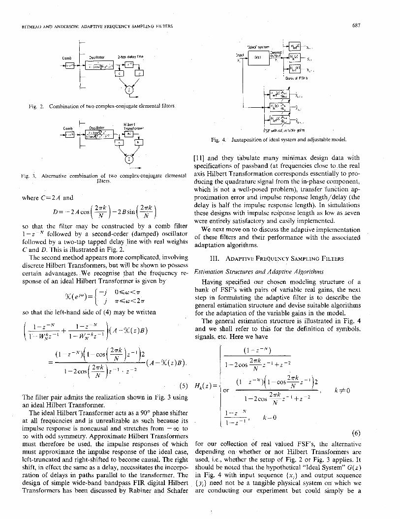
Fig. 4. Juxtaposition of ideal system and adjustable model.

[ l I] and they tabulate many minimax design data with specifications of passband (at frequencies close to the real axis Hilbert Transformation corresponds essentially to pro- ducing the quadrature signal from the in-phase component, which is not a well-posed problem), transfer function approximation error and impulse response length/delay (the delay is half the impulse response length). In simulations these designs with impulse response length as low as seven were entirely satisfactory and easily implemented.

We next move on to discuss the adaptive implementation of these filters and their performance with the associated adaptation algorithms.

111. ADAPTIVE FREQUENCY SAMPLING FILTERS

Estimation Structures and Adaptive Algorithms Having specified our chosen modeling structure of a

bank of FSF‘s with pairs of variable real gains, the next step in formulating the adaptive filter is to describe the general estimation structure and devise suitable algorithms for the adaptation of the variable gains in the model.

The general estimation structure is illustrated in Fig. 4 and we shall refer to this for the definition of symbols, signals, etc. Here we have

r (1 - z - N )

1-2cos-z ‘ + z - 2 2ak -

N

U

I- 1-z-N 1-z-1

, k=O

(6) for our collection of real valued FSF’s, the alternative depending on whether or not Hilbert Transformers are used, i.e., whether the setup of Fig. 2 or Fig. 3 applies. It should be noted that the hypothetical “Ideal System” G ( z ) in Fig. 4 with input sequence {xi} and output sequence {y , } need not be a tangible physical system on which we are conducting our experiment but could simply be a


mental construct representing an abstract linking between the two sequences. Obviously an interpretation of the adaptive filter as an approximate model then needs to be decided.

The aim of the exercise is to choose the variable gains A, , Bk so that the error between narrow-band components y k , , - jk , , is small in a certain sense. We treat this as a collection of independent (decoupled) estimation problems, for each of the two-vectors (Ak , Bk)T and the scalar A, , and concentrate without loss of generality on one real elemental filter from the bank of FSF-we shall discuss the dc filter H,(z ) later. The rationale behind this decoupling is that the outputs of the FSF for different k have an approximate orthogonality property by virtue of their being in different narrow frequency bands.'

We shall consider firstly the adaptive implementation of the FSF's using the filters of Fig. 2. We call this the direct implementation. We then examine the set up with filters of Fig. .3 involving the Hilbert Transformer and refer to this as the transformed implementation. As we are studying a single representative component, we shall drop the sub- script k from the sequences.

For the direct implementation we recall (4) and write {si} for the output of the filter

(1-z-~)(1-2cos- 2nkr - l+2-2 ) - " N

driven by {x;}. Thus we seek to have yj = Cs, + Dsi-

which is equivalent to a simple two-tap delay line. We may use LMS, (l) , to update estimates e;, D , of the optima C and D by using w=(?,, Di)T, d, =y, and X ; = ( S ; , S , _ , ) ~ . This implementation is shown in Fig. 5. The most striking comparison between this adaptive filter and the time- domain transversal filter is that they both utilize the same 'update algorithm but the time-domain N-vector adaptation is reduced to a collection of [N/2J two-vector adaptations plus one scalar adaptation. This and its consequences will be discussed more fully after the following presentation of the transformed implementation.

Denoting by { u , } the output sequence of the FSF

( 1 - 2 - ~ ) ( 2 - 2 c o s ~ 2 - ~ ) ( l - 2 c o s - z N 2ak N + + j - ' driven by {x,} and writing {o;} as the Hilbert Transform of the sequence {u;} we have from (5) that ideally

~ , = A u ; - B v ,

where A and B are, respectively, the real and imaginary parts of the gain at the particular frequency. This again conforms to a two-vector identification problem amenable to the LMS algorithm with v. =(a,, si)', d, =y, and X, = (u;, -vi)' in (1).

As remarked earlier an ideal Hilbert Transformer is an unrealizable filter and approximate transformers require

'In case ( X , I S wlde-sense stationary, the outputs are mutually uncorrelated, other t b an for ' effects induced by the overlap of passbands of the nonideal elemental filters. If {x,} is nonstationary, but approximately stationary, the outputs will be only approximately uncorrelated even discounting the overlaD of Dassbands.

I I I

Fig. 5. Direct implementation.

lo LMS Error

Fig. 6. Transformed implementation.

the introduction of a delay (usually half the length of the impulse response for FIR approximations) to try to com- pensate for the noncausality of the ideal filter. Denoting this delay by I we see that the implementation requires the use of j j - / =Aui - / -Bo,. The transformed implementation is shown in Fig. 6.

Performance and Comparison of Structures We now turn to consider the performance of and com-

parisons between the direct and transformed FSF approaches and the time-domain approach. As stated above the obvious point of comparison between these approaches is the reduction in the dimension of the X vector in the LMS algorithm. The primary effects of this are to alter the convergence rate of the adaptive filter and to allow us to predict this rate more accurately.

When the sequences { X , } and { d , } are random it is straightforward to show that, subject to independence [ l ] or mild forms of asymptotic independent [12], the LMS algorithm converges exponentially fast to a neighborhood of the best solution at a rate (1 -p ) j , where /3 depends roughly linearly on p (the adaptation gain) and the minimum eigenvalue of the covariance R = E [ X , X T ] or the time average of this quantity, and the degree of dependence of neighboring X,. This property arises basically because these methods are a form of steepest descent procedure to minimize a quadratic form with average weighting R with step size proportional to p (which in turn must be less than the reciprocal of the maximum eigenvalue of R for convergence of LMS). These steepest descent or gradient methods typically exhibit slow convergence when the condition number of the quadratic form is large [ 131. This dependence of convergence rate upon condition number of steepest descent methods is alleviated in the use of Newton- Raphson algorithms by premultiplying the gradient step by R- ' . This latter technique is exemplified in the more rapidly converging Recursive Least Squares algorithms.

When the dimension of X, is large it is often difficult to estimate both the minimum and maximum eigenvalues of

BITMEAD AND ANDERSON: ADAPTIVE FREQUENCY SAMPLING FILTERS

R and so a slow convergence rate often occurs because one naturally chooses a conservative value of p. Quite apart from these problems of ignorance, ill-conditioning problems become increasingly prevalent with increasing dimension. As the dimension is decreased the severity of these problems decreases until, with a scalar quadratic minimisation, the steepest descent procedure is equivalent to Newton-Raphson. The possible advantages of a collection of small dimension minimizations over one large dimension problem then become apparent and we will demonstrate how the proposed implementations allow effective reduction to a collection of N scalar adaptations.

These sorts of arguments are also advanced in [3]-[7] in support of the use of FFT-based adaption algorithms. However, as [3] makes clear, one may well be facing a constrained optimization problem, a fact which can negate much of the advantage.

The dc FSF requires only a single real gain so that its associated adaptive algorithm is a scalar minimization for both FSF implementations. Consequently, the steepest descent methods converge as fast as Newton-Raphson. Fur- thermore, the convergence rate is easily related to the magnitude of the scalar { X i } sequence. We may therefore easily choose an appropriate value for p. This will be discussed again later.

We now estimate the convergence rate and performance of the two-vector adaptations of the two adaptive FSF implementations.

As two preliminary comments, we note that when adaptive control is envisaged, the delay associated with use of the second FSF implementation (involving Hilbert transformers) may make this unacceptable. Second, we note that we shall discuss convergence of real and imaginary parts in the following, although for some purposes, convergence of magnitude and phase may be more relevant to consider, and the conclusions may be a little different.

We use the following notation: C and D , and A and B are the optimum values of the coefficients (assumed stationary for the moment) for the two implementations with a minimum mean square error criterion; {n ,} is the minimum mean square error yi - Cs, - Dsi- I and y, - h i + Bvi (delays assumed to be already accounted for); i j i is the coefficient estimate error (ti - C, ~5~ -olT or (A, - A , Si - B y .

The adaptation algorithms for the direct implementation are described by the equations

The associated homogeneous equation for sufficiently small p is known to be exponentially convergent under various mild conditions, see, e.g., [12]. Its time constants determine for (7) the time constant associated with convergence of the moments of iji. We shall now examine the homogeneous version of (7) to gain insight into what these time constants are.

Our arguments lack full rigor, but are certainly sugges-

689

tive. Because si is a narrow-band process, we represent it as

Here, ri and (pi are slowly varying processes. The coefficient matrix in (7) can be written as

If p is small enough in (7), the fast frequency (4nk/N) variations in the i:, sf- , , sisi- terms are inconsequential, i.e., the coefficient matrix can be replaced to a good approximation by its slow-varying part:

This shows that the time constants associated with (7) are those associated with the scalar equations

and

Particularly for small k, i.e., frequencies close to dc, the second equation will. have a much longer time constant than the first.

We shall now analyze the transformed algorithm, and show that again two equations are obtained; the time constants however are the same and independent of the frequency band.

The transformed algorithm has the following description:


We replace u;, vi by ajcos2nki/N and pjsin2nki/N, where, if ui , ui are Gaussian and exact Hilbert transforms, ai and pi are also Gaussian and band limited to 2n-/N. The coefficient matrix in (10) becomes

2nk; 1 1 -pa' cos2 - N

2nk- 1 - pp,' sin2 2

N

with the approximation involving elimination of fast time variation. The time constants associated with (10) are then those associated with

X;+l=(l-;pa;)hi (114

E;+ 1 = (1 - 4pP:)E; (1 1b)

and these are the same, since ai, pi are identically distributed.

We may use the results of the Appendix to estimate the time constants of (9a), (9b), (1 la), and (1 lb). These results state that, e.g., (1 la) converges with time constant at least as fast as the deterministic equation

xi+, = [ 1 - i p E ( a;)] x; when ai is ergodic. Generalization to the nonstationary case is possible. The differing time constants of (9) and (1 1) become evident.

The overall effect of the FSF adaptive filters compared to the time domain is to reduce a single N-vector problem to a collection of [N/2] two-vector problems plus one scalar problem, with each two-vector problem being equivalent to a pair of one-vector problems.

Whilst pointing out the advantages of these adaptive FSF's, firstly of the direct implementation over time- domain implementation, and then of the transformed implementation over the direct, it is pertinent to reiterate that the dominant dictator of which filter to use is the applications context. For example, if a measure of transient performance is desired by approximating an impulse response then the use of FSF would clearly be unwarranted over the time-domain approach. Similarly, the use of the transformed implementation instead of the direct implementation is not necessarily better. Indeed the convergence rate of the direct algorithm for the estimate of C+D may be faster than that of the transformed method-C+D is related to the transfer function magnitude-so that the direct method is to be preferred in some instances.

Performance with Noise Many calculations relating to the performance of LMS-

type algorithms rely upon assumptions of whiteness of the

input signals, see [l]. While this assumption can be relaxed [ 121, it allows us to easily produce good rules of thumb for design and to roughly quantify the filter behavior.

Here, we need to make different sorts of assumptions, using the narrow-band properties of the signals in each channel. We perform an analysis for the transformed algorithm only. Then ni =y, -Aui +Bo,. In a noiseless situation, with ideal filters with rectangular arbitrarily narrow pass bands, and with perfect Hilbert transformers, we could expect n i S O . However, we shall assume that n, is a narrow-band signal representable as

2nk. 2nki y , c o s d +6,sin -

Here, y, and 6, are slowly varying random process. In order that A and B be optimum (least mean square) coefficients, we demand that they minimize

N N -

E ( ( y i - A u , + B v ; ) ' } .

Of course, this ensures that at the optimum, E [ n j ] =0, E[n,u,]=O and E[nivi]=O. Let us also suppose that the inexactitudes giving rise to n , have a symmetry property which ensures that the probability densities p ( n j l u i ) and p ( n j l u , ) are symmetric in ni for all ui, vi with the associated variances independent of u, and u ~ . Then E [ n , 1 u ; ] = E [ n i l v i ] = O which implies that E[yjjai]=O, E[8,1pj]=O, and E[y," I a,] and E[S: I p i ] are independent of ai and pi.

Previously, we approximated the homogeneous part of (IO), eliminating fast time variations, with (1 1). If we now include the driving term in (lo), the approximation becomes

xi+ 1 = (1 - +pa?)h, - ;pylai ( W

'g;+l=(l-l 2~ p q - ' 1 I 2p'iP;.

It is only necessary to study one of these equations.

write (strictly an approximation) We now appeal to the slow variation property of ai to

~ [ ~ ; + l l ~ , + l l = ~ [ ~ ; + l I ~ , l .

(The signal a, has a bandwidth of 2a/N. Thus if the sampling rate for the parameter update equation is signifi- cantly faster than this-as it will have to be in order that sampling occur at a frequency in excess of the overall system bandwidth- the approximation is well justified.)

It follows that

E[~~+,ICY~]=(~-~~.Q?)E(~;((Y;)-~~~~E(Y~I(Y,) or

E [ ~ , + , I ~ ; + ~ I = ( ~ - ~ ~ C Y ? ) E ( X , I ~ ~ ) . Then E [ A, I a,] -+ 0 with a time constant the same as that of the homogeneous (lla), as then does E [ X i ] and E [ h j a j ] .

Next, we look at the second moment. As a preliminary, we consider the quantity E[h,y,ailai]. From (12a) and the slow variation of yi and a,, we have

E t ~ , + I Y , + I ~ i + l / ~ ; + I l

= ( 1 -+?)E[ hiYlCY, j a;] - i p a f E [ Y,"]


or, with E [ y i z , l ] = E [ y f ] by stationarity,

~ [ ' i + l ~ i + l " i + l ~ " i + l I + ~ [ ~ ~ + l ]

=(l-fpaf){EIXjyjai~aj]+E[y,Z]}

EIAiyiai lai]+ -E[y,Z]. (13)

whence we see that as i+ 00,

Now squaring (12a) and conditioning with the slow- variation property gives

E[A;+,~ai+I]=(1-fpaf)2E[A~~ai]+ap~afE[Y~]

-p ( 1 - fpaj')E[ A,yiailai]

2 = (1 - +pa?) E [ A; I ai] +p( 1 - apaf)E[ $1

by (13). It then follows that

Multiplying by a: and invoking slow variation of ai and stationarity of E [ y f ] we have

~ i 2 + I ~ [ ~ ~ ~ + l 1 ~ i + l l - ~ [ y i : l l

=(1-~paf)"aj'E[A~~ai]-E[y,2]}.

Hence [ 141, provided E 1 af I <2p-', as i-+ 00

a f ~ [ A: I ai] -+E[ y:] a.s.

and taking expectations

E [ a 3 ; ] + E [ y?] . ( 14)

Thus we see that, despite the correlation of all the signals involved in the LMS algorithm, the output error, q A i , converges to the optimum value as measured by the first two moments of the error distribution. The correlation of the signals has not affected the performance of the LMS algorithm in this application.

The crucial assumptions in the above analysis have been the slow variation of the magnitude signals such as mi and the slow variation of the parameter estimate errors A, relative to the signal frequencies. It is to be expected that as these restrictions become less valid, either by moving to higher frequencies or by increasing the value of p, the assumptions behind the analysis become less justifiable implying that a change in performance will arise.

IV. SIMULATION RESULTS

Simulations of both types of adaptive frequency sampling filter were conducted for a variety of different systems including both those FIR systems which could be exactly modeled by a collection of weighted FSF's and systems (FIR and IIR) which could not. The performance of both adaptive filter implementations were compared for both types of systems above, with and without noise, and with differing gains.

The Hilbert transformers for the transformed implementation were approximated by FIR Minimax approximations of [ll]. It was found that approximate transformers

31

2-

1-

Fig. 7. Ensemble performance measures of transformed adaptive FSF. No noise, adaptive gain 0. I.

of impulse response length 7 were workable for frequency separations of 2n/20 radians and that those with length 15 were entirely adequate.

The gain p used in both implementations was ap- propriately scaled to the signal power, as is common, to allow comparison between the convergence rates and it was found that,' as predicted, the convergence rate of the transformed implementation was indeed faster than that of the direct implementation especially close to the real axis. The difference between rates decreased as the frequency ap- proached n/2 radians. Except for systems with transfer functions such as 1 -z - I , which are perfectly describable by the direct implementation, the transformed algorithm appeared to perform more accurately.

We present below several simulation graphs which il- lustrate for the transformed algorithm the effect of varying the signal to noise ratio and the adaptive gain p. Similar effects are exhibited by the other implementation. 'These simulations were carried out with random input sequences to the adaptive filter and measurement noise. An ensemble of 100 simulations was performed and the ensemble mean parameter value together with the ensemble standard deviation are plotted.

There are several effects limiting the accuracy of the transformed adaptive FSF. Firstly, there is model mismatch due to the inability of describing exactly the plant system by a bank of weighted FSFs. This manifests itself as an extra forcing function to the homogeneous parameter update equations resulting in a time-variation of the parameter about the optimum value. The smaller the value p is, the smaller is the amplitude of this time variation. Allied with this mismatch and contributing time variations possibly with dc offset is the inaccuracy of the Hilbert transformer. In the simulations presented this latter effect was negligible, however. Associated with model mismatch is the overlapping of neighboring frequency sampling filters due to their nonideal bandpass nature- this too may intro- duce a time variation and offset in the parameter estimate.

The above sources of parameter error arise even when the adaptive filter operates in the absence of measurement noise. The situation is illustrated in Fig. 7 for the system

G( z ) = 1+3z-'+32-*+2-3 6+z-'

692 IEEE TRANSACTIONS ON ACOUSTICS, SPEECH, AND SIGNAL PROCESSING, VOL. ASP-29, NO. 3, JUNE 198 1

2 3A

Fig. 8. Effect on ensemble performance of additive noise. Signal-to-noise ratio I O dB, adaptive gain 0.1.

'iE 0' ?o

/ 7 7 1 M

-2 -'p Fig. 9. Effect on ensemble performance of adaption gain. Signal-to-noise

ratio 10 dB, adaptive gain 0.25.

at the frequency 0.171- with gain p=O.1 with normalization to signal level. The straight lines on the graph represent the real and imaginary parts of G[exp(O.lj.rr)]. Note the width of the standard deviation band and the convergence rate.

With the addition of measurement noise at 10 dB below the signal power, the simulation was repeated. The measurement noise added onto the system output was white Gaussian noise independent of the system output. Fig. 8 illustrates the outcome of this simulation. Notice that the predictable effect of the inclusion of this noise is to leave the mean value unaltered while causing a spreading of the standard deviation from the mean due to the included uncorrelated random process. The convergence rate has not been perceptibly altered, although it is known (see Ap- pendix) that an extremely large noise signal can prevent convergence of the filter.

Fig. 9 demonstrates the effect of altering the gain p. In Fig. 9 p has been changed from 0.1 to 0.25 (after signal strength scaling) and the noise has been left at 10 dB below the signal. The most startling effects to be noticed are the increased convergence rate, the increased standard deviation and the lack of smoothness.

V. CONCLUSIONS We have presented two new adaptive filters based on

frequency sampling/sliding spectrum ideas and LMS-type estimation algorithms. The first of these filters- the direct

implementation-involves a bank of filters each followed by a separate two-tap delay line which incorporates the adaptive gains. This was shown to reduce the N-vector transversal filter problem of the time domain to a collection of LN/2J two-vector transversal filter problems plus a single scalar problem. The second filter- the transformed implementation-involves a similar bank of filters and the use of a Hilbert Transformer at the output of each together with the two adaptive gains. While this latter scheme is more complicated in concept, it allows us to further decou- ple the two-vector adaptations so that the single N-vector problem reduces to N scalar ones.

The advantages of this reduction in dimension of the adaptation were shown to be related to the convergence rate (especially the "transient" convergence rate), to our ability to predict this rate and performance, to have confi- dence in our design, of parameters for different frequency bands. The convergence rate is related to the eigenvalue properties of a certain matrix having the same dimension as the transversal filter involved. By lowering this dimension through using FSF methods we reduce the likelihood of condition number problems and increase the predictabil- ity of the adaptive performance.

Finally, it should again be remarked that we do not intend that adaptive FSF's should be used to the exclusion of familiar time domain filters, especially tapped delay line filters, but rather that they should be thought of as another valid alternative possessing certain advantages in many situations. The choice of adaptive filter should be dictated by the ultimate application.

APPENDIX

We consider the apparently trivial problem of the stability of the equation

xk+, = ( Y k x k , X I = 1. ( A 0

The problem is made nontrivial by the assumption that { a k } is an ergodic random process. We shall find a sufficient condition for the exponential stability of { x k } , i.e., for the existence of a constant a E(0,l) such that a - k ~ k + 0 as., or equivalently, the existence of p(u) and constant a E(O,1) such that I xk 1 <p( u)ak . A similar result has been obtained in continuous-time by Parthasarathy and Evan- Iwanowski [ 141.

It is clear that the solution of (Al) is exponentially convergent if and only if the solution of yk+, = 1 ak I y,, x, = 1 is exponentially convergent.

We need to partition the set of events Si? into Go UO,, where 8, = { u l a k = O for some k } and 8, = { c d l a k # O for any k } . We first argue that P(02,)=0 or 1. Suppose that P ( a , = O ) = O (Note: this is a probability, not a probability density.) Then it is clear that P(QO)=O, Q0 being a count- able union of events of zero probability. Suppose then that P ( a , =O)#O. Define xi by xi = O if ai #0, x i = 1 if ai = O . By the ergodic theorem

lim x , + x , + * . .+x,

+ E [ x , ] = P ( a , =o) iI - 00 n

w.p.1. Thus if P( a , =O)#O, we have w.p.1 an infinite


number of xi are 1, and thus an infinite number of ai zero, i.e., P(Po) = 1.

If P(Po) = 1, exponential stability is immediate. So sume P( !d ,) = 1. On PI, we shall study the solution of related equation

Yk+I=Iaklyk, Y I z 1

which can be written as

are

as- the

Now

so that

It follows that a necessary and sufficient condition for exponential stability is

E[lnla,ll<O (-43)

provided this expected value exists. Evidently, the dependence properties of the { a k } are irrelevant. By Jensen’s inequality, a sufficient condition is

ln E[la,Il<O (A41

E[la , l l< l . (A51 or

If (A5) is satisfied then using events like Po and PC = {a[ -€<ak < E for some k } it is possible to extend this sufficient condition to hold even when the expectation in (A3) does not exist.

This condition should be compared to the sufficient condition of [14]. A more refined sufficient condition follows by rewriting (A3) as

E{lna,Ia,>O}P(a,>O)

+E{ln(-a,)la, < o } P ( ~ , <o)<o which again by Jensen’s inequality yields

{In E [ a , / a , >OI}P(a, > O )

+{InE[-a , Ia ,<O])P(a ,<O)tO or

{ E [ a , ~ a l > O ] } P ~ a ~ ~ o ~ { E [ - ~ l ~ ~ l < O ] } p(a1 <O)< 1.

(A61 Holder’s inequality shows that if (A5) holds, then so must (A6). So there may be instances where (A6) can be used to conclude exponential stability, but not (A5). If ai has a symmetric density;(A5) and (A6) are equivalent.

Example I : Suppose a, is Gaussian, with mean 0 and variance u2. Then

is sufficient for stability.

Example 2: Suppose a , is Gaussian, with mean p and variance u2. Then

E [ l a , ~ ] = ~ ~ e x p ( - p ~ / 2 ~ ~ ) + ~ e r f ( ~ / ~ ~ ) .

Example 3: a , = 1 -p: where PI is Gaussian with mean zero and variance u. Then

E [ ~ a , ~ ] = ( a 2 - l

If {ak} is no longer ergodic but has a suitable mixing property, such as +mixing with a summability condition on the square roots of the mixing parameters, see [ 151 then we can still obtain a convergence result which may be applied in nonstationary cases. Assume that P(P,)= 1. Then (A3) is replaced by

The application we make of these results is to equations of adaptive estimation which arise with ai = 1 -p:, {p,} ergodic or +mixing, for which a sufficient condition is EI1-/321<1.

REFERENCES [ l ] B. Widrow, J. M. McCool, M. G. Larimore, and C. R. Johnson, Jr.,

“Stationary and nonstationary learning characteristics of the LMS adaptive filter,” Proc. IEEE, vol. 64, pp. 1151-1 162, Aug. 1976.

[2] L. J. Griffiths, “Rapid measurement of digital instantaneous frequency,” IEEE Truns. Acoust. Speech Signul Processing, vol. ASSP-23, pp. 207-222, Apr. 1975.

[3] T. Waltzman and M. Schwartz, “Automatic equalization using the discrete freauencv domain.” IEEE Truns. Inform. Theorv, vol. IT-19, pp. 59-68, jan. i973. W. S. Hodgkiss, “Adaptive array processing: Time vs frequency domain,” in 1979 Proc. lnt. Conf. Acoust. Speech and Signul Process- ing, Washington, DC, pp. 282-285, Apr. 1979. M. Dentino, J. McCool, and B. Widrow, “Adaptive filtering in the frequency domain,” Proc. IEEE, vol. 66, pp. 1658- 1659, Dec. 1978. D. Mansour, “Frequency domain ada tive filter by overlap-save method,” Tech. Rep., Dep. Elect. an8Computer Eng., Univ. of California, Santa Barbara, 1979. N. J. Bershad and P. L. Feintuch, “Analysis of the frequency domain adaptive filter,” Proc. IEEE, vol. 67, pp. 1658- 1659, Dec.

,,

1070

[X] B ‘Gold and C. M. Rader, Digitul Processing of Signals. New York: McGraw-Hill, 1969.

[9] L. R. Rabiner and B. Gold, Theory und Applicution of Digitul Signul Processing. Englewood Cliffs, NJ: Prentice-Hall, 1975.

[IO] M. I. Skolnik. Introducfion to Rudur Systems. New York: McGrawHiil, 1962.

[ I I] L. R. Rabiner and R. W. Schafer, “On the behaviour of minimax FIR digital Hilbert transformers,” Bell System Tech. J., vol. 53, no. 2, pp. 363-390, Feb. 1974.

[I21 R. R. Bitmead and B. D. 0. Anderson, “Performance of adaptive estimation algorithms in dependent random environments,” I E E E Truns. Automut. Contr., vol. AC-25, pp. 788-794. Aug. 1980.

[I31 D. G. Luenberger, Introduction to Lineur und Nonlineur Progrum- ming. Reading, MA: Addison-Wesley, 1973.

[14] A. Parthasarathy and R. M. Evan-Iwanowski, “On the almost sure stability of linear stochastic systems,” S I A M J . Appl. Muth., vol. 34,

[ 151 M. Iosifescu and R. Theodorescu, Rundom Processes und Leurning. no. 4, pp. 643-656, June 1978.

[I61 E. R. Ferrara, “Fast implementation of LMS adaptive filters,” New York: Springer-Verlag, 1969.

IEEE Truns. Acoust., Speech Signul Processing, vol. ASSP-28, pp. 414-475, Aug. 1980.


A Performance Analysis of Adaptive Line Enhancer-Augmented Spectral Detectors

0096-35 18/81/0600-0694$00.75 0 198 1 IEEE

Adaptive frequency sampling filters

Documents

Transcript of Adaptive frequency sampling filters