Sampling Random Transfer Functions

C. M. Lagoa1, X. Li2, M. C. Mazzaro3, and M. Sznaier4

1 EE Dept., The Pennsylvania State University. University Park, PA 16802, USA,lagoa@engr.psu.edu

2 EE Dept., The Pennsylvania State University. University Park, PA 16802, USA,xiangli@psu.edu

3 EE Dept., The Pennsylvania State University. University Park, PA 16802, USA,cmazzaro@gandalf.ee.psu.edu

4 EE Dept., The Pennsylvania State University. University Park, PA 16802, USA,msznaier@frodo.ee.psu.edu

Summary. Recently, considerable attention has been paid to the use of probabilis-tic algorithms for analysis and design of robust control systems. However, since thesealgorithms require the generation of random samples of the uncertain parameters,their application has been mostly limited to the case of parametric uncertainty. Inthis paper, we provide the means for further extending the use of probabilistic al-gorithms for the case of dynamic causal uncertain parameters. More precisely, weexploit both time and frequency domain characterizations to develop efficient algo-rithms for generation of random samples of causal, linear time-invariant uncertaintransfer functions. The usefulness of these tools will be illustrated by developingalgorithms that address the problem of risk-adjusted model invalidation. Further-more, procedures are also provided for solving some multi–disk problems arisingin the context of synthesizing robust controllers for systems subject to structureddynamic uncertainty.

1 Introduction

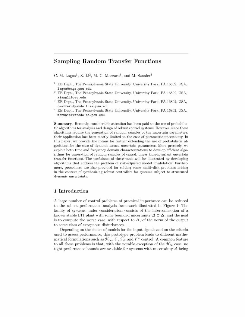
A large number of control problems of practical importance can be reducedto the robust performance analysis framework illustrated in Figure 1. Thefamily of systems under consideration consists of the interconnection of aknown stable LTI plant with some bounded uncertainty ∆ ⊂ ∆, and the goalis to compute the worst–case, with respect to ∆, of the norm of the outputto some class of exogenous disturbances.

Depending on the choice of models for the input signals and on the criteriaused to assess performance, this prototype problem leads to different mathe-matical formulations such as H∞, `1, H2 and `∞ control. A common featureto all these problems is that, with the notable exception of the H∞ case, notight performance bounds are available for systems with uncertainty ∆ being

2 C. M. Lagoa, X. Li, M. C. Mazzaro, and M. Sznaier

--

�

-G

∆

S

wy

Fig. 1. The Robust Performance Analysis Problem

a causal bounded LTI operator5. Moreover, even in the H∞ case, the problemof computing a tight performance bound is known to be NP–hard in the caseof structured uncertainty, with more than two uncertainty blocks [6].

Given the difficulty of computing these bounds, over the past few years,considerable attention has been devoted to the use of probabilistic methods.This approach furnishes, rather than worst case bounds, risk–adjusted bounds;i.e., bounds for which the probability of performance violation is no largerthan a prescribed risk level ε. An appealing feature of this approach is that,contrary to the worst–case approach case, here, the computational burdengrows moderately with the size of the problem. Moreover, in many cases,worst–case bounds can be too conservative, in the sense that performancecan be substantially improved by allowing for a small level of performanceviolation. The application of Monte Carlo methods to the analysis of controlsystems was recently in the work by Stengel, Ray and Marrison in [18, 22, 26]and was followed, among others, by [4, 2, 7, 11, 15, 27, 31, 34]. The designof controllers under risk specifications is also considered in some of the workabove as well as in [3, 12, 17, 29, 30].

At the present time the domain of applicability of Monte Carlo techniquesis largely restricted to the finite–dimensional parametric uncertainty case.The main reason for this limitation resides in the fact that up to now, theproblem of sampling causal bounded operators (rather than vectors or ma-trices) has not appeared in the systems literature. A notable exceptions tothis limitation is he algorithm for generating random fixed order state spacerepresentations in [8]. In this paper, we provide two algorithms aimed at re-moving this limitation when the set ∆ consists of balls in H∞. We use resultson interpolation theory to develop three new procedures for random transferfunction generation. The first algorithm generates random samples of the firstn Markov parameters of transfer functions whose H∞ norm is less than orequal to one. This algorithm is particularly useful for problems like model in-validation where only the first few Markov parameters of the systems involvedare used. The second algorithm generates random transfer functions having

5 Recently some tight bounds have been proposed for the H2 case, but these boundsdo not take causality into account; see [19].

Sampling Random Transfer Functions 3

the property that, for a given frequency, the frequency response is uniformlydistributed over the interior of the unit circle. This algorithm is useful forproblems such as model (in)validation, where the uncertainty that validatesthe model description is not necessarily on the boundary of the uncertaintyset ∆. Finally, the third algorithm provides samples uniformly distributedover the unit circle, and is useful for cases such as some robust performanceanalysis/synthesis problems where the worst–case uncertainty is known to beon the boundary of ∆.

The usefulness of these tools is illustrated by developing algorithms formodel invalidation. Moreover, we also provide an algorithm aimed at solvingsome multi–disk problems arising in the context of synthesizing robust con-trollers for systems subject to structured dynamic uncertainty. More precisely,we provide a modification of the algorithm in [16] that when used togetherwith the sampling schemes mentioned above, enables one to solve the problemof designing a controller that robustly stabilizes the system for a “large” setof uncertainties while guaranteeing a given performance level on a “smaller”uncertainty subset.

2 Preliminaries

2.1 Notation

Below we summarize the notation used in this paper:

bxc largest integer smaller than or equal to x ∈ R.x ∈ Rm real–valued column vector.AT conjugate transpose of matrix A.Ai,j (i, j) element of A.σ (A) maximum singular value of the matrix A.BX(γ) open γ-ball in a normed space X: BX(γ) = {x ∈ X : ‖x‖X < γ}.BX(γ) closure of BX(γ).

BX (BX) open (closed) unit ball in X.vol(X) k-th dimensional Lebesgue measure of X ⊂ Rk.

Projl(C) projection operator. Given a set C ⊂ Rm and l < m:

Projl(C).=

{x ∈ Rl :

[xT yT

]T∈ C for some y ∈ Rk−l

}.

SkC

k-th section of a set C ⊂ Rn. Given y ∈ Rn−k:

SkC(y)

.=

{x ∈ Rk :

[yT xT

]T∈ C

}.

E[X|Y ] conditional expected value of X given Y .Fl(M,∆) lower linear fractional transformation:

Fl(M,∆) = M11 + M12∆(I − M22∆)−1M21.Fu(M,∆) upper linear fractional transformation:

Fu(M,∆) = M21∆(I − M11∆)−1M12 + M22.

4 C. M. Lagoa, X. Li, M. C. Mazzaro, and M. Sznaier

`mp extended Banach space of vector valued real sequences equipped

with the norm:

‖x‖p.=

(∑∞i=0 ‖xi‖

pp

) 1p

p ∈ [1,∞), ‖x‖∞.= supi ‖xi‖∞.

L∞ Lebesgue space of complex–valued matrix functions essentiallybounded on the unit circle, equipped with the norm: ‖G‖∞

.=

ess sup|z|=1 σ (G(z)).

H∞ subspace of transfer matrices in L∞ with bounded analyticcontinuation inside the unit disk, equipped with the norm:‖G‖∞

.= ess sup|z|<1 σ (G(z)).

H∞,ρ space of transfer matrices in H∞ with analytic continuationinside the disk of radius ρ ≥ 1, equipped with the norm‖G‖∞,ρ

.= sup|z|<ρ σ (G(z)).

BHn∞ set of (n − 1)th order FIR transfer matrices that can be com-

pleted to belong to BH∞, i.e. BHn∞

.=

{H(z) = H0+H1z+. . .+

Hn−1zn−1 : H(z) + znG(z) ∈ BH∞, for some G(z) ∈ H∞

}.

RX subspace of X ⊆ L∞ composed of real rational transfer matrices.H2 Hilbert space of complex matrix valued functions analytic in the

set {z ∈ C : |z| ≥ 1}, equipped with the inner product

〈H,T 〉 =1

2π

∫ 2π

0

Re{Trace[H(ejθ)∗T (ejθ)]}dθ.

and norm

‖T‖2 =

(1

2π

∫ 2π

0

Re{Trace[T (ejθ)∗T (ejθ)]}dθ

) 12

.

RH2 subspace of all rational functions in H2.X(z) z transform of a right–sided real sequence {x}, evaluated at 1

z :

X(z) =∞∑

i=0

xizi.

2.2 Space of Proper Rational Transfer Functions

Define the space G as the space of rational functions G : C → Cn×m that canbe represented as

G(z) = Gs(z) + Gu(z).

where Gs(z) ∈ RH2 and Gu(z) is strictly proper and analytic in the set{z ∈ C : |z| < 1}. Now, given two functions G,H ∈ G and 0 < γ < 1 definethe distance function d as where Gs(z) analytic in the set {z ∈ C : |z| ≥ α}and Gu(z) is strictly proper, analytic in the set {z ∈ C : |z| < α} and0 < β < α < 1. Now, given two functions G,H ∈ G define the distancefunction d as

Sampling Random Transfer Functions 5

d(G,H).=

(‖Gs(z) − Hs(z)‖2

2 + ‖Gu(β/z) − Hu(β/z)‖22)

) 12 .

The results later in the paper that make use of this distance function aresimilar for any value of α and β. However, α and β are usually taken to bevery close to one.

2.3 Convex Functions and Subgradients

Consider a convex function g : H2 → R. Then, given any G0 ∈ H2, thereexists a ∂Gg(G0) ∈ H2 such that

g(G) − g(G0) ≥ 〈∂gG(G0), G − G0〉. (1)

for all G ∈ H2. The quantity ∂Gg(G0) is said to be a subgradient of g at thepoint G0. For example if g(G) = ‖G‖2 and G is a scalar; i.e.,

g(G) =

(1

2π

∫ 2π

0

|G(ejθ)|2dθ

)1/2

then [5] indicates that

∂Gg(G) =1

2π‖G‖2G. (2)

2.4 Closed Loop Transfer Function Parametrization

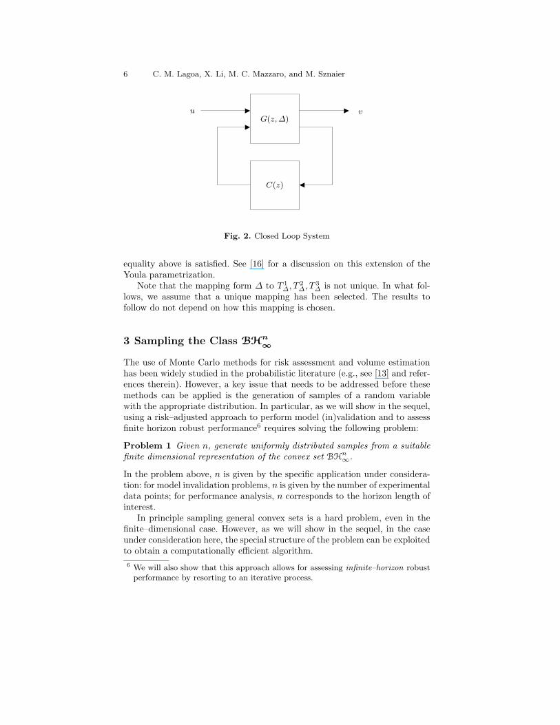
Central to the results on design presented in this paper is the parametrizationof all closed loop transfer functions. Consider the closed loop plant in Figure 2with uncertain parameters ∆ ∈ ∆. The Youla parametrization (e.g., see [24])indicates that, given ∆ ∈ ∆ and a stabilizing controller C ∈ G, the closedloop transfer function can be represented as

TCL(z,∆,C) = T 1∆(z) + T 2

∆(z)Q∆,C(z)T 3∆(z), (3)

where T 1∆, T 2

∆, T 3∆ ∈ RH2 are determined by the plant G(z,∆) (and, hence,

they also depend on the uncertainty ∆) and Q∆,C ∈ RH2 depends on both theopen loop plant G(z,∆) and the controller C(z). Also, given any Q∆,C(s) ∈RH2, there exists a controller C ∈ G such that the equality above is satisfied.

This parametrization also holds for all closed loop transfer functions, stableand unstable. Using a frequency scaling reasoning one can prove the followingresult: Given ∆ ∈ ∆ and a controller C ∈ G, the closed loop transfer functioncan be represented as

TCL(z,∆,C) = T 1∆(z) + T 2

∆(z)Q∆,C(z)T 3∆(z), (4)

where T 1∆, T 2

∆, T 3∆ ∈ RH2 are the same as above and Q∆,C(s) ∈ G. Further-

more, given any Q∆,C(s) ∈ G there exists a controller C ∈ G such that the

6 C. M. Lagoa, X. Li, M. C. Mazzaro, and M. Sznaier

G(z, ∆)

C(z)

u v

Fig. 2. Closed Loop System

equality above is satisfied. See [16] for a discussion on this extension of theYoula parametrization.

Note that the mapping form ∆ to T 1∆, T 2

∆, T 3∆ is not unique. In what fol-

lows, we assume that a unique mapping has been selected. The results tofollow do not depend on how this mapping is chosen.

3 Sampling the Class BHn

∞

The use of Monte Carlo methods for risk assessment and volume estimationhas been widely studied in the probabilistic literature (e.g., see [13] and refer-ences therein). However, a key issue that needs to be addressed before thesemethods can be applied is the generation of samples of a random variablewith the appropriate distribution. In particular, as we will show in the sequel,using a risk–adjusted approach to perform model (in)validation and to assessfinite horizon robust performance6 requires solving the following problem:

Problem 1 Given n, generate uniformly distributed samples from a suitablefinite dimensional representation of the convex set BH

n∞.

In the problem above, n is given by the specific application under considera-tion: for model invalidation problems, n is given by the number of experimentaldata points; for performance analysis, n corresponds to the horizon length ofinterest.

In principle sampling general convex sets is a hard problem, even in thefinite–dimensional case. However, as we will show in the sequel, in the caseunder consideration here, the special structure of the problem can be exploitedto obtain a computationally efficient algorithm.

6 We will also show that this approach allows for assessing infinite–horizon robustperformance by resorting to an iterative process.

Sampling Random Transfer Functions 7

3.1 Reducing the Problem to Sampling Finite Dimensional Sets

We begin by showing how Problem 1 can be reduced to the problem ofsampling a finite–dimensional convex set. From Caratheodory-Fejer Theo-rem (see appendix?????) it follows that given the first n Markov parametersHi ∈ Rs×m, i = 0, 1, . . . , n − 1 of a matrix operator H(z) ∈ H∞, the corre-sponding H(z) ∈ BH

n∞ if and only if

σ (TnH) ≤ 1,

where

TnH(H0,H1, . . . ,Hn−1)

.=

Hn−1 · · · H1 H0

Hn−2 · · · H0 0...

...H0 0 · · · 0

.

Thus, a natural representation for BHn∞ in Problem 1 is the set

CHn

.=

{{Hi}

n−1i=0 : σ (Tn

H) ≤ 1}.

This leads to the problem below.

Problem 2 Given n > 0, generate uniform samples over the convex set CHn.

In the sequel, we present an algorithm for generating uniform samples overarbitrary finite dimensional convex sets and we solve Problem 2 as a specialcase.

3.2 Generating Uniform Samples Over Convex Sets

Let C ⊂ Rn denote an arbitrary convex set. Given x ∈ C, partition the vectorconformably to some given structure in the following form

x =[xT

1 xT2 · · · xT

m

]T

where xi ∈ Rni and∑m

i=1 ni = n.Consider now the following algorithm:

Algorithm 1 1. Let k = 0. Generate N samples, xl1, l = 1, 2, . . . , N , uni-

formly distributed over the set Io.= Projn1(C).

2. Let k := k + 1. For every generated sample (xl1,x

l2, . . . ,x

lk−1), let

Ck(xl1,x

l2, . . . ,x

lk−1)

.= Sn∗

C

([(xl

1)T (xl

2)T · · · (xl

k−1)T ]T

)

Ik(xl1,x

l2, . . . ,x

lk−1)

.= Projnk(Ck),

with n∗ .=

∑mi=k ni. Generate

Nk.= bαkNvol (Ik)c

samples uniformly over the set Ik, where αk is an arbitrary positive con-stant.

8 C. M. Lagoa, X. Li, M. C. Mazzaro, and M. Sznaier

3. If k < m go to step 2. Else stop.

Next we show that the probability distribution of the samples generatedby this algorithm converges, with probability one, to a uniform distributionas N → ∞.

Theorem 1 Consider any setA ⊆ C. For a given N , denote by Nt(N) andNA(N)7 the total number of samples generated by Algorithm 1 and the numberof those samples that belong to A, respectively. Then

NA(N)

Nt(N)

w.p.1−→

vol(A)

vol(C). (5)

Proof. See Appendix B.

Remark 1 The main reason that prevents the estimate of probability pro-duced by the samples generated by Algorithm 1 from being unbiased is thefact that, in general, at step s,

bNαsvs(Xk1 ,Xm

2 , . . . ,Xns−1)c

N6= αsvs(X

k1 ,Xm

2 , . . . ,Xns−1).

due to the rounding. Indeed, for any union of hyper-rectangles A ⊆ C satisfy-ing:

bNαsvs(Xk1 ,Xm

2 , . . . ,Xns−1)c

N= αsvs(X

k1 ,Xm

2 , . . . ,Xns−1).

it can be shown that, for any value of N ,

E[NA]

E[Nt]=

vol(A)

vol(C)

Unfortunately, in the general case this equality is not true. However, as weshow next, the difference between these values can be made very small evenfor relatively small values of N .

Theorem 2 Consider a set A ⊆ C. Then, there exist constants k1, k2 and k3

such that, for any N ,∣∣∣∣E[NA]

E[Nt]−

vol(A)

vol(C)

∣∣∣∣ ≤1

N

k1

k2 + k3

N

.

Proof. see Appendix C

Remark 2 The main difference between “traditional” Monte Carlo simu-lation for risk assessment and risk assessment using Monte Carlo methodstogether with the sample generation algorithm above is the fact that here onehas to determine the volume of several sets in order to compute the sam-ples. However, as we will see in the next section, for the problem at hand

7 Note that both Nt and NA are random variables.

Sampling Random Transfer Functions 9

we do not need to estimate these volumes. The structure is such that onecan determine them up to a multiplicative constant. Therefore, the number ofsamples needed to compute reliable estimates of risk is similar to the ones in“traditional” Monte Carlo simulations. For bounds on the number of samplesrequired for reliable estimation of risk see [15] and [27].

3.3 BHn

∞as a Simpler Case

In the case of general convex sets C, Algorithm 1 requires knowledge of thevolume of the projection sets up to a multiplying constant. However, as weshow in the sequel, for sets of the form CHn

.=

{{Hi}

n−1i=0 : σ (Tn

H) ≤ 1}

it ispossible to analytically find these quantities. Since these are precisely the setsarising in the context of Problem 1, and since the linear spaces Rs×m andRsm are isomorphic, it follows that this problem can be efficiently solved byapplying Algorithm 1.

Specifically, given {H0,H1, . . . ,Hk−1}, 1 ≤ k ≤ n, consider the problemof determining the set

Projnk(Ck(H0,H1, . . . ,Hk−1)

)

.=

{Hk : (H0, . . . ,Hk−1,Hk,Hk+1, . . . ,Hn−1) ∈ CHn

,

for some (Hk+1, . . . ,Hn−1)}. (6)

From Parrott’s Theorem (Appendix A) it follows that the set (6) is given by:

{Hk : σ

(Tk+1

H (H0,H1, . . . ,Hk))≤ 1

}.

Moreover, an explicit parameterization of this set can be obtained as follows.Consider the partition,

Tk+1H (H0,H1, . . . ,Hk) =

[Hk BC A

]

and let the matrices Y and Z be a solution of the linear equations

B = Y(I − AT A)12

C = (I − AAT )12 Z

σ (Y) ≤ 1, σ (Z) ≤ 1.

Then

{Hk : σ (T)

k+1H ≤ 1

}

={Hk : Hk = −YAT Z + (I − YYT )

12 W(I − ZT Z)

12 , σ (W) ≤ 1}.

Hence, generating uniform samples over the set (6) reduces to the problemof uniformly sampling the set {W : σ (W) ≤ 1}. Algorithms to do sampling

10 C. M. Lagoa, X. Li, M. C. Mazzaro, and M. Sznaier

over such sets are readily available (see for instance [7]). In addition, this pa-rameterization allows for easily computing, up to a multiplying constant, thevolume of the set Projnk(Ck), required in step 2 of Algorithm 1. This followsfrom the fact that Projnk

(Ck(H0,H1, . . . ,Hk−1)

)is a linear transformation

of the set M({W : σ (W) ≤ 1}

)and thus

J(H0,H1, . . . ,Hk−1) =vol

(Projnk

(Ck(H0,H1, . . . ,Hk−1)

))

vol(M

({W : σ (W) ≤ 1}

)) .

whereJ(H0,H1, . . . ,Hk−1) = |(I − YYT )

12 |m|(I − ZT Z)

12 |s (7)

is the Jacobian of the transformation above (see [7], Appendix F). Combiningthese observations leads to the following algorithm for solving Problem 1.

Algorithm 2 1. Let k = 0. Generate N samples uniformly distributed overthe set

{H0 : σ (H0) ≤ 1}.

2. Let k := k + 1. For every generated sample (Hl0,H

l1, . . . ,H

lk−1), consider

the partition

Tk+1H (Hl

0,Hl1, . . . ,Hk) =

[Hk BC A

]

and let the matrices Y and Z be a solution of the linear equations

B = Y(I − AT A)12

C = (I − AAT )12 Z

σ (Y) ≤ 1, σ (Z) ≤ 1.

Generate bNJ(H0,H1, . . . ,Hk−1)c samples uniformly over the set{W : σ (W) ≤ 1} and for each of those samples Wi, take

Hik = −YAT Z + (I − YYT )

12 Wi(I − ZT Z)

12 .

3. If k < m go to step 2. Else stop.

3.4 Extension to the infinite horizon case

In this section we show that the results above can be extended to assess infinitehorizon robust performance. Due to space constraints, we provide only anoutline of the ideas involved. Begin by noting that, Caratheodory-Fejer onlyspecifies the values of the function and its first n − 1 derivatives at z = 0.However, these conditions do not impose any constraints on the smoothnessof the function over the unit disk and can lead to transfer functions whichdo not represent a physical uncertainty. For example, h = {0, 0, . . . , 0 γ

(1+γ)2 }

Sampling Random Transfer Functions 11

has all the hi, i ≤ n − 1 arbitrarily small and satisfies the Caratheodory-Fejer theorem. Moreover, it can be easily shown that a suitable interpolant isgiven by

H(z) =γ

1 + γ − zn.

Clearly, H(z) ∈ BH∞. However, ‖ ddz H(z)‖∞ = n

γ → ∞. Since these func-tions are arguably not a good abstraction of physical uncertainty, estimatingworst–case performance bounds using samples from the set Fn can lead to con-servative results. This effect can be avoided by working with the ball BH∞,ρ,instead of BH∞, since restricting all the poles of the system to the exterior ofthe disk |z| ≥ ρ induces a smoothness constraint. This leads to the followingmodified version of Problem 1:

Problem 3 Given n > 0, ρ > 1, ρ ∼ 1, generate uniformly distributed sam-ples over an appropriate finite–dimensional representation of the set

Fn,ρ.=

{H(z) = H0 + H1z + . . . + Hn−1z

n−1 : H(z) + znG(z) ∈ BH∞,ρ,

for some G(z) ∈ BH∞,ρ

}.

As we show next, this problem readily reduces to Problem 2 and thus can besolved using Algorithm 1. To this end, note that F (z) = H(z) + znG(z) ∈BH∞,ρ is equivalent to F (ρz) ∈ BH∞. Combining this observation withCaratheodory-Fejer Theorem, it follows that, given {H0,H1, . . . ,Hn−1}, then

there exists G(z) ∈ BH∞,ρ such that∑n−1

i=0 Hizi + znG(z) ∈ BH∞,ρ if and

only ifσ

(Tn

H

)(H0, H1, . . . , Hn−1) ≤ 1,

where Hi = ρiHi. It follows that Problem 3 reduces to Problem 2 simply withthe change of variables Hk → ρkHk.

Next, we show that the norm of the tail ‖znG(z)‖∞ → 0 as n → ∞.Thus, sampling the set Fn,ρ indeed approximates sampling the ball BH∞,ρ.To establish this result note that if F ∈ BH∞,ρ, then its Markov parameterssatisfy

Fk =1

2π

∮

∂Dρ

F (z)dz

zk+1⇒ σ (Fk) ≤

1

ρk

where Dρ denotes the disk centered at the origin with radius ρ. Thus

‖znG(z)‖∞ = ‖∞∑

i=n

Fizi‖∞ ≤

∞∑

i=n

1

ρi=

1

ρn−1

1

ρ − 1.

¿From this inequality it follows that ‖F (z) − H(z)‖∞ ≤ ε for n ≥ no(ε),for some no(ε) that can be precomputed a priori. Recall (see for instanceCorollary B.5 in [19]) that robust stability of the LFT interconnection shownin Figure 1 implies that (I − M11∆)−1 is uniformly bounded over BH∞. Inturn, this implies that there exists some finite β such that ‖Fu(M,∆)‖∞ ≤ β

12 C. M. Lagoa, X. Li, M. C. Mazzaro, and M. Sznaier

for all ∆ ∈ BH∞. Thus, given some ε1 > 0, one can find ε and no(ε) suchthat ‖Fu(M,F ) − Fu(M,H)‖∗ ≤ ε1, where ‖ · ‖∗ denotes a norm relevant tothe performance specifications.

Finally, we conclude this section by showing that the proposed algorithmcan also be used to assess performance against uncertainty in RBH∞. Con-sider a sequence ρi ↓ 1 and let ∆i be the corresponding worst–case uncer-tainty. Since BH∞,ρ ⊂ BH∞ and ‖Fu(M,∆)‖∞ ≤ β it follows that both ∆i

and Fu(M,∆i) are normal families (see Appendix A). Thus, they contain anormally convergent subsequence ∆i → ∆ and Fl(M,∆i) → Fl(M, ∆i). Itcan be easily shown that ∆ is indeed the worst case uncertainty over RBH∞.Thus, robust performance can be assessed by applying the proposed algorithmto a sequence of problems with decreasing values of ρ.

4 Sampling BH∞ - A Frequency Domain approach

We now present two algorithms for generating random transfer functions inBH∞ which use a frequency domain approach. More precisely, we rely onNevanlinna-Pick interpolation results to develop two efficient sampling algo-rithms.

4.1 Sampling the “Inner” BH∞

The first one, based on “ordinary” Nevanlinna-Pick interpolation, providestransfer functions with H∞ norm less or equal than 1 and whose frequencyresponse, at given frequency grid points, is uniformly distributed over thecomplex plane unit circle.Algorithm 3 1. Given an integer N , pick N frequencies λi such that |λi| =

1, i = 1, 2, . . . , N .2. Generate N independent samples wi uniformly distributed over the set

{w ∈ C : |w| < 1}.3. Find 0 < r < 1 such that the matrix Λ with entries

Λi,j =1 − wiw

∗j

1 − r2λiλ∗j

is positive definite.4. Find a rational function hr(λ) analytic inside the unit circle satisfying

hr(rλi) = wi; i = 1, 2, . . . , N

‖hr‖∞ ≤ 1

by solving a “traditional” Nevanlinna-Pick interpolation problem.5. The random transfer function is given by

h(z) = hr(rz−1).

Sampling Random Transfer Functions 13

We refer the reader to Appendix A for a brief review of results onNevanlinna-Pick interpolation and state space descriptions of the interpolat-ing transfer function h(z).

4.2 Remarks

Note that, there always exists an 0 < r < 1 that will make the matrix Λpositive definite. This is a consequence of the fact that the diagonal entriesare positive real numbers and that, as one increases r < 1, the matrix willeventually be diagonally dominant.

4.3 Sampling the Boundary of BH∞

We now present a second algorithm for random generation of rational func-tions. The algorithm below generates random transfer functions whose fre-quency response, at given frequency grid points, is uniformly distributed overthe boundary of the unit circle. Recall that the rational for generating thesesamples is that in many problems it is known that the worst case uncertaintyis located in the boundary of the uncertainty set , and thus there is no pointin generating and testing elements with ‖∆‖∞ < 1.Algorithm 4 1. Given an integer N , pick N frequencies λi such that |λi| =

1, i = 1, 2, . . . , N .2. Generate N independent samples wi uniformly distributed over the set

{w ∈ C : |w| = 1}.3. Find the smallest possible ρ ≥ 0 such that the matrix Λ with entries

Λi,j =

{1−w∗

i wj

1−λ∗

i λji 6= j

ρ i = j

is positive definite.4. Let

θ(λ) =

[θ11(λ) θ12(λ)θ21(λ) θ22(λ)

]

be a 2 × 2 transfer function matrix given by

θ(λ) = I + (λ − λ0)C0(λI − A0)−1Λ−1(λI − A∗

0)−1C∗

0J

where

C0 =

[w1 . . . wN

1 . . . 1

]; A0 =

λ1 0. . .

0 λN

; J =

[1 00 −1

]

and λ0 is a complex number of magnitude 1 and not equal to any of thenumbers λ1, λ2, . . . , λN .

14 C. M. Lagoa, X. Li, M. C. Mazzaro, and M. Sznaier

5. The random transfer function is given by

h(z) =θ12(z

−1)

θ22(z−1).

The algorithm above provides a solution of the boundary Nevanlinna-Pickinterpolation problem

h(λi) = wi; i = 1, 2, . . . , N

h′(λi) = ρλ∗i wi; i = 1, 2, . . . , N

‖h‖∞ = 1.

A proof of this result can be found in [1]. A more complete description of theresults on boundary Nevanlinna-Pick interpolation used in this paper is givenin Appendix B.

4.4 Remark

The search for the lowest ρ that results in a positive definite matrix Λ isequivalent to finding the interpolant with the lowest derivative.

5 Application 1: Risk–Adjusted Model (In)Validation

∆ζ η�

P QR S-

- -u j+6

-

ω

y

Fig. 3. The Model (In)validation Set–up

In this section we exploit the sampling framework introduced in section3.3 to solve the problem of model (in)validation in the presence of structuredLTI uncertainty. Consider the lower LFT interconnection, shown in Figure 3,of a known model M and structured dynamic uncertainty ∆. The block M

M.=

[P QR S

](8)

Sampling Random Transfer Functions 15

consists of a nominal model P of the actual system and a description, givenby the blocks Q, R and S8 of how uncertainty enters the model. The block ∆is known to belong to a given set ∆st:

∆st(γ).= {∆ : ∆ = diag(∆1, . . . ,∆l), ∆i ∈ BH∞(γ),∀i = 1, . . . , l} (9)

Finally, the signals u and y represent a known test input and its correspondingoutput respectively, corrupted by measurement noise ω ∈ N

.= B`m

p [0, n](εt).The goal is to determine whether the measured values of the pair (u, y) areconsistent with the assumed nominal model and uncertainty description, thatis:

Problem 4 Given the time-domain experiments:

u.= {u0,u1, . . . ,un}, y

.= {y0,y1, . . . ,yn} (10)

determine if they are consistent with the assumed a priori information(M,N,∆st), i.e. whether the consistency set

T(y) = {(∆,ω) : ∆ ∈ ∆st, ω ∈ N and yk =(Fl(M,∆)∗u+ω

)k, k = 0, . . . , n}

(11)is nonempty.

Model (in)validation of Linear Time Invariant (LTI) systems has been ex-tensively studied in the past decade (see for instance [9, 21, 25] and referencestherein). The main result shows that in the case of unstructured uncertainty,it reduces to a convex optimization problem that can be efficiently solved.In the case of structured uncertainty, the problem leads to bilinear matrixinequalities, and has been shown to be NP–hard in the number of uncertaintyblocks [28]. However, (weaker) necessary conditions in the form of LMIs areavailable, by reducing the problem to a scaled unstructured (in)validation one([9, 28]).

5.1 Reducing the problem to finite–dimensional sampling

In the sequel we show that the computational complexity of the model(in)validation problem can be overcome by pursuing a risk–adjusted approach.The basic idea is to sample the set ∆st in an attempt to find an element that,together with an admissible noise, explains the observed experimental data. Ifno such uncertainty can be found, then we can conclude that, with a certainprobability, the model is invalid. Note that, given a finite set of n input/outputmeasurements, since ∆ is causal, only the first n Markov parameters affect theoutput y. Thus, in order to approach this problem from a risk–adjusted per-spective, we only need to generate uniform samples of the first n Markovparameters of elements of the set ∆st. Combining this observation with Al-gorithm 2, leads to the following model (in)validation algorithm:

8 We will assume that ‖S‖∞ < γ−1, so that the interconnection Fl(M, ∆) is well–posed.

16 C. M. Lagoa, X. Li, M. C. Mazzaro, and M. Sznaier

Algorithm 5 Given γst, take Ns samples of ∆st(γst), {∆i(z)}Ns

i=1, accordingto the procedure described in Section 3.3.

1. At step s, letωs .

= {(y − Fl(M,∆s) ∗ u)k}nk=0. (12)

2. Find whether ωs ∈ N. If so, stop. Otherwise, consider next sample∆s+1(z) and go back to step 2.

Clearly, the existence of at least one ωs ∈ N is equivalent to T(y) 6= ∅. Thealgorithm finishes, either by finding one admissible uncertainty ∆s(z) thatmakes the model not invalidated by the data or after Ns steps, in which casethe model is deemed to be invalid. The following Lemma gives a bound onthe probability of the algorithm terminating without finding an admissibleuncertainty even though the model is valid, e.g. the probability of discardinga valid model.

Lemma 1 Let (ε, δ) be two positive constants in (0, 1). If Ns is chosen suchthat

Ns ≥ln(1/δ)

ln(1/(1 − ε)), (13)

then, with probability greater than 1 − δ, the probability of rejecting a modelwhich is not invalidated by the data is smaller that ε.

Proof. Define the function f(∆s(z)).= εt −‖ωs‖p[0,N ], with ωs given by (12).

Note that the model is not invalidated by the data whenever one finds at leastone ∆s(z) so that f(∆s(z)) > 0. Equivalently, if ∀∆s, f(∆s(z)) ≤ 0, we mightbe rejecting a model which is indeed not invalidated by the data. Following[27], if the number of samples is at least of Ns then

prob{prob{∃∆(z) : f(∆(z)) > 0|{f(∆i(z))}Ns

i=1 ≤ 0} ≤ ε}≥ (1 − δ), (14)

which yields the desired result.

Thus, by introducing an (arbitrarily small) risk of rejecting a possibly goodcandidate model, we can substantially alleviate the computational complexityentailed in validating models subject to structured uncertainty.

In addition, as pointed out in [33] the worst-case approach to model in-validation is optimistic since a candidate model will be accepted even if thereexists only a very small set (or even a single) of pairs (uncertainty,noise)that validate the experimental record. On the other hand, both the approachin [33] and the one proposed here will reject (with probability close to 1)such models. The main difference between these approaches is related to theexperimental data and the a priori assumptions. The approach in [33] usesfrequency domain data and relies heavily on the whiteness of the noise processand independence between samples at different frequencies –as a consequenceof Nevannlina-Pick boundary interpolation theory– to obtain mathematically

Sampling Random Transfer Functions 17

tractable, frequency–by– frequency estimates of the probability of the modelnot being invalidated by the data. On the other hand, the approach pursued inthis paper is based on time–domain data, and while ∆ is treated as a randomvariable, the risk estimates are independent of the specific density function[27].

5.2 A Simple (In)Validation Example

In order to illustrate the proposed method, consider the following system:

G(z) = Fl(M, ∆), (15)

with:

P (z) =0.2(z + 1)2

18.6z2 − 48.8z + 32.6Q(z) =

[1 0 −1

]

R(z) =

011

S(z) =

0 1 00 0 00 0 0

and

∆(z) =

0.125(5.1−4.9z)(6.375−3.6250z) 0 0

0 0.1(5.001−4.9990z)(6.15−3.85z) 0

0 0 0.05(5.15−4.85z)(6.95−3.05z)

. (16)

Our experimental data consists of a set of n = 20 samples of the im-pulse response of G(z) = F`(P, ∆), corrupted by additive noise in N

.=

B`∞[0, n](0.0041). The noise bound εt represents a 10% of the peak value ofthe impulse response. Our goal is to find the minimum size of the uncertainty,γst, so that the model is not invalidated by the data. A coarse lower boundon γst can be obtained by performing an invalidation test using unstructureduncertainty ∆(s) ∈ ∆u, which reduces to an LMI feasibility problem [9]. Inour case, this approach led to the lower bound 0.0158 ≤ γst.

Direct application of Lemma 1 indicates that using Ns = 6000 samplesguarantees a probability of at least 0.9975 that prob {f(∆) > 0} ≤ 0.001.Thus, starting from γst = 0.0158, we generated 3 sets of Ns = 6000 samplesover BH∞(γst), one for each of the scalar blocks ∆i(z), i = 1, 2, 3, whichyields one single set of samples {∆n(z)}Ns

n=1 over ∆st9. Following Section 3,

at each given value of γst, we evaluated the function

f(∆s) = εt − ‖{Fl(M,∆s) ∗ u − y}nk=0 ‖∞[0,n]

for all ∆s ∈ ∆st(γst). If ∀∆s, f(∆s) < 0, then the model is invalidated bythe data with high probability. It is then necessary to increase the value of

9 The corresponding samples over the set ∆(γst) were obtained by appropriatescaling of the impulse response of each given sample by γst.

18 C. M. Lagoa, X. Li, M. C. Mazzaro, and M. Sznaier

γst and continue the (in)validation test. In this particular example, the testwas repeated over a grid of 1000 points of the interval I until we obtained thevalue γst of 0.0775, the minimum value of γst for which the model was notinvalidated by the given experimental evidence.

The proposed approach differs from the one in [9] in that here the invali-dation test is performed by searching over ∆st with the hope of finding oneadmissible ∆ ∈ ∆st that makes the model not invalid; while there it is done bysearching over the class of unstructured uncertainties ∆u and by introducing,at each step, diagonal similarity scaling matrices with the aim of invalidat-ing the model. More precisely, if at step k the model subject to unstructureduncertainty remains not invalidated (which is equivalent to the existence ofat least one feasible pair (ζ,Dk) so that a given matrix M(ζ,Dk) ≤ 0), onepossible strategy is to select the scaling Dk+1 so as to maximize the traceof M. See [10, Chap. 9,pp. 301–306] for details. However, for this particularexample Dk = diag(d1k, d2k, d3k) and this last condition becomes:

supd1k,d2k,d3k

−n(1 +

1

γ2

)(d2k + d3k) + n

(1 −

1

γ2

)d1k, d1k, d2k, d3k ≥ 0.

For 0 < γ < 1, clearly the supremum is achieved at d1k = 0, d2k = 0 andd3k = 0. As an alternative searching strategy, one may attempt to randomlycheck condition M(ζ,Dk) ≤ 0 by sampling appropriately the scaling matrices,following [28]. Using 6000 samples led to a value of γst of 0.03105 for which themodel was invalidated by the data. For larger values of γst in [0.03105, 0.125]nothing can be concluded regarding the validity of the model.

Combination of these bounds with the risk–adjusted ones obtained ear-lier shows that the model is definitely invalid for γst ≤ 0.03105, invalid withprobability 0.999 in 0.03105 < γst < 0.0755 and it is not invalidated by theexperimental data available thus far for 0.0755 ≤ γst ≤ 0.125. Thus theseapproaches, rather than competing, can be combined to obtain sharper con-ditions for rejecting candidate models.

As a final remark, note that it seems possible to reduce the number ofsamples required by the proposed method, at the expense of requiring addi-tional a priori information on the actual system. This situation may arise forexample when it is known that the uncertainty affecting the candidate modelis exponentially stable or even real, if the system has uncertain parameters.The former case amounts to sampling BH∞,ρ ⊂ BH∞, ρ > 1, while the latterinvolves samples of constant matrices.

6 Application 2: Multi–Disk Design Problem

In this section we use discuss a second application of the sampling algorithmsdeveloped in this paper. More precisely, we introduce an stochastic gradientbased algorithm to solve the so–called multi–disk design problem. We aim

Sampling Random Transfer Functions 19

at solving the problem of design a robustly stabilizing controller that resultsin guaranteed performance in a subset of the uncertainty support set. Thealgorithm presented is an extension of the algorithms developed in [16]. Beforeproviding the controller design algorithm, we first provide a precise definitionof the problem to be solved and the assumptions that are made.

6.1 Problem Statement

Consider the closed-loop system in Figure 2 and a convex objective functiong1 : H2 → R. Given a performance value γ1 and uncertainty radii r2 > r1 >0, we aim at designing a controller C∗(s) such that the closed loop systemTCL(z,∆,C∗) is stable for all ‖∆‖∞ ≤ r2 and satisfies

g [TCL(z,∆,C∗)] ≤ γ1

for all ‖∆‖∞ ≤ r1. Throughout this paper, we will assume that the problemabove is feasible. More precisely, the following assumption is made:

Assumption 1 There exists a controller C∗ and an ε > 0 such that

d(Q∆,C∗ , Q) < ε ⇒ g1

[T 1

∆(z) + T 2∆(z)Q(z)T 3

∆(z)]≤ γ1

for all ‖∆‖∞ ≤ r1 and there exists a γ2 (sufficiently large) such that

d(Q∆,C∗ , Q) < ε

⇒ g2

[T 1

∆(z) + T 2∆(z)Q(z)T 3

∆(z)] .

=∥∥T 1

∆(z) + T 2∆(z)Q(z)T 3

∆(z)∥∥

2≤ γ2

for all ‖∆‖∞ ≤ r2.

6.2 Remark

Even though it is a slightly stronger requirement than robust stability, theexistence of a large constant γ2 satisfying the second condition above can beconsidered to be, from a practical point of view, equivalent to robust stability.

6.3 Controller Design Algorithm

We now state the proposed robust controller design algorithm. This algorithmhas a free parameter η that has to be specified. This parameter can be arbi-trarily chosen from the interval (0, 2).

Algorithm 6 1. Let k = 0. Pick a controller C0(z).2. Generate sample ik with equal probability or being 1 or 2.3. Draw sample ∆k over BH∞(rik). Given G(z,∆K), compute T 1

∆k(z),T 2

∆k(z) and T 3∆k(z) as described in [24].

20 C. M. Lagoa, X. Li, M. C. Mazzaro, and M. Sznaier

4. Let Qk(z) be such that the closed loop transfer function using controllerCk(s) is

TCL(z,∆k, Ck) = T 1∆k(z) + T 2

∆k(z)Qk(z)T 3∆k(z)

5. Do the stabilizing projection10

Qk,s(z) = πs(Qk(z)).

6. Perform update

Qk+1(z) = Qk,s(z) − αk(Qk,z,∆k)(z)∂Qgik(TCL(z,∆k, Q))|Qk,s

(17)

where

αk(Qk,∆) =

ηg

ik (TCL(z,∆,Qk))−γik+ε ‖∂Qg

ik (TCL(z,∆,Q))|Qk‖2

‖∂Qgik (TCL(z,∆,Q))|Qk

‖22

if gik(TCL(z,∆,Qk)) > γik

0 otherwise,

.

(18)7. Determine the controller Ck+1(z) so that

Q∆k,Ck+1= Qk+1.

8. Let k = k + 1. Go to Step 2.

It can be proven that the algorithm described above indeed converges toa controller that robustly satisfies the performance specifications. The exactstatement is given below. The proof is follows the same line of reasoning asin [16] and it is omitted due to space constraints.

Theorem 3 Let g1 : H2 → R be a convex function with subgradient ∂g1 ∈RH2 and let γ1 > 0 be given. Also let g2(H) = ‖H‖2. Define

Pk,1.= Prob{g1(TCL(z,∆,Ck)) > γ1}

with ∆ having the distribution over BH∞(r1) used in the algorithm. Similarlytake

Pk,2.= Prob{g2(TCL(z,∆,Ck)) > γ2}

with ∆ having the distribution over BH∞(r2) used in the algorithm. Giventhis, define

Pk.=

1

2Pk,1 +

1

2Pk,2.

Then, if Assumption 1 holds, the algorithm described above generates a se-quence of controllers Ck for which the risk of performance violation satisfiesthe equality

limk→∞

Pk = 0.

Hence, risk tends to zero as k → ∞.

10 Note that, since Ck is not guaranteed to be a robustly stabilizing controller, Qk

might not be stable.

Sampling Random Transfer Functions 21

6.4 A Simple Numerical Example

Consider the uncertain system

P (z,∆) = P0(z) + ∆(z),

with nominal plant

P0(z) =0.006135z2 + 0.01227z + 0.006135

z2 − 1.497z + 0.5706

and stable causal dynamic uncertainty ∆. The objective is to find a con-troller C(z) such that, for all ‖∆‖∞ ≤ r1 = 1,

‖W (z)(1 + C(z)P (z,∆))−1‖2 ≤ γ1 = 0.089

where

W (z) =0.0582z2 + 0.06349z + 0.005291

z2 + 0.2381z − 0.6032.

and the closed loop system is stable for all ‖∆‖∞ ≤ r2 = 2. Since theplant P (z,∆) is stable in spite of the uncertainty, according to the Youlaparametrization, all stabilizing controllers are of the form

C =Q(z)

1 − Q(z)P (z,∆)

where Q(z) is a stable rational transfer function. To solve this problem usingthe algorithm presented in the previous section, we take γ2 = 109 (which is inpractice equivalent to requiring robust stability for ‖∆‖ ≤ r2) and generatethe random uncertainty samples using Algorithm 4 by taking zi = ej2πi/11,i = 1, 2, . . . , 10.

We first consider a design using only the nominal plant. Using Matlab’sfunction dh2lqg(), we obtain the nominal H2 optimal controller

Cnom(s) =138.2z3 − 93.78z2 − 90.4z + 64.5

z4 + 2.238z3 + 0.8729z2 − 0.9682z − 0.6031

and a nominal performance ‖Tcl(z)‖2 = 0.0583. However, this controller doesnot robustly stabilize the closed loop plant for ‖∆‖∞ ≤ 2. We next applyAlgorithm 6 to design a risk–adjusted controller and, after 1,500 iterations,we obtain

C1(s) =−0.003808z14

z14 − 0.1778z13 + 0.6376z12 + 0.09269z11

−0.01977z13

+0.2469z10 + 0.06291z9 + 0.08426z8 + 0.0433z7

−0.002939z12

+0.07403z6 + 0.0004446z5 − 0.1107z4 − 0.07454z3

+0.04627z11

−0.08156z2 − 0.05994z + 0.01213.

22 C. M. Lagoa, X. Li, M. C. Mazzaro, and M. Sznaier

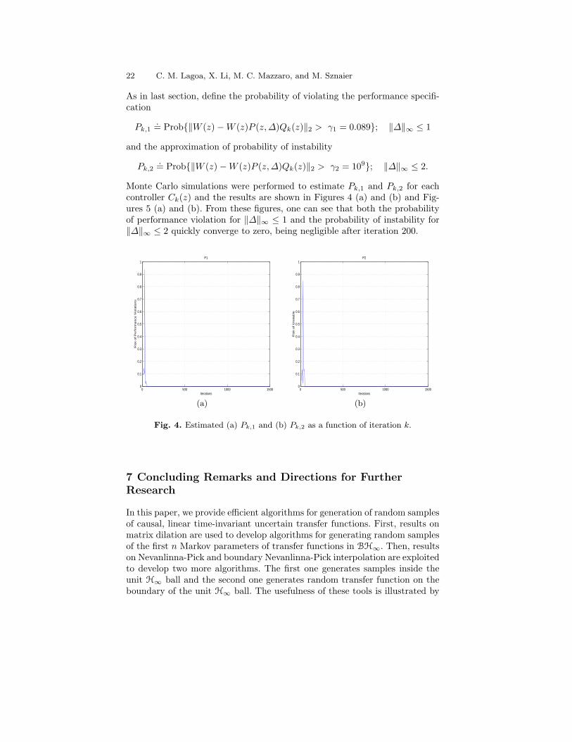
As in last section, define the probability of violating the performance specifi-cation

Pk,1.= Prob{‖W (z) − W (z)P (z,∆)Qk(z)‖2 > γ1 = 0.089}; ‖∆‖∞ ≤ 1

and the approximation of probability of instability

Pk,2.= Prob{‖W (z) − W (z)P (z,∆)Qk(z)‖2 > γ2 = 109}; ‖∆‖∞ ≤ 2.

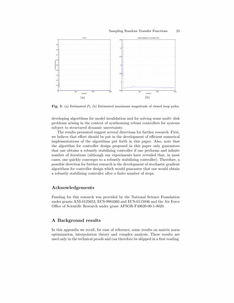
Monte Carlo simulations were performed to estimate Pk,1 and Pk,2 for eachcontroller Ck(z) and the results are shown in Figures 4 (a) and (b) and Fig-ures 5 (a) and (b). From these figures, one can see that both the probabilityof performance violation for ‖∆‖∞ ≤ 1 and the probability of instability for‖∆‖∞ ≤ 2 quickly converge to zero, being negligible after iteration 200.

0 500 1000 15000

0.1

0.2

0.3

0.4

0.5

0.6

0.7

0.8

0.9

1

Iterations

Ris

k o

f P

erf

orm

ance V

iola

tions

P1

(a)

0 500 1000 15000

0.1

0.2

0.3

0.4

0.5

0.6

0.7

0.8

0.9

1

Iterations

Ris

k o

f U

nsta

ble

P2

(b)

Fig. 4. Estimated (a) Pk,1 and (b) Pk,2 as a function of iteration k.

7 Concluding Remarks and Directions for FurtherResearch

In this paper, we provide efficient algorithms for generation of random samplesof causal, linear time-invariant uncertain transfer functions. First, results onmatrix dilation are used to develop algorithms for generating random samplesof the first n Markov parameters of transfer functions in BH∞. Then, resultson Nevanlinna-Pick and boundary Nevanlinna-Pick interpolation are exploitedto develop two more algorithms. The first one generates samples inside theunit H∞ ball and the second one generates random transfer function on theboundary of the unit H∞ ball. The usefulness of these tools is illustrated by

Sampling Random Transfer Functions 23

0 500 1000 15000

0.1

0.2

0.3

0.4

0.5

0.6

0.7

0.8

0.9

1

Iterations

Com

bin

ed R

isk

P1+P2

(a)

0 500 1000 15000.95

1

1.05

1.1

1.15

1.2

1.25

Iterations

Maximal Magnitude of Closedloop Poles

(b)

Fig. 5. (a) Estimated Pk (b) Estimated maximum magnitude of closed loop poles.

developing algorithms for model invalidation and for solving some multi–diskproblems arising in the context of synthesizing robust controllers for systemssubject to structured dynamic uncertainty.

The results presented suggest several directions for further research. First,we believe that effort should be put in the development of efficient numericalimplementations of the algorithms put forth in this paper. Also, note thatthe algorithm for controller design proposed in this paper only guaranteesthat one obtains a robustly stabilizing controller if one performs and infinitenumber of iterations (although our experiments have revealed that, in mostcases, one quickly converges to a robustly stabilizing controller). Therefore, apossible direction for further research is the development of stochastic gradientalgorithms for controller design which would guarantee that one would obtaina robustly stabilizing controller after a finite number of steps.

Acknowledgements

Funding for this research was provided by the National Science Foundationunder grants ANI-0125653, ECS-9984260 and ECS-0115946 and the Air ForceOffice of Scientific Research under grant AFSOR-F49620-00-1-0020.

A Background results

In this appendix we recall, for ease of reference, some results on matrix normoptimization, interpolation theory and complex analysis. These results areused only in the technical proofs and can therefore be skipped in a first reading.

24 C. M. Lagoa, X. Li, M. C. Mazzaro, and M. Sznaier

A.1 Matrix Dilations

Theorem 4 (Parrott’s Theorem) ([32], page 40). Let A, B and C begiven matrices of compatible dimensions. Then:

minX

∥∥∥∥[X BC A

]∥∥∥∥.= γo = max

{∥∥[C A

]∥∥ ,

∥∥∥∥[BA

]∥∥∥∥}

,

where ‖ · ‖ stands for σ (·). Moreover, all the solutions X to the above problemare parameterized by

X = −YAT Z + γo(I − YYT )12 W(I − ZT Z)

12 (19)

where the free parameter W is an arbitrary contraction and the matrices Yand Z solve the linear equations:

B = Y(γ2oI − AT A)

12

C = (γ2oI − AAT )

12 Z

σ (Y) ≤ 1, σ (Z) ≤ 1.

Theorem 5 (Caratheodory-Fejer) ([1]) Given a matrix–valued sequence{Li}

n−1i=0 , there exists a causal, LTI operator L(z) ∈ BH∞ such that

L(z) = L0 + L1z + L2z2 + . . . + Ln−1z

n−1 + . . .

if and only if Mc.= I − Tn

L(TnL)T ≥ 0 where

TnL =

L0 L1 · · · Ln−1

0 L0 · · · Ln−2

.... . .

. . ....

0 · · · 0 L0

.

A.2 Complex analysis

Let fn denote a sequence of complex-valued functions, each of whose domaincontains an open subset U of the complex plane. The sequence fn convergesnormally in U to f if fn is pointwise convergent to f in U and this convergenceis uniform on each compact subset of U . A family F of functions analytic inU is said to be normal if each sequence fn from F contains at least onenormally convergent subsequence. Given a sequence of functions fn, each ofwhose terms is analytic in an open set U , it is of interest to know whether fn isnormal, i.e., if it is possible to extract a normally convergent subsequence. Ananswer to this question is given by Montel’s theorem, which requires a certainequi–boundedness assumption. A family F is said to be locally bounded in Uif its members are uniformly bounded on each compact set in U .

Sampling Random Transfer Functions 25

Theorem 6 (Montel’s Theorem.) [20] Let F be a family of functions thatare analytic in an open set U . Suppose that F is locally bounded in U . ThenF is a normal family in this set.

In particular, if F ⊂ H∞ is such that f ∈ F ⇒ ‖f‖∞ ≤ M , then the theoremimplies that F is normal inside the unit disk. Thus, every sequence {fi} ∈ F

contains a normally convergent subsequence.

A.3 Nevanlinna-Pick Interpolation

We start by focusing our attention in a more general result in interpolationtheory. Let T and BT denote the space of complex valued rational functionscontinuous in |λ| = 1 and analytic in |λ| < 1, equipped with the ‖.‖L∞

norm,and the (open) unit ball in this space, respectively (i.e. f(λ) ∈ BT ⇐⇒f( 1

z ) ∈ BH∞).

Theorem 7 There exists a transfer function f(λ) ∈ BT (BT) such that:∑

λo∈D

Resλ=λof(λ)C−(λI − A)−1 = C+ (20)

if and only if the following discrete time Lyapunov equation has a uniquepositive (semi) definite solution.

M = A∗MA + C∗−C− − C∗

+C+ (21)

where A,C− and C+ are constant complex matrices of appropriate dimensionsand D denotes the open unit circle. If M > 0 then the solution f(λ) is non–unique and the set of solutions can be parameterized in terms of q(λ), anarbitrary element of BT, as follows:

f(λ) =T11(λ)q(λ) + T12(λ)

T21(λ)q(λ) + T22(λ)(22)

T (λ) =

[T11(λ) T12(λ)T21(λ) T22(λ)

](23)

where T (λ) is the J-lossless11 matrix:

T (λ) ≡

[AT BT

CT DT

]

AT = A

BT = M−1 (A∗ − I)−1 [

−C∗+ C∗

−

]

CT =

[C+

C−

](A − I)

DT = I +

[C+

C−

]M−1 (A∗ − I)

−1 [−C∗

+ C∗−

]

11 A transfer function H(λ) is said to be J-lossless if HT (1/λ)JH(λ) = J when

|λ| = 1, and HT (1/λ)JH(λ) < J when |λ| < 1. Here J =

[I 00 −I

].

26 C. M. Lagoa, X. Li, M. C. Mazzaro, and M. Sznaier

Proof See [1, 23].

Note that the matrices A and C− provide the structure of the interpolationproblem while C+ provides the interpolation values. The following corollariesshow that both the Nevanlinna-Pick and the Caratheodory-Fejer problems arespecial cases of this theorem, corresponding to an appropriate choice of thematrices A and C−,

Corollary 1 (Nevanlinna-Pick) Let Γ = diag{λi} ∈ Cr×r and take

A = Γ (24)

C− =[1 1 . . . 1

]∈ Rr (25)

C+ =[w1 w2 . . . wr

](26)

then (20) is equivalent to

f(λi) = wi i = 1, . . . , r (27)

and the solution to (21) is the standard Pick matrix:

P =

[1 − wiwj

1 − λiλj

]

ij

(28)

Proof . Replace A,C−, C+ in (20). See [23] for details.

Corollary 2 (Caratheodory-Fejer) Let In×n denote the identity matrix,and Af ∈ R(n+1)×(n+1),

Af =

[0 In×n

0 0

](29)

Take

A = Af (30)

C− =[1 0 . . . 0

]∈ Rn+1 (31)

C+ =[f0 f1 . . . fn

](32)

then (20) is satisfied if and only if f(λ) can be written as,

f(λ) = f0 + f1λ + f2λ2 + . . . + fnλn + . . . (33)

and the solution to (21) is the matrix: Mc = I − FT F where

F =

f0 f1 . . . fn

0 f0 . . . fn−1

......

. . ....

0 0 . . . f0

(34)

Note that Mc > 0 if and only if σ(F) < 1.

Sampling Random Transfer Functions 27

Proof . Replace A,C−, C+ in (20). See [23] for details.

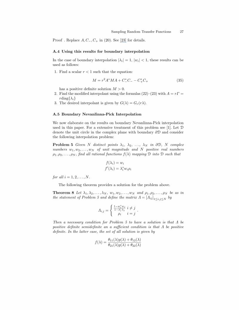
A.4 Using this results for boundary interpolation

In the case of boundary interpolation |λi| = 1, |wi| < 1, these results can beused as follows:

1. Find a scalar r < 1 such that the equation:

M = r2A∗MA + C∗−C− − C∗

+C+ (35)

has a positive definite solution M > 0.2. Find the modified interpolant using the formulas (22)–(23) with A = rΓ =

rdiag{λi}3. The desired interpolant is given by G(λ) = Gr(rλ).

A.5 Boundary Nevanlinna-Pick Interpolation

We now elaborate on the results on boundary Nevanlinna-Pick interpolationused in this paper. For a extensive treatment of this problem see [1]. Let D

denote the unit circle in the complex plane with boundary ∂D and considerthe following interpolation problem:

Problem 5 Given N distinct points λ1, λ2, . . ., λN in ∂D, N complexnumbers w1, w2, . . . , wN of unit magnitude and N positive real numbersρ1, ρ2, . . . , ρN , find all rational functions f(λ) mapping D into D such that

f(λi) = wi

f ′(λi) = λ∗i wiρi

for all i = 1, 2, . . . , N .

The following theorem provides a solution for the problem above.

Theorem 8 Let λ1, λ2, . . . , λN , w1, w2, . . . , wN and ρ1, ρ2, . . . , ρN be as inthe statement of Problem 5 and define the matrix Λ = [Λij ]1≤i,j≤N by

Λi,j =

{1−w∗

i wj

1−λ∗

i λji 6= j

ρi i = j.

Then a necessary condition for Problem 5 to have a solution is that Λ bepositive definite semidefinite an a sufficient condition is that Λ be positivedefinite. In the latter case, the set of all solution is given by

f(λ) =θ11(λ)g(λ) + θ12(λ)

θ21(λ)g(λ) + θ22(λ)

28 C. M. Lagoa, X. Li, M. C. Mazzaro, and M. Sznaier

where g(λ) is an arbitrary scalar rational function analytic on D withsup{|g(λ)| : z ∈ D} ≤ 1 such that θ21(λ)g(λ) + θ22(λ) has a simple poleat the points λ1, λ2, . . . , λN . Here

θ(λ) =

[θ11(λ) θ12(λ)θ21(λ) θ22(λ)

]

is given by

θ(λ) = I + (λ − λ0)C0(λI − A0)−1Λ−1(λI − A∗

0)−1C∗

0J

where

C0 =

[w1 . . . wN

1 . . . 1

]; A0 =

λ1 0. . .

0 λN

; J =

[1 00 −1

]

and λ0 is a complex number of magnitude 1 and not equal to any of thenumbers λ1, λ2, . . . , λN .

Proof: See [1].Note that if only the values w1, w2, . . . , wN of magnitude one are specified

at the boundary points λ1, λ2, . . . , λN , then the matrix Λ in the theorem abovecan always be made positive definite by choosing the unspecified quantitiesρ1, ρ2, . . . , ρN sufficiently large. This leads to the following corollary.

Corollary 3 Let 2N complex numbers of magnitude one λ1, λ2, . . . , λN andw1, w2, . . . , wN be given, where λ1, λ2, . . . , λN are distinct. Then, there alwaysexist scalar rational functions f(λ) analytic in D with

sup{|f(λ)| : λ ∈ D} ≤ 1

which satisfy the set of interpolation conditions

f(λi) = wi; i = 1, 2, . . . , N.

B Proof of Theorem 1

For the sake of notational simplicity we will prove the result for the case wherethe number of partitions of the vector x is m = 4, but the same reasoningapplies to arbitrary dimensions.

Consider a rectangle

R.= R1 × R2 × R3 × R4 ⊆ C

where Ri ⊂ Rki , i = 1, 2, 3, 4. Let Nt and NR be the total number of samplesgenerated and the number of hits of R respectively. We will show that

Sampling Random Transfer Functions 29

NR

Nt

w.p.1−→

vol(R1)vol(R2)vol(R3)vol(R4)

vol(C).

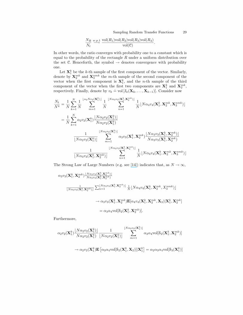
In other words, the ratio converges with probability one to a constant which isequal to the probability of the rectangle R under a uniform distribution overthe set C. Henceforth, the symbol → denotes convergence with probabilityone.

Let Xk1 be the k-th sample of the first component of the vector. Similarly,

denote by Xmk2 and Xnmk

3 the m-th sample of the second component of thevector when the first component is Xk

1 , and the n-th sample of the thirdcomponent of the vector when the first two components are Xk

1 and Xmk2 ,

respectively. Finally, denote by vk.= vol [Ik(X1, . . . ,Xk−1)]. Consider now

Nt

N4=

1

N

N∑

k=1

1

N

bα2Nv2(Xk1 )c∑

m=1

1

N

bNα3v3(Xk1 ,Xmk

2 )c∑

n=1

1

NbNα4v4(X

k1 ,Xmk

2 ,Xnmk3 )c

=1

N

N∑

k=1

α2v2(Xk1)

bNα2v2(Xk1)c

Nα2v2(Xk1)

1

bNα2v2(Xk1)c

bNα2v2(Xk1 )c∑

m=1

α3v3(Xk1 ,Xmk

2 )bNα3v3(X

k1 ,Xmk

2 )c

Nα3v3(Xk1 ,Xmk

2 )

1

bNα3v3(Xk1 ,Xmk

2 )c

bNα3v3(Xk1 ,Xmk

2 )c∑

n=1

1

NbNα4v4(X

k1 ,Xmk

2 ,Xnmk3 )c

The Strong Law of Large Numbers (e.g. see [14]) indicates that, as N → ∞,

α3v3(Xk1 ,Xmk

2 )bNα3v3(X

k1 ,Xmk

2 )c

Nα3v3(Xk1,Xmk

2)

1bNα3v3(Xk

1,Xmk

2)c

∑bNα3v3(Xk1 ,Xmk

2 )cn=1

1N bNα4v4(X

k1 ,Xmk

2 ,Xnmk3 )c

→ α3v3(Xk1 ,Xmk

2 )E[α4v4(Xk1 ,Xmk

2 ,X3)|Xk1 ,Xmk

2 ]

= α3α4vol[S2(Xk1 ,Xmk

2 )].

Furthermore,

α2v2(Xk1)

bNα2v2(Xk1)c

Nα2v2(Xk1)

1

bNα2v2(Xk1)c

bNα2v2(Xk1 )c∑

m=1

α3α4vol[S2(Xk1 ,Xmk

2 )]

→ α2v2(Xk1)E

[α3α4vol[S2(X

k1 ,X2)]|X

k1

]= α2α3α4vol[S3(X

k1)]

30 C. M. Lagoa, X. Li, M. C. Mazzaro, and M. Sznaier

and

1

N

N∑

k=1

α2α3α4vol[S3(Xk1)] → E [α2α3α4vol[S(X1)]] =

α2α3α4

v1vol(C).

HenceNt

N4→

α2α3α4

v1vol(C)

as N → ∞.Next, consider the number of hits of the rectangle R, which we denote

by NR. The Strong Law of Large Numbers implies that

NR

N

∣∣∣∣Xk1 ∈ R1,X

mk2 ∈ R2,X

nmk3 ∈ R3

→ α4v4(Xk1 ,Xmk

2 ,Xnmk3 )

vol(R4)

v4(Xk1 ,Xmk

2 ,Xnmk3 )

= α4vol(R4)

which is independent of the values of Xk1 , Xmk

2 and Xnmk3 . Using the same

reasoning, we have

NR

N2

∣∣∣∣Xk1 ∈ R1,X

mk2 ∈ R2 → α3v3(X

k1 ,Xmk

2 )vol(R3)α4vol(R4)

v3(Xk1 ,Xmk

2 )

= α3vol(R3)α4vol(R4)

NR

N3

∣∣∣∣Xk1 ∈ R1 → α2v2(X

k1)

vol(R2)α3vol(R3)α4vol(R4)

v2(Xk1)

= α2vol(R2)α3vol(R3)α4vol(R4).

Finally, this implies that

NR

N4→

1

v1α2α3α4vol(R1)vol(R2)vol(R3)vol(R4).

Hence,NR

Nt→

vol(R1)vol(R2)vol(R3)vol(R4)

vol(C)

as N → ∞. This completes the proof.

C Proof of Theorem 2

Proof. As in the proof of Theorem 1, only m = 4 is considered and it isassumed that

A.= R1 × R2 × R3 × R4 ⊆ C

Sampling Random Transfer Functions 31

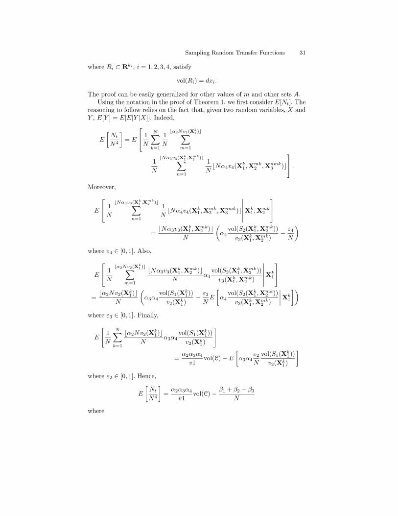
where Ri ⊂ Rki , i = 1, 2, 3, 4, satisfy

vol(Ri) = dxi.

The proof can be easily generalized for other values of m and other sets A.Using the notation in the proof of Theorem 1, we first consider E[Nt]. The

reasoning to follow relies on the fact that, given two random variables, X andY , E[Y ] = E[E[Y |X]]. Indeed,

E

[Nt

N4

]= E

1

N

N∑

k=1

1

N

bα2Nv2(Xk1 )c∑

m=1

1

N

bNα3v3(Xk1 ,Xmk

2 )c∑

n=1

1

NbNα4v4(X

k1 ,Xmk

2 ,Xnmk3 )c

.

Moreover,

E

1

N

bNα3v3(Xk1 ,Xmk

2 )c∑

n=1

1

NbNα4v4(X

k1 ,Xmk

2 ,Xnmk3 )c

∣∣∣∣∣∣Xk

1 ,Xmk2

=bNα3v3(X

k1 ,Xmk

2 )c

N

(α4

vol(S2(Xk1 ,Xmk

2 ))

v3(Xk1 ,Xmk

2 )−

ε4

N

)

where ε4 ∈ [0, 1]. Also,

E

1

N

bα2Nv2(Xk1 )c∑

m=1

bNα3v3(Xk1 ,Xmk

2 )c

Nα4

vol(S2(Xk1 ,Xmk

2 ))

v3(Xk1 ,Xmk

2 )

∣∣∣∣∣∣Xk

1

=bα2Nv2(X

k1)c

N

(α3α4

vol(S1(Xk1))

v2(Xk1)

−ε3

NE

[α4

vol(S2(Xk1 ,Xmk

2 ))

v3(Xk1 ,Xmk

2 )

∣∣∣∣Xk1

])

where ε3 ∈ [0, 1]. Finally,

E

[1

N

N∑

k=1

bα2Nv2(Xk1)c

Nα3α4

vol(S1(Xk1))

v2(Xk1)

]

=α2α3α4

v1vol(C) − E

[α3α4

ε2

N

vol(S1(Xk1))

v2(Xk1)

]

where ε2 ∈ [0, 1]. Hence,

E

[Nt

N4

]=

α2α3α4

v1vol(C) −

β1 + β2 + β3

N

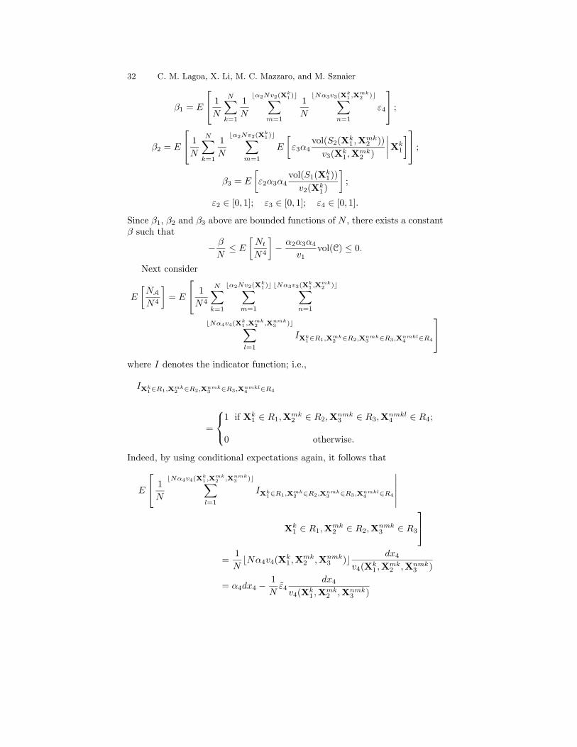
where

32 C. M. Lagoa, X. Li, M. C. Mazzaro, and M. Sznaier

β1 = E

1

N

N∑

k=1

1

N

bα2Nv2(Xk1 )c∑

m=1

1

N

bNα3v3(Xk1 ,Xmk

2 )c∑

n=1

ε4

;

β2 = E

1

N

N∑

k=1

1

N

bα2Nv2(Xk1 )c∑

m=1

E

[ε3α4

vol(S2(Xk1 ,Xmk

2 ))

v3(Xk1 ,Xmk

2 )

∣∣∣∣Xk1

] ;

β3 = E

[ε2α3α4

vol(S1(Xk1))

v2(Xk1)

];

ε2 ∈ [0, 1]; ε3 ∈ [0, 1]; ε4 ∈ [0, 1].

Since β1, β2 and β3 above are bounded functions of N , there exists a constantβ such that

−β

N≤ E

[Nt

N4

]−

α2α3α4

v1vol(C) ≤ 0.

Next consider

E

[NA

N4

]= E

1

N4

N∑

k=1

bα2Nv2(Xk1 )c∑

m=1

bNα3v3(Xk1 ,Xmk

2 )c∑

n=1

bNα4v4(Xk1 ,Xmk

2 ,Xnmk3 )c∑

l=1

IX

k1∈R1,Xmk

2∈R2,Xnmk

3∈R3,Xnmkl

4∈R4

where I denotes the indicator function; i.e.,

IX

k1∈R1,Xmk

2∈R2,Xnmk

3∈R3,Xnmkl

4∈R4

=

1 if Xk1 ∈ R1,X

mk2 ∈ R2,X

nmk3 ∈ R3,X

nmkl4 ∈ R4;

0 otherwise.

Indeed, by using conditional expectations again, it follows that

E

1

N

bNα4v4(Xk1 ,Xmk

2 ,Xnmk3 )c∑

l=1

IX

k1∈R1,Xmk

2∈R2,Xnmk

3∈R3,Xnmkl

4∈R4

∣∣∣∣∣∣bNα4v4(X

k1 ,Xmk

2 ,Xnmk3 )c∑

l=1

Xk1 ∈ R1,X

mk2 ∈ R2,X

nmk3 ∈ R3

=1

NbNα4v4(X

k1 ,Xmk

2 ,Xnmk3 )c

dx4

v4(Xk1 ,Xmk

2 ,Xnmk3 )

= α4dx4 −1

Nε4

dx4

v4(Xk1 ,Xmk

2 ,Xnmk3 )

Sampling Random Transfer Functions 33

where ε4 ∈ [0, 1]. Repeating this reasoning for the other three coordinatesleads to the following result:

E

[NA

N4

]= dx1dx2dx3dx4

α2α3α4

v1vol(C) −

γ1 + γ2 + γ3

N

where

γ3 = E

1

N3

N∑

k=1

bα2Nv2(Xk1 )c∑

m=1

bNα3v3(Xk1 ,Xmk

2 )c∑

n=1

ε4dx4

v4(Xk1 ,Xmk

2 ,Xnmk3 )

γ2 = E

1

N2

N∑

k=1

bα2Nv2(Xk1 )c∑

m=1

ε3dx3dx4

v3(Xk1 ,Xmk

2 )

γ1 = E

[1

N

N∑

k=1

ε2dx2dx3dx4

v2(Xk1)

]

ε2 ∈ [0, 1]; ε3 ∈ [0, 1]; ε4 ∈ [0, 1].

Since γ1, γ2 and γ3 above are bounded function of N , there exists a constantγ such that

−γ

N≤ E

[NA

N4

]− dx1dx2dx3dx4

α2α3α4

v1vol(C) ≤ 0.

The proof is completed by noting that given the results above, one can deter-mine constants k1, k2 and k3 such that

∣∣∣∣E[NA]

E[Nt]−

vol(A)

vol(C)

∣∣∣∣ =

∣∣∣∣E[NA/N4]

E[Nt/N4]−

vol(A)

vol(C)

∣∣∣∣

≤1

N

k1

k2 + k3

N

.

References

1. J. A. Ball, I. Gohberg, and L. Rodman. Interpolation of rational matrix func-tions. In Operator Theory: Advances and Applications, volume 45. Birhauser,Basel, 1990.

2. B. R. Barmish and C. M. Lagoa. The uniform distribution: A rigorous justifi-cation for its use in robustness analysis. Mathematics of Control, Signals and

Systems, 10:203–222, 1997.3. B. R. Barmish and C. M. Lagoa. On convexity of the probabilistic design prob-

lem for quadratic stabilizability. In Proceedings of the 1999 American Control

Conference, volume 1, pages 430–434, San Diego, CA, 1999.

34 C. M. Lagoa, X. Li, M. C. Mazzaro, and M. Sznaier

4. B. R. Barmish and B. T. Polyak. A new approach to open robustness prob-lems based on probabilistic prediction formulae. In Proceedings of IFAC World

Congress, San Fancisco, CA, June 1996.5. S. Boyd and C. Barratt. Linear Controller Design - Limits of Performance.

Prentice Hall, Englewood Cliffs, N.J., 1991.6. R. D. Braatz, P. M. Young, J. C. Doyle, and M. Morari. Computational complex-

ity of µ calculation. IEEE Transactions on Automatic Control, 39:1000–1002,1994.

7. G. C. Calafiore, F. Dabbene, and R. Tempo. Randomized algorithms for prob-abilistic robustness with real and complex structured uncertainty. IEEE Trans-

actions on Automatic Control, 45(12):2218–2235, December 2000.8. G. C. Calafiore and F. Dabbene. Randomization in RH∞: An approach to

control design with Hard/Soft performance specications. In Proceedings of the

41st IEEE Conference on Decision and Control, pages 2260–2265, Las Vegas,Nevada, 2002.

9. Jie Chen and Shuning Wang. Validation of linear fractional uncertain models:solutions via matrix inequalities. IEEE Transactions on Automatic Control,41(6):844–849, 1996.

10. J. Chen and G. Gu. Control–oriented System Identification : an H∞ Approach.John Wiley & Sons, New York, 2000.

11. Xinjia Chen and Kemin Zhou. A probabilistic approach to robust control. InProceedings of the 36th IEEE Conference on Decision and Control, pages 4894–4895, San Diego, CA, 1997.

12. X. Chen and K. Zhou. Constrained optimal synthesis and robustness analy-sis by randomized algorithms. In Proceedings of the 1998 American Control

Conference, volume 3, pages 1429–1433, Philadelphia, PA, 1998.13. D. S. K. Fok and D. Crevier. Volume estimation by Monte Carlo methods.

Journal of Statistical Computation and Simulation, 31(4):223–235, 1989.14. G. R. Grimmett and D. R. Stirzaker. Probability and Random Processes. The

Clarendon Press Oxford University Press, New York, second edition, 1992.15. P. Khargonekar and A. Tikku. Randomized algorithms for robust control anal-

ysis and synthesis have polynomial complexity. In Proceedings of the 35th IEEE

Conference on Decision and Control, pages 3470 – 3475, Kobe, Japan, 1996.16. Constantino Manuel Lagoa, Xiang Li, and Mario Sznaier. On the design of

robust controllers for arbitrary uncertainty structures. IEEE Transactions on

Automatic Control, 48(11):2061–2065, November 2003.17. Constantino M. Lagoa. A convex parametrization of risk-adjusted stabilizing

controllers. Automatica, 39(10):1829–1835, October 2003.18. C. I. Marrison and R. F. Stengel. The use of random search and genetic al-

gorithms to optimize stochastic robustness functions. In Proceedings of the

American Control Conference, pages 1484 – 1489, Baltimore, 1994.19. F. Paganini. Sets and Constraints in the Analysis of Uncertain Systems. PhD

thesis, Caltech, Pasadena, CA, 1996.20. B. Palka. An Introduction to Complex Function Theory. Springer-Verlag, New

York, 1992.21. Kameshwar Poolla, Pramod Khargonekar, Ashok Tikku, James Krause, and Kr-

ishan Nagpal. A time-domain approach to model validation. IEEE Transactions

on Automatic Control, 39(5):951–959, 1994.22. Laura Ryan Ray and Robert F. Stengel. A Monte Carlo approach to the analysis

of control system robustness. Automatica, 29(1):229–236, 1993.

Sampling Random Transfer Functions 35

23. Hector Rotstein. A Nevanlinna-Pick approach to time-domain constrained H∞

control. SIAM Journal on Control and Optimization, 34(4):1329–1341, 1996.24. Ricardo S. Sanchez-Pena and Mario Sznaier. Robust Systems: Theory and Ap-

plications. John Wiley, New York, 1998.25. Roy S. Smith and John C. Doyle. Model validation: a connection between

robust control and identification. IEEE Transactions on Automatic Control,37(7):942–952, 1992.

26. Robert F. Stengel and Laura R. Ray. Stochastic robustness of linear time-invariant control systems. IEEE Transactions on Automatic Control, 36(1):82–87, January 1991.

27. R. Tempo, E. W. Bai, and F. Dabbene. Probabilistic robustness analysis: Ex-plicit bounds for the minimum number of samples. In Proceedings of the 35th

IEEE Conference on Decision and Control, pages 3424 – 3428, Kobe, Japan,1996.

28. O. Toker and Jie Chen. Time domain validation of structured uncertainty modelsets. In Proceedings of the 35th IEEE Decision and Control, volume 1, pages255–260, Kobe, Japan, December 1996.

29. Q. Wang and R. F. Stengel. Robust control of nonlinear systems with paramet-ric uncertainty. In Proceedings of the 37th IEEE Conference on Decision and

Control, pages 3341 – 3346, Tampa, FL, 1998.30. A. Yoon, P. Khargonekar, and K. Hebbale. Design of computer experiments

for open-loop control and robustness analysis of clutch-to-clutch shifts in auto-matic transmissions. In Proceedings of the 1997 American Control Conference,volume 5, pages 3359–3364, Albuquerque, NM, 1997.

31. A. Yoon and P. Khargonekar. Computational experiments in robust stabilityanalysis. In Proceedings of the 36th IEEE Conference on Decision and Control,pages 3260–3265, San Diego, CA, 1997.

32. K. Zhou, J. C. Doyle, and K. Glover. Robust and Optimal Control. PrenticeHall, New Jersey, 1996.

33. Tong Zhou. Unfalsified probability estimation for a model set based on frequencydomain data. International Journal of Control, 73(5):391–406, 2000.

34. Xiaoyun Zhu, Yun Huang, and J. Doyle. Soft vs. hard bounds in probabilisticrobustness analysis. In Proceedings of the 35th IEEE Conference on Decision

and Control, pages 3412 – 3417, Kobe, Japan, 1996.