RANDOM PROCESS
79
RANDOM PROCESS
-
Upload
khangminh22 -
Category
Documents
-
view
11 -
download
0
Transcript of RANDOM PROCESS

RANDOM PROCESS
CONTENTS:
•CLASSIFICATION OF RANDOM PROCESS
•STATIONARITY
•WSS and SSS PROCESS
•POISSON RANDOM PROCESS
•PURE BIRTH PROCESS
•RENEWAL PROCESS
•MARKOV CHAIN
•TRANSITION PROBILITIES
CLASSIFICATION OF RANDOM PROCESS
RANDOM PROCESS:
A random process is a collection of random variables {X(s,t)}
that are functions of a real variable, namely time ‘t’ where sєS
and t єT.
• Concepts of deterministic and random processestationarity, ergodicity
• Basic properties of a single random process
mean, standard deviation, auto-correlation, spectral density
• joint properties of two or more random processes
correlation, covariance, cross spectral density, simple input-output relations
Random processes - Basic concepts
• Deterministic random processes :
• deterministic processes :
physical process is represented by explicit mathematical relation
• Example :
response of a single mass-spring-damper in free vibration in laboratory
• Random processes :
result of a large number of separate causes. Described in probabilistic terms and by properties which are averages
• both continuous functions of time (usually), mathematical concepts
Random processes - basic concepts
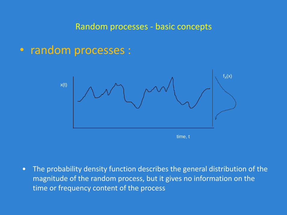
• random processes :
• The probability density function describes the general distribution of the magnitude of the random process, but it gives no information on the time or frequency content of the process
fX(x)
time, t
x(t)
Random processes - basic concepts
• Stationary random process :
• Ergodic process :
stationary process in which averages from a single record are the same as those obtained from averaging over the ensemble
Most stationary random processes can be treated as ergodic
• Ensemble averages do not vary with time
Wind loading from extra - tropical synoptic gales can be treated as stationary random processes
Wind loading from hurricanes - stationary over shorter periods <2 hours
- non stationary over the duration of the storm
Wind loading from thunderstorms, tornadoes - non stationary
Random processes - basic concepts
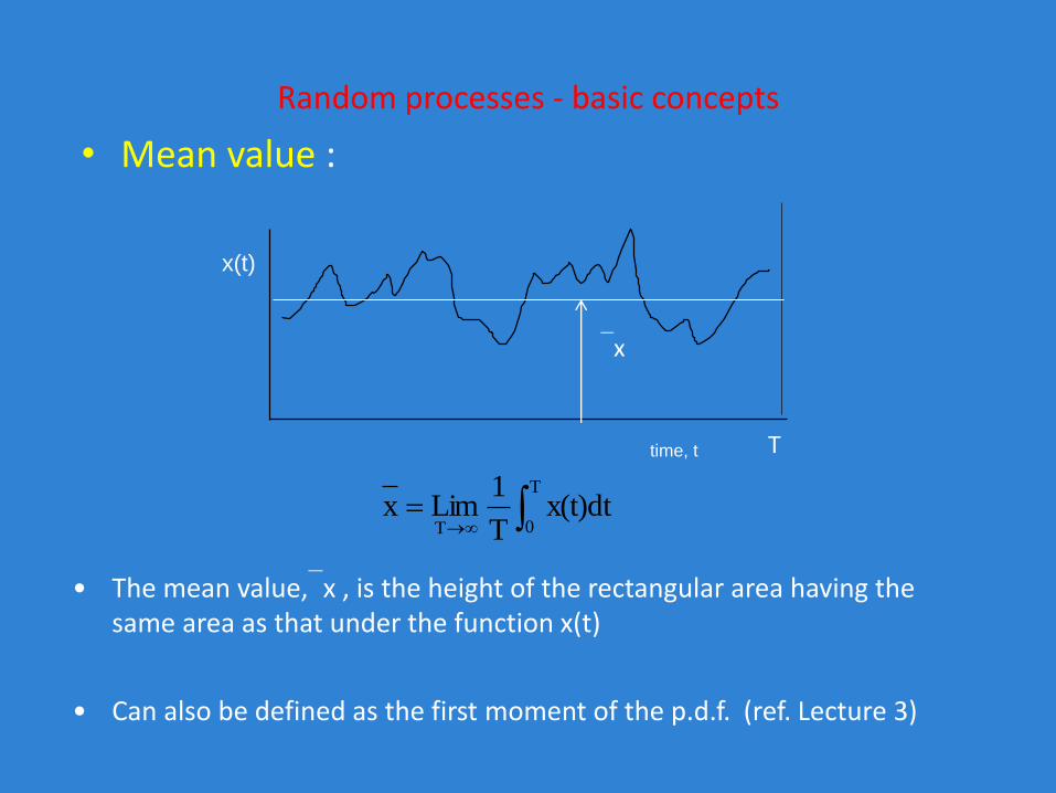
• Mean value :
• The mean value,x , is the height of the rectangular area having the same area as that under the function x(t)
time, t
x(t)
x
T
T
0Tx(t)dt
T
1Limx
• Can also be defined as the first moment of the p.d.f. (ref. Lecture 3)
Random processes - basic concepts
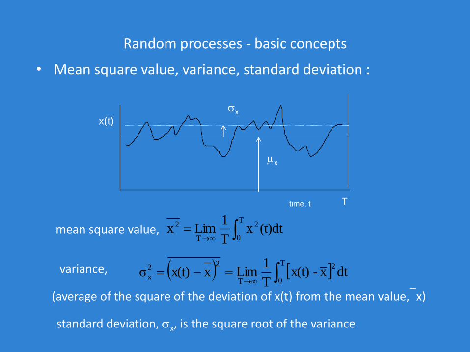
• Mean square value, variance, standard deviation :
variance,
T
0
2
T
2 (t)dtxT
1Limx
standard deviation, x, is the square root of the variance
mean square value,
22
x xx(t)σ
(average of the square of the deviation of x(t) from the mean value,x)
time, t
x(t)
x
T
x
T
0
2
Tdtx-x(t)
T
1Lim
Random processes - basic concepts
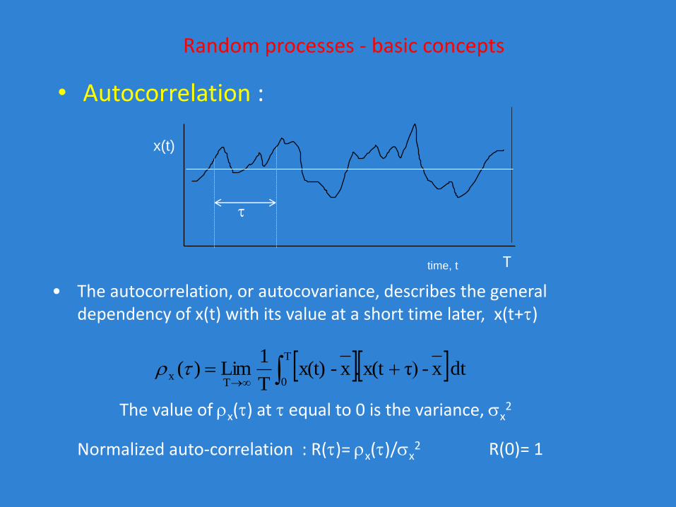
• Autocorrelation :
The value of x() at equal to 0 is the variance, x2
T
0Tx dt x-τ)x(t.x-x(t)
T
1Lim)(
• The autocorrelation, or autocovariance, describes the general dependency of x(t) with its value at a short time later, x(t+)
time, t
x(t)
T
Normalized auto-correlation : R()= x()/x2 R(0)= 1
Random processes - basic concepts
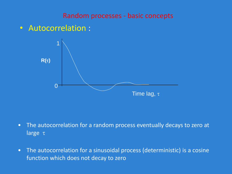
• Autocorrelation :
• The autocorrelation for a random process eventually decays to zero at large
R()
Time lag,
1
0
• The autocorrelation for a sinusoidal process (deterministic) is a cosine function which does not decay to zero
Random processes - basic concepts
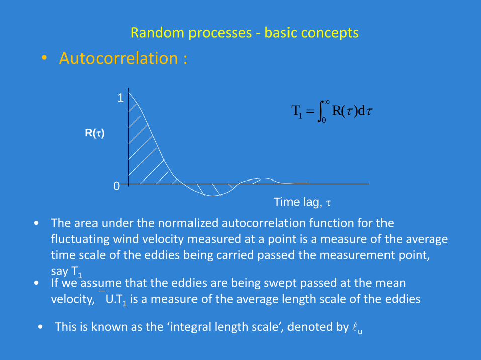
• Autocorrelation :
• The area under the normalized autocorrelation function for the fluctuating wind velocity measured at a point is a measure of the average time scale of the eddies being carried passed the measurement point, say T1
R()
Time lag,
1
0
• If we assume that the eddies are being swept passed at the mean velocity, U.T1 is a measure of the average length scale of the eddies
• This is known as the ‘integral length scale’, denoted by lu
0
1 )dR(T
Random processes - basic concepts
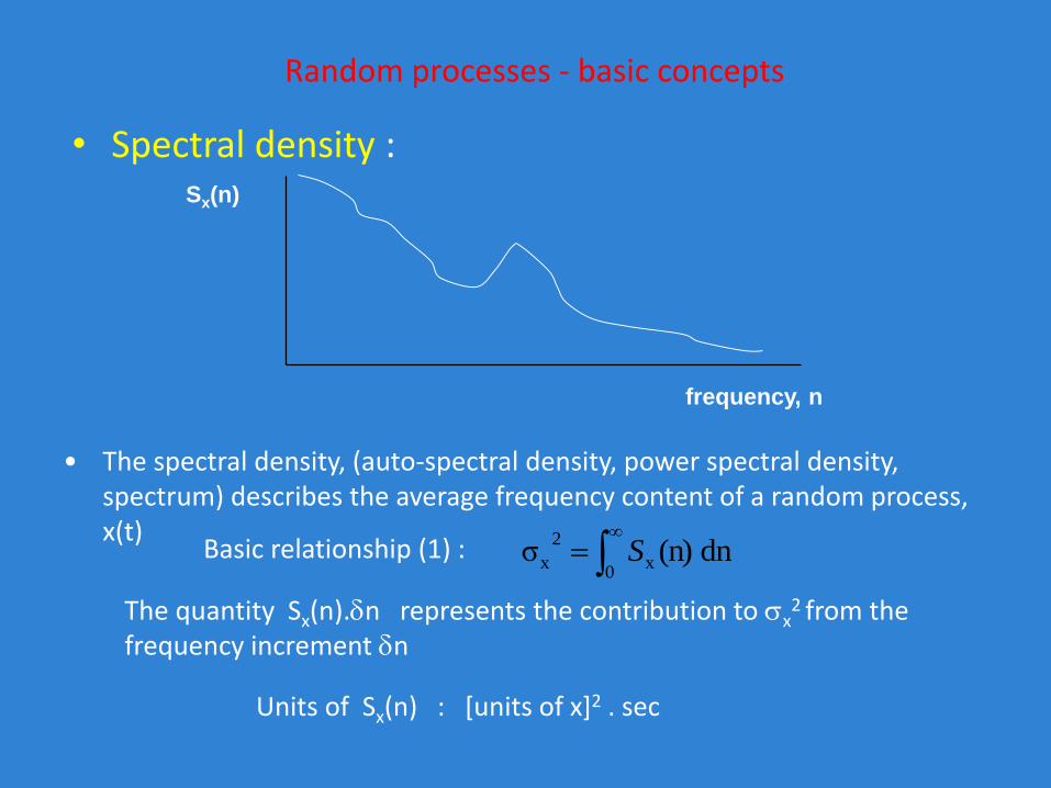
• Spectral density :
Basic relationship (1) :
0
x
2
x dn (n)σ S
• The spectral density, (auto-spectral density, power spectral density, spectrum) describes the average frequency content of a random process, x(t)
frequency, n
Sx(n)
The quantity Sx(n).n represents the contribution to x2 from the
frequency increment n
Units of Sx(n) : [units of x]2 . sec
Random processes - basic concepts
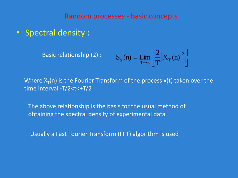
• Spectral density :
Basic relationship (2) :
Where XT(n) is the Fourier Transform of the process x(t) taken over the time interval -T/2<t<+T/2
The above relationship is the basis for the usual method of obtaining the spectral density of experimental data
2
TT
x (n)XT
2Lim(n)S
Usually a Fast Fourier Transform (FFT) algorithm is used
Random processes - basic concepts
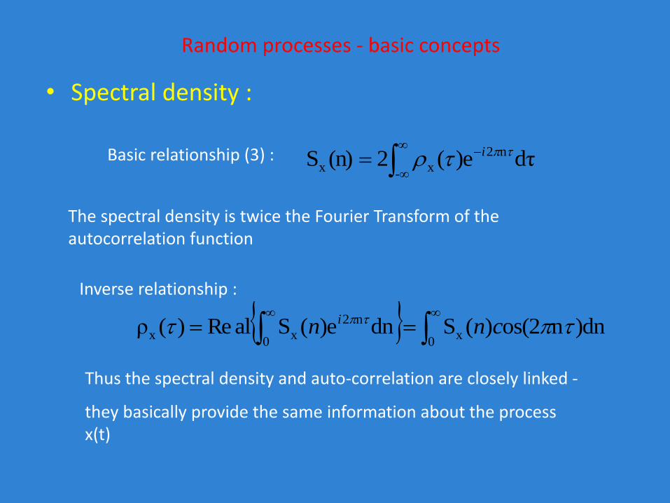
• Spectral density :
Basic relationship (3) :
The spectral density is twice the Fourier Transform of the autocorrelation function
Inverse relationship :
Thus the spectral density and auto-correlation are closely linked -
they basically provide the same information about the process x(t)
-
n2
xx dτ)e(2(n)S i
0
x0
n2
xx )dnnos(2)(Sdn)e(SalRe)(ρ cnn i
Random processes - basic concepts
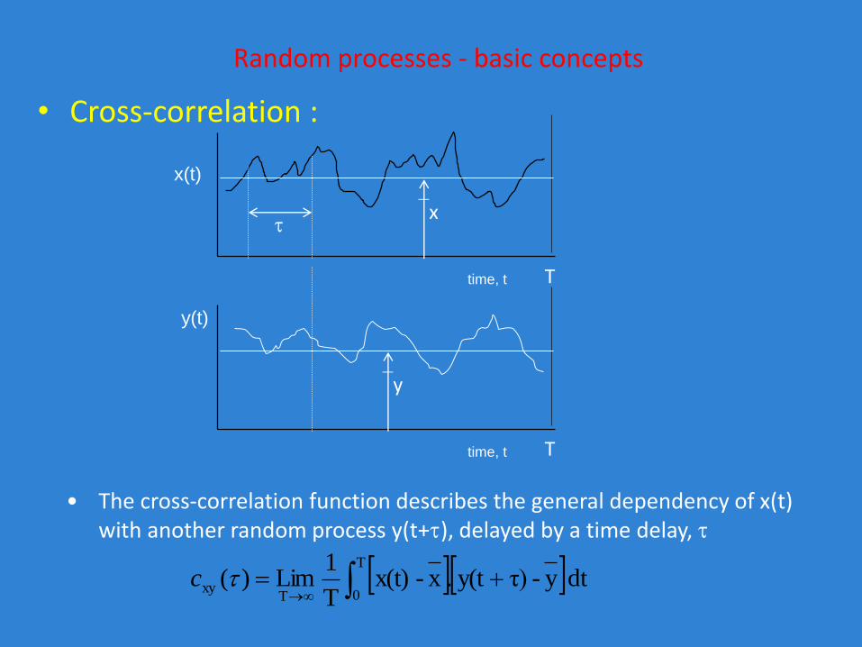
• Cross-correlation :
T
0Txy dt y-τ)y(t.x-x(t)
T
1Lim)(c
• The cross-correlation function describes the general dependency of x(t) with another random process y(t+), delayed by a time delay,
time, t
x(t)
T
time, t
y(t)
T
x
y
Random processes - basic concepts
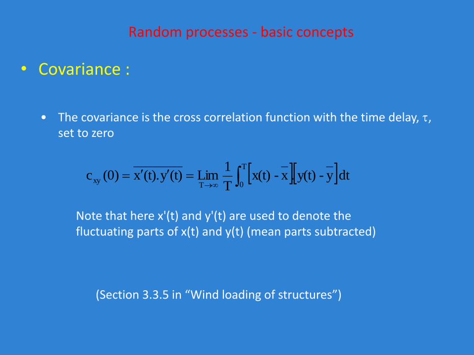
• Covariance :
T
0Txy dt y-y(t).x-x(t)
T
1Lim(t)y(t).x(0)c
• The covariance is the cross correlation function with the time delay, , set to zero
(Section 3.3.5 in “Wind loading of structures”)
Note that here x'(t) and y'(t) are used to denote the fluctuating parts of x(t) and y(t) (mean parts subtracted)
Random processes - basic concepts
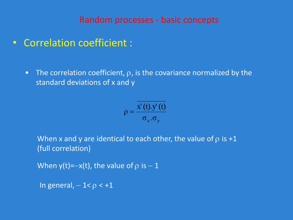
• Correlation coefficient :
• The correlation coefficient, , is the covariance normalized by the standard deviations of x and y
When x and y are identical to each other, the value of is +1 (full correlation)
When y(t)=x(t), the value of is 1
In general, 1< < +1
yx .σσ
(t)(t).y'x'ρ
Random processes - basic concepts
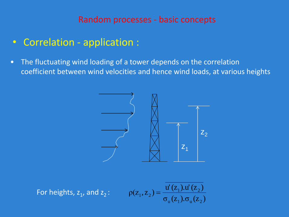
• Correlation - application :
• The fluctuating wind loading of a tower depends on the correlation coefficient between wind velocities and hence wind loads, at various heights
For heights, z1, and z2 : )(z).σ(zσ
)(z).u'(zu')z,ρ(z
2u1u
2121
z1
z2
Random processes - basic concepts
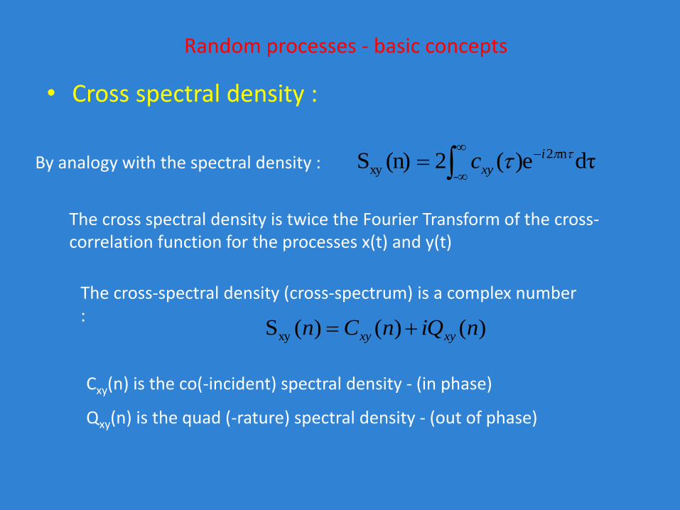
• Cross spectral density :
By analogy with the spectral density :
The cross spectral density is twice the Fourier Transform of the cross-correlation function for the processes x(t) and y(t)
The cross-spectral density (cross-spectrum) is a complex number :
Cxy(n) is the co(-incident) spectral density - (in phase)
Qxy(n) is the quad (-rature) spectral density - (out of phase)
-
n2
xy dτ)e(2(n)S i
xyc
)()()(Sxy niQnCn xyxy
Random processes - basic concepts
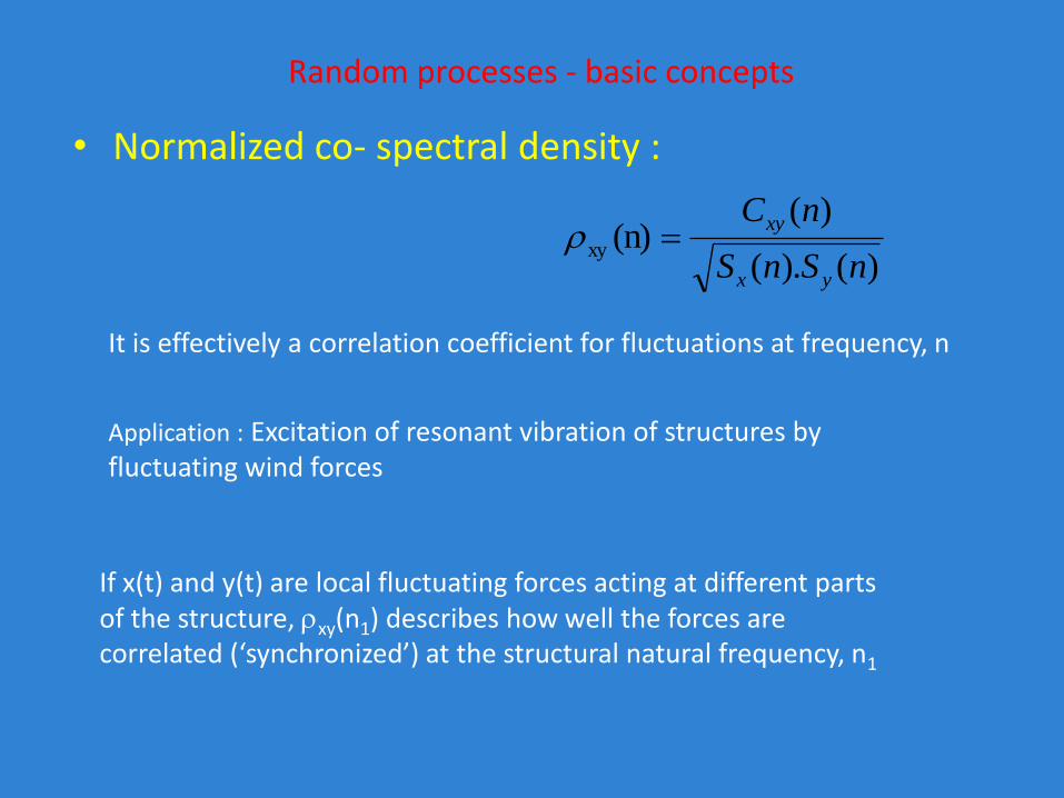
• Normalized co- spectral density :
It is effectively a correlation coefficient for fluctuations at frequency, n
Application : Excitation of resonant vibration of structures by fluctuating wind forces
If x(t) and y(t) are local fluctuating forces acting at different parts of the structure, xy(n1) describes how well the forces are correlated (‘synchronized’) at the structural natural frequency, n1
)().(
)((n)xy
nSnS
nC
yx
xy
Random processes - basic concepts
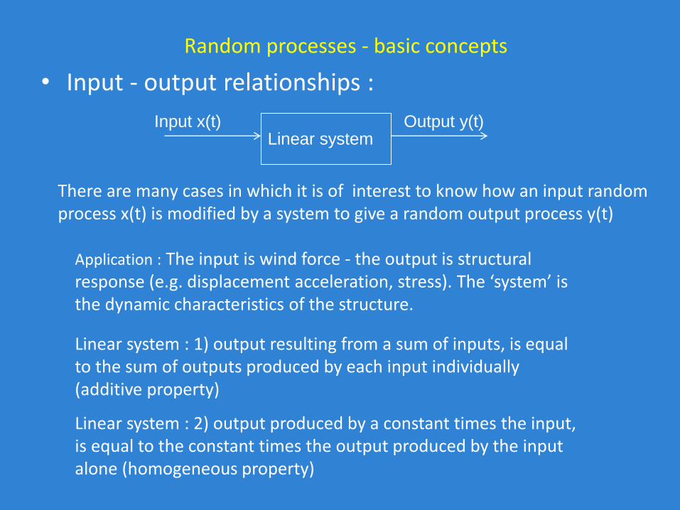
• Input - output relationships :
There are many cases in which it is of interest to know how an input random process x(t) is modified by a system to give a random output process y(t)
Application : The input is wind force - the output is structural response (e.g. displacement acceleration, stress). The ‘system’ is the dynamic characteristics of the structure.
Linear system : 1) output resulting from a sum of inputs, is equal to the sum of outputs produced by each input individually (additive property)
Linear systemInput x(t) Output y(t)
Linear system : 2) output produced by a constant times the input, is equal to the constant times the output produced by the input alone (homogeneous property)
Random processes - basic concepts
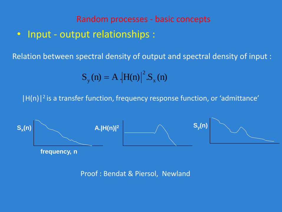
• Input - output relationships :
Relation between spectral density of output and spectral density of input :
|H(n)|2 is a transfer function, frequency response function, or ‘admittance’
Proof : Bendat & Piersol, Newland
(n)S.H(n).A (n)S x
2
y
Sy(n)
frequency, n
Sx(n) A.|H(n)|2
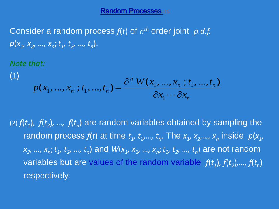
Consider a random process f(t) of nth order joint p.d.f.
p(x1, x2, …, xn; t1, t2, …, tn).
Note that:
(1)
Random Processes (23)
n
nn
n
nnxx
ttxxWttxxp
1
1111
...,,;...,,...,,;...,,
)()(
(2) f(t1), f(t2), …, f(tn) are random variables obtained by sampling the
random process f(t) at time t1, t2,…, tn. The x1, x2,…, xn inside p(x1,
x2, …, xn; t1, t2, …, tn) and W(x1, x2, …, xn; t1, t2, …, tn) are not random
variables but are values of the random variable f(t1), f(t2),…, f(tn)
respectively.
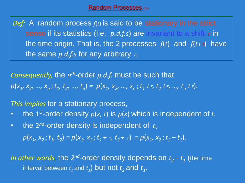
Random Processes (24)
Consequently, the nth-order p.d.f. must be such that
p(x1, x2, …, xn ; t1, t2, …, tn) = p(x1, x2, …, xn ; t1 +, t2 +, …, tn +).
This implies for a stationary process,
• the 1st-order density p(x, t) is p(x) which is independent of t.
• the 2nd-order density is independent of ,
p(x1, x2 ; t1, t2) = p(x1, x2 ; t1 + , t2 + ) = p(x1, x2 ; t2 – t1).
In other words, the 2nd-order density depends on t2 – t1 (the time
interval between t2 and t1) but not t2 and t1.
Def: A random process f(t) is said to be stationary in the strict
sense if its statistics (i.e. p.d.f.s) are invariant to a shift in
the time origin. That is, the 2 processes f(t) and f(t+) have
the same p.d.f.s for any arbitrary .
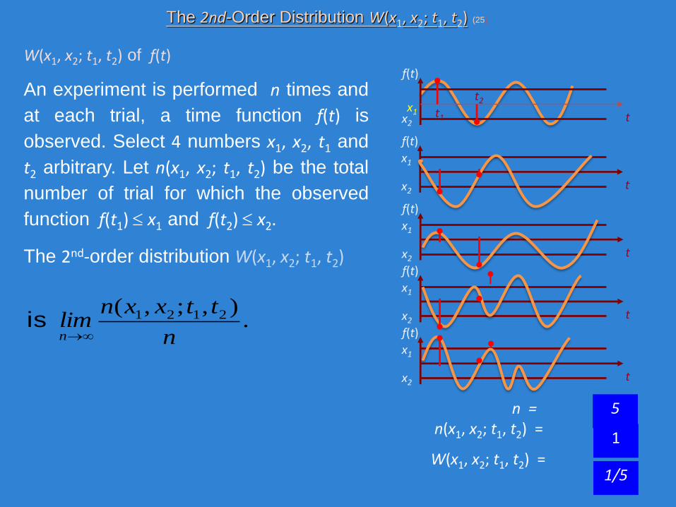
The 2nd-Order Distribution W(x1, x2; t1, t2) (25)
W(x1, x2; t1, t2) of f(t)
An experiment is performed n times and
at each trial, a time function f(t) is
observed. Select 4 numbers x1, x2, t1 and
t2 arbitrary. Let n(x1, x2; t1, t2) be the total
number of trial for which the observed
function f(t1) x1 and f(t2) x2.
The 2nd-order distribution W(x1, x2; t1, t2)
.),;,( 2121
n
ttxxnlimn
is
n = n(x1, x2; t1, t2) =
W(x1, x2; t1, t2) = 1/5
5
1
f(t)
x1x2
tt1
t2
f(t)
x1
x2t
f(t)
x1
x2t
f(t)
x1
x2t
f(t)
x1
x2t
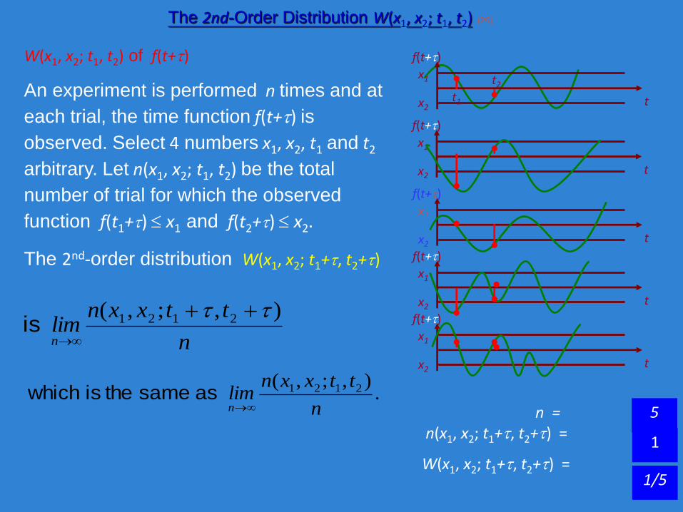
The 2nd-Order Distribution W(x1, x2; t1, t2) (26)
W(x1, x2; t1, t2) of f(t+)
An experiment is performed n times and at
each trial, the time function f(t+) is
observed. Select 4 numbers x1, x2, t1 and t2
arbitrary. Let n(x1, x2; t1, t2) be the total
number of trial for which the observed
function f(t1+) x1 and f(t2+) x2.
The 2nd-order distribution W(x1, x2; t1+, t2+)
.),;,( 2121
n
ttxxnlimn
as same the is whichn =
n(x1, x2; t1+, t2+) =
W(x1, x2; t1+, t2+) = 1/5
5
1
f(t+)
x1
x2tt1
t2
f(t+)
x1
x2t
f(t+)
x1
x2t
f(t+)
x1
x2t
f(t+)
x1
x2t
n
ttxxnlimn
),;,( 2121
is
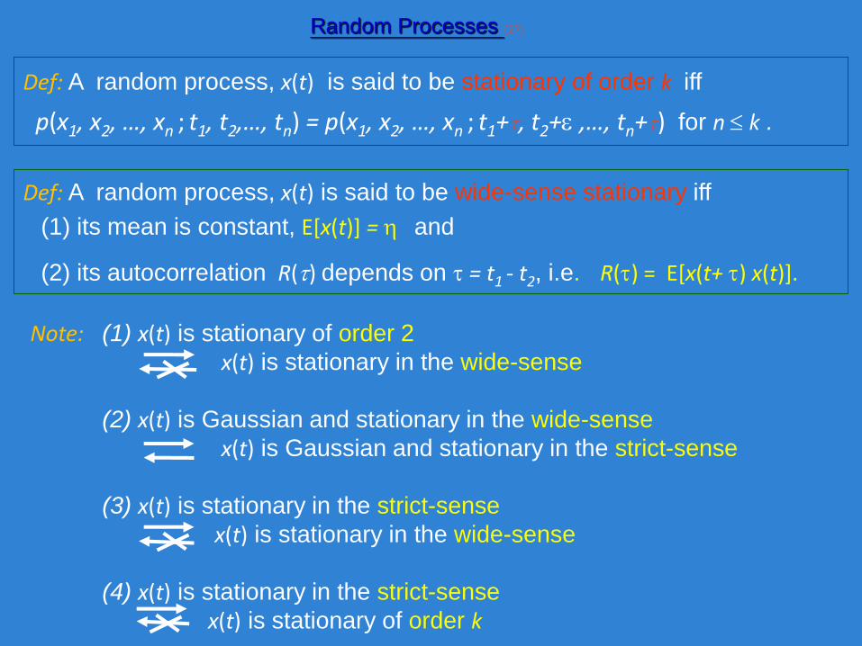
Def: A random process, x(t) is said to be stationary of order k iff
p(x1, x2, …, xn ; t1, t2,…, tn) = p(x1, x2, …, xn ; t1+, t2+ ,…, tn+) for n k .
Random Processes (27)
(1) x(t) is stationary of order 2
x(t) is stationary in the wide-sense
(2) x(t) is Gaussian and stationary in the wide-sense
x(t) is Gaussian and stationary in the strict-sense
(3) x(t) is stationary in the strict-sense
x(t) is stationary in the wide-sense
(4) x(t) is stationary in the strict-sense
x(t) is stationary of order k
Def: A random process, x(t) is said to be wide-sense stationary iff
(1) its mean is constant, E[x(t)] = and
(2) its autocorrelation R() depends on = t1 - t2, i.e. R() = E[x(t+ ) x(t)].
Note:
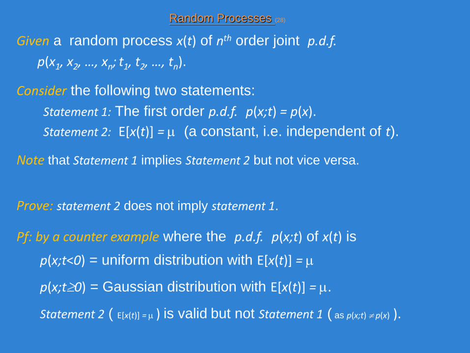
Given a random process x(t) of nth order joint p.d.f.
p(x1, x2, …, xn; t1, t2, …, tn).
Consider the following two statements:
Statement 1: The first order p.d.f. p(x;t) = p(x).
Statement 2: E[x(t)] = (a constant, i.e. independent of t).
Note that Statement 1 implies Statement 2 but not vice versa.
Random Processes (28)
Prove: statement 2 does not imply statement 1.
Pf: by a counter example where the p.d.f. p(x;t) of x(t) is
p(x;t<0) = uniform distribution with E[x(t)] =
p(x;t0) = Gaussian distribution with E[x(t)] = .
Statement 2 ( E[x(t)] = ) is valid but not Statement 1 ( as p(x;t) p(x) ).
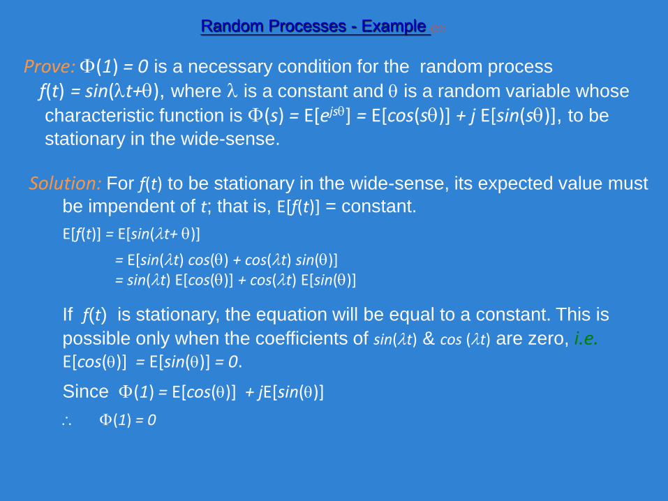
Prove: (1) = 0 is a necessary condition for the random process
f(t) = sin(t+), where is a constant and is a random variable whose
characteristic function is (s) = E[ejs] = E[cos(s)] + j E[sin(s)], to be
stationary in the wide-sense.
Random Processes - Example (29)
Solution: For f(t) to be stationary in the wide-sense, its expected value must
be impendent of t; that is, E[f(t)] = constant.
E[f(t)] = E[sin(t+ )]
= E[sin(t) cos() + cos(t) sin()]= sin(t) E[cos()] + cos(t) E[sin()]
If f(t) is stationary, the equation will be equal to a constant. This is
possible only when the coefficients of sin(t) & cos (t) are zero, i.e.E[cos()] = E[sin()] = 0.
Since (1) = E[cos()] + jE[sin()]
(1) = 0
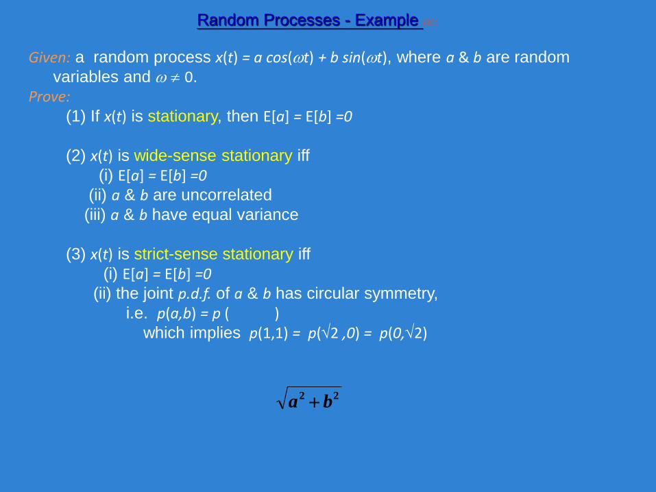
Given: a random process x(t) = a cos(t) + b sin(t), where a & b are random
variables and 0.
Prove:(1) If x(t) is stationary, then E[a] = E[b] =0
(2) x(t) is wide-sense stationary iff
(i) E[a] = E[b] =0(ii) a & b are uncorrelated
(iii) a & b have equal variance
(3) x(t) is strict-sense stationary iff
(i) E[a] = E[b] =0(ii) the joint p.d.f. of a & b has circular symmetry,
i.e. p(a,b) = p ( )which implies p(1,1) = p(2 ,0) = p(0,2)
22ba
Random Processes - Example (30)
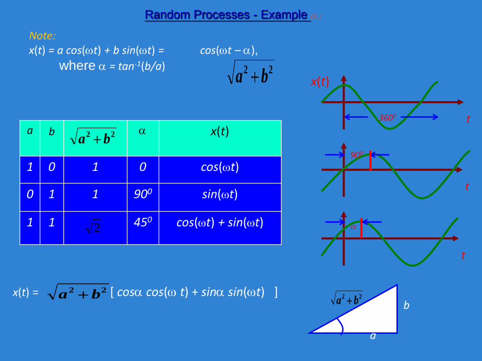
Note:x(t) = a cos(t) + b sin(t) = cos(t – ),
where = tan-1(b/a) 22ba
2
cos(t)0101
cos(t) + sin(t)45011
sin(t)900110
x(t)ba 22ba
2
t
b
a
22ba
x(t) = [ cos cos( t) + sin sin(t) ]22ba
Random Processes - Example (31)
x(t)
t3600
t
900
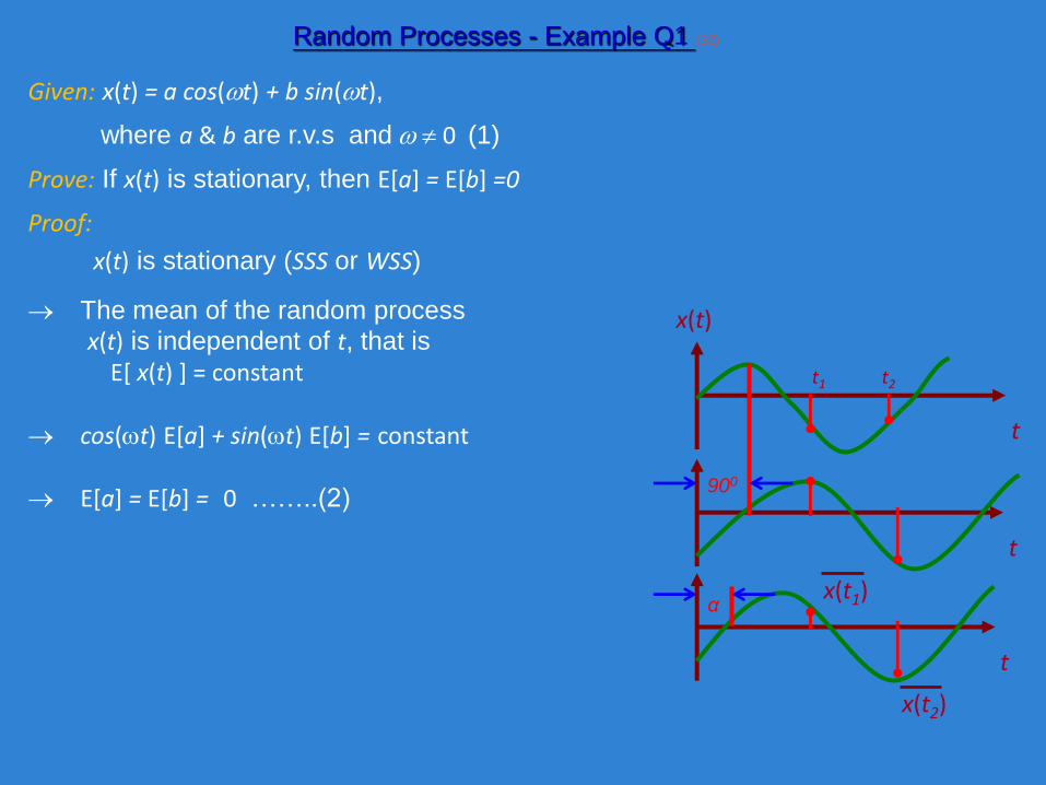
Given: x(t) = a cos(t) + b sin(t),
where a & b are r.v.s and 0 (1)
Prove: If x(t) is stationary, then E[a] = E[b] =0
Proof:
x(t) is stationary (SSS or WSS)
The mean of the random process
x(t) is independent of t, that is
E[ x(t) ] = constant
cos(t) E[a] + sin(t) E[b] = constant
E[a] = E[b] = 0 ……..(2)
x(t)
t
t
t
900
α
t1 t2
x(t1)
x(t2)
Random Processes - Example Q1 (32)
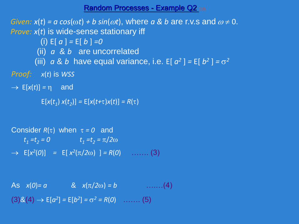
Given: x(t) = a cos(t) + b sin(t), where a & b are r.v.s and 0.Prove: x(t) is wide-sense stationary iff
(i) E[ a ] = E[ b ] =0(ii) a & b are uncorrelated
(iii) a & b have equal variance, i.e. E[ a2 ] = E[ b2 ] = 2
Random Processes - Example Q2 (33)
Proof: x(t) is WSS
E[x(t)] = and
E[x(t1) x(t2)] = E[x(t+)x(t)] = R()
Consider R() when = 0 and
t1 =t2 = 0 t1 =t2 = /2
E[x2(0)] = E[ x2(/2) ] = R(0) ……. (3)
As x(0)= a & x(/2) = b ….…(4)
(3)&(4) E[a2] = E[b2] = 2 = R(0) ……. (5)
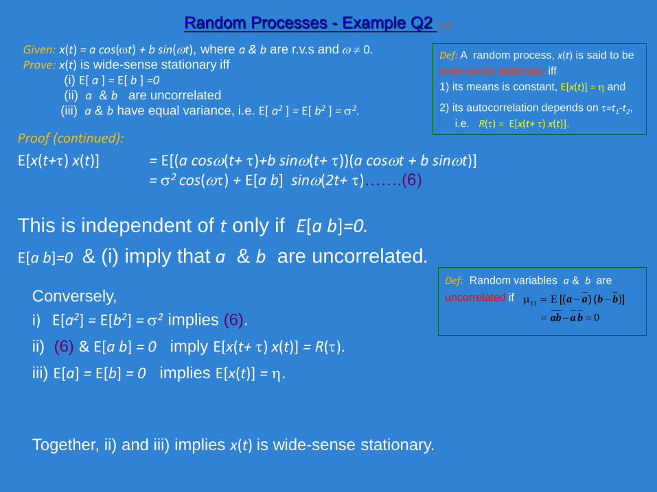
Given: x(t) = a cos(t) + b sin(t), where a & b are r.v.s and 0.Prove: x(t) is wide-sense stationary iff
(i) E[ a ] = E[ b ] =0(ii) a & b are uncorrelated
(iii) a & b have equal variance, i.e. E[ a2 ] = E[ b2 ] = 2.
Random Processes - Example Q2 (34)
This is independent of t only if E[a b]=0.
Conversely,
i) E[a2] = E[b2] = 2 implies (6).
ii) (6) & E[a b] = 0 imply E[x(t+ ) x(t)] = R().
iii) E[a] = E[b] = 0 implies E[x(t)] = .
Together, ii) and iii) implies x(t) is wide-sense stationary.
Def: A random process, x(t) is said to be
wide-sense stationary iff
1) its means is constant, E[x(t)] = and
2) its autocorrelation depends on =t1-t2,
i.e. R() = E[x(t+ ) x(t)].
Proof (continued):
E[x(t+) x(t)] = E[(a cos(t+ )+b sin(t+ ))(a cost + b sint)]= 2 cos() + E[a b] sin(2t+ )…….(6)
Def: Random variables a & b are
uncorrelated if
0
11
baab
bbaa )]()[( E
E[a b]=0 & (i) imply that a & b are uncorrelated.
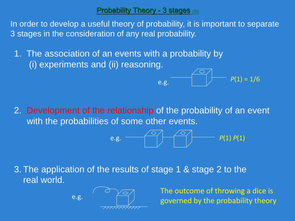
Probability Theory - 3 stages (35)
In order to develop a useful theory of probability, it is important to separate
3 stages in the consideration of any real probability.
1. The association of an events with a probability by
(i) experiments and (ii) reasoning.
e.g. P(1) = 1/6
e.g. P(1) P(1)
2. Development of the relationship of the probability of an event
with the probabilities of some other events.
e.g.
3. The application of the results of stage 1 & stage 2 to the
real world.The outcome of throwing a dice is governed by the probability theory.
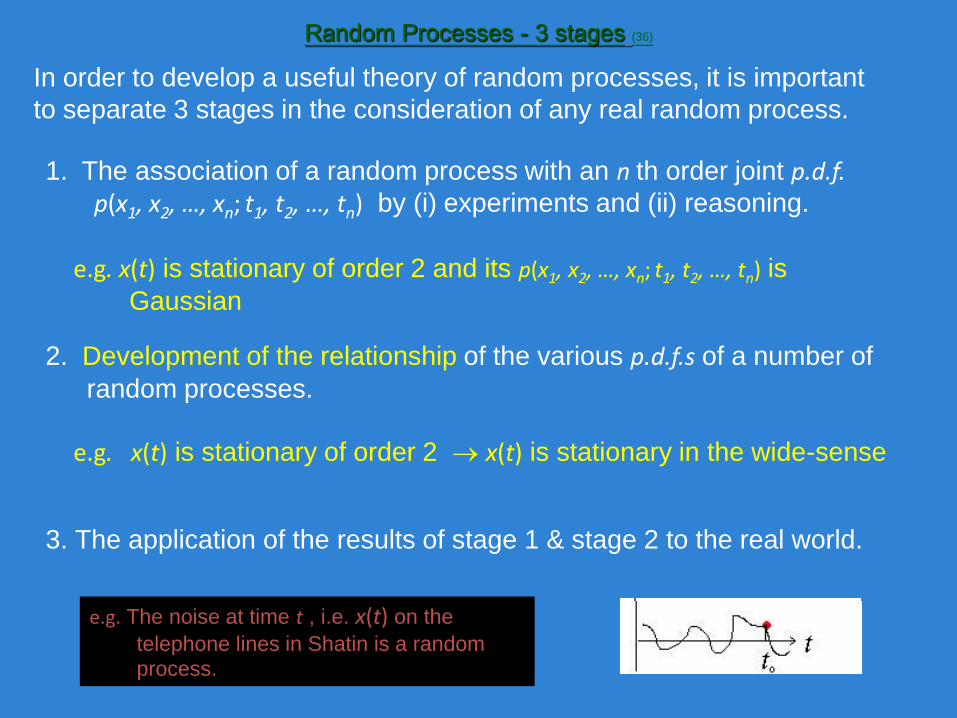
Random Processes - 3 stages (36)
In order to develop a useful theory of random processes, it is important
to separate 3 stages in the consideration of any real random process.
1. The association of a random process with an n th order joint p.d.f.p(x1, x2, …, xn; t1, t2, …, tn) by (i) experiments and (ii) reasoning.
2. Development of the relationship of the various p.d.f.s of a number of
random processes.
3. The application of the results of stage 1 & stage 2 to the real world.
e.g. The noise at time t , i.e. x(t) on the
telephone lines in Shatin is a random
process.
e.g. x(t) is stationary of order 2 x(t) is stationary in the wide-sense
e.g. x(t) is stationary of order 2 and its p(x1, x2, …, xn; t1, t2, …, tn) is
Gaussian
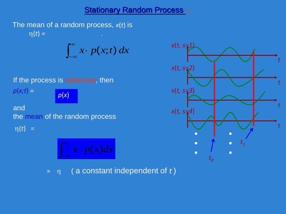
If the process is stationary, then
p(x;t) =
and
the mean of the random process
(t) =
Stationary Random Process (37)
The mean of a random process, x(t) is(t) = .
dxtxpx )( ;
• •• •• •
x(t, s=1)
tx(t, s=2)
tx(t, s=3)
tx(t, s=4)
t
t1
t0
p(x)
dxxpx )(
= ( a constant independent of t )
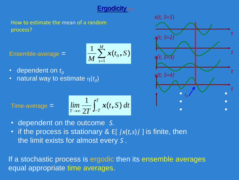
Ergodicity (38)
How to estimate the mean of a random process?
Ensemble-average =
• dependent on t0
• natural way to estimate (t0)
M
s
StM 1
0
1)( ,x
T
TTdtSt
Tlim )( ,x
2
1
If a stochastic process is ergodic then its ensemble averages
equal appropriate time averages.
x(t, S=1)
tx(t, S=2)
tx(t, S=3)
tx(t, S=4)
tt0
• •• •• •
Time-average =
• dependent on the outcome S.• if the process is stationary & E[ |x(t,s)| ] is finite, then
the limit exists for almost every S .
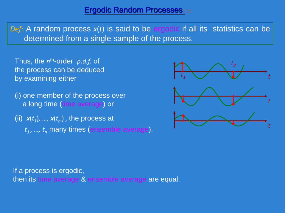
Ergodic Random Processes (39)
Thus, the nth-order p.d.f. of
the process can be deduced
by examining either
(i) one member of the process over
a long time (time average) or
(ii) x(t1), …, x(tn ) , the process at
t1 , …, tn many times (ensemble average).
tt1
t
t
t2
If a process is ergodic,
then its time average & ensemble average are equal.
Def: A random process x(t) is said to be ergodic if all its statistics can be
determined from a single sample of the process.
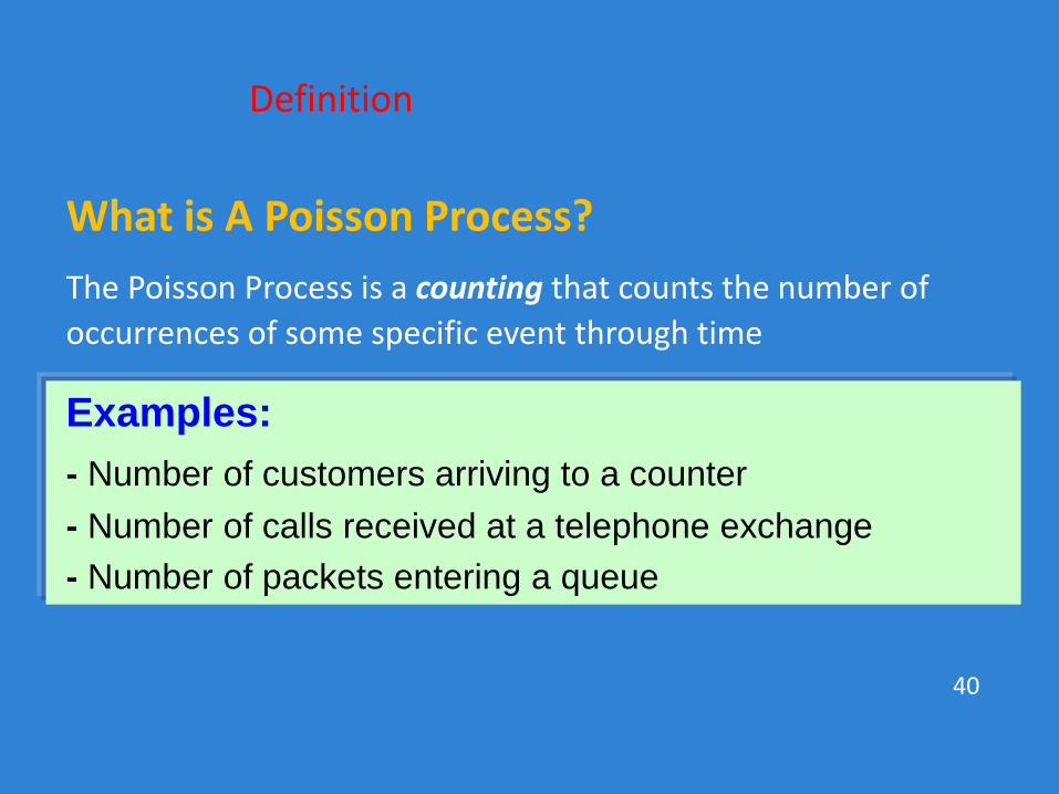
Definition
What is A Poisson Process?
The Poisson Process is a counting that counts the number of
occurrences of some specific event through time
40
Examples:
- Number of customers arriving to a counter
- Number of calls received at a telephone exchange
- Number of packets entering a queue
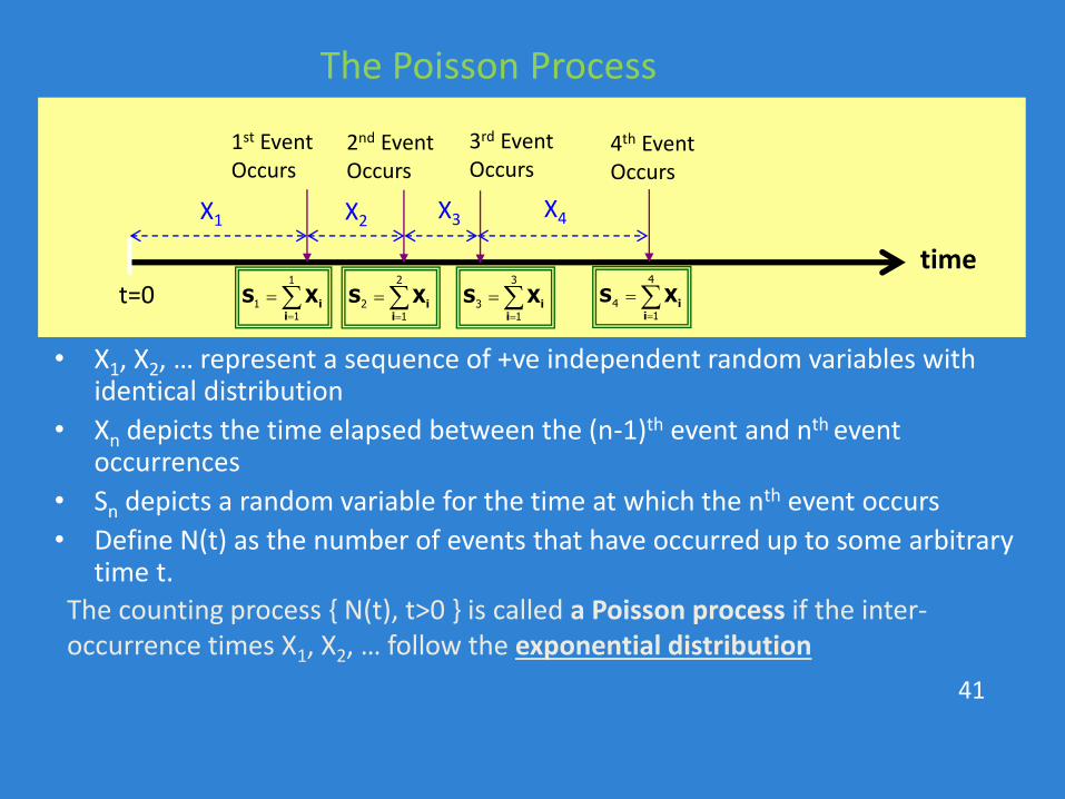
The Poisson Process
• X1, X2, … represent a sequence of +ve independent random variables with identical distribution
• Xn depicts the time elapsed between the (n-1)th event and nth event occurrences
• Sn depicts a random variable for the time at which the nth event occurs
• Define N(t) as the number of events that have occurred up to some arbitrary time t.
41
time
X1
t=0
X2 X3 X4
1st Event Occurs
2nd Event Occurs
3rd Event Occurs
4th Event Occurs
4
41
ii
S X
3
31
ii
S X
2
21
ii
S X
1
11
ii
S X
The counting process { N(t), t>0 } is called a Poisson process if the inter-occurrence times X1, X2, … follow the exponential distribution
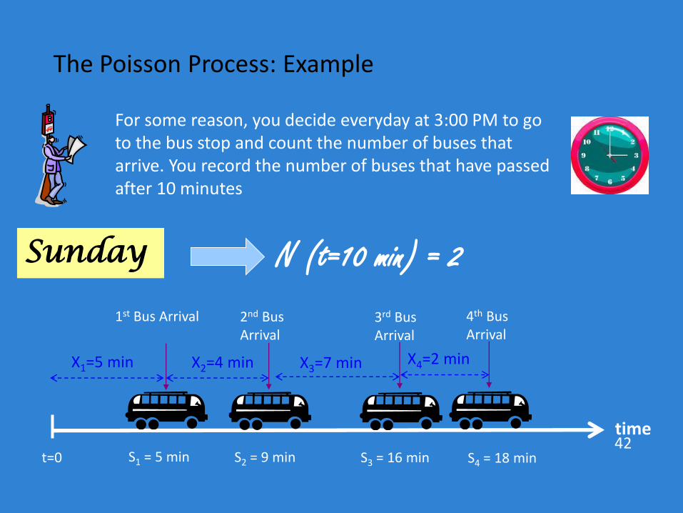
The Poisson Process: Example
42time
X1=5 min X2=4 min
1st Bus Arrival 2nd Bus Arrival
X3=7 min X4=2 min
3rd Bus Arrival
4th Bus Arrival
S1 = 5 mint=0 S2 = 9 min S3 = 16 min S4 = 18 min
Sunday
For some reason, you decide everyday at 3:00 PM to go to the bus stop and count the number of buses that arrive. You record the number of buses that have passed after 10 minutes
N (t=10 min) = 2
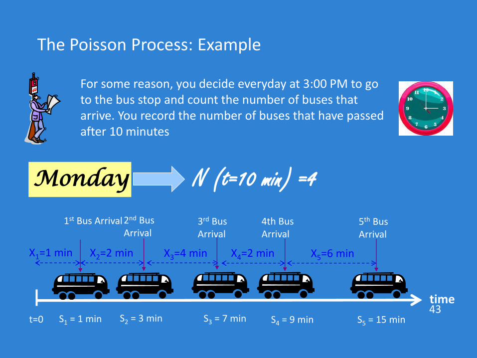
The Poisson Process: Example
43
Monday
For some reason, you decide everyday at 3:00 PM to go to the bus stop and count the number of buses that arrive. You record the number of buses that have passed after 10 minutes
N (t=10 min) =4
time
X1=1 min X2=2 min
1st Bus Arrival 2nd Bus Arrival
X3=4 min
4th Bus Arrival
5th Bus Arrival
S1 = 1 mint=0 S2 = 3 min S3 = 7 min S5 = 15 min
X4=2 min
3rd Bus Arrival
S4 = 9 min
X5=6 min
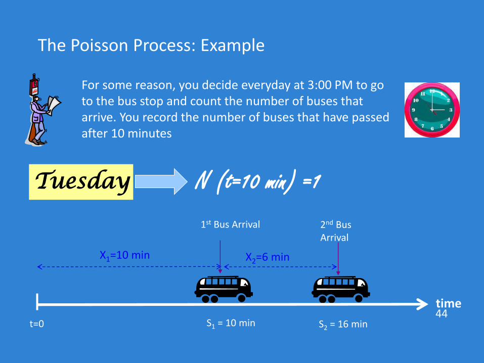
The Poisson Process: Example
44
Tuesday
For some reason, you decide everyday at 3:00 PM to go to the bus stop and count the number of buses that arrive. You record the number of buses that have passed after 10 minutes
N (t=10 min) =1
time
X1=10 min
2nd Bus Arrival
t=0 S1 = 10 min S2 = 16 min
1st Bus Arrival
X2=6 min
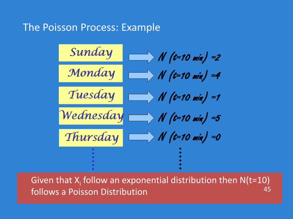
The Poisson Process: Example
Given that Xi follow an exponential distribution then N(t=10) follows a Poisson Distribution 45
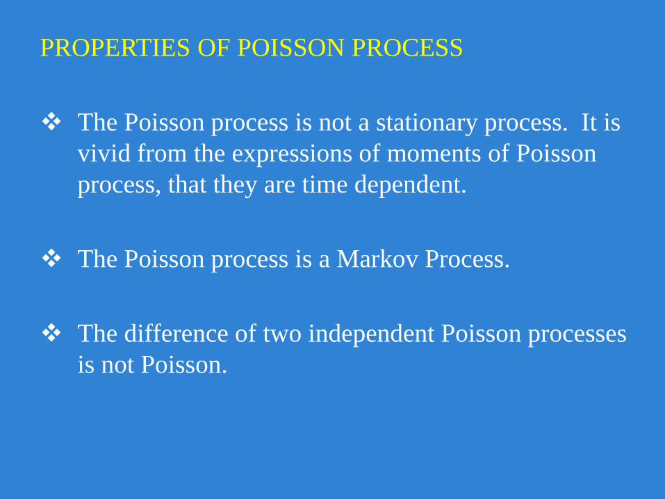
PROPERTIES OF POISSON PROCESS
The Poisson process is not a stationary process. It is
vivid from the expressions of moments of Poisson
process, that they are time dependent.
The Poisson process is a Markov Process.
The difference of two independent Poisson processes
is not Poisson.
Problems:
1.Suppose that customers arrive at a bank according to a
Poisson process with a mean rate of 3 per minute; find the
probability that dsuring a time interval of 2 min (i) exactly 4
customers arrive and (ii)more than 4 customers arrive.
2. A machine goes out of order, whenever a component fails.
The failure of this part follows a Poisson process with a mean
rate of 1 per week. Find the probability that 2 weeks have
elapsed since last failure. If there are 5 spare parts of this
component in an inventory and that the next supply is not due
in 10 weeks, find the probability that the machine will not be
out of order in the next 10 weeks.
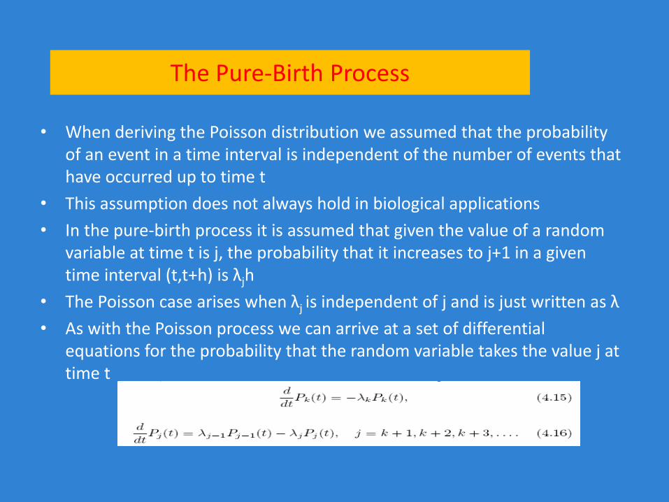
The Pure-Birth Process
• When deriving the Poisson distribution we assumed that the probability of an event in a time interval is independent of the number of events that have occurred up to time t
• This assumption does not always hold in biological applications
• In the pure-birth process it is assumed that given the value of a random variable at time t is j, the probability that it increases to j+1 in a given time interval (t,t+h) is λjh
• The Poisson case arises when λj is independent of j and is just written as λ
• As with the Poisson process we can arrive at a set of differential equations for the probability that the random variable takes the value j at time t
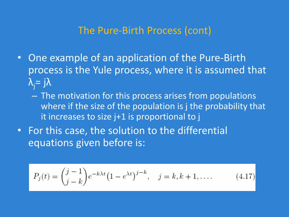
The Pure-Birth Process (cont)
• One example of an application of the Pure-Birth process is the Yule process, where it is assumed that λj= jλ– The motivation for this process arises from populations
where if the size of the population is j the probability that it increases to size j+1 is proportional to j
• For this case, the solution to the differential equations given before is:
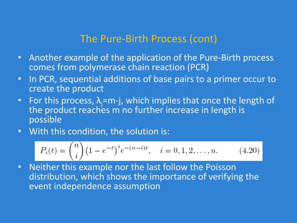
The Pure-Birth Process (cont)
• Another example of the application of the Pure-Birth process comes from polymerase chain reaction (PCR)
• In PCR, sequential additions of base pairs to a primer occur to create the product
• For this process, λj=m-j, which implies that once the length of the product reaches m no further increase in length is possible
• With this condition, the solution is:
• Neither this example nor the last follow the Poisson distribution, which shows the importance of verifying the event independence assumption
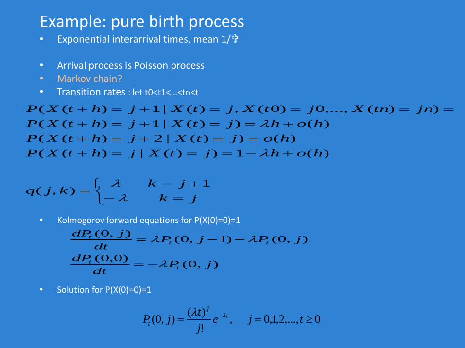
Example: pure birth process• Exponential interarrival times, mean 1/
• Arrival process is Poisson process• Markov chain? • Transition rates : let t0<t1<…<tn<t
• Kolmogorov forward equations for P(X(0)=0)=1
• Solution for P(X(0)=0)=1
0,...,2,1,0,!
)(),0( tje
j
tjP t
j
t
jk
jkkjq
hohjtXjhtXP
hojtXjhtXP
hohjtXjhtXP
jntnXjtXjtXjhtXP
1),(
)(1))(|)((
)())(|2)((
)())(|1)((
))(,...,0)0(,)(|1)((
),0()0,0(
),0()1,0(),0(
jPdt
dP
jPjPdt
jdP
tt
ttt
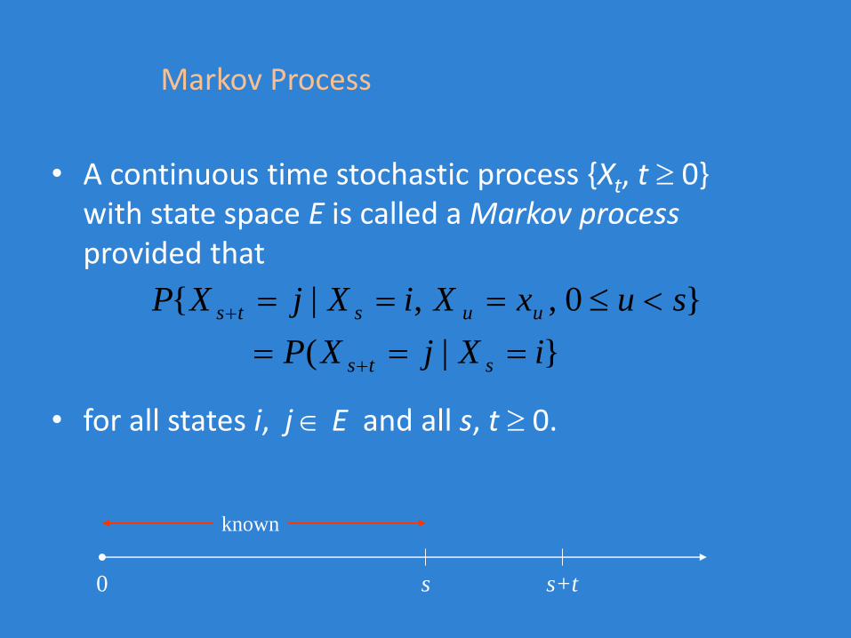
Markov Process
• A continuous time stochastic process {Xt, t 0}with state space E is called a Markov processprovided that
• for all states i, j E and all s, t 0.
}|(
}0,,|{
iXjXP
suxXiXjXP
sts
uusts
s+ts0
known
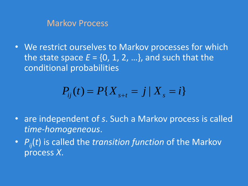
Markov Process
• We restrict ourselves to Markov processes for which the state space E = {0, 1, 2, …}, and such that the conditional probabilities
• are independent of s. Such a Markov process is called time-homogeneous.
• Pij(t) is called the transition function of the Markov process X.
}|{)( iXjXPtP stsij
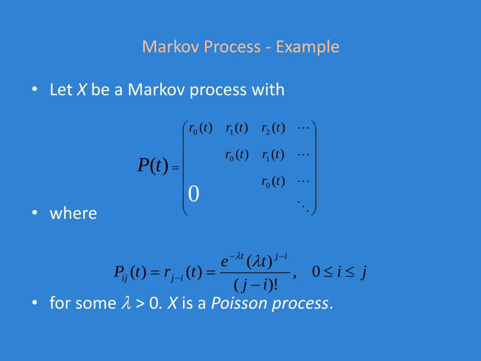
Markov Process - Example
• Let X be a Markov process with
• where
• for some > 0. X is a Poisson process.
)(
)()(
)()()(
0
10
210
)(tr
trtr
trtrtr
tP
jiij
tetrtP
ijt
ijij
0,)!(
)()()(
0
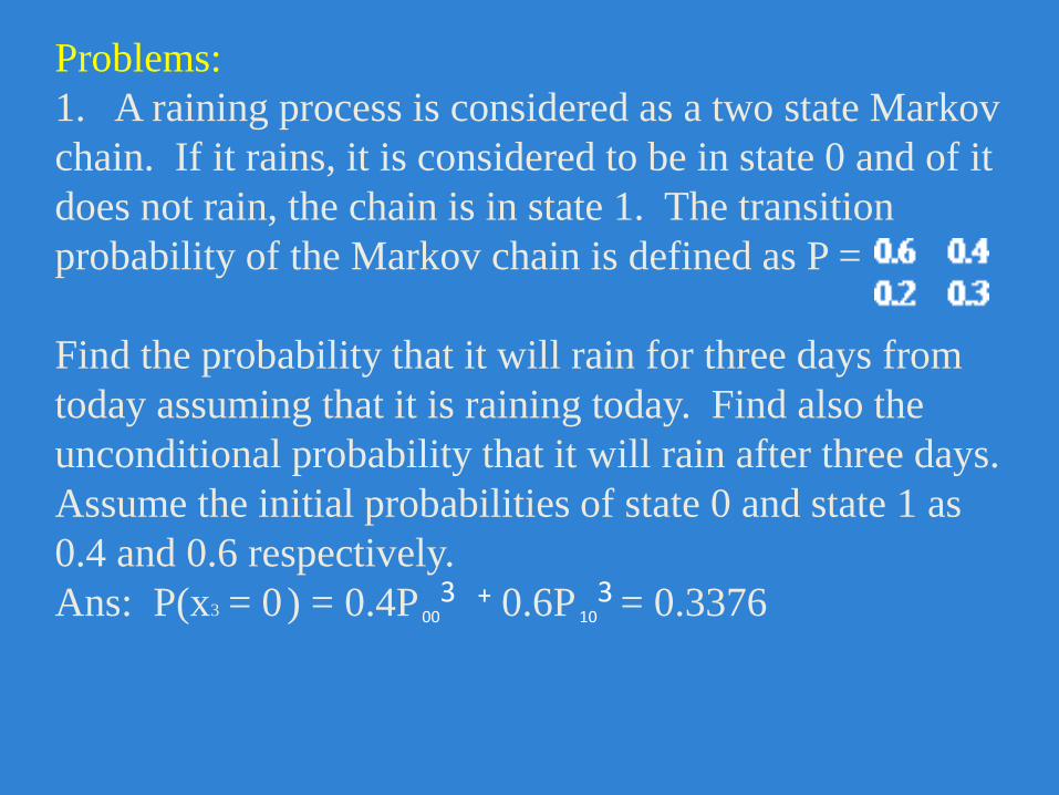
Problems:
1. A raining process is considered as a two state Markov
chain. If it rains, it is considered to be in state 0 and of it
does not rain, the chain is in state 1. The transition
probability of the Markov chain is defined as P =
Find the probability that it will rain for three days from
today assuming that it is raining today. Find also the
unconditional probability that it will rain after three days.
Assume the initial probabilities of state 0 and state 1 as
0.4 and 0.6 respectively.
Ans: P(x3 = 0) = 0.4P 003 + 0.6P 10
3 = 0.3376
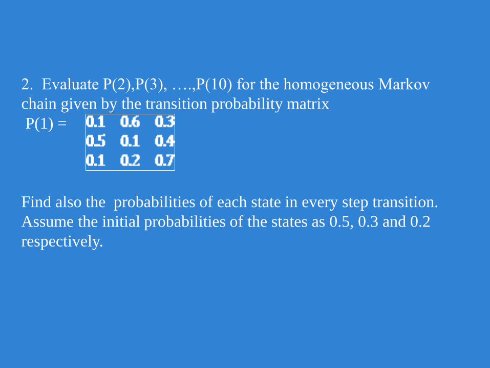
2. Evaluate P(2),P(3), ….,P(10) for the homogeneous Markov
chain given by the transition probability matrix
P(1) =
Find also the probabilities of each state in every step transition.
Assume the initial probabilities of the states as 0.5, 0.3 and 0.2
respectively.
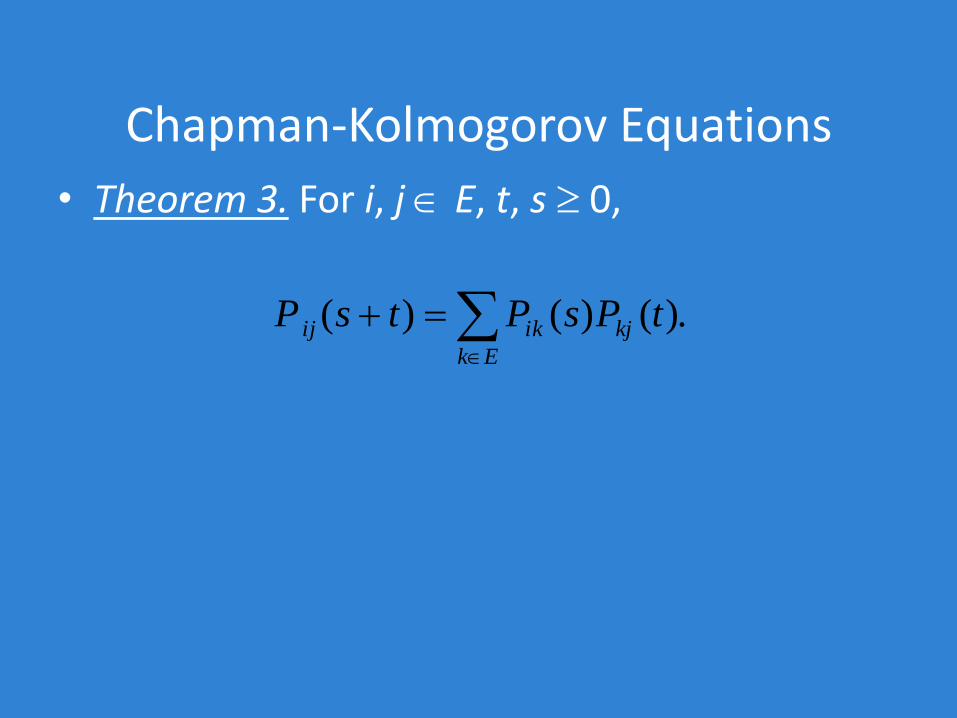
Chapman-Kolmogorov Equations
• Theorem 3. For i, j E, t, s 0,
.)()()(
Ek
kjikij tPsPtsP
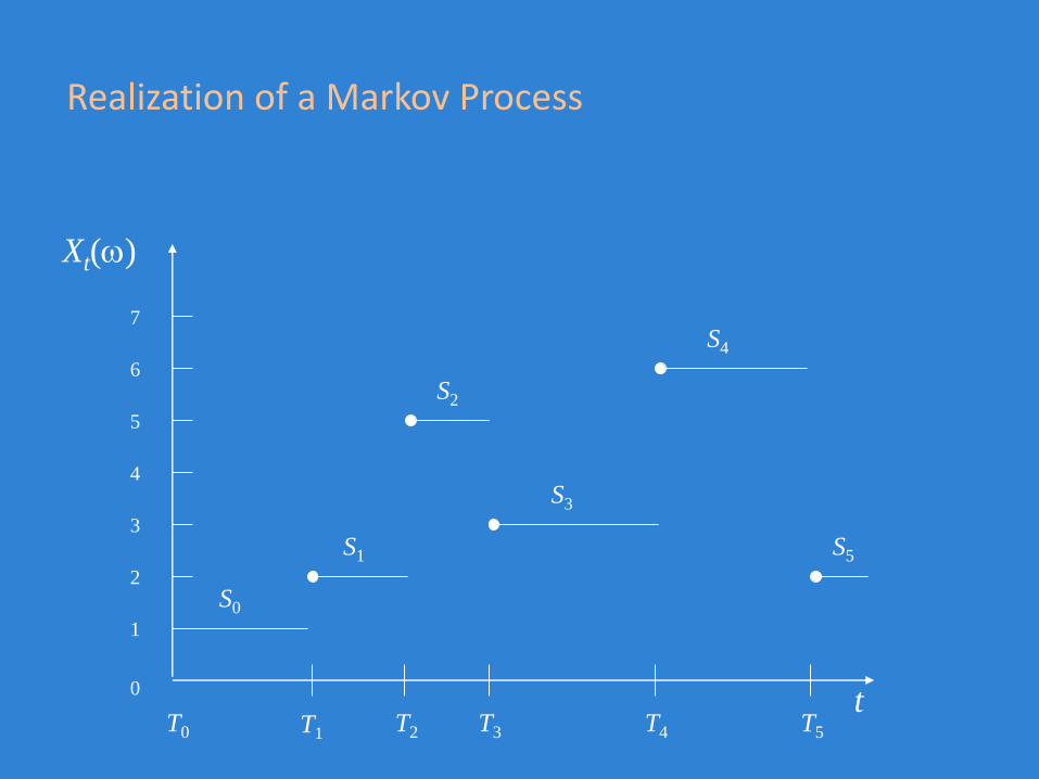
Realization of a Markov Process
t
Xt()
T1 T5T3 T4T2T0
1
3
4
5
6
7
0
2S0
S1
S3
S2
S4
S5
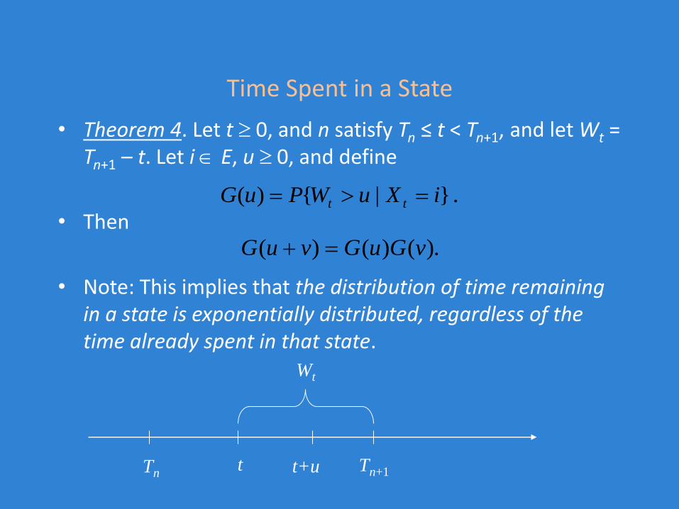
Time Spent in a State
• Theorem 4. Let t 0, and n satisfy Tn ≤ t < Tn+1, and let Wt = Tn+1 – t. Let i E, u 0, and define
• Then
• Note: This implies that the distribution of time remaining in a state is exponentially distributed, regardless of the time already spent in that state.
.}|{)( iXuWPuG tt
).()()( vGuGvuG
Tn+1tTn
Wt
t+u
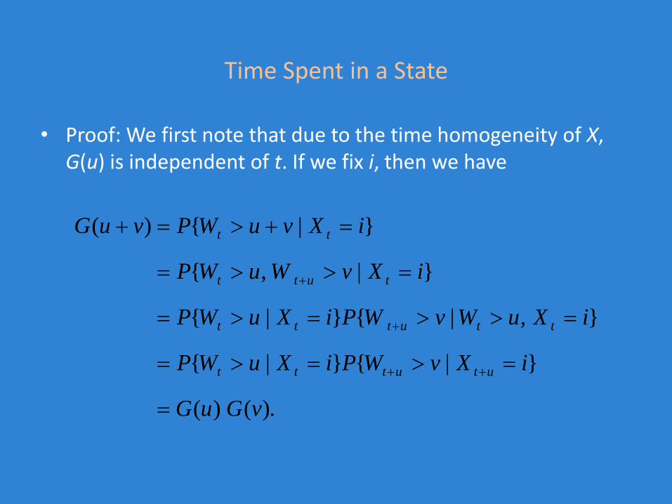
Time Spent in a State
• Proof: We first note that due to the time homogeneity of X, G(u) is independent of t. If we fix i, then we have
).()(
}|{}|{
},|{}|{
}|,{
}|{)(
vGuG
iXvWPiXuWP
iXuWvWPiXuWP
iXvWuWP
iXvuWPvuG
ututtt
ttuttt
tutt
tt
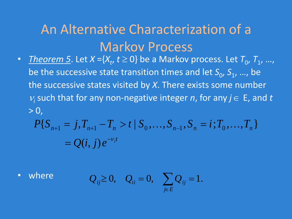
An Alternative Characterization of a Markov Process
• Theorem 5. Let X ={Xt, t 0} be a Markov process. Let T0, T1, …,
be the successive state transition times and let S0, S1, …, be
the successive states visited by X. There exists some number
i such that for any non-negative integer n, for any j E, and t
> 0,
• where
t
nnnnnn
iejiQ
TTiSSStTTjSP
),(
},,;,,,|,{ 01011
.1,0,0 Ej
ijiiij QQQ
An Alternative Characterization of a Markov Process
• This implies that the successive states visited by a Markov process form a Markov chain with transition matrix Q.
• A Markov process is irreducible recurrent if its underlying Markov chain is irreducible recurrent.
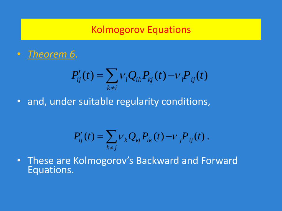
Kolmogorov Equations
• Theorem 6.
• and, under suitable regularity conditions,
• These are Kolmogorov’s Backward and Forward Equations.
.)()()( tPtPQtP ijj
jk
ikkjkij
)()()( tPtPQtP iji
ik
kjikiij
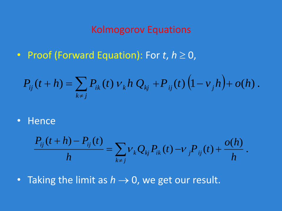
Kolmogorov Equations
• Proof (Forward Equation): For t, h 0,
• Hence
• Taking the limit as h 0, we get our result.
.)(1)()()( hohvtPQhtPhtP jij
jk
kjkikij
.)(
)()()()(
h
hotPtPQ
h
tPhtPijj
jk
ikkjk
ijij
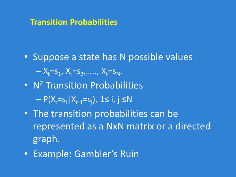
Transition Probabilities
• Suppose a state has N possible values
– Xt=s1, Xt=s2,….., Xt=sN.
• N2 Transition Probabilities
– P(Xt=si|Xt-1=sj), 1≤ i, j ≤N
• The transition probabilities can be represented as a NxN matrix or a directed graph.
• Example: Gambler’s Ruin
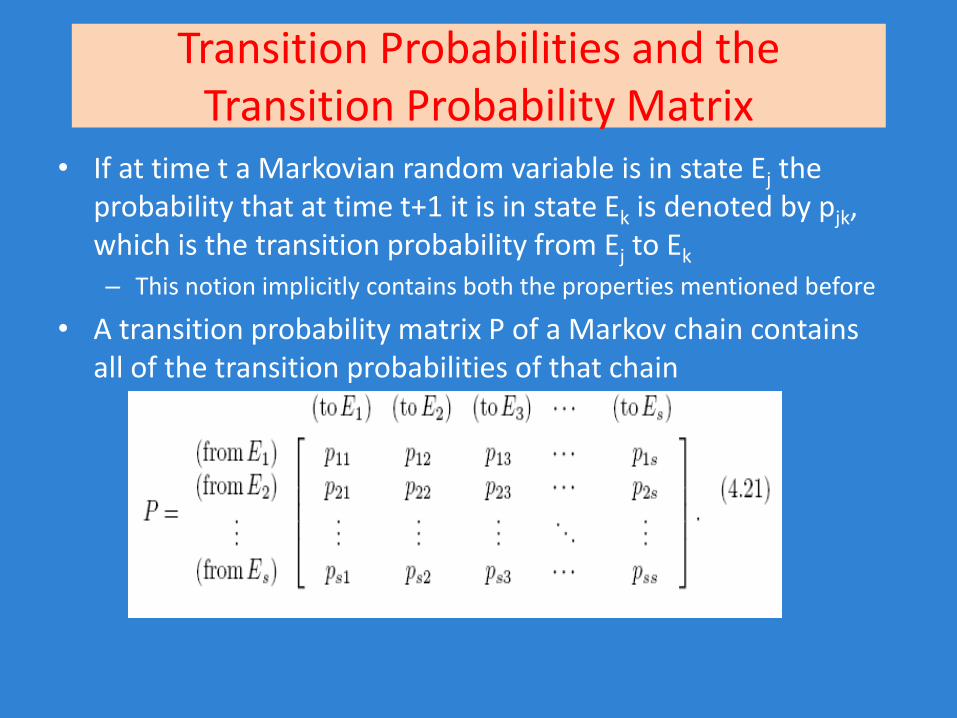
Transition Probabilities and the Transition Probability Matrix
• If at time t a Markovian random variable is in state Ej the probability that at time t+1 it is in state Ek is denoted by pjk, which is the transition probability from Ej to Ek
– This notion implicitly contains both the properties mentioned before
• A transition probability matrix P of a Markov chain contains all of the transition probabilities of that chain
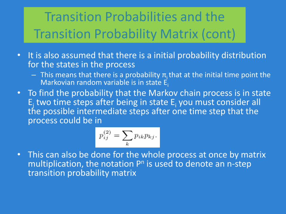
Transition Probabilities and the Transition Probability Matrix (cont)
• It is also assumed that there is a initial probability distribution for the states in the process– This means that there is a probability πi that at the initial time point the
Markovian random variable is in state Ei
• To find the probability that the Markov chain process is in state Ej two time steps after being in state Ei you must consider all the possible intermediate steps after one time step that the process could be in
• This can also be done for the whole process at once by matrix multiplication, the notation Pn is used to denote an n-step transition probability matrix

Markov Chains with Absorbing States
• A Markov chain with an absorbing state can be recognized by the appearance of a 1 along the main diagonal of its transition probability matrix
• A Markov chain with an absorbing state will eventually enter that state and never leave it
• Markov chains with absorbing states bring up new questions, which will be addressed later, but for now we will only consider Markov chains without absorbing states
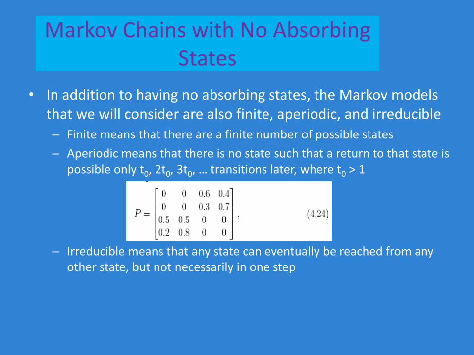
Markov Chains with No Absorbing States
• In addition to having no absorbing states, the Markov models that we will consider are also finite, aperiodic, and irreducible– Finite means that there are a finite number of possible states
– Aperiodic means that there is no state such that a return to that state is possible only t0, 2t0, 3t0, … transitions later, where t0 > 1
– Irreducible means that any state can eventually be reached from any other state, but not necessarily in one step
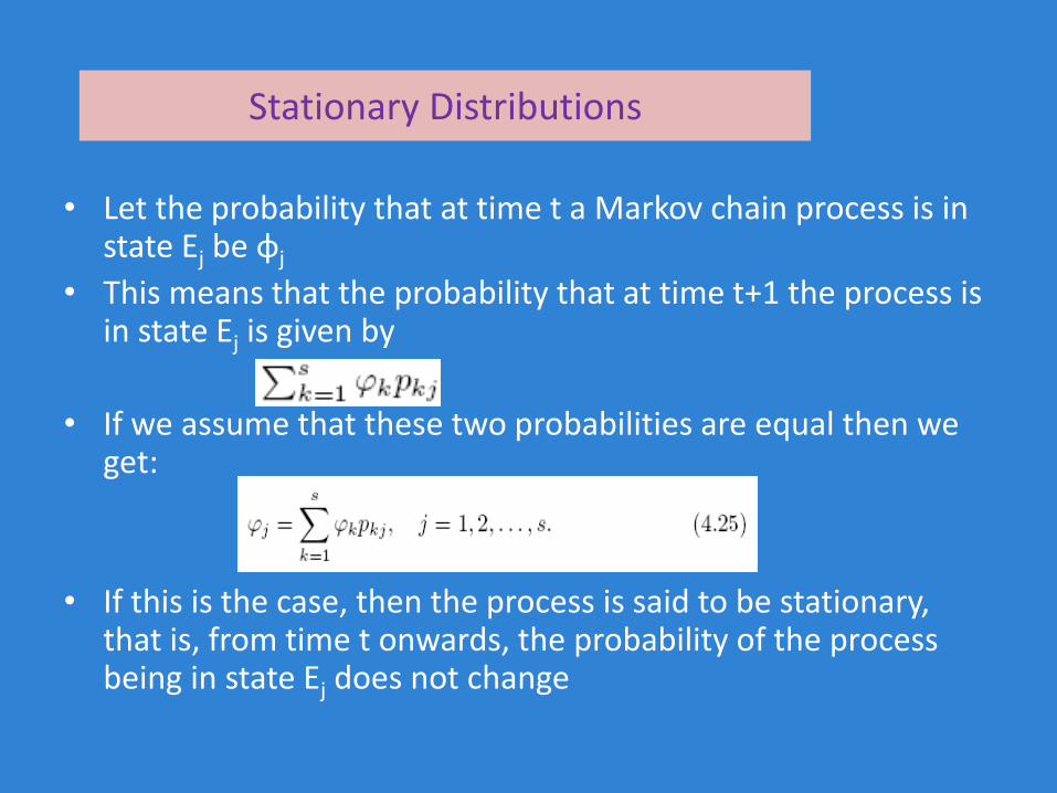
Stationary Distributions
• Let the probability that at time t a Markov chain process is in state Ej be φj
• This means that the probability that at time t+1 the process is in state Ej is given by
• If we assume that these two probabilities are equal then we get:
• If this is the case, then the process is said to be stationary, that is, from time t onwards, the probability of the process being in state Ej does not change
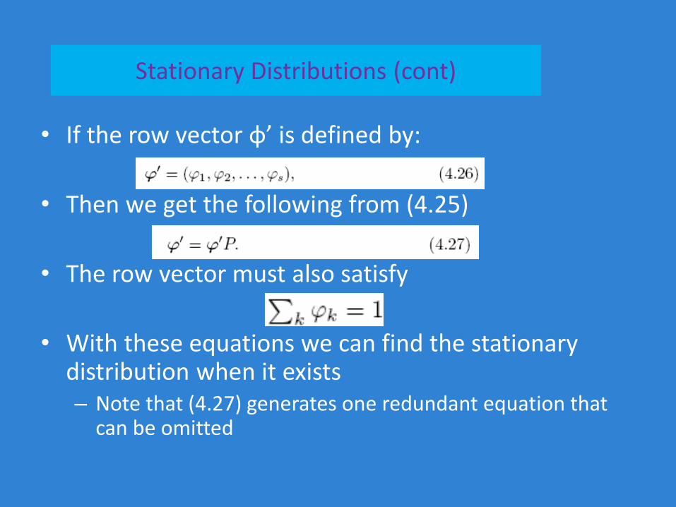
Stationary Distributions (cont)
• If the row vector φ’ is defined by:
• Then we get the following from (4.25)
• The row vector must also satisfy
• With these equations we can find the stationary distribution when it exists– Note that (4.27) generates one redundant equation that
can be omitted
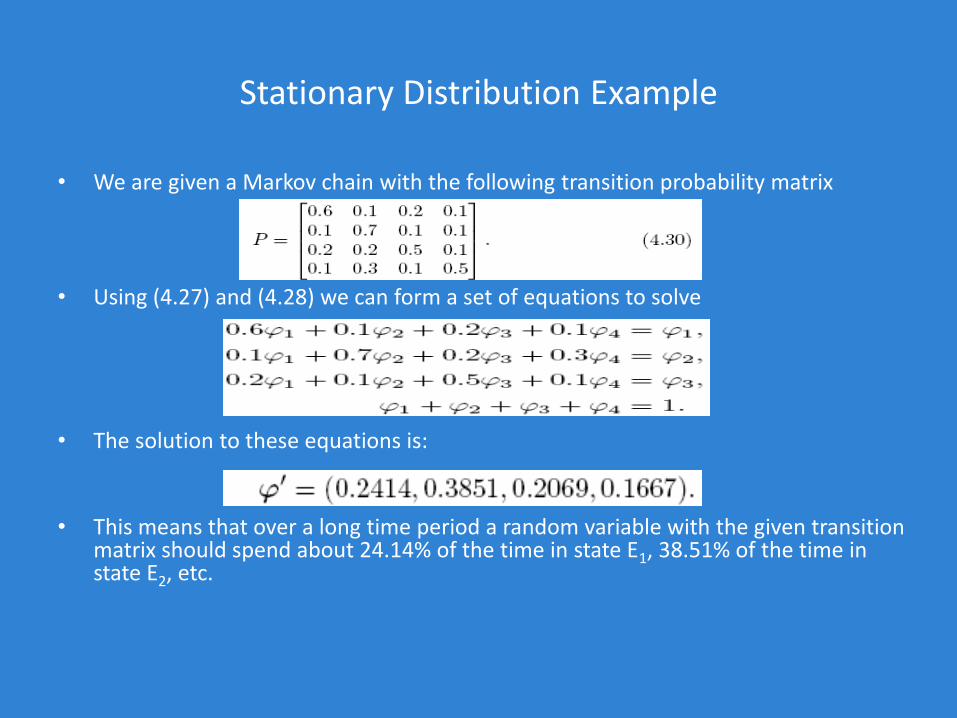
Stationary Distribution Example
• We are given a Markov chain with the following transition probability matrix
• Using (4.27) and (4.28) we can form a set of equations to solve
• The solution to these equations is:
• This means that over a long time period a random variable with the given transition matrix should spend about 24.14% of the time in state E1, 38.51% of the time in state E2, etc.
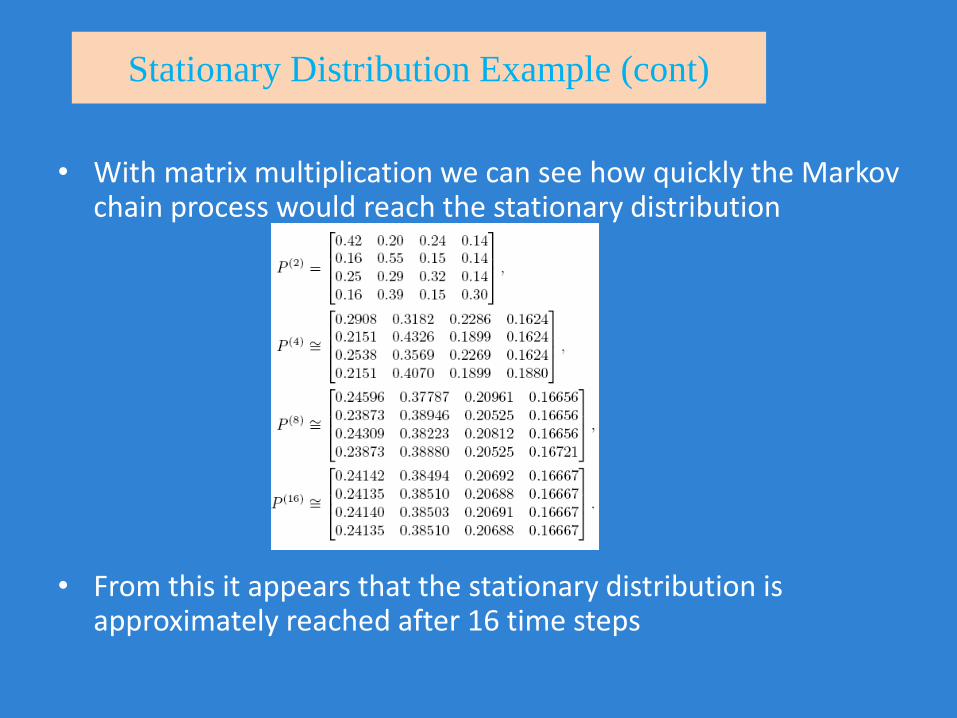
Stationary Distribution Example (cont)
• With matrix multiplication we can see how quickly the Markov chain process would reach the stationary distribution
• From this it appears that the stationary distribution is approximately reached after 16 time steps
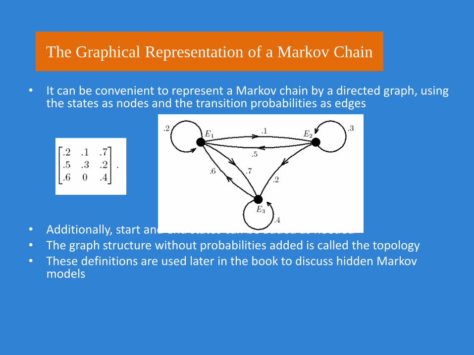
The Graphical Representation of a Markov Chain
• It can be convenient to represent a Markov chain by a directed graph, using the states as nodes and the transition probabilities as edges
• Additionally, start and end states can be added as needed• The graph structure without probabilities added is called the topology• These definitions are used later in the book to discuss hidden Markov
models
What can Markov Chains Do?
• Example: Gambler’s Ruin
– The probability of a particular sequence
• 3, 4, 3, 2, 3, 2, 1, 0
– The probability of success for the gambler
– The average number of bets the gambler will make.
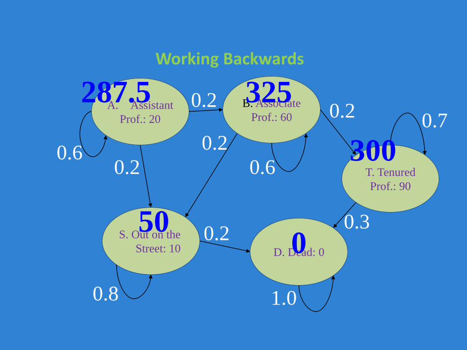
Working Backwards
A. Assistant
Prof.: 20
B. Associate
Prof.: 60
T. Tenured
Prof.: 90
S. Out on the
Street: 10 D. Dead: 0
1.0
0.60.2
0.2
0.8
0.2
0.6
0.2
0.20.7
0.3
0
300
50
325287.5
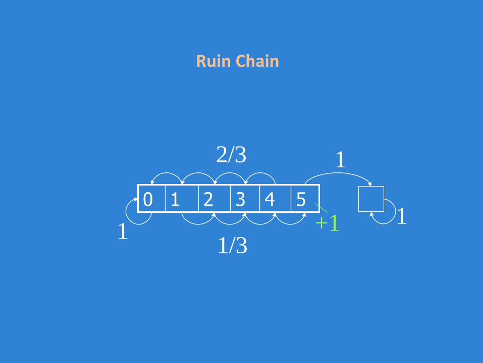
Ruin Chain
0 1 2 3 4 5
1/3
2/3
1
1
1+1
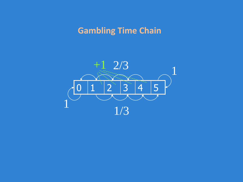
Gambling Time Chain
0 1 2 3 4 5
1/3
2/31
1
+1
Refs. :
1.J.S. Bendat and A.G. Piersol “Random data: analysis and measurement procedures” J. Wiley, 3rd ed, 2000.
2.D.E. Newland “Introduction to Random Vibrations, Spectral and Wavelet Analysis” Addison-Wesley 3rd ed. 1996
3. wwwhome.math.utwente.nl/~boucherierj/.../158052sheetshc2.ppt
4. aplcenmp.apl.jhu.edu/Notes/Akinpelu/Markov%20Processes.ppt
5. webdocs.cs.ualberta.ca/~lindek/650/Slides/MarkovModel.ppt