PHYSICAL REVIEW E 88, 012103 (2013)

Stiff directed lines in random media

Horst-Holger Boltz* and Jan KierfeldPhysics Department, TU Dortmund University, 44221 Dortmund, Germany

(Received 26 April 2013; published 8 July 2013)

We investigate the localization of stiff directed lines with bending energy by a short-range random potential.We apply perturbative arguments, Flory scaling arguments, a variational replica calculation, and functionalrenormalization to show that a stiff directed line in 1 + d dimensions undergoes a localization transition withincreasing disorder for d > 2/3. We demonstrate that this transition is accessible by numerical transfer matrixcalculations in 1 + 1 dimensions and analyze the properties of the disorder-dominated phase in detail. On thebasis of the two-replica problem, we propose a relation between the localization of stiff directed lines in 1 + d

dimensions and of directed lines under tension in 1 + 3d dimensions, which is strongly supported by identicalfree-energy distributions. This shows that pair interactions in the replicated Hamiltonian determine the natureof directed line localization transitions with consequences for the critical behavior of the Kardar-Parisi-Zhangequation. We support the proposed relation to directed lines via multifractal analysis, revealing an analogousAnderson transition-like scenario and a matching correlation length exponent. Furthermore, we quantify how thepersistence length of the stiff directed line is reduced by disorder.

DOI: 10.1103/PhysRevE.88.012103 PACS number(s): 05.40.−a, 64.70.−p, 64.60.Ht, 61.41.+e

I. INTRODUCTION

Elastic manifolds in random media, especially the problemof a directed line (DL) or directed polymer in a randompotential, are one of the most important model systems in thestatistical physics of disordered systems [1]. DLs in randommedia are related to important nonequilibrium statisticalphysics problems such as stochastic growth, in particular theKardar-Parisi-Zhang (KPZ) equation [2], Burgers turbulence,or the asymmetric simple exclusion model (ASEP) [3].Furthermore, there are many and important applications ofDLs in random media such as kinetic roughening [3], pinningof flux lines in type II superconductors [4,5], domain walls inrandom magnets, or wetting fronts [1,6].

Directed lines have a preferred direction and no overhangswith respect to this direction. The energy of DLs such asflux lines, domain walls, wetting fronts is proportional totheir length; therefore, the elastic properties of directed linesare governed by their line tension, which favors the straightconfiguration of shortest length. Both thermal fluctuations anda short-range random potential (point disorder) tend to roughenthe DL against the line tension. As a result of the competitionbetween thermal fluctuations and disorder, DLs in a randommedia in D = 1 + d dimensions exhibit a disorder-drivenlocalization transition [7] for dimensions d > 2, i.e., abovea critical dimension dc = 2. These transitions have beenstudied numerically for dimensions up to d = 4 [8–18]. Atlow temperatures, the DL is in a disorder-dominated phaseand localizes into a path optimizing the random potentialenergy and the tension energy. Within this disorder-dominatedphase, the DL roughens, and there are macroscopic energyfluctuations and a finite pair overlap between replicas [19–21](introduced below). At high temperatures, the disorder is anirrelevant perturbation, and the DL exhibits essentially thermalfluctuations against the line tension. It has been suggested thatthe critical temperature for the localization transition of a DL in

*horst-holger.boltz@udo.edu

a random medium and the binding of two DLs by a short-rangeattractive potential coincide [11,14].

DLs in a random medium map onto the dynamic KPZequation for nonlinear stochastic surface growth with therestricted free energy of DLs in 1 + d dimensions satisfyingthe KPZ equation of a d-dimensional dynamic interface. Thelocalization transition of DLs with increasing disorder corre-sponds to a roughening transition of the KPZ interface withincreasing nonlinearity. In the context of the KPZ equation,it is a long-standing open question (recently discussed, forexample, in Ref. [22]) whether there exists an upper criticaldimension where the critical behavior at the localizationtransition is modified. Therefore, the critical behavior of linesin random media can eventually also shed light onto the criticalproperties of the KPZ equation.

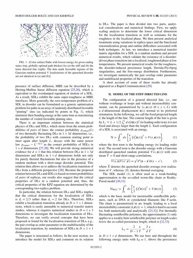
In the present paper, we study the localization transition ofstiff directed lines (SDLs). We define SDLs as directed lineswith preferred orientation and no overhangs with respect tothis direction but with a different elastic energy as compared toDLs: SDLs are governed by bending energy, which penalizescurvature, rather than line tension, which penalizes stretchingof the line. This gives rise to configurations which are locallycurvature free, i.e., straight but straight segments can assumeany orientation even if this increases the total length of the line.We investigate the disorder-induced localization transitionof SDLs for a short-range random potential and the scalingproperties of conformations in the disordered phase. A typicaloptimal SDL configuration in the presence of an additionalshort-range random potential at zero temperature is shown inFig. 1(a), in comparison to a typical optimal DL configurationsin Fig. 1(b).

There are a number of applications for SDLs in randommedia. SDLs describe semiflexible polymers smaller than theirpersistence length, such that the assumption of a directed line isnot violated. Our results apply to semiflexible polymers suchas DNA or cytoskeletal filaments like F-actin in a randomenvironment as it could be realized, for example, by a porousmedium [23]. Moreover, SDLs are closely connected to surfacegrowth models for molecular beam epitaxy (MBE) [24]. In the

012103-11539-3755/2013/88(1)/012103(16) ©2013 American Physical Society

HORST-HOLGER BOLTZ AND JAN KIERFELD PHYSICAL REVIEW E 88, 012103 (2013)

(b)(a)

FIG. 1. (Color online) Paths with lowest energy for given endingstates (top, globally optimal path thicker) for (a) the stiff and (b) thetense directed line (right). The dots mark favorable regions of theGaussian random potential V [realizations of the quenched disorderare not identical in (a) and (b)].

presence of surface diffusion, MBE can be described by aHerring-Mullins linear diffusion equation [25,26], which isequivalent to the overdamped equation of motion of a SDL.As a result, SDLs exhibit the same super-roughness as MBEinterfaces. More generally, the zero-temperature problem of aSDL in disorder can be formulated as a generic optimizationproblem for paths in an array of randomly distributed favorable“pinning” sites (as indicated by points in Fig. 1), whichminimize their bending energy at the same time as maximizingthe number of visited favorable pinning sites.

There is an important relation between the statisticalphysics of DLs and SDLs, which stems from the return prob-abilities of pairs of lines: the contact probability pcontact(L)of two thermally fluctuating DLs in 1 + 3d dimensions, i.e.,the probability of two DLs with common starting point tomeet again after length L, decays with the same powerlaw pcontact ∼ L−3d/2 as the contact probability of SDLs in1 + d dimensions [27,28]. We will provide strong numericalevidence for d = 1 that this relation between DLs in 1 + 3d

dimensions and SDLs in 1 + d dimensions holds not onlyfor purely thermal fluctuations but also in the presence of arandom medium with a short-range disorder potential. Thisrelation then allows us to address the localization transition ofDLs from a different perspective [28]. Because the proposedrelation between DLs and SDLs is based on return probabilitiesof pairs of replicas, our results also suggest that the criticalproperties of DLs in a random potential and, thus, thecritical properties of the KPZ equation are determined by thecorresponding two-replica problem.

In particular, the relation between DLs and SDLs impliesthat the critical dimension for the localization of SDLsis dc = 2/3 rather than dc = 2 for DLs. Therefore, SDLsexhibit a localization transition already in D = 1 + 1 dimen-sions, which is easily amenable to numerical transfer matrixstudies, whereas it requires numerical studies in D = 1 + 3dimensions to investigate the localization transition of DLs.Therefore, we can verify several concepts that have beenproposed or found for the localization transition of DLs, e.g.,the pair overlap as order parameter or the multifractality of thelocalization transition, by simulations of SDLs in D = 1 + 1dimensions.

The paper is structured as follows. In the next section, weintroduce the model for SDLs and comment on its relation

to DLs. The paper is then divided into two parts, analyt-ical considerations and numerical findings. First, we applyscaling analysis to determine the lower critical dimensionfor the localization transition as well as estimates for theroughness in the localized phase. We then present analyticaltreatments using variations in replica space and the functionalrenormalization group and outline difficulties associated withboth techniques. At last, we introduce a numerical transfermatrix algorithm for a SDL in a random medium and presentnumerical results, which validate the existence of a disorder-driven phase transition into a localized, roughened phase at lowtemperatures. We present numerical results for the roughness,the disorder-induced persistence length, Derrida-Flyvbjergsingularities, and the free-energy distribution. Furthermore,we investigate numerically the pair overlap order parameterand multifractal properties of the transition.

A short account of some of these results has alreadyappeared as a Rapid Communication [29].

II. MODEL OF THE STIFF DIRECTED LINE

The configuration of a general directed line, i.e., onewithout overhangs or loops and without inextensibility con-straint, can be parametrized by (x,z(x)) (0 � x � L) witha d-dimensional displacement z(x) normal to its preferredorientation. In the following, we call the fixed projected lengthL the length of the line. The contour length of the line is givenby Lc ≈ L + 1/2

∫ L

0 dx[∂z(x)]2 (to leading order in z); it is notfixed and always larger than the length L. Each configurationof a SDL is associated with an energy,

H =∫ L

0dx

[κ

2

(∂2x z(x)

)2 + V (x,z(x))

], (1)

where the first term is the bending energy (to leading orderin z). The second term is the disorder energy with a Gaussiandistributed quenched random potential V (x,z(x)) with zeromean V = 0 and short-range correlations,

V (x,z)V (x ′,z′) = g2δd (z − z′)δ(x − x ′), (2)

where X denotes the quenched disorder average over realiza-tions of V , whereas 〈X〉 denotes thermal averaging.

The SDL model (1) is often used as a weak-bendingapproximation to the so-called worm-like chain or Kratky-Porod model [30,31]

HWLC =∫ L

0ds

[κ

2

(∂2s r(s)

)2 + V (r(s))

], (3)

which is the basic model for inextensible semiflexible poly-mers, such as DNA or cytoskeletal filaments like F-actin.The chain is parametrized in arc length, leading to a localinextensibility constraint |∂sr(s)| = 1, which is hard to accountfor, both numerically and analytically [23,32]. For thermallyfluctuating semiflexible polymers, the approximation (1) onlyapplies to a weakly bent semiflexible polymer on length scalesbelow the so-called persistence length, which is [32,33]

Lp = 2

D − 1

κ

T= 2

d

κ

T. (4)

in D = 1 + d dimensions. We use here and throughout thefollowing energy units with kB ≡ 1. Above the persistence

012103-2

STIFF DIRECTED LINES IN RANDOM MEDIA PHYSICAL REVIEW E 88, 012103 (2013)

length, a semiflexible polymer loses orientation correlationsand starts to develop overhangs.

Also in a quenched random potential the SDL modeldescribes semiflexible polymers in heterogeneous media, onlyas long as tangent fluctuations are small such that overhangscan be neglected, which is the case below a disorder-inducedpersistence length, which we will derive below.

We consider the SDL model also in the thermodynamiclimit beyond this persistence length, because we find evidencefor a relation to the important problem of DLs in a randommedium in lower dimensions. This relation is based onreplica pair interactions and shows that pair interactionsalso determine the nature of the DL localization transition.Moreover, this relation can make the DL transition in highdimensions computationally accessible. We will now outlinethe idea behind this relation.

III. RELATION TO DIRECTED LINES

The difference between SDLs and DLs [1] is the secondderivative in the first bending energy term in Eq. (1) forSDLs, which differs from the tension or stretching energy∼∫

dx τ2 (∂xz(x))2 of DLs with line tension τ . This results in

different types of energetically favorable configurations (seeFig. 1): large perpendicular displacements z of SDLs as shownin Fig. 1(a) are not unfavorable as long as their “direction”does not change, i.e., as long as they are locally straight and,therefore, do not cost bending energy. Such configurationsincrease, however, the length of the line and are suppressedfor DLs by the tension or stretching energy.

The statistics of displacements z is characterized by theroughness exponent ζ , which is defined by 〈z2(L)〉 ∼ L2ζ .The thermal roughness is ζth,τ = 1/2 for DLs and ζth,κ = 3/2for SDLs: Equating the thermal energy T with the respectiveelastic energies gives T ∼ τz2/L for DLs and T ∼ κz2/L3

for SDLs. Here and in the following we use subscripts τ

(tension) and κ (bending stiffness) to distinguish between thetwo systems.

Although typical configurations differ markedly, a SDLsubject to a short-ranged (around z = 0) attractive potentialV (z) can be mapped onto a DL in high dimensions d ′ = 3d [27,28]. This equivalence is based on the probability that a free lineof length L starting at [z(0) = 0] “returns” to the origin, i.e.,ends at z(L) = 0. This return probability is characterized bya return exponent χ : Prob(z(L) = 0) ∼ L−χ . The same returnexponent characterizes the contact probability pcontact(L) ∼L−χ , i.e., the probability of two lines with a common startingpoint to meet again after length L, as follows from consideringthe relative coordinate. For DLs, which are essentially randomwalks in d transverse dimensions, the return exponent is χτ =d/2 [35], whereas it is χκ = 3d/2 for a SDL (after integratingover all orientations of the end) [34]; they are related to theroughness exponents by χ = ζd [28]. The return exponent χ

governs the critical properties of the binding transition to ashort-range attractive potential or, equivalently, of the bindingtransition of two lines interacting by such a potential [27,28].This follows, for example, directly from a necklace modeltreatment [35]. The relation

χτ (3d) = χκ (d) (5)

implies that the binding transition of two DLs in 3d dimensionsmaps onto the binding transition of two SDLs in d dimensions.

In the replica formulation of line localization problems suchas in (1), the random potential gives rise to a short-rangeattractive pair interaction (see below). Therefore, pairwiseinteractions of DLs play a prominent role also for the physicsof a single DL in a random potential. Furthermore, the criticaltemperature Tc,τ for a DL in a random potential is believed tobe identical to the critical temperature T2,τ for a system withtwo replicas [11,14]. In Sec. VII D, we will show numericallythat also for SDLs in a random medium Tc,κ = T2,κ holds. Theimportant role of pairwise interactions suggests that not onlythe binding transition of two DLs in 3d dimensions mapsonto the binding transition of two SDLs in d dimensionsbut that the same dimensional relation holds for the local-ization transitions of DLs and SDLs in a short-range randompotential.

One aim of this work is to support this conjecture byproviding strong numerical evidence that the d → 3d analogybetween DLs and SDLs in a random potential holds for theentire free-energy distributions for DLs in 1 + 3 and SDLsin 1 + 1 dimensions. Because this analogy is rooted in thebinding transition of replica pairs, we can conclude that criticalproperties of the localization transition are determined by pairinteractions in the replicated Hamiltonian, which has beenpreviously suggested in Refs. [36,37].

Moreover, it has been proposed that pair interactions canbe used to formulate an order parameter of the disorder-drivenlocalization transition of DLs in terms of the overlap q ≡limL→∞ 1

L

∫ L

0 dxδ[z1(x) − z2(x)] [19–21], i.e., the averagenumber of sites per length, that two lines in the same realizationof the disorder have in common. Localization by disorder givesrise to a finite value of the pair overlap q. This coincides withthe binding energy per length that characterizes binding oftwo polymers by a pair potential. We will also show that thepair overlap indeed provides a suitable order parameter forthe localization transition of SDLs in 1 + 1 dimensions. Aschematic summary of the relation of DLs and SDLs together(together with some relevant numeric results) is shown inFig. 2.

IV. SCALING ANALYSIS

A. Lower critical dimension

We start with a scaling analysis by use of a Flory-typeargument. For displacements ∼z the bending energy in Eq. (1)scales as Eb ∼ z2L−3, which also leads to 〈z2〉 ∼ L3/Lp andthe thermal roughness exponent ζth,κ = 3/2. The disorderenergy in Eq. (1) scales as Ed ∼ √

Lz−d , as can be seenfrom Eq. (2). Using the unperturbed thermal roughness inthe disorder energy we get Ed ∼ L(2−3d)/4, from which weconclude that the disorder is relevant below a lower criticaldimension dc,κ with

dc,κ = 2/3. (6)

Above this critical dimension for d > 2/3 and, thus, in allphysically accessible integer dimensions, the SDL shouldexhibit a transition from a thermal phase for low g to adisorder-dominated phase above a critical value gc of the

012103-3

HORST-HOLGER BOLTZ AND JAN KIERFELD PHYSICAL REVIEW E 88, 012103 (2013)

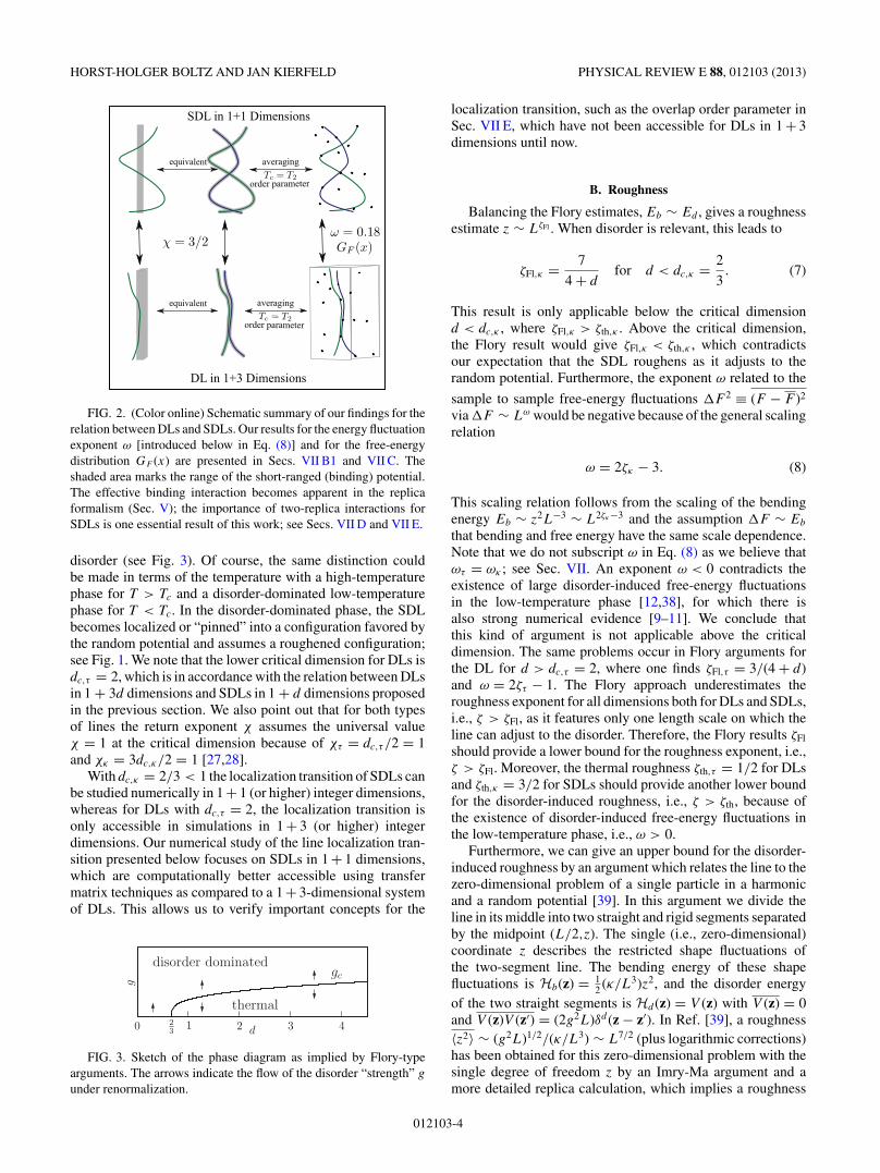
FIG. 2. (Color online) Schematic summary of our findings for therelation between DLs and SDLs. Our results for the energy fluctuationexponent ω [introduced below in Eq. (8)] and for the free-energydistribution GF (x) are presented in Secs. VII B1 and VII C. Theshaded area marks the range of the short-ranged (binding) potential.The effective binding interaction becomes apparent in the replicaformalism (Sec. V); the importance of two-replica interactions forSDLs is one essential result of this work; see Secs. VII D and VII E.

disorder (see Fig. 3). Of course, the same distinction couldbe made in terms of the temperature with a high-temperaturephase for T > Tc and a disorder-dominated low-temperaturephase for T < Tc. In the disorder-dominated phase, the SDLbecomes localized or “pinned” into a configuration favored bythe random potential and assumes a roughened configuration;see Fig. 1. We note that the lower critical dimension for DLs isdc,τ = 2, which is in accordance with the relation between DLsin 1 + 3d dimensions and SDLs in 1 + d dimensions proposedin the previous section. We also point out that for both typesof lines the return exponent χ assumes the universal valueχ = 1 at the critical dimension because of χτ = dc,τ /2 = 1and χκ = 3dc,κ/2 = 1 [27,28].

With dc,κ = 2/3 < 1 the localization transition of SDLs canbe studied numerically in 1 + 1 (or higher) integer dimensions,whereas for DLs with dc,τ = 2, the localization transition isonly accessible in simulations in 1 + 3 (or higher) integerdimensions. Our numerical study of the line localization tran-sition presented below focuses on SDLs in 1 + 1 dimensions,which are computationally better accessible using transfermatrix techniques as compared to a 1 + 3-dimensional systemof DLs. This allows us to verify important concepts for the

disorder dominated

thermal

gc

0 2 3 4d

g

23

1

FIG. 3. Sketch of the phase diagram as implied by Flory-typearguments. The arrows indicate the flow of the disorder “strength” g

under renormalization.

localization transition, such as the overlap order parameter inSec. VII E, which have not been accessible for DLs in 1 + 3dimensions until now.

B. Roughness

Balancing the Flory estimates, Eb ∼ Ed , gives a roughnessestimate z ∼ LζFl . When disorder is relevant, this leads to

ζFl,κ = 7

4 + dfor d < dc,κ = 2

3. (7)

This result is only applicable below the critical dimensiond < dc,κ , where ζFl,κ > ζth,κ . Above the critical dimension,the Flory result would give ζFl,κ < ζth,κ , which contradictsour expectation that the SDL roughens as it adjusts to therandom potential. Furthermore, the exponent ω related to the

sample to sample free-energy fluctuations F 2 ≡ (F − F )2

via F ∼ Lω would be negative because of the general scalingrelation

ω = 2ζκ − 3. (8)

This scaling relation follows from the scaling of the bendingenergy Eb ∼ z2L−3 ∼ L2ζκ−3 and the assumption F ∼ Eb

that bending and free energy have the same scale dependence.Note that we do not subscript ω in Eq. (8) as we believe thatωτ = ωκ ; see Sec. VII. An exponent ω < 0 contradicts theexistence of large disorder-induced free-energy fluctuationsin the low-temperature phase [12,38], for which there isalso strong numerical evidence [9–11]. We conclude thatthis kind of argument is not applicable above the criticaldimension. The same problems occur in Flory arguments forthe DL for d > dc,τ = 2, where one finds ζFl,τ = 3/(4 + d)and ω = 2ζτ − 1. The Flory approach underestimates theroughness exponent for all dimensions both for DLs and SDLs,i.e., ζ > ζFl, as it features only one length scale on which theline can adjust to the disorder. Therefore, the Flory results ζFl

should provide a lower bound for the roughness exponent, i.e.,ζ > ζFl. Moreover, the thermal roughness ζth,τ = 1/2 for DLsand ζth,κ = 3/2 for SDLs should provide another lower boundfor the disorder-induced roughness, i.e., ζ > ζth, because ofthe existence of disorder-induced free-energy fluctuations inthe low-temperature phase, i.e., ω > 0.

Furthermore, we can give an upper bound for the disorder-induced roughness by an argument which relates the line to thezero-dimensional problem of a single particle in a harmonicand a random potential [39]. In this argument we divide theline in its middle into two straight and rigid segments separatedby the midpoint (L/2,z). The single (i.e., zero-dimensional)coordinate z describes the restricted shape fluctuations ofthe two-segment line. The bending energy of these shapefluctuations is Hb(z) = 1

2 (κ/L3)z2, and the disorder energyof the two straight segments is Hd (z) = V (z) with V (z) = 0and V (z)V (z′) = (2g2L)δd (z − z′). In Ref. [39], a roughness〈z2〉 ∼ (g2L)1/2/(κ/L3) ∼ L7/2 (plus logarithmic corrections)has been obtained for this zero-dimensional problem with thesingle degree of freedom z by an Imry-Ma argument and amore detailed replica calculation, which implies a roughness

012103-4

STIFF DIRECTED LINES IN RANDOM MEDIA PHYSICAL REVIEW E 88, 012103 (2013)

exponent,

ζ0,κ = 74 , (9)

for the stiff two-segment line. For the directed line, ananalogous argument gives ζ0,τ = 3/4. In the framework ofa functional renormalization group (FRG) calculation bothroughness exponents can be written as ζ0 = ε/4 in a dimen-sional expansion with the appropriate ε = 4 − d for DLs andε = 8 − d for SDLs (see Sec. VI below). Using the scalingrelations (8), this results in ω0 = 1

2 for two-segment lines(both for SDLs and DLs), which should be considered anupper bound to the energy fluctuation exponent, because theadaptation of the line to the potential must not lead to largerfluctuations as compared to the trivial case of summing uprandom numbers [40]. Therefore, ζ0 also should provide anupper bound for the roughness exponent, i.e., ζ < ζ0. Theupper bound ζ < ε/4 is also found in the FRG calculation [40].

All in all, we have obtained bounds

max(ζth,ζFl) < ζ < ζ0, (10)

which apply both for SDLs and DLs. For SDLs, this gives arelatively small window of possible roughness exponents,

max

(3

2,

7

4 + d

)< ζκ <

7

4, (11)

which, for example, limits ζκ for SDLs in 1 + 1 dimensions to1.5 < ζκ < 1.75.

V. VARIATION IN REPLICA SPACE

To go beyond scaling arguments we use the replicatechnique [41] following the treatment of directed manifoldsby Mezard and Parisi [42]. For the sake of convenience, werestrict ourselves to d = 1 throughout this section. Later wewill comment on how to adapt this to higher dimensions. Thequenched average of the free energy F = −β−1ln Z is treatedin the representation

ln Z = limn→0

n−1(Zn − 1), (12)

calculating averages Zn of an n-times replicated system in thelimit n → 0. For the calculation we introduce an additionalparabolic potential or “mass” term,

∫dxμz2(x), in Eq. (1) as

an infrared regularization and a finite correlation length λ inthe disorder correlator,

V (x,z)V (x ′,z′) = g2fλ((z − z′)2)δ(x − x ′), (13)

where we use fλ(x) =√

2πλ2−1

exp (−x/(2λ2)) to retainthe original δ correlator [compare Eq. (2)] for λ ≈ 0. Wewrite the replicated and averaged partition function as Zn =∏

α(∫Dzα) exp (−βHrep) with the following replica Hamilto-

nian in Fourier space:

Hrep = 1

2L

n∑α=1

∑k

(κk4 + μ)z2α

− βg2

2

n∑α,β=1

∫ L

0dx f [(zα − zβ)2]. (14)

As mentioned before, Hrep is related to a pair bindingproblem: In the limit λ ≈ 0 the second term becomes

− βg2

2

∑α,β

∫ L

0 dxδ(zα − zβ), which is an attractive short-range interaction of two replicated lines.

We use variation in replica space with the quadratic, i.e.,Gaussian, trial Hamiltonian

HV = (2L)−1∑

k

∑α,β

zαG−1αβ zβ, (15)

with G−1αβ = (κk4 + μ)δαβ + σαβ , with the self-energy matrix

σ providing variational parameters. Extremizing the lower freeenergy bound F � FV + 〈Heff − HV 〉V with respect to theself-energy matrix σ gives (in the continuum limit L−1 ≈ 0) aself-consistent equation for the self-energy matrix [42],

σαβ ={−∑

α′ �=α σαα′ α = β

−2βg2f ′[(∫ dk2πβ

(Gαα+Gββ−2Gαβ )]

α �= β,

(16)

with

fλ(x) ≡∫

dy√

2π−1

e−y2/2fλ(y2x) =√

2π−1√

λ2 + x−1

.

(17)

Following Mezard and Parisi, we choose a one-step hi-erarchical replica symmetry-breaking ansatz for σ . Replicasymmetry breaking is relevant here, because there is nonontrivial replica symmetric solution in the limit μ ≈ 0 apartfrom σαβ = 0. Furthermore, there is no continuous replicasymmetry breaking since ζFl < ζth for d > dc,κ [42]. Thus, σ

can be parametrized by a diagonal element σ and a functionσ (u) (0 � u � 1) giving the nondiagonal elements in the limitn → 0. For one-step replica symmetry breaking, the lattertakes the form σ (u) = σ0 + �(u − uc)(σ1 − σ0). Using thealgebra developed by Parisi [43] and performing the limit ofan unbounded system μ → 0, we find

σ0 = 0, (18)

σ1 = −2βg2f ′(πS1), (19)

with S1 = S1(�) ≡ 1√2β

κ−1/4�−3/4 and � ≡ ucσ1. In higherdimensions, d > 1, the stationary equation (16) as well as theresult for one-step replica symmetry breaking would be ofthe same form with different numerical constants, given thefunctions fλ and fλ are adapted accordingly, see Ref. [43].In d = 1, the variation of the free-energy estimate yields twoself-consistent equations,

uc ∝ S1(�)[λ2 + S1(�)]−1 and � ∝ (β20g16κ3u20

c

)−1,

(20)

for uc and �, where we omitted numerical constants. We arenot able to give a closed solution, because

�1/20 ∼ λ2 + �−3/4

�−3/4, (21)

∼ λ2�15/20 + const. (22)

Nonetheless, using the condition uc < 1, we can show thatthere is no solution unless the potential strength g andcorrelation length λ are above finite values. Although variationin replica space is known [42] to fail in reproducing the exactsolution [44] for the problem of the DL in disorder in finite

012103-5

HORST-HOLGER BOLTZ AND JAN KIERFELD PHYSICAL REVIEW E 88, 012103 (2013)

dimensions, we interpret this as an indication for the existenceof a critical disorder strength or a critical temperature. Thereplica approach leads, however, to the thermal roughnessexponent also in the low-temperature phase.

VI. FUNCTIONAL RENORMALIZATION GROUP

There has been some success studying elastic mani-fold problems in disordered potentials using FRG analysis[40,45–49]. This method can be adapted to generalized elasticenergies,

Hm ∼∫

dDx(∇m

x z)2

, (23)

for D-dimensional elastic manifolds with d transverse di-mensions (in the FRG literature, the number of transversedimensions is frequently denoted by N ). The case m = 1corresponds to elastic manifolds as they have been alreadyextensively studied [40,45–49], whereas m = 2 corresponds tomanifolds dominated by bending energy. Lines are manifoldswith D = 1, i.e., DLs correspond to m = 1 and D = 1 andSDLs with a bending energy to m = 2 and D = 1. In the FRGapproach we take the Gaussian distributed random potential tohave zero mean and a correlator of the general form

V (x,z)V (x′,z′) = R(z − z′)δ(D)(x − x′), (24)

where the whole function R(z) is renormalized under a changeof scale.

In renormalization, we integrate out short-wavelengthfluctuations in a shell �/b < |k| < � in momentum spaceand perform a subsequent infinitesimal scale change (SC) bya factor b = edl ,

x → bx, (25)

z → bζ z, (26)

in order to restore the high-momentum cutoff �. This leads tothe following FRG flow equations:

dT

dl

∣∣∣∣SC

= 2(ζth − ζ )T , (27)

∂R

∂l

∣∣∣∣SC

= (ε − 4ζ )R + ζ (z · ∇z)R + O(R2) + O(R3),

(28)

with

ε = 4m − D (29)

and ζth = (2m − D)/2.1 The flow equation (27) for thetemperature is believed to be exact due to a Galilean invarianceof the Hamiltonian. For a disorder-dominated phase withζ > ζth corresponding to ω > 0, the system is characterizedby a T = 0 RG fixed point, at which we want to determine theroughness exponent ζ .

1For D � 2k the manifold does not have a macroscopic roughnessand ζth can no longer be interpreted as the thermal roughnessexponent.

The terms O(R2) and O(R3) in the RG flow equation (28)of the disorder correlation function R(z) are additional one-loop [46] and two-loop [40,47–49] contributions, respectively.In Ref. [40], a generalized elasticity with a general parameterm has already been discussed up to the two-loop level ford = 1. The one-loop contributions are independent of m andassume exactly the same form for m = 2 as for standard elasticmanifolds with m = 1 and as they have been calculated inRefs. [40,45,48] for d = 1 and Refs. [46,49] for general d.For d = 1, it has been shown that the two-loop contributions,however, acquire a m-dependent numerical prefactor [40,48].For general d and m, the two-loop contribution has not beencalculated. The exponent ζ is determined from the FRGequation (28) for R(z) by requiring a fixed-point solution forshort-range disorder to be positive and vanish exponentially forlarge z. Therefore, in one-loop order results for the roughnessexponent ζ depend on m only through the dimensionalexpansion parameter ε = 4m − D.

For d = 1, we can adapt the final results achieved inRef. [45] in one loop, which have been extended in Refs. [40,48] to two loops,

ζFRG = 0.20830ε + 0.00686 Xm ε2, (30)

with the m-dependent numerical prefactor Xm [X1 = 1, X2 =−1/6 to leading order in ε]. For a SDL (D = 1, m = 2, ε =7) with d = 1 transverse dimensions, we obtain a roughnessexponent ζFRG,κ ≈ 1.4571 in one loop, which is close to theFlory estimate ζFl,κ = 7

5 but also violates the lower boundset by the thermal roughness, ζFRG,κ < ζth,κ = 3/2, implyingω < 0. On the two-loop level, we find a negative prefactorX2 < 0 and, thus, still ζFRG,κ < ζth,κ = 3/2.

In the literature, the existence of an upper critical dimensiondu, above which ζ < ζth applies, has been discussed, inparticular for DLs (D = 1, m = 1) and as a candidate forthe upper critical dimension of the KPZ equation to whichthe DL problem can be mapped. Our above finding, ζFRG,κ <

ζth,κ = 3/2, in two-loop order, indicates that for SDLs withm = 2, d = 1 is already above the upper critical dimensiondu,κ , i.e., du,κ < 1. Using the one-loop result for general d, wecan estimate this upper critical dimension du,κ for SDLs. Theapproximate formula

ζFRG(d) = ε

4 + d

[1 + 1

4e2−(d+2)/2 (d + 2)2

d + 4

](31)

from Ref. [46] gives a critical dimension du,κ = 0.937669 < 1.Solving the FRG fixed-point equation for R(z) numerically,we find du,κ ≈ 0.84 < 1 using the one-loop equations andthe numerical methods outlined in Ref. [40] (we use Taylorexpansions up to order 12, which allows us to determineζ to four digits). The result, du,κ < 1, remains valid usingthe two-loop equations, where the additional two-loop termscontain the same factor Xm as for d = 1. However, thetwo-loop result for the critical dimension is lower because,analogously to the DL results of Ref. [49], the two-loopcorrections are negative for d > du,κ . In the following section,we present numerical results which show that there existsa disorder-dominated phase with ζκ > ζth,κ = 3/2 for SDLsin d = 1 below a critical temperature, which shows that

012103-6

STIFF DIRECTED LINES IN RANDOM MEDIA PHYSICAL REVIEW E 88, 012103 (2013)

the FRG results are questionable for lines with D = 1 and,correspondingly, large values for the expansion parameter ε.

VII. NUMERICAL RESULTS

Returning from (D + d)-dimensional manifolds to theproblem of (1 + d)-dimensional SDLs in disorder, furtherprogress is possible by numerical studies using the transfermatrix method [1,50] for T = 0 (see Fig. 1) and for T > 0.

Previous numerical studies for DLs in 1 + 3 dimensionsoffer the opportunity for a comparison of the exponents ω

(energy fluctuations), describing the low-temperature phase,and ν (correlation length), describing the transition,2 in thelow-temperature phase, to test the aforementioned analogy toa SDL in 1 + 1 dimensions. The values found there are ω ≈0.186 [10,11,51,52] and either ν ≈ 2 [8,11,14] or ν ≈ 4 [9,11].

A. Transfer matrix algorithm

From a discretization of the energy functional given inEq. (1) we conclude that a segment of a SDL with lengthL = 1 starting at z with orientation dz/dx = v and endingat z′ with orientation v′ contributes an energy,

Ex(v − v′,z′) = κ

2(v − v′)2 + V (x,z′), (32)

where the additional condition z′ = z + v applies whichconnects positions and tangents. We will also exploit thequadratic behavior in v − v′ and consider only segmentswith (v − v′)2 � 2

v with a constant v > 1 in the partitionsum. The random potential V (x,z) is represented by Gaussianrandom variables [53] with V (x,z) = 0 and V (x,z)V (x ′,z′) =g2δxx ′δzz′ . For the sake of simplicity and comparabilitywe choose g = 1 and vary the temperature. Unless stateddifferently we set κ = 5 and v = 5 and simulate lengthsup to L = 100 using, in principle, all intermediate lengths andat least 104 realizations of the disorder.

1. Zero temperature

For vanishing temperature T = 0 there are no entropiccontributions to the free energy. Hence, the line is alwaysin its ground state and minimizing the energy E0

L, where thesubscript denotes the length and the superscript is a reminderthat these considerations are valid for T = 0. This can be doneiteratively,

E0L(z′,v′) = min

v

[E0

L−1(z′ − v,v) + EL(v − v′,z′)], (33)

and all quantities X are to be measured in the resulting(nondegenerate) ground state,

〈X〉T =0 = X(zmin,vmin), (34)

with E0L(zmin,vmin) = minz,v E0

L(z,v).

2. Finite temperature

At finite temperatures T > 0, the restricted partitionfunction ZL(z,v) = ∫ z(L)=z,v(L)=v

z(0)=v(0)=0 Dz exp (−βH) has to be

2To fully describe the behavior at criticality an infinite number ofexponents is needed; see Refs. [14,37] and Sec. VII F.

evaluated. We are using the transfer matrix approach and dividethe line into straight segments which are connected by thetransfer matrix. This allows for an iterative computation of therestricted partition function

ZL(z′,v′) =∑v,

z = z′ − v

exp (−βEL(v − v′,z′))ZL−1(z,v);

(35)

for numerical stability reasons, the ZL(z,v) are normalized ineach length iteration such that

∑ZL(z,v) = 1. The normal-

ization constant is a useful quantity as it is the total partitionfunction and, therefore, gives the free energy. Additionally,the normalized restricted partition function is used in thecomputation of thermal averages,

〈X〉 =(∑

z,v

ZL(z,v)

)−1 ∑z,v

X(z,v)ZL(z,v). (36)

This averaging procedure is correct only for quantities X

that are measured at the end of the line; moments of theenergy (potential or total) are accumulated along the contourof the line and have, therefore, to be computed in aniteration scheme [50] very similar to Eq. (35). Finally, forall observables, the quenched average over realizations of thedisorder has to be performed.

B. Existence and nature of the disorder-dominated phase

1. Roughness

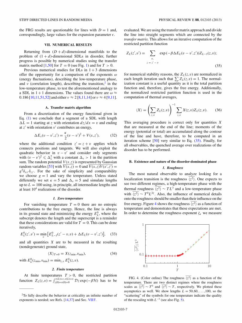
The most natural observable to analyze looking for alocalization transition is the roughness 〈z2〉. One expects tosee two different regimes, a high-temperature phase with thethermal roughness 〈z2〉 ∼ T L3 and a low-temperature phasewith 〈z2〉 ∼ T 0L2ζ . Also, the influence of numerical detailsonto the roughness should be smaller than their influence on thefree energy. Figure 4 shows the roughness 〈z2〉 as a function oftemperature and demonstrates that these expectations are met.In order to determine the roughness exponent ζκ we measure

0.1

1

0.1 1 10T

〈 z2〉 /

L3

FIG. 4. (Color online) The roughness 〈z2〉 as a function of thetemperature. There are two distinct regimes where the roughnessscales as 〈z2〉 ∼ T 0 and 〈z2〉 ∼ T , respectively. We plotted theseasymptotics as well. We show lengths L = 50,60, . . . ,100, so the“scattering” of the symbols for one temperature indicate the qualityof the rescaling with L−3 (see also Fig. 5).

012103-7

HORST-HOLGER BOLTZ AND JAN KIERFELD PHYSICAL REVIEW E 88, 012103 (2013)

2.98

3

3.02

3.04

3.06

3.08

3.1

3.12

0 1 2 3 4 5

2ζ κ

T

FIG. 5. (Color online) Roughness exponent 2ζκ for varioustemperatures, computed via (37). The deviation for high temperaturesfrom the analytical value 2ζ = 3 indicates numerical shortcomings;nonetheless, there is a clear “dip” at T ≈ 1.4, which we identify as thecritical temperature. For low temperatures, we find values consistentwith ω ≈ 0.11.

a “local” roughness exponent [18],

2ζ (L) = log5(z2(L)/z2(L/5)). (37)

The data for ζκ as a function of temperature presented in Fig. 5exhibits two distinct high- and low-temperature regimes anda significant “dip” of the local roughness exponent aroundT ≈ 1.4. This method of determining ζ gives better resultsthan fitting 〈z2〉(L).

Via the scaling relation (8), ω = 2ζκ − 3, we obtain theexponent ω from the roughness exponent ζκ . As in thecontext of DLs [54], it can be argued that ω should vanishat the disorder-induced localization transition, resulting in aroughness exponent ζκ = 3/2. This seems to hold, even thoughthe numerical value for high temperatures is slightly aboveζκ = 3/2. This is strong evidence for a phase transition atTc ≈ 1.4. For low temperatures, the values 2ζκ ≈ 3.11 giveω ≈ 0.11 according to Eq. (8), which is slightly lower thanω = 0.186, which is the literature value for DLs in 1 + 3dimensions [10,11,51,52].

2. Disorder-induced persistence length

The roughness is closely related to the averaged tangentdirections 〈v2〉 ≡ 〈(∂xz)2〉, which should scale as

〈v2〉 ∼ 〈z2〉/L2 ∼ L2(ζ−1) ∼ L1+ω. (38)

We define an effective disorder-induced persistence length Lp

for the SDL as the length scale at which the tangent fluctuationsbecome equal to 1,

〈v2〉(Lp) = 1. (39)

This generalized definition for the disordered system isconsistent with the standard definition for the persistencelength Lp of a thermally fluctuating SDL in the absence ofdisorder, where we expect 〈v2〉 ≈ L/Lp with Lp = βκ . Apartfrom numerical prefactors this gives the standard persistencelength of the WLC model, see Eq. (4), which is defined as thedecay length of tangent correlations.

In the low-temperature phase, we expect a disorder-dominated roughness and, therefore, temperature-independenttangent fluctuations 〈v2〉, which results in a temperature-

0.1

1

10

0. 0111

Lp

T

1

100

g0.1

Lp

101

FIG. 6. (Color online) The generalized persistence length Lp

according to Eqs. (39) and (43) as a function of the temperatureT (43). Lp matches its thermal value (solid line) for T > Tc and isreduced and approximately constant for T < Tc. Inset: Lp at T = 0versus the potential strength g. The Flory result Lp ∼ g−1 (dottedline), see Eq. (40), matches the data.

independent disorder-induced persistence length Lp ∼ β0.The line roughens in the low-temperature phase, which givesrise to a persistence length decrease as compared to thethermal persistence length Lp ∼ κ/kBT . From the Floryresult z ∼ (g/κ)2/(4+d)L7/(4+d) at low temperatures, we expectv ∼ (g/κ)2/(4+d)L(3−d)/(4+d) for the disorder-induced tangentfluctuations and

Lp ∼ (κ/g)2/(3−d) (40)

at low temperatures according to the criterion (39). For SDLsin 1 + 1 dimension, we expect Lp ∝ g−1.

To determine the generalized persistence length fromEq. (39) numerically, we used the tilt symmetry of the repli-cated Hamiltonian [55], according to which the “connected”average

〈v2〉 − 〈v〉2 ≈ L/βκ (41)

is independent of the disorder strength. Therefore, we can usea fit to the sample-to-sample tangent fluctuations of the form

〈v〉2(T ,L) = a(T )L1+ω′(T ), (42)

with an amplitude a(T ) and an exponent ω′(T ), which shouldagree with the free-energy exponent ω. We then can rewrite〈v2〉 as

〈v2〉 = 〈v2〉 − 〈v〉2 + 〈v〉2 = L/βκ + a(T )L1+ω′(T ) (43)

and determine Lp using Eq. (39). Our results for Lp areshown in Fig. 6. In the low-temperature phase for T < Tc ≈1.4, the persistence length becomes indeed disorder induced,i.e., almost independent of temperature and our results areconsistent with the above scaling result (40). We consider thisnondivergent persistence length at low temperatures also to beconsistent with previous results for the nondirected version ofthe SDL, the WLC in disorder [23]. In the high-temperaturephase, our results approach the standard thermal persistencelength Lp ∼ βκ .

The fit results for a(T ) and ω′(T ) are shown in Fig. 7. ForT < Tc our results are consistent with ω ≈ 0.186, which is theliterature value for DLs in 1 + 3 dimensions [10,11,51,52]. Infact, we get very similar results for Lp if we fix ω′(T ) = ω =0.186.

012103-8

STIFF DIRECTED LINES IN RANDOM MEDIA PHYSICAL REVIEW E 88, 012103 (2013)

0

0.05

0.1

0.15

0.2

0.25

0 1 2 3 4 5 6 7 8 9T

FIG. 7. (Color online) Parameters a(T ) (blue plus signs) andω′(T ) (red Xs) used in fitting 〈v〉2 [cf. Eq. (42)]. The latter vanishesaround, but not exactly at, T = Tc. The horizontal line correspondsto the literature value for DLs in 1 + 3 dimensions, ω = 0.186.

3. Derrida-Flyvbjerg singularities

One of the features expected in a disorder-dominated phaseare Derrida-Flyvbjerg singularities [15,56]. These are featuresof the statistical weights, here the normalized restrictedpartition w(z) = Z(z)/Z function for the SDL to end at aspecific point z. As the phase is disorder dominated, somecharacteristics of these weights should originate from merestatistics and the distribution used for the random potentialrather than details of the Hamiltonian involved. According toDerrida and Flyvbjerg, the distributions P1(w1) and P2(w2)of the largest and the second largest weight, respectively,should exhibit singularities at 1/n (n = 1,2,3, . . . ) in adisorder-dominated phase with a multivalley structure of phasespace [56]. For SDLs in disorder, we calculated the distributionof the value of the largest and the second-largest weightnumerically as shown in Fig. 8 and indeed find singularitiesat 1 and 1/2 for T < Tc. We are not able to clearly resolvehigher singularities at 1/n with n � 3, which might bedue to the underlying (Gaussian) distribution or the numberof samples used. Analogous singularities can be found inthe distribution of the information entropy s = −∑

z w ln w

at values − ln(1), − ln(2), − ln(3), whereas nothing similarcan be observed at high temperatures, where the entropydistribution is Gaussian and the distribution of the (second)largest weight is sharply peaked around zero. We see this as a

10−4

10−3

10−2

10−1

100

101

102

1 1.5 2 2.5 3 3.5 4 4.5 5X

P (w1 = 1/X)P (w2 = 1/X)

P (s = − lnX)

FIG. 8. (Color online) Distribution of the largest (w1, light greensolid line) and second-largest (w2, blue dashed line) statistical weightw(z) = Z(z)/Z and the information entropy s = −∑

z w(z) ln w(z)(black solid line).

00.020.040.060.080.1

0.120.140.16

0 1 2 3 4 5 6 7 8 9

ω( T

)

T

FIG. 9. (Color online) Fluctuation exponent ω determined by thefree-energy fluctuations.

confirmation that the SDL indeed undergoes a transition to adisorder-dominated phase at Tc ≈ 1.4.

C. The free-energy distributions of SDL in 1 + 1 andDL in 1 + 3 dimensions are identical

The exponent ω can alternatively be determined ina more direct way by fitting F = (F 2 − F 2)1/2 ∝ Lω

at temperatures T � Tc, giving values of ω ≈ 0.15–0.16(cf. Fig. 9).

We can go one step further and consider not only the secondmoment but the whole distribution of the free energy as shownin Fig. 10, which is obtained by computing the free energy forevery sample and rescaling to zero mean and unit variance,

GF (X) = Prob((F − F )/F = X). (44)

This rescaling should make GF more robust against theinfluence of numerical details. For DLs in d = 1 it hasbeen found that this distribution is of a universal form [57].The asymptotic behavior of the negative tail of the rescaledfree-energy distribution for low temperatures is of the form

ln GF (X) ∼ −|X|η (X < 0,|X| � 1). (45)

This allows us to determine the energy fluctuation exponent ω

via the Zhang argument [1,11,13]: A saddle-point integrationgives ln Zn ∼ −nF/T − (nF/T )η/(η−1); on the other hand,

SDL, d = 1

DL, d = 3η ≈ 1.23

−4

−3

−2

−1

0

−4 −3 −2 −1 0 1 2 3x

Gaussian

log 1

0G

F(x

)

T > Tc

T = 0T < Tc

T ≈ Tc

T < Tc

FIG. 10. (Color online) Rescaled GF (X) = P [(F − F )/F ]free-energy distribution for a stiff directed line (SDL) in 1 + 1dimensions. We show distributions for T = 0 [light (blue) squares,ground-state energy] as well as for three finite temperatures, T < Tc

(black thin solid line), T ≈ Tc (red, thicker solid line), and T > Tc

(green, light thin solid line). Results for a directed line (DL) in 1 + 3dimensions are shown (dark circles).

012103-9

HORST-HOLGER BOLTZ AND JAN KIERFELD PHYSICAL REVIEW E 88, 012103 (2013)

ln Zn ∼ L should be extensive, resulting in F ∼ L1−1/η or

η = (1 − ω)−1. (46)

We find η ≈ 1.23 (dashed black line in Fig. 10) or ω ≈ 0.18.This is in agreement with the values reported for DLs in 1 + 3dimensions.

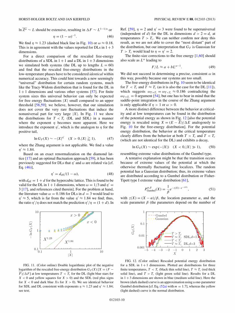
For a direct comparison of the rescaled free-energydistributions of a SDL in 1 + 1 and a DL in 1 + 3 dimensionswe simulated both systems (the DL up to lengths L = 60)and find that the rescaled free-energy distributions in thelow-temperature phases have to be considered identical withinnumerical accuracy. This could hint towards a new seemingly“universal” distribution for certain random systems, muchlike the Tracy-Widom distribution that is found for the DL in1 + 1 dimensions and various other systems [57]. For finitesystem sizes this universal behavior can only be expectedfor free energy fluctuations |X| small compared to an upperthreshold [58,59]; we believe, however, that our simulationdoes not cover the very rare fluctuations that induce thenonuniversal part for very large |X|. In Fig. 11 we showthe distributions for T < Tc (DL and SDL) in a mannerwhere the exponent η becomes more apparent. Here weintroduce the exponent η′, which is the analogon to η for thepositive tail,

ln GF (X) ∼ −|X|η′(X > 0,|X| � 1), (47)

where the Zhang argument is not applicable. We find a valueη′ ≈ 1.84.

Based on an exact renormalization on the diamond lat-tice [17] and an optimal fluctuation approach [59], it has beenpreviously suggested for DLs that η′ and ω are related via [cf.Eq. (46)],

η′ = deff/(1 − ω), (48)

with deff = 1 + d for the hypercubic lattice. This is found to bevalid for the DL in 1 + 1 dimensions, where ω = 1/3 and η′ =3 [17], and references cited therein]. For the problem at hand,the literature value ω = 0.186 for DLs in d = 3 would lead toη′ ≈ 5, which is far from the value η′ ≈ 1.84 we find; thus,the ratio η′/η does not match the prediction η′/η = (1 + d). In

x < 0

x > 0

X1.84X1.23

0.1

1

10

0.1 1 10

−ln

GF

(X)

|X|

FIG. 11. (Color online) Double logarithmic plot of the negativelogarithm of the rescaled free-energy distribution GF (X) [X = (F −F )/F ] at low temperatures T < Tc for the DL (light blue stars forX < 0 and yellow squares for X > 0) and the SDL (red plus signsfor X < 0 and dark blue Xs for X > 0). We see identical behaviorfor SDL and DL consistent with exponents η ≈ 1.23 and η′ ≈ 1.84;see text.

Ref. [59], η = 2 and η′ = 3 were found to be superuniversal(independent of d) for the DL in dimensions d > 2 = dc attemperatures T > Tc. We can neither confirm nor deny thisresult, as we are not able to cover the “most distant” part ofthe distribution, but our interpretation that GF is Gaussian forT > Tc would lead to η = η′ = 2.

The finite-size corrections to the free energy [1,60] shouldalso scale as Lω leading to

F/L ≈ a + bLω−1. (49)

We did not succeed in determining a precise, consistent ω inthis way, possibly because our systems are too small.

The free-energy distributions in Fig. 10 seem to be identicalfor T < Tc and T ≈ Tc (as it is also the case for the DL [11]),which suggests ωT =Tc

= ωT <Tc≈ 0.186 contradicting the

ωT =Tc= 0 argument [54], but one has to bear in mind that the

saddle-point integration in the course of the Zhang argumentis only applicable if η > 1 or ω > 0.

A more distinct difference between the behavior at critical-ity and at low temperatures can be found in the distributionof the potential energy as shown in Fig. 12 [also the potentialenergy is rescaled using X = (E − E)/E analogously toFig. 10 for the free-energy distribution]. For the potentialenergy distribution, the behavior at the critical temperatureclearly differs from the behavior at both T > Tc and T < Tc

(which are not identical for the DL) and exhibits a decay,

ln GE(X) ∼ exp (−|X|) (X < 0,|X| � 1), (50)

resembling extreme value distributions of the Gumbel type.A tentative explanation might be that the transition occurs

because of extreme values of the potential at which theotherwise thermally fluctuating line localizes. The randompotential has a Gaussian distribution; thus, its extreme valuesare distributed according to a Gumbel distribution or Fisher-Tipett type I extreme value distribution [61],

Pα,β

Gumbel(X) = 1

βe−z(X)−e−z(X)

, (51)

with z(X) = (X − α)/β, the location parameter α, and thescale parameter β (the parameters depend on the number of

SDL,d=1

DL,d=3

Gaussian

0.001

0.01

0.1

1

−5 −4 −3 −2 −1 0 1 2 3

GE

( X)

X

Gumbel

T ≈ Tc

T ≈ Tc

T < Tc

T > Tc

FIG. 12. (Color online) Rescaled potential energy distributionfor a SDL in 1 + 1 dimensions. Plotted are distributions for threefinite temperatures, T < Tc (black thin solid line), T ≈ Tc (red thicksolid line), and T > Tc (light green solid line). Results for a DLin 1 + 3 dimensions are shown in blue (medium solid line). Here thebrown (dark dashed) curve is an approximation using a one-parameterGumbel distribution [cf. Eq. (52a) with m = 1.7], whereas the yellow(light dashed) curve is the normal distribution.

012103-10

STIFF DIRECTED LINES IN RANDOM MEDIA PHYSICAL REVIEW E 88, 012103 (2013)

“trials”). The distribution of the potential energy at the criticaltemperature might be of a similar shape. As we are studyingthe rescaled distribution of the potential energy, which has zeromean and unit variance, we can use a one-parameter versionof the Gumbel distribution,

gm(X) = ψ1(m)mm

�(m)exp [hm(X) − ehm(X)]

m, (52a)

with the shape parameter m, the abbreviationhm(X) ≡ (X + ψ(m))ψ1(m) − ln m, (52b)

and the usual �(m) = ∫ ∞0 dt tm−1e−t (gamma function),

ψ(m) = d ln �(m)/dm (digamma function), and ψ1(m) =d2 ln �(m)/dm2 (trigamma function) [62]. This distributioninherently features the correct decay at the tails, with ln gm(X)decreasing faster than algebraic for X < 0 and linearly withslope mψ1(m) for X > 0. However, our best approximation tothe data with m = 1.7 deviates for X > 0. It is remarkablethat the potential energy distribution is well described byan extreme value distribution only right at the transition atT = Tc, whereas it approaches a Gaussian not only for T > Tc

but also for T < Tc; see Fig. 12. The Gaussian distribution atlow temperatures might stem from the Gaussian distributionused in the realization of the disorder potential.

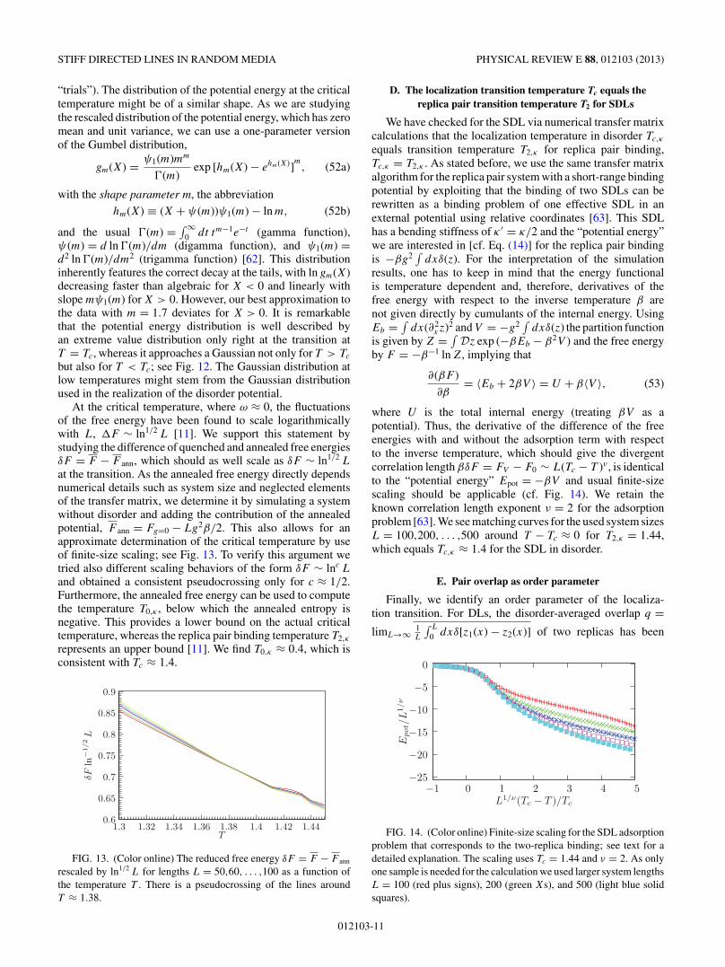
At the critical temperature, where ω ≈ 0, the fluctuationsof the free energy have been found to scale logarithmicallywith L, F ∼ ln1/2 L [11]. We support this statement bystudying the difference of quenched and annealed free energiesδF = F − F ann, which should as well scale as δF ∼ ln1/2 L

at the transition. As the annealed free energy directly dependsnumerical details such as system size and neglected elementsof the transfer matrix, we determine it by simulating a systemwithout disorder and adding the contribution of the annealedpotential, F ann = Fg=0 − Lg2β/2. This also allows for anapproximate determination of the critical temperature by useof finite-size scaling; see Fig. 13. To verify this argument wetried also different scaling behaviors of the form δF ∼ lnc L

and obtained a consistent pseudocrossing only for c ≈ 1/2.Furthermore, the annealed free energy can be used to computethe temperature T0,κ , below which the annealed entropy isnegative. This provides a lower bound on the actual criticaltemperature, whereas the replica pair binding temperature T2,κ

represents an upper bound [11]. We find T0,κ ≈ 0.4, which isconsistent with Tc ≈ 1.4.

0.6

0.65

0.7

0.75

0.8

0.85

0.9

1.3 1.32 1.34 1.36 1.38 1.4 1.42 1.44

δFln

−1/2L

T

FIG. 13. (Color online) The reduced free energy δF = F − F ann

rescaled by ln1/2 L for lengths L = 50,60, . . . ,100 as a function ofthe temperature T . There is a pseudocrossing of the lines aroundT ≈ 1.38.

D. The localization transition temperature Tc equals thereplica pair transition temperature T2 for SDLs

We have checked for the SDL via numerical transfer matrixcalculations that the localization temperature in disorder Tc,κ

equals transition temperature T2,κ for replica pair binding,Tc,κ = T2,κ . As stated before, we use the same transfer matrixalgorithm for the replica pair system with a short-range bindingpotential by exploiting that the binding of two SDLs can berewritten as a binding problem of one effective SDL in anexternal potential using relative coordinates [63]. This SDLhas a bending stiffness of κ ′ = κ/2 and the “potential energy”we are interested in [cf. Eq. (14)] for the replica pair bindingis −βg2

∫dxδ(z). For the interpretation of the simulation

results, one has to keep in mind that the energy functionalis temperature dependent and, therefore, derivatives of thefree energy with respect to the inverse temperature β arenot given directly by cumulants of the internal energy. UsingEb = ∫

dx(∂2x z)2 and V = −g2

∫dxδ(z) the partition function

is given by Z = ∫Dz exp (−βEb − β2V ) and the free energy

by F = −β−1 ln Z, implying that

∂(βF )

∂β= 〈Eb + 2βV 〉 = U + β〈V 〉, (53)

where U is the total internal energy (treating βV as apotential). Thus, the derivative of the difference of the freeenergies with and without the adsorption term with respectto the inverse temperature, which should give the divergentcorrelation length βδF = FV − F0 ∼ L(Tc − T )ν , is identicalto the “potential energy” Epot = −βV and usual finite-sizescaling should be applicable (cf. Fig. 14). We retain theknown correlation length exponent ν = 2 for the adsorptionproblem [63]. We see matching curves for the used system sizesL = 100,200, . . . ,500 around T − Tc ≈ 0 for T2,κ = 1.44,which equals Tc,κ ≈ 1.4 for the SDL in disorder.

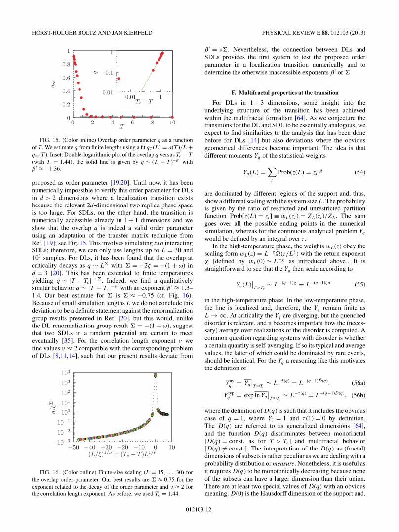
E. Pair overlap as order parameter

Finally, we identify an order parameter of the localiza-tion transition. For DLs, the disorder-averaged overlap q =limL→∞ 1

L

∫ L

0 dxδ[z1(x) − z2(x)] of two replicas has been

−25

−20

−15

−10

−5

0

−1 0 1 2 3 4 5

Epot/L

1/ν

L1/ν(Tc − T )/Tc

FIG. 14. (Color online) Finite-size scaling for the SDL adsorptionproblem that corresponds to the two-replica binding; see text for adetailed explanation. The scaling uses Tc = 1.44 and ν = 2. As onlyone sample is needed for the calculation we used larger system lengthsL = 100 (red plus signs), 200 (green Xs), and 500 (light blue solidsquares).

012103-11

HORST-HOLGER BOLTZ AND JAN KIERFELD PHYSICAL REVIEW E 88, 012103 (2013)

0

0.2

0.4

0.6

0.8

1

0 2 4 6 8 10T

0.01

0.1

1

1Tc − T

0.01

q ∞

q

FIG. 15. (Color online) Overlap order parameter q as a functionof T . We estimate q from finite lengths using a fit qT (L) = a(T )/L +q∞(T ). Inset: Double-logarithmic plot of the overlap q versus Tc − T

(with Tc = 1.44), the solid line is given by q ∼ (Tc − T )−β ′with

β ′ ≈ −1.36.

proposed as order parameter [19,20]. Until now, it has beennumerically impossible to verify this order parameter for DLsin d > 2 dimensions where a localization transition existsbecause the relevant 2d-dimensional two replica phase spaceis too large. For SDLs, on the other hand, the transition isnumerically accessible already in 1 + 1 dimensions and weshow that the overlap q is indeed a valid order parameterusing an adaptation of the transfer matrix technique fromRef. [19]; see Fig. 15. This involves simulating two interactingSDLs; therefore, we can only use lengths up to L = 30 and103 samples. For DLs, it has been found that the overlap atcriticality decays as q ∼ L� with � = −2ζ = −(1 + ω) ind = 3 [20]. This has been extended to finite temperaturesyielding q ∼ |T − Tc|−ν� . Indeed, we find a qualitativelysimilar behavior q ∼ |T − Tc|−β ′

with an exponent β ′ ≈ 1.3–1.4. Our best estimate for � is � ≈ −0.75 (cf. Fig. 16).Because of small simulation lengths L we do not conclude thisdeviation to be a definite statement against the renormalizationgroup results presented in Ref. [20], but this would, unlikethe DL renormalization group result � = −(1 + ω), suggestthat two SDLs in a random potential are certain to meeteventually [35]. For the correlation length exponent ν wefind values ν ≈ 2 compatible with the corresponding problemof DLs [8,11,14], such that our present results deviate from

10−3

10−2

10−1

100

101

102

103

104

−50 −40 −30 −20 −10 0 10

q/ξΣ

(L/ξ)1/ν = (Tc − T )L1/ν

FIG. 16. (Color online) Finite-size scaling (L = 15, . . . ,30) forthe overlap order parameter. Our best results are � ≈ 0.75 for theexponent related to the decay of the order parameter and ν ≈ 2 forthe correlation length exponent. As before, we used Tc = 1.44.

β ′ = ν�. Nevertheless, the connection between DLs andSDLs provides the first system to test the proposed orderparameter in a localization transition numerically and todetermine the otherwise inaccessible exponents β ′ or �.

F. Multifractal properties at the transition

For DLs in 1 + 3 dimensions, some insight into theunderlying structure of the transition has been achievedwithin the multifractal formalism [64]. As we conjecture thetransitions for the DL and SDL to be essentially analogous, weexpect to find similarities to the analysis that has been donebefore for DLs [14] but also deviations where the obviousgeometrical differences become important. The idea is thatdifferent moments Yq of the statistical weights

Yq(L) =∑

i

Prob(z(L) = zi)q (54)

are dominated by different regions of the support and, thus,show a different scaling with the system size L. The probabilityis given by the ratio of restricted and unrestricted partitionfunction Prob[z(L) = zi] ≡ wL(zi) = ZL(zi)/ZL. The sumgoes over all the possible ending points in the numericalsimulation, whereas for the continuous analytical problem Yq

would be defined by an integral over z.In the high-temperature phase, the weights wL(z) obey the

scaling form wL(z) = L−χ�(z/Lζ ) with the return exponentχ [defined by wL(0) ∼ L−χ as introduced above]. It isstraightforward to see that the Yq then scale according to

Yq(L)∣∣T >Tc

∼ L−(q−1)χ = L−(q−1)ζd (55)

in the high-temperature phase. In the low-temperature phase,the line is localized and, therefore, the Yq remain finite asL → ∞. At criticality the Yq are diverging, but the quencheddisorder is relevant, and it becomes important how the (neces-sary) average over realizations of the disorder is computed. Acommon question regarding systems with disorder is whethera certain quantity is self-averaging. If so its typical and averagevalues, the latter of which could be dominated by rare events,should be identical. For the Yq a reasoning like this motivatesthe definition of

Y avq = Yq

∣∣T ≈Tc

∼ L−τ (q) = L−(q−1)D(q), (56a)

Y typq = exp ln Yq

∣∣T ≈Tc

∼ L−τ (q) = L−(q−1)D(q), (56b)

where the definition of D(q) is such that it includes the obviouscase of q = 1, where Y1 = 1 and τ (1) = 0 by definition.The D(q) are referred to as generalized dimensions [64],and the function D(q) discriminates between monofractal[D(q) = const. as for T > Tc] and multifractal behavior[D(q) �= const.]. The interpretation of the D(q) as (fractal)dimensions of subsets is rather peculiar as we are dealing with aprobability distribution or measure. Nonetheless, it is useful asit requires D(q) to be monotonically decreasing because noneof the subsets can have a larger dimension than their union.There are at least two special values of D(q) with an obviousmeaning: D(0) is the Hausdorff dimension of the support and,

012103-12

STIFF DIRECTED LINES IN RANDOM MEDIA PHYSICAL REVIEW E 88, 012103 (2013)

D(q)

D(q)

ζth = 3/2

0.20.40.60.8

11.21.41.61.8

2

0 2 4 6 8 10 12 14 16 18 20q

FIG. 17. (Color online) Generalized dimensions D(q) and D(q)at criticality T = Tc,κ . The dashed line is DT >Tc

= 3/2. Solid linesare monomial fits for large q, see text.

thus, directly related to the geometry of the system3 and D(1) iscalled the information dimension as it appears like a dimensionin the Shannon information entropy,

s = −∑

i

w(zi) ln w(zi) = − ∂qYq

∣∣q=1 ≈ D(1) ln L. (57)

However, D(1) cannot be computed directly (Y1 ≡ 1) but onlyas an analytic continuation of D(q). A measure is called fractalif and only if D(0) > D(1) [65].

In Fig. 17, we present numerical results for D(q) andD(q) for a SDL in disorder at criticality. As a controlfor the numerics one can use the information dimensionD(1), which should coincide with its high-temperature valueD(1)|T >Tc

= χ = ζd = 3/2 at criticality. The data appear toresemble the Anderson transition-like scenario that has beenreported for the DL [14] with D(q) = D(q) for q < q∗ ≈1.5. The separation of D(q) and D(q) indicates differentbehaviors of typical and average values of Yq>q∗, from whichone is tempted to conclude that these quantities are notself-averaging. Furthermore, both Y av

q and Ytypq are diverging

faster than exponential for q < 0, which leads to D(q < 0) =D(q < 0) = ∞. The information dimension D(1) is measuredto be about 1.4 and, therefore, does not coincide with theexpected high-temperature value 3/2. However, this could bea numerical artifact from limited system sizes.

For Anderson transitions, the finite-size scaling of the Yq atcriticality does involve the multifractal spectrum but only onecorrelation length exponent ν [11,66],

Yq = L−τ (q)f [(Tc − T )L1/ν]. (58)

Thus, it allows for a completely independent validation (cf.Fig. 18) of the critical temperature and the correlation lengthexponent, yielding a more exact value Tc ≈ 1.44 compatiblewith our result from Secs. VII B and VII D and, unambigu-ously, a value 1/ν ≈ 0.5 for the correlation length exponent.

3The Hausdorff dimensions for the measures related to DLs andSDLs with d transverse dimensions are Dτ (0) = d and Dκ (0) = 2d

(z and v = ∂xz), respectively, which gives Dτ (0) = 3 for DLs in 1 + 3dimensions and Dκ (0) = 2 for SDLs in 1 + 1 dimensions.

Y2L

τ(2

)

L1/ν(Tc − T )/Tc

0.1

1

10

100

−70 −60 −50 −40 −20 −10 0 10 20−30

FIG. 18. (Color online) Finite-size scaling Y2Lτ (2)[(Tc −

T )/TcL1/ν] giving ν = 2 and Tc = 1.41429 for lengths L =

20,30, . . . ,100, the points for L = 100 are interconnected by a line asa visual guidance. This does not work for the alternatively proposedvalue ν = 4. For T < Tc, Y2 remains finite for large L and, therefore,the finite-size scaling observable diverges as Lτ (2).

An equivalent description of the multifractal nature isrelated to the Legendre transform f (α) of τ (q) given by

q = f ′(α), (59a)

τ (q) = αq − f (α). (59b)

The function f (α) is called the singularity spectrum, becauseit gives the number N (α) ∼ Lf (α) of points z, where theweight w(z) has a singularity w ∼ L−α . A Legendre transformof the measured τ (q) and τ (q) would require an analyticalcontinuation and, thus, be very error prone. Fortunately, it ispossible to directly measure α(q) and f (q) [67] and, thus, thesingularity spectrum f (α) parametrically:

f (q) = − limL→∞

∑i

μ(q,zi) ln μ(q,zi)/ ln L, (60a)

α(q) = − limL→∞

∑i

μ(q,zi) ln w(zi)/ ln L, (60b)

with

μ(q,zi) ≡ wq(zi)/

⎛⎝∑

j

wq(zj )

⎞⎠ . (60c)

This method of computing f (α) gives the Legendre transformof τ (q), because Eq. (59) implies (omitting the limits)

τ (q) = α(q)q − f (q)

= −ln∑

i

wq(zi)/ ln L

= −ln Yq(L)/ ln L, (60d)

in agreement with Eq. (56b), and, therefore, f (α) corre-sponds to typical values of Yq . Note that α(q) = τ ′(q) isfulfilled by construction. This is the common definition ofthe (multifractal) singularity spectrum that is also applicablefor nondisordered systems.

Here disorder is relevant and we need to capture not only thetypical but also the (differing, cf. Fig. 17) average behaviors.Analogously to Eq. (60), we derive the following computationof the Legendre transform f (α) of τ (q) (we distinguish

012103-13

HORST-HOLGER BOLTZ AND JAN KIERFELD PHYSICAL REVIEW E 88, 012103 (2013)

−2.5−2

−1.5−1

−0.50

0.51

1.52

0 1 2 3 4 5

bisector

f(α)

f(α)

FIG. 19. (Color online) The singularity spectrum f (α); seeEq. (60). For a better comparison with the expectations the plot alsoshows lines corresponding to f (α) = D(2) = 2, f (α) = D(1), andf (α) = α; see text. The bisector and f (α) touch at an α that is slightlysmaller than α = 1.5. We consider this to be wrong, but it is consistentwith the determined generalized dimensions; see also Fig. 20.

between α and α to avoid ambiguities as both are directlymeasured). We use Eq. (56) and the inverse transform of (59)

τ (q) = − ln∑

i

wq(zi)/ ln L, (61a)

α(q) = τ ′(q)

= −∑

i

wq(zi) ln w(zi)/(ln L∑

i

wq(zi)), (61b)

f (α) = αq − τ (q)

= −∑

i

wq(zi)(ln wq(zi)/∑

j

wq(zj ) − 1)/ ln L.

(61c)

The spectrum f (α) is shown in Fig. 19. Its shape matchesthe expectations that origin from general properties and theknown results for the DL [14] and is consistent with theresults for the Legendre transform τ (q). Our results showthat f (α) is a monotonic function starting at a finite αmin =Dmin(q) ≈ 0.8, which is close to the DL value αmin

τ ≈ 0.77and ending at αmax = ∞, which corresponds to the infinitelylarge values τ (q) for q < 0. The maximum value of f (α)is f (α → ∞) → D(0) and it touches the bisector f = α

around α = D(1) ≈ 1.4, thus confirming the previously founddeviation D(1) �= 3/2. We see no indication that f (α) becomes

f(q)

α(q)

0

0.5

1

1.5

2

2.5

3

3.5

0 2 4 6 8 10 12 14q

FIG. 20. (Color online) The directly measurable α(q) (green) andf (q) (red) from which Fig. 19 was created. The contact point is atα = f (α) ≈ 1.4.

negative somewhere, which would describe rare events (num-ber decreases exponentially in L), but this is to be expectedas f (α) contains the typical behavior and should not becomenegative [14]. The average behavior that leads to f (α) doesinclude rare events and does not seem to have a finite αmin,implying D(∞) = 0. We back this by noting that the we canachieve a good fit of the data for τ (q) and τ (q) at large q (weused 5 < q < 20) with an monomial Ansatz f (q) = aqb. Foran approximate analysis we round b to one decimal, giving

τ (q � 1) ≈ aq, (62)

τ (q � 1) ≈ aq2/5, (63)

with some constants a,a. We apply the Legendre transformand get for q � 1

α(q) ≈ a ≈ 0.81 f (α) ≈ 0α(q) ∼ q−3/5 → 0 f (α) ∼ −α−2/3 → −∞.

In summary, we see a (Anderson transition-like) scenarioin the multifractal analysis of the localization transition of aSDL in 1 + 1 dimensions which is very similar to the findingsin Ref. [14] for a DL in 1 + 3 dimensions despite obviousdifferences due to the different geometry. In particular, themultifractal structure of the statistical weights differs betweentypical and average values both for DLs and SDLs. Thisbecomes apparent in the generalized dimensions D(q),D(q),which differ for q � 1.5. We also find a matching criticalcorrelation length exponent ν. Additionally, we showed thatthe average behavior is significantly influenced by rare events,leading to negative values in f , the Legendre transform ofD(q). The significance of rare (extreme) events at criticality isin accordance with our findings for the energy distribution.

VIII. CONCLUSION

We studied SDLs in 1 + d dimensions subject to quenchedshort-range random potential analytically and numerically.Using Flory-type scaling arguments and a replica calculation,we show that, in dimensions d > 2/3, a localization transitionexists from a high-temperature phase, where the system isessentially annealed, to a disorder-dominated low-temperaturephase. The low-temperature phase is characterized by largefree-energy fluctuations with an exponent ω > 0 and a rough-ness exponent ζ , which slightly exceeds the thermal valueζth = 3/2 for a SDL. Flory arguments suggest ζ = 7/(4 + d)for a SDL. Both exponents are related by ω = 2ζ − 3.

We find a reduction of the persistence length of a stiffdirected line by disorder. In the low-temperature phase,the persistence length is disorder induced and temperatureindependent.

We also performed variational replica FRG calculations.The replica approach gives no conclusive results on theexponents for d > 2/3 but supports the existence of a localiza-tion transition. The FRG calculation is performed for D + d

dimensional manifolds governed by bending energies withthe SDL corresponding to D = 1 and employs an expansionin ε = 8 − D dimensions. For a SDL in 1 + d dimensions,the FRG result suggests the existence of an upper criticaldimension du < 1, which we can rule out by numericalcalculations.

012103-14

STIFF DIRECTED LINES IN RANDOM MEDIA PHYSICAL REVIEW E 88, 012103 (2013)

Tc = T2

continuous discontinuouspair transition

dc

dominateddisorder

thermal

dτ , DLdκ, SDL

g/T

432024

31230

1

FIG. 21. Schematic summary of our results supporting a relationbetween DLs in 1 + 3d and SDLs in 1 + d dimensions and theimportance of replica pair interactions for the localization transitionin a random potential.

For the SDL in 1 + 1 dimensions we performed extensivenumerical transfer matrix calculations and find the existenceof a localization transition and an exponent ω ≈ 0.18 in thelow-temperature disorder-dominated phase. The value forω is close to the established value ω ≈ 0.186 for directedlines (DLs) under tension in 1 + 3 dimensions. Moreover, therescaled free-energy distributions are identical. Both pointssuggest that the nature of the low-temperature phase is verysimilar, if not identical.

The multifractal analysis reveals a very similar structureof the statistical weights at the critical temperature for DLs in1 + 3 dimensions and SDLs in 1 + 1 dimensions. It also allowsfor a determination of the correlation length exponent ν, forwhich we find, again in accordance with the findings for a DLin 1 + 3 dimensions, ν = 2. Additionally, we find evidence forthe relevance of rare events at criticality.

This strongly supports a relation between DLs in 1 + 3d andSDLs in 1 + d dimensions, which is based on identical returnexponents χ for two replicas to meet. The validity of a relationbased on properties of a single replica pair suggests that thecritical properties of DLs in a short-range random potential aregoverned by replica pair interactions. The mapping can makeDL transitions in high dimensions computationally accessible,which we demonstrated in showing that the two-replica overlapprovides a valid order parameter across the localization transi-tion of SDLs in 1 + 1 dimensions. Furthermore, the importanceof pair interactions suggests that the critical temperature forDLs in random potentials is indeed identical to the temperaturebelow which the ratio of the second moment of the partitionfunction and the square of its first moment diverges, whichimplies that the localization transition temperature Tc in arandom potential equals the replica pair transition temperatureT2 for replica pair binding. The equality T2 = Tc has beenoriginally put forward and verified numerically for DLs in1 + 3 dimensions [11,14]. Using the numerical transfer matrixapproach, we could verify this conjecture also for SDLs in1 + 1 dimensions. Our findings are summarized schematicallyin Figs. 2 and 21.

The binding transition of DL pairs becomes discontinuousfor d > 4 and, analogously, the binding of SDL pairs ford > 4/3 [28,63]. Because DLs in random potentials areequivalent to the KPZ equation [2], the validated relationto the SDL suggests that the roughening transition of theKPZ problem could acquire similar discontinuous featuresfor d > 4 dimensions. Thus, d = 4 would remain a specialdimension, although it is not the upper critical dimension [68].

ACKNOWLEDGMENTS

We acknowledge financial support by the DeutscheForschungsgemeinschaft (KI 662/2-1).

[1] T. Halpin-Healy and Y. Zhang, Phys. Rep. 254, 215 (1995).[2] M. Kardar, G. Parisi, and Y. C. Zhang, Phys. Rev. Lett. 56, 889

(1986).[3] J. Krug, Adv. Phys. 46, 139 (1997).[4] G. Blatter, M. V. Feigelman, V. B. Geshkenbein, A. I. Larkin,

and V. M. Vinokur, Rev. Mod. Phys. 66, 1125 (1994).[5] T. Nattermann and S. Scheidl, Adv. Phys. 49, 607 (2000).[6] P. J. Yunker, M. A. Lohr, T. Still, A. Borodin, D. J. Durian, and

A. G. Yodh, Phys. Rev. Lett. 110, 035501 (2013).[7] J. Z. Imbrie and T. Spencer, J. Stat. Phys. 52, 609 (1988).[8] B. Derrida and O. Golinelli, Phys. Rev. A 41, 4160 (1990).[9] J. M. Kim, A. J. Bray, and M. A. Moore, Phys. Rev. A 44, R4782

(1991).[10] J. M. Kim, M. A. Moore, and A. J. Bray, Phys. Rev. A 44, 2345

(1991).[11] C. Monthus and T. Garel, Eur. Phys. J. B 53, 39 (2006).[12] C. Monthus and T. Garel, Phys. Rev. E 74, 011101 (2006).[13] C. Monthus and T. Garel, Phys. Rev. E 74, 051109 (2006).[14] C. Monthus and T. Garel, Phys. Rev. E 75, 051122 (2007).[15] C. Monthus and T. Garel, J. Stat. Mech.: Theory Exp. (2007)

P03011.

[16] C. Monthus and T. Garel, Markov Process. Related Fields 13,731 (2007).

[17] C. Monthus and T. Garel, J. Stat. Mech.: Theory Exp. (2008)P01008.

[18] M. Schwartz and E. Perlsman, Phys. Rev. E 85, 050103(R)(2012).

[19] M. Mezard, J. Phys. France 51, 1831 (1990).[20] S. Mukherji, Phys. Rev. E 50, R2407 (1994).[21] F. Comets, T. Shiga, and N. Yoshida, Bernoulli 9, 705 (2003).[22] A. Pagnani and G. Parisi, Phys. Rev. E 87, 010102(R) (2013).[23] A. Dua and T. Vilgis, J. Chem. Phys. 121, 5505 (2004).[24] A. Barabasi and H. E. Stanley, Fractal Concepts in Surface

Growth (Cambridge University Press, Cambridge, 1995).[25] S. Da Sarma, S. V. Ghaisas, and J. M. Kim, Phys. Rev. E 49, 122

(1994).[26] Z. Racz and M. Plischke, Phys. Rev. E 50, 3530 (1994).[27] R. Bundschuh, M. Lassig, and R. Lipowsky, Eur. Phys. J. E 3,

295 (2000).[28] J. Kierfeld and R. Lipowsky, J. Phys. A 38, L155 (2005).[29] H.-H. Boltz and J. Kierfeld, Phys. Rev. E 86, 060102(R) (2012).[30] R. A. Harris and J. E. Hearst, J. Chem. Phys. 44, 2595 (1966).

012103-15

HORST-HOLGER BOLTZ AND JAN KIERFELD PHYSICAL REVIEW E 88, 012103 (2013)

[31] O. Kratky and G. Porod, Recl. Trav. Chim. Pays-Bas 68, 1106(1949).

[32] H. Kleinert, Path Integrals in Quantum Mechanics, Statistics,Polymer Physics, and Financial Markets (World Scientific,Singapore, 2006).

[33] P. Gutjahr, R. Lipowsky, and J. Kierfeld, Europhys. Lett. 76,994 (2006).

[34] G. Gompper and T. W. Burkhardt, Phys. Rev. A 40, 6124 (1989).[35] M. E. Fisher, J. Stat. Phys. 34, 667 (1984).[36] R. Bundschuh and M. Lassig, Phys. Rev. E 54, 304 (1996).[37] S. Mukherji and S. M. Bhattacharjee, Phys. Rev. B 53, R6002

(1996).[38] D. S. Fisher and D. A. Huse, Phys. Rev. B 43, 10728

(1991).[39] A. Engel, Nucl. Phys. B 410, 617 (1993).[40] P. Le Doussal, K. J. Wiese, and P. Chauve, Phys. Rev. E 69,

026112 (2004).[41] V. Dotsenko, Introduction to the Replica Theory of Disordered

Statistical Systems (Cambridge University Press, Cambridge,2001).

[42] M. Mezard and G. Parisi, J. Phys. I 1, 809 (1991).[43] G. Parisi, J. Phys. A 13, 1887 (1980).[44] M. Kardar, Nucl. Phys. B 290, 582 (1987).[45] D. S. Fisher, Phys. Rev. Lett. 56, 1964 (1986).[46] L. Balents and D. S. Fisher, Phys. Rev. B 48, 5949 (1993).[47] P. Chauve, P. Le Doussal, and K. J. Wiese, Phys. Rev. Lett. 86,

1785 (2001).[48] P. Le Doussal, K. J. Wiese, and P. Chauve, Phys. Rev. B 66,

174201 (2002).[49] P. Le Doussal and K. J. Wiese, Phys. Rev. E 72, 035101(R)

(2005).

[50] X. Wang, S. Havlin, and M. Schwartz, J. Phys. Chem. B 104,3875 (2000).

[51] T. Ala-Nissila, T. Hjelt, J. M. Kosterlitz, and O. Venalainen,J. Stat. Phys. 72, 207 (1993).

[52] E. Marinari, A. Pagnani, and G. Parisi, J. Phys. A: Math. Gen.33, 8181 (2000).

[53] G. Marsaglia and W. W. Tsang, J. Stat. Soft. 5, 1 (2000).[54] C. A. Doty and J. M. Kosterlitz, Phys. Rev. Lett. 69, 1979 (1992).[55] T. Giamarchi and P. Le Doussal, Phys. Rev. B 52, 1242 (1995).[56] B. Derrida and H. Flyvbjerg, J. Phys. A: Math. Gen. 20, 5273

(1987).[57] V. S. Dotsenko, Phys.-Usp. 54, 259 (2011).[58] I. V. Kolokolov and S. E. Korshunov, Phys. Rev. B 75, 140201

(2007).[59] I. V. Kolokolov and S. E. Korshunov, Phys. Rev. B 78, 024206

(2008).[60] J. Krug and P. Meakin, J. Phys. A: Math. Gen. 23, L987 (1990).[61] E. J. Gumbel, Statistical Theory of Extreme Values and Some

Practical Applications, Applied Mathematics Series, Vol. 33(National Bureau of Standards, Washington, DC, 1954).

[62] M. Abramowitz and I. A. Stegun, Handbook of MathematicalFunctions, Applied Mathematics Series, Vol. 55 (NationalBureau of Standards, Washington, DC, 1972).

[63] J. Kierfeld and R. Lipowsky, Europhys. Lett. 62, 285 (2003).[64] M. H. Jensen, L. P. Kadanoff, and I. Procaccia, Phys. Rev. A 36,

1409 (1987)[65] T. Tel, Z. Naturfors. Teil A 43, 1154 (1988).[66] B. Huckestein, Rev. Mod. Phys. 67, 357 (1995).[67] A. Chhabra and R. V. Jensen, Phys. Rev. Lett. 62, 1327 (1989).[68] E. Marinari, A. Pagnani, G. Parisi, and Z. Racz, Phys. Rev. E

65, 026136 (2002).

012103-16