Goal Directed Dynamics

Emanuel TodorovUniversity of Washington and Roboti LLC

Abstract— We develop a general control framework wherea low-level optimizer is built into the robot dynamics. Thisoptimizer together with the robot constitute a goal directeddynamical system, controlled on a higher level. The highlevel command is a cost function. It can encode desiredaccelerations, end-effector poses, center of pressure, and otherintuitive features that have been studied before. Unlike thecurrently popular quadratic programming framework, whichcomes with performance guarantees at the expense of modelingflexibility, the optimization problem we solve at each time stepis non-convex and non-smooth. Nevertheless, by exploiting theunique properties of the soft-constraint physics model we haverecently developed, we are able to design an efficient solverfor goal directed dynamics. It is only two times slower thanthe forward dynamics solver, and is much faster than realtime. The simulation results reveal that complex movementscan be generated via greedy optimization of simple costs. Thisnew computational infrastructure can facilitate teleoperation,feature-based control, deep learning of control policies, andtrajectory optimization. It will become a standard feature infuture releases of the MuJoCo simulator.

I. INTRODUCTION

The motivation of this work is to improve robot autonomy,namely the ability to map high-level commands to suitablelow-level controls. This is generally what optimal controlaims to achieve, but it involves optimization through timewhich can be hard to solve. In contrast, our approach hereis instantaneous and greedy.

We define goal directed dynamics (GDD) as the dynamicsof a robot with a layer of control intelligence built into it;see Figure 1. Instead of sending a control signal to the robotat each point in time, we send a cost function. This functionis defined over accelerations, but later we show how it canalso encode spatial goals, desired contact forces, center-of-pressure targets etc. Once this function is specified, the robotdoes two things at each point in time: (i) find the controlsignal that minimizes the specified cost; (ii) apply this controlsignal to the usual dynamics. This simplifies teleoperationwhere a human can provide goals/costs interactively, as wellas facilitates the design of intuitive feature-based controllers.Optimal control also becomes easier when applied to the goaldirected dynamics instead of the usual robot dynamics; thisis because part of the problem is offloaded to the low-leveloptimizer.

Goal directed dynamics is the most general instance ofan intuitive approach which has a long history. The simplestspecial case is computed torque control: a reference trajec-tory specifies the desired acceleration at the current position

This work was supported by NSF grant 1602141 to Roboti LLC. Thanksto Yuval Tassa and Igor Mordatch for comments on the manuscript.

robot

optimizer

controlstate

humanoperator,or automaticcontroller state

cost

Goal DirectedDynamics

High LevelControl

Fig. 1. Illustration of the proposed framework. A human operator or ahigh-level controller sends goals encoded as cost functions. An optimizermaps these instantaneous goals to control signals. The optimizer togetherwith the robot constitute a goal directed dynamical system.

and velocity, and inverse dynamics are used to computethe necessary control force, assuming full actuation and noconstraints. Operational space control [1], [2] is also related.There one defines an end-effector and its correspondingJacobian, specifies goals in end-effector space, and usesthe Jacobian to construct various mappings between end-effector and joint space. Multiple Jacobian-based methodsinvolving differently weighted pseudo-inverses have beendeveloped [3]. That line of work has leveraged the factthat linear algebra and matrix factorization in particularcan be performed in real-time, and is still used today. Forexample, [4] approximate unilateral constraints with equalityconstraints and reduce the problem to linear algebra.

As computers become faster and numerical algorithmsbecome more efficient, new types of computational prob-lems become tractable in real-time. The current trend is toformulate control schemes that reduce to convex quadraticprograms (QP). This has been successful in quadrotor control[5]. It is also used in locomotion, where a QP can jointlycompute control torques and contact forces such that thecenter-of-mass accelerates according to some high-level planwhile the contact forces remain in the friction cone. Thecone is approximated with a pyramid whose faces becomelinear inequality constraints in the QP. Another application ismanipulation, where a QP can compute control torques andcontact forces that stabilize an object in the hand. Multiplevariations on this theme have recently been explored [6], [7],[8], [9]. There is however an important limitation in suchcontrol schemes: in order to keep the QP convex, the com-plementarity condition in the LCP formulation of frictionalcontact [13], [14] is ignored, or alternatively the frictioncomponents are ignored (recall that the LCP describingfrictional contact is equivalent to a non-convex QP which is

NP-hard). Because of this simplification, the solver is free tochoose any contact force in the friction cone, even if it is verydifferent from the actual contact force that results from thecontrol torques being applied. Thus treating contact forcesas independent decision variables (as in convex QP) makeslittle physical sense. Our framework removes this limitation,in a way that is numerically efficient. Note that if we arenot concerned with numerical efficiency, it is straightforwardto throw every desirable constraint into a general-purposeoptimizer and hope that it finds a reasonable solution ina reasonable amount of time. However such hope is notjustified in the general case of non-convex optimization.

A similar criticisms of the QP approach was recentlypresented in [12], and indeed that work is the most closelyrelated to ours in the Robotics literature. These authorsfocused on robots in multiple contacts with the environmentbut under static conditions. They took into account the actualcontact forces resulting from the control torques, using aspring-damper contact model, and were able to stabilize thesystem by solving a convex optimization problem. Howeverit is not clear how to extend this work to dynamic conditions,given that spring-damper contact models have well-knowndifficulties and have been largely superseded by modernlinear complementarity problem (LCP) solvers [13], [14].Our agenda here is related to [12] but the techniques aredifferent and apply to dynamic settings. This is possiblethanks to a new formulation of the physics of soft contactsdeveloped in [15], [16] and implemented in MuJoCo [17].It combines the stability and long time steps of LCP-typesolvers, with the softness and analytical advantages of spring-damper contacts.

As already alluded to, if we want to develop an instanta-neous control scheme that is more powerful than the currentQP-based schemes, we have no choice but to solve a harderoptimization problem in real-time. QPs are by no means thelimit of what modern computers can do. LCP-type solvers arean existence proof of this. Such solvers have been available inmultiple physics engines for over a decade, and the problemthey solve at each time step (albeit approximately) is anNP-hard non-convex optimization problem. While the softcontact model in [16] reduces to convex optimization inthe case of forward dynamics, the goal directed dynamicsdeveloped here require solving a non-convex optimizationproblem.

Related non-convex optimization problems have beenstudied in Computer Graphics, in the context of controllinghigh-level features [18], [19], [20], [21], [22]. These features(corresponding to goals in our terminology) are varied online,using either hand-crafted or numerically optimized high-levelcontrollers. The available optimization schemes however donot have robustness and performance comparable to the QPapproach. In general it is difficult to think of them as givingrise to a new dynamical system that can be readily simulatedin place of the usual forward dynamics. This is because theproblem is formulated as generic non-convex optimization,without special structure that can enable efficient solvers.Indeed the emphasis in that literature has been not so

much on efficient optimization, but rather on design of costfunctions whose instantaneous optimization yields interestingbehaviors. This is very much complementary to our work.Existing cost functions that are already known to work wellcan be plugged in our framework and work even better.

A. Alternative view: Combining physics and control

An alternative way to understand GDD is to think of itas combining physics and control in a single computation.This is appealing because forward dynamics, i.e. computingthe acceleration v̇ resulting from control force τ , alreadyrequire some form of numerical optimization when unilateralconstraints are present [13], [14], [16]:

v̇(τ) = argmina physics(a, τ)s.t. constraint(a, τ) (1)

One way to combine physics and control is to simplyadd a task-related term to the objective, and obtain boththe acceleration and the (one-step-optimal) control force bysolving a single optimization problem:

(v̇, τ) = argmina,t physics(a, t) + task(a, t)s.t. constraint(a, t) (2)

This is essentially what the QP approach does. The problemhowever is that the result is no longer consistent with thephysics. Instead, in GDD we start with nested optimizationwhich is physically-consistent by construction:

(v̇, τ) = argmina,t task(a, t)s.t. a = argminb physics(b, t)

s.t. constraint(b, t)(3)

Our key insight then is to exploit MuJoCo’s inverse dynamics– which enables us to avoid the above nested optimization,and yields an efficient yet physically-consistent GDD solver.

II. GENERAL FRAMEWORK

We begin with a general definition of GDD, and laterspecialize it to rich yet computationally-tractable systems.Consider the second-order system

configuration: q ∈ Rm

velocity: v ∈ Rn

applied force: τ = (u, z) ∈ Rn

control force: u ∈ U ⊆ Rk

root force: z ∈ Rn−k

forward dynamics: v̇ = f (q, v, u)

inverse dynamics: τ = g (q, v, v̇) = (gu, gz)

inertia matrix: M(q) ∈ Rn×n

(4)

The dimensionality n of the velocity and applied forcevectors equals the number of degrees of freedom (DOF).We assume for simplicity that actuators are in one-to-onecorrespondence with scalar joints, and partition the DOFspace into actuated (u) and unactuated (z) subspaces. This iswhat the bracket notation τ = (u, z) and g = (gu, gz) means.The more general approach would be to write τ = B(q, v)ufor a generic control gain matrix B. Our setup correspondsto B = (Ik×k 0k×(n−k))

T .

The time-derivative v̇ denotes the actual acceleration ofthe system. Below we will also use a to denote hypotheticalaccelerations, which are optimization variables in variouscost functions. The reason for using v instead of q̇ is becauseq is a point on the configuration manifold while v is a vectorin the tangent space to this manifold. The orientations offloating bases and free-moving objects are best representedwith quaternions, in which case dim(q) = 4 while dim(v) =3 per joint, and so m > n. When the system is under-actuated, we also have k < n. Most interesting systems havethese two properties. For example, a humanoid robot hasm = n + 1 and k = n − 6. The same holds for a fixed-base arm manipulating one object. For a humanoid robotmanipulating two objects, m = n+ 3 and k = n− 18.

An important assumption implicit in (4) is that the inversedynamics g(q, v, v̇) exist and are uniquely defined. This isnot the case for systems with hard state constraints. But as wewill see later, we can use soft constraints to obtain realisticbehavior with uniquely-defined inverse dynamics.

The set of admissible controls U is usually a box. The setof feasible accelerations A is more difficult to characterize.It can be defined through the forward dynamics:

A(q, v) = {a ∈ Rn : ∃u ∈ U s.t. f (q, v, u) = a} (5)

or through the inverse dynamics:

A(q, v) = {a ∈ Rn : gu(q, v, a) ∈ U , gz(q, v, a) = 0} (6)

These two definitions are mathematically equivalent. We willuse the latter to obtain efficient algorithms.

Let `(·) denote the scalar cost over accelerations used tospecify the instantaneous goal. The space of such functions isinfinite-dimensional, so we cannot directly use them as high-level controls, but we will choose suitable finite-dimensionalparameterizations later.

Now we can define the goal directed dynamics in twoways, using the forward dynamics or the inverse dynamics ofthe original system. Both definitions correspond to forwardGDD. They are mathematically equivalent, but again theinverse definition yields more efficient algorithms. In bothcases the state (q, v) as well as the cost `(·) are given, and weseek to define the goal directed acceleration v̇. The forwarddefinition is:

v̇ = f

(q, v, argmin

u∈U{‖(u, 0)‖R + ` (f (q, v, u))}

)(7)

while the inverse definition is:

v̇ = arg mina∈A(q,v)

{‖g (q, v, a)‖R + ` (a)} (8)

We have added a regularizing cost on the applied forces, inaddition to imposing actuation constraints. This regularizingcost is the weighted L2 norm

‖τ‖R ≡1

2τTRτ (9)

The weighting matrix R can in principle be any s.p.d.matrix. Here we use R =M−1. The rationale for weightingby the inverse inertia is to match units in mixed cost

functions penalizing both forces and accelerations. FromNewton’s second law f = ma we have f2m−1 = a2m,suggesting that forces should be weighted by M−1 whileaccelerations should be weighted by M . More formally, theinertia M(q) is the metric tensor over the configurationmanifold parameterized by q. It is used to compute dot-products for tangent vectors (velocities and accelerations),while its inverse is used to compute dot-products for co-tangent vectors (moments and forces).

The constraint gz = 0 in the inverse definition (8)removes infeasible accelerations which cannot be generatedby the actuators. The external forces needed to generatesuch infeasible accelerations are sometimes called ‘rootforces’ or ‘magic forces’. They may be beneficial for taskachievement if we could somehow generate them. Thus whenoptimization is used in a continuation regime (i.e. startingwith an easier problem and gradually transitioning towardsa harder problem while tracking the solution), it is oftenuseful to allow infeasible accelerations early on and suppressthem later. The augmented Lagrangian primal-dual methodwe adopt later does that automatically.

Example: end-effector control with full actuation

We now illustrate our general framework with an examplewhere the above optimization problem can be solved inclosed form. Let M (q) denote the configuration-dependentinertias as before, and c (q, v) the vector of centripetal,Coriolis, gravitational and any other control-independentforces. Since the system here is fully actuated, we have u = τand z = ∅. The inverse dynamics are

τ =M (q) v̇ + c (q, v) (10)

Since M is always s.p.d. the above equation can be solvedfor v̇ to obtain the corresponding forward dynamics.

Let our end-effector have Jacobian Je (q) and desiredacceleration a∗e in end-effector space. The simplest costfunction for specifying this acceleration goal is

` (a) =1

2‖Jea− a∗e‖

2 (11)

Substituting in either the forward or inverse definition for thegeneral case and assuming no actuation limits, we obtain thefollowing acceleration for the GDD:

v̇ =(M + JT

e Je)−1 (

JTe a∗e − c

)(12)

This is an instance of a Jacobian pseudo-inverse. Note thatwe could have chosen a different L2 norm in end-effectorspace, resulting in a differently weighted pseudo-inverse. Theweighting consistent with our unit-matching approach in thiscase is given by the inverse end-effector inertia JeM−1JT

e .We could extend this example to under-actuated systems

and still obtain an analytical solution. As long as the rootforce gz (q, v, a) is linear in a, it will add a linear equalityconstraint to the quadratic optimization problem, resulting ina differently weighted pseudo-inverse. Real robots howeverare subject to contacts, joint limits and dry friction. Thesephenomena make it impossible to solve our optimization

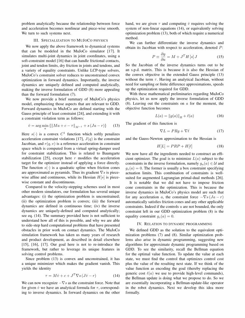
problem analytically because the relationship between forceand acceleration becomes nonlinear and piece-wise smooth.We turn to such systems next.

III. SPECIALIZATION TO MUJOCO PHYSICS

We now apply the above framework to dynamical systemsthat can be modeled in the MuJoCo simulator [17]. Itsimulates multi-joint dynamics in joint coordinates, using asoft-constraint model [16] that can handle frictional contacts,joint and tendon limits, dry friction in joints and tendons, anda variety of equality constraints. Unlike LCP-type solvers,MuJoCo’s constraint solver reduces to unconstrained convexoptimization in forward dynamics. Importantly, the inversedynamics are uniquely defined and computed analytically,making the inverse formulation of GDD (8) more appealingthan the forward formulation (7).

We now provide a brief summary of MuJoCo’s physicsmodel, emphasizing those aspects that are relevant to GDD.Forward dynamics in MuJoCo are defined starting with theGauss principle of least constraint [24], and extending it witha constraint violation term as follows:

v̇ = argmina{‖Ma+ c− τ‖M−1 + s (Ja− r)} (13)

Here s(·) is a convex C1 function which softly penalizesacceleration constraint violations [17], J(q) is the constraintJacobian, and r(q, v) is a reference acceleration in constraintspace which is computed from a virtual spring-damper usedfor constraint stabilization. This is related to Baumgartestabilization [25], except here r modifies the accelerationtarget for the optimizer instead of applying a force directly.The function s(·) is a quadratic spline when friction conesare approximated as pyramids. Thus its gradient ∇s is piece-wise affine and continuous, while its Hessian H[s] is piece-wise constant and discontinuous.

Compared to the velocity-stepping schemes used in mostother modern simulators, our formulation has several uniqueadvantages: (i) the optimization problem is unconstrained;(ii) the optimization problem is convex; (iii) the forwarddynamics are defined in continuous time; (iv) the inversedynamics are uniquely-defined and computed analytically;see eq. (14). The summary provided here is not sufficient tounderstand how all of this is possible, and why we are ableto side-step hard computational problems that have presentedobstacles in prior work on contact dynamics. The MuJoCosimulation framework has taken us many years of researchand product development, as described in detail elsewhere[15], [16], [17]. Our goal here is not to re-introduce theframework, but rather to leverage its unique features insolving control problems.

Since problem (13) is convex and unconstrained, it hasa unique minimizer which makes the gradient vanish. Thisyields the identity

τ =Mv̇ + c+ JT∇s (Jv̇ − r) (14)

We can now recognize −∇s as the constraint force. Note thatfor given v̇ we have an analytical formula for τ , correspond-ing to inverse dynamics. In forward dynamics on the other

hand, we are given τ and computing v̇ requires solving thesystem of non-linear equations (14), or equivalently solvingoptimization problem (13), both of which require a numericalmethod.

We can further differentiate the inverse dynamics andobtain its Jacobian with respect to acceleration, denoted P :

P ≡ ∂g

∂a=M + JTH [s] J (15)

So the Jacobian of the inverse dynamics turns out to bean s.p.d. matrix. This is because it is also the Hessian ofthe convex objective in the extended Gauss principle (13)without the term τ . Having an analytical Jacobian, withoutneed for sampling or finite difference approximations, speedsup the optimization required for GDD.

With these mathematical preliminaries regarding MuJoCophysics, let us now apply the inverse formulation of GDD(8). Leaving out the constraints on a for the moment, theobjective function becomes

L(a) = ‖g(a)‖R + `(a) (16)

The gradient of this function is

∇L = PRg +∇` (17)

and the Gauss-Newton approximation to the Hessian is

H[L] = PRP +H[`] (18)

We now have all the ingredients needed to construct an effi-cient optimizer. The goal is to minimize L(a) subject to theconstraints in the inverse formulation, namely gu(a) ∈ U andgz(a) = 0. The former is usually a box constraint specifyingactuation limits. This combination of constraints is well-suited for augmented Lagrangian primal-dual methods [26].

It is notable that we did not have to impose frictioncone constraints in the optimization. This is because theinverse dynamics in MuJoCo’s physics model are such thatfor any acceleration a, the constraint force −∇s (Ja− r)automatically satisfies friction cones and any other applicableconstraints. Indeed if the controls u are not bounded, the onlyconstraint left in our GDD optimization problem (8) is theequality constraint gz(a) = 0.

IV. RELATION TO DYNAMIC PROGRAMMING

We defined GDD as the solution to the equivalent opti-mization problems (7) and (8). Similar optimization prob-lems also arise in dynamic programming, suggesting newalgorithms for approximate dynamic programming based onGDD. To see the similarity, recall the Bellman equationfor the optimal value function. To update the value at eachstate, we must find the control that optimizes control costplus the value of the resulting next state. If we think of thevalue function as encoding the goal (thereby replacing thegeneric cost `(a) we use to provide high-level commands),the Bellman update is doing what we propose to do. So weare essentially incorporating a Bellman-update-like operatorin the robot dynamics. Next we develop this idea moreformally.

Consider the discrete-time version of our second-ordercontrol system (4), namely:

qt+h = qt + hvtvt+h = vt + hf(qt, vt, ut)

(19)

Define the running cost as

‖(u, 0)‖R + p(q, v) (20)

The first term is our previous regularization cost, while thesecond term is a new state-dependent cost that can be used tospecify desirable states. The latter corresponds to the runningcost in optimal control formulations.

Let V ∗(q, v) denote the optimal value function for theabove optimal control problem (first-exit formulation). ThenV ∗ satisfies the Bellman equation

V ∗(q, v) = p(q, v) +minu∈U‖(u, 0)‖R + V ∗(q + hv, v + hf(q, v, u))

(21)The Bellman equations for finite horizon, average cost anddiscounted formulations have similar structure. Note that theminimization in (21) is identical to the minimization in theforward definition of GDD (7) when the goal-setting cost`(·) is defined as

`(a) = V ∗(q + hv, v + ha) (22)

This of course is not a coincidence; the optimal valuefunction has the key property that the policy which is greedywith respect to it is the optimal policy. Conversely, if wecould somehow guess `(·) that takes into account the long-term value of the state, the goal directed dynamics will matchthe optimally controlled dynamics.

Thus far the relation between goal-directed dynamics anddynamic programming is intuitive but does not seem tosuggest new algorithms. Things get more interesting howeverwhen we turn to the inverse formulation. We will nowredefine the optimal control problem as follows. Instead ofusing the control u to drive the system, we will use theacceleration a. So the control system becomes

qt+h = qt + hvtvt+h = vt + hat

(23)

When q contains quaternions, the summation q+hv denotesintegration over the 4D unit sphere; this is the only remainingnonlinearity, and it is kinematic rather than dynamic. Therunning cost is

‖g(q, v, a)‖R + p(q, v) (24)

This is the same as the previous definition (20) but has beenexpressed as a function of acceleration.

We can now write down the Bellman equation for theinverse dynamics (or acceleration-based) formulation of op-timal control:

V ∗(q, v) = p(q, v) +min

a∈A(q,v)‖g(q, v, a)‖R + V ∗(q + hv, v + ha)

(25)

This is mathematically equivalent to the Bellman equa-tion (21) for the forward dynamics formulation of optimalcontrol, meaning that the two equations characterize thesame optimal value function. But as in GDD, the inverseformulation offers algorithmic advantages, in particular whenit comes to trajectory optimization methods such as dif-ferential dynamic programming (DDP) [27] and iterativelinear-quadratic-Gaussian control (iLQG) [28]. Such meth-ods maintain a local quadratic approximation to V ∗ whichis propagated backwards in time through the linearized (inthe case of iLQG) dynamics. But in the inverse dynamicsformulation, our control system (23) became linear! There-fore propagation errors due to dynamics linearization willnot accumulate. This of course is not a free lunch: what wedid is to hide the complexity of the nonlinear dynamics inthe cost over accelerations. So when we approximate thiscost with a quadratic, the approximation error is likely to begreater compared to approximating a traditional control cost.However, control costs are often used to tame the optimizerand produce sensible behavior, and not because we careabout the specific expression; for example the quadratic costsused in practice do not correspond to power or any otherphysically meaningful quantity. This is why we refer to themas regularization costs and control costs interchangeably. Soif we could put all approximation errors in one place, thecontrol cost is the ideal place. Another advantage in thecontext of MuJoCo physics is that we are working withinverse dynamics, which are computed analytically unlikeforward dynamics. We have not yet developed a specificalgorithm exploiting this new inverse formulation of optimalcontrol, although we already have a name for it: acceleration-based iterative LQR (AILQR). We are looking forward todeveloping this algoritghm in future work.

V. COST FUNCTION DESIGN

Coming back to the instantaneous optimization in GDD,we need a cost function `(·). We already discussed oneexample, namely the end-effector acceleration cost (11). Thiswas used in an analytically-solvable special case, but it canbe used in the general case as well. Another setting where wecan readily obtain a desired acceleration in joint space, andconstruct a cost `(·) around it, are policies that are trained tooutput acceleration targets. For example, [23] trained such aneural network controller capable of stable 3D locomotionto spatial targets specified interactively.

Recall that the constraint forces in the MuJoCo physicsmodel we are using are computed analytically given theacceleration: the vector of all such forces is −∇s(Ja − r)where J, r are fixed given the state (q, v). This includesfrictional contact forces, joint limit forces, dry friction forcesand equality constraint forces. Therefore all these quantitiescan be used to construct cost functions for the purpose ofGDD. For example, the center of pressure can be computedby identifying all contact points between the robot and theground plane, and weighting their positions by the corre-sponding contact normal forces.

Spatial goals can be specified by computing a desired end-effector acceleration and using a cost similar to (11). Thisdesired acceleration can be obtained from a virtual spring-damper, or perhaps a minimum-jerk spline which will likelyresult in smoother and more human-like movements [29].

Finally, as already summarized earlier, there is a rich lit-erature in both Robotics and Graphics proposing to optimizevarious quantities instantaneously. These include center ofpressure, ZMP and related ‘capture points’ [9], [10], [11],as well center of mass, linear and angular momentum, andmany other intuitive features that have proven useful. Ourgoal here is not to design new costs, but rather to develop thecomputational infrastructure which can be used to optimizeefficiently any cost in this broad family, without the modelinglimitations imposed by the QP framework.

VI. NUMERICAL BENCHMARKS

Here we describe simulation results from two MuJoComodels: a humanoid and a disembodied hand; see Figure 2and the accompanying movie. In each case we selected abody segment and used the mouse to interactively specifya spatial goal. The cost `(·) had two terms. The first termwas an end-effector acceleration term for the selected bodysegment, as in (11), specifying a desired acceleration towardsthe spatial goal. The second term was

α

2‖a+ βv‖R (26)

where α is the relative weight of the cost term and β isa virtual damping coefficient. This tells the GDD to stopmoving, resembling a joint-space damping mechanism. Inthis way, once the first term drives a given body segment toa desired location, it can be disabled and the second termmakes GDD hold it in place – although with this particularcost it slowly falls under gravity, because we also have acost on τ .

We used the interactive simulation described above tocollect a dataset of records, each containing (q, v, a, τ) forone model and one point in time. We then re-run thesimulations offline, disabling rendering and interaction sothat we could time the solvers more accurately. The datasetfor each model had 20, 000 records. We tested performanceon an Intel i7-6700K 4 GHz processor. The average CPUtimes per step in a single thread were as follows:

CPU time per step (µs) humanoid hand

forward 49 128

goal-directed 90 182

goal-directed + forward 99 194

Note that these times are in microseconds. So in all cases ittakes well below a millisecond to execute the GDD solverto convergence (to a feasible but possibly local minimum).The GDD solver is only two times slower than the for-ward solver, which is impressive given that it is solvinga non-convex and non-smooth problem. Even though GDDcomputes both the control and the acceleration, the control

Fig. 2. Physics models used to benchmark the GDD solver.

may not be exactly feasible, since we are using a primal-dual method. Therefore we clamp the control to the feasibleset and execute forward dynamics. This clamping operationintroduces a very small change and the forward solver iswarmstarted with the acceleration found by GDD, thus theforward solver converges almost immediately and adds only10 microseconds on average (last line in the above table).

Next we present statistics characterizing the behavior ofthe GDD solver over the 20, 000 simulation step for eachtest model. For each statistic we show the 50th percentile(i.e. the median) and the 95th percentile:

satistic (50% (95%)) humanoid hand

constraints 23 (38) 19 (30)

iterations 4 (9) 5 (9)

dual updates 1 (1) 1 (3)

physics violation 3e-11 (6e-7) 2e-8 (5e-7)

residual gradient 1e-7 (1e-6) 1e-9 (8e-9)

The number of constraints reflects the number of activecontacts and joint limits, and corresponds to the number ofrows in the Jacobian J . Each iteration involves a Newtonstep to find the search direction, followed by exact line-search exploiting the structure of the objective function. Dualupdates are needed to re-estimate the Lagrange multipliersfor the constrained optimization problem. The last two rows

characterize the quality of the solution. The bottom line isthat both the physics violation error and the residual gradientare very small, and the number of iterations is also very smallconsidering the problem class.

VII. CONCLUSIONS AND FUTURE WORK

We developed a general control framework using costfunctions in place of traditional control signals. The em-bedded GDD solver computes the optimal controls giventhe instantaneous cost/goal, and applies them to the physicalsystem. This solver is sufficiently fast and robust to be usedin a low-level control loop, generalizing the QP solvers thatare currently popular in robotics. While some illustrationsof behaviors generated by our new solver can be foundin the accompanying movie, our objective here was not toexplore what cost functions are needed to generate interestingbehaviors. This has been done extensively before. Insteadwe focused on developing a more general optimizationframework that can make prior cost functions work better.

In future work we will experiment with more elaboratecosts and applications to physical systems. We will alsodevelop the new trajectory optimizer outlined earlier, usingGDD in an inner loop and replacing the user-defined in-stantaneous cost in GDD with an approximation the optimalvalue function. Another possible application of GDD is inthe context of model-based Reinforcement Learning, where itcan be used to optimize over actions given an approximationto the optimal value function. GDD can also facilitate policygradient methods: learn a controller that outputs desiredaccelerations rather than forces, and then use GDD online tocompute the corresponding forces and execute the controller.

REFERENCES

[1] O. Khatib, A unified approach for motion and force control of robotmanipulators: The operational space formulation. IEEE Journal onRobotics and Automation, 3: 43-53, 1987.

[2] L. Sentis, J. Park, O. Khatib, Compliant control of multicontact andcenter-of-mass behaviors in humanoid robots. IEEE Transactions onRobotics 26: 483-501, 2010.

[3] R. Featherstone, O. Khatib, Load-independence of the dynamically-consistent inverse of the Jacobian matrix. International Journal ofRobotics Research, 16: 168-170, 1997.

[4] L. Righetti, J. Buchli, M. Mistry, M. Kalakrishnan, S. Schaal, Optimaldistribution of contact forces with inverse-dynamics control. Interna-tional Journal of Robotics Research, 32: 280-298, 2013.

[5] D. Mellinger, N. Michael, V. Kumar, Trajectory generation and controlfor precise aggressive maneuvers with quadrotors. International Journalof Robotics Research, 31: 664-674, 2012.

[6] A. Escande, N. Mansard, P. Wieber, Hierarchical quadratic program-ming: Fast online humanoid-robot motion generation. InternationalJournal of Robotics Research, 33: 1006-1028, 2014.

[7] S. Feng, W. Whitman, X. Xinjilefu, C. Atkeson, Optimization-basedfull body control for the DARPA Robotics Challenge. Journal of FieldRobotics, 32: 293-312, 2015.

[8] S. Kuindersma, R. Deits, M. Fallon, A. Valenzuela, H. Dai, F. Perme-nter, T. Koolen, P. Marion, R. Tedrake, Optimization-based locomotionplanning, estimation, and control design for the Atlas humanoid robot.Autonomous Robots, 40: 429-455, 2016.

[9] T. Koolen, T. De oer, J. Rebula, A. Goswami, J. Pratt, Capturability-based analysis and control of legged locomotion. Part 1: Theoryand application to three simple gain models. International Journal ofRobotics Research, 2012.

[10] P. Saradain, G. Bessonnet, Forces acting on a biped robot. Centerof pressure – zero moment point. IEEE Trans. Systems, Man, andCybernetics, Part A, 34: 630637, 2004.

[11] M. Vukobratovic, B. Borovac, Zero-moment point – Thirty five yearsof its life. International Journal of Humanoid Robotics, 1: 157173, 2004.

[12] E. Farnioli, M. Gabiccini, A. Bicchi, Optimal contact force distributionfor compliant humanoid robots in whole-body loco-manipulation tasks.ICRA 2015.

[13] D. Stewart, J. Trinkle, An implicit time-stepping scheme for rigid-bodydynamics with inelastic collisions and coulomb friction. InternationalJournal Numerical Methods Engineering, 39: 2673-2691, 1996.

[14] M. Anitescu, F. Potra, D. Stewart, Time-stepping for three dimensionalrigid body dynamics. Computer Methods in Applied Mechanics andEngineering, 177: 183-197, 1999.

[15] E. Todorov, T. Erez, Y. Tassa, MuJoCo: A physics engine for model-based control. International Conference on Itelligent Robots and Sys-tems (IROS) 2012.

[16] E. Todorov, Convex and analytically-invertible dynamics with contactsand constraints: Theory and implementation in MuJoCo. ICRA 2014.

[17] E. Todorov, MuJoCo: Modeling, Simulation and Visualization ofMulti-Joint Dynamics with Contact. Seattle WA: Roboti Publishing,2016. www.mujoco.org/book

[18] Y. Abe, M. da Silva, J. Popovic, Multiobjective control with frictionalcontacts. ACM SIGGRAPH/Eurographics Symposium on ComputerAnimation 2007.

[19] M. de Lasa, I. Mordatch, A. Hertzmann, Feature-based locomotioncontrollers. SIGGRAPH 2010.

[20] M. Al Borno, M. de Lasa, A. Hertzmann, Trajectory optimizationfor full-body movements with complex contacts. IEEE Transactions onVisualization and Computer Graphics, vol 19, 2013.

[21] Y. Lee, M. Park, T. Kwon, J. Lee, Locomotion control for many-muscle humanoids. SIGGRAPH 2016.

[22] A. Macchietto, V. Zordan, C. Shelton, Momentum control for balance.SIGGRAPH 2009.

[23] I. Mordatch, K. Lowrey, G. Andrew, Z. Popovic, E. Todorov, Interac-tive control of diverse complex characters with neural networks. NIPS2015.

[24] R. Kalaba, H. Natsuyama, F. Udwadia, An extension of Gauss’sprinciple of least constraint. International Journal of General Systems,33: 63-69, 2004.

[25] J. Baumgarte, Stabilization of constraints and integrals of motionin dynamical systems. Computer Methods in Applied Mechanics andEngineering, 1: 1-16, 1972.

[26] A. Forsgren, P. Gill, Primal-dual interior methods for nonconvexnonlinear programming. SIAM J Optim 8: 1132-1152, 1998.

[27] D. Jacobson, D. Mayne, Differential Dynamic Programming. ElsevierPublishing Company, New York, 1970.

[28] E. Todorov, W. Li, A generalized iterative LQG method for locally-optimal feedback control of constrained nonlinear stochastic systems.American Control Conference, 2005.

[29] T. Flash, N. Hogan, The coordination of arm movements: An exper-imentally confirmed mathematical model. Journal of Neuroscience, 5:1688-1703, 1985.