Utility Models for Goal-DirectedDecision-Theoretic PlannersPeter Haddawy1, Steve HanksDepartment of Computer Science and EngineeringUniversity of WashingtonSeattle, WA 98195Technical Report 93{06{04June 15, 1993

1 Department of EE & CS, University of Wisconsin{Milwaukee, Milwaukee WI 53201

Utility Models for Goal-DirectedDecision-Theoretic Planners�Peter HaddawyDepartment of EE & CSUniversity of Wisconsin{MilwaukeeMilwaukee WI 53201haddawy@cs.uwm.edu Steve HanksDepartment of CS&E, FR{35University of WashingtonSeattle WA 98195hanks@cs.washington.eduJune 22, 1993University of WashingtonDepartment of Computer Science & EngineeringTechnical report 93-06-04AbstractAI planning agents are goal-directed: success is measured in terms of whether ornot an input goal is satis�ed, and the agent's computational processes are driven bythose goals. A decision-theoretic agent, on the other hand, has no explicit goals|success is measured in terms of its preferences or a utility function that respects thosepreferences.The two approaches have complementary strengths and weaknesses. Symbolic plan-ning provides a computational theory of plan generation, but under unrealistic assump-tions: perfect information about and control over the world and a restrictive model ofactions and goals. Decision theory provides a normative model of choice under uncer-tainty, but o�ers no guidance as to how the planning options are to be generated. Thispaper uni�es the two approaches to planning by describing utility models that supportrational decision making while retaining the goal information needed to support plangeneration.We develop an extended model of goals that involves temporal deadlines and main-tenance intervals, and allows partial satisfaction of the goal's temporal and atemporal�Thanks to Tony Barrett, Denise Draper, Dan Weld, MikeWellman, and Mike Williamson for many usefulcomments. Thanks to Meliani Suwandi for helping develop the re�nement planning example. Haddawy wassupported in part by NSF grant IRI{9207262 and in part by a grant from the graduate school of the Universityof Wisconsin-Milwaukee. Hanks is supported in part by NSF Grant IRI{9008670.i

components. We then incorporate that goal information into a utility model for theagent. Goal information can be used to establish whether one plan has higher expectedutility than another, but without computing the expected utility values directly; wepresent a variety of results showing how plans can be compared rationally, but usinginformation only about the probability that they will satisfy goal-related propositions.We then demonstrate how this model can be exploited in the generation and re�nementof plans.

ii

Contents1 Introduction 11.1 Contributions : : : : : : : : : : : : : : : : : : : : : : : : : : : : : : : : : : : 21.2 Outline : : : : : : : : : : : : : : : : : : : : : : : : : : : : : : : : : : : : : : : 32 Classical Goal-Directed Agents 32.1 Limitation of goal-directed behavior : : : : : : : : : : : : : : : : : : : : : : : 43 Utility Models for Goal-Directed Agents 73.1 Syntactic forms for goals : : : : : : : : : : : : : : : : : : : : : : : : : : : : : 93.1.1 The language Ltca : : : : : : : : : : : : : : : : : : : : : : : : : : : : : 93.1.2 Goal expressions : : : : : : : : : : : : : : : : : : : : : : : : : : : : : 103.1.3 Utility function for individual goals : : : : : : : : : : : : : : : : : : : 104 Partial Goal Satisfaction 114.1 Partial satisfaction of the atemporal component : : : : : : : : : : : : : : : : 114.1.1 Goals with symbolic attributes : : : : : : : : : : : : : : : : : : : : : : 114.1.2 Goals with quantitative attributes : : : : : : : : : : : : : : : : : : : : 134.1.3 Conjunctive quantitative attributes : : : : : : : : : : : : : : : : : : : 134.1.4 Summary : : : : : : : : : : : : : : : : : : : : : : : : : : : : : : : : : 144.2 Partial satisfaction of the temporal component : : : : : : : : : : : : : : : : : 144.2.1 Deadlines : : : : : : : : : : : : : : : : : : : : : : : : : : : : : : : : : 144.2.2 Maintenance intervals : : : : : : : : : : : : : : : : : : : : : : : : : : 164.2.3 Summary : : : : : : : : : : : : : : : : : : : : : : : : : : : : : : : : : 165 Utility Functions for Individual Goals 175.1 Combining the temporal coe�cient and the atemporal degree of satisfaction 175.1.1 Deadline goals : : : : : : : : : : : : : : : : : : : : : : : : : : : : : : : 175.1.2 Maintenance goals : : : : : : : : : : : : : : : : : : : : : : : : : : : : 195.2 Summary : : : : : : : : : : : : : : : : : : : : : : : : : : : : : : : : : : : : : 206 Using the Utility Functions to Rank Plans 206.1 Deadline goals : : : : : : : : : : : : : : : : : : : : : : : : : : : : : : : : : : : 216.1.1 Bounds for symbolic attributes : : : : : : : : : : : : : : : : : : : : : 216.1.2 Bounds for quantitative attributes : : : : : : : : : : : : : : : : : : : : 236.1.3 Bounds for strictly ordered atemporal attributes : : : : : : : : : : : : 246.1.4 Example : : : : : : : : : : : : : : : : : : : : : : : : : : : : : : : : : : 256.2 Maintenance goals : : : : : : : : : : : : : : : : : : : : : : : : : : : : : : : : 266.2.1 Bounds for symbolic attributes : : : : : : : : : : : : : : : : : : : : : 266.2.2 Bounds for quantitative attributes : : : : : : : : : : : : : : : : : : : : 286.2.3 Bounds for strictly ordered atemporal attributes : : : : : : : : : : : : 296.3 Summary : : : : : : : : : : : : : : : : : : : : : : : : : : : : : : : : : : : : : 29iii

7 Multiple Goals, Residual Utility, and Computational Issues 297.1 Plan generation and re�nement : : : : : : : : : : : : : : : : : : : : : : : : : 307.1.1 Partial-order planning and search control : : : : : : : : : : : : : : : : 317.1.2 Re�nement planning : : : : : : : : : : : : : : : : : : : : : : : : : : : 318 Summary and Related Work 418.1 Related work : : : : : : : : : : : : : : : : : : : : : : : : : : : : : : : : : : : 428.1.1 Goals and utility models : : : : : : : : : : : : : : : : : : : : : : : : : 428.1.2 Decision-theoretic planning and control : : : : : : : : : : : : : : : : : 438.1.3 Fuzzy decision theory : : : : : : : : : : : : : : : : : : : : : : : : : : : 448.2 Future work : : : : : : : : : : : : : : : : : : : : : : : : : : : : : : : : : : : : 44

iv

1 IntroductionReasoning about and planning for an uncertain world raises both representational and algo-rithmic problems: we need to represent change, uncertainty, and value or utility, and to usethose concepts to represent various plans of action. And given such a representation for theworld and for plans that might be executed in the world, we further need an e�cient wayto generate plausible plans, anticipate their results, improve their performance, and choosethe best option from among them.Decision theory addresses the representational problem, providing a rational basis forchoice under uncertainty. The framework starts with the agent's preferences over an abstractset of possible outcomes, and guarantees the existence of probability and utility functionssuch that acting to maximize expected utility is rational in the sense that it respects thosepreferences. (The planner need not explicitly perform the decision-theoretic analysis|itsu�ces that the planner act according to the recommendations that such an analysis wouldmake.)Decision theory does not, however, constitute a theory of reasoning about plans. The the-ory does not provide a vocabulary for describing planning problems, a method for generatingoptions, or a computational model for choosing among plan alternatives. It merely dictatesa rational choice given such a capability. Decision analysis|the study of applying decision-theoretic framework|addresses these limitations, but in a subjective and non-algorithmicfashion.The capabilities provided by symbolic planning and decision theory are therefore com-plementary: the former provides methods for representing planning problems and generatingalternative plans in response to externally supplied goals (but under restrictive conditionsthat don't include uncertainty); the latter provides a method for choosing among alterna-tives and a language that allows reasoning with uncertainty, but provides (1) no guidance instructuring planning knowledge, (2) no way of generating alternatives, and more generally,(3) no computational model. The �rst step toward integrating these two methodologies isto reconcile the two representations.Planning problems are described in terms of� a set of operators that e�ect change in the world,� a description of some initial world state (usually expressed in some logical or quasi-logical language), and� a goal state description.Decision-theoretic problems, on the other hand, are stated in terms of� a probability distribution over possible outcomes, and� preferences over those outcomes. 1

The relationship between the probabilistic model of the world and the operators andinitial state has been studied as a problem of probabilistic temporal inference, [Haddawy,1991b], [Hanks and McDermott, 1993], [Hanks, 1993]. The relationship between the goalstate description and the agent's utility model has received less attention, and is the topicof this paper.1.1 ContributionsThis paper presents a utility model for goal-directed agents that allows rational choice amongplanning alternatives but that also can be exploited by a plan-generation algorithm to guidethe process of building e�ective plans. It therefore directly addresses the gap between AIand decision-theoretic planners, providing a richer representation language for the formerand a computational framework for the latter.The main contributions of the paper are:1. A detailed analysis and taxonomy of goal forms. We break a goal into atemporal andtemporal components: what is to be true and when it is to be true. We consider twomain forms of temporal constraints: deadline goals and maintenance goals, and variousforms of atemporal constraints, including symbolic and numeric goals.2. A model of partial satisfaction that allows reasoning about partial satisfaction of agoal's atemporal component, temporal component or both. Partial satisfaction infor-mation for a goal is supplied in terms of� A function DSA measuring the extent to which the goal's atemporal componentis satis�ed at a point in time.� A function measuring the extent to which the goal's temporal component is sat-is�ed:{ For deadline goals, a function CT that measures the extent to which a timepoint meets the deadline.{ For maintenance goals, a function CP that measures the extent to which atime interval satis�es the maintenance constraint.We develop a method for combining these two pieces of information into a coherentassessment of the goal's level of satisfaction.3. A utility model for an agent that allows reasoning about trading o� (partial) successin achieving one goal against (partial) success in achieving another, and trading o�success in achieving goals with resource consumption.4. E�ective methods for comparing two plans: relationships that imply that one plan hashigher expected utility than another, but that do not require computing the expectedutilities directly. 2

5. An example of how the model can be exploited by a planning algorithm to prune thespace of partial plans explicitly considered.1.2 OutlineSection 2 begins by de�ning a goal-directed agent, and pointing out the limitations of aplanning strategy guided only by conjunctive goal expressions. Section 3 de�nes an extendedutility model for goal-directed agents, which includes a richer notion of goal than the onetypically used by classical planners. Section 4 confronts the problem of specifying preferencesover partially satis�ed goals, and Section 5 de�nes a model that allows partial satisfactionof a goal's temporal and atemporal components simultaneously.Sections 6 and 7 address the question of how the goal-based utility model can be ex-ploited in comparing and building plans. Section 6 presents a variety of results describingcircumstances under which deciding that one plan is preferable to another amounts to estab-lishing a relationship between probabilities involving the respective goal expressions. Section7 discusses how the model might be used in generating plans, exploring extensions to theclassical partial-order generation algorithm and the idea of planning by re�nement. Section8 summarizes and discusses related work.2 Classical Goal-Directed AgentsBefore we proceed with a formal analysis of goals and utilities we need to de�ne moreprecisely what role these concepts will play in a planning system. Goals play three roles inautomated planning systems:� Goals act as a device for communicating information about the planning problem. Inparticular they provide a concise de�nition of what constitutes a successful plan.� Goals act as a means of limiting inference in the planning process by allowing theplanner to backchain over goal propositions. In that sense they de�ne exactly what isrelevant to the planning problem.� Goals limit the temporal scope of the planning problem, imposing a temporal \hori-zon," beyond which planning is irrelevant.In the �rst case goals can be communicated more easily than utility functions, and in thesecond and third cases the goals' symbolic content can aid the search for good plans.Figure 1 makes the relationship more clear: let us assume some manager, who has autility function over outcome states. He is designing an agent, and has a model of theagent's capabilities. The manager wants to communicate information to the agent that willcause it to act so as to increase the manager's utility; he uses goal expressions to communicatethat information to the agent. The agent uses this goal information|along with informationlike the anticipated state of the world at execution time and the cost of various resources|to produce a utility function that serves to guide its actions.3

Manager’sUtility Function

Agent’sUtilityFunction

Domain model(resource costs)

ActionUtility / GoalInformationFigure 1: Goals as a means of communicationThis model applies classical goal-directed agents as well as decision-theoretic agents. Thequestion is what language the manager should use to convey the utility/goal information, andhow that information restricts the possible behaviors available to the agent. The classicalplanning model restricts this information to a conjunction of goal propositions, which aresupposed to hold at the end of plan execution. We will show that restricting the form ofutility information to goal conjunctions of this form places severe restrictions on the agent'sproblem-solving abilities, then develop more expressive forms of goal expressions that stillallow the agent to be an e�ective problem solver.2.1 Limitation of goal-directed behaviorSuppose the manager communicates only symbolic goal expressions to the agent|he tellsthe agent to achieve some goal G, a conjunction g1 ^ g2 : : : gn, and the agent builds a planthat maximizes the probability that satisfying G will be true at the end of executing theplan. (This is the probabilistic analogue of logical goal-directed planning, in which the agentconstructs a plan that provably achieves G.) What limits does this model place on the agent'spreference struture? In other words, under what circumstances is planning to maximizeexpected utility equivalent to planning to maximize the probability of goal satisfaction?We start by introducing some notation. We will talk about time points t, and can talkabout a proposition � being true over an interval of time [t1; t2] by saying HOLDS (�; t1; t2)(see Section 3.1.1 for more details).A plan P can be viewed as de�ning a probability distribution over chronicles, where achronicle is a set of time points representing one possible course of execution for the plan.We can therefore talk about the probability P(cjP).1 We will generally be interested inthe time point representing the moment the plan �nishes executing; we will use end(c) torepresent this point. The probability of success in the classical paradigm is the probabilitythat the goal conjunction will hold when the plan �nishes executing:P(P succeeds) � P(GjP) � Xc:HOLDS (G;end(c);end(c))P(cjP) (1)1[McDermott, 1982] de�nes chronicles in terms of a temporal logic, and [Hanks, 1990] and [Haddawy,1991b] extend the notion to a probabilistic framework.4

and the planner will try to �nd the plan maximizing that value.A decision-theoretic planner has the same probabilistic model as the probabilistic planner,but it has an explicit utility function over chronicles, a function U(c) that maps chroniclesinto real values. The expected utility of a plan is de�ned to beEU(P) �Xc U(c) �P(cjP) (2)and the decision-theoretic planner will try to �nd the plan maximizing that value.The question arises as to under what circumstances the two models are equivalent: forwhat utility models (de�nitions of U(c)) is it the case that the plan that maximizes the prob-ability of goal achievement (Equation (1)) will always be the plan that maximizes expectedutility (Equation (2))?The answer is that this relationship holds only for simple step utility functions, functionsfor which utility is a constant low value UG for chronicles in which the goal does not holdat the end of plan execution and a constant high value UG for chronicles in which it does.Figure 2 shows such a function|utility is represented along the vertical axis and the spaceof chronicles along the horizontal axis. G and G designate the set of all chronicles in whichthe goal holds and does not hold, respectively.Previous work, [Haddawy and Hanks, 1990], demonstrates the correspondence betweenthese two policies, showing that the simple class of step functions pictured in Figure 2 is theonly class of utility functions for whichP(GjP1) > P(GjP2)) EU(P1) > EU(P2) (3)holds for any plans P1 and P2. In other words, describing the desired state of the world interms of a goal conjunction restricts a problem-solver's preference structure to those thatcan be characterized by a simple step function. ([Haddawy and Hanks, 1990] explores therelationship between goal satisfaction and probability maximization for other situations,e.g. cases in which goal expressions are combined with some preference information aboutresource consumption.)The analysis points out four obvious limitations to the endeavor of planning to achievea goal conjunction:1. Temporal extentDe�ning plan success in terms of what is true at the end of execution|de�ning asuccessful chronicle only in terms of whether the goal holds at end(c))|rules out goalslike deadlines (have g1 true by noon and g2 true by midnight), maintenance (keep gtrue continuously between noon and midnight), and prevention (make g1 true, butwithout allowing g2 to become true in the meantime). (The last is a combination ofdeadline and maintenance goals.) It is important not only what is accomplished, butalso when or for how long.2. Tradeo�s among the goalsThe classical model dictates that the satisfaction of all goal conjuncts is necessary and5

chronicles (c)

U(c)

GG

UG

UG

Figure 2: Step utility functionsu�cient for success. More realistic is the view that satisfying some of the conjuncts ispreferable to satisfying none, motivating the idea that success in achieving one conjunctcould be traded o� against success in achieving others.3. Partial satisfactionSymbolic goals imply an all-or-nothing success criterion, either the goal form holds atthe end of execution or it does not. This criterion is re ected in the step function:utility is either at a constant high value or at a constant low value. A realistic repre-sentation should allow the manager to communicate the fact that satisfying G is mostpreferred, but satisfying G partially is better than not satisfying it at all.4. Incidental costs and bene�tsSymbolic goals imply that the goal attributes are the only aspects of an outcome thatare relevant to assessing utility, which rules out the possibility that plan P1 is preferableto P2 because it is as e�ective at achieving the goal as P2, but does so more cheaply.Symbolic goals provide no way to specify the \more cheaply" part, nor do they providethe language to express the tradeo� between e�ectiveness in achieving the goal andthe cost involved in doing so.The analysis in this section demonstrates the steps necessary to unify goal-directed anddecision-theoretic plan evaluation:� The language of goals needs to be extended to represent partial goal satisfaction andresource-related utility.� In order to e�ectively use these extended goal forms (more complicated utility func-tions) in planning we need to establish relationships like Equation 3: circumstancesunder which planning to maximize the probability of goal satisfaction ensures rationalbehavior in the decision-theoretic sense.� We need to exploit these relationships as we build or re�ne plans.6

This paper will have four concerns:� Presenting a framework for analyzing a goal-directed agent's utility function, whichincludes goal and resource components.� De�ning a language for goals that provides for expressing preferences among situationsinvolving partial satisfaction of the goals.� Developing relationships that allow the agent to build plans based on the symboliccontent of its goals, while simultaneously guaranteeing that following those plans willcause it to act so as to maximize expected utility.� Demonstrating how those relationships can be exploited by a planning algorithm.3 Utility Models for Goal-Directed AgentsThis section de�nes a utility model for a goal-directed agent by describing the form of thefunction U(c) mentioned in the previous section. The task is simple for the simple goalmodel in the previous section:U(c) = ( 1 if HOLDS(G,end(c),end(c))0 otherwise (4)But we want our model to capture the fact that goal satisfaction can be measured at othertime points and over intervals, that goals can be partially satis�ed, that (partial) satisfactionof one goal can be traded o� against (partial) satisfaction of other goals, and that resourcecosts a�ect the extent to which a plan succeeds as well.In that case what can we say about a goal's role in the utility function? There are twomain properties we want to capture:1. That satisfying a goal to a greater extent is preferable to satisfying it to a lesser extent,all other things being equal2.2. That success in satisfying one goal component can be traded o� against success insatisfying another goal, or against consuming resources.We begin by de�ning a goal-oriented agent in terms of its top-level utility function:De�nition 1 A goal-directed agent is a decision maker whose preferences correspond to thefollowing utility function:U(c) = �ni=1kiUGi(c) + krUR(c) (5)2See [Wellman and Doyle, 1991] for a more general interpretation of this criterion.7

The utility function is de�ned in terms of n subutility functions UGi associated withthe agent's n explicit goals. Each of these functions maps the chronicle into a real numberbetween 0 and 1, where 0 represents the situation in which the goal is satis�ed not at all inthe chronicle and 1 indicates that the chronicle satis�es the goal fully.The function UR (for \residual" or \resource" attributes) also maps a chronicle into [0; 1],and measures the extent to which the chronicle produces or consumes non-goal attributes,e.g. time, fuel, wear and tear on equipment, money lost or gained. A value of 1 indicates thebest possible use of non-goal attributes; a value of 0 indicates that resources were consumedat the theoretical maximum.The model is also de�ned in terms of n+ 1 numeric parameters: k1; k2; : : : kn; kr. Theseparameters make explicit the tradeo�s among the component goals and between the goalsand resource consumption. The ratio of any two of these numbers indicates the amountthe agent is willing to sacri�ce in satisfaction of one goal in order to satisfy another, orthe amount of satisfaction in resource consumption he is willing to \spend" in order toaccomplish an increase in satisfaction for a goal. We return to these tradeo�s in Section 7.Equation (5) also implies that the agent's preferences over the component goals areadditive independent: preferences over lotteries on the goals depend only on the marginalprobability distributions for the goals and not on their joint probability distribution [Keeneyand Rai�a, 1976, Sect 6.2]. In other words we assume that preference for a particular level ofsatisfaction for one goal does not depend on the extent to which the other goals are satis�ed.The function furthermore implies that goal satisfaction is additive independent in resourceconsumption: the agent's preferences over patterns of resource consumption are the sameregardless of the extent to which the top-level goals are satis�ed.The power of the independence assumption is that it allows us to reason easily about thetradeo� between levels of the various goals, and also about how much additional resource wewould be willing to expend to improve the chances of satisfying a goal or to satisfy it morefully (see Section 7).The independence restriction on top-level goals seems troubling on the surface, since AIplanning research has focused mainly on interactions among the goals, and our assumptionseems to rule out those interactions. In particular the assumption runs counter to the analysisof conjunctive-goal planning we presented in the previous section. Equation (5) means, forexample, that we cannot represent conjunctive goals like \have the truck fueled and loadedby 7AM" as two separate top-level goals, since presumably satisfying either one without theother a�ords low utility but their conjunction a�ords high utility. This is indeed the case,and our argument is that these two statements do not involve two goals, but rather twocomponents of a single goal. Section 4.1.1 addresses the problem of dealing with interactionsamong symbolic interacting components that comprise a goal|that section demonstrate howto represent traditional goals of the form \G is satis�ed only if its components g1 : : :gn areall satis�ed."We should also note that the assumption of utility independence does not imply thatthat goals are probabilistically independent. One might object that two goals, say \have thetruck at the depot by noon" and \have the truck clean," interact strongly if the only road8

to the depot is muddy and there's no way to wash the truck once at the depot. In particularthere's no plan that might make them both true. But this is not a violation of probabilisticindependence, not utility independence. The assumption of additive utility independenceimplies only that the utility derived from satisfying one top-level goal does not depend onthe extent to which the other goals are achieved; it does not comment on the likelihoodof achieving either in isolation or both simultaneously. In this example there might be nochronicle in which both propositions are true, in which case the likelihood of achieving thegoal, and presumably the expected utility of any plan, will be low. But this interaction isproperly re ected in the probabilistic model of the domain and the operators|it does notinvolve the agent's preferences.The main implication of the additive independence is that the decision maker has tostructure his preferences, identifying those that are utility independent and those that arenot. The former are divided into separate goals and the latter become components of indi-vidual goals. Subsequent sections provide methods for describing interactions among goalcomponents.We now turn to the question of how the goal information|the UGi(c) functions|isexpressed. We will temporarily ignore the top-level utility function U(c) as well as the residualutility function UR(c), and concentrate on how to build utility functions for individual goals.3.1 Syntactic forms for goalsGoals in classical planning algorithms consist of a symbolic expression to be achieved. Wewant to extend the idea in several directions:� Goals should have a temporal extent|a time at which or an interval over which theproposition is to be achieved. The classical goal representation has the planner achievethe goal by the end of plan execution.� Goals should be partially satis�able|if the goal is to produce 10 widgets it might bebetter to produce 5 than none at all. Partial satisfaction can extend to the temporalcomponent as well: if the deadline is noon, �nishing by 12:05 might be better than�nishing the next morning.3.1.1 The language LtcaIn order to talk about temporally quali�ed sentences in a probabilistic setting, we need alogic that can represent both time and probability. The logic of time, chance, and actionLtca is well suited to our purposes. A simpli�ed version of the logic is described in [Haddawy,1991a] and the full logic is described in [Haddawy, 1991b]. We describe here just that portionof the language relevant to this paper. We will use the single predicate HOLDS to associatefacts with temporal intervals. The sentence HOLDS (FA; t1; t2) is true if fact FA holds overthe time interval t1 to t2. We impose the constraint that if a fact holds over an interval itholds over any subinterval. 9

Probability is treated as a sentential operator so it can be combined freely with otherlogical operators. We write Pt(�) to denote the probability of a formula � at time t. Theprobability of a formula is de�ned as the probability of the set of chronicles in which theformula is satis�ed. Although the language can represent the dynamics of probability overtime by allowing the probability operator to be indexed by any time point, in this paper wewill only index it by the current time (now) and sometimes will omit the index altogether:P(�) understood to mean Pnow (�).3.1.2 Goal expressionsWe begin by breaking a goal into atemporal and temporal components. The former indicateswhat is to be achieved, the latter when it is to be achieved.We de�ne two types of temporal goals: deadline goals and maintenance goals. A deadlinegoal is a function of the deadline time point td, and its atemporal component is just a formula� containing only the HOLDS predicate with only temporal parameter td. For shorhand wewill notate a formula � that contains only temporal parameters t; t0 as �(t; t0). A deadlinegoal says only that � should hold at the deadline point, but we will discuss below ways ofexpressing preferences over making � \partially true" at td or making � true \shortly after"td, or both. Two examples of deadline goals are:� Have block A on block B on block C by noon.HOLDS (on(A,B);noon;noon) ^ HOLDS (on(B,C);noon;noon)� Have two tons of rocks to the depot by 2:00 this afternoon.HOLDS (=(tons-delivered-to-depot,2); 2PM ; 2PM )A maintenance goal represents a desire to keep a proposition true over an interval oftime. It is a formula containing only the HOLDS predicate with temporal arguments tb andte, the begin and end points of the maintenance interval. An example of a maintenance goalwould be \keep the temperature between 65 and 75 degrees from 9am until 5pm:HOLDS (� (temp, 65); 9am; 5pm) ^ HOLDS (� (temp, 75); 9am; 5pm)3.1.3 Utility function for individual goalsThe ith individual goal appears in the top-level utility function as a function UGi(c) of achronicle. Above we made the distinction between a goal's temporal and atemporal com-ponents, and that distinction is re ected in the UGi function as well. We will explore thisfunction in more detail below, but begin by dividing it into two components:� A function DSAi(t) which is a measure of the extent to which the atemporal componentof the ith goal is satis�ed at time t (where t is implicitly a member of some chroniclec). DSA stands for \degree of satisfaction of the atemporal component."10

� A function that de�nes the extent to which the goal's temporal component is satis�ed,which depends on the form of the temporal component. For deadline goals we de�ne atemporal coe�cient CTi(t), measuring the extent to which the deadline is satis�ed attime t. For maintenance goals we de�ne a persistence coe�cient CPi(t; t0) measuringthe extent to which the maintenance condition is satis�ed over the interval t; t0.Subsequent analysis addresses how the DSA, CT, and CP functions are speci�ed and exactlyhow they are combined to form the utility function for the ith goal, UGi(c).We next address the problems associated with specifying and reasoning with preferencesover partial satisfaction of goal forms.4 Partial Goal SatisfactionSo far we have de�ned the syntactic goal expressions in terms of an atemporal formulaand a temporal parameter (time point or interval). We still need a language for expressingpreferences over partial satisfaction of both. Partial satisfaction of the atemporal componentmight be possible by satisfying most but not all of the members of a conjunctive goal or byalmost satisfying a numerical equality or inequality constraint. Partial satisfaction of thetemporal component might be possible by achieving the atemporal component at a timesoon after the deadline point, or keeping it true through most of the maintenance interval.We start by considering in turn partial satisfaction of the atemporal component of thegoal and partial satisfaction of the temporal (deadline or maintenance) component.4.1 Partial satisfaction of the atemporal componentIn the next sections we show how to specify partial satisfaction of two types of atemporalcomponents:� symbolic attributes|a conjunction of symbolic propositions like \a big red cylinder onthe table," and� quantitative attributes|the value of a real- or integer-valued quantity like the truck'sfuel level or the number of items in a box.In focusing on the atemporal goal component we are addressing the question of whatform the goal's atemporal component, DSAi(t), should take.4.1.1 Goals with symbolic attributesHere we consider how to de�ne a function specifying partial satisfaction of symbolic-attributegoals. A symbolic attribute is any logical formula containing only the HOLDS predicate.For example, the (deadline) goal of having block A on top of a red block by noon would berepresented as9xHOLDS (On(A;x);noon;noon) ^ HOLDS (Red(x);noon;noon)11

We want to represent situations like one in which it is important to have A on an object,but perhaps less important that the object be red.The degree of satisfaction (DSA) function for a symbolic-attribute goal is de�ned interms of an application-supplied sequence S of mutually exclusive and exhaustive formulas(�1; �2; :::; �n) such that� �n is the actual atemporal component of the goal (thus representing complete satisfac-tion), and� �i represents a greater degree of satisfaction than �j if i > j.The application also provides a function dsa(�) that associates a degree of satisfactionvalue with each �i. The function must have the property that dsa(�1) = 0 and dsa(�n) = 1.For the above example S might bei �i dsa(�i)1 :9xHOLDS (On(A;x); t; t) 0.02 9xHOLDS (On(A;x); t; t)^ :HOLDS (Red(x); t; t) 0.73 9xHOLDS (On(A;x); t; t)^ HOLDS (Red(x); t; t) 1.0(Note that t is a free variable in these expressions; it is not the deadline point. We willdiscuss below the matter of what times the function should be evaluated at.)The simplest such function would be one that admits no partial satisfaction of the goal.Recall the example from Section 3, to have the truck loaded and fueled by 7AM, whereaccomplishing one without the other yields no utility. The dsa function would bei �i dsa(�i)1 :(HOLDS (truck-loaded; t; t) ^ HOLDS (truck-fueled; t; t)) 0.02 HOLDS (truck-loaded; t; t) ^ HOLDS (truck-fueled; t; t) 1.0Note that as we suggested, some partial satisfaction is accrued from making the ONrelationship true even without the RED, but no satisfaction is accrued if RED is true withoutON.To be clear about the notation: the function DSAi for the ith goal is a function ofa time point. It is de�ned in terms of a function dsai which is a function of the goal'satemporal component, e.g. a symbolic goal component. We integrate the two by takingDSAi(t) = dsai(�), where � is the (unique) formula among the �i that is true at time t.There must be a unique such formula since the �i are mutually exclusive and exhaustive.For some specialized types of symbolic goal structures the degree of satisfaction functioncan be de�ned more succinctly than by supplying the full table of �i and dsa values. Forexample, if the atemporal component is a conjunction of atomic formulas not sharing anyvariables, and if preferences over changes in the degree of satisfaction associated with eachof the conjuncts are additive independent, then we can de�ne the degree of satisfaction foreach conjunct individually, and the utility associated with a time point is the sum of theutilities taken over all the conjuncts. 12

4.1.2 Goals with quantitative attributesA quantitative attribute is a special kind of symbolic attribute: a logical formula containingonly the HOLDS predicate in which the �rst argument expresses equality or inequality be-tween a term and a numeric quantity. An example of a quantitative-attribute deadline goalis to have two tons of rocks at the depot by noon:HOLDS (= (tons-rocks-delivered-to-depot 2);noon;noon)The dsa function for such a goal could in principle be de�ned in the same way as we didfor symbolic attributes above, but such a de�nition would be unmanageably large. Sincethe degree of satisfaction for quantitative attributes is simply a function of the quantity'smagnitude, we can de�ne the dsa function directly in terms of that magnitude. The degree ofsatisfaction for the goal to deliver a ton of rocks would simply be a function of the quantityof rocks delivered, e.g. dsa(r) = 1� 2000�r2000 where r is the weight of rocks delivered, measuredin pounds. We again de�ne DSA(t) = dsa(r), where r is the number of rocks delivered attime t.4.1.3 Conjunctive quantitative attributesThings get a little more complicated when a goal's temporal component consists of a con-junction of quantitative attributes. Suppose we have the goal of delivering 12,000 pounds ofpolystyrene, 480 pounds of colorant, and 120 pounds of UV stabilizer to a plastics manufac-turing plant by time t2:HOLDS (= (poly-delivered 12,000); t2; t2) ^HOLDS (= (colorant-delivered 480); t2; t2) ^HOLDS (= (UV-delivered 120); t2; t2)These quantities were not chosen arbitrarily; they represent the quantities of materialsneeded to manufacture 2000 units of a particular product. They need to be present at theplant in a particular proportion in order to be useful. That is to say, only that quantitythat is present in the right proportion can be used. This is a common characteristic ofconjunctive quantitative attributes. Consequently, degree of satisfaction will be a functionof the maximumamount of the materials that have been delivered in the required proportion.In this case, the necessary proportion is 100:4:1. So to derive the degree of satisfaction of atime in a chronicle, we letq = min(x=100; y=4; z)where x,y, and z are the quantities of polystyrene, colorant, and UV stabilizer, respectively.Then if we require 6 pounds of polystyrene to manufacture one unit, the degree of satisfactionwould be some nondecreasing function of b100q=6c, normalized to range between 0 and 1.13

4.1.4 SummaryWe have de�ned the atemporal part of a goal's component in the utility function, for sym-bolic, quantitative, and conjunctive quantitative goals. This representation applies both todeadline and maintenance goals. The function DSAi(t) measures the extent to which theatemporal component is satis�ed at a particular time point (implicitly within a particularchronicle). In each case DSA(t) is de�ned in terms of an application-supplied function dsa(�),where � is speci�c to the goal's atemporal form: for symbolic goals the programmer suppliesa dsa function in the form of a table with entries for various combinations of the symboliccomponents, along with a partial-satisfaction number for each. For quantitative attributeshe supplies a dsa function directly in terms of the quantity's value.4.2 Partial satisfaction of the temporal componentEach goal's utility function also contains a weighting coe�cient, CTi for deadlines and CPi formaintenance intervals, measuring the extent to which the deadline or maintenance intervalwas respected. CTi is a function of a time point within a chronicle and measures the extentto which that time point meets the deadline. CPi is a function of two time points, andmeasures the extent to which the maintenance interval was respected. These coe�cients arespeci�ed independent of the goals' atemporal components. We now consider in turn partialsatisfaction of deadline and maintenance constraints.4.2.1 DeadlinesWe �rst have to be precise about what is meant by a goal involving a deadline, for example\have the report on my desk by 10 tomorrow morning." We interpret the goal as a transferof control over a resource, in this case the report. The deadline is the earliest time at whichthe transfer has value to the agent; in other words I am saying that I will be able to use thereport at 10, but no earlier. So there is no utility associated directly with making the goaltrue before the deadline; there might or might not be utility associated with making it trueafter the deadline.The word \directly" refers to the fact that there is obviously some advantage to deliveringthe report early. But that advantage is indirectly accrued: planning to have the reportdelivered an hour early makes it more likely that it will indeed be available at the deadline;in most cases the more slack built into the plan, the more likely the plan is to meet thedeadline, even if things get behind schedule.Of course there are also circumstances in which it is best to accomplish the goal as closeto the deadline as possible. Perhaps the report is likely to be stolen if it is delivered early,or perhaps it has to be stored between the time it is delivered and the deadline, and storageincurs a cost. Both of these e�ects are indirect too, however, and should not be a part ofthe goal-related utility measure. Suppose that the probability of theft increases with theamount of time the report is delivered before the deadline. In that case projecting the planwill generate a chronicle in which the report is stolen and chronicles in which it is not. The14

1

0

t dt d

(a) (b)

CT(t) CT(t)

t tFigure 3: Two partial-satisfaction functions for deadlineschronicle in which the report is stolen will not satisfy the goal at all, thus will have lowutility. The chronicle in which it is not stolen will satisfy the goal fully (since the reportwill be available at the deadline) and will have high utility. Delivering the report earlier willincrease the probability of the chronicle in which the report is stolen, thus will lower theexpected utility of the plan, all else being equal.In the second case the cost of storing the report is a resource, which is measured in the URutility function. The earlier it is delivered the more storage cost is incurred, again loweringthe utility of the plan.To summarize: the deadline represents the earliest point at which satisfying the goal hasany direct value. At the deadline point itself the temporal component is fully satis�ed. Theremight or might not be utility in satisfying the goal after the deadline|that will depend onthe goal itself.The coe�cient CTi(t) measure the degree to which the deadline is considered to besatis�ed at time t. Our analysis requires that for a goal i with a deadline point td,� CTi(t) = 0 for all t < td.� CTi(td) = 1� CTi(t) is a nonincreasing function of t for all t � td.If the deadline is absolute, then CTi(t) will be 0 for all points t 6= td. CTi need not be strictlydecreasing. A at region on the curve over some time interval after the deadline representsindi�erence about which time in that region the goal is satis�ed.Figure 3 shows two examples: the �rst (a) shows a situation in which full satisfaction isguaranteed for some period of time after the deadline, then decreases thereafter. The second(b) shows an absolute deadline: satisfying the goal is useful at the deadline point but at noothers. 15

0

(a) (b)

1

0 0CP(t,t’)

interval width interval width

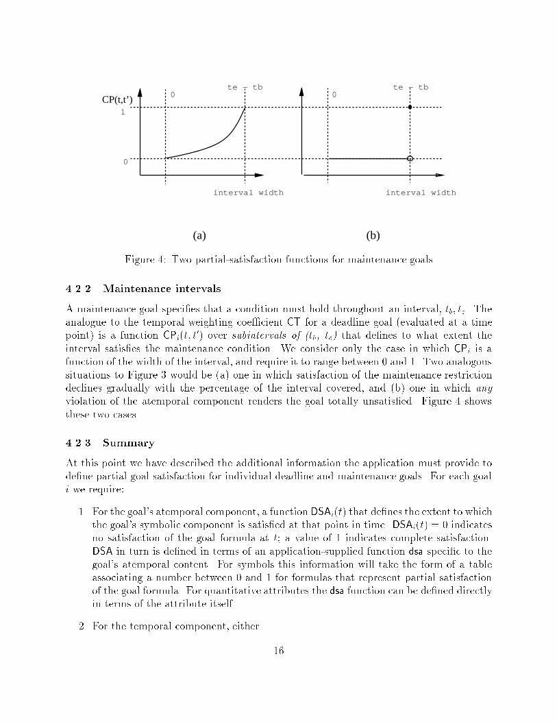
te − tb te − tb

Figure 4: Two partial-satisfaction functions for maintenance goals4.2.2 Maintenance intervalsA maintenance goal speci�es that a condition must hold throughout an interval, tb; te. Theanalogue to the temporal weighting coe�cient CT for a deadline goal (evaluated at a timepoint) is a function CPi(t; t0) over subintervals of (tb, te) that de�nes to what extent theinterval satis�es the maintenance condition. We consider only the case in which CPi is afunction of the width of the interval, and require it to range between 0 and 1. Two analogoussituations to Figure 3 would be (a) one in which satisfaction of the maintenance restrictiondeclines gradually with the percentage of the interval covered, and (b) one in which anyviolation of the atemporal component renders the goal totally unsatis�ed. Figure 4 showsthese two cases.4.2.3 SummaryAt this point we have described the additional information the application must provide tode�ne partial goal satisfaction for individual deadline and maintenance goals. For each goali we require:1. For the goal's atemporal component, a function DSAi(t) that de�nes the extent to whichthe goal's symbolic component is satis�ed at that point in time. DSAi(t) = 0 indicatesno satisfaction of the goal formula at t; a value of 1 indicates complete satisfaction.DSA in turn is de�ned in terms of an application-supplied function dsa speci�c to thegoal's atemporal content. For symbols this information will take the form of a tableassociating a number between 0 and 1 for formulas that represent partial satisfactionof the goal formula. For quantitative attributes the dsa function can be de�ned directlyin terms of the attribute itself.2. For the temporal component, either 16

� a function CTi(t) that speci�es the extent to which time t satis�es the deadline,or� a function CPi(t; t0) that speci�es the extent to which the interval (t; t0) satis�esthe maintenance requirement.The utility function UGi for an individual goal is a combination of these two functions,and the next section confronts the problem of how and when to combine them.5 Utility Functions for Individual GoalsWe have now supplied functional forms for describing satisfaction of a goal's atemporal andtemporal component. The former is supplied in the form of a function DSAi(t), de�ned interms of the atemporal attribute. The DSA function varies between 0.0 and 1.0, representingrespectively no satisfaction and complete satisfaction. The latter is supplied in terms of aweighting coe�cient, either CTi(t) or CPi(t1; t2) depending on whether the goal is a deadlineor a maintenance interval.5.1 Combining the temporal coe�cient and the atemporal de-gree of satisfactionBoth of the partial-satisfaction functions are functions of time points, whereas the goal's con-tribution to the utility function (the UGi function) is de�ned in terms of an entire chronicle.To form the utility function for a deadline goal we need to evaluate and combine DSA andCT values at selected time points within the chronicle and to form the utility function for amaintenance goal we need to evaluate and combine the DSAi and CPi values over selectedintervals within the chronicle.The real problem therefore is when to evaluate the functions, and this is a di�cult questiononly when partial satisfaction is allowed both in the atemporal and temporal components.Take a deadline goal, for example|if we were to allow partial satisfaction of the atemporalcomponent but not the temporal component, we could just evaluate the atemporal goal ex-pression DSA at the deadline point. Likewise, if we allow partial satisfaction of the temporalcomponent but not the atemporal component then we could just evaluate the CT componentat the earliest time point (at or after the deadline) at which the atemporal component isfully satis�ed. But suppose that we allow partial satisfaction in both components|at whattime point(s) should we evaluate and combine the DSA function and the CT coe�cient?5.1.1 Deadline goalsWe motivate our solution with an example. Suppose we are employing a delivery agentwhose task it is to deliver two tons of rocks to the depot by 2PM. Several trips might berequired. Abstractly we can think about how to structure payments to the driver so that ifhe acts rationally he will act so as to maximize our utility.17

A reasonable way to reward the driver is to pay him in proportion to each quantity ofrocks he delivers on each trip, up to a total of two tons. The pay for each delivery would bediscounted by an amount proportional to the amount of time by which each delivery missesthe deadline. The amount the driver gets paid is then the sum of the rewards for all thedeliveries he makes up to two tons. If the driver acts to maximize his expected pay, we willalso be maximizing our utility relative to the goal.Even though the deadline goal is stated in terms of the level of a quantity, it is importantto note that it is proper to reward the driver for the quantities delivered, and not for the levelattained. Otherwise the driver would be penalized if rocks were removed. But we also have tomake sure that there is no incentive for the driver to remove rocks then immediately deliverthem. So the proper reward structure is to pay for deliveries that increase the attribute'slevel of satisfaction. A delivery is analogous to an increase in the dsa value of the atemporalcomponent, not directly to a dsa value.We also make the following assumptions about changes in atemporal utility:� All preferences for lotteries over changes in dsa at any time t are the same as preferencesfor lotteries at any other time t0.� There are a countable number of changes in the dsa over the course of a chronicle.Under these assumptions the appropriate reward structure for the agent|and by analogythe proper expression for the goal's utility|is an additive utility function:UGi(c) = DSAi(td) + (6)Xft>tD: :9t0 (tD�t0<t)^DSAi(t0)�DSAi(t)g(DSAi(t)�maxtD�t̂<tDSAi(t̂)) � CTi(t)where td is the time of the deadline. The intuition is that we accrue utility for the level ofsatisfaction that is true at the deadline point (thus rewarding early satisfaction), and also forevery time the DSA function increases over a previous value. The amount of utility accruedfor a change is the increase in atemporal utility over the previous maximum, weighted bythe CT function that discounts the change according to how well it satis�es the deadline.The basic form of this utility function is similar to that presented by Meyer [Keeney andRai�a, 1976, Sect. 9.3.2] for the utility of a consumption stream. The only di�erence is thatMeyer's formulation de�nes utility directly in terms of consumption|which is the change inthe agent's wealth|while our DSA functions specify this change in utility indirectly. Anotherminor di�erence is that Meyer's formulation allows consumption to be negative, indicatinga loss of wealth, whereas we are only interested in positive changes in degree of satisfaction.Consider, for example, the goal to have two tons of rocks at the depot by noon. We canuse one of two trucks. The big truck carries two tons in one load but is slow: it will getall two tons to the depot by 2pm. The small truck carries only one ton but is fast: it willget one ton there by 1pm and two tons there by 2pm. Which plan a�ords higher utility?The answer depends, of course, on the utility decay associated with missing the deadlinecompared to the utility decay associated with missing some rocks. Suppose that the degree18

of satisfaction of zero tons is 0.0, the degree of satisfaction of one ton is 0.5 and the degreeof satisfaction of two tons is 1.0. Suppose further that the temporal coe�cient is a linearlydecreasing function that goes from 1.0 at noon to 0.0 at 3pm. So CT(t) = 1 � t=3, wheret is the number of hours past noon. Based on these values, the utility of the chronicle thatresults from using the big truck is (1)(1/3) = 1/3 and the utility of the chronicle that resultsfrom using the small truck is (1/2)(2/3)+(1/2)(1/3) = 1/2. Hence we prefer to use the smalltruck over the big truck. This preference �ts our intuition since based on the speci�cationsof the atemporal utility function and the temporal coe�cient, we associate some bene�t withhaving some portion of the two tons of rocks at the depot earlier.This example is an instance of a general probabilistic dominance relation that holds fordeadline goal utility functions as de�ned above. If8i; t; n:P(fc : DSAi(t) � ngjP1) < P(fc : DSAi(t) � ngjP2);where i ranges over all goals and fc : DSAi(t) � ng denotes the set of chronicles in whichDSAi(t) � n, then P1 has higher expected utility than P2 and is thus preferred.5.1.2 Maintenance goalsA maintenance goal states that a condition should be maintained over an interval of time.Partial atemporal satisfaction of a maintenance goal is expressed (as in deadline goals) interms of the degree of satisfaction of the atemporal component. Partial temporal satisfactionis expressed in terms of the length of the interval or intervals over which the atemporalcomponent is partially satis�ed. Partial temporal satisfaction can be a non-linear functionof interval length. For example, we may wish to keep a machine running from 9:00 until5:00 and if it has a production cycle time of 30 minutes, we may not accrue any reward forhaving it running for intervals shorter than 30 minutes. So we de�ne a persistence coe�cientfunction CP that maps a temporal interval into a number between zero and one.The question again is how to combine the atemporal and temporal satisfaction into autility function for the maintenance goal. We need to measure how long the atemporalcomponent persists at each level of partial satisfaction. Since we are measuring the amountof time over which a quantity persists, we need to �x the quantity and �nd the intervalsover which the quantity is at that level. If we have a DSA function that is only either 0or 1, we simply sum the CP values of the intervals over which the atemporal component issatis�ed. If the DSA can have intermediate value the procedure is roughly to integrate overall possible DSA values and �nd intervals over which DSA is maintained at a given level.Notice that if the satisfaction level is low over some interval and higher over a secondinterval then the atemporal component was at least at that low level of satisfaction over bothintervals. For example, suppose that the DSA is above some high level, say 0.8, throughoutthe interval of interest but that it uctuates above that level at some high frequency. Supposefurther that our CP function assigns zero satisfaction to any interval shorter than half of theinterval of interest. If we measure the utility in terms of the intervals over which the DSA isat a given level, we would wind up assigning zero utility to this chronicle even though the19

DSA is above 0.8 for the entire interval. So the following expression assigns utility in termsof the intervals over which the DSA is maintained above each possible value.UGi(c) = Z 10 XfI: 8t2IDSAi(t)�x ^ :9I 0�I 8t2I 0DSAi(t)�xgCPi(I) dx (7)where I and I 0 denote temporal intervals. Notice the symmetry between the above expres-sion and that for deadline goals. To compute the utility of a deadline goal, we sum changesin DSA over time. For maintenance goals, we sum time over DSA i.e., we sum the CP ofintervals over which DSA exceeds a given value over all values of DSA.5.2 SummaryThis section completes the de�nition of utility functions for individual goals, providing ade�nition for the UGi functions. The main problem we solved is how to combine partialsatisfaction of a goal's temporal component with partial satisfaction of a goals' atemporalcomponent.For deadline goals the problem amounts to deciding when to evaluate the DSA function|the degree of satisfaction of the goal's atemporal component. The main idea is to evaluatethe DSA function once at the deadline point, and then at every time point at which the DSAfunction increases. At every such point the increase in atemporal satisfaction is weighted bythe temporal coe�cient CTi.For maintenance goals combining the temporal and atemporal components involves iden-tifying the intervals of DSA over which to evaluate CP. The main idea is to evaluate the CPof the longest continuous intervals over which the DSA exceeds each possible value.Now that we have the basic form of the agent's top-level utility function we turn to theproblem of how to use that function to establish qualitative di�erences in the quality ofalternative plans.6 Using the Utility Functions to Rank PlansOne of the main goals of the present work is to use information in the utility function's sym-bolic structure to guide the building of good plans, which generally will involve demonstratingthat one plan is preferable to another. At worst establishing this relationship involves com-puting the expected utility of both plans, a process that requires generating and evaluatingall possible chronicles for each.By exploiting the structure of the utility functions we can establish the same relation-ships without performing the full expected-utility calculation. We do so by establishingrelationships among the individual goals' symbolic components that indicate correspondingrelationships among the corresponding utility functions. Here is an abstract characterizationof the sorts of relationships we will establish:20

Suppose that one of the agent's goals is g and that there are two formulas �and that bear some relation to g. More particularly, the truth of � indicatesa high goal-related utility (DSA) whereas the truth of indicates a low DSAvalue. Further suppose that there are two alternative plans, P1 and P2. If theprobability that � is true by some time t1 given P1 is at least �, and if theprobability that is true at all times before t2 given P2 is at least �, and if �exceeds some function of �, dsa(�), dsa( ), t1, and t2, then P1's expected utilityis guaranteed to be greater than P2's.Having established a relationship of that form the planner need only establish two proba-bility bounds associated with propositions � and in order to eliminate P2 from furtherconsideration.Two advantages accrue from this technique:1. it reduces the general problem of expected-utility calculations to the more speci�c taskof deciding whether a particular probability exceeds a particular threshold, and2. it allows us to perform the expected-utility analysis incrementally|at each stage ofthe planning process we can eliminate some plans from consideration, again limitingthe amount of inference needed to choose a good course of action.We will demonstrate these advantages in Section 7, but �rst establish relationships for thegoal types we de�ned in the previous section.6.1 Deadline goalsWe �rst derive results for deadline goals, attacking symbolic atemporal attributes, thenquantitative atemporal attributes.6.1.1 Bounds for symbolic attributesWe are comparing two plans on the basis of their performance on a goal whose temporalcomponent is a deadline td and whose atemporal component is symbolic. We have a formula� that indicates a high level of goal satisfaction (dsa value) and a formula with a low dsavalue. Consider the case in which P1 is likely to achieve � at some time at or close to thedeadline, and P2 is likely to achieve at best only some time well after the deadline. Underwhat circumstances can we say that P1 has higher expected utility than P2?Suppose that the goal's atemporal component isHOLDS (On(A,B); td; td) ^ HOLDS (On(B,C); td; td)and we de�ne the dsa function as follows:i �i dsa(�i)1 :On(B;C) 0.02 :On(A;B) ^ On(B;C) 0.53 On(A;B) ^ On(B;C) 1.021

In other words we accrue partial satisfaction by achieving On(B,C) alone, but no partialsatisfaction by achieving On(A,B) alone. In that case the two formulas might be� = HOLDS (On(B;C); t; t0) = :HOLDS (On(B;C); t; t0):Now suppose that for plan P1 we can �nd some time point t1 � td such thatP(�(t1; t1)jP1) � �and for plan P2 we can �nd some time point t2 � td such thatP(8t; t0 (td � t � t0 < t2)! (t; t0)jP2) � �. Under what conditions can we say that plan P1 is preferable to plan P2? We mustdetermine the lowest value of EU(P1) and the highest value of EU(P2) consistent with thesetwo constraints. Let �� be the formula of lowest dsa consistent with � (in the example�� = �3). We are guaranteed the existence of such a formula since the �i are exhaustive.The expected utility of plan P1 is minimized if1. with probability �, �� is achieved at time t1 and the goal is not partially achieved atany time earlier than t1, and2. with probability 1 � � the goal is completely unsatis�ed.So by Equation 6 we haveEU(P1) � � � dsa(��) � CT(t1) + (1� �) � 0Now let � be the formula of highest dsa consistent with conjunct (� = �2). Theexpected utility of plan P2 is highest if1. with probability �, � is achieved by the deadline and the goal is completely achievedimmediately after time t2, and2. with probability 1 � � the goal is completely satis�ed at the deadline.Again by Equation 6:EU(P2) � �[dsa(� ) + (1� dsa(� ))CT(t2)] + (1 � �) � 1And we therefore know that P1's expected utility is higher than P2's if� > �[dsa(� ) + (1� dsa(� ))CT(t2)] + (1� �)dsa(��) � CT(t1) (8)The values for �� and � and the times t1 and t2 will determine how useful our probabilitybounds are. A t1 close to the deadline and a � that is inconsistent with low-utility �i valueswill give us a high lower bound on EU(P1). Similarly, a t2 well after the deadline and a inconsistent with high utility �i values will give us a low upper bound on EU(P2).22

6.1.2 Bounds for quantitative attributesNow suppose that our deadline goal is stated in terms of some quantity Q. Assume that thedsa is a monotonically increasing function of the quantitative attribute3. Suppose we canestablish that P1 will achieve some high level of Q by some time close to the deadline, andthat P2 can not establish more than some low level of Q until well after the deadline. Whatdo the levels and times have to be in order to conclude that P1 dominates P2?Suppose we know that for plan P1 we �nd a time point t1 � td and some attribute valuek1 for whichP(HOLDS (� (Q; k1); t1; t1)jP1) � �and for plan P2 we �nd a time point t2 � td and a value k2 such thatP(8t; t0 (td � t � t0 < t2)! HOLDS (� (Q; k2); t; t0)jP2) � �Under what conditions can we say that P1 dominates plan P2? The expected utility of P1is lowest if1. with probability �, we achieve a level k1 for Q at time t1 and Q has value zero at alltimes prior to t1, and2. with probability (1 � �), Q has its minimum value at all times.Under those circumstances we know thatEU(P1) � � � dsa(k1) � CT(t1)The expected utility of plan P2 is highest if1. with probability �, Q attains level k2 at the deadline and the maximum possible valueof Q is attained immediately after t2, and2. with probability 1 � � the maximum possible value of Q is attained by the deadline.Then we know thatEU(P2) � � � [dsa(k2) + (1� dsa(k2)) � CT(t2)] + (1 � �);and P1 is preferred to P2 if� > � � [dsa(k2) + (1� dsa(k2)) � CT(t2)] + (1� �)dsa(k1) � CT(t1) (9)3A symmetric analysis can be performed for monotonically decreasing atemporal utility.23

6.1.3 Bounds for strictly ordered atemporal attributesAdditional structure in the atemporal component can make dominance relationships easierto come by. In this section we will consider a common atemporal component that has anadditional structural feature: a ordered conjunction of expressions in which each conjunctdominates subsequent conjunct|any chronicle that satis�es g1 is preferable to every chron-icle that does not satisfy g1, even it satis�es all the others. For example, if our conjunctsare g1, g2, and g3 our strictly ordered atemporal utility function would satisfy the constraintthat satisfying g1 is preferable to not satisfying it, regardless of whether g2 or g3 are satis�ed:dsa(g1 ^ g2 ^ g3) > dsa(:g1 ^ g2 ^ g3)dsa(g1 ^ :g2 ^ g3) > dsa(:g1 ^ g2 ^ g3)dsa(g1 ^ g2 ^ :g3) > dsa(:g1 ^ g2 ^ g3)dsa(g1 ^ :g2 ^ :g3) > dsa(:g1 ^ g2 ^ g3)dsa(g1 ^ g2 ^ g3) > dsa(:g1 ^ :g2 ^ g3)dsa(g1 ^ :g2 ^ g3) > dsa(:g1 ^ :g2 ^ g3)...dsa(g1 ^ :g2 ^ :g3) > dsa(:g1 ^ :g2 ^ :g3)and likewise, given that g1 is true, it's always preferable to satisfy g2 regardless of g3's state:dsa(g1 ^ g2 ^ g3) > dsa(g1 ^ :g2 ^ g3)dsa(g1 ^ g2 ^ :g3) > dsa(g1 ^ :g2 ^ g3)dsa(g1 ^ g2 ^ g3) > dsa(g1 ^ :g2 ^ :g3)dsa(g1 ^ g2 ^ :g3) > dsa(g1 ^ :g2 ^ :g3)Finally we note that if g1 and g2 are both true then g3 is preferable to its negation:dsa(g1 ^ g2 ^ g3) > dsa(g1 ^ g2 ^ :g3)Notice that we did not specify that g2 dominates g3 in cases where g1 is false. The reasonis that we will often assign zero utility to all states in which the most important goal is notsatis�ed. For example, given the goal to have the truck fueled and clean by noon, it mightdo us no good to have it clean if it is not fueled.The structure of a utility function of this form allows us to prune away suboptimal plansby considering each conjunct individually in the priority order dictated by the dsa values.As above suppose that we have a time t1 at which P1 is likely to achieve g1, but for P2g1 is liable to be false until at least t2:P(g1(t1; t1)jP1) � �P(8t; t0 (td � t � t0 < t2)! :g1(t; t0)jP2) � �24

Under what conditions can we say that plan P1 is preferable to plan P2? We have noinformation about the probabilities of the atemporal component's other conjuncts, so a lowerbound on the expected utility of P1 isEU(P1) � � � dsa(g1 ^i :gi) � CT(t1)and an upper bound on the expected utility of plan P2 isEU(P2) � � � [dsa(:g1 ^i gi) + (1� dsa(:g1 ^i gi))CT(t2)] + (1� �):So plan P1 is preferred to plan P2 if� > �[dsa(:g1 ^i gi) + (1� dsa(:g1 ^i gi))CT(t2)] + (1� �)dsa(g1 ^i :gi)CT(t1) (10)In this case we can eliminate some suboptimal plans using based only on their abilityto satisfy the �rst goal conjunct. Having done so we can then compare the probability ofsatisfying the �rst and second conjuncts to the probability of satisfying the �rst conjunctbut not the second, and so forth. We continue until we have incorporated all the conjuncts,at which point we can compute the expected utility of any remaining plans.This ability to consider the conjuncts sequentially has important consequences for theprojection process. [Hanks, 1993] presents a probabilistic projection algorithm demonstratingthat:� it can be much cheaper to project a plan with respect to a single proposition (like oneof our goal conjuncts) than it is to reason about all of the plan's e�ects,� it can be much cheaper to determine whether the probability of a proposition exceedsa speci�c threshold than it is to compute the exact value of that probability.6.1.4 ExampleLet's consider a speci�c example of how these relationships can be used to compare plans.Suppose our goal is to be home by 6:00 with some Thai food and some beer:HOLDS (Loc(me,home); 6:00; 6:00) ^HOLDS (Possess(me,thai-food); 6:00; 6:00) ^HOLDS (Possess(me,beer); 6:00; 6:00)Assume that these propositions persist: any of the goals I achieve before the deadline willbe true at the deadline.Suppose we have the dsa function appearing in Figure 5, and that the temporal coe�cientfunction falls o� linearly from 1.0 at 6:00pm to 0.0 at 10:00pm, so CT(t) = 1� t=4, where t ismeasured in hours past 6:00pm. Now consider two plans P1 and P2 such that for plan P1 wehave established a time t1 prior to which the formula � = Loc(me,home) is likely to be true,25

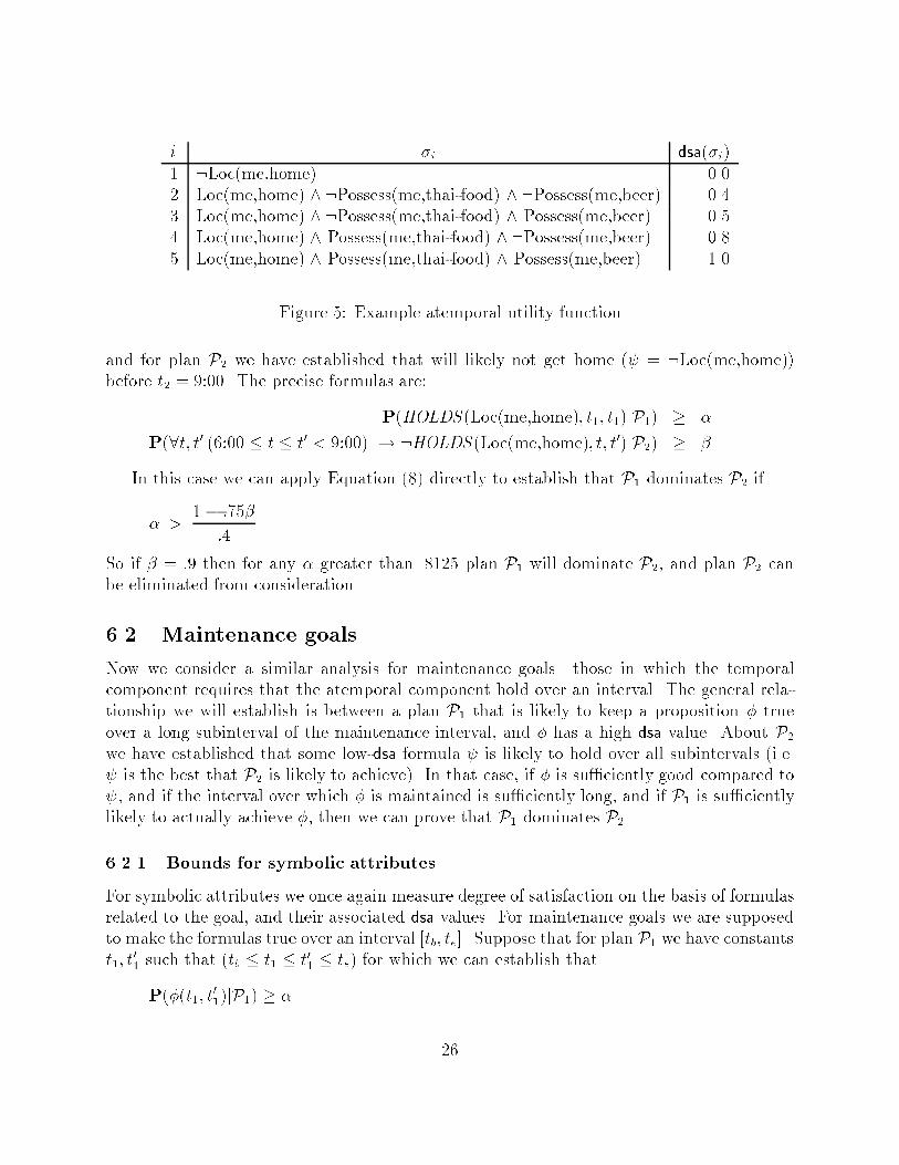
i �i dsa(�i)1 :Loc(me,home) 0.02 Loc(me,home) ^ :Possess(me,thai-food) ^ :Possess(me,beer) 0.43 Loc(me,home) ^ :Possess(me,thai-food) ^ Possess(me,beer) 0.54 Loc(me,home) ^ Possess(me,thai-food) ^ :Possess(me,beer) 0.85 Loc(me,home) ^ Possess(me,thai-food) ^ Possess(me,beer) 1.0Figure 5: Example atemporal utility functionand for plan P2 we have established that will likely not get home ( = :Loc(me,home))before t2 = 9:00. The precise formulas are:P(HOLDS (Loc(me,home); t1; t1)jP1) � �P(8t; t0 (6:00 � t � t0 < 9:00) ! :HOLDS (Loc(me,home); t; t0)jP2) � �In this case we can apply Equation (8) directly to establish that P1 dominates P2 if� > 1� :75�:4So if � = :9 then for any � greater than .8125 plan P1 will dominate P2, and plan P2 canbe eliminated from consideration.6.2 Maintenance goalsNow we consider a similar analysis for maintenance goals|those in which the temporalcomponent requires that the atemporal component hold over an interval. The general rela-tionship we will establish is between a plan P1 that is likely to keep a proposition � trueover a long subinterval of the maintenance interval, and � has a high dsa value. About P2we have established that some low-dsa formula is likely to hold over all subintervals (i.e. is the best that P2 is likely to achieve). In that case, if � is su�ciently good compared to , and if the interval over which � is maintained is su�ciently long, and if P1 is su�cientlylikely to actually achieve �, then we can prove that P1 dominates P2.6.2.1 Bounds for symbolic attributesFor symbolic attributes we once again measure degree of satisfaction on the basis of formulasrelated to the goal, and their associated dsa values. For maintenance goals we are supposedto make the formulas true over an interval [tb; te]. Suppose that for plan P1 we have constantst1; t01 such that (tb � t1 � t01 � te) for which we can establish thatP(�(t1; t01)jP1) � � 26

(P1 is likely to make � true over a subinterval [t1; t01] of the maintenance interval [tb; te]), andfor plan P2 we have constants t2; t02 such that (tB � t2 � t02 � tE) for which we can establishthat P( (t2; t02)jP2) � �(P2 is likely to make hold over subinterval [t2; t02] of the maintenance interval [tb; te].)Under what conditions can we say that P1 dominates P2? Again we must determine thelowest value of EU(P1) and the highest value of EU(P2) consistent with these two constraints.Let �� be the formula of lowest dsa consistent with �. The expected utility of plan P1 islowest if1. with probability �, �� holds throughout t1; t01 and the atemporal component is notpartially satis�ed at any time outside of [t1; t01], and2. with probability 1� � the atemporal component is completely unsatis�ed throughout[tb; te].So by Equation (7) we haveEU(P1) � � � Z dsa(��)0 CP(t1; t01) dx= � � CP(t1; t01) � dsa(��)Now let � be the formula of highest dsa consistent with . The expected utility of planP2 is highest if1. with probability �, � holds throughout [t2; t02] and the atemporal component is com-pletely satis�ed at all time outside [t2; t02], and2. with probability 1�� the atemporal component is completely satis�ed throughout theinterval [tb; te].Again by Equation (7):EU(P2) � � � "Z dsa(� )0 CP(tB; tE) dx + Z 1dsa(� ) CP(tB; t2) + CP(t02; tE) dx#+ (1 � �)(1)= �[dsa(� ) + (CP(tB; t2) + CP(t02; tE)) � (1 � dsa(� ))� 1] + 1and then P1 dominates P2 if� > �[dsa(� ) + (CP(tB; t2) + CP(t02; tE)) � (1� dsa(� ))� 1] + 1CP(t1; t01) � dsa(��) (11)27

6.2.2 Bounds for quantitative attributesIn this case our atemporal goal is stated in terms of some quantity Q, and the dsa functionassociated with Q is monotonically increasing. We discover that P1 is likely to achieve alevel of Q at least equal to k1 throughout some subinterval [t1; t01] of the maintenance interval[tb; te]; P2 is likely to achieve a level of Q at most k2 throughout some subinterval [t2; t02] of[tb; te]. The two equations are:P(HOLDS (� (Q; k1); t1; t01)jP1) � �P(HOLDS (� (Q; k2); t2; t02)jP2) � �Under what conditions can we say that P1's expected utility is greater than P2's? Theexpected utility of P1 is lowest if1. with probability �, a level k1 for Q is maintained throughout the interval [t1; t01] andQ has the value corresponding to a dsa of zero at all times outside of [t1; t01], and2. with probability (1 � �) Q has the value corresponding to a dsa of zero at all timesduring [tb; te].Under those circumstances we know thatEU(P1) � � � CP(t1; t01) � dsa(k1)The expected utility of plan P2 is highest if1. with probability �, Q maintains a level of k2 throughout the interval t2; t02 and Qmaintains the value corresponding to complete satisfaction at all times outside t2; t02,and2. with probability 1 � � Q maintains the value corresponding to complete satisfactionthroughout the interval tB; tE.Then we know thatEU(P2) � �[dsa(k2) + (CP(tB; t2) + CP(t02; tE)) � (1� dsa(k2))� 1] + 1and then P1 is preferred to P2 if� > �[dsa(k2) + (CP(tB; t2) + CP(t02; tE)) � (1� dsa(k2))� 1] + 1CP(t1; t01) � dsa(k1) (12)28

6.2.3 Bounds for strictly ordered atemporal attributesFinally we reconsider the case of Section 6.1.3, where the atemporal component consists of aconjunction of formulas that can be ordered such that each conjunct dominates those laterin the sequence. This time we establish that P1 is likely to make the dominant attribute g1true over some subinterval [t1; t01], and P2 is likely to make that same attribute false over thesubinterval [t2; t02]:P(g1(t1; t01)jP1) � �P(:g1(t2; t02)jP2) � �Under what conditions can we say that plan P1 is preferable to plan P2? This is just aspecial case of an atemporal attribute, where the formula of lowest dsa consistent with g1 is�� � g1 ^i :gi and the formula of highest dsa consistent with :g1 is � � :g1 ^i gi. So bythe results of section 6.2.1 plan P1 is preferred to plan P2 if� > �[dsa(:g1 ^i gi) + (CP(tB; t2) + CP(t02; tE)) � (1� dsa(:g1 ^i gi))� 1] + 1CP(t1; t01) � dsa(g1 ^i :gi) (13)6.3 SummaryThe main point of this section was to establish circumstances under which the question ofwhether one plan is preferable to another (in the sense of having higher expected utility) couldbe answered by determining bounds on the probabilities of goal-related propositions. Thegeneral procedure for determining that a plan P1 dominates a plan P2 is to �nd a proposition� associated with high (atemporal) satisfaction that P1 is likely to achieve and a proposition associated with low atemporal satisfaction that P2 is likely to achieve. We then comparethe worst case for P1 (that it establishes � with low probability, and otherwise providesno atemporal goal satisfaction) agains the best case for P2 (that it establishes with lowprobability, and the rest of the time provides complete goal satisfaction). This analysis leadsto an inequality involving the probabilities of � and , indicating circumstances under whichP1 dominates P2. We provided equations for symbolic, numeric, and ordered conjunctiveatemporal attributes, �rst for deadline goals (Equations (8), (9), and (10)) and analogouslyfor maintenance goals (Equations (11), (12), and (13)).The analysis in this section studies a single goal in isolation; we next consider a multi-goalutility model, and how it can be exploited in the process of generating plans.7 Multiple Goals, Residual Utility, and ComputationalIssuesThe previous sections established bounds on the probabilities of outcomes that could be usedto determine whether one plan is preferable to another. These analyses were performed on29

the utility functions for individual goals, implicitly assuming that utility for other goals andfor resource consumption were the same.The assumption that global utility is linear additive in the goal utilities (Section 3)makes explicit the tradeo� between satisfying the top-level goals, and between satisfying agoal and consuming resources. The assumption that resource consumption (counted in theresidual utility term) is independent of the goal utilities means that we can regard resourceconsumption as a goal as well. Take the two-goal case, for example, for which we can writethe equation for the expected utility of a plan P as follows:EU(P) = k1EU1(P) + k2EU2(P) + krEUr(P) (14)whereEUi(P) = �cUGi(c)P(cjP):Now suppose that we have already generated a plan P1 and we know its expected utilityEU(P1) = u1.Further suppose that we have begun generating an alternative plan P2, in particular wehave generated a subplan that achieves the �rst goal. From this subplan we can compute1. an upper bound on the utility associated with �rst goal, EU1(P2) � u12, and2. a minimum level of resource consumption which provides us with an upper bound onresidual utility, EUr(P2) � ur2.We can then calculate that for P2 to be preferred to P1 it must at least satisfy goal two tothe degreeEU2(P2) � u1 � k1u12 � krur2k2which represents the required utility level for the second goal assuming no additional resourceconsumption. Examining the symbolic structure of the second goal may indicate exactlywhat propositions must be made true or what quantity level must be attained, and by when,in order to attain that level of utility. The ratio between kr and k2 along with the residualutility function indicates how e�ciently the second goal must be satis�ed as well.7.1 Plan generation and re�nementThe results in previous sections all involved comparing two complete plans; the relationshipswe provided reduced the question of which was preferable in the sense of maximizing utilityto one of establishing a relationship between probabilities over the symbolic attributes thatcomprise one of the goal expressions. The algorithm in [Hanks, 1993] exploits both the sym-bolic content of the relationship and the numeric threshold to limit inference in establishingwhether or not this relationship holds. Therefore deciding which of two partial plans ispreferable might be considerably cheaper than computing the expected utility of each.30

The result earlier in this section demonstrates that given one complete plan and a partialplan we can characterize the interesting possible completions of the partial plan|the onesthat satisfy the remaining goals with a certain probability and with a certain e�ectiveness ifthe second plan is to be preferred to the �rst. Therefore deciding if a partial plan is worthpursuing can be considerably cheaper than examining all of its completions.The question arises in general, however, as to what extent these relationships can aid theplanning process. What can we say about the relationship between two partial plans? Thenext two sections discuss how our model might be applied to two plan-generation paradigms:partial-order planning and re�nement planning.7.1.1 Partial-order planning and search controlThe buridan planner [Kushmerick et al., 1993] is an extension to classical nonlinear plannersthat allows uncertainty in the initial world state and in the e�ects of operators. The buridanalgorithm takes as input a problem description (a goal formula and a probability distributionover initial world states) and a probability threshold, and produces a plan that satis�esthe goal with probability at least equal to the threshold. The analysis in this paper iscomplementary: it is a theory of how to generate the threshold values, but does not suggestan algorithm for exploiting them.Two problems (at least) complicate the problem of applying our theory of utility to aprobabilistic planner like buridan. The �rst is that the buridan algorithm generates alower bound on the probability that the current plan or its completions satisfy the goal, andgenerally the lower the threshold the less work buridan need do to generate an appropriateplan. A lower bound is of limited use in and of itself, however: you generally can't proveone plan superior to another without a lower bound on the performance of one and an upperbound on the other. The problem with a generative or transformational planner is that it iscan be impossible to establish the point at which the plan cannot be further improved.The second limitation in applying our theory to buridan is that its notion of a goal islimited to propositional formulas, so concepts of partial satisfaction, deadlines, and resourcesare di�cult to represent. Ongoing work is directed toward enhancing buridan's represen-tation language so it can naturally represent the concepts developed in this paper, andalso to explore how this framework can be used to provide the planner with search-controlinformation.7.1.2 Re�nement planningOne special case of partial planning that is amenable to our analysis is that in which theplanner's only operation is to re�ne its current plan, which amounts to replacing an abstractaction in the plan with a more speci�c version of that action. More precisely a re�nementoperator can never increase the set of possible outcomes consistent with the plan's execution,and thus tends to resolve uncertainty about its quality. An abstract plan's outcomes are setsof outcomes of more concrete plans. Since di�erent probability and utility values may beassociated with each speci�c outcome, in general a probability range and a utility range will31

be associated with each abstract outcome. Thus the expected utility of an abstract plan isrepresented by an interval, which includes the expected utilities of all possible instantiationsof that abstract plan. Re�ning the plan, i.e. choosing an instantiation, tends to narrow theinterval. Comparing two abstract plans can stop as soon as their expected-utility intervalsno longer overlap4.The type of abstraction we use has been formalized by Tenenberg [1991] within the frame-work of the STRIPS representation and termed inheritance abstraction. He contrasts this tothe type of abstraction used in ABSTRIPS [Sacerdoti, 1974], which Tenenberg calls relaxedmodel abstraction. For examples of the use of inheritance abstraction in plan generationin a deterministic setting see [Nau, 1987, Anderson and Farley, 1988]. The present workgeneralizes the notion of inheritance abstraction by introducing time, probability, and utilityinto the representation.We illustrate the planning technique with an example. Consider the following problemof planning a delivery task. We wish to generate the best plan for delivering two tons oftomatoes from a farm to a warehouse within 85 minutes. The utility of a plan outcome is afunction of the deadline goal and the residual utility, which is determined by the amount offuel consumed. The components of the utility function are shown in Figure 7. The overallutility isU(c) = UG(c) + (:02)UR(c)The delivery plan will consist of driving a truck from the depot to the farm, loading thetruck, and driving the loaded truck to the warehouse. Planning is the process of generatingthis plan as well as choosing among the various ways this plan can be realized in such away that expected utility is maximized. The descriptions of the available actions are shownin Figure 6. The action descriptions are similar to those in [Hanks, 1990]. Actions haveconditional e�ects, and are represented by a tree with conditions labeling the branches. Theleaves of the tree are labeled with the outcomes of the action. Deterministic actions arelabeled with a single outcome. The probability of an outcome is the probability conditionedon the action and the conjunction of all conditions on all branches leading to the outcome.Outcomes are described in terms of a duration, as well as any changes in attribute values.Attributes are represented as functions of time. The variable t represents the beginning timeof the action, making the action descriptions temporally indexical.There are two possible routes we can take from the depot to the farm: road A and roadB. Road A is longer but has no delays, while travel along road B might be delayed due toconstruction. The probability that construction is taking place is 0.2. These options arerepresented by the �rst two action descriptions in the Figure 6.Once at the farm we must load the truck. We have two trucks at the depot to choosefrom: an open truck and a closed, cushioned truck. The open truck is easy to load, whilethe closed truck can be loaded easily if a special quick-loading device is available. There is4Or when the intervals narrow to the point where the distinction between the two does not warrantfurther attention, as [Russell and Wefald, 1991b] point out.32

Go to farmon road A

dur1 = 30fuel(t+dur1) = fuel(t)–1

Go to farmon road B

dur2 = 15fuel(t+dur2) = fuel(t)–1/2

dur2 = 45fuel(t+dur2) = fuel(t)–1/2

P(¬construction)=.8

P(construction)=.2

Load opentruck

Load closedtruck

dur3 = 15tons–in–truck(t+dur3) = 2

P(quick–loader)=.8

P(¬quick–loader)=.2

dur4 = 10tons–in–truck(t+dur4) = 2

dur4 = 25tons–in–truck(t+dur4) = 2

Drive open truckon mountain road

Drive open truckon valley road

dur5 = 60fuel(t+dur5) = fuel(t)–2tons–delivered(t+dur5) = (.8) tons–in–truck(t)

dur6 = 90fuel(t+dur6) = fuel(t)–3tons–delivered(t+dur6) = (.9) tons–in–truck(t)

dur6 = 90fuel(t+dur6) = fuel(t)–3tons–delivered(t+dur6) = tons–in–truck(t)

P(sunny) = .7

P(cloudy) = .3

Drive closed truckon mountain road

Drive closed truckon valley road

dur7 = 60fuel(t+dur7) = fuel(t)–2tons–delivered(t+dur7) = tons–in–truck(t)

dur7 = 90fuel(t+dur7) = fuel(t)–3tons–delivered(t+dur7) = tons–in–truck(t)Figure 6: Action descriptions33

20

dsa

1

tons

1

16585 time

ct

1

UR

4.52.5 fuelFigure 7: Speci�cation of delivery utility function.34

an 80% chance this device will be available. The next two diagrams in the Figure 6 depictthese two actions.Once the truck is loaded we must drive it to the warehouse. We have two routes to choosefrom: the mountain road and the valley road. The mountain road is shorter but bumpy.If we drive the open truck on the mountain road, the bottom 20% of the tomatoes will becrushed. If we drive the open truck on the valley road and the sun is shining, the top 10%of the tomatoes will be spoiled by the sun. This combination of options results in the lastfour action descriptions in the Figure 6.In order to perform the re�nement type planning described, we organize the planningknowledge in an abstraction/decomposition network, shown in Figure 8. Solid links showdecompositions [Charniak and McDermott, 1985, Ch9], while dashed links show possiblere�nements. For example the task \deliver tomatoes" is decomposed into the sequence ofthe two actions \go to farm" and \load & drive truck". The arrow between the actionssigni�es temporal succession. The abstract action \go to farm" can be realized by driving onroad A or road B. Since both elements of a decomposition must be realized, decompositionlinks are AND links and since either element of an instantiation may be used, instantiationlinks are OR links. So this network forms an AND/OR tree.Descriptions of the abstract actions are shown in Figure 9. A set of actions is abstractedby grouping together their outcomes into abstract outcomes which represent the range ofpossible outcomes of the instantiations. Care must be taken to group together similar out-comes. For example, the \drive open truck" action is an abstraction of \drive open truck onmountain road" and \drive open truck on valley road." Since the single outcome of \driveopen truck on mountain road" is more similar to the outcome of the upper branch of \driveopen truck on valley road" than to the outcome of the lower branch, it is grouped withthe former. While similarity is fairly clear in this case, determining similarity of outcomeswith multiple attributes may not be straightforward in general. (In fact, one may wish toproduce more than one abstraction based on di�erent similarity measures and try each oneon a given problem. One would use the hierarchy that resulted in the most pruning for thegiven problem.) The outcomes of the abstract action are now speci�ed simply as the rangeof outcomes grouped together. Once the outcomes have been abstracted, probabilities mustbe assigned to them. This is done by taking the range of probabilities of the outcomes in thegroup. So for the \drive open truck" action, the range on the upper branch is [min(P(sunny),1) max(P(sunny), 1)], which is just [P(sunny) 1].Given this representation of the planning problem, we evaluate plans at the abstract leveland prune suboptimal plans before re�ning candidate plans further. There are eight possibleplans implicitly encoded in the abstraction/decomposition network, and we want to choosethe one that maximizes expected utility.According to the network, the task of delivering tomatoes is �rst decomposed into goingto the farm and loading, then driving the truck. We can �rst choose either which road totake to the farm or which truck to load and drive. Suppose we make the latter choice �rst.Because the utility function is a function over chronicles, the value of a particular action in aplan depends on when in the plan it occurs, so options can only be evaluated in the context35

deliver tomatoes

go to farm load & drive truck

road A road B load & driveopen truck

load & driveclosed truck

load open truck

drive open truckto warehouse

load closedtruck

drive closed truckto warehouse

drive open onmountain road

drive open onvalley road

drive closed onmountain road

drive closed on valley roadFigure 8: Abstraction/decomposition network

36

Go to farm

dur8 = [15 30]fuel(t+dur8) = fuel(t)–[1/2 1]

dur8 = 45fuel(t+dur8) = fuel(t)–1/2

[P(¬construction) 1]

[0 P(construction)]

Drive open truck

dur9 = [60 90]fuel(t+dur9) = fuel(t)–[2 3]tons–delivered(t+dur9) = [.8 .9] tons–in–truck(t)

dur9 = 90fuel(t+dur9) = fuel(t)–3tons–delivered(t+dur9) = tons–in–truck(t)

[P(sunny) 1]

[0 P(cloudy)]

Drive closed truckdur10 = [60 90]fuel(t+dur10) = fuel(t)–[2 3]tons–delivered(t+dur7) = tons–in–truck(t)Figure 9: Abstract action descriptions

37

P1: Go to farm �! Load & drive open truckchronicle time fuel tons U(chronicle) probabilityc1 [90 135] [2.5 4] [1.6 1.8] [.005 .02] [.56 1]c2 [120 135] [3.5 4] 2 [.380 .5725] [0 .3]c3 [120 150] [2.5 3.5] [1.6 1.8] [.01 .02] [0 .2]c4 150 3.5 2 .1975 [0 .06]P2: Go to farm �! Load & drive closed truckchronicle time fuel tons U(chronicle) probabilityc1 [85 130] [2.5 4] 2 [.4425 1.02] [.64 .8]c2 [100 145] [2.5 4] 2 [.255 .8325] [.16 .2]c3 [115 145] [2.5 3.5] 2 [.255 .635] [0 .16]c4 [130 160] [2.5 3.5] 2 [.0675 .4475] [0 .04]Table 1: Highest level abstract plan outcomes.of an overall plan. Consequently, we combine the \load & drive open truck" and the \load& drive closed truck" actions with the \go to farm" action to obtain a complete abstractplan that can be evaluated.Each abstract plan results in four chronicles (Table 1). For example, for plan P1 weobtain these chronicles by concatenating the \go to farm," \load open truck," and \driveopen truck" action descriptions. Doing so results in four chronicles, since \go to farm" and\drive open truck" each have two branches. Rather than showing the complete chronicles,the relevant attributes of the resulting chronicles are summarized in Table 1, which showsfor each chronicle the range of times, fuel consumption, and tons of tomatos delivered. Thetime refers to the time that the delivery is made. We assume that the plan begins executionat time zero and we take the beginning time of an action to be the beginning time of theprevious action plus its duration. So for example the fuel consumption for chronicle c1 iscomputed according tofuel(dur8) = fuel(0)� [:5 1]fuel(dur8 + dur9) = fuel(dur8)� [2 3]so fuel(dur8 + dur9) = fuel(0)� [2:5 4]We illustrate how the utility range is computed by showing the computation for chroniclec2 of plan P1; the computation for the other chronicles is similar. Let UGmin and UGmaxbe the lower and upper bounds on the goal utility, respectively, and let URmin and URmaxbe the lower and upper bounds on residual utility, respectively. Since we are computing theutility of a deadline goal, we can minimize the utility of the abstract chronicle by choosing38

the latest delivery times and the smallest delivery amounts, we can maximize the utility bychoosing the earliest delivery times and the largest amounts. SoUGmax(c2) = dsa(2) � ct(120) = 0:5625UGmin(c2) = dsa(2) � ct(135) = 0:375URmin(c2) = 0:25URmax(c2) = 0:5Since our global utility function is U(c) = UG(c) + (0:02)UR(c), we have U(c2) = [0.3800.5725].Using the utility and probability information in the table we can compute the expectedutility bounds for each plan. Computing a bound for a plan involves choosing the probabili-ties within the given ranges that minimize and maximize the expected utility. We can do soby solving a small linear programming problem in which the objective function is the expres-sion for the expected utility and the constraints are the probability bounds. For example,the upper bound for plan P1 can be computed by maximizing the objective function:02p1 + :5725p2 + :02p3 + :1975p4subject to the constraints:56 � p1 � 10 � p2 � :30 � p3 � :20 � p4 � :06p1 + p2 + p3 + p4 = 1The maximizing probabilities arep1 = .56p2 = .3p3 = .08p4 = .06So the upper bound on expected utility is(:56)(:02) + (:3)(:5725) + (:08)(:02) + (:06)(:1975) = :1964So for plan P1 and P2 we obtain the expected utility ranges39

P2:1: Go to farm �! Load closed truck �! Drive closed on mountain roadchronicle time fuel tons U(chronicle) probabilityc1 [85 100] [2.5 3] 2 [.8275 1.02] [.64 .8]c2 [100 115] [2.5 3] 2 [.64 .8325] [.16 .2]c3 115 2.5 2 .645 [0 .16]c4 130 2.5 2 .4575 [0 .04]P2:2: Go to farm �! Load closed truck �! Drive closed on valley roadchronicle time fuel tons U(chronicle) probabilityc1 [115 130] [3.5 4] 2 [.4425 .635] [.64 .8]c2 [130 145] [3.5 4] 2 [.255 .4475] [.16 .2]c3 145 3.5 2 .26 [0 .16]c4 160 3.5 2 .0725 [0 .04]Table 2: Intermediate level abstract plan outcomes.EU(P1) = [.005 .1964]EU(P2) = [.3673 .9825].Since the lower bound for P2 is greater than the upper bound for P1, we can eliminatefrom consideration all possible re�nements of P1 and concentrate on re�ning P2. So at thispoint we have chosen the option of using the closed truck. By making this choice, we havepruned away the left-hand subnetwork underneath the \load & drive truck" node in Figure8, resulting in pruning half the space of possible plans from consideration.We are left with two more actions to re�ne: \go to farm" and \drive closed truck towarehouse." Suppose we next choose to re�ne the \drive" action. Again the instantiationsinvolving the mountain road and the valley road must be evaluated in the context of acomplete plan. So we compose the descriptions of the concrete actions \drive closed onmountain road" and \drive closed on valley road" with the descriptions of the concreteaction \load closed truck" and the abstract action \go to farm." Table 2 summarizes theoutcomes for the two alternative plans. We use this information to compute expected-utilitybounds for the two alternatives:EU(P2:1) = [.7533 .9825]EU(P2:2) = [.3683 .5975].Notice that the EU intervals for the two plans are contained in the EU interval for theabstract plan of which they are a re�nement. Since the lower bound for plan P2:1 is greaterthan the upper bound for plan P2:2, we can eliminate P2:2 from consideration, pruning awaytwo more possible concrete plans. By eliminating plan P2:2, we have chosen to take themountain road.Finally we re�ne plan P2:1. Our two options are taking either road A or road B to thefarm. The outcomes of the plans incorporating these options are summarized in table 3.40

P2:1:1: Go to farm on road A �! Load closed truck �! Drive closed on mountain roadchronicle time fuel tons U(chronicle) probabilityc1 100 3 2 .8275 .8c2 115 3 2 .64 .2P2:1:2: Go to farm on road B �! Load closed truck �! Drive closed on valley roadchronicle time fuel tons U(chronicle) probabilityc1 85 2.5 2 1.02 .64c2 100 2.5 2 .8325 .16c3 115 2.5 2 .645 .16c4 130 2.5 2 .4575 .04Table 3: Concrete plan outcomes.Since the plans now include only concrete actions, the attribute, probability, and utilityvalues are now point values. The expected utilites of the two remaining plans areEU(P2:1:1) = .79EU(P2:1:2) = .9075so we choose plan P2:1:2. Since this is a complete concrete plan, we have generated the planthat maximizes expected utility and are �nished.Although it is probably unrealistic to expect any planner to employ only re�nementoperators, the idea of modeling an execution system using a hierarchy of abstract actions isconsistent with Firby's [1989] RAP system, and the architecture for planning and executionproposed in [Hanks and Firby, 1990].8 Summary and Related WorkOur goal in this work was to take the concept of goals as they have been used in symbolicplanning systems and simultaneously extend their functionality and recast the intuitions ina form that can be exploited by a decision-theoretic planning algorithm.Our framework involves building a utility model �rst by identifying the agent's top-level goals plus the residual attributes that measure resource consumption and productionin service of those goals. The assumption of utility independence among these attributesmeans that their interactions can be summarized by n+ 1 numeric parameters representingthe relative weights for the n goals and residual attributes.We then extended the notion of a goal to one that involves both a temporal component(deadline or maintenance interval) and an atemporal component (a formula to be achievedsubject to the temporal constraint). We discussed various forms for the atemporal goal com-ponent: symbolic and numeric attributes, conjunctions of numeric attributes, and orderedconjunctions. 41

For each of the goals the user supplies two components that describe preferences overpartial-satisfaction scenarios: the atemporal degree of satisfaction function and the tempo-ral weighting coe�cient. The former de�nes what it means to satisfy the goal's atemporalcomponent, either partially or fully. The latter indicates how utility declines as a functionof missing the deadline or violating the maintenance interval. We described how to com-bine those functions to produce a utility function for the entire goal. The problem was howto combine partial satisfaction of both the atemporal and the temporal components simul-taneously, and we developed model in which utility is accrued each time the value of theatemporal component increases over the interval de�ned by the temporal coe�cient.We then showed how the model's information, both numeric and symbolic, could beexploited to compare plans: to decide whether one plan's expected utility was greater thananother and to generate bounds on the quality of a partial plan in order that it should bechosen over an alternative. The general form of these relationships was to consider a plan P1that was likely to achieve at worst a high level of satisfaction, and a plan P2 that was likelyto achieve at best a low level of satisfaction. The result was a function of the respectiveformulas, their likelihoods, and their times, ensuring that P1's expected utility was greaterthan P2's, regardless of the two plans' other e�ects.Finally we demonstrated how these relationships could be exploited by two existing plan-ning techniques, particularly in the area of re�nement planning.8.1 Related workA discussion of related work should begin with a mention of multiattribute decision theory,especially [Keeney and Rai�a, 1976]. What we have done is built a multiattribute utilitymodel for goal-oriented planning problems that feature partial goal satisfaction and dead-lines.Our discussion of strictly ordered goals was motivated by the work in goal program-ming [Schniederjans, 1984] a mathematical optimization technique that deals with orderedcon icting goals.8.1.1 Goals and utility modelsIn the AI literature the work closest to our own is byWellman and Doyle [1991], [Wellman andDoyle, 1992], which also analyzes the relationship between goals and preference structures.Their work confronts the question of what it means to say that an agent has some goal. Themost fundamental di�erence between their work and ours is that they begin by examiningan agent's preference structure directly and produce a de�nition of what it means to saythat an agent has a goal . In contrast, we adopt various intuitive notions about goals atthe outset (e.g. that they are utility independent at the top level), and structure the agent'sutility function (and therefore his preferences) to accommodate those ideas. Our work ismainly oriented toward using the resulting structure to build and exploit representationsfor concepts like partial satisfaction and temporal deadlines in the process of building andcomparing plans. 42

A few e�orts have been made in the classical planning literature to extend the form ofgoal expressions: [Drummond, 1989] introduces a crudeform of maintenance goals, allowingthe constraint that a proposition remain true throughout the execution of a plan. [Vere,1983] implements a concept related to deadline goals: a temporal window or interval withinwhich an action must be executed, and [Dean et al., 1988] handles deadlines and actionswith duration. None of these e�orts incorporate uncertainty or partial satisfaction into therepresentation, nor do they consider partial satisfaction of the goal's atemporal component.8.1.2 Decision-theoretic planning and controlDecision-theoretic techniques have been applied both to the planning problem [Koenig, 1992],[Feldman and Sproull, 1975], [Dean and Kanazawa, 1989] and to the problem of control-ling reasoning|choosing among computational actions as well as those that make physicalchanges to the world [Russell and Wefald, 1991a], [Boddy, 1991], [Etzioni, 1991], [Horvitz etal., 1989].Most of these works use some variant of the utility model common to Markov decisionprocesses [Howard, 1960]: there is a reward function associated with certain states and acost function associated with actions. The value of a plan is the value associated with theend state less the cost of the actions (e.g. the time they consume) that comprise the plan.This model implies a number of assumptions about the agent's preference structure.First it assumes that the value and cost attributes are measured in units that are directlycomparable. Second the idea that reward is accrued as a result of arriving at a \goal" statemeans that any value or cost associated with achieving the goal must be captured in thecost attribute. There is no obvious way to capture maintenance and deadline goals, and nomodel of partial goal satisfaction, either temporal or atemporal.Etzioni's [1991] model is more similar to ours: admitting both partial satisfaction of thegoals and also the idea that the value of achieving the goal will tend to change over time.Both of these elements are supplied directly to the model, in the form of three functions:� a function i(g) measuring the \intrinsic value" of goal g,� a function d(s; g) measuring the extent to which goal g is satis�ed in state s, and� a function F (i(g)d(s; g); s) measuring the extent to which the bene�t of goal g shouldbe realized in state s.The �rst two functions correspond roughly to our atemporal component, the third to ourtemporal weighting coe�cient. There is no analogue in his model to our discussion of main-tenance goals. He makes the same assumption we do about the utility independence oftop-level goals.These e�orts are basically complementary to ours: they make simplifying assumptionsabout the utility model and concentrate on algorithms to solve the planning problem; wedevelop a richer utility model but provide no algorithm, only relationships implied by themodel that might guide a planning algorithm. The challenge will be to integrate our modeland the relationships it implies into these algorithms.43

8.1.3 Fuzzy decision theoryThe notion of partially satis�ed goals and their role in the decision-making process appearsprominently in the literature on fuzzy mathematics and decision analysis. In particular ournotion of a degree of satisfaction function bears close resemblance to a fuzzy-set membershipfunction. The seminal paper in this area is [Bellman and Zadeh, 1980]; also see the papersin [Zimmerman et al., 1984], of which the most relevant to this paper is [Dubois and Prade,1984]. They discuss the role of aggregation operators in the decision-making process. In thelanguage of fuzzy-set theory a goal may be expressed as a fuzzy set, a plan's membershipfunction with respect to that set indicates the extent to which the plan satis�es that goal. Anaggregation operator combines membership functions for individual goals into an aggregatemembership function which is an indicator of global success|this is called the decision set.A decision maker then selects an alternative that is \strongly" a member of the decision set.Dubois and Prade categorize and analyze various aggregation functions.So our analysis is similar to the e�orts in fuzzy decision making in that it emphasizesthe representation problems associated with expressing partial satisfaction of goals. Fuzzysets may be a more appropriate representation than degree of satisfaction when the latter(a numeric function) cannot reasonably be assessed. If we can only assess vague satisfactionmeasures like \reasonably well satis�ed," \utter failure," and \complete success," the fuzzy-set methodology provides a way to incorporate these measures into a precise analysis. Assuch it is essentially complementary to our analysis.8.2 Future workThe formal model can be extended to cover more types of goals. The representation in thispaper covers only goals that mention facts but goals can refer to events as well. An examplemight be \ ip the switch at noon." Goals mentioning events would be restricted to deadlinegoals since it does not make sense to maintain an event over an interval of time. Deadlinegoals involving events could be represented in a way similar the representation of goals witha symbolic atemporal component. But the current de�nition could not be used unchangedsince we have de�ned DSA in terms of formulas that hold at time points, while events occurover time intervals.Deadline goals will often have a maintenance component to them: we want to achieve agiven state by a time and once achieved we want it to persist for a given period of time. Theexpressions for deadline and maintenance goals could be combined to represent such goals.We would perform a maintenance goal computation at each time that a term for deadlinegoal utility is calculated, i.e., at each time that DSA changes to a value higher than anyprevious value. At each of these times, we would perform a maintenance goal computation.The most important area of future work is to incorporate our model into decision-theoreticplanning algorithms. We have mentioned several candidates above: the state-space plannersbased on Markov decision processes, and two symbolic algorithms|probabilistic nonlinearplanning and re�nment planning. We are currently working on an implementation of there�nement planning algorithm. But to handle a realistic range of problems, the algorithm44

needs to be extended in several ways. In the example, actions have only discrete outcomes butmore realistically some actions would be described in terms of a continuous distribution overoutcomes, e.g. a normal distribution over durations. Representing such distributions is notdi�cult but we need to �nd ways of grouping such distributions to describe the outcomes ofabstract actions. Our network decomposed actions into totally ordered sequences of actions.We need to incorporate other decompositions such as partial orders. Our example includedno interacting actions. We need to develop mechanisms to handle interactions such as thee�ects of one action depending on the choice of a previous action. This particular interactioncan be handled by an application of abstraction. It is probably unrealistic to expect thata planner will explicitly store all possible action decompositions, so we need to integratethe re�nement algorithm with a nonlinear planner to generate the decompositions on the y. Finally we need to test the e�ectiveness of both the representation and the planningalgorithm on some large problems.References[Anderson and Farley, 1988] J. Anderson and A. Farley. Plan abstraction based on operatorgeneralization. In Proceedings AAAI, pages 100{104, 1988.[Bellman and Zadeh, 1980] R.E. Bellman and L.A. Zadeh. Decision-making in a Fuzzy En-vironment. Management Science, 17:B141{B164, 1980.[Boddy, 1991] Mark Boddy. Solving Time-Dependent Problems: A Decision-Theoretic Ap-proachPlanning in Dynamic Environments. Technical Report CS{91{06, Brown Univer-sity, Department of Computer Science, May 1991.[Charniak and McDermott, 1985] E. Charniak and D. McDermott. Introduction to Arti�cialIntelligence. Addison-Wesley, Reading, MA, 1985.[Dean and Kanazawa, 1989] Tom Dean and Keiji Kanazawa. A Model for Projection andAction. In Proceedings IJCAI, pages 985{990, 1989.[Dean et al., 1988] T. Dean, J. Firby, and D. Miller. Hierarchical Planning involving dead-lines, travel times, and resources. Computational Intelligence, 4(4):381{398, 1988.[Drummond, 1989] M. Drummond. Situated Control Rules. In Proceedings of the FirstInternational Conference on Knowledge Representation and Reasoning, May 1989.[Dubois and Prade, 1984] Didier Dubois and Henri Prade. Criteria Aggregation and Rank-ing of Alternatives in the Framework of Fuzzy Set Theory. In H.J Zimmerman, L.A.Zadeh, and B.R Gaines, editors, Fuzzy Sets and Decision Analysis, pages 209{240. NorthHolland, 1984.[Etzioni, 1991] Oren Etzioni. Embedding Decision-analytic Control in a Learning Architec-ture. Arti�cial Intelligence, 1{3(49):129{160, 1991.45

[Feldman and Sproull, 1975] J.R. Feldman and R.F. Sproull. Decision Theory and Arti�cialIntelligence II: The Hungry Monkey. Cognitive Science, 1:158{192, 1975.[Firby, 1989] R. James Firby. Adaptive Execution in Complex Dynamic Worlds. TechnicalReport 672, Yale University, Department of Computer Science, January 1989.[Haddawy and Hanks, 1990] Peter Haddawy and Steve Hanks. Issues in Decision-TheoreticPlanning: Symbolic Goals and Numeric Utilities. In DARPA Workshop on InnovativeApproaches to Planning, Scheduling, and Control. Morgan Kaufmann, November 1990.[Haddawy, 1991a] P. Haddawy. A Temporal Probability Logic for Representing Actions. InRichard Fikes James Allen and Erik Sandewall, editors, Principles of Knowledge Represen-tation and Reasoning: Proceedings of the Second International Conference, pages 196{207.Morgan Kaufman, San Mateo, CA, 1991.[Haddawy, 1991b] P. Haddawy. Representing Plans Under Uncertainty: A Logic of Time,Chance, and Action. PhD thesis, University of Illinois, 1991. (Report no. UIUCDCS-R-91-1719).[Hanks and Firby, 1990] Steve Hanks and R. James Firby. Issues and Architectures forPlanning and Execution. In DARPA Workshop on Innovative Approaches to Planning,Scheduling, and Control. Morgan Kaufmann, November 1990.[Hanks and McDermott, 1993] Steve Hanks and Drew McDermott. Modeling a Dynamicand Uncertain World I: Symbolic and Probabilistic Reasoning about Change. Arti�cialIntelligence, 1993. To appear.[Hanks, 1990] Steven Hanks. Projecting Plans for Uncertain Worlds. Technical Report 756,Yale University, Department of Computer Science, January 1990.[Hanks, 1993] Steven Hanks. Modelling a Dynamic and Uncertain World II: Action Repre-sentation and Plan Evaluation. Journal of Logic and Computation, 1993. Submitted.[Horvitz et al., 1989] Eric J. Horvitz, Gregory F. Cooper, and David E. Heckerman. Re ec-tion and Action Under Scarce Resources: Theoretical Principles and Empirical Study. InProceedings IJCAI, pages 1121{1127, 1989.[Howard, 1960] Ronald A. Howard. Dynamic Programming and Markov Processes. MITPress, 1960.[Keeney and Rai�a, 1976] Ralph L. Keeney and Howard Rai�a. Decisions with MultipleObjectives: Preferences and Value Tradeo�s. John Wiley & Sons, 1976.[Koenig, 1992] Sven Koenig. Optimal Probabilistic and Decision-Theoretic Planning usingMarkovian Decision Theory. Technical Report UCB/CSD 92/685, Computer Science Di-vision (EECS), UC Berkeley, May 1992. 46

[Kushmerick et al., 1993] Nick Kushmerick, Steve Hanks, and Dan Weld. An Algorithm forProbabilistic Planning. Arti�cial Intelligence, 1993. Submitted.[McDermott, 1982] Drew McDermott. A Temporal Logic for Reasoning About Processesand Plans. Cognitive Science, 6:101{155, 1982.[Nau, 1987] D. Nau. Hierarchical abstraction for process planning. In Proc. of the Int'sConference on Applications of Arti�cial Intelligence in Engineering, 1987.[Russell and Wefald, 1991a] Stuart J. Russell and Eric H. Wefald. Do the Right Thing:Studies in Limited Rationality. MIT Press, 1991.[Russell and Wefald, 1991b] Stuart J. Russell and Eric H. Wefald. Principles of Metarea-soning. Arti�cial Intelligence, 1{3(49):361{396, 1991.[Sacerdoti, 1974] E.D. Sacerdoti. Planning in a hierarchy of abstraction spaces. Arti�cialIntelligence, 5(2):115{135, 1974.[Schniederjans, 1984] Marc J. Schniederjans. Linear Goal Programming. Petrocelli Books,1984.[Tenenberg, 1991] J.D. Tenenberg. Reasoning About Plans, chapter Abstraction in Planning,pages 213{283. Morgan Kaufmann, San Mateo, CA, 1991.[Vere, 1983] S. Vere. Planning in Time: Windows and Durations for Activities and Goals.IEEE Trans. on Pattern Analysis and Machine Intelligence, 5, 1983.[Wellman and Doyle, 1991] Michael P. Wellman and Jon Doyle. Preferential Semantics forGoals. In Proceedings AAAI, 1991.[Wellman and Doyle, 1992] Michael P. Wellman and Jon Doyle. Modular Utility Represen-tation for Decision-Theoretic Planning. In Proceedings, First International Conference onAI Planning Systems, 1992.[Zimmerman et al., 1984] H.J Zimmerman, L.A. Zadeh, and B.R Gaines, editors. Fuzzy Setsand Decision Analysis. North Holland, 1984. TIMS Studies in the Management Sciences,Volume 20.47