A Graph-theoretic Account of Logics

A graph-theoretic account of logics

A. Sernadas1 C. Sernadas1 J. Rasga1 M. Coniglio2

1 Dep. Mathematics, Instituto Superior Tecnico, TU LisbonSQIG, Instituto de Telecomunicacoes, Portugal

2 Dep. of Philosophy and CLEState University of Campinas, Brazil

{acs,css,jfr}@math.ist.utl.pt, [email protected]

March 12, 2009

Abstract

A graph-theoretic account of logics is explored based on the generalnotion of m-graph (that is, a graph where each edge can have a finitesequence of nodes as source). Signatures, interpretation structures anddeduction systems are seen as m-graphs. After defining a category freelygenerated by a m-graph, formulas and expressions in general can be seenas morphisms. Moreover, derivations involving rule instantiation are alsomorphisms. Soundness and completeness theorems are proved. As a conse-quence of the generality of the approach our results apply to very differentlogics encompassing, among others, substructural logics as well as logicswith nondeterministic semantics, and subsume all logics endowed with analgebraic semantics.

1 Introduction

Diagrammatic representation has been used in several areas of knowledge rang-ing from basic and human sciences to engineering as can be witnessed by severalconferences in very different areas dedicated to the topic every year (for instancesee [25, 30, 28]). One of the reasons is because diagrams are intuitive and pro-vide a clear view of the phenomena they explain. Moreover, they can be usedto make inferences about the reality they describe (see for instance [15] for avery broad introduction to diagrammatic techniques, [29] for a specific examplein justice consisting of the use of a mathematical diagrammatic layout of argu-ments to make inferences instead of adopting only a traditional jurisprudentialmodel, and [11] for applications in argumentation theory). Another example iscategory theory [20] that provides a diagrammatic notation for abstract algebra,where, for instance, an equation is substituted by a commutative diagram.

The quest for rigorous diagrammatic reasoning has old roots and at thesame time is very contemporary. For instance, L. Euler employed diagramsin order to illustrate relations between classes. J. Venn greatly improved theEuler’s approach [31], and later on, an important contribution to the furtherdevelopment of Euler-Venn diagrams was made by C. S. Peirce [23]. Recently,

1

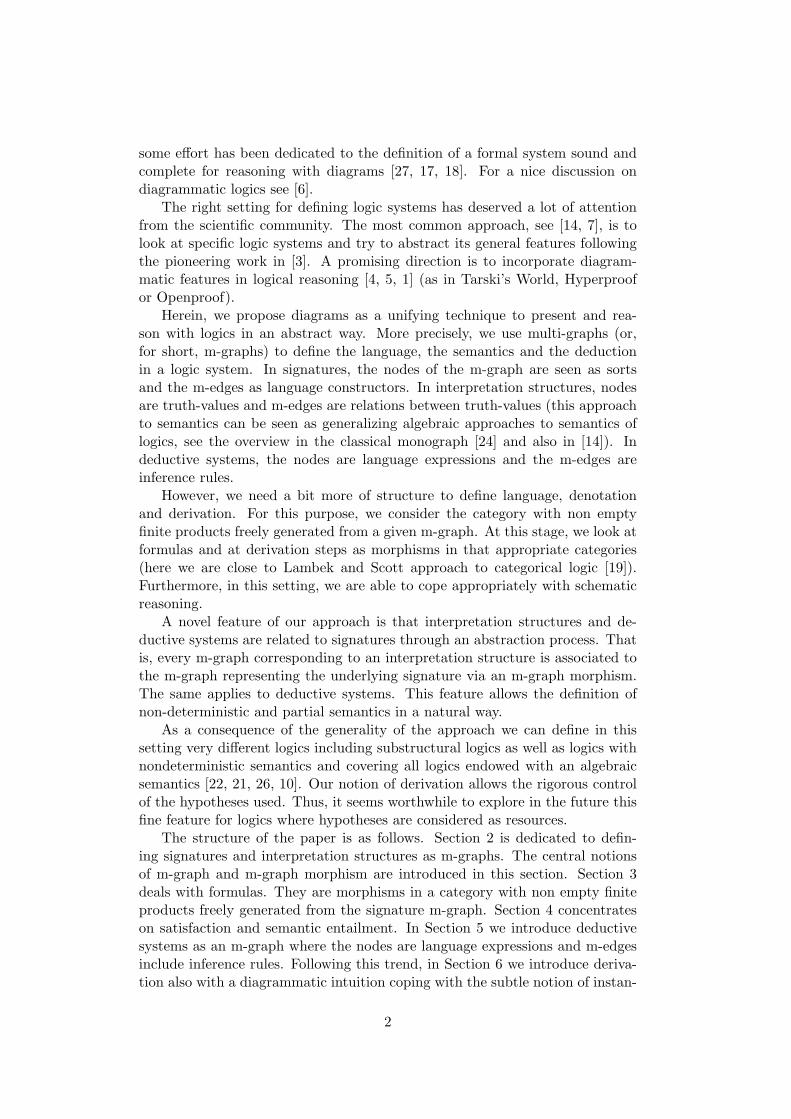
some effort has been dedicated to the definition of a formal system sound andcomplete for reasoning with diagrams [27, 17, 18]. For a nice discussion ondiagrammatic logics see [6].

The right setting for defining logic systems has deserved a lot of attentionfrom the scientific community. The most common approach, see [14, 7], is tolook at specific logic systems and try to abstract its general features followingthe pioneering work in [3]. A promising direction is to incorporate diagram-matic features in logical reasoning [4, 5, 1] (as in Tarski’s World, Hyperproofor Openproof).

Herein, we propose diagrams as a unifying technique to present and rea-son with logics in an abstract way. More precisely, we use multi-graphs (or,for short, m-graphs) to define the language, the semantics and the deductionin a logic system. In signatures, the nodes of the m-graph are seen as sortsand the m-edges as language constructors. In interpretation structures, nodesare truth-values and m-edges are relations between truth-values (this approachto semantics can be seen as generalizing algebraic approaches to semantics oflogics, see the overview in the classical monograph [24] and also in [14]). Indeductive systems, the nodes are language expressions and the m-edges areinference rules.

However, we need a bit more of structure to define language, denotationand derivation. For this purpose, we consider the category with non emptyfinite products freely generated from a given m-graph. At this stage, we look atformulas and at derivation steps as morphisms in that appropriate categories(here we are close to Lambek and Scott approach to categorical logic [19]).Furthermore, in this setting, we are able to cope appropriately with schematicreasoning.

A novel feature of our approach is that interpretation structures and de-ductive systems are related to signatures through an abstraction process. Thatis, every m-graph corresponding to an interpretation structure is associated tothe m-graph representing the underlying signature via an m-graph morphism.The same applies to deductive systems. This feature allows the definition ofnon-deterministic and partial semantics in a natural way.

As a consequence of the generality of the approach we can define in thissetting very different logics including substructural logics as well as logics withnondeterministic semantics and covering all logics endowed with an algebraicsemantics [22, 21, 26, 10]. Our notion of derivation allows the rigorous controlof the hypotheses used. Thus, it seems worthwhile to explore in the future thisfine feature for logics where hypotheses are considered as resources.

The structure of the paper is as follows. Section 2 is dedicated to defin-ing signatures and interpretation structures as m-graphs. The central notionsof m-graph and m-graph morphism are introduced in this section. Section 3deals with formulas. They are morphisms in a category with non empty finiteproducts freely generated from the signature m-graph. Section 4 concentrateson satisfaction and semantic entailment. In Section 5 we introduce deductivesystems as an m-graph where the nodes are language expressions and m-edgesinclude inference rules. Following this trend, in Section 6 we introduce deriva-tion also with a diagrammatic intuition coping with the subtle notion of instan-

2

tiation of schematic rules and formulas. In Section 7, we state general resultsfor soundness and completeness of logic systems. Finally, in Section 8, we givesome insight of how to accommodate provisos and quantification in our setting.

We assume a very moderate knowledge of category theory (the interestedreader can consult [20]).

2 Signatures and models as m-graphs

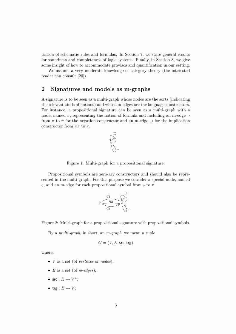
A signature is to be seen as a multi-graph whose nodes are the sorts (indicatingthe relevant kinds of notions) and whose m-edges are the language constructors.For instance, a propositional signature can be seen as a multi-graph with anode, named π, representing the notion of formula and including an m-edge ¬from π to π for the negation constructor and an m-edge ⊃ for the implicationconstructor from ππ to π.

π��

⊃

¬\\

Figure 1: Multi-graph for a propositional signature.

Propositional symbols are zero-ary constructors and should also be repre-sented in the multi-graph. For this purpose we consider a special node, named♦, and an m-edge for each propositional symbol from ♦ to π.

π��

⊃

¬\\♦

q1''q2 22

q3

88

Figure 2: Multi-graph for a propositional signature with propositional symbols.

By a multi-graph, in short, an m-graph, we mean a tuple

G = (V,E, src, trg)

where:

• V is a set (of vertexes or nodes);

• E is a set (of m-edges);

• src : E → V +;

• trg : E → V ;

3

where V + denotes the set of all finite non-empty sequences of V . We may writee : s → v or e ∈ G(s, v) when e ∈ E, src(e) = s and trg(e) = v, and may writeG(−,−) for the collection of m-edges in E.

A language signature or, simply, a signature is a tuple Σ = (G, π, ♦) whereG = (V,E, src, trg) is a m-graph, π and ♦ are in V , and such that no m-edge has ♦ as target. The nodes in V play the role of language sorts, node πbeing the propositions sort (the sort of schema formulas), and node ♦ being theconcrete sort. The m-edges play the role of constructors for building expressionsof the available sorts. The concrete sort allows the construction of concreteexpressions.

Example 2.1 Let Π be a set of propositional symbols. The propositional sig-nature ΣΠ is a m-graph with sorts π and ♦ and the following m-edges:

• p : ♦→ π for each p in Π;

• ¬ : π → π;

• ⊃ : ππ → π.

The m-edges ¬ and ⊃ represent the connectives negation and implication, re-spectively. ∇

Example 2.2 The modal signature Σ�Π is a m-graph obtained from ΣΠ by

adding the m-edge � : π → π for representing the modal operator � of necessity.∇

Example 2.3 The propositional signature with conjunction and disjunctionΣ∧,∨Π is a m-graph obtained from ΣΠ by adding the m-edges ∧,∨ : ππ → πfor representing conjunction ∧ and disjunction ∨. ∇

Example 2.4 The propositional signature Σ∧,∨,◦Π is a m-graph obtained fromΣ∧,∨Π by adding the m-edge ◦ : π → π. ∇

Example 2.5 Let F = {Fn}n∈N0 be a family where Fn is a set (with thefunction symbols of arity n). The equational signature ΣEQ

F is a m-graph withthe sorts π, ♦ and θ, and the following m-edges:

• f : ♦→ θ for each f in F0;

• f :

n︷︸︸︷θ . . . θ → θ for each f in Fn;

• ≈: θθ → π.

The m-edge ≈ represents the equality symbol. ∇

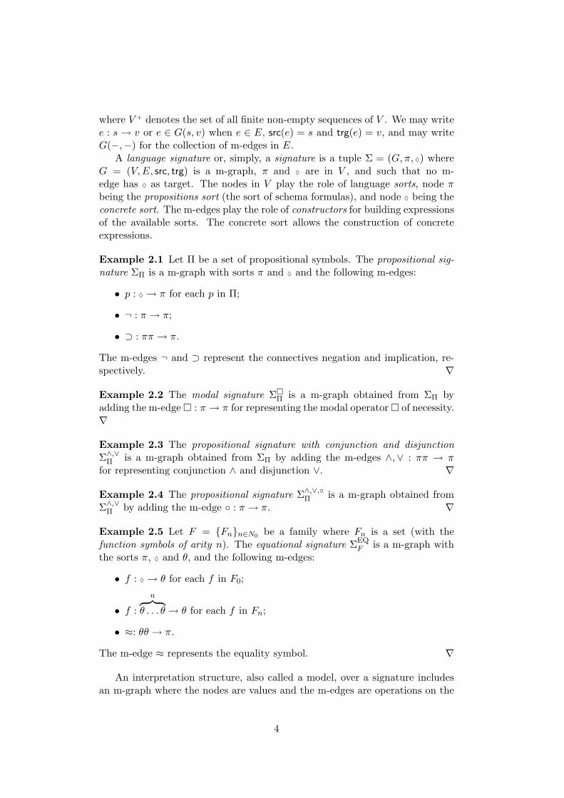
An interpretation structure, also called a model, over a signature includesan m-graph where the nodes are values and the m-edges are operations on the

4

t

f

¬f

KK

¬t

��

--⊃tt nn ⊃ft

oo ⊃tf

??⊃ff

� q′1 33

q′2

��

q′3

""

Figure 3: The operations m-graph for an interpretation structure over thepropositional signature described in Figure 2.

values. For instance, in the case of propositional logic, that m-graph could bethe one specified in Figure 3.

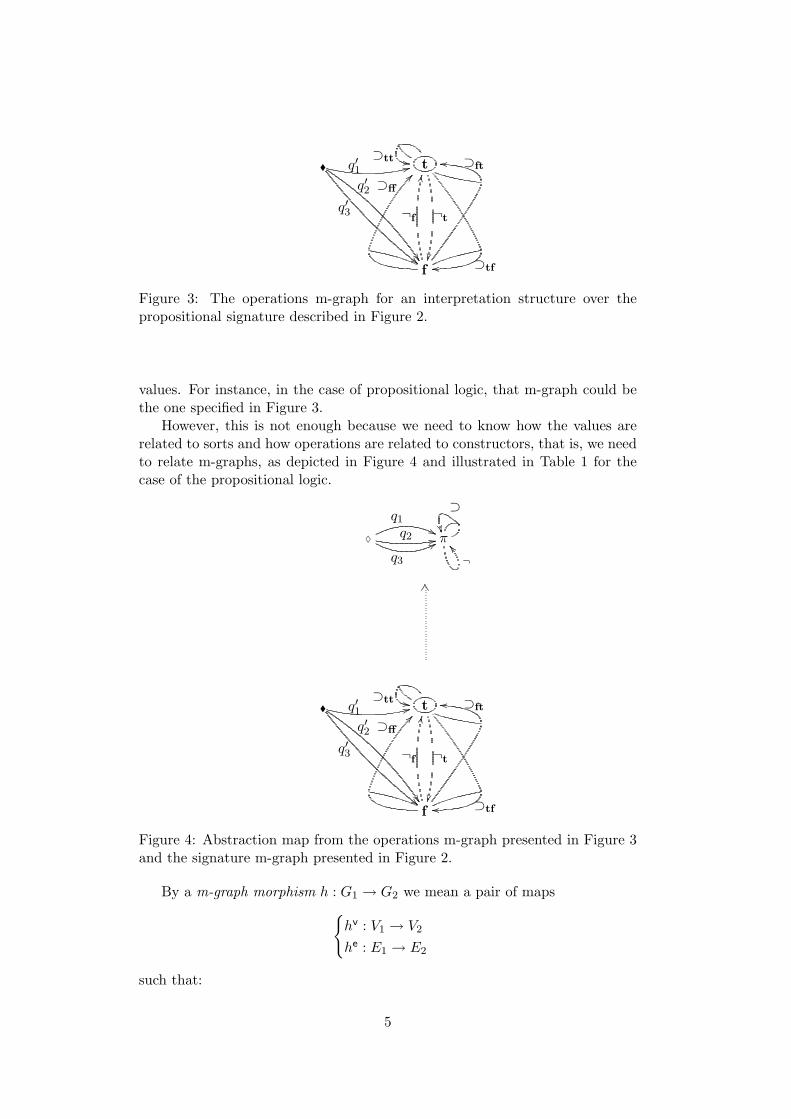
However, this is not enough because we need to know how the values arerelated to sorts and how operations are related to constructors, that is, we needto relate m-graphs, as depicted in Figure 4 and illustrated in Table 1 for thecase of the propositional logic.

π��

⊃

¬\\♦

q1''q2 22

q3

88

t

f

¬f

KK

¬t

��

--⊃tt nn ⊃ft

oo ⊃tf

??⊃ff

� q′1 33

q′2

��

q′3

""

KS

Figure 4: Abstraction map from the operations m-graph presented in Figure 3and the signature m-graph presented in Figure 2.

By a m-graph morphism h : G1 → G2 we mean a pair of maps{hv : V1 → V2

he : E1 → E2

such that:

5

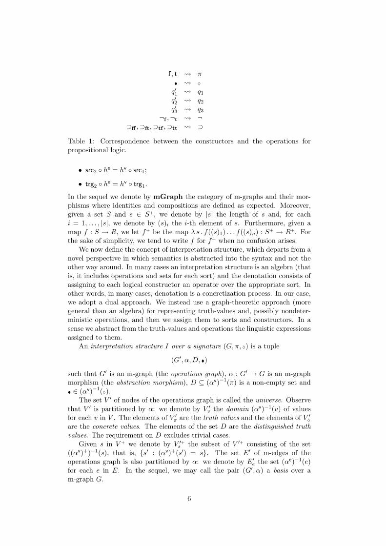
f , t π� ♦

q′1 q1

q′2 q2

q′3 q3

¬f ,¬t ¬⊃ff ,⊃ft,⊃tf ,⊃tt ⊃

Table 1: Correspondence between the constructors and the operations forpropositional logic.

• src2 ◦ he = hv ◦ src1;

• trg2 ◦ he = hv ◦ trg1.

In the sequel we denote by mGraph the category of m-graphs and their mor-phisms where identities and compositions are defined as expected. Moreover,given a set S and s ∈ S+, we denote by |s| the length of s and, for eachi = 1, . . . , |s|, we denote by (s)i the i-th element of s. Furthermore, given amap f : S → R, we let f+ be the map λ s . f((s)1) . . . f((s)n) : S+ → R+. Forthe sake of simplicity, we tend to write f for f+ when no confusion arises.

We now define the concept of interpretation structure, which departs from anovel perspective in which semantics is abstracted into the syntax and not theother way around. In many cases an interpretation structure is an algebra (thatis, it includes operations and sets for each sort) and the denotation consists ofassigning to each logical constructor an operator over the appropriate sort. Inother words, in many cases, denotation is a concretization process. In our case,we adopt a dual approach. We instead use a graph-theoretic approach (moregeneral than an algebra) for representing truth-values and, possibly nondeter-ministic operations, and then we assign them to sorts and constructors. In asense we abstract from the truth-values and operations the linguistic expressionsassigned to them.

An interpretation structure I over a signature (G, π, ♦) is a tuple

(G′, α,D, �)

such that G′ is an m-graph (the operations graph), α : G′ → G is an m-graphmorphism (the abstraction morphism), D ⊆ (αv)−1(π) is a non-empty set and� ∈ (αv)−1(♦).

The set V ′ of nodes of the operations graph is called the universe. Observethat V ′ is partitioned by α: we denote by V ′v the domain (αv)−1(v) of valuesfor each v in V . The elements of V ′π are the truth values and the elements of V ′♦are the concrete values. The elements of the set D are the distinguished truthvalues. The requirement on D excludes trivial cases.

Given s in V + we denote by V ′+s the subset of V ′+ consisting of the set((αv)+)−1(s), that is, {s′ : (αv)+(s′) = s}. The set E′ of m-edges of theoperations graph is also partitioned by α: we denote by E′e the set (αe)−1(e)for each e in E. In the sequel, we may call the pair (G′, α) a basis over am-graph G.

6

An interpretation structure is a pair (Σ, I) where Σ is a signature and I isan interpretation structure over Σ. An interpretation system I is a pair (Σ, I)where Σ is a signature and I is a class of interpretation structures over Σ.

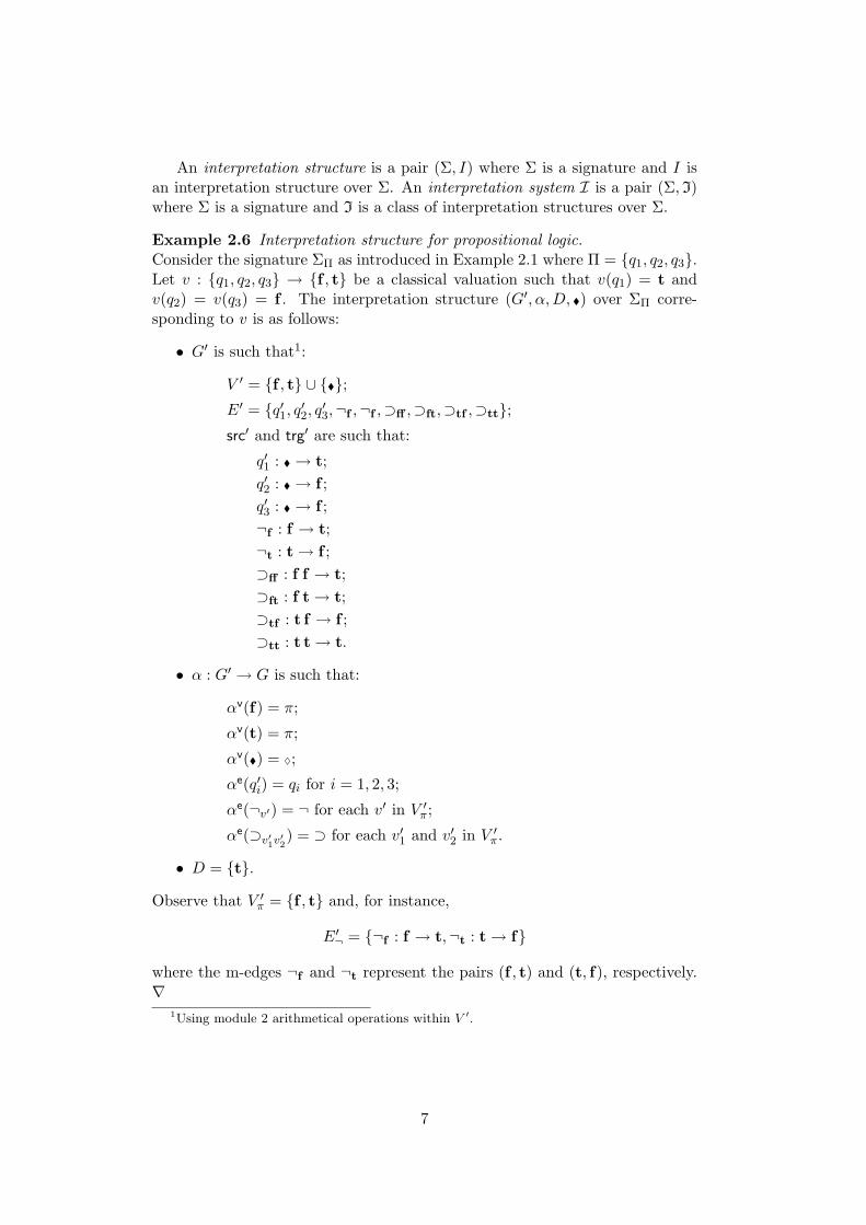
Example 2.6 Interpretation structure for propositional logic.Consider the signature ΣΠ as introduced in Example 2.1 where Π = {q1, q2, q3}.Let v : {q1, q2, q3} → {f , t} be a classical valuation such that v(q1) = t andv(q2) = v(q3) = f . The interpretation structure (G′, α,D, �) over ΣΠ corre-sponding to v is as follows:

• G′ is such that1:

V ′ = {f , t} ∪ {�};E′ = {q′1, q′2, q′3,¬f ,¬f ,⊃ff ,⊃ft,⊃tf ,⊃tt};src′ and trg′ are such that:

q′1 : �→ t;q′2 : �→ f ;q′3 : �→ f ;¬f : f → t;¬t : t→ f ;⊃ff : f f → t;⊃ft : f t→ t;⊃tf : t f → f ;⊃tt : t t→ t.

• α : G′ → G is such that:

αv(f) = π;

αv(t) = π;

αv(�) = ♦;

αe(q′i) = qi for i = 1, 2, 3;

αe(¬v′) = ¬ for each v′ in V ′π;

αe(⊃v′1v′2) = ⊃ for each v′1 and v′2 in V ′π.

• D = {t}.

Observe that V ′π = {f , t} and, for instance,

E′¬ = {¬f : f → t,¬t : t→ f}

where the m-edges ¬f and ¬t represent the pairs (f , t) and (t, f), respectively.∇

1Using module 2 arithmetical operations within V ′.

7

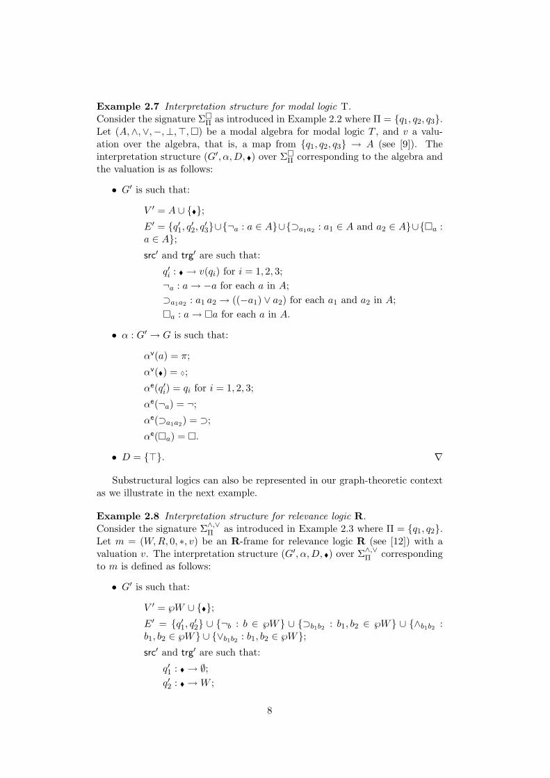
Example 2.7 Interpretation structure for modal logic T.Consider the signature Σ�

Π as introduced in Example 2.2 where Π = {q1, q2, q3}.Let (A,∧,∨,−,⊥,>,�) be a modal algebra for modal logic T , and v a valu-ation over the algebra, that is, a map from {q1, q2, q3} → A (see [9]). Theinterpretation structure (G′, α,D, �) over Σ�

Π corresponding to the algebra andthe valuation is as follows:

• G′ is such that:

V ′ = A ∪ {�};E′ = {q′1, q′2, q′3}∪{¬a : a ∈ A}∪{⊃a1a2 : a1 ∈ A and a2 ∈ A}∪{�a :a ∈ A};src′ and trg′ are such that:

q′i : �→ v(qi) for i = 1, 2, 3;¬a : a→ −a for each a in A;⊃a1a2 : a1 a2 → ((−a1) ∨ a2) for each a1 and a2 in A;�a : a→ �a for each a in A.


αv(a) = π;

αv(�) = ♦;

αe(q′i) = qi for i = 1, 2, 3;

αe(¬a) = ¬;

αe(⊃a1a2) = ⊃;

αe(�a) = �.

• D = {>}. ∇

Substructural logics can also be represented in our graph-theoretic contextas we illustrate in the next example.

Example 2.8 Interpretation structure for relevance logic R.Consider the signature Σ∧,∨Π as introduced in Example 2.3 where Π = {q1, q2}.Let m = (W,R, 0, ∗, v) be an R-frame for relevance logic R (see [12]) with avaluation v. The interpretation structure (G′, α,D, �) over Σ∧,∨Π correspondingto m is defined as follows:


V ′ = ℘W ∪ {�};E′ = {q′1, q′2} ∪ {¬b : b ∈ ℘W} ∪ {⊃b1b2 : b1, b2 ∈ ℘W} ∪ {∧b1b2 :b1, b2 ∈ ℘W} ∪ {∨b1b2 : b1, b2 ∈ ℘W};src′ and trg′ are such that:

q′1 : �→ ∅;q′2 : �→W ;

8

¬b : b→ {w ∈W : w∗ /∈ b};⊃b1b2 : b1 b2 → {w ∈W : Rww1w2 and w1∈b1 implies w2 ∈ b2};∧b1b2 : b1 b2 → b1 ∩ b2;∨b1b2 : b1 b2 → b1 ∪ b2.


αv(b) = π;

αv(�) = ♦;

αe(q′i) = qi for i = 1, 2;

αe(¬b) = ¬;

αe(⊃b1b2) = ⊃;

αe(∧b1b2) = ∧;

αe(∨b1b2) = ∨.

• D is the set of all subsets of W containing 0. ∇

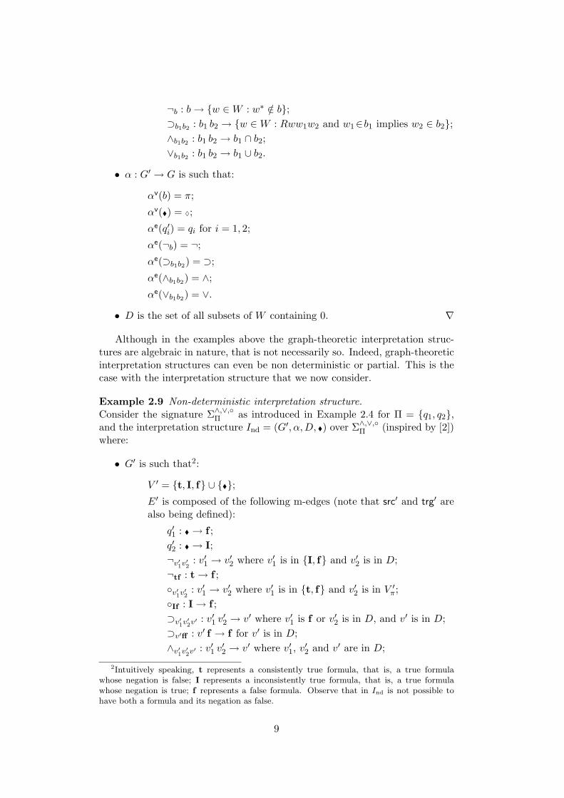
Although in the examples above the graph-theoretic interpretation struc-tures are algebraic in nature, that is not necessarily so. Indeed, graph-theoreticinterpretation structures can even be non deterministic or partial. This is thecase with the interpretation structure that we now consider.

Example 2.9 Non-deterministic interpretation structure.Consider the signature Σ∧,∨,◦Π as introduced in Example 2.4 for Π = {q1, q2},and the interpretation structure Ind = (G′, α,D, �) over Σ∧,∨,◦Π (inspired by [2])where:

• G′ is such that2:

V ′ = {t, I, f} ∪ {�};E′ is composed of the following m-edges (note that src′ and trg′ arealso being defined):

q′1 : �→ f ;q′2 : �→ I;¬v′1v′2 : v′1 → v′2 where v′1 is in {I, f} and v′2 is in D;¬tf : t→ f ;◦v′1v′2 : v′1 → v′2 where v′1 is in {t, f} and v′2 is in V ′π;◦If : I→ f ;⊃v′1v′2v′ : v′1 v

′2 → v′ where v′1 is f or v′2 is in D, and v′ is in D;

⊃v′ff : v′ f → f for v′ is in D;∧v′1v′2v′ : v′1 v

′2 → v′ where v′1, v′2 and v′ are in D;

2Intuitively speaking, t represents a consistently true formula, that is, a true formulawhose negation is false; I represents a inconsistently true formula, that is, a true formulawhose negation is true; f represents a false formula. Observe that in Ind is not possible tohave both a formula and its negation as false.

9

∧v′1v′2f : v′1 v′2 → f where v′1 is f or v′2 is f ;

∨v′1v′2v′ : v′1 v′2 → v′ where v′1 or v′2 are in D, and v′ is in D;

∨fff : f f → f .


αv(v′) = π with v′ in {t, I, f};αv(�) = ♦;

αe(q′1) = q1;

αe(q′2) = q2;

αe(¬v′1v′2) = ¬ for every ¬v′1v′2 in E′;

αe(◦v′1v′2) = ◦ for every ◦v′1v′2 in E′;

αe(⊃v′1v′2b) = ⊃ for every ⊃v′1v′2b in E′;

αe(∧v′1v′2b) = ∧ for every ∧v′1v′2b in E′;

αe(∨v′1v′2b) = ∨ for every ∨v′1v′2b in E′.

• D = {t, I}.

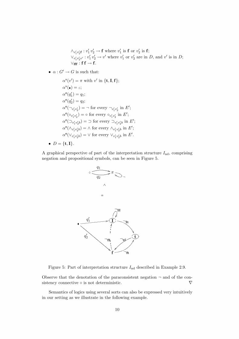
A graphical perspective of part of the interpretation structure Ind, comprisingnegation and propositional symbols, can be seen in Figure 5.

π¬

cc♦

q1**

q2

44

�I

t

f

q′1 11

q′2

""

¬II

��¬It

��

¬fI

KK

¬ft

GG¬tf

��

α

KS

Figure 5: Part of interpretation structure Ind described in Example 2.9.

Observe that the denotation of the paraconsistent negation ¬ and of the con-sistency connective ◦ is not deterministic. ∇

Semantics of logics using several sorts can also be expressed very intuitivelyin our setting as we illustrate in the following example.

10

Example 2.10 Interpretation structure for equational logic.Consider the signature ΣEQ

F as introduced in Example 2.5. Let (A, {FnA : n ≥0}) be an algebra for (one-sorted) equational logic EQ where fA : An → A foreach fA ∈ FnA (see [8, 16]). The interpretation structure (G′, α,D, �) over ΣEQ

F

corresponding to the algebra is as follows:


V ′ = A ∪ {�} ∪ {0, 1};E′ = {fa1...an : a1, . . . , an ∈ A} ∪ {≈a1a2 : a1, a2 ∈ A};src′ and trg′ are such that:

fa1...an : a1 . . . an → fA(a1 . . . an);≈a1a2 : a1a2 → b where b is 1 iff a1 is equal to a2.


αv(a) = θ;

αv(�) = ♦;

αv(0) = π;

αv(1) = π;

αe(fa1...an) = f ;

αe(≈a1a2) is ≈.

• D = {1}. ∇

3 Formulas as paths

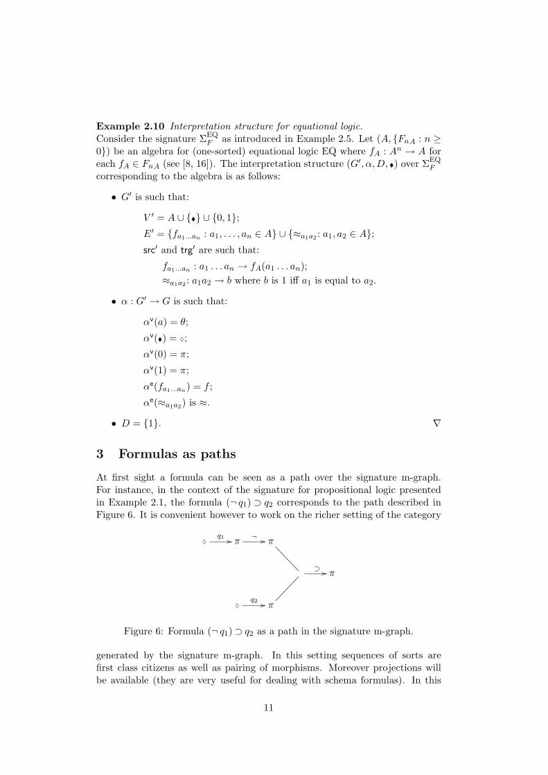
At first sight a formula can be seen as a path over the signature m-graph.For instance, in the context of the signature for propositional logic presentedin Example 2.1, the formula (¬ q1) ⊃ q2 corresponds to the path described inFigure 6. It is convenient however to work on the richer setting of the category

♦q1 // π

¬ // π

>>>>>>>>

⊃ // π

♦q2 // π

��

Figure 6: Formula (¬ q1)⊃ q2 as a path in the signature m-graph.

generated by the signature m-graph. In this setting sequences of sorts arefirst class citizens as well as pairing of morphisms. Moreover projections willbe available (they are very useful for dealing with schema formulas). In this

11

♦ π⊃ ◦ 〈¬ ◦ q1, q2〉 //

Figure 7: Formula (¬ q1)⊃ q2 as a morphism in the category generated by thesignature m-graph.

context, the formula (¬ q1) ⊃ q2 corresponds to the morphism presented inFigure 7.

Before proceeding with the study of language expressions in the graph-theoretic account of logics proposed herein, we have to present first some tech-nical preliminaries (we illustrate some of the constructions with the runningexample of the formula (¬ q1)⊃ q2).

By a non-empty path en . . . e1 over a m-graph G we mean a finite and non-empty sequence of elements of E such that src(ek+1) = trg(ek) for k = 1, . . . , n−1. The source of a non-empty sequence en . . . e1 is src(e1) and the target of thatsequence is trg(en). To each element s of V + we associate an empty path,denoted by εs. The source and target of an empty sequence εs is s. A path wcan be written as w : s → t whenever the source of w is s and the target of wis t. We denote by paths(G) the set of all paths over the m-graph G.

The main objective now is to freely generate a category with non empty finiteproducts out of a given m-graph. The idea is that the objects of the generatedcategory are non-empty finite sequences of vertexes of the m-graph and thateach path w : s → t induces a morphism w : s → t. Moreover, the objectv1 . . . vn is the object v1 × · · · × vn in the obtained category. The constructionis done in several steps. (i) From a m-graph G we obtain a (classical) graph G†

where the vertexes are in V + and the edges besides containing the m-edges in Gcontain also additional edges for projections and tuples; (ii) from G† we freelygenerate a category G‡ whose objects are the same as the vertexes of G† andincluding morphisms for edges, paths, projections and tuples; (iii) from G‡ weget the envisaged category G+ by making a quotient over the class of morphismsensuring that projections and tuples have the required universal properties.

Before presenting the construction we introduce some notation. Let fpCatbe the category of categories with non empty finite products. As usual in acategory with products, we denote by pb1×...×bni the i-th canonical projection ofthe product b1×. . .×bn for n ≥ 1. Given morphisms f1 : b→ b1, . . . , fn : b→ bn,we refer to

〈f1, . . . , fn〉 : b→ (b1 × . . .× bn)

as the unique morphism such that pb1×...×bni ◦ 〈f1, . . . , fn〉 = fi for every i. Iff1 : b1 → b′1, . . . , fn : bn → b′n are morphisms then

f1 × . . .× fn : b1 × . . .× bn → b′1 × . . .× b′n

will stand for the morphism 〈f1 ◦ pb1×...×bn1 , . . . , fn ◦ pb1×...×bnn 〉. As usual,〈f1, . . . , fn〉 and f1 × . . .× fn will be identified with f1 when n is 1.

The aim now is to define the category with non empty finite products G+

from a m-graph G, following the steps sketched above.

12

i. From a m-graph G to a graph G†. We start by defining a family

{G†k = (V +, E†k, src†k, trg

†k)}k≥1

of m-graphs such that

• E†1 = E ∪ {pv1...vni : v1, . . . , vn ∈ V, n ≥ 2, i = 1, . . . , n};

• src†1(e) = src(e) and trg†1(e) = trg(e) whenever e is in E, src†1(pv1...vni ) =

v1 . . . vn and trg†1(pv1...vni ) = vi;

• E†k is the union of E†k−1 with ∪j=2,...,k{〈w1, . . . , wj〉 : w1, . . . , wj arepaths over G†k−1 with target in V and with the same source};

• src†k(e) = src†k−1(e) and trg†k(e) = trg†k−1(e) if e ∈ E†k−1, otherwise e is〈w1, . . . , wj〉, src†k(e) = src†k−1(w1) and trg†k(e) = trg†k−1(w1) . . . trg†k−1(wj).

So G† is (V +, E†, src†, trg†) where E† is ∪k∈NE†k, src†(e) = src†j(e) and trg†(e) =

trg†j(e) for e in E†j .

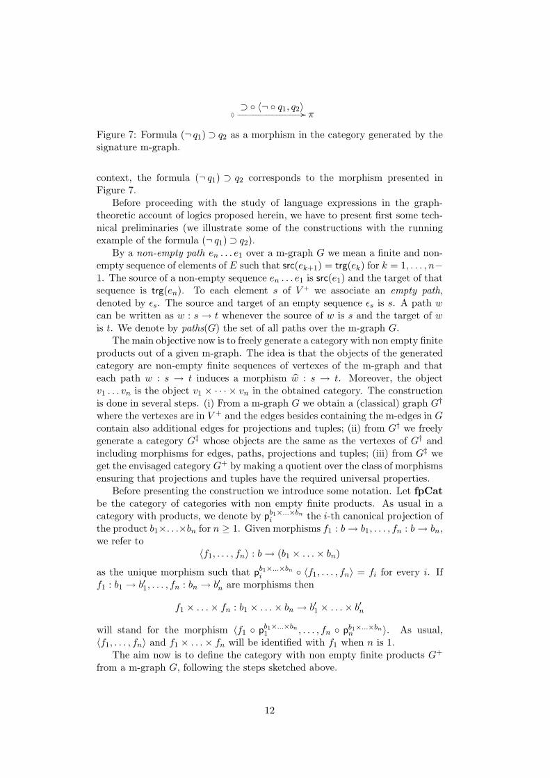
♦ ππ π〈¬q1, q2〉 // ⊃ //

Figure 8: Formula (¬ q1)⊃q2 represented as a path over the graph G† generatedby the signature m-graph G described in Example 2.1.

ii. From a graph G† to a category G‡. Given a graph G†, G‡ is the categoryfreely generated by graph G†. That is, the category obtained as follows:

• the objects are the vertexes of G†;

• each path w : s→ t in over G† determines a unique morphism w‡ : s→ tin G‡ in such a way that if w is in E we set w‡ = w;

• the identity morphism ids : s→ s is εs‡;

• (w2)‡ ◦ (w1)‡ = (w2w1)‡ whenever w2 : s→ t and w1 : r → s.

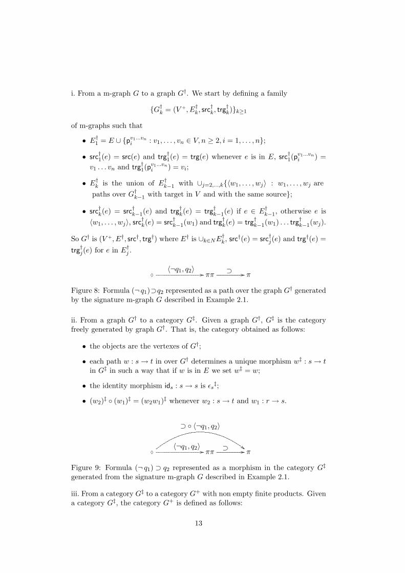
♦ πππ

⊃ ◦ 〈¬q1, q2〉

##〈¬q1, q2〉 // ⊃ //

Figure 9: Formula (¬ q1) ⊃ q2 represented as a morphism in the category G‡

generated from the signature m-graph G described in Example 2.1.

iii. From a category G‡ to a category G+ with non empty finite products. Givena category G‡, the category G+ is defined as follows:

13

• the set of objects of G+ is the same as the set of objects of G‡, i.e., is V +;

• the collection G+(−,−) of morphisms in G+ is the quotient G‡(−,−)/∆‡

where ∆‡ ⊆ G‡(−,−)2 is the least equivalence relation such that:

– ((pv1...vni 〈w1, . . . , wn〉)‡, wi‡) is in ∆‡ for i = 1, . . . , n, where wj : s→

vj are paths over G† and vj is in V for j = 1, . . . , n;

– (w‡, 〈u1, . . . , un〉‡) is in ∆‡ if ((pv1...vni w)‡, ui‡) is in ∆‡ where w : s→

v1 . . . vn and ui : s→ vi are paths over G† and vi ∈ V , i = 1, . . . , n;

– ((w2w1)‡, (u2u1)‡) is in ∆‡ if (w2‡, u2

‡) and (w1‡, u1

‡) are in ∆‡ wherew2, u2 : s1 → t and w1, u1 : s→ s1 are paths over G†;

• in G+ the identity in s is the morphism [εs‡]∆‡ ;

• in G+ the operation ◦ is such that [w2‡]∆‡ ◦ [w1

‡]∆‡ = [(w2w1)‡]∆‡ .

We denote byw

the equivalence class [w‡]∆‡ . The first clause of the equivalence relation es-tablishes that the i-th projection has the expected behavior when applied to atuple, that is, is equivalent to the i-th component. The second clause imposesthe universal property of the product. Finally, the third clause asserts thatcomposition preserves equivalence.

♦ ππ π

⊃ ◦ 〈¬ ◦ q1, q2〉

%%〈¬ ◦ q1, q2〉 // ⊃ //

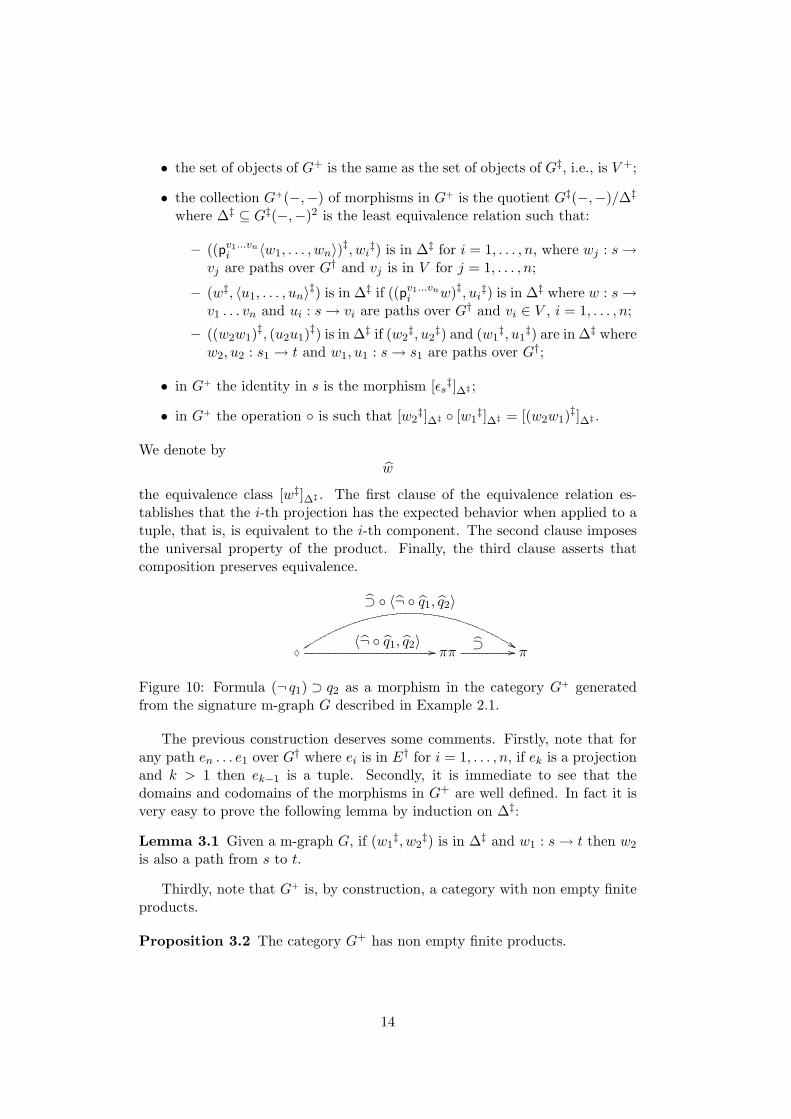
Figure 10: Formula (¬ q1) ⊃ q2 as a morphism in the category G+ generatedfrom the signature m-graph G described in Example 2.1.

The previous construction deserves some comments. Firstly, note that forany path en . . . e1 over G† where ei is in E† for i = 1, . . . , n, if ek is a projectionand k > 1 then ek−1 is a tuple. Secondly, it is immediate to see that thedomains and codomains of the morphisms in G+ are well defined. In fact it isvery easy to prove the following lemma by induction on ∆‡:

Lemma 3.1 Given a m-graph G, if (w1‡, w2

‡) is in ∆‡ and w1 : s→ t then w2

is also a path from s to t.

Thirdly, note that G+ is, by construction, a category with non empty finiteproducts.

Proposition 3.2 The category G+ has non empty finite products.

14

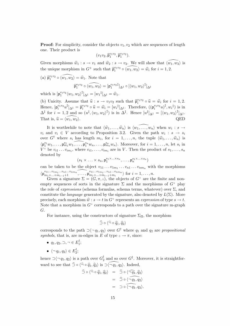
Proof: For simplicity, consider the objects v1, v2 which are sequences of lengthone. Their product is

(v1v2, pv1v21 , pv1v2

1 ).

Given morphisms w1 : s → v1 and w2 : s → v2. We will show that 〈w1, w2〉 isthe unique morphism in G+ such that pv1v2

i ◦ 〈w1, w2〉 = wi for i = 1, 2.

(a) pv1v21 ◦ 〈w1, w2〉 = w1. Note that

pv1v21 ◦ 〈w1, w2〉 = [pv1v2

1‡]∆‡ ◦ [〈w1, w2〉‡]∆‡

which is [pv1v21 〈w1, w2〉‡]∆‡ = [w1

‡]∆‡ = w1.

(b) Unicity. Assume that u : s → v1v2 such that pv1v2i ◦ u = wi for i = 1, 2.

Hence, [pv1v2i u‡]∆‡ = pv1v2

i ◦ u = wi = [wi‡]∆‡ . Therefore, ((pv1v2i u)‡, wi‡) is in

∆‡ for i = 1, 2 and so (u‡, 〈w1, w2〉‡) is in ∆‡. Hence [u‡]∆‡ = [〈w1, w2〉‡]∆‡ .That is, u = 〈w1, w2〉. QED

It is worthwhile to note that 〈w1, . . . , wn〉 is 〈w1, . . . , wn〉 when wi : s →vi and vi ∈ V according to Proposition 3.2. Given the path wi : s → siover G† where si has length mi, for i = 1, . . . , n, the tuple 〈w1, . . . , wn〉 is

〈ps11 w1, . . . , ps1m1w1, . . . , p

sn1 wn, . . . , p

snmnwn〉. Moreover, for i = 1, . . . , n, let si in

V + be vi1 . . . vimi , where vi1, . . . , vimi are in V . Then the product of s1, . . . , sndenoted by

(s1 × . . .× sn, ps1×...×sn1 , . . . , ps1×...×snn )

can be taken to be the object v11 . . . v1m1 . . . vn1 . . . vnmn with the morphisms〈pv11...v1m1 ...vn1...vnmn

m1+...+mi−1+1 , . . . , pv11...v1m1 ...vn1...vnmnm1+...+mi−1+mi

〉 for i = 1, . . . , n.Given a signature Σ = (G, π, ♦), the objects of G+ are the finite and non-

empty sequences of sorts in the signature Σ and the morphisms of G+ playthe role of expressions (schema formulas, schema terms, whatever) over Σ, andconstitute the language generated by the signature, also denoted by L(Σ). Moreprecisely, each morphism w : s→ t in G+ represents an expression of type s→ t.Note that a morphism in G+ corresponds to a path over the signature m-graphG.

For instance, using the constructors of signature ΣΠ, the morphism

⊃ ◦ 〈¬ ◦ q1, q2〉

corresponds to the path ⊃〈¬ q1, q2〉 over G† where q1 and q2 are propositionalsymbols, that is, are m-edges in E of type ♦→ π, since:

• q1, q2,⊃,¬ ∈ E†1;

• 〈¬ q1, q2〉 ∈ E†2;

hence ⊃〈¬ q1, q2〉 is a path over G†2 and so over G†. Moreover, it is straightfor-ward to see that ⊃ ◦ 〈¬ ◦ q1, q2〉 is ⊃〈¬ q1, q2〉. Indeed,

⊃ ◦ 〈¬ ◦ q1, q2〉 = ⊃ ◦ 〈¬ q1, q2〉

= ⊃ ◦ 〈¬ q1, q2〉

= ⊃ ◦ 〈¬ q1, q2〉.

15

In the sequel, when there is no ambiguity, we may denote a morphism e of G+

where e is a m-edge of E simply by e. Expressions with the object ♦ as sourceare said to be concrete expressions. Thus, G+(♦, π) is the set of all concreteformulas, or simply the set of all formulas in the language of Σ. This setcorresponds to the traditional (set-theoretic) notion of language of propositionsover Σ.

For instance, the morphism:

⊃ ◦ 〈¬ ◦ p1,⊃ ◦ 〈p2, p1〉〉 : ♦→ π

is an expression of type ♦ → π and so is a formula, represented more simplyas ((¬ p1) ⊃ (p2 ⊃ p1)). In the sequel we may simplify the representation ofmorphisms in a similar way. Clearly, it is possible to write expressions with anon-concrete object as source. Such expressions are said to be schema expres-sions because only part of their structure is known (or determined), and whenits target is π we may call them schema formulas. So by a schema formulawe mean a morphism in G+ whose target is π and with no constraints overthe source. Schema variables are projections from π . . . π to π, or from π . . . π♦

to π, where the π-sequence at the source is non-empty, and are denoted byξ, ξ′, ξ′′, . . . , ξ1, ξ

′1, ξ′′1 , . . . , ξ2, ξ

′2, ξ′′2 , . . ..

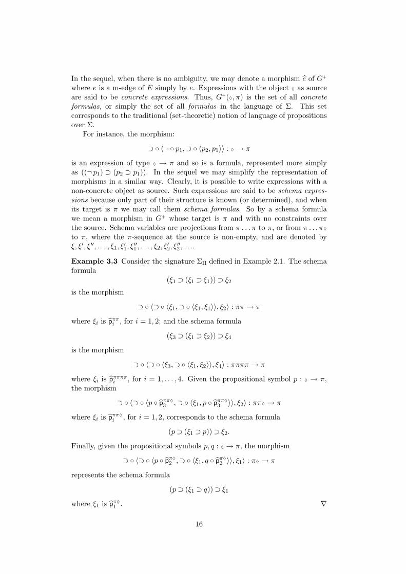
Example 3.3 Consider the signature ΣΠ defined in Example 2.1. The schemaformula

(ξ1 ⊃ (ξ1 ⊃ ξ1))⊃ ξ2

is the morphism

⊃ ◦ 〈⊃ ◦ 〈ξ1,⊃ ◦ 〈ξ1, ξ1〉〉, ξ2〉 : ππ → π

where ξi is pππi , for i = 1, 2; and the schema formula

(ξ3 ⊃ (ξ1 ⊃ ξ2))⊃ ξ4

is the morphism

⊃ ◦ 〈⊃ ◦ 〈ξ3,⊃ ◦ 〈ξ1, ξ2〉〉, ξ4〉 : ππππ → π

where ξi is pππππi , for i = 1, . . . , 4. Given the propositional symbol p : ♦ → π,the morphism

⊃ ◦ 〈⊃ ◦ 〈p ◦ pππ♦3 ,⊃ ◦ 〈ξ1, p ◦ pππ♦

3 〉〉, ξ2〉 : ππ♦→ π

where ξi is pππ♦i , for i = 1, 2, corresponds to the schema formula

(p⊃ (ξ1 ⊃ p))⊃ ξ2.

Finally, given the propositional symbols p, q : ♦→ π, the morphism

⊃ ◦ 〈⊃ ◦ 〈p ◦ pπ♦2 ,⊃ ◦ 〈ξ1, q ◦ pπ♦

2 〉〉, ξ1〉 : π♦→ π

represents the schema formula

(p⊃ (ξ1 ⊃ q))⊃ ξ1

where ξ1 is pπ♦1 . ∇

16

Non-concrete expressions are very useful for setting up deductive rules thatcan be instantiated using substitutions. Deductive rules with non-concrete ex-pressions are called schema rules. Expression instantiation and rule instantia-tion is achieved using morphism composition. Given the expressions w : s2 → s3

and u : s1 → s2, the expression instantiation of the former by the latter is theexpression w ◦ u.

Example 3.4 Let ϕ be the schema formula

⊃ ◦ 〈⊃ ◦ 〈¬ ◦ ξ, ξ′〉,⊃ ◦ 〈ξ, ξ′′〉〉

where ξ is pπππ1 , ξ′ is pπππ2 and ξ′′ is pπππ3 . We can interchange ξ with ξ′ byinstantiating ϕ with 〈ξ′, ξ, ξ′′〉 : πππ → πππ, obtaining the following schemaformula

ϕ ◦〈ξ′, ξ, ξ′′〉 = ⊃ ◦ 〈⊃ ◦ 〈¬ ◦ ξ, ξ′〉 ◦ 〈ξ′, ξ, ξ′′〉,⊃ ◦ 〈ξ, ξ′′〉 ◦ 〈ξ′, ξ, ξ′′〉〉

= ⊃ ◦ 〈⊃ ◦ 〈¬ ◦ ξ′, ξ〉,⊃ ◦ 〈ξ′, ξ′′〉〉

from πππ to π. On the other hand, if we want to make concrete the second slotof ϕ we could consider the propositional symbol p : ♦→ π, and then instantiateϕ with 〈ξ1, p ◦pππ♦

3 , ξ2〉 : ππ♦→ πππ where ξj = pππ♦j for j = 1, 2 obtaining the

following schema formula

ϕ ◦〈ξ1, p ◦pππ♦3 , ξ2〉 =

= ⊃ ◦ 〈⊃ ◦ 〈¬ ◦ξ, ξ′〉 ◦ 〈ξ1, p ◦pππ♦3 , ξ2〉,⊃ ◦ 〈ξ, ξ′′〉 ◦ 〈ξ1, p ◦pππ♦

3 , ξ2〉〉

= ⊃ ◦ 〈⊃ ◦ 〈¬ ◦ ξ1, p ◦pππ♦3 〉,⊃ ◦ 〈ξ1, ξ2〉〉

from ππ♦ to π. ∇

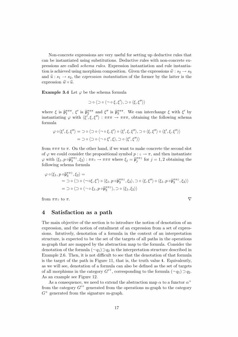
4 Satisfaction as a path

The main objective of the section is to introduce the notion of denotation of anexpression, and the notion of entailment of an expression from a set of expres-sions. Intutively, denotation of a formula in the context of an interpretationstructure, is expected to be the set of the targets of all paths in the operationsm-graph that are mapped by the abstraction map to the formula. Consider thedenotation of the formula (¬ q1)⊃q2 in the interpretation structure described inExample 2.6. Then, it is not difficult to see that the denotation of that formulais the target of the path in Figure 11, that is, the truth value t. Equivalently,as we will see, denotation of a formula can also be defined as the set of targetsof all morphisms in the category G′+, corresponding to the formula (¬ q1)⊃ q2.As an example see Figure 12.

As a consequence, we need to extend the abstraction map α to a functor α+

from the category G′+ generated from the operations m-graph to the categoryG+ generated from the signature m-graph.

17

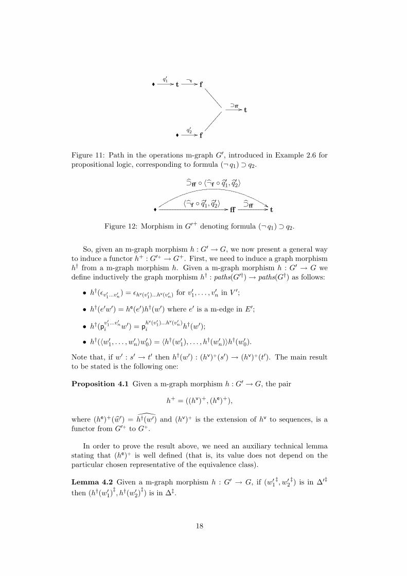
�q′1 // t

¬t // f

;;;;;;;;

⊃ff // t

�q′2 // f

��

Figure 11: Path in the operations m-graph G′, introduced in Example 2.6 forpropositional logic, corresponding to formula (¬ q1)⊃ q2.

� ff t

⊃ff ◦ 〈¬f ◦ q′1, q′2〉

%%〈¬f ◦ q′1, q′2〉 // ⊃ff //

Figure 12: Morphism in G′+ denoting formula (¬ q1)⊃ q2.

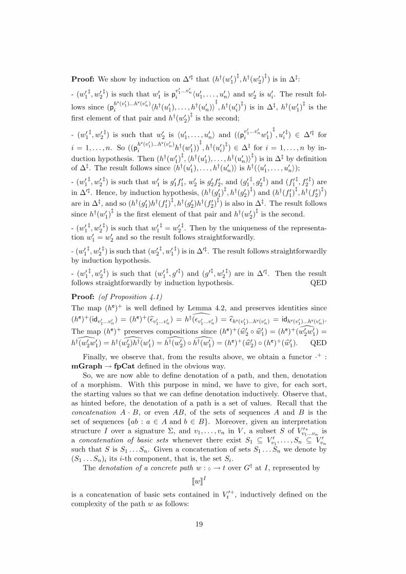
So, given an m-graph morphism h : G′ → G, we now present a general wayto induce a functor h+ : G′+ → G+. First, we need to induce a graph morphismh† from a m-graph morphism h. Given a m-graph morphism h : G′ → G wedefine inductively the graph morphism h† : paths(G′†)→ paths(G†) as follows:

• h†(εv′1...v′n) = εhv(v′1)...hv(v′n) for v′1, . . . , v′n in V ′;

• h†(e′w′) = he(e′)h†(w′) where e′ is a m-edge in E′;

• h†(pv′1...v

′n

i w′) = phv(v′1)...hv(v′n)i h†(w′);

• h†(〈w′1, . . . , w′n〉w′0) = 〈h†(w′1), . . . , h†(w′n)〉h†(w′0).

Note that, if w′ : s′ → t′ then h†(w′) : (hv)+(s′) → (hv)+(t′). The main resultto be stated is the following one:

Proposition 4.1 Given a m-graph morphism h : G′ → G, the pair

h+ = ((hv)+, (he)+),

where (he)+(w′) = h†(w′) and (hv)+ is the extension of hv to sequences, is afunctor from G′+ to G+.

In order to prove the result above, we need an auxiliary technical lemmastating that (he)+ is well defined (that is, its value does not depend on theparticular chosen representative of the equivalence class).

Lemma 4.2 Given a m-graph morphism h : G′ → G, if (w′1‡, w′2

‡) is in ∆′‡

then (h†(w′1)‡, h†(w′2)‡) is in ∆‡.

18

Proof: We show by induction on ∆′‡ that (h†(w′1)‡, h†(w′2)‡) is in ∆‡:

- (w′1‡, w′2

‡) is such that w′1 is pv′1...v

′n

i 〈u′1, . . . , u′n〉 and w′2 is u′i. The result fol-

lows since (phv(v′1)...hv(v′n)i 〈h†(u′1), . . . , h†(u′n)〉

‡, h†(u′i)

‡) is in ∆‡, h†(w′1)‡ is thefirst element of that pair and h†(w′2)‡ is the second;

- (w′1‡, w′2

‡) is such that w′2 is 〈u′1, . . . , u′n〉 and ((pv′1...v

′n

i w′1)‡, u′i‡) ∈ ∆′‡ for

i = 1, . . . , n. So ((phv(v′1)...hv(v′n)i h†(w′1))

‡, h†(u′i)

‡) ∈ ∆‡ for i = 1, . . . , n by in-duction hypothesis. Then (h†(w′1)‡, 〈h†(u′1), . . . , h†(u′n)〉‡) is in ∆‡ by definitionof ∆‡. The result follows since 〈h†(u′1), . . . , h†(u′n)〉 is h†(〈u′1, . . . , u′n〉);

- (w′1‡, w′2

‡) is such that w′1 is g′1f′1, w′2 is g′2f

′2, and (g′1

‡, g′2‡) and (f ′1

‡, f ′2‡) are

in ∆′‡. Hence, by induction hypothesis, (h†(g′1)‡, h†(g′2)‡) and (h†(f ′1)‡, h†(f ′2)‡)are in ∆‡, and so (h†(g′1)h†(f ′1)‡, h†(g′2)h†(f ′2)‡) is also in ∆‡. The result followssince h†(w′1)‡ is the first element of that pair and h†(w′2)‡ is the second.

- (w′1‡, w′2

‡) is such that w′1‡ = w′2

‡. Then by the uniqueness of the representa-tion w′1 = w′2 and so the result follows straightforwardly.

- (w′1‡, w′2

‡) is such that (w′2‡, w′1

‡) is in ∆′‡. The result follows straightforwardlyby induction hypothesis.

- (w′1‡, w′2

‡) is such that (w′1‡, g′‡) and (g′‡, w′2

‡) are in ∆′‡. Then the resultfollows straightforwardly by induction hypothesis. QED

Proof: (of Proposition 4.1)The map (he)+ is well defined by Lemma 4.2, and preserves identities since(he)+(idv′1...v′n) = (he)+(εv′1...v′n) = h†(εv′1...v′n) = εhv(v′1)...hv(v′n) = idhv(v′1)...hv(v′n).

The map (he)+ preserves compositions since (he)+(w′2 ◦ w′1) = (he)+(w′2w′1) =

h†(w′2w′1) = h†(w′2)h†(w′1) = h†(w′2) ◦ h†(w′1) = (he)+(w′2) ◦ (he)+(w′1). QED

Finally, we observe that, from the results above, we obtain a functor ·+ :mGraph→ fpCat defined in the obvious way.

So, we are now able to define denotation of a path, and then, denotationof a morphism. With this purpose in mind, we have to give, for each sort,the starting values so that we can define denotation inductively. Observe that,as hinted before, the denotation of a path is a set of values. Recall that theconcatenation A · B, or even AB, of the sets of sequences A and B is theset of sequences {ab : a ∈ A and b ∈ B}. Moreover, given an interpretationstructure I over a signature Σ, and v1, . . . , vn in V , a subset S of V ′+v1...vn isa concatenation of basic sets whenever there exist S1 ⊆ V ′v1

, . . . , Sn ⊆ V ′vnsuch that S is S1 . . . Sn. Given a concatenation of sets S1 . . . Sn we denote by(S1 . . . Sn)i its i-th component, that is, the set Si.

The denotation of a concrete path w : ♦→ t over G† at I, represented by

[[w]]I

is a concatenation of basic sets contained in V ′+t , inductively defined on thecomplexity of the path w as follows:

19

• [[ε♦]]I is {�};

• [[pv1...vmi w1]]I is ([[w1]]I)i where v1, . . . , vm are in V ;

• [[〈w1, . . . , wn〉w0]]I is [[w1w0]]I . . . [[wnw0]]I ;

• [[ew1]]I is the union of trg′(E′e(v′,−)) for each v′ in [[w1]]I , when e is in E.

For instance, for evaluating ew1 over I, we start by evaluating w1 and gettinga set of values. For each value s′ in the evaluation of w1, we pick all the m-edges in G′ with source s′ and which are mapped into e. Finally, the envisageddenotation is obtained by taking the collection of targets of such m-edges.

Denotation is now extended to non-concrete paths. The denotation of theschema variables is given by an assignment, which must be also a componentin the denotation process. An assignment

ρ

for an interpretation structure I over a signature Σ is a family {ρs}s∈V + suchthat ρs is [[ws]]

I for some concrete path ws : ♦→ s. Observe that ρs is containedin V ′+s and is a concatenation of basic sets, and ρ♦ = {�}.

The denotation of a path w : s→ t over G† at I and ρ, denoted by

[[w]]Iρ

is a concatenation of basic sets contained in V ′+t , inductively defined on thecomplexity of the path w similarly to the denotation of a concrete path withthe exception that [[εs]]

Iρ is ρs.

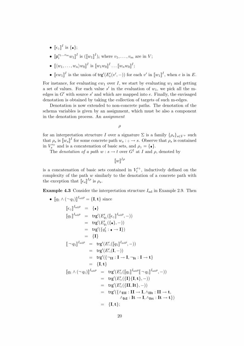
Example 4.3 Consider the interpretation structure Ind in Example 2.9. Then

• [[q1 ∧ (¬ q1)]]Indρ = {I, t} since

[[ε♦]]Indρ = {�}

[[q1]]Indρ = trg′(E′q1([[ε♦]]Indρ,−))= trg′(E′q1({�},−))= trg′({q′1 : �→ I})= {I}

[[¬ q1]]Indρ = trg′(E′¬([[q1]]Indρ,−))= trg′(E′¬(I,−))= trg′({¬II : I→ I,¬It : I→ t}= {I, t}

[[q1 ∧ (¬ q1)]]Indρ = trg′(E′∧([[q1]]Indρ[[¬ q1]]Indρ,−))= trg′(E′∧({I}{I, t},−))= trg′(E′∧({II, It},−))= trg′({∧III : II→ I,∧IIt : II→ t,

∧ItI : It→ I,∧Itt : It→ t})= {I, t};

20

• [[ ◦ q1]]Indρ = {f} since

[[ ◦ q1]]Indρ = trg′(E′◦([[q1]]Indρ,−))= trg′(E′◦({I},−))= trg′({◦If : I→ f})= {f}

∇

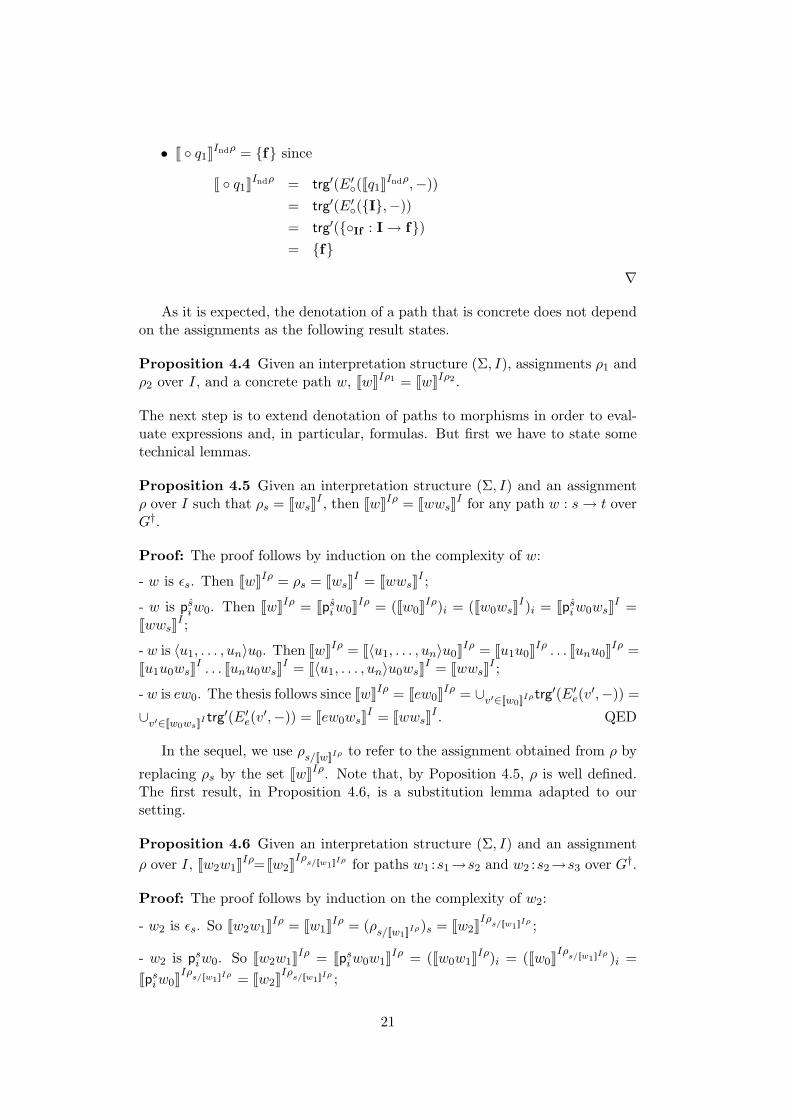
As it is expected, the denotation of a path that is concrete does not dependon the assignments as the following result states.

Proposition 4.4 Given an interpretation structure (Σ, I), assignments ρ1 andρ2 over I, and a concrete path w, [[w]]Iρ1 = [[w]]Iρ2 .

The next step is to extend denotation of paths to morphisms in order to eval-uate expressions and, in particular, formulas. But first we have to state sometechnical lemmas.

Proposition 4.5 Given an interpretation structure (Σ, I) and an assignmentρ over I such that ρs = [[ws]]

I , then [[w]]Iρ = [[wws]]I for any path w : s→ t over

G†.

Proof: The proof follows by induction on the complexity of w:

- w is εs. Then [[w]]Iρ = ρs = [[ws]]I = [[wws]]

I ;

- w is psiw0. Then [[w]]Iρ = [[psiw0]]Iρ = ([[w0]]Iρ)i = ([[w0ws]]I)i = [[psiw0ws]]

I =[[wws]]

I ;

- w is 〈u1, . . . , un〉u0. Then [[w]]Iρ = [[〈u1, . . . , un〉u0]]Iρ = [[u1u0]]Iρ . . . [[unu0]]Iρ =[[u1u0ws]]

I . . . [[unu0ws]]I = [[〈u1, . . . , un〉u0ws]]

I = [[wws]]I ;

- w is ew0. The thesis follows since [[w]]Iρ = [[ew0]]Iρ = ∪v′∈[[w0]]Iρtrg′(E′e(v

′,−)) =

∪v′∈[[w0ws]]I trg′(E′e(v

′,−)) = [[ew0ws]]I = [[wws]]

I . QED

In the sequel, we use ρs/[[w]]Iρ to refer to the assignment obtained from ρ by

replacing ρs by the set [[w]]Iρ. Note that, by Poposition 4.5, ρ is well defined.The first result, in Proposition 4.6, is a substitution lemma adapted to oursetting.

Proposition 4.6 Given an interpretation structure (Σ, I) and an assignmentρ over I, [[w2w1]]Iρ=[[w2]]Iρs/[[w1]]Iρ for paths w1 :s1→s2 and w2 :s2→s3 over G†.

Proof: The proof follows by induction on the complexity of w2:

- w2 is εs. So [[w2w1]]Iρ = [[w1]]Iρ = (ρs/[[w1]]Iρ)s = [[w2]]Iρs/[[w1]]Iρ ;

- w2 is psiw0. So [[w2w1]]Iρ = [[psiw0w1]]Iρ = ([[w0w1]]Iρ)i = ([[w0]]Iρs/[[w1]]Iρ )i =[[psiw0]]Iρs/[[w1]]Iρ = [[w2]]Iρs/[[w1]]Iρ ;

21

- w2 is 〈u1, . . . , un〉u0. Then [[w2w1]]Iρ = [[〈u1, . . . , un〉u0w1]]Iρ = [[u1u0w1]]Iρ . . .[[unu0w1]]Iρ = [[u1u0]]Iρs/[[w1]]Iρ . . . [[unu0]]Iρs/[[w1]]Iρ = [[〈u1, . . . , un〉u0]]Iρs/[[w1]]Iρ =[[w2]]Iρs/[[w1]]Iρ ;

- w2 is ew0. Therefore [[w2w1]]Iρ = [[ew0w1]]Iρ = trg′(E′e([[w0w1]]Iρ,−)) =trg′(E′e([[w0]]Iρs/[[w1]]Iρ ,−)) = [[ew0]]Iρs/[[w1]]Iρ = [[w2]]Iρs/[[w1]]Iρ . QED

The following result states that denotation is well defined.

Proposition 4.7 Given an interpretation structure (Σ, I), if (w‡, u‡) is in ∆‡

then [[w]]Iρ = [[u]]Iρ for any assignment ρ over I.

Proof: The proof follows by induction on ∆‡:

- (w‡, u‡) is such that w is pv1...vni 〈w1, . . . , wn〉 and u is wi. Then [[w]]Iρ =

[[pv1...vni 〈w1, . . . , wn〉]]Iρ = ([[〈w1, . . . , wn〉]]Iρ)i = ([[w1]]Iρ . . . [[wn]]Iρ)i = [[wi]]

Iρ =[[u]]Iρ;

- (w‡, u‡) is such that u is 〈u1, . . . , un〉, w : s → v1 . . . vn, ui : s → vi and((pv1...vn

i w)‡, ui‡) is in ∆‡ for i = 1, . . . , n. Hence [[pv1...vni w]]Iρ = [[ui]]

Iρ byinduction hypothesis, for i = 1, . . . , n. So ([[w]]Iρ)i = [[ui]]

Iρ for i = 1, . . . , n.Since [[w]]Iρ is a concatenation of basic sets then [[w]]Iρ = [[u1]]Iρ . . . [[un]]Iρ, andso the thesis follows straightforwardly;

- (w‡, u‡) is such that w is w2w1, u is u2u1, and (w2‡, u2

‡) and (w1‡, u1

‡) are in∆‡. So [[w1]]Iρ = [[u1]]Iρ and [[w2]]Iρ = [[u2]]Iρ by induction hypothesis for anyassignment ρ. Then, by Proposition 4.6, [[w]]Iρ = [[w2w1]]Iρ = [[w2]]Iρs/[[w1]]Iρ =[[u2]]Iρs/[[u1]]Iρ = [[u2u1]]Iρ = [[u]]Iρ;

- (w‡, u‡) is such that w‡ = u‡. Then by the uniqueness of the representationw = v and so the result follows straightforwardly;

- (w‡, u‡) is such that (u‡, w‡) is in ∆‡. The result follows straightforwardly byinduction hypothesis;

- (w‡, u‡) is such that (w‡, u0‡) and (u0

‡, u‡) are in ∆‡. Then the result followsstraightforwardly by induction hypothesis. QED

Capitalizing on Proposition 4.7, the denotation [[w]]Iρ of a morphism w inG+ over I and ρ is defined as

[[w]]Iρ = [[w]]Iρ.

The notions of local and global satisfactions are the usual ones. A schemaformula ϕ is said to be satisfied by I and ρ, written as

I, ρ ϕ

whenever [[ϕ]]Iρ is non-empty and is contained in D. Moreover, we say I satisfiesϕ, written as

I ϕ

22

whenever I, ρ ϕ for every assignment ρ over I. Satisfaction is extended tosets of schema formulas as expected: I, ρ Γ if I, ρ γ for each γ ∈ Γ, andsimilarly for sequences of schema formulas: I, ρ ϕ1 . . . ϕn if I, ρ ϕi fori = 1, . . . , n.

The definition of denotation given above is the usual for most logics. Exam-ples of logics with a different notion of denotation are the paraconsistent logicsreferred to in [2]. In the case of these logics, although some of the operationsare non deterministic, the denotation of a formula is always a fixed truth value.The definition in our approach of that variant of denotation seems feasible andwe intend to explore the details in the future.

Example 4.8 Consider the interpretation structure Ind in Example 2.9. Then

Ind q1 ∧ (¬ q1)

since [[q1 ∧ (¬ q1)]]Indρ = {I, t} is contained in D, see Example 4.3. Moreover,

Ind 6 ◦q1

since [[ ◦ q1]]Indρ = {f} is not contained in D as shown in the same example.Therefore,

Ind 6 (q1 ∧ (¬ q1))⊃ (◦q1)

as expected for logics of formal inconsistency, see [10]. ∇

We are now ready to define semantic entailment. Given an interpretationsystem I = (Σ, I) and a set Γ ∪ {ϕ} of schema formulas over Σ, we say that Γentails ϕ in I, written as

Γ �I ϕ,

whenever I Γ implies I ϕ for every I in I. Similarly we define entailmentover sequences of schema formulas as follows: ~γ �I ~ϕ whenever I ~γ impliesI ~ϕ for every I in I.

The graph-theoretic semantics developed in this work can be said to sub-sume algebraic semantics, in the sense that, any logic endowed with an algebraicsemantics can be presented in our setting in such a way that satisfaction andentailment are preserved. By a logic with an algebraic semantics we mean apair composed by a signature and a class of algebras over that signature. Eachalgebra A is a triple (A, ·, DA) composed by a set A of (truth values) withan operation cA : An → A for each constructor c of arity n in the signatureand a subset DA contained in A of distinguished values. In this context thedenotation [[ϕ]]A is homomorphic, that is

[[c(ϕ1, . . . , ϕn)]]A = cA([[ϕ1]]A, . . . , [[ϕn]]A).

A logic L with an algebraic semantics induces an interpretation system I(L)with the obvious signature and containing, for each algebra A, an interpretationstructure IA = (G′, α,DA, �) defined as follows:

• V ′ is the set of truth values of the algebra;

23

• E′ is composed, for each n-ary constructor c, by the set of m-edgesca1,...,an : a1 . . . an → cA(a1, . . . , an) for each a1, . . . , an ∈ A when n ≥ 1,or by c : �→ cA when n = 0;

• αv(a) = π for each a ∈ A;

• αe(ca1,...,an) = c for each a1, . . . , an ∈ A and αe(c) = c.

The graph-theoretic semantics induced by the algebraic semantics coincidesexactly in terms of denotation, satisfaction and entailment with the algebraicsemantics, as we show now.

Lemma 4.9 Given a logic with an algebraic semantics and an algebra A, then

[[ϕ]]A = [[ϕ]]IA .

Proof: By induction on the structure of ϕ: ϕ is c(ϕ1, . . . , ϕn). Therefore[[ϕ]]A = [[c(ϕ1, . . . , ϕn)]]A = cA([[ϕ1]]A, . . . , [[ϕn]]A) = cA([[ϕ1]]IA , . . . , [[ϕn]]IA) =trg′(c[[ϕ1]]IA ,...,[[ϕn]]IA ) = trg′(E′c([[ϕ1]]IA . . . [[ϕn]]IA ,−)) = [[ϕ]]IA . QED

Lemma 4.10 Given a logic with an algebraic semantics and an algebra A, then

A ϕ iff IA ϕ.

Proof: Assume that A ϕ. Then [[ϕ]]A ∈ DA. Hence [[ϕ]]IA ∈ DA byLemma 4.9. So IA ϕ. The other direction follows similarly. QED

Proposition 4.11 Let L be a logic with an algebraic semantics. Then, L andI(L) share the same entailment.

Proof: Suppose Γ �L ϕ and let IA be in I(L) such that IA Γ. Then A Γby Lemma 4.10 and so A ϕ. Hence also by Lemma 4.10, IA ϕ as we wantedto show. The other direction follows similarly. QED

5 Deductive systems as m-graphs

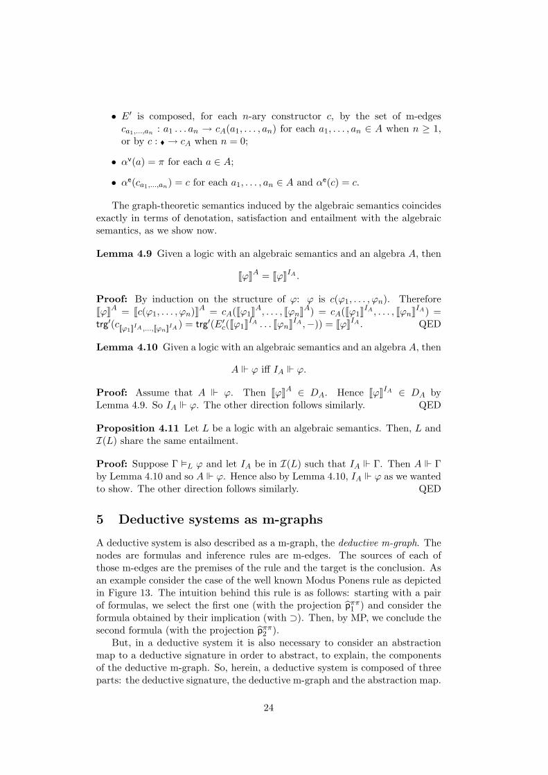
A deductive system is also described as a m-graph, the deductive m-graph. Thenodes are formulas and inference rules are m-edges. The sources of each ofthose m-edges are the premises of the rule and the target is the conclusion. Asan example consider the case of the well known Modus Ponens rule as depictedin Figure 13. The intuition behind this rule is as follows: starting with a pairof formulas, we select the first one (with the projection pππ1 ) and consider theformula obtained by their implication (with ⊃). Then, by MP, we conclude thesecond formula (with the projection pππ2 ).

But, in a deductive system it is also necessary to consider an abstractionmap to a deductive signature in order to abstract, to explain, the componentsof the deductive m-graph. So, herein, a deductive system is composed of threeparts: the deductive signature, the deductive m-graph and the abstraction map.

24

ππ

π

pππ1

�� ππ

π

⊃�� ππ

π

pππ2

��

MP//

Figure 13: Modus Ponens as an m-edge.

The deductive signature is a language signature enriched with new m-edges forrepresenting inference rules and new m-edges for axioms.

By a deductive signature or, simply, a meta-signature we mean a tuple

Φ = (Σ,>,R)

where Σ = (G, π, ♦) is a language signature such that

GΦ = (V Φ, EΦ, srcΦ, trgΦ)

is a m-graph extending G with

• V Φ = V ;

• EΦ = E ∪ R where R = {Rn :n︷︸︸︷

π . . . π → π}n>0;

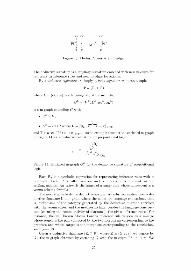
and > is a set {>s : s→ π}s∈V + . As an example consider the enriched m-graphin Figure 14 for a deductive signature for propositional logic.

π��

⊃,R2

. . . ¬,R1

cc♦p //

Figure 14: Enriched m-graph GΦ for the deductive signature of propositionallogic.

Each Rn is a symbolic expression for representing inference rules with npremises. Each >s is called s-verum and is important to represent, in oursetting, axioms. An axiom is the target of a unary rule whose antecedent is averum schema formula.

The next step is to define deductive system. A deductive system over a de-ductive signature is a m-graph where the nodes are language expressions, thatis, morphisms of the category generated by the deductive m-graph enrichedwith the verum edges, and the m-edges include, besides the language construc-tors (ensuring the commutativity of diagrams), the given inference rules. Forinstance, the well known Modus Ponens inference rule is seen as a m-edgewhose source is the pair composed by the two morphisms corresponding to thepremises and whose target is the morphism corresponding to the conclusion,see Figure 13.

Given a deductive signature (Σ,>,R), where Σ is (G, π, ♦), we denote byG> the m-graph obtained by enriching G with the m-edges >s : s → π. We

25

say that a morphism w of G+

> is in G+ whenever there is a path u over G† andu = w. We may denote a schema formula of G+

> not in G+ as a verum schemaformula. Given morphisms w1 : s → s1 and w2 : s1 → s2 of G+

> in G+ it isstraightforward to see that w2 ◦ w1 is also in G+. Moreover given the morphism>s : s→ π of G+

> it is straightforward to see that for any u : s→ s1 in G+

> themorphism >s ◦ u is also not in G+.

By a deductive system over a meta-signature Φ we mean a basis (G′′, β) overGΦ where G′′ = (V ′′, E′′, src′′, trg′′) is such that

• V ′′ is the class of morphisms of G+

> whose target is in V ;

• E′′(w1 : s→ v1 . . . wn : s→ vn, w : s→ v), for w in G+, contains, amongothers, the m-edges e : v1 . . . vn → v of E such that w = e ◦ 〈w1, . . . , wn〉in G+;

• E′′(w1 : s1 → v1 . . . wn : sn → vn, w : s→ v) = ∅ whenever w is not in G+

or si 6= s for some i = 1, . . . , n, or wi is not in G+ and n 6= 1;

and β is such that

• βv(w : s→ v) = v;

• βe(e : (w1 : s → v1 . . . wn : s → vn) → (w : s → v)) = e if e is in E andw = e ◦ 〈w1, . . . , wn〉;

• βe(f ′) ∈ R otherwise.

The first condition on E′′ imposes that E′′ contains the language construc-tors, as it is usually considered in categorical logic. As imposed in the lastcondition for βe the other m-edges correspond to inference rules. All the m-edges corresponding to inference rules must have as premises and conclusion,expressions with the same source, and with target π. The same source conditionis imposed by the second condition on E′′ and is crucial for defining instanti-ation as we will see below. The target is π by definition of β and of R. Them-edges in (βe)−1(Rn) are called n-ary inference rules or simply n-ary rules.

By a deductive system D we mean a triple

(Φ, G′′, β)

such that Φ is a meta-signature and (G′′, β) is a deductive system over Φ. Wenow illustrate our notion of deductive system by presenting deductive systemsfor a variety of logics.

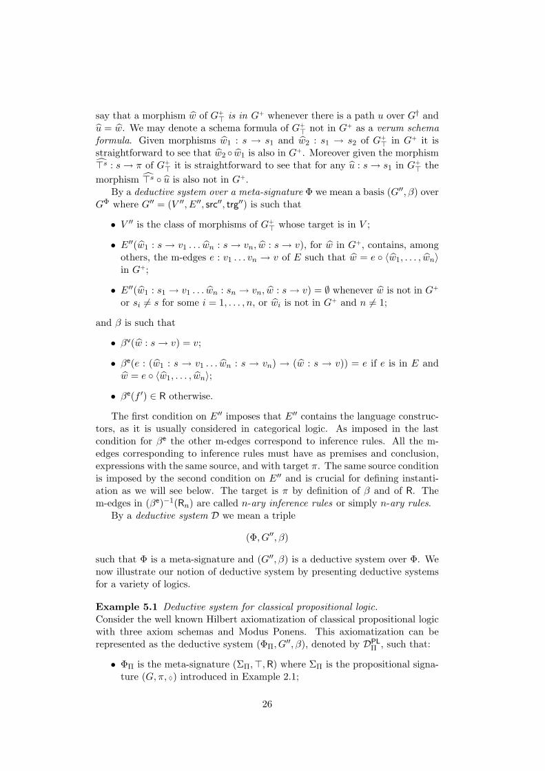
Example 5.1 Deductive system for classical propositional logic.Consider the well known Hilbert axiomatization of classical propositional logicwith three axiom schemas and Modus Ponens. This axiomatization can berepresented as the deductive system (ΦΠ, G

′′, β), denoted by DPLΠ , such that:

• ΦΠ is the meta-signature (ΣΠ,>,R) where ΣΠ is the propositional signa-ture (G, π, ♦) introduced in Example 2.1;

26

β

KS

π��

⊃,R2

. . . ¬,R1

cc♦p //

ππ

π>ππ��

� ππ

πA1��

�ax1 //

πππ

π>πππ��

� πππ

πA2��

�ax2 //

ππ

π>ππ��

� ππ

πA3��

�ax3 //

ππ

π

pππ1

�� ππ

π

⊃�� ππ

π

pππ2

��

MP//

s

π

s

π

ϕ��

¬ ◦ ϕ��

¬//

. . .

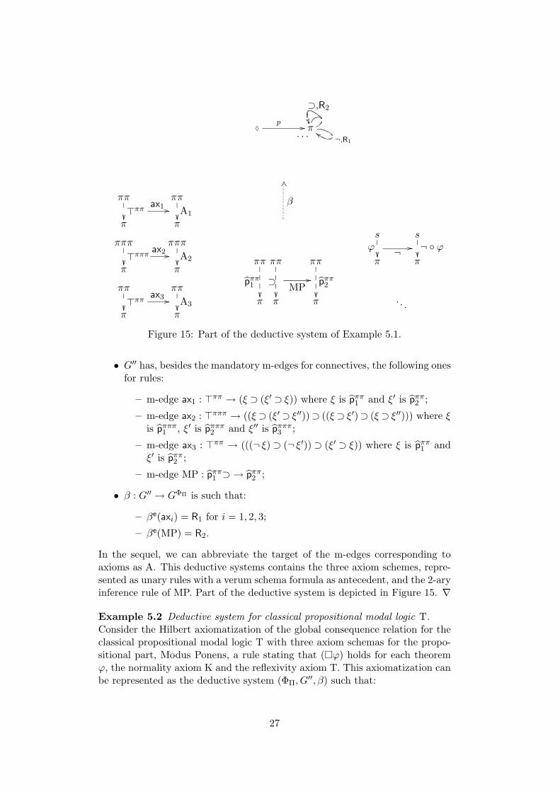
Figure 15: Part of the deductive system of Example 5.1.

• G′′ has, besides the mandatory m-edges for connectives, the following onesfor rules:

– m-edge ax1 : >ππ → (ξ ⊃ (ξ′ ⊃ ξ)) where ξ is pππ1 and ξ′ is pππ2 ;

– m-edge ax2 : >πππ → ((ξ ⊃ (ξ′ ⊃ ξ′′))⊃ ((ξ ⊃ ξ′)⊃ (ξ ⊃ ξ′′))) where ξis pπππ1 , ξ′ is pπππ2 and ξ′′ is pπππ3 ;

– m-edge ax3 : >ππ → (((¬ ξ) ⊃ (¬ ξ′)) ⊃ (ξ′ ⊃ ξ)) where ξ is pππ1 andξ′ is pππ2 ;

– m-edge MP : pππ1 ⊃ → pππ2 ;

• β : G′′ → GΦΠ is such that:

– βe(axi) = R1 for i = 1, 2, 3;

– βe(MP) = R2.

In the sequel, we can abbreviate the target of the m-edges corresponding toaxioms as A. This deductive systems contains the three axiom schemes, repre-sented as unary rules with a verum schema formula as antecedent, and the 2-aryinference rule of MP. Part of the deductive system is depicted in Figure 15. ∇

Example 5.2 Deductive system for classical propositional modal logic T.Consider the Hilbert axiomatization of the global consequence relation for theclassical propositional modal logic T with three axiom schemas for the propo-sitional part, Modus Ponens, a rule stating that (�ϕ) holds for each theoremϕ, the normality axiom K and the reflexivity axiom T. This axiomatization canbe represented as the deductive system (ΦΠ, G

′′, β) such that:

27

• ΦΠ is the meta-signature (Σ�Π,>,R) where Σ�

Π is the propositional modalsignature (G, π, ♦) introduced in Example 2.2;

• G′′ has, besides the mandatory m-edges for connectives, the followingones:



– m-edge ax3 : >ππ → (((¬ ξ) ⊃ (¬ ξ′)) ⊃ (ξ′ ⊃ ξ)) where ξ is pππ1 andξ′ is pππ2 ;

– m-edge axK : >ππ → ((�(ξ ⊃ ξ′)) ⊃ ((�ξ) ⊃ (�ξ′))) where ξ is pππ1

and ξ′ is pππ2 ;

– m-edge axT : >ππ → ((�ξ)⊃ ξ) where ξ is idπ;


– m-edge � : idπ → �;


– βe(axi) = R1 for i = 1, 2, 3,K, T ;

– βe(MP) = R2;

– βe(�) = R1. ∇

Example 5.3 Deductive system for intuitionistic propositional logic.Consider the well known Hilbert axiomatization of intuitionistic propositionallogic with axiom schemas and Modus Ponens. This axiomatization can berepresented as the deductive system (ΦΠ, G


• ΦΠ is the meta-signature (Σ∧,∨Π ,>,R) where Σ∧,∨Π is the intuitionisticpropositional signature (G, π, ♦) introduced in Example 2.3;




– m-edge ax3 : >ππ → (ξ ⊃ (ξ′ ⊃ (ξ ∧ ξ′)) where ξ is pππ1 and ξ′ is pππ2 ;

– m-edge ax4 : >ππ → ((ξ ∧ ξ′)⊃ ξ) where ξ is pππ1 and ξ′ is pππ2 ;

– m-edge ax5 : >ππ → ((ξ ∧ ξ′)⊃ ξ′) where ξ is pππ1 and ξ′ is pππ2 ;

– m-edge ax6 : >ππ → (ξ ⊃ (ξ ∨ ξ′)) where ξ is pππ1 and ξ′ is pππ2 ;

– m-edge ax7 : >ππ → (ξ′ ⊃ (ξ ∨ ξ′)) where ξ is pππ1 and ξ′ is pππ2 ;

– m-edge ax8 : >πππ → ((ξ ⊃ ξ′′)⊃ ((ξ′ ⊃ ξ′′)⊃ ((ξ ∨ ξ′)⊃ ξ′′))) whereξ is pπππ1 , ξ′ is pπππ2 and ξ′′ is pπππ3 ;

28

– m-edge ax9 : >ππ → ((ξ ⊃ ξ′)⊃ ((ξ ⊃ (¬ ξ′))⊃ (¬ ξ))) where ξ is pππ1

and ξ′ is pππ2 ;

– m-edge ax10 : >ππ → (ξ ⊃ ((¬ ξ)⊃ ξ′)) where ξ is pππ1 and ξ′ is pππ2 ;



– βe(axi) = R1 for i = 1, . . . , 10;

– βe(MP) = R2. ∇

Example 5.4 Deductive system for propositional relevance logic R.Consider the Hilbert axiomatization of relevance logic R with axiom schemas,MP and AR. This axiomatization can be represented as the deductive system(ΦΠ, G


• ΦΠ is the meta-signature (Σ∧,∨Π ,>,R) where Σ∧,∨Π is the intuitionisticpropositional signature (G, π, ♦) introduced in Example 2.3;


– m-edge ax1 : >ππ → (ξ ⊃ ξ) where ξ is idπ;

– m-edge ax2 : >πππ → ((ξ ⊃ ξ′) ⊃ ((ξ′′ ⊃ ξ) ⊃ (ξ′′ ⊃ ξ′))) where ξ ispπππ1 , ξ′ is pπππ2 and ξ′′ is pπππ3 ;

– m-edge ax3 : >ππ → ((ξ ⊃ (ξ ⊃ ξ′))⊃ (ξ ⊃ ξ′)) where ξ is pππ1 and ξ′

is pππ2 ;

– m-edge ax4 : >πππ → ((ξ ⊃ (ξ′ ⊃ ξ′′)) ⊃ (ξ′ ⊃ (ξ ⊃ ξ′′))) where ξ ispπππ1 , ξ′ is pπππ2 and ξ′′ is pπππ3 ;

– m-edge ax5 : >ππ → ((ξ ∧ ξ′)⊃ ξ) where ξ is pππ1 and ξ′ is pππ2 ;

– m-edge ax6 : >ππ → ((ξ ∧ ξ′)⊃ ξ′) where ξ is pππ1 and ξ′ is pππ2 ;

– m-edge ax7 : >πππ → (((ξ ⊃ ξ′) ∧ (ξ ⊃ ξ′′))⊃ (ξ ⊃ (ξ′ ∧ ξ′′))) where ξis pπππ1 , ξ′ is pπππ2 and ξ′′ is pπππ3 ;

– m-edge ax8 : >ππ → (ξ ⊃ (ξ ∨ ξ′)) where ξ is pππ1 and ξ′ is pππ2 ;

– m-edge ax9 : >ππ → (ξ′ ⊃ (ξ ∨ ξ′)) where ξ is pππ1 and ξ′ is pππ2 ;

– m-edge ax10 : >πππ → (((ξ ⊃ ξ′′) ∧ (ξ′ ⊃ ξ′′))⊃ ((ξ ∨ ξ′)⊃ ξ′′)) whereξ is pπππ1 , ξ′ is pπππ2 and ξ′′ is pπππ3 ;

– m-edge ax11 : >πππ → ((ξ ∧ (ξ′ ∨ ξ′′)) ⊃ ((ξ ∧ ξ′) ∨ ξ′′)) where ξ ispπππ1 , ξ′ is pπππ2 and ξ′′ is pπππ3 ;

– m-edge ax12 : >π → ((ξ ⊃ (¬ ξ))⊃ (¬ ξ)) where ξ is idπ;

– m-edge ax13 : >ππ → ((ξ ⊃ (¬ ξ′))⊃ (ξ′ ⊃ (¬ ξ))) where ξ is pππ1 andξ′ is pππ2 ;

– m-edge ax14 : >π → ((¬(¬ ξ))⊃ ξ) where ξ is idπ;


– m-edge AR : pππ1 pππ2 → (∧ ◦ 〈pππ1 , pππ2 〉);

29


– βe(axi) = R1 for i = 1, . . . , 14;

– βe(MP) = R2;

– βe(AR) = R2. ∇

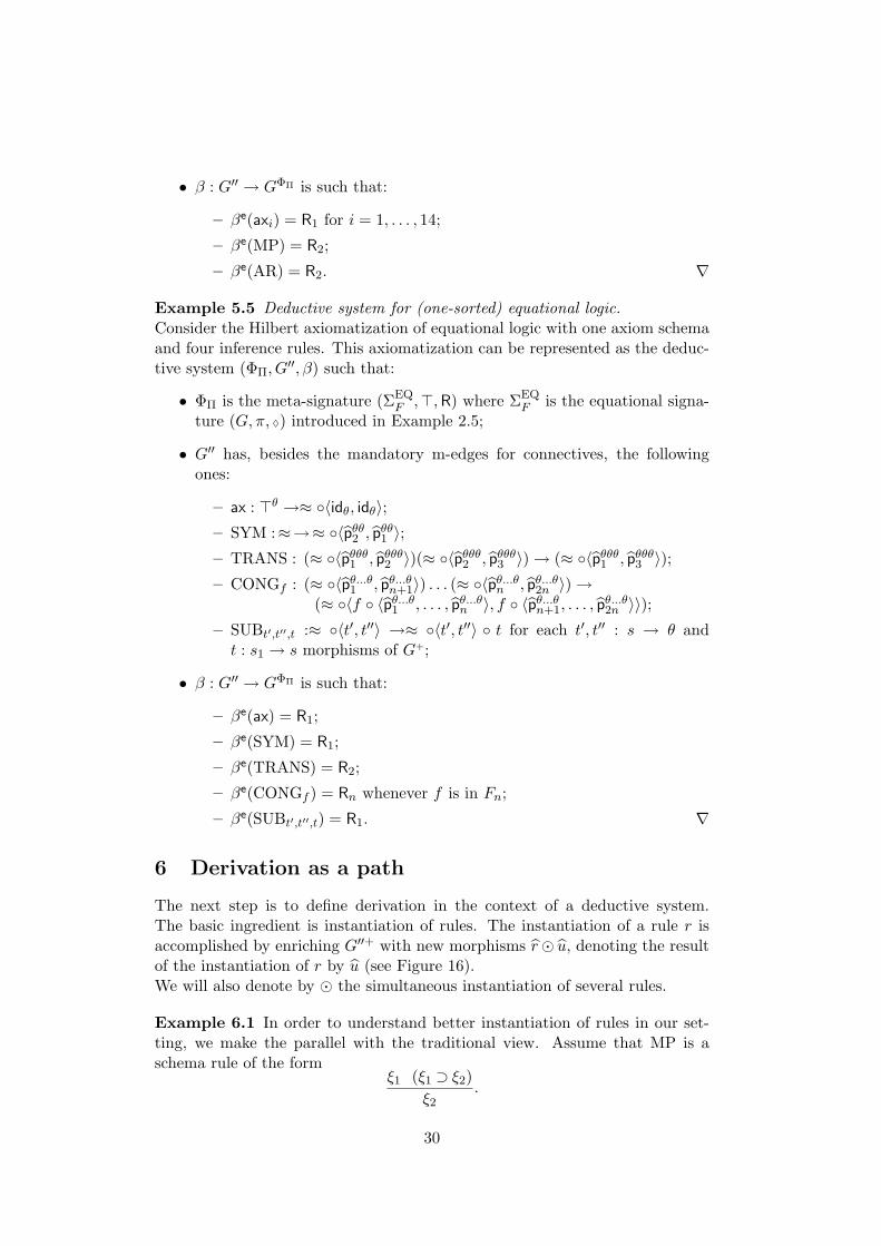
Example 5.5 Deductive system for (one-sorted) equational logic.Consider the Hilbert axiomatization of equational logic with one axiom schemaand four inference rules. This axiomatization can be represented as the deduc-tive system (ΦΠ, G


• ΦΠ is the meta-signature (ΣEQF ,>,R) where ΣEQ

F is the equational signa-ture (G, π, ♦) introduced in Example 2.5;


– ax : >θ →≈ ◦〈idθ, idθ〉;– SYM :≈→≈ ◦〈pθθ2 , pθθ1 〉;– TRANS : (≈ ◦〈pθθθ1 , pθθθ2 〉)(≈ ◦〈pθθθ2 , pθθθ3 〉)→ (≈ ◦〈pθθθ1 , pθθθ3 〉);– CONGf : (≈ ◦〈pθ...θ1 , pθ...θn+1〉) . . . (≈ ◦〈pθ...θn , pθ...θ2n 〉)→

(≈ ◦〈f ◦ 〈pθ...θ1 , . . . , pθ...θn 〉, f ◦ 〈pθ...θn+1, . . . , pθ...θ2n 〉〉);

– SUBt′,t′′,t :≈ ◦〈t′, t′′〉 →≈ ◦〈t′, t′′〉 ◦ t for each t′, t′′ : s → θ andt : s1 → s morphisms of G+;


– βe(ax) = R1;

– βe(SYM) = R1;

– βe(TRANS) = R2;

– βe(CONGf ) = Rn whenever f is in Fn;

– βe(SUBt′,t′′,t) = R1. ∇

6 Derivation as a path

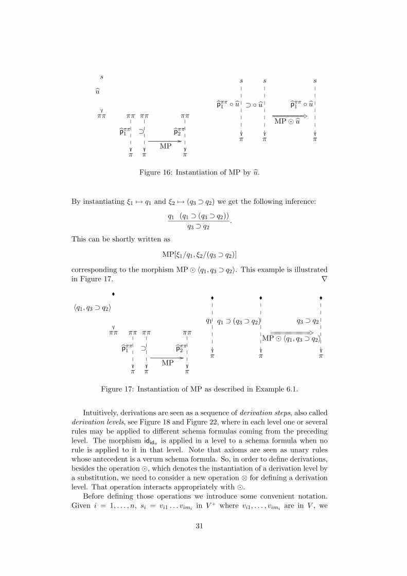
The next step is to define derivation in the context of a deductive system.The basic ingredient is instantiation of rules. The instantiation of a rule r isaccomplished by enriching G′′+ with new morphisms r� u, denoting the resultof the instantiation of r by u (see Figure 16).We will also denote by � the simultaneous instantiation of several rules.

Example 6.1 In order to understand better instantiation of rules in our set-ting, we make the parallel with the traditional view. Assume that MP is aschema rule of the form

ξ1 (ξ1 ⊃ ξ2)ξ2

.

30

ππ

π

pππ1

�� ππ

π

⊃

�� ππ

π

pππ2

��

MP//

s

ππ

u

��

s

π

pππ1 ◦ u

��

��

s

π

⊃ ◦ u

��

��

s

π

pππ1 ◦ u

��

��

MP� u+3

Figure 16: Instantiation of MP by u.

By instantiating ξ1 7→ q1 and ξ2 7→ (q3 ⊃ q2) we get the following inference:

q1 (q1 ⊃ (q3 ⊃ q2))q3 ⊃ q2

.

This can be shortly written as

MP[ξ1/q1, ξ2/(q3 ⊃ q2)]

corresponding to the morphism MP� 〈q1, q3 ⊃ q2〉. This example is illustratedin Figure 17. ∇

ππ

π

pππ1

�� ππ

π

⊃

�� ππ

π

pππ2

��

MP//

�

ππ

〈q1, q3 ⊃ q2〉

��

�

π

q1

��

��

�

π

q1 ⊃ (q3 ⊃ q2)

��

��

�

π

q3 ⊃ q2

��

��

MP� 〈q1, q3 ⊃ q2〉+3

Figure 17: Instantiation of MP as described in Example 6.1.

Intuitively, derivations are seen as a sequence of derivation steps, also calledderivation levels, see Figure 18 and Figure 22, where in each level one or severalrules may be applied to different schema formulas coming from the precedinglevel. The morphism ididπ is applied in a level to a schema formula when norule is applied to it in that level. Note that axioms are seen as unary ruleswhose antecedent is a verum schema formula. So, in order to define derivations,besides the operation �, which denotes the instantiation of a derivation level bya substitution, we need to consider a new operation ⊗ for defining a derivationlevel. That operation interacts appropriately with �.

Before defining those operations we introduce some convenient notation.Given i = 1, . . . , n, si = vi1 . . . vimi in V + where vi1, . . . , vimi are in V , we

31

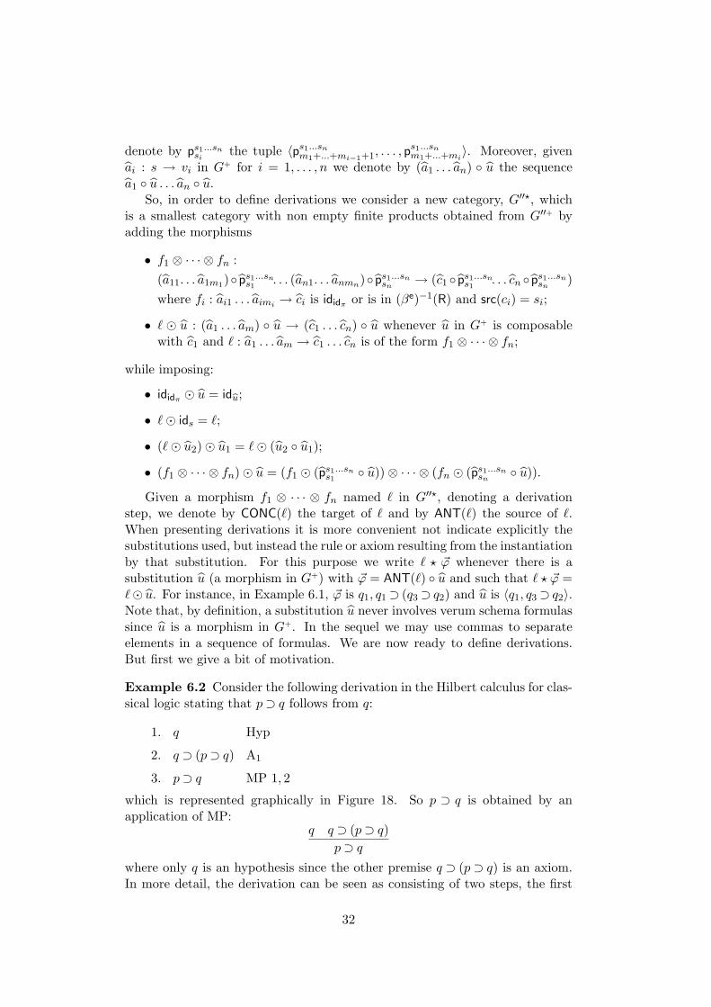
denote by ps1...snsi the tuple 〈ps1...snm1+...+mi−1+1, . . . , ps1...snm1+...+mi

〉. Moreover, givenai : s → vi in G+ for i = 1, . . . , n we denote by (a1 . . . an) ◦ u the sequencea1 ◦ u . . . an ◦ u.

So, in order to define derivations we consider a new category, G′′?, whichis a smallest category with non empty finite products obtained from G′′+ byadding the morphisms

• f1 ⊗ · · · ⊗ fn :(a11. . . a1m1)◦ ps1...sns1 . . . (an1. . . anmn)◦ ps1...snsn → (c1 ◦ ps1...sns1 . . . cn ◦ ps1...snsn )where fi : ai1 . . . aimi → ci is ididπ or is in (βe)−1(R) and src(ci) = si;

• ` � u : (a1 . . . am) ◦ u → (c1 . . . cn) ◦ u whenever u in G+ is composablewith c1 and ` : a1 . . . am → c1 . . . cn is of the form f1 ⊗ · · · ⊗ fn;

while imposing:

• ididπ � u = idbu;

• `� ids = `;

• (`� u2)� u1 = `� (u2 ◦ u1);

• (f1 ⊗ · · · ⊗ fn)� u = (f1 � (ps1...sns1 ◦ u))⊗ · · · ⊗ (fn � (ps1...snsn ◦ u)).

Given a morphism f1 ⊗ · · · ⊗ fn named ` in G′′?, denoting a derivationstep, we denote by CONC(`) the target of ` and by ANT(`) the source of `.When presenting derivations it is more convenient not indicate explicitly thesubstitutions used, but instead the rule or axiom resulting from the instantiationby that substitution. For this purpose we write ` ? ~ϕ whenever there is asubstitution u (a morphism in G+) with ~ϕ = ANT(`) ◦ u and such that ` ? ~ϕ =`� u. For instance, in Example 6.1, ~ϕ is q1, q1⊃ (q3⊃ q2) and u is 〈q1, q3⊃ q2〉.Note that, by definition, a substitution u never involves verum schema formulassince u is a morphism in G+. In the sequel we may use commas to separateelements in a sequence of formulas. We are now ready to define derivations.But first we give a bit of motivation.

Example 6.2 Consider the following derivation in the Hilbert calculus for clas-sical logic stating that p⊃ q follows from q:

1. q Hyp

2. q ⊃ (p⊃ q) A1

3. p⊃ q MP 1, 2

which is represented graphically in Figure 18. So p ⊃ q is obtained by anapplication of MP:

q q ⊃ (p⊃ q)p⊃ q

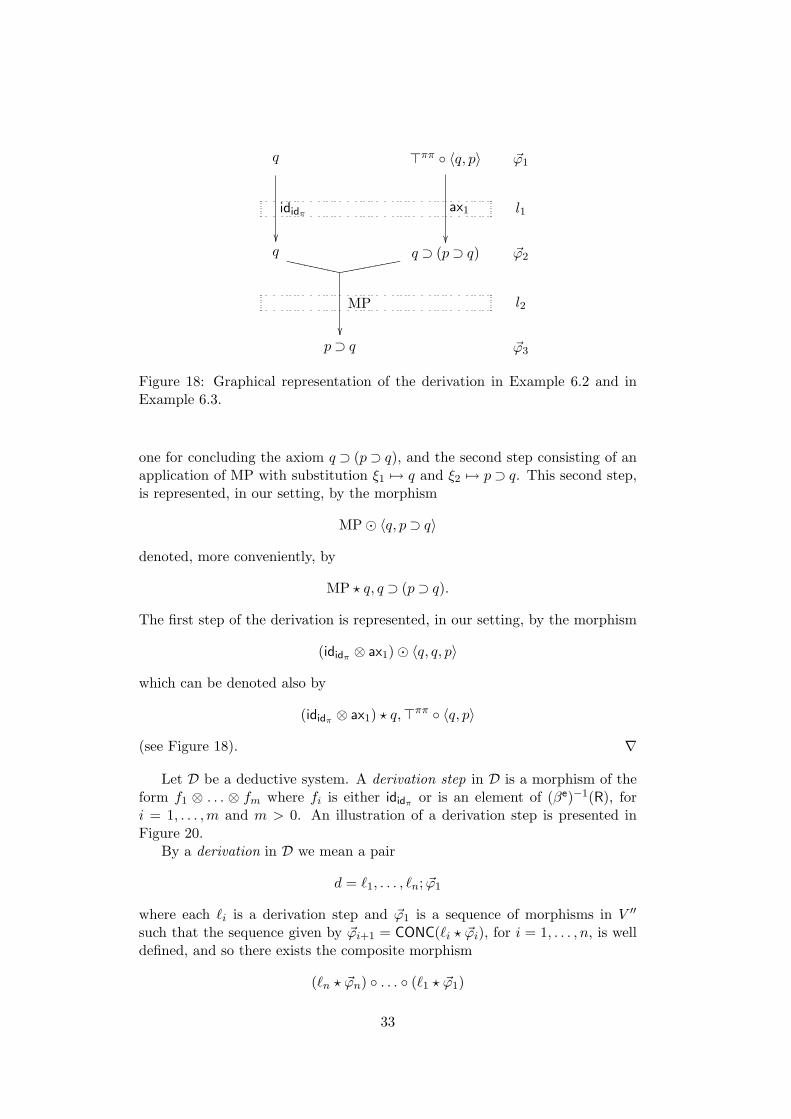
where only q is an hypothesis since the other premise q ⊃ (p ⊃ q) is an axiom.In more detail, the derivation can be seen as consisting of two steps, the first

32

q >ππ ◦ 〈q, p〉 ~ϕ1

q q ⊃ (p⊃ q) ~ϕ2

p⊃ q ~ϕ3

ididπ

��

ax1

��

XXXXXXXXXeeeeeeeeee

MP

��

l1

l2

Figure 18: Graphical representation of the derivation in Example 6.2 and inExample 6.3.

one for concluding the axiom q ⊃ (p⊃ q), and the second step consisting of anapplication of MP with substitution ξ1 7→ q and ξ2 7→ p⊃ q. This second step,is represented, in our setting, by the morphism

MP� 〈q, p⊃ q〉

denoted, more conveniently, by

MP ? q, q ⊃ (p⊃ q).

The first step of the derivation is represented, in our setting, by the morphism

(ididπ ⊗ ax1)� 〈q, q, p〉

which can be denoted also by

(ididπ ⊗ ax1) ? q,>ππ ◦ 〈q, p〉

(see Figure 18). ∇

Let D be a deductive system. A derivation step in D is a morphism of theform f1 ⊗ . . . ⊗ fm where fi is either ididπ or is an element of (βe)−1(R), fori = 1, . . . ,m and m > 0. An illustration of a derivation step is presented inFigure 20.

By a derivation in D we mean a pair

d = `1, . . . , `n; ~ϕ1

where each `i is a derivation step and ~ϕ1 is a sequence of morphisms in V ′′

such that the sequence given by ~ϕi+1 = CONC(`i ? ~ϕi), for i = 1, . . . , n, is welldefined, and so there exists the composite morphism

(`n ? ~ϕn) ◦ . . . ◦ (`1 ? ~ϕ1)

33

sπ

sπ

sπ

sπ

sπ

sπ

sπ

sπ

sπ

sπ

oo_ _ _ _ _ _ _ _ _ _ _ _ _ _...oo_ _ _ _ _ _ _ _ _ _ _ _ _ _

~ϕ1

oo_ _ _ _ _ _ _ _ _ _ _ _ _ _...oo_ _ _ _ _ _ _ _ _ _ _ _ _ _

~ϕ2

oo_ _ _ _ _ _ _ _ _ _ _ _ _ _...oo_ _ _ _ _ _ _ _ _ _ _ _ _ _

~ϕ3

oo_ _ _ _ _ _ _ _ _ _ _ _ _ _...oo_ _ _ _ _ _ _ _ _ _ _ _ _ _

~ϕn

oo_ _ _ _ _ _ _ _ _ _ _ _ _ _...oo_ _ _ _ _ _ _ _ _ _ _ _ _ _

~ϕ

l1 ? ~ϕ1��

l2 ? ~ϕ2��

...

...

ln ? ~ϕn��

ln ? ~ϕn ◦ . . . ◦ l1 ? ~ϕ1

��

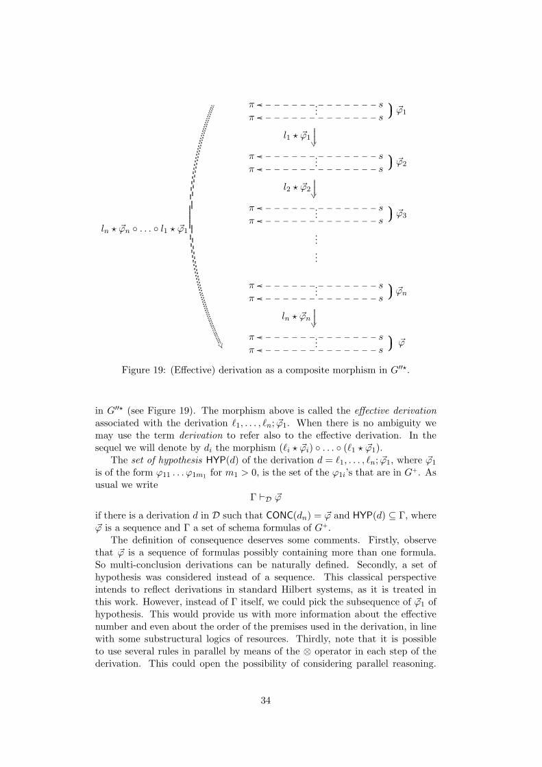
Figure 19: (Effective) derivation as a composite morphism in G′′?.

in G′′? (see Figure 19). The morphism above is called the effective derivationassociated with the derivation `1, . . . , `n; ~ϕ1. When there is no ambiguity wemay use the term derivation to refer also to the effective derivation. In thesequel we will denote by di the morphism (`i ? ~ϕi) ◦ . . . ◦ (`1 ? ~ϕ1).

The set of hypothesis HYP(d) of the derivation d = `1, . . . , `n; ~ϕ1, where ~ϕ1

is of the form ϕ11 . . . ϕ1m1 for m1 > 0, is the set of the ϕ1i’s that are in G+. Asusual we write

Γ `D ~ϕ

if there is a derivation d in D such that CONC(dn) = ~ϕ and HYP(d) ⊆ Γ, where~ϕ is a sequence and Γ a set of schema formulas of G+.

The definition of consequence deserves some comments. Firstly, observethat ~ϕ is a sequence of formulas possibly containing more than one formula.So multi-conclusion derivations can be naturally defined. Secondly, a set ofhypothesis was considered instead of a sequence. This classical perspectiveintends to reflect derivations in standard Hilbert systems, as it is treated inthis work. However, instead of Γ itself, we could pick the subsequence of ~ϕ1 ofhypothesis. This would provide us with more information about the effectivenumber and even about the order of the premises used in the derivation, in linewith some substructural logics of resources. Thirdly, note that it is possibleto use several rules in parallel by means of the ⊗ operator in each step of thederivation. This could open the possibility of considering parallel reasoning.

34

πππbpππ1oo_ _ _ _ _

πππ⊃oo_ _ _ _ _

πππbpππ2oo_ _ _ _ _

MP��

ππidπoo_ _ _ _ _

ππidπoo_ _ _ _ _

ididπ��

ππππbpππ1 ◦bpπππ1,2oo ______

ππππ⊃◦bpπππ1,2oo ______

ππππidπ◦bpπππ3oo ______

ππππbpππ2 ◦bpπππ1,2oo ______

ππππidπ◦bpπππ3oo ______

MP⊗ ididπ��

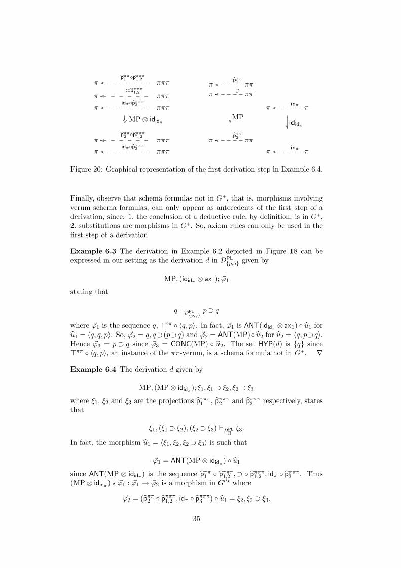
Figure 20: Graphical representation of the first derivation step in Example 6.4.

Finally, observe that schema formulas not in G+, that is, morphisms involvingverum schema formulas, can only appear as antecedents of the first step of aderivation, since: 1. the conclusion of a deductive rule, by definition, is in G+,2. substitutions are morphisms in G+. So, axiom rules can only be used in thefirst step of a derivation.

Example 6.3 The derivation in Example 6.2 depicted in Figure 18 can beexpressed in our setting as the derivation d in DPL

{p,q} given by

MP, (ididπ ⊗ ax1); ~ϕ1

stating that

q `DPL{p,q}

p⊃ q

where ~ϕ1 is the sequence q,>ππ ◦ 〈q, p〉. In fact, ~ϕ1 is ANT(ididπ ⊗ ax1) ◦ u1 foru1 = 〈q, q, p〉. So, ~ϕ2 = q, q⊃ (p⊃q) and ~ϕ2 = ANT(MP)◦ u2 for u2 = 〈q, p⊃q〉.Hence ~ϕ3 = p ⊃ q since ~ϕ3 = CONC(MP) ◦ u2. The set HYP(d) is {q} since>ππ ◦ 〈q, p〉, an instance of the ππ-verum, is a schema formula not in G+. ∇

Example 6.4 The derivation d given by

MP, (MP⊗ ididπ); ξ1, ξ1 ⊃ ξ2, ξ2 ⊃ ξ3

where ξ1, ξ2 and ξ3 are the projections pπππ1 , pπππ2 and pπππ3 respectively, statesthat

ξ1, (ξ1 ⊃ ξ2), (ξ2 ⊃ ξ3) `DPLΠξ3.

In fact, the morphism u1 = 〈ξ1, ξ2, ξ2 ⊃ ξ3〉 is such that

~ϕ1 = ANT(MP⊗ ididπ) ◦ u1

since ANT(MP ⊗ ididπ) is the sequence pππ1 ◦ pπππ1,2 ,⊃ ◦ pπππ1,2 , idπ ◦ pπππ3 . Thus(MP⊗ ididπ) ? ~ϕ1 : ~ϕ1 → ~ϕ2 is a morphism in G′′? where

~ϕ2 = (pππ2 ◦ pπππ1,2 , idπ ◦ pπππ3 ) ◦ u1 = ξ2, ξ2 ⊃ ξ3.

35

πππ

πππ

bu1=〈ξ1,ξ2,ξ2⊃ξ3〉��

ππππξ1=bpππ1 ◦bpπππ1,2 ◦bu1

oo ______________

ππππξ1⊃ξ2=⊃◦bpπππ1,2 ◦bu1

oo ______________

ππππξ2⊃ξ3=idπ◦bpπππ3 ◦bu1oo ______________

ππππξ2=bpππ2 ◦bpπππ1,2 ◦bu1=bpππ1 ◦bu2

oo ______________

ππππξ2⊃ξ3=idπ◦bpπππ3 ◦bu1=⊃◦bu2oo ______________

(MP⊗ididπ)?~ϕ1 =(MP⊗ididπ)�u1��

πππ

πππ

bu2=〈ξ2,ξ3〉��

MP ? ~ϕ2 = MP� u2��

ππππξ3=bpππ2 ◦bu2oo ______________

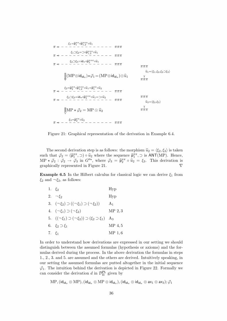
Figure 21: Graphical representation of the derivation in Example 6.4.

The second derivation step is as follows: the morphism u2 = 〈ξ2, ξ3〉 is takensuch that ~ϕ2 = (pππ1 ,⊃) ◦ u2 where the sequence pππ1 ,⊃ is ANT(MP). Hence,MP ? ~ϕ2 : ~ϕ2 → ~ϕ3 in G′′?, where ~ϕ3 = pππ2 ◦ u2 = ξ3. This derivation isgraphically represented in Figure 21. ∇

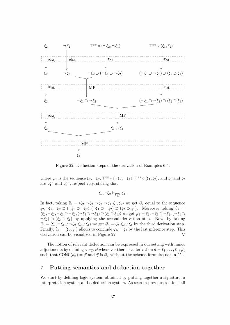
Example 6.5 In the Hilbert calculus for classical logic we can derive ξ1 fromξ2 and ¬ ξ2, as follows:

1. ξ2 Hyp

2. ¬ ξ2 Hyp

3. (¬ ξ2)⊃ ((¬ ξ1)⊃ (¬ ξ2)) A1

4. (¬ ξ1)⊃ (¬ ξ2) MP 2, 3

5. ((¬ ξ1)⊃ (¬ ξ2))⊃ (ξ2 ⊃ ξ1) A3

6. ξ2 ⊃ ξ1 MP 4, 5

7. ξ1 MP 1, 6

In order to understand how derivations are expressed in our setting we shoulddistinguish between the assumed formulas (hypothesis or axioms) and the for-mulas derived during the process. In the above derivation the formulas in steps1., 2., 3. and 5. are assumed and the others are derived. Intuitively speaking, inour setting the assumed formulas are putted altogether in the initial sequence~ϕ1. The intuition behind the derivation is depicted in Figure 22. Formally wecan consider the derivation d in DPL

Π given by

MP, (ididπ ⊗MP), (ididπ ⊗MP⊗ ididπ), (ididπ ⊗ ididπ ⊗ ax1 ⊗ ax3); ~ϕ1

36

ξ2 ¬ ξ2 >ππ ◦ 〈¬ ξ2,¬ ξ1〉 >ππ ◦ 〈ξ1, ξ2〉

ξ2 ¬ ξ2 ¬ ξ2 ⊃ (¬ ξ1 ⊃ ¬ ξ2) (¬ ξ1 ⊃ ¬ ξ2)⊃ (ξ2 ⊃ ξ1)

ξ2 ¬ ξ1 ⊃ ¬ ξ2 (¬ ξ1 ⊃ ¬ ξ2)⊃ (ξ2 ⊃ ξ1)

ξ2 ξ2 ⊃ ξ1

ξ1

YYYYYYhhhhh

MP

��

ZZZZZZZZZZZZZZZccccccccccccccccccccc

MP

��

ZZZZZZZZZZZZZZZZZccccccccccccccccc

MP��

ididπ

��

ididπ

��

ax1

��

ax3

��

ididπ

��

ididπ

��

ididπ

��

Figure 22: Deduction steps of the derivation of Examples 6.5.

where ~ϕ1 is the sequence ξ2,¬ ξ2,>ππ ◦ 〈¬ ξ2,¬ ξ1〉,>ππ ◦ 〈ξ1, ξ2〉, and ξ1 and ξ2

are pππ1 and pππ2 , respectively, stating that

ξ2,¬ξ2 `DPLΠξ1.

In fact, taking u1 = 〈ξ2,¬ ξ2,¬ ξ2,¬ ξ1, ξ1, ξ2〉 we get ~ϕ2 equal to the sequenceξ2,¬ξ2,¬ξ2 ⊃ (¬ξ1 ⊃ ¬ξ2), (¬ξ1 ⊃ ¬ξ2) ⊃ (ξ2 ⊃ ξ1). Moreover taking u2 =〈ξ2,¬ ξ2,¬ ξ1⊃¬ ξ2, (¬ ξ1⊃¬ ξ2)⊃ (ξ2⊃ ξ1)〉 we get ~ϕ3 = ξ2,¬ ξ1⊃¬ ξ2, (¬ ξ1⊃¬ ξ2) ⊃ (ξ2 ⊃ ξ1) by applying the second derivation step. Now, by takingu3 = 〈ξ2,¬ ξ1⊃¬ ξ2, ξ2⊃ξ1〉 we get ~ϕ4 = ξ2, ξ2⊃ξ1 by the third derivation step.Finally, u4 = 〈ξ2, ξ1〉 allows to conclude ~ϕ5 = ξ1 by the last inference step. Thisderivation can be visualized in Figure 22. ∇

The notion of relevant deduction can be expressed in our setting with minoradjustments by defining ~γ `D ~ϕ whenever there is a derivation d = `1, . . . , `n; ~ϕ1

such that CONC(dn) = ~ϕ and ~γ is ~ϕ1 without the schema formulas not in G+.

7 Putting semantics and deduction together

We start by defining logic system, obtained by putting together a signature, ainterpretation system and a deduction system. As seen in previous sections all

37

of these components are defined in terms of m-graphs. More rigorously, a logicsystem is a triple

L = (Σ, I,D)

such that:

• I = (Σ, I) is an interpretation system;

• D = (Φ, G′′, β) is a deductive system where Φ is a meta-signature over Σ.

The logic system L is said to be sound if Γ �I ϕ whenever Γ `D ϕ, where ϕis a formula and Γ is a set of formulas of G+, and is said to be complete if theconverse holds. A logic system is said to be weakly complete if `D ϕ whenever�I ϕ, for each formula ϕ of G+.

7.1 Soundness

Given a logic system L, I in I is said to be sound for a deductive rule r in D, ifI, ρ CONC(r) whenever I, ρ proper(ANT(r)) for every assignment ρ over I,where the map proper(·) when applied to a sequence ~ϕ of schema formulas inG+

> returns the subsequence of schema formulas that are in G+. These schemaformulas are called proper. The logic system L is said to be sound for a deductiverule r in D, if all its interpretation structures over its signature are sound for r.

We now prove two propositions useful to establish the soundness theorem.

Proposition 7.1 A logic system L sound for a deductive rule r is such thatI, ρ CONC(r) ◦ u whenever I, ρ proper(ANT(r)) ◦ u for I in I, assignmentρ over I and morphism u in G+ composable with the schema formulas in r.

Proof: Let r : (ψ1 : s → π . . . ψm : s → π) → (ϕ : s → π) and denote byϕ1, . . . , ϕn the proper antecedents of r. Assume that I, ρ proper(ANT(r)) ◦ u,that is, I, ρ ϕi ◦ u for i = 1, . . . , n. Hence, [[ϕi ◦ u]]Iρ ⊆ D, and so, usingProposition 4.6, [[ϕi]]

Iρs/[[u]]Iρ ⊆ D, for i = 1, . . . , n. Since L is sound for r,

then [[ϕ]]Iρs/[[u]]Iρ ⊆ D, and by Proposition 4.6 and definition of denotation,[[ϕ ◦ u]]Iρ ⊆ D. So I, ρ CONC(r) ◦ u. QED

Proposition 7.2 Given a logic system L sound for its rules, a derivation step`, and a morphism u in G+ such that `� u is definable, then I, ρ CONC(`� u)whenever I, ρ proper(ANT(`� u), for every I in I and assignment ρ over I.

Proof: Assume I, ρ proper(ANT(` � u) and let ` be f1 ⊗ . . . ⊗ fn wherefi : a′i1 . . . a

′im′i→ ci is ididπ or is in (βe)−1(R), and i = 1, . . . , n. Denote by

ai1 . . . aimi the subsequence of proper antecedents of fi. Then proper(ANT(`�u) = ((a11 . . . a1m1)◦ps1...sns1 . . . (an1 . . . anmn)◦ps1...snsn )◦u and CONC(`�u) = (c1◦ps1...sns1 . . . cn◦ ps1...snsn )◦ u. So I, ρ proper(ANT(fi)◦(ps1...snsi ◦ u) for i = 1, . . . , n.We now show that I, ρ CONC(`� u) that is I, ρ CONC(fi) ◦ (ps1...snsi ◦ u) fori = 1, . . . , n. Let i ∈ {1, . . . , n}. There are two cases to consider: (i) fi is ididπ .Then CONC(fi) = proper(ANT(fi)) and so I, ρ CONC(fi) ◦ (ps1...snsi ◦ u) usingthe hypothesis. (ii) f1 is in (βe)−1(R), and so f1 is a deductive rule. Then theresult follows by Proposition 7.1. QED

38

The soundness theorem establishes soundness for rules as a sufficient con-dition for a logic system to be sound.

Theorem 7.3 A logic system is sound if it is sound for its deductive rules.

Proof: Let L = (Σ, I,D) be a logic system sound for all its deductive rules,and assume that Γ `D ~ϕ for a sequence ~ϕ and a set Γ of formulas of G+. Let`1, . . . , `n; ~ϕ1 be a derivation for Γ `D ~ϕ, and I in I such that I Γ. Denoteby ~ϕ1p the sequence with the proper formulas of ~ϕ1. Since the schema formu-las in ~ϕ1p are in Γ, by definition of derivation, we can conclude that they areconcrete formulas and that I ~ϕ1p using the hypothesis. We prove that I ~ϕby induction on n. Let ρ be an assignment over I.

Base (n = 1) Note that proper(ANT(`1 ? ~ϕ1)) = ~ϕ1p , and that there is a mor-phism u1 inG+ such that ~ϕ1p = proper(ANT(`1))◦u1 and `1?~ϕ1 = `1�u1. HenceI proper(ANT(`1 � u1)) and so, by Proposition 7.2, I, ρ CONC(`1 � u1),that is, I, ρ CONC(`1 ? ~ϕ1). The thesis follows since CONC(`1 ? ~ϕ1) = ~ϕ.

Step: Let ~ϕn = CONC(`n−1 ? ~ϕn−1 ◦ . . .◦`1 ? ~ϕ1). Note that the schema formulasin ~ϕn are in G+, that is, they do not involve verum schema formulas. On theother hand, `1, . . . , `n−1; ~ϕ1 is a derivation for Γ `D ~ϕn. Hence, by the inductionhypothesis, Γ �I ~ϕn. So I ~ϕn since I Γ. Therefore I ANT(`n ? ~ϕn), andthere is a morphism un in G+ such that ~ϕn = ANT(`n)◦un and `n?~ϕn = `n�un.Hence I ANT(`n� un) and so, by Proposition 7.2, I, ρ CONC(`n� un), thatis, I, ρ CONC(`n ? ~ϕn). The thesis follows since CONC(`n ? ~ϕn) = ~ϕ. QED

7.2 Completeness

Our completeness result relies on the notion of a canonical interpretation struc-ture generated by a deductive system and a set of formulas. More rigorously,let D be a deductive system and Γ a set of formulas in G+. The canonical in-terpretation structure SΓ(D) = (Σ, (G′, α,D, �)) generated by D and Γ, is suchthat:

• G′ = (V ′, E′, src′, trg′) where

– V ′ are the morphisms of G+ whose target is an element of V ;

– E′(w1 . . . wn, w) is composed by all the m-edges e of E such thatw = e ◦ 〈w1, . . . , wn〉 in G+;

– the definition of src′ and trg′ is straightforward from the definitionof m-edges;

• αv(w : s→ v) = v and αe(e) = e;

• D = {w ∈ V ′ : Γ `D w};

• � is the morphism id♦ in G+.

We may write S(D) for S∅(D). Denotation in the canonical structure has avery simple form as we show in the next lemma.

39

Lemma 7.4 Given a deductive system D, a set Γ of formulas in G+, a pathw : s→ t over G†, and an assignment ρ over SΓ(D), then [[w]]S

Γ(D),ρ = w ◦ ρs.

Proof: The proof follows by induction on the complexity of w:

- w is εs. Then [[w]]SΓ(D),ρ = ρs = ids ◦ ρs = εs ◦ ρs = w ◦ ρs;

- w is ps1i w1. Then [[w]]SΓ(D),ρ = [[ps1i w1]]S

Γ(D),ρ = ([[w1]]SΓ(D),ρ)i = (w1 ◦ ρs)i =

ps1i ◦ w1 ◦ ρs = w ◦ ρs;

- w is 〈w1, . . . , wn〉w0. Hence [[w]]SΓ(D),ρ = [[w1w0]]S

Γ(D),ρ . . . [[wnw0]]SΓ(D),ρ =

(w1 ◦ w0 ◦ ρs) . . . (wn ◦ w0 ◦ ρs) = 〈w1, . . . , wn〉 ◦ w0 ◦ ρs as we wanted to show;

- w is ew1. Therefore [[w]]SΓ(D),ρ = trg′(E′e([[w1]]S

Γ(D),ρ,−)) = trg′(E′e(w1 ◦ρs,−)) = e ◦ w1 ◦ ρs = w ◦ ρs. QED

Capitalizing on the result of denotation in the canonical structure, it ispossible to establish an important lemma relating satisfaction in the canonicalstructure with derivation.

Lemma 7.5 Given a deductive system D, a set Γ of formulas and a schemaformula ϕ : s→ π over the signature of D, Γ `D ϕ◦ρs if and only if SΓ(D), ρ ϕ, for every assignment ρ over SΓ(D).

Proof: Let ρ be an assignment over SΓ(D). Then Γ `D ϕ ◦ ρs if and only if,by Lemma 7.4, Γ `D [[ϕ]]S

Γ(D),ρ iff [[ϕ]]SΓ(D),ρ ⊆ D iff SΓ(D), ρ ϕ. QED

In a subsequent proposition we show that SΓ(D) is sound for the rules inD, but first we show a useful lemma.

Lemma 7.6 For every deductive rule r in D, set of formulas Γ, and expressionu in G+, then Γ `D CONC(r) ◦ u whenever Γ `D proper(ANT(r)) ◦ u.

Proof: Let ANT(r) be the sequence ϕ1 . . . ϕn. We start by considering thecase that all the antecedents of r are in G+, that is, proper(ANT(r)) is equal toANT(r). Assume that Γ `D ϕi ◦ u for i = 1, . . . , n. Let ì1, . . . , ìmi ; ~ϕi1 be aderivation for Γ `D ϕi ◦ u for i = 1, . . . , n. Let m be the maximum of the mi,and let ìmi+1, . . . , ìm denote the morphism ididπ , for i = 1, . . . , n. Moreover,assume that ìj is fij1⊗. . .⊗fijmij for i = 1, . . . , n and j = 1, . . . ,m, and denoteby `k the morphism f1k1 ⊗ . . .⊗ f1km1k

⊗ fnk1 ⊗ . . .⊗ fnkmnk for k = 1, . . . ,m.Note that `1, . . . , `m; ~ϕ11 . . . ~ϕn1 is a derivation for Γ `D ϕ1 ◦ u . . . ϕn ◦ u. So`1, . . . , `m, r; ~ϕ11 . . . ~ϕn1 is a derivation for Γ `D CONC(r) ◦ u as we wanted toshow.

Assume now that r has an antecedent a1 not in G+, that is, involving a verumschema formula. Then r has no other antecedent. So r; (a1 ◦ u) is a derivationfor `D CONC(r) ◦ u and so for Γ `D CONC(r) ◦ u. QED

Proposition 7.7 For every deductive rule r in D, set of formulas Γ, and as-signment ρ over SΓ(D), SΓ(D), ρ CONC(r) if SΓ(D), ρ proper(ANT(r)).

40

Proof: Assume that SΓ(D), ρ proper(ANT(r)) and denote by ϕ1 . . . ϕn thesequence proper(ANT(r)). Then Γ `D ϕi ◦ ρs, by Lemma 7.5, for i = 1, . . . , n.Hence Γ `D CONC(r) ◦ ρs, by Lemma 7.6, and so, SΓ(D), ρ CONC(r), byLemma 7.5. QED

In order for completeness to hold in a logic system it is not necessary toimpose as sufficient condition that its interpretation system contains canonicalstructures, as we show below. It is enough to guarantee that its interpretationsystem contains structures that share with canonical structures some charac-teristics. We call these structures, representatives of a canonical structure. Alogic system contains a representative of the canonical structure over a set Γwhen it contains an interpretation structure IΓ such that

• IΓ ϕ implies SΓ(D) ϕ;

• IΓ Γ;

for every formula ϕ and set of formulas Γ in G+.

Theorem 7.8 A logic system with representatives of the canonical structuresover all sets of formulas is complete.

Proof: Let Γ be a set of formulas and ϕ a formula. Assume that Γ 6`D ϕ. LetIΓ ∈ I be the representative of SΓ(D). Then SΓ(D) Γ and SΓ(D) 6 ϕ byLemma 7.5. Then IΓ Γ and IΓ 6 ϕ. So Γ 6�I ϕ since IΓ ∈ I. QED

A similar theorem can be established for weak completeness. The proof ofthe theorem is omitted since it very similar to the proof of Theorem 7.8.

Theorem 7.9 A logic system is weakly complete if it contains a representativeof the canonical structure over the empty set.

Corollary 7.10 A logic system is (weakly) complete whenever it contains allthe interpretation structures that are sound with respect to the rules.

Proof: Assume that L contains all the interpretation structures that are soundwith respect to the rules. Then SΓ(D) ∈ I, for any set Γ, using Proposition 7.7and so, by Theorem 7.8, we conclude that L is complete. QED

We now present several cases of logic systems enjoying sufficient conditionsfor completeness.

Example 7.11 Some logic systems to which Corollary 7.10 apply:

• the logic system for classical propositional logic with the deductive systempresented in Example 5.1 and all the interpretation structures sound forMP and the axioms;

• the logic system for classical propositional modal logic T with the deduc-tive system presented in Example 5.2 and all the interpretation structuressound for MP, K, T and the axioms;

41

• the logic system for intuitionistic propositional logic with the deductivesystem presented in Example 5.3 and all the interpretation structuressound for MP and the axioms;

• the logic system for relevance logic R with the deductive system presentedin Example 5.4 and all the interpretation structures sound for MP, ARand the axioms, provided some minor adjustments are made in the def-inition of consequence in order to accommodate the notion of relevantdeduction. In this case we only apply Corollary 7.10 in order to establishweak completeness.

• the logic system for one-sorted equational logic with the deductive systempresented in Example 5.5 and all the interpretation structures sound forSYM, TRANS, CONGf , SUBt′,t′′,t and the axiom A. ∇

8 Towards provisos and quantification

The next step extending this work is to investigate how to accommodate quan-tification and provisos in deduction rules. We now give some preliminary ideason how to proceed in this direction, using as example the logic in [13] includingclassical and intuitionistic connectives. More specifically we are interested inits axiom (ϕ⊃c (ψ ⊃i ϕ)) which has the proviso that ϕ is a persistent formula.A persistent formula is one where every occurrence of classical implication ⊃cand classical negation ¬c is in the scope of the intuitionistic implication ⊃i orin the scope of the intuitionistic negation ¬i.

In our setting this proviso should be accommodated at all levels: at thesignature level, at the semantic level and at the deductive level. At the signaturelevel, a new sort ν and a m-edge P : π → ν should be introduced. At thesemantic level, ν should be interpreted as either true or false and the m-edgesmapping to P relate a truth value with true if the proviso is satisfied by all the(schema) formulas that may have as denotation that truth value, and to falseotherwise. At the deductive level we should consider (ϕ⊃c (ψ⊃i ϕ)) as a unaryrule having as antecedent P (ϕ) (stating that ϕ is persistent) and as consequentthe axiom. Moreover, we should add specific rules for dealing with persistency.For instance, we should add a rule stating that for every formula ϕ, we haveP ◦ ¬i ◦ϕ.

Dealing with quantification is also a challenge. Besides accommodatingthe first-order provisos we have to deal with the definition in our setting ofthe substitution of variables and its relationship with quantification. In thepresence of quantifiers, the interplay between the variables and term schemashould also be clarified.

9 Concluding remarks

We presented a uniform and diagrammatic way of describing logics systemsusing m-graphs. Signatures, interpretation structures and deductive systemsare based on m-graphs. Under this perspective, formulas and derivations are

42

morphisms in the appropriate generated categories. The approach is generalenough to represent logics in different guises, namely substructural logics andlogics endowed with a nondeterministic semantics. Moreover, it subsumes alllogics endowed with an algebraic semantics. It seems worthwhile to explore inour setting the notion of denotation of a formula as a single truth-value even inthe presence of non-deterministic operations as in the case of some paraconsis-tent logics [2]. General soundness and completeness results were proved.

One of the major challenges is to extend the graph-theoretic approach tologics that support provisos and quantification as we already anticipated inSection 8. Another topic of interest is to investigate how to adjust our approachfor algebraizable and protoalgebraic logics. On the deductive side, herein weconcentrated on Hilbert axiomatizations. We intend to extend it to other kindsof deductive systems, namely sequent calculi. Furthermore, deductive systemsover higher-order languages are also worthwhile to explore. General resultsabout cut elimination and interpolation are also envisaged in this extendedframework.

Acknowledgments

This work was partially supported by FCT and EU FEDER, namely via Quant-Log PPCDT/MAT/55796/2004 Project, KLog PTDC/MAT/68723/2006 Proj-ect, QSec PTDC/EIA/67661/2006 Project and under the GTF (Graph The-oretic Fibring) initiative of IT. Marcelo Coniglio acknowledges support fromFAPESP, Brazil, namely via Thematic Project 2004/14107-2 (“ConsRel”), andby an individual research grant from CNPq, Brazil. The authors are gratefulto the anonymous referee for the comments and suggestions.

References

[1] G. Allwein and J. Barwise, editors. Logical Reasoning with Diagrams,volume 6 of Studies in Logic and Computation. The Oxford UniversityPress, 1996.

[2] A. Avron. Non-deterministic semantics for logics with a consistency op-erator. International Journal of Approximate Reasoning, 45(2):271–287,2007.

[3] J. Barwise. Axioms for abstract model theory. Annals of MathematicalLogic, 7:221–265, 1974.

[4] J. Barwise and J. Etchemendy. The language of first-order logic, volume 23of CSLI Lecture Notes. Stanford University Center for the Study of Lan-guage and Information, second edition, 1991.

[5] J. Barwise and J. Etchemendy. Hyperproof, volume 42 of CSLI LectureNotes. CSLI Publications, 1994.

43

[6] J. Barwise and E. Hammer. Diagrams and the concept of logic system. InAllwein and Barwise [1], pages 49–78.

[7] J.-Y. Beziau, editor. Logica Universalis. Birkhauser Verlag, second edition,2007. Towards a general theory of logic.

[8] G. Birkhoff. On the structure of abstract algebras. Proceedings of theCambridge Philosophical Society, 31:433–454, 1935.

[9] P. Blackburn, M. de Rijke, and Y. Venema. Modal Logic, volume 53 ofCambridge Tracts in Theoretical Computer Science. Cambridge UniversityPress, 2001.

[10] W.A. Carnielli, M.E. Coniglio, and J. Marcos. Logics of formal inconsis-tency. In D. Gabbay and F. Guenthner, editors, Handbook of PhilosophicalLogic (2nd. edition), volume 14, pages 15–107. Springer, 2007.

[11] A. S. d’Avila Garcez, D. M. Gabbay, and L. C. Lamb. Value-based ar-gumentation frameworks as neural-symbolic learning systems. Journal ofLogic and Computation, 15(6):1041–1058, 2005.

[12] J. Dunn. Relevance logic and entailment. In D. Gabbay and F. Guenthner,editors, Handbook of Philosophical Logic, Vol. 3, pages 117–224. KluwerAcademic Publishers, 1986.

[13] L. Farinas del Cerro and A. Herzig. Combining classical and intuitionisticlogic. In Frontiers of Combining Systems, volume 3, pages 93–102. KluwerAcademic Publishers, 1996.

[14] D. M. Gabbay, editor. What is a Logical System?, volume 4 of Studies inLogic and Computation. The Clarendon Press Oxford University Press,New York, 1994.

[15] M. Gardner. Logic Machines and Diagrams. University of Chicago Press,second edition, 1982.

[16] J. A. Goguen and J. Meseguer. Completeness of many-sorted equationallogic. Houston Journal of Mathematics, 11(3):307–334, 1985.

[17] E. Hammer and N. Danner. Towards a model theory of diagrams. Journalof Philosophical Logic, 25:463–482, 1996.

[18] E. M. Hammer. Logic and Visual Information. Studies in Logic, Languageand Information. CSLI Publications, 1995.

[19] J. Lambek and P. J. Scott. Introduction to Higher Order Categorical Logic,volume 7 of Cambridge Studies in Advanced Mathematics. Cambridge Uni-versity Press, 1988. Reprint of the 1986 original.

[20] S. Mac Lane. Categories for the Working Mathematician, volume 5 ofGraduate Texts in Mathematics. Springer-Verlag, New York, second edi-tion, 1998.

44

[21] H. Ono. Substructural logics and residuated lattices—an introduction. InTrends in logic, volume 21 of Trends Logic Studies Log. Libr., pages 193–228. Kluwer Acad. Publ., 2003.

[22] F. Paoli. Substructural logics: A primer, volume 13 of Trends in Logic—Studia Logica Library. Kluwer Academic Publishers, 2002.

[23] C. S. Peirce. Collected papers. Edited by Charles Hartshorne and PaulWeiss. The Belknap Press of Harvard University Press, 1960.

[24] H. Rasiowa and R. Sikorski. The Mathematics of Metamathematics.PWN—Polish Scientific Publishers, third edition, 1970.

[25] Stanford University Rehseis and the Suppes Foundation. The Role of Dia-grams in Mathematics: History, Logic, Philosophy and Cognitive Sciences,2008.

[26] G. Restall and F. Paoli. The geometry of non-distributive logics. TheJournal of Symbolic Logic, 70(4):1108–1126, 2005.

[27] S.-J. Shin. The Logical Status of Diagrams. Cambridge University Press,1994.

[28] IEEE Symposium. Visual Languages and Human-Centric Computing,2008.

[29] S. E. Toulmin. The Uses of Argument. Cambridge University Press, secondedition, 2003.

[30] UK University of Brighton. International Conference on the Theory andApplication of Diagrams, 2008.

[31] J. Venn. Symbolic logic. Chelsea Publishing Co., 1971. Reprint of the 1894second edition, revised and rewritten.

45

A Graph-theoretic Account of Logics

Documents

Transcript of A Graph-theoretic Account of Logics