Game-theoretic models of bargaining
400
Game-theoretic models of bargaining
-
Upload
khangminh22 -
Category
Documents
-
view
1 -
download
0
Transcript of Game-theoretic models of bargaining

Game-theoretic models of bargaining

Game-theoreticmodels of bargaining
Edited byALVIN E. ROTHUniversity of Pittsburgh
The right of theUniversity of Cambridge
to print and sellall manner of books
was granted byHenry VIII in 1534.
The University has printedand published continuously
since 1584.
CAMBRIDGE UNIVERSITY PRESSCambridgeLondon New York New RochelleMelbourne Sydney

Published by the Press Syndicate of the University of CambridgeThe Pitt Building, Trumpington Street, Cambridge CB2 1RP32 East 57th Street, New York, NY 10022, USA10 Stamford Road, Oakleigh, Melbourne 3166, Australia
© Cambridge University Press 1985
First published 1985
Library of Congress Cataloging in Publication DataMain entry under title:
Game theoretic models of bargaining.
1. Game theory-Congresses. 2. Negotiation-Mathematical models-Congresses. I. Roth, Alvin E.,1951-HB144.G36 1985 302.3'0724 84-28516ISBN 0-521-26757-9
Transferred to digital printing 2004
Contents
List of contributors viiPreface ix
Chapter 1. Editor's introduction and overview 1Alvin E. Roth
Chapter 2. Disagreement in bargaining: Models with incompleteinformation 9Kalyan Chatterjee
Chapter 3. Reputations in games and markets 27Robert Wilson
Chapter 4. An approach to some noncooperative game situationswith special attention to bargaining 63Robert W. Rosenthal
Chapter 5. Infinite-horizon models of bargaining with one-sidedincomplete information 73Drew FudenbergDavid LevineJean Tirole
Chapter 6. Choice of conjectures in a bargaining game withincomplete information 99Ariel Rubinstein
Chapter 7. Analysis of two bargaining problems with incompleteinformation 115Roger B. Myerson
Chapter 8. Sequential bargaining mechanisms 149Peter C. Cramton
Chapter 9. The role of risk aversion in a simple bargaining model 181Martin J. Osborne
vi ContentsChapter 10. Risk sensitivity and related properties for bargaining
solutions 215StefTijsHans Peters
Chapter 11. Axiomatic theory of bargaining with a variablepopulation: A survey of recent results 233William Thomson
Chapter 12. Toward a focal-point theory of bargaining 259Alvin E. Roth
Chapter 13. Bargaining and coalitions 269K. G. Binmore
Chapter 14. Axiomatic approaches to coalitional bargaining 305Sergiu Hart
Chapter 15. A comment on the Coase theorem 321William Samuels on
Chapter 16. Disclosure of evidence and resolution of disputes:Who should bear the burden of proof? 341Joel Sobel
Chapter 17. The role of arbitration and the theory of incentives 363Vincent P. Crawford

Contributors
KEN BINMORE is Professor of Mathematics and Chairman of the EconomicTheory Workshop at the London School of Economics, where he has taught since1969. He has a Ph.D. in Mathematics from Imperial College, London, and is anAssociate of the Royal College of Science.KALYAN CHATTER JEE has been an Assistant Professor of Management Science atThe Pennsylvania State University since 1979. He obtained a D.B.A. from Har-vard University in 1979. Prior to that he studied at the Indian Institute of Manage-ment and at the University of Calcutta.PETER c. CRAMTON is Assistant Professor at the Yale School of Organization andManagement. He received his Ph.D. from Stanford University in 1984.VINCENT p. CRAWFORD is Associate Professor of Economics at the University ofCalifornia at San Diego, where he has taught since 1976, when he received hisPh.D. from the Massachusetts Institute of Technology.DREW FUDENBERG is Assistant Professor of Economics at the University of Cali-fornia at Berkeley. He was awarded his Ph.D. from the Massachusetts Institute ofTechnology in 1981.SERGIU HART is Associate Professor of Statistics in the School of MathematicalSciences at Tel-Aviv University where he received his Ph.D. in 1976.DAVID LE VINE is an Assistant Professor of Economics at the University of Califor-nia at Los Angeles. He received his Ph.D. from the Massachusetts Institute ofTechnology in 1981.ROGER B. MYERSON is Professor of Managerial Economics and Decision Sciencesat Northwestern University, where he has taught since 1976, when he was grantedhis Ph.D. from Harvard University. He has been awarded a Guggenheim Fellow-ship and an Alfred P. Sloan Research Fellowship, and is a Fellow of the Econo-metric Society.MARTIN J. OSBORNE is an Assistant Professor of Economics at Columbia Univer-sity. He received his Ph.D. from Stanford University in 1979.HANS PETERS teaches in the Economics Department of the University of Lim-burg, Maastricht, The Netherlands.ROBERT w. ROSENTHAL was awarded the Ph.D. in Operations Research fromStanford University in 1971. He served on the faculty of the Department ofIndustrial Engineering and Management Sciences at Northwestern University
vii

viii Contributors
from 1970 to 1976, on the technical staff at Bell Laboratories from 1976 to 1983,and on the faculty of the Department of Economics at Virginia PolytechnicInstitute and State University from 1983 to 1984. He is currently a Professor ofEconomics at the State University of New York at Stony Brook.ALVIN E. ROTH is the A. W. Mellon Professor of Economics at the University ofPittsburgh, where he has taught since 1982. He received a Ph.D. from StanfordUniversity in 1974. He has been awarded the Founders' Prize of the Texas Instru-ments Foundation, a Guggenheim Fellowship, and an Alfred P. Sloan ResearchFellowship. He is a Fellow of the Econometric Society.ARIEL RUBINSTEIN is Senior Lecturer in the Department of Economics of theHebrew University of Jerusalem, which granted him a Ph.D. in 1979.WILLIAM SAMUELSON is Associate Professor of Economics at Boston UniversitySchool of Management. He received a Ph.D. from Harvard University in 1978.JOEL SOBEL is Associate Professor of Economics at the University of California atSan Diego, where he has taught since 1978, when he was awarded his Ph.D. fromthe University of California at Berkeley.WILLIAM THOMSON is Associate Professor of Economics at the University ofRochester, where he has taught since 1983. He received his Ph.D. from StanfordUniversity in 1976.STEF TIJS is Professor in Game Theory, Mathematical Economics, and Opera-tions Research in the Department of Mathematics of the Catholic University inNijmegen, The Netherlands, where he has taught since 1968. He received a Mas-ter's degree at the University of Utrecht in 1963, and wrote a Ph.D. dissertation inNijmegen in 1975.JEAN TIROLE has taught at Ecole Nationale des Ponts et Chaussees, Paris, since1981. He received engineering degrees from Ecole Polytechnique (1976) andEcole Nationale des Ponts et Chaussees (1978), a "Doctorat de 3eme cycle" inDecision Mathematics from University Paris 9 (1978), and a Ph.D. in Economicsfrom the Massachussetts Institute of Technology (1981).ROBERT WILSON is the Atholl McBean Professor of Decision Sciences at StanfordUniversity, where he has taught since 1964. He received a D.B.A. from HarvardUniversity in 1963. He has been awarded a Guggenheim Fellowship, and is aFellow of the Econometric Society.

Preface
The readings in this volume are revised versions of papers presented at theConference on Game-Theoretic Models of Bargaining held June 27-30,1983, at the University of Pittsburgh. Support for the conference wasprovided by the National Science Foundation and by the University ofPittsburgh.
The conference would not have been possible without the support atthe University of Pittsburgh of Chancellor Wesley Posvar, Dean JeromeRosenberg, and my colleague Professor Mark Perlman. Michael Roths-child was instrumental in arranging the NSF support.
A. E. Roth
IX


CHAPTER 1
Editor's introduction and overview
Alvin E. RothUNIVERSITY OF PITTSBURGH
There are two distinct reasons why the study of bargaining is of funda-mental importance to economics. The first is that many aspects of eco-nomic activity are influenced directly by bargaining between and amongindividuals, firms, and nations. The second is that bargaining occupies animportant place in economic theory, since the "pure bargaining prob-lem" is at the opposite pole of economic phenomena from "perfect com-petition."
It is not surprising that economic theory has had less apparent successin studying bargaining than in studying perfect competition, since perfectcompetition represents the idealized case in which the strategic aspect ofeconomic interaction is reduced to negligible proportions by the disci-pline of a market that allows each agent to behave as a solitary decisionmaker, whereas pure bargaining is the case of economic interaction inwhich the market plays no role other than to set the bounds of discussion,within which the final outcome is determined entirely by the strategicinteraction of the bargainers. The fact that the outcome of bargainingdepends on this strategic interaction has led many economists, at leastsince the time of Edgeworth (1881), to conclude that bargaining is charac-terized by the indeterminacy of its outcome. In this view, theories ofbargaining cannot, even in principle, do more than specify a range inwhich an agreement may be found; to attempt to accomplish more wouldbe to introduce arbitrary specificity.
The contrary view, of course, is that sufficient information about theattributes of the bargainers and about the detailed structure of the bar-gaining problem that these bargainers face will allow the range of indeter-minacy to be narrowed, and perhaps eliminated. This view was illustratedin an article written by John Nash (1950a), making use of the properties ofexpected utility functions outlined by John von Neumann and OskarMorgenstern in their book Theory of Games and Economic Behavior(1944).
Nash (1950a) developed what has come to be called an axiomatic
1

2 Alvin E. Rothmodel of bargaining. (It is also sometimes called a cooperative model,since it models the bargaining process as a cooperative game.) He wasinterested in predicting a particular outcome for any given bargainingsituation, and his approach was to propose a set of postulates, or axioms,about the relationship of the predicted outcome to the set of feasibleoutcomes, as represented in terms of the utility functions of the bar-gainers. In this way, he characterized a particular function that selects aunique outcome from a broad class of bargaining problems. By concen-trating on the set of potential agreements, and abstracting away from thedetailed procedures by which a particular set of negotiations might beconducted, Nash's approach offered the possibility of a theory of bargain-ing that would enjoy substantial generality. This was perhaps the firstgeneral model of bargaining to gain wide currency in the theoreticalliterature of economics.
Three years later, Nash (1953) published another article on bargaining,which extended his original analysis in several ways. Perhaps the mostsignificant of these extensions was the proposal of a specific strategicmodel that supported the same conclusions as the general axiomaticmodel outlined earlier. His approach was to propose one very particularbargaining procedure embodied in a noncooperative game in extensiveform. (The extensive form of a game specifies when each agent will makeeach of the choices facing him, and what information he will possess atthat time. It thus allows close attention to be paid to the specific strategicquestions that arise under a given set of bargaining rules.) Nash thenargued that the predicted outcome of this noncooperative bargaininggame would be the same as the outcome predicted by the axiomaticmodel. To show this, he called on the newly developing theory of nonco-operative games, to which he had made the seminal contribution of pro-posing the notion of equilibrium (Nash 19506) that today bears his name.Although the noncooperative game he proposed possessed a multitude(indeed, a continuum) of Nash equilibria, he argued that the one corre-sponding to the prediction of his axiomatic model had distinguishingcharacteristics.
In subsequent years, the axiomatic approach pioneered by Nash wasdeveloped widely. The particular model he proposed was studied andapplied extensively, and other axiomatic models were explored. By con-trast, there was much less successful development of the strategic ap-proach. In 1979, when my monograph Axiomatic Models of Bargainingwas published, most of the influential game-theoretic work on bargainingfit comfortably under that title. However, since then, there has been arenewed interest in the strategic approach, resulting in a number of strik-ing developments in the theory of bargaining.

Introduction and overview 3
Recent progress in the strategic approach to the theory of bargaininghas been due in large part to two developments in the general theory ofnoncooperative games. One of these developments, originating in thework of Harsanyi (1967, 1968#, 19686), extends the theory to includegames of "incomplete information," which allow more realistic modelingof bargaining situations in which a bargainer holds private information(e.g., information that only he knows, such as how much he values somepotential agreement). The other development, originating in the work ofSelten (1965, 1973, 1975) on "perfect equilibria," offers a technique forreducing the multiplicity of Nash equilibria found in many noncoopera-tive games, by proposing criteria to identify a subset of equilibria thatcould credibly be expected to arise from certain kinds of rational play ofthe game. (An important reformulation of some of these ideas on credibleequilibria, which makes explicit how certain kinds of behavior depend onagents' beliefs about one another's behavior, has been given by Kreps andWilson (1982).)
Two articles that demonstrate how these two developments have sepa-rately contributed to the recent progress in the theory of bargaining arethose by Rubinstein (1982) and Myerson and Satterthwaite (1983). Thepaper by Rubinstein develops a model of multiperiod bargaining undercomplete information, in which two agents alternate proposing how todivide some desirable commodity between them, until one of them ac-cepts the other's proposal. When the agents discount future events, so thatthe value of the commodity diminishes over time, Rubinstein character-izes the agreements that could arise from perfect equilibria, and showsthat the model typically predicts a unique agreement.
Myerson and Satterthwaite consider the range of bargaining proce-dures (or "mechanisms") that could be used to resolve single-period bar-gaining under incomplete information, in which two agents negotiateover whether, and at what price, one of them will buy some object fromthe other, when each agent knows his own value for the object and has acontinuous probability distribution describing the other agent's value.They show that, when no outside subsidies are available from third par-ties, no bargaining procedure exists with equilibria that are ex post effi-cient, that is, with equilibria having the property that a trade is made if andonly if the buyer values the object more than does the seller. The intuitionunderlying this is that a bargainer who behaves so that he always makes atrade when one is possible must, in most situations, be profiting less fromthe trade than he could be. Equilibrium behavior involves a tradeoffbetween the expected profitability of each trade and the probability ofreaching an agreement on the terms of trade.
These and related results derived from strategic models have added a

4 Alvin E. Roth
dimension to the game-theoretic treatment of bargaining that was notpresent when my book on axiomatic models appeared in 1979. In addi-tion, there have been subsequent developments in the study of axiomaticmodels, and some encouraging progress at bridging the gap between thesetwo approaches, as well as in identifying their limitations. It was for thepurpose of permitting these developments to be discussed in a unified waythat the Conference on Game-Theoretic Models of Bargaining, fromwhich the readings in this volume come, was held at the University ofPittsburgh in June 1983. Together, these papers provide a good picture ofsome of the new directions being explored.
The first two selections, those by Chatterjee (Chapter 2) and by Wilson(Chapter 3), are surveys that put in context some of the theoretical devel-opments that depend critically on the ability to model rational play ofgames under incomplete information. Chatterjee focuses on models thatpredict a positive probability of disagreement in bargaining, as a conse-quence of the demands of equilibrium behavior. Wilson focuses on therole of players' expectations and beliefs about one another in games andmarkets that have some degree of repeated interaction among agents. Anagent's "reputation" is the belief that others have about those of hischaracteristics that are private information. In particular, Wilson dis-cusses the role that agents' reputations, and the opportunities that agentshave to influence their reputations, play in determining their equilibriumbehavior.
The next reading, by Rosenthal (Chapter 4), discusses a rather differentapproach to the effects of reputation. In his models, Rosenthal viewsreputation as a summary statistic of an agent's past behavior, in bargain-ing against previous opponents. He considers how the reputations of theagents mediate the play of the game when the members of a large popula-tion of potential bargainers are paired randomly in each period.
The paper by Fudenberg, Levine, and Tirole (Chapter 5), and the paperby Rubinstein (Chapter 6), both define a multiperiod game of incompleteinformation that is sufficiently complex to allow a variety of bargainingphenomena to be exhibited at equilibrium. Both papers conclude that thebeliefs that agents hold play an important part in determining equilibriumbehavior, and both discuss some of the methodological and modelingissues that arise in studying bargaining in this way.
The readings by Myerson (Chapter 7) and Cramton (Chapter 8) eachconsider the problem of mechanism design for bargaining with incom-plete information. Myerson examines some single-period bargainingmodels in terms of the comprehensively articulated approach to bargain-ing that he has explored elsewhere. Cramton addresses similar questionswith respect to bargaining that takes place over time. The inefficiencies

Introduction and overview 5due to equilibrium behavior that appear as disagreements in single-periodmodels appear in his model as delays in reaching agreement.
The next two papers, by Osborne (Chapter 9) and by Tijs and Peters(Chapter 10), address a different kind of question: the relationship be-tween risk posture and bargaining ability. This question was first raised inthe context of axiomatic models, when it was shown in Roth (1979) andKihlstrom, Roth, and Schmeidler (1981) that a wide variety of thesemodels predict that risk aversion is disadvantageous in bargaining whenall of the potential agreements are deterministic. (The situation is a littlemore complicated when agreements can involve lotteries; see Roth andRothblum (1982).) A similar result has now been shown to hold for thestrategic model proposed by Rubinstein (1982) (see Roth (1985)). How-ever, in his selection in this volume, Osborne explores a strategic modelthat yields more equivocal results. Tijs and Peters adopt the axiomaticapproach and explore how various properties of a bargaining model arerelated to the predictions it makes about the influence of risk aversion.
The reading by Thomson (Chapter 11) presents a survey of a newdirection in the axiomatic tradition. Thomson looks at axiomatic modelsdefined over a domain of problems containing different numbers ofagents, and interprets the problem as one of fair division, which is anorientation that reflects the close association between bargaining andarbitration. (The problems he considers can also be viewed as multipersonpure bargaining problems if the rules state that no coalition of agents otherthan the coalition of all the agents has any options that are not available tothe agents acting individually.)
I am the author of the next reading (Chapter 12), which reviews someexperimental results that point to limitations of the descriptive power ofboth axiomatic and strategic models as presently formulated. The papersuggests an approach that may hold promise for building descriptivegame-theoretic models of bargaining, and suggests in particular that dis-agreement at equilibrium may have systematic components that cannotbe modeled as being due to incomplete information.
The readings by Binmore (Chapter 13) and by Hart (Chapter 14) canboth be viewed as extending bargaining models from the two-person caseto the case of multiperson games (which differ from multiperson purebargaining problems in that subsets of agents acting together typicallyhave options not available to individuals). In his analysis of three-persongames Binmore follows (as he has elsewhere) in the tradition proposed byNash, of developing solution concepts for cooperative games from strate-gic considerations. Hart reviews some recent axiomatizations of solutionconcepts for general multiperson games. (Both papers have the potentialto shed some light on the ongoing discussion that Binmore refers to as the

6 Alvin E. Roth
"Aumann-Roth debate" concerning the interpretation of the nontrans-ferable utility, NTU, value.)
The final three selections attempt to bridge the gap between abstractmodels of bargaining and more institutionally oriented models of disputeresolution. Samuelson (Chapter 15) focuses on the consequences for effi-ciency of assigning property rights in cases involving externalities (e.g., theright to unpolluted air). Sobel (Chapter 16) considers the role played byassigning the burden of proof in a model of litigation in which a third party(a judge) is available to settle disputes. Crawford (Chapter 17) considerspoints of potential contact between the literature on mechanism designfor bargaining under incomplete information and the literature on third-party arbitration. His paper makes clear both the necessity and the diffi-culty of establishing two-way contact between the abstract theoreticalliterature and the institutionally oriented applied literature in this area.
REFERENCES
Edgeworth, F. Y.: Mathematical Psychics. London: Kegan, Paul, 1881.Harsanyi, John C: Games with Incomplete Information Played by "Bayesian"
Players I: The Basic Model. Management Science, 1967, 14, 159-82.Games with Incomplete Information Played by "Bayesian" Players II: Bayes-
ian Equilibrium Points. Management Science, 1968a, 14, 320-34.Games with Incomplete Information Played by "Bayesian" Players III: The
Basic Probability Distribution of the Game. Management Science, 1968ft,14,486-502.
Kihlstrom, Richard E., Alvin E. Roth, and David Schmeidler: Risk Aversion andSolutions to Nash's Bargaining Problem. Pp. in Game Theory and Mathe-matical Economics. Amsterdam: North-Holland, 1981, 65-71.
Kreps, David M, and Robert Wilson: Sequential Equilibria. Econometrica, 1982,50,863-94.
Myerson, R. B., and M. A. Satterthwaite: Efficient Mechanisms for BilateralTrading. Journal of Economic Theory, 1983, 29, 265 - 81.
Nash, John F.: The Bargaining Problem. Econometrica, 1950<z, 18, 155-62.Equilibrium Points in ^-Person Games. Proceedings of the National Academy
of Science, 1950ft, 36, 48-9.Two-Person Cooperative Games. Econometrica, 1953, 21, 128-40.
Roth, Alvin E.: Axiomatic Models of Bargaining. Berlin: Springer, 1979.A Note on Risk Aversion in a Perfect Equilibrium Model of Bargaining. Econ-
ometrica, 1985,53,207-11.Roth, Alvin E., and Uriel G. Rothblum: Risk Aversion and Nash's Solution for
Bargaining Games with Risky Outcomes. Econometrica, 1982, 50, 639-47.
Rubinstein, Ariel: Perfect Equilibrium in a Bargaining Model. Econometrica,1982, 50, 97-110.
Selten, Reinhard: Spieltheoretische Behandlung eines Oligopolmodells mitNachfragetragheit. Zeitschrift fur die gesamte Staatswissenschaft, 1965,121, 301-24 and 667-89.

Introduction and overview 7
A Simple Model of Imperfect Competition where 4 Are Few and 6 Are Many.International Journal of Game Theory, 1973, 2, 141-201.
Reexamination of the Perfectness Concept for Equilibrium Points in Exten-sive Games. International Journal of Game Theory, 1975, 4, 25-55.
von Neumann, John, and Oskar Morgenstern: Theory of Games and EconomicBehavior. Princeton, N.J.: Princeton University Press, 1944.

CHAPTER 2
Disagreement in bargaining: Models withincomplete information
Kalyan ChatterjeeTHE PENNSYLVANIA STATE UNIVERSITY
2.1 Introduction
This essay serves as an introduction to recent work on noncooperativegame-theoretic models of two-player bargaining under incomplete infor-mation. The objective is to discuss some of the problems that motivatedformulation of these models, as well as cover some of the issues that stillneed to be addressed. I have not set out to provide a detailed survey of allthe existing models, and I have therefore discussed only certain specificaspects of the models that I believe to be especially important. The readerwill find here, however, a guide to the relevant literature.
The title of this chapter was chosen to emphasize the phenomenon ofdisagreement in bargaining, which occurs almost as a natural conse-quence of rational behavior (i.e., equilibrium behavior) in some of thesemodels and is difficult to explain on the basis of equilibrium behaviorusing the established framework of bargaining under complete informa-tion. Disagreement, of course, is only one reflection of the problem ofinefficient bargaining processes. I also spend some time on the generalquestion of efficiency and its attainment. Whereas in most models classi-cal Pareto-efficiency is not attainable in equilibrium, it may be obtainedby players who deviate from equilibrium, as will be shown.
The chapter is organized as follows. Section 2.2 lays out the problemand discusses the important modeling approaches available. Section 2.3focuses on a particular group of models, each of which specifies a strategic(i.e., extensive) form of the bargaining process. Section 2.4 is concernedwith studies in which the strategic form is not specified. The final sectioncontains conclusions about the material covered.
I am grateful to Al Roth, Gary Lilien, and an anonymous referee for their valuablecomments.
10 Kalyan Chatterjee
2.2 Problem context and modeling approaches
The process of resource allocation through bargaining between two par-ties who have some common interests and some opposing ones is wide-spread in the modern world. Examples include negotiations between anindustrial buyer and a potential supplier (or, in general, between anybuyer and any seller), between management and union representatives,and between nations. (Raiffa (1982) contains accounts of many differentbargaining situations.)
In view of its importance, it is not surprising that bargaining has gener-ated much theoretical interest, beginning with the classic work of Nash(1950,1953) and Raiffa (1953). Until a few years ago, most of the theoreti-cal work had assumed complete information; that is, the bargainers' util-ity functions, the set of feasible agreements, and the recourse optionsavailable if bargaining failed were all considered to be common knowl-edge. Any uncertainty present in the situation would be shared uncer-tainty, with both bargainers having the same information about the un-certain event.
Within this set of assumptions, the problem has been explored usingone of three broad categories of theoretical endeavor. The first approach,present in Nash (1950, 1953) and Raiffa (1953) and extended and com-pleted in recent work (see Roth (1979)), has not sought to describe thebargaining process explicitly through a specific extensive form. Rather, ithas concentrated on formulating and exploring the implications of gen-eral principles that are compatible with possibly many different extensiveforms. These principles can be interpreted as descriptive of actual bar-gaining but often have been regarded as normative rules.
The main theoretical results in this type of work lead to the specifica-tion of a rule for choosing an agreement (usually leading to a uniquesolution) that is characterized by a particular set of principles or axioms.
This approach is often described as "cooperative" since the jointlyagreed-upon solution is implemented presumably by a bindingagreement.
The second way of exploring the bargaining process specifies a bar-gaining game, whose equilibrium outcome then serves as a predictor ofthe actual bargaining process. For example, the Nash solution is an equi-librium (only one of many) of a simple one-stage demand game in whichplayers make demands simultaneously, and the agreement occurs if thetwo demands can be met by a feasible agreement. (If the demands are notcompatible in this way, a conflict occurs, and the "status-quo point" is thesolution.) Work by Harsanyi (1956), Binmore (1981), and others hassought to explain why the equilibrium given by the Nash solution would,in fact, be the one chosen in the bargaining.

Disagreement in bargaining 11
Note that the presence of multiple equilibria may explain why bar-gainers disagree, even under complete information. In Chapter 12 of thisvolume, Roth proposes a simple coordination game in which players usemixed strategies and thus may, with positive probability, not choose thesame outcome.
The third approach to investigating bargaining, which will not be con-sidered here, applies general theories to construct explanations for specificproblems, for example the determination of the wage and the amount oflabor used in management-union bargaining (e.g., see McDonald andSolow(1981)).
Each of the first two approaches has its strengths and weaknesses.Specifying an extensive form enables us to model (e.g., in the work underincomplete information) the strategic use of private information and,therefore, has implications that could prove useful for individual bar-gainers. However, an extensive form is bound to be arbitrary to someextent, and the axiomatic approach cuts through disputes about choice ofextensive forms.
The focus of the remainder of this chapter is on models of bargainingunder incomplete information. These models are concerned with situa-tions wherein each party has private information (e.g., about preferences)that is unavailable to the other side. This relaxation of the assumptionsmade in the complete-information framework has crucial implications.The most interesting one for economists is the persistence of Pareto-inefficient outcomes in equilibrium, the most striking of which is theexistence of disagreement even when mutually beneficial agreementsexist. The bargaining research has also generated new notions of con-strained efficiency that appear to be of general relevance in many differentareas of economics.
As before in the case of complete information models, the theoreticalstudies under conditions of incomplete information have employed twosomewhat different research strategies. The axiomatic approach was pio-neered by Harsanyi and Selten (1972). The strategic approach is based onHarsanyi (1967, 1968), work that supplied the extension of the Nash-equilibrium concept essential to explaining games of incomplete infor-mation. The two basic contributions of this series of papers by Harsanyiwere: (1) the specification of the consistency conditions on the probabilitydistributions of the players' private information (or, to use Harsanyi'sterm, "types"); and (2) the specification that a player's strategy consistedof a mapping from his type to his action. A conjecture about an oppo-nent's strategy combined with the underlying probability distribution ofthe opponent's type would generate a probability distribution over theopponent's actions. A player would maximize his conditional expectedutility given his type and this conjectured probability distribution.

12 Kalyan Chatterjee
Table 2.1. Strategic models of bargaining under incomplete information
Features
Models 1 2 3 4 5 6 7 8
Binmore(1981) / /Chatterjee and Samuelson (1983) / / / /Cramton(1983) S S S SCrawford (1982) / / •Fudenberg and Tirole (1983) Sa S SFudenberg, Levine, and Tirole
(Chapter 5, this volume) </ Sa </ VRubinstein (1983) S SSobel and Takahashi (1983) • / •Wilson (1982) / / / / •
Key to Features:1 - Two-sided incomplete information2 - Continuous probability distributions3 - Both parties make offers4 - Sequential-information transmission incorporated in model5 - Bargaining on more than one dimension6 - Explicit consideration of alternatives to current bargain7 - Many buyers and sellers in market8 - Bargainers uncertain before bargaining of the size of gains from tradea This feature is included in some of the models proposed.
Selten (1975) and, more recently, Kreps and Wilson (1982a, 19826)have proposed that an equilibrium pair of strategies should satisfy anadditional requirement, that of "perfectness," or "sequential rationality,"in order to be considered an adequate solution. This requirement entailsthat a player's equilibrium strategy should still be optimal for him at everystage of a multistage extensive-form game, given his beliefs about thefuture and current position in the game. For example, an equilibriumbased on a threat strategy (e.g., to blow up the world) that would clearlynot be in a player's best interest to implement would not be a perfectequilibrium.
The theoretical research in strategic models of bargaining is summa-rized in Table 2.1. This summary table is by no means an exhaustive list ofall the features important to modeling the bargaining process. It does,however, contain some salient ones useful for comparing the differentmodels.
Three explanatory notes are in order here. First, papers such as Craw-ford (1982) are written in terms of utility-possibility sets and therefore

Disagreement in bargaining 13theoretically encompass bargaining on more than one dimension. How-ever, players engaged in such bargaining will not find any strategic advicein these papers.
Second, feature 6 refers to determining explicitly what recourse playershave in the event of disagreement - in other words, models of variableconflict outcomes. Crawford (1982) contains some pointers on develop-ing such a model, although a scheme is not fully laid out.
Third, one area of analytical research is not included in Table 2.1. Thisarea consists of the asymmetric decision-analytic models inspired byRaifFa (1982). In these models, no equilibrium conjectures are used togenerate probability distributions of the other player's acts. Rather, suchprobability distributions are assessed directly, based either on subjectivejudgment or on empirical observation of the other player's past behavior.Although this approach is evidently incomplete as a formal theory ofinteraction, it has the advantage of being able to provide advice to bar-gainers faced with complex tasks. For example, in Chatterjee and Ulvila(1982), a start is made (in work by Ulvila) in analyzing multidimensionalbargaining problems. In this study, bargainers possess additive linearutility functions over two attributes, with the relative importance ac-corded to each attribute being private information. The bargainers an-nounce these weights, and the Nash solution conditional on theseannouncements is used to determine the attribute levels. The analy-sis is done for a given probability distribution of announcements by theopponent, and an optimal strategy, which proves to be discontinuous,is calculated.
Papers by Chatterjee (1982) and Myerson and Satterthwaite (1983)provide a bridge between the extensive forms of Table 2.1 and the full-fledged axiomatic approach of Myerson (1983, 1984). Essentially, thesepapers show the general Pareto-inefficiency of bargaining proceduresunder incomplete information and the tradeoffs needed to restoreefficiency.
In the new cooperative theory developed by Myerson, there is explicitrecognition of the constraints imposed by incomplete information. Notall binding contracts are possible; since players' strategies are unobserv-able, a requirement of any contract is that it is sustainable as an equilib-rium of some extensive-form game. These recent papers by Chatterjeeand by Myerson and Satterthwaite therefore constitute a synthesis of thetwo prevalent approaches.
Finally, bargaining is especially suited to controlled experimentation.Various carefully designed experiments involving conditions of completeinformation have been conducted by Roth (see Chapter 12 in this vol-ume) and others. Somewhat more informal experimentation under in-

14 Kalyan Chatterjee
complete information is reported in Chatterjee and Ulvila (1982) andChatterjee and Lilien (1984). These latter articles cast some doubt on thevalidity of Bayesian equilibrium as a predictor of the outcome of bargain-ing under incomplete information.
2.3 Models of disagreement andincomplete information
In this section, models that seek to explain the inefficiency of actualbargaining as an equilibrium phenomenon are considered. The conceptof efficiency used here is the familiar one of Pareto-efficiency (often called"full-information efficiency") - namely, trade takes place if and only if itis mutually advantageous for both bargainers to conclude a trade. Thenext section presents a discussion of the study of efficient procedures ormechanisms for bargaining (which could, in general, lead to inefficientoutcomes).
The concept of equilibrium used is the Nash-equilibrium notion in thesetting of incomplete information (developed by Harsanyi (1967, 1968)and called Bayesian equilibrium in the literature). Models that involvemultistage extensive forms need, in addition, to consider whether com-mitments made at one stage would be rational to carry out in future stages.Some models accomplish this by explicitly using perfect equilibrium asthe solution concept, whereas others use an implicit perfectness notion inthe model formulation (see Chapter 3 in this volume for a more detaileddiscussion of the numerous papers in various fields of economics thatcould be completed by making an explicit perfectness argument).
All of the models presented here involve incomplete information, andsome also include sequential offers (see Table 2.1). The main concern isthat most of these models do not have equilibria that are full-informationefficient, with finite-horizon models expressing this inefficiency throughdisagreement in the presence of gains from trade, and infinite-horizonones through delayed agreement. However, there are incomplete-infor-mation models that exhibit efficient equilibria.
An example is Binmore (1981). I shall mention briefly some aspects ofthis model relevant to this chapter, although the main thrust of Binmore'swork lies elsewhere.
The paper by Binmore considers the "divide-the-dollar" game withincomplete information. That is, there is some perfectly divisible com-modity of a known amount that has to be divided between two players, Iand II. Player I could be one of a finite set of types /' = 1, 2, . . . ,m,withcommonly known probabilities Al5 A2, . • . , Am, respectively. Player Iknows his type, but player II knows only the probabilities of the various

Disagreement in bargaining 15
different types. Similarly, player II could be any one of types7 = 1 , 2 , . . . , n, with commonly known probabilities fiii,ju2, . . . , / / „ ,respectively. Player II knows his own type, but player I knows only theprobabilities. Each player has a von Neumann-Morgenstern utilityfunction on the amount of the commodity that he obtains in the event ofan agreement and on his payoff if there is no agreement. A player's utilityfunction depends also on his type.
Binmore then considers a bargaining game in which players makedemands in terms of amounts of the commodity desired. If the sum of thetwo demands is at most the amount of the commodity available, eachplayer gets his demand. If not, each gets his conflict payoff. Note that thedemands are firm commitments from which neither player is permitted toback down in the event of a disagreement.
It is clear that there exists a set of "just-compatible commitment"equilibria (using Crawford's (1982) terminology), with all types of player Idemanding x{ and all types of player II demanding x2, where the sum of x{and x2 equals the amount of the commodity available. Such equilibria are"nonrevealing" or "pooling," in that the demand is the same for all typesof a given player. They are also efficient despite the incomplete knowledgeof the players' payoffs involved in the model. On the other hand, it ispossible, as Binmore shows, to obtain "revealing" or "separating" equi-libria in such models, wherein the demand made by a player does dependon his type. Such separating equilibria could involve some probability ofdisagreement (even though both players are manifestly better off agreeingthan not agreeing).
This brings us to the tricky question of which equilibrium, separatingor pooling, will be the more accurate predictor in a given bargainingsituation. Empirical data on this might be the best indicator. Anotherindicator might be the theoretical properties of the equilibrium itself. Theefficiency of a nonrevealing equilibrium in this setting is an attractivefeature, as is Binmore's demonstration that nonrevealing equilibria of asmoothed demand game approximate the Harsanyi-Selten generalizedNash bargaining solution (Harsanyi and Selten (1972)).
The key features of the Binmore example for the present discussion arethat the efficient equilibrium outcome is not "responsive" to the types ofthe players (the same outcome is obtained for all types), and that the sizeof the total gains from trade is fixed.
Two points should be noted in passing. First, Binmore's model hasalready specialized the abstract Nash framework to bargaining over asingle issue, as do most of the studies discussed here. Second, a version ofthe game discussed previously in which bargainers' nonnegative costs ofdisagreement were private information, would have the same just-

16 Kalyan Chatterjeecompatible commitment equilibria because any agreement would bepreferable to no agreement.
A natural extension of the Binmore approach might be to make theamount of the divisible commodity variable and dependent on the bar-gainers' private information. An article by Bill Samuelson and myself(Chatterjee and Samuelson (1983)) could be interpreted as providing thisextension. Once again, the bargaining is on a single issue, namely, theprice of an object owned by a seller who is willing to part with it foranything less than an amount v{ (which we call the seller's "reservationprice") and desired by a buyer who is unwilling to pay any more than v2(the buyer's reservation price). The size of the potential pie is then v2 — vl9ifv2 > vx. However, in our model, each bargainer knows his own reserva-tion price but not the other player's. Probability distributions on thereservation prices are commonly known and are, in the model, continu-ous. The bargaining game consists in each player making an offer or ademand. If the buyer's offer, a2, is at least as great as the seller's offer, a{,there is an agreement at a price between ax and a2, perhaps midwaybetween them. If not, there is no agreement, and the players obtain zeropayoffs. Once again, therefore, irreversible commitments are assumed.
We looked for equilibrium strategies in this game that were revealing inthat a player's offer would be strictly increasing in his type (or reservationprice). A player would choose an offer to maximize his conditional ex-pected return given his type and a probability distribution over the otherplayer's offers. An optimal strategy would therefore be a Bayes' decisionrule against the probability distribution of the other player's offers. Inequilibrium, this probability distribution of offers would be identical tothat generated by the other player's equilibrium strategy and the underly-ing probability distribution on that player's reservation price. (ThisBayesian/Nash equilibrium therefore has a fulfilled-expectations prop-erty, not unexpectedly, as several authors have pointed out earlier.)
We found that if there were revealing strategies in equilibrium, wecould characterize them as involving a positive difference between aplayer's reservation price and his offer, with the amount of the differencebeing dependent on the derived probability distribution of offers. Ofcourse, this meant that the bargaining game was not full-informationefficient and could lead to disagreement. This equilibrium was notunique. In particular, there were uninteresting (and inefficient) nonre-vealing equilibria that would never lead to an agreement (e.g., offer some-thing such that the probability of agreement is zero), and sometimespartially revealing equilibria.
We could not show, however, the existence of such revealing equilibriaunder general conditions. A weakening of the requirement to a revealingepsilon equilibrium might lead to more positive results.

Disagreement in bargaining 17Despite this problem, we believed that the revealing equilibrium stud-
ied would have considerable appeal to bargainers who would want theiroffers to be strictly monotonic in their reservation prices. To some extent,this belief was bolstered by the strategies obtained from classroom simula-tion in Howard Raiffa's course at Harvard. Of the groups that played thisgame with which I am familiar, very few chose nonrevealing strategies,and those that did fared badly. (Some of these results are reported inChatterjee and Ulvila (1982) and in Raiffa (1982).)
As contrasted with Binmore's model, in this model the final outcomewas responsive to the types.
An alternative explanation for disagreement is offered by Crawford(1982), who relaxes the requirement that commitments, once made, areirreversible, and allows bargainers to reverse them at a cost. (The costcould be private information to the individual bargainer, but a playerlearns his costs only after the first-stage decisions have been made.) Craw-ford shows in his model that, in some instances, commitments to incom-patible demands are in equilibrium. The intuition comes through clearlyin the section of the article where he assumes that players have constantprobabilities of not backing down in the second stage from incompatiblecommitments made in the first stage. Thus, if incompatible commit-ments (or demands) are attempted in the first stage, there is a positiveprobability of disagreement resulting from both bargainers holding firm.Crawford then shows that when dominated options are removed, thechoice of demanding one's maximum utility level dominates that of notmaking any commitments, and so ex ante one would expect a positiveprobability of disagreement.
Crawford's model might be useful in developing a theory for negotia-tion between agents with principals exercising veto power on the finalagreement. An initial demand, once made, may be costly to back awayfrom, because some principals might lose by the concession. However, theinitial demand might be sufficiently high as to convince the principals thatthe agent was bargaining honestly on their behalf.
The Crawford model also begins to address an issue that has beendeveloped further in several recent papers. The issue is the descriptiverelevance of a model that assumes irreversible commitments (or, to put itanother way, a one-stage bargaining game), possibly ending in disagree-ment even though both sides are aware after the fact (perhaps by invertingthe equilibrium strategies) that an agreement is possible.
Such an argument has been made in the recent literature on sequentialbargaining models (Cramton (1983), Fudenberg and Tirole (1983), Ru-binstein (1983), Sobel and Takahashi (1983), and Chapter 5 of this vol-ume). All of these models involve incomplete information, at least aboutthe buyer's reservation price, with Fudenberg and Tirole (1983) consider-

18 Kalyan Chatterjeeing incomplete information about both sides' reservation prices for adiscrete probability distribution, and Cramton (1983) extending theframework to continuous uniform distributions. Because these modelsare discussed elsewhere in this volume (see Chapter 3). I will not considerthem in detail here. The essential difference with the one-stage and otherfinite-horizon models is that the bargaining inefficiency does not resultfrom a lack of agreement when agreement is mutually beneficial but froma delay in the eventual agreement caused by information being revealedover time in the bargaining process. Of course, because of unequal timepreferences, an agreement may not be beneficial at the time all the infor-mation is revealed (and therefore will not occur), even though it may havebeen beneficial in the first stage of the game. The models that involveone-sided incomplete information (e.g., Sobel and Takahashi (1983))contain the intuitive feature that perfect equilibrium offers by the sellerinvolve concessions over time. (In this model, the seller can commit torepeating the same offer before the bargaining begins, but this is not acredible commitment once the bargaining is in process.) The modelsinvolving two-sided incomplete information need not have an equilib-rium with this structure.
Except for that proposed by Rubinstein (1983), who discusses bargain-ing over a pie of fixed size, these models all have one active player, whomakes offers, and one passive player, who responds. Most of these modelsalso use discounting to express time preference. This specification, ratherthan the use of stage costs and a quit option, is justified by Fudenberg,Levine, and Tirole (see Chapter 5 of this volume). However, casual obser-vation does seem to indicate frequent real-world use of the quit option bybargainers whose expected value of continuing may be low. This may bedue to real bargains being over a finite horizon (because the end of theuniverse is guaranteed in finite time), or due to use of a bargaining processdifferent from the ones that have been modeled.
To summarize the contents of this section, the advent of noncoopera-tive bargaining models with incomplete information has explained theoccurrence of inefficient outcomes in equilibrium, both in single-stagegames and in more realistic, multistage games. However, the presence ofincomplete information does not automatically result in all equilibriabeing inefficient. In the examples discussed, this result seemed to havesomething to do with the nonresponsiveness of equilibrium outcomes toplayers' types.
The finding of inefficiency for type-responsive equilibria in bargainingruns somewhat counter to the positive results obtained by Bhattacharya(1982) in the context of signaling environments. In these environments,with only one-sided incomplete information, and with varying amounts

Disagreement in bargaining 19
o
(1/3) (1/3) (1/3)
1 2.75
BUYER RESERVATION PRICE
SELLER RESERVATION PRICE(1/3) (1/3) (1/3)
Figure 2.1 Example of an efficient bargaining procedure
of a commodity (rather than a fixed item of uncertain value) being traded,it is possible to design mechanisms that guarantee full-information effi-ciency. The role of two-sided incomplete information may therefore becrucial.
2.4 The efficiency questionNow that we know that bargaining under incomplete information gener-ally leads to inefficient outcomes, we might explore the question ofwhether any bargaining procedure could be devised that would lead toefficient outcomes. If the answer to that question is no, we might think ofsearching for a procedure that is optimal in some sense, even though it isnot full-information efficient. To these ends, we will discuss one of mypapers (Chatterjee (1982)), and also a more general presentation byMyerson and Satterthwaite (1983).
The notion of efficiency is a difficult one in incomplete-informationsituations, especially if we conceive of a prebargaining game in whichplayers try to reach an agreement on the procedure to use in the actualbargaining. Once the procedure is selected, the players could resolve theactual bargaining by playing their equilibrium strategies, conditional onthe information received in the course of the choice of mechanism. In tworecent papers, Myerson (1983,1984) has provided important insights intothese questions, and we shall consider them briefly.
In this section, I also mention some recent empirical work that couldhave some bearing on the issues discussed.
An example based on one given in Myerson and Satterthwaite's paperclarifies the nature of the problem. Suppose that the seller reservationprice is 1,2.75, or 4 with equal probabilities and that the buyer reservationprice is 0, 2.5, or 3, also with equal probabilities (Figure 2.1). In addition,suppose that the bargaining procedure is as follows. The seller and thebuyer announce their respective valuations simultaneously, with the

20 Kalyan Chatterjeebuyer restricted to announcing at most 3 and the seller at least 1. If thebuyer's valuation is greater than the seller's, an agreement takes place at apricep = 2 unless the seller's valuation is 2.75, in which case the prices is2.85. If there is no agreement, payoffs are zero to both.
Consider a seller with reservation price 1 who assumes a truthful reve-lation on the part of the buyer. Does the seller have any incentive not toannounce his valuation (i.e., reservation price) truthfully? If an an-nouncement of 1 is made, agreements are realized with buyers of reserva-tion price 2.5 and 3 at a price of 2. The expected payoff to the seller is then
Any announcement up to 2.5 will give the seller the same expected payoff.An announcement of 2.6 will lead to an expected payoff of , becauseagreement takes place only with a buyer of reservation price 3. If the sellerannounces 2.75, his expected payoff is (2.85 — l)(i), or .617, a numberless than \. It is therefore optimal to announce 1. What about a seller ofvaluation 2.75? In this case, there is no reason to announce less since thisleads to a negative payoff, and announcing 2.75 gives the seller a positiveexpected payoff of (2.85 — 2.75)(^). A seller of reservation price 4 willobviously never agree with any buyer.
What about a buyer who assumes a truthful seller? Would he announcetruthfully? Since the buyer's announcement has no effect on the price butonly on the probability of agreement, there is no incentive for the buyer tounderstate his reservation price. A buyer of reservation price 0 wouldprefer no agreement to one at price 2 and therefore has no incentive tooverstate. A buyer of reservation price 2.5 would increase his probabilityof obtaining an agreement by overstating, but the only additional agree-ment he would get would be with the seller of reservation price 2.75,whose announcement would cause the agreed price to go to 2.85, causinga negative payoff. Therefore, the procedure is incentive compatible; thatis, it induces truthful revelation and is efficient in the full-informationsense - an agreement is obtained whenever it is mutually advantageous.It is also individually rational since neither player, whatever his reserva-tion price, would ever receive a negative expected payoff. In general, thesedesirable properties are difficult to obtain simultaneously, and so it mightbe worth pointing out that the probability distributions are discrete andthat the agreed price is not responsive to the announced valuations, exceptfor one change when the seller's price becomes 2.75.
Now, suppose that we make the probability distributions continuousin the following way. For the probability density of the seller reservationprice, we take the sum of three normal densities, normalized to be of mass

Disagreement in bargaining 21j each, and centered around 1, 2.75, and 4, respectively, with arbitrarysmall standard deviation e. We perform a like construction for the buyerreservation price. Suppose that we use a similar procedure, modified bymaking the agreed price 0 if the seller announces a value of less than1 — 6e and 2.85 if the seller announces a value of more than 2.75 — 6e.
It is easy to see that the procedure is no longer incentive compatible forthe seller even if the buyer is assumed to be truthful. However, the devia-tions from incentive compatibility take place if the seller's valuation is farenough away from the three mass points. Such valuations occur with verylow probability.
Thus, a procedure may be "almost" efficient in the sense of beingincentive compatible for all but a small set of types. Similarly, there couldbe several different versions of individual rationality, namely, nonnega-tive expected payoff prior to learning one's reservation price, nonnegativeexpected payoff conditional on one's reservation price, nonnegative con-ditional expected payoff for almost all reservation prices, and nonnega-tive payoffs for all types.
The consensus among investigators of this issue seems to be that theappropriate version of individual rationality is the one that generatesnonnegative conditional expected payoffs for #//reservation prices. Usinga stronger version of this assumption, assuming responsiveness of thefinal outcome to announcements, and considering only one-stage proce-dures, it is easy to see (refer to Chatterjee (1982)) that a full-information-efficient procedure is impossible. Note that the responsiveness assump-tion is violated by the bargaining procedure in the discrete example given,even the procedure that is almost incentive compatible under the contin-uous distributions of types.
Myerson and Satterthwaite (1983) begin their presentation by demon-strating that the restriction to one-stage games where players are asked toreveal their reservation prices is not a real restriction, since, for any equi-librium outcome of any procedure, there exists an equivalent incentive-compatible procedure in a one-stage revelation game. This is the "revela-tion principle" (Myerson (1979)) and is based essentially on the ability ofthe system designer to mimic the game playing of bargainers through asuitable outcome function mapping reservation prices to final payoffs (seealso Chapter 7 in this volume).
They then show that full-information efficiency and individual ratio-nality in the sense of nonnegative conditional expected payoffs for allvalues of reservation prices are incompatible provided the underlyingreservation-price distributions are absolutely continuous, with positivedensities everywhere on the respective domains. They do not needthe responsiveness assumption because they limit themselves to suchdistributions.
22 Kalyan Chatterjee
Incidentally, if the individual rationality requirement is imposed in anex ante sense prior to bargainers learning their reservation prices, and ifthe reservation prices are independently distributed, the simultaneous-offers procedure can be made full-information efficient with side pay-ments. This result is based on the work of D'Aspremont and Gerard-Veret(1979) on public goods and is contained in Chatterjee (1982).
Full-information efficiency may also be obtained by the followingbidding procedure, if players are naive in the sense of not taking intoaccount the information revealed by winning the bid. In this procedure,the players bid for the right to make an offer. The winner then makes asingle take-it or leave-it offer.
Given this general finding of inefficiency, Myerson and Satterthwaiteproceed to the problem of characterizing efficient solutions. They showthat, subject to incentive-compatibility and individual-rationality con-straints, the ex ante expected gains from trade are maximized (for the caseof [0,1 ] uniform distributions) by the simultaneous-revelation game stud-ied in Chatterjee and Samuelson (1983). However, the mechanism thatmaximizes the expected sum of payoffs before bargainers know theirprivate information may not seem very attractive after each player learnshis reservation price. Myerson (1983, 1984) has formulated a theory onthe choice of mechanism under such circumstances. He first restricts themechanisms that can be chosen to "incentive-efficient" ones, that is, toprocedures such that there is no other incentive-compatible procedurethat does at least aS/Well for every type (value of private information) ofevery player and strictly better for at least one. Myerson then shows thatsuch mechanisms can be characterized as those that maximize the sum of"virtual utilities" for the players, where virtual utilities are, broadlyspeaking, actual utilities reduced by the cost of satisfying the incentive-compatibility constraints. Using an axiomatic structure that generalizesNash's, Myerson arrives at a new cooperative-solution concept, which hecalls a "neutral bargaining mechanism."
Although I am not sure that Myerson would agree, the story here seemsto be that the players bargain cooperatively on the choice of mechanismand perhaps arrive at a neutral bargaining mechanism that implies acertain incentive-compatible, direct-revelation game, which the bar-gainers then play. Their choice of strategy in this cooperatively chosendirect-revelation game is not enforceable by any contract due to theconstraints of information availability (i.e., because each person has someprivate information) and hence the requirement that the mechanism beincentive compatible (or, equivalently, that the strategies be in equilib-rium so that no player has an incentive to deviate from his strategy). Inother words, a player cannot be penalized for not revealing his private

Disagreement in bargaining 23
information, since this information is unobservable. It is possible, how-ever, for the players to write down an enforceable contract prior to thegame, restricting it to one stage. (Violations of such a contract could beobserved and hence punished.)
Similarly, prior to knowing their reservation prices, the players couldcooperatively commit themselves to the Myerson-Satterthwaite mecha-nism by writing a binding contract. It might be argued that this distinctionbetween cooperative games where players are permitted to make bindingcontracts that can be enforced, and noncooperative games where playersmake the decisions to make and obey such contracts, is not valid, since allgames are really noncooperative. If such an assertion is accepted, Cram-ton's (Chapter 8 in this volume) contribution to restricting the class ofallowed bargaining mechanisms to those that are "sequentially rational"becomes relevant. Cramton contends that there could be direct-revela-tion mechanisms in the sense of Myerson and Satterthwaite that cannotbe implemented as perfect (or sequential) equilibria of a suitably designedbargaining game, even though they could be equilibria of such a game.For example, the Chatterjee-Samuelson game that implements theMyerson-Satterthwaite ex ante optimal mechanism in the uniform-distribution example is not permissible in Cramton's theory because bar-gainers walk away even when it is common knowledge that gains fromtrade are possible. Of course, given the one-stage extensive form, thisequilibrium is perfect, but Cramton appears to be criticizing nonsequen-tial extensive forms. Instead of defining an outcome function as an ex-pected payment to the seller and a probability of agreement contingent onthe revealed private information, Cramton defines a sequential bargain-ing mechanism outcome as an expected payment and a time that theagreement is to be reached. (This time is infinity if an agreement is neverreached.) Whereas a positive probability of disagreement is needed tokeep players honest in the Myerson-Satterthwaite game, a delayed timeof agreement performs a similar role in Cramton's discussion. It is notclear, however, what extensive form would implement a "sequential bar-gaining mechanism."
In concluding this section, we might pause to consider the relevance ofthe discussion of inefficiency and disagreement contained in the litera-ture. In equilibrium in incomplete-information games, such inefficiencyoccurs either because of disagreement or because of delayed agreement.How serious is the phenomenon in the real world, and what is the sourceof inefficiency - incomplete information, an inability to make commit-ments, or some less complicated mechanism?
In simulated games with student players, "good" solutions are reachedwith high frequency, especially in multistage games. The inefficiency

24 Kalyan Chatterjee
question is clearly an important conceptual issue in the design of betterbargaining processes. In practice, however, where nonequilibrium behav-ior may occur or players may bring in longer-term considerations, theactual inefficiency due to incomplete information may not be as great asmight be predicted by equilibrium behavior in simply specified games.Perhaps future modeling activity could be based on exploring weakerrationality requirements or a different solution concept. The efficiencyproblem might also be alleviated if reservation prices were verifiable expost with some probability, and contingent agreements were possible.Recent empirical work (Chatterjee and Lilien (1984)) seems to indicatethat unsophisticated bargainers, such as most people in real life, behaveless strategically and reveal more information than our equilibriumcalculations would indicate. Paradoxically, when confronted with a styl-ized "no-tomorrow" game such as that in the Chatterjee-Samuelsonarticle, these bargainers react by being more aggressive than they are inequilibrium.
2.5 ConclusionsIn the last few sections, I have reviewed the recent work on bargainingunder incomplete information that seems to have potential as a beginningof a descriptive theory. This work has explained disagreement and ineffi-ciency as results of equilibrium behavior and has offered a rationale forconcession strategies in multistage games. It has also made clear the limitsof designing better mechanisms for bargaining, as well as provided a wayof choosing among efficient mechanisms.
I think that empirical work is needed to demonstrate whether or not thetheories hold up when real-world bargainers confront each other. Perhapsattempts should be made to involve business decision makers in additionto students in order to strengthen the experimental results.
In addition, theoretical work might concern itself with more explicitmodels in an attempt to fill in Table 2.1, and to use the new theories inapplied contexts, such as wage bargaining. We might also try to see if ournegative conclusions on efficiency are sustained by alternative solutionconcepts.
I also believe that the field of bargaining is sufficiently developed towarrant an attempt at synthesizing it with other areas in the economics ofinformation and uncertainty. This might give us more insight into howexactly to resolve the general problems of inefficiency caused in differentcontexts by incomplete information. An example of such work, noted inTable 2.1 but not discussed here in detail, is Wilson's (1982) work ondouble auctions. Wilson generalizes the Chatterjee-Samuelson trading

Disagreement in bargaining 25
framework to many buyers and sellers, each of whom submits a sealedprice offer. The trading rule specifies the resulting price, and it is shownthat, for large numbers of traders, such a trading rule is incentive efficientin the sense of Myerson.
REFERENCES
Bhattacharya, Sudipto (1982): Signalling Environments, Efficiency, SequentialEquilibria, and Myerson's Conjecture. Mimeo, Stanford University.
Binmore, K. G. (1981): Nash Bargaining and Incomplete Information. Depart-ment of Applied Economics, Cambridge University.
Chatterjee, Kalyan (1982): Incentive Compatibility in Bargaining under Uncer-tainty. Quarterly Journal of Economics, Vol. 96, pp. 717-26.
Chatterjee, Kalyan, and Gary L. Lilien (1984): Efficiency of Alternative Bargain-ing Procedures: An Experimental Study. Vol. 28, pp. 270-295. Journal ofConflict Resolution, June.
Chatterjee, Kalyan, and William F. Samuelson (1983): Bargaining under Incom-plete Information. Operations Research, Vol. 31, pp. 835-51.
Chatterjee, Kalyan, and Jacob W. Ulvila (1982): Bargaining with Shared Infor-mation. Decision Sciences, Vol. 13, pp. 380-404.
Cramton, Peter (1983): Bargaining with Incomplete Information: An Infinite-Horizon Model with Continuous Uncertainty. Graduate School of Business,Stanford University.
Crawford, Vincent P. (1982): A Theory of Disagreement in Bargaining. Econo-metrica, Vol. 50, pp. 607-38.
D'Aspremont, Claude, and L. A. Gerard-Varet (1979): Incentives and IncompleteInformation. Journal of Public Economics, Vol. 11, pp. 25-45.
Fudenberg, Drew, and Jean Tirole (1983): Sequential Bargaining with IncompleteInformation. Review of Economic Studies, April, pp. 221-248.
Harsanyi, John C. (1956): Approaches to the Bargaining Problem before and afterthe Theory of Games. Econometrica, Vol. 24, pp. 144-57.
(1967, 1968): Games of Incomplete Information Played by "Bayesian"Players. Management Science, Vol. 14, pp. 159-83, 320-34, 486-502.
Harsanyi, John C, and Reinhard Selten (1972). A Generalized Nash Solution forTwo Person Bargaining Games with Incomplete Information. Manage-ment Science, Vol. 18, pp. 80-106.
Kreps, David, and Robert B. Wilson (1982a): Sequential Equilibria. Economet-rica, Vol. 50, pp. 863-94.
(1982&): Reputation and Imperfect Information. Journal of Economic Theory,Vol. 27, pp. 253-79.
McDonald, I. M., and Robert M. Solow (1981): Wage Bargaining and Employ-ment. American Economic Review, Vol. 71, pp. 896-908.
Myerson, Roger B. (1979): Incentive Compatibility and the Bargaining Problem.Econometrica, Vol. 47, pp. 61-73.
(1983): Mechanism Design by an Informed Principal. Econometrica, Vol. 51,pp. 1767-97.
(1984): Two-Person Bargaining Problems with Incomplete Information.Econometrica, Vol. 52, pp. 461-88.

26 Kalyan Chatterjee
Myerson, Roger, and Mark Satterthwaite (1983): Efficient Mechanisms for Bilat-eral Trading. Journal of Economic Theory, Vol. 29, pp. 265-81.
Nash, John F. (1950): The Bargaining Problem. Econometrica, Vol. 18, pp. 155 —62.
(1953): Two-Person Cooperative Games. Econometrica, Vol. 21, pp. 128-40.Raiffa, Howard (1953): Arbitration Schemes for Generalized Two-Person
Games. Pp. 361-87 in H. W. Kuhn and A. W. Tucker (eds.), Contributionsto the Theory of Games II. Annals of Mathematics Studies No. 28, Prince-ton University Press.
(1982): The Art and Science of Negotiation. The Belknap Press of HarvardUniversity Press.
Roth, Alvin E. (1979): Axiomatic Models of Bargaining. Springer-Verlag.Rubinstein, Ariel (1983): A Bargaining Model with Incomplete Information.
Mimeo, Hebrew University of Jerusalem.Selten, Reinhard (1975): Reexamination of the Perfectness Concept For Equilib-
rium Points in Extensive Games. International Journal of Game Theory,Vol. 4, pp. 25-55.
Sobel, Joel, and Ichiro Takahashi (1983): A Multistage Model of Bargaining.Review of Economic Studies, July, pp. 411 -26.
Wilson, Robert B. (1982): Double Auctions. Mimeo, Graduate School of Busi-ness, Stanford University.
CHAPTER 3
Reputations in games and markets
Robert WilsonSTANFORD UNIVERSITY
3.1 Introduction
The notion of reputation found in common usage represents a conceptthat plays a central role in the analysis of games and markets with dy-namic features. The purpose of this exposition is to describe how mathe-matical constructs roughly interpretable as reputations arise naturally aspart of the specification of equilibria of sequential games and markets. Inaddition, several examples will be sketched, and a few of the economicapplications surveyed.
The main theme here is that reputations account for strong intertem-poral linkages along a sequence of otherwise independent situations.Moreover, from examples one sees that these linkages can produce strate-gic and market behavior quite different from that predicted from analysesof the situations in isolation. The economic applications, for instance,indicate that a firm's reputation is an important asset that can be built,maintained, or "milked," and that reputational considerations can bemajor determinants of the choices among alternative decisions.
The key idea is that one's reputation is a state variable affecting futureopportunities; moreover, the evolution of this state variable depends onthe history of one's actions. Hence, current decisions must optimize thetradeoffs between short-term consequences and the longer-run effects onone's reputation. As the discussion proceeds, this general idea will beshown to have a concrete formulation derived from the analysis of se-quential games.
SemanticsIn common usage, reputation is a characteristic or attribute ascribed toone person (firm, industry, etc.) by another (e.g., "A has a reputation for
Research support for this presentation came from a Guggenheim Fellowship,NSF grants SES-81-08226 and 83-08723, and Office of Naval Research contractONR-N00014-79-C-0685.
27

28 Robert Wilson
courtesy"). Operationally, this is usually represented as a prediction aboutlikely future behavior (e.g., "A is likely to be courteous"). It is, however,primarily an empirical statement (e.g., "A has been observed in the past tobe courteous"). Its predictive power depends on the supposition that pastbehavior is indicative of future behavior.
This semantic tangle can be unraveled by the application of gametheory. In a sequential game, a player's strategy is a function that assignsthe action to be taken in each situation (i.e., each possible informationcondition) in which he might make a choice. If the player has some privateinformation (e.g., his preferences), then the choices of actions may de-pend on this information. In this case, others can interpret his past actions(or noisy observations that embody information about his past actions) assignals about what his private information might have been. More specifi-cally, they can use Bayes' rule to infer from the history of his observedactions, and from a supposition about what his strategy is, a conditionalprobability assessment about what it is that he knows. Further, if theinformation concerns something that persists over time, then these infer-ences about the private information can be used to improve predictions ofhis future behavior.
In a narrow sense, the player's reputation is the history of his previouslyobserved actions. The relevant summary, however, is simply the derivedprobability assessment whenever this is a sufficient statistic. The opera-tional use of this probability assessment is to predict the player's futureactions; the probability distribution of his actions in a future circum-stance is the one induced from his supposed strategy, regarded as a func-tion of his private information.
The sketch just described has important ramifications for the behaviorof the player. To be optimal, the player's strategy must take into consider-ation the following chain of reasoning. First, his current reputation affectsothers' predictions of his current behavior and thereby affects their cur-rent actions; so he must take account of his own current reputation toanticipate their current actions and therefore to determine his best re-sponse. Second, if he is likely to have choices to make in the future, thenhe must realize that whatever are the immediate consequences of hiscurrent decision, there will also be longer-term consequences due to theeffect of his current decision on his future reputation, and others' antici-pation that he will take these longer-term consequences into accountaffects their current actions as well.
The role of reputations in the calculation of optimal strategies is rathercomplex, more so than the simple language of common usage mightindicate. Moreover, the effects are subtle and, from a practical empiricalviewpoint, discouragingly ephemeral. An outside observer may have no

Reputations in games and markets 29way to measure a player's reputation, since in substance it exists only asprobability assessments entertained by other participants. Without somestructure imposed on the unobserved state variable hypothesized to ex-plain the actions observed, nearly any history of play in a game could beinterpreted as being consistent with the hypothesis that reputations havean explanatory role. It is important, therefore, to study reputational ef-fects within tightly specified models. We shall see that in well-specifiedmodels, reputational effects can explain behavior that has often beenconstrued as inexplicable with any other hypothesis.1
IngredientsAt least four ingredients are necessary to enable a role for reputations. (1)There must be several players in the game, and (2) at least one player hassome private information that persists over time. This player (3) is likelyto take several actions in sequence, and (4) is unable to commit in advanceto the sequence of actions he will take. The last ingredient requires expla-nation. The essential requirement for a player's reputation to matter forhis current choice of action is his anticipation that his later decisions willbe conditioned by his later reputation. That is, he must anticipate thatwhen a later choice arrives, he will look at the matter anew and take anaction that is part of an optimal strategy for the portion of the game thatremains. On that later occasion, he will, in effect, reinitialize the subgamethat remains by taking his reputation and the reputations of others as theinitializing probability assessments that complete the specification of thesubgame. It is this anticipation that brings into play the tradeoffs betweenthe short-term consequences and the long-term reputational effects of theaction he takes on an earlier occasion. Thus, the player's strategy is thesolution to a dynamic programming problem in which his and the others'reputations are among the state variables that link successive stages of thegame. This aspect of the calculation of strategies will be illustrated in theexamples that follow.
The argument just outlined has an explicit formulation that occupies acentral role in the analysis of sequential games. Game theory can beconstrued as the analysis of multiperson decision problems in which theparticipants share a base of common knowledge. That is, there exists abody of information that is known to all, that each knows is known to all,that each knows that each knows is known to all, ad infinitum. Thecommon knowledge comprises the "rules of the game." The strategiesavailable to a participant consist of those functions that specify for eachcircumstance in which he might choose an action (depending, for exam-ple, on his private information and the observations he has made of his

30 Robert Wilson
and others' actions2), the action he will take among those available. Con-tained in the common knowledge, since it is a logical implication of therules of the game, is the specification of those combinations of strategiesfor the players that are Nash equilibria; that is, each player's strategy is anoptimal response to the others' strategies. Among the Nash equilibria,moreover, are sequential equilibria (Kreps and Wilson (1982a)); in eachcircumstance, a player's strategy for the remainder of the game is anoptimal response to the others' strategies, conditional on the prior historyof the game.3 An assumption in the following discussion is that the playersmake common suppositions about which sequential equilibrium isselected.
Sequential equilibria invoke the criterion of sequential rationality. Ineach circumstance, a player chooses an action that is part of an optimalstrategy for the remainder of the game. Thus, optimality (i.e., rationality)is tested repeatedly as the game proceeds; or in reverse, the strategy iscomputed by backward recursion using the technique of dynamic pro-gramming. Part of this computation is the construction in each circum-stance of a probability assessment for those events about which the playeris uncertain. One of the implications of optimality is that this probabilityassessment is a conditional probability satisfying Bayes' rule whenever theconditioning event (i.e., the circumstance in which the player finds him-self) has nonzero probability according to the supposed strategies of theother players.
Among the sequential equilibria are the perfect equilibria (Selten(1975)).4 Say that a strategy combination is positive if each player in everycircumstance takes each feasible action with positive probability. A par-ticular strategy combination is a perfect equilibrium if there exists asequence of positive combinations converging to it such that each player'sdesignated strategy is an optimal response to each member of the se-quence. The motivation for this definition is the requirement that theequilibrium strategies be robust best responses, in the sense that theyremain optimal even for some small probabilities that the others will err.An important implication of this specification is that a perfect equilib-rium entails well-specified probability assessments for the players in eachcircumstance. (To demonstrate this, let <r = (cr1?. . . , an) represent acombination of strategies for the n players. If this is a positive combina-tion, then Bayes' rule is surely applicable in each circumstance to com-pute for the player taking an action a conditional probability assessmentover those events he does not know; let n[a] = (nu . . . , nn) representthese. Then, a sequence ak of positive strategies converging as k —* °° to aperfect equilibrium a includes a subsequence for which n[ok] convergesto a combination n[a] of probability assessments associated with the

Reputations in games and markets 31
perfect equilibrium a. One can verify, moreover, that the probabilityassessments n[a] justify the sequential rationality of cr, in the sense thatwith these probability assessments, each player's strategy solves the asso-ciated dynamic programming problem that confirms that it meets therequirements for a sequential equilibrium.5)
ExamplesThe following examples will help to clarify the ideas presented.
Sequential bargaining. Consider a model of sequential bargaining overprice between a seller and a buyer, studied in various versions by Cramton(1983<3, 19836), Fudenberg and Tirole (1983(2), and Sobel and Takahashi(1980). In its simplest form, the seller makes repeated offers until thebuyer accepts. All features are common knowledge except the buyer'svaluation of the item offered, which he knows privately. Both players areassumed to be impatient for a trade; payoffs are discounted according tothe time a trade is concluded. A sequential equilibrium entails a decreas-ing sequence of offers by the seller and, for the buyer, a maximum price atwhich he will accept that is an increasing function of his valuation.6 Beforeeach offer, the buyer's reputation, that is, the seller's probability assess-ment for his valuation, is conditioned on the history of past rejections.Hence, it is obtained by truncating the original probability assessment atthe upper end at that valuation beyond which the seller anticipated ac-ceptance from his previous offer. The buyer's reputation affects his behav-ior since, rather than accepting a favorable offer, he might defer andobtain a later, lower offer that would be the seller's optimal one to offergiven his later (perhaps false) reputation that his valuation is lower than itis. The equilibrium offer sequence and acceptance rule are computed tofake full account of these considerations.7
The chain-store game. Consider the chain-store game studied by Selten(1978), Easley, Masson, and Reynolds (1981), Rosenthal (1981), Krepsand Wilson (19826), and Milgrom and Roberts (19826). In the simplestversion, a firm (the "store") plays in sequence against n opponents (the"entrants") the following stage game with simultaneous moves that areobserved by all players. The entrant chooses to be "out," obtaining anassured payoff of zero, or "in" obtaining a payoff of 1 or —1 depending onwhether the store chooses to be "soft" or "tough" The store's payoff iszero if (in,soft) is played, and it costs 1 to be tough, whereas out yields abenefit of 2. Each entrant maximizes its expected payoff; the store maximizes the sum of its expected payoffs over the n stage games. It is obviou

32 Robert Wilson
that the only equilibrium has (in,soft) played at every stage, since soft is adominant strategy for the store in each stage game and in is the entrant'sbest response.
Now, suppose that the entrants initially assign a probability S > 0 thattough is the store's only feasible action; that is, that the store is "strong"rather than "weak" In this case, a sequential equilibrium is the following.Let /?, be the entrants' probability assessment that the store is strong when tstages remain; that is, pn = S. Then, the weak store plays tough if pt ^.5 '"1 , and otherwise it plays tough with a probability determined by thecondition that pt_x will be .5'~l if the entrant plays tough (and zero if heplays soft). Note that necessarily pt__x = pt if pt ^ .5 '"1 , since both thestrong and weak stores play tough in this case. The entrant plays out ifpt > .5', plays in if/?, < .5', and randomizes equally if/?, = .5'. (The detailsof these calculations are described in Kreps and Wilson (1982&).)
Of course, it is pt that one interprets as the store's reputation. Thisequilibrium will be used to illustrate how reputational considerationsaffect the players' choices of actions. An entrant prefers out if he assignsthe store's choice of tough a probability exceeding .5; this is certainly thecase if/?, ^ .5 '" 1 , since both the strongand the weak stores then play tough.Otherwise, the marginal probability of tough is determined by the condi-tion (from Bayes' rule) that the ratio of/?, and this probability must be theposterior probability .5 ' " 1 ; hence, the marginal probability isz?,/^'"1, andwe see that the entrant prefers out if /?, > .5', as specified in the equilib-rium. The weak store's expected payoff when t stages remain, assumingthe preceding strategies, is 0, 1, or 2 + t — T(/?,) according as/?, < , = , or>.5r , where T(/?,) = inf{T|/?, > .5T}. Hence, if/?, > .5 '" 1 , the entrant couldsave 1 now by playing soft, but it would cost more than that in the longrun, since it would reveal that he is weak, that is, pt_x = 0 after soft isobserved by subsequent entrants; whereas, if/?, ^ .5 ' " \ then the savings of1 from playing soft is offset exactly by the long-term effect, and so theentrant is indifferent and the randomized strategy is among the optimalones. Note that the preceding analysis of the weak store's decision prob-lem amounts to a verification that the entrant's strategy solves the asso-ciated dynamic programming problem, given the way in which the repu-tation evolves according to Bayes' rule.
We observe here the gist of reputational effects. If the weak store'sreputation for possibly being strong is sufficiently large compared to thenumber of stages remaining, the weak store prefers to imitate the behaviorof the strong store so as to deter later entrants from choosing in. Thestore's reputation is an asset that it acts to maintain, even if doing so iscostly in the short term, so as to reap the benefits in subsequent stages ofthe game. Indeed, if the number n of stages is very large (i.e., z{6) is small

Reputations in games and markets 33compared to ri), then the weak store obtains an expected payoff per stageof nearly 1, whereas if it were to reveal itself by playing soft, its payoffwould be 0 thereafter.
Another version of the chain-store game, with a more detailed model-ing of the economic structure, is presented in Benoit (1983).
BeliefsThe preceding examples illustrate the role of reputational effects in se-quential games with incomplete information. The key ingredient is that aplayer can adopt actions that sustain the probability assessments made byother participants that yield favorable long-term consequences. When-ever it is feasible to imitate the behavior one would adopt if one's privateinformation were different than it is, and this would affect others' actionsfavorably, there is a potential role for reputational effects.8 The operativemechanism is the process of inference by which observed actions aretaken as signals of private information. Behavior that in common usage isinterpreted as bluffing, imitation, dissembling, or the like, can all beconsidered as designed to affect others' responses by sustaining or alteringtheir beliefs. Nor need this behavior have a role only in competitivecontexts; as we shall see later, it can be an important factor in cooperativebehavior.
Milgrom and Roberts (19826) emphasize that these ingredients areavailable whenever any of the players has information that is not commonknowledge among all of them. It may be, in fact, that they have the sameimmediate perceptions but this fact is not common knowledge.
3.2 ConceptsThis section contains a description of some of the key ideas obtained fromanalyses of reputational effects in sequential games. The intention is toindicate those concepts that have validity in circumstances more generalthan the examples with which they are illustrated.
DisequilibriumOne of the strengths of game theory is the precision and completenesswith which it describes and analyzes multiperson decision problems. Forexample, the rules of the game are completely specified, and a strategyindicates what to do in every possible circumstance; in particular, anequilibrium predicts not only what is expected to happen (i.e., thosesequences of actions and events having positive probability using the

34 Robert Wilsonequilibrium strategies - we call these the equilibrium paths), but also theanticipated consequences of any deviation from the optimal strategies ofthe players. In the case of reputations, the game-theoretic analysis revealsthat the anticipated equilibrium behavior depends sensitively on theplayers' interpretations of the significance of disequilibrium actions (Ru-binstein (1983b)). This feature derives from the fact that after an unanti-cipated action by one player, the other players cannot use Bayes' rule toobtain a conditional probability assessment for the player's private infor-mation. Yet, the equilibrium is sustained by the player's expectation ofwhat assessments they will make and thus what responses they will be ledto choose. In the chain-store game described previously, this feature didnot arise since the action soft was conclusive evidence that the store wasweak, for the reason that the strong store was incapable of that action. Theequilibrium remains unchanged, however, if we allow that the strongstore could choose soft but that this action is dominated by the actiontough. In this case, the equilibrium depends critically on the suppositionthat the entrants interpret the action soft as conclusive evidence that thestore is weak. Other suppositions are possible, and some of these lead toequilibria that are qualitatively different. We find, therefore, that sequen-tial equilibria are sustained by suppositions about what beliefs (i.e., proba-bility assessments) will be entertained off the equilibrium paths. Tech-nically, the disequilibrium beliefs are determined by the sequence{ok,n[ok]) whose limit justifies the equilibrium pair (a,n) of strategies andbeliefs (compare with "Ingredients" in Section 3.1). From a practicalpoint of view, this amounts to saying that the beliefs are determined by asupposition as to which types (i.e., the private information) of a player aremore likely to deviate or err. In the chain-store game, the salient supposi-tion is that the weak store is more likely to play soft, since in the stage gameit is dominant for the weak store and dominated for the strong store. Ingeneral, considerations of this kind would seem to be crucial ingredientsof a fully predictive theory as to which sequential equilibrium will befound in practice.
ImitationIn the chain-store game, the weak store chooses tough i£pt ^ .5'"1, eventhough this action is costly whether the entrant chooses in or out. As wasindicated, a plausible interpretation of this strategy is that imitating thedominant behavior of the strong store yields the future benefit of deterringlater entrants by sustaining their belief that the store might be strong.Imitation in this case has a competitive advantage for the weak store, andit is disadvantageous for the entrants; were there no possibility of imita-

Reputations in games and markets 35
tion (e.g., 6 = 0), the payoffs to the store and the entrant would bereversed.
Imitation may, however, confer joint advantages, and indeed it can bethe foundation for mutual cooperation. The following example illustratesthis possibility.
The prisoners' dilemma game. Consider the finitely repeated version ofthe symmetric prisoners' dilemma studied by Kreps, Milgrom, Roberts,and Wilson (1982). In each stage, the two players move simultaneously,choosing either to cooperate or to not cooperate, and each then observesthe other's choice. If neither cooperates, their payoffs are zero, and eachgains 3 from the other's cooperation but it costs the other 1 to cooperate.Each seeks to maximize the sum of his payoffs over n repetitions of thestage game. The only equilibrium of this game has both players choosingnot to cooperate every time, regardless of the number of repetitions. Atthe final stage, cooperation is disadvantageous for both players; at thepenultimate stage, therefore, there is no chance that cooperation will bereciprocated in the next stage and so again cooperation is disadvanta-geous; and so on ad infinitum.
Suppose, however, that player A entertains a positive probability S,possibly very small, that player B is addicted to the strategy TIT-FOR-TAT, that is, that B will cooperate unless A does not, in which case hisfollowing action will be to not cooperate.9 In this case, there is a sequentialequilibrium in which they both cooperate for all but a relatively fewstages. The lengthy derivation of this result invokes the following argu-ment, which is stated intuitively and somewhat imprecisely here.
Suppose that B is not addicted to TIT-FOR-TAT. We argue that formost of the game, B will want to imitate TIT-FOR-TAT. The first part istrivial: He surely must punish any noncooperative behavior by A sincethis yields a short-term advantage and does not alter his reputation. Thekey, therefore, is to establish that B will reciprocate A's cooperation ifmany stages remain. The argument uses the following inequalities, inwhich A(r,s) and B(r,s) represent A's and 5's expected payoffs if they usestrategies r and s, respectively. Also, let t represent 5's TIT-FOR-TATstrategy, and let (r°9s°) be a sequential equilibrium.
1. B(r°,s°) > B(r°,t), since s° is £'s optimal response to r°.2. B(r°,t) ^ A(r°,t) - 4, since by using TIT-FOR-TAT, B is assured of a
payoff within 1 + 3 of .4's payoff, regardless of which strategy A uses.Moreover, when B uses the strategy TIT-FOR-TAT, B's expected payoffis the same as the contingent payoff depending on B's type, since bothtypes use TIT-FOR-TAT.
3. A(r°,t) ^ A(r°,s°)9 since B's use of TIT-FOR-TAT can only benefit A.

36 Robert Wilson
This is based on the fact that s° punishes A for noncooperation just asTIT-FOR-TAT does, but possibly s° does not reciprocate cooperation tothe degree that TIT-FOR-TAT does.
4. A(r°,s°) ^ 2S(n — 1) — 2. If A previously cooperated, then by continu-ing cooperation until B does not, 's payoff is at least 2n if 2? is addictedto TIT-FOR-TAT, and it is at least —1 otherwise. Similarly, if A pre-viously did not cooperate, then B is sure to not cooperate, and so withthis strategy A gets —1 immediately by cooperating plus a continuationvalue that is at least the corresponding amounts given: 2{n — 1), or — 1.Either way, the expected payoff, using the initial probability assessment,is at least the stated amount.
Combining these results, we see that B's expected payoff is at least26(n — 1) — 6 when his reputation is S and n stages remain. Conse-quently, when B considers whether to reciprocate cooperation, he calcu-lates as follows. He can choose to not cooperate, yielding an immediatepayoff of at most 3 but zero thereafter (since his type is revealed, the onlyequilibrium path thereafter has no cooperation). Or he can cooperate,yielding at least—1 immediately and at least 2S(n — 2) — 6 in the remain-ing n — 1 stages (which he will begin with a reputation that is at least S if hereciprocates cooperation). Thus, if n and S satisfy —1 + 2S(n — 2) — 6 >3, then B's best choice is to reciprocate cooperation.
This result can be strengthened further to provide a bound, indepen-dent of the length of the game, on the number of noncooperative episodes.Thus, we see that cooperative behavior (from both players) prevails for allbut a relatively few stages of a long game.
This equilibrium stems from the basic observation that each playerprefers to play with another who uses TIT-FOR-TAT, will respond inkind if the actions taken are consistent with TIT-FOR-TAT, and willinitiate TIT-FOR-TAT if there is some chance that the other player willplay TIT-FOR-TAT and there are sufficiently many stages remaining.What is needed to bootstrap the equilibrium is A's assessment that Bmight be addicted to TIT-FOR-TAT, in which case A is willing to cooper-ate until it is not reciprocated; in turn, B wants to maintain this belief inA's mind by imitating addiction and thus reaping the long-term rewardsof cooperation. The first time that B fails to follow TIT-FOR-TAT, heruins the prospects for further cooperation, whereas as long as there is achance that B is addicted, so that even if he is not addicted he will imitateaddiction, A's optimal response is to cooperate until it is not reciprocated.
A striking aspect of this game is that a little private information is goodfor both parties. Even before B knows his type, both players prefer that thisinformation not be revealed once it is known to B. For example, A prefersthat B has an opportunity to imitate an addiction to TIT-FOR-TAT.

Reputations in games and markets 37
Monopoly power. Imitation can be an intrinsic ingredient of monopolypower. This is indicated obliquely by the chain-store game describedearlier in which the weak store's tough actions until near the end of thegame deter entrants from entering. An example in the classical mode isderived from studies of durable-good monopoly. Consider Picasso'sproblem as rendered by Moorthy (1980). During his lifetime, the artistPicasso can command a price for his work that depends on the totalsupply that will exist when he dies; collectors who purchase from Picassorealize that the resale value later will be high or low depending on whetherhe produces few or many paintings during his lifetime. Naturally, Picassowould like to select an optimal quantity to produce during his lifetime,say, to maximize his lifetime income. This strategy is not credible, how-ever, since collectors realize that, regardless of what he produced pre-viously, each year Picasso will reconsider the problem and again attemptto maximize his income for the remainder of his life. In doing so, Picassowill regard his previous production as a shift in the demand function forhis paintings. Anticipating this, collectors expect him to increase his out-put rate as he ages until he nearly exhausts the demand before he dies;thus, even when he is young, they are willing to pay only the low pricecorresponding to his large lifetime output. Thus, Picasso's monop-oly power evaporates, due essentially to the ramifications of sequentialrationality.
Suppose, on the other hand, that collectors are uncertain whetherPicasso's maximum output rate is high or low, and that initially theyassign probability S > 0 that it is low. In this case, there is a sequentialequilibrium rather like the one for the chain-store game: For all but thelast few years of his life, Picasso's output rate is low. If he actually has ahigh output rate, then late in life he randomizes between a high and a lowproduction rate, until the first time he produces at a high rate collectorsrealize that this is possible, and thereafter he produces at a high rate. Withthis strategy, Picasso realizes a substantial portion of his monopoly power.Without the uncertainty about his production rate, Picasso is unable tocapture these monopoly profits if his output rate is actually high. (As ithappens, after their deaths, both Pablo Picasso and Norman Rockwellwere discovered to have numerous paintings in storage that were notpreviously known to collectors.)
General theorems. The chain-store game, the finitely repeated pris-oners' dilemma, and Picasso's problem as analyzed here are all examplesof a general theory of finitely repeated games with incomplete informa-tion that has been developed by Maskin and Fudenberg (1983). In atwo-player, one-stage game, say that a vector of payoffs for the players is

38 Robert Wilson
attainable if there are strategies the players could use that yield thesepayoffs, and for each player the payoff exceeds what the player couldguarantee (using his max-min strategy); if there are more than twoplayers, require further that each player's payoff exceeds what he gets insome Nash equilibrium. Their theorem states that for each attainablevector of payoffs and each e > 0, there exists an integer n and a corre-sponding repeated game of incomplete information with the followingproperties. First, each player has probability 1 — e of having the prefer-ences specified in the stage game, and a complementary probability, e, ofhaving preferences that lead him to play differently, as will be specifiedlater. Second, there exists a sequential equilibrium such that for all but thelast n stages (or fewer), the equilibrium specifies actions that result in thespecified attainable vector of payoffs. Thus, if the number of repetitions islarge, then the attainable vector is realized for most of the history of thegame, the exceptions occurring only near the end of the game. The con-struction that makes this result possible specifies that with probability e, aplayer has preferences (not further specified) that lead him to play thefollowing strategy: He will use the action required to obtain the attainablevector for as long as the other player(s) do the same, after which for theremainder of the game he will play the max-min strategy (if there are twoplayers) or the Nash equilibrium strategy for the stage game. This con-struction is somewhat different than the ones employed in the previousexamples, but the gist of the result is the same. It shows that a small dose ofincomplete information, and a long repetition of a stage game, are suffi-cient to induce equilibrium strategies that yield any attainable vector ofpayoffs, except near the end of the game.
adverse selection and self-selection
Imitation is not the only mode in which reputational features operate.This section focuses on two other possibilities. One is that other uncer-tainties in the situation are sufficient to make imitation unnecessary, andyet, as we shall see, the effects of reputations can continue to be substan-tial. The other is the possibility that a player's goal in the situation is tomake sure he is identified correctly, so that the unfortunate consequencesof a false identification do not result.
Repeated auctions. Bikhchandani (1982) has pursued a preliminarystudy of the following repeated auction affected by the "winner's curse."Consider a sequence of auctions in which each prize is awarded to thebidder submitting the highest bid, at the price equal to the second highestbid. It suffices to consider just two bidders and suppose that they submitbids for every prize, each seeking to maximize the expectation of the sum

Reputations in games and markets 39of the values of the prizes he wins net of the prices paid for them. Thevalues of the prizes are the same to the two bidders but unobservable untilthe game is over; instead, each bidder has some sample information aboutthe value of each prize. Assume that the values of the prizes are distributedindependently and identically, and that conditional on each prize's value,the two samples observed by the bidders are independently and identi-cally distributed. It is clear that with this setup, the bidders will treat theauctions as independent, and in each one a bidder will bid an amount thatdepends on his sample observation.
A key fact here is that an optimal bid must take account of the observa-tion that in order to win, the bid must exceed the opponent's bid, and thisin turn implies that the opponent's sample observation was sufficientlysmall. That is, winning an auction is an informative event, since it tells thewinner something about the samples observed by other bidders, andthereby it adds further information about the value of the prize.
Now, suppose that bidder A assigns a small probability S > 0 to thepossibility that bidder B obtains a payoff from each prize he wins that is $ 1more than its value to bidder A. Bidder B is assumed to know whetherprizes are worth $ 1 more to him, and of course all of this is commonknowledge. In this case, the auctions obviously are not independent, sinceA may use his observations of 5's bids to infer information about his type.Because the sampling process adds so much noise to the inferential pro-cess, B may have little incentive to modify his bids directly either to hideor to advertise his type. There is, however, an indirect effect that should beemphasized. Bidder A realizes that the implications of winning are moresevere than before: If A wins, his bid was sufficient to beat out the B bidderof the ordinary type, but now there is the added possibility that it was alsosufficient to beat out the B bidder who values the prize more, whichimplies that B observed an even lower sample than before. Thus, bidder Awill select a lower bid than previously. Realizing this, bidder B of theordinary type sees that winning implies that bidder 's sample may havebeen higher than previously allowed; hence, the ordinary bidder B isinclined to raise his bid. However, this rebounds to reinforce A's conclu-sion, and therefore i?'s conclusion. Thus, we see that the ultimate effect ofA's incomplete information is to lower 4's bids and to raise the ordinary2?'s bids until a new equilibrium is reached. The result of this, of course, isthat bidder B of either type is more likely to win auctions, althoughobviously the high-value B will win more often than the ordinary B. Ifmany auctions remain, the ordinary B may be in danger of detection by A,which may motivate him to raise his bid further to match the bids by thehigh-value bidder B. This has been verified in one numerical examplestudied by Bikhchandani.
As this example illustrates, reputational effects can interact with and

40 Robert Wilsonreinforce other informational effects in a sequential game. Here, £'s repu-tation that he might value prizes more accentuates the adverse-selectionproblem faced by A, and this rebounds to affect i?'s bids as well.
Limit pricing. The preceding examples reflect the fact that reputationalfeatures are associated most often with "pooling equilibria," in which aplayer's type cannot be inferred completely from his actions. There is,however, a related feature that arises in "screening equilibria," in which aplayer's actions completely reveal his type. A prime example is found inthe models of limit pricing formulated by Milgrom and Roberts (1982a),Saloner (1982), and Matthews and Mirman (1983). A monopolist firmoperates in two periods, and in the second of these periods there is thepossibility that a potential entrant will choose to enter. Assume that themonopolist acquieces to entry; even so, the entrant's anticipated profitsdepend on its estimate of the monopolist's costs, since these affect themonopolist's price or output decisions in a duopoly. Assuming that theentrant incurs fixed costs to enter, its decision will be influenced by itsobservation of what the monopolist does in the first period, since that canbe interpreted as a signal about what the monopolist's costs are. In somemodels of this sort, there is no other source of uncertainty, and so theentrant can determine from observable market data what price or outputdecisions the monopolist selected. Then, from this and a suppositionabout the monopolist's strategy, the entrant can calculate exactly what themonopolist's costs are, if the strategy specifies a one-to-one relationshipbetween costs and first-period actions. Consequently, the entrant's deci-sion about whether to enter is based on a correct assessment of the mo-nopolist's costs. In most cases, the monopolist's best strategy necessarilyinvolves actions that depend on its costs; consequently, the one-to-onerelationship is inevitable, and it follows that the entrant will act with aperfect inference about the monopolist's true costs.
Since the sequential-equilibrium strategy does not deter entry (theentrant enters under precisely the circumstances it would if it had perfectinformation from the beginning), it appears that the monopolist's first-period action is fruitless in deterring entry, and therefore that the monop-olist should adopt ordinary monopoly practices in the first period -revealing its costs by doing so but reaping maximum profits in theinterim. What appears to be true is not, however; in fact, the firm's actionsin the first period imply prices lower than monopoly prices. The explana-tion for this is that the firm must price low enough (as specified by theequilibrium) to signal its costs correctly, so that higher prices (e.g., mo-nopoly prices) are not interpreted as a sign that its costs are high and thusencourage excessive entry. It is certainly clear that the equilibrium cannot
Reputations in games and markets 41entail ordinary monopoly pricing in the first period, since if the prospec-tive entrant assumed such pricing in the first period, then the monopolistwould have an incentive to set its price somewhat lower so as to realizesome of the tradeoffs between first-period profit and diminishing thechance of subsequent entry.
It is evident from this analysis that in some cases, a player must workhard to establish an accurate reputation, signaling his type via his actions,in order to avoid incorrect inferences by others. As in most signaling and"rat-race" models (Spence (1974)), the result tends to be a heavy invest-ment in the signal. In the present example, the investment in the signalmanifests itself as limit pricing. First-period prices are below the monop-oly price, but they limit or deter entry only to the extent that they preventinferences that the monopolist's costs are higher than they actually are.Indeed, in Saloner's (1982) multistage model with noisy observations, theamount of entry exceeds that which would occur with complete informa-tion, because there is the chance that entrants enter early and mistakenlydue to exceptionally optimistic observations that, in fact, reflect onlynoise.
Bargaining languageA standard view of bargaining asserts that one can say anything but whatcounts are the actions taken. What, then, is the language of negotiation bywhich accords are reached? From the game-theoretic viewpoint, bargain-ing is a sequential game in which the actions selected by the partiesdetermine the outcome. The informational content of the process, that is,the semantic content of the negotiation, comprises the inferences eachparty makes about the other's preferences and other relevant informationfrom the actions taken. These inferences depend, of course, on supposi-tions the players make about each other's equilibrium strategy. The fol-lowing examples are presented to illustrate this interpretation. They areall quite simple in that the language is limited to two alternatives; either tocontinue the negotiation or to stop. For this reason, a participant's strat-egy takes the form of a stopping rule.
Litigation. Consider the model of pretrial negotiations studied by Or-dover and Rubinstein (1983). Parties A and B are negotiating a pretrialsettlement of a dispute that will be settled in favor of either one or theother. If they fail to agree within T periods, the matter will be settled attrial. Party A knows privately the information that will be revealed at trialand therefore knows the outcome of the trial, whereas party B initiallyassigns probability S that it will be settled in his favor. In each of the first T
42 Robert Wilsonperiods, first A and then B has an opportunity to concede. Therefore, astrategy specifies (in the case of A, depending on his private information)at each time the probability that he will concede if the other has not doneso previously. Assume that player f s payoff if player j wins in period t isuJUW, where ut(j) ^ 0, 0 < 6< 1; ut(i) > ut(j\ if/ *j\ and uA(A)6T>uA{B). In particular, the latter implies that if A knows that the trial willyield a judgment in his favor (i.e., A is strong), then he will never concede.Let (xt) and (yt) be the strategies of A if weak and of B in a sequentialequilibrium, respectively. Associated with these is the posterior probabil-ity pt at time t when B moves that A is weak if he has not previouslyconceded; of course, p0 = S, and according to Bayes' rule,
„ pt(l~xt+l)
provided the denominator of this expression is not zero (i.e., ptxt+l < 1).Let at = pt-\Xt and /?, = yt be the marginal probabilities that A and B,respectively, concede in period /. Ordover and Rubinstein construct asequential equilibrium in which these marginal probabilities are deter-mined by the condition that in each period each player is indifferent towhether he concedes or does not; that is, at and /?, are determined inde-pendently of t by the conditions that
uB{A) = atuB(B)6 + (1 - at)uB(A)6.Thus, in each period a player's value of continuation is the same as thevalue of concession. These conditions determine the equilibrium exceptin the case when S is initially so small that A does not concede and B doesconcede in the first period.
A summary description of this equilibrium is that each player picks arandom stopping time at which he will concede. As periods pass without aconcession being made, the uniformed player B updates his probabilityassessment that he will win in a trial, and indeed his prospects will appearless favorable as time passes. Alternatively, one can say that^'s reputationthat he is likely to win in trial grows the longer he refuses to concede. Ineach period, he faces the choice between conceding immediately andholding out to build his reputation further. Improving his reputationenhances his prospects that B will concede first. 5's inferential process, orequally A's continued insistence on going to trial, constitutes the infor-mational content of the negotiations.
Attrition. The archetype for many of the studies of bargaining is theclassical war of attrition. The original context was the study of evolution-

Reputations in games and markets 43ary biologists of competition between animals of the same species for preyor a mate, but of course such contests have an analog in economic com-petition. In the simplest case, suppose that two players are battling for aprize of value 1. Each player / incurs a cost ct per unit time for continuingthe fight. These costs are privately known, but it is common knowledgethat they are independently and identically distributed according to thedistribution function F having the positive density/on an interval ofpositive costs. A strategy in this case is a function T(c) that specifies that ifthe player's cost is c, then he will continue to fight for at most a durationT(c). A symmetric equilibrium in which Tis a smooth declining functioncan be characterized simply in terms of the inverse function C(t) thatidentifies the cost of a player who quits when a duration t has passed. Notethat F(C(t)) is the probability that a player will last for a duration exceed-ing t, and that conditional on this event, the probability density that hewill expire in the next small interval dt is [\ - F(C(t))]'/F(C(t)) dt. This,then, is the probability that the other player will win the prize of value 1 byincurring the cost c dt, and so he will want to stop when the marginal costequals the expected marginal benefit:
_ F(C(t))
that is, at the time t = T(c). Making this substitution yields the followingdifferential equation characterizing the symmetric-equilibrium strategy:
r(c){C) cF(c)'
together with the boundary condition that T(c*) = 0 if F(c*) = 1. Forexample, if each player's cost is uniformly distributed between zero and 1,then T(c) = 1/c — 1. The gist of the matter is that after a duration t inwhich a player has continued fighting, the other player assesses a distribu-tion function F(c)/F(C(t)) for his cost c. This process of continuouslytruncating the cost distribution conveniently summarizes the evolutionof the player's reputation that he possibly has the lower cost of continuingto fight.
In a similar vein, economic competition among firms is often implic-itly a negotiation over prices or market shares in which the language is thesequence of competitive actions that are taken by the participants. Typi-cally, these actions are costly in the short run but they sustain the credibil-ity of the players' claims for more market share.
Consider the game between a monopolist and an entrant studied byKreps and Wilson (19826). This is the same as the chain-store gamedescribed earlier, except that there is a single entrant against whom the

44 Robert Wilsonmonopolist plays repeatedly. As was the case before, the entrant initiallyassesses probability S > 0 that the monopolist is strong; in addition, it isassumed that the monopolist initially assesses probability y > 0 that theentrant's stage-game payoffif he enters (chooses in) is positive whether themonopolist plays soft or tough; that is, y is the initial probability that theentrant is strong.
A sequential equilibrium for this game has the following features. Ofcourse, the strong monopolist always plays tough and the strong entrantalways plays in. If the monopolist ever plays soft, the entrant concludesthat the monopolist is weak, and thereafter the entrant (of either type)plays in; similarly, if the entrant ever plays out, the monopolist concludesthat the entrant is weak, and thereafter the monopolist plays tough until (ifhe is weak) the last few periods - as described previously. The weak mo-nopolist and the weak entrant each pick (random) stopping times thatspecify how long they will play tough and in, respectively, if the other hasnot stopped previously. When the time remaining is t, the prior history ofthe game is summarized by the triplet (pt,qt',t), where pt is the entrant'sassessed probability that the monopolist is strong and qt is the monopo-list's assessed probability that the entrant is strong; initially, of course, thistriplet is (5,y\ri). As time progresses with the players continuing to playtough and in, pt and qt increase (following the evolution prescribed byBayes' rule and the hypothesized equilibrium strategies), and either/?, or qtreaches 1 only if the corresponding player is actually strong. At each stage,the conditional probabilities that the weak players will continue to imi-tate strong players are functions solely of this state variable.
As in the previous example, the nature of this negotiation is that theweak monopolist accedes to the entrant and allows a continuing duopoly,rather than force him out of the market, only if the entrant persists for alonger time than the monopolist persists with his aggressive response toentry - thereby establishing the entrant's credibility that he is likely to bestrong. Similarly, the weak entrant is increasingly likely to back out as themonopolist's reputation that he is likely to be strong increases with acontinuing history of tough play. Price wars, labor-management con-tract negotiations (or strikes), and other games of attrition amongcompeting economic actors often seem to follow this scenario. For pur-poses of the present discussion, the key feature is that the informationalcontent of the negotiation is contained in the sequence of actionstaken, which provides the language from which inferences are madeby the participants.
A similar model with a more detailed economic structure has beenstudied by Fudenberg and Tirole (19836), who consider the war of attri-tion between two firms in a market that is a natural monopoly. Each

Reputations in games and markets 45
firm's fixed cost of maintaining a presence in the market is known pri-vately. As in the previous model, each firm picks a stopping time (de-pending on its fixed cost) after which it will exit if the other has not leftpreviously. The model involves continuous time and is sufficiently gen-eral to encompass technologies and market conditions that vary withtime, such as a growing or declining industry.
All of the models addressed here allow only two actions for each player(essentially either "m" or "out"), and this accounts for the fact that thestrategies take the form of stopping times. Generally, the passage of timeproduces a truncation of each player's probability assessment about theother's possible types. Models with richer languages of communicationremain to be studied in detail.
General theory. Hart (1982) has developed a complete theory of thecommunication that transpires in the course of equilibrium play in infi-nitely repeated games (without any discounting of future payoffs) withincomplete information. His results are described here only briefly. In theabsence of discounting, a player's long-run average payoff does not de-pend on any finite history; consequently, during an initial finite phase ofthe game, the players can use their actions solely for the purpose ofcommunication and bargaining over the strategies that they will use there-after for the remaining (infinite) portion of the game. These strategiesmust, of course, amount to a contract that is self-enforcing due to thethreat of reprisal from the injured party if the other fails to sustain his roleagreed to in the initial phase. Moreover, the terms of the contract dependon the information revealed in the initial phase. Anticipating this, theplayers, during the initial phase, reveal information gradually throughtheir choices of actions, which constitute an alphabet for communication.Hart shows that the equilibrium strategies in the initial phase are charac-terized by an implicit set of rules about the informational content ofactions (i.e., the relationship between the player's private information andthe action he will choose) and the subsequent revision of probabilityassessments (using Bayes' rule) to take account of this information.
In summary, an equilibrium consists of a family of possible communi-cation sequences, each terminating in a self-enforcing agreement that issustained for the remainder of the game. Each communication sequencecorresponds to a particular configuration of the players' private informa-tion, which is partially revealed over time as the sequence evolves. Alongthe sequence, each player's actions are optimal responses to the other'sstrategy and the information so far revealed by the history of previouscommunication.
Of course, in finite-horizon games, or in games with discounting, this

46 Robert Wilsonconvenient separation between the communication phase and the subse-quent agreement phase is not likely to occur. Nevertheless, the character-ization reveals the essential role of the communication process in the earlystages of a long game with incomplete information.
Expectations. Roth and Schoumaker (1983) have devised an experi-ment that illustrates the role of reputational effects in bargaining. Theintention is to show that if both parties have experienced, and have repu-tations for, only one way to divide a prize, and therefore presumablyexpect to divide it in this way, then in fact that will be the experimentalresult. A subject is engaged in a series of negotiations with different oppo-nents. In each negotiation, the subject and his opponent either agree onthe division of a prize or forfeit it; each first states a proposed division, andthen in a second stage each can either repeat his proposal or accept theother's. Unknown to the subject, the first part of the series is a "training"phase in which the subject is allowed to claim a fixed fraction of each prizefrom opponents acting under the experimentors' instructions. Followingthe training phase, the subject encounters as opponents other subjects,who have been "trained" to accept the complementary fraction of eachprize. Moreover, each subject is provided a history of the opponent'schoices in recent bargaining sessions. The striking result is that mostsubjects continue to bargain for and accept the divisions for which theywere trained.10
This result accords well with a prediction based on reputational effects:The histories of prior actions and observations affect expectations andthereby influence current actions.
One can, of course, imagine a similar scenario in more complex negoti-ations. The subject is initially uncertain whether opponents view hisarguments for a division of the prize in his favor as more or less pursuasive(deserving, meritorious, convincing, threatening etc.); that is, he is uncer-tain about the effectiveness of his skills as a negotiator or about the appealof his claims. After a history of bargains concluded in his favor, he assessesa high probability that he is extraordinarily effective, and the reverse if heconsistently fails to get more than a small share. In subsequent negotia-tions, if he encounters an opponent with a reputation that confirms hisown, then he bargains for and accepts the share he expects.
CredibilityDirect information transmission (e.g., via natural language) from oneindividual to another is especially susceptible to the hazard of deception iftheir motivations differ. What, then, determines the reliability that the

Reputations in games and markets 47receiver assigns to the message from the sender? Since ultimately the roleof information is encompassed entirely by its effect on decisions, this issuemust be studied in the context of the game between the sender and thereceiver. First, an important result for the static case is considered.
The sender-receiver game. Consider the game studied by Crawfordand Sobel (1982) in which the sender first receives superior information (areal-valued signal 5E[0,l] having a positive density) and then sends amessage (s) to the receiver, who in turn takes an action (a real number x)that affects the payoffs to both players. Assume that each player's pre-ferred choice of x is a continuous increasing function of s, but that theirpreferred choices differ. In all of the sequential equilibria of this game, thereceiver takes only a finite number of different actions. One interpretationof these equilibria is that the sender selects among a finite set of messages,which have the effect of informing the receiver as to which element of afinite partition of the domain [0,1] of signals contains the signal observedby the sender. Alternatively, the equilibria can allow randomization, inwhich case the sender can be construed as randomizing as to whichmessage in the same element of the partition as the signal he will send.Interestingly, these equilibria are ordered by the Pareto-criterion: Thefinest partition admitting an equilibrium is the one that is best for bothplayers. It is clear that this finest partition cannot induce a continuum ofresponses by the receiver, since if that were true, the sender could inducehis preferred action, whereas it is assumed that their preferences differ. Wesee from this analysis that the reliability of an information channel isendogenously determined by the sequential equilibrium of the game be-tween the sender and the receiver if their preferences differ. This conclu-sion has obvious implications for bargaining processes in which informa-tion is transmitted verbally.
The George Smiley game. A dynamic version of the sender-receivergame has been studied by Sobel (1982). A spymaster (George) and his spyrepeatedly play a stage game in which the spy observes a signal and thentransmits a message to George, who in turn takes one of two actions. Aftermaking his decision, George observes the signal originally observed by hisspy. The players' stage-game payoffs depend on the signal, the action, andanother variable (the "importance" of the decision) that scales the payoffs(not necessarily proportionately) and is observed by both players. Eachplayer seeks to maximize the expectation of the sum of his stage-gamepayoffs over n repetitions in which the signal and the scaling variable areindependently and identically distributed. Assume that George initiallyassigns a probability 1 — S that the spy shares his preferences, that is, that

48 Robert Wilsonthey are a team; and a probability 8 > 0 that the spy's preferences arediametrically opposed (as in a zero-sum game), that is, that the spy is adouble agent. A sequential equilibrium of this game has the feature that ifGeorge ever discovers that the spy has lied to him, then he concludes thattheir interests are opposed and thereafter adopts his minimax strategy inthe zero-sum game - in effect, ignoring any further messages from thedouble agent. Until that happens, the spy of either type sends truthfulmessages, and so (according to Bayes' rule) George continues to assessprobability at most 3 that the spy is a double agent, and this affectsGeorge's selection of his action. If the spy is a double agent, then the spywaits until the importance of the decision is large enough (declining as thenumber of stages remaining declines, and depending on the signal) toexecute his double cross, deceiving George by sending a false message thatleads him to take the wrong action. Because the equilibrium may in somecircumstances entail the double agent randomizing between doublecrossing or not, his reputation that he might be loyal may in fact increaseas episodes pass in which there was some chance that a double agentwould have lied. This example illustrates in stark form the importance tothe double agent of maintaining his reputation that he is likely to be loyal,so that he can wait for an opportune time to deceive George.
Auditing. In Wilson (1983), I have discussed informally the applicationof these ideas to the study of the auditing industry. A public accountingfirm charges fees that reflect its reputation for accuracy (as well as fairness,independence, etc.) in verifying client firms' financial statements distrib-uted to potential investors. The firm whose statements are verified is theauditor's client, but the auditor's reputation resides with investors. Ineffect, the firm "rents" the reputation of the auditor to lend credibility tothe statements of assets, liabilities, and earnings. Credibility might belacking in the judgments of potential investors if the firm were to offerunverified statements (due to the "moral hazard" that present investorsmight stand to gain from deceptive statements). Because an auditor canrent its reputation frequently, there are economies of specialization real-ized by an auditor that can not be obtained by a firm that is new or thatissues financial instruments infrequently. The auditor's strategic problemcan be viewed as the choice of a balance between acceding to the interestsof the client (either to acquire the account or to keep it) and the long-termmaintenance of its reputation among investors. The auditor that caters toclients to acquire business in the short term is likely to find that, asinvestors subsequently discover favoritism in the statements it has certi-fied, the rental value of its reputation will decline among future clients.We see here that a reputation for veracity in the reporting of information

Reputations in games and markets 49has an asset value (the capitalized value of the auditor's goodwill) thatreflects past actions and that influences the selection of subsequent strat-egy. The strategy can build or maintain the reputation, or the reputationcan be "milked" for short-term gains. This scenario does not seem todepend greatly on what the auditor's reputation is about. One possibilityis that the investors assess the likelihood that the auditor has enoughclients, sufficient financial resources of its own, and sufficient foresightand patience to be uninterested in catering to clients; another is that theyassess the probability that the auditor is addicted to scrupulously ethicalconduct. In any case, one can conjecture that in a well-formulated se-quential equilibrium, even an unscrupulous auditor will find it in his bestinterest to imitate ethical behavior.
The auditing context has a nearly exact parallel in the case of legal firmsthat prepare legal opinions. Somewhat different is the physician-patientrelationship studied by Dranove (1983). The purpose of the analysis is toelucidate the factors that temper the physician's opportunities to "in-duce" demand. That is, the physician's superior information about thesignificance of symptoms observed by the patient enables the physician torecommend more or fewer procedures (e.g., surgery), which the physicianthen supplies. The argument is that the physician's ability to recommendexcessive procedures is limited by the fact that the patient's choice ofphysician and willingness to follow a prescription for treatment dependon the physician's reputation - the history of his other recommendationsand their ultimate consequences as observed by the community generally.Consequently, the physician's optimal strategy if his motives were tomaximize revenues would balance the short-term gains from induceddemand and the long-term effects on his reputation. This scenario fits asmall community better than a metropolis, but it has implications for thelatter as well when one considers the medical profession's standards fortreatment and the maintenance of norms of conduct.
Beliefs and expectationsReputations in the customary sense reflect the evolution of players' prob-ability assessments as a game progresses. Even at the beginning of a game,however, players' expectations are important determinants of the initialchoices. In some cases, these initial assessments are subject to the samekinds of considerations examined earlier, to the extent that it is plausibleto interpret any game as a subgame of some larger game. In such cases,expectations play a key role in the selection among equilibria of thesubgame, and in the attainment of coordination between the players.
50 Robert Wilson
Presumptive reputations. Some one-shot situations are affected by repu-tations the parties bring to the encounter. For example, an economistmight favor the simplistic definition of predatory practices (by a monopo-list against an entrant) that accepts as sufficient evidence that the monop-olist could have adopted other practices that would be more profitable inthe long run //the entrant stays in the market. Thus, in a trial the prosecu-tion must offer evidence that it could have done a better job than thefirm's management. If jurors presume that management is more likelythan are outside lawyers to know what actions are optimal in the long run,then convictions may be difficult to obtain. In this case, the professionalhistories of the disputants support the presumption that one is betterinformed or has better managerial skills than the other.
A somewhat different presumption is applicable in other instancesnoted by Kreps and Wilson (1982tf) and studied by Kohlberg and Mertens(1982). In these cases, there is a presumption about the connection be-tween a player's past and future equilibrium actions. Abstracting awayfrom other features, suppose that A and B are playing a (sub)game that hasmultiple equilibria, only one of which gives a positive payoff to A.lfBknows that A entered this game voluntarily, forsaking a zero payoffelsewhere, shouldn't B presume that A will play the strategy that is part ofthe equilibrium in which he can expect a positive payoff? A presumptionof this kind is tied closely to reputational features since it identifies theprobability assessments that each player must make to sustain the distin-guished equilibrium. A typical example is the following.
Firm B reads in a trade journal that firm A has formed a subsid-iary, obviously preparing to enter the market for a certain low-volume technical product. Firm B, which is already in the mar-ket, awaits A's entry but is unsure whether A's intent is tomove quickly or slowly to bring out an advanced design thathas recently become technologically feasible. B knows thatwhichever firm is first to market the new design will profit and theother will lose, and that they will both fail to recover their in-vestments if they split the market at the same time. B wonderswhether to initiate an accelerated research program.
In an example such as this, one presumes that A's reputation, namely5's probability assessment as to the chances that A has already initiated anaccelerated program, is that indeed such a program is already underway(and B should plan to bow out, having missed its chance to be first).Otherwise, A would never have wanted to enter the market. Similarly, onepresumes that B's reputation is that it is not considering an acceleratedprogram and that it will exit the market when A enters it.

Reputations in games and markets 51We see here that reputations about actions undertaken privately with-
out the opportunity for observation by other players may be formedpresumptively on the basis of intertemporal consistency with prior ac-tions that were observable. A firm's reputation for the quality of theproduct offered currently (observable by a buyer after some delay orexperience using the product) may be assessed presumptively by cus-tomers on the grounds that it is consistent with the quality the firm hasprovided previously. That is, for example, the firm would not previouslyhave incurred the cost of providing high quality if it did not intend torecoup those costs in the future, enjoying high prices for as long as itcontinues to provide high-quality products. A model that incorporatesthese features will be examined later in the Chapter, when market modelsof product quality are considered.
Expectations and coordination. An alternative view of Roth and Schou-maker's experimental results, and of bargaining in general, is that thegame ordinarily has multiple equilibria and therefore the players face aninitial task of focusing on one equilibrium. Experience with one equilib-rium could be the basis for a player's expectation that it will be repeated insubsequent encounters.
A formal development of this view is given by Rosenthal and Landau(1979).11 These investigators consider the steady state associated with theinfinitely repeated version of a stage game played among randomlymatched players from a large population. The stage game allows each pairof players to divide a prize if at least one "yields" to the other (if only oneyields, he gets less than the other), and otherwise they get nothing. The keyfeature is that each player is identified to his opponent by his reputation,which in this case is a finite-valued integer label that reflects his pastactions. In one variant, the label is (approximately) the player's percentileranking in the population with respect to how frequently he has refused toyield to opponents. Different equilibrium steady states are associated withdifferent specifications of the reputations, and with how these are used bythe players to coordinate their play of a particular stage-game equilib-rium. One such coordinating custom is: A player is expected to yield toanother player with a higher reputation, and not to one with a lowerreputation (C1). Another is: A player is expected to yield to another playerwith a lower reputation, and not to one with a higher reputation (C2). Forboth of these customs, players with equal reputations adopt randomizedstrategies, and therefore there is a chance of no agreement, as there is inthe corresponding symmetric randomized equilibrium of the stage gamecorresponding to: Ignore the reputations (C3). In the example studied,these customs all sustain equilibrium steady states. Moreover, the coordi-

52 Robert Wilsonnation is successful to the extent that the frequency of impasses is less withC1 and C2 than with C3; somewhat surprising is the fact that C2 has fewerimpasses than Cl.
These results illustrate the general principle that reputations, or anylabels or identifiers from the past, can be used to coordinate selections ofequilibria, and in particular to favor those that are more efficient. There isalso the possibility that reputations will allow behavior to be sustained inequilibrium steady states that cannot otherwise be expected.
This view is developed in more general terms by Rosenthal (1979). Asbefore, members of a large population of players are randomly matchedon each of many occasions to play a stage game. Each player knows hisown reputation and observes the reputation of his current opponent. Inthis case, the player's reputation is a history (of fixed finite length) of hisrecent moves. An equilibrium steady state is specified by the probabilitydistribution of reputations that will exist, and by the probability distribu-tion of the actions taken by each reputational class (possibly depending onprivate information of the individuals); and to be in equilibrium, thesespecifications must be confirmed by the players' optimal responses tothese hypotheses. Refer to Chapter 4 in this volume for more informationon this approach.
3.3 Market modelsWe turn now to an examination of the role of reputations in markets.Necessarily, the opportunity for such a role depends on the market beingimperfectly competitive or lacking complete contingent contracts, and itarises most clearly when these features stem from informational asym-metries. Of the many possible applications, the focus here is on productand factor markets with unobserved quality attributes and on implicitcontracts that are sustained by reputational effects. Unfortunately, mostof the work on these topics does not make explicit the source of thereputational effects; rather, it simply presumes that they are present.
Product qualityA firm's reputation for the quality of its product is an important determi-nant of demand whenever quality is unobservable at the time of purchase(although observable later) and contingent contracts (warranties, servicecontracts, etc.) are not offered, presumably because of the moral hazardthat defects and careless usage cannot be distinguished. The central issuein the theory of this topic is to account for the higher quality that higher-priced products provide; the resolution is found in the seller's incentive to

Reputations in games and markets 53maintain or build its reputation. In particular, a seller earns a rent on itsreputation, which repays the cost of building and maintaining it.
A simple model The following is the model developed by Shapiro(1985). Consider a market with free entry and exit by firms that at eachtime can offer one unit of the product with any quality q ^ 0 at a cost c{q)that is an increasing and strictly convex function of the actual quality q,which is observed by consumers after a lag of one period. Assume theexistence of a price schedule p(q) anticipated by consumers. It suffices tosuppose here that at time t, consumers anticipate qt = qt_ x if the firm soldin the previous period. Any market equilibrium in which firms maintainquality must have the property that
\-pwhere p < 1 is the factor by which firms discount future profits, sinceotherwise the present value of the profits from maintaining quality wouldbe less than the immediate profit from offering the least quality, zero, atthe price p(q) and then exiting the market. This must be an equality atq = 0, and therefore p(0) = c(0), since firms insist on p(0) ^ c(0), and ifthis inequality were strict, then an entrant could make a positive profit byoffering quality 0. On the other hand, if an entrant initially obtains a pricep 0 , then the equilibrium condition that no entry be profitable yields thecondition that
Po ~ c(q) + y ^ - (p(q) ~ c(q)) < 0,
since otherwise it would be profitable to enter and supply quality q there-after. The equilibrium must entail p0 = c(0), since if p0 > c(0), then anentrant could profitably enter for one period, and the reverse inequalityimplies that a firm offering quality 0 takes an initial loss that cannot berecovered. Combining these results yields p{q) = c(q) + r(c(q) — c(0)),where r — {\/p) — 1 is the interest rate. To show that this equilibriumprice schedule sustains quality maintenance by firms, observe that afirm's problem of choosing its sequence of qualities qt to maximize itsdiscounted profit,
00
max ^ p%p(qt) - c(qt)),{.Qt) t=0
subject to the constraint qt = qt_x, has the necessary condition p\qt) =(1 + r)c'{qt). Because this condition is satisfied identically for the equilib-
54 Robert Wilson
rium price schedule, the firm's optimal strategy is to maintain the reputa-tion q0 it starts with. The value of the maximand is computed to be(c{Qo) ~~ c(0))/p, which is precisely the capitalized value of the extra costthe firm incurred to establish the reputation q0. Similarly, the price sched-ule allows the firm a premium of r(c(q0) — c(0)) over the actual cost c(q0),which is the return on this capitalized value of the reputation at theinterest rate r. We see from this example that a firm can build and main-tain a reputation for product quality, and charge prices sufficient to earnthe required return on its investment in its reputation that it incurredwhen initially it offered high quality at the entrant's price/?0 = c(0) corre-sponding to the lowest quality. A dynamic version of Shapiro's model isstudied by Salant (1983). A model in which consumers have imperfectinformation initially and make imperfect observations about productquality is developed by Rogerson (19826); in this case, reputation effectsderive from probability assessments.
Labor effortLabor inputs to production are especially subject to reputational effects.An employer may be unable to observe the quantity or quality of workprovided, or to monitor an individual's output exactly. In such instances,long-term employment relationships enable better monitoring and per-mit intertemporal incentives that sustain more efficient production. Theincentives can take the form of remuneration that depends in each periodon the history of observations the employer has made; thus, the worker ineach period takes account of the effect of his actions on his current wageand its effect on his subsequent wages. This is the kind of system that willbe considered shortly. A somewhat different form is one in which a wage ispaid until evidence accumulates that the required work has not beenperformed; see Radner (1981) for a study of this.
Managers' careers. Holmstrom (1982) studies a model in which a man-ager's measurable effect on output in each period is the sum of threeeffects: a fixed component, a component chosen by the manager, and arandom noise term. Interpreting the fixed component as talent, ability, orskill pertinent to the managerial task in the firm, and the second as ameasure of the intensity of effort or work, assume that the manager incursdisutility from effort (and, of course, utility from consumption out ofwages). The fixed component is assumed to move over time as a randomwalk. At all times, the manager knows his effort contribution to output,whereas the owner of the firm cannot distinguish between effort andtalent from his (noisy) observations of output. Assume that the manager

Reputations in games and markets 55does not know his talent except as he infers it from his observations ofoutput and the effort he supplies. In a competitive market, neutral to risk,the manager's wage is equal to his expected contribution to output. In thiscase, it is the sum of his expected contributions from ability and effort,where ability is the mean of the owner's current probability assessment forthe fixed component conditional on past observations of output (i.e., themanager's reputation), and effort is the manager's optimal effort given hisreputation. A market equilibrium requires fulfilled expectations; the wageis based on a supposed effort contribution that is, in fact, the optimal onefor the manager to provide, taking account of both the immediate disutil-ity and the subsequent effect on his reputation. The situation is againrather like a "rat race," in that the manager must provide sufficient effortto prevent the owner from inferring that his ability contribution is low.For a class of models, Holmstrom shows that a stationary equilibriuminduces a supply of effort that is close to the efficient one to the degree thatthe manager's interest rate is near zero, and the variance of ability'srandom walk is large relative to the variance of the noise term.
This model illustrates a general feature about the role of reputations inproviding incentives in labor markets. To the extent that quality, quan-tity, and output are substitutes and unobservable, long-term contractswith remuneration contingent on the history of measured performanceprovide incentives for workers to invest effort (quantity) in building areputation for quality that will sustain wages and productivity near opti-mal levels.
An empirical study by Wolfson (1983) measures the returns to reputa-tion earned by general partners of oil-drilling ventures. Provisions in thetax code create an incentive for general partners to complete fewer wellsthan the limited partners prefer. In addition, the skill of a general partneris an important factor of production that is not directly observed and isinferred only imperfectly from the record of past performance. New part-nerships are formed repeatedly, and with each new venture, investorsjudge the skill of the general partner from the disclosures in the prospec-tus, including the general partner's record in previous ventures. (Prospec-tuses discuss incentive problems with candor and often include explicitpromises that the general partner will not take certain actions that benefitthe general partner at the expense of the limited partners who invest in theventure.) To build and maintain a reputation as a skillful operator, thegeneral partner can complete more wells than he would choose based onhis private information and personal incentives were he not dependent onobtaining funds from investors in subsequent ventures. This strategyimproves performance from the perspective of the investors, but at aconsiderable private expense to the general partner. The general partner's

56 Robert Wilson
motivation to follow this strategy is the prospect that his current "invest-ment" can be recovered in subsequent partnerships through better profit-sharing arrangements that he can command if he has a reputation as askillful operator. Wolfson finds statistically significant evidence that ageneral partner's reputation is effectively priced in the market. He alsofinds statistically significant evidence, however, that residual incentiveproblems remain and that these also are priced by the market for limitedpartners' shares.
Repeated contracting. Rogerson (1982a) studies a model of repeatedcontracting with a supplier who has superior information about thebuyer's benefits from each project and recommends its purchase to thebuyer. The buyer and supplier face a known sequence of projects, each ofwhich may either succeed or fail, and the supplier has superior informa-tion about the chances of failure. The strategies studied have the form thatthe buyer contracts for those projects recommended by the supplier,paying a cost plus fixed fee, so long as the number of failures experiencedpreviously is less than a fixed bound. The key result is that the supplierreveals truthfully his private information about the chances for successonly if he has no more than a certain critical number of failures left in hisquota. If the supplier is initially given a larger quota than this criticalnumber, then he will distort his recommendations in order to be hiredmore often, until he exhausts his excess opportunities for failure and thenreturns to truthful reports. Thus, the relationship must surely end even ifthe supplier is being truthful; the buyer can induce truthful revelationonly by limiting the supplier's number of chances for projects to fail.
This model does not invoke reputational effects of the sort discussedpreviously, since the supplier has no private information that persistsfrom one project to another. Nevertheless, the supplier's reputation inanother sense - his history of failed projects that were recommended -plays the key role. The supplier entertains the hypothesis that the sup-plier's recommendation is truthful only if the residual quota does notexceed the critical number that ensures a sufficient incentive to recom-mend accurately.
Implicit contractsA legal enforceable contract between two parties modifies the sequentialgame they play by altering the payoffs. That is, noncompliance (i.e.,failure to take the actions prescribed by the contract) results in penaltiessufficiently severe to make compliance the best strategy. It is also useful,however, to interpret a contract as altering the requirements for sequen-

Reputations in games and markets 57tial rationality in the choice of actions. In other words, if a contract is inforce, then in each circumstance in which the contract specifies a pre-scribed action for one party, that party chooses that action if for eitherparty it is part of an optimal strategy for the remainder of the game. Inparticular, one party takes the prescribed action if the other party finds itin his interest to enforce the terms of the contract.
In the case of an implicit contract, penalties based on restitution ordamages are not explicitly available. Nevertheless, if noncompliancewould result in responses that are sufficient to deter offenders, then thecontract is effectively enforceable. The theory of this subject typicallyomits an explicit description of the responses that deter noncompliance.Nevertheless, in some cases it is fairly clear that the operative effect is thatthe offender loses the reputation that is necessary in the future to reapgains from such agreements. Market models with this feature characteris-tically require that there be multiple equilibria in order that noncom-pliance can be punished compared to compliance.
Firing shirkers. A typical example of this genre is the model of a labormarket studied by Shapiro and Stiglitz (1981). There are many identicalworkers, each of whom has an exogenously specified quit rate. There isalso an exogenous rate at which new jobs open up, so at all times there is apool of unemployed workers. Employed workers can work or shirk, andshirking is detected by employers with a specified probability. The em-ployment contract calls for firing a worker caught shirking. If a firedworker's expected time in the pool of unemployed is long enough and theunemployment benefits, if any, are sufficiently less than the wage, thenthis contract deters shirking.
Such a contract is presumably implicit. Moreover, its enforcement isproblematic, since neither the worker nor the employer has an immediateincentive to carry it out; knowing that the workers are identical, theemployer gains nothing by replacing the worker. To understand thisequilibrium, it is helpful to consider an equilibrium in which there are twokinds of firms: those that workers expect to enforce the no-shirking provi-sion and those that offer a lower wage in anticipation of shirking. Such anequilibrium is sustained by its disequilibrium features. A firm that fails toenforce the no-shirking rule loses its credibility, perhaps only temporarily;to first establish or subsequently regain credibility, the firm must pay highwages to workers who expect to be allowed to shirk. This cost of establish-ing a reputation for enforcement is an investment (as in Shapiro's (1985)product-quality model, examined in Section 3.3) that ultimately the firmsrecover through the wage. Once a reputation is established, the firm'sincentive is to maintain it. Apparently, any proportion of the firms might

58 Robert Wilson
have reputations in an equilibrium; the one in the previous paragraph issimply the extreme case where the proportion is 100 percent.
Credit markets. A complex example of implicit contracts is the model ofcredit markets studied by Stiglitz and Weiss (1983). These authors assumeoverlapping generations of identical borrowers, each of whom lives twoperiods. Borrowers seek money from banks to invest in risky projects,although the banks cannot observe the riskiness of the projects selected.The key feature is a loan contract that specifies that borrowers who defaultin the first half of life are denied loans in the second half, whereas thosewho repay are given loans at less than the market rate of interest. Thus, aproject that succeeds enables a borrower to obtain a prize in the form of aprofitable loan to finance another project in the second half of life. Theprize for repayment is sufficient to deter young borrowers from investingin excessively risky projects (which otherwise they would do since thebank bears the risk of default). Of course, this two-period loan contract isnot the only one possible, and another equilibrium exists in which all loancontracts are for one period only. In this second equilibrium, credit is notrationed, and borrowers, except lucky old ones, undertake projects thatare more risky than before. Because this risk is borne by the lenders, whocompete for the funds of savers, the end result is that the second equilib-rium transfers income from savers to borrowers.
The features of the second equilibrium explain why banks enforce theterms of the two-period contract in the first equilibrium. The banks haveno immediate incentive to deny credit to the unlucky old and awardprizes to the lucky (although the lucky ones have an incentive to claimtheir prizes). However, if they were to fail to maintain a reputation forcarrying through the original understanding, then the contractual rela-tionship with borrowers would degenerate to that associated with theequilibrium of one-period contracts. A bank cannot afford to do this,since it competes for loanable funds, and it can offer the highest rate tosavers only if it uses the two-period contract form.
One could, of course, imagine an alternative setup in which bankscompete mainly for loans rather than deposits; in this case, it would bemore plausible that the equilibrium involves only one-period contracts.
This result is not unique to market models. Whenever the stage gamefor a repeated game has multiple equilibria, a player may aim to develop areputation for playing the equilibrium he prefers.
3.4 Conclusion
The purpose of this survey has been to illustrate the many ways thatreputational considerations arise in games and markets with dynamic

Reputations in games and markets 59
features and informational differences among the participants. More-over, several examples have been offered in which reputational featuresaccount for behavior that is precluded in static- or complete-informationversions of the same model.
The key idea has been that differences in the information available toparticipants make their strategies acutely sensitive to their beliefs andexpectations. This in turn affects the behavior not only of the uninformedperson, but also of the informed one, who realizes that his current actionsaffect others' later beliefs, their expectations about his subsequent behav-ior, and ultimately their choice of actions. Knowing that this chain ofevents will occur, the informed person has an incentive to trade off theimmediate consequences of his current decision against the long-termeffects on his reputation.
The examples provided emphasized mainly the role of one's privateinformation about preferences, feasible actions, or environmental condi-tions; however, in some cases the private information is simply that oneknows one's recent action and others do not. Reputational features weresaid to appear most clearly in models admitting pooling equilibria (so thatimitation is possible), but that screening equilibria (in which self-selectionis the dominant motive) include such features implicitly. In negotiations,the informational content of the actions taken comprises the inferencesdrawn from these actions about the motives of the parties; thus, in a sensenegotiations are the evolution of the parties' reputations. In the case ofdirect information transmission, the imputed reliability of the informa-tion channel from one person to another is determined endogenouslywithin the sequential game they play, and depends on the degree to which,or the likelihood that, their preferences are aligned. Cooperative behaviorin the finitely repeated prisoners' dilemma game depends in a fragile wayon the small chance that one player is committed to cooperation, in whichcase he will imitate this behavior even if he is not committed, and theother player will reciprocate. The same kind of reasoning, however, im-plies aggressively competitive behavior in the chain-store game and itsmany variants, including the hiding of productive capacity as in thePicasso scenario. All told, there are myriad sorts of behavior that reputa-tional considerations can make into optimal behavior as part of a sequen-tial equilibrium.
The discussion of the market models emphasized that reputations areassets that, like any other asset, are subject to economic analysis, and thatin some cases (e.g. auditing, product quality) they account for the promi-nent features observed in practice. In the case of implicit contracts, repu-tational considerations are likely the glue that sustains the incentives forcompliance.
The final words of this chapter are ones of encouragement and caution.

60 Robert Wilson
Reputations can explain many behaviors - perhaps too many. It is tooeasy to suppose that there is an unobserved state variable called reputationthat explains all that happens. The better approach is to develop a well-specified model in which the effects of reputations are delineated, and thatcircumscribes the observations that an outside observer might make.
NOTES1. References are provided for the formulations and analyses of models that are
described here only briefly.2. It is sufficient to assume that each player's information, whether private or
not, includes his preferences. The game is assumed to have perfect recall; thatis, no player ever forgets what he knew or did previously. Randomized actionsare interpreted as depending on the private observation of an independentrandom variable.
3. The discussion will subsequently clarify what this conditioning entails.4. Actually, the perfect equilibria are generically the same as the sequential
equilibria; compare Kreps and Wilson (1982#).5. In the general case, one specifies that (a,n) is a sequential equilibrium if it is in
the closure of the set of pairs {o',n[o']) for which a' is positive, and using n thedynamic programming problems for the players are solved by o.
6. This description applies along the equilibrium path, that is, as long as theseller adheres to the equilibrium sequence of offers. If the seller deviates, thebuyer's acceptance price may depend on the history of the seller's offers.
7. See Chapters 5 and 8 in this volume.8. Reputations need not be sustained via a "pooling" equilibrium in which
one's actions are independent of one's private information. So long as one'saction does not fully reveal one's information, reputational effects are possi-ble. Moreover, the role of reputational features even in screening equilibriawill be considered later on.
9. That is, using TIT-FOR-TAT, B initially cooperates and thereafter playswhatever A played on the previous round.
10. This experiment is conducted by using lottery tickets as the prize; moreover,there are two kinds of subjects, each of which gets a different monetary prizefrom the lottery. This scheme makes it possible to train the subjects either todivide the tickets equally or to divide the expected monetary value equally.
11. See also Chapter 4 in this volume.
REFERENCES
Benoit, Jean-Pierre (1983): Entry with Exit: An Extensive-Form Treatment ofPredation with Financial Constraints. Technical Report 405, Institute forMathematical Studies in the Social Sciences, Stanford University, May.
Bikhchandani, Sushil (1982): Repeated Auctions with Reputations. Unpub-lished, Graduate School of Business, Stanford University.
Cramton, Peter C. (1983#): Bargaining with Incomplete Information: A Two-Period Model with Continuous Uncertainty. Research Paper 652, GraduateSchool of Business, Stanford University, February.

Reputations in games and markets 61
(1983Z>): Bargaining with Incomplete Information: An Infinite-Horizon Modelwith Continuous Uncertainty. Research Paper 680, Graduate School ofBusiness, Stanford University, March.
Crawford, Vincent P., and Joel Sobel (1982): Strategic Information Transmis-sion. Econometrica, 50, 1431-51.
Dranove, David (1983): An Economic Model of the Physician - Patient Relation-ship. Ph.D. thesis, Graduate School of Business, Stanford University.
Dybvig, Phillip, and Chester Spatt (1980): Does It Pay To Maintain a Reputation?Technical Report 32, Financial Research Center, Princeton University.
Easley, David; Robert Masson; and R. J. Reynolds (1981): A Dynamic Analysisof Predatory Pricing with Rational Expectations. Unpublished, CornellUniversity.
Fudenberg, Drew, and Jean Tirole (1983a): Sequential Bargaining with Incom-plete Information. Review of Economic Studies, 50, 221-47.
(1983&): A Theory of Exit in Oligopoly. Technical Report 429, Institute forMathematical Studies in the Social Sciences, Stanford University, July.
Hart, Sergiu (1982): Non-Zero-Sum Two-Person Repeated Games with Incom-plete Information. Technical Report 367, Institute for Mathematical Stud-ies in the Social Sciences, Stanford University, February.
Holmstrom, Bengt (1982): Managerial Incentive Problems: A Dynamic Perspec-tive Pp. 209 - 30, in Essays in Economics and Management in Honour ofLars Wahlbeck. Helsinki: Swedish School of Economics.
Kohlberg, Elon, and Jean-Francois Mertens (1982): On the Strategic Stability ofEquilibria. Technical Report 8248, CORE, Universite Catholique de Lou-vain, Belgium, November.
Kreps, David M., and Robert B. Wilson (1982#): Sequential Equilibria. Econo-metrica, 50, 863-94.
(1982Z?): Reputation and Imperfect Information. Journal of Economic Theory,27, 253-79.
Kreps, David M.; Paul Milgrom; John Roberts; and Robert Wilson (1982): Ratio-nal Cooperation in the Finitely Repeated Prisoners' Dilemma. Journal ofEconomic Theory, 27, 245-52.
Maskin, Eric, and Drew Fudenberg (1983): Folk Theorems for Repeated Gameswith Discounting and Incomplete Information. Working Paper 310, Mas-sachusetts Institute of Technology, August; forthcoming in Econometrica.
Matthews, Steven, and Leonard Mirman (1983): Equilibrium Limit Pricing: TheEffects of Private Information and Stochastic Demand. Econometrica, 51,981-996.
Milgrom, Paul, and D. John Roberts (1982#): Limit Pricing and Entry underIncomplete Information: An Equilibrium Analysis. Econometrica, 50,443-59.
(1982&): Predation, Reputation, and Entry Deterrence. Journal of EconomicTheory, 27,280-312.
Moorthy, K. Sridhar (1980): The Pablo Picasso Problem. Working Paper, Gradu-ate School of Business, Stanford University.
Ordover, Janusz A., and Ariel Rubinstein (1983): On Bargaining, Settling, andLitigating: A Problem in Multistage Games with Imperfect Information.Technical Report 83-07, New York University, April.
Radner, Roy (1981): Monitoring Cooperative Agreements in a RepeatedPrincipal-Agent Relationship. Econometrica, 49, 1127-48.
62 Robert Wilson
Rogerson, William (1982#): The Role of Reputation in a Repeated Agency Prob-lem Involving Information Transmission. Technical Report 377, Institutefor Mathematical Studies in the Social Sciences, Stanford University, May.
(19826): Reputation and Product Quality. Technical Report 384, Institute forMathematical Studies in the Social Sciences, Stanford University, October.
Rosenthal, Robert W. (1979): Sequences of Games with Varying Opponents.Econometrica, 47, 1353-66.
(1981): Games of Perfect Information, Predatory Pricing, and the Chain-StoreParadox. Journal of Economic Theory, 25, 92- 100.
Rosenthal, Robert W., and Henry J. Landau (1979): A Game-Theoretic Analysisof Bargaining with Reputations. Journal of Mathematical Psychology, 20,233-255.
Roth, Alvin E., and Francoise Schoumaker (1983): Expectations and Reputationsin Bargaining: An Experimental Study. American Economic Review, 73,362-372.
Rubinstein, Ariel (1983a): A Bargaining Model with Incomplete Informationabout Time Preferences. Unpublished, Hebrew University, Jerusalem.Forthcoming in Econometrica.
(1983/?): The Choice of Conjectures in a Bargaining Game with IncompleteInformation. Unpublished, Institute for International Economic Studies,University of Stockholm.
Salant, Stephen W. (1983): Analysis of the Dynamic Competitive Equilibriumin Shapiro's Model of Reputation Building. Unpublished, The RANDCorporation.
Saloner, Garth (1982): Essays on Information Transmission under Uncertainty.Ph.D. thesis, Graduate School of Business, Stanford University.
Selten, Reinhard (1975): Re-Examination of the Perfectness Concept for Equilib-rium Points in Extensive Games. International Journal of Game Theory, 4,25-55.
(1978): The Chain-Store Paradox. Theory and Decision, 9, 127-59.Shapiro, Carl (1982): Consumer Information, Product Quality, and Seller Repu-
tation. Bell Journal of Economics, 13, 20-35.(1985): Premiums for High-Quality Products as Rents for Reputation. Quar-
terly Journal of Economics, 1985, in press.Shapiro, Carl, and Joseph E. Stiglitz (1981): Equilibrium Unemployment as a
Worker Discipline Device. Unpublished, Woodrow Wilson School, Prince-ton University.
Sobel, Joel (1982): A Theory of Credibility. Technical Report 82-33, University ofCalifornia at San Diego, September.
Sobel, Joel, and Ichiro Takahashi (1980): A Multi-Stage Model of Bargaining.Technical Report 80-25, University of California at San Diego, October.
Spence, A. Michael (1974): Market Signalling. Cambridge, Mass.: Harvard Uni-versity Press.
Stiglitz, Joseph E., and Andrew Weiss (1983): Incentive Effects of Terminations:Applications to the Credit and Labor Markets. American Economic Re-view, 73, pp. 912-27.
Wilson, Robert B. (1983): Auditing: Perspectives from Multiperson DecisionTheory. A ceo unting Review, 58, 305-18.
Wolfson, Mark A. (1983): Empirical Evidence of Incentive Problems and TheirMitigation in Oil and Gas Tax Shelter Programs. Technical Report, Gradu-ate School of Business, Stanford University, June.

CHAPTER 4
An approach to some noncooperative gamesituations with special attentionto bargaining
Robert W. RosenthalSTATE UNIVERSITY OF NEW YORK AT STONY BROOK
4.1 Introduction
In this paper, I consider an approach to modeling certain kinds of gamesituations that is somewhat different from the standard noncooperative-game approach. Roughly speaking, the situations have the following fea-tures in common: (1) a large number of players; (2) repeated partitioningof the player set over time into small, randomly selected groups; (3)gamelike interaction of the members of each group over a brief span oftime; and (4) extensive knowledge by each player about the past history ofactions taken by aggregates from the population, but limited informationabout the past history of actions taken by identifiable individuals in thepopulations. I have already applied this approach to an election model(Rosenthal (1982)) and, jointly with Henry Landau, to two bargainingmodels (Rosenthal and Landau (1979, 1981)). (In addition, Shefrin(1981) has worked on a related approach, with a view toward economicapplications. An early version of this paper antedated and stimulated mywork in this general area.) My goals in this chapter are to describe theapproach (first spelled out in Rosenthal (1979)), its applicability, its ad-vantages and disadvantages relative to alternative approaches, and also todiscuss some side issues. In keeping with the spirit of this volume, how-ever, I concentrate on the bargaining models.
Because the actions of individuals in the situations under considera-tion have little influence on the population aggregates, the approachassumes implicitly that individuals neglect this influence in making their
I am greatly indebted to Henry Landau, who collaborated on much of what isdescribed here, but who should not necessarily be presumed to agree with all ofthe opinions expressed. This presumption extends to Bell Laboratories, whichprovided financial support.
63

64 Robert W. Rosenthaldecisions. And, because individuals in these situations are usually anony-mous as well, the approach similarly assumes that individuals do notadmit the possibility that their present actions can affect the way othersperceive and interact with them in the future, except insofar as theiractions move them from one aggregated class within the population toanother. In these two respects, the approach deviates from the pervasiverationality normally assumed in game-thoretic modeling. However, thesetwo behavioral assumptions, together with an assumed stationary struc-ture in the partitioning process, permit use of a model of a stationarystochastic process in which calculations are greatly simplified. The bene-fits of simplicity to the user of any model are obvious; in the present case,these benefits also accrue to the individuals being modeled, whose (lessthan completely rational) simple calculations might be interpreted ashaving been discovered (in some unspecified, transient part of the pro-cess) even when the underlying structure of the situation might not beknown by the individuals. The approach is therefore responsive to thecriticism of game-theoretic modeling that holds that assuming excessiverationality limits the applicability of models, since real-world players mayhave neither the abilities nor the resources to do the required calculations.On the other hand, the assumptions underlying the models directly limitthe situations to which the models may usefully be applied.
In the next two sections, I describe informally the models and resultsfrom Rosenthal and Landau (1979, 1981). Following that will be a moregeneral discussion of bargaining and other potential applications. Withthe two bargaining models having served as illustrations of the approach, Ireturn in the final section to a discussion of the general philosophy under-lying the approach, and contrast it with the philosophies underlying moreconventional approaches.
4.2 A model of bargaining with reputations
In this section, I summarize the model and results of Rosenthal andLandau (1979). The motivation for that paper is that individuals are facedrepeatedly with bargaining games over time. In such games, the oppo-nents are not always the same, and information about the opponents' pastbehaviors may be fragmentary. It seems desirable, therefore, to expose thetemporal linkages between the games in some simple way.
For purposes of the present discussion, a particularly simplistic view ofthe one-shot bargaining games is taken: They are all two-person noncoop-erative games, as pictured here.

Some noncooperative game situations 65
Y Y
2,2
3,1
1,3
0,0
Each player in each of these games either yields (Y) or does not yield (Y).If at least one player yields, a total of four units of von Neumann -Morgenstern utility is divided as indicated; if neither yields, the outcomeis (0,0). (Think of the situation where neither yields as being the noncoop-erative analog of the disagreement outcome in the Nash bargainingmodel.) The one-shot game depicted here has three Nash equilibria: thetwo ofF-diagonal, pure-strategy combinations and the mixed-strategycombination in which both individuals play \ — \ and receive j in expec-tation.
Let us suppose that each individual expects to play this game repeat-edly against a succession of randomly drawn opponents, about each ofwhose pasts the individual will have only a single piece of information,which represents the opponent's reputation. Let us also assume: that theindividual discounts the future with the factor a (0 < a < 1); that both hisand the opponents' reputations are always elements from the finite set{1, . . . , « } ; that these reputations change in the same known, but notnecessarily deterministic, way at each time as a function of current-periodreputations and actions of the population; and that the population ofplayers is in a steady state with reputation frequency vector n =(nl, . . . , nn) and with action frequencies ptj and (1 — ptj\ denoting theprobabilities with which a randomly drawn player chooses Y and Y,respectively, whenever he has reputation / and his opponent has reputa-tion j . (Let p denote {p(j: 1 ^ ij =s «}.) With such a view, the individualdoes not consider himself to be a player in a game in the usual sense;rather, he considers himself to be facing a Markovian decision problem(e.g., Derman (1970)) in which the state space is a pair of reputations (theindividual's and his current opponent's), the discount factor is <j, thesingle-period rewards are expected payoffs from the bargaining game_(ifthe state is (ij), the reward for Yis 2pjt + (1 — pjt) and the reward for Y is3pji), and the transition probabilities are the relevant functions of n, p, andthe individual's own action. A steady-state equilibrium consists of partic-ular values for the vectors n and p such that/? is itself an optimal solutionto the Markovian decision problem (i.e., an individual cannot increase hisexpected payoff beyond what he gets by randomizing with probabilities(Pij, 1 ~ Ptj) whenever he has reputation / and his opponent has reputation

66 Robert W. Rosenthal
j) and such that n is an invariant distribution for the Markov chaindescribing an individual's reputation when the individual behaves ac-cording to p and the rest of the population's (including his opponents')reputations and actions from i.i.d. sequences generated by n and p.
In Rosenthal and Landau (1979), two variants of this model are ex-plored corresponding to two particular examples of rules whereby reputa-tions are updated. Essentially, both of these rules admit the_interpretationthat plays of Y tend to lower reputation and plays of Y tend to raisereputation. Three classes of possible steady-state equilibria are consideredfor each of the two rules. The first class, Cl, arises from what might becalled the social custom that if two players with unequal reputations arematched, then the player with the higher reputation plays Y and theplayer with the lower reputation plays Y\ that is, the class Cl is the set of(n,p) satisfying the restrictions that
Pij = 0 whenever / > j and ptj = 1 whenever / < j .A steady-state equilibrium from class Cl would seem to agree with theintuition that individuals with relatively weak reputations yield and indi-viduals with relatively strong reputations do not yield. If the populationadopts reputation as a coordinating device to reduce the frequency ofconflict, a C1 steady-state equilibrium seems to be an intuitively plausibleway for the society to organize itself (albeit noncooperatively). On theother hand, if some (n,p) from Cl can be a steady-state equilibrium, whynot also some (n,p) from the (counterintuitive?) class C2, for which
pv = 1 whenever / > j and ptj = 0 whenever i < j ?
Finally, we also consider the class C3, which admits only one value for p,namely,
pv = i for all ij.In class C3, all individuals ignore reputations and always play the mixedequilibrium for the one-shot game. It is obvious that there is always asteady-state equilibrium from C3 no matter what a or the rules for updat-ing reputation are.
So much for a general description of the setup in Rosenthal and Lan-dau (1979). We had initially hoped that results about the nature of steady-state equilibria would not be sensitive to variations in the reputation-update rules so long as the theme was maintained that plays of Y tend toincrease reputation whereas plays of Y tend to decrease it. Furthermore,we were interested in evaluating steady-state equilibria from the variousclasses to see whether one class or another would be best for the popula-tion as a whole, in the sense that in the steady state, the incidence of the

Some noncooperative game situations 67conflict outcome (Y,Y) would be minimized. In particular, we specu-lated that the intuitive appeal of Cl might be related, in some social-Darwinian sense, to the evolutionary success of societies in the real worldwith C1 steady-state equilibria. However, we found that the results gener-ally were sensitive to the exact nature of the reputation-update rule. Forone of the rules, we were able to show only that with a fixed, both Cl andC2 steady-state equilibria exist when n is sufficiently large (unboundedlylarge as a approaches 1). For the other rule, the size of n played no role inthe existence results, and we could prove existence of both C1 and C2steady-state equilibria only when a < \. For the latter rule and n > 6, theCl equilibrium dominates the C2 equilibrium, which in turn dominatesthe C3 equilibrium, in the sense of minimizing the incidence of conflict(as our intuition suggested). For the former rule, however, the socialpreference between Cl and C2 is reversed.
Although the results from this study are far from significant in either anormative or a positive sense, the fact that it was possible for us to generatedetailed comparisons encourages me that further explorations into theparticular questions addressed about bargaining in the presence of reputa-tions using this general approach may prove to be fruitful.
4.3 Repeated bargaining with opportunitiesfor learning
In this section, I summarize the model and results of Rosenthal andLandau (1981). Our intention in this paper was to incorporate into amodel of bargaining what seems to be a significant feature of many bar-gaining situations - the possibility of information acquisition. In this pre-sentation, individuals are repeatedly matched to play a bargaining gamesimilar to the one considered in the preceding section, except that there issome uncertainty about the stength of individual preferences regardingthe conflict outcome (Y,Y). The game that is played by any pair at anytime may be described as
Y Y
Y
Y
where xR is a number characteristic of the specific row player and xc isspecific to the column player. No player ever knows his opponent's valueof x\ and each player initially is ignorant of his own number as well,learning it only after the outcome (Y,Y) occurs in one of his bargaining
2,2
3,1
1,3
xR,xc

68 Robert W. Rosenthal
games for the first time (after which he continues to remember it.) It iscommon knowledge among the members of the population that the x'sare all drawn from some common distribution with probability density/(the support of/is assumed to lie within (— <», 1) to rule out uninterestingcomplications), and each player assumes that his draw and that of each ofhis opponents form an independent sequence. So that ignorance will be arecurring feature of this model, it is assumed that a fixed proportion(1 — P) of the population (randomly chosen) dies after each period and isreplaced by an equal-sized cohort of ignorant individuals. The condi-tional survival probability /?(< 1) is taken to be also the discount factor inthe individual Markovian decision problems. In this model, individualsreceive no information about their opponents. A state of the individual'sMarkovian decision problem is here simply a possible value of his infor-mation about himself; that is, the state space is the support of/togetherwith the state of ignorance. If individuals believe that their opponents'actions are independent draws from some distribution (/z, 1 — h) on{7,7}, then a steady-state equilibrium is such an h and a stationaryMarkovian decision rule (function from the state space to distributions on{Y,Y}), which, if used by the entire population, reproduces h.
It is easy to see that any optimal stationary Markovian decision rulemay be characterized by a probability p that 7 is played in the state ofignorance and a value x E (supp/) above which the individual plays 7and below which the individual plays 7.
The main result of this work by Rosenthal and Landau is that for anygiven/and /?, there exists a unique steady-state equilibrium. This steady-state equilibrium is characterized fairly extensively. In particular, thecharacterization enables us to examine the effect of changes in ft on thesteady-state equilibrium that are not apparent a priori.
The results indicate that it is possible to generate detailed testablehypotheses from our general approach. Furthermore, the analysis dem-onstrates that our approach can deal (at least in one example) with theimportant bargaining issue of information acquisition, even though theapproach is essentially a picture of a stationary game-playing process. Theinformation-acquisition possibilities modeled are, of course, quite spe-cific and serve only to illustrate an application of the general approach.
4.4 General discussion of applicationsDespite the enormous body of literature based on Nash's fixed-threatbargaining model and its extensions (e.g., Roth (1979) and referencestherein), and despite the increasing popularity of Nash's model in recentapplied work (e.g., McDonald and Solow (1981) and Crawford (1982)), I

Some noncooperative game situations 69
believe that this model contains too little detail to be of much practical usefor either positive or normative purposes. Instead of the considerationsrepresented by the axioms typical of that literature as being what deter-mine the choice of outcomes in bargaining situations, I suggest that in thereal world, it is certain other factors in bargaining situations (e.g., socio-logical and psychological factors), not accounted for in Nash's model, thatturn out to be decisive. (I would interpet some of the experimental resultsin Roth and Malouf (1979), for example, as supporting this view.) Themodels I have described illustrate one way of incorporating such factors.In Rosenthal and Landau (1979), it is the availability of reputations thatallows individuals in a population to reduce the incidence of bargainingimpasse. In Rosenthal and Landau (1981), the presence of uncertaintyabout utilities and the possibility that individuals may learn throughexperience are explicitly accounted for, again in a model of self-interestedbargaining. Of course, the approach of those papers is limited to situationsin which the bargaining games arise from independent matchings in alarge population; hence, the sociological and psychological factors mustthemselves be well modeled by some stationary process. Nevertheless, itseems to me that some such large-population factors are to some extentpresent in some interesting bargaining situations. (The motivations be-hind this approach should not be confused with those of other recentnoncooperative bargaining models [e.g., Harsanyi and Selten (1972) andRubinstein (1982)], which aim more at exposing how bargaining out-comes are affected by the specific dynamic features present in individualbargaining situations.)
The results about bargaining presented in the papers described in thepreceding sections are not definitive for any purpose; rather, these papersare intended as illustrations of the types of questions that might be ad-dressed with the approach being advocated. It seems to me that if some-one wanted to study, say, the long-run relationship between a firm and alabor union in which periodic negotiations over short-run contracts werethe interesting points of interaction between the two organizations, theapproach described in the present paper might generally be inappropriatefor viewing the overall situation; but it might be effective as a way offocusing on specific aspects of the relationship (e.g., informational asym-metries between the firm and the union or between the union's leadershipand its membership; the role of reputations of the negotiators, the firm'sexecutives, and the union's leaders; the effect of the availability or impo-sition of third-party mediation or arbitration; and the motivations result-ing from the procedures used by the firm to select its executives and theunion to elect its leaders).
Turning briefly to the question of the applicability of this approach

70 Robert W. Rosenthaloutside the specific context of bargaining, it seems to me that the ap-proach is potentially useful in economic situations in which questionsabout the effects of institutional and informational details on individualmarket transactions are of interest. In such situations, however, the ran-dom matching of players seems a limiting feature (although random-matching assumptions already play key roles in some of this literature(e.g., see Butters (n.d.) and Diamond and Maskin (1979)); for instance,shoppers typically choose stores for specific reasons, such as: reputationfor quality, proximity, exposure to advertising, and knowledge aboutprices. (On the other hand, the random-matching assumption in a simplemodel may not be especially unrealistic as a description of how a shopperlimits the set from which further nonrandom selection is to be made.)
As noted earlier, I have also worked on an application of the approachin an election model (Rosenthal (1982)). There, politicians are randomlymatched in sequences of elections. The link between the elections arisesfrom the assumptions that the outcome of a specific election is influencedby the relative positions of the specific candidates on issues and that anindividual cannot make a major change in his position in any singleelection campaign. Although this work may not by itself be of majorinterest to political scientists, I hope it indicates how certain dynamicquestions resulting from spatial political models can be addressed.
4.5 General remarks about the approach
The approach of this paper is related to that of stochastic games, in whichmuch of the interest focuses on equilibria composed of stationary, Mar-kovian strategies. In such an equilibrium, each player chooses optimallyin some Markovian decision problem, just as here, but the way in whichthe different players' decision problems tie together in equilibrium is quitedifferent. There are also connections between the approach of this paperand that of rational expectations, which has been popular in recent yearsamong economists (e.g., Grossman (1981)). Roughly speaking, the ap-proach of rational expectations is that the individual actors in a modeldevelop hypotheses about their environment that turn out to be consis-tent with their experiences (compare with the present approach of sta-tionary processes of opponents' states and actions, which in steady-stateequilibria are consistent with individual optimizing actions for the entirepopulation).
One interesting question is whether the steady-state equilibria of theapproach presented here bear some relationship to ordinary Nash equilib-ria of the associated dynamic game played by a large player set in whichthe roles of the matching process and information restrictions about

Some noncooperative game situations 71opponents are appropriate analogs. It might be expected, for example,that as the player set in that game becomes large, some subset of the Nashequilibria converges in some sense to the steady-state equilibria of thepresent approach. Although I have not explored that particular question,there is a related result in Rosenthal (1979), which, roughly speaking, is(for the model of that paper): As the player set becomes large, if eachindividual plays his part of the steady-state equilibrium, then the errorthat each individual makes by solving the Markovian decision problem,instead of the non-Markovian problem resulting when the individualincludes the extra information acquired through his past interactions,becomes vanishingly small.
Existence results for steady-state equilibria in the approach of thischapter are routine (e.g., theorem 1 in Rosenthal (1979)); the usual fixed-point approach is applicable. Questions about stability and non-steady-state behavior are intriguing, however. How might individuals learnabout population averages? How important is it that an individual under-stand the stochastic matching process? Shefrin (1979) has made a start onanswering some such questions in a related model.
REFERENCES
Butters, G.: Equilibrium Price Distributions in a Random Meetings Market.Mimeo, n.d.
Crawford, V.: Long-Term Relationships Governed by Short-Term Contracts.Discussion Paper 926, Harvard Institute of Economic Research, November1982.
Derman, C: Finite State Markovian Decision Process. New York: AcademicPress, 1970.
Diamond, P., and E. Maskin: An Equilibrium Analysis of Search and Breach ofContract I. Steady States. BellJ. Econ. 10 (1979), pp. 282-316.
Grossman, S.: An Introduction to the Theory of Rational Expectations underAsymmetric Information. Rev. Econ. Studies 48 (1981), pp. 541-59.
Harsanyi, J., and R. Selten: A Generalized Nash Solution for Two-Person Bar-gaining Games with Incomplete Information. Man. Sci. 18 (1972), pp.P80-P106.
McDonald, I., and R. Solow: Wage Bargaining and Unemployment. Amer. Econ.Rev.11 (1981), pp. 896-908.
Rosenthal, R.: Sequences of Games with Varying Opponents. Econometrica 47(1979), pp. 1353-66.
A Model of Far-Sighted Electoral Competition. Math. Soc. Sci. 2 (1982), pp.289-97.
Rosenthal, R., and H. Landau: A Game-Theoretic Analysis of Bargaining withReputations. / Math. Psych. 20 (1979), pp. 233-55.
Repeated Bargaining with Opportunities for Learning. /. Math. Soc. 8(1981),pp. 61-74.
Roth, A.: Axiomatic Models of Bargaining. Berlin: Springer- Verlag, 1979.

72 Robert W. Rosenthal
Roth, A., and M. Malouf: Game-Theoretic Models and the Role of Informationin Bargaining. Psych. Rev. 86 (1979), pp. 574-94.
Rubinstein, A.: Perfect Equilibrium in a Bargaining Model. Econometrica 50(1982), pp. 97-109.
Shefrin, H.: Bayesian Learning, Convergence, and Information Equilibrium.Mimeo, 1979.
Games with Self-Generating Distributions. Rev. Econ. Studies 48 (1981), pp.511-19.

CHAPTER 5
Infinite-horizon models of bargaining withone-sided incomplete information
Drew FudenbergUNIVERSITY OF CALIFORNIA AT BERKELEY
David LevineUNIVERSITY OF CALIFORNIA AT LOS ANGELES
Jean TiroleECOLE NATIONALE DES PONTS ET CHAUSSEES
5.1 Introduction
Bargaining occurs whenever two or more parties can share a surplus if anagreement can be reached on how the surplus should be shared, with astatus-quo point that will prevail in the event of disagreement. Untilrecently, bargaining has been analyzed using the cooperative approach,which typically consists of specifying a set of axioms that the bargainingoutcome should satisfy, and then proving that a solution satisfying theseaxioms exists and is unique. More recently, a second approach hasemerged, which relies on the theory of noncooperative games. The typicalpaper of this type specifies a particular extensive form for the bargainingprocess, and solves for the noncooperative equilibria. Thus, the noncoop-erative approach replaces the axioms of the cooperative approach with theneed to specify a particular extensive form.
Although this chapter is based on the noncooperative approach, whichwe believe has considerable power, we should point out that the relianceof the noncooperative approach on particular extensive forms poses twoproblems. First, because the results depend on the extensive form, oneneeds to argue that the chosen specification is reasonable - that it is agood approximation to the extensive forms actually played. Second, evenif one particular extensive form were used in almost all bargaining, theanalysis is incomplete because it has not, at least to-date, begun to addressthe question of why that extensive form is used. This chapter will consider
We thank Peter Cramton for his helpful comments. Research support from NSFgrant SES 82-07925 is gratefully acknowledged.
73

74 Fudenberg, Levine, and Tirole
the first point of extending the class of bargaining games for which wehave solutions. The second and harder problem, we will leave unresolved.
Fudenberg and Tirole (1983) analyzed the simplest model of noncoop-erative bargaining that captures bargaining's two key aspects: Bargaininginvolves a succession of steps, and the bargainers do not know the value toothers of reaching an agreement. Their model had only two periods, andonly two possible valuations for each player. In each period, one player(the "seller") makes an offer, which the other player (the "buyer") caneither accept or reject. Each player is impatient and prefers an agreementtoday to the same agreement tomorrow. The simplicity of the modelpermitted a complete characterization of the equilibria. Several commonperceptions about the effects of parameter changes on bargaining out-comes were found to be suspect.
However, finite-horizon models are inevitably contrived: Why shouldnegotiations be constrained to end after a fixed number of periods? More-over, the specification of two-point distributions for the valuations of thebargainers is special. Finally, the assumption that the seller makes all theoffers can also be questioned. The present chapter investigates the effect ofrelaxing the first two assumptions, and discusses relaxing the third, in thecase of one-sided incomplete information. The seller's valuation is com-mon knowledge, and only the buyer's valuation is private information.
We find that, as long as the seller makes all of the offers, the conclusionsof Fudenberg and Tirole for the one-sided case are essentially unchangedby allowing an infinite bargaining horizon and general distributions: Anequilibrium exists and is essentially unique, and the offers decline overtime. Although many infinite-horizon games have multiple equilibria,this uniqueness result should not be surprising, since (1) if an agreementoccurs, it occurs in finite time; and (2) the seller's offers convey no infor-mation because the seller's valuation is common knowledge. "Super-game"-type "punishment strategies" are not equilibria in bargaininggames, because a bargainer cannot be punished for accepting the "wrong"offer. Once an offer is accepted, the game ends. The fact that offersdecrease over time is similarly intuitive. The seller becomes increasinglypessimistic as each offer is refused. However, neither uniqueness nordecreasing offers holds with two-sided incomplete information, as Fu-denberg and Tirole demonstrated in a two-period model. With two-sidedincomplete information, the buyer's beliefs about the seller depend on theseller's offers. In particular, we must specify what the buyer infers from anoffer to which the equilibrium strategies assign zero probability. In suchcircumstances, Bayes' rule is inapplicable, and many different inferencescan be specified. This leeway in choosing the buyer's "conjectures" gener-ates many equilibria.

Infinite-horizon models of bargaining 75
The conclusions of noncooperative models of bargaining depend notonly on the extensive form chosen but also, of course, on the specificationof the payoffs. In particular, models of sequential bargaining assume somesort of impatience on the part of the players. Although most work hasmodeled these costs as arising from discounting future payoffs, a fewstudies have modeled impatience as fixed per-period bargaining costs. Weexamine the fixed per-period cost specification, and explain why thatspecification may lead to implausible equilibria.
The chapter is organized in the following manner. Section 5.2 reviewssome previous work on infinite-horizon bargaining with incomplete in-formation. Section 5.3 proves that if the seller makes all of the offers, anequilibrium exists, and is unique if it is common knowledge that thebuyer's valuation strictly exceeds the seller's. This section also investigatesthe existence of differentiate equilibria. Section 5.4 discusses the case inwhich the buyer and the seller alternate making offers, and Section 5.5discusses the specification of the costs of bargaining. Sections 6 and 7 offersome brief thoughts about the choice of the extensive form and the specifi-cation of uncertainty.
5.2 Infinite-horizon bargaining underincomplete information: The state of the art
Here, we review briefly the models of Cramton (1983tf), Sobel and Taka-hashi (1983), and Rubinstein (1985). (Perry (1982a) will be discussed inSection 5.5.) Very schematically, we can distinguish the following stepsinvolved in building these models.
Specification of an extensive form. Cramton (1983a) and Sobel andTakahashi (1983) assume that the seller makes all of the offers, at the rateof one per period. Bargaining stops only when the buyer accepts thecurrent offer, then trade takes place at the agreed-upon price. Rubinstein(1985), on the other hand, assumes that the traders take turns makingoffers. These two representations have a number of features in common.First, the extensive form is given from the outside. As indicated earlier, wehave little to say about this assumption. Second, traders are not allowed tobargain with other traders; or, equivalently, bargaining with a given traderis not affected by the potential of bargaining with another trader. Actually,in the three contributions mentioned, traders will never quit the bargain-ing process. Not only are they prevented from bargaining with otherparties, but their costs of bargaining take the form of discounting, and sothey have no incentive to stop bargaining with their (unique) partner.

76 Fudenberg, Levine, and Tirole
Specification ofthe payoff structure. We just mentioned that in the threemodels, the cost of disagreement comes from discounting. Let SB and 8Sdenote the buyer's and the seller's discount factors, respectively. Typi-cally, if the buyer has valuation b for the object and the seller has valuationor production cost s, agreement at price p at time t yields utilities^(b ~ P) to the buyer and S's(p — s) to the seller (Cramton). This frame-work is rich enough to include two interesting cases: (1) the productioncost is already incurred (the seller owns the object before bargaining, thatis, s = 0 (Sobel and Takahashi)); and (2) the traders bargain on how todivide a pie of a given size (Rubinstein). However, it does not formalizethe cases in which bargaining may stop because of disagreement; forexample, if Vs(t,s) denotes Xime-t valuation of a seller with cost s when hequits the bargaining process at time (t — 1) to start bargaining with some-one else at time t, the seller's payoff is S's Vs(t,s).
Specification of the prior information structure. Sobel and Takahashiassume that the asymmetric information concerns the buyer's valuation,which is known only to the buyer. All the rest is common knowledge.Rubinstein assumes instead that one of the traders' discount factors isunknown. Cramton considers two-sided incomplete information: Boththe buyer and the seller have incomplete information about the otherparty's valuation (or production cost).
Solution. The three papers look for special types of equilibria instead ofcharacterizing the equilibrium set. We give only a very brief description ofthe restrictions used because these are clearly detailed by the authors andthey differ greatly. Sobel and Takahashi look for an equilibrium that is thelimit of finite-horizon equilibria.
To this purpose, they compute explicitly a sequence of finite-horizonequilibria in a simple case, and derive a limit. Rubinstein imposes somemonotonicity conditions on off-the-equilibrium-path conjectures; healso rules out mixed strategies despite using a two-point distribution forthe private information. And Cramton looks for equilibria in which theseller at some point of time reveals his information so that the bargaininggame becomes a one-sided incomplete-information game, for which hetakes the Sobel-Takahashi solution.
5.3 Seller makes the offersWe now consider a model in which the seller makes all ofthe offers andhas incomplete information about the buyer's valuation. The seller has

Infinite-horizon models of bargaining 77
production cost 5 = 0 (the object has already been produced and the selleris not allowed to bargain with any other buyer). He has discount factor Ss,which is common knowledge. The buyer's valuation, b, is known only tohim. The seller has a smooth prior cumulative-distribution function F{b),with bounded density/(&), with 0 </</ (&) < / concentrated on theinterval [b,b], where b^O. The buyer's discount factor, SB, is commonknowledge. A perfect Bayesian equilibrium is a history-contingent se-quence of the seller's offers (pt), of the buyer's acceptances or refusals ofthe offers, and of updated beliefs about the buyer's valuation satisfying theusual consistency conditions (i.e., the actions must be optimal given thebeliefs, and the beliefs must be derived from the actions by Bayes' rule).
The general caseWe will show that an equilibrium exists and that it is unique if b strictlyexceeds s. We begin with two lemmas that hold in either case.
Lemma 1 (Successive skimming). In equilibrium and at any instant, theseller's posterior about the buyer's valuation is the prior truncated at somevalue be: F(b)/F(be) for b =£ be, 1 for b > be.
Proof. Lemma 1 follows from the fact that for any time r less than orequal to t, if a buyer with valuation b is willing to accept an offer px, then abuyer with valuation b'' > b accepts the offer with probability 1. To provethe latter fact, notice that since b accepts pr,
where VB(b,HT) is the time-(r + 1) valuation of a buyer with valuation bwhen the history of the game up to and including r is HT. Let us show that
b'-pT>SBVB(b\HT\so that a buyer with valuation b' accepts/?T with probability 1. Since fromtime (T + 1) on, buyer b can always adopt the optimal strategy of buyer b',that is, accept exactly when buyer b' accepts, then
VB(b'9HT) - VB(b,Hr) < £ S« Bar+l+u(b',Hr)(b' - b\
where u is the index of time periods and aT+l+u(b\Hr) is the probabilityconditional on Hr that agreement is reached at time (T + 1 + w) and the

78 Fudenberg, Levine, and Tirolebuyer uses buyer bns optimal strategy from time (r 4- 1) on. Therefore,
VB(b',HT) - VB{b,Hx) < bf - b,and the conclusion follows by a simple computation.
Lemma 1 implies that the seller's posterior at any instant can be char-acterized by a unique number, the buyer's highest possible valuation be.By abuse of terminology, we will call be the posterior.
Lemma 2. The seller never (i.e., in no subgame) charges a price below b.
Proof. We know that the seller's equilibrium valuation musjt be nonneg-ative, and that expected equilibrium surplus cannot exceed b, so that theexpectation over all possible types of the buyer's equilibrium valuationcannot exceed b. Moreover, following the proof of lemma 1, we can showthat the buyer's equilibrium valuation is nondecreasing and has modulusof continuity no greater than 1; that is, ifb'>b, then
(because the buyer of type b can always play as though he were type b').Since the buyer's equilibrium valuation is nondec£easing anddoes notexceed b in expected value, it must be that VB(b) ^ b, and so_V(b) <2b —b. This implies that all buyers accept any price below (b — b), and there-fore the seller would never charge such prices. Knowing that the lowestpossible price is (b — ft), all buyers accept prices such that b — p>$B[b — (ft — ft)], or p < ft — dBb. Proceeding^ before, this implies thatfor every positive n, all prices below b — SBb are accepted by all buyers,and thus the seller never charges less than ft.
Now we specialize to the case ft > 0. The next lemma shows that if theposterior is sufficiently low the seller charges b, and uses this fact toestablish that the rate at which the seller's posterior decreases is uniformlybounded below over all subgames.
Lemma 3. Ifb > 0, there exists TV* such that in all equilibria with proba-bility 1, an offer is accepted in or before period (TV* + 1).
Proof. First, we show that there exists aft* such that if the seller's poste-rior is below b *, he charges b. We do this by demonstrating that such a b *exists if the buyer plays myopically and accepts all prices less than hisvaluation. If a seller chooses to jump down to b against a myopic buyer, hewill do so against a nonmyopic one, since nonmyopic buyers are less likely

Infinite-horizon models of bargaining 79
to accept prices above b but just as likely to accept b (because no lowerprice is ever charged).
Thus, we consider the maximization problem of a seller facing a myo-pic buyer, when the seller's posterior is be. The seller's return to chargingprice p is at most
M(p) = [(F(b*) - F(p))p + ds j sf(s) dsy F{be).b
Taking the derivative with respect to p , we haveM\p) oc F{be) - F(p) + pf(p)(Ss - 1).
As f(p) is bounded below, for be sufficiently near b, M\p) is negative forall p between be and b. Quantity M(p) overstates the "continuation"payoff if p is refused, and so when be is sufficiently small, a seller withposterior be would charge b if the buyer was myopic, and a fortiori woulddo so against nonmyopic buyers. This establishes the existence of thedesired b*.
Next, we show that there exists N* such that all equilibria end in(N* + 1) periods. We do this by showing that in TV* periods, the seller'sposterior drops below b*. We claim that there are constants k and w suchthat for all initial beliefs be > b*, the seller's posterior is no higher thanmax{b,be — w) after k additional periods. Assume not - then
where Vs is the seller's valuation and the term in brackets is an upperbound on the probability that an offer is accepted in the first k periods. Butfor w sufficiently small and k sufficiently large, the right-hand side of thisequation is less than b. Thus, we can define N* as
and all equilibria must end in (N* + 1) periods.
The proof of lemma 3 makes clear the importance of our assumptionthat b > 0. With b > 0, the potential surplus the seller might hope toextract eventually becomes insignificant compared to the "sure thing" ofb, and thus when the posterior is less than b*9 the seller settles for b. Thesecond part of the lemma in turn relies crucially on the first: Without the"termination condition" at b*9 the rate at which the seller's posterior fellwould not be uniformly bounded below, but would instead decrease with

80 Fudenberg, Levine, and Tirolethe seller's posterior. When b is zero, the equilibria will clearly not be ofbounded length, because the seller will never charge zero. This explainswhy we prove uniqueness only for b > 0; existence will not be a problem.
Now, we can characterize the unique equilibrium when b > 0. LetP{pt,Ht_x) be the least (inf) value of any buyer to buy in period t. Anequilibrium is called "weak-Markov" if fi(pt,Ht_{) depends only on pt(which implies that Vs(b,Ht-i) depends only on b). Let a(be,Ht_l) be theseller's probability distribution over prices in period t. An equilibrium willbe called "strong-Markov" if it is weak-Markov and in addition a dependsonly on be. In a strong-Markov equilibrium, players' actions dependsolely on the "relevant" part of the history, namely, the seller's beliefs andthe current offer.
Strong-Markov equilibria do not necessarily exist, as was discovered byFudenberg and Tirole (1983) in a two-period model with a discrete distri-bution over the buyer's valuation, and by Kreps and Wilson (\982a) intheir treatment of the chain-store paradox. The same forces lead to non-existence here. Strong-Markov equilibria fail to exist in general, because itmay be necessary for the probability of acceptance, /?(/?), to be constantover some interval. The seller's posterior will be the same after any offer insuch an interval is refused, but in order forfi(p) to be constant, the seller'snext price will have to depend on the current one. As this discussionsuggests, a necessary and sufficient condition for a weak-Markov equilib-rium to be strong-Markov is that /? be strictly increasing.
We will show that if b > 0, the unique equilibrium is weak-Markov.The weak-Markov property is unsurprising given that the game ends infinite time and that the seller's offers convey no information. When 6 = 0,bargaining can continue indefinitely and we have not been able to showthat equilibria must be weak-Markov.
Our proof of uniqueness proceeds inductively. We start by solvingwhat we will call the "one-period" game, in which we impose the con-straint that the seller charge b. Recall from the proof of lemma 3 that if theseller's posterior is sufficiently low (less than b*), then this constraint isnot binding because the seller chooses b when he is sufficiently pessimis-tic. In fact, there exists b2 that is the largest value of be such that the sellercharges b when his posterior falls below b2. We then proceed to "workbackward" on both the number of "periods remaining" and the seller'sposterior simultaneously. Let px be the highest price that buyer b2 willaccept if he expects the price to be b next period. In the "two-period"game, the seller is constrained not to charge prices above px, and thus thegame indeed ends in two periods. Then, we solve for the seller's optimalaction in the two-period game. The key to the proof is that if be ^ b2, theseller will choose to charge b in the two-period game, and indeed in anyequilibrium the seller must charge b when be ^ b2. We then proceed to the

Infinite-horizon models of bargaining 81"three-period" game, and so on. Because we know that all equilibria endwith probability 1 by time (TV* + 1), we need only work backward (N* + 1)steps. At that point, we will have worked out unique strategies such that(1) the buyer's decisions are best responses to the strategy of the seller, (2)the seller's strategy is an optimal response under the constraint thatthe seller's first-period price be less than pN*, and (3) the game ends by(N* + 1). This immediately implies that at most one equilibrium exists.We claim that it also establishes existence. The only way that the com-puted strategies could fail to be an equilibrium would be if the first-periodconstraint on the seller's action were binding. Holding the buyer's strategyfixed, let us consider the seller's optimization. The seller's choice set iscompact (in the product topology) and his expected payoffis continuous;therefore, an optimal choice exists. The argument of lemma 3 shows thatthe seller's optimal choice must terminate the game by (N* + 1), and sothe first-period constraint cannot bind.
After this lengthy overview, we now state and prove our main result.The statement is only generic, since the seller may have several optimalfirst-period offers.
Proposition 1. If b > 0, an equilibrium exists and is genetically unique.The equilibrium is weak-Markov; it is strong-Markov if and only if thebuyer's reservation function /?(/?) is strictly increasing.
Proof. See Appendix 1.
We now assume that there is "enough concavity" in the problem thatthe seller's optimal action at each instant is unique, in order to give asimpler proof of uniqueness. Moreover, we can show that the equilibriumis (strong-)Markov. The single-valuedness assumption permits us to use asimple dominance argument to show that when the seller's posterior isbelow bn
9 his price is low enough that next period his posterior will bebelow bn~l.
To state the single-valuedness assumption, (5), we need the followingnotation:
Wl(be) - max{[F(be) - F(fi\p))]p + dsF{p\P))b),
where P2{p) is the value of the buyer who is indifferent between paying pnow or paying b next period, and W2
s{be) is the seller's maximal payoffwhen he is constrained to change b next period multiplied by the probabil-ity that the seller's posterior is below be. In other words, we work with

82 Fudenberg, Levine, and Tirole"unconditional probabilities" rather than conditional ones. This is a re-normalization and does not change the seller's behavior.
Let o\be) denote the arg max, which we assume to be unique. Notethat a2 increases with be, and let b2 be uniquely defined by
b2 = mzx{be< b\W2s{be) = F(be)b).
Quantity b2 is the highest posterior for which the seller would choose tocharge b now, given that b will be charged next period.
Let Pn(p) be such that
Pn{p) is well defined and unique if an~x is an increasing function. Con-sider
W» s(b<) - max{[F(Z>') - F(fi\P))\P + <^**T W P ) » -p
Let on(be) denote the arg max, which we assume to be unique. This isassumption (S).
Assumption (S). For all n, on(be) is single valued.We have verified that assumption (S) is satisfied for a uniform distri-
bution. The assumption is quite strong; we use it only to be able to providea simpler proof of our result.
Under (S), on{be) is an increasing function ofbe. Then, bn is uniquelydefined by
bn = max{6*< b\Wns{be) = Wn
s-\be)}.
Proposition V'. Under (S), the equilibrium is generically unique and is(strong-)Markov.
Proof. Lemma 3 proved that there exists b* close to b such that if theposterior be belongs to [b,b*], the seller charges b whatever the history.We now proceed by upward induction on be.
Lemma 4. If b*G [b,b2\ then ot{Ht) = b.
Proof. Choose ex sufficiently small such that for every b E [b*,b2],(F(b + €X) - F(b))(b + ex) + SsF(b)b < F(b + ex)b
andb* + ex<b2.
We claim that if at time t, for some history, bet belongs to (b *9b * + ex]9 the
seller charges b. He can guarantee himself Z? by offering b.
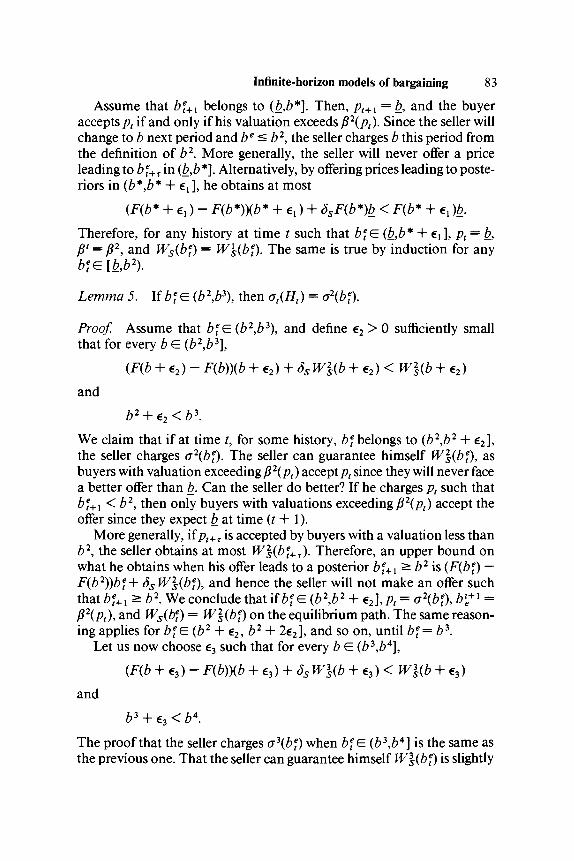
Infinite-horizon models of bargaining 83
Assume that bet+l belongs to (b,b*]. Then, pt+l = b, and the buyer
accepts pt if and only if his valuation exceeds f$2{pt). Since the seller willchange to b next period and be ^ b2, the seller charges b this period fromthe definition of b2. More generally, the seller will never offer a priceleading to Z?f+T in (b,b*]. Alternatively, by offering prices leading to poste-riors in (b*,b* + e{ ], he obtains at most
ex) - F(b*))(b* + €{) + SsF(b*)b <F(b* + ex)b.
Therefore, for any history at time t such that betE: (b,b* + er ], pt = b,
/?' = /?2, and Ws(bf) = Wls(bf). The same is true by induction for any
Lemma 5. If b*E (b2,b3), then ot{Ht) = o\b%
Proof. Assume that bet E (b2,b3), and define e2 > 0 sufficiently small
that for every b E (b2,b3],
(F(b + e2) - F(b))(b + e2) + SsW2(b + e2) < W\(b + e2)and
b2 + e2<b3.We claim that if at time t, for some history, be
t belongs to (b2,b2 + e2],the seller charges cF2(bf). The seller can guarantee himself Wl(bf), asbuyers with valuation exceedingP2(pt) acceptpt since they will never facea better offer than b. Can the seller do better? If he charges pt such thatbe
t+l<b2, then only buyers with valuations exceeding P2{pt) accept theoffer since they expect b at time (t+ 1).
More generally, if pt+T is accepted by buyers with a valuation less thanb2, the seller obtains at most W2
s(bet+X). Therefore, an upper bound on
what he obtains when his offer leads to a posterior bet+l ^ b2 is (F(£f) —
F{b2))bet + SsW2
s{bf), and hence the seller will not make an offer suchthat be
t+l > b2. We conclude that if Z>f e (b2,b2 + e2], pt = o\b% b?x =fi2(pt), and Ws(bf) = W2
s(bf) on the equilibrium path. The same reason-ing applies for be
t E (b2 + e2, b2 + 2e2], and so on, until bet = Z?3.
Let us now choose e3 such that for every b E (63,64],
€3) - F(b)){b + 63) + SsW3s(b + €3) < » W + €3)
and
The proof that the seller charges o\bf) when Z?f E (b3,b4] is the same asthe previous one. That the seller can guarantee himself W3
s{bf) is slightly

84 Fudenberg, Levine, and Tirolemore complicated to demonstrate. It suffices to show that when the sellerchargespt = o\bf), & buyer with valuation fi3(pt) accepts it. Imagine thatthis buyer refuses. Then, be
t+l>P\pt), which implies that pt+l ^o2{be
t+l) > o2{p\pt)). Hence, buyer P\pt) will not buy at time (t + 1),since fi\pt) ~Pt< SB{P\pt) — pt+l) would contradict the definition of/?3. Similarly, he would not buy later on, and hence he accepts pt now.
The rest of the proof is by induction on n. Lemma 3 guarantees that thisinduction takes at most (TV* + 1) steps. Finally, the equilibrium is(strong)-Markov since, by construction, pt depends only on the posterior
We would prefer not to invoke the restriction that b > 0 = s. Onemight expect that the buyer's valuation could sometimes be less than sand that such buyers would not enter the bargaining game, but any buyerwhose valuation exceeds s would enter, and thus effectively b = s. For thiscase, we can prove that an equilibrium exists by considering a sequence ofgames with b? —* s, showing that there is a limit point of the associatedequilibria, and further that this limit is an equilibrium. With b = s, theseller will never choose to offer price b, and so bargaining can continueindefinitely. This lack of an "endpoint" has prevented us from establish-ing uniqueness for this case.
Proposition 2. When b = 0, a weak-Markov equilibrium exists.
Proof. See Appendix 2.
Smooth-Markov equilibriaAnother approach to solving infinite-horizon bargaining games is to as-sume that a smooth, (strong)-Markov equilibrium exists, and to try tocompute it from the differential equation resulting from the first-orderconditions for the seller's maximization.
Let Ws(be) be the seller's valuation when his posterior is be, multipliedby F(be). Define
& - \ Ws( •)) = [F(b<) - F{(S(p))]p + Ss
Then, o{be) must be an arg max of/, and Ws(be) the maximized value. Asin our previous discussion, we see that a is strictly increasing if/? is strictlyincreasing. When p has "flat spots," the induced a will not be strictlyincreasing and a smooth-Markov equilibrium need not exist.
Differentiating /with respect to be and using the envelope theorem, we

Infinite-horizon models of bargaining 85
find that
Maximizing / with respect to p, we then find the first-order condition
m- P'(°(b))f\P{o{be))]{o{be) - dso[IS{o{be))]} = 0. (5.1)
In case the second-order condition is also satisfied, (5.1) and its asso-ciated/^/?) characterize a Markov equilibrium. One such instance occurswhen F(b) = (b/b)m for 0 <b<b and m > 0. In this case, F(/3)/F(b) hasthe same functional form as F, and we can find a smooth-Markov equilib-rium, with the linear form P(b) = pp and a(b) = ob. It can be verified thatthe second-order condition corresponding to (5.1) is satisfied, and theconstants a and /? may then be computed to be the unique solution of
(fa)~m + Ssm{po) = l + mPo)
] ^ ( 5 . 2 )1 — oB
from which it follows that /? > 1 and jia < 1. This is the solution obtainedas a limit of finite-horizon games by Sobel and Takahashi (1983), whichwas known to be an equilibrium from Fudenberg and Levine (1983). Wehave just provided a simpler derivation.
We now comment on a number of features of equilibrium in thismodel. First, in all cases o( •) is nondecreasing so that equilibrium in-volves gradual concessions. How general a result this is remains to be seen.Fudenberg and Tirole (1983) show that in a finite-horizon model withtwo-sided incomplete information, prices may rise over time. Whetherthis can occur in infinite-horizon models is as yet unknown but seemslikely.
It can be shown that when the buyer's and the seller's discount factorsconverge to 1, the seller's payoff converges to zero. In other words, theseller loses all ability to price discriminate when the time period goes tozero (since then both Ss and SB approach 1). This result was obtained bySobel and Takahashi and is similar to results of Kreps and Wilson (1982a)in the chain-store paradox and of Bulow (1982) and Stokey (1980) in workon durable-goods monopoly. Let us give a rough intuition. The incentiveto bargain is due to the destruction of the pie by discounting. By makingoffers, the seller makes the buyer responsible for destroying the pie if herejects the offer. The seller uses this leverage to extort the buyer's surplusand, when there is incomplete information, price discriminate. With

86 Fudenberg, Levine, and Tirole
short time periods, higher-valuation buyers are more willing to free rideon lower-valuation buyers. The seller consequently loses his ability toprice discriminate.
Finally, note that if Vs(be) = Ws{be)/F(be\lim lim Vs(b) = 0 < lim lim Vs(b) = b.m—*» Ss,SB-* I <5s»£j9—1 rn-+°°
Here, m-*™ means that the seller is nearly certain that the buyer hasvaluation b. Thus, in the infinite horizon, it makes a difference what orderwe pass to the limit.
5.4 Alternating offers
Thus far, we have assumed that the seller makes all of the offers, that is,that the buyer is not allowed to make counter offers but can only accept orreject offers of the seller. This assumption is far from innocuous, espe-cially coupled with our assumption that only the buyer's valuation isprivate information, which as we suggested seems a good approximationif the seller owns the object before the bargaining starts, and values theobject only for its eventual sale. If the seller makes all of the offers and theseller's valuation is known, the offers reveal no information. If the buyer isallowed to make counteroffers, in equilibrium the seller must update hisposterior to reflect the information thereby transferred. In particular, wemust specify how the seller revises his beliefs if the buyer makes an offerthat according to the equilibrium strategies is not made by any type ofbuyer. Bayes' rule places no restrictions on such inferences, nor doesKreps and Wilson's (19826) more restrictive concept of a sequential equi-librium. This leeway can be used to support a multiplicity of equilibria. Ifonly the seller can make offers, the only zero-probability event that doesnot terminate the game immediately is if the buyer refuses a price below b;however, as lemma 2 illustrated, the seller would never charge such a pricein any equilibrium, and thus what the seller infers from this event isirrelevant. In contrast, when the buyer can make counteroffers, the seller'sinferences can change the set of actions that occur in equilibria.
Let us illustrate this point with an example, which has the additionalvirtue of providing a form of justification for our seller-makes-the-offersspecification. Specifically, we will describe an equilibrium in which, al-though the buyer does make counteroffers, these counteroffers are alwaysrejected by the seller, so that the equilibrium is "observationally equiva-lent" to one in which the seller makes all of the offers but the time period istwice as long.
Before we present this equilibrium, recall that Rubinstein (1982)proved that for the corresponding complete-information game, there

Infinite-horizon models of bargaining 87exists a unique equilibrium. The seller always offers b(\ — SB)/(\ —dsdB), the buyer offers Ss[b(l — dB)/(l — SSSB)]9 and these offers areaccepted.
Our example is a "pooling equilibrium," in that all types of the buyermake the same offers, so that the buyer's offer conveys no information.All types of the buyer always offer price zero, which the seller alwaysrefuses. Were the buyer to offer aprice other than zero, the seller wouldbelieve that the buyer has type Kb, where K is some large number (suchbeliefs are not consistent with the spirit of sequential equilibrium, becausethey put weight on types outside the initial support of the buyer's valua-tion. Such beliefs can be understood as resulting from trembles by natureas opposed to the trembles by players which are considered in sequentialequilibrium.) The seller's offers are made as with one-sided offers, dis-cussed in Section 5.3, except that the discount factors are S2
S and SB. Theperiods in which the buyer makes offers do not count, and play evolves asthough the seller made all of the offers and the period length is equal totwice that of the alternating-offers game.
For this to be an equilibrium, it is necessary and sufficient that no typeof buyer wish to charge a price other than zero. However, any unexpectedprice causes the seller to believe that the buyer's valuation is Kb, and thusthe seller refuses p unless p ^ [Kb{\ — 5B)/{\ — SSSB)]. Clearly, for Ksufficiently large, this will require p ^ b, which no buyer would offer.
There certainly are many other equilibria. Grossman-Perry (1985)have shown how to embed the one-sided offer equilibrium into the two-sided offer structure using beliefs which assign weight only to types in theinterval support of the buyer's calculation.
5.5 Specification of the costs of bargainingThe models that we have discussed so far have modeled the costs ofprolonged negotiations as the discounting of future outcomes. This sec-tion contrasts that form of the costs with two others; fixed per-periodbargaining costs and costs of changing offers.
The assumption of fixed per-period costs is that agreement at price p inperiod / yields utilities {b — p — cBt) and (p — s — cst), respectively. Fixedper-period costs were included in Rubinstein's (1982) complete-informa-tion bargaining model; in equilibrium, the player with lower cost capturedthe entire surplus. However, as pointed out in Fishburn and Rubinstein(1982), per-period costs are inconsistent with the existence of a "zeroagreement," for which the trader has no impatience. Fishburn and Ru-binstein show that any preferences at bargaining outcomes that aremonotonic, impatient, continuous, and stationary can be represented bydiscounting if such a zero agreement is possible. Thus, the existence of a

88 Fudenberg, Levine, and Tirole
zero agreement is of primary importance in choosing a functional formfor time preference.
In the absence of a zero agreement, there are outcomes that are inferiorto "leaving the game," even when there are known to be gains from trade.Thus, to avoid violating (ex ante) individual rationality, an "exit option"must be included in the specification of the extensive form. With dis-counting, the exit option is superfluous in a model with only two traders:The value of the outside opportunity is normalized to be zero (and,therefore, even a greatly postponed agreement is preferred to none at all).Rubinstein's (1982) paper did not allow an exit option, so that the lower-cost trader could inflict "infinite damage" on his opponent "relatively"cheaply. This may partially explain his troublesome conclusions in thefixed-cost case. Perry's (1982a) model of bargaining with many sellerssimilarly assumes that the buyer cannot leave the game; and thus itsconclusions may be similarly misleading.
The obvious alternative to requiring the players to potentially sufferarbitrarily large bargaining costs is to allow for the possibility of exit,which ensures the (current) reservation value. Although such an optioncan sensibly be added to bargaining models with complete information,with incomplete information the possibility of exit combined with fixedcosts of continuing yields a trivial equilibrium, as was pointed out inFudenberg and Tirole (1983). The equilibrium is trivial because, when anagent chooses not to exit, he signals that his expected value to continuing,and in particular his valuation, exceeds the sum of the per-period cost andhis surplus in the eventual agreement. Consider, for example, the modelof Fudenberg and Tirole (1983), with the addition that the buyer decidesat the end of the first period whether or not to exit. Let b(cB) denote thetype of buyer that is just indifferent between exiting and paying cost cB tocontinue. Clearly, the seller will never offer a price below b(cB) in thesecond period, and so there is no equilibrium in which buyers choose tocontinue. Perry (19826) analyzes an infinite-horizon, alternating-offersmodel, and obtains the same result. The only equilibrium in any subgamethat begins with the buyer making an exit decision is the trivial one that allbuyers leave immediately. Thus, if the seller makes the first move, theequilibrium is simply that of the one-period game, because everyoneknows that all valuations of buyer will leave at the end of the first period. Ifthe buyer pays a fee in order to play, the seller will charge a high enoughprice that the buyer who had been indifferent about staying in will regrethaving done so. Thus, in the presence of incomplete information, thespecification of fixed bargaining costs results in a trivial outcome in whichno bargaining in fact occurs. This is highly reminiscent of Diamond's(1971) observation about the effect of fixed search costs, which allowedfirms to charge the monopoly price and thus precluded search.

Infinite-horizon models of bargaining 89
Fixed bargaining costs are formally similar to entry fees to participate;yet entry fees have been shown to be optimal in the theory of optimalauctions (Maskin and Riley (1980)). The difference is that in auctiontheory, unlike bargaining, the seller is allowed to precommit to futureactions, and thus to "promise" a nonnegative expected return to thosewho choose to pay the fee. Note that one way out of the dilemma inbargaining may be to modify the extensive form to allow such payments,so that the seller can pay the continuation fee.
The second alternative specification of bargaining costs that we wish todiscuss is one in which it is costly to change offers. Such costs wereintroduced to the bargaining literature by Crawford (1981), who assumedthat having made initial demands, bargainers could "back down" at acost. More recently, Anderson (1983) studied repeated games with costsof adjustment. Although costs of adjustment may seem artificial and adhoc in the context of bargaining between individuals, they are perhapsmore plausible if the bargainers are agents for others, as in union-management negotiations.
These are the main alternatives to the discounting formulation that wehave employed. Still other formulations may emerge with the continueddevelopment of the empirical literature on sequential bargaining.
5.6 Why should we study sequential processes?The thorny question of the extensive form
Here, we offer a few thoughts on the nature of the extensive form. Itshould be clear that these thoughts are incomplete. Their only purpose isto raise some questions we deem important for bargaining theory.
Myerson and Satterthwaite (1983) have studied the optimal negotia-tion mechanisms between a buyer and a seller. This work has been ex-tended to situations with multiple buyers and sellers (double auctions) byWilson (1982). According to the revelation principle, the optimal negotia-tion is a revelation game in which the buyer(s) and the seller(s) announcetheir characteristics simultaneously. Therefore, it seems that one could aswell restrict attention to static revelation games and never be interested insequential bargaining. A number of considerations actually go against thisfirst intuition.
For one thing, real-world bargaining is almost always sequential.Myerson - Satterthwaite-type revelation games are not played. Thus, itseems that there is scope for sequential bargaining theory. Students ofbargaining theory cannot content themselves with this proof-of-the-pudding argument. One must ask why such revelation games arenot played, and when the Myerson-Satterthwaite model is internallyconsistent.

90 Fudenberg, Levine, and Tirole
Imagine that two parties meet and want to discuss freely the possibilityof a trade that might be advantageous. Their using the Myerson-Satterthwaite mechanism requires two fundamental assumptions: (1) thetraders agree to bargain this way, and (2) the traders can commit them-selves to not ever reopen the bargaining process in case of disagreement. Itis immediately evident that these two conditions are likely not to besatisfied in real-world conditions, for the following reasons.
1. Most of the time, the traders have at least some of their private informa-tion before meeting. Depending on his information, a trader may wantto use a bargaining mechanism that differs from the revelation game.One could object to this reasoning by noticing that, because the revela-tion game is the most efficient game, there could be transfers inducingthe traders to play that game. However, this neglects the fact that choos-ing a bargaining mechanism itself conveys information and changes theoutcome of the subsequent bargaining game. In particular, accepting therevelation game is not neutral: It says something about the trader. Weare aware that we are raising a deep question without bringing anyelement of answer.
2. It is well known that any bargaining mechanism under asymmetricinformation and individual rationality constraints implies inefficiency.Traders may quit without realizing gains from trade. This is especiallycharacteristic of the Myerson-Satterthwaite mechanism. Thus, there isan incentive to renegotiate later. This point is addressed in greater detailin Cramton (1983ft).
What, then, is left of the Myerson-Satterthwaite analysis? We thinkthat this mechanism is of interest for two reasons:
1. From a normative point of view, it gives a lower bound on the ineffi-ciency associated with voluntary bargaining.
2. From a positive point of view, it may be applied to some special cases.Imagine, for example, that the parties meet when they have symmetricinformation. They know that later on they will acquire private informa-tion (value of a project, its cost), and that they will have to make adecision (production) on this basis. In this case, they decide to bargainaccording to the Myerson-Satterthwaite mechanism if they have ameans of enforcing the absence of renegotiation in case of disagreement.One could think of reputation as an incentive not to renegotiate.
5.7 Specification of the information structure
The literature on sequential bargaining has up to now assumed that therandom variables on which there is asymmetric information are uncorre-lated. This may be a reasonable assumption in a number of cases. Forexample, the seller's production cost and the buyer's valuation for the

Infinite-horizon models of bargaining 91
object can be assumed to be independant. Similarly, costs of bargainingare likely to be uncorrelated between them and with the previous vari-ables. However, there are two channels through which a trader can learnabout his own valuation.
1. Correlated values. Imagine, for example, that the seller owns a used car,and knows its quality. His willingness to sell the car depends on thisquality. In addition, the buyer's willingness to buy the car would dependon this parameter if he knew it. In this case, the valuations are correlatedand the buyer is eager to learn about the seller's information not only todiscover his bargaining power but also to assess the value of a deal.
2. Learning from an unknown distribution. Imagine that there are severalsellers, whose production costs are drawn from a probability distributionthat is unknown to the buyer. Imagine further that the buyer can switchsellers. When the buyer bargains with a given seller, he learns not onlythe specific characteristics of this seller (and therefore about his bargain-ing power), but also about the other sellers' characteristics. Therefore,the buyer learns about his expected profit if he switches to another seller.Even though the buyer and the seller's characteristics may be uncorre-lated, the buyer learns about more than his bargaining power. Anotherpossibility leading to the same effect is the correlation of productioncosts between sellers. Indeed, the case of independent draws from adistribution that is unknown to the buyer is processed like that of corre-lated draws by the buyer.
An interesting example that combines items (1) and (2) can be found inthe work of Ordover and Rubinstein (1983) on litigation. In their paper,one of the bargaining parties knows who will win if the dispute is resolvedin court, that is, if disagreement occurs. On the one hand, the parties areinterested in their valuations after disagreement, and they can learn some-thing about them before disagreement as outlined in item (2). On theother hand, the valuations after disagreement are correlated.
Whereas in the independent-draws model, the only purpose of learningis to discover one's bargaining power, when draws are correlated betweentraders the parties learn about their positions after bargaining with thecurrent partner whether there is agreement or disagreement. Conse-quently, during the bargaining process the parties must take into accounttwo kinds of "curses":
1. The celebrated winner's curse in case of agreement. For example, the factthat the seller of the used car accepts the buyer's offer may be a bad signalabout the quality of the car.
2. The "bargaining curse. "The seller's making a low offer may not be goodnews to the buyer if the seller knows the quality of the car. In the un-known-distribution framework, the seller's making a high offer maysignal that the production costs of the other potential sellers are likely to

92 Fudenberg, Levine, and Tirole
be high as well. On the other hand, such learning may not be a curse, butgood news. For instance, in the used car example the seller's turningdown the buyer's offer may signal a high quality. Such transmission ofinformation can easily be embodied in bargaining models. Although wewill not pursue this topic here, it is clear that some new insight can begained from it.
5.8 Conclusion
As we stated in Section 5.3, the outcome of bargaining with one-sidedinformation is fairly easy to characterize if the player whose valuation isknown makes all of the offers. In this case, the price must decrease overtime, and things are generally "well behaved." With alternating offers,however, there are multiple equilibria, which are qualitatively very dis-similar. Thus, the problem of the choice of extensive form is fairly severe,even when only one-sided incomplete information is being considered. Ifboth player's valuations are private information, the situation is evenmore complex. We fear that in this case, few generalizations will bepossible, and that even for convenient specifications of the functionalform of the distributions over the valuations, the problem of characteriz-ing the equilibria will be quite difficult. Cramton (\9S3a) is a start in thisdirection.
Throughout this paper, because the bargaining costs took the form ofdiscounting and players had no other opportunities to trade, players hadno incentive to stop bargaining. If traders have alternative bargainingpartners, we would expect them to switch to a new partner whenever theybecome sufficiently pessimistic about the valuation of the party withwhom they are currently negotiating. Thus, the length of bargaining be-tween any pair of traders could be endogeneously determined by theoutside opportunities. Shaked and Sutton (1984) have modeled bargain-ing with several sellers under complete information. Because the sellersare known to have the same valuation in equilibrium, traders never quitbargaining without an agreement if there exist gains from trade. Thus, theShaked-Sutton model again predicts that traders will never stop nego-tiating. In a forthcoming paper, we analyze bargaining with many tradersand incomplete information to study the effect of outside opportunitieson equilibrium prices and on the length of negotiations.
The noncooperative approach to bargaining theory is still in its in-fancy. Although much remains to be done, substantial progress has beenmade in the past few years. Solving a wider variety of extensive forms maypermit some generalizations to emerge. The problem of the choice ofextensive forms by the players remains open.

Infinite-horizon models of bargaining 93
APPENDIX 1Proof of Proposition 1
We proceed by induction on n. For each n, we construct pn, the highestprice the seller is allowed to charge. The index n will keep track of thenumber of periods remaining: When /?</?", the game will be shown toend in at most n periods. For n = 1, set
p> = b, W&b*) = F(b*)b, E ^
a\be) = o\be\p) = b, and bl = b,Here, p1 = b is the price the seller is required to charge to guarantee thatthe game ends immediately, and W\{be) is the seller's payofFto charging Z?multiplied by the probability that the posterior is below be. In other words,we work with "unconditional probabilities" instead of conditional ones;the conditional probability of a sale at b is 1, but the unconditionalprobabilities prove simpler to work with. Note that this renormalizationdoes not affect the seller's optimal behavior. Quantity /?2(/?) is the reserva-tion value of the buyer who is just indifferent between p in this period andb in the next one. Because the seller's offers will be nonincreasing and noless than b, if the seller charges b in this period, buyers must expect b insubsequent periods. The term fjn+l (p) will be the lowest reservation valueof a buyer who accepts/? when there will be n subsequent periods, that is, inthe (n + l)-period game. Observe that Wl
s and /?* are continuous andnondecreasing. If/? < p\ the game is over; if/? > p1, it (with some proba-bility) lasts at least one more period. Value a\be) is the correspondencethat yields the seller's optimal choices in the ^-period game when he isconstrained to charge no more than/?" (when n = 1, this constraint forcesa1 to be single valued). Quantity al(be\p) is the expected value of theseller's price if the last price was /?. And bl is a dummy, which will not beused; for larger n, bn will be a bound on be that guarantees that the sellercharges no more than z?""1 in the next period.
In the ^-period game, the seller is constrained to not charge more than/?", where pn is chosen such that if/?" is charged, the buyer's reservationvalue is at most bn\ so the next period's price is below pn~l and, byinductive hypothesis, the game ends in (n — 1) additional periods.
We will now define Wns(be\ Pn+\p\ pn, o\be\ and on{b\p) recur-
sively, and prove by induction that
1. Wns and Pn+l are continuous and nondecreasing, and that jln is the
unique solution of/? G (1 - dB)pn(p) + dBan{P\p)\ where an is theconvexification of an\
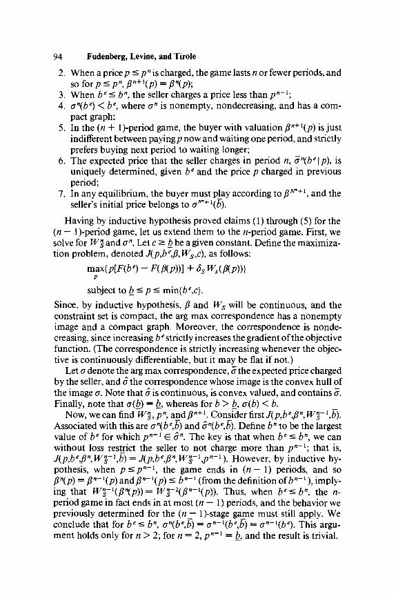
94 Fudenberg, Levine, and Tirole2. When a pricep ^pnis charged, the game lasts n or fewer periods, and
so for p < pn, pn+ \p) = p\p)\3. When be ^ bn, the seller charges a price less than pn~l;4. a\be) < b\ where an is nonempty, nondecreasing, and has a com-
pact graph;5. In the (n + l)-period game, the buyer with valuation Pn+l(p) is just
indifferent between paying/? now and waiting one period, and strictlyprefers buying next period to waiting longer;
6. The expected price that the seller charges in period n, an(be\p), isuniquely determined, given be and the price p charged in previousperiod;
7. In any equilibrium, the buyer must p]ay according to PN*+\ and theseller's initial price belongs to crNm+l(b).
Having by inductive hypothesis proved claims (1) through (5) for the(n — l)-period game, let us extend them to the ^-period game. First, wesolve for Wn
s and an. Let c ^ b be a given constant. Define the maximiza-tion problem, denoted J(p,be,fi,Ws,c), as follows:
- F(p(p))] + Ss Ws{p{p))}
subject to b ^ p ^ min{be,c).Since, by inductive hypothesis, fi and Ws will be continuous, and theconstraint set is compact, the arg max correspondence has a nonemptyimage and a compact graph. Moreover, the correspondence is nonde-creasing, since increasing Z? strictly increases the gradient of the objectivefunction. (The correspondence is strictly increasing whenever the objec-tive is continuously differentiable, but it may be flat if not.)
Let a denote the arg max correspondence, o the expected price chargedby the seller, and a the correspondence whose image is the convex hull ofthe image a. Note that a is continuous, is convex valued, and contains o.Finally, note that a(b) = b, whereas for b > b, o{b) <b.
Now, we can find Wns, pn, and jS^1. Consider first J(p,be,/]n, Wn
s~\b).Associated with this are an(be,b) and an(be,b). Define bn to be the largestvalue of be for which pn~l E an. The key is that when be ^ bn, we canwithout loss restrict the seller to not charge more than pn~l\ that is,J(p,be,fln,Wn
s-\b) = J(p,be,j3n,Wns-\pn~l). However, by inductive hy-
pothesis, when p<pn~l, the game ends in (n— 1) periods, and soP%p) = Pn~\p) and/?""1^) ^ bn~l (from the definition of bn~l), imply-ing that Wn
s-\p\p))= Wns-2(Pn-\p)). Thus, when be<b\ the n-
period game in fact ends in at most (n — 1) periods, and the behavior wepreviously determined for the (n— l)-stage gajme must still apply. Weconclude that for be < bn, an(be,b) = on~\be,b) = an~\be\ This argu-ment holds only for n > 2; for n = 2, pn~l = b, and the result is trivial.

Infinite-horizon models of bargaining 95
Next, we must define pn, the bound on the seller's price that ensuresthat next period's price is less than pn~l and therefore that the game endsin n periods. This situation is complicated slightly by the possible disconti-nuity of a. Let pn~l be the largest value in on~~\bn) less than or equal topn~ Sand define/?" = (1 — 8B)bn + J^/?""1. We claim that if/? </?"inthe^-period game, then the next-period price will be less than pn~l and thegame in fact ends in n periods. Assume not - then the seller's posteriornext period, /?"(/?), must exceed bn. From the definition of/?n, this impliesthat (1 - SB)/3n(p)>pn - SBpn-\ Since /?"(/?)</?< /?", an~\pn{p)) <an~\pn) < an~\bn) <pn~\ Yet, by inductive hypothesis, 0" satisfiesp G (1 - dB)p\p) + SBo»-\nP)\ and so (1 - SB)p\p) *P~ SBpn~\which is a contradiction. This means that imposing the constraint/? ^ pn
guarantees that the ^-period game in fact ends in n periods. Later, we willshow that if/? ^ pn, the (n + l)-stage game ends in n periods as well.
Given /?", we consider the optimization problem J(p,be,fin, Wns~l,pn).
The solution to this problem is <Jn(be), with convex null an{be). As shownabove, we know that for be < bn,Wn
s(be) = Wns~\be\ and on{be,b) =
an{be) = on~l{be)\ therefore, behavior below bn is not changed by in-creasing the number of periods.
Next, we work backward one period to show that fi"+l(p) is uniquelydefined by the assumed equation. The valuation of the buyer who is justindifferent between paying p in period (n + 1) and waiting must satisfy
U$n+\P)-P) E SB[fi»+\p) - o\p»or
p G (1 - SB)P«+\p) + SBoXP»+\p)). (A.I)
The right-hand side of (A. 1) is a continuous, convex-valued, strictly in-creasing correspondence, and thus has a unique inverse function fin+ *(/?),which is nondecreasing and has modulus of continuity smaller than
Note that since max{<7n(/?"+*(/?))} <Pn+\p\ the choice of buyerPn+l(p) whether to accept /? in period (n + 1) or to wait one period andthen buy is unaffected if we replace the anticipated next-period probabil-ity distribution over elements of on{Pn+l{p)) by its expected value an.Because an must lie in an, equation (A. 1) defining fin+l ensures that thebuyer of valuation Pn+l(p) is indifferent between paying /? in period(n + 1) and waiting to face on next period. If buyer Pn+ *(/?) were willing towait more than one period, then all buyers with lower valuations wouldstrictly prefer to wait, and there would be no sales in period n. This wouldcontradict the behavior that we derived for the ^-period game.
Thus, we have verified the inductive hypotheses for k = n. Because weknow that all equilibria end in at most (N* + 1) periods, we know that

96 Fudenberg, Levine, and Tiroleafter (N* + 1) steps, we will have bN*+1 = b, and the induction incom-plete. Thus, the first price charged must (1) be an element of aN*+ l(b) and,moreover, (2) be less than or equal to pN*+\ and that thereafter equilib-rium play is uniquely determined. Thus, if an equilibrium exists, it isunique up to the seller'^ choice of an initial price (or any probabilitydistribution over crN*+l(b)). The argument given before the statement ofproposition 1 shows that an equilibrium does in fact exist, because giventhe functions /?"(/?), the seller will choose to end the game in no more than(N*+ 1) periods.
APPENDIX 2Proof of Proposition 2
To proceed, we need the following lemma.
Lemma 6. The functions /?(/?) and W{be) derived in the proof of propo-sition 1 are equicontinuous.
Proof. We observed earlier that the modulus of continuity offi(p) is nogreater than 1/(1 - SB). Recall the definition of W(be):
W{be) = max{[F(6') - F(fi(p))]p + SW(fi(p))}.P
Now, consider W{b\) - W(b\\ where b\> b\. Let p{ and p2 be therespective maximizing prices. We claim that
W(b\) - W{bi) * (F(b\) - F{be2))px,
because the seller could always choose to offer price px when his beliefswere b f, and so we have used a lower bound on W(b f). However, since thedensity,/(Z?), is bounded b y / we have
W(b\)- W(be2)<bf\b\-be
2\.
Proof of proposition 2. Consider the sequence of games with buyer valu-ation densities
f"(b)=\\-F{b»)0 ifb<bn,
where 6"—»0as«—»°°. Each of these games has a unique weak-Markovequilibrium (/?", W",a"). Since the family of functions (P",W") is equi-
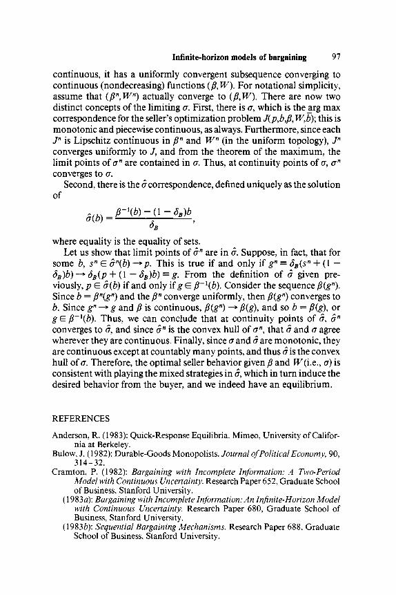
Infinite-horizon models of bargaining 97
continuous, it has a uniformly convergent subsequence converging tocontinuous (nondecreasing) functions {P,W). For notational simplicity,assume that {fin,Wn) actually converge to {P,W). There are now twodistinct concepts of the limiting a. First, there is <7, which is the arg maxcorrespondence for the seller's optimization problem J(p,b,fi, W,b)\ this ismonotonic and piecewise continuous, as always. Furthermore, since eachJn is Lipschitz continuous in fin and Wn (in the uniform topology), Jn
converges uniformly to /, and from the theorem of the maximum, thelimit points of an are contained in cr. Thus, at continuity points of a, a"converges to a.
Second, there is the a correspondence, defined uniquely as the solutionof
where equality is the equality of sets.Let us show that limit points of an are in a. Suppose, in fact, that for
some b, sn E an{b) —* p. This is true if and only if gn = SB(sn + (1 —$B)b)-* SB(p + (I —S B)b) = g. From the definition of a given pre-viously, p E a{b) if and only if g E fi~l(b). Consider the sequence f5{gn).Since b = fin{gn) and the /Jn converge uniformly, then fi{gn) converges tob. Since gn~* g and fi is continuous, fi(gn) —> fi(g), and so b = /?(#), org E P~l{b). Thus, we can conclude that at continuity points of a, an
converges to <r, and since an is the convex hull of cr", that a and a agreewherever they are continuous. Finally, since a and a are monotonic, theyare continuous except at countably many points, and thus a is the convexhull of c. Therefore, the optimal seller behavior given fi and W(i.e., a) isconsistent with playing the mixed strategies in a, which in turn induce thedesired behavior from the buyer, and we indeed have an equilibrium.
REFERENCES
Anderson, R. (1983): Quick-Response Equilibria. Mimeo, University of Califor-nia at Berkeley.
Bulow, J. (1982): Durable-Goods Monopolists. Journal of Political Economy, 90,314-32.
Cramton, P. (1982): Bargaining with Incomplete Information: A Two-PeriodModel with Continuous Uncertainty. Research Paper 652, Graduate Schoolof Business, Stanford University.
(1983a): Bargaining with Incomplete Information: An Infinite-Horizon Modelwith Continuous Uncertainty. Research Paper 680, Graduate School ofBusiness, Stanford University.
(1983&): Sequential Bargaining Mechanisms. Research Paper 688, GraduateSchool of Business, Stanford University.

98 Fudenberg, Levine, and Tirole
Crawford, V. (1981): A Theory of Disagreement in Bargaining. Econometrica, 50,607-38.
Diamond, P. (1971): A Model of Price Adjustment. Journal of Economic Theory,3, 156-68.
Fishburn, P., and A. Rubinstein (1982): Time Preference. International Eco-nomic Review, 23, 677-94.
Fudenberg, D., and D. Levine (1983): Subgame-Perfect Equilibria of Finite- andInfinite-Horizon Games. Journal of Economic Theory, 31, 251 -68.
Fudenberg, D., and J. Tirole (1983): Sequential Bargaining under IncompleteInformation. Review of Economic Studies, 50, 221-47.
Grossman, S., and M. Perry (1985): "Sequential Bargaining under AsymmetricInformation." Mimeo.
Kreps, D., and R. Wilson (1982(2): Reputation and Imperfect Information. Jour-nal of Economic Theory, 27, 253-79.
(19826): Sequential Equilibria. Econometrica, 50, 863-94.Maskin, E., and J. Riley (1980): Auctioning an Indivisible Object. Discussion
Paper #87D. Kennedy School of Government.Myerson, R., and M. Satterthwaite (1983): Efficient Mechanisms for Bilateral
Trading. Journal of Economic Theory, 29, 265-81.Ordover, J., and A. Rubinstein (1983): On Bargaining, Settling, and Litigating: A
Problem in Multistage Games with Imperfect Information. Mimeo, NewYork University.
Perry, M. (1982a): A Theory of Search. Mimeo, Princeton University.(19826): Who Has the Last Word: A Bargaining Model with Incomplete Infor-
mation. Mimeo, Princeton University.Rubinstein, A. (1982): Perfect Equilibrium in a Bargaining Model. Econometrica,
50,97-109.(1985): Choice of Conjectures in a Bargaining Game with Incomplete Informa-
tion. Chapter 6 in this book.Shaked, A., and J. Sutton (1984): Involuntary Unemployment as Perfect Equilib-
rium in a Bargaining Model. Econometrica, 52, 1351 -1364.Sobel, J., and I. Takahashi (1983): A Multi-Stage Model of Bargaining. Review of
Economic Studies, 50, 411 -26.Stokey, N. (1980): Rational Expectations and Durable Goods Pricing. Bell Jour-
nal of Economics, Spring, 11, 112-28.Wilson, R. (1982): Double Auctions. Technical Report 391, Institute for Mathe-
matical Studies in the Social Sciences, Stanford University.

CHAPTER 6
Choice of conjectures in a bargaining gamewith incomplete information
Ariel RubinsteinTHE HEBREW UNIVERSITY, JERUSALEM
6.1 Introduction
The axiomatic approach to bargaining may be viewed as an attempt topredict the outcome of a bargaining situation solely on the basis of the setof pairs of utilities that corresponds to the set of possible agreements andto the nonagreement point.
The strategic approach extends the description of a bargaining situa-tion. The rules of bargaining are assumed to be exogenous, and the solu-tion is a function not only of the possible agreements but also of theprocedural rules and the parties' time preferences.
The aim of this chapter is to show that in the case of incompleteinformation about the time preferences of the parties, the bargainingsolution depends on additional elements, namely, the players' methods ofmaking inferences when they reach a node in the extensive form of thegame that is off the equilibrium path.
The solution concept commonly used in the literature on sequentialbargaining models with incomplete information is one of sequential equi-librium (see Kreps and Wilson (1982)). Essentially, this concept requiresthat the players' strategies remain best responses at every node of decisionin the extensive form of the game, including nodes that are not expected tobe reached. The test of whether a player's strategy is a best responsedepends on his updated estimation of the likelihood of the uncertainelements in the model. For nodes of the game tree that are reachable, it isplausible to assume that the players use the Bayesian formula. Off theequilibrium path, the Bayesian formula is not applicable. The formula-tion of a game with incomplete information does not provide the descrip-tion of how the players modify their beliefs when a "zero-probability"
I would like to thank Al Roth and Asher Wolinsky for valuable comments, andMargret Eisenstaedt, who drew the diagrams.
99

100 Ariel Rubinstein
event has occurred. (A zero-probability event occurs when the playersreach a node in the extensive form of the game that is off the equilibriumpath.) The concept of sequential equilibrium requires that the solutionspecifies the players' new beliefs after a zero-probability event occurs. Thenew beliefs that a player adopts after a zero-probability event is called aconjecture. The sequential-equilibrium concept also requires that a con-jecture be the basis for continuing the updating of the player's beliefsunless another zero-probability event occurs, in which case the playermust choose another conjecture.
Although we have great freedom to select conjectures to support strate-gies to be best responses, ideally the sequential-equilibrium conceptshould enable selection of a unique outcome out of the set of sequential-equilibrium outcomes. Indeed, several sequential bargaining modelsreach uniqueness of the sequential equilibrium (see Sobel and Takahashi(1983), Ordover and Rubinstein (1983), and Perry (1985)). The unique-ness of sequential-equilibrium outcomes in sequential bargaining modelsis not robust to changes in the procedural bargaining rules or the informa-tional structure. Even in simple models such as Fudenberg and Tirole's(1983) two-period seller-buyer bargaining game, where only the sellermakes offers, the incomplete information about the seller's reservationprice makes a multiplicity of equilibria possible.
In the current paper, I argue that the multiplicity of equilibria is not adrawback either of the model or of the solution concept, but rather anoutcome of the arbitrariness of the choice of conjectures. Specification ofrules that the players use to choose conjectures enables us to restrict the setof outcomes of the sequential equilibria. A comparison between the set ofsequential-equilibrium outcomes under various assumptions about theproperties of the choice of conjectures, clarifies the connection betweenthe choice of conjectures and the outcome of the game.
To present a more concrete discussion of the conjectures problem, Ianalyze a special case of the model for bargaining over a partition of adollar that I presented earlier (Rubinstein (1982)). In the present versionof the model, each bargainer bears a constant cost per period of negotia-tion. One of the players has incomplete information about the bargainingcost of his opponent, which may be higher or lower than his own. Theinferences that the player with the incomplete information makes abouthis opponent's bargaining cost lie at the center of the following discussion.
6.2 The model
The basic model used here is a subcase of the model analyzed in Rubin-stein (1982). Two players, 1 and 2, are bargaining on the partition of one

Choice of conjectures in a bargaining game 101
dollar. Each player in turn makes an offer; his opponent may agree to theoffer (Y) or reject it (N). Acceptance of an offer terminates the game.Rejection ends a period, and the rejecting player makes a counteroffer,and so on without any given time limit.
Let S = [0,1 ]. A partition of the dollar is identified with a number s in Sby interpreting s as the proportion of the dollar that player 1 receives.
A strategy specifies the offer that a player makes whenever it is his turnto do so, and his reaction to any offer made by his opponent. Let F be theset of all strategies available to a player who starts the bargaining. For-mally, Fis the set of all sequences of functions/= {/0£«i> where
For feven, / ' :S ' -> (7,7V),
where S* is the set of all sequences of length t of elements of S. (In whatfollows, G is the set of all strategies for a player whose first move is aresponse to the other player's offer.)
A typical outcome of the game is a pair (s,t), which is interpreted asagreement on partition s in period /. Perpetual disagreement is denoted by(0,oo).
The outcome function of the game P(f,g) takes the value (s9t) if twoplayers who adopt strategies/and g reach an agreement s at period t, andthe value (0,°°) if they do not reach an agreement. The players are assumedto bear a fixed cost per period. Player 1 's utility of the outcome (s,t) iss — cxt, and player 2's utility of the outcome (s,t) is 1 — s — c2t. Thenumber ct is player f s bargaining cost per period. The outcome (0,00) isassumed to be the worst outcome (utility — °°). It is assumed that theplayers maximize their expected utility.
Assume one-sided incomplete information. Player 1 's cost, cx = c, iscommon knowledge. Player 2's cost might be either cw or cs, where cw >c > cs > 0. Assume that co0 is player l's subjective probability that player2's cost is cw, and that 1 — co0 is his probability that player 2's cost is cs. Ifplayer 2's cost is cW9 it is said that he is of type 2W9 or the "weaker" type;if player 2's cost is cs, it is said that he is of type 2S9 or the "stronger" type.Consider these numbers to be small; specifically, assume that1 > cw + c + cs.
It was shown in Rubinstein (1982) that if it is common knowledge thatplayer 2 is of type 2W9 then the only perfect equilibrium is for player 1 todemand and receive the entire one dollar in the first period. If player 1knows he is playing against 2S9 the only perfect equilibrium is for him todemand and receive cs in the first period.
The game just described is one with incomplete information. Let
102 Ariel Rubinstein(f,g,h) G F X G X G b e a triple of strategies for player 1, player 2W9 andplayer 25, respectively. The outcome of the play of (f,g,h) is
that is, a pair of outcomes for the cases of player 2 actually being type 2W or2,.
The set of Nash equilibria in this model is very large. In particular, forevery partition s, the pair ((5,1),(5,1)) is an outcome of a Nash equilib-rium (see Rubinstein (1985)).
We turn now to the definition of sequential equilibrium. Define abelief system to be a sequence co = (0*0,-0,2,4,... > su°h that co° = co0 and col:St —• [0,1]. The term co%s\ . . . , s') is player l's subjective probabilitythat player 2 is 2W after the sequence of offers and rejections s\ . . . ,s'~\ after player 2 has made the offer s* and just before player 1 has toreact to the offer s*.
A sequential equilibrium is a four-tuple {f,g,h,co) satisfying the re-quirement that after any history, a player's residual strategy is a bestresponse against his opponent's residual strategy. The belief system isrequired to satisfy several conditions: It has to be consistent with theBayesian formula; a deviation by player 1 does not change his own belief;after an unexpected move by player 2, player 1 chooses a new conjectureregarding player 2's type, which he holds and updates at least until player2 makes another unexpected move.
So far, the choice of new conjectures is arbitrary. In Section 6.4, severalpossible restrictions on the choice of new conjectures are presented. Thestudy of these restrictions is the central issue of the present paper.
6.3 Review of the complete-information model
In this section, the characterization of the perfect-equilibrium outcomesin the complete-information model (where the bargaining costs are com-mon knowledge) is reviewed.
Proposition 1 (Conclusion 1 in Rubinstein (1982)). Assume that cx and c2are common knowledge. If cx < c2, the outcome (1,1) (i.e., player 1 getsthe whole dollar in the first period) is the only perfect-equilibrium out-come, and if cx > c2, the outcome (c2,l) (i.e., player 2 gets 1 — c2 in thefirst period) is the only perfect-equilibrium outcome.
Remark. The asymmetry is due to the procedure of the bargaining. If thesize of the costs is "small," the dependence of the bargaining outcome onthe bargaining order is negligible.

Choice of conjectures in a bargaining game 103
Figure 6.1
Proof.
ASSERTION 1 A. If Cj < c2 > the outcome (1,1) is a perfect-equilibriumoutcome.
PROOF. Define a pair of strategies (f,g), such thatFor t odd,/ ' = 1 and gl = Y,For t even, gl = 1 — cx,
and
TV otherwise.The procedure for checking that (f,g) is a perfect equilibrium is straight-forward and is illustrated diagrammatically in Figure 6.1. The circled

104 Ariel Rubinstein
numbers in the diagram are the "names" of the players who must move atthe corresponding node of the game. The edges correspond to moves inthe game. Heavy edges correspond to moves planned by the pair of strate-gies (f,g). Light edges are deviations. Whenever the continuation of thestrategies is the same for a range of moves, one of two types of notation isused. A light edge with a formula like s < 1 — cx means that the continua-tion is the same for every offer s satisfying the formula s < 1 — cx. An archwith a formula like 0 ^ s ^ 1 means that the continuation of the strategiesis the same for every offer s satisfying the formula 0 ^ s ^ 1. The heavyedge of the segment corresponds to the only offer in the range that is theplanned offer. The small solid squares designate terminal points of thegame.
ASSERTION IB. If cx < c2, the outcome (1,1) is the only perfect-equi-librium outcome.
PROOF. Let Ul be the set of all u = s — cx(t — 1), where (s,t) is aperfect-equilibrium outcome in a subgame starting with player l's offer.Let U2 be the set of all u = s — cx(t — 1), where (s,t) is a perfect-equilib-rium outcome of a subgame starting with player 2's offer. By assertion 1 A,1 G U1 and 1 — cx E U2. Since player 1 always accepts an offers > 1 — cx, then \ — cx = max U2.
Next, it is proved that inf U2 ^ inf Ul — cx. Assume thatinf Ul - cx > inf U2. Pick u E U2, such that u < inf Ul - cx, and select aperfect equilibrium that corresponds to this u. It must be that player 2'sfirst offer in this perfect equilibrium is u and that player 1 accepts it;otherwise, u — cx E UK However, player 1 gains if he deviates and rejectsthis offer, since then he receives at least inf U\ and inf Ul — cx > u.
Assume that inf Ul < 1. Let u E U\ u < 1, and e > 0. Pick a perfectequilibrium that corresponds to this u. Player 2 must reject a demand byplayer 1 of u + e. Thus, for every e > 0, inf U2 < u + e — c2, and there-fore inf U2 ^ inf Ul — c2, which contradicts inf U2 ^ inf Ul — cx. Con-sequently, in Ul = 1 and Ul = {1}.
The rest of proposition 1 is proved in similar fashion.The players' dilemma is now clearer. If it is common knowledge that
player 2 is type 2W, then player 1 gets the entire dollar. If it is commonknowledge that player 2 is type 2S, then player 1 gets only cs. These are thetwo extreme possible outcomes of the bargaining. Here, player 1 does notknow player 2's identity, and the solution is likely to depend on co0. In therest of the chapter, we study possible ways in which the bargaining out-come depends on player l's initial beliefs.

Choice of conjectures in a bargaining game 105
6.4 Conjectures
The sequential-equilibrium concept allows the free choice of an arbitrarynew conjecture when a zero-probability event occurs. It seems reasonablethat adopting new conjectures is not an arbitrary process. In this section,several possible consistency requirements for the choice of conjectures aredescribed.
(C-l) Optimistic conjecturesThe conjectures of (f,g,h,co) are said to be optimistic conjectures if,whenever a zero-probability event occurs, player 1 concludes that he isplaying against type 2W (i.e., the weaker type). Thus, a player whose con-jectures are optimistic has the prejudgment that a deviator is type 2W.Such conjectures serve as a threat to player 2. Any deviation by player 2will make player 1 "play tough." It is shown in Section 6.6 that optimisticconjectures support many sequential-equilibrium outcomes. In the com-plete-information game, the (subgame) perfectness notion eliminatesmany unreasonable threats. In the incomplete-information game, manyof these threats are possible, being supported by the optimistic conjec-tures. Optimistic conjectures have often been used in bargaining literature(see Cramton (1982), Fudenberg and Tirole (1983), and Perry (1985)).They are very useful in supporting equilibrium outcomes because theyserve as the best deterring conjectures.
(C-2) Pessimistic conjecturesThe conjectures of (f,g,h,co) are said to be pessimistic conjectures if,whenever a zero-probability event occurs, player 1 concludes that he isplaying against type 2S (i.e., the stronger type).
In what follows, denote by ^ {, ^ w, and ^s the preferences of players 1,2W9 and 2S on the set of all lotteries of outcomes.
(C-3) Rationalizing conjecturesThe conjectures of (f,g,h,co) are said to be rationalizing conjectures if
1. Whenever a/-2Cs<~2) 1, (s'A) s (s'~lfi), and (s^fi) >w (s',1), thenc/teO = 0, and,
2. In any other zero-probability event, co'is1) = ^t~2(st~2)-In order to understand condition (1), imagine that player 1 makes the
offer s'~\ and player 2 rejects it and offers s', which satisfies that

106 Ariel Rubinstein
(s',1) ^5 (s'~l90) and (s'~l
90) >w (sl,l). That is, player 2 presents a coun-teroffer that is better for type 2S and worse for type 2W than the originaloffer, s'~l. Then, player 1 concludes that he is playing against type 2S.
The rationalizing conjectures enable player 2S to sort himself out byrejecting s*~l and demanding an additional sum of money that is greaterthan cs but less than cw.
The underlying assumption here is that a player makes an offer hopingthat his opponent will accept it. Thus, making an offer s', where(s'-^O) >w (s',1) and (V,l) ^s (sl~\0), is not rational for type 2W, and isrational for type 2S. Therefore, player 1 adopts a new conjecture thatrationalizes player 2's behavior.
By condition (2), in the case of any other unexpected move made byplayer 2, player 1 does not change his prior.
The analysis of a weaker version of the rationalizing requirement for amore general framework of the bargaining game with incomplete infor-mation is the issue of a previous paper (Rubinstein (1985)).
There are many reasonable requirements on conjectures that are notdiscussed here. Let me briefly mention three other requirements found inthe literature.
(C-4) Passive conjecturesThe conjectures of (f,g,h,co) are passive if crfis') = o/~2(s'~2) wheneverneither type 2W nor type 2S plans to reject sl~l and to offer sl after thehistory s'~2 and after player 1 offered the partition s'~l. In other words,unless the Bayesian formula is applicable, player 1 does not change hisbeliefs.
It should be noted that in complete-information game-theoreticmodels, it is usually assumed that players react passively about the basicconjecture, that is, that all of the players behave rationally. Even when aplayer makes a move that is strongly dominated by another move, all ofthe other players continue to believe that he is a rational player.
(C-5) Monotonic conjecturesThe conjectures of (f,g,h,a>) are said to be monotonic if, for everys\ . . . , s'~l andx < y (t even), col(sl,. . . , sl~\y) > crf(sl,. . . , s'~l,x).In other words, the lower player 2's offer, the greater player 1 's probabilitythat he is playing against type 2S.

Choice of conjectures in a bargaining game 107
(C-6) Continuous conjectures
The belief system co is said to be continuous if, for every t, co^s1, . . . , sl) isa continuous function.
Note that although the preceding consistency requirements are definedin terms of the present bargaining game, the definitions may be naturallyextended to a wider class of games. In particular, it is easy to define theanalogs of these properties for seller-buyer games in which the buyer's orthe seller's reservation price is unknown.
6.5 Several properties of sequential equilibriumin this model
The following several properties of sequential equilibrium in this modelare valid without further assumptions about the choice of conjectures.
Proposition 2. In any sequential equilibrium,
1. Whenever it is player 2's turn to make an offer, players 2W and 2S makethe same offer (although they might respond differently to player l'sprevious offer);
2. If player 1 makes an offer and player 2S accepts it, then player 2W alsoaccepts the offer;
3. If player 1 makes an offer, x, that player 2W accepts and player 2S rejects,then player 2S makes a counteroffer, y, which is accepted by player 1where x — cs > y > x — cw.
Outline of the proof (For a full proof see Rubinstein (1985)).
1. Assume that there is a history after which players 2W and 2S make twodifferent offers, y and z, respectively. After player 2 makes the offer,player 1 identifies player 2's type. Player 1 accepts z because otherwise hegets only cs in the next period. If in the sequential equilibrium player 1rejects the offer y, then he would get the whole dollar in the next periodand player 2W does better by offering z. If player 1 accepts both offers, yand z, the type that is supposed to make the higher offer (the worst forplayer 2) deviates to the lower offer and gains.
2. Note that if player 2S accepts player 1 's offer and player 2W rejects it, thenplayer 2W reveals his identity and player 1 receives the whole dollar in thenext period. Player 2W gains by accepting player l's offer.
3. If player 2W accepts x and player 2S offers y, player 1 identifies player 2Sand accepts y. Thus, if y < x — cw, player 2W does better by rejecting x;and if y > x — cs, player 2S does better by accepting x.

Figure 6.2

Choice of conjectures in a bargaining game 109
6.6 Pessimistic and optimistic conjecturesThe following two propositions show how dramatically the equilibriumoutcomes vary under different methods of choosing conjectures.
Proposition 3. In any sequential equilibrium with pessimistic conjec-tures, the outcome is
cw+c'
if , ^>co 0 > ' c
Figure 6.2 illustrates sequential equilibrium with pessimisticconjectures in both cases. By proposition 2, both types of player 2,2W and2S9 always make the same offer. In sequential equilibrium with pessimisticconjectures, the offer must be 0 and has to be accepted by player 1;otherwise, player 2 would deviate, offering some small positive e. Thispersuades player 1 that player 2 is type 25, and player 1 accepts the offer.Since player 1 accepts the offer of 0 in the second round, the only twopossible outcomes of a sequential equilibrium are ((cw,l),(0,2)) and((c5,l),(c5,l)). The exact outcome is determined by the relationship be-tween o)0 and (cs + c)/(cw + c).
Proposition 4.
1. If co0 < 2c/(c + cw)9 then, for every 1 - c + cs > x* > c9 <(**, 1 ),(x*, 1 )>is a sequential-equilibrium outcome with optimistic conjectures.
2. If co0>(cs + c)/(cw + c)9 then for every 1 - c + cs >x* > cw,((x*,l),(x* — cw,2)) is a sequential-equilibrium outcome with optimis-tic conjectures.
Proof.Figure 6.3 is a diagrammatic description of a sequential equilibriumwith optimistic conjectures whose outcome is ((x*, 1 ),(x*, 1)). The sym-bol 1 o 2W stands for the continuation of the equilibrium as in thecomplete-information game with players 1 and 2W. Note that a deviationby player 1, by demanding more than x*, is not profitable since the mostthat he can hope for from a deviation is
co0(x* - c + c J + (1 - CDO)(X* - 2c) = JC* + co0cw - c(2 - co0) x*.
The restriction x* ^ 1 — c + cs is needed for assuming that player 2S willnot prefer to reject the offer x*.

110 Ariel Rubinstein
M
N
1 «-*
)
2w
( 1
N
I\
Figure 6.3
2. Figure 6.4 is an illustration of a sequential equilibrium with opti-mistic conjectures whose outcome is ((;c*, 1 ),(** — cw,2)). Note that ifplayer 1 demands only x* — cw + cs, he does not gain, since if
cw)<coQ,
x* — cw CQOX* — co0)(x* — cw — c).
We have shown that optimistic conjectures turn almost every outcomeinto a sequential-equilibrium outcome. A very small co0 is sufficient tosupport a sequential equilibrium in which player 1 receives almost asmuch of the dollar as he would receive had he known with certainty thathe was playing against player 2W. On the other hand, pessimistic conjec-tures shrink the set of sequential equilibrium outcomes such that player 1receives virtually nothing, since player 2 is always able to persuade himthat he is type 2S.

Choice of conjectures in a bargaining game 111
1
N
y
r^ Y( 1 )
N
w
Figure 6.4
The sharp differences between the set of sequential-equilibrium out-comes under pessimistic and optimistic conjectures is no coincidence. Itpoints to a sensible connection between conjectures and the bargainingoutcome: Optimism strengthens player 1 's position by limiting player 2'sprospects of deviation.
6.7 Rationalizing conjectures
The next proposition states that for almost all a>0, there is a unique (C-3)sequential-equilibrium outcome. If co0 is small enough (under a certaincutting point, a>*), player 1 receives almost nothing. If co0 is high enough(above a>*), player 1 receives almost the entire dollar.

112 Ariel Rubinstein
Proposition 5.jectures,
For any sequential equilibrium with rationalizing con-
1. If a)0 > 2c/(c + cw\ its outcome is <(1,1),(1 - cw,2)>;2. If 2c/(c + O > co0 > (c + cs)l(c + cw), its outcome is <(cw,l),(0,2)>;3. If (c + cs)/(c + cw) > co0, its outcome is ((cS9\)9(cS9l))-
The proof of this proposition follows the basic logic of the main theoremin Rubinstein (1985). Here, many simplifications are possible because thetime preferences are very simple. In this review, I will settle for presentinga sequential equilibrium with the outcome <( 1,1),(1 — cw,2)) for the casewhere co0 > 2c/(c + cw). Figure 6.5 describes this sequential equilibrium.
Player 1 offers the partition 1, player 2W accepts the offer, and player 2Srejects it and offers 1 — cw. The offer 1 — cw persuades player 1 that he is

Choice of conjectures in a bargaining game 113playing against type 2S9 and he accepts the offer. Even if player 1 demandsx < 1, player 2S rejects the offer x (unless x ^ cs) and makes the offermax{0,x — cs}9 which persuades player 1 that player 2 is type 2S. If player 2offers player 1 less than x — cW9 then player 1 rejects it without chang-ing his subjective probability, co0. The rejection is optimal for player 1because co0(l — c) + (1 — a>0)(l —2c — cw)>l—c w9 since co0 >2c/(c + cw).
Remark. The characterization of sequential equilibrium remains validwhen we replace (C-3,b) with a weaker condition, (C-3,b*).
(C-3,b*) Monotonicity with respect to insistenceThe conjectures of (f,g,h,co) are said to be monotonic with respect toinsistence if, whenever o;'"2^'"2) ¥= 1, and player 2 rejects an offer s'~l
and offers the partition sl satisfying that for both types, (sr, 1) is better than(s'-^O) (i.e., s* ^ s'~l - cw)9 then w'is1) ^ a)1"2^1'2).
The role of condition (C-3,b*) is to prevent player 1 from "threaten-ing" player 2 that insistence will increase player l's probability that he isplaying against player 2W.
Remark: I have little to say about sequential equilibrium with passiveconjectures. However, the following partial observations indicate astrengthening in player l's position relative to sequential equilibriumwith rationalizing conjectures. This occurs because, with rationalizingconjectures, player 2S could identify himself only by rejecting an offer xand making a new offer x — cw. With passive conjectures, it might also bethat in equilibrium, player 2S identifies himself by rejecting x and offeringa certain y0 satisfying x — cs > y0 > x — cw.
Proposition 6. The following are possible outcomes of sequential equi-librium with passive conjectures:
1. If co0 ^ c/cw, ((1,1),(1 — e,2)) is a sequential-equilibrium outcome forC/C00 >6>Cw.
2. If co0 ^ 2c/(c + cw), either <(cw,l),(0,2)> or <(c5,l),fe,l)> is a sequential-equilibrium outcome.
The proof is omitted since it repeats ideas that appear in the constructionof equilibria in previous proofs.

114 Ariel Rubinstein
6.8 Final remarks
The results in Sections 6.6 and 6.7 reveal systematic differences betweenbargaining outcomes due to systematic differences in the choice of con-jectures. What has been done here is partial in many ways:
1. The informational structure is very special: one-sided uncertainty andonly two possible types.
2. A special class of time preferences (fixed bargaining costs) is used.3. A special bargaining problem is studied: partition of a dollar.4. Only three sets of conjectures are analyzed.
However, I believe that the results indicate the spirit of more generalresults pertaining to the influence of the choice of conjectures on thebargaining outcome.
It seems that the next important task in extending the analysis is asystematic study of the choice of conjectures. Interesting partial orderingson conjectures-choice methods are likely to derive interesting compara-tive static results.
REFERENCES
Cramton, P. C. (1982): A Bargaining Model with Incomplete Information. Grad-uate School of Business, Stanford University, Research Paper 652.
Fudenberg, D., and J. Tirole (1983): Sequential Bargaining under IncompleteInformation. Review of Economic Studies 50, pp. 221-48.
Kreps, D. M., and R. Wilson (1982): Sequential Equilibria. Econometrica 50, pp.863-94.
Ordover, J., and A. Rubinstein (1983): On Bargaining, Settling, and Litigating: AProblem in Multistage Games with Imperfect Information. Mimeo, NewYork University.
Perry, M. (1985): A Theory of Price Formation in Bilateral Situations. Economet-rica (forthcoming).
Rubinstein, A. (1982): Perfect Equilibrium in a Bargaining Model. Econometrica50, pp. 97-109.
(1985): A Bargaining Model with Incomplete Information about Time Prefer-ences. Econometrica (forthcoming).
Sobel, J., and I. Takahashi (1983): A Multi-Stage Model of Bargaining. Review ofEconomic Studies 50, pp. 411 -26.
CHAPTER 7
Analysis of two bargaining problems withincomplete information
Roger B. MyersonNORTHWESTERN UNIVERSITY
7.1 Introduction
In analyzing a cooperative game with incomplete information, threekinds of solution concepts should be considered. First, we should charac-terize the set of coordination mechanisms or decision rules that are feasi-ble for the players when they cooperate, taking account of the incentiveconstraints that arise because the players cannot always trust each other.Second, we should characterize the mechanisms that are efficient withinthis feasible set. Efficiency criteria for games with incomplete informationhave been discussed in detail by Holmstrom and Myerson (1983). Third,we should try to identify equitable mechanisms on the efficient frontierthat are likely to actually be implemented by the players if they aresophisticated negotiators with equal bargaining ability. (We might alsowant to consider cases where one player has more bargaining ability thanthe others, as in principal - agent problems.) For this analysis, a concept ofneutral bargaining solution has been axiomatically derived by Myerson(1983, 1984).
In this chapter, two bilateral trading problems with incomplete infor-mation are analyzed in terms of these three solution concepts. Sections7.2 through 7.4 consider the symmetric uniform trading problem, a sim-ple problem in which the buyer and seller each have private informationabout how much the object being traded is worth to him. This problemwas first studied by Chatterjee and Samuelson (1983), and was also con-sidered by Myerson and Satterthwaite (1983). Sections 7.5 and 7.6 con-tain a discussion of the lemon problem, in which only the seller has privateinformation, but the value of the object to the buyer may depend on thisinformation. Akerlof (1970) first studied a version of the lemon problem,in a market context, and Samuelson (1984) characterized the seller's exante optimal mechanisms. Section 7.7 contains the more technical proofs
115

116 Roger B. Myersonrelating to the neutral bargaining solutions. Readers who are not familiarwith the earlier papers on this subject may prefer to omit this final section.
7.2 The symmetric uniform trading problem:Feasibility
In this section and the next two, a bargaining problem is considered inwhich there is only one seller (trader 1) and one potential buyer (trader 2)for a single indivisible object. Both buyer and seller have risk-neutralutility for money. We let Vx denote the value of the object to the seller andV2 denote the value to the buyer. We assume that Vl and V2 are indepen-dent random variables, and that each is uniformly distributed over theinterval from 0 to 1 (in some monetary scale). Thus, the bargainingsituation may be termed the symmetric uniform trading problem.
We assume that each trader i knows his own valuation Vt at the time ofbargaining, but that he considers the other's valuation as a random vari-able. Furthermore, neither trader can observe directly the other's valua-tion. The traders can communicate with each other, but each would befree to lie about the value of the object to him, if he expected to get a betterprice by doing so.
A direct trading mechanism is one in which each trader simultaneouslyreports his valuation to a mediator or broker, who then determineswhether the object is transferred from seller to buyer and how much thebuyer must pay the seller. A direct mechanism is thus characterized bytwo outcome functions, denoted by /?(•,•) and x{ •, •), where p(v{ ,v2) isthe probability that the object is transferred to the buyer and x(vx ,v2) is theexpected payment to the seller, if vx and v2 are the reported valuations ofthe seller and buyer, respectively. A direct mechanism is (Bayesian) in-centive compatible if honest reporting forms a Bayesian/Nash equilib-rium. That is, in an incentive-compatible mechanism, each trader canmaximize his expected utility by reporting his true valuation, given thatthe other trader is expected to report honestly.
We can, without loss of generality, restrict our attention to incentive-compatible direct mechanisms. This is possible because, for any Bayesianequilibrium of any bargaining game, there is an equivalent incentive-compatible direct mechanism that always yields the same outcomes(when the honest equilibrium is played). This result, which is well knownand very general, is called the revelation principle. The essential idea isthat, given any equilibrium of any bargaining game, we can construct anequivalent incentive-compatible direct mechanism as follows. First, weask the buyer and seller each to confidentially report his valuation. Then,we compute what each would have done in the given equilibrium strate-

Analysis of two bargaining problems 117
gies with these valuations. Finally, we implement the outcome (i.e.,transfers of money and the object) as in the given game for this computedbehavior. If either individual had any incentive to lie to us in this directmechanism, then he would have had an incentive to lie to himself in theoriginal game, which is a contradiction of the premise that he was inequilibrium in the original game. (For more on this revelation principle,see Myerson (1979).)
Given a direct mechanism with outcome functions (p,x), we define thefollowing quantities:
i i
xx(vx) = I x(vl9t2)dt2, x2(v2)= I x(tl9v2)dtl9
1
= J P(P\ >h) dt29 p2(v2) = I p(tx 9 v2) dtx,
Ux(vx ,p,x) = xx(vx) - vxpx(vx\ U2(v2,p,x) = v2p2(v2) - x2(v2).
Thus, Ul(vl ,p,x) represents the expected profits or gains from trade forthe seller if his valuation is vl9 since xx(vx) is his expected revenue andpx(vx) is his probability of losing the object given Vx = vx. Similarly,U2(v2,p,x) is the expected gains from trade for the buyer, x2(v2) is thebuyer's expected payment, and p2(v2) is the buyer's probability of gettingthe object, if his valuation is v2.
In this formal notation, (p,x) is incentive compatible if and only ifUx(vx,p,x) > xx(tx) - vxpx(tx) and U2(v2,p,x) > v2p2(t2) - x2(t2)for every vl9v2,tl9 and t2 between 0 and 1. These two inequalities assertthat neither trader should expect to gain in the mechanism by reportingvaluation tt when vt is his true valuation.
We say that a mechanism (p,x) is individually rational if and only ifeach trader gets nonnegative expected gains from trade given any valua-tion, that is,
Ux(vx, p,x) > 0 and U2(v2, p9x) > 0for every vx and v2 between 0 and 1. Since each individual already knowshis valuation when he enters the bargaining process and neither individ-ual can be forced to trade, a feasible mechanism should be individuallyrational in this sense, as well as incentive compatible. We say that amechanism is feasible if and only if it is both individually rational andincentive compatible.

118 Roger B. Myerson
Many bargaining games satisfy a stronger individual-rationality condi-tion: that neither individual ever consents to a trade that leaves him worseoff ex post. Formally, this condition is given as
V2) ~~ viP(v\ >V2) — 0 and v2p(vx ,v2) — x(vx ,v2) ^ 0
for every vx and v2. If (p,x) satisfies this condition, then we must haveUx( 1 ,/?,*) = 0 and U2(0,p,x) = 0.
That is, the seller expects no gains from trade if Vx = 1, since he knowsthat the buyer's valuation is lower; and, similarly, the buyer expects nogains from trade if V2 = 0. We may say that a feasible mechanism (p,x) isnormal if and only if Ux(l,p,x) = 0 = U2(0,p,x).
The following proposition characterizes completely the set of feasiblemechanisms for the symmetric uniform trading problem.
Proposition 1. Given any function p: [0,l]X[0,l] —> [0,1], there existssome function x( •, •) such that (p,x) is a feasible mechanism for thesymmetric uniform trading problem if and only if px( •) is a weaklydecreasing function, p2( •) is a weakly increasing function, and
i i
" J / {Vl " Vl "o o
Furthermore, x can be constructed so that (p,x) is normal if and only if(7.1) is satisfied with equality. In general, for any incentive-compatiblemechanism (p,x),
i i
Ux{ 1 ,p,x) + U2(0,p,x) = 2 J J (v2 - vl - .5)p(Vl ,v2) dvx dv2 (7.2)0 0
and, for every vx and v2,i
^,(r,,p,x) = Ux(\,p,x) + J px{sx) dsl, (7.3)
v2
U2(v2,p,x) = t/2(0,p,x) + J p2(s2) ds2. (7.4)o
Proof. This proposition is a special case of theorem 1 of Myerson andSatterthwaite(1983).

Analysis of two bargaining problems 119
It is straightforward to check that1 v2
I J \v2- vx--\dvxdv2 = 0.0 0
Thus, conditional on the event that V2 Vx (so that the individuals havesomething to gain from trading), the expected value of (V2 — V{) equals j .However, condition (7.1) asserts that, conditional^on the event that atrade actually occurs, the expected value of (F2 — Vy) must be at least i,for any feasible mechanism. Thus, it is not possible to construct a feasiblemechanism in which trade occurs if and only if V2— V\-
Condition (7.1) has experimentally testable implications. If we observemany instances of the symmetric uniform trading problem, with Vx andV2 chosen independently each time, and with each buyer and seller facingeach other at most once (to avoid the complications of a repeated game),then the average difference (V2— Vx) in those instances where tradeoccurs should be close to \. This prediction holds no matter what socialconventions regulate the negotiation process. We need to assume onlythat buyer and seller in each instance are playing some Bayesian/Nashequilibrium of some bargaining game in which neither individual ever hasto trade at a loss.
To interpret proposition 1 geometrically, consider Figure 7.1. Thedashed line represents the set of points where v2 = vx + £. If we draw anyincreasing curve in the unit square such that the center of gravity of the
120 Roger B. Myersonregion above the curve lies on or above the dashed line, then there existssome feasible mechanism such that trade occurs if and only if (V{, V2) liesabove the curve. For a normal mechanism, the center of gravity must beon the dashed line.
7.3 The symmetric uniform trading problem:Efficient mechanisms
If two individuals can communicate effectively in a bargaining problem,then we may expect them to use a trading mechanism that is efficient, inthe sense that there is no other incentive-compatible mechanism that theyboth would surely prefer. That is, we may say that an incentive-compati-ble mechanism (p,x) is efficient if and only if there does not exist any otherincentive-compatible mechanism (p,x) such that
Ux{v{ ,P,$) > Ux(vx ,p,x) and U2{vx ,p,x) > U2(v2,p,x)
for every vx and v2 between 0 and 1. In the terminology of Holmstrom andMyerson (1983), this concept of efficiency corresponds to a weak form ofinterim incentive efficiency.
Using a standard separation argument, we can show that this definitionis equivalent to the following, more tractable characterization. A givenincentive-compatible mechanism is efficient if and only if there exist twoweakly increasing functions L{: [0,1 ] —> [0,1 ] and L2: [0,1 ] —• [0,1 ], withLx(0) = L2(0) = 0 and L{( 1) = L2( 1) = 1, such that the given mechanismmaximizes
1 1
J Ufa ,PJ) dLfa) + JdLfa) + J U2(v29p,x) dL2(v2) (7.5)
over all incentive-compatible mechanisms (p,x). (It can be easily shownthat Li(l) — Lx(0) must equal L2{\) — L2(0), because otherwise a lump-sum transfer of money could make (7.5) arbitrarily large.) If Lx and L2 aredifferentiate, with L\ = €i9 then the Riemann-Stieltjes integrals in (7.5)may be rewritten as
1 1
I Ux{vx,p,x)£x{vx) dvx + I Ux{v2,p,x)£2{v2)dv2
The following proposition gives us a direct computational procedure forverifying efficiency of a mechanism.

Analysis of two bargaining problems 121
Proposition 2. Suppose that (p,x) is an incentive-compatible mecha-nism for the symmetric uniform trading problem and that Lx( •) andL2{') are weakly increasing functions such that L{(0) = L2(0) = 0 andLx{ 1) = L2{ 1) = 1. Suppose also that, for every vx and v2 between 0 and 1,
fl if2vl-Ll(vl)<2v2-L2(v2\P(vl9V2) | Q i{2Vl-Ll(vl)>2v2-L2(v2).
Then, (p,x) is efficient.
Proof: By proposition 1, if (p,x) is incentive compatible, then
0
- f/,(l,
1 1
- / /0 0
! ,p,x) dLx(vx) 4 10
i I
x)+ ( [-0 »|
p,x) + U2(0,p,x) +
(2r, — 2r, — l)p(r,
Ul{v2,P
h dLl(v
1
0
,z;2) rf^
[(2v2 - L2(v2)) - {2Vl - L.
•,x) rfL2(^)
0 + U2(0,p,x)
h)P2(si) dsx 4
I i
< f o 2 + J J i0 0
+ 1
•Xv))]p(v,,v)
1 v2
+• 1 1 i^te)0 0
1
•J V-L2{s,0
(^l(^l)
- L2(s2))p(sl
1 rf^i , ^ 2 .
ds2
l))P2
,s2)
dL2(v2)
,(s2) ds2
ds{ ds2
0 0
The conditions in proposition 2 imply that p maximizes this doubleintegral over all functions from [0,l]X[0,l] to [0,1].
Let us now consider three specific mechanisms that were studied byChatterjee and Samuelson (1983). The first mechanism corresponds to agame in which the seller has the authority to demand any price for hisobject, and then the buyer can either take it or leave it. The seller's optimal

122 Roger B. Myerson
price in this game is qx = (1 4- Vx)/29 which maximizes his expected profit0 ~ tfiXtfi"~ ^i). Thus, this mechanism is represented by (p\xl), where
PliP\ ,v2) = *
x\vuv2) = '
2 '
0 if 2 '
2 '
0 2 '
It is straightforward to verify that (pl,xl) is efficient, using proposition 2with
= v\0 if
if u, > 0.
Figure 7.2 shows the trading region for this mechanism (p\xl).The second mechanism corresponds to a game in which the buyer can
commit himself to any offer price for the object, and then the seller canonly accept it or reject it. The buyer's optimal price in this game isQi = V2I2, which maximizes his expected profit q2(V2 — q2)- Thus, this
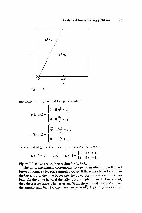
Analysis of two bargaining problems 123
Figure 7.3
mechanism is represented by (p2,x2), where
vx ,v2) = '
xl(vi,v2)= <
1 iff^,,
0 if^<t>,;
2
0
To verify that (p2,x2) is efficient, use proposition 2 with
{0 if vx < 1,1 ifz; = 1
Figure 7.3 shows the trading region for (p2,x2).The third mechanism corresponds to a game in which the seller and
buyer announce a bid price simultaneously. If the seller's bid is lower thanthe buyer's bid, then the buyer gets the object for the average of the twobids. On the other hand, if the seller's bid is higher than the buyer's bid,then there is no trade. Chatterjee and Samuelson (1983) have shown thatthe equilibrium bids for this game are qx = \VX + i and q2 = \V2 + -fe.

124 Roger B. MyersonNote that q{ ^ q2 if and only if V2>VX + \. Thus, this mechanism isrepresented by (p3,x3), where
To verify that (p3,x3) is efficient, use proposition 2 with
ift;2 = 0,if i;2>0.
Figure 7.4 shows the trading region for (p3,x3).Myerson and Satterthwaite (1983) showed that (p3,x3) maximizes the
expected sum of the two traders' profits over all feasible mechanisms. Toverify this, let Lx and L2 be as in the preceding paragraph, and observe that
1 1
I U1(vl9p9x)dLl(vl) + I U2(v2,p,x) dL2(v2)o
J Ul(vl9p,x)dvl+ I U2(v2,p,x) dv2
The expression in brackets may be interpreted as the Lagrangian functionfor the problem of maximizing the expected sum of the traders' profits,when we give a shadow price of \ to each of the individual-rationalityconstraints Ux{\,p,x) ^ 0 and U2(0,p,x) ^ 0. Since (p3,x3) maximizesthis expression over all incentive-compatible mechanisms (by the proof ofproposition 2) and satisfies these two individual-rationality constraintswith equality, it maximizes the expected sum of profits over all feasiblemechanisms.

Analysis of two bargaining problems 125
7.4 The symmetric uniform trading problem:Neutral solutions
Let us suppose now that the seller and buyer in the symmetric uniformtrading problem can negotiate face to face (perhaps with some time limit)to try to determine a mutually acceptable price for the object. In a real-world setting, such negotiations would be much more complicated thanthe three simple games discussed in the preceding section. In real negotia-tions, each trader's strategy is a plan for making a sequence of demands,offers, and arguments, which may be chosen from the infinite richness ofhuman language. Obviously, we have no simple mathematical model ofthe traders' strategy sets in such face-to-face negotiations. However, if onecould construct a realistic model of face-to-face negotiations as a nonco-operative game in strategic form, any equilibrium of the model would stillcorrespond to some feasible mechanism, by the revelation principle.Thus, instead of trying to model the negotiation process as a game instrategic form, we may try to model it as a direct mechanism. That is, byanalyzing the various incentive-compatible mechanisms, we may findone that is a realistic description of face-to-face negotiations.
A concept of neutral bargaining solutions has been defined by Myerson(1984) for general bargaining problems with incomplete information.This solution concept generalizes Nash's (1950) bargaining solution, andis based on axioms of equity, efficiency, and independence of irrelevant
126 Roger B. Myersonalternatives. For the symmetric uniform trading problem, this solutionconcept identifies a new efficient mechanism, different from the threemechanisms that were discussed in the preceding section. However, be-fore we consider this mechanism and argue why it may be a good model offace-to-face negotiations for this symmetric uniform trading problem, letus reconsider the mechanism (p3,x3) discussed in the preceding section.
At first glance, (p3,x3) seems to have many good properties to recom-mend it as a bargaining solution for symmetric uniform trading. As wehave seen, (p3,x3) is efficient. It treats the two traders symmetrically. It isalso ex ante efficient, in the sense that, among all feasible mechanisms forthe symmetric uniform problem, (p3,x3) maximizes the sum of the twotraders' ex ante expected gains from trade. Thus, if the traders couldcommit themselves to a mechanism before either learns his own valuationVi9 then the best symmetric mechanism for both would be (p3,x3).
However, each trader already knows his actual valuation Vt when henegotiates, and this is not assumed to be a repeated game. Therefore, eachtrader cares only about his conditionally expected gains given his actualvaluation. Ex ante expected gains are not relevant to the actual tradersduring negotiations, so ex ante efficiency should be irrelevant to ourtheory of negotiations. In fact, if the seller's valuation is higher than .75,then the mechanism (p3,x3) is among the seller's least preferred mecha-nisms, since Ux{vup3,x3) = 0 for all vx ^ .75.
Suppose, for example, that the seller's valuation is Vx = .8, and that heis negotiating with a buyer who wants to play the simultaneous-bid split-the-difference game with the equilibrium that is equivalent to (p3,x3).The seller knows that he has nothing to gain by playing this game, sincethe buyer will never bid above .75. Thus, the seller has nothing to lose byrefusing to play by its rules, and instead trying to make a nonnegotiablefirst-and-final offer to sell at price .9. The buyer may be antagonized bysuch an arrogant "Boulware" strategy, but if V2 .9, there should be atleast some positive probability that the buyer would accept. Thus, theseller would be strictly better off than in the mechanism (p3,x3).
Similarly, U2(v2,p3,x3) = 0 if v2 .25, and so the buyer would havenothing to lose by refusing to participate in the (p3,x3) mechanism andinstead trying to make a nonnegotiable first-and-final offer to buy at somelow price. Thus, the mechanism that accurately describes the real negotia-tion process should have more trade occurring when Vx ^ .75 or V2 < .25than in the (p3,x3) mechanism. To satisfy the "center-of-gravity" condi-tion (7.1) of proposition 1, the mechanism must also have less trade than(p3,x3) under some other circumstances, when Vx and V2 are in themiddle of their range.
The following mechanism (p4,x4) satisfies the conditions for a neutral

Analysis of two bargaining problems 127
0.75 -
0.25
Figure 7.5
bargaining solution from Myerson (1984), and it differs qualitativelyfrom (p3,x3) exactly as described previously:
P\VUV2) =if v2 > 3vx or 3v2 — 2 > v x,if y2 < 3vx and 3i;2 — 2 < vx;
p\vx ,v2)v2 if v2 1 -
if ^2 > \ - v x .
Figure 7.5 shows the trading region for (p4,x4). (The kink in the boundaryof the trading region is at (.25,.75).)
It is straightforward to check that this neutral mechanism (p4,x4) isincentive compatible and individually rational. To verify that (p4,x4) isefficient, use proposition 2 with
=[0 if^<4>(7.6)
We say that the seller is in a strong bargaining position if Vx is close to 1,since he has very little to lose by not trading. Similarly, we say that thebuyer is in a strong bargaining position if V2 is close to 0. The formula for
128 Roger B. Myerson
x4 can then be interpreted as follows. If V2 < 1 — Vx, then the buyer is in astronger bargaining position than the seller (since V2 is closer to 0 than V{is to 1). In this case, if trade occurs, then it takes place at price V2 /2, whichis the buyer's optimal first-and-final offer, as in (p2,x2). If V2> I — V i9then the seller is in a stronger bargaining position than the buyer, and anytrade is at the seller's optimal first-and-final offer (1 + Vx)/29 as in (p\xl).Thus, if the seller is stronger than the buyer, the neutral bargaining solu-tion (p4,x4) resembles the mechanism (p\xl), in which the seller controlsthe price, except that the trading region is slightly smaller (compare theupper wedge in Figure 7.5 with the form of Figure 7.2). Similarly, if thebuyer is stronger than the seller, the neutral bargaining solution (p4,x4)resembles the mechanism (p2,x2), in which the buyer controls the price,except that the trading region is again slightly smaller (compare the lowerwedge in Figure 7.5 with the form of Figure 7.3).
The neutral bargaining-solution concept of Myerson (1984) is meantto be applied to two-person bargaining problems with incomplete infor-mation in which the two players have equal bargaining ability. Here,bargaining ability means the ability to argue articulately and persuasivelyin the negotiation process. Myerson (1983) defined a theory of solutionsfor cooperative games with incomplete information in which one individ-ual has all of the bargaining ability. In the terminology of that paper, if theseller had all of the bargaining ability, then (p\xl) would be the seller'sneutral optimum (because it is undominated for the seller and is safe, inthe sense that it would be incentive compatible and individually rationaleven if the buyer knew the seller's valuation). Similarly, (p2,x2) would bethe buyer's neutral optimum if he had all of the bargaining ability.
Thus, the neutral bargaining solution (p4,x4) is a first illustration of thefollowing important property, which we may call arrogance of strength. Iftwo individuals of symmetric bargaining ability negotiate with each other,but one individual has a surprisingly strong bargaining position (i.e., therange of agreements that would be better for him than the disagreementoutcome is smaller than the other individual expects), then the outcomeof the neutral bargaining solution tends to be similar to what would havebeen the outcome if the strong individual had had all of the bargainingability, except that the probability of disagreement (no trade) is higher.
The proof that (p4,x4) is a neutral bargaining solution for the symmet-ric uniform trading problem is given in Section 7.7. However, it may behelpful to discuss here the essential properties of (p4,x4) that identify it asa bargaining solution. The neutral bargaining solutions were defined byMyerson (1984) using axioms that generalize the axioms of Nash's (1950)bargaining solution. Then, in a theorem, it was shown that these neutralbargaining solutions can also be characterized by two properties: effi-

Analysis of two bargaining problems 129ciency and virtual equity. The efficiency property has already been dis-cussed, but the virtual-equity property needs more explanation.
Given any Lx and L2 as in proposition 2, we define functions Wx andW2, respectively, by
Wx(vx) = 2vx - Lx(vx) and W2(v2) = 2v2 - L2(v2\
We call Wt(y^ the virtual valuation of the object to trader i if vt is his truevaluation. For Lx and L2 as in (7.6), the virtual valuations are
if vx < i,
^ ^ (7.7)
i fz ; 2 > i
By proposition 1, for any feasible mechanism there must be a positiveprobability of negotiations ending without a trade when the object isworth more to the buyer than to the seller. Such a conclusion may seemparadoxical if the traders have the option to continue negotiating. Whyshould they stop negotiating when they know that there is still a possibilityof mutual gains from trade? One possible explanation is that each trader ideliberately distorts his preferences in bargaining, in response to theother's distrust, and acts as if the object were wojth the virtual valuationWi(Vt) to him, instead of the actual valuation Vt. (In (7.7), Wx(vx) > vxand W2{v2) ^ v2, and so the seller is overstating and the buyer is under-stating the object's value.) The mechanism (p4,x4) has trade occurring ifand only if W2{ V2) > Wx{ Vx)\ thus, there is no possibility of further virtualgains from trade after (p4,x4).
Of course, any efficient mechanism that satisfies proposition 2 wouldsatisfy a similar property (which we may call virtual ex-post efficiency) interms of some other virtual valuation function. However, (p4,x4) is alsovirtually equitable, in terms of the same virtual valuations (7.7) that makeit virtually ex post efficient. To see this, consider any vx \. If the seller'strue valuation is vl9 then his conditionally expected virtual gains in(p\x4) are
18

130 Roger B. Myersonwhich is equal to his conditional expectation of the buyer's virtual gains in
j(W2(v2)P\v1,v2)-x\vl,v2))dv2 =0
18 'Similarly, if V2 = v2 | , then the buyer's conditional expectation of hisown virtual gains in (p4,x4),
v2/3
( (v2ff (2v2 v2
0
is equal to his conditional expectation of the seller's virtual gains,
(v2
\ ) IF'0
For vl^iovv2^ 1, these equalities do not hold, but Lx and L2 from (7.6)are constant over these intervals, so that the corresponding objectivefunction (7.5) puts no weight on these valuations. Thus, with respect tothe virtual valuations in (7.7), (p4,x4) is both virtually ex post efficient andvirtually equitable, except for some weak types that get no weight in thecorresponding objective function. These are necessary conditions for aneutral bargaining solution derived in Myerson (1984). However, moreimportant, they demonstrate that (p4,x4) can be justified as both efficientand equitable, in a newly recognized sense.
7.5 The lemon problem: Feasibilityand efficiency
Let us now consider some trading problems in which the seller has privateinformation related to the quality of the object being sold, so that thevalue of the object to the buyer is a function of the seller's valuation. Tokeep the problem tractable, let us assume that the seller knows this func-tion and the buyer has no private information. We may call this the lemonproblem, after Akerlof's (1970) seminal paper "The Market forLemons," which studied a special case of this problem, in a market con-text. (In colloquial American, a bad used car is a "lemon.")

Analysis of two bargaining problems 131
Again, let trader 1 be the only seller and trader 2 be the only potentialbuyer of a single indivisible object. Both have risk-neutral utility formoney. The quality of the object, which is known only to the seller, ismeasured by the random variable Vx, which is the value of the object tothe seller. The buyer has a probability distribution for Vx with cumulativedistribution F(vx) = P r o b ^ < vx), and with a continuous densityf{vx) = F'(vx) that is positive over a bounded interval 0 ^ vx ^ M. Thevalue of the object to the buyer is g( Vx), where g: [0,M] —> IR is a continu-ous function.
A direct trading mechanism for the lemon problem is characterized bytwo outcome functions,/?: [0,M] —• [0,1] andx: [0,M] -> R, wherep{vx)is the probability of trade occurring and x(vx) is the expected revenue tothe seller, if the seller's valuation equals vx. The expected gain to the buyerfrom (p,x) is
M
U2(p,x) = I (g(vMvi) - x(vx)) dF(vi).0
The expected gain to the seller from (p,x) if his valuation equals vx isUx(vx,p,x) = x(vx) - vxp(vx).
In this context, mechanism (p,x) is incentive compatible if and only if, forevery vx and tx in [0,M],
Mechanism (p,x) is individually rational if and only if U2(p,x) ^ 0 and,for every vx in [0,M], Ux(vx ,p,x) ^ 0. As before, a mechanism is feasible ifand only if it is incentive compatible and individually rational.
(In this formulation, we are assuming that the terms of trade cannot bemade conditional on the actual quality of the object, only on the seller'sreport of it. Presumably, the buyer will eventually learn the quality of theobject if he buys it, but too late to renegotiate the price.)
The following proposition characterizes the set of feasiblemechanisms.
Proposition 3. Given any function p: [0,M] —* [0,1], there exists somefunction x( •) such that (p,x) is a feasible mechanism for the lemonproblem if and only if p( •) is a weakly decreasing function and
M
j ( g(vi) -vt- j^jpivJM) dv, s 0.

132 Roger B. MyersonIn general, for any incentive-compatible mechanism (p,x), /?(•) is weaidydecreasing,
M
M
U2(p,x) = j (g(vx) ~vx- j^pivjfivj dvx
and, for every vx in [0,M],
Ul(vl ,p,x) = Ux(M,p,x) + I p(s) ds.
Proof. The proof of the equation for Ul(vl ,p,x) and of p decreasing isexactly as in the proof of theorem 1 of Myerson and Satterthwaite (1983).The equation for Ux{M,p,x) + U2(p,x) is derived from the following chainof equalities:
M MJ \{V\,P,x)f(Vi) dvx + U2(p,x)
p(s) dsf(vx) dvx + Ux(M,p,x) + U2(p,x)
0 0M M
0 v{
M
x)p(vx) dvx + Ux(M,p,x) + U2(p,x).o
Finally, if p is weakly decreasing and satisfies the inequality in proposition3, then we can construct a feasible mechanism by using
M
Ix(vx) = vxp{vx) + p(s) ds,
which is straightforward to check.
As in the symmetric uniform example, our next task is to characterizethe efficient mechanisms for the lemon problem. Again, we use the termefficient in the sense of weak interim incentive efficiency; that is, (p,x) isefficient if and only if there exists no other incentive-compatible mecha-nism (p,x) such that U2{p,x) > U2(p,x) and, for every vl9 Ul{vlp,x) >

Analysis of two bargaining problems 133
For any number s between 0 and M, let (p(s\x(s)) denote themechanism
ifvx>s'9
0 ifvx>s.We may refer to any such mechanism (x^s\p^s)) as a simple mechanism,since there are only two possible outcomes: Either the object is sold for sdollars (if Vx < s) or it is not sold at all. These simple mechanisms areimportant because they represent the extreme points of the set of incen-tive-compatible mechanisms for the lemon problem, up to addition of alump-sum transfer between buyer and seller. To understand why, notethat any incentive-compatible mechanism differs by a lump-sum transfer(i.e., a constant added to x( •)) from an incentive-compatible mechanismwith Ux(M,p,x) = 0. By proposition 3, any such mechanism is then char-acterized completely by the weakly decreasing functionp\ and both Ux(vx)and U2 are linear functions of p. However, any weakly decreasing functionfrom [0,M] into [0,1] can be approximated arbitrarily closely (exceptpossibly on a countable set) by a convex combination of the step functions{/7(5)}. Since we are assuming that Fis a continuous distribution, changingp on a countable set would not change any of the expected payoffs inproposition 3. (Without this continuity assumption, we would have todistinguish (p(s\xis)) from the mechanism in which the object is sold for sdollars if and only if Vx < s, and we also would add such mechanisms tothe list of extreme points.)
A mechanism is efficient for the lemon problem if and only if it maxi-mizes some linear functional of the form
M
Ux (vx ,/?,*) dLx(vx) + U2(p,x) (7.8)
over the set of all incentive-compatible mechanisms, where Lx( •) isweakly increasing, Lx(0) = 0, and LX{M) = 1. However, the maximum ofany such linear functional must be attained at some simple mechanism(p{s\xis)), because these are the extreme points. (Similarly, the maximumof any linear functional subject to one linear constraint can always beattained at a simple mechanism or a linear combination of two simplemechanisms. Thus, as Samuelson [1984] has shown, the seller's ex anteoptimum, subject to nonnegative expected utility for the buyer, canalways be attained at a mechanism with a one-step or two-stepp function.)

134 Roger B. Myerson
To characterize the set of efficient mechanisms for the lemon problem,we need some additional definitions. Let Y(s) denote the expected gain tothe buyer from mechanism (p(J),Jt(5)); that is,
- JY(s) = U2(p(*\x^) = I teto) - s)f(v{) dvx.0
Let Y: [0,M] ~~* R be the lowest concave function that is greater than orequal to Y( •) and has a slope between 0 and — 1 everywhere. That is, Ydiffers from the concave hull of Y only in that Y is constant over theinterval where the concave hull is increasing, and Y has slope — 1 overany interval where the concave hull is decreasing at a steeper slope than- 1 . Finally, let Lf: [0,Af]-> [0,1] be defined such that Lf(0) = 0,L*(M)= l,and
at every v{ in (0,AQwhere the derivative Y' is defined. (Define L* by leftcontinuity when Y' jumps.) Notice that L* is an increasing function,since Y is concave. Note also that Y(0) = max5(E[(W] Y(s).
The set of efficient mechanisms for the lemon problem has a remark-ably simple structure: It is a flat set contained in a hyperplane. That is,given any two efficient mechanisms, their convex combination is alsoefficient. The function Lf gives us the normal to this flat efficient set, as isshown in the following proposition.
Proposition 4. Let (p,x) be any incentive-compatible mechanism for thelemon problem. Then, (p,x) is efficient if and only if
M
U{(v\ ,p,x) dLt(vx) + U2(p,x) = 7(0). (7.9)o
Equivalently, (p,x) is efficient if and only if p satisfies the following threeconditions: p(0) = 1 if Y(0) > 0, p(M) = 0 if Y(M) > Y{M\ and
M
(Y(vx)-Y(vx))dp(vx) = O,o
so that p must be constant over any interval in which Y > Y.
Proof. Notice first that, from the definition of Y,7(0) = 0 and Y'{vx) = (g(vx) - vx)f{vx) - F(vx).

Analysis of two bargaining problems 135
Now, using proposition 3, for any incentive-compatible mechanism( « v\
M
J Ux(vxj>jc)dLftvx)+U2(pjc)0
M M
= J J p(s) ds dL*(vx) + UAMjtj) + U2(p,x)0 vi
M M
= J LftvMvi) dvx + | ((g(vx) - vx)f(vx) - F(vx))p(vx) dvx
0 0M
= \{Y\vl)-Y'(vl))p(Vx)ch)x
0M
= Y(0)p(0) - (Y(M) - Y(M))p(\) + [ (Y{vx) - Y(vx)) dp(vx).o
Since Y(vx) ^ Y(vx) for all vx, the decreasing function p that maximizesthe last expression must have p(0) = 1 if Y(0) > 0, /?(M) = 0 ifY (M) > Y(M), and must be constant over any interval in which Y > Y.(Note that the integral is not positive, because p is decreasing.) Such afunction p does exist and gives the maximum value Y(0). Thus, p isefficient if it satisfies (7.9). _
Let rx be the lowest number in [0,M] such that Y(rx) = Y(rx), and let r2be the highest such number (see Figure 7.6). Now, consider any simplemechanism (p(s\x(s)) that does not satisfy (7.9). Then,
M
Y(0) > j Ux(vx,p(*\xM) dL*(vx) + W>,x<*>) = F(0) - (Y(s) - Y(s))9
oand so Y(s) > Y(s). We will show that (p(s\x(s)) is not efficient. There arethree cases to consider: s'<rx, s> r2, and rx< s <r2.
If s < rl5then Y(s) < Y(rx) = F(0). Therefore, the buyer would strictlyprefer (p^\x^) to (/?(5),JC(5)). The seller also prefers (p(ri),;c(ri)) to (p(s\xis)\since
Ux(vx ,p(s\x(s)) = max{0,s - vx)
is increasing in s. Thus, (p(s\x(s)) is not efficient.

136 Roger B. Myerson
Y(0)Y ( s )
Figure 7.6
If s > r2, then Y(s) < Y(r2) + (r2 - s), since the slope of Y is - 1 for allvx > r2. Thus, the buyer would strictly prefer to pay s — r2 as a lump-sumtransfer and then implement (p(r2\x(r2)). It is easy to see that the sellerwould also prefer this change, and so (/?(5),x(5)) is not efficient.
If r} < s < r?, then there exist numbers sy, s,9 and X such thats = Xs{ + (1 - A)s2, 0 < X < 1, and Y(s) < XY(sx) + (1 - X)Y(s2). There-fore, the buyer would strictly prefer to randomize between (p(Sl\x(Sl)) withprobability A and (p(S2\x(S2)) with probability 1 — A, rather than use(p(s\x(s)). Since Ux{vx ,p{s\x(s)) is a convex function of s, the seller wouldalso prefer this randomization. Thus, (p(s\x(s)) is not efficient if it violates(7.9).
Any efficient mechanism must be equal to some convex combinationof efficient simple mechanisms plus a lump-sum transfer. Thus, anyefficient mechanism must satisfy condition (7.9) of proposition 4.
Furthermore, if g(v{) ^ vx for every vx between 0 and M, thenL *{vx) ^ F(v{) for every v{ between 0 and M. That is, if the object is alwaysworth more to the buyer than to the seller, then L f puts more weight onthe higher valuations of the seller than F does, in the sense of first-orderstochastic dominance. To verify this fact, observe that if L^(vx) > 0, thenthere exists some w{ such that w{ < v{ and
- Y\vx) = - = F{wx) - - w{) < F(w{) <To illustrate these results, consider first the example studied by Akerlof
(1970), in which M= 2, F(v{) = ,5vl9 and g(vx) = 1.5^. That is, the

Analysis of two bargaining problems 137seller's valuation is uniformly distributed over [0,2], and the object wouldalways be worth 50 percent more to the buyer, if he knew the seller'svaluation. For this example,
g(vx) -vx- F(vx)/f(vx) = ~.5vx < 0.So, by proposition 3, there does not exist for Akerlof's example anyfeasible mechanism with a positive probability of trade.
For a second example, let M = l,F(vx) = vl,z.ndg{vl) = v{ + a, where0 < a < 1. We may call this the uniform additive lemon problem. For thisexample, there are many feasible mechanisms (e.g., (pis\x(s)) for everys < 2a). To apply proposition 4,
Y(s) = I (vx + a — s) dvx = as — .5s2,o
and so
(s) \.5a2 >Y(s) ifs<a.
Thus, an incentive-compatible mechanism (p,x) is efficient if and only ifp{v{) = 1 for every v{ such that 0 ^ v{ < a.
7.6 The uniform additive lemon problem:Neutral solutions
As in Section 7.4, let us now try to make some prediction as to whichefficient mechanism may actually be implemented by the seller and buyerin the lemon problem if they negotiate face to face. To simplify theanalysis, we will consider only one specific case: the uniform additive casewith a = .4. That is, the seller knows his valuation Vx, which is a uniformrandom variable on [0,1], and if the buyer gets the object, then it will beultimately worth Vx + .4 to him. The seller is free to make statements tothe buyer about Vx, but there is no way for the buyer to verify whetherthese claims are true or false until after the negotiations end and the termsof trade are fixed.
For simplicity, let us begin with the assumption that the buyer has all ofthe bargaining ability, perhaps because he is much more articulate andpersuasive in negotiations than the seller. The best feasible mechanism forthe buyer is the simple mechanism (p(A\x(A)). That is, if the buyer cancontrol the negotiations, he wants to make a nonnegotiable first-and-finaloffer to buy the object for a price of .4. To verify that this mechanism is

138 Roger B. Myerson
optimal, note thats
- \Y{s)= (vx + .4 - s) dvx = As - .5s2,
o
which is maximized at s = .4. The buyer's expected gain from his optimalmechanism is Y(A) = .08.
Now, let us assume that the seller has all of the bargaining ability. Theproblem of determining which mechanism he should implement is aproblem of mechanism design by an informed principal, as studied inMyerson (1983).
Among the simple mechanisms, Ux(vx ,p(s\xis)) is increasing in s, andU2(p(s\x(s))> 0 if and only if s < .8. That is, for any price s that is higherthan .8, the expected value of the object to the buyer conditional on Vx < sis. 5 s + .4, which is less than s, and so the buyer expects to lose. Thus, if theseller were to implement a simple mechanism, his best choice would be(/?(8),.x(-8)). (Even though the object is always worth more to the buyer thanto the seller, there is no feasible mechanism in which the buyer always getsthe object, because the inequality in proposition 3 would fail if p(vx) = 1for all vx.)
The mechanism (/?(-8),x(-8)) maximizes both the probability of trade andthe seller's ex ante expected gains (/£ Ul(vl ,p,x) dvx) over all feasiblemechanisms for this example. Thus, if the seller could have selected anyfeasible mechanism before he learned Vx, he would certainly have se-lected (p(-s\x(-S)). However, this argument is not necessarily relevant toour analysis of negotiations, because we are assuming that the sellerknows Vx when the negotiations begin, and this is not a repeated game.
There exist other mechanisms that the seller would prefer to (p(-s\x(-S))if Vx were relatively high. (Observe that Ux(vx ,p( 8),JC(8)) = 0 if vx > .8.) Forexample, consider (p,x) defined by
p(vx) = e~^A and jc^) = (vx + A)p(vx).
That is, the seller demands that the buyer pay the full value q = Vx + .4,and the buyer accepts with probability e~(g~~A)/A. It is straightforward tocheck that (p9x) is individually rational and incentive compatible. If theseller demanded a higher price, the decrease in probability of acceptancewould be just enough to prevent him from gaining more. Among all of themechanisms in which the buyer never loses ex post (safe mechanisms, inthe terminology of Myerson (1983)), (p,x) is the best for the seller. IfVx > .74, then the seller would prefer (p,x) over (p^\x(-S)) {Ae~JAfA >.8 - .74).
Analysis of two bargaining problems 139One theory of negotiations that cannot be valid is to suggest that the
seller would implement (/?(-8),JC(*8)) if Vx < .74 and would implement (p,x)if V{ > .74. The buyer would refuse to buy the object for .8 if he believedthat the seller would make this demand only when Vx < .74, because theconditionally expected value of the object to him would be only.74/2 + .4 = .77. On the other hand, the buyer would never expect lossesin (p,x\ even if he inferred that Vx > .74. Therefore, (/?(8),x( 8)) is blockedfor the seller by (p,x), since the buyer knows that (p(8),xC8)) would beimplemented by the seller only if Vx were in [0v74], where the buyerexpects to lose on average.
However, (p,x) is not an efficient mechanism, because any efficientmechanism must have p(vx) = 1 for all vx in the interval [0,.4) (whereY(v{) > ^(^i)), as was shown at the end of Section 7.5. For example, (p,x)is dominated by the mechanism (/?*,.**) defined by
- {.4;
.6 i f^<.4 ,A)p(vx) i f^>.4 .
It is straightforward to verify that (p*,x*) is incentive compatible, thatU2{p*jc*) = U2(p,x) = 0, and that Ufa ,p*,x*) > Ufa j>jc) for all vx.Also, (p*,x*) is efficient because a sale will always occur if 0 < Vx < .4. IfVx > .4, then the seller insists on getting the buyer's reservation priceVx + .4, and the buyer's probability of acceptance decreases in the price insuch a way as to keep the seller honest. It can be shown (see Section 7.7)that this mechanism (p*,x*) is a neutral optimum for the seller, in thesense of Myerson (1983).
Thus, we predict that the outcome of negotiations would be as in(p(A\x{A)) if the buyer had all of the bargaining ability, and would be as in(/?*,**) if the seller had all of the bargaining ability.
Let us now assume that the buyer and seller have equal bargainingability. In this case, the solution theory of Myerson (1984) identifies theaverage of these mechanisms, (p%x°) = .5(p(A\x{A)) + .5(p*,x*), as aneutral bargaining solution. That is, the neutral bargaining solution is
ifvx<A9Vi—A)/A if«« > A>II Vx — ,T-,
x + A)p°(vx) ifi>! 2>.4.Notice that if Vx > .4, the seller fully exploits the buyer in (p\x°) by
charging him Vx + .4 when trade occurs, just as in (/?*,.**). However, the

140 Roger B. Myersonprobability of trade occurring when Vx > .4 in (p°,x °) is half of what it isin (p*,**). Thus, the neutral bargaining solution (p°,x°) has the propertyof arrogance of strength, defined in Section 7.4. That is, if the traders haveequal bargaining ability but the seller is in a surprisingly strong bargainingposition, then the outcome is the same as when the seller has all of thebargaining ability, except that the probability of disagreement is higher.
The mechanism (p °,x°) may seem more equitable when we look atvirtual-utility payoffs. For this example, the function Lf, which supportsall efficient mechanisms (as stated in proposition 4), is
Because the seller's valuation is uniformly distributed over [0,1], his vir-tual valuation is 2VX — L*(VX) (as in the symmetric uniform tradingproblem), which equals Vx + .4 if Vx ^ .4 (except at the endpoint Vx = 1,which has zero probability). Thus, when Vx > .4, the seller's virtual valua-tion equals the buyer's valuation, and so Vx + .4 is the only virtuallyequitable price. (Since the buyer has no private information in this exam-ple, his virtual and real valuations are equal.) When Vx is in the interval[0,.4), the seller's average virtual valuation (i.e., 2 Vx) is .4, and the buyer'saverage valuation (i.e., Vx + .4) is .6; thus, the price .5 in (p°,x°) isvirtually equitable on average.
7.7 Derivation of the neutral solutions
To show how the solution concepts of Myerson (1983, 1984) are appliedto the examples of this chapter, let us first consider a discrete approxima-tion to the lemon problem. That is, let S be a small number, and letTx = (0, S, 2(5, 3<5, . . . , M) be the set of possible seller's valuations for theobject. Letf(vx)d = F(vx) — F(vx — S) be the probability that Vx = vx forany vx that is a multiple of S. Given an increasing function 1^ as in (7.8), let€(vx) = (Lx(vx) — Lx(vx — S))/d. Thus, the discrete analog of (7.8) is
2 ((*(*i) - »i PWWvtf + (g(vx)p(v,) - x{vx))f{vx)S). (7.10)
It can be shown that, for the discrete lemon problem, local incentivecompatibility implies global incentive compatibility. (That is, if for everyvx, the seller with valuation vx could not gain by reporting vx + S forvx — (5, then the seller cannot gain by any lie.) Furthermore, in most casesthe binding incentive constraint for the seller is the one in the upward

Analysis of two bargaining problems 141direction, that is, that the seller should not gain by reporting vx + d whenhis valuation is vx. So, let A(vx) denote the shadow price of this incentiveconstraint in the problem of maximizing (7.10) among all incentive-com-patible mechanisms. Then, the Lagrangian function for this problem canbe written
- vxp(vx))€{vx)S + (g(vx)p(vx) - x(vx))f{vx)S
+ A(vx)((x(vx) - vxp(vx)) - (x(vx + S)- vxp(vx + S))))= 2 ([WvJS + A(vx))(x(vx) - vx p(vx)) - A(vx - S)(x(vx)
- (vx - S)p{vx))) + (givMvi) - x{vx))f{vx)d). (7.11)The coefficient of x(vx) in this Lagrangian formula must be zero, sincex(vx) is an unconstrained variable. Thus, we must have, for all vx,
A(vx) - A(vx - S) =f(vx)S - €(vx)S9
and so
A(vx) = F(vx) - Lx(vx).
The seller's virtual utility is defined in Myerson (1984) as the bracketedexpression in (7.11) divided by the probability/^ )S. That is, if the seller'svaluation is vx, if his expected revenue is y = x(vx), and if his probability ofsale is q = p(vx), then his virtual-utility payoff zx(vx) is defined as
_ {£{vx)d + A(vx))(y -vxq)- A(vx - S)(y - (vx - S)q)
7
Equivalently, if we let ux(vx) = y — vxq denote the seller's actual-utilitypayoff when his valuation is vx (and let u(vx — S) = y — (vx — S)q), thenthe seller's virtual-utility payoff can be rewritten
At the maximum of (7.10), the product of incentive constraint timesshadow price is always zero, by complementary slackness, and so (7.11)implies that
X (x(vx)-vxp(vx))€(vx)S= ^ ^ i ) / ( ^ -

142 Roger B. MyersonNow, letting 8 go to zero, let us return to the continuous version of the
lemon problem. The immediately preceding three equations become
)-^)'Avl), (7.13)
M M
(7.14)M M
respectively, where
LAvT) = lim Ll(vl — d).6-+0+
The seller's virtual valuation for the object is, from (7.12),
11/ t~. \ . I V 1/ 1\ 1 /
In the uniform case with i ^ ) = vx on [0,1], when Lx is continuous thisvirtual valuation is simply Wx{v{) = 2vx — L^vJ, as in Section 7.4.
Since the buyer has no private information in the lemon problem andgets a weight of 1 in the objective functions (7.8) and (7.10), the buyer'svirtual utility is the same as his real utility.
We are now ready to verify that (p°,x°) is the neutral bargainingsolution for the uniform additive lemon problem with g(v{) = v{ + .4. Toprove this, we must apply theorem 4 of Myerson (1984), which givesnecessary and sufficient conditions for a neutral bargaining solution. Thistheorem requires us to consider a sequence of virtual-utility scales, each ofwhich is generated by an objective function that puts positive weight on alltypes of all players. (For the lemon problem, this means that Lx must bestrictly increasing over the whole range of possible valuations.) For eachvirtual-utility scale, we must first compute the virtually equitable alloca-tions, in which the traders plan to divide the available virtual gains equallyamong themselves in every state. Then, we must solve equations (7.13)and (7.14) to find which allocations of real utility would correspond to theequitable allocations of virtual utility. The corresponding allocations ofreal utility are called the warranted claims of the seller and the buyer. If the

Analysis of two bargaining problems 143
limit of these warranted claims (over the sequence of virtual-utility scales)does not exceed the actual expected utility generated by our mechanismfor any type, then that mechanism is a neutral bargaining solution.
The sequence of objectives that supports (p°,x°) is
.4" M-e'
y i ~ - 4 i f T—Z~ v i
1 ^ = 1,
where the index e is positive and converging to zero. Notice that each L\ isstrictly increasing over [0,1 ] and converges to L f of Section 7.6 as e goes tozero.
With respect to Lx = L\, if the seller's actual valuation is vx, then hisvirtual valuation (from (7.15)) is
Wl(vl)=\(2-e)vx if
vx + .4 if
.4
.41 - e
1 - e '
and so the total available virtual gains from trade are
g(vx) -.4 - (1-e) ! ; , if
if-
A
.41 - e
The virtually equitable allocation with respect to L\ would give the sellerhalf of these virtual gains; that is, he would get
. 2 - . 5 ( l - e ) i > i i f O s i > ! < -.4
if-.4
< v, < 11 -e
in virtual utility when his valuation is vx. The seller's warranted claimswith respect to L\ are the values of ux{vx) that satisfy (7.13) and (7.14) for
144 Roger B. Myerson
this zx function. That is, ux must satisfy
.2 - .5(1 - e)vx = ux(vx) + (1 - e)vxu'x(vx)
0 = ux(vx) + Au\(vx) if .4/(1 - 6) < < 1,•4/(1-€)
J (.2-.5(l-€)^)^i= J ux(vx)edvx
1
I ux(vx) dvx + Aux(l)..4/(1-e)
(The term .4^(1) comes from the jump in L\ at vx = 1.) The uniquesolution to these equations is
UX(VX) = <., A
1 - .As 6 goes to zero, these warranted claims converge to
VA if . 4 ^ ^ < i.
The seller's actual payoff from the mechanism (p°,x°) is
~v> if 0 17! < .4,^-(r,-.4)/.4 i f 4 < ^ < 1 ?
and so ^(i^,/?0,.*0) ^ w t?!) for all vx in [0,1].Since the buyer has only one possible type in this problem, his war-
ranted claim with respect to L\ is simply half of the expected virtual gainsfrom trade:
.4
ux = I (.2 - .5(1 - e)vx) dvx = .04(1 + e).
As e goes to zero, this expression converges to .04 = U2(p\x°).So the mechanism (p ° ,x °) fulfills all of the limiting warranted claims,
and therefore is a neutral bargaining solution, by theorem 4 of Myerson(1984).
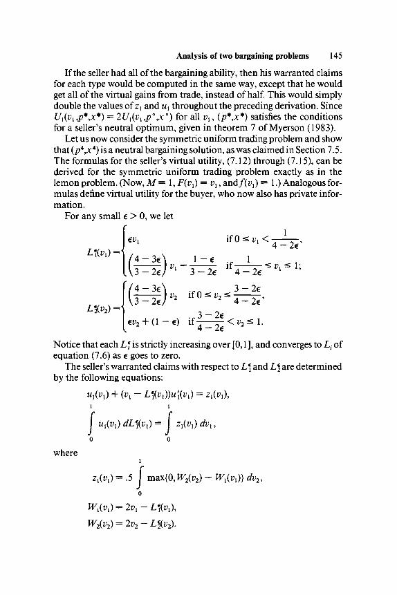
Analysis of two bargaining problems 145If the seller had all of the bargaining ability, then his warranted claims
for each type would be computed in the same way, except that he wouldget all of the virtual gains from trade, instead of half. This would simplydouble the values of zx and ux throughout the preceding derivation. SinceUx(vx,p*,x*) = 2Ux(vx,p°,x°) for all vl9 (p*9x*) satisfies the condit ionsfor a seller's neutral optimum, given in theorem 7 of Myerson (1983).
Let us now consider the symmetric uniform trading problem and showthat (p4,x4) is a neutral bargaining solution, as was claimed in Section 7.5.The formulas for the seller's virtual utility, (7.12) through (7.15), can bederived for the symmetric uniform trading problem exactly as in thelemon problem. (Now, M = 1, F(vx) = vx, andf(Vi) = 1.) Analogous for-mulas define virtual utility for the buyer, who now also has private infor-mation.
For any small 6 > 0, we let
LftDi) = '
L\Xv2) =
4-3e
\3-2e/ v2
6fl2 + ( 1 - 6 ) if
1 -
1
if3
e2e
-v2
- 2 e
ifO
4
1
- 2 e- 2 e
. < 1
K 41
- 2 6 '
4-2e
Notice that each Lf is strictly increasing over [0,1 ], and converges to Lt ofequation (7.6) as e goes to zero.
The seller's warranted claims with respect to L\ and L\ are determinedby the following equations:
I ux(vx)dL\(v^= I zx(vx)dvu
where
zfa) = .5 [ max{0,PF2(i;2) - Wx(vx)) dv2,o
W2(v2) = 2v2 - L%v2).

146 Roger B. MyersonIt can be shown (somewhat tediously) that the unique solution to theseequations is
if- 14 - 2e "
As € converges to zero, these warranted claims converge to
• V, < 1.
«l(f,) ="16
if 0 <vx<.25,
if .25 <vx < 1.
If the seller's valuation is vx, then his actual expected utility from themechanism (p4,x4) is
6 — 15 , + 12(^)2 .32
if .25 1.
It is straightforward to check that Ul(vl ,p4,x4) ^ u^v^ for every vx, andthus (p4,x4) fulfills all of the seller's limiting warranted claims. A symmet-ric argument shows that (p4,x4) satisfies the buyer's limiting warrantedclaims for every v2 as well. Thus, (p4,x4) satisfies the conditions for aneutral bargaining solution.
A final remark about the uniqueness of these solutions is in order. Thegeneral conditions for a neutral bargaining solution are well determined,in the sense of giving us as many equations as unknowns (see theorem 5 ofMyerson (1984)), but there is no general uniqueness theorem. For thesymmetric uniform trading problem, some inessential nonuniqueness isknown. There exist other functions x such that (p4,x) is a feasible mecha-nism, and all of these mechanisms are neutral bargaining solutions givingthe same expected utility allocations as (p4,x4). Apart from this non-uniqueness in x, it is my unproven belief that (p4,x4) is probably theunique neutral bargaining solution for the symmetric uniform tradingproblem, and that (p°,x°) is the unique neutral bargaining solution forthe uniform additive lemon problem considered in Section 7.6.

Analysis of two bargaining problems 147
REFERENCES
Akerlof, G. (1970): The Market for Lemons: Qualitative Uncertainty and theMarket Mechanism. Quarterly Journal of Economics 84, 488-500.
Chatterjee, K., and W. Samuelson (1983): Bargaining under Incomplete Informa-tion. Operations Research 31, 835-51.
Holmstrom, B., and R. B. Myerson (1983): "Efficient and Durable DecisionRules with Incomplete Information. Econometrica 53, 1799-1819.
Myerson, R. B. (1979): Incentive Compatibility and the Bargaining Problem.Econometrica 47, 61-73.
(1983): Mechanism Design by an Informed Principal. Econometrica 53,1767-97.
(1984): Two-Person Bargaining Problems with Incomplete Information,Econometrica 52, 461-87.
Myerson, R. B., and M. A. Satterthwaite (1983): "Efficient Mechanisms for Bilat-eral Trading. Journal of Economic Theory 29, 265-81.
Nash, J. F. (1950): The Bargaining Problem. Econometrica 18, 155-162.Samuelson, W. (1984): Bargaining under Asymmetric Information. Economet-
rica 52, 995-1005.


CHAPTER 8
Sequential bargaining mechanisms
Peter C. CramtonYALE UNIVERSITY
8.1 Introduction
A fundamental problem in economics is determining how agreements arereached in situations where the parties have some market power. Ofparticular interest are questions of efficiency and distribution:
• How efficient is the agreement?• How can efficiency be improved?• How are the gains from agreement divided among the parties?
Here, I explore these questions in the context of bilateral monopoly, inwhich a buyer and a seller are bargaining over the price of an object.
Two features of my analysis, which are important in any bargainingsetting, are information and impatience. The bargainers typically haveprivate information about their preferences and will suffer some delaycosts if agreement is postponed. Information asymmetries between bar-gainers will often lead to inefficiencies: The bargainers will be forced todelay agreement in order to communicate their preferences. Impatiencewill tend to encourage an early agreement and will make the parties'communication meaningful. Bargainers with high delay costs will acceptinferior terms of trade in order to conclude agreement early, whereaspatient bargainers will choose to wait for more appealing terms of trade.
Some authors have examined the bargaining problem in a static con-text, focusing solely on the role of incomplete information and ignoringthe sequential aspects of bargaining. Myerson and Satterthwaite (1983)analyze bargaining as a direct revelation game. In this game, the playersagree to a pair of outcome functions: one that maps the players' state-ments of their types into an expected payment from buyer to seller, andone that maps the players' statements into a probability of trade. Theseoutcome functions are chosen in such a way that truthful reporting is an
I am indebted to Robert Wilson for his encouragement and inspiration. Mythanks to Drew Fudenberg for his helpful comments.
149

150 Peter C. Cramtonequilibrium strategy for the players. An important feature of this game isthat it is static: Outcome functions are selected, the players report theirtrue types, and then dice are rolled to determine the payment and whetheror not trade occurs. To ensure that the players have the proper incentivesfor truthful reporting, the game will end with positive probability indisagreement even when there are substantial gains from trade. Thus, inthe event that the randomization device calls for disagreement, theplayers may find themselves in a situation in which it is common knowl-edge that there are gains from trade.
Chatterjee and Samuelson (1983) analyze a strategic game in whichboth players make offers simultaneously, and trade occurs at a pricebetween the two offers if the seller's offer is less than the buyer's offer. Thisgame is closely related to the direct revelation game, in that it is static.Moreover, it can be shown that for a particular class of examples, thesimultaneous-offers game implements the direct revelation game inwhich the outcome functions are chosen to maximize the players' ex anteutility. As in the direct revelation game, this game ends with positiveprobability in a state in which both bargainers know that gains are possible(since their respective reservation prices have been revealed), and yet theyare forced to walk away from the bargaining table. Thus, the bargaininggame assumes implicitly that the players are able to commit to walkingaway without trading, after it has been revealed that substantial gainsfrom trade exist.
In situations where the bargainers are unable to make binding agree-ments, it is unrealistic to use a bargaining mechanism that forces them towalk away from known positive gains from trade. Such mechanismsviolate a broad interpretation of sequential rationality as discussed bySelten (1976) (in terms of subgame perfection), and later by Kreps andWilson (1982), if one applies sequential rationality not only to the hy-pothesized game, but to the game form as well. In particular, one shouldrestrict attention to mechanisms that satisfy sequential rationality: Itmust never be common knowledge that the mechanism induced at anypoint in time is dominated by an alternative mechanism.
When there is uncertainty about whether or not gains from trade exist,any static game will violate sequential rationality. The players must havetime to learn through each other's actions whether gains are possible. In asequential game, the players communicate their preferences by exhibitingtheir willingness to delay agreement. Bargainers who anticipate largegains from trade (low-cost sellers and high-valuation buyers) will be un-willing to delay agreement, and so will propose attractive terms of tradethat the other is likely to accept early in the bargaining process. On theother hand, high-cost sellers and low-valuation buyers will prefer to wait

Sequential bargaining mechanisms 151
for better terms of trade. Static games must use a positive probability ofdisagreement to ensure incentive compatibility, where the probability ofdisagreement increases as the gains from trade shrink. The advantage ofdelaying agreement rather than forbidding agreement is that mechanismscan be constructed in which negotiations continue so long as each bar-gainer expects positive gains. Thus, the bargaining will not end in a state inwhich it is common knowledge that the players want to renege on theiragreed-upon outcome.
Two approaches can be taken in the analysis of perfect bargaininggames. The first approach is to examine specific extensive-form games,which determine the set of actions available to the players over time.Intrinsic to any bargaining process is the notion of offers and replies:Bargaining consists of a sequence of offers and decisions to accept or rejectthese offers. Who makes the offers; the time between offers, responses,and counteroffers; and the possibilities for commitment are determinedby the underlying communication technology present in the bargainingsetting. This communication technology will imply, in part, a particularbargaining game in extensive form. Cramton (1984), Sobel and Takaha-shi (1983), and Fudenberg, Levine, and Tirole (Chapter 5 in this volume)illustrate the analysis of particular extensive forms that are perfect bar-gaining games.
The second approach, and the one adopted in this chapter, is to analyzea general direct revelation game, which maps the players' beliefs intobargaining outcomes. An important distinction between direct revelationgames and strategic games is that the direct revelation game does notexplicitly model the process of bargaining. The sequence of offers andreplies that eventually leads to an outcome is not studied in the directrevelation game as it is in strategic games. However, embedded in eachsequential bargaining mechanism is a particular form of learning behav-ior, which can be analyzed. In addition, much can be learned about howinformation and impatience influence the efficiency of the bargainingoutcome and the allocation of gains between players. Thus, even thoughbargainers will not play direct revelation games in practice, analysis ofthese games is a useful tool to determine how well the bargainers can hopeto do by adopting an appropriate strategic game.
The difference between the static direct revelation game analyzed byMyerson and Satterthwaite (1983) and the sequential direct revelationgame considered here is that in the sequential game, the outcome func-tions not only determine the probability and terms of trade, but alsodictate when trade is to take place. In the static game trade may occur onlyat time zero whereas in the sequential game trade may occur at differenttimes depending on the players' reports of their private information.

152 Peter C. CramtonThus, by analyzing sequential bargaining mechanisms, one is able to inferwhat the players' learning process is over time. Furthermore, by analyzingmechanisms that are sequentially rational, one can study what bargainingoutcomes are possible when -the bargainers are unable to make bindingagreements.
The introductory discussion presented in this chapter considers thesimplest type of sequential bargaining games in which the players' timepreferences are described by known and fixed discount rates. I begin bycharacterizing the class of perfect bargaining mechanisms, which satisfythe desirable properties of incentive compatibility (i.e., each player re-ports his type truthfully), individual rationality (i.e., every potentialplayer wishes to play the game), and sequential rationality (i.e., it is nevercommon knowledge that the mechanism induced over time is dominatedby an alternative mechanism). It is shown that ex post efficiency is unob-tainable by any incentive-compatible and individually rational mecha-nism when the bargainers are uncertain about whether or not they shouldtrade immediately. I conclude by finding those mechanisms that maxi-mize the players' ex ante utility, and show that such mechanisms violatesequential rationality. Thus, the bargainers would be better off ex ante ifthey could commit to a mechanism before they knew their private infor-mation. In terms of their ex ante payoffs, if the seller's delay costs arehigher than those of the buyer, then the bargainers are better off adoptinga sequential bargaining game rather than a static mechanism; however,when the buyer's delay costs are higher, then a static mechanism is op-timal.
The methodology of this paper is based on Myerson and Satterthwaite(1983). I have freely borrowed from their insightful work in much of myanalysis. Complete proofs for each proposition, even though many areonly slightly different from the proofs found in Myerson and Satter-thwaite, are given as an aid to the reader.
8.2 Formulation
Two parties, a buyer and a seller, are bargaining over the price of an objectthat can be produced by the seller at a cost s and is worth b to the buyer.The seller's cost s and the buyer's valuation b are also called their reserva-tion prices, since they represent, respectively, the minimum and maxi-mum price at which each party would agree to trade. Both the buyer andthe seller have costs of delaying the bargaining process. Specifically, thevalue of the object is discounted in the future according to the positivediscount rates p for the seller and a for the buyer. Thus, the payoffs, if thebargainers agree to trade at the discounted price x at time t, are x — se~pt

Sequential bargaining mechanisms 153
for the seller and be~at — x for the buyer. Should the players fail to reachagreement, both of their payoffs are zero. Implicit in this formulation isthe assumption that the bargainers discount future money at the samerate, so that at any time t the discounted payment by the buyer equals thediscounted revenue to the seller. Without this assumption, it would bepossible for the players to achieve an infinite payoff by having the playerwith the lower discount rate lend an arbitrarily large amount of money tothe other player.
The buyer, although aware of his own valuation b, does not know theseller's cost of production s, but assesses this cost to be distributed accord-ing to the distribution F(s), with a positive density/(s) on [s,s ]. Similarly,the seller knows his cost s, but only assess the buyer's valuation to bedistributed according to the distribution G(b), with a positive density g(b)on [ b,b ]. Their discount rates and the distributions of the potential buyersand sellers are common knowledge. In addition, it is assumed that boththe buyer and the seller are interested solely in maximizing their expectedmonetary gain.
To summarize, let (F,G,p,a) be a sequential direct revelation game,where
F = the distribution of the seller's cost s on [s,s],G = the distribution of the buyer's valuation b on [b,b],p = the seller's discount rate for the object,a = the buyer's discount rate for the object.
In the revelation game, the players' actions consist of reports of theirtypes, which are mapped into the bargaining outcome by the bargainingmechanism. Thus, the seller s reports that his_cost is s' E [s,s], and thebuyer b reports that his valuation is b' E [b,b]. The revelation game issaid to be direct if the equilibrium strategies of the players involve truthfulreporting, that is, {s\b') = (s,b). The important role of direct revelationgames stems from the fact that one can, without loss of generality, restrictattention to direct mechanisms. For any Nash equilibrium of any bar-gaining game, there is an equivalent direct mechanism that always yieldsthe same outcomes. This well-known result is called the revelation princi-ple. Given any mechanism Mthat maps reports into outcomes, and a setof equilibrium strategies x that maps true types into reported types, thenthe composition M = M ° x is a direct mechanism that achieves the sameoutcomes as the mechanism M.
For the revelation game (F9G9p9a)9 a sequential bargaining mechanismis the pair of outcome functions 9~( • | •, •) and x{ •, •), where ZT(t \ s,b) isthe probability distribution that the object will be transferred to the buyerat time t, and x(s,b) is the discounted expected payment from the buyer to
154 Peter C. Cramtonthe seller, given that the seller and buyer report the reservation prices s andb, respectively.
Typically, randomization of the outcomes over time is not necessary.Without randomization, the outcome function 2T can be replaced by thefunction t( •, •), which determines the time of trade given the players'reports. A sequential bargaining mechanism, then, is the set of outcomefunctions (t,x) where t(s,b) is the time of trade and x(s,b) is the discountedexpected payment, given that the seller reports s and the buyer reports b.Most bargaining mechanisms seen in practice require that the exchange ofmoney and goods take place at the same time. Such a requirement is notrestrictive in this model, because there is no benefit to be gained byexchanging money at a different time from the exchange of the good, sinceboth players have identical time preferences for money. For reasons oftractability, I will frequently restrict attention to the simplified mecha-nism (t,x).
8.3 Perfect bargaining mechanisms
The weakest requirements one would wish to impose on the bargainingmechanism (STJX) in the direct revelation game are (1) individual ratio-nality, that is, that everyone wishes to play the game, and (2) incentivecompatibility, that is, that the mechanism induces truth telling. In addi-tion, when the bargainers are unable to make binding commitments, oneneeds the further restriction of sequential rationality: It must never becommon knowledge that the mechanism induced over time is dominatedby an alternative mechanism. Bargaining schemes that satisfy incentivecompatibility, individual rationality, and sequential rationality are calledperfect bargaining mechanisms. The adjective perfect is adopted becauseof the close relationship between perfect bargaining mechanisms in thedirect revelation game and perfect (or sequential) equilibria in an infinite-horizon extensive-form game. It remains to be proven that a sequentialbargaining mechanism is perfect if and only if it is a perfect equilibriumfor some infinite-horizon extensive-form game. This issue will be ad-dressed in future research.
In this section, I derive necessary and sufficient conditions for thesequential bargaining mechanism to be perfect. The incentive-compati-bility and individual-rationality conditions were first established inMyerson and Satterthwaite (1983), and later extended to the case ofmultiple buyers and sellers by Wilson (1982) and Gresik and Satter-thwaite (1983). It is important to realize that these properties are actuallynecessary and sufficient conditions for any Nash equilibrium of any bar-gaining game, since every Nash equilibrium induces a direct revelationmechanism, as mentioned in Section 8.2.
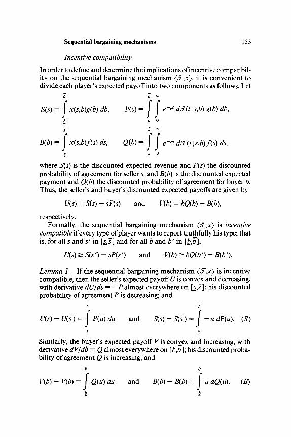
Sequential bargaining mechanisms 155
Incentive compatibilityIn order to define and determine the implications of incentive compatibil-ity on the sequential bargaining mechanism (^,JC), it is convenient todivide each player's expected payoff into two components as follows. Let
b b oo
S(s) = j x(s,b)g(b) db, P(s) = j j e-<* dST(t I s,b) g(b) db9b b 0
B{b) = J x(s,b)f(s) ds, Q(b) = J J e-« d°T{t \ s,b)f(s) ds,s s 0
where S(s) is the discounted expected revenue and P(s) the discountedprobability of agreement for seller s, and B(b) is the discounted expectedpayment and Q(b) the discounted probability of agreement for buyer b.Thus, the seller's and buyer's discounted expected payoffs are given by
U(s) = S(s) - sP(s) and V(b) = bQ(b) - B(b\
respectively.Formally, the sequential bargaining mechanism (9~jc) is incentive
compatible if every type of player wants to report truthfully his type; thatis, for all s and sf in [s,s] and for all b and b' in [b,b],
U(s) ^ S(s 0 - sP(s') and V(b) > bQ(b') - B(b').
Lemma 1. If the sequential bargaining mechanism (ZT,x) is incentivecompatible, then the seller's expected payoff U is convex and decreasing,with derivative dU/ds = —P almost everywhere on [s,s ]; his discountedprobability of agreement P is decreasing; and
5 S
U(s) -U(s)= I P(u) du and S{s) -S(s)= I -u dP(u). (S)S S
Similarly, the buyer's expected payoff V is convex and increasing, withderivative dV/db = Q almost everywhere on [b,b]; his discounted proba-bility of agreement Q is increasing; and
b b
V(b) - V(b) = I Q(u) du and B(b) - B(b) = I u dQ(u). (B)b

156 Peter C. CramtonProof. By definition, seller s achieves the payoff U(s) = S(s) — sP(s).Alternatively, seller s can pretend to be seller s', in which case his payoff isS(s') — sP(s'). In the direct revelation game, the seller s must not want topretend to be seller s', and so we have U(s) ^ S(s') — sP(s') for all s,s' G[s,s], or
U(s)>U(s')-(s-s')P(s'),implying that Uhas a supporting hyperplane at s' with slope — P(s') ^ 0.Thus, U is convex and decreasing with derivative (dU/ds){s) = —P(s)almost everywhere, and P must be decreasing, which implies the firstintegral in (S) (I will use the Stieltjes integral throughout, so that anydiscontinuities in the probability of agreement are accounted for in theintegral.) From integration by parts,
I P(u) du = sP{s) - sP(s) - I u dP(u\
which, together with the definition of U, yields the second integral in (S).The proof for the buyer is identical.
Lemma 1 indicates the stringent requirements that incentive compati-bility imposes on the players' utilities. In particular, it suggests how onecan construct an incentive-compatible payment schedule x, given a prob-ability of agreement distribution ST for which the seller's discounted prob-ability of agreement P(s) is decreasing in s and the buyer's discountedprobability of agreement Q(b) is increasing in b.
Lemma 2. Given the sequential bargaining mechanism <5",JC) such thatPis decreasing, Q is increasing, and S and B satisfy (S) and (B) of lemma 1,then <5",x) is incentive compatible.
Proof. A mechanism is incentive compatible for the seller if for alls,s' G [s,s],
S(s)-sP(s)>S(s')-sP(s').Rearranging terms yields the following condition for incentive compati-bility:
s(P(s') - P(s)) + S(s) - S(s') > 0. (£')From (5), we have
S(s)-S(s')= I -udP(u),
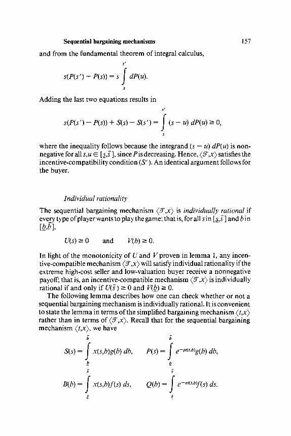
Sequential bargaining mechanisms 157
and from the fundamental theorem of integral calculus,
i = s J dP(u).s(P(s')-P(s))
Adding the last two equations results in
s(P(s') - Pis)) + S(s) - S(s') = J (s-u) dP(u) > 0,s
where the inequality follows because the integrand (s — u) dP{u) is non-negative for all s,uE. [s,s], since Pis decreasing. Hence, (3~,x) satisfies theincentive-compatibility condition (Sf). An identical argument follows forthe buyer.
Individual rationalityThe sequential bargaining mechanism (3~,x) is individually rational ifevery type of player wants to play the game; that is, for all s in [s,s ] and b in
U(s) > 0 and V(b) > 0.
In light of the monotonicity of U and V proven in lemma 1, any incen-tive-compatible mechanism (2T,x) will satisfy individual rationality if theextreme high-cost seller and low-valuation buyer receive a nonnegativepayoff; that is, an incentive-compatible mechanism (^,x) is individuallyrational if and only if U(s)>0 and V(b) > 0.
The following lemma describes how one can check whether or not asequential bargaining mechanism is individually rational. It is convenientto state the lemma in terms of the simplified bargaining mechanism (t,x)rather than in terms of (3',xs). Recall that for the sequential bargainingmechanism (t,x), we have
b b
= I x(s,b)g(b) db, P(s) = I e-rt'^gib) db,
= j x(s,b)f(s) ds, Q(b) = J

158 Peter C. CramtonLemma 3. If the sequential bargaining mechanism (t,x) is incentivecompatible and individually rational, then
Us) + V(,b) - { ( ^ j f p )
i ) ]E0' mwhere the expectation is taken with respect to s and b.
Proof. First note that from lemma 1, for (t,x) to be individually rational,it must be that U(s) > 0 and V(b) > 0. For the seller, we have
f tW(5) </* = £/(J) + j j P(u) duf{s) dsS S
s
i= U(s)+ I F(s)P(s) dsS
b s
= U{s)+\ I F{s)e-^b)g{b) ds db, (US)b s
where the first equality follows from lemma 1 and the second equalityresults from changing the order of integration. Similarly, for the buyer wehaveb b I
I V(b)g(b) db=V(b)+ I 1 ( 1 - G(b))e~^bY(s) ds db. (UB)b b s
Rearranging terms in (US) and (UB) and substituting the definitions forU(s) and V(b), result in the desired expression (IK) for U(s) + V(b).
Lemma 4. If the function t( •, •) is such that P is decreasing, Q is in-creasing, and (IK) is satisfied, then there exists a function x( -, •) such that(t,x) is incentive compatible and individually rational.
Proof. The proof is by construction. Letb s
x(s,b) = ( u dQ(u) + I u dP(u) + c,b s

Sequential bargaining mechanisms 159
where c is a constant chosen such that V{ b) = 0. To compute c, notice that
V(b) = bQ(b) - j x(s,b)f(s) dsS
s s
= bQ(b)-c- I I udP{u)f{s)dss s
s
= kQ(b) -c+ I s(l - F(s)) dP{s) = 0.S
Thus,S
c = tQ(b) + I 5(1 - F(s)) dP(s).S
Incentive compatibility for the seller is verified by showing that theseller s is better off reporting s than s' ¥= s: For all s,s' E.[s,s],
s' s'
s(P(s') - P(s)) + S(s) - S(s') = s J dP(u) - \ u
since P is decreasing. An identical argument holds for the buyer.Since V(b) = 0 and <7,JC) is incentive compatible and satisfies (7i?), it
follows from lemma 3 that U(s) ^ 0. Thus, the bargaining mechanism<7,s) is incentive compatible and individually rational.
Sequential rationalityTo understand how learning takes place in a sequential bargaining mech-anism, it is best to interpret the direct revelation game as follows. At timezero (but after the players know their private information), the playersagree to adopt a particular sequential bargaining mechanism (t,x) that isinterim efficient. (Note that any interim-efficient mechanism can be cho-sen as a Nash equilibrium in an appropriately defined "choice-of-mechanism" game.) The players then report their private information in
160 Peter C. Cramtonsealed envelopes to a mediator, who will then implement the mechanism(t,x). (Actually, a third party is not necessary, since the role of the media-tor can be carried out by a computer programmed by the bargainers toexecute the mechanism.) After opening the envelopes, the mediator doesnot announce the outcome immediately by saying something like, "Tradeshall occur two months from now at the price of one thousand dollars,"but instead waits until two months have passed and then announces,"Trade shall occur now at the price of one thousand dollars." The media-tor must wait until the time of trade in order that the mechanism besequentially rational, since otherwise the bargainers would have an in-centive to ignore the mediator's announcement and trade immediately.
As time passes, the players are able to refine their inferences about theother player's private information based on the information that themediator has not yet made an announcement about. Initially, it is com-mon knowledge that the players' valuations are distributed according tothe probability distributions F and G, but after r units of time thecommon-knowledge beliefs become the distributions F and G condi-tioned on the fact that an announcement has not yet been made; that is,
Fx(s) = F(s | t(s,b) > T) and GT(b) = G(b | t(s,b) > r).Thus, at any time r > 0, the mechanism (t,x) induces an outcome func-tion t(s,b) = t(s,b\FX9Gx) for all s and b. A mechanism (t,x) is sequen-tially rational if at every time r ^ 0, the induced outcome functiont(s,b | Fr,GT) is interim efficient, that is, there does not exist a mechanism(t\x* > preferable to (t,x) at some time r > 0 for all remaining traders andstrictly preferred by at least one trader.
The following lemma relates the definition of sequentially rational tocommon-knowledge dominance.
Lemma 5. A sequential bargaining mechanism (t,x) is sequentiallyrational if and only if it is never common knowledge that the mechanismt( •, • \FX,GT) that it induces over time is dominated by an alternativemechanism.
Proof. From theorem 1 of Holmstrom and Myerson (1983), we knowthat a mechanism is interim efficient if and only if it is not commonknowledge dominated by any other incentive-compatible and individu-ally rational mechanism.
A necessary condition for a mechanism to be sequentially rational isthat the bargainers continue negotiations so long as each expects positivegains from continuing. For the model here, since there are no transaction

Sequential bargaining mechanisms 161
costs (only delay costs), this means that negotiations cannot end if thereexists a pair of players that have not yet come to an agreement, but forwhich agreement is beneficial at some point in the future. Formally, forthe bargaining mechanism (t,x) to be sequentially rational, it must bethat for all potential players, a failure to reach agreement implies thatthere is some point beyond which agreement is never beneficial; that is,for all s and b,t{s,b) = °° ==> there exists f > 0 such that for every r > f, > be(p~a)T.The condition s ^ be{p~a)x is simply a statement that trade is not benefi-cial at time r, sincex - se-*" + be~m - x > 0 <=» se'^ ^ be'™ <^> s > be^~o)x.Notice that the strength of this requirement depends on the relative mag-nitudes of the players' discount rates. When p > a, then e{p~a)x —> °o asr —» oo, and so for all potential pairs of players it is always the case thatthere exists a time at which trade is beneficial. Thus, when p > a, themechanism (t,x) is sequentially rational only if trade always occurs; thatis, t(s,b) < °° for all s and b. Likewise, when p < a, then eip~a)T —» 0 asT —* oo, and so for every pair of players there is always a point at whichtrade becomes undesirable for all times in the future. Finally, if p = a,then the necessary condition for sequential rationality becomes t{s,b) =oo => s ^ b; that is, trade must occur whenever the gains from trade areinitially positive.
To state this necessary condition in a lemma, it will be useful to define% as the set of potential traders for which trade is always beneficial at sometime in the future; that is,
^ = {(s,b) | p>a or (p=o and s^b)}.
Lemma 6. Any mechanism (t,x) that excludes trade over a nonemptysubset of ^ violates sequential rationality.
Proof. Let N C ^ be the set for which trade never occurs. Then, at somepoint in time r, the induced mechanism has t(s,b | Ft,GT) = °° for allremaining traders, which includes Jf. However, this mechanism is notinterim efficient, since it is dominated by a mechanism that results in apositive probability of trade for some traders in N (a partially poolingequilibrium with this property will always exist).
I claim that sequential rationality is a necessary conditiQn for rational-ity in games with incomplete information in which commitment is not
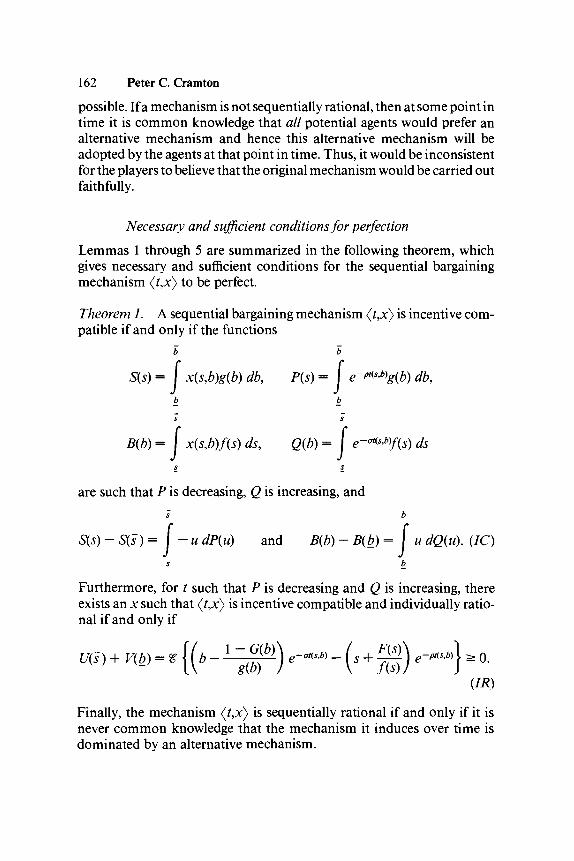
162 Peter C. Cramtonpossible. If a mechanism is not sequentially rational, then at some point intime it is common knowledge that all potential agents would prefer analternative mechanism and hence this alternative mechanism will beadopted by the agents at that point in time. Thus, it would be inconsistentfor the players to believe that the original mechanism would be carried outfaithfully.
Necessary and sufficient conditions for perfectionLemmas 1 through 5 are summarized in the following theorem, whichgives necessary and sufficient conditions for the sequential bargainingmechanism (t,x) to be perfect.
Theorem 1. A sequential bargaining mechanism (t,x) is incentive com-patible if and only if the functions
b b
= I x{s,b)g{b) db, P(s) = J e-o^g(b) db,* b
S(s)-
B{b) = I x(s,b)f(s) ds, Q(b) = I e~<"<s>by(s) dss s
are such that P is decreasing, Q is increasing, andJ b
S(s) ~S(s)= I - u dP(u) and B{b) - B{b) = I u dQ{u). (IC)s b
Furthermore, for t such that P is decreasing and Q is increasing, thereexists an x such that (t,x) is incentive compatible and individually ratio-nal if and only if
)} -°-e~aKs'b)-(s + 7 S ) e~Ms'b)}(IR)
Finally, the mechanism (jt,x) is sequentially rational if and only if it isnever common knowledge that the mechanism it induces over time isdominated by an alternative mechanism.

Sequential bargaining mechanisms 163
8.4 Efficiency
The set of perfect bargaining mechanisms is typically quite large, whichmeans that there are many extensive-form games with equilibria satisfy-ing incentive compatibility, individual rationality, and sequential ratio-nality. To narrow down this set, it is natural to assume additional effi-ciency properties. Three notions of efficiency, described at length byHolmstrom and Myerson (1983), are ex post, interim, and ex ante effi-ciency. The difference between these concepts centers on what informa-tion is available at the time of evaluation: Ex ante efficiency assumes thatcomparisons are made before the players know their private information,interim efficiency assumes that the players know only their private infor-mation, and ex post efficiency assumes that all information is known.
Ex post efficiency
Ideally, one would like to find perfect bargaining mechanisms that are expost efficient. The mechanism (t,x) is ex post efficient if there does notexist an alternative mechanism that can make both players better off interms of their ex post utilities (after all of the information is revealed).(This is often called full-information efficiency in the literature. Holm-strom and Myerson (1983) term this "ex post classical efficiency" todistinguish it from their concept of ex post incentive-efficiency, in whichincentive constraints are recognized.) Equivalently, for a mechanism tobe ex post efficient, it must maximize a weighted sum a{ (s,b)u(s) +a2(s,b)v(b) of the players' ex post utilities for all s and b, where ax{ •, •) ,a2( •, •) — 0 a n d the ex post utilities of seller s and buyer b are
u(s,b) = x(s,b) - se~pt^b) and v(s,b) = be~at^b) - x(s,b).
Since the payoff functions are additively separable in money and goods,and thus utility is transferable between players, we can assume equalweights (i.e., (x^s.b) = a2(s,b) = 1 for every s,b) without loss of generality.To simplify notation, define p(s,b) = e~^b\ so that p(s,b)p is the dis-counted probability of agreement for seller s given that the buyer hasvaluation b, and p(s,b)a is the discounted probability of agreement forbuyer b given that the seller has cost s. With this change, a sequentialbargainingjnechanism becomes the pair of functions (p,x) where p:[s,s] X [b,b] —> [0,1]. The bargaining mechanism (/?,JC), then, is ex postefficient if for all s E [s,s] and b E [b,b], the function p(s,b) is chosen tosolve the program
max n(p) = bpa — spp.[0l]
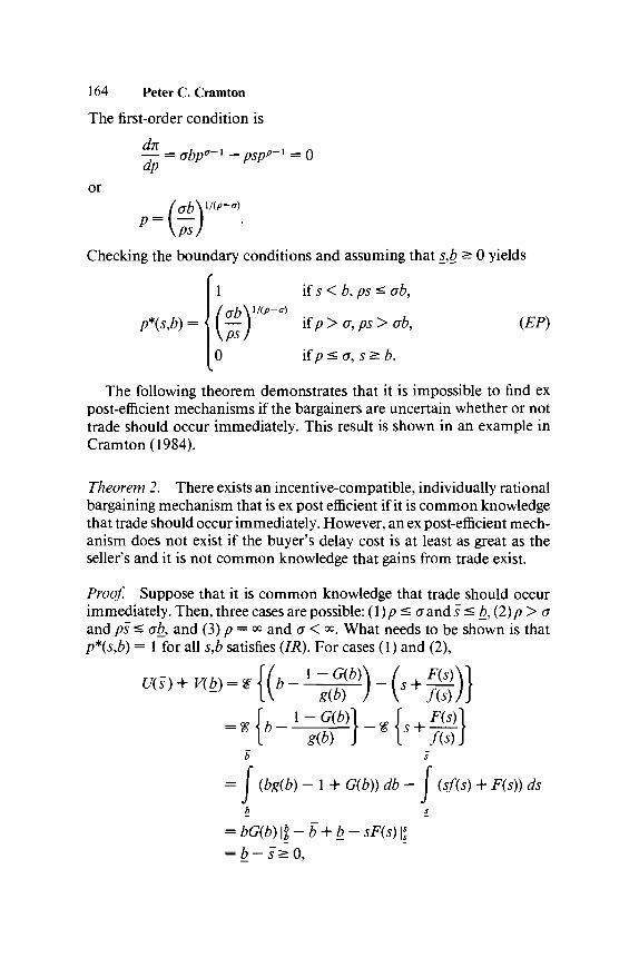
164 Peter C. CramtonThe first-order condition is
dpor
Checking the boundary conditions and assuming that s,b ^ 0 yields
1 if s < b, ps ^ ab,
, ps > ab, (EP)
0 if p < cr, s > b.
The following theorem demonstrates that it is impossible to find expost-efficient mechanisms if the bargainers are uncertain whether or nottrade should occur immediately. This result is shown in an example inCramton (1984).
Theorem 2. There exists an incentive-compatible, individually rationalbargaining mechanism that is ex post efficient if it is common knowledgethat trade should occur immediately. However, an ex post-efficient mech-anism does not exist if the buyer's delay cost is at least as great as theseller's and it is not common knowledge that gains from trade exist.
Proof. Suppose that it is common knowledge that trade should occurimmediately. Then, three cases are possible: (1) p ^ a and s^b,(2)p>aand ps^ crb, and (3) p = °° and a < °°. What needs to be shown is thatp*(s,b) = 1 for all s,b satisfies (IR). For cases (1) and (2),
b s
= \ (bg(b) - 1 + G{b)) db- J(bg(b) - 1 + G{b)) db- J (sf(s) + F(s)) ds

Sequential bargaining mechanisms 165where the integration is done by parts. In case (3),
U(s) + V(b) = % [b - 1 ^ ° j = 6 a 0.
Then, by lemma 4, there exists an x such that (p,x) is incentive compati-ble and individually rational.
Now, assume that it is not common knowledge that gains from tradeexist and the buyer's delay cost is at least as great as the seller's (i.e., p ^ a).Notice that when p < a, we find that (p,x) is ex post efficient if tradeoccurs without delay whenever there are positive gains from trade:
if s < b,
Substituting this function for p into (IR) yields
U(s) + V(b)b min{b,s)
-II {bg{b) + G(b)~ \)f{s)dsdbb s
b rmn{b,s)
- F(s)) ds g{b) dbb s
b b
= I (bg(b) + G(b) - l)F(b) db - I mm{bF(b\s)g{b) dbb b
b b
= - J (1 - G(b))F(b) db+ j (b- s)g(b) dbb
b b
= - 1 ( 1 - G(b))F(b) db + I (1 -G{b)) db
s
= - J (1 - G(u))F{u) du.

166 Peter C. CramtonThus, any incentive-compatible mechanism that is ex post efficient musthave
s
= - I (1 - G{u))F{u) du < 0,U(s)b
and so it cannot be individually rational.
When the seller's delay cost is greater than the buyer's and it is notcommon knowledge that trade should occur immediately, a general proofthat ex post efficiency is not achievable cannot be given due to the com-plicated expression for p*(s,b) in this case. However, analysis of examples(see Section 8.5) suggests that ex post efficiency is typically unobtainable.
Ex ante efficiencyThe strongest concept of efficiency, other than ex post efficiency (which isgenerally unobtainable), that can be applied to games of incomplete in-formation is ex ante efficiency. A player's ex ante utility is his expectedutility before he knows his type. Thus, given the sequential bargainingmechanism (p,x), the seller's and buyer's ex ante utilities are
J J b
°U=\ U(s)f(s) ds = J J (x(s,b) - sp(s,bY)g(b) dbf(s) ds,
u
-Is b
b s
V = J V(b)g(b) db= I I (bp(s,by-x(s,b))f(s) dsg(b) db.b s
The mechanism (p,x) is ex ante efficient if there does not exist an alterna-tive mechanism that can make both players better off in terms of their exante utilities. Thus, for a mechanism to be ex ante efficient, it mustmaximize a weighted sum ax°U + a2V of the players' ex ante utilities,where a{ ,a2 ^ 0. For tractability and reasons of equity, I will assumeequal weights (i.e., ax = a2 = 1). (One might think that the assumption ofequal weights is made without loss of generality, because the payoff func-tions here are additively separable in money and goods, and thus utility istransferable between players. Although this intuition is correct in a settingof complete information, it is false when there is incomplete information,

Sequential bargaining mechanisms 167because an ex ante transfer of utility will violate individual rationality forsome players.) The use of unequal weights would not significantly changethe results, but would greatly complicate the analysis.
If the bargainers were to choose a bargaining mechanism before theyknew their types, it would seem reasonable that they would agree to ascheme that was ex ante efficient. It is generally the case, however, that theplayers know their private information before they begin negotiations,and therefore would be unable to agree on an ex ante-efficient mecha-nism, since the players are concerned with their interim utilities U{s) andV(b) rather than their ex ante utilities °U and Y. Nevertheless, it may bethat the sequential bargaining mechanism is chosen by an uninformedsocial planner or arbitrator, in which case the selection of an ex ante-effi-cient mechanism would be justified. Alternatively, one might supposethat the choice of a bargaining mechanism is based on established normsof behavior and that these norms have evolved over time in such a way asto produce ex ante-efficient mechanisms. In situations where the choice ofa bargaining mechanism does not occur before the players know theirtypes or is not handled by an uninformed third party, ex ante efficiencyis too strong a requirement. The weaker requirement of interim effi-ciency-Xhat there does not exist a dominating mechanism in terms ofthe players' interim utilities U(s) and V(b)-is more appropriate.
The sum of the players' ex ante utilities for the bargaining mechanism(p,x) is given by
by-sP(s9by)f(s)g(b)dsdb.b s
A bargaining mechanism, then, is ex ante efficient if it maximizes this sumsubject to incentive compatibility and individual rationality:
max %{bp{s,b)a - sp(s,by)
such that (P)
where p is chosen such that P is decreasing and Q is increasing. Multiply-ing the constraint by A ^ 0 and adding it to the objective function yields

168 Peter C. Cramtonthe Lagrangian
For any a > 0, define the functions
c(s,a) = s + a -7— and d(b,a) = b — a 7 .g(b)Then, the Lagrangian (ignoring the constant (1 + X)) becomes
,X) = %{d(b,a)p(s,bY - c(s9a)p(s9b)<>),which is easily maximized by pointwise optimization. The first-ordercondition is
- 7 - = o dp°~l — pcpp~l
dp
or
Establishing the boundary conditions and noticing that c( •, •) — 0 yieldsthe optimal solution
if c(s,a) < d(b,a), pc(s,a) ^ ad{b,a),
pa(s,b) =
0 if (p < cr, c(s,a) > d(b,a)) or rf(fe,o:) < 0.The following theorem determines how to find an ex ante-efficient
mechanism for any sequential bargaining game.
Theorem 3. If there exists an incentive-compatible mechanism (p,x)such that p = pa for some a in [0,1 ] and U(s) = V(b) = 0, then this mech-anism is ex ante efficient. Moreover, if c( • ,1) and d( • ,1) are increasing
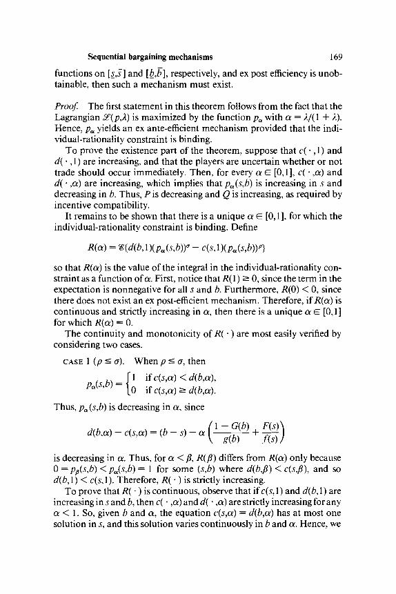
Sequential bargaining mechanisms 169
functions on [s,s] and [b,b], respectively, and ex post efficiency is unob-tainable, then such a mechanism must exist.
Proof. The first statement in this theorem follows from the fact that theLagrangian £(p,A) is maximized by the function pa with a = A/(l + A).Hence, pa yields an ex ante-efficient mechanism provided that the indi-vidual-rationality constraint is binding.
To prove the existence part of the theorem, suppose that c( •, 1) andd( •, 1) are increasing, and that the players are uncertain whether or nottrade should occur immediately. Then, for every a E [0,1], c( • ,a) andd{ • ,a) are increasing, which implies that pa(s9b) is increasing in s anddecreasing in b. Thus, P is decreasing and Q is increasing, as required byincentive compatibility.
It remains to be shown that there is a unique a E [0,1 ], for which theindividual-rationality constraint is binding. Define
R(a) = %{d(b,\)(pa(s,b)y - c(s,\)(pa(s,b))p)
so that R(a) is the value of the integral in the individual-rationality con-straint as a function of a. First, notice that R( 1) > 0, since the term in theexpectation is nonnegative for all s and b. Furthermore, R(0) < 0, sincethere does not exist an ex post-efficient mechanism. Therefore, if R(a) iscontinuous and strictly increasing in a, then there is a unique a E [0,1]for which R(a) = 0.
The continuity and monotonicity of R( •) are most easily verified byconsidering two cases.
CASE 1 (p < a). When p^ a, then
) < d(b9a)9Ptt(S'D) [0 if c(s9a)^d(b9a).
Thus, pa(s9b) is decreasing in a, since
is decreasing in a. Thus, for a < /?, R(fi) differs from R(a) only because0 = Pp{s,b) < pa(s,b) = 1 for some (s,b) where d(b9fi) < c(s9fi)9 and sod(b9l) < c(s9l). Therefore, R( -) is strictly increasing.
To prove that R(-)is continuous, observe that if c(s,l) and d(b,\) areincreasing in s and b, then c{ • ,a) and d( • ,a) are strictly increasing for anya < 1. So, given b and a, the equation c(s,a) = d(b,a) has at most onesolution in s, and this solution varies continuously in b and a. Hence, we

170 Peter C. Cramtonmay write
b r(b,at)
{d{b,\)-c{s,\))f(s)g{b)dsdb,b s
where r(b,a) is continuous in b and a. Thus, R(a) is continuous in a.CASE 2 (p > a). When p > a, then
1 if oc{s,a) ad(b,a),
a) > ad(b,a) > 0,
0 ifd(b,a)^0.
Since
ad(b,a) -pc(s,a) = ob-ps-ot [a\
777) ,f(s)),ct) = a (b-a[(l-G(b))/g(b)]\,a) p\ S +
(pc(s,a) p\ S + a[F(s)/f(s)]
and d(b,a) are decreasing in a, pa(s,b) is decreasing in a. Thus, for a < /?,i?(/J) differs from JR(a) only becausePp(s,b) < pa(s,b) for some (s,b) wheread{b,a) < pc{s,a). Therefore, R( •) is strictly increasing.
Since c( • ,a) and rf( • ,a) are strictly increasing for any a < 1, the equa-tion d(b,a) = 0 has at most one solution in b and the equation pc(s,a) =ad(b,a) has at most one solution in 5, and the solutions vary continuouslyin b and a. Hence, we may write
b r(b,a)
(j (d(b,l)-c(b,l))f(s)ds
s
+ j [d(b, 1 )(pa(s,b)Y ~ c(s91XA, (s,b))p] f(s) ds^j g(b) db,r(b,a)
where q{a) and r(b9a) are continuous in b and a. Therefore, R(a) iscontinuous in a.
Since i ( •) is continuous and strictly increasing, with R(0) < 0 andR( 1) > 0, there must be a unique «G[0, l] such that R(a) = 0 and/?a (5,6)is ex ante efficient.

Sequential bargaining mechanisms 171It is worthwhile to point out that the requirement in the existence part
of theorem 3 that c( •, 1) and d{ •, 1) be increasing functions is satisfied bya large range of distribution functions. A sufficient condition for c{ •, 1)and d{ •, 1) to be increasing is for the ratio of the distribution and thedensity to be increasing. This is a local characterization of the monotonelikelihood ratio property and is satisfied by many distributions, such asthe uniform, exponential, normal, chi-square, and Poisson distributions.
I now prove that the ex ante-efficient mechanism typically violatessequential rationality, and hence show that bargainers who are unable tomake binding commitments are worse off (in an ex ante sense) thanbargainers who are able to commit to particular strategies.
Corollary L If ex post efficiency is unobtainable, c( •, 1) and d( •, 1) areincreasing functions, and d(b,l) < 0 if p > a, then the ex ante-efficientmechanism violates sequential rationality.
Proof. By theorem 3, the ex ante-efficient mechanism exists and is givenby pa for some a > 0. Consider the set of traders who never trade underpa, but for whom trade is always beneficial at some point in the future:
Jf = {(s,b)\pa(s,b)=O and [p>o or {p=o and s<bj\).By our hypothesis, this set is nonempty. Thus, from lemma 6, the mecha-nism pa violates sequential rationality.
8.5 The case of uniform symmetric exchange:An example
To illustrate the theory presented in the earlier sections, it will be useful tolook at an example. In particular, consider the case of uniform symmetricexchange in which both the seller's cost and the buyer's valuation areuniformly distributed on [0,1]. Then, c(s,a) = (\ + a)s and d(b,a) =(1 + a)b — a, which are strictly increasing when a = 1, and so bytheorem 3 we know that, for some a G [0,1 ], the mechanism p = pa is exante efficient. The desired a is found by setting R(a) to zero, so thatU(s) = V(b) = 0. Again, it will be useful to consider two cases dependingon whether p ^ o or p > o.
CASE 1 (p < a). When p < a, then
a1 if s<b-
pa(s,b) = )0 if s ^ b — 1 +a

172 Peter C. CramtonDefine ju = a/(\ + a). Then, we wish to find ju G [0,i] such that
1 b-fi
R(a)i= ) I (2(b-s)- \)dsdb = 0.fj, 0
Performing the integration yields
which has a root in [0,i] at n = $. Thus, a = ^ and
1 i f j < 6 - | ,
0 ifs*b-\.4
When /? < cr, ex ante efficiency is obtained by a mechanism that transfersthe object without delay if and only if the buyer's valuation exceeds theseller's by at least \. Perhaps somewhat surprisingly, the ex ante-efficientmechanism in this case does not depend on p or a. Since the value of theobject is declining more rapidly for the buyer than for the seller, it isalways better to transfer the item immediately, if at all. Hence, eventhough the players can reveal information by delaying agreement, in theex ante-efficient mechanism they choose to trade immediately or not atall, so that a static mechanism ex ante dominates any sequential bargain-ing mechanism. This static mechanism, however, is not sequentially ra-tional, which illustrates corollary 1.
An extensive-form game that implements the ex ante-efficient mecha-nism when p ^ a has been studied by Chatterjee and Samuelson (1983).They consider the simultaneous-offers game, in which the players simul-taneously announce prices and the object is traded if the buyer's bidexceeds the seller's offer. For this example, the seller's optimal strategy isto offer the price \s + i, and the buyer's best response is to bid \b + ^which implies that trade occurs provided that \s + \ < \b 4- ^ or s <b — i, as in the ex ante-efficient mechanism. For this equilibrium, theprice at which the object is sold is
x(s,b) =
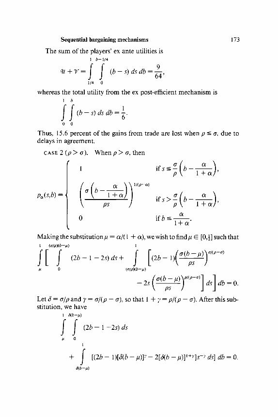
Sequential bargaining mechanisms
The sum of the players' ex ante utilities is1 6-1/4
9(b — s) ds db = —,64
1/4 0
whereas the total utility from the ex post-efficient mechanism is1 b
6
173
0 0
Thus, 15.6 percent of the gains from trade are lost when p < a, due todelays in agreement.
CASE 2 (p > a). When p> a, then
pa(s,b) ='AP-«)
ps
0
*,>
if 6
p \ 1 + a)a
aMaking the substitution fi = a/(l + a), we wish to find/i e [0, ] such that1 (a/p)(b-n) 1
'a(b -(2b - 1 - 2s) ds
0 (o/pXb-M)!
Let ^ = a//? and y = o/{p — a), so that 1 + y == /?/(/? — cr). After this sub-stitution, we have
(2b - 1 -2s) ds
I+ I [(2b - l)[S(b - ju)f - 2[S(b - //)]1+y].ry ds] db = 0.

174 Peter C. Cramton
P e r f o r m i n g t h e i n n e r i n t e g r a t i o n ( a s s u m i n g y ^ \ ) y i e l d s
f[3(b-ii)[(2-S)b + Spi-l]
+ — — [2(1 - 3)b + 28\x - \\\S(b-ii)\\\ - [S(b - ju)]l~y} I db
= I S{(2 - «
-S)b + 2SJU - l]{[3(b-fj)Y ~ S(b-ju)} db
W ~ {y[l + 2/*( 1 - 3)] - 2Sju}b
+ Sju2 - yju(l - S/j) + [2(1 - S)b + 23ju - \]S^-\b-/iy \db = 0.
Since
+ y1
and
after integration we have
(1 - ju3)[S - y(2 - . 2
\+y
Dividing by <S( 1 — //)/(1 — y), yields

Sequential bargaining mechanisms 175
+M2)[S-y(2-S)] + (\ +nMl + 2 (1 -S)] - 2dn)
dn) + Sr~l{l+~^y (R)
Given S = a/p, a root ju E [0,£l to (R) is easily found numerically.The sum of the players' ex ante utilities is computed as follows:
1 S(b-M) 1
= I I (b-s)ds+ I
+ y ^ [(1 - 5)b + Sn][S{b - fi)]V - [S(b - ti)]l-y)\ db1
J 737 [ ( I %l + y)-y)b2 + [fir - <W + y))b
+1 Sn2{\ +y) + S^Kl - S)b + d^]{b - iiy db
The value of// and the efficiency of the ex ante-efficient mechanismrelative to the first-best (full-information) solution are shown in Figure8.1 and Figure 8.2, respectively, as the ratio of the players' discount rates is
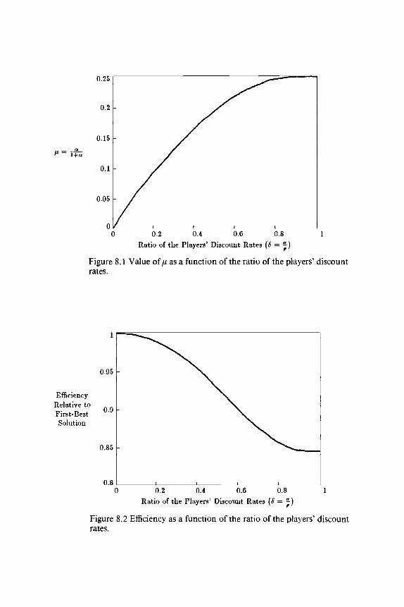
0.25
0.2
0.15
0.1
0.05
0 /0 0.2 0.4 0.6 0.8 1
Ratio of the Players' Discount Rates (6 = J)
Figure 8.1 Value of// as a function of the ratio of the players' discountrates.
EfficiencyRelative toFirst-BestSolution
0.95 -
0.85 -
0.80.2 0.4 0.6 0.8
Ratio of the Players' Discount Rates (6 — - )
Figure 8.2 Efficiency as a function of the ratio of the players' discountrates.

Sequential bargaining mechanisms 177
varied from 0 to 1. Bargaining efficiency improves as the seller's discountrate is increased relative to the buyer's. When the players' discount ratesare equal, 15.6 percent of the gains from trade are lost due to delays inagreement. This inefficiency decreases to zero as /> —* °°, illustratingtheorem 2.
8.6 Conclusion
Two important features of any bargaining setting are information andtime. Bargainers typically have incomplete information about eachother's preferences, and therefore must communicate some of their pri-vate information in order to determine whether or not gains from tradeexist. One means of communication is for the agents to signal their privateinformation through their willingness to delay agreement: Bargainerswho anticipate large gains from trade will be unwilling to delay agreementand so will propose attractive terms of trade that the other is likely toaccept early in the bargaining process, whereas bargainers expecting smallgains will prefer to wait for better offers from their opponent. In thischapter, I have described the properties of such a bargaining model, byanalyzing a sequential direct revelation game.
Modeling the bargaining process as a sequential game, where the agentscommunicate their private information over time, has two main advan-tages. First, from the point of view of realism, one commonly observesbargaining taking place over time. Second, any static bargaining mecha-nism, because it does not permit the agents to learn about their oppo-nent's preferences, must end with positive probability in a situation wheregains from trade are possible and yet no agreement is reached. If bothbargainers know that gains from trade exist, what prevents them fromcontinuing negotiations until an agreement is reached? By introducingthe time dimension, and hence allowing the bargainers to communicatethrough their actions over time, one is able to construct perfect bargainingmechanisms, in which the bargainers continue to negotiate so long as theyexpect positive gains from continuing.
When the bargainers discount future gains according to known andfixed discount rates, it was found that the bargainers may be better off (interms of their ex ante utilities) using a sequential bargaining mechanismthan a static scheme. This is the result of the time dimension introducingan additional asymmetry into the problem, which may be exploited toconstruct sequential bargaining mechanisms that ex ante dominate themost efficient static mechanisms. Even in situations where a static mecha-nism is ex ante efficient, it is unlikely that such a mechanism would be

178 Peter C. Cramtonadopted by the bargainers, since it necessarily would violate sequentialrationality.
The analysis presented here represents an early step toward under-standing how agreements are reached in conflict situations under uncer-tainty. Several simplifying assumptions have been made in order to keepthe analysis manageable. First, modeling the agents' time preferences withconstant discount rates is an appealing example, but not an accuratedescription of all bargaining settings. (Fishburn and Rubinstein (1982)derive under which circumstances the discounting assumption is valid. Inparticular, they prove that any preferences over bargaining outcomes thatare monotonic, continuous, and stationary can be represented by dis-counting provided the bargainers exhibit impatience over all outcomesexcept that of no agreement.) Second, the agents have been assumed to berisk neutral, but in many bargaining situations the agents' willingness totake risks is an important bargaining factor. Third, I have restricted atten-tion to rational agents who can calculate (at no cost) their optimal strate-gies. Certainly, few agents are so consistent and calculating. With less-than-rational agents, an agent's capacity to mislead his opponentbecomes an important variable in determining how the gains from tradeare divided. Finally, I have assumed that the players' valuations are inde-pendent. However, in many settings the bargainers' valuations will becorrelated, and so, for example, the seller's willingness to trade may be asignal of the valuation of the object to the buyer.
Although it would be useful in future research to weaken the simplify-ing assumptions made here, perhaps the most fruitful avenue for furtherstudy is the analysis of specific extensive-form bargaining games. Theadvantage of looking at specific extensive-form games is that the bargain-ing rules are independent of the probabilistic beliefs that the players haveabout each other's preferences. In a direct revelation game, on the otherhand, the bargaining rule depends in a complicated way on these probabi-listic beliefs. Because of this dependence, direct revelation games are notplayed in practice.
Can one find a strategic game that comes close to implementing the exante-efficient bargaining mechanism over a wide range of bargainingsituations? Initial studies along these lines have been conducted by Cram-ton (1984), Fudenberg and Tirole (1983), and Sobel and Takahashi(1983). All three papers consider a model in which only one of the bar-gainers makes offers. When the players' reservation prices are uniformlydistributed on [0,1 ] and their discount rates are equal, it was found thatthis model results in 32 percent of the gains from trade being lost, asopposed to 16 percent being lost when the ex ante-efficient bargainingmechanism is adopted (Cramton (1984)). Thus, the players' inability to

Sequential bargaining mechanisms 179
commit to ending negotiations results in a bargaining outcome that issignificantly less efficient than if commitment were possible.
Perhaps a better candidate for a strategic bargaining game that is nearlyex ante efficient is the game in which the bargainers alternate offers. Thisgame was analyzed by Rubinstein (1982) in a setting of complete infor-mation, but an analysis with incomplete information has yet to be done.Of particular interest is the alternating-offers game as the time betweenoffers goes to zero, because this strategic game represents a very generalbargaining rule: At any time, a bargainer may make a new offer or acceptthe most recent offer of his opponent. It would be a pleasant surprise ifsuch a reasonable bargaining game was nearly ex ante efficient over avariety of circumstances.
A second promising area for research is further study on the implica-tions of sequential rationality to bargaining and to more general games ofincomplete information. I intend to address this issue in depth in futureresearch.
REFERENCES
Chatterjee, Kalyan, and William Samuelson (1983): Bargaining under Incom-plete Information. Operations Research, Vol. 31, pp. 835-51.
Cramton, Peter C. (1984): Bargaining with Incomplete Information: An Infinite-Horizon Model with Continuous Uncertainty. Review of Economic Stud-ies, Vol. 51, pp. 579-93.
Fishburn, Peter C, and Ariel Rubinstein (1982): Time Preference. InternationalEconomic Review, Vol. 23, pp. 719-36.
Fudenberg, Drew, and Jean Tirole (1983): Sequential Bargaining with IncompleteInformation. Review of Economic Studies, Vol. 50, pp. 221-47.
Gresik, Thomas A., and Mark A. Satterthwaite (1983): The Number of TradersRequired To Make a Market Competitive: The Beginnings of a Theory.Research Paper No. 551, Graduate School of Management, NorthwesternUniversity.
Holmstrom, Bengt, and Roger B. Myerson (1983): Efficient and Durable Deci-sion Rules with Incomplete Information. Econometrica, Vol. 51,1799 -1820.
Kreps, David M., and Robert Wilson (1982): Sequential Equilibria. Economet-rica, Vol. 50, pp. 863-94.
Myerson, Roger B., and Mark A. Satterthwaite (1983): Efficient Mechanism forBilateral Trading. Journal of Economic Theory, Vol. 28, pp. 265-81.
Selten, R. (1976): Reexamination of the Perfectness Concept for EquilibriumPoints in Extensive Games. International]ournal of Game Theory, Vol. 4,pp. 25-53.
Sobel, Joel, and Ichiro Takahashi (1983): A Multi-Stage Model of Bargaining.Review of Economic Studies, Vol. 50, pp. 411 -26.
Wilson, Robert (1982): Double Auctions. Technical Report No. 391, StanfordInstitute for Mathematical Studies in the Social Sciences.


CHAPTER 9
The role of risk aversion in a simplebargaining model
Martin J. OsborneCOLUMBIA UNIVERSITY
The purpose of this paper is to study the effect of a change in an individ-ual's degree of risk aversion on the perfect Bayesian Nash equilibrium in asimple model of bargaining. I find that, contrary to the results in theaxiomatic model with riskless outcomes due to Nash, an opponent maybe made worse off by such a change. Further, an individual may want totake an action that identifies him as more, rather than less, risk aversethan he really is. In the course of the analysis, I fully characterize theequilibria of a class of "wars of attrition" with incomplete information,and single out one as "perfect" in a certain sense; this result may be ofindependent interest.
9.1 Introduction
The role of risk aversion in bargaining has been widely studied within theaxiomatic framework of Nash (1950) (see, for example, Roth (1979),Perles and Maschler (1981)). It has been found that if the negotiationconcerns riskless outcomes, then the more risk averse an individual is, thehigher the payoff of his opponent. Related results show that in this case itis to the advantage of an individual to "pretend" to be less risk averse than
I am grateful to Vincent Crawford, Vijay Krishna, Carolyn Pitchik, John Riley,Alvin Roth, Ariel Rubinstein, Charles Wilson, Allan Young, and two anonymousreferees for very helpful discussions and comments. A number of participants inthe Conference on Game-Theoretic Models of Bargaining at the University ofPittsburgh, June 1983, also made valuable comments. I first worked on the issueconsidered in this paper during a most enjoyable visit to the Institute for Ad-vanced Studies, Hebrew University of Jerusalem, in Spring 1980; I am grateful tothe Institute for its hospitality and for partial financial support. This work wasalso partially supported by grants from the Council for Research in the SocialSciences at Columbia University in the summers of 1981-83, and from theNational Science Foundation (SES-8318978).
181

182 Martin J. Osbornehe really is (Kurz (1977, 1980), Thomson (1979), Sobel (1981)). Theseresults have some intuitive appeal: Given any (probabilistic) beliefs aboutthe behavior of his opponent, it seems that an individual should behavemore cautiously, the more risk averse he is. However, this fact influenceshis opponent's behavior, and without a more detailed specification of theinformation possessed by both parties and of the precise structure of thenegotiation, it is not clear how the equilibrium behavior changes. (In thecase where the potential agreements involve lotteries, the axiomaticmodel predicts that an increase in an individual's risk aversion mayreduce the payoff of his opponent (see Roth and Rothblum (1982)). Here,I restrict attention to the case in which agreements concern risklessoutcomes.)
It is natural to investigate these issues by modeling the process ofnegotiation as a (noncooperative) strategic game, and by studying theeffect of changes in the players' risk aversions on the characteristics of theNash equilibria. For such a comparative static exercise to make sense, thegame must have a unique equilibrium. It is clear that if the equilibriumstrategies are pure, then a change in a player's risk aversion that preserveshis preferences over certain outcomes has no effect on his opponent'spayoff. (This is the case, for example, in Rubinstein's (1982) model.1)Thus, for the degree of risk aversion to influence the outcome, the equilib-rium strategies must involve randomization.
The model that I analyze is designed with these facts in mind. It is asimple version of those formulated by Hicks (1932), Bishop (1964), andCross (1965). At each time in [0,1 ], two individuals can produce a flow ofone unit of some good desirable to them both. Before production canbegin, a contract must be negotiated that specifies how the flow of outputwill be divided between the two parties. At time 0, each party begins bydemanding some fraction of the flow - say individual / demands dt(0). Solong as the demands are incompatible (i.e., sum to more than the outputavailable), no production takes place. In the most general version of themodel, at each time, each individual may adjust his demand. If t is the firsttime at which the demands are compatible, and in fact dx(t) + d2(t) = 1,then at each time in [/,1] each individual / receives the flow dt{t). Thismost general form of the model is unwieldy; in order to get some ratherspecific results, I assume that the allowable concession patterns are veryspecial.
In the simplest case (considered in Sections 9.2 and 9.3), the demandsof both individuals at time 0 are fixed, incompatible, and the same. Ateach time, each individual may leave his demand the same, or concede tothat of his opponent. I model the interaction between the individuals as astrategic game2 in which a pure strategy of an individual is an element t of

The role of risk aversion 183
[0,1], with the interpretation that the individual will concede at t if hisopponent has not done so by then. (Once his opponent has conceded,there is no cause for further action on his part.) In a slightly richer versionof the model (considered in Section 9.4), each individual may choose howmuch to demand at time zero, but may subsequently only stand firm orconcede. Though there are clearly many aspects of negotiation not in-cluded in this model, it does capture the tradeoff involved in the intuitivearguments concerning the effects of changes in risk aversion. That is, bydelaying concession, an individual sacrifices payoff now in return for thechance that his opponent will concede in the future.
As regards the informational structure of the negotiation, I assume thateach individual may be one of many types, which differ in their degrees ofrisk aversion. The solution is that of Bayesian Nash equilibrium, modifiedby "perfection" of a certain sort (see Section 9.3). This standard solutioncaptures the idea that each player is uncertain of the type of his opponent.However, it may also be given a more concrete interpretation. Thus,suppose that there are two populations, each consisting of a continuum ofindividuals of different types. In any play of the game, each member ofone population is randomly matched with a member of the other popula-tion. A Bayesian Nash equilibrium has the property that if each individ-ual's beliefs about the distribution of concession times in the opponentpopulation is correct, then his equilibrium strategy is optimal. Given thisinterpretation, it is natural to consider also the case where members of asingle population are matched with each other. From the point of view ofthe Bayesian Nash equilibrium, this is, of course, simply a special case ofthe two-population model, in which the characteristics of both popula-tions are the same, and attention is restricted to symmetric equilibria (i.e.,equilibria in which the strategies used in both populations are the same).However, the comparative static question, which is my main focus, re-quires separate analysis in the two cases. Viewed as a special case of thetwo-population model, a change in risk aversion of a potential opponentin the one-population case is a change not only in the characteristics of theopponent population, but also in the characteristics of the player's ownpopulation. Given this, I analyze the two cases separately.
First, consider the case in which initial demands are fixed. In theone-population model, there is a unique equilibrium distribution of con-cession times3; in the two-population model, there is a set of equilibria(characterized in theorem 3), but only one is perfect in a certain sense (seeproposition 5). In both cases, more risk averse individuals concede earlierin the (perfect) equilibrium. The comparative static results are as follows.
In the one-population case, an individual is made better off by anincrease in the risk aversion of his potential opponents, whereas in the

184 Martin J. Osbornetwo-population case, the opposite is true. Thus, in the two-populationmodel, the prediction of Nash's model is not supported. Unless one arguesthat the model does not capture some essential aspect of bargaining, orthat Nash equilibrium is an inappropriate solution concept, the conclu-sion is that the effect of a change in an opponent's risk aversion on anindividual's negotiated payoff can go in either direction, depending on theprecise structure of the negotiation.
To address the issue of "distortion" of preferences in this simple model,I consider how an individual's payoff changes as the fraction of his ownpopulation that is less risk averse than him increases. This change causeshis opponents to believe with smaller probability that he is risk averse, andso gives him an opportunity to "pretend" that he is not. However, such achange does not affect his equilibrium payoff, although it does reduce thepayoff of his less risk averse colleagues.
Although the simple version of the model does not fit into Nash'sframework (the set of payoffs to possible agreements may not be convex),it is clear that the solution does not obey appropriately modified versionsof his axioms. Most conspicuously, the (perfect) equilibrium is notPareto-efficient. This lack of efficiency does not derive from uncertaintyabout opponents' payoffs - even if everyone is identical, the solution isnot efficient. Rather, it is the (inevitable) uncertainty about opponents'actions that prevents agreement at time zero. It seems that the continuousnature of the model contributes to this outcome: If disagreement is once-and-for-all (as in Nash's (1953) "demand game"), then it seems less likelythat it will be the outcome of negotiation. If, on the other hand, demandsmay be adjusted continuously (or, in the simple case here, a concessioncan be made at any time), then it seems quite unlikely that an equilibriumwill involve agreement from the very beginning.
My analysis of the case in which initial demands may be chosen islimited. I show that when there are two types in each population and twopossible initial demands, there is no separating equilibrium in which allmembers of a given type choose the same demand and the two types ineach population choose different demands. The reason for this is that theless risk averse individuals can benefit from pretending to be more riskaverse (see Section 9.4). There is thus another sense in which the modelworks differently from the axiomatic one of Nash. I also show that there isa continuum of pooling equilibria, in which a positive fraction of eachtype in each population makes each initial demand. Given this non-uniqueness, it is not possible to perform the comparative static exercisesdiscussed previously; it is an open question whether the model can bemodified to produce a unique equilibrium. However, the analysis doesshow that the basic model does not degenerate when choice of initialdemand is allowed.

The role of risk aversion 185Recently, a number of authors (e.g., Samuelson (1980), McLennan
(1981), Crawford (1982), Rubinstein (1982), Chatterjee and Samuelson(1983), Fudenberg and Tirole (1983a), and Sobel and Takahashi (1983))have modeled bargaining as a noncooperative strategic game. None ofthese focuses specifically on the role of risk aversion. In most cases, thebargaining parties are assumed to be risk neutral (although Samuelson(1980) and Chatterjee and Samuelson (1983) do contain some analysis ofthe effect of changes in the players' risk aversions). The model here,designed specifically to address the role of risk aversion, differs in severalrespects from these models. Most significantly, time runs continuously,so that the players have great flexibility in choosing their time of action. Aplayer can always wait a short time (thereby losing at most a very smallamount of payoff) in case his opponent will concede; if time is discrete,this is not possible. Note, however, that because the possibility for chang-ing demands is so limited, players' actions (or lack thereof) transmit nouseful information during the course of play (except for their choice ofinitial demand, when this is allowed), whereas this information transmis-sion is central to some of the models just cited. Young (1983) analyzes amodel that is in some respects similar to the simple model consideredhere. However, the structure of the payoffs in his model is not quite thesame, and time is discrete; he does not consider the effect of changes inrisk aversion.
The game associated with the simple version of my model is what isknown in the literature as a "war of attrition" (see, for example, Riley(1980)). Nalebuff and Riley (1984) have (independently) found a class ofequilibria in a model that is different in some respects from mine (e.g., thetime horizon is infinite, and there is a continuum of types), but is similarin general structure. However, they do not show that they have found allof the equilibria; nor do they consider the issue of perfection, or the effectof a change in an individual's risk aversion. Also related is the work ofFudenberg and Tirole (19836), who have (independently) shown that, inanother version of a war of attrition, there is a unique Bayesian Nashequilibrium that is perfect in a certain sense.
9.2 Bargaining within a single population
The modelThe population consists of a continuum of individuals. The environmentof the negotiation between any two individuals is as follows. Time runscontinuously in [0,1 ]. At each point in time, a flow of one unit of outputcan be produced, if the individuals can agree how to split it between them.The rules of negotiation are simple. At time 0, each individual demands

186 Martin J. Osborne\ < a < 1 units of output. At any subsequent time in [0,1], each mayconcede to the demand of the other. The outcome of negotiation for eachindividual is an output stream x: [0,1 ] —• [0,1 ] of the form
0 if 0 < 5 < r,
where 0 ^ t ^ 1 and 0 ^ x ^ 1. Such an output stream is characterized bythe pair (x,t) E [0,1 ]2. If an individual is first to concede, and does so at t,he receives the output stream (1 — a,t)\ his opponent receives (a,t). If theindividuals concede simultaneously at t, the equilibrium of the game thatI study is independent of the output stream received by each individual, solong as that stream is of the form (c,t), where 1 — a < c < a; for notationalconvenience, I assume that it is {\J). There are m types of individuals. Thefraction yt > 0 of the population is of type z(= 1, . . . , m). The prefer-ences over lotteries on output streams of individuals of type / are repre-sented by a von Neumann-Morgenstern utility function ut: [0,l]2—» U+with the following properties:
(P.I) For each (x,t), Mf-(x,l) = ut(09t) = 0;(P.2) For each t < 1, ux is increasing in x;(P. 3) For each x > 0, w, is continuous in t, and continuously differentiate and
decreasing in t whenever t < 1.
In order to isolate the role of risk aversion, I assume that all of the typeshave the same preferences over sure outcomes; they differ only in theirdegrees of risk aversion, type / being more risk averse than type / + 1.Precisely, a utility function v is more risk averse than a utility function u ifthere is a strictly concave function/: U+ —»R+ such that v=f°u.I assumethe following:
(P.4) For each / = 1, . . ., m — 1, ut is more risk averse than ui+l.
It is easy to check that an example of a collection {ut} of utility func-tions that satisfies (P.I) through (P.4) is that for which uf(x,t) =(1 - t)aix% with 0 < ax < a2 < • • • < am < 1.
The only choice an individual has is the time at which to concede.Thus, a (mixed) strategy of an individual is simply a cumulative probabil-ity distribution on [0,1 ]. Only the average strategy of individuals of type /is determined in equilibrium, not the strategy of any particular individual.I refer to this average strategy as the strategy ofi, and denote it Et. For each0 < J< 1, let
mG{t) = £ ytEt{f), (9.1)

The role of risk aversion 187
so that G(t) is the probability that a randomly selected individual con-cedes at or before 1.1 refer to G as the distribution ofconcession times in thepopulation. The distribution of concession times relevant to an individ-ual's choice is the one generated by all of the other individuals' strategies.However, since the population is nonatomic, this is the same as G. If anindividual of type / uses the pure strategy t, his expected payoffin negotia-tions with a randomly selected opponent is
I UiPt(t9G) = I ut(a9s) dG(s) + ut{\,t)JG{t) + K,(1 -aj)(\ - G{t)\ (9.2)[0,0
where JG{t) is the size of the atom in G at t. The payoff to the mixedstrategy Et is Pt(Ei9G) = f[0A] Pt(t9G) dEt(t)9 and (El9 . . . , £ J is a(Bayesian Nash) equilibrium if for / = 1, . . . , m we have
Pt{EhG) > P/(£,G) for all strategies £,where G is defined in (9.1).
EquilibriumThere is a unique equilibrium (El9 . . . , Em), defined as follows. Thereexist numbers 0 = p0 < • • • <p y= • • • p m = 1 such that the supportof Ei (denoted supp Et) is equal to [pi_l,/?,] for / = 1,. . . , m. The strate-gies Ej are nonatomic on [0,1), and such that G causes the payoffi*(t,G) ofan individual of type / to be constant on [pt-i 9pt], A distribution G withthis property can be found by solving the differential equations obtainedby setting equal to zero the derivative with respect to t of each Pt(t,G). Wefind that, for some A > 0, for pi_l < t <pi9
i.
expU
where, for any \<a< \,\<b< 1, and 0 ^ s < 1, and any utility func-tion u: [0,l]2 -^ M+, the function [/is defined by
U(a,b,s)= u(b,s)- u{\ -(I have made the definition of U more general than necessary for thepresent purposes; it will be used also later.) Now, the fact that G is gener-ated by the is/s means that the equilibrium is as follows. For notationalconvenience, let F(0) = 0 and F(/c) = Sf=1, yt^ for k = 1, . . . , m. Thep/s

188 Martin J. Osborneare defined iteratively. First, p0 = 0. Now, given pi_l < 1, suppose thatthere exists p < 1 such that
1 i r a ( - i ) = e x p ( ~ / Ui{a'a's)ds)•) ( 9 - 4 )
Pi-1
Then, let pt = p, and continue the process. If there is no such p, set / = yand let py = py+l = • • • = pm = 1. For / = 1, . . . , y, the equilibriumstrategy £, of type / has support [pt-x ,p(],
[ l - exp( - J £/,(*,*,.*) rfsj]E,(t) = [i - n / - i)] — ifP/_, ^ t<Pl,
(9.5)and Et(t) = 1 if/?, ^ /. For / = y + 1, . . . , m, the equilibrium strategy £, ispurely atomic, with mass at t = 1 (i.e., Et{t) = 0 if £ < 1 and 2?,-(l) = 1).
The fact that this defines an equilibrium, and that there is no other,follows from the results of Section 9.3 (see corollary 4). However, it is easyto check that each Et is a strategy and that Pt{t,G) is constant on [/?,_x ,pt](=supp£,).
Note that if all individuals are identical, the equilibrium does notdegenerate - in fact, all individuals then use mixed strategies with support[0,1 ]. The only efficient outcome is for all to concede at time 0, but this isnot an equilibrium. If all individuals in a set S of positive measure concedeat time 0, the distribution of concession times in the population containsan atom at 0. Hence, every individual, including those in S, can benefitfrom waiting a short period, and so it is not optimal for them to concede attime 0.
The effect of a change in risk aversionLet k be such that pk < 1 (i.e., in the unique equilibrium, individuals oftype k concede with probability 1 before time 1). Now, suppose thatindividuals of type k become more risk averse, but not more so thanindividuals of type k — 1. That is, consider a new game in which the utilityfunction of type k is uk, which is more risk averse than uk, and less riskaverse than uk_ x. (Throughout, I use a circumflex to denote the new valueof an object.) This means that the order in which the types concede inequilibrium is preserved (since the ordering of risk aversions is preserved,and the unique equilibrium has the property that the most risk averse

The role of risk aversion 189
types concede first). In particular, the support of Ek lies between thosef £ d i
I first argue that this change has no effect on the equilibrium payoffs oftypes 1,. . . , k — 1. To see this, note that from the definition of pt (see(9.4)), we have/5, = pxfor / = 1, . . . , k — 1, and hence from (9.5) we haveEi = Eifori = 1, . . . , k - 1. Thus, G(t) = G(t) forallO < t <p^^ Now,Pf(t,G) is constant on supp Eh and so the equilibrium payoff of type / isequal to Pi{pi_l,G), which depends on the form of G only on [0,pi_l ] (see(9.2)). Hence, the equilibrium payoff of types 1, . . . , k — 1 is unaffectedby the change.
To analyze the changes in the payoffs of the remaining types, I need thefollowing result (see (9.3) for the definition of U). (The result is moregeneral than necessary for the present analysis; it will be used also in thenext section.)
Lemma L Suppose that the utility function u is more risk averse thanthe utility function u. Then, for any \ < a < 1 and \ < b < 1, we haveU(a,b,s) > U(a,b,s) for all 0 < s < 1.
Proof. Let u=f°u. The result follows from the fact that, since/ isstrictly concave and 1 — a<\<b, if 0 ^ s < 1, then
- a,s))(u(b,s) - u{\ - a,s)) >f(u(b,s)) -f(u(\ - a,s)).
This result implies that Uk(a,a,s) > Uk(a,a,s) for all 0 < s < 1, andthus from (9.4) we have/3^ < pk, and from (9.5) we have Ek(t) > Ek{t) forallp*-! = pk-i <t^Pk. Thus, G(t) > G(t) on (pk_{ ,pk] (see Figure 9.1).Now, ux, = uxr for i = k 4- 1, . . . , m, so that Ut = Ut\ but sincepk < pk, wehave/\+1 ^ pk+l, with strict inequality ifp^+i < 1 (see (9.4)), and so from(9.5), we have Ek+l(t) > Ek+l(t) for all pk<t< pk+l. Thus, G(t) > G(t)also on (pk,pk+l). Continuing this argument, we see that G(t) > G(t) on(Pk+\M
Now, as noted previously, the equilibrium payoff of type / is equal toPiiPi-^G). If we integrate by parts in the expression for Pi(pi^l9G) (see(9.2)), using the fact that G is nonatomic on [0,1) and ut(x, 1) = 0 for all x(see (P.I)), then, given that each ux is decreasing in t (see (P.3)) andG(t) > G{t) on (pk-u\\ we see that P^p^^G) > PZ(A_I ,G) for all / =k + 1, . . . , m. That is, the equilibrium payoffs of types k + 1, . . . , mincrease. We can summarize these results as follows.
Proposition 2. Let k be a type that in equilibrium concedes with proba-bility 1 before time 1. Then, if individuals of type k become more riskaverse (but not more so than those of type k — 1), the equilibrium payoffs
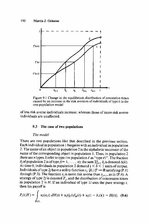
190 Martin J. Osborne
Hk+l)
f(k-l)
Figure 9.1 Change in the equilibrium distribution of concession timescaused by an increase in the risk aversion of individuals of type k in theone-population model
of less risk averse individuals increase, whereas those of more risk averseindividuals are unaffected.
9.3 The case of two populations
The model
There are two populations like that described in the previous section.Each individual in population 1 bargains with an individual in population2. The name of an object in population 2 is the alphabetic successor of thename of the corresponding object in population 1. Thus, in population 2there are n types. I refer to type i in population £ as "type €V\ The fractionJ/ofpopulation2isoftype;(= 1,. . . , «);thesum2JLi d3is denoted A(k).At time 0, individuals in population 2 demand \ < b < 1 units of output.Individuals of type 2/ have a utility function vy. [0,1 ]2 -* U satisfying (P. 1)through (P.3). The function Vj is more risk averse than vj+ {, as in (P.4). Astrategy of type 2/ is denoted Fj9 and the distribution of concession timesin population 2 is H. If an individual of type 1/ uses the pure strategy t,then his payoff is
- /u((a,s) dH{s) M,(1 - b,t\\ - 7/(0); (9.6)
[0,0.

The role of risk aversion 191if an individual of type 2/ uses the pure strategy t, then his payoff is
Qj(t,G) = J vj(b,Qj(t,G) = J vj(b,s) dG(s) + VjG,t)JG(t) + Vj(l - aj){\ - G(t)). (9.7)[0,0
(Once again, for convenience I assume that simultaneous concessionsgive a payoff of \ to each individual.)
EquilibriumIn this model, there are many equilibria; they are fully characterized intheorem 3, to be given later. However, I will argue (in the next subsection)that only one equilibrium is perfect in a certain sense. It is this equilibriumthat I describe first. Although the details of its definition are somewhatcomplex, its structure is easy to outline. Within each population, thepattern of concessions is similar to the equilibrium pattern in the one-population model. That is, there exist numbers 0 = p0 < • • • < py =' * ' = Pm
= 1 a n d 0 = Qo < " " ' <Qz= ' * * = Qn = 1 s u ch that thesupport of the equilibrium strategy Et of type 1 i is [/?,_ x,/?, ] and that of theequilibrium strategy F} of type 2/ is [q^x ,qj]. Informally, the p/s and q/scan be defined as follows. First, find the distributions of concession timesGx and Hx that make types 11 and 21, respectively, indifferent betweenconceding at any point in [0,1 ]. Now, the equilibrium distributions G andH have to be generated by the actions of the individuals in the twopopulations. Since type 11 constitutes the fraction yx of population 1, thismeans that only that part of Gx up to the point sx where Gx(sx) = yx can begenerated by the actions of individuals of type 11. After that point, theactions of type-12 individuals have to generate Gx. However, in order forthe strategy of type-12 individuals to have support commencing at si9from this point H has to be such that these individuals, not those of type11, are indifferent. Similarly, if we try to generate Hx by the actions ofindividuals in population 2, we run out of individuals of type 21 at thepoint tx where H(tx) = Sx. After this point, G has to be such that type-22individuals are indifferent. Thus, the equilibrium distributions G and Hcan be constructed as follows. Start at t = 0 with G/= Gx and H = Hx.Increase t to the point where either Gx (t) = yx or Hx (t) = Sx (i.e., sx or tx inthe preceding discussion), whichever comes first. Suppose that sx comesfirst. Then, starting from sx, H has to be modified so that type-12 individ-uals are indifferent. Then, H no longer reaches Sx at tx, but at some otherpoint, say t\. After t[, G must be modified so that type-22 individuals areindifferent; a new point, s2, for which G(s2) = yx + y2 (= F(2)), is defined,and the process of building G and H can continue.
Formally, G and H, and hence the equilibrium strategies El9 . . . , Em

192 Martin J. Osborneand Fx,. . . , Fn, can be defined iteratively. The iterative procedure that Idescribe is slightly more general than necessary to define the presentequilibrium, because I will use it later to define other equilibria. For any0 ^ a < 1 and 0 ^ /? < 1, the procedure H(a,fi) is as follows.
Procedure H(a,fi). Let w and x be such that T(w) ^ a < T(w + 1) andA(x) < p < A(x + 1) (possibly w = 0 and/or x = 0), and let 0 = p0 =- • • =p vv and 0 = qo= • - • = q x. Suppose that the numbers 0 <
pw+l < - • • < p k < 1 and 0 < qx+l < • • • < q € < 1, where 0 ^ k <m— \,0 <£ <n— 1, and, say, q € Pk, satisfy the following properties.First, let (7(0) = a, and define G on (qj^.l9qj] forj = w + 1,. . . , £ and on( ] foj €+ 1 by
G(t) = 1 - (1 - G(^_1))exp(- | K / a , M rfj); (9.8)
let //(0) = jS, and define H on (/?,._!,/?,.] for / = x + 1, . . . , k by
H(0 = 1 - (1 - tf(A-i ))exp(- J Ut(b,a,s) ds}. (9.9)Pi-1
Now, assume that the p/s and <7/s are such that G{pt) = F(/) for / =fc f
(Refer to Figure 9.2.) Note that G and H are continuous and increasing,and G(t) < 1 and H(t) < 1 for all 0 ^ t ^ pk. Now, as noted before, for any//the payoff Pt(t,H) of type 1 / depends on the form of//only on [0,t] (see(9.6)), and similarly for Qj(t,G). Thus, even though G and H are not yetdefined on the whole of [0,1], we can calculate Pt{t,H) on [p,_i>A] f°r
i = w+\,...,k (i.e., Pt(t,H) is independent of the way in which H isextended to [0,1]); it is easy to check that it is constant there. Similarly,G is designed so that Qj(t,G) (see (9.7)) is constant on Ufy-i ,<?,•] for; =x + 1, . . . , € and on [qj_x ,pk] for; = £ + 1.
We now extend G and / / to the next pt or qj9 whichever comes first. Todo so, for pk < t ^ 1, let
Gk+l(t) = 1 - (1 - F(/c))exp(- J V€+l(a9b9s) dsj
and lett
Hf+l(t)=\-{\- H(pk))expl- J Uk+i(b,a,s) dsj.

The role of risk aversion 193
1
Hk+1)Hk)
rck-i)
a
1|
1111|1 .
q (=1)
Figure 9.2 Construction of the functions G and / / in procedure II(a,/?)
Let G(t)_= G{t) for 0 < t <pk and_G(f) = Gk+l{t)tor pk < t < 1, anddefine H similarly. Then, Pk+l(t,H) and Qf+l(t,G) are constant on[PkM- Now, define numbers p and <? as follows. If G{\) < T(k +_1), letp = 1; otherwise, let p be the unique number in (/\,1) such that G(p) =T(k + 1). If / /(I) < A(€ + 1), let ? = 1; otherwise, let ^ be the uniquenumber jn (pk,\) such that H{q) = A(^ + 1). (Such numbers exist sinceG and H are continuous and increasing.) Now, if mm(p,q) = 1, let
* "_; =Pm =_l_and_^+1 = • • • = (^ = 1; if min(p,q) = p< 1,1 = p\ if min(p,^) = q < 1, letjj>+1 = q. In each case, extend G and
/ / to [0,min(A<7)] by letting G(t) = G(t) and H(t) = H(t)ifO < / < l,andG(l) = H(l)_=L
If minC/?, ) = 1, then the process ends and G and H are defined on thewhole of [0,1]. If this is not so, then either the collection of p/s or thecollection of q/s has been augmented and G and //have been extended ina way that satisfies the conditions necessary to repeat the process. Thus,

194 Martin J. Osbornethis procedure defines uniquely numbers 0 = p0 = • • • = pw < • • • <Py= ' ' • =Pm=l a n d ° = Qo:= * ' * = Qx < * * * < Qz = ' ' ' =qn = 1 and continuous and increasing functions G and H on [0,1) withG(Pi) = T(i) for i=w+l,...,y, H(qj) = A(j) for j = x + 1, . . . , z,
Define strategies Ex
E^t) = '
Ftt) ~
'0Git)
1
'0Hit)
,...,Em and F,, . .if 0 s
— r(i — i)
- A ( ; ' - l )
. , Fn as follows:f<p,-,,<
A, (9.10)
(9.11)
(Note that this means, for example, that El9 . . . , Ew are pure strategiesinvolving concession at f = 0, £y+1 may have an atom at t= 1, and£" +2, . . . ,Em are pure strategies involving concession at t= 1.) Thiscompletes the description of the procedure T\{OL$).
Now, I claim that the strategies defined by 11(0,0) constitute an equilib-rium of the game. Note that all of the strategies thus defined are non-atomic on [0,1). As noted in the construction, G and H are such thatQj(t,G) is constant on [qj-^qj] for; = 1, . . . , « , and Pt(t,H) is constanton [pt_ u/?,] for / = 1 , . . . , m. To show that the £/s and F/s constitute anequilibrium, it suffices to show that Qj(t,G) is increasing on (0,^.!) anddecreasing on (^,1), and similarly for Pl{t,H) (since the nonatomicity ofG and H on [0,1) implies that Pt and Qj are continuous in t).
Consider Qj(t,G) on (qh_ {,qh), with h-^j — 1. Using the definition of G(see (9.8)), the derivative ofQj(t,G) with respect to t on (qh_x,qh) is
(1 - G(t))(vj(b9t) - vj(l - a,t))(Vh(aAt) -Vj(a,b,t)).However, from lemma 1 we have Vh(a,b,t) > Vj(a,b,t) (since h is morerisk averse than;), so that the derivative is positive, as required. A similarargument establishes that the derivative on (^,1) is negative, and a likeargument can be made for Pt. Hence, the E-s and Ffs defined by 11(0,0)constitute an equilibrium.
The remaining equilibria are of two types. One type is closely related tothe equilibrium just defined. In fact, it should be clear (by arguments

The role of risk aversion 195similar to the preceding) that for any 0 < a < 1 and any 0 < /? < 1, thestrategies defined by IT(a,0) and those defined by 11(0,/?) are equilibria ofthe game.
The final type of equilibria involves all individuals in one populationconceding with probability 1 at time 0. The members of the other popula-tion use any strategies that generate a distribution of concession times thatputs enough weight near / = 1 to make the members of the first popula-tion concede at t = 0. (Such strategies clearly exist - for example, allindividuals can concede at t— 1 with probability 1.) This defines anequilibrium: Since all members of the first population concede at time 0,all members of the second population are indifferent between all conces-sion times in (0,1 ] (they always receive a payoff stream equal to theirdemand from time 0).
It is much more difficult to argue that every equilibrium of the game isof one of these types; a proof is given in the Appendix. We can summarizethe results as follows.
Theorem 3. (Eu . . . , Em\Fl9 . . . , Fn) is an equilibrium of the two-population model if and only if it is one of the following:
1. Et(i = 1,. . . , m) and Fj(j = 1,. . ., n) are defined by 11(0,0).2. For some 0 < a < 1 and 0 < /? < 1, Et{i = 1, . . . , m) and Fj(j =
1, . . . , « ) are defined by either II(a,0) or U(0,fi).3. Either (a) Et{t) = 1 for all 0 < t < 1, for all i = 1,. . ., m, and
Fx, . . . , Fn are any strategies that generate a distribution H of conces-sion times for which Pt(0,H) > Pt(t,H) for any 0 < £ < 1, for i =1, . . . , m\ or (b) the equilibrium is similar to this, with the roles ofpopulations 1 and 2 reversed.
An immediate consequence of this result is the following.
Corollary 4. If the characteristics of populations 1 and 2 are the same,then the only symmetric equilibrium is the one defined by 11(0,0). That is,the only equilibrium in the one-population model is the one defined in theprevious section.
Perfect equilibriumSelten (1975) argues that equilibria in games with finite pure strategy setsshould possess a certain robustness. Suppose that a game is perturbed byinsisting that each player devote at least some small probability to somecompletely mixed strategy. An equilibrium is perfect if it is close to anequilibrium of such a perturbed game. Okada (1981) suggests that one

196 Martin J. Osborneshould insist that the equilibrium be close to an equilibrium of every suchperturbed game; he calls such an equilibrium strictly perfect. Kohlbergand Mertens (1982) study a related notion (a strictly perfect equilibrium isa stable component in their sense), and show that the equilibria it gener-ates have a number of attractive properties.
In the game here, each player has a continuum of pure strategies. Insuch a game, it is not clear how to formulate these notions of perfection. Ido not attack this problem. Rather, I consider a small collection of per-turbed games, in which the perturbing strategy is concession at time 0 withprobability 1. (Note that this is an equilibrium strategy - of type (3)). Thefollowing result shows that the only equilibrium that is robust with respectto small perturbations of the strategy sets in the direction of this strategy isthe one of type (1). That is, in the game in which each individual thinksthat there is a positive probability that his opponent will concede at time 0,the only equilibrium is close to the one of type (1). It seems likely that thisequilibrium is the only one that satisfies an appropriately modified ver-sion of strict perfection - that is, it is robust with respect to all smallperturbations of the strategy sets. However, a precise argument to thiseffect is beyond the scope of this paper.
Proposition 5. For each e > 0, let F e be the perturbed game in which thestrategy space of each player is the set of cumulative probability distribu-tions Fon [0,1] such that F(0) ^ e. Then, for each € > 0, the game F€ has aunique equilibrium, which converges to the one defined in (1) of theorem3 as € -» 0.
Proof. Let Et{i = 1, . . . , m) and Fj(j = 1, . . . , « ) be the equilibriumstrategies given in (1) of theorem 3, and let G and H be the correspondingdistributions of concession times in the two populations. For each e > 0,let Eft) = € + (1 - e)Ej(t) andFJ(t) = e + (1 - e)Fj(t) for all 0 < r < 1,/ = 1, . . . , m, and7= 1, . . . , n. Now, (E\, . . . , E€
m;F€u . . . , F*)isan
equilibrium of Fe, because the derivative with respect to t on (0,1) of thepayoff Pi(t,H€\ where H%t) = 2;=1 SjFJ(t) = e + (1 - e)H(t) for all 0 <t < 1, is precisely (1 - e) times the derivative ofPt{UH). Hence, Pt(t,H€)is increasing on ((),/?,_!), constant on {p(-x ,pt), and decreasing on (/?,-, 1).Also, P,(0,i/€) is less than P,(y/,//€) for some r\ > 0, since H€ has an atomat 0 (compare lemma A3 of the Appendix). Similar arguments can ob-viously be made for the payoffs of individuals in population 2. Further,since there is no other nonatomic equilibrium of the original game (F°),and no equilibrium in which the strategies of players in both populationshave atoms at 0, it is clear that this is the only equilibrium of F€. Inaddition, the Ef s and F]9s converge (pointwise) to the E/s and F/s.

The role of risk aversion 197
The effect of a change in risk aversionHere, I investigate the effect of an increase in the risk aversion of individ-uals of type 2£ on the equilibrium singled out as perfect by the precedingarguments. Suppose that the utility function v€ is more risk averse than v€,and less risk averse than v€_ x (so that the ordering of risk aversions inpopulation 2 is preserved).
Suppose that q€ < 1 and qe_x e supp Ek. Then, as in the one-popula-tion case, pi = pifori= 1, . . . , k — 1, = qj for 7 = 1, . . . , / — 1, andG(t) = G(t) and H(t) = H(t) for 0 < t < q€_x, so that the equilibriumpayoffs of types 11, . . . , \k and 21, . . . , 2{€ — 1) are unaffected.
Now, consider the changes in G and Hon (q€_l9l]. From lemma 1, wehave V€(axb,s) > V,(a9b,s) for aH0 ^ s < 1, so that from (9.8) (with; = £\we have G(t) > G{t) on (q€_l,min{q€,q€)] (since on this interval, both Gand G have to keep type 2( indifferent). (Refer to Figure 9.3.) This meansthat^_! <pk <^.On(^_1,p^),//isunchanged(since%isunchanged).However, on [pk,min(pk9pk+l)], H has to keep type fc+ 1 indifferent,whereas H keeps type k indifferent. Since H(pk) = H(pk) and, fromlemma 1, Uk+l(b,a,s) < Uk(b,a,s) for all 0 ^ s < 1, we have, from (9.9),H{t) < H(t) for pk<t< min(pk,pk+l). Now, there are several cases toconsider, but the arguments are very similar. Suppose that pk < qe andG{q€) < T{k + 1), so that q€ <pk+l. Then, on [pk,mm(Pk+i A+i )]> h a s
to keep type l(k+ 1) indifferent, as H did. However, since H(pk) <H(Pk\ w e deduce, from (9.9), that H{t) < H(t) on [pk,min(pk+l ,pk+l)].Now, suppose that H(pk+l) > A(/). Then, qe> q€, and we can considerthe behavior of G on [q€,q€]. Now, G has to keep type 2£ indifferentwhereas G keeps type 2{€ + 1) indifferent; also, G{q€) < G(q€), and sofrom (9.8), G{t) > G(t) on [q/9Qr], On [q€,q€+x], both G and G keep type2{€+\) indifferent; since G{q€) > G(q<\ we have G(t) > G(t) on'thisinterval. Continuing in the same way, we see that G(t) > G{t) for allq€-x < t < 1 and H{t) < H{i) for all pk < t < 1.
Then, arguing exactly as in the one-population case (integrating byparts in the expressions for Pi(pi_l,H) and Qjiq^^G) for i = k +1, . . . , m and j = £ + 1, . . . , « ) , we find that the equilibrium payoffs oftypes \{k + 1), . . . , Ira decrease and those of types 2{£ + 1 ) , . . . , « in-crease. That is, an increase in risk aversion in population 2 causes thoseindividuals in population 1 who in (perfect) equilibrium concede later tobe made worse off, whereas the members of population 2 who concedelater are better off. Summarizing, we have the following.4
Proposition 6. Suppose that individuals of type € in population 2 be-come more risk averse (but not more so than those of type £ — 1). Suppose

198 Martin J. Osborne
1
Hk+l)
T(k)
f(k-l)
6
/
/
//
A1|
^T 11 11 11 1I I
G 1ii1ii
111 i i 1
" n i T " r r i T - ii i ii i ii
Ii1
i i
i i
11
r ~ Tu
H
Figure 9.3 Changes in the perfect equilibrium distributions of conces-sion times caused by an increase in the risk aversion of individuals oftype £ in population 2 in the two-population model
also that in the old (perfect) equilibrium, type 2£ concedes with probabil-ity 1 before time 1, and the smallest point in the support of the strategy oftype 2£ is a member of the support of the strategy of type Ik. Then, the(perfect) equilibrium payoffs of the types at least as risk averse as type k inpopulation 1 are unaffected, whereas those of the less risk averse typesdecrease; the equilibrium payoffs of the types more risk averse than type £in population 2 are unaffected, whereas those of the less risk averse typesincrease.
Thus, in the two-population model the effect of a change in risk aver-sion is exactly the opposite of that predicted by the axiomatic models. The

The role of risk aversion 199reason is that in equilibrium, the concession pattern in population 1 mustmake the actions of the individuals in population 2 optimal, and viceversa. Thus, if some members of population 2 become more risk averse,the individuals in population 1 have to concede on average earlier in orderto keep the members of population 2 indifferent over some interval ofconcession times. However, if concessions in population 1 are on averageearlier, the optimal concessions in population 2 are later; hence, thepayoffs of individuals in population 1 decrease. (This type of argument isa standard one concerning mixed-strategy Nash equilibria; it is not madepossible by some peculiar feature of the model.)
The effect of a change in the size of a typeFinally, I consider the effect of a change in the fraction of a populationthat is of a given type. I do so to see if any meaning can be given to theclaim that in equilibrium, individuals will pretend to be less risk aversethan they really are. Suppose that the fraction of the population taken upby relatively risk neutral individuals increases. Then, one might imaginethat since this causes an opponent to ascribe a lower probability to anindividual being risk averse, those who are risk averse can do better - theycan "hide" among the mass of relatively risk neutral individuals. It turnsout that this is not the case, although it is true that the ratio of the payoffsof the more risk averse to those of the less risk averse increases; the formerare constant, whereas the latter decrease.
To see why this is true, we can use the previous result concerning achange in the degree of risk aversion. Suppose that the fraction of popula-tion 2 occupied by individuals of type € increases from 8e to S€ = S€ + c,and the fraction of type £ — 1 decreases from 5€_x to S€-x = S€_x — e (sothat the population becomes on average less risk averse). This change isequivalent to one of the types considered in the previous subsection.Thus, break types £ — 1 and € into three types, which constitute thefractions S€_x — €, e, and S€ of the population (the first two types havingthe same utility function before the change,5 and the second two havingthe same utility function after the change). Then, the change definedpreviously is a decrease in the risk aversion of the middle type. Hence, byproposition 6 the equilibrium payoffs of the types more risk averse than €are unaffected, whereas those of type £ and the less risk averse typesdecrease. That is, we have the following.
Corollary 7. Suppose that the fraction of individuals of type £ in somepopulation increases, whereas the fraction of those of type € — 1 decreases

200 Martin J. Osborne
by the same amount, and those of type £ — 1 concede with probability 1before time 1. Then, the equilibrium payoff of every individual more riskaverse than type € in that population is unaffected, whereas the equilib-rium payoff of every individual at most as risk averse as type € decreases.
9.4 The case in which there is a choice ofinitial demand
Here, I elaborate on the previous model by allowing individuals to choosea "demand" at time 0.1 assume that there are only two possible demands,a and b(0 ^ a< b < 1). I study the perfect (Bayesian Nash) equilibria ofthe two-population model in which each individual simultaneously firstchooses a demand, and then negotiates as in the previous model (i.e.,subsequently simply chooses a time at which to concede). Throughout, Iconsider only the perfect equilibrium described in the previous section.To keep the analysis relatively simple, I assume that there are only twotypes in each population (m = n = 2). Note that in this model, the actionsof an individual do, in general, convey useful information to his oppo-nent. Unless the same fraction of each type demands a, the demand thatan individual makes at time 0 allows his opponent to revise the probabil-ity that the individual is of a given type. Note, however, that an individ-ual's subsequent behavior does not convey any additional useful infor-mation to his opponent.
I show that if a > \, there is no separating equilibrium in which the twotypes in each population choose different demands. I also show that in thiscase there is a continuum of pooling equilibria, in which a positive frac-tion of each type in each population chooses each possible demand.
Given the results in the axiomatic models that an individual can bene-fit from pretending to be less risk averse than he really is, one mightimagine that the reason no separating equilibrium exists is that a morerisk averse individual can benefit from changing his demand to that of aless risk averse individual. However, given the result of the previoussection (proposition 6), it should come as no surprise that the opposite istrue. That is, the less risk averse can benefit from pretending to be morerisk averse (see the arguments that follow). Thus, there is another sense (inaddition to the one considered in the previous subsection) in which theresult derived in the axiomatic framework does not hold in my model.
If a < i, then there is no equilibrium of either type. Later, under theheading "Discussion" I consider briefly what may happen when there aremore than two types in each population. However, I do not consideranother natural extension, in which there are many, even a continuum, ofpossible demands. My analysis is not comprehensive, but is simply in-
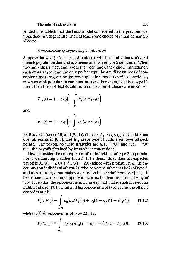
The role of risk aversion 201
tended to establish that the basic model considered in the previous sec-tions does not degenerate when at least some choice of initial demand isallowed.
Nonexistence of separating equilibriumSuppose that a > \. Consider a situation in which all individuals of type 1in each population demand a, whereas all those of type 2 demand b. Whentwo individuals meet and reveal their demands, they know immediatelyeach other's type, and the only perfect equilibrium distributions of con-cession times are given by the two-population model described previouslyin which each population contains one type. For example, if two type l'smeet, then their perfect equilibrium concession strategies are given by
En(t)'
and
l - e x p ( - | Vx(a9a,s
Fn(t) = 1 - expf- I U{(a9a9s) ds\
for 0 < t < 1 (see (9.10) and (9.11)). (That is, Fx {keeps type 11 indifferentover all points in [0,1], and En keeps type 21 indifferent over all suchpoints.) The payoffs to these strategies are u{(\ — afi) and v^l — afi)(i.e., the payoffs obtained by immediate concession).
Next, consider the consequence of an individual of type 2 in popula-tion 1 demanding a rather than b. If he demands b, then his expectedpayoff is 3^(1 — afi) + S2u2(\ — bfi) (since with probability Sh he en-counters an individual of type 2/, who correctly infers that he is of type 2,and uses a strategy that makes such individuals indifferent over [0,1]). Ifhe demands a, then any opponent incorrectly identifies him as being oftype 11, so that the opponent uses a strategy that makes such individualsindifferent over [0,1 ]. That is, if his opponent is of type 21, his payoff if heconcedes at t is
Pi(UFn)= j u2(a,s)Fn(s) + u2{\ - aj){\ - Fn(t))\ (9.12)(o,n
whereas if his opponent is of type 22, it is
P2(t,F2l)= j u2(a,s)F2l(s) + u2(l - 6,0(1 - F2l(t))9 (9.13)

202 Martin J. Osbornewhere
t
F2l(t) = 1 - expf - J Ux(b9a9s) dsjo
for all 0 ^ t < 1. Differentiating with respect to t in (9.12), we obtain
(1 - Fn(t))(u2(a9t) - u2{\ - a9t))(Ux(a9a9t) - U2(a,a9t)).From lemma 1, this is positive if t < 1, so that an optimal action for theindividual in this case is to concede at time 1. His payoff is then P2{ 1 9FX {),which, since P2(t9Fn) is increasing in /, exceeds P2(0,Fu) = u2(\ — <z,0),the payoff he obtains when he demands a in this case. Similarly, differen-tiating in (9.13), we obtain
(1 - F2l(t))(u2(a,t) - 1*2(1 - b9t)\Ux(b9a9t) - U2(b9a9t)\So by the same argument as before, the individual can obtain P2(l,F2l),which exceeds P2(0,F2l ) = u2(\ — 6,0), the payoff when he demands a inthis case. Thus, his expected payoff against a random opponent exceeds5xu2{\ — aft) + S2 u2(\ — 6,0), and therefore he is better off demandinga, pretending to be more risk averse than he really is.
Thus, no separating equilibrium of this type exists. It is easy to see thatthe same argument also rules out any separating equilibrium in which allindividuals of type 1 in one population demand 6, whereas all individualsof type 2 in that population demand a, and the members of the otherpopulation act either similarly, or as they did before. So there is noseparating equilibrium in which within each population the two typeschoose different demands.
If a < i, then when two individuals who demand a meet, they canreach agreement immediately; if a + b < 1, this is also true if individualsdemanding a and 6 meet. It matters precisely what the payoffs are in thesecases. I assume that if individual / demands d(,i= 1, 2, and dx + d2 < 1,then individual / receives the output stream ((1 + dt — dj)/2fi) (i.e., theindividuals split equally the amount left over after their demands aresatisfied; the precise method of splitting the excess does not matter for myargument, so long as the amount that / receives increases with dt). First,consider the possibility of a separating equilibrium when a < \ and a +6 > 1. In such an equilibrium, there are individuals in both populationswho demand a. If the opponent of such an individual demands a, then theindividual receives the output stream (i,0), whereas if the opponent de-mands 6, the equilibrium payoff of this individual is the utility of theoutput stream (1 — 6,0). If the individual switches to a demand of 6, theoutput stream he receives if his opponent demands a is ((1 + 6 —

The role of risk aversion 203
and if his opponent demands b, he again receives the utility of (1 — bfi).Since (1 + b — a)/2 > \, the individual will switch from a to b. A similarargument can obviously be made if a + b < 1. Thus, no separating equi-librium exists for any values of a and b.
Pooling equilibriaNow, consider the possibility of an equilibrium in which the fractions0 < nt < 1 of type 1 / and 0 < pj< 1 of type 2/ demand a, whereas all otherindividuals in both populations demand b. Then, if for example a type-11individual demands a and bargains with a type-21 individual who de-mands a, the equilibrium concession times are those given by the two-population model in which the fractions of the types in population 1 aren{/(nl + n2) and n1l{nx + n2) and those in population 2 are px /(p{ + p2)and p2/(P\ + Pi)- For l^i^i^PuPi) t 0 constitute an equilibrium, eachindividual in each population must be indifferent between demanding aand b.
First, consider the case a> \. Note than an individual of type 1 ineither population is always indifferent between demanding a and b. Thisis the case because 0 is always an element of the support of the equilibriumstrategy of such an individual, whoever is his opponent (since type 1 is themost risk averse). Thus, the equilibrium payoff when the opponent de-mands a is u{(\ — afi) (or ^(1 — afi)), and when the opponent demandsb it is u{(\ — b,0) (or v^l — 6,0)), independent ot{nx,n2,pup2).
Consider the behavior of individuals of type 2 in population 1. Fix0 < n2 < 1 and 0 < p2 < 1, and let Pi(c,nl ,p{) be the equilibrium payoffof an individual of type / in population 1 who demands c when thefractions of those who demand a among types 11 and 21 are nx and px;similarly define Qj(c;nl ,p{) for type; in population 2. Suppose that n{ = 1(i.e., that all type-11 individuals demand a). Then, if a type-12 individualdemands b, he identifies himself to be of type 2, and the equilibriumreached is the one in a two-population model where there is only one typein population 1. Hence, the support of the individual's strategy is [0,1],and his equilibrium payoff is u2( 1 — afi) or u2( 1 — 6,0), depending on thedemand of his opponent. Thus, for each 0 ^ p{ ^ 1,
P2(6;1,A) = (Pi+P2)u2(l - afi) + (1 - A - p2)u2(\ - bfi). (9.14)Now, fix 0 < p{ < 1 and reduce n{. As n{ falls, the fraction of type 2'samong those demanding b in population 1 decreases. Hence, by corollary7, the equilibrium payoff of type 2, whether the opponent demands a or b,increases. That is, for each 0 ^ p{ ^ 1,
P2(b;n{,/?!) is decreasing in nl. (9.15)
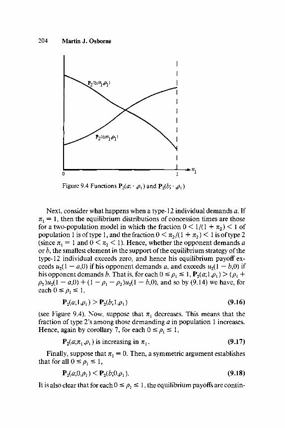
204 Martin J. Osborne
o 1Figure 9.4 Functions P2(a; • ,p{) and P2(i; • ,px)
Next, consider what happens when a type-12 individual demands a. Ifnl = I, then the equilibrium distributions of concession times are thosefor a two-population model in which the fraction 0 < 1/(1 + n2) < 1 ofpopulation 1 is of type 1, and the fraction 0 < n2/( 1 + n2)< 1 is of type 2(since nl = 1 and 0 < n2 < 1). Hence, whether the opponent demands aor b, the smallest element in the support of the equilibrium strategy of thetype-12 individual exceeds zero, and hence his equilibrium payoff ex-ceeds u2( 1 — afi) if his opponent demands a, and exceeds u2( 1 — bfi) ifhis opponent demands b. That is, for each 0 ^ px < 1, P2(a;l,/?1 ) > (A +p2)u2(l — afi) + (1 — px — p2)u2(\ — bfi), and so by (9.14) we have, for
1,(9.16)
(see Figure 9.4). Now, suppose that nx decreases. This means that thefraction of type 2's among those demanding a in population 1 increases.Hence, again by corollary 7, for each 0 ^ px ^ 1,
P2(a;nl ,px) is increasing in nx. (9.17)
Finally, suppose that nl = 0. Then, a symmetric argument establishesthat for all 0 < p{ < 1,
?2(afi,Pi) < P2(*;0,A). (9.18)It is also clear that for each 0 ^ p{ ^ 1, the equilibrium payoffs are contin-
The role of risk aversion 205uous in n{. (For example, if nl is close to zero, so that almost all type-11individuals demand b, then the equilibrium payoffof a type-12 individualwho demands a is close to u2( 1 — afi) or u2( 1 — b,0) [depending on theopponent's demand], since the fraction of type 11's in the concessiongame after the demands are revealed is close to zero, so that the smallestelement in the support of the equilibrium strategy of type 12 is close tozero.)
Combining (9.15) through (9.18), we conclude that for each 0 < p{ <1, there exists a unique n{ such that P2(a',nl ,P\) = 1*2(^1 ,Pi )• Denote thisnl by Y(p{). Since all of the functions involved are continuous, so is Y.Symmetric arguments can obviously be made for population 2. That is,for each 0 ^ nl < 1, there exists a unique px such that Q2(a\nx,px) =
Q2(b\nl ,px). Denote this px by 0(7^); O is continuous.Now, the function O ° Y: [0,1] —* [0,1] is continuous and hence has a
fixed point, say /?*. Let 7r*=Y(/?*). Then, (ft*,/?*) is such thatP2(tf;7r*,/?*) = P2(6;TT*,/>*) and Q2(a;n*,p*) = Q2(6;TT*,/?*). By (9.16) and(9.18), we have 0 < 7r* < 1 and 0 < pf < 1. That is, given the fixed (n2 ,p2),and the fact that type 1 is indifferent between a and b for any (nun2 ,p{ ,p2),(7r*,7r2,/?*,y92) is a pooling equilibrium.
Proposition 8. If a > \, then for each (n2 ,p2) G (0,1 )2, there exists a pool-ing equilibrium in which a positive fraction of each type in each popula-tion make each demand.
When a < i, it is easy to show that there is no pooling equilibrium. Thereason is that, exactly as in the case of a separating equilibrium, an indi-vidual of type 1 in each population can increase his payoff by demand-ing b.
DiscussionGiven the continuum of pooling equilibria in proposition 8, we cannotperform the comparative static exercises of Section 9.3. It is not clearwhether there are assumptions under which a unique equilibrium is se-lected. One possibility is to increase the number of types in each popula-tion. The arguments presented establish that the most risk averse individ-uals in both populations are always indifferent between demanding a andb. All other types are indifferent only in particular cases. This suggests thathowever many types there are, there is always a one-dimensional contin-uum of equilibria; as the size of the most risk averse type shrinks, the rangeof the equilibria may contract. Thus, in the limit, when there is a contin-uum of types, there is a possibility that an essentially determinate equilib-rium is defined.

206 Martin J. Osborne
APPENDIXThe Characterization of All Equilibria in the Two-Population Model
I repeatedly use the following expression for the difference between thepayoffs of conceding at r and at t. If r ^ t, then
Pt(t,H) - P((rM) =
+ J (ut(a,s) - ut(\ - b,r)) dH(s) + JH(t)(ut{y) - ut{\ - b,r)) (A.I)
+ (1 - i/(0)(^(l - b,t) - ut{\ - b,r)).Throughout, Et(i = 1, . . . , m) is an equilibrium strategy of 1/, and Fj(j — 1 , . . . , « ) is an equilibrium strategy of 2/; G and H are the equilib-rium distributions of concession times in populations 1 and 2, respec-tively. Let J(G) and J(H) be the set of atoms (jumps) of G and H, respec-tively. Note that
If * £ J{H) and t G supp Eh then />,(*,#) = Pt(EhH). (A.2)The following gives conditions on a distribution of concession times
under which more risk averse individuals concede earlier.
Lemma Al. If [0,s0] C supp H, H is atomless on (0,s0] n (0,1), r e[0,50], £ G [0,s0], r G supp £,, and / G supp £,_!, then / ^ r.
If r = s0 = 1, the result is immediate. So suppose that r < 1. Letr G supp £, and suppose that 0 < r < t < s0. Then, Pt(UH) - Pt(r,H) <0. Now, ui_l =f° ut, where/is strictly concave, so that/(w) — f(z) <
— z), with strict inequality if w =£ z. Hence,
unless 5 is such that ut(a9s) = M/(l — b,r); by (P.2) and (P.3), there is onlyone such s. Hence, given that [0,s0] C supp //,
J (ut-fas) ~ w*-i(l - 6,(r,t)
f'(ut{\ - b,r)) j {ut{a,s) - K,(1 - b,r)) dH(s).(r,t)
Also,
M/-iCl - b9t) - ut-yil - b,r) < / ' ( K , ( 1 - 6,r))(wz(l - b,t) - ut{\ - b9r)).
The role of risk aversion 207However, since t G supp //, then either H{i) — H{r) > 0 or H{t) < 1.Hence, given that r is not an atom of//, and either / is not an atom of//, ort = s0 = 1 and hence w,-(i,0 = 0 = ut(\ — b,t), the preceding inequalitiesimply, using (A.I), that
- P,(r,H)) ^ 0.Hence, t ^ supp Ei_l. So if t e supp /?,_!, then £ < r.
Corollary A2. If [0,s0] C sw/?p G, [0,s0] C supp //, G is atomless on(0,s0 ] n (0,1), and H is atomless on [0,s0] n (0,1), then there exist 0 =A) = P\ = ' * * = Pi < AM-I < * * * < Pk-i < s0 and 0 = q0 < qx <• • • < qh-x < s0 such that[0,50] n supp Et = {0} for / = 1, . . . , €\
[0,^0] H supp Et = [A_I ?A] for / = € + 1, . . . , fc - 1,and [0,50] n supp Ek = [ p ^ ! , ^ ] ;
[0,50] n supp F; = [%•_!,%•] for; = 1, . . . , h - 1,and [0,50] n supp FA = [ph_x,s0].
Proof. Immediate from lemma A1 (using (9.1), and the analogous rela-tion between H and the E/s).
Now, I show that G and //cannot have atoms at the same point, exceptpossibly at 1. The reason is simple: If, for example, G has an atom at t0,then all members of population 2 obtain a higher payoff by conceding justafter t0, rather than at t0.
Lemma A3. If t0 E J(G) a n d to<l, t hen t0 <fc J(H).
Proof. Let t0 E / ( / / ) , f0 < 1. T hen, for each S > 0 there exists 0 < e < Ssuch that r0 + e £ / ( / / ) . Next, consider P,(/o + € , # ) - PtUoM) (see(A.I)). The first term is positive, independent of 6; the second term isnonnegative for small e; the third is zero; and the fourth can be made assmall as necessary for choosing e small enough. Hence, for e smallenough, we have Pt(t0 + e,H) > Pt(t0,H).
The following is a very useful result, which says that if G has an atom att0 G (0,1), then no member of population 2 concedes in some open inter-val before t0 (when t0 is imminent, it is better to wait until afterward, sincethere is a positive probability of a concession occurring at t0).

208 Martin J. OsborneLemma A4. If t0 G J(G) and 0 < t0 < 1, then there exists e > 0 such that
Proof. Let S > 0. For any; = 1, . . . , « , we have
Qj(t09G) - Qj(t0 - S9G) = JG(t0 - 6)(vj(b,t0 -S)- vtf,t0 ~ &))
(Vj(b9s)-Vj(l-a,t0-S))dG(s)
+ JG(to)(Vj(yo) ~ vj(l - a9t0 - 6)) +(1 - G(to))(vj(l - a9t0) - vj(\ - a9t0 - S))
(see (A.I)). However, Vj(b,t0 ~ S) - Vj{\,t0 — <5) > 0 and, since t0 < 1, wecan find e{> 0 and a > 0 such that for all 0 < d < €x, we have
and for all t0 — S < s < t0, we have
vj(b9s) > vj(b9to) > vj(yo) > vj{\ - a9t0 - S).Hence, for all 0 < S < e{,
Qj(to,G) - Qj(t0 - S9G) ^ aJG(t0)+ (1 - G(to))(vj(l - a9t0) - vj(\ - a9t0 - S)).
However, there also exists e2 > 0 such that for all S < e2, we have Vj(\ —a,to)-Vj(\-a,to-S)>-aJG(to)/2. But then for all 0<S<e =m i n ^ ! ^ ) , we have
Qj(to9G) - Qj(t0 - S,G) > f^ > 0,
and so Qj(t,G) < Qj(to,G) for all te(to-e9to). Hence, (to-e,to)nsupp H = 0.
The following states that if there is an interval not in the support of//,at the endpoints of which G does not have atoms, then the largest point inthe interval can be in the support of G only if / / is already 1 at that point.The reason is that the payoff to any member of population 1 is decreasingin the interval whenever there is a positive probability of a future conces-sion by an opponent.
Lemma A5. If H(r) = H(t), 0 < r < t < 1, r £ / ( / / ) , t £ / ( / / ) , and t Gsupp G, then / / (0= 1.
The role of risk aversion 209
Proof. For all / = 1, . . . , m,
Pi(t,H) - Pt(r,H) = (1 - //(O)(W/(1 " b9t) - w,(l - b,r))
(using (A. 1)). Hence, Pt(t9H) < Pt(r,H) unless H{t) = 1. Since t £ / ( / / ) ,this means (from (A.2)) that t $. supp G.
We can now restrict quite substantially the nature of the supports of theequilibrium distributions of concession times.
Lemma A6. If70 E /(G)andO < £0 < 1, then there exists s0 E [0,£o)suchthat supp H = [0,s0], [0,S0] C supp G, and G and H are atomless on
From lemma A4, there exists e > 0 such that (to — e,to)nsupp H = 0. Now, let r= t0 — e/2 and ^ = £0 in lemma A5. Since £0 E/(G), 0 £ / ( / / ) by lemma A3, and so H(r) = H{t). Hence, by lemma A5,H(t0) = 1. Let s0 = max supp H. Then, s0 < t0. Now, if there is an atom ofG in (0,s0], say at tx, the same argument establishes that H(t2) = 1 forsome t2<tu contradicting the fact that s0 E supp H. Similarly, H canhave no atom in (0,50].
Now, suppose that there exists y E supp H, and 0 < x < y such thatH(x) = H(y). Then, y < s0, and so H(y) < 1, and* £ / ( # ) , y £ / ( / / ) bythe preceding argument, and thus by lemma A5 we know thaty ^ supp G. But then we know that there exists w < y such that G(w) =G(y) < 1; reversing the roles of G and H in lemma A5, and letting r = wand t = y, we conclude that y ^ supp H, a contradiction. Hence,supp / / = [0,s0] and, similarly, supp G D [0,50].
Now, we can conclude that if one distribution of concession times hasan atom in the interior of its support, then all individuals in the opponentpopulation must concede at time 0 with probability 1.
Lemma A 7. If t0 E J(G) and 0 < t0 < 1, then supp H = {0}.
Proof. By lemma A3, G and //cannot both have atoms at 0. Let s0 comefrom lemma A6, and assume that s0 > 0. Then, from corollary A2 andlemma A6, we know that there exist k and 0 ^ Pk-\ < o s u ch that[0,s0] n supp Ek = [Pk-i ,s0]. Hence, H is such that Pk(t,H) is constant,equal to Pk(Ek,H), for all / E (pk_l9s0]. That is,
J uk(a,s) dH{s) + (1 - H{t))uk{\ - b,t) = Pk{Ek,H)[0,t]

210 Martin J. Osborne
(since His atomless on (pk_i,s0]) for a l l p k _ l < t ^ s Q . Because the inte-gral is (as a function of t) absolutely continuous, / / i s absolutely continu-ous. But then we can integrate by parts to obtain
uk(a,t)H(t) - uk(a,0)H(0) - j H(s) D2uk(a,s) ds[0,t]
+ (l-H(t))uk(l-b,t) =Since D2uk is continuous in s, and H is atomless on (09s0 ], this shows thatH is differentiate. Differentiating, we find that every solution of theresulting differential equation is of the form
t
H(t) =\-A expf - I Uk(b,a,s) ds) (A.3)o
for some A > 0. Now, we need H(s0) = 1. Since s0 < t0 < 1, the integralwith t = s0 is always finite, and so we must have A = 0. But thenH(uk_{) = 1, and thus s0 supp //. So the only possibility is s0 = 0.
As noted in the text, there exists an equilibrium of this type. Forexample, if supp Et = {1} for / = 1, . . . , m, and supp Fj = {0} for j =1, . . . , « , then (£\, . . . , Em;Fl, . . . , Fn) is an equilibrium.
We can now use lemma A5 to restrict the nature of the supports of Gand H when G and H are atomless on (0,1).
Lemma A8. If G and H are atomless on (0,1) and there exists 0 < t < 1such that G(t) < 1 and H{f) < 1, then [0,t] C supp //.
Proof. Suppose, to the contrary, that 0 < x < t and x supp //. LetyG = min{z > x: z E supp G) and define yH similarly. Since x supp //,we have y# > x. Also, yG > x (since if yG = x, then there exists 3; > x,y G supp G such that //(x) = H(y) and //(y) < 1, contradicting lemmaA5). Let y = mm{yG,yH) > x. First, suppose that y < 1. If y = yG, thenG(x) = G(y)<\, x£j(G) and y£J(G\ and so by lemma A5,
supp //. Hence, there exists w < y such that H(w) = H(y), w / ( / / ) ,/ ( / / ) , and H(y) < 1, and so by lemma A5 again, y supp G, contra-
dicting the definition of y (=yG). If y = yH, a similar argument can bemade. Hence, the only possibility is y = 1. But then
Pt(y,H) ~ Pi(x,H) = JH(y)(ut&y) ' ut(\ - b,x)).However, ut{\,y) = 0 if y = 1, and so this is negative unless JH(y) = 0. Butthis is impossible, since we assumed that G(t) = G(y) — JH{y) = 1 —
The role of risk aversion 211JH(y) < 1. Hence, [0,t] c supp H. A symmetric argument implies that[0/] C supp G.
Lemma A9. If neither supp G = {0} nor supp H = (0), then neithersupp G = {1} nor supp H= {1}.
Proof. If, for example, supp G = {1}, then clearly Qj(0,G) > Qj{UG) forall t > 0, so that supp / / = {0}.
Corollary A10. If neither supp G = {0} nor supp H = {0}, then thereexists 0 < t < 1 such that G{t) < 1 and H(t) < 1.
Lemma All. If G and / / are atomless on (0,1) and neither supp G = {0}nor supp H = {0}, then there exists s0 > 0 such that either supp G = [0,50 ]and supp H D [0,s0], or supp / / = [0,s0] and supp G D [0,s0].
Proof. Let zG = max supp G > 0 and z# = max supp H > 0, and lets0 = minlz^z^} > 0. The result then follows by letting t = s0 — e for anye > 0 in lemma A8, and using corollary A10.
Lemma Al2. If G and Hare atomless on (0,1) and neither supp G = {0}nor supp H = (0), then there exist 0 ^ a < 1 and 0 ^ /? < 1 such that Gand / / are as specified either by the procedure lT(a,0) or by the procedure
Proof Suppose that supp H = [0,s0 ] (see lemma All). Then, from cor-ollary A2, there exist k and pk_{<s0 such that [0,s0 ] n supp Ek =\pk-1 ,s0 ]• But then we can argue, as in the proof of lemma A7, that H hasthe form given in (A.3) on [pk-{ ,s0). Now, if s0 < 1, then by assumption,s0 is not an atom of//, and so we need H(s0) = 1; but this is possible only ifA = 0, in which case s0 = 0, contradicting the assumption that supp H =£{0}. Hence, s0 = 1, and so supp G = supp / / = [0,1]. By lemma A3, atmost one of G and //have an atom at 0. But then using corollary A2, andsolving the differential equation on each [pt-i ,pt] and [Qj-i ,#,], as before,we find that the only solutions are those defined in the procedure n(a,0)or n(0,/?) by (9.8) and (9.9).
We have now proved that the only equilibria are those characterized intheorem 3. Lemma A12 states that the only equilibria in which G and Hare atomless on (0,1) and neither supp G — {0} nor supp H = {0} arethose described in (1) and (2) of theorem 3; lemma A7 states that when-ever G or H has an atom in (0,1), then either supp G = {0} or supp H ={0}, when the equilibrium is of the type specified in (3) of theorem 3.
212 Martin J. Osborne
NOTES1. The change in risk aversion considered in Roth (1985) does not preserve a
player's preferences over certain outcomes.2. A continuous extensive game fits more directly with the preceding description.
By analogy with discrete extensive games, a pure strategy in such a gamespecifies, for each time t, whether or not to concede. That is, it is a functionfrom [0,1] to {C(oncede),iS(tand firm)}. However, for each such strategy of anopponent, every strategy of an individual that has the same time of first con-cession yields the same outcome. Thus, there is a reduced strategic form for thegame in which the pure strategies of each individual are those functions/from[0,1 ] to {C,S} such that/(O = Sif 0 < t < t0 and/(0 = Cif t0 < t < 1, for somet0. This reduced strategic form is isomorphic to the strategic form specified inthe text, and its Nash equilibria are of course outcome equivalent to the Nashequilibria of the extensive form.
3. Given the discussion of the previous paragraph, this is the same as saying thatthere is a unique symmetric equilibrium in the two-population model when thecharacteristics of the two populations are identical.
4. If a type that, in equilibrium, concedes with probability 1 at time 1 becomesmore risk averse, then no individual's equilibrium payoff is affected.
5. This violates (P.4) (the function relating the utility functions of the two identi-cal types is not strictly concave), but it should be clear that this assumptionaffects only some of the finer details of the results.
REFERENCES
Bishop, R. L. (1964): A Zeuthen-Hicks Theory of Bargaining. Econometrica, 32,410-17.
Chatterjee, K., and W. Samuelson (1983): Bargaining under Incomplete Informa-tion. Operations Research, 31, 835-51.
Crawford, V. P. (1982): A Theory of Disagreement in Bargaining. Econometrica,50,607-37.
Cross, J. G. (1965): A Theory of the Bargaining Process. American EconomicReview, 55,66-94.
Fudenberg, D., and J. Tirole (1983(2): Sequential Bargaining with IncompleteInformation. Review of Economic Studies, 50, 221-47.
(19836): A Theory of Exit in Oligopoly. Draft.Hicks, J. (1932): The Theory of Wages. Macmillan, London.Kohlberg, E., and J.-F. Mertens (1982): On the Strategic Stability of Equilibrium.
Discussion Paper 8248, C.O.R.E., November.Kurz, M. (1977): Distortion of Preferences, Income Distribution, and the Case for
a Linear Income Tax. Journal of Economic Theory, 14, 291 -8 .(1980): Income Distribution and the Distortion of Preferences: The /'-Com-
modity Case. Journal of Economic Theory, 22, 99-106.McLennan, A. (1981): A General Noncooperative Theory of Bargaining. Draft,
Department of Political Economy, University of Toronto.Nalebuff, B., and J. Riley (1984): Asymmetric Equilibrium in the War of Attrition.
Working Paper 317, University of California at Los Angeles, January.Nash, J. F. (1950): The Bargaining Problem. Econometrica, 28, 155-62.
(1953): Two-Person Cooperative Games. Econometrica, 21, 128-40.

The role of risk aversion 213
Okada, A. (1981): On Stability of Perfect Equilibrium Points. International Jour-nal of Game Theory, 10, 67-73.
Perles, M. A., and M. Maschler (1981): The Super-Additive Solution for the NashBargaining Game. InternationalJournal ofGame Theory, 10, 163-93.
Riley, J. G. (1980): Strong Evolutionary Equilibrium and the War of Attrition.Journal of Theoretical Biology, 82, 383-400.
Roth, A. E. (1979): Axiomatic Models of Bargaining. Springer-Verlag, New York.Roth, A. E. (1985): A Note on Risk Aversion in a Perfect Equilibrium Model of
Bargaining. Econometrica, 53, 207-11.Roth, A. E., and U. G. Rothblum (1982): Risk Aversion and Nash's Solution for
Bargaining Games with Risky Outcomes. Econometrica, 50, 639-47.Rubinstein, A. (1982): Perfect Equilibrium in a Bargaining Model. Econometrica,
50,97-109.Samuelson, W. (1980): First Offer Bargains. Management Science, 26, 155-64.Selten, R. (1975): Reexamination of the Perfectness Concept for Equilibrium
Points in Extensive Games. International Journal of Game Theory, 4,25-55.
Sobel, J. (1981): Distortion of Utilities and the Bargaining Problem. Economet-rica, 49, 597-619.
Sobel, J., and I. Takahashi (1983): A Multistage Model of Bargaining. Review ofEconomic Studies, 50, 411 -26.
Thomson, W. (1979): TheManipulabilityoftheShapley-Value. Discussion Paper79-115, Center for Economic Research, Department of Economics, Uni-versity of Minnesota.
Young, A. R. (1983): Iterated Demand Game. Draft, August.


CHAPTER 10
Risk sensitivity and related properties forbargaining solutions
StefTijsUNIVERSITY OF NIJMEGEN, THE NETHERLANDS
Hans PetersUNIVERSITY OF NIJMEGEN, THE NETHERLANDS
10.1 Introduction
In this chapter, we consider n-person bargaining games (n ^ 2), that is,pairs (S,d) where
(G. 1) The space S of feasible utility payoffs is a compact and convex subset of
(G.2) The disagreement outcome d is an element of S.
Furthermore, for mathematical convenience, we will also assume that
(G.3) jc>(G.4) There is an x E S with xt > dt for each / E N = {1,2,. . . , ri),(G.5) For all y E Rn with d < y < .x for some x E S, we have y E S.
Such a game (5,^) corresponds to a situation involving « bargainers(players) 1, 2, . . . , « , who may cooperate and agree upon choosing apoint 5 E 5, which has utility st for player /, or who may not cooperate. Inthe latter case, the outcome is the point d, which has utility dt for player/ E N. The family of all such bargaining games, satisfying (G. 1) through(G.5), is denoted by Gn.
For a bargaining game (S,d) EG", the Pareto-set P{S) is defined by
P(S): = {x
The authors are indebted to Ehud Kalai for drawing their attention to the twistproperty of bargaining solutions and for some helpful discussions, and to Al Rothfor numerous valuable comments. The paper has benefitted also from the com-ments of two anonymous referees.
215

216 Tijs and Peters
and the Utopia point h{S) = {hx{S\ . . . , hn(S)) e Un byht(S): = max{xiixl, . . . , xi9 . . . , xn) E 5} for all / E TV.
(The letter h is the first letter of heaven.)We call a map (/>: Gn —* IR" an n-person bargaining solution. If, addi-
tionally, the following two properties hold, we call 0 a classical bargain-ing solution:
PO: For each (S,d) eG",we have </>(S;d) G P(S) {Pareto-optimality).IEUR: For each (S9d) E G" and each transformation ^: Rn -> Rn of the formA(xl9x2, . . . ,xn) = (alxl + bua2x2 + b2, . . ., anxn + bn) for allxe Rn,
where bl9 b2, . . . , bn are real numbers and ai9 a2,. . . 9 an are positivereal numbers, we have <f>(A(S),A(d)) = A(<p(S,d)) (independence ofequivalent utility representations).
The PO property can be considered a basic property (see also ourremark with regard to this point in Section 10.6). One of the arguments fortaking the IEUR property as basic is a theorem in Kihlstrom, Roth, andSchmeidler (1981), which states that every (2-person) bargaining solutionthat is Pareto-optimal and risk sensitive satisfies also IEUR; so this latterproperty is, under the assumption of PO, a necessary condition for risksensitivity.
Since, in this chapter, we will consider only classical solutions, we maywithout loss of generality restrict our attention here to ^-person bargain-ing games with disagreement outcome 0. From now on, we assume thatevery (S,d) E Gn
9 besides (G.I) through (G.5), satisfies
(G.6) d=09
and we will write S instead of (S,d).The purpose of this chapter is to establish relations between some
well-known and some new properties of bargaining solutions, where acentral position is given to the risk-sensitivity property. Special attentionwill be paid to the risk aspects of solutions satisfying the following prop-erty, which was introduced by J. F. Nash (1950) in his fundamental paper.
IIA: A solution cf>: Gn —> Rn is called independent of irrelevant alternatives if forall S and Tin Gn
9 we have </>(£) = <f)(T) if S c Tand cj>{T) e S.
In addition, risk aspects of individually monotonic solutions (see Kalaiand Smorodinsky (1975), Roth (19796)) will be discussed.
IM: A bargaining solution </>: Gn —»U n is called individually monotonic if, forevery / E TV, the following condition holds:
IM,: For all S,T<= Gn with Sc Tand hj(S) = hj(T) for each) E TV- {/} wehave friS) *4>t(T).

Risk sensitivity and related properties 217The organization of the chapter is as follows. Section 10.2 is devoted to
the risk-sensitivity property of bargaining solutions and contains an over-view of known results. In Section 10.3, the relation between risk sensitiv-ity and twist sensitivity of two-person classical solutions is studied. Weprove in Section 10.4 that all two-person classical IIA solutions and alsoall individually monotonic classical solutions are risk sensitive, using theresult of Section 10.3, which states that all 2-person twist-sensitive classi-cal solutions are risk sensitive. Section 10.5 discusses the risk profit oppor-tunity and its relation to risk sensitivity and twist sensitivity for ^-personclassical solutions. Section 10.6 summarizes the results, and some con-cluding remarks are made.
10.2 Risk sensitivity of bargaining solutionsPioneering work on the problem of how to compare the aversion to risk ofdecision makers was done by Pratt (1964), Yaari (1969), Arrow (1971),and Kihlstrom and Mirman (1974). Let A be the set of riskless alternativesfor decision makers and L(A) the set of finite lotteries over A. Let u and vbe von Neumann-Morgenstern utility functions on L(A) for two deci-sion makers. Closely following Yaari (1969) and Kihlstrom and Mirman(1974), the following result was derived.
Theorem L (Peters and Tijs (1981)): The following two assertions areequivalent:
1. For all a(EA:{€<E L{A)\v(f) > v(a)) C ( / E L(A)\u{€)2. There exists a nondecreasing concave function k: u(A) —• R such that
v(a) = k ° u(a) for all a G A .In view of this result, we have the following.
Definition 2. If u and v satisfy one of the equivalent conditions intheorem 1, then we say that the decision maker with utility function v ismore risk averse than the decision maker with utility function u.
In the recent literature, the effects of increasing or decreasing riskaversion in bargaining situations have been studied in two directions. Inthe first direction, attempts have been made to answer the question ofwhether it is advantageous or disadvantageous for bargainers to havemore risk averse opponents. This question was raised for the first time byKihlstrom, Roth, and Schmeidler (1981). It also represents the approachfollowed in this chapter. In the second direction, investigators have triedto determine whether it is advantageous for a bargainer to pretend to bemore (or less) risk averse in a bargaining situation. Interesting, in this

218 Tijs and Peters
context, is a remark by Kannai (1977, p. 54) - that in a resource-alloca-tion problem of two agents, where the Nash bargaining solution is used,and where each bargainer knows only the preferences of the other bar-gainer and not the utility function, it is advantageous to announce thatone's utility function is a minimally concave utility function, correspond-ing to the preferences. Other contributions in this second direction can befound in Kurz (1977, 1980), Crawford and Varian (1979), and Sobel(1981).
Let us first introduce some notation and then give the definition of risksensitivity that we will use here. In this definition, it is implicitly assumedthat all Pareto-optimal elements in a game S correspond to riskless alter-natives (i.e., elements of A).
For S E Gn and / E N9 let Ct(S) be the family ofnonconstant, nonde-cr easingcontinuous concave functions on the closed interval [0,ht{S)\ thathave value 0 on 0; and for each kt E Ct(S)9 let
Kt(x) = to, . . . , *,_! ,ki(Xi)>Xi+i > .••>*«) f o r e a c h x G £
Lemma 3. Let S<EGn,ieN, and kt E Ct(S). Then, Kt(S) E Gn.
Proof We have to prove (G. 1) through (G.6) for Kt(S).
1.0 = Kt(0) E Kt(S), and so (G.2) and (G.6) hold.2. Lety E Un andx E 5such that 0 < y < K-(x). Then, 0 < yx < £,-(*,), and
so since kt is continuous, there exists ztE. [0,xt] such that kfa) =yt. Hence, y = (yi9..., yt-i Mzt\yi+i> • • •, y j E Kt(S) since 0 <(yl9..., zi9 yt-u yi+i,...,yn)^x. Thus, (G.5) holds.
3. Kt(x) ^ Kt{0) = 0 for all x E S since kt is nondecreasing. Therefore,(G.3) holds.
4. Since S is compact and X, is continuous, Kt(S) is compact. Let x,y E5 and A E (0,1). Then, kKt{x) + (1 - A)Al(y) ^ J^[A^ + (1 - A)y] 6^ ( 5 ) since A:, is concave and S is convex. So A^(S) is convex, in view of(2) and (3). Hence, (G.I) holds
5. Let x E S, with x > 0. Then, fc^jc,-) > 0 since kt is nondecreasing, non-constant, and concave. So Kt{x) > 0, and (G.4) holds.
The bargaining game K((S) can be seen as the game that arises from thebargaining game S, if the rth player there (with utility function u) isreplaced by a more risk averse player (with utility function kt ° u).
Definition 4. A bargaining solution is called risk sensitive (RS) if for allS E Gn, i E N9 and kt E Ct{S\ we have for ally E N\{i),

Risk sensitivity and related properties 219We can interpret risk sensitivity of a bargaining solution as follows:
The solution assigns higher utilities to all bargainers in TV— {/}, if bar-gainer / is replaced by a more risk averse opponent.
Our risk-sensitivity property is fairly strong. It is even stronger than, forexample, the risk-sensitivity property in Roth (1979a), since we allow kt tobe nondecreasing in view of theorem 1. The difference, however, is only aminor one and it allows us the advantage of simplifying the proof oftheorem 9, to follow. For more information on risk sensitivity for n > 2,see the end of this section, and Section 10.5.
In their fundamental paper, Kihlstrom, Roth, and Schmeidler (1981)prove that the symmetric 2-person bargaining solutions proposed byNash (1950), Kalai and Smorodinsky (1975), and Perles and Maschler(1981) are all risk sensitive. Peters and Tijs (1981) prove that everynonsymmetric two-person classical IIA solution, as proposed in Harsanyiand Selten (1972), is also risk sensitive. In de Koster, Peters, Tijs, andWakker (1983), it is shown that all two-person classical IIA solutions arerisk sensitive; moreover, this class is described there. The class consists ofthe Harsanyi-Selten solutions and two other dictatorial bargaining solu-tions, Dl and D2. Here, Z)'(S) is the point of the Pareto-set P(S) withmaximal z'th coordinate (/ = 1, 2). As is well known, the Harsanyi - Seltensolutions are the solutions F<: G2 -> U2 (t E (0,1)) where, for every S<EG2
and t E (0,1), F\S) maximizes the product x\ xl2~' on S. In Peters and Tijs
(1982a), it is proved that every individually monotonic two-person classi-cal solution is risk sensitive. Moreover, all of these solutions are describedin that paper, as follows. In view of IEUR, it is sufficient to look at gamesS in G2 with h(S) = (1,1). A monotonic curve is a map k [1,2] —>conv{(l,0),(0,l),(l,l)} with k(s) < k{t) and kx(s) + X2{s) = s for all s,t E[1,2] with s ^ t. For every monotonic curve A, the classical solution nk\G2 -* R2 is defined as follows: nk (S) is the unique point in P(S) n {k{t)\?6 [ 1,2]}, for every S E G2 with h(S) = ( 1,1). Then, {nx\ X is a monotoniccurve) is the family of all individually monotonic 2-person classical solu-tions. In particular, the Kalai-Smorodinsky solution is thesolution n** with 1>(T): = (%,#) for every t E [ 1,2], and Dl = n±,D2 = nx
where X(t)\ = (l ,f" 1) and A(f): = (t- 1,1) for every t E [1,2]. SoD1 andD2 also satisfy IM.
For all results with regard to risk sensitivity mentioned thus far, it isassumed implicitly that all points of the Pareto-set correspond to risklessalternatives. For results in the case of risky Pareto-points, we refer toPeters and Tijs (1981, 1983) and Roth and Rothblum (1982). In Petersand Tijs (1984), for a subclass of Gn, all individually monotonic ^-personclassical solutions are described, and it is proved that all of these bargain-ing solutions are risk sensitive. (It is well known (Roth (1979b)) that there

220 Tijs and Petersdoes not exist a symmetric ^-person classical solution on the whole classGn that is individually monotonic.) In Section 10.5, we will see that the^-person Nash solution is not risk sensitive. This is one of the indicationsthat for n > 2, risk sensitivity is a rather strong property. Two suitableweaker properties, risk profit opportunity and the worse-alternative prop-erty, will be introduced in that section. All of the ^-person classical IIAsolutions possess these properties (see Peters and Tijs (1983)). In the nextsection, we compare for two-person classical solutions the risk-sensitivityproperty and the twist-sensitivity property, and in Section 10.4 we presentnew short proofs of the fact that all two-person classical IIA solutions andall classical IM solutions are risk sensitive.
10.3 Risk sensitivity and twist sensitivity
LetS, T<E Gn, i e N, and a, G [0,^(5)]. Then, we say that Tisafavorabletwisting of S for player i at level a( if
xt > at for all x G T\S, (10.1)jcf-<£*, for all JcGS\r , (10.2)
and an unfavorable twisting of S for player i at level at ifxt < at for all x G T\S, (10.3)x(> at for a& x£S\T. (10.4)
Definition 5. A bargaining solution 0: Gn —* Un is called twist sensitive(TW) if for each Sand T G Gn, with <f>(S) G P{T\ we have for each / G N,
TWj: <j>i(T) ^ <f>i(S), if Tis a favorable twisting of S for player / at level (/>,(£).TW2: 4>i(T) < (f)i(S), if Tis an unfavorable twisting of S for player / at level
Twist-sensitive bargaining solutions respond with a better payoff for aplayer in case a favorable twisting for that player is made at his payofFlevelin the solution point. Note that ifn = 2, for Pareto-optimal solutions thisnotion TW is equal to the twisting property Tw, introduced by Thomsonand Myerson (1980, p. 39). In general, Tw => TW for n = 2.
The following theorem is one of the main results of the presentdiscussion.
Theorem 6. Each twist-sensitive two-person classical solution is risksensitive.

Risk sensitivity and related properties 221
Proof. Let 0: G2 —* (R 2 be a twist-sensitive classical solution. We have toprove RS! and RS2. We show only RS2. Let 5 E G2 and fc2 E C2(5). Wehave to prove that
ð x(K2(S)) s> <t>x(S). (10.5)If (t>2(K2(S)) = 0, then by PO,
^X(K2(S)) = hx(K2(S)) « h {(S) > 0 ^ ) ,and thus (10.5) holds. Suppose now that <t>2(K2(S)) > d2. Since 0 satisfiesthe IEUR property, it is no loss of generality to suppose that
= q2, (10.6)
where q = (q{ ,q2) is the point of P(S) with first coordinate (fa^K^S)). Bythe concavity of k2, we then have
k2(x) ^ x for all x E [0,^2 ] fc2(x) ^ x for all x>q2. (10.7)From (10.6) and (10.7) it follows that Sis an unfavorable twisting of K2(S)for player 1 at level (fc^K^S)). From TW2, we may conclude that (10.5)holds.
The converse of theorem 6 does not hold, as example 10 at the end of thissection shows. We introduce now another property for two-person bar-gaining solutions, which, for classical solutions, is also implied by twistsensitivity.
Definition 7. A bargaining solution 0: G2 —»IR 2 is said to have the sliceproperty (SL), if for all 5 ,TE G2, with h(S) = h(T) and Tc 5, we have
SLj: 0!(D ^ 01(5') if *2 > 02(5) for all x £SL2: 02(D ^ 02(5) if xx > 01(5') for all x e
Thus, a bargaining solution 0: G2 —»IR 2 is said to have the slice property ifit favors the opponent of a player / when a piece of the set of utility payoffs,preferred by / over 0(5), is sliced off, the Utopia point remaining the same.For n = 2, the slice property resembles the cutting axiom of Thomson andMyerson (1980). The difference (for Pareto-optimal solutions) is that inthe cutting axiom, there is no condition on the Utopia point. Therefore,SL is considerably weaker than cutting. Theorem 9, to follow, shows thatrisk-sensitive classical solutions are twist sensitive if they additionallysatisfy SL.
Theorem 8. Each twist-sensitive two-person classical solution has theslice property.

222 Tijs and Peters
Proof. Let 0: G2 —• R2 be twist sensitive. We prove only that SL holds.Therefore, let S,TG G2, with h(S) = h(T\ r c 5, and x2 > 02(5) for allx G 5 \ r . We must show that
01(r)2,01(5). . (10.8)Note that 0(5) G P(7) and xx < 0^5) for all x G 5 \ r because 0(5) G-P(S). Since r \ 5 = 0, we may conclude that Tis a favorable twisting of 5for player 1 at level 01(£t). Thus, (10.8) follows from
Example 11 will show that the converse of theorem 8 does not hold.The following theorem gives a characterization of twist sensitivity of
two-person classical solutions.
Theorem 9. A 2-person classical solution is twist sensitive if and only if ithas the slice property and is risk sensitive.
Proof. (See Figure 10.1.) In view of theorems 6 and 7, we have only toshow the "if" part of the theorem. Hence, let 0: G2 —* R2 be a risk-sensi-tive classical solution having the slice property. We demonstrate only thatTW2 for / = 1 holds. Suppose that TW2 does not hold for / = 1. Then,there are S and T G G2 with 0(5) G P(T) and
02(5), (10.9)
whereasxx
xx
< 0i(>01<
[S) for;5) for
allall
X
X
G
G
T\S,S\T.
(10.10)(10.11)
Let kx: [0,^(5)] -* R be the function defined by kx(X) = X if 0 < X <hx{T) and kx{K) = hx(T) if hx(T) < /I < A^^). Then, kx G (5 ) , and
KX(S) = [x G 5;x2 < A^r)}. (10.12)Since 0 is risk sensitive, we have
02(^(5)) > 02(5). (10.13)Formula (10.13) and P{KX{S)) C P(S) imply that
0 ^ ( 5 ) ) < 0,(5). (10.14)Let D = 5 n T. Then,
A(D) = h(K{(S)) = (hATMS)). (10.15)By (10.11), (10.12), and (10.14), we have
jd > 0t(5) > 01(#1(5)) for all x G KX(S) \D. (10.16)

Risk sensitivity and related properties 223
Figure 10.1 <j>{D) e a as well as <f)(D) E /?, a contradiction
Since D C A^S), we have, by (10.15), (10.16), and the slice property of 0,
02(D) > 02(^(5)). (10.17)From (10.14), (10.11), and PO, it follows that <t>(Kx(S)) G />(£>). Then,(10.17) implies that
ðx(Kx(S))>(f>x(D). (10.18)By (10.18) and (10.14), we obtain
(f>x(D) * (f>x(S). (10.19)Since, by (10.9), <f>x(T) > (f)x (S), we can apply the same line of reasoningfor T instead of S, interchanging the roles of players 1 and 2, to finallyobtain
ct>x(D)><t>x(T). (10.20)Now, (10.9), (10.19), and (10.20) yield a contradiction. Hence, TW2 holdsfor /= 1.
We now discuss some examples of bargaining solutions with respect tothe three properties that play a role in this section.
Example 10. The superadditive solution of Perles and Maschler (1981)is risk sensitive but not twist sensitive and does not have the slice property.See counter-example 7.1, p. 189, in Perles and Maschler (1981).
Example 11. Let the classical solution </>: G2 —* R2 be defined by thefollowing: For all SGG2 with h(S) = (1,1), (f)(S) is the point of intersec-tion of P(S) with y with maximal second coordinate, where y is the curvedepicted in Figure 10.2. Let a:=% — ^V5, then between (1,1) and (a,a),

224 Tijs and Peters
Figure 10.2 Curve y, and game S
y = conv{( 1,1 ),(a,a)}, and between (a,a) and (1,0), y is an arc of the circle(*! - 2)2 + (x2 - I)2 = 2. By IEUR, 0 is determined for all S E G2. It iseasy to see that (/> has the slice property. However, 0 is not twist sensitive.Let S: = conv{(0,0),(l,0),(a,a:),(0,l)} and T: = conv{(0,0),(l,0),(0,a(l - a)"1)}. Then, Tis an unfavorable twisting of S for player 1 atlevel # = (/>! (S), but (j>x{T) = 1 > a = 01(5), and so 0 is not twist sensi-tive.
Example 12. Let a: G2 —• IR2 be the £#t/tf/ araz split solution; that is, forevery SE G2, a(S) is that point of P(S) such that the area in Slying abovethe line through 0 and a(S) equals half the area of S. Then, a is a classicalsolution, which is twist sensitive, and consequently is also risk sensitiveand has the slice property.
In the next section, we investigate the classical HA and IM solutionswith respect to the three properties in this section.
10.4 Two-person classical HA solutions andIM solutions
We start with considering the family {Dl9D2,F';t E (0,1)} of two-person
classical IIA solutions (compare with Section 10.2). In de Koster, Peters,Tijs, and Wakker (1983), it was proved that all elements in this family arerisk sensitive. A new proof of this fact is given now, using theorem 9. Seealso Thomson and Myerson (1980, lemma 5).
Theorem 13. All two-person classical IIA solutions are risk sensitive,twist sensitive, and have the slice property.

Risk sensitivity and related properties 225Proof. Let 0: G2 —> R2 be a classical IIA solution. In view of theorem 9, itis sufficient to show that 0 is twist sensitive. We prove only TWj for player1. Let 5and The elements of G2 and suppose that Tis a favorable twistingof 5 for player 1 at level 01(S), that is, 0(5) E T and
xx > 01(S) for all x E 7\S, (10.21)
xx < <f>x(S) for all x e 5 \ r . (10.22)We have to prove that
0^7) > 0^5). (10.23)Let D = 5 n T. Since D C 5 and 0(5) E T, the IIA property implies that
<KD) = 0(5). (10.24)Since D C T, the IIA property implies
orIn the case where <j>{D) = 0(7), we have </>(r) = 0(5) in view of (10.24),and so (10.23) holds. If 0(7) (£ D, then 0(7) E T\5, and then (10.23)follows from (10.21).
Now, we want to look at the family of two-person individually mono-tonic classical solutions, that is, the family {nk\ A is a monotonic curve} asdescribed in Section 10.2. In Peters and Tijs (1985), it was proved that allclassical two-person IM solutions are risk sensitive. A new proof is pre-sented now, using theorem 6.
Theorem 14. All classical two-person IM solutions are risk sensitive,twist sensitive, and have the slice property.
Proof. Let 0: G2 —* M2 be a classical IM solution. In view of theorems 6and 8, we only have to show that 0 is twist sensitive. We prove only thatTWj holds for player 1. Let 5, T E G2 and suppose that 0(5) E Tand that(10.21) and (10.22) hold. We have to show that
<t>x(T) ^ 0 ^ 5 ) . (10.25)Let D = 5 fl T. Since D C 5 and hx(D) = hx(S) by (10.22), the IM2 prop-erty implies that 02(5) > 02(D). Then, since 0(5) E D and 0(Z)) E P{D\02(5) > 02(Z>) implies that
<t>x(S) ^ faiD). (10.26)

226 Tijs and PetersFrom D C T, h2(D) = h2(T), and IM2, we may conclude that
<t>x(D) ^ faiT). (10.27)Now, (10.26) and (10.27) imply (10.25).
Thomson and Myerson (1980) show (lemma 9, for n = 2) that theirproperty WM (which is somewhat stronger than IM) together with WPO(for all S G G2 and x G U2, ifx> 0(5), then x ^ S) implies Tw.
In this section, we have proved that the family of two-person twist-sensitive classical solutions T contains the families of classical IIA solu-tions and IM solutions. The family T also contains solutions that areneither IIA or IM, as example 12 shows.
10.5 New risk properties for /i-personbargaining solutions
In this section, we want to extend some of the results of Sections 10.3 and10.4 to n-person bargaining solutions. Not all results can be extended, asthe following example illustrates.
Example 15. Let S be the three-person bargaining game with S theconvex hull of the points (0,0,0), (1,0,0), (0,1,0), (0,0,1), and (1,0,1). Let Nbe the three-person IIA Nash solution, assigning to S the unique point atwhich the function (xl9x2,x3) —>x xx2x3 takes its maximum. Let k3 GC3(S) be the function with k3(x) = yfx. Then, P(S) = {(a,\ -a,a)E.R 3 ; 0 < a < 1},
P(K3(S)) = {(a,l - a,Vex) G [R3; 0 < a < 1),N(S) = (UA), N{K3{S)) = (hhtffi).
Note that N2(K3(S)) > N2(S) but N{(K3(S)) < NX(S). Hence, TV is not risksensitive. However, O_3(S,N) C O_3(K3(S\N), where
O_3(S,N): = {(xl9x2) G R2;(x1?x2,7V3(5)) G S),O_3(K3(S\N): = {(xx ,x2) G R*;(Xl ,x2,N3(K3(S)) G S}.
Nielsen (1984) also shows, using the same example, that the three-person IIA Nash solution is not risk sensitive. In addition, he proves thatthe ^-person IM Kalai-Smorodinsky solution is risk sensitive (see Petersand Tijs (1984)), and that both the ^-person IIA Nash and IM Kalai-Smorodinsky solutions satisfy a weaker property, the worse-alternativeproperty, which can also be found in Peters and Tijs (1983), in definition17, to follow. In Peters and Tijs (1983), it is shown that none of the

Risk sensitivity and related properties 227nonsymmetric strongly individually rational ^-person classical IIA solu-tions (see Roth (1979#, p. 16)), for n > 2, satisfy the risk-sensitivity prop-erty. Of all ^-person classical IIA solutions (described in Peters (1983)),only a small subclass is risk sensitive, and all of these solutions are dicta-torial (see Peters and Tijs (1983)). This motivated us to look for weakerrisk properties. Before introducing two such weaker properties, we pro-vide some notation.
For i e N9 the map n_ t,: Un —• Un~l assigns to a vector x E Un the vector7t-i(x) = (x{, . . . , xi-lxi+l, . . . , xn), which is obtained from x by delet-ing the z'th coordinate. Let 0 be an ^-person bargaining solution, S E Gn
and i E N. Then, the opportunity set O^t{S,(f)) for the bargainers in N —{/} with respect to S and 0, is defined by
0_,(S,0): = n^{x E S;xt = 0,(5)}.The opportunity set O^i(S9<l>) consists of those payoff (n— l)-tuples,available for the collective N — {/}, if bargainer / obtains 0,(5). We areinterested in bargaining solutions where, if one of the players is replacedby a more risk averse player, the opportunity set of the other playersincreases. Formally, we have the following.
Definition 16. We say that a bargaining solution 0: Gn —» Un has the riskprofit opportunity (RPO) property if for all S G G B , / 6 N , and kt E Cx{S\we have
<9_,OS,0) c O_,.(
Peters and Tijs (1983) show that, for classical solutions, risk profitopportunity is equivalent to another property, which here we call theworse-alternative property. We first state this property informally. LetS E Gn and / E N, and suppose that player / is replaced by a more riskaverse player, t. If, in such a situation, both player / and player f prefer thealternative (in the underlying set of alternatives A; see Section 10.2) as-signed by an ^-person classical solution 0 in the game with player / to thealternative assigned by 0 in the game with player i, then we say that 0 hasthe worse-alternative property (WA). Peters and Tijs (1983) show that, forgames with risky outcomes, the equivalence between RPO and WAbreaks down, and argue there that WA is the most elementary property.We think, however, that the RPO property is attractive because it sayssomething about the possible benefits for the other players, if one player isreplaced by a more risk averse one. We will now give the formal definitionof the worse-alternative property. To avoid having to introduce manyadditional notations, we will state it in terms of utilities rather thanalternatives.

228 Tijs and Peters
KO(S)
\- ^
Figure 10.3 z = <f>(S), yx = <t>x(K2{S)\ ab = O_2(S,0),ac = O.2{K2{S\cf>)
Definition 17. We say that a bargaining solution 0: Gn —• R" has theworse-alternative (WA) property if all 5 e G", /" E TV, and fc,. E C^S), wehave
where z = 0(5) , and y E S such that AT^y) =
Of course, we also have fc^z,-) fc,-(y,-) in definition 17, since kt isnondecreasing. For a two-person classical solution 0: G2 —> IR2 and 5 EG, we have
O-i(5,0) = [O,02(5)] O_2(5,0) = [0 ,0^ ) ] .From this and (essentially only the) Pareto-optimality (of a classical solu-tion) follows immediately.
Theorem 18. For two-person classical solutions, the properties RS,RPO, and WA are equivalent.
Example 15 shows that there are RPO solutions that are not risk sensi-tive. In general, the RPO property is weaker than the RS property, as thefollowing theorem demonstrates.
Theorem 19. Each risk-sensitive classical solution has the RPOproperty.
Proof. Let 0: Gn —> Un be a risk-sensitive classical solution. Take S EGn, kt E Ct(S). Let y be the point in P(S) for which
Ki(y) = (y, • • •, yi-iMytlyi+i, y n) = <KKt(S)). (10.28)

Risk sensitivity and related properties 229By risk sensitivity, we have
yj > (f)j(S) for all; E N- {/}. (10.29)Since y E P(S) and (f)(S) E P(5), the PO property and (10.29) imply
fl^0/(S). (10.30)But then by (10.30), G.5, and (10.28),
= *_,{* e S;x, = 0,(5)} c n_t{x E S;x, = yt)
= 7r_,{w E Kt{S)\ut =Hence, (f) has the RPO property.
In Peters and Tijs (1983), it is proved that all ^-person classical IIAsolutions have the RPO property. Another proof of this result can be givenby looking at twist sensitivity. Then, by modifying in a trivial way theproofs of theorems 13 and 6, we obtain the following.
Theorem 20.1. Each -person classical IIA solution is twist sensitive;2. Each -person twist-sensitive classical solution has the RPO property.
10.6 Summary and remarksIn the foregoing, we have shown that for two-person classical solutions,the following logical implications between the discussed properties hold:
IIA
IM
TW RS
SL
RPO WA
For ^-person classical solutions, we have the following implications:IIA > TW * RPO, RS > RPO <—> WA.
In an obvious way, many results in this chapter can be extended toWPO (weak Pareto-optimal; see text immediately following theorem 14)solutions. Similar results can be derived for bargaining multisolutions

230 Tijs and Peters(i.e., correspondences ju: Gn —> Un such thatpi(S) C Sfor every 5EG") .See Peters, Tijs, and de Koster (1983) for a description of (two-person)weak (multi-)solutions with the IIA or the IM property.
REFERENCES
Arrow, K. J.: Essays in the Theory of Risk Bearing. Markham, Chicago, 1971.Crawford, V. P., and H. R. Varian: Distortion of Preferences and the Nash Theory
of Bargaining. Economics Letters 3, 203-6, 1979.Harsanyi, J. C, and R. Selten: A Generalized Nash Solution for Two-Person
Bargaining Games with Incomplete Information. Management Science 18,80-106, 1972.
Kalai, E., and M. Smorodinsky: Other Solutions to Nash's Bargaining Problem.Econometrica 43, 513-18, 1975.
Kannai, Y.: Concavifiability and Constructions of Concave Utility Functions.J. of Math. Econ. 4, 1-56, 1977.
Kihlstrom, R. E., and L. J. Mirman: Risk Aversion with Many Commodities. /. ofEcon. Theory 8, 361-88, 1974.
Kihlstrom, R. E.; A. E. Roth; and D. Schmeidler: Risk Aversion and Solutions toNash's Bargaining Problem, pp. 65 - 71 in Game Theory and MathematicalEconomics (O. Moeschlin, D. Pallaschke, eds.). North Holland, Amster-dam, 1981.
de Koster, R.; H. J. M. Peters; S. H. Tijs; and P. Wakker: Risk Sensitivity, Inde-pendence of Irrelevant Alternatives and Continuity of Bargaining Solu-tions. Mathematical Social Sciences 4, 295-300, 1983.
Kurz, M.: Distortion of Preferences, Income Distribution, and the Case for aLinear Income Tax. /. of Econ. Theory 14, 291 -8 , 1977.
Income Distribution and the Distortion of Preferences: The /'-Commodity Case.J. of Econ. Theory 22, 99-106, 1980.
Nash, J. F.: The Bargaining Problem. Econometrica 18, 155-62, 1950.Nielsen, L. T.: Risk Sensitivity in Bargaining with More Than Two Participants.
Journal of Economic Theory 32, 371-76, 1984.Perles, M. A., and M. Maschler: The Super-Additive Solution for the Nash Bar-
gaining Game. Int. J. of Game Theory 10, 163-93, 1981.Peters, H.: Independence of Irrelevant Alternatives for n-Per son Bargaining Solu-
tions. Report 8318, Dept. of Math., Nijmegen, The Netherlands, 1983.Peters, H., and S. Tijs: Risk Sensitivity of Bargaining Solutions. Methods of Oper-
ations Research 44, 409-20, 1981.Risk Properties of n-Person Bargaining Solutions. Report 8323, Dept. of
Math., Nijmegen, The Netherlands, 1983.Individually Monotonic Bargaining Solutions for ^-Person Bargaining
Games. Methods of Operations Research 51, 377-84, 1984.Characterization of All Individually Monotonic Bargaining Solutions. Int. J.
of Game Theory (forthcoming).Peters, H.; S. Tijs; and R. de Koster: Solutions and Multisolutions for Bargaining
Games. Methods of Operations Research 46, 465-76, 1983.Pratt, J. W.: Risk Aversion in the Small and in the Large. Econometrica 32,
122-36, 1964.Roth, A. E.: Axiomatic Models of Bargaining. Springer-Verlag, Berlin, 1979a.

Risk sensitivity and related properties 231
An Impossibility Result concerning A2-Person Bargaining Games. Int. J. ofGame Theory 8, 129-32, 19796.
Roth, A. E., and U. G. Rothblum: Risk Aversion and Nash's Solution for Bar-gaining Games with Risky Outcomes. Econometrica 50, 639-47, 1982.
Sobel, J.: Distortion of Utilities and the Bargaining Problem. Econometrica 49,597-619, 1981.
Thomson, W., and R. B. Myerson: Monotonicity and Independence Axioms. Int.J. of Game Theory 9, 37-49, 1980.
Yaari, M. E.: Some Remarks on Measures of Risk Aversion and on Their Uses.J. ofEcon. Theory 1, 315-29, 1969.


CHAPTER 11
Axiomatic theory of bargaining with avariable population: A survey ofrecent results
William ThomsonUNIVERSITY OF ROCHESTER
11.1 Introduction
In the traditional formulation of the bargaining problem, it is typicallyassumed that a fixed number of agents are involved. The possibility thattheir number varies has recently been the object of a number of studies,which it is the purpose of the present chapter to review in a unified way,with emphasis on the main results and on the main lines of their proofs.
I propose to evaluate solutions by focusing on their behavior in cir-cumstances where new agents come in without their entry being accom-panied by an expansion of opportunities. The standard economic prob-lem that motivated much of the work presented here is that of dividingfairly a bundle of goods among a group of agents. The number of agentsinvolved in the division is allowed to vary while the resources at theirdisposal remain fixed. (Technically, this implies that the intersection inutility space of the set of alternatives available to the enlarged group withthe coordinate subspace corresponding to the original group coincideswith the set of alternatives initially available to that group.) Of course, thisdoes not mean that new agents are required never to bring in additionalresources nor that their presence itself may not affect the alternativesavailable to the original group. I simply want to allow for the case of fixedresources, and I claim that a study of this special situation yields impor-tant insights into the relative merits of solutions.
This review is organized around three themes. The first one deals withthe possibility that when new agents come in, one of the agents originallypresent gains despite the fact that the claims of more agents on a pie that
The author thanks NSF for its support under grant 8311249, and the referee andthe editor for their helpful comments.
233

234 William Thomson
has remained fixed have to be accommodated. I see this possibility as anegative feature of a solution, and investigate the existence of solutionsthat would not permit it. I show that such solutions exist and offer axiom-atic characterizations of two of them involving this requirement of mono-tonicity.
If a solution does not satisfy monotonicity, it is natural to be concernedwith the extent to which it permits violations of the property. A measureof the opportunity for gain offered by solutions to agents initially presentwhen new agents come in is proposed, and it is used to rank solutions.Conversely, one may be concerned with the losses that a solution mayinflict on an agent initially present upon the arrival of new agents andprefer solutions for which these losses are small. A measure of the guaran-tees offered by solutions is defined and also is used to rank solutions. Thetwo rankings essentially agree. However, if solutions are ranked on thebasis of either the opportunities for gains or the guarantees offered toinitial groups seen as a whole, different answers are obtained. These con-siderations of opportunities and guarantees constitute the second theme.
The third theme is that of stability. This is the property that a solutionrecommends for each group and for each problem faced by this group, anoutcome that is consistent with what the solution recommends for anysubgroup when facing the problem derived from the original one by givingall agents not in the subgroup what had been decided they should receivein the original problem. Although not all solutions satisfy this property,some do, and I conclude by presenting characterizations involving therequirement of stability.
In the course of this review, we will encounter all of the best knownsolutions - the Nash, Kalai-Smorodinsky, egalitarian, and utilitariansolutions. Each of the three themes will highlight different solutions, andthe reader should not expect a definite recommendation in favor of aparticular one. However, it is hoped that the results presented here willelucidate their relative merits.
The chapter is organized as follows. Section 11.2 introduces definitionsand notation. The following three sections are successively devoted toquestions of monotonicity, opportunity and guarantees, and stability.Section 11.6 offers some conclusions.
11.2 Bargaining problems and solutions
A bargaining problem, or simply & problem, is given by specifying a list of"alternatives" available to a group of agents through some joint action.Agents are equipped with von Neumann-Morgenstern utility functions,

Axiomatic theory of bargaining 235and the problem is given directly as a subset of the utility space. Becausethe agents' preferences over the alternatives usually conflict, the questionarises how to establish a compromise, that is, how to select an alternativethat achieves an acceptable balance between the agents' respective aspira-tions and sacrifices. When such problems are repeatedly encountered, itbecomes natural to look for a general rule that could be used to solve all ofthem. This requires that the class of the possible problems be identified;then, the desired rule can be described as a function defined on that class,which associates to each problem in the class a feasible alternative for thatproblem, interpreted as the recommended compromise. Such a functionis called a solution, and the value it takes when applied to a particularproblem is termed the solution outcome for that problem.
The axiomatic study of solutions consists of formulating propertiesthat one would expect, or desire, solutions to satisfy, and in checkingwhether there are solutions satisfying these properties. A theorem giving alist of axioms that are satisfied by, and only by, a particular solution is saidto be an axiomatic characterization of the solution. This is the methodol-ogy that Nash (1950) adopted in his pioneering paper on the bargainingproblem, and that will be followed here. However, whereas Nash consid-ered only the two-person case, the focus of the present study is on situa-tions in which the number of agents may vary. This more general situa-tion is formally described as follows.
There is an infinite population / of agents, indexed by the positiveintegers. Arbitrary finite subsets of/may be confronted by a problem. Thefamily of these subsets is denoted &. Given PG2P, Ep is the class ofproblems that the group P may conceivably face. Each S E 2 p is a subsetof [R£, the nonnegative portion of the |/^dimensional euclidean spacewith coordinates indexed by the members of P, with each point of Srepresenting the von Neumann-Morgenstern utilities achievable by themembers of P through some joint action. It is assumed that
1. S is a compact subset of R+ containing at least one strictly positivevector;
2. S is convex;3. S is comprehensive (i.e., if x,y E IR£, x E S, and x ^ y, then y E S)}
Compactness of S is a technical assumption, made for convenience.Requiring that S C IR£ implies that an appropriate choice of a zero of theutilities has been made. We could have dispensed with that assumption,but at a significant notational cost. Assuming that S contains a strictlypositive vector ensures that all agents are nontrivially involved in thebargaining. Convexity of S holds in particular if agents can randomizejointly, since utilities are von Neumann-Morgenstern utilities, but this

236 William Thomson
property of S may hold even in situations where randomization is notpermitted. Similarly, comprehensiveness holds in particular if, but notonly if, utilities are freely disposable. ^
We will also consider the domain Xp of problems satisfying the addi-tional condition
4. If x,y E S and x ^ y, then there exists z E S with z > y.
Then, the undominated boundary of S contains no segment parallel to acoordinate subspace. Note that any element of Spcan be approximated inthe Hausdorff topology by a sequence of elements
Finally, we set
2 = U Zp and ± = U ±p.
Because an important motivation for the work reviewed here is the"economic" problem of dividing among a group of agents P a fixedbundle of freely disposable and infinitely divisible commodities, it is ofinterest that the image in the utility space of the set of such possibledivisions is an element of E p if the utilities are continuous, nonconstantand nondecreasing, concave, and normalized by assigning zero utility tothe zero bundle. (An element of i p results if utilities are, in fact, strictlyincreasing.) The converse question, whether any subset of 2 P satisfying(1) through (3) represents some economic problem satisfying the preced-ing regularity assumptions, is studied by Billera and Bixby (1973).
A solution is a function defined on 2 and associating for each P E ^and to each S E 2P , a unique point of S called the solution outcome of S.
Finally, we turn to a formal presentation of the main solutions dis-cussed in the literature on bargaining. All of these solutions will continueto be central to the analysis of bargaining with a variable population.
Letting Pbe an arbitrary element of 9 and San arbitrary element of 2 p,for the Nash solution,2 N(S) is the unique maximizer of UP xt for x in S\for the Kalai-Smorodinsky solution,3 K{S) is the maximal feasible pointon the segment connecting the origin to the "ideal point" a{S) where foreach i in P, at(S) = maxfo-1 x E S); and for the egalitarian solution,4E(S) is the maximal feasible point with equal coordinates. Mention willalso be made of utilitarian solutions; in this case, for each member of thefamily, U(S) is chosen among the maximizers of 2 P xt for x in S. Note thatthe Kalai-Smorodinsky solution is a normalized version of the egalitar-ian solution. Even on the somewhat restricted domain considered here,these two solutions may fail to yield Pareto-optimal outcomes, but theirlexicographic extensions do. For the lexicographic maximin solution,5L{S) is obtained as follows: Given x E Up, let 3cE Rp be defined by

Axiomatic theory of bargaining 237
Agent 2
S\ Agent I
,a(S) 45°
E(S)
(a) (b) (c)
(d)
F i g u r e 11.1
rewriting the coordinates of x in decreasing order; given x, y E Up, x issaid to be lexicographically greater than y if for some k xk > yk whileXj = yt for all / > k\ finally, L{S) is the unique point of S that is lexico-graphically greater than all other points of S. A similar extension of theKalai-Smorodinsky solution can be defined. Several natural variants ofthese solutions, some new, will also be discussed. The definitions justgiven are illustrated in Figure 11.1 for P = {1,2}.
We conclude this section by introducing some additional notation.Given P in & and x{,. . . , xkinUp,cch{xl, . . . , xk) is the convex andcomprehensive hull of these k points, that is, the smallest convex andcomprehensive subset of Up containing them. Also, eP is the vector inUp
whose coordinates are all equal to one. Given / in P, et is the zth unitvector. Given P,Q in 9 with P C Q, y, a point of R Q, and T, a subset of R Q,yP and TP designate the projections on Up of y and T, respectively.
11.3 MonotonicityWe will begin the discussion here by asking whether it is possible for asolution to assign greater utility to an agent initially present, after thearrival of some newcomers with equally valid claims on the fixed re-sources, than the utility he had been assigned originally. The answer is yes,and it is easy to construct examples showing that the Nash solution, for

238 William Thomsoninstance, does permit this phenomenon. Are there solutions that do notallow it? Yes again. The Kalai-Smorodinsky solution is one such solu-tion. Our first result will, in fact, be a characterization of that solutioninvolving a requirement of monotonicity, which formally expresses theidea that if more agents have claims on given resources, all agents initiallypresent should contribute to their welfare.
This characterization also involves more familiar axioms, which willplay a role in the other results as well. They are as follows.
Weak Pareto-optimality (WPO): For all ?6^>, for all S E 2 p, for all y E R£, ify > F(S), then y$S.
Pareto-optimality (PO): for all PE.&, for all 5 e ^ , for all yERJ, ify ss F(S), then y £ S.
We denote by WPO(S) and PO(S), respectively, the sets of points thatare weakly Pareto-optimal and Pareto-optimal for S (observe thatPO(S) C WPO(S)).
Symmetry (SY): for all P E 0>, for all S E 2P, if for all one-one functions y:P -* P9S = {*' E R£ 13x E 5 such that V/ E P, JCJ(0 = xt), then for all/j E P, F^S) = P}(S). A related condition is
Anonymity (AN): For all P,P' E 0> with |P| = |P'|, for all one-one functions y:P -»P', for all 5 E 2* 5' E 2' ' , if 5" = {*' E R£ | 3* E S such thatV/ E P, x'yi0 = xt), then for all / E P, Fy(i)(S") = F,(5).
5c«fe invariance (S.INV): For all PG^, for all S,S' G l ? , for all a E R^+, ifS" = {xf E 1RP | V/ E P, x; = art), then for all z E P, .(5') = flI-FJ-(Sf).
Continuity (CONT)6: For all P<=&, for all sequences {Sv} of elements of 2P, if(Sv->5Gl/>, then F(5V) -» F(5). (In this definition, convergence of v
to 5 is evaluated in the Hausdorff topology.)These axioms are standard. WPO states that it is infeasible to make all
agents simultaneously better off, and PO that it is infeasible to make oneagent better off without hurting some other agent. SY states that if aproblem is invariant under all permutations, then all agents should get thesame amount. AN states that the names of the agents do not matter; onlythe geometrical structure of the problem at hand is relevant. S.INV statesthat the solution is independent of the choice of particular members of theequivalence classes of utility functions representing the agents' vonNeumann-Morgenstern preferences. CONT states that small changesin the data defining the problem cause only small changes in solutionoutcomes.
The following axiom is the first one to relate solution outcomes acrosscardinalities.
Monotonicity with respect to changes in the number of agents (MON): For allP,QE9> with PCQ, for all S E S ' , r e 2 ^ if S = TP, then

Axiomatic theory of bargaining
Agent 2
239
(b)
Figure 11.2
This axiom is illustrated in Figure 11.2a, where P = {1,2} and Q = {1,2,3).(Unless indicated otherwise, the indexing of the axes by agents of allforthcoming figures will be as in Figure 11.2a.) S is a two-person problemin the 1 -2 plane. It is obtained from the three-person problem Thy settingthe utility of agent 3 equal to 0. The axiom states that the projection ofF{T) on the 1-2 plane is weakly dominated by F(S).
An example of a situation that gives rise to this particular relationshipbetween S and T is the economic problem of fair division mentionedearlier. In the usual specification of the problem, there is a fixed amount ofprivately appropriable commodities to which the agents are collectivelyentitled. If one more agent were to be added to the list of claimants, theintersection of the problem faced by the large group with the coordinate

240 William Thomsonsubspace pertaining to the initial group would coincide precisely with theproblem originally faced by that group, provided that the presence of thenew agents itself does not create external effects. This is the situationrepresented in Figure 11.2a. The requirement of monotonicity is that inorder to accommodate the claims of the newcomers, sacrifices are re-quired of all of the agents orginally present.
The axiom does not apply when the newcomers come in with their ownresources (e.g., commodity endowments, special productive abilities) orwhen their very existence has positive external effects (e.g., if they are thechildren of the agents initially present); these possibilities are illustrated inFigure 11.2b, and the case of negative external effects (e.g., crowding) inFigure 11.2c. Note that we are not excluding such cases. We simply wantour solution to behave well (also) when they do not occur.
In Figure 11.3, we present examples showing that none of N, L, or Usatisfy MON and illustrating the fact that both AT and E do. In the exam-ples, P = {1,2} and Q = {1,2,3}. In Figure 11.3a, T = cch{el9e29e39x)with x - (•&,$&), S=TP = cch{el9e?)9 N(T) = x, and N(S) = \eP\therefore, N does not satisfy MON since N2(T)> N2(TP). In Figure11.3b, T = cch{el9e29e39(e + $)eP9x) for e > 0 small, S = TP =cch{el9e2,(e + ±)eP}9 U(T) = x9 and U(S) = (e + ±)eP9 therefore, Udoesnot satisfy MON since U2(T) > U2(TP). It should be clear intuitively fromFigure 11.3c that E, and consequently K, which is a normalized version ofE, satisfy MON. In Figure 11.3d, T = cch{y9e29e3) with y = (l,i,i),S=TP= cch{(l£)9e2}9 L(T) = y, and L(S) = ($,$); therefore, L does notsatisfy MON since LX{T) > LX(TP).
We are now ready for our first main result.
Theorem 1 (Thomson (1983c)). A solution satisfies WPO, AN, S.INV,MON, and CONT if and only if it is the Kalai-Smorodinsky solution.
Proof. The proof that the Kalai - Smorodinsky solution satisfies the fiveaxioms is omitted. Conversely, let F be a solution satisfying the fiveaxioms. Also, let P E 9 and S E S p be given. We will only show thatF(S) = K(S) if |P| = 2. Without loss of generality, we suppose thatP = {1,2} and, appealing to S.INV, that S is normalized so that a(S) = eP(see Figure 11.4). We introduce agent 3, and we define Q = {1,2,3} andr e 22 by T=cch{S,S\S2,aeQ), where Sl and S2 are replicas of S inIR(2'3} and R{1'3}, respectively, and a is the common value of the coordi-nates of K(S). More precisely, S1 = {(x2,x3)\3 (x\,x'2)<ES withx2 = x\ and x3 = x2) and S2 = {(x1?x3)|3 (x[,x'2)ES withx3 = x\ and xx = x2}. We note that Tis invariant under rotations of theagents, so that by AN, F(T) has equal coordinates. This in conjunction

Axiomatic theory of bargaining 241
U(T) = x
U(S)
(b)
(c) (d)
Figure 11.3
with WPO and the fact that aeQ E WPO(r) implies that F{T) = aeQ.Also, TP = S. By MON, F(S) ^ FP(T) = aeP = K(S). Since aePe
), F(S) = K(S).
Several remarks concerning the case in which \P\ > 2 are in order. First,it may not be sufficient to add only one agent in order to reach the desiredconclusion. Second, CONT, which was not used in the preceding proof,becomes necessary; we did not need it there because for \P\ = 2, ^satisfiesPO (and not just WPO). To adapt the proof to the case |P| > 2, we firstshow that F(S) = K(S) for all S in 2 p such that K(S) <E PO(S). Then, weextend the argument to the case where K(S) E WPO(5f)\PO(S) by apply-ing CONT. Third, there is no solution satisfying PO (instead of just

242 William Thomson
Agent 2
a ( S ) * e p
WPO), AN, S.INV, and MON (i.e., even if CONT is sacrificed). Finally,on the subdomain 2, K satisfies PO (and not just WPO) and can becharacterized by the listPO, AN, S.INV, and MON (i.e., CONT is notneeded for this result).
The Kalai-Smorodinsky solution is not the only one to satisfy MON.The egalitarian solution also does. In fact, E satisfies all but one, (S.INV)of the axioms used to characterize K, and a characterization of E can beobtained by replacing S.INV by the axiom of independence of irrelevantalternatives. This is our second result.
Independence of Irrelevant Alternatives (IIA): For all P G ^ , for all S,S' E 2P ,if S' C S and F(S) G S", then F(S) = F(S').
Theorem 2 (Thomson (1983*/)). A solution satisfies WPO, SY, CONT,IIA, and MON if and only if it is the egalitarian solution.
Proof. The proof that the egalitarian solution satisfies the five axiomsis omitted. Conversely, let Fbe a solution satisfying the five axioms. Also,

Axiomatic theory of bargaining 243let P G 9 with \P\ = 2 and S G 2 P be given. We will show that F(S) =E(S). Without loss of generality, we suppose that P = {1,2} and thatE(S) = e> (see Figure 11.5(2). Let « be an integer such that n ^
c! + x 2 | x E 5 } + l . Note that w ^ 3. Let Q = {1, . . . , n) and22 be defined by T s {xGRJlSgJc, ^ «} (in Figure 11.5a,
2 s {1,2,3}). By WPO and SY, we have that F(T) = eQ. Let T' e 2Gbedefined by T' = cch{S9e^. We note that T' C Tand F(7) G 7 ' . By IIA,F(T') = F(T). Also, TP = 5. By MON, F(S) ^ FP(T) = eP.lfS(E±p,this is possible only if F(S) = eK. Otherwise, we approximate S bya sequence {Sk} of elements of i p with £(5^) = eP for all /:. Then,F(Sk) = eP for all k and, F(5) = eP by CONT.
Next, let Q G 0> with |Q| > 2 and T G 2 G be given. We will show thatF(T) = E(T). Without loss of generality, we suppose that Q ={1,. . . , n) for n > 2 (in Figure 11.5b, (? = {1,2,3}) and, in a first step,that r £ X G . Supposing, by way of contradiction, that F(T) ¥= E(T), weconclude from WPO and the fact that TG i G , that there exist ij G Qsuchthat^(r ) > Et(T) = Ej(T) > Fj(T). Then, let Tf G ^bcdefinedby T' = cch{E{T\F{T)}. Clearly, r c l and F(7) G r ' , so thatF ( r ) = F(rO by IIA. Now, let P={iJ) and S= TP. We have thatE(S) = £"P(r). Since F(5) = E(S) by the first step of the proof, we con-clude that Ft(T') > Fi(T'P) =fi(S) = E^S), in contradiction to MON.The conclusion for TE '1Q\^Q follows from an application of CONT.
When WPO is dropped from the list of axioms of theorem 2, the newfamily of truncated egalitarian (TE) solutions is obtained. To define sucha solution, let a = {ap \ P G 9} be a list of nonnegative numbers such thatap ^ a Q if and only if P C Q. Then, the TE solution relative to a, Ea, isdefined by setting Ea(S) = E(S) if apeP does not belong to S andEa(S) = apeP otherwise. For each P, Ea behaves like E for "small prob-lems," that is, if not too much is at stake, but selects some maximalfeasible point apeP otherwise. However, weak Pareto-optimality is lessand less likely to be achieved as a group enlarges. This result, due to themonotonicity condition imposed on the ap, reflects the fact that negotia-tions are more difficult in large groups than in small groups.
It can be shown (Thomson (1983a)) that any solution satisfying SY,IIA, MON, and CONT differs from a TE solution only for two-personproblems, in which case some limited utility substitution becomes feasi-ble. This is of course of interest because of the central role played bytwo-person problems, both in practice and in theoretical developments.As an example, define a by a p = 1 for all P and choose FXo coincide withEa on all 2 P except when \P\ = 2. If \P\ = 2, given S<E^P, selectF(S) = E(S) if eP £ S and argmaxl*! x2 \ x G S,xx + ex2 = 1 + e9ex{ +x2 = 1 + e) otherwise, where e is some small positive number.

Agent 2
Figure 11.5

Axiomatic theory of bargaining 245
11.4 Guarantees and opportunities
Note that the axiom of monotonicity specifies that agents should not gainwhen new agents come in. If a solution satisfies WPO, (at least) one of theagents originally present will (usually) lose upon the arrival of the newagents. It is natural to worry about the magnitude of these losses and bemore interested in solutions for which they are smaller. However, inattempting to formulate this notion precisely, we come up against twodifficulties. The first difficulty is that the loss incurred by an agent willtypically depend on the specific initial and the final problems. If someprobabilistic structure were given on the class of admissible problems, onecould measure "expected" losses and evaluate a solution on that basis, butthe conclusions so obtained would only be relative to that structure.Instead, our approach here will be to focus on the maximal loss that thesolution may inflict on an agent when new claimants come in. Seenpositively, we will look for the minimum that an agent will always retainupon the arrival of the newcomers. This minimum can be viewed as theguarantee offered by the solution to the individual. In general, of course,agents will do better than their minima.
The second difficulty involves the way losses themselves are measured.Whatever measure we adopt should be consistent with the invarianceproperties the solutions are assumed to satisfy. We will require here solu-tions to be invariant under positive scale changes (i.e., to satisfy S.INV);and to ensure that our measures of guarantees are also invariant under thesame transformations, we will base them on proportional losses. Givensome original problem S involving the members of some group P, weconsider the problem T obtained after the expansion of P to some largergroup Q. As before, we assume that the new agents do not bring inadditional resources, so that S= TF, and we consider the ratio Ft(T)/Fj(S) of final utility to initial utility of some member i of P. The guaranteeoffered by Fto / is then given by the infimum taken by this ratio subject tothe preceding conditions on S and T. Of course, the guarantee so mea-sured pertains to the triple (/,P,(>), but if a solution satisfies AN, it is, infact, only the cardinalities of P and Q that matter; then, we can speak ofthe guarantee a *pn offered by Fto any agent originally part of any group ofcardinality m upon the arrival of any group of cardinality n. Formally,ar s inf{F/(r)/F/(5') | / G P, P C Q, \P\ = m, \Q\ = m + n, S G 2*,T G 2 Q, S = Tp). The collective guarantee structure of Fis finally definedas the list aF = {a J?n | m,n e / } .
We are now ready to compare solutions on the basis of their guaranteestructures. Among the solutions discussed thus far, only two satisfyS.INV - the Nash solution and the Kalai - Smorodinsky solution. First,

246 William Thomsonwe compute the guarantee structure of the Nash solution. Figure 11.6adepicts an example of a pair S, T for which a fy is attained: P = (1,2), Q —{1,2,3}, T<E 2 c is defined by Q = cch{eQ,(a9b,0)}, where a = 6/(6 - VI2)and b = 3 - a. Let S = TP = cch{eP,(a,b)}> We note that N(r) = ^Q andthat 7V(S) = (fl,6). Also, N^TyN^S) = I/a. This pair (S,T) is an exam-ple of a worst configuration for agent 1 as the number of agents increasesfrom 2 to 3. More generally, we have
Theorem 3 (Thomson and Lensberg (1983)). The guarantee structure ofthe Nash solution is given by
mn _ - 2) — ylmn(mn + 4m — 4)° " r 2(m + /i)
for all m,n E /.
Proo/ The proof is outlined here and can be followed on Figure 11.6a.In searching for a worst configuration (S,T) for some agent, we canassume by S.INV that TE 2 G is normalized so that N(T) = eQ. Thisimplies that Tis below the hyperplane inUQ of equation 2 Q xt, = \Q\ andthat (1) S = TP is below the hyperplane in Rp of equation ^LPxi = |(2I;because Tis comprehensive, and ePis the projection of eQ E Ton Rp, wealso need (2) eP E 5. Our task reduces to finding S E 2 p satisfying (1) and(2) and being such that (3) x = N(S) has the greatest^ coordinate, agentj'being an arbitrary member of P (in Figure 11.6a, j = 1). It is enough tofind x G i J with the greatest 7 coordinate such that 2 P xx^ \ Q\ (becauseof (1)) and since TV satisfies IIA, such that x = N(cch{eP,x}) (because of (2)and (3)). The proof involves showing that the inequality ^Pxt^\Q\should be satisfied as an equality (in Figure 11.6a, this means that x mustbe on the line segment [3e{ ,3e2]\ that all of the coordinates of x differentfrom the one that is being maximized must be equal, and that the segment[x,^P]must be tangentatxto the level curve ofthe function II P x- = /cthatgoes through x. The proof concludes with some elementary but laboriousalgebra, which is omitted here. (In Figure \\.6a, x = (a,b).)
Several observations are in order. First, we note that ot™n ^ \ for allm,n E /. Moreover, and somewhat paradoxically, for each fixed n, themaximal proportional loss inflicted by the Nash solution on one of theoriginal agents increases with the size of the original group. One wouldhope that the burden of supporting one additional person be light on eachof the original agents if there are many of them, and perhaps even go to 0as their number increases to infinity. But this is not the case for the Nashsolution.

Agent 2
(a)
ep=K(S)
K(T)
(b)
Figure 11.6

248 William ThomsonLet us now turn to the Kalai-Smorodinsky solution. We have the
following theorem.
Theorem 4 (Thomson and Lensberg (1983)). The guarantee structure ofthe Kalai-Smorodinsky solution is given by a%n = \/{n+ 1) for allm,n E /.
Proof. We simply exhibit an example with m = 2 and n = 1 for whichthe minimum a2/ = \ of K^T)/^(S) is attained (see Figure 11.66). LetP={192)9 Q = {1,2,3}, and let Te2<2 and S(EZP be defined byr=ccA{(l,l,0)(0,l,l)} and S=TP. We note that K(S) = eP andK(T) = \eQ, as desired. The proof of the theorem is obtained by a simplegeneralization of this example.
We note that a%n ^ a%n for all m,n E /, and so the guarantee structureof the Kalai-Smorodinsky solution dominates that of the Nash solution.However, it is still not the case that a%n —» 1 as m —> o° for each fixed n, aswas hoped. In fact, this is impossible, as is shown next.
Theorem 5 (Thomson and Lensberg (1983)). If a solution satisfies WPOand AN, then its guarantee structure is dominated by a defined byamn = \/(n + 1) for all m,n E /.
Proof. The example of Figure 11.6b can be used to prove this for m = 2,n = 1. Let Fbe a solution satisfying WPO and AN. Note that by WPO andAN, F(S) = eP. By AN, FX(T) = F3(T), but any x E Tsatisfying xx = x3is such that xx ^ ±. Together, we have that
Theorems 4 and 5 show that the Kalai-Smorodinsky solution offersmaximal guarantees. Other solutions offering maximal guarantees as wellas satisfying WPO, AN, S.INV, and CONT can be constructed. Theproblem of characterizing them all is open.
It should be stressed that the guarantees studied thus far are individualguarantees. However, it may be that offering good guarantees to individ-uals is very costly to the group of which they are originally part. Tomeasure the extent to which the interests of groups are protected by ananonymous solution F, we introduce the notion of the collective guaran-tee structure of F by setting ft™" to be the average value of the ratios ofinitial to final utilities of all the members of the group. Formally, /?J?" =(l /mJinfCSpF^rVF^JIPC Q,\P\ = m,\Q\ = m + « , 5 E r , TE 2<2,S = TP). The collective guarantee structure of Fis then defined as the list

Axiomatic theory of bargaining 249If we compare solutions on the basis of their collective guarantee struc-
tures, we find that the ordering previously obtained on the basis of indi-vidual-guarantee structures is reversed.
Theorem 6 (Thomson (19836)). The Nash solution offers better collec-tive guarantees than the Kalai-Smorodinsky solution, and in fact thanany other solution satisfying WPO and AN. However, it is not the onlysolution to have that property, even among solutions satisfying S.INVand CONT as well.
Proof. Computations analogous to those in the proofs of theorems 3 and4 show that /?#" = n/(n + 1) for all m,n G /, and that fiK = aK.
The results described above concern the losses to the original agentsinflicted by a solution, but it is just as natural to study the gains that thesolution permits the original agents to achieve. Earlier, a preference wasexpressed for solutions that do not allow such gains; however, since manysolutions do allow them, it seems desirable to be able to rank them on thebasis of the extent to which they do. Such a ranking would constitute auseful complement to the ranking obtained by examining guarantees.Proceeding as we did for guarantees, we measure the opportunity for gainoffered by an anonymous solution Fto some agent originally part of somegroup of cardinality m when the group enlarges to some group ofcardinality m + n, by yT = suptF^rV/^S) | / G P, PcQ, \P\ = m,| Q\ = m + n, S G 2 p, T G 2 Q, S = TP). The opportunity structure of F isthen defined as the list yF = {y^n \ m,n G / } .
The following results are established in Thomson (1983e).
Theorem 7. The opportunity structure of the Nash solution is given byy%n = m/(m + n)a%" for all m,n G /.
Theorem 8. The opportunity structure of the Kalai - Smorodinsky solu-tion is given by y%n = 1 for all m,n G /.
Theorem 9. If a solution satisfies WPO and AN, then its opportunitystructure dominates y defined by ymn = 1 for all m,n G /.
These results confirm the ordering of TV and K obtained earlier on thebasis of individual-guarantee structures, since they imply that the Kalai-Smorodinsky solution is better than any solution satisfying WPO andAN, and, in fact, strictly better than the Nash solution.
If we focused on the opportunities for gains offered to groups instead

250 William Thomsonof those offered to individuals, we would computem)sup{"ZPFi(T)/Fi(S)\PcQ, \P\ = m, \Q\ = m + n, 5 E ^S = TP) and define the collective opportunity structure of F a s <Jf =(<5£?" | m,n E / } . However, this concept permits a less fine discriminationamong solutions than the previous one.
Theorem 10. The collective opportunity structures of the Kalai-Smorodinsky and Nash solutions are given by S%n = S%n = 1 for allm,n E /, and for any F satisfying WPO and AN, S™ ^ 1 for all m,n E /.
11.5 StabilityWe turn now to considerations of stability. The idea here is that whatsolutions recommend for any group should be consistent with what theyrecommend for subgroups.
Given P,Q E 9 with P C Q, TE 2<2, and x E R£, txP(T) denotes the
intersection of T with a hyperplane through x parallel to U £. We are nowready to formally introduce the axiom of stability.
Stability (STAB): For all P,Qe & with PC Q, for all SE 2 P , r e 20 ifS = tf,(T), where x = F(T), then xP = F(S).
This axiom is illustrated in Figure 11.7, where P = {1,2} and Q = {1,2,3).The large problem TE 2 G is solved at x The small problem S E S p isobtained by taking a "slice" of T through x parallel to Up. The require-ment is that the solution outcome of S coincide with the restriction ofjctoP.
Several motivations can be offered for the axiom. First of all, it can beinterpreted as stating that an overall compromise is acceptable only if it iscompatible wfth what negotiations among small groups would yield.Checking this involves, for each group of agents, setting the utilities of itsmembers at the values specified by the proposed compromise and consid-ering the resulting subset of the original problem as a problem involvingthe complementary group; then requiring that this problem be solved at apoint that also assigns to each of the members of that group the utility ofthe proposed compromise. This motivation was offered by Harsanyi(1959), who first introduced the condition.
The axiom also has an interesting interpretation when agents receivetheir payoffs at different times. After a compromise x has been agreedupon, some of the agents may receive their payoffs first. The alternativesthat are left open to the remaining agents constitute a problem S', whichin general will be a subset of the intersection S of the original problem witha plane through x parallel to the coordinate subspace pertaining to that

Axiomatic theory of bargaining
Agent 2
251
group. For the stability of the agreement to be guaranteed, the solutionoutcome of S' should coincide with the restriction of x to the group P. Theaxiom applies only if S' = S, which will happen in particular if the feasibleset is derived from an economic problem of fair division in the one-com-modity case. Since, in general, it is known only that S' is a subset of Scontaining x, as illustrated in Figure 11.76 the requirement is a weak one.This motivation of stability under temporal implementation of the solu-tion was offered by Lensberg (1981).
Figure 11.8 presents examples illustrating that U, N9 and L satisfySTAB and proving that neither K nor E do. In these examples, P = {1,2},Q = {1,2,3}, S e S ^ , r e 2 G , and S=tx
P{T\ where x = F(T) for thesolution F under consideration.
To illustrate that TV and U satisfy STAB, note that if the product xx x2 x3is maximized over T at x* > 0, then the product xlx2x% (and thereforethe product xlx2) is maximized over S= tp*{T) = TO (xG UQ\ x3 = x*}at (xf,x$) (see Figure 11.8a). Similarly, if the sum xx + x2 + x3 is maxi-mized over T at x*9 then the sum xx + x2 + x$ (and therefore the sumxx + x2) is maximized over S at (xf,xf) (see Figure 11.8b). (In the case ofU, we ignore the difficulties that occur when a tie-breaking rule has tobe used to yield a well-defined [that is, single-valued] solution.) To showthat E does not satisfy STAB, note that in Figure 11.8c, where
eQ^x, and E(S) = E{cch{2eP}) = 2eP±xP.

252 William Thomson
Agent 2
/
2
•E(T)
S
/IE(S)
h/
Figure 11.8
The example represented in Figure 11.8<i illustrates that L satisfiesSTAB.There, T= cch{(2939l)}9L(T) = (2,3,1) = x,L(S) =L(cch{(293))) =(2,3) = xp. In Figure 11.8e, T= cch{2e{ ,(0,2,2)}, K(T) = eQ = x, K(S) =K(cch{eP,2e2}) = (f ,f) ¥= xP. Therefore, AT does not satisfy STAB.
Harsanyi (1959) proved that if F satisfies STAB and coincides withthe Nash solution for groups of cardinality 2, then it coincides with theNash solution for all cardinalities. Of course, this is not a complete char-acterization of the Nash solution. Lensberg gave the following fullcharacterization.
Theorem 11 (Lensberg (1981)). If a solution satisfies PO, AN, S.INV,and STAB, then it is the Nash solution.

Axiomatic theory of bargaining 253
3/2
Agent 2
VeP
Agent 2
Agent I
(a)
Figure 11.9
Proof. It is clear that TV satisfies the four axioms. Conversely, we firstestablish that if F satisfies the four axioms, then F = N for two-personproblems. Without loss of generality, we take P = {1,2} and, appealing toS.INV, we take S e 2 p with N(S) = eP. The idea of the proof is to add athird agent, agent 3, yielding Q = {1,2,3,} and to construct a three-personproblem whose solution outcome x is easy to determine-by appealingonly to PO and AN - and such that its slice parallel to IRP through x isprecisely S. This approach is illustrated with the example of Figure 11.9.Let S = cch{2ex ,($£)} (Figure 11.9a). First, S is translated parallel to IR(3}
by the vector e3, yielding S3 = S + {e3} (Figure 11.9b). Then, S1 and S2
are obtained from S3 by replications analogous to the ones performed inthe proof of theorem 1 (Figure 11.9c). Formally, Sl = {x E R£ 13.x' G S3
such that, JC'J = x2, x'2 = JC3, and x'3 = xx), and 5 2 = (JC E R? | 3 X ' E 5 3
such that, x[ = x3, x'2 = x{, and X3 = x2}. Finally, T= cch{S\S2,S3} isconstructed (Figure 11.9d). We note that eQ E PO(r) and that Tis invari-

254 William Thomson
Agent 2 Agent 2
Agent 1
(a)
ant under rotations of the agents, and so by PO and AN, F(T) = eQ = x.Also, tx
P(T) = S\ and thus by STAB, F(S3) = xP, implying thatF(S) = N(S), the desired conclusion.
This argument is unfortunately not applicable to all S, as illustrated inFigure 11.10, where S — cch{2ex,eP}. If we follow the same sequence ofsteps for that example, we still obtain that F(T) = eQ = x (note, in fact,that T is the same here as it was in the previous example), but nowtP(T) J S3. Thus, an application of STAB tells us nothing about S3, andtherefore nothing about S.
To obtain an argument applicable to all S, S3 may have to be replicatedmore than twice, that is, more than one agent may have to be added; howmany additional agents are necessary depends on how "flat" S is aroundN(S). The piece t^(T)\S3 that is added on to S3 by the convexificationyielding T gets smaller and smaller as the number of additional agentsincreases. For a number sufficiently large, nothing is added if the Pareto-

Axiomatic theory of bargaining 255
Agent 2
\ Agent 1
Agent 2
(a)
/Agent 3
(b)
F i g u r e 1 1 . 1 1
optimal boundary of S contains a nondegenerate segment around N(S)(the conclusion can be extended to all S by a continuity argument) and theproof concludes as for the first example. The laborious algebra necessaryto make the argument rigorous is omitted.
Having proved that F = N for |P| = 2, we then appeal to Harsanyi'sresult to conclude for an arbitrary number of agents.
It is of particular interest here to see what happens when PO is deletedfrom the list of axioms of theorem 11, a question that is investigated inThomson (1982fl). If a solution F is required to satisfy only AN, S.INV,and STAB, it can be shown that either it satisfies PO as well, and thereforeit is the Nash solution by theorem 11, or there exists X < 1 such that givenany P E 9 and any S E 2 P , F(S) is a point x such that for all / E P,Xj/maxix-1 (x'i9X-i) G5} = A, where Ox-,*-,) designates the vector* afterreplacement of its zth coordinate by x\. This definition is illustrated inFigure 11.11 for |P| = 2 and \P\ = 3. In the illustrations, {xj^x^ isdenoted yt.
Note that as X —* 1, any point x so defined converges to N(S). This canbe seen most easily in the two-person example since the slope of thesegment [0, x] is the negative of the slope of the segment [y x, y2]. As A -* 1,x approaches the boundary of S, the latter slope approaches the slope of aline of support of S at x, and the equality of slopes at the limit is the onethat characterizes the Nash solution.

256 William Thomson
There is no difficulty in showing, for any 0 ^ A < 1, the existence of apoint x satisfying the equalities xt/max{Xi \ (x'i9X-i) E S} = X for all i.However, uniqueness is not guaranteed (Lensberg (19386), Moulin(1983)). Therefore, the list of axioms SY, S.INV, and STAB does not seemto characterize a unique one-parameter family NA of solutions, althoughthere may be some ways of performing selections that would have appeal-ing properties.
We will conclude this section by stating two additional results based onthe stability axiom. In addition to stability, the first result involves thenatural generalization to an arbitrary number of agents of the axiom ofindividual monotonicity formulated by Kalai and Smorodinsky (1975)for the two-person case and used by them to characterize their solution.This axiom states that if a problem is expanded "in a direction favorableto an agent," the agent should not lose. Formally, we have
Individual monotonicity (I.MON): For all P<E@, for all S,S' £ 2 P , for all/ e P, if Sp\t = S'PXi and S' D S, then Ft(S') ^ Ff(S).
I.MON is satisfied by K as well as by E and L. However, L also satisfiesSTAB, which neither K nor E do. Again, L satisfies PO almost by defini-tion. In fact, we have
Theorem 12 (Lensberg (1982)). A solution satisfies PO, AN, I.MON,and STAB if and only if it is the lexicographic maximin solution.
The last theorem is interesting in that it involves considerations of bothmonotonicity and stability. Recall that E satisfies WPO, AN, MON, andCONT, but that it fails to satisfy STAB. However, on the domain 2 ofproblems whose set of weakly Pareto-optimal points coincides with the setof Pareto-optimal points, STAB is in fact also satisfied. Obviously, on thisrestricted domain, E satisfies PO and not just WPO. Our final result is
Theorem 13 (Thomson (19826)). A solution defined on the restricteddomain 2 satisfies PO, AN, MON, CONT, and STAB if and only if it isthe egalitarian solution.
11.6 Concluding comments
This review was intended to show that much of the theory of bargainingcan be rewritten in the context of a variable population and that usefulinsights into the behavior of solutions can be gained by studying them inthis more general framework. This work is far from complete. Of particu-larly interest are the recent results of Lensberg (1983#), in which PO,
Axiomatic theory of bargaining 257
CONT, and STAB are shown to characterize the general class of solutionsdefined by the maximization of a sum (one for each agent) of increasingand strictly concave functions. The axiom of stability is shown there to beclosely related to the axioms of revealed preference in demand theory, andcertain formal similarities between that theory and axiomatic bargainingare brought out in an illuminating way.
NOTES1. Given x,y E Rp
9 x ^ y means that x{ ^ yt for all i E P; x ^ y means that x ^ yand x ¥= y\ x > y means that xt > yt for all / e P.
2. The Nash solution was introduced by Nash (1950) and further discussed byhim (1953), as well as by many other writers.
3. This solution was introduced and characterized by Kalai and Smorodinsky(1975) for the two-person case. A closely related solution had been definedpreviously, but not axiomatized, by Raiffa (1953). Rosenthal (1976) proposedand axiomatized another related solution. Although the definition of theKalai-Smorodinksy solution can be generalized easily to the ^-person case,the property it has in the two-person case of yielding Pareto-optimal outcomesdoes not extend unless comprehensiveness of the problems is required, as is thecase here (to be precise, this assumption guarantees only weak Pareto-optimal-ity). It is not straightforward to extend the characterization of the solutiongiven in the two-person case to the ^-person case, as discussed by Roth (1980),although such extensions are possible, as shown by Segal (1980) and Imai(1983), who is concerned with the lexicographic extension of the solution.
4. This solution and variants of it have been characterized by Kalai (1977),Myerson (1977), Roth (1979a, 19796), Thomson and Myerson (1980), andMyerson (1981).
5. This solution has been characterized by Imai (1983).6. For a thorough study of the continuity properties of various solutions, see
Jansen and Tijs (1983).
REFERENCESBillera, L. F., and R. E. Bixby (1973): A Characterization of Pareto Surfaces.
Proceedings of the American Mathematical Society 41: 261 - 7.Harsanyi, J. C. (1959): A Bargaining Model for the Cooperative ^-Person Game.
In Tucker, A. W., and R. D. Luce (eds.). Contributions to the Theory ofGames, Vol. 4. Princeton University Press, 324-56.
(1977): Rational Behaviour and Bargaining Equilibrium in Games and SocialSituations. Cambridge University Press.
Imai, H. (1983): Individual Monotonicity and Lexicographic Maxmin Solution.Econometrica 51: 389-401.
Jansen, M., and S. Tijs (1983): Continuity of Bargaining Solutions. InternationalJournal of Game Theory 12: 91 -105.
Kalai, E. (1977): Proportional Solutions to Bargaining Situations: InterpersonalUtility Comparisons. Econometrica 45: 1623-30.

258 William Thomson
Kalai, E., and M. Smorodinsky (1975): Other Solutions to Nash's BargainingProblem. Econometrica 43: 513-18.
Lensberg, T. (1981): The Stability of the Nash Solution. Norwegian School ofManagement and Economics, Discussion Paper No. 05.
(1982): The Lexicographic Maximin Solution. Mimeograph.(1983a): A Family of Pareto-Bergson-Samuelson Solutions. Mimeograph.(1983Z?): Private communication.
Moulin, H. (1983): Private communication.Myerson, R. B. (1977): Two-Person Bargaining Problems and Comparable Util-
ity. Econometrica 45: 1631-7.(1981): Utilitarianism, Egalitarianism, and the Timing Effect in Social Choice
Problems. Econometrica 49: 883-97.Nash, J. F. (1950): The Bargaining Problem. Econometrica 18: 155-62.
(1953): Two-Person Cooperative Games. Econometrica 21: 129-40.Raiffa, H. (1953): Arbitration Schemes for Generalized Two-Person Games. In
Kuhn, H. W., and A. W. Tucker (eds.). Contribution to the Theory ofGames, Vol. 2. Princeton University Press.
Rosenthal, R. W. (1976): An Arbitration Model for Normal Form Games. Mathe-matics of Operations Research 2: 82-8.
Roth, A. E. (1977): Individual Rationality and Nash's Solution to the BargainingProblem. Mathematics of Operations Research 2: 64-5.
(1979a): Proportional Solutions to the Bargaining Problem. Econometrica 47:775-8.
(1979Z?): Axiomatic Models of Bargaining. Springer-Verlag.(1980): An Impossibility Result for TV-Person Games. International Journal of
Game Theory %\ 129-32.Segal, U. (1980): The Monotonic Solution for the Bargaining Problem: A Note.
Hebrew University. Mimeograph.Thomson, W. (1982a): Notes on Solving Choice Problems without Pareto-
Optimality. Mimeograph.(1982&): Monotonicity, Stability, and Egalitarianism. Harvard University,
Discussion Paper No. 895. Forthcoming in Mathematical Social Sciences.(1983a): Truncated Egalitarian and Monotone Path Solutions. University of
Minnesota Discussion paper (January).(1983/?): Collective Guarantee Structures. Economics Letters 11: 63-8.(1983c): The Fair Division of a Fixed Supply among a Growing Population.
Mathematics of Operations Research 8: 319-26.(1983d): Problems of Fair Division and the Egalitarian Solution. Journal of
Economic Theory 31: 211 - 226.(1983^): Individual and Collective Opportunities. University of Rochester
Discussion paper (October).Thomson, W., and T. Lensberg (1983): Guarantee Structures for Problems of Fair
Division. Mathematical Social Sciences 4: 205 -18.Thomson, W., and R. B. Myerson (1980): Monotonicity and Independence
Axioms. International Journal of Game Theory 9: 37-49.

CHAPTER 12
Toward a focal-point theory of bargaining
Alvin E. RothUNIVERSITY OF PITTSBURGH
12.1 Introduction
The purpose of this chapter is to consider some recent experimentalevidence that existing models of bargaining, both axiomatic and strategic,are incomplete in ways that make them unlikely candidates from which tobuild powerful descriptive models of bargaining. After reviewing some ofthis evidence, a direction will be proposed that seems to offer some prom-ising possibilities, and this will be briefly explored with the aid of anextremely simple preliminary model.
The plan of the chapter is as follows. Section 12.2 reviews some experi-ments in which certain kinds of information that are assumed by existinggame-theoretic models not to influence the outcome of bargaining werenevertheless observed to have a dramatic effect. The data from theseexperiments make it plausible to suggest that bargainers sought to identifyinitial bargaining positions that had some special reason for being credi-ble, and that these credible bargaining positions then served as focal pointsthat influenced the subsequent conduct of negotiations, and their out-come. Section 12.3 explores this idea by investigating a simple model ofcoordination between two well-defined focal points. This model exhibitssome of the same qualitative features observed in the bargaining data,concerning the frequency of disagreements as a function of the focalpoints. The section concludes with a brief discussion.
12.2 Review of four experimentsTo test theories that depend on the expected utilities of the players, it isdesirable to design experiments that allow the participants' utility func-tions to be determined. A class of games allowing this was introduced in
This work has been supported by grants from the National Science Foundationand the Office of Naval Research, and by Fellowships from the John SimonGuggenheim Memorial Foundation and the Alfred P. Sloan Foundation.
259

260 Alvin E. Roth
Roth and Malouf (1979). In that experiment, players bargained over theprobability that they would receive some monetary prize, possibly a dif-ferent prize for each player. Specifically, they bargained over how todistribute "lottery tickets" to determine the probability that each playerwould win his personal lottery (i.e., a player who received 40 percent ofthe lottery tickets would have a 40-percent chance of winning his mone-tary prize and a 60-percent chance of winning nothing). The rules of thegame specified which distributions of lottery tickets were allowable. If noagreement was reached in the allotted time, each player received nothing.We call such games, in which each player has only two possible monetarypayoffs, binary lottery games.
To interpret the outcomes of a binary lottery game in terms of eachplayer's utility for money, recall that if each player's utility function isnormalized so that the utility for receiving his prize is 1, and the utility forreceiving nothing is 0, then the player's utility for any lottery betweenthese two alternatives is the probability of winning the lottery. The set offeasible utility payoffs in such a game equals the set of allowable divisionsof lottery tickets. Thus, binary lottery games can be used to test experi-mentally theories of bargaining that depend on the set of feasible utilitypayoffs. Note that the set of feasible utility payoffs does not depend on theprizes, and so a binary lottery game in which the players know the allow-able divisions of lottery tickets is a game of complete information, regard-less of whether each player also knows the other's prize. The classicalmodels of bargaining that follow the work of John Nash (1950) anddepend on only the set of feasible utility payoffs to the players (see Roth(1979)) thus predict that the outcome of a binary lottery game will notdepend on whether the players know their opponent's prize.
The experiment of Roth and Malouf (1979) was designed to test thishypothesis, among others. Participants played binary lottery games undereither full or partial information. In the full-information condition, eachplayer knew his own potential prize and his opponent's potential prize.Under partial information, each player knew only his own prize. Contraryto the predictions of the classical models in the tradition of Nash (1950),the outcomes observed in the two information conditions exhibited dra-matic differences: Under partial information, outcomes tended to be veryclose to an equal division of the lottery tickets, whereas under full infor-mation, outcomes showed a pronounced shift toward equal expectedpayoffs.
Of course, other classical models describe games in greater detail. Thestrategic form of a game describes not only the feasible utility payoffs, butalso the strategies available to the players. In the games described pre-viously, strategy choices concern the formulation of messages and pro-

Toward a focal-point theory 261posals during negotiations. Since the strategies available to the playersdepend on the information those players possess, we must considerwhether the observed results can be accounted for by the different strate-gies available to the players in the two information conditions.
The experiment of Roth, Malouf, and Murnighan (1981) was designedto address this question and involved binary lottery games with prizesstated in terms of an intermediate commodity. Prizes were expressed inchips having monetary value, and each player played four games undereither high, intermediate, or low information. (See Table 12.1.) In eachcondition, each player knew the number of chips in his own potentialprize and their value, but a player's information about his opponent'sprize varied with the information condition. In the high-informationcondition, each player knew the number of chips in his opponent's prize,and their value. Under intermediate information, each player knew thenumber of chips in his opponent's prize, but not their value. Under lowinformation, each player knew neither the number of chips in his oppo-nent's prize, nor their value. In the latter two conditions, players wereprevented from communicating the missing information about theprizes.
The experiment took advantage of two kinds of strategic equivalencerelations.1 Binary lottery games with prizes expressed in both chips andmoney, played in the low-information condition of this experiment, arestrategically equivalent to binary lottery games with the same monetaryprizes expressed in money alone, played in the partial-information condi-tion of the previous experiment, because under the rules of the two infor-mation conditions, any legal message in one kind of game would be legalin the other. So the strategy sets are the same for both kinds of games, asare the utility functions and the underlying set of alternatives. Also, gamesexpressed in both chips and money, played in the intermediate-informa-tion condition of this experiment, are strategically equivalent to games
Table 12.1.
Player 1 Player 2
Numberofchips
Valueperchip
Valueofprize
Numberofchips
Valueperchip
Valueofprize
Game 1Game 2Game 3Game 4
6080
100150
$0.050.030.090.08
$ 3.002.409.00
12.00
20240300
50
$0.450.040.010.06
$9.009.603.003.00

262 Alvin E. Rothexpressed in money alone, played in the full-information condition of theprevious experiment. This is the result of the fact that any legal message inone kind of game can be transformed into a legal message in the other kindof game by substituting references to chips for references to money (orvice versa) in any message concerning the value of the prizes.
If the observed difference between the partial- and full-informationconditions of the previous experiment was due to the players' differentstrategy sets in the two conditions (the strategic hypothesis), then a similardifference should be observed between the low- and intermediate-infor-mation conditions of the present experiment. The observed results didnot support the strategic hypothesis. The low- and high-information con-ditions replicated the partial- and full-information conditions of the pre-vious experiment, but the outcomes observed in the intermediate-information condition did not differ significantly from those in thelow-information condition: The observed agreements tended to give bothplayers equal probabilities, regardless of the size of their prize in chips.Thus, information about the artificial commodity, chips, did not affectthe outcomes in the same way as did strategically equivalent informationabout money.
Both of the experiments discussed here revealed an effect of informa-tion that cannot be explained by existing models. The experiment of Rothand Murnighan (1982) was conducted to separate this effect into compo-nents resulting from the possession of specific information by specificindividuals, and to assess the extent to which the observed behavior can becharacterized as equilibrium behavior.2
In the two earlier experiments, either both bargainers knew their oppo-nents's prize, or neither bargainer knew his opponent's prize. Also, it wasalways common knowledge whether the bargainers knew one another'sprizes. Information is common knowledge in a game if it is known to all ofthe players, and if every player knows that all the players know, and thatevery player knows the others know that he knows, and so forth. Twobargainers can be thought of as having common knowledge about anevent if the event occurs when both of them are present to see it, so thatthey also see each other seeing it, and so on. In these experiments, a setof instructions provides common knowledge to the bargainers if it con-tains the information that both of them are receiving exactly the sameinstructions.
Each game of the third experiment was a binary lottery game in whichone player had a $20 prize and the other a $5 prize. In each of the eightconditions of the experiment, each player knew at least his own prize. Theexperiment used a 4 (information) X 2 (common knowledge) factorialdesign. The information conditions were: (1) neither knows his oppo-

Toward a focal-point theory 263
nent's prize; (2) the $20 player knows both prizes, but the $5 player knowsonly his own prize; (3) the 55 player knows both prizes, but the $20 playerknows only his own prize; and (4) both players know both prizes. Thesecond factor made this information common knowledge for half of thebargaining pairs, but not common knowledge for the other half.
The results of this experiment permitted three principal conclusions.First, the effect of information on the agreements reached is primarily afunction of whether the player with the smaller prize knows both prizes.Second, whether this information is common knowledge influences thefrequency of disagreement, with more disagreements occurring in thenoncommon-knowledge conditions. Third, in the noncommon-knowl-edge conditions, the relationship among the outcomes showed virtuallyno departure from equilibrium.
Together, these three experiments allowed fairly specific speculation asto the cause of the observed information effects. The first experimentdemonstrated an effect of information about the prizes that could not beaccounted for in terms of players' preferences over consequences (lot-teries). The second experiment showed that this effect could not be ac-counted for by the set of available actions (strategies). The third experi-ment showed that the effect is consistent with rational (equilibrium)behavior. Thus, if we continue to hypothesize that the players are (approx-imately) Bayesian utility maximizers, it must be that the effect of infor-mation is due to a change in the players' subjective beliefs.
The experiment of Roth and Schoumaker (1983) was conducted toinvestigate this hypothesis. The design of the experiment took advantageof the fact that agreements in the previous experiments tended to clusteraround two divisions of the lottery tickets: One kind of agreement split thelottery tickets equally between the bargainers, and the other gave thebargainers equal expected monetary payoffs. The experiment of Roth andSchoumaker investigated whether, by manipulating the bargainers' ex-pectations, one or the other of these two kinds of agreements could beobtained as a stable equilibrium.
Each player played 25 identical binary lottery games. Although playerswere told that they bargained with another individual in each game, eachindividual in fact played against a programmed opponent in the first 15games. Half the participants had a prize of $40 and half a prize of $10;both players knew both prizes, and players whose prize was $40 alwaysbargained against players whose prize was $ 10 (each player had the sameprize in all 25 games). Subjects were divided into three experimentalconditions. The first was a 20-80 condition in which the programmedopponent promoted a 20-80 division of the lottery tickets, which yieldsequal expected payoffs. The second was a 50-50 condition in which
264 Alvin E. Rothsubjects bargained with a programmed opponent designed to promote theequal division of lottery tickets. The third condition was the control:Subjects never bargained with a programmed opponent, but always withother members of the control group.
The experiment was designed to distinguish between two competinghypotheses. The classical game-theoretic hypothesis, which states that theoutcome of a game can be predicted from the set of feasible utility payoffsand strategic possibilities, implies that, in this experiment, the differentexperimental conditions should have no continuing effect. Specifically, ifthis is correct, we would expect to observe that, starting with trial 16, anydifferences between the two experimental conditions and the controlcondition would begin to disappear and the outcomes in the three condi-tions should converge over time, as continued play removes any transienteffects due to the initial experience of players in the 20-80 and 50-50conditions.
However, if the expectations have a critical role in determining theoutcome, as suggested by the earlier experiments, then we should expectto see divergent outcomes, established in the first 15 trials, persist in astable fashion in each of the three conditions. We would expect the firstcondition's mean agreement to be near 20 - 80 and the second condition'sto be near 50-50. The control condition's mean agreement should besomewhere between these two. This would be consistent with the hypoth-esis that the players' expectations were the uncontrolled factor accountingfor the results of the previous experiments. The observed results clearlysupported this latter hypothesis, since the observed agreements in thethree conditions diverged just as the hypothesis predicts.
12.3 Focal points
The agreements observed in the experiment of Roth and Murnighan(1982) were distributed bimodally. One mode was at the 50,50 agreement,which gave the bargainers an equal chance of winning their prize; theother was at the 80,20 agreement, which gave the bargainers an equalexpected (monetary) value by giving the bargainer with a $5 prize fourtimes the probability of winning his prize as the bargainer with a $20 prize.This suggests that these equal-probability (EP) and equal-value (EV)agreements served as some sort of focal points for the bargaining. Exami-nation of the transcripts from all the experiments supports this suggestion,since the EP and EV agreements also figure in the discussions betweenbargainers.
Recall, however, that in the experiment of Roth, Malouf, and Mur-nighan (1981), the "equal-chips" agreement failed to function as a focal

50,50
dxA
(50 + h)/2, (150 - h)/2
h,\00-h
Toward a focal-point theory 265
Table 12.2.
h > 50 > dx50 > 100 - h
point in the intermediate-information condition, even though it was stra-tegically equivalent to the EV agreement in the high-information condi-tion. Thus, focal points are not determined by the usual (strategic) datawith which existing theories describe a game. Nevertheless, focal pointsappear to play a significant role in determining the outcome of bargain-ing. For this reason, it seems sensible to attempt to construct theories ofbargaining that treat focal points as an (empirically determined) part ofthe data used to model a game, and to test the ability of such theories topredict and explain other observable regularities of bargaining behavior.
Let us therefore take the focal points in a bargaining situation as given.In the binary lottery games that we have been considering, the EP agree-ment has always been a focal point, whereas the EV agreement appears asa focal point only when there is sufficient information about the prizes toallow the bargainer who would prefer it to identify it.
Perhaps the simplest model of bargaining with focal points is the coor-dination game in which each player has only two strategies: to demand thefocal point that is more favorable to himself, or to acquiesce to the lessfavorable focal point. If both players demand the focal point that favorsthem, a disagreement results. If only one player demands the focal pointthat favors him, then that focal point is the resulting agreement. If bothplayers acquiesce to their less favored focal point, some sort of compro-mise between the two focal points is the final agreement. Table 12.2represents the simple coordination game in which the outcomes are bi-nary lotteries of the kind discussed here, and the second focal point (asidefrom (50,50)) is (A, 100 - h) for some h ^ 50. For simplicity, compromiseagreements are here taken to have an expected value halfway between thetwo focal points. (In all of the experiments discussed here, the disagree-ment payoffs dx and d2 have been equal to zero.)
For h > 50, this coordination game has two pure-strategy equilibria(corresponding to the focal points), and one mixed-strategy equilibrium.When h = 50 (so that there is only one focal point), there is a unique,pure-strategy, equilibrium.
The data from the bargaining experiments conducted to date are sug-gestive of the hypothesis that, when there is only one focal point, we areobserving the unique equilibrium in such a coordination game, and whenthere are two, we are observing the mixed-strategy equilibrium. This

266 Alvin E. Roth
Table 12.3. Frequency of disagreement
Experiment
Roth and Malouf( 1979)
Roth, Malouf, and Murnighan(1981)
Roth and Murnighan (1982)
All experiments combined
Prediction of the coordinationmodel (mixed-strategy equilibrium)
(50,50)
2% (1/54)°
6% (2/32)c
11% (7/63)'
7% (10/149)
0%
(h,\OO-h)
(75,25)
14% (3/21)*
20% (6/30)'
18% (9/51)
7%
(80,20)
24% (7/29)*
25% (37/146)*
25% (44/175)
10%
a Games with only a (50,50) focal point in this experiment are all those in the partial-infor-mation condition, and games with equal prizes for both bargainers in the full-informationcondition.b Games with a (75,25) focal point in this experiment are games 3 and 4 in the full-informa-tion condition.c Games with only a (50,50) focal point in this experiment are all games in the low-informa-tion condition.d Games with a (75,25) focal point in this experiment are games 1 and 3 in the high-informa-tion condition.e Games with an (80,20) focal point in this experiment are games 2 and 4 in the high-infor-mation condition.' Games with only a (50,50) focal point in this experiment are those in which neither playerknows both prizes, in the common- and noncommon-knowledge conditions.8 Games with an (80,20) focal point in this experiment are all those in conditions in whichthe $5 player knows both prizes.
hypothesis allows predictions to be made about observable bargainingphenomena, such as the frequency of disagreement, as a function of thefocal points.3 Table 12.3 compares this predicted frequency with theobserved frequency of disagreements as a function of the second focalpoint (/z,100 — h) for each of the experiments discussed previously (ex-cept that of Roth and Schoumaker, in which the degree of coordinationwas subjected to experimental manipulation).
Note that a prediction of the coordination model is that the frequencyof disagreement should increase as h increases, and that this is, in fact,observed within each experiment and across experiments. Comparing thedisagreement frequency predicted by the coordination model with thefrequency observed across all experiments, it appears plausible that thereis a coordination component to the observed disagreements. Of course,
Toward a focal-point theory 267
such connections between disagreement in bargaining and disagreementsarising from coordinating between two focal points must remain specula-tion until they can be subjected to a test by means of experiments specifi-cally designed for the purpose.
It should be noted in passing that the coordination model makes othertestable predictions that appear plausible as well. For example, it predictsthat the frequency of disagreement should increase as the disagreementpayoff to either player increases. Of course, the model is also incompletein a number of important ways. For example, it gives no guidance as towhen we should expect to observe a mixed-strategy equilibrium as op-posed to a pure-strategy equilibrium as the parameters of the model vary.This kind of incompleteness in the coordination model can perhaps beseen as complementary to the different sorts of incompleteness in theaxiomatic models, which, for example, make no predictions about thefrequency of disagreement.
In closing, it should be emphasized that the disagreements discussedhere are quite different in origin from the disagreements predicted by thechapters in this volume that study strategic models of bargaining underincomplete information. In those papers, the positive probability of dis-agreement at equilibrium is entirely due to the presence of incompleteinformation. Here, both the disagreements observed in the experimentsdiscussed, and those predicted by the coordination model, occur in gameshaving complete information. The purpose of this chapter, therefore, is tosuggest that some of the disagreement observed in bargaining has nothingto do with incomplete information, and might better be understood asresulting from the questions of coordination inherent in bargaining.
NOTES1. Two games are strategically equivalent if they both can be represented by the
same game in strategic form. Thus, any theory of games that depends only onthe strategic form of a game yields the same prediction for strategically equiva-lent games.
2. Reference here is to the familiar noncooperative equilibrium of Nash (1951).3. The frequency of disagreement at the mixed-strategy equilibrium of the coor-
dination game is equal to the product of two probabilities: the probability xthat player 1 demands the EV focal point, and the probability y that player 2demands the EP focal point. These quantities are given by x = (h/2 — 25)/(75 - h/2 - d2\ and y = (h/2 - 25)/(h/2 + 25 - dx). At the mixed-strategyequilibrium, the probability chosen by each player is the one that makes hisopponent indifferent between playing either of his two pure strategies. This hasthe (perverse) effect of having each player's probability of choosing either of hispure strategies at equilibrium depend only on his opponent's payoffs.

268 Alvin E. Roth
REFERENCES
Nash, John: The Bargaining Problem. Econometrica, 1950, 18, 155-62.Non-Cooperative Games. Annals of Mathematics, 1951, 54, 286-95.
Roth, Alvin E.: Axiomatic Models of Bargaining. Berlin: Springer, 1979.Roth, Alvin E., and Malouf, Michael: Game-Theoretic Models and the Role of
Information in Bargaining. Psychological Review, 1979, 86, 574-94.Roth, Alvin E., and Murnighan, J. Keith: The Role of Information in Bargaining:
An Experimental Study. Econometrica, 1982, 50, 1123-42.Roth, Alvin E., and Schoumaker, Francoise: Expectations and Reputations in
Bargaining: An Experimental Study. American Economic Review, 1983,73, 362-72.
Roth, Alvin E.; Malouf, Michael; and Murnighan, J. Keith: Sociological versusStrategic Factors in Bargaining. Journal of Economic Behavior and Organi-zation, 1981,2, 153-77.
CHAPTER 13
Bargaining and coalitions
K. G. BinmoreLONDON SCHOOL OF ECONOMICS
13.1 Introduction
This chapter represents the first of several putative papers on bargainingamong a small number of players. The problem treated in the currentpaper may be thought of as the "three-player/three-cake" problem. Eachpair of players exercises control over the division of a different cake, butonly one of the cakes can be divided. Which of the cakes is divided andhow much does each player receive? This problem is, of course, a para-digm for a much wider class of problems concerning the conditions underwhich coalitions will or will not form.
The general viewpoint is the same as that adopted in our previouspapers on bargaining (e.g., [3], [4], and [5]). Briefly, we follow Nash ([15],[16], and [ 17]) in regarding "noncooperative games" as more fundamen-tal than "cooperative games."1 Operationally, this means that coopera-tive solution concepts need to be firmly rooted in noncooperative theoryin the sense that the concept should be realizable as the solution of at leastone interesting and relevant noncooperative bargaining game2 (and pref-erably of many such bargaining games).
The cooperative concept that we wish to defend in the context of thethree-person/three-cake problem is a version of the "Nash bargainingsolution." A precise statement of the version required is given in Section13.3. For the moment, we observe only that the notion can be thought ofas synthesizing to some extent the different approaches of Nash and vonNeumann and Morgenstern.3 The ^-player version of the Nash bargain-ing solution that is usually quoted (see, for example, Roth [19]) is, ofcourse, not relevant to the three-player/three-cake problem but to thethree-player/one-cake problem.
Our defense of what we feel to be the appropriate version of the Nashbargaining solution is based on the construction of noncooperative bar-gaining models in which the bargaining process is described explicitly.Our purpose in studying these models is not to attempt to show that the
269

270 K. G. Binmore
cooperative concept on which we focus is the only one worthy of atten-tion. Indeed, it is well known that a considerable variety of cooperativeconcepts can be implemented noncooperatively by using sufficiently in-genious bargaining models (see, for example, Moulin [14]). Our purposeis rather to provide some reasonably solid grounding for judgments aboutthe circumstances under which our cooperative solution concept is likelyto be applicable instead of another.
In particular, it seems often to be the imperfections in the negotiationprocess that resolve the indeterminacy of the basic bargaining problem.But it is seldom obvious a priori precisely how the final outcome and theimperfections of the negotiation process are related. The use of a specificbargaining model (in which imperfections are modeled by constraining aplayer to remain within his strategy set) allows one to get some feel for thisissue. Of course, if a particular bargaining model imposes constraints on aplayer's behavior that he would prefer to violate and no mechanism existsin the situation one is trying to model that would prevent such violations,then little insight can be expected from the model. The question ofwhether a model is vulnerable to such criticism is a matter for the judg-ment of the modeler. This approach therefore does not avoid the necessityof exercising one's judgment but at least one does succeed in transferringthe judgment from the rather diffuse question of what is a "reasonableoutcome" to the more down to earth question of the nature of the "im-perfections" in the negotiation process.
The noncooperative bargaining models to be considered here are basedon the very natural two-person model described by Rubinstein4 in [21 ]. Inthis model, the imperfections of the negotiation process lie in the fact thata player cannot respond immediately with a counter offer to an offermade by his opponent but must wait for a given time period.5 We followRubinstein in studying the perfect equilibria of such games where "per-fect" is used in Selten's original sense (i.e. subgame perfect6). It is worthnoting that Rubinstein's arguments can be simplified even when themodel is generalized (see Binmore [5] and Fudenberg and Levine [7]). Formodels with some element of stationarity over time, an especially simpletechnique is described in Shaked and Sutton [25]. My indebtedness toShaked and Sutton however is much wider, and I would like to take thisopportunity to acknowledge the numerous useful discussions I have hadwith them, both separately and together, on this topic and others.
We conclude this introduction by noting that Sections 13.5 and 13.6contain some implications of our results for the RaifFa/Kalai-Smorodinsky bargaining solution and for the nontransferable utility Sha-pley value. As far as the former is concerned, we hope that our remarkswill be seen as evidence that the notion is complementary to the Nash
Bargaining and coalition 271bargaining solution rather than contradictory. As far as the latter is con-cerned, we contend that this is perhaps best not thought of as a bargainingconcept except possibly in a modified form and then only under restric-tive conditions.
13.2 The two-player/one-cake problemOur version of the Nash bargaining solution for the three-player/three-cake problem requires some preliminary discussion of the two-player/one-cake problem. The "cake" is identified with a set X in M%. (We use M+for the nonnegative reals and U++ for the positive reals.) Each point xrepresents a pair of utilities corresponding to a possible division of thecake. We assume that % is compact, strictly convex,7 and satisfies
x E X <=> Vy E IR2(0 < y < x ==> y e X).The "status-quo" point is normalized at 0. We use quotation marks herebecause we will not always wish to identify the "status-quo" point with autility pair that results from disagreement. As far as the mathematicalderivation of the Nash bargaining solution from Nash's axioms is con-cerned, the interpretation of the "status-quo" point is irrelevant. All thatis necessary is that a reference point £ be given with the property that thesolution/(<^,£) depends only on the feasible set X and the given referencepoint £
A basic assumption in this paper is that the two-person/one-cake prob-lem as just described should be "solved" with an (asymmetric) Nashbargaining solution as presented, for example, by Roth in [19]. Variousnoncooperative justifications can be advanced (see, for example, [3] or[5]). One of these justifications is mentioned below in a somewhat moreelaborate context. The word "asymmetric" is used in association with theNash bargaining solution to indicate that we intend to use the version inwhich each player is assigned a positive8 "bargaining power9". The asym-metric Nash bargaining solution corresponding to the bargaining powersTX and r2 is the point a E X at which x\lxl2 is maximized subject to theconstraints x G f and x ^ 0.
In this section, we will be concerned with the stability of this resolutionof the two-player/one-cake problem given that one or both of the playersmay have the opportunity to go and bargain elsewhere if displeased withthe course of the negotiations thus far. Any bargaining solution mustpresumably be stable in the presence of small enough perturbations fromoutside of this type, if it is to have any hope of realistic application.
Suppose that, if the first player breaks off negotiations and goes else-where to bargain, then the first player will obtain a utility mx and the

272 K. G. Binmore
I2 = c
"statusquo"
O
Figure 13.1
mt
asymmetric Nashbargaining solutionwith outside-optionpair m E $?
second player will be left with utility 0; similarly for the second player,with m2 replacing ml.\\ seems not unreasonable under these circum-stances to propose that the fact that mx and m2 might be positive should beirrelevant provided that the asymmetric Nash bargaining solution a satis-fies a^m. We will go somewhat farther than this and resolve the two-player/one-cake problem with an "outside-option" pair m E d£ by maxi-mizing x\xx\2 subject to the constraints x G f and x^ m (see Figure13.1). Note that we do not use masa new "status quo". The "status quo"remains10 at 0. The outside-option pair m is accommodated by replacingSf with
and then applying the (asymmetric) Nash bargaining solution as usual.11
We now briefly describe a version of the Rubinstein bargaining modelthat supports the preceding resolution of the two-person/one-cake prob-lem with outside-option pair m. A feature of this model is that, if thebargaining question is still open at time T, then matters look much thesame to the players at time Tas they did at time 0 (except that all payoffsare appropriately discounted). In so far as traditional thinking about astatus-quo point is concerned it follows that, if the bargaining is not overby time T, then the status-quo point £(T) used by the players at time Tandthe solution a(T) of their bargaining problem at time T should be related

Bargaining and coalition 273by an equation of the form
Such considerations would seem relevant whenever forward commit-ment in the bargaining process is not possible. But the case of forwardcommitment would seem by far the less interesting. Thus, although 0 willcontinue to be called the "status-quo" point, and although it is true that ifthe players never agree to anything (including their outside options), thenthe result will be 0, it is nevertheless misleading to think of 0 in terms of a"disagreement point."
Returning to the appropriate version of the Rubinstein model, we firstassign each player a discount factor from the interval (0,1). These factorsare labeled S{ and S2. Next, we fix t > 0 as the time interval betweensuccessive "negotiation rounds." At time 2nt (n = 0,1, . . .), player 2makes an offer (dl9d2) to player 1. If player 1 agrees, then the offer isimplemented provided {8~[2ntdl,d2
2ntd2) e X. If player 1 disagrees, hemay either take up his outside option,12 thereby implementing (S2ntml ,0),or else wait until time {In + 1 )t and make a counteroffer (ex ,e2) to player2. If player 2 agrees, then the offer is implemented provided((j-(2n+i)^i j-{2n+\)te^ G ^ Alternatively, player 2 may take up his out-side option. Otherwise, we pass to time (In + 2)t and proceed as before,with n + 1 replacing n.
As far as the analysis of the game is concerned, there is nothing worthadding to what is stated in [3] and [5], The unique (subgame) perfectequilibrium converges to what we have called the (asymmetric) Nashbargaining solution for the two-person/one-cake problem with outside-option pair m E 3f as the time interval between successive proposalsbecomes vanishingly small (i.e., /—•()+). The appropriate bargainingpowers are given by rz = (—log dt)~l (i = 1, 2, . . .).
Note that, in the limit as / —• 0 +, it does not matter to the outcomewhether we begin with player 1 or with player 2 making an offer at time 0.The result will be the same in either case.
We have two motives for reviewing the Rubinstein model in this con-text. The first is to clarify the "status-quo" issue, on which we now under-take to remain silent in the remainder of this chapter. The other is toprovide a rationale for the assumptions we wish to make about whathappens when m$L$£, that is, when the outside-option pair is not feasible.
We are interested in the situation in which one player or the other canbe regarded as having the "initiative" in the sense that, if disagreementarises, then it will be the player with the "initiative" who secures hisoutside option13 if there is competition among the players.14 We regardthe "initiative" as an ephemeral phenomenon in that, if not taken up, it

274 K. G. Binmore
Figure 13.2
passes to the other player. Thus, in the preceding bargaining model, the"initiative" at time 0 is with player 1, although this makes no difference tothe outcome if m e X and t —> 0 +. However, if m £ X, a perfect equilib-rium will clearly have to assign player 1 a payoff of mx, whereas if the rolesof 1 and 2 were reversed, player 2 would be assigned a payoff of m2.
In the diagrams of Figure 13.2, we suppose that player 1 has the "initia-tive". The point a represents the actual outcome of the bargaining pro-cess, and p represents the "standby" outcome. By this we mean the out-come that would result if player 2 had the "initiative". In particular, p is

Bargaining and coalition 275the outcome of the game that will result if player 1 fails, or is unable forsome reason, to exercise his "initiative". We suggest that the plausibilityof the proposed "solutions" be studied with the help of the bargainingmodel introduced earlier in the case when m^% and t —* 0 +.
Although the nomenclature is clumsy, we will refer to a in the diagramsof Figure 13.2 as the (asymmetric) Nash bargaining solution with outside-option pair m when player 1 has the initiative.
13.3 The three-player/three-cake problem
We label the three players with the numerals 1, 2, and 3. The coalitions{2,3}, {3,1}, and {1,2} are labeled /, / , and K, respectively. Associated witheach coalition Cis a cake <^cin IR . with the property that if x E <^candp isthe player excluded from C, then xp = 0. In so far as the players other thanp are concerned, we assume that d6c satisfies properties analogous to thoseassumed in Section 13.2 for d£. The situation is illustrated in Figure 13.3.
We are interested in a bargaining game in which at most one of thecoalitions /, /, or K can form. The formation of a coalition consists of anagreement by its members on a point x E $6C. If no coalition forms, eachplayer receives 0; that is, the "status-quo" point is normalized at 0.
The question we address is: //coalition C forms, on what point x E %c
will its members agree? Insufficient structure has been provided to resolvethe question of which coalition will form in the general case.15 Of course,in taking this view we simply follow von Neumann and Morgenstern. Werefer to our proposed resolution of this question as the three-player/three-cake (asymmetric) Nash bargaining solution.
Figure 13.3

276 K. G. BinmoreBefore describing this proposed solution, we wish to make some com-
ments on the possible "stickiness" of the two-person/one-cake solution.That the two-person/one-cake solution should remain unaffected by theintroduction of a third player and two further cakes is not surprising if alldivisions of the new cakes yield a utility to the original players of less thanwhat they will enjoy at their original agreement point. This observationwas incorporated in the discussion of Section 13.2. It might be thoughthowever that, if the third player were able to offer one or both of theoriginal players more than they enjoy at the original agreement point,then the original agreement point would automatically be abandoned.Indeed, perfect-competition arguments in this context take the proposi-tion for granted. Thus, for example, the introduction of a second buyer toa one-buyer/one-seller problem is usually assumed to result in an out-come in the core16, and the bargaining solution described shortly will alsoyield this result. However, the three-player noncooperative model consid-ered in Section 13.4 shows that the two-player/one-cake solution can besurprisingly resistant to the introduction of a third player even when thisplayer is able to offer both original players more than they obtain at theoriginal agreement point. In this model, although the original players arefree to open a channel of communication to the third player, it is optimalfor them not to do so and the third player has no means of forcing hisattentions on them. The result is that the two-player/one-cake solutionsurvives the introduction of the third player. It follows that, when an"outsider" is not able to guarantee the attention of the "insiders," it maybe rational for the insiders to ignore the outsider even though they areaware of his existence and of the cakes that can be divided with hiscooperation. The bargaining solution we now describe is not intended toapply in these circumstances but to the "mainstream" situation17 inwhich potential outsiders do not require the consent of potential insidersin order to gain an ear for their proposals. The idea is very simple and notparticularly original.18
We begin with three positive8 parameters, T1 ,T2 ) and r3, which repre-sent the bargaining powers of the three players. If C = {p,q} and theexcluded player is r, we define19 a point
in U\ as follows. We take the rth coordinate to be 0, and the remaining pairof coordinates is taken to be the (asymmetric) Nash bargaining solutionfor the two-player/one-cake problem for the case when
1. The players are p and q2. The cake is d6c (with the rth coordinate suppressed)

Bargaining and coalition 277
3. The status quo is 04. The outside-option vector is nf as defined shortly (but with
the rth coordinate suppressed)5. Player p has the initiative.
The outside-option vectors nf are defined19 by
6. mI = (0,af\aJ3'll
7. m;=((jf2,0,(jf),8. mK = (a{>\(TJ
2>\0).
We will interpret ac>p as the outcome that will result //the negotiationsconclude with the formation of coalition C and the division of the cakethat C controls. This interpretation requires that, when ac'p ^ %?c, coali-tion C will never form.
Some comment is also necessary on the interpretation of the outside-option vectors. Observe that, if p exercises his initiative and defects fromC = O,#}> it is assumed20 that it will be r who holds the initiative in thesubsequent negotiations between p and r. One may imagine that thebargaining model of Section 13.2 is employed, with p playing the role ofplayer 2 and r that of player 1.
We now define an (asymmetric) Nash bargaining solution for thethree-player/three-cake problem to be a function
such that
1. For each C E {I,J,K}, there exists a p E C for which
2. The outside-option vectors defined by (6), (7) and (8) alsosatisfy
m 1 = (0,<7f,<7J3),
mK=(a{,(jI2fl).
The rationale for condition (1) will be clear from the discussion accompa-nying the definition of aCtP. Condition (2) simply requires that, where/assigns the initiative to a player, then this assignment be consistent withthe assumptions players are making about the values of their outsideoptions.
To characterize the function/ it is necessary to distinguish two cases(Figure 13.4). Observe that the coordinates of the point P illustrated forcase I are strictly decreasing functions of x, and hence the locus of P cutsthe Pareto-boundary of dC1 in at most one point. If there is a point of

278 K. G. Binmore
Case II
intersection, it follows that there exists a unique triple (vJ,vJ,vK) as illus-trated for case I. For obvious reasons, we call (vJ,vJ,vK) a "vonNeumann - Morgenstern triple." If there is no point of intersection, thenthe game has a nonempty "core" S, as illustrated for case II (although Smight equally well be a subset of 96J or XK in the general case).
Proposition 1. An (asymmetric) Nash bargaining solution for the three-player/three-cake problem always exists and is unique (for fixed values ofr1? T2,andr3).
I. If a von Neumann - Morgenstern triple (vJ,vJ,vK) exists, then
f(C) = vc
for each C e {IJ,K) (Figure 13.5)II. If a von Neumann-Morgenstern triple does not exist, then
the game has a nonempty core S, which is a subset of either « 7,%J, or XK. If S c ^ c , then f(C) is the (asymmetric) Nashbargaining solution for the two-player/one-cake problem inwhich the players are the members of C, the status quo is 0 andthe cake has Pareto-boundary S. If D is a coalition other thanC, then/(Z>) is the point on the Pareto-boundary of XD thatassigns 0 to the player excluded from C (Figure 13.5).
Note 1. Given proposition 1, one may ask which coalition would beexpected to form. This question clearly is unanswerable as far as case I isconcerned15 without further structure being supplied. In case II, however,

Bargaining and coalition 279
f(J)
\
Case IIFigure 13.5
one might reasonably focus attention on the coalition C with S C d6c. Butsome care is necessary here. The situation in case II is rather similar to anexample given by Roth [20], in which he argues that coalition C willnecessarily form. Roth then advances the example as a criticism of thenontransferable utility Shapley value. Aumann [2] has challenged Roth'sconclusion, and his arguments certainly cast doubt on the propositionthat coalition C will necessarily form. On the other hand, Aumann'sarguments do not seem adequate to demolish the somewhat more tem-perate claim that the formation of C should be seen as the "mainstream"result.21
Proof of proposition 1. There is no difficulty in verifying that the func-tions/described in proposition 1 satisfy the conditions for an (asymmet-ric) Nash bargaining solution for the three-player/three-cake problem.We therefore concentrate on the uniqueness question. Suppose thereforethat there exists an appropriate/ {I,J,K} —* RJ..
I. Suppose that each outside-option vector m c is either exteriorto Xc or else is Pareto-efficient in a?c. Under these conditions,

280 K. G. Binmore
Figure 13.6
mc > cc with equality if and only if mc £ $?c- But, by condi-tion (2) of the definition of/
m1 = (0,<rf M) * WMM) = (0,<T$,a$) = <Z7,and thus m1 = a7. Similarly, m7 = g_J and ra* = aK. We con-clude that {o1^^) is a von Neumann-Morgenstern triple.
II. If the hypothesis of case I just considered does not hold, thenat least one mc E %c but is not Pareto-efficient in #fc. Sup-pose that this is true in the case C = /. Either mf> < <7f> o r
mJ3< (J3. Suppose the former. Because m*= G\ and crf =
m^, it follows that mf > cf and hence that mf = af = af'1.But mf = erf, and also mf = erf'2. We deduce that erf1 = <rf2.But, since mf > erf, m^ ^ %K, and it must therefore be thecase that mf = erf1 = erf2 = 0. Since m{= erf and m\ =erf1, we also conclude that m{ = a{>1 = a{>2 — 0. We are there-fore left with the configuration shown in Figure 13.6.
Note 2. The considerations of this section are closely related to Albers'notion of "stable demand vectors" described by Selten in [24]. In fact, incase I, a stable demand vector is a member of the von Neumann-Morgenstern triple, whereas in case II, the stable demand vectors are theelements of the core S (assuming the obvious adaptation of Albers' defini-tion necessary in the absence of a characteristic function description of thegame). If this were not the case, there would be grounds for concern in
Bargaining and coalition 281
view of the noncooperative implementation results that Selten obtains in[24]. In this paper, Selten characterizes stable demand vectors as certainequilibrium outcomes of noncooperative bargaining games related tothose studied here.
Note 3. It is natural to ask what happens if there are more players and/ormore cakes. We do not have adequate bargaining models to defend theobvious generalizations. However, for the three-player/four-cake prob-lem (i.e. one "large" cake under the control of all three players and three"small" cakes, each under the control of a different pair of players), itseems clear that one should first calculate the subset S of the big cake thatassigns each player at least as much as he would obtain at his most favoredsolution outcome for the corresponding three-player/three-cake prob-lem. If Sis empty, then one would expect the result of the bargaining to bea solution outcome of the three-player/three-cake problem. If S is non-empty, then one would expect the result of the bargaining to be the(asymmetric) Nash bargaining solution for the three-player/one-cakeproblem with cake S and "status quo" 0.
The four-player/six-cake problem is less easily dealt with. But assum-ing that only one cake can be divided, presumably the solution outcomescan be described in terms of one of the four three-player/three-cake prob-lems obtained by omitting one of the four players. Where two cakes can bedivided simultaneously, a two-stage analysis would seem necessary. Thisapproach clearly involves combinatorial difficulties but such difficultiesare presumably intrinsic to the problem.
13.4 Noncooperative bargaining models
The origin of the models discussed in this section is the Rubinstein [21]model for the two-player/one-cake problem. For alternative methodolo-gies and related models, see Binmore [5], Fudenberg and Levine [7] andShaked and Sutton [25]. As a first step in the direction of an incomplete-information analysis, see Rubinstein [22]. It is perhaps worth noting that,although Rubinstein-type models accord better with our intuitive feelingsabout the nature of negotiation processes, nevertheless the results oneobtains often turn out to be the same as those obtained by studyingsimpler models based on Nash's original demand game [15] and the factthat we do not employ the latter in this paper does not mean that we nowregard it as redundant.
To recapitulate some of what was said in Section 13.2, the version ofthe two-player/one-cake model of Rubinstein that we wish to generalizehas the following properties. Two players, labeled 1 and 2, alternate in

282 K. G. Binmoremaking offers in the presence of a shrinking cake. The shrinkage is to beinterpreted as representing disutilities derived from delays in agreement.At time 0, the cake is assumed to be a set X satisfying the conditions ofSection 13.2, and at time tn, the cake is
where dx and S2 are real numbers in the interval (0,1) representing theplayers' respective discount rates.22 At time 2nt(n = 0, 1,2,.. .), player 1makes an offer x E X2n, which player 2 may accept or reject. If the offer isaccepted, the game terminates with the implementation of x: If the offer isrejected, then player 2 makes an offer y E X2n+1; and so on. This game hasa unique perfect-equilibrium outcome. The interesting case occurs whent —• 0 +, since without constraint on their behavior, players would wish toget their offers in as early as possible (see [5], p. 29). As t —> 0 +, the uniqueperfect-equilibrium outcome approaches an (asymmetric) Nash bargain-ing solution in which the "bargaining powers" satisfy T, = (—log S^"1
(i= 1, 2). For the latter result, see Binmore [3], MacLennan [13] orMoulin [14].
There are problems in generalizing this model to more complicatedbargaining solutions and it would be misleading simply to present a modelthat implements the results of Section 13.3 without drawing attention tothem. We therefore propose to discuss a number of possible generaliza-tions in the three-player context. (Readers who prefer to ignore theseconsiderations should skip forward to the subsection entitled "A marketbargaining model.")
The problems with these generalizations fall into two distinct classes,which it seems important to separate carefully. The first class of problemis that of multiple equilibria. In the absence of an adequate theory ofequilibrium selection, we do not know how to proceed in general whenthere is more than one equilibrium.23 Personally, I feel that progress canbe made on this front via refinements of the perfect-equilibrium concept,but this is too large a subject for the current paper. Here, we simply setaside models with multiple equilibria.
The second class of problem concerns the range of application of themodel. This is the more difficult type of problem since it calls for theexercise of good judgment rather than technical expertise. The traditionalview is that if there are no "imperfections" in the bargaining procedure,then the result of the bargaining will be indeterminate. If this not-unrea-sonable proposition is accepted, then we must look for the force thatdrives bargainers to a determinate outcome among the imperfections (i.e.costs, delays etc.) of the bargaining procedure. But what is it reasonable toassume about such imperfections? The difficulty is compounded by the

Bargaining and coalition 283fact that, if one were to observe rational bargainers using, for example, theRubinstein two-player/one-cake model, one would never directly observethe imperfections resulting from the necessary delays in making counter-offers because all plays of the game would end with the acceptance of theopening offer. The existence of potential imperfections would thereforehave to be deduced indirectly from the value of the opening offer and thefact of its acceptance. All I feel able to do is point out that any bargainerswill be subject to constraints on their behavior (if only physical con-straints), and although one may be tempted to neglect these constraintsfor the same reason that a physicist might neglect a very low coefficient offriction or for the reason that the constraints seldom seem "active," never-theless it is to be expected that such constraints will, in fact, determine thebargaining outcome. In the future, it is to be hoped that we will obtain abetter understanding of which constraints really matter. The only firmprinciple would seem to be that one cannot expect players to submit toconstraints that limit their payoffs unless there is some mechanism thatforces the constraints on them. Although these remarks may not be veryconstructive, they may serve to indicate that we do not subscribe to theschool that maintains that a bargaining model (or a cooperative solutionconcept) is "successful" because it has a unique equilibrium or because itimplements a favored economic notion. Such considerations may well benecessary for "success" in some circumstances but are most certainly notsufficient.
Returning to the specifics of the Rubinstein model, the most naturalgeneralization is to the three-player/one-cake problem. The three players,labeled 1, 2, and 3, rotate in making offers. The player making an offer attime nt (n = 0, 1,2,...) will be denoted by pn, where p0 = 1, px = 2,Pi = 3, p3 = 1, pA = 2, . . . , that is, pn = /?(mod 3) + 1. At time nt, playerpn makes an offer x E $Pm, and the game terminates if the offer is acceptedby both of the players.24 This game has a unique "stationary"25 perfect-equilibrium outcome, and the perfect-equilibrium outcomes of the corre-sponding finite-horizon games converge to this outcome as the horizonrecedes to infinity. Moreover, this outcome is the unique "strong"26 per-fect equilibrium (this is a result of Maria Herrero). None of this evidence,however, seems adequate in the context of this paper to counterbalancethe fact that any efficient point of #f is an ordinary perfect-equilibriumpoint provided / is sufficiently small. We propose to consider the three-player/one-cake problem in a later paper since we are anxious to avoidmultiple-equilibrium problems in what is already a lengthy discussion.
This paper is concerned with the three-player/three-cake problem, andhere the simplest Rubinstein-type model would again seem to be the onein which the players rotate in having the opportunity to make offers. As

284 K. G. Binmore
pass
Figure 13.7
before, we denote the player with the opportunity to offer at time nt(n = 0, 1, 2, . . .) by pn = «(mod 3) + 1. At time nt, we suppose that thecake available is that controlled by coalition Cn = {pnipn+i}. Thus, Co =K, Cx = /, C2 = /, C3 = K, C4 = /, . . . An offer by player pn at time «*therefore consists of a vector x E X^\ If an offer is made by player^ andaccepted by player pn+l, the game terminates at time nt with the imple-mentation of x. The game tree is illustrated in Figure 13.7. The doublelines in this figure indicate strategy choices leading to the acceptance of anoffer of^2 by player 3 to player 1 being accepted at time 2t.
Not only is this game the most direct generalization of the two-player/one-cake problem. In addition, the two-player analysis of, for example,[5] can be applied directly to this model. As is pointed out in Shaked andSutton [25], a perfect-equilibrium analysis of the game will be unaffectedif we replace our three players by only two players who alternate inmaking offers, provided we make a suitable assumption about the cakeavailable at time nt in the new situation. The assumption is that, if qn is theplayer making an offer at time nt in the new situation whereas it was pn in

Bargaining and coalition 285
the old situation, then the utility pairs available to qn and qn+l respec-tively, at time nt will be the same as the utility pairs available at time nt topn and pn+l respectively.
We illustrate the technique in the most primitive case when S{ = d2 =83 = S and
: x2 > 0, x3 > 0, x2 1},
with symmetric definitions for dtJ and 2CK.Observe that, in Figure 13.8, the cake available to coalition / = {2,3} at
time t has been drawn with player 3's utility plotted on the xraxis. Simi-larly, the cake available to coalition / = {3,1} at time It has been drawnwith player 3's utility still plotted on the xraxis but with player 1 's utilitynow plotted on the x2-axis. The argument of [5] for the two-player casesurvives and shows that the set of perfect-equilibrium outcomes is theintersection of the sets En(n = 0, 1, 2, . . .). In the current case, this is asingle point that converges to (i,i,0) as t —* 0 +.
To link this result with Section 13.3, it is necessary only to observe thatfor this version of the three-player/three-cake problem, there is a uniquevon Neumann-Morgenstern triple,27 namely, {(0,^,i), (i,0,i)> (idfi))-The bargaining model considered implements the third point of the triple,
1 2
Figure 13.8

286 K. G. Binmorebecause the coalition K— {1,2} has the first opportunity to form. Theother points in the triple may be obtained either by permuting the playersin the bargaining model or by examining the perfect-equilibrium out-comes of subgames in the original model.
In Figure 13.8, the cakes shrink steadily, allowing an easy calculation ofthe set En. However, the analysis of [5] works even when the cakes do notshrink steadily. But, in the latter case, a unique perfect-equilibrium out-come is not guaranteed, and sometimes there will be multiple perfect-equilibrium outcomes (see [5], p. 42). This is not the only difficulty. If caseII of Section 13.3 arises (see Figure 13.4), then the model imposes anunnatural constraint on player 3, who would typically wish to address anoffer to player 2 given the opportunity whereas the model insists that anyoffers made by player 3 be to player 1. The model therefore suffers fromboth types of difficulty mentioned earlier and we therefore set it aside. It isworth noting, however, that in those special cases when these difficultiesare absent (i.e. case I with a unique perfect-equilibrium outcome), themodel does implement the appropriate result of Section 13.3 (i.e., the vonNeumann -Morgenstern triple).
To avoid the second difficulty mentioned in the previous paragraph,one can relabel the decision nodes of Figure 13.7 in such a way that theplayers are treated more symmetrically. Alternatively, one can introducechance moves to determine who makes an offer to whom at each time nt(n = 0, 1,2,.. .). However, both of these alternatives seem too contrivedfor it to be possible to bestow much significance on the result of theiranalysis. Instead, we prefer to look at models in which a player with theinitiative is not subject to an exogenous constraint that determines towhom he can make an offer.
Two models suggest themselves. The first is based on the practicalitiesof telephone conversations and so we refer to this as the "telephonebargaining model". One player phones another and they exchange offersuntil there is agreement or one of them hangs up and phones the thirdplayer, whereupon the situation repeats itself. This story is very similar tothat of Section 13.2, and it is perhaps surprising that an analysis does notyield the results presented there. The second model is based on whattranspires at gatherings of brokers and so we call this the "market bar-gaining model". Players shout their offers and settle with the first playerwho is willing to meet their terms. It is this model that implements theresults of Section 13.3.
It seems likely that there is some practical significance to the dichot-omy just mentioned. To the layman it seems extraordinary that largesums of money should be risked in commodity markets by individualswho shout and wave their arms in the air, and the temptation is to dismiss

Bargaining and coalition 287
Figure 13.9
this exchange mechanism as an archaic survival. However, even recentlyestablished markets operate in this way,28 and our analysis suggests thatthere may be good reasons for this. In particular, if it were the custom todeal exclusively by telephone (or bilaterally through private conversa-tions), then there would be players who would wish to disturb the customby advertising or shouting or whatever else was necessary to gain attentionfor their offers.
A telephone bargaining modelThe game tree is illustrated in Figure 13.9. It differs from that illustrated inFigure 13.7 in that a player with the initiative is free to choose to whom tomake an offer, whereupon the initiative is transferred to the object of thatchoice.
We consider the special case in which
2 > 0, x3 > 0, x2 + x3 < 1},
with symmetric definitions for %J and %K. The case Sx = S2 = S3 = S isnot very ins1|ructive here, and instead we assume that Sl<S2<S3. Wewill exhibit a* perfect equilibrium in which the outcome is the same as itwould be if player 3 were absent.29
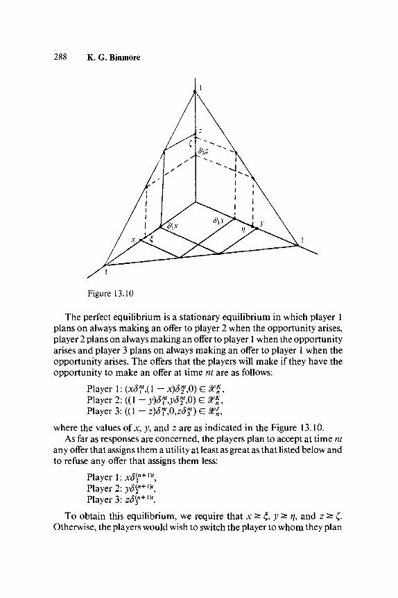
288 K. G. Binmore
Figure 13.10
The perfect equilibrium is a stationary equilibrium in which player 1plans on always making an offer to player 2 when the opportunity arises,player 2 plans on always making an offer to player 1 when the opportunityarises and player 3 plans on always making an offer to player 1 when theopportunity arises. The offers that the players will make if they have theopportunity to make an offer at time nt are as follows:
Player 1: (JC<J?,(1 - x)Sf,0) G %%,Player 2: ((1 - y)Sf,ydffi) e a?*,Player 3: ((1 - z)S790,zS?) e X'n,
where the values of x, y, and z are as indicated in the Figure 13.10.As far as responses are concerned, the players plan to accept at time nt
any offer that assigns them a utility at least as great as that listed below andto refuse any offer that assigns them less:
Player 1: xS\n+l)t,Player 2: yS^+l\Player 3: zd{n+lK
To obtain this equilibrium, we require that x ^ 4 y ^ r\, and z > f.Otherwise, the players would wish to switch the player to whom they plan
Bargaining and coalition 289to make offers. Checking these inequalities involves some elementaryalgebra. Equilibrium requires that
x + sy^iX
S\x =
C + S'2y=lm
From the first pair of equations, we obtain
\-S\d2 y \-6\d\*
which are the values one would obtain if player 3 were absent and players1 and 2 were involved in a two-player Rubinstein bargaining model. Since6X<52, we have that y > x. Also,
x > £ <=> x ^ 1 - 8\z = 1 - S3y<=>x + S3y^ 1<=> S3y — S2y ^ 0 (Because x + S2y = 1)
Similarly,
As always, the most interesting situation is when f—»0+. Then,players 1 and 2 split the cake a?* according to the (asymmetric) Nashbargaining solution with "bargaining powers" xx = (— log Sx)~\ T2 =(—log d2yl. This remains true if we allow player 2 to open the bidding. Ifplayer 3 opens the bidding, then players 1 and 3 will split the cake #f7, butnot according to the (asymmetric) Nash bargaining solution with xx =(—log dx )~l and T3 = (—log S3)~l. Instead, player 1 will receive the sameas he would if he were bargaining with player 2 and player 3 has to becontent with what remains of the cake.
Note that this conclusion means that the stronger a player would be in atwo-player problem, the weaker he will be in a three-player problem. Inparticular, player 3 is either excluded altogether or else, if he happens tobegin with the initiative, can secure only what player 2 would secure in

290 K. G. Binmore
Figure 13.11
this position. But player 3 is the least impatient and hence has the largestvalue of r. Clearly, an instability is built into this model.
The same phenomenon occurs with the one-seller/two-buyer case inwhich ^ a n d ^ a r e as in the previous discussion but $f7 = {(0,0,0)}. Theconsiderations remain exactly the same and the object is sold by player 1to player 2 as if the second buyer, player 3, did not exist.
A market bargaining modelIn this model, player 1 begins by announcing a real number x, whichrepresents the utility he requires if agreement is to be reached. This re-quirement is conveyed to both player 2 and player 3 but player 2 has thefirst opportunity to accept. If player 2 refuses, then player 2 announces areal number y9 which represents the utility he requires if agreement is to bereached. If the game reaches this stage, player 3 then has two offers to

Bargaining and coalition 291
consider and we suppose that he first considers player l's offer and thenplayer 2's offer. If he refuses both, then player 3 announces a real numberz and it is now player 1 who has two offers to consider. If player 1 refusesboth, then the entire situation is repeated from the beginning. The gametree of this model is illustrated in Figure 13.11. The strategy choicesindicated by double lines result in the acceptance of player 2's demand ofy by player 1.
This bargaining model implements the (asymmetric) Nash bargainingsolution for the three-player/three-cake problem as described in Section13.3 provided suitable assumptions are made about discounting and thetiming of offers. As explained in proposition 1, the solution has differentdescriptions depending on whether case I or case II applies and it willsimplify the discussion to consider the two cases separately.
Case I. Here we have a von Neumann-Morgernstern triple {v1^^}(see Figure 13.12). The problem is to show that a perfect-equilibriumoutcome of the game is one of the points in this triple. (It will, in fact, be vK
because player 1 opens the bidding and player 2 has first refusal.) Toobtain the required result in case I, we do not even need to assume that theplayers suffer disutilities from delays in agreement and we will present theargument for the case dx = S2 = S3 = 1.
The argument is based on Figure 13.12. We will show that a perfectequilibrium in pure strategies requires player 1 to open with the demand aand that this offer will be accepted by player 2, thereby implementing vK.That a perfect equilibrium exists with this property is trivial.
The first observation is that a perfect equilibrium in pure strategies forthe subgame that follows an initial offer of a < a by player 1 cannot have
Figure 13.12
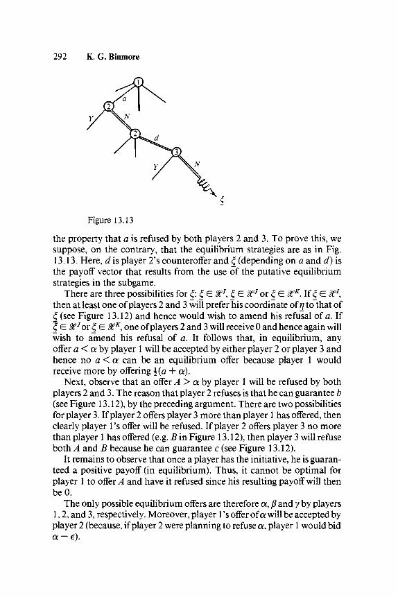
292 K. G. Binmore
Figure 13.13
the property that a is refused by both players 2 and 3. To prove this, wesuppose, on the contrary, that the equilibrium strategies are as in Fig.13.13. Here, d is player 2's counteroffer and £ (depending on a and d) isthe payoff vector that results from the use of the putative equilibriumstrategies in the subgame.
There are three possibilities for £ £ G 7, f G XJ or £ G XK. If f G ^7,then at least one of players 2 and 3 will prefer his coordinate of q to that of£ (see Figure 13.12) and hence would wish to amend his refusal of a. Ifk £ %Jor £ G 3f* one of players 2 and 3 will receive 0 and hence again willwish to amend his refusal of a. It follows that, in equilibrium, anyoffer a < a by player 1 will be accepted by either player 2 or player 3 andhence no a < a can be an equilibrium offer because player 1 wouldreceive more by offering \{a + a).
Next, observe that an offer A > a by player 1 will be refused by bothplayers 2 and 3. The reason that player 2 refuses is that he can guarantee b(see Figure 13.12), by the preceding argument. There are two possibilitiesfor player 3. If player 2 offers player 3 more than player 1 has offered, thenclearly player l's offer will be refused. If player 2 offers player 3 no morethan player 1 has offered (e.g. B in Figure 13.12), then player 3 will refuseboth A and B because he can guarantee c (see Figure 13.12).
It remains to observe that once a player has the initiative, he is guaran-teed a positive payoff (in equilibrium). Thus, it cannot be optimal forplayer 1 to offer A and have it refused since his resulting payoff will thenbeO.
The only possible equilibrium offers are therefore a, p and y by players1,2, and 3, respectively. Moreover, player 1 's offer of a will be accepted byplayer 2 (because, if player 2 were planning to refuse a, player 1 would bida — e).
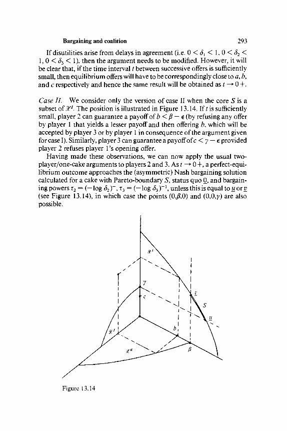
Bargaining and coalition 293
If disutilities arise from delays in agreement (i.e. 0 < dx < 1, 0 < S2 <1, 0 < S3 < 1), then the argument needs to be modified. However, it willbe clear that, if the time interval t between successive offers is sufficientlysmall, then equilibrium offers will have to be correspondingly close to a, b,and c respectively and hence the same result will be obtained as t —* 0 +.
Case II. We consider only the version of case II when the core S is asubset of VC1. The position is illustrated in Figure 13.14. If r is sufficientlysmall, player 2 can guarantee a payoff of b < P — e (by refusing any offerby player 1 that yields a lesser payoff and then offering b, which will beaccepted by player 3 or by player 1 in consequence of the argument givenfor case I). Similarly, player 3 can guarantee a payoff of c < y — e providedplayer 2 refuses player 1 's opening offer.
Having made these observations, we can now apply the usual two-player/one-cake arguments to players 2 and 3. As t —> 0 +, a perfect-equi-librium outcome approaches the (asymmetric) Nash bargaining solutioncalculated for a cake with Pareto-boundary S, status quo 0, and bargain-ing powers r2 = (— log S2)", r3 = (— log S 3)~\ unless this is equal to u or v(see Figure 13.14), in which case the points (0,/?,0) and (0,0,y) are alsopossible.
Figure 13.14

294 K. G. Binmore
13.5 The nontransferable utility Shapley value
For a general discussion of this concept together with an axiomatic deri-vation, we refer to a recent paper by Aumann [ 1 ]. In this paper, Aumannsuggests that the notion is best seen as a "group decision" or an "arbitratedoutcome" or a "reasonable compromise." This viewpoint implies that thenontransferable utility (NTU) Shapley value is best studied under theheading of social-choice theory rather than of game theory proper. How-ever, it remains the case that the Shapley value is often cited in the lattercontext (as the Aumann/Roth debate mentioned in note 1 of Section 13.3confirms). It is therefore necessary to explain how the material of thispaper relates to the NTU Shapley value.
In particular, one might ask whether the results of this paper are con-sistent with the use of the NTU Shapley value when one imposes thesymmetry requirements that xx = T2 = r3 and that equal probabilities areassigned to the formation of each of the coalitions /, / , and K. Since thereappears to be much confusion on this issue (not least in the mind of theauthor) it does not seem adequate simply to remark that the answer is thatour results are not consistent with the NTU Shapley value. For somereaders, it may be enough to comment that neither Pareto-efficiency (inthe context of an averaging process) nor Additivity makes much sense fora game-theoretic interpretation (although this certainly does not apply inthe social choice context). However, we propose to examine more closelythe question of why our considerations diverge from those implicit in theuse of a Shapley value.
The first point to be made is that our whole approach is founded on thenotion that forward commitments are not possible. Any threats that theplayers make must therefore be "credible threats" if they are to influencethe outcome: hence the use of a perfect-equilibrium analysis. We madethis point about single players in Section 13.2. But, obviously, it wouldmake little sense to forbid forward commitment for single players but toallow forward commitment for coalitions. Consistency therefore requiresthat we forbid binding agreements between players concerning the con-duct of the future negotiations between themselves and other players.Indeed, the only binding agreements admissible are cake-division agree-ments (and note that our utilities are very definitely nontransferable).None of this is meant to imply that games with forward commitment arenever relevant, only that we prefer to study what seems to be the logicallyprior and more natural case in which forward commitment is not possi-ble. A consequence of this assumption is that, if a coalition C forms, allthat it can do is agree to an unconditional division of the cake #fc. It cannotagree to a conditional division of the cake contingent on some event being

Bargaining and coalition 295
observed during the future negotiations. This means that Harsanyi's ideaof all coalitions simultaneously guaranteeing their members a minimumpayoff with which he defends the transferable utility (TU) Shapley-valuenotion is not applicable. Or, to put the same point more crudely, onecannot think in terms of coalitions forming by accretion, with each extraplayer contributing a little more, as is the essence of the TU Shapley-valueidea. The claim that our assumptions are logically prior to these necessaryfor dealing with conditional agreements or other forward commitments isbased on the proposition that a formal analysis of forward commitmentshould incorporate the appropriate commitments within the game struc-ture itself, which should then be analyzed without commitment assump-tions. This view derives from Nash and has been emphasized by Harsanyiand Selten. The claim that our assumptions are more natural refers to thepractical difficulties in making commitments stick. This view has beenstressed by Schelling, among others. To me, it seems that the role of thelegal profession in this context has been much overrated. A considerationof greater relevance is the fact that games are often in reality stages in asupergame but then, of course, a formal analysis would be directed towardthe supergame to which the consideration would not apply.
An example may assist. Consider a "transferable utility" game withcharacteristic function Fthat assigns single players 0 and otherwise has
V(J) = V(K) = 2,V(I)=V(G) = 3,
where G is the grand coalition {1,2,3}. One may compute the TU Shapleyvalue from the following table:
Order ofPlayers
Player 1
Player 2
Player 3
123
(1)
0
2
1
132
(2)
0
1
2
213
(3)
2
0
1
231
(4)
0
0
3
312
(5)
2
1
0
321
(6)
0
3
0
Sum ofrows
4
7
7
Shapleyvalue
2/3
7/6
7/6
Note that all but columns 4 and 6 implicitly assume a "two-stage" agree-ment. It is therefore not surprising that the Shapley value ($,£,J) differsfrom (£,1,1), which is the average of the von Neumann-Morgensterntriple {(0,|, j),Q,O, j),(i,f ,0)}, since the latter is computed on the assump-
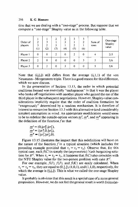
296 K. G. Binmore
tion that we are dealing with a "one-stage" process. But suppose that wecompute a "one-stage" Shapley value as in the following table.
Order ofplayers
Player 1
Player 2
Player 3
123
(1)
0
2
0
132
(2)
0
0
2
213
(3)
2
0
0
231
(4)
0
0
3
312
(5)
2
0
0
321
(6)
0
3
0
Sum ofrows
4
5
5
One-stageShapleyvalue
2/3
5/6
5/6
Note that (i,|,£) still differs from the average (i,l,l) of the vonNeumann - Morgenstern triple. There is a good reason for this difference,which we now discuss.
In the presentation of Section 13.13, the order in which potentialcoalitions formed was essentially "endogenous" in that it was the playerwho broke off negotiations with another player who gained the ear of thethird player in the subsequent negotiations. However, Shapley-value con-siderations implicitly require that the order of coalition formation be"exogenously" determined by a random mechanism. It is therefore ofinterest to reexamine Section 13.3 with this alternative (and considerablysimpler) assumption in mind. An appropriate modification would seemto be to redefine the outside-option vectors m1, mK, and mK appearing inthe definition of the function/so that
Figure 13.15 illustrates the impact that this redefinition will have onthe nature of the function/in a typical situation (which includes thepreceding example provided that TX = T2 = T3). Observe that, for thistypical case, each/(C) is simply the (asymmetric) Nash bargaining solu-tion for %?c. When xx = r2 = T3, it happens that/(C) also coincides withthe NTU Shapley value for the two-person problem with cake %c.
For our example,/(/), /(/), and/(/if) are easily calculated. WhenTj = r2 = T3 , they are equal to (0,$,$), (1,0,1), and (1,1,0), respectively, forwhich the average is ($,£,£)• This is what we called the one-stage Shapleyvalue.
It probably is obvious that this result is a special case of a more generalproposition. However, we do not feel the general result is worth formulat-

Bargaining and coalition 297
f(K)Figure 13.15
ing for two reasons. The first is that the general result will apply only in thetypical case illustrated in Figure 13.15 (and which corresponds to case I ofSection 13.13). For situations corresponding to that of case II, the resultwill not hold (and, in any event, one would be very suspicious aboutattaching equal probabilities to the coalitions). Second, the considera-tions necessary to try to force some relevance for the NTU Shapley valuefor problems more complex than the three-player/three-cake problemseem excessively Machiavellian.
Where does this leave the NTU Shapley value? Certainly nothing thathas been said affects the notion in so far as it is a construct of social choice(or social valuation) theory. Likewise, nothing has been said that deniesthe validity of Harsanyi's [9] analysis given the basic assumptions onwhich the analysis is based. However, it is to be hoped that the discussionoffered does raise doubts about the use of the NTU Shapley value as ageneral principle in bargaining theory except in the case of the two-player/one-cake problem. Even here, the observation that the (symmet-ric) Nash bargaining solution and the NTU Shapley value happen tocoincide would seem more reasonably attributable to the fact that only alimited number of invariances are available in such a simple situationthan to any intrinsic merit of the NTU Shapley value. (Of course,independent arguments are available in favor of the Nash bargainingsolution.)

298 K. G. Binmore
"statusquo"
Xl Kalai and Smorodinskysolution
"utopia point"
(symmetric) Nashsolution
O
Figure 13.16
13.6 The Raiffa/Kalai - Smorodinsky solution
Various alternatives have been offered to the Nash bargaining solution forthe two-player/one-cake problem (see Roth [19]). Some of these areclearly not genuine competitors because they relate to informational as-sumptions that differ from those appropriate to the Nash bargainingsolution. However, the Kalai-Smorodinsky [11] solution certainly doesshare the same informational base as the Nash solution (Figure 13.16).
In this section, we hope to offer a reason for regarding the Nash bar-gaining solution and a variant of the Kalai-Smorodinsky solution ascomplementary rather than rival notions. Perhaps this variant is betterdescribed as the Raiffa solution. The difficulty with Kalai and Smoro-dinsky's monotonicity axiom is its implicit assumption that the replace-ment of one cake, #f, by another cake 9, may put one player in a "strongerbargaining position" than previously, and hence he ought to receive atleast the payoff he would have received with the original cake, $?. How-ever, it is difficult to understand what mechanism could generate thisstronger bargaining position given that we are supposed to assume that theonly threat available to either player is the threat to disagree and thatdisagreement by either player leads simply to the status quo. We proposeto avoid this difficulty by arguing as in Section 13.2 that the status quoshould be seen as a reference point rather than a unique disagreement

Bargaining and coalition 299
point. We are then free to admit the possibility discussed in Section 13.2 ofthe players having open the opportunity to bargain elsewhere if the negoti-ations are unsatisfactory. The simplest such situation is precisely thatdiscussed in Section 13.3 with a single third player in the background, andwe will work with this situation although it will be evident that similarconsiderations may apply with a more complex scenario.
We adapt the notation of Section 13.3 by taking a? to be b u t with thethird coordinate of its elements suppressed. Similarly, we suppress thefirst and second coordinates, respectively, of the sets < 7 and $fy, andassume that the resulting sets are both 2£. Since the Kalai-Smorodinskysolution requires a symmetry axiom, we cannot dispense with this as-sumption. We regards as fixed and #? as a variable. Where does the Nashbargaining solution for the three-person/three-cake problem place theagreement point aK for the coalition {1,2} as a function of the set Sf ? Thequestion is answered in Figure 13.17 provided that the point v illustrateddoes not lie in #f.
For circumstances under which the best possible result for the playerswill be the same no matter with whom this result is negotiated (i.e.,
Figure 13.17

300 K. G. Binmore
O
Figure 13.18
exogenously determinedcurve
Ax= A2 and i?! = B2), the "utopia point" u of Figure 13.16 and the pointv of Figure 13.17 will be the same, and hence aK will be precisely theKalai-Smorodinsky solution K. Without a symmetry assumption, thestraight line joining 0 and v in Figure 13.17 will be replaced by a curve.
Finally, it may be worth noting what an outside observer would recordafter watching a sequence of independent bargaining games with differentcakes X and a fixed status quo 0 in ignorance of the existence of a thirdplayer and two further fixed cakes XJ and %J. This situation is illustratedin Figure 13.18. The "solution" for Xt on the basis of the analysis ofSection 13.3 is denoted by at. (Of course, a0 is to be interpreted as theresult //agreement were reached, which would seem unlikely in general.)Note the mixture of different ideas.
13.7 Axiomatization
The question of an axiomatic characterization has been left until last fortwo reasons. The first reason is that it seems inappropriate to say morethan a few words unless the general ra-player/«-cake problem is to be

Bargaining and coalition 301
examined. The second reason is that undue weight seems to be attached toconcepts that admit simple axiomatic characterizations.
Briefly, however, we note that [3] provided an axiomatic characteriza-tion of the Nash bargaining solution in the two-player/one-cake case inwhich the "independence of irrelevant alternatives" axiom was replacedby a "multiplicative axiom." The latter bears a family resemblance to theShapley "additivity axiom" but requires invariance when two games are"multiplied" rather than "added". Refer to [3] for an explanation of whyit may be reasonable to wish to multiply two games. In the current contextof the three-player/three-cake example, such a multiplicative axiomwould reduce the problem to the consideration of games that admit acharacteristic function description; that is, the use of the multiplicativeaxiom would correspond to the reduction in the Shapley context of non-transferable utility games to transferable utility games. How one dealswith a game in characteristic function form remains a matter for debatebut at least this is familiar ground.
NOTES1. This view has been championed perhaps most effectively by Harsanyi and
Selten.2. This observation is not of course intended to apply to cooperative solution
concepts that are justified as "fair arbitration schemes" or the like. My ownview is that "fair arbitration schemes" are best studied under the heading ofsocial-choice theory rather than game theory (although admittedly someblurring of the distinction is inevitable once the question of implementationarises).
3. It is important to note that various ^-person cooperative concepts have atendency to coalesce in the three-person/three-cake case and that, in choosingto couch the required cooperative idea in terms of Nash bargaining solutions,I am vulnerable to accusations of prejudice. It would be possible, for example,to make do with the two-person Nash solution and graft this onto the notionof the core of a game together with Vickrey's strengthening of the vonNeumann - Morgenstern idea of a stable set to that of a strongly stable set (see,for example, [12], p. 213). Alternatively, one could use a stability notion ofAlbers as a substitute for the core and strongly stable sets. This path is fol-lowed by Selten [24] in a paper with similar aims to the current paper. Yet,again, one could adopt the Aumann - Maschler notion of a bargaining set (see[18]). What is certain is that, if there is a "correct" description of the appropri-ate cooperative bargaining concept, the three-person/three-cake problem hastoo simple a structure to reveal this.
4. Rubinstein worked independently, but his work is of course closely related tothat of Stahl [26], and of Harsanyi and Selten and others. Rubinstein hasrecently made an important advance in extending his work to a case whereinformation is not complete (see [22]).
5. Such a constraint must exist if only for physical reasons. Naturally, however,

302 K. G. Binmore
players would prefer to respond at the earliest possible moment and so inter-est centers on what happens when the response times are small comparedwith the other parameters of the problem.
6. This means that strategy -tuples are Nash equilibria not only in the game as awhole but also in every subgame (see Selten [23]).
7. The assumption that #f is compact and convex is standard. The other as-sumptions on #f are not essential and are introduced to avoid the discussionof technicalities.
8. For simplicity, we exclude the degenerate case of zero bargaining powers.9. This usage of the term "bargaining power" is quite different from that of
Harsanyi. Incidentally, it is important that the parameters xx and T2 be deter-mined entirely by the players and are independent of f. In Section 13.4, TXand T2 measure the players' impatience at delays in agreement but otherinterpretations are possible.
10. To ignore the location of the original "status quo" point would certainly notbe correct with the interpretation of m given in this section, although this isdisguised to some extent by the fact that the original "status quo" is normal-ized at 0. However, even if one assumed that both player 1 and player 2receive their respective coordinates of m if negotiations break down (i.e. m isthe disagreement point), it does not necessarily follow that one should simplyuse the Nash bargaining solution with "status quo" transferred to m. It stillmay be appropriate, as in the entirely natural bargaining model describedlater in this section, to use a point other than m (in our case 0) as a referencepoint.
11. As far as an axiomatic characterization is concerned, one simply needs toclassify those i G f that do not satisfy x ^ m a s "irrelevant alternatives".
12. For the purposes of interpretation, one may imagine that player 1 threatens touse his outside option before the preceding offer by player 2. Player 2 will thenhave to consider whether this threat is credible. This consideration is takencare of by using a perfect-equilibrium analysis.
13. The player with the initiative, for example, might be the first to notice theopportunity for outside activity.
14. We do not consider the situation in which both players can simultaneouslysecure their outside options, although this is an easier case to analyze. Thiscase is not relevant to the application required in Section 13.3.
15. As Selten observes in [24], in practice one would expect this question to beresolved by issues such as who first notices that a bargaining situation existsand whom it is convenient for him to contact first. Since the factors governingsuch items are likely to be ephemeral, there seems little point in trying tomodel them explicitly other than by attaching equal probabilities to the threecoalitions where necessary.
16. Sometimes this is assumed, as in [27], even when the possibility of the buyersbeing able to form an unbreakable coalition has not been excluded.
17. The fact that we reject the survival of the two-person/one-cake solution in thepresence of the three-person/three-cake problem as "mainstream", does notmean that we deny the existence of important situations in which such "stick-iness" is the overriding factor.
18. It is similar to an idea of Harsanyi ([9], p. 248) embodied in what has beencalled the Harsanyi/Nash/Shapley value. An important difference betweenthe situation considered here and that considered by Harsanyi is that, in hiscase, a coalition is able to guarantee its members certain utility levels inde-

Bargaining and coalition 303
pendently of the guarantees made by other coalitions, whereas for the three-person/three-cake problem considered in this paper, this is impossible.Among other things, this means that there is a difference in the interpretationof the solution payoffs. For Harsanyi, these are actual payoffs, whereas in thispaper they are potential payoffs contingent on an appropriate coalition beingformed.
19. The word "define" is premature since it remains to be established that theproperty offered is consistent and categorical.
20. Of course, there may be situations in which if player p breaks off negotiations,then he will not necessarily gain the ear of player r; that is, the idea of the"initiative" is inappropriate. If, for example, the breaking off of negotiationsbetween players 2 and 3 led to a random move with probability \ that player 2would be involved in the subsequent negotiations with player 1 and probabil-ity i that player 3 would be involved, then it would make sense to take^3 = W + iO and mI
1 = ±0 + \o$.21. In the sense that, if one were assigning probabilities to the three possible
outcomes in the spirit of the Shapley value, one would attach a high probabil-ity to f(C).
22. As explained in [5], the argument goes through under very much more gen-eral conditions on %n, but there seems little point in describing a very generalmodel for our purposes.
23. Indeed, we sometimes do not know how to proceed when there is a uniqueequilibrium. However, at least the bargaining games considered here are freeof this type of problem. As far as the general problem of equilibrium selectionis concerned, attention should be drawn to the theory of Harsanyi and Selten[10]. I cannot claim to appreciate fully the guiding philosophy behind thistheory but the relevance of much of what is said cannot be denied. Myproblem lies in fitting all the many considerations into a coherent whole. Inany case, I am not competent to attempt to apply the theory in the currentcontext.
24. One may model them as voting in sequence or simultaneously. In the lattercase, it would seem sensible to introduce a Selten "trembling hand" to avoidthe trivial equilibrium in which all players always vote in the negative. For astudy of a finite-horizon version, see Dutta and Gevers [6].
25. One in which actions chosen at time t are independent of history, that is, ofwhat happened at times s < t.
26. Strong in the sense of Aumann (i.e. the strategies are optimal not only forsingle players but also for coalitions, given no deviations by outsiders).
27. The "discriminating" von Neumann-Morgenstern solution sets do not ap-pear in any of the bargaining models considered here.
28. We have the London financial futures market in mind here.29. One can use the method of Shaked and Sutton [25] to show that this is the
only perfect-equilibrium outcome in this particular case but I do not know ofa technique adequate to handle the general case.
REFERENCES[1] Aumann, R.: An Axiomatization of the Non-Transferable Utility Value.
Working paper (1983a).[2] On the Non-Transferable Utility Value. Working paper (19836).
304 K. G. Binmore
[3] Binmore, K. G.: Nash Bargaining Theory I, II, and III ICERD DiscussionPapers 9, 14, and 15, LSE (1980-81).
[4] Nash Bargaining and Incomplete Information. Economic Theory Discus-sion Paper No. 45, Dept. of Applied Economics, Cambridge University(1981).
[5] Perfect Equilibria in Bargaining Models. ICERD Discussion Paper 58, LSE(1982).
[6] Dutta, G., and L. Gevers: On Majority Rules and Perfect Equilibrium Allo-cation of a Shrinking Cake. Working paper, Namur University (1981).
[7] Fudenberg, D., and J. Levine: Perfect Equilibria of Finite and Infinite Hori-zon games. Working Paper 216, Dept. of Economics, UCLA (1981).
[8] Harsanyi, J.: An Equilibrium-Point Interpretation of Stable Sets and a Pro-posed Alternative Definition. Management Science 20 (1974), 1422-95.
[9] Rational Behaviour and Bargaining Equilibrium in Games and Social Situ-ations. Cambridge University Press, Cambridge (1977).
[10] Harsanyi, J., and R. Selten: A Non-Cooperative Solution Theory with Coop-erative Applications. Working Papers, Institute of Economics, Bielefeld,Nos. 91, 92, 105, and 114 (1980-82).
[11] Kalai, E., and M. Smorodinsky: Other Solutions to Nash's Bargaining Prob-lem". Econometrica 43 (1975), 513-18.
[12] Luce, R., and H. Raiffa: Games and Decisions. Wiley, New York (1957).[13] MacLennan, A.: A General Non-Cooperative Theory of Bargaining. Work-
ing paper, Dept. of Political Economy, University of Toronto (1980).[14] Moulin, H.: Bargaining and Non-Cooperative Implementation. Ecole Poly-
technique (Laboratoire d'Econometrie) Discussion Paper A239 0282(1982).
[15] Nash, J. F.: The Bargaining Problem. Econometrica 18 (1950), 155-62.[16] Non-Cooperative Games. Annals of Mathematics 54 (1951), 286-95.[17] Two-Person Cooperative Games. Econometrica 21 (1953), 128-40.[18] Owen, G.: Game Theory (2nd Ed.). Academic Press, New York (1982).[19] Roth, A. E.: Axiomatic Models of Bargaining. Lecture Notes in Economics
and Mathematical Systems No. 170, Springer-Verlag, Berlin (1979).[20] Values for Games without Side Payments: Some Difficulties with Current
Concepts. Econometrica 48 (1980), 457-65.[21] Rubinstein, A.: Perfect Equilibrium in a Bargaining Model. Econometrica
50(1981), 97-110.[22] A Bargaining Model with Incomplete Information. Working paper, Dept. of
Economics, Hebrew University (1983).[23] Selten, R.: Re-Examination of the Perfectness Concept for Equilibrium
Points in Extensive Games. International]ournal of Game Theory 4 (197 5),25-55.
[24] A Non-Cooperative Model of Characteristic Function Bargaining. Workingpaper, Institute of Mathematical Economics, Bielefeld, No. 90 (1980).
[25] Shaked, A., and J. Sutton: Involuntary Unemployment as a Perfect Equilib-rium in a Bargaining Model. ICERD Discussion Paper 63 (1983).
[26] Stahl, I.: Bargaining Theory. Economic Research Institute, Stockholm(1972).
[27] Weintraub, R.: Conflict and Cooperation in Economics. Macmillan, Lon-don (1975).

CHAPTER 14
Axiomatic approaches tocoalitional bargaining
Sergiu HartTEL-AVIV UNIVERSITY
14.1 Introduction
The simplest bargaining situation is that of two persons who have to agreeon the choice of an outcome from a given set of feasible outcomes; in caseno agreement is reached, a specified disagreement outcome results. Thistwo-person pure bargaining problem has been extensively analyzed, start-ing with Nash (1950).
When there are more than two participants, the ^-person straightfor-ward generalization considers either unanimous agreement or completedisagreement (see Roth (1979)). However, intermediate subsets of theplayers (i.e., more than one but not all) may also play an essential role inthe bargaining. One is thus led to an n-person coalitional bargainingproblem, where a set of feasible outcomes is specified for each coalition(i.e., subset of the players). This type of problem is known as a game incoalitional form without side payments (or, with nontransferable utility).It frequently arises in the analysis of various economic and other models;for references, see Aumann (1967, 1983a).
Solutions to such problems have been proposed by Harsanyi (1959,1963, 1977), Shapley (1969), Owen (1972), and others. All of these wereconstructed to coincide with the Nash solution in the two-person case.Unlike the Nash solution, however, they were not defined (and deter-mined) by a set of axioms.
Recently, Aumann (19836) has provided an axiomatization for theShapley solution. Following this work, further axiomatizations were ob-tained: for the Harsanyi solution by Hart (1983), and for a new class ofmonotonic solutions by Kalai and Samet (1983). The purpose of thischapter is to review and compare these three approaches.
The discussion is organized as follows. The mathematical model isdescribed in Section 14.2, and is followed by the definitions of the solu-tions in Section 14.3. The axioms that determine these solutions are
305
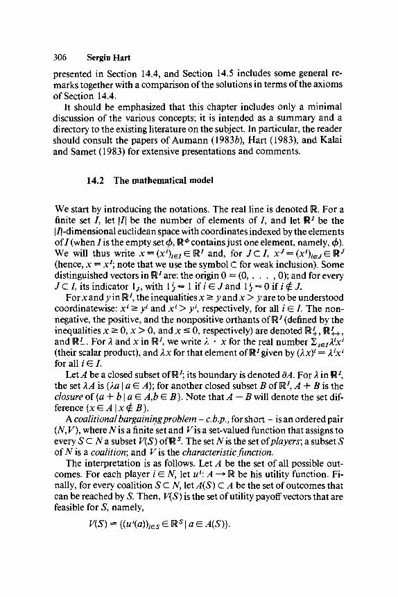
306 Sergiu Hartpresented in Section 14.4, and Section 14.5 includes some general re-marks together with a comparison of the solutions in terms of the axiomsof Section 14.4.
It should be emphasized that this chapter includes only a minimaldiscussion of the various concepts; it is intended as a summary and adirectory to the existing literature on the subject. In particular, the readershould consult the papers of Aumann (1983&), Hart (1983), and Kalaiand Samet (1983) for extensive presentations and comments.
14.2 The mathematical model
We start by introducing the notations. The real line is denoted R. For afinite set /, let |/| be the number of elements of /, and let IR7 be the|/|-dimensional euclidean space with coordinates indexed by the elementsof/(when /is the empty set 0, R* contains just one element, namely, </>).We will thus write x = (xi)ieIGUI and, for / C / , xJss(xi)iGJBUJ
(hence, x = x1; note that we use the symbol C for weak inclusion). Somedistinguished vectors in R7 are: the origin 0 = (0,. . . ,0); and for everyJCI, its indicator lj9 with 1>= 1 if i G / and 1>= 0 if i'£ / .
For x and y in R7 the inequalities x ^ y and x > y are to be understoodcoordinatewise: x' ^ y' and xl > y\ respectively, for all i G /. The non-negative, the positive, and the nonpositive orthants of R7 (defined by theinequalities x ^ 0, x > 0, and x ^ 0, respectively) are denoted R+, R7^,and RL For X and x in R7, we write X • x for the real number 2 /e/A/x/
(their scalar product), and Xx for that element of R7given by (Xx){ = A'JC1'for all / G /.
Let A be a closed subset of R7; its boundary is denoted dA. For X in R7,the set XA is {Xa \ a G A); for another closed subset B of R7, A + B is theclosure of{a + b\aE A,b G B). Note that A — B will denote the set dif-ference {xGA\x$.B}.
Kcoalitional bargaining problem - c.b.p., for short - is an ordered pair(N, V), where TV is a finite set and Fis a set-valued function that assigns toevery S C TVa subset V(S) of Rs. The set TV is the set of players; a subset Sof TV is a coalition; and Kis the characteristic function.
The interpretation is as follows. Let 4 be the set of all possible out-comes. For each player / G TV, let uu. A —> R be his utility function. Fi-nally, for every coalition SCN, let A(S) C A be the set of outcomes thatcan be reached by S. Then, K(5) is the set of utility payoff vectors that arefeasible for S, namely,

Axiomatic approaches to coalitional bargaining 307In game theory, such a pair (N, V) is called a game in coalitional (or,
characteristic function) form with nontransferable utility (or, without sidepayments).
The set TV of players will be fixed throughout this chapter; a c.b.p. willthus be given by its characteristic function V. The space F = F(N) of allc.b.p.'s that we will consider consists of all members of Fthat satisfy thefollowing conditions:
(1) For every S C N, the set V(S) isa. A non-empty subset of IR7,b. Closed,c. Convex,d. Comprehensive (i.e., x G V(S) and x ^ y imply y G V(S)).
We will also consider the following additional regularity conditions:
(2) The set V(N) isa. Smooth (i.e., V(N) has a unique supporting hyperplane at
each point of its boundary dV(N))9b. Nonlevel (i.e., x,y G dV(N) and x ^ y imply x = y).
(3) For every ScN, there exists x G UN such that
(4) For every S C TV and every sequence {xm} ~ « { C F(5) that is non-decreasing (i.e., xm+! ^ xm for all m ^ 1), there exists y G IR s suchthat xm ^ y for all m ^ 1.
Denote the set of all Fin T that satisfy (2) by Tx, those that satisfy (4) byF2, and those that satisfy (2) and (3) by T3.
Conditions (1) are standard. Condition (2b) is a commonly used regu-larity condition, meaning that weak and strong Pareto-optimality coin-cide for V(N). The smoothness of V(N) is an essential condition; (2a)implies that, for every x£d V(N), there exists a unique normalized vectorX in UN such that X • x > X - y for all y in V(N). Note that X must bepositive (i.e., X G JJ++) by (Id) and (2b). Condition (3) may be viewed asan extremely weak kind of monotonicity: There exists some translate ofV(N) that includes all of the payoff vectors that are feasible for 5* andassign zero to the players outside S. Finally, (4) is a boundedness-from-above condition. A thorough discussion on assumptions and their impactcan be found in Sections 9 and 10 in Aumann (19836).
For a coalition S C N, an S-pay off vector is simply an element of Rs'9when S = N, it is a payoff vector. A collection x = (xs)SGN of S-payoffvectors for all coalitions S is called a payoff configuration (thus,xs~ (xs)i<Es£- ^s f° r a^ S c N). The space of payoff configurations
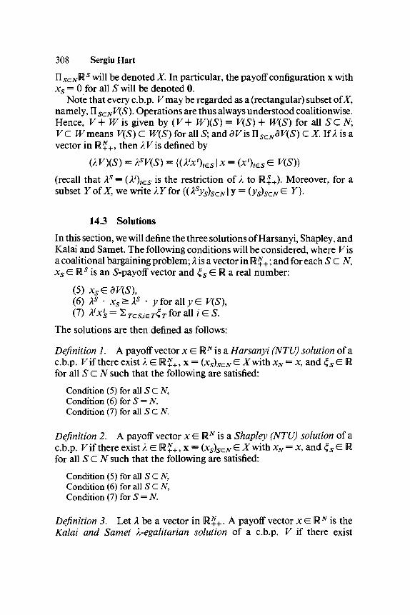
308 Sergiu HartlR5 will be denoted X In particular, the payoff configuration x with
xs = 0 for all S will be denoted 0.Note that every c.b.p. Fmay be regarded as a (rectangular) subset of X,
namely, n^^F^S). Operations are thus always understood coalitionwise.Hence, F + W is given by (F + W)(S) = V(S) + W{S) for all S C N\Vc JF means V(S) C W{S) for all 5; and dFis HS(ZNdV(S) C X If A is avector in IR^+, then AFis defined by
{XV){S) = XSV{S) = {(A'x'),es I* = (*')/« e F(5)}(recall that ks = (A0,-es is the restriction of A to R++). Moreover, for asubset y of X, we write XY for {(A5y5)ScAr | y =
14.3 Solutions
In this section, we will define the three solutions of Harsanyi, Shapley, andKalai and Samet. The following conditions will be considered, where Fisa coalitional bargaining problem; A is a vector in U £+; and for each ScN,xs E Rs is an S-payoff vector and £s E IR a real number:
(5) xs<EdV(S),(6) Xs • xs>ks - yforallyE V(S\(7) X'x's = 2 ra,/er£r for all / E 5.
The solutions are then defined as follows:
Definition 1. A payoff vector x E UN is a Harsanyi (NTU) solution of ac.b.p. F if there exist A E U%+, x = (x5)5cA, E X with.% = x, and £s E IRfor all 5* C A such that the following are satisfied:
Condition (5) for all ScN,Condition (6) for S = N,Condition (7) for all ScN.
Definition 2. A payoff vector x E UN is a Shapley (NTU) solution of ac.b.p. F if there exist Ae.R%+,x = (xs)Sc:N E X with x^ = x, and <J5 E IRfor all S C N such that the following are satisfied:
Condition (5) for all ScN,Condition (6) for all S C N,Condition (7) for S = N.
Definition 3. Let A be a vector in R?+ . A payoff vector x E R^ is theKalai and Samet ^-egalitarian solution of a c.b.p. F if there exist

Axiomatic approaches to coalitional bargaining 309x = (xs)SGN G X with xN = x and £s G R for all S C TV such that the fol-lowing are satisfied:
Condition (5) for all ScN,Condition (7) for all S C N.
Note that Kalai and Samet define a class of solutions, parameterized byk (which is thus exogenously given, besides V)\ moreover, each c.b.p. canhave at most one A-egalitarian solution (for every k\ see the end of thissection). In both the Harsanyi and Shapley solutions, k is endogenouslydetermined, and there may be no solution or more than one. When the k*are all equal (i.e., k = cl^for some c G R J , the corresponding Kalai andSamet solution is called the symmetric egalitarian solution. The vector kyields an interpersonal comparison of the utility scales of the players;whether it is obtained from the bargaining problem itself, or it is anadditional datum of the problem, is thus an essential distinction (see alsoSection 14.5).
The associated payoff configuration x = (xs)S(ZN specifies for every co-alition S a feasible (and even efficient, by condition (1)) outcome xs. Onemay view xs as the payoff vector that the members of S agree upon fromtheir feasible set V(S); if coalition S "forms," then x's is the amount thatplayer i (in S) will receive (note that these are contingent payoffs - ifSforms). Following Harsanyi, one may furthermore regard xs as an optimalthreat of coalition S (against its complement TV — S), in the bargainingproblem. More discussion on these interpretations can be found at theend of section 5 in Hart (1983).
The three conditions (5), (6), and (7) may be interpreted as efficiency,k-utilitarity, and k-equity (oxfairness), respectively. Indeed, condition (5)means that the S-payoff vector xs is Pareto-efficient for the coalition S:There is no vector y G R s that is feasible for S (i.e., y G V(S)) such that allmembers of S prefer y to xs (i.e., y > xs). Condition (6) means that xs isA-utilitarian for S, since it maximizes the sum of the payoffs for membersof 5, weighted according to k, over their feasible set V(S). And, finally, theweighted payoff k'x's of each member of the coalition S is the sum of thedividends £ rthat player i has accumulated from all subcoalitions TotSXowhich he belongs; because the dividend <Jr is exactly the same for allmembers of T (for each T), xs is thus A-equitable or A-fair.
In the two-person simple bargaining problem, the Nash solution isefficient, and for an appropriate vector k > 0, it is both A-utilitarian andA-equitable. Both the Harsanyi and the Shapley solutions to the generalcoalitional bargaining problem require efficiency (5) for all coalitions

310 SergiuHarttogether with utilitarity (6) and equity (7) for the grand coalition N. Theydiffer in the condition imposed on subcoalitions (other than N and thesingletons): The Harsanyi solution requires equity, and the Shapley solu-tion utilitarity. The Kalai and Samet solutions do not consider utilitarityat all, but only equity (for all coalitions). Thus, the weights A have to begiven exogenously, whereas in the other two solutions they are deter-mined by the conjunction of (6) and (7). Note further that, in the two-person case, all of the egalitarian solutions (including the symmetric one)differ from the Nash solution (they are the proportional solutions of Kalai(1977)).
In general, some of the coordinates of A may be zero (and thusA E R% - {0} instead of A E R++); the simplifying assumption (2b) rulesout this for the Harsanyi and the Shapley solutions (by (6) for S = N); forthe egalitarian solutions, the positivity of A is part of the definition.
The three definitions have been stated in order to facilitate comparisonamong the solutions. For alternative (and more constructive) definitions,we need the following.
A transferable utility game (TU game, for short) consists of a finite setof players TV and a real function v that assigns to each coalition S C Nits worth v(S), with v(<f>) = 0. The Shapley (1953) value of such a TUgame (N9v) is a payoff vector JCEIR^, which will be denotedSh(N,v) = (Sh\N,v))ieN. It is defined by a set of axioms, and it equals thevector of average marginal contributions of each player to those precedinghim in a random order of all the players.
Using this concept, one can rewrite the condition "there exist realnumbers £T E U for all T C S such that (7) is satisfied for all T C S" as:
(8) A ^ = Sh'iStV), where v(T) = kT • xT = 2 ^ A ^ for all Tc S
We then obtain the following.
Definition lf. A payoff vector x E RNis a Harsanyi solution ofa c.b.p. Vif there exist A E [R£+ and x = (xs)ScN E X with xN = x such that condi-tions (5) and (8) are satisfied for all S C TV and condition (6) is satisfied forS = N.
Definition 2'. A payoff vector x E IR^is a Shapley solution of a c.b.p. Vifx E V{N) and there exists A E M%+ such that
= Shf(N,v\
where v(S) = max{ Xs • y \ y E V(S)} for all S C N.

Axiomatic approaches to coalitional bargaining 311
(Note that (6) implies (5) and that the TU game v in (8) coincides with vdefined previously.)
Definition 3'. Let X G U%+. A payoff vector x G UN is the Kalai andSamet X-egalitarian solution of a c.b.p. V if there exists x = (xs)ScN G Xwith xN = x such that conditions (5) and (8) are satisfied for all S C TV.
How are the solutions of a given c.b.p. ^constructed? In the case of theShapley solution, for each X G R++, one computes the TU game vx by
v,(S) = mzx{Xs • y\yEV(S)}for all S C N, and then obtains its Shapley TU value Sh(N,vx). If the payoffvector x = (ATOIEJV given by x* = Sh'(N,vx)/A? for all / E iV belongs toV(N), then x is a Shapley solution of F
The Kalai and Samet A-egalitarian solution (for a given X G U++) isobtained as follows. Inductively on the lattice of all subsets S of N, wedefine
where zs(t) = (z^(r))/e5 G IR5 is given by
2
If we put
then x^ is the A-egalitarian solution of V.Finally, to obtain the Harsanyi solution, we compute the A-egalitarian
solution x( k) for each X G R %+; then, x = x( X) is a Harsanyi solution of FwheneverX • x(A) = max{/l • y |yG F(A )}.
Thus, both the Harsanyi and the Shapley approaches require essen-tially a fixed-point construction, whereas the Kalai and Samet approachdoes not (again, X is exogenously given there). It is now clear that each FinF has at most one A-egalitarian solution, and precisely one (for each X) if Vbelongs to F2.
14.4 AxiomatizationsIn this section, we will present an axiomatization for each one of the threesolutions defined previously. By axiomatization is meant a set of axiomsthat uniquely characterize the corresponding solution.

312 SergiuHart
As is usually the case, there are various ways of choosing an appropriateset of axioms. We will follow here the choices made by each author in thepapers we review. This will enable us to exhibit a large number of axiomsemphasizing a variety of reasonable principles for solving coalitionalbargaining problems.
The first solution studied will be the Shapley solution, according toAumann's (19836) pioneering paper. For every c.b.p. Fin F, let A(F)denote the set of Shapley solutions of F; A(F) is thus a (possibly empty)subset of RN.
Let F4 denote the set of all c.b.p.'s in F3 that possess at least one Shapleysolution (i.e., F4 = ( F e F | Vsatisfies (2), (3), and A(F) ¥= <£}). The set-valued function A from F4 to IR^ will be called the Shapley function. Thefollowing axioms will characterize it.
AO. O is a non-empty-set-valued function from F4 to UN.
(For each KG F4, O(F) is a nonempty subset of IR .)
Al. O(F) C dV(N) for all KG F4.
(Efficiency: Every solution must be Pareto-efficient [for the grandcoalition].)
A2. O(AF) = AO(F) for all X G R£+ and F E F4.
{Scale covariance: If the payoffs of the players are rescaled independently,all solutions will be rescaled accordingly.)
A3. If U=V+W, then O(C7) D (O(F) + O(W)) n dU(N) for all
(Conditional additivity: If x G O(F) is a solution of V,y G ®(W) is asolution of W9 and z = x + y is efficient for U = V + W, then z is asolution of C/[i.e., z G
. If V(N)dW(N) and F(5) = W[5) for all S* N, thenD <&(W) n F(iV) for all V,WG F4.
(Independence of irrelevant alternatives: If Fis obtained from fFby re-stricting the feasible set of the grand coalition, then any solution of Wthatremains feasible in F will be a solution of Fas well.)
For the next axiom, we define a class of c.b.p.'s usually referred to as
Axiomatic approaches to coalitional bargaining 313unanimity games. For every nonempty TCN and every real number c,let uT>c be the TU game given by uT>c(S) = c if S D T and uTtC(S) = 0otherwise; then, UTtC(S) = {xGR 5 | 2 f e 5x< < uTtC(S)} for all Sc N.
A5. &(UTtl) = {\TI\T\} for all TcN,T*<f).
(Unanimity games: UTl models the situation where each coalition Scanarbitrarily divide among its members the amount 1, if it contains all theplayers of T - or nothing, otherwise. This c.b.p. has a unique solution,where the members of Treceive equal shares (1 /1 T\), and the other playerszero.)
Theorem A (Aumann (19836)). There exists a unique function O satis-fying AO through A5; it is the Shapley function A.
We continue next with the Harsanyi solution, according to Hart(1983). We will consider here not only the payoff vector x = xN of thegrand coalition, but rather the full payoff configuration x = (xs)S(ZN. LetH( V) stand for the set of all x = (xs)ScN E X associated with a Harsanyisolution of a c.b.p. V\ that is, x = (xs)sc:N E H(V) if there exists X G IR£+such that conditions (5) and (8) are satisfied for all S C N and condition(6) is satisfied for S — N\ see definition 2'). The set-valued function Hfrom Tx to X will be called the Harsanyi function; we will refer tox = (xs)S(ZN E H(V) as a Harsanyi solution of V(rather than just to xN).Note that H( V) may well be an empty set for some V E Tx. Consider nowthe following axioms.
BO. *¥ is a set-valued function from T{ to X.
(For each F E Tx, *F(F) is a subset of X.)
BL 4 /(F)C(9Fforall
{Efficiency: Every solution x = (xs)s<zNE H(V) must be Pareto-efficientfor all coalitions: xs E dV(S) for all S C N.)
B2. ^{XV) = X¥(V) for all X E n»+ and F G T , .
(Scale covariance: If the payoffs of the players are rescaled independently,all solutions will be rescaled accordingly.)
B3. If U=V+W, then ^U) D (*¥(¥) +^W)) n dU for all

314 SergiuHart(Conditional additivity: If x = (xs)ScN E *F( V) is a solution of F,y = (ys)scN e $K W) is a solution of PF, and z = x + y is efficient for£/= F + W[i.e., z5 E dV(S) for all 5 C TV], then z is a solution of [/[i.e.,z £¥(£/)].)
B4. If FC FT, then *F(K) D (H^) n Ffor all
(Independence of irrelevant alternatives: If Fis obtained from Why re-stricting the feasible set of some coalition(s), then any solution of P^thatremains feasible in Vwill be a solution of Fas well: x = (xs)S(ZN E *F( W)and ;c5 E F(S) C W^) for all S C TV imply x E *F( F).)
B5. V(UTtC) = (z(r,c)} = {zs(T,c))ScN} for all TC TV, T* 0, and allc 6 R , where z^^c) = c l r / | r | if SD T and z^^c) = 0 otherwise.
(Unanimity games: UTc models the situation where each coalition S canarbitrarily divide among its members the amount c if it contains all theplayers of T - or nothing, otherwise. This c.b.p. has a unique solutionz = z(r,c); the S-payoff vector zs of a coalition S that contains T assignsequal shares (c/\ T\) to all members of Tand zero to the rest; if Sdoes notcontain T, everyone gets zero.)
B6. IfOEdF, t h e n O E ^ F ) .
(Inessential games: A c.b.p. is called zero inessential if 0 E dV(S) for allS C TV, that is, if the zero payoff vector is efficient for all coalitions. Thismeans that for all coalitions, 0 is feasible, whereas no positive vector isfeasible. In particular, F({/}) = (x 'E U{i) \xl < 0). For such a game,where there is nothing to bargain on, the payoff configuration zero is asolution.)
Theorem B (Hart (1983)). There exists a unique function *F satisfyingBO through B6; it is the Harsanyi function H.
It is remarkable that the two solutions of Shapley and Harsanyi aredetermined by very similar sets of axioms. The main difference lies in therange: payoff vectors for the former versus payoff configurations for thelatter (see Section 5 in Hart (1983) for further discussion of this subject).
We come now to the class of Kalai and Samet solutions. For everyX E R%+9 let Ek be the function from T2 into RN that assigns to eachF E F2 its A-egalitarian solution E\ V). We will refer to Ex as the ^-egali-tarian function. Consider now the following axioms, according to Kalaiand Samet (1983).

Axiomatic approaches to coalitional bargaining 315CO. F is a function from T2 into UN.
As usual, we will write F(V) = (Fi(V))ieNeRN and FT(V) =( ^ ( F ) ) , ^ E R r for all TcN. Given a c.b.p. F, a coalition TC TV is acarrier of V if F(S) = V(SD T)XR?rT for all 5 C N.
CL If Tis a carrier of F, then F r ( F ) e <9F(r) for all K G T2and T c N.
(Carrier: The solution is Pareto-efficient for any carrier of F) This axiomimplies both an efficiency axiom and a dummy axiom (where any playeroutside a carrier is a dummy). Note that if T is a carrier of F, then anyT' D T (in particular T' = N, for all F) is also a carrier, and thus
Given a c.b.p. F, let F+ denote its individually rational restriction,defined as follows:
t>< = max{x | x G F({/})} for all / e TV,
K+(5) = {x E F(5) | x^ > i>' for all i G 5),
for SCN. Note that F+ does not belong to F (it does not satisfy compre-hensiveness nor possibly nonemptiness [see (1) in Section 14.2]). A c.b.p.F is individually rational monotonic (monotonic in Kalai and Samet(1983)) if for all ScNandi£ S.
In such a c.b.p., the contribution of a player is never detrimental, so longas only individually rational outcomes are considered. Note thatF+({/}) = (i)1}, and repeated applications of the preceding inclusion implyi)s G V+(S) C V(S) for all S C N.
C2. If F is individually rational monotonic, then F(V) > t> for allV<ET2.
(Individual rationality: The solution is individually rational (i.e.,F*(V) > z)1' for all iGN), provided that every player always contributesnonnegatively to all coalitions he may join.)
Given a nonempty coalition TcN and a payoff vector a^RN witha1 = 0 for all i £ T, let AT be the c.b.p. defined by
T ||R£ otherwise.
C3. lfF(AT) = a, then F ( F + AT) = F(V) + a for all VG T2.

316 SergiuHart
(Translation invariance: If the payoffs of each member / of T in eachcoalition that contains Tare translated by a \ and moreover the vector a isacceptable (meaning that the solution of the c.b.p. 4ris precisely a), thenthe solution of the new c.b.p. will be translated by a; note that the c.b.p.W= V + AT\s given by W(S) = V(S) + {as}forSD Tand W(S) = V(S)otherwise.)
C4. If T C Nis such that V(S) = W(S) for all S ¥= Tand V(T) C W(T\then FT(V) < Fr(JF) for all V,WGT2.
(Monotonicity: If the feasible set of some coalition Tis enlarged (and allthe other feasible sets remain unchanged), then the payoff of eachmember of T does not decrease.)
On the space of c.b.p.'s, consider the product of the Hausdorff topolo-gies for all S C TV: A sequence {Fw}~ = 1 converges to Fif, for each S C N9the sequence {Vm(S)}^l of subsets of Us converges in the Hausdorfftopology to V(S).
C5. The function F is continuous on T2.
(Continuity: If a sequence {Vm) „= 1 in F2 converges to V e T2, then F\ Vm)converges to F\V) for all iEN.)
Theorem C (Kalai and Samet (1983)). A function F satisfies axioms COthrough C5 if and only if there exists X e IR£+ such that F = Ek is theA-egalitarian function.
Thus, each Ex (for X e R++) satisfies CO through C5; moreover, those arethe only functions to do so.
This completes the presentation of the three axiomatic systems. Wenote again that we have considered here only one of the various ways ofcharacterizing the three solutions; there are other combinations of thepostulates given (and others) that could do as well.
14.5 Discussion
This last section will include some remarks on the solutions presentedearlier, together with a comparison of their properties in terms of theaxioms presented in Section 14.4.
The basic assumption underlying all the approaches is that the onlyinformation available is the characteristic function of the coalitional bar-gaining problem. Thus, nothing is given on the extensive form of thebargaining process: how the players are discussing, who talks to whom,
Axiomatic approaches to coalitional bargaining 317whether there are procedures for making proposals - or threats - and forrejecting them, for making coalitions, and so on. The solutions thuscannot depend on such data; moreover, any particular assumptions ofthis kind must necessarily be ad hoc. This implies that the solutionsproposed must be based on rather general principles, which should hold inall situations described by the same characteristic function. The Nashsolution in the two-person case is an example of such an axiomatic ap-proach applied to the characteristic-function form. (See Sections 5through 7 in Aumann (1983a) for further discussion on this point; and seeBinmore (1983) for an "extensive-form" approach to three-person coali-tional bargaining.)
The solutions discussed in this chapter are of two types. The Harsanyiand Shapley solutions depend only on the cardinal representation of theutility of each player separately. Thus, if a positive linear transformationis applied to some player's payoffs, the same transformation applies to thesolutions as well (for rescaling, see axioms A2 and B2). The Kalai andSamet solutions are different. If only one player's utility is rescaled, thesolution may change completely. Only joint rescaling of the utilities of allplayers leads to the same change in the solution as well. In the former twosolutions, independent rescaling is allowed; here, only common rescaling.Formally, for every / G N, let lx,: U —• U be a positive linear transformationgiven by lt(x) = alx + b\ where a1 > 0 and bl are real constants. For eachc.b.p. V, let W= l(V) be the transformed c.b.p., namely,
W(S) = {/(X) = (lKx%eS G US | X = (.xO/eS G V(S)}for all ScN. If a payoff vector x G R is a Harsanyi or a Shapley solutionof V, then the payoff vector l(x) G R^is a Harsanyi or a Shapley solution,respectively, of W= l(V). Let X G R£+; if a payoff vector x G UN is theKalai and Samet A-egalitarian solution of V, and moreover all the a1 areidentical (i.e., a1! = a for all / G N)9 then the payoff vector l(x) is theA-egalitarian solution of W= l(V).
According to Shapley's (1983) classification, the Harsanyi and Shapleysolutions are both of category CARDN, whereas the egalitarian solutionsare of category CARDN. The interpersonal comparison of utility is ob-tained endogenously in the former, and it is exogenously given in thelatter.
We conclude this paper with a comparison of the three solutions via theaxioms presented in Section 14.4. Table 14.1 points out for each solutionfunction which axioms it satisfies and which it does not. The domain is Txfor the Shapley and the Harsanyi functions, and F2 for the Kalai andSamet functions. Note that axioms A1 through A5 regard the solution as aset-valued function that assigns a subset of UN to each c.b.p. (possiblyempty, since we consider F{ and not F4); similarly for axioms B1 through
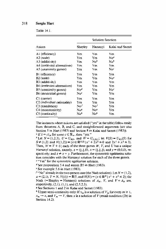
318 Sergiu Hart
Table 14.1.
Solution function
Axiom Shapley Harsanyi Kalai and Samet
Al (efficiency) Yes Yes YesA2 (scale) Yes Yes No*A3 (additivity) Yes No* No*A4 (irrelevant alternatives) Yes Yes YesA5 (unanimity games) Yes Yes Noc
Bl (efficiency) Yes Yes YesB2 (scale) Yes Yes Noa
B3 (additivity) Yes Yes YesB4 (irrelevant alternatives) Yes Yes YesB5 (unanimity games) No^ Yes Noc
B6 (inessential games) No* Yes YesCl (carrier) Yes Yes YesC2 (individual rationality) Yes Yes YesC3 (translation) No-' No / YesC4 (monotonicity) No* No* YesC5 (continuity) No* No* Yes
The instances where axioms are satisfied ("yes" in the table) follow easilyfrom theorems A, B, and C, and straightforward arguments (see alsoSection 5 in Hart (1983) and Section 8 in Kalai and Samet (1983))."If A = cl^for some c e U+, then "yes."*Let #={1,2,3}, U= UNfi, and W= £/{12}1; let V(S)=UKl(S) forS*{1,2) and K({1,2}) = {xe R ^ l * 1 + 2x2 < 0 and 2.x1+x2 < 3}.Then, W= V+ U; each of the three games W, V, and £/has a uniqueHarsanyi solution, namely, z = (i,i,0), x = (\,\,\\ and y = (0,0,0), re-spectively; and z # x + y. Furthermore, the symmetric egalitarian solu-tion coincides with the Harsanyi solution for each of the three games.c "Yes" for the symmetric egalitarian solution.d See proposition 5.4 and axiom B5 in Hart (1983).e See example 5.6 in Hart (1983).f "No" already in the two-person case (the Nash solution): Let N = {1,2),a = (2,1), T=N, V({i}) = RW and V(N) = ( x e UN\xl + x2 < 2}; theNash (= Shapley = Harsanyi) solutions of AN, V, and V + AN are,respectively, (2,1), (1,1), and (2.5,2.5).* See Sections 1 and 2 in Kalai and Samet (1983).h Upper-semi-continuity only: If xm is a solution of Vm for every m ^ 1,xm —• x, and Vm —• V, then x is a solution of V (recall condition (2b) inSection 14.2).

Axiomatic approaches to coalitional bargaining 319
B6, with the range being the subsets of X (the set of payoff configurations).Axioms Cl through C5 refer to a (point-valued) function into UN, al-though they can be extended in a straightforward manner to apply to aset-valued function.
REFERENCES
Aumann, R. J. (1967): A Survey of Cooperative Games without Side Payments.In Essays in Mathematical Economics in Honor ofOskarMorgenstern, ed.by M. Shubik. Princeton University Press, Princeton, New Jersey, 3-27.
(1983a): On the Non-Transferable Utility Value. RM-55, Center for Researchin Mathematical Economics and Game Theory, The Hebrew University,Jerusalem, forthcoming in Econometrica.
(19836): An Axiomatization of the Non-Transferable Utility Value. RM-57,Center for Research in Mathematical Economics and Game Theory, TheHebrew University, Jerusalem, forthcoming in Econometrica.
Binmore, K. (1983): Bargaining and Coalitions I. Theoretical Economics DP-83/71, ICERD, London School of Economics.
Harsanyi, J. C. (1959): A Bargaining Model for the Cooperative ^-Person Game.In Contributions to the Theory of Games /F(Annals of Mathematics Stud-ies 40), ed. by A. W. Tucker and R. D. Luce. Princeton University Press,Princeton, New Jersey, 325-55.
(1963): A Simplified Bargaining Model for the ^-Person Cooperative Game.International Economic Review, 4, 194-220.
(1977): Rational Behavior and Bargaining Equilibrium in Games and SocialSituations. Cambridge University Press, Cambridge.
Hart, S. (1983): An Axiomatization ofHarsanyVs Non-Transferable Utility Solu-tion. DP-573, The Center for Mathematical Studies in Economics andManagement Science, Northwestern University, Evanston, Illinois, forth-coming in Econometrica.
Kalai, E. (1977): Proportional Solutions to Bargaining Situations: InterpersonalUtility Comparisons. Econometrica, 45, 1623-30.
Kalai, E., and D. Samet (1983): A Monotonic Solution to General CooperativeGames. DP-567, The Center for Mathematical Studies in Economics andManagement Science, Northwestern University, Evanston, Illinois, forth-coming in Econometrica.
Nash, J. F. (1950): The Bargaining Problem. Econometrica, 18, 155-62.Owen, G. (1972): Values of Games without Side Payments. InternationalJournal
of Game Theory, 1, 94-109.Roth, A. E. (1979): Axiomatic Models of Bargaining. Springer-Verlag, Berlin,
Heidelberg, New York.Shapley, L. S. (1953): A Value for ^-Person Games. In Contributions to the Theory
of Games II (Annals of Mathematics Studies 28), ed. by H. W. Kuhn andA. W. Tucker. Princeton University Press, Princeton, New Jersey, 307-17.
(1969): Utility Comparison and the Theory of Games. In La Decision: Aggre-gation et Dynamique des Ordres de Preference, Editions du Centre Nationalde la Recherche Scientifique, Paris, 251-63.
(1983): Bargaining without Cardinal Utility. Paper presented at the Confer-ence on Game-Theoretic Models of Bargaining, University of Pittsburgh.


CHAPTER 15
A comment on the Coase theorem
William Samuel sonBOSTON UNIVERSITY SCHOOL OF MANAGEMENT
15.1 Introduction
Beginning with the observation of Ronald Coase, it has long been heldthat private bargaining can provide an antidote to the inefficienciescaused by externalities. Coase (1960) argued that
1. A pair of agents, by striking a mutually advantageous agreement, wouldobtain an efficient economic solution to the externality, and
2. A change in the assignment of property rights or in the liability rulewould not affect the attainment of efficient agreements.
The Coase "theorem" relies on a number of assumptions, some explicit,some implicit, among which are that: agents have perfect knowledge ofthe economic setting including each other's utility function; in the ab-sence of transaction costs, the agents will strike mutually beneficial agree-ments; and there exists a costless mechanism (a court system) for enforc-ing such agreements.
As many observers have pointed out, the presumptions that the bar-gainers have perfect knowledge of, and pursue, mutually beneficial agree-ments - assumptions borrowed from the theory of cooperative games -are crucial for the Coase results.1 The usual argument is that rationalbargainers would (should) never settle on a given set of agreement terms ifinstead they could agree on alternative terms that were preferred by bothsides. The conclusion, according to this argument, is that any final agree-ment must be Pareto-optimal.
Although this argument seems compelling, it leaves a number of ques-tions unanswered. By what bargaining procedure do the individuals actu-ally arrive at a Pareto-efficient agreement? Will alternative proceduresattain such agreements? The usual presentation of the Coase theorem
This research was supported by National Science Foundation GrantSES-8309345.
321

322 William Samuelson
omits the specifics of the bargaining process. The presumption is simplythat such agreements can and will be reached since it is in the joint interestof the parties to do so. Although this conclusion is appealing, it is consid-erably stronger than the economist's customary hypothesis of individualrationality. Even under perfect information, this presumption is far fromobvious. Each individual seeks only to maximize his individual utility anddoes not seek a point on the utility-possibility frontier per se. Moreover, inany interesting problem, there will be a multiplicity (in fact, an infinity) ofefficient agreements - such that an improvement in one agent's welfarenecessitates a sacrifice in the other's. Thus, one would expect the agents tonegotiate (or haggle) over these candidates - a process that may in turnexpend resources and delay agreement. Other types of strategic behaviorare also possible. In pursuit of a preferred agreement, one party maythreaten the other and, for credibility's sake, bind himself to carry out thethreat some portion of the time. When he does, efficiency fails.2 Alterna-tively, the parties may adopt the standard negotiation bluff, insisting onultrafavorable (and incompatible) terms of agreement. If agents persist inthese demands, a mutually beneficial agreement may be lost. Althoughproponents of the Coase presumption may regard these actions as irratio-nal, it is no less true that such behavior (e.g., strikes, the carrying out ofcostly threats) frequently occurs.
Moreover, it is unrealistic to suppose that the bargaining setting is oneof perfect information. To a greater or lesser degree, each party will beuncertain about key aspects of the bargaining situation - possibly abouthis own payoffs for alternative agreements and almost certainly about theother side's potential payoffs. As an example, consider a simple setting ofbilateral monopoly in which a single seller and buyer are negotiating thesale price of a good. Although each may have relatively precise informa-tion about his own monetary value for the good, each will have only aprobabilistic assessment of the other's walk-away price. In the case of anexternality, two firms (e.g., one a polluter and one a victim of the pollu-tion) would be engaged in negotiations aimed at a mutually beneficialagreement. Each firm would be knowledgeable about its own cost (clean-up cost or pollution cost) but would have limited information about thecost of the other side.
The presence of limited or imperfect information is an impediment tothe attainment of efficient agreements. Before the fact, neither side willknow whether, or what, mutually beneficial agreements are available.Such agreements, when they exist, must be uncovered by the bargainingprocess itself. Thus, the key question is whether there exists a suitablebargaining method, conducted by self-interested individuals, that canalways achieve Pareto-efficient agreements.

A comment on the Coase theorem 323
This chapter addresses this question by exploring the Coase theorem ina setting of incomplete information. In contrast to the traditional versionof the Coase theorem, the propositions under incomplete information areas follows:
1. The parties affected by an externality will, in general, be unable to nego-tiate efficient agreements all of the time, or if an efficient agreement isreached it may come only after costly delay;
2. The degree of efficiency of a negotiated agreement depends ona. which party is assigned the specific property right, andb. the bargaining process used by the parties;
3. Efficiency can be increased by allocating the property right via competi-tive bid, rather than relying on some preassignment.
Proposition 1 indicates that the presence of incomplete information im-poses a second-best negotiation solution - one in which agent welfarefalls short of that attainable under perfect information. Once an initialrights assignment is made, bargaining cannot ensure the costless transferof the right to the party that values it most highly.3 In this sense, thecondition of incomplete information creates a kind of trading friction or abarrier to trade. Proposition 2 follows as an immediate consequence.Given the informational barriers to trade, the ultimate solution to theexternality depends directly on the initial assignment of the right and onthe bargaining method adopted by the parties. Proposition 3 indicates apotential remedy: Efficiency can be increased by foregoing the rightsassignment in the first place. Instead, the right is allocated via competitivebid (so that the agent willing to pay the most for the right obtains it)without recontracting.
The main propositions in this chapter are applications or extensions ofrecent results in the area of resource allocation under uncertainty. Impor-tant contributions are provided by Myerson (1979) and Harris andTownsend (1981). Despite their importance, many of these results are notwell known (or if known, not assimilated into mainstream economicthinking). Proposition 1 has been noted by several authors - by Arrow(1979) and Samuelson (1980) for specific bargaining procedures and in animportant paper by Myerson and Satterthwaite (1983) for the class of allbargaining procedures (under independent information). Nonetheless,the importance of this amendment to the Coase theorem has gone largelyunrecognized. Thus, the conventional wisdom holds that in the absense oftransaction costs (caused, for instance, by numerous interested parties),bargaining can solve in principle the externality problem. However,whether bargaining is an appropriate remedy depends on the kind ofmarket failure present. If external effects are the sole cause of the failure, a
324 William Samuelson
bargaining solution that, in effect, internalizes the externality will beappropriate. But in the common case when external effects are accompa-nied by the presence of imperfect information, a property-rights assign-ment followed by private bargaining will not be a fully efficient remedy.The present study emphasizes this basic point and attempts to explore itslogical consequences, for example, the importance, so far as efficiency isconcerned, of the bargaining method used by the agents and of the initialrights assignment.
The chapter is organized as follows. Section 15.2 outlines the basicmodel and presents propositions 1 and 2. Section 15.3 suggests a remedyin the form of rights bidding, and Section 15.4 examines a specific appli-cation - the siting of hazardous-waste-processing facilities. A final sectionoffers a summary and concluding remarks.
15.2 Bargaining and externalities
The Coase theorem is a proposition not only about externalities and theirremedies, but also about the efficiency of bargaining in general. Coaseviewed the externality problem (its specific features notwithstanding) as amember of the general class of bargaining problems. Examples in thisclass range from negotiated purchase-and-sale agreements to the signingof international treaties to management - labor contract bargaining.Why should parties to the externality not negotiate mutually beneficialagreements as in these other cases? In the spirit of cooperative gametheory, Coase concluded that they could, provided that a definite prop-erty-right assignment was made. This assignment would specify the out-come in the event that the interested parties failed to reach an agreement.For instance, in the purchase-and-sale example, the seller retains the goodin the event of a disagreement. In the externality example, the propertyright would reside with one of the parties in the event of a disagreement.Clearly, then, one can think of the right holder as a kind of seller and theother party as a buyer who must compensate the holder if he is to obtain abetter outcome (than the disagreement alternative) for himself.
To begin, it will be convenient to focus on the general bargainingproblem, of which the externality problem is a special case. The simplestsuch problem can be described as follows. Suppose that two individualsare negotiating over two possible outcomes. Agent preferences are inconflict. The first agent prefers one outcome, the second prefers the other.To keep things simple, let us suppose that each individual is risk neutraland assigns a monetary value to his preferred outcome — a value that isindependent of income effects. If negotiations end in a disagreement, oneagent (labeled the right holder) will obtain his preferred alternative. Thus,

A comment on the Coase theorem 325the would-be acquirer, if he is to secure his favored outcome, must pro-vide monetary compensation to the right holder.
When individual values are common knowledge, ex post efficiencyrequires that the agent with the greater value obtain his preferred outcome(or, equivalently, the right to this outcome). Short of this full-informationcase, ex post-efficient outcomes cannot always be secured, a result con-tained in an initial proposition.
Proposition 1. The parties affected by an externality will, in general, beunable to negotiate efficient agreements all of the time, or if an efficientagreement is reached it may come only after costly delay.
The following is a simple but graphic example of this basic result.
Example 1. A buyer and a seller are negotiating the price at which asingle, indivisible good might be sold. Both parties know that the buyerhas a comparative advantage for the good. In fact, the buyer's monetaryvalue for the good is 50 percent greater than the seller's value, that is,vb = 1.5 vs. The complication is that only the seller knows these underly-ing values vs and vb. The buyer knows only that vs is uniformly distributedon the interval [0,1].
To examine bargaining possibilities, we model the negotiation processas a two-person game of incomplete information following Harsanyi(1967). The information structure of this game is as specified previously.Because both parties know of the buyer's 50 percent advantage, it isnatural to expect a sale always to occur, and, of course, ex post efficiencyrequires this. Nevertheless, it is straightforward to confirm that self-interested and rational bargainers can never conclude a mutually benefi-cial agreement in these circumstances. For instance, suppose that underthe rules of the bargaining game, the buyer has the opportunity to make afirst-and-final price offer, which the seller can then accept or reject. Whatoffer should he make? An offer of (let us say) .6 will be accepted 60 percentof the time by a seller holding an average value vs = .6/2 = .3. Thus, thebuyer's average acquisition value is vb = (1.5)(.3) = .45, and his expectedprofit is (.6)(.45 — .6) = — 0.9. More generally, any buyer offer b results ina negative profit of — 25b2. Clearly, no offer that the buyer can make isprofitable.
What if the informed seller makes the first-and-final offer? For in-stance, consider a seller who demands a price that is 30 percent greaterthan his value, that is, s = I3vs. Anticipating this strategy, a buyer canprofitably accept all seller offers (even a price of 1.3). Against such anaccepting buyer, however, a profit-maximizing seller would choose to

326 William Samuelsonprice at 1.3 for all vs, in which case the buyer would suffer an average lossof .75 — 1.3, or — .55, in accepting this offer. The same result holds if thebuyer commits himself to accept any seller offer no greater than s, for anys. The seller's best response is to quote s for all vs < s9 leaving the buyerwith an average loss. Thus, in equilibrium, no offer made by a rationalseller could ever be profitably accepted by the buyer. Although these twoprocedures do not exhaust the bargaining possibilities (e.g., offer, coun-teroffer, and so on), more general methods can be used to show that thebuyer's most preferred bargaining procedure is to make a first- and finaloffer.4 Since even this is unprofitable, mutually beneficial agreementsunder any bargaining procedure are impossible.
This example points up the conflict between the collective and individ-ual interests of the parties. Even though the bargainers share the desire toconclude a mutually beneficial agreement, each individual pursues anegotiation strategy that maximizes his own expected profit. In the pres-ence of asymmetric information, bargaining self-interest precludes theattainment of any agreements. Thus, despite his comparative advantagefor the good, it is impossible for the uninformed buyer to conclude aprofitable agreement. It is not only the buyer who suffers. The informa-tion asymmetry robs the informed seller of trading profit as well. Clearly,this barrier to trade would not exist if both players knew vb and vs, inwhich case they could conclude an agreement at some ? E [i?5,i^]. Inshort, although a mutually beneficial agreement is always economicallyfeasible, such an agreement is impossible given the self-interest of theparties.
This finding of bargaining inefficiency is not limited to the case ofasymmetric information. As a second example, consider a bargainingsetting in which each side holds a personal monetary value concerning theissue at stake — a value that is known only to himself. For instance,suppose that an upstream paper mill is negotiating a pollution agreementwith a downstream fishery that has the right to clean water. The mill seeksto obtain the right to discharge moderate amounts of pollution and iswilling to pay the fishery for the privilege. Denote the mill's value for thisright by vm (embodying the clean-up cost it avoids) and the fishery'spollution cost by vf. Then, if ty < vm, both sides can profit from a pollutionagreement whereby the mill obtains the right to pollute and makes apayment P to the fishery, where P E. [vf9vm]. The difficulty is that eachvalue is known only to the player himself. The fishery's probabilistic beliefabout the mill's value is summarized by the cumulative distribution func-tion Gj{vm), the mill's probability assessment is denoted by Gm(vf\ andthese distributions are common knowledge.
The usual description of bargaining involves unrestricted offers and

A comment on the Coase theorem 327counteroffers until an agreement is concluded or an impasse is reached.To bring out the main points, however, it is convenient to begin bypresenting a highly stylized bargaining procedure such as the following.
a. Ascending offers. The agents place oral ascending bids for the right,where the last and highest bidder obtains it. If this last and highest bidderis the right holder, he retains the right. If this bidder is the other agent, hepurchases the right and pays the holder his bid price.
Though unconventional, this bargaining procedure has the virtue ofbeing "competitive." The would-be acquirer can secure the right by mak-ing an unmatched competitive bid and paying this amount to the holder.Alternatively, the right holder retains the right by "outbidding" the otheragent. How will profit-maximizing individuals bargain under theseground rules? The answer to this question requires a complete descriptionof each agent's bargaining strategy, that is, a specification of the offers hewill make contingent on his value and the offer history to date. In general,this may be a formidable task. Under ascending offers, however, thestrategy description is quite simple. The mill, seeking to acquire the right,has a dominant strategy: If necessary, it should bid up to a price notexceeding its true value, that is, make a maximum bid bm = vm. Antici-pating this behavior, the fishery determines its own "ceiling bid" to maxi-mize its expected profit:
(bf- vf)Prob(bm < bf) = (bf- iy)(l - Gfibf)).
Here, it is presumed that the mill obtains the right by matching thefishery's offer bf (or, in an alternative interpretation, by bidding bf+ e).Thus, if the right is transferred, the fishery's profit is bf— ty, and this eventoccurs with probability 1 — Gf{bf). The fishery's optimal strategy deter-mines bfby trading off the probability and profitability of an agreement(where the latter is increasing in and the former decreasing in bf). It isevident that the fishery's ceiling bid is in excess of its value (bf> vf).Consequently, the bargaining procedure fails to attain an ex post-efficientoutcome when bf> vm> vf. Here, the fishery retains the right although itis more valuable to the mill.
A similar finding of bargaining inefficiency occurs under more con-ventional bargaining methods. In the usual description of negotiations,the bargainers begin with incompatible demands, and over time the sidesconverge to an agreement (if one is possible) by making staged conces-sions. In keeping with the postulate of individual rationality, it is naturalto insist that each side use a Nash-equilibrium bargaining strategy; that is,each should make offers (contingent upon its personal value) that maxi-mize its expected profit given the bargaining strategy of the other side.
328 William SamuelsonThen, given the actual values vm and vf, the agents will engage in bargain-ing (according to their specified strategies), with the result that an agree-ment is reached or bargaining terminates with no settlement.
The attainment of efficient outcomes requires that both bargainers bewilling to concede up to their true values if necessary, thereby securing amutually beneficial agreement, whenever trading gains (no matter howsmall) are present. It can be shown, however, that such concession makingcannot constitute an equilibrium. More specifically, against a conces-sion-making opponent, a profit-maximizing bargainer should stop con-ceding short of his true value. (The right holder makes a final demandbf> Vf, and the other bargainer a final offer bm < vm.) Although thissacrifices some probability of agreement, the bargainer more than com-pensates by improving the terms of those agreements that are reached. Asa result, bargaining fails to attain certain ex post-efficient agreements.
Proposition 1 's finding of bargaining inefficiency is the foundation fora second basic result.
Proposition 2. The degree of efficiency of a negotiated agreement de-pends on (a) which party is assigned the property right, and (b) the bar-gaining process used by the parties.
To demonstrate proposition 2, it is convenient to compare the negotia-tion outcomes under the ascending-offer procedure with outcomes underthe following pair of stylized bargaining procedures.
b. Sealed offers. The agents submit written sealed bids, and the high bidderobtains the right. If the high bidder is the right holder, no payment ismade. If this bidder is the other agent, he purchases the right and pays theholder his bid price.
c. Split-the-difference offers. The parties submit written sealed bids, andthe high bidder obtains the right. If the other agent's bid exceeds theholder's bid, the right is transferred at a price that "splits the difference"between the bids. Otherwise, the holder retains the right and no paymentis made.
Consider agent bargaining behavior under each of these procedures. Sup-pose, as before, that the fishery holds the water right. Then, under sealedoffers, it is easy to check that the fishery has a dominant strategy wherebyit submits a sealed bid equal to its true value, that is, bf= vf. Clearly, itshould not bid any less, since this would risk transferring the right at aprice less than its value. Nor should it bid any more. Such a deviation fromtruthful bidding is of no benefit if vf<bf< bm but results in a loss of aprofitable sale if vf< bm < bf. Thus, truthful bidding is optimal.

A comment on the Coase theorem 329
The mill, on the other hand, submits an optimal bid to maximize itsexpected profit:
(vm - bm)Prob(bm > bf) = (vm - bm)Gm{bm\
where the equality stems from the fact that the right holder bids truthfully.It is evident from this expression that the mill uses a "shading" strategy,submitting a bid below its true value.
Under split-the-difference offers, if bm ^ bf9 then the mill purchases theright and pays the fishery a price P = (bm + bf)/2. Otherwise, the fisheryretains the right. Here, the sale price depends on both offers, not on oneside's offer as in the ascending-offer and sealed-offer procedures. It can beshown (see Chatterjee and Samuelson (1983)) that in equilibrium thefishery uses a "mark-up" strategy and the mill a "shading" strategy; thatis, bf= bf(vf) > lyfor all lyand bm = bm(vm) < vm for all vm.
Example 2. Suppose that it is common knowledge that the agents'values are uniformly and independently distributed on the interval [0,1 ].When the fishery holds the property right, the bargaining methods yieldthe following results.
a. Ascending offers. The fishery's optimal strategy is bf— .5 + .5iy. Thus,the mill obtains the right if and only if vm bf= .5 + .5vf.
b. Sealed offers. The mill's optimal bargaining strategy is bm = . 5 vm, and soit obtains the right if and only if bm = ,5vm ^ iyor, equivalently, whenvm > 2vf.
c. Split-the-difference offers. The agents' optimal bargaining strategies arebf=i + \vf and bm = -fc + \vm. Thus, the mill obtains the right if andonly if bm bf or, equivalently, if and only if i;m > iy+ \.
These outcomes are depicted in Figures 15.1 a - c, which indicate the agentwho obtains the right via bargaining for all possible combinations ofplayer values. Efficiency in the ex post sense requires that the fisheryretain the right if and only if vf ^ vm (i.e., in the domain to the southeast ofthe 45 ° line in each figure). But under incomplete information, the origi-nal right holder retains the right over a larger domain of values (extendingto the northwest of the line), regardless of the specific bargaining proce-dure - that is, the fishery may retain the right even though vf<vm. As thefigures indicate, the domains of inefficient outcomes vary according tothe bargaining procedure. (Of course, if the mill were originally assignedthe right, the domain of the mill's retention would extend to the southeastof the 45° line under each procedure.)
Under perfect information, the mill would obtain the right with proba-bility \. By comparison, under either the ascending-offer or sealed-offer

330 William Samuelson
(c)
Figure 15.1 (a) Ascending offers, (b) Sealed offers, (c) Split-the-difference offers.
procedures, the probability that the mill obtains the right is j , whereasunder split-the-difference offers, this probability is slightly higher, ^ . Anatural measure of bargaining performance is the expected collectivebenefit that is generated. If ex post-efficient outcomes were alwaysachieved, the expected benefit sum would be E[2 B] = E[max(vf,vm)] =, where the expectation is taken over all possible values vf and vm. By
comparison, the expected group benefit is f under either the ascending-

A comment on the Coase theorem 331offer or sealed-offer procedures and is slightly higher, | i , under split-the-difference offers.5
Example 3. Now, suppose that the values are independently and uni-formly distributed with vfE [0,2] and vm E [0,1], reflecting the fact thatthe right is worth more on average to the fishery.
It is straightforward to derive equilibrium strategies and outcomesunder each of the bargaining procedures and for each initial assignment ofthe right. Figure 15.2 displays the bargaining outcomes for different valuecombinations, as well as the expected benefits generated. It is evident thatthese benefits vary systematically according to the original rights assign-ment. In this example, if a rights assignment is made, it should be to thefishery, the firm that values the right more highly on average. However,although this assignment rule seems to be appealing, it is easy to constructother examples in which the attainment of maximum benefits calls forexactly the reverse assignment.
15.3 Rights bidding
There is a simple remedy to the failure of bargaining based on a rightspreassignment. In the absense of a preassignment, let the parties bid forthe right. For historical, political, or legal reasons, an initial right assign-ment may be a foregone conclusion in many settings. In other circum-stances, however, bidding for the right is natural and feasible.
The bidding method envisioned is akin to a standard auction with oneexception. There is no seller to collect the proceeds; instead, the proceedsare returned to the parties themselves. Thus, failing to acquire the right,an agent will obtain compensation. Consider the following biddingprocedure.
Split-the-difference bidding. Agents submit sealed bids, and the high bidderacquires the right and pays the sum (£y + bm )/4 to the other agent, wherebm and £yare the respective bids of the parties.
Although the assignment of the right is straightforward, the amount ofcompensation deserves comment. The payment is most easily under-stood by noting that the agents are, at the same time, bidders for and jointowners of the right. In this light, the bidding procedure described hereparallels split-the-difference offers. First, the purchase price is determinedby the average of the bids, (bf+ bm)/2. This revenue is collected andshared equally by the joint owners of the right, so that the acquirer's netpayment is simply (bf+ bm)/4.

332 William Samuelson
FISHERY HOLDSWATER RIGHT
MILL HOLDSWATER RIGHT
Ascending Offers
E[ZB] = 1.06 E[£B] = 1.00
Sealed Offers
Split the Difference Offers
1 2
E[2B] = 1.07
Figure 15.2 Bargaining outcomes

A comment on the Coase theorem 333
Bids
y2 .
3/4Values
Figure 15.3 Split-the-difference bidding
Suppose that this bidding procedure is adopted and that the agents'values are drawn independently from the same distribution (i.e.,Gf{ ) = Gm{ )). Then, it is straightforward to show that the split-the-difference bidding scheme is ex post efficient. The reasoning is simple. Inequilibrium, each agent will use the same bidding strategy that is strictlyincreasing in his value. Consequently, bf^ bm if and only if ty> vm.
Example 2'. Suppose that the values are independently and uniformlydistributed on the interval [0,1 ], and that the right is assigned by competi-tive bid. Then, the equilibrium bid function is b{v) = \ + $v, as graphed inFigure 15.3. At the mean value v = ±, an agent makes a "truthful" bidb = \. For larger values, he shades his bid b(v) < v, and for smaller values,he marks up his bid b(v) > v.
The intuition behind this behavior should be clear. For v>\9 the agent ismore likely than not to obtain the right. Thus, as a potential buyer, he hasan incentive to shade his bid and so pay a lower price. For v < £, on theother hand, the likelihood is that he will be outbid for the right. Conse-quently, he exaggerates the value of the right in order to raise his monetaryreceipt. At v = \9 these incentives to shade and to mark up balance out,

334 William Samuelson
Bids
1/ 1/ 3/ 1 V a l L j e S
74 1/2 3/4 1
Figure 15.4 Split-the-difference bargaining
and so he bids b = v = \. Furthermore, it is easy to check that the biddingis profitable for both the winner and the loser of the right. Even a playerholding v = 0 profits. Although he is always outbid for the right, hisreceipt is (bf+ bm)/4 or (£ + £)/4 = i on average (where \ is the averagewinning bid). In the example, the expected profit of each player condi-tional on his own value increases quadratically according \o\ + v2/2.
Although bids differ from agent values, the allocation of the right isefficient (since the agent bidding strategies are identical). Figure 15.4displays and compares the agent strategies under split-the-difference bar-gaining. Even though this bargaining behavior bears a superficial re-semblance to split-the-difference bidding (both involve shading andmarkups), there is a crucial difference. The bidding procedure ensures expost efficiency; the bargaining procedure cannot. Once a rights assign-ment is made, there is an inevitable divergence between the bargainingstrategies of the agents - that is, the fishery and mill offers, respectively,overstate and understate true values.
The same point can be made in a slightly different way by showing thatthere is no bidding procedure that is ex post efficient and that compen-sates the holder for relinquishing his right. For instance, suppose that thebidding procedure in example 2' is modified in order to provide addi-

A comment on the Coase theorem 335tional compensation to the fishery (the would-be right holder). One sim-ple means is via a lump-sum payment between the parties prior to thebidding. Under the requirement that the mill obtain a nonnegative profit(for all vm\ the largest possible lump-sum payment is \. With this pay-ment, the conditional expected profits of the bidders become nm{vm) =v2j2 and nf{vf) = \ + v}/2. If the fishery is to be compensated for givingup the right, it must be the case that nf(vf) ^ lyfor all vf. However, itis easy to check that this constraint is violated for vf> 1 — Vj. In short,there is no allocation mechanism that is both efficient and guarantees thatXmiVm) - 0 a n d nf(Vf) - vff°r a^ vm a n d vf- However, if the last constraintis weakened to nf{Vf) ^ 0, efficient outcomes are attainable via competi-tive bids.6
The lesson of this simple example holds more generally. Because of therights assignment, the bargaining solution to the externality problemintroduces a constraint that (in general) prohibits an ex post-efficienttransfer of the right. By foregoing an initial rights assignment, the biddingsolution relaxes this constraint. (The only "individual-rationality" con-straint implicit in the bidding solution is that agents who forego the rightshould not be made to pay.) As a result, efficiency increases. This result issummarized in the following proposition.
Proposition 3. Efficiency can be increased by allocating the propertyright via competitive bid, rather than relying on some preassignment.
15.4 Siting hazardous-waste facilitiesThe preceding sections have compared the alternatives of bargaining andbidding in determining rights assignments in the presence of externalities.The important point is that foregoing a rights assignment can be crucialfor efficiency.
Many of the differences between the bargaining and bidding remediesfor externalities can be illustrated by the process used in the state ofMassachusetts for siting hazardous-waste facilities. As outlined in 1980legislation, the siting process relies on developers (waste-managementcompanies) and local communities to negotiate siting agreements benefi-cial to both, subject to certain safety and environmental standards en-forced by state agencies. Besides safety and mitigation measures, thenegotiation agenda includes issues of compensation, both monetary(taxes, service fees) and nonmonetary (jobs, payments in kind). Thus, incontrast to practices in many other states, the siting process is intended tobe voluntary, providing neither state override of local decisions nor localveto of development proposals. (These aspirations notwithstanding, to

336 William Samuelsondate none of the half-dozen or so proposals for which the siting process hasbeen initiated have resulted in a negotiated siting agreement.)
No short summary can do justice to the many complex issues inherentin the siting legislation. However, the main economic objectives underly-ing the legislation are not difficult to ascertain and appear to be twofold.First, a facility should be sited where it generates the greatest net socialbenefit (an efficiency objective). Second, the siting process should bevoluntary, that is, mutually beneficial to all affected parties (an equityobjective). A short list of these affected parties would include (most ob-viously) the developer, the potential host community, neighboring com-munities possibly affected by the facility, and in-state business and con-sumers that benefit directly or indirectly from the provision of disposalservices. (In terms of aggregate net benefit, this last, general-interest groupmay be the most important.) Of course, the precise magnitudes of thebenefits and costs accruing to affected groups remain private information.Thus, the siting process occurs in a setting of imperfect information.
In light of the arguments presented herein, and based on the experienceto date with the siting process, one can identify several obstacles to theattainment of the efficiency and equity goals.
1. The exchange of information between prospective developers and po-tential host communities is severely limited. With few exceptions, indi-vidual developers have considered (and subsequently pursued) a limitednumber of sites based solely on their own costs and profits. (This is duein no small part to the significant transaction cost, in time and money, ofthe siting process itself.) Often, a developer's least costly site lies in acommunity with high cost burdens, for instance centrally located, high-density areas. In short, sites with the highest net benefits (or, conversely,lowest total costs) may not be uncovered.
2. The negotiations between the developer and the local community neces-sarily fail to take into account the external benefits (consumer surplus)conferred on businesses and consumers in-state. Consequently, it maybe impossible for the bargaining parties to conclude a mutually benefi-cial agreement (i.e., the potential developer profit is insufficient to com-pensate the community for its costs) even when the site is socially benefi-cial. (Reports of the Massachusetts regulatory agencies stress repeatedlythese social benefits but fail to supply a serious benefit-cost confirma-tion.) Of course, the presence of third-party effects is the standard prob-lem posed by externalities.
3. Even if a mutually beneficial agreement between the developer and localcommunity is possible, the parties may fail to attain it under incompleteinformation (e.g., when the local community exaggerates its cost burdenand the developer downplays his potential profit for strategic reasons).
4. Under the siting act, the assignment of the property right is ambiguous.

A comment on the Coase theorem 337
The local community cannot unilaterally refuse to negotiate, and if aftersixty days the talks are at an impasse, an arbitration board is convened toresolve the dispute. (According to the legislative mandate, the boardshould seek a settlement that conforms as closely as possible to the finalpositions of both parties.) Thus, the local community does not have theright to deny the facility under any circumstances. Furthermore, thevery ambiguity surrounding the holding of the property right may deternegotiated agreements (e.g., when each side is optimistic about themerits of its case and therefore prefers arbitration).
As an alternative to the negotiation mechanism, a system of competi-tive bids could be used to establish the location of the facility and todetermine the compensation to be paid to the host community. Such aprocedure would change the property-right focus by requiring the com-munities to give up the local veto right but to share the responsibility forpaying compensation to the host location. To illustrate, suppose that eachcommunity is asked to submit a self-assessed estimate of the cost burdenof a local site. At the same time, the developer submits a list of costestimates for the possible sites. Based on these submissions, the site withthe least total cost is selected and appropriate compensation is paid. Thesource of this compensation includes a sum comprising the expectedstatewide benefits generated by the facility, a sum paid by the developer,and pro rata shares contributed by the other communities. In practice, aworkable system might simply compensate the host community anamount corresponding to its bid.
Beyond the political and institutional obstacles, in order for a biddingsystem to work, each community must be willing to put a dollar value onits cost of hosting the facility. Indeed, one might expect communities tooverstate the burden of the facility for strategic reasons or simply to avoidit. Nonetheless, as long as these overstatements are anticipated and acommon bidding strategy is used, an efficient (i.e., least-cost) assignmentof the facility will be maintained. By paying compensation based on bids,the mechanism increases the chances that the host community will acceptthe facility voluntarily. At the same time, one would expect that the prorata contributions of the other communities would not be burdensome.
15.5 Concluding remarks
The present discussion has examined bargaining remedies to the exter-nality problem in the presence of incomplete information and found that,in contrast to the usual Coase result, private bargaining cannot guaranteeefficient solutions to the externality. Under these circumstances, thechoice of rights assignment is not simply a question of equity. Rather, the
338 William Samuelsonassignment influences the efficiency of ultimate negotiated outcomes inconjunction with the bargaining method used. Indeed, foregoing a rightsassignment altogether can increase efficiency. In this case, a system ofcompetitive bids-not bargaining-determines the allocation of the right.
In actual practice, a number of other issues may play an important rolein the choice of rights assignment, and in determining whether a rightsassignment should be made. In many cases, the rights assignment embod-ied in the status quo is adopted. As we saw, a chief intent of the Massachu-setts siting legislation was that developer and community preferencesshould count - in particular, that community preferences should not beoverruled by state-government fiat. In practice, however, granting thisright to communities (even in its present ambiguous form) has preventedthe siting of any facility in the state. An alternative is for communities togive up this veto right but to share in the responsibility of paying compen-sation to the community within which the site is built.
In addition, it is important that the rights allocation be responsive tochanges in relevant benefits and costs that may occur over time. Althoughit is true that bargainers can renegotiate agreements in response to suchchanges, the fact of bargaining inertia suggests that such negotiations maywell fail the test of dynamic efficiency. By contrast, intertemporal effi-ciency can be maintained in principle (and approximated in practice) bythe simple expedient of assigning rights (via competitive bid) for limitedperiods only and reauctioning the rights at frequent intervals.
Finally, although the focus here has been on two-party bargaining, thegeneral results extend to multiagent settings. With large numbers ofagents, the bidding procedure resembles a quasi-market in which compet-itive bids determine an ex post-efficient allocation of rights (e.g., in thecase of pollution permits). Alternatively, if a preassignment of rights ismade, the players in the "bargaining" market would include numerouscompeting right holders facing numerous would-be acquirers. It remainsthe case that under uncertainty, an ex post-efficient allocation cannot beguaranteed. However, it can be shown that the bargaining market ap-proaches full efficiency as the number of participants on both sides of themarket approach infinity. Thus, so far as efficiency is concerned, the keyissue in the large-numbers case is the creation and institution of themarket; the rights assignment is of secondary importance.
NOTES1. For a succinct discussion, see Arrow (1979).2. Crawford (1982) presents an interesting model in which precommitments lead
to bargaining impasses.3. The first proposition also holds in the case where bargaining extends over time

A comment on the Coase theorem 339
and involves transaction or time-related costs. Here, it is possible to achieve expost-efficient assignment of the right but only at a bargaining cost that exceedsthe additional efficiency gains. For an analysis of bargaining over time, seeChapter 8 in this volume.
4. A complete analysis of this example is found in Samuelson (1984).5. Myerson and Satterthwaite (1982) show that of all of the possible bargaining
methods, the split-the-difference procedure achieves the greatest expectedgroup benefit.
6. The efficiency of allocation by competitive bid (as illustrated in this example) isa special case of general results proved by d'Aspremont and Gerard-Varet(1979) and Laffont and Maskin (1979). In the case of identical distributions,the split-the-difference scheme is just one of many fully efficient bidding pro-cedures. An alternative well-known scheme requires each player to pay theexpected externality associated with his bid. In our examples, firm / submitsbid bt and pays tt = /»} Vjgiivj) dVj to the other firm, and the right is awarded tothe firm making the highest bid. When bt ^ bj, agents is outbid for the right andsuffers an economic cost Vj. Consequently, tt represents the expected cost, byagent f s reckoning, suffered by agent/ By internalizing the expected externa-lity, this bidding scheme induces each agent to make an equilibrium bid bt =vh and therefore ensures an ex post-efficient assignment of the right.
REFERENCES
Arrow, K. (1979): The Property Rights Doctrine and Demand Revelation underIncomplete Information. In M. Boskin (ed.), Essays in Honor of TiborScitovsky. New York: Academic Press.
Chatterjee, K. and W. Samuelson (1983): Bargaining under Incomplete Informa-tion. Operations Research, 31, 835-51.
Coase, R. H. (I960): The Problem of Social Cost. Journal of Law and Economics,3, 1-31.
Crawford, V. C. (1982): A Theory of Disagreement in Bargaining. Econometrica,50,607-31.
d'Aspremont, C, and L. Gerard-Varet (1979): Incentives and Incomplete Infor-mation. Journal of Public Economics, 11, 25-45.
Harris, M., and R. Townsend (1981): Resource Allocation under AsymmetricInformation. Econometrica, 49, 33-64.
Harsanyi, J. C. (1967, 1968): Games with Incomplete Information Played byBayesian Players. Management Science, 14, 159-82, 321-34, 486-502.
Laffont, J.-J., and E. Maskin (1979): A Differential Approach to Expected UtilityMaximizing Mechanisms. In J.-J. Laffont (ed.), Aggregation and Revela-tion of Preferences. Amsterdam: North-Holland.
Myerson, R. B. (1979): Incentive Compatibility and the Bargaining Problem.Econometrica, 49, 61-73.
Myerson, R. B., and M. Satterthwaite (1983): Efficient Mechanisms for BilateralTrading. Journal of Economic Theory, 29, 265-81.
Samuelson, W. (1980): First-Offer Bargains. Management Science, 26, 155-64.(1984): Bargaining under Asymmetric Information. Econometrica, 52, 995-
1005.


CHAPTER 16
Disclosure of evidence and resolution ofdisputes: Who should bear the burdenof proof?
Joel SobelUNIVERSITY OF CALIFORNIA AT SAN DIEGO
16.1 Introduction
This chapter discusses the role of a third party in settling disputes. A judgeis responsible for deciding which of two bargainers should win a dispute.There is a social value associated with giving the disputed item to aparticular bargainer. This is the bargainer's claim to the item. Each bar-gainer knows the strength of his claim and can provide evidence thatproves his claim to the judge. Presenting proof is costly and distortion isimpossible. However, it is possible to refuse to present evidence. Thejudge has a prior distribution about the strength of the claims, but does notknow them exactly. The judge uses the information provided by thebargainers' disclosures (or decision not to provide evidence) and thenrules in favor of the bargainer who has the best expected claim. When thebargainers must decide whether to provide evidence simultaneously,there are typically two types of equilibria. In one, each bargainer has apositive probability of winning if he does not provide evidence. In theother, one of the bargainers wins only if he proves his claim. Thus, rulesabout which bargainer has the burden of proof, that is, who must provideevidence in order to win the dispute, serve to select an equilibrium out-come. This discussion compares the welfare obtainable from differentrules. The results are ambiguous. In general, the costs of providing evi-dence are smallest if the burden of proof is placed on the bargainer whohas the lower cost of proving his claim, provided that this bargainer has astronger expected claim. However, to maximize the social value of thesettlement, excluding disclosure costs, it is best to place the burden of
I received helpful comments from several conference participants as well as fromSteve Bundy, Joe Farrell, Lewis Kornhauser, and Craig Weinstein. NSF providedfunding through SES-82-04038.
341

342 Joel Sobelproof on the higher-cost bargainer. In this way, bargainers present moreevidence and the judge makes better decisions.
My model differs from standard models of bargaining. Bargainers arenot allowed to misrepresent their private information. This assumption isjustified if the information revealed is verifiable, so that misrepresenta-tion can be identified and punished. Also, if well-informed attorneysrepresent the bargainers, then requiring all information disclosed to beaccurate is consistent with the view that an advocate should make the bestpossible case for his client without telling lies.
There is an explicit distinction between private and social valuations inmy model. This makes the role of the judge differ from his role in othermodels of arbitration. Here, the judge selects a winner on the basis of thequality of a bargainer's claim, which I assume to be verifiable. Although abargainer's private valuation influences his decision to present evidence,his preferences do not directly enter the utility function of the judge.
Ordover and Rubinstein (1983), Fng (1983), and Samuelson (1983)present game-theoretic models of the legal process. They discuss howincomplete information affects the decision to settle a dispute. The judgeis not an active player in these models. In market settings, Grossman(1981), Milgrom (1981), and Farrell and Sobel (1983) study situations inwhich agents may disclose information, but cannot distort it.
16.2 The modelThere are two bargainers and a judge. For / = 0 and / = 1, bargainer / ischaracterized by xt E [0,xf], which is his claim to the disputed item. Hisstrategy is a function s( defined on [0,xf]. For fixed xi9 either (jc,-) = xt orsi(xi) = n- If si(xi) = xt> then the bargainer proves that his claim is xt(presents evidence) and incurs the nonnegative cost C;(x,). If st(x^ = n,then the bargainer does not prove his claim and incurs no cost.1 BecauseSj(xt) can take on only two values, distortion is impossible; bargainerseither truthfully reveal xt or disclose no information. I assume that bar-gainer /'s von Neumann-Morgenstern utility function Ut takes the form
where vt(x^ > 0 is the private value he places on winning, ct(x)is the cost of proving that his claim is xt (when his claim is, in fact, equal toxt), and Cj(n) = 0. Without further loss of generality, I normalize the utilityfunction by taking vt{x) = 1. Thus, ct{x) £E (0,1) is the cost of providingevidence relative to the private value of winning. It follows that if pt is theprobability that bargainer / expects to win given st and xi9 then his ex-pected utility is pt —

Disclosure of evidence and resolution of disputes 343The judge chooses the probability/?, that bargainer i wins the dispute.
Thus, the judge's strategies consist of pairs of functions (po,Pi) such thatpo + Pi = 1 and p0,px ^ 0. These functions depend on whatever informa-tion the judge has when he makes his decision. The judge tries to maxi-mize expected social welfare, which I take to be a weighted average of thesocial value of assigning the object to a particular bargainer net of the costsof providing evidence, if any. Thus,
x) = poxo + p{x{ - k[co(so(xo)) + c^iCxi))], (16.1)where k ^ 0. Equation (16.1) assumes that the social value of not assign-ing the item is zero.
The judge does not know the values of x0 and xl; a probability distribu-tion function Fsummarizes his information. Here, F{yo,yx) is the proba-bility that CxOv*i) £ [0,y0] X [0,yJ. I assume that F has a continuous,positive density function/on [0,xJ] X [0,xf ], The conditional distribu-tion of x, given x^t describes bargainer /'s beliefs about his opponent'scase. The functions F, UO,UX, and Uj are common knowledge, and so theonly uncertainty concerns the values x0 and xx.
I assume that the bargainers learn the value of their claim simulta-neously, and then prove their case to the judge (or decline to provideevidence). At this point, the judge, knowing what the bargainers havedisclosed, decides which bargainer should win. The strategy for the judgeis an allocation rule, which selects the winner. I allow the judge to usemixed strategies and, if he prefers, to select no winner. In addition, thejudge is able to condition his action on the signals of the bargainers.Therefore, I represent the judge's strategy by functions Pi(yi9yi-i) definedfor
(yo,yi) e (n U [0,x0r]) X (n U [0,xf])
so that pjt yt, yl _,-) is the probability that bargainer / wins given the signalsy0 and yx. This describes the game. Before I describe the equilibrium, Iintroduce some notation.
Let Ft{xt | xx _,) be the conditional probability that bargainer /'s claim isless than or equal to xt given xx_h so, for example,
//•*„<
f{xx,t)dt
344 Joel SobelLet fi(Xi | *!_,•) be the associated density function, and let /^(A^A7^,) bethe expected value of xt given that xt E Nt and xl_l, e Nx_t. Finally, let
be the expected change in utility associated with revealing xt rather thannot revealing xt (excluding costs), when the strategies of the other playersare fixed.
In this setting, an equilibrium consists of strategies st(x) defined on[0,xf] for / = 0 and z = l and probabilities A - O ^ I - I ) defined for(yo,yi) E (rc U [0,x0
r]) X (n U [0,*f]) such that
El. If ViiXfiPi^-,) > Ci(Xi), then s^x,) = xi9If Vfai'j)^-,) < Ci(Xi), then s/x,) = n.
E2a. For all 0>0,J>i), A-O^tt-i) = ° and/?o(yOJyi) +Pi(>;i»>;o) = L
E2b. For any y0 and ! ,po(yo,yi) andpl(yl,y0) maximize the expected value ofUj. Thus, if TV, = {xf E [0,xf]: s^x,) = «}, thenpt(n,n)=l if/jL^i9Nl-i)>fii-i(Nl-i9Ni),Piix^ri) = 1 ifjUjix^N^i) > ju^iiN^^Xi),A(*/,*!-/)= 1 if*/
These conditions guarantee that players best respond to their opponents'strategies. El states that a bargainer proves his claim exactly when itimproves his probability of winning enough to compensate for the cost ofproviding evidence. E2a states that the judge's strategy choice must be aprobability distribution. In particular, since the only way to obtain posi-tive value from the item is to award it to one of the bargainers, the judgecannot be best responding if p0 + px < 1. The conditions in E2b followfrom the form of the judge's utility function. When the judge makes hisdecision, he either knows the value of bargainer /'s claim or knows thatxt E Nt. Consequently, he maximizes his expected utility by awarding theitem to the bargainer who has the greater claim (in expected value). Sincethe judge makes his decision after the bargainers have incurred the costs ofproviding evidence, his decision must be based only on the quality ofevidence. In order for the strategies to constitute a Nash equilibrium, thejudge's strategies must satisfy E2b only for (x0 ,x{) in the range of (s0,s{). Irequire that E2b holds for all (Jtov*i); that is, I require the judge to bestrespond to all signals, not just those used in equilibrium.
The analysis in Section 16.3 applies only to equilibria in whichSi(xi) = xt if and only if JC,- > xt so that only bargainers with good claimspresent evidence. Therefore, equilibrium is characterized by cutoff values

Disclosure of evidence and resolution of disputes 345
x0 and xx. If xt > xt for / = 0 and i = 1, then the judge awards the item tothe bargainer with the greater claim. Otherwise, the judge must weigh theexpected claim of one bargainer against what he knows about the otherbargainer's claim.
16.3 Characterization of equilibria
This section characterizes the equilibria of the model when ct{x^ = ct isindependent of xt for xt E [0,xf ] and the social values of the bargainersare independently distributed. Thus, F(xo,xx) = F0(x0)Fx(xx), the condi-tional distributions are independent of private information, and the meanof bargainer fs claim does not depend on xx-t. Keeping these facts inmind, I write Fjixj) for Fj(Xj | xx-j) and let
0
^ ™ ifJc,>0,
l O i f Jc> = 0be the expected value of bargainer f s claim given that it is no greater thanXj. Here, ft is the density of Ft.
When the social values are independent, the expected gain from dis-closing xt is increasing in xh whereas the gain from not disclosing xt isindependent of xt. Thus, Vt{ •) is increasing in xh and when the costs ofproviding evidence are constant, equilibrium strategies are characterizedby cutoff values x0 and xx.
The results of this section continue to hold if x0 and xx are stochasticallydependent provided that increasing xt induces a leftward shift in thedistribution of xx _,-. This guarantees that Vt( •) is increasing in xt, and thatif disclosing xt wins if bargainer 1 — / does not disclose, then disclosingyt > xt also wins if the other bargainer does not disclose. If ct(x^ is increas-ing, then the results do not change provided that Vt{ •) increases morerapidly than ct{ •). These cases add little insight, but much notation, so Iassume them away.
The nature of equilibrium depends on whether or not//0(x0) = jux(xx).If fio(xo) = jux(xx), then I call the equilibrium symmetric. Iffii(xt) > //1_z(x1_/), then it is an asymmetric equilibrium with the burdenof proof on bargainer 1 — /. I discuss the case in which juo(xo) ¥= ju x(xx) first.If /LLO(XO) ¥= JUX(XX), then the burden of proof is on bargainer / if ju^Xj) <jux_i(xx_l) because he must provide evidence in order to win the dispute.

346 Joel SobelTheorem 1. An equilibrium characterized by cutoff values x0 and xxwith /i^Xj) > jux_i(xx_l) exists if
iV/(*,) ~ ct - F ^ m ) ^ 0. (16.2)
If (16.2) holds, then 3c0 and xx are equilibrium cutoff values if and only ifxx_t = //,-(Jcj-) and xt satisfies
Fx _,(*,) - ct - F^i/ifo)) = 0 and xt ^ xt (16.3)or xt = xj and
Fx-t(xJ) - ct ~ Fx.t(iit(xJ)) ^ 0. (16.4)
Proof. If (16.2) holds, then there exists an xt that satisfies (16.3) when-ever (16.4) does not hold. This follows from the continuity of Fx_t. Let xtsatisfy (16.3) if a solution exists or let xt = xj if (16.4) holds and letxx_t = pijiXt). It follows that bargainer 1 — / receives — cx_t if he revealsxx_i<xl_i, and at least F^xi) — cx-t if he reveals xx_t> xx_t, because, ifxx_t > xx-i = jUjiXt), then bargainer 1 — / wins whenever bargainer / doesnot provide evidence. Since xt ^ xt,
so that, given xt, bargainer 1 — / optimizes by using the strategy character-ized by xx _,:. Similarly, given that bargainer 1 — / is proving his case if andonly if Xi_z > x^h and therefore the judge awards the item to bargainer /if Xx-j ^ xx-t or if bargainer / discloses xt > xx-i9 bargainer / receivesFx_i(xx_l) if he does not present evidence and Fx_i(xi) if he discloses aclaim ofx, > xx_t. Since xt > //,-(J ) = xx_h the definition ofxtguaranteesthat bargainer / optimizes by revealing xt if and only if x, > xt. Finally, ifxx_t¥= jUjiXj) or if (16.3) or (16.4) does not hold, then x0 and xx could not becutoff values for an equilibrium with JU^X,) > jux-i(xx-l).
Note that in an asymmetric equilibrium, it is possible for one or bothbargainers to provide no evidence. If the bargainer who does not bear theburden of proof never provides evidence, then he wins if and only if theother bargainer does not prove his claim. If the bargainer who bearsthe burden of proof never provides evidence, then he never wins, and theother bargainer never proves his claim. This happens, for example, ifxT<Ho(Xo)> a n d s o bargainer l's strongest claim cannot win againstbargainer 0 when bargainer 0 never proves his claim.
Corollary 1. There exists an asymmetric equilibrium. If Ft ^ Fx_t andct ^ cx^t, then there exists an equilibrium with //,-(3c)) > jul-i(xx_l).

Disclosure of evidence and resolution of disputes 347Proof. From theorem 1, it follows that an equilibrium with iit{x) >//1_,-(3c1_I-) exists if
Fx-t(FT\cx-d) ^ ct or Fj\cx^ ^ Fjl^). (16.5)If (16.5) does not hold for i = 0, then it must hold when / = 1. Thisestablishes the first part of the corollary. Since Fl ^ Fx_t implies thatFjlt = F~\ the remainder of the corollary follows from (16.5).
There may be multiple equilibria in which one bargainer has the bur-den of proof. However, if Fl_i(x) — Fx_i(jui(x)) is strictly increasing, then(16.2) is necessary as well as sufficient for the existence of this type ofequilibrium, and if (16.2) is satisfied, then the equilibrium is unique. Thisresults because any equilibrium with ju^x,) > jux-i(xx-i) must satisfy(16.3) orx^xf and (16.4).
Corollary 1 establishes that there always exists an equilibrium in whichthe burden of proof is on one bargainer. Moreover, it suggests that theburden of proof is likely to be placed on the bargainer with lower costs or astronger (in the sense of first-order stochastic dominance) claim. How-ever, there are many situations in which the burden of proof can be placedon either bargainer in equilibrium. For example, let Ft(x^ = b^ forxt E [O,^"1] for / = 0 and / = 1. From theorem 1, there exists an equilib-rium with the burden of proof on bargainer 1 — / provided that
Therefore, if 61_l-c1_l- E [£,•<:,•/2,26,-cJ, then an equilibrium in which theburden of proof is on bargainer / exists for / = 0 and / = 1. A straightfor-ward computation reveals that these equilibria, when they exist, areunique, and that xx-t = min[2c/Z?7'i/,Z?~1] and xt = xx_i/2.
In an asymmetric equilibrium, the probability that the judge is indiffer-ent about who should receive the item is zero, and specification of hisbehavior in these situations does not change the nature of equilibrium. IfoC*o) = iC*i)> then the judge is indifferent whenever neither party pro-
vides evidence. Unless x0 or xx is equal to zero, this event occurs withpositive probability. In order to support an equilibrium, the judge mustrandomize in a particular way when neither party provides evidence.
Suppose, for definiteness, that jUo(*o) =/*i(*f) a n d define £{x±) tosatisfy juo(€(xx)) —/*i(*i) for a l i x\ e [O^fl- J t follows that if fio(xo) =ftiixx), then x0 = €{xx). Further, if at = Pi(n,n) is the probability that bar-gainer / wins if neither bargainer presents proof, then
a0 + ax = 1, ao,ax ^ 0, and (16.6)Fx_i(max[x0,xx]) — ct aiFl_i(xx_i) with equality if xt < xj. (16.7)
348 Joel SobelThe right-hand side of (16.7) is the probability that bargainer / wins if hedoes not provide evidence; he wins precisely when xx-t ^ xx-t and thejudge rules in his favor, which occurs with probability at. The left-handside of (16.7) is the payoff to revealing xt = xt. If xt ^ xx _,f, then bargainer/ wins whenever his opponent does not prove his claim, since xt > ju^x^.However, he never wins if bargainer 1 — / presents proof. If xt > xt-l9then bargainer / wins whenever xt > xx_,-. When (16.7) holds, bargainer /best responds if he discloses xt if and only if xt > xt. This follows becausethe right-hand side of (16.7) is independent of xt whereas the left-hand sideis increasing in xt. Furthermore, if fio(x^) ^ jux(xj), then if there exists asymmetric equilibrium, there exists a symmetric equilibrium with
, ^ ] ) - c0
This follows directly from (16.7) if /z0Cx<D >^iC*f) or if x{ <xf. IfM^o) = Hi(xl) andxx = xf, thenx0 = x{and
- ct = 1 - ct > 0,and thus (16.7) reduces to
1 -Ci^at. (16.8)But there exist a0 and ax that satisfy (16.6) and (16.8) if and only if
and in this case a0 = 1 - c0 cx < 1 and ax = c0 1 - cx also satisfy(16.6) and (16.8). Hence, symmetric equilibria exist if and only if thereexist ax E [0,1] and j ^ E [0,xf ] such thatJ7" (TYXCk'Yi ^l Y" i Y" 1 | —
Fotmaxf^),^]) -Co= (\-a
^ axF0(€i
i)Fx(xx)
{xx)) withand
equality ifjq < xx.(16.9)
(16.10)
In order to characterize the equilibrium, I must describe the cutofflevels for the bargainers. If bargainer 1 proves his claim whenever itexceeds x, then in a symmetric equilibrium the other bargainer presentsproof whenever his claim exceeds €(x). If both bargainers present evi-dence with positive probability, then the cutoff value x must satisfy
for / = 0 and i = 1.Let
X= {x E [0,xf]: min[F;(max[/(.x;),.x]) - d_J ^ 0}i—O.l

Disclosure of evidence and resolution of disputes 349
and let
~ f i n f AT if AT # 0 ,X \x{ if AT = 0 .
Ifj?! E Xand 3c0 = ^(x^, then bargainer / receives positive expected utilityif he reveals xt ^ xt. Therefore, in any symmetric equilibrium, bargainer1 's cutoff value must be at least x From (16.9) and (16.10), it follows thatif xx is an equilibrium cutoff value for bargainer 1, then
c0 , F0(max[€(xx)£x]) - cx
The next theorem states that if (16.11) is satisfied for X, then a symmetricequilibrium exists. To demonstrate this, it is convenient to define thefunction G by
G(xx) = F0(max[€(xx)9xx]) - c x -[Fx(xx) - Fx{m?Lx[€{xx\xx)) + co]Fo{£{xx))
Theorem 2. If G(x) 0, then there exists a symmetric equilibrium. If asymmetric equilibrium exists, then the cutoff values x0 and xx satisfyx0 = £{xx), and either G{xx) = 0 w i t h x ^ x o r G(xx) ^ 0 andxx=xf.
Proof. If x = xlri then there exists an equilibrium with xo =
xx = xf, a0 = 1 — cx, and ax = cx. This follows since, in this case, (16.9)becomes 1 — c0 = 1 — ax and (16.10) is always satisfied because x = xfimplies that F0(max[^(x f ),x f ] — ^ ^ 0. If X > xx, then the left-hand sideof (16.9) or (16.10) is negative for x{ = xx, and so no symmetric equilib-rium exists with this cutoff value. Thus, if X<xx
r, then a symmetricequilibrium exists if and only if (16.9) and (16.10) can be satisfied forsome xx E [x,xf ]. Since the left-hand sides of (16.9) and (16.10) are non-negative for xx E [Jc,xf], any a{ that satisfies (16.9) and (16.10) forxx G [x,xf] must also satisfy a{ E [0,1]. It follows that a symmetric equi-librium exists with
_ Fx(xx) - Fx(max[t(xx)9xx]) + c0 (16 12)^i(-^i)
and x0 = £(xx) provided thatG(xx) = 0 and xx ^ X
350 Joel Sobelor
G(xx)^0 and xx=x{.This results because (16.12) comes from solving (16.9) for ax and G is thedifference between the left- and right-hand sides of (16.10), when theexpression for ax in (16.12) is used. By the continuity of G, a sufficientcondition for an equilibrium of this type to exist is G{x) ^ 0.
Symmetric equilibria need not exist. For example, if c0 > cx = 0 and£(xx) < xx for xx > 0, then bargainer 1 always wants to prove his claim,and so xx = 0. But if xx = 0, then x0 = 0 in a symmetric equilibrium.Hence, (16.9) is not satisfied and therefore this type of equilibrium cannotexist.
Corollary 2. If juo(x%) ^ jux(xf), then there exists a symmetric equilib-rium if Fx(x) - c0 F0(x) - cx.
Proof If Fx(x) — c0 F0(x) — c{, then F0(x) — cx = 0, and henceG(x) ^ 0. The corollary now follows from theorem 2.
As with asymmetric equilibria, there may be multiple symmetric equi-libria. However, if G is strictly increasing, then the condition G(x) ^ 0 isnecessary and sufficient for the existence of a symmetric equilibrium and,if it exists, then the cutoff values are unique. The judge's strategy whenneither bargainer proves his claim is uniquely determined by (16.9) and(16.10) when xx <xj. Otherwise, a range of values for ax may support theequilibrium.
The condition in corollary 2 is sufficient, but not necessary, for theexistence of a symmetric equilibrium. A straightforward argument showsthat if Fj(Xi) = biXi for xt E [O,^"1], then there exists a unique symmetricequilibrium. If bx ^ b0, then the equilibrium cutoff values satisfy
x0 = xx = min[(boco + bxcx)/(bobx)-\bY1].Therefore, for this example, there are three equilibria for a broad range ofparameter values.
The analysis of this section suggests that there are frequently multipleequilibria in this model. The equilibria can be classified according to whathappens when neither bargainer proves his claim. There always exists anequilibrium in which one bargainer can win only if he proves his claim.However, there may also exist equilibria in which the other bargainer hasthe burden of proof, and in which both bargainers have a positive proba-bility of winning if they do not present proof. The example with

Disclosure of evidence and resolution of disputes 351btXi shows that all three types of equilibria may exist simultaneously.
The multiple-equilibrium problem suggests that there is a role for thejudge in selecting equilibria. This role may be viewed in two ways. First,by custom or tradition, players may learn to coordinate on a particularequilibrium if it has attractive features. Second, the judge (or someoneelse) may have a more tangible role in designing the rules of evidence. Forexample, the formal game may be modified to include a move by thejudge that is made before the bargainers learn their xt. In this move, thejudge commits himself to a future strategy when neither bargainerpresents evidence. Assuming that commitment only to a pure strategy ispossible, this game has no more equilibria than the game analyzed in thissection. Moreover, if the judge prefers one of the equilibria in which theburden of proof lies on a particular bargainer, then he is able to select it.To see this, note that if the judge has committed himself to Pi(n,n) = 0 for/ = 0 or / = 1, then it is a best response for the bargainers to play accordingto the equilibrium selected in the continuation and, if they do this, thenthe judge actually prefers to use the strategy he is committed to use.Therefore, the judge is able to select an equilibrium with the burden ofproof on a particular bargainer (if that equilibrium is unique). Note alsothat there can be no equilibrium to the modified game with the judgecommitting to Pj(n,n) = 0 unless an equilibrium in which bargainer /bears the burden of proof exists. Therefore, at least in those situationswhere there is no more than one equilibrium of each type, the judge canselect explicitly the asymmetric equilibrium he prefers by committing to arule of evidence. If the judge does not commit to a rule of evidence, thenthere is a suggestion that the symmetric equilibrium is salient, because thejudge could have picked either of the other equilibria if he wished. Thisargument might have sufficient force to help the bargainers coordinate onthe symmetric equilibrium.
If the judge is able to make a selection from the equilibrium set, thenthe welfare properties of the equilibria should be compared. This is thesubject of the next section.
16.4 Welfare comparisonsIn this section, I compare the costs and benefits of the asymmetric equilib-ria characterized in Section 16.3. Although I have no general resultscomparing the costs and benefits of asymmetric equilibria to those ofsymmetric equilibria, I discuss an example in which these costs and bene-fits are comparable at the end of the section. The analysis suggests that anasymmetric equilibrium with the burden of proof on the bargainer withthe stronger claim or lower costs minimizes the expected cost of providing
352 Joel Sobelevidence whereas the most efficient allocations are obtained when theburden of proof is placed on the higher-cost bargainer.
If cutoff values x0 and xx determine an equilibrium, then the expectedcost of providing evidence is
The next theorem states that placing the burden of proof on the bargainerwith the lower costs minimizes the costs of providing evidence amongasymmetric equilibria.
Theorem3. lie, ^ c0, and for all* G [O,JC<H, F^x) ^^(//oW) = F0(x) — FQ^I^X)), and there exists an equilibrium with cutoffvalues x0 and xx that places the burden of proof on bargainer 0, then thereexists an equilibrium with cutoff values y0 and yx that places the burden ofproof on bargainer 1 in which
c^X-F^ + c^-F^))^ co(l - F0(y0)) + c,(l - Fifc)). (16.13)
Proof. By theorem 1, xx ^ xx and
F0(x{) - F0{^(xx)) ^ c{ with equality if xx < xf. (16.14)
Also, F{(x) ^ F0(x) and cx ^_c0 implyjhat x{ = FTl(c0) ^ F^c,) ^ x0.Therefore, F^)- F^/ioix^) ^ /^(xO - Foiju^xJ) ^cx^c0 impliesthat there exists a y0 ^ xx such that
Fi(yo) ~ FMyo)) ^ cQ with equality if y0 < xor. (16.5)
Thus, if j7j = juo(yo), then y0 and yx are cutoff values for an asymmetricequilibrium with the burden of proof on bargainer 1. If xx <x{, thenalgebraic manipulation using (16.14) and (16.15) shows that (16.13) holdswhenever
1) - F0(x0)) + (F0(y0)Fiiyi))^. (16.16)
However, (16.16) holds because y0 ^ xx, xx ^ x0, and y0 ^ yx, and so allof the factors on the left-hand side of (16.16) are nonnegative. If jcx = xf,then (16.13) holds whenever

Disclosure of evidence and resolution of disputes 353
The theorem follows because
~ F0(x0)) =
where the steps follow because x0 = jul(xl),y0 ^ xi9 co^cu F0(x) —i= Fx(x) - Fii/ioix)), y{ = juo(yo\ and yo^x{.
The assumption that
Fx(x) - FMx)) ^ F0(x) -is satisfied whenever bargainer 1 has a stronger claim than bargainer 0 inthe following sense. I will say that bargainer 1 has a stronger claim thanbargainer 0 if there exists a probability distribution function H withH(xl) = 0 and A G (0,1) such that
If bargainer 1 has a stronger claim than bargainer 0, then for x E [0,XQ ],
F{(x) - ^(/ZoCx)) = l[F0(x) -
and
Fx(x) =so that the restrictions on Fo and Fx in theorem 3 are satisfied. If F{ takesthis form, bargainer l's claim is drawn from the same distribution asbargainer 0's claim with probability A; otherwise, it is strictly larger. Thus,the conditions in theorem 3 combine to state that in order to minimize thecosts of providing evidence, the judge should place the burden of proof onthe bargainer (if one exists) who is able to prove his claim for less and whohas the stronger claim.
However, there is a tension between reducing the costs of providingevidence and obtaining information needed to make better judgments.The next theorem gives conditions under which the expected social valueof the claim is greater in the equilibrium in which the burden of proof isplaced on the higher-cost bargainer.
Theorem 4. lfc{ ^ c0, bargainer 1 has a stronger claim than bargainer 0,and there is an equilibrium that places the burden of proof on bargainer 0,

354 Joel Sobelthen there is an equilibrium that places the burden of proof on bargainer 1that yields a lower expected social value.
Proof. If y0 and yx are the cutoff values for an equilibrium that places theburden of proof on bargainer 1, then the expected social value isYT YT YT X,
I I *o/o(*o)/i(*i) dxo dxx + I I (xx - xo)fo(xo)fx(xx) dx0 dxx
<i - xo)Mxo)fl(xl) dx0 dxx.
Expression (16.17) reflects the fact that bargainer 0 wins unless xx ^ y0and xx ^ x0 (so that bargainer 1 presents proof and his claim is better thanhis opponent's claim) or y0 ^ xx ^ yx and y0 ^ x0 ^ xx (so that bargainer 1presents proof and bargainer 0 does not prove a claim that would havewon). Similarly, the expected social value of an equilibrium with theburden of proof on bargainer 0 and cutoff values x0 and xx isxl xf x% x0
I I *i/i(-Xi)/oC*o) dxx dx0 + I I (x0 - xx)fx(xx)f0(x0) dxx dx0
1° -° (16.18)Xi A]
I I (*o - *i)/i(XQ XQ
However,xf
I I (*i - xo)fo(xo)fx(xx) dx0 dxx
T
= I Foix^iXi - Ho(Xi))fi(Xi) dxi
- f - [ - TJ 0 1 1 0 1 1 1 ' J 1
P> xl (16.19)

Disclosure of evidence and resolution of disputes 355
x\ xi
= J I (*i - dxx
where the equations follow, respectively, from the definition of JUO\ thedefinition of xf; the definition of//!; and the definition of//0 and the factthat JU{(XQ) = JUO(XQ), which follows because bargainer 1 has a strongerclaim than bargainer 0. Substituting (16.19) into (16.17) and comparingthe result with (16.18) reveals that if x0 and xx are cutoff values for anequilibrium that puts the burden of proof on bargainer /, then the ex-pected social value is
Xi-j Xi-j
+ I I (xt-Xi-M-fa-MWdx^tdx,.
Because bargainer 1 has a stronger claim than bargainer 0, (16.20) de-pends only on the cutoff values, not on which bargainer bears the burdenof proof. Moreover, (16.20) is decreasing in xx_t. To show this, we differ-entiate (16.20) to obtain
Xy-i
J (x( - Xi-A/i-^i-M*,) dxt
(16.21)
Xl-I

356 Joel SobelThe first term in (16.21) is negative, and the bracketed term reduces to
since ^• = ^1_I.(x1_I.).I have shown that the expected social value is decreasing in the cutoff
value of the bargainer who does not bear the burden of proof. Therefore,to prove the theorem, I need only show that if x0 is a cutoff value in anequilibrium that places the burden of proof on bargainer 0, then there is acutoff value y0 ^ xx in an equilibrium that places the burden of proof onbargainer 1. However, the assumptions of the theorem guarantee that for
Fx(x) - c 0 - F M x ) ) ^ F0(x) - c Y -Thus, the theorem follows from theorem 1.
As a special case, theorem 4 implies that if there exists a unique asym-metric equilibrium that places the burden of proof on the lower-cost (orstronger-claim) bargainer, then it generates less social value than anyasymmetric equilibrium that places the burden of proof on the otherbargainer.
Theorems 3 and 4 indicate that the two kinds of asymmetric equilib-rium have different advantages. A bargainer who must present evidencein order to win proves his claim relatively more often than a bargainerwho can win with positive probability even if he does not provide evi-dence. Thus, when the burden of proof is on the lower-cost bargainer, lessis spent on providing evidence. Also, asymmetric equilibria are character-ized by the cutoff value of the bargainer who does not bear the burden ofproof. The better this bargainer's claim or the lower his costs, the moreoften he will present evidence. Thus, less evidence is provided when thebargainer with the stronger claim bears the burden of proof. This is whythe cost of providing evidence falls if the stronger bargainer must prove hisclaim to win.
Theorem 4 demonstrates that placing the burden of proof on thehigher-cost bargainer tends to increase social value. The proof really doestwo things. First, I show that higher equilibrium cutoff values reduce theexpected social value regardless of who has the burden of proof. Thisfollows because the more evidence provided, the more accurate thejudge's decisions. However, in order to show that the result holds inde-pendently of which bargainer has the burden of proof, I need to assumethat the distribution functions are related. (That one bargainer has astronger claim is sufficient.) Second, I show that more evidence is pro-vided when the weaker bargainer bears the burden of proof.

Disclosure of evidence and resolution of disputes 357Theorems 3 and 4 suggest that the judge's most preferred outcome
cannot be identified without knowing more about the tradeoff betweencosts and benefits. Also, I have been unable to obtain general resultscomparing asymmetric equilibria to symmetric equilibria. To give an ideaabout what the tradeoffs look like, I conclude this section by discussing anexample.
Let Ftix^biXi on [O,^1] and let bo^bx. If 26/cI-<61_I-, andbi-fCi-i E [bjCj/l^bjC;] for / = 0 and / = 1, then there exist three equilib-ria: a symmetric equilibrium and two assymmetric equilibria, one wherebargainer 0 bears the burden of proof and the other where bargainer 1bears the burden of proof. Table 16.1 summarizes the properties of theequilibria.
Several comparative statics results follow easily. In all of the equilibria,bargainer fs payoff improves if his claim improves (bt decreases) or if hisopponent's claim worsens. Similarly, increasing ct harms bargainer / andhelps bargainer 1 — / in the symmetric equilibrium. This result holds inthe asymmetric equilibria as well, with one exception. When the burdenof proof is on bargainer /, changing ct does not affect bargainer 1 — /, andincreasing c^ may make bargainer 1 — / better off- by reducing theprobability that he must prove his claim - if cx-t is large. Increasing ctincreases the expected costs when the burden of proof is on bargainer /',but may reduce costs if the burden of proof is on bargainer 1 — z. Also,increasing q may reduce the expected costs in the symmetric equilibrium.This results because the change reduces the probability that evidence isprovided in equilibrium as well as increases the cost of providing thatevidence. The first effect dominates when costs are high. If the claim of thebargainer who bears the burden of proof improves, then bargainers dis-close evidence less frequently, and so the costs decrease. If the otherbargainer's claim improves, then he proves his claim more often and costsrise. The same arguments explain why social value (measured as thefraction of the maximum available value obtained in equilibrium) riseswhen b0 rises or when bx falls if bargainer 0 has the burden of proof. Theeffects of changes in b0 and bx on the social value and the expected cost inthe symmetric equilibrium are ambiguous. However, if c0 cx, so thatbargainer 1 has a stronger claim and lower costs, then increasing bx orreducing b0 (i.e., making the distributions more similar) increases welfareand costs by increasing the probability of disclosure. In all cases, increas-ing costs reduce the fraction of social value obtained in equilibrium (al-though changing ct has no effect on social value when bargainer i bears theburden of proof).
A comparison of the equilibrium outcomes verifies theorems 3 and 4for the example. Also, it shows that the asymmetric-equilibrium values of

Table 16.1. Description of equilibria when Ft(x^ = btXj for xt E [0,bt l]
Equilibrium
Symmetric
Asymmetric,burden on 0Asymmetric,burden on 1
•xb
K
bo2c0
Cutoff values
1" biCx boco + b^Cxb, bobl
2c,K
Expectedsocialvalue
M _ ^ b x3
6
6M-bob^xi
6
Expectedutility tobargainer 0
b^bi-2co + boblxi2
2-co + cocx
bo~{b1 — 2c0 4- /^O^JXQ2
Expectedutility tobargainer 1
2-bo1bl-2cl + boblxi2
2
2 - cx + coc!
In all cases, expected costs are co(l — boxo) + ct(l — bxxx\ and M= (b\ -f 3bl)/(6blbl) is the maximum social value.

Disclosure of evidence and resolution of disputes 359
costs and social value are between those of the asymmetric equilibria.Simple computations show that the symmetric equilibrium never maxi-mizes social value nor minimizes costs over the three equilibria. Finally,in the example, each bargainer prefers that the burden of proof fall on hisopponent. This suggests that it might be in the interest of a bargainer toincrease his cost, if by doing so he can shift the burden of proof to hisopponent.
16.5 Alternative notions of proof
The basic model assumes that proof can be presented conclusively bypaying a fee. Other formulations are possible. This section describes twoand discusses their implications.
Proof allows the judge to have more precise information about whatthe bargainers know. The greater the effort the bargainers make in pre-paring and presenting their claim, the more accurate the judge's view ofthe claim's true value. Assume that the bargainers observe their claim; forconcreteness take this to be a real number m. Proof could be identifiedwith selecting an effort level v. The quality of the claim and the effort levelcombine to give the judge a "reading" of the bargainer's true claim; takethis reading to be generated by a normally distributed random variablewith mean m and variance v2. Here, it is natural to assume that a bar-gainer's utility is decreasing in v so that providing more accurate informa-tion is more costly. If higher readings suggest stronger claims, then abargainer will try to maximize the probability that the reading he gener-ates exceeds that of his opponent. In this framework, bargainers with poorclaims gain nothing from providing evidence. Their main hope of win-ning comes from the judge misinterpreting vague evidence in their favor.Increasing the effort spent on providing proof reduces this possibility. Onthe other hand, bargainers with strong positions may be able to establishtheir claims with little effort. Thus, in this setting, the most effort may bemade by bargainers with evidence of intermediate quality who have themost to gain from minimizing the probability and magnitude of a misin-terpretation.
Another variation is to let effort augment the true information to formthe signal on which the judge bases his settlement. If the effort needed toinduce a certain signal decreases with a bargainer's social value, then astandard signaling model results. In such a model, there will typically bean equilibrium in which the judge can invert the bargainers' signals tolearn their true information. In addition, there will be other equilibria inwhich discrete threshold levels of evidence are needed to achieve certainprobabilities of winning. These equilibria may be preferred by the judge ifhe is willing to trade off reduced signaling costs against increased probabil-ities of misallocation.

360 Joel Sobel
16.6 Conclusion and extensions
In this chapter, I have discussed the role that different rules of evidencehave on disclosure and on the quality of settlements. Even in symmetricsituations, it is often in the interest of the judge to assign the burden ofproof to one of the bargaining parties.
The essential features of the model are the existence of a third party incharge of setting disputes and the restrictions that bargainers cannot mis-represent their information. In this model, the judge must be uncertainabout the bargainers' evidence. Otherwise, he could make the correctdecision without hearing the arguments of bargainers. In addition, theremust be restrictions on how much bargainers can misrepresent theirclaims. If bargainers could make any statement without cost, then bothwould make only the most extravagent claims and these claims would bemeaningless.
The nature of proof and evidence can be modified. I suggested twopossible variations in Section 16.5. In the first, providing evidence makesa bargainer's true information clearer to the judge. In the second, theamount of evidence presented combines with the quality of the claim tomake a claim convincing. Both of these modifications, and possiblyothers in which the decision to prove is not binary, have a feature that isqualitatively different from the basic model: Bargainers with better claimsdo not necessarily provide more evidence since their claim may be goodenough to be convincing without the proof. Finally, if the judge wasuncertain about what information the bargainers have or about their costsof proving their claims, then I could better characterize which pieces ofevidence are omitted and which are emphasized.
The extensive form of the game could be changed. There are twonotable possibilities. My model assumes that the judge cannot commithimself to a decision rule. Thus, he must award the item to the bargainerwho has the better claim. However, if the judge could commit himself to adecision rule, then he might increase his utility by making allocations thatare not optimal ex post. For example, to reduce the costs of providingevidence, the judge might bias his decisions in favor of a bargainer whodoes not attempt to prove his claim.
The other possibility is to allow bargainers to present evidence insequence. In such a model, the judge can decide which bargainer mustpresent evidence first in order to have an opportunity to win. The bar-gainer who does not bear the burden of going forward need pay the cost ofpresenting evidence only if the other bargainer goes forward. It is notdifficult to show that the judge can induce any cutoff values that are inequilibrium for the simultaneous-disclosure model by picking the bar-

Disclosure of evidence and resolution of disputes 361
gainer who must go forward first and selecting a probability that the otherbargainer will be required to prove his claim to win even if the firstbargainer does not come forward. These equilibria will have lower ex-pected costs of providing evidence, since typically no more than onebargainer will provide evidence. For this reason, they are attractive. Onthe other hand, if preparing a case takes time and a bargainer mustrespond to the other bargainer's evidence immediately, then the simulta-neous-disclosure model of this chapter seems to be appropriate.
In my model, no settlement can be made without the judge. Thisassumes implicitly that neither party has property rights to the disputedobject. Taking this as given, third-party settlements arise naturally, pro-vided that both bargainers expect to make a positive surplus from thejudgment. On the other hand, the question of who should bear the burdenof proof would have a different answer if one side has rights to the disputedobject, unless the judge decides otherwise or the parties are able to make asettlement without the judge. An appropriate modification of the modelwould answer questions about which cases should be brought before thejudge and who should bear the burden of proof.
NOTES1. I ignore mixed strategies for the bargainers. Because I assume that x0 and xx are
continuously distributed, mixed strategies for the bargainers add nothing es-sential to the analysis. I allow the judge to use a mixed strategy.
REFERENCES
Farrell, J., and J. Sobel (1983): Voluntary Disclosure of Information. Draft.Grossman, S. (1981): The Information Role of Warranties and Private Disclosure
about Product Quality. Journal of Law and Economics, 24, 461-83.Milgrom, P. R. (1981): Good News and Bad News: Representation Theorems and
Applications. Bell Journal of Economics, 12, 380-91.Ordover, J. A., and A. Rubinstein (1983): On Bargaining, Settling, and Litigating:
A Problem in Multistage Games with Imperfect Information. TechnicalReport 83-07, New York University, April.
P'ng, I. P. L. (1983): Strategic Behavior in Suit, Settlement, and Trial. Bell Journalof Economics, 14, 539-50.
Samuelson, W. (1983): Negotiation vs. Litigation. Discussion Paper, Boston Uni-versity School of Management, April.


CHAPTER 17
The role of arbitration and the theoryof incentives
Vincent P. CrawfordUNIVERSITY OF CALIFORNIA AT SAN DIEGO
17.1 Introduction
Recent years have seen the parallel but largely independent developmentof two literatures with closely related concerns: the theory of arbitrationand the theory of incentives. Most of the theoretical arbitration literatureseeks to predict and compare the allocative effects of the simple compul-sory-arbitration schemes frequently used to resolve public-sector bar-gaining disputes in practice. Crawford (1981) provides a general intro-duction and a brief survey of this area. Sample references include Donn(1977), Crawford (1979, 1982a, 19826), Farber and Katz (1979), Farber(1980), Bloom (1981), Hirsch and Donn (1982), Brams and Merrill(1983), and Donn and Hirsch (1983). These papers draw on, and givesome references to, the large empirical and institutional arbitration litera-ture. The incentives literature concerned directly with bargaining focusesinstead on the theoretical limits of mechanism design in environmentswith asymmetric information. The papers by Kalai and Rosenthal (1978),Rosenthal (1978), Myerson (1979, 1983), Holmstrom (1982), Holm-
This paper was written in part while I enjoyed the hospitality of the Department ofEconomics at Harvard University. My understanding of this subject has beenenhanced greatly by years of argument with Clifford Donn, whose work led to myinterest in arbitration. Special thanks are due him and Theodore Groves, both ofwhom carefully read the manuscript and provided valuable comments. I am alsograteful for helpful conversations with David Bloom, Bengt Holmstrom, WilliamSamuelson, Joel Sobel, and Richard Zeckhauser; for the comments of partici-pants in seminar presentations at Harvard and Northwestern universities; toMerton Miller for calling my attention to the work of Carliss Baldwin; and to theNSF for financial support provided through grants SES-81 -06912 to Harvard andSES-82-04038 to the University of California, San Diego. Finally, only readingSchelling's The Strategy of Conflict (1963) can make clear the extent of myintellectual debt to his thoughts on the role of arbitration.
363

364 Vincent P. Crawfordstrom and Myerson (1983), Myerson and Satterthwaite (1983), Samuel-son (1984), and Crawford (1985), are a representative sample.
Although both literatures have the same goal - achieving better bar-gaining outcomes - this difference in focus, together with differences instyle and analytical technique, has almost completely shut down commu-nication between them, with discernible adverse effects on both. On theone hand, a large body of ad hoc, application-oriented analysis and mea-surement has developed in arbitration without recourse to carefully speci-fied and worked-out models. This precludes a serious analysis of thestrategic interactions that necessarily influence how bargainers respond toarbitration and, in particular, rules out a credible discussion of the incen-tive problems caused by asymmetric information, which is probably es-sential even to a complete understanding of the purpose of arbitration.
The dangers of overspecialization are most strikingly illustrated by thehistory of Carl Stevens's (1966) proposal to replace, in the arbitrationstatutes that frequently govern public-sector bargaining, a widely usedscheme that I shall call "conventional" compulsory arbitration, with whatis now called "final-offer" arbitration. Stevens's analysis is persuasive,respects existing institutions, and is sensitive to the goals of policy makers.However, it contains very little that is both correct in theory and germaneto the question of which scheme is likely to perform better, even when allthat is sought is a clear statement of the role of arbitration and how it isserved by the two schemes. (Crawford (1979) provides background anddiscusses this point in detail; see also Crawford (1981).) Despite this, andsome other serious drawbacks, Stevens's suggestion has been adopted in alarge minority of states, and in some settings outside the public sector(e.g., professional baseball) as well. It has, in other words, enjoyed aninfluence on policy much greater than that of most microeconomic policyproposals based on sound analysis.
Even when based on incompletely specified and incorrectly analyzedmodels, arbitration studies that are sensitive to institutional detail and thepractical concerns of policy makers guide empirical work and influencepolicy, because they have little competition. A reorientation of mecha-nism-design theory to provide this competition would yield obvious di-rect benefits. It may be less clear that it would also help to resolve openquestions and suggest fruitful new directions for research in the theory ofmechanism design. Arbitration, in its several forms, has survived in envi-ronments where there are real penalties for poor performance. Althoughthe competition that imposes these penalties is less rigorous than someforms of market competition, I believe that surviving it still conveysuseful information; this information is a large fraction of all we haveabout how best to resolve bargaining disputes. It seems likely that many of

Role of arbitration and the theory of incentives 365the mechanisms taken seriously in the incentives literature would notsurvive, even in simplified form. Trying to understand why, or whether,this is so, and trying to design workable mechanisms, should serve as auseful discipline in the theory of mechanism design.
This chapter attempts to support these views by examining severalpotential points of contact between arbitration theory and the theory ofincentive schemes, with the goal of seeing whether the techniques andbehavioral assumptions of the latter can resolve the problems consideredmost important in the former. The discussion will be organized around aparticular problem - the role of arbitration - which is of primary impor-tance and has not, to my knowledge, been treated adequately. Section17.2 defines terms, introduces the model, and considers the correspon-dence between concepts in the two literatures. Section 17.3 discusses thelink between actual and potential roles of arbitration: whether it is reason-able to predict that bargainers who could benefit from arbitration, will.Sections 17.4, 17.5, and 17.6 examine potential roles for arbitration thatare consistent with the assumptions maintained in the incentives litera-ture, under the headings "Contract completion," "Safety net," and (dis-cussed together) "Information buffering and Coordination."
17.2 Definitions, assumptions, andcorrespondence between concepts
This section outlines the approach to be followed in the present discussionand attempts to identify correspondences between concepts used in thetwo literatures. Attention will be restricted to interest arbitration (i.e., thearbitration of disputes over new agreements), as opposed to grievancearbitration (i.e., the resolution of disputes about the interpretation ofexisting agreements). Many of my observations carry over to grievancearbitration, but interest arbitration corresponds most closely to the situa-tions considered in mechanism design. Except where noted, the discus-sion will apply both to legally imposed compulsory arbitration and tobinding arbitration agreed upon in collective bargaining. Examples of theformer are easily found in bargaining between public-sector unions andthe jurisdictions that employ them. The most important example of thelatter arose in the U.S. steel industry, which in 1974 negotiated the Experi-mental Negotiating Agreement (recently ended) with the United Steel-workers, prohibiting strikes and providing for binding interest arbitrationas a substitute.
For my purposes, arbitration can be defined by the presence of anarbitrator who is empowered (possibly with constraints, as in final-offerarbitration) to impose a settlement when bargainers cannot agree on one.

366 Vincent P. Crawford
{Mediation, on the other hand, typically refers to the presence of a thirdparty who can make suggestions but has no power to impose settlements.What power to influence bargaining outcomes this leaves a mediator is aninteresting theoretical question, not considered here.)
For simplicity, unions and managements will be treated as single bar-gainers with coherent goals, even though they really represent overlappinggenerations of workers or managers with different goals. Arbitrationpractice suggests a model with the following general structure. First, thearbitrator (or each potential arbitrator) commits himself to a mechanism(defined later), respecting any constraints that exist, and announces hiscommitment to bargainers. Then, the arbitrator (or the procedure forselecting an arbitrator) is imposed or agreed upon by bargainers, depend-ing on the context. Whether this step occurs before or after bargainersobserve any private information relevant to the negotiations in question isspecified where pertinent. Finally, bargainers negotiate, with the arbitra-tor's mechanism being imposed if they fail to reach an agreement.
Several comments on this specification are in order. First, it presup-poses that bargainers always have the right to negotiate their own settle-ment rather than accept an arbitral settlement. Arbitral settlements canoccur only by agreement, by "accident," or default. This assumptionreflects the almost universal recognition in practice of bargainers' right tonegotiate their own agreements; this right is often treated as inalienable.The belief that arbitration may interfere with the right to bargain seems toaccount for much of the opposition to it. Limiting consideration toschemes that allow bargainers to negotiate "around" arbitration may helpto defuse this objection, and turns out to restrict the role of arbitration lessthan one might expect. Recognizing the right to bargain, however, may becostly when there is a significant public interest in the agreement reached(and not just in avoiding strikes) that is not adequately represented by oneof the bargainers. In extreme cases (e.g., price fixing), these external effectsmay be handled adequately by legal fiat. But in other cases (e.g., "infla-tionary" wage settlements), the public interest seems to depend on moresubtle tradeoffs among the issues resolved in bargaining, and it mighttherefore be helpful to have a more direct influence on negotiations. I donot consider such roles for arbitration further, because the incentivesapproach seems to add little to understanding them, and because it isdifficult in such cases to justify intervention only when impasses occur,whereas this restricted intervention is all that is considered in the arbitra-tion literature.
Second, I have assumed that the arbitrator selects and enforces a mech-anism, rather than a settlement. A mechanism, as the term is used in theincentives literature, is simply a set of rules used to determine outcomes

Role of arbitration and the theory of incentives 367
and, thereby, control agents' incentives. For example, each agent might beasked to report his private information, and these reports used to deter-mine the outcome in some prespecified way. (There need be no presump-tion that the reports are truthful, although the mechanism can be designedso that truthful reporting is a rational response to the incentives it creates.)This specification may appear to be in conflict with the arbitration litera-ture, where it is almost universally assumed that the arbitrator imposes asettlement if negotiations break down. In fact, the two notions are essen-tially equivalent in the absence of uncertainty, which is rarely consideredexplicitly in the arbitration literature. Thus, the assumptions maintainedby writers on arbitration need not be viewed as carefully consideredpositions on this point. In practice, the arbitrator, quite sensibly, solicitsinformation about bargainers' preferences and what is feasible beforefashioning a settlement. The closest analog to this in the incentives litera-ture is choosing a mechanism, rather than choosing a settlement.
Third, I have assumed that the arbitrator has powers of commitmentthat bargainers do not possess. Although ideally this might be explainedrather than assumed, it appears quite realistic and follows naturally frominstitutional and reputational considerations. "Track records" and, to alesser extent, long-term relationships between bargainers and arbitrators,are considered to be of paramount importance in arbitration practice.These powers of commitment give the arbitrator the power to override hispersonal preferences, transforming himself into an instrument for im-proving bargaining outcomes. This is the primary difference between thearbitrator and bargainers, and between bargaining under arbitration andin more general social institutions. The arbitrator's commitment neednot be explicit for this model to be appropriate. It entails only that anarbitrator's intention and ability to fashion a fair and efficient settlementcan be credibly communicated, before he is selected, to the agent or agentsresponsible for selection, and that the arbitrator does not engage in negoti-ations with bargainers about his standards of fairness and efficiency.
To close the model, it is necessary to specify how agents' behavior isdetermined, and to describe the bargaining environment. Given the rulesspecified previously, all parties are assumed to pursue their goals ratio-nally, in the sense of playing strategies that are in Bayesian Nash equilib-rium. An additional requirement that the equilibrium be perfect or se-quential (see Kreps and Wilson (1982); the distinction is not importantfor my purposes) is imposed to ensure equilibrium play in every stage ofthe game. This specification is compatible with a wide range of noncoop-erative models of bargaining; some samples of such models are describedin Crawford (1981,1982c). It specializes to the ordinary (subgame perfect)Nash equilibrium when information is perfect or symmetric.

368 Vincent P. CrawfordMy observations do not depend on precise specifications of bargainers'
or the arbitrator's preferences. However, it is useful, for definiteness, tothink of bargainers as "selfish," whereas the arbitrator may be thought ofas seeking to maximize the quality of bargaining outcomes according tosome criterion. (An alternative view, that this desire is coupled with adesire to maximize fees from clients, is used in Section 17.6 to describe theimplications of arbitrators' having to compete for clients. Because bar-gainers' views of the quality of outcomes may resemble closely those ofarbitrators, and an arbitrator with no clients can have only a weak, indi-rect effect on outcomes, these two goals need not be in sharp conflict.)
The physical aspects of the bargaining environment are assumed to beindependent of the presence of an arbitrator. This assumption rules outseveral phenomena that are important in practice but do not help toexplain the role of arbitration. In particular, it implies that arbitratorshave no advantage over bargainers in identifying feasible agreements; andit rules out the so-called narcotic effect, whereby bargainers rely exces-sively on arbitration because it is (physically or politically) easier thanbargaining. Also ruled out is the symmetric possibility that arbitral settle-ments are distasteful to bargainers per se, or that a given agreement ismore likely to enlist the allegiance of bargainers in trying to make it workif they have fashioned it themselves. This seems to be the main reason whythe narcotic effect, as its pejorative connotation suggests, is considered abad thing.
Finally, this assumption prevents arbitrators from administering in-centive schemes that might violate the physical constraints that bindbargainers when they form a closed system. In theory, there might easilybe a potential role for the arbitrator in allowing commitment to suchschemes, because in some cases they allow a more effective response tobargainers' incentive problems. This possibility is discussed by Myersonand Satterthwaite (1983) and, in a different context, by Holmstrom(1982). I do not consider it here mainly because it is apparently neverdone in practice, which suggests - but does not prove - that it is not trulyhelpful in arbitration. There may be sound theoretical reasons for this. Inthe simple bargaining environments studied by Myerson and Satter-thwaite, only subsidies to bargainers are helpful in increasing efficiency.(When their assumption that bargainers' valuations of the object theyseek to exchange are independent is relaxed, roles for arbitration that donot depend on subsidization may appear; see Samuelson 1984.) Thesesubsidies would need to be very large, some of the time, in significantapplications of Myerson and Satterthwaite's schemes. Distributional con-siderations aside, the moral-hazard and collusion considerations asso-ciated with this kind of administration of funds, public or private, aredisturbing to contemplate.
Role of arbitration and the theory of incentives 369To complete the specification of the bargaining environment, I assume
that all aspects of it are common knowledge, making one exception whendiscussing roles of arbitration that depend on informational asymmetries.In those cases, it is assumed that an agent privately observes an informa-tion variable, called his type, which can be thought of as reflecting otherparties' uncertainty about his preferences or information. In most cases,only bargainers are assumed to have private information, so that thearbitrator knows exactly what is common knowledge to bargainers.
These strong restrictions on the information structure are convenientfor the purpose of identifying potential roles of arbitration for severalreasons. First, the case where some private information becomes com-mon knowledge ex post, and it is possible to make contracts contingent onthis information, is easily fitted into this framework by reinterpretingpreferences and the set of feasible mechanisms. Second, given the arbitra-tor's powers of commitment and that I will follow the incentives literaturein allowing him to use randomization if this is helpful,1 allowing himprivate information would not contribute to the goal of identifying po-tential roles of arbitration. Neither, of course, would putting him at aninformational disadvantage relative to bargainers' common knowledge. Itis interesting to note, however, that informational disadvantages of thistype might not impair the arbitrator's ability to achieve his goals, either.As suggested by Kalai and Rosenthal (1978), and by Rosenthal (1978), thearbitrator can ask bargainers to submit independent reports of their com-mon-knowledge information, punishing them severely for any discrepan-cies and treating their reports, when there are no discrepancies, as thetruth. This makes truthful reporting uniquely salient among a continuumof equilibria. As Kalai and Rosenthal are aware, this result takes fulladvantage of assumptions (in particular, exact knowledge of the informa-tion structure) not usually taken literally, so that practical applicationwould be premature. Applicable schemes might be sought, however, byconsidering whether theoretical performance can be made less sensitive tounrealistic assumptions and trying to explain why it is considered soimportant in practice for the arbitrator to begin with as much informationas possible about bargainers and their environment, even when that in-formation is common knowledge to bargainers.2
With asymmetric information, the natural objects of choice are rela-tionships between the environment and agents' types, and the final out-come. I will follow Holmstrom and Myerson (1983) in calling these rela-tionships decision rules. (A mechanism, together with agents' responses tothe incentives it creates, induces a decision rule.) My assumptions implythat bargainers, taken together, and the arbitrator face the same menu ofphysically feasible decision rules. When the arbitrator has no privateinformation (or, more generally, when he needs no incentives to reveal

370 Vincent P. Crawford
any private information he has), bargainers and the arbitrator face thesame incentive problems as well. It follows that any role for arbitrationthat emerges under my assumptions must stem from the effect of arbitra-tion on the set of decision rules that can arise in bargaining equilibrium.
17.3 Actual and potential roles of arbitration
In Sections 17.4 through 17.6, several potential roles of arbitration thatare compatible with the model outlined in Section 17.2 will be discussed. Iwill argue that there are several ways in which arbitration could improvethe quality of bargaining outcomes. These roles of arbitration are poten-tial, in the sense that they indicate the possibility of welfare gains but donot establish how, or whether, those gains will be realized in practice.
In applications where arbitration is imposed from outside the bargain-ing relationship, this creates no new conceptual difficulties in evaluatingits actual impact. One simply concludes that if arbitration is used skillfullywhen it is needed, it will help bargainers; otherwise, it will not. (It is worthnoting that the impact of arbitration on the bargaining environment, evenwhen there are no arbitral settlements, means that there is no guaranteethat unskillful use of arbitration will not hurt bargainers.) Even if bar-gainers can influence the choice of arbitrator, but their influence is con-veyed through a procedure that results in a selection even if they cannotagree, no conceptual difficulties arise. The analysis of the choice of arbi-trator in these procedures, which typically begin with each side makingseveral proposals and end with a series of alternating, limited vetoes, is aninteresting problem in applied social-choice theory, on which Moulin(1981) and others have made some progress.
The real puzzle arises when binding interest arbitration must be nego-tiated by bargainers themselves, within the collective-bargaining agree-ment.3 (Such applications are growing in importance. A leading exampleis discussed in Section 17.4.) Then, a subtle question arises in evaluatingthe actual role of arbitration. It might be expressed as follows:
Arbitration's only direct influence on outcomes occurs whenbargainers cannot reach an agreement on their own. But choos-ing an arbitrator is itself a bargaining problem: If bargainers canpredict arbitrators' intentions without bias, choosing an arbitra-tor amounts to choosing a settlement to be imposed if bargainerscannot reach one. An actual role of privately agreed-upon arbi-tration therefore depends on the assumption that bargainers canreach an agreement, in one guise, that matters only when they areunable to reach the same agreement in another guise.

Role of arbitration and the theory of incentives 371
This view, although stated strongly to provide a clear target, is widely held,and deserves to be taken seriously. It can be answered in at least threeways. All three answers rest on differences between bargaining over arbi-trators and bargaining over settlements that arise even when bargainerscan predict what settlements arbitrators will impose. All three answersalso need to be backed up by more theoretical, experimental, or empiricalwork before they can be viewed as full explanations.
First, notions of "fairness" play a crucial role in determining whatoffers bargainers will accept. This is particularly apparent if bargaining ismodeled as a noncooperative coordination game (see Schelling (1963) forthe leading development of this view), since then fairness notions provideimportant clues to help bargainers select one of the many possible equilib-ria. It seems unlikely that bargainers' notions of fairness are exclusively, oreven mostly, "end-state" notions. It is easy to imagine someone agreeingto follow the dictates of a procedure he perceives as fair, even when itsoutcome is predictable and violates the end-state notion of fairness hewould apply if it had been suggested in isolation. Arbitration may there-fore be agreed upon simply because it is more nearly congruent to bar-gainers' notions of fairness.
In repeated bargaining, our prevalent procedural notions of fairnessmay even enjoy significant efficiency advantages. When impasses arecostly and cannot always be avoided in bargaining without arbitration(see Section 17.5), bargainers might benefit by being constrained for sev-eral bargains in a way that avoids impasses, even though these constraintssometimes lead to settlements that would be "unacceptable" in isolation.Section 17.6 considers how such constraints might help bargainers dealmore effectively with incentive problems. Since the constraints must beimposed before the particulars of each application are known, they tend tobe "procedural." Arbitration mandated by law or social custom might bethe easiest way to impose and enforce them.
Finally, even when the preceding arguments do not apply, the choice ofarbitrator is still a different bargaining problem than the choice of asettlement. It is resolved earlier, when bargainers may have less informa-tion. And, particularly if bargainers eschew explicit randomization, itsapparently simpler set of feasible agreements might facilitate coordina-tion. Although arbitral settlements occur only as a result of bargainingimpasses, arbitration can have a significant indirect effect on outcomeseven when impasses never occur (see Crawford (1982^)). This implies thatbargainers' negotiating strategies will generally differ in the two problems.It follows that there is no necessary link between the occurrence of im-passes in bargaining over settlements and in bargaining over arbitrators.Bargainers might easily have better luck in agreeing on an arbitrator thanin agreeing on a settlement.

372 Vincent P. CrawfordIn summary, the potential roles of arbitration identified in Sections
17.4- 17.6 should also convey some useful information about how arbi-tration is used in practice, even when such use requires that bargainersbind themselves to follow the dictates of an arbitrator. The associatedopportunities for potential gain should thus be realized some, if not all, ofthe time.
17.4 Contract completion
This section discusses the role of interest arbitration as a substitute forcomplete contracts. The role of grievance arbitration in collective bar-gaining, and of arbitration in commercial contract disputes, is commonlyconsidered to be contract completion in legal theory, where it is taken forgranted that dealing by contract with every contingency, no matter howunlikely ex ante, is impractical (see Fuller (1963), for example). But con-tract completion may be a somewhat novel view of the role of interestarbitration, which by definition deals with contracts not yet made.
This role is possible because many important economic relationships,particularly employment relationships, extend over long periods and in-volve important intertemporal allocation decisions, but are governed bycontracts or agreements shorter than their anticipated lives. Although theuse of short-term contracts economizes on contracting costs and providesvaluable flexibility, it also means that some decisions about the organiza-tion of the relationship have consequences that extend beyond the hori-zon of any single contract. This partial loss of control over incentives,even when it is the only imperfection in the model, can cause inefficiencyin some settings. In the remainder of this section, I will describe a model,originally presented in Crawford (1983), that supports this claim, andthen show how the appropriate use of binding interest arbitration canrestore efficiency while allowing bargainers always to negotiate their ownsettlements. The section concludes with a discussion of two importantapplications of binding interest arbitration that seem to be well explainedby these results.
In the model of Crawford (1983), it is assumed that there are twobargainers, each with perfect information and perfect foresight, whoalways negotiate agreements that are efficient relative to their contractingpossibilities. There are two periods, and two contracting regimes are com-pared. In one regime, complete, long-term (two-period) contracts arepossible; in the other, contracting is complete within each period, butmust be done period by period, so that only current-period actions can beenforceably agreed upon in a given period. Bargainers decide, for eachperiod, whether to cooperate in production, how to share the resulting
Role of arbitration and the theory of incentives 373
output, and how much (if any) current output to set aside as an invest-ment in the relationship. (Such investments are assumed to raise therelationship's productivity in the future, but not in the current period;thus, in the two-period model being considered, they make sense only inthe first period.) Two different kinds of investment are compared, whichdiffer according to whether the capital they create, once invested, can laterbe economically withdrawn from the relationship. A sunk-cost invest-ment in the relationship is one whose returns depend on the bargainers'continued cooperation in production, and which are otherwise irrecover-able. A reversible investment is one whose capital can later be withdrawnand either consumed or reinvested in another relationship.
When long-term contracts are possible, the assumption that partiesalways negotiate efficiently, relative to the contracting possibilities, im-mediately implies that the level of investment in the relationship is chosenefficiently, no matter what combination of sunk-cost and reversible in-vestment efficiency happens to require. When only period-by-periodcontracts are possible, however, the efficiency of investment may dependcrucially on whether costs must be sunk for efficient organization of therelationship. Inefficiency can arise, in abstract terms, because of the time-consistency constraints that must be satisfied by bargainers' contractswhen long-term contracts are unenforceable. To see this more concretely,consider the extreme case where only sunk-cost investment is required forefficiency, and assume that bargainers' efficient agreements result in co-operation in each period. The sunk-cost character of the investment mayseem unlikely to cause problems under these circumstances. However,any returns that a bargainer anticipates from such an investment after thecurrent contract expires must be negotiated in bargaining environmentsthat are completely independent of which bargainer sunk the associatedcosts. Thus, to the extent that a bargainer pays for such an investment byforegoing his own current consumption, his position resembles that of aprivate provider of public goods: He pays full cost but can rationallyexpect to receive only part of the benefit. This analogy suggests stronglythat sunk-cost investments will not be undertaken to the full extent re-quired for efficiency under period-by-period contracting.
As it happens, this intuition is not fully borne out by analysis of themodel, but it does contain an important kernel of truth. There are twothings wrong with it. First, in the pure sunk-cost case, a bargainer whobears (part of) the cost of the investment can expect no return for doing sobeyond the period covered by the current contract, but nothing preventshim from being compensated in the current contract. In some environ-ments, this kind of compensation at the time of the investment is costless,in the sense that it is consistent with some fully efficient plan with the

374 Vincent P. Crawford
distribution of surplus that bargainers would negotiate under long-termcontracting. This is the case, for example, if bargainers have access to aperfect capital market, or if their preferences make them indifferent aboutthe time pattern of compensation. But more generally, and more realisti-cally, this kind of compensation, although it can be used to restore theincentives for efficient sunk-cost investment under period-by-periodcontracting, itself has costs. Bargainers' best response to these costs is asecond-best-efficient compromise between efficient investment and effi-cient patterns of compensation. It turns out that these compromises gen-erally involve some of each kind of inefficiency, but that standard as-sumptions about preferences, technology, and surplus-sharing rules donot necessarily support the intuition that the bias in sunk-cost investmentis toward too little investment. There is, however, some basis for beliefthat this direction of bias is more likely than the reverse direction.
The second flaw involves the extreme assumption that efficiency re-quires only sunk-cost investment. One might suspect that, normally,some reversible investment is also required or, more generally, that effi-ciency also requires some investment with technologically linked sunk-cost and reversible components. It turns out that if the preponderance ofreversible investment in the efficient plan is sufficiently great, the ineffi-ciencies associated with sunk-cost investment in its pure form can beeliminated, even under period-by-period contracting.
To see this, it is helpful to begin with an analysis of the case where onlyreversible investment is required for efficiency. The crucial feature ofreversible investment is that its absence of sunk costs implies the existenceof costlessly enforceable property rights in the capital created by it, withequal value inside and outside the relationship. (If property rights werecostly, or uneconomic, to enforce, then the costs of enforcement, up to theexternal value of the investment, would by definition be sunk at the timeof investment.) It follows that if the property rights that reversibilityentails are costlessly transferable and perfectly divisible, they allow bar-gainers costlessly to guarantee future compensation, and thereby provide,within a sequence of short-term contracts, the incentives for efficientinvestment even when it has long-term consequences. This is done byassigning property rights in the reversible capital, in each period's con-tract, in such a way that the next period's negotiations yield the pattern ofcompensation associated with the fully efficient plan. Bargainers' rationalanticipations of the outcomes of future bargains make the current-periodpart of the efficient plan efficient relative to current-period contractingpossibilities. It is not hard to see that this argument remains valid so longas there is not "too much" sunk-cost investment in the efficient plan,

Role of arbitration and the theory of incentives 375where what is too much, of course, depends in a complex way on prefer-ences and technology, and on bargainers' relative bargaining powers.
I will now consider two applications of binding interest arbitration, onein the public sector, and one in the private sector, that seem to be ex-plained, in part, by considerations like those just outlined. In each case,efficient organization of the relationship in question requires irreversibleactions that resemble (but are more complex than) sunk-cost investmentdecisions. In each case, the role of the arbitrator is, in effect, to rememberwho sunk costs in the past, and to ensure that future compensation is paidin a way that creates the "correct" incentives to make such investments. Itis important that he can do this without infringing on the right to bargain,simply by "threatening," in each period, an arbitral settlement that leadsbargainers to negotiate, for themselves, the appropriate agreement. Thefact that arbitration can solve this kind of problem so well without in-fringing on the right to bargain may account for the empirical importanceof this kind of application.
My public-sector illustration is an explanation of the pattern of use ofcompulsory interest arbitration in dealing with local public-sector em-ployees. (Long-term labor contracts are, by law, not binding on workers,and only partly binding on firms in practice.) Here, applications com-monly occur in conjunction with a strike prohibition, and cover policeofficers and fire fighters much more often than most other types of publicemployees. This raises the question, Why police officers and fire fighters,and not, say, librarians? On a common-sense level, the answer is clear: It isdifficult, on short notice, to find trained replacements for employees likepolice officers and fire fighters, and extremely costly to do without them,even for a short time. Thus, once a particular group of such employees hasbeen hired and trained, it enjoys a great deal of monopoly power in theshort run. The right to strike would make it difficult for the employingjurisdiction to resist attempts to exploit this monopoly power.
It is important to note that this difference between police officers andfire fighters and most other workers arises purely because efficient organi-zation of the employment relationship (e.g., training the workers, but nottraining substitutes just as a bargaining chip) causes large variations inrelative bargaining power over its lifetime. Before a police officer is hired,his bargaining position with respect to his employer is not radically differ-ent from that of a librarian. Losing the opportunity to hire a particularpolice officer would be costly, but not especially costly. Thus, if the rela-tionship could be governed by a single, costlessly enforceable, long-termcontract, the difference would be irrelevant. Employees who are expectedto acquire excessive monopoly power could simply agree never to strike,

376 Vincent P. Crawfordand be compensated in the agreement for this concession according totheir ex ante bargaining power. There would remain a "safety-net" rolefor arbitration, as discussed in Section 17.5, in limiting the costs of bar-gaining impasses in the initial negotiations, but this role would emergewith roughly equal force for all types of employees.
It is also possible, in principle, for unions and employers simply torecognize that the union will acquire and exploit monopoly power in thecourse of the relationship, and to adjust the pattern of compensation inanticipation of this. This would, no doubt, require workers to post a largebond when hired, or at least to undergo a long apprenticeship without pay.This is unthinkable in real labor relations, of course, for reasons that areobvious (but not correspondingly easy to model). The use of arbitrationallows a solution of the problem without incurring the costs of suchdistortions in the pattern of compensation over time. I interpret the wide-spread adoption of compulsory interest arbitration for this kind of appli-cation as powerful evidence in favor of the model proposed in Crawford(1983).
The second illustration of the contract-completion role is the mostimportant instance, to date, of voluntarily agreed-upon compulsory inter-est arbitration in the private sector. (The qualification is necessary to ruleout the National War Labor Board in World War II, which of course didnot rely on the consent of firms and workers.) From 1974 until early 1983,new contracts in the American steel industry were negotiated under theExperimental Negotiating Agreement, which substituted binding interestarbitration for the right to strike. Baldwin (1983) gives an explanation ofthis partly in contract-completion terms, using a model similar in spirit tobut different in substance from the model just described.
Two parts of Baldwin's argument are directly relevant to the role ofarbitration. First, stability of steel supply over time is very valuable tocustomers. As a result, steel suppliers engage in a great deal of costlystockpiling, both to reduce the costs of strikes when they occur and toenhance their bargaining positions by reducing their vulnerability tostrike threats. The first of these motives leads to a safety-net role forarbitration, discussed in Section 17.5; the second creates a contract-completion role similar to that just outlined, in allowing the industry toavoid the costs of stockpiling that takes place just to enhance firms'bargaining positions.
Second, new investment in steel capacity has a particularly large sunk-cost component. The U.S. steel industry has long experienced difficultycompeting with foreign suppliers because its plant and equipment are oldand inefficient. Baldwin explains this by suggesting that new investment isweak because investors are reluctant to invest in "hostage capital," whose

Role of arbitration and the theory of incentives 377
rents are vulnerable to expropriation by unions once investment costs aresunk.
The Experimental Negotiating Agreement ended in early 1983, tomixed reviews, with the U.S. steel industry still facing great difficulties. Itwill be of great interest to watch the postmortems for clues to the uses andlimitations of arbitration.
17.5 Safety netThis section discusses the safety-net role of arbitration in reducing theexpected costs of bargaining impasses. I assume in this section that bar-gainers can make complete contracts (except as limited by informationalasymmetries; see Myerson (1979) for a good discussion of how to incorpo-rate incentive constraints). Under my assumptions, the effect of arbitra-tion on bargaining is transmitted entirely through the substitution of anarbitral settlement for the status-quo impasse outcome. A safety-net roleexists only when there is some chance that bargainers will fail to reach anagreement on their own, and so I shall begin with a critical discussion ofthe explanations of the occurrence of impasses that are used in the twoliteratures.
The kinds of environments in which the bargaining impasses that leadto arbitral settlements will occur is a central question in the arbitrationliterature. The law and economics literature faces analytically equivalentproblems in explaining, for example, why not all civil suits are settled outof court. Despite the importance of these questions, both of these litera-tures suffer greatly from a failure to give a serious explanation of bargain-ing impasses.
This failure seems due in part to the technical difficulties involved, butit also seems to stem from an honest distrust of the strong rationalityassumptions necessary to make strategic interactions with asymmetricinformation analytically tractable. This distrust deserves some sympathy,because real bargainers undeniably behave irrationally much of the time,and even a fully rational bargainer would need to take this into account.However, game-theoretic rationality, with simple rules to govern themaking of agreements and informational asymmetries introduced in acontrolled way, is the only mode of analysis yet proposed that is parsimo-nious enough to yield strong, but not arbitrary, predictions about theinfluence of the bargaining environment on outcomes. I therefore main-tain these rationality assumptions, which are standard in the incentivesliterature, with a clear conscience.
In view of these difficulties and the absence of convincing competitorsto the game-theoretic approach, one might expect writers on arbitration

378 Vincent P. Crawford
to be circumspect about bargaining impasses. Boldness rather than cau-tion has been the rule, however. Several views of how the frequency ofimpasses is related to the bargaining environment, of varying levels ofsophistication, have emerged. All are based on a flawed analogy betweenbargaining and individual decision making, where large costs, takinguncertainty and the difficulty of decision making into account, are morelikely to be avoided than small costs, other things being equal. The flaw is,of course, that bargaining is one of the most interactive of all economicsituations, so that there is no reason to expect bargainers' collective behav-ior to resemble individual decision making. (This is why there is animportant distinction between actual and potential roles of arbitration.)
I now summarize the most common views of why arbitral settlementsoccur, in increasing order of sophistication, and then explain what I thinkis wrong with the most sophisticated one, which rests on a relatively subtlelogical error. The simplest view is that bargaining outcomes are alwaysefficient, taking into account bargainers' beliefs and the costs of bargain-ing. Impasses can occur only when they are efficient, in the sense justdefined. This view becomes both more prevalent and more tautologicalthe nearer one approaches Chicago (in the intellectual sense), where bar-gaining costs are sometimes even defined as anything that stands in theway of efficiency. This theory could, of course, be made operational byappending a specification of what observable variables determine bar-gaining costs.
The limitations of this view have been recognized by some arbitrationwriters, who have modified it by assuming that the probability of impassesis a decreasing function of the size of the contract zone - the set of feasibleagreements preferred by both bargainers to the prospect of an impasse.This is less extreme than the first view, but it does not represent a realimprovement. Some attempts to justify it refer to the difficulties of identi-fying agreements in the contract zone. In fact, in simple bargaining exper-iments, Malouf and Roth (1981) found that the size of the contract zonewas a good predictor of how long it took bargainers who eventuallyreached an agreement to do so, but a poor predictor of how often anagreement was reached. Further, bargaining impasses seem intuitivelylikely to occur not when competition shrinks the contract zone to a point,but when there is enough surplus to be worth fighting over. Thus, it wouldbe somewhat surprising if the frequency of impasses were always inverselyrelated to the size of the contract zone.
The third view rests on bargainers' optimism about the impasse out-come. If bargainers have identical probabilistic beliefs about the conse-quences of an impasse, it is evident (and sometimes recognized in theliterature) that bargainers can always duplicate by agreement the prospect

Role of arbitration and the theory of incentives 379
of an impasse. (There is no reason to rule out random agreements if theyappear mutually beneficial.) Bargainers who can negotiate efficient agree-ments will therefore never have a positive interest in allowing an impasseto occur, and in general the prospect of an impasse will actually be ineffi-cient in the set of feasible agreements. It is argued in response to this thatbargainers are commonly quite uncertain about the impasse outcome.This tends to make impasses still worse for risk-averse bargainers, but italso has the advantage of making it more plausible to assume that bar-gainers' beliefs about the impasse outcome are significantly different. Iftheir beliefs are relatively optimistic, in the sense of being better for bothbargainers than some efficient agreements, an impasse is perceived asefficient, and assumed to occur. (What happens when some feasibleagreements also remain efficient is not discussed.) Under this assumption,a modeler who could observe everything but bargainers' beliefs wouldobserve a negative correlation between the estimated size of the contractzone and the frequency of impasses.
This view has been taken still further; see Farber (1980) for the cleareststatement. It is recognized as a flaw that bargainers have unexplaineddifferences in their perceptions of the arbitrator's intentions. Farber ex-plains these differences by assuming that bargainers start with a commonprior, but receive different observations relevant to the arbitrator's behav-ior. Some of the time, rational optimism (the term is mine, not Farber's)results, and an impasse occurs. There are two problems with this explana-tion. First, many factors handicap arbitrators in fashioning settlements.Also, arbitrators' track records are almost public knowledge, and there areother reasons to believe that an arbitrator's intentions are not wildlyunpredictable (see Crawford (1979, Section I)). I will argue later that, inreasonable models of bargaining, many feasible agreements (defined tak-ing into account incentive constraints, if any) are not really available, withcertainty, to bargainers, because bargaining outcomes must arise as equi-libria under the rules of the bargaining game. If all feasible agreementswere available to bargainers, with no risk of impasses, it would take quite abit of optimism to prevent all of the available agreements from beingbetter for both bargainers than the prospect of an arbitral settlement. It isonly human for a bargainer to see the merits of his own arguments andgoals more clearly than those of the other bargainer. But I cannot believethat there is enough optimism in this and in differences in information toexplain anything like the large number of arbitral settlements that occur.4
The second problem concerns the logical underpinnings of the ratio-nal-optimism theory. If bargainers could be sure of reaching an efficientagreement on their own, then an arbitral settlement could not truly bebetter for both bargainers than all of the agreements available by negotia-

380 Vincent P. Crawfordtion. Thus, the rational-optimism theory raises the difficult question ofwhether such rationally misguided bargainers should be allowed to "hangthemselves" when society knows better, or if the paternalism needed toprevent this would be a still greater evil. Fortunately, what I have calledrational optimism is not truly rational, so that theorists, at least, can avoidthis dilemma. To see this, suppose that bargainers have identical priorsand that all aspects of the bargaining environment are common knowl-edge except for some private information that is relevant to the arbitra-tor's behavior. (This is true to the spirit of Farber's (1980) arguments.)Suppose further that any outcome the arbitrator can achieve is also apotential negotiated settlement. Then, an argument like that used toestablish Milgrom and Stokey's (1982) "no-trade" theorem shows that itcan never be common knowledge that both prefer the prospect of anarbitral settlement to an efficient negotiated settlement. (See Holmstromand Myerson (1983) [Sections 4 and 5] for a simple proof, and Milgromand Stokey for a good exposition of the argument and its implications in amarket setting.) It follows that if bargainers could be sure of reaching anefficient agreement, they could never rationally agree to rely on arbitra-tion, since that agreement would make their mutual preference for thearbitral settlement common knowledge, contradicting efficiency.
The intuitive reason for this is that it is common knowledge that anyfeasible change from an efficient outcome must be to the detriment of atleast one party. That one bargainer is willing to approve such a change istherefore proof that he knows something that means the other should not.The result has been called the Groucho Marx theorem, because it isreminiscent of his remark that he would never join a club willing to accepthim as a member. (This characterization is attributed to Milton Harris byMilgrom and Stokey.) As Marx's remark suggests, the no-trade argument,although it requires some effort to formalize, has a powerful, common-sense element one would expect bargainers to appreciate. I therefore viewit not as a technical quibble, but as a serious criticism of the rational-optimism theory. Like its less sophisticated predecessors, this theory canexplain impasses only by assuming that bargainers do not fully under-stand their situation.
These arguments establish that a "fully rational" explanation for theoccurrence of arbitral settlements, and therefore for the safety-net role ofarbitration, must rest on bargainers' inability always to realize all physi-cally feasible gains from trade. There are two different types of rationaliza-tion for this. The first assumes implicitly that bargainers can reach anyincentive-compatible outcome. Impasses arise because in some environ-ments a positive probability of impasse is an efficient way to achieveincentive compatibility. Efficiency is defined here taking into account

Role of arbitration and the theory of incentives 381incentive-compatibility constraints. From now on, I will use Holmstromand Myerson's (1983) term incentive efficiency to express this qualifica-tion when necessary. (This general approach to bargaining is outlined inMyerson (1979). Further developments, for particular specifications ofthe bargaining environment, have been given by Myerson and Satter-thwaite (1983) and Samuelson (1984).)
This explanation of impasses is of interest and, in my opinion, vastlysuperior to those criticized earlier. It also has an important element ofrealism. Indeed, the earliest recorded example of arbitration of which I amaware, in which King Solomon identified the true mother of a baby bythreatening to resolve a maternity dispute via equal division in a highlynonconvex environment, can be interpreted in this way. Even the possi-bility that Solomon fooled the women about his true intentions could beaccommodated in this explanation.
One reservation should be recorded, however, as a suggestion for futureresearch along these lines. To date, almost all of the models in whichincentive compatibility has been shown to require a positive probabilityof impasse are ones in which that is the only possible failure of fullefficiency. (Some exceptions are given in Samuelson (1984).) Thesemodels therefore contain little to suggest that risking an impasse, as op-posed to other forms of inefficiency, is the most efficient way to ensureincentive compatibility. Studying static models in which the physicalenvironment is richer than a single, indivisible good, and further study ofdynamic models in which waiting costs can serve as a sorting device,should help to resolve these doubts. It should be noted, however, that thecommon use of discrete sets of feasible outcomes, or risk-neutrality, mayobscure some realistic features that bear on this question.
The second type of rationalization focuses on the effect of the rules ofbargaining on which incentive-compatible outcomes bargainers canachieve. Here, impasses sometimes occur because the rules create incen-tives for bargainers to risk them, in an attempt to capture a larger share ofthe gains from trade. Examples of this approach are Chatterjee and Samu-elson (1983) and Crawford (1982c), which are discussed elsewhere in thisvolume. For reasonable specifications of the rules of bargaining, equilib-rium relationships between agents' types and the final outcome are ingeneral not incentive-efficient decision rules.
The two kinds of explanation of the occurrence of impasses just de-scribed have very different implications for the role of arbitration, underthe assumptions outlined in Section 17.2. If bargainers could achieve anyincentive-compatible outcome, with impasses occurring solely to guaran-tee incentive-compatibility, then arbitration would be irrelevant. Theentire bargaining game, with arbitration replacing the status-quo impasse
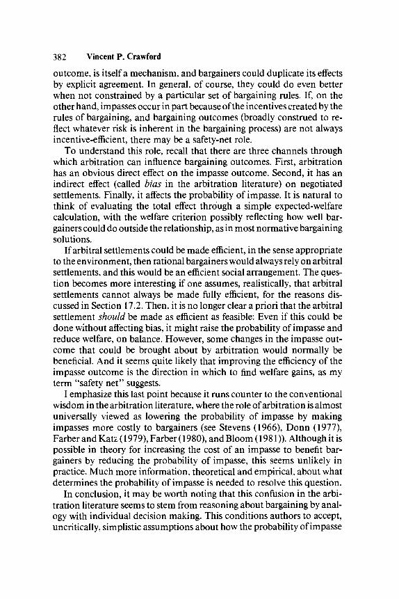
382 Vincent P. Crawfordoutcome, is itself a mechanism, and bargainers could duplicate its effectsby explicit agreement. In general, of course, they could do even betterwhen not constrained by a particular set of bargaining rules. If, on theother hand, impasses occur in part because of the incentives created by therules of bargaining, and bargaining outcomes (broadly construed to re-flect whatever risk is inherent in the bargaining process) are not alwaysincentive-efficient, there may be a safety-net role.
To understand this role, recall that there are three channels throughwhich arbitration can influence bargaining outcomes. First, arbitrationhas an obvious direct effect on the impasse outcome. Second, it has anindirect effect (called bias in the arbitration literature) on negotiatedsettlements. Finally, it affects the probability of impasse. It is natural tothink of evaluating the total effect through a simple expected-welfarecalculation, with the welfare criterion possibly reflecting how well bar-gainers could do outside the relationship, as in most normative bargainingsolutions.
If arbitral settlements could be made efficient, in the sense appropriateto the environment, then rational bargainers would always rely on arbitralsettlements, and this would be an efficient social arrangement. The ques-tion becomes more interesting if one assumes, realistically, that arbitralsettlements cannot always be made fully efficient, for the reasons dis-cussed in Section 17.2. Then, it is no longer clear a priori that the arbitralsettlement should be made as efficient as feasible: Even if this could bedone without affecting bias, it might raise the probability of impasse andreduce welfare, on balance. However, some changes in the impasse out-come that could be brought about by arbitration would normally bebeneficial. And it seems quite likely that improving the efficiency of theimpasse outcome is the direction in which to find welfare gains, as myterm "safety net" suggests.
I emphasize this last point because it runs counter to the conventionalwisdom in the arbitration literature, where the role of arbitration is almostuniversally viewed as lowering the probability of impasse by makingimpasses more costly to bargainers (see Stevens (1966), Donn (1977),Farber and Katz (1979), Farber (1980), and Bloom (1981)). Although it ispossible in theory for increasing the cost of an impasse to benefit bar-gainers by reducing the probability of impasse, this seems unlikely inpractice. Much more information, theoretical and empirical, about whatdetermines the probability of impasse is needed to resolve this question.
In conclusion, it may be worth noting that this confusion in the arbi-tration literature seems to stem from reasoning about bargaining by anal-ogy with individual decision making. This conditions authors to accept,uncritically, simplistic assumptions about how the probability of impasse

Role of arbitration and the theory of incentives 383
is related to the bargaining environment. Further, it leads to a misinter-pretation of the bargaining problems that originally led to public-sectorcompulsory arbitration. The need for prohibiting costly strikes by policeofficers and fire fighters is accepted on common-sense grounds. Then, it isobserved that employers who can no longer lose anything by intransi-gence are unlikely to bargain seriously. The final leap, to assuming theproblem is that impasses are sufficiently costly for both bargainers, ismade by false analogy. The end result is a serious misinterpretation of therole of arbitration.
17.6 Information buffering and coordination
The last roles of arbitration that I consider are information buffering andcoordination. Information buffering refers to the arbitrator's role in en-forcing mechanisms that deal efficiently with incentive problems butcannot be implemented by bargainers unaided. Coordination refers to therole of arbitrators and mediators in solving multiple-equilibrium prob-lems. These two roles are discussed together because they are linked in mymain illustrations.
Although the information-buffering and safety-net roles overlap some-what, there is a significant distinction between them. The safety-net rolediscussed in Section 17.5 can arise even when the set of fully efficientagreements is common knowledge, provided that there is a positive prob-ability that bargaining will end in an impasse. Examples where this hap-pens can be found in Crawford (1982c), where the rules of bargainingcreate incentives for bargainers to "burn their bridges" to an uncertainextent, thereby risking an impasse, in attempts to capture a larger share ofthe gains from cooperation; in Chatterjee and Samuelson (1983), whereimpasses can occur in equilibrium even when the supports of the distri-butions of bargainers' reservation prices do not overlap; and in Nash's(1953) "demand game," which has perfect, mixed-strategy equilibria witha positive probability of impasse even with complete information. Al-though, in the examples analyzed to date, incentive-inefficiency alwaysappears in the form of a positive probability of impasse (no trade, whentrade is efficient, in the language of Chatterjee and Samuelson (1983),Myerson and Satterthwaite (1983), and Samuelson (1984)), this form isby no means inevitable in more general, multi-issue models of bargaining.For these more general models, an information-buffering role mayemerge even when bargainers, in isolation, would always reach some sortof agreement.
Information buffering allows bargainers, by tacitly agreeing to rely onan arbitral settlement, to override the rules of bargaining and replace

384 Vincent P. Crawfordthem with an alternative mechanism. Although examples are knownwhere simple, realistic bargaining rules are an incentive-efficient mecha-nism,5 this is unlikely to be true in any reasonably general environment.(One possible reason for this is that incentive-efficient mechanismstypically depend sensitively on the details of the environment, whereasperhaps only simple bargaining institutions can enjoy an evolutionaryadvantage over other mechanisms.) When bargaining is not incentive-efficient, it may be possible for an arbitrator to commit himself to amechanism that is better for each type of each bargainer than the antici-pated bargaining equilibrium. If there is only one possible arbitrator, hewill have some incentive to make such a commitment, since this maxi-mizes the number of his clients. If he does so, bargainers can rely on anarbitral settlement without leaking any of their private information, be-cause it is already common knowledge that the arbitral settlement is betterfor both bargainers. Since this ensures that the arbitrator's mechanismwill operate as intended, it is rational for bargainers, who can each insiston an arbitral settlement, to do so.
Here, the arbitrator may play a coordination role as well, in ensuring,by suggestion, that the desired mechanism equilibrium is played. Thismay overcome multiple-equilibrium selection problems that are assumedaway in the standard use of the revelation principle to characterize incen-tive constraints.
The argument just outlined depends on several assumptions. First, it isimportant that the arbitrator can commit to a mechanism that is knownto be better for both bargainers, independent of their private information.Otherwise, the tacit decision to rely on arbitration may leak some of theirprivate information, altering the incentives created by the arbitrator'smechanism. This is not certain to cause problems, but the associatedpartial loss of control over incentives may prevent the arbitrator fromimproving on the bargaining outcome.
Second, it is important that either there be only one sensible choice ofarbitrator, or that bargainers can commit themselves to an arbitrator (whohas, by assumption, first committed himself to a mechanism) beforeobserving their private information. To see why competition among arbi-trators that takes place after bargainers have observed their private infor-mation may cause problems, it is helpful to model the process of choosingamong arbitrators as the application of a bargaining solution to the set ofpossible arbitrators (evaluated by the anticipated effects of their mecha-nisms). With symmetric information, a solution like Nash's (1950) mightbe used; the generalization to asymmetric information might use theHarsanyi-Selten (1972) solution.

Role of arbitration and the theory of incentives 385
This model of competition among arbitrators has several interestingfeatures. If arbitrators commit themselves to mechanisms simulta-neously, it is analogous to the Rothschild-Stiglitz-Wilson model ofcompetitive insurance markets (Rothschild and Stiglitz (1976) and Wil-son (1977)); the analogy suggests that neither pure-strategy equilibria norpooling equilibria (where all arbitrators propose the same mechanism) arelikely to exist in general. In a nonpooling equilibrium, the choice ofarbitrator, if it takes place after bargainers have observed their privateinformation, will generally leak information, causing problems similar tothose described earlier. (Since there are fewer arbitrators than mecha-nisms, partial information buffering, which may still be beneficial, willoccur.) This suggests that arbitration may have elements of natural mo-nopoly, for novel, informational reasons. It also underscores the benefitsof long-term commitments between arbitrators and clients, which, in-terestingly (although mainly for other reasons), are often thought togive arbitration an "unfair" advantage over bargaining (e.g., see Fuller(1963)). Finally, the demand for a particular arbitrator's services respondsfavorably to the equity as well as the efficiency of his settlements, if oneaccepts the equity notion built into the bargaining solution. (This is natu-ral if one views the bargaining solution as a focal-point resolution of themultiple-equilibrium problems in bargaining; see Schelling (1963).)Thus, the model provides a framework in which to evaluate Landes andPosner's (1979) claim that competition will eliminate bias in the analo-gous setting of private adjudication. This claim seems unlikely to be validunder realistic assumptions about the joint distribution of arbitrators'skills and their preferences for bias, or about the information structure.
Perhaps somewhat surprisingly, there may exist an information-buffering role even if bargainers can make binding agreements about themechanism that will be used to control their incentives. The implicationsof this possibility were first discussed formally by Holmstrom and Myer-son (1983), and are the subject of Crawford (1985), whose arguments aresummarized here.
When bargainers can bind themselves to a mechanism, it is natural toassume that they evaluate possible mechanism agreements according totheir rational expectations of the effect of the incentives they create,taking into account any information that is leaked in the process ofselecting a mechanism. Given this, the choice of a mechanism becomesanalogous to the choice of an allocation in "ordinary" bargaining theory,which suggests natural models of the process of agreeing on a mechanism.
Two cases can be distinguished. In the first, agents can bind themselvesto a mechanism before observing their private information, and standard

386 Vincent P. Crawfordarguments suggest that they can agree on a mechanism whose ultimateeffect will be an incentive-efficient allocation, evaluated according tobargainers' ex ante preferences (ex ante incentive-efficient, in Holmstromand Myerson's terminology). This immediately implies that there is noinformation-buffering role for arbitration.
In the second case, where agents observe their private informationbefore they can agree on a mechanism, it turns out that reasonable specifi-cations of the rules for bargaining over mechanisms imply that bargainerscannot generally achieve incentive-efficiency. (Here, the appropriate no-tion of incentive-efficiency treats each possible realization of an agent'sprivate-information variable as a separate person; I will use Holmstromand Myerson's term interim incentive-efficiency to refer to this concept.Roughly speaking, an allocation is interim incentive-efficient if there is noother attainable allocation, taking into account incentive constraints, aswell as physical constraints, that is better for all agents independent oftheir private information.) The problem is that the process of mechanismdesign, to yield good results, must aggregate information about bar-gainers' preferences over mechanisms. Because these preferences gener-ally depend on bargainers' types, mechanism design in this case may leaksome of their private information, altering the incentives created by themechanism that is chosen. Even if the effects of this information leakageare rationally anticipated, they can make it impossible for bargainers toachieve a result that is interim incentive-efficient.
Since, under my assumptions, an arbitrator is simply a predictable andenforceable choice of mechanism, there remains in this case no role forarbitration as defined so far. If, however, the arbitrator's powers are ex-panded somewhat, to allow him to enforce the rules of a particular mecha-nism-design process, a striking result emerges. With these expandedpowers, the arbitrator can make it possible for bargainers to achieve, afterthey have observed their private information, any desired interim incen-tive-efficient outcome. (As before, this need not be in conflict with theright to bargain, although information-leakage problems may arise.)Since these are the best outcomes attainable when mechanism design cantake place before agents observe their types - or in any case - this form ofarbitration can be said to allow bargainers to retreat behind the veil ofignorance to bargain over mechanisms, even when they are no longertruly ignorant. This is accomplished by using rules for bargaining overmechanisms that allow bargainers endogenously to restrict the languagethey use to bargain over mechanisms, in a way that permits aggregation oftheir preferences, but prevents them from encoding their private infor-mation in their mechanism proposals. I will now briefly describe these

Role of arbitration and the theory of incentives 387rules, and conclude by discussing the nature of the expansion of thearbitrator's powers, and his role as coordinator.
The mechanism-design process in Crawford (1985) is a generalizationof Nash's (1953) demand game, modified to allow for bargainers' privateinformation. It is assumed, for simplicity only, that there is a common-knowledge normalization of each bargainer's types' von Neumann-Morgenstern utility functions, with no agreement on a mechanism, andno information leakage, yielding zero utility for each type. Bargainers,after learning their types, simultaneously announce demands andweights. A bargainer's demand specifies a utility level for each of his types.His weights are nonnegative real numbers, one for each type of the otherbargainer. If each bargainer's demand is proportional to his opponent'sweights, and if bargainers' demands are compatible, in the sense that thedemanded type-contingent utility levels are realized in equilibrium bysome mechanism, then such a mechanism is implemented. (There is acommon-knowledge "tie-breaking" rule, and the mechanism is imple-mented whether or not bargainers learn about each other's types in theprocess.) If not, the underlying game is played with no agreement, hencenoncooperatively.
It is not difficult to show that for this mechanism-design process, anyinterim incentive-efficient outcome can be achieved as a "reasonable"equilibrium. A partial converse, using strong restrictions on equilibria,singles out these interim incentive-efficient outcomes as especially rea-sonable, in a weak but not implausible sense. Thus, an arbitrator whosesuggestions are taken seriously (as they might well be in a game with suchformidable multiple-equilibrium problems) might be able to use thismechanism-design process to get around the difficulties associated withbargainers already knowing their private information. This is accom-plished by creating incentives for each bargainer to ignore proposals bythe other bargainer that favor one or more of his types more (or less) thanthe arbitrator has suggested is appropriate. Although the rules of thismechanism-design process can be specified using only bargainers'common-knowledge information, they are highly sensitive to the detailsof the environment, and are quite complex. Even though this sensitivitymay be necessary to achieve interim incentive-efficiency when mecha-nism design takes place after bargainers have already observed their types,the associated complexity makes it clear that this process is far removedfrom anything that could be taken literally as a solution to the problem.(Crawford (1985) discusses some recent work that may make it possible toachieve good results in a more decentralized way.) However, the part ofthe arbitrator's task that involves figuring out how to reconcile bargainers'

388 Vincent P. Crawforddemands with their incentives appears quite realistic. This suggests thatfurther analysis of the process of mechanism design might lead to a deeperunderstanding of what arbitrators actually do.
NOTES1. Explicit randomization would be considered bizarre in arbitration circles, but
uncertainty about the arbitrator's intentions has been deemed vital to theeffectiveness of arbitration since the time of King Solomon, albeit for reasons Iconsider misguided (see Section 17.5). In practice, one would expect to seerandomization only in "purified" form, based on private information pos-sessed by the arbitrator, which in his opinion is not relevant to finding the bestsettlement.
2. Access to bargainers' private information would, of course, help the arbitratormitigate incentive problems. But access to their common-knowledge informa-tion would be important only if information-gathering difficulties are muchgreater than is usually assumed in the incentives literature.
The most striking evidence of the importance of information-gatheringcosts is implicit in Stevens's (1966) proposal to replace conventional compul-sory arbitration with final-offer arbitration, and its subsequent widespreadadoption. Recall that in conventional arbitration, the arbitrator is permitted toimpose an unrestricted settlement if negotiations break down, whereas in thesimplest form of final-offer arbitration, he is required to choose without com-promise between bargainers' final offers. Stevens's proposal was motivated bythe common belief that, in rendering their decisions, arbitrators tend to splitthe difference between bargainers' final positions. This makes concessions inbargaining doubly costly to a bargainer, since they then reduce the value of thearbitral settlement, if one occurs, as well as the negotiated settlement. Theresulting distortion of bargainers' concession decisions is known as the chillingeffect. Final-offer arbitration presumably weakens the chilling effect by makingit possible for concessions to improve the arbitral settlement for the bargainerwho makes them, by raising the probability that his final offer will be selected.
Stevens viewed final-offer arbitration as a way of intimidating bargainersinto negotiating their own agreements (thought desirable both intrinsically andfor efficiency reasons) without undermining their ability to do so by the tradi-tional series of gradual concessions. He did not notice that if intimidation wasthe true function of arbitration, it would be better accomplished in a nondissi-pative way (e.g., by fines) than by threatening bargainers with a risky settle-ment that might not reflect their preferences as efficiently as possible. (This hasbeen suggested, more recently, by Hirsch and Donn (1982), for example.) It issignificant that Stevens did not suggest (or apparently even consider) eliminat-ing the chilling effect by sealing the bargaining record and requiring the arbi-trator, when he is called upon to render a judgment, to gather his own informa-tion. This is now done sometimes, and has been discussed, for example, byWheeler (1977). However, despite great dissatisfaction with both formsof arbitration, it is far from universal. I conclude from this that information-gathering costs are probably of much greater significance than the focus ofresearch in mechanism design would suggest.
3. It is amusing that one of the most hotly contested issues in collective bargaining

Role of arbitration and the theory of incentives 389
is whether such an arbitrator can award, as part of his settlement, bindinginterest arbitration as the impasse procedure in the next negotiations.This issue is misperceived in the arbitration literature partly because of exces-sive reliance on one-issue models of bargaining, in which inefficiency arisessolely from the interaction of risk aversion and arbitral risk. This eliminationfrom consideration of the most important sources of inefficiency overstates thecase for the rational-optimism explanation. See Crawford (1981) for an elabo-ration of this point.Myerson and Satterthwaite (1983), for example, demonstrate that this is true,in a class of examples, for the bargaining rules studied by Chatterjee andSamuelson (1983). This is no longer the case, however, as demonstrated bySamuelson (1984), when Myerson and Satterthwaite's assumption that bar-gainers' valuations of the object to be traded are independent is relaxed.
REFERENCES
Baldwin, C: Productivity and Labor Unions: An Application of the Theory ofSelf-Enforcing Contracts. Journal of Business 56 (1983), 155-85.
Bloom, D.: Is Arbitration Really Compatible with Bargaining? Industrial Rela-tions 20 (1981), 233-44.
Brams, S., and S. Merrill, III: Equilibrium Strategies for Final-Offer Arbitration:There Is No Median Convergence. Management Science 29 (1983), 927-41.
Chatterjee, K., and W. Samuelson: Bargaining under Incomplete Information.Operations Research 31 (1983), 835-51.
Crawford, V. P.: On Compulsory-Arbitration Schemes. Journal of Political Econ-omy 87 (197'9), 131-59.
Arbitration and Conflict Resolution in Labor-Management Bargaining.American Economic Review Papers and Proceedings 71 (1981), 205 - 210.
Compulsory Arbitration, Arbitral Risk, and Negotiated Settlements: A CaseStudy in Bargaining under Imperfect Information. Review of EconomicStudies 49 (1982a), 69 -82.
A Comment on Farber's Analysis of Final-Offer Arbitration. Journal of Con-flict Resolution 26 (1982£), 157-60.
A Theory of Disagreement in Bargaining. Econometrica 50 (1982c), 607-37.Dynamic Bargaining: Long-Term Relationships Governed by Short-Term
Contracts. University of California, San Diego, Discussion Paper No. 83-13(1983), revised May.
Efficient and Durable Decision Rules: A Reformulation. Econometrica 53(1985), in press.
Donn, C: Games Final-Offer Arbitrators Might Play. Industrial Relations 16(1977), 306-14.
Donn, C, and B. Hirsch: Making Interest Arbitration Costly: A Policy Proposal.Journal of Collective Negotiations 12 (1983), 21-32.
Farber, H.: An Analysis of Final-Offer Arbitration. Journal of Conflict Resolution24(1980), 683-705.
Farber, H., and H. Katz: Interest Arbitration, Outcomes, and the Incentive ToBargain. Industrial and Labor Relations Review 33 (1979), 55-63.
390 Vincent P. Crawford
Fuller, L.: Collective Bargaining and the Arbitrator. Wisconsin Law Review 1963(1963), 3-46.
Harsanyi, J., and R. Selten: A Generalized Nash Solution for Two-Person Bar-gaining Games with Incomplete Information. Management Science 18(1972), P80-P106.
Hirsch, B., and C. Donn: Arbitration and the Incentive To Bargain: The Role ofExpectations and Costs. Journal of Labor Research 3 (1982), 55-68.
Holmstrom, B.: Moral Hazard in Teams. BellJournal of Economics 13 (1982),324-40.
Holmstrom, B., and R. Myerson: Efficient and Durable Decision Rules withIncomplete Information. Econometrica 51 (1983), 1799-1819.
Kalai, E., and R. Rosenthal: Arbitration of Two-Party Disputes under Ignorance.InternationalJournal of Game Theory 7(1978), 65-72.
Kreps, D., and R. Wilson: Sequential Equilibria. Econometrica 50 (1982), 863-94.
Landes, W., and R. Posner: Adjudication as a Private Good. Journal of LegalStudies 8 (1979), 235-84.
Malouf, M., and A. Roth: Disagreement in Bargaining: An Experimental Study.Journal of Conflict Resolution 25 (1981), 329-48.
Milgrom, P., and N. Stokey: Information, Trade, and Common Knowledge.Journal of Economic Theory 26 (1982), 17-27.
Moulin, H.: Prudence versus Sophistication in Voting Strategy. Journal of Eco-nomic Theory 24 (1981), 398-412.
Myerson, R.: Incentive Compatibility and the Bargaining Problem. Economet-rica 47 (1979), 61-73.
Mechanism Design by an Informed Principal. Econometrica 51 (1983),1767-97.
Myerson, R., and M. Satterthwaite: Efficient Mechanisms for Bilateral Trading.Journal of Economic Theory 29 (1983), 265 - 81.
Nash, J.: The Bargaining Problem. Econometrica 18 (1950), 155-62.Two-Person Cooperative Games. Econometrica 21 (1953), 128-40.
Rosenthal, R.: Arbitration of Two-Party Disputes under Uncertainty. Review ofEconomic Studies 45 (1978), 595-604.
Rothschild, M., and J. Stiglitz: Equilibrium in Competitive Insurance Markets:An Essay on the Economics of Imperfect Information. Quarterly Journal ofEconomics 90 (1976), 629-49.
Samuelson, W.: Bargaining under Asymmetric Information. Econometrica 52(1984), 995-1005.
Schelling, T.: The Strategy of Conflict. London and New York: Oxford UniversityPress, 1963.
Stevens, C: Is Compulsory Arbitration Compatible with Bargaining? IndustrialRelations 5 (1966), 38-52.
Wheeler, H.: Closed Offer: Alternative to Final Offer. Industrial Relations 16(1977), 298-305.
Wilson, C: A Model of Insurance Markets with Incomplete Information. Journalof Economic Theory 16 (1977), 167-207.