Information theoretic modeling of dynamical systems
213
ETH Library Information theoretic modeling of dynamical systems Estimation and experimental design Doctoral Thesis Author(s): Busetto, Alberto-Giovanni Publication date: 2012 Permanent link: https://doi.org/10.3929/ethz-a-009765795 Rights / license: In Copyright - Non-Commercial Use Permitted This page was generated automatically upon download from the ETH Zurich Research Collection . For more information, please consult the Terms of use .
-
Upload
khangminh22 -
Category
Documents
-
view
3 -
download
0
Transcript of Information theoretic modeling of dynamical systems

ETH Library
Information theoretic modeling ofdynamical systemsEstimation and experimental design
Doctoral Thesis
Author(s):Busetto, Alberto-Giovanni
Publication date:2012
Permanent link:https://doi.org/10.3929/ethz-a-009765795
Rights / license:In Copyright - Non-Commercial Use Permitted
This page was generated automatically upon download from the ETH Zurich Research Collection.For more information, please consult the Terms of use.

Diss. ETH No. 20918
Information Theoretic
Modeling of Dynamical Systems:
Estimation and Experimental Design
A dissertation submitted toETH Zurich
for the degree ofDoctor of Sciences
presented byAlberto Giovanni Busetto
Dott. Mag. in Ingegneria Informatica,Università degli Studi di Padovaborn November 26, 1983 in Venicecitizen of the Italian Republic
accepted on the recommendation ofProf. Dr. Joachim M. Buhmann, examinerProf. Dr. Manfred Morari, co-examinerProf. Dr. Jörg Stelling, co-examiner
2012


Abstract
Dynamical systems are mathematical models expressing cause-eectrelations of time-varying phenomena. This thesis focuses on learn-ing dynamical systems from empirical observations. Three settingsare considered: unsupervised, supervised, and active learning. Theunifying goal is to extract predictive information from data.
A method is introduced to cluster time-series and perform modelvalidation. The method addresses order and model selection withthe principle of Approximation Set Coding [Buhmann (2010)]. Ex-perimental verication is performed in the context of relational clus-tering of temporal gene expression proles. The results demonstratewide applicability and consistency with the Bayesian Information Cri-terion. Then, discrete dynamic transitions are reconstructed fromhigh-dimensional time-series with an unsupervised approach. Theapproach, based on Hidden Markov Models over Gaussian Mixtures,is applied to predict cell morphology classes from time-resolved mi-croscopy data. Experimental validation with uorescent markers andscreening data demonstrates accurate identication of human cell phe-notypes. Reported results highlight competitiveness and increasedobjectivity in comparison to supervised approaches based on user la-beling.
In the supervised setting, clustering is employed to improve con-ventional particle ltering for generalized state estimation. Preven-tive clustering mitigates the inevitable divergence of resampling forsequential Monte Carlo methods. Supervised learning with dynamic
i

Bayesian Networks is employed to model human learning for eectivetreatment of learning disabilities. In dyslexia, the model predicts for-getting, focus and receptive states of the subject on the basis of inputbehavior. In dyscalculia, numerical cognition is enhanced throughmodel-based adaptive training.
In the context of active learning, the thesis focuses on the near-optimal design of experiments for dynamical system modeling. Anecient method is introduced to select informative time points andmeasurable quantities. The design method is guaranteed to yieldnear-optimal informativeness with a polynomial number of evalu-ations of the objective function. The method builds on previouswork on submodular active learning [Krause and Guestrin (2005)]and achieves the best possible constant approximation factor, unlessP=NP [Feige (1998)]. Experimental design is applied to the recon-struction of cell signaling networks in systems biology.
The introduced contributions highlight fundamental analogies be-tween learning and communication. In conclusion, the results demon-strate that predictive models can be built from ecient strategies ofinformation transmission over a noisy channel. On the basis of statis-tical arguments, the presented results formalize and automate aspectsof the hypothetico-deductive method of scientic inquiry.

Acknowledgments
We are nothing without the work of others our
predecessors, others our teachers,
others our contemporaries.
J. R. Oppenheimer
I dedicate the thesis to my wife Simonetta, my parents Patrizia& Giovanni and my brother Gianluca. They support me with love,patience, and knowledge. My sincerest gratitude goes to my grand-parents Cesira, Imelde, Dobrillo and Egisto, who encouraged my stud-ies and made them possible. Without them and their work thisthesis would not have been written. My thankful thoughts are ad-dressed to the loving memory of Cesira and Egisto. My deepestappreciation goes to all my teachers (and in particular to AntonioRosino), for conveying a spirit of adventure in regard to researchand scholarship. Among them, I am grateful to Joachim M. Buh-mann for oering me the opportunity to pursue my doctoral studies.I feel honored to have been part of the Machine Learning Labora-tory with Brian V. McWilliams, Cheng Soon Ong, David Balduzzi,Elias August, Gabriel Krummenacher, Kay H. Brodersen, LudwigBusse, Manfred Claassen, Morteza Haghir Chehreghani, Peter Or-banz, and Thomas Fuchs. These are amazing persons from whomI learned a lot. I would like to thank my colleagues and friendsElias Zamora-Sillero, Francesco Dinuzzo, Irene Otero-Muras, MikaelSunnåker, Nelido Gonzales-Segredo, Riccardo Porreca, Rajesh Ra-
iii

maswamy, Sarvesh Dwivedi and Sotiris Dimopoulos. I had a greattime interacting with them; they are a group of creative, hard-working,cheerful and helpful individuals who enriched my experience at ETHZurich. I am particularly grateful to my collaborators A. Hauser,D. Stekhoven, G.-M. Baschera, T. C. Käser and Q. Zhong. Guid-ance, assistance, and insightful discussions provided by Marcus Hut-ter, Volker Roth, Peter Grünwald, Marcus Gross, Daniel W. Gerlich,Andreas Krause, and especially by the members of the thesis com-mittee Jörg Stelling and Manfred Morari, were greatly appreciated. Iwish to acknowledge my friends Nicola Carlon, Ruggero Dalla Santa,Francesco Gibaldi, Andrea Gesmundo, and Andrea Ierace for sup-porting my enthusiasm in science and for the amazing time that wehave had together. A further word of acknowledgment goes to thememory of Giuseppe Dalla Santa and Riccardo Carlon.
The collaboration work presented in this thesis has been nancedin part by the following agencies and institutions. The Machine Learn-ing Laboratory received funding from the SystemsX.ch initiative (Liv-erX and YeastX projects), evaluated by the Swiss National ScienceFoundation, and support by the DFG-SNF research cluster FOR916.The laboratory headed by D. W. Gerlich received funding from theEuropean Community's Seventh Framework Programme FP7/2007-2013 under grant agreements no. 241548 (MitoSys) and no. 258068(Systems Microscopy), from a European Young Investigator award ofthe European Science Foundation, from an EMBO Young InvestigatorProgramme fellowship to D. W. Gerlich and from the Swiss NationalScience Foundation. J. P. Fededa was funded by an EMBO long-termfellowship. The study on dyscalculia was funded by the CTI-grant11006.1 and the BMBF-grant 01GJ1011. The work on dyslexia wasfunded by the CTI-grant 8970.1. Together with the co-authors of therespective works, we thank C. S. Ong, J. M. Buhmann, S. Dimopou-los, D. Scheder, C. Sommer, E. Zamora-Sillero, J. Stelling, U. Sauer,M. Kast, K. H. Brodersen, and B. Solenthaler for helpful suggestionsand/or feedback on the published manuscripts, M. Held for processingimage data, and R. Stanyte for user annotations of image data.

I acknowledge these organizations, institutions, and initiatives:
• Eidgenössische Technische Hochschule Zürich, CH
• Università degli Studi di Padova, IT
• Scuola Matematica Interuniversitaria, IT
• University of Illinois at Urbana-Champaign, US
• Stanford University, US
• Massachusetts Institute of Technology, US
• California Institute of Technology, US
• University of Cambridge, UK
• Centrum Wiskunde & Informatica, NL
• International Centre for Mathematical Sciences, UK
• Competence Center for Systems Physiology and Metabolic Diseases, CH
• Max-Planck-Gesellschaft zur Förderung der Wissenschaften, DE
• The Royal Society of London for Improving Natural Knowledge, UK
• Swiss National Science Foundation, CH
• Deutsche Forschungsgemeinschaft, DE
• Life Science Zurich Graduate School, CH
• SystemsX.ch, CH
• Society for Industrial and Applied Mathematics
• Institute of Electrical and Electronics Engineers
• Functional Genomics Center Zurich, CH
• Free Software Foundation Europe
• Free Software Foundation
• European Science Foundation
• European Molecular Biology Organization
• Public Library of Science
• Wikimedia Foundation
1

2

Contents
1 Introduction 5
1.1 Contributions . . . . . . . . . . . . . . . . . . . . . . . 11
1.2 Terminology and Abbreviations . . . . . . . . . . . . . 18
2 Background 23
2.1 Systems Theory . . . . . . . . . . . . . . . . . . . . . . 24
2.1.1 State-space Modeling . . . . . . . . . . . . . . . 24
2.1.2 Dierential Models . . . . . . . . . . . . . . . . 26
2.1.3 Noisy Time Series Data . . . . . . . . . . . . . 28
2.2 Probability Theory . . . . . . . . . . . . . . . . . . . . 30
2.2.1 Modeling Justied Belief . . . . . . . . . . . . . 31
2.2.2 Bayesian Inference . . . . . . . . . . . . . . . . 33
2.2.3 Modeling Uncertainty . . . . . . . . . . . . . . 34
2.3 Information Theory . . . . . . . . . . . . . . . . . . . . 38
2.3.1 Uncertainty Quantication . . . . . . . . . . . 38
2.3.2 Learning and Communication . . . . . . . . . . 41
2.4 Main Assumptions . . . . . . . . . . . . . . . . . . . . 44
3 Unsupervised Learning 49
3.1 Time Series Clustering and Validation . . . . . . . . . 49
3.1.1 The Principle of Approximation Set Coding . . 50
3.1.2 Cluster Validation of Multivariate Time Series . 61
3.2 Modeling of High-dimensional Sequences . . . . . . . . 83
3.2.1 Modeling the Cell Cycle . . . . . . . . . . . . . 84
3
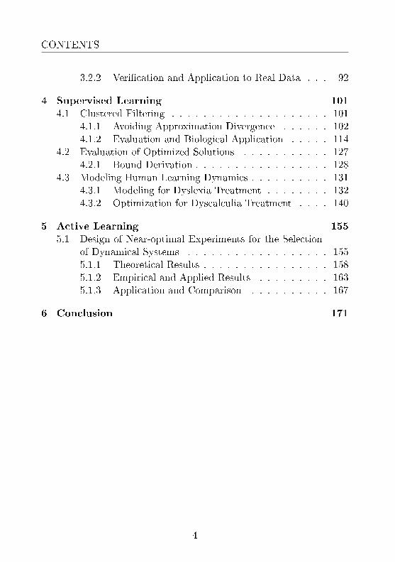
CONTENTS
3.2.2 Verication and Application to Real Data . . . 92
4 Supervised Learning 101
4.1 Clustered Filtering . . . . . . . . . . . . . . . . . . . . 1014.1.1 Avoiding Approximation Divergence . . . . . . 1024.1.2 Evaluation and Biological Application . . . . . 114
4.2 Evaluation of Optimized Solutions . . . . . . . . . . . 1274.2.1 Bound Derivation . . . . . . . . . . . . . . . . . 128
4.3 Modeling Human Learning Dynamics . . . . . . . . . . 1314.3.1 Modeling for Dyslexia Treatment . . . . . . . . 1324.3.2 Optimization for Dyscalculia Treatment . . . . 140
5 Active Learning 155
5.1 Design of Near-optimal Experiments for the Selectionof Dynamical Systems . . . . . . . . . . . . . . . . . . 1555.1.1 Theoretical Results . . . . . . . . . . . . . . . . 1585.1.2 Empirical and Applied Results . . . . . . . . . 1635.1.3 Application and Comparison . . . . . . . . . . 167
6 Conclusion 171
4

Chapter 1
Introduction
It is those who know little, and not those who
know much, who so positively assert that this or
that problem will never be solved by science.
C. R. Darwin
This chapter starts by outlining the content of the thesis. Focusand motivation are described in the rst paragraph. The second para-graph gives an introductory survey of the relevant literature, and isfollowed by a rst positioning of the work. The organization of themanuscript and the main contributions of the thesis are described inthe following. For clarity, the last section of the introduction containsan informal explication of the terminology used through the text, aswell as of the most commonly used abbreviations. Before the bibli-ography, the nomenclature consists of a topic-wise description of theformal notation.
Focus of the thesis. The thesis focuses on modeling dynamicalsystems from empirical observations. Dynamical systems are powerfultools to predict and control time-varying phenomena. At present, dy-namical models are employed in a variety of domains, such as physics,
5

CHAPTER 1. INTRODUCTION
economics, biology, medicine, and engineering. They are fundamen-tal: the foundation of entire scientic theories relies upon them. Dy-namical systems are particularly useful models which express cause-eect relations between the interacting components of a system.
This work entertains the idea that the value of a dynamical systemdepends, among other things, on its predictive capacity with respectto an objective. In the hands of a modeler, dynamical systems canbe employed as mathematical tools useful for prediction. Ultimately,the expected quality of such predictions depends on the amount ofavailable information regarding the relevant aspects of the problem.The modeler extracts such information from empirical observationsas well as, when possible, by incorporating previous knowledge. Themodeling process often involves both the estimation of the internalstates over time, as well as of the structural interactions between thecomponents of the system state. The models are, in practice, identi-ed through a combination of assumptions and accumulated evidence.The central question is: on the basis of nite and noisy observations,which dynamical system should be selected for a certain application?In this thesis, the value of a dynamical system is established by itsability to perform accurate predictions within the application scope.To make the goal precise, the evaluation of the predictive power re-quires a formal denition of success in prediction. On the basis ofstatistical arguments, the presented results aim at formalizing andautomating aspects of the hypothetico-deductive method of scien-tic inquiry [Whewell (1837)]. Information theory provides a formalframework to quantify uncertainty in terms of transmission rates overcommunication channels. The theory constitutes the central themeand the mathematical cornerstone on which the following results arebased upon.
Main motivation. By construction, dynamical models include timeas an independent variable. The models are able to incorporate reg-ularities beyond those exhibited by primarily static (or stationary)phenomena. Modeling of dynamical systems can be dened as the
6

discipline which aims at selecting dynamic models from empirical ob-servations. This research eld has a long and successful history, andcurrently oers important questions which remain open to furtherresearch and improvement. A relevant epistemological question is:how to perform induction? In technical terms, the question becomes:how to build a learning agent? At present, learning agents are basedon estimation techniques which are empirically evaluated within thescope of a given task. Some approaches are more general than oth-ers, and are applicable to multiple concrete problems [Nelles (2001)].Reasonable claims of universality are based on an assumption whichis often implicit: phenomena of interest do not exhibit absolute arbi-trariness. They do exhibit special regularities which, however, mightbe partially unknown to the modeler. Dynamical models aim at cap-turing the regularities which can be expressed as interactions betweenthe constituting components of the system. In this sense, modelingconsists of capturing such regularities from a nite set of empiricalobservations. When such observations are obtained in a controlledsetting, the measurements qualify as experimental data. Ideally, themodels obtained from data reect the available evidence and the as-sumptions taken by the modeler. In many applications, however,data acquisition is a signicantly resource-demanding process. Directinspection of the inner workings of the system is often not possibleto the modeler, and thus datasets may consist of scarce and noisyindirect observations. The limitation is severe because the expectedquality of the model predictions is constrained by that of the availabledata. How to reliably extract genuine regularities from scarce data?On the one hand, the modeler aims at capturing as many regularitiesas possible from the available observations. On the other hand, themodeler should lter out the spurious noise eects to avoid predictionerrors. Noise ltering is necessary to avoid confusing noisy uctua-tions as genuine regularities. In a prediction scenario, there existsa justied tradeo between the two antagonistic goals: the optimalbalance yields the lowest error rate. How to dene and calculate sucha tradeo? The available answers are well-justied but incomplete
7

CHAPTER 1. INTRODUCTION
[Nelles (2001); Bishop (2006); MacKay (2003)]. The results presentedin this thesis aim at contributing to this active eld of research.
Introductory Survey of the Field. A variety of mathematicalmethods are employed to model dynamical systems. In its essence,the eld can be seen as a branch of control engineering which signi-cantly overlaps with statistics and machine learning. In many cases,it shares not only the goals of these disciplines, but also the mathe-matical tools [Bishop (2006); MacKay (2003)]. There exists a rich andcomprehensive literature of the eld, which is condensed in this briefintroduction. Precise surveys are postponed to the respective sections.For now, it suces to refer the reader to a eld of large applicability:Model Predictive Control (MPC) [García and D. M. Prett (1989)].MPC is theoretically sound and practically useful: it makes a directuse of explicit and separately identiable models to control physicalprocesses. Of direct relevance to the topics of this thesis are two set-tings: that of modeling with non-linear systems and of learning undersignicant uncertainty. The former setting exhibits challenges whosenature is primarily computational. In many practical problems, thecomputational limitations of estimation are enormously aggravatedby the fact there are no known regularities which can provide an ad-vantage for optimization. However, there also exist cases in whichsuch knowledge is available. This is often the case for concrete ap-plications with well-studied models [Nelles (2001)]. High uncertaintyremains, however, a separate issue: it is exhibited when the modelerhas limited access to data which are very noisy. In such cases, themodeler may not be able to satisfy an important requirement: that ofquantifying and assessing the uncertainty associated with the results.
Systems biology is a domain in which the described conditionsconstitute the norm, rather than the exception. On the one hand,bio-medical experimentation is particularly resource-demanding. Onthe other hand, the investigated phenomena seem to exhibit excep-tional complexity. As a research eld, modeling of dynamical systemsoverlaps with active learning when actions are possible. The eld
8

of system identication covers the design of experiments aimed atpredictive modeling [Pronzato (2008); Atkinson and Donev (1992)].Experimental design can be seen as a research area at the interfacewith statistics. It encompasses the design of passive strategies, as wellas of active ones. In the passive setting, the modeler selects a subsetof measurable quantities from a pool of available candidates. Thiscase is in contrast to that in which interventions are performed byan agent, which might, for instance, exercise its agency through theactuation of input perturbations [He and Geng (2010)]. A comprehen-sive literature covers both passive as well as active design strategies[Pronzato (2008); Chaloner and Verdinelli (1995)]. Established pro-cedures have been recently applied to related domains, such as thoseinvolving Partial Dierential Equations (PDEs) models [Banks andRehm (2013)].
In summary, a central theme is that of dening and selecting theoptimal trade-o between model informativeness and estimation sta-bility [Buhmann (2010)]. The issue is of theoretical as well as practicalimportance: which model best generalizes the available data?
Positioning of the work. The work presented in the next chapterinterfaces with multiple research areas: unsupervised (cluster vali-dation), supervised (parameter estimation and model selection), andactive learning (experimental design) [Nelles (2001); Bishop (2006)].The central topics in the thesis are unied by a common theme: in-formation theory provides a useful framework to evaluate the predic-tive power of dynamic models [Cover and Thomas (1991); MacKay(2003)]. From a mathematical perspective, the thesis is based uponthree main frameworks: probability, information, and systems the-ory. The contributions presented here are primarily methodologicaland exhibit wide applicability. They are motivated, however, by openquestions in systems biology and human learning.
Organization The thesis is organized as follows. This chapter isintroductory: it describes structure and main contributions of the
9

CHAPTER 1. INTRODUCTION
thesis. The second chapter contains the necessary background andlists the main assumptions. The background consists of basic notionsfrom systems theory, probability theory, and information theory. Re-sults are organized in three chapters: supervised, unsupervised, andactive learning of dynamical systems. The conclusion discusses thereported results, and provides an analysis of limitations and potentialimprovements.
10

1.1. CONTRIBUTIONS
1.1 Contributions
If I have seen further, it is by standing
on the shoulders of giants.
I. Newton
The contributions encompass multiple aspects of information the-oretic modeling of dynamical systems. The organization follows thestructure of the three chapters described below. Detailed results arereported in the respective sections and summarized in the conclusion.
• Unsupervised learning: (Chapter 3)
Clustering of time series and validation (Sec. 3.1)Objective 1: which measured trajectories are statisticallydistinguishable? The task consists of selecting cost modelsfor clustering multivariate time series.Motivation: when one can select between cost models, it isoften a central issue to decide which model best generalizesthe available observations. Approximation Set Coding isa recently introduced principle which exhibits the poten-tial to address the issue of model selection in this setting[Buhmann (2010)].Contribution: an ASC-based method is introduced to per-form order and model selection of costs for relational clus-tering of time series.
Modeling of high-dimensional sequences (Sec. 3.2)Objective 2: how to build a dynamic model from high-dimensional data sequences without supervision? The taskof estimating the dynamic transition function aims at cap-turing the behavior in a space of statistically distinguish-able system states.Motivation: human labeling of sequential data such as im-age patches is not only time-consuming, but also tendsto lack self-consistency. Automated procedures are highly
11

CHAPTER 1. INTRODUCTION
desirable because they enable objective inference with re-producible and coherent results.Contribution: a method is introduced with the aim of re-constructing the dynamics of a system which evolves ina high-dimensional space. The method is applied to mi-croscopy image analysis; validation is performed with cellcycle data and compared with supervised results.
• Supervised learning: (Chapter 4)
Preventive resampling for generalized state estima-
tion: (Sec. 4.1)Objective 3: how to reliably estimate the parameters ofa dynamic system from time series? Bayesian approachessuch as particle ltering approximate the posterior distri-bution of the parameters through sampling. However, theytend to suer progressive information loss due to sampleimpoverishment and approximation degeneracy.Motivation: particle lters are established techniques whoseapplicability is limited by computational constraints. Im-proving the eciency of the techniques is important toextend the scope of practical applicability of the methods.Contribution: a preventive approach is introduced to miti-gate the information loss due to divergent approximationsbased on conventional resampling for generalized state es-timation.
Quality assessment of heuristic solutions for global
optimization problems: (Sec. 4.2)Objective 4: what is the relative position of a solution ob-tained from a given heuristic approach to optimization?Optimization problems are often computationally hard tosolve. The available solutions obtained heuristically mightnot be globally optimal. The task is to estimate how manysolutions are better than the best available heuristic ap-proximation.
12
1.1. CONTRIBUTIONS
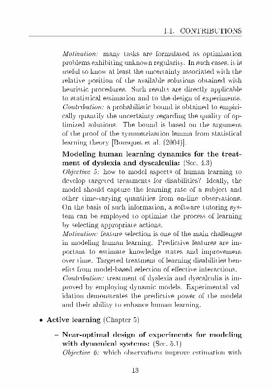
Motivation: many tasks are formulated as optimizationproblems exhibiting unknown regularity. In such cases, it isuseful to know at least the uncertainty associated with therelative position of the available solutions obtained withheuristic procedures. Such results are directly applicableto statistical estimation and to the design of experiments.Contribution: a probabilistic bound is obtained to empiri-cally quantify the uncertainty regarding the quality of op-timized solutions. The bound is based on the argumentof the proof of the symmetrization lemma from statisticallearning theory [Bousquet et al. (2004)].
Modeling human learning dynamics for the treat-
ment of dyslexia and dyscalculia: (Sec. 4.3)Objective 5: how to model aspects of human learning todevelop targeted treatments for disabilities? Ideally, themodel should capture the learning rate of a subject andother time-varying quantities from on-line observations.On the basis of such information, a software tutoring sys-tem can be employed to optimize the process of learningby selecting appropriate actions.Motivation: feature selection is one of the main challengesin modeling human learning. Predictive features are im-portant to estimate knowledge states and improvementover time. Targeted treatment of learning disabilities ben-ets from model-based selection of eective interactions.Contribution: treatment of dyslexia and dyscalculia is im-proved by employing dynamic models. Experimental val-idation demonstrates the predictive power of the modelsand their ability to enhance human learning.
• Active learning (Chapter 5)
Near-optimal design of experiments for modeling
with dynamical systems: (Sec. 5.1)Objective 6: which observations improve estimation with
13

CHAPTER 1. INTRODUCTION
dynamical system? The modeler aims at actively tuningexperimental variables to perform better predictions.Motivation: experiments are often resource-demanding. Therational allocation of such resources is important to achievehigh eciency in learning.Contribution: a near-optimal design method is introducedto select informative time points and measurable quanti-ties. The method exhibits formal performance guaranteesof near-optimality, which are proven by building on previ-ous work [Krause and Guestrin (2005)].
14
1.1. CONTRIBUTIONS
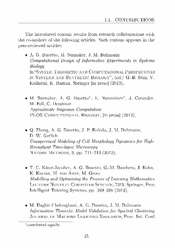
The introduced content results from research collaborations withthe co-authors of the following articles. Such content appears in thepeer-reviewed articles:
• A. G. Busetto, M. Sunnåker, J. M. BuhmannComputational Design of Informative Experiments in SystemsBiologyin System Theoretic and Computational Perspectives
in Systems and Synthetic Biology , (ed.) G.-B. Stan, V.Kulkarni, K. Raman, Springer [in press] (2013),
• M. Sunnåker, A. G. Busetto∗ , E. Numminen∗, J. Corander,M. Foll, C. DessimozApproximate Bayesian ComputationPLOS Computational Biology, [in press] (2012),
• Q. Zhong, A. G. Busetto, J. P. Fededa, J. M. Buhmann,D. W. GerlichUnsupervised Modeling of Cell Morphology Dynamics for High-throughput Time-lapse MicroscopyNature Methods, 9, pp. 711713 (2012),
• T. C. Käser-Jacober, A. G. Busetto, G.-M. Baschera, J. Kohn,K. Kucian, M. von Aster, M. GrossModelling and Optimizing the Process of Learning MathematicsLecture Notes in Computer Science, 7315, Springer, Proc.Intelligent Tutoring Systems, pp. 389398 (2012),
• M. Haghir Chehreghani, A. G. Busetto, J. M. BuhmannInformation Theoretic Model Validation for Spectral ClusteringJournal of Machine Learning Research, Proc. Int. Conf.
∗contributed equally.
15

CHAPTER 1. INTRODUCTION
on Articial Intelligence and Statistics, pp. 495503 (2012),
• G.-M. Baschera, A. G. Busetto, S. Klingler, J. M. Buhmannand M. GrossModeling Engagement Dynamics in Spelling LearningLecture Notes in Computer Science, 6738, Springer, Proc.Articial Intelligence in Education, pp. 3138 (2011)(Best Student Paper Award),
• A. G. Busetto, J. M. BuhmannStable Bayesian Parameter Estimation for Biological DynamicalSystemsIEEE CS Press, Proc. Int. Conf. on Computational Scienceand Engineering, pp. 148157 (2009)(Best Paper Award),
• A. G. Busetto, C. S. Ong, J. M. BuhmannOptimized Expected Information Gain for Nonlinear DynamicalSystemsACM Series, 382, Proc. Int. Conf. on Machine Learning, pp.97104 (2009),
• A. G. Busetto, J. M. BuhmannStructure Identication by Optimized InterventionsJournal of Machine Learning Research, Proc. Int. Conf.on Articial Intelligence and Statistics, pp. 5764 (2009),
and, for collaborations with advised students, on the master theses:
• A. Hauser,advised by A. G. Busetto and supervised by J. M. Buhmann
16

1.1. CONTRIBUTIONS
Entropy-based Experimental Design for Model Selection in Sys-tems BiologyETH Zurich, Department of Computer Science (2009),
• G. Krummenacher,advised by A. G. Busetto and supervised by J. M. BuhmannLarge-scale Experimental Design Toolbox for Systems BiologyETH Zurich, Department of Computer Science (2010).
17

CHAPTER 1. INTRODUCTION
1.2 Terminology and Abbreviations
My diculty is only an enormous diculty of
expression.
L. Wittgenstein (transl.)
For clarity, this section explains some terms used through the text.These informal denitions serve the purpose of introducing the readerto the setting of the study. Formal denitions are introduced in therespective sections. The interdisciplinary nature of the work requiresan additional eort to explicate the terms which are shared amongseveral disciplines. The author apologizes in advance for slight abusesof terminology. Particular emphasis has been placed on terms withoverloaded (and context-specic) connotations, such as model andhypothesis.
• Computation: the process of deterministic execution of a nitesequence of symbolic operations. The thesis deals with com-putation in the abstract, that is regardless of physical imple-mentation. Results are based on the notion of digital computa-tion and, more precisely, on the relation between abstract andconcrete computation expressed by the Church-Turing Thesis[Church (1932); Turing (1937)].
• Measurement: the process of obtaining and recording numericaldata from the studied phenomenon. The observational quanti-ties obtained through the operation of an experimental appara-tus are referred to as measurement data.
• Epistemic Agent: a learning entity which is capable of computa-tion and action. The agent exhibits internal consistency, means-end coherence, and consistency with belief acquired throughpassive or active observations [Bratman (1987)]. In this work,the epistemic agent denes a formal modeling system. Such sys-tem is capable to process information, retrieve and record data,perform measurements and interventions.
18
1.2. TERMINOLOGY AND ABBREVIATIONS
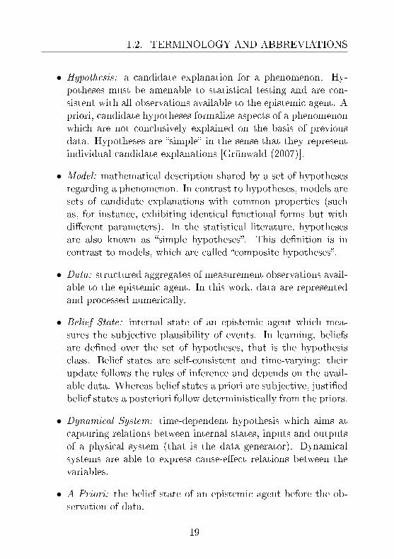
• Hypothesis: a candidate explanation for a phenomenon. Hy-potheses must be amenable to statistical testing and are con-sistent with all observations available to the epistemic agent. Apriori, candidate hypotheses formalize aspects of a phenomenonwhich are not conclusively explained on the basis of previousdata. Hypotheses are simple in the sense that they representindividual candidate explanations [Grünwald (2007)].
• Model: mathematical description shared by a set of hypothesesregarding a phenomenon. In contrast to hypotheses, models aresets of candidate explanations with common properties (suchas, for instance, exhibiting identical functional forms but withdierent parameters). In the statistical literature, hypothesesare also known as simple hypotheses. This denition is incontrast to models, which are called composite hypotheses.
• Data: structured aggregates of measurement observations avail-able to the epistemic agent. In this work, data are representedand processed numerically.
• Belief State: internal state of an epistemic agent which mea-sures the subjective plausibility of events. In learning, beliefsare dened over the set of hypotheses, that is the hypothesisclass. Belief states are self-consistent and time-varying: theirupdate follows the rules of inference and depends on the avail-able data. Whereas belief states a priori are subjective, justiedbelief states a posteriori follow deterministically from the priors.
• Dynamical System: time-dependent hypothesis which aims atcapturing relations between internal states, inputs and outputsof a physical system (that is the data generator). Dynamicalsystems are able to express cause-eect relations between thevariables.
• A Priori: the belief state of an epistemic agent before the ob-servation of data.
19

CHAPTER 1. INTRODUCTION
• A Posteriori: the belief state of an epistemic agent after theupdate of the prior on the basis of the newly available data,which consist of single or multiple measurement instances.
20

1.2. TERMINOLOGY AND ABBREVIATIONS
The following abbreviations appear in the text:
Alg. : AlgorithmDef. : DenitionFig. : FigureObj. : ObjectiveSec. : SectionTab. : Table
Asc : Approximation set codingBic : Bayesian information criterionCc : Correlation clusteringCi : Condence interval
Cse : Constant shift embeddingDbn : Dynamic Bayesian networkEm : Expectation maximizationEss : Eective Sample Size
Fn/Tp : False negative/positiveHmm : Gaussian mixture modelGs : Gold standard
Hmm : Hidden Markov modelIid : Independent identically distributedIvp : Initial value problemMap : Maximum a posteriori
Mcmc : Markov chain Monte CarloMdl : Minimum description lengthMpc : Model predictive controlOde : Ordinary dierential equationPc : Pairwise clusteringPca : Principal component AnalysisPde : Partial dierential equation
RNAi : RNA interferenceSd : Standard deviationSde : Stochastic dierential equationSmc : Sequential Monte CarloSvm : Support vector machineT3c : Temporal constrained combinatorial clustering
Tn/Tp : True negative/positive
21

CHAPTER 1. INTRODUCTION
22

Chapter 2
Background
Those who are in love with practice without
knowledge are like the sailor who gets into a ship
without rudder or compass and who never can be
certain whether he is going.
L. Da Vinci (transl.)
This chapter recapitulates basic notions from systems theory, prob-ability theory, and information theory. The expert reader can skip therst three sections, which cover the minimal introductory background.The end of the chapter lists the main assumptions on this work. De-spite the simplistic nature of the assumptions, they constitute a usefulstarting point to clarify the scope of the reported results. For reasonsof space, these sections gloss over technical subtleties. Further in-sights are left to the specialized literature in the respective elds.The presented notions are covered in considerable depth by the liter-ature [Hopcroft et al. (2007); Li and Vitányi (1997); MacKay (2003);Jaynes (2004); Cover and Thomas (1991); Nelles (2001)].
23

CHAPTER 2. BACKGROUND
2.1 Systems Theory
Science is what we understand well
enough to explain to a computer.
Art is everything else we do.
D. E. Knuth
The term dynamical system typically refers to the model of anatural or articial phenomenon which is referred to as the physicalsystem. In engineering applications, dynamical systems are used forcontrol, design, diagnosis, simulation and optimization. In a learningsetting, a dynamical system Σ can be seen as a tool aimed at predic-tion. The learned system captures aspects of interests of the studiedphysical system Σ∗. Dynamical systems are often modeled throughthe combination of rst-principle assumptions and experimental data[Nelles (2001)].
2.1.1 State-space Modeling
Among the existing alternative denitions, this thesis denes dynam-ical systems as computable state-space models. State-space modelsexpress input-output relations in terms of causal eects between theinternal states of a system. In this study, however, the modeler isunable to observe the inner workings through direct inspection.
Let X denote the state space, that is the set of all possible distin-guishable states x of a system. The state space might be continuous ordiscrete, depending on the case. Let nx ∈ N>0 denote the dimensionof the state space.
Let T ⊂ R be the discrete set of time points ti from the initialtime point t0, i ∈ N. Every pair of time points (ti, tj) ∈ T 2 obeys thetotal order ti > tj induced by the ordering i > j of the indexes.
The transition function F : X × T → X maps current states ontoconsequent ones (in some cases, the denition may be restricted to
24
2.1. SYSTEMS THEORY
time-invariant transition functions). The function is the map
F : (ti, x(ti)) 7→ x(ti+1). (2.1)
Denition 1. A dynamical system Σ is dened as
Σ := (X , T ,F), (2.2)
where X is the state space, and T is a set of time points. The systemobeys the transition function F(x, t).
It is worth noting that, with the provided formulation, the mem-ory of the system solely consists of the conguration expressed bythe current state. Denition 1 captures a simplistic notion of causaldeterministic behavior. It is, however, in theory sucient for ourpurposes. The denition, in fact, captures a rich set of possible be-haviors [Li and Vitányi (1997)]. The scope of the denition includesa dynamical system capable of universal computation: a universalTuring machine U [Turing (1937)]. Universal Turing machines aretheoretical systems which are able to emulate the behavior of anyother Turing machine without any loss of information [Hopcroft et al.(2007)]. The Church-Turing thesis states that the set of all numericalfunctions amenable to eective computation coincides with the classof partial recursive functions (that are those calculated by Turing ma-chines) [Turing (1937); Church (1932); Li and Vitányi (1997)]. WhenΣ denes a universal Turing machine, the function F implements auniversal partial recursive function [Li and Vitányi (1997)].
In its full generality, systems theory also considers systems beyondthose of Def. 1. The set of considered systems includes, for instance,stochastic and continuous dynamical systems (with continuous timeand state space). In the thesis, such systems are considered withinthe limits of their eective numerical approximation. In the caseof stochastic and continuous systems, the results that follow applyto their numerical approximation [Stoer (2002)]. Consistently withthat, data representation and information processing are intended tobe algorithmic in nature.
25

CHAPTER 2. BACKGROUND
The transition function F denes explicitly the causal relationsamong the components of the state. It also denes implicitly thetrajectory of the system over time. The initial condition of the systemΣ is denoted as
x0 := x(t0) ∈ X . (2.3)
The trajectory of length s+ 1 for the system Σ from x0 is
ϕ := (x(t0), . . . , x(ts)). (2.4)
So far, the denitions described only autonomous dynamical sys-tems, that are systems without input interventions. When the activityof the epistemic agent is limited to passive modeling, the transitionfunction already incorporates by denition all external inputs andinuences (through time-dependency, for instance). There are othercases, however, which are interesting in the context of active learning.When the agent can interact with the system, input interventions areconsidered explicitly in the denition of Σ.
In the non-autonomous case, the dynamical system Σt is subjectto series of instantaneous input interventions
u := (u(t0), . . . , u(ts)). (2.5)
Each intervention is denoted as u(t) ∈ U , for the intervention spaceU . The interventions inuence the behavior of the system throughthe transition function. In the active setting, the denition of F isextended to
F : (ti, x(ti), u(ti)) 7→ x(ti+1). (2.6)
2.1.2 Dierential Models
In the rest of the manuscript, continuous dynamical systems are de-ned in terms of dierential equations. For systems of ordinary dif-ferential equations (ODEs), the system ΣODEs is dened as follows.
26

2.1. SYSTEMS THEORY
Denition 2. A system of ODEs ΣODEs is given by
dx(t)dt
= FODEs(x(t), θ), (2.7)
where the function FODEs denotes the system of equations dening theinnitesimal increments in the trajectory over the state space.
The reader should note that system of ODEs may exhibit time-dependency as well. The numerical approximation of such systemis performed up to a tolerance which is xed a priori. The resultsthat follow assume negligible numerical errors for the discretizationof the system. Analogous denitions are introduced for systems ofStochastic Dierential Equations, which are introduced in Sec. 3.2.
The parameter vector of Eq. (2.7) is denoted as θ ∈ Θ, and denedover the parameter space Θ. The functional form FODEs is an exampleof a model M , that is a family of hypotheses sharing the functionalform of Eq. (2.7) in the range of parameters dened by Θ. Whenmodeling, the model classM is assumed to be xed a priori. It may,however, still be data-dependent, as in clustering. From a model M ,hypotheses are identied with their individual parameters θ ∈ Θ. Ina learning scenario, the modeler is often assumed to know X andT . In this setting, the modeler aims at estimating from the data thefunction F∗ of the physical process Σ∗ := (X , T ,F∗).
For a given initial condition x0, one can determine the integralsolution of the system over time. The task constitutes a conventionalinitial value problem (IVP). Whereas the solution of IVPs is straight-forward for discrete cases, the denition of continuous IVPs may re-quire careful restrictions on the set of allowable functions describingthe innitesimal transitions in the state space. All results in the thesisassume that the necessary conditions for the well-posedness of IVPsare satised. Well-posedness is dened in the sense of Hadamard1.The requirement extends to the numerical approximations of Eq. (2.7)and of other dierential systems such as those described by delay or
1Informally, a problem is well-posed when its solution exists, is unique, anddepends continuously on the data [Hadamard (1902)].
27

CHAPTER 2. BACKGROUND
partial dierential equations (DDEs and PDEs, respectively). Alter-native formulations are also considered through the text, includinghidden Markov models and dynamic Bayesian networks. The formaldenition of these model classes is postponed to the relevant chapters.
2.1.3 Noisy Time Series Data
In the thesis, the epistemic agent is able to perform imperfect mea-surements of the physical system Σ∗. The experimental observationsavailable to the modeler consist of nite datasets which are noisy.Noise terms are here denoted as ν and distributed according to therespective distributions N(N ). The noise variables are dened overthe noise space N . When measuring the state of Σ∗ at time point ti,for every i, the observer obtains the readout samples
y(ti) := h(x(ti), ti, νi) (2.8)
whereh : X × T ×N → Y. (2.9)
The measurement space is denoted as Y. Measurements are taken atthe time points
T ↓ ⊆ T , (2.10)
where the nite sample size is
n := |T ↓|. (2.11)
Individual trajectories measured at time points T ↓ are denoted as
ψ := (y(tj), . . . , y(tn)), (2.12)
with 1 ≤ j ≤ n. Time series are obtained by combining trajectorieswith the respective sampling points, giving
Ψ := (tj , y(tj))tj∈T ↓ . (2.13)
Data availability and noise level are dened by the experimentalsetting. Individual experiments are dened as ε ∈ E, over the spaceof experimental settings E.
28

2.1. SYSTEMS THEORY
Denition 3. The experimental setting ε ∈ E can be dened as
ε := (T ↓, N, h). (2.14)
Experimental design aims at selecting the best ε according to agiven objective. In practice, the process of design amounts to settingthe tunable parameters of ε to the most informative values. Sec-tion 5.1 adopts a simpler denition for ε: the experiment consists ofa set of indexes which refer to individual observations, thus indirectlyoperating on h.
29

CHAPTER 2. BACKGROUND
2.2 Probability Theory
One sees, from this Essay, that the theory of
probabilities is basically just common sense
reduced to calculus.
P.-S. Laplace (transl.)
This section recalls the basics of probability theory, which playsa central role in many (but not all) approaches to learning [Bishop(2006)]. Currently, probability theory remains the prevalent frame-work to quantify and update the justied belief states of epistemicagents. It is, however, not the only option available to the modeler.An alternative to probability theory would be given, for instance, bypossibility theory [Dubois and Prade (1988)] (which is based on fuzzyset theory [Zadeh (1978)]). Another alternative could be Dempster-Shafer theory of belief functions [Dempster (1968); Shafer (1976)]. Incontrast to probability theory, transferable belief model theory [Smetsand Kennes (1994)] separates belief from decisions2. Discussing aboutthe relative merits of alternative approaches to quantify belief wouldbe epistemologically interesting and intellectually valuable, but thetopic goes beyond the scope of this work. The thesis is based onprobabilistic grounds, which also constitute the foundation of (classi-cal) information theory [Cover and Thomas (1991)].
Probability theory has been formalized according to alternativesets of axioms. At this point, it is important to note that the frame-work of probabilistic inference is not a choice made ad-hoc: thereexist dierent sets of axioms for belief quantication which invari-ably lead to the conventional rules of probability [Bishop (2006)].Alternative formalizations of probability theory are dierent in phi-losophy and purpose. Among others, there exist theories of Ram-sey [Ramsey (1931)], Kolmogorov [Kolmogorov (1933, 1965)], Cox
2The formalization rejects the validity of betting arguments which are widelyemployed to justify probabilistic belief.
30

2.2. PROBABILITY THEORY
[Cox (1946, 1961)], Good [Good (1950)], Savage [Savage (1961)], deFinetti [de Finetti (1970)] and Lindley [Lindley (1982)]. They sug-gest dierent interpretations3, but the distinguishing technical detailsseem to be negligible for most practical purposes. As a rst drasticsimplication, it is customary to dene the two main interpretationsof probabilities as either classical (sometimes called frequentist) orBayesian. It is important to highlight, however, that no single classi-cal or Bayesian interpretation exist [Bishop (2006); Jaynes (2004)].
2.2.1 Modeling Justied Belief
The thesis subscribes to the Pólya-Cox axioms, which assign proba-bilities on logical grounds. Pólya-Cox axioms satisfy three minimaldesiderata of rationality and consistency [Cox (1946); Jaynes (2004)].To formalize these ideas, let us denote B(ρ) as the degree of belief inproposition ρ, and B(ρ|%) as the degree when % is true. In brief, theaxiomatic desiderata are [Jaynes (2004); MacKay (2003)]:
PC-A1: Probability values are divisible, comparable, bounded,and depend on the available information4:
B : Ξ→ [0, 1], (2.15)
where Ξ is a set of propositions.
PC-A2: The degree of belief in a proposition ρ ∈ Ξ is a functionof its negation ¬ρ ∈ Ξ:
B(ρ) = χ[B(¬ρ)],
for a certain function χ.
3Even the term interpretation is not strictly applicable in its typical sense tothis topic. A more denition would be explication [Carnap (1945)], since theredoes not exist a single formal system of probability. This topic is philosophicallyimportant and deserves attention, but goes beyond the scope of this work.
4Probabilities are here arbitrarily (yet conventionally) normalized betweenB(False) = 0 and B(True) = 1. The choice is without any loss of general-ity.
31
CHAPTER 2. BACKGROUND
PC-A3: The degree of belief in the conjunction of ρ ∈ Ξ and% ∈ Ξ is a function of the degrees of plausibility of ρ given %and that of % alone:
B(ρ ∧ %) = ζ[B(ρ|%), B(%)],
for a function ζ.
In the limit of absolute certainty, these requirements are consistentwith Aristotelian deductive logic obeying a Boolean algebra. No-tably, the formalization generalizes Aristotelian logic by includingweak (but still valid) syllogisms [Jaynes (2004)]. The axioms, in con-junction with the additional dierentiability condition for ζ, deter-mine uniquely the set of valid reasoning rules (up to normalization)[Jaynes (2004)]. Invariably, one has that B(ρ) ≡ p(ρ). The obtainedrules consist of the (familiar) sum and product rules of conventionalprobability calculus. In the end, all existing denitions of probabilityinvariably lead to the same set of rules. In probability theory, thejustication of any set of axioms is currently not undisputed [Jaynes(2004)]. However, it is noteworthy that the Pólya-Cox system is in es-sential agreement with that derived from Kolmogorov's axioms. Thedierence between the two is primarily epistemological: Pólya-Coxaxioms provide a foundation based on logic [Jaynes (2004)].
Several of the results in this thesis are better understood within aBayesian framework, while others, such as Approximation Set Coding(ASC), not necessarily. In the Bayesian setting, distributions quantifythe belief state of the epistemic agent [Bishop (2006); Jaynes (2004)].Bayesian belief states are thus subjective, yet not arbitrary. In fact,they are justied on the basis of the available evidence [Jaynes (2004)]and coincide under the same priors. The Bayesian perspective is incontrast to the interpretation of probabilities in terms of frequencies ofrandom and repeatable events. In all cases, probabilities are intendedas carriers of information5. The isomorphism of the alternative def-
5To be more precise, it would be better to talk about probabilities in termsof carriers of incomplete information, that is uncertainty. This subtle but impor-
32

2.2. PROBABILITY THEORY
initions of probability makes the axiomatic dierences of negligibleimpact for the overwhelming majority of practical purposes [Bishop(2006); Jaynes (2004)].
2.2.2 Bayesian Inference
Combining the sum and product rules, one obtains the cornerstoneof Bayesian inference: Bayes' theorem. For two random variables Mand D, Bayes' rule is given by
p(M |D) ≡ p(D|M)p(M)p(D)
. (2.16)
Letting model and data be denoted, respectively, as M and D, theterms of Bayes' theorem are conventionally referred to as
• p(M): prior probability(probability of model M before observing data D);
• p(M |D): posterior probability(probability of model M after observing data D);
• p(D|M): likelihood(probability of generating data D from model M);
• p(D): the evidence(general probability of observing data D).
The class of models, that is the sample space for M , is denoted asMand called the model class. The calculation of the model posteriorinvolves the marginalization for all individual hypotheses. In fact,taking hypotheses H from the hypothesis class H into account, onehas
p(M |D) ≡∑H∈H
p(M,H|D). (2.17)
tant distinction is claried in the next section, which introduces basic ideas frominformation theory.
33
CHAPTER 2. BACKGROUND
The data space D∗ indicates the space of datasets, which consists ofall possible sequences of samples y(ti) of size n obtainable from Σ∗
through the measurement process of Eq. (2.8). In the rest of the the-sis, H will indicate hypothetical transition functions F. Similarly, Mwill indicate families of hypothetical transition functions sharing thesame functional form (but, for instance, subject to dierent assign-ments of the parameters).
2.2.3 Modeling Uncertainty
A signicant advantage of Bayesian inference is the direct inclusion ofprevious knowledge in terms of prior probabilities. In the case of in-dependent experiments, the posterior of the last iteration constitutesthe prior of the current one without suering any loss of informa-tion. The Bayesian reliance on priors is, however, also the subjectof heated controversies [Bishop (2006)]. One might ask: where arethe priors coming from? Are they chosen according to mathematicalconvenience or on the basis of previous evidence? These questionsare important because the eect of the prior on the posteriors mightbe signicant. Multiple solutions have been proposed to solve theissue of assigning priors. All these solutions, in a way, are attemptsat modeling ignorance.
The agnostic learner wants to avoid assigning zero priors to ele-ments of H. Imposing such prior would make any posterior zero bydefault, irrespective of the data. No evidence would be strong enoughto modify the belief state for models which are excluded a priori. Thisproblematic situation is avoided by Cromwell's rule [Lindley (1991)].The rule states that the assignment of 1 or 0 to prior probabilitiesshould be exclusively restricted to statements which are logically trueor false, such as logical propositions.
Other approaches to assign priors require the transfer of aggregatestatistics from previous experiments. The technical way to incorpo-rate into the prior some non-probabilistic information is delicate anddeserves special attention. To set the prior, Bayes rule must be com-
34

2.2. PROBABILITY THEORY
plemented by subscribing to one or more external assumptions. Inthe agnostic case, one could apply the principle of indierence. Infor-mally, it states that, given insucient reasons to distinguish individ-ual hypotheses, all available candidates should be considered equallyplausible [Keynes (1921)]. Formally, the principle sets the prior tothe uniform distribution6. More generally, non-informative priors areattempts at exercising minimal inuence on posteriors. Among otherissues, they might even be improper due to lack of normalization. As-signing a prior gets even more problematic when densities are trans-formed according to non-linear changes of variables [Bishop (2006);Berger (1985)]. Jereys' rule addresses this issue by constructing in-variant non-informative prior distributions on the parameter space.Such distributions exhibit invariance under a class of reparameteriza-tions. The rule assigns priors which are proportional to the squareroot of the determinant of the Fisher information [Jaynes (2004)].
When only partial information is available, the principle of maxi-mum entropy provides a way to incorporate the available testable in-formation7. As shown later, testable information has to be amenableto statistical verication. In the continuous case, which is introducedbelow, the application of the principle of maximum entropy requiresthe specication of an invariant measure function. The requirementis necessary to avoid dependency on the choice of the parameters[Jaynes (2004)]. Informally, the principle of maximum entropy statesthat no additional information should be presumed (the formal de-nition is postponed to the next section). Notably, several well-knowndistributions are obtainable from maximum entropy arguments. Thisset of distributions includes uniform, exponential, Gaussian, Laplaceand Gibbs distributions [Bishop (2006)]. With awareness regardingthe limitations of maximum entropy arguments, the principle may beemployed as an additional assumption. In principle, there exists an
6Additional considerations are required in the case of non-bounded hypothesesclasses [Jaynes (2004)]. In such cases, transformation invariance may become aparticularly dangerous issue.
7One has to be careful, however, on how testable information is dened andobtained [Jaynes (1957a,b); Shannon and Weaver (1963)]
35
CHAPTER 2. BACKGROUND
elegant way to dene a general prior which is, in a technical sense,objective and universal [Rathmanner and Hutter (2011)]. Such dis-tribution, named Solomono-Levin distribution, species a prior overthe set of computable functions [Solomono (1964a,b)]. The universalprior is
M(z) ∝∑
pg:U[pg]=z∗
2−len(p), (2.18)
where z = z1z2 . . . zn is a string of length n. In the equation, theterms zi ∈ Z for all i = 1, . . . , n, indicate symbols from the alphabetZ. Now, z∗ denotes the subset of strings of arbitrary (but alwaysnite) length having z as a prex. The minimal program pg of lengthlen(pg) outputs string z when emulated by the universal Turing ma-chine U [Rathmanner and Hutter (2011); Solomono (1964a,b)]. Theprior M(z) relies on quantities which cannot be computed even inprinciple, and thus requires practical approximations. Under ratherminimal assumptions, inference based on the universal prior can, how-ever, be regarded as a gold standard [Rathmanner and Hutter (2011)].At present, the application of such concepts remains an area of ac-tive research [Li and Vitányi (1997); Rathmanner and Hutter (2011)].
The likelihood function p(D|M) constitutes a probability withrespect toD, but not with respect toM (due to lack of normalization).It plays a central role both in Bayesian inference through Bayes' rule,and in the classical framework. In classical statistics, conclusionsare often drawn according to the principle of maximum likelihood[Fisher (1922)]. The normalization of p(D|M) is given by Bayes' rule.Bayesian agents perform inference by calculating posteriors from priorand likelihood (given the data). In the Bayesian setting, the evidenceterm is not as fundamental as the prior and the likelihood; in fact,it constitutes just a normalization constant (for a given dataset). Inpractice, the evidence can be calculated as
p(D) ≡∑M∈M
p(D|M)p(M), (2.19)
36

2.2. PROBABILITY THEORY
whereM is the hypothesis class, that is the set of candidate modelsavailable to the modeler.
So far, probabilities have been dened over propositions. Equiv-alently, they may be expressed as functions on sets of events (con-sistently with established formulations). It is possible to extend thegiven denitions to continuous random variables, obtaining similarproperties for density functions. In the easy univariate case, a prob-ability density may be dened as
p(z ∈ (a, b)) :=∫ b
ap(z) dz, (2.20)
where z ∈ Ω denotes the value taken by a continuous random variableZ. Here, (a, b) denotes the continuous interval on the real line R. Sumand product rules of probability apply to densities as well, and alsoto combinations of discrete and continuous variables [Bishop (2006)].Similar properties extend the univariate denitions to multivariatesettings [Jaynes (2004)]. For mean and covariance parameters µ andΣ, the multivariate normal distribution of dimension r is dened as
Nor(z|µ,Σ) :=1
(2π)r/2|Σ|1/2exp
(−1
2(z − µ)TΣ−1(x− µ)
).
The sample space is Ω = Rr and the covariance matrix Σ is sym-metric and positive denite. With a slight (but conventional) abuseof notation, the rest of the thesis will homogeneously refer to bothprobability distributions and densities as p(Z). The distinction istypically clear from the context. If Z is a random variable and z ∈ Ωis an element of the sample space Ω, one may for simplicity use p(z)or p(Z) rather than p(Z = z).
37
CHAPTER 2. BACKGROUND
2.3 Information Theory
Information can tell us everything. It has all the
answers. But they are answers to questions we
have not asked, and which doubtless
don't even arise.
J. Baudrillard (transl.)
This section starts by dening two central concepts: self-informationand entropy. These concepts are consistent with commonly acceptednotions of uncertainty [MacKay (2003); Cover and Thomas (1991)].The Shannon self-information content for the outcome z in the samplespace Ω of the random variable Z is given by
h(z) := − log2 p(z), (2.21)
where p(z) is the probability distribution for Z [Shannon (1948);Shannon and Weaver (1963)]. Except otherwise specied, the baseof the logarithm will remain xed to 2. The choice of measuringinformation in Bits is arbitrary and without any loss of generality8.
2.3.1 Uncertainty Quantication
Shannon entropy is a measure of the uncertainty associated with thedistribution of the random variable Z. Informally, entropy measuresthe missing information over a weighted ensemble of possible out-comes.
The Shannon entropy of the random variable Z is given by
H[p] := E[h(z)] ≡ −∑z∈Ω
p(z) log2 p(z), (2.22)
that is by the expected self-information for the ensemble.
8There will be other cases in which the base of the logarithm is e, leading toalternative measures in Nats.
38

2.3. INFORMATION THEORY
In a communication scenario, Shannon entropy arises as an an-swer to the following technical question: what is the average length ofthe shortest description of the random instance emitted by a station-ary source [Shannon (1948); Cover and Thomas (1991)]? Shannon-Khinchin axioms provide the foundation for the derivation of Shannonentropy from a set of minimal requirements [Khinchin (1957); Shan-non and Weaver (1963)]. Dening the probabilities pi := p(zi) withzi ∈ Ω for all i = 1, . . . , n, the axioms are dened for an uncertaintymeasure S [Khinchin (1957); Suyari (2004)]:
SK-A1: for every n ∈ N>0, S(p) is continuous with respect tothe argument p := (p1, . . . , pn).
SK-A2: for a given n ∈ N>0, the point of global maximum forS(p) is un := (1/n, . . . , 1/n) (that gives the uniform distributionUnif (Ω)).
SK-A3: the function S is additive with respect to every pij ≥ 0,that is
S(p11, . . . , pnmn) = S(p) +n∑i=1
piS
(pi1pi, . . . ,
pimipi
), (2.23)
for all i = 1, . . . , n and all j = 1, . . . ,mi, where pi :=∑mi
j=1 pij .
SK-A4: the function S is expandable, that is
S(p1, . . . , pn, 0) = S(p1, . . . , pn). (2.24)
These requirements are met by a single function, which is Shannonentropy (up to scaling)9. One has, in fact, that S(p) ∝ H[p]. LetZ∗ denote the set of strings of arbitrary length composed of symbolsfrom the alphabet Z.
9Please note that, since limpi→0 pi log pi = 0, the work subscribes to the con-vention of taking pi log pi = 0 for pi = 0.
39

CHAPTER 2. BACKGROUND
The prex-free Kolmogorov complexity K(z) [Solomono (1964a,b);Kolmogorov (1965); Chaitin (1966); Li and Vitányi (1997)] is denedfor the string z ∈ Z∗ as
K(z) := minpr : U[pr]=z
len[pr], (2.25)
where U is a prex-free universal Turing machine.Notably, the choice of the universal machine aects the program
length by at most a constant number of bits [Li and Vitányi (1997)].A fundamental notion relates the Kolmogorov complexity to Shannonentropy. In fact [Li and Vitányi (1997)],∑
z∈Z∗p(z)K(z) ≤ H[p] + K(p) +O(1), (2.26)
for every recursive probability p over Z∗.Dierential entropy exhibits similar (but not exactly the same)
properties holding for Shannon entropy [Bishop (2006); Li and Vitányi(1997)]. The dierential version is obtained by quantizing the con-tinuous random variable and eliminating the logarithmic term (whichdiverges in the innitesimal quantization limit).
Denition 4. The dierential entropy of the density p is
H[p] := −∫
Ωp(z) log p(z) dz. (2.27)
For precision and consistency with the principle of maximum en-tropy, the thesis considers dierential entropy with respect to theinvariant measure function m(z). The precise (and preferable) deni-tion of dierential entropy then becomes [Jaynes (2004)]
Hm[p] := −∫
Ωp(z) log
p(z)m(z)
dz. (2.28)
As for probabilities, the thesis homogenizes the notation for discreteand continuous cases. This overload is acceptable since the case is
40

2.3. INFORMATION THEORY
typically clear from the context10.
On the basis of these denitions, it is now possible to formalizethe principle of maximum entropy (to incorporate it as an additionalaxiom). Let T denote the available testable information (that is,amenable to statistical verication), then
ME-A1: the candidate distribution over the models in the hy-pothesis class is given by
pME = arg maxp:Υ[p]=T
H[p]. (2.29)
where Υ[p] is the function producing statistics as T from p.
The principle it not only used to set priors, but also as a stand-aloneprinciple for model specication [Jaynes (1957a)].
2.3.2 Learning and Communication
A fundamental quantity which relates two probability distributions pand q is the relative entropy [Kullback and Leibler (1951)], which issometimes called Kullback-Leibler divergence.
Relative entropy is dened as follows:
KL[p ‖ q] :=∑z∈Ω
p(z) logp(z)q(z)
. (2.30)
The interpretation of Eq. (2.30) is the following: given the approxi-mating distribution q of the unknown stationary source p, KL[p ‖ q] isthe expected number of additional bits required for communication.The equation is obtained under the assumption that transmission isperformed with respect to an optimal coding for q (rather than for p,which is the source generator). It is important to note that relative
10Depending on the context, entropy is denoted either as H[p] or as H(z). Theformer notation highlights the dependency on the distribution, whereas the latteremphasizes the random variable associated with the distribution.
41

CHAPTER 2. BACKGROUND
entropy is not symmetric, that is KL[p ‖ q] 6≡ KL[q ‖ p], and thus can-not be a distance [Kullback and Leibler (1951); Cover and Thomas(1991)]. Another fundamental quantity from information theory isthe mutual information, which measures the statistical dependence oftwo random variables Z1 and Z2 (with respective sample spaces Ω1
and Ω2). The mutual information between two random variables is
I(Z1, Z2) :=∑z1∈Ω1
∑z2∈Ω2
p(z1, z2) logp(z1, z2)p(z1)p(z2)
. (2.31)
Mutual information is a measure of statistical dependence, in thesense that
I(z1, z2) = 0⇐⇒ z1 ⊥ z2, (2.32)
where ⊥ indicates statistical independence, that is
p(z1, z2) = p(z1)p(z2). (2.33)
Conditional entropy is dened as
H(Z1|Z2) := −∑z1∈Ω1
∑z2∈Ω2
p(z1, z2) log p(z1|z2). (2.34)
Hence, mutual information can be seen as the relative entropy betweenthe joint distribution and the product of the marginal distributions:
I(Z1, Z2) ≡ KL[p(z1, z2) ‖ p(z1)p(z2)]≡ H(Z1) + H(Z2)−H(Z1, Z2)≡ H(Z1)−H(Z1|Z2),
(2.35)
where the term H(Z1|Z2) denotes the conditional entropy. The lastequivalence of Eq. (2.35) oers a particularly valuable interpreta-tion. Mutual information can be seen as the reduction of uncertaintyabout Z1 as a consequence of observing Z2 [Bishop (2006); Cover andThomas (1991)]. The dierential versions of the introduced quanti-ties share fundamental similarities with their discrete counterparts11.
11They also exhibit important dierences [Bishop (2006); Cover and Thomas(1991); Jaynes (2004)].
42

2.3. INFORMATION THEORY
The dierential relative entropy, mutual information, and conditionalentropy are, respectively, the following:
KL[p ‖ q] :=∫
Ωp(z) log
p(z)q(z)
dz
I(Z1, Z2) :=∫
Ω1
∫Ω2
p(z1, z2) logp(z1, z2)p(z1)p(z2)
dz1dz2
H(Z1|Z2) − :=∫
Ω1
∫Ω2
p(z1, z2) log p(z1|z2) dz1dz2;
(2.36)
in all these, the random variables are continuous. As for the dier-ential entropy, there exist analogous (and preferable) versions whichinclude an invariant measure function.
43
CHAPTER 2. BACKGROUND
2.4 Main Assumptions
Making assumptions simply means believing
things are a certain way with little or no evidence
that shows you are correct, and you can see how
this can lead to terrible trouble.
L. Snicket in The Austere Academy
The main assumptions of this work are explicitly stated below.This section contains informal and simplistic formulations. Rigorousspecications and exceptions are introduced in the respective sections.
• There exists a data generating model. The studied phe-nomenon admits a formal (that is, mathematical) representationΣ∗, that is called the physical system. The system is associatedwith a model M∗ which indicates the transition function of thesystem, as in Eq. (2.2). The model may or may not (dependingon the case) be an element of the hypothesis class of an epistemicagent. The evaluation of experimental design, for instance, con-siders both settings. Nonetheless, data are always assumed tobe consistently generated according to Σ∗. Whereas guaran-tees and designs are formulated with respect toM∗, results andmodel predictions are evaluated empirically with external test-ing. The assumption is in contrast, for instance, to the view ofextreme empiricism for which phenomena are not even in prin-ciple amenable to formal representation [van Fraassen (1980)].Justication: the assumption provides a framework to evaluatelearning rates and to provide statistical guarantees.
• Belief states may be subjective, but inference is ob-
jective. The conclusions of epistemic agents coincide whenprior information, evidence, and inference method are sharedby the agents. The assumption means that the belief state isB(M |D) := Ψ(B(M), D) for a certain function Ψ. Moreover,
44

2.4. MAIN ASSUMPTIONS
conclusions are derived taking into account all available evi-dence: data points are not selected and no presumed evidencecan be incorporated if it is not already in the prior. The as-sumption is in contrast, for instance, to radical subjectivism[Dancy (1985)].Justication: the assumption is useful to justify the derivationof objective conclusions from subjective belief states and appliesto Bayesian inference.
• The dynamic behavior of the physical system is sep-
arable from the belief state of the modeler. With theexclusion of active interventions, the belief state of an agent ex-ercises no eect on the behavior of the physical system (withthe additional requirement that the denition of the physicalsystem does not include the epistemic agent). It means that,for every ti ∈ T , the state x(tj) (for j > i) of Σ∗ may dependexclusively on the belief state of the agent at times . . . , ti−1, tithrough active interventions. The assumption is in contrast to,for instance, EEG feedback systems in which the denition ofthe physical system includes the agent itself [Engstrom et al.(1970)].Justication: the assumption simplies the modeling process byimposing independence of the behavior of the physical systemfrom the belief of the (passive) agent.
• The measurement apparatus exercises negligible inter-
ference on the physical system. As in classical mechanics,for every ti ∈ T , the state x(ti) does not depend on the oper-ations of obtaining, storing, and processing data D producedat time ti (assuming all of them to be instantaneous processeswith respect to T ). Future states of Σ∗ may, however, be a func-tion of interventions selected on the basis of previously availabledata. The assumption is in contrast, for instance, to the Copen-hagen interpretation of quantum mechanics [Brock (2003)].Justication: the assumption simplies the inference process by
45

CHAPTER 2. BACKGROUND
making the behavior of the physical system independent fromthe eects of the measurement process.
• The physical process is causal. The future behavior of thephysical system can be described solely as the function of cur-rent and past states. The assumption, implicitly incorporated inEq. (2.2), imposes that transitions to future states x(ti+1) maydepend only on states and interventions acting at time pointstj with j < i. In other words, anticipatory eects are excluded.The assumption is in contrast, for instance, to anti-causal ef-fects in batch image processing.Justication: the assumption signicantly restricts the set ofpossible behaviors for the physical system.
• Consecutive experiments are independent. The observedoutcomes of separate experiments are conditionally independentgiven the behavior of the physical system and of the measure-ment apparatus. This assumption requires that
I(Di, Dj |M∗, ε) = 0 (2.37)
for every measured dataset with i 6= j. As before, M∗ denotesthe data generator and ε ∈ E is the experimental setting. Theassumption is in contrast, for instance, to the case in whichmemory eects are not negligible between experiments (and arenot already captured by M∗).Justication: the assumption enables the recursive combinationof evidence resulting from sequences of experiments.
• Axiomatic foundations. Unless otherwise specied, the worksubscribes to
Zermelo-Fraenkel set theory (with the axiom of choice)[Zermelo (1908); Hardin and Taylor (2008)],
the Church-Turing Thesis[Church (1932); Turing (1937)],
46

2.4. MAIN ASSUMPTIONS
Pólya-Cox axioms(PC-A1,2,3) [Jaynes (2004)],
Shannon-Khinchin axioms(SK-A1,2,3,4) [Khinchin (1957)],
the Principle of Maximum Entropy(ME-A1) [Jaynes (1957a)].
An additional disclaimer should be made here. Overall, the thesismaintains a pragmatic standpoint. In spite of the apparent simplicityof the denitions, their application to real problems often requiresintricate justications to maintain precision regarding the range ofvalidity of the obtained conclusions. The thesis is guided by the un-derlying rationale of the theory, while empirical results are evaluatedexternally in the context of the respective application domains.
47

CHAPTER 2. BACKGROUND
48
Chapter 3
Unsupervised Learning
Science is the belief in the ignorance of experts.
R. P. Feynman
3.1 Time Series Clustering and Validation
Clustering is one of the cornerstones of unsupervised data analysis.It proves particularly useful in the rst stages of modeling dynami-cal systems, for instance to extract compressed information regardingthe distribution of trajectories in the state space. In brief, the goal ofclustering is to select informative label assignments on the basis of theavailable observations. The fundamental modeling question is: whichmodel should be selected? When models are seen as tools aimed atprediction, the question ultimately relies on a measure of information.Ideally, the modeler should select cluster assignments which are infor-mative, as well as reasonably stable under the uctuations induced bythe noise. The central idea is the following: the modeler selects themodel yielding the highest reliable information capacity. Models arepredictive if they are able to consistently distinguish candidate solu-tions on the basis of the data. The capacity quanties the degree of
49

CHAPTER 3. UNSUPERVISED LEARNING
statistical detail which is extracted by the model. The solutions con-sist, in this setting, of cluster assignments from the hypothesis classC. The hypothesis class contains all possible assignments of samplesto cluster labels.
This section introduces a method to cluster time series and vali-date the obtained results1. The introduced method is based on Ap-proximation Set Coding, a recently introduced principle for modelvalidation [Buhmann (2010)]. In ASC validation, consistently withmost of statistical learning theory, the task of model selection is for-mulated with respect to a class of cost models. The class is givento the modeler a priori and might consist of costs such as those fromcorrelation and pairwise clustering. Each cost model expresses a data-dependent preference towards certain assignment solutions. For eachmodel, rather than selecting the individual best solution, ASC aimsat selecting the best set of assignments which are statistically indis-tinguishable. By doing so, ASC enables
• the quantication of the informativeness of the optimal set ofcluster assignments and
• the selection of the best cost model, that is the one maximizingthe informativeness in the prediction task.
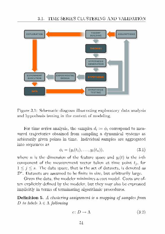
The results of cluster validation with ASC may also be employedas initial preprocessing steps for the nal aim of supervised learning[Nelles (2001)]. Figure 3.1 illustrates the position of exploratory dataanalysis in a diagram which represents a drastic simplication of themodeling process.
3.1.1 The Principle of Approximation Set Coding
In one of its conventional formulations, clustering aims at partitioningobjects into clusters according to a cost model R. In a general setting,data available to the modeler are denoted as D = djnj=1 and consistof n individual samples.
1Parts of this section appear in [Chehreghani et al. (2012)].
50
3.1. TIME SERIES CLUSTERING AND VALIDATION
Figure 3.1: Schematic diagram illustrating exploratory data analysisand hypothesis testing in the context of modeling.
For time series analysis, the samples di := φi correspond to mea-sured trajectories obtained from sampling a dynamical systems atarbitrarily given points in time. Individual samples are aggregatedinto sequences as
φi = (yi(t1), . . . , yi(tn)), (3.1)
where n is the dimension of the feature space and yi(t) is the i-thcomponent of the measurement vector taken at time point tj , for1 ≤ j ≤ s. The data space, that is the set of datasets, is denoted asD∗. Datasets are assumed to be nite in size, but arbitrarily large.
Given the data, the modeler minimizes a cost model. Costs are of-ten explicitly dened by the modeler, but they may also be expressedimplicitly in terms of terminating algorithmic procedures.
Denition 5. A clustering assignment is a mapping of samples fromD to labels λ ∈ Λ following
c : D → Λ (3.2)
51

CHAPTER 3. UNSUPERVISED LEARNING
with c : d 7→ λ.
The assignments are elements of the hypothesis class C(D). Theclass is data-dependent, as it maps individual data points to the as-signed labels.
For every trajectory j = 1, . . . , l, let Vk denote the set of indexeswhich correspond to samples assigned to the k-th cluster. Formally,the sets are
Vk := i ∈ [1, . . . , n] : c(i) = λk (3.3)
for k = 1, . . . ,K and K = |Λ|.Such index sets partition the sample indexes 1, . . . , n ⊂ N>0
into K subsets. In this setting, individual models are identied bytheir associated cost functions.
Denition 6. A cost model is a function evaluating hypothesis c givendata D as
R : C(D)× Y∗ → R. (3.4)
Implicitly, cost models specify regularities which can be extractedfrom the data. The goal of model validation is to assess the degree ofmatching between the regularities expressed by the model and thoseexhibited by the data. Given a dataset and a cost model, the pro-cess of learning terminates as soon as an optimal solution is found.Depending on the cost model, on the algorithm, as well as on the avail-able computational resources, the solutions which are found might beoptimal in a local or global sense.
At present, there already exist several established principles andprocedures for model selection. Among these, it is worth mentioningMinimum Description Length [Rissanen (1978)], Kolmogorov Struc-ture Function [Kolmogorov (1974)], BIC [Schwarz (1978)], AIC [Akaike(1974)], Minimum Message Length [Wallace and Boulton (1968)],Solomono's Induction [Solomono (1964a,b)], PAC [Valiant (1984)],as well as PAC-Bayesian generalization bounds [Seldin and Tishby(2010a)]. These approaches rely on convincing justications from in-
52

3.1. TIME SERIES CLUSTERING AND VALIDATION
formation theory, probability and statistical learning theory2. Ap-proximation Set Coding (ASC) shares the aim of the mentioned ap-proaches, but with a dierent goal: that of selecting models by mea-suring the informativeness associated with the best set of indistin-guishable solutions. Rather than evaluating individual solutions orglobal distributions over the hypothesis class, ASC extracts sets ofpredictive hypotheses. This study focuses on ASC for clustering [Buh-mann (2010)]. In this setting, clustering assignments are partitionedinto equivalence classes induced by noise uctuations. The classes de-pend on the model: under the same noise conditions, some models arebetter than others at distinguishing sets of solutions. In this sense,ASC operates on the eective resolution induced by the noise.
An informal justication for ASC is the following. For a givenmodel, learning can be seen as nding the best tradeo between infor-mativeness and stability of the solutions. Previous results emphasizedthe importance of estimation stability alone [Dudoit and Fridlyand(2002); Lange et al. (2004)], although not undisputedly [S. Ben-David(2006)]. Other appeals to stability in estimation for data analysis arebased upon the concepts of well-posedness [Hadamard (1902); Kochaand Tataru (2001)] and experimental repeatability. One requirementis undisputed: in controlled settings, experiments are expected toproduce similar readouts under similar conditions. Yet estimationstability alone is not enough. By itself, it does not take into accountthe information contained in the data. A model should not onlyreplicate the data, but also generalize to other datasets. The modelermust be careful: there exists an overtting risk when the amount ofavailable information is overestimated. What is the optimal tradeo?Reductions of estimation stability are tolerable when compensatedby appropriate improvements in predictive power (measurable, for in-stance, in terms of generalization capacity) [Vapnik (1982); Tishbyet al. (1999)]. If the modeler selects only few solutions, the selec-tion is informative but possibly unstable [S. Ben-David (2006)]. In
2Discussing the individual merits of established approaches goes beyond thescope of this thesis.
53

CHAPTER 3. UNSUPERVISED LEARNING
fact, the set of optimal solutions for a given dataset might not co-incide exactly with those selected by another dataset sampled fromthe same (stationary) source. The opposite tends to happen whentoo many solutions are selected. Sets consisting of many solutionsare certainly more stable with respect to resampling, but are not par-ticularly informative. ASC formalizes this tradeo idea on the basisof a fundamental analogy between learning and communication. Theoptimal tradeo is the one which maximizes the capacity to transmitset indexes through a noisy channel.
Empirical Minimizers and Approximation Sets
Formally, let us consider a setting with two datasets: D1 and D2.Each dataset is of size n and is independently sampled from the samestationary source. The asymptotic equipartitioning property guaran-tees that, with overwhelming probability, the datasets tend towardstypicality as the sample size grows [Cover and Thomas (1991)] Therequirement of two separate datasets is not limiting the generality ofthe approach. When a single dataset instance is available and theindividual samples drawn independently from the same distribution,a two sample set scenario can be eectively obtained through randomsplitting of data D into sets D1 and D2. The scenario can be ex-tended straightforwardly to cases in which more than two instancesexist. The conclusions are analogous and there is no loss of generality.
In the learning scenario, individual solutions are evaluated on thebasis of the data through the cost model. According to the preva-lent convention from statistical learning theory, smaller costs indicatepreferable solutions. The total ordering of the solutions is, therefore,directly induced by the cost model. The empirical minimizers are theoptimal solutions for the minimization of the cost model R(c|Dm) (form = 1, 2) and are dened as follows:
C⊥(Dm) := arg minc∈C(Dm)
R(c|Dm). (3.5)
For simplicity of notation, the cost of the empirical minimizers is
54

3.1. TIME SERIES CLUSTERING AND VALIDATION
denoted asR⊥(Dm) := R(c⊥|Xm) (3.6)
for c⊥ ∈ C⊥(Dm), m = 1, 2.To assess the predictive capacity of a model, one has to estimate
the variability of the optimal solutions with respect to that of the dataDm. Due to limited knowledge, average-case analysis is not possibleat this point: the data distribution is unknown to the modeler andvery hard to estimate directly (predominantly due to the high dimen-sion of the data space). Instead, performing operations directly onthe solution space might be a tractable task. Even without average-case analysis, it is still possible to say something regarding the rangeof plausible uctuations in the data on the basis of the empirical evi-dence provided by at least two instances. How to compare solutions?The two hypothesis classes are dataset-dependent. Then, to trans-fer solutions between instances one has to choose a mapping functionfrom C(D1) to C(D2). The denition of the mapping function is amodeling choice which is necessary to assess the generalization capac-ity from training to test data.
The mapping function performs the mapping from the rst datasetinstance to the second one. It is dened as
ψ : C(D1)→ C(D2). (3.7)
Relating solutions between hypothesis classes, ψ denes how themodeler intends to generalize across instances (by mapping to thenearest neighbor, for instance). For convenience of notation, subsetsof solutions A ⊆ C(D1) are mapped to other subsets through thesample-wise application of ψ as
ψ A := ψ(a), a ∈ A ⊆ C(D2). (3.8)
Because of noise, the set of mapped empirical minimizers ψ C⊥(D1)do not necessarily coincide with the set C⊥(D2). The intersectionbetween the two is given by(
ψ C⊥(D1))∩(C⊥(D2)
). (3.9)
55

CHAPTER 3. UNSUPERVISED LEARNING
The cardinality of the intersection might be small or even empty. Thelocations of the empirical minimizers, in fact, tend to diverge as thenoise level increases.
The central idea of ASC is that of selecting larger sets of clustersolutions from the hypothesis classes to avoid instability in the esti-mation. Approximation sets are dened as sets of solutions which areγ-minimal.
Denition 7. The approximation sets (AS) are
Cγ(Dm) := c ∈ C(Dm) : R(c|Dm) ≤ R⊥(Dm) + γ, (3.10)
for the respective dataset instances indexed by m = 1, 2.
The variable γ denes how close is the cost of the accepted solu-tions with respect to the cost R⊥(Dm) of the empirical minimizers.Hence, the elements of the approximation sets are at last γ-optimal.
The selection of an appropriate γ permits the optimization of thetradeo between selection stability and the informativeness of thesolutions. When γ = 0, the approximation sets consist solely of therespective empirical minimizers, thus yielding unstable results. Bycontrast, a too large value of γ forces the approximation sets to includea large number of solutions from the hypothesis class. Large selectionstend to yield results which are stable. However, the conclusions areuninformative if the selections are too large.
Learning and Communication
The optimal γ is found through information-theoretic optimization.ASC entertains the idea that learning and communication share fun-damental properties: performing predictions can be seen as codingwith error control and correction. The communication analogy pro-ceeds as follows: in the sender-receiver scenario, distinguishing indi-vidual solutions based on data corresponds to transmitting messagesover a noisy channel. The ability to discriminate solutions throughapplied transformations of the data reects the communication ca-pacity between the sender and the receiver. In learning as well as
56
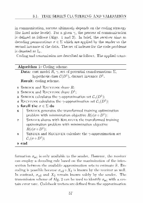
3.1. TIME SERIES CLUSTERING AND VALIDATION
in communication, success ultimately depends on the coding strategy(for xed noise levels). For a given γ, the process of communicationis dened as follows (Algs. 1 and 2). In brief, the receiver aims atdecoding permutations σ ∈ Σ which are applied by the sender to thesecond instance of the data. The set of indexes for the code problemsis denoted as Iσ.Coding and transmission are described as follows. The applied trans-
Algorithm 1: Coding scheme.
Data: cost model R, γ, set of potential transformations Σ,hypothesis class C(D1), dataset instance D1.
Result: coding scheme.
1 Sender and Receiver share R;2 Sender and Receiver share D1;3 Sender calculates the γ-approximation set Cγ(D1);4 Receiver calculates the γ-approximation set Cγ(D1);5 forall the σ ∈ Σ do
6 Sender generates the transformed training optimizationproblem with minimization objective R(c|σ D1);
7 Sender shares with Receiver the transformed trainingoptimization problem with minimization objectiveR(c|σ D1);
8 Sender and Receiver calculate the γ-approximation setCγ(σ D1);
9 end
formation σsel is only available to the sender. However, the receivercan employ a decoding rule based on the maximization of the inter-section between the available approximation sets to estimate σ. De-coding is possible because σsel X2 is known by the receiver as well.In contrast, σsel and X2 remain known solely by the sender. Thetransmission scheme of Alg. 2 can be used to identify σsel with a cer-tain error rate. Codebook vectors are dened from the approximation
57

CHAPTER 3. UNSUPERVISED LEARNING
Algorithm 2: Transmission scheme.
Data: cost model R, γ, set of potential transformations Σ,approximation sets Cγ(σ D1) for all σ ∈ Σ, hypothesisclasses C(D1) and C(D2), mapping function ψ, datasetinstances D1 and D2.
Result: set of estimated σ.
1 forall the σsel selected by the Sender do2 Sender applies σsel to D
2;3 Sender sends σsel D2 to Receiver;4 Receiver calculates the γ-approximation set given
σsel D2;5 Receiver estimates σsel with σ through the decoding rule:
σ ∈ arg maxσ∈Σ
ψ Cγ(σ D1) ∩ Cγ(σsel D2) ; (3.11)
6 end
58

3.1. TIME SERIES CLUSTERING AND VALIDATION
sets. A large value for γ corresponds to few distinct vectors for cod-ing, whereas small values produce higher error rates for decoding. The(asymptotic) transmission rate denes the tradeo between estima-tion stability and informativeness on the basis of the same currency:bits of information. The goal of communication is that of achievingoptimal communication (that is, maximally reliable and informativetransmission).
When σ 6= σsel, the receiver performs the wrong decoding. Thenoise uctuations produced a communication error. The intersectionbetween approximation sets is given by
∆Cqγ :=(ψ Cγ(σq D1)
)∩ Cγ(σsel D2) (3.12)
for all σq ∈ Σ. This term indicates the intersection between the q-thtraining approximation set and the test set, for q ∈ Iσ.
Bounding of Error Probability
At this point, it is possible to bound the decoding error probabilityp(σ 6= σsel|σsel) [Buhmann (2010)]. Due to the union bound, one hasthat
p(σ 6= σsel|σsel) ≤∑q∈Iσ
P
(|∆Cqγ | ≥ |∆Csγ |
∣∣∣∣σsel) . (3.13)
The bound is necessary since direct evaluation of the error probabil-ity might be challenging and no closed-form solution is known. Byintroducing the indicator function
Ia =
1 a is true0 a is false
, (3.14)
the bound in Eq. (3.13) becomes
p(σ 6= σsel|σsel) ≤∑q∈Iσ
EEσsel
[I|∆Cqγ |≥|∆Csγ |
∣∣∣∣σsel] . (3.15)
59

CHAPTER 3. UNSUPERVISED LEARNING
In the equation, the rst expectation is taken with respect to the pairof instances D1 and D2. It constitutes an annealed approximation.Since
I|∆Cqγ |≥|∆Csγ | = Ilog |∆Cqγ |≥log |∆Csγ |, (3.16)
one has that, because Ix≥0 ≤ exp(x) the bound becomes
Eσsel
[I|∆Cqγ |≥|∆Csγ |
∣∣∣∣σsel] ≤ |Cγ(D1)| |Cγ(D2)||Σ| |∆Cγs|
. (3.17)
Since the σ are identically distributed and sampled independently,the upper bound for the error probability of decoding is given by
p(σ 6= σsel) ≤ (|Σ| − 1) exp (−nIγ(σsel, σ)) , (3.18)
where the mutual information Iγ(σsel, σ) follows the denition below.The mutual information for two approximation sets is given by
Iγ(σsel, σ) :=1n
log( |Σ| |∆Csγ ||Cγ(D1)| |Cγ(D2)|
). (3.19)
At this point, it is possible to determine the optimal γ as follows. Theoptimal approximation threshold is
γ∗ ∈ arg maxγ∈[0,∞)
Iγ(σsel, σ). (3.20)
The described procedure provides to the epistemic agent:
• the set of γ-optimal cluster solutions which are statistically in-distinguishable, as well as
• an absolute measure of the informativeness of the cost modelR, which is called approximation capacity.
Denition 8. The approximation capacity (AC) for cost R and datasetsD1 and D2 is
AC[R|D1, D2] := I∗γ(σsel, σ). (3.21)
60
3.1. TIME SERIES CLUSTERING AND VALIDATION
The approximation capacity can be used to compare and selectcosts from a set of candidates. The class of candidate cost models isthe model class
R ⊆ R : C(D)× Y∗ → R. (3.22)
In practical applications, the set of candidate models may consists ofdierent functional forms as well as of alternative parametrization ofthe same function.
3.1.2 Cluster Validation of Multivariate Time Series
In clustering, ASC can then be employed for
• model selection (selecting between alternative costs models, suchas K-Means, pairwise clustering, or others),
• model order selection (selecting the number of clusters for anindividual cost model).
When analyzing multivariate time series, the modeler might employclustering to abstract, denoise, or compress trajectories in the mea-surement space. Informally, clustering addresses the question: whatis the eective resolution of the data? The modeler can select fromthe plethora of alternative methods which is available in the litera-ture. This study concerns the selection of relational cost models forclustering multivariate time series. Relational clustering (sometimesreferred to as spectral clustering) is a general approach whose the-oretical and practical importance is well recognized [Burnham andAnderson (2002)]. Characterizing time points by relations ratherthan vectors may prove particularly useful when the modeler doesnot know a priori a predictive similarity measure between trajectories.Until recently, model selection in relational clustering has been per-formed primarily according to heuristics and expert knowledge [Langeet al. (2004); Slonim et al. (2005)]. In this context, the Bayesian In-formation Criterion (BIC) is a simple and well-justied model selec-tion method whose eectiveness has been extensively proved [Schwarz(1978); Bishop (2006)].
61

CHAPTER 3. UNSUPERVISED LEARNING
Denition 9. The BIC cost is dened as follows:
BIC[M |D] := −2 log p(D|M) +$(M) log n (3.23)
where $(M) is the number of parameters for model M .
The direct application of BIC to relational clustering seems to beproblematic. From the denition, BIC requires the specication of thenumber of free parameters. In its standard form, it can be applieddirectly only to nite dimensional parameter spaces. In relationalclustering, the number of (eective) free parameters is not availableto the modeler. Furthermore, the eective dimension may grow as afunction of the sample size. As a substitute, one could employ theprinciple of Minimum Description Length (MDL), provided that anappropriate strategy for coding is available [Rissanen (1978); Grün-wald (2007)]. Alternatively, PAC-Bayesian analysis could providegeneralization bounds for model order selection [Seldin and Tishby(2010b)].
The following part concerns the automatic determination of thenumber of clusters as well as the selection of the cost model for clus-tering time series with ASC [Chehreghani et al. (2012)]. The rest ofthe section is organized in three parts: model order selection, modelselection, and application to scientic data analysis in systems biol-ogy. The cost model class consists of pairwise clustering (PC) [Hof-mann and Buhmann (1997a)] and correlation clustering (CC) [Bansalet al. (2004)]. The obtained results are compared with the selectionsprovided by the stability criterion [S. Ben-David (2006); Dudoit andFridlyand (2002); Lange et al. (2004)] and by BIC [Schwarz (1978)].The model validation task is formalized as follows.
Objective 1. Given data D, select the cost model in R∗ ∈ R withthe highest approximation capacity AC[R|D1, D2].
62

3.1. TIME SERIES CLUSTERING AND VALIDATION
Approximation with Boltzmann Factors
Up to logarithmic corrections, the cardinality of the approximationsets can be estimated by borrowing the concept of canonical ensemblesfrom statistical mechanics [Buhmann (2010)].
The partition function approximates the cardinality of a set as
|Cγ(Dm)|'Zm :=∑
c∈C(Dm)
exp (−βR(c|Dm)), (3.24)
for m = 1, 2, where β is the inverse computational temperature andan=bn denotes the asymptotic relation
limn→∞
1n
log(anbn
)= 0. (3.25)
In Eq. (3.24) and (3.26), the exponential weights are the Boltzmannfactors. The cardinality of the intersections can be similarly approx-imated by taking
|∆Cγ(D)| 'Z12 :=∑
c∈C(D)
exp(−β(R(c|D1) +R(c|D2))
). (3.26)
The inverse temperature β can be normalized by imposing that theaverage cost in Cγ(D) must yield R⊥(D) + γ.
Relational Clustering
For a cost model R, letK denote the number of clusters. Furthermore,let Xij denote to the pairwise similarity between sample i and j, for1 ≤ i, j ≤ n. For each sample and for each cluster, the given potentialhik quanties the cost of assigning the i-th sample to cluster k, for1 ≤ i ≤ n and 1 ≤ k ≤ K.
In the case of K-Means [Steinhaus (1957); MacQueen (1967)], thecost function minimizes the within-cluster sum of squares giving
Rkm(c|D) :=K∑k=1
∑i∈Vk
‖φi − µc(i)‖2, (3.27)
63

CHAPTER 3. UNSUPERVISED LEARNING
where i ∈ Vk when c(i) = λk, and µc(i) denotes the mean of the clusterassignment for φi. K-Means can be reduced to a model in which thepotentials are given by
hi,c(i) = ‖φi − µc(i)‖2, (3.28)
for all i = 1, . . . , n. The potentials consists of squared Euclidean dis-tances between data vectors and cluster centroids. K-means is oneof the most popular choices for clustering due to its simplicity. Thegenerality of the model is restricted to Euclidean vector data. Rela-tional clustering, in contrast, goes beyond this limitation: it clustersdata in terms of pairwise similarities (or dissimilarities). In relationalcost models, the potentials hi,c(i) may not be directly available tothe modeler from the formulation. Thus, equivalent potentials arecalculated through a mean-eld approximation, as described below.
Relational clustering is conventionally dened in terms of an at-tributed graph G = (V, E). The vertex set and the edge sets arerespectively denoted as V and E . The aim is that of clustering
Gu := i : c(i) = u (3.29)
for 1 ≤ u ≤ K. The set of edges between elements of cluster Gu andGv is
Euv := (i, j) : c(i) = u ∧ c(j) = v. (3.30)
Rewritten in terms of potentials, the weight sums of Eqs. (3.24)
64
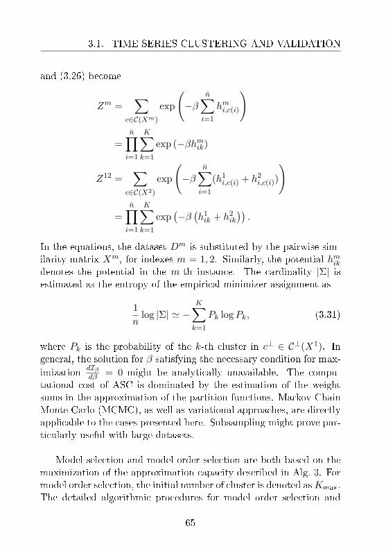
3.1. TIME SERIES CLUSTERING AND VALIDATION
and (3.26) become
Zm =∑
c∈C(Xm)
exp
(−β
n∑i=1
hmi,c(i)
)
=n∏i=1
K∑k=1
exp (−βhmik)
Z12 =∑
c∈C(X2)
exp
(−β
n∑i=1
(h1i,c(i) + h2
i,c(i))
)
=n∏i=1
K∑k=1
exp(−β(h1ik + h2
ik
)).
In the equations, the dataset Dm is substituted by the pairwise sim-ilarity matrix Xm, for indexes m = 1, 2. Similarly, the potential hmikdenotes the potential in the m-th instance. The cardinality |Σ| isestimated as the entropy of the empirical minimizer assignment as
1n
log |Σ| ' −K∑k=1
Pk logPk, (3.31)
where Pk is the probability of the k-th cluster in c⊥ ∈ C⊥(X1). Ingeneral, the solution for β satisfying the necessary condition for max-
imizationdIβdβ = 0 might be analytically unavailable. The compu-
tational cost of ASC is dominated by the estimation of the weightsums in the approximation of the partition functions. Markov ChainMonte Carlo (MCMC), as well as variational approaches, are directlyapplicable to the cases presented here. Subsampling might prove par-ticularly useful with large datasets.
Model selection and model order selection are both based on themaximization of the approximation capacity described in Alg. 3. Formodel order selection, the initial number of cluster is denoted asKmax.The detailed algorithmic procedures for model order selection and
65

CHAPTER 3. UNSUPERVISED LEARNING
cost model selection are given by Algs. 4 and 5, respectively. Formodel selection, let R = RlLl=1 indicate the class of candidate costmodels, each with its own respective hypothesis class dependent onthe similarity matrices Xm, for m = 1, 2.
Algorithm 3: Calculation of AC.
Data: computational temperature range W, permutations Σ,k, cost model R, set of hypothesis classes Ck(Xm) andsimilarity matrices Xm for m = 1, 2.
Result: ACk[R|X1, X2] for model order k.
1 forall the β−1 ∈ W do
2 calculate the potentials hik at β−1 (either by annealed
Gibbs sampling or annealed mean-eld approximation);
3 calculate the mutual information Ikβ ;4 end
5 Compute the approximation capacity
ACk[R|X1, X2] := maxβ Ikβ .
Algorithm 4: Model order selection.
Data: computational temperature range W, set oftransformations Σ, order range 1, . . . ,Kmax, cost modelR, set of hypothesis classes Ck(Xm)Kmax
k=1 andsimilarity matrices Xm for m = 1, 2.
Result: optimal model order k∗.
1 for k = 2 to Kmax do
2 Compute the approximation capacity ACk[R|X1, X2] for k;3 end
4 Select k∗ := arg max1≤k≤KmaxACk.
The subsection proceeds by comparing two established cost mod-els for relational clustering: pairwise and correlation clustering.
66

3.1. TIME SERIES CLUSTERING AND VALIDATION
Algorithm 5: Model selection.
Data: computational temperature range W, set oftransformations Σ, order range 1, . . . ,Kmax, cost modelR, set of hypothesis classes Ck(Xm)Kmax
k=1 for allmodels in R and similarity matrices Xm for m = 1, 2.
Result: optimal model order k∗.1 forall the R ∈ R do
2 Select k∗ := arg max1≤k≤KmaxACk for the cost R;
3 Compute ACk∗[R|X1, X2];
4 end
5 Select R∗ := arg maxR∈R ACk∗[R|X1, X2].
Denition 10. Given the similarity matrix X, the pairwise clusteringcost [Hofmann and Buhmann (1997b)] for K clusters is given by
Rpc(c|X) := −12
K∑k=1
|Gk|∑
(i,j)∈Ekk
Xij
|Ekk|. (3.32)
For pairwise clustering, there exists a way to calculate exactly thepotentials without distortion of the solutions through constant shiftembedding (CSE) [Roth et al. (2003)]. CSE embeds relational datainto a high-dimensional Euclidean vector space. In summary, CSEtakes advantage of the fact that Rpc(c|X) sums the average similari-ties per cluster weighted by size. Since the cost is shift-invariant, nodistortion of the solutions is introduced by adding a constant to allpairwise similarities. This operation just adds a constant multipliedby n to the costs of each solution. Consistent cost shifting neitherchanges the total ordering induced by the cost, nor the obtainableapproximation capacities. The samples are embedded into a kernelspace of dimension n− 1. The components Xij of the similarity ma-trix are then interpreted as scalar products between the two vectorsrepresenting the objects i and j, for 1 ≤ i, j ≤ n.
67

CHAPTER 3. UNSUPERVISED LEARNING
Dissimilarities are obtained from similarities through the transfor-mation
Ddiss := −X + %, (3.33)
where % is a constant. In the kernel space, pairwise clustering solu-tions share the same K-means costs [Roth et al. (2003)]. Hence, thecalculation of the weight sums is performed exactly by employing theanalytic solution available for K-means [Roth et al. (2003)].
As shown before, for factorial models the calculation of the poten-tials is straightforward. For non-factorial models, the potentials arecalculated through approximations. This situation applies to correla-tion clustering, for which no product form is known in terms of weightsums as in Eqs. (3.24) and (3.26). The approximation capacity is thencalculated by mean-eld approximation as follows [Chehreghani et al.(2012)]. Essentially, the cost function of correlation clustering sumsthe object disagreements, which are given by the negative intra-clusteredges and the positive inter-cluster ones. The cost of correlation clus-tering for K clusters is
Rcc(c,X) :=12
K∑k=1
∑(i,j)∈Ekk
(|Xij | −Xij)
+12
K∑k=1
k−1∑v=1
∑(i,j)∈Ekv
(|Xij |+Xij).
(3.34)
The mean-eld approximation holds for non-factorial models suchas correlation clustering [Chehreghani et al. (2012)]. It is noteworthythat, in this case, the mean-eld approximation admits an analyticform. In other cases, one could approximate the weight sums bysampling. Since the Boltzmann weights do not assume a productform, the potentials hik are determined by employing a factorial formto approximate the Gibbs distribution
pGibbs(c) := w(c,X)/Z, (3.35)
68

3.1. TIME SERIES CLUSTERING AND VALIDATION
where the Boltzmann weights are
w(c,X) := exp(−βR(c|X)) (3.36)
and Z is the normalizing partition function. The mean-elds of theapproximating distributions correspond to the adjustable parameters.Given the potentials, the cluster assignments are conditionally inde-pendent. The distribution for the factorial form is dened with respectto the set
Q :=
Q : Q(c) =
n∏i=1
qi,c(i), qi,c(i) ∈ [0, 1]
. (3.37)
The best approximation is the one minimizing the relative entropywith respect to pGibbs(c). Formally, it minimizes
KL [Q ‖ Pcc] =∑
c∈C(X)
Q logQ
exp(−β(Rcc − Fcc))
=n∑i=1
K∑k=1
qik log qik + βEQ[Rcc]− βFcc.(3.38)
The free energy is given by
Fcc := −β logZ (3.39)
Notably, the free energy does not depend on qik. Satisfying the nor-malization constraint
K∑k=1
qik = 1 (3.40)
for all i = 1, . . . , n, the minimization of KL (Q ‖ Pcc) is performedwith respect to qik. One proceeds by imposing the necessary condition
0 =∂
∂qik
KL [Q ‖ Pcc] +n∑j=1
Λj(K∑k=1
qjk − 1)
=
∑c∈C(D)
∏j≤n:j 6=i
qj,c(j)Ic(i)=kRcc +1β
(log qik + 1) + Λi.
(3.41)
69

CHAPTER 3. UNSUPERVISED LEARNING
which determines the mean-eld assignments
qik =exp(−βhik)∑k′ exp(βhik′)
, (3.42)
wherehik = EQi→k [Rcc]. (3.43)
The term EQi→k [Rcc] denotes the expectation taken over all congu-rations which assign object index i to the k-th cluster. Finally, themean-eld approximation of correlation clustering yields
hik =12
∑j≤n:j 6=i
(|Xij |+Xij)(1− EQi→k [Ic(j)=k])
+12
∑j≤n:j 6=i
(|Xij | −Xij)EQi→k [Ic(j)=k] + %
=12
∑j≤n:j 6=i
(|Xij |+Xij)(1− qjk)
+12
∑j≤n:j 6=i
(|Xij | −Xij)qjk + %.
(3.44)
where % indicates an additive constant. The cost is decomposed intocontributions depending on the i-th sample and on the cost of allother samples. Each qik is hence inuenced by terms depending onthe i-th sample.
Through mutual conditioning, mean-elds and probabilities canthus be eectively approximated for each β. This step is performediteratively with an algorithm following the Expectation-Maximizationprocedure [Bishop (2006)], as described by Alg. 6.
Proof-of-concept for PC and CC
Below are a couple of examples for illustration. In the following,L = 2 and R = Rpc, Rcc. First, let us consider pairwise clusteringwith two datasets X1 and X2 of dimension n = 800 each. Samples
70
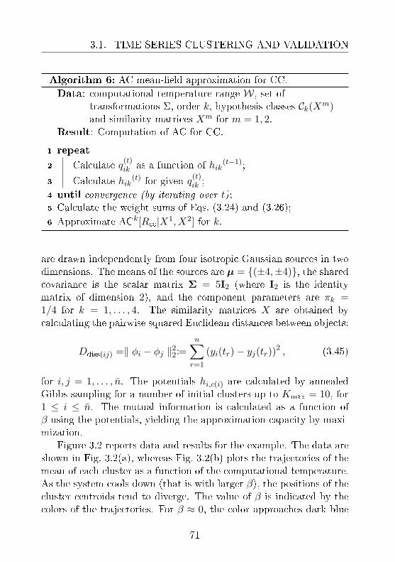
3.1. TIME SERIES CLUSTERING AND VALIDATION
Algorithm 6: AC mean-eld approximation for CC.
Data: computational temperature range W, set oftransformations Σ, order k, hypothesis classes Ck(Xm)and similarity matrices Xm for m = 1, 2.
Result: Computation of AC for CC.
1 repeat
2 Calculate q(t)ik as a function of hik
(t−1);
3 Calculate hik(t) for given q
(t)ik ;
4 until convergence (by iterating over t);5 Calculate the weight sums of Eqs. (3.24) and (3.26);
6 Approximate ACk[Rcc|X1, X2] for k.
are drawn independently from four isotropic Gaussian sources in twodimensions. The means of the sources are µ = (±4,±4), the sharedcovariance is the scalar matrix Σ = 5I2 (where I2 is the identitymatrix of dimension 2), and the component parameters are πk =1/4 for k = 1, . . . , 4. The similarity matrices X are obtained bycalculating the pairwise squared Euclidean distances between objects:
Ddiss(ij) =‖ φi − φj ‖22:=n∑r=1
(yi(tr)− yj(tr))2 , (3.45)
for i, j = 1, . . . , n. The potentials hi,c(i) are calculated by annealedGibbs sampling for a number of initial clusters up to Kmax = 10, for1 ≤ i ≤ n. The mutual information is calculated as a function ofβ using the potentials, yielding the approximation capacity by maxi-mization.
Figure 3.2 reports data and results for the example. The data areshown in Fig. 3.2(a), whereas Fig. 3.2(b) plots the trajectories of themean of each cluster as a function of the computational temperature.As the system cools down (that is with larger β), the positions of thecluster centroids tend to diverge. The value of β is indicated by thecolors of the trajectories. For β ≈ 0, the color approaches dark blue
71
CHAPTER 3. UNSUPERVISED LEARNING
and, viceversa, values of β 1 are associated to the red color. At hightemperatures, all centroids tend to coincide since the process cannotdistinguish but a single cluster. The contrary holds at very low tem-peratures, that is when too many clusters are estimated. The clusterlocations are highly susceptible to the inuence of the uctuationsand thus exhibit signicant instability in estimation. At the optimalinverse temperature, which is denoted by β∗, there is a split from fourto eight clusters (transition from green to yellow). The optimizer es-timates the correct number of clusters with the optimal temperature,that is the one yielding the approximation capacity. The AC for adierent number of clusters is shown in Fig. 3.2(d). Whereas themutual information is an objective function, BIC values (representedin Fig. 3.2(c)) constitute costs to be minimized. It is noteworthythat ASC and BIC yield consistent results in this case. The plot inFig. 3.2(e) shows the mutual information as a function of β. Its max-imum denes the AC of the cost model Rpc. At the optimal valueof the inverse computational temperature 1/β∗, the approximationcapacity reaches the bitrate of ≈ 1.5 bits per sample. In the noiselesscase, the bitrate of the AC approaches 2 bits per sample (that is thelogarithm of the number of distinct sources).
As a second example, let us consider correlation clustering withthe introduced mean-eld approximation. The datasets are pairs ofcorrelation graphs Xm, m = 1, 2, with n = 1500 and 5 source clus-ters. For varying level of noise, the datasets are generated as follows.At rst, the underlying structure is determined by setting a positivesimilarity label (+1) to intra-cluster edges and a negative one (−1)to inter-cluster edges. Then, each edge in Euv, for v 6= u, is randomlyipped to +1 with an independent and identically distributed (IID)Bernoulli probability Bern(ε|ξ). The parameter ξ is xed to the value0.35 and denes the complexity of the underlying structure. As a laststep, the value of each edge Euv, for v 6= u, is replaced by a randomvalue with probability η. The noise parameter η determines the ob-servational noise. The samples are mapped by the ψ function which
72
3.1. TIME SERIES CLUSTERING AND VALIDATION
identies samples according to their associated index. The order ofthe samples coincides in all data instances. The pairs are generatedat noise levels ranging from 0.75 to 0.95.
The mean-eld algorithm is executed with ten random initializa-tions per model order. Initial values are varying from 1 to 10. The mu-tual information is calculated at each round by taking the best resultsin terms of costs. The approximation capacity is calculated selectingthe mutual information for the best numerical approximation of β∗.The quality of the mean-eld approximation is numerically veriedby checking consistency with estimates obtained by Gibbs sampling.
As shown by Fig. 3.3, a noise level of η = 0.75 does not presentmajor challenges. Gibbs sampling and mean-eld approximation in-variably select the correct number of clusters. In case the initializationcontains too many clusters, the superuous ones are left empty. Anoise level of η = 0.85 makes the task more complicated but still learn-able. In this setting, signicant variations due to noise are visible inthe plot, which orders the samples according to the cluster assignmentof the nal selection. The approach determines the correct numberof clusters. Higher levels of noise induce a reduced approximationcapacity. Figure 3.3(b) shows that the stability criterion, based onthe instability measure [Lange et al. (2004)], yields results which areconsistent with ASC both for η = 0.75 and η = 0.85. The settingwith η = 0.95 exhibits high level of noise. In this case, the edge labelsare eectively almost entirely random. Figure 3.3(a) shows that thestructure which can be extracted from the data is not learnable anymore and, therefore, only a single valid cluster is obtained. Estima-tion instability, which is an undened measure for a single cluster,cannot be evaluated in this case.
73

CHAPTER 3. UNSUPERVISED LEARNING
(a) Available data (b) Cluster trajectories
(c) BIC scores (d) Approximation Capacity
(e) Mutual Information
Figure 3.2: AC score (Fig. 3.2(d)) and BIC cost (Fig. 3.2(c)) forpairwise clustering as a function of the number of clusters K for thesynthetic data (Fig. 3.2(a)). The model selection principles yieldconsistent results on the data. The calculation of the mutual infor-mation (Fig. 3.2(e)) for pairwise clustering has been performed withannealed Gibbs sampling as a function of β. Figure 3.2(b) shows theinuence of the stopping temperature for annealed optimization onthe localization of the cluster centroids (Figures from [Chehreghaniet al. (2012)]).
74

3.1. TIME SERIES CLUSTERING AND VALIDATION
(a) Approximation Capacities (b) Instability Measures
Figure 3.3: On the left, the approximation capacities are estimatedfor correlation clustering with ξ = 0.35 and noise parameters η takingthe values0.75, 0.85 and 0.95. On the right, the instability measureyields consistent results with ASC in two out of three settings. In theremaining case with η = 0.95, instability cannot be compared: themeasure is not dened for a single cluster (Figures from [Chehreghaniet al. (2012)]).
75

CHAPTER 3. UNSUPERVISED LEARNING
Clustering of Time Series
The introduced method for model selection and model order selec-tion is now applied to cluster the time-varying states of a biologicalprocess. The experimental data consist of readouts of gene expressionproles obtained at uniformly spaced time-points. Published data areextracted from the female digestive gland of Mytilus galloprovincialis[Banni et al. (2011)], an organism studied to assess the impact ofenvironmental pollutants. The challenging nature of the applicationdomain motivates the introduced approach: the choice of an appro-priate metric to analyze trajectories is far from obvious. Relationalclustering overcomes this limitation by comparing the informativenessof the solutions through ASC.
The available dataset consists of relative gene expression mea-surements for 12 consecutive months, with the rst sample (January)taken as a reference. The dataset contains information which is valu-able to the biologists to study how seasonal environmental changesaect physiology across the annual cycle of the organism [Banni et al.(2011)]. The samples consist of n = 295 dierentially expressedgenes (with intensities evaluated on a log-scale). There exists a singledataset, from which two similarity matrices are obtained by split-ting. The separation is performed by interleaving the features, thuscapturing the statistical dependence and yet avoiding the risk of un-dersampling small clusters. Feature splitting takes advantage of thenature of the data, associating the months (Mar, May, Jul, Sep, Nov)to the rst sample set, and (Apr, Jun, Aug, Oct, Dec) to the second.The similarity matrices are calculated from the respective datasets bytaking the Pearson correlation coecient for each pair of genes.
The approximation capacity is calculated by initializing the num-ber of clusters to 10 and then by computing the mutual information atdierent (inverse) computational temperatures. The approximationcapacities yielded by pairwise clustering and correlation clustering areplotted in Fig. 3.4 as a function of the respective inverse temperatures.The capacities demonstrate the ability of pairwise clustering over cor-relation clustering to capture predictable regularities in the data. The
76

3.1. TIME SERIES CLUSTERING AND VALIDATION
results are revealing: under the same noise, pairwise clustering is ableto discover more statistically valid structure from data than correla-tion clustering. On this dataset, ASC validates pairwise clusteringas ≈ 3.5 times more informative than correlation clustering. The re-spective approximation capacities for the optimal model order are, infact, ACpc = 1.03 and ACcc = 0.272. Figure 3.4(b) shows the accu-racy of the mean-eld approximation compared with Gibbs sampling.Whereas pairwise clustering is able to discover 7 valid clusters at op-timal temperature, correlation clustering is able to detect only 2. Thenumber of valid clusters identied by pairwise clustering at varyingtemperature is plotted in Fig. 3.4(c). Correlation clustering is unableto discover more since it exhibits a strong bias which favors clustersof equal size. By contrast, pairwise clustering is unbiased to size. Theconsistency between the optimal solution of pairwise clustering andcorrelation clustering is substantial: ≈ 3/4 of the co-clustered pairs inpairwise clustering are members of the same cluster in correlation clus-tering. For completeness, the model selection results obtained withASC are compared to those yielded by other established model selec-tion criteria: BIC and the (in)stability criterion. The former is useful,well-justied and simple to apply. However, it lacks a well-understoodapplicability in cases where the eective number of parameters is un-known. This analysis exhibits such a limitation which is due to lowereective dimension in the feature space. Thus, the application of BICis not straightforward in the case of pairwise clustering and even lessso for correlation clustering. For pairwise clustering, the BIC scorehas been computed according to the eective number of dimensions,that is the ratio between the trace and the largest data eigenvalue[Kirkpatrick (2009)]. The stability criterion is a heuristic approachwhich shares the spirit of cross-validation [Lange et al. (2004)]. Incontrast to BIC, the stability criterion is directly applicable to bothcost models, but exhibits the severe limitation of being applicableonly to alternatives with comparable informativeness. Figures 3.6(b)and 3.6(c) illustrate the results obtained by BIC and the stability cri-terion. Once again, it is worth noting the consistency between ASC
77
CHAPTER 3. UNSUPERVISED LEARNING
and BIC. The individual assignment of the samples to the clusters arereported in Fig. 3.5. The similarity matrix based on correlations isplotted in Fig. 3.5(c). In both gures, the samples are sorted accord-ing to increasing numerical value of the cluster labels. The inducedorder highlights the co-clustering structure of the optimal pairwiseclustering solution, which is visible in Fig. 3.5(a). Figure 3.5(b) putsin contrast the co-clustering blocks of pairwise clustering and correla-tion clustering (according to the permutation of the indexes obtainedfor PC). Let us denote the co-clustering matrices for pairwise clus-tering and correlation clustering as Hpc and Hcc, respectively. Thevalues of Hij for samples i and j, with 1 ≤ i, j ≤ n, is 1 when thelabel is identical, and 0 otherwise. Subscribing to this convention,Fig. 3.5(b) employs the following encoding for the pair (Hpc
ij , Hccij ):
`yellow' for (1, 1), `red' for (1, 0), `light blue' for (0, 1), `dark blue' forthe pair (0, 0). In brief, (0, 0) and (1, 1) denote assignment agreement,while (0, 1) and (1, 0) denote disagreement. Compared to correlationclustering, pairwise clustering is able to discover valid clusters at ahigher level of resolution. The enhanced statistical detail is also con-sistent with the coarser results obtained through correlation cluster-ing. Each cluster identies an equivalence class of trajectories whichare statistically indistinguishable. Elements of dierent clusters are,by contrast, distinguishable. The aggregate trajectories for the opti-mal pairwise clustering solution are reported in Fig. 3.7. The trajec-tories are normalized with respect to the intra-cluster means and withunitary variance. Such pre-processing of the trajectories is useful toperform parameter estimation and model selection, as discussed inthe next chapters.
In summary, the task of model selection has been addressed byASC to estimate the optimal tradeo between solution stability andinformativeness. ASC exhibited consistency with BIC in the analyzeddataset of gene expression dynamics. In this application, pairwiseclustering is able to capture three times more information than cor-relation clustering thanks to its unbiasedness with respect to clustersize.
78

3.1. TIME SERIES CLUSTERING AND VALIDATION
(a)Pairwiseclustering
(b)Correlationclustering
(c)Number
ofclustersforPC
Figure
3.4:
ACforPC(Fig.3.4(a))andCC(Fig.3.4(b))applied
totimeseries
ofgeneexpressions
from
theannualcycleof
Mytilusgalloprovincialis[Banniet
al.(2011)].Figure
3.4(b)compares
the
estimated
mutual
inform
ationwithmean-eldapproxim
ationandwithGibbssampling.
Thenum-
ber
ofclustersforPCat
dierenttemperaturesisshow
nin
Fig.3.4(c)
(Figuresfrom
[Chehreghani
etal.(2012)]).
79

CHAPTER 3. UNSUPERVISED LEARNING
(a)Pairw
iseClusterin
g(b)PCVsCC
(c)Correla
tionmatrix
Figu
re3.5:
Theoptim
alsolu
tionfor
pairw
iseclu
steringisplotted
inFig.
3.5(a)(black
indicates
co-clu
steringof
theelem
ents).
Resu
ltsfrom
pairw
iseclu
steringandcorrelation
clusterin
gare
reported
andcom
pared
inFig.
3.5(b)(w
ithindexes
perm
uted
consisten
tlywith
PCassign
ments).
Colors
areassign
edaccord
ingto
thefollow
ingrule:
therst
bitrefers
topairw
iseco-clu
steringandthesecon
doneto
correlationco-clu
stering.
Thesim
ilaritymatrix
ofpair-w
isecorrelation
sobtain
edfrom
the
measu
rementdata
isplotted
inFig.
3.5(c)(Figu
resfrom
[Chehregh
aniet
al.(2012)]).
80

3.1. TIME SERIES CLUSTERING AND VALIDATION
(a)InstabilityforPC
(b)InstabilityforCC
(c)BIC
forPC
Figure
3.6:
Thevalueof
theinstability
measure
iscomputed
forPC
(Fig.3.6(a))and
CC
(Fig.3.6(a)).
Figure
3.6(c)
reports
theresultsobtained
fortheBIC
cost,whichiscalculatedfor
theeective
dim
ension.Notably,theresultsobtained
withASCareconsistentwiththoseof
BIC
(Figuresfrom
[Chehreghaniet
al.(2012)]).
81

CHAPTER 3. UNSUPERVISED LEARNING
Figu
re3.7:
Trajectories
foreach
cluster
fromtheoptim
alclu
sterassign
mentgiven
bypairw
ise(left)
andcorrelation
clusterin
g(righ
t).Thetim
efram
eran
gesfrom
March
(M)to
Decem
ber
(D).
Cluster
mean
sare
plotted
inblue(PC)andgreen
(CC),while
norm
alizedSDsappear
inred
.The
comparison
ofthetra
jectoriesdem
onstrate
thehigh
erresolu
tionof
pairw
iseclu
steringcom
pared
tocorrelation
clusterin
g.
82

3.2. MODELING OF HIGH-DIMENSIONAL SEQUENCES
3.2 Modeling of High-dimensional Sequences
The great tragedy of Science the slaying of a
beautiful hypothesis by an ugly fact.
T. H. Huxley
This section introduces a method for the unsupervised modelingof discrete dynamical systems3. Whereas the previous section aimedat quantizing the set of trajectories in the state space, the goal ofthis section is to model the dynamic transitions between states. Thestudy is motivated by the current limitations in the analysis of cellularphenotypes from image data [Zhong et al. (2012)].
In combination with large-scale perturbation by RNA interference(RNAi), live-cell microscopy is a particularly informative approach todiscover gene function [Conrad and W. (2010); Goshima et al. (2007);Collinet et al. (2010); Schmitz et al. (2010); Neumann et al. (2010)].State-of-the-art methods analyze cell morphologies and phenotypeswith supervised statistical models, that is with approaches which com-pletely rely on user annotation. In such settings, the data which areavailable to the modeler consist of large sequences of time-resolvedmicroscopy images. So far, the task of modeling cell morphologieshas been formulated mainly as a conventional supervised learningproblem [Neumann et al. (2010); Boland and Murphy (2001); Heldet al. (2010); Harder et al. (2009); Wang et al. (2008); Loo et al.(2007); Jonesa et al. (2009); Conrad et al. (2011)]. By subscribing tothe supervised framework, previous approaches implicitly limited theapplicability of cell-based screening to cases in which extensive knowl-edge regarding morphology is already available. There exists anothersignicant practical limitation associated with supervised approaches:human labeling exhibits low consistency. This problem is enormouslyaggravated when researchers compare results originating from dier-ent laboratories (due to bias and subtle change of controlled condi-tions). The following annotation-free method overcomes these two
3Parts of this section appear in [Zhong et al. (2012)].
83
CHAPTER 3. UNSUPERVISED LEARNING
issues. The method enables the automatic prediction of cell morphol-ogy dynamics from time-resolved images [Zhong et al. (2012)]. Theapplication target of the method is the full automation of data label-ing in image-based systems biology. The methodological goal is toincrease objectivity, reproducibility, and validity of the results. Beingunsupervised, the method has the additional advantage of being sig-nicantly faster, since it does not rely on human labor. The methodis applied to unsupervised modeling of human cell phenotypes withdiverse uorescent markers and screening data. Experimental resultsin various experimental conditions verify the accuracy of the method,which is highly competitive even compared to state-of-the-art super-vised labeling [Zhong et al. (2012)].
3.2.1 Modeling the Cell Cycle
The cell cycle exhibits an important regularity: a quasi-periodic be-havior. A central modeling question is: which related aspects areamenable to predictive modeling? The obtained model demonstratesthat both morphological and dynamical aspects of the process can bepredicted eectively by dynamic modeling. The method is based onTemporal Constrained Combinatorial Clustering (TC3), which takesadvantage of the quasi-periodicity of the cycle to initialize Gaussianmixture models (GMMs). The individual cell dynamics are capturedby hidden Markov models (HMMs) through the incorporation of spa-tial information. Figure 3.8 illustrates the pipeline designed for un-supervised modeling of cell cycle dynamics.
Let Cj indicate the j-th cell in a population of size l. Furthermore,let x indicate the time-varying state of the cell. Assume that each cellbehaves according to the following Ito stochastic dierential equation(SDE):
dx(j)(t) = f(x(j)(t), t, θ)dt+ σ(x(j)(t), t)dWt, (3.46)
for an unknown function f and with a standard Wiener process Wt
whose time-dependent diusion coecient is σ(x(t), t) [Wilkinson (2006)].
84

3.2. MODELING OF HIGH-DIMENSIONAL SEQUENCES
Figure 3.8: Overview of the processing pipeline for unsupervised mod-eling of cell cycle dynamics from microscopy images. The obtainedunsupervised results are compared with the ones obtained throughthe supervised workow (Figure from [Zhong et al. (2012)]).
According to this formulation, future states follow the current statewith indeterminacy due to the stochastic transitions.
Measurements are performed simultaneously by sampling the tra-jectories φ(j) of each cell, obtaining data D = (ti, y(ti))ni=1. At timepoint ti, the measurement for the j-th cell is given by
y(j)(ti) = h(x(j)(ti), ν(j)i ), (3.47)
where h(x, ν) is the measurement function for a xed setting ε ∈ E.In such setting, h is assumed to be a time-invariant non-linear vectorfunction of the state and of the experimental error νi. The errordistribution is estimated from the data.
The cell population is measured in sequences of images recordedby a digital microscope. The rst step in the analysis is that of cellseparation and segmentation. Images of the population are processedby extracting features to detect and capture the current state foreach individual cell. Let Φ = (φ(1), . . . , φ(l)) indicate the set of lsynchronized multivariate time series, where each measured trajectoryφ(j) is a sequence of division phases of an individual cell recorded
85

CHAPTER 3. UNSUPERVISED LEARNING
between time frames t1 and tn:
φ(j) := ((t1, y(j)(t1)), . . . , (tn, y(j)(tn))). (3.48)
Multivariate time series are thus represented as sequences of numericalarrays [Held et al. (2010)]. Each element of Φ is a measurement ofthe feature vector φ(j) ∈ Rr×n in the space of r dimensions describingphysiological states over time points.
At each frame, high-dimensional features can be extracted by pre-processing techniques. The obtained features are statistically depen-dent and their relation is, in general, nonlinear. Nonetheless, correla-tion can be taken as a rst-order approximation to study the struc-ture of the system. Principal Component Analysis (PCA) [Pearson(1901)], for instance, may be used to reduce dimension while preserv-ing fundamental characteristics of the data [Pham and Tran (2006);Wang et al. (2007)]. PCA oers the possibility to transform someoriginally correlated feature variables into combinations which areuncorrelated. In combination with that, feature normalization can beperformed by z-score standardization [Wasserman (2003)]. The noisymeasurements of the trajectories PCA-reduced to r dimensions aredenoted as φ. The tensors are obtained from keeping all features ac-counting for up to 99% accumulative explained variance [Zhong et al.(2012)].
Denition 11. Each dataset is a third order tensor (l-by-n-by-r)constructed as follows:
Y :=
y(1)(t1) y(1)(t2) · · · y(1)(tn)y(2)(t1) y(2)(t2) · · · y(2)(tn)
......
. . ....
y(l)(t1) y(l)(t2) · · · y(l)(tn)
. (3.49)
where y(j)(ti) is the r-dimensional reduction of the measured samplesthrough PCA, with 1 ≤ i ≤ n and 1 ≤ j ≤ l.
86
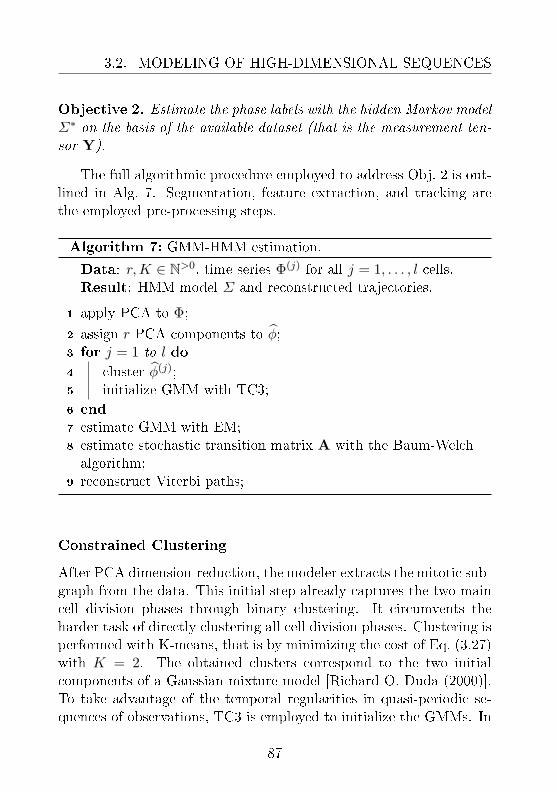
3.2. MODELING OF HIGH-DIMENSIONAL SEQUENCES
Objective 2. Estimate the phase labels with the hidden Markov modelΣ∗ on the basis of the available dataset (that is the measurement ten-sor Y).
The full algorithmic procedure employed to address Obj. 2 is out-lined in Alg. 7. Segmentation, feature extraction, and tracking arethe employed pre-processing steps.
Algorithm 7: GMM-HMM estimation.
Data: r,K ∈ N>0, time series Φ(j) for all j = 1, . . . , l cells.Result: HMM model Σ and reconstructed trajectories.
1 apply PCA to Φ;2 assign r PCA components to φ;3 for j = 1 to l do
4 cluster φ(j);5 initialize GMM with TC3;
6 end
7 estimate GMM with EM;8 estimate stochastic transition matrix A with the Baum-Welchalgorithm;
9 reconstruct Viterbi paths;
Constrained Clustering
After PCA dimension-reduction, the modeler extracts the mitotic sub-graph from the data. This initial step already captures the two maincell division phases through binary clustering. It circumvents theharder task of directly clustering all cell division phases. Clustering isperformed with K-means, that is by minimizing the cost of Eq. (3.27)with K = 2. The obtained clusters correspond to the two initialcomponents of a Gaussian mixture model [Richard O. Duda (2000)].To take advantage of the temporal regularities in quasi-periodic se-quences of observations, TC3 is employed to initialize the GMMs. In
87
CHAPTER 3. UNSUPERVISED LEARNING
contrast to the previous section, clustering is now applied to partitionsamples over time.
For K,n ∈ N>0, the set of indexes 1, . . . , n can be partitionedinto K distinct clusters. If index i and j, with j > i, are in the samecluster Vk 6= ∅, for k = 1, . . . ,K, then r must be in Vk as well.
Denition 12. Let ζ(n,K) be the number of possible clustering as-signments of the measured time series (t, y(ti))ni=1 into K clusters.The function obeys the recurrence relation
ζ(n,K) :=
ζ(n− 1,K − 1) + ζ(n− 1,K) 1 < K < n
1 K = 1 ∨K = n
0 K > n.
(3.50)
The complete enumeration of all possible assignments of n indexesinto K clusters is given by the Stirling numbers of the second kind[Fortier and Solomon (1966); Jensen (1969)], giving
S(n,K) :=1K!
K∑j=0
(−1)K−j(K
j
)jn. (3.51)
Conveniently, the temporal structure of the task signicantly con-strains the space of possible cluster solutions to be considered. Asa consequence, the growth of ζ(n,K) is modest compared to that ofgeneral combinatorial clustering [Jain and Dubes (1988); Hastie et al.(2001)]. Solving the recurrence relation of Eq. (3.50), one has that
ζ(n,K) ≡(n− 1K − 1
)<
(n
K
)≤ S(n,K). (3.52)
In many cases, the number of constrained combinations satises theinequality (
n
K
) S(n,K), (3.53)
88

3.2. MODELING OF HIGH-DIMENSIONAL SEQUENCES
with the exception of cases close to the boundary conditions (that areclose to K = 1 ∨K = n). For instance, when n = 19 and K = 4,
ζ(19, 4) = 816 1010 ≈ S(19, 4), (3.54)
which already constitutes a dierence of seven orders of magnitude.
In the analysis, TC3 is applied twice. Firstly, it is applied toall cell time series in mitotic and non-mitotic subgraphs after binaryclustering. The step already reduces the number of possible assign-ments. The search space is further reduced by the second application,which imposes a minimal size for clusters. By imposing the minimumcardinality mink |Vk| = q one has that the size becomes
ζ(n− (q − 1)K,K). (3.55)
In the case of the cell cycle, the search space is thus relatively lim-ited. Optimization can be performed exhaustively to set the bestinitial conditions for the GMM.
For all cells, that is for all j = 1, . . . , l, the intra-cluster scatter ofthe trajectories is minimized with respect to the cost
W(c|D) :=K∑k=1
∑j∈Vk
‖ φ(j) − µk ‖22, (3.56)
where the clustering assignment c ∈ C(D) associates label λk to clus-ter set Vk for all k = 1, . . . ,K. Recalling Eq. (3.27), W(c|D) is theK-means cost for the measured trajectories. Equation (3.56) mea-sures dissimilarities in terms of squared Euclidean distances from thecluster centroids µk (for the PCA-reduced trajectories).
When K = 6 the cluster labels can be associated with the conven-tional names of the cell cycle phases [Zhong et al. (2012)]. Sequentially
89
CHAPTER 3. UNSUPERVISED LEARNING
ordered, the names of the labels in Λ are
λ1 = inter(-phase),
λ2 = pro(-phase),
λ3 = prometa(-phase),
λ4 = meta(-phase),
λ5 = ana(-phase),
λ6 = telo(-phase).
(3.57)
Denition 13. The labeled dataset obtained from the population is
Dλ := (φ(j), c(j))lj=1, (3.58)
with c(j) ∈ Λ for all j = 1, . . . , l.
Discrete States: Mixtures and Transitions
Modeling proceeds by assigning a Gaussian component from a GMMto each phase of the cycle [Pham and Tran (2006); Wang et al. (2007)].Discrete states are identied with the latent variables of the GMM,hence yielding X = Λ.
Denition 14. The mixture model for the measured trajectories isgiven by
pGMM(φ) :=K∑k=1
πkNorm(φ|µk,Σk), (3.59)
where πk are the mixing coecients satisfying normalization
K∑k=1
πk = 1. (3.60)
To t the GMM, the initial value of the mixing coecients is givenby the probabilistic membership of the samples. Means are initial-ized to the class discriminative sample means fromDλ. The maximum
90

3.2. MODELING OF HIGH-DIMENSIONAL SEQUENCES
likelihood estimation of the GMM is performed with the ExpectationMaximization (EM) algorithm for xed K.
On the basis of the obtained GMM structure, two models areobtained: a discrete and a continuous hidden Markov model [Rabiner(1989)].
Denition 15. A stochastic transition matrix is the matrix
A := [ai,j ] ∈ [0, 1]K×K , (3.61)
with transition probabilities ai,j such that
K∑j=1
ai,j = 1, i ∈ Y (3.62)
for all i = 1, . . . ,K.
In general, HMMs are represented in terms of a single (often dis-crete, but possibly continuous) random state variable x(t) ∈ X .
Denition 16. The HMM ΣHMM is dened by
• the transition model p(x(ti)|x(ti−1)),
• the observation model p(y(ti)|x(ti)),
• and the initial state distribution p(x(t0)).
The stochastic transitions between the K hidden states of a dis-crete HMM are governed by the matrix A. Measured emissions arenoisy, satisfying the assumption of identically distributed and condi-tionally independent noise terms. In the continuous case, the obser-vation density for each state is given by the corresponding Gaussiancomponent Norm(φ|µk,Σk). Transition probabilities are constrainedto traverse hidden states in a specic forward order by imposing
ai,j = 0, (3.63)
91
CHAPTER 3. UNSUPERVISED LEARNING
for j < i or j > i+ 1 and with
ai,j 6= 0, (3.64)
with j = 1 and i = K. By applying the Baum-Welch algorithm [Baumet al. (1970)] in combination with the Viterbi algorithm [Viterbi (1967)],parameters and hidden states are estimated from the datasetDλ. Theestimated states of the learned HMM system Σ are denoted as x(ti)for i = 1, . . . , n. When a priori domain knowledge is not available,validation of model order can be performed with ASC [Chehreghaniet al. (2012)].
3.2.2 Verication and Application to Real Data
The method is evaluated in its application to diverse uorescent mark-ers and screening data for the classication of cell phenotypes [Zhonget al. (2012)]. Precisely, reference data consist of time-lapse mi-croscopy images of human tissue culture cells (HeLa "Kyoto" cells).The uorescent chromatin marker employed in the study is the hi-stone H2B-monomeric mCherry. Object detection, tracking of cellsover time, and feature extraction are carried out using the imageanalysis framework CellCognition [Held et al. (2010)]. Detailed im-age segments with user-labeled phases are shown in Fig. 3.9.
The applied aim of modeling is that of predicting cell morphologylabels from image data. In this experimental setting, the numberof distinct phases is known to the modeler. The labels correspondto interphase and to the phases of mitosis: prophase, prometaphase,metaphase, anaphase and telophase.
Figure 3.10 shows that user annotation exhibits signicant incon-sistency. The image visualizes the degree of dissimilarity of threetrained biologists with respect to a gold standard (GS). The standardis given by the consensus approximation to ground truth obtainedthrough a majority vote of multiple user label annotations. The dis-similarity matrix reveals relatively modest inconsistency for the sameuser on dierent days. By contrast, the inconsistency in the anno-
92

3.2. MODELING OF HIGH-DIMENSIONAL SEQUENCES
Figure 3.9: Fluorescence images from time-lapse microscopy of a liveHeLa cell with user-labeled morphology phases. The cell expressesHistone 2B fused to mCherry. The time lapse is of 4.6 min per framewith a scale bar of 10 µm (Figure from [Zhong et al. (2012)]).
tations performed by dierent users is statistically and scienticallysignicant.
The analysis is based on seven image sequences with 326 cell di-vision events. The images are sampled uniformly in time with time-lapse interval of 4.6 min. Segmentation is performed with CellCog-nition [Held et al. (2010)]. The total number of cells is l = 13, 040.The result of the extraction of the principal components is reportedin Fig. 3.11.
After the application of PCA, the labels obtained from the datawith various methods are compared. Figure 3.12 visualizes the labelswith the color-coding of Fig. 3.9. Each of the l = 51 rows in thematrices is a labeled cell trajectory in n = 40 consecutive time pointsfrom T ↓. The GMM alone exhibits a poor match with respect to userannotation. The direct application of the GMM results in low predic-tive capacity, predominantly due to sensitivity to local maxima andto initial conditions. In Fig. 3.12, comparison with other approachesdemonstrates the benets of incorporating additional knowledge foreective learning of cell morphologies. To improve classication ac-curacy, TC3 is used to initialize the GMM as described in the pre-
93
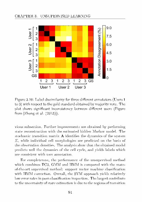
CHAPTER 3. UNSUPERVISED LEARNING
Figure 3.10: Label dissimilarity for three dierent annotators (Users 1to 3) with respect to the gold standard obtained by majority vote. Theplot shows signicant inconsistency between dierent users (Figurefrom [Zhong et al. (2012)]).
vious subsection. Further improvements are obtained by performingstate reconstruction with the estimated hidden Markov model. Thestochastic transition matrix A identies the dynamics of the systemΣ, while individual cell morphologies are predicted on the basis ofthe observation densities. The analysis show that the obtained modelpredicts well the dynamics of the cell cycle, and yields labels whichare consistent with user annotation.
For completeness, the performance of the unsupervised methodwhich combines TC3, GMM and HMM is compared with the state-of-the-art supervised method: support vector machine classicationwith HMM correction. Overall, the SVM approach yields relativelylow error rates in post-classication inspection. The largest contributeto the uncertainty of state estimation is due to the regions of transition
94

3.2. MODELING OF HIGH-DIMENSIONAL SEQUENCES
Figure 3.11: On the left, the plot visualizes the rst seven principalcomponents of 51 cell trajectories. On the right, the distribution ofthe samples is projected with respect to the two main principal com-ponents. Color-coding is consistent with that of Fig. 3.9. Dots andblack crosses indicate, respectively, individual cell objects and samplemeans per component according to human annotation. Temporal pro-gression is indicated by the cyclic arrows (Figure from [Zhong et al.(2012)]).
between phases. Ambiguity in transitional cell morphology makes theestimation of absolute error rates particularly challenging. Validationis performed as follows: an SVM is independently trained on celltrajectories from 7 image sequences, using the other 6 image sequencesas test datasets. Detailed results of precision, recall, and F -score arereported in Tab. 3.1. Figure 3.13 visualizes the total accuracy ofeach approach. In the analysis, true positives, true negatives, falsepositives, and false negatives are respectively denoted as TP, TN, FP,
95

CHAPTER 3. UNSUPERVISED LEARNING
FN. The measures are
Precision :=TP
TP + FP,
Recall :=TP
TP + FN,
F -score := 2Precision · RecallPrecision + Recall
.
(3.65)
The results show that supervised SVM learning with HMM errorcorrection yields slightly lower mean total accuracy than the unsu-pervised method, as shown in Fig. 3.13. Overall, unsupervised learn-ing achieves classication accuracy comparable to that of supervisedmethods and is more objective [Zhong et al. (2012)].
Application of the modeling approach to additional markers inlive imaging of HeLa cells expressing EGFP-tagged proliferating cellnuclear antigen (PCNA) yields labels that closely match user annota-tion with 86.7% total accuracy [Zhong et al. (2012)]. Total accuracyof 75.5% is achieved when modeling mitotic spindle dynamics of HeLacells expressing uorescently tagged α-tubulin. This analysis demon-strates that there exists a non-negligible degree of confusion betweenmidbody and interphase morphologies [Zhong et al. (2012)].
96

3.2. MODELING OF HIGH-DIMENSIONAL SEQUENCES
Figure 3.12: Organized plot of the labeled trajectories of all cells fromthe image containing the example in Fig. 3.9. Progressing clock-wisefrom the upper-left corner, the plots visualize the labels obtained fromGMM (alone), TC3 (alone), GMM initialized by TC3, HMM exten-sion of GMM with TC3, and SVM followed by HMM error correction(Figure from [Zhong et al. (2012)]).
97

CHAPTER 3. UNSUPERVISED LEARNING
Table3.1:
Meth
odcom
parison
:precision
,recall,
andF-score
Approach
Precision
Interp
hase
Prophase
Prometa
Meta
phase
Anaphase
Telo
phase
TC3
93.3
2±
0.7
373.9
0±
5.0
870.0
2±
2.9
987.6
6±
2.1
749.3
0±
4.4
269.9
0±
5.3
9TC3+GMM
94.8
6±
0.8
485.4
3±
2.8
177.6
9±
3.0
098.1
2±
0.5
674.5
7±
8.5
479.1
4±
5.3
3TC3+GMM+DHMM
95.9
7±
0.8
383.5
3±
2.0
791.4
7±
2.4
596.8
2±
0.9
280.5
7±
7.6
784.5
7±
5.2
8TC3+GMM+CHMM
96.6
8±
0.6
183.5
9±
2.6
485.6
5±
3.0
794.8
2±
0.9
877.6
0±
7.6
377.6
0±
4.3
6SVM+DHMM
95.4
6±
0.5
076.5
4±
1.6
980.4
2±
2.2
493.8
9±
0.8
679.4
9±
2.7
678.1
7±
4.2
9
Recall
Interp
hase
Prophase
Prometa
Meta
phase
Anaphase
Telo
phase
TC3
98.2
1±
0.3
868.9
6±
3.1
783.9
8±
4.2
362.1
6±
3.1
062.2
3±
3.2
457.2
0±
2.8
4TC3+GMM
99.1
8±
0.3
080.9
7±
3.8
883.2
4±
4.7
979.6
9±
4.4
670.3
6±
5.5
377.2
7±
4.8
4TC3+GMM+DHMM
99.5
1±
0.3
282.7
5±
4.1
384.4
3±
2.9
688.2
4±
3.6
380.2
2±
6.2
479.5
0±
5.0
9TC3+GMM+CHMM
97.8
9±
0.7
585.1
1±
3.2
785.9
0±
4.6
285.9
0±
3.2
572.6
7±
5.5
183.0
6±
4.7
7SVM+DHMM
97.2
0±
0.4
179.3
5±
2.9
985.0
8±
1.3
984.9
0±
2.5
181.1
9±
2.1
476.2
3±
3.4
7
F-score
Interp
hase
Prophase
Prometa
Meta
phase
Anaphase
Telo
phase
TC3
95.6
9±
0.4
170.7
4±
3.3
975.6
8±
2.1
972.3
7±
2.2
054.6
5±
3.8
762.3
7±
3.5
3TC3+GMM
96.9
6±
0.3
782.6
4±
2.4
179.7
0±
2.9
587.5
1±
2.7
372.1
2±
6.9
777.7
7±
4.7
1TC3+GMM+DHMM
97.6
9±
0.3
682.8
4±
2.6
287.6
4±
2.3
592.0
5±
2.0
080.0
3±
6.7
981.5
1±
4.7
0TC3+GMM+CHMM
97.2
5±
0.2
383.9
8±
2.0
485.1
0±
2.8
989.8
6±
1.5
474.8
9±
6.4
679.9
0±
4.1
0SVM+DHMM
96.3
2±
0.3
377.6
6±
1.6
482.4
8±
0.8
989.0
5±
1.5
079.9
9±
1.3
776.2
1±
2.3
1
Mean
sandstan
dard
errorsof
themean
sfor
eachphase
andmeth
od.Thenal
modelisselected
onthebasis
ofgrid
searchwith
5-foldcross-valid
ation.In
theevalu
ation,grou
ndtru
thisdened
bysin
gleuser
annotation
(Tablefrom
[Zhonget
al.(2012)]).
98
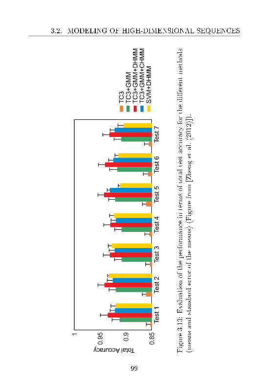
3.2. MODELING OF HIGH-DIMENSIONAL SEQUENCES
Figure
3.13:Evaluationoftheperform
ance
interm
softotaltestaccuracy
forthedierentmethods
(meansandstandarderrorof
themeans)
(Figure
from
[Zhonget
al.(2012)]).
99

CHAPTER 3. UNSUPERVISED LEARNING
100

Chapter 4
Supervised Learning
Prediction is very dicult,
especially about the future.
N. Bohr (attr.)
4.1 Clustered Filtering
Given a model M and data D, parameter estimation can be formu-lated as the task of evaluating parameters on the basis of the data1. Inthe Bayesian setting, the aim is to calculate the posterior distributionp(θ|D) over the parameter space Θ. When the model M correspondsto a parametric form for the transition function f of a dynamicalsystem, θ incorporates all free parameters of f . Recalling Def. 2 andEq. (3.46), the following section refers to the parameters of FODEs forODEs, as well as for the deterministic component of SDEs.
Objective 3. Calculate the parameter posterior p(θ|D) for the freeparameters θ ∈ Θ given the data D.
1Parts of this section appear in [Busetto and Buhmann (2009)].
101
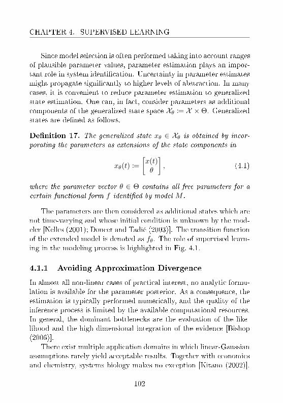
CHAPTER 4. SUPERVISED LEARNING
Since model selection is often performed taking into account rangesof plausible parameter values, parameter estimation plays an impor-tant role in system identication. Uncertainty in parameter estimatesmight propagate signicantly to higher levels of abstraction. In manycases, it is convenient to reduce parameter estimation to generalizedstate estimation. One can, in fact, consider parameters as additionalcomponents of the generalized state space Xθ := X ×Θ. Generalizedstates are dened as follows.
Denition 17. The generalized state xθ ∈ Xθ is obtained by incor-porating the parameters as extensions of the state components in
xθ(t) :=[x(t)θ
], (4.1)
where the parameter vector θ ∈ Θ contains all free parameters for acertain functional form f identied by model M .
The parameters are then considered as additional states which arenot time-varying and whose initial condition is unknown by the mod-eler [Nelles (2001); Doucet and Tadic (2003)]. The transition functionof the extended model is denoted as fθ. The role of supervised learn-ing in the modeling process is highlighted in Fig. 4.1.
4.1.1 Avoiding Approximation Divergence
In almost all non-linear cases of practical interest, no analytic formu-lation is available for the parameter posterior. As a consequence, theestimation is typically performed numerically, and the quality of theinference process is limited by the available computational resources.In general, the dominant bottlenecks are the evaluation of the like-lihood and the high-dimensional integration of the evidence [Bishop(2006)].
There exist multiple application domains in which linear-Gaussianassumptions rarely yield acceptable results. Together with economicsand chemistry, systems biology makes no exception [Kitano (2002)].
102

4.1. CLUSTERED FILTERING
Figure 4.1: This reduced representation of the modeling process speci-es the position of the supervised approaches discussed in this section.
In such domains, particle lters are generally applicable approacheswhich often enable eective state-space estimation [Gordon et al.(1993); Doucet and Tadic (2003)]. Alternatively, the modeler couldaim at approximate Bayesian computation methods, which approx-imate the likelihood function, for instance by performing rejectionsampling with a given tolerance [Sunnåker et al. (2012)]. Exact-likelihood sampling approaches are approximate inference techniqueswhich are more computationally intensive, but exhibit the potentialto reproduce rather complex multimodal belief states over Xθ [Banga(2008)]. Particle ltering is based on sequential resampling of theposterior and are asymptotically correct as the number of samplesgrows. However, straightforward ltering suers from well-known de-generacy problems since the resampling phase exhibits a systematicloss of information [King and Forsyth (2000)]. Precisely, the method
103

CHAPTER 4. SUPERVISED LEARNING
produces the approximate posterior
p(θ|D) ' p(θ|D) (4.2)
which exhibits a tendency to diverge from the correct posterior p(θ|D).The quality of the approximation can be quantied in terms of relativeentropy, that is a fundamental measure of information loss. RecallingEq. 2.30, the approximation should aim at minimizing the number ofadditional bits which is given by KL[p ‖ p]. Increased computationalpower is sucient but not necessary to address the issue of estimationdivergence. This section introduces a method to mitigate the problemof divergence by keeping track of multimodal posteriors [Busetto andBuhmann (2009)].
The learning scenario is the following. Time series data Φ ofsample size n are given to the modeler, who knows the functionalform of the physical system Σ∗. The parameters of the model areuncertain and subject to a given prior density p(θ). The parameterposterior follows from Bayes' rule as
p(θ|Φ) =p(Φ|θ)p(θ)p(Φ)
, (4.3)
and the same holds for the posterior of the extended space p(xθ|Φ).The goal is the approximation of the posterior given the data at timetn. At any time point, the posterior incorporates all the knowledgeavailable to the modeler. The posterior is the solution of the optimalltering problem [Arulampalam et al. (2002)]. Assuming IID noise,the likelihood can be factorized and, consequently, Bayes' rule can becalculated recursively for each sample point. This property permitsincremental storing of the data and enables online inference. Recur-sive Bayesian lters are based on the iteration of two stages: updateand propagation. During the former, new data are incorporated intothe belief state. During the latter, the belief state is propagated withits uncertainty following drift and diusion between measurements.
104
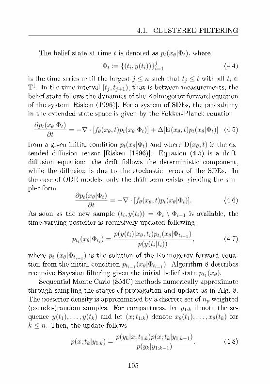
4.1. CLUSTERED FILTERING
The belief state at time t is denoted as pt(xθ|Φt), where
Φt := (ti, y(ti))ji=1 (4.4)
is the time series until the largest j ≤ n such that tj ≤ t with all ti ∈T↓. In the time interval [tj , tj+1), that is between measurements, thebelief state follows the dynamics of the Kolmogorov forward equationof the system [Risken (1996)]. For a system of SDEs, the probabilityin the extended state space is given by the Fokker-Planck equation
∂pt(xθ|Φt)∂t
= −∇ · [fθ(xθ, t)pt(xθ|Φt)] + ∆[Ð(xθ, t)pt(xθ|Φt)] (4.5)
from a given initial condition pt(xθ|Φt) and where Ð(xθ, t) is the ex-tended diusion tensor [Risken (1996)]. Equation (4.5) is a drift-diusion equation: the drift follows the deterministic component,while the diusion is due to the stochastic terms of the SDEs. Inthe case of ODE models, only the drift term exists, yielding the sim-pler form
∂pt(xθ|Φt)∂t
= −∇ · [fθ(xθ, t)pt(xθ|Φt)]. (4.6)
As soon as the new sample (ti, y(ti)) = Φi \ Φi−1 is available, thetime-varying posterior is recursively updated following
pti(xθ|Φti) =p(y(ti)|xθ, ti)pti(xθ|Φti−1)
p(y(ti|ti)), (4.7)
where pti(xθ|Φti−1) is the solution of the Kolmogorov forward equa-tion from the initial condition pti−1(xθ|Φti−1). Algorithm 8 describesrecursive Bayesian ltering given the initial belief state pt1(xθ).
Sequential Monte Carlo (SMC) methods numerically approximatethrough sampling the stages of propagation and update as in Alg. 8.The posterior density is approximated by a discrete set of np weighted(pseudo-)random samples. For compactness, let y1:k denote the se-quence y(t1), . . . , y(tk) and let (x; t1:k) denote xθ(t1), . . . , xθ(tk) fork ≤ n. Then, the update follows
p(x; tk|y1:k) =p(yk|x; t1:k)p(x; tk|y1:k−1)
p(yk|y1:k−1). (4.8)
105

CHAPTER 4. SUPERVISED LEARNING
Algorithm 8: Recursive Bayesian ltering.
Data: Φ and pt1(xθ), f and ÐResult: ptn(xθ|Φ).
1 for i = 1 to n do2 in [ti−1, ti): calculate the Kolmogorov forward equation
from pti−1(xθ|Φti−1) ;3 at ti: calculate the posterior pti(xθ|Φti);4 end
Denition 18. Let us denote as xi, wi(t) a random measure forthe posterior p(xθ,0:k|yj : tj < tk), for i = 1, . . . , np. The measureis approximated by
p(xθ,0:k|yj : tj < tk) :=np∑i=1
wikδ(xθ,0:k − xiθ,0:k). (4.9)
The weights are normalized to one
np∑j=1
wj = 1 (4.10)
and obtained according to importance sampling [Doucet (1998)]
wik ∝p(xθ,0:k|yj : tj < tk)q(xθ,0:k|yj : tj < tk)
. (4.11)
The proposal importance density can be factorized as
q(xθ,0:k|yj : tj < tk) =q(x; tk|xθ,0:k−1, yj : tj < tk)· q(xθ,0:k−1|yj : tj < tk−1).
(4.12)
The factorization leads to the recursive update of the time-varyingweights
wik ∝ wik−1
p(yk|xiθ,k)p(xiθ,k|xiθ,k−1)
q(xiθ,k|xiθ,k−1, yk). (4.13)
106

4.1. CLUSTERED FILTERING
At this point, the system of SDEs can be numerically integrated (forinstance with the Euler-Maruyama method) to sample from
q(xiθ,k|xiθ,k−1, yk) = p(x; tk|xiθ,k−1). (4.14)
Iteratively, this means that
wik ∝ wik−1p(yk|xiθ,k), (4.15)
where the likelihood in p(yk|xiθ,k) is dened by the measurement pro-cess (assumed to be known).
After several iterations, however, most of the weight mass mightalready concentrate on only few samples. In this divergent behav-ior, the overwhelming majority of the particles are updated despitetheir overall negligible contribution to the approximation [King andForsyth (2000)]. The problem leads to signicant waste of the avail-able computational resources. Two techniques are typically employedto counteract the divergence: importance resampling and careful de-sign of proposal densities. In standard resampling, the new set ofsamples xi∗θ,k
npi=1 is obtained from the approximated density. Resam-
pling is useful and, in many cases, even necessary, but suers from twolimitations: sample impoverishment and unimodal divergence. Theformer issue refers to the tendency towards a systematic reductionof the diversity of the sample set. Divergence is due to the inabilityto maintain multimodal densities: there is a systematic bias whichfavors unimodal densities. The presented approach addresses bothissues with resampling through clustering and appropriate proposaldensities [Busetto and Buhmann (2009)].
Resampling from the approximating discrete density involves aloss of information. Over time, iterated resampling behaves as a gen-erally inhomogeneous Markov chain [King and Forsyth (2000)]. Thechain exhibits a tendency to make the sample set collapse into a sin-gle mode, diverging from the possibly multimodal posterior. For il-lustration, consider the following simple example in the state spaceXA,B = A,B. Let 2m be the available number of samples, and
107
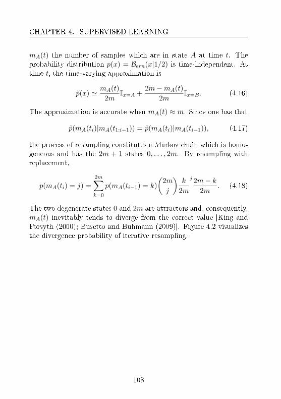
CHAPTER 4. SUPERVISED LEARNING
mA(t) the number of samples which are in state A at time t. Theprobability distribution p(x) = Bern(x|1/2) is time-independent. Attime t, the time-varying approximation is
p(x) ' mA(t)2m
Ix=A +2m−mA(t)
2mIx=B. (4.16)
The approximation is accurate when mA(t) ≈ m. Since one has that
p(mA(ti)|mA(t1:i−1)) = p(mA(ti)|mA(ti−1)), (4.17)
the process of resampling constitutes a Markov chain which is homo-geneous and has the 2m + 1 states 0, . . . , 2m. By resampling withreplacement,
p(mA(ti) = j) =2m∑k=0
p(mA(ti−1) = k)(
2mj
)k
2m
j 2m− k2m
. (4.18)
The two degenerate states 0 and 2m are attractors and, consequently,mA(t) inevitably tends to diverge from the correct value [King andForsyth (2000); Busetto and Buhmann (2009)]. Figure 4.2 visualizesthe divergence probability of iterative resampling.
108

4.1. CLUSTERED FILTERING
Figure 4.2: Starting from a balanced approximation with mA(1) =m = 10, iterative resampling rapidly increases the probability ofreaching one of the attractors at the boundaries. In the case study ofEq. (4.16), the two degenerate representations (mA = 0 andmA = 20)are probabilistically inevitable with consecutive resampling (Figurefrom [Busetto and Buhmann (2009)]).
Let ti be the time point at which the new measurement y(ti) isavailable to the modeler and let t−i ∈ T indicate the previous timestep. In the propagation phase, the posterior predicts the value at tion the basis of the data accumulated until t−i through Eq. (4.5) (or,more generally, through the forward equation of the system). At thispoint, the samples are grouped into K clusters. Their indexes arepartitioned into the sets Vk for k = 1, . . . ,K. Clustering is performedwith weighted K-means [Tseng (2007)]. At time t−i , every cluster has|Vk| = pk samples and
K∑k=1
pk = np. (4.19)
109

CHAPTER 4. SUPERVISED LEARNING
To maintain multiple modes, resampling is performed by keeping thecardinality of each cluster constant over time. The process is basedon the estimation, for every cluster, of two multivariate normal com-ponents. The component N−k is obtained at time t−i , while N
+k is
obtained at time ti. Independently, each component is employed asa proposal distribution for the importance resampling of the densityfrom time t−i . The centroids µk of the components dene a Voronoitessellation of partitions (X × Θ)kKk=1 of the parameter space Θ[Aurenhammer (1991); Busetto and Buhmann (2009)]. New samplesare taken within each cluster, keeping pk constant in each partition(X ×Θ)k. Each new sample xjθ is sampled from N−k and accepted ifIxjθ∈(X×Θ)k
= 1. When accepted, the weight is computed according
to the ratio
wj+ ∝N−k (xj−θ )
N−k (xj−θ ), (4.20)
where xj− denotes a sample of the extended state at time t−i . Theprocedure guarantees a constant number of samples in every partition.The weight mass tends to concentrate in regions with signicant con-tributions to the approximation. The procedure is outlined in Alg. 9.
How to measure the quality of the approximation? Eective Sam-ple Size (ESS) can be employed to measure the quality of a sampledapproximation [Doucet and Johansen (2011)].
Denition 19. The ESS is given by
Ne :=np
1 + V[w∗ji ], (4.21)
where
w∗ji =p(xjθi|y1:i)
q(xjθi−1, yi). (4.22)
Since the quantity cannot be evaluated exactly, one can evaluatethe following approximation
Ne :=1∑np
j=1(wji )2. (4.23)
110

4.1. CLUSTERED FILTERING
Algorithm 9: Filtering with preventive clustering.
Data: Σ, xθ(t0), Φ, Θ, K.Result: p(xθ).
1 for i = 1, . . . , n do2 draw np samples from pt(xθ) with importance sampling;3 propagate the samples according to the forward equation of
Σ;
4 weighted K-means of the samples xjθ, j = 1, . . . , n;5 for k = 1, . . . ,K do
6 estimate components N−k and N+k ;
7 resample xjθ within each cluster keeping pk xed;8 recalculate weights wj+ from importance sampling as in
Eq. (4.20);
9 end
10 end
Cases in which Ne ≈ Ne is small are pathological and indicate de-generacy in the approximation. It has also been proved that, as V[w∗ji ]does not increase with time, Ne cannot increase without resampling[Doucet (1998)]. Small values of Ne indicate that, among all updatedsamples, very few exhibit non-negligible contributions to the approx-imation. In other words, Ne is a practical estimate of the eectivenumber of contributing samples in the approximation. Bottlenecks inESS result in serious instability of the modes, since they aggravatethe tendency to drift towards the unimodal attractors [Busetto andBuhmann (2009)]. Standard techniques for resampling are able toregenerate the weights of the samples obtaining intervals exhibitinghigh ESS. However, they also create ESS bottlenecks. Resamplingwith preventive clustering mitigates the problem by drastically re-ducing frequency and intensity of the bottlenecks. Figure 4.3 illus-trates preventive resampling with an proof-of-concept. In the gure,the Bayesian update of the weights of the samples from prior (upper
111

CHAPTER 4. SUPERVISED LEARNING
plot) to posterior (lower plot) is shown on the left. After the update,only a fraction of the samples maintain a non-negligible weight. Incontrast, on the right, resampling is performed with preventive clus-tering. From the same prior (upper plot), resampling is performed be-fore the update (plot in the middle). The resampled posterior (lowerplot) exhibits a sample concentration in regions of higher density, thusretaining a large number of eective samples.
112

4.1. CLUSTERED FILTERING
Figure
4.3:
Ontheleft,standardupdatingfrom
prior
(top)to
posterior
(bottom)concentrates
theweightson
fewsamples.
Incontrast,on
theright,preventive
cluster
resamplingregenerates
the
samplesfrom
theprior
(top)byconcentratingthem
inregionswithhighposterior
density
(bottom).
Theinterm
ediateresamplingstep
(onthemiddleoftheplotson
theright)maintainsalargenumber
ofeective
samples(Figure
from
[BusettoandBuhmann(2009)]).
113

CHAPTER 4. SUPERVISED LEARNING
4.1.2 Evaluation and Biological Application
The application of techniques from Bayesian inference is expandingrapidly in several domains. This section focuses on the motivating ap-plication, which comes from computational systems biology [Wilkin-son (2007)]. The following considerations apply to general systemsof chemical equations. In the considered domain, MCMC approacheshave been remarkably successful in a variety of applications [Golightlyand Wilkinson (2008)], but remain rather computationally intensive.The established approaches known as SMC suer the limitations de-scribed before.
Let us consider a dynamical system modeling the behavior of a bio-chemical reaction network at thermodynamic equilibrium. Let nc de-note the number of distinguishable chemical species Ci in the system,for i = 1, . . . , nc. There are nr chemical reactions Ri, for i = 1, . . . , nr.Assuming thermal equilibrium and homogeneous spatial distribution,one can indicate reaction Rj as
Rj : Nin1jC1 + . . .+ Nin
ncjCnc −→ Nout1j C1 + . . .+ Nout
ncjCnc (4.24)
where each Ninij is the element at the i-th column and j-th row of the
input stoichiometric matrix Nin ∈ Nn×r. Similarly, each Noutij is an
element of the output stoichiometric matrix Nout ∈ Nn×r.
Denition 20. The stoichiometric matrix N ∈ Nn×r associated witha biochemical reaction network is given by
N := Nout −Nin. (4.25)
The stoichiometric matrix represents the net eects of all involvedreactions in the considered physical system. Let vj(C, θj) denote therate law associated with reaction Rj , for all j, which depends on thecurrent state C and on parameter θj .
The chemical master equation quanties the probability that, forall t ∈ T, the biochemical system is in state C. The state is discrete
114

4.1. CLUSTERED FILTERING
and describes the time-varying number of molecules for each of thenc species. The chemical master equation gives the transition proba-bilities for the dynamics of the biochemical system. Its solutions canbe computed explicitly only in rare cases of practical interest [Wilkin-son (2011)]. Dividing by the nite volume ∆σ, the chemical speciesconcentrations can be dened as
xci =Ci
∆σ. (4.26)
At time t+ ∆t, the master equation gives, up to o(∆t)
pc(t+ ∆t) 'nr∑j=1
p(C−Nj ; t)vj(C−Nj , θj)∆t
+ p(C; t)
1−nr∑j=1
vj(C, θj)∆t
,
(4.27)
where Nj denotes the j-th column of the stoichiometric matrix. Tak-ing the the innitesimal limit for ∆t→ 0, the chemical master equa-tion is given by
∂p(C; t)∂t
=nr∑j=1
(p(C−Nj ; t)vj(C−Nj , θj)−p(C; t)vj(C, θj)) (4.28)
which is a continuous-time discrete-state Markov process. A drift-diusion equation is obtained by truncating the Taylor expansion ofEq. (4.28) to the second order, giving the Langevin equation
∂p(xci; t)∂t
=−nc∑i=1
∂
∂xciµi(xc)p(xci; t)
+12
nc∑i=1
nc∑j=1
∂2
∂xci∂xcjDcij(xc)p(xci; t),
(4.29)
where the drift term is given by
µi(xc) = lim∆t→0
1∆t
E[xci(t+ ∆t)− xci(t)|xc(t) = xc], (4.30)
115

CHAPTER 4. SUPERVISED LEARNING
and the diusion tensor has elements
Dcij(xc) = lim∆t→0
1∆t
C[∆xci(t), ∆xcj(t)|xc(t) = xc], (4.31)
with dierences dened as ∆xci(t) = xci(t+∆t)−xci(t). Under weakconditions [Wilkinson (2011)], the dynamics follows the systems ofSDEs
dxc(t) = µ(xc(t), θ)dt+D1/2(xc(t), θ)dWt, (4.32)
with
µ(xc(t), θ) = Nv(xc, θ) (4.33)
and
D(xc(t), θ) = Ndiag[v(xc, θ)]NT . (4.34)
Estimating the parameters of the chemical master equation involveschallenging computations and, therefore, the Langevin equation is em-ployed as an eective approximation [Golightly andWilkinson (2008)].The quality of the approximation increases as the Markov process ex-hibits smaller jumps and slower variations in the solution of p(xc; t)with respect to the state xc.
Generalized state space estimation can be performed as describedat the beginning of this section, that is by extending the state space Xto incorporate the parameters in X ×Θ. To improve resampling, themodeler can subject the extended state space to an invertible trans-formation [Busetto and Buhmann (2009)]. The transformation makesall components of the state space time-varying, still maintaining xθthe result of a bijective function of x and θ for any time point. Thetransformation could, for instance, consider dynamic uxes as well asHill variables as additional states of the biochemical reaction network[Bullinger et al. (2008)]. The most common functional forms for thereaction rate laws are mass action for signal transduction, MichaelisMenten for metabolic pathways and Hill for gene regulation [Szallasiet al. (2006); Wilkinson (2011); Farina et al. (2006)]. All these forms
116

4.1. CLUSTERED FILTERING
and their products can be expressed as
vj(xc, θ) = vj,nom
nc∏i=1
cνj,ii
Kηj,ij,i + x
ηj,ici
, (4.35)
where the parameters vj,nom,Kj,i, νj,i and ηj,i are elements of the pa-rameter vector. This formulation is remarkably expressive and ableto model realistic combinations of activation, inhibition, and cooper-ative behavior. By expressing the new xθ = [xc, v,m] as a function ofuxes and Hill variables, one can write the transformed dynamics as
d
dtmj,i= fm(xθ(t), θ)
d
dtvj= fv(xθ(t), θ)
(4.36)
with
fm(xθ(t)) = ηj,ix(ηj,i−1)ci
dxcidt
fv(xθ(t)) = vj
nc∑i=1
(vνj,i
1xci
dxcidt− 1mj,i
dmj,i
dt
),
(4.37)
where mj,i = Kηi,ji,j +c
ηi,jj and vj denote, respectively, the components
of m and v [Bullinger et al. (2008)]. Given the initial condition, thesystem of SDEs can be written as
d
xcmv
=
Nvfm(xc,m, v)fv(xc,m, v)
dt+[I0
]D([xc,m, v], θ)1/2dWt. (4.38)
The parameters, which are unknown to the modeler, appear as ex-tended initial conditions.
The described approach is applied to a dynamical system whichmodels the circadian clock [Busetto and Buhmann (2009)]. The sys-tem is a modied version of the Goodwin model for the molecu-lar mechanisms of the circadian clock of Neurospora and Drosophila
117

CHAPTER 4. SUPERVISED LEARNING
[Goodwin (1965)]. The model has interesting features: Hill and massaction kinetics, as well as an inhibitory feedback loop. The system isdened as the system of SDEs with deterministic function
dxc1(t)dt
= 3− v1 − v2 − v4
dxc2(t)dt
= v1 − v3
dxc3(t)dt
= v2 − v3
dxc4(t)dt
= 6v3.
(4.39)
In the equation, the rate laws are
v1 = θ1xc1
v2 = θ2xc1
v3 = θ3xc2xc3
v4 = θ4x2c4
x2c4 + θ2
5
.
(4.40)
The stochastic terms are dened by the elements of the covariance ma-trix of W, which are Dij = δij10−3 for i, j 6= 1 with D11 = 10−2. Fig-ure 4.4 illustrates with a diagram the reaction network of the doubleGoodwin model. The initial conditions are xc(t0) = [3, 0.6, 0.4, 0.8]T
and the nominal values for the parameters are θ = [7, 1, 10, 3, 1]T .The measurement noise is additive, white, and normal with vari-
ance σ2N = 0.6 per component of the measurement space. Only xc1
and xc4 are directly measurable, whereas xc2 and xc3 are measured asa linear combination. For all ti ∈ T↓, the available measurements areobtained from
y(ti) =
1 0 0 00 1/2 0 00 0 1/2 00 0 0 1
·xc1(ti)xc2(ti)xc3(ti)xc4(ti)
+
ν1(ti)ν2(ti)ν3(ti)
, (4.41)
118

4.1. CLUSTERED FILTERING
Figure 4.4: Diagram illustrating the reaction network of the doubleGoodwin model (Figure from [Busetto and Buhmann (2009)]).
with νj(ti) IID according to N = N (νj |0, σ2N ) for j = 1, 2, 3 and
i = 1, . . . , n. An individual trajectory of the system, as well as anoisy realization of readout data are visualized in Fig. 4.6. Figure 4.5compares the Ne obtained with dierent resampling strategies as afunction of time. The introduced approach regenerates the ESS, thusmitigating the bottlenecks introduced by standard resampling.
On the left, Fig. 4.7 contains the plots of the marginalized pos-teriors for each parameter. The surface on the right represents themarginalized joint posterior for θ1 and θ2. In the calculation, np =2 · 103 samples. Figure 4.8 illustrates the eect of preventive clusterresampling in the parameter space. The approach avoids the situ-ation in which particles with dierent coordinates in the extendedspace collapse into the same position in the parameter space. Pre-ventive clustering maintains the equilibrium in multimodal cases, asshown in Fig. 4.9. As visible in Fig. 4.7, the posterior density re-mains bimodal in the parameter space. The plots of Fig. 4.9 show themarginalized distribution for θ1 − θ2 of the number of samples (withnp = 200) staying the largest mode. With time, standard resamplingdiverges in the overwhelming majority of the cases by accumulatingmore and more samples with each iteration. Clustering helps by keep-ing the number of particles constant in both regions of the parameter
119

CHAPTER 4. SUPERVISED LEARNING
space. The nal distributions are obtained by generating 500 IIDdatasets. Figure 4.10 shows the marginal posterior for θ1 − θ2 overtime, demonstrating the persistence of the two modes with clusterresampling.
In summary, the introduced approach yields two benecial prop-erties: it mitigates sample degeneracy by preemptive resampling, andcontrasts unimodal attractors through clustering. It is worth high-lighting the importance of selecting the appropriate number of clus-ters K, a task which can be addressed by ASC validation (as shownin the previous chapter).
120
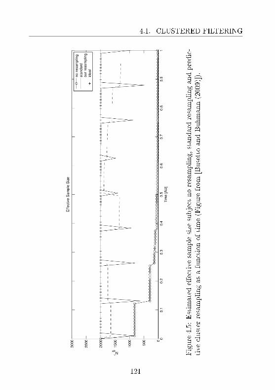
4.1. CLUSTERED FILTERING
Figure
4.5:
Estim
ated
eective
samplesize
subject
noresampling,standardresamplingandpredic-
tive
cluster
resamplingas
afunctionof
time(Figure
from
[BusettoandBuhmann(2009)]).
121
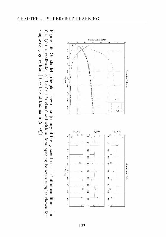
CHAPTER 4. SUPERVISED LEARNING
Figu
re4.6:
Ontheleft,
theplot
show
satra
jectoryof
thesystem
fromtheinitial
condition
.On
therigh
t,arealization
ofthedata
isvisu
alizedwith
uniform
spacin
gbetw
eensam
ples
chosen
forsim
plicity
(Figu
refrom
[Busetto
andBuhmann(2009)]).
122
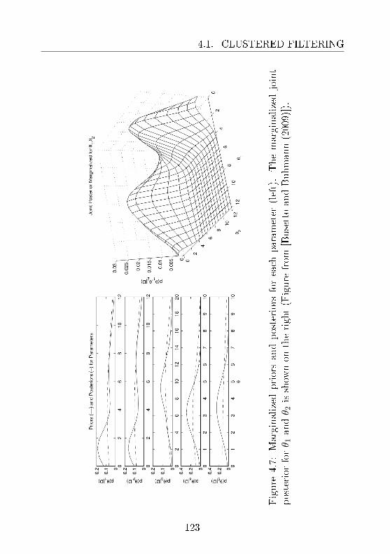
4.1. CLUSTERED FILTERING
Figure
4.7:
Marginalized
priorsandposteriorsforeach
param
eter
(left).Themarginalized
joint
posterior
forθ 1
andθ 2
isshow
non
theright(Figure
from
[BusettoandBuhmann(2009)]).
123
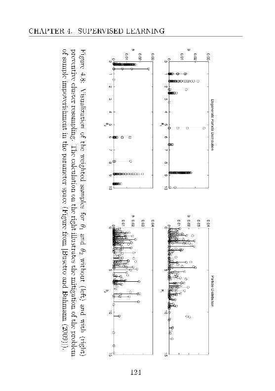
CHAPTER 4. SUPERVISED LEARNING
Figu
re4.8:
Visu
alizationof
theweigh
tedsam
ples
forθ
1andθ
2with
out(left)
andwith
(right)
preven
tiveclu
sterresam
plin
g.Thecalcu
lationon
therigh
tillu
stratesthemitigation
oftheprob
lemof
sampleim
poverish
mentin
theparam
eterspace
(Figu
refrom
[Busetto
andBuhmann(2009)]).
124

4.1. CLUSTERED FILTERING
Figure4.9:
Inthestudiedcase,theposterior
isbim
odalintheparam
eterspace.
Theplotshow
show
manyof
thenp
=20
0samplespersistin
thelargestmodeover
500experim
entswithindependently
sampleddatasets.Ontheleft,standardresamplingexhibitsthetendency
toaccumulate
allsamples
inonemode.
Incontrast,therightplotshow
sthat
theequilibrium
isstablewithcluster
resampling
(Figure
from
[BusettoandBuhmann(2009)]).
125
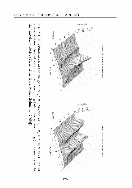
CHAPTER 4. SUPERVISED LEARNING
Figu
re4.10:
Visu
alizationof
themargin
alizedjoin
tposterior
forθ
1 −θ
2as
afunction
oftim
efor
agiven
dataset.
Incon
trastto
standard
resamplin
g(left),
cluster
resamplin
g(righ
t)main
tainsthe
thebim
odal
posterior
(Figu
refrom
[Busetto
andBuhmann(2009)]).
126

4.2. EVALUATION OF OPTIMIZED SOLUTIONS
4.2 Evaluation of Optimized Solutions
I believe that we do not know anything for
certain, but everything probably.
C. Huygens
Many estimation tasks are dened in terms of a cost functionR(c|D), which is minimized with respect to c ∈ C given the data.Minimization is performed over a search space of candidate solutions.The problem can also be equivalently formulated as an optimizationproblem in which the objective function Fobj(c) := −R(c|D) is max-imized. Practical examples of this setting are those of regularizedmaximum likelihood and maximum a posteriori estimation. In prac-tice, optimization is performed by the means of digital computation,eectively on a nite search space C (for instance, that of boundedoat-point numbers). Despite being nite, the space is typically solarge that it would be impractical to nd the globally optimal solu-tion c∗ by inspection. In principle, one could take advantage of theregularities of the objective function to make the problem tractable(for instance, by excluding regions which are a priori known to yieldsuboptimal scores). There as cases, such as in submodular optimiza-tion [Nemhauser et al. (1978)], in which certain algorithms produceoptimized solutions whose scores are guaranteed to be near-optimal.In practice, however, in most cases no regularities are known aboutthe objective. Because of that, the modeler has access to the bestsolution c obtained from heuristic algorithms. In this general set-ting, one thing can be said for sure: the optimized solution c ∈ C isthe best solution among the evaluated candidates. To the modeler,such heuristic solution is often the best available approximation of theglobally optimal solution c∗. Computational limitations, in fact, maylimit signicantly the number of possible evaluations of the objectivefunction. In many cases of practical interest, no guarantees are avail-able to the modeler for a general optimization task with objectiveFobj(c). However, even when nothing can be said regarding the value
127

CHAPTER 4. SUPERVISED LEARNING
of the optimized score, the relative position of the optimized solutioncan still be estimated with some additional empirical observations.
Denition 21. For a nite search space C, the relative position pos(c)of the solution c ∈ C is given by the ratio
pos(c) :=|C+c ||C|
, (4.42)
where
C+c := c ∈ C : Fobj(c) ≥ Fobj(c) (4.43)
is the set of solutions which are better or equal than c according to thetotal order induced by Fobj.
If a solution has pos(c) = α, then it can be said that it is in thetop α · 100% for Fobj(c).
Objective 4. For the objective function Fobj(c) over the search spaceC, what is the relative position pos(c) of a given optimized solution c?
4.2.1 Bound Derivation
The central idea is to employ a bound to estimate the relative posi-tion of the best available solution c, which is given by the heuristicalgorithm. The estimation can be performed through sampling, andthe uncertainty can be bounded by a Chebyshev-type inequality. Theresults obtained here are an application of ideas employed as an ar-gument in the proof of the symmetrization lemma from statisticallearning theory [Bousquet et al. (2004)].
In the optimization setting, the heuristic algorithm terminates andyields the solution c. At that point, let the available computationalresources allow the additional evaluation of np samples. Let then cj ,for j = 1, . . . , np, denote the IID samples drawn from the uniformdistribution Unif (C). The question is: what can be said about pos(c)on the basis of these additional np evaluations? Let us introduce
128

4.2. EVALUATION OF OPTIMIZED SOLUTIONS
the indicators Ijcj∈C+
c
for j = 1, . . . , np. The indicators are random
variables as well, IID drawn from the the Bernoulli distribution
Bern(Ijcj∈C+
c
= 1|pos(c)) = pos(c). (4.44)
One can, at this point, introduce the additional random variable
kp =np∑j=1
Ijcj∈C+
c
∼ Bin(kp|np, pos(c)), (4.45)
where Bin(kp|np, pos(c)) denotes the Binomial distribution
Bin(kp = k|np, pos(c)) =(n
k
)pos(c)k(1− pos(c))np−k. (4.46)
From the equations above, one has that the relative position pos(c))can be estimated as the ratio
pos(c) :=kpnp. (4.47)
Essentially, such ratio counts the proportion of uniformly sampled so-lutions which yield better scores than Fobj(c). If pos(c) is small (thatis when its position is close to that of the point of global optimum),the modeler can expect kp = 0 for small np with high probability.
Theorem 1. For any Fobj(c) over the search space C, the absoluteerror between pos(c) and the estimated pos(c) satises the bound
p(|pos(c)− pos(c)| ≥ ε) ≤ 14npε2
, (4.48)
for any ε > 0 and np ∈ N>0.
Proof. Chebyshev's inequality gives
p(|E[Z]− Z| ≥ ε) ≤ V[Z]ε2
, (4.49)
129

CHAPTER 4. SUPERVISED LEARNING
for the random variable Z. For Z = kp/np, one has that, since kp ∼Bin(kp|np, pos(c)),
E[kp] = nppos(c)V[kp] = nppos(c)(1− pos(c))
(4.50)
and, thus, that
E[kpnp
]= pos(c)
V[kpnp
]=
pos(c)(1− pos(c))np
≤ 14np
.
(4.51)
Finally, the bound is obtained with
p
(∣∣∣∣kpnp − pos(c)∣∣∣∣ ≥ ε) ≤ pos(c)(1− pos(c))
Nε2≤ 1
4npε2. (4.52)
When kp = 0, as in many cases of practical interest, the boundsimplies to
p(|pos(c)| ≥ ε) ≤ 14npε2
, (4.53)
and can be interpreted as follows: the probability that the optimizedsolution c is not in the ε · 100% is smaller than 1/(4npε2).
The bound is also useful considering the dependence of R(c|D)on the uctuations of the data, so that the relative position reectsthe variability due to the noise. In the context of statistical learningtheory, the upper bound is calculated with the intention of estimatingthe deviation of empirical measures [Bousquet et al. (2004)]. In thissetting, the bound is used to quantify the uncertainty regarding therelative position of a solution obtained through heuristic optimization.To employ such result for estimation, one has to note that, by itself,the bound does not address the problem of overtting.
130

4.3. MODELING HUMAN LEARNING DYNAMICS
4.3 Modeling Human Learning Dynamics
All models are wrong, but some are useful.
G. E. P. Box
This section introduces two models of human learning aimed attreating dyslexia and dyscalculia, respectively2.
Objective 5. On the basis of interaction data D, select models M ofhuman learning to design eective treatments for dyslexia and dyscal-culia.
For dyslexia, the model of engagement dynamics in spelling learn-ing is obtained from experimental data consisting of recorded user-computer interactions. The model relates patterns of typed inputs tothree aspects of human learning. It relates learning rates to engage-ment dynamics, predicting focused and receptive states, as well asforgetting. The nal model has been selected from a set of candidatedynamic Bayesian networks (DBNs) which are estimated from data[Murphy (2002)]. The available dataset contains more than 150, 000complete inputs recorded over several months through a training soft-ware for spelling.
The second model is introduced to enhance the numerical cogni-tion of children with developmental dyscalculia through a computer-based training program. The model aims at predicting aspects ofcognitive processes to control stimulation levels. The purpose is tooptimize the learning process with targeted selection of informativeexercises. The optimization process is based on a dynamic Bayesiannetwork model which represents domain knowledge and predicts thelevel of accumulated knowledge of the subject over time. Estimationis employed to perform action selection on the basis of the state ofknowledge of the subject.
2Parts of this section appear in [Baschera et al. (2011); Käser-Jacober et al.(2012)].
131

CHAPTER 4. SUPERVISED LEARNING
4.3.1 Modeling for Dyslexia Treatment
Sensor data [Cooper et al. (2010); Heray and Frasson (2009)] and in-put data [Baker et al. (2005); Johns and Woolf (2006); Arroyo andWoolf (2006)] are useful sources for modeling learning and aectivedynamics. These sources dier in quality and quantity: sensor dataare more direct and comprehensive, whereas input data are more gen-eral. The extraction of input logs, in fact, is not limited to labo-ratory experimentation. Predictive modeling and control are possi-ble through software tutoring systems, since large and well-organizedsample sets are available to the modeler. Inputs can be automati-cally recorded onto log les to capture informative features such astime lags and hints per problem, as well as interval lengths betweenconsecutive solution attempts [Arroyo and Woolf (2006)].
Experimental Setting
The following results are obtained with data coming from Dybuster,a multimodal spelling software designed for dyslexic children [Grossand Vögeli (2007)]. During training, the tutoring system selects andgenerates sequences of test words which are prompted orally. An-swers are typed in by the user, with acoustic signals notifying errorswhen incorrect letters are typed. Interactions are time-stamped andstored in comprehensive log les. Data are available from large-scalestudies spanning an interval of several months [Kast et al. (2007);Baschera et al. (2011)]. The participants are German-speaking sub-jects in the age group between 9 and 11 years, trained four times aweek for three months. The length of each session ranges from 15to 20 minutes, summing up to ≈ 950 minutes of interactive trainingper user. Complete training is available for 28 dyslexic and 26 con-trol subjects, for a total of 159, 699 records of entered words, inputs,errors, and respective timestamps.
132

4.3. MODELING HUMAN LEARNING DYNAMICS
Feature Selection and Modeling
Table 4.1 shows the main features extracted from the log data. Theselection includes input and error behavior, timing, and controller-induced setting variations. The features measure quantities whichare consistent with those of previous studies [Baker et al. (2005);Johns and Woolf (2006); Arroyo and Woolf (2006)]. The engagementstate of the subject is estimated on the basis of the available datawithout external direct assessment. Error repetitions are employedto evaluate learning rates as well as forgetting. The analysis is re-stricted to phoneme-grapheme matching errors. Such errors belongto a category representing missing knowledge in spelling [Bascheraand Gross (2010)]. In total, 14, 892 error observations are availablein D. The features are processed according to the assumption thatsustainable progress is separable in terms of time scales from localeects due to transitions between emotional and motivational states.Long-term variations are extracted from the time series φ throughuser-dependent regression under the assumption of additive white nor-mal noise. Initial feature processing include scaling, outlier detection,low-pass and variance ltering [Baschera et al. (2011)]. The relationbetween the processed features D and the error repetition γr is es-timated via LASSO logistic regression with 10-fold cross-validation[Bishop (2006)]. Table 4.3.1 reports the values of the estimated pa-rameters θ and the signicance for the selected features. The modelbased on the processed features exhibits a better BIC score of −6369compared to that obtained with unprocessed regression −6742. Theselected features highlight three main time-varying components whichinuence the state of knowledge of the user:
• focus: indicating whether the subject is focused or distracted;
• receptivity: indicating the level of receptiveness of the subject;
• forgetting: indicating whether the subject is forgetting.
Non-focused states exhibit larger rates of non-serious errors which aredue to lapses of concentration. However, these errors are less likely
133

CHAPTER 4. SUPERVISED LEARNING
to be committed again at later repetitions (that is, they exhibit lowererror repetition probability). In contrast, non-receptive states inhibitlearning, thus causing higher error repetition probabilities. Forgettingof learned spelling, which is due to time decay and interference be-tween error and repetition, increases the error repetition probabilityas well.
The components of the parameter vector θ of the logistic regres-sion indicate the relation between the individual features and theerror repetition probability. The parameter θEF = 0.06 demonstratesthat there exists a dependency between higher than expected errorfrequency and lower error repetition probability. In fact, non-focusedsubjects tend to commit more errors, but the errors are typically non-serious. By contrast, when the answer is complete but contains errors(that is, when FC = 0), the error repetition probability increases(θFC = −0.49). The fact indicates that the subjects which do notcorrect the errors before answering are less likely to learn the correctspelling.
In the estimation setting, the model class consists of dynamicBayesian networks. Such models are dynamical systems dened interms of a Bayesian network graph structure which does not changeover time3. The main dierence between HMMs and DBNs is that,whereas the former class represents the state x(t) ∈ X by a singlerandom variable, the latter allows the state space to be representedin factored form [Murphy (2002)]. DBNs do, in this sense, gener-alize HMMs. In DBNs, the hidden state is represented in terms ofa set of (discrete or continuous) nh random variables. In contrastto HMMs, which are dened by their transition model, the nh statecomponents and the no measured emissions are modeled as sets ofrandom variables subject to conditional distributions described by atwo-slice Bayes net.
Denition 22. In a DBN ΣDBN, transitions and observations are
3time-varying structures are also possible but are here seen as extensions ofthe conventional denition [Murphy (2002)]
134

4.3. MODELING HUMAN LEARNING DYNAMICS
described by the conditional distributions
p(Z(ti)|Z(ti−1)) =nh+no∏j=1
p(Zj(ti)|Pa(Zj(ti))), (4.54)
where Z(ti) denotes the node Z at time ti (hidden or observed) andPa(Z) are the parents of Z [Murphy (2002)].
Let xF and xR denote, respectively, the state components (nodesin a DBN) indicating focus and receptiveness. Three candidate mod-els are tested as on the basis of data D:
• (xF ⊥ xR) xF and xR are mutually independent;
• (xF xR) xF depends on xR;
• (xF xR) xR depends on xF.
The parameters of the dynamic Bayesian network are estimated withEM (Bayes Net Toolbox for MATLAB [Murphy (2001)]. On the basisof D, the respective BIC costs of the models are
BIC[xF ⊥ xR|D] =− 724, 111
BIC[xF xR|D] =− 718, 654
BIC[xF xR|D] =− 718, 577.
(4.55)
BIC selects the model ΣDBN in which the receptive component de-pends on the focus of the subject. Figure 4.11 plots the diagram ofthe selected model. The joint probability distribution for xF and xRis reported on a log-scale in Fig. 4.12 (on the left). It is worth notingthat, when the subject is fully focused, complete non-receptivenessis negligible. In contrast, it is not uncommon for the subjects to benon-focused despite being in an overall receptive state. This eectmight be due, for instance, to temporary distraction. The error rep-etition probability is plotted on the right of Fig. 4.12 conditioned onthe two components xR and xF. The top surface is obtained during
135

CHAPTER 4. SUPERVISED LEARNING
forgetting, and shows a greater oset in states of high focus. Theavailable evidence is consistent with the assumption that in statesof low focus the subjects tend to commit predominantly non-seriouserrors, since the correct spelling is already known. In contrast toforgetting, which has low impact on the error repetition probability,non-receptive states are associated with higher rates of error repeti-tion. The eect, though, is reduced for non-serious errors in stateswith reduced focus. Table 4.3.1 reports parameter values for the se-lected DBN [Baschera et al. (2011)]. A conclusive remark can bemade regarding the age-dependence of the engagement states. Non-receptive and non-focused states are more frequently found in subjectsbelow the median of approximately 10 years (with p-value < 0.001).For this group, the prevalence of non-receptive states is 24.2% andthat of non-focused states is 32.5%. In contrast, for subjects abovethe median the respective prevalence is 20.0% and 27.0% [Bascheraet al. (2011)].
Figure 4.11: Diagram representing the dynamic Bayesian networkselected by BIC. Dynamic components are indicated by rectangles.Shaded nodes are directly observed (Figure from [Baschera et al.(2011)]).
136

4.3. MODELING HUMAN LEARNING DYNAMICSFeature
Description
Tim
ing
InputRate
Keystrokesper
second.
InputRateVariance
Secondsper
keystroke
variance.
ThinkTim
eTim
ebetweendictation
ofawordto
rsttyped
letter.
Tim
eforError
Tim
ebetweenlast
correctinputto
error.
Tim
eto
NoticeError
Tim
efrom
errorto
rstcorrective
action.
OTim
eLongest
timeinterval
betweenconsecutive
letter
inputs.
Inputs
&Errors
HelpCalls
Number
ofhelpcallsfordictation
repetition.
Finished
Correctly
Indicator
that
allerrors
arecorrectedwhen
enterkeyispressed.
Sam
ePositionError
Indicator
formultipleerrors
forasingleletter.
RepetitionError
Inputstateof
thepreviousinputforthesametest
word(C
orrect/
Erroneous/NotObserved).
ErrorFrequency
Relativeentropybetweenobserved
andexpectederrordistributions
estimated
over
ve
inputswiththestudentmodelBascheraandGross
(2010).
Controller
Induced
Tim
eto
Repetition
Tim
efrom
erroneousinputto
respective
wordrepetition.
Lettersto
Repetition
Number
ofenteredlettersfrom
erroneousinputto
respective
word
repetition.
Table4.1:
Extractedfeatureswithabbreviationsin
bold(Tablefrom
[Bascheraet
al.(2011)]).
137

CHAPTER 4. SUPERVISED LEARNING
Feature
Processin
gθ
sig.
p1 [%
]/µ
Focu
sedState
focused
non-f.
EF
Exp
0.062e-4
0.16-0.34
IRLog
-DevC-Learn
C-Var
-0.124e-6
-0.410.87
IRV
Log
-DevC-Learn
C-0.22
2e-11-0.36
0.78REc
-0.288e-8
45%32%
TfE
Log
-DevC-Learn
C-Low
P-0.50
1e-9-0.13
0.28
Recep
tiveState
receptive
non-r.
FC
-0.491e-7
95%88%
HC
Split(zero/n
on-zero)
0.292e-4
4%28%
OT
Log
-DevC-Learn
C-Low
P0.27
1e-9-0.35
1.20REe
Low
P0.20
1e-90.07
-0.24TtN
EExp-DevC-Learn
C-0.18
1e-50.11
-0.36
Forgettin
gTtR
Exp
-0.292e-8
LtR
Log
0.341e-9
Table4.2:
Estim
atedparam
etersandsign
ican
cefor
features
selectedbyLASSOlogistic
regression.
Theinuence
oftheengagem
entstates
onthefeatu
resmodeled
inthedynam
icBayesian
netw
orkis
show
nin
thelast
twocolu
mns:
prob
ability
p1of
bein
gtruefor
binary
nodes
andestim
atedmean
µfor
Gaussian
nodes
(Tablefrom
[Basch
eraet
al.(2011)]).
138

4.3. MODELING HUMAN LEARNING DYNAMICS
Figure
4.12:Ontheleft,theplotshow
s,on
alogarithmicscale,thejointprobabilitydistribution
offocused(F)andreceptive
(R)states.Ontheright,thesurfaces
correspondto
theerrorrepetition
probabilitiesconditioned
ontheengagementstates
forforgetting(top)andnon-forgetting(bottom)
(Figure
from
[Bascheraet
al.(2011)]).
139

CHAPTER 4. SUPERVISED LEARNING
4.3.2 Optimization for Dyscalculia Treatment
Computer-assisted learning is helpful to overcome learning disabili-ties [Käser-Jacober et al. (2012)]. Conventional learning therapy canbe complemented by computer-based approaches which rely on for-mal modeling. Domain knowledge can, in fact, be directly incorpo-rated into the DBN to enhance numerical cognition. Developmentaldyscalculia is a learning disability with an estimated prevalence rang-ing from 3% to 6% [Shalev and von Aster (2008)]. The disabilitysystematically aects the acquisition of arithmetic skills [Shalev andvon Aster (2008)]. Due to its diusion, large amounts of genetic,neurobiological, and epidemiological data are available to the mod-eler [Käser-Jacober et al. (2012)]. With developmental dyscalculia,the subjects are not only impaired by the disability itself, but tendto develop additional anxiety and aversion to mathematics [Rubin-sten and Tannock (2010)]. Furthermore, the subjects face individualchallenges which are mostly subject-dependent. Hence, training in-dividualization has the potential of being particularly benecial fortreatment. The introduced model-based optimization system aims atimproving success as well as at making the subject more motivated.The introduced results demonstrate substantial improvements veriedby internal and external experimental evidence.
Learning Environment
Current models of neuropsychological development postulate the exis-tence of cognitive representational modules. These modules are task-specic and localized in circumscribed regions of the brain. Recentstudies identied specic functions related to adult cognitive numberprocessing and calculation [Dehaene (2011)]. A reference framework isgiven by Dehaene's triple-code model, which is based on three distinctrepresentational modules. The modules are associated to complemen-tary aspects of number processing: understanding based on verbal,symbolic, analogue magnitudes operations [Dehaene (1992)]. Further-more, compelling justications exist for two additional assumptions.
140
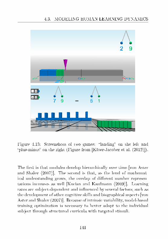
4.3. MODELING HUMAN LEARNING DYNAMICS
Figure 4.13: Screenshots of two games: landing on the left andplus-minus on the right (Figure from [Käser-Jacober et al. (2012)]).
The rst is that modules develop hierarchically over time [von Asterand Shalev (2007)]. The second is that, as the level of mathemat-ical understanding grows, the overlap of dierent number represen-tations increases as well [Kucian and Kaufmann (2009)]. Learningrates are subject-dependent and inuenced by several factors, such asthe development of other cognitive skills and biographical aspects [vonAster and Shalev (2007)]. Because of intrinsic variability, model-basedtraining optimization is necessary to better adapt to the individualsubject through structured curricula with targeted stimuli.
141
CHAPTER 4. SUPERVISED LEARNING
The training system is based upon a hierarchical structure con-sisting of multiple games. Each game focuses on a specic skill takenfrom one of the two main training areas. The rst area specializes onnumber representations and understanding. The second one primarilytrains cognitive operations and numerical procedures. The dicultyof each game is reected by the respective position in the hierarchicalstructure, which contains tasks of increasing complexity. To reinforcelinks between dierent number representations, numerical propertiesare associated to auditory and visual cues (color, form, and topology),while numerical values are associated to visual representations (blocksand positions in the place-value system) [Käser-Jacober et al. (2012)].For illustration, the screenshots of two games are shown in Fig. 4.13.The game on the left is designed to train number representation andunderstanding. The one on the right aims at training and automatingarithmetical operations.
Student Modeling and Action Selection
Training decisions are made online by the pedagogical module, whichis a software system that adaptively selects games and congurations.Selections are made on the basis of the current knowledge state, whichis estimated on the basis of the accumulated user inputs. The estima-tion of the time-varying learning state x(t) is performed with respectto the student model, a xed DBN which incorporates domain knowl-edge [Käser-Jacober et al. (2012); Dehaene (1992); von Aster andShalev (2007); Geary et al. (1992); Ostad (1997, 1999)]. The networkconsists of a directed acyclic graphical model which satises Def. 22.The structure of the student DBN model, containing 100 skills, is vi-sualized in Fig. 4.14. Each skill xs ∈ Xs is a node in the network. Adirected connection from skill xsA to xsB indicates that mastering theformer is a prerequisite for learning the latter. Following the condi-tional network structure, one has that the probability of having xsA
142

4.3. MODELING HUMAN LEARNING DYNAMICS
in a certain learning state is
p(xs) =∏
xsj∈Xs
p(xsj |Pa(xsj)). (4.56)
The state of each skill cannot be directly observed, and thus thesystem performs online inference on the basis of the answers to theposed task questions. Error patterns are identied from the measuredactions of the subject, and matched with those available on the buglibrary. The generation of remediation skills is triggered by the detec-tion of the respective errors. Denoting observations as yE, the net pos-teriors p(xsA|yEk) are updated taking into account the observationscoming the k-th task using the sum-product algorithm (through thelibDAI library for discrete approximate inference in graphical mod-els [Mooij (2010)]). The initial condition of all such probabilities isinitialized to the uniform distribution, subscribing to the principle ofindierence. The DBN has a memory of ve time points.
Training interventions are rule-based and non-sequential. Learn-ing paths are adapted to the estimated state of knowledge expressedby p(xs) at each time point. Three actions are available to the con-troller:
• Go Back: train a precursor skill;
• Stay: train the current skill (by generating a new task for thesame skill);
• Go Forward: train a successor skill.
Decisions are based on the state of the skill net posteriors p(xs|yE) asdescribed below. The posterior is compared to the values of an upperthreshold pu and a lower one pl. The action Stay is selected when theprobability for skill xs is in the interval [pl, pu]. Above and below theinterval, the training system selects Go Back and Go Forward,
143
CHAPTER 4. SUPERVISED LEARNING
respectively. The thresholds are time-varying and follow
pl = pl(init) · lnccpu = pu(init) · uncc ,
(4.57)
where nc denotes the number of accumulated samples for the testedskill, and parameters (lc, uc) and initial conditions (pl(init), pu(init))are determined heuristically [Käser-Jacober et al. (2012)]. The aimof these decision rules is to balance two learning aspects. On the onehand, the system has to guarantee a sucient number of tests per skill.On the other hand, it avoids frustration in case of repeated failure.The decision trees for the action selection are shown in Fig. 4.15.
Experimental Results
The quality of the control system based on the student model is as-sessed on the basis of external testing. Input data are collected fromtwo large-scale studies from Germany and Switzerland [Käser-Jacoberet al. (2012)]. Both studies are conducted with cross-over design.The set of participating subjects U is partitioned into two groups:one starting the training immediately, the other waiting. Groups aremapped according to intelligence score, gender and age (second to fthgrade of elementary school). The participants are German-speakersand attend normal public schools in the respective countries. Overall,the subjects exhibit diculties in learning mathematical concepts, asindicated by the following below-average performances in arithmetictests [Haner et al. (2005)]:
T-score SD
Addition 35.4 7.1Subtraction 35.4 7.9
Available data consists of 33 complete logles for participants trainedwith ve 20-minutes sessions a week for 6 weeks. On average, 29.84sessions are completed per user (SD 2.87, minimum 24, maximum
144

4.3. MODELING HUMAN LEARNING DYNAMICS
36.96), solving a total of 1562 tasks (SD 281.53, minimum 1011, max-imum 2179). The number of solved tasks per session is 52.37 (SD 7.9,minimum 37.8, maximum 68.1).
Denition 23. A skill xsA is a key skill for the subject u ∈ U if ugoes back to a precursor skill xsB of xsA at least once before passingxsA. The set of key skills for u is denoted as Ku.
Key skills are the hardest skills to pass. The set of key skillsKu reects the particular diculties encountered by an individualsubject. The tutoring system adjusts rapidly to the estimated stateof knowledge of the subject. In fact, starting the training from theeasiest skill, subjects encounter the rst key skill after solving 144.3tasks on average (SD 113.2, minimum 10, maximum 459), that is afteran average of 1.95 sessions (SD 1.63, minimum 0.08, maximum 6.48).
For each subject u ∈ U, improvement is quantied as the learningrate over Ku on the basis of all the available samples. The improve-ment is estimated with a non-linear mixed eect model employing onegroup per user and key skill [Pinheiro and Bates (1995)]. Denotingsample correctness as yi ∼ Bern(θi), zero-mean normal noise termsas εi, and normalized sample indexes xi between [0, 1], learning isestimated as
θi =1
1 + e−(b0+b1xi+εi). (4.58)
Table 4.3 reports the estimation results, while Fig. 4.16 illustrates theimprovement over time.
The analysis of the 533 Go Back cases shows that the option isbenecial in two ways: it reduces the error rate, and it increases thelearning rate. Evaluation is performed for all cases in which a subjecttrains with a certain skill (samples xb), goes back to one or severaleasier skills, and nally passes them to come back to the current skill(samples xa). For each k-th case, the correct rates over time ca,kand cb,k are estimated separately for xa and xb. Logistic regression isperformed with bootstrap aggregation (with resampling parameter B
145

CHAPTER 4. SUPERVISED LEARNING
b0
b1
value(SD)
0.09(0.06)
1.0(0.06)
sig.0.16
<1e-4
95%CI
[-0.073,0.21]
[0.89,1.11]
Table
4.3:Estim
atedcoe
cients
ofthenon-lin
earmixed
eects
model
with
standard
deviation
s,sign
ican
ce(sig.),
andcon
dence
intervals
(Tablefrom
[Käser-J
acober
etal.
(2012)]).
146

4.3. MODELING HUMAN LEARNING DYNAMICS
µ sig. 99% CI of µ SD σ 99% CI of of σ
d 0.1494 <1e-6 [0.1204, 0.1784] 0.2593 [0.2403, 0.2814]r 0.3758 <1e-6 [0.3236, 0.4280] 0.4662 [0.4319, 0.5059]
Table 4.4: Improvement statistics related to Go Back actions. Themean is denoted as µ (Table from [Käser-Jacober et al. (2012)]).
= 200) [Breiman (1996)]. For the k-th case, the direct improvementis
dk := cb,k − ca,k, (4.59)
that is the dierence between the correct rates for xa = 0 and xb = 1.The average direct improvement is denoted as d. Similarly, rk indi-cates the learning rate improvement as the dierence in learning rateover ca,k and cb,k. The average learning rate improvement is denotedas r. Figure 4.17 visualizes the histograms for d and r and their nor-mal approximation. Both averages are positive and a two-sided t-testindicates that their dierence from zero is statistically signicant, asshown in Tab. 4.4.
Two external tests are employed to evaluate training eects:
• HRT is a paper-pencil test in which the subjects solve as manyaddition (subtraction) tasks as possible within a time frame of2 minutes. Tasks are ordered according to increasing diculty[Haner et al. (2005)];
• AC is an arithmetic test in which the subjects solve addition(subtraction) tasks of increasing diculty in a time frame of10 minutes. The test exists both in paper-pencil as well as incomputer-based versions.
The analysis compares the eects during training and waiting peri-ods, respectively denoted as Tc and Wc. Results are available for 33
147

CHAPTER 4. SUPERVISED LEARNING
training subjects (26 females, 7 males) and 32 waiting subjects (23females, 9 males). Whereas pre-tests indicate no signicant dierencebetween the groups, Tab. 4.5 shows that training induces a signicantimprovement in subtraction (for both HRT and AC) and no improve-ment is found after waiting.
There exists additional evidence of learning with respect to a spe-cic indicator: the relative amount of training time spent by the sub-jects for subtraction tasks. Subtraction is considered the main indi-cator for numerical understanding [Dehaene (2011)]. During training,62% (73% for key skills) of arithmetical tasks consist of subtractions.Consistent results are obtained for the improvement in the context ofnumber line representation.
Accuracy analysis is performed using the non-linear mixed modelbased on a Poisson distribution of the deviance yi ∼ Pois(λi) in whichthe parameter θi is given by
λi = eb0+b1xi+εi (4.60)
with zero-mean additive normal noise terms εi. In the estimation,tting is performed using a single group per user. Numerical results,reported in Tab. 4.6 and plotted in Fig. 4.18, indicate that the subjectsachieved greater accuracy in positioning numbers on a line [Käser-Jacober et al. (2012)].
148
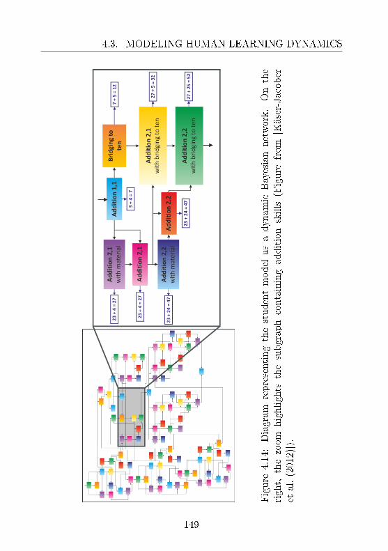
4.3. MODELING HUMAN LEARNING DYNAMICS
Figure
4.14:Diagram
representingthestudentmodel
asadynam
icBayesiannetwork.Onthe
right,
thezoom
highlights
thesubgraphcontainingadditionskills
(Figure
from
[Käser-Jacober
etal.(2012)]).
149

CHAPTER 4. SUPERVISED LEARNING
Figure 4.15: Simplied decision diagram for Go Back and Go For-
ward options (Figure from [Käser-Jacober et al. (2012)]).
Figure 4.16: For the key skills, the percentage of correctly solved tasksexhibits an increase of 22.6% over the training interval (Figure from[Käser-Jacober et al. (2012)]).
150
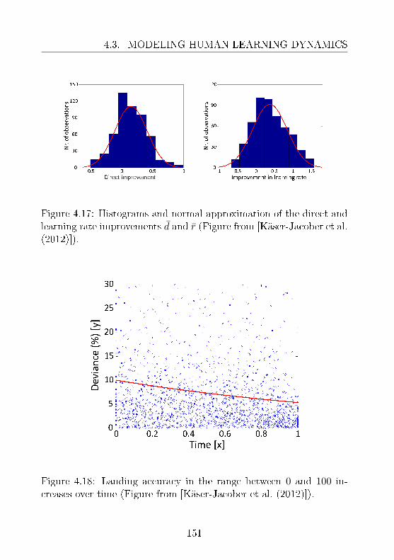
4.3. MODELING HUMAN LEARNING DYNAMICS
Figure 4.17: Histograms and normal approximation of the direct andlearning rate improvements d and r (Figure from [Käser-Jacober et al.(2012)]).
Figure 4.18: Landing accuracy in the range between 0 and 100 in-creases over time (Figure from [Käser-Jacober et al. (2012)]).
151

CHAPTER 4. SUPERVISED LEARNING
Cond.Pre-Score(SD)
Post-S
core(SD)
sig.
Compariso
n
HRT
Tc
12.9(5.38)
16.7(5.3)
1.5e-82.6e-5
(2.9e-5)W
c14.84
(6.47)15.06
(5.87)0.72
AC
Tc
50.53(27.25)
60.63(26.3)
4.5e-41.9e-3
(2.0e-3)W
c55.18
(25.24)52.9
(27.74)0.42
Table
4.5:Com
parison
oftest
improvem
entdurin
gtrain
ingandwaitin
g.T-test
results
onthe
improvem
ents
assumingsam
eanddieren
tvarian
cesare
reported
inthelast
column.
152

4.3. MODELING HUMAN LEARNING DYNAMICS
b0 b1
Estimate(SD) 2.3 (0.07) -0.63 (0.02)sig. <1e-4 <1e-495% CI [2.17, 2.44] [-0.67, -0.58]
Table 4.6: Estimated coecients of the non-linear mixed eectsmodel.
153

CHAPTER 4. SUPERVISED LEARNING
154

Chapter 5
Active Learning
Doubt is the origin of wisdom.
R. Descartes (transl.)
5.1 Design of Near-optimal Experiments for
the Selection of Dynamical Systems
The previous sections focused on modeling given the data. This chap-ter reports results in the setting of active learning1.
These contributions nd their position in the context of optimalexperimental design, that is the eld in which the variables of an ex-periment are tuned to yield maximally informative results. Designoptimization is motivated by the fact that, for many applications,the quality of the obtainable predictions is severely limited by datascarcity. In the hypothetico-deductive method of scientic inquiry,optimal experimental design nds its place in the iterative loop link-ing experimentation to modeling and viceversa. Figure 5.1 illustrates
1Parts of this section appear in [Hauser (2009); Krummenacher (2010); Busettoet al. (2009, 2013)].
155

CHAPTER 5. ACTIVE LEARNING
experimental design at the interface between the process of inferenceand the execution of new experiments. Informally, the task of ex-perimental design can be formulated as the selection of preparations,interventions, and observations which, on the basis of the availableknowledge, yields the maximal amount of information. The generalobjective is the following.
Objective 6. Given a set of candidate experiments E, a class ofdynamical systems functions F = fimi=1 and prior information p(f),select the most informative experiment ε∗ ∈ E to maximize predictivecapacity.
This section concerns the design of experiments aimed at selectingdynamical systems from empirical data in a Bayesian setting. Pre-cisely, the aim is to jointly select a set of informative time points andmeasurable quantities.
Figure 5.1: Schematic diagram illustrating the place of experimentaldesign in the iterative loop between modeling and experimentation.
At present, there remain a number of open questions regarding ex-perimental design aimed at selecting dynamical systems [Kreutz and
156
5.1. DESIGN OF NEAR-OPTIMAL EXPERIMENTS FOR THESELECTION OF DYNAMICAL SYSTEMS
Timmer (2009); Faller et al. (2003); Myung and Pitt (2009)]. By con-trast, extensive and conclusive results already exist for design aimedat parameter estimation [Bandara et al. (2009); Faller et al. (2003)].The design of experiments for dynamical system selection remainsa challenging eld especially when the hypothesis class F containsstrongly nonlinear systems. In systems biology and other applica-tion domains, in fact, F often contains nonlinear systems which arenot well approximated through local linearization [Nelles (2001); Ki-tano (2002); Balsa-Canto et al. (2008)]. For such settings, the set ofBayesian techniques which are available to the designer has grown sig-nicantly in recent years, particularly in the domains of neuroimagingand biochemical modeling [Busetto et al. (2009); Kramer and Radde(2010); Daunizeau et al. (2011); Steinke et al. (2007)]. Methods rootedin classical statistics are employed as well, and among them ensemblenoncentrality constitutes a reference approach [Skanda and Lebiedz(2010); Atkinson and Fedorov (1975); Ponce de Leon and Atkinson(1991)].This section introduces a method which is based on previous re-sults from the elds of active learning and optimization [Krause andGuestrin (2005, 2007); Krause et al. (2008); Nemhauser et al. (1978);Feige (1998)]. Building on such results, one can prove that, under con-ditions which are satised for systems of ODEs, the expected infor-mation gain is a submodular function [Krause and Guestrin (2005)].As a consequence of that, it is possible to prove that a greedy methodyields near-optimal solutions eciently (that is, with a polynomialnumber of evaluations) [Krause and Guestrin (2005); Nemhauser et al.(1978)]. Furthermore, the introduced method dominates all other ef-cient techniques, unless P=NP. The result is proved by reducingthe dynamical system scenario to a known setting which provides thebest constant approximation factor to the value of the optimal solu-tion [Krause and Guestrin (2005); Feige (1998)]. The design methodexhibits general applicability and is motivated by biological ques-tions. It addresses a challenging task in systems biology: the identi-cation of the Target-of-Rapamycin (TOR) pathway, an open prob-
157

CHAPTER 5. ACTIVE LEARNING
lem of high relevance for understanding metabolic operation [Kuepferet al. (2007)]. Numerical evaluation demonstrates that the introducedmethod yields solutions with almost optimal informativeness whenapplied to glucose tolerance modeling. The design method has beenrecently applied to ongoing work in phosphoproteomics with the goalof modeling the key control mechanisms of nuclear phosphorylation.
5.1.1 Theoretical Results
Consider the model class of dynamical systems expressed in termsof systems of ODEs as in Def. 2, with known initial conditions andparameters. In the learning scenario, the task is that of estimatingthe transition function f∗ of Σ∗. The prior p(f) incorporates allavailable information for all candidate dynamical systems fi ∈ F . Inthe concrete application to biochemical modeling, for instance, f isthe vector-valued function of a set of ODEs describing the dynamicsof a chemical reaction network with xed rates parameters and knownkinetic constants. Let the pair of indexes (i, j) indicate to the noisymeasurement
yj(ti) = xj(ti) + νij , (5.1)
that is the observation at time point ti ∈ T ↓ of the j-th component ofthe state vector x(ti) ∈ X . The noise terms νij are independent anddistributed according to the respective arbitrary distributions Nij .
For simplicity, let us dene the space of (i, j) index pairs as
Yij := 1, . . . , n × 1, . . . , nx. (5.2)
In this setting, each candidate experiment ε ∈ E consists of a set ofindex pairs (i, j) ∈ Yij . Each experiment ε is, hence, an element of thepowerset E = P(Yij). The random variable Dε denotes the datasetobtained from measuring yj(ti) for all index pairs in ε. Formally, thedataset obtained through ε is
Dε = (ti, xj(ti)) ∈ T ↓ ×X : (i, j) ∈ ε. (5.3)
158
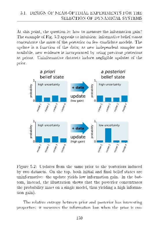
5.1. DESIGN OF NEAR-OPTIMAL EXPERIMENTS FOR THESELECTION OF DYNAMICAL SYSTEMS
At this point, the question is: how to measure the information gain?The example of Fig. 5.2 appeals to intuition: informative belief statesconcentrate the mass of the posterior on few candidate models. Theupdate is a function of the data; as new independent samples areavailable, new evidence is incorporated by using previous posteriorsas priors. Uninformative datasets induce negligible updates of theprior.
Figure 5.2: Updates from the same prior to the posteriors inducedby two datasets. On the top, both initial and nal belief states areuninformative: the update yields low information gain. In the bot-tom, instead, the illustration shows that the posterior concentratesthe probability mass on a single model, thus yielding a high informa-tion gain).
The relative entropy between prior and posterior has interestingproperties: it measures the information loss when the prior is em-
159
CHAPTER 5. ACTIVE LEARNING
ployed as an approximation to the posterior [Baldi and Itti (2010)].Such quantity is called information gain and is dened as follows
IG(Dε|p(f)) := KL[p(f |Dε) ‖ p(f)], (5.4)
where p(f |Dε) is, in the case of dynamical systems, found by solvinga system of dierential equations. In the context of communication,the information gain corresponds to the loss of information incurredwhen the dataset is ignored. Extraordinary evidence yields large in-formation gain, strongly revising the belief state of the observer (asillustrated by Fig. 5.2). For any experiment ε, IG(Dε|p(f)) dependson the experimental data. The data instances, however, are a pri-ori unknown to the modeler. Nonetheless, predictions can be madeon the basis of available information. By taking advantage of all par-tial information, the task of designing experiments becomes a decisionproblem under uncertainty. The objective is to maximize the expectedinformation gain, where the expectation is taken over all possible ex-perimental outcomes induced by ε. Weighting the informativeness ofindividual outcomes by their respective probabilities, one has
I(ε) := I(f,Dε) = EDε [IG(Dε|p(f))] , (5.5)
which is the mutual information between Dε and f . Such quantitymeasures the degree of statistical dependence between data and hy-potheses [Busetto et al. (2009); Daunizeau et al. (2011); Chalonerand Verdinelli (1995)]. The optimization task becomes the follow-ing decision-theoretic problem: maximize the score of Eq. (5.5) withrespect to ε, and subject to the constraint
|ε| ≤ κ ≤ n · nx, (5.6)
for a given κ. The cardinality constraint reects the fact that theepistemic agent can select only a reduced set of measurements. It isimportant to note that the following complexity results refer to thenumber of evaluations of the objective I(ε).
The solution of the optimization task can be approximated e-ciently with formal worst-case performance guarantees [Nemhauser
160

5.1. DESIGN OF NEAR-OPTIMAL EXPERIMENTS FOR THESELECTION OF DYNAMICAL SYSTEMS
et al. (1978); Feige (1998); Krause and Guestrin (2005)]. Startingfrom the individual sample yielding the largest mutual information,the designer proceeds by greedily selecting the pair of indexes (i, j)maximizing the contribution to the objective in combination with thecurrent selection. Algorithm 10 formally describes the design process.
Algorithm 10: Greedy experimental design for the selection ofdynamical systems (joint selection of time points and measurablequantities).
Data: set of hypotheses H with respective initial conditionsand assigned parameters, prior p(f), maximum numberof measurements κ ≤ n · nx, noise distributions Nij .
Result: selection ε.
1 initialization: ε0 := ∅;2 forall the f ∈ H do
3 forall the (i, j) ∈ Yij do4 calculate (t(f)
i , x(f)j (ti));
5 end
6 end
7 for k = 1 to κ do8 εk := εk−1 ∪ arg max(i,j)∈Yij\εk−1
I(εk−1 ∪ (i, j));9 end
10 ε := εκ;
161

CHAPTER 5. ACTIVE LEARNING
By reduction to the active learning setting of graphical models[Krause and Guestrin (2005)], the following properties of the methodcan be proved.
Theorem 2. The method described by Algorithm 10 nds a near-optimal joint subset ε of time points and measurable quantities for theselection of dynamical systems with a polynomial number of evalua-tions of I(·). Such approximate design satises the formal guarantee
I(ε) ≥(
1− 1e
)I(ε∗), (5.7)
where ε∗ := arg maxε∈E : |ε|≤κ I(ε). Moreover, the provided constantapproximation factor is the best one for polynomial-time algorithms,unless P=NP.
Proof. Let F = fkmk=1 denote the hypothesis class of transitionfunctions for dynamical systems dened on the state space X . Thetrajectory of each dynamical system is determined, given x0 ∈ X andθ ∈ Θ, by the respective integral solution of the system of ODEsdened by f ∈ F . Let Φk indicate the noisy evaluation of the integralsolution under the measurement model of Eq. (5.1), that is
Φk = (ti, y(ti))ni=1. (5.8)
Let a graphical model be constructed by having the set of nodes
V = f ∪ yj(ti)(i,j)∈Yij , (5.9)
where the yj(ti) are those of Φk. The sets f and yj(ti)(i,j)∈Yij aredisjoint and, furthermore, one has that
I(yj(ti), yj′(ti′)|f, x0, θ) = 0 (5.10)
for all (i, j) 6= (i′, j′) ∈ Yij , because the measurements follow Eq. (5.1)given the deterministic solution of the IVP in Eq. (2.7) for xed θ.The optimization of the mutual information with respect to ε then
162

5.1. DESIGN OF NEAR-OPTIMAL EXPERIMENTS FOR THESELECTION OF DYNAMICAL SYSTEMS
becomes a special case of the known submodular setting for graphicalmodels [Krause and Guestrin (2005)]. This is because the variablesyj(ti)(i,j)∈Yij are independent given f . One has that I(ε) is a sub-modular set function, that is
I(ε1) + I(ε2) ≥ I(ε1 ∪ ε2) + I(ε1 ∩ ε2), (5.11)
and non-decreasing on (i, j) ∈ Yij , and I(∅) = 0. In this setting,the greedy method of inclusion of Alg. 10 with unit cost per obser-vation selects κ elements yielding the constant approximation factorof (1 − 1/e) [Krause and Guestrin (2005); Nemhauser et al. (1978)].Such factor is also the best for polynomial algorithms, unless P=NP[Krause and Guestrin (2005); Feige (1998)].
5.1.2 Empirical and Applied Results
This subsection reports empirical evaluations and application to sys-tems biology. First, the design method is numerically evaluated in acontrolled set of frequency and time point selection experiments. Nu-merical evaluation with the Bergman glucose tolerance models showsthat the obtained solutions yield tight approximations of the optimalinformativeness. Secondly, the introduced method is compared withalternative approaches in a controlled setting with an external mea-sure of success. Finally, design is applied to select dynamical systemsof cell signaling pathways. Such results are biologically relevant tounderstand metabolic control operation. Submodular optimization isperformed with SFO, the toolbox for submodular function optimiza-tion [Krause (2010)]. It is noteworthy that reliable parameter estima-tion constitutes an important requirement for successful design. Thisissue is important but goes beyond the scope of this study.
Frequency and Time Point Selection
Bergman glucose tolerance models are phenomenological dynamicalsystems which predict the eects of insulin on the degradation ofblood glucose [Bergman et al. (1979)]. The study considers a set of
163
CHAPTER 5. ACTIVE LEARNING
four models (I,IV,V,VI). These models are nonlinear, but relativelysimple and well-understood. Reliable parameter estimates are basedon comprehensive empirical observations [Hauser (2009); Bergmanet al. (1979)].
The plot in Fig. 5.3 shows the expected information gain as a func-tion of sampling frequency in the range of [0, 1] samples/min. Noiseterms are assumed to be additive and normally distributed. The plotshows that mutual information is a function subject to diminishingreturns with respect to sample frequency. Precisely, uniform sam-pling at approximately 1/300 Hz already yields more than 90% ofthe experimentally available information. In the experimental set-ting, mutual information is calculated by marginalizing the uncertainparameters through unscented ltering [Julier and Uhlmann (2004)].For solving the updated Bayesian drift equation with standard errorsof 10−2 nats, the unscented approximation is signicantly faster (onaverage between 40 to 400 times faster) than standard sequential MCsampling. For comparable numerical errors, in fact, SMC required atleast 104 samples [Hauser (2009)].
With the same class of dynamical systems (models I,IV,V,VI),the greedy solution is compared with the optimal one (obtained byinspection) for the selection from a pool of n = 20 time points withκ = 3, 4, 5. Table 5.4 reports the solutions and shows that, not onlythe greedy solutions yield comparable informativeness, but they arealso composed of very similar time points. Greedy solutions are, thus,eectively indistinguishable from the optimality for all practical pur-poses (below error tolerance) [Krummenacher (2010)].
164

5.1. DESIGN OF NEAR-OPTIMAL EXPERIMENTS FOR THESELECTION OF DYNAMICAL SYSTEMS
Figure 5.3: Already ≈ 90% of the experimentally available informa-tion for modeling glucose tolerance dynamics is obtainable with asampling frequency of 0.2 min−1. The numerical approximation ex-hibits standard errors of 10−2 nats (not visible). In the plot, the mu-tual information is normalized to one (Figure from [Hauser (2009)]).
165

CHAPTER 5. ACTIVE LEARNING
κGreedySolutio
ns
Optim
alSolutio
ns
Igreedy
[nats]
Ioptim
al [n
ats]
331,
34,37
34,
37,40
1.0004±
0.004
1.0009413,
31,34,
3710
,34,
37,40
1.0910±
0.004
1.0940510,
31,34,
37,40
10,
34,37,
40,43
1.1564±
0.016
1.1585
Figu
re5.4:
Calcu
latedmutual
inform
ationfor
subsets
ofmeasu
rementtim
epoin
tswith
dieren
tcard
inality
constrain
sκ
=2,3,4.
Measu
rementtim
epoin
tsare
selectedfrom
theset
ofindexes
1,4,...,60.
Greed
ysolu
tionsare
almost
optim
al(Figu
refrom
[Krummenach
er(2010)]).
166

5.1. DESIGN OF NEAR-OPTIMAL EXPERIMENTS FOR THESELECTION OF DYNAMICAL SYSTEMS
5.1.3 Application and Comparison
For the benchmark task, the set of hypotheses F consists of candidatemodels for the Target-of-Rapamycin (TOR) pathway in yeast. TOR isa cell signaling structure which is highly conserved and whose mam-malian homologue is implicated in cancer, cardiovascular diseases,autoimmunity, as well as metabolic disorders. Models are built bycombining a core model with 18 hypothetical elementary extensions[Kuepfer et al. (2007)]. The core model represents the consensus basedon all known molecular interactions from the inhibition of TOR ki-nases to the activation of PP2A. The extensions consists of additionalreactions corresponding to putative mechanistic explanations of thebiochemical system. In principle, not all the elementary extensionsare mutually exclusive [Raman and Wagner (2011)]. By combiningthe core with compatible extensions, the study considers a representa-tive class of 200 hypothetical dynamical systems. The systems exhibitheterogeneous complexity and the noise terms of Eq. (5.1) are additivenormal [Krummenacher (2010)]. In the design, the nx = 24 chemi-cal species which are shared by all models are considered measurablecandidates for the selection. Figure 5.5 shows the expected infor-mation gain by increasing the number of selected chemical species(from left to right). For completeness, oine and online submod-ular optimization bounds are reported as well [Krause and Guestrin(2007); Minoux (1978)]. Notably, the complex Tap42pP-PPA2, whichis known for its central role [Kuepfer et al. (2007)], exhibits the high-est individual information content. The selection of the readouts isperformed by sampling a maximum of 50 regularly spaced time pointsin the dynamic range of 0 to 1.4 [AU] (arbitrary time units consistentwith [Kuepfer et al. (2007)]). The number of candidate experimentsamounts to |E| = 1200.
The empirical success rate is the external measure employed tocompare the introduced approach, which is Bayesian, with classicalalternatives [Atkinson and Donev (1992)]. Comparison with other ap-proaches is performed in two settings: realizable and non-realizable.In the former setting, the hypothesis class F contains the data gen-
167

CHAPTER 5. ACTIVE LEARNING
erator f∗. By contrast, the non-realizable scenario considers the casein which f∗ 6∈ F . Overall, the success rate is estimated over 103
numerical simulations with synthetic data.In each iteration, the method selects a set of measurable com-
ponents of the TOR models. Each candidate model is employed togenerate data with normal noise (variance corresponding to half of theconcentration). In the realizable case, the success rate is calculated asthe fraction of matches between the best a posteriori f ∈ F and f∗.In the non-realizable case, the success rate is dened as the fraction ofmatches between the best a posteriori model and the hypothesis in Fwhich minimizes the information loss for all shared species (in termsof relative entropy). Figure 5.6 compares the success rate obtainedwith the introduced methods with those of alternative approaches (onthe left, with the ensemble method). The analysis highlights the factthat signicant computational load is the main practical disadvantageof ensemble methods for model selection. In fact, ensemble methodsexhibits a bottleneck due to parameter tting: all tted parametercongurations are tested against what is assumed to be the correctmodel. The procedure is so resource-intensive that the hypothesisclass is limited to four models with two unknown parameters and twounknown initial conditions.
On the right of Fig. 5.6, the analysis proceeds with the non-realizable setting, which captures the fact that hypothesis classes areapproximations of reality. When f∗ 6∈ F , ensemble non-centralityis not directly applicable because it assumes that the true model isamong the candidates (and performs selections with respect to it).The alternative cost which is here considered is the average residualsum of squares. In Fig. 5.6, the results on the right are obtained withall 200 models by measuring 50 equally spaced time points.
168

5.1. DESIGN OF NEAR-OPTIMAL EXPERIMENTS FOR THESELECTION OF DYNAMICAL SYSTEMS
Figure 5.5: Mutual information for greedy selection of componentsof the measurement space is plotted in green, while online and oineoptimization bounds appear in blue and red, respectively (Figure from[Krummenacher (2010)]).
169

CHAPTER 5. ACTIVE LEARNING
Figure 5.6: Success rate comparison for the selection of TOR pathwaymodels in a controlled setting. The realizable case appears on the left,non-realizable one on right. The abbreviations EIG, ANC, and EUDdenote, respectively, the designs obtained with expected informationgain, ensemble non-centrality and sum of Euclidean distances. Ratesare dened in the range [0, 1], that is from complete lack of success tocomplete success. The plot on the right oers a relative interpretationof success, since the maximal rate achievable for the sample size isunknown (Figure from [Krummenacher (2010)]).
170
Chapter 6
Conclusion
We can only see a short distance ahead, but we
can see plenty there that needs to be done.
A. Turing
The thesis introduced methods to model dynamical systems fromdata in the settings of unsupervised, supervised and active learning.The results are better understood within the hypothetico-deductivemethod of scientic inquiry: modeling opens the way to further exper-imentation, which in turn provides additional evidence for predictivemodeling. Below are summarized the main contributions, togetherwith an assessment of the respective limitations and an outline of fu-ture research directions.
Clustering of Time Series and Validation.
Results: Section 3.1 presented an eective method to perform modeland order selection for relational clustering of time series. The methodis based on the principle of Approximation Set Coding [Buhmann(2010)]. In the application to temporal gene expression proles, themethod showed consistency with the Bayesian Information Criterionand wide applicability. In the considered experimental setting, pair-wise clustering provides approximately three-times more information
171
CHAPTER 6. CONCLUSION
available for prediction than correlation clustering. In the reportedresults, pairwise clustering with correlation similarity extracts moreinformation from the data; it generalizes better than correlation clus-tering the available trajectories.Limitations and Outlook: The thesis does not provide a study of thetheoretical relation between ASC and other principles for model selec-tion. It is not known whether alternative approaches can be reducedto the information theoretic framework of ASC. This topic deservesattention and is the subject of active research.
Modeling of High-dimensional Sequences.
Results: Section 3.2 introduced an unsupervised approach to recon-struct the transition function of a dynamical system. Hidden Markovmodels derived from Gaussian mixture models yield accurate pre-dictions of the trajectories extracted from pre-processed data. Theapproach is applied to model the dynamic behavior of the cell cyclefrom images sequences. Validation with biological data demonstratesthat the unsupervised method is highly competitive to supervisedapproaches based on trained human labeling. Comprehensive testingprovides evidence that the introduced approach signicantly improvesthe objectivity of the results.Limitations and Outlook: This study relies on pre-processing withPCA. In the general case, it would be useful to perform model andorder selection directly with ASC.
Preventive Resampling for Generalized State Estimation.
Results: Section 4.1 proposed a resampling approach which mitigatesthe approximation divergence of conventional particle ltering. Nu-merical results show systematic increment of the eective number ofsamples.Limitations and Outlook: In high-dimensional ltering, the task of se-lecting the appropriate number of clusters might become intractable.Future work will focus on bounding techniques to estimate the qualityof the empirical approximations.
172

Quality Assessment of Heuristic Solutions for Global Opti-
mization Problems.
Results: In Sec. 4.2, a Chebyshev-type bound estimates the relativeposition of an optimized solution on the basis of a limited amount ofadditional empirical evaluations. The bound provides formal prob-abilistic guarantees for the estimation error of the relative positionof heuristic solutions with respect to the total order induced by theobjective function.Limitations and Outlook: The probabilistic bound is exact, but itremains to be seen if tighter bounds are generally available. Impor-tantly, the bound is only useful to estimate the relative position ofa solution, and says nothing regarding the closeness of the obtainedobjective with respect to its maximum value. For this purpose, cur-rent work focuses on approximate bounds taking into account furtherregularities of the objective function.
Modeling Human Learning Dynamics for the Treatment of
Dyslexia and Dyscalculia.
Results: Section 4.3 introduced a predictive model for the dynamicsof engagement in spelling learning. The model is a dynamic Bayesiannetwork which relates typing errors to levels of receptiveness, focus,and forgetting of the subject. For dyscalculia treatment, a dynamicBayesian network model is employed to improve learning of mathe-matical concepts through optimized cognitive stimulation. Extensiveresults with external validation provide evidence of eective learningimprovement.Limitations and Outlook: The presented work is limited to basic as-pects of human learning. Whereas data scarcity constitutes a primarysource of uncertainty, modeling could be improved by incorporatingadditional knowledge through transfer learning. Future work will at-tempt at generalizing the models to other aspects of human learning.
173
CHAPTER 6. CONCLUSION
Near-optimal Design of Experiments for Modeling with Dy-
namical Systems.
Results: Section 5.1 introduced an ecient method to design experi-ments for selecting dynamical systems with formal guarantees of near-optimal informativeness. The method builds on recent results fromsubmodular optimization in machine learning [Krause and Guestrin(2005)]. With a polynomial number of evaluations, the method yieldsa design solution which achieves the best constant approximation fac-tor, unless P=NP. Numerical evaluation shows that quasi-optimal so-lutions are eciently found to address modeling questions from sys-tems biology.Limitations and Outlook: The presented method has not been ap-plied to the design of input interventions, which are useful tools forlearning. It would be valuable to know which classes of interventionscan be eciently selected for informative design. Furthermore, themethods requires reliable estimates of the parameters of the dynami-cal systems in the hypothesis class. Finding such values is a separatetask which is computationally challenging.
In conclusion, the results presented in this thesis highlight thefundamental analogies between learning and communication. Suchperspective yields a rich theory and abundant applications. The in-troduced contributions facilitate the transfer of information theoreticconcepts to guide and improve learning of dynamical systems. Quot-ing Francis Bacon:
The eye of the understanding is like the eye of the sense:for as you may see great objects through small cranniesor levels, so you may see great axioms of nature throughsmall and contemptible instances.
174

Nomenclature
The world is a beautiful book,
but of little use to him who cannot read it.
C. O. Goldoni
The thesis conforms to the following notation.
Fundamentals:
∅ empty setN natural numbers with zero
N>0 natural numbers without zeroZ rational numbersR real numbers
R≥0 non-negative real numbersRr r-dimensional Euclidean space
ρ ∧ % logical Andρ ∨ % logical Or¬ρ logical negation
a ∈ A element of a set(a1, a2) open interval[a1, a2] closed intervala : . . . set builderA1 ∪A2 set-theoretic union
δ(a) Kronecker/Dirac delta|A| cardinality
175
CHAPTER 6. CONCLUSION
A1 ∩A2 set-theoretic intersectionA1 \A2 set-theoretic minusA1 ×A2 set-theoretic product
P(A) power setρ1 ⇐⇒ ρ2 double implication
dg(a) innitesimal incrementdg(a)/da rst derivative
∂g(a1, a2)/∂a1 partial derivative∫A g(a)da integral
Wt Wiener processσ(g(a)) diusion coecient∇ · [g(a)] divergence operator
∆[g(a)] diusion operatorIA indicator function Eq. (3.14)ρ logical proposition Sec. 2.2Ξ set of propositions Sec. 2.2
‖ v ‖r vector norm Eq. (3.45)
Computation:
Z alphabet Sec. 2.3z ∈ Z symbol Sec. 2.3Z∗ set of strings Sec. 2.3
z ∈ Z∗ string Sec. 2.2pg minimal program Sec. 2.3
U[pg] universal Turing Machine Sec. 2.1len(pg) length of a program Sec. 2.3K(z) Kolmogorov (prex-free) complexity Eq. (2.25)
176

Matrices and Graphs:
MT matrix transpositionM−1 matrix inversion|M| matrix determinant
diag[v] diagonal matrix0 zero matrixI identity matrix
Pa(v) node parentsG graph Sec. 2.3V set of nodes Sec. 2.3E set of edges Sec. 2.3Eij edge Eq. (3.30)
Information Theory:
S(p) uncertainty measure Sec. 2.3h(a) self-information Sec. 2.2H[p] entropy Sec. 2.2
KL[p1 ‖ p2] relative entropy Eq. (2.30)I(Z1, Z2) mutual information Eq. (2.31)H(Z1|Z2) conditional entropy Eq. (2.34)pME(Z) maximum entropy distribution Eq. (2.29)
pGibbs(Z) Gibbs distribution Eq. (3.35)M(z) universal prior Sec. 2.2
IG(Dε|p(f)) information gain Eq. (5.4)I(ε) design objective Eq. (5.5)
177

CHAPTER 6. CONCLUSION
Relations and Functions:
v := g(a) denitiona1 > (≥)a2 grater (or equal) thana1 < (≤)a2 smaller (or equal) than
a1 a2 much greater thana1 a2 much smaller thana1 ≈ a2 approximatelya1 ' a2 similarity
g : A1 → A2 functiong1 ≡ g2 equivalenceg1 ∝ g2 proportionalityO(g) asymptotic behavior
a factorial(a1
a2
)binomial coecient
log a logarithmexp a exponential function
maxA g(a) maximumminA g(a) minimum
arg minA g(a) (set or element) argument of themaximum
arg maxA g(a) (set or element) argument of theminimum∑
A a sum over a set∏A a product over a set
g2 g1 function compositiong1=g2 asymptotic equivalence Eq. (3.25)
S(n,K) 2nd kind Stirling numbers Eq. (3.51)
Statistical Mechanics:
Z ∈ R≥0 partition function Sec. 3.1F free energy Eq. (3.39)
w(c,X) Boltzmann weights Eq. (3.36)
178
Dynamical Systems:
Σ dynamical system Sec. 2.1Σ∗ physical system Sec. 2.1
ΣHMM Hidden Markov model Def. 16ΣDBN dynamic Bayesian network Def. 22X state space Sec. 2.1F class of transition functions Sec. 5.1
nx ∈ N>0 dimension of the state space Sec. 2.1T time interval Sec. 2.1
t ∈ T time point Sec. 2.1t0, ts ∈ R initial and nal time points Sec. 2.1
F(x, t) ∈ F transition function Sec. 2.1F∗ ∈ F transition function of Σ∗ Sec. 2.1x ∈ X system state Sec. 2.1
s ∈ N>0 number of time points Sec. 2.1ϕ ∈ X s system trajectory Sec. 2.1x0 ∈ X initial condition Sec. 2.1ΣODEs system of ODEs Def. 2
Θ parameter space Sec. 2.1θ ∈ Θ parameter vector Sec. 2.1
f(x, t, θ) ∈ F deterministic update Def. 2U) intervention space Sec. 2.1
u(t) ∈ U instantaneous intervention Sec. 2.1u ∈ U2 series of interventions Sec. 2.1
A stochastic transition matrix Eq. (15)Xθ generalized state space Sec. 4.1
xθ(t) ∈ Xθ generalized state Def. 17fθ ∈ F extended transition function Sec. 4.1Ð(xθ, t) diusion tensor Sec. 4.1
nh ∈ N>0 number of DBN state components Sec. 4.3no ∈ N>0 number of DBN readout compo-
nentsSec. 4.3
179

CHAPTER 6. CONCLUSION
Probability and Statistics:
E[Z] expectationV[Z] variance
C[Z1, Z2] covariancen ∈ N>0 sample sizeZ1 Z2 statistical dependencep1 ⊥ p2 statistical independence Sec. 2.3
Ω sample space Sec. 2.2B(ρ) plausibility measure Sec. 2.2p(Z) probability (distribution/density) Sec. 2.2
p probability vector Sec. 2.2M model class Sec. 2.1
M ∈M model Sec. 2.1p(M |D) posterior Sec. 2.2p(D|M) likelihood Sec. 2.2p(M) prior Sec. 2.2p(D) evidence Sec. 2.2H hypothesis class Sec. 2.2
H ∈ H hypothesis Sec. 2.2Υ[p] statistics functional Sec. 2.3T testable statistics Sec. 2.3
$(M) number of model parameters Def. 9BIC[M |D] Bayesian Information Criterion Def. 9
Q set of factorial distributions Eq. (3.37)Q(Z) factorial distribution Eq. (3.37)
µ ∈ Rr mean parameter Sec. 2.2Σ ∈ Rr×r covariance parameter Sec. 2.2
Norm(z|µ,Σ) multivariate normal distribution Sec. 2.2
180

p(θ|D) approximate posterior Def. 18np ∈ N>0 MC sample size Sec. 4.1wj ∈ [0, 1] sample weight Def. 18Ne ∈ R≥0 ESS Def. 19
Ne ∈ R≥0 approximate ESS Eq. (4.23)Unif (Ω) uniform distribution Sec. 2.2Bern(z|θ) Bernoulli distribution Sec. 4.2
Bin(z|θ1, θ2) Binomial distribution Sec. 4.2Pois(z|θ) Poisson distribution Sec. 4.2
Measurement Processes:
E set of experiments Def. 3ε ∈ E experimental setting Def. 3ε ∈ E near-optimal design Sec. 5.1ε∗ ∈ E optimal design Sec. 5.1ν ∈ N noise instance Sec. 2.1
νi noise variable Sec. 2.1N noise space Sec. 2.1N noise distribution Sec. 2.1Y measurement space Sec. 2.1
y(ti) ∈ Y measured sample Eq. (2.8)y ∈ Rr PCA-reduced sample Sec. 3.2
νi noise variable Sec. 2.1h measurement function Eq. (2.8)
T ↓ ⊆ T sampled time points Sec. 2.1φ ∈ Yn measured trajectory Sec. 2.1φi ∈ Yn measured component Eq. (3.1)
φ ∈ Rr×n PCA-reduced trajectory Sec. 3.2
Φ ∈ (T ↓ × Y)s↓
measured time series Sec. 2.1Y ∈ Y l×s measurement tensor Def. 11x(ti) ∈ X estimated states Sec. 3.2
D processed features Sec. 4.3κ ∈ N>0 maximum number of samples Sec. 5.1
181

CHAPTER 6. CONCLUSION
Clustering:
n ∈ N>0 clustering sample sizeK ∈ N>0 number of clusters Sec. 3.1
di clustering sample Sec. 3.1D∗ dataset space Sec. 3.1
D ∈ D∗ dataset Sec. 3.1C(D) clustering hypothesis class Sec. 3.1
c ∈ C(D) clustering assignment Def. 5R(c|D) ∈ R cost model Def. 6
Λ Label space Def. 5λ ∈ Λ cluster label Def. 5
Vk set of elements in the k-th cluster Sec. 3.1Rkm(c|D) K-means clustering cost Eq. (3.27)
hi,c(i) clustering potentials Def. 3.1
Pk cluster probability Eq. (3.31)Xij similarity between samples i and j Sec. 2.3X similarity matrix Sec. 2.3
Rpc(c|D) pairwise clustering cost Def. 10Rcc(c|D) correlation clustering cost Eq. (3.34)
H co-clustering matrix Sec. 2.3Hij co-clustering indicator Sec. 2.3Ddiss dissimilarity matrix Eq. (3.33)
EQi→k [Rcc] expectation over assignments Sec. 3.1η ∈ R≥0 noise level Sec. 3.1
ζ(s, k) ∈ N>0 counted assignments Def. 12W(c) intra-cluster cost Eq. (3.56)Yij set of index pairs Sec. (5.1)
182

Optimization:
Λ Lagrange multiplierc⊥ ∈ C⊥(D) empirical minimizer Eq. (3.5)R⊥(D) ∈ R cost of the empirical minimizer Eq. (3.6)
γ ∈ R≥0 approximation threshold Def. 7Fobj(c) objective function Sec. 4.1c∗ ∈ C globally optimal solution Sec. 4.1c ∈ C optimized solution Sec. 4.1
pos(c) ∈ [0, 1] relative position Def. 21pos(c) ∈ [0, 1] estimated pos(c) Eq. (4.47)
Approximation Set Coding:
Kmax initial number of clusters Sec. 2.3ψ(D) mapping function Sec. 3.1
Cγ(D) ⊆ C(D) approximation set Def. 7∆Cγ intersection set Eq. (3.12)
Σ set of permutations Alg. 1σ ∈ Σ permutation Alg. 1
σsel ∈ Σ sent permutation Alg. 2σ ∈ Σ estimated permutation Alg. 2
Iσ set of index permutations Sec. 3.1γ∗ optimal threshold Eq. (3.20)
Iγ(σsel, σ) ASC information Eq. (3.19)ACk[R|X1, X2] approximation capacity Def. 8
R cost model class Sec. 3.1β−1 ∈ W computational temperature Sec. 3.1
W computational temperature range Alg. 31/β∗ ∈ W optimal temperature Sec. 3.1
k∗ optimal model order Alg. 4
183
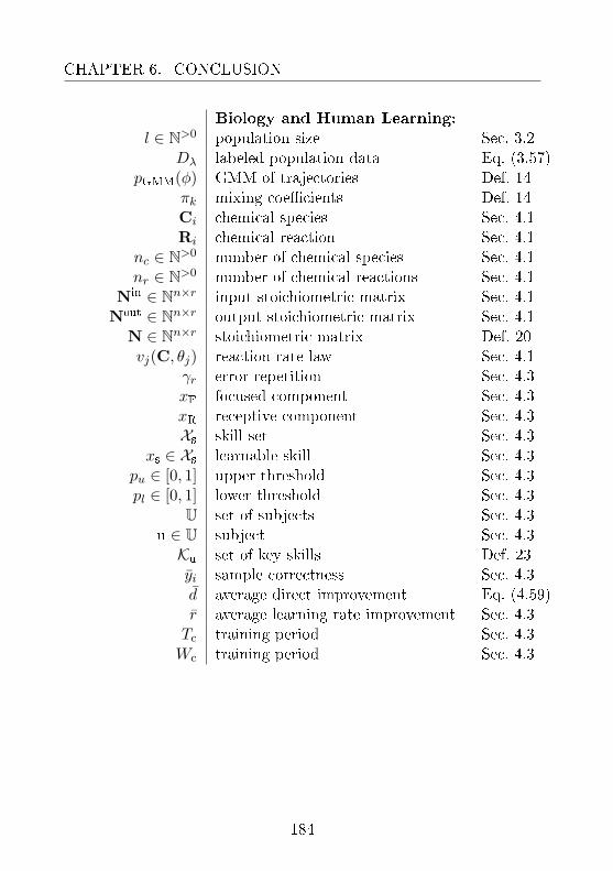
CHAPTER 6. CONCLUSION
Biology and Human Learning:
l ∈ N>0 population size Sec. 3.2Dλ labeled population data Eq. (3.57)
pGMM(φ) GMM of trajectories Def. 14πk mixing coecients Def. 14Ci chemical species Sec. 4.1Ri chemical reaction Sec. 4.1
nc ∈ N>0 number of chemical species Sec. 4.1nr ∈ N>0 number of chemical reactions Sec. 4.1
Nin ∈ Nn×r input stoichiometric matrix Sec. 4.1Nout ∈ Nn×r output stoichiometric matrix Sec. 4.1
N ∈ Nn×r stoichiometric matrix Def. 20vj(C, θj) reaction rate law Sec. 4.1
γr error repetition Sec. 4.3xF focused component Sec. 4.3xR receptive component Sec. 4.3Xs skill set Sec. 4.3
xs ∈ Xs learnable skill Sec. 4.3pu ∈ [0, 1] upper threshold Sec. 4.3pl ∈ [0, 1] lower threshold Sec. 4.3
U set of subjects Sec. 4.3u ∈ U subject Sec. 4.3Ku set of key skills Def. 23yi sample correctness Sec. 4.3d average direct improvement Eq. (4.59)r average learning rate improvement Sec. 4.3Tc training period Sec. 4.3Wc training period Sec. 4.3
184

Bibliography
Akaike, H. (1974). A new look at the statistical model identication.IEEE Transactions on Automatic Control, 19(6):716723.
Arroyo, I. and Woolf, B. (2006). Inferring learning and attitudes froma Bayesian network of log le data. In Proc. AIED, pages 3340.
Arulampalam, M. S., Maskell, S., Gordon, N., and Clapp, T.(2002). A tutorial on particle lters for online nonlinear/non-Gaussian Bayesian tracking. IEEE Transactions on Signal Pro-cessing, 50:174188.
Atkinson, A. C. and Donev, A. N. (1992). Optimum ExperimentalDesign. Oxford Science Publications.
Atkinson, A. C. and Fedorov, V. V. (1975). Optimal design: Ex-periments for discriminating between several models. Biometrika,62(2):289303.
Aurenhammer, F. (1991). Voronoi diagrams - a survey of a fundamen-tal geometric data structure. ACM Computing Surveys, 23(3):345405.
Baker, R. S., Corbett, A. T., and Koedinger, K. R. (2005). Detectingstudent misuse of intelligent tutoring systems. In Springer LectureNotes in Computer Science, 3220 Proc. ITS, pages 531540.
185

BIBLIOGRAPHY
Baldi, P. F. and Itti, L. (2010). Of bits and wows: A Bayesian the-ory of surprise with applications to attention. Neural Networks,23(5):649666.
Balsa-Canto, E., Alonso, A. A., and Banga, J. R. (2008). Compu-tational procedures for optimal experimental design in biologicalsystems. IET Systems Biology, 2(4):163172.
Bandara, S., Schlöder, J. P., Eils, R., Bock, H. G., and Meyer, T.(2009). Optimal experimental design for parameter estimation of acell signaling model. PLoS Computational Biology, 1:e1000558.
Banga, J. R. (2008). Optimization in computational systems biology.BMC Systems Biology, 2(47).
Banks, H. T. and Rehm, K. L. (2013). Applied mathematics let-ters. Experimental Design for Distributed Parameter Vector Sys-tems, 26(1):1014.
Banni, M., Negri, A., Mignone, F., Boussetta, H., Viarengo, A.,and Dondero, F. (2011). Gene expression rhythms in the mus-sel Mytilus galloprovincialis (lam.) across an annual cycle. PLoSONE, 6(5):e18904.
Bansal, N., Blum, A., and Chawla, S. (2004). Correlation clustering.Machine Learning, 56:89113.
Baschera, G.-M., Busetto, A. G., Klingler, S., Buhmann, J. M., andGross, M. (2011). Modeling engagement dynamics in spelling learn-ing. In Springer Lecture Notes in Computer Science, 6738 Proc.AIED, pages 3138.
Baschera, G.-M. and Gross, M. (2010). Poisson-based inference forperturbation models in adaptive spelling training. InternationalJournal of Articial Intelligence in Education, 20(4):333360.
186

BIBLIOGRAPHY
Baum, L. E., Petrie, T., Soules, G., and Weiss, N. (1970). A max-imization technique occurring in the statistical analysis of proba-bilistic functions of Markov chains. The Annals of MathematicalStatistics, 41(1):164171.
Berger, J. O. (1985). Statistical Decision Theory and Bayesian Anal-ysis. Springer.
Bergman, R. N., Ider, Y. Z., Browden, C. R., and Cobelli, C. (1979).Quantitative estimation of insulin sensitivity. American Journal ofPhysiology, 236(6):G667G677.
Bishop, C. M. (2006). Pattern Recognition and Machine Learning.Springer.
Boland, M. V. and Murphy, R. F. (2001). A neural network clas-sier capable of recognizing the patterns of all major subcellularstructures in uorescence microscope images of HeLa cells. Bioin-formatics, 17(12):12131223.
Bousquet, O., Boucheron, S., and Lugosi, G. (2004). Introductionto statistical learning theory. In Bousquet, O., von Luxburg, U.,and Rätsch, G., editors, Advanced Lectures on Machine Learning,volume 3176 of Lecture Notes in Computer Science, pages 169207.Springer.
Bratman, M. (1987). Intention, Plans, and Practical Reason. HarvardUniversity Press.
Breiman, L. (1996). Bagging predictors. Machine Learning,24(2):123140.
Brock, S. (2003). Niels Bohr's Philosophy of Quantum Physics in theLight of the Helmholtzian Tradition of Theoretical Physics. LogosVerlag.
Buhmann, J. M. (2010). Information theoretic model validation forclustering. In Proceedings of the 2010 IEEE International Sympo-sium on Information Theory, pages 13981402.
187

BIBLIOGRAPHY
Bullinger, E., Fey, D., Farina, M., and Findeisen, R. (2008). Identika-tion Biochemischer Reaktionsnetzwerke: ein BeobachterbasierterAnsatz. Automatisierungstechnik, 56(5):269279.
Burnham, K. P. and Anderson, D. R. (2002). Model Selection andInference: A Practical Information-Theoretic Approach, 2nd ed.Springer, New York.
Busetto, A., Sunnåker, M., and Buhmann, J. M. (2013). SystemTheoretic and Computational Perspectives in Systems and SyntheticBiology, chapter Computational Design of Informative Experimentsin Systems Biology. (in press).
Busetto, A. G. and Buhmann, J. M. (2009). Stable Bayesian param-eter estimation for biological dynamical systems. In Proceedings ofthe 12th IEEE International Conference on Computational Scienceand Engineering, pages 148157. IEEE Computer Society Press.
Busetto, A. G., Ong, C. S., and Buhmann, J. M. (2009). Optimizedexpected information gain for nonlinear dynamical systems. In Pro-ceedings of the 26th International Conference on Machine Learning,pages 97104.
Carnap, R. (1945). The two concepts of probability: The problem ofprobability. Philosophy and Phenomenological Research, 5(4):513532.
Chaitin, G. (1966). On the length of programs for computing nitebinary sequences. Journal of the ACM, 13(4):547569.
Chaloner, K. and Verdinelli, I. (1995). Bayesian experimental design:a review. Statistical Science, 10:273304.
Chehreghani, M. H., Busetto, A. G., and Buhmann, J. M. (2012).Information theoretic model validation for spectral clustering. InJournal of Machine Learning Research, Proceedings of AISTATS2012, pages 495503.
188

BIBLIOGRAPHY
Church, A. (1932). A set of postulates for the foundation of logic.Annals of Mathematics, 33(2):346366.
Collinet, C., Stöter, M., Bradshaw, C. R., Samusik, N., Rink, J. C.,Kenski, D., Habermann, B., Buchholz, F., Henschel, R., Mueller,M. S., Nagel, W. E., Fava, E., Kalaidzidis, Y., and Zerial, M. (2010).Systems survey of endocytosis by multiparametric image analysis.Nature, 464:243249.
Conrad, C. and W., G. D. (2010). Automated microscopy for high-content RNAi screening. Journal of Cell Biology, 188(4):453461.
Conrad, C., Wünsche, A., Tan, T. H., Bulkescher, J., Sieckmann, F.,Verissimo, F., Edelstein, A., Walter, T., Liebel, U., Pepperkok, R.,and Ellenberg, J. (2011). Micropilot: Automation of uorescencemicroscopy-based imaging for systems biology. Nature Methods,8:246249.
Cooper, D. G., Muldner, K., Arroyo, I., Woolf, B. P., and Burleson,W. (2010). Ranking feature sets for emotion models used in class-room based intelligent tutoring systems. In Springer Lecture Notesin Computer Science, 6075 Proc. UMAP, pages 135146.
Cover, T. M. and Thomas, J. A. (1991). Elements of InformationTheory. Wiley-Interscience.
Cox, R. T. (1946). Probability, physics, and reasonable expectation.American Journal of Physics, 14:113.
Cox, R. T. (1961). The Algebra of Probable Inference. Johns HopkinsUniversity Press.
Dancy, J. (1985). Introduction to Contemporary Epistemology. Black-well.
Daunizeau, J., Preuscho, K., Friston, K., and Stephan, K. (2011).Optimizing experimental design for comparing models of brainfunction. PLoS Computational Biology, 11(7):e1002280.
189

BIBLIOGRAPHY
de Finetti, B. (1970). Theory of Probability. Wiley and Sons.
Dehaene, S. (1992). Varieties of numerical abilities. Cognition, 44:142.
Dehaene, S. (2011). The Number Sense: How the Mind Creates Math-ematics. Oxford University Press.
Dempster, A. P. (1968). A generalization of Bayesian inference. Jour-nal of the Royal Statistical Society, B, 30:205247.
Doucet, A. (1998). On sequential Monte Carlo methods for Bayesianltering. Technical report, Department of Engineering, Universityof Cambridge, Cambridge.
Doucet, A. and Johansen, A. M. (2011). A tutorial on particle l-tering and smoothing: Fifteen years later. In Oxford Handbook ofNonlinear Filtering.
Doucet, A. and Tadic, V. (2003). Parameter estimation in generalstate-space models using particle methods. Annals of the Instituteof Statistical Mathematics, 55(2):409422.
Dubois, D. and Prade, H. (1988). Possibility Theory, An Approach toComputerized Processing of Uncertainty. Plenum.
Dudoit, S. and Fridlyand, J. (2002). A prediction-based resamplingmethod for estimating the number of clusters in a dataset. GenomeBiology, 3(7).
Engstrom, D. R., London, P., and Hart, J. T. (1970). Hypnotic sus-ceptibility increased by eeg alpha training. Nature, 227:12611262.
Faller, D., Klingmüller, U., and Timmer, J. (2003). Simulation meth-ods for optimal experimental design in systems biology. Simulation,79(12):717725.
190
BIBLIOGRAPHY
Farina, M., Findeisen, R., Bullinger, E., Bittanti, S., Allgower, F.,and Wellstead, P. (2006). Results towards identiability propertiesof biochemical reaction networks. In Proceedings of the Conferenceon Decision and Control, pages 21042109.
Feige, U. (1998). A threshold of Ln n for approximating set cover.Journal of the ACM, 45(4):634652.
Fisher, R. A. (1922). On the mathematical foundations of theoreti-cal statistics. Philosophical Transactions of the Royal Society, A,222:309368.
Fortier, J. J. and Solomon, H. (1966). Clustering procedures. InKrishnaiah, P. R., editor, Multivariate Analysis, pages 493506.Academic Press.
García, C. E. and D. M. Prett, M. M. (1989). Model predictive control:Theory and practice a survey. Automatica, 25(3):335348.
Geary, D. C., Bow-Thomas, C. C., and Yao, Y. (1992). Countingknowledge and skill in cognitive addition: A comparison of nor-mal and mathematically disabled children. Journal of ExperimentalChild Psychology, 54:372391.
Golightly, A. and Wilkinson, D. J. (2008). Bayesian inference fornonlinear multivariate diusion models observed with error. Com-putational Statistics and Data Analysis, 52(3):16741693.
Good, I. J. (1950). Probability and the Weighing of Evidence. Hafners.
Goodwin, B. C. (1965). Oscillatory behavior in enzymatic controlprocesses. Advances in Enzyme Regulation, 3:425438.
Gordon, N. J., Salmond, D. J., and Smith, A. F. M. (1993). Novel ap-proach to nonlinear/non-gaussian Bayesian state estimation. IEEEProceedings on Radar and Signal Processing, 140(2):107113.
191

BIBLIOGRAPHY
Goshima, G., Wollman, R., Goodwin, S. S., Zhang, N., Scholey, J. M.,Vale, R. D., and Stuurman, N. (2007). Genes required for mitoticspindle assembly in Drosophila S2 cells. Science, 316:417421.
Gross, M. and Vögeli, C. (2007). A multimedia framework for eectivelanguage training. Computer & Graphics, 31:761777.
Grünwald, P. D. (2007). The Minimum Description Length Principle.MIT Press.
Hadamard, J. (1902). Sur les problèmes aux dérivées partielles et leursignication physique. Technical report, Bullettin of the Universityof Princeton.
Haner, J., Baro, K., Parzer, P., and F., R. (2005). HeidelbergerRechentest (HRT): Erfassung Mathematischer Basiskompetenzenim Grundschulalter. Hogrefe Verlag.
Harder, N., Mora-Bermúdez, F., Godinez, W. J., Wünsche, A., Eils,R., Ellenberg, J., and Rohr, K. (2009). Automatic analysis of di-viding cells in live cell movies to detect mitotic delays and correlatephenotypes in time. Genome Research, 19:21132124.
Hardin, C. S. and Taylor, A. D. (2008). A peculiar connection be-tween the axiom of choice and predicting the future. AmericanMathematical Monthly, 115(2):9196.
Hastie, T., Tibshirani, R., and Friedman, J. (2001). The Elementsof Statistical Learning: Data Mining, Inference and Prediction.Springer.
Hauser, A. (2009). Entropy-based experimental design for model se-lection in systems biology. Master's thesis, advised by A. G. Busettoand supervised by J. M. Buhmann, Deparment of Computer Sci-ence, ETH Zurich.
He, Y. B. and Geng, Z. (2010). Journal of machine learning research.Active Learning of Causal Networks with Intervention Experimentsand Optimal Designs, 9:25232547.
192

BIBLIOGRAPHY
Held, M., Schmitz, M. H. A., Fischer, B., Walter, T., Neumann,B., Olma, M. H., Peter, M., Ellenberg, J., and Gerlich, D. W.(2010). CellCognition: Time-resolved phenotype annotation inhigh-throughput live cell imaging. Nature Methods, 7(9):747754.
Heray, A. and Frasson, C. (2009). Predicting learner answers correct-ness through brain-waves assessment and emotional dimensions. InProc. AIED, pages 4956.
Hofmann, T. and Buhmann, J. (1997a). Pairwise data clustering bydeterministic annealing. IEEE Transaction on Pattern Analysisand Machine Intelligence, 19(1):114.
Hofmann, T. and Buhmann, J. M. (1997b). Pairwise data clusteringby deterministic annealing. IEEE Transactions on Pattern Analysisand Machine Intelligence, 19(1):114.
Hopcroft, J., Motwani, R., and Ullman, J. (2007). Introduction toAutomata Theory, Languages, and Computation. Pearson/AddisonWesley.
Jain, A. K. and Dubes, R. C. (1988). Algorithms for Clustering Data.Prentice-Hall.
Jaynes, E. T. (1957a). Information theory and statistical mechanics.Physical Rewiew Series II, 106(4):620630.
Jaynes, E. T. (1957b). Information theory and statistical mechanicsii. Physical Rewiew Series II, 109(2):171190.
Jaynes, E. T. (2004). Probability Theory. Cambridge University Press.
Jensen, R. E. (1969). A dynamic programming algorithm for clusteranalysis. Operations Research, 17:10341057.
Johns, J. and Woolf, B. (2006). A dynamic mixture model to detectstudent motivation and prociency. In Proc. AAAI, pages 163168.
193

BIBLIOGRAPHY
Jonesa, T. R., Carpentera, A. E., Lamprechtb, M. R., Moat, J.,Serena, J. S., Greniera, J. K., Castorenod, A. B., Eggertd, U. S.,Roota, D. E., Gollandc, P., and M., S. D. (2009). Scoring diversecellular morphologies in image-based screens with iterative feed-back and machine learning. Proceedings of the National Academyof Sciences, 106(6):18261831.
Julier, S. J. and Uhlmann, J. K. (2004). Unscented ltering andnonlinear estimation. Proceedings of the IEEE, 92(3):401422.
Käser-Jacober, T. C., Busetto, A. G., Baschera, G.-M., Kohn, J.,Kucian, K., von Aster, M., and Gross, M. (2012). Modelling andoptimizing the process of learning mathematics. In Springer LectureNotes in Computer Science, 7315 Proc. ITS, pages 389398.
Kast, M., Meyer, M., Vögeli, C., Gross, M., and Jäncke, L. (2007).Computer-based multi-sensory learning in children with develop-mental dyslexia. Restorative Neurology and Neuroscience, 25(3-4):355369.
Keynes, J. M. (1921). A Treatise on Probability. MacMillan and Co.
Khinchin, A. I. (1957). Mathematical Foundations of InformationTheory. Dover.
King, O. D. and Forsyth, D. A. (2000). How does CONDENSATIONbehave with a nite number of samples? In Proceedings of theEuropean Conference on Computer Vision, pages 695709.
Kirkpatrick, M. (2009). Patterns of quantitative genetic variation inmultiple dimensions. Genetica, 136:271284.
Kitano, H. (2002). Computational systems biology. Nature, 420:206210.
Kocha, H. and Tataru, D. (2001). Well-posedness for the Navier-Stokes equations. Advances in Mathematics, 157(1):22 35.
194

BIBLIOGRAPHY
Kolmogorov, A. N. (1933). Grundbegrie der Wahrscheinlichkeitrech-nung. Ergebnisse Der Mathematik.
Kolmogorov, A. N. (1965). Three approaches to the quantitativedenition of information. Problems of Information Transmission,1(1):47.
Kolmogorov, A. N. (1974). Complexity of algorithms and objectivedenition of randomness. In Talk at Moscow Mathematical SocietyMeeting (transl. from Russian by L. A. Levin), Moscow.
Kramer, A. and Radde, N. (2010). Towards experimental design us-ing a Bayesian framework for parameter identication in dynamicintracellular network models. In Proceedings of the InternationalConference on Computational Science, pages 16451653.
Krause, A. (2010). SFO: A toolbox for submodular function opti-mization. Journal of Machine Learning Research, 11:11411144.
Krause, A. and Guestrin, C. (2005). Near-optimal nonmyopic value ofinformation in graphical models. In Proceedings of the Conferenceon Uncertainty in Articial Intelligence.
Krause, A. and Guestrin, C. (2007). Near-optimal observation se-lection using submodular functions. In Proceedings of the 22ndConference on Articial Intelligence, pages 16501654.
Krause, A., McMahan, B., Guestrin, C., and Gupta, A. (2008). Ro-bust submodular observation selection. Journal of Machine Learn-ing Research, 9:27612801.
Kreutz, C. and Timmer, J. (2009). Systems biology: Experimentaldesign. FEBS Journal, 276:923942.
Krummenacher, G. (2010). Large-scale experimental design toolboxfor systems biology. Master's thesis, advised by A. G. Busetto andsupervised by J. M. Buhmann, Deparment of Computer Science,ETH Zurich.
195

BIBLIOGRAPHY
Kucian, K. and Kaufmann, L. (2009). A developmental model ofnumber representation. Behavioral and Brain Sciences, 32:313373.
Kuepfer, L., Peter, M., Sauer, U., and Stelling, J. (2007). Ensemblemodeling for analysis of cell signaling dynamics. Nature Biotech-nology, 25(9):10011006.
Kullback, S. and Leibler, R. A. (1951). On information and suciency.Annals of Mathematical Statistics, 22(1):7986.
Lange, T., Braun, M., Roth, V., and Buhmann, J. M. (2004).Stability-based validation of clustering solutions. Neural Computa-tion, 16(6):12991323.
Li, M. and Vitányi, P. (1997). An Introduction to Kolmogorov Com-plexity and Its Applications. Springer.
Lindley, D. (1991). Making Decision. Wiley.
Lindley, L. J. (1982). Scoring rules and the inevitability of probability.International Statistical Review, 50:126.
Loo, L. H., Wu, L. F., and Altschuler, S. J. (2007). Image-basedmultivariate proling of drug responses from single cells. NatureMethods, 4(5):445453.
MacKay, D. (2003). Information Theory, Inference, and LearningAlgorithms. Cambridge University Press.
MacQueen, J. B. (1967). Some methods for classication and analysisof multivariate observations. In Proceedings of 5th Berkeley Sym-posium on Mathematical Statistics and Probability, volume 1, pages281297.
Minoux, M. (1978). Accelerated greedy algorithms for maximizingsubmodular set functions. Optimization Techniques, 7:234243.
196

BIBLIOGRAPHY
Mooij, J. M. (2010). Libdai: A free & open source C++ libraryfor discrete approximate inference in graphical models. Journal ofMachine Learning Research, 11:21692173.
Murphy, K. P. (2001). The bayes net toolbox for MATLAB. Com-puting Science and Statistics, 33:2001.
Murphy, K. P. (2002). Dynamic Bayesian Networks: Representa-tion, Inference and Learning. PhD thesis, University of California,Berkeley.
Myung, J. I. and Pitt, M. A. (2009). Optimal experimental design formodel discrimination. Psychological Review, 116(3):499518.
Nelles, O. (2001). Nonlinear System Identication. Springer.
Nemhauser, G. L., Wolsey, L. A., and Fisher, M. L. (1978). An anal-ysis of approximations for maximizing submodular set functions.Mathematical Programming, 14(1):265294.
Neumann, B., Walter, T., Hériché, J. K., Bulkescher, J., Ere, H.,Conrad, C., Rogers, P., Poser, I., Held, M., Liebel, U., Cetin, C.,Sieckmann, F., Pau, G., Kabbe, R., Wünsche, A., Satagopam, V.,Schmitz, M. H., Chapuis, C., Gerlich, D. W., Schneider, R., Eils, R.,Huber, W., Peters, J. M., Hyman, A. A., Durbin, R., Pepperkok,R., and Ellenberg, J. (2010). Phenotypic proling of the humangenome by time-lapse microscopy reveals cell division genes. Nature,464:721727.
Ostad, S. A. (1997). Developmental dierences in addition strategies:A comparison of mathematically disabled and mathematically nor-mal children. British Journal of Education Psychology, 67:345357.
Ostad, S. A. (1999). Developmental progression of subtraction strate-gies: A comparison of mathematically normal and mathematicallydisabled children. European Journal of Special Needs Education,14:2136.
197
BIBLIOGRAPHY
Pearson, K. (1901). On lines and planes of closest t to systems ofpoints in space. Philosophical Magazine, 2:559572.
Pham, T. and Tran, D. (2006). Gaussian mixture and Markov modelsfor cell-phase classication in microscopic imaging. In Proceedingsof the 2006 IEEE/SMC International Conference on System of Sys-tems Engineering, pages 328333.
Pinheiro, J. C. and Bates, D. M. (1995). Approximations to the log-likelihood function in non-linear mixed-eects models. Journal ofComputational and Graphical Statistics, 4(1):1235.
Ponce de Leon, A. C. and Atkinson, A. (1991). Optimum experi-mental design for discriminating between two rival models in thepresence of prior information. Biometrika, 78(3):601608.
Pronzato, L. (2008). Optimal experimental design and some relatedcontrol problems. Automatica, 44(2):303325.
Rabiner, L. R. (1989). A tutorial on hidden Markov models and se-lected applications in speech recognition. Proceedings of the IEEE,77(2):257286.
Raman, K. and Wagner, A. (2011). Evolvability and robustness in acomplex signalling circuit. Molecular Biosystems, 7(4):10811092.
Ramsey, F. (1931). Truth and Probability. Humanities Press.
Rathmanner, S. and Hutter, M. (2011). A philosophical treatise ofuniversal induction. Entropy, 13(6):10761136.
Richard O. Duda, Peter E. Hart, D. G. S. (2000). Pattern Classica-tion. Wiley-Interscience Publication.
Risken, H. (1996). The Fokker-Planck Equation: Methods of Solutionsand Applications. Springer.
Rissanen, J. (1978). Modeling by shortest data description. Automat-ica, 14:465471.
198
BIBLIOGRAPHY
Roth, V., Laub, J., Kawanabe, M., and Buhmann, J. M. (2003). Op-timal cluster preserving embedding of non-metric proximity data.IEEE Transactions on Pattern Analysis and Machine Intelligence,25(12):15401551.
Rubinsten, O. and Tannock, R. (2010). Mathematics anxiety in chil-dren with developmental dyscalculia. Behavioral and Brain Func-tions, 6(46).
S. Ben-David, U. von Luxburg, D. P. (2006). A sober look at cluster-ing stability. In Springer Verlag LNAI 4005 Proceedings of COLT,pages 519.
Savage, L. J. (1961). The subjective basis of statistical practice. Tech-nical report, Department of Statistics, University of Michigan, AnnArbor.
Schmitz, M. H., Held, M., Janssens, V., Hutchins, J. R., Hudecz, O.,Ivanova, E., Goris, J., Trinkle-Mulcahy, L., Lamond, A. I., Poser,I., Hyman, A. A., Mechtler, K., Peters, J. M., and Gerlich, D. W.(2010). Live-cell imaging RNAi screen identies PP2A-B55alphaand importin-beta1 as key mitotic exit regulators in human cells.Nature Cell Biology, 12(9):886893.
Schwarz, G. (1978). Estimating the dimension of a model. Annals ofStatistics, 6(2):461464.
Seldin, Y. and Tishby, N. (2010a). Pac-Bayesian analysis of co-clustering and beyond. Journal of Machine Learning Research,11:35953646.
Seldin, Y. and Tishby, N. (2010b). Pac-Bayesian analysis of co-clustering and beyond. Journal of Machine Learning Research,11:35953646.
Shafer, G. (1976). A Mathematical Theory of Evidence. PrincetonUniversity Press.
199
BIBLIOGRAPHY
Shalev, R. and von Aster, M. G. (2008). Identication, classica-tion, and prevalence of developmental dyscalculia. Encyclopedia ofLanguage and Literacy Development, pages 19.
Shannon, C. E. (1948). A mathematical theory of communication.Bell System Technical Journal, 27:379423.
Shannon, C. E. and Weaver, W. (1963). The Mathematical Theory ofCommunication. University of Illinois Press.
Skanda, D. and Lebiedz, D. (2010). An optimal experimental designapproach to model discrimination in dynamic biochemical systems.Bioinformatics, 26(7):939945.
Slonim, N., Atwal, G. S., Tracik, G., and Bialek, W. (2005).Information-based clustering. Proceedings of the National Academyof Sciences, 102:18271830.
Smets, P. and Kennes, R. (1994). The transferable belief model. Ar-ticial Intelligence, 66:191234.
Solomono, R. (1964a). A formal theory of inductive inference, parti. Information and Control, 7(1):122.
Solomono, R. (1964b). A formal theory of inductive inference, partii. Information and Control, 7(2):224254.
Steinhaus, H. (1957). Sur la division des corps matériels en parties.Bulletin de l'Academie Polonaise des Sciences, 4(12):801804.
Steinke, F., Seeger, M., and Tsuda, K. (2007). Experimental designfor ecient identication of gene regulatory networks using sparseBayesian models. BMC Systems Biology, 1(51).
Stoer, J., B. R. (2002). Introduction to Numerical Analysis. Springer.
Sunnåker, M., Busetto (eq.), A. G., Numminen (eq.), E., Corander,J., Foll, M., and Dessimoz, C. (2012). Approximate bayesian com-putation. PLoS Computational Biology, page (in press).
200

BIBLIOGRAPHY
Suyari, H. (2004). Generalization of shannon-khinchin axioms tononextensive systems and the uniqueness theorem for the nonex-tensive entropy. IEEE Transactions on Information Theory,50(8):17831787.
Szallasi, Z., Stelling, J., and Periwal, V. (2006). System Modeling inCell Biology: from Concepts to Nuts and Bolts. MIT Press.
Tishby, N., Pereira, F. C., and Bialek, W. (1999). The informa-tion bottleneck method. In Proceedings of the 37-th Annual Aller-ton Conference on Communication, Control and Computing, pages368377.
Tseng, G. C. (2007). Penalized and weighted K-means for clusteringwith scattered objects and prior information in high-throughputbiological data. Bioinformatics, 23(17):22472255.
Turing, A. M. (1937). On computable numbers, with an applicationto the Entscheidungsproblem. Proceedings of the London Mathe-matical Society, 2(42):230265.
Valiant, L. (1984). A theory of the learnable. Communications of theACM, 27:11341142.
van Fraassen, B. (1980). The Scientic Image. Oxford UniversityPress.
Vapnik, V. N. (1982). Estimation of the Dependencies Based on Em-pirical Data. Springer.
Viterbi, A. J. (1967). Error bounds for convolution codes and anasymptotically optimum decoding algorithm. IEEE Transactionson Information Theory, 13:260269.
von Aster, M. G. and Shalev, R. (2007). Number development anddevelopmental dyscalculia. Developmental Medicine and Child Neu-rology, 49:868873.
201

BIBLIOGRAPHY
Wallace, C. and Boulton, D. (1968). An information measure forclassication. Computer Journal, 11(2):185194.
Wang, M., Zhou, X., King, R., and Wong, S. (2007). Context basedmixture model for cell phase identication in automated uores-cence microscopy. BMC Bioinformatics, 8(32).
Wang, M., Zhou, X. B., Li, F. H., Huckins, J., King, R. W., andWong,S. T. C. (2008). Novel cell segmentation and online SVM for cellcycle phase identication in automated microscopy. Bioinformatics,24(1):94101.
Wasserman, L. (2003). All of Statistics: A Concise Course in Statis-tical Inference. Springer.
Whewell, W. (1837). History of the Inductive Sciences. John W.Parker.
Wilkinson, D. J., editor (2006). Stochastic Modelling for SystemsBiology. Chapman & Hall/CRC.
Wilkinson, D. J. (2007). Bayesian methods in bioinformatics andcomputational systems biology. Bioinformatics, 8:109116.
Wilkinson, D. J. (2011). Stochastic Modelling for Systems Biology.Chapman and Hall.
Zadeh, L. A. (1978). Fuzzy sets as a basis for a theory of possibility.Fuzzy Sets and Systems, 1:328.
Zermelo, E. (1908). Untersuchungen über die Grundlagen der Men-genlehre i. Mathematische Annalen, 65:261281.
Zhong, Q., Busetto, A. G., Fededa, J. P., Buhmann, J. M., and Ger-lich, D. W. (2012). Unsupervised modeling of cell morphology dy-namics for time-lapse microscopy. Nature Methods, 9:711713.
202

Alberto Giovanni Busetto
20072012:Doctoral StudiesETH Zurich, Department of Computer Science & CC-SPMD;
20022007:Laurea Specialistica (e Triennale) in Ingegneria InformaticaUniversità degli Studi di Padova;
19972002:Diploma di Maturità Scientica, PNILiceo Scientico G. B. Benedetti, Venezia.
203

BIBLIOGRAPHY
204

Sommario
I sistemi dinamici sono modelli matematici che esprimono relazionidi causa-eetto riguardanti fenomeni soggetti a variazione temporale.Questa tesi si concentra sulla stima di sistemi dinamici sulla base diosservazioni empiriche. Si considerano tre scenari: stima senza super-visione, con supervisione e attiva. L'obiettivo unicante è l'estrazionedi informazione predittiva dai dati.
Viene introdotto un metodo per il raggruppamento di serie tem-porali e la validazione statistica di modelli. Il metodo si propone dirisolvere le questioni di selezione d'ordine e di modello con il principiodella Codica tramite Insiemi di Approssimazione [Buhmann (2010)].La verica sperimentale è perseguita nell'ambito di raggruppamentorelazionale per proli temporali di espressione genetica. I risultati di-mostrano vasta applicabilità e congruenza col Criterio d'InformazioneBayesiano. Inoltre, le transizioni dinamiche discrete sono ricostru-ite sulla base di serie temporali d'alta dimensionalità tramite un ap-proccio privo di supervisione. L'approccio, che si basa su ModelliMarkoviani Nascosti su Miscele Gaussiane, trova applicazione nellapredizione di classi morfologiche da dati di microscopia che tengonoconto del fattore tempo. La conferma sperimentale con marcatoriuorescenti e cernita dei campioni dimostra la capacità di accurataidenticazione dei fenotipi cellulari umani. I risultati riportati evi-denziano competitività e miglioramento dell'oggettività rispetto agliapprocci supervisionati basati sulla catalogazione operata da partedell'utente.
205

Nello scenario con supervisione, il processo di raggruppamentotrova impiego nel perfezionamento del ltraggio convenzionale di cam-pioni al ne di ottenere stime di stato generalizzate. Il raggruppa-mento preventivo mitiga l'inevitabile divergenza del ricampionamentoimpiegato nei metodi sequenziali di tipo Monte Carlo. La stima su-pervisionata con reti Bayesiane dinamiche è utilizzata nella model-listica dell'apprendimento umano con il ne di curare ecacementealcune disabilità dell'apprendimento. Per la dislessia, il modello è ingrado di predire rate di dimenticanza, livelli di concentrazione e incli-nazione all'apprendimento del soggetto sulla base del comportamentomisurato. Per la discalculia, la cognizione numerica è migliorata permezzo di una terapia adattabile ottenuta sulla base del modello.
Nel contesto della stima attiva, la tesi si concentra sulla proget-tazione quasi ottima di esperimenti nalizzati alla modellistica di sis-temi dinamici. Viene introdotto un metodo eciente per selezionarequantità misurabili e istanti temporali particolarmente informativi. Sigarantisce la quasi ottima informatività del metodo di progettazione,il quale richiede un numero polinomiale di valutazioni della funzioneobiettivo. Il metodo si basa su lavoro precedente nell'ambito dellastima attiva sotto-modulare [Krause and Guestrin (2005)] e ottiene ilmigliore fattore costante di approssimazione possibile, a meno che nonvalga P=NP [Feige (1998)]. La progettazione di esperimenti trova ap-plicazione nella ricostruzione di reti cellulari segnalatrici nell'ambitodella biologia dei sistemi.
I contributi presentati sottolineano le analogie fondamentali trastima e comunicazione. In conclusione, i risultati dimostrano chemodelli predittivi possono essere costruiti sulla base di ecienti strate-gie di trasmissione d'informazione tramite un canale rumoroso. Sullabase di argomentazioni di natura statistica, i risultati esibiti formal-izzano e automatizzano aspetti del metodo ipotetico-deduttivo di in-vestigazione scientica.
206