Stochastic embedding of dynamical systems

arX

iv:m

ath/

0509

713v

1 [

mat

h.PR

] 3

0 Se

p 20

05 Jacky CRESSON

Sebastien DARSES

STOCHASTIC EMBEDDING OF

DYNAMICAL SYSTEMS

http://arXiv.org/abs/math/0509713v1

Jacky CRESSON

Universite de Franche-Comte, Equipe de Mathematiques de Besancon, CNRS-UMR

6623, 16 route de Gray, 25030 Besancon cedex, France..

E-mail : [email protected]

Sebastien DARSES

Universite de Franche-Comte, Equipe de Mathematiques de Besancon, CNRS-UMR

6623, 16 route de Gray, 25030 Besancon cedex, France..

E-mail : [email protected]

2000 Mathematics Subject Classification. — Primary 54C40, 14E20;

Secondary 46E25, 20C20.

Key words and phrases. — Stochastic calculus, Dynamical systems, Lagrangian

systems, Hamiltonian systems.

July 2, 1991

STOCHASTIC EMBEDDING OF DYNAMICAL

SYSTEMS

Jacky CRESSON, Sebastien DARSES

5

Abstract. — Most physical systems are modelled by an ordinary or a partial differential

equation, like the n-body problem in celestial mechanics. In some cases, for example when

studying the long term behaviour of the solar system or for complex systems, there exist

elements which can influence the dynamics of the system which are not well modelled

or even known. One way to take these problems into account consists of looking at

the dynamics of the system on a larger class of objects, that are eventually stochastic.

In this paper, we develop a theory for the stochastic embedding of ordinary differential

equations. We apply this method to Lagrangian systems. In this particular case, we

extend many results of classical mechanics namely, the least action principle, the Euler-

Lagrange equations, and Noether’s theorem. We also obtain a Hamiltonian formulation

for our stochastic Lagrangian systems. Many applications are discussed at the end of the

paper.

CONTENTS

Introduction. . . . . . . . . . . . . . . . . . . . . . . . . . . . . . . . . . . . . . . . . . . . . . . . . . . . . . . . . . . . . . . . . . . . . . . . 11

Part I. The stochastic derivative. . . . . . . . . . . . . . . . . . . . . . . . . . . . . . . . . . . . . . . . . . . . . . . 19

1. About Nelson stochastic calculus. . . . . . . . . . . . . . . . . . . . . . . . . . . . . . . . . . . . . . . . . . . . . 21

1.1. About measurement and experiments. . . . . . . . . . . . . . . . . . . . . . . . . . . . . . . . . . . . . . . . . 21

1.2. The Nelson derivatives. . . . . . . . . . . . . . . . . . . . . . . . . . . . . . . . . . . . . . . . . . . . . . . . . . . . . . . . 23

1.3. Good diffusion processes. . . . . . . . . . . . . . . . . . . . . . . . . . . . . . . . . . . . . . . . . . . . . . . . . . . . . . 24

1.4. The Nelson derivatives for good diffusion processes. . . . . . . . . . . . . . . . . . . . . . . . . . . . 25

1.5. A remark about reversed processes. . . . . . . . . . . . . . . . . . . . . . . . . . . . . . . . . . . . . . . . . . . . 27

2. Stochastic derivative. . . . . . . . . . . . . . . . . . . . . . . . . . . . . . . . . . . . . . . . . . . . . . . . . . . . . . . . . . . 29

2.1. The abstract extension problem. . . . . . . . . . . . . . . . . . . . . . . . . . . . . . . . . . . . . . . . . . . . . . . 29

2.2. Stochastic differential calculus. . . . . . . . . . . . . . . . . . . . . . . . . . . . . . . . . . . . . . . . . . . . . . . . . 30

2.2.1. Reconstruction problem and extension. . . . . . . . . . . . . . . . . . . . . . . . . . . . . . . . . . . . 31

2.2.2. Extension to complex processes. . . . . . . . . . . . . . . . . . . . . . . . . . . . . . . . . . . . . . . . . . . 32

2.2.3. Stochastic derivative for functions of diffusion process. . . . . . . . . . . . . . . . . . . . 36

2.2.4. Examples. . . . . . . . . . . . . . . . . . . . . . . . . . . . . . . . . . . . . . . . . . . . . . . . . . . . . . . . . . . . . . . . . 37

3. Properties of the stochastic derivatives. . . . . . . . . . . . . . . . . . . . . . . . . . . . . . . . . . . . . . 41

3.1. Product rules. . . . . . . . . . . . . . . . . . . . . . . . . . . . . . . . . . . . . . . . . . . . . . . . . . . . . . . . . . . . . . . . . . 41

3.1.1. A new algebraic structure. . . . . . . . . . . . . . . . . . . . . . . . . . . . . . . . . . . . . . . . . . . . . . . . . 43

3.2. Nelson differentiable processes. . . . . . . . . . . . . . . . . . . . . . . . . . . . . . . . . . . . . . . . . . . . . . . . . 43

3.2.1. Definition. . . . . . . . . . . . . . . . . . . . . . . . . . . . . . . . . . . . . . . . . . . . . . . . . . . . . . . . . . . . . . . . . 43

3.2.2. Examples of Nelson-differentiable process. . . . . . . . . . . . . . . . . . . . . . . . . . . . . . . . . 44

3.2.3. Product rule and Nelson-differentiable processes. . . . . . . . . . . . . . . . . . . . . . . . . . 45

Part II. Stochastic embedding procedures . . . . . . . . . . . . . . . . . . . . . . . . . . . . . . . . . . . . 47

8 CONTENTS

4. Stochastic embedding of differential operators . . . . . . . . . . . . . . . . . . . . . . . . . . . . . 49

4.1. Stochastic embedding of differential operators. . . . . . . . . . . . . . . . . . . . . . . . . . . . . . . . . 50

4.1.1. Abstract embedding. . . . . . . . . . . . . . . . . . . . . . . . . . . . . . . . . . . . . . . . . . . . . . . . . . . . . . 50

4.1.2. Nelson Stochastic embedding. . . . . . . . . . . . . . . . . . . . . . . . . . . . . . . . . . . . . . . . . . . . . 51

4.2. First examples. . . . . . . . . . . . . . . . . . . . . . . . . . . . . . . . . . . . . . . . . . . . . . . . . . . . . . . . . . . . . . . . 53

4.2.1. First order differential equations. . . . . . . . . . . . . . . . . . . . . . . . . . . . . . . . . . . . . . . . . . 53

4.2.2. Second order differential equations. . . . . . . . . . . . . . . . . . . . . . . . . . . . . . . . . . . . . . . . 53

5. Reversible stochastic embedding . . . . . . . . . . . . . . . . . . . . . . . . . . . . . . . . . . . . . . . . . . . . . 55

5.1. Reversible stochastic derivative. . . . . . . . . . . . . . . . . . . . . . . . . . . . . . . . . . . . . . . . . . . . . . . . 55

5.2. Iterates. . . . . . . . . . . . . . . . . . . . . . . . . . . . . . . . . . . . . . . . . . . . . . . . . . . . . . . . . . . . . . . . . . . . . . . . 58

5.3. Reversible stochastic embedding. . . . . . . . . . . . . . . . . . . . . . . . . . . . . . . . . . . . . . . . . . . . . . . 59

5.4. Reversible versus general stochastic embedding. . . . . . . . . . . . . . . . . . . . . . . . . . . . . . . . 59

5.5. Stochastic mechanics and the Stochastization procedure. . . . . . . . . . . . . . . . . . . . . . 60

5.5.1. The Stochastic Newton Equation. . . . . . . . . . . . . . . . . . . . . . . . . . . . . . . . . . . . . . . . . 60

Part III. Stochastic embedding of Lagrangian and Hamiltonian systems . 61

6. Stochastic Lagrangian systems. . . . . . . . . . . . . . . . . . . . . . . . . . . . . . . . . . . . . . . . . . . . . . . . 63

6.1. Reminder about Lagrangian systems. . . . . . . . . . . . . . . . . . . . . . . . . . . . . . . . . . . . . . . . . . 63

6.2. Stochastic Euler-Lagrange equations. . . . . . . . . . . . . . . . . . . . . . . . . . . . . . . . . . . . . . . . . . 65

6.3. The coherence problem. . . . . . . . . . . . . . . . . . . . . . . . . . . . . . . . . . . . . . . . . . . . . . . . . . . . . . . . 65

7. Stochastic calculus of variations . . . . . . . . . . . . . . . . . . . . . . . . . . . . . . . . . . . . . . . . . . . . . . 67

7.1. Functional and L-adapted process. . . . . . . . . . . . . . . . . . . . . . . . . . . . . . . . . . . . . . . . . . . . . 67

7.2. Space of variations. . . . . . . . . . . . . . . . . . . . . . . . . . . . . . . . . . . . . . . . . . . . . . . . . . . . . . . . . . . . 68

7.3. Differentiable functional and stationary processes. . . . . . . . . . . . . . . . . . . . . . . . . . . . . 68

7.3.1. The P = C1(I) case. . . . . . . . . . . . . . . . . . . . . . . . . . . . . . . . . . . . . . . . . . . . . . . . . . . . . . . 69

7.3.2. The P = N1(I) case. . . . . . . . . . . . . . . . . . . . . . . . . . . . . . . . . . . . . . . . . . . . . . . . . . . . . . . 69

7.4. A technical lemma. . . . . . . . . . . . . . . . . . . . . . . . . . . . . . . . . . . . . . . . . . . . . . . . . . . . . . . . . . . . 70

7.5. Least action principles. . . . . . . . . . . . . . . . . . . . . . . . . . . . . . . . . . . . . . . . . . . . . . . . . . . . . . . . 71

7.5.1. The P = C1(I) case. . . . . . . . . . . . . . . . . . . . . . . . . . . . . . . . . . . . . . . . . . . . . . . . . . . . . . . 71

7.5.2. The P = N1(I) case. . . . . . . . . . . . . . . . . . . . . . . . . . . . . . . . . . . . . . . . . . . . . . . . . . . . . . . 72

7.6. The coherence lemma. . . . . . . . . . . . . . . . . . . . . . . . . . . . . . . . . . . . . . . . . . . . . . . . . . . . . . . . . 73

8. The Stochastic Noether theorem. . . . . . . . . . . . . . . . . . . . . . . . . . . . . . . . . . . . . . . . . . . . . 75

8.1. Tangent vector to a stochastic process. . . . . . . . . . . . . . . . . . . . . . . . . . . . . . . . . . . . . . . . . 75

8.2. Canonical tangent map. . . . . . . . . . . . . . . . . . . . . . . . . . . . . . . . . . . . . . . . . . . . . . . . . . . . . . . . 75

8.3. Stochastic suspension of one parameter family of diffeomorphisms. . . . . . . . . . . . 76

CONTENTS 9

8.4. Linear tangent map. . . . . . . . . . . . . . . . . . . . . . . . . . . . . . . . . . . . . . . . . . . . . . . . . . . . . . . . . . . 78

8.5. Invariance. . . . . . . . . . . . . . . . . . . . . . . . . . . . . . . . . . . . . . . . . . . . . . . . . . . . . . . . . . . . . . . . . . . . . 78

8.6. The stochastic Noether’s theorem. . . . . . . . . . . . . . . . . . . . . . . . . . . . . . . . . . . . . . . . . . . . . 79

8.7. Stochastic first integrals. . . . . . . . . . . . . . . . . . . . . . . . . . . . . . . . . . . . . . . . . . . . . . . . . . . . . . . 80

8.7.1. Reminder about first integrals. . . . . . . . . . . . . . . . . . . . . . . . . . . . . . . . . . . . . . . . . . . . 80

8.7.2. Stochastic first integrals. . . . . . . . . . . . . . . . . . . . . . . . . . . . . . . . . . . . . . . . . . . . . . . . . . . 80

8.8. Examples. . . . . . . . . . . . . . . . . . . . . . . . . . . . . . . . . . . . . . . . . . . . . . . . . . . . . . . . . . . . . . . . . . . . . . 81

8.8.1. Translations. . . . . . . . . . . . . . . . . . . . . . . . . . . . . . . . . . . . . . . . . . . . . . . . . . . . . . . . . . . . . . . 81

8.8.2. Rotations. . . . . . . . . . . . . . . . . . . . . . . . . . . . . . . . . . . . . . . . . . . . . . . . . . . . . . . . . . . . . . . . . 81

8.9. About first integrals and chaotic systems. . . . . . . . . . . . . . . . . . . . . . . . . . . . . . . . . . . . . . 82

9. Natural Lagrangian systems and the Schrodinger equation . . . . . . . . . . . . . . . 85

9.1. Natural Lagrangian systems. . . . . . . . . . . . . . . . . . . . . . . . . . . . . . . . . . . . . . . . . . . . . . . . . . . 85

9.2. Schrodinger equations. . . . . . . . . . . . . . . . . . . . . . . . . . . . . . . . . . . . . . . . . . . . . . . . . . . . . . . . . 85

9.2.1. Some notations and a reminder of the Nelson wave function. . . . . . . . . . . . . . 85

9.2.2. Schrodinger equations as necessary conditions. . . . . . . . . . . . . . . . . . . . . . . . . . . . 86

9.2.3. Remarks and questions. . . . . . . . . . . . . . . . . . . . . . . . . . . . . . . . . . . . . . . . . . . . . . . . . . . 87

9.3. About quantum mechanics. . . . . . . . . . . . . . . . . . . . . . . . . . . . . . . . . . . . . . . . . . . . . . . . . . . . 89

10. Stochastic Hamiltonian systems. . . . . . . . . . . . . . . . . . . . . . . . . . . . . . . . . . . . . . . . . . . . . 91

10.1. Reminder about Hamiltonian systems. . . . . . . . . . . . . . . . . . . . . . . . . . . . . . . . . . . . . . . . 91

10.2. The momentum process. . . . . . . . . . . . . . . . . . . . . . . . . . . . . . . . . . . . . . . . . . . . . . . . . . . . . . 92

10.3. The Hamiltonian stochastic embedding. . . . . . . . . . . . . . . . . . . . . . . . . . . . . . . . . . . . . . 93

10.4. The Hamiltonian least action principle. . . . . . . . . . . . . . . . . . . . . . . . . . . . . . . . . . . . . . . 94

10.5. The Hamiltonian coherence lemma. . . . . . . . . . . . . . . . . . . . . . . . . . . . . . . . . . . . . . . . . . . 95

11. Conclusion and perspectives. . . . . . . . . . . . . . . . . . . . . . . . . . . . . . . . . . . . . . . . . . . . . . . . . 97

11.1. Mathematical developments. . . . . . . . . . . . . . . . . . . . . . . . . . . . . . . . . . . . . . . . . . . . . . . . . . 97

11.1.1. Stochastic symplectic geometry. . . . . . . . . . . . . . . . . . . . . . . . . . . . . . . . . . . . . . . . . . 97

11.1.2. PDE’s and the stochastic embedding. . . . . . . . . . . . . . . . . . . . . . . . . . . . . . . . . . . . 97

11.2. Applications. . . . . . . . . . . . . . . . . . . . . . . . . . . . . . . . . . . . . . . . . . . . . . . . . . . . . . . . . . . . . . . . . 98

11.2.1. Long term behaviour of chaotic Lagrangian systems. . . . . . . . . . . . . . . . . . . . . 98

11.2.2. Celestial mechanics. . . . . . . . . . . . . . . . . . . . . . . . . . . . . . . . . . . . . . . . . . . . . . . . . . . . . . 101

11.2.3. Strange attractors. . . . . . . . . . . . . . . . . . . . . . . . . . . . . . . . . . . . . . . . . . . . . . . . . . . . . . . 102

Notations. . . . . . . . . . . . . . . . . . . . . . . . . . . . . . . . . . . . . . . . . . . . . . . . . . . . . . . . . . . . . . . . . . . . . . . . . . . 105

Bibliography. . . . . . . . . . . . . . . . . . . . . . . . . . . . . . . . . . . . . . . . . . . . . . . . . . . . . . . . . . . . . . . . . . . . . . . 107

INTRODUCTION

Ordinary as well as partial differential equations play a fundamental role in most parts

of mathematical physics. The story begins with Newton’s formulation of the law of attrac-

tion and the corresponding equations which describe the motion of mechanical systems.

Regardless the beauty and usefulness of these theories in the study of many important

natural phenomena, one must keep in mind that they are based on experimental facts,

and as a consequence are only an approximation of the real world. The basic example we

have in mind is the motion of the planets in the solar system which is usually modelled by

the famous n-body problem, i.e. n points of mass mi which are only submitted to their

mutual gravitational attraction. If one looks at the behaviour of the solar system for finite

time then this model is a very good one. But this is not true when one looks at the long

term behaviour, which is for instance relevant when dealing with the so called chaotic

behaviour of the solar system over billions years, or when trying to predict ice ages over

a very large range of time. Indeed, the n-body problem is a conservative system (in fact

a Lagrangian system) and many non-conservative effects, such as tidal forces between

planets, will be of increasing importance along the computation. These non-conservative

effects push the model outside the category of Lagrangian systems. You can go further

by considering effects due to the changing in the oblateness of the sun. In this case, we

do not even know how to model such kind of perturbations, and one is not sure of staying

in the category of differential equations(1).

(1)Note that in the context of the solar system we have two different problems: first, if one uses onlyNewton’s gravitational law, one must take into account the entire universe to model the behaviour of theplanets. This by itself is a problem which can be studied by using the classical perturbation theory ofordinary differential equations. This is different if we want to speak of the “real” solar system for whichwe must consider effects that we ignore. In that case, even the validation of the law of gravitation as areal law of nature is not clear. I refer to [16] for more details on this point.

12 INTRODUCTION

As a first step, this paper proposes tackling this problem by introducing a natural

stochastic embedding procedure for ordinary or partial differential equations. This con-

sists of looking for the behaviour of stochastic processes submitted to constraints induced

by the underlying differential equation(2). We point out that this strategy is different from

the standard approach based on stochastic differential equations or stochastic dynamical

systems, where one gives a meaning to ordinary differential equations perturbed by a

small random term. In our work, no perturbations of the underlying equation are carried

out.

A point of view that bears some resemblance to ours is contained in V.I. Arnold’s

materialization of resonances ([6],p.303-304), whose main underlying idea can be briefly

explained as follows: the divergence of the Taylor expansion of the arctan x function

at 0 for | x |> 1 can be proved by computing the coefficients of this series. However,

this does not explain the reason for this divergence behaviour. One can obtain a better

understanding by extending the function to the complex plane and by looking at its

singularities at ±i. The same idea can be applied in the context of dynamical systems.

In this case, we look for the obstruction to linearization of a real systems in the complex

plane. Arnold has conjectured that this is due to the accumulation of periodic orbits in the

complex plane along the real axis. In our case, one can try to understand some properties

of the trajectories of dynamical systems by using a suitable extension of its domain of

definition. In our work, we give a precise sense to the concept of differential and partial

differential equations in the class of stochastic processes. This procedure can be viewed

as a first step toward the general “stochastic programme” as described by Mumford in [51].

Our embedding procedure is based on a simple idea: in order to write down differential

or partial differential equations, one uses derivatives. An ordinary differential equation

is nothing else but a differential operator of order one(3). In order to embed ordinary

differential equations, one must first extend the notion of derivative so that it makes

sense in the context of stochastic processes. By extension, we mean that our stochastic

derivative reduces to the classical derivative for deterministic differentiable processes.

Having this extension, one easily defines in a unique way, the stochastic analogue of a

differential operator, and as a consequence, a natural embedding of an ordinary differential

(2)This strategy is part of a general programme called the embedding procedure in [15] and which can beused to embed ordinary differential equations not only on stochastic processes but on general functionalspaces. A previous attempt was made in [13],[14] in the context of the non-differentiable embedding ofordinary differential equations.(3)In this case, we can also speak of vector fields.

https://www.researchgate.net/publication/222560838_Non-differentiable_variational_principles?el=1_x_8&enrichId=rgreq-7dda1c88-e8b1-4054-9900-be366efce6b7&enrichSource=Y292ZXJQYWdlOzIxMjI3Mjc7QVM6MTAxODczOTUyNDkzNTcwQDE0MDEzMDAwNTE5ODE=

https://www.researchgate.net/publication/228602062_Scale_calculus_and_the_Schrodinger_equation?el=1_x_8&enrichId=rgreq-7dda1c88-e8b1-4054-9900-be366efce6b7&enrichSource=Y292ZXJQYWdlOzIxMjI3Mjc7QVM6MTAxODczOTUyNDkzNTcwQDE0MDEzMDAwNTE5ODE=

https://www.researchgate.net/publication/268974795_A_stochastic_model_for_the_orbits_of_planets_and_satellites_An_interpretation_of_Titius-Bode_law?el=1_x_8&enrichId=rgreq-7dda1c88-e8b1-4054-9900-be366efce6b7&enrichSource=Y292ZXJQYWdlOzIxMjI3Mjc7QVM6MTAxODczOTUyNDkzNTcwQDE0MDEzMDAwNTE5ODE=

https://www.researchgate.net/publication/265436998_Chapitres_supplementaires_de_la_theorie_des_equations_differentielles_ordinaires_Traduit_du_russe_par_Djilali_Enbarek?el=1_x_8&enrichId=rgreq-7dda1c88-e8b1-4054-9900-be366efce6b7&enrichSource=Y292ZXJQYWdlOzIxMjI3Mjc7QVM6MTAxODczOTUyNDkzNTcwQDE0MDEzMDAwNTE5ODE=

INTRODUCTION 13

equation on stochastic processes.

Of course, one can think that such a simple procedure will not produce anything new

for the study of classical differential equations. This is not the case. The main problem

that we study in this paper is the embedding of natural Lagrangian systems which are

of particular interest for classical mechanics. In this context, we obtain some numerous

surprising results, from the existence of a coherent least action principle with respect to

the stochastic embedding procedure, to a derivation of a stochastic Noether theorem,

and passing by a new derivation of the Schrodinger equation. All these points will be

described with details in the following.

Two companion papers ([18],[9]) give an application of this method to derive new

results on the formation of planets in a protoplanetary nebulae, in particular a proof of

the existence of a so called Titus-Bode law for the spacing of planets around a given star.

The plane of the paper is as follow:

In a first part, we develop our notion of a stochastic derivative and study in details all

its properties.

Chapter 1 gives a review of the stochastic calculus developed by Nelson [53]. In partic-

ular, we discuss the classical definition of the backward and forward Nelson derivatives,

denoted by D and D∗, with respect to dynamical problems. We also define a class of

stochastic process called good diffusion processes for which one can compute explicitly

the Nelson derivatives.

In Chapter 2 we define what we call an abstract extension of the classical derivative. Us-

ing the Nelson derivatives, we define an extension of the ordinary derivative on stochastic

processes, which we call the stochastic derivative. As pointed out previously, one imposes

that the stochastic derivative reduces to the classical derivative on differentiable determin-

istic processes. This constraint ensures that the stochastic analogue of a PDE contains the

classical PDE. Of course such a gluing constraint is not sufficient to define a rigid notion

of stochastic derivative. We study several natural constraints which allow us to obtain a

unique extension of the classical derivative on stochastic processes as

(0.1) Dµ =D +D∗

2+ iµ

D −D∗

2, µ = ±1.

https://www.researchgate.net/publication/277291524_Dynamical_Theories_of_Brownian_Motion_-_Second_Edition?el=1_x_8&enrichId=rgreq-7dda1c88-e8b1-4054-9900-be366efce6b7&enrichSource=Y292ZXJQYWdlOzIxMjI3Mjc7QVM6MTAxODczOTUyNDkzNTcwQDE0MDEzMDAwNTE5ODE=

14 INTRODUCTION

By extending this operator to complex valued stochastic processes, we are able to define

the iterate of D, i.e. D2 = D D and so on. The main surprise is that the real part of D2

correspond to the choice of Nelson for acceleration in his dynamical theory of Brownian

motion. However, this result depends on the way we extend the stochastic derivative to

complex valued stochastic processes. We discuss several alternative which covers well

known variations on the Nelson acceleration.

In Chapter 3 we study the product rule satisfied by the stochastic derivative which

is a fundamental ingredient of our stochastic calculus of variation. We also introduce

an important class of stochastic processes, called Nelson differentiable, which have the

property to have a real valued stochastic derivative. These processes play a fundamental

role in the stochastic calculus of variation as they define the natural space of variations

for stochastic processes.

The second part of this article deals specifically with the definition of a stochastic

embedding procedure for ordinary differential equations.

Chapter 4 associate to a differential operator of a given form acting on sufficiently

regular functions a unique operator acting on stochastic processes and defined simply by

replacing the classical derivative by the stochastic derivative. This is this procedure that

we call the stochastic embedding procedure. Note that the form of this procedure acts

on differential operators of a given form. Although the procedure is canonical for a given

form of operator, it is not canonical for a given operator.

The previous embedding is formal and does not take constraints which are of dynamical

nature, like the reversibility of the underlying differential equation. As reversibility plays a

central role in physics, especially in celestial mechanics which is one domain of application

of our theory, we discuss this point in details. We introduce an embedding which respect

the reversibility of the underlying equation. Doing this, we see that we must restrict

attention to the real part of our operator, which is the unique one to possess this property

in our setting. We then recover under dynamical and algebraic arguments studies dealing

with particular choice of stochastic derivatives in order to derive quantum mechanics from

classical mechanics under Nelson approach.

The third part is mainly concerned with the application of the stochastic embedding

to Lagrangian systems.

INTRODUCTION 15

We consider autonomous(4) Lagrangian systems L(x, v), (x, v) ∈ U ⊂ Rd × R

d, where

U is an open set, which satisfy a number of conditions, one of it being that it must

be holomorphic with respect to the second variable which represent the derivative of

a given function. Such kind of Lagrangian functions are called admissible. Using the

stochastic embedding procedure we can associate to the classical Euler-Lagrange equation

a stochastic one which has the form

∂L

∂x(X(t),DX(t)) = D

[∂L

∂v(X(t),DX(t))

], (SEL)

where X is a real valued stochastic process.

At this point, our manipulation is only formal and one can ask if this embedding is

significant or not. We then remark that the Lagrangian function L keep sense on stochastic

processes and can be considered as a functional. As a consequence, we can search for the

existence of a least action principle which gives the stochastic Euler-Lagrange equation

(SEL). The existence of such a stochastic least action principle is far from being trivial with

respect to the embedding procedure. Indeed, it must follows from a stochastic calculus of

variations which is not developed apart from this procedure. Our problem can then be

formalize as the following diagram:

(0.2)

L(x, dx/dt)LAP−−−−→ EL

yS

yS

L(X,DX)SLAP ?−−−−−−→ (SEL),

where LAP is the least action principle, S is the stochastic embedding procedure, (EL)

is the classical Euler-Lagrange equation associated to L and SLAP the at this moment

unknown stochastic least action principle. The existence of such a principle is called the

coherence problem.

Chapter 7 develop a stochastic calculus of variations for functionals of the form

(0.3) E

[∫ b

aL(X(t),DX(t)) dt

],

where E denotes the classical expectation. Introducing the correct notion of extremals

and variations we obtain two different stochastic analogue of the least action principle

depending on the regularity class we choose for the admissible variations. The main

point is that for variations in the class of Nelson differentiable process, the extremals

of our functional coincide with the stochastic Euler-Lagrange equation obtained via the

stochastic embedding procedure. This result is called the coherence lemma. In the

(4)This restriction is due to technical difficulties.

16 INTRODUCTION

reversible case, i.e. taking as a stochastic derivative only the real part of our operator, we

obtain the same result but in this case one can consider general variations.

In chapter 8 we provide a first study of what dynamical data remain from the classical

dynamical system under the stochastic embedding procedure. We have focused on

symmetries of the underlying equation and as a consequence on first integrals. We prove

a stochastic analogue of the Noether theorem. This allows us to define a natural notion

of first integral for stochastic differential equations. This part also put in evidence the

need for a geometrical setting governing Lagrangian systems which is the analogue of

symplectic manifolds.

Chapter 9 deals with the stochastic Euler-Lagrange equation for natural Lagrangian

systems, i.e. associated to Lagrangian functions of the form

(0.4) L(x, v) = T (v) − U(x),

where U is a smooth function and T is a quadratic form. In classical mechanics U

is the potential energy and T the kinetic energy. The main result of this chapter is

that by restricting our attention to good diffusion processes, and up to a a well chosen

function ψ, called the wave function, the stochastic Euler-Lagrange equation is equivalent

to a non linear Schrodinger equation. Moreover, by specializing the class of stochastic

processes, we obtain the classical Schrodinger equation. In that case, we can give a very

interesting characterization of stochastic processes which are solution of the stochastic

Euler-Lagrange equation. Indeed, the square of the modulus of ψ is equal to the density

of the associated stochastic process solution.

In chapter 10, we define a natural notion of stochastic Hamiltonian system. This result

can be seen as a first attempt to put in evidence the stochastic analogue of a symplectic

structure. We define a stochastic momentum process and prove that, up to a suitable

modification of the stochastic embedding procedure called the Hamiltonian stochastic em-

bedding, and reflecting the fact that the “speed” of a given stochastic process is complex,

we obtain a coherent picture with the classical formalism of Hamiltonian systems. This

first result is called the Legendre coherence lemma as it deals with the coherence between

the Hamiltonian stochastic embedding procedure and the Legendre transform. Secondly,

we develop a Hamilton least action principle and we prove again a coherence lemma, i.e.

INTRODUCTION 17

that the following diagram commutes

H(x(t), p(t))

Hamilton least action principle

SH// H(X(t), P (t))

Stochastic Hamilton least action principle

(HE)SH

// (SHE)

where SH denotes the Hamiltonian stochastic embedding procedure.

The last chapter discuss many possible developments of our theory from the point of

view of mathematics and applications.

PART I

THE STOCHASTIC DERIVATIVE

CHAPTER 1

ABOUT NELSON STOCHASTIC CALCULUS

1.1. About measurement and experiments

In this section, we explain what we think are the basis of all possible extensions of the

classical derivative. The setting of our discussion is the following:

We consider an experimental set-up which produces a dynamics. We assume that each

dynamics is observed during a time which is fixed, for example [0, T ], where T ∈ R∗+. For

each experiment i, i ∈ N, we denote by Xi(t) the dynamical variable which is observed

for t ∈ [0, T ].

Assume that we want to describe the kinematic of such a dynamical variable. What is

the strategy ?

The usual idea is to model the dynamical behaviour of a variable by ordinary differential

equations or partial differential equations. In order to do this, we must first try to have

access to the speed of the variable. In order to compute a significant quantity we can

follow at least two different strategies:

– We do not have access to the variable Xi(t), t ∈ [0, T ], but to a collection of mea-

surements of this dynamical variable. Assume that we want to compute the speed at

time t. We can only compute an approximation of it for a given resolution h greater

than a given threshold h0. Assume that for each experiment we are able to compute

the quantity

(1.1) vi,h(t) =Xi(t+ h) −Xi(t)

h.

We can then try to look for the behaviour of this quantity when h varies. If the

underlying dynamics is not too irregular, then we can expect a limit for vi,h(t) when

22 CHAPTER 1. ABOUT NELSON STOCHASTIC CALCULUS

h goes to zero that we denote by vi(t).

We then compute the mean value

(1.2) v(t) =1

n

n∑

i=1

vi(t).

If the underlying dynamics is not too irregular then v(t) can be used to model the

problem. In the contrary the basic idea is to introduce a random variable.

Remark that due to the intrinsic limitation for h we never have access to vi(t) so

that this procedure can not be implemented.

– Another idea is to look directly for the quantity

(1.3) vh,n(t) =1

n

n∑

i=1

vi,h(t).

Contrary to the previous case, if there exists a well defined mean value vh(t) when

n goes to infinity then we can have a as close as we want approximation. Indeed it

suffices to do sufficiently many experiences. We then look for the limit of vh(t) when

h goes to zero.

For regular dynamics these two procedures lead to the same result as all these quantities

are well defined and converge to the same quantity. This is not the case when we deal

with highly irregular dynamics. In that case the second procedure is easily implemented

contrary to the first one. The only problem is that we loose the geometrical meaning of

the resulting limit quantity with respect to individual trajectories as one directly take a

mean on all trajectories before taking the limit in h.

This second alternative can be formalized using stochastic processes and leads to the

Nelson backward and forward derivatives that we define in the next section.

We have take the opportunity to discuss these notions because the previous remarks

proves that one can not justify the form of the Nelson derivatives using a geometrical argu-

ment like the non differentiability of trajectories for a Brownian motion. This is however

the argument used by E. Nelson ([54],p.1080) in order to justify the fact that we need a

substitute for the classical derivative when studying Wiener processes. This misleadingly

suggest that the forward and backward derivative capture this non differentiability in their

definition, which is not the case.

https://www.researchgate.net/publication/257964808_Nelson_E_Derivation_of_the_Schrodinger_equation_from_Newtonian_mechanics_Phys_Rev_150_1079-1085?el=1_x_8&enrichId=rgreq-7dda1c88-e8b1-4054-9900-be366efce6b7&enrichSource=Y292ZXJQYWdlOzIxMjI3Mjc7QVM6MTAxODczOTUyNDkzNTcwQDE0MDEzMDAwNTE5ODE=

1.2. THE NELSON DERIVATIVES 23

1.2. The Nelson derivatives

Let X(t), 0 6 t 6 1 be d-dimensional continuous random process defined on a prob-

ability space (Ω,A, P ), where A is the σ-algebra of all measurable events and P is a

probability measure defined on A. We denote by I the open interval (0, 1).

Definition 1.1. — The random process X(t), a 6 t 6 b, is an SO-process if each X(t)

belongs to L1(Ω) and the mapping t→ X(t) from R to L1(Ω) is continuous.

Let P = Pt and F = Ft be an increasing and a decreasing family of sub-σ-algebras,

respectively, such that X(t) is Ft-measurable and Pt-measurable. In other words, F and

P are two filtration to which X(t) is adapted. We let E[• | B] denote the conditional

expectation with respect to any sub-σ-algebra B ⊂ A.

Definition 1.2. — The random process X(t), a 6 t 6 b, is an S1-process if it is an

SO-process such that

(1.4) DX(t) = limh→0+

E

[X(t+ h) −X(t)

h| Pt

],

and

(1.5) D∗X(t) = limh→0+

E

[X(t) −X(t− h)

h| Ft

],

exist in L1(Ω) and the mappings t 7→ DX(t) and t 7→ D∗X(t) are both continuous from R

to L1(Ω).

Definition 1.3. — The random process X(t), a 6 t 6 b, is an S2-process if it is an

S1-process, and

(1.6) σ2X(t) = limh→0+

E

[(X(t+ h) −X(t))2

h| Pt

],

and

(1.7) σ2∗X(t) = lim

h→0+E

[(X(t+ h) −X(t))2

h| Ft

],

exist in L1(Ω).

Definition 1.4. — We denote by C1(I) the totality of S2-processes with continuous sam-

ple paths, such that X(t), DX(t) and D∗X(t), a 6 t 6 b, all lie in the Hilbert space L2(Ω)

and are continuous functions of t in L2(Ω).

A completion of C1(I) in the norm

(1.8) ‖ X ‖= supt∈I

(‖ X(t) ‖L2(Ω) + ‖ DX(t) ‖L2(Ω) + ‖ D∗X(t) ‖L2(Ω)),

is also denoted by C1(I), where ‖ . ‖L2(Ω) denotes the norm of Hilbert space L2(Ω).


Remark 1.1. — The main point in the previous definitions for a forward and backward

derivative of a stochastic process, is that the forward and backward filtration are fixed by the

problem. As a consequence, we have not an intrinsic quantity only related to the stochastic

process. A possible alternative definition is the following:

Definition 1.5. — Let X be a stochastic process, and σ(X) (resp. σ∗(X)) the forward

(resp. backward) adapted filtration. We definedX(t) = limh→0+

h−1E[X(t+ h) −X(t) | σ(Xs, 0 6 s 6 t)],(1.9) d∗X(t) = limh→0+

h−1E[X(t) −X(t− h) | σ(Xs, t 6 s 6 1)].(1.10)

In this case, we obtain intrinsic quantities, only related to the stochastic process.

However, these new operators behave very badly from an algebraic view point. Indeed,

without stringent assumptions on stochastic processes, we do not have linearity of d or d∗.This difficulty is not apparent as long as one restrict attention to a single stochastic

process.

1.3. Good diffusion processes

We introduce a special class of diffusion processes for which we can explicitly compute

the derivative D, D∗, DD∗, D∗D, D2 and D2∗ .

Definition 1.6. — We denote by Λd the space of diffusion processes X satisfying the

following conditions:

i- X solves a stochastic differential equation :

dX(t) = b(t,X(t))dt + σ(t,X(t))dW (t), X(0) = X0,(1.11)

where X0 ∈ L2(Ω), b : [0, T ]×Rd → R

d and σ : [0, T ]×Rd → R

d⊗Rd are Borel measurable

functions satisfying the hypothesis : there exists a constant K such that for every x, y ∈ Rd

we have

supt

(|σ(t, x) − σ(t, y)| + |b(t, x) − b(t, y)|) 6 K |x− y| ,(1.12)

supt

(|σ(t, x)| + |b(t, x)|) 6 K(1 + |x|).(1.13)

ii- For any t > 0, X(t) has a density pt(x) at point x.

1.4. THE NELSON DERIVATIVES FOR GOOD DIFFUSION PROCESSES 25

iii- Setting aij = (σσ∗)ij , for any i ∈ 1, · · · , n, for any t0 > 0, for any bounded open set

D ⊂ Rd,

(1.14)

∫ 1

t0

∫

D|∂j(aij(t, x)pt(x))| dxdt < +∞.

iv- b and (t, x) → 1

pt(x)∂j(aij(t, x)pt(x)) are continuous and bounded functions.

Remark 1.2. — – Hypothesis iii) ensures that (1.11) has a unique t−continuous so-

lution X(t).

– Hypothesis i), ii) and iii) allow to apply theorem 2.3 p.217 in [49].

– We may wonder in which cases hypothesis ii) holds. Theorem 2.3.2 p.111 of [58]

gives the existence of a density for all t > 0 under the Hormander hypothesis which

is involved by the stronger condition that the matrix diffusion σσ∗ is elliptic at any

point x. A simple example is given by a SDE where b is a C∞(I × Rd) function with

all its derivatives bounded, and where the diffusion matrix is a constant equal to cId.

In this case, pt(x) belongs to C∞(I × Rd); moreover, if X0 has a differentiable and

everywhere positive density p0(x) with respect to Lebesgue measure such that p0(x)

and p0(x)−1∇p0(x) are bounded, then b(t, x)− c∇log(pt(x)) is bounded as noticed in

the proof of proposition 4.1 in [64]. So hypothesis ii) seems not to be such a restrictive

condition.

– Assumption iv) is necessary to compute explicitly the second order operators of D

and D∗. The existence of D and D∗ is ensured under a weaker condition, the finite

entropy condition equivalent to

(1.15) E

[∫ 1

0(b(t,X(t))2 dt

]<∞.

We refer to Follmer ([25],proposition 2.5 p.121 and lemma 3.1 p.123) for more

details.

According to the theorem 2.3 of [49] and thanks to iv), we will see that Λd ⊂ C1([0, T ])

and that we can compute DX and D∗X for X ∈ Λd (see Theorem 1.1).

1.4. The Nelson derivatives for good diffusion processes

A useful property of good diffusions processes is that their Nelson’s derivatives can be

explicitly computed. Precisely, we have:

https://www.researchgate.net/publication/38361079_Integration_by_Parts_and_Time_Reversal_for_Diffusion_Processes?el=1_x_8&enrichId=rgreq-7dda1c88-e8b1-4054-9900-be366efce6b7&enrichSource=Y292ZXJQYWdlOzIxMjI3Mjc7QVM6MTAxODczOTUyNDkzNTcwQDE0MDEzMDAwNTE5ODE=


Theorem 1.1. — Let X ∈ Λd which writes dX(t) = b(t,X(t))dt+σ(t,X(t))dW (t). Then

X is Markov diffusion with respect to an increasing filtration (Pt) and a decreasing filtra-

tion (Ft). Moreover, DX and D∗X exists w.r.t. these filtration and :

DX(t) = b(t,X(t))(1.16)

D∗X(t) = b∗(t,X(t))(1.17)

where x→ pt(x) denotes the density of X(t) at x and

bi∗(t, x) = bi(t, x) − 1

pt(x)∂j(a

ij(t, x)pt(x))

with the convention that the term involving 1pt(x) is 0 if pt(x) = 0.

Proof. — The proof uses essentially theorem 2.3 of Millet-Nualart-Sanz [49] and the

techniques of M. Thieullen for the proof of proposition 4.1 in [64].

(1) Let X ∈ Λd. Then X is a Markov diffusion w.r.t. the increasing filtration (Pt)

generated by the Brownian Motion W (t) and so :

E

[X(t+ h) −X(t)

h|Pt

]= E

[1

h

∫ t+h

tb(s,X(s))ds |Pt

],

and

E

[∣∣∣∣E[X(t+ h) −X(t)

h|Pt

]− b(t,X(t))

∣∣∣∣]

6 E

[1

h

∫ t+h

t|b(s,X(s)) − b(t,X(t))| ds

].

We can apply the dominated convergence theorem since b is bounded and

1

h

∫ t+h

t|b(s,X(s)) − b(t,X(t))| ds h→0−→ 0 a.s.

(for b is continuous and X has a.s. continuous paths).

Therefore DX exists and DX(t) = b(t,X(t)).

(2) As X ∈ Λd, we can apply theorem 2.3 in [49]. So X(t) = X(1 − t) is a diffusion

process w.r.t. an increasing filtration (P t) and whose generator reads Ltf = bi∂if +

12a

ij∂ijf with aij(1 − t, x) = aij(t, x) and bi(1 − t, x) = −bi(t, x) +

1

pt(x)∂j(a

ij(t, x)pt(x)).

Setting Ft = P1−t, X is a Markov diffusion w.r.t. the decreasing filtration (Ft). We have

:

E

[X(t) −X(t− h)

h|Ft

]= E

[X(1 − t) −X(1 − t+ h)

h

∣∣P1−t

]

= −E[

1

h

∫ 1−t+h

1−tb(s,X(s))ds

∣∣P1−t

].(1.18)



1.5. A REMARK ABOUT REVERSED PROCESSES 27

Using the same calculations and arguments as above (since hypothesis iv) in the definition

of class Λd implies that b is continuous and bounded), we obtain that D∗X(t) exists and

is equal to −b(1 − t,X(1 − t)).

In the case of fractional Brownian motion of order H 6= 1/2, the Nelson derivatives do

not exist. However, one can define new operators using the so-called quasi conditional

expectation introduced by [1]. We refer to the work of Darses and Sausserau [19] for more

details.

1.5. A remark about reversed processes

This part reviews basic results about reversed processes, with a special emphasis to

diffusion processes. We use Nelson’s stochastic calculus.

Let X be a process in the class C1([0, 1]). We denote by X the reversed process :

X(t) = X(1 − t), with his ”past” Pt and his ”future” Ft. As a consequence, we also have

x ∈ C1([0, 1] → H).

Using the operators d and d∗ defined in definition 1.5,we have:

Lemma 1.1. — d∗x(t) = −dx(1 − t) = −dx(t).Proof. — The definition of d∗ gives immediately:d∗x(t) = lim

ǫ→0+E

[x(1 − t) − x(1 − t+ ǫ)

ǫ

∣∣∣∣Ft

].

But Ft = σx(s), t 6 s 6 1 = σx(u), 0 6 u 6 1 − t = P1−t.

Thus: d∗x(t) = limǫ→0+

−E[x(1 − t+ ǫ) − x(1 − t)

ǫ

∣∣∣P1−t

]= −dx(1 − t) = −dx(t).

The same computation is not at all possible when dealing with the operators D and

D∗.

https://www.researchgate.net/publication/24055640_White_Noise_Generalizations_of_the_Clark-Haussmann-Ocone_Theorem_with_Application_to_Mathematical_Finance?el=1_x_8&enrichId=rgreq-7dda1c88-e8b1-4054-9900-be366efce6b7&enrichSource=Y292ZXJQYWdlOzIxMjI3Mjc7QVM6MTAxODczOTUyNDkzNTcwQDE0MDEzMDAwNTE5ODE=



CHAPTER 2

STOCHASTIC DERIVATIVE

In this part, we construct a natural extension(1) of the classical derivative on real

stochastic processes as a unique solution to an algebraic problem. This stochastic deriva-

tive turns out to be necessarily complex valued. Our construction relies on Nelson’s

stochastic calculus [53]. We then study properties of our stochastic derivative and es-

tablish a number of technical results, including a generalization of Nelson’s product rule

[53] as well as the stochastic derivative for functions of diffusion processes . We also com-

pute the stochastic derivative in some classical examples. The main point is that, after

a natural extension to complex processes, the real part of the second derivative of a real

stochastic process coincide with Nelson’s mean acceleration. We define a special class of

processes called Nelson differentiable, which will be of importance for the stochastic cal-

culus of variations developed in chapter 7. This part is self contained and all basic results

about Nelson’s stochastic calculus are reminded.

2.1. The abstract extension problem

In this section, we discuss in a general abstract setting, what kind of analogue of the

classical derivative we are waiting for on stochastic processes.

We first remark that real(2) valued functions naturally embed in stochastic processes.

Indeed, let f : R → R be a given function. We denote by Xf the deterministic stochastic

process defined by

(2.1) Xf (ω) = f ∀ω ∈ Ω.

(1)A precise meaning to this word will be given in the following. It should be noted that Malliavin calculusis not an extension of the ordinary differential calculus (see below).(2)Our aim was first to study dynamical systems over R

n. However, as we will see we will need to considercomplex valued objects.



30 CHAPTER 2. STOCHASTIC DERIVATIVE

We denote by ι : RR → P the map associating to f ∈ R

R the stochastic process Xf .

We denote by Pdet the subset of P consisting of deterministic processes, and by Pkdet

the set ι(Ck), k > 1.

As a consequence, we have a natural action of the classical derivative on the set of

differentiable deterministic processes, that we denote again d/dt.

Let K = R or C. In the sequel, we denote by PK ⊂ SK a subset of the set of K-valued

stochastic processes(3).

Let K = R or C.

Definition 2.1. — Let K = R or C. An extension of d/dt on PK is an operator δ, i.e.

a map δ : PK → SK such that:

i) δ coincides with d/dt on P1det,

ii) δ is R-linear.

Condition i), which is a gluing condition on the classical derivative is necessary as

long as one wants to relate classical differential equations with their stochastic counterpart.

Condition ii) is more delicate. Of course, one has linearity of δ on Diff. A natural idea is

then to preserve fundamental algebraic properties of d/dt, R-linearity being one of them.

This condition is not so stringent, if for example we consider K = C. But, following this

point of view, one can ask for more precise properties like the Leibniz rule

(2.2) d/dt(X · Y ) = d/dt(X) · Y +X · d/dt(Y ), ∀X,Y ∈ P1det.

In what follows, we construct a stochastic differential calculus based on Nelson’s deriva-

tives.

2.2. Stochastic differential calculus

In this part, we extend the classical differential calculus to stochastic processes using a

previous work of Nelson [53] on the dynamical theory of Brownian motion. We define a

stochastic derivative and review its properties.

(3)We do not give more precisions on this set for the moment, the set P can be the whole set of real orcomplex valued stochastic processes, or a particular class like diffusion processes,...etc.


2.2. STOCHASTIC DIFFERENTIAL CALCULUS 31

2.2.1. Reconstruction problem and extension. — Let us begin with some heuristic

remarks supporting our definition and construction of a stochastic derivative.

Our aim is to construct a ”natural” operator on C1(I) which reduces to the classical

derivative d/dt over differentiable deterministic processes(4). The basic idea underlying

the whole construction is that, for example in the case of the Brownian motion, the

trajectories are non-differentiable. At least, this is the reason why Nelson [53] intro-

duces the left and right derivatives DX and D∗X for a given process X. If we refer to

geometry, forgetting for a moment processes for trajectories, the fundamental property

of the classical derivative dx/dt(t0) of a trajectory x(t) at point t0, is to provide a first

order (geometric) approximation of the curve in a neighbourhood of t0. One wants to

construct an operator, that we denote by D, such that the data of DX(t0) allows us to

give an approximation of X in a neighbourhood of t0. The difference is that we must

know two quantities, namely DX and D∗X, in order to obtain the information(5). For

computational reasons, one wants an operator with values in a field F . This field must

be a natural extension of R (as we want to recover the classical derivative) and at least of

dimension 2. The natural candidate to such a field is C. One can also recover C by saying

that we must consider not only R but the doubling algebra which corresponds to C.

This informal discussion leads us to build a complex valued operator D : C1(I) → C

1C

(I),

with the following constraints:

i) (Gluing property) For X ∈ P1det, DX(t) = dX/dt,

ii) The operator D is R-linear,

iii) (Reconstruction property) For X ∈ C1(I), let us denote by

DX = A(DX,D∗X) + iB(DX,D∗X),

where A and B are linear R-valued mappings by ii). We assume that the mapping

(DX,D∗X) 7→ (A(DX,D∗X), B(DX,D∗X))

is invertible.

(4)A rigourous meaning to this sentence will be given in the sequel.(5)This remark is only valid for general stochastic processes. Indeed, as we will see, for diffusion processes,there is a close connection between DX and D∗X, which allows to simplify the definition of D.



Lemma 2.1. — The operator D has the form

DµX = [aDX + (1 − a)D∗X] + iµb [DX −D∗X] , µ = ±1,

where a, b ∈ R and b 6= 0.

Proof. — We denote by A(X) = aDX+ bD∗X and B(X) = cDX+dD∗X. If X ∈ C1(I),

we have DX = D∗X = dX/dt, and i) implies

a+ b = 1, c+ d = 0.

We then obtain the desired form. By iii), we must have b 6= 0 in order to have invertibility.

In order to rigidify this operator, we impose a constraint coming from the analogy with

the construction of the scale-derivative for non-differentiable functions in [13].

iv) If D∗ = −D, then A(X) = 0, B(X) = D.

We then obtain the following result:

Lemma 2.2. — An operator D satisfying conditions i), ii), iii) and iv) is of the form

(2.3) Dµ =D +D∗

2+ iµ

D −D∗

2, µ = ±1.

Proof. — Using lemma 2.1, iii) implies the relations: 2a − 1 = 0 and 2b = 1, so a = b =

1/2.

We then introduce the following notion of stochastic derivative:

Definition 2.2. — We denote by Dµ the operators defined by

Dµ =D +D∗

2+ iµ

D −D∗

2, µ = ±1.

2.2.2. Extension to complex processes. — In order to embed second order differ-

ential equations, we need to define the meaning of D2, and more generally of Dn, n ∈ N.

The basic problem is that, contrary to what happens for the ordinary differential operator

d/dt, even if we consider real valued processes X, the derivative DX is a complex one.

As a consequence, one must extend D to complex processes.

For the moment, let us denoted by DC the extension to be define of D, to complex

processes. Let F be a field containing C to be defined, and DC : C1C(I) → F . There

are essentially two possibilities to extend the stochastic derivative leading to the same

definition: an algebraic and an analytic one.



2.2.2.1. Algebraic extension. — Let us assume that:

i) the operator DC is R-linear.

Let Z = X + iY be a complex process, where X and Y are two real processes. By

R-linearity, we have

DC(Z) = DCX + DC(iY ).

As DC reduce to D on real processes, we obtain

DC(Z) = DX + DC(iY ),

which reduce the problem of the extension to find a suitable definition of D on purely

imaginary processes.

We now make an assumption about the image of DC:

ii) The operator DC is C-valued.

This assumption is far from being trivial, and has many consequences. One of them is

that, whatever the definition of DC(iY ) is, we will obtain a complex quantity which mixes

with the quantity DX in a non trivial way.

Remark 2.1. — One can wonder if another choice is possible, as for example, using

quaternions in order to avoid this mixing problem. However, a heuristic idea behind the

complex nature of D is that it corresponds to a fundamental property of Nelson processes,

the (in general) non-differentiable character of trajectories. Then, the doubling of the

underlying algebra is related to a symmetry breaking(6). The computation of D2 is not

related to such phenomenon.

In the following, we give two different extensions of D to complex processes under

hypothesis i) and ii). The basic problem is the following:

Let Y be a real process. We denote

(2.4) DY = S(Y ) ± iA(Y ),

where

(2.5) S(Y ) =

[D +D∗

2

](Y ), and A(Y ) =

[D −D∗

2

](Y ),

(6)This reduces to DX = D∗X for deterministic differentiable processes, namely the invariance underh → −h.


and the letters S and A stand for the symmetric and antisymmetric operators with

respect to the exchange of D with D∗.

We denote

(2.6) DC(iY ) = R(Y ) + iI(Y ),

where R(Y ) and I(Y ) are two real processes.

One can ask if we expect for special relations between R(Y ), I(Y ) and S(Y ), A(Y ).

2.2.2.1.1. C-linearity. — If no relations are expected for, the natural hypothesis is to

assume C-linearity of DC, i.e.

(2.7) DC(iY ) = iDY.

As a consequence, we obtain the following definition for the operator DC:

We denote by C1C

(I) the set of stochastic processes of the form Z = X + iY , with

X,Y ∈ C1(I).

Definition 2.3. — The operator DC : C1C→ C

1C

is defined by

DC,µ(X + iY ) = DµX + iµDµY, µ = ±1,

where X,Y ∈ C1.

In the sequel, we denote DC for DC,σ.

The following lemma gives a strong reason to choose such a definition of DC. We denote

by

DnC

= DC · · · DC.

Lemma 2.3. — We have

D2C

=

[DD∗ +D∗D

2

]+ i

[D2 −D2

∗

2

].(2.8)

Proof. — One use the C-linearity of operator D.

We note that the real part of D2 is the mean acceleration as defined by Nelson [53].

Remark 2.2. — In ([53],p.81-82), Nelson discusses natural candidates for the stochastic

analogue of acceleration. More or less, the idea is to consider quadratic combinations of

D and D∗, respecting a gluing property with the classical derivative:



Let Qa,b,c,d(x, y) = ax2 + bxy + cyx + dy2 be a real non-commutative quadratic form

such that a+ b+ c+ d = 1. A possible definition for a stochastic acceleration is Q(D,D∗).

We remark that the condition a + b + c + d = 1 implies that when D = D∗, we have

Q(D,D∗) = D = D∗.

The simplest examples of this kind are: D2, D2∗, DD∗ and D∗D.

We can also impose a symmetry condition in order to take into account that we do not

want to give a special importance to the mean-forward or mean-backward derivative, by

assuming that Q(x, y) = Q(y, x), so that Q is of the form

Qa(x, y) = a(x2 + y2) + (1 − 2a)xy + yx

2, a ∈ R.

The simplest example in this case is obtained by taking a = 0, i.e.

Q0(D,D∗) =DD∗ +D∗D

2.

This last one corresponds to Nelson’s mean acceleration and coincide with the real part of

our stochastic derivative.

It must be pointed out that Nelson discuss only five possible candidates where at least

a three parameters family can be defined by Qa,b,c,1−a−b−c(D,D∗). His five candidates

correspond to the simplest cases we have described.

The choice of Q0(D,D∗) as a mean acceleration is justified by Nelson using a Gaussian

Markov process X(t) in equilibrium, satisfying the stochastic differential equation

dX(t) = −ωX(t)dt + dW (t).

We will return to this problem below.

2.2.2.2. Analytic extension. — We first remark thatD andD∗ possess a natural extension

to complex processes. Indeed, let X = X1 + iX2, with Xi ∈ C1(I) then

D(X1 + iX2) = D(X1) + iD(X2) and D∗(X1 + iX2) = D∗(X1) + iD∗(X2).

As a consequence, the quantities S(Y ) and A(Y ) introduced in the previous section for

real valued processes make sense for complex processes, and the quantity A(X) + iS(X)

is well defined for the complex process X ∈ C1C(I). As a consequence, we can naturally

extend D(X) to complex processes by simply posing

D(X) =D +D∗

2+ µi

D −D∗

2,


with the natural extension of D and D∗.

2.2.2.3. Symmetry. — A possible way to extend D is to assume that the regular part

of DC(iY ) is equal the imaginary part of D(Y ), i.e. that the geometric meaning of the

complex and real part of DY is exchanged. We then impose the following relation:

R(Y ) = σA(Y ).

This leads to the following extension:

Definition 2.4. — The operator DC : C1C→ C

1C

is defined by

DC,µ(X + iY ) = DµX − iµDµY, µ = ±1,

where X,Y ∈ C1.

2.2.3. Stochastic derivative for functions of diffusion process. — In the following,

we need to compute the stochastic derivative of f(t,Xt) where Xt is a diffusion process

and f is a smooth function. Our main result is the following lemma:

Lemma 2.4. — Let X ∈ Λd and f ∈ C1,2(I × Rd) such that ∂tf , ∇f and ∂ijf are

bounded. Then, we have:

Df(t,X(t)) =

[∂tf +DX(t) · ∇f +

1

2aij∂ijf

](t,X(t)),(2.9)

D∗f(t,X(t)) =

[∂tf +D∗X(t) · ∇f − 1

2aij∂ijf

](t,X(t)).(2.10)

Proof. — Let X ∈ Λd and f ∈ C1,2(I × Rd) such that ∂tf , ∇f and ∂ijf are bounded.

Thus f belongs to the domain of the generators Lt and Lt of the diffusions X(t) and X(t).

Moreover these regularity assumptions allow us to use the same arguments as in the proof

of theorem 1.1 in order to write :

Df(t,X(t)) = ∂tf(t,X(t)) + Lt(f(t, ·))(X(t))

=

[∂tf + bi∂if +

1

2aij∂ijf

](t,X(t))

=

[∂tf +DX(t) · ∇f +

1

2aij∂ijf

](t,X(t))

and

D∗f(t,X(t)) = ∂tf(t,X(t)) − L1−t(f(t, ·))(X(t))

=

[∂tf +D∗X(t) · ∇f − 1

2aij∂ijf

](t,X(t))

We deduce immediately the following corollary :


Corollary 2.1. — Let X ∈ Λd and f ∈ C1,2(I × Rd) such that ∂tf , ∇f and ∂ijf are

bounded. Then, we have:

Dµf(t,X(t)) =

[∂tf + DµX(t) · ∇f +

iµ

2aij∂ijf

](t,X(t)).(2.11)

and

Corollary 2.2. — Let X ∈ Λd with a constant diffusion coefficient σ and f ∈ C1,2(I×Rd)

such that ∂tf , ∇f and ∂ijf are bounded. Then, we have:

Dµf(t,X(t)) =

[∂tf + DµX(t) · ∇f +

iµσ2

2∆f

](t,X(t)).(2.12)

2.2.4. Examples. — We compute the stochastic derivative in some famous examples,

like the Ornstein-Uhlenbeck process and a Brownian mation in an external force.

2.2.4.1. The Ornstein-Uhlenbeck process. — A good model of the Brownian motion of a

particle with friction is provided by the Ornstein-Uhlenbeck equation:

(2.13)

X ′′(t) = −αX ′(t) + σξ(t)X(0) = X0, X

′(0) = V0,

where X(t) is the position of the particle at time, α is the friction coefficient, σ is the

diffusion coefficient, X0 and V0 are given Gaussian variables, ξ is ”white noise”. The term

−αX ′(t) represents a frictional damping term.

The stochastic differential equation satisfied by the velocity process V (t) := Y ′(t) is

given by:

(2.14)

dV (t) = −αV (t)dt + σdW (t)V (0) = V0,

We can explicitly compute DV and D2V :

Lemma 2.5. — Let V (·) be a solution of

(2.15)

dV (t) = −αV (t)dt + σdW (t)V (0) = V0,

where V0 has a normal distribution with mean zero and variance σ2

2α .

Then V ∈ C2(]0,+∞)) and:

DV (t) = −iαV (t)(2.16)

D2V (t) = −α2V (t).(2.17)

Proof. — The solution is a Gaussian process explicitly given by:

(2.18) ∀t > 0, V (t) = V0e−αt + σ

∫ t

0e−α(t−s)dW (s).


Therefore, we can compute the expectation and the variance of the normal variable

V (t) :

(2.19)

E[V (t)] = E[V0]e

−αt

Var(V (t)) = σ2

2α +(Var(V0)) − σ2

2α

)e−2αt,

We notice, as in [30], that if V0 has a normal distribution with mean zero and varianceσ2

2α , then X is a stationary gaussian process which distribution pt(x) at each time t reads

(2.20) pt(x) =

√α√πσ

e−αx

2

σ2 .

As a consequence, we have

(2.21) ∀t > 0, ln(pt(x)) = ln(

√α√πσ

) − αx2

σ2,

and

(2.22) σ2∂x ln(pt(x)) = σ2−2αx

σ2= −2αx.

Moreover, we have

(2.23) DV (t) = −αV (t),

and according to theorem 1.1, we obtain

(2.24) D∗V (t) = −αV (t) − σ2∂x ln(pt(V (t))) = αV (t).

Therefore DV (t) = −iαV (t), and using the C−linearity of D, we obtain D2V (t) =

−α2V (t), which concludes the proof.

2.2.4.2. Brownian particle submitted to an external force. — In some examples of random

mechanics, one has to consider the stochastic differential system:

(2.25)

dX(t) = V (t)dtdV (t) = −αV (t)dt +K(X(t))dt + σdW (t)X(0) = X0, V (0) = V0,

X and V may represent the position and the velocity of a particle of mass m being under

the influence of an external force F = −∇U where U is a potential. Set K = F/m. The

”free” case K = 0 is the above example.

When K(x) = −ω2x (a linear restoring force), the system can also be seen as the ran-

dom harmonic oscillator. In this case, it can be shown that if (X0, V0) has an appropriate

gaussian distribution then (X(t), V (t)) is a stationary gaussian process in the same way

as before.

Let us come back to the general case.

https://www.researchgate.net/publication/274908686_Brownian_Motion_and_Stochastic_Calculus?el=1_x_8&enrichId=rgreq-7dda1c88-e8b1-4054-9900-be366efce6b7&enrichSource=Y292ZXJQYWdlOzIxMjI3Mjc7QVM6MTAxODczOTUyNDkzNTcwQDE0MDEzMDAwNTE5ODE=


First, we remark that X is Nelson-differentiable and we have DX(t) = D∗X(t) = V (t).

Moreover, Nelson claims in ([53],p.83-84) that, when the particle is in equilibrium with a

special stationary density,

DV (t) = −αV (t) +K(X(t)),(2.26)

D∗V (t) = αV (t) +K(X(t)).(2.27)

We can summarize these results with the computation of D :

DX(t) = V (t),(2.28)

D2X(t) = K(X(t)) − iαV (t).(2.29)


CHAPTER 3

PROPERTIES OF THE STOCHASTIC DERIVATIVES

3.1. Product rules

In chapter 7, we develop a stochastic calculus of variations. In many problems,we will

need the analogue of the classical formula of integration by parts, based on the following

identity, called the product or Leibniz rule

d

dt(fg) =

df

dtg + f

dg

dt, (P )

where f, g are two given functions.

Using a previous work of Nelson [53], we generalize this formula for our stochastic

derivative. We begin by recalling the fundamental result of Nelson on a product rule

formula for backward and forward derivatives:

Theorem 3.1. — Let X,Y ∈ C1(I), then we have:

d

dtE[X(t) · Y (t)] = E[DX(t) · Y (t) +X(t) ·D∗Y (t)](3.1)

We refer to ([53],p.80-81) for a proof.

Remark 3.1. — It must be pointed out that this formula mixes the backward and for-

ward derivatives. As a consequence, even without our definition of the stochastic deriva-

tive, which takes into account these two quantities, the previous product rule suggests the

construction of an operator which mixes these two terms in a ”symmetrical” way.

We now take up the various consequences of this formula regarding our operator D. A

straightforward calculation gives:

Lemma 3.1. — Let X,Y ∈ C1(I), we then have:

d

dtE[X(t) · Y (t)] = E[Re(DX(t)) · Y (t) +X(t) · Re(DY (t))](3.2)

E[Im(DX(t)) · Y (t)] = E[X(t) · Im(DY (t))](3.3)



42 CHAPTER 3. PROPERTIES OF THE STOCHASTIC DERIVATIVES

Lemma 3.2. — Let X,Y ∈ C1C(I). We write X = X1 + iX2 and Y = Y1 + iY2 where

Xi, Yi ∈ C1(I). Therefore :

(3.4) E[DµX · Y +X · DµY ] =d

dtg(X(t), Y (t)) + r(X(t), Y (t)),

where

(3.5) g(X,Y ) = E[X · Y ],

and

(3.6)r(X,Y ) = −2E[Y1 · Im(DµX2)] − 2E[Y2 · Im(DµX1)]

+i (2E[Y1 · Im(DµX1)] − 2E[Y2 · Im(DµX2)]) .

Proof. — We have

(3.7)YDµX = Y1Re(DµX1) − Y1Im(DµX2)

−Y2Im(DµX1) − Y2Re(DµX2)+i (Y1Im(DµX1) + Y1Re(DµX2) + Y2Re(DµX1) − Y2Im(DµX2)) .

In a symmetrical way, we obtain

(3.8)XDµY = X1Re(DµY1) −X1Im(DµY2)

−X2Im(DµY1) −X2Re(DµY2)+i (X1Im(DµY1) +X1Re(DµY2) +X2Re(DµY1) −X2Im(DµY2)) .

Forming the sum of these expressions and using lemma 3.1, we obtain (3.4).

The next lemma will be of importance in chapter 7 for the derivation of the stochastic

analogue of the Euler-Lagrange equations:

Lemma 3.3. — Let X,Y ∈ C1C(I). We write X = X1 + iX2 and Y = Y1 + iY2 where

Xi, Yi ∈ C1(I). Therefore, we have:

(3.9) E[DµX · Y +X · D−µY ] =d

dtg(X(t), Y (t))

where g(X,Y ) = E[X1 · Y1 −X2 · Y2] + iE[Y1 ·X2 + Y2 ·X1] = E[X · Y ]

Proof. — We have

(3.10)YDµX = Y1ℜ(DµX1) − Y1ℑ(DµX2)

−Y2ℑ(DµX1) − Y2ℜ(DµX2)+i (Y1ℑ(DµX1) + Y1ℜ(DµX2) + Y2ℜ(DµX1) − Y2ℑ(DµX2)) ,

and in a symmetrical way

(3.11)

XD−µY = (X1 + iX2)(DµY1 + iDµY2)= X1ℜ(DµY1) +X1ℑ(DµY2)

+X2ℑ(DµY1) −X2ℜ(DµY2)+i (−X1ℑ(DµY1) +X1ℜ(DµY2) +X2ℜ(DµY1) +X2ℑ(DµY2)) .

We form the sum of these expressions and we use the lemma 3.1 to obtain (3.4).

3.2. NELSON DIFFERENTIABLE PROCESSES 43

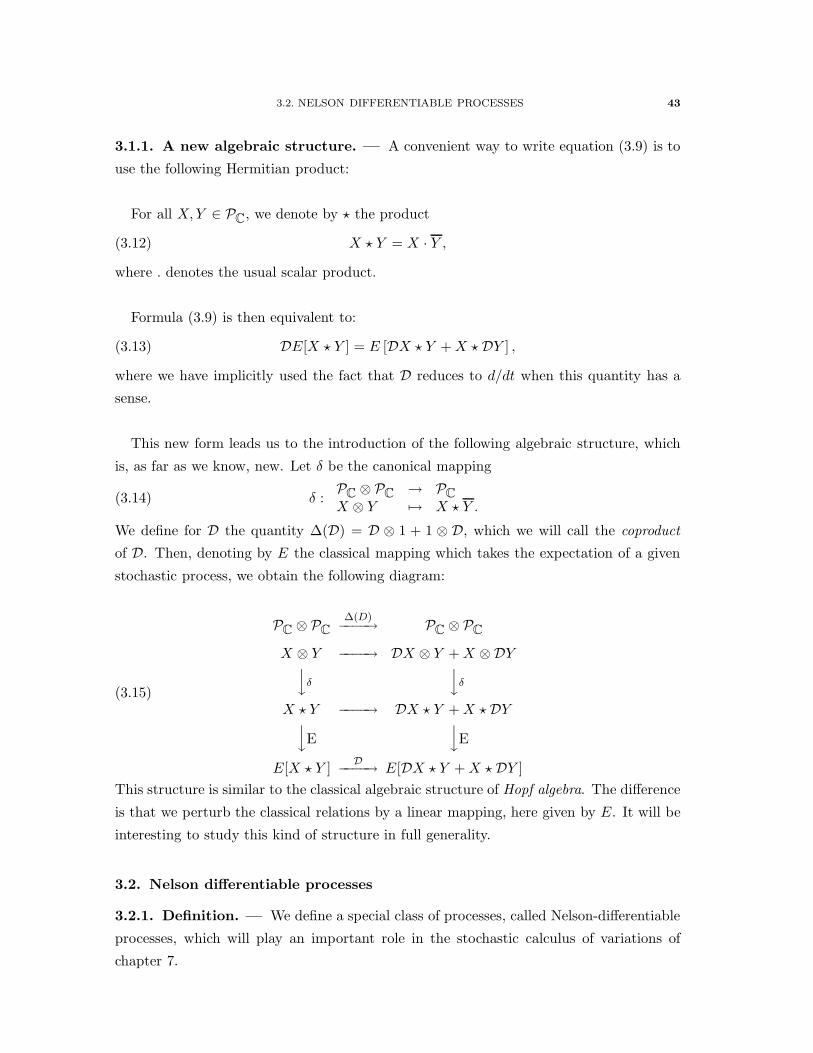
3.1.1. A new algebraic structure. — A convenient way to write equation (3.9) is to

use the following Hermitian product:

For all X,Y ∈ PC, we denote by ⋆ the product

(3.12) X ⋆ Y = X · Y ,

where . denotes the usual scalar product.

Formula (3.9) is then equivalent to:

(3.13) DE[X ⋆ Y ] = E [DX ⋆ Y +X ⋆DY ] ,

where we have implicitly used the fact that D reduces to d/dt when this quantity has a

sense.

This new form leads us to the introduction of the following algebraic structure, which

is, as far as we know, new. Let δ be the canonical mapping

(3.14) δ :PC ⊗ PC → PC

X ⊗ Y 7→ X ⋆ Y .

We define for D the quantity ∆(D) = D ⊗ 1 + 1 ⊗ D, which we will call the coproduct

of D. Then, denoting by E the classical mapping which takes the expectation of a given

stochastic process, we obtain the following diagram:

(3.15)

PC ⊗ PC

∆(D)−−−−→ PC ⊗ PC

X ⊗ Y −−−−→ DX ⊗ Y +X ⊗DYyδ

yδ

X ⋆ Y −−−−→ DX ⋆ Y +X ⋆DYyE

yE

E[X ⋆ Y ]D−−−−→ E[DX ⋆ Y +X ⋆DY ]

This structure is similar to the classical algebraic structure of Hopf algebra. The difference

is that we perturb the classical relations by a linear mapping, here given by E. It will be

interesting to study this kind of structure in full generality.

3.2. Nelson differentiable processes

3.2.1. Definition. — We define a special class of processes, called Nelson-differentiable

processes, which will play an important role in the stochastic calculus of variations of

chapter 7.

44 CHAPTER 3. PROPERTIES OF THE STOCHASTIC DERIVATIVES

Definition 3.1. — A process X ∈ C1(I) is called Nelson differentiable if DX = D∗X.

Notation 3.1. — We denote by N 1(I) the set of Nelson differentiable processes.

A better definition is perhaps to use D instead of D and D∗ saying that Nelson

differentiable processes have a real stochastic derivative.

The main idea behind this definition is that we want to define a class P of processes in

C1(I) such that if X ∈ C

1(I) then for all Y ∈ P, we have

Im(D(X + Y )) = Im(DX).

This condition imposes that Im(DY ) = 0.

This condition will appear more clearly in chapter 7 concerning the stochastic calculus

of variations.

Remark 3.2. — We must keep in mind that our definition of the stochastic derivative

follows the idea of the scale calculus developed in [13] to study non-differentiable functions.

In that context, the existence of an imaginary part for the scale derivative of a function

is seen as a resurgence of its non-differentiability. In particular, when the underlying

function is differentiable then the scale derivative is real. That is why we have chosen to

call processes such that D = D∗ Nelson differentiable.

The definition of Nelson differentiable processes is only given for processes in C1(I). It

is not at all clear to know what is the correct extension to C1C(I). As we have no use of

such kind of notion on C1C(I) we don’t discuss this point here.

Of course a difficult problem is to characterize these processes. The next section dis-

cusses some examples.

3.2.2. Examples of Nelson-differentiable process. — We give examples of Nelson-

differentiable processes.

3.2.2.1. Differentiable deterministic process. — It is probably the first and the simplest

example. Let x(·) be a differentiable deterministic process defined on I × Ω. The past Pand the future F are trivial:

∀t ∈ I, Pt = Ft = ∅,Ω.

As a consequence, we have

∀t ∈ I, Dx(t) = D∗x(t) = x′(t),

where x′ is the usual derivative of x.


3.2. NELSON DIFFERENTIABLE PROCESSES 45

3.2.2.2. A very special random example. — Let X ∈ C1(I). In [53], Nelson shows that

X is a constant (i.e. X(t) is the same random variable for all t) if and only if : ∀t ∈I, DX(t) = D∗X(t) = 0. So it provides us a random example of N 1(I)−process.

3.2.2.3. Nelson-differentiable diffusion processes. — Using theorem 1.1, we can find a

sufficient and necessary condition for a diffusion process to be a Nelson-differentiable

process:

Lemma 3.4. — Let X ∈ Λd with σ = const, then X ∈ N 1(I) if and only if

(3.16) ∇(σ2p)(t,X(t)) = 0.

When the diffusion equation is time homogeneous and the solutions have a density, we

note that this density must be a stationary density. Moreover, the Fokker-Planck equation

(Kolmogorov forward equation) allows us to give a necessary condition (a relation between

the drift and the diffusion coefficient) for a diffusion equation to give a Nelson-differentiable

solution.

3.2.2.4. The random harmonic oscillator. — The random harmonic oscillator satisfies the

stochastic differential equation:

(3.17)

dX(t) = V (t)dtdV (t) = −αV (t)dt − ω2X(t)dt + σdW (t)X(0) = X0, V (0) = V0,

As a consequence, we have X(t) =

∫ t

0V (s)ds with E

[∫ b

0|V (s)|2 ds

]<∞ (b > 0), and

X has a strong derivative in L2. We then obtain DX(t) = D∗X(t) = V (t). Finally, we

have X ∈ N 1([0, b]) and DX(t) = V (t).

3.2.3. Product rule and Nelson-differentiable processes. —

Corollary 3.1. — Let X,Y ∈ C1C(I). If X is Nelson-differentiable then :

(3.18) E[DµX(t) · Y (t) +X(t) · DµY (t)] =d

dtE(X(t), Y (t))

Proof. — This is a simple consequence of the fact that if X = X1 + iX2 is Nelson-

differentiable then Im(DµX1) = Im(DµX2) = 0.


PART II

STOCHASTIC EMBEDDING

PROCEDURES

CHAPTER 4

STOCHASTIC EMBEDDING OF DIFFERENTIAL

OPERATORS

A natural question concerning ordinary and partial differential equations concerns their

behaviour under small random perturbations. This problem is particularly important in

natural phenomena where we know that models are only an approximation of the real

setting. For example, the study of the long term behaviour of the solar system is usually

done by running numerical computations on the n-body problem. However, many effects

in the solar systems are not included in this model and can be of importance if one looks

for a long term integration, as non conservative effects (due to tidal forces between planets)

and the oblatness of the sun which is not yet modelled by a differential equation.

The main problem is then to find the correct analogue of a given differential equation

taking into account the following facts:

i) The classical equation is a good model at least in first approximation,

ii) One must extend this equation to stochastic processes.

Using the stochastic derivative introduced in the previous part, we give a natural em-

bedding of partial or ordinary differential equations into stochastic partial or ordinary

differential equations. It must be pointed out that we do not perturb the classical equa-

tion by a random noise or anything else. In this respect we are far from the usual way of

thinking underlying the fields of stochastic differential equations or stochastic dynamical

systems.

Of course, having this natural embedding, we can naturally define what a stochastic

perturbation of a differential equation is. This is simply a stochastic perturbation of the

stochastic embedding of the given equation. The main point is that we stay in the same

class of objects dealing with perturbations, which is not the case in the stochastic theory

of differential equations, where we jump from classical solutions to stochastic processes in

50 CHAPTER 4. STOCHASTIC EMBEDDING OF DIFFERENTIAL OPERATORS

one step using for example Ito’s stochastic calculus(1).

In this part we first give a general embedding procedure for partial differential equations.

We discuss classical examples, in particular first and second order differential equations.

The case of Lagrangian systems is studied in details in chapter 7. An important part

of classical differential equations coming from mechanics are reversible. This property

is not conserved by the previous stochastic embedding procedure. We define a special

embedding called reversible, which preserves this property, meaning that if X is a solution

of the stochastic embedded equation, then X , the reversed process, is again a solution.

4.1. Stochastic embedding of differential operators

In this part, we first give an abstract embedding procedure based on an extension of

the classical derivative defined in the previous part. We then specialize our embedding

procedure using the stochastic derivative.

4.1.1. Abstract embedding. — Let A be a ring, we denote by A[x] the ring of poly-

nomials with coefficients in A. Let A = C1(Rd × R).

Definition 4.1. — A differential operator is an elements of A[d/dt].

Let O ∈ A[d/dt], the differential operator O is of the form

(4.1) O = a0(•, t) + a1(•, t)d

dt+ · · · + an(•, t) d

n

dtn, ai ∈ A, = 0, . . . , n,

for a given n ∈ N, called the degree of O.

The action of O on a given function x : R → Rd, t 7→ x(t) is denoted O · x and defined

by

(4.2) O · x =

n∑

i=0

ai(x(t), t)dx

dt.

Definition 4.2 (Abstract stochastization). — Let O ∈ A[d/dt] be a differential op-

erator, of the form

(4.3) O = a0(•, t) + a1(•, t)d

dt+ · · · + an(•, t) d

n

dtn, ai ∈ A, = 0, . . . , n,

where n ∈ N is given.

(1)This remark is also valid for all the theories of this kind, using your favourite stochastic calculus, likeMalliavin calculus for example.

4.1. STOCHASTIC EMBEDDING OF DIFFERENTIAL OPERATORS 51

The stochastic embedding of O with respect to the extension δ : P → P is an element

Oδ of P[δ] defined by

(4.4) Oδ = a0(•, t) + a1(•, t)δ + · · · + an(•, t)δn, ai ∈ P, i = 0, . . . , n,

where δn = δ · · · δ.

The action of Oδ on a given stochastic process X, denoted by Oδ ·X is defined by

(4.5) Oδ ·X =

n∑

i=0

ai(X, t)δiX,

where the notation ai(X, t) stands for the stochastic process defined for all ω ∈ Ω by

(4.6) ai(X, y)(ω) = ai(X(ω, t), t).

The main property of this embedding is the fact that

(4.7) Oδ |Pn

det= O,

so that the classical differential equation associated to O, and given by

O · x = 0, (E)

is contained in the stochastic differential equation

Oδ ·X = 0. (SE).

4.1.2. Nelson Stochastic embedding. — Using the stochastic derivative, we have a

particular stochastic embedding procedure.

Definition 4.3 (Stochastization). — Let O ∈ A[d/dt] be a differential operator, of the

form

(4.8) O = a0(•, t) + a1(•, t)d

dt+ · · · + an(•, t) d

n

dtn, ai ∈ A, = 0, . . . , n,


The stochastic embedding of O with respect to the stochastic extension Dµ is an element

Ostoc of C1(I)[Dσ ] defined by

(4.9) Ostoc = a0(•, t) + a1(•, t)D + · · · + an(•, t)Dn, ai ∈ C1(I), i = 0, . . . , n.

We denote by S the operator associating to an operator O of the form 4.8 the operator

Ostoc. As a consequence, we will frequently use the notation S(O) for Ostoc.


In some occasions, in particular for the Euler-Lagrange equation, we will need to con-

sider differential operators in a non-standard form. Precisely, we need to consider operators

like

(4.10) Ba =d

dt a(•, t).

This notation means that Ba acts on a given function as

(4.11) Ba · x =d

dt(a(x(t), t))) .

The basic idea is to define the stochastic embedding of Ba as follow:

Definition 4.4. — The stochastic embedding of the basic brick Ba is given by

(4.12) Ba = D a(•, t).

However, classical properties of the differential calculus allow us to write Ba equivalently

as

(4.13) Ba · x = a′(x)dx

dt.

The stochastic embedding of this new form of Ba is given by

(4.14) Ba.X = a′(X)DX.

The main problem is that in general, we do not have

(4.15) Ba = Ba,

as in the classical case.

This reflects the fact that S acts on operators of a given form and not on operators as

an abstract element of a given algebra. In particular, this is not a mapping.

Nevertheless, there exists a class of functions a such that equation (4.15) is valid:

Lemma 4.1. — Equation (4.15) is satisfied on the set Λd with constant diffusion if a is

an harmonic function.

Proof. — This follows easily from corollary 2.2.

In the sequel we study some basic properties of this embedding procedure on differential

equations.

4.2. FIRST EXAMPLES 53

4.2. First examples

4.2.1. First order differential equations. — Let us consider a first order differential

equation

dx

dt= f(x, t), 1 − (ODE)

where x ∈ R and f : R×R → R is a given function. The stochastic embedding of (1-ODE)

leads to

DX = F (X, t), 1 − (SODE)

where F is real valued.

The reality of F imposes important constraints on solutions of 1-(SODE). Indeed, we

must have

DX = D∗X,

so that X belongs to the class of Nelson-differentiable processes.

In our general philosophy, ordinary differential equations are only coarse approxima-

tions to reality which must include stochastic behaviour in its foundation. A stochastic

perturbation of a first order differential equation is then highly non-trivial. Indeed, we

must consider SODE’s of the form

DX = F (X, t) + ǫG(X, t),

where G(X, t) is now complex valued. As a consequence, we allow solutions to leave the

Nelson-differentiable class.

4.2.2. Second order differential equations. — Let us consider a second order dif-

ferential equation

d2x

dt2+ a(x)

dx

dt+ b(x) = 0, (2 − (ODE)

where x ∈ R, and a, b : R → R are given functions. The stochastic embedding of (2 −(ODE)) leads to

D2X + a(X)DX + b(X) = 0.

In this case, contrary to what happens for first order differential equations, we have no

reality condition which constrains our stochastic process.

In order to study such kind of equations, one can try to reduce it to a first order

equation, using standard ideas. We denote by Y = DX, then the second order equation


is equivalent to the following system of first order stochastic differential equations:

(4.16)

DX = Y,DY = −a(X)Y − b(X).

One must be careful to take Y ∈ C1C(I) as Y is a priori a complex stochastic process. This

remark is of importance since if we apply the stochastic embedding procedure(2) to the

classical system of first order differential equations

(4.17)

dx

dt= y,

dy

dt= −a(x)y − b(x),

by saying that we apply separately the stochastic embedding on each differential equa-

tions, we obtain the stochastic equation (4.16) but with Y ∈ C1(I), which imposes strong

constraints on the solutions of our equations.

This example proves that the stochastic embedding procedure is not so easy to define

if one wants to deal with systems of differential equations. We will return on this problem

concerning the stochastic embedding of Hamiltonian systems.

(2)Note that we have not defined the stochastic embedding procedure on systems of differential equations.

CHAPTER 5

REVERSIBLE STOCHASTIC EMBEDDING

5.1. Reversible stochastic derivative

In our construction of the stochastic derivative, we have imposed some constraints as for

example the gluing to the classical derivative on differentiable deterministic processes. We

have moreover kept some properties of the classical derivative such as linearity. However,

we have not conserved more important properties of the classical derivative which are used

in the study of classical differential equations. For example, let us consider

d2x

dt2= f(x), (E)

which is the basic equation of Newton’s mechanics. An important property of this kind

of equations is its reversibility:

Let t→ x(t) be a solution of (E). We denote by x(t) = x(−t). Then, we have

d2x

dt2=

d

dt(−dx

dt(−t)) =

d2x

dt2(−t) = f(x(−t)) = f(x(t)),

proving that the reversed solution x(t) is again a solution of the same equation. In this

case, we say that the differential equation is reversible.

The reversibility argument used the following important property:

d

dt(x(−t)) = −dx

dt(−t). (R)

The natural way to introduce a notion of reversibility is then to look for the stochastic

differential equation satisfied by X(t) = X(−t) ∈ C1(I) the reversed processes. However,

in general, we do not have access to DX or D∗X. As a consequence, a definition using

this characterization is not effective. In the following, we follow a different strategy.

56 CHAPTER 5. REVERSIBLE STOCHASTIC EMBEDDING

A convenient way to characterize the reversibility of a given differential equation, de-

scribed by a differential operator

(5.1) O =∑

i

aidi

dti∈ R[d/dt]

is to prove that this operator is invariant under the substitution

(5.2) r : R[d/dt] −→ R[d/dt]

which is R linear and defined by

(5.3) r(d/dt) = −d/dt.

We then introduce in our setting, the following analogous substitution:

Definition 5.1. — The reversibility operator R : C[D,D∗] → C[D,D∗] is a C morphism

defined by

(5.4) R(D) = −D∗, R(D∗) = −D.

We have the following immediate consequence of the definition:

Lemma 5.1. — The reversibility operator is an involution of C[D,D∗].

This operator acts non trivially on our stochastic derivative. Precisely, we have:

Lemma 5.2. —

(5.5) R(D) = −D.

The complex nature of the stochastic derivative induces new phenomenon which are

different from the classical case. For example, we have

(5.6) R(D2) = D2,

contrary to what happens for r.

We now define our notion of a reversible stochastic equation.

Definition 5.2. — [Reversibility] Let O ∈ R[D,D∗], then the stochastic equation O ·X =

0 is reversible if and only if R(O) ·X = 0.

A natural problem is the following:

Reversibility problem: Find an operator such that the stochastic embedding of a

reversible equation is again a reversible equation in the sense of definition 5.2.

5.1. REVERSIBLE STOCHASTIC DERIVATIVE 57

Let us consider the family of stochastic derivatives Dµ, µ = 0,±1. Without assuming

a particular form for the underlying equation, the preservation of the reversible character

reduces to prove that the operator δ which is chosen satisfies

(5.7) R(δ) = −δ.

In the family of stochastic derivatives Dµ, µ = 0,±1, only one case is possible:

Lemma 5.3. — A reversibility of a differential equation is always preserved under a

stochastic embedding if and only if this embedding is associated to the stochastic derivative

D0.

Proof. — Essentially this follows from equation (5.5). If we want to preserve reversibility

then the operator Dµ must satisfied R(Dµ) = −Dµ. This is only possible if Dµ is real, i.e.

µ = 0.

It must be pointed out that the operator

D0 =D +D∗

2,

has been obtained by different authors using the following argument:

If we use only D (or D∗) then, we give a special importance to the future (or past) of

the process, which has no physical justification. As a consequence, one must construct

an operator which combines these two quantities in a more or less symmetric way. The

simplest combination is a linear one aD + bD∗ with equal coefficients a = b. The gluing

to the classical derivative leads to a = b = 1/2.

The problem with this construction is that this argument is used on diffusion processes,

where D and D∗ are not free. As a consequence, working with D is the same (even if

the connection with D∗ is not trivial) than working with D∗. We can not really justify

then the use of D0. It must be pointed out that E. Nelson [53] does not use D0 in his

derivation of the Schrodinger equation, but simply D.

Here, this operator is obtained by specialization of Dµ, which form is imposed by our

construction (linearity, gluing to the classical derivative, reconstruction property). The

reconstruction property imposes that µ 6= 0 unless we work with diffusion processes.

Imposing a new constraint on the reversibility on this operator leads us to µ = 0. The

operator D0 is of course defined on C1(I), but in order to satisfy the whole constraints of


our construction, we must restrict its domain to diffusion processes.

We can of course find reversible equations without using D0 but Dµ. We keep the

notations and conventions of chapter 4. We first define the action of R on a given operator

of the form

(5.8) O =

n∑

i=0

ai(•, t)(−1)iDi.

Definition 5.3. — The action of R on (5.8) is denoted R(O) and defined by

(5.9) R(O) =

n∑

i=0

ai(•, t)Di.

The definition 5.2 of a reversible equation can then be extended to cover operators of

the form 5.8.

Using this definition, we can prove that the stochastic equation

D2µX = −∇U(X), (E)

is reversible.

Indeed, we have:

Lemma 5.4. — Equation (E) is reversible.

Proof. — We have

(5.10)R(D2

µX + ∇U(X)) = D2X + ∇U(X),

= D2µX + ∇U(X).

As U is real valued and X are real stochastic processes, we deduce from (E) that

(5.11) D2µX = −∇U(X) = −∇U(X).

We deduce that

(5.12) R(D2µX + ∇U(X)) = 0,

which concludes the proof.

5.2. Iterates

There exists a fundamental difference between D0 and Dµ, µ 6= 0. The operator D0

send real stochastic processes to real stochastic processes in the contrary of Dµ, µ 6= 0,

5.4. REVERSIBLE VERSUS GENERAL STOCHASTIC EMBEDDING 59

which leads to complex stochastic processes. As a consequence, the n-ieme iterates of D0

is simply defined by

(5.13) Dn0 = D0 · · · D0,

without problem, where a special extension of Dµ, µ 6= 0 to complex stochastic processes

must be discussed.

5.3. Reversible stochastic embedding

Using D0, we can define a stochastic embedding which conserves the fundamental prop-

erty of reversibility of a given equation. We keep notations from chapter 4.

Definition 5.4 (Reversible stochastization). — Let O ∈ A[d/dt] be a differential op-

erator, of the form

O = a0(•, t) + a1(•, t)d

dt+ · · · + an(•, t) d

n

dtn, ai ∈ A, = 0, . . . , n,


The reversible stochastic embedding of O is an element Orev of C1(I)[D0] defined by

(5.14) Orev = a0(•, t) + a1(•, t)D0 + · · · + an(•, t)Dn0 , ai ∈ C

1(I), i = 0, . . . , n.

A differential equation (E) is defined by a differential operator O ∈ A[d/dt], i.e. an

equation of the form

O · x = 0, (E)

where x is a function.

Using stochastization, the reversible stochastic analogue of (E) is defined by

Orev ·X = 0, (RSE)

where X is a stochastic process.

5.4. Reversible versus general stochastic embedding

The reversible stochastic embedding leads to very different results than the general

stochastic embedding. We can already see this difference on first order differential equa-

tions. Let us considerdx

dt= f(x),

where x ∈ R and f is a real valued function. The reversible stochastic embedding gives

D0X = f(X).

Contrary to what happens for the stochastic embedding, this equation does not impose

for the solution to be a Nelson differentiable processes.


5.5. Stochastic mechanics and the Stochastization procedure

5.5.1. The Stochastic Newton Equation. — The stochastized version of the classical

system:

x(t) = v(t)

v(t) = K(x(t))(5.15)

is given by:

DX(t) = V (t)

DV (t) = K(X(t))(5.16)

where V ∈ C1C(I) and K is a force: K(x) = −∇U(x) and U a potential.

We can give at least two different kind of solutions of this equation, and so two relevant

models.

In the first one, the component X is the position in the Ornstein-Uhlenbeck theory of

Brownian Motion and is not submitted to a random noise. The system writes:

(5.17)

dX(t) = V (t)dtdV (t) = −αV (t)dt +K(X(t))dt + σdW (t)X(0) = X0, V (0) = V0,

We have noticed in a previous section that, at an equilibrium (i.e. X has a stationary

density) and if e−U is integrable, then:

DX(t) = V (t),(5.18)

D2X(t) = K(X(t)) − iαV (t).(5.19)

Therefore (X,V ) solves the Newton stochastized system (5.16) if and only if α = 0.

Moreover we note in this particuliar case that X is a Nelson-differentiable process.

The second one is described by

(5.20) dX(t) = b(t,X(t))dt + σdW (t),

where the function b must be determined. In this case, we proved that the density pt(x)

of a solution X of (5.16) writes pt(x) = Ψ(t, x)Ψ(t, x) where Ψ solves the Schrodinger

equation: iσ2∂tΨ + σ4

2 ∂xxΨ = UΨ. In this case, X is driven by a Brownian motion and is

not Nelson-differentiable.

PART III

STOCHASTIC EMBEDDING OF

LAGRANGIAN AND HAMILTONIAN

SYSTEMS

CHAPTER 6

STOCHASTIC LAGRANGIAN SYSTEMS

Most of classical mechanics can be formulated using Lagrangian formalism ([5],[2]).

Lagrangian mechanics contains important problems, like the n-body problem. Using our

framework, we study Lagrangian dynamical systems under stochastic perturbations(1).

Our approach is first to embed classical Lagrangian systems, in particular the associated

Euler-Lagrange equation (EL) in order to obtain an idea of what kind of equation govern

stochastic Lagrangian systems. We then develop a stochastic calculus of variations. We

obtain an analogue of the least-action principle(2) which gives a second stochastic Euler-

Lagrange equation, denoted by (SEL) in the sequel. We then prove the following surprising

result, called the coherence lemma: we have S(EL) = (SEL).

The principal interest of Lagrangian systems is that the action of a group of symmetries

leads to first integrals of motion, i.e. functions which are constants on solutions of the

equations of motion. The celebrated theorem of E. Noether gives a precise relation between

symmetries and first integrals. We prove a stochastic analogue of E. Nother theorem.

Finally, we prove that the stochastic embedding of Newton’s Lagrangian systems lead

to a non linear Schrodinger’s equation for a given wave function whose modulus is equal

to the probability density of the underlying stochastic process.

6.1. Reminder about Lagrangian systems

We refer to [5] for more details, as well as [2].

(1)For the n-body problem, which is usually used to study the long term behavior of the solar system[47], this problem is of crucial importance. Indeed, the n-body problem is only an approximation of thereal problem, and even if some numerical simulations take into account relativistic effects [40], this is notsufficient [50].(2)In our case, the word least-action is misleading and a better terminology is stationary (see below).

https://www.researchgate.net/publication/31933049_Laskar_J_A_numerical_experiment_on_the_chaotic_behaviour_of_the_Solar_System_Nature_338_237-238?el=1_x_8&enrichId=rgreq-7dda1c88-e8b1-4054-9900-be366efce6b7&enrichSource=Y292ZXJQYWdlOzIxMjI3Mjc7QVM6MTAxODczOTUyNDkzNTcwQDE0MDEzMDAwNTE5ODE=

https://www.researchgate.net/publication/226515008_Is_the_solar_system_stable?el=1_x_8&enrichId=rgreq-7dda1c88-e8b1-4054-9900-be366efce6b7&enrichSource=Y292ZXJQYWdlOzIxMjI3Mjc7QVM6MTAxODczOTUyNDkzNTcwQDE0MDEzMDAwNTE5ODE=

https://www.researchgate.net/publication/238727546_Mathematical_Methods_of_Classical_Mechanics_GTM_60?el=1_x_8&enrichId=rgreq-7dda1c88-e8b1-4054-9900-be366efce6b7&enrichSource=Y292ZXJQYWdlOzIxMjI3Mjc7QVM6MTAxODczOTUyNDkzNTcwQDE0MDEzMDAwNTE5ODE=

64 CHAPTER 6. STOCHASTIC LAGRANGIAN SYSTEMS

Lagrangian systems play a central role in dynamical systems and physics, in particular

for mechanical systems. A Lagrangian system is defined by a Lagrangian function, com-

monly denoted by L, and depending on three variables: x, v, and t which belongs in the

sequel to R. As Lagrangian systems come from mechanics, the letter x stands for position,

the letter v for speed and the letter t for time. In what follows, we consider a special type

of Lagrangian function called admissible in the following.

Definition 6.1. — An admissible Lagrangian function is a function L such that:

i) The function L(x, v, t) is defined on Rd ×C

d ×R, holomorphic in the second variable

and real for v ∈ R.

ii) L is autonomous, i.e. L does not depend on time.

Condition i) is fundamental. This condition is necessary in order to apply the stochas-

tization procedure (see below). The fact that we only consider autonomous Lagrangian

function is due to technical difficulties in order to take into account backward and forward

filtrations in the computation of the stochastic Euler-Lagrange equation (see below).

Remark 6.1. — In applications, admissible Lagrangian functions L are analytic exten-

sions to the complex domain of real analytic Lagrangian functions. For example, the

classical Newtonian Lagrangian L(x, v) = (1/2)v2 − U(x), defined on an open(3) subset of

R × R, with an analytic potential is an admissible Lagrangian function.

A Lagrangian function L being given, the equation

d

dt

(∂L

∂v

)=∂L

∂x. (EL)

is called the Euler-Lagrange equations.

An important property of the Euler-Lagrange equation is that it derives from a vari-

ational principle, namely the least action principle (see [5],p.59). Precisely, a curve

γ : t 7→ x(t) is an extremal(4) of the functional

Ja,b(γ) =

∫ b

aL(x(t), x(t), t)dt,

on the space of curves passing through the points x(a) = xa and x(b) = xb, if and only if

it satisfies the Euler-Lagrange equation along the curve x(t).

(3)This Lagrangian function is not always defined on R × R. An example is given by Newton’s potentialU(x) = 1/x, x ∈ R

∗.(4)We refer to [5], chapter 3, §.12 for an introduction to the calculus of variations.



6.3. THE COHERENCE PROBLEM 65

6.2. Stochastic Euler-Lagrange equations

We now apply our stochastic procedure S to an admissible Lagrangian.

Lemma 6.1. — Let L(x, v) : Rd × C

d → C be an admissible Lagrangian function. The

stochastic Euler-Lagrange equation obtained from (EL) by the stochastic procedure is given

by

Dµ

(∂L

∂v(X(t),DµX(t)

)=∂L

∂x(X(t),DµX(t)). S(EL)

Proof. — The Euler-Lagrange equation associated to L(x, v) can be seen as the following

differential operator

OEL =d

dt ∂L∂v

− ∂L

∂x,

acting on (x(t), x(t)). The embedding of OEL gives

OEL = Dµ ∂L∂v

− ∂L

∂x.

As OEL acts on (x(t), x(t)), the operator OEL acts on (X(t),DµX(t)). This concludes the

proof.

The free parameter µ ∈ −1, 0, 1 can be fixed depending on the nature of the extension

used.

It must be pointed out that there exist crucial differences between all these extensions

due to the fact that Dµ is complex valued for µ = ±1 and real for µ = 0. Indeed, let us

consider the following admissible Lagrangian function:

L(x, v) =1

2v2 − U(x),

where U is a smooth real valued function. Then, equation S(EL) gives

DµV = U(X),

where V = DµX. When µ = ±1, this equation imposes strong constraints on X due to

the real nature of U(X), namely that D2µX ∈ N

1(I).

On the contrary, when µ = 0, i.e. in the reversible case, these intrinsic conditions

disappear.

6.3. The coherence problem

Up to now, the stochastic embedding procedure can be viewed as a formal manipulation

of differential equations. Moreover, as most classical manipulations on equations do not

66 CHAPTER 6. STOCHASTIC LAGRANGIAN SYSTEMS

commute with the stochastic embedding, this procedure is not canonical (5). In order

to rigidify this construction and to make precise the role of this stochastic embedding

procedure, we study the following problem, called the coherence problem:

We know that the Euler-Lagrange equations are obtained via a least-action principle

on a functional. The main problem is the existence of a stochastic analogue of this least-

action principle, that we can call a stochastic least action principle, compatible with the

stochastic embedding procedure.

L(x(t), x(t))

Least action principle

S// L(X(t),DX(t))

Stochastic least action principle ?

(EL)S

// (SEL)

(6.1)

In the next chapter, we develop the necessary tools to answer to this problem, i.e. a

stochastic calculus of variations. Note that due to the fact that the stochastic Lagrangian

as well as the stochastic Euler-Lagrange equation are fixed, this problem is far from being

trivial. The main result of the next chapter is the Lagrangian coherence lemma which

says precisely that the stochastic Euler-Lagrange equation obtained via the stochastic

embedding procedure coincide with the characterization of extremals for the functional

associated to the stochastic Lagrangian function using the stochastic calculus of varia-

tions. As a consequence, we obtain a rigid picture involving the stochastic embedding

procedure and a first principle via the stochastic least action principle.

This picture will be then extended in another chapter when dealing with the Hamilto-

nian part of this theory.

(5)We return to this problem in our discussion of a stochastic symplectic geometry which can be used tobypass this kind of problem.

CHAPTER 7

STOCHASTIC CALCULUS OF VARIATIONS

The embedding procedure allows us to associate a stochastic Euler-Lagrange equation

to a stochastic Lagrangian function. A basic question is then the existence of an analogue

of the least action principle. In this section, we develop a stochastic calculus of variations

for our Lagrangian function following a previous work of K. Yasue [71]. Our main result,

called the coherence lemma, states that the stochastic Euler-Lagrange equation can be

obtained as an application of a stochastic least action principle. Moreover, this derivation

is consistent with the stochastic embedding procedure.

7.1. Functional and L-adapted process

In the sequel we denote by I a given open interval (a, b), a < b.

We first define the stochastic analogue of the classical functional.

Definition 7.1. — Let L be an admissible Lagrangian function. The functional associ-

ated to L is defined by

Ja,b(X) = E

[∫ b

aL(X(t),DµX(t))dt

],(7.1)

for all X ∈ C1(I).

In what follows, we need a special notion introduced by Yasue [71], and called L-

adaptation:

Definition 7.2. — Let X ∈ C1(I) be a stochastic process. We denote by P and F

the past and the future of X. Let L be an admissible Lagrangian function. A process

X ∈ C1(I) is called L-adapted if:

i)∂L

∂v(X(t),DµX(t)) is adapted to P and F .

https://www.researchgate.net/publication/222600211_Stochastic_calculus_of_variations?el=1_x_8&enrichId=rgreq-7dda1c88-e8b1-4054-9900-be366efce6b7&enrichSource=Y292ZXJQYWdlOzIxMjI3Mjc7QVM6MTAxODczOTUyNDkzNTcwQDE0MDEzMDAwNTE5ODE=


68 CHAPTER 7. STOCHASTIC CALCULUS OF VARIATIONS

ii)∂L

∂v(X(t),DµX(t)) ∈ C

1(I).

Diffusion processes are L-adapted.

7.2. Space of variations

Calculus of variations is concerned with the behaviour of functionals under variations

of the underlying functional space, i.e. objects of the form γ + h, where γ belongs to the

functional space and h is a given functional space of variations. A special care must be

taken in our case to define what is the class of variations we are considering. In general,

this problem is not really pointed out as both variations and curves can be taken in the

same functional space (see [5],p.56,footnote 26). We introduce the following terminology:

Definition 7.3. — Let P be a subspace of C1(I) and X ∈ C

1(I). A P -variation of X is

a stochastic process of the form X + Z, where Z ∈ P .

In the sequel, we consider two subspaces of variations: N1(I) and C

1(I).

The choice of C1(I) is natural. However, doing this we can obtain stochastic processes

with completely different behaviour than X(1).

What is the specific property of X ∈ C1(I) that we want to keep ?

If we refer to the construction of the stochastic derivative, then a main point is the exis-

tence of an imaginary part in DµX(2). This property is related to the non-differentiability

of the underlying stochastic process. We are then lead to search for variations Z which con-

serve this imaginary part. As a consequence, we must consider Nelson difference processes

introduced in the previous part(3), and denoted by N1(I).

7.3. Differentiable functional and stationary processes

We now define our notion of differentiable functional. Let P be a subspace of C1(I).

(1)Of course, this is not the case in the classical case: one consider x ∈ C∞(I) and z ∈ C∞(I) such thatx + h ∈ C∞(I) is very similar to x. For example, we don’t choose z ∈ C0(I) which leads to radically newbehaviour of x + z with respect to x.(2)Of course, as long as µ = ±1. This is of importance since we will be able to choose a more generalvariations space in this case.(3)An analogous problem is considered in [14], where a non differentiable variational principle is defined.



7.3. DIFFERENTIABLE FUNCTIONAL AND STATIONARY PROCESSES 69

Definition 7.4. — Let L be an admissible Lagrangian function and Ja,b the associated

functional. The functional Ja,b is called P -differentiable at an L-adapted process X ∈ C1(I)

if

(7.2) Ja,b(X + Z) − Ja,b(X) = dJa,b(X,Z) +R(X,Z),

where dJa,b(X,Z) is a linear functional of Z ∈ P and R(X,Z) = o(‖ Z ‖).

The stochastic analogue of a stationary point is then defined by:

Definition 7.5. — A P -stationary process for the functional Ja,b is a stochastic process

X ∈ C1(I) such that dJ(X,Z) = 0 for all Z ∈ P .

7.3.1. The P = C1(I) case. — Our main result is:

Lemma 7.1. — The functional Jab defined by (7.1) is C1(I)-differentiable at any L-

adapted process X ∈ C1(I), and for all Z ∈ C

1(I), the differential is given by:

(7.3)

dJab(X,Z) = E

[∫ b

a

[∂L

∂x(X(u),DµX(u)) −D−µ

(∂L

∂v(X(u),DµX(u))

)]Z(u)du

]

+g(Z, ∂vL)(b) − g(Z, ∂vL)(a),

where

(7.4) g(Z, ∂vL)(s) = E [Z(u)∂vL(X(u),DµX(u))] .

Proof. — Let X and Z be two L-adapted processes. The Taylor expansion of L gives:

(7.5)L(X + Z,Dµ(X + Z)) − L(X,Dµ(X)) = ∂xL(X,Dµ(X))Z

+∂vL(X,Dµ(X))Dµ(Z)+o(‖Z‖),

which yields (7.6) by integration and (3.9).

7.3.2. The P = N1(I) case. — Our main result is:

Lemma 7.2. — The functional Jab defined by (7.1) is N1(I)-differentiable at any L-

adapted process X ∈ C1(I), and for all Z ∈ N

1(I) the differential is given by:

(7.6)dJab(X,Z) = E

[∫ b

a(∂xL−Dµ∂vL)(X(u),DµX(u))Z(u)du

]

+g(Z, ∂vL)(b) − g(Z, ∂vL)(a),

where

(7.7) g(Z, ∂vL)(s) = E [Z(u)∂vL(X(u),DµX(u))] .


Proof. — Let X a L−adapted process and H a Nelson-differentiable process. The Taylor

expansion of L gives

(7.8)L(X +H,Dµ(X +H)) − L(X,Dµ(X)) = ∂xL(X,Dµ(X))H

+∂V L(X,Dµ(X))Dµ(H)+o(‖H‖),

which yields (7.6) by integration and (3.18).

7.4. A technical lemma

The classical derivation of the least action principle used a well known result about

bump functions (see [5],p.57). In the stochastic framework, we will need the following

result:

Lemma 7.3. — Let Y ∈ PC be a complex stochastic process. If Y satisfies

(7.9)

∫ 1

0E [Y (u)DµZ(u)] du = 0,

for all Z ∈ N 1([0, 1]) then Y is a constant process.

Proof. — We denote Y = Y1 + iY2, where Yi ∈ PR and DµZ = A, where A ∈ PR. The

equation (7.9) is equivalent to

(7.10)

∫ 10 E [Y1(u)A(u)] du = 0,∫ 10 E [Y2(u)A(u)] du = 0,

for all A ∈ PR such that there exists Z ∈ C1([0, 1]) satisfying DµZ = A.

Let ZY1 be the process defined by

(7.11) ZY1(u) =

∫ u

0Y1(s)ds − u

∫ 1

0Y1(s)ds.

We have ZY1 ∈ N 1(I) with Z(0) = Z(1) = 0. Indeed, we have

(7.12) DµZ(u) = Y1(u) −∫ 1

0Y1(s) ds.

As a consequence, we have in our notations B = 0 and the first equation of (7.10) reduces

to

(7.13)

∫ 1

0E[Y1(u)A(u)]du = E

[∫ 1

0

(Y1(u) −

∫ 1

0Y1(s)ds

)2

du

].

We deduce that Y1 is a constant process, that is for all u ∈ I, Y1(u) = C a.s., where C is

a random variable.

The same argument with the second equation of (7.10) and ZY2 concludes the proof of

the lemma.




7.5. LEAST ACTION PRINCIPLES 71

7.5. Least action principles

As for the computation of the differential of functionals, we must consider two cases:

P = C1(I) and P = N

1(I).

7.5.1. The P = C1(I) case. — The main result of this section is the following analogue

of the least-action principle for Lagrangian mechanics.

Theorem 7.1 (Global Least action principle). — A necessary and sufficient condi-

tion for an L-adapted process to be a C1(I)-stationary process of the functional Jab with

fixed end points X(a) := Xa ∈ H et X(b) := Xb ∈ H is that it satisfies

∂L

∂x(X(t),DµX(t)) −D−µ

[∂L

∂v(X(t),DµX(t))

]= 0.(7.14)

We call this equation the Global Stochastic Euler-Lagrange equation (GSEL).

We have conserved the terminology of least-action principle even if we have no notion

of extremals for our complex valued functional.

Proof. — We denote by I =]0, 1[. Let X ∈ C1(I) be a solution of

(7.15) (∂xL −Dµ∂vL)(X(u),DµX(u)) = 0,

then X is a N 1(I)-stationary process for the functional JI .

Conversely, let X is a C1(I)-stationary process for the functional JI , i.e. dJI(X,Z) = 0.

Writing

(∂xL −Dµ∂vL)(X(u),DµX(u)) = DµY (u),

where

(7.16) Y (u) =

∫ u

0∂xL(X(s),DµX(s))ds − ∂vL(X(u),DµX(u)),

we obtain for any Z ∈ C1(I) with Z(0) = Z(1) = 0:

dJI(X,Z) = E

[∫ 1

0DµY (u)Z(u)du

](7.17)

=

∫ 1

0E[DµY (u)Z(u)]du.

Using the C1(I)-product rule (see equation 3.9), we obtain

(7.18) dJI(X,Z) = −∫ 1

0E[Y (u)DµZ(u)]du.

Using lemma 7.3 we obtain that Y is a constant process.


Hence, we have DµY (u) = 0 and

(7.19) (∂xL −Dµ∂vL)(X(u),DµX(u)) = 0,


7.5.2. The P = N1(I) case. — Our main result is:

Theorem 7.2 (least action principle). — A necessary and sufficient condition for an

L-adapted process to be a N1(I)-stationary process of the functional Jab with fixed end

points X(a) := Xa ∈ H et X(b) := Xb ∈ H is that it satisfies

∂L

∂x(X(t),DµX(t)) −Dµ

[∂L

∂v(X(t),DµX(t))

]= 0.(7.20)

We call this equation the weak stochastic Euler-Lagrange equation (SEL).

Proof. — We denote by I =]0, 1[. Let X ∈ C1(I) be a solution of

(7.21) (∂xL −Dµ∂vL)(X(u),DµX(u)) = 0,

then X is a N 1(I)-stationary process for the functional JI .

Conversely, let X is a N 1(I)-stationary process for the functional JI , i.e. dJI(X,Z) = 0.

Writing

(∂xL −Dµ∂vL)(X(u),DµX(u)) = DµY (u),

where

(7.22) Y (u) =

∫ u

0∂xL(X(s),DµX(s))ds − ∂vL(X(u),DµX(u)),

we obtain for any Z ∈ N 1(I) with Z(0) = Z(1) = 0:

dJI(X,Z) = E

[∫ 1

0DµY (u)Z(u)du

](7.23)

=

∫ 1

0E[DµY (u)Z(u)]du.

Using the N 1(I)-product rule (see equation 3.18), we obtain

(7.24) dJI(X,Z) = −∫ 1

0E[Y (u)DµZ(u)]du.

Using lemma 7.3, we deduce that Y is a constant process, that is for all u ∈ I, Y (u) = C

a.s. where C is a random variable.

Hence, we obtain DµY (u) = 0 and

(7.25) (∂xL −Dµ∂vL)(X(u),DµX(u)) = 0,

7.6. THE COHERENCE LEMMA 73


7.6. The coherence lemma

It is not clear that the stochastic Euler-lagrange equation obtained by the stochastiza-

tion procedure and the N1(I) or C

1(I) least-action principle coincide. One easily sees that

this is not the case for P = C1(I). In the contrary, we have the following lemma, called

the coherence lemma, which ensure that for P = N1(I) we obtain the same equations.

Lemma 7.4 (coherence lemma). — The following diagram commutes :

L(x(t), x′(t))


S// L(X(t),DX(t))

Stochastic Least action principle

(EL)S

// (SEL)

(7.26)

Proof. — This is an immediate consequence of the previous results.

Remark 7.1. — When µ = 0, i.e. in the reversible case, the previous lemmas and the-

orems are true under C1(I) variations. Note that when µ = 0, our stochastic derivatives

coincides with the Misawa-Yasue [52] canonical formalism for stochastic mechanics.

CHAPTER 8

THE STOCHASTIC NOETHER THEOREM

A natural question arising from the stochastization procedure of classical dynamical

systems, in particular, Lagrangian systems, is to understand what remains from classical

first integrals of motion. First integrals play a central role in many problems like the n-

body problem. In this section, we obtain a stochastic analogue of the Noether theorem. We

then defined the notion of first integrals for stochastic dynamical systems. We also discuss

the consequences of the existence of first integrals in the context of chaotic dynamical

systems.

8.1. Tangent vector to a stochastic process

Let X ∈ C1(I) be a stochastic process. We define the analogue of a tangent vector to

X at point t.

Definition 8.1. — Let X ∈ C1(I), I ⊂ R. The tangent vector to X at point t is the

random variable DX(t).

Remark 8.1. — Of course, in order to define stochastic Lagrangian systems in an in-

trinsic way, one must define the stochastic analogue of the tangent bundle to a smooth

manifold. In our case, it is not clear what is the adequate geometric object underlying

stochastic Lagrangian dynamics. For example, we can think of multidimensional Brow-

nian surfaces ([23],§.16.4). All these questions will be developed in a forthcoming paper

[17].

8.2. Canonical tangent map

In the sequel, we will need the following mapping called the canonical tangent map:

76 CHAPTER 8. THE STOCHASTIC NOETHER THEOREM

Definition 8.2. — For all X ∈ C1(I), we define the canonical tangent map as

(8.1) T :C

1(I) −→ C1(I) × PC,

X 7−→ (X,DX).

The mapping T will be used in the following section to define the analogue of the linear

tangent map for a stochastic suspension of a one parameter group of diffeomorphisms.

8.3. Stochastic suspension of one parameter family of diffeomorphisms

We begin by introducing a useful notion of stochastic suspension of a diffeomorphism.

Definition 8.3. — Let φ : Rn → R

n be a diffeomorphism. The stochastic suspension of

φ is the mapping Φ : P → P defined by

(8.2) ∀X ∈ P, Φ(X)t(ω) = φ(Xt(ω)).

In what follows, we will frequently use the same notation for the suspension of a given

diffeomorphism and the diffeomorphism.

Remark 8.2. — It seems strange that we have not defined directly the notion of diffeo-

morphism on a subset E of the stochastic processes, i.e. mapping Φ : E → E which are

Frechet differentiable with an inverse which is also Frechet differentiable. However, these

objects do not always exist.

Using the stochastic suspension, we are able to define the notion of stochastic suspension

for a one-parameter group of diffeomorphisms.

Definition 8.4. — A one-parameter group of transformations Φs : A→ A, s ∈ R, where

A ⊂ P, is called a φ-suspension group acting on A if there exist a one parameter group of

diffeomorphisms φs : Rn → R

n, s ∈ R, such that for all s ∈ R, we have:

i) Φs is the stochastic suspension of φs,

ii) for all X ∈ A, Φs(X) ∈ A.

This notion of suspension group comes from our framework. It relies on the fact

that we want to understand how symmetries of the underlying Lagrangian systems are

transported via the stochastic embedding. The non-trivial condition on the stochastic

suspension of a one-parameter group of diffeomorphisms acting on A comes from condition

ii). However, imposing some conditions on the underlying one parameter group, we can

obtain a stochastic one parameter group which acts on the set E of good diffusion processes.

Precisely, let us introduce the following class of one-parameter groups:

8.3. STOCHASTIC SUSPENSION OF ONE PARAMETER FAMILY OF DIFFEOMORPHISMS 77

Lemma 8.1. — An admissible one parameter group of diffeomorphisms Φ = φss∈R is

a one parameter group of C2-diffeomorphisms on Rn such that

(8.3) (s, x) 7→ ∂

∂xφs(x) is C2.

The main property of admissible one parameter groups is the fact that they are well-

behaved on the set of good diffusions.

Lemma 8.2. — Let Φ = (φs)s∈R be a stochastic suspension of an admissible one param-

eter group of diffeomorphisms. Then, for all X ∈ E, we have for all t ∈ I, and all s ∈ R:

i) The mapping s 7→ DµΦsX(t) ∈ C1(R), (a.s.),

ii) We have∂

∂s[Dµ(φs(X))] = Dµ

[∂φs(X)

∂s

](a.s.).

This lemma is trivial in the classical case where X is a smooth function and Dµ is

the classical derivative with respect to time. Indeed, it reduces to the Schwarz lemma.

However, this inequality plays an essential role in the derivation of the classical Noether’s

theorem (see [5],p.89).

Proof. — According to (2.4),

Dµφs(X)(t) = DµX(t) · ∂xφs

∂xX(t) + iµ

σ(t,Xt)2

2

∂2xφs

∂x2X(t) (a.s.).

So :

∂

∂sDµφs(X)(t) = DµX(t) · ∂

∂s

∂xφs

∂xX(t) + iµ

σ(t,Xt)2

2

∂

∂s

∂2xφs

∂x2X(t) (a.s.).

Since (s, x) 7→ φs(x) is C2, we have∂

∂s

∂

∂xφs(x) =

∂

∂x

∂

∂sφs(x) by the Schwarz lemma. In

the same way,∂

∂s

∂2

∂x2φs(x) =

∂

∂x

∂

∂s

∂

∂xφs(x)

because (s, x) 7→ ∂∂xφs(x) is C2.

Therefore :∂

∂s

∂2

∂x2φs(x) =

∂2

∂x2

∂

∂sφs(x).

Applying (2.4) to∂

∂sφs, we can conclude that :

∂

∂s[Dµ(φs(X))] = Dµ

[∂φs(X)

∂s

](a.s.).

It must be pointed out that every extension of this lemma will lead to a substantial

improvement of the following stochastic Noether theorem.



8.4. Linear tangent map

Let X ∈ C1(I) and φ : R

n → Rn be a diffeomorphism. The image of X under the

stochastic suspension of φ, denoted by Φ, induces a natural map for tangent vectors de-

noted by Φ∗, called the linear tangent map, and defined as in classical differential geometry

by:

Definition 8.5. — Let Φ be a stochastic suspension of a diffeomorphism. The linear

tangent map associated to Φ, and denoted by Φ∗, is defined for all X ∈ C1(I) by

(8.4) Φ∗(X) = T (Φ(X)) = (Φ(X),D(Φ(X))).

All the quantities are well defined as diffeomorphisms send C1(I) on C

1(I).

8.5. Invariance

We then obtain the following notion of invariance under a one parameter group of

diffeomorphisms.

Definition 8.6. — Let Φ = φss∈R be a one-parameter group of diffeomorphisms and

let L be a functional L : C1(I) → C

1C(I). The functional L is invariant under the one-

parameter group of diffeomorphisms Φ if

L(φ∗X) = L(X), for all φ ∈ Φ.

As a consequence, if L is invariant under Φ, we have

L(φs(X),D(φs(X))) = L(X,DX),

for all s ∈ R and X ∈ C1(I).

Remark 8.3. — We note that this notion of invariance under a one parameter group

of diffeomorphisms does not coincide with the same notion as defined by K. Yasue ([71],

p.332, formula (3.1)) which in our notation is given by:

L(φs(X), φs(DX)) = L(X,DX), for all s ∈ R and X ∈ C1(I).

In fact, K. Yasue definition of invariance does not reduce to the classical notion (see for

example [5],p.88) for differentiable deterministic stochastic processes.

Moreover, Yasue’s definition is not coherent with the invariance notion used in his proof

of the stochastic Noether’s theorem ([71],theorem 4,p.332). See the comment below.


8.6. THE STOCHASTIC NOETHER’S THEOREM 79

8.6. The stochastic Noether’s theorem

Noether’s theorem has already been generalized a great number of times and covers

sometimes different statements [32]. Here, we follow V.I. Arnold’s ([5],p.88) presentation

of the Noether theorem for Lagrangian systems. We correct a previous work of K. Yasue

([71], Theorem 4,p. 332-333).

Theorem 8.1. — Let Ja,b be a functional on C1(I) given by

Ja,b(X) = E

[∫ b

aL(X(t),DX(t))dt

].

with L invariant under the one-parameter group Φ = φss∈R.

Let X ∈ C1(I) be a C

1(I)-stationary point of Ja,b with fixed end points condition

X(a) = Xa, and X(b) = Xb.

Then, we haved

dtE

[gradvL

∂Y

∂s

∣∣∣∣s=0

]= 0,

where

(8.5) Ys = Φs(X).

Proof. — Let Y (s, t) = φsX(t) for s ∈ R and a 6 t 6 b.

As L is invariant under Φ = φss∈R, we have

∂

∂sL(Y (s, t),DµY (s, t)) = 0 (a.s.).

As Y (., t) and DµY (., t) belong to C1(R) for all t ∈ [a, b] by definition 8.4, iii), we obtain

(8.6) gradxL · ∂Y∂s

+ gradvL∂DµY

∂s= 0 (a.s.).

Using (Lemma 8.2,ii), this equation is equivalent to

(8.7) gradxL · ∂Y∂s

+ gradvLDµ

(∂Y

∂s

)= 0 (a.s.).

As X = Y |s=0 is a stationary process for Ja,b, we have

(8.8) gradxL = D−µgradvL.

As a consequence, we deduce that(

[DµgradvL] · ∂Y∂s

+ gradvLDµ

(∂Y

∂s

))∣∣∣∣s=0

= 0 (a.s.).

Taking the absolute expectation, we obtain

(8.9) E

[([DµgradvL] · ∂Y

∂s+ gradvLDµ

(∂Y

∂s

))∣∣∣∣s=0

]= 0.




Using the product rule, we obtain

d

dtE

[gradvL

∂Y

∂s

∣∣∣∣s=0

]= 0,


8.7. Stochastic first integrals

The previous theorem leads us to the introduction of the notion of first integral for

stochastic Lagrangian systems(1).

8.7.1. Reminder about first integrals. — Let X be a Ck vector field or Rn, k > 1

(k could be ∞ or ω, i.e. analytic). We denote by φx(t) the solution of the associated

differential equation, such that φx(0) = x and by S the set of all these solutions.

A first integral of X is a real valued function f : Rn → R such that for all φx(t) ∈ S,

we have

(8.10) f(φx(t)) = cx,

where cx is a constant.

We have not imposed any kind of regularity on the function f , so that f can be just

C0. In this case, the existence of a first integral does not impose many constraint on the

dynamics.

If f is at least C1, then we can characterize first integrals by the following constraint:

(8.11) X · f = 0.

8.7.2. Stochastic first integrals. — The previous paragraph leads us to searching for

an analogue of the classical notion of first integrals as a functional defined on the set of

solutions of a given stochastic Euler-Lagrange equation(2) and real valued. Looking for

the stochastic Noether theorem, we choose the following definition:

Definition 8.7. — Let L be an admissible Lagrangian system. A functional I : C1(I) →

R is a first integral for the Euler-Lagrange equation associated to L if

(8.12)d

dt[I(X)] = 0,

for all X satisfying the Euler-Lagrange equation.

(1)Of course, one can extend this definition to general stochastic dynamical systems.(2)Of course, this definition will extend to arbitrary stochastic dynamical systems.

8.8. EXAMPLES 81

We can now interpret the stochastic Noether theorem in term of first integrals, i.e.

the fact that the invariance of the Lagrangian L under of a one parameter group of

diffeomorphisms Φ = (φs)s∈R induces the existence of a first integral for the associated

Euler-Lagrange equation, defined by

(8.13) I(X) = E

[gradvL

∂φsX(t)

∂s

∣∣∣∣s=0

].

8.8. Examples

8.8.1. Translations. — We follow the first example given by V.I. Arnold ([5],p.89) for

Noether theorem. Let L be the Lagrangian defined by

(8.14) L(X,V ) =V 2

2− U(X), where X ∈ R

3,

V = (V1, V2, V3) ∈ C3, V 2 := V 2

1 + V 22 + V 2

3 and U is taken to be invariant under the one

parameter group of translations:

(8.15) φs(x) = x+ se1,

where e1, e2, e3 is the canonical basis of R3.

Then, by the Stochastic Noether’s theorem, the quantity

(8.16) E[DX1]

is a first integral since ∂V L = V and ∂sφs(X1(ω)) = e1.

8.8.2. Rotations. — We keep the notations of the previous paragraph. We consider

the Lagrangian of the two-body problem in R3, i.e.

(8.17) L(X,V ) = q(V ) − 1

|X| where q(V ) =V 2

2,

where | . | denotes the classical norm on R3 defined for all X ∈ R

3, X = (X1,X2,X3) by

| X |2= X21 +X2

2 +X23 .

We already know that the classical Lagrangian L is invariant under rotations when

X ∈ R3 and V ∈ R

3. Here, we must prove that the same is true for the extended object,

i.e. for L defined over R3 \ 0 × C

3. This extension, as long as it is defined, is canonical.

Indeed, we define q(z) for z ∈ C3 as

(8.18) q(z) =1

2(z2

1 + z22 + z2

3), z = (z1, z2, z3) ∈ C3.

Note that our problem is not to discuss an analytic extension of the real valued kinetic

energy but only to look for the same function on C3 simply replacing real variables by

complex one. As long as the new object is well defined this procedure is canonical, which



is not the case if we search for an analytic extension of q over C3 which reduces to q on

R3.

Our main result is then that this group of symmetry is preserved under stochastization,

which is in fact a general phenomenon that will be discuss elsewhere.

Lemma 8.3. — The lagrangian L defined over R3 \0×C

3 is invariant under rotations

φθ,k around the ek axis by the angle θ, k = 1, 2, 3.

The proof is based on the two following facts:

– As φθ,k is a linear map whose matrix coefficients do not depend on t, we have

(8.19) Dµ [φθ,k(X)] = φθ,k [DµX] ,

where φθ,k is trivially extended to C3.

– A simple calculation gives

(8.20) ∀ z ∈ C3, q(φθ,k(z)) = q(z).

We easily deduce the φθ,k invariance of L, i.e. that

(8.21) L(φθ,kX,D(φθ,kX)) = L(X,DX).

We now compute: ∂θφθ,k(X)|θ=0 = ek ∧X and

∂V L(X,DX) · ∂θφθ,k(X)|θ=0 = (X ∧ DX)k.

Therefore the expectation of the ”complex angular momentum” X ∧DX is a conserved

vector (∧ is extended in a natural way to complex vectors).

8.9. About first integrals and chaotic systems

In this section, we discuss some consequences of the stochastic Noether’s theorem in

the context of chaotic dynamical systems. The study of deterministic chaotic dynamical

systems is difficult.

Here again, we return to the classical n-body problem, n > 3. In this case, in particular

for large n, the dynamics of the system is very complicated and only numerical results give

a global picture of the phase space. Despite the existence of a chaotic behaviour, there

exist several well known first integrals of the system.

These integrals are used as constraints on the dynamics and can give interesting results,

as for example J. Laskar’s [41] approach to the Titus-Bode law for the repartition of the

https://www.researchgate.net/publication/12304849_On_the_Spacing_of_Planetary_Systems?el=1_x_8&enrichId=rgreq-7dda1c88-e8b1-4054-9900-be366efce6b7&enrichSource=Y292ZXJQYWdlOzIxMjI3Mjc7QVM6MTAxODczOTUyNDkzNTcwQDE0MDEzMDAwNTE5ODE=

8.9. ABOUT FIRST INTEGRALS AND CHAOTIC SYSTEMS 83

planets in the solar systems and extra-solar systems.

Using our approach, we can go further by claiming that such kind of integrals continue to

exist even if one consider a more general class of perturbations including stochasticity. We

note that this result is fundamental as long as one wants to relate numerical computations

on the n-body problem with the real dynamical behaviour of the solar systems, and in

this particular example, the dynamics of the protoplanetary nebulae.

CHAPTER 9

NATURAL LAGRANGIAN SYSTEMS AND THE

SCHRODINGER EQUATION

In this section, we explore in details the stochastization procedure for natural La-

grangian systems. In particular, by introducing a suitable analogue of the action

functional, we prove that the stochastic Euler-Lagrange equation leads to a non-linear

Schrodinger equation, depending on a free parameter related to a normalization constraint.

For a suitable choice of this parameter we then obtain the classical linear Schrodinger

equation.

9.1. Natural Lagrangian systems

In ([5],p.84), V.I. Arnold introduces the following notion of natural Lagrangian systems:

Definition 9.1. — A Lagrangian system is called natural if the Lagrangian function is

equal to the difference between kinetic and potential energy:

L(x, v) = T (v) − U(x).

As an example, we have the natural Lagrangian function associated to Newtonian me-

chanics:

L(x, v) =1

2v2 − U(x),

where U is of class C∞.

9.2. Schrodinger equations

9.2.1. Some notations and a reminder of the Nelson wave function. — We recall

that Λd is the space of ”good” diffusion processes. Let Λgd be the subspace of Λd whose

elements have a smooth gradient drift. We then set:

S = X ∈ Λd | D2X(t) = −∇U(X(t)).


86 CHAPTER 9. NATURAL LAGRANGIAN SYSTEMS AND THE SCHRODINGER EQUATION

For a diffusion X in Λd with drift b and density function pt(x), we set:

(9.1) Θ = (R+ × Rd) \ (t, x), | pt(x) = 0.

If X ∈ Λgd then there exist real valued functions R and S smooth on Θ such that

(9.2) DX(t) =

(b− σ2

2∇ log(pt) + i

σ2

2∇ log(pt)

)(X(t)) = (∇S + i∇R)(X(t)),

since b is a gradient. Obviously:

(9.3) R(t, x) =σ2

2log(pt(x)).

In this case, we introduce the function:

(9.4) Ψ(t, x) = e

(R + iS)(t, x)

K

(where K is a positive constant) called the wave function.

The wave function has the same form than that of Nelson one (see [53]). We then set

A = S − iR. So Ψ = eiA

K and ∇A(t,X(t)) = DX(t). For a suitable K, Nelson shows

that if X satisfies its stochastized Newton equation (which is the real part of ours) then

Ψ satisfies a Schrodinger equation. We show, by using our operator D, the same kind of

result in the next section.

9.2.2. Schrodinger equations as necessary conditions. —

Theorem 9.1. — If X ∈ S ∩ Λgd, then the wave function (9.4) satisfies the following

non-linear Schrodinger equation on the set Θ:

(9.5) iK∂tΨ +K(K − σ2)

2

(∂xΨ)2

Ψ+σ2

2∆Ψ = UΨ,

Proof. — As U is a real valued function, X ∈ S implies

D2X(t) = −∇U(X(t)).

The definition of Ψ implies that on Θ

∇A = −iK∇Ψ

Ψ.

Since ∇A(t,X(t)) = (DX)(t), we obtain

iKD∂xΨ

Ψ(t,X(t)) = ∇U(t,X(t)).

Therefore, considering the k-th component of the last equation and using lemma 2.4, we

deduce

iK

(∂t∂kΨ

Ψ+ DX(t) · ∇∂kΨ

Ψ− i

σ2

2∆∂kΨ

Ψ

)(t,X(t)) = ∂kU(X(t)).

9.2. SCHRODINGER EQUATIONS 87

Now DX(t) = −iK∇Ψ

Ψ(t,X(t)). Thus, by Schwarz lemma, we obtain

DX(t) · ∇∂kΨ

Ψ= −iK

d∑

j=1

∂jΨ

Ψ∂j∂kΨ

Ψ= − iK

2∂k

d∑

j=1

(∂jΨ

Ψ

)2

,

and

∆∂kΨ

Ψ=

d∑

j=1

∂2j

∂kΨ

Ψ= ∂k

d∑

j=1

∂j

(∂jΨ

Ψ

)= ∂k

d∑

j=1

∂2j Ψ

Ψ−

(∂jΨ

Ψ

)2

.

Therefore

iK∂k

∂tΨ

Ψ+ i

σ2 −K

2∂k

d∑

j=1

(∂jΨ

Ψ

)2

− iσ2

2

∆Ψ

Ψ

(t,X(t)) = ∂kU(X(t)).

By adding an appropriate function of t in S, we can arrange the constant in x of integration

in equation to be zero, and formula (9.5) follows as claimed.

In order to recover the classical linear Schrodinger equation, we must choose the nor-

malization constant K. The main point is that in this case, we obtain a clear relation

between the modulus of the wave function and the density of the underlying diffusion

process. Precisely, we have:

Corollary 9.1. — We keep the notations and assumptions of theorem (9.2.3). We as-

sume that

K = σ2.

Then the wave functional Ψ satisfies the linear Schrodinger equation

iσ2∂tΨ +σ4

2∆Ψ = UΨ,(9.6)

Moreover, if pt(x) is the density of the process X(t) at point x, then we have

(ΨΨ)(t, x) = pt(x).

Proof. — K = σ2 kills the non-linearity in equation (9.5) and furthermore

log(ΨΨ) =2

KR =

2

σ2R = log(p).


9.2.3. Remarks and questions. —

– Obviously Λ1 ⊂ Λg1 since b is continuous.

– A natural question is to know if the converse of the corollary of () is true. More

precisely, if Ψ satisfies a linear Schrodinger equation, can we construct a process X

which belongs to S ∩ Λgd and whose density is such that pt(x) = |Ψ(t, x)|2 ?

88 CHAPTER 9. NATURAL LAGRANGIAN SYSTEMS AND THE SCHRODINGER EQUATION

R. Carmona tackled the problematic of the so-called Nelson processes and proved

in [11] under some conditions the existence of a process X with gradient drift related

to Ψ and whose density is such that pt(x) = |Ψ(t, x)|2. However we do not know

if this process belongs to our space of good diffusions processes (which may turn

to be a little restrictive class in this case), but we can prove formally, i.e. even so

assuming that the formulae of the stochastized derivative to a function of the process

holds, that X satisfies the Newton stochastized equation. Therefore, this leads one

to question the extension of the derivative operator and the way it acts on a large

class of processes. This problem will be treated in a forthcoming paper (See [18]).

– The fact that a processX satisfies the stochastized Newton equation of Nelson implies

(D2−D2∗)X = 0 (for the potential U is real). This is a general fact for diffusion with

gradient drift. Indeed, we can prove:

Lemma 9.1. — Let X ∈ Λd, b its drift and p its density function. Let Gi be the

i-th column of the matrix (Gij) := (∂jbi − ∂ibj). Then (D2 −D2∗)X = 0 if and only

if for all t > 0, div(ptGi) = 0.

Thus, if X ∈ Λgd it is clear that (D2 −D2

∗)X = 0 since the form∑bk∂k is closed

and so G = 0. An interesting question is then to know if the converse is true. So we

may wonder ourselves if S ⊂ Λgd.

The difficulty relies on the fact that p and b are related via the Fokker-Planck

equation, so the condition div(ptGi) = 0 may not be the good formulation. However,

one could use the work of S. Roelly and M. Thieullen in [61] who use an integration

by parts via Malliavin Calculus to characterize gradient diffusion, in order to give a

positive or negative answer to our question.

– A basic notion in mechanics is that of action (see [5],p.60). The action associated

to a Lagrangian system is in general obtained via the action functional. In our

framework, a natural definition for such an action functional is given by:

Definition 9.2. — Let A be the functional defined on [a, b] × C1([a, b]) by:

(9.7) ∀t ∈ [a, b], ∀X ∈ C1(I), A(t,X) = E

[∫ t

aL(Xs, (DX)s)ds |Xt

].

This functional is called the action functional.

https://www.researchgate.net/publication/225745588_A_characterization_of_reciprocal_processes_via_an_integration_by_parts_formula_on_the_path_space?el=1_x_8&enrichId=rgreq-7dda1c88-e8b1-4054-9900-be366efce6b7&enrichSource=Y292ZXJQYWdlOzIxMjI3Mjc7QVM6MTAxODczOTUyNDkzNTcwQDE0MDEzMDAwNTE5ODE=

9.3. ABOUT QUANTUM MECHANICS 89

Using this action functional, we have some freedom to define the corresponding

“action”. The natural one is defined by

(9.8) AX(t, x) = E

[∫ t

aL(Xs, (DX)s)ds |Xt = x

].

Usually, the wave function associated to AX an denoted by ψ is then defined as

(9.9) ψX(t, x) = expiAX(t,x) .

However, it is not at all clear that such kind of function satisfies the gradient condi-

tion, i.e. that

(9.10) ∇A(t,X(t)) = DX(t),

which is fundamental in our derivation of the Schrodinger equation.

However, the condition 9.10 is equivalent to prove that the real part of DX is a

gradient, which is not at all trivial in dimension greater than two.

9.3. About quantum mechanics

Even if we look for dynamical systems, our work can be used in the context of the

so-called Stochastic mechanics, developed by Nelson [53]. The basic idea is to reexpress

quantum mechanics in terms of random trajectories. We refer to [12] for a review.

The stochastic embedding theory can be seen as a quantization procedure, i.e. a formal

way to go from classical to quantum mechanics. This approach is already different from

Nelson’s approach, which do not define a rigid procedure to associate to a given equation

a stochastic analogue. Moreover, the acceleration defined by Nelson as

(9.11) a(X) =DD∗(X) +D∗D(X)

2,

is only a particular choice. Many authors have tried to justify this form ([59],[60]) or to

try another one. In our context, the form of the acceleration is fixed and corresponds, as

in the usual case, to the second (stochastic) derivative of X. As a consequence, stochastic

embeddings can be used to provide a conceptual framework to stochastic mechanics.

We refer to [59] where a complex valued velocity for a stochastic process is introduced

corresponding to the stochastic derivative of X.

However, stochastic mechanics as well as its variants have many drawbacks with respect

to the initial wish to describe quantum mechanical behaviours. We refer to [55] and [12]

for details. This is the reason why we will not develop further this topic.

https://www.researchgate.net/publication/229318265_A_new_formulation_of_stochastic_mechanics?el=1_x_8&enrichId=rgreq-7dda1c88-e8b1-4054-9900-be366efce6b7&enrichSource=Y292ZXJQYWdlOzIxMjI3Mjc7QVM6MTAxODczOTUyNDkzNTcwQDE0MDEzMDAwNTE5ODE=


https://www.researchgate.net/publication/234998853_Hamilton's_principle_in_stochastic_mechanics?el=1_x_8&enrichId=rgreq-7dda1c88-e8b1-4054-9900-be366efce6b7&enrichSource=Y292ZXJQYWdlOzIxMjI3Mjc7QVM6MTAxODczOTUyNDkzNTcwQDE0MDEzMDAwNTE5ODE=

CHAPTER 10

STOCHASTIC HAMILTONIAN SYSTEMS

In this part, we introduce the stochastic pendant of Hamiltonian systems for classical

Lagrangian systems. The strategy is first to define the stochastic analogue of the classical

momentum. We then define a stochastic Hamiltonian. However, this Hamiltonian is not

obtained by the classical stochastic embedding procedure. This is due to the fact that the

momentum process is complex valued. As a consequence, we must modify the procedure in

order to obtain a coherent picture between the classical formalism and the stochastic one.

This leads us to define the stochastic Hamiltonian embedding procedure which reflects in

fact the non trivial character of the underlying stochastic symplectic geometry to develop.

Having the stochastic Hamiltonian we prove a Hamilton least action principle using our

stochastic calculus of variations. We then obtain an analogue of the Lagrangian coherence

lemma in this case up to the fact that the underlying stochastic embedding procedure is

now the Hamiltonian one.

10.1. Reminder about Hamiltonian systems

We denote by I an open interval (a, b), a < b.

Let L : Rd × R

d × R → R be a convex Lagrangian. The Lagrangian functional over

C1(R) is defined by

(10.1) L :C1(R) −→ C1(R),x 7−→ L(x, x, t).

We can associate to L a Hamiltonian function using the Legendre transformation

([5],p.65). From the functional side, this induces a change of point of view, as the func-

tional is not seen as acting on x(t), which is the so-called configuration space of classical

mechanics, but on (x(t), x(t)) which is associated to the phase-space. This dichotomy

between position and velocities has of course many consequences, one of them being that

the system is more symmetric (the symplectic structure).

92 CHAPTER 10. STOCHASTIC HAMILTONIAN SYSTEMS

Definition 10.1. — Let L(x, v) be an admissible Lagrangian system. For all x ∈ C1, we

denote by

(10.2) p(x) =∂L

∂v(x, x),

the momentum variable.

We now introduce an important class of Lagrangian systems.

Definition 10.2. — Let L(x, v) be an admissible lagrangian system. The Lagrangian L

is said to possess the Legendre property if there exists a function f : Rd → R

d, called the

Legendre transform, such that

(10.3) x = f(x, p),

for all x ∈ C1.

Most classical examples in mechanics possess the Legendre property. This follows from

the convexity of L in the second variable (see [5],p.61-62).

We can introduce the fundamental object of this section:

Definition 10.3. — Let L be an admissible Lagrangian system which possesses the Leg-

endre property. The Hamiltonian function associated to L is defined by

(10.4) H(p, x) = pf(x, p) − L(x, f(x, p)),

where f is the Legendre transform.

The Hamiltonian function plays a fundamental role in classical mechanics. We introduce

the stochastic analogue in the next section.

10.2. The momentum process

A natural stochastic analogue of the momentum variable is defined as follow:

Definition 10.4. — Let L(x, v) be an admissible Lagrangian system. For all X ∈ C1(I),

we define the stochastic process P (t), called the canonical momentum process, by

(10.5) P (t) =∂L

∂v(X(t),DX(t)).

This definition can be made more natural using the embedding ι defined from C0(I) on

Pdet and the linear tangent map introduced in chapter 8. Indeed, the momentum process

can be viewed as a functional on X ∈ C1(I), P : C

1(I) → PC defined by (10.5). We have

for all X ∈ P1det = ι(C1(I)),

(10.6) P (X) = ι(p(x)),

10.3. THE HAMILTONIAN STOCHASTIC EMBEDDING 93

where x ∈ C1(I) is such that X = ι(x). As by definition, we have

(10.7) ι(p(x)) = p(ι(x)) = p(X).

As p keeps a sense for X ∈ C1(I), we extend formula (10.7) to C

1(I) leading to definition

10.4.

If we assume that the Lagrangian possesses the Legendre property, then there exists a

Legendre transform f such that for all x ∈ C1, x = f(x, p). We can ask if such a property

is conserved for the momentum process. We have:

Lemma 10.1. — Let L(x, v) be an admissible Lagrangian system possessing the Legendre

property. Let f be the Legendre transform associated to L. We have

(10.8) DX(t) = f(X,P ),

for all X ∈ C1(I).

We can now define the stochastic Hamiltonian associated to L:

Definition 10.5. — Let L(x, v) be an admissible Lagrangian system possessing the Leg-

endre property. The stochastic Hamiltonian system associated to L is defined by

(10.9) H :PC × C

1(I) −→ PC

(P,X) 7−→ Pf(X,P ) − L(X, f(X,P )).

10.3. The Hamiltonian stochastic embedding

As in the previous chapter, we want to use the stochastic embedding procedure to

associate a natural stochastic analogue of the Hamiltonian equations. However, we must

be careful with such a procedure, as already discussed in chapter 4, §.4.2.2. Indeed, the

embedding procedure does not allow us to fix the notion of embedding for systems of

differential equations. Moreover, we must keep in mind that the principal idea behind the

Hamiltonian formalism is to work not in the configuration space, i.e. the space of positions,

but in the phase space, i.e. the space of positions and momenta. As the stochastic speed

is by definition complex, this induces a particular choice for the embedding procedure in

the case of Hamiltonian differential equations.

Definition 10.6. — Let F : Rd × C

d 7→ C be a holomorphic function, real valued on

real arguments. This function defines a real valued functional over C1(I)×C1(I), for I a

given open interval of R. The Hamiltonian embedding of the functional F is the functional

denoted by FS, defined on C1(I) × PC(I) by H, i.e.

(10.10) FS(X,P )(t) = F (X(t), P (t)).


We denote by SH the procedure associating the stochastic functional FS to F . This

procedure reduces to change the functional spaces for F from C1(I)×C1(I) to C1(I)×PC.

The main property of the Hamiltonian stochastic embedding procedure (and in fact

it can be used as a definition) is to lead to a coherent definition with respect to the

momentum process. Precisely, we have:

Lemma 10.2 (Legendre coherence lemma). — Let L(x, v) be an admissible La-

grangian system possessing the Legendre property. The following diagram commutes

(x, p)

SH

H// H(x, p)

SH

(X,P )HS

// H(X,P )

(10.11)

The proof follows essentially from the fact that the stochastic Hamiltonian embedding

of the functional H, denoted by HS coincide with the definition 10.5 of the stochastic

Hamiltonian system associated to H via the Legendre transform and the definition of the

momentum process.

10.4. The Hamiltonian least action principle

Using the stochastic Hamiltonian function, we can use the stochastic calculus of vari-

ations in order to obtain the set of equations which characterize the stationary processes

of the following functional:

(10.12) Ia,b(X,P ) = E

[∫ b

a(P (t)DX −H(X(t), P (t))) dt

],

defined on C1(I) × PC.

In order to apply our stochastic calculus of variations, we restrict our attention to I on

C1(I) × C

1(I). The fundamental result of this section is the following:

Theorem 10.1. — A necessary and sufficient condition for an L-adapted process (X,P )

to be N 1(I)-stationary process of the functional Ia,b with fixed end points (X(a), P (a)) =

(Xa, Pa) ∈ H, (X(b), P (b)) = (Xb, Pb) ∈ H is that it satisfies the stochastic Hamiltonian

equations

(10.13)DX =

∂H

∂P(X(t), P (t)),

DP = −∂H∂X

(X(t), P (t)).

10.5. THE HAMILTONIAN COHERENCE LEMMA 95

Proof. — We must use the weak least action principle using the process Z = (X,P ) ∈C

1(I) × PC and the Lagrangian denoted by L defined on Rd × C

d × Cd × C

d by

(10.14) L(x, p, v, w) = pv −H(x, p).

As L(x, p, v, w) = L(x, v) formally via the Legendre transform, and L is assumed to be

admissible, we deduce that L is again admissible.

Let δZ be a N 1(I) variation of the form Z + δZ = (X +X1, P +P1), where X1 and P1

are N 1 processes.

The Euler-Lagrange equation associated to L is given by

(10.15)

∂L∂x

(Z(t),DZ(t)) −Dµ

[∂L∂v

(Z(t),DZ(t))

]= 0,

∂L∂p

(Z(t),DZ(t)) −Dµ

[∂L∂w

(Z(t),DZ(t))

]= 0.

An easy computation leads to

(10.16)−∂H∂x

(Z(t),DZ(t)) −DµP (t) = 0,

DX(t) − ∂H

∂p(Z(t),DZ(t)) = 0.

This concludes the proof.

Remark 10.1. — In this proof we do not need a uniform assumption on the set of vari-

ations as the Lagrangian does not depend on the variable w. In fact, we can assume a

variation in the direction P which belongs to C1(I).

10.5. The Hamiltonian coherence lemma

In this section, we derive the Hamiltonian analogue of the Lagrangian coherence lemma.

Lemma 10.3 (The Hamiltonian cohrence lemma). — Let H : Rd × R

d → R be an

admissible Hamiltonian system. Then, the following diagram commutes

H(x(t), p(t))


SH// H(X(t), P (t))

Stochastic least action principle

(HE)SH

// (SHE)

(10.17)

The main point is that this result is not valid if one replaces the Hamiltonian stochastic

embedding by the natural stochastic embedding that we have used up to now. We can

keep the classical embedding procedure only when dealing with real valued versions of

the stochastic derivative. For example, if one deals with the reversible stochastic embed-

ding procedure, we obtain a unified stochastic embedding procedure for both Lagrangian


an Hamiltonian systems. We think however that as well as the complex nature of the

stochastic derivative has a fundamental influence on the form of the stochastic Lagrangian

equations, i.e. that we obtain the Nelson acceleration, the fact to move from S to SH

reflects a basic properties of the underlying stochastic symplectic geometry we must take

into account this complex character of the speed. This problem will be studied in another

paper.

CHAPTER 11

CONCLUSION AND PERSPECTIVES

This part aims at discussing possible developments and applications of the stochastic

embedding procedure.

11.1. Mathematical developments

11.1.1. Stochastic symplectic geometry. — The Hamiltonian formalism developed

in the last part suggest the introduction of what can be called a stochastic symplectic

geometry. An interesting construction of symplectic structures on Hilbert spaces is given

in [34].

The main point here is to construct an analogue of the geometrical structure which

puts in evidence the very particular symmetries of the Lagrangian equations in classical

mechanics. There exists already many attempt to construct a given notion of symplectic

geometry or at least a given geometry for stochastic processes, but they are as far as

we know of a different nature. We refer to the book of Elworthy, LeJan and Li [44] for

an overview. These geometries are only associated to stochastic processes and translate

into data of geometrical nature properties of the underlying stochastic processes (like the

Riemannian or sub-Riemannian structure associated to Brownian motions and diffusions).

A recent work of J-C. Zambrini and P. Lescot ([37] and [38]) deals specifically with

symplectic geometry and a notion of integrability by quadratures.

For a discussion of integrability in our context see section 11.1.2.

11.1.2. PDE’s and the stochastic embedding. — The stochastic embedding of La-

grangian systems over diffusion processes lead to a PDE governing the density of the

https://www.researchgate.net/publication/2252878_On_the_Geometry_of_Diffusion_Operators_and_Stochastic_Flows?el=1_x_8&enrichId=rgreq-7dda1c88-e8b1-4054-9900-be366efce6b7&enrichSource=Y292ZXJQYWdlOzIxMjI3Mjc7QVM6MTAxODczOTUyNDkzNTcwQDE0MDEzMDAwNTE5ODE=

https://www.researchgate.net/publication/259149384_Analysis_of_Hamiltonian_PDEs?el=1_x_8&enrichId=rgreq-7dda1c88-e8b1-4054-9900-be366efce6b7&enrichSource=Y292ZXJQYWdlOzIxMjI3Mjc7QVM6MTAxODczOTUyNDkzNTcwQDE0MDEzMDAwNTE5ODE=

98 CHAPTER 11. CONCLUSION AND PERSPECTIVES

solutions of the stochastic Euler-Lagrange equation. Moreover, we have defined a stochas-

tic Hamiltonian system naturally associated to the Lagrangian. However, some classical

PDEs, as for example the Schrodinger equation, possess an Hamiltonian formulation. This

remark, which goes back to the work of Zakharov V.E. and Faddeev D. [72] is now an

important subject in PDEs known as Hamiltonian PDEs (see for example [34]). As a

consequence, we have the following situation:

(11.1)HS

↓PDE −→ H

Of course the relation between the PDE and HS is not of the same nature as the relation

with H.

In the sequel, we list a number of problems and questions which naturally arise from

the previous diagram:

– There exists a notion of completely integrable Hamiltonian PDE (see [34]). What

about out stochastic Hamiltonian systems ?

Assuming that we have a good notion of integrability for HS, we have the following

questions:

– Are there any relations between the integrability of H and HS?

– Is there a stochastic analogue of the Arnold-Liouville theorem?

– Is there a special set of “coordinates” similar to the action/angle variables?

We note that there already exists such a notion for Hamiltonian PDEs (see [72]).

– Is there a notion of integrability by “quadratures”?

In that respect, we think about Lax work [36] on the integrability of PDEs.

11.2. Applications

11.2.1. Long term behaviour of chaotic Lagrangian systems. — The dynamical

behaviour of unstable or chaotic dynamical systems is far from being understood, unless

we restrict to a very particular class of systems like hyperbolic systems or weak version

of hyperbolicity. This question arises naturally for small perturbations of Hamiltonian

systems for which there exists a large family of results dealing with this problem, as for

https://www.researchgate.net/publication/220026875_Integrals_of_Nonlinear_Equations_of_Evolution_and_Solitary_Waves?el=1_x_8&enrichId=rgreq-7dda1c88-e8b1-4054-9900-be366efce6b7&enrichSource=Y292ZXJQYWdlOzIxMjI3Mjc7QVM6MTAxODczOTUyNDkzNTcwQDE0MDEzMDAwNTE5ODE=



11.2. APPLICATIONS 99

example the KAM (Kolmogorov-Arnold-Moser) theorem, Nekhoroshev theorem and spe-

cial phenomena like the Arnold diffusion related to the so-called quasi-ergodic hypothesis.

Unfortunately, these results are difficult to use in concrete situations and only direct

numerical simulations provide some understanding of the dynamics [22].

There exists of course ergodic theory which tries to look for weaker information on

the dynamics than a direct qualitative approach. However, this theory leads also to very

difficult problems when one tries to implement it, as for example in the case of Sinai

billiard. Moreover, there is a widely opinion in the applied community that the long term

behaviour of a chaotic systems is more or less equivalent to a stochastic process. One

example of such opinion is well expressed in the article of J. Laskar [41] in the context

of the chaotic behaviour of the Solar system: “Since the characteristic time scale for

the divergence of nearby orbits in the Solar system is approximately 5 Myr, the orbital

evolution of the planet becomes practically unpredictable after 100 Myr. Thus in the

long term, the motion of the Solar system may be described by a random process, where

orbits wander erratically in a chaotic zone.”

What are the arguments leading to this idea ?

The first point is that chaotic dynamical systems are in general characterized by the so-

called sensitivity to initial conditions, meaning that a small error on the initial condition

leads to very different solutions. Of course, one must quantify this kind of sentence, and

we can do that, with more or less canonicity, by introducing Lyapounov exponents and

Lyapounov time. Whatever we do, there is a non canonical data in this, which is precisely

to what extent we consider that two solutions are different. This must be a matter of

choice for a given system, and cannot be fixed by any mathematical tool. In the sequel,

we assume that a system is sensitive to initial conditions in some region R of the phase

space, and for a given metric, if for all x0 ∈ R and all ǫ > 0, the distance at time t between

a trajectory starting at x0 and x0 + ǫ, denoted by d(t) is (1) approximately given by

(11.2) d(t) = ǫet/T ,

(1)As we already stress, we can in some situations gives a precise meaning to all this point, like for examplein the Smale Horseshoes, but this is far to cover the wide variety of chaotic behaviour which are studiedin the applied literature.


https://www.researchgate.net/publication/13236114_Global_dynamics_and_long-time_stability_in_Hamiltonian_systems_via_numerical_frequency_analysis?el=1_x_8&enrichId=rgreq-7dda1c88-e8b1-4054-9900-be366efce6b7&enrichSource=Y292ZXJQYWdlOzIxMjI3Mjc7QVM6MTAxODczOTUyNDkzNTcwQDE0MDEzMDAwNTE5ODE=


where T > 0 is the so-called Lyapounov time or horizon of predictability for the system(2).

For an example of such an estimate, we refer to J. Laskar [42] where he gives numerical

evidences for the chaotic behaviour of the solar system.

As a consequence, for t sufficiently large with respect to T , we have no prediction any

more, or in other words, we can not assign to a given prediction a precise initial condition.

We then have lost the deterministic character of the equations of motions. An idea is

then to say that one musts then consider not a fixed initial condition x0, but a given

random variable representing all the possible behaviours (kind of trajectories) one is lead

to after a fixed time t: for example, ǫ > 0 being fixed, we consider all the intersections of

trajectories starting in the disk D(x0, ǫ) with the ball B(x0, ǫ). We then obtain a family of

directions. Assuming that we can compute an average over the family of such a quantity

which obtain an averaged direction which select a given point of the ball B(x0, ǫ). We

then follow the selected trajectory during the time t, and continue again this procedure.

Such a construction is reminiscent of the classical construction of the Brownian motion

(see [30],p.66). Of course, this programme can only be carried in some specific examples.

We refer to the article of Y. Sinai [62] for an heuristic introduction to all these problems.

If we agree with the previous heuristic idea, one can then ask for the following: how is

the underlying stochastic process governed by the dynamical system ?

We return again to the Hamiltonian/Lagrangian case. The stochastic embedding

procedure answers precisely this question. The stochastic Euler-Lagrange equation is the

track of the underlying Lagrangian system on stochastic processes. As a consequence,

we can think that we are able to capture even the desired long term behaviour of the

Lagrangian system using this procedure.

In order to support our point of view, we suggest the following strategy:

Consider a perturbation of a completely integrable Hamiltonian system Hǫ(x) = h(x)+

ǫf(x), with x ∈ R2n for example. Let us assume that h(x) leads to a particular PDE

under stochastic embedding, which can be well understood and solved. The long term

behaviour of the completely integrable Hamiltonian system is trivial. This not the case

for the stochastic analogue. What about the long term behaviour of Hǫ ? We think that

(2)In concrete systems, one must involve a macroscopic scale (see [21],p.17), which bound the admissiblesize of an error on a prediction. Here, this quantity is arbitrary replaced by e.

https://www.researchgate.net/publication/227009505_Chaos_in_the_Solar_System?el=1_x_8&enrichId=rgreq-7dda1c88-e8b1-4054-9900-be366efce6b7&enrichSource=Y292ZXJQYWdlOzIxMjI3Mjc7QVM6MTAxODczOTUyNDkzNTcwQDE0MDEzMDAwNTE5ODE=



it is controlled by the stochastic analogue of the unperturbed Hamiltonian. This result is

related to a kind of stochastic stability which we must define. However, this approach can

be tested on a wide variety of examples, in particular celestial mechanical problems.

11.2.2. Celestial mechanics. — There exist many theories dealing with the problem

of the formation of gravitational structures. For planetary systems this question is related

to a long standing problem related to the “regular” spacing of planets in the Solar system.

This problem which goes back to Kepler (1595), Kant (1755), von Wolf (1726), Lambert

(1761), takes a mathematical form under the Titius (1766) formulation of the so called

Titius-Bode law giving a geometric progression of the distance of the planets from the

sun. We refer to the book of Nieto [56] for more details. Even if this empirical law fails to

predict correctly the real distance for the Planet Pluto for example, its interest is that it

suggests that the repartition of exoplanet orbital semi-major axes could satisfy a simple

law. As a consequence, one searchs for a possible physical/dynamical theory supporting

the existence of such kind of law. Moreover, the discovery of many exo-planetary systems

can be used to test if the theory is based on universal phenomena and not related to our

knowledge of the Solar system.

All the actual theories about the origin of the solar system presuppose the formation

of a protoplanetary nebula, formed by some material (gas, dust, etc ...) with a central

body (a star or a big planet). We refer to Lissauer [43] for more details.

Instead, we use a simplified model consisting of a large central body of mass m0 with a

large number of small bodies (mj)j=1,...,n, whose mass is assumed to be small with respect

to m0. The main problem is to understand the long term dynamics of this model.

Following the work of Albeverio S., Blanchard Ph. and R. Hoegh-Krohn ([3], see also

[4]), we can modelize the motion of a given grain in the protoplanetary nebula by a

stochastic process (see [3],p.366-367), more precisely a diffusion process. The problem is

then to find what is the equation governing the dynamics of such a stochastic process.

Using our stochastic embedding theory, we can use the classical formulation in order to

obtain the desired equation. This question will be detailed in a forthcoming article.

The main idea behind stochastic modelisation is the following:

The motion of a given small body in a protoplanetary nebula is given by the Kepler

model and a perturbation due to the large number of number of small bodies. In [3],

https://www.researchgate.net/publication/234346591_The_Titius-Bode_Law_of_Planetary_Distances_Its_History_and_Theory_Pergamon_Press_New_York?el=1_x_8&enrichId=rgreq-7dda1c88-e8b1-4054-9900-be366efce6b7&enrichSource=Y292ZXJQYWdlOzIxMjI3Mjc7QVM6MTAxODczOTUyNDkzNTcwQDE0MDEzMDAwNTE5ODE=





this perturbation is replaced by a white noise. As a consequence, the movement of a

small body is assumed to be described by a diffusion process. It must be noted that this

assumption is related to a number of arguments, one of them being that the dynamics of

the underlying classical system is unstable. We then return to our previous description of

the chaotic behaviour of a dynamical system. However, using the stochastic embedding

theory, we can try to justify the passage from a classical motion to a stochastic one

looking at the following problem:

Let Lǫ = LKepler +Pǫ, be the Lagrangian system describing the dynamics of our model.

The Lagrangian LKepler is the classical Lagrangian of the Kepler problem, and Pǫ is the

perturbation. Using the stochastic embedding theory, we can deduce two stochastic dy-

namical systems, one associated to Lǫ and denoted by Sǫ and one associated to LKepler

denoted by SKepler. If the previous strategy to replace the perturbative effect by a White

noise is valid, then we must have a kind of stochastic stability between SKepler and Sǫ.

The notion of stochastic stability must be defined rigorously and be consistent with the

stochastic embedding theory(3). Why such a stability result is reasonable ? The main

thing is that we already look in SKepler for statistical properties of the set of trajectories

of stochastic (diffusion) processes under the Kepler Lagrangian. There is no reason that

the statistic of this trajectories really differs when adding a small perturbation. This is

of course different if one look for the underlying deterministic system. All these questions

will be studied in a forthcoming paper.

11.2.3. Strange attractors. — Strange attractors play a fundamental role in turbu-

lence and lead to many difficult problems. Most of the time, one is currently interested

in the geometrical properties of attractors (Hausdorf dimension,...), special dynamical

properties (existence of an SRB (Sibai-Ruelle-Bowen) measure [68], stability under

perturbations....). However, focusing on a given attractor hides the fact that most of the

time we can not predict from the equation the existence of such an attractor. This is

in particular the case for the Lorenz attractor or the Henon attractor. These attractors

are obtained numerically. In some models, we can construct a geometric model from

which we can prove the existence of such a structure (this is the case for the geometric

Lorenz model) [27]. For example, S. Smale [63] asks for an existence proof for the

Lorenz equation of the attractor. This has been done recently by W. Tucker ([66], [67]).

However, no general strategy exists in order to predict such an attractor.

(3)It must be noted that there exists already several notion of stochastic stability in the literature, as forexample Has’inskii [29], Kushner [35] and more recently Handel [28].

https://www.researchgate.net/publication/2641515_Mathematical_Problems_for_the_Next_Century?el=1_x_8&enrichId=rgreq-7dda1c88-e8b1-4054-9900-be366efce6b7&enrichSource=Y292ZXJQYWdlOzIxMjI3Mjc7QVM6MTAxODczOTUyNDkzNTcwQDE0MDEzMDAwNTE5ODE=

https://www.researchgate.net/publication/220104401_A_rigorous_ODE_Solver_and_Smale's_14th_problem?el=1_x_8&enrichId=rgreq-7dda1c88-e8b1-4054-9900-be366efce6b7&enrichSource=Y292ZXJQYWdlOzIxMjI3Mjc7QVM6MTAxODczOTUyNDkzNTcwQDE0MDEzMDAwNTE5ODE=

https://www.researchgate.net/publication/225075579_Stochastic_Stability_and_Control?el=1_x_8&enrichId=rgreq-7dda1c88-e8b1-4054-9900-be366efce6b7&enrichSource=Y292ZXJQYWdlOzIxMjI3Mjc7QVM6MTAxODczOTUyNDkzNTcwQDE0MDEzMDAwNTE5ODE=

https://www.researchgate.net/publication/2116090_Almost_Global_Stochastic_Stability?el=1_x_8&enrichId=rgreq-7dda1c88-e8b1-4054-9900-be366efce6b7&enrichSource=Y292ZXJQYWdlOzIxMjI3Mjc7QVM6MTAxODczOTUyNDkzNTcwQDE0MDEzMDAwNTE5ODE=

https://www.researchgate.net/publication/2636598_The_Lorenz_attractor_exists?el=1_x_8&enrichId=rgreq-7dda1c88-e8b1-4054-9900-be366efce6b7&enrichSource=Y292ZXJQYWdlOzIxMjI3Mjc7QVM6MTAxODczOTUyNDkzNTcwQDE0MDEzMDAwNTE5ODE=

https://www.researchgate.net/publication/224043755_Non-Linear_Oscillations_Dynamical_Systems_and_Bifurcations_of_Vector_Fields?el=1_x_8&enrichId=rgreq-7dda1c88-e8b1-4054-9900-be366efce6b7&enrichSource=Y292ZXJQYWdlOzIxMjI3Mjc7QVM6MTAxODczOTUyNDkzNTcwQDE0MDEzMDAwNTE5ODE=


Our idea is to use the stochastic embedding theory in order to predict the existence

of such an object. Let us consider the Lorenz equations. These equations are not a

Lagrangian system. However, there exits a canonical embedding in a Lagrangian system

(see the report of M. Audin [7]). This lagrangian can then be studied via the stochastic

embedding procedure. The solutions are stochastic processes whose density is controlled

by a PDE. As we already explain, we expect that the long term behaviour of the system

is coded by this PDE. As the long term dynamics of the Lorenz system if precisely

supported by the Lorenz attractor, we think that this structure can be detected in the

PDE (as a stationary state for example).

We can also take this problem as a first step towards understanding the existence

of coherent structures in chaotic dynamical systems. Moreover, the Lorenz attractor is

widely studied and there exists a great amount of results like the existence of a unique

SRB measure (see [67]). We can then take this example as a good system to compare

classical methods of ergodic theory and our approach. For more problems related to the

Lorenz attractor, SRB measure . . . , see ([69],[70]).

https://www.researchgate.net/publication/2617724_Dynamical_Systems_Moving_into_the_Next_Century?el=1_x_8&enrichId=rgreq-7dda1c88-e8b1-4054-9900-be366efce6b7&enrichSource=Y292ZXJQYWdlOzIxMjI3Mjc7QVM6MTAxODczOTUyNDkzNTcwQDE0MDEzMDAwNTE5ODE=


https://www.researchgate.net/publication/2642577_Dynamics_A_Probabilistic_and_Geometric_Perspective?el=1_x_8&enrichId=rgreq-7dda1c88-e8b1-4054-9900-be366efce6b7&enrichSource=Y292ZXJQYWdlOzIxMjI3Mjc7QVM6MTAxODczOTUyNDkzNTcwQDE0MDEzMDAwNTE5ODE=

https://www.researchgate.net/publication/281050716_Les_systemes_hamiltoniens_et_leur_integrabilite_Cours_Specialises?el=1_x_8&enrichId=rgreq-7dda1c88-e8b1-4054-9900-be366efce6b7&enrichSource=Y292ZXJQYWdlOzIxMjI3Mjc7QVM6MTAxODczOTUyNDkzNTcwQDE0MDEzMDAwNTE5ODE=

NOTATIONS

d: dimension

(Ω,A, P ) a probability space

- Stochastic processes

– We denote by

dX = b(t,X)dt + σ(t,X)dW, (∗)

the stochastic differential equation where b is the drift, σ the diffusion matrix and

W is a d-dimensional Wiener process defined on (Ω,A, P ).

– We denote by X(t) the solution of (*) and by pt(x) its density (when it exists) at

point x.

– σ(Xs, a 6 s 6 b): the σ-algebra generated by X between a and b

– Ft: an increasing σ algebra

– Pt: an decreasing σ algebra

– E [• | B]: the conditional expectation.

– ‖ . ‖: norm on stochastic processes.

- Functional spaces

– PR: real valued stochastic processes

– PC: complex valued stochastic processes

– Pdet: the set of deterministic stochastic processes

– Pkdet: the set of deterministic stochastic processes such that X(ω) is of class Ck

– Λd: good diffusion processes

– Λgd: good diffusion processes with a gradient drift

106 NOTATIONS

– Lp(Ω): set of random variables which belongs to Lp

– L2: the set of real valued processes which are Pt and Ft adapted and such that

E

[∫ 1

0X2

t dt

]<∞.

– C1,2((0, 1) × Rd) the set of function which are C1 in the first variable and C2 in the

second one.

– N 1: the set of Nelson differentiable processes.

- Operators

– ∇: the gradient

– ∆: the Laplacian

– Let f(x1, . . . , xn) be a given function. We denote by ∂xif the partial derivative of f

with respect to xi

– Let f(x1, . . . , xn, y1, . . . , ym) be a given function. We denote by ∂xf , x = (x1, . . . , xn)

the partial differential of f in the direction x.

– D: Nelson forward derivative

– D∗: Nelson backward derivative

– D: the stochastic derivative

– Dn, Dn∗ , Dn: the n-th iterate of D, D∗ or D

– d and d∗: adapted forward and backward derivative

k > 1

– Ck: the set of real valued processes which are Pt and Ft adapted and such that Di

exists, 1 6 i 6 k.

– CkC: the set of complex valued processes which are Pt and Ft adapted and such that

Di exists, 1 6 i 6 k.

– Re(z): real part of z ∈ C.

– Im(z): imaginary part of z ∈ C.

BIBLIOGRAPHY

[1] Aase K., Oksendal B., Privault N., Uboe J., White noise generalizations of the

Clark-Haussmann-Ocone theorem with application to mathematical finance, Finance

Stochast. 4, 465-496 (2000).

[2] Abraham R., Marsden J.E., Foundations of Mechanics, 2d edition, Ben-

jamin/Cummings Pub. Comp., 1978.

[3] Albeverio S., Blanchard Ph., Hoegh-Krohn R., A stochastic model for the orbits of

planets and satellites: an interpretation of Titius-Bode law, Expositiones Mathemat-

icae 4, 363-373 (1983).

[4] Albeverio S., Blanchard Ph., Hoegh-Krohn R., Newtonian diffusions and planets, with

a remark on non-standard Dirichlet forms and polymers,

[5] Arnold V.I., Mathematical Methods of Classical Mechanics, 2d edition, Springer, 1989.

[6] Arnold V.I., Chapitres supplementaires de la theorie des equations differentielles or-

dinaires, Editions Mir Moscou, Editions Librairie du Globe, Paris, 1996.

[7] Audin M., Les systemes hamiltoniens et leur integrabilite, Cours specialise, 8, Societe

Mathematiques de France et EDP Sciences, 2001.

[8] Bates S., Weinstein A., Lectures on geometric quantization, Berkeley Mathematics

Lectures Notes 8, Amer. Math. Soc., Providence, 1997.

[9] Biernacki C, Cresson J, Chretien S, Darses S, About the Titus-Bode law, in prepara-

tion.

[10] Bismut J.-M., Mecanique aleatoire, Lecture Notes in Mathematics 866, 1981.





https://www.researchgate.net/publication/228481668_Lectures_on_the_Geometry_of_Quantization?el=1_x_8&enrichId=rgreq-7dda1c88-e8b1-4054-9900-be366efce6b7&enrichSource=Y292ZXJQYWdlOzIxMjI3Mjc7QVM6MTAxODczOTUyNDkzNTcwQDE0MDEzMDAwNTE5ODE=

https://www.researchgate.net/publication/228481668_Lectures_on_the_Geometry_of_Quantization?el=1_x_8&enrichId=rgreq-7dda1c88-e8b1-4054-9900-be366efce6b7&enrichSource=Y292ZXJQYWdlOzIxMjI3Mjc7QVM6MTAxODczOTUyNDkzNTcwQDE0MDEzMDAwNTE5ODE=










108 BIBLIOGRAPHY

[11] Carmona R, Probabilistic construction of Nelson processes, Taniguchi Symp. PMMP

Katata, 1985, pp. 55-81.

[12] Chung K.L., Zambrini J.C., Introduction to random time and quantum randomness,

Monographs of the Portuguese Mathematical society, Vol. 1, World Scientific, 2003.

[13] Cresson J., Scale calculus and the Schrodinger equation, Journal of Mathematical

Physics, Vol. 44, no. 12, 32.p, 2003.

[14] Cresson J., Non-differentiable variational principles, Journal of Mathematical analysis

and Applications, Vol. 307, no. 1, 48-64, 2005.

[15] Cresson J., Theories de plongement des systemes dynamiques - un programme, 21.p,

2005.

[16] Cresson J., Sur les lois de la nature [des lois de Kepler aux lois du chaos], in prepa-

ration, 2005.

[17] Cresson J., Darses S., Stochastic symplectic geometry, in preparation.

[18] Cresson J., Darses S., Long term behaviour of Lagrangian systems, in preparation.

[19] Darses S., Saussereau B., Time reversal for stochastic differential equations driven by

fractional Brownian motion, in preparation.

[20] Doob J., The Brownian movement and stochastic equtions, Annals of Mathematics

Vol. 43, No. 2, 1942.

[21] Douady A., Determinisme et indeterminisme dans un modele mathematique, in Chaos

et determinisme, A. Dahan Dalmedico, J.-L. Chabert, K. Chemla, Editions du Seuil,

1992, pp. 11-18.

[22] Dumas S., Laskar J., Global dynamics and long-time stability in Hamiltonian systems

via numerical frequency analysis, Phys. Rev. Letters Vol. 70, No. 20, 2975-2979, 1993.

[23] Falconer K, Fractal geometry; Mathematical Foundations and Applications, John Wi-

ley and Sons ed, 1990.

[24] Feynman R., The development of the space-time view of quantum electrodynamics,

Nobel lecture, December 11, 1965.

[25] Follmer H., Time reversal on Wiener space, in Stochastic processes - Mathematics

and Physics, Proc. Bielefeld, 1984, Lecture Notes in Math. 1158 (1986), 119-129.





https://www.researchgate.net/publication/6049649_The_Development_of_the_Space-Time_View_of_Quantum_Electrodynamics?el=1_x_8&enrichId=rgreq-7dda1c88-e8b1-4054-9900-be366efce6b7&enrichSource=Y292ZXJQYWdlOzIxMjI3Mjc7QVM6MTAxODczOTUyNDkzNTcwQDE0MDEzMDAwNTE5ODE=

https://www.researchgate.net/publication/6049649_The_Development_of_the_Space-Time_View_of_Quantum_Electrodynamics?el=1_x_8&enrichId=rgreq-7dda1c88-e8b1-4054-9900-be366efce6b7&enrichSource=Y292ZXJQYWdlOzIxMjI3Mjc7QVM6MTAxODczOTUyNDkzNTcwQDE0MDEzMDAwNTE5ODE=

https://www.researchgate.net/publication/252525010_The_Brownian_Movement_and_Stochastic_Equations?el=1_x_8&enrichId=rgreq-7dda1c88-e8b1-4054-9900-be366efce6b7&enrichSource=Y292ZXJQYWdlOzIxMjI3Mjc7QVM6MTAxODczOTUyNDkzNTcwQDE0MDEzMDAwNTE5ODE=

https://www.researchgate.net/publication/252525010_The_Brownian_Movement_and_Stochastic_Equations?el=1_x_8&enrichId=rgreq-7dda1c88-e8b1-4054-9900-be366efce6b7&enrichSource=Y292ZXJQYWdlOzIxMjI3Mjc7QVM6MTAxODczOTUyNDkzNTcwQDE0MDEzMDAwNTE5ODE=



BIBLIOGRAPHY 109

[26] Gignoux C., Silvestre-Brac B., Mecanique de la formulation lagrangienne au chaos

hamiltonien, EDP Sciences, 2002.

[27] Guckenheimer J., Holmes P., Nonlinear oscillations, dynamical systems, and bifurca-

tions of vector fields, Appl. Math. Sciences 42, (1983).

[28] Handel R.V., Almost global stochastic stability, arxiv/Math.PR/0411311, 2004.

[29] Has’manskii R.Z., Stochastic stability of differential equations, Sijthoff and Noordhoff,

1980.

[30] Karatzas I., Schreve S.E., Brownian motion and stochastic calculus, 2d edition, Grad-

uate Text in Mathematics 113, Springer, 1991.

[31] Katok A., Hasselblatt B., Introduction to the modern theory of dynamical systems,

Cambridge University Press, 1999.

[32] Kosmann-Schwarzbach Y, Les theoremes de Noether; Invariance et lois de conserva-

tion au XXeme siecle, Les editions de l’Ecole Polytechnique, 2004.

[33] Kostant B., Quantization of unitary representations, part 1: prequantization, Lecture

Notes in Mathematics 170 (1970), 87-208.

[34] Kuksin S.B., Analysis of Hamiltonian PDEs, Oxford Lecture Series in Mathematics

and its applications, 19, 2000.

[35] Kushner R.J., Stochastic stability and control, Academic Press, 1967.

[36] Lax P.D., Integrals of Nonlinear equations of evolution and solitary waves, Commu-

nications on pure and applied Mathematics, Vol. XXI, 467-490, 1968.

[37] Lescot P., Zambrini J-C, Isovectors for Hamilton-Jacobi-Bellman equation, formal

stochastic differentials and first integrals in Euclidean Quantum Mechanics, in Semi-

nar on Stochastic Analysis, random fields and applications IV, Ascona 2002, Progress

in probability, Vol. 58, 187-202, Birkhauser, 2004.

[38] Lescot P., Zambrini J-C, private communication, 2005.

[39] Lamb J, Roberts A, Time-reversal symmetry in dynamical systems, preprint, 1997.

[40] Laskar J, A numerical experiment on the chaotic behaviour of the solar system, Nature

338 (1989), 237-238.



https://www.researchgate.net/publication/225075579_Stochastic_Stability_and_Control?el=1_x_8&enrichId=rgreq-7dda1c88-e8b1-4054-9900-be366efce6b7&enrichSource=Y292ZXJQYWdlOzIxMjI3Mjc7QVM6MTAxODczOTUyNDkzNTcwQDE0MDEzMDAwNTE5ODE=

https://www.researchgate.net/publication/2116090_Almost_Global_Stochastic_Stability?el=1_x_8&enrichId=rgreq-7dda1c88-e8b1-4054-9900-be366efce6b7&enrichSource=Y292ZXJQYWdlOzIxMjI3Mjc7QVM6MTAxODczOTUyNDkzNTcwQDE0MDEzMDAwNTE5ODE=



https://www.researchgate.net/publication/37446268_Mecanique_De_la_formulation_lagrangienne_au_chaos_hamiltonien?el=1_x_8&enrichId=rgreq-7dda1c88-e8b1-4054-9900-be366efce6b7&enrichSource=Y292ZXJQYWdlOzIxMjI3Mjc7QVM6MTAxODczOTUyNDkzNTcwQDE0MDEzMDAwNTE5ODE=

https://www.researchgate.net/publication/37446268_Mecanique_De_la_formulation_lagrangienne_au_chaos_hamiltonien?el=1_x_8&enrichId=rgreq-7dda1c88-e8b1-4054-9900-be366efce6b7&enrichSource=Y292ZXJQYWdlOzIxMjI3Mjc7QVM6MTAxODczOTUyNDkzNTcwQDE0MDEzMDAwNTE5ODE=



https://www.researchgate.net/publication/216638237_Introduction_to_the_Modern_Theory_of_Dynamical_Systems?el=1_x_8&enrichId=rgreq-7dda1c88-e8b1-4054-9900-be366efce6b7&enrichSource=Y292ZXJQYWdlOzIxMjI3Mjc7QVM6MTAxODczOTUyNDkzNTcwQDE0MDEzMDAwNTE5ODE=

https://www.researchgate.net/publication/216638237_Introduction_to_the_Modern_Theory_of_Dynamical_Systems?el=1_x_8&enrichId=rgreq-7dda1c88-e8b1-4054-9900-be366efce6b7&enrichSource=Y292ZXJQYWdlOzIxMjI3Mjc7QVM6MTAxODczOTUyNDkzNTcwQDE0MDEzMDAwNTE5ODE=





110 BIBLIOGRAPHY

[41] Laskar J., On the spacing of planetary systems, Phys. Rev. Let., 84, 15, pp. 3240-3243,

2000.

[42] Laskar J., Chaos in the solar system, 2003.

[43] Lissauer J., in Origins, Proceedings of the ASP conference edited by C.E. Woodward,

J.M. Shull, H.A. Thronson, Astronomical Society of the Pacific, San Francisco, p.

327, 1998.

[44] Elworthy K.D., LeJan Y., Li X-M, On the geometry of diffusion operators and stochas-

tic flows, Lecture Notes in Mathematics 1720, Springer, 1999.

[45] Mackey G.W., The mathematical foundations of quantum mechanics, W.A. Benjamin,

Inc., New York, 1963.

[46] Marle C-M., De la mecanique classique a la mecanique quantique: pourquoi et com-

ment quantifier ?, preprint

[47] Marmi S, Chaotic behaviour in the solar system [following J. Laskar], Seminaire

Bourbaki, 51eme annee, 1998-99, no. 854.

[48] McDonald S., Beard R., An application of stochastic calculus of variations and the

stochastic Euler equation to financial economics, preprint, 2003.

[49] Millet A, Nualart D., Sanz M., Integration by parts and time reversal for diffusion

processes, The Annals of Probability 1989, Vol. 17, No. 1, 208-238.

[50] Moser J., Is the solar system stable ?,

[51] Mumford D., The dawning of the age of stochasticity, in Mathematics: Frontiers and

perspectives, V. Arnold, M. Atiyah, P. Lax, B. Mazur editors, AMS, 2000, 197-218.

[52] Misawa T., Yasue K., Canonical dynamical systems, J. Math. Phys. 28(11), 1987,

2569-2573.

[53] Nelson E., Dynamical theories of Brownian motion, second edition, Princeton, 2001.

[54] Nelson E., Derivation of the Schrodinger equation from Newtonian mechanics, Phys-

ical Review, Vol. 150, No. 4, 1079-1084 (1966).

[55] Nelson E., Stochastic mechanics and random fields, in Ecole d’ete de Probabilite

de Saint-Flour XV-XVII, edited by P.L. Hennequin, Lecture Notes in Mathematics,

Springer-Verlag, 1988, Vol. 1362, pp. 428-450.







https://www.researchgate.net/publication/226515008_Is_the_solar_system_stable?el=1_x_8&enrichId=rgreq-7dda1c88-e8b1-4054-9900-be366efce6b7&enrichSource=Y292ZXJQYWdlOzIxMjI3Mjc7QVM6MTAxODczOTUyNDkzNTcwQDE0MDEzMDAwNTE5ODE=

https://www.researchgate.net/publication/252742778_Canonical_stochastic_dynamical_systems?el=1_x_8&enrichId=rgreq-7dda1c88-e8b1-4054-9900-be366efce6b7&enrichSource=Y292ZXJQYWdlOzIxMjI3Mjc7QVM6MTAxODczOTUyNDkzNTcwQDE0MDEzMDAwNTE5ODE=

https://www.researchgate.net/publication/252742778_Canonical_stochastic_dynamical_systems?el=1_x_8&enrichId=rgreq-7dda1c88-e8b1-4054-9900-be366efce6b7&enrichSource=Y292ZXJQYWdlOzIxMjI3Mjc7QVM6MTAxODczOTUyNDkzNTcwQDE0MDEzMDAwNTE5ODE=

https://www.researchgate.net/publication/227009505_Chaos_in_the_Solar_System?el=1_x_8&enrichId=rgreq-7dda1c88-e8b1-4054-9900-be366efce6b7&enrichSource=Y292ZXJQYWdlOzIxMjI3Mjc7QVM6MTAxODczOTUyNDkzNTcwQDE0MDEzMDAwNTE5ODE=



https://www.researchgate.net/publication/43486975_An_application_of_stochastic_calculus_of_variations_and_the_stochastic_euler_equation_to_finance?el=1_x_8&enrichId=rgreq-7dda1c88-e8b1-4054-9900-be366efce6b7&enrichSource=Y292ZXJQYWdlOzIxMjI3Mjc7QVM6MTAxODczOTUyNDkzNTcwQDE0MDEzMDAwNTE5ODE=

https://www.researchgate.net/publication/43486975_An_application_of_stochastic_calculus_of_variations_and_the_stochastic_euler_equation_to_finance?el=1_x_8&enrichId=rgreq-7dda1c88-e8b1-4054-9900-be366efce6b7&enrichSource=Y292ZXJQYWdlOzIxMjI3Mjc7QVM6MTAxODczOTUyNDkzNTcwQDE0MDEzMDAwNTE5ODE=

https://www.researchgate.net/publication/269839658_The_Mathematical_Foundations_of_Quantum_Mechanics?el=1_x_8&enrichId=rgreq-7dda1c88-e8b1-4054-9900-be366efce6b7&enrichSource=Y292ZXJQYWdlOzIxMjI3Mjc7QVM6MTAxODczOTUyNDkzNTcwQDE0MDEzMDAwNTE5ODE=

https://www.researchgate.net/publication/269839658_The_Mathematical_Foundations_of_Quantum_Mechanics?el=1_x_8&enrichId=rgreq-7dda1c88-e8b1-4054-9900-be366efce6b7&enrichSource=Y292ZXJQYWdlOzIxMjI3Mjc7QVM6MTAxODczOTUyNDkzNTcwQDE0MDEzMDAwNTE5ODE=


BIBLIOGRAPHY 111

[56] Nieto M.M., The Titius-Bode law of planetary distances: its history and theory, Perg-

amon Press, Oxford, 1972.

[57] Nottale L, New formulation of stochastic mechanics. Application to chaos, in “Chaos

and diffusion in Hamiltonian systems”, Proceedings of the fourth workshop in As-

tronomy and Astrophysics of Chamonix (France), 7-12 February 1994, Eds. D. Benest

and C. Froeschle (Editions Frontieres), pp. 173-198 (1995).

[58] Nualart D., The Malliavin calculus and related topics, Probability and its applications,

Springer, 1995.

[59] Pavon M., A new formulation of stochastic mechanics, Physics Letters A 209 (1995),

143-149.

[60] Pavon M., Hamilton’s principle in stochastic mechanics, J. Math. Phys. 36 (1995),

6774.

[61] Roelly S., Thieullen M., A characterizatin of reciprocal processes via an integration

by part formula on the path space, Prob. Th. Rel. Fields 123 (2002) 97-120.

[62] Sinai Y.G., L’aleatoire du non aleatoire, in Chaos et determinisme, A. Dahan

Dalmedico, J.-L. Chabert, K. Chemla, Editions du Seuil, 1992, pp. 68-87.

[63] Smale S., Mathematical problems for the Next century, Math. Intell., 1998.

[64] Thieullen M., Second order stochastic differential equations and non-Gaussian recip-

rocal diffusions, Proba. Theory and Rel. Fields 97, 231-257 (1993).

[65] Souriau J-M, Structure des systemes dynamiques, Dunod, Paris, 1970.

[66] Tucker W., A rigorous ODE solver and Smale’s 14th problem, Found. Comp. Math.

2:1, 53-117, 2002.

[67] Tucker W., The Lorenz attractor exists, C. R. Acad. Sci. Math. t. 328, Serie I, 1197-

1202, 1999.

[68] Viana M., Stochastic dynamics of deterministic systems, Braz. Math. Colloq. 21,

IMPA, 1997.

[69] Viana M., Dynamical systems: moving into the next century, in Mathematics unlim-

ited, 2001.

https://www.researchgate.net/publication/2641515_Mathematical_Problems_for_the_Next_Century?el=1_x_8&enrichId=rgreq-7dda1c88-e8b1-4054-9900-be366efce6b7&enrichSource=Y292ZXJQYWdlOzIxMjI3Mjc7QVM6MTAxODczOTUyNDkzNTcwQDE0MDEzMDAwNTE5ODE=















112 BIBLIOGRAPHY

[70] Viana M., A probabilistic and geometric perspective, Doc. Math. Extra Volume ICM

1998.

[71] Yasue K, Stochastic calculus of variations, Journal of functional Analysis 41, 327-340

(1981).

[72] Zakharov V.E., Faddeev L.D., Korteweg-de Vries equation: a completely integrable

Hamiltonian system, Functional analysis and its applications, 5:4 (1971), 280-287.

[73] Zheng W.A., Meyer P.A., Quelques resultats de mecanique stochastique, Seminaire

de Probabilites XVIII, 223-243

[74] Zambrini J.-C., Yasue K., Semi-Classical quantum mechanics and stochastic calculus

of variations, Annals of Physics 143, 54-83 (1982).

https://www.researchgate.net/publication/243369935_Semiclassical_quantum_mechanics_and_stochastic_calculus_of_variations?el=1_x_8&enrichId=rgreq-7dda1c88-e8b1-4054-9900-be366efce6b7&enrichSource=Y292ZXJQYWdlOzIxMjI3Mjc7QVM6MTAxODczOTUyNDkzNTcwQDE0MDEzMDAwNTE5ODE=

https://www.researchgate.net/publication/243369935_Semiclassical_quantum_mechanics_and_stochastic_calculus_of_variations?el=1_x_8&enrichId=rgreq-7dda1c88-e8b1-4054-9900-be366efce6b7&enrichSource=Y292ZXJQYWdlOzIxMjI3Mjc7QVM6MTAxODczOTUyNDkzNTcwQDE0MDEzMDAwNTE5ODE=





Stochastic embedding of dynamical systems

Documents

Transcript of Stochastic embedding of dynamical systems