K-Dynamical Self Organizing Maps�

Carolina Saavedra1, Hector Allende1,Sebastian Moreno1, and Rodrigo Salas1,2

1 Universidad Tecnica Federico Santa Marıa,Dept. de Informatica, Casilla 110-V, Valparaıso-Chile

{hallende, smoreno, saavedra}@inf.utfsm.cl2 Universidad de Valparaıso, Departamento de Computacion

{rodrigo.salas}@uv.cl

Abstract. Neural maps are a very popular class of unsupervised neuralnetworks that project high-dimensional data of the input space onto aneuron position in a low-dimensional output space grid. It is desirablethat the projection effectively preserves the structure of the data.

In this paper we present a hybrid model called K-Dynamical Self Or-ganizing Maps (KDSOM ) consisting of K Self Organizing Maps with thecapability of growing and interacting with each other. The input space issoft partitioned by the lattice maps. The KDSOM automatically findsits structure and learns the topology of the input space clusters.

We apply our KDSOM model to three examples, two of which involvereal world data obtained from a site containing benchmark data sets.

Keywords: Self Organizing Maps, Clustering Algorithms, Artificial Neu-ral Networks.

1 Introduction

Real cases often contain many high dimensional data and the neural designerhas the difficulty to decide in advance the architecture of the model, to be usedto capture particular features of the data. To overcome the architectural designproblem several algorithms with adaptive structure have been proposed, for ex-ample, we refer to the growing SOM [2], Growing cell Structures [5],HierarchicalGrowing Neural Gas [4] and Robust Growing Hierarchical Self OrganizingMap [12].

In this paper we propose a hybrid problem-dependent model based on a Ko-honen’s Self Organizing Maps [7] with the Bauer et al. growing variant of theSOM [2], the Martinez et al. Neural Gas (NG) [9], the K-means [11] and the Sin-gle Linkage clustering algorithm [6]. We call our hybrid algorithm K-DynamicalSelf Organizing Maps (KDSOM ). The KDSOM is a hybrid model that adapts Kgrowing self organizing maps to the input signals and introduces a soft partitionto the input space. Each of the K maps of the KDSOM model automatically� This work was supported in part by Research Grant Fondecyt 1040365, DGIP-

UTFSM, BMBF-CHL 03-Z13 from German Ministry of Education, DIPUV-22/2004and CID-04/2003.

A. Gelbukh, A. de Albornoz, and H. Terashima (Eds.): MICAI 2005, LNAI 3789, pp. 702–711, 2005.c© Springer-Verlag Berlin Heidelberg 2005

K-Dynamical Self Organizing Maps 703

finds its structure to learn the topology of its respective partition and, throughthe interaction with the neighbors maps, it also learns the data belonging toother partitions. The number of maps and prototypes are automatically found.

The remainder or this paper is organized as follows. In the next section webriefly introduce the unsupervised clustering algorithms while in the third sectionthe topology preserving neural models is presented. In the fourth section, ourproposal of the KDSOM model is stated. Simulation results on synthetic andreal data sets are provided in the fifth section. Conclusions and further work aregiven in the last section.

2 Unsupervised Clustering Algorithms

Clustering can be considered as one of the most important unsupervised learn-ing problems. A cluster is a collection of “similar” objects and they should be“dissimilar” to the objects belonging to other clusters. Unsupervised clusteringtries to discover the natural groups inside a data set.

The purpose of any clustering technique [10] is to evolve a K × N partitionmatrix U(χ) of the data set χ = {x1, ..., xN}, xj ∈ R

n, representing its parti-tioning into a number, say K, of clusters C1, ..., CK . Each element ukj , k = 1..Kand j = 1..n of the matrix U(χ) indicates the membership of pattern xj tothe cluster Ck. In crisp partitioning of the data, the following condition holds:ukj = 1 if xj ∈ Ck; otherwise, ukj = 0.

There are several clustering techniques classified as partitional and hierachi-cal [6]. In this paper we based our model in the K-means and Single Linkagealgorithms.

2.1 K-Means

The K-means method introduced by McQueen [11] is one of the most widelyapplied partitional clustering technique. This method basically consists on thefollowing steps. First, K randomly chosen points from the data are selected asseed points for the centroids zk, k = 1..K, of the clusters. Second, assign eachdata to the cluster with the nearest centroid based on some distance criterion,for example, xj belongs to the cluster Ck if the distance d(xj , zk) =

∥∥xj − zk

∥∥

is the minimum for k = 1..K. Third, the centroids of the clusters are updatedto the “center” of the points belonging to the partition, for example, zk =1

Nk

∑

xj∈Ckxj , where Nk is the number of data belonging to the cluster k. Finally,

repeat the procedure until either the cluster centroids do not change or someoptimal criterion is met.

This algorithm is iteratively repeated for K = 1, 2, 3, ... until some va-lidity measure indicates that partition UKopt is a better partition than UK ,K < Kopt (see [10] for some validity indices). In this work we use the F -testto specify the number K of clusters. The F -test measures the variability reduc-tion by comparing the sum of distance squared of the data to their centroidsEK =

∑Nj=1

∑Kk=1 ukj

∥∥xj − zk

∥∥

2of K and K + 1 groups. The test statistic is

704 C. Saavedra et al.

F = EK−EK+1EK+1/(n−K−1) and is compared with the F statistical distribution with p

and p(n − K − 1) degrees of freedom.

2.2 Single Linkage

The Single Linkage clustering scheme, also known as the nearest neighbormethod, is usually regarded as a graph theoretical model [6]. It starts by consid-ering each point as a cluster on its own. The single linkage algorithm computesthe distance between two clusters Ck and Cl as δSL(Ck, Cl) = min

x∈Ck,y∈Cl

{d(x, y)}.

If the distance between both clusters is less than some threshold θ then theyare merged into a new cluster. The process continues until the distances betweenall the clusters are greater than the threshold θ.

This algorithm is very sensitive to the determination of the parameter θ, forthis reason we compute its value proportional to the average distance betweenthe points belonging the same clusters, i.e., θ(χ)α 1

Nk

∑

xi,xj∈Ckd(xi, xj). At the

beginning θ can be set as a fraction (bigger than one) of the minimum distanceof the two closest points. When the algorithm is done, clusters consisting of lessthan l data are merged to the nearest cluster.

3 Topology Preserving Neural Models

In addition, it is also interesting to explore the topological structure of the dataof each cluster. The Kohonen’s Self Organizing Map [7] and their variants areuseful for this task.

3.1 Self Organizing Maps

The self-organizing maps (SOM ) neural model is an iterative procedure capableof representing the topological structure of the input space (discrete or contin-uous) by a discrete set of prototypes (weight vectors) which are associated toneurons of the network.

The map is generated by establishing a correspondence between the inputsignals x = [x1, ..., xn]T , x ∈ χ ⊆ R

n, and neurons located on a discrete lattice.The correspondence is obtained by a competitive learning algorithm consistingon a sequence of training steps that iteratively modifies the weight vector mk =(mk

1 , ..., mkn), mk ∈ R

n, of the neurons, where k is the location of the prototypein the lattice.

When a new signal x arrives, every neuron competes to represent it. Thebest matching unit (bmu) is the neuron that wins the competition and togetherwith its neighbors on the lattice are allowed to learn the signal. The bmu is thereference vector c that is nearest to the input and is obtained by some metric,c = arg mini{‖x − mi‖}.

During the learning process the reference vectors are changed iteratively ac-cording to the following adaptation rule,

mj(t + 1) = mj(t) + α(t)hc(j, t)[x − mj(t)] j = 1..M

K-Dynamical Self Organizing Maps 705

where M is the number of prototypes that must be adjusted. The learning pa-rameter α(t) ∈ [0, 1] is a monotonically decreasing real valued sequence. Theamount that the units learnt will be governed by a neighborhood kernel hc(j, t),which is a decreasing function of the distance between the unit j and the bmucbmu. The neighborhood kernel is usually given by a Gaussian function:

hc(j, t) = exp

(

−∥∥rj − rc

∥∥

2

σ(t)2

)

(1)

where rj and rc denote the coordinates of the neurons c and i in the lattice.In practice the neighborhood kernel is controlled by the parameter σ(t) and ischosen wide enough in the beginning of the learning process to guarantee globalordering of the map, and both its width and height decrease slowly during thelearning process. More details and some properties of the SOM can be found in[7] and further improvements can be found in [1].

3.2 Neural Gas

The “Neural-Gas” (NG) is a variant introduced by Martinetz et al. to the SOMmodel [9]. In the NG the neighborhoods are adaptively defined during trainingby the ranking order of the distance of the codebooks to the data.

The Neural Gas consists of a set of M units: A = (c1, ..., cM ), where eachunit has an associated reference vector mci

∈ �n indicating its position in theinput space. When a data vector x is presented, the “neighborhood-ranking”(mi0 , mi1 , ..., miM−1

) is determined, with mi0 being the closest to x, mi1 beingsecond closest, until miM−1

the most distance prototype.If κi(x, m) denotes the number κ associated with each vector mi, then the

adaptation step for adjusting the mi’s is given by:

mi(t + 1) = mi(t) + α(t)hλ(t)(κi(x, m))(x − mi) i = 1, .., M

where the neighborhood kernel hλ(t)(κi(x, m)) is one for ki = 0 and decays tozero for increasing κi. In this paper we use the following neighborhood kernelfunction:

hλ(κi(x, m)) = expκi(x,m)/λ(t) (2)

where both the learning parameter α(t) ∈ [0, 1] and λ(t) being real valued se-quences that monotonically decrease in time.

4 The K Dynamical Self Organizing Maps Model

The KDSOM is a hybrid model that adapts K growing self organizing mapsto the input signals by introducing a soft partition to the input space. Each ofthe K maps of the KDSOM model automatically finds its structure and learnthe topology of its respective partitions. Due to the interaction between the

706 C. Saavedra et al.

maps, it also learn the data of neighboring partitions. The number of maps andprototypes are automatically found.

The training process has three stages, the first part consists in finding thepossible number of clusters and their centroids. During the second stage SOMlattices are associated to each cluster and the prototypes of each grid will learnthe topological structure of their partitions. Finally, in the third stage the mapsgrow if the topological representation is not good enough. The model iterativelyadapts its parameters and grows its maps until some criterion is met.

First Stage: Clustering the data. The purpose of this stage is to find thenumber of clusters presented in the data. To this purpose, first we execute theK-means algorithm, presented in section 2.1, with a very low threshold in orderto find more clusters than really expected. Then, the Single Linkage algorithmis executed to merge clusters that are closer to obtain, hopefully, the optimalnumber of clusters. When the number of clusters K and their respective centroidszk, k = 1..K, are obtained the first stage is considered done.

Second Stage: Topological Learning. Now, we proceed to create a grid ofsize 2 × 2 under each cluster identified in the previous stage. The maps arecreated randomly around the centroid zk.

Centroid neurons m[k] representing the center of the k − th grid and theclusters k are created as well . The position of these centroids neurons are com-puted by the mean value of the prototypes belonging to their map lattice, i.e.,m[k] = 1

Mk

∑Mk

j=1 m[k]j , where m

[k]j is the j−th prototype of the grid k and Mk is

the number of neurons of that lattice.During the learning process when a new signal x is presented to the model

at time t the best matching map (bmm) is found as follows. Let Mk be the setof prototypes that belongs to the map k. The best matching units (bmu) m

[k]ck

to the data x for each of the K maps are computed. The map that contains theclosest bmu will be the bmm, i.e.,

η = arg mink=1..K

{∥∥∥x − m[k]

ck

∥∥∥ , m[k]

ck∈ Mk} (3)

The prototypes will be updated iteratively according to the following learningrule:

m[k]j (t + 1) = m

[k]j (t) + α(t)

(

hλ(κη(x, m[k], t)))β(t)

h[k]ck

(j, t)[x − m[k]j (t)] (4)

where β(t) ∈ [1, ∞] controls the degree of influence of neighboring maps andis a real valued sequence that monotonically increases in time. The adaptationamount of the units are given by the difference between the codebooks and thedata [x − m

[η]j (t)] weighted by the prototype neighborhood kernel of the units

belonging to the grid k, h[k]ck (j, t), and also weighted by the map neighborhood

kernel(

hλ(κη(x, m[k], t)))β(t)

. Both kernels are given by equations (1) and (2)respectively.

K-Dynamical Self Organizing Maps 707

It is important to note that we are treating the maps, represented by theircentroid m[k], as neurons of the Neural Gas model where the neighborhoods ofthe maps are defined by the ranking order of the distance of the centroid neuronsto the training sample. When a data vector x is presented, the “neighborhoodranking” (m[η], m[η1], ..., m[ηK ]) is determined, with m[η] being the bmm, m[η1]

the second closest map, and so on. κη(x, m[ηi], t) denotes the number of theranking κ associated to each vector m[ηi].

The learning parameters α(t) and β(t) are specified as follows: α(t) is a mono-tonically decreasing function of time, while β(t) is an increasing function. Forexample this functions could be linear (α(t) = α0+(αf −α0)t/tα) or exponential(α(t) = α0(αf/α0)t/tα), where α0 is the initial learning rate, αf is the final rateand tα is the maximum number of iteration steps to reach to αf (Analogouslyfor β(t), but β0 < βf ).

Third Stage: Growing the Maps Lattices. In this part we introduce thevariant proposed by Bauer et. al. for growing the SOM [2]. If the topologicalrepresentation of the partitions of the input space is not good enough the mapswill grow by increasing the number of their prototypes.

The quality of the topological representation of each map k of the KDSOMmodel is measured in terms of the deviation between the units. At the beginningwe compute the quantization error qe

[k]0 of the centroid neurons m[k] over the

whole data belonging to the cluster Ck.All units must represent their respective Voronoi polygons of data at a quan-

tization error smaller than a fraction τ of qe[k]0 , i.e., qe

[k]j < τ · qe

[k]0 , where

qe[k]j =

∑

xi∈C[k]j

∥∥∥xi − m

[k]j

∥∥∥, C[k]

j �= φ and C[k]j is the set of input vectors belong-

ing to the Voronoi polygon of the unit j in the map lattice k. The units that donot satisfy this criterion require a more detailed data representation.

When the map lattice k is chosen to grow, we compute the value of qe[k]j for

all the units belonging to the map. The unit with the highest qe[k]j , called error

unit e, and its most dissimilar neighbor d are detected. To accomplish this thevalue of e and d are computed by e = arg maxj

{∑

xi∈C[k]j

∥∥∥xi − m

[k]j

∥∥∥

}

and d =

argmaxj

(∥∥∥m

[k]e − m

[k]j

∥∥∥

)

respectively, where C[k]j �= φ, m

[k]j ∈ Ne and Ne is the

set of neighboring units of the error unit e. A row or column of units is inserted be-tween e and d and their model vectors are initialized as the means of their respectiveneighbors. After insertions, the map is trained again by using equation (4).

Clustering and labelling the data. To classify the data xj to one of thecluster k = 1..K, we find the best matching map given by equation (3) and thenthe data receive the label of this map η, i.e, for the data xj we set ujη = 1and ujk = 0 for k = η. To evaluate the clustering performance we compute thepercentage of right classification given by:

PC =1N

∑

xj ,j=1..N

ujk∗ k∗ = True class of xj (5)

708 C. Saavedra et al.

Evaluation of the adaptation quality. To evaluate the quality of the parti-tions topological representation, a common measure to compare the algorithmsis needed. The following metric called the mean square quantization error isused:

MSQE =1N

∑

Mk,k=1..K

∑

m[k]j ∈Mk

∑

xi∈C[k]j

∥∥∥xi − m

[k]j

∥∥∥

2(6)

5 Simulation Results

To validate the KDSOM model we first apply the algorithm to computer ge-nerated data and then to two real data sets obtained from a site containingbenchmark data sets.

The summary of the simulation results are shown in table 1. The columnDataset is the experimental dataset used and Model is the type of model ap-plied. The columns Neurons and Grids give the number of prototypes and mapsgenerated respectively. Finally, the columns PC and MSQE are the percentageof right classification (5) and mean square quantization error (6) respectively,both applied to the training and test set.

The algorithms selected to compare the results are GSOM, KDSOM andKDSOM β. The difference of the last two is that the update rule given byequation (4) for the KDSOM is with β = ∞, i.e. there is no interaction betweenthe maps. While for the KDSOM β the parameter β is greater than or equal to1, so it induces an interaction between the maps.

To execute the simulations and to compute the metrics, all the dimensionsof the training data were scaled to the unit interval. The test sets were scaledusing the same scale applied to the training data (Notice that with this scalingthe test data will not necessarily fall in the unit interval).

5.1 Experiment #1: Computer Generated Data

Five clusters from the two-dimensional Gaussian distribution Xk ∼ N (µk, Σk),k = 1, ..., 5 were constructed, where µk and Σk are the mean vector and thecovariance matrix respectively, of the cluster k. A total of 1000 training samplesand 1000 test samples were drawn. The information about the parameters usedto generate the clusters is given by:

Cluster Ntrain Ntest µ Σ

1 150 150 [0.8; 0.1]T 0.032 ∗ I2

2 150 150 [1; −0.1]T 0.032 ∗ I2

3 200 200 [0.1; 0.1]T 0.102 ∗ I2

4 200 200 [0.9; 1]T 0.152 ∗ I2

5 300 300 [0.1; 1]T 0.012 ∗ I2

Total 1000 1000

K-Dynamical Self Organizing Maps 709

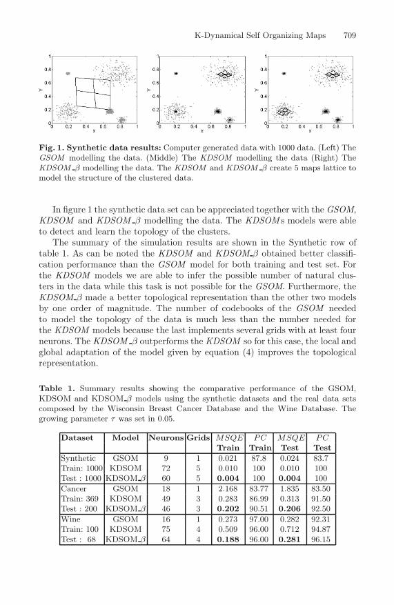
Fig. 1. Synthetic data results: Computer generated data with 1000 data. (Left) TheGSOM modelling the data. (Middle) The KDSOM modelling the data (Right) TheKDSOM β modelling the data. The KDSOM and KDSOM β create 5 maps lattice tomodel the structure of the clustered data.

In figure 1 the synthetic data set can be appreciated together with the GSOM,KDSOM and KDSOM β modelling the data. The KDSOM s models were ableto detect and learn the topology of the clusters.

The summary of the simulation results are shown in the Synthetic row oftable 1. As can be noted the KDSOM and KDSOM β obtained better classifi-cation performance than the GSOM model for both training and test set. Forthe KDSOM models we are able to infer the possible number of natural clus-ters in the data while this task is not possible for the GSOM. Furthermore, theKDSOM β made a better topological representation than the other two modelsby one order of magnitude. The number of codebooks of the GSOM neededto model the topology of the data is much less than the number needed forthe KDSOM models because the last implements several grids with at least fourneurons. The KDSOM β outperforms the KDSOM so for this case, the local andglobal adaptation of the model given by equation (4) improves the topologicalrepresentation.

Table 1. Summary results showing the comparative performance of the GSOM,KDSOM and KDSOM β models using the synthetic datasets and the real data setscomposed by the Wisconsin Breast Cancer Database and the Wine Database. Thegrowing parameter τ was set in 0.05.

Dataset Model Neurons Grids MSQE PC MSQE PCTrain Train Test Test

Synthetic GSOM 9 1 0.021 87.8 0.024 83.7Train: 1000 KDSOM 72 5 0.010 100 0.010 100Test : 1000 KDSOM β 60 5 0.004 100 0.004 100Cancer GSOM 18 1 2.168 83.77 1.835 83.50Train: 369 KDSOM 49 3 0.283 86.99 0.313 91.50Test : 200 KDSOM β 46 3 0.202 90.51 0.206 92.50Wine GSOM 16 1 0.273 97.00 0.282 92.31Train: 100 KDSOM 75 4 0.509 96.00 0.712 94.87Test : 68 KDSOM β 64 4 0.188 96.00 0.281 96.15

710 C. Saavedra et al.

5.2 Experiment #2: Real Datasets

In the second experiment we test the algorithm with two real datasets knownas the Wisconsin Breast Cancer Database and Wine datasets obtained from theUCI Machine Learning repository [3].

The Cancer data was collected by Dr. Wolberg, N. Street and O. Mangasar-ian at the University of Wisconsin [8]. The samples consist of visually assessednuclear features of fine needle aspirates (FNAs) taken from patients’ breasts. Itconsist in 569 instances, with 30 real-valued input features and a diagnosis (M= malignant, B = benign) for each patient. We partitioned the dataset into theTraining and Test with sizes of 369 and 200 data respectively.

The Wine recognition data was collected by Stefan Aeberhard [3]. This dataset is the result of a chemical analysis of wines grown in the same region in Italybut derived from three different cultivars. The analysis determined the quantitiesof 13 constituents found in each of the three types of wines. It consist in 178instances and 13 attributes (all continuous). We partitioned the dataset into theTraining and Test with sizes of 100 and 78 data respectively.

The summary of the simulation results are shown in the Cancer and Winerows of table 1, the results are very similar to the synthetic case. As can benoted the KDSOM and KDSOM β obtained better classification performancethan the GSOM model for both training and test set with the exception of thePC train column of the Wine dataset. For the KDSOM models we are able toinfer the possible number of natural clusters in the data while this task is notpossible for the GSOM. Furthermore, the KDSOM β made a better topologicalrepresentation than the other two models for the train and test set, specially forthe Cancer database. The number of codebooks of the GSOM needed to modelthe topology of the data is much less than the number needed for the KDSOMmodels because the last implements several grids with at least four neurons each.The KDSOM β outperforms the KDSOM model, so for this cases the local andglobal adaptation of the model given by equation (4) improves the topologicalrepresentation.

6 Concluding Remarks

In this paper we have introduced the K-Dynamical Self Organizing Maps. Thismodel has the capability to learn the topology of clustered data by making a softpartition of the input space. The KDSOM is a hybrid model that automaticallyfinds its structure to learn the topology of its respective partition and, throughthe interaction with the neighbor maps, it also learns the data of neighboringpartitions.

The performance of our algorithm shows better results in the simulationstudy in both the synthetic and real data sets. In the real case, we investi-gated two benchmark data known as Cancer and Wine databases. The compar-ative study with the GSOM and KDSOM without improvement shows that ourmodel the KDSOM with improvement outperforms the alternative models. The

K-Dynamical Self Organizing Maps 711

KDSOM models were able to find the possible number of clusters and learn thetopological representation of the partitions.

Further studies are needed in order to analyze the convergence and the or-dering properties of the maps. Possible interesting applications of the KDSOMcould be Web-Mining.

Acknowledgement. The authors wish to thank Prof. Dr. Claudio Moraga,Prof. Dr. Jorge Galbiati and all the unknown referees for their valuable com-ments.

References

1. H. Allende, S. Moreno, C. Rogel, and R. Salas, Robust self organizing maps,CIARP-2004. LNCS 3287 (2004), 179–186.

2. H. Bauer and T. Villmann, Growing a hypercubical output space in a self-organizingfeature map, IEEE Trans. on Neural Networks 8 (1997), no. 2, 226–233.

3. C.L. Blake and C.J. Merz, UCI repository of machine learning databases, 1998.4. K.A.J Doherty, R.G. Adams, and N. Davey, Hierarchical growing neural gas, To

be published in proceedings of ICANNGA 2005 (2005).5. B. Fritzke, Growing cell structures - a self-organizing network for unsupervised and

supervised learning, Neural Networks 7 (1994), no. 9, 1441–1460.6. A.K. Jain and R.C. Dubes, Algorithms for clustering data, Prentice Hall, 1988.7. T. Kohonen, Self-Organizing Maps, Springer Series in Information Sciences, vol. 30,

Springer Verlag, Berlin, Heidelberg, 2001, Third Extended Edition 2001.8. O. Mangasarian, W. Street, and W. Wolberg, Breast cancer diagnosis and prognosis

via linear programming, Operations Research 43 (1995), no. 4, 570–577.9. T. Martinetz, S. Berkovich, and K. Schulten, Neural-gas network for vector quan-

tization and its application to time-series prediction, IEEE Trans. on Neural Net-works 4 (1993), no. 4, 558–568.

10. U. Maulik and S. Bandyopadhyay, Performance evaluation, IEEE. Trans. on Pat-tern Analysis and Machine Intelligence 24 (2002), no. 12, 1650–1654.

11. J. McQueen, Some methods for classification and analysis of multivariate observa-tions, In Proceedings of the Fifth Berkeley Symposium on Mathematical Statisticsand probability, vol. 1, 1967, pp. 281–297.

12. S. Moreno, H. Allende, C. Rogel, and R. Salas, Robust growing hierarchical selforganizing map, IWANN 2005. LNCS 3512 (2005), 341–348.