Noname manuscript No.(will be inserted by the editor)

Using Self-organizing Maps withComplex Network Topologiesand Coalitions for Time SeriesPrediction

Juan C. Burguillo

Received: date / Accepted: date

Abstract A Self-organizing Map (SOM) is a competitivelearning neural network architecture that make available acertain amount of classificatory neurons, which self-organizespatially based on input patterns. In this paper we explorethe use of complex network topologies, like small-world,scale-free or random networks; for connecting the neuronswithin a SOM, and apply them for Time Series Prediction(TSP). We follow the VQTAM model for function predic-tion, and consider several benchmarks to evaluate the qual-ity of the predictions. Afterwards, we introduce the CASOMalgorithm (Coalitions and SOM) that uses coalitions to tem-porarily extend the neighborhood of a neuron, and to providemore accuracy in prediction problems than classical SOM.The results presented in this work suggest that the most reg-ular the network topology is, the better results it provides inprediction. Besides, we have found that not updating all theneurons at the same time provides much better results. Fi-nally, we describe how the use of coalitions can enhance thecapability of SOM for Time Series Prediction.

Keywords Time Series Prediction · Self-organizing Maps(SOM) · Complex Networks · Coalitions

1 Introduction

Time Series Prediction (TSP) is a function approximationto estimate (predict) future values after a time sequence ofordered observations. The aim of TSP methods is to findthe model that best fits with the empirical observations, and

Juan C. BurguilloDep. of Telematic Engineering. Univ. of Vigo. 36310-Vigo (Spain)Tel.: +34-986-813869Fax: +34-986-812116E-mail: J.C.Burguillo@uvigo.es

once a particular model has been selected for TSP, the nextstep concerns with estimating its parameters from the avail-able data. Finally, a model evaluation is done concerning itspredictive ability usually over a new set of testing data.

In the last two decades, a growing interest in TSP meth-ods has been observed, particularly within the field of neuralnetworks [24,22] with the application of some well-knownsupervised neural architectures, such as the Multilayer Per-ceptron (MLP), the Radial Basis Functions (RBF) networksand, more recently, the Self-organizing Maps (SOM) [6].The application of these neural networks architectures inTSP problems can be explained because of prediction canbe considered as a supervised learning problem.

Among those possible architectures, the Self-organizingMap (SOM) [14] is a well-known competitive learning neu-ral network. SOM learns from examples a mapping (projec-tion) from a high-dimensional continuous input space onto alow-dimensional discrete space (lattice). After training, theneuron weights in the map can provide a model of the train-ing patterns mainly through: vector quantization, regressionand clustering. Using these techniques, self-organizing mapshave been applied in the last decades to multiple applica-tions [12] in areas like automatic speech recognition, mon-itoring of plants and processes, cloud classification, micro-array data analysis, document organization, image retrieval,etc. In the last decade, there has been also an increasing in-terest in using SOM for TSP problems [6].

In this article we consider the use of complex networktopologies [3] like spatial, small-world, scale-free or ran-dom networks for connecting the neurons within a SOM andexplore its performance for time series prediction using theVQTAM model [5]. Yang et al. [25] implemented a SOMwith small-world topology, in which neighborhood sizes areprogressively reduced during the learning process. The re-sulting SOM seems to have a faster convergence and havea more reasonable weight distribution. Jiang et al. [13] useSOM with dynamic complex networks topologies, obtainedby means of evolutionary optimization algorithms, and ap-ply them for classification purposes. To our knowledge, oursis the first work exploring the use of SOM together withcomplex networks for prediction purposes.

The main contribution of the article is threefold: a) to ex-plore the application of this self-organizing neural networkwith different complex topologies for time series prediction,b) to evaluate the topologies and the conditions for cell up-dating that provide a better quality in prediction, and c) toconsider the use of coalitions for cell updating as temporaryneighborhoods to extend the influence of a relevant neuron,and therefore, enhance the performance of the network.

The rest of the paper is organized as follows. Sect. 2 in-troduces Self-organizing Maps together with the VQTAMmodel that we use for time series prediction. Sect. 3 pro-vides a short introduction of Game Theory and specially to

2 Juan C. Burguillo

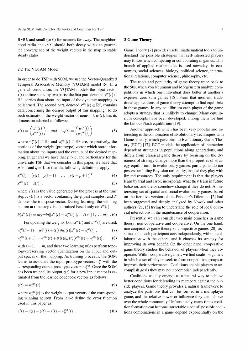
Fig. 1 A SOM map with an input vector, a winner neuron and itsneighborhood.

the use of coalitions in games. Sect. 4 describes the differenttypes of complex networks that we use in the paper. Sect. 5describes the results obtained after using the network topolo-gies to connect the neurons in the SOM, and apply them todifferent TSP problems. Then, Sect. 6 defines precisely anew Coalition Algorithm for SOM (CASOM). Afterwards,Sect. 7 shows the results obtained after applying CASOMover the set of benchmarks. Finally, Sect. 8 presents our con-clusions and describe some future work.

2 Self-organizing Maps (SOM) and Time SeriesPrediction (TSP)

Self-organizing Maps (SOM) [14], also denoted as Self-orga-nizing Feature Maps (SOFM) or Kohonen Neural Networks,make available a certain amount of classificatory resources,usually denoted as neurons, cells or units, which self-organizebased on the input patterns. From a topological point ofview, a SOM is a single layer neural network, where theneurons are set along a d-dimensional grid. In most applica-tions this grid is 2-dimensional and rectangular, but hexago-nal grids or other dimensional spaces have been also used inthe literature. Associated with each neuron is a weight vec-tor of the same dimension as the input vectors (patterns) anda position in the map space (see Fig.1). The self-organizingmap describes a mapping from a higher dimensional inputspace to a lower dimensional map space. The procedure forplacing a vector from the input space onto the map is to findthe neuron with the closest (smallest metric distance) weightvector. After several iterations, the result is an ordered net-work in which nearby neurons will share certain similari-ties. Therefore similar input patterns activate similar areasin the SOM producing a local specialization in the globalself-organized network.

Before training, the neurons may be initialized randomly,and like most artificial neural networks, SOMs operate intwo modes: training and mapping. Training builds the map

Fig. 2 The picture presents a comparison between SOM and PCA fordata approximation (source Wikimedia Commons).

using input examples (it is a competitive process, also calledvector quantization), while Mapping automatically classifiesa new input vector.

Fig. 2 presents a comparison between SOM and PCAmethods for data approximation. The 2-dimensional inputdata points are represented by circles, while the SOM net-work contains 20 nodes and are represented by squares.

2.1 SOM Formal Definition

The SOM learns from the input patterns a mapping froma high-dimensional continuous input space X onto a low-dimensional discrete space L (the lattice) of m neurons whichare arranged in fixed topological forms, e.g., as a rectangular2-dimensional array. The number of neurons m in the map isusually defined after experimentation with the dataset.

The function map b(x) : X → L is defined by assigningto the current input vector x(t) ∈ X ⊂ Rn a neuron index bin the map obtained by:

b(x(t)) = argmin||x(t)−wi(t)||, ∀i ∈ {1, . . . ,m} (1)

where || · || denotes the Euclidean distance, n is the input vec-tor dimension and t is the discrete time step associated withthe iterations of the algorithm. The weight vectors wi(t) inthe map are trained according to a competitive-cooperativelearning rule, where the weight vector of a winning neuronwith index b (usually denoted as Best Matching Unit, BMU)and its neighbors in the output map array are updated withthis formula:

wi(t +1) = wi(t)+α(t)hbi(t)[x(t)−wi(t)], (2)

with i= 1, . . . ,m, and where 0<α(t)< 1 is the learning rateand hbi(t) is a weighting function which limits the neigh-borhood of the BMU. This neighborhood function assumesvalues in [0,1] and is high for neurons that are close to the

Using SOM with Complex Networks and Coalitions for TSP 3

BMU, and small (or 0) for neurons far away. The neighbor-hood radio and α(t) should both decay with t to guaran-tee convergence of the weight vectors in the map to stablesteady states.

2.2 The VQTAM Model

In order to do TSP with SOM, we use the Vector-QuantizedTemporal Associative Memory (VQTAM) model [5]. In ageneral formulation, the VQTAM models the input vectorx(t) at time step t by two parts: the first part, denoted xin(t)∈Rp, carries data about the input of the dynamic mapping tobe learned. The second part, denoted xout(t) ∈ Rq, containsdata concerning the desired output of this mapping. To dosuch estimation, the weight vector of neuron i, wi(t), has itsdimension adapted as follows:

x(t) =(

xin(t)xout(t)

)and wi(t) =

(win

i (t)wout

i (t)

), (3)

where wini (t) ∈ Rp and wout

i (t) ∈ Rq are, respectively, theportions of the weight (prototype) vector which store infor-mation about the inputs and the outputs of the desired map-ping. In general we have that p > q, and particularly for theunivariate TSP that we consider in this paper, we have thatp > 1 and q = 1, so that the following definitions apply:

xin(t) = [y(t) y(t−1) . . . y(t− p+1)]T (4)

xout(t) = s(t) , (5)

where s(t) is the value generated by the process at the timestep t, y(t) is a vector containing the p past samples, and Tdenotes the transpose vector. During learning, the winningneuron at time step t is determined based only on xin(t):

b(xin(t)) = argmin||xin(t)−wini (t)||, ∀i ∈ {1, . . . ,m} . (6)

For updating the weights, both xin(t) and xout(t) are used:

wini (t +1) = win

i (t)+α(t)hbi(t)[xin(t)−wini (t)], (7)

wouti (t +1) = wout

i (t)+α(t)hbi(t)[xout(t)−wouti (t)], (8)

with i = 1, . . . ,m, and these two learning rules perform topo-logy-preserving vector quantization on the input and out-put spaces of the mapping. As training proceeds, the SOMlearns to associate the input prototype vectors win

i with thecorresponding output prototype vectors wout

i . Once the SOMhas been trained, its output z(t) for a new input vector is es-timated from the learned codebook vectors as follows:

z(t) = woutb (t) , (9)

where woutb (t) is the weight output vector of the correspond-

ing winning neuron. From it we define the error functionused in this paper as:

e(t) = s(t)− z(t) = s(t)−woutb (t) . (10)

3 Game Theory

Game Theory [7] provides useful mathematical tools to un-derstand the possible strategies that self-interested playersmay follow when competing or collaborating in games. Thisbranch of applied mathematics is used nowadays in eco-nomics, social sciences, biology, political science, interna-tional relations, computer science, philosophy, etc.

The roots and popularity of game theory trace back tothe 50s, when von Neumann and Morgenstern analyze com-petitions in which one individual does better at another’sexpense: zero sum games [18]. From that moment, tradi-tional applications of game theory attempt to find equilibriain these games. In any equilibrium each player of the gameadopts a strategy that is unlikely to change. Many equilib-rium concepts have been developed, among them we findthe famous Nash equilibrium [19].

Another approach which has been very popular and in-teresting is the combination of Evolutionary Techniques withGame Theory, which gave birth to Evolutionary Game The-ory (EGT) [17]. EGT models the application of interactiondependent strategies in populations along generations, anddiffers from classical game theory by focusing on the dy-namics of strategy change more than the properties of strat-egy equilibrium. In evolutionary games, participants do notpossess unfailing Bayesian rationality, instead they play withlimited resources. The only requirement is that the playerslearn by trial and error, incorporate what they learn in futurebehavior, and die or somehow change if they do not. An in-teresting set of spatial and social evolutionary games, basedon the iterative version of the Prisoner’s Dilemma [2] hadbeen suggested and deeply analyzed by Nowak and otherauthors [21,15] trying to understand the role of local or so-cial interactions in the maintenance of cooperation.

Presently, we can consider two main branches in gametheory: non cooperative and cooperative. On the one hand,non cooperative game theory, or competitive games [20], as-sumes that each participant acts independently, without col-laboration with the others; and it chooses its strategy forimproving its own benefit. On the other hand, cooperativegame theory studies the behavior of players when they co-operate. Within cooperative games, we find coalition games,in which a set of players seek to form cooperative groups toimprove their performance. Coalitions enable players to ac-complish goals they may not accomplish independently.

Coalitions usually emerge as a natural way to achievebetter conditions for defending its members against the out-side players. Game theory provides a natural framework toanalyze the partitions that can be formed in a multiplayergame, and the relative power or influence they can achieveover the whole community. Unfortunately, many times coali-tion formation can become intractable since all possible coali-tions combinations in a game depend exponentially on the

4 Juan C. Burguillo

number of players. Therefore, finding the optimal partitionby checking the whole space may be too expensive from acomputational point of view. In the literature, authors haveapplied evolutionary techniques to try to avoid the coali-tion formation problem [26]. Other recent approaches uselocal decisions to create dynamic coalitions that emerge andevolve adapting to the present needs of every player [8].

4 Complex Networks

In this work we consider, besides spatial SOM topologies,other types of complex network topologies in order to ex-plore their performance in time series prediction problems.In the last years, complex network topologies, e.g. small-world or scale-free ones, have been applying in multipleresearch works [3]. According to the famous algorithm ofWatts and Strogatz [23], small-world networks are interme-diate topologies between regular and random ones. Theirproperties are most often quantified by two key parameters:the clustering coefficient and the mean-shortest path.

On the one hand, the clustering coefficient quantifieshow the neighbors of a given network node (i.e., the nodes towhich it is connected) are on average interconnected. It re-flects the network capacities of local information transmis-sion. The distance between two nodes of the network is thesmallest number of links one has to travel to go from onenode to the other. On the other hand, the mean-shortest pathis the average graph distance of the network, and indicatesthe capacities of long distance information transmission.

Random Networks (RN) are randomly generated by plac-ing a fixed number of edges between vertices at random withuniform probability [11]. Random networks are character-ized by their short characteristic path length, i.e., the maxi-mum distance between any to nodes in the graph is short.

Small-world (SW) networks [1] share properties of bothrandom nets and regular lattices, because they have a shortcharacteristic path length and a high clustering coefficient,i.e., there is a high connectivity degree among the vertices inthe graph. This SW topology can be generated by the Wattsand Strogatz algorithm [23]. Formally, we note them as W k;p

V, where V is the number of nodes, k the average connectivity,i.e., the average size of the node’s neighborhood, and p therewiring probability.

Finally, Scale-free (SF) networks follow a power lawconcerning degree distribution, at least asymptotically, i.e,the fraction P(k) of nodes in the network having k connec-tions to other nodes goes for large values of k as P(k) ∼k−λ usually having 2 < λ < 3. Formally we denote them asSk;−λ

V , where V is again the number of nodes. Scale-free net-works show characteristics present in many real world net-works like the presence of “hubs” connecting almost discon-nected sub-networks. The “preferential attachment method”

[4] can be used to build such topologies, reflecting also thedynamical aspect of those networks.

5 Experimental Results for Complex Networks andSOM

In this section we present the results obtained after apply-ing the VQTAM model in TSP scenarios considering severalcomplex network topologies. All the simulations have beenrepeated 30 times and, except it is explicitly said, the resultscorrespond to the average value obtained all along the 30runs. The simulations have been performed in a Java simu-lator, and every execution took less than a minute in a Pen-tium dual-core 3GHz with 3 GBytes of RAM. The particularparameters used in all the next simulations are: p = 2 (inputvalues), q = 1 (output value), initial α = 0.99 that decreaseslinearly reaching zero at the end of the training phase. Everytraining set is repeated 20 times (epochs) before proceedingto the testing phase. The values selected for these parametershave been applied after an exhaustive testing in multiple ex-periments, providing us the best results. In order to simplifythe analysis as much as possible, and considering the partic-ularities introduced by the complex topologies, our neigh-borhood function hbi(t) considers only the closer neuron’sneighborhood, which means the four neurons conformingthe Von Neumman neighborhood (North, East, South, West)in the spatial case, and the direct neighbors in the case ofthe complex topologies used here (SW, SF and RN). Thevalue defined for the BMU is hbi(t) = 1 and for its neighborneurons is hbi(t) = 0.5. Finally, we consider also 4 initialneighbors in all the possible topologies, so the parametersused for building the SW and SF networks are W 4;0.1

m andS4;−2

m respectively.We have tested several functions and benchmarks for

TSP, and in this section we present three representative casesthat we consider interesting. We have selected a trigonomet-ric function (SCSTS) obtained by f (x)= 2sin(x)−cos(3x)+sin(5 ∗ x) because it is continuous and its smooth variationinduced higher error rates than classical discrete TSP bench-marks. We also have consider the benchmark (BRTS) pre-sented in [6] and the Mackey-Glass time series (MGTS),which are based on the Mackey-Glass differential equation[16]. This is a benchmark widely regarded for comparing thegeneralization ability of different methods, and correspondsto a chaotic time series generated from a time-delay ordinarydifferential equation.

5.1 Number of Neurons in the Lattice

We first start considering how many neurons there must be inthe lattice for a particular problem, depending on the topol-ogy. There is a heuristic value, used in the SOM literature

Using SOM with Complex Networks and Coalitions for TSP 5

2 4 6 8 10Number of neighbors

0.00

0.05

0.10

0.15

0.20

0.25

0.30

0.35

0.40

Avg

. E

rror

SOM results for SCSTS

SPSWSFRN

Fig. 3 The figure shows the influence of the parameter Ku in the er-ror rate, depending on the type of topology: spatial (SP), small-world(SW), scale-free (SF) and random net (RN).

and in the SOM toolbox released by [14], which is: m =

Ku.√

NIn where usually Ku = 5 and NIn is the number of in-put samples available.

Fig. 3 describes the influence of the Ku parameter overthe error rate depending on the type of topology and usingthe function SCSTS. We can see in the figure how the bestresults are obtained using a spatial network, while the worstones are provided by the scale-free net. We shall explainin subsection 7.2 a reason for these results. Besides, usingvalues of Ku above 5 does not improve the error rate signifi-cantly. The results are similar, with minor variations for theother benchmarks. The variance in the error value obtainedalong the different executions has the order (1e− 6), so ingeneral different executions provide similar results. There-fore, for the next experiments presented here, we have se-lected m = 5.

√NIn neurons, as recommended by the litera-

ture, for all the topologies.

5.2 Probability of Neighbor Updating

Now we consider what happens if we do not select all theneurons in the BMU’s neighborhood always for update, asit is done in the literature. We define Pu as the probability ofupdating a particular neighbor neuron. We will consider herethe MGTS benchmark introduced before. Fig. 4 presents asnapshot of this benchmark after 10,000 iterations over theinput samples. Fig. 5 describes the normalized results ob-tained after applying our prediction model over the bench-mark. In the horizontal axis we represent the probability ofupdating the weights of a BMU’s neighbor neuron, accord-ing to the VQTAM model introduced before. We only haveconsidered four probabilities [0.25, 0.5, 0.75, 1] correspond-ing respectively to select in average one neighbor, two, threeor the four neurons in a Von Neumann neighborhood. We didthe same in the other complex network topologies, where a

Fig. 4 Snapshot of the MGTS values (blue), the prediction (green) andthe error (red) at the bottom.

0.2 0.4 0.6 0.8 1.0Probability of neuron update

0.010

0.015

0.020

0.025

0.030

Avg

. E

rror

SOM results for MGTS

SPSWSFRN

Fig. 5 Average error depending on the probability of updating a neigh-bor neuron (Mackey-Glass).

neuron may have an arbitrary number of neighbors. As wecan see, the best results correspond again to the spatial topol-ogy, but in all topologies it seems that we get better resultsif we do not update all the neurons in the neighborhood atthe same time.

Finally, Table 1 presents the results for the three bench-marks considered here, but only considering the spatial topol-ogy that provides the best results in our experiments. Thetable mainly describes the influence of Pu in the average er-ror obtained in every case along the 30 executions. As wecan see, Pu values around 0.25 seem to be the best optionfor neuron updating, and the variance obtained is low in allcases. The average accuracy improvement of the best case(in bold font in the table) and the standard SOM (i.e., whenall neighbors are updated) is 32.17%, 6.94%, and 11.4% forSCSTS, MGTS, and BRTS problems, respectively.

6 Juan C. Burguillo

Table 1 Results obtained for several problems using the spatial topology, and selecting different probabilities for Pu. The best result for everyproblem appears in bold font.

Problem Pu Avg. Error Var. ErrorSCSTS 0.25 0.03132 1.3443314897497158E-6SCSTS 0.50 0.03774 8.070066737617545E-6SCSTS 0.75 0.04244 1.2399366548484838E-4SCSTS 1.00 0.04618 4.789858730510971E-5MGTS 0.25 0.01259 1.1286199180388548E-8MGTS 0.50 0.01306 5.794091294210585E-8MGTS 0.75 0.01356 3.460033223761095E-7MGTS 1.00 0.01353 1.6062622390451002E-6BRTS 0.25 0.03472 1.1137671061480401E-6BRTS 0.50 0.03692 2.564077340881391E-6BRTS 0.75 0.03807 7.312130032126494E-10BRTS 1.00 0.03919 6.688382929482581E-7

6 Coalitions, Complex Networks and SOM

The work presented in [10] describes an Evolutionary Al-gorithm (EA) with Coalitions (EACO), designed on a dy-namic topology that takes advantage of both cellular and is-land population models. It is basically a cellular EA in whichcoalitions of individuals are automatically formed and main-tained. Individuals in the population will choose a coalitionto join at every time in terms of some rewards they canexpect from it. Neighborhoods are defined by these coali-tions, and coalitions can be understood as small panmic-tic subpopulations (i.e., islands) that emerge in the cellu-lar topology providing dynamic neighborhoods. EACO re-moves some classical required parameters for distributed EAs,like the fixed neighborhoods, or the islands connectivity topol-ogy, the migration frequency, or the policies to exchange anddiscard individuals.

Afterwards, [9] describes the strong similarities betweencEAs and SOM models, and argues about the strong poten-tial for using similar approaches as a way to define dynamicneighborhoods, and apply them to SOM models.

In this section we will continue the work hinted in [9],and present a new algorithm CASOM using Coalitions andSOM that can be used for Time Series Prediction. First, weintroduce the basics of the algorithm, then a more formaldefinition, and finally we present a set of results that enhanceeven more the results obtained in the previous section.

6.1 Introducing a General Coalitional Algorithm for SOM

An algorithm for training the SOM network with coalitionscould be defined as:

For each input pattern x(t):

1. Find the closest neuron with index b in the map:b(x(t)) = argmin||x(t)−wi(t)||, ∀i ∈ {1 . . .m}

2. Update each neuron in the grid according to the rule:wi(t+1)=wi(t)+α(t)hcbi(t)[x(t)−wi(t)], i= 1 . . .m

3. Infect neurons in the neighborhood of the BMU and jointhen to its coalition:cb(t + 1) = { j | j ∈ cb(t)

⋃In f ectNeighbors(b, t)},

j = 1 . . .m4. Repeat the process until a certain stop condition is met.

A main difference with the classical algorithm is the in-fection process introduced in item 3, where a BMU neu-ron b may infect neighbor neurons with index j in order tospread its neighborhood. In this context, we define the in-fection procedure as the way that every BMU uses to extendits influence, dynamically joining other neurons to its coali-tion. These coalition neurons will be afterwards updated byit. This is a big difference with the general algorithm pro-posed in [9], as along the simulation process, we realize thatthe BMUs’ infection is a much more interesting model toextend dynamically the neighborhoods.

A second difference with the classical SOM algorithmis the new neighborhood function hcbi(t) in step 2 that takesinto account if the neurons b and i belong to the same coali-tion or not. Even we can define multiple neighborhood func-tions considering coalitions, a basic proposal could be:

hcbi(t)=

i f ((ci(t) = /0)&||b(t)− i(t)||)≤ r(t))⇒ 0.5elsei f (cb(t) = ci(t))⇒ 0.5else⇒ 0

(11)

where if the BMU neuron is independent, then thoseneurons close to it are in the neighborhood. Otherwise, ifBMU is in a coalition, those neurons in the same coalitionare also neighbors. Concerning the general rules for creat-ing, joining or leaving a coalition; we review the ones con-sidered in [10], and rewrite them as:

– Neurons can only belong to a single coalition.– Neurons compete to extend their coalitions, and we will

consider this process from a game theory point of view,as neurons will try to extend their influence “infecting”other neurons to join them to their coalition.

– Neurons from a given coalition are updated by the BMU,so the coalition behaves like a panmictic island.

Using SOM with Complex Networks and Coalitions for TSP 7

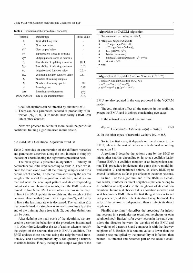
Table 2 Definitions of the procedures’ variables

Variable Description Initial value

b Best Matching Unit -

xin New input value -

xout New output Value -

wini Input pattern stored in neuron i -

wouti Output pattern stored in neuron i -

Pu Probability of updating a neuron [0, 1]

Pin f Probability of infecting a neuron 0.05

hbi neighborhood function value 0.5,−hcbi coalitional neighb. function value 0.5,−Ts Number of training samples -

Te Number of training epochs 20

α Learning rate 0.99

4α Learning rate decrement 1Ts.Te

StopCondition End of the training phase Ts.Te

– Coalition neurons can be infected by another BMU.– There can be a parameter, denoted as probability of in-

fection (Pin f ∈ [0,1]), to model how easily a BMU caninfect other neurons.

Now, we proceed to define in more detail the particularcoalitional training algorithm used in this article.

6.2 CASOM: a Coalitional Algorithm for SOM

Table 2 provides an enumeration of the different variablesand parameters described along the text, in order to simplifythe task of understanding the algorithms presented next.

The main cycle is presented in algorithm 1. Initially allparameters are initialized according to table 2. Then we it-erate the main cycle over all the training samples and for acertain set of epochs, in order to train adequately the neuronweights. The rest of this algorithm is intuitive, and it is sum-marized now: the new input pattern and its correspondingoutput value are obtained as inputs, then the BMU is deter-mined. In line 6 the BMU infect other neurons in the map.In line 7 the BMU updates its weights and the weights of theneurons related with it (described in algorithm 2), and finallyin line 8 the learning rate α is decreased. The variation4α

has been defined in a simple way to reach zero linearly at theend of the training phase (see table 2), but other definitionscan be done.

After defining the main cycle of the algorithm, we pro-ceed to describe the behavior of the procedures instantiatedin it. Algorithm 2 describes the set of actions taken to modifythe weight of the neurons that are in BMU’s coalition. TheBMU updates those neurons using the neighborhood func-tion hcbi, and a certain probability Pu for updating a neuron,as defined before. Finally the input and output weights of the

Algorithm 1: CASOM Algorithm1 Set parameters according to table 2;

2 while Not StopCondition do3 xin = getInputPattern();4 xout = getOutputValue ();5 b = getBMU (xin);6 b.infectNeurons ();7 b.updateCoalitionNeurons (xin, xout );8 α = α -4α;9 end

Algorithm 2: b.updateCoalitionNeurons (xin, xout )1 updateNeuronsInCoalition (hcbi, Pu);2 win = win +α.(xin−win);3 wout = wout +α.(xout −wout);

BMU are also updated in the way proposed in the VQTAMmodel.

The hcbi function affect all the neurons in the coalition,except the BMU, and is defined considering two cases:

1. If the network is a spatial one, we have:

hcbi =1

1+ToroidalDistance(Pos(b)−Pos(i))(12)

2. In the other types of networks we have hcbi = 0.5.

So in the first case, it depends on the distance to theBMU; while in the rest of networks it is defined accordingto equation 11.

Algorithm 3 describe the actions done by the BMU toinfect other neurons depending on its role: a coalition leader(former BMU), a coalition member or an independent neu-ron. This procedure implements the game theory model in-troduced in [9] and mentioned before, i.e., every BMU try toextend its influence as far as possible over the other neurons.

In line 1 of the algorithm, and if the BMU is a coali-tion leader, it infects its direct neighbors (that can belong toits coalition or not) and also the neighbors of its coalitionmembers. In line 4, it checks if it is a coalition member, andas it becomes a BMU, then the first thing it does is to getindependence, and then infect its direct neighborhood. Fi-nally, if the neuron is independent, then it infects its directneighbors.

Finally, algorithm 4 describes the procedure for infect-ing neurons in a particular set (coalition neighbors or ownneighborhood). Basically, for every neuron in the set, it con-siders the distance between the weights of the BMU andthe weights of a neuron i, and compares it with the farawayneighbor of b. Besides if a random value is lower than thelearning rate multiplied by the probability of infection, thenneuron i is infected and becomes part or the BMU’s coali-tion.

8 Juan C. Burguillo

Algorithm 3: b.infectNeurons ()1 if isCoaLeader() then2 infect (Neighbors);3 infect (CoaNeighbors);4 else if isCoaMember() then5 getIndependence ();6 infect (Neighbors);7 else // b is independent8 infect (Neighbors);9 end

There are two main ideas under the behavior of this sim-ple algorithm. First, to infect only neurons with weights nearto the BMU, which means that they could be potentially partof the neighborhood, even if they are far away. Second, tohave a bigger rate of infection (i.e., more frequent and big-ger coalitions) at the beginning of the simulation. As soon asthe simulation gets closer to its end it becomes much moredifficult to infect other neurons, and coalitions break downas their members get independence when becoming BMUs.The reason for this behavior is also related with the resultsobtained with Pu and SOM in section 5, i.e., to reduce theamount of neurons that become updated as the simulationgoes by.

Algorithm 4: b.infect (neuronSet, val)1 foreach i ∈ m do2 if (Distance(win

b ,wini )<= maxNeighborDistance(b) ) &

(rand()< α.Pin f ) then3 infect (i);4 end5 end

7 Experimental Results Obtained with CASOM

In this section we present the experimental results obtainedusing the CASOM algorithm for TSP. First we analize howcoalitions and results evolve depending on the probability ofinfection Pin f . Then we present the results obtained by CA-SOM over the three training sets used in this article: SCSTS,MGTS and BRTS. Finally we compare these results with theones provided by SOM in section 5.

7.1 Influence of the Infection Parameter

The parameter that has a main influence over the behaviorof the CASOM algorithm is the probability of infection Pin f .From our experiments it is really important to tune this pa-rameter to the right value in order to get the best results.Luckily we have found that almost the same value for Pin f is

0.00 0.05 0.10 0.15 0.20Probability of infection

0.00

0.05

0.10

0.15

0.20

Avg

. E

rror

CASOM results for SCSTS changing Pinf

SPSWSFRN

Fig. 6 CASOM results for SCSTS varying Pin f with Pu = 0.25.

adequate for the three training sets we use in this article. Fig-ure 6 presents the results obtained by CASOM over SCSTSand considering the four different types of networks. Thefigures obtained with the other training sets are very simi-lar, and in all of them values around (Pin f = 0.05) providethe best results, specially in the spatial case. Again, we canobserve that the spatial networks provides the best results inall cases.

7.2 Results Obtained by CASOM over the Benchmarks

Figures 7, 8 and 9 present the results obtained by CASOMchanging the probability of update Pu and the type of net-work (SP, SW, SF and RN) over the three training sets con-sidered for SOM: SCSTS, MGTS and BRTS. As the readermay observe, the results are very similar to section 5, in thesense that Pu has a strong influence in the quality of the re-sults; and in all the cases using a spatial network (SP) andlow values of Pu provides better results. The scale-free net-works provides the worst results, while small-world (SW)and random-networks (RN) provide a similar performance.The bad results provided by scale-free topologies, comparedwith the other alternatives, clearly are related with the het-erogeneity of the networks belonging to this topology. Re-member that in scale-free there are some nodes, denoted ashubs, that have a higher number of connections than the av-erage, while other nodes have a much lower number. Con-sidering the good results obtained with spatial topologies(regular grids) it seems that topologies with a regular num-ber of connections are better for using SOM and CASOM inprediction.

Figure 10 describes how the number of coalitions (CN)evolve during the first 1000 samples of the Mackey-Glassbenchmark. After the first 800 samples these graphics re-main almost stable, but slowly decreasing to zero as the sim-ulation approaches its end. As the reader may observe, the

Using SOM with Complex Networks and Coalitions for TSP 9

0.2 0.4 0.6 0.8 1.0Probability of neuron update

0.00

0.02

0.04

0.06

0.08

0.10

Avg

. E

rror

CASOM results for SCSTS

SPSWSFRN

Fig. 7 CASOM results over SCSTS with Pin f = 0.05.

0.2 0.4 0.6 0.8 1.0Probability of neuron update

0.010

0.012

0.014

0.016

0.018

0.020

Avg

. E

rror

CASOM results for MGTS

SPSWSFRN

Fig. 8 CASOM results over MGTS with Pin f = 0.05.

0.2 0.4 0.6 0.8 1.0Probability of neuron update

0.030

0.035

0.040

0.045

0.050

0.055

0.060

Avg

. E

rror

CASOM results for BRTS

SPSWSFRN

Fig. 9 CASOM results over BRTS with Pin f = 0.05.

Fig. 10 Evolution of independent neurons (IC), member neurons (CC)and number of coalitions (CN) in a MGTS training with Pin f = 0.05.

0.2 0.4 0.6 0.8 1.0Probability of neuron update

0.020

0.025

0.030

0.035

0.040

0.045

0.050

Avg

. E

rror

SOM vs. CASOM results for SCSTS (SP)

SOMCASOM

Fig. 11 SOM vs. CASOM in SCSTS with Pin f = 0.05.

number of coalitions in red (CN) is similar to the number ofcells in coalitions (CC) meaning that most of coalitions havea small size.

7.3 SOM vs. CASOM

Finally, it is the time to analyze how good are the resultsprovided by CASOM compared with the ones obtained bySOM in section 5. Figures 11, 12 and 13 compare the resultsprovided by both algorithms. The results presented by thosefigures correspond to the best results obtained in every case,and they correspond to the spatial topology.

Watching the figures two observations are clear: the evo-lution of the curves depending on the probability of updatePu are equivalent, and CASOM outperforms SOM in all cases.

Table 3 presents precisely the best values obtained inthe three figures and also the average error. The accuracyimprovement provided by CASOM over SOM corresponds

10 Juan C. Burguillo

Table 3 Comparison between SOM and CASOM in several problems using the spatial topology. The best result per problem appears in bold font.

Problem Algorithm Pu Avg. Error Var. ErrorSCSTS SOM 0.25 0.03132 2.4238491363156E-5SCSTS CASOM 0.25 0.02480 8.356549725205973E-6MGTS SOM 0.25 0.01259 1.4387791306418415E-7MGTS CASOM 0.25 0.01199 3.900890360211602E-9BRTS SOM 0.25 0.03472 4.855712863773361E-8BRTS CASOM 0.25 0.03271 7.844401596893082E-7

0.2 0.4 0.6 0.8 1.0Probability of neuron update

0.0115

0.0120

0.0125

0.0130

0.0135

0.0140

Avg

. E

rror

SOM vs. CASOM results for MGTS (SP)

SOMCASOM

Fig. 12 SOM vs. CASOM in MGTS with Pin f = 0.05.

0.2 0.4 0.6 0.8 1.0Probability of neuron update

0.030

0.032

0.034

0.036

0.038

0.040

Avg

. E

rror

SOM vs. CASOM results for BRTS (SP)

SOMCASOM

Fig. 13 SOM vs. CASOM in BRTS with Pin f = 0.05.

to 20.81%, 4.76% and 5.78% for the SCSTS, MGTS andBRTS training sets respectively.

8 Conclusions

In this paper we consider the Time Series Prediction prob-lem (TSP), and the use of Self-organizing Maps (SOM) neu-ral networks for modeling it. We have selected the VQTAMmodel from the recent literature as a particular case of SOMapplication in TSP scenarios. We have considered the use ofcomplex network topologies like small-world, scale-free and

random networks for connecting the neurons within a SOM,and explore its performance considering several benchmarksfor TSP. To our knowledge, this is the first paper studyingprediction problems with different types of complex net-work topologies for interconnecting the neurons in a SOM.

The results presented in this work suggest that the clas-sical spatial SOM network topology provides better resultsthan the other types studied. Among them, small-world andrandom networks provide similar results considering thatthe resulting nets have a relatively regular structure and lowclustering coefficient. We have found specially inadequatethe use of scale-free topologies for TSP, mainly due to itsheterogeneity in the number of connections among its nodes.

Another relevant contribution presented in this article isthat it seems better to do not update all the neurons at thesame time in the BMU’s neighborhood. In this sense, wegot up a relevant improvement in the average accuracy ofthe SOM. This means that even with the case of a minimalneighborhood used in a classical SOM (i.e., the Von Neu-mann neighborhood), it is much better to do not update thefour neurons always, but subsets of them.

The last contribution concerns CASOM, a coalition basedalgorithm for SOM. CASOM is based in the use of coali-tions for spreading the otherwise fixed neighborhoods. Thesecoalitions use a probability of infecting other neurons tochange dynamically the neighborhood of a BMU. The im-provement provided by CASOM relays strongly in the ade-quate tuning of the probability of infecting other cells (avoid-ing too big coalitions). We have found that a value of Pin f =

0.05 is adequate in the cases analyzed.Future work will consider to evaluate a higher spectra

of network topologies, the use of more complex neighbor-hood functions, and to explore the conditions for selectingthe right neurons to be updated in the BMU’s neighborhood.

Acknowledgements The author thanks Bernabe Dorronsoro for hishelpful collaboration in previous works, and anonymous reviewers fortheir hints and comments.

References

1. Albert, R., Barabasi, A.L.: Statistical mechanics of complex net-works. Reviews of Modern Physics. vol. 74, 47–97 (2002)

2. Axelrod, R.: 1984. The evolution of Cooperation. Basic Books,New York.

Using SOM with Complex Networks and Coalitions for TSP 11

3. Boccaletti, S., Latora, V., Moreno, Y., Chavez, M., Hwang, D.U.:Complex networks: Structure and dynamics. Physics Reports,424, 175–308 (2006)

4. Barabasi, A.L., Albert, R.: Emergence of scaling in random net-works. Science 286 (5439), 509-512 (1999)

5. Barreto, G.A., Araujo, A.F.R.: Identification and control of dy-namical systems using the self-organizing map. IEEE Transac-tions on Neural Networks, 15(5), 1244–1259 (2004)

6. Barreto, G.A.: Time Series Prediction with the Self-OrganizingMap: A Review. Perspectives of Neural-Symbolic Integration,Studies in Computational Intelligence Volume 77, 135-158(2007)

7. K. Binmore, Game Theory, Mc Graw Hill, 1994.8. J.C. Burguillo, A Memetic Framework for Describing and Simu-

lating Spatial Prisoner’s Dilemma with Coalition Formation, 8thInternational Conference on Autonomous Agents and MultiagentSystems, 2009.

9. J.C. Burguillo, Playing with complexity: From cellular evolution-ary algorithms with coalitions to self-organizing maps, Comput-ers and Mathematics with Applications 66, (2013) 201-212.

10. B. Dorronsoro, J.C. Burguillo, A. Peleteiro, P. Bouvry, Evolution-ary Algorithms based on Game Theory and Cellular Automatawith Coalitions, Handbook of Optimization, Intelligent Systems(38), Springer (2013) 481-503.

11. Erdos, P., Renyi, A.: On random graphs. Publicationes Mathemat-icae, 6, 290–297 (1959)

12. Van Hulle, M.M.: Self-organizing maps: Theory, design, and ap-plication, Tokyo. (2001)

13. Jiang, F., Berry, H., Schoenauer, M.: The Impact of NetworkTopology on Self-Organizing Maps. GEC09, Shanghai, China(2009)

14. Kohonen, T.: Self-Organizing Maps, 3rd Edition, Springer-Verlag. (2001)

15. P. Langer, M.A. Nowak, C. Hauert, Spatial invasion of coopera-tion, Journal of Theoretical Biology 250 (2008) 634-641.

16. Mackey, M.C., Glass, J.: Oscillation and chaos in physiologicalcontrol systems. Science, vol. 197, 287 (1977)

17. J. Maynard Smith, Evolution and the Theory of Games, Cam-bridge University Press, 1982.

18. O. Morgenstern, J. von Neumann, The theory of games and eco-nomic behavior. Princeton University Press, 1947.

19. J. Nash, Equilibrium points in n-person games, Proceedings of theNational Academy of Sciences of the United States of America”,36 (1) (1950) 48-49.

20. J. Nash, Non-Cooperative Games, The Annals of Mathematics,54 (2) (1951) 286-295.

21. M.A. Nowak, R.M. May, Evolutionary games and spatial chaos.Nature 359 (1992) 826-829.

22. Palit, A.K., Popovic, D.: Computational Intelligence in Time Se-ries Forecasting: Theory and Engineering Applications. Springer,1st edition. (2005)

23. Watts, D.J., Strogatz, S.H.: Collective dynamics of small-worldnetworks. Nature, vol. 393 440–442 (1998)

24. Weigend A., Gershefeld. N.: Time Series Prediction: Forecastingthe Future and Understanding the Past. Addison-Wesley. (1993)

25. Yang, S., Luo, S., Li, J.: An extended model on self-organizingmap. Proceedings of the 13 international conference on NeuralInformation Processing (ICONIP’06) (2006)

26. J. Yang, Z. Luo, Coalition formation mechanism in multi-agentsystems based on genetic algorithms, Applied Soft Computing,7(2) (2007) 561-568.