Traffic Routing under Dynamic Network Topologies - TU Delft ...
85
Delft Center for Systems and Control Traffic Routing under Dynamic Network Topologies M. Leeuwenberg Master of Science Thesis
-
Upload
khangminh22 -
Category
Documents
-
view
5 -
download
0
Transcript of Traffic Routing under Dynamic Network Topologies - TU Delft ...

Delft Center for Systems and Control
Traffic Routing underDynamic Network Topologies
M. Leeuwenberg
Mas
tero
fScie
nce
Thes
is

Traffic Routing underDynamic Network Topologies
Master of Science Thesis
For the degree of Master of Science in Systems and Control at DelftUniversity of Technology
M. Leeuwenberg
December 28, 2021
Faculty of Mechanical, Maritime and Materials Engineering · Delft University of Technology

Copyright © Delft Center for Systems and Control (DCSC)All rights reserved.

Abstract
Inefficient road usage in a traffic network context – i.e. over-saturation on one route, whereother roads are still available – is an important problem. It appears often and in different typesof situations. We concentrate on congestion caused by predicted temporary road blockades,such as open bridges. This research aims to reduce such congestion by focussing on solving arouting problem that accounts for these road blockades.
More specifically, we consider traffic that is to be guided through a network with a numberof different routes, where bridges function as temporary blockades when they are opened. Ariver that is used by freight transport runs through this network, in which road traffic usesbridges to cross the river. These bridges would open to let the freight ships pass. In such asituation, open bridges are a predictable temporary blockade for the vehicles on the road, adisturbance on the traffic flow.
We propose a model predictive controller that routes the vehicles efficiently to their desti-nations, making a trade-off between waiting in front of bridges and taking a detour. Modelpredictive control has been selected because it can handle these predicted disturbances thatthe bridges pose. Furthermore, it can be tuned to make a trade-off between a computationallyfast and an accurate solution. A traffic split determines which part of the incoming traffic flowon a road interchange is sent towards which emanating road. These traffic splits representthe actuator variables of the controller. The total time spent by all vehicles in the network isthe cost function to be minimised.
We describe a motorway network with METANET, a macroscopic traffic model. We do notuse the full model, but a piecewise-affine approximation, in order to simplify the optimisationcalculations significantly. We discuss two ways of modelling this approximation: an existingMixed Logical Dynamical (MLD) formulation and a novel Linear Programming (LP) formu-lation. An analysis of the novel LP model in an N -step-ahead simulation is performed. Weshow that this problem cannot be written in a single LP problem, but that it is actually alinear multilevel programming problem (where N LP problems have to be solved consecu-tively).As a means to model predicted disturbances, a novel store-and-forward bridge element is
added to the nonlinear and the MLD model. A case study is performed to evaluate the
Master of Science Thesis M. Leeuwenberg

ii Abstract
effectiveness of this new bridge element. The results of this case study were satisfactory.Moreover, the results obtained with the MLD model provided an acceptable approximationof the results obtained with the nonlinear model.
M. Leeuwenberg Master of Science Thesis
Table of Contents
Abstract i
1 Introduction 11-1 General Introduction . . . . . . . . . . . . . . . . . . . . . . . . . . . . . . . . . 11-2 Problem Statement . . . . . . . . . . . . . . . . . . . . . . . . . . . . . . . . . 21-3 Structure of the Thesis . . . . . . . . . . . . . . . . . . . . . . . . . . . . . . . 4
2 Traffic Network Modelling 52-1 Graph Modelling . . . . . . . . . . . . . . . . . . . . . . . . . . . . . . . . . . . 5
2-1-1 Vertices and Links . . . . . . . . . . . . . . . . . . . . . . . . . . . . . . 52-1-2 Shortest Path Problems . . . . . . . . . . . . . . . . . . . . . . . . . . . 62-1-3 Network Flow Problems . . . . . . . . . . . . . . . . . . . . . . . . . . . 7
2-2 Traffic Modelling . . . . . . . . . . . . . . . . . . . . . . . . . . . . . . . . . . 82-2-1 Motorway Traffic Models . . . . . . . . . . . . . . . . . . . . . . . . . . 82-2-2 METANET . . . . . . . . . . . . . . . . . . . . . . . . . . . . . . . . . 92-2-3 Piecewise-Affine and Linear Approximations of Nonlinear Functions in ME-
TANET . . . . . . . . . . . . . . . . . . . . . . . . . . . . . . . . . . . 112-2-4 Piecewise-Affine Approximation of METANET Combined with Mixed Inte-
ger Linear Programming . . . . . . . . . . . . . . . . . . . . . . . . . . 132-3 Model Predictive Control . . . . . . . . . . . . . . . . . . . . . . . . . . . . . . 152-4 Summary . . . . . . . . . . . . . . . . . . . . . . . . . . . . . . . . . . . . . . . 16
3 Improved METANET and Traffic Control 173-1 Considerations about Improvements to the Mixed Logical Dynamical Model . . . 173-2 Piecewise-Affine Approximation of METANET Combined with Linear Programming 18
3-2-1 Function Evaluation Using Linear Programming Problems . . . . . . . . . 183-2-2 Application to METANET . . . . . . . . . . . . . . . . . . . . . . . . . 20
3-3 Accounting for Predicted Disturbances . . . . . . . . . . . . . . . . . . . . . . . 25
Master of Science Thesis M. Leeuwenberg
iv Table of Contents
3-3-1 Modified METANET . . . . . . . . . . . . . . . . . . . . . . . . . . . . 253-3-2 Describing Temporarily Unavailable Segments in METANET . . . . . . . 26
3-4 Time-Dependent State Space Representation of the Mixed Logical DynamicalModel and the Linear Programming Model . . . . . . . . . . . . . . . . . . . . . 32
3-5 Control Implementation . . . . . . . . . . . . . . . . . . . . . . . . . . . . . . . 333-6 Summary . . . . . . . . . . . . . . . . . . . . . . . . . . . . . . . . . . . . . . . 35
4 Simulation Results 374-1 Setup . . . . . . . . . . . . . . . . . . . . . . . . . . . . . . . . . . . . . . . . . 374-2 Analysis of a Single N -Step-Ahead Simulation with the Linear Programming Model 384-3 Case Studies on Bridge Elements in METANET . . . . . . . . . . . . . . . . . . 43
4-3-1 Zero-Length Bridges . . . . . . . . . . . . . . . . . . . . . . . . . . . . . 444-3-2 Store-and-Forward Bridges . . . . . . . . . . . . . . . . . . . . . . . . . 47
4-4 Summary . . . . . . . . . . . . . . . . . . . . . . . . . . . . . . . . . . . . . . . 49
5 Conclusions and Recommendations 515-1 Project Summary and Discussion . . . . . . . . . . . . . . . . . . . . . . . . . . 515-2 Contributions . . . . . . . . . . . . . . . . . . . . . . . . . . . . . . . . . . . . 535-3 Recommendations . . . . . . . . . . . . . . . . . . . . . . . . . . . . . . . . . . 53
5-3-1 Recommendations Concerning the Control Implementation . . . . . . . . 535-3-2 Recommendations Concerning Model Improvements . . . . . . . . . . . . 555-3-3 Recommendations Concerning Model Validation and Real-Time Implemen-
tation . . . . . . . . . . . . . . . . . . . . . . . . . . . . . . . . . . . . 56
A Approximations of Functions in METANET 57A-1 Piecewise-Affine Approximation of the Desired Speed Function . . . . . . . . . . 57A-2 Piecewise-Affine Approximation of the Flow Function . . . . . . . . . . . . . . . 58A-3 Rewriting Equations in the Form of a Mixed Logical Dynamical Model . . . . . . 60
A-3-1 Desired Speed Function . . . . . . . . . . . . . . . . . . . . . . . . . . . 60A-3-2 Outflow at an Origin . . . . . . . . . . . . . . . . . . . . . . . . . . . . 61
B Network Flow Problems 63B-1 Minimum-Cost Flow Problem . . . . . . . . . . . . . . . . . . . . . . . . . . . . 63B-2 Multi-Commodity Flow Problem . . . . . . . . . . . . . . . . . . . . . . . . . . 64B-3 Linear Programming Problem . . . . . . . . . . . . . . . . . . . . . . . . . . . . 64
Glossary 73List of Acronyms . . . . . . . . . . . . . . . . . . . . . . . . . . . . . . . . . . . 73List of Symbols . . . . . . . . . . . . . . . . . . . . . . . . . . . . . . . . . . . 74
Index 74
M. Leeuwenberg Master of Science Thesis

“Comes a time when you’re driftin’Comes a time when you settle down.”— Neil Young

Chapter 1
Introduction
This chapter provides an introduction to the subject of this thesis: traffic routing underdynamic network topologies. It starts with a general introduction in Section 1-1, that empha-sises the relevance of the subject. Thereafter, a specific problem statement is given in Section1-2. Lastly, an overview of the chapter is given in Section 1-3.
1-1 General Introduction
Human driving can be unpredictable, and especially in high-intensity traffic it is likely to causecongestion. Over the past decades, the number of road users has only increased and congestionhas therefore been a widely recognised and studied problem for a long time [9, 52, 69, 71].Under high-intensity traffic, efficient road usage is a very relevant topic for a number ofreasons. Reducing traffic congestion will not only lower the travel time of individual users,it can also result in drivers travelling at a more stable speed and therefore in more efficientfuel consumption which is an environmental benefit. Furthermore, congested traffic situationshave a negative influence on safety.Congestion might theoretically be permanently solved by increasing the infrastructure’s
capacity such that it can handle the worst-case traffic peaks, provided that the roads arefilled with predictable and optimally platooning (smart) cars. However, this solution addressesthe efficiency of the usage of a single road. We suggest that inefficient road usage across anetwork is a different problem that has to be tackled as well. Research is conducted to findeffective solutions for minimising traffic congestion caused by inefficient road usage across anetwork [21,42,43,59,70]. In the context of a routing problem, we deem a network inefficientlyused when one road is over-saturated, where other roads in the network (that could be usedas an alternative route) still have a relatively low traffic density.
Congestion occurs in both urban and motorway traffic. In the literature, traffic control ap-plied to both urban [22,50,56] and motorway models [11,20,60] can be found. In present-daymotorway traffic, possible solutions for congestion include variable speed limits and on-rampcontrol [10, 40], whereas control applications that involve (future) smart cars also try to
Master of Science Thesis M. Leeuwenberg
2 Introduction
achieve a reduction of congestion with adaptive cruise control, platooning or by other waysof intercommunicating vehicles [17, 59]. Traffic congestion is also researched in other areasof science; think of road pricing [69], analysing the effects of road widening, and Braess’sparadox [9].1In the light of this thesis, inefficient road usage can mean two things. Either it means that
on one single road the traffic does not adjust to other traffic properly, causing the flow tobe suboptimal, or it means that too many cars take one (temporary blocked) road instead ofother roads, causing inefficient usage of the available roads. The first case is a more fundamen-tal problem because it will always exist on roads with too little capacity and unpredictablehuman drivers. The latter is the subject of this thesis.The massive congestion on motorways that can occur during holidays or in the weekends
is an example of such a problem. Note that especially weekend and holiday traffic is lessbounded to the time at which it wants to arrive or the route it takes and in addition, thedistances they travel are usually larger than for commuting traffic. Therefore, it is expectedthat the number of acceptable route alternatives is higher and that the traffic can be spreadout over these routes in such a way that the congestion can be significantly reduced. Anotherexample of this subject is the routing of traffic through a network with reduced or zero ca-pacity on certain locations caused by a blocked road due to an accident, road maintenance oran open bridge.
A measure for efficient road usage in a traffic network context is provided by the Wardropprinciples [71].2 In this thesis, we will strive for a system optimal control implementation byminimising the total time spent by all vehicles in the network.We consider the traffic network as a graph through which vehicles are to be routed. In
this graph, each edge has an associated travel time. At specified moments in time we haveeither unavailable edges, or edges with an increased weight to reflect a temporary blockedroad. Furthermore, we assume that we specify one origin and one destination vertex for eachvehicle in the graph.
1-2 Problem Statement
A road blockage may have several causes. We focus our research on predicted blockages,i.e. the moment at which they take place is exactly known in advance. In this context, weconsider the following two research questions:
How can we route traffic through a motorway network, where certainroads are blocked at known time periods, with as objective to minimisethe total time spent by all vehicles in the network?How can this be done in the most computationally efficient way?
1Braess’s paradox reads: “Adding extra capacity to a network in which the moving entities chose theirroutes individually, can in some cases lead to a decrease of the performance of the network as a whole.”
2Wardrop’s first principle is known as the selfish Wardrop equilibrium. This is a user optimal equilibriumthat is obtained when all road users try to minimise their own travel time. The second principle is animprovement by Wardrop, in which he proposes a new, system optimal equilibrium where road users cooperate.In the social Wardrop equilibrium, the average journey time is minimised.
M. Leeuwenberg Master of Science Thesis

1-2 Problem Statement 3
The first research question involves a dynamic traffic routing problem. In order to solvethis problem, a macroscopic traffic flow model of a motorway network has to be selected.This model should be able to accurately reflect the event of a road blockage, for example bythe deletion or insertion of links. Moreover, when a link is unavailable, the traffic that stillarrives at that link has to be queued in some way. In order to achieve a social equilibrium,a queue element should be implemented, in such a way that there is a penalty on letting toomany vehicles wait in front of a road blockage. We will focus on solving this problem withpredicted disturbances in the motorway network simulation model METANET in a ModelPredictive Control (MPC) context. We use the Total Time Spent (TTS) by all vehicles in thenetwork as a measure for efficient road usage. If environmental effects are also to be takeninto account, METANET can be extended with the VT-macro model [75] so that the modelincludes fuel consumption. The controller will route the traffic by actuating the traffic splitsat interchanges. The recurring question is: will it be preferable to avoid a blocked road, orto direct the traffic straight to it and wait until the road is unblocked. It is expected that inan optimal solution – when the roads are most efficiently used – a part of a traffic flow hasto take a detour around the blocked road and the rest of the traffic has to wait for the roadto be unblocked.We assume that a static origin-destination matrix is provided.3 Moreover, we assume that
the predicted disturbances are caused by bridges that open and close at times that are knownbeforehand. Store-and-forward links should then allow traffic to queue in front of the bridges,in the case that they are open.
Considering the second research question, we suggest that an MPC approach is promising, as itcan take into account the known future disturbances and moreover, it is easy to tune with onlytwo parameters, Np and Nc, offering a trade-off between computation speed and precision.The computational complexity of an MPC optimisation problem is heavily dependent onthe underlying models used. In our case, this model is METANET, a nonlinear nonconvexmodel that results in high-complexity optimisation problems when used in combination withMPC. Note that METANET and MPC have been used before by others in dynamic routingproblems. However, our problem differs from them mainly because we assume predictableunavailability of links. When a controller for motorway traffic routing is to be used in realtime, the control optimisations should be calculated faster than a single simulation time step.METANET is a nonconvex and nonlinear model and is deemed too complex for such a cause.Therefore, a proposed simplification of the model by Groot et al. [34, 35] is expected to be agood starting point.Since we use a mathematical model of a traffic network, we are able to use the traffic
splits at interchanges as a control input. When actually implementing a real-time controller,the routes that vehicles take can only be advised, but not controlled. If we would wantto achieve a real-time implementation, a Dynamic Route Information Panel (DRIP) couldprovide advisory information on a motorway traffic network [21,42,43].
3In an origin-destination matrix, we can find the traffic demand for every origin-destination pair, i.e. thenumber of vehicles that are leaving from origin o to destination d. Such a matrix is said to be static if it isindependent of time.
Master of Science Thesis M. Leeuwenberg

4 Introduction
1-3 Structure of the Thesis
This thesis is organised in the following manner. In Chapter 2, we discuss literature regardinggraph modelling, shortest path problems, cost flow problems, and state-of-the-art motorwaytraffic models. Thereafter, in Chapter 3, we propose two contributions to the literature: anapproximation of METANET that can be evaluated with Linear Programming (LP) and theaddition of bridge elements to METANET. Chapter 4 provides an analysis of an N -step-ahead simulation with the newly presented LP model as well as the results of a number ofcase studies with the novel bridge element. Lastly, some conclusions and recommendationsare presented in Chapter 5.
M. Leeuwenberg Master of Science Thesis
Chapter 2
Traffic Network Modelling
In this chapter we explain how to model traffic networks and more specifically we zoom in onMETANET, a motorway traffic model. We start with a short general introduction to networksin Section 2-1 to provide some background knowledge. We elaborate on the traffic modelMETANET in Section 2-2. This model is simplified by means of a Piecewise-Affine (PWA)approximation and we show how a tractable conversion of the model can be embedded ina Model Predictive Control (MPC) framework. In Section 2-3 we further elaborate on thiscontrol method. The findings of this chapter are summarised in Section 2-4.
2-1 Graph Modelling
We discuss some graph theory in this section. This is by no means intended to be a completeoverview, but rather to serve as a bridge towards the much more specific modelling of a trafficnetwork. Next to the graph theory, we discuss some other operations research problems.This field is interesting because it gives a different view to a similar problem; (re-)routingtraffic in case of a blocked link. The content of this section is largely based on [16, 23]covering both basic graph modelling and basic algorithms that can be used on graphs. Foroperations research literature related to routing problems under dynamic network topologies,the interested reader is kindly referred to [13,26,32,37,61].
2-1-1 Vertices and Links
A graph G(M,V ) is a data structure that can be used to model networks. Here, V is afinite set of vertices (in the literature also called nodes). In a graph, a vertex ν ∈ V can e.g.represent an intersection between roads on which vehicles can travel, a railway station, or adead end. Moreover,M ⊂ V ×V is a finite set of edges; they can represent a road or a railwaybetween two intersections or stations. An edge m = (ν1, ν2) ∈M corresponds to a vertex pair.In an undirected graph we refer to such pairs as edges, whereas in case of a directed graph,we call them links (or arcs). A graph is said to be directed if its links (ν1, ν2) can only be
Master of Science Thesis M. Leeuwenberg

6 Traffic Network Modelling
crossed from ν1 to ν2, and not the other way around. This is contrary to an undirected graphwhere an edge (ν1, ν2) can also be crossed from ν2 to ν1. When an (undirected) edge existsbetween vertices ν1 and ν2, they are said to be adjacent to each other; adj(ν) is the set of allvertices adjacent to ν. In case of a directed graph, we define adji(ν) as the set of incominglinks at vertex ν and adjo(ν) as the set of emanating links at vertex ν.In a weighted graph G(M,V,w), we assign weight w(ν1, ν2) to link (ν1, ν2). The weight
can e.g. represent the length of the link or the time it takes to cross it. We consider a staticnetwork, when these weights are constant over time. If on the other hand, a dynamic modelis desired, the values of w can vary with time t and are then written as w(ν1, ν2, t). In thecase of a spatial network we also assign a geographical location to every vertex.In Figure 2-1, a static directed weighted graph G(M,V,w, c) is considered. The links have
a capacity c, which is the amount of traffic that can traverse the link in a certain amount oftime, expressed for example in (veh/h).
In the context of this thesis, we consider a directed dynamic network topology. The linkweights w(x, y, t) can vary over time, or specific links can be unavailable at certain times.Therefore, depending on how we model this, the set M does not necessarily contain a fixednumber of n links. This can be either:
n not fixed When a link is temporarily unavailable, it is also deleted in the model, givingthe set M size n− 1.
n fixed The approach that is for example used in [15]. In the case of an unavailable link, itstill exists in the model, but is given a relatively high value.
Weight updates and adding or removing links are closely related to each other [32]. It istherefore not expected that preferring one above the other will cause implementation issues.
22
4
31
(15,30)
(5,25)
(15,20)(1
0,20)
(5,5)
(5,45)
Figure 2-1: Simple network with four vertices and six directed links. The numbers betweenbrackets are respectively the weight w and the capacity c.
2-1-2 Shortest Path Problems
A path is a sequence of adjacent vertices p(ν1, ν2, ..., νn) that form a route through a network.The (time dependent) length of a path is calculated as
M. Leeuwenberg Master of Science Thesis

2-1 Graph Modelling 7
L(p) = w(ν1, ν2, t1) + w(ν2, ν3, t2) + ...+ w(νn−1, νn, tn−1). (2-1)
The single-pair shortest path, given as SP(s, d), is the path between a source vertex s and adestination vertex d on which the parameter L(p) is minimal. The shortest path from vertexνx to νy can be formulated as
minp∈P(νx,νy)
L(p), (2-2)
where P(νx, νy) is the set of paths with source vertex νx and destination vertex νy. Note thatthe shortest path from νx to νy can, but does not have to differ from the shortest path fromνy to νx. Also note that it is possible that multiple shortest paths are found between twovertices.It is a well known and widely studied problem to find the shortest path between two
vertices, and moreover to find it as fast as possible [2,3,16,24,25,28,30,33,36]. The shortestpath distance from vertex νx to νy and is defined as δ(νx, νy). It is the optimal value ofL(p) that follows from the minimisation in (2-2). The shortest path itself is defined asSP(νx, νy) = argminp∈P(νx,νy) L(p).
2-1-3 Network Flow Problems
We assume a graph that is defined by a node-node adjacency matrix Gij , with i and j thematrix indices.1 Furthermore, on link (i, j), we have the cost (or weight) Wij , flow Fij , andcapacity Cij . When applied to a traffic network, the link cost is the travel time in (h), the flowis the amount of traffic on a link in (veh/h), and the capacity is the maximum flow allowedon a link in (veh/h).
In the appendix we have defined two traffic routing problems: the minimum-cost flow problemin (B-1) and the multi-commodity flow problem in (B-2). When solved, they provide anoptimal traffic flow distribution in a network with link weights and capacities.The multi-commodity flow problem can be written in the form of a Linear Programming
(LP) problem, which results in relatively low computation times (in Appendix B-3 we derivehow to do this). We could run this problem in a discrete-time environment, so that we areable to route the traffic in a dynamic network. Then, in case of an unavailable link at acertain time step, we could update the graph matrix Gij in between time steps and alsoupdate matrices Wij and Cij accordingly.In the case we have 1 origin-destination pair and a Cij ∀ (i, j) ∈ M , the solution to
the multi-commodity flow problem would coincide with the shortest path that Dijkstra’salgorithm [24] would find. We could say that this solution is the selfish Wardrop equilibrium(cf. footnote 2 in Chapter 1 on page 2). In the case of multiple origin-destination pairs andwhen the demand a exceeds the link capacity Cij for one or more links, the minimisationresults a social Wardrop equilibrium, without exceeding the network capacity.
1A node-node adjacency matrix that describes a network with n vertices can be created by starting withan n × n matrix filled with zeros and setting a 1 on every entry where a link exists. So, if Gνxνy = 1, a linkexists from vertex νx to νy. Row i of Gij represents the links emanating from vertex i. Similarly, column jrepresents the incoming links at vertex j.
Master of Science Thesis M. Leeuwenberg
8 Traffic Network Modelling
The multi-commodity flow problem provides a partial answer to our research questions. How-ever, it has some drawbacks too that we will address now.The first problem is the accuracy of the model. Although many real-life traffic situations
could be represented by a graph Gij with weights and capacities, this traffic representation isa relatively low-detailed description. It does not include the traffic speed or density at a link.This has the implication that, regardless of the amount of traffic flow, the travel time on anedge is the same (that is, as long as the flow is not larger than the capacity). Furthermore,when the required flow would become higher than the capacity, the traffic is put in an originqueue until the network has the capacity again to dissolve the queue. An alternative wouldbe to use a more realistic motorway model that is also capable of describing a jam underblocked road conditions in case of an unavailable link.Secondly, the multi-commodity flow problem does not account for topology changes in ad-
vance. Notice that it is a static problem. That is, each instance is run on a specific situationat a set time and the optimisation does not take future disturbances into account. Suppose abridge opens and closes again before the traffic arrives at that bridge. The multi-commodityflow problem (and other algorithms from the operations research literature [26, 32, 63–65])would re-route the traffic twice, which is undesired. Solutions that account for dynamic net-work topologies are also found in the operations research literature [13, 37, 62], but they arecomputationally intensive because they consider the network at all time instants. Anothersolution can be provided by a motorway traffic model combined with MPC, which is a con-trol approach capable of handling a topology change in advance. MPC provides a trade-offbetween speed and accuracy because the amount of time it predicts ahead can be tuned.
2-2 Traffic Modelling
We give a high-level overview of motorway traffic models in Section 2-2-1. The METANETmodel is selected and presented in Section 2-2-2, its nonlinearities are discussed in Section2-2-3 and a PWA approximation that is known from the literature is given in Section 2-2-4,as well as the embedding of that PWA approximated model in an MPC optimisation thatcan be solved with Mixed Integer Linear Programming (MILP).
2-2-1 Motorway Traffic Models
Traffic models are usually divided in three types: microscopic models that are highly detailedand describe each vehicle separately, macroscopic models that have a more high-level approachand describe the average traffic behaviour in low detail, while the third category, mesoscopicmodels, uses characteristics from both microscopic and macroscopic models by describing thetraffic in medium detail, mostly in a probabilistic manner. In [44] an extensive overview ofthese different types of models is provided. Our focus lies on fast state prediction, so thatwe can quickly route traffic with a priori knowledge of road blockades. We chose to useMETANET, since this macroscopic model provides relatively good accuracy compared to itscomputation time. The traffic is represented by a flow, rather than by individual vehicles,giving a more high-level, general idea of the traffic distribution instead of a highly detaileddescription. Therefore, METANET is expected to be a good starting point.
M. Leeuwenberg Master of Science Thesis
2-2 Traffic Modelling 9
2-2-2 METANET
METANET [53, 60] is used to model motorway networks.2 In a graph representation of asuch a network, vertices mark the changes in motorway situations, like on-ramps or a changein the number of lanes. Links are pieces of road with a constant number of lanes and speedlimits (we use a speed limit of vfree on all links) connecting the vertices to each other. Alllinks consist of a predetermined number of segments on which traffic progresses at each timestep, so METANET is a deterministic, discrete-time, discrete-space model. It keeps track ofthe traffic flow qm,i in (veh/h), density ρm,i in (veh/km/lane), and speed vm,i in (km/h) oneach segment i of link m.
The flow at time step k is calculated by
qm,i(k) = λmρm,i(k)vm,i(k), (2-3)
where λm is the number of lanes.The update equations for ρ and v are
ρm,i(k + 1) = ρm,i(k) + TsLmλm
[qm,i−1(k)− qm,i(k)] (2-4)
andvm,i(k + 1) = vm,i(k) + Ts
τ[V [ρm,i(k)]− vm,i(k)]
+ Tsvm,i(k)[vm,i−1(k)− vm,i(k)]Lm
− Tsη[ρm,i+1(k)− ρm,i(k)]τLm(ρm,i(k) + κ) ,
(2-5)
with
V [ρm,i(k)] = vfree,m exp[− 1am
(ρm,i(k)ρcr,m
)am]. (2-6)
In order of appearance, Ts (h) is the sample time, Lm (km) is the length of the segments oflink m and τ (h), η (km2/h), and κ (veh/km/lane) are model parameters.In order to use METANET, the traffic network links are to be cut into road segments. The
traffic advances from one segment into its adjacent segment at each time step, that is as longas the Courant-Friedrichs-Lewy (CFL) condition Lm < Tsvfree ∀ m ∈M is preserved [18].In (2-6), V is the desired speed, vfree,m is the free-flow speed, ρcr,m the critical density on
link m, and am is a model parameter. Unless stated otherwise, we use the following values:
Ts = 10 sLm = 0.5 kmvfree = 102 km/hτ = 18 sκ = 40 veh/km/lane
ρjam = 180 veh/km/laneρcr = 33.5 veh/km/laneam = 1.867η = 60 km2/hCo = 2000 veh/h,
2METANET stands for Modèle d’Ecoulement du Trafic Autoroutier: NETwork
Master of Science Thesis M. Leeuwenberg
10 Traffic Network Modelling
where Co is the capacity of origins (discussed below). This is a standard parameter set thatis also used in [39,54].
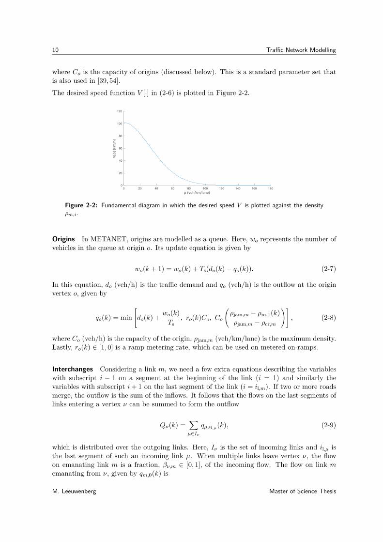
The desired speed function V [·] in (2-6) is plotted in Figure 2-2.
0 20 40 60 80 100 120 140 160 180
0
20
40
60
80
100
120
Figure 2-2: Fundamental diagram in which the desired speed V is plotted against the densityρm,i.
Origins In METANET, origins are modelled as a queue. Here, wo represents the number ofvehicles in the queue at origin o. Its update equation is given by
wo(k + 1) = wo(k) + Ts(do(k)− qo(k)). (2-7)
In this equation, do (veh/h) is the traffic demand and qo (veh/h) is the outflow at the originvertex o, given by
qo(k) = min[do(k) + wo(k)
Ts, ro(k)Co, Co
(ρjam,m − ρm,1(k)ρjam,m − ρcr,m
)], (2-8)
where Co (veh/h) is the capacity of the origin, ρjam,m (veh/km/lane) is the maximum density.Lastly, ro(k) ∈ [1, 0] is a ramp metering rate, which can be used on metered on-ramps.
Interchanges Considering a link m, we need a few extra equations describing the variableswith subscript i − 1 on a segment at the beginning of the link (i = 1) and similarly thevariables with subscript i+ 1 on the last segment of the link (i = il,m). If two or more roadsmerge, the outflow is the sum of the inflows. It follows that the flows on the last segments oflinks entering a vertex ν can be summed to form the outflow
Qν(k) =∑µ∈Iν
qµ,il,µ(k), (2-9)
which is distributed over the outgoing links. Here, Iν is the set of incoming links and il,µ isthe last segment of such an incoming link µ. When multiple links leave vertex ν, the flowon emanating link m is a fraction, βν,m ∈ [0, 1], of the incoming flow. The flow on link memanating from ν, given by qm,0(k) is
M. Leeuwenberg Master of Science Thesis
2-2 Traffic Modelling 11
qm,0(k) = βν,m(k)Qν(k). (2-10)
In (2-5), the upstream velocity vm,i−1 and downstream density ρm,i+1 on the first and lastsegment of a link respectively are calculated as follows. In the update equation for the speed,ρm,il+1 is written as
ρm,il+1(k) =∑µ∈Oν ρ
2µ,1(k)∑
µ∈Oν ρµ,1(k) , (2-11)
where Oν denotes the set of all outgoing links at vertex ν.For links in the set Iν incoming at vertex ν, vm,0(k) is given by
vm,0(k) =∑µ∈Iν vµ,il,m(k)qµ,il,m(k)∑
µ∈Iν qµ,il,m(k) . (2-12)
The full nonlinear behaviour in METANET is not deemed necessary, because for traffic routingwe assume that only a global idea of the network behaviour is needed, i.e. we accept anapproximation error. Therefore, we propose a simplification of METANET, largely basedon [34,35]. These papers implement a PWA approximation and an MILP algorithm to use inan MPC environment. When making this approximation of the model, the calculation timesbecome a lot smaller. The main ideas behind the work in these papers are discussed next.
2-2-3 Piecewise-Affine and Linear Approximations of Nonlinear Functions in ME-TANET
In this section, we point out the nonlinearities that are present in METANET, as well asmethods to linearise them or to make a PWA approximation of them. The results of thePWA approximations are graphically depicted in Figure 2-3. We sum up the adaptationsmade to the model below:
The Desired Speed Function We have the nonlinear function V [ρm,i], a single-variate equa-tion that can be efficiently approximated by a PWA function with a least-squares optimisation.The minimisation function is the squared error between the original function and its piecewiseapproximation. This is mathematically written as
minα1..αn−1,β1..βn
∫ xmax
xmin(fPWA,n(x)− f(x))2dx, (2-13)
in which the PWA function fPWA,n(x) in n regions is defined on the interval [xmin, xmax] bythe pattern
fPWA,n(x) =
β0 + x−xmin
α1−xmin(β1 − β0), for xmin ≤ x < α1
β1 + x−α1α2−α1
(β2 − β1), for α1 ≤ x < α2
:βn−1 + x−αn−1
xmax−αn−1(βn − βn−1), for αn−1 ≤ x ≤ xmax.
(2-14)
Master of Science Thesis M. Leeuwenberg
12 Traffic Network Modelling
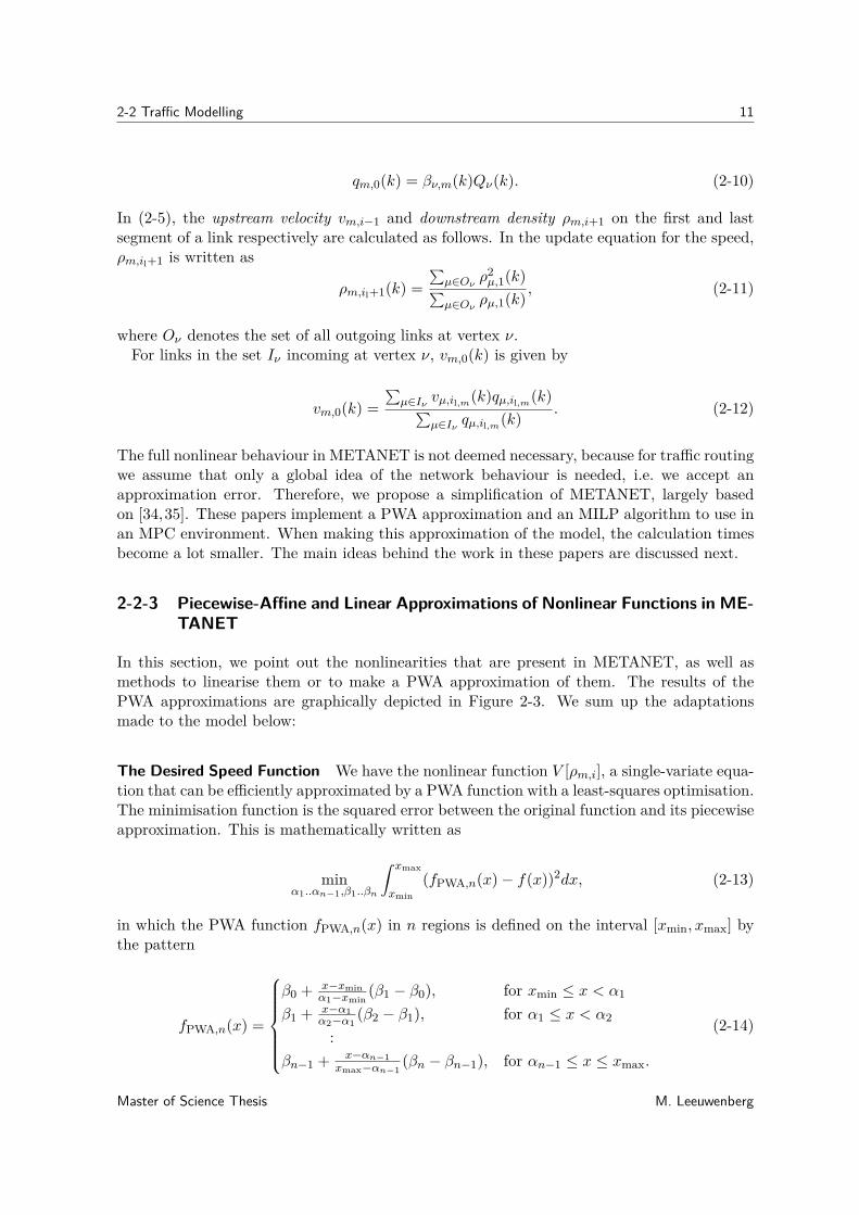
The n regions of which this continuous function consists are defined by parameters α and β.These parameters respectively define the x and y coordinates of the intersections of the affinefunctions, i.e. fPWA(αj) = βj for j = 1, 2, ..., n− 1.In the specific case of the desired speed function V , we add two constraints to the least-
squares optimisation: VPWA(αn−1) = 0 and VPWA(xmax) = 0, so that the last affine function,with domain [αn−1, xmax], has zero slope. When we do not impose these constraints, in anextreme case when ρ > ρjam, we could have VPWA(ρ) < 0 and thus a negative speed and flow(traffic driving in reverse). Note that βn−1 = 0 and βn = 0 are not added to the constraints,but rather excluded from the optimisation. To solve the unconstrained least-squares problem,we use a multi-start Levenberg-Marquardt algorithm. The result for a PWA function withthree regions is plotted in Figure 2-3a. More details on the PWA approximation (in three butalso in two regions) are given in Appendix A-1.
0 20 40 60 80 100 120 140 160 180
0
20
40
60
80
100
120
(a) PWA approximation of the fundamen-tal diagram in 3 regions. This approxima-tion is very similar to the one used in [35].
(b) PWA approximation in 3 regions of theflow function. This figure is taken from[34].
Figure 2-3: The two nonlinear functions in METANET that are approximated by PWA functions.On the left, we have the desired speed V from (2-6) and on the right the flow q from (2-3).
The Flow Function The second nonlinear function is q = ρv in (2-6). This bivariate equa-tion is harder to capture in a PWA approximation. The accuracy of this approximation isdependent on e.g. the number of regions in the PWA functions and the method used formaking the approximation. We describe two different methods in this thesis. The first isa three-dimensional PWA identification. In the second approach, the PWA identification isperformed in two dimensions, after a separation of the bivariate equation.The three-dimensional PWA identification used by Groot et al. [34, 35] consists of three
methods that are all available in the Hybrid Identification Toolbox (HIT) [27], which is aplatform embedded within the Multi-Parametric Toolbox (MPT) for Matlab [41]. An ap-proximation is created with the aid of this toolbox using three PWA functions, the result ofwhich is illustrated in Figure 2-3b.The second method is the PWA approximation after a separation of the flow function.
This method is proposed by [73]. A bivariate function x1x2 can be separated by writing thefunction as
M. Leeuwenberg Master of Science Thesis
2-2 Traffic Modelling 13
x1x2 = 14[(x1 + x2)2 − (x1 − x2)2
],
so that at this point, the two quadratic functions can be approximated by a two-dimensionalPWA identification. This method will be more elaborately discussed in Section 3-2-2.
The Update Equation The update equation for vm,i in (2-5) contains two nonlinear parts.Firstly, a multiplication by the speed vm,i(k) in vm,i(k)[vm,i−1(k) − vm,i(k)] and secondly adivision by the density ρm,i(k) in (ρm,i+1(k)− ρm,i(k))/(ρm,i(k) + κ). Both are linearised bykeeping terms constant, i.e. the first term in the first equation, vm,i(k), and the denominatorρm,i(k) in the second equation. This can be done by either keeping them constant according tohistorical data or, since the model is eventually controlled by MPC, by keeping them constantover the prediction horizon.This is justified by the fact that the multiplication factor (Ts/Lm) in the first equation is
relatively small and the multiplication factor (Tsη/τLm) as well as κ in the second equationare relatively large. These three factors all positively contribute to keeping the error causedby the substitution minimal.The downstream density on the last segment of a link in (2-12) and the upstream velocity
at the first segment of a link in (2-11) are linearised in a similar way by keeping the densityρµ,1 and velocity vµ,il constant.
A PWA system can be rewritten to a mixed logical dynamical model. This too has been doneby Groot et al. [34, 35]. This conversion is described in the next section.
2-2-4 Piecewise-Affine Approximation of METANET Combined with Mixed In-teger Linear Programming
Using the aforementioned methods to remove the nonlinearities from METANET, we arriveat a PWA system [68] of the form
x(k + 1) = Aix(k) +Biu(k) + fi
y(k) = Cix(k) +Diu(k) + gifor[x(k)u(k)
]∈ Ωi and for i ∈ 1, ..., N (2-15)
in which Ω1, ...,ΩN are convex polyhedra. Furthermore, x(k), y(k) and u(k) denote the state,output and input respectively.Using this PWA model with MPC is possible, but becomes computationally intractable
very fast. A last conversion is done, in order to make the MPC problem tractable for largernetworks. The PWA model is rewritten in the form of a Mixed Logical Dynamical (MLD)model [4–7, 73]. In such a model, binary decision variables indicate in which region of thePWA functions the state variables are. The model description is given by
x(k + 1) = Ax(k) +B1u(k) +B2δ(k) +B3z(k) + f
y(k) = Cx(k) +D1u(k) +D2δ(k) +D3z(k) + g
E1x(k) + E2u(k) + E3δ(k) + E4z(k) ≤ h,(2-16)
Master of Science Thesis M. Leeuwenberg
14 Traffic Network Modelling
in which δ(k) ∈ 0, 1nb is the binary decision variable and z(k) an auxiliary variable thatarises from the procedure explained next.For the conversion of the PWA functions into a tractable MPC model, the next three
statements (adapted from [6,73]) are used:
f(x) ≤ 0⇔ [δ = 1] is equivalent to:f(x) ≤M(1− δ)f(x) ≥ ε+ (m− ε)δ,
(2-17)
δ = δ1δ2 ⇔
−δ1 + δ ≤ 0−δ2 + δ ≤ 0δ1 + δ2 − δ ≤ 1,
(2-18)
z = δf(x)⇔
z ≤Mδ
z ≥ mδz ≤ f(x)−m(1− δ)z ≥ f(x)−M(1− δ),
(2-19)
in which δ1, δ2 ∈ 0, 1 are binary variables. We use m and M as a lower and upper boundrespectively of the function f(·) and ε is a small tolerance variable. Now, if f(·) is an affinefunction defined on a bounded set X, then m and M are finite and the right-hand sides ofthe equivalences in (2-17)-(2-19) are (mixed integer) linear inequalities.A single MLD-MPC iteration can now be written as an MILP problem in which the integer
variables all belong to the set 0, 1. The approximations of the desired speed function VPWAand the flow function qPWA can now be rewritten in the from of an MLD model. An exampleof how to do this is provided in Appendix A-3-1. A few extra considerations to take intoaccount when implementing the MLD model are mentioned next.
Suppose we have a PWA function with n regions and thus n functions aiρ+bi i ∈ 1, 2, ..., n.We observe that we do not need an explicit binary decision variable for the first region, a1ρ+b1.In other words, the system is always on the first region of the PWA function unless a decisionvariable prevents that. Therefore, if all binary variables are equal to 0, the system is on thefirst region a1ρ+b1. Therefore, a PWA function with n regions results in n−1 binary decisionvariables.With m the number of decision variables, we could theoretically use 2m combinations of
binary values to describe 2m + 1 different settings of a PWA model. Put differently, we couldsay that in a PWA function with n regions, in principle a number of
m = dlog2(n− 1)e,
decision variables, where d·e is the ceiling function, would be sufficient to define all affineregions. Suppose we have a PWA function with 5 regions, then we could, using a differentconversion to an MLD system, theoretically use only dlog2(n − 1)e = 2 binary variables (re-sulting in four unique configurations [0, 0], [1, 0], [0, 1], and [1, 1], and the first affine function).In our current model description, we use n − 1 = 4 decision variables. When the number ofbinary variables increases, the resulting MILP problem is expected to be computationallymore intensive. That is, in the specific case of using more regions and thus binary variablesfor the description of the desired speed function or the flow in Figure 2-3, we expect thecalculations to be slower and the results more accurate. Therefore, using less binary variables
M. Leeuwenberg Master of Science Thesis
2-3 Model Predictive Control 15
is thought to speed up the calculation times. However, using a description with dlog2(n− 1)ebinary variables results in a more complex MLD system, and thus it is difficult to predictwhich of the two descriptions can be most efficiently solved (cf. [4]).We add δi ≥ δi+1 ∀ i ∈ 1, 2, ..., n − 1 as extra constraints to the ones we already men-
tioned. The decision variable δi+1 can only be equal to 1 if all decision variables before it, δ1to δi, are equal to 1. We use these constraints, because a situation where δi+1 = 1 ∧ δi = 0,does not describe an affine function that we want to use. We expect this to speed up theoptimisation.Apart from the functions for the desired speed and the traffic flow, the function for the outflowat origin qo, given in (2-8), needs to be rewritten as well. The derivation of the conversion ofthis minimisation of three parameters to MLD form is provided in Appendix A-3-2.
2-3 Model Predictive Control
We use both the MLD and the yet to describe LP model as prediction models in an MPCcontext. This control method is expected to provide accurate predictions, which is desiredbecause we want to efficiently route traffic through a network that is subject to predicteddisturbances, meaning that we know beforehand when and where the disturbance is going totake place.Model Predictive Control started to be used since Cutler and Ramaker [19] and Richalet etal. [66] pioneered it simultaneously. Nowadays it is a widely studied model-based controlapproach and it has been used many times in traffic control (e.g. [12,46,70]). In MPC a costfunction J is minimized over a prediction horizon Np. The prediction horizon is an integernumber of time steps (Ts) over which the controller predicts the states by means of a givenmodel. The minimisation of the cost function J is done at each time step, resulting in a setof control actions for the entire prediction horizon. Of this set, only the control input for thenext time step is used. At the next time step, the optimisation problem is run again. Becausethe prediction horizon is shifted forward in each time step we also speak of receding horizoncontrol. Sometimes, a control horizon Nc is added to the MPC problem. In that case, thecontrol actions are determined over the first Nc time steps and kept constant over the nextNp − Nc time steps. This procedure makes the calculations computationally less intensiveand, in case of LP, it is sometimes used for robustness.We expect that using MPC will yield favourable results because it is an optimisation problemthat takes the dynamics of the system into account. The performance of MPC is for a largepart determined by the cost function. We could implement a cost function that has a selfishgoal, but MPC has the potential of performing better than this. If, contrary to the individualjourney times, the average journey time of all users is minimised we might achieve system-optimality. We want to investigate if there will be less congestion when implementing sucha social goal. This would come close to the social Wardrop equilibrium contrasting to theselfish Wardrop equilibrium (cf. footnote 2 in Chapter 1 on page 2).The cost function used for the MPC problem is the Total Time Spent (TTS) over the predic-tion horizon, which is given by
JMPCTTS (k) = Ts
Np∑j=1
∑(m,i)∈Iall
Lmλmρm,i(k + j) +∑o∈Oall
wo(k + j)
. (2-20)
Master of Science Thesis M. Leeuwenberg
16 Traffic Network Modelling
2-4 Summary
We have started with a few basics on graph modelling, after which we have discussed howto model a (time-dependent) graph and how to find a shortest path in one. This graphtheory served as a starting point for explaining a traffic network model. We have showedhow to model a traffic network by means of METANET. This is a macroscopic nonlinearand nonconvex model in which the traffic is represented with a flow q, a speed v, and adensity ρ on each road segment. We have discussed a method from the literature that reducesthe nonlinearities in METANET by creating a PWA approximation that can be captured inan MLD model description. This model is used in combination with MPC, a widely usedpredictive control strategy, and the resulting optimisation problem can be solved with MILP.The cost function that is used for the MPC problem is the TTS.
M. Leeuwenberg Master of Science Thesis
Chapter 3
Improved METANET and TrafficControl
In this chapter we describe two contributions to the literature. In Section 3-1, we brieflydiscuss where and how the current state of the art could be improved. Firstly we propose apossible alternative for the Mixed Logical Dynamical (MLD) model that was explained in theprevious chapter. More specifically, in Section 3-2, we provide a method that makes the controloptimisation problem suitable to be solved with Linear Programming (LP) instead of MixedInteger Linear Programming (MILP), removing the computationally heavy binary decisionvariables that occur in the latter. This step to LP is possible under the condition that we useconvex Piecewise-Affine (PWA) functions to approximate the nonlinear METANET variablesand that we use the LP model as simulation model – when it is used as prediction model, weneed to solve a linear multilevel programming problem. The second contribution, accountingfor predicted disturbances in a traffic control context, is elaborated on in Section 3-3. We givea more in-depth model description and describe how the time-dependent network topologychanges can be incorporated in the model; in Section 3-4, we define the time-dependent statespace equations for both the LP and the MLD model. In Section 3-5, we discuss the differentcontrol methods in which the model will be embedded. The chapter will be summarised inSection 3-6.
3-1 Considerations about Improvements to the Mixed Logical Dy-namical Model
From MILP to Multilevel LP In the previous chapter, we have discussed the main findingsfrom [34, 35]. The approximation discussed in that chapter has the disadvantage that theMILP problem is expected to become harder to solve when increasing the accuracy by usingmore PWA regions. In a case study in [35], the error percentages are given for METANETwith some levels of approximation w.r.t. to the original nonlinear model, when the TotalTime Spent (TTS) was compared. The relative errors presented next result from using (a
Master of Science Thesis M. Leeuwenberg

18 Improved METANET and Traffic Control
combination of) the methods for removing the nonlinearities in METANET, proposed inSection 2-2-3. It resulted in a 3.3% relative error in the TTS w.r.t. the original model whenonly using the approximation of keeping both v(k) and ρ(k) constant in the update equation(2-5). When only using the approximation of a PWA function in 3 regions of the desired speedfunction, this resulted in a 3.4% error w.r.t. the original model and when using 2 regions itresulted in an 8.8% error. Finally, when only approximating the flow function with a PWAfunction with 4 regions, this resulted in a relative error of 15%.Concluding, we expect that, especially when using the PWA approximation in three regions
for the desired speed function, this method can be mainly improved by adding more regions tothe PWA approximation for the flow function q. However, the calculation times are expectedto increase exponentially when doing so using MILP. We propose a new method, that providesthe embedding in the eventual Model Predictive Control (MPC) optimisation to be a linearmultilevel programming problem.
Predicted Disturbances Since we aim to use the models in a routing context under blockedroad conditions, the insertion and deletion of segments is added to METANET in the formof a novel bridge element. The new model can still be used in combination with MPC, sincethe moments of opening and closing of the bridges are assumed to be known in advance.Furthermore, the traffic split Fν,m, defined later in this chapter, is used as the control input,such that the controller determines the routes of the traffic flows while minimising the TTS.
3-2 Piecewise-Affine Approximation of METANET Combined withLinear Programming
In this section, we propose a new method that might improve the calculation speed of the MLDmodel in an MPC context. We describe a linear minimization problem that can determinethe value of a convex PWA function. This is described in Section 3-2-1. The LP methodis incorporated into METANET, congruent to the original MILP approximation describedin the previous chapter, so that a meaningful comparison can be made between the two. Adetailed description of how this theory is implemented is given in Section 3-2-2.
3-2-1 Function Evaluation Using Linear Programming Problems
Two types of approximations of nonlinear equations in METANET are addressed here. ThePWA approximations and the minimum of several parameters. The first covers the desiredspeed function V and the flow function q, the second covers the traffic outflow at an originqo.
A linear minimisation with convex piecewise-affine constraints
Given a convex PWA function fPWA,K(x) : Rn → Rm with K regions
fi(x) = aTi x+ bi,
M. Leeuwenberg Master of Science Thesis
3-2 Piecewise-Affine Approximation of METANET Combined with Linear Programming 19
where x ∈ Ni with Ni the active region and i ∈ 1, ...,K. The function value can be evalu-ated at x in the following manner:
fPWA(x) = maxi
(aTi x+ bi). (3-1)
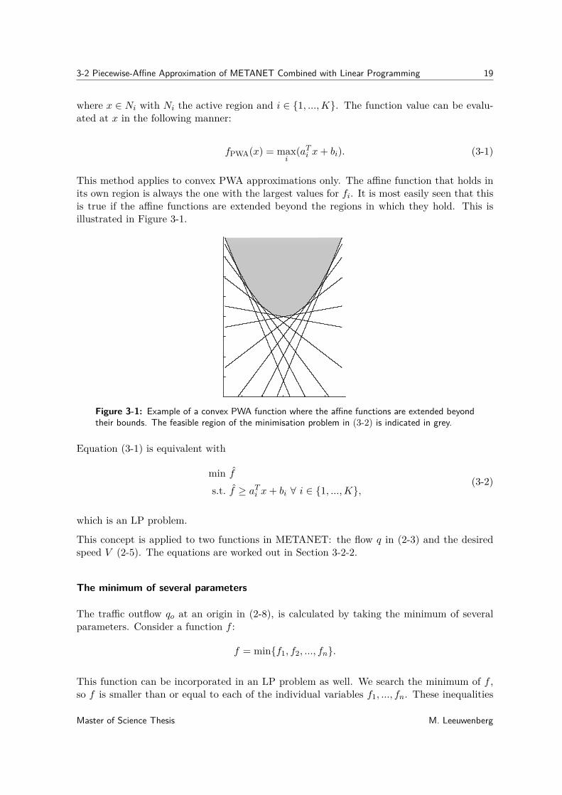
This method applies to convex PWA approximations only. The affine function that holds inits own region is always the one with the largest values for fi. It is most easily seen that thisis true if the affine functions are extended beyond the regions in which they hold. This isillustrated in Figure 3-1.
Figure 3-1: Example of a convex PWA function where the affine functions are extended beyondtheir bounds. The feasible region of the minimisation problem in (3-2) is indicated in grey.
Equation (3-1) is equivalent with
min f
s.t. f ≥ aTi x+ bi ∀ i ∈ 1, ...,K,(3-2)
which is an LP problem.
This concept is applied to two functions in METANET: the flow q in (2-3) and the desiredspeed V (2-5). The equations are worked out in Section 3-2-2.
The minimum of several parameters
The traffic outflow qo at an origin in (2-8), is calculated by taking the minimum of severalparameters. Consider a function f :
f = minf1, f2, ..., fn.
This function can be incorporated in an LP problem as well. We search the minimum of f ,so f is smaller than or equal to each of the individual variables f1, ..., fn. These inequalities
Master of Science Thesis M. Leeuwenberg
20 Improved METANET and Traffic Control
are the constraints to the following linear programming problem, where we find the maximumof f :
f = minf1, f2, ..., fn ⇔
max fs.t. f ≤ f1
f ≤ f2
:f ≤ fn.
(3-3)
In Section 2-2-4, we provided an MLD method from the literature to find the minimum ofseveral parameters, the notation given here provides an alternative to that minimisation. Wewill compare the performance of both methods in the next chapter.
3-2-2 Application to METANET
We now apply the methods from the previous section to the following functions in METANET:the outflow at origins qo in (2-8), the desired speed V in (2-5) and the flow q in (2-3).
Outflow at Origins
In METANET, origins are modelled by (2-8), which is repeated here and generalised to theminimisation of three time dependent functions as:
qo(k) = min[do(k) + wo(k)
Ts, ro(k)Co, Co
(ρjam,m − ρm,1(k)ρjam,m − ρcr,m
)]qo(k) = min[f1(k), f2(k), f3(k)].
(3-4)
To find the minimum of the three parameters f1(k), f2(k), and f3(k), we use the modificationdescribed in the previous section, so that we are able to incorporate it in an LP minimisationproblem as
min − qo(k)qo(k) ≤ f1(k)qo(k) ≤ f2(k)qo(k) ≤ f3(k),
(3-5)
where qo(k) is the approximation of qo(k).
Desired Speed Function
This nonlinear and nonconvex function needs to be altered so that it is solvable with a linearprogramming problem. We approximate
M. Leeuwenberg Master of Science Thesis
3-2 Piecewise-Affine Approximation of METANET Combined with Linear Programming 21
V(ρm,i(k)
)= vfree,m exp
[− 1am
(ρm,i(k)ρcr,m
)am]
by a PWA function with three regions as
min V (ρ)s.t. − V (ρ) ≤ −aTi ρ− bi ∀ i ∈ 1, 2, 3,
(3-6)
where V (ρ) is the LP evaluation in ρ using the PWA function VPWA(ρ). Here, VPWA(ρ) is thePWA approximation of the function V (ρ).
0 20 40 60 80 100 120 140 160 180
0
20
40
60
80
100
120
1 2 3
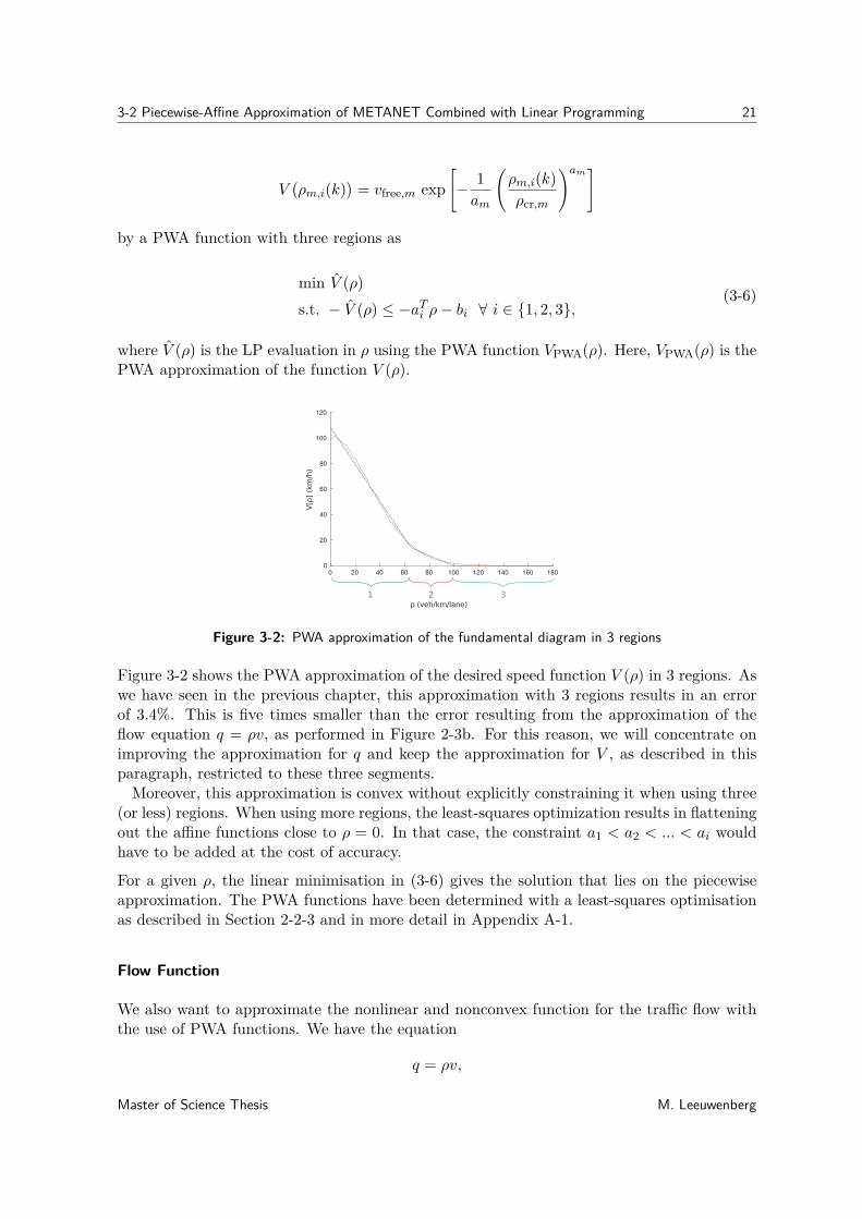
Figure 3-2: PWA approximation of the fundamental diagram in 3 regions
Figure 3-2 shows the PWA approximation of the desired speed function V (ρ) in 3 regions. Aswe have seen in the previous chapter, this approximation with 3 regions results in an errorof 3.4%. This is five times smaller than the error resulting from the approximation of theflow equation q = ρv, as performed in Figure 2-3b. For this reason, we will concentrate onimproving the approximation for q and keep the approximation for V , as described in thisparagraph, restricted to these three segments.Moreover, this approximation is convex without explicitly constraining it when using three
(or less) regions. When using more regions, the least-squares optimization results in flatteningout the affine functions close to ρ = 0. In that case, the constraint a1 < a2 < ... < ai wouldhave to be added at the cost of accuracy.
For a given ρ, the linear minimisation in (3-6) gives the solution that lies on the piecewiseapproximation. The PWA functions have been determined with a least-squares optimisationas described in Section 2-2-3 and in more detail in Appendix A-1.
Flow Function
We also want to approximate the nonlinear and nonconvex function for the traffic flow withthe use of PWA functions. We have the equation
q = ρv,
Master of Science Thesis M. Leeuwenberg
22 Improved METANET and Traffic Control
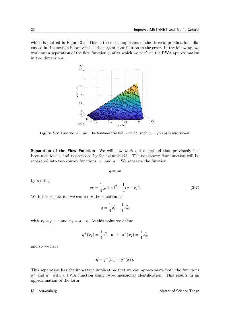
which is plotted in Figure 3-3. This is the most important of the three approximations dis-cussed in this section because it has the largest contribution to the error. In the following, wework out a separation of the flow function q, after which we perform the PWA approximationin two dimensions.
Figure 3-3: Function q = ρv. The fundamental line, with equation qe = ρV (ρ) is also shown.
Separation of the Flow Function We will now work out a method that previously hasbeen mentioned, and is proposed by for example [73]. The nonconvex flow function will beseparated into two convex functions, q+ and q−. We separate the function
q = ρv
by writingρv = 1
4(ρ+ v)2 − 14(ρ− v)2. (3-7)
With this separation we can write the equation as
q = 14x
21 −
14x
22,
with x1 = ρ+ v and x2 = ρ− v. At this point we define
q+(x1) = 14x
21 and q−(x2) = 1
4x22,
and so we have
q = q+(x1)− q−(x2).
This separation has the important implication that we can approximate both the functionsq+ and q− with a PWA function using two-dimensional identification. This results in anapproximation of the form
M. Leeuwenberg Master of Science Thesis
3-2 Piecewise-Affine Approximation of METANET Combined with Linear Programming 23
qPWA = q+PWA(x1)− q−PWA(x2). (3-8)
Note that we could have used the same PWA function as an approximation for both q+
and q−. However, when we define the two functions separately, as we have done here, wereduce the number of regions in the PWA approximations and hence the number of decisionvariables in the MLD system as well as the number of inequality constraints in the LP system,cf. Figure 3-4.
Constraints on PWA Identification Problem Suppose we have a situation in which ρ = ρjamand v = 0. The traffic is jammed and we expect q = ρjam · 0 = 0. We fill in (3-8) withx1 = ρjam + 0 and x2 = ρjam − 0 and obtain qPWA = q+
PWA(ρjam) − q−PWA(ρjam). Since thefunctions q+
PWA and q−PWA have a different domain on which they hold, when a least-squaresoptimisation would be run on them separately, the PWA approximations would (slightly)differ from each other. This is expected to become problematic when x1 = ±x2, because inthese situations the approximated flow qPWA is expected to be equal to 0. However, whenq−PWA is larger than q+
PWA, which could occur when these approximations differ from eachother, this would result in qPWA being negative, i.e. the traffic flows backwards. To preventthis from happening we impose that q+
PWA(ρjam) = q−PWA(ρjam).The other extreme scenario is when ρ = 0 and v = vfree. Similarly to the above, the flow
could potentially become negative when the PWA approximations do not meet the constraintq+
PWA(vfree) = q−PWA(−vfree).
To implement these constraints, we adapt the PWA identification to perform only one least-squares optimisation on the negative half of the horizontal axis (x1, x2 < 0) after which wemirror the solution over the vertical axis, satisfying the constraint q+
PWA(vfree) = q−PWA(−vfree),and we use the solution for both q+
PWA and q−PWA simultaneously, which will satisfy the con-straint q+
PWA(ρjam) = q−PWA(ρjam). These measures might result in the approximation becom-ing less accurate than it potentially could be. It is preferred however over an approximationthat potentially results in negative flows. We define
q±PWA(z) = 14z
2
as the mirrored approximation of both q+PWA and q−PWA.
Bounds on PWA Identification Problem We note that an approximation on the entiredomain −(ρjam + vfree) ≤ z ≤ ρjam + vfree is not necessary because not all theoreticallypossible values for q are equally likely to be encountered (for example q = ρjamvfree will notactually occur in METANET). To get an idea of what values for q are typical, we evaluatethe expected flow with v = V (ρ) as
qe = ρV (ρ). (3-9)
This line is plotted in Figure 3-3. These are not the only feasible values that q can have,i.e. the update equation for vm,i(k) in (2-5) is not equal to V (ρ) but it will mostly be in thevicinity of this line, since the corrections on vm,i−1(k) and ρm,i+1(k) are relatively small andthe other terms steer the function towards V (ρ) and thus towards this line.
Master of Science Thesis M. Leeuwenberg

24 Improved METANET and Traffic Control
For an indication of the bounds on the PWA identification problem, we calculate the ex-pected values for q+ and q− in the same manner. We obtain the functions
q+e (ρ) = 1
4(ρ+ V (ρ)
)2 and q−e (ρ) = 14(ρ− V (ρ)
)2. (3-10)
Here, the domains of q+e and q−e are respectively given by
minρ
(ρ+ V (ρ)) ≤ ρ ≤ maxρ
(ρ+ V (ρ)) and minρ
(ρ− V (ρ)) ≤ ρ ≤ maxρ
(ρ− V (ρ)).
-200 -150 -100 -50 0 50 100 150 200
0
1000
2000
3000
4000
5000
6000
7000
8000
9000
10000
Configuration 1
(a) PWA approximation in 2 regions. Here, q+PWA
is always in the second region and q−PWA is in both
regions, so we have 1 decision variable in this con-figuration.
-200 -150 -100 -50 0 50 100 150 200
0
1000
2000
3000
4000
5000
6000
7000
8000
9000
10000
Configuration 2
(b) PWA approximation in 3 regions. Here, q+PWA
is always in the third region and q−PWA is in all three,
so we have 2 decision variables in this configuration.
-200 -150 -100 -50 0 50 100 150 200
0
1000
2000
3000
4000
5000
6000
7000
8000
9000
10000
Configuration 3
(c) PWA approximation in 4 regions. Here, q−PWA
is in all four regions. The minimum of q+PWA is only
just in the fourth region, so we have chosen a safetyregion and divided q+
PWA in 2 regions. We have 4decision variables in this configuration.
-200 -150 -100 -50 0 50 100 150 200
0
1000
2000
3000
4000
5000
6000
7000
8000
9000
10000
Configuration 4
(d) PWA approximation in 5 regions. Here, q+PWA
is in the last two regions and the minimum of q−PWA
is only just in the second region, so we have chosena safety region and divided q−
PWA in 5 regions. Wehave 5 decision variables in this configuration.
Figure 3-4: The four configurations of q±PWA, with increasing numbers of decision variables,
that we have chosen to run simulations on. We show the original function 14 (ρ ± v)2 and the
approximations q±PWA of this function. The minimum and maximum of (ρ± V ) are also shown.
M. Leeuwenberg Master of Science Thesis
3-3 Accounting for Predicted Disturbances 25
An estimate of the domain on which q±(z) holds, is then acquired by calculating
zmin = minρ
(ρ+ V (ρ), ρ− V (ρ)
)and
zmax = maxρ
(ρ+ V (ρ), ρ− V (ρ)
).
We note that q± is symmetrical over the vertical axis. Then,
ζ = max(|zmin|, zmax
)= 180
provides an estimate for both the upper and lower bound, so q±(z)| − ζ ≤ z ≤ ζ.We use these bounds in the optimisation problem to determine q±PWA. We perform thisunconstrained least-squares optimisation with a multi-start Levenberg-Marquardt approach.The required symmetry is embedded in the cost function. Therefore, we were still able to usethe Levenberg-Marquardt algorithm on the minimisation problem. The exact functions thatresulted from these optimisations are given in (A-3), (A-4), (A-5), and (A-6) in Appendix A.
Improving the Results Let us now analyse the effect of reducing the number of regionsof the PWA functions q+
PWA and q−PWA using the estimate of the bounds that we previouslycalculated in (3-10). Fewer PWA regions result in fewer decision variables, which can speedup the calculation times. The result of this simplification is captured in Figure 3-4, wherefour configurations of PWA approximations are shown, with 1, 2, 4, and 5 decision variablesrespectively. In configuration 3, we have used an extra PWA function for q+
PWA as a safetyregion. The same has been done for q−PWA in configuration 4. A more elaborate discussionabout the PWA identification of this flow function can be found in Appendix A-2. Theconfigurations in the final form of Figure 3-4 have been used in the case studies that arediscussed in Chapter 4.
3-3 Accounting for Predicted Disturbances
In this section, we propose a method that incorporates bridges in METANET. We interpretthe opening or closing of these bridges as a predicted disturbance and we model these eventsas an alteration in the network topology. Therefore at least one of the system matrices in theMLD and LP (prediction) models has to be time dependent. We encounter time-dependentbehaviour, both in the state space equations and in the linear (in)equalities that apply on thestates and control actions. Furthermore, we describe the implementation of a controller thataccounts for these predicted disturbances, caused by the opening and closing of bridges.We start with a description of the modifications to METANET. More specifically, in Section
3-3-1 we zoom in on road interchanges and turning fractions. Here we define control input ofthe models. In Section 3-3-2 we describe several ways of modelling a bridge that opens andcloses at predetermined moments in time.
3-3-1 Modified METANET
We analyse METANET again, to investigate which variables are suitable to be used as controlinput u.
Master of Science Thesis M. Leeuwenberg
26 Improved METANET and Traffic Control
We propose a modification of the equations that govern the traffic progression in and around aMETANET vertex, defined earlier in (2-9) and (2-10). In METANET, β specifies the fractionsby which the summed incoming flow at a vertex ν is split and divided over the emanatinglinks. The flow towards link m was previously given as
qm,0(k) = βν,m(k)Qν(k).
We propose to omit this variable qm,0(k), and instead use the traffic split Fν,m(k). Here,Fν,m(k) is the traffic flow (veh/h) at vertex ν towards link m at time step k. This traffic splitis used as the only control input, so
u(k) = Fν,m(k). (3-11)
Now, at the first segment of a link, we use the update equation
ρm,1(k + 1) = ρm,1(k) + TsLmλm
[Fν,m(k)− qm,1(k)], (3-12)
instead of the update equation in (2-4) used otherwise.
This implies that we do not use on-ramp metering or variable speed limits as control inputs.We have chosen to use the traffic split over the turning fractions, because the system wouldhave to be quadratic in order to multiply βν,m(k) with Qν(k). This means that we work withactual flows Fν,m(k), and not with the percentages βν,m(k). When the turning fractions areneeded, which is the case when we use the nonlinear model as simulation model, they can beeasily calculated back from (3-11) as
βν,m(k) = Fν,m(k)/Qν(k). (3-13)
The equality conditions and bounds that hold for Fν,m are given next. The sum of the turningfractions at each vertex should be equal to Qν and each Fν,m in ν has a value between 0 andQν , thus we have
∑µ∈Iν
Fν,µ(k) = Qν(k) ∀ ν ∈ N (3-14)
and
0 ≤ Fν,m(k) ∀ ν ∈ N, ∀ m ∈ Iν . (3-15)
3-3-2 Describing Temporarily Unavailable Segments in METANET
We speak of a topology change when a network structure alters. In this section we propose ameans of handling topology changes in METANET. More specifically, we describe a coupleof possible methods for implementing a bridge element in the model.A bridge consists of two parts. Firstly, we have the queue area (on two sides of the bridge)
M. Leeuwenberg Master of Science Thesis
3-3 Accounting for Predicted Disturbances 27
which is typically but not necessarily a short area where vehicles wait in front of a boombarrier when the bridge is open. Secondly, we have the part of the bridge that actually opensto let water traffic pass. This is also typically a short segment compared to a METANETsegment (which measures 500 metres). If this bridge is open, the traffic should be stoppedand unable to flow to the downstream segment.Bridges that can actually open are fairly uncommon on motorways, but they do exist.
However, we will not run a case study on an real traffic situation, so the model does not yethave to exactly simulate an existing bridge.
METANET Segment
Both the queue area and the bridge itself are typically short elements compared to the 500metres of a regular METANET segment. A straightforward method would be to let both thequeue areas and the bridge itself be normal METANET segments. This implies that at leasttwo segments are needed (with a combined length of at least 1000 metres), where an entirebridge might not even be as long as 500 metres. Creating a METANET segment that is shorterthan the original 500 metres is possible, but this could result in the Courant-Friedrichs-Lewy(CFL) condition [18] being violated. The CFL condition is given as
Ts ≤ minm∈Ilink
Lmvfree,m
, (3-16)
where Ilink is the set of all the links in a network. This condition ensures that traffic does nottraverse more than one segment in a single time step. When we would implement a segmentas short as the movable part of a bridge, the CFL condition is very likely to be violated.
Zero-Length Bridges
Another way to model a topology change is to place a bridge on the node in between twosegments. This generalisation consists of two adjacent METANET segments somewhere ina link that can be disconnected from each other when the bridge opens. This bridge haszero length and only one segment upstream from the bridge node is used as queue area. Thelength of the bridge is included in the downstream segment, because the bridge itself is not apart of the queue area.
This is implemented in METANET as follows. We call the segment upstream from the bridgenode iu and the downstream segment id. When the bridge opens, the upstream traffic shouldbe stopped and thus we set qiu = 0. So we evaluate the flow qiu,b at a segment upstream froma bridge b as
qiu,b(k) =qiu if δb = 00 if δb = 1,
(3-17)
where δb(k) is a binary value indicating whether a bridge b is open (1) or closed (0) at timestep k. Furthermore, we have qiu(k) = ρiu(k)viu(k). When δb = 1, the traffic is preventedfrom flowing out of iu and so it fills up that segment, whilst maintaining the total amount oftraffic.The upstream velocity correction at segment id needs to be addressed, because when a
Master of Science Thesis M. Leeuwenberg

28 Improved METANET and Traffic Control
bridge opens we have vid−1 6= viu . We set vid−1 = vid , as if the bridge node was an originnode.The downstream velocity correction at the upstream side of the bridge ρiu+1 also needs to
be addressed, because when a bridge opens we have ρiu+1 6= ρid . We set ρiu+1 = ρiu , as if thebridge node was a destination node.
Using this method can easily result in unsatisfactory METANET behaviour. To illustratewhat happens we work out a potential case. Suppose a bridge has been open for a while andsegment iu is filled to its maximum capacity, so ρiu = ρjam and viu = 0. Then we must haveqiu−1 = 0, otherwise segment iu would still be filled with traffic and when that happens ρiucrosses the maximum capacity and the model bounds are violated. However, segment iu−1might not yet be full so ρiu−1 6= ρjam. Therefore, Viu−1(ρ) 6= 0 and this would cause viu−1 tobe larger than 0. This is a contradiction because we specifically required qiu−1 = 0 in orderto stop the traffic flow to segment iu. We conclude that we use a single segment as queuearea and that we have to make sure that the densities do not increase to values close to ρjam.The main problem with this method is that METANET cannot handle an abrupt blockage
very well. Even in a less extreme scenario (ρiu < ρjam), the model is expected to cross themaximum capacity relatively easily. The update equations are based on traffic flows and thussetting one of these flows to 0 will very likely result in abnormal behaviour. Upstream traffickeeps filling the segment in front of the bridge, even when the maximum capacity ρjam ofthat segment is reached. To prevent this from happening we take two measures. Firstly, weput speed restrictions in the area upstream from the bridge, by using a minimum speed ofvmin = 4 km/h on all segments, to regulate the inflow of traffic. Secondly, we simply limitthe time the bridge is open.
Store-and-Forward Bridges
In explaining the previous method, we observed that the maximum capacity ρjam in the queuearea can be exceeded relatively easily. To address this and other issues, we now propose avehicle store-and-forward method that is more elaborate and therefore expected to be morerobust the zero-length bridges method. Vehicles that are waiting in front of a bridge can bestacked in a queue similar to one used for an origin. Whenever the queue is empty and thebridge is closed, the queue segment is unused, but when the bridge opens, the queue segmentstarts storing traffic in a queue wb with a maximum queue length of Mw,b (and a minimumof mw,b = 0).
Nonlinear Store-and-Forward Model The update equation for the bridge queue length wbis given by
wb(k + 1) = wb(k) + Ts (qu,b(k)− qw,b(k)) , (3-18)
where qu,b(k) is the inflow of traffic from segment iu to the bridge queue and qw,b(k) is thetraffic outflow from the bridge queue towards segment id. The outflow qw,b of the queue ofbridge b is equal to 0 when the bridge is open, but also when the bridge is closed and the
M. Leeuwenberg Master of Science Thesis
3-3 Accounting for Predicted Disturbances 29
queue is empty. This variable is described in more detail further on. The traffic inflow to thebridge queue is given by
qu,b(k) =
0 if δb(k) = 0 ∧ wb(k) = 0qin,b(k) otherwise.
(3-19)
Furthermore, we define the actual value of the flow qin,b from segment iu to the bridge queueby
qin,b(k) = min[qiu(k), Mw,b − wb(k)
Ts
], (3-20)
withqiu(k) = ρiu(k)viu(k). (3-21)
Only when the queue segment is empty again after a bridge has closed, we have qu,b = 0.This makes sense, because if the queue in front of the bridge has not dissolved yet, newlyarriving traffic has to queue first before crossing the bridge. As with the zero-length bridgesmethod, the bridge can be located in the middle of a link, in which case (3-20) holds. Whenhowever the bridge is located in between a vertex ν and the first segment i of link µ, we setqin,b(k) = min[Fν,µ(k), (Mw,b − wb(k))/Ts]. For simplicity, in the following we will assumethat the bridge is located in the middle of an edge.
The maximum queue length Mw,b can be reached if bridge b is open for a long enough timeperiod. WhenMw,b is reached, the queue cannot hold more traffic, and from that moment on,the traffic is stored in the upstream segment iu in the same way as in the zero-length bridgesmethod.Suppose we are at time step km, the bridge is open, and the queue length will reach Mw,b
at the next time step. We have, from (3-20), the inflow at that time step
qin,b(km) = Mw,b − wb(km)Ts
.
Because the bridge is still open we have δb(km) = 1 and thus qu,b(km) = qin,b(km) andqw,b(km) = 0 so
wb(km + 1) = wb(km) + Tsqin,b(km) = Mw,b.
It is important to make sure that the queue length at time step km + 1 is exactly Mw,b,otherwise we lose traffic, i.e. the density of segment iu is not updated correctly.
When the bridge closes, the traffic flow starts up again, beginning with emptying the queue wbinto segment id, followed by the regular progression of the traffic in the network. Rememberthat, as long as wb 6= 0, the queue is being filled at the same time. So the queue is emptiedlike a regular origin while (3-18) is still valid. The outflow qw,b is based on the outflow at anorigin given in (2-8):
qw,b(k) =qout,b(k) if δb(k) = 00 if δb(k) = 1,
(3-22)
Master of Science Thesis M. Leeuwenberg
30 Improved METANET and Traffic Control
with
qout,b(k) = min[qu,b(k) + wb(k)
Ts, Cb
(ρjam,m − ρm,id(k)ρjam,m − ρcr,m
), Cb
]. (3-23)
Here, Cb (veh/h) is the capacity of the bridge. Unless otherwise specified, we will use
Cb = 2000 veh/h.
The regular METANET equations are only used when both the bridge queue is empty andthe bridge is closed. Similarly, the store-and-forward element is only used if either the bridgeis open or the bridge queue is not empty. Therefore, the outflow qiu,b at segment iu and theinflow qid−1,b at segment id are defined by
qiu,b(k) =qiu(k) if δb(k) = 0 ∧ wb(k) = 0qin,b(k) otherwise,
(3-24)
and
qid−1,b(k) =qiu(k) if δb(k) = 0 ∧ wb(k) = 0qw,b(k) otherwise.
(3-25)
At the time step at which we can completely empty a traffic queue, we make sure that this isdone correctly. Suppose that at time step kw we have
qout,b(kw) = qu,b(kw) + wb(kw)Ts
,
which implies that at this time step, the queue can be emptied in the adjacent segment. Thenthe last bit of traffic in the queue wb(kw) is summed with the incoming traffic qu,b(kw) =qiu(kw) at that time step and directly forwarded to the outgoing traffic via
qw,b(kw) = qout,b(kw) = qu,b(kw) + wb(kw)Ts
.
This results in
wb(k + 1) = wb(k) + Ts (qu,b(k)− qw,b(k)) = 0,
so the bridge queue is empty and qw,b = qu,b = 0 from that point on and the queue segmentstays empty until the bridge opens again. Moreover, there is no traffic lost or excess trafficleft in the queue.Furthermore, we note that the queue element is always emptied at the maximum rate. At
time step kw+1, the segments iu and id are reconnected and the traffic the regular METANETmodel equations are used again for the state evolution.
M. Leeuwenberg Master of Science Thesis
3-3 Accounting for Predicted Disturbances 31
Remark 3.1. A zero-length bridge is essentially a special case of a store-and-forward bridgewith Mw,b = 0.When a store-and-forward bridge queue is full, i.e. when at some time step wb(k) = Mw,b,
the METANET segment upstream from this bridge has to hold the excess traffic. This isrealised by forcing qiu,b = 0, so that the outflow at that upstream segment is blocked. Similarly,when using a zero-length bridge, the outflow is forced to 0 to block the outflow, c.f. (3-17) and(3-24). Therefore, when we set Mw,b = 0 in the store-and-forward model, we observe the samebehaviour as with the zero-length bridges.
MLD Store-and-Forward Model The new equations introduced above can be added to thenonlinear model, but have to be rewritten for usage in the MLD model. This can be achievedusing the methods described in [6, 73].
For the flow qin,b to the bridge we have
qin,b(k) = δqin,b(k)qiu(k)− [1− δqin,b(k)]Mw,b − wb(k)Ts
, (3-26)
where qiu(k) = q+iu(k)− q−iu(k) and
qiu(k) ≤ Mw,b − wb(k)Ts
⇔ [δqin,b(k) = 1]. (3-27)
For the conversion of qu,b to MLD form, we first define
δbwb(k) = δb(k)δwb(k). (3-28)
Now we have
qu,b(k) = [δb(k) + δwb(k)− δbwb(k)] qin,b(k), (3-29)
which is in MLD form if we add the three constraints given in (2-18) on δbwb(k). Furthermorewe have
δwb(k) =
1 if wb(k) > 00 if wb(k) = 0,
which translates towb(k) ≤Mw,bδwbwb(k) ≥εδwb ,
(3-30)
where ε is the machine precision.
The MLD form of qw,b(k) is derived next. We start with rewriting (3-23) as
qout,b(k) = min[qu,b(k) + wb(k)
Ts, Cb
(ρjam,m − ρm,id(k)ρjam,m − ρcr,m
), Cb
]
qout,b(k) = min[qoutb,1 (k), qout
b,2 (k), Cb], (3-31)
Master of Science Thesis M. Leeuwenberg
32 Improved METANET and Traffic Control
which is similar to the equation for the outflow at an origin; cf. Appendix A-3-2. In a similarmanner, we can rewrite (3-31) in MLD form as
qout,b(k) = qoutb,1 (k)δout
b,1 (k) + qoutb,2 (k)δout
b,2 (k) + Cbδoutb,3 (k), (3-32)
where
[δoutb,1 (k) = 1]⇔ [qout
b,1 (k) ≤ qoutb,2 (k) and qout
b,1 (k) ≤ Cb][δoutb,2 (k) = 1]⇔ [qout
b,2 (k) ≤ qoutb,1 (k) and qout
b,2 (k) ≤ Cb][δoutb,3 (k) = 1]⇔ [Cb ≤ qout
b,1 (k) and Cb ≤ qoutb,2 (k)].
(3-33)
Now we can write the MLD equivalent of qw,b as
qw,b(k) = [1− δb(k)]qout,b(k). (3-34)
The last two variables we rewrite to MLD form are qiu,b(k) and qid−1,b(k). We have
qb,iu(k) = qiu(k) +(δb(k) + δwb(k)− δbwb(k)
)(qin,b(k)− qiu(k)
), (3-35)
and
qb,id−1(k) = qiu(k) +(δb(k) + δwb(k)− δbwb(k)
)(qw,b(k)− qiu(k)
). (3-36)
Again, we removed the multiplications of the binary decision variables δb(k)δwb(k) in (3-35)and (3-36) by replacing them with the already introduced binary variable δbwb and the threeconstraints in (2-18).
Topology Changes
Because we approached the opening of a bridge in METANET as a topology change in theunderlying network, we can generalise these methods to be applicable to a variety of trafficsituations, i.e. the road can be obstructed for more reasons than an open bridge, for examplean accident that blocks the motorway, red traffic lights, or road maintenance. The methodsfor describing temporarily unavailable connections in METANET could be used in these casesas well.
3-4 Time-Dependent State Space Representation of the MixedLogical Dynamical Model and the Linear Programming Model
At this point, as all the different parts of the models have been discussed separately, we putthem together to arrive at a generalised form of a state space system that fits both the MLDand LP model as
M. Leeuwenberg Master of Science Thesis
3-5 Control Implementation 33
x(k + 1) = A(k)x(k) +B(k)u(k) + B(k)υ(k) + f(k)y(k) = C(k)x(k) +D(k)u(k) + D(k)υ(k) + g(k)
E1(k)x(k) + E2(k)u(k) + E(k)υ(k) ≤ h(k),(3-37)
where x(k) are the states, u(k) the control inputs, the optimisation variables υ(k), and y(k)the system’s outputs.The MLD and LP model have a time-dependent nature because they can account for
predicted disturbances. A change in the topology of the network (i.e. when a bridge opens orcloses) results in an update of the system matrices.
The state x is given as x(k) = [wo(k), wb(k), ρ(k), v(k)]T in the MLD model, where we usethe store-and-forward method for the bridges. For the LP model it is defined by x(k) =[wo(k), ρ(k), v(k)]T , because we use the zero-length bridges method here.
The control input is given by the controlled traffic split u(k) = Fν,m(k). This is the only realcontrol input, i.e. only by controlling Fν,m(k) we can steer the system.
The optimisation variables for the MLD model are given as a stacked vector with all theauxiliary variables, υ(k) = [δT (k), zT (k)]T . In the LP model, we use a vector containing allthe dummy variables υ(k) = [qo(k), V (k), q+(k), q−(k)].
The output y(k) is a linear combination of the input and the state. It is a (not always directlymeasurable) system parameter that can say something about the performance of a controlleror the system in general.In this thesis, we use the TTS to evaluate the overall performance of the different models
and controllers. This variable was already given in (2-20) and is a little more elaboratelydiscussed in the next section. In the scope of this thesis, the system does not necessarilyrequire any more outputs. However, since the outputs are a linear function of the states andinputs, we can use them to get insight in the inputs. This is especially useful for summingthe (sometimes elaborate) functions that q(k) consists of, for qo(k), and V (k). Thus we usey(k) = [JyTTS(k), V (k), qo(k), q(k)]T , where JyTTS(k) is the TTS at an instant of time. In theMLD model, where we use store-and-forward bridges, we add the most important variablesof this element to the output; we have y(k) = [JyTTS(k), V (k), qo(k), q(k), qu,b(k), qw,b(k)]T .
3-5 Control Implementation
In this section, we discuss the control implementation that we use in combination with thetraffic models. The only available actuators are the traffic splits. Many control methodsare suitable for obtaining an input vector u(k) = Fν,m(k) at each time step. We propose toapply MPC, which is used in combination with both the MLD and the LP model describedthroughout this thesis.
Control Framework
When implementing a controller, we close the control loop and link the outputs back to theinputs. In the context of this thesis, the aim of the controllers is to minimise the TTS.
Master of Science Thesis M. Leeuwenberg
34 Improved METANET and Traffic Control
In the case we use the store-and-forward method for bridges, we add the bridge queue wb tothe function for the TTS, which is then given by
JTTS = Ts
Nsim∑k=1
∑(m,i)∈Iall
Lmλmρm,i(k) +∑o∈Oall
wo(k) +∑b∈Ball
wb(k)
, (3-38)
where Nsim is the number of time steps in the simulation, Iall are all possible (m, i) pairs, Oallis the set of all origins, and Ball the set of all bridges in the network.
A major motivation for computationally light controllers is real-time implementation. Whenusing a controller in real time, we require the control inputs before moving to the next timestep. That means that the computation time Tc always has to be less than the time step, i.e.Tc < Ts.
Model Predictive Control Applied to the Modified Models
We use MPC in combination with the generalised time-dependent system described in (3-37)for both the MLD and LP model. This is possible under the condition that the disturbanceson the system are known beforehand. We can for example anticipate on the opening of abridge easily because ships travel at a relatively constant speed. We can use the models incombination with MPC because, although the system matrices are time dependent, we updatethem at each time step in which a bridge opens. Sudden topology changes are not accountedfor by this controller, so we leave disturbance rejection outside the scope of this thesis.
The cost function used for the MPC problem is TTS over the prediction horizon, is given by
JMPCTTS (k) = Ts
Np∑j=1
∑(m,i)∈Iall
Lmλmρm,i(k + j) +∑o∈Oall
wo(k + j) +∑b∈Ball
wb(k + j)
. (3-39)
Remark 3.2. An implementation issue arises when using a control horizon Nc. In the timesteps from Nc to Np, the input u(k) = Fν,m(k) is kept constant, and the auxiliary variablesin υ(k) are still updated at each time step. Therefore, we encounter an inaccuracy. Sincethe values in u(k) are traffic flows and not the turning fractions, they need to be constantlyupdated in order to obtain an accurate prediction.If we would choose Nc < Np, we would have the constant traffic splits Fν,m(k), next to the
variable flows q(k) in the constraints on the inputs given in (3-14) and (3-15). This wouldcause the prediction values to be inaccurate. The model is infeasible in that case, unless wedisable the constraints on the inputs. Therefore, the usage of a control horizon Nc is up tothis point undesired and we will use Nc = Np in the following.
An N -step-ahead simulation with the LP model cannot be accurately solved using a single LPoptimisation, but only with a sequence of LP problems. We provide a theoretical motivationfor this statement in Section 4-2. We propose to use time-dependent weighing factors asa potential way of solving the N -step-ahead simulation with a single LP problem. In theLP-MPC model, we use
M. Leeuwenberg Master of Science Thesis
3-6 Summary 35
JMPCLP (k) = wTTS
Jnom,TTSJMPC
TTS (k) +Np−1∑j=0
(wV (k)Jnom,V
V (k + j) +wq+(k)Jnom,q+
q+(k + j)
+wq−(k)Jnom,q−
q−(k + j)− wqo(k)Jnom,qo
qo(k + j)),
(3-40)
as the objective function, where wTTS, wV (k), wq±(k) and wqo(k) are weighting factors. InSection 5-3, we briefly discuss a potential way of solving the N -step-ahead simulation in asingle LP problem with the use of these time-dependent weighing factors.
3-6 Summary
In this chapter, we have made two contributions to the literature. We have expanded thealready existing method that approximates METANET with an MLD model that can beevaluated with MILP. This resulted in a model that can be evaluated using LP, which isexpected to improve the trade-off between speed and accuracy significantly. Furthermore,using MPC, we are able to account for predicted topology changes. MPC can be used incombination with both the MLD and LP model. The computation times of MPC problems,where either the MLD or LP model is used as prediction model, need to be compared to eachother.The second contribution to the literature is an extension to METANET that allows for
topology changes in the network. More specifically we have proposed a method that incorpo-rates store-and-forward bridges in the nonlinear and in the MLD model.
Master of Science Thesis M. Leeuwenberg

36 Improved METANET and Traffic Control
M. Leeuwenberg Master of Science Thesis
Chapter 4
Simulation Results
In this chapter, we run a number of simulations using the newly proposed Linear Programming(LP) model, and using the newly added bridge elements in the Mixed Logical Dynamical(MLD) model. In Section 4-1, we describe the general setup of the simulations: the softwarewe have used and the tuning of the Model Predictive Control (MPC) problems. Thereafter,in Section 4-2, we describe an N -step-ahead simulation with the LP model in detail andwe show that, to solve this simulation correctly, it should be written as a linear multilevelprogramming problem. Since we expected the resulting problem to be a single LP problem,we do not run further simulations with the LP model. Instead, to provide a proof of conceptof the newly proposed bridge elements, we run a number of simulations on both the nonlinearand MLD model in Section 4-3.
4-1 Setup
In this section, we describe the setup used for the simulations performed in this chapter.
Software For the simulations that have been run in this chapter we have used Gurobi 8.1.0 toevaluate the LP and Mixed Integer Linear Programming (MILP) problems. We have used theMATLAB Application Programming Interface (API) for MATLAB R2019b on both Ubuntuand Windows.
Tuning the Model Predictive Controller In MPC, we can tune the performance using theparameters Np and Nc. In Remark 3.2 we have already discussed that we need to haveNp = Nc in order to satisfy the equality constraints on Fν,m. Furthermore, we choose theirvalue according to a rule of thumb that is closely related to the one proposed by Hegyi [38,49],according to whom Np should be larger, but not much larger than the typical travel time inthe network. That rule of thumb is based on a network with a single stretch of road withvariable speed limits. However, we consider a motorway network with multiple routes of
Master of Science Thesis M. Leeuwenberg
38 Simulation Results
different lengths and therefore we will use a different rule of thumb.We choose
Np ≥ |Il|Ts,
where Il is the set of segments that comprise the longest route in the network and |Il| is thenumber of elements in that set. If there is some traffic in a segment, some of it progressesto the downstream segment at each time step, unless a bridge is open. Therefore, we cansay that in |Il| time steps, the prediction horizon spans the entire network size (if we do notconsider bridges), which is the minimum requirement for the MPC to work properly. Thisis most easily understood when filling an empty network with two routes of unequal length.When the prediction horizon is shorter than the time it takes to fill the shortest route withtraffic, the Total Time Spent (TTS) has the same value no matter the values of Fν,m, whetherwe route all traffic over the longest or the shortest route, because for either choice the amountof traffic in the network is exactly the same. From the moment the traffic disappears at adestination, a difference can be found.
If we compare the LP model with the MLD model, when used as prediction model in an MPCcontext, we expect them to give the same predictions when the same Piecewise-Affine (PWA)configurations are used and the prediction and control horizon have the same length. Whenused for routing on a large scale network, we allow for some deviation from the MLD model,as long as the prediction with the LP model is reasonably accurate. However, when used ina simple single-lane network where no routing is required, we expect the predictions to beexactly the same. We will show that this is not the case when solving anN -step-ahead problemin a single LP problem, and that it should be written as a linear multilevel programmingproblem instead.
4-2 Analysis of a Single N-Step-Ahead Simulation with the LinearProgramming Model
The LP model does not prove to work as expected when we use it as prediction model. We havenoticed that the MPC implementation gives incorrect results, even for very small networkswhere no routing is required and with wTTS = 0, in which case we expected the outcomes tobe exactly the same as the results obtained with the MLD model used as prediction model.To get a better understanding of what the underlying reason for these incorrect results is, weprovide an analysis of the equations that arise when we use the LP model in an N -step-aheadsimulation.
Setup This analysis is performed on a very small network with one single-lane link, onesegment, one origin, and one destination. We solve the N -step-ahead simulation with N = 2.We define the cost function for this problem as
JLP =N−1∑k=0
(wV V (k) + wq+ q+(k) + wq− q−(k)− wqo qo(k)
), (4-1)
with wV = 1, wq+ = 1, wq− = 0.1, and wqo = 1. For clarity, we repeat the update equationsfor the LP model. Since we only have one link, we leave out the link index m and write
M. Leeuwenberg Master of Science Thesis
4-2 Analysis of a Single N -Step-Ahead Simulation with the Linear Programming Model 39
wo(k + 1) = wo(k) + Ts(do(k)− qo(k)),
ρi(k + 1) = ρi(k) + TsLλ
[qi−1(k)− qi(k)],
andvi(k + 1) = vi(k) + Ts
τ[V [ρi(k)]− vi(k)]
+ Tsvi(k)[vi−1(k)− vi(k)]L
− Tsη[ρi+1(k)− ρi(k)]τL(ρi(k) + κ) ,
Since we only use one lane and one segment, we have λ = 1 and i = 1. Furthermore, we havethe following boundary conditions for this problem:
q0(k) = qo(k), ρ2(k) = ρ1(k), and v0(k) = v1(k).
We substitute these equations in the update equations and obtain
wo(k + 1) = wo(k) + Ts(do(k)− qo(k))
ρ1(k + 1) = ρ1(k) + TsL
[qo(k)− q1(k)]
v1(k + 1) = v1(k) + Tsτ
[V1(k)− v1(k)].
The number of regions in the PWA approximations of V and q are chosen as small as possible.We use a PWA approximation VPWA in two regions, q+
PWA in one region, and q−PWA in tworegions; so we have:
VPWA(k) =aV ρ1(k) + bV if ρ1(k) ≤ sV0 if ρ1(k) > sV
q+PWA(k) = aq(ρ1(k) + v1(k))
q−PWA(k) =−aq(ρ1(k)− v1(k)) if ρ1(k)− v1(k) ≤ 0aq(ρ1(k)− v1(k)) if ρ1(k)− v1(k) > 0.
Here, aV and aq indicate the slope and bV indicates the y-intercept of the corresponding affinefunction. Furthermore, sV is the x-coordinate of the intersection of the two affine functionsin VPWA.Note that the approximations for q+ and q− are based on the same parameter aq and
are mirrored over the vertical axis, as has been explained in Section 3-2-2 and visualised inFigure 3-4a.
The constraints to which the dummy variables in the LP model are subject at a given timestep k are:
Master of Science Thesis M. Leeuwenberg
40 Simulation Results
V1(k) ≥ aV ρ1(k) + bv
V1(k) ≥ 0qo(k) ≤ do(k) + wo(k)/Tsqo(k) ≤ Co
qo(k) ≤ Co
(ρjam − ρ1(k)ρjam − ρcr
)q+
1 (k) ≥ aq(ρ1(k) + v1(k))q−1 (k) ≥ − aq(ρ1(k)− v1(k))q−1 (k) ≥ aq(ρ1(k)− v1(k))
(4-2)
Next, we state the values of the variables in the update equations (ρ, v, and wo) at time stepk = 1 as a function of the initial condition. For given ρ(0), v(0), and wo(0), their values atthe next time step are:
wo(1) = wo(0) + Ts(do(0)− qo(0)),
ρ1(1) = ρ1(0) + TsL
[qo(0)− (q+1 (0)− q−1 (0))]
v1(1) = v1(0) + Tsτ
[V1(0)− v1(0)].
We aim to write the constraints in the MPC problem as a function of the initial condition, i.e.the values of the state variables at k = 0. This way, we get a good insight in the optimisationproblem and we will be able to see where it contradicts.We write the constraints on the dummy variables for the two time steps in the prediction
horizon by evaluating (4-2) for k = 0 and k = 1 and obtain the following inequality constraints:
V1(0) ≥ aV ρ1(0) + bv V1(1) ≥ aV ρ1(1) + bv
V1(0) ≥ 0 V1(1) ≥ 0qo(0) ≤ do(0) + wo(0)/Ts qo(1) ≤ do(1) + wo(1)/Tsqo(0) ≤ Co qo(1) ≤ Co
qo(0) ≤ Co
(ρjam − ρ1(0)ρjam − ρcr
)qo(1) ≤ Co
(ρjam − ρ1(1)ρjam − ρcr
)q+
1 (0) ≥ aq(ρ1(0) + v1(0)) q+1 (1) ≥ aq(ρ1(1) + v1(1))
q−1 (0) ≥ − aq(ρ1(0)− v1(0)) q−1 (1) ≥ − aq(ρ1(1)− v1(1))q−1 (0) ≥ aq(ρ1(0)− v1(0)) q−1 (1) ≥ aq(ρ1(1)− v1(1)).
(4-3)
Furthermore, we can write the constraints in the second time step as a function of the variablesin the previous time step. We substitute the equations that we have for ρ(1), v(1), and wo(1)in the second column of inequalities in (4-2). The set of constraints that results from thissubstitution can be further simplified and is stated next (we leave working out these equationsto the reader). We have:
M. Leeuwenberg Master of Science Thesis

4-2 Analysis of a Single N -Step-Ahead Simulation with the Linear Programming Model 41
V1(1) ≥aV(ρ1(0) + Ts
L[qo(0)− q+
1 (0) + q−1 (0)])
+ bV
V1(1) ≥0
qo(1) ≤wo(0)Ts
+ do(0) + do(1)− qo(0)
qo(1) ≤Co
qo(1) ≤Co
ρjam −(ρ1(0) + Ts
L [qo(0)− q+1 (0) + q−1 (0)]
)ρjam − ρcr
q+
1 (1) ≥aq(ρ1(0) + Ts
L[qo(0)− q+
1 (0) + q−1 (0)] + v1(0) + Tsτ
[V1(0)− v1(0)])
q−1 (1) ≥− aq(ρ1(0) + Ts
L[qo(0)− q+
1 (0) + q−1 (0)]− v1(0) + Tsτ
[V1(0)− v1(0)])
q−1 (1) ≥aq(ρ1(0) + Ts
L[qo(0)− q+
1 (0) + q−1 (0)]− v1(0) + Tsτ
[V1(0)− v1(0)]).
(4-4)
Evaluation We have deliberately chosen not to use the nominal values Jnom, defined in(3-40), in this evaluation. Since we have wTTS = 0, we expect that the results we obtainwith a single control optimisation are independent of the weights on the dummy variables.Regardless of what values we pick for these weights, we expect that the dummy variablesare pushed on the PWA function lines and evaluate the model progression correctly (whichmeans that they have exactly the same values as the MLD equivalent of this problem).
Next, we evaluate the N -step-ahead simulation with initial condition
wo(0) = 0ρ1(0) = 0v1(0) = 106.78.
Here, v1(0) = VPWA(0). When we specify the initial condition, we can compare the resultthat we expect from the MLD solution with the optimal solution that we obtain with the LPmodel as prediction model in a single LP problem.
We ran the simulation with the LP model in a single LP problem and compared the resultwith the values based on the MLD solution. In Table 4-1 we state all the values of thestate and dummy variables for both the expected and the unexpected solution. For the costfunctions we found the following values:
JLP,e = 6303JLP,u = 6142,
where JLP,e denotes the MLD-based solution and JLP,u is the cost of the solution to the singleLP problem.
Master of Science Thesis M. Leeuwenberg
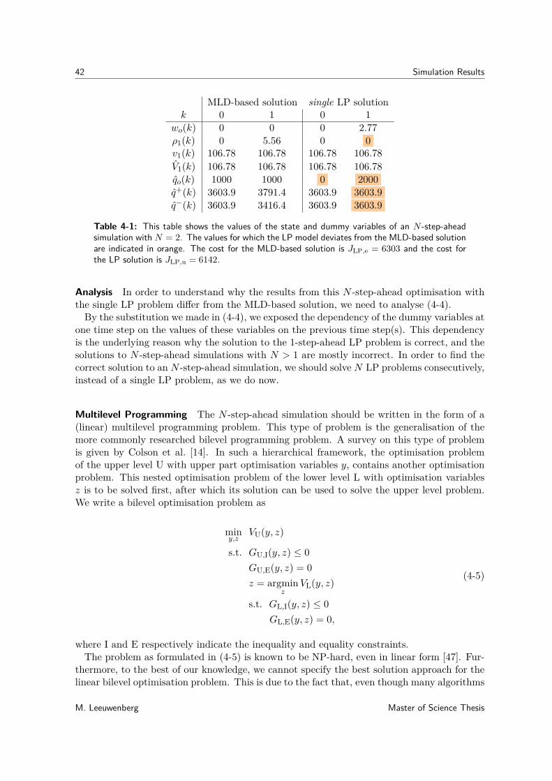
42 Simulation Results
MLD-based solution single LP solutionk 0 1 0 1
wo(k) 0 0 0 2.77ρ1(k) 0 5.56 0 0v1(k) 106.78 106.78 106.78 106.78V1(k) 106.78 106.78 106.78 106.78qo(k) 1000 1000 0 2000q+(k) 3603.9 3791.4 3603.9 3603.9q−(k) 3603.9 3416.4 3603.9 3603.9
Table 4-1: This table shows the values of the state and dummy variables of an N -step-aheadsimulation with N = 2. The values for which the LP model deviates from the MLD-based solutionare indicated in orange. The cost for the MLD-based solution is JLP,e = 6303 and the cost forthe LP solution is JLP,u = 6142.
Analysis In order to understand why the results from this N -step-ahead optimisation withthe single LP problem differ from the MLD-based solution, we need to analyse (4-4).By the substitution we made in (4-4), we exposed the dependency of the dummy variables at
one time step on the values of these variables on the previous time step(s). This dependencyis the underlying reason why the solution to the 1-step-ahead LP problem is correct, and thesolutions to N -step-ahead simulations with N > 1 are mostly incorrect. In order to find thecorrect solution to an N -step-ahead simulation, we should solve N LP problems consecutively,instead of a single LP problem, as we do now.
Multilevel Programming The N -step-ahead simulation should be written in the form of a(linear) multilevel programming problem. This type of problem is the generalisation of themore commonly researched bilevel programming problem. A survey on this type of problemis given by Colson et al. [14]. In such a hierarchical framework, the optimisation problemof the upper level U with upper part optimisation variables y, contains another optimisationproblem. This nested optimisation problem of the lower level L with optimisation variablesz is to be solved first, after which its solution can be used to solve the upper level problem.We write a bilevel optimisation problem as
miny,z
VU(y, z)
s.t. GU,I(y, z) ≤ 0GU,E(y, z) = 0z = argmin
zVL(y, z)
s.t. GL,I(y, z) ≤ 0GL,E(y, z) = 0,
(4-5)
where I and E respectively indicate the inequality and equality constraints.The problem as formulated in (4-5) is known to be NP-hard, even in linear form [47]. Fur-
thermore, to the best of our knowledge, we cannot specify the best solution approach for thelinear bilevel optimisation problem. This is due to the fact that, even though many algorithms
M. Leeuwenberg Master of Science Thesis
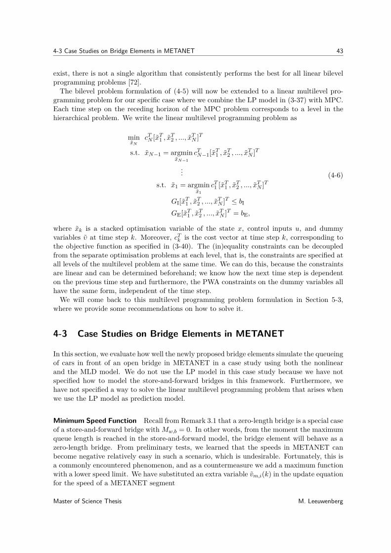
4-3 Case Studies on Bridge Elements in METANET 43
exist, there is not a single algorithm that consistently performs the best for all linear bilevelprogramming problems [72].The bilevel problem formulation of (4-5) will now be extended to a linear multilevel pro-
gramming problem for our specific case where we combine the LP model in (3-37) with MPC.Each time step on the receding horizon of the MPC problem corresponds to a level in thehierarchical problem. We write the linear multilevel programming problem as
minxN
cTN [xT1 , xT2 , ..., xTN ]T
s.t. xN−1 = argminxN−1
cTN−1[xT1 , xT2 , ..., xTN ]T
...s.t. x1 = argmin
x1cT1 [xT1 , xT2 , ..., xTN ]T
GI[xT1 , xT2 , ..., xTN ]T ≤ bI
GE[xT1 , xT2 , ..., xTN ]T = bE,
(4-6)
where xk is a stacked optimisation variable of the state x, control inputs u, and dummyvariables υ at time step k. Moreover, cTk is the cost vector at time step k, corresponding tothe objective function as specified in (3-40). The (in)equality constraints can be decoupledfrom the separate optimisation problems at each level, that is, the constraints are specified atall levels of the multilevel problem at the same time. We can do this, because the constraintsare linear and can be determined beforehand; we know how the next time step is dependenton the previous time step and furthermore, the PWA constraints on the dummy variables allhave the same form, independent of the time step.We will come back to this multilevel programming problem formulation in Section 5-3,
where we provide some recommendations on how to solve it.
4-3 Case Studies on Bridge Elements in METANET
In this section, we evaluate how well the newly proposed bridge elements simulate the queueingof cars in front of an open bridge in METANET in a case study using both the nonlinearand the MLD model. We do not use the LP model in this case study because we have notspecified how to model the store-and-forward bridges in this framework. Furthermore, wehave not specified a way to solve the linear multilevel programming problem that arises whenwe use the LP model as prediction model.
Minimum Speed Function Recall from Remark 3.1 that a zero-length bridge is a special caseof a store-and-forward bridge withMw,b = 0. In other words, from the moment the maximumqueue length is reached in the store-and-forward model, the bridge element will behave as azero-length bridge. From preliminary tests, we learned that the speeds in METANET canbecome negative relatively easy in such a scenario, which is undesirable. Fortunately, this isa commonly encountered phenomenon, and as a countermeasure we add a maximum functionwith a lower speed limit. We have substituted an extra variable vm,i(k) in the update equationfor the speed of a METANET segment
Master of Science Thesis M. Leeuwenberg
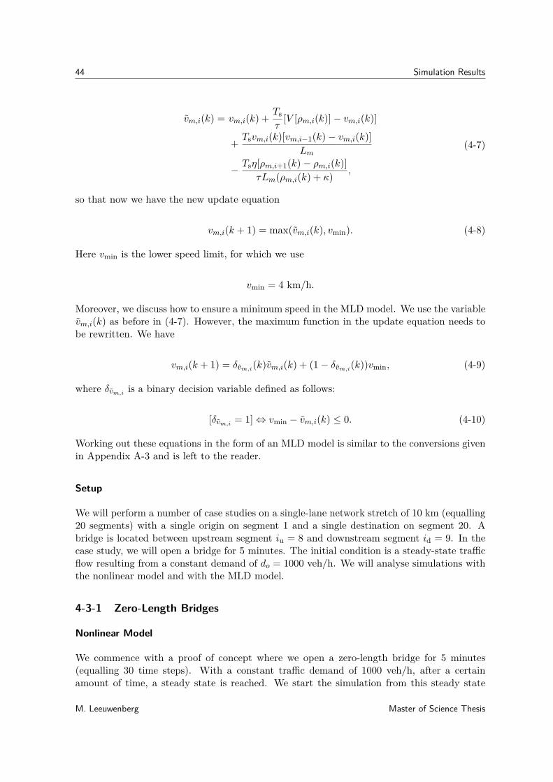
44 Simulation Results
vm,i(k) = vm,i(k) + Tsτ
[V [ρm,i(k)]− vm,i(k)]
+ Tsvm,i(k)[vm,i−1(k)− vm,i(k)]Lm
− Tsη[ρm,i+1(k)− ρm,i(k)]τLm(ρm,i(k) + κ) ,
(4-7)
so that now we have the new update equation
vm,i(k + 1) = max(vm,i(k), vmin). (4-8)
Here vmin is the lower speed limit, for which we use
vmin = 4 km/h.
Moreover, we discuss how to ensure a minimum speed in the MLD model. We use the variablevm,i(k) as before in (4-7). However, the maximum function in the update equation needs tobe rewritten. We have
vm,i(k + 1) = δvm,i(k)vm,i(k) + (1− δvm,i(k))vmin, (4-9)
where δvm,i is a binary decision variable defined as follows:
[δvm,i = 1]⇔ vmin − vm,i(k) ≤ 0. (4-10)
Working out these equations in the form of an MLD model is similar to the conversions givenin Appendix A-3 and is left to the reader.
Setup
We will perform a number of case studies on a single-lane network stretch of 10 km (equalling20 segments) with a single origin on segment 1 and a single destination on segment 20. Abridge is located between upstream segment iu = 8 and downstream segment id = 9. In thecase study, we will open a bridge for 5 minutes. The initial condition is a steady-state trafficflow resulting from a constant demand of do = 1000 veh/h. We will analyse simulations withthe nonlinear model and with the MLD model.
4-3-1 Zero-Length Bridges
Nonlinear Model
We commence with a proof of concept where we open a zero-length bridge for 5 minutes(equalling 30 time steps). With a constant traffic demand of 1000 veh/h, after a certainamount of time, a steady state is reached. We start the simulation from this steady state
M. Leeuwenberg Master of Science Thesis
4-3 Case Studies on Bridge Elements in METANET 45
Traffic Evolution with Nonlinear Simulation Model
5 10 15 200
1
2
3
4
5
6
7
8
9
10
10
20
30
40
50
60
70
80
5 10 15 200
1
2
3
4
5
6
7
8
9
10
10
20
30
40
50
60
70
80
90
100
110
5 10 15 200
1
2
3
4
5
6
7
8
9
10
0
500
1000
1500
2000
2500
3000
3500
4000
Figure 4-1: Case with a zero-length bridge being open for 5 minutes, starting from a steady statesolution (where ρ = 10.42 veh/km and v = 96.01 km/h) that resulted from a constant inflowof 1000 veh/h. The maximum value of the density is ρ = 85.84 veh/km (reached one time stepbefore the bridge closes again). Linear speed trajectories are shown in the density plot with blackdashed lines. The TTS in this simulation is 22.18 veh·h.
Traffic Evolution with MLD Simulation Model
5 10 15 200
1
2
3
4
5
6
7
8
9
10
10
20
30
40
50
60
70
80
90
5 10 15 200
1
2
3
4
5
6
7
8
9
10
10
20
30
40
50
60
70
80
90
100
110
5 10 15 200
1
2
3
4
5
6
7
8
9
10
0
500
1000
1500
2000
2500
3000
3500
4000
4500
5000
Figure 4-2: Case with a zero-length bridge being open for 5 minutes, starting from a steadystate solution (where ρ = 14.73 veh/km and v = 87.23) that resulted from a constant inflow of1000 veh/h. The maximum value of the density is ρ = 96.97 veh/km (reached one time stepbefore the bridge closes again). Linear speed trajectories are shown in the density plot with blackdashed lines. The TTS in this simulation is 27.27 veh·h.
solution, where ρ = 10.42 veh/km and v = 96.01 km/h for all segments in the network.The traffic evolution is shown in Figure 4-1. We observe a build up of traffic in the segments
upstream from the bridge from the moment it opens until it closes.
Furthermore, what stands out is that the maximum value of the density is 85.84 veh/kmat segment iu, when the bridge has been open for 5 minutes. The desired speed at thatvalue equals V (85.84) = 4.5 km/h. However, when the bridge closes at the subsequent timestep, the speed at that upstream segment increases to 50.38 km/h, while the density hardlychanges. This results in an extremely high flow, with a maximum of 4318 veh/h (normally,
Master of Science Thesis M. Leeuwenberg
46 Simulation Results
the maximum flow is 2000 veh/h) which only lasts for 2 time steps. We note that thisis unavoidable METANET behaviour that is due to the relatively large density differencebetween the upstream and the downstream segment. Concluding, we can state that theresults in Figure 4-1, obtained with the nonlinear model, are satisfactory.
Mixed Logical Dynamical Model
In this section, we perform the same case study as before, but now using the MLD model assimulation model. We use the settings with the PWA configuration with the highest accuracyin Figure 3-4, i.e. we approximate V in 3 regions and q in 5 regions. We use the same networkand the same parameters as before, however, when we start with the same constant trafficdemand of do = 1000 veh/h, we arrive at a steady state with ρ = 14.73 veh/km and v = 87.23km/h (these values differ from the nonlinear model due to the PWA approximations in theMLD model).
The result of this simulation is plotted in Figure 4-2. Overall, this traffic evolution is anacceptable approximation of the traffic evolution in the previous case study, visualised inFigure 4-1. A difference can be observed in the traffic speeds. The linear trajectories plottedin Figures 4-1 and 4-2 provide information about the pace of the traffic evolution. The steeperthis trajectory, the slower the traffic moves. When we compare the lower trajectory in bothimages, we observe that the speed in the MLD model is lower than in the nonlinear model,given a steady-state flow of 1000 veh/h on all segments. On the other hand, the speed atwhich the traffic starts up after the bridge closes is a little higher in the MLD model than inthe nonlinear model (which can be observed from the upper trajectory in both figures).Furthermore, the maximum density, observed to be 96.97 veh/km, is bit higher than the
maximum density observed in the simulation with the nonlinear model, which is 85.84 veh/km.This happens partly because the steady state solution obtained with the MLD model (theinitial condition of the simulation) has a higher density than the steady state solution thatwe obtained with the nonlinear model, and partly because of the approximation error thatwe have with the MLD model.Lastly, we compare the maximum flow. In the simulation with the MLD model, we find
a maximum flow of 5027 veh/h. This was 4318 veh/h in the simulation with the nonlinearmodel.In Section 3-1, we have stated that our anticipation was a 15% error in the TTS w.r.t.
the nonlinear model when the only approximation used is the flow function with a PWAfunction with 4 regions. Comparing the two simulations in Figures 4-1 and 4-2, we have a19% relative error in the TTS w.r.t. the nonlinear model. To put this into perspective, wenote that the calculation of the error is more fair when we start the MLD simulation withthe same initial condition as the nonlinear model. In doing so, we obtain a TTS for thesimulation with the MLD model of 23.22 veh·h, which is only a 5.2% relative error w.r.t. thenonlinear model. Furthermore, this result could be improved by simply adding more regionsto the PWA approximation of the flow function. Note however, that the aim is to use theMLD model as prediction model in combination with MPC. We observe that the MLD modelcaptures the dynamics of an open bridge to a certain extent, so that the model is suitableto be used as prediction model for routing in an MPC context. We conclude that the MLDapproximation of the nonlinear model is acceptable, and if necessary can be further improvedby adding more regions to the PWA approximation of the flow function.
M. Leeuwenberg Master of Science Thesis
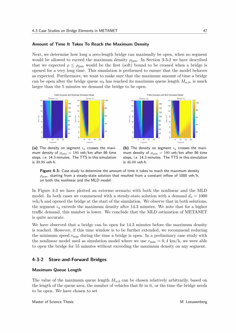
4-3 Case Studies on Bridge Elements in METANET 47
Amount of Time It Takes To Reach the Maximum Density
Next, we determine how long a zero-length bridge can maximally be open, when no segmentwould be allowed to exceed the maximum density ρjam. In Section 3-3-2 we have describedthat we expected ρ ≤ ρjam would be the first (soft) bound to be crossed when a bridge isopened for a very long time. This simulation is performed to ensure that the model behavesas expected. Furthermore, we want to make sure that the maximum amount of time a bridgecan be open after the bridge queue wb has reached its maximum queue length Mw,b, is muchlarger than the 5 minutes we demand the bridge to be open.
Traffic Evolution with Nonlinear Simulation Model
5 10 15 20
0
2
4
6
8
10
12
14
20
40
60
80
100
120
140
160
5 10 15 20
0
2
4
6
8
10
12
14
20
40
60
80
100
(a) The density on segment iu crosses the maxi-mum density of ρjam = 180 veh/km after 86 timesteps, i.e. 14.3 minutes. The TTS in this simulationis 39.98 veh·h.
Traffic Evolution with MLD Simulation Model
5 10 15 20
0
2
4
6
8
10
12
14
0
20
40
60
80
100
120
140
160
5 10 15 20
0
2
4
6
8
10
12
14
20
40
60
80
100
(b) The density on segment iu crosses the maxi-mum density of ρjam = 180 veh/km after 86 timesteps, i.e. 14.3 minutes. The TTS in this simulationis 46.08 veh·h.
Figure 4-3: Case study to determine the amount of time it takes to reach the maximum densityρjam, starting from a steady-state solution that resulted from a constant inflow of 1000 veh/h,on both the nonlinear and the MLD model.
In Figure 4-3 we have plotted an extreme scenario with both the nonlinear and the MLDmodel. In both cases we commenced with a steady-state solution with a demand do = 1000veh/h and opened the bridge at the start of the simulation. We observe that in both solutions,the segment iu exceeds the maximum density after 14.3 minutes. We note that for a highertraffic demand, this number is lower. We conclude that the MLD estimation of METANETis quite accurate.We have observed that a bridge can be open for 14.3 minutes before the maximum densityis reached. However, if this time window is to be further extended, we recommend reducingthe minimum speed vmin during the time a bridge is open. In a preliminary case study withthe nonlinear model used as simulation model where we use vmin = 0, 4 km/h, we were ableto open the bridge for 55 minutes without exceeding the maximum density on any segment.
4-3-2 Store-and-Forward Bridges
Maximum Queue Length
The value of the maximum queue length Mw,b can be chosen relatively arbitrarily, based onthe length of the queue area, the number of vehicles that fit in it, or the time the bridge needsto be open. We have chosen to set
Master of Science Thesis M. Leeuwenberg
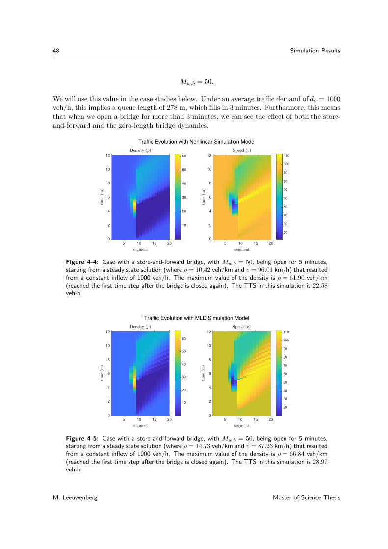
48 Simulation Results
Mw,b = 50.
We will use this value in the case studies below. Under an average traffic demand of do = 1000veh/h, this implies a queue length of 278 m, which fills in 3 minutes. Furthermore, this meansthat when we open a bridge for more than 3 minutes, we can see the effect of both the store-and-forward and the zero-length bridge dynamics.
Traffic Evolution with Nonlinear Simulation Model
5 10 15 20
0
2
4
6
8
10
12
10
20
30
40
50
60
5 10 15 20
0
2
4
6
8
10
12
20
30
40
50
60
70
80
90
100
110
Figure 4-4: Case with a store-and-forward bridge, with Mw,b = 50, being open for 5 minutes,starting from a steady state solution (where ρ = 10.42 veh/km and v = 96.01 km/h) that resultedfrom a constant inflow of 1000 veh/h. The maximum value of the density is ρ = 61.90 veh/km(reached the first time step after the bridge is closed again). The TTS in this simulation is 22.58veh·h.
Traffic Evolution with MLD Simulation Model
5 10 15 20
0
2
4
6
8
10
12
10
20
30
40
50
60
5 10 15 20
0
2
4
6
8
10
12
20
30
40
50
60
70
80
90
100
110
Figure 4-5: Case with a store-and-forward bridge, with Mw,b = 50, being open for 5 minutes,starting from a steady state solution (where ρ = 14.73 veh/km and v = 87.23 km/h) that resultedfrom a constant inflow of 1000 veh/h. The maximum value of the density is ρ = 66.84 veh/km(reached the first time step after the bridge is closed again). The TTS in this simulation is 28.97veh·h.
M. Leeuwenberg Master of Science Thesis
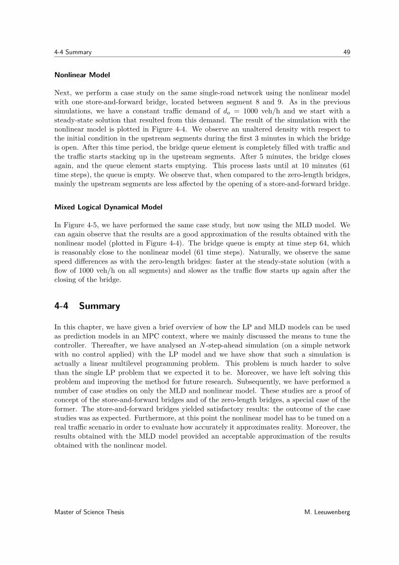
4-4 Summary 49
Nonlinear Model
Next, we perform a case study on the same single-road network using the nonlinear modelwith one store-and-forward bridge, located between segment 8 and 9. As in the previoussimulations, we have a constant traffic demand of do = 1000 veh/h and we start with asteady-state solution that resulted from this demand. The result of the simulation with thenonlinear model is plotted in Figure 4-4. We observe an unaltered density with respect tothe initial condition in the upstream segments during the first 3 minutes in which the bridgeis open. After this time period, the bridge queue element is completely filled with traffic andthe traffic starts stacking up in the upstream segments. After 5 minutes, the bridge closesagain, and the queue element starts emptying. This process lasts until at 10 minutes (61time steps), the queue is empty. We observe that, when compared to the zero-length bridges,mainly the upstream segments are less affected by the opening of a store-and-forward bridge.
Mixed Logical Dynamical Model
In Figure 4-5, we have performed the same case study, but now using the MLD model. Wecan again observe that the results are a good approximation of the results obtained with thenonlinear model (plotted in Figure 4-4). The bridge queue is empty at time step 64, whichis reasonably close to the nonlinear model (61 time steps). Naturally, we observe the samespeed differences as with the zero-length bridges: faster at the steady-state solution (with aflow of 1000 veh/h on all segments) and slower as the traffic flow starts up again after theclosing of the bridge.
4-4 Summary
In this chapter, we have given a brief overview of how the LP and MLD models can be usedas prediction models in an MPC context, where we mainly discussed the means to tune thecontroller. Thereafter, we have analysed an N -step-ahead simulation (on a simple networkwith no control applied) with the LP model and we have show that such a simulation isactually a linear multilevel programming problem. This problem is much harder to solvethan the single LP problem that we expected it to be. Moreover, we have left solving thisproblem and improving the method for future research. Subsequently, we have performed anumber of case studies on only the MLD and nonlinear model. These studies are a proof ofconcept of the store-and-forward bridges and of the zero-length bridges, a special case of theformer. The store-and-forward bridges yielded satisfactory results: the outcome of the casestudies was as expected. Furthermore, at this point the nonlinear model has to be tuned on areal traffic scenario in order to evaluate how accurately it approximates reality. Moreover, theresults obtained with the MLD model provided an acceptable approximation of the resultsobtained with the nonlinear model.
Master of Science Thesis M. Leeuwenberg

50 Simulation Results
M. Leeuwenberg Master of Science Thesis

Chapter 5
Conclusions and Recommendations
In the final chapter of this thesis, we give a project summary in Section 5-1, after which wehighlight our contributions to the literature in Section 5-2. Lastly, in Section 5-3, we list anumber of ideas for future research.
5-1 Project Summary and Discussion
In this thesis we have considered the following research questions:
How can we route traffic through a motorway network, where certainroads are blocked at known time periods, with as objective to minimisethe total time spent by all vehicles in the network?How can this be done in the most computationally efficient way?
We have regarded these questions as a dynamic traffic routing problem and addressed them asa search for an algorithm that efficiently controls the traffic flows through a network. We havefocussed on finding a computationally fast solution that potentially could be implemented inreal time, and in the best case could be extended to other fields of science. Our approach inanswering these research questions is described next.
We have selected the macroscopic (i.e. relatively low-detailed) motorway model METANETto simulate a traffic network. Furthermore, since METANET had been successfully used be-fore in combination with Model Predictive Control (MPC) [31,49], we have selected MPC asa promising control method for our research. From the perspective of computation times,METANET is a nonlinear and nonconvex model and therefore not necessarily the moststraightforward choice for fast state predictions with MPC. However, a major motivationfor this choice in our research was the work by Groot et al. [34, 35], who derived a sim-plification of METANET that consists of the Piecewise-Affine (PWA) approximation of thenonlinear functions in the model. This approximated model fits a Mixed Logical Dynami-cal (MLD) description that can be used in combination with MPC and that can be solved
Master of Science Thesis M. Leeuwenberg

52 Conclusions and Recommendations
with Mixed Integer Linear Programming (MILP).We have proposed a Linear Programming (LP) model that approximates METANET, i.e.
a simulation model that can be evaluated with LP. The expectation beforehand was thatwe could write the MPC implementation with our LP model in a single LP problem, whichwe had expected to result in a major calculation speed improvement compared with Grootet al. [34, 35]. However, when this novel model is used in an N -step-ahead prediction (or incombination with MPC), N consecutive LP problems need to be solved instead of a single LPproblem. It remains to be seen whether the resulting linear multilevel programming problemresults in a speed improvement compared to the existing MLD model.Furthermore, we have expanded the existing MLD model and the nonlinear model with
a novel store-and-forward bridge element. The implementation of this element includes theopening and closing of a bridge and the queueing of arriving traffic in front of an open bridge.The element is therefore capable of simulating a predicted disturbance, and more specificallya blocked road condition. The effectiveness of this novel bridge element has been evaluatedin a case study, from which we have concluded that the nonlinear store-and-forward bridgesfunctioned as expected and that the MLD model provides an acceptable approximation ofthe nonlinear model.
To the best of our knowledge the most computationally efficient way of solving an N -step-ahead simulation, that has an underlying model that is an approximation of METANET,is given by Lu et al. [57, 58]. Their approximation of METANET is used in combinationwith MPC and is written in a single LP problem. This method has been used in real-timetraffic control and has shown that it can, in some cases, reduce traffic congestion [74]. Theapproach uses a rough approximation of METANET and relies heavily on driver compliance,which they justify by stating that if the density is high enough even 30% driver compliancewith the variable speed limits will force the rest of the drivers to also reduce their speed and,secondly, that when the variable speed limits are strictly enforced, the actual speed will beclose to the designed variable speed limits. The desired variable speed limit at all segmentsin the network is used as a predetermined control variable. This value is determined on thebasis of an elaborate design strategy that is partly based on either historic data or on theoperator’s experience. The desired variable speed limits are used to substitute the speed inthe density update function (2-4) and to substitute the nonlinear desired speed function V in(2-5). Furthermore, the on-ramp and origin queue dynamics are predetermined by predictingthe traffic demand. These predetermined variables are subsequently used to solve the MPCproblem that is now an LP problem. The control inputs of this MPC problem are the coor-dinated ramp metering rates. Furthermore, the objective function is a combination of bothminimising the Total Time Spent (TTS) and maximising the total travel distance.In this thesis we have proposed a completely different approach for creating an approxi-
mation of METANET that can be evaluated with LP (that is, only when used as simulationmodel). From the field test in [74], we know that the control method proposed by Lu et al.did not improve the traffic flow in all cases. This suggests that there is room for improve-ment. Furthermore, since our approximation of METANET is closer to the original nonlinearmodel, we suggest that the prediction models in our approach could have a higher accuracy.We conclude that there is still a significant need for a model approximation or simplificationof METANET (or nonlinear functions in general) that is relatively accurate and that can beused in real time in combination with MPC.
M. Leeuwenberg Master of Science Thesis
5-2 Contributions 53
5-2 Contributions
With respect to the research questions, we summarise the contributions of this thesis:
1. The LP model can equally well be used in a single-step-ahead simulation asthe MLD model.In this thesis, we have proposed a model description that is an approximation ofMETANET and that we can evaluate using LP. This model, when used as a simu-lation model, is equivalent with the already existing MLD model (which is evaluatedwith MILP). Moreover, the methods that we have used to capture the complexities ofMETANET in a simple LP format, could provide an alternative in many other engi-neering applications.
2. When the LP model is used as prediction model in combination with MPC,a linear multilevel programming problem needs to be solved.We have not managed to write the MPC implementation of the LP model in a computa-tionally very light, single LP problem. Instead, we have presented the linear multilevelprogramming problem that solves a general N -step-ahead prediction with the LP model.
3. METANET has been extended with a store-and-forward element.We have added a store-and-forward element to METANET. This element can be usedto model predicted disturbances. More specifically, we have used it to model bridges.Furthermore, we have specified a special case of the store-and-forward element witha zero-length queue (Mw,b = 0) which we have called a zero-length bridge. We havedescribed how to add the store-and-forward element to METANET and to the MLDmodel, but not how to add it to the LP model.
5-3 Recommendations
In this section, we discuss some recommendations for future research. These are ideas thathave been formed during the course of this project. Firstly, we discuss recommendations con-cerning the control implementation in Section 5-3-1. Secondly in Section 5-3-2, we have somerecommendations concerning model improvements, mainly concerning the LP model. Finally,we have a number of recommendations with respect to the validation and implementation ofour models on real traffic situations in Section 5-3-3.
5-3-1 Recommendations Concerning the Control Implementation
Implementing exponentially decreasing weighing factors in the LP-MPC problemWe propose a weight selection method that might enable solving an N -step-ahead simulationwith the LP model in a single LP problem. When we consider Table 4-1 again, we observethat even in the first time step, the prediction of the single LP solution deviates from thecorrect MLD-based solution. Therefore, we suggest that a weight on the dummy variables,that decreases at each consecutive time step might improve the results. The correspondingcost function for the LP problem with time-dependent weights is given in (3-40).
Master of Science Thesis M. Leeuwenberg
54 Conclusions and Recommendations
To obtain a starting point for the selection of values of the weighting factors, we analysethe first constraint in (4-4), being
V1(1) ≥ aV(ρ1(0) + Ts
L[qo(0)− q+
1 (0) + q−1 (0)])
+ bV . (5-1)
Here, we recognize the recursiveness in these constraints when we write
V1(1) ≥ r[qo(0)− q+1 (0) + q−1 (0)] + . . .
V1(2) ≥ r[qo(1)− q+1 (1) + q−1 (1)] + . . . ,
(5-2)
wherer = aV Ts
L.
From here, we have a rough estimate of the weighing factors for V as
wV (k) = rk. (5-3)
With the same approach we can determine weighing factors on all the dummy variables.A major disadvantage of these exponentially decreasing weighing factors is that, especially
for larger prediction horizons, the weighing factors can become so small that numerical issuesare very probable.
Solving the linear multilevel programming problem with the LP model used asprediction modelWe come back to the linear multilevel programming problem posed in (4-6) and discuss somemethods of solving it. Multilevel programming has been used in combination with MPC be-fore [1,45,48], albeit not always in the same framework that we have in (4-6). Sometimes, theMPC problem is incorporated in one single level of the multilevel problem. In our definitionhowever, each time step on the receding horizon of the MPC problem corresponds to a levelin the hierarchical optimisation problem. Therefore, we recommend to use a general solverfor a multilevel problem.Many of the algorithms rely on the assumption that a lower-level problem that is con-
vex and satisfies some specific regularity conditions can be rewritten using its equivalentKarush-Kuhn-Tucker conditions. The resulting problem can in the linear case be solved withMILP [1, 14]. This is a promising direction. Even though the MLD model that we havestudied in this thesis was also solved using MILP, we can only conclude whether either of thetwo outperforms the other when a quantitative comparison on evaluation time is performedwith both models on the same simulation problem.In [8], a branch-and-bound algorithm is proposed to solve the linear multilevel program-
ming problem.Another method for solving this complex problem is provided in [67], where a linear multi-
level problem is studied, similar to the problem we have in (4-6). They rewrite the problemso that it can be solved with fuzzy programming.
M. Leeuwenberg Master of Science Thesis
5-3 Recommendations 55
5-3-2 Recommendations Concerning Model Improvements
Adding store-and-forward bridges to the LP modelIn this thesis we have derived the relations for zero-length bridges in the LP model. However,the relations for store-and-forward bridges in this model have not been derived. Rewritingthese equations for usage with the LP model is a complex extra step. Since we have not (yet)succeeded in making the comparison with the MLD model to establish whether one of thetwo solution approaches outperforms the other, we do not know whether the linear multilevelproblem can be solved more efficiently than the MILP approach that already exists. Therefore,we have left these store-and-forward bridge relations for future research.
Adding vehicular emissions and fuel consumption to the LP modelWhen we complement METANET by the VT-macro model [75], we can take vehicular emis-sions and fuel consumption into account. Groot et al. [34] use PWA approximations of thefunctions for the total emissions and fuel consumption that are compatible with the MLDformulation they use. These PWA approximations must be rewritten in such a way that theyare convex before they are also compatible with the LP formulation of METANET. Thiscould always be possible when an approximation error of a certain extent is accepted. Thequestion whether a convex approximation can be found for the VT-macro model with a lowapproximation error, is left for future research.
Making the models robust for disturbance rejection in case of unexpected topol-ogy changesIn this thesis we have focussed on predictable disturbances. We have used bridges as a phys-ical embodiment of this predicted disturbance. However, we could equally well have used thelevel crossing (an intersection with a railroad). A mathematical description of a level crossingin METANET would be practically identical to the bridge models that we have discussed inthis thesis.However, a blocked road due to a traffic accident does not fall under this category. Traffic
lights, on the other hand, could be an interesting extension to this research. Controlling thetraffic by routing it around the busy traffic lights whilst keeping the queue lengths minimalcan be contradictory and it would probably be more efficiently solved with a distributed con-trol method. Blocked roads due to road maintenance can be interesting, but it has a verydifferent time scale from opening and closing bridges. Therefore, a model that queues trafficin front of the blocked road is most likely not needed, because the road is blocked for a verylong time and a detour is suggested. However, it could be more efficient (system optimal) todynamically reroute the traffic (over multiple routes) instead of providing a static detour.
Accurately determining the domain of q±PWAWe have run some tests in the 3rd and 4th configuration in Figure A-3, without the imposedsafety region. These tests yielded unsatisfactory results because some values fell outside thePWA regions. This can be explained by the difference between V and V and the fact that theMETANET values do not lie exactly on the fundamental line but somewhere close. Therefore,we suggest that finding an accurate way of globally determining min(ρ± v) and max(ρ± v)would be valuable. In some configurations this might result in using less PWA regions inq±PWA, which can be a computational benefit for the MLD model, especially when used as aprediction model in an MPC context.
Master of Science Thesis M. Leeuwenberg
56 Conclusions and Recommendations
5-3-3 Recommendations Concerning Model Validation and Real-Time Imple-mentation
Testing the accuracy of the model for bridges on historical dataWe have proposed a simple store-and-forward model to simulate bridges in METANET. How-ever, in order to evaluate how well this model represents reality, i.e. real-live traffic queueingin front of an open bridge, a comparative study should be performed using historical data ofa real traffic network. Using this data, our simulation model should be validated and tuned.
Testing the accuracy of the approximated model on historical data.We can perform a case study on an existing motorway network. In order to do so, we need tocollect data (traffic distribution, inflows, and splits) for a certain amount of time during whichwe have significant traffic demands in this network, where there is no routing applied. Then,if we extract the traffic splits at interchanges, we can subsequently compare the performanceof our MPC implementation with the performance of the uncontrolled network. In this way,we can evaluate the difference in performance between an uncontrolled and a controlled trafficsituation without doing it in real time.A difficulty that is encountered when implementing a real-time solution in a real traffic
network is that the routes that vehicles take can only be advised, but not controlled. A firststep in that direction would be to use an advisory implementation on a motorway trafficnetwork, which could be achieved with Dynamic Route Information Panels (DRIPs) [21, 42,43].In a situation with (future) smart cars, distributed control is preferably used to route
the traffic. A low-level controller in the cars should take care of the faster dynamics that areassociated with the driving of the car (think of lane changing and decelerating and acceleratingin jams). A high-level controller then controls the slower dynamics and thus ensures efficientrouting and that the pressure is spread equally over the network. However, designing this high-level controller is a challenging task. The hardest challenge of which is in the second researchquestion; the computational efficiency. If we are ever to implement real-time MPC in a realtraffic network using DRIPs that can provide the passing vehicles with traffic information,it is important that we have an accurate model that can be used in a predictive controlimplementation and that has a low time complexity.
Implementing an observer for real-time traffic controlBecause we use a simulation model as a substitute for reality, we have full knowledge ofthe states and outputs at each time step when we perform a case study. If we were toimplement the controller on a real motorway, we would have to suffice with real-time networkmeasurements. Some system parameters, like the flow at a certain point, would be moreeasily obtained than others, like the TTS of the entire network at a moment in time.When controlling a real network in real time, the only way to track how well we are doing
is to translate these measurements to the outputs and states in our models. A filter (e.g. anExtended Kalman Filter) or an observer can help with that translation.
M. Leeuwenberg Master of Science Thesis
Appendix A
Approximations of Functions inMETANET
In this chapter, we discuss the Piecewise-Affine (PWA) approximated functions in more detail.The exact values of the optimal solutions are given as well as the settings with which theywere obtained. Section A-1 discusses the desired speed function VPWA and Section A-2 doesthis for the traffic flow q±PWA(ρ± v).
A-1 Piecewise-Affine Approximation of the Desired Speed Func-tion
Equation (A-1) below gives the PWA approximation in 2 regions of V (ρ). The parametersof (A-1) are obtained by solving the least-squares problem, given in (2-13) with a multi-startLevenberg-Marquardt algorithm (see Section 2-2-3 for the details about this optimisation).The PWA approximation of V [ρ] in 2 regions that we have used is:
VPWA(ρ) =−1.377ρ+ 106.8 for 77.55 > ρ ≥ 0
0 for 77.55 ≤ ρ.(A-1)
Equation (A-2) gives the PWA approximation of V in 3 regions:
VPWA(ρ) =
−1.465ρ+ 108.8 for 64.27 > ρ ≥ 0−0.4239ρ+ 41.90 for 64.27 ≤ ρ < 98.85
0 for 98.85 ≤ ρ.(A-2)
We set the last region of each PWA approximation to ρ = 0. This makes sure that theapproximated desired speed function and therefore the flows never become negative. Forall density values ρ > 77.55 veh/m in the PWA approximation with two regions we have
Master of Science Thesis M. Leeuwenberg
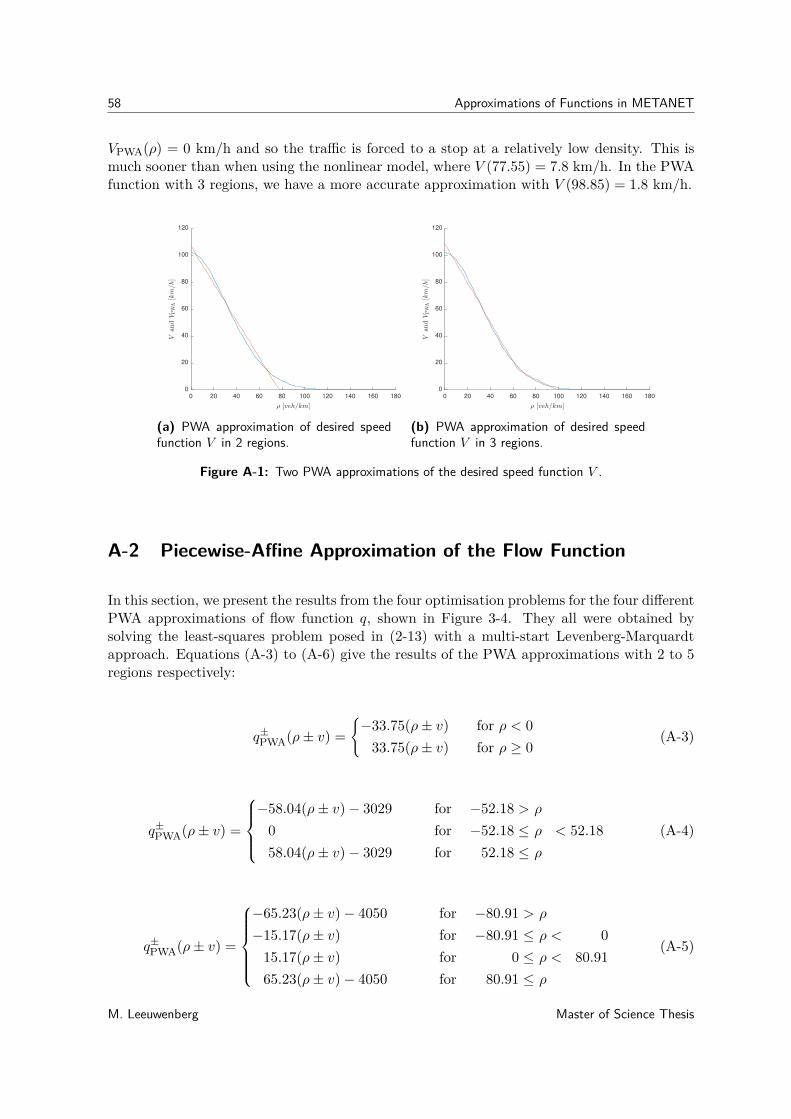
58 Approximations of Functions in METANET
VPWA(ρ) = 0 km/h and so the traffic is forced to a stop at a relatively low density. This ismuch sooner than when using the nonlinear model, where V (77.55) = 7.8 km/h. In the PWAfunction with 3 regions, we have a more accurate approximation with V (98.85) = 1.8 km/h.
0 20 40 60 80 100 120 140 160 180
0
20
40
60
80
100
120
(a) PWA approximation of desired speedfunction V in 2 regions.
0 20 40 60 80 100 120 140 160 180
0
20
40
60
80
100
120
(b) PWA approximation of desired speedfunction V in 3 regions.
Figure A-1: Two PWA approximations of the desired speed function V .
A-2 Piecewise-Affine Approximation of the Flow Function
In this section, we present the results from the four optimisation problems for the four differentPWA approximations of flow function q, shown in Figure 3-4. They all were obtained bysolving the least-squares problem posed in (2-13) with a multi-start Levenberg-Marquardtapproach. Equations (A-3) to (A-6) give the results of the PWA approximations with 2 to 5regions respectively:
q±PWA(ρ± v) =−33.75(ρ± v) for ρ < 0
33.75(ρ± v) for ρ ≥ 0(A-3)
q±PWA(ρ± v) =
−58.04(ρ± v)− 3029 for −52.18 > ρ
0 for −52.18 ≤ ρ < 52.1858.04(ρ± v)− 3029 for 52.18 ≤ ρ
(A-4)
q±PWA(ρ± v) =
−65.23(ρ± v)− 4050 for −80.91 > ρ
−15.17(ρ± v) for −80.91 ≤ ρ < 015.17(ρ± v) for 0 ≤ ρ < 80.9165.23(ρ± v)− 4050 for 80.91 ≤ ρ
(A-5)
M. Leeuwenberg Master of Science Thesis
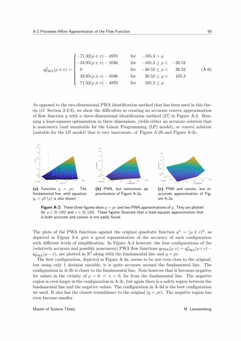
A-2 Piecewise-Affine Approximation of the Flow Function 59
q±PWA(ρ± v) =
−71.32(ρ± v)− 4970 for −105.3 > ρ
−33.95(ρ± v)− 1036 for −105.3 ≤ ρ < −30.520 for −30.52 ≤ ρ < 30.5233.95(ρ± v)− 1036 for 30.52 ≤ ρ < 105.371.32(ρ± v)− 4970 for 105.3 ≤ ρ.
(A-6)
As opposed to the two-dimensional PWA identification method that has been used in this the-sis (cf. Section 2-2-3), we show the difficulties in creating an accurate convex approximationof flow function q with a three-dimensional identification method [27] in Figure A-2. Run-ning a least-squares optimisation in three dimensions, yields either an accurate solution thatis nonconvex (and unsuitable for the Linear Programming (LP) model), or convex solution(suitable for the LP model) that is very inaccurate, cf. Figure A-2b and Figure A-2c.
(a) Function q = ρv. Thefundamental line, with equationqe = ρV (ρ) is also shown.
0
0.5
1
1.5
200
2
2.5
10 4
q (
ve
h/h
)
100
v (km/h)2001501000 500
(b) PWA, but nonconvex ap-proximation of Figure A-2a.
0
150
0.5
1
10 4
1.5
100
2
q (
veh/h
)
v (km/h)20050 150
100500 0
(c) PWA and convex, but in-accurate approximation of Fig-ure A-2a.
Figure A-2: These three figures show q = ρv and two PWA approximations of q. They are plottedfor ρ ∈ [0, 180] and v ∈ [0, 120]. These figures illustrate that a least-squares approximation thatis both accurate and convex is not easily found.
The plots of the PWA functions against the original quadratic function q± = (ρ ± v)2, asdepicted in Figure 3-4, give a good representation of the accuracy of each configurationwith different levels of simplification. In Figure A-3 however, the four configurations of the(relatively accurate and possibly nonconvex) PWA flow functions qPWA(ρ, v) = q+
PWA(ρ+v)−q−PWA(ρ− v), are plotted in R3 along with the fundamental line and q = ρv.The first configuration, depicted in Figure A-3a, seems to be not even close to the original,
but using only 1 decision variable, it is quite accurate around the fundamental line. Theconfiguration in A-3b is closer to the fundamental line. Note however that it becomes negativefor values in the vicinity of ρ = 0 ∧ v = 0, far from the fundamental line. The negativeregion is even larger in the configuration in A-3c, but again there is a safety region between thefundamental line and the negative values. The configuration in A-3d is the best configurationwe used. It also has the closest resemblance to the original (q = ρv). The negative region haseven become smaller.
Master of Science Thesis M. Leeuwenberg
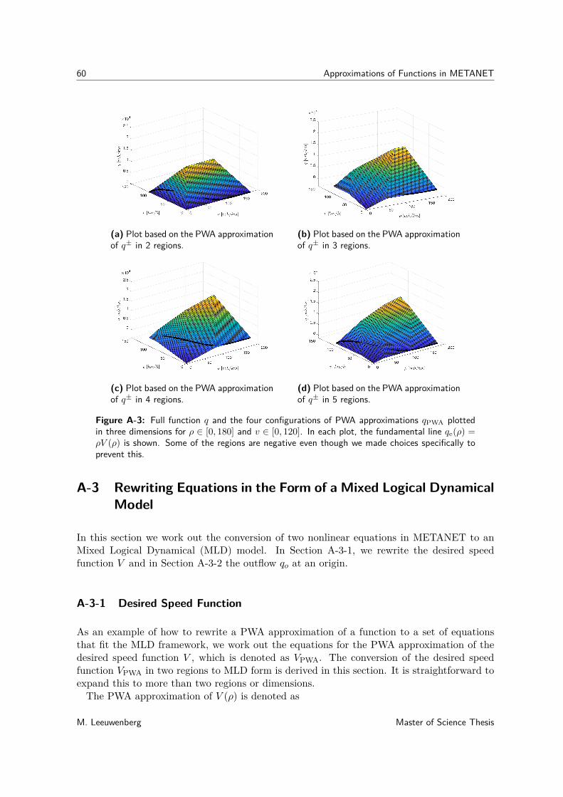
60 Approximations of Functions in METANET
(a) Plot based on the PWA approximationof q± in 2 regions.
(b) Plot based on the PWA approximationof q± in 3 regions.
(c) Plot based on the PWA approximationof q± in 4 regions.
(d) Plot based on the PWA approximationof q± in 5 regions.
Figure A-3: Full function q and the four configurations of PWA approximations qPWA plottedin three dimensions for ρ ∈ [0, 180] and v ∈ [0, 120]. In each plot, the fundamental line qe(ρ) =ρV (ρ) is shown. Some of the regions are negative even though we made choices specifically toprevent this.
A-3 Rewriting Equations in the Form of a Mixed Logical DynamicalModel
In this section we work out the conversion of two nonlinear equations in METANET to anMixed Logical Dynamical (MLD) model. In Section A-3-1, we rewrite the desired speedfunction V and in Section A-3-2 the outflow qo at an origin.
A-3-1 Desired Speed Function
As an example of how to rewrite a PWA approximation of a function to a set of equationsthat fit the MLD framework, we work out the equations for the PWA approximation of thedesired speed function V , which is denoted as VPWA. The conversion of the desired speedfunction VPWA in two regions to MLD form is derived in this section. It is straightforward toexpand this to more than two regions or dimensions.The PWA approximation of V (ρ) is denoted as
M. Leeuwenberg Master of Science Thesis
A-3 Rewriting Equations in the Form of a Mixed Logical Dynamical Model 61
VPWA(ρ) =a1ρ+ b1 if ρ ≤ s1
a2ρ+ b2 if ρ > s1.
The decision variable δV (k) is used to indicate which region of the PWA function is active attime step k. It must change value at the intersection ρ(k) = s1 where a1ρ(k)+b1 = a2ρ(k)+b2,so
ρ(k) ≥ s1 ⇔ [δV (k) = 1],
which can be written asgV (x) ≤ 0⇔ [δV (k) = 1],
where gV (x) = s1 − ρ(k). This results in the last two constraints in (A-7).The approximation V (ρ) is incorporated in the state space equations, as
V (ρ) = a1ρ(k) + b1 + [a2ρ(k) + b2 − [a1ρ(k) + b1]] δV (k)
= a1ρ(k) + [b2 − b1]δV (k) + [a2 − a1]zV (k) + b1,
where zV (k) = δV (k)ρ(k). This results in the first four constraints in (A-7). Note that thefirst PWA region is active unless δV (k) = 1. This saves one decision variable compared tousing a one for each region, i.e. δV,i(k) = 1 if aiρ(k) + bi is active.When we work out (2-17) and (2-19), we arrive at the following constraints for the MLD
system:zV (k) ≤MzV δV (k)zV (k) ≥ mzV δV (k)zV (k) ≤ ρ(k)−mzV [1− δV (k)]zV (k) ≥ ρ(k)−MzV [1− δV (k)]gV (x) ≤MgV [1− δV (k)]gV (x) ≥ ε+ [mgV − ε]δV (k),
(A-7)
where the minima and maxima are evaluated as
mzV = ρmin, MzV = ρjam
mgV = s1 − ρjam, MgV = s1 − ρmin.
A-3-2 Outflow at an Origin
This minimisation of three parameters, given in (2-8) can be written in MLD form too.The method we use is derived from [6]. For simplicity, we write this minimisation of threeparameters as
qo(k) = min[f1(k), f2(k), f3(k)].
We rewrite this equation in MLD form, with three decision variables. This is realised by using
qo(k) = f1(k)δqo,1(k) + f2(k)δqo,2(k) + f3(k)δqo,3(k), (A-8)
Master of Science Thesis M. Leeuwenberg

62 Approximations of Functions in METANET
with[δqo,1(k) = 1]⇔ [f1(k) ≤ f2(k) and f1(k) ≤ f3(k)][δqo,2(k) = 1]⇔ [f2(k) ≤ f1(k) and f2(k) ≤ f3(k)][δqo,3(k) = 1]⇔ [f3(k) ≤ f1(k) and f3(k) ≤ f2(k)].
(A-9)
Note that these inequalities imply an exclusive or condition on the decision variables, i.e.exactly one of the three binary decision variables is equal to 1 at each time step. So we havethe equality condition
3∑n=1
δqo,n(k) = 1 ∀k. (A-10)
The conditions in (A-9) translate to the following inequality constraints:
f1(k)− f2(k) ≤M12[1− δqo,1] f2(k)− f3(k) ≤M23[1− δqo,2]f1(k)− f3(k) ≤M13[1− δqo,1] f3(k)− f1(k) ≤M31[1− δqo,3]f2(k)− f1(k) ≤M21[1− δqo,2] f3(k)− f2(k) ≤M32[1− δqo,3]
(A-11)
with
M12 = max[f1(k)− f2(k)], M21 = max[f2(k)− f1(k)], M31 = max[f3(k)− f1(k)]M13 = max[f1(k)− f3(k)], M23 = max[f2(k)− f3(k)], M32 = max[f3(k)− f2(k)].
Lastly, (A-8) has three multiplications that we rewrite with the use of an auxiliary variablez, as we have explained before, by writing
zqo,1(k) = f1(k)δ1(k), zqo,2(k) = f2(k)δ2(k). zqo,3(k) = f3(k)δ3(k),
So we obtain
qo(k) = zqo,1(k) + zqo,2(k) + zqo,3(k), (A-12)
where zqo,1(k), zqo,2(k), and zqo,3(k) are (as before) subject to the constraints given in (2-19):
zqo,n(k) ≤Mqo,nδqo,n(k) for n ∈ 1, 2, 3zqo,n(k) ≥ mqo,nδqo,n(k) for n ∈ 1, 2, 3zqo,n(k) ≤ fn(k)−mqo,n[1− δqo,n(k)] for n ∈ 1, 2, 3zqo,n(k) ≥ fn(k)−Mqo,n[1− δqo,n(k)] for n ∈ 1, 2, 3,
(A-13)
where Mqo,n = max fn(k) and mqo,n = min fn(k).
M. Leeuwenberg Master of Science Thesis

Appendix B
Network Flow Problems
This chapter is an extension to Section 2-1-3, where we discussed the effectiveness of theuse of a minimum-cost flow problem as a solution to the dynamic routing problem thatwe considered in this thesis. Here, we state the definitions of both the minimum-cost flowproblem in Section B-1 and the multi-commodity flow problem in Section B-2. Furthermore,we rewrite the definition of the minimum-cost flow problem to a Linear Programming (LP)problem in Section B-3.
B-1 Minimum-Cost Flow Problem
The minimum-cost flow problem seeks for the optimal flow on each link that minimizes thecost function WijFij when a required flow a is to be transported through the network fromorigin node s to destination node d. We define the problem as
minFij
∑(i,j)∈M
WijFij
s.t.Inflow at node s
∑j∈adjo(s)
Fsj = a
Outflow at node d∑
i∈adji(d)Fid = a
Inflow equals outflow∑
i∈adji(u)Fiu −
∑j∈adjo(u)
Fuj = 0 ∀ u ∈ V \ s, d
Capacity at each link Fij − Cij ≤ 0 ∀ (i, j) ∈M.
(B-1)
The minimum-cost flow problem has been known and studied for a long time, e.g. by Fordand Fulkerson [29] and Klein [51].
Master of Science Thesis M. Leeuwenberg
64 Network Flow Problems
B-2 Multi-Commodity Flow Problem
The multi-commodity flow problem is a generalisation of the minimum-cost flow problemthat allows for a set P of origin-destination pairs. It is a set of paired origin and destinationvertices, coupled with a their corresponding required flows. We indicate the nth pair asOD(n) = (sn, dn, an), a subset of P with a required flow an from source sn to destination dn.We have a flow adjacency matrix Fij,n for each origin-destination pair n. The complete flowadjacency matrix, summed over all origin-destination pairs becomes
Fij =∑n∈P
Fij,n.
We write the multi-commodity flow problem as
minFij,n
∑(i,j)∈M
Wij(∑n∈P
Fij,n)
s.t. ∑
j∈adjo(sn)Fsnj,n = an ∀ n ∈ P
∑i∈adji(dn)
Fidn,n = an ∀ n ∈ P
∑i∈adji(u)
Fiu −∑
j∈adjo(u)Fuj = 0 ∀ u ∈ V \ sn, dnn∈P
(∑n∈P
Fij,n)− Cij ≤ 0 ∀ (i, j) ∈M.
(B-2)
B-3 Linear Programming Problem
The conversion to an LP problem is performed on the equations in (B-1). We rewrite theproblem to
minFij
∑(i,j)∈M
WijFij
s.t.∑k∈V
Fsk = a and∑k∈V
Fdk = −a
∑j∈V
Fij = 0 ∀ i ∈ V \ s, d
Fij = −Fji ∀ i, j ∈ VFij ≤ Cij ∀ i, j ∈ V.
(B-3)
We replaced the third constraint in (B-1) (inflow equals outflow) with two new constrains:the flow matrix has to be skew symmetric, i.e. Fij = −Fji, and the constraint that the sum
M. Leeuwenberg Master of Science Thesis

B-3 Linear Programming Problem 65
of each row r in the flow matrix Frj equals zero, except for the rows associated with s and d.This conversion to an LP problem is not directly applicable to undirected graphs, however,
it is possible after a transformation proposed by Lau [55]. A minor disadvantage of thistransformation is that it increases the size of the LP problem significantly.
Master of Science Thesis M. Leeuwenberg

66 Network Flow Problems
M. Leeuwenberg Master of Science Thesis
Bibliography
[1] R. Baker and C.L.E. Swartz. Interior point solution of multilevel quadratic programmingproblems in constrained model predictive control applications. Industrial & engineeringchemistry research, 47(1):81–91, 2008.
[2] M. Barbehenn. A note on the complexity of dijkstra’s algorithm for graphs with weightedvertices. IEEE Transactions on Computers, 47(2):263, 1998.
[3] R. Bellman. On a routing problem. Quarterly of Applied Mathematics, 16:87–90, 1958.
[4] A. Bemporad. Efficient conversion of mixed logical dynamical systems into an equivalentpiecewise affine form. IEEE Transactions on Automatic Control, 49(5):832–838, May2004.
[5] A. Bemporad, G. Ferrari-Trecate, and M. Morari. Observability and controllabilityof piecewise affine and hybrid systems. IEEE Transactions on Automatic Control,45(10):1864–1876, 2000.
[6] A. Bemporad and M. Morari. Control of systems integrating logic, dynamics, and con-straints. Automatica, 35(3):407–427, 1999.
[7] A. Bemporad, F.D. Torrisi, and M. Morari. Optimization-based verification and stabilitycharacterization of piecewise affine and hybrid systems. In International Workshop onHybrid Systems: Computation and Control, pages 45–58, 2000.
[8] H.P. Benson. On the structure and properties of a linear multilevel programming prob-lem. Journal of Optimization Theory and Applications, 60(3):353–373, 1989.
[9] D. Braess, A. Nagurney, and T. Wakolbinger. On a paradox of traffic planning [Trans-lated from German: D. Braess. Über ein Paradoxon aus der Verkehrsplanung. Un-ternehmensforschung, 12:258-268, 1968.]. Transportation Science, 39(4):446–450, 2005.
[10] P. Breton, A. Hegyi, B. De Schutter, and H. Hellendoorn. Shock wave elimination/reduc-tion by optimal coordination of variable speed limits. In Proceedings of the IEEE 5th In-ternational Conference on Intelligent Transportation Systems (ITSC’02), page 225–230,Singapore, Sept. 2002.
Master of Science Thesis M. Leeuwenberg
68 Bibliography
[11] C. Buisson, J.P. Lebaque, and J.B. Lesort. STRADA, a discretized macroscopic modelof vehicular flow in complex networks based on the godunov scheme. In Proceedings ofthe CESA’96 IEEE Conference, France, 1996.
[12] M. Burger, M. van den Berg, A. Hegyi, B. De Schutter, and J. Hellendoorn. Considera-tions for model-based traffic control. Transportation Research Part C, 35:1–19, 2013.
[13] X. Cai, D. Sha, and C. K. Wong. Time-Varying Network Optimization, volume 103 ofInternational Series in Operations Research & Management Science. Springer Science &Business Media, 2007.
[14] B. Colson, P. Marcotte, and G. Savard. Bilevel programming: A survey. 4or, 3(2):87–107,2005.
[15] K.L. Cooke and E. Halsey. The shortest route through a network with time-dependentinternodal transit times. Journal of Mathematical Analyis and Applications, 14:493–498,1966.
[16] T.H. Cormen, C.E. Leiserson, R.L. Rivest, and C. Stein. Introduction to Algorithms.MIT Press, Cambridge, MA, USA, 2009.
[17] D. Corona, I. Necoara, B. De Schutter, and T. van den Boom. Robust hybrid MPCapplied to the design of an adaptive cruise controller for a road vehicle. In Proceedingsof the 45th IEEE Conference on Decision and Control, pages 1721–1726, San Diego,California, 2006.
[18] R. Courant, K. Friedrichs, and H. Lewy. On the partial difference equations of math-ematical physics. IBM Journal of Research and Development, 11(3):215–234, March1967.
[19] C.R. Cutler and B.L. Ramaker. Dynamic matrix control – a computer control algorithm.In Proceedings of the 86th AIChE National Meeting, Houston, TX, USA, 1979.
[20] C.F. Daganzo. The cell transmission model: A dynamic representation of highway trafficconsistent with the hydrodynamic theory. Transportation Research Part B: Methodolog-ical, 28(4):269–287, 1994.
[21] F.P. Deflorio. Evaluation of a reactive dynamic route guidance strategy. TransportationResearch Part C, 11(5):375–388, 2003.
[22] C. Diakaki, M. Papageorgiou, and T. McLean. Integrated traffic-responsive urban corri-dor control strategy in Glasgow, Scotland. Transportation Research Record, 1727(1):101–111, 2000.
[23] R. Diestel. Graph Theory, volume 173 of Graduate Texts in Mathematics. Springer-Verlag, New York, 2nd edition, 2000.
[24] E.W. Dijkstra. A note on two problems in connexion with graphs. Numerische Mathe-matik, 1:269–271, 1959.
[25] J. Doran. An approach to automatic problem-solving. Machine Intelligence, 1:105–124,1967.
M. Leeuwenberg Master of Science Thesis
69
[26] D. Ferone, P. Festa, A. Napoletano, and T. Pastore. Reoptimizing shortest paths: fromstate of the art to new recent perspectives. In 18th International Conference on Trans-parent Optical Networks (ITCON), 2016.
[27] G. Ferrari-Trecate. Hybrid identification toolbox (HIT). http://sisdin.unipv.it/lab/personale/pers_hp/ferrari/HIT_toolbox.php, 2005.
[28] L.R. Ford, Jr. Network flow theory. The RAND Corporation, No. P-923, 1956.
[29] L.R. Ford, Jr. and D.R. Fulkerson. Flows in Networks. R-375-PR. The RAND Corpora-tion, Santa Monica, CA, USA, 1962.
[30] M.L. Fredman and R.E. Tarjan. Fibonacci heaps and their uses in improved network op-timization algorithms. Journal of the Association for Computing Machinery, 34(3):596–615, 1987.
[31] J.R.M Frejo and E.F. Camacho. Global versus local MPC algorithms in freeway trafficcontrol with ramp metering and variable speed limits. IEEE Transactions on IntelligentTransportation Systems, 13(4):1556–1565, 2012.
[32] D. Frigioni, A. Marchetti-Spaccamela, and U. Nanni. Fully dynamic algorithms formaintaining shortest paths trees. Journal of Algorithms, 34:251–281, 2000.
[33] A.V. Goldberg and C. Harrelson. Computing the shortest path: A* meets graph theory.ACM-SIAM Symposium on Discrete Algorithms, 16:156–165, 2005.
[34] N. Groot, B. De Schutter, and H. Hellendoorn. Integrated model predictive traffic andemission control using a piecewise-affine approach. IEEE Transactions on IntelligentTransportation Systems, 14(2):587–598, 2013.
[35] N. Groot, B. De Schutter, S. Zegeye, and H. Hellendoorn. Model-based predictive trafficcontrol: A piecewise-affine approach based on METANET. In Proceedings of the 18thIFAC World Congress, pages 10709–10714, Milan, Italy, 2011.
[36] P.E. Hart, N.J. Nilsson, and B. Raphael. A formal basis for the heuristic determination ofminimum cost paths. IEEE Transactions on Systems Science and Cybernetics, 4(2):100–107, 1968.
[37] S.M. Hashemi, S. Mokarami, and E. Nasrabadi. Dynamic shortest path problems withtime-varying costs. Optimization Letters, 4:147–156, 2010.
[38] A. Hegyi. Model Predictive Control for Integrating Traffic Control Measures. PhD thesis,Delft University of Technology, 2004.
[39] A. Hegyi, B. De Schutter, and H. Hellendoorn. Model predictive control for optimalcoordination of ramp metering and variable speed limits. Transportation Research PartC, 13(3):185–209, 2005.
[40] A. Hegyi, B. De Schutter, H. Hellendoorn, and T. van den Boom. Optimal coordinationof ramp metering and variable speed control – an MPC approach. In Proceedings of the2002 American Control Conference, pages 3600–3605, Anchorage, Alaska, 2002.
Master of Science Thesis M. Leeuwenberg
70 Bibliography
[41] M. Herceg, M. Kvasnica, C.N. Jones, and M. Morari. Multi-Parametric Toolbox 3.0.In Proceedings of the European Control Conference, pages 502–510, Zürich, Switzerland,Jul. 2013. http://control.ee.ethz.ch/~mpt.
[42] B.H. Heutinck, M. van den Berg, J. Hellendoorn, and L.H. Immers. Dynamic route guid-ance during maintenance works, a case study. IFAC Proceedings Volumes, 39(12):380–385, 2006.
[43] S.P. Hoogendoorn. Optimal control of dynamic route information panels. IFAC Proceed-ings, 30(8):399–404, 1997.
[44] S.P. Hoogendoorn and P.H.L. Bovy. State-of-the-art of vehicular traffic flow modelling.Proceedings of the Institution of Mechanical Engineers, Part I: Journal of Systems andControl Engineering, 215(4):283–303, 2001.
[45] M. Hovd. Multi-level programming for designing penalty functions for MPC controllers.IFAC Proceedings Volumes, 44(1):6098–6103, 2011.
[46] A. Jamshidnejad. Efficient Predictive Model-Based and Fuzzy Control for Green UrbanMobility. PhD thesis, Delft University of Technology, 2017.
[47] R.G. Jeroslow. The polynomial hierarchy and a simple model for competitive analysis.Mathematical programming, 32(2):146–164, 1985.
[48] C.N. Jones and M. Morari. Approximate explicit MPC using bilevel optimization. In2009 European control conference (ECC), pages 2396–2401, 2009.
[49] A. Karimi, A. Hegyi, B. De Schutter, H. Hellendoorn, and F. Middelham. Integration ofdynamic route guidance and freeway ramp metering using model predictive control. InProceedings of the 2004 American Control Conference, pages 5533–5538, Boston, Mas-sachusetts, June-July 2004.
[50] H.R. Kashani and G.N. Saridis. Intelligent control for urban traffic systems. Automatica,19(2):191–197, 1983.
[51] M. Klein. A primal method for minimal cost flows with applications to the assignmentand transportation problems. Management Science, 14(3):205–220, 1967.
[52] F.H. Knight. Some fallacies in the interpretation of social cost. The Quarterly Journalof Economics, 38(4):582–606, 1924.
[53] A. Kotsialos, M. Papageorgiou, C. Diakaki, Y. Pavlis, and F. Middelham. Trafficflow modeling of large-scale motorway networks using the macroscopic modeling toolMETANET. IEEE Transactions on Intelligent Transportation Systems, 3(4):282–292,2002.
[54] A. Kotsialos, M. Papageorgiou, and A. Messmer. Optimal coordinated and integratedmotorway network traffic control. In Proceedings of the 14th International Symposiumof Transportation and Traffic Theory (ISTTT), pages 621–644, Jerusalem, Israel, Jul.1999.
M. Leeuwenberg Master of Science Thesis
71
[55] H.T. Lau. A note on the shortest path through a given link in a network. IEEE Trans-actions on Circuits and Systems, 33(1):109–110, 1986.
[56] H.K. Lo, E. Chang, and Y.C. Chang. Dynamic network traffic control. TransportationResearch Part A, 33(8):721–744, 2001.
[57] X.Y. Lu and S. Shladover. MPC-based variable speed limit and its impact on trafficwith V2I type ACC. In 2018 21st International Conference on Intelligent TransportationSystems (ITSC), pages 3923–3928, Maui, HI, USA, 2018.
[58] X.Y. Lu, P. Varaiya, R. Horowitz, D. Su, and S.E. Shladover. Novel freeway traffic con-trol with variable speed limit and coordinated ramp metering. Transportation ResearchRecord: Journal of the Transportation Research Board, 2229:55–65, 2011.
[59] R. Luo, T. J. van den Boom, and B. De Schutter. Multi-agent dynamic routing of a fleetof cybercars. IEEE Transactions on Intelligent Transportation Systems, 19(5):1340–1352,2017.
[60] A. Messner and M. Papageorgiou. METANET: A macroscopic simulation program formotorway networks. Traffic Engineering & Control, 31(8-9):466–470, 1990.
[61] A. Orda and R. Rom. Shortest-path and minimum-delay algorithms in networks withtime-dependent edge-length. Journal of the Association for Computing Machinery,37(3):607–625, 1990.
[62] A. Orda and R. Rom. Minimum weight paths in time-dependent networks. Networks,21:295–319, 1991.
[63] G. Ramalingam. Bounded Incremental Computation, volume 1089 of Lecture Notes inComputer Science. Springer-Verlag, Berlin, 1971.
[64] G. Ramalingam and T. Reps. An incremental algorithm for a generalization of theshortest paths problem. Journal of Algorithms, 21:267–305, 1996.
[65] G. Ramalingam and T. Reps. On the computational complexity of dynamic graph prob-lems. Theoretical Computer Science, 158:233–277, 1996.
[66] J. Richalet, A. Rault, J.L. Testud, and J. Papon. Model predictive heuristic control:Applications to industrial processes. Automatica, 14:413–428, 1978.
[67] M. Sakawa, I. Nishizaki, and Y. Uemura. Interactive fuzzy programming for multilevellinear programming problems. Computers & Mathematics with Applications, 36(2):71–86,1998.
[68] E.D. Sontag. Nonlinear regulation: The piecewise linear approach. IEEE Transactionson Automatic Control, 26(2):346–357, 1981.
[69] J.M. Thomson. Reflections on the economics of traffic congestion. Journal of TransportEconomics and Policy, 32(1):93–112, 1997.
Master of Science Thesis M. Leeuwenberg
72 Bibliography
[70] M. van den Berg, B. De Schutter, J. Hellendoorn, and A. Hegyi. Influencing route choicein traffic networks: A model predictive control approach based on mixed-integer linearprogramming. In Proceedings of the 17th IEEE International Conference on ControlApplications, pages 299–304, San Antonio, TX, USA, 2008.
[71] J.G. Wardrop. Some theoretical aspects of road traffic research. Proceedings of theInstitution of Civil Engineers, 1(3):325–362, 1952.
[72] U.P. Wen and S.T. Hsu. Linear bi-level programming problems—a review. Journal ofthe Operational Research Society, 42(2):125–133, 1991.
[73] H. Williams. Model Building in Mathematical Programming. Wiley, New York, NY,USA, 3rd edition, 2013.
[74] C.J. Wu, X.Y. Lu, J. Spring, and R. Horowitz. Field test implementation of coordi-nated ramp metering control strategy: a case study on SR-99N. In Proceedings of theTransportation Research Board Meeting 96th Annual Meeting, 2018.
[75] S. Zegeye, B. De Schutter, H. Hellendoorn, and E. Breunesse. Model-based traffic controlfor balanced reduction of fuel consumption, emissions, and travel time. In Proceedings ofthe 12th IFAC Symposium on Transportation Systems, pages 149–154, Redondo Beach,CA, USA, 2009.
M. Leeuwenberg Master of Science Thesis

Glossary
List of Acronyms
DRIP Dynamic Route Information Panel
LP Linear Programming
METANET Modèle d’Ecoulement du Trafic Autoroutier: NETwork
MILP Mixed Integer Linear Programming
MLD Mixed Logical Dynamical
MPC Model Predictive Control
PWA Piecewise-Affine
TTS Total Time Spent
Master of Science Thesis M. Leeuwenberg

74 Glossary
List of Symbols
am METANET model parameterCb Outflow capacity (veh/h) of bridge bCo Outflow capacity (veh/h) of origin odo Traffic demand (veh/h) at origin oFν,m Split (veh/h) of traffic leaving vertex ν for link mG GraphJTTS Total time spent (veh·h)Lm Length (km) of segments in link mm Linkqm,i Traffic flow (veh/h) on segment i of link mqin,b Potential traffic inflow (veh/h) from segment iu to the queue at bridge bqu,b Traffic inflow (veh/h) from segment iu to the queue at bridge bqout,b Potential traffic outflow (veh/h) from the queue at bridge b to segment idqw,b Traffic outflow (veh/h) from the queue at bridge b to segment idqo Traffic outflow (veh/h) at origin oQν Summed traffic outflow at vertex ν (veh/h)ro Ramp metering rate at origin oTs Sample time (s)vm,i Traffic speed (km/h) on segment i of link mvfree Free-flow speed (km/h)Vi,m Desired speed (km/h) on segment i of link mwb Queue (veh) at bridge bwo Queue (veh) at origin oβν,m Percentage of traffic that leaves vertex ν for link mη METANET model parameter (km2/h)κ METANET model parameter (veh/km/lane)λm Number of lanes on link mν Vertexρm,i Traffic density (veh/km) on segment i of link mρcr,m Critical traffic density (veh/km) on link mρjam Maximum traffic density (veh/km)τ METANET model parameter (s)
M. Leeuwenberg Master of Science Thesis
Index
AAdjacency, 6
BBilevel Programming, 42Braess’s paradox, 2
DDirectionality, 5Downstream Density, 11Dynamic Network, 6
LLeast-Squares Problem, 11
MMETANET, 9Minimum-Cost Flow Problem, 7, 63Model Predictive Control, 15Multi-Commodity Flow Problem, 7, 64Multilevel Programming, 42
NNode-Node Adjacency Matric, 7
OOrigin-Destination Pair, 3, 64
SSelfish Wardrop Equilibrium, 7, 15Shortest Path Problem, 6Social Wardrop Equilibrium, 7, 15Static Network, 6Store-and-Forward Bridge, 28
UUpstream Velocity, 11
ZZero-length Bridge, 27
Master of Science Thesis M. Leeuwenberg