ABSTRACT

THE PREDICTION OF THE SHIP'S MANEUVERABILITY

IN THE DESIGN STAGE

By: Dr. J.P. Hooft, member and Dr. U. Nienhuis,

MARIN, Wageningen

TECHNISCHE UNIVERSITEITLabOratoijurn voOt

8homectatchet

Mekelweg 2, 2628 CD DelftTeL O15.78

This paper contains the evaluation of the ship's maneuverability in the design stage during, which

the underwater hull form and the äppendages are to be determined. For this purpose two basic

aspects in the assessment of the ship's maneuverability are discerned, i.e. (1) the determination

of the influence of the hull form and of the appendages on the ship's hydrodynamic phenomena

such as added mass and damping coefficients, and (2) the determination of the effect of the

hydrodynarnic aspects on the ship's maneuvering properties. This second aspect will be

elucidated by means of computer simulations which are applied for predicting the ship's

maneuverability in the design stage.

In the paper information will be given first about the hydrodynamic aspects by which the forces

are generated on the hull in reaction to the ship's motions while maneuvering. After that the

forces will be described which are caused by the rudders.

Having determined all relevant hydrodynamic quantities, then the ship's maneuverability can be

predicted by using computer simulations. Results from such simulations will be shown in.

comparison to model test results and to full scale trial resUlts.

1. INTRODUCTION

In the design stage of a ship all its dimensions and those of the appendages are considered with

respect to the consequences ori the various aspects of the ship's performance such as the

powering, the sealoeeping and the maneuverability. The result of the optimization of the design

is a compromise of each of the components of the total performance.

In literature a lot of information is available to establish the influence of the hull forni on the ship's

powering (resistance and propulsion) and on the ship's dynamic behavior in a seaway (the

so-called seakeeping properties). Therefore in this paper the attention will be focused on the

influence of the ship's hull form and its appendages on the maneuverability.

One of the serious problems in designing the hull form from a point of view of maneuverability

is caused by the uncertainty in specifying the maneuvering performances which have to be

satisfied. Depending on the ship's mission various types of maneuvers have to be performed each

of which are difficult to define let alone to describe. In addition to this problem the assessment

of a maneuver depends on the ship's type (defined by its form) which is affected largely by its

mission and the environment in which it operates. Examples of completely different ship types

which perform completely different maneuvering tasks are: freighters, tugboats, minesweepers,

etc. In Section 2 the various aspects of the maneuvering performance will be discussed in detail.

Some of the above problems with respect to the definition of the ship's maneuverability in the

design stage have been solved for a large category of ships by the 1993 1MO regulations; see

1MO 1993. In these regulations the following aspects were specified:

1. The types of maneuvers on which the maneuverability of new ships longer than 100 m will

be judged, and

-2-

2. The limits within which the maneuvers have to be executed.

The 1MO regulations also require that in the design stage predictions are to be performed to prove

that the ship's maneuvering performance will comply with the 1MO criteria. lt is required also that

the predictions have to be validated by the results of sea thäls with the new ship. In this respect

still some serious pròblems exist about (1) the reliability of the prediction method, and (2) the

accuracy of the sea trial results. These two problems will b elucidated as follows:

Reliability of the, prediction method

Various types of prediction methods exist such as e.g.

extrapolation from past experience; in this method the maneuvering characteristics, are

predicted by means of empirical descriptions between the maneuvering properties measured

during sea trials and the ship's dimensions;

computer simulations using'hydrodynamic cOefficients derived from an empirical relation. with

the ship's dimensions;

experiments with self propelled ship models;

computér simulations using hydrodynamic coefficients derived from experiments with ship

models restrained to a towing carriage (often referred to as PMM tests).

The reliability of a prediction method depends mainly on the following two items:

The method is defined to be reliable if the prediction result has proven to be in agreement

with resUlts from other (mainly experimental) methods to ascertain' the ship's maneuverability,

especially so from sea trials.

lt shòuld be realized that there will always be some error bandwidth in the results of each of

these prediction methods. That means that small changes in the input parameters will shov

a variation in the result of the method. The method is defined to be reliable if also the

variation in the results will be small for small changes in the input.

The accuracy of the sea trials

lt is assumed that it wiN be possible nowadays to measure the various maneuvering properties

(rudder angle, ship's position, speed and rate of turning) rather accurately. However the recording

of these items and of the conditions of the ship and the environment are often less

conscientiously performed. This can be indicated by the foliowing examples of problems in

recording precisely the needed information;

The ship's behavior before the start of a test maneuver (e.g a turning circle or zig-zag

maneuver) can have a large impact on the maneUver considered. lt is therefore

recommended to record the ship's behavior well in advance of the official beginning of the

maneuver.

The ship's maneuverability will be influenced largely by its loading condition. Mostly only the

draft and the trim will be recorded. HoWever for various types of ships also the metacenter

height will affect the maneuverability. Therefore this item should also' be taken into

consideration.

The accuracy of the rudder angle and the ship's course angle should be given prime

attention. For an optimal recording of these items elaborate calibrations should be carried out.

The enviionmental conditions can have a significant influence on the tship's maneuvering

properties. These conditions should therefore be recorded appropriately.

Even when due attention ¡s given to thè recording of all aspects relevant to maneuvering tests

then still some degree of inaccuracy in the results of the sea trials have to be accepted because

of the fact that the tests can never be executed under loo % ideal circumstances. This means

that when considering the hypothetical case of, a large number of identical tests under identical

circumstances then the measurements will be defined to be accurate ¡f and only if the deviation

in the results óf all tests remains relatively small (e.g. 5%).'

-4-

BASIC MANEUVERING PROPERTIES

When considering the ship's maneuverability as an open loop system then the following aspects

can be discerned:

1. The attainability by which the inherent maneuvering performance of the ship is defined. This

aspect describes the complete set of maneuvers that can be performed by all possible rudder

executions for all environmental conditions. Mostly one only defines the attainability for a

subset of conditions such as for example the maneuverability in deep water at the service

speed.

2.. The (coUrse) stability according tö the following definition; see also FIgure 1: "At a constant

position of the steering systems (rudders, thrusters, etc.) the ship is defined to be course

stable if after some short disturbance it will resume the original maneuver without any use of

the steering means". Mostly only the stability on a straight course is considered with the

rudder in the equilibrium position.

The sensitivity according to the following definilion: "The sensitivity S of the ship's

maneuverability to external variations is defined by the ratiò of the relative change óT/T of

the maneuvering performance T in comparison to the relative disturbance &/a of any

parameter a that has an effect on the maneuverability".

COURSE StASLE

Rate at turning

-5-

COURSE UNST.ABLE

Rate ot turning r

N\

Fig. 1. Definition of the course stability from the results of the spiral test.

width aihysteresis4

height öthysteresis

rudder angle &

Table 1. 1MO maneuvering criteria for ships longer than loo m

From the turning circle maneuver:* TURNING ABILITY AT 35 ÓEG RUDDER ANGLE

- advance < 4.5 L

- tactical diameter < 5 L* COURSE INITIATING ABILITY AT 10 DEG RUDDER ANGLE

- travelled distance < 2.5 L at lo deg change of heading

From the zig-zag maneuver:* COURSE CHECKING ABILITY

- lo/lo Z-maneuver

first overshoot < lo deg if Lpp/U < i O sec

first overshoot < 20 deg if LpdU.> 30 sec

first overshoot: (5 + ½*L/U) for 10 sec < LWU <30 sec

second execute <first overshoot + 15 deg

20/20 maneuver

first overshoot < 25 deg* STOPPING ABILITY

track reach < 15

The attainability is öonsidered ¡n order to ascertain the area that is needed by the ship while

executing its mission which consists for instance of accelerating, course keeping (and sometimes

also track keeping), course changing, course checking, stopping, etc.

För the assessment of the maneuverability of a seagoing vessel longer than 100 m the 1MO 1993

has specified four maneuvérs which have to be executed within certain limits; see Table 1. Apart

from the stopping there are basically two types of maneuvering properties considered by the 1MO

critèriá:

-6-

i

The ability to change the heading of the ship by mean.of the available steering systems: the

so-called "course changing ability" of thè ship. This aibillty is determined from the first part of

the turning circle maneuver (see Figure 2) at 35 deg and 10 deg rudder angle. lt will be

obvious that the safety of the ship is good if it is possIble to initiatô rapidly a change of

heading in order to avoid a suddén obstacle.

The ability to bring the ship on a straight course from the condition in which it is turning: the

so-called "course chécking ability". This ability is deterrn med by the overshoot angle and

overshoot time in the zig-zag maneuver; see Figure 3. In case that the ship is turning and will

continue to turn for some time in the same direction after the rudder has been put. in the

opposite direction then it will be obvious that one considers the ship to be out of coñtrol if the

time of vershoot is too large. lñ that òase thé ship's rnaneuver during such an excessive

overshoót time will seem to proceed independent of thé rudder action. Therefore, it will be

beneficiai for the ship's safety when it càn be kept under control properly by responding

quickly to the steering means without too much overshOot.

uC'U

Tactical diameter

o

Track of centro atPosition et Oat rudder execute reference O

Dritt angle

6

i st

SecondA

overshoot Iañ9ló 'I

Period

2nd 3rd

First overshoot angie

First overshoot lime

angle c

Time

Ruddorangle 6

Second overshoot Urne

4th rudder-execute

Fig. 2. Description of the turning circle maneuver. Fig. 3. Dèscription of the zig-zag maneuver.

Various aspects of the ships maneuvering performance such as the ucourse keoping, the "course

changing" and the "çourse checkirig are influenced significantly by the ship's course stability

according to the above given definition:

- Course keeping: According to the definition a course unstable ship with the rudder in the

equilibrium position wiH immediately start to turn after any disturbance. Therefore, in order to

keep the ship on a straight course continuous rudder actions are required to. correct for the

continuous disturbances. A course stable ship with the rudder ¡n the equilibrium position will

not continue to turn after a short limited disturbance. However, after the disturbance has

vanished the course of the ship will have been altere4. To restore the course deviation

continuous rudder actions are also needed to keep a course stable ship on a straight course.

No general conclusions can be drawn about the difference in rudder activity in the course

keeping of a stable ship and that of a course unstable ship.

Course chanQing: In case of a course stable s.hip it will be m'ore difficult to introduce ¿ change

of course. Large rudder forces have to be applied to generate an adequate rate of turning

frörn..a straight course. However, in case of a course unstable ship the ship will start to

deviate from a straight course, easily at appreciably high rates of turning with only relatively

small rudder forces.

Course checking: In case of a course stable ship the ship will have a natural tendency to stop

turning and to resume to sail along a straight course in the absence of any disturbance.

Therefore a course stable ship will have a good "course checking ability" irrespective o the

rudder effectiveness. lt should be noted however that sometimes larger rudders are required

to rnak.e the ship course stable; see Section 6. In case of a course unstable ship it will be

quite cumbersome to stop the turning rate once the ship has started to turn. Therefore, an

insufficient course checking ability is mostly caused primarily by the course instability for two

reasons: (1) the course unstable ship will turn quite fast which is more difficult to be

counteracted, and (2) the course unstable ship is inherently more inclined to turn and it

therefore requires more effort to stop this tendency. For a course unstable ship large forces

-8-

will be required by the reversed rudder angle ¡n order to stop the ship's turning and bring her

on à straight course. Large rudders will be required in this case (1) to make the ship course

stable and (2) to achieve an acceptable course checking ability". If the ship is course

unstable while large rudders háve already been applied then there are two reasons to apply

stabilizing fins instead of further increasing the rudders, Le.

with larger rudders the turning rate of the ship might become unacceptably large by which

it will become even more difficult to stop the turning of the ship, and

during the deceleration procedure the rudder effectiveness might be reduced drastically

while fins will Still remain appropriately effective (see also Section 6).

Taking into account the above consideratjons then it sometimes happens that the maneuverability

of a course unstable ship may still be acceptable if the following two criteria are satisfied; see e.g.

the 1MO 1991 document:

The rate of turning at the equilibrium rudder position should remain within acceptable limits;

see e.g. ITTC-'87. Such a limit is for instance about 30% of the turning rate at the maximum

rudder angle. From Figure 1 it is seen that the rate of turning at the equilibrium rudder

position corresponds to half the height of the hysteresis in the relation r(6) betweèn the

turning rate and the rudder angle if the ship is course unstable. -

The tüming at the equilibrium rudder position should be stopped by means of opposite rudder

angles of limited amount; see e.g. Nomoto (1977). Such a limit is for instance a rudder angle

of 5 degrees. From Figure 1 it is Seen that the rudder angle at which the turning can be

reversed corresponds to half the width of the hysteresis ¡n the relation r(8) between the

turning rate and the rudder angle if the ship ¡s course unstable.;

If these two criteria (which have not beén incorporated by the 1MO) are satisfied then it may

happen that this typé of course unstable ship falls in the category of good controllable ships. lt

is difficult to explain theoretically why such a ship is considered to be good còntroflable. However

from a practical point of view it is assumed that a ship with a limited course instability will respond

easily to any outside force and therefore also to any rudder action In Sections 3 and 4 a

derivation will be given about the hydrodynamic origin of the course stability..

In order to assess the ship's maneuverability aiso the sensitivity to variations according to the

earlier given definition has tobe considered in additiòn to the above shown aspects of attainability

and stability. Examples of variable parameters which may affect the maneuverability are:

- steering devices

- loading condition of the ship

- environmental conditions.

For a proper assessment of a system it is required that it is quite insensitive to variations of all

kinds of nature. A system is considered more reliable when its sensitivity to variations of the

influencing parameters is small. A low sensitivity, of the maneuverability of a ship will make, the

maneuverability of that ship much more acceptable because of the increased reliability to the ship

operator and to the certifying authority.

With respect to the certification of the ship's maneuverability:

If the maneuverability ¡s very sensitive to external disturbances then this will cause large

variations in the maneuvering performance measured during various trials Under nearly equal

circumstances. This means that if the maneuverabIity is sensitive to the circumstances then the

maneuverability can not be measured with great accuracy. In that case orle will not only find that

there is no coherency in the trial results but also that the agreement will be small between the

full scale trial results and the predictions from eithér model tests or computer simulations.

Therefore it will be quite unreliable to determine whether the maneuverability will satisfy the

criteria and thus will be acceptable or not.

-lo-

With respect to the controllability of the ship:

If the maneuverability is insensitive to external disturbances then the ship's operator (either

captain or pilot) will remain confident about the consequences of his contrôl actions. In that case

no continuous corrections have t be applied to realize the maneuver as anticipated.

For a large category of ships the maneuverability will be notably sensitive to variations in all kinds

of parameters. Two examples öf such sensitivities are:

- The maneuverability of containerships may vary with the metacenter height; see e.g. Oltmann

(1993). If the standard maneuvers were performed at a large MG. then the maneuverability

may satisfy the 1MO criteria. However, it may then occur that the maneuverability, will be

unacceptable in the normal operation condition at which the MG value will be much smaller.

The maneuverability may be influenced significantly by the trim of the. ship; seO e.g. Kijima

(1993) whø presents some results frOm 10/10 and 20/20 zig-zag maneuvers as a function of

the trim conditiòn. lt is strongly recommended to determine the trim as accurately as possible.

In general the sensitivity of the maneuverability is independerit of the course stability. However,

it appears that the maneuverability of long slender ships -which are course stable- are quite

insensitive to disturbances. On thé opposite, the maneuverability of short fat ships -which are

course unstable- appear to be quite sensitive to disturbances.

MATHEMATICAL.DESCRIPTION OF THE SHIPS MANEUVERABILITY

In this section the set-up Will b discussed of the mathematical model describing the

hydrodynamic phenomena which influence the ship's maneuverability. Such a mathematiçai model

is used in computer programs by means of which the ship's maneuverability can be simulated;

see e.g. Barr (1993).

When all relevant phenomena affecting the ship's maneuverability have to be taken into account

then a quite extensive mathematical model will be required. However, from a practical point of

view, the mathematical modél should be kept as simple as possible. Generally two criteria are

regarded to establish the extent of a. mathematical model with respect t the number of coupled

motions (degrees óf freedom) and the range of motions for Which the equations are still valid.

These criteria are: -.

The availability of accurate and extensive information about the hydrodynamic aspects

influencing the ship's behavior; only simple mathematical models (e.g. linear models) can be

arranged When little is known about the effect to be simulated.

Theôomplexity of the problem. to be solved by means of the simulation. The mathematical

model can be kept simple if only rough descriptions of the ship's behavior (e.g. the initial

stability or the controllability on a straight course) are needed or if. only rough indications are

required about the influence of some environmental óffect on the ship's maneuverability.

The simplest mathematical description of the ship's maneuverability was originally presented by

Nomoto (1957) and consists of a single differential equation describing only the ship's turning

ability. Davidson and Schiff (1946) described the drifting and turning performance by a two

degrees of freedom system consisting of linear terms only. The next extension consists of the

inflLence of the ship's forward speed on the transverse force and the yawing moment in

combination with the effect of the sway and the yaw on the longitudinal force. Such an influence

-12-

of the drifting and the turning on the longitudinal force can be so significant that the ship's Speed

in a turn might decrease to only 30% of the approach speed. This three degrees of freedom

system appears to be quite eff ective to describe the maneuvèririg performance of a large category

of ships; see e.g. Norrbin (1971), ¡noue (1981), Ankudinov (1993) and many others. Ships with

small MG values will roll during the maneuvering ¡ri the horizontal plane by which the surge and

sway force and the yawing moment are affected arid therefore also the ship's maneuverability.

In that case the ship's maneuvering behavior should be described, by a set of four coupled

equations of motion; see e.g. Eda. (1 980), Hirano (1980) and Oltmann(1 993).

When also the ship's sinkage and trim variations affect th rudder force and the hull reaction

forces while maneuvering (such as e.g. for SWATH ships) then the ship's maneuverability should

be déscribed by the complete set of six coupled equations of motions. This 6 DOF dscription

is also required fór the description of the ship's maneuverability in waves; see e.g. Ankudinov

(1983) and Hooft and Pieffers (1988).

Inmost time domain computer simulations a conti.nuoùs evaluation is perfòrmed of the dynamic

variation of the various motion componentS. These motions are basically derived from Newton's

differential equations of motion; see e.g. Hóoft (1986):

dt2IMI-1.

in which:

= à(t) = acceleration of the generalized motion § as a function of time

= (x,y,z.,4,O,)' = the generalized motiOn

È = (X,Y,Z,K,M,N) = the generalized force

1Ml =massmatrix

t =time.

-13-

(3.1)

The force and mass in relation (3.1) depend on many factors such as the position s(t) and velocity

y ( ds/dt) óf. the ship, the actions of the steering devices, the environmental conditions, etc. lt

Will be ôbvious. that all these factors may vary in time. Therefore proper knwlede abäut the

relation between the influencing factors and the resulting force or mass components will bé

required at any moment of time for an accurate derivation of the momentaty accelerations in Order

to reach a reliable simulation of the ship's performance.

When neglecting the inflUence of the heel angle then the description of the shIp's maneuverability

in still water follows from the following reduction of equation (3.1.):

These differential equations of the motions are defined relative to the ship fixed coordinate system

through th ship's center. of gravity. The force F (Xt,Y,N1), is partiy dependent on the ship's

acceleration. This part is, defined by the added mass coefficients m = -X, m =

m, -Y, m. = -N and my,. = -N. lt is assumed that these coefficients remain independent ol

other factors such as the ship's position and velocity or the environmental conditions of wind,

waves and current.

In general the added mass coefficients can be predicted rather accurately. In the Initiai design

stage empirical methods are availàble to determine these coefficients as a function of the main

dimensions of the ship; see e.g. Motora (1960), Soding (1982) and hIC (1984). In a further stage

of the design these coefficients can be determined more accurately by means of two-dimensiónal.

(stripwise) or thtee-dirnensionai analytical methods based on potential flow 'theories; see eg.

Oortmerssen (1976). It:should be noted that. in general it is not necessary to determine the added

-14-

m.(du/dt -r.v) =X (3.2)

m. (dv/dt + r.u) .= Yt (3.3)

l.dr/dt (3.4)

mass coefficients very accurately. This is due to the fact that the results of the computations will

not be influenced very much by variations in the amount of the added mass coefficients. From

these considerations ¡t is concluded that no further attention is needed here to the derivation of

the added mass coefficients.

In the case of constant added mass coefficients then equations (3.2) to (3.4) are rewritten as

follows:

Thèse equations dèscribe the generation of the ship's motions by the generalized force

F (X,Y,N). It consists of (1) the excitation force by the., rudder, the propeller and the

environmental phenomena such as wind, waves and current in addition to (2) the hydrodynamic

reaction (damping) force on the hull. For a proper analysis of each of the above aspects on the

ship's maneuverability during the design process use is made of the modular description:

-(X,Y,N) 'IH + +FR +FE . (3.8)

with the following notation:

FH - being the hull forces; see Sections 4 and 5

F - being the forces excited by the propeller(s)

FR - being thé forces excited by the rudder(s); see Sections 6 and 7

FE - being the forces generated by environmental phenomena.

With the equations (3.5) to (3.7) the simulation statts at an. initial position of the ship in which the

externalforce F(t1=O) is known. At this moment of time the acceleration a. (du/dt,dv/dt,dr/dt) is

- -15-

(m + m)du/dt - m.r.v + X (3.5)

(m + m)dv/dt + m.dr/dt = -m.r.0 +'( (3.6)

dv/dt + (' + mr.r).. dr/dt = N (3.

determined from the solution of the above coupled equatiOns. From an integration one finds the

velocity components u, v and r along the ship fixed coordinate System through the center of

gravity:

u(t) = u(t-O) + j'.4t (3.9)

v(t) = v(t»O) + -th (3,10)

r(t) r(t'O) + f.. dt (3.11)

When assuming that all force components are described in some reference point O (often taken

amidships) then the excitation force F(t2=t) at the next moment of time is determined as follows:

First the velocitycomponents u0 = u and y0 = v-x.r are established in the reference point O with

XG being the distance of the center of gravity ¡n front of the reference point O. With these

velocities the force F0 ¡n the reference point O is determined using the formulations that hold for

this point. The fórce F in the center of gravity is then determined by:

XX0; Y=Y0; N =N0 -X0.YQ (3.12)

With these forces at the next time step it will be possible to determine the accelerations at this

moment of time by solving the equations (3.5) to (3.7) again. And so the Whole process is

continued fOr äs long a period of time as is desired to complete a specific maheuver.

The track of the ship's path is described in an earth fixed system of cOordiñates XE and YE In this

reference system the ship's heading j, (course angle) relative to XE ¡S determined at each moment

of time in the simulation by a continuous integration of the ship's rate of turn r(t) that was

determined by equation (3.11):

-+ fr(t) dt (3.13)

-16-

The ship's velocity components in the earth fixOd coordinate system can now be transformed from

the ship fixed velocity components by:

UE «u.cos(ji) -v.sin() (3.14)

-v.cos() +u.sin(w) (3.15)

Integration of these velocities will provide the ship's position at each moment in the earth fixed

system of coordinates:

XE(t) - XE(t"O) + fUE(t) dt (3.16)

yE(t) YE(t"O) + fVE(t) dt (3.17)

For the assessment of the ship's course stability use is made of equations (3.6) and 3.7) i.n which

the lateral force Y and yawing moment N are described by the following Iinearizations. Equation

(3.5) can be neglected while assuming that the forward speed remains virtually unchanged by the

small deviations of the side velocity y and turning rate r.

(m +m)dv/dt + m,.dr/dt (''ur-m).tIj + Y.u.v (3.18)

mvr.dv/dt + (' + m.).dr/dt = N1.u.r + (3.19)

Without the use of the rudder the development of the motions y and r after some small

disturbance will depend on the. following criteria. The ship will be course stable if the motions will

extinguish after the disturbance is vanished. This will be the case if the following relation holds:

course stable if:

or iñ a non-dimensiònal way:

course stable if:

N N

"uv ("ur

N./-<Y' (Y7' -m1)

-17-

(3.20)

(3.21)

in which the forces have been made non-dimensional by dividig by (b.5pLTU2) while the

moments have been dividòd by (Q.5pL,2TU2). The non-dimensional mass m' corresponds to

2.CB.BIL. -

The cenier of application of the lateral force coefficient Y is défihOd by the static stability lever

x aheàd of the center of gravity while the center of application of the lateral foçce coefficient

(Yam) is defined by the damping lever Xr ahead of the conter of gravity:

x, N,/Y(J, and Xr Nur/(Yur - m) (3.22)

In Figures 4 and 5 the static stability lever XHV respectively the damping lever XHr for the bare hull

are shown as a function of the ship's main parameters LIB, B/T and block coefficient CB for the

even keel coñdition.

The difference between the damping lever Xr and static stability lever x is defined by the dynamic

stability lever 1; see e.g. Rosemàn (1987):

dynamic stability lever: = X - X (3.23)

With these distances the relations (3.20) or (3.21) result into:

course stable if: or 'd' > 0 (3.24)

in which the distances have been made non-dimensional by dividing by the ship's length L

Equation (3.24) leads to the conclusiòn that the ship is course stable if the center of application

of the force Y(v) due to drifting lies aft of the center of application of the apparent force

ÇY(r)-m.u.r) in reaction to the ship's rate of turning; see alsO Figure 6.

-18-

UB = 5

B/T- 2.5

B/T-3.5 -

0.6 0.7 0.8Ca

LIB = 6

0.9

i9-

I I

0.6 0.7 0.8CB

Fig. 4. Influence of the. main parameters of Fig. 5. Influence of the main parameters of

the bare hull in the even keel conditiOn the bare hull in the even keel condition

on the static stability lever XHV'. on the damping lever XH/.

0.9

0.6 0.7CB

0.8

,,.-"/

0.9

///1/B/T-4.5

X

0.6

0.5

Hr

0.4

0.3

0.2

0.6

'-s'.-

0.7 r 0.8 0.9

L/B = T

BIT-25

CB

L/B =7

8/7=2.5

-B/T - 3.5

---s- -s-s- -s--.5- -s- ----BIT -4.5 -s- -

I.I___0.6 - ......Q,_ -. 0.8 0.9 0.6 0.7 0.8

CB0.9

C9

L/B =50.5

0.4 B/T 2.5

0.3 B/T -3.5

0.2 B/T-4.5

0.5

B/T-4.5

0.4 I I I

0.6

XHV

B/T2.5 0.6

J

0.5

XHr

BIT 4.50.4

0.3

0.2

0.6

PtXHv

0.5

0.4

0.6

ÎXH,

0.5

04

Fig. 6. Schematic review of the forces on a çourse stable ship generated by the drift velOcity v

turning rate r and ruddèr angle &

From equations (320) and (322) it is seen that the mass m of the ship has a significant influence

on the fact whether the ship will be course stable or not; see e.g. Figure 7. A slender ship (small

m') with small block coefficient and large length/beam ratio will tend to be more course stable

than a short full ship (large m) irrespective of the hydrodynamic characteristics of the ship

course ùnstabie1.0

-1.0

IJT-23.00.15

course stable

Fig. 7. nfluence of the ship's parameters Lir and m' = 2.C8.B/L on. the course stability of a bare

hull on even keel; from Jacobs (1964.).

-20-

L! 18.730.25

4. LINEAR HYDRÓDYNAMIC REACTION FORCES ON A BARE HULL

In reaction to the ship's motions hydrodynamic fOrces are generated on the hull of the ship and

on itS appendages. In this section only the reaction forces on the bare hull will be discussed as

a fünction of the ship's velocity components; the so-called damping forces. In general these forces

are described by a subdivision into linear effects (such as the forces in an Ideal" fluid Which can

be described by potentials) and non-linear effects (such as resistance forces in a viscous fluid).

Experimentally the linear contributions are determined for small deviations from the equilibrium

position such as for small angles of attack at f rward speed of the ship. The non-linear

contributiôn is then derived from tests at larger angles of attack while assuming that the linear

coefficients remain constant at the larger angles of attack.

In the initial design stage usually no model test results are available from which the hydrodynamic

damping forces can be derived. One then cän se computer simulations only if the hydrodynaniic

forces cari be established otherwise.

Nowadays it is not'yet possible to determine the hydrodynaniic maneuvering forces analytically.

Therefore, empirical methods have been developed by means of which in the initial design stage

the hydrodynamic coefficients can be éstirnated as a function of the ship's dimensions; see e.g.

moue (1981), Kijima (1993), Ankudinov (1993) and others.

In empirical methods the linear hydródynamic coefficients are described rather accurately as a

function, of only a few aspects of the ship's dimensions. Two reasons can be given for the

achièved accuracy:

1. 'The linear hydrodynamic coefficients are most probably rather independent of local variations

in the ship's hull form (at the bow and/or the stem).

2 For a wide range of ships the linear hydrodynamic coefficients have been determined

-21-

experimentally. This means that an acceptable level of: confidence has been achieved in the

description of the coefficients as a function of the main ship parameters.

lt appears that the non-linear contribution of the hydrodynamic characteristics can only roughly

be estimated by empirical methods. This is very inconvenient when tight turns have to be

predicted by means of computer simulations. In such maneuvers the non-linear contributions play

a significant role. Three reasons are mostly giveh for this unfavorable aspect:

The non-linear hydrodynamic coefficients are rather sensitive to local form parameters of the

ship. This means that much more information is reqUired as a function of the larger number

of parameters.

Only for a limited number of ships the non-linear hydrodynamic coefficients have been

determined experimentally. This means that only a limited level of confidence has been

achieved in the description of the coefficients as a function of the ship parameters.

Often only the hydrodynamic coefficients have been published without the actual model, test

results. Some of the authors use quadratic non-linear coefficients while others apply tertiary

non-linear coefficients. In this way the validity of a presented non-linear coefficient is limited

and can not be compared with the corresponding coefficient for another hull form.

lt was thought that a better description of the non-linear component of the lateral force coUld be

achieved if one couÈd establish the local non-linear force component instead of the total force on

the ship; see Fedyayevski (1964). This local non-linear component is defined by the local cross

flow drag coefficient; see e.g. Sharma (1982) and Hooft (1987 and 1993).

In the next section a description is given about the non-linear hydrodynamic component of the

lateral hull force as derived from experiments with segmented models; see Matsumoto and

Suernitsu. (1983) and Beukelman (1988). From thèse tests the transverse forces on each of the

N segments are determined as a function of the drift velocity y arid turning rate r. In Figures 8 and.

-22-

-23-

9 some examples of' the results of such experiments are 'shown in Which the transverse fOrces

are shown in a non-dimensional form according to:

Y1 «Y/(Ó.5pSU2) (4.1)

in which V is the lateral force on the n-th of the N segments while Sn is the lateral area of the

segment.

Pure drifting (r=O)

First the hull damping forces are considered in reaction t the ship's drift velocity y. From the

measurements with segmented models presented by Matsumoto and Suemitsu (1983) and

Beukelman (1988) the following results are derived. ' -

lt ¡s assumed that the non-dimensional local lateral force Y,1 as a function of the drift, angle 13 can

be described by means of a linear coefficient Cy and a non-linear coefficient CD:

- Cy(n) .cos2(13).sin(13) - CD(n).sin(13). Isin(13) I (4.2)

in which Cy(n) is the local linear coefflcient and CD(n) the local cross flow drag coefficient.

lt can be shown that in equation (4.2) the linear contribution depends on the longitudinal velocity

component u=U.cos(13) and not on thé resultant velocity U. This means that for zero forward

speed (uO) no linear contribution in the lateral force exists.

In the application f equation (4.2) Use 'is made of the assutflpUøn that the linear coefficient Cy

is independent of the drift angle 13. This means that it is accepted that the local cross flow drag

coefficient CD is a function of the drift angle 13. Various physical arguments can be given to prove

'this assumption to be correct; see e.g. Tinling and Allen (1962) and Sarpkaya (1965).

Y4,

-0.4

-08o

-24-

-0.4

o

Y10'

-0.4

-0.8

o

-08o

10

o

wOoo a

lo

15

15 20

Fig. 8. Influence of the drift angle 13 on the lateral forces measured on ach of the lo segments;

see Matsumoto and Suemitsu (1983,).

o

Y2'

-04

-0.8

o

-0.4

-0.8

o

Y7,

-0.4

-0.8

o

"8'-04

-08-o

ao

20

o'o D$3 o°o Do

o

o 5 lo 15 o 5 10 f3 15 20

i ÖDO ojJ Q1J0

o

u

o lo l 0 15 20

wooo ID

o

ooD

1315 20 lo 15 20

0.2 04 V 06

- -25-

o 0.2 0.4

C

T oè

Fig. 9. Influence of the non-dimensional rate of tmingy on thé laterá! forces meàsured on each

of the la segments; see MatsumotO ánd Suemitsu (1983).

OE25

o

Y1,

-0.25

-0.5

0.25

o

-0.25

-05

25

O Tanker

D Container

0.25

o

-025

-05

025

Y7.

-025

-05

0.25

oO

o 0.2 04 Y 06 o 0.2 0.4 Y 0.6

o

o 0.2 0.4 Y 0.6 o 0.2 OE4 y 0.6

o

Y3,

-0.25

-0.5

0.25

o

Y4.

-0.25

-0.5

0.25

o o o

'Y'8'

-0.25

0.25

o

Y9.

-0.25

-05

0:25

B Y1

o 0.2 0.4 'f 0.6 o 0.2 0.4 0:6

O41O O O

D

0.2 0.4 0.6 o 0.2 OE4 'f 0.5

oDO

Oo

vio.o

Y&.

-0.25 -0.25

-05

From the test results on each segment as presented in Figure 8 one determines the local linear

coefficient Cy(n) from the, range of small drift angles . Once this value of Cy(n) has been

established for each segment then the cross flow drag coefficient can de derived from the

measurements at higher drift angles.

From the above descriptions it is found that both the linear coefficient and the. cross flow drag

coefficient vasies over the length of the shIp. In Figure 1 Oa the longitudinal distribution is given.

of the linear coefficient Cy describing the linear contribution to the lateral force in reaction to a

drift angle 13. In Table 2 the. main characteñstiçs are presented of the ships of which the Cy0

distribution is shown in Figura lOa.

Theoretically (see e.g. Jones (1946) and Jacobs (1964)) it'can be shown that the local linear force

per unit length Y(13) is determined by the instantaneous apparent acòeleration of the lOcal lateral

added mass of water alongside the ship:

Y(13) - -u.v.m . (4.3)

with m being the lateral added mass of water per unit length of the ship and being the

distance of the cross section from the forward perpendicular. The derivatives Y and are

deflned by: .

Y - dY/dT m = dm/d (4.4)

When the n-th segment ranges from '(n) behind the forward perpendicular to 'a(h1) then one finds

from equatión (4.3) that the lateral force on this segment is theoretically determined by:

(n)

Y1,(13) .- $ YU3) . d, = -u . y. va(u1)) m(f(fl))] (4.5)

-26-

Table 2. Non-dimensional characteristics of the bare hull of two types of ships

course uñstable course unstable

-27-

Ship 1: Container Ship 2: Tanker

Dimensions

LIB 6.90Ô 5.730

LIT 20.550 15.310

BIT 2.979 2.673

CB 0.562 0.825

m' = 2 CB B/L 0.1629 0.2880

Trim 0.33° 0.0°

Position of CG

(forward of midships)

-1.80% +2.80%

Hydrodynamics

Y' = YJ(0.5 p T) -0.2402 -0.2816

N' = NJ(0.5 p L,2 T) -0.08707 -0.1325

XHV' = Xy/Lpp = NV/YV 0.3625 0.4705

= YJ(0.5 p L2 T) 0.03732 0.0666

N,' = N/(0.5 p L3 T) -0.03227 -0.04325

XH,' = xHLpp = Nr'/(Yr'm') 0.2570 0.1953

'Hd = XHr' - XHV' -0.1055 -0.2752

-28-

AP 4 FP

0.40-

0.30- m1 s'

0.20

0.10- Container,

- Tanker

00

Fig. lOa. Longitudinal distributiön of the linear Fig. lOb. Longitudinal distribution of ifie lateral

lateral force coefficient due to added mass..

drifting.

In Figure 1 Ob the longitudinal distribution of the non-dimensional lateral added mass

m/(O.5pLT) is preseñted of the two ships of which the linear coefficients are shown in Figure

lOa. Comparing the results in Figures lOa and lOb it is seen that the tendencies in these figures

correspond with the theory in equation (4.3), such as:

At the forward perpendicular there is a stepwise increment of the lateral added mass (large

positive value of m.,); see Figure lOb. This corresponds to the relatively large negative

measured lateral force coefficient on the first segment at the bow; see Figure lOa.

At the even keel condition the lateral added mass at the fore ship increases gradually

(moderate positive values of m) with increasing distance from the forward perpendicuiar

which corresponds to a measuréd moderate negative coefficient Cy at the fore ship.

At the even keel condition thé lateral added mass remains approximately constant (m is

zero) over the parallel midship while over this length of the ship a nearly zero value is

measured for the linear coefficient Cy.

-29-

At the even keel condition the lateral added mass at the aft ship decreases gradually at

increasing distance from the bow (rti is moderately negative) which corresponds to a

moderate positive linear lateral force coefficient that was found from the experiments. It

should be realized that a positive linear coefficient corresponds to a positive lateral force ¡n

reaction to a positive drift velocity y.

The resultant damping coefficients and NH follow from the summation of the lateral

force coefficients Cy(n) on each of the segments:

Y' - (Cy(n)S)/(LT) and NH' - (4.6)

At the even keel condition the positive reaction force in the aft part counteracts the negative

reaction force in the fore ship and magnifies the negative yawing moment at the fore ship.

Theoretically one would find that in an ideal fluid the resultant force coefficient H' would

be zero while the resultant yawing moment NH' would correspond to the theory of Munk

(1924).

At the even keel condition the diminished lateral äìè coefficient H' and the amplified

resultant yawing moment NH' causes a relatively large value of the distance xHV; see

equation (3.22). However, from equation (3.24) a small value of the distance x' is desired

for the ship to be stable. In Figure 4 it can 'be seen in which way the static stability lever XHV'

¡s influenced by the 'ship's main parameters LiB, BIT and Ob.

In order to improve the course stability the static stability lever XHV' has to be reduced. This

can be realized by increasing the' absolute value of the hull force coefficient and

decreasing the absolute value of the hull moment coefficient NH'. This can be achieved by

decreasing the positive reaction force coefficient Cy at the aft part of the ship while applying

more added mass towards the stem (local higher values of' mfl), by which Im/ is reduced.

Two examples of such applications are:

1. Elongation of a center skeg will result in larger added mass coefficients at the stèrn and

thus of an increment of the absolute value of and a decrement of the 'absolute value

of NHP; see Figure 11. In the ¡TIC 1993 report of the Manoeuvring Cmmittee

information is given about the influence of the stem shape and skeg on the added mass

at the stem.

2. At a positive blm (bow up) the added mass will increase more or less continuously

toWards the aft perpendicular (see Figure 1 2b) leading to a continuous negative vâlue of

the lateral force per segment over the whole length of the ship; see Êigure 12a.

A P.

-30-

N.

w(j.0

0.1

0.0

-0.1

-0.2

-0.3

-0.4

D,wu,

o

Fig. 11. Influence of the center skg on the linear hydrodynamic coefficients accàrdìng to Jacobs

(1964).

1.0

tCy

-0.5

1.0

-1.5

.2.0AP

'IiPositive trimEven keelNegative trim

4t;' FP

-31

0.10-

0.0AP

0.40-tPositive trim-'

0.30- -

0.20- m'

(bow out) ___. . J

trim (bow in)

Even keel

Fig. 12a. InflUence of the trim on the lÖngitudilnal Fig. 12b Influence of the trim on the longitudinal

distribution of the linear lateral fOrce distribution of the lateral added mass.

coefficient Cy due to drifting.

Pre turning (v=O)

The hull damping forces are now considered in reaction to the ship's rate of turning r. In Figure

9 the measured lateral forces on the various segments are shown as a function of the räte of

turning. These data have been preseñted by Matsumoto äpd. Suemitsu (1983). From these

measured values the following results are derived.

lt is assumed that the non-dimensional local lateral force Y' (see equation (4.1)) on the n-th

segment as a function of the rate of turning r can be descríbd by means of a linear coefficient

Cy.,(n) and a non-lineär coefficient. CD(n):

Y(y)' = Cy7(n).y - CD(n).(xfl'.y). Ixn,. (4.7)

In the application of equation (4.7) use ¡s made of the assumption that the linear cbefficient

Cy.,(n) does not change at increasing rate of tUrning. This means that ¡t is accepted that the local

cross flow drag coefficient CD does vary with the amount of turning rate r.

From the test results on each segment as presented in Figure 9 one determines the local linear

coefficient Cy7(n) at the range of small turning rates r. Once this value of Cy7(n) has been

established for each segment then. the cross flow drag coefficient on each segment can be

derived frOm the measurements at higher turning rates.

From the above descriptions, it is found that both the linear coefficient and the cross flow drag

coefficient varies over the length ,f the ship. In Figure 13a the longitudinal distribUtion, of the

linear coefficient Cy7 is given by which the linear component of the lateral force is described in

reaction t a 'turning rate r. The main characteristics of the ships, used in this figure are shown

¡n Table 2.

Theoretically (see e.g Jacobs (1964)) one finds that the local linear component of the lateral fOrce

coefficient per unit length Y(r) ¡s proportional to the local moment per unit length Ç of the lateral

added mass of water alongside the ship:

Y(r) -u.r.i (4.8)

with Ç being the moment Of the lateral added mass of water pet unit length of the ship m and

the distance Of the cross section from the forward perpendicular1 The derivatives Y and Ç are

defined by:

dYIdT = dÇ/d with iv = x . (4.9)

When the n-th segment ranges from (n) behind the forward perpendicular to(n) then one finds

from equation (4.8) that the lateral force on this segment is theoretically determined by:

(n)

Y(r)= f Y(r).d -u.r.[iv(a(n)) - (4.10)

-32-

0.5

0.25

0.0Cyy.0.25

-0.5

-0.75

-1.0

Fig. 13a. Longitudinal distribution of the lineat

lateral force coefficient y.1, due to

turning.

-33-

0.15-

0.10-

0.05-

0.0

.005-

.0.10-

.0.15

f= x'rn

AP 0

/

Container- - - Tanker

Fig. 13b. Longitudinal distnbution of the mcnent

of the lateral added mass.

FP

In Figure 13b the longitudinal distribütiön of the non-dimensional moment Ç' of the lateral added

mass is presented of the two ships of whjch the linear coefficiént. Cy.), is shown in Figure 13a.

Comparing the results in Figures 13a and 13b it is seen that the tendencies in these figures

correspond with the theory in equatjon (4.8), such as:

From Figure 1 3b it, is seeñ that a stepwise increment of the moment öf the lateral added

mass exists at the forward perpendicular. This corresponds to the rather large negative lateral

force measured on the first most forward segment; see Figure 13a.

At the even keel condition the moment Ç decreases continuously behind the forward.

perpendicular which corresponds to the positive lateral fórces measured on all segments

behind the first one.

- The resultant damping coefficients ''Hr' and NHr' follow from the summation of the lateral force

coefficients Cy(n) on. each of the segments:

- (E Cy7(n) Sn)/(LppT) and NHr' ( X11'. Cy.1(n) S)I(LT) (4.11)

At the even keel conditiön the ñegative linear fOrce coefficient Cy on the first segment and

the poiti'ìe force coefficients on the successive segments cancel each other; see equation

(4.11). As a consequence one finds a relatively small, value for the hull linear coefficient ''Hr

which can be either positive or negative.

The above described distribution of Cy7 for the even keel condition will also lead to a

relatively small value of the resultant damping moment coefficient NH(' at the even keel

condition. According to equation (3.22) a small moment coefficient NH,.' will result into a

relative small value of the damping lever XH,.'. However, from equation (3.24) the value of the

damping lever XHr' should be as large as possible for the ship to be course stable.

In Figure 5 the damping lever XH,.' is shòwn as a function of the ship's main parameters LIB,

B/T and block coefficient Cb at the even keel condition. In order to ascertain the ship's course

stability in the design stage it is helpful to consider the effect of the ship's main characteistics

on the damping lever XHr' in relation to the static stability lever XHV' presented in Figure 4.

In order to improve the course stability the damping lever XH,.' has to be increased by

increasing the reaction force Hr' -by which (YH('-m') decreases- and increasing the absôlute

value of the yaw moment NH,.'. This can be achieved by increasing the added mass towards

the stem by which the moment Ç of the added mass m decreases more rapidly. This

phenomenon can be elucidated by elongation of a center skeg by Which the moment of the

added mass coethcients at the stern are enlarged. Thus y! will increase and also the

absolute value of Nr'; seeFigure 11.

From the above considerations the following conclusions can be drawn with respect to the linear

aspects of the hIl damping' forces on a bare hull:

1. In Figures 4 and 5 the static stability lever XHV' respectively the damping lever XH,.' are

presented as a function of the main parameters LIB, B/T and Cb of the ship in the even keel

condition. Using these figures in the initiai design stage a clear indication is obtained about

the amount of the course instability of the bare hull. It is rernatk le that the values derived

from these figutes remain valid for a wide range of local variations ¡n the hull form. This

means that ¡t will be nearly impossible to influence the course stability (that means to

decrease the course iñstàbilit') by changing the hil form locally. In Figure 15 the results are

shown of tests with three stem forms shown in Figurö 14: pram form, moderate pram form

and conventional stern form. lt is seen that there is hardly any influence of the stem form on

the bare hull force for small values of the drift angle.

pramform afterbody

moderate pramform afterbody

convential afterbody

Fib. 14. Systématic variation of hull forms for whíôh model test have been pedorrned.

0.01

0.002

o

-0.002

-0.004

-0.006

-0.008

moderate

conventional

-36-

10 15 20 25 30 35 40

pratntorm

moderate pramtorni.-..,

conventional_e',.,

o 5 10 15 20 25 30 35 40

13

Fig. 15. Influence of the stem form shown in Figure 14 on the lateral force and yaw moment on

the bare hull of a short full ship.

From the findings in Item lit can be assessed how much effort has to be put iñ

limiting the instability by increasing the local non-linear contribution of the lateral force;

see Section 5 or

- reducing the course instability by applying stabilizing appendages -such as ruddòrs

and/or fins- to the hull; see Section 6.

From Figure 5 ¡t is seen that the damping lever XHr' of a slender ship with large LIB and small

block coefficient C8 will be larger than that of a short full ship while from Figure 5 it appears

that the static stabiiity lever XHV' of the slender ship will be smaller than that of a short full

ship. lt is thereforè likely that the slender ship will be more course stable respectively less

-0.01Y..

-0.02

-0.03

-0.04

course unstable than the full bodied ship as a result of the fact that the dynamic stability lever

1Hd' (being xHr'-xHv'; see equation 3.23) will be more pósitive respectively less negative for the

slender ship. This result is also confirmed by the data presented in Tablé 2 for the

containership (CB = 0.562 and LJB = 6.9) in comparison to the tanker (LIB = 5.73 and

CB = 0.825).

-37-.

-38-

5. NON-LINEAR HYDRODYNAMIC REACTION FORCES

ON A BARE HULL

In the previous section the linearized damping forces on the bare hull have been evaluated.

For the description of the hull forces in reaction to large hull velocities such as drifting and

turning more insight is needed in the origin of the non-linear contributions to the damping

forces. For this purpose again the results of segmented model tests are of essential need; see

Matsumoto and Suemitsu (1983) and Beukelman (1988). From these tests the transverse

force on each segment is determined as a function of the drift velocity y and turning rate r in

relation to the forward speed component u:

3 =atan(v/u) and y =r.LIu (5.1)

with being the drift angle and y the non-dimensional rate of turning. In Figures 8 and 9

some results of the segmented model tests are presented in which the transverse forces Y

on the n-th element are shown in a non-dimensional form according to equation (4.1).

In the previous section it was shown how the linear coefficients Cy(n) and Cy.(n) on each

segment were derived from the tests at small drift angles and small turning rates respectively.

When assuming that the linear coefficients of each segment remain constant for the larger

velocities then the non-linear contribution can be derived from equations (4.2) and (4.7)

according to:

Y11(n) - Y'(measured)

- Cy(n).sin(l3).cos2() - Cy(n).y(5.2)

with Y1'(n) being the non-linear contribution of the non-dimensional force on the n-th segment.

The non-linear contribution Y1'(n) is described by the cross flow drag coefficient C0(n) accord-

ing to:

-Y'(n)C0(n)

- 0.5pSvIvI = vn,.Ivn'I.

with the following parameters on the n-th segment:

C0(n) = IoOal cross flow drag. coefficient

Sn = lateral area of the segment

= local lateral velocity ( v+x.r)

Y1(n) = non-linear contribution of the transverse force on the segment.

As it is assumed that the linear coefficients in e uation (5.2) remain constant it will be obvious

that the cross flow drag coeffiòient C0(n) of each segment will vary with the velocity conditiOn

of the hull: CD(n) E CD(n;,'y as will be elucidated ¡n the following.

For pure transverse motions (zero forward speed and thus 900 drift angle ) one often finds a

rather smooth longitudir!ai distribution of the cross flow drag coefficient C0 which increases or

decreases towards the ships ends depending on the form of the ends: For fine ships with

sharp ends the CD value increases towards the ends while for full bodied ships the CD vaJue

decreases towards the ends; see e.g. Faltinsen (1990). In Figure 16 the distribution of. the

cross flow drag coefficient C0U3=9O°) is shown for a container vessel and a tanker; see

Matsumoto and Suemitsu (1983). It is assumed that the cross flow drag coefficient at the mid-

ships section will depend mainly on the local form of the underwater hull (ratio B/T and

mids..ps section coefficient CM) and to a lesser degree on the local Reynolds number; see

e.g. Hoerner (1965) and Kapsenberg (1989). .

(5.3)

-39-

11.0CD

1.5

0.5

0.0

-40-

AP FP

Fig. 16. Longitudinal distribution of the cross flow drag coefficient at 900 drift ángle; from

Matsumoto and Suemitsu (1983).

During maneuvèring at the service speed one will find that the drjft. angles remain smaller than

about 300. For these smaller drift angles the local cross flòw drag coeffiôients have been

determined according to the derivation in equation (5.2). The results of this derivation are

presented in Figure 17. From the results in this figure the. following conclusions can be drawn:

Thé cross flow dra coeffident on the first segment from the bow is most próbably caused

by thé bow wave. Therefore it is assumed that this value depends on the forward speed of

the ship; see also the findings by Matsumoto and Suemitsu (1983).

Aside of the cross flow drag coefficient on the most forward segment(s) it is seen from the

results in Figure 17 that for small drift angles the values of ÖD increase ät larder diS-

tances from thé bow until sâme maximUm value is attained after which Cd decreases a

little. At: ¡ncteásfrg drift angles this curve of Cd over the ship's length moves forward.

CD

1.5

0.5

1.5

0.5

o

AP

AP

FP

FP

-41-

CD

1.5

0.5

1.5

0.5

o

AP

AP

= 12°

FP

FP

Fig. 17. Longitudinal distribution of the cross flow drag coefficient at drift angles up till 20°;

frOm Beuke/man (1988).

Lpp/T = 22.81Todd6O model, even keel;Fn = 0.15 Lpp/T = 17.50

LppíT= 14.20

f3= 16° = 20°

1h

13

CCD

0.5

o

-42-

(5.4)

AP FP

p200

AP FP

Fig. 18. Longitudinal distribution of the corrected cross flow drag coefficient C0 derived from

the experiments with segmented models performed by Matsumoto and Suemitsu

(1983).

The value of CD() at a given cross section varies at increasing drift angles from the

values shown in Figure 17 to the values shown in Figure 16 for the 900 drift angle. There-

fore, the relation is considered between 0Dn(l3900) at an arbitrary drift angle and

CDfl(P=9O°) at a drift angle of 900 for the various ship types and ship conditions. For this

purpose use is made of the corrected drag coefficient Ccon(f3) which is defined by:

CD(9O)CcD()

- CD(9O)

leading to the fact that at 900 drift angle the coefficient CCD equals unity over the whole

length of the ship.

Combining the results in Figures 16 and 17 according to equation (5.4) will yield the results

presented in Figure 18.

N

-43-

g0

0 0 0a-10 ' -30 ' e-50 e-70\ \\

N1

cc0

AP. 0.5 FP.

4

Fig. 19. Schematic indication of the forward shift of the dis fribution of the corrected cross flow

drag coefficient C0 at increasing drift angles !3 for small forward speed (Fn is small).

From the results of the corrected drag coefficient 0CD() in Figure 18 it is concluded that this

coefficient depends on the longitudinal locatioh behind the ÊP and on the drift angÍe as

shown schematically in Figure 19.

lt is assumed that the local cross flow drag coeffiòient for any arbitrary hull form can be

derived from using equation (5.4) in which:

-. the "corrected cross flow coefficient1 C from Figure 19 ¡s taken invariable for any arbi-

trary hUH form, and

the cioss-flow drag coefficient CD«3=900) at 900 drift angle being a function of the hull

form as is shown for example in Figure 16.

When applying this method for a short full bodied ship then an acceptable agreement is found

between the resUlts from the calculätions based on the longitudinal distribution of the cross

flow drag coefficient on the one side and the results from model tests on the other; see Figure

20.

0.01O Model test- Calculated

O o

0.001

toN

-0.002

-0.004

-0.006

-0.008o

oo

O

O Model test- Calculated

o

15 30 45 600 75 90

Fig. 20. Lateral force and yawing moment on a short full bodied hull from calculations based

on the cross flow drag distribution in comparison with model test results.

From the longitudinal distribution of the cross flow drag coefficient at the service speed (see

Figure 17) it is seen that the non-linear contribution of the local transverse force leads to a

stabilization of the ships maneuverability which is explained as follows:

Up till about 3Ø0 drift angle the lateral force H() on the hull increases more than linearly

with increasing drift angles; see e.g. Figure 21. However, from this figure it ¡s also seen

that the total yawing moment NH(J3) increases almost linearly with increasing drift angle

because of the fact that the non-linear transverse force contribution applies mainly at the

aft part of the hull. The result of these two tendencies ¡s that the center of application of

the lateral force Y(v) is shifted backwards as x decreases at increasing drift angle:

XHV = NH(v)/YH(v) (5.5)

-44-

7545 60 90o I5 30

toY..

-0.02

-0.04

-0.06

o 5 10 15.--* 20

-45-

o

O TankerD Container

O

5 10 15 20

Fig. 21. Influence of drift angle oli the láteral force and yawing moment for two hull forms

without appendages; from Matsumotô and Suerhitsu (1983,).

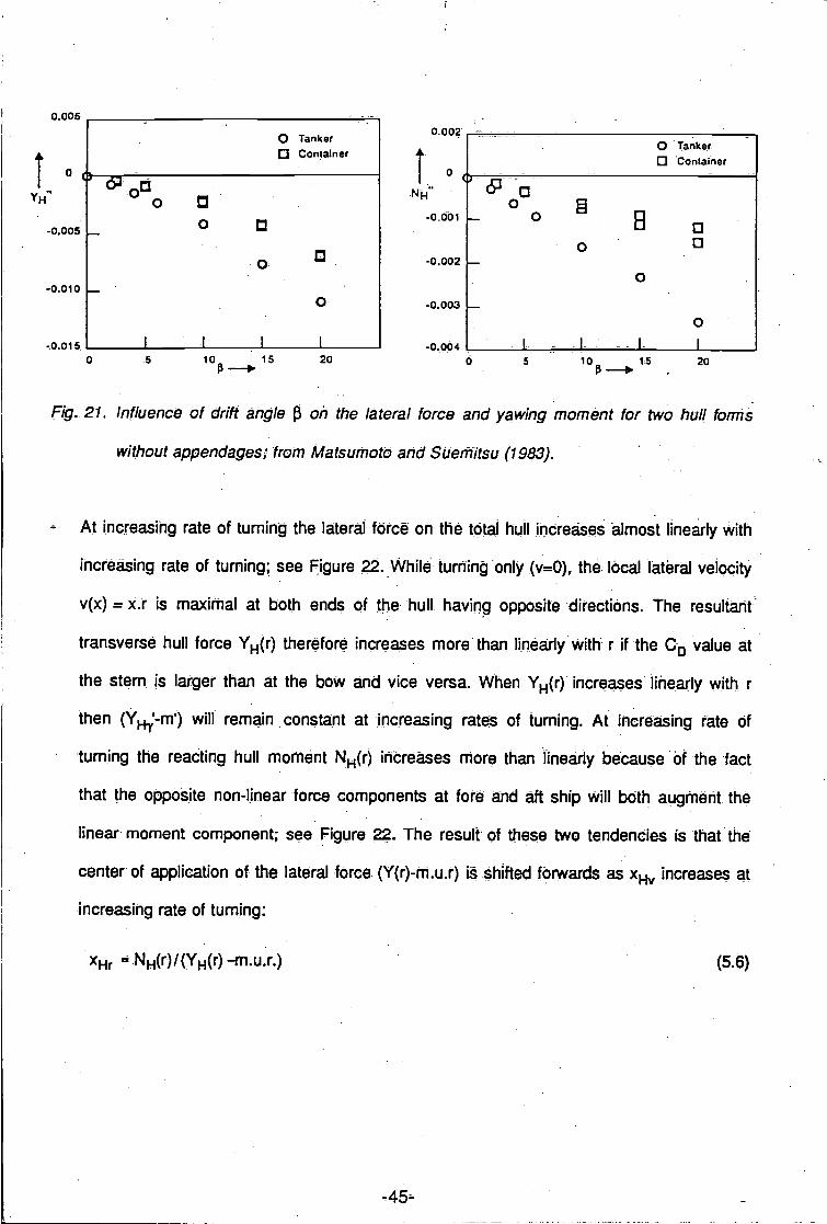
At increasing rate of turning the lateral fOrce on the tta hull increases älmost linearly with

increasing rate of turning; see Figure 22. While turning only (vRO), the. local látéral veÊocity

v(x) = x.r is maximal at both ends of the hull having opposite directions. The resultant

transverse hull force YH(r) therefore increases more than linéarly With r if the C0 value at

the stem is larger than at the bw and vice versa. When YH(r) increases linearly with r

then (Y-m') will remain cônstant at increasing rates of turning. At increasing rate of

turning the reacting hull momént NH(r) increases mOre than linearly because óf the fact

that th oppOsite non-linear force components àt fore and aft ship will both augment the

linear moment component; see Figure 22. The result of these two tendencies is that the

center of application of the lateral force. (Y(r)-m.u.r) is shifted fôrwards as x1, increases at

increasing rate of turning:

.NH(r)/(YH(r) -m.u.r.) . (5.6)

-0.005 o D-0.001 O

oDD

o -0.002

o-0.0 10

o -0.003

O

-0.0 15 I I -0 004 I-

0.002

L. o

0.005

H"

O TankerD Container

o

-46-

0.001

-0.001

0.000'

D

O TankerD Container

NH01

-0.0005

O TankerD Container

oD

o BD

O

Do U

-0.002 Do -0.0011....0

-0.003 o .0.0015}.I o o

o

-0.004 I I I t I .0.002 I I I I I I

o 0.1 0.2 0.3 0.4 0.5 0.6 0 0.1 0.2 0.3 0.4 0.5Ts. T s.

Fig. 22. Influence of non-dimensional turning rate y on the lateral force and yawing moment

for two hull forms without appendages; from Matsumoto and Suemitsu (1983).

From the above it is seen that the static stability lever XHV decreases at increasing drift angle

while the damping lever XHr increases at increasing turning rate. As a result of the non-linear

viscous contribution of the transverse hull force it is found that the dynamic stability lever

'Hd E XH(XHv will increase at increasing ship motions y and r.

Inì case that the ship is course unstable then it was found at negligibly small motions y and r

that the dynamic stability lever 'Hd is negative. From the above it is seen that at increasing

motions the dynamic stability lever will increase until the motions have reached some kind of

equilibrium in which 'EId is zero at which the ship will continue to turn at some drift angle :

XHV Hr and YH(v) YÑ(r) -rn.u.r (5.7)

6. APPENDAGES IMPROVING THE COURSE STABILITY

The ship's maneuverability might be seriously deteriorated by the fact that the ship is very

course unstable. In that case it is observed for instance that the ship has a bad "course

checking ability" which follows from the large overshoot angles in the Z-maneuver. To improve

this type of bad maneuverability one tries in the first place to make the ship more course

stable (decreasing the còurse instability).

Improving the ship's stability can be realized by applying larger rudders (see e.g. Figures 23

and 24), fins and such at the stern of the ship. Basically the improvement is seen from the

following considerations.

BARE HULL

1_0

o

-1.0

-2.0

HULL WITH RUDDER AND PROPELLER

Fig. 23. Improving the course stability (more negative stability index a7) due tO the application

of rudder nd propeller; from Jacobs (1964).

- A 7..

V= atan( - -0.5 y

-rudder area as a percentageof the lateral area Lpp.T

Fig. 24. Improving the course stability (more negative stability index ) as a result of an

increasing rudder area; from Jacobs (1964).

In the neutral position of the rudder (rudder angle 6=0) the angle of incidênce of the flow 8H

to- the -rudder, as a- consequence of the ship mötiön components u, y- arid r described

theoretically by: - - -

(6.1)

in which XR is the distance of the rudder relative to the center of reference. For small angles

of incidence the effectiveness of the rudder or the fin is expressed by the coefflcient Y8 being

positive as Will be shown in Section 7. One thus finds that due to the ship's motions the lateral

fOrce Yinduced by the rudderfollows from: - -

Y(ruddèr) -Y6 *3 - - (6.2)

From a combination of equations (6.1) and (6.2) -one fiñds the rudder force- YRU) due to the

ship's drifting and YRy dúe to the ship's turning from (see also Figure 25):

'RU) = -Y8 ! and YRy) = 0.5 Y6.y - -- (6.3)

- -48-

2.0

1.0

O

-2.0

LIB

LIT =B/T

CB =

7

18.75

2.680.6

o i Ó 2.0 3.0

-49-

Ht (r) - H (r)- mur

"H (r)

FIg. 25. Review of forceson the ship.

With these results one finds that:

1. With the rudder or fin the reactiOn force Y()' due to a drift angle iñcreases (more nega-

tive) because of the negative value of R'(); see also Figure 25:

H 'p - -/ // / 'JI (6.4)

However, the reacting moment N()' due to drifting, decreases as the negative momeñt

NH()' is compensated by the positive moment NR( generated by the rudder:

N =N' +N' =NH' +O.5Y8' (6.5)

Combining equations (6.4) and (6.5) shOws that the total reaction forcé n the hùll with

rudder Y(f3)' will shift backwards which means that the static stability lever x,' for the shjp

with rudder Or fin will be smaller than that of the bare hull:

xv,N'+OE5Y'

(6.6)

2. With the rudder or fin the reaction force Y(y)' = Y(y)'-m due to a turning rate decreases

(less negative) because of the positive value of R(7)'; see also Figure 25:

- (Y11' IY./) -mt 'Ç4f/ +0.5V8t) -rn' (6.7)

However, the reacting moment N(y)' due tò turning increaseS as the negative moment

NH(y)' becomes more negative due to the negative moment NR(y)' generated by the

rudder:

N./ - N/ + ¿N./ N. - 0.25 Y81 (6.8)

Combining equations (6.7) 'and (6.8) shows that. the total reaction force on the hull with

rudder Y(y)' will shift forwards which means that the damping lever xr' for the ship with

rudder or fin will be larger than that of the bare hull:

XI_ NH?' -0.25Y6r

''Ht7' +0.5Y6

In Figures 26 and 27 two exaniles are given of the. influence of the rudder area on the linear

hydrodynamic coefficients described in equations (6.4), (6.5), (6.7) and (6.8)

Combining equations (6.6) arid (6.9) one finds that the application of a rudder or a finj at the

stem will decrease the static 'stability lever and will increase the damping lever Xr'.. The

application of a rudder or a' fin will therefore improve the course stability. The stabilizing ap-

pendages for improving the course stability will be made so large as is needed to compensate

for the instability of the bare huJl to such a degree that the instabilIty will become acceptable.

lt should be noted that from a pòint of view of maneuvering it is sometimes preferred to apply

fins instead of enlarging the rudders such as will be elucidated in the following examples.

-50-

(6.9)

0.1 -

0.0

-0.1 -

-0.2 -

-0.3 -,

A.P.

Ni

Rudder area = 1.6 % LT

Fig. 26. Influence of the rudder on the linear

hydrodynamic coefficients for a ship

with a block coefficient of 0.6; from

Jacobs (1964).

If the course instability of the bare hull is rather large then the ship will become quite course

unstable fOr the condition in which the rudder has lost all its effecthieness (Y5'-40; see. Section

7) such as during stopping of the ship; see e.g. Yoshimura, (1993) who describes the prob-

lems which may occur during stopping of an unstable single screw ship by means of a CP

propeller. To overcome the problem of course instability during stopping one sometimes

applies fins and sometimes modifies the rudder configuration such that the rudder will remain

effective dUring the stopping procedure.

-51-

A

0.1 -

0.9

D

w

= Do-

'Q. w

Rudder area 1.6% LT

base line

Fig. 27. Influence of the rudder on the linear

hydrodynamic coefficients for a ship

with a block coefficient of 0.8; from

Jacobs (1964).

LIB = 7L/T = 18.75-B/T = 2.68CB = 0.8

L/B = 7LIT = 18.75BIT 2.68CB = 0.6

In case that the ship's response to the rudder is rather sensitive (a violent response of the

ship to the rudder) then it is not recommended to enlarge the rudder for decreasing the course

instability. In that case the ship can only be made course stable by means of applying fins.

The results in Figures 26 and 27 show the effect of the rudder on the linear hydrodynarnic

coefficients. As indicated in the figures this effect applies to ships with a length/beam ratib of

L./B 7. However, for a short full bodied ship one may find that the rudder will have less

effect. In Figures 28 and 29 it is shown that for the = 5.48 hull of Figure 14 the rudder

will have n effect at all for the range of small motions. For the conventional hull form the

rudder does not have any effect for drift angles Up till about loo; see Figure 28. For the hull

with the pram form stem one finds that the rudder does not have any effect on the transverse

force for drift angles up till about 10° and on the yawing moment up till 50 drift angles; see

Êigure 29. In his paper of 1993 Kose reports that he has tested hull forms for which in the

ballast condition the rudder did not have any stabilizing effect up till 150 drift angles.

For ¿Il these types of ships one finds that the application of the rudder did not improve the

course stability. If the ship is unacceptably course unstable then the stability can only be

improved by applying fins at thé sides of the stem where it is expected that the stabilizing

capacity (of the fins) will be more effective than near the center plane of the ship.

Also from the results by Róseman (1987) for full, bodied ships one finds that the rudder

stabilizing capacity is less effective than follows from the descriptions for óY' in equation

(6.4). ¿N' in equation (6.5), in equation (6.7) and 4V; in equation (6.8). Roseman

gives for example values of betweén 0.6 and 0.685 for the ratio between and -'(5':

For CB>0.8 = -O.65Y5 (6.10)

-52-'

0 5 10 15 2Ö 25 30 35 40

j3

Fig. 28. Influence of rudder on the transverse

force and yawing moment on a short

full bodied ship with a conventional

stem form (see Figure 14).

This result only indicates that the stabilizing capàcity of the rudder is less effective than may

be expected from its control capacity as expressed by the coefficient Y5. However, the details

of some of the data presented by Roseman are not clear. As an example, the ratio between

and Y5' ¡s considered. According to Roseman a value of about 0.8 is found for this ratio

while according to his formula ¡t is expected that this value should be less than 0.5.

- -53.

bare hullhull with rudde? .

and propeller

5 10 15 20 25 30 35 40

bare hull

hull with rudderand propeller

0 5 10 15 20 25 30 35 40

13

Fig. 29. InflUence of rudder on the transverse

force and yawing moment on a short

full bodied ship with a pram form.

stem (see Figure 14).

0.01

o

-0.01Y..

0.02

-0.03

-0.04

0.002

o

-0.002N

-0.004

-0.006

-0.008

0.01

-0.01Y..

-0.02

-0.03

-0.04

0.002

O

-0.002

-0.004

-0.006

-0.008

-% - bare hullhuIl with rudde?and propeller

I- I0 5 10 15 20 25 30 35 40

p

0

hull with rudder.._and propeller

bare hull - -

-54-

Fig. 30. Schematic indication of the flow straightening effect along the ship's hull by which the

lateral velocity component decreases towards the stern.

The reduction of the stabilizing effectiveness of the rudder behind short full bodied ships is

explained by the so-called flow straightening effect; see Figure 30. Due to this effect the trans-

verse velocity component is reduced towards the stem of the ship such that the effective

angle of incidence 8H due to the ship's motions will be smaller than described in equation

(6.1). Therefore, equation (6.1) ¡s rewritten according to (6.11) to describe the effective angle

of incidence 6H due to the ship's motions:

= atan(Cdb.!. +2Cdr) = Cdbt3 - GdrY (6.11)

in which the coefficients Cdb and °dr can be approximated by means of the empirical relations

presented by Kijima (1993) and by Ankudinov (1993).

From the description in equation (6.11) it is seen that the stabilizing capacity of the rudder will

not be very effective behind ships with a large flow straightening effect. For such ships one

will find small values for the coefficients Cdb and Cdr. The stabilizing capacity of a rudder

behind these ships will be small because of the fact that the angle of incidence of the flow to

the rudder 8H due to the ships motions will be small. lt wiIJ be clear that in this case hardly

any effect on the stabilizing capacity will be derived frOm an increment 0f the rudder effective-

ness by increásing its size or by adopting a high lift profile.

In the above only the influence has been discussed of the appendages at the stem such as

rudders and fins. However, other types Of appendages may also influence the ships m.aneu-

verability as well such as for example bilge keels. These can cause an increase of about 30%

on the drift forces when attached to a slender hull with a rather low midship section coefficient.

of CM 0.75. .

-55-

7. CONTROL MEANS

Most commonly the ship is controlled by means of one or more rudders at the stem. In that case

the control function of the rudder has to be considered in eIation to its cOurse stabilizing function

as has been described by Davidson and Schiff (1946).

The rudder effèctiveness is defined by the transverse force that is generated ¿t a given rudder

angle 6. lt is observed that at a given rudder angle a transverse fOrce Y(6) is generated which

is larger than the trànsverse force generated on the rudder only; see Figure 31:

Y(8) = R() + 'T'H(ö) = (1 +aH)YR(6) (7.1)

in which the coefficient aH can be approximated by mèans of the empirical formulae presented

by Kijima (1993) and Ankudinov (1993).

In Figure 31 and in eqùation (7.1) it is assumed that the difference .Y(6) between the total

transverse force Y(8) and the force R(8) on the rudder is generated on the hull and is therefore

described by YH(6). With this descriptiOn the yaw moment N(8) generated by a rudder angle can

be formulated by:

N(3) XRYR(8) + xYH(3) = (xR+xaH)YR(8) (7.2)

H (6)

Fig. 31. Forces excited on the rudder and the hull due to rudder déflection.

-56-

8

in which xÁ is the distance of the rudder from the ship's center of reference while the distance

XHS can be approximated by means of the empirical formulae presented by Kijirna and

Ankudinóv.

For a further evaluation of. the rudder effectiveness (see also the application in Section 6) one

uses the rudder coefficient Y5 which is defined by:

Y5 =Y(5)/sin(5) or Y =Y(6)'/sin(6) (7.3)

with

Y(6)' =Y()/(O.5pSRU2) (7.4)

in which SR is the lateral area of the rudder and U is the ship's resultant velocity.

For rudder, angles smaller than the stall angle st the force YR(5) on the rudder mainly depends

on the lift LR which is the force component on the rudder that is perpendicular to the. incoming

flow; see Figure 32. Aside f the lift also the resistance R along the rudder, the drag force Di in

the direçtion of the flow and the normal drag force YN perpendicular to the rudder are generated

on the rudder as shown in Figure 32.

L

Fig. 32. Schematic decomposition of the total force on a rudder..

-57-

-58-

in which CR is the chord (length) of the rudder. lt is noted that in comparing the resistance of the

high-lift rudder with that of a conventional rudder one should consider that in addition to the

resistance increment of the high-lift rudder also the resistance of the head box, which is needed

to àttach the rudder to the hull, has to be taken into account.

The resistance R is described according to the general procedures. f 9r describing the longitudinal

resistance of a Streamlined object:

RR(8) - 0.5 p SWA CTA u (7.5)

¡ri which the flow velocity UR will be described later on. In equation (7.3) SWR is the wetted surface

area of the rudder and CTR is the rudder resistance coefficient:

CTR CFR(60) (1 +kR) (7.6)

with CFR being the frictional resitance coefficient and kR b&ng the form factor of the rudder. The

effective angle of incidence e of the flow to the rudder ¡s described by:

" H (7.7)

with 8H being the effective angle of the flow due to the ship's motions relative to the zero position

of the rudder; see also equations (6.1) and (6.11).

From equation (7.5) it is seen that the rudder resistance ¡s described by the resistance coefficient

C- which depends strongly on the profile of the rudder. lt is often found for example, that, the

resistace coefficient 0TR of a high-lift rudder will be larger than that of a rudder with more

conventional profile; see e.g. Figure 33. From the results in Figure 33 it ¡s seen that the increase

of resistance coefficient CTA of the high-lift rudder does not change over a wide range. of

Reynolds numbers RnA of the rudder:

UR CR(7.8)

V

o 020

0.016

0.012

CT

0.008

0.004

o

5.75

Convenhid rudder IIh Noca profileHigh lLft ruer Att Fish-toil profiléFroudesldn friction

6.0 6.25

log Rn

-59-

Fig. 33. Resistance coefficients of two types of rudders for a wide 'range of Reynolds numbers.

Attention should be given to the fact that when the flow approaches the rudder under sorné angle

of attack then the resistance coefficient C in equation (7.6) 'will increase a little 'due Sto' the

circulation around the rudder; see e.g. Abbott and von Doenhoff (1965):

CFR(6e) = CFR (1 +Cl:Sjfl2(6e)SR/SWR) (7.9)

¡n which SR is the lateral area of the rudder. The lift coefficient Cl5 is described as follóws:

lithe effective rudder angle is smaller than the stall angle then the lift force L (perpendicular to

the incoming flow) is determined by: '

LR() = 0.5 p SR CI5 u Sfl(e) (7.10)

in which Cl5 is the lift coefficient which depends among other things on the profiJe and the plan

form of the rudder. The influence of the profile is for example shown in Figure 34 in which the

measured lift coefficient is 'presented of a rudder with a conventiónal profile (NACA profile), and

that of a rudder with a fish-tail profile. The results in Figure 34 were derived fröm experiments

with deeply submerged rudders both having the same geometric aspect ratio of Ag = '1.5. These

test results confirm the assumption that the influence of the Reynolds number ön the lift

6.5 6.75

coefficient is negligible. This means that when 30% higher lift is found on a rudder model with a

particular profile then also 30% higher lift is expected for the full scale rudder of that profile.

A

CI6

p---e--4

3

2

0

it Ae C16(Ae ce)Cl5 =

C15(Ae=Qo) +7tIAe244

- ..(Fn) withAg Ag

Conventid rudder v.4th Noca profile

High litt rudder v.ith Fish-toil profile

from which it is seen that the lift coefficient Cl8 increases with increasing effective aspect ratio

Ae. For rudders piercing the free water surface one finds that the ratio Ae/Ag between the

effective aspect ratio and the geometric aspect ratio depends on the Froude number FnR related

to the rudder conditions:

FnR =uR/g.cR

-60-

(7.12)

(7.13)

5.75 6.0 6.25 6.5 6.75

lOg

Fig. 34. Lift coefficients of two types of rudders for a wide range of Reynolds numbers.

The influence of the plan forni on the lift coefficient Cl5 is expressed for instance by the

geometric aspect ratio Ag:

Ag =SRIc (7.11)

According to Whicker and Fehlner (1956), one finds the following description of Cl8 as a function

of the aspect ratio:

e ao e

a

From the experimental results in Figure 35 it is seen thát t relatively low speeds (harbor

maneuvering) the rudder will be more effective (larger relative effective aspect ratio) than for the

service speed condition. To elucidate the results ¡n Figure 35 one considers a flow velocity to the

rudder of about 8 rn/s. From Figure 35 one finds that the effective ¿pect ratio Will nearly be. equal

to the geometric aspect ratic. (Ae/Ag-1) for all rudders with a chord smaller than 2.9 m (FnR>l .5)

which holds for a large category of ships.

In equations (7.5) and (7.10) UR is the velocity of the flow to the rudder. If there is no propeller

in front of the rudder then:

UR =u(l WR) (7.14)

in Whiòh WR is the wake fraction of the flow to the rudder.

However, ¡n case of a propeller in front of the rudder then UR ¡s largely influenced by the thrust

of the propeller; see e.g. Molland and Turnock (1993).

UR Up +CDUAUP (7.15)

-61

0 0.5 1.0 1.5FnR -

Fig. 35. Influence of the Froude number on the effective aspect ratio relative to the geometric

aspect ratio for surface piercing rudders.

in which uf, = u(1-w) is the incoming flow to the propeller and Up is the increase of flow velocity

by the propeller. The coefficient CDU describes the effectiveness of the velocity increment induced

by the propeller on the rudder and depends for instance on the propeller diameter D relative to

the rudder height bR (ratio Dp/bR), on the distance of the rudder to the propeller and on the lateral

position of the rudder in the propefler stream. For more details one s referred to Kijima (1993),

Kose (1993) and Molland (1993)

Theoretically the velocity increment Up at a large distance behind the propeller follows from:

Taking into account, the: velocity increment due to the propeller one finds:

1. The effectiveness Y5' of a rudder behind a propeller with positive thrust T will be

significantly larger than that of a rudder ¡n the free stream; see eg. Figure 36.

. The effectiveness Y5' of a rudder behind a propeller will increase at increasing propeller

thrust T suôh as occurs when the propeller RPM is larger than that at a stationary speed.

This condition will occur when during maneuvering the ship's speed will be reduced due to

the increased resistance while the propeller RPM has not decreased accordingly. This

condition will also occur whèn at low speeds (harbor maneuvering) the propeller RPM is

increased during a restricted period of time; see e.g. Hooft (1970). From the results in Figure

37 for a 200 kDWT tanker one finds for example that the rudder effectiveness Y5 at a lòw

speed of Fn 0.0725 can be doubled by increasing the propeller revolutions from 40 RPM

(SPP condition .at Fn = 0725) to 80 RPM.

I 2 8T¿upIup+

2

-62-

- Up (7.16)

Y..

0.010 -

0.0075

0.ô05

0.0025

0.0o

2 semi baianced rudders r

single balanced rudder

10 20 30

rudder angle 5

-63-

40 50

Fig. 36 Non-dimensiOnal lateral force as a functioñ of the rudder angle. for two rudder

configurations behind a slender twin screw ship; from measurements at shallow water

depth of 1.2 T.

3. The effectiveness Y5' Of a rudder behind a propeller will be reduced significantly during the

stopping procedure. In this condition the propeller thn.st is decreased significantly and can

even become negative. From the results in Figure 37 for a 200 kDWT tanker one finds for

example that the rudder effectiveness Y5 at the service speed of Fn = 0.145 cari be reduced

by about 70% by deçreasing the propeller revolutions from 80 RPM (SPP condition at

Fn 0.145) to 30 RPM. With the propeller ¡n the backing. mOde it even may o cur that the

rudder will have no control effect at all (Y,0) suòh as has been described e.g. by Yoshimura

(1993).

2 semi balanced rudders single balanced rudderbehind the propellers in the free stream

LO5

o

-64-

Fig. 37. Rudder generated side force (expressed by the derivative Y&) on a 200 kDWT tanker

with single screw-single rudder configuration for various combinations of ship speed and

propeller RPM.

Another contribution to the rudder force is the drag in the direction of the flow. This force is the

so-called lift induced drag Di which is excited by the loss of pressure over the tips of the rudder.

This force is determined by:

DIR(60) = 0.5 p SR COiR UR S2(e) (7.17)

in which the lift induced drag coefficient CDiR of the rudder is related to the lift coefficient Cl5

according to Whicker and Fehlner (1958):

with the coefficient e being Oswald's efficiency factor. When comparing the measured coefficient

°DIR for the conventional profile in Figure 38 with the measured lift coefficient Cl5 in Figure 34

then one finds e=1 for the conventional profile. Applying this same value for the high-lift profile

then one finds that the effective aspect ratio of that rudder is about 30% larger than the geometric

o 20 40 60 80 looopeIIer RPM .

2

COIR -e irAe

(7.18)

aspect ratio. This finding for the effective aspect ratio is in agreement with the earlierfinding that

the 30% increment of the lift coefficiênt of the high-lift rudder is caused by the increment of the

effective aspect ratio. In Figure 39 the relation between the resulting lift coefficient CL and the

resulting drag coefficient CD for varying rudder angles is shown for two rudder forms.

Irrespective of the effective angle of incidence a normal force YN is generated on the rudder due

to the lateral drag coefficient CN perpendicular to the rudder:

YNR(Ö) 0.5 p SR CN U sin(50) I Sfl(6) I (7.19)

in which the coefficient CN depends on the plan form and profile of the rudder:

CN = C(tm/c,Ae,rounding of tips) (7.20)

in which tmR is the maximum thickness of the rudder at half height. For mQre information one is

referred to e.g. Winter (1935), Wadlin (1955) and Whicker and Fehlner (1958).

Conventlol rudder Mth Naco profile

- - -e - High lift rudder 'with Fish-toil profile

-65-

5.75 6.0 6.25 6.5 6.75

IORflp

Fig. 38. Lift induced drag coefficients of two types of rudders for a wide range of Reynolds

numbers.

o- - -* - -- 2_. -o o

u

4

f312

coi

o

0.12

'D

0.04

log RnR= 6.4584

-xRR sin(Ö) - XR Dsin(5H)

In Figure 40 the overall forces due to a rudder angle are given which were measured for three

different stem förms shóWn in Figure 14. From the results in this Figure 40 it is seen that also for

a short fUll shi nò influence can be. discerned of the stem. form on the rudder elf ectivertess.

O Noca poflle

O Fish - toiIpotiI

Fig. 39. Relation between the non-dimensional lift añd drag at váring rudder ancles.

Taking into account the various force contributions n the rudder one finds the following resultant

rudder force components in the ship fixed coordinate system:

-66-

XR = -Rcos(6) Dcos(H) - YNsin(5) -Lsin(5H) (7.21)

- YN cos(ö) + L COS(ÖH) - R sin(6) - D Sifl(ÖH) (7.22)

XR VN cos(6) + (XR + XHÖ aH) L COS(&H)(7.23)

010.2 0.4c.

-0.001Y..

-0.002

0.001

o

-0.003

-0.004

o

conventional

pram form

moderate pramform

I t

conventional

0.00l - moderate pramform

-67-

0 5 10 15 20 25 30 35 40

3

pram form

-0.002 t t

0 5 10 15 20 25 30 35 40

3

Fig. 40. Rudder effectiveness for various stern forms of a short full bodièd ship.

The formulations in the above considerations were based on the assumption that the effective

rudder angle is smaller than the stall angle 6. In this respect the stall angle is defined .to

correspond to the angle of incidence of the flow to the rudder at Which the lift will not be

developed completely. This aspect is clearly observed for a profile in the free stream. In that case

it is found that the stall angle will increase at decreasing effective aspect ratio Äe. However, for

the performance of a rudder behind a ship it appears that the stall angle ¡s even larger than in

the free-stream condition. lt ¡s assumed that this phenomenon corresponds to the large stall angle

of a trim flap behind a flapped rudder. In general ¡t appeajs that there ¡s no need to consider

stalling as a serious aspect of the effectiveness of a rudder.

In Figure 41 the non-dimensional transverse force and yawing moment is shown for various

combinations of drift angle and rudder angle 3. The results in this figure are derived from

captive model tests with a short full bodied hull with different stem forms as shown in Figure 14.

With respect to the results in Figure 41 the following remarks can be made:

At a rudder angle to starboard (3<0) the ship will turn with the bow to starboard while drifting to

port «3<0). Due to this combination of negative drift angle and negative rudder angle a positive

yawing moment is generated. From Figure 41 it is seen that the yawing moment will reduce by

reducing the rudder angle. Even when the rudder is put in the opposite position then the yawing

moment will decrease continuously when the drift angle remains constant. This continuous

change of the yawing moment as well as that of the lateral force shows that it is not possible to

discern any stall phenomenon even not at 40° rudder angle to starboard while the ship is drifting

to port at -40° drift angle.

The other remarkable aspect from the results in Figure 41 follows from the fact that there ¡s hardly

any difference in the transverse force or yawing moment for the three different stern

configurations. This means that also with respect to the effectiveness of the rudder in the

opposing direction no influence of the stern form is found.

-68-

0.04

A

Y

D

o

002

pramform aiterbody

a

+

D

+

A

Q

+

A

o

+ + +

A

o

A

D

A

+

A

a o

moderate pramform afterbody

convential afterbody

-69-

00 10

r0.005

o

pramform afterbody

D

o

moderate pramform afterbody

+

A

C

+

A

o

o

+

A

o

o

A

Q

A +A

QD

¿ I

A

o

+

A -30D

o

+ +

A A

a

convential afterbody

+

o

++

A 4-A

o oI I Ç

+4.

D

AD A Ao

o

I I I

+

o

-40 -30 -20 -10 0 10 20 30 40 40 -30 -20 -10 0 10 20 30 40rudder angle rudder angle

-40 -30 -20 -10 0 10 20 30 40 -40 -30 -20 -10 0 10 20 30 40rudder angle rudder angle

Fig. 41. Non-dimensional side force and ya wing moment n a short full bodied ship as a function

of the stem form, the drift, angle 3 (pOsitive when drifting to starboard) and rudder angle

8 (positive when rotated to port).

40 .30 -20 -10 0 10 20 30rudder angle

-40 -30. -20 -10 0 10 20' 30

rudder angle

t I I I ¿ e o ? f

+ + 4. ++

4.++ +

A A A

A A A A A A

D Q o D o o o Q

I I I

++A

A

a o

0.0 10

r.4

0.005 o

o

+A

+

A p--30D

4. 0A

+

A

A+

4-

A

DD

o oI I 'P ¿

+ +D D

+++

++

A

+

A A£AA

A

QD aaDDoD

, I¿

0.04

r..02

0.04

r.0.02

0.0 10

r.0.005

o

8. PREDICTING THE MANEUVERABILITY IN THE DESIGN STAGE

Executing free running model tests is òonsidered to be the most reliable method nowadays for

predicting the ship's maneuvering performance; se e.g. Figure 42. The reliability of this method

is based on the vast experience gained with this technique.

Except for a few special cases no significant scale effects have been found on the results derived

from free running model tests in deep water; see e.g. Nikolaev and Lebedeva (1979), Oltmann

etal. (1979), Kose et al. (1980), Yoshimura et al. (1981).

Often, the most' significant scale effect influencing the maneuverability is supposed to originate

fröm the scale effeöt on the resistanöe. As a result the propeller load during the free running

model test is too high relative to the full scale, condition. One then assumes that the rudder

effectiveness will be relatively high due to the relatively higher propeller load. Based on this

reas6ning one often assumes that the results of the free running model tests will be too optimistic.

Hôwever, no systematicproof for this statement has been found yet.

Full scale trials

Model tests

-70

Fig. 42. Results of 200/200 zig-zag maneuver for á short full bodied ship as derived from the free

running model test in comparison to the sea fríal.

In literature some cases are mentioned in which the ship's maneuverability appeared to be very

unsatisfactory while it was suggested that an acceptable maneuverability would have been

predicted from free running model tests if they had been executed. In order to explain this

assumed discrepancy a study was performed to ascertain the origin of possible scale effects. For

this purpose systematic free running model tests have been carried out for a short full bodied

ship; L,/B = 5.48 and 0B =0.814.

During the sea trials large overshoot angles of over 40° had been measured during 100/100 as

well as 200/200 Z-maneuvers. Based on these results the maneuverability of the ship was

cónsidered to be unacceptable and that additional means had to be applied to the ship for

improving its maneuverability. In the study afterwards, free running model tests for this ship were

performed for both the self propulsion point of model (overloaded prçpeller) and for the self

propulsion pôint of ship (propeller load of model equal to that of the ship).. The tests with the free.

running model at the self propulsion point of ship have been executed with the help of a.wind

ventilator on the deck of the model. The thrust of the wind, ventilator was cöntrolled to correspond

to the friction deduction force Fd(u) as a function of the model speed. The friction deduction force

is determined by the difference (scale effect) between the resistance coefficient of the model and

that of the ship.

In Table 3 the results of the Z-maneuvers are presented. From this table it is seen that the results

of the standard free running model tests (SPP of modél) show unacceptably large ovCrshoot

angles. Based on the. results of these standard model tests it is concluded that the

maneuverability is unacceptable as had already been found from the sea trials. From Table 3 it

is furthermore seen that the effect of the propeller loading on the ship's maneuverability ¡s

negligible. From these model tests no indication coUld be derivéd about scale effects in the

maneUvering performance of free running models.

-71-

Table 3. Results frOm Z-maneuvers with a free running model of a short fui! bodièd ship

at constant RPM.

Table 4. Results from turning circle, tests with a free running model

of a short (ui/bodied ship at constant RPM.

-72-

bescription

of maneuver

- First overshoot angle Second overshoot angle

SPP model SPP ship SPPmode-

SPP ship

20/20 P

2Ol20 SB

.1.0/10 P

10/10 SB

42

31

48

21

48

32

. 48

-

20

30

28 .

20

28

>31

-

Description . 'Advance/L Tactical diameter/L

of maneuver'SPP model SPP Ship SPP model SPP ship

35 P; 2.62 2.77 2.00 2.01

35 SB 2.97 3.11 2.29 2.28

20 P ' 2.89 2.98 2.69 2.72.

20 SB 3.31 . 3.45 3.23 3.26

In Table 4 the results of 'the turning circle tests are presented. From the results in this table it is

seen that only a small effect of the propeller loading is noted with respect to the advance while

no effect is noted on the tactical diameter.. No exact valves from sea. trials are available except

that the turning circle diameter is in between and 2.5L?p. However, for a comparable ship

hardly any difference was found between the turning circle characteristics from free running model

tests and those from sea trials.

In the above the results of free running model tests have been presented while the propeller

revolutions were kept constant during the whole maneuver. However, during sea trials the,

propeller revolutioñs will drop due t an incremònt of the propeller loading as the ship's speed will

decrease while maneuvering. The reduction of propeller RPM Will depend on the type of the main

power plant. Fora diesel engine the reduction of revolutions will approximately correspànd to the

condition that the torque will, remain constant. Èor a turbine plant the revolutions wiil

approximately be reduced according to 'the condition of constant power.

In order to simulate the ship's maneuverability correctly during the free running model tests it will

be necessary to adjust the 'propeller revolutions to its loading. For this reason two additional

series of free running model' tests have been executed with the above short full bodied hull: (1)

with, the RPM adjusted such that the propeller torque remains constant during each maneuver,.

and (2) with the RPM adjusted such that the propeller power remains constant during each.

maneuver. These additional tests have been performed for the SPP of ship with the aid of a

ventilator on deck of the model. '

The results of the additional tests with adjustments of the propeller revolutions are given in Tables

5 and 6. At the "constant power" tests an RPM reduction of maximal 18% was found while during

the "co'nstant torque" tests the RPM dropped maximally 27%. From the results in Tables 5 and

6 in comparison to the results ¡n Tables 3 respectively 4 one finds that:

-73-

Table 5. Results from Z-maneuvers with a free running model at SPP of ship.

Table 6. Results from turning circle tests with a free running model at SPP of ship.

-74-

Description

of maneuver

First overshoot angle Second overshoot angle

Constant power

18% RPM

reduction

Constant torque

27% RPM

reduction

Constant power

18% RPM

reduction

Constant torque

27% RPM

reduction

20/20 P

20/20 SB

10/10 P

10/10 SB

49

40

48

31

51

39

70

34

18

28

-

>50

20

27

-

>50

Description

of maneuver

Advance Tactical diameter

Constant power

18% RPM

reduction

Constant torque

27% RPM

reduction

Constant power

18% RPM

reduction

Constant torque

27% RPM

reduction

35 P

35 SB

20 P

20 SB

2.87

2.87

3.46

3.29

2.94

2.82

3.41

-

2.06

2.29

2.95

2.99

2.08

2.25

2.91

-

The ovórshoot angles during the Z-maneuvers with adjustments in propeller RPM are only

a little larger than those derived trbm the tests with cànstant RPM. From both test. series the

overall impression is that the ship's maneuverability is unacceptable.

No clear difference can be found ¡ri the advance and tactical diameter during the turning

circles with adjustments in propeller RPM and those derived from the tests at constant RPM.

Only the final speed and rate of turning wiJI be lower in the turning circle with reductions in

the propeller RPM than those encountered in the tests with constant RPM.

The overall conclusion from the above described study is that even forshort full bodied ships no

obvious scale effect can be observed in the results from free running model tests. The results of

these tests correspond well with full scàle observations.

In the initial design stage use is made of computer simulations before executing the rather costly

free running tests. For this purpose MARIN' developed the simulation prögram SURSIM in which

all hydrodynamic properties are derived from empirical mèthods as have been described in the

previous sections. In SURS IM the non-Ilnear hull forces are based on the concept of longitudinal

distribution of the cross flow drag coefficient which varies With the changing velocity cOnditions

while maneuvering.

The simulation program has been validated by means of:

Comparing calculated forces at given velocity combinations With the results from captive

model tests either in a towing tank or in a rotating arm facility; see e.g. Figure 20.

Comparing calculated maneuvers at the SPP of model with the results from free running

model tests; see e.g. Figure 43 and Tables 7 and 8 for a full bodied ship.

Comparing calculated maneuvers at the SPP of ship with the results from sea trials; see e.g.

Figure 44.

-75-

// /

Initial position

Model tests

SURSIM calculations

-76-

,

Fig. 43. Results of turning circle maneuver at 350 rudder angle for a short full bodied ship as

derived from computer simulations in comparison to the free running model test.

- -/

-/

Table 7. Results from Z-maneuvers derived frOm model tests and computer simulations for a

shOrt full bodied ship.

-77-

Description

of maneuver

First overshoot angle Second overshoot angle

Model tests Simulations Model tests Simulations

SPP of model;

constant RPM

20/2Ó P 42 4Ö 20 47

20/20 SB 31 40 30 47

10/10 P 48 35 28 63

10/10 SB 21 35 >55 63

SPP of ship;

conslant RPM

20120P 48 46 20 54

20/20 SB 32 46 28 54

10/10 P 48 47 >31 80

10/10 SB - 47 - 80

Table 8. Results from turning circles derived from model tests and computer simulations for a

short full bodied ship.

-78-

Description

of maneuver

Advance Tactical diameter

Model tests.

Simulations Model tests Simulations

SPP of model;

constant RPM

35 P 2.62 2.53 2.00 2.03

35 SB 2.97 2.53 2.29 2.03

20 P 2.89 2.94 2.69 2.62

20 SB 3.31 2.94 3.23 2.62

SPP of ship;

constant RPM

35 P 2.77 2.67 2.01 2.11

35 SB 3.11 2.67 2.28 2.11

20 P 2.98 3.10 2.72 2.69

20 SB 3.45 3.10 3.26 2.69

SURSIM calculations = Full scale trials

Fig. 44. Comparison between the results from computer simulations with those from sea trials

with respect to the turning circle at 350 rudder angle.

From the results shown above about the validation of the computer program it is concluded that

in the initial design stage a good impression can be achieved about the ship's maneuverability

by using a computer simulation program such as SURSIM.

When in the initial design stage only the main dimensions are available while the local details of

the hull form are not yet known then use can be made of computer simulations using only very

rough estimates of the hydrodynamic characteristics based on the experience with available

hydrodynamic characteristics derived from previously designed ships. This method will be

discussed in more detail in the next section.

-79-

C8 0.56 0.60 0.62 0.75 0.76 0.81 0.83

L/B 6.60 5.13 5.43 6.39 7.27 6.02 6.13

9. TEST CASE

In this section a procedure will be. given to apply the information presented ¡ri this paper for

evaluating the ship's maneuverability in the initial design stage by means of computer simulations.

In this stage of the design no hydrodynarnic information is yet available from captive model tests

such as PMM tests or rotating arm tests. In the procedure to be presented the hydrodynamic

characteristics will be derived from a combination of hydrodynamic data available from earlier

model tests and existing empirical methods.

A full wide beam ship will be considered of which the main dimensions are characterized as

follows:

the length-beam ratio should be minimal: therefore Lw/B = 4 is chosen,

the beam-draft ratio should be maximal: therefore BiT = 3.75 is chosen,

the block coefficient is chosen to be: CB = 0.825.

Furthermore it is chosen that the ship with these parameters should be as large as possible. For

all kinds of reasons it is decided that a width of B = 75.00 m is maximally feasible. In this way

a ship is considered with the following main dimensions:

= 300.00 m

B = 75.00m

T = 20.00m

CB = 0.825

XG = 7.50 m; position of center of gravity ahead of the reference point O amidships.

-80-

The ship will be driven by two propellers with the following characteristics:

D =1O.25m

P/D = 0.7

AE/Ao = 0.57 (blade area ratio)

z =4

The propeller shafts are contained in a twin gondola configuration. Behind each propeller a rudder

will be mounted. The dimensions of each rudder are:

Height bR = 12.5 m

Chord CR = 6.0 m

Lateral area SR = 75.0 m2 (1.25% of the hull lateral area

From the information presented by Holtrop and Mennen (1982) one finds that the wake fraction

will be w = 0.3 while the thrust deduction fraction will amount to t = 0.22.

The set-up of the mathematical model Will be based on the review in Section 3. The various force

components (i.e. hull forces, propeller forces and rudder fOrces) in equation (3.8) will be described

here in detail.

Bare hull forces

The ship's resistance is approximated according to Holtrop and Mermen (1982):

XH(u) = -(3.057 E4).0 - (2.221 E4).u2- (1.019 E3).u3 (N) (9.1)

-81 -

For the derivation of the other bare hull hydrodynamic coefficients use is made of the values from

measurements performed with a comparable model. For this reference model use is made of

model D that has been described by Roseman (1987). The main characteristics of the reference

model D are given ¡n Table 9 ¡n comparison with the characteristics of the ship considered here.

Table 9. Main characteristics of model D of which the hydrodynamic coefficients

are known from model tests.

In Table 10 the hydrodynamic coefficients of the new design are shown as derived from the

reference ship D with the aid of empirical methods. The derivation is as follows (see also Kose,

1993): Each of the hydrodynamic coefficients HCND for the new design is derived from the

available coefficient HCD of model D as shown in the following extrapolation. If the coefficient

HCD from the measurements has the same sign as the coefficient HCD(emp.) from the empirical

method, then:

HCNDHCND(emp.)

*HCDHCD(emp.)

(9.2)

however, ¡f the sign of both coefficients are opposite then the following extrapolation is applied:

HCNO = HC0 + (HCND(emp.) - HCD(emp.)) (9.3)

-82-

Main characteristics Model D (reference) New design

LW/B 4.500 4.000

LWrr 13.50 15.00

B/I 3.000 3.750

CB 0.850 0.825

xGILPP +0.025 +0.025

Table 10. Review of derivation of bare hull hydrodynamic coefficients.

-83-

Ship D Empiric

method

described

New design

Experimental Empiric Erripiric Recommended

jñ text

-0.001 72 -0.003025 *1 -0.004262 -0.002423

YÇ -0.02473 -0.02169 *2 00iM2 -O.Ó1872

-0.00035 -0.001766 *2 .. -0.001693 -0.00034

N" 0.000.10 -0.001563 *2 -0.001691 -0.00003

Ñ" 0.00i685 -0.001106 *2 -0.000746 -0.001136

Xvr" 0.01855 0.02473 *3 0.01872 0.01404

0.00164 -0.00252 *3 -0.00628 -0.00212

X.y." 0.*3

- 0.

-0.0235 !0.03683 *4 -0.03321 -0.02119

-0.05857 -0.04630 *4 -0.04111 . -0.05200

0.00788 0.00700 *4 Ö.00688 0.00764

Yr"IrI 0.00225 0.00201 *4 0.000364 00004t- - -0.01851 -0.01851

''vvr" - - 0.02133 0.02133

N" . -0.01273 -0.01097 "4 -0.008889 -0.010315

N"II 001441

-0.00582

-0.00133

-0.00430

"4

"4

-0.001413

-0003615

0.01433,

-0.004893

Nr"lrI 0.00049 0.00033 *4 0.000875 . 0.00006

- *4 0.00400 0.00400

Nwr" - - 0.01 673 -0.01 673

The empirical methods used in Table lo for the prediction of the hydrodynamic coefficients are

as follows:

(1) For the derivation of the longitudinal added mass coefficient -X use has been made of the

method presented by Soding (1982).

(*2) For the derivation of the lateral added mass coefficient -Yo, -Yr, -N and -N use has been

made of the method presented by the lITO 1984.

(3) For the derivation of the longitudinal damping coefficients use has been made of the

following approximations:

- X = -Y - D ¡n which the longitudinal drag D ¡s determined by:

D = CDV.(O.5 p.L,.T) with: CDV = CLV2.(LPp/2T)/it? and

CLV =

- Xvr = -Y according to Norrbin (1971).

(*4) For the derivation of the sway and yaw damping coefficients use has been made of the

method presented by Kijima (1993).

lt should be noted that the bare hull coefficients ¡n Table 10 may be slightly affected by the twin

gondola configuration.

Propeller forces

From Kuiper (1992) one finds the following description of the performance of each propeller:

K.1. = 0.294 - O.247.J - O.227.J2 + O.0693.J3 (9.4)

in which the following notation is used:

K.1- = T/(p.D4.n2) and J = u.(1-w)I(n.D) (9.5)

The total longitudinal force generated by the propellers amounts to:

X = (l-t)(T) (9.6)

-84-

Rudder forces

For each rudder the following force components are described. The resultant drag in the ditection

of the incoming flow, while the rudder rèsistancò is incorporated ¡n the total resistance of the ship:

b - X55.u.sin(69)2 (9.7)

The resultant lift perpendicular to the incoming flow:

L h1'Y8.U.SIfl(6e) (9.8)'

In these equations use ¡s made of the following characteristics:

The effective rudder angle 3e amounts to:

6e 16 6H (9.9)

with 8 being the rudder angle while 6H is the flow deviation due to the ship's motion at the

location of the rudder:

6H 1CdbI3 Cdr1 (9.10)

in which ß = atan(v/u) and y = r.L./u. For the prèsent configuration use is made of

0db = Cdr = 0.26 according to Kijima (1,993).

- The effective velocity UR of the fløw at the location of the ñidder in the above equations about

the rudder drag D and lift L is derived from:

UR Up. + C0Up

in which CDU = 0.7 Dp/bR and in which. the incremental propeller velocity Up is derivedfrom:

-85

I 2Up

+ 2-Up

p.7t.Dp

The rudder coeffiòients X and Y8 in the äbove equations for the drag and lift are derived

from

-O.5pSC and O5pSRCIs (9.13)

in which the lift coefficient Cl6 = 2.678 follows from Whicker and Fehlner (1958 )while using

an effective aspect ratio A0 equal to the geometric aspeçt ratio Ag hR/cR = 2.083. The drag

coefficient C0 = 1.096 is derived from:

=

From the drag and lift on each rudder one finds the following force contr butions XR, R and

yawing moment NR of the rudders:

XR E(D COS(H) - L Sfl(&H))

= E(D Sifl(8H) + (1 + ah) L CÓS(3H))

NR [YR<R + (XR ai...XH) L COS(6H) + XRD 1(6H)]

in which aH = 1 and XH = O follow from Kijima (1993).

Having inserted the above hydrodynamic characteristics ¡n equation (3.8) will lead to a

mathematical model by means of which the ship's maneuvering performance can be predicted;

see the simulation results in Table 11. From these results it ¡s seen that the ship is rather sluggish

and course unstable.

-86

(9.12)

(9.14)

Table 1. Review of the maneuvering perfOrmance of a wide beam tanker LB=4

with a twin screw and twin rudder arrangement

* TURNING ABILITY AT 35 DEG RUDDER ANGLE

- advance = 1203 m (4.01 L)

- tactical diameter = 1405 m (4.683 L)* COURSE INITIATING ABILITY AT 10 DEG RUDER ANGLE

- travelled distance at 10 deg change of heading =. 606 m (2.02 L)* COURSE CHECKING ABILITY

10/10 Z-maneuver (LN 38.9 sec)

first overshoot = 9 deg

second Overshoot = 6 deg20/20 Z-rnaneuver

first overshoot = 14 deg* COURSE STABILITY

- height of hysteresis = 2 * 0.12 deg/sec = 0.24 deg/sec

(cónstànt räte of turning 0.26 deg/sec at 3 = 35 deg)

-87-

For the assessment of the ship's maneuverability one now compares the results in Table 11 with

the 1MO criteria in Table i It appears that the ship's maneuverability satisfies the 1MO criteria

except for the course initiating ability at lo deg. However the difference with the 1MO criterion for

this aspect is negligible.

It is expected that the course instability will not have too much effect on the course keeping ability

during stopping because of the fact that there will be no serious asymmetric disturbance clue to

the propulsion as the ship is equipped with two propellers.

The overall conclusion with respect to the maiieuverability of the neWly designed wide beam ship

reads: Based on the apprbximated hydrodynamic coefficients one finds, in the initial design stage,

that thè maneuverability öf the wide beam ship ¡s marginal and that fürther attention should be

given to reach a more reliable prediction of the maneuverability by applying either:

mre precise prediction methods such as SURSIM ¡n which use is made of the concept of

the cross flow drag coefficient, or

more precise mathematical models based on experimentally derived hydrodynamic

coefficients, or

free running model tests.

For a fuilher evaluation of the predicted maneuvering performance a sensitivity analysis will be

useful to ascertain the effect of the uncertainties in the estimated hydrödynarnic coefficients. For

the present study the following aspects have been considered:

The consequence of the rudder effectiveness: see coefficient Y5 in equatiOns (9.8) ¿.nd

(9.13). Decreasing Y5 with 20% leads to a 4.7% increase of the advance and a 5.5%

increase of the tactical diameter. This means that for this ship an uncertainty in the rudder

effectiveness expressed by the coefficient '1's will have some effect on the acceptability of the

ship's maneuverability.

-88-

The. consequence of the flow straightening effect while turning: see coefficient 0dr fl equation

(9.10). Increasing Cdr with 20% will lead tO an increment of 0.7% in advance and an

increment of 1:. 1 in the tactical diameter. This means that the, uncertainty in the flow

straightening while turning expressed by Cd,. will have hadly any effect on the predicted

maneuverability.

The consequence of the propeller flow acceleration: see cOefficient CDU in equation (9.11).

Decreasing CDU with 20% leads to a 3.0% increase of the advance and a 4.3% increase of

the tactical diameter. This means that the uncertainty in the propeller thrust on the rudder

expressed by the coefficient CO3 will have sorné effect on the acceptability of the ships

maneuverability.

If it is found from the additional moré precise studies that the maneuverability doés not satisfy the

1MO criteria then it is expected that the ships maneuverability can easily be improved to meet

the 1MO criteria by increasing the rudders a little.

From the above considerations it is concluded that it will be possible to design a wide beam ship

with the above dimensions with a satisfactory maneuvering performance.

89-

10'. CONCLUSIONS

In this paper a ròview is given of the hydrodynarnic aspects with respect to the prediction of the

ship's maneuverability in the design stage. Also the derivation of the hydrodynamic characteristics

is given for performing the prediction by means of computer simulations. For most of these

characteristics approximate descriptions have been formulated while for the others it is indicated

from which literature théy can be derived.

Fröm the descrition of the hydrodynamic characteristics and from the application in the prediction

of the ship's maneuveräbility the following conclusions are drawn:

The dèsign considerations with respect to the ship's maneuverability can be summarized as

fóllows

Some ships have an insufficient course initiating ability 'which appears from their slow

turning capacity in response to a rudder angle. These. ships are rather course stable

while the control effectiveness of the rudder(s) on these ships is inadequate. The.

maneuverability of these ships can be improved by 'applying rudder(s) with increased

coñtrol effectiveness which can be realized for example by increasing théir size or by

¡nàreasing their lift coefficient or by placing the rudders behind the propellers if the

rudders were originally placed in the free stream.

Some ships have an insufficient course checking ability which appears from, the large

overshoot angles in the zig-zag maneuver. These ships are rather course Unstable while

the stabilizing effectiveness of the rudder(s) on these ships is inadequate. The

maneuverability of these ships is most effectively improved by ap''plying fins at the outer

sides of the stern.

-90-

The initial maneuverability frOm a stráight course is described by the course stability and the

course initiating ability. These ásects are for one epart determined by the linear

hydrodynamic coefficients of the hull and for the other part by thé control effectivèness of the

rudder. From the results in Section 4 it is concluded that the linear hydrodynamic coefficients

of the hull are mainly determined, by the overall dimensions of the hull. lt ¡s shown that only

drastic changes in the hull form will affect the linear hydrodynarnic coefficients of the hull.

From the results in Section 7 various suggestions can be derived to improve the control

effectiveness of the rudder. Due attention has to be given to the fact that sometimes a

compromise has to be föund in the increase of the rudder effectiveness and the penalty in

resistance.

The maximum turning capacity of the ship ¡s toa large degree jointly determined by 'the non-

linear hydrodynamic characteristics on the hull. In Section 5 'an elaborate description is given

about the non-linear transvérse forces on the hull by means of the longitudinal distribution

of the cross flow drag coefficient. This öoefficient strongly depends on both the overall

dimensions of the hull and also the local form of the hull.

In Section 9 an elucidation is given to applying the data presanted in this paper for predicting

the ship's maneuverability in the initial design stage. For this purpose the derivation of 'all

relevant hydrodynamic coefficients has been worked oUt for a new ship design. In the

example the maneuverability of a wide beam tanker is considered. lt is shown that already

a realistic impression can be obtained about the ship's maneuverability in the design stage

when only the main dimensions of thö ship and its appendages are known.

-91-

NOMENCLATURE

AM midships section area

AP = aft perpendicular

= generalized description of the acceleration

(u,v,w,p,q,r)

a.4 = hull interaction coefficient on the rudder effectiveness

B = ship's breadth at the midships section

bR = rudder height (span)

= block coefficient; V/(LBT)

C0 corrected öross flow drag coefficient

0D(Í900)'0D(900)

CDj = lift induced drag coefficient

C0(x) = local cross flow drag coefficient

C0(n) = cross flow drag coefficient of the n-th segment of a segmented model

midships section coefficient; AM/(B.T)

coefficient of the foróe perpendicular to the rudder

resistance coefficient

= flow straightening coefficient for drifting

°dr flow straightening coefficient for turning

Cy = lateral force coefficient describing the relation between the linear lateral foçce

component and the drift: angle 3

= lateral force cöefficient describing the relation between the linear lateral force

component and the non-dimensional rate of turning y

CR = rudder length (chord)

D propeller diameter

Fn = Froude number; U/(g.L)°5

-92-

CM =

CN =

CT =

-93-

FP = forward perpendicular

F = generalized description of the force

E (X,Y,Z,K,M,N)

G center of gravity

= moment of inertia around the ship fixed z-coordinate

= moment of lateral added mass per unit length =

J = propeller advance coefficient

K = rolling moment around the ship fixed y-coordinate

= length between perpendiculars (L)

M = pitching moment

MG = metaceritric height

M I = mass matrix

m = mass of the ship

= added mass of water in the j-direction due to an acceleration in the i-direction

= lateral added mass per unit length; m' = m/(O.5pLT)

N = yawing moment around the ship fixed z-coordinate

O = center of reference; mostly at the center of the midships section

r = ship's rate of turning; yaw rate

R = resistance

Rn = Reynolds number; u L/v

Sri = lateral area of the n-th segment of a segmented model

SL = area of the underwater lateral surface

SR = lateral area of the rudder

§ = generalized description of the position

E

T = ship's draft at the midships section

-94-

t =time

t = thrust deduction coefficient

tAl = maximum thickness of a profile

u = longitudinal velocity component; U cos()

U = resultant horizontal velocity; (u2 + v2)05

y = lateral velocity component of the midships; U sin()

v(x) = local lateral velocity component at the location x

= v+xr

w = vertical velocity component

w = wake fraction

X = longitudinal force component on the ship

x = distance from the midships section in the longitudinal direction; positive when forward

of the midships section

XH5 = longitudinal position of the rudder induced hull force

Y = lateral force component on the ship

YN = side force on the rudder perpendicular to its center plane

= lateral force on the n-th segment of a segmented model

Y = lateral force per unit length YÑ

= non-linear component of the transverse force

y = lateral position; positive to starboard

Z = vertical force

z = vertical position; positive in the downward direction

= drift angle = atan(v/u); positive when drifting to starboard

= non-dimensional rate of turning; r.L,JU

6 = rudder angle; positive when turned to port

= effective angle of incidence of the flow to the rudder

=

-95-

= angle of incidence of the flow to the rudder as a consequence of the ships motions in

the horizontal plane

5st stall angle

E effective rudder angle at which the lift force will ñot be developed completely

O = pitch angle

y = dynamic viscosity of water

= distance along the ship. behind the FP

p = density of water

t ship's Ulm angle in radians; atan«TAP - TFP)/Lpp) positive when bow up

= roll angle

w = course angle relative to the earth fixed coordinate XE

V = volume of underwater displacement

where:

Primes denote that forces respectively moments have been made non-dimensional by

dividing by (O.5pLT) respectively by (O.5pL2T).

Double primes denote that forces respectively moments have been made non-dimensional

by dividing by (O.5pL2) respectively by (O5pL3)

Subscripts of physical variables denote rate of change of some quantity with respect to the

subscripted variable, thus: Y, = d(Y)/d(v).

Subscripts of items denote the relation of a quantity to the subscripted item, thus: 'H =

transverse force Y on the hull.

REFERENCES

Abbott, J.H. and Doenhoff, A.E. von, "Theory of wing sections", Dover Publications Inc., New

York, 1959

Ankudinov, V.K., "Simulation analysis of ship motions in waves", International Workshop on

Ship and Platform Motions, University of California at Berk&ey, 1983.

Ankudinov, V.K. et ai., "Assessment and principal structure of the modUlar mathematical

model for ship manoéuvrability prediction and real-time manoeuvring simulations", mt.

Conference on Marine Simulation and Ship Manoeuvrability MARSIM '93, St. John's,

Ñewfoundland, 1993.

Barr, R.A., "A reviéw and comparison of ship maneuvering simulations methods", Transactions

of the SNAME, VI. 101, 1993.

Beukelman, W., "Longitudinal distribution of drift forces for a ship model", Technical University-

of Delft, Óept. of Hydronautica, Report No. 810, 1988.

Beukelman, W., "Cross f low drag on a segmented model", Föurth International Symposium on

Practical Design of Ships and Mobile Units PRADS, Varna, Bulgaria, 1989.

Brix, J., "Manoeuyring Technical Manual", Seehafen Verlag GmbH, Hamburg, 1993.

Burchër, R.K., "DeveÌopments in ship manoeuvrability", Journal of the Royal Institute of Naval

Architects, VOl. 114, 1972.

Davidson, K.S.M. and Schiff, L.J., "Turning and course-keeping qualities", SNAME Proceed-.

ings, New York NY, 1946.

Eda, H., "Maneuvering performance of high speed ships with effect of roll motion", Ocean

Engineering, Vol. 7, pp. 379-397, 1980.

Fáltinsen, O.M., "Sea loads on ships and offshore structures", Cambridge Uhiversity Press,

Carnridge, 1990.

Fedyayevsky, K.K. and Sobolev, G.V., "Control and stability in ship design", Translation of

U.S. Dept. of Commerce, Washington DC, 1964.

-96-

Hirano, M. and Takashina, J., "A calculation of ship turning motion taking coupling effect due

to heel ¡rito consideration", Transactions WJSNA, 1980.

Hoemer, S.F., "Fluid dynamic drag", Hoerner Fluid Dynamics Inc., Albuquerque NM, 1965.

Holtrop, J. and Mermen, G.G.J., "An approximate power prediction method", LS.P., Vol. 24,

1982.

Hooft, J.P. and Oosterveld, M.W.C., "The manoeuvrability of ships at low speed", MARIN

publication No. 355, Wageningen, 170.

Hooft, J.P., "Computer simulations of the behaviour of maritime structures", Marine Technolo-

gy, Vôl. 23, ApriI 1986.

Hooft, J.P., "Further considerations on mathematical marioeuvring models", RINA. mt. Conf.

"Qn Ship Manoeuvrability - Prediction and Achièvement", London, April 1987.

Hoöft, J.P. and Pieffers, J.B.M., "Maneuverability of frigates in waves", Marine Technology,

Vol. 25, No. 4, 1988.

Hooft, J.P., "The cross flow drag on a manceuvring ship", MARIN Publication No. 93-001,

Wageningen,. 1993.

moue, S. et al.,. "A practical calculation method of ship manoeuvring motion", International

Shipbuilding Progress, Vol. 28, 1981.

1MO, "Draft resolution relating to the establishment of manoeuvring performance standards",

Document DE 34/WP.7, London, 1980.

1MO, "Interim standards for ship manoeuvrability", Document DE 36/WP.3, London, 1993.

hiC 84, "Report of the Manoeuvrability Committee", 17th ITIC Conferende, Gotheriborg,

Sweden, 1984.

ITTC 87, "Report of the Manoeuvrability Committee", 18th ITTC, Kobe, Japan, 1987.

liTC 93, "Report of the Manoeuvrability Committee", 20th ITIC Conference, San Francisco

CA, 1993.

-97-

Jacobs, W.R., "Estimation of stability derivatives and indices of varioús ship forms and corn-

pausan with experimental results", Stevens Institute of Technology, Davidson Labora-

tory Report, No 1035, Hobokën NJ, 1964.

Jones, R.T., "Properties of low-aspect ratio pointed wings at speeds below and above the

speed of sound", NACA Report No. 835, 1946.

Kapsenberg, G K, "Cross flow drag forces on 2-D sections", MARIN Report No 50956-1-DR,

Wageningen, 1989.

Kijima, K. et al., "On a prediction method of ship manoeuvring characteristics", mt. Conference

on Marine Simulation and Ship Manoeuvrability MARSIM '93 St. John's, Newfound-

land, 1993.

Kose, K. and Missiag, W., "A sytematic procedure for predicting manoeuvring performance",

nt. Conference on Marine $irnulation and Ship ManoeuvrabIity MARSIM '93, St.

John's, Newfoundland, 1993.

Kose, K. et al., "Qn the unusual phenomena in manoeuvrability of ships", Nay. Arch. and

Ocean Engineering, Vol. 18, 1980.

Kuiper, G., "The Wageningen propeller series", MARIN Publication 92-001, Wageriingen,

1992.

Matsurnoto, N. and Suemitsu, K., "Hydrodynamic force acting on a hull in manoeuvring

motion", Journal of the Kansal Society of Naval Architects, Japan, No. 190, Sept.

1983.

Molland, A.F. and Turnock, S.R., "The prediction of ship rudder performance characteristics in

the presence of a propeller", Second International Conference on "Manoeuvring and

Control of Marine Craft", Southampton U.K., 1992.

Motora, S., On the measurement of added mass and added moment of inertia for ship mo-

tions", First Symposium on Ship Maneuverability, DTMB Report 1461, Washington

DC, 1960.

Munk, M.M., "The aerodynamic forces on airship hulls", NACA Report No. 184, 1924.

-98-

-99-

Nikolaev, E. and Lebedeva, M., "On the nature of scálö effect ¡n manoeuvring tests with full

bodied ship models", 13th ONR symposiUm on ÑávâiHydrodynarnics, Tokyb, 1979.

Nomoto, K. et al., "On the steering qualities of ships", LS.P., VoI. 4, No. 35, 1957.

Ñornoto, K., "Some aspects of simulator studiés ön ship handUng", PRADS-International,

Tokyo, 1977.

Norrbin, N.H., "Theory and observations on the use of a mathematical model for ship

manøeuvring ¡n deep and confined waters", SSPA Report No. 68, Gothenborg, 1971..

Oltmann, P. et al., "An investigation of certain scale effécts in maneuvering tests with sh.ip

models", 13th ONR Symposium on Naval Hydrodynamics, Tokyo, 1979.

Oltmann, P., "Roll - An often neglected element of manoeuvring", lnt. Conference on Marine

Simulation and Ship Manoeuvrability MARSIM '93, St. John's, NeÑfoundland, 1993.

Qortmerssen, G. van, "The motions of a moored ship in waves" MARIN publication No. 510.

Rosemän D.P., editor of "The MAAAD systematic series of full-form ship models", The

Society of Naval Architects and Marine Engineers, Jersey City NJ, 1987.

Sarpkaya, T., "Separated flow about lifting bodies and ¡mpulsive flow about cylinders", AIAA

Journal 4, No. 3, 1965.

Sharma, S.D. and Zimmerman, B., "Schrägschlep- und Drehversuche in Vier Quadranten",

Schiff und Hafen/Kommandobrücke, Vol. 10, 1981 and Vol. 9, 1982.

Soding, H., "Prediction of ship steering capabilities", Schiffstechnik, Bd. 29, 1982.

Tinling, B.E. and Allen, C.Q., "An investigation of the normal force and vortex wake character-

istics of an ogive cylinder body at subsonic speeds", NASA TN D-1297, 1962.

Wadlin, J., "Hydrodynamic rectangular plates", NACA TN 2790, 3079 and 3249 or T report

1246, 1955.

Whicker, L.F. and Fehlner, L.F., "Free stream characteristics of a family of low aspect all

movable control surfaces for application to ship design", DTNSRDC Report No. 933,

Washington DC, 1958.

Winter, H., "Plates and wings of short span", NACA translation T Memo 798, 1935.

Yoshimura, Y. et al., "Steering quality and scale effect on it for 564,000 DWT ULCC", Kansai

Society of Naval Architects, Japan, No. 183.

Yoshimura, Y. et al., "Coasting manoeuvrability of single CPP equipped ship and the applica-

tion of a new CPP controller", lnt. Conference on Marine Simulation and Ship

Manoeuvrability MARSIM '93, St. John's, Newfoundland, 1993.

-100-