Handling Disruptions in Supply Chains:

An Integrated Framework and an Agent-based Model

Handling Disruptions in Supply Chains:

An Integrated Framework and an Agent-based Model

PROEFSCHRIFT

ter verkrijging van de graad van doctor aan de Technische Universiteit Delft,

op gezag van de Rector Magnificus Prof. ir. K.C.A.M. Luyben, voorzitter van het College voor Promoties,

in het openbaar te verdedigen op

dinsdag 22 januari 2013 om 12:30 uur

door

Behzad BEHDANI

Master of Science in Energy Systems Engineering, Sharif University of Technology

geboren te Birjand, Iran

Dit proefschrift is goedgekeurd door de promotor:

Prof. dr. ir. M.P.C. Weijnen

Copromotor: Dr. ir. Z. Lukszo

Samenstelling promotiecommissie:

Rector Magnificus, voorzitter Prof. dr. ir. M.P.C. Weijnen, Technische Universiteit Delft, promotor Dr. ir. Z. Lukszo, Technische Universiteit Delft, copromotor Prof. dr. L. Puigjaner, Universitat Politècnica de Catalunya Prof. dr. R. Zuidwijk, Technische Universiteit Delft Prof. dr. ir. L. Tavasszy, Technische Universiteit Delft Prof. dr. ir. P. Herder, Technische Universiteit Delft Dr. ir. R. Srinivasan, National University of Singapore

Published and distributed by:

Next Generation Infrastructures Foundation

P.O. Box 5015, 2600 GA, Delft, the Netherlands

info@nginfra.nl, www.nginfra.nl

This research was funded by the Next Generation Infrastructures Foundation.

This thesis is number 54 in the NGInfra PhD Thesis Series on Infrastructures. An overview of the titles in this series is included at the end of this book.

ISBN: 978-90-79787-43-2

Keywords: supply chain, disruption, supply chain risk management, agent-based modeling

Copyright © 2013 by B. Behdani

All rights reserved. No part of the material protected by this copyright notice may be reproduced or utilized in any form or by any means, electronic or mechanical, including photocopying, recording or by any information storage and retrieval system, without written permission from the author.

Printed in the Netherlands by Gildeprint Drukkerijen, Enschede.

to my parents

to Elham

to whom we are waiting for so long

vii

ACKNOWLEDGEMENTS

First of all, I would like to express my ultimate and deepest gratitude to the Almighty

God for his favor and grace in every single moment of my life including every step to

accomplish this research work.

Second, I owe a great deal of gratitude to many people who in one way or another

contributed and extended their valuable assistance in the preparation and completion of

my PhD study. It would not have been possible to write this doctoral thesis without so

much help and support of these kind people, to only some of whom it is possible to give

particular mention here.

I am deeply grateful to my promotor, Prof. Margot Weijnen. I have enormously benefited

from her invaluable scientific and spiritual support, advice, and continuous

encouragement, especially in writing this PhD book. I thank Dr. Zofia Lukszo for her

committed supervision and encouraging advice during the period of my study at Delft

University of Technology.

I am also thankful to the members of my thesis committee for all the time they spent to

read my dissertation and for their insightful comments. I would also like to thank the

MSc students that I supervised during my PhD study; Yonis Mustefa Mussa, for his

contribution to Chapter 5 and Zahra Mobini, for the great work we did together which

enriched Chapters 6 and 7 of this thesis.

I thank my dear colleagues at the Energy and Industry section for the great working

atmosphere and the nice activities. I learned a lot from them about life, research, how to

tackle new problems and how to develop techniques to solve them. I am especially

thankful to Andreas for translating my propositions to Dutch and Reiner for translating

the summary. I am also very grateful to Igor, Koen, Rob, Emile and Andreas for all

constructive discussions which have significantly improved my work and inspired many

new research directions. Many thanks also to Prisca, Connie, Angelique, Rachel, Inge and

Liefke for their unlimited help for so many official things in TU!

During my PhD, I also had a great opportunity to work as a visiting researcher in

National University of Singapore (NUS) with a group of researchers in the lab of

Intelligent Applications in Chemical Engineering. I would like to thank NUS and Dr. Raj

Srinivasan for inviting me and also for so many fruitful discussions we had together. My

dear friends in NUS, including Arief, Kaushik, Sathish, Shima, Alireza and Hamed

viii

helped me a lot to have a nice time far from my home and family. I would like to thank

them all and others who are not mentioned here. I am especially thankful to Arief for all

his support and for so many nice collaborations we had during last four years.

In my daily life in Delft I have been blessed with so many wonderful friends that I'm

afraid I cannot mention them one by one here. I am indebted to all of them and I will

forever be thankful for their support and so many wonderful gatherings and fun activities

we’ve had together.

I would like to express my deepest thanks to my family for their love and blessings in

every moment of my life. It is definitely beyond my ability to thank my parents in a way

they deserve. I can just say: “thank you for your infinite support and everlasting love and

sacrifice in raising me”. Behnam, Behrouz, Bahareh and Bahereh, I do not know how to

express my love to you. I believe you are the best brothers and sisters one could have.

Last but not least, my greatest gratitude to my lovely wife. Elham, not just this PhD book

but everything I have in my personal and professional life is what we’ve achieved

together. You are always there cheering me up and standing by me through the good and

bad times. Thank you for everything!

Delft, December 2012

Behzad Behdani

ix

CONTENTS

Acknowledgements ......................................................................................................... vii 

Contents ............................................................................................................................ ix 

List of Tables ................................................................................................................... xii 

List of Figures ................................................................................................................. xiii 

1. Introduction ................................................................................................................... 1 

1.1.  Background and motivations .............................................................................. 1 1.1.1.  Supply chain ................................................................................................ 1 1.1.2.  Four key trends in managing supply chains ................................................ 3 1.1.3.  Riskier supply chains .................................................................................. 7 1.1.4.  Solution: Passively avoiding the trends or Actively managing the risk? .... 9 1.1.5.  The necessity of modeling and simulation in managing disruptions ........ 11 

1.2.  Research objectives and thesis storyline ........................................................... 13 1.3.  Outline of the thesis .......................................................................................... 14 

2. Handling supply chain disruptions: two different views ......................................... 17 

2.1.  Introduction ....................................................................................................... 17 2.2.  Handling disruptions in supply chains- two common perspectives .................. 18 2.3.  Importance of both views in handling supply chain disruptions ...................... 19 2.4.  An overview of frameworks to handle disruptions in supply chains ................ 21 2.5.  Chapter summary .............................................................................................. 27 

3. Handling supply chain disruptions: an integrated framework .............................. 29 

3.1.  Introduction ....................................................................................................... 29 3.2.  Framework development process ..................................................................... 29 3.3.  Integrated Framework for Managing Disruption Risks in Supply Chains (InForMDRiSC) ............................................................................................................ 32 

3.3.1.  Some introductory definitions ................................................................... 32 3.3.2.  The Integrated Framework structure ......................................................... 34 

3.4.  Evaluation of framework .................................................................................. 42 3.5.  Chapter summary .............................................................................................. 49 

4. Handling supply chain disruptions: A review of key issues .................................... 51 

4.1.  Introduction ....................................................................................................... 51 4.2.  Risk Identification ............................................................................................. 52 

4.2.1.  Risk identification method ........................................................................ 52 

x

4.2.2.  Risk classification scheme ........................................................................ 56 4.3.  Risk Quantification ........................................................................................... 59 

4.3.1.  Likelihood estimation methods ................................................................. 59 4.3.2.  Impact estimation methods ....................................................................... 60 

4.4.  Risk Evaluation & Treatment ........................................................................... 62 4.4.1.  Risk acceptance ......................................................................................... 64 4.4.2.  Risk reduction ........................................................................................... 64 4.4.3.  Risk avoidance .......................................................................................... 70 4.4.4.  Risk transfer .............................................................................................. 71 

4.5.  Risk Monitoring ................................................................................................ 71 4.6.  Disruption Detection ......................................................................................... 72 

4.6.1.  Visibility and information access .............................................................. 72 4.6.2.  Information analysis tools ......................................................................... 72 4.6.3.  Disruption causal analysis ......................................................................... 73 

4.7.  Disruption Reaction & Recovery ...................................................................... 73 4.7.1.  Resource finding and (re-)allocation ........................................................ 74 4.7.2.  Communication and information sharing ................................................. 74 4.7.3.  Coordination of activities and actors ........................................................ 75 

4.8.  Learning & SC Redesign .................................................................................. 75 4.9.  The analysis of literature and identified gaps ................................................... 75 4.10.  Chapter summary .............................................................................................. 78 

5. Modeling for disruption management: choice of simulation paradigm ................ 81 

5.1.  Introduction ....................................................................................................... 81 5.2.  How to develop a simulation model: an overview of main steps ..................... 84 5.3.  Supply chains as socio-technical systems ......................................................... 87 5.4.  Supply chains as Complex Adaptive Systems .................................................. 90 

5.4.1.  Micro-level properties of complex adaptive systems ............................... 91 5.4.2.  Macro-level properties of complex adaptive systems ............................... 94 

5.5.  Modeling requirements for disruption management in supply chain ............... 96 5.6.  Overview of simulation paradigms for complex socio-technical systems ........ 97 

5.6.1.  System Dynamics (SD) ............................................................................. 98 5.6.2.  Discrete-Event Simulation (DES) ........................................................... 100 5.6.3.  Agent-based Modeling (ABM) ............................................................... 102 

5.7.  Choice of simulation paradigm ....................................................................... 104 5.7.1.  Capturing micro-level complexity .......................................................... 105 5.7.2.  Capturing macro-level complexity ......................................................... 108 5.7.3.  Flexibility in modeling for disruptions management in supply chains ... 111 

5.8.  Choice of agent-based modeling as simulation paradigm .............................. 112 5.9.  Analysis of supply chain simulation literature ................................................ 114 5.10.  Chapter summary ............................................................................................ 118 

6. Modeling for disruption management: an ABM framework ............................... 121 

6.1.  Introduction ..................................................................................................... 121 6.2.  A framework for supply chain disruption modeling ....................................... 122 6.3.  Supply chain modeling ................................................................................... 124 

6.3.1.  System sub-model ................................................................................... 124 

xi

6.3.2.  Environment sub-model .......................................................................... 157 6.4.  Disruption modeling ....................................................................................... 158 6.5.  Disruption management modeling .................................................................. 161 6.6.  Software implementation ................................................................................ 163 6.7.  Chapter summary ............................................................................................ 166 

7. Lube oil SC case: model development and use for normal operation .................. 167 

7.1.  Introduction ..................................................................................................... 167 7.2.  Case description .............................................................................................. 167 7.3.  Computer model development ........................................................................ 174 7.4.  Simulation set-up ............................................................................................ 181 7.5.  Validation and verification ............................................................................. 187 7.6.  Experimental set-up ........................................................................................ 192 7.7.  Model application for normal operation of supply chain ................................ 196 

7.7.1.  Experiment set-up 1: inventory management in MPE supply chain ....... 196 7.7.2.  Experiment set-up 2: negotiation-based order acceptance process ......... 204 

7.8.  Model application for supply chain disruption management .......................... 217 7.9.  Model application for pre-disruption process ................................................. 219 

7.9.1.  Numerical Experiment 1: mitigation of supplier risk ............................. 221 7.9.2.  Numerical Experiment 2: managing multiple types of disruptions ........ 224 

7.10.  Model application for post-disruption process ............................................... 226 7.10.1.  Numerical Experiment 1: model application for Disruption Detection .. 229 7.10.2.  Numerical experiment 2: model application for Disruption Reaction & Recovery 230 7.10.3.  Numerical experiment 3: model application for Disruption Learning & Network Redesign ................................................................................................... 236 

7.11.  Discussion on modeling framework ............................................................... 238 7.12.  Application of modeling framework for future cases ..................................... 243 7.13.  Chapter summary ............................................................................................ 249 

8. Conclusions and future research ............................................................................. 251 

8.1.  Conclusions ..................................................................................................... 251 8.1.1.  An integrated framework for handling disruptions in supply chains ...... 251 8.1.2.  A modeling framework for disruption management in supply chains .... 255 

8.2.  Reflection ........................................................................................................ 259 8.2.1.  Reflection on InForMDRiSC development and application ................... 259 8.2.2.  Reflection on simulation framework development and application ....... 260 8.2.3.  Reflection on agent based modeling (ABM) .......................................... 260 

8.3.  Recommendations for future research ............................................................ 261 8.3.1.  Extending the Integrated Framework (InForMDRiSC) .......................... 261 8.3.2.  Developing the modeling framework ..................................................... 261 8.3.3.  Research on socio-technical complexity of supply chains ..................... 262 8.3.4.  Recommendations for further research on supply chain risk management 262 

Appendix A: Description of steps in the existing frameworks .................................. 265 

Appendix B: The list of experts for framework evaluation ...................................... 273 

xii

Appendix C: The extended structure of InForMDRiSC ........................................... 275 

C.1. Introduction ......................................................................................................... 275 C.2. The extended structure of InForMDRiSC ........................................................... 275 C.3. The illustrative case ............................................................................................. 286 

Appendix D: Supply chain disruption/risk literature ................................................ 299 

Appendix E: Application of ABM in Supply chain simulation literature ............... 305 

Bibligraphy .................................................................................................................... 307 

Summary ........................................................................................................................ 345 

Samenvatting ................................................................................................................. 349 

LIST OF TABLES

Table 2.1. An overview of the frameworks to handle disruptions 22 Table 4.1. A summary of literature on risk identification method 52 Table 4.2. A summary of supply chain risk categorization literature 56 Table 4.3. A list of mostly-discussed supply chain disruptions in the literature 58 Table 4.4. A summary of supply chain impact estimation methods 60 Table 4.5. A summary of risk treatment methods 63 Table 4.6. Simulation studies for managing supply chain disruptions 78 Table 5.1. Summary of main characteristics of three simulation paradigms 104 Table 5.2. Comparison of simulation paradigms for supply chain disruption modeling 113 Table 6.1. Summary of classes and their attributes in ontology 131 Table 6.2. Summary of classes and their attributes in Negotiation ontology 150 Table 6.3. A summary of main feature to describe supply chain disruption in the literature 158 Table 6.4. Properties of SupplyChainDisruption class 160 Table 7.1. Lubricant products and grades 169 Table 7.2. Instances of Agent in the computer model 177 Table 7.3. Attributes of MultiPlantEnterprise Agent 177 Table 7.4. Attributes of ProductionPlant1 Agent 178 Table 7.5. Attributes of StorageDepartment1 Agent 178 Table 7.6. Attributes of BO1Storage Technology 179 Table 7.7. Attributes of RMDeliveryLink 179 Table 7.8. Attributes of ProductOrder 183 Table 7.9. Nominal Values and assumptions for model start-up 186 Table 7.10. Experimental factors and their level for inventory management process 198 Table 7.11. Different experiment set-ups for inventory management process 198 Table 7.12. Results of experiments for inventory management process 199 Table 7.13. Examples of tests for the evaluation of negotiation model 212 Table 7.14. Negotiation attributes of NegotiationParties 212 Table 7.15. Comparing the simulation results for different settings for OA process 215 

xiii

Table 7.16. Effect of mitigation strategies on enterprise profit (standard deviation over different scenarios is mentioned in brackets) 224 Table 7.17. An example of SupplierDisruption instance 225 Table 7.18. An example of TransportationDisruption instance 225 Table 7.19. Effect of mitigation strategies on enterprise profit for case of multiple disruptions 226 Table 7.20. The SupplierDisruption instance for post-disruption experimentation 228 Table 7.21. Simulation results for Decentralized and Centralized order re-assignment policy 234 Table 7.22. Different policies to handle disruption impact 235 Table 7.23. Comparing different network redesign options 237 Table C.1. Examples of Potential Disruptions in the supply base 288 

LIST OF FIGURES

Figure 1.1. A schematic presentation of supply chain (Chopra and Meindl, 2007) ........... 2 Figure 1.2. Different types of decisions in managing a supply chain (Fleischmann et al., 2002) ................................................................................................................................... 2 Figure 1.3. An example of global sourcing in supply chain (Daniels et al., 2004) ............ 6 Figure 1.4. The story-line of this thesis ............................................................................ 13 Figure 2.1. The impact of supply chain disruption on the performance (from Sheffi and Rice, 2005) ........................................................................................................................ 18 Figure 2.2. Two views on handling disruptions in supply chains ..................................... 19 Figure 2.3. From discrete to integrated perspective in managing supply chain disruptions ........................................................................................................................................... 21 Figure 2.4. The 3R framework for mitigating product recall risk (from Pyke and Tang, 2010) ................................................................................................................................. 24 Figure 2.5. Model to assess supply chain risk management programs (from Berg et al., 2008) ................................................................................................................................. 26 Figure 3.1. The integrated framework development ......................................................... 31 Figure 3.2. Supply Chain Disruption Lifecycle ................................................................ 33 Figure 3.3. The overall structure of InForMDRiSC ......................................................... 34 Figure 3.4. The feedback from Risk Monitoring step to other steps in Risk Management Cycle ................................................................................................................................. 38 Figure 3.5. The summary of steps and their inter-relations in InForMDRiSC ................. 41 Figure 3.6. The background and experience of experts .................................................... 42 Figure 3.7. The experts’ view about the necessity of Integrated View ............................. 43 Figure 3.8. The experts’ view about (a) Question 1: clearness of presented framework; (b) Question 2: usefulness of presented framework; (c) Question 1: comparative value of presented framework ......................................................................................................... 44 Figure 4.1. An example of AHP application for supply chain risk identification, from Schoenherr et al. (2008) .................................................................................................... 54 Figure 4.2. An example of Ishikawa diagram for supply chain risk identification, from Wiendahl et al. (2008) ....................................................................................................... 55 

xiv

Figure 4.3. An example of assessment scale for qualitative probability estimation, from Hallikas et al. (2004) ......................................................................................................... 59 Figure 4.4. The main elements of PN model .................................................................... 61 Figure 4.5. The focus of papers on different parts of InForMDRiSC ............................... 76 Figure 4.6. The research methods used in supply chain risk/disruption literature ........... 77 Figure 5.1. Modeling and simulation to support decision-making in different steps of INForMDRiSC .................................................................................................................. 82 Figure 5.2. Key stages in simulation studies (Robinson, 2004) ........................................ 84 Figure 5.3. Conceptual modeling (Robinson, 2008) ......................................................... 85 Figure 5.4. “What-if” analysis with simulation (Robinson, 2004) ................................... 86 Figure 5.5. The structure of a socio-technical system (after van Dom, 2009) .................. 87 Figure 5.6. A schematic model of a supply chain (Ghiani et al., 2004) ........................... 88 Figure 5.7. Micro-Level vs. Macro-Level Complexity ..................................................... 91 Figure 5.8. Causal relation diagram for the operation of a production plant (Mussa, 2009) ........................................................................................................................................... 99 Figure 5.9. Stock-flow diagram for inventory management in a plant (Mussa, 2009) ... 100 Figure 5.10. The main building blocks of DES: Event, Activity and Process (Page, 1994) ......................................................................................................................................... 102 Figure 5.11. A simple structure for an Agent in ABM (after Nikolic, 2009) ................. 103 Figure 5.12. The difference in event occurrence in DES vs. ABM (from: www.anylogic.com) ........................................................................................................ 108 Figure 5.13. Supply chain simulation literature analysis: application of different methods ......................................................................................................................................... 116 Figure 5.14. The main classes of concepts in Garcia-Flores and Wang (2002) modeling framework ....................................................................................................................... 118 Figure 6.1. The structure of chapters based on Robinson’ simulation process ............... 122 Figure 6.2. Basic constructs of Supply Chain Risk Management (Jüttner et al., 2003) . 123 Figure 6.3. Main steps in developing supply chain disruption modeling framework ..... 123 Figure 6.4. The overall structure of supply chain model ................................................ 124 Figure 6.5. The distinction between structure and operation of supply chain model ..... 125 Figure 6.6. Using different types of Edges to describe nestedness in supply chain ....... 127 Figure 6.7. Activity as the main driver of changes in the system ................................... 128 Figure 6.8. The main concepts and relations in supply chain ontology .......................... 130 Figure 6.9. A generic structure for Agent in ABM (after Joslyn and Rocha 2000) ........ 141 Figure 6.10. The structure of Agent in the model ........................................................... 141 Figure 6.11. (s, S) policy for inventory management ..................................................... 145 Figure 6.12. A heuristic rule to determine Order amount ............................................... 146 Figure 6.13. An example of learning in inventory management process ....................... 147 Figure 6.14. Different types of Negotiation (adapted from Wong and Fang (2010)) ..... 148 Figure 6.15. Concepts and relations in the negotiation ontology ................................... 149 Figure 6.16. Examples of evaluation function for price and delivery time .................... 154 Figure 6.17. The structure/ behavior of Technology ...................................................... 156 Figure 6.18. The interaction of system and environment in the model .......................... 157 Figure 6.19. Three main dimensions in disruption definition ......................................... 159 Figure 6.20. Disruption profile with gradual recovery ................................................... 160 Figure 6.21. Possible disruption responses to implement in the model .......................... 162 

xv

Figure 6.22. Coordination scheme to define multi-actor disruption response ................ 163 Figure 6.23. Procedure from conceptual model to computer model for specific case .... 163 Figure 6.24. Sub-classes of Agent for case multi-plant lube oil supply chain of Chapter 7 ......................................................................................................................................... 164 Figure 7.1. Schematic of multi-plant lube oil supply chain ............................................ 168 Figure 7.2. Different arrangements of completion dates for an order by different production plants in order assignment policy ................................................................. 171 Figure 7.3. Reorder point inventory management policy ............................................... 173 Figure 7.4. Agents and their relations in the model. ....................................................... 176 Figure 7.5. Technologies and their relation with Agents in the model ........................... 176 Figure 7.6. Three main processes in supply chain conceptualized in Activities and Flows ......................................................................................................................................... 180 Figure 7.7. Flowchart to describe the logic behind sendOrderProcessingInfo Activity . 181 Figure 7.8. Demand curve for different products (Siang, 2008) ..................................... 185 Figure 7.9. The procedure to define the order quantity .................................................. 185 Figure 7.10. Model behavior under different extreme condition tests ............................ 189 Figure 7.11. A debugging example in Eclipse ................................................................ 189 Figure 7.12. Schematic of causal relations in inventory management process .............. 197 Figure 7.13. Impact of different factors on performance of enterprise ........................... 200 Figure 7.14. Effects of factors interaction on performance of enterprise ....................... 200 Figure 7.15. The effect of reorder value on operational performance of supply chain .. 201 Figure 7.16. Causal relation diagram in the SD model of a production plant (Mussa, 2009) ......................................................................................................................................... 202 Figure 7.17. Possible cases for GSD pre-negotiation phase ........................................... 207 Figure 7.18. The agents' interaction diagram (three negotiation phases, decisions and activities) ......................................................................................................................... 214 Figure 7.19. Impact of different settings for OA process on profit and customer satisfaction ...................................................................................................................... 215 Figure 7.20. Impact of different settings for OA process for a low-demand environment ......................................................................................................................................... 216 Figure 7.21. The effect of profitability threshold on the profit of enterprise .................. 217 Figure 7.22. Simulation-based Risk Analysis Approach ................................................ 220 Figure 7.23. An example of disruption scenarios in supplier disruption experiment ..... 222 Figure 7.24. Procedure for scenario generation .............................................................. 223 Figure 7.25. The distribution of best mitigation strategy: (a) first 20 scenarios; (b) for 10 extra scenarios ................................................................................................................. 224 Figure 7.26. The distribution of dominant mitigation strategy: (a) first 20 scenarios; (b) for 10 extra scenarios ...................................................................................................... 226 Figure 7.27. The sequence of events in disruption setting .............................................. 228 Figure 7.28. The cumulative effect of abnormal event on the performance of enterprise. ......................................................................................................................................... 229 Figure 7.29. The daily effect of abnormal event on the performance of enterprise. ...... 229 Figure 7.30. Effect of delay in placing emergency order on the performance of enterprise ......................................................................................................................................... 230 Figure 7.31. Decentralized vs. Centralized order re-assignment policy ......................... 233 

xvi

Figure 7.32. The distribution for different redesigning options: (a) first 20 scenarios; (b) for 10 extra scenarios ...................................................................................................... 237 Figure 7.33. Model development process and deliverables ............................................ 242 Figure 7.34. Process for developing models for other case studies ................................ 245 Figure 8.1. The structure of the Integrated Framework for Managing Disruption Risks in Supply Chains (InForMDRiSC) ..................................................................................... 253 Figure 8.2. The steps in developing the supply chain disruption modeling framework . 257 Figure 8.3. Model development process and deliverables .............................................. 257 Figure C.1. The main steps and sub-steps of Risk Management Cycle .......................... 276 Figure C.2. An example of Risk Matrix and rating system ............................................ 279 Figure C.3. The main steps and sub-steps of Disruption Management Cycle ................ 281 Figure C.4. Schematic of supply base of company ......................................................... 287 Figure C.5. A part of Causal Pathway for identified disruptions ................................... 289 Figure C.6. Part of Risk Catalogue and its mapping in Risk Matrix .............................. 291 Figure C.7. The possible treatment for Dis1 and Dis9 ................................................... 292 

1

1. INTRODUCTION

his chapter introduces the research presented in this thesis. The chapter begins with the

motivation and background and subsequently, two research questions are formulated.

Next, an overview of research objectives and the contributions are presented. The chapter

ends with an outline of the remainder of the thesis.

1.1. Background and motivations

1.1.1. Supply chain

A supply chain is an integrated system of companies involved in the upstream and

downstream flows of products, services, finances, and/or information from a source to a

customer (Mentzer et al., 2001; Min and Zhou, 2002).

Despite the term, most supply chains are not linked in a linear and sequential way (Figure

1.1). For instance, a manufacturer might have direct contact with some retailers or final

customers. Moreover, more than one actor might be involved in each stage of supply

chain; for example, a manufacturer may receive the raw material from different suppliers

in different locations and produce many types of products and send them to different

distributers. Accordingly, the terms “supply network” or “supply web” can be more

accurate to describe the structure of most supply chains (Chopra and Meindl, 2007).

Nonetheless, the majority of researchers consider the term “supply chain” as a standard

term to describe the network of inter-related entities structured to acquire raw materials,

convert them into finished products, and distribute these products to customers (Burges et

al., 2006). Similarly, through the whole of this thesis, we indicate the same implication

with term supply chain.

Managing a supply chain involves numerous decisions about the flow of information,

product, and funds which are together termed “Supply Chain Management (SCM)”

(Chopra and Meindl, 2007). These decisions mostly span multiple functions in each

organization and are usually made in multiple levels (Figure 1.2).

T

2

Figure 1.2. Different types of decisions in managing a supply chain (Fleischmann et al.,

2002)

At the strategic (or long-term level), a company decides about the design and structure of

supply chain over the next several years (Chopra and Meindl, 2007; Fleischmann et al.,

2002). These decisions include the location and capacities of production and warehouse

facilities, the products to be manufactured or stored at different locations and sometimes

the supply channels.

For mid-term decisions, the time frame is a quarter to a year. These decisions are

constrained by strategic decisions for a supply chain. For instance, based on the

configuration of the network, a supply chain manager must decide which markets will be

Figure 1.1. A schematic presentation of supply chain (Chopra and Meindl, 2007)

3

supplied from which warehouse or production locations, which inventory policies to be

followed and how the timing and size of marketing promotions must be aligned with

production plans.

In the short-term or operational level the time horizon is weekly or daily. At this level,

supply chain configuration and planning policies are already defined. The goal is to fulfill

the incoming customer orders in the best possible manner. During this phase, firms

allocate inventory or production to individual plans and place replenishment orders for

raw materials (Chopra and Meindl, 2007).

The central idea in SCM is that we must have a systemic view about all these decisions

and functions and they must be integrated and coordinated in order to improve customer

service, cut costs and increase the profit for a company (Chopra and Meindl, 2007). To

this aim, a company may possibly collaborate with other actors in the supply chain (e.g.,

its suppliers).

1.1.2. Four key trends in managing supply chains

Managing supply chains has experienced numerous trends, especially in the last two

decades. Globalization of business, outsourcing of internal functions and reducing buffer

levels across the chain by Just-In-Time philosophy are examples of typical trends in

supply chain management. These trends are concerned with reducing the cost across the

entire supply chain and give companies the opportunity to better compete against other

players in the market. However, while these trends made supply chains more efficient,

they have also made modern supply chains more vulnerable to different disruptions.

Some of these important trends and their impact on supply chain risk aspects are

discussed in the following sub-sections.

- Just-in-Time

Just-in-Time (JIT) was mainly developed within Toyota manufacturing plants, during the

1970’s and it was intended to eliminate all wastes, reduce inventories and increase

production efficiency in order to maintain Toyota's competitive edge.

In the JIT philosophy, “waste” results from any activity that adds cost without adding

value, such as the unnecessary moving of materials, the accumulation of excess

inventory, or the use of faulty production methods that create products requiring

subsequent rework. To reduce the waste, the basic premise of JIT is that all materials and

products must become available when they are needed (van Weele, 2002). In other

words, JIT implies that nothing is produced if there is no demand. The production process

4

is in fact “pulled” by the demand of downstream customers. The “customer” is actually

the organizational entity which is “next-in-line”. It can be another process further along

the production line or the external customers, outside the organization.

The other characteristic of JIT is related to the quality aspects. With no buffer of excess

parts and smaller batch sizes in JIT, it is necessary to detect the quality defects at an early

stage. To achieve this, JIT suggests the “quality at source”; each operator is responsible

for the quality of his work and if a particular part does not meet the specifications, the

operator immediately notifies the previous link in the production process (Waters-Fuller,

1995).

With JIT, the stock levels for raw materials, work in progress and finished products – and

accordingly, the operating costs - can be kept to a minimum. Likewise, storing less

material reduces the need for investment in storage space. Therefore, the capital tied up in

stock is reduced and the profit and return on investment will be improved. Improving

product quality, reducing complexity, preventing over-production and reducing

production/delivery lead times are examples of other benefits of JIT (Fullerton and

McWatters, 2001). However, in the context of supply chain management, a close

relationship with suppliers, effective communication across the supply chain, reliable

transportation and logistics and quality/delivery performance of suppliers are some of the

main pre-requisites for successful implementation of JIT (Taylor, 2001; Kannan and Tan,

2005). Moreover, JIT exposes businesses to a number of risks, especially those

originating from the supply base. With no buffer, a disruption in supplies from just one

supplier can force production to shutdown at very short notice (Sodhi and Lee, 2007).

- Outsourcing

Outsourcing refers to the strategic decision to shift one or more of an organization’s

activities to a third-party specialist (Browne and Allen, 2001).

Traditionally, many companies carried out a wide range of activities internally. This

resulted in the development of large, vertically integrated manufacturing and retailing

organizations which had the capability to perform all activities with internal resources.

However, starting in the 1990’s, a new paradigm emerged emphasizing that an

organization should identify its “core competencies”1 and commit the resources to these

competencies. All non-core activities must be outsourced to third party service providers.

1 “Core competencies” are activities and skills in which the organization has long-term competitive advantage (Tompkins et al., 2005). These competencies are mostly activities that the organization can perform more effectively than its competitors, and which are of importance to customers and tend to be knowledge-based rather than simply depending on owning assets.

5

For example, there has been a significant trend towards logistics outsourcing in the last

two decades and many third party logistics (3PL) companies have been formed that offer

a wide range of services from freight transport handling and warehousing services to

product and package labeling (Browne and Allen, 2001).

Outsourcing has many benefits for the outsourcer; it helps firms to reduce fixed capital

invested in in-house capabilities and decrease operating costs (due to economies of scale,

specialization of contractors and lower labour rates for third party operators). In addition,

with a focus on core competencies, companies have the opportunity to improve their

service level and create better value for their customers. Some other factors like greater

flexibility in terms of supply chain reconfiguration and access to latest technology and

skilled people without actually employing them might also motivate a company to

outsource some of its internal functions (Browne and Allen, 2001; Johnson et al., 2006).

However, from a risk perspective, outsourcing creates new risk factors and also

influences the resource availability to manage disruptions as will be discussed later in this

chapter.

- Global Sourcing

To increase the economic competitiveness and in order to seize the opportunities in the

global marketplace, an increasing number of companies have started combining domestic

and international sourcing as a means of achieving a sustainable competitive advantage

(Johnson et al., 2006). This practice is mostly referred to as global sourcing.1

The motivations behind global sourcing are many and vary according to specific cases.

However, the primary factor and the most frequently cited reason for pursuing a global

sourcing strategy is cost saving and access to cheaper resources (Johnson et al., 2006).

Meanwhile, unavailability of items domestically, access to technical expertise of local

suppliers and exploiting new potential markets might also trigger the sourcing of parts

and components from foreign suppliers (Bozarth et al., 1998; Johnson et al., 2006).

Moreover, global business helps companies to better handle local trade regulations and

restrictions.

Despite its benefits, global sourcing may result in some managerial challenges. Longer

lead-times, higher logistics and transport costs, cultural differences and

communication/coordination issues are some of the problem areas frequently discussed

1Several other terms like ‘global procurement’ and ‘international sourcing’ are also often being used synonymously with global sourcing in the literature (Holweg et al., 2010).

6

for global sourcing (Johnson et al., 2006; Holweg et al., 2010).1 Moreover –as discussed

later- global sourcing creates new risks in a supply chain.

- Supply-base Reduction

Another trend which has been observed in the last decades is reducing the number of

suppliers that an organization utilizes (Ogden, 2006).2 For example, from 1989 to 1993,

Chrysler reduced its production supplier base from 2500 companies to 1114 (Baldwin et

al., 2001); similarly, Sun Computer Systems reduced its supplier base from 100 suppliers

in 1990 to 20 in 1995 (Goffin et al., 1997).

1 The other factor that is being discussed as a main challenge is the incompatibility of just-in-time (JIT) and global sourcing (Holweg et al., 2010). The key conflict is because of lack of buyer–supplier proximity, as JIT places the most emphasis on the delivery of small quantities in frequent intervals, whereas the large distance of global sources calls for transportation in large batches (e.g., to achieve the economies of scale in transportation). Moreover, longer transportation roots will impact the reliability of raw material delivery and accordingly the effectiveness of JIT. As an illustration, “Toyota … demands that the main suppliers have production plants within a radius of 30 kilometer!” (van Weele, 2002, p:224). 2 The issue of supply-base reduction is also discussed as “single vs. multiple sourcing” in the literature (Burke, 2007). The term “supply base rationalization” is also sometimes used interchangeably—and incorrectly—with “supply base reduction”. Supply base rationalization mostly consists of two phases: (1) Determination of the optimum size of the supply base and (2) Identification of those who should constitute this base (Sarkar and Mohapatra, 2006). Consequently, rationalization of supply base may result in an expanded or contracted supply base depending on the number of existing suppliers.

Figure 1.3. An example of global sourcing in supply chain (Daniels et al., 2004)

7

Generally, JIT purchasing is seen as a major factor behind supply base reduction

(Monczka et al., 2009). By reducing the number of suppliers in the supply base, the buyer

can devote its effort to build better and stronger relationships with remaining suppliers.

Moreover, having additional suppliers is typically considered as a source of waste

incurring more administrative and transaction costs. A reduction in supply base, however,

creates several problems. Firstly, the cost savings may not last on the long term,

especially because suppliers may increase prices and decrease service as they realize that

the buyers are in dependent relationships (Cousins, 1999). In addition, reducing the

number of suppliers (and specially, single sourcing) increases the dependency on the

supplier’s capacity and capabilities (e.g., in developing new products) and reduces

flexibility in the supply chain (Choi and Krause, 2006). Consequently, failure in the

single source of supply for a critical component may result in the temporary shutdown of

manufacturing plants, with severe financial impacts.1

1.1.3. Riskier supply chains

The aforementioned trends in supply chain management - no matter how well intended -

put most companies in a riskier situation.2 This is, firstly, because companies have to deal

with more risk factors in their supply chains and secondly, due to faster propagation of

risk impact in the network.

- More risk sources in supply chains

In comparison with the traditional business, supply chain managers face more risk

factors. Most of these new risk factors have been triggered by globalization of business

and outsourcing.

Before the globalization of economy, some types of risk factors such as exchange rate

fluctuations, social instability and even natural disasters were considered as local or

regional events. However, with global trade, a disaster in a specific place in the world is

not local anymore; it can easily influence many companies working far from the

originating regions and countries. Just two recent examples; the terrifying pain of Tōhoku

earthquake and the destructive tsunami afterwards, has not only felt by many local

Japanese plants but also across supply chains of many international companies (like

Toyota, Sony, GM and Apple), even in other continents (Behdani, 2011). Not long after

1 As an example, in the well-documented case of “fire in Philips plant in Albuquerque”, the major semiconductors supplier for Nokia and Ericsson, Ericsson’s single-source strategy caused it to lose over $400 million in potential revenue (Tomlin, 2006). 2 This challenge is called the “threat of Over-optimized Supply Chains” by World Economic Forum in 2009 (Astley, 2010).

8

that, the worst flooding in Thailand in more than 50 years hit many global automobile

and electronics supply chains including Toyota, Ford, Nissan and Sony among many

others (Zolkos, 2011).

Some other significant challenges caused by globalization in managing supply chains

stem from communication difficulties and cultural differences. For example, cultural

differences and the attitude towards food hygiene in China are blamed as one of the main

reasons for the increasing rate of product recalls in recent years (Roth et al., 2008).

Another challenge is longer lead-time (and consequently, higher uncertainty) in the

extended supply chains which has resulted in a critical role for transportation in the

global business. As an explicit consequence, another important class of risk has become

highlighted in the risk profile of global companies, i.e. transportation risk.1

Besides globalization, outsourcing has created several new types of risks. The possibility

of opportunistic behavior for participants with different and even conflicting goals is an

example of these new risk factors (Kavčič and Tavčar, 2008). Another risk originating

from outsourcing is the "intellectual property risk”. Inadequate regulation in some of the

host countries might even intensify the issue (the Economist, 2008).

- Faster risk propagation in supply chains

In addition to new types of risks introduced by cost-efficiency trends in supply chain

management, disruption in one specific part of a global supply chain can ripple down the

chain much faster nowadays. In fact, due to JIT and supply-base reduction, there are very

limited buffers in different tiers of supply chains to bear the impact of a disruption. As a

result, the adverse effects of an initiating event spread quickly to the downstream of a

supply chain and practically, there is little time for the companies to find appropriate

response solutions to handle the abnormalities (Sheffi, 2005a). In addition, because of

outsourcing and fragmentation of management in the chain, the decision-making process

for handling disruptions is slower than before.

- Less resources to handle risky situations

Increasing risk factors in supply chains and the rapid propagation of disruption impacts in

the network (because of high level of interdependencies and lack of buffer), are not the

only undesirable effects of modern trends on supply chain operation; the access to the

resources needed to manage the risks has also become more limited due to the

aforementioned trends. Firstly, implementing JIT resulted in eliminating many, if not all, 1 A survey by PRTM found that companies consider on-time delivery of critical products as well as overall product/supply availability as major risks when globalizing their supply chain (Cohen et al., 2010).

9

types of buffers –in different forms like finished goods, work-in-process and raw

materials inventory- in the supply chains. Consequently, when disruptions occur, a

company has little resources and alternatives to handle the shocks and abnormalities.

Additionally, by outsourcing, most companies have lost the control of the resources and

also the visibility1 across their supply chain (Zsidisin et al., 2005). This loss of control

and visibility - that is reflected in the uncertainty about the state of the supply chain -

affects the companies’ ability to detect disruption and have a full image of the situation.

Furthermore, it limits the degrees of freedom which companies have to cope with

abnormalities in their supply network.

1.1.4. Solution: Passively avoiding the trends or Actively managing the risk?

The business for supply chains is riskier nowadays and the resources needed to handle

abnormal events are scarce and distributed among different actors; the explicit

1 Visibility is the ability to see information at different points and track the status of supply chain when required (Mangan et al., 2009). The access to timely, complete and accurate information is a necessity in making decisions in different steps of a supply chain.

Box 1.1- Practitioners’ View on Supply Chain Risk

Many reports – which studied the practitioners’ point of view on disruptions in supply

chains - have confirmed the increase in riskiness of the supply chains for most of

companies. Almost two third (65%) of about 3000 executives surveyed in 2006

McKinsey & Co. Global Survey of Business Executives reported that their firm's

supply chain risk had increased over the past five years (during the 2001-2006 period)

(McKinsey & Company, 2006). In 2008 report, the situation is even worse when 77 %

of respondents believe that the degree of risk their companies must face in the supply

chain has increased in past five years (McKinsey & Company, 2008).

Another study by Lloyd’s in association with the Economist Intelligence Unit in 2006

shows that over a one-year period, one in five companies suffered significant damage

from failure to manage risk and more than half experienced at least one near miss

(Lloyd’s and the Economist Intelligence Unit, 2006).

Finally, in a most recent survey published by Zurich Financial Services Group and

Business Continuity Institute (BCI), 85% of companies reported at least one supply

chain disruption over the last 12 months (Zurich Financial Services Group and

Business Continuity Institute, 2011). Respondents to this survey were from 62

countries and 14 different industry sectors.

10

consequence of this situation is higher impact on the smooth operation of supply chains.1

However and despite the influence of disruptions on supply chain performance,

customers constantly demand a higher level of service which includes higher reliability

and near-instantaneous delivery of products. This puts companies in a challenging

position.2 To handle this challenge in managing supply chains, two options might be

considered:

the passive option in which companies avoid the aforementioned supply chain

strategies (e.g., JIT, global sourcing or outsourcing) as they have made supply

chains increasingly vulnerable; and

the active option in which companies acknowledge the risks imposed by cost-

efficiency trends to the supply chain operation; but, at the same time, try to

manage the risks in a systematic way.

Despite many criticisms highlighting the growing vulnerability of supply chains, the

value of global sourcing, JIT and outsourcing in the daily business of companies –

especially in a stable environment and normal conditions- is so significant that for most

supply chain managers, the active option is the first –and perhaps, the only- choice. In

that case, a highly-relevant question is:

“How can disruptions be systematically handled in supply chains?”(Research

Question 1)

Companies need a framework that guides them in their efforts to handle disruptions. Such

a framework would define the necessary steps that must be followed to identify potential

disruptions, define preventive measures and react to a disruption as it happens. Moreover,

it must describe how all these steps are inter-related and how they support each other in

an organized way.

1 The negative effects of a vulnerable Supply chain on the short-term and long term performance of focal companies are also confirmed by empirical studies. Based on a large sample - 519 glitches announcements made during 1989 to 2000- Hendricks and Singhal (2003) underscore the impact of disruptions in supply chains on the shareholder value (Hendricks and Singhal, 2003). The message is alarming: on average “supply chain glitch announcements are associated with an abnormal decrease in shareholder value of 10.28%”. In another work, based on a sample of 885 supply chain events announced by publicly traded firms, they showed abnormal events have a significant negative impact on operational performance, and profitability of focal company as well. For example, on average, firms that experience disruptions reported 6.92% lower sales growth and10.66% higher growth in cost (Hendricks and Singhal, 2005). 2 Based on interviews with nearly 400 supply chain executives worldwide, IBM reported five major challenges with which companies struggle (IBM, 2010). “Supply Chain Risk” is indicated by respondents as the second important challenge which "impacts their supply chains to a significant or very significant extent."

11

Adopting a systematic approach by companies is key to their success in managing

disruptions; yet, informed decision-making in handling supply chain disruptions can be

very challenging and calls for decision-making tools- as discussed in the next section.

1.1.5. The necessity of modeling and simulation in managing disruptions

Even with a disciplined process in place, managing disruptions in supply chains may face

two main difficulties which necessitate developing modeling and simulation tools.

The first difficulty is evaluating the overall impact of disruptions on the supply chain

performance. This can be a major challenge as the modern supply chains are highly

complex systems, in which many actors with many forms of interdependencies

(physical/social/informational) are working in parallel to deliver the right products, in the

right quantity, at the right place, at the right time, in a cost effective manner to final

customers (Chapman et al, 2002). Because of the high level of dependencies and

interactions among different entities in the chain, a disruption in one part of a supply

chain is rarely local; it may spread through the system and affect other elements of that

network and the system’s overall performance. For example, a shutdown in one supplier

can affect the production of one manufacturing plant and other customers in the

downstream of a supply chain. In addition, if this plant is part of a multi-plant enterprise,

this abnormal event would -directly and indirectly- affect other plants and the enterprise

as a whole. Defining appropriate policies in managing supply chain disruptions requires

Box 1.2- Practitioners’ View: Lack of Formal Frameworks for Supply Chain

Disruption Management

A research study conducted in September 2007 by Aberdeen Group from 225

companies with global supply chains shows that 60% of these companies did not have

a formal framework for addressing disruptions in their supply chains, despite being

highly concerned about supply chain risk (Aberdeen Group, 2008).

Another study of 110 North American risk managers in 2008 by Marsh Insurance

Company in cooperation with Risk& Insurance magazine finds that 73% of managers

believe their supply chain risk has risen since 2005; however, only 35% considered

their companies to be "moderately effective" at managing supply chain risk (Marsh

Inc., 2008). Nearly two-thirds (65%) characterized their supply chain risk programs as

having "low" or "unknown" effectiveness, or they lacked any formal supply chain risk

framework.

12

an overall understanding of this system-wide impact of disruptions which cannot be

captured without appropriate modeling and simulation tools.

The other challenge in managing supply chain risks is that supply chain disruptions can

occur for a wide variety of reasons such as industrial plant fires, transportation

breakdown and supplier bankruptcy. Likewise, many possible approaches can be used to

handle a specific type of disruption. For example, to handle the risk of supplier failure,

multiple sourcing (Tomlin, 2006), extra inventory carrying (Wilson, 2007) and demand

management (Stecke and Kumar, 2009) are some of the possible actions suggested in the

literature. As another example, buffer storage in the supply chain is frequently mentioned

as a generic method to reduce the risk of supply chain disruptions, but the amount of

buffer and the place in the supply chain to put that buffer is not a trivial issue (Mudrageda

and Murphy, 2007). Consequently, although the literature on supply chain risk

management is full of different strategies to manage the risk1, the adoption of those

generic methods for specific cases calls for proper decision-making tools and modeling

approaches. Subsequently, a company can make a model of its own supply chain,

formulate many experiments related to potential disruptions in its own supply chain,

study the performance of supply chains under different scenarios and find effective

strategies to handle the effects of possible disruptions. The relevant question can be:

“How can appropriate models be developed to support better-informed decision-

making in handling supply chain disruptions?” (Research Question 2)

An appropriate model in this thesis is a model which can adequately reflect the main

characteristics of a supply chain. These characteristics include the socio-technical

complexity of a supply chain – as discussed in detail in Chapter 5 of the thesis. Moreover,

the modeling framework must be flexible to model different types of supply chain

disruption and disruption management practices.

1 An overview of different methods presented in managing supply chain disruptions and the important aspects discussed in the literature is presented in the Chapter 4.

13

1.2. Research objectives and thesis storyline

This thesis is dedicated to answering two aforementioned questions. Therefore, there are

two specific objectives for this research1:

RO1: To develop a systematic framework for handling disruptions in supply chains

Handling disruptions in supply chain has been studied form two different perspectives in

the literature:

Pre-disruption view which focuses on what must be done before a disruption

happens; and

Post-disruption view which focuses on what must be done after a disruption has

materialized in the real world2.

Considering that:

1 In fact, each research objective is to answer one of research questions. 2 These two views are discussed in details in Chapter 2 of thesis.

Figure 1.4. The story-line of this thesis

Introduction & Problem Statement

Overview of the Frameworks to Handle Disruptions in SC’s

Integrated Framework to Manage Disruptions in SC’s

Literature Review Based on the Framework

Approach to Develop ABM’s to Handle Disruptions in SC’s

Modeling Illustration with a Case Study

Theoretical Part Modeling & Simulation Part

Question1: How to handle 

disruptions in SC’s?

Gap1: Need for  integrated framework & lack of integrated frameworks

Question2:  How  to  develop/use models  for managing disruptions  in SC’s?

Gap2:  Lack  of  modeling/simulation  for managing disruptions in SC’s

Introductory Part

Conclusion Part Conclusion & Future Work

Requirements for SC Modeling and Choice of 

ABM Gap2’:  Lack  of  modeling/ simulation  to  adequately  reflect the characteristics of SC’s

14

“in order to systematically handle supply chain disruptions, both views are

necessary and important and must be considered together in a comprehensive

process for handling supply chain disruptions.”1; and

“currently there are very few frameworks which consider both pre- and post-

disruption process to handle supply chain disruptions”2

an "Integrated Framework for Managing Disruption Risks in Supply Chains

(InForMDRiSC)" is presented and discussed in this thesis to fulfill the first research

objective.

RO2: To develop a modeling approach to support the decision-making process in

handling supply chain disruptions

Considering that:

“there are very few simulation works to support decision-making for handling

supply chain disruptions"3; and

“global supply chains are characterized by both technical and social complexity

which must be reflected in the supply chain simulation”4

an Agent-based Modeling approach to support decision-making for handling supply chain

disruptions is presented. This modeling approach describes how different disruptions,

possible disruption management responses and also the supply chain entities can be

conceptualized in an agent-based model. Subsequently, the developed agent-based model

can be used to formulate many what-if scenarios related to different types of disruptions,

study the performance of supply chain under different scenarios and find effective

strategies to mitigate the effects of possible disruptions and react to real disruptions when

they happen.

1.3. Outline of the thesis

The rest of this thesis is organized as follows:

1 This statement will be discussed with an extensive argument in Chapter 2 and also evaluated based on expert view in Chapter 3 of the thesis. 2 This statement will be elaborated more and evaluated in Chapter 2 of this thesis. 3 This statement has been discussed and evaluated in Chapter 4 of the thesis. However, several current studies in the literature also confirm this assumption at this stage of thesis (Buscher and Wels, 2010; Wagner and Neshat, 2011). 4 This statement will be discussed in Chapter 5 of the thesis.

15

Chapter 2 discusses the supply chain disruption concept and how it is being handled in

the literature. Two main views are described and the importance of both views is

elaborated. Moreover, it is also argued that two views in managing disruptions should not

be regarded as separate, independent processes. Rather, they must be seen as integrated

and interconnected cycles that give feedback to and receive feedback from each other.

Then, a review of the existing frameworks for managing supply chain disruptions in the

literature is presented. This overview shows that developing integrated frameworks has

not received the adequate attention.

Chapter 3 describes the framework presented by this thesis: the "Integrated Framework

for Managing Disruption Risks in Supply Chains (InForMDRiSC)". Firstly, the process

of developing framework is discussed. Then, the framework steps and sub-steps are

described. The evaluation of framework through expert view is discussed afterward.

Chapter 4 is a review of the literature on the supply chain Risk/Disruption management.

The classification scheme is the integrated framework discussed in Chapter 3.

Accordingly, for each step in the framework, the key aspects and specific methods are

presented. By analyzing the current literature, two main observations are discussed. One

of these observations is lack of quantitative approaches to support decision-making in

managing disruptions in supply chains. This lack of quantitative methods is the

motivation for the rest of thesis which is developing models to support managing supply

chain disruptions.

Chapter 5 describes the appropriate simulation paradigm for handling supply chain

disruption. Firstly, a supply chain is described from a complex socio-technical

perspective. Then, the major simulation paradigms used for modeling supply chains are

discussed and critically evaluated. Subsequently, the use of Agent-based Modeling

(ABM) is justified for modeling supply chains. Finally, a review on supply chain

simulation literature is presented.

Chapter 6 presents an agent-based modeling approach for handling disruptions in supply

chain. The conceptualization for the main aspects of research (system, environment,

disruption and disruption management practices) is presented.

Chapter 7 provides a case of lube oil supply chain to illustrate the application of

modeling framework presented in previous chapter. First, a description of the case is

presented. Next, we describe how this case definition can be translated into the model.

The developed model, then, will be used in some experimental set-ups to support the

decision-making in relevant steps of the InForMDRiSC framework.

16

Chapter 8 presents the overall conclusion from this research and a discussion of

directions for future research.

17

2. HANDLING SUPPLY CHAIN DISRUPTIONS: TWO DIFFERENT VIEWS

his chapter describes two perspectives on handling supply chain disruptions. The first

one focuses on what must be done before a disruption happens (Pre-disruption) and the

second view focuses on the necessary steps after a disruption has materialized in the real

world (Post-disruption). The importance of both perspectives and the necessity of developing

an integrated framework are discussed. Finally, some of main frameworks in the literature are

also presented and evaluated.

2.1. Introduction

A supply chain disruption is an event that takes place at one point in the chain and can

adversely affect the performance of one or more elements located elsewhere in the supply

chain and the normal flow of goods and materials within a supply chain (Craighead et al.,

2007; Melnyk et al., 2009). The supply chain risk is, then, the expected exposure of a

supply chain to the potential impact of disruptions which is usually characterized by the

likelihood of a disruption and the impact of disruption if it occurs (Zsidisin et al., 2005).

Considering a supply chain as a network, a disruption can occur in any node (e.g., a

supplier or the manufacturer) or link (e.g., the raw material transportation between

supplier and manufacturer) of the chain. The source of disruption may be located inside

or outside the chain. For instance, an interruption in the expected flow of materials from a

supplier can be because of bankruptcy of the supplier itself or might be caused by

catastrophes (e.g., an earthquake) or political events in the supplier’s region.1

A disruption may impact several performance indicators in a supply chain. The

performance of a supply chain is generally analyzed in terms of customer service level

(e.g., tardiness, number of late orders), financial aspects (e.g., profit or operational cost)

or a combination of both (Beamon, 1999). For example, an emergency shutdown in one

of suppliers may delay the order delivery to customers and also reduce the expected

profit. The impact of disruption, however, is not always immediate; it sometimes takes

1 In addition to inside/outside or internal/external classification of disruption sources, some other classifications are presented which are discussed further in Chapter 4.

T

18

time for the abnormality to show its full impact on the system performance (Figure 2.1).

Besides, a disruption may have a long-term impact on the company. For example, if

customer relationship or company reputation is damaged, the impact of disruption can be

long-lasting and difficult to recover (Sheffi, 2005a).

Figure 2.1. The impact of supply chain disruption on the performance (from Sheffi and Rice, 2005) 

2.2. Handling disruptions in supply chains- two common perspectives

Handling disruptions in supply chains can take different forms and include different types

of activities. From a "time perspective", all these activities can be classified into two

major categories: "Pre-Disruption" vs. "Post-Disruption" (Figure 2.2). The two distinctive

views on handling disruptions are also called "Prevention" vs. "Response" (Dinis, 2010;

Thun and Hoenig, 2011). Some activities and measures are taken by companies to

minimize the exposure to potential disruptions. However and despite all the efforts,

disruptive events1 might happen and their impact on supply chain operation must be

managed to restore the system to its normal conditions. Another classification used for

similar purpose is "Proactive (Predictive)" vs. "Reactive" (Dani and Deep, 2010). In this

classification, proactive risk management refers to taking precautionary measures to

1 Through whole this thesis, we use terms “disruption” and “disruptive event” interchangeably. With both terms we imply the definition presented in section 2.1.

19

tackle the risk of disruptive events while reactive refers to reacting once an event

materializes.1

Figure 2.2. Two views on handling disruptions in supply chains

Despite the different classifications, managing supply chain disruptions might be

supported by systematic approaches to:

Identify potential disruptions and recognize/invest in the resources needed to

manage them in advance.

Use the available resources to manage disruptions when disruptions happen.

The former is broadly recognized as supply chain risk management (Finch, 2004;

Hallikas et al., 2004; Tang, 2006b; Ritchie and Brindley, 2007) or supply chain risk

analysis (Sinha et al., 2004) which primarily deals with pre-disruption activities (e.g.,

identification, assessment and mitigation of potential disruptions). The latter is usually

called supply chain disruption management (Yu and Qi, 2004; Blackhurst et al., 2005) or

abnormal-situation management (Adhitya et al., 2007a) and focusses on the necessary

support in handling an actual disruption after it has materialized.

2.3. Importance of both views in handling supply chain disruptions

For effectively managing disruptions in supply chains, both views are crucial and need to

be addressed.

1 The " Proactive/Reactive” classification can be, however, a confusing classification because as companies might be proactive in eliminating or minimizing the risk in the supply chain, they can also proactively invest in capabilities providing support in handling disruptions after they happen. As an example, a company might proactively design disruption learning procedures which are used solely after a disruptive event happens and it is managed by company. Thus, classifying the activities and capabilities to "Pre-disruption/Post-disruption" or "Prevention/Response" better illustrates the time-related distinction between different activities in managing disruptions.

20

By investing in risk prevention, many problems can be avoided and companies will face

less number of disruptive events. Moreover, without plans and necessary resources the

disruption management process – when a disruption happens in the real world - would be

very slow.

However, for many reasons, no company can eliminate or even have plans for every

possible disruption. First of all, some disruptions are not known beforehand. For

example, the ash cloud from an erupting Icelandic volcano, Eyjafjallajökull, in 2010 –

and its impact on airport operations in Britain - or the earthquake and tsunami in the

Fukushima region of Japan in 2011, is not the kind of event that most companies

expected and have included in their risk profile. Even for disruptions that companies

expect, they cannot afford to invest in the resources necessary to prevent each one.

Consequently, it is neither possible nor economically sensible to invest for every

disruption in advance. Of course, for those disruptions that a company can't or don’t

prevent, more attention must be paid to the response side of the disruption management

process. For instance, for rare events like an earthquake, companies would prefer to have

a contingency option, as related costs are incurred only in the event of a disruption

(Tomlin, 2006).

In addition to the aforementioned issues, having well-designed plans and effectively

executing these plans when a disruption occurs are two separate issues and require

different sets of capabilities (Xiao et al., 2007). In other words, having response plans and

putting resources in place are not necessarily the guarantee for companies’ success in

handling disruption; companies must also know “when” and “how” to use the available

resources and plans. These capabilities - sometimes called predictive intelligence and

real-time supply-chain reconfiguration (Blackhurst, et al., 2005) or smart supply chain

(Butner, 2010) - support companies to better utilize the available resources to manage

disruptions when they happen. Furthermore, the reliance on static plans for managing

disruptions that are inherently dynamic events has also been often questioned (Iakovou et

al., 2010). Most response plans are developed based on some assumptions that are seldom

reviewed. Indeed, when a disruption happens, the capability to gather accurate

information about the event and the state of system and also revising the pre-defined

plans based on the information are as important as the response plan itself.

21

 

To sum up, in managing a disruption, what companies do before and after its occurrence

are both important. Meanwhile, it is emphasized that these two views should not be

considered as mutually exclusive alternatives (Micheli et al., 2008). Instead, both of them

should be implemented and coordinated to achieve the best performance in handling

disruptions in supply chains. Moreover, two views in managing disruptions should not be

regarded as separate and independent processes. Rather, they must be seen as integrated

and interconnected cycles that give feedback to and receive feedback from each other

(Pyke and Tang, 2010; Dani and Deep, 2010). This necessity calls for frameworks that

present an integrated approach to handle pre- and post-disruption activities (Figure 2.3).

2.4. An overview of frameworks to handle disruptions in supply chains

Table 2.1 shows a review of frameworks presented in the literature for managing

disruptions in supply chains. As can be seen, the main focus of the literature is on risk

management (pre-disruption) process and little works are presented on disruption

management (post-disruption) activities. There is also little research discussing the

importance of both views and presenting frameworks consisting of all pre- and post-

disruption steps.

Figure 2.3. From discrete to integrated perspective in managing supply chain disruptions

22

Table 2.1. An overview of the frameworks to handle disruptions

Perspective Article Steps in handling disruptions

Pre-disruption

Adhitya et al. (2009)

Risk identification, consequence analysis, risk estimation, risk assessment, risk mitigation, risk monitoring

Cigolini and Rossi (2010)1

Risk analysis, risk assessment, risk control

Finch (2004) Risk identification, risk analysis, risk reduction-transfer and acceptance, risk monitoring

Harland et al. (2003)

Map supply network, identify risk and its current location, assess risk, manage risk, form collaborative supply network risk strategy, implement supply network risk strategy

Hallikas et al. (2004)

Risk identification, risk assessment, decision and implementation of risk management actions, risk monitoring

Knemeyer et al. (2009)

Identifying key locations and threats, estimating probabilities and loss for each key location, evaluating alternative countermeasures for each key location, selecting countermeasures for each key location

Manuj and Mentzer (2008)

Risk identification, risk assessment and evaluation, risk management strategy selection, implementation of supply chain risk management strategy (s), mitigation of supply chain risks

Norrman and Jansson (2004)

Risk identification, risk assessment, risk treatment, risk monitoring, incident handling, contingency planning

Oehmen et al. (2009)

Risk identification, risk assessment, risk mitigation

Sinha et al. (2004)

Risk identification, risk assessment, risk planning and solution implementation, conducting failure modes and effect analysis, continuously improvement

VanderBok et al. (2007)

Risk planning, risk identification, risk analysis, risk handling, risk monitoring

Wiendahl et al. (2008)

Risk identification, risk assessment, risk control

Wu et al. (2006)

Risk classification, risk identification, risk calculation

Post-disruption

Adhitya et al. (2007a)

Key Performance Indicators (KPI) Monitoring, root cause identification, rectification strategy proposal, rectification strategy selection (optimization), scheduling and coordination

Blackhurst et al. (2005)

Disruption discovery, disruption recovery, supply-chain redesign

Integrated

Berg et al. (2008)

Proactive supply chain risk management processes: risk identification, risk evaluation, risk management, residual risk monitoring and making contingency plans; Reactive supply chain risk handling: incident handling, accident handling and execution of contingency plans

Pyke and Tang (2010)

3R framework: Readiness, Responsiveness and Recovery

1 One issue in the supply chain risk/disruption literature is the terminology inconsistency. For instance, while “risk analysis” is used by Sinha et al. (2004) to describe the whole process of managing risks, in other papers it has been used for a particular step in the process. With “risk analysis”, VanderBok et al. (2007) imply assessing the risk factors in terms of the likelihood of occurrence and the estimated impact (which is usually called “risk assessment” or “risk quantification”). For Cigolini and Rossi (2010), however, “risk analysis” is the definition of the system’s boundaries and identifying the risky events (equivalent with “risk identification” step).

23

Despite differences in the terminology in different frameworks, there is an overall

agreement on pre-disruption steps in handling disruptions; the risk factors in a supply

chain must be identified, their risk level must be assessed and the necessary treatments

must be selected and implemented.1 Some papers also discuss monitoring the risk level to

evaluate the effectiveness of risk treatment. For post-disruption process, the disruption

discovery is the first step (Blackhurst et al., 2005). This is partly equivalent with “Key

Performance Indicators (KPI) Monitoring”2 in Adhitya et al. (2007a). After discovering a

disruption in the supply chain, the next step in Blackhurst et al. (2005) is disruption

recovery. In this step, a company quickly reacts to the disruption and implements

solutions to manage the impact of the event and recover the supply chain to its normal

operation. The recovery from a disruption is described in more detail in the model of

Adhitya et al. (2007a); the possible solutions must be listed (rectification strategy

proposal), the appropriate option need to be selected (rectification strategy selection) and

– if needed – the existing operations must be re-scheduled and the implementation of

selected rectification strategies must be coordinated (scheduling and coordination).

Finally, after recovery from a disruption, the supply chain can be re-designed to become

more resilient in future (Blackhurst et al., 2005).

One of the few studies presenting an integrated approach to handling disruptions is the

3R framework of Pyke and Tang (2010) which is presented for a specific case of product

safety risk (Figure 2.4). Pyke and Tang (2010) discuss that the process for managing

supply chain operation “before, during, and after” product recall must include three main

stages: “Readiness, Responsiveness, and Recovery”. Before a potential recall, the

company should implement policies - such as TQM practices and statistical sampling

inspection- to improve product safety and reduce the likelihood of having a product

recall. It should also prepare the necessary channels in case a recall becomes necessary

(Readiness). During the recall, the company should create an action plan which allows a

quick response to the problems at hand (Responsiveness). After a recall, the company

should take steps to restore its supply chain back to normality (Recovery). Moreover, the

company must review the recall procedure and take corrective actions (product design,

process control, supplier audits, etc.) to prevent or reduce the likelihood of future product

recalls. Pyke and Tang (2010) illustrate their framework with three examples of products

1 The detailed description of different steps in each of these frameworks is presented in Appendix A. These definitions are, in fact, the basis for developing the integrated framework of Chapter3. 2 In fact, the performance indicators for a supply chain are monitored by comparing the daily values against their pre-specified limits and generating an alarm, when a sustained deviation is detected Adhitya et al. (2007a).

24

recalls; one example of poor recall management in Ford’s Pinto recall case and two

successful product recall processes: Black & Decker’s recall of Spacemaker Plus

Coffeemaker in the late 1980s and Mattel’s toy recall in 2007.

Figure 2.4. The 3R framework for mitigating product recall risk (from Pyke and Tang, 2010) 

A major strength of the 3R framework is that it offers a full picture – including both

perspectives - of what must be done in managing product safety issues. Moreover, it

considers the whole process, in an integrated way, as a closed loop and describes the

feedback between “Recovery” and “Readiness” stages. Whereas 3R framework presents

compelling evidence of benefit for an integrated approach in handling product safety

issues, it is yet difficult to operationalize these concepts since this framework does not

present the details of each of three stages and the necessary sub-steps. For example,

although they discuss “Readiness”, a detailed description of how this “Readiness” must

be achieved or implemented is lacking in their work. The other drawback of this model is

that the feedback is solely considered from Recovery to Readiness. However, in handling

disruptions, it is also possible that “Responsiveness” stage provides feedback for

“Readiness”. For instance, the difficulties in a rapid detection or rapid response to the

product safety problem can give insights to improve the procedures and invest in the

necessary capabilities to faster detect a safety issue. Finally, the other limitation of this

work is its main focus on a specific type of disruption which is “product safety”. Of

course, three concepts of the framework are generic; nonetheless, the application of

model must be shown with cases of other types of disruptions in supply chains. Despite

these issues, the 3R framework of Pyke and Tang (2010) is a valuable work in the supply

chain risk/disruption literature because it is the first and single effort in the existing

supply chain literature which explicitly discussed the benefits of integrated view for a

specific disruptive event and presented a model which accommodates the pre- and post-

disruption steps and their relations. These two views are, however, implicitly presented in

one other study in the literature too. Based on the European Foundation for Quality

Management (EFQM) Excellence Model, Berg et al. (2008) has presented a framework

for assessing supply chain risk management programs in companies (Figure 2.5). The

25

basic idea in this framework is that to evaluate the success of efforts of one company in

supply chain risk management, we must evaluate the “Capabilities” of a company and the

“Results” of the risk management efforts. For example, achieving positive outcomes in

managing supply chain risks needs the support of senior management in the firm (Risk

Leadership). Therefore, risk leadership in a company is considered as a “Capability”

which may result in positive “Results”. Similarly, enriching “People” and involving them

in the risk management process, defining appropriate “Risk Policy and Strategy” and

investing on “Supply Chain Partnerships” for managing risks are considered as other

capabilities which put companies in the conditions to achieve the excellent results in the

supply chain risk management. The last capability considered in this model is the

“proactive supply chain risk management processes” which itself includes five sub-

processes: “risk identification”, “risk evaluation”, “risk management”, “residual risk

monitoring” and “making contingency plans”. Berg et al. (2008) believed that having

these capabilities help companies to achieve outstanding results in supply chain risk

management. These “Results” are categorized in two classes. The first class is termed

“reactive supply chain risk handling” which directly defines the success of risk

management process and includes “incident handling”, “accident handling” and

“execution of contingency plans”. In other words, how companies handle

incidents/accidents1 (e.g., the time to react) or how well the developed contingency plans

are followed, are measures which determine the effectiveness of risk management

programs. The second group of results are called “Outputs” and includes there sub-

categories of “achievement of business objectives”, “cost of risk and risk management”

and “health and safety”. Examples of what could be measured are Business Interruption

Value2 or the reduction in insurance premiums (resulting from insurance companies’

finding that the risks have decreased).

1 The term “incident” is used to imply an event with potential undesired impact in the system or loss of operability. It is generally consists of “accidents” - an incident that involves some form of loss to an individual, environment, property, and/or process- and “near misses” - the incidents which have the potential to, but do not result in loss (Phimister et al., 2003). 2 The Business Interruption Value (BIV) is the measure of financial loss because of a disruption and is usually calculated by the product of gross margin and the time a business needs to recover from a disruption plus extra costs such as idle capacity labor and equipment, inventory carrying etc. (Norrman and Janson, 2004).

26

Figure 2.5. Model to assess supply chain risk management programs (from Berg et al.,

2008)

Box 2.1- The EFQM Excellence Model

The EFQM Excellence Model is introduced by EFQM (European Foundation for

Quality Management) in 1992 and is reviewed and refined every three years; the last

version published in 2010. This model is the most widely-used Business Excellence

Framework in Europe, with over 30,000 businesses using the Excellence Model to

improve their performance. This EFQM Excellence Model is based on nine criteria.

Five of these are 'Enablers' and four are 'Results'. The 'Enabler' criteria cover what an

organization does and include “leadership”, “policy and strategy”, “people”,

“partnership and resources”, and “processes, products and services”. The 'Results'

criteria cover what an organization achieves and consist of “customer results”, “people

results”, “society results”, and “key performance results”. 'Results' are caused by

'Enablers' and 'Enablers' are improved using feedback from 'Results'. The EFQM

Excellence Model can be used for self-assessment to evaluate an organization’s

progress towards excellence. It helps organizations to identify current strengths and

areas for improvement. It is also used as the basis for assessing organizations in the

European Quality Award. (Ref: http://www.efqm.org )

27

Although, the model presented by Berg et al. (2008) explicitly distinguishes between

“proactive” and “reactive” aspects, it doesn’t go deeply into each step and there is no

discussion about the relations and interactions between different parts of the process. This

is perhaps because the disruption handling process is only considered as one component

in a bigger framework with a basically-different aim – i.e., evaluating the success of

supply chain risk management programs in companies. Additionally, the other criticism

of work of Berg et al. (2008) is its sole emphasis on pre-disruption “Capabilities”; yet, in

the literature many post-disruption “Capabilities” like Predictive Analysis – having

capability to analyze the available information to perceive when a disruption may happen

and how it may impact the supply chain operation - (Blackhurst et al., 2005) or having

tools for KPI Monitoring and Root Cause Identification (Adhitya et al., 2007a) are

discussed for the success of supply chain risk management. These are, in fact, examples

of essential capabilities that help companies in achieving significant “Results” in

handling supply chain disruptions - like response time reduction or fast reaction to events

- and are being ignored by Berg et al. (2008).

2.5. Chapter summary

In this chapter two common perspectives on handling disruption in supply chain are

discussed. The first one focuses on pre-disruption activities to prevent disruptions from

happening or reduce their risk and the second view highlights the necessary steps for

managing an actual disruption when it happens. It is extensively argued that both views

are necessary and important and must be considered together in a comprehensive process

for handling supply chain disruptions. In summary:

With investment in risk prevention, companies can reduce the number of

disruptions or reduce the severity of their adverse impact.

Without plans and the necessary resources in place, the disruption management

process will be very slow.

However:

Not all potential disruptions are known to the company and even for known ones,

no company can afford to invest enough to mitigate the risk of all possible

disruptions.

Having resources and pre-defined plans does not guarantee success in coping with

disruptions; how to use those resources and execute the plans in real-time is also a

critical issue.

28

A review of frameworks for handling supply chain disruptions is also presented in this

chapter. This review shows that the current literature on supply chain risk/disruption is

mostly about one of above-mentioned views – especially, the pre-disruption view. The

first and single effort to integrate pre- and post-disruption views is the 3R framework of

Pyke and Tang (2010) which conceptualizes the process of managing product recall in

three phases of “Readiness”, “Responsiveness” and “Recovery”. While 3R framework

presents compelling evidence of importance of a comprehensive integrated view in

managing abnormal situations, the concepts in this framework are difficult to

operationalize since no details of each of three stages is presented in their work.

Moreover, this framework is primarily developed for a specific type of disruption (i.e.,

product safety issues). Consequently, a generic framework that incorporates both views

and details the pre- and post-disruption steps and their inter-relations is still lacking in the

supply chain risk literature. To fill this gap, the "Integrated Framework for Managing

Disruption Risks in Supply Chains (InForMDRiSC)" is presented and discussed in next

chapter.

29

3. HANDLING SUPPLY CHAIN DISRUPTIONS: AN INTEGRATED FRAMEWORK

n this chapter, an integrated framework for handling disruptions in supply chains is

presented. This framework incorporates both pre- and post-disruption views on managing

disruptions. The integrated framework has been developed based on the existing literature on

supply chain risk/ disruption management and evaluated with expert judgement. Different

applications for this framework are also discussed in the chapter.

3.1. Introduction

In Chapter 2, the necessity of developing an integrated framework for handling supply

chain disruptions has been discussed and some of the efforts to combine pre- and post-

disruption management views have been presented. These works demonstrate the

significant need and the practical importance of considering both views in handling

disruptions in supply chains1. Based on the analysis of literature in Chapter 2, this chapter

assembles an integrated framework that facilitates a holistic and systematic approach to

handle disruptions in a supply chain. This integrated framework, called "Integrated

Framework for Managing Disruption Risks in Supply Chains (InForMDRiSC)", describes

the steps which must be followed to handle supply chain disruptions and the relations

between different steps. Firstly, the process of developing the framework is discussed.

Next, the framework and its steps are described followed by an expert evaluation in

section 3.4.

3.2. Framework development process

The integrated framework for handling disruptions in supply chains has been developed

based on the existing frameworks as shown in Table 2.1. A detailed description of

different steps in each of these frameworks is presented in Appendix A. The frameworks

and the definition for each step were carefully studied and the common steps have been

combined to derive an initial structure for the integrated framework (Figure 3.1). For the

pre-disruption process, Risk Identification, Risk Assessment and Risk Control are the most

1 Both models presented by Berg et al. (2008) and Pyke and Tang (2010) are developed based on the practitioners’ view and the experience of real companies.

I

30

prominent steps mentioned in the majority of existing frameworks1; the risk factors must

be identified, the risk level must be evaluated and the necessary treatments must be

chosen and implemented. Two additional steps are also discussed by some authors that

were found relevant and included in the framework. Firstly, before starting to recognize

the risk factors, we need to define the supply chain boundaries (Harland et al., 2003) and

develop an overall plan for the process and actors that might be involved in the process

(VanderBok et al., 2007). This is described as “delimitation of scope” by Oehmen et al.

(2009) and is considered as part of the risk identification step. Similarly, Wiendahl et al.

(2008) suggest that “the first step when identifying risks is to define the system

boundary” (Wiendahl et al., 2008, p.426). Hence, in the second revision of the framework,

the Risk Planning was included as part of the Risk Identification step (Figure 3.1). The

other step which is discussed by several authors is Risk Monitoring2. “The company and

its environment are not static, and thus also the risk status changes. The recognized risk

factors can be monitored to identify the potential increasing trends in their probability or

consequences” (Hallikas et al., 2004, p.54). Besides, despite all safeguards to manage

disruptive events, a supply chain can never be “totally risk-free” (Harland et al., 2003;

Sinha et al., 2004); there is always “Residual Risk” which remains after treatment and

must be continuously monitored (Norrman and Jansson, 2004). Considering these

arguments, the Risk Monitoring step is also an important step and consequently, is

included in the revised version of framework. Moreover, by giving feedback to other

steps in the framework, the Risk Monitoring step makes the pre-disruption process a

cyclic and continuous process; by monitoring the environment of business new risk

factors might be identified, the risk level for identified risk factors might be updated and

the existing risk response plans can be improved (Sinha et al., 2004; Hallikas et al., 2004).

1 Of course, the exact terminology may differ from one paper to another one. 2 This step is also termed “continuously improvement” by Sinha et al. (2004).

31

Risk management starts

Disruption Management Cycle

Risk Management Cycle

Risk Planning & Identification

Risk Evaluation, Management (or Control, Mitigation) & Implementation

Learning & Supply‐chain Redesign

KPI Monitoring and Disruption Discovery

Root Cause Identification & Execution Of Contingency Plans 

Disruption occurs

Risk Monitoring

Disruption is managed

Rectification Finding, Implementation & Disruption Recovery

Risk Assessment (or Analysis, Calculation) 

Disruption is managed

Risk management starts

Disruption Management Cycle

Risk Management Cycle

Scope Definition & Risk Identification

Risk Quantification

Risk Evaluation & Treatment

Disruption  Learning

Disruption Detection

Disruption Reaction

Disruption Recovery

Disruption occurs

Risk Monitoring

Disruption is managed

Risk management starts

Disruption Management Cycle

Risk Management Cycle

Risk Identification

Risk Assessment (or Analysis, Calculation) 

Risk Evaluation, Management (or Control, Mitigation) & Implementation

Learning & Supply‐chain Redesign

KPI Monitoring and Disruption Discovery

Root Cause Identification & Execution Of Contingency Plans 

Rectification Finding, Implementation & Disruption Recovery

Disruption occurs

Existing safeguards

Additional actions

Pre‐disruption View Post‐disruption View

Pre‐disruption View Post‐disruption ViewIntegrated Framework to Manage 

Disruptions in Supply Chains

Figure 3.1. The integrated framework development

Similarly, for the post-disruption process, the steps in the available frameworks were

studied and incorporated in the initial version of the integrated framework. As a

disruption happens in a supply chain, the first step is detecting that disruption as quickly

as possible (Blackhurst et al., 2005). For this purpose, “the firm must have in place an

effective means of discovering supply-chain disruptions” (Blackhurst et al., 2005,

p.4069). This mostly happens by “measure[ing] KPIs and identify[ing] their effect on the

supply chain. These KPIs are monitored by comparing their day-to-day values against

their pre-specified limits and generating an alarm, when a sustained deviation is detected”

(Adhitya et al., 2007a, p.497). Once the disruption is detected in a part of the supply

32

chain, a company must react quickly to manage the impact of disruption and return the

system to normal operation (Blackhurst et al., 2005; Adhitya et al., 2007a). The response

to a supply chain disruption, may take two different forms. The first response is the

execution of response plans which have been pre-defined by the firm (Blackhurst et al.,

2005; Berg et al., 2008). For this purpose, the possible cause for a disruption must be

identified (Adhitya et al., 2007a). If the first response is found inadequate to control the

impact of disruption on the supply chain or if no response plan has been defined for a

specific disruption, a “list of corrective actions to rectify the root cause [must be]

generated” (Adhitya et al., 2007a, p.497) and the appropriate “rectification strategy [must

be] selected” (Adhitya et al., 2007a, p.497) until the system recovers from a disruption

(Blackhurst et al., 2005; Pyke and Tang, 2010). After restoring everything back to normal,

“management should review the … procedure, so that the company can take corrective

actions (product design, process control, supplier audits, etc.) to prevent or reduce the

likelihood” of future disruptions (Pyke and Tang, 2010, p.247). This might also include

redesigning the supply network to make it more resilient when facing similar disruptions

in the future (Blackhurst et al., 2005).

Once the first draft of the framework is created, the main issues in each step are renamed

to have the final version of framework as shown in Figure 3.1. The building blocks of this

final version are further discussed in the next section.

3.3. Integrated Framework for Managing Disruption Risks in Supply Chains (InForMDRiSC)

In this section, the structure of InForMDRiSC is discussed. First, a set of definitions

which help to better define the framework is presented. Next, the steps of framework are

explained in detail.

3.3.1. Some introductory definitions

To discuss the framework, first some introductory definitions and explanations are given.

Definition 1- Supply Chain Disruption: A Supply Chain Disruption is an event that

might happen in any part of the chain and if happened, it causes undesired impacts on the

(achievement of) objective and the performance of supply chain.

As a corollary, if an event has no adverse effect on the achievement of the objectives, it is

not regarded as a disruption. This emphasis on the impact on the objectives is essential as

33

it also helps better justify the investment of resources for managing disruptions (Berg et

al. 2008).

Potential Disruption

Actual Disruption

Pre‐disruption View

Post‐disruption View

Figure 3.2. Supply Chain Disruption Lifecycle

Definition 2- Disruption Lifecycle: For each disruption in the supply chain, the lifecycle

with two distinct phases can be considered (Figure 3.2). There is a period of time over

which a disruption is latent and only a possibility; it exists basically as a Potential

Disruption. When an instance of the disruption occurs in reality, it is an Actual

Disruption.

To best handle a disruption, both phases of the Lifecycle must be properly addressed.

Each of the two views, which have been already discussed in Chapter 2, focuses on one

these two phases; the effort of pre-disruption view are aimed to discover the Potential

Disruptions and prevent them from becoming Actual Disruptions. The main goal of post-

disruption view is to handle the Actual Disruption once it has occurred and to use that

experience to learn so as to avoid, reduce or transfer the risk of happening similar

Potential Disruptions in the future.

With the definition of Disruption Lifecycle, a comprehensive definition for Supply Chain

Disruption Management can be presented as follows.

Definition 3- Supply Chain Disruption Management: Supply Chain Disruption

Management is a structured and continuous process to analyze the impact of disruptions

34

across a supply chain on the predefined objectives and to handle these disruptions in their

whole Lifecycle1.

Such a systematic process would give insight into the steps that must be followed to

better address the capabilities and the resources necessary to handle each Supply Chain

Disruption in its entire lifecycle. For some disruptions, indeed, the main focus might be

on pre-disruption capabilities/actions; for others, the main attention might be on the

proper response to disruption when it happens.

Figure 3.3. The overall structure of InForMDRiSC

3.3.2. The Integrated Framework structure

The overall structure of InForMDRiSC is shown in Figure 3.3. In this framework,

managing disruptions is a continuous process with two main cycles. The first cycle –

called the Risk Management Cycle- is about Potential Disruptions. Firstly, the Potential

Disruptions in the supply chain (or a subset of supply chain that is chosen to study) must

be identified; next, for identified disruptions, the risk level is quantified and based on that,

the necessary treatments must be provided. When (after treatment) the risks level seems

acceptable, supply chain operations proceed. However, the level of risk must be

monitored and re-evaluated frequently due to changes in the business environment or

within the supply chain.

1 As can be seen, the main emphasis in this definition is the focus of process on whole Lifecycle of Disruption. This point makes the main distinction with traditional definition of disruption management which solely discusses the post-disruption activities.

Disruption is managed

Risk management starts

Disruption Management Cycle

Risk Management  Cycle

R1: Scope Definition & Risk Identification

R2: Risk Quantification

R3: Risk Evaluation & Treatment

R4: Risk Monitoring D4: Disruption Learning

D1: Disruption Detection

D2: Disruption Reaction

D3: Disruption Recovery

Disruption occurs

35

The second cycle is Disruption Management Cycle. Despite enough safeguards,

sometime, an Actual Disruption will happen. The first step is to detect the event as

quickly as possible. The next step is using the resources and pre-defined plans to react to

the detected disruption. If the pre-defined plans do not cover the full impact of a

disruptive event, alternative solutions should be found to restore the system to normal

operation. After recovering from a disruption, lessons should be learned and used in

handling similar disruptions in the future. For example, the response plans might be

revised or the supply chain might be restructured to reduce the probability or severity of

similar disruptions in future.

The steps of the framework are described in more detail in the following subsections.

- R1: Scope Definition& Risk Identification

To start the process for handling disruptions, it is important to carefully define the system,

delineate its boundaries and give a clear description of the system structure (Wiendahl et

al., 2008; Oehmen et al., 2009). The disruption management process might focus on a

“Direct Supply Chain” which consists of a company and its immediate suppliers and

customers or an “Extended Supply Chain” which includes other tiers in the upstream and

downstream of the supply chain (e.g., the suppliers of supplier or the customers of the

immediate customer) (Mentzer et al., 2001). For practical reasons, a company may also

primarily focus on disruptions happening in a sub-set of the supply chain, e.g., the

supply-side or demand-side of the network or the supply chain for some core products.

This delineation of the system can be based on the criticality of different parts of the

supply chain or the value of different products in the company’s portfolio (Norrman and

Jansson, 2004).

In addition to the system delineation, the critical objectives and performance indicators

must be addressed in defining the scope of study (Oehmen et al., 2009). This is especially

important because a supply chain disruption is characterized by its impact on the

performance of the supply chain and its objectives. In other words, an event can be

included in the list of Possible Disruptions if it reasonably impacts one or more

performance measures in a supply chain. Profit, cost, market share, order lead-time and

customer response time are examples of supply chain performance measures that might

be considered in the scope definition. The identified performance measures in this step

are the basis for evaluating disruption impact in the next step of the framework – i.e.,

“Risk Quantification”.

36

When the system of study and the expected consequences are defined, a list of Potential

Disruptions in the supply chain (or the selected part of it) must be defined for further

analysis in the next steps. An extensive list of Potential Disruptions can be generated by

analysis of past losses, intensive literature review or insurance company checklists. Next,

this extensive list might be narrowed down to key Potential Disruptions by interviewing

employees or meetings with experts (Canbolat et al., 2008; Yang, 2010).

- R2: Risk Quantification

For the Potential Disruptions identified, the expected impact on the objectives and the

performance of the defined system must be evaluated. This evaluation is basically

concerned with two main questions; firstly, “how likely a disruption is” (i.e., the

frequency/likelihood of disruption) and secondly, “how bad it can be if it occurs” (i.e.,

severity/impact of disruption) (Harland et al., 2003; Sheffi, 2005a). Moreover, each

disruption may influence multiple objectives of a company and consequently, have a

range of possible consequences (VanderBok et al., 2007). Determining all these

consequences in a complex network of actors and activities can be a challenge for most

companies. Accordingly, using modeling and simulation to evaluate the impact of

disruption is very much suggested (Wu et al., 2006; Wilson, 2007; Wagner and Neshat,

2010).

Having the likelihood and the expected impact, the risk level for a Potential Disruption

can be calculated by multiplying these two dimensions (VanderBok et al., 2007). The risk

levels calculated for all Potential Disruptions are used for deciding whether an identified

disruption needs to be treated in the next step of the framework.

- R3: Risk Evaluation & Treatment

After the risk levels for all identified Potential Disruptions are calculated, the next step is

to determine whether the risk level for Potential Disruptions is acceptable or mitigation

actions and safeguards must be provided. For this purpose, a firm may define a threshold

for the acceptable risk level (Harland et al., 2003). For unacceptable disruptions the

possible treatment options must be identified. In selecting a safeguard for each of the

Potential Disruptions several aspects should be taken into account.

First of all, the related costs and gains expected from implementing each treatment action

must be carefully evaluated and compared with other options and also with the case of no

action (Knemeyer et al., 2009). In addition, investing in risk mitigation measures may

provide additional benefits in better managing the day-to-day supply chain mismatches

37

(e.g., protection against demand forecast errors). This impact on the daily operation of the

supply chain must be considered in the evaluation of options as well (Sheffi, 2005a).

The second key issue in choosing the appropriate action is the impact of a disruption on

other Potential Disruptions. Reducing the risk level for one specific disruption may

increase the risk level for another one or even introduce new sources of risk. For example,

although a deep relationship with suppliers might provide extra resources in the case of

an emergency in the chain, it can also increase the exposure of the company to some new

types of risk, e.g., intellectual property risks (Choi and Krause, 2006). Another example

is carrying extra inventory to reduce the risk of delays, which, on the other hand, incurs

much greater inventory-related types of risk such as material out-dating or spoilage

(Olson and Wu, 2010). Therefore, the interdependencies among different disruptions can

be a crucial factor in making a final decision on selecting the treatment. Moreover, some

actions to handle a disruption might change the structure and boundary of the system of

study which, consequently, calls for repeating the whole Risk Management Cycle. For

example, to handle supply-side disruptions, a company may add a new supplier to its

supply base; but, this modification changes the system definition and consequently, for

the new system –or the parts added to the system- we must start the cycle by identifying

new Potential Disruptions.

As a last important issue, since some countermeasures may address more than one

Potential Disruption in a supply chain, it is recommended to consider the whole risk

profile of the company – and not single disruptions- in selecting the safeguards

(Knemeyer et al., 2009). For instance, carrying extra raw material inventory may reduce

the risk of supplier emergency shutdown and also transportation disruption due to a port

strike. With this view on risk treatment –that can be called "Holistic Risk Treatment"-,

resources invested to mitigate the risk of one specific disruption might be also deployed

as alternative solutions for other disruptions.

- R4: Risk Monitoring

As Potential Disruptions are identified, their expected impact on the system is quantified

and the necessary treatments are implemented, a supply chain is ready to continue with its

operation. However, for many reasons the risk profile of a company may change over

time. Due to changes in the system (e.g., change in customer needs or partner strategies)

or in the business environment (e.g., new regulations or new competitors), the likelihood

and expected impact of Potential Disruptions keep changing (Hallikas et al., 2004;

Ravindran et al., 2010). Moreover, the quantification and treatment of identified

38

disruptions can be based on some assumptions that could turn out to be wrong or subject

to change. Accordingly, the effectiveness of implemented risk treatment measures must

be reevaluated on a continuous basis (Schoenherr et al., 2008). In addition, despite all

safeguards to prevent disruptive events, there is always a “Residual Risk” which remains

after treatment and must be continuously monitored (Tah and Carr, 2001; Norrman and

Jansson, 2004). For all these reasons, a firm must have a dynamic view on managing

disruptions in the supply chain and frequently update its risk profile by monitoring the

changes in the system and its environment.

Figure 3.4. The feedback from Risk Monitoring step to other steps in Risk Management Cycle 

Besides the risk profile, the system boundaries and structure of a supply chain may also

change in different ways (VanderBok et al., 2007). For example, a new supplier might be

added to the supply base, a new warehouse might be launched or a new set of products

might be introduced to the market. As a result of these changes in the supply chain, the

system definition –that is the starting point of the whole disruption management process-

would change from time to time. Thus, it is imperative to repeat the whole Risk

Management Cycle by a new definition for the system and identifying the new

disruptions. In addition, the risk level for currently-listed disruptions might need to be

updated –because of interdependencies between different risk factors.

- D1: Disruption Detection

Up to now, the focus of study was on the Potential Disruptions in a supply chain but an

Actual Disruption can occur at any time and impact one or some of the components in the

chain. To handle an actual disruption, the first step is detecting the location of disruption,

its profile and the expected consequences on the system as quickly as possible.

Risk Monitoring (R4)

Risk Evaluation & Treatment (R3)

Risk Quantification (R2)

Scope Def. & Risk Identification (R1) 

New system definitionNew disruptions

New risk level for identified disruptions

Effectiveness of risk treatments

39

Detecting a disruption can take two forms. The first case is when an actor can directly

observe (or is informed by other partners of) the occurrence of an event in a part of the

supply chain (Blackhurst et al., 2005). For example, a supplier may send a message that

there is an emergency shutdown in one of its plants which may cause delay in raw

material shipment to the manufacturer. After a company is informed about a disruptive

event in one part of the supply chain, the first action must be an assessment of the impact

disruption on the operation of the supply chain (Blackhurst et al., 2005). This assessment

might take two forms. A disruption might push the performance measures out of the

acceptable range (Adhitya et al., 2007a; Wilson, 2007) or make the operational plans

non-optimal or even infeasible (Qi et al., 2004; Yu and Qi, 2004). Each of these two

conditions can be called an Abnormal Situation in the supply chain and requires the

organization to take response actions to remediate the situation.

In the second type of disruption detection, a firm can see solely the impact of disruptive

events on its performance and it needs to explore the cause of deviations observed

(Adhitya et al., 2007a). Fining the cause of deviations can be, however, a challenge due

to lack of visibility in a supply chain (Christopher and Peck, 2004; Tang, 2006a) and the

motives that each player in a supply chain has to hide its internal problems (Williamson,

2008). As an example, there might be frequent delays from a supplier and, with more

investigation, the manufacturer may realize that there was an operational problem in one

of the plants of a supplier who deliberately hid it. Another example is using

banned/unsafe ingredients by suppliers which is traced in the downstream of supply chain

which may lead to product recalls (Pyke and Tang, 2010). In such cases, the manufacturer

has to test the products to determine which ingredient (and which supplier) may have

caused the safety issue.

Once a deviation in the performance is identified, a company must find the main factors

that cause that abnormality in the supply chain operation (Adhitya et al., 2007a). The

cause of deviation can be one of the Potential Disruptions identified in the Risk

Management Cycle or a new type of disruption which has been overlooked in the Risk

Identification step.

- D2: Disruption Reaction

As the Actual Disruption is detected in a part of supply chain, a company must react

quickly to manage the adverse effects and return the supply chain to its normal operation1.

1 A normal operation for supply chain is characterized when the performance indicators return to the acceptable range.

40

The primary response to a disruption is on the basis of response plans that are previously

defined in the Risk Evaluation and Treatment step (Blackhurst et al., 2005). Having a pre-

defined plan saves time in reaction to a disruptive event which is a crucial factor in

controlling the effects of disruption (Dani and Deep, 2010; Wagner and Bode, 2006).

After implementing the response plan, its effectiveness in returning the system to normal

operation must be evaluated. If this plan cannot successfully recover the system, it is

necessary to continue with the next step – Disruption Recovery- to find alternative

solutions.

- D3: Disruption Recovery

If the pre-defined response plan is found inadequate to control the impact of disruption on

supply chain or if no response plan has been defined for a specific disruption, the firms

must look for alternative solutions to restore the normal supply network operations. To

define alternative solutions, a company must have the capability to estimate the necessary

resources to manage disruption (Charles et al., 2010). Meanwhile, finding alternative

resources for the Disruption Recovery step can start in parallel with the first response in

the Disruption Reaction step (Sheffi, 2005a). For example, when rescheduling the orders

might be a first response to raw material delay from a supplier, qualifying new suppliers

and finding customers that might be willing to re-negotiate their due-dates can follow at

the same time.

During the Disruption Reaction and Disruption Recovery steps, monitoring the event by

collecting and analyzing information about the disruptive event and the action of other

actors in handling the disruptive event is also extremely important. In fact, a disruptive

event is a dynamic phenomenon and its state can change frequently (Blackhurst et al.,

2005). In addition, when disruptions occur, the actors in the chain may have little or

inaccurate information about the state of disruption. For example, the supplier’s

estimation of an operational problem in one of its production facilities might be biased.

Moreover, it might not be feasible for the firms to have all related information in the early

stages of disruption (Chen et al., 2010). Accordingly, a supplier which initially

announced a shutdown in one of its plants for one week may give an update on the

expected time of returning to normal operation. Considering all these aspects, it is

imperative for the company to continuously monitor the event, gather information from

different sources and exchange information with other actors in the chain. Moreover, with

initial information on the scope of disruption, the first response might seem adequate;

however, by gathering more information or by updates from other actors in the chain,

looking for additional options might be necessary to cover the full impact of disruption.

41

- D4: Disruption Learning

After a company can manage the Actual Disruption in its supply chain and gets back to

the normal operation, it must review the process and extract lessons from its handling the

Abnormal Situation. Firstly, based on the company’s experience with a real disruption,

the estimation of likelihood or impact of that type of disruption in the risk profile can be

updated. Moreover, during handling a specific disruption, new disruptions might be

identified that were not known before or being considered as less significant ones (Cheng

and Kam, 2008). In addition to updating the risk profile, an Actual Disruption in the

supply chain gives a company the opportunity to test and verify the response plans with a

real case (Norrman and Jansson, 2004). By reviewing the effectiveness of existing plans

to handle an Actual Disruption, the weaknesses of an existing response plan can be

identified and the strengths can be kept or used as a basis for defining improved response

plans. Finally, once the company recovers from a disruption, it may decide to redesign

the supply chain with the goal of minimizing the probability or impact of similar

disruptions in future (Blackhurst et al., 2005). For example, a new warehouse might be

added to the current supply network or a new contract might be signed with a local

supplier. These modifications in a supply chain imply changes in the system structure and

its boundaries and accordingly, it is a necessity to repeat the Risk Management Cycle by

identifying new Potential Disruptions.

Figure 3.5. The summary of steps and their inter-relations in InForMDRiSC 

The steps of the integrated framework and their inter-relations are summarized in Figure

3.5. Moreover, an extended version of the framework in which the description of steps

Scope Def. & Risk Identification 

Risk Quantification 

Risk Evaluation & Treatment (R3)

Risk Monitoring (R4)

Disruption Detection (D1)

Disruption Reaction (D2)

Disruption Recovery (D3)

Disruption Learning (D4)

Updated risk level

New supply chain Design

List of Potential Disruptions

Risk level for identified disruptions

Alternative options

Response Plan

System after implementing risk treatment options

Effectiveness of risk treatments

New Potential Disruptions/ New System definition

Lessons Learned

Detected Disruption’s 

Profile

Lessons Learned

Effectiveness of Response Plan + Disruption Profile

Updated response plans Lessons Learned

Important performance measures

New System design after treatment

42

has been formalized and decomposed into several sub-steps is presented and explained

with an illustrative case in Appendix C of this thesis.

3.4. Evaluation of framework

To evaluate the structure and applicability of presented framework, we sought domain

experts’ opinion. Experts in relevant fields -supply chain management, logistics,

operations management, warehouse/inventory management and quality control- were

asked to assess the integrated framework. The information on background and experience

of these experts is presented in the Appendix B and is summarized in Figure 3.6. In total,

33 experts have participated in the evaluation process, sharing their reflections on

InForMDRiSC. Most of the experts had experience in more than one field and the

majority of them worked in supply chain management, operations management or

logistics. Moreover, 77% of the experts had previous experience in managing disruptions

in supply chains.

Figure 3.6. The background and experience of experts

To evaluate the framework, a copy of framework description and an illustrative case was

sent to experts. In order to reduce the possibility of misunderstandings, we have also

conducted meetings (real or Skype meetings) to further clarify the framework structure.

Next, the experts were asked to evaluate the 1) clearness and understandability of

framework; 2) its usefulness (to give a good understanding of disruption handling

process); and 3) its comparative value (in comparison with separate “Risk/Disruption

Management” frameworks). These aspects are formalized in a questionnaire and experts

were asked to express their view on a 5-point Likert scale:

43

Question 1: Is there a need to have the "Integrated View" (considering pre- and

post- Disruption processes together) in managing Disruptions in Supply Chains?

(The necessity of Integrated View)

Question 2: Is the presented framework clear and understandable for you? (The

clearness of presented framework)

Question 3: Is this framework useful to you to get a better understanding of

disruption handling? (The usefulness of presented framework)

Question 4: Does this framework provide a better process to handle disruption

than separate “Risk/Disruption Management”? (The comparative value of

presented framework)

Figure 3.7. The experts’ view about the necessity of Integrated View

Box 3.1- Likert scale

Likert scale (named for its inventor, Rensis Likert) is a survey scale which requires

respondents to indicate the level of agreement or disagreement with a given statement

in an ordinal scale going from most to least agreement (Colburn, 2003). Likert scale is

very common in surveys for social science and management studies as it is relatively

easy to collect information and the information gathered in the standardized way can

be easily compared and analyzed (Taylor et al., 2006). A Likert scale can have any

number of response choices; however, an odd number of choices (e.g., 5) leaves

respondents the option of choosing a response that is often set up to be neutral. For

example, the scale we used in the survey was a 5-point scale with “Strongly Agree”,

“Agree”, “Neither Agree or Disagree”, “Disagree” and “Strongly Disagree” scales.

44

(a)

(b)

(c)

Figure 3.8. The experts’ view about (a) Question 1: clearness of presented framework; (b) Question 2: usefulness of presented framework; (c) Question 1: comparative value of presented framework

45

The analysis of expert responses shows that:

The majority of experts (more than 90 percent) believe that an integrated view on

managing supply chain disruptions is an important and necessary issue (Figure

3.7). This supports the conclusions in the Chapter 2 of this thesis on the

importance of including both views in managing disruptions.

For more than 96 percent of the consulted experts, the framework was clear and

understandable.

Approximately, 8 out of 10 experts believe that the integrated framework

discussed in this chapter is useful to get a better understanding of disruption

handling.

65 percent of respondents confirmed that this framework provides a better process

for handling disruptions than separate “Risk/Disruption Management”. 27 percent

neither “Neither Agree nor Disagree" with this fact and only 7 percent disagree.

In addition to evaluation of framework, the experts were asked in an open question to

inform us about the activities regarding disruption handling in their company (or in the

companies they have worked with) that are not addressed in the presented framework. In

answering this question, most of experts believe that framework is full complete and no

additional step has been suggested to add to this framework. Some experts have also

mentioned that the overall concept of InFormDRiSC is a good match with the procedure

they follow in their companies. Meanwhile, in the input from experts in answering this

open question and also during our meetings, some remarks have been raised which are

discussed in detail in the following. These remarks help us to see framework from

different viewpoints and reveal potential areas for improving the framework in future

research.

Difficulty in defining system and disruptions:

One issue which was raised by some of experts is difficulty in defining the scope for

supply chain disruption management. This difficulty can be in defining the boundary for

the system of study:1

“Many problems seem to originate in tier 2, 3 or 4 suppliers, and getting visibility

into subsequent tiers becomes geometrically more difficult.”

1 Quotes in this section are from our discussions with experts or from their answer to open question in our questionnaire.

46

“Amongst the major contributors to cause disruptive events are the layers of

contractors, subcontractors and sub-subcontractors.”

“A supply chain, theoretically, includes all companies from raw material supplier

to end customer. Besides, each company may also have multiple products and

therefore must manage multiple supply chains. So, defining a boundary to start

risk management process seems very difficult in this complicated network.”

It might be also difficult to decide which disruptions must be included in the risk analysis

process:

“I found the work interesting and a very good start. In my experience, I found

two really driving factors in disruptions. One was "time", in other words, how

long will it last? The other, more difficult one to handle is the scope of the

disruption. In the example mentioned1, there was a linear relationship between

late vendor and purchasing. This is entirely different from an event that is

external and affects either regionally, Area or Globally. It can be as simple as the

local prime carrier going bankrupt to a global carrier going bankrupt. The scale of

an event causes pressure on the remaining capacity within the entire supply chain.

As an example, a local port facility in Rotterdam shutting down is different than

the entire port closing, different again if all European ports closed down. This

situation is more common for air travel as displayed by the Iceland Volcano and

just this past Christmas with less than 10 cm of snow.”

To summarize these points:

1- In a complex supply chain with many tiers, defining the system boundary is

difficult.

2- Identifying events that may impact the supply chain performance can be a

challenge.

We agree that defining the system boundary and identifying supply chain disruptions

might be a challenging task. These difficulties are mentioned in some other papers in the

supply chain risk management literature as well (for example, see Norrman and Jansson

(2004) and Blackhurst et al. (2008)). In most cases, we cannot practically consider an

extended supply chain from raw material supplier to final customer in the risk analysis

process. Characterizing a disruption based on the impact on the system performance – as

1 The example we shared with experts to illustrate the framework.

47

discussed in section 3.3- can be also a challenge since in some cases “the impact of an

event may change from time to time or it may be even seen in long future.”

However, defining the system boundary and identifying potential disruptions – i.e., Scope

Definition& Risk Identification step - is still a critical step in the disruption management

process. Without defining the scope of study, disruption management could consume a

significant amount of resources and still not deliver the performance improvements as

some important parts of the system might be omitted in the risk analysis process. The

importance of different segments of a supply chain or the value of different products in

the company’s portfolio can be guiding factors to define the scope of the disruption

management process (Norrman and Jansson, 2004). For example, one company may

primarily focus on disruptions in the supply-side of its supply chain and another company

may prefer to focus on the whole supply chain for a particular product.

Recognizing the risk factors in the first step is also crucial because it influences all the

forthcoming steps in the framework; the risk factors that are not identified will not be

included in further analysis in risk quantification and treatment steps. Of course, - as has

been raised during one of our interview sessions - we can see the scope definition and

risk identification step as an iterative process:

“We can define a boundary for risk analysis and start with a preliminary list of

disruptions and then we can perform a sensitivity analysis on the system

boundaries. For instance, a company may primarily start with disruptions

happening in a sub-set of supply chain and if there are still resources left for risk

mitigation, the boundary of risk analysis can be expanded and include other parts

of supply chain.”

If some of the potential disruptions are not identified in the Definition& Risk

Identification step, they might be found later in the Risk Monitoring step; the cyclic

nature of InFormDRiSC allows for adjustment of the system boundary, so that

overlooked risk factors may later be included in the risk analysis process.

Organizational issues in handling supply chain disruptions:

There were some other comments by experts about organizational issues in using the

framework. In fact, some experts noted that risk management is mostly seen as a strategic

subject and handling disruptions – which usually happens on a daily basis at the

operational level. The involvement of different departments and different actors in a

supply chain may create difficulties in integrating pre- and post-disruption processes for

some companies:

48

“Most global companies plan for risk prevention centrally but perform event

response locally. This certainly impacts the feasibility of the interaction loop you

propose between risk management and disruption management.”

In addition, one expert suggested that the learning from a disruption can be a network-

wise activity as multiple companies can share their experience about a specific disruption:

“A more complex supply chain would necessitate driving the learning through the

supply chain. For instance, if a company uses a number of regional contract

packing facilities, what the company has learned would have to be passed on to

each of the contract packers so they'd be prepared to react quickly to any future

disruption.”

These two comments show that the organizational and network-related issues may impact

the implementation of integrated framework in a number of industrial cases and must be

investigated more in detail in future studies. It is, of course, important to emphasize that

InFormDRiSC is primarily about which steps must be followed for handling disruptions

and not how these steps must be followed. Therefore, the way to use this framework can

be different for different cases and - based on the size of a company and the complexity

of its supply chain - one department, several departments inside the company or even

multiple companies might be involved in some or all steps of the disruption management

process.

In addition to organizational aspects, one expert mentioned that cultural differences may

also impact using framework. A study conducted by MIT Global Scale Risk Initiative in

2010 showed that practitioners from different countries have different attitude toward risk

prevention and response (Dinis, 2010). For instance, while practitioners in Brazil, Canada

and China mostly leaned toward response, experts from Spain, Switzerland and India

believed that prevention should be the focus in handling supply chain disruptions. These

cultural differences may especially influence the implementation of framework for a

global supply chain spanning multiple countries and consisting of parties with different

cultural backgrounds. Studying the cultural and organizational issues in implementing the

InFormDRiSC is an important step in implementing this framework in industrial cases

and an important direction for future research as discussed in more detail in Chapter 8.

Other comments about InFormDRiSC:

In addition to aforementioned comments some other remarks and suggestions were

provided by the experts. One expert pointed out that:

49

“In the framework, it seems that the process must necessarily start with the outer

cycle [risk management cycle]; however, it is also possible that during operation

of a supply chain a disruption happens that has not been faced or considered

before. Therefore, it is also possible to start from the internal cycle when a new

and unknown disruption is discovered.”

We also agree that the framework can be seen both from outer cycle (risk management

cycle) and from inner cycle (disruption management). Another expert suggested that

models developed in other sectors like infrastructure (railroad, computer network

security …) can be compared with InFormDRiSC and the necessary improvement can be

made. This can be also a direction for future research as we further discussed in Chapter 8.

3.5. Chapter summary

In this chapter an integrated framework for handling disruptions in supply chain has been

presented. In Chapter 2, we discussed two main (but quite separate and isolated) views on

handling disruptions in supply chains – i.e., pre- and post-disruption views. Despite the

necessity and great importance of both views in handling supply chain disruptions, very

few research have been done to combine these two views in one framework. The

integrated framework of this chapter (i.e., InForMDRiSC) aimed to fill this gap and

present all relevant steps in handling supply chains disruptions - before and after its

occurrence - in one framework. Throughout this chapter the structure of this framework

and its application for supply chain disruption management has been discussed. Moreover,

to evaluate the framework and check its applicability and usefulness, it has been shared

with experts in the related fields (supply chain management, operations management,

logistics, etc.). The evaluation study largely supports the argument of Chapter 2 on the

necessity of including both views in managing disruptions. Experts’ reflection on the

framework, moreover, showed that the framework is understandable and there is a

general agreement that it is useful in handling disruptions.

51

4. HANDLING SUPPLY CHAIN DISRUPTIONS: A REVIEW OF KEY ISSUES

onsidering the framework presented in previous chapter as our classification scheme,

in this chapter we will have a review on the supply chain Risk/Disruption management

literature. Accordingly, for each of the steps in the framework, we will discuss what is

presented in the literature; what aspects are regarded as important; what methods are

presented, e.g., for risk identification or risk quantification etc. Finally, two main

observations in the existing literature on supply chain risk/disruption management are

discussed.

4.1. Introduction

In Chapter 3 an integrated framework for handling supply chain disruptions has been

presented. The presented framework determines which steps must be followed to handle

supply chain disruptions in their whole lifecycle and how the steps are inter-related.

However, which specific methods must be used and which explicit aspects must be

considered for each step are beyond the scope of this framework and might be different

for different specific cases. As an example, the framework prescribes that the risk level

for potential disruptions must be firstly quantified before decisions on necessary

treatments are made; but the framework does not suggest any specific method for

quantifying the risk level. The selection of a method for risk quantification might depend

on, e.g., the experience of company or the resources it would like to invest in managing

disruptions. One company may use sophisticated quantitative modeling and simulation

approaches but another company may prefer to use expert judgment for ranking the risk

level of identified disruptions. Likewise, many different aspects of and specific methods

for each step of the framework have been discussed in supply chain risk/disruption

management literature. This chapter presents an overview of these aspects1. The outcome 1 The papers that are reviewed in this chapter are published in the peer-reviewed journals and are selected from Scopus database with key words “supply chain” + “risk management” and “supply chain”+ “disruption”. With these key words, more than 530 non-repeated articles were found. These papers were carefully scanned based on their abstract and about 150 papers were selected considering the number of steps of frameworks discussed by that paper and number of citations per year. For each of selected papers, the full text was read and a summary sheet was prepared discussing which step(s) of framework is discussed and which aspects (or methods) of that step is presented.

C

52

of this chapter can be, therefore, regarded as a guide to operationalize the steps of

integrated framework. Meanwhile, with extended review of literature in this chapter we

aimed to evaluate if InForMDRiSC steps can adequately reflect the issues raised by

supply chain risk and disruption management literature or other steps are necessary to add.

4.2. Risk Identification

The literature on supply chain risk/disruption management has discussed two important

issues on risk identification. Firstly, different risk identification methods have been

discussed and secondly, different risk classification schemes are presented to support a

more structured risk identification process.

4.2.1. Risk identification method

Risk Identification is the first step in managing disruptions in supply chains. This step is

especially important because a disruption in supply chain cannot be managed unless it is

first identified. To facilitate the risk identification, a wide range of methods are presented

in the literature. Some widely-applied methods are presented in Table 4.1.

One of the most frequently used approaches for risk identification in the supply chains is

expert view which can be in different forms like survey (Thun and Hoenig, 2011) or

brainstorming (Norrman and Jansson, 2004). Historical data for past events and the review

of literature or reports of similar companies can support experts in a better-informed risk

identification process. It is also recommended to involve a cross-functional team of

employees and a diverse group of experts in the process (Hallikas et al., 2004; Norrman

and Jansson, 2004). This is beneficial both for the variety of perspectives such a group can

provide and to build commitment to the risk management process in the whole company.

Table 4.1. A summary of literature on risk identification method Reference Risk Identification Method

Norrman and Jansson (2004) Personnel brainstorming

Wu et al. (2006) Literature review and expert interviews

Canbolat et al. (2008) Literature review and expert interviews

Schoenherr et al. (2008) Analytic Hierarchy Process (AHP)

Wiendahl et al. (2008) Ishikawa Diagrams

Thun and Hoenig (2011) Expert view (survey)

Adhitya et al. (2009) HAZard and OPerability (HAZOP)

Yang (2010) literature review, interviews with personnel, and a questionnaire survey

Tuncel and Alpan (2010) Personnel interview

Among more systematic methods, Schoenherr et al. (2008) used the Analytic Hierarchy

Process (AHP) to identify the risk factors related to the offshoring decision in a US

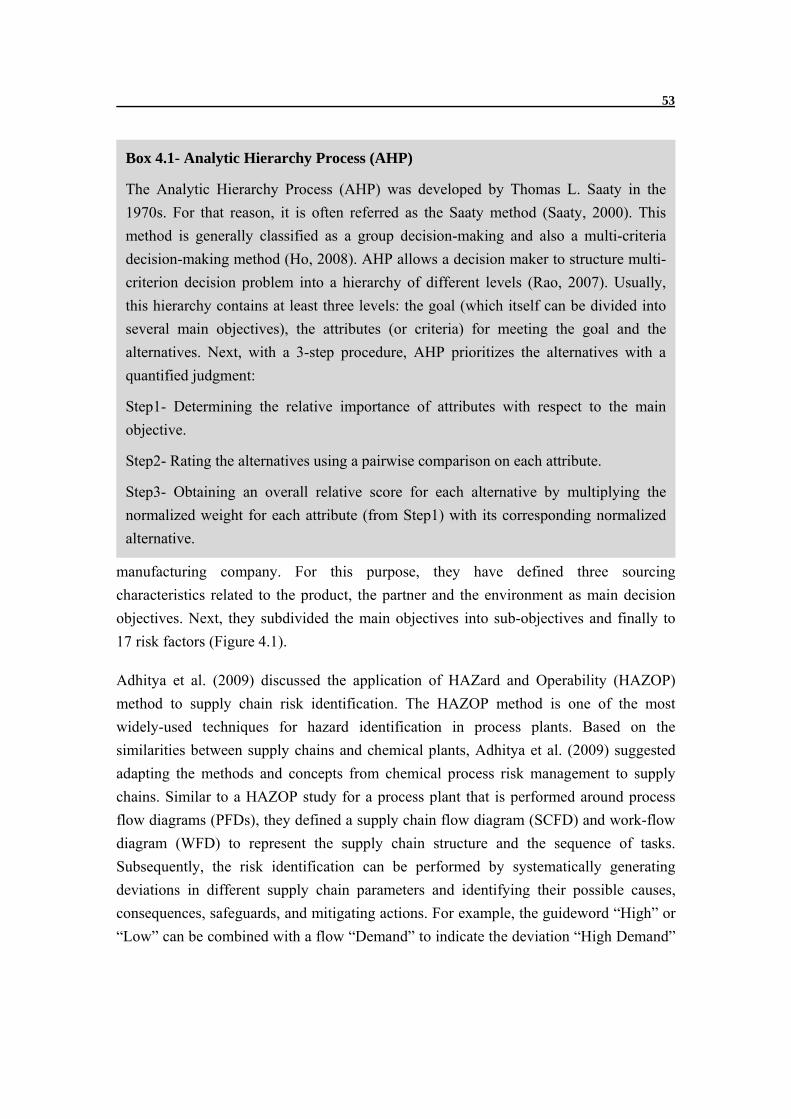
53

manufacturing company. For this purpose, they have defined three sourcing

characteristics related to the product, the partner and the environment as main decision

objectives. Next, they subdivided the main objectives into sub-objectives and finally to

17 risk factors (Figure 4.1).

Adhitya et al. (2009) discussed the application of HAZard and Operability (HAZOP)

method to supply chain risk identification. The HAZOP method is one of the most

widely-used techniques for hazard identification in process plants. Based on the

similarities between supply chains and chemical plants, Adhitya et al. (2009) suggested

adapting the methods and concepts from chemical process risk management to supply

chains. Similar to a HAZOP study for a process plant that is performed around process

flow diagrams (PFDs), they defined a supply chain flow diagram (SCFD) and work-flow

diagram (WFD) to represent the supply chain structure and the sequence of tasks.

Subsequently, the risk identification can be performed by systematically generating

deviations in different supply chain parameters and identifying their possible causes,

consequences, safeguards, and mitigating actions. For example, the guideword “High” or

“Low” can be combined with a flow “Demand” to indicate the deviation “High Demand”

Box 4.1- Analytic Hierarchy Process (AHP)

The Analytic Hierarchy Process (AHP) was developed by Thomas L. Saaty in the

1970s. For that reason, it is often referred as the Saaty method (Saaty, 2000). This

method is generally classified as a group decision-making and also a multi-criteria

decision-making method (Ho, 2008). AHP allows a decision maker to structure multi-

criterion decision problem into a hierarchy of different levels (Rao, 2007). Usually,

this hierarchy contains at least three levels: the goal (which itself can be divided into

several main objectives), the attributes (or criteria) for meeting the goal and the

alternatives. Next, with a 3-step procedure, AHP prioritizes the alternatives with a

quantified judgment:

Step1- Determining the relative importance of attributes with respect to the main

objective.

Step2- Rating the alternatives using a pairwise comparison on each attribute.

Step3- Obtaining an overall relative score for each alternative by multiplying the

normalized weight for each attribute (from Step1) with its corresponding normalized

alternative.

54

or “Low Demand” respectively and its possible causes and consequences can be

identified by tracing the flows in the diagram.

Figure 4.1. An example of AHP application for supply chain risk identification, from Schoenherr et al. (2008) 

Another method mentioned in the literature is the Ishikawa Diagram which is used by

Wiendahl et al. (2008) to identify the logistic risks for a case study of a forging company.

They started with an objective and the possible negative consequences (like “low output

rate”) and made a list of possible events that may lead to each adverse effect in five main

actuating variables -material, machine, method, human and environment.

Box 4.2- HAZard and OPerability (HAZOP)

HAZard and OPerability (HAZOP) is a structured and systematic technique for

identifying the hazards (Crawley et al., 2000). Hazard in HAZOP studies are

characterized by the deviations in the normal/designed operation of a system (e.g., a

manufacturing plant). Such deviations are defined by using a group of “Guide Words”.

Examples of common HAZOP guide words include "No or Not" (e.g., Not material

flow), "Less" (e.g., Less quality of material) and "Part of" (Part of material delivered).

The HAZOP guide words are applied to each element of the defined system (which is

usually called a "Node") to create different deviations. Subsequently, all possible

causes for such deviation and the adverse consequences of this deviation must be

determined. Finally, the safeguards which reduce the frequency of the deviation or to

mitigate its consequences must be found.

55

Figure 4.2. An example of Ishikawa diagram for supply chain risk identification, from Wiendahl et al. (2008)

Some other methods discussed for risk identification in the supply chain risk literature are

presented in Table 4.1. Although a wide spectrum of methods is available for companies

to identify risks, the choice of the risk identification method is different for different

cases. Some factors which may influence the chosen method are time, experience

availabile and the complexity of supply chain. In general, the basic expert-based methods

for risk identification (like brainstorming or risk questionnaire) are fast; however, they

need a level of expertise which might not be available inside the company. The other

issue with expert-based methods is that for a complicated supply chain with several tiers,

they cannot guarantee to provide a full picture of all relevant disruptions. More

systematic and disciplined approaches, however, can facilitate a more comprehensive risk

identification process. Reproducibility is the other advantage of systematic methods since

the results of the risk identification process can be easily evaluated and also extended in

future. As a generic recommendation, in most cases, a combination of methods for risk

identification may prove to be more useful (Hallikas et al., 2004). As an example, instead

of performing AHP by one expert in a company, several experts might use the method

and share the output in some meetings to make a final list of potential disruptions.

Box 4.3- Ishikawa diagram

Ishikawa diagram (also called fishbone diagram or cause-and-effect diagram) is

invented by Kaoru Ishikawa in the 1940s (Munro, et al., 2008). The Ishikawa diagram

is a graphical analysis tool that supports tracing the causes of a certain event or

problem.

56

4.2.2. Risk classification scheme

To facilitate a systematic and comprehensive risk identification process, some

classification schemes are presented and discussed in the literature (Table 4.2).

Categorizing disruptions also supports a better communication among actors involved in

the process (Stecke and Kumar, 2009).

One of the most common risk categorization schemes involves classifying supply chain

disruptions based on the location of the source of disruption. Christopher and Peck (2004)

considered three main categories of risk sources in the supply chain:

“Internal to the firm” which are subcategorized into “process risks” - disruptions

within the value-adding activities of a company like loss of operating resources-

and “control risks” - disturbances in the management systems/procedures that

govern how an organization exerts control over the processes, e.g., wrong

assumptions or decision rules, misapplication of rules, etc.

“External to the firm but internal to the supply chain network” which are

subcategorized into “demand risk” - potential disturbances to the flow of product,

information, and cash between the focal firm and the customers -and “supply risk”

– disruptions in the product, information, and cash flows in the upstream of the

focal firm.

“External to the network” or “environmental risks” which are exemplified by

natural disasters, terrorist attacks and regulatory changes.

Table 4.2. A summary of supply chain risk categorization literature

Risk Classification Reference

Location-based classification

Christopher and Peck (2004), Jüttner (2005), Bogataj and Bogataj (2007), Oehmen et al. (2009), Thun and Hoenig (2011), Trkman and McCormack (2009), Kumar et al. (2010), Dani and Deep (2010), Olson and Wu (2010)

Scale-based classification Kleindorfer and Saad (2005), Gaonkar and Viswanadham (2007), Lodree and Taskin (2008), Knemeyer et al. (2009), Huang et al. (2009), Ravindran et al. (2010)

other Cavinato (2004), Chopra and Sodhi (2004), Peck (2005), Kleindorfer and Saad (2005), Sheffi (2005a), Tang (2006b), Wu et al. (2006), Matook et al. (2009), Tang and Musa (2010)

Similar classifications have been discussed by many other researchers too (as mentioned

in Table 4.2). As another example for location-based classification, Thun and Hoenig

(2011) made a distinction between “internal company risks” and “cross-company-based

risks”. The “cross-company-based risks” are further divided into “purchasing risks

57

(upstream risks)” and “demand risks (downstream risks)”. The “external supply chain

risks” is the other group which is subcategorized into sociopolitical, economic,

technological or geographical disruptions.

Another approach suggested in the literature is categorizing the supply chain disruptions

according to the likelihood and impact which is called “scale-based classification” in Table

4.2. In this classification, supply chain disruptions are generally categorized into:

Low-probability, high-severity disruptions: the disruptions with very low

probability of occurrence but significant consequences if they occur (for example,

labor strike, terrorist attack or natural disaster). This class is also termed Value-at-

risk (VaR) type disruptions by Ravindran et al. (2010) and “catastrophes” or

“catastrophic events” by Lodree and Taskin (2008), Knemeyer et al. (2009) and

Huang et al. (2009).

High-probability, low-severity disruptions: the events that might happen more

frequently with less damage to the supply chain operation (for example, late

delivery or missing quality requirements). This is frequently called the

“operational disruptions” or “day-to-day disruptions” (Kleindorfer and Saad, 2005;

Huang et al., 2009). “Miss-the-target (MtT) risks” is also the term which is

suggested by Ravindran et al. (2010).

In general, the location-based approach for risk classification has two main advantages

over scale-based approach. Firstly, it is clearer and much more straightforward for a

supply chain manager because the starting point for classification is different sections

(e.g., demand side or supply side) in the supply network. The other difficulty with the

scale-based approach is that the quantification of risk mostly happens after identifying the

potential disruptions in the chain. Having a precise estimation of the level of risk for a

specific disruption is mostly difficult at the start of risk identification step. Therefore, -

unless for specific type of disruptions like natural disasters – it might be very difficult to

decide whether a disruption is a Low-Likelihood/High-Impact (LL-HI) event or a High-

Likelihood/Low-Impact (HL-LI) one. In fact, determining the exact category of a specific

disruption requires an assessment of its likelihood and the expected impact which is done

in the next step of framework – i.e., Risk Quantification step.

Besides location-based and measure-based classifications, several other approaches for

categorizing supply chain disruptions can be found in the literature. From these works,

the multi-level classification of Peck (2005) has received more attention. In Peck’s

classification, the sources for supply chain abnormality are presented in four main levels

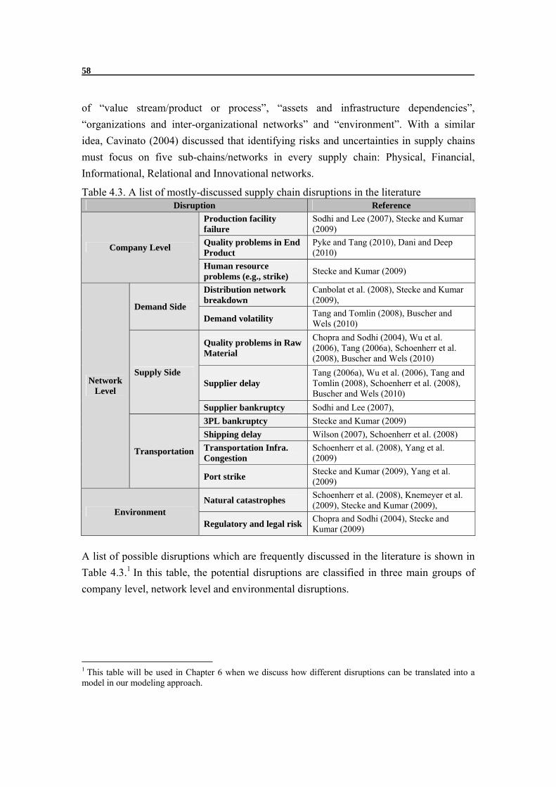
58

of “value stream/product or process”, “assets and infrastructure dependencies”,

“organizations and inter-organizational networks” and “environment”. With a similar

idea, Cavinato (2004) discussed that identifying risks and uncertainties in supply chains

must focus on five sub-chains/networks in every supply chain: Physical, Financial,

Informational, Relational and Innovational networks.

Table 4.3. A list of mostly-discussed supply chain disruptions in the literature Disruption Reference

Company Level

Production facility failure

Sodhi and Lee (2007), Stecke and Kumar (2009)

Quality problems in End Product

Pyke and Tang (2010), Dani and Deep (2010)

Human resource problems (e.g., strike)

Stecke and Kumar (2009)

Network Level

Demand Side

Distribution network breakdown

Canbolat et al. (2008), Stecke and Kumar (2009),

Demand volatility Tang and Tomlin (2008), Buscher and Wels (2010)

Supply Side

Quality problems in Raw Material

Chopra and Sodhi (2004), Wu et al. (2006), Tang (2006a), Schoenherr et al. (2008), Buscher and Wels (2010)

Supplier delay Tang (2006a), Wu et al. (2006), Tang and Tomlin (2008), Schoenherr et al. (2008), Buscher and Wels (2010)

Supplier bankruptcy Sodhi and Lee (2007),

Transportation

3PL bankruptcy Stecke and Kumar (2009)

Shipping delay Wilson (2007), Schoenherr et al. (2008)

Transportation Infra. Congestion

Schoenherr et al. (2008), Yang et al. (2009)

Port strike Stecke and Kumar (2009), Yang et al. (2009)

Environment Natural catastrophes

Schoenherr et al. (2008), Knemeyer et al. (2009), Stecke and Kumar (2009),

Regulatory and legal risk Chopra and Sodhi (2004), Stecke and Kumar (2009)

A list of possible disruptions which are frequently discussed in the literature is shown in

Table 4.3.1 In this table, the potential disruptions are classified in three main groups of

company level, network level and environmental disruptions.

1 This table will be used in Chapter 6 when we discuss how different disruptions can be translated into a model in our modeling approach.

59

4.3. Risk Quantification

Risk quantification is the process for evaluating the disruptions that have been identified

and developing the basis for making decisions on the relative importance of each

disruption. The risk level of disruptions is mostly quantified in two dimensions; the

likelihood (or frequency) of the disruption occurring and the impact of disruption on the

performance of the supply chain.

4.3.1. Likelihood estimation methods

Appropriate methods to estimate the probability of supply chain disruptions have

received little attention in supply chain management research so far. An exception is the

work of Knemeyer et al. (2009) in which some approaches for probability estimation of

catastrophic events are discussed. For some types of catastrophic events, such as aircraft

accidents, the historical data is available and can be used for estimating the transportation

disruption likelihood. Simulation is another approach for likelihood estimation. This

method can be used when the factors that cause a disruption are well-known. As an

example, Knemeyer et al. (2009) discussed a hurricane (or tropical cyclone) simulator

which uses input (like, central pressure, maximum wind radius, etc.) from government

and private sources to generate probability distributions for the number, intensity and

location of hurricane activity. The simulation results, subsequently, can be used for

making decision about the location of production and warehousing facilities.

Figure 4.3. An example of assessment scale for qualitative probability estimation, from Hallikas et al. (2004) 

In addition to these methods, expert judgment is also used by literature for evaluation of

disruption likelihood. For example, Hallikas et al. (2004) suggested a five-class scale for

qualitative estimation of disruption probability by experts. Similarly, Yang (2010) used 5-

point Likert scales for rating the risk frequency in a questionnaire to evaluate the risk

factors in container security.

60

4.3.2. Impact estimation methods

Systematic methods for assessing the disruption impact have gained more attention in the

supply chain risk management literature. Table 4.4 presents some of these methods.

Among the most-commonly-used methods is the Analytic Hierarchy Process (AHP).

Gaudenzi and Borghesi (2006) applied the AHP method in two phases to identify supply

chain risk factors and evaluate the intensity of each risk factor. Firstly, the supply chain

objectives (e.g., on-time delivery, order completeness, order correctness, and damage-free

delivery) have been prioritized. Subsequently, the relative importance of identified risk

factors regarding each of these objectives was assessed. Similarly, Wu et al. (2006) have

used AHP to analyze the risk factors in the supply base of companies. For this purpose,

they firstly classified the supplier-oriented risk factors into six categories (e.g., Internal

Controllable, Internal Uncontrollable, External Controllable, etc.). Then, they applied

AHP technique to calculate the weight of risk factors in two steps. In the first step, it is

used to rank how important one category is over another category. Next, the pair-wise

comparison of risk factors was done in each category. Multiplying these two weights and

the probability of occurrence for each risk factor, an overall risk index was calculated.

Some of other recent applications of AHP for assessing the risk factors in supply chain

can be found in Schoenherr et al. (2008) and Enyinda et al. (2010).

Table 4.4. A summary of supply chain impact estimation methods Reference Risk Quantification Method

Qualitative/semi-quantitative

Wu et al. (2006) AHP

Gaudenzi and Borghesi (2006) AHP

Schoenherr et al. (2008) AHP

Levary (2008) AHP

Enyinda et al. (2010) AHP

Matook et al. (2009) Expert group rating

Norrman and Jansson (2004) Expert group rating and historical data

Thun and Hoenig (2011) Expert opinion (survey)

Blackhurst et al. (2008) Multi-criteria scoring and historical data

Yang (2010) Expert opinion (survey)

Quantitative (Modeling and Simulation)

Appelqvist and Gubi (2005) Discrete event simulation

Wu et al. (2007) Petri net

Tuncel and Alpan (2010) Petri net

Wilson (2007) System dynamics

Munoz and Clements (2008) Discrete event simulation

Wei et al. (2010) Inoperability input-output modeling (IIM)

Besides AHP, some other efforts for qualitatively assessing the impact of disruptions are

discussed in the literature. Table 4.4 gives an overview of these qualitative methods

61

which mainly rely upon experts’ judgment and experience. A few quantitative approaches

have been also proposed. Wu et al. (2007) presented a Petri net-based (PN) modeling

approach, termed Disruption Analysis Network (DA_NET), to model how disruption

effects propagate through a supply chain. Another application of Petri net (PN) based

simulation for risk management in supply chains is presented by Tuncel and Alpan

(2010). They used Petri net (PN) to evaluate the impact of multiple-disruption scenarios

(disruptions in demand, transportation and quality) and possible mitigation actions on the

supply chain performance.

To study the impact of transportation disruptions on the supply chain performance,

Wilson (2007) presented a system dynamics model for a supply chain which contains five

echelons: retailer, warehouse, tier-1 supplier, tier-2 supplier and raw material supplier.

Box 4.4- Petri Nets (PN)

Petri Nets (PN) – which were firstly proposed by Carl Adam Petri in 1962- is a

graphical tool for the formal description of the processes and flow of events in a

system (Diaz, 2009). It also offers a mathematical network model to analyze the

behavior of dynamic systems.

The basic elements in PN include “places” – which are the states and conditions of the

system and are mostly shown with circles- , “transition” – which are the actions in the

system and are drawn as bars or boxes - “tokens” – which are resources responsible

for the changes in the system and are usually shown with black (or colored) dots - and

“directed arcs” – which indicate the direction of token (resources) travel (Cortellessa

et al., 2011). When the number of token in a place meets the minimum requirements

for firing (or executing a transition), some of tokens are moving from one place to

another place. This rule – which is called firing rule- is the basis for the simulation of

dynamic behavior of system (Cortellessa et al., 2011).

Figure 4.4. The main elements of PN model

62

Different possibilities for a transportation disruption – which might occur between

adjacent echelons - are modeled and their impact on customer orders fulfillment rate and

inventory fluctuations are evaluated. As a result, they concluded that the greatest impact

occurs when transportation is disrupted between the tier 1 supplier and warehouse.

Among more recent quantitative methods for supply chain risk assessment, Wei et al.

(2010) have introduced the application of Inoperability Input-output Modeling (IIM) to

analyze the ripple effects caused by disruption at a particular node. The IIM simulation

results can be used to prioritize nodes for planning potential actions to manage the impact

of disruptive events. To illustrate the application of the model, they discussed an example

of a Chinese white alcohol manufacturer. A potential disruption in one of the suppliers

was modeled and increasing the number of suppliers as a possible risk mitigation strategy

has been studied.

4.4. Risk Evaluation & Treatment

Once the risk factors have been identified and assessed, the appropriate response must be

selected and implemented in the supply chain.

In general, the possible response to a disruption can fall within four main categories.

Box 4.5- Inoperability Input-Output Model (IIM)

The Inoperability Input-Output Model (IIM) is a modeling approach to analyze how

perturbations in one part of a system propagate to other parts through the exchange of

input and output that link them. This modeling approach is developed by Yacov

Haimes and his colleagues in University of Virginia – based on the Leontief’s Input-

Output (I-O) Model which describes the indirect ripple effects among the industry

sectors of the economic system - to evaluate the impact of a disruption in one

infrastructure and the cascading effects on all other interconnected and interdependent

infrastructures (Haimes, 2009). This effect is mainly evaluated with “inoperability”

measure which represents the gap between planned or business-as-usual level and

current levels of operation caused by a disruptive event. For example, if the major

evaluating metric of a system is the production level, then the inoperability can be

defined as the unrealized production (Wei et al., 2010).

63

Table 4.5. A summary of risk treatment methods Risk Treatment Method Reference

Risk Acceptance Tomlin (2006), Khan and Burnes (2007)

Risk Reduction

Flexibility

Flexible Supply Base

Choi and Krause (2006), Tomlin (2006), Babich (2006), Tan and Enderwick (2006), Tang (2006a-b), Tang and Tomlin (2008), Deane et al. (2009), Thun and Hoenig (2011), Yang et al. (2009), Wang et al. (2010), Iakovou et al. (2010)

Flexible Product Configuration (Postponement)

Sheffi (2005a-b), Tang (2006a-b), Babich (2006), Tang and Tomlin (2008), Manuj and Mentzer (2008), Wagner and Bode (2008), Ji (2009), Yang and Yang (2010)

Flexible Manufacturing

Sheffi (2005a-b), Tomlin (2006), Sodhi and Lee (2007), Tang and Tomlin (2008), Stecke and Kumar

Flexible Transportation

Tang (2006a), Stecke and Kumar (2009), Knemeyer et al. (2009), Colicchia et al. (2010)

Redundancy

Extra Inventory (Redundant Stock)

Chopra and Sodhi (2004), Sheffi (2005a), Hale and Moberg (2005), Tomlin (2006), Tang (2006a), Khan and Burnes (2007), Mudrageda and Murphy (2007), Wilson (2007), Ratick et al. (2008), Knemeyer et al. (2009), Stecke and Kumar (2009), Schmitt and Snyder (2010)

Backup Supplier

Tomlin (2006), Wilson (2007), Sodhi and Lee (2007), Deane et al. (2009), Knemeyer et al. (2009), Yang et al. (2009), Xu and Nozick (2009), Schmitt and Snyder (2010)

Overcapacity Chopra and Sodhi (2004), Goh et al. (2007)

Control/ Incentives

Security Improvement

Manuj and Mentzer (2008), Stecke and Kumar (2009), Knemeyer et al. (2009)

Demand Management

Tang (2006a-b), Tang and Tomlin (2008), Stecke and Kumar (2009), Ji (2009)

Supplier Qualification Screening

Sheffi (2005a-b), Sodhi and Lee (2007), Roth et al. (2008), Wagner and Bode (2008), Manuj and Mentzer (2008), Yang et al. (2009), Sanchez-Rodrigues et al. (2010)

Organizational Aspects

Sheffi (2005a-b), Knemeyer et al. (2009)

Cooperation

Resource Sharing Hale and Moberg (2005), Tuncel and Alpan (2010)

Collective Response Planning

Hallikas et al (2004), Tan and Enderwick (2006), VanderBok et al. (2007), Knemeyer et al. (2009), Stecke and Kumar (2009), Butner (2010)

Risk Avoidance

Tang (2006b), Tomlin (2006), Wu and Olson (2008), Levary (2008), Manuj and Mentzer (2008), Stecke and Kumar (2009), Xu and Nozick (2009), Knemeyer et al. (2009)

Risk Transfer Giannoccaro and Pontrandolfo (2004), Manuj and Mentzer (2008), Wagner and Bode (2008), Stecke and Kumar (2009), Knemeyer et al. (2009)

64

4.4.1. Risk acceptance

The consequences and likelihood of a particular disruption might be accepted if the risk

level is less than a specific threshold. Moreover, for cases where the problem owner

cannot find a reasonable response or the cost of available solutions outweighs the

anticipated disruption risk, the risk acceptance might be considered a default action

(Tomlin, 2006).

4.4.2. Risk reduction

For disruptions with unacceptable level of risk, appropriate actions must be taken to

reduce the risk to the acceptable threshold. The risk of disruption can be reduced by

reducing the likelihood of its occurrence or reducing the severity of disruption (Zsidisin

et al., 2005; Tang and Tomlin, 2008). For this purpose, many different approaches are

discussed in the literature.

- Flexibility

One way for managing disruptions is to create flexibility in the supply chain. Flexibility

is the ability to take different positions to better respond to an abnormal situation and

rapidly adapt to significant changes in the supply chain (Lee, 2004). The necessary

condition for flexibility in the supply chain is having multiple interchangeable resources

(Ji, 2009). For example, by having different manufacturing plants in different locations -

with the capability to produce a similar set of products- a company can move the business

among them should one fail because of disruption in its supply chain.

Different types of flexibility strategies are suggested in the literature to handle the risk of

supply chain disruptions.

Flexible supply base: One method for mitigation of risk in a supply chain is

establishing a flexible supply base. To have a flexible supply base, two main

tactics are commonly discussed in the literature. One is to diversify the material

supply through multiple-sourcing (Tang, 2006a; Tomlin, 2006; Thun and Hoenig

(2011); Iakovou et al., 2010), so that, when the supply from one supplier is

disrupted (as a result of, e.g., supplier failure or transportation disruptions), the

company can temporarily shift the orders (or at least some part of its demand) to

another supplier.

Another element of a flexible supply base is flexible contracting with suppliers

(Tang and Tomiln, 2008; Tang, 2006b). In flexible supply contracts, the ordering

65

firm can adjust the agreed quantity or time of delivery1. Thus, with disruption in

one supplier, a manufacturer has the immediate option to increase the order size

from other suppliers (Wang et al., 2009; Babich, 2006). Flexible supply

contracting is also beneficial to cope with demand risks (Tang and Tomlin, 2008).

In fact, the buyer can change the supply orders (increase or decrease volumes and

change delivery timing) with fluctuations in demand in the downstream supply

chain.

Flexible product configuration (Postponement): Postponement - also known as

"delayed differentiation” (Anand and Girotra, 2007) or “late product

differentiation” (Wagner and Bode, 2008) - is a frequently discussed method to

handle demand risks in supply chains (Sheffi, 2005a; Tang and Tomlin, 2008).

The main assumption in this strategy is that the production process can be divided

1 In a flexible contract, the adjustment in the order quantity is mostly restricted to a few percent of original quantity and must be announced to the supplier in a specific period of time before order delivery (Tang and Tomlin, 2008).

Box 4.6- An example of product postponement: HP DeskJet printer

To satisfy certain country-specific requirements, Hewlett-Packard (HP) has to develop

multiple versions for each model of their printers to serve different geographical

regions (Asia-Pacific, Europe, or Americas). For example, HP printers in North

American and the European market have different power supplies and instruction

manuals in different languages.

Previously, the manufacturing was done in the North America factories and finished

products were shipped to the three distribution centers in Asia-Pacific, Europe and US

(Johnson and Anderson, 2000). However, due to uncertain demand in each region, HP

could end up with more printers than it required in one area (overstocking) and less

printers in the other regions (under-stocking) (Tang and Tomlin2008). To solve this

problem, HP redesigned the process for producing its DeskJet printers by delaying the

point of product differentiation. Specifically, HP first produces the generic printers

and ships them to the distribution centers in different regions. These generic printers

are then customized for specific markets in the last stage of process by distributers.

This postponement strategy has enabled HP to respond to the demand changes quickly

and more accurately as the printer is customized only when HP sees the demand for

printers in a certain region. Moreover, transportation cost is decreased because printers

are shipped in bulk and the final reconfiguration is done in the destination.

66

into two sub-processes of “general production” and “customization”. Based on

postponement strategy, the product customization must be made at a point in the

supply chain which is closer to the customer and the uncertainty in the demand of

specific products is less (Ji, 2009). Consequently, postponement reduces the

demand risk, because the product will stay in an undifferentiated state as long as

possible allowing to respond to unexpected market shifts (Manuj and Mentzer,

2008; Wagner and Bode, 2008; Yang and Yang, 2010).

Flexible manufacturing process: In a flexible manufacturing process, different

types of products can be manufactured in the same plant at different volumes

(Tang and Tomlin, 2008) and the production can be moved easily among different

plants (Sheffi, 2005a-b). With a flexible process, companies can shift to other

products when the demand for some specific products is disrupted (e.g., because

of new safety regulations) or if a disruption in the supply base impacts the normal

rate of production for some products. It is also possible to shift the demand to

other plants when the production in a specific plant is impacted by a disruptive

event.

Flexible transportation: Flexibility in transportation is a critical issue for smooth

operation of supply chains, especially for companies that source globally and

supply different markets in different places around the world. Flexibility in

transportation can be achieved by multi-modal logistics strategy (Tang, 2006a;

Knemeyer et al., 2009; Colicchia et al., 2010); to prevent supply chain breakdown

due to disruptions in one mode of transportation, some companies may prefer to

utilize multiple modes of transportation including air, ground, and sea shipping.

Other options such as working with multiple logistics companies and defining

alternative routes for the case of disruption are also important to better handle

transportation disruptions (Tang, 2006a; Stecke and Kumar, 2009).

- Redundancy

One way to manage the risk of potential disruptions is creating redundancies across the

supply chain. In general, redundancies are considered as expensive options for handling

disruptions because they are put to use only when certain unanticipated events occur

(Sheffi, 2005b). For example, contracting with a local backup supplier to supply the

needed material (or a part of it), when the main global supplier is disrupted, can be a

costly decision. More administrative cost might be imposed to find and monitor the

secondary supplier and higher unit prices might be paid for low-volume material delivery

67

from a secondary supplier. However, as a disruption occurs (e.g., an emergency in the

main supplier facilities), the secondary supplier can be used to ensure a steady flow of

materials across the chain. The disruption reaction process is also faster as lots of hours

needed to find (and set) alternative resources will be saved.

Redundancy in a supply chain can take different forms as discussed in the following.

Extra inventory (redundant stock): One of possible approaches to handle

disruption is keeping buffer stocks in different parts of the supply chain. A

company might carry extra inventory for finished goods to handle fluctuations in

market demand (demand risk) or have a buffer in the raw material storage to cope

with potential disruptions in the supply base (e.g., late raw material order

delivery). Despite its advantage to prevent production shutdown and avoiding

stock-outs, carrying additional inventory can result in increased costs and reduced

quality (Sheffi, 2005a). Thus, this strategy is mostly advised for items that have a

low holding cost and will not be outdated (Wilson, 2007).

Backup supplier: Contracting with a backup supplier helps companies to insure

the raw material stream against possible disruptions in the main supplier (Tomlin,

2006; Sodhi and Lee, 2007). This is usually materialized with a "capacity

reservation contract" in which a secondary supplier guarantees any amount of

delivery up to the reserved capacity (Xu and Nozick, 2009). Therefore, comparing

with buffer stock, a company can mitigate the risk in the supply base without

incurring the cost of keeping excess inventory.

One aspect in selecting extra suppliers is avoiding "share of similar disruption

risk" among different suppliers (Wilson, 2007). For example, sourcing from two

suppliers in the same region would impact the material supply when a disaster

(e.g., an earthquake) happens in that region. Likewise, when suppliers deliver

their materials through similar transportation routes, (e.g., they use similar same

ports), a disruption in that route (e.g., closure of port because of strike) might

leave the company with no option to supply its needed material.

Overcapacity: Another method that ban be beneficial in mitigating the supply

chain risk is designing/installing a certain level of excess capacity in some key

nodes of the network (Chopra and Sodhi, 2004; Goh et al., 2007). Consequently,

the disruption impact can be partially absorbed in the chain. For example, an

emergency shutdown in one of the production plants in a multi-plant enterprise

can be handled for a period of time by over-production in other plants if they have

68

excess manufacturing capacity. The excess capacity can also be used to manage

the daily variations in customer demand, i.e., demand risk (Chopra and Sodhi,

2004).

- Control/ Incentives

The potential disruptions in the supply chain might be reduced with a higher level of

control and supervision. Moreover, some incentives might be created to involve different

actors in managing disruptive events in the supply chain.

Security improvement: One method for risk mitigation, especially when

intentional threats are concerned, such as terrorism attacks, thefts or piracy risk, is

enhancing the security (Manuj and Mentzer, 2008; Stecke and Kumar, 2009).

Stecke and Kumar (2009) have enumerated three types of security initiatives in

the supply chain: physical security (e.g., in ceasing security personnel or

implementing camera systems), information security (e.g., firewalls, antiviruses)

and freight security (e.g., cargo inspections before shipping and Tracking the

track cargo movements by RFID and GPS systems).

Demand management: Demand management is suggested as a contingent

response supply chain disruptions by some authors. This might happen in two

main ways (Ji, 2009); firstly, shifting the demand across product portfolio which

is also termed “responsive pricing” or “flexible pricing” by Tang and Tomlin

(2008). Thus, when a disruption (e.g., delayed supply of certain components)

interrupts manufacturing of some specific products, a firm can use the price

mechanism and promotions to temporarily change the demand pattern and shift

customer choices to available products. A classic example of this form of demand

management is the Dell response to the Taiwan earthquake in 1999 (Tang, 2006a).

The second form of demand management is shifting demand across time. Thus,

facing a disruption, a company may start negotiating with the customers or offer

discounts to change their orders’ due date or accept a delayed shipment.

69

Supplier qualification screening: A well-established quality control process

decreases the exposure to supply chain risks in several ways. Firstly, it allows

better/faster identifying the possible cause of disruptions, reducing their frequency

and also avoiding the propagation of trouble to the downstream supply chain

(Sanchez-Rodrigues et al., 2008). This is especially important for customer-

related disruptions such as product recalls due to safety and product quality issues

(Roth et al., 2008; Pyke and Tang, 2010). Moreover, regular auditing of suppliers

might reduce supply chain risks by giving suppliers an incentive to improve their

internal weaknesses (Yang et al., 2009).

Organizational aspects:

One other issue which might impact the success of disruption management is increasing

the knowledge of employees with training programs (Stecke and Kumar, 2009). A

training program must inform workers about how to avoid potential risks (which

consequently reduces the probability of disruption in the plant) and also better handle

abnormalities when they occur (which, in fact, reducing the expected impact of

disruption). Moreover, the response plans that are developed for specific disruptions must

be regularly rehearsed and, if necessary, modified (Knemeyer et al., 2009). Sheffi (2005a-

b) call all these aspects “creating the corporate security culture".

Box 4.7- An example of demand management: Dell response to Taiwan earthquake

In 21st of September 1999, the 7.6 earthquake hit the Chi-Chi region in Taiwan.

Because of extensive power outages and damaged plants, the supply of PC

components to numerous companies was disrupted for several months. To handle the

disruption, Dell immediately deployed a contingency plan by offering special “low-

cost upgrade” options to customers if they chose similar computers with components

from other suppliers (Tang, 2006a). The ability of Dell to steer customers to where

Dell wants them by selling the available configurations, increased its third quarter

earnings by 41% over the same period of previous year in spite of disaster in Taiwan

(Tang, 2006a).

At the same time, the other main PC producer in market, Apple, – that had announced

the launch of some new products and received thousands of order- faced product

backlogs due to component shortages and inability to alter product configurations. The

abnormal situation in Apple's supply chain resulted in many cancelled orders and

consumer complaints (Sheffi, 2005b; Tang, 2006a).

70

- Cooperation

In contrast with unilateral control actions, co-operative responses to supply chain

disruptions involve joint agreement/action by several actors in the chain (Jüttner et al.,

2003). Two possible cooperative strategies are discussed here.

Collective response planning: Planning for supply chain disruption management

might involve other actors in the chain (Hallikas et al., 2004; Vanderbok et al.,

2007)1. This is especially important as modern supply chains are complex systems

and no one actor has all the necessary information for identifying and mitigating

the possible risks in the system (Butner, 2010). Additionally, in a joint risk

management process, the options that might be too expensive to be implemented

by a single partner can be discussed and agreed upon (Hallikas et al., 2004). One

of these methods is investing in shared resources as discussed further below.

Resource sharing: In some cases, the necessary capital might be a significant

barrier to implement a specific risk mitigation option, particularly, for those

disruptions of which the likelihood is not so high but the expected impact on

supply chain operation can be significant (Hale and Moberg, 2005). In these cases,

collaboration would help companies to pool resources and share the expenses of

disruption response. Tang (2006a) discussed the cases of Toyota and Sears in

which these companies keep certain inventories at some locations in their supply

chains so that all retailers in the nearby region share these inventories for the case

of disruption or demand fluctuation. In the same view, Hale and Moberg (2005)

presented an optimization-based decision process to design a network for shared

Just-In-Case resources. Firstly, an estimation of the necessary resources must be

made. Next, the decision about the maximum time it should take for each facility

in the supply chain to gain access to shared resources must be made. Finally, a

mathematical programming model is used to determine the number and locations

of storage areas for shared resources.

4.4.3. Risk avoidance

For some disruptions, the risk level is so high that even with partial reduction in the

likelihood or impact of disruption, the risk level is still unacceptable. For these disruptive

events, the decision is to avoid the risk and eliminate the possible causes, might be the

only reasonable decision. Moving the production facilities to safe locations (e.g., places

1 As an example, Stecke and Kumar (2009) mentioned cases of auto manufacturers such as GM that these companies help their suppliers develop certain strategies to mitigate disruptions.

71

with less probability of earthquake) or working with suppliers located in safe areas

(Stecke and Kumar (2009), focus on secure markets or products with constant demand

(Thun and Hoenig, 2011) and dropping troublesome suppliers from the supply base

(Manuj and Mentzer, 2008) are examples of risk avoidance in the supply chain.

4.4.4. Risk transfer

Another method that can be used to control risk is shifting the negative consequences of a

risky factor to another entity inside or outside the supply chain. The classic example of

risk transfer is insurance (Lodree and Taskin, 2008). Different parts of the supply chain

such as facilities, transport, and labor can be insured against natural disasters, accidents,

and theft (Stecke and Kumar, 2009).

Contracting is also frequently discussed as a form of risk transfer or risk sharing in the

supply chain. A contract defines the way in which the risk arising from different sources

of uncertainty (like demand and price) is shared among different actors in the supply

chain (Giannoccaro and Pontrandolfo, 2004). Accordingly, with a fair contracting, certain

risks can be allocated to the parties who are in the best position to manage those risks.

4.5. Risk Monitoring

Supply chain risks change constantly. The likelihood and severity of disruption may

change; some risks can be reduced or even eliminated, while new risk factors may appear.

A necessary part of supply chain risk management process is monitoring changes in the

network, customer needs, technology, partner strategies and competitors and updating the

risk assessment correspondingly (Hallikas et al., 2004; Pyke and Tang, 2010). However,

despite its profound importance, there is very little rigorous research presenting the

methods, tools and procedures for supply chain risk monitoring. Two fairly recent papers

that discuss risk monitoring methods are Blackhurst et al. (2008) and Schoenherr et al.

(2008). For a case of an automotive manufacturer, Blackhurst et al. (2008) presented a

multi-criteria scoring procedure for measuring, tracking and analyzing supplier and part

specific risk indices over time to identify trends towards higher risk levels. With this

method, the focal company can better recognize the potential risky parts of the supply

base. In a similar way, Schoenherr et al. (2008) presented an AHP-based decision-making

tool which was used to assess risk factors and alternatives in an international sourcing

context. They also discussed that the evaluation must be a continuous process; the

selected alternatives need to be reevaluated regularly, and risk factors must be reassessed

as changes occur in the market environment.

72

4.6. Disruption Detection

An effective response to a disruption requires detecting quickly the location and nature of

disruption. With faster detection of disruption in the chain, corrective actions can be

started sooner, the escalation of the disruption impact can be avoided, and consequently,

the impact of the disruption can be reduced.

To quickly detect a disruption, several aspects are regarded as important issues and some

capabilities are listed in the literature.

4.6.1. Visibility and information access

One of the issues frequently discussed in the literature is improving the “end-to-end”

visibility in the supply chain (Christopher and Lee, 2004; Glickman and White, 2006).

Supply chain visibility is the ability to track the status of the supply chain (e.g., the health

of different parts of chain, the material in transit in the network, etc.) from suppliers to

end customers (Christopher and Lee, 2004). It is primarily achieved by collaborative

relationships and real-time sharing of correct information among actors in the chain

(Blackhurst et al., 2005). The information sharing – which may include the actual or

forecast demand, inventory levels (excess, shortage), and processing capacities (Stecke

and Kumar, 2009; Tang, 2006) - helps companies to faster discover an abnormal situation

in the network and also have a better understanding of the available resources to handle

disruptions (Li et al., 2006).

The other issue which improves the visibility in the supply chain –and accordingly, faster

detection of disruption- is investing in performance monitoring and early warning

systems (Stecke and Kumar, 2009). For instance, a firm may have various IT systems for

monitoring the material flows (inventory level, quality, product delivery and sales) or

information flows (demand forecasts, production schedule …) along the supply chain.

These monitoring systems would reduce the detection time by tracking the deviations in

the performance of supply chain (Huang et al., 2009). Moreover, the implementation of

technologies like RFID that will increase the speed of information flow throughout a

supply chain can assist to minimize the time of detection of disruption (Munoz and

Clements, 2008).

4.6.2. Information analysis tools

In addition to information availability, developing tools for analyzing the information is

an important issue in disruption detection. Such tools support decision makers in better

understanding the disruption profile, how far disruptions propagate through a supply

73

chain and which parts of the system may be affected more by the event (Blackhurst et al.,

2005). Some of the tools to analyze real-time information on disruptions are presented in

recent literature on supply chain disruption management. Wu et al. (2007) discussed a

network-based modeling methodology – termed “DA_NET”- to determine how

disruptions propagate in supply chains and how these disruptions affect the supply chain

operation. Accordingly, the user can assess which areas of the supply chain and which

performance measures (such as cost or lead-time) might be affected by the disruption.

Among more recent works, Huang et al. (2009) described a dynamic system model and

used it to check if a disruption (like demand shock) can be absorbed by a supply chain

without affecting the expected order delivery performance. Tuncel and Alpan (2010) also

proposed a Petri net (PN) based decision support tool for tracking material and

information flows in the supply network.

4.6.3. Disruption causal analysis

The other key aspect - which is somewhat related to the previous issue of information

analysis - is searching for the real cause or causes for an abnormal event (Adhitya et al.,

2007a; Gaonkar and Viswanadham, 2007). This is especially important when the

triggering event cannot be directly observed and only the deviation in the supply chain

performance can be detected.

The causal analysis might also investigate the causal relations among disruptions as one

disruptive event might cause another set of events in the supply chain (Gaudenzi and

Borghesi, 2006). For example, a problem for a 3PL service provider, which is responsible

for managing the material delivery for a focal company and its supplier, would directly

and indirectly impact the company’s performance.

Finding the main cause of disruptions and the interdependencies among different

disruptions help decision makers in choosing the corrective actions in disruption reaction

and recovery steps.

4.7. Disruption Reaction & Recovery

Once a disruption is detected, a company must quickly react and restore the normal

operation of the supply chain. Some key issues are discussed in the literature for better

reaction to disruption in supply chains.

74

4.7.1. Resource finding and (re-)allocation

Disruptions in the supply chain may lead to a shortage of resources and efficient use of

available resources is a crucial issue in handling the event (Dani and Deep, 2010).

For example, an earthquake in a specific region might impact the supply of some specific

materials to the manufacturing plants. Consequently, the firm must look for alternative

supplies. Moreover, because of new resource constraints, the pre-defined plans for supply

chain operation may no longer be optimal or even feasible and should be revised

according to the new situation (Xiao et al., 2005; Huang et al., 2006).

The search for resources to handle a disruption should start with an evaluation of needs

and resource requirements (Charles et al., 2010). Subsequently, a company should

determine the remaining resources after disruption and also look for alternative resources

to cover the needs. Some of necessary resources to react to a disruptive event can be

previously-planned/invested in the risk treatment step. For example, carrying extra

inventory, investing in flexible supply contracts or flexible transportation will provide

some degrees of freedom in handling disruptions in real-time (Stecke and Kumar, 2009;

Tomlin, 2006). Moreover, some actions like product redesign or demand shifting can

provide extra resources to manage the impact of the event (Sheffi, 2005b). Multiple

partners in a supply chain may also decide to temporarily share some of their resources to

better handle an event (Mudrageda and Murphy, 2007).

Based on the available/found resources, possible reactions to a disruption can be defined

and the appropriate options must be implemented (Adhitya et al., 2007a). In some

situations, finding the appropriate option can be a challenge as many (and, sometimes,

conflicting) objectives might be considered in managing disruptions. To better handle this

difficulty, simulation and modeling can provide a sound basis to better analyze the

reaction to the disruption (Adhitya et al., 2007a; Tuncel and Alpan, 2010).

4.7.2. Communication and information sharing

The other factor that would influence an effective disruption reaction is the continuous

sharing of information among different actors in the supply chain (Dani and Deep, 2010).

Generally, an abnormal situation in the supply chain is characterized by a high degree of

uncertainty and lack of accurate information (Chen et al., 2010); for example, the

supplier’s estimation of its trouble might be biased. Moreover, for most actors in the

chain, it might not be feasible to make reasonable estimates of the disruption profile,

especially in the early stages. The uncertainty about the extent of the disruption and the

75

lack of knowledge can impact the resource allocation across the supply chain and might

delay the disruption recovery.

4.7.3. Coordination of activities and actors

Proper coordination is usually a key requirement for managing disruptions in a supply

chain; because, in many cases, disruption management is a cross-functional and even

cross-company process and requires close involvement of several actors in the chain

(Blackhurst et al., 2005; Braunscheidel and Suresh, 2009; Hendricks et al. 2009).

Moreover, collaboration among different actors by sharing the existing resources calls for

an effective coordination scheme. For example, managing a disruption in one

manufacturing plant in a multi-plant enterprise might necessitate sharing the resources

among the plants. In these cases, lack of coordination and inter-functional conflicts may

slow down the efforts to manage disruption and worsen the disruption effects (Stecke and

Kumar, 2009).

4.8. Learning & SC Redesign

Once a supply chain recovers from a disruptive event, it is necessary to capture the

lessons learned from the disruption management process (Dani and Deep, 2010). This

step is generally ignored in the literature. One exemption is the description of Norrman

and Jansson (2004) of Ericsson’s proactive supply chain risk management approach after

a fire at its supplier plant (Philips microchip plant in Albuquerque) in March 2000. After

this disruptive event, Ericsson developed new processes and tools to “minimize risk

exposure in the supply chain”.

Pyke and Tang (2010) also described cases of product safety recalls in which the

impacted companies have designed new plans to prevent safety problems in the future

and reported these plans to their stakeholders to rebuild confidence.

4.9. The analysis of literature and identified gaps

A detailed analysis of papers in this review is presented in Appendix D of thesis. For each

paper we have shown which steps of the framework are discussed. The methods that are

used by in each paper are also presented. Based on this analysis, two observations – and

subsequently, two gaps in the research – have been identified and discussed in the

following.

The literature on supply chain risk/disruption is not uniform; some parts of the

framework have received detailed attention and some parts are mostly overlooked.

76

One of the most evident observations to emerge from our review is that the literature has

not uniformly discussed different parts of the InForMDRiSC (Figure 4.5). Some steps of

the framework have been explored extensively in the supply chain disruption/risk

management literature. Some other steps, however, have not been adequately investigated.

Overall, the steps of the disruption management cycle (i.e., disruption detection,

disruption reaction and recovery and disruption learning) have received less attention

than the risk management cycle (i.e., scope definition and risk identification, risk

quantification, risk evaluation& treatment and risk monitoring). Different steps of the risk

management cycle have also received different levels of attention. For example, although

the literature on risk identification and risk treatment steps is very rich, the risk

monitoring step, with a few exceptions, is generally overlooked in the literature.

Moreover, comparing with risk identification and treatment, only a small fraction of the

literature presents rigorous approaches or well-documented methods for risk

quantification in supply chains.

Figure 4.5. The focus of papers on different parts of InForMDRiSC

The review evidences a lack of quantitative efforts for handling supply chain

disruptions.

77

Another finding from the literature analysis is the relative lack of quantitative modeling

and simulation works to support the decision makers in better handling supply chain

disruptions1. As can be seen in Figure 4.6, qualitative methods like survey, interview and

case study dominate. Very few papers have used quantitative methods for supply chain

risk analysis. Moreover, flexible simulation frameworks to support decision-making in

specific cases are lacking in the existing literature. The lack of simulation studies implies

that although the literature on some parts of the framework – e.g., risk identification or

treatment - is informative, the issues are mainly addressed from a general and high-level

perspective. There is a vast body of knowledge presenting general recommendations for

possible risk treatments; however, providing appropriate simulation frameworks for

adopting these generic methods in specific real cases has not received adequate attention.

This, actually, reduces the practical value of those generic recommendations since in any

real application – to implement a specific risk treatment option- the detailed supply chain

structure, procedures and circumstances for a specific company must be dealt with.

Figure 4.6. The research methods used in supply chain risk/disruption literature

A more detailed analysis of available simulation studies for supply chain risk is presented

in Table 4.6. As can be seen, the focus of simulation works presented in the literature is

1 This lack of quantitative efforts has been reported by several other recent studies, e.g., Buscher and Wels (2010) and Wagner and Neshat (2011).

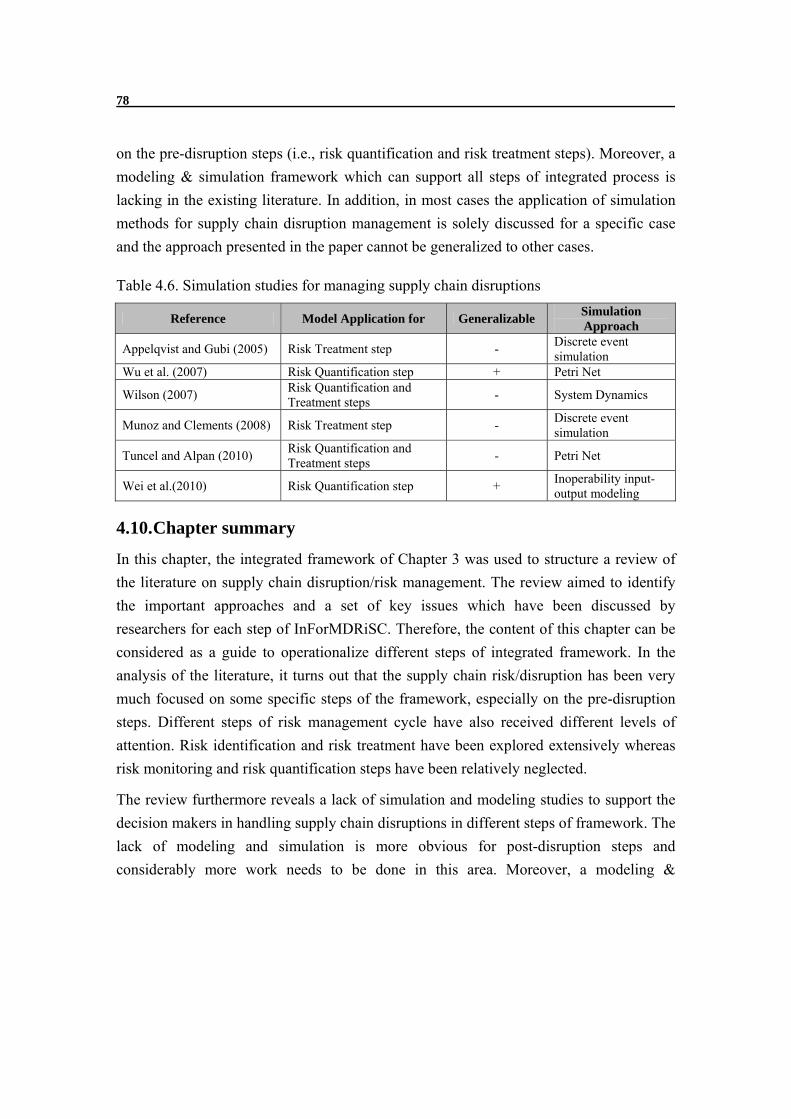
78

on the pre-disruption steps (i.e., risk quantification and risk treatment steps). Moreover, a

modeling & simulation framework which can support all steps of integrated process is

lacking in the existing literature. In addition, in most cases the application of simulation

methods for supply chain disruption management is solely discussed for a specific case

and the approach presented in the paper cannot be generalized to other cases.

Table 4.6. Simulation studies for managing supply chain disruptions

Reference Model Application for Generalizable Simulation Approach

Appelqvist and Gubi (2005) Risk Treatment step - Discrete event simulation

Wu et al. (2007) Risk Quantification step + Petri Net

Wilson (2007) Risk Quantification and Treatment steps

- System Dynamics

Munoz and Clements (2008) Risk Treatment step - Discrete event simulation

Tuncel and Alpan (2010) Risk Quantification and Treatment steps

- Petri Net

Wei et al.(2010) Risk Quantification step + Inoperability input-output modeling

4.10. Chapter summary

In this chapter, the integrated framework of Chapter 3 was used to structure a review of

the literature on supply chain disruption/risk management. The review aimed to identify

the important approaches and a set of key issues which have been discussed by

researchers for each step of InForMDRiSC. Therefore, the content of this chapter can be

considered as a guide to operationalize different steps of integrated framework. In the

analysis of the literature, it turns out that the supply chain risk/disruption has been very

much focused on some specific steps of the framework, especially on the pre-disruption

steps. Different steps of risk management cycle have also received different levels of

attention. Risk identification and risk treatment have been explored extensively whereas

risk monitoring and risk quantification steps have been relatively neglected.

The review furthermore reveals a lack of simulation and modeling studies to support the

decision makers in handling supply chain disruptions in different steps of framework. The

lack of modeling and simulation is more obvious for post-disruption steps and

considerably more work needs to be done in this area. Moreover, a modeling &

79

simulation framework which can support all steps of the integrated disruption

management process is missing in the existing literature. 1

The motivation for the rest of this thesis is the development of a modeling framework that

enables a decision maker to create models of its own supply chain and experiment with

different issues that may impact the supply chain disruption management in different

steps of InForMDRiSC.

1 The need for developing decision making tools is also discussed from practitioners’ perspective (Kinaxis, 2009). These tools, additionally, must include both pre-disruption (risk prevention) and post-disruption (response) as emphasized by Kinaxis (2009): “To have an effective supply chain risk management strategy, companies need a tool that addresses risk assessment and mitigation as well as event response. This tool must support:

Visibility and analytics capable of modeling the entire supply chain Simulation combined with the ability to compare resolution alternatives Event detection and alerting to instantly notify of supply disruptions – and their impact to the

business Collaboration among knowledge experts in the company to develop the most robust mitigation

strategies and event responses.”

81

5.MODELING FOR DISRUPTION MANAGEMENT: CHOICE OF SIMULATION PARADIGM

his chapter is the first of three consecutive chapters in which a simulation framework

for supply chain disruption management is presented. To select an appropriate

paradigm, we start by describing the major challenges in disruption management process and

the main characteristics of a supply chain as a complex socio-technical system. Based on

these features, then, the major simulation paradigms for modeling supply chains are

discussed and critically evaluated.

5.1. Introduction

In Chapter 4, we discussed that the literature on supply chain disruption/risk management

provides ample support in identifying potential disruptions and possible strategies to

manage disruption. However, the detailed dynamic analysis of supply chain behavior in

order to understand the suitability of different strategies over time and under different

scenarios is generally ignored by the literature.

The ability to assess the potential impact of disruptions on supply chain performance as

well as the effectiveness of possible responses are critical components of the supply chain

disruption management process. For the Risk Management Cycle (Pre-disruption

process), it is necessary to evaluate the probability and expected severity of disruptions in

the Risk Quantification step before making decisions on which disruptions have higher

priority in the risk profile and, therefore, need treatment. In the Risk Evaluation &

Treatment step, the expected costs/benefits of implementing disruption management

strategies must be carefully estimated prior to the decision on the most suitable treatment

for a disruption. Similarly, for the Disruption Management Cycle (Post-disruption

process), a crucial element for fast disruption detection is assessing the potential future

consequences of a triggering event; there is a need to examine the different disruption

responses to determine the appropriate option. And finally, in the Disruption Learning

step, it is necessary to evaluate different alternatives to reduce the probability or severity

of similar disruptions in the future. Making decisions in all these steps can be very

T

82

challenging and calls for appropriate decision support tools (Figure 5.1), due to the

following reasons:

Figure 5.1. Modeling and simulation to support decision-making in different steps of INForMDRiSC

A supply chain is a dynamic system. The behavior of a supply chain

dynamically changes over time either as a result of interactions between the

decisions at various levels inside each company or as a consequence of

interactions with other parties (Swaminathan et al, 1998). Moreover, the

(exogenous) parameters which influence the operation of the chain are

continuously changing and are mostly uncertain (Puigjaner et al., 2009); the

market demand fluctuates; the raw material availability and the price of material

vary over time; even supply chain structures keep changing with new customers

and suppliers (Fine, 2000). When a disruption happens, the disruptive event has

also a dynamic impact on the supply chain with a rippling effect throughout

multiple companies (Liberatore et al., 2012). A detailed analysis of disruption

impacts on a supply chain and the definition of appropriate policies to manage

supply chain disruptions need an overall understanding of this dynamic behavior

which is, in most cases, beyond the cognitive capability of decision makers

(Eysenck and Keane, 2005).

Decision-making for managing supply chain disruptions needs different

trade-offs. To handle a supply chain disruption, the related costs and gains

Risk management starts

Disruption Management Cycle

Risk Management Cycle

R1: System Definition & Risk Identification

R2: Risk Quantification

R3: Risk Evaluation & Treatment

R4: Risk Monitoring D4: Disruption Learning

D1: Disruption Detection

D2: Disruption Reaction

D3: Disruption Recovery

Disruption occurs

To determine the impact of Potential Disruptions on supply chain

To determine the possible treatment for Potential Disruption and to define the response plan

To determine the consequences of a triggering event and Actual Disruption

To experiment with alternative options to handle Actual Disruption 

To experiment with supply chain redesign options and to improve the response plan

To update the response plan based on current situation of supply chain

83

expected from implementing each alternative treatment action must be carefully

evaluated and compared (Sheffi, 2005a). Moreover, selecting an appropriate

treatment for a disruption requires a trade-off among different performance

measures (Jüttner et al., 2003). Faster delivery of raw material from a local

reliable supplier might impose higher operational cost to a company; however, it

can reduce the number of late orders to customers. An enterprise might also

decide to rank different customers and treat them differently in the case of a

disruption. Relying on personnel’s expertise is mostly inadequate to make

judgment about these trade-offs; models and simulations, however, can support

the decision makers to arrive at well-informed conclusions.

Disruption in supply chains is characterized by resource scarcity and calls

for effective coordination. Disruptions in supply chains may lead to a shortage

of resources and efficient use of available assets is crucial for disruption

management (Dani and Deep, 2010). It might even be essential that the existing

resource for each actor be known and shared with others and this requires

coordination across a network of stakeholders (Blackhurst et al., 2005;

Braunscheidel and Suresh, 2009). Accordingly, proper coordination is a key

requirement for managing disruptions in supply chains. However, how to

effectively use the available resources and how to design the coordination

structures and evaluate their effectiveness in managing disruptions is a

challenging issue.

Decision-making for disruption management is time critical. The speed and

accuracy of decision-making, especially in Disruption Reaction and Recovery

steps are critical issues and have great impact on operational loss (Kinaxis, 2009).

A delay in the selection of an appropriate response can be caused by late detection

of disruption and the vast amount of information that needs to be processed.

Because of these issues, making well-informed decisions in managing supply chain

disruptions can be very difficult and needs flexible simulation frameworks enabling

decision makers to explore a range of what-if scenarios and experiment with different

disruption management strategies. The rest of this thesis explores how simulation models

can be developed and used to support decision makers in managing disruptions in supply

chains.

84

5.2. How to develop a simulation model: an overview of main steps

To develop simulation models, many approaches are presented and discussed in literature

(examples can be found in Law and Kelton (2007) and Heath et al. (2009)). Robinson

(2004) and Robinson (2008) review these simulation development methods and explain

that despite some differences, all methods are basically very similar, outlining a set of

processes that must be performed. The differences, however, are mostly related to the

naming of steps or the number of sub-steps for each main step. By analyzing these

methods, Robinson (2004) presents a systematic approach for simulation studies with

four main processes (Figure 5.2), which are briefly described below.

Figure 5.2. Key stages in simulation studies (Robinson, 2004)

Conceptual modeling:

The starting point in any simulation design is to identify the system of study and define

the problems observed in the real world. From the understanding of the system and

problem situation the “Conceptual Model” can be derived. This model is only a partial

description of the real world, however it is sufficient to address the problem situation

(Robinson, 2008). The conceptual model generally consists of four main components: the

objectives of modeling, inputs (experimental factors), outputs (responses) and model

content (Figure 5.3). The inputs are those elements of the model that can be altered to

effect an improvement in, or better understanding of, the problem situation. Meanwhile,

the outputs report the results from a run of the model. Inputs and outputs are determined

by the objectives, which, in our case, is the application of simulation modeling for

managing disruptions in supply chains. Therefore, the inputs of the model are different

potential disruptions and disruption management practices. The expected output of

85

simulation is the impact of disruptions or different disruption management strategies on

the performance of supply chains.

Figure 5.3. Conceptual modeling (Robinson, 2008)

The most important part of a conceptual model, however, is the model content, which

consists of the components that are represented in the model and their interconnections.

While making decisions about the content of the model, various assumptions and

simplifications are normally introduced. While assumptions are needed when there are

uncertainties or different beliefs about the real world being modeled, the simplifications

are different ways of reducing the complexity of the model. Part of these assumptions and

simplifications are imposed by the choice of simulation paradigm. Each paradigm is

characterized by a set of core – or fundamental - assumptions and some underlying

concepts (Lorenz and Jost, 2006) or, as Meadows and Robinson (1985, p. 17) explain,

“every modeling discipline depends on unique underlying assumptions; that is, each

modeling method is itself based on a model of how modeling should be done”. For

example, when a modeler selects System Dynamics as a simulation paradigm, he

explicitly assumes that “the world is made up of rates, levels and feedback loops”

(Meadows, 1989). The types of assumptions brought by selection of a particular

modeling and simulation paradigm are also called “heroic assumptions” by North and

Macal (2007). The existence of these assumptions in each simulation paradigm implies

that selection of a modeling paradigm is part of the conceptualization process in a

simulation study.

Model Coding:

86

Once a “Conceptual Model” for the problem and system of study is created, we must

implement the model in an appropriate modeling and programming environment. The

output of this process is called "Computer Model" (Robinson, 2004).

Figure 5.4. “What-if” analysis with simulation (Robinson, 2004)

Experimentation:

Following Model Coding, experiments are performed with “Computer Model" in order to

obtain insight into the nature of the system and find solutions to problems (Robinson,

2004). This is mostly an iterative “what-if” analysis process in which different changes in

model “inputs” are made, then the simulation is run, the “outputs” are analyzed and –if

necessary- new modifications to the inputs are made and so on (Figure 5.4). The outcome

of this experimentation process is described as "solution/or understanding". In fact, the

simulation models are not necessarily aimed at finding concrete solutions for specific

problems; they rather provide a better understanding of the system and real world. In both

cases, simulation can support actors to make better-informed decisions.

Implementation:

Finally, the Implementation stage represents the idea of putting the outcomes of a

simulation study into practice. Sometimes, the study might have led to an improved

understanding and, subsequently, those outcomes cannot be implemented immediately;

they can solely impact future decisions to be made about the system. In other situations,

the simulation result itself is implemented. For instance, a simulation model might be

used to generate a production schedule. In this case, the output of simulation can be

immediately implemented in the real world.

These four are the main steps in each simulation study. Two other points, however, are

also discussed by Robinson (2004). Firstly, despite the fact that the movement through

the process generally goes from conceptual modeling towards the implementation, the

simulation process is not linear and might involve iterations; a modeler can start with a

primary model with partial understanding about the problem and, based on this

understanding, he improves the conceptual model and develops a new computer model.

87

Another important point in Robinson's (2004) methodology is the fact that model testing

(verification and validation) is not considered as a single explicit process in the

simulation modeling, but it is a continuous process performed throughout the model

development and use.

The Robinson's methodology is the basis for developing simulation models in this thesis.

We start with the description of the system which is a supply chain. Two well-established

theories are used to describe a supply chain. Firstly, supply chains are described from

socio-technical systems theory perspective. Afterwards, they are described as complex

adaptive systems. In each of these two parts, we also discuss the specific implications for

supply chain disruption management. Based on the system description, major

characteristics of supply chains are derived. These characterizations have two

implications for conceptual modeling of supply chains. Firstly they provide a basis for

selecting the appropriate simulation paradigm1. The description of system presented here

provides also a basis for the conceptual model which is presented in Chapter 6.

5.3. Supply chains as socio-technical systems

Socio-technical systems are “systems that involve both complex physical-technical

systems and networks of interdependent actors” (de Bruijn and Herder, 2007). The key

contribution of the socio-technical theory is that the system behavior can be analyzed

(and improved) only by considering both social and technical subsystems and the

interdependencies between them (Otten et al., 2006). In other words, the structure and

behavior of both social and technical sub-systems gives rise to the overall behavior of a

socio-technical system (Figure 5.5). Modern supply chains – whose characteristics were

described in Chapter 1 – can be typically viewed as socio-technical systems.

Figure 5.5. The structure of a socio-technical system (after van Dom, 2009) 

1 As mentioned before, part of the assumptions and simplifications in a conceptual model is reflected in the choice of simulation paradigm.

Environment

Social Network Social Network

Physical Network Physical Network

88

On the one hand, the supply chain is a network of technical elements (e.g., manufacturing

facilities, warehouses, etc.) which are physically connected to each other: the material

flows by trucks or ships from suppliers to manufacturers; components and semi-finished

parts are produced in manufacturing centers and finished goods are assembled at different

assembly plants; the final product is then shipped to Central Distribution Centers (CDC)

and Regional Distribution Centers (RDC) and finally to retailers and final consumers in

different locations (Figure 5.6). Each of the physical nodes and links in this extended

network may itself comprise several other physical subsystems. For example,

manufacturing plants contain production lines, storage facilities and material handling

equipment, while the transportation link between assembly plants and distribution centers

may include large scale vessels, cargo terminals and material handling equipment in ports,

train or road infrastructures.

Figure 5.6. A schematic model of a supply chain (Ghiani et al., 2004)

On the other hand, in a supply chain, suppliers, manufacturers, retailers and customers

form a social network with many formal and informal interactions. The most formal

interaction among actors is through contracts specifying the commitments and terms of

transactions between different parties. In addition, information flows among actors

influence the decision-making process for the operation and development of physical

entities. For example, sharing Point-of-Sale (POS) information between retailers and

manufacturers can influence the production planning in manufacturing plants and also

reduce the risk of stock-outs and improve on-shelf availability in retailer shops (Zhao et

al., 2002). Different types of interactions in the chain might also directly or indirectly

depend on each other. For instance, sharing information between supply chain parties can

be influenced by formal interaction (e.g., the terms of contract) or informal social factors

89

(e.g., the trust between parties) in the chain. The decisions in the social network are also

influenced and constrained by characteristics of physical components. For instance, the

rate of producing different products in a manufacturing plant is not only determined by

customers’ orders and contract setting (e.g., the requested product by customer or the

time of order delivery) but also controlled by the characteristics of production facilities

(e.g., production capacity or the cost/speed of switching from one product to another on a

production line). Consequently, the overall behavior of a supply chain is the output of

behavior of both the social and physical networks and the interactions and

interdependencies among these networks.

Describing a supply chain as a socio-technical system has specific implications for the

disruption management process. Firstly, disruptions can happen in both the physical and

social networks. For example, the material delivery from a supplier to a manufacturer

might be delayed because of machine breakdown and emergency shutdown in one of the

supplier’s production lines (disruption in physical sub-system) or the bankruptcy of

supplier because of financial issues (disruption in social sub-system). Similarly, possible

strategies to handle disruptions can be defined and implemented in both physical and

social sub-systems. For instance, to handle late raw material delivery from suppliers, a

manufacturer might look for alternative sources of raw material or change the production

recipe (response in physical level). He can also start negotiating with customers to extend

the delivery date for orders (response in social level). Moreover, the performance of the

disruption recovery process is determined by restrictions in the physical and social sub-

systems. For example, a quantity-flexible contract1 between manufacturer and suppliers

gives the opportunity to rapidly change the order quantity when a disruption halts the

material delivery from one of the suppliers. Similarly, the start-up conditions for

production facilities (e.g., the time and costs of plant startup) determine the speed of

recovery from an emergency shutdown. Consequently, the capabilities for response to a

disruption are determined by characteristics of both the social and physical networks.

Based on all these aspects, an appropriate model for supply chain disruption management

must necessarily capture the social and physical characteristics of the supply chain and

allow alterations in both networks.

1 In a flexible contract, the ordering firm (buyer) can adjust the agreed quantity or time of delivery. Of course, the adjustment is mostly restricted to a few percent of original quantity and must be announced to the supplier in a specific period of time before order delivery (Tang and Tomlin, 2008).

90

5.4. Supply chains as Complex Adaptive Systems

Complexity has been discussed in a wide range of literatures, including philosophy,

physical sciences, psychology, engineering and management, among others (Bozarth et

al., 2009). With this broad attention, a wide range of definitions regarding what

constitutes a Complex Adaptive System (CAS) can be found. A widely accepted

description of complex adaptive systems comes from Holland:

“A complex adaptive system is a system that emerges over time into a coherent

form, and adapts and organizes itself without any singular entity deliberately

managing or controlling it” (Choi et al., 2001, p. 352).

In another definition, he discusses some other properties of complex adaptive systems,

which consist of:

“...a dynamic network of many agents (which may represent cells, species,

individuals, firms, nations) acting in parallel, constantly acting and reacting to what

the other agents are doing. The control of a CAS tends to be highly dispersed and

decentralized. If there is to be any coherent behavior in the system, it has to arise

from competition and cooperation among the agents themselves. The overall

behavior of the system is the result of a huge number of decisions made every

moment by many individual agents” (Waldorp, 1992, p. 144).

Another definition from the psychology domain, Tetlock and Belkin (1996) states that:

“A complex adaptive system is an adaptive network exhibiting aggregate properties

that emerges from local interactions among many agents mutually constituting their

own environment” (Tetlock and Belkin, 1996, p. 206).

Plsek (2003) also describes a complex adaptive system as:

“A collection of individual agents that have the freedom to act in ways that are not

always predictable and whose actions are interconnected such that one agent’s

actions change the context for other agents”.

Although these definitions are presented in different domains and from different

perspectives, several common features have been discussed for complex adaptive systems.

All these features can be generally classified into “Micro-level” and “Macro-level”

91

characteristics.1 Micro-level characteristics are about the building blocks of the system -

which are commonly called “Agents” (Holland, 1996) - and describe the internal

structure of a complex system. The macro-level properties, on the other hand, describe

how a complex system behaves if we observe it at the whole system level. The micro-

and macro-level characteristics of complex adaptive systems are described in the

following sub-sections.2 We also argue that a supply chain has most of these features and

accordingly, it needs to be treated as a complex adaptive system.

Figure 5.7. Micro-Level vs. Macro-Level Complexity

5.4.1. Micro-level properties of complex adaptive systems

The micro-level features describe the structure of a complex adaptive system and

properties of its constituting components. Consequently, the terms “Structural

Complexity” (Senge, 1990; Daft, 2004) or “Microstructure” of complex system (Yolles,

2006) can be also used to refer to these properties.

Numerousness and heterogeneity:

1 It is frequently discussed in the literature that a comprehensive understanding of a complex system needs studying both the macro- and micro-level features of these systems (Chen and Stroup, 1993; Mittleton-Kelly, 2003; Squazzoni, 2008; McDonald and Kay, 2010). Chen and Stroup (1993) describe this with “[t]he ability to understand the world on more than one level is important for engaging complexity. We believe large and complex systems need to be analyzed at both the individual (micro) and collective (macro) levels” (Chen and Stroup, 1993, p. 457). 2 It must be emphasized that there is no general agreement on the specific characteristics of a complex system in each of these two levels. The features which are presented here are those attributes of a complex adaptive system which are mostly described in literature.

92

Numerousness is one of well-established attributes of complex systems in the literature

(Simon, 1962); a complex system consists of many elements. In addition, these elements

normally differ in their characteristics. This property is frequently called “Diversity”

(Page, 2011), “Heterogeneity” (Miller and Page, 2007) or “Differentiation” (Foster and

Hölzl, 2004). For instance, a supply chain consists of a variety of actors (suppliers,

customers, etc.) with different needs, objectives and decision-making behaviors. They are

located in different geographic locations (with unique cultures and local business

environment), possess different type of technologies and ask for specific types of

products. Therefore, the numerousness and diversity can be seen in both physical and

social sub-systems of a chain. The number of products (and their differentiation), the

number of production lines (with different level of flexibility to produce different range

of products) and the number of parts which are needed in producing the final products are

examples of supply chain complexity at the physical level. The greater number of

suppliers in the upstream of supply chain with diverse characteristics (e.g., delivery

performance) and more customers with different preferences in terms of product features

and order delivery expectations are examples of social-level issues that increase the

supply chain complexity (Choi and Krause, 2006, Bozarth et al., 2009).

Local Interactions:

Another key feature of complex systems is local interactions and interdependencies of the

system elements (Bar-Yam, 2003). In general, higher interactions among system

components increase the system complexity (Daft and Lengel, 1984; Robinson, 2007).

Like system components themselves, the interactions can be seen in both social and

physical levels of the system. For instance, in the physical level, the technical entities of a

supply chain are connected through material and energy flows. In the social level,

however, interactions are usually in the form of contracts and information flows among

different actors.

The other key point is that interactions in complex systems are local (Lane, 2002); two

components in the system (in social or physical level) are either connected to each other

or not1. Therefore, each component in a complex system is connected only to a small

number of other components and assuming an average value for sub-systems’ interactions

is not acceptable (Finnigan, 2005). For instance, in analyzing the cooperation among

1 When the local interactions become important we will come to the concept of “Network” to represent the structure of complex systems.

93

actors, the results with local interactions will differ from the results for well-mixed

populations where everyone can potentially contact everyone (Helbing et al., 2011).

The other important issue about interactions in complex systems is that – as the system

components are numerous and heterogeneous - the interactions between two components

can be also numerous and heterogeneous. For example, a manufacturer may have

different contracts for different materials with different terms of delivery with one

specific supplier (i.e., multiple social connections). For shipping the raw material from a

supplier to its plants, the manufacturer may also consider different routes and modes of

transportation (i.e., multiple physical connections). The multiple interactions among two

agents are also usually interdependent. For instance, the material flow from supplier

storage facilities to the manufacturing plants is dependent on the flow of information

between these two actors.

The complexity of a system due to the nature of interactions and relations among its

components is often referred to as Interconnection Complexity or Relationship

Complexity (Boisot and Child, 1999).

Nestedness:

Another characteristic of complex systems is that the internal organization of the system

displays some type of hierarchical organization which is usually termed “Nestedness”

(Allen and Starr, 1982). In other words, complex systems are built up from other complex

systems and we can call them “systems of systems” (Eisner, 2005). For example, as in a

supply network, suppliers, manufacturers, retailers and customers form a complex

adaptive system; each of these actors (e.g., the manufacturer) has also several production

plants in different locations and each of these plants has some internal departments that

are responsible for some internal activities. The interaction and behavior of internal

departments determine the behavior of each plant; the collective behavior of plants gives

rise to the behavior of each company in the network; and the interactions among different

companies and their individual behavior define the behavior of a supply network as a

whole. The nestedness of a complex system is also sometimes called Organizational

Complexity in the literature (Baccarini, 1996).

Adaptiveness:

Adaptiveness refers to the ability of components of a complex system to change their

behavior as a result of their interactions with the other components and the environment

(Kauffman and MacReady, 1995; Macal and North, 2010). For example, customers in a

supply chain change their opinion and perception about the manufacturer after each

94

transaction. The manufacturer also adapts its policies (e.g., raw material ordering policy)

based on the history of interactions with other actors (e.g., the history of order delivery

from a specific suppliers). The interaction with the environment can also adaptively

influence the behavior of actors (Surana et al., 2005); suppliers define their acceptable

range for raw material price according to the average market price for a specific product

and new international or national regulations to ban some materials in specific products

may force a company to redesign its whole supply chain.

5.4.2. Macro-level properties of complex adaptive systems

In this section several important features of a complex system which are observable at the

system-level will be presented. These features include emergence, self-organization, path

dependency and co-evolution. Emergence and self-organization can be called “scale-

related” features of a system as they describe the relation between micro-structure of the

system and system-level behavior. (Co-)evolution and path dependency are, however,

“time-related” or dynamic features and describe the changes in the structure and state of

the system over time.

Emergence:

The “system-level” behavior in a complex system emerges from the behavior of

individual components (both social and physical) and their interactions (Holland, 1999).

The delivery performance of a supply chain – e.g., the customer order cycle time - and

the robustness of a supply chain to cope with abnormal events are examples of emergent

properties. None of these properties can be assigned to one specific individual entity but

they emerge from the micro-structure of the system and all individual behaviors.

Self-organization:

Emergence is a property of every system; in every system the system-level properties are

the result of sub-system behavior and their interactions. But what is specific about a

complex adaptive system is that the emergent behavior arises without any external

influence or a central controller1; it is the result of interactions of local autonomous

decision makers (Finnigan, 2005). This property is called self-organization (Kauffman,

1993), self-governance (Berkes, 2006) or distributed decision-making (Schneeweiss,

2003). To illustrate, complicated artifacts like cars also have emergent features in the

sense that the overall functioning of a car is the output of interactions among different

parts of the car. However, contrary to a car in which the properties are pre-designed and 1 In a simple and intuitive definition, Dempster (1998) defines self-organization of a system as the system’s capability to organize itself without external direction, manipulation, or control.

95

imposed by an external designer, in a complex system like a supply chain, there is no one

external controller or planner and the overall system behavior emerges from interactions

of local autonomous and heterogeneous actors.

Co-evolution:

The components of a complex adaptive system change over time. The social entities learn

and adapt to the changing environment and the actions of other actors. Likewise, the

physical components might change with time; new production lines may be installed at

some of the production plants, new products might be designed to fulfill new needs of

final customers and new transportation modes and routes are being selected by

manufacturers or suppliers. As a result of all these changes, the system structure and

content change and evolve over time making the supply chain a dynamic system (Choi et

al., 2001).

The changes in the system are co-evolutionary in two perspectives. Firstly, the

constituents of a complex (socio-technical) system are evolving together in a

complimentary way (Mittleton-Kelly, 2003). Changes in one component in the system

alter the context for all other entities. For instance, a supplier’s switch to a new

production technology (e.g., with faster production rate) would influence all its customers

downstream in the supply chain. Similarly, if a manufacturer likes to introduce a new

product, it might need suppliers to adapt their technologies to provide some specific parts

for new products. Therefore, all entities within a complex system mutually co-evolve.

Moreover, the structural changes in a complex system cause the co-evolution of the

system and its environment (Choi et al., 2001). As an example, when a buying firm

switches to a new supplier for a specific material, this action in turn creates a whole new

set of second- and third-tier suppliers who will now deliver parts to this new supplier.

Moreover, changing the supplier puts the supply chain in a new business environment

with new cultural, economic, social and regulatory issues.

Path dependency:

Path-dependency means that current and future states and decisions in a complex system

depend on the path of previous states, actions, or decisions, rather than simply on current

conditions of the system (Choi et al., 2001; Page, 2006). 1 Path-dependency is also

reflected in the decision-making of each of the actors at the micro-level of the system as

1 Antonelli describes path-dependency by “[the] past narrows the scope of possible outcomes” (Antonelli, 2011, p.48).

96

past decisions made by that actor (and other actors in the system) constrain the current

options. For example, in a supply chain, the decision to install a specific physical setting

influences all operational decisions and possible states of the system in the future. A

flexible multi-product production line gives the opportunity to better adapt to demand

volatility and changes in customer taste. Another example in a supply chain is the order

acceptance process; the decision for accepting a new order from a customer highly

depends on the previously-accepted orders waiting for processing in the production plants.

5.5. Modeling requirements for disruption management in supply chain

Supply chains as described in sections 5.4 and 5.5 can be considered as “Complex Socio-

technical Systems” with micro-level characteristics, summarized as follows:

Numerousness and diversity: a supply chain consists of many heterogeneous

constituents both in the technical (physical) and social level.

Local Interactions: the constituents of a supply chain are interconnected and

interact with each other in different ways. These interactions are in both social

and technical levels; they are local and also interdependent.

Nestedness: a complex supply chain may be nested; the components of the system

may themselves be complex systems.

Adaptiveness: the social components of a supply chain are adaptive; they change

their behavior as a result of their interactions with the other components and the

environment.

These four features describe the micro-level complexity of supply chains and must be

adequately reflected in supply chain modeling.

A fairly good representation of micro-level complexity in a supply chain is especially

important for analysis of disruptions in the chain as “[a]n unplanned event that disrupts a

complex supply chain would be more likely to be severe than the same supply chain

disruption occurring within a relatively less complex supply chain” (Craighead et al.,

2007, p. 141) and “[a]n unplanned event that disrupts one or more complex portions of a

supply chain would be more likely to be severe than the same supply chain disruption

affecting relatively less complex portions of the supply chain” (Craighead et al., 2007, p.

142). These two statements show that the number of entities, the way they are connected

to each other and the location of the disruption in a supply network are among the

determinant factors of the impact on supply chain performance and accordingly the

decision-making for supply chain disruption management.

97

The supply chain modeling approach must (be capable to) capture the macro-level

complexity of a system as well. At the macro-level, a supply chain has four basic features:

Emergence: the structure and behavior of a supply chain as a whole emerge from

the behavior of individual components (both social and physical) and their

interactions.

Self-organization: in a supply chain, there is no external controller or planner and

the overall system behavior emerges from the interaction of local autonomous and

heterogeneous actors.

Co-evolution: the structure and behavior of a supply chain are not fixed; they

evolves over time together with its environment.

Path-dependency: in a supply chain the current and future state of the system and

the decision of actors depend on previous states and decisions.

In addition to the important features of the system (i.e., supply chain), the simulation

approach must adequately support the decision makers in handling the problem of study

(i.e., disruption management). Different disruptions occur in a supply chain and a variety

of mitigation and response strategies might be necessary to evaluate – before

implementing them in the real world; therefore, a successful model needs to be flexible

enough to perform experiments with disruptions and disruption responses in different

parts of the system – both in the social and technical networks.

The three mentioned criteria – capability to capture the micro-level complexity,

capability to capture the macro-level complexity and flexibility to model different

disruptions and disruption management practices – are the basis for selecting the

appropriate simulation paradigm. Of course, we might not necessarily model a whole

supply chain at once. However, the chosen paradigm must have the capability to capture

the characteristics of the system and the problem domain.

5.6. Overview of simulation paradigms for complex socio-technical systems

Three main paradigms have been frequently discussed for simulation of complex systems:

System Dynamics (SD), Discrete-Event Simulation (DES) and Agent-Based Modeling

(ABM). Each of these paradigms comes along with a set of (implicit or explicit)

assumptions regarding the key aspects of the world (Borshchev and Filippov, 2004;

Lorenz and Jost, 2006). In the following sub-sections the assumptions of the three

competing simulation paradigms will be discussed. Subsequently, in section 5.7, we will

98

discuss which paradigm is more compatible with the criteria that are derived from system

and problem description as mentioned in section 5.5.

5.6.1. System Dynamics (SD)

System Dynamics is a field of study that Jay Forrester developed at the Massachusetts

Institute of Technology (MIT) in the 1950s. Forrester called this new field “Industrial

Dynamics” and defined it as: “the study of information feedback characteristics of

industrial activity to show how organizational structure, amplification (in policies), and

time delays (in decisions and actions) interact to influence the success of the enterprise”

(Forrester, 1961, p. 13). To capture the complexity of a system, Forrester suggested the

“feedback loop” concept and discussed that a “complex system has a multiplicity of

interacting feedback loops” (Forrester, 1969, p. 9). In other words, the feedback loop is

the basic building block of a complex system and the existence of multiple feedback

loops is the driver of complex dynamic behavior in a system (Richardson, 1991).

Intuitively, a feedback loop exists when information resulting from one action travels

through a system and eventually returns in some form to its point of origin, potentially

influencing future action (Sterman, 2000). If the tendency in the loop is to reinforce the

initial action, the loop is called a positive or reinforcing feedback loop; on the other hand,

if the tendency is to oppose the initial action, it is called a negative or balancing feedback

loop. Balancing loops can be characterized as goal-seeking, equilibrating, or stabilizing

processes. Reinforcing loops are sources of growth and destabilization in the system

(Sterman, 2000).

All feedback loops identified for a system from the Causal Loop Diagram (or also called

the Influence Diagram (Coyle, 1996)). As an example, Figure 5.8 shows the causal loop

diagram for the operation of a production plant.

Causal loop diagrams aid in visualizing a system’s structure and behavior and analyzing

the system qualitatively. However, the overall net effect of all the feedback loops in a

very complex system cannot be determined merely by inspecting the causal loop diagram.

The same system element can belong to several feedback loops, some negative and some

positive, and it may not be instantly obvious which loop dominates and drives system

behavior (Heath et al., 2011). To determine this, a detailed quantitative analysis of system

behavior is necessary. For this purpose, a causal loop diagram needs to be transformed to

a stock-flow diagram (Forrester, 1968) which consists of two fundamental types of

variables: Stocks (or levels) and Flows (or Rates). Stocks are the accumulations of rates

of flow, which themselves are the output of decision rules. The process of accumulation

99

is mathematically expressed by integrating the net difference between inflow and outflow

over time (Forrester, 1968). Therefore, the state of a system at any specific point in time

is solely described by the level variables. This explicitly means that the system dynamics

paradigm models the systemic problems at an aggregate level over time. Moreover,

system dynamics models are typically formulated in continuous time and assume

continuous variables, though most simulators discretize the time to solve the set of

differential equations describing the system behavior (Brailsford and Hilton, 2001).

Figure 5.8. Causal relation diagram for the operation of a production plant (Mussa, 2009)

As an example of a stock-flow diagram, Figure 5.9 shows the inventory management for

a raw material in a production plant.

100

Figure 5.9. Stock-flow diagram for inventory management in a plant (Mussa, 2009) 

In summary, system dynamics is a feedback-based simulation paradigm. The feedback

concept is at the heart of system dynamics; diagrams of information feedback loops and

circular causality are tools for conceptualizing the structure of complex systems

(Forrester, 1961; Richardson, 1991). The feedback loops are, then, represented in stock-

flow diagrams in order to formalize the whole structure of a complex system in terms of

stocks, the flows between these stocks, and information that determines the value of these

flows. This structure is finally represented as a set of differential and algebraic equations

which are solved numerically to describe the dynamic behavior of the system over time.

5.6.2. Discrete-Event Simulation (DES)

The greater majority of processes around us appear to be consisting of continuous

changes. However, when analyzing those processes, in many cases it makes sense to

abstract from their continuous nature and consider only some important events and

moments in the system lifetime. This is particularly the case for many dynamic processes

in industrial contexts (e.g. manufacturing, transportation and inventory management). In

most of these systems the state of the system changes at discrete points in time (i.e. at

events), rather than through a continuous state of fluctuation. For example, suppose we

simulate the operation of a warehouse. Purchase orders come in and are fulfilled.

Consequently, the inventory level is reduced; however, it is replenished from time to time.

Here, considering the number of items in stock for a given product (or “inventory level”)

as a typical variable to describe the system states, the events -decreases and increases in

the inventory—are occurring in a discrete manner. The modeling paradigm that suggests

approximating the real-world processes with such events is called Discrete Event

Simulation (Altiok and Melamed, 2007). In this simulation paradigm, the system

Inventory of Raw Material

Delivery Rate ofRaw Material

Usage rate of Raw Material

Lead Time of Raw Material delivery

Reorder Quantity Raw Material Production rate of

Product AProduction rate of

Product B

Replenishment time

101

possesses at any point in time a state whose change over time is triggered by discrete

events. In other words, the simulation state remains unchanged unless an event occurs, at

which point the model undergoes a state transition. The model evolution is governed by a

clock and a chronologically ordered event list. A simulation run starts by placing an initial

event in the event list, proceeds as an infinite loop that executes the current most

imminent event (the one at the head of the event list), and ends when an event stops or the

list becomes empty.

In addition to this formalization for DES –which is usually termed “Event-Scheduling

(ES)” (Cassandras and Lafortune, 1999) or “Event-Oriented Modeling” (Silver et al.,

2010) - a number of other methods and formalizations for carrying out discrete-event

simulation have been discussed in the literature (Pidd, 1998). Two important

formalizations are “Activity Scanning (AS)” and “Process-Interaction (PI)”. These

different formalisms are usually called different “worldviews” (Altiok and Melamed,

2007) or different “simulation strategies” (Martinez, and Ioannou, 1999) in DES literature.

In the activity scanning approach, the model focuses on activities and their preconditions.

An activity consists of a pair-event (a start and an end event) and is preformed when its

preconditions become true (Silver et al., 2010). For instance in the Petri-Nets approach -

which is classified as an activity scanning method-the model consists of two types of

nodes, “transition” and “place”, and a “transition” will fire if there are enough “tokens” at

each of its input “places” (Miller et al., 2004). The Process-Interaction approach focuses

on processes which describe the life cycle of one entity in the system (Banks et al., 2010).

PI assumes that entities in the system will progress through a set of steps and each step

requires one or more resources and takes a certain (usually stochastic) amount of time

(Silver et al., 2010). The process view is the most-commonly-used formalism for DES

and most of commercial DES software such as GPSS, SIMAN, SIMSCRIPT and SLAM

are based on this approach. Because of the popularity of this method, DES is also

sometimes termed the “process-centric” simulation paradigm (Salamon, 2011).

Besides these three classical worldviews, there are other popular modeling approaches

which are usually classified as DES. State-Transition models (e.g., Markov Chains)

whose focus is on identifying the system states, determining which of the states are linked

and describing the transitions, is one example (Miller et al., 2004).

102

Figure 5.10. The main building blocks of DES: Event, Activity and Process (Page, 1994)

As can be seen, whereas SD has a more-commonly-accepted conceptualization for a

system, DES has many different forms to conceptualize a system. However, in all these

approaches, the entities that describe the structure of system (events, activities and

processes) are passive ‘objects’ (Siebers et al., 2010); they are pre-defined by the modeler.

The main strength of DES, however, is its capability to model distinctive entities with

heterogeneous characteristics.

5.6.3. Agent-based Modeling (ABM)

Agent-based modeling is a type of modeling in which the focus is on representing the

individual decision makers in the system – which are termed “Agents” - (such as people

or companies) and their interaction with each other and their environment (North and

Macal, 2007).The global (system-level) behavior then emerges as a result of agents’

individual behaviors and their interactions.

To describe an “Agent” –as core element of ABM- a wide range of properties have been

discussed in the literature. There is a general consensus that the agent needs to be

autonomous but there is little agreement beyond this because the potential properties vary

in their importance in different domains and different applications (Wooldridge, 2002).

The following characteristics are, however, among the features which are usually

mentioned for an agent in agent-based modeling (Wooldridge and Jennings, 1995; North

and Macal, 2007):

Autonomy: agents have a certain level of autonomy; they can take decisions

without a central controller or commander. To achieve this, they are driven by a

set of rules that determines their behavior.

Reactivity: agents are capable of reacting to their environment; they are able to

perceive the changes in the environment in which they are immersed and respond

to those changes with their own actions whenever necessary.

103

Pro-activeness: agents have proactive ability; they do not just act in response to

changes that have occurred in their environments but they have their own goals.

Social ability: agents have social ability to interact and communicate with each

other.

Adaptiveness: agents may have memory and learn and adapt their behaviors based

on experience.

Figure 5.11. A simple structure for an Agent in ABM (after Nikolic, 2009) 

Developing an agent-based model typically starts by defining the internal states (or

attributes) and behavioral rules of different types of agents (Figure 5.11). The behavioral

rules describe, e.g., how an agent changes state or selects an action to do, how agents

interact with each other and how the agents interact with the environment. The agents -

states and behavior- and the environment are next structured in a simulation program.

ABM programming can be done in any language, but “Object-Oriented Programming” is

the most appropriate programming paradigm because of similarities between the concepts

of “object” and “agent” (Gilbert and Terna, 2000).

ABM is a relatively new simulation paradigm. However, some specific features of ABM

make it a popular paradigm for modeling complex systems in different domains. First, it

is easy to model heterogeneous agents in an agent-based model. The heterogeneity can be

expressed in the behavioral (decision-making) rules of agents and their attributes (Gilbert,

2007). Second, learning mechanisms and adaptive behavior can be easily represented in

an agent-based model. This is especially important in the domains in which an explicit

representation of human decision-making is necessary to model the system behavior.

Examples include economics (Tesfatsion, 2006), crowd simulation (Shendarkar et al.,

2006) and traffic management (Helbing, 2001). The other particular feature of ABM is its

ability to model spatial aspects. In some cases, like ecological problems (Heckbert et al.,

104

2010), land use modeling (Valbuena et al., 2010) or urban systems planning (Crooks et

al., 2008), an explicit spatial representation may be required for the analysis. Finally, an

agent-based model can be easily extended or used for other purposes. For instance, it is

easy to add more agents to a previously-developed model or change the level of detail by

“tuning the complexity” of agents, e.g., in terms of degree of rationality and rules of

interactions (Bonabeau, 2002b). This is especially useful when the appropriate level of

description or complexity is not known ahead of time and finding it requires some

tinkering. Moreover, it gives the opportunity to develop agent-based models in an

iterative process in which the modeler may start out with an idealized and general model

and make the underlying structure of the model more complicated by iteratively adding

details (Epstein, 2006).

5.7. Choice of simulation paradigm

Three main paradigms for modeling complex systems have been discussed in section 5.6.

As mentioned, each of these paradigms has specific features, considers different building

blocks for describing the system structure/behavior and has some key assumptions about

the world. A summary of the main characteristics of these approaches is presented in

Table 5.1.

Table 5.1. Summary of main characteristics of three simulation paradigms

System Dynamics (SD) Discrete-event Simulation (DES) Agent-based Simulation

System-oriented; focus is on modeling the system observables

Process-oriented; focus is on modeling the system structure and behavior in detail

Individual-oriented; focus is on modeling the behavior of entities and interactions between them

Homogenized entities; all entities are assumed have similar features; working with average values

Heterogeneous entities Heterogeneous entities

No representation of micro-level entities

Micro-level entities are “passive objects” (with no intelligence or decision-making capability) that move through a system in a pre-specified process

Micro-level entities are “active entities (agents)” that can make sense of the environment, interact with others and make autonomous decisions

Driver for dynamic behavior of system is “feedback loops”.

Driver for dynamic behavior of system is “event occurrence”.

Driver for dynamic behavior of system is “agents' decisions & interactions".

Computer formalization of system is in “Stock & Flow”

Computer formalization of system is with “Event, Activity and Process”.

Computer formalization of system is by “Agent and Environment”

Handling of time is continuous (and discrete)

Handling of time is discrete Handling of time is discrete

System structure is fixed The process is fixed The system structure is not fixed

105

In this section, we discuss which simulation paradigm can better meet the three criteria

mentioned in section 5.5. In fact, we would like to examine which paradigm is

“naturally”1 more capable to capture the micro- and macro-level characteristics of a

supply chain as a complex socio-technical system. Moreover, we would like to select a

paradigm which provides flexibility in modeling disruptions and disruption responses in

the social and physical sub-systems. Of course, it might be impossible for one model to

accommodate all the complexities of a specific supply chain and model every possible

disruption; nonetheless, the challenge is to select a paradigm which best fits the system

characteristics and does not constrain developing a model with the necessary level of

detail.2

5.7.1. Capturing micro-level complexity

ABS, DES and SD modeling paradigms take fundamentally different perspectives when

modeling the micro-level complexity of supply chains. SD basically belongs to a class of

modeling approaches which are usually labeled “top-down modeling”, i.e., focusing on

system observables and modeling the system components with aggregated state variables

(Heath et al., 2011). In contrast, DES and ABM have a “bottom-up” perspective in

modeling; they start with a detailed representation of individual parts of the system and

their interactions.

This top-down approach and high aggregation level in SD could be problematic for

modeling complex system. Firstly, SD is unable to model the heterogeneity and

numerousness in a complex system. The discrete entities which compose a complex

supply chain (people, firms, products, etc.) are modeled homogenously and represented

by their quantities (described as system's observables) in SD models (Rahmandad and

Sterman, 2008). To put it another way, instead of working with distinctive entities with

different characteristics, SD works with an “average individual” which represent a

population of entities (Scholl, 2001). Similarly, SD has an aggregative view of the

interactions in a complex system and assumes perfect mixing within compartments of the

1 The emphasis on “natural-representation” is important because – as described in the text- some aspects of a complex supply chain cannot be modeled by a specific paradigm; however, there are aspects which can be modeled with all paradigms but might be easier to model with a specific one. Moreover, sometimes a modeling paradigm needs to relax some of its core assumptions to be able to model a specific feature of complex supply chains. 2 Parunak et al. (1998) discuss that understanding the capabilities of modeling approaches is of ethical and practical importance for system modelers and simulators. It is important ethically because the duty of simulators ought to be first of all to the domain being simulated, not to a given simulation paradigm, and the choice of technology should be driven by its adequacy for the modeling task. Selection of the appropriate paradigm is also important practically because the available resources for modeling and simulation must be used to deliver the best possible results.

106

system where everybody is connected to everybody else (Rahmandad and Sterman, 2008).

Assuming uniform distribution for the interactions among agents in the system is a

challenging issue because –as mentioned before- the interactions in a complex system are

local and we cannot define an average value to represent them in a model (Finnigan,

2005).

Although there is general agreement among scholars that the aggregate philosophy in SD

limits modeling the basic micro-level features of complex system, there is still much

debate on the importance of these features on the dynamic behavior of system and also on

which specific issues can/cannot be captured by a SD model. In an effort to evaluate the

impact of aggregation assumptions, Rahmandad and Sterman (2008) developed agent-

based and SD models for a case of contagious disease epidemic in a classic SEIR model1.

Experimenting with different network topologies- including fully connected, random,

scale-free and lattice networks – they concluded that the effect of network representation

on the results are small except for lattice networks. They also evaluated the impact of

heterogeneity and claimed that in their case the effect of heterogeneity assumption on the

results was small and negligible. However, they also believed that “AB models enable

analysts to examine questions not easily modeled in the DE [Differential Equation]

paradigm2, e.g., creating and removing nodes and links to simulate random failures or

targeted attacks” (Rahmandad and Sterman, 2008, p. 1012).

In another study, Demirel (2007) compared two models of SD and ABM for a case of a

three-level supply chain consisting of retailers, wholesalers, and manufacturers. Many

different issues including different ordering policies, shadow ordering3, dynamic pricing

and the impact of supplier prices and loyalty in supplier selection are modeled and

analyzed with both models. Based on the analysis of the two models, Demirel (2007)

made some general conclusions regarding the comparison of aggregated (SD) and

disaggregated (AB) modeling approaches. Some factors are shown to be difficult or

1 The susceptible-exposed-infectious-recovered (SEIR) model is a model for diffusion of disease in which all members of a population are categorized in are categorized as susceptible, exposed, infected, or recovered (Zhang, and Ma, 2003; Rahmandad and Sterman, 2008). Contagious individuals can infect susceptible ones before they are “removed” (i.e., recover or die). The exposed state captures latency between infection and the emergence of symptoms. Depending on the disease, exposed individuals may become infected. Typically, such individuals have more contacts than those in later stages because they are asymptomatic. 2 The DE paradigm implies system dynamics in Rahmandad and Sterman (2008). 3 When the supply is scarce in the market and accordingly the delivery time is high, there is a competition among the firms to gather the supplied goods and each firm might show its demand more than its original need. This attitude of firms is usually term “shadow (or phantom) ordering” (Demirel, 2007). This phenomenon especially can be seen in cases that customers can cancel their orders at any time of production or even during the delivery process (Sterman, 2000).

107

impossible to define with a system dynamics model at an aggregate level. For instance,

when the interactions between agents is impacted by discrete factors – e.g., considering

the price in the selection of supplier- SD cannot capture this detail as there is no

distinction among individual agents and individual entities in the model. Consequently,

there may be factors which significantly affect the supply chain behavior, but the

dynamics generated by these factors cannot be captured by the SD model at an aggregate

level. In addition, Demirel (2007) showed that assuming the heterogeneity among the

agents can result in a different dynamic behavior for the system which cannot be captured

in a SD model. Based on his study, Demirel (2007) concluded that “there are factors, the

effects of which can be captured by System Dynamics at an aggregate level; however …

System Dynamics may miss the dynamics at [a] more detailed level resulting from the

emerging heterogeneity among individual agent behaviors in these cases. There are also

cases where System Dynamics cannot capture the dynamics generated by ABM, even at

an aggregate level.”

In addition to numerousness, heterogeneity and interconnectedness, the aggregated view

in SD makes it difficult to model the nestedness and multi-level characteristics of

complex supply chains (Mussa, 2009; Yang et al., 2012). There are, however, several

efforts in the literature to model the nestedness of complex systems; one of them is the

work of Mussa (2009) in which a SD model for a chemical enterprise with multiple levels

of decision-making is presented. In this case, the enterprise consists of several plants and

each of the plants has some departments. The behavior of each department is described

with a stock-flow diagram. The behaviors of departments give rise to the behavior at the

plant-level and plants together form the behavior at the enterprise-level.

Probably the main strength of SD is in modeling the adaptiveness in a complex system;

because, feedback loops is the key driver of dynamic behavior in a SD model (Sterman,

2000). This fact, however, can be challenged as in a complex system the individual

agents learn or adapt (Holland, 1999). In other words, the learning and adaptiveness for a

complex system happen at the individual-level and not at the system-level.

All in all, the general conclusion is that SD is not capable –in nature- to capture most of

the micro-level features of a complex adaptive system and this would influence the

validity of results of SD for a complex system like a supply chain. In contrary, discrete

event and agent-based simulations have the capability to model the micro-level of a

system in details. There are, however, basic differences between these two paradigms.

Firstly, in DES the events are the atomic part of the model and the occurrence of events is

triggered by previous events or timing rules (Figure 5.12). In ABM, the atomic part is the

108

agent and all events and activities are triggered by decisions of agents (actors) in the

system (Heath et al., 2011). This difference in the micro-level components of two

approaches is described in Siebers et al. (2010) as “Passive vs. Active”. In event-driven

simulation, the contents of model are “Passive” objects, on which in some sequence some

set of operations is performed. In ABM, the entities themselves can take on the initiative

to do something; they are “Active” entities. This explicitly indicates that modeling the

social-level behavior in a complex socio-technical system is not straightforward in a DES

model (Becker et al., 2006). The knowledge sharing and change of opinion among

different actors in the system about each other are examples of challenging aspects to

capture with a DES model. This is especially an issue as the social interaction in a supply

chain is a main driver of dynamic behavior of the system. Customers might share their

experience with a manufacturer or specific brand and this sharing of information may

impact the attitude of other customers for transaction with that manufacturer or towards

that brand. Moreover, the adaptiveness of actors is not usually modeled in a DES model

as entities in the system are considered as passive. Modeling these aspects is solely

possible in an ABM.

Figure 5.12. The difference in event occurrence in DES vs. ABM (from: www.anylogic.com)

Altogether, DES is an appropriate paradigm for modeling the details of physical

components of a complex system; however, it is not usually considering the social

entities and the social-level complexity in supply chain modeling.

5.7.2. Capturing macro-level complexity

Similar to micro-level complexity, the three modeling paradigms -i.e. SD, DES and ABS

– are distinct in the way that they capture the macro-level complexity of supply chains.

At the first look, one may think the emergence in complex system can be addressed in

every simulation approach; in all cases the simulation outputs are emerging from model

components and their interaction. But, the capability of SD to produce the emergent

109

properties in a complex system has been challenged by several authors. In their book –

Simulation for Social Scientist - Gilbert and Troitzsch (1999) argue that as the emergent

properties are the “system properties” resulting from “individual-level” behavior and

interactions, “A technique capable of modeling two or more levels is required to

investigate emergent phenomena” (Gilbert and Troitzsch, 1999, p. 12). In other words,

the necessary condition for emergent properties in a system is existence of hierarchy of

system level.1 Therefore, since SD models the behavior of system in an aggregate level,

Gilbert and Troitzsch (1999) explicitly deny the ability of SD approach to display

emergence in a complex system. With similar reasoning, Bonabeau (2002a) claimed that

the only way to analyze and understand emergent phenomena is to model them from the

bottom up.

Similar to SD, some authors also criticized modeling emergence in DES. They argued

that in DES, the “macro behavior is modeled” by the programmer and it is not emerging

in the system level (Siebers et al., 2010). This is in contrast with ABM in which “macro

behavior is not modeled; it emerges from the micro decisions of the individual agents”

(Siebers et al., 2010, p. 207). The programmer only models the behavior of individuals in

the ABM and the system behavior emerges collectively from the interactions of

individuals (Garcia, 2005).

Despite these arguments, the main drawback of SD and DES in modeling macro-level

behavior is not in capturing the emergence but it is about the self-organization

characteristics of complex systems. The decentralized decision-making is not (adequately)

modeled in either one of these two simulation paradigms. As mentioned before, SD is not

individual-based modeling in nature. Likewise, DES models also ignore the self-

organization in the system as system-level rules govern the movement and behavior of

entities and these entities do not have any intelligence or decision-making capability

within them (Siebers et al., 2010; Heath et al., 2011). This is, however, basically different

in ABM in which agents – as autonomous decision makers- have rules and can alter the

interactions with other agents and the environment (Heath et al., 2011).

1 The emergence phenomenon in complex systems is frequently described by two main necessary conditions. Firstly, the system must show nonlinearity in its behavior (Goldspink, 2002). This, in fact, implies that the system observables cannot be decomposed to properties of its constituents. Gilbert and Troitzsch (1999) explain this with “a phenomenon is emergent if it requires new categories to describe it that are not required to describe the behavior of the underlying components. For example, temperature is an emergent property of the motion of atoms. An individual atom has no temperature, but a collection of them does” (Gilbert and Troitzsch, 1999, p. 11). The second necessary condition to show emergence is the existence of at least two levels for system (or in conceptualizing the system) (Goldspink, 2002; Gilbert and Troitzsch, 1999). In other words, emergence is regarded as a macro phenomenon that results from interactions of components on a lower level.

110

Both SD and DES have also difficulty to capture the evolution of complex adaptive

systems; because in both paradigms, the system structure is assumed fixed. In a System

Dynamics model, the structure of system – in form of causal diagrams and stock-level

diagrams- has to be defined before starting the simulation (Schieritz and Grobler, 2003).

This structure is constant and cannot be modified throughout the course of the simulation

(Schieritz and Milling, 2003). Similarly, in DES, the process must be well-defined

beforehand (Siebers et al., 2010). On the contrary, for an agent-based model the

underlying processes are not fixed; but, based on its decision-making rules and the

interactions with other agents and with environment, an agent may select a different

course of actions and follow a different process. Consequently, the network structure is

modified dynamically (Achorn, 2004).

About path-dependency, in comparing three simulation approaches, we need to explicitly

differentiate between two main issues. As mentioned, path-dependency means that the

current and future states of a complex system depend on previous states and decisions

(Page, 2006). This firstly implies that a small change in the initial condition or the early

stages is exacerbated over the course of time and results in a basically-different present

state for the system (Choi et al., 2001). This aspect of path-dependency can be captured

by all three simulation paradigms: in every model, any event which alters one of previous

states of the system can be a critical determinant of current state of the system and any

change in the path of events would result in a different final state and configuration for

the system (Sterman and Wittenberg, 1999). The path-dependency in a complex system,

however, has an added implication which is in the transition from current state to the next

state of the system, the path of events and states –and not solely the current state of

system- is influential and must be taken into account (Schieritz and Milling, 2003). With

this aspect of path-dependency, there is a basic difference between ABM and two other

paradigms. Actually, the future behavior of a system in a SD or DES model only depends

on the current state of system. For example, for a SD model, the state of system at time

“t” is calculated based on the state variables at previous time and the “Net Rate” at time

“t” (i.e., St = f(St-1, Rt) or in the simplest form St=St-Δt + Rt*Δt) and no explicit

dependence on the past states is usually reflected in the model.1 For DES, however, the

path-dependency can be captured in the model because models mostly have queues with a

certain length which represent a history of arrivals and the decisions are made based on

the queues (and not solely one specific job or order). In an Agent-based Simulation model,

1 In fact the behavior of system in SD is modeled as a “Memoryless System”, meaning that the future state of the system depends only on its present state and not the history of system states (Zeigler et al., 2000).

111

also, individual agents possess internal memory of past events (e.g., the history of

interactions with other agents) which impacts every future decision of that agent and

consequently, the next state of the system (Schieritz and Milling, 2003; North and Macal,

2007).

5.7.3. Flexibility in modeling for disruptions management in supply chains

To support decision makers in handling supply chain disruptions, flexibility in modeling

approach is desired to allow for experimentation with different types of disruptions and

disruption management practices at both social and physical sub-systems. In comparing

simulation paradigms to capture the micro-level complexity of system, we argued that

some aspects of the system are hard to grasp with SD and DES models. SD has difficulty

in modeling the distinctive entities (at social and physical level) as well as the decision-

making of individual actors. Modeling a supply chain in DES is also normally focused on

the physical network and generally ignores the social level and individual decision-

making. This explicitly means that some disruptions in the physical and social levels of

system are very difficult, if not impossible, to represent in SD or DES models. ABMs,

however, offer a good way to include different aspects of complex socio-technical

systems (van Dam, 2009; Chappin, 2011). This is primarily because ABM - in terms of

software implementation - naturally follows the object-oriented software paradigm

(Gilbert, 2005). The physical components of technical sub-systems in a supply chain,

both nodes (e.g., storage and production facilities) and links (e.g., the raw material pipes

between storage and production facilities) can be presented by separate objects in an

agent-based model. In addition, the social actors in the system can also be represented as

agents making decisions about the operation and development of the technical network.

With this flexibility in modeling socio-technical systems, various types of disruptions can

be modeled in the social or physical dimension of the system. Moreover, ABM is very

flexible to define and encode different behavioral settings for agents and experiment with

possible disruption management strategies. This is an important feature of ABM as in

most cases the disruption management practices are basically defined by change in the

behavior of actors at the individual-level of system and their way of interaction. For

instance, faster response to an initial event by an actor can be a determining factor for the

degree of disruption impact on the supply chain. As another example, the disruption

response plan may describe which actor must interact with which actor and which

resources should be shared. Representing these disruption management practices is very

difficult in a simulation paradigm – like SD - which cannot adequately capture the micro-

level structure of supply chains. Likewise, modeling some issues such as information

112

exchange, resource sharing and coordination mechanisms to manage disruptions are not

in the standard procedures for developing discrete event models and require complicated

modules.

The natural representation of complex socio-technical systems in ABM has another

important advantage too; ABM’s are easier to translate back into practice (Parunak et al.,

1998). Because an agent-based model is expressed and modified directly in terms of

behaviors, implementation of its recommendations is simply a matter of transcribing the

modified behaviors of the agents into task descriptions for the represented entities in the

real world.

The other important feature of ABM is ease of extending the model. The model structure

can be adjusted by adding more agents or revising the behavioral rule for current agents.

This is very challenging in other simulation paradigms. For example, changing the

structure of the system by adding new entities may take a lot of time in a system dynamic

model; because in SD the structure has to be determined before starting the simulation

(Schieritz and Grobler, 2003). So, to introduce new variables, the implications for all

current system variables and the overall (feedback) structure of the model have to be

checked. This makes the task of extending a system dynamic model more difficult and

time-consuming as compared to agent based modeling (Mussa, 2009).

5.8. Choice of agent-based modeling as simulation paradigm

Based on the discussion of section 5.7, Table 5.2 summarizes how alternative simulation

paradigms are fitting with system and problem features.

The main difficulty with SD paradigm is its inability to capture the distinctive entties – in

the socil and technical level of a supply chain - and their interactions. Likewise, the focus

of DES is on technical entities and their interactions. However, ABM is the modeling

approach which can capture the properties of supply chains as complex socio-technical

systems and also provides the greatest flexibility in experimenting with different settings

in a disruption management problem. Therefore, it is chosen for the model development

in the next chapters of this thesis. For two other simulation paradigms, capturing some

characteristics of a supply chain is difficult – if not impossible. Indeed, the need for a

model to grasp all key system features is also dependent on the problem and the

necessary interventions. For instance, with a system dynamic model, it is possible to

model the impact of variations in market demand on the manufacturing performance (e.g.,

in Beer Game (Sterman, 2000)); but, the intervention to steer customer and change the

demand pattern needs to include the individual customers’ decision-making in the

113

conceptual model which is not straightforward in SD. Likewise, DES might be very well-

suited if the focus lies on the logistics of order fulfillment and delivery. However,

modeling the information exchange between customers about a brand or sharing their

transaction experience with a particular company is impossible with the fundamental

concepts and standard procedure of discrete modeling.

Table 5.2. Comparison of simulation paradigms for supply chain disruption modeling

System Dynamics (SD)

Discrete-event Simulation (DES)

Agent-based Simulation

micro-level complexity

Numerousness and heterogeneity

No distinctive entities; working with average system observables (homogenous entities)

distinctive and heterogeneous entities in the technical level

distinctive and heterogeneous entities in both technical and social level

Local Interactions Average value for interactions

Interactions in technical level

Interactions in both social and technical level

Nestedness Hard to present Not usually presentedStraightforward to present

Adaptiveness No adptiveness at individual level

No adptiveness at individual level

Adaptiveness as agent property

macro-level complexity

Emergence

Debatable because of lack of modeling more than one system level

Debatable because of pre-designed system properties

Capable to capture because of modeling system in two distinctive levels

Self-organization

Hard to capture due to lack of modeling the individual decision-making

Hard to capture due to lack of modeling the individual decision-making

Capable to capture because of modeling autonomous agents

Co-evolution Hard to capture because system structure is fixed

Hard to capture because processes are fixed

Capable to capture because network structure is modified by agents interactions

Path dependency

Debatable because of no explicit consideration of history to determine future state

Capable to capture because current and future state are explicitly defined based on system history

Capable to capture because current and future state are explicitly defined based on system history

Flexibility in modeling

Difficulty in modeling disruptions and disruption management at social/technical level

Difficulty in modeling disruptions and disruption management at social level

Flexible to model disruptions and disruption management at social/technical level

It is noteworthy to mention that the arguments for suitability of ABM for supply chain

simulation in this chapter are for the conceptualization step; ABM can help to better

114

conceptualize the complexity features of a supply chain. However, at software

implementation and model coding stage, several issues may limit the applicability of

ABM. The first issue is that using ABM is justified solely as long as a fairly good

description of micro-level behavior of system – i.e., Agents – is available or can be

discovered by some sort of observation. The usefulness of this approach is largely

challenged when a good theoretical basis or adequate information to describe the actors’

behavior does not exist for developing a simulation model. The other barrier that impacts

the application of ABM for every industrial case is difficulty in the model development

and coding agent-based models. Developing an agent-based model mostly needs a good

knowledge of (object-oriented) programming languages (especially, Java). Meanwhile,

although several academically-developed tools for ABM (like Repast or NetLogo) are

available for researchers, the commercial software tools with “drag and drop” features are

generally lacking for managers who like to easily model a system and solve their

problems. The story is completely different for other simulation paradigms, like DES, for

which several user-friendly software tools are available. Because of availability of

software tools, DES is usually seen as an accepted simulation approach unless some

social factors involved the system and must be reflected in the simulation model.

As a final point, it must be emphasized that although the focus of this chapter was on

choice paradigm for supply chain modeling, the arguments of section 5.7 and Table 5.2

can be generalized for modeling any complex socio-technical system.

5.9. Analysis of supply chain simulation literature

In this section, an analysis of supply chain simulation literature is presented and

discussed. The literature search was done in Scopus (2012), using the "supply chain" and

"simulation" terms in the abstract, title and keywords. Moreover, the search was limited

to articles or reviews that have been published before 2012.1 A first search in Scopus

resulted in about 1510 papers. To confine the literature analysis, we next did a quick

scanning of abstract of these papers (and the full text, if needed) to check if they really

present a simulation model for supply chains. In fact, despite inclusion of simulation or

supply chain terms in the abstract, not all papers were about supply chains or have

presented a simulation model that can be used to solve specific supply chain problems or

define experiments and answer “what if” questions. In addition, in some cases, the paper

was about analytical modeling for supply chains. Moreover, for cases that the abstract did

1 The Scopus query TITLE-ABS-KEY("supply chain" AND "simulation") AND DOCTYPE(ar OR re) AND PUBYEAR < 2012 was used for our literature analysis.

115

not verify the relevance of paper and the full text could not be accessed for the

evaluation, the paper was excluded from further analysis. With this refinement, total

number of 855 papers has been selected for the next stage of analysis. For this set of

papers, the simulation method is identified and subsequently presented in Figure 5.13. As

can be seen, the number of publications on supply chain simulation has been constantly

growing in last two decades. Moreover, Discrete Event Simulation (DES) has been the

preferred method used for supply chain simulation in the literature1. System Dynamics

(SD) is the second mostly-used method. There are also papers which have used other

approaches like graph theory, Inoperability input-output modeling (Wei et al., 2010) or

Bayesian networks to model supply chains (Chen et al., 2010). There have also been

some efforts on Agent-based Modeling (ABM) in the literature. However and despite its

high relevance - as described in this chapter - ABM has not yet become the mainstream

method for supply chain simulation. Moreover, it does not seem that there has been a

specific change in the tendency towards using ABM in last few years. For example,

although the papers using SD or DES have steadily increased from 2009 to 2011, the

number of papers using ABM is almost unaltered. This lack of using ABM for supply

chain simulation might be because of difficulties in implementing agent-based models. In

fact, although ABM is a suitable paradigm to capture the main characteristics of a supply

chain in the conceptualization step, at the software implementation stage developing an

agent-based model mostly needs a profound knowledge of (object-oriented) programming

languages (especially, Java). Moreover, although some academically-developed tools for

ABM (like Repast) are available for researchers, commercial easy-to-use software tools

are mostly lacking. The story is completely different for other simulation paradigms,

especially DES, for which many user-friendly software tools are available for application

in the industrial practices. Such a wide availability of software applications, in fact, has

facilitated the acceptance of DES as a simulation paradigm. In addition to these issues,

ABM is not yet adequately known to practitioners and even researchers and more

research is needed to demonstrate the full capabilities of ABM in modeling complex

systems like supply chains.

1 In total, about 66 % of papers have used DES for SC simulation, 14 % used SD and about 5 % were ABM.

116

Figure 5.13. Supply chain simulation literature analysis: application of different methods 

Continuing the analysis of supply chain simulation literature, we next focused on the

papers using ABM as simulation method. A list of these papers is presented in Appendix

E. For each paper the aim and specific problem that is studied together with a more

detailed study of following attributes is presented:

Socio-technical view: is the supply chain modeled as a socio-technical system in

the paper?

Generalizable: Can the approach presented in the paper be generalized to other

cases or does it present a simulation model (or results of simulation) for a specific

case?

As can be seen, ABM has been used to study different types of supply chain problems.

However, the majority of these papers have not used a socio-technical representation of

supply chain in developing the model. Two exemptions are the work of van Dam et al.

(2009) and Behdani et al. (2010a) which are extensively discussed in chapters 5 to 7 of

this thesis. Some of these papers have solely focused on the social issues in a supply

chain. For example, Lin et al. (2005) and Tykhonov et al. (2008) have presented models

to analyze the effect of trust on supply-chain performance; Hofstede et al. (2009)

117

modeled the cultural aspects in the behavior of agents; Giannoccaro and Pontrandolfo

(2009) studied the conditions in which revenue sharing contracts may form between

different actors. Other papers are mostly concerned with modeling the technical aspects

of supply chains. The majority of these papers are looking at the logistical issues and

flow of material in the supply chain. For instance, the order fulfillment process in supply

chain networks is modeled by Lin et al. (1998) and different strategies for improving this

process are analyzed. As another example, managing reverse flows of material in an

automotive supply chain is modeled by Golinska and Kawa (2011). There are also some

papers that - although do not explicitly model supply chains from a socio-technical

perspective- consider some elements of social level together with some elements in the

technical level in developing agent-based models. See for example the work Garcia-

Flores and Wang (2002), who presented an agent-based simulation framework to study

the dynamic behavior and support the management of chemical supply chains. In their

modeling approach, they made a distinction between two types of agents; functional and

information agents. Functional agents are those through which there is a material flow

(retailers, warehouses, plants and raw material suppliers), whereas information agents

refer to those that support the activities of functional agents through taking decisions or

facilitating certain operations (logistics and purchasing departments). Functional agents

carry inventories of raw materials (if they are located in the supply side of the chain, i.e.

suppliers and plants) or finished products (if they are located in the demand side of the

chain, i.e. warehouses and retailers) and are assigned a physical location. There is no

material flow through information agents, so no physical locations are considered for

them. Figure 5.14 shows the class relationships and main concepts in the model of

Garcia-Flores and Wang (2002). As can be seen, althoygh Garcia-Flores and Wang

(2002) have not used an explicit socio-technical representation of supply chains, they

implicitly consider some social elements and some technical elements in the conceptual

model for a supply chain. Similarly, some other papers like Allwood and Lee(2005),

Labarthe et al. (2007) and Forget et al. (2009) have considered separate social and

technical elements in their modeling approach.

118

Figure 5.14. The main classes of concepts in Garcia-Flores and Wang (2002) modeling framework 

To sum up, the analysis of supply chain simulation literature shows that:

Despite its relevance and capability to capture the socio-technical complexity of

supply chains, ABM has not been the mainstream simulation paradigm in the

existing literature. More research is needed to demonstrate the capability of ABM

for supply chain simulation.

A simulation approach to model supply chains from a socio-technical perspective

and capture both the physical and social reality of a supply chain and their

interactions with one another is lacking in the existing literature.

5.10. Chapter summary

In order to select an appropriate simulation paradigm, this chapter has described a supply

chain from two perspectives: a socio-technical system perspective and a complex

adaptive systems perspective. This study gives a set of features for supply chains as

complex socio-technical systems which is subsequently used to compare three simulation

paradigms – namely, system dynamics, discrete-even simulation and agent-based

modeling. Comparing these three paradigms, we conclude that agent-based modeling is

the preferred simulation paradigm as it is able to capture the properties of supply chains

as complex socio-technical systems and also provides the greatest flexibility in

experimenting with different settings in a disruption management problem.

119

In this chapter, a review of literature on supply chain simulation has also been presented

and discussed. From literature analysis, we can conclude - despite its high relevance -

ABM has not yet become the mainstream method for supply chain simulation and other

simulation paradigms (especially, DES) are used more often for supply chain modeling.

Additionally, developing a supply chain model for a complex socio-technical perspective

– in which the explicit distinction between social and technical elements and their

interactions in the model is made - has not been addressed in the existing literature.

121

6. MODELING FOR DISRUPTION MANAGEMENT: AN ABM FRAMEWORK

his chapter presents an agent-based modeling framework for handling disruptions in

supply chains. This framework includes the conceptualization for the main aspects of

supply chain disruption management (i.e., supply chain, disruption and disruption

management practices). We also discuss how this framework is implemented in the software

environment and how it can be customized to develop computer models for specific cases.

Such a computer model can be used to experiment with different aspects that impact the

operation of supply chain. Meanwhile, it provides support for the decision-making process in

handling disruptions at different steps of the integrated framework of Chapter 3.

6.1. Introduction

In Chapter 5, the Robinson process for simulation studies has been discussed. In this

process, the simulation study is arranged in four main phases: Conceptual Modeling,

Model Coding, Experimentation and Implementation. We started the simulation process

in Chapter 5 by discussing the main issues in disruption management as well as

describing supply chains as complex sociotechnical system. Based on that, we have

chosen Agent-based Modeling (ABM) as an appropriate simulation paradigm for this

research. Meanwhile, as each simulation paradigm depends on some underlying

assumptions, the choice of ABM can be considered as the starting point for the

conceptual modeling step.

The conceptual modeling for supply chain disruption management will be further

discussed in this chapter. To develop the conceptual model we will use the existing

knowledge on modeling socio-technical systems. Meanwhile, proven supply chain

management theories and existing literature on supply chain disruption/risk management

are used to define the factors that need to be reflected in the conceptual model.1

Besides conceptual modeling, we discuss how the conceptual model is implemented in a

programming environment and how the experiments can be performed with the model.

1 The application of proven theories in developing agent-based model is discussed extensively by Gilbert (2005).

T

122

These two aspects will be elaborated in more details and illustrated with a case study in

Chapter 7.

Figure 6.1. The structure of chapters based on Robinson’ simulation process 

6.2. A framework for supply chain disruption modeling

To define the concept of “Supply Chain Risk Management” Jüttner et al. (2003) has

presented a theoretical framework as shown in Figure 6.2. In this framework – which is

widely accepted as a reference definition for supply chain risk in the literature- they

distinguish four basic constructs for supply chain risk management: 1) supply chain risk

sources (or disruptive events), 2) supply chain structure, 3) risk mitigating strategies and

4) risk consequences.1 In fact, the level of impact and the consequences of each supply

chain disruption are the result of supply chain structure, the magnitude and profile of

disruptive event (or risk source) and also the coping and mitigation strategies that are in

place. Consequently, the same event, e.g. the supplier’s plant emergency shutdown,

would have a different impact on supply chains with different structures and with

different resources and strategies to handle disruption.

1 A similar approach to define supply chain risk has been discussed by Wagner and Bode (2008).

123

Figure 6.2. Basic constructs of Supply Chain Risk Management (Jüttner et al., 2003) 

Based on this theoretical framework, the conceptual model for supply chain disruption

management is developed in three following steps (Figure 6.3):

“Supply chain modeling” which defines the structure and behavior of a supply

chain.

“Disruption modeling” which describes the characteristics of disruptive events.

“Disruption management modeling” which outlines how different disruption

management practices can be modeled.

Among three components in the conceptual model, the system conceptualization is

central and other two modeling components are constructed based on the model for

supply chain. Therefore, we start with “supply chain modeling” in section 6.3, followed

by “supply chain disruption modeling” and “supply chain disruption management

modeling” in sections 6.4 & 6.5 respectively.

Figure 6.3. Main steps in developing supply chain disruption modeling framework  

(1) Supply Chain (SC) Modeling

(2) SC Disruption Modeling 

(3) SC Disruption Management Modeling

Modeling for SC Disruption Management

124

6.3. Supply chain modeling

To develop a supply chain model, we primarily make a distinction between system and

environment. The system sub-model describes the supply chain entities, their interactions

and behavior. The environment sub-model includes all the aspects that are outside the

supply chain boundaries but influence its operation.

Figure 6.4. The overall structure of supply chain model

6.3.1. System sub-model

Designing an agent-based model for a system consists of two main steps (Gilbert, 2005).

Firstly, the types of objects to include in the simulation need to be defined. Defining these

objects is much “easier if there is already a body of theory to draw on” (Gilbert, 2005- p.

9). These theories are, in fact, the basis to determine what factors are likely to be

important in the model. Meanwhile, the other function of theory is to clearly identify the

Supply Chain Model

System Sub‐model

Environment Sub‐model

Social Network 

Technical Network 

Box 6.1- Ontology: one concept with many applications

Ontology is the “formal explicit description of concepts in a domain of discourse

(classes, sometimes called concepts), properties of each concept describing various

features and attributes of the concept (slots, sometimes called roles or properties), and

restrictions on slots (facets, sometimes called role restrictions)” (Noy and

McGuinness, 2001). An ontology is usually used to make explicit the knowledge

within software applications for a particular domain (Gruber, 2008; Muñoz et al.,

2011; Muñoz et al., 2012); however, for simulation and modeling, it is also found

useful to define the conceptual model of a system (Silver et al., 2007; Turnitsa et al.,

2010; Muñoz et al., 2010). Meanwhile, in multi-agent systems, the ontology is a

formal language, used for agents’ communication (Hadzic et al., 2009); therefore,

FIPA agent specification (IEEE Foundation for Intelligent Physical Agents, 2012) is

requiring defining an ontology for every multi-agent system.

125

assumptions on which the model is built (Gilbert, 2005). The types of object that are

found useful to reflect in the model are finally shown in a class hierarchy (or ontology).

For each object, the set of attributes must be defined and the relationship between objects

is clearly described. The ontology which is created in this way is basically the conceptual

model for the system of study (Silver et al., 2007; Turnitsa et al., 2010).

As the main objects in the system are conceptualized, “[t]he next step is to add some

dynamics, that is, to work out what happens when the model is executed” (Gilbert, 2005,

p. 10). In other words, we must define how the concepts in the ontology are used in

describing the behavior of Agents and how this leads to the dynamic behavior of system

as a whole.

These two steps to define the “system sub-model” are discussed in following subsections.

6.3.1.1. Static representation of system

In Chapter 5 we extensively argued that ABM is the appropriate modeling paradigm to

capture the main characteristics of a supply chain. Selecting ABM as simulation

paradigm explicitly means that a supply chain must be modeled by defining the

individual building blocks of the system – i.e., Agents- and their interactions. However,

as a supply chain is also a socio-technical system, we must explicitly consider the

technical sub-system in conceptual modeling as well. Meanwhile, in developing the

conceptual model, we distinguish between components that describe the structure and the

operation of a supply chain (Figure 6.5). This distinction is frequently discussed and

emphasized in modeling and simulation literature (Maria, 1997; Thierry et al., 2008). In

fact, a modeler must define both structural/operational constituents of system.

Figure 6.5. The distinction between structure and operation of supply chain model  

To support the model development process for socio-technical systems, van Dom (2009)

has presented an ontology which is the starting point for developing a conceptual model

Agent

Technology 

Ownership

Agent

Ownership

Organizational  Connection

Physical  Connection

Agent

Activity 

Agent

InformationFlow

Material Flow

SC Structure SC Operation 

Social Network 

Physical Network 

Information Flow Information Flow

Activity 

Contract

Financial Flow

Order Flow

Technology  Technology  Technology 

126

for supply chains in this section. The central concepts in this ontology are two types of

nodes: SocialNode1 or Agent is the building block of social sub-system and PhysicalNode

or Technology is the main building block for technical sub-system modeling. Agent

represents the actors which make decisions about other entities in the system.

Technologies describe the technical elements of system and are owned/ operated by

Agents. Each Technology is characterized by OperationalConfiguration that defines

which set of Goods is needed as input and which Goods are produced as output. Of

course, for some technical artifacts, like storage facilities, the operational inputs and

outputs can be the same. Based on the current situation of system and environment,

Agents make decisions about the current OperationalConfiguration and other properties

of Technology like production throughput2.

The Nodes in the system are connected through Edges. Just like Nodes, the Edges in the

system are either social or physical. The link between two technologies is represented by

a PhysicalConnection. It describes the infrastructure - such as a pipeline or road- which is

used to transport the material in a supply chain. A social Edge, however, is aimed to

describe the social network connections as well as the link between social network and

physical network. The social Edges in a supply chain are:

Contract which defines the formal connection between two companies in the

supply chain;

OrganizationalConnection which describes the link between two Agents inside a

company;

1 The convention for naming can be found in Box 6.2. 2 These properties are presented in Table 6.1.

Box 6.2- Rules for Naming Conventions

For concepts (or classes) in the ontology, we use CamelCase (also known as Upper

CamelCase) naming convention. That is, the first letter is capital and if compound

words are used for naming, they are joined without spaces, with each element's initial

letter capitalized (e.g., PhysicalConnection). The Attributes for each class follow the

Lower CamelCase format in which the first letter is in lower case (e.g.,

physicalProperties). These naming rules are consistent with the overall-accepted

naming convention in Java programming language in which class names are in Upper

CamelCase format and properties and methods are in Lower CamelCase (Sun

Microsystems, 1997).

127

Ownership which connects an Agent to a Technology or a PhysicalConnection. In

fact, every technical artifact in the system must be owned and operated by an

Agent. An Ownership can be also defined between two Agents. For instance, the

relation between a company and its departments is described by Ownership.

The Ownership and OrganizationalConnection help us to model the nestedness and multi-

level characteristics of a supply chain (Figure 6.6). For instance, a supply chain may

include several enterprises; each enterprise may have different plants and each of plants

may have several departments that are responsible for internal activities. The relation

between departments is described by OrganizationalConnection; the link between plants

and their departments is defined by Ownership and the connection between enterprises is

presented by Contract.

Figure 6.6. Using different types of Edges to describe nestedness in supply chain 

Agent, Technology, PhysicalConnection, Contract, OrganizationalConnection and

Ownership are the main concepts to represent the structure of a supply chain as a

sociotechnical system. To describe the operation of supply chains, we need some

additional concepts (Figure 6.5). Two main concepts are Activity and Flow. The Activity

is the unit of behavior of Agent and causes changes in the state of Agent and Technology

– as will be discussed in next subsection. Flow represents the movable items in the supply

chain.1 Four main flows are usually considered in a supply chain (Lambert and Pohlen,

2001; Mentzer et al., 2001):

1 Looking at a supply chain in the operational level, supply chain management is generally defined as the integration of different activities and actors in a supply chain through these flows to achieve supply chain objectives (Lalonde and Pohlen, 1996; Towill, 1997; Mentzer et al., 2001; Coyle et al., 2008; Sehgal, 2009).

 Supplier Manufacturer Customer

Sourcing  Operation  Sales

Enterprise Level

Plant  Level

Department Level

Owner

Organizational Connection

Organizational Connection

Organizational Connection

Organizational Connection

Owner

128

MaterialFlow which is the Flow of physical Goods in a supply chain. For instance,

raw material flows from suppliers to manufacturers and final products move from

manufacturers to customers.

InformationFlow which is the Flow of Data. Examples of Data are actual or

forecast demand, inventory levels and processing capacities. With these data the

MaterialFlow can be more accurately planned and controlled by an Agent.

FinancialFlow which is the Flow of Money. This includes both the Flow of cash

from downstream actors as they receive the MaterialFlow and also the Money that

upstream actors in the supply chain must pay as a penalty of not fulfilling their

commitments.

OrderFlow which is the Flow of Order. An Order describes the request for

purchasing Goods and is usually from upstream actors to downstream actors in a

supply chain.

Among these four Flows, MaterialFlow is defined in the technical level; it is between two

Technologies. FinancialFlow and OrderFlow are flows of entities between two Agents.

InformationFlow can be between two Agents or between an Agent and a Technology. For

example, the point-of-sale information might Flow from a retailer to manufacture. On the

other hand, the Data on the level of inventory might Flow from storage facilities (as one

type of Technology) to Agent.

During operation of a supply chain, an Agent constantly monitors the current situation of

Environment1, other Agents and Technologies and based on that, makes decision and

performs Activities. Performing an Activity by Agents may directly change the state of a

Technology or may trigger a Flow to other Agents or between Technologies.

Subsequently, the dynamic behavior of the supply chain emerges. This dynamic behavior

will be discussed further in next subsections.

Figure 6.7. Activity as the main driver of changes in the system

All elements to describe the conceptual model for a supply chain are represented in the

ontology of Figure 6.8. This ontology contains the formalized concepts and how they are

1 The interaction of Agent with Environment is discussed in section 6.3.2.

Old State of System 

New State of System 

Activitytriggers causes

129

related to each other. The relation is shown with arrows in the figure. As a general rule,

the existence of operational elements of the model depends on the structural elements. As

an example, for MaterialFlow between two Technologies there must exist a

PhysicalConnection. The behavioral elements are also constrained by structural elements.

For instance, the time of delivering Order to customers is constrained by Contract

specifications or the amount of MaterialFlow is bounded by the capacity of

PhysicalConnection.

For each concept in the ontology a set of attributes are defined and presented in the Table

6.1. The naming for attributes follows the naming convention of Box 6.2. Each attribute

has a value type which is either primitive (e.g., String) or an instance (or set of instances)

of other concepts in the ontology. The properties for classes in Table 6.1 are, of course,

the necessary properties to model that entity and it is possible to include other properties

as we use the ontology for specific cases.

130

Agent 

Contract 

Technology 

OrganizationalConnection

Activity

FinancialFlow

Money

InformationFlow

Data

OrderFlow

Order

MaterialFlow

Good

OwnershipPhysicalConnection

to/from

to/ from

to

to/from

has ahas a

performs 

has a has a has a

triggerstriggers

triggers 

has a

has ato/from

to/fromto/from

has a

to/from

has a

has ahas a

has a

OperationalConfiguration  has a

has a

input/ output

has a

to/ from

changes‐state

to

Figure 6.8. The main concepts and relations in supply chain ontology

131

Table 6.1. Summary of classes and their attributes in ontology

Concept Description

Attributes

Name Value type

Allowed classes Description

Agent

Represents actors which make decisions about other entities in the system

label primitive String The tag to be identified by others

status primitive String The tag to describe if this entity is disrupted (see section 6.4 for more details)

physicalProperties instances Property* Properties to define the physical aspects of Agent (e.g., location)

economicProperties instances Property Properties to define the economic aspects of Agent (e.g., profit)

operationalProperties instances Property

Properties that are related to the operation of an Agent or the physical systems that each Agent owns (e.g., number of late orders)

inEdges instances Ownership/ OrganizationalConnection/ Contract

Connections with other Agents or Technologies coming into this Agent

outEdges instances Ownership/ OrganizationalConnection/ Contract

Connections with other Agents or Technologies going out of this Agent

inFlows instances InformationFlow/ FinancialFlow/ OrderFlow

Flows coming into this Agent from other Agents or Technologies

outFlows instances InformationFlow/ FinancialFlow/ OrderFlow

Flows going out of this Agent to other Agents

performingActivities instances Activity Set of Activities must be executed by this Agent

currentActivity instance Activity The current Activity that Agent is performing

ownedComponents instances Agent/ Technology/ PhysicalConnection

The entities that are owned by this agent including other Agents (e.g., departments of a plant),

132

Concept Description

Attributes

Name Value type

Allowed classes Description

Technologies (e.g., production lines) or PhysicalConnection (e.g., vessels owned by a shipper)

Technology

Represents the technical elements of system which are owned/operated by Agents

label primitive String The tag to be identified by others

status primitive String The tag to describe if this entity is disrupted.

disruptedAttribute instance Property

Describes which characteristics of entity is disrupted; e.g., the production rate of plant may become half because of disruption (see section 6.4 for more details)

physicalProperties instances Property Properties to define the physical aspects (e.g., location)

economicProperties instances Property Properties to define the economic aspects of Technology (e.g., cost of operation)

designProperties instances Property Properties related to the design of a physical system (e.g., capacity or maximum production rate)

operationalProperties instances Property

Properties that are related to the operation of a physical system (e.g., current production rate) and are set by Agent (see section 6.3.1.2 for more details); operationalProperties are constrained by designProperties.

possibleOperationalConfigurations instances OperationalConfiguration Set of possible OperationalConfigurations for a Technology

currentOperationalConfiguration instance OperationalConfiguration Describe the current OperationalConfiguration for a

133

Concept Description

Attributes

Name Value type

Allowed classes Description

Technology OperationalConfiguration

Describes the production recipe by defining the input-output specification

label primitive String The tag to be identified by others

operationalInputs instances Good The input requirements for a Technology

operationalOutputs instances Good The produced materials as output of a Technology

Good

Describe the material that is handled in different parts of supply chain

label primitive String The tag to be identified by others amount primitive Float The quantity of Good

amoun tUnit primitive String The unit in which the amount is expressed

price primitive Float The price of each amountUnit of Good

priceUnit primitive String The unit in which the price is expressed

physicalProperties instances Property Properties to define the physical aspects of Good (e.g., quality of material)

Ownership

Describes the link between a Technology (or Agent) and Agent (as its owner)

label primitive String The tag to be identified by others from instance Agent Defines the owner

to instance Agent/ Technology/ PhysicalConnection

The entity that is owned by "from" Agent

OrganizationalConnection

Describes the link between two Agents inside a company

label primitive String The tag to be identified by others

from instance Agent By convention, we define "form" for the Agent in the upstream (closer to supplier)

to instance Agent By convention, we define "to" for the Agent in the downstream (closer to customer)

Contract

Describes the link between two companies in a

label primitive String The tag to be identified by others

status primitive String The tag to describe if this entity is disrupted; for example if a

134

Concept Description

Attributes

Name Value type

Allowed classes Description

supply chain

Contract suddenly terminated by one Agents

disruptedAttribute instance Property Describes which characteristics of entity is disrupted

from instance Agent Agent in the upstream of supply chain

to instance Agent Agent in the downstream of supply chain

startTime primitive Float The starting date of Contract

endTime primitive Float The date until which Contract is valid

contractedForMaterial instances Good The material that this Contract is signed for

economicProperties instances Property

Properties to define the economic aspects of Contract (e.g., cost per unit of material or penalty for late delivery)

commitments instances Property Defines the commitments of Agents (e.g., accepted delay time)

PhysicalConnection

Describes the link between two Technologies

label primitive String The tag to be identified by others

status primitive String The tag to describe if this entity is disrupted

disruptedAttribute instance Property Describes which characteristics of entity is disrupted

from instance Technology The Technology that the flow of material is originating from

to instance Technology The Technology that the flow of material is going to

physicalProperties instances Property Properties to define the physical aspects (e.g., location)

economicProperties instances Property Properties to define the economic

135

Concept Description

Attributes

Name Value type

Allowed classes Description

aspects of this connection (e.g., cost of operation)

designProperties instances Property Properties related to the design of a physical system (e.g., capacity or maximum transferring rate)

operationalProperties instances Property

Properties related to the operation of a physical system (e.g., current transferring amount); operationalProperties are constrained by designProperties

transportModality primitive String The modality of the transport going through this connection, such as pipe, road or sea

content instance MetrialFlow The MaterialFlow going through this PhysicalConnection

MaterialFlow**

Describes the flow of Good in a PhysicalConnection

label primitive String The tag to be identified by others

from instance Technology

The Technology that the flow of material is originating from; by flow of material, the operationalProperties of this Technology change (see section 6.3.1.2 for more details)

to instance Technology

The Technology that the flow of material is going to; by flow of material, the operationalProperties of this Technology change.

content instances Good The set of Goods that flow

potentialCarrier instances PhysicalConnection

The PhysicalConnection that could carry this MaterialFlow; more than one PhysicalConnection might be

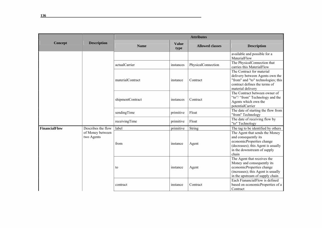
136

Concept Description

Attributes

Name Value type

Allowed classes Description

available and possible for a MaterialFlow

actualCarrier instances PhysicalConnection The PhysicalConnection that carries this MaterialFlow

materialContract instance Contract

The Contract for material delivery between Agents own the "from" and "to" technologies; this contract defines the terms of material delivery

shipmentContract instances Contract

The Contract between owner of “to”/ “from” Technology and the Agents which own the potentialCarrier

sendingTime primitive Float The date of starting the flow from "from" Technology

receivingTime primitive Float The date of receiving flow by "to" Technology

FinancialFlow

Describes the flow of Money between two Agents

label primitive String The tag to be identified by others

from instance Agent

The Agent that sends the Money and consequently its economicProperties change (decreases); this Agent is usually in the downstream of supply chain

to instance Agent

The Agent that receives the Money and consequently its economicProperties change (increases); this Agent is usually in the upstream of supply chain

contract instance Contract Each FianancialFlow is defined based on economicProperties of a Contract

137

Concept Description

Attributes

Name Value type

Allowed classes Description

content instance Money The cash that flows between two Agents

sendingTime primitive Float The date of sending Money by "from" Agent

receivingTime primitive Float The date of receiving Money by "to" Agent

Money

Describe the cash that is transferred between supply chain entities

label primitive String The tag to be identified by othersmoneyAmount primitive Float The amount of Money

moneyUnit primitive String The unit in which the Money is expressed

InformationFlow***, ****

Describes the flow of Data between two Agents

label primitive String The tag to be identified by others from instance Agent The Agent that sends the Data to instance Agent The Agent that receives the Data

content instances Data

Data cover any type of information that can be transferred between two Agents; it is one of properties of Agents, Technologies, Edge or Flows that is accessible to one Agent ("form Agent") and sends it to other Agent

Data

Describes the piece of information that is transferred between two entities

label primitive String The tag to be identified by others

value primitive Float/ Boolean/ String The value of one property of an entity in the system

OrderFlow

Describes the request for purchasing material which is usually from upstream actors to

label primitive String The tag to be identified by others

from instance Agent The Agent that sends the Order; this Agent is usually in the upstream of supply chain

to instance Agent The Agent that receives the Order: this Agent is usually in the

138

Concept Description

Attributes

Name Value type

Allowed classes Description

downstream actors in a supply chain

downstream of supply chain

contract instance Contract The Contract that defines the terms of order delivery between two Agents

content instances Order The specifications for material delivery

sendingTime primitive Float The date of sending Order by "from" Agent

receivingTime primitive Float The date of receiving Order by "to" Agent

Order

Describe the characteristics of order for one or more materials

label primitive String The tag to be identified by others

orderAmount primitive Float The amount of material that is ordered

orderedMaterial instances Good The order can be for one or more Goods

fulfillingActor***** instance Agent The Agent which fulfills the Order

timingConditions instances Property The requested timing conditions for Order (e.g., order due date)

operationalConditions instances Property The requested operational conditions for Order (e.g., type of packaging)

fulfillmentState primitive String Determines the state of an Order which can be "fulfilled", "pending" or "cancelled"

fulfillmentProperties instances Property The properties of order that is fulfilled (e.g., time of delivery)

Actvitiy

Describes the unit of behavior of actors in the system; each Activity triggers a

label primitive String The tag to be identified by others

performingActor instance Agent The Agent who performs the Activity

triggeredFlow instances MetrialFlow/ InformationFlow/

The flows that are activated when this Activity is ended

139

Concept Description

Attributes

Name Value type

Allowed classes Description

Flow or changes the state of a Technology

FinancialFlow/ OrderFlow

affectedArtifact instances Technology/ PhysicalConnection

The state of this Technology/ PhysicalConnection would change when Activity is ended

precedingActivity instances Activity Activities need to be finished before starting this Activity

followingActivity instances Activity Activities must be done after this Activity is ended

temporalCondition primitive Float The constraint for time to start performing this Activity

initiationTime****** primitive Float An Activity begins at this time completionTime primitive Float An Activity ends at this time

Property

Defines the features of entities in the system

label primitive String The tag to be identified by others propertyValue primitive Float/ Boolean/ String The value of a Property

propertyUnit primitive String The unit in which the Property is expressed

* The Property items can be defined differently for each specific case. Examples are presented in Chapter 7. ** For a MaterialFlow between companies in a supply chain, two types of Contacts are needed: materialContract which is, e.g., between a

supplier and manufacturer and shipmentContract which is between a shipping company (or 3rd party logistics provider) and sender/receiver of material (In different cases, one of buyer or seller is responsible for material delivery and subsequently, must have a contract with shipping company).

*** Unless other Flows, we assume that flow of Information happens instantly. Therefore, we do not consider sendingTime and receivingTime for InformationFlow.

**** InformationFlow is the only Flow that does not need a Contract. It is basically defined between each two Agents in the system. Other Flows need a Contract to be available.

***** The fulfillingActor is not necessarily the actor which receives the order. For example, sales department may receive the Order but operations department fulfills the Order. Similarly, the supplier may sub-contract the order to other agent.

****** By default, the initiationTime and completionTime of an Activity are the same unless the opposite is mentioned in the description of Activity.

140

6.3.1.2. System’s dynamic behavior

In the last section, the main elements to conceptualize a supply chain as a complex socio-

technical system are presented. Here, we discuss how these concepts are used in a

simulation model to describe the dynamic behavior of a supply chain. As for all agent-

based models, the main driver for dynamic behavior of system is the agent’s behavior

(Gilbert, 2007). However, in a socio-technical system, the state of technical artifacts

might also change because of physical rules which can influence the dynamic behavior of

the system as described in the following.

- Social sub-system dynamics

Agents in an agent-based model are usually described by “State” and “Behavioral Rules”

(Epstein, 1999; Gilbert, 2007; North and Macal, 2007). The State of Agent includes the

Agent’s Attributes – which are the set of properties to define the identity of agent at each

moment - and Agent’s Memory. The Agent’s attributes in an agent-based model function

like variables in a mathematical model (Gilbert, 2005). They change during simulation;

they decrease or increase. For instance, the profit of a company is an attribute which

dynamically changes based on transactions with other companies. The Memory of agent

represents the history of Agent States and the history of interactions with external world1.

Finally, the behavioral rules of Agent2 describe how an Agent behaves based on its

current state and the memory of past states. This usually happens in three steps (Sterman,

2000; Joslyn and Rocha 2000); firstly an Agent must monitor the situation of world. Next,

it must decide what to do based on the available information and take one action

subsequently (Figure 6.9). As an example, a manufacturing company monitors the level

of inventory for different products in the storage facilities and based on the inventory

level (current state) – and also considering the demand pattern of previous periods

(memory)-makes a decision about which products must be produced at which moment of

time and how much of these products need to be processed. When the decision on type of

product, timing of production and the quantity of products are made, company can take

action and start the production.

1 The external world in our modeling approach includes technical artifacts, other Agents and the Environment. 2 The behavioral rules of agent are also term its “Schema” by Anderson (1999).

141

Figure 6.9. A generic structure for Agent in ABM (after Joslyn and Rocha 2000) 

Considering all these, Figure 6.10 shows the internal structure of Agent in our modeling

approach.

Figure 6.10. The structure of Agent in the model

The Agent’s Attributes are the properties we have described in Table 6.1. For an Agent,

these Attributes are physicalProperties, economicProperties, inEdges, outEdges, inFlows,

outFlows, perfromingActivties, currentActivity and ownedComponents. The attributes of

Agent in the model work as variables in the equation-based modeling. They, by definition,

can change during simulation runs. To model the supply chain operation, however, some

Behavioral Rules 

Monitor

Make Decision

Take Action

Agent State

World

World’ Dynam

ics

Agent

SSttaattee  

BBeehhaavviioorr  

Attributes

Decision Making Part

Functional Part

Monitoring  Part

Negotiation Part

Activities

Environment 

Technology

Other AgentOther Agent

Technology

Other Agent

Memory

142

of these properties might be assumed fixed at the start of simulation. For instance, the

ownedComponents of an agent are considered fixed when we model a supply chain at the

operational level.1

The Memory of Agent includes the history of Agent’s attributes and the state of technical

artifacts – i.e., Technologies or PhysicalConnection - that are owned by this Agent.

Although, Agent has access to all characteristics of its owned technical components, it

does not necessarily monitor all those characteristics and record them in the memory.

Therefore, to start modeling, it must be clearly described which aspects of technical sub-

system is monitored by an Agent and which of them is used in its decision-making

process. In the Memory, Agent also has a record of past interactions in OrderList (list of

OrderFlows received or sent by Agent), FinancialList (list of FinancialFlows that are paid

or received by Agent), InformationList (list of InformationFlows) and MaterialFlowList

(list of MaterialFlows that are received or sent by Technologies which are owned by

Agent). Finally, Memory may include a history of past States of Environment, e.g. the

market price for raw material for a period of time.

The behavioral part of Agent has three main components (Figure 6.10). The Monitoring

Part of Agent reads the inFlows to Agent or technical artifacts that are owned by Agent.

These inFlows are from other Technologies (i.e., MaterialFlow) or from Technologies

owned by this Agent (i.e., InformationFlow), from other Agents (i.e., InformationFlow/

FinancialFlow/ OrderFlow) or from Environment (i.e, InformationFlow/ FinancialFlow)2.

These Flows change the State of Agent and its Technologies. For instance, the Money

received from other Agents in the FinancialFlow increase the Agent’s revenue (as one of

economicProperties) or new data about the inventory level (as an InformationFlow) from

a storage tank (as a Technology) is stored in the Memory of Agent. Similarly, receiving

the raw material (as a MaterialFlow) from a supplier increases the inventory level (as one

of operationalProperties) of storage facilities (as a Technology). Therefore, at each time

step of simulation, the Monitoring Part monitors the inFlows and subsequently, updates

the State of Agent and the Technologies owned by Agent.

With the updated State for Agent and Technologies, next, the agent must decide how to

react and make changes in the State in the next time interval. The specific tool for this

1 As a general rule we assume that the structural elements are fixed when we model the supply chain at the operational level. More specifically, all inEdges/outEdges –like contracts or ownership – and ownedComponents must be set before we start modeling the supply chain. Of course, to model the supply chains tactical and strategic issues (e.g., the design of distribution network) the structural elements (e.g., terms of contracts or type of technologies) must also be considered as varying attributes in the simulation. 2 The interaction of Agent with Environment will be discussed in more details in section 6.3.2.

143

aim in the model is Activity. In fact, performing an Activity is the driver for change of

state of Agent and Technology throughout the simulation. Deciding about next Activity at

each time step of simulation happens in two phases by decision-making part of Agent.

Firstly, it must be determined which Activity has to performed next. In order to do that,

two aspects have to be evaluated:

1. If previous Activity is completed? This can be checked by completionTime of

currentActivity of Agent.

2. What is the next Activity in thread of activities? Each agent has one or more

thread of Activities to do. At each point of time, the Activity with the highest

priority in each thread must be investigated for execution. Such an investigation

entails checking “preconditions”. The pre-conditions to activate an activity are

one or more of following requirements:

- The temporal conditions: an Activity might be triggered by time; for

example, a company might place an order for raw material in specific time

intervals (e.g., once in a month).

- The availability of the required inputs to define the characteristics of an

Activity: the execution of one Activity may require receiving a Flow or

performing some Activities by other Agents. For instance, starting

production in the manufacturing plants depends on the information of

inventory in warehouses of distribution centers. Without this information,

a manufacturer cannot decide about the type/amount of product that must

be produced next. The availability of these inputs in Agent/Technology

State has to be checked before execution of Activity. When we model a

real case, these types of “preconditions” can be shown by flowcharts or

Activity Diagrams as further discussed in section 6.6.

As next Activity is determined, the decision-making part of Agent must define the

Activity’s characteristics. These characteristics are, in fact, a set of decision variables

which must be adjusted for the next time interval. Part of these variables is about the

timing of an Activity (i.e., initiationTime and completionTime) and some others are about

characteristics of impactedArtifacts (Technology or PhysicalConnection) and

triggeredFlows. For instance, a manufacturer must decide about the type of Good to

produce. This basically implies a new value for currentOperationalConfiguration and

“rate of production” – as one of operationalProperties – for production facility (as a

Technology). As another example, the manufacturer must define the orderAmount and

144

order due date (as one of timingConditions) for a raw material OrderFlow before sending

to supplier.

Making a decision about characteristics of each Activity is usually done by one actor in

the system. There are, however, cases in a supply chain in which multiple actors might be

involved in the decision-making process. For example, the specification of raw material

order (e.g., delivery timing or price) might be defined beforehand in a contract between

actors in the chain. It is also possible that one actor (mostly, the buyer) makes the timing

and quantity decisions and subsequently, sends the orderFlow to its supplier. As another

alternative, the timing and price of raw material Order can be defined by joint decision-

making of both buyer and seller. In other words, decisions are being made from the

viewpoint of more than one decision entity (Raiffa et al., 2002). In these cases, the

involved actors need to have the capability to negotiate.

In following sub-sections we discuss how single- and multi-actor decision-making are

represented in the system model.

Single-actor decision-making:

For cases in which decisions on features of Activities are made by one Agent, four

options are possible to include in the model:

1. The values of decision variables are previously defined and agreed by Agents in

the chain (i.e., in the terms of Contract or Orders). For instance, the Money that a

manufacturer must pay for late delivery in a FinancialFlow to its customers is

defined in the Contract. As another example, when a manufacturer selects one

customer Order to produce at this moment of time, the “current product” and the

“batch size” (as instance of operationalProperties for production facility) are

previously defined in the Order specification from customers.

2. The decision-making style of Agent can be defined by some policies that are

selected for operation of the supply chain.

3. The Agent has a set of heuristic rules to define the value for decision variables.

4. Agent might have a utility which defines the value for decision variables.

145

Last three options are illustrated in the following with an example of storage department

which is responsible for raw material inventory management in a production plant. Two

main decisions must be made about inventory management in the plant:1

1. When the raw material Order must be placed (i.e., initiationTime for “order

placement” Activity)?

2. How much material is needed (orderAmount for raw material Order)?

A policy can determine both of these two aspects for an Agent. For instance, the (s, S)

policy defines when the inventory reaches a specified reorder point, “s”, sufficient units

must be ordered to bring up the inventory to a pre-determined level “S” (Wisner et al.,

2009). The inventory policy can also determine the period of monitoring. For instance, (R,

s, S) policy implies checking inventory position every “R” time units.

Figure 6.11. (s, S) policy for inventory management

Instead of having a policy, the storage department can make the two aforementioned

decisions based on some heuristic rules. For example, it may order in fixed periods – e.g.,

every one month- and to determine the inventory, it may assume that next period’s

demand will remain equal to current period’s and based on material requirement to

produce this demand pattern, it determines the raw material order size. These heuristics

for decision-making can be presented in a flowchart as shown in Figure 6.12.

1 The decisions that are mentioned here are decisions at the operational level of a supply chain. At the tactical level, other decisions must be made for material sourcing in a plant – e.g., who must be the supplier and how the contract terms must be set? Likewise, at the strategic level other types of decisions are important – e.g., how much capacity must be considered for storage facilities?

S

s

Order Quantity 

Order Lead Time

Inventory Level 

Time

146

Figure 6.12. A heuristic rule to determine Order amount

As a third option, the storage department might define a total cost function for material

handling as:

Total Cost = Material ordering costs +Inventory costs + Warehousing costs

+Transport costs

Each cost term in this equation can be defined as a function of time and material quantity

and by minimizing this total cost, the orderAmount and time of order placement can be

determined.

The logic to value decision variables is implemented in each Activity when we develop

the computer model in programming environment (this is discussed in more details in

section 6.6). Meanwhile, this logic can be updated during simulation by Agent learning.

For instance, in above-mentioned example, the procedure for defining the orderAmount

can be changed by storage department learning. To define the first estimation for

orderAmount, the Agent may use historical data for product demand. This amount,

however, can be improved considering the real demand data and material stock-out in the

last period of time (Figure 6.13). Other examples of Agent learning can be found in

Chapter 7.

Determine the needed raw material for the same demand pattern (orderAmount)  

Assume the period to cover  (e.g., one month) 

Read the product demand pattern for last period from Memory

147

Figure 6.13. An example of learning in inventory management process

All four mentioned methods are to set the value of decision variables by one Agent.

However, there are cases in which more than one Agent is involved in determining the

value for one or more decision variables. For these cases, agents must be able to negotiate

the case as further described in following sub-section.

Multi-actor decision-making1:

Negotiation is a type of interaction between two or more self- interested actors ( each

with its own objectives, needs and viewpoints) seeking to find a common ground and

reach an agreement to settle a matter of mutual concern or resolve a conflict (Raiffa et al.,

2002). Negotiation challenges researchers and practitioners from many disciplines

including psychology and sociology (Bazerman et al., 2007; Francis, 2008), political

sciences (Zartman and Rubin, 2002; Slantchev, 2004), economics (Kremenyuk and

Sjostedt, 2000; Tollison and Willett, 2009) and law (McMains and Mullins, 2001).

Supply chain management literature is also informative about different negotiation-

related topics (an overview can be found in Tsay et al., 1999 and Monczka et al., 2009).

1 This sub-section is partly based on Mobini (2010) – title: “An Agent-Based Model to Support Negotiation-Based Order Acceptance in a Multi-Plant Enterprise” -, Behdani et al. (2011a) – title: “Negotiation based approach for order acceptance in a multi-plant specialty chemical manufacturing enterprise”- and Mobini et al. (2011) - title: “An Agent-Based Model to Support Negotiation-Based Order Acceptance in a Multi-Plant Enterprise”.

Determine the needed raw material for the same demand pattern (orderAmount)  

Assume the period to cover  (e.g., one month) 

Read the product demand pattern for last period from Memory

orderAmount = orderAmount (1 ‐ α) orderAmount = orderAmount (1 + α)

Raw material stock‐out in last period?

No Yes

148

The majority of work in supply chain management, however, is focused on buyer-seller

negotiation where two or more parties negotiate on terms of transactions like price or

delivery time (Talluri, 2002). On the basis of activities and their sequence that form the

interaction between parties, negotiation processes are usually categorized as auction or

bargaining (Wong and Fang, 2010). In auctions, the auctioneer – buyer or seller - initiates

an auction with an initial offer and monitors the auction process while bidders send their

own bids in response to the initial offer or bids from other offers. The auctioneer follows

a certain auction protocol to pick the final partner. In a bargaining case, however, the

bargainers try to solve the conflicts by alternating offer and counteroffer round by round

until an agreement is reached. This process is referred to as Rubinstein’s bargaining

model in the literature (Rubinstein, 1982). There are also several variations of bargaining:

bilateral bargaining (one-to-one), multilateral bargaining (one-to-many, many-to-one and

many-to-many), single-issue bargaining and multi-issue bargaining (Wong and Fang,

2010). Multi-issue bargaining, according to the order of issues bargained, can further be

divided into two categories: bargaining in-bundle over multiple issues and bargaining

issues one by one. In the former, there is bargaining on multiple issues simultaneously

and it is possible to make trade-offs among different issues, but the negotiation space is

more complex. The issue-by-issue approach has a simpler computation, but an important

question that arises is the order in which the issues are bargained (Fatima et al. 2004).

Based on the order of exchanging offers, in some bargaining situations parties submit

offers simultaneously. In contrast, there are some other situations in which iterative

exchange of offers is possible.

Figure 6.14. Different types of Negotiation (adapted from Wong and Fang (2010)) 

As it can be observed from the mentioned literature, there are various types of negotiation

processes based on set of activities, number of actors involved and negotiation rules that

govern the process. However – and without considering the details of different cases -

several concepts are common in each negotiation problem; a number of parties with

different objectives and behavior are involved in the negotiation process negotiating on a

149

negotiation subject that can be described by several issues such as price, lead time and

quality.

All relevant concepts can be formalized in the negotiation ontology as shown in Figure

6.15. In brief, a number of NegotiationParties with diverse characteristics participate in

the NegotiationProcess. The NegotiationProcess is governed by a NegotiationProtocol

which defines the rules of interaction between parties (i.e., NegotiationRules). The

NegotiationProcess also consists of a set of NegotiationActivities which are performed by

the NegotiationParties. NegotiationActivities deal with OfferFlows which contain an

Offer that itself is described by several NegotiationIssues (e.g., price). A successful

negotiation eventually defines the Agreement between NegotiationParties which is a type

of Offer (it contains the agreed value for NegotiationIssues). Each of the concepts of the

ontology is further characterized by a set of attributes as described in Table 6.2.

Figure 6.15. Concepts and relations in the negotiation ontology

150

Table 6.2. Summary of classes and their attributes in Negotiation ontology

Concept Description Attributes

Name Value type Allowed classes Description NegotiationParty

Describes the participants in the negotiation. The NegotiationParty is a subclass of Agent and extends its properties; In fact, the Agent with negotiation capability has this set of additional properties.

negotiationFeatures instances Property

describes the negotiation attributes of NegotiationParty (e.g., Step limit which is the maximum number of negotiation rounds for each party).

perfromingNegActivties instances NegotiationActivity Set of Activities must be executed during negotiation

negotiationProtocol instance NegotiationProtocol

NegotiationParty knows/ follows this set of rules during the NegotiationProcess.

NegotiationProcess

Defines the allowed activities and terms of negotiation between NegotiationParties

label primitive String The tag to be identified by others

allowedActivties instances NegotiationActivity

Set of Activities are allowed during negotiation; for instance if the negotiation is an Auction or a Bargaining case, the set of activities would be different

negotiationProtocol instance NegotiationProtocol

Set of rules must be followed by NegotiationParties during negotiation

NegotiationActivity

Defines the activities that are done by Negotiation Parties in a Negotiation Process. The NegotiationActivity is a sub-class of Activity. It has all properties of Activity but triggeredFlow is over-written.

triggeredFlow instances OfferFlow The flows that each NegotiationActivity must deal with

151

Concept Description Attributes

Name Value type Allowed classes Description

OfferFlow*

Describe the flows of Offers between Agents during NegotiationProcess

label primitive String The tag to be identified by others

from instance Agent The Agent that sends the Offer

to instance Agent The Agent that receives the Offer

content instance Offer The offer that is exchanged between NegotiationParties

Offer

Consists of a number of NegotiationIssues and an assigned value for each of them

label primitive String The tag to be identified by others

composingIssues instances NegotiationIssue

Each offer consists of a number of Negotiation Issues and an assigned value for each of them.

NegotiationIssue

Is an issue under negotiation between the parties during the NegotiationProcess

label primitive String The tag to be identified by others

negotiationObject instance Thing

Defines the component in the model that NegotiationParties are negotiating about. In general, this can be any entity in the model like an Order or properties of Technology.

issuesUnderNegotiation instance Property The specific properties of negotiationObject which are under negotiation.

Agreement

Defines the agreed value for NegotiationIssues at the end of NegotiationProcess; Agreement is a sub-class of Offer.

see Offer

152

Concept Description Attributes

Name Value type Allowed classes Description

NegotiationProtocol

Defines the rules and restrictions must be followed in the NegotiationProcess

label primitive String The tag to be identified by others

consistsOf instances NegotiationRule Defines the content of NegotiationProtocol

initiatingAgent instance NegotiationParty The NegotiationParty that must start the negotiation process

NegotiationRule Describes any restriction in the NegotiationProcess

label primitive String The tag to be identified by others

* We assume that flow of offers happens instantly. Therefore, we do not consider sendingTime and receivingTime for OfferFlow.

153

During simulation runs, if the decision-making for a specific decision variable calls for

involving multiple Agents, a negotiation session must be started. This negotiation occurs

in one or more rounds (based on the NegotiationProcess that is defined for Agents1).2 In

each round of negotiation, one NegotiationParty must select a NegotiationActivity to

perform. Eight sub-classes of NegotiationActivity have been defined in the model:

“PrepareOffer”, “SendOffer”, “ReceiveOffer”, “EvaluateOffer”, “AcceptOffer”,

“RejectOffer”, “ContinueNegotiation” and “QuitNegotiation”. Negotiation starts by one

of Agents (i.e., the initiatingAgent of NegotiationProtocol) by PrepareOffer Activity. The

prepared offer must be sent to other NegotiationParty by SendOffer with an OfferFlow.

The counterparty receives offer and evaluates the Offer in EvaluateOffer Activity. After

evaluation, the second party must choose next activity. There could be three situations:

(a) If Offer is acceptable, it performs the AcceptOffer Activity which activates an

InformationFlow with acceptance message.

(b) The terms of Offer is rejected and the NegotiationParty breaks off the

negotiation (e.g., because of time limitation 3 ). In this case, NegotiationParty

performs QuitNegotiation Activity which triggers an InformationFlow with quitting

message.

(c) The offer is rejected but the second party sends a counter-offer. Preparing a

counter-offer is done by PrepareOffer Activity and finally, SendOffer triggers an

OfferFlow to other party.

The negotiation is terminated when the parties end in agreement (the Offer of one party is

accepted by counter- party) or disagreement (when one of them quits the negotiation).

Throughout the whole NegotiationProcess, the NegotiationRules constrain the

interactions between Agents. For instance, there might be a “response time limit rule”

which defines for each party to respond to the offer of its counter-party. After this time,

one of parties can quit the negotiation. Similarly, there can be a NegotiationRule for the

number of negotiation rounds as no negotiation can continue forever.

To prepare and evaluate the Offers, each NegotiationParty has a utility function (Russell

and Norvig, 2002). This utility function assigns a single number to express the

1 Clearly, if the NegotiationProcess is an auction, there is no iteration in the negotiation. One side is allowed to propose counter-offers but the other side can only accept/reject the opponent's counter-offers. 2 We assume that all rounds of negotiation occur in one simulation step unless the opposite is definite in the description of a case. This means that when negotiation starts, it continues until an agreement is reached. Then, the time step can change to next simulation tick. 3 This is defined as negotiationFeatures of NegotiationParty.

154

desirability of each Offer in the negotiation. The objective of a party in the negotiation

would be to maximize its utility function. A widely used type of utility function is the

type of linear additive utility function in which the contribution of every issue to the

utility is linear and does not depend on the values of other issues (Keeney and Raiffa,

1993). The value of each issue in a specific offer can be assessed using “evaluation

functions”. These evaluation functions map the value of issue to a single number

indicating its desirability.1

As an illustration, consider price as an issue for negotiation between a buyer and a seller.

The buyer prefers to purchase with the lowest possible price. So, the evaluation function

of price for the risk-neutral buyer could have the decreasing form (similar to what is

presented in Figure 6.16). Similarly, a Trapezoid evaluation function can represent the

desirability of different delivery dates for buyer. In fact, the order delivery in a period

between an earliest due date and a latest due date is acceptable. The utility function for

the buyer is then the sum of evaluation functions for each issue which is multiplied by a

weight representing the importance (sensitivity) of that particular issue from the buyer

viewpoint. Assuming the buyer is price sensitive and has more interest to buy at a low

price, the utility function would be:

Utility = w1 f(price) + w2 f(delivery time)

In which w1 and w2 are the weights for price and delivery time respectively. Evaluation

functions are denoted by f(price) and f(delivery time). For a price sensitive buyer, w1 has

a higher value compared to w2 (e.g. 0.7 for w1 and 0.3 for w2).

 

Figure 6.16. Examples of evaluation function for price and delivery time

Four types of evaluation functions are widely used in the literature (Chen and Huang,

2007; Tykhonov, 2010):

Downhill function: minimal issue values are preferred over other values of issue.

1 A utility function is used to evaluate the desirability of an offer as a whole, while an evaluation function is utilized to assess a single issue.

Utility

Price  Lower Bound

Price  Upper Bound

Price

Utility

Delivery DateEarliest Due Date 

Latest Due Date 

155

Uphill function: maximal issue values are preferred over other issue values.

Triangular function: a specific issue value somewhere in the issue range is valued

most and issues to the right and left are valued less.

Trapezoid function: a specific range of values somewhere in the issue range is

valued most and issues to the right and left are valued less.

Based on its utility function, NegotiationParties PrepareOffer and EvaluateOffer of their

counter-parties. There could be also some limitations for each party during the

negotiation. These limitations are defined in the negotiationFeatures of each

NegotiationParty. An example is the time limitation for an actor to continue negotiation.1

The involved actors may also have different constraints regarding different

NegotiationIssues. For example, a seller or a buyer may have different acceptable ranges

for price or due date of an order and they are not willing to accept or negotiate the values

beyond those ranges. Meanwhile, each party has an option outside the negotiation (Raiffa

et al, 2002). In case negotiation fails, the outside option would be the alternative for that

party. This is called Best Alternative to the Negotiated Agreement (BATNA). As an

example, BATNA for a buyer could be, purchasing the desired product from the spot

market.

To sum-up, each NegotiationParty makes decisions about the NegotiationActivity by its

utility function in different rounds of negotiation. This, basically, drives the negotiation

progress until an Agreement is reached, one of NegotiationParties quits the negotiation or

a termination rule is imposed by NegotiationProtocol. In that case, the final Agreement or

BATNA defines the value for decision variables (or NegotiationIssues) of

negotiationObject.

- Technical sub-system dynamics

Similar to Agents, the Technologies are also modeled with two distinctive parts: the state

and the behavior (Figure 6.17). The state is described by a set of properties as discussed

in Table 6.1. During simulation, these properties are constantly altered by acts of Agents

or by technical (behavioral) rules. For example, the decision for the product that must be

produced at each time step is made by Agent and subsequently, the state of technology is

being changed. The properties of technical artifacts can also be updated by technical

behavioral rules which are defined based on engineering principles. An example is the

1 This limitation is important as Muthoo (1999) claimed that the parties will reach an agreement if and only if time is valuable to at least one of the two parties in a bilateral situation.

156

dynamics of producing goods in a chemical reactor or the dynamic degradation of raw

material quality in the storage tanks. In both cases, the physical rules are defined by

algebraic equations and functions. Therefore, at each time step, the value of properties

needs to be re-assessed before Agent starts monitoring the technical artifacts’ State.

Figure 6.17. The structure/ behavior of Technology

The Technology’s state changes through interaction with other technical artifacts as well.

The interaction at the technical level is modeled by MaterialFlow. At each time step, the

inFlows to each Technology are monitored by Agent. In addition, the outFlows from each

Technology are triggered by Agent’s decisions and Activities. Monitoring the inFlows

and triggering outFlows, subsequently, cause changes in the state of technical entities

during simulation runs. An example is when the production agent activates the flow of

material from production facility to storage facility. By this flow, the level of material in

the production facility decreases and the level at the storage facility increases.

To sum up, the technical artifacts in the model are also defined by state and technical

behavioral rules. At each time step of simulation, the state of these entities is updated by

direct acts of Agents or indirectly through triggering MaterialFlows from/to each

Technology. The state of Technology might also change because of physical rules.

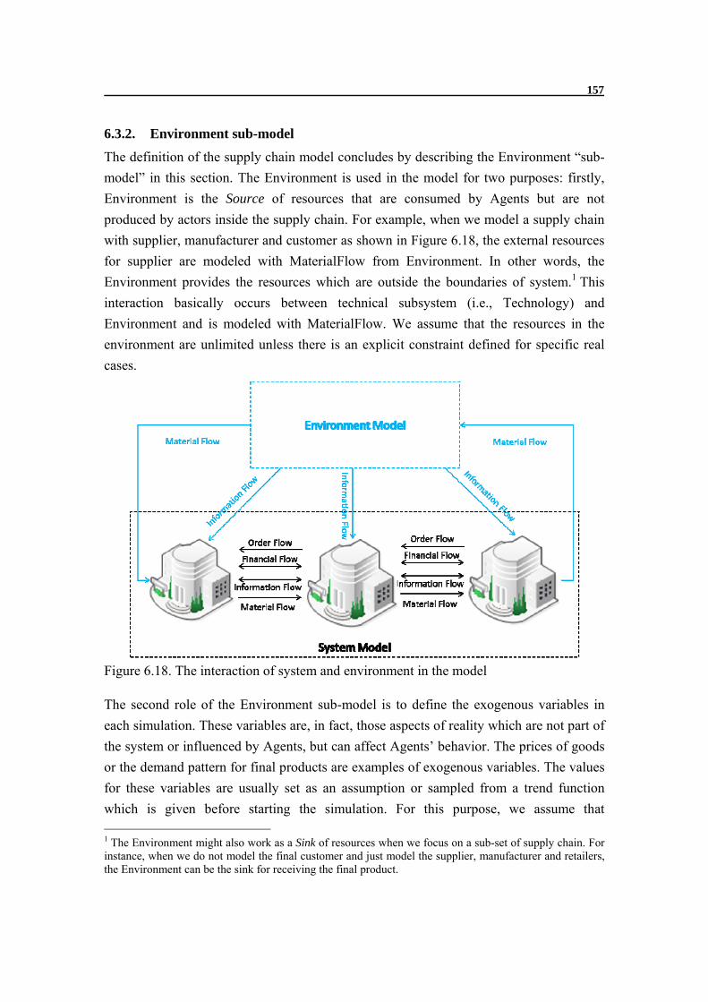
157

6.3.2. Environment sub-model

The definition of the supply chain model concludes by describing the Environment “sub-

model” in this section. The Environment is used in the model for two purposes: firstly,

Environment is the Source of resources that are consumed by Agents but are not

produced by actors inside the supply chain. For example, when we model a supply chain

with supplier, manufacturer and customer as shown in Figure 6.18, the external resources

for supplier are modeled with MaterialFlow from Environment. In other words, the

Environment provides the resources which are outside the boundaries of system.1 This

interaction basically occurs between technical subsystem (i.e., Technology) and

Environment and is modeled with MaterialFlow. We assume that the resources in the

environment are unlimited unless there is an explicit constraint defined for specific real

cases.

Figure 6.18. The interaction of system and environment in the model

The second role of the Environment sub-model is to define the exogenous variables in

each simulation. These variables are, in fact, those aspects of reality which are not part of

the system or influenced by Agents, but can affect Agents’ behavior. The prices of goods

or the demand pattern for final products are examples of exogenous variables. The values

for these variables are usually set as an assumption or sampled from a trend function

which is given before starting the simulation. For this purpose, we assume that

1 The Environment might also work as a Sink of resources when we focus on a sub-set of supply chain. For instance, when we do not model the final customer and just model the supplier, manufacturer and retailers, the Environment can be the sink for receiving the final product.

158

Environment has also a State/Behavior structure. State is defined by the set of exogenous

variables (e.g., price of goods) and behavior represents how this state changes over time.

This is shown by algebraic equations which, for instance, describe the relationship

between time and material price during the simulation horizon. The value of exogenous

variables is updated at each time step and it is read by Agents through InformationFlow.

Next, Agents use this information in their decision-making process in that time step of

simulation.

As different kinds of information are important for different Agents in the system, we

define two types of Environment in each simulation model. There is a Global

Environment which is accessible by all Agents. However, each Agent in the model may

have its own Local Environment too. For example, in modeling a multi-plant enterprise,

the raw material price or demand pattern might be different in different geographical

locations and subsequently they are represented in the local Environment of each

production plant.

6.4. Disruption modeling

The “Disruption Modeling” component in the framework of Figure 6.2 describes the

characteristics of a disruptive event in the simulation model. Different features have been

discussed in the literature to define a supply chain disruption (Table 6.3).

Table 6.3. A summary of main feature to describe supply chain disruption in the literature

Reference Disruption Feature Erhun and Deleris (2005) Failure time, Duration of Disruption, Location of Disruption Losada et al. (2010) Duration of Disruption, Recovery Profile Jin and Zhuang (2010) Failure time, Duration of Disruption Schmitt and Singh (2009) Duration of Disruption, Location Sheffi and Rice (2005) Failure Time, Recovery Profile, Length of Disruption Adhitya et al. (2007a) Detection Time, Disrupted Object, Disruption Duration Falasca et al. (2008) Location of Disruption, Recovery Profile, Duration of Disruption

These features can be classified in three main dimensions (Figure 6.19):

Locational dimension: In general, a supply chain disruption might occur in each

of the structural components of the system model - which is termed

“disruptedObject” – and subsequently one of the attributes of that entity – which

is called “disruptedAttribute” – would be changed. Therefore, the disruptedObject

can be:

159

1. A Technology: for example, the production rate (disruptedAttribute) of a

plant can be reduced to a fraction of its nominal production capacity

because of machine breakdown.

2. An Agent: for instance, the logistics service provider might stop its

business temporarily or permanently.

3. A Connection: as an example, the physicalConnection between supplier

and production plant might be temporarily disrupted because of a strike in

the main delivery port.1

Figure 6.19. Three main dimensions in disruption definition

Time-related dimension: Some other features of disruption are time-related

aspects of disruption. Two specific features are “disruptionOccurenceTime” -

which describes the time that a disruption starts - and “disruptionDuration” -

which determines the length of time that is needed to return the

“disruptedAttribute” to “normalValue”2.

Scale-related dimension: The scale of disruption defines the level of impact on

“disruptedObject”. This can be simply defined as a percentage of “normalValue”

– which is itself one of properties of disruptedObject. For instance, the

“production capacity” –as one of designProperties of a Technology - can be

reduced to 50% because of machine breakdown or “material transferring

capacity” – as one of designProperties of a PhysicalConnection – may be reduced

due to port strike and subsequently, material shipment can be delayed. We can

also consider more sophisticated profiles for disruption with gradual recovery as

shown in Figure 6.20. In that case, a “rateOfRecovery” needs to be also defined in

the Disruption description.

1 As can be seen, a disruption can occur in both physical and social networks of a supply chain. 2 NormalValue is the value of disruptedAttribute before disruption.

Disruption

Time

Scale Location 

160

Figure 6.20. Disruption profile with gradual recovery

All characteristics of a supply chain disruption are represented in the

SupplyChainDisruption class (Table 6.4). Of course, the complete description is not

necessarily considered in every simulation and – as discussed further in Chapter 7 – for

specific case, we may just consider some of these features.

Table 6.4. Properties of SupplyChainDisruption class

Attributes

Name Value type Allowed classes Description

disruptedObject instance Agent/ Technology/ PhysicalConnection

Defines the component in the model which is disrupted

disruptedAttribute instance Property Describes which characteristics of disruptedObject is disrupted

disruptionOccurenceTime primitive Float The disruption occurs at this time disruptionDuration primitive Float Describes the length of disruption period

normalValue primitive Float The value of disruptedAttribute before disruption

disruptedValue primitive Float The value of disruptedAttribute after disruption

rateOfRecovery primitive Float Describes the rate of recovery of the recovery profile is gradual

During the simulation, SupplyChainDisruption is the means by which we can create the

disruptive events based on disruption scenarios or disruption inputs (more details can be

found in section 6.6). More specifically, when the simulation time equals

disruptionOccurenceTime, the disruption model changes the disruptedAttribute of

disruptedObject to disruptedValue and its Status to “disrupted”. The disruptedObject

returns to normalValue when the simulation time equals “disruptionOccurenceTime +

disruptionDuration”. If disruption has a gradual recovery profile, at each simulation time

step, the disruption class must update the disruptedValue for disruptedAttribute.

161

6.5. Disruption management modeling

The model of the system which is presented in section 6.3 describes the normal operation

of supply chain entities. To handle a disruption, Agents in the model must have the

capabilities to detect and react to disruption. These capabilities are in fact areas for

improving the supply chain disruption management process in the system.

Detection of disruption can be implemented in the model in two ways. Firstly, the

disrupted Agent or the Agent that owns the disruptedObject sends a message with an

InformationFlow to other Agents. The logic for this process has to be designed and

implemented inside the Agents beforehand. 1 For this purpose, each Agent has the

necessary AnnounceDisruption Activity in its performingActivities which describe that as

disruption happens, the “disruption occurrence message” must be sent in an

InformationFlow to other relevant Agents.

The second possibility for disruption detection by an Agent is through monitoring the

“Status” (see Table 6.1) of technical artifacts and other Agents in the system. This

monitoring is done through a CheckStatus Activity. This Activity has a

temporalCondition which defines the interval of checking. As an example, the Agent may

check the “Status” of a PhysicalConnection every time step or every two time steps.

Which Agents or technical artifacts are monitored and how frequently this monitoring

occurs are important factors to define the disruption detection capability of Agent and

impact the performance of the disruption management process (Blackhurst et al., 2008).

The second issue in the disruption management is defining the disruption responses. As

disruption is detected, Agents can go forward and take the necessary actions to handle

disruptions. The responses to a disruption are defined by changes in the Structure or

Behavior of system. The former is modifying the structural elements of system. These

modifications might be at the technical level (changing the technology/physical

connection’s attributes) or social level of the system (change of agent/social connection

states). For instance, as a SocialNode, the financial state of an Agent can be improved by

a loan and consequently the money level for agent will increase. Similarly, the capacity

of a storage facility (as a TechnicalNode or Technology) might be increased by a few

percent to better handle the unexpected delays in raw material delivery.

1 In real world this can be a part of obligations in the contract settings in the supply chain. For example, a manufacturer may legally oblige its suppliers – in the contract setting – to notify any disruption that leads to late delivery of material in less than 24 hours after disruption occurrence.

162

Figure 6.21. Possible disruption responses to implement in the model

The behavioral changes in the system can happen in two different ways; firstly, it might

involve one Agent. This class is termed “Single-Actor Response” in Figure 6.21. In this

case, the disruption management practice is described by a set of Activities that must be

performed when a disruption is detected by Agent.

The second class of behavioral changes in the system involves multiple actors in the

system. To describe the disruption management in this case, we need a coordination

scheme (Figure 6.22). This coordination scheme must describe which Agents are

involved in the disruption process, which activities must be done by each Agent and

which temporary Flows must be defined among them (Malone and Crowston, 1994;

Behdani, et al. 2011c). For example, the production plants in an enterprise might

exchange their orders or raw material with each other when there is a disruption in the

supply chain of one of them. This implies that a new pattern of information and material

Flows must be defined for the case of disruption.

SC Disruption Response 

Structural Improvement 

Behavioral Improvement 

Social Changes 

Technical Changes 

Single‐Actor Response

Multi‐Actor Response

163

Figure 6.22. Coordination scheme to define multi-actor disruption response 

6.6. Software implementation

All concepts that are presented in sections 6.3, 6.4 and 6.5 together provide us with a

framework to conceptualize disruption management in the supply chain. With framework

we imply the definition of Gamma et al. (1995) who describes a framework as “a set of

cooperating classes that make up a reusable design for a specific class of software.” Each

concept in the conceptual model is, in fact, a class of entities and the ontology is basically

the class structure for software implementation.

Figure 6.23. Procedure from conceptual model to computer model for specific case 

Conceptual Model (Ontology)

Generic Objects (Java)

Instances from Generic Objects 

(Java)

Simulation Environment (Repast)

Computer Model for Specific case

Case Description

Experimentation  

164

The concepts in the framework are coded in Java programming language. For each

concept, the properties are considered as fields in the java class and behavior is presented

as methods. Consequently, a set of generic objects are developed in Java which can be

customized for specific cases by sub-classing and composing instances (Gamma et al.,

1995). For example, for the case study of Chapter 7, twelve different instances of Agent

are defined to describe various actors involved in the operation of supply chain (Figure

6.24). Of course, from these instances, further sub-classes can also be defined to more

concretely specify a given case (e.g., sub-classes of each department are defined for each

plant). Because of inheritance, each sub-class has the properties of super-class in the

model. For instance, all defined Agents have label, status, inEdges, outEdges, etc.

Meanwhile, each lower-level class (instance) can extend the set of properties or specify

properties further. Moreover, the object-oriented environments like Java are flexible

enough to define new concepts (classes) for specific cases if needed.

Figure 6.24. Sub-classes of Agent for case multi-plant lube oil supply chain of Chapter 7

As the description of a case is conceptualized with the classes in the framework, their

behavior must be implemented in Java codes. To facilitate this process, first the case

description can be shown in flowcharts or other graphical representations (like Activity

Diagrams). The informal description of a real case can also be expressed in pseudo-codes

before writing specific computer codes (Forsyth and Ponce, 2003). As the model

structure and behavior are implemented in Java codes, we need a simulation environment

to run the codes. The simulation platform that is selected is Repast. Repast is a Java-

based open source simulation toolkit for agent-based modeling (North et al., 2006). It

Agent

Production Plant

Global Sales Department 

Scheduling Department 

Operations Department 

Storage Department 

Packaging Department 

Procurement Department 

Logistics Department 

Supplier Customer

is a

Multi‐Plant Enterprise

Third‐Party Logistics

165

offers the necessary support code, like a scheduler, graph plotting, statistics collection,

experiment setups, etc.

The codes from simulation tool (Repast) and the model which is defined by customizing

framework classes form the computer model for a specific case. This computer model,

next, can be used for experimentation and decision support.

Box 6.3- Repast Agent Simulation Toolkit

The Recursive Porous Agent Simulation Toolkit (Repast) is a free open source toolkit

for agent-based simulation (North et al., 2006). Originally developed by the Social

Science Research Computing at the University of Chicago and subsequently,

maintained by Argonne National Laboratory, Repast provides a core collection of

classes for the building and running of agent-based simulations and for the collection

and display of data through tables, charts, and graphs (Repast, 2012).

Besides Repast, several other agent modeling toolkits are available such as Swarm,

Ascape, NetLogo, MASON. Reviews of these agent-modeling toolkits can be found in

Serenko and Detlor (2002), Gilbert and Bankes (2002) and Railsback et a. (2006).

Tobias and Hofmann (2004) also had a review and comparison among different agent-

based simulation tools and concluded that Repast, in general, is the most suitable

simulation framework for modeling social systems.

Each Repast model usually has three main methods (Repast, 2012):

• buildModel: is responsible for creating the main body of simulation. More

specifically, the agents and their environment are created here, together with

any optional data collection objects. Clearly, this part of simulation is largely

case-specific.

• buildSchedule: builds the Schedule of actions in the simulation. This, in fact,

means what methods to call on which objects and when. Repast scheduler is a

discrete time simulator where every tick was checked to see if any actions were

scheduled for that tick.

• buildDisplay: creates those parts of the simulation that have to do with

displaying the simulation to a user.

More information on using Repast for modeling can be found in Repast web site

(http://repast.sourceforge.net/)

166

The steps to develop the model for a specific case and how this model is used to

experiment with different aspects of disruption management are further discussed for a

case of lube oil supply chain in Chapter 7.

6.7. Chapter summary

In this chapter a conceptual modeling framework for disruption management in supply

chains is presented. This framework consists of three main components. Firstly, an agent-

based representation of a supply chain is discussed in which “Agent” (representing the

decision-making units in the system) is the central concept. Agent together with other

main concepts to describe the structure and operation of a supply chain are, next,

formalized in an ontology. This ontology is basically the conceptual model for a supply

chain as a complex sociotechnical system. Afterward, the conceptual model of supply

chain disruption is discussed. Finally, we described how different disruption management

practices can be defined and implemented in the model. These three components present

a conceptual modeling framework for disruption management in the supply chains. This

framework is very flexible in modeling different types of disruption and disruption

management practices. Firstly, they can be defined in both social and technical entities

within the system. Moreover, the disruption management can be by improving the

structure or behavior of system elements. For instance, the structure of a supply chain can

be improved by changing the characteristics of technology and physical facilities (e.g.,

increasing the storage capacity) or by a new contract with a backup supplier. As an

alternative, to handle disruption we can define new logic for decision-making or different

types of activities for different agents in the system. This flexibility in modeling is further

elaborated in the next chapter for a case of lube oil supply chain.

167

7. LUBE OIL SC CASE: MODEL DEVELOPMENT AND USE FOR NORMAL OPERATION

n this chapter, the application of modeling framework of chapter 6 for a case of lube oil

supply chain is presented. First, we discuss how a computer model for a specific case can

be developed with generic objects of modeling framework. Next, the application of this

model to handle different aspects related to normal and abnormal operation of supply chain is

explored.

7.1. Introduction

In Chapter 6 a modeling framework for supply chain disruption management was

presented. In this chapter we discuss the application of this modeling framework for a

case of Lube Oil Supply Chain. First, a description of the case is presented. Next, we

describe how this case definition could be translated into the computer model. The

developed model, then, will be used in some experimental set-ups to support the decision-

making in the normal operations management in the supply chain and managing

disruption in different steps of the InForMDRiSC framework.

7.2. Case description

The model of supply chain in this chapter is developed based on the case of an

international Lube Oil Company. The description of the system layout and operating

procedures are described in a report by (Wong, 2007) and was the motivation to develop

a multi-plant simulator (Adhitya and Srinivasan, 2010). As in the two mentioned studies,

the name and profile of the company remains confidential throughout this chapter and it

is called MPE hereafter. The lube oil supply chain consists of a lube additive

manufacturing enterprise, its customers in the downstream and the suppliers for raw

materials (i.e., base oils and additives) in the upstream (Figure 7.1). The enterprise has

three production plants in US, South Asia and East Asia. Each of these plants has its own

functional departments with a specific role and certain tasks to perform. The enterprise

has also a central sales department which directly interacts with customers around the

world. The overall goal for the whole enterprise is to fulfill customer orders by assigning

I

168

them to different plants and coordinating the behavior of different departments in each

plant.

Supplier

Supplier

Supplier

Figure 7.1. Schematic of multi-plant lube oil supply chain

Actors and their behavior in lube oil supply chain:

The actors in the lube oil supply chain can be viewed at three levels:

Global level: There are four actors at the global level – customers, the enterprise,

third-party Logistics Company and suppliers.

Enterprise level: The manufacturing enterprise consists of the global sales

department and a number of plants.

Plant level: Each plant has six different functional departments – representative

for scheduling, operations, storage, packaging, procurement and logistics.

In the following, the behavior of each of these actors is described in more detail.

(1) Customers: The customers in the supply chain place orders based on their material

requirements and send these orders to the enterprise. Each order from customers is

normally described by:

169

Product type and grade: the product portfolio of enterprise includes three main

types of Lubricant products (based on the type of base oil used) and five grades

for each type. Different grades for a specific lubricant have a different ratio of

additives and base oil as shown in Table 7.1.

Table 7.1. Lubricant products and grades

Product A

Grade Base Oil 1 ZDDP1 Dispersants MMA2 Anti-

OxidantsMetal

Sulfonates 1 0.8 0.1 - - - 0.1 2 0.75 0.15 - - 0.1 3 0.8 0.05 - - 0.15 - 4 0.7 - 0.15 0.15 - - 5 0.7 - - 0.2 - 0.1

Product B

Grade Base Oil 2 ZDDP Dispersants MMA Anti-

OxidantsMetal

Sulfonates 1 0.7 0.15 - - - 0.15 2 0.8 - 0.1 - - 0.1 3 0.7 0.2 - 0.1 - - 4 0.8 - 0.05 - 0.15 - 5 0.75 - - 0.15 - 0.1

Product C

Grade Base Oil 3 ZDDP Dispersants MMA Anti-

OxidantsMetal

Sulfonates 1 0.75 0.1 - - - 0.15 2 0.8 - - 0.15 - 0.05 3 0.7 - 0.2 - 0.1 - 4 0.8 0.1 - - 0.1 - 5 0.7 - 0.15 - - 0.15

Order quantity: defines the amount of product that is needed for a customer.

Packaging type: the products can be sent to customers in two different forms; Iso-

Tank Containers or Drums.

Transportation type: the transportation of final product to the customer location

can be arranged by the production plant or the customer himself might be

responsible for order pick-up from plant location. The actor who is responsible for

order delivery must be determined in order specifications.3

1 Zinc dialkyldithiophosphates (ZDDP) is a regular anti-wear additive to lubricants such as greases, gear oils, and motor oils (Štìpina and Veselý, 1992). 2 Methyl Mehtacrylate(MMA) is used as an additives for improving the viscosity and rheological properties of the lubricant (Mortier, R. M., Qrszulik, 1997). 3 In order fulfillment process, determining the actor who is in charge for order delivery is important because that actor is assumed responsible for transportation risk and insurance coverage.

170

Due date range: is the window when the final products have to reach the

customer’s location, regardless of whether the products are picked up by the

customer or sent by the plant. This window is described by an Earliest Due Date

and a Latest Due Date.

The customers are heterogeneous in various aspects; firstly they are located in different

geographical locations. This, in fact, impacts the logistics and transportation cost for

order delivery. Meanwhile, although the majority of customers are global customers

which send their orders to the global sales department (GSD), each production plant has

also some local customers that send their purchasing orders directly to that plant. In order

negotiation and order assignment, GSD also classifies customers in two classes of

“Important Customers” and “Regular Customers”. Important Customers place more

frequent orders with the enterprise and their orders have special priority, especially

during disruption occurrence in the supply chain.

As a last important feature, the customers are classified in two groups of wholesalers and

industrial customers. The main distinction between these two classes is reflected in their

sensitivity to price and delivery time during negotiation with GSD (more details are

discussed in section 7.4.1).

(2) Manufacturing Enterprise: The Multi-Plant Enterprise (MPE) has a global sales

department (GSD) that directly interacts with the customers and three production plants

in different geographical locations.

Global Sales Department (GSD): Global Sales Department (GSD) is responsible

for order acceptance and order negotiation with customers. After receiving a purchasing

order, the Global Sales Department (GSD) also assigns the order to one of the available

plants. For this purpose, GSD passes the order details to the scheduling departments of

each plant and requests information on order processing (e.g., the earliest date when the

plant can produce the order and deliver to the customer). The schedulers reply with the

requested information and based on the replies, GSD assigns the customer order to one of

the plants according to its “order assignment policy”. The assignment policy is called

“First Completion Date Policy”. In this policy, GSD asks for the first date that the new

order can be processed and sent to the customer by each of the plants. Based on the

replies from each plant, assigning order to one of plants is done based on the following

rules (Figure 7.2):

The plant with the Completion Date which falls in the Due Date Range and is the

closest to the Earliest Due Date will be selected.

171

If all plants can only complete the order before the Earliest Due Date, the plant

with the Completion Date closest to the Earliest Due Date will be selected.

If all plants can only complete the order after the Latest Due Date, the plant with

the Completion Date closest to the Latest Due Date will be selected. Negotiations

with the customer to extend the Latest Due Date will be held.

Figure 7.2. Different arrangements of completion dates for an order by different

production plants in order assignment policy

Production Plant: the enterprise has three production plants. Each plant has some

distinctive characteristics. This ranges from the geographical location, the production

characteristics (e.g., production rate and operation costs) and the suppliers that each plant

works with. Despite these differences, all plants operate on make-to-order (MTO) basis;

they only begin production after receiving an "Order" that is received from customers and

assigned by GSD.

Inside each production plant, many activities are done on a daily basis. These activities

are divided among a number of departments which are responsible for a set of specific

tasks:

- Scheduling department: This department performs two main functions:

Firstly, after receiving a new order from GSD, it sends the required information (e.g.,

the first possible time for fulfilling the new order) to GSD. For this purpose, the

scheduler attempts to insert the new order into the current production schedule. Based

on that, the scheduling department calculates the expected completion time for the

172

new order and conveys that information to GSD for making a decision on order

assignment.

As the second main function, the scheduling department determines the job schedule

for the plant and informs the operations department of which job to process and when.

To fulfill this task, the scheduler must communicate with the storage department to

ensure the availability of raw materials before sending the order to the operations

department.

The logic to determine the schedule of jobs is defined by the scheduling policy. The

scheduling policy is Processing Earliest Due Date (PEDD). In this policy, the PEDD is

calculated based on following formula:

PEDD = Earliest Due Date – Packaging Time – Processing Time – Expected Delivery

Time

The order with earlier PEDD has the highest priority in the list of order jobs.

- Operations department: The operations department is responsible for supervising

the processing of raw materials into various products through reaction and blending

following a unique recipe. The recipe of production for different products and

different grades is shown in Table 7.1.

Box 7.1- Make-To-Order (MTO) vs. Make-To-Stock (MTS) Production

Generally, manufacturing environments can be divided into Make-To-Stock (MTS)

and Make-To-Order (MTO) categories. MTS is the traditional production environment

in which producing a product is driven by the demand forecast rather than actual

customer orders (Kolisch, 2001). In other words, a company produces products and

stocks them as inventory until they are sold.

In contrast, in the Make-To-Order (MTO) environment, production, final assembly

and distribution of products are driven by the customers' orders; i.e. the firm produces

after an order arrives, and produces only the quantity ordered (Gunasekaran and Ngai,

2005; Parry and Graves, 2008). With MTO process, therefore, a product is

individually manufactured for a particular customer according to its specific

requirements. Adopting the MTO production strategy creates the opportunity for a

firm to offer greater product variety. In addition, the inventory holding cost will be

reduced by eliminating the finished goods inventory.

173

To process each order, the operations department, firstly, sends a request for the

release of raw materials to the storage department. Each batch of reactants is fed to the

reactors and blenders (not described in detail here) and processed following pre-

specified recipes to produce the products matching the specifications in the order.

Following this production step, the products are sent for packaging.

- Packaging department: this department is responsible for product packaging. As

mentioned before, products can be packaged in drums or iso-tanks. This depends on

the packaging type specified by the customer in their order specification.

Subsequently, packed products are either transferred to:

i) The storage department and wait for the customer to pick them up;

ii) The 3PL to deliver the products to the customer.

- Storage department: The storage department keeps tracks of the raw material

storage of the plant. Meanwhile, it provides the raw materials for the operations

department as it starts processing orders.

The other task of the storage department is to inform the scheduling department of the

current inventory levels and ask the procurement agent to make a raw material order,

whenever necessary.

Figure 7.3. Reorder point inventory management policy

There are eight separate storage facilities for different base oils and additives in each

plant. The inventory level in each of these storage tanks is continuously monitored by

the storage department and , if necessary, the new orders for material are placed. The

timing for raw material procurement is defined by reorder point policy. In this policy,

whenever the remaining inventory is reduced to “s” (i.e., reorder point), the storage

department asks the procurement department to place an order for the desired raw

Order Level “S”

s

Order Quantity

Order Lead Time

Inventory Level 

Time

174

material to bring the inventory up to a specific target level of “S”, which is the

maximum capacity of storage tanks in our case (Figure 7.3).1

- Procurement department: The procurement department communicates with

suppliers and places orders for raw materials based on the order specification that is

defined by storage department. As a raw material order is received from a supplier, the

procurement department has to make the payment.

The Procurement department also keeps track of pending orders which are in the

process of being delivered by the Supplier. This is to avoid any potential repeat orders.

- Logistics Department: The logistics department arranges the shipping of raw

material and distribution of finished product orders to customers. For this purpose,

each plant has a transportation contract with a Third-party Logistics (3PL) company.

Every day, the logistics department communicates with 3PL to give details on which

orders must be transported to which customer and which orders of which supplier are

ready to be shipped. The payment of logistics costs to 3PL and payment of lateness

penalty to customers are also arranged by this department. The penalty for late

delivery is defined in the contract between the enterprise and its customers.

(3) Third-party Logistics Company (3PL): 3PL provides the service of transportation

for raw material from suppliers to the plant, and for the packaged lubricant products from

the plant to the customer.

(4) Supplier: Suppliers provide various raw materials according to orders that are placed

by the production plants. Each plant has a contract with one supplier for base oils and

another contract for a second supplier to provide the additives. Each supplier has different

geographical locations that can affect the delivery time. This aspect and some other

characteristics of suppliers are also experimented in section 7.7.

The description of this global multi-plant specialty chemical manufacturing enterprise is

formalized according to the modeling framework of Chapter 6 as described in the next

section.

7.3. Computer model development

In this section, we discuss how the computer model for the specific case of the lube oil

supply chain must be developed. In section 6.6, we discussed that for each concept in the

1 Some other possible inventory control policies are discussed and experimented in section 7.7.

175

conceptual model an Object in Java has been defined. To design a computer model for

the lube oil supply chain case, these generic objects must be customized by defining the

instances and the necessary attributes which are needed to describe this specific case.

It is noteworthy to emphasize that despite numerous actors in each system, in developing

the model (as a decision support tool) only one of these actors is considered as the

problem owner for whom the computer model is designed. This has two main

implications in the modeling process. First, during the experiment design phase, the

performance of the supply chain is studied from the perspective of this actor (i.e., the

problem owner).1 The second implication is in the level of detail for different actors in

the model; for the problem owner - as the main actor - the structure and operation is

defined with more detail while for other actors, the structure is usually much simpler. It is

even possible that full operation details of other actors are unavailable during model

development and consequently, most of assumptions in the experimentation phase are

usually made about them. In our case of lube oil supply chain, the main actor and

problem owner is the multi-plant enterprise (MPE). Therefore, in all experimental

designs, the performance (or output as mentioned in section 5.3) is defined from the

perspective of this actor. Meanwhile, the majority of efforts in the computer modeling are

focused on presenting the structure and operation of MPE.

In Chapter 6, we made a distinction between static and dynamic representations of supply

chains. Moreover, for static representation, the distinction between structural and

operational components has been discussed. Based on this distinction, building the

computer model starts by presenting the structure of lube oil supply chain. This

description includes the Agents and links between Agents (Figure 7.4), Technologies and

their relations with each other in the form of PhysicalConnection and the relations

between Technologies and Agents in the form of Ownership (Figure 7.5).

1 This issue will be further discussed in section 7.6.

176

Figure 7.4. Agents and their relations in the model.

Figure 7.5. Technologies and their relation with Agents in the model

The model of the MPE supply chain has 82 instances of Agent (Table 7.2) for which the

related attributes – as mentioned in Table 6.1 –must be defined. Just as examples, Table

7.3 to Table 7.5 show the attributes for MultiPlantEnterprise, ProductionPlant1 and

StorageDepartment1. To experiment with the computer model, some of these attributes

must be valued before simulation (this will be discussed in more detail in section 7.6).

Some other attributes, i.e., operationalProperties and currentActivity, are continuously

changing during the simulation runs.

ProductionPlant1

ThirdPartyLogisti

Supplier1

Supplier2

StorageDepartme

nt 

SchedulingDepartment 

ProcurementDepartment 

OperationsDepartment 

LogisticsDepartm

ent 

PackagingDepartment 

ProductionPlant1

ThirdPartyLogisti

Supplier1

Supplier2

StorageDepartme

nt 

SchedulingDepartment 

ProcurementDepartment 

OperationsDepartment 

LogisticsDepartm

ent 

PackagingDepartment 

MultiPlantEnterprise Customer

GlobalSalesDepartment

ProductionPlant1

ThirdPartyLogistics

Supplier1

Supplier2

StorageDepartme

nt1 

SchedulingDepartment1 

ProcurementDepartment1 

OperationsDepartment1 

LogisticsDepartment1 

PackagingDepartment1 

Contract OrganizationalConnection

Ownership

177

Table 7.2. Instances of Agent in the computer model

Type of Agent No. of instances MultiPlantEnterprise 1 ProductionPlant 3 GlobalSalesDepartment 1 SchedulingDepartment 3 OperationsDepartment 3 StorageDepartment 3 ProcurementDepartment 3 LogisticsDepartment 3 PackagingDepartment 3 Customer 50 Supplier 6 ThirdPartyLogistics 3 Total 82

Table 7.3. Attributes of MultiPlantEnterprise Agent

Agent Attributes

Name value type

Mu

ltiP

lan

tEn

terp

rise

label "MultiPlantEnterprise" String status "NormalState" String economicProperties

totalProfit Property totalCost Property

operationalProperties

totalProcessedOrders Property totalLateOrders Property

outEdges

plant1Ownership Ownership plant2Ownership Ownership plant3Ownership Ownership owningGSD Ownership prodcutPurchasingContract Contract

performingActivities

calculateEnterpriseProfit Activity calculateEnterpriseCost Activity calculateTotalLateOrders Activity calculateTotalProcssedOrders Activity

ownedComponents

ProductionPlant1 Agent ProductionPlant2 Agent ProductionPlant3 Agent GlobalSalesDepartment Agent

178

Table 7.4. Attributes of ProductionPlant1 Agent

Agent Attributes

Name value type

Pro

du

ctio

nP

lan

t1

label "ProductionPlant1" String status "NormalState" String economicProperties

totalProfit Property totalCost Property

physicalProperties

xLocation Property yLocation Property

operationalProperties

totalProcessedOrders Property totalLateOrders Property

inEdges

plant1Ownership Ownership baseOilContract Contract additiveContract Contract

outEdges

departmentOwnership Ownership inTheSameEnterprise OrganizationalConnection

performingActivities

calculatePlantProfit Activity calculatePlantCost Activity calculateTotalLateOrders Activity calculateTotalProcssedOrders Activity

ownedComponents

SchedulingDepartment1 Agent OperationsDepartment1 Agent StorageDepartment1 Agent ProcurementDepartment1 Agent LogisticsDepartment1 Agent PackagingDepartment1 Agent

Table 7.5. Attributes of StorageDepartment1 Agent

Agent AttributesName value type

Sto

rage

Dep

artm

ent1

label "StorDepForPlant1" String status "NormalState" String economicProperties materialStorageCost Property operationalProperties currentInventoryLevelForBO Property

currentInventoryLevelForAdd Property reorderPoint Property safetyStock Property

inEdges storDep1Ownership Ownership outEdges storageFacilityOwnership Ownership

inTheSamePlant OrganizationalConnection inFlows rMAvailabilityCheck Flow

askForRM Flow outFlows rMAvailabilityInfo Flow

rMOrderSpec Flow performingActivities checkReorderPoint Activity

defineRMOrderSpec Activity receiveRM Activity sendRMForProcessing Activity sendRMAvailabilityInfo Activity

currentActivity Default is “no-Activity” Activity

179

Just like Agents, the Technologies in the system must be formalized by defining the

instances and their relevant attributes. As examples, BO1Storage and RMDeliveryLink

are defined in Table 7.6 and Table 7.7 respectively.

Table 7.6. Attributes of BO1Storage Technology

Technology AttributesName value type

BO

1Sto

rage

label "BO1StorageForPlant1" String status "NormalState" String economicProperties unitStorageCost Property designProperties storageCapaciity Property operationalProperties currentLevel Property

Table 7.7. Attributes of RMDeliveryLink

PhysicalConnection AttributesName value type

RM

Del

iver

yLin

k

label "RMDeliveryLinkForPlant1" String status "NormalState" String from SupplierFacility Technology to RMStorageFacility Technology economicProperties unitShimpentCost Property designProperties shipmentCapaciity Property

deliveryRate Property operationalProperties currentLevel Property content rawMaterialFlow MaterialFlow

After defining the Agents, the Technologies and their interrelations, the structure of

system is ready.1 Next, we need to define the operational entities in the system and how

the dynamic behavior is simulated.

The operation of lube oil supply chain – with the case description of Section 7.1 - is

represented in 3 main processes - Figure 7.6. The figure shows the main constructs to

describe the operation of lube oil supply chain. These constructs include the Activities

that are done by each Agent and the interactions between supply chain entities which are

shown by different types of Flows. Some of the Activities have a more detailed logic

which is presented in the flowcharts. These flowcharts describe in detail when an Activity

must be started, what decisions must be made for that Activity, how those decisions must

be made and which aspects of system will be influenced by performing this Activity. For

example, the logic behind sendOrderProcessingInfo of order acceptance process is

described in flowcharts of Figure 7.7.

1 As our focus here is on modeling the supply chain at the operational level, we assume that this structure is fixed during simulation.

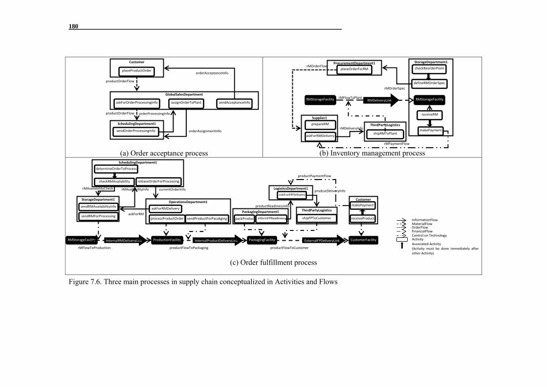
180

(a) Order acceptance process

(b) Inventory management process

(c) Order fulfillment process

Figure 7.6. Three main processes in supply chain conceptualized in Activities and Flows

Customer

GlobalSalesDepartment

SchedulingDepartment1 

placeProductOrder

askForOrderProcessingInfo

sendOrderProcessingInfo

assignOrderToPlant sendAcceptanceInfo

productOrderFlow

productOrderFlow orderProcessingInfo

orderAssignmentInfo

orderAcceptanceInfo

StorageDepartment1 

checkReorderPoint

defineRMOrderSpec

RMStorageFacility

ProcurementDepartment1 

placeOrderForRM

Supplier1

prepareRM

RMStorageFacility

askForRMDelivery

ThirdPartyLogistics

shipRMToPlant

RMDeliveryLink

receiveRM

rMOrderSpec

rMOrderFlow

rMDeliveryInfo

rMFlowToPlant 

makePayment

rMPaymentFlow

SchedulingDepartment1  determineOrderToProcess

checkRMAvailability

StorageDepartment1  sendRMAvailabilityInfo

releaseOrderForProcessing

sendRMForProcessing

OperationsDepartment1 

askForRMDelivery

processProductOrder sendProductForPacakging

ProductionFacility

PackagingDepartment1 

packProduc

PackagingFacility

LogisticsDepartment1  askForFPDelivery

informFPReadiness

ThirdPartyLogistics

shipFPToCustomer

Customer

receiveProduct

CustomerFacility RMStorageFacility InternalProductDeliveryLinkInternalRMDeliveryLink ExternalFPDeliveryLink

rMFlowToProduction  productFlowToPackaging  productFlowToCustomer

rMAvailabilityCheck rMAvailabilityInfo  currentOrderInfo

productReadinessInfo 

prodcutDeliveryInfo 

askForRM InformationFlowMaterialFlowOrderFlow

makePayment

productPaymentFlow

FinancialFlowControl on Technology Activity Associated Activity(Activity must  be  done  immediately  after other Activity)

181

Figure 7.7. Flowchart to describe the logic behind sendOrderProcessingInfo Activity  

As system structure and operation are formalized with pre-defined concepts and coded in

Java Objects, the next stage is to specify the Environment. In the model of lube oil supply

chain, two types of Agents have direct interactions with Environment. Firstly, a

physicalConnection is defined between supplier and Environment. Through

physicalConnection material flows unlimitedly from Environment to supplier as the level

of raw material in the SupplierFacilities goes lower than a specific level. The other

interaction with Environment is the flow of information to Customer which is formalized

in demandInformationFlow and spotMarketPriceFlow. These two Flows and their

application for experimentation with model are described in section 7.7.

7.4. Simulation set-up

As instances from generic objects are created for the specific case of Lube Oil Supply

Chain, the computer model is ready. The next steps, is defining the initial value for the

attributes of each instance in the model. We call this step simulation model set-up. Model

set-up also implies making the assumptions explicit for those aspects of the system for

which the exact value is not available. The majority of these assumptions are about the

downstream supply chain as the precise profile of customers and the order pattern for

Insert new order in the order list

Calculate PEDD for all orders 

Make the rescheduling 

If inserting new order causes delay for other orders? 

Adjust the new order’s position one step in the orders’ sequence 

Is there still any delay in orders’ 

delivery?

Determine the expected completion time for new order

Send the expected completion time for new order to GSD

182

each individual customer is not known. In fact, as the enterprise is working on a make-to-

order basis and the orders are placed by different customers around the world, the exact

pattern of orders is not available to use in the simulation. Instead, based on available data,

we need to define an order pattern and use that pattern as input for simulation runs.

Developing this customer order pattern is done in three main steps.

(1) Defining customer list:

Firstly, we defined a customer list for the enterprise. This customer list describes the

characteristics of 50 customers which place the orders with the enterprise. 1 These

characteristics include:

customerID: which defines the ID of the Customer.

Customer location: the location of customer is defined by xLocation and

yLocation. To specify the location for each Customer we assumed a world map

which resides in a 10 by 10 grid. As such, any location in the model can be

represented by the coordinates between (0, 0) to (10, 10). Based on this grid map,

we have defined the location for customers of enterprise in the model.

orderFrequency: Besides the xLocation and yLocation, for each customer an

orderFrequency parameter is defined which determines the frequency that the

orders are sent by this customer. Some of the customers – which are determined

by their ID - are important customers which place orders more frequently (in

average 4 times more than regular customers). These frequent customers are

determined by importantCustomer tag and are given priority when processing the

job orders in the plants.

(2) Defining the order specification

As the customer list is defined, the second step is defining the characteristics of orders.

The description of each ProductOrder from Customers includes the set of attributes

presented in Table 7.8.

1 The customer list, in fact, reflects the heterogeneity in the downstream of supply chain.

183

Table 7.8. Attributes of ProductOrder

Concept Attributes

Name value type Description

Pro

du

ctO

rder

label primitive String The tag to be identified by others

productQuantity primitive Float The amount of material that is ordered

product Type instances Good The order can be for one of 3 Products A, B or C

productGrade primitive String Each Product can have grade from 1 to 5 which defines a specific recipe for the production

placingCustomer instance Agent The Customer who places this order

fulfillingActor instance Agent The ProductionPlant which fulfills this order

timingConditions dateOfOrderPlacement Property The date of placing order by Customer

earliestDueDate Property EarliestDueDate is the first possible date that order must be received by Customer; it is assumed as “dateOfOrderPlacement” + [14 ~ 21] days

latestDueDate Property LatestDueDate is the last acceptable date for order delivery for a Customer; it is assumed as “earliestDueDate” + [1 ~ 14] days

operationalConditions packagingType Property Tht type of pacakaging for fininshed product which can be "Drum" or"Isotank"

pickupType Property There are two options for finshed product delivery: "Customer Pick up" or "Sent by the plant"

fulfillmentState primitive String Determines the state of an Order which can be "fulfilled", "pending" or "cancelled"

fulfillmentProperties dateOfFulfillment Property The time that order is delievred at cutomer place

ifdelayedOrder Property Determines if order is delayed

For each ProductOrder some of these attributes (i.e., packagingType and pickupType) are

defined by a uniform random function. For example, on average, 50 percent of orders are

delivered to customers by the plant and for other orders the customer itself is responsible

184

for order pickup after finishing. Defining productQuantity, productType and

dateOfOrderPlacement is, however, a more complicated task and is done based on the

procedure that is described in (Wong, 2007) and Adhitya and Srinivasan (2010). The

input to this procedure is the yearly demand pattern for each product. For this purpose,

based on the history of demand and the expectation of the sales department, an estimated

demand curve is generated for each product type for a time span of one year (Figure 7.8).

This curve is increasing in slope which implies an increasing demand for the products

during one year. The demand curves are next translated to discrete orders for each

product in several steps (Figure 7.9). Firstly, the curves are divided into 30-day periods

and the daily demandsfor a particular period is summed up to determine the cumulative

monthly demand (MDp,m; “p” is the index for each product and “m” is the index for each

month). Next, each monthly demand is redistributed throughout the days in the month

according to the order frequency index fp, representing the probability of a customer

order on a given day for product p, where 0 ≤ fp ≤ 1. We assume that, on each day, there

can be at most one order for each product type. The higher the fp value, the more frequent

the orders for product “p” throughout the month. To check the order placement on a

particular day, a uniform [0, 1] random variable, μp,d, is generated for every day in the

month and compared to fp:

,

1,

0,

p d

fp d p

OPf

p d p

(7.1)

OPp,d is the binary parameter which determines whether an order is placed for product

“p” on day “d”. The demand amount following an order occurrence is next generated as:

,, ,30

,30( 1) 1

p dp d p mm

p dd m

OPDD MD

OP

(7.2)

for each month “m”. For each product “p”, DDp,d is the portion of monthly demand

(MDp,d) that is placed on day “d”. Because this value might be unreasonably low or high,

we limit the minimum and maximum order size with the following equation:

0, min

, , min , max

max , max

DD Dp d

AD DD D DD Dp d p d p d

D DD Dp d

(7.3)

185

ADp,d is the actual demand for product “p” on day “d” after accounting for the minimum

and maximum order size limits, (i.e., Dmin and Dmax). If ADp,d > 0, then a customer order

will be created for which:

dateOfOrderPlacement = d

productQuantity = ADp,d

productType = p

Figure 7.8. Demand curve for different products (Siang, 2008)

Figure 7.9. The procedure to define the order quantity

When the dateOfOrderPlacement is determined, the due date range1 is also defined by a

uniform random function in the range shown in Table 7.8.

(3) Assigning orders to customers

1 The Due Date Range is the window when the final products have to reach the customer’s location, regardless of whether the products are picked up by the customer or sent by the plant. This window is defined by earliestDueDate and latestDueDate for each Order.

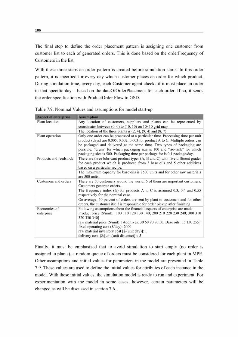
186

The final step to define the order placement pattern is assigning one customer from

customer list to each of generated orders. This is done based on the orderFrequency of

Customers in the list.

With these three steps an order pattern is created before simulation starts. In this order

pattern, it is specified for every day which customer places an order for which product.

During simulation time, every day, each Customer agent checks if it must place an order

in that specific day – based on the dateOfOrderPlacement for each order. If so, it sends

the order specification with ProductOrder Flow to GSD.

Table 7.9. Nominal Values and assumptions for model start-up

Aspect of enterprise Assumption Plant location Any location of customers, suppliers and plants can be represented by

coordinates between (0, 0) to (10, 10) on 1010 grid map The location of the three plants is (2, 4), (9, 4) and (8, 7)

Plant operation Only one order can be processed at a particular time. Processing time per unit product (days) are 0.005, 0.002, 0.003 for product A to C. Multiple orders can be packaged and delivered at the same time. Two types of packaging are possible: “drum” for which packaging size is 100 and “iso-tank” for which packaging size is 500. Packaging time per package for is 0.1 package/day.

Products and feedstock There are three lubricant product types (A, B and C) with five different grades for each product which is produced from 3 base oils and 5 other additives based on a particular recipe. The maximum capacity for base oils is 2500 units and for other raw materials are 500 units.

Customers and orders There are 50 customers around the world; 6 of them are important customers. Customers generate orders. The frequency index (fP) for products A to C is assumed 0.3, 0.4 and 0.55 respectively for the nominal case. On average, 50 percent of orders are sent by plant to customers and for other orders, the customer itself is responsible for order pickup after finishing

Economics of enterprise

Following assumptions about the financial aspects of enterprise are made: Product price ($/unit): [100 110 120 130 140; 200 210 220 230 240; 300 310 320 330 340] raw material price ($/unit): [Additives: 30 60 90 70 50; Base oils: 35 130 255] fixed operating cost ($/day): 2000 raw material inventory cost [$/(unit day)]: 1 delivery cost {$/[unit(unit distance)]}: 5

Finally, it must be emphasized that to avoid simulation to start empty (no order is

assigned to plants), a random queue of orders must be considered for each plant in MPE.

Other assumptions and initial values for parameters in the model are presented in Table

7.9. These values are used to define the initial values for attributes of each instance in the

model. With these initial values, the simulation model is ready to run and experiment. For

experimentation with the model in some cases, however, certain parameters will be

changed as will be discussed in section 7.6.

187

7.5. Validation and verification

The developed computer model must be verified and validated through a set of

preliminary experiments before conducting the experiments to examine the impact of

different factors on the operation of supply chain.1 The verification and validation tests 2

are, however, not limited to the initial version of model; in all steps of simulation

whenever changes in the model are made, verification and validation must be done before

defining the experiments and analyzing the experiment results.

- Verification:

Verification is the process of ensuring that the model behaves as intended: whether the

concepts and relations are coded correctly in the computer model (Balci, 1994). There

could be different types of test in this stage. To facilitate the verification process for a

computer model it is important to check if the model:

1. is well-written and readable. Developing a readable model is extremely helpful

in finding the source of probable errors. Also, a readable model can be used easily

either by others who may join the model development later or by the client who is

going to use the model. During the development of the model, we should always

bear in mind to make clear, understandable documentation for each part of the

code. Choosing proper names for the attributes and methods is another way to make

the model easily understandable

2. behaves properly in extreme conditions. The Extreme-Conditions Tests can be

used to check the sub-models (e.g., each agent’s behavior) and the model of system

as a whole. In these tests – in which selected parameters have extreme input values,

such as zero or very large values – the model should behave according to our

expectations.

3. does what it is supposed to do. For this purpose, debugging should be performed.

This could be done by using a simple System.out.println() method or by more

advanced debuggers in Java. In the Eclipse integrated development environment

which is used for developing Java codes in this thesis, the Java program can be run

1 The main purpose of model testing is to build confidence in the model. However, no model can be a “fully-validated model”. It is generally possible only to prove the model is not wrong for the situations compared and a detailed validation/verification solely increases the confidence, but prove nothing! In the words of Quade (1980), “a particularly dangerous myth is the belief that a policy model can be fully validated—that is, proved correct. Such models, at best, can be invalidated.” or North and Macal (2007): “no model using ABMS or any other computational technique will ever be fully validated. A high degree of statistical certainty is all that can be realized for any model using ABMS.” 2 A good review of verifications and validation methods is described in van Dom et al. (2012).

188

in the "Debug mode". In this mode, a modeler can set breakpoints in the Java code

at which the execution of the Java code will stop. Subsequently, it allows a modeler

to run the program interactively, watch the source code and examine the value for

model variables during the execution of the simulation.

During the development of the computer model for the lube oil supply chain case, all

these tests were performed. The attempt was to choose clear names, make simple

documentation for each method used and provide explanation for the methods.

Documentation also involves the purpose and assumptions used in the method.

Several extreme value tests are also done with the model. Some hypotheses were made,

and the model has been checked whether it provides the expected results. To show the

results of the model under these extreme cases, Figure 7.10 represents the inventory

levels of different raw materials for the production plant 1:

• The test related to Figure 7.10-a was conducted with the assumption of no

consumer orders for the duration of the simulation. So, as we expected, the

inventory level for raw materials is unaltered. The other two production plants

produced similar results.

• In Figure 7.10-b, we set the reorder amount to zero. The results show that the

production plant will use its initial raw material in the storage facilities, but as

there is no replenishment, the raw material level will be zero for the rest of

simulation time.

Figure 7.10-c shows a case in which the reorder point is set to 0.9; i.e. when the

raw material inventory level falls below 90 percent of storage capacity, a new raw

material order is placed. The expected result is frequent raw material orders, and

this is confirmed in the figure.

Figure 7.10-d shows the results of a test similar to the previous case but with

immediate raw material delivery (the raw material delivery time is set to zero).

Again, the model behaves as expected and the stock is always near maximum

capacity.

189

(a)

(b)

(c)

(d)

Figure 7.10. Model behavior under different extreme condition tests

Similar tests can be done by using extreme values for other parameters (e.g. order

processing time, storage capacity or plant availability) to study whether those factors

have the expected effect on the model outcomes.

Figure 7.11. A debugging example in Eclipse

190

Finally, after any change has been made in the model, the formulas and methods are

individually checked by debugging mode in Eclipse. Debugging allowed us to step

through code, freeze output, and inspect variables. Figure 7.11 shows an example of

debugging in which, the method of determineSchedulePEDD is checked line by line. The

return value of the method is the schedule of orders for the plant.

- Validation:

After the model is checked in terms of consistency and we ensure that no errors have

been made in representing the model in computer codes, a series of tests should be

performed to validate the model. The validation in the modeling literature usually

conveys two different meanings. Firstly, validation ensures that no significant difference

exists between the model and the real system (Balci, 1994). Additionally, the validation

of a model must show it is fit for its purpose and meets the objective of the modeling

study (the usability of the model).

Validation of an agent-based model with the first view is a challenging process. The key

caveat, in fact, is the effect of complexity and non-linear relationships in the model which

can generate complex and often surprising results (Manson, 2002). Therefore, if there is

an inconsistency between the model results and the reality, there is no straightforward

procedure to check whether it is because of logical errors in the model development

process or created by chaotic behavior of a complex system (Manson, 2002).

Nonetheless, the outcome of an agent-based model must be evaluated and approved by

the greatest possible number of benchmarks. For this purpose, use of multiple

complementary methods is recommended by literature to provide confidence in an agent-

based model’s outcomes (Siebers et al., 2010). The most common, practical and readily-

available validation method for agent-based models is expert validation in which the

behavior of agents (micro-level) and the patterns of behavior of system (macro-level) are

shared with domain experts. Such expert evaluation occurs in the model development,

model testing and also model experimentation. More specifically, the following steps are

followed to check the validity of models in our work:

- Validation of conceptual model: the conceptual model – as presented in Chapter

6 – has been developed in an iterative process. First a generic conceptual model

for a supply chain was developed. Then, the negotiation among actors was

conceptualized and put in the model. Finally, the disruption and disruption

management practices are formalized. These steps are in fact in line with the

experiments that are presented in sections 7.7 to 7.10. In each step, after the

191

concepts have been extracted and formalized, the conceptual model has been

discussed and evaluated by experts in supply chain (modeling) domain. The

conceptual model was next encoded in Java to have generic modeling objects.

- Validation of computer model for specific case: to develop the computer model

for specific case of lube oil supply chain, the instances from generic objects are

created. This computer model is also shared with experts to see if current

conceptual model can capture the description of lube oil case. If needed, the

conceptual model was improved or additional instances from existing generic

objects were defined.

- Evaluation of simulation results: after running the computer model, the

simulation results were also evaluated and discussed with experts. In addition, the

procedure discussed in last subsection - in which some hypotheses were defined

and the simulation results were tested to compare with expectations- were done

after each change in the computer model. The results were also discussed with

experts to see their implications for decision-making in lube oil supply chain.

As the second view on validation, the major concern is to ensure that the model is fit for

its purpose. This view is principally based on the idea that a(n agent-based) model is not

necessarily created for prediction purposes but it is developed for the purpose of

exploration of different possible designs for the system. According to Balci (1994), in the

modeling effort, we must show the relevance of the model for the study objective that it

was developed for. Hence, the main concern would be to become sure that the model is

applicable for its domain and can help better understanding of the problem under study.

This application relevance can be shown by different experiments performed with the

model and getting insight about, e.g. the behavior of the system. A series of experiments

in the following sections of this chapter shows that the developed model is fit for its

purpose. Different settings for different parts of supply chain are designed and

implemented in the model in order to evaluate the performance of the enterprise and get

insight about different operational strategies in the lube oil supply chain. Meanwhile, the

model application for different steps of disruption management process is illustrated with

several experiments in this chapter.

As a last point, it must be emphasized that the verification and validation of a model is a

continuous process, not a single test at the start of experimentation with the model. In

fact, in all steps of simulation whenever the changes in the model are done the set of

192

above-mentioned verification and validation tests must be used to find the possible errors

and check if the model is useful and convincing.

7.6. Experimental set-up

Once the computer model is ready and tested, it must be used for examining the

performance of alternative system configurations and/or alternative operating procedures

for a system.

Through experimentation with the model we can obtain a better insight into the nature of

dynamic behavior of supply chain and find solutions to the problems in a supply chain.

The experimentation with model consists of three main stages (Robinson and Bhatia,

1995; Law and Kelton, 2007):

Designing the experiments

Performing the experiments

Analyzing the results

In each of these three steps, several issues have to be considered as discussed in the

following.

(1) Designing the experiments:

To clearly define an experiment some specific parts must be determined:

-Defining the Goal of experiment:

The main goal of simulation is to support the actors in making better-informed decisions

and solving complex problems which are not possible to solve by simple calculations or

solely based on the experience. Each of these decisions or problems can be considered as

the goal of designing a specific experiment. In other words, the objective of experiment is

answering the following questions:

What is the specific problem in the enterprise that needs to be solved?

What is the lack of insight that we aim to address by simulation?

For instance, in the experiment of section 7.7 the goal is making decision about the

inventory aspects in the enterprise.

-Defining the input/output of experiment:

193

As mentioned earlier in the section 5.3, in each experiment a set of changes in the

structure or parameters in the system are considered as the input of experiment. In the

classical experimental design terminology, each of these changes is called a factor. Each

factor in the experiment design can take one or more values (or levels). For example, to

study the inventory management process in section 7.7, we experiment with two main

factors: (1) different suppliers with different delivery lead time and (2) different raw

material ordering policy by storage department. Each of these two factors can get several

levels as shown in Table 7.10. For example, the ordering policy can be reorder point

policy or fixed interval policy. By different combinations of factors, we can design

different experiment runs to study the impact on some specific performance measures–

i.e., outputs. To illustrate, all possible combinations of factor levels for inventory

management case are presented in 8 experiment runs as shown in Table 7.11.

Based on the model for supply chain described in section 6.3, the input of the experiment

design can be:

1- Structural changes in the system which include:

Defining new entities or removing some entities

Defining new properties for current entities

2- Behavioral changes in the system which might be:

Defining new set of Activities for Agents

Defining new logic for current Activities

For example, in the case of inventory management process, the first experimental factor –

i.e., working with different suppliers with different characteristics- is a structural change

in the system while the second factor – i.e., using different raw material ordering policy

by storage department- is basically a behavioral change.

As input for each experiment run is defined, we must determine the output1. The output

of experiment is the desired performance indicators for the system. These are, in fact, the

important aspects of system performance that form the basis for decision-making for the

problem owner. All experiments of this chapter are originally designed to study the

influence of different alterations on the performance of the enterprise as a whole. In

general, this performance can be analyzed in terms of customer service level (e.g.,

1 In the classical experimental design terminology, the term response is used to describe the output of the experiment.

194

tardiness and number of late orders), financial aspects (e.g., profit and overall operational

cost) or a combination of both. The specific performance indicators considered here are

“Number of late orders” and “profit”. It should be stressed that the flexibility of modeling

framework guarantees an easy extension of the performance indicators in case that

additional analysis is necessary. Meanwhile, the simulation can produce numerical

outputs for different entities in the system. For instance, the profit or number of late

orders for each production plant can be separately reported and analyzed through

experimentation phase.

- Defining the time-frame of experiment:

The other important issue in the experiment design is deciding on how long a simulation

run must be (Robinson and Bhatia, 1995; Kelton, 2000). Based on this issue, two classes

of simulations are frequently discussed in the literature. Sometimes there is a natural or

obvious termination point which is set by system or problem characteristics (terminating

simulation); for instance, a shop closes at the end of day at 10 P.M. In such a case, there

is no question about starting and ending the simulation experiments. There is however a

second type of simulations which have no such a clear terminating point (non-terminating

simulation). In this case, the main interest is in the long-run behavior of the system and

accordingly, sometimes they are termed “infinite-horizon or steady-state simulation”

(Kelton, 2000). For non-terminating simulation the basic rule is the longer the run, the

better (Robinson and Bhatia, 1995).

The type of simulations which are presented in this section belongs to the first class. This

is primarily because the decisions which are tested (as input of simulation experiments)

here are mostly in the tactical/operational level of supply chain; therefore, the time

horizon of simulation is also defined by these tactical/operational issues. More

specifically, because the contracts of the enterprise with its suppliers and customers are

mostly signed for one year, the simulation horizon in the majority of experiments of this

chapter is also one year.

(2) Performing the experiments:

Based on the factors we identified in the previous step, we can define different runs of

experiments. Each run of experiment simulates a specific setting for input and analyzes

the impact on the output. The results of an experiment run, however, can be impacted

because of randomness in the model. Meanwhile, the starting conditions can be different

(as discussed in section 7.4). Therefore, every experiment with the model should be

carried out several times and then the results of the individual trials averaged together. A

195

single run of simulation in each experimental set-up of model is a replication. Performing

multiple replications is basically a means to increase the sample size for the results

collected and so improving confidence on the decision support tool. There is no

generally-accepted method to define the number of replications for each experiment run.

As a general rule, an experiment should be repeated with different random numbers as

many times as it is convenient and practical to do so. In our case of multi-plant supply

chain, we repeat each experiment run for 50 times. Considering that each replication of

simulation – with the setting that are discussed in sections 7.3.1 and 7.3.2 - takes about 3

to 4 minutes on a single desktop computer (with Intel CPU of 3.16 GHz and RAM of 4

GB), the execution time for each experiment run is approximately three hours (which

seems an acceptable execution time).

(3) Analyzing the results:

After conducting the experiments, the results need to be analyzed to find the answer for

the deriving question that initially motivated the design of experiment. This analysis

consists of two main steps. Firstly, the multiple replications for each run of experiment

must be studied by statistical techniques. For this purpose, for each run of experiment the

“mean value” – i.e., the average of all replications for an experiment run- and the

“standard deviation” - which defines the variation of results for that experiment runs from

the mean value - are calculated.

The second step is analyzing the mean values for different runs of experiments. In

analyzing and comparing the result of different experiments, we would like to know

about the effect of each factor on the performance of system (main effect of each factor)

and how combinations of several factors might influence the output of simulation

(Kelton, 2000).

After analyzing the results of experiment runs, it may be necessary to go back to the first

step of experimentation to redesign the experiments taking into account the insight gained

so far. There might be new important factors that are identified and call for further

experimentation. Moreover, some new possible levels for current factors (e.g., new

inventory control policy in inventory management experiment of section 7.7) might be

necessary to test. There can be also new performance measures of interest which can be

considered as output in designing new experiments.

196

7.7. Model application for normal operation of supply chain

In this section, the experiment design to support decision-making in different processes in

the supply chain is discussed. The first experiment is focused on inventory management

process and the important factors to improve this process are studied. The second

experiment is about order acceptance process. Different aspects related to this process are

discussed and experimented with simulation model.

7.7.1. Experiment set-up 1: inventory management in MPE supply chain1

One important process in each production plant is managing raw material inventory. This

is a complicated task because the inventory-related issues may impact the cost and

revenue – and subsequently, the profit – of company in many different ways. A schematic

causal relation for these effects is shown in Figure 7.12. At the tactical level, an important

issue is “supplier selection” and “supplier characteristics”. Two important features of

each supplier that impact the performance of company are supplier lead time and the

price of raw material. At the operational level, the inventory management process is

mainly impacted by selection of “inventory management policy”. This policy determines

when an order for raw material must be placed and how much of raw material must be

asked for. As can be seen in Figure 7.12, all these factors can influence each other and the

financial performance of company which makes the decision-making more complex.2

Meanwhile, no general recommendation about ordering policy or supplier selection can

be made for a complex supply chain like lube oil case. Instead, the experiments must be

designed to see what setting can lead to more improvement in the performance of system.

1 The experiment design and results presented here are partly based Behdani et al. (2010a) – title: “Performance analysis of a multi-plant specialty chemical manufacturing enterprise using an agent-based model” and Behdani et al. (2010c) – title: “Agent-based Modeling to Support Operations Management in a Multi-plant Enterprise”. 2 It must be emphasized that Figure 7.12 shows some of causal relations and more factors can be found in the literature or based on the experience for specific cases. Regardless of this issue, this figure gives an overall feeling how complicated decision making on inventory management is.

197

Figure 7.12. Schematic of causal relations in inventory management process 

In this section, two above-mentioned factors are used for experiment design – i.e.,

supplier features and inventory control policy. For inventory control policy, the company

can select between two policies: the reorder point policy or (s, S) policy in which as

inventory level reaches a specified reorder point, “s”, sufficient units are ordered to bring

up the inventory to a pre-determined level “S” (Wisner et al., 2009) and fixed interval

procurement policy or (R, S) in which the procurement department places orders for each

raw material at every fixed interval “R” to a pre-defined top level point “S” (Tarim and

Kingsman, 2006). As can be seen, each of these two policies is defined by some

parameters. For reorder point policy the reorder point is the determining factor; for

example, the reorder point can be on 25% or 40% of capacity of storage tanks. The top-

up-to level parameter – i.e., “S” – is also set as the maximum capacity of storage tanks.

For fixed interval policy the main parameters are the interval length and the top level

point; for example, the new order can be placed every 10 days to increase the raw

material order to 50% of storage tanks or every 20 days to increase the raw material level

to 100% of storage tank.

198

The second experimental factor is supplier characteristics. Similarly, different levels can

be defined for supplier features. In the experiment design of this section, we assume that

two options for supplier lead time are available. A global supplier with delivery time of 7

days and a local supplier with delivery time of 4 days but with 25% higher unit price for

raw material. These factors and levels that are used for the design of experiment are

summarized in Table 7.10.1

Table 7.10. Experimental factors and their level for inventory management process

Experimental Factor Levels Inventory management policy

(s, S) policy with s = 25%

(s, S) policy with s = 40%

(R, S) policy with R = 10 days and S = 50%

(R, S) policy with R = 20 days and S = 100%

Supplier lead time 7 days 4 days (with 25 % higher RM price)

Based on the combination of different factors, 8 different experiment runs are defined and

performed by model (Table 7.11). The objective of these experiments was to evaluate the

effect on two performance measures: profit of enterprise and number of late customer

orders. The simulation results for these experiments are presented in Table 7.12. The

results of this table for each experiment run are the average of 50 replications for that

experimental set-up. For each of replications a different demand pattern is defined

according to the method we previously discussed in section 7.3.

Table 7.11. Different experiment set-ups for inventory management process

Experiment run Inventory management policy Supplier lead time

1 (s, S) policy, s = 25% 7 days 2 (s, S) policy, s = 40% 7 days 3 (R, S) policy, R = 10 days, S = 50% 7 days 4 (R, S) policy, R = 20 days, S = 100% 7 days 5 (s, S) policy, s = 25% 4 days 6 (s, S) policy, s = 40% 4 days 7 (R, S) policy, R = 10 days, S = 50% 4 days 8 (R, S) policy, R = 20 days, S = 100% 4 days

1 Note that the simulation model user can easily define a different set of experiments be changing the level for each experimental factor (e.g., different reorder points or different supplier lead time)

199

Table 7.12. Results of experiments1 for inventory management process

Experiment run Number of Late

orders Profit of

Enterprise (m$) 1 54 8.56 2 0 11.15 3 8 9.26 4 14 9.56 5 47 9.23 6 0 11.65 7 6 9.36 8 11 9.75

The results of Table 7.12 are used to evaluate the impact of different factors on the

performance of enterprise. To better understand this impact, the main effect of each factor

is plotted in Figure 7.13. The main effect for each factor is the average change in the

output (i.e., profit and number of late orders) when that factor moves between its possible

levels. For example, to evaluate the main effect for supplier delivery time the average

value for first four rows in Table 7.11 (for which delivery time is set to 7 days) are

compared with the average value for last four rows (for which the supplier lead time is 4

days). Analyzing the main effects of Figure 7.13 can give us several conclusions about

the case. Firstly, it shows that supplier lead time, in general, cannot be considered as

important factor as inventory control policy in this case – although two factors are not

completely independent as shown in Figure 7.14. Therefore, setting an appropriate

inventory control policy must be regarded as the main factor in improving the inventory

management process. The second obvious conclusion is that (s, S) policy with s = 40%

performs better than other policies both regarding the profit of enterprise and also the

number of late orders. Based on these two observations, in the following we are going to

focus on (s, S) policy and define more experiment runs to tune the reorder point for the

inventory management process. As a last observation, it must be noted that in some cases

there is a trade-off between two performance measures. For example, for (R, S) policy

moving from (10, 50%) setting to (20, 100%) setting, the overall profit of enterprise

decreases. This is because with (10, 50%) policy, the average raw material in the storage

tanks is lower and subsequently the inventory cost will be less. On the other hand, the

number of late orders with (20, 100%) policy is less as a result of higher inventory and

fewer stock-out situation in the production plants.

1 In all experiments of this chapter, the results that are presented in Tables and Figures are the “mean” value for multiple replications of one experiment run unless otherwise is stated.

200

Impact of supplier lead time on profit

Impact of supplier lead time on late orders

Impact of inventory control policy on profit

Impact of inventory control policy on late orders

Figure 7.13. Impact of different factors on performance of enterprise

Effects of factors interaction on profit

Effects of factors interaction on number of late orders

Figure 7.14. Effects of factors interaction on performance of enterprise

201

As mentioned before, we continue experimentation with (s, S) policy to check different

reorder points (“s”) and get an insight into the appropriate level for this parameter. For

this analysis we focus on the operational performance and the impact of reorder point on

customer order delivery performance. Figure 7.15 shows the effect of changing the

reorder point on the enterprise-level performance. As the reorder value increases, the

overall performance of the enterprise improves in terms of number of late orders and also

total tardiness; since without raw material, the operation department must pause the

execution of an order and wait to receive the raw materials from the supplier. This causes

delay in fulfilling customer orders that are assigned to that production plant. Generally

speaking, with a higher reorder point the raw material availability can be a less important

bottleneck for the production plant. Figure 7.15 also suggests considering a reorder point

between 34 and 36 percent can be an appropriate set point for this case. This is because

this range of reorder point is the first reorder value at which both total tardiness and

number of late orders are zero; all customer orders are fulfilled here without any delay.

Meanwhile, selecting a higher reorder point will increase the raw material holding cost

and subsequently decreases the profit for enterprise.

Figure 7.15. The effect of reorder value on operational performance of supply chain 

Based on the case descriptions of section 7.2, a System Dynamics (SD) model is also

developed for similar multi-plant enterprise (Mussa, 2009). With this SD model, we

aimed to compare our agent-based model with a system dynamics representation of the

202

same system. To compare two modeling approaches1, we have used three following

criteria:

Figure 7.16. Causal relation diagram in the SD model of a production plant (Mussa, 2009) 

- Ease of model development: the first criterion was the ease of the

conceptualization of a system into a model through each of two paradigms. Some

aspects can be quickly implemented in the agent-based approach and were very

difficult, if not impossible, to model in System Dynamics.

One example of such variable is the due date of an order from customer. Even

though this variable plays a major role to conduct number of experiments, we

1 In this case we have compared ABM with SD model for the same system to see which aspects are difficult to model by SD. Clearly for, the case of Experiment1, there is no fundamental benefit for ABM over discrete-event simulation (DES). In Experiment 2 in section 7.7.2 – which is more focused on the social aspects of supply chain – a DES model cannot adequately reflect the social aspects – i.e., the negotiation process – between actors. Of course, it must be emphasized here that our main goal in comparing models in this section is to show that ABM is conceptually more capable to capture the social and technical complexity of a supply chain (i.e., we can model the socio-technical characteristics of a supply chain in more details); but “if this level of complexity is needed to model for every supply chain” and “how considering more details may impact the output of a model” are secondary issues which are highly dependent on the specific supply chain we work on and specific problems we aim to tackle.

203

found it very difficult to include in the system dynamics model. Because of this

difficulty, experimentation with some policies – like earliest due date policy for

order scheduling – is very difficult, if not impossible. Likewise, SD model,

because of its aggregative view, was unable to capture the attributes of individual

entities in the system. In addition, the heterogeneity in the customer’s

characteristics and the orders’ properties – e.g., the type of products or pickup

type - was very difficult to model in the SD model.

- Ease of experimenting with the model: as far as changing the value for some of

the parameters are concerned, both modeling approaches had the same levels of

ease. But, the structural changes in the system is very time-taking in the system

dynamics model as compared to agent based modeling. This is because in system

dynamics approach, the structure has to be determined before starting the

simulation (Schieritz and Grobler, 2002). Consequently, before adding any new

variable to the model, its implication to the overall structure of the model and the

feedback structure have to be checked. This makes the task of extending system

dynamic model more time consuming. About ABM, adding a new concept – e.g.,

a new agent or a new type of product - into an already established model is much

easier and less time-consuming. The modeler can independently define the new

concepts by creating subclasses and introduce them to the existing model to

experiment with new factors.

- Ease of re-use: the integration of earlier works into new projects makes modeling

a more versatile tool in problem solving. This is an important aspect of model

development. It is not only in terms of saving time and cost but also to develop

models based on previously-validated components.

In developing the system dynamics model in our study, the inventory

management is adapted from a model presented by Sterman (2000). Similarly, the

components developed in our model can facilitate the development of other

models in the same problem area in the future. The same is true for agent-based

model. It is possible to take part of the developed model and customize it for

another case description. For example, one agent from a given model can be taken

easily with its possible behavior and introduced to a new model. Therefore, with

respect to this criterion, both modeling approaches have a good prospect of re-

usability once developed for a specific problem.

204

7.7.2. Experiment set-up 2: negotiation-based order acceptance process1

As a second set of experiments with the model, the order acceptance (OA) process is

analyzed in this section. We, specifically, discuss how the negotiation with customers

may impact this process. In fact, instead of a pre-defined setting for order specifications –

in terms of, e.g., price or time of delivery -, we assume here that the order features are

determined through negotiation between customers and enterprise. Therefore, multiple

actors are involved in the decision-making on order specifications (see section 6.3.1.2 for

details on modeling the multi-actor decision-making).

Order acceptance has a large influence on the performance of enterprise. On the one hand,

accepting every incoming order when the capacity is available may restrict the system to

accept more profitable orders in the future. On the other hand, rejecting too many orders

leads to low capacity utilization and also further impacts future customer relations. In

addition, accepting too many orders leads to an over-loaded production environment,

where lead times increase and orders are delivered late that will affect the customer

satisfaction. Most of these aspects of order acceptance decision-making can be handled

by having a proper negotiation with customers on order terms. However, this is a

complex problem because the actors involved (customer and enterprise) have different

interests and asymmetric information. Accordingly, to provide insight for the decision

makers in the firms to develop proper strategies for order acceptance, developing

appropriate models seems necessary. In this section, we discuss how simulation can help

to experiment with different issues that influence the order acceptance process. First, the

model set-up is described in 3 stages. Next, some experiments with different settings for

the order acceptance process are presented and discussed.

7.7.2.1. Model set-up for negotiation-based order acceptance

To support the order acceptance process, some changes must be made in the developed

model of section 7.3 and several features must be added. As mentioned in section 7.2, in

the lube oil enterprise, the global sales department (GSD) has the key role in the order

acceptance process and is responsible for order negotiation with customers and order

assignment to the plants. To model the order acceptance, we firstly conceptualized the

interaction between GSD and Customers in three main phases: pre-negotiation,

negotiation and post-negotiation. In the pre-negotiation phase, two parties (i.e., Customer

1 The experiment design and results presented here are partly based on Mobini (2010) – title: “An agent-based model to support negotiation-based order acceptance in a multi-plant enterprise” - , Behdani et al. (2011a) – title: “Negotiation based approach for order acceptance in a multi-plant specialty chemical manufacturing enterprise”- and Mobini et al. (2011) – title: “An agent-based model to support negotiation-based order acceptance in a multi-plant enterprise”.

205

as buyer and GSD as seller) separately evaluate the counter-party and decide whether to

enter into negotiation. Following the pre-negotiation phase, the actors who decided to

enter negotiation, exchange offers one after the other to reach an agreement on the order

issues, or quit negotiation either because of their constraints (e.g. time) or because of a

more preferable option outside the negotiation. On the basis of the results in the

negotiation phase, negotiation parties update their history about other actors in the post-

negotiation phase. This history updating plays an important role in opponent-evaluation

and making decision for the future trades with the counter-party. Based on this

conceptualization the necessary changes in the model are done as mentioned in more

details in the following.

1) Pre-negotiation phase:

In this phase, each party separately evaluates its counter-party and decides whether to

enter into the order negotiation. The evaluation is performed according to the history

(perception) formed on previous trading experiences.

The buyer (Customer) makes decisions based upon previous ordering experiences and the

delivery performance of the enterprise. In the model, this is conceptualized with an

attribute for Customer which is termed willingnessToReorder. WillingnessToReorder

has a value between 0 and 1 and is updated based on the interactions with enterprise as

discussed in the post-negotiation phase. At each step of simulation, a uniform [0, 1]

random variable is generated and compared with willingnessToReorder for that customer.

In the case that random number is higher than willingnessToReorder, the Customer

places an order with enterprise.

On the other side, the decision of the seller (GSD) to initiate the negotiation depends on

several factors derived from OA literature (see Box 7.2 for a review on order acceptance

literature). These factors include profit contribution of an order, production feasibility of

an order and the value of the customer placing an order. Based on these three factors, 6

different cases are considered for the pre-negotiation phase of GSD (Figure 7.17). When

the order is placed by Customer, first, the GSD determines the profitability level of the

received order. For this purpose, revenue and costs of the order will be calculated.

Revenue is formalized as:

Revenue= Initial price offered by Customer*Order quantity (7.4)

The total cost of the order is the sum of raw materials, processing, packaging, inventory,

and fixed costs (the details of cost estimation is presented in Table 7.9). An order is

considered profitable if its revenue is equal or larger than a specific threshold that is

assumed here as 20% of its incurred costs.

206

Box 7.2- Main directions of research in the order acceptance literature

Order Acceptance (OA) is a complex issue in a company as several internal business

functions in the firm such as production planning/scheduling and sales management

and also external parties – i.e., customers - are usually involved in this process. Based

on this complexity, OA has been investigated from different perspectives in the

literature. Some researchers have focused on the integration of sales/marketing and

production, claiming that, in practice, the sales department often makes independent

decisions on bids without consulting the production department (Cakravastia and

Nakamura, 2002). In one of the first works on this topic, ten Kate (1994) showed that

in tight situations with short lead-times and high utilization rate, the integrated

management of sales and production performed better than cases where these

functions were not closely integrated.

Another stream of research in the OA literature is order selectivity. In this approach,

which is also referred as “revenue-based capacity management” (Defregger and Kuhn,

2007), the aim is to satisfy customer demand by allocating resources so that the firm’s

revenue and profitability are optimized. Subsequently, a firm primarily serve valuable

orders and reserve the capacity for future orders with higher profit margins. Missbauer

(2003) used a stochastic model to derive optimal lower bounds for the profit margin of

arriving orders. Only orders whose contribution margins exceeded the optimal lower

bounds were accepted. In a more recent work, Arredondo and Martinez (2010) applied

reinforcement learning for making OA decisions. The profit threshold was

dynamically changed based on acceptance or rejection of similar orders in previous

decision periods.

OA is also closely intertwined with a firm’s customer relationship management, with

many studies focusing on managing incoming orders from different customer

segments and assigning capacity to more profitable customers. The aim in customer

segmentation is to keep valuable customers satisfied and therefore increase the

probability of repeat purchase and long-term profitability (Korpela, et al., 2002). Meyr

(2009) showed that customer segmentation on the basis of customer’s value, in terms

of previous revenue brought to the firm, could improve profit substantially.

207

Figure 7.17. Possible cases for GSD pre-negotiation phase

After the profitability of an order is checked, 6 possible cases can be considered. These

cases are summarized Figure 7.17. In three following cases the GSD is willing to enter

the negotiation with Customers:

Profitable order from a valuable Customer for which there is not enough

production capacity (case 2). For valuable customers, the enterprise is willing to

make concession in the price of product till 5% profit level.

Profitable order from a not-valuable Customer for which there is not enough

production capacity (case 3). For non-valuable customers, the price negotiation is

limited till 10% profit level.

Not-profitable order from a valuable Customer for which there is enough

production capacity (case 4). Similar to case 2, the maximum concession on

product price from GSD is limited to 5% profit level.

If an order is profitable and there is enough capacity in one of plants, the order will be

accepted (case 1). If the order is not profitable and the customer is non-valuable (case 6)

or customer is valuable but there is no enough capacity (case 5), the order will be

rejected by GSD. The nested logic for entering negotiation based on these cases is

implemented in GlobalSalesDepartment Agent before experimentation with model in the

following.

2) Negotiation phase:

Those cases in the pre-negotiation phase in which GSD is willing to enter into negotiation

are dealt with in this phase. In the negotiation phase, the involved Agents or

NegotiationParties (i.e., GSD and Customer) take turns to make Offers in order to reach

an agreement on a specific value for each NegotiationIssue. The specific

208

NegotiationIssues in this case are two characteristics of ProductOrder; order due date and

price for unit of product. The NegotiationProcess in this thesis is based on the work of

Jonker and Treur (2001). This procedure has been validated in several experiments with

human as well as computer negotiators in different domains (Jonker et al., 2007). First a

brief description of what happens in the negotiation phase is presented; then, details are

provided on how Offers are evaluated and prepared in the model.

The process of negotiation includes several steps. These steps are implemented in both

NegotiationParties with different type of Activities. The first counter-offer is made by the

seller agent (GSD) since the buyer (Customer) has sent its Offer before in the order

specification. GlobalSalesDepartment Agent sends the counter-offer to the Customer

(SendOffer Activity). The Customer assesses the Offer using its utility function

(EvaluateOffer Activity). If the counter-offer is acceptable in terms of utility and does not

violate the Customer's constraints, then negotiation ends in agreement. If it is not

acceptable, then the Customer Agent decides whether it wants to continue the negotiation

with this enterprise or not. The Customer continues negotiation if:

1. its order was not accepted by an alternative seller. In fact, we assume that, at

the same time that each customer places an order with MPE, it also places order

with other sellers with non-negotiable price and delivery time values. This can be

considered as the outside option1 for the buyer. It is assumed that alternative

suppliers accept the order with a probability (SP) that is an increasing function as

negotiation proceeds in order to consider the effect of time implicitly

PS round of negotiation Step Limit (7.5)

Whenever a Customer agent has to make a decision on continuing the negotiation

process with this specific seller, it first checks the alternative sellers. This is

checked in the model at each round of negotiation by a random number. If the

random number is higher than SP, the customer continues the negotiation with

GSD; otherwise, it steps out of negotiation with this enterprise.

2. it does not reach its Step Limit. We assume that there is a limit for the number

of negotiation rounds that a Customer is willing to continue the negotiation.

1 In each negotiation setting, each party has an alternative option in case that negotiation fails. This option is called an “outside option” in the negotiation theories (Muthoo, 1999).

209

If these conditions are satisfied, then the Customer makes an Offer (PrepareOffer

Activity); otherwise, it quits the negotiation (QuitsNegotiation Activity). When an Offer

is sent by a Customer, GSD also has conditions for accepting an Offer:

1. if the value for issues fall within the acceptable range. Each NegotiationParty

has an acceptable range for each NegotiationIssue and they are not willing to

accept or negotiate the values beyond those ranges. For MPE, this range for price

is defined based on the profitability level and the customer value as mentioned

before. For due date, the lower bound is defined based on the first possible time

for processing orders in the production plants.

2. the difference between the utility of the received order and the utility of last

Offer by GSD is acceptable.

If the Offer is acceptable, then negotiation ends in agreement. If it is not acceptable, then

GSD would ask the Customer whether it wants to negotiate on NegotiationIssues. If it has

the intention to continue, the negotiation process explained in this section will start over.

According to this process, the negotiation phase is derived by choosing different

Activities by NegotiationParties in different rounds of negotiation. The logic for each of

these Activities – as mentioned before- is implemented in both parties (i.e.,

GlobalSalesDepartment and Customer Agents). EvaluateOffer and PrepareOffer

Activities have a more sophisticated logic as described below (Jonker and Treur, 2001).

- Offer evaluation and preparation procedure:

In the negotiation procedure mentioned above, in each round each party must evaluate the

Offer of it counter-party and determine the counter-offer if needed. Assessing an Offer

from the counter party is done in two steps:

Issue Evaluation: to evaluate each Offer, each NegotiationParty firstly evaluates

the desirability of each NegotiationIssue in that Offer. The evaluation functions of

each issue in the negotiation are part of parties’ profile – as presented in Table

7.14. Each negotiation round (except the initial round) starts with the evaluation

of issues - i.e. price and delivery time - in the previous Offer using evaluation

functions for each issue.

Utility Determination: The utility (U) of an Offer is the weighted sum of issue

evaluation values (Ej) for different NegotiationIssues denoted by j.

j jjU w E (7.6)

210

In the case that Agent is willing to continue the negotiation, it must prepare the counter-

offer. The procedure for preparing counter-offers is somewhat in the opposite way of

Offer evaluation:

Utility Planning: to prepare the counter-offer, the Agent must decide about the

amount of concession it wants to make for the next Offer. This concession amount

will be subtracted from the utility value of the previous Offer, providing the

Target Utility (TU) for the next Offer:

sTU U CS (7.7)

Where Us is the utility of the last Offer of the party, and CS is the concession step.

The concession step is the amount of utility that a party is willing to give up at

each round of negotiation. It is, in fact, a portion of difference between utility of

last Offer by other party (UO) and US. This portion is determined by β or

negotiation speed.

Issue Planning: after target utility is calculated, the target values for each

NegotiationIssue in the next Offer must be defined. To find a value for an issue,

first the portion of utility (UP) reduction for a discrete issue (j) (due date in our

case) is determined by the following formula:

( )( )j j sUP w TU U (7.8)

where wj is the weight of that issue in the NegotiationParty's profile. Having the

portion of utility, the value for issue must be determined with evaluation function

in the way that is as close as possible to the portion. When the values for discrete

issues are determined, the same procedure is followed for the continuous issues

(price in our case) to compensate possible remaining utility. Following this

approach, Offers that exactly match the target utility are prepared and sent to the

counter-party.

3) Post-negotiation phase: On the basis of the interactions in the previous steps and the

performance of enterprise in fulfilling the order of customer, in the post-negotiation phase,

the two parties update the perception they have about one another. This perception

updating, representing the adaptive decision-making behavior of agents, plays a key role

in the future decisions regarding trade with the counter-party.

For the customer-side, the adaptive behavior is reflected in updating the

willingnessToReorder after each trade with MPE. To model this, we consider two factors

that influence willingnessToReorder:

211

1. The outcome of negotiation which can be successful or failed negotiation,

2. The delivery performance of enterprise as it is possible that agreement is

reached on order due date but the actual delivery of the order is not on the agreed

time.

These two factors influence the experience of each customer with this enterprise and are

formalized in the following formula:

( ) , ( )

( ) , OA

OA

willingnessToReorder old d if negotiationis successfulwillingnessToReorder new

willingnessToReorder old d if negotiationisunsuccessful

(7.9)

where OAd and OAd are updating values for success/failure order negotiation which are

assumed equal in the following experiments.

Similarly as fulfilling an order is finished in a plant and the final product is delivered to

the Customer, the willingnessToReorder of Customer is updated with this formula:

( ) , ( )

( ) , DP

DP

willingnessToReorder old d if order is delivered ontimewillingnessToReorder new

willingnessToReorder old d if order is delevered with delay

(7.10)

where DPd and DPd are positive and negative impact of delivery performance of

enterprise on customer. We also assume that:

, 0 1DP DP DP DPd d F F (7.11)

FDP is the relative importance of positive and negative effects of delivery performance.

Consequently, this equation implies that any delay in the order delivery has more impact

than on-time delivery performance.

To get an overall review, Figure 7.18 shows the whole process in each three phases.

The three phases of pre-negotiation, negotiation and post-negotiation can be generic for

any case of order acceptance process in a supply chain. Meanwhile, this process tries to

encompass different aspects that impact the order performance of enterprise. To make

some numerical experiments, two sets of experiments are described in the following.

However, before running experiments, the simulation model has been evaluated based on

procedure we formerly discussed in section 7.5. Some hypotheses were made, and the

model was checked whether it gives the expected results. Some of tests for evaluation of

model are presented in Table 7.13.

212

Table 7.13. Examples of tests for the evaluation of negotiation model

Hypothesis Result

If the value of concession set as 0, there will be no successful negotiation.

The hypothesis is accepted; the agents remain on their initial offer till the step limit reaches.

By setting the step limit to 100, number of successful negotiations should increase.

The hypothesis is accepted; the effect of time is reduced. Thus, the number of successful negotiations increases. This is checked for several single session negotiations.

If the weight factor of one of the issues is set to 0, then concession should be made only on the other issues.

The hypothesis is accepted; the price weight factor is set to 0 for the buyer, and in the subsequent offers, the buyer insisted on the initial price but made concession on the delivery date.

Table 7.14. Negotiation attributes of NegotiationParties

Attribute/ Agent

Enterprise Customer

Acceptable range for price

For valuable Customer: 1.05 (order cost/order quantity) < price < 1.2 (order cost/order quantity) For others: 1.1 (order cost/order quantity) < price < 1.2 (order cost/order quantity)

P = average price in the market1 For Price-sensitive Customers2 0.95P < price < 1.05P For others: 0.9P < price < 1.1P

Evaluation function for price

Acceptable range for delivery date

First Possible Time (FPT) < delivery date < First Possible Time + Flexibility duration(FD =14 days)

EDD = Earliest Due Date in the initial Offer LDD = Latest Due Date in the initial Offer EDD – 2 < delivery date < LDD +2

Evaluation function for delivery date

Issue weight factors

wP= 0.5, wDD=0.5

For Price-sensitive Customers: wP= 0.7, wDD=0.3 For other: wP= 0.5, wDD=0.5

Step limit 7 7

1 This price is read from Environment with an InformationFlow- please see section 7.3. 2 We assumed that 50 % of Customers are Price-sensitive.

Utility

Price Lower Bound

Price  Upper Bound

 Price

1

Utility

Delivery Date

EDD LDD LDD + 2 EDD ‐ 2

1

Utility

Price Lower Bound

Price Upper Bound

Price

1

Utility

Delivery Date

FPT FPT + FD

1

FPT + FD/2

213

7.7.2.2. Numerical Experiment 1: different settings for order acceptance

In this experiment different views on order acceptance by enterprise are experimented.

Three specific cases are defined. In the first case (No-Negotiation Case), customer orders

will be accepted as long as one of production plants can produce the required products

before the due date; otherwise, the order will be rejected. In the second case (Order

Selectivity Case), the profit contribution of orders received from customers is checked

first (case 1 in Figure 7.17); if an order meets the profitability requirement, the feasibility

of the plants’ production schedules will be checked. Subsequently, the profitable orders

for which the requested delivery time is feasible are accepted and all others are rejected.

In the third case (Negotiation Case) all cases in Figure 7.17 are considered. In fact, if an

order does not meet the profitability requirement (short-term goal), it is not immediately

rejected by enterprise but a negotiation session will be initiated to reach an agreement on

the issue values. The enterprise expands the acceptable range of issue values and

decreases the profitability lower bound for a valuable customer in order to maintain a

good relationship. The assumptions for the attributes of Agents that are involved in the

negotiation process are presented in Table 7.14. Based on these assumptions, the changes

in the model have been made and the experiments were done. The results of simulation

the profit of enterprise and average willingnessToReorder for all customers in the three

settings described above are shown in Figure 7.19. In the case of No-negotiation, the total

number of accepted orders by the enterprise is considerably larger than in the other two

cases, as the only criterion for OA is availability of production capacity. As a result, the

experience could be completely positive in Equation 7.9 and the willingnessToReorder is

increasing at the start. This increase in willingnessToReorder, however, will be

compromised later when customers receive their orders with delay. The delayed

deliveries not only harm the reputation of the enterprise - and the future behavior of

customers - but also decrease the enterprise profit because of lateness penalties paid on

late orders.

214

Check to place the Order?

Determine the ProductOrder specification

Send ProductOrder to GSD

Receives the ProductOrder from 

Customer 

Determine the order’s profit 

margin 

Is ProductOrder  profitable?

Is there enough capacity?

Yes

Accept ProductOrder 

Yes 

Is it a valuable Customer?

No Is there enough 

capacity?Yes

Reject ProductOrder 

No

Ask for Negotiation on Order terms

No

Yes 

No

Check Order acceptance by alternative seller?

Customer quits the Negotiation

Yes

Accept Negotiation on Order terms 

No 

Determine constraints on 

NegotiationIssues  

GSD starts the Negotiation

Prepare counter‐offer

Send counter‐offer to Customer

Determine the utility of received 

Offer

Check if Offer is acptable?

Accept the Offer

Yes

Reject the OfferNo

Check Order acceptance by alternative seller?

Customer quits the Negotiation

Yes 

Willing to continue the Negotiation?

No

Customer quits the Negotiation

No

Prepare counter‐offer

Yes 

Send counter‐offer to GSD

Determine the utility of received 

Offer

Check if Offer is acptable?

Willing to continue the Negotiation?

No

Accept the Offer

Yes

Yes

GSD quits the Negotiation

No

Update valuable Customer list

Update willingnessToReorder

Customer Pre‐negotiation Phase

GSD Pre‐negotiation Phase

Customer Post‐negotiation Phase GSD Post‐negotiation Phase

GSD Negotiation Phase

Customer Negotiation Phase

Figure 7.18. The agents' interaction diagram (three negotiation phases, decisions and activities)

215

The profit of enterprise

Average willingnessToReorder for all Customers Figure 7.19. Impact of different settings for OA process on profit and customer satisfaction Table 7.15. Comparing the simulation results for different settings for OA process

No-Negotiation

Case Order Selectivity

Case Negotiation

Case

Number of Orders assigned 534 265 373

Number of Late Orders 135 0 0

Total Profit (m$) 10.74 11.44 14.20

7.7.2.3. Numerical Experiment 2: impact of demand load

In the previous experiment, the rate of order placement by customers was assumed 1.75

orders per day. In this condition, the utilization rate of each production plant is

216

approximately 90%, which is a high-load. To evaluate the effect of demand load, the

arrival rate of orders is set to 1.25 orders per day. In this case, the utilization rate of the

production plants is roughly reduced to 65%. In this lower-loaded environment, using the

previous profitability bound of 20% leads to rejection of a high number of orders and

weak performance in all dimensions as compared to other policies (Figure 7.20).

The profit of enterprise

Average willingnessToReorder for all Customers

Figure 7.20. Impact of different settings for OA process for a low-demand environment

217

In the previous experiment, considering negotiation simultaneously with order selectivity

(based on profit of each order) made a considerable improvement in the performance of

order acceptance process; however, in the low-demand situation, negotiation with the

same threshold for profit (20%) does not have a positive impact on the profit of MPE

comparing with the case of No-Negotiation in which every incoming order is accepted as

long as there is enough capacity. In other words, with a high profitability threshold for

order selectivity, many orders are rejected by GSD and the production facilities are left

idle for a portion of simulation horizon. To adjust the lower bound of profitability, some

exploratory experiments have been conducted as shown in Figure 7.21. As can be seen,

decreasing the profitability threshold prevents rejecting some orders in the first place and

subsequently, improves the profit of MPE. A value between 10-12% is a recommended

setting for profitability check in this case because a lower margin for order’s profit may

result in accepting low-profit orders and negatively impact the performance of enterprise.

This experiment clearly shows the capability of the developed model for fine-tuning

model parameters under different situations.

Figure 7.21. The effect of profitability threshold on the profit of enterprise 

7.8. Model application for supply chain disruption management

In the previous section, we discussed how the modeling framework can be used to design

experiments to manage the normal and daily operation of a lube oil supply chain. In this

section and two following sections, the focus is on the application of simulation models

to support disruption management. In Chapter 2 of this thesis, we made a distinction

between two main perspectives on handling supply chain disruptions. In pre-disruption

view, a company tries to identify the potential disruptions and makes investment in

resources to reduce the risk of these disruptions. For example, to avoid the impact of late

order delivery, a company may carry more inventories in its storage facilities which

218

minimizes the adverse consequence of delay in raw material shipment. Of course, as a

disruption is not a certain event, the cost of investing in advance of disruption occurrence

is incurred to a company even if it does not happen at all. However, by investing in risk

prevention, the likelihood and expected impact of some disruptive events can be reduced.

For example, carrying more inventories may help to manage the impact of a short-time

emergency shutdown of a supplier. Moreover, without investing in some resources,

managing disruptions – as they happen - can be very slow. In other words, having some

resources – even if they are inadequate to cover the full impact of disruption - gives a

company the extra time to find additional resources. In the post-disruption view, on the

other hand, a company accepts the risk of disruption and instead of investing on resources,

it tries to better react once the event materializes. This can be done, e.g., by developing a

contingency plan which is used just in the case of disruption occurrence. Of course,

managing a disruption in the real world can happen by a combination of both pre- and

post- disruption options.

As we discussed before, modeling and simulation (M&S) can be used to provide support

in both these two phases. For pre-disruption, it can help to evaluate the impact of

different possible disruptions and determine the possible treatments. For post-disruption,

a model can help in faster detecting a disruption – by evaluating the expected impact of a

triggering event on supply chain operation - and finding the appropriate solutions to

handle the consequence of an actual disruption.

Application of modeling and simulation and design of experiments for disruption

management might be however a challenging task. The main issue is the uncertainty

about timing and magnitude of disruption. This uncertainty is especially important in pre-

disruption steps as we do not know precisely when disruptions happen and how big they

might be (e.g., how long a supplier disruption may last). In the best situation, we just

have an estimation of likelihood of disruption occurrence. For post-disruption, this is less

challenging because the approximate timing of disruption or an estimation of its

magnitude is available (or will be available very soon after disruption occurrence) to use

as simulation input. For example, a supplier may have an emergency shutdown which

causes a delay in the raw material delivery for one week. So, the scale of disruption is

reasonably known to the enterprise.1 Because of this difference - comparing with post-

disruption process - the experiment design for pre-disruption management has an 1 Of course, the first estimation of supplier of magnitude of event might be imprecise or biased and after a while it may give an update on the time of returning to normal operation or a new expected time for order delivery. But in any case, after a disruption happens, an acceptable estimation of timing and profile of disruption is available sooner or later.

219

additional feature. This additional feature is defining some disruption scenarios to handle

the uncertainty about the disruption timing and profile which is discussed in more detail

in section 7.9.

The experiment design for pre- and post-disruption management has another difference as

well. This difference is the time frame of simulation. In the post-disruption view, the

simulation is used as a support for the daily operational issues and therefore the time

horizon of simulation is days, weeks and at the most several months. Pre-disruption view,

however, is mostly about decision in a longer period of time (e.g., one year) and it is

usually focused on the tactical (and sometimes strategic) level of decision-making in the

enterprise. Consequently, in the experiment design, the simulation horizon for pre-

disruption view is a longer period.

Considering these two differences, section 7.9 focuses on experiment design for pre-

disruption view; we describe a simulation-based risk analysis approach and its application

for a specific case of supplier disruption. Next, in section 7.10, the experimentation with

the model for post-disruption steps is discussed in detail.

7.9. Model application for pre-disruption process1

This section discusses the experiment design to support risk assessment and treatment

decisions in the lube oil supply chain. As mentioned before, supply chain disruptions are

generally uncertain events happening randomly during the operation of system. This

creates the main challenge in the experimentation for pre-disruption view. To handle this

challenge a simulation-based risk analysis approach is discussed in the following for the

cases in which the probability distribution of disruption occurrence and an estimation of

its duration is available. Several sources of information such as statistical time series or

expert opinion might be the basis to estimate the disruption’s likelihood and scale. The

central idea in this risk analysis approach is the repeated simulation of different possible

scenarios with the model. Firstly, based on a probabilistic description of disruption, we

generate some disruption scenarios that define the day of occurrence and the duration of a

potential disruption. For each scenario, the agent-based model is then used to model

different possible disruption management actions and assess the impact of disruption on

the supply chain performance. The steps of this approach are discussed in more details in

the following.

1 The method for risk management and the experiments of this section are the extension of work of Behdani et al. (2012) – title: “Mitigating supply disruption for a global chemical supply chain - application of agent-based modeling”.

220

Figure 7.22. Simulation-based Risk Analysis Approach

Generating disruption scenarios:

A disruption scenario is a description of a particular event and how it is expected to

happen and evolve in time. For instance, one disruption scenario could be that a supplier

has an emergency shutdown for a 10-day period starting at day 118 and another

production stoppage at day 312 which lasts for 5 days. Therefore, each scenario defines

the time of disruption occurrence and the severity of this event if it happens.

As the number of plausible scenarios can be infinite, we start with a random sample of

scenarios and by analyzing the simulation results of this sample, the decision for defining

more scenarios can be made.

Defining possible mitigation actions:

In section 7.6, we discussed that each experiment with the model is analyzing the impact

of some experimental factors (or input) on some performance measures (or output). The

experimental factors for supply chain risk management are alternative risk treatment

practices. To handle the risk of each potential disruption in the supply chain, many

different responses can be defined and implemented. An overview of main supply chain

risk mitigation strategies has been presented in Chapter 4. A good review of supply chain

risk mitigation strategies can be also found in Tang (2006a) and Stecke and Kumar

(2009). Expert opinion and personnel brainstorming are other possible sources for

defining the risk mitigation actions (Norrman and Jansson, 2004). Based on these

resources, some possible mitigation approaches must be defined for experimentation with

the model.

Evaluating SC performance with Agent-based Model:

Once a list of mitigation actions is generated, the necessary changes in the model need to

be done. Next, the developed model can be used to estimate the impact of a particular

221

disruption on the performance of the supply chain under different mitigation actions in

each disruption scenario.

Analyzing the simulation results:

With a primary set of disruption scenarios, decision makers can compare alternative risk

mitigation approaches and choose the best one for each scenario. Subsequently, the

mitigation approach which is dominant in the majority of scenarios must be determined.

However, to be sure that the chosen strategy is a robust strategy and is generally

dominant, it is necessary to generate a new sample of disruption scenarios and study the

appropriate disruption management action for this new set of scenarios. If a new set of

scenarios leads to a similar best disruption response, that response can be selected as the

final option to implement. Otherwise, the process must continue with defining a new set

of disruption scenarios. With such an iterative process, the final disruption management

action can be determined.

Using this four-step experimental process, two experiments for mitigating supply chain

disruptions are discussed in the following.

7.9.1. Numerical Experiment 1: mitigation of supplier risk

This experiment is aimed to find effective risk mitigation strategies to manage the risk of

“Supplier Disruption”. This disruption might occur in each supplier in the supply network

(each production plant has a supplier for base oil and a supplier for additives) and

subsequently, results in the late delivery of raw material orders to the production plants.

- Disruption scenarios:

The supply chain is subject to random supplier disruptions. These supplier disruptions are

assumed to occur with probability (Dp) 0.005 (or the expected frequency of once in each

200 days). The duration of a disruption is also sampled from a triangular distribution with

a minimum value of 5 days, a most likely value of 10 days, and a maximum value of 20

days. With these inputs, different scenarios for disruption occurrence are generated. One

example of these disruption scenarios is presented in Figure 7.23. The procedure to

generate a disruption scenario is given in Figure 7.24. First, the occurrence of disruption

for each “day” in the simulation horizon (which is one year) is checked. For this purpose,

for every day within the simulation horizon a uniform [0,1] random number is generated

and compared with Dp. In the case that the random number is less than Dp, there is a

supplier disruption in that day. In the case of disruption occurrence in a specific day, next,

the duration of disruption is determined according to triangular distribution with a similar

222

procedure. With this method, 20 starting scenarios for experimentation are defined. Each

scenario describes the starting date(s) and the duration of supplier failure in one year

(Figure 7.23).

Figure 7.23. An example of disruption scenarios in supplier disruption experiment

223

Figure 7.24. Procedure for scenario generation

- Disruption management practices:

Two strategies to handle supplier disruptions are modeled:

Inventory mitigation: the production plants source exclusively from one supplier

but carry some excess inventory to mitigate disruptions (the reorder point is

considered 40% instead of 35% for other cases).

Sourcing mitigation: the production plants source from two suppliers; one global

low-cost supplier and a second backup supplier for the cases that there is an

interruption in the raw material delivery from main supplier (the raw material

price for local supplier is assumed 25% higher than main supplier).

As different disruption scenarios and the disruption management practices are defined,

the necessary changes in the model must be done. This, in fact, includes two main types

of changes. The first change in the model is implementing the disruption management

practices. These changes include the parametric change for case of inventory mitigation

and the structural/behavioral changes for case of sourcing mitigation. All these changes

are done in the model in a way similar to experiment designs that are discussed before in

Section 7.7. The second change in the model is defining the SupplierDisruption class.

SupplierDisruption class is basically an instance of SupplyChainDisruption Object as

described in section 6.4. Considering 2 suppliers per each plant, 6 classes of

SupplierDisruption are defined for the simulation. The disruptedObject in these classes

are one of suppliers in the supply network of enterprise.

- Analysis of results:

To understand the system behavior, we started running the simulation model for 20

disruption scenarios. For each scenario, two strategies are compared with each other and

also with the case of no action (Table 7.16). Each simulation run yields different results;

however, in general, the sourcing mitigation strategy was the dominant choice for

224

managing supplier disruptions in most of scenarios (Figure 7.25). To evaluate the

robustness of choosing this strategy, we generated 10 new disruption scenarios and ran

the model for each scenario. In these new set of scenarios, the sourcing mitigation was

again the best option in 6 disruption scenarios. With this analysis, it can be concluded that

sourcing mitigation is the proper strategy to handle supplier disruptions in lube oil supply

chain. Table 7.16 shows the mean value for enterprise profit over 20 and 30 scenarios.

As can be seen with defining a mitigation strategy, the profit of enterprise can be

improved up to between 5-12 percent. The mean profit for sourcing mitigation is however

higher comparing with two other options in both cases. Moreover, the “mean” profit is

relatively similar for 20 and 30 scenarios which reinforce the argument of selecting

sourcing mitigation as the final choice.

Table 7.16. Effect of mitigation strategies on enterprise profit (standard deviation over

different scenarios is mentioned in brackets)

No disruption management

Sourcing mitigation

Inventory mitigation

Average profit for 20 scenarios (m$) 9.65 (0.77) 10.77 (0.60) 10.12 (0.69) Average profit for 30 scenarios (m$) 9.58 (0.75) 10.73 (0.58) 10.22 (0.66)

(a) (b)

Figure 7.25. The distribution of best mitigation strategy: (a) first 20 scenarios; (b) for 10

extra scenarios

7.9.2. Numerical Experiment 2: managing multiple types of disruptions

One important feature of the modeling framework of Chapter 6 is the modularity of the

computer model. This modularity allows us to experiment with multiple disruptions in the

supply chain. In fact, different instances of SupplyChainDisruption object can be defined

and included in the model. Each of these instances interrupts the operation of one

disruptedObject according to disruption scenarios. This also implies considering multiple

types of disruptive events in defining the disruption scenarios. The experimentation with

multiple types of disruptions is particularly useful as resources that are invested for one

225

risk factor can be used to handle other types of disruptions as well (Knemeyer et al.,

2009). For instance, carrying extra raw material inventory may reduce the risk of supplier

emergency shutdown and also transportation disruption due to a port strike.

To show the applicability of the model, we repeated the previous experiment for a case

that the risk of transportation infrastructure failure is also included in the model.

Interruptions in material shipment can be due to wide range of causes like union strikes,

bad weather or natural disaster. For the experimentation with the model, we assume that

the probability of this disruptive event is also 0.005. For duration of shipment disruption,

however, a wider triangular distribution with a minimum value of 1 day, a most likely

value of 7 days, and a maximum value of 30 days is considered. Based on these values,

20 starting scenarios for experimentation are defined in which the disruption occurrence

in supplier is similar to previous experiment and disruptions in RMDeliveryLinks are

created and included. For each disruption, an instance of SupplyChainDisruption is

defined and implemented in the computer model (in total 6 instances SupplierDisruption

and 6 instances of TransportationDisruption are created in this case). Two instances of

disruption objects are presented in Table 7.17 and Table 7.18. as can be seen,

TransportationDisruption is a disruption in an Edge at the technical level of supply chain while

SupplierDisruption is a disruption at one Node in the social level of system.

Table 7.17. An example of SupplierDisruption instance

Attributes Name Value

disruptedObject BOSupplierForPlant1

disruptedAttribute utilizationFactor

disruptionOccurenceTime Based on Disruption Scenario

disruptionDuration Based on Disruption Scenario

normalValue 1

disruptedValue 0

Table 7.18. An example of TransportationDisruption instance

Attributes Name Value

disruptedObject BODeliveryLinkForPlant1

disruptedAttribute utilizationFactor

disruptionOccurenceTime Based on Disruption Scenario

disruptionDuration Based on Disruption Scenario

normalValue 1

disruptedValue 0

226

The results of experiment in this case for 20 and 30 scenarios are presented in Figure 7.26

and Table 7.19. Comparing with case of “No disruption management”, defining and

implementing a mitigation strategy can improve the profit of enterprise up to 20 percent.

Based on the simulation results, again, the backup sourcing strategy is a more appropriate

strategy in the majority of scenarios. Meanwhile, if we compare the results of two

experiments, it can be concluded that for this specific case, the sourcing strategy is even

more dominant as we consider multiple types of disruption in selecting the safeguards.

Table 7.19. Effect of mitigation strategies on enterprise profit for case of multiple disruptions

No disruption management

Sourcing mitigation

Inventory mitigation

Average profit for 20 scenarios (m$) 8.79 (0.74) 10.55 (0.58) 9.97 (0.66) Average profit for 30 scenarios (m$) 8.76 (0.71) 10.53 (0.54) 10.01 (0.61)

(a) (b)

Figure 7.26. The distribution of dominant mitigation strategy: (a) first 20 scenarios; (b)

for 10 extra scenarios

7.10. Model application for post-disruption process1

This section is focused on post-disruption experimentation and studies if and how the

developed models for lube oil supply chain can be used as a support to handle disruptions

as they happen. The steps to handle disruption are thoroughly discussed in Chapter 3 and

Appendix B of thesis. The first step is detecting the disruption and estimating the possible

consequences on the system performance. The performance of a supply chain can be

evaluated by different measures. For the post-disruption process, it is recommended to

evaluate the impact by more operational and detailed measures. This is especially

1 The experiments of this section are partly discussed previously in Behdani et al. (2010a) – title: “Performance analysis of a multi-plant specialty chemical manufacturing enterprise using an agent-based model”-, Behdani et al. (2010b) – title: “Decentralized vs. centralized management of abnormal situations in a multi-plant enterprise using an agent-based approach” and Behdani et al. (2011b) – title: “Agent-based modeling for disruption management in industrial networks and supply chains”.

227

important because an aggregated measure like profit or operational cost might hinder the

impact of disruption in the short-time. For example, a disruption may take time to impact

the profit of company; however the daily operational measures (like order delivery

performance which is measured in number of late customer orders) can more directly

show the influence of a disruption on the supply chain operation.1 Consequently, in the

majority of experiments in this section, the delivery performance is considered as the

output of simulation process.

Besides evaluating the impact of disruption on performance measures, defining an

acceptable range of deviation for these performance indicators is necessary for disruption

detection (Sheffi, 2005a). In fact, it must be clear which level of impact is acceptable and

when a company must take action to react to a disruptive event.

As a disruption is detected in a part of supply chain, the alternative solutions must be

defined, evaluated and implemented to manage the adverse effects of disruption and

restore the normal operation of supply chain. This happens in the disruption reaction and

recovery phase. Finally, once the company recovers from a disruption, in the disruption

learning step, it may decide to redesign the supply chain with the goal of minimizing the

risk of similar disruptions in future.

These three steps are the basis for the experimental set-up in this section. In fact, we want

to elaborate how a computer model for lube oil supply chain can provide support in

disruption detection, disruption reaction& recovery and supply chain redesign steps.

For this experimentation, the following settings are considered:

Disruption management settings: To define a disruption management problem,

performance indicators and their acceptable ranges for the problem owner (i.e.,

multi-plant enterprise) should be known. The performance indicators to define

disruption in this case are “number of late orders” and “total tardiness (in days)”;

the acceptable level for these indicators is “zero late orders” (and consequently,

“zero tardiness”). Therefore, if any event (such as interruption in raw material

shipment) causes delay in the customer orders, there is a disruption from the

enterprise’s point of view.

1 The impact of disruption on profit can be twofold. In the short-term, the number of processed orders from customers – and subsequently, the revenue of company - can be reduced. Moreover, the operational cost might increase because of several factors like lateness penalty for late order delivery or low capacity utilization for production facilities. In the mid-term, however, the impact of disruption might be amplified because of future order placement behavior of customer is influenced by poor order delivery performance.

228

Disruption set-up: The disruptive event considered for experimentation in this

section is an operational problem in BOSupplierForPlant2 which happens at day

41 of the simulation horizon. This disruption is announced by supplier 5 days later;

on day 46 the supplier sends a message to ProductionPlant2 that the order for

Base Oil 2 which was expected to be delivered on day 47, will be delivered with

one week delay on day 54. Figure 7.27 shows the timing of events for this

disruption set-up.

Figure 7.27. The sequence of events in disruption setting1

To model this abnormal situation, a SupplierDisruption instance is defined and

implemented in the computer model. SupplierDisruption stops the operation of

BOSupplierForPlant2 on day 41of simulation horizon and resumes its nominal operation

at day 46. Subsequently, we can experiment with different possible settings to handle the

event in each phases of the disruption management process as described in the following.

Table 7.20. The SupplierDisruption instance for post-disruption experimentation

Attributes

Name Value

disruptedObject BOSupplierForPlant2

disruptedAttribute utilizationFactor

disruptionOccurenceTime 41

disruptionDuration 5

normalValue 1

disruptedValue 0

1 As can be seen, there is a difference between time of disruption occurrence and time of disruption announcement (and subsequently, disruption detection by MPE).

229

7.10.1. Numerical Experiment 1: model application for Disruption Detection

The first step is disruption detection in which an estimation of disruption impact on the

performance of MPE must be made. Simulating the disruption situation can help us in

this evaluation. Using simulations and without any modification in the structure and

operation of supply chain, we can expect that the mentioned abnormal event in the

supplier results in 7 late orders for the enterprise with 13 tardy days. Figure 7.28 and

Figure 7.29 show the total number of late orders and tardy days and also the daily value

of these indicators for a simulation horizon of 100 days.

Figure 7.28. The cumulative effect of abnormal event on the performance of enterprise.

Figure 7.29. The daily effect of abnormal event on the performance of enterprise. 

The first and most obvious consideration is that the performance of supply chain is out of

acceptable range and the necessary actions must be taken to manage the disruption. Of

course, the effect of this disruptive event is not instantaneous and the first late order will

230

be delivered to the customer on day 56. This is primarily because the production plants

still have raw material for several days after disruption. Meanwhile, the impact of

disruption on supply chain performance lasts more than event duration itself as the last

late order is delivered on day 71 to customers.

Simulation can also provide more details about the impact of disruption. For example, the

orders that are delayed due to disruption can be determined. These orders are of two main

types; the first type is the orders which are already accepted – before disruption is

detected – but are not processed yet. There are also orders which are accepted after

disruption is detected. This distinction is important when we define possible solutions in

the reaction step.

7.10.2. Numerical experiment 2: model application for Disruption Reaction & Recovery

After a disruption has been detected and an insight of its impact is provided with the

model, the next step is reacting to the event and managing the impact. For this purpose,

different possible actions can be defined, tested with model and implemented in the

supply chain. These actions are basically the experimental factors during experimentation

with the model – see section 7.6 for details. Some of the possible reactions to supplier

disruption are presented here. A reaction to disruption is generally aimed to:

1) create new resources for disruption management process.

2) re-assign the currently-available resources to better handle the disruption effects.

From a modeling perspective, each of these two classes has different modeling

implications. While the second class mostly implies changes in the social-level behavior

(i.e., the decision-making structure) of the system, creating new resources can be done by

changes in both social and physical level as is described in some possible actions below.

Figure 7.30. Effect of delay in placing emergency order on the performance of enterprise

231

From first category, one possibility is “emergency raw material procurement” from spot

market. This is modeled in the system by a MaterialFlow from Environment to

BO2Storgae tank in the ProductionPlant2. We also assume that raw material delivery

takes 3 days. However, the process for finding and arranging this emergency procurement

may take some additional days. Figure 7.30 shows the effect of delay in placing an

emergency order on the performance of enterprise. Thus, placing an emergency order,

immediately after the delay is announced (day 46) or at most one day after disruption

detection (day 47), will avoid negative effects on the performance of enterprise.

Postponing this decision, however, will influence the enterprise’ performance and cause

delay in customers’ orders.1

An example in the second class of disruption reaction practices is order re-assignment. As

we mentioned in the disruption detection, some of late orders are the orders which are

accepted by enterprise before disruption detection but are not processed yet. The basic

idea here is exchanging those orders among different plants in the enterprise. In other

words, the available resources (i.e., the raw material in all plants) are re-allocated to

customer orders based on the raw material constraint in plant 2. For this policy – which is

called “order re-assignment policy”- two different settings are defined to experiment with

the model:

- Case 1: Decentralized (Plant-level) disruption management

In this case, the affected plant (plant 2) itself tries to manage the disruption in its supply

chain by negotiation with other production plants to exchange the orders. The disruption

management process is done in four main steps:

1. Considering the current level of Base Oil2, plant 2 determines the schedule of

orders in the plant.

2. For orders that are expected to be late, the order information is sent to other two

plants.

3. Other plants reschedule their orders considering the new orders sent by plant 2.

If fulfilling extra orders does not result in any delay in their previously-committed

orders, they accept them; otherwise they determine their late orders and send this

information to plant 2.

1 It needs to emphasize that as the future pattern of orders is not certainly-known, each experiment with model is run several time (50 replications) with different order patterns as defined in section 7.3. Therefore, the results that are presented here are the average for those replications. For more details on number of simulation replications, please see section 7.6 of this thesis.

232

4. If none of production plants 1 or 3 accepts fulfilling the orders, plant 2 considers

the orders received from plant 1 and 3 and reschedules its orders:

a.Plant 2 checks if order exchange with plant 1 results in lower delay

comparing with the lateness of job schedule in step1. If not, the negotiation

with plant 1 is terminated. If yes, it proceeds to step 4-b.

b.Plant 2 checks if order exchange with plant 3 results in lower delay

comparing with lateness because of raw material delivery delay. If not, the

negotiation with plant 3 is terminated. If yes, it proceeds to step 4-c.

c.If the total tardiness because of fulfilling the orders of plant 1 and 3 is less

than the lateness because of raw material delivery delay, the plant 2 will

exchange its orders with the plant in which fulfilling its orders causes least

delay.

- Case 2: Centralized (Enterprise-level) disruption management

To handle the effects of disruption, Global Sales Department (GSD) collects the orders

from all plants and re-assigns them considering the new raw material constraint for plant

2. The process has two main steps:

1. If the raw material disruption causes delay in the committed orders by plant 2,

GSD collects the information of all unfulfilled orders from three plants.

2. GSD arranges all collected orders and sends them, one-by-one, to all plants

taking into account that orders requiring unavailable raw material – i.e., Base Oil 2

- can only be sent to plant 1 or 3. After receiving the order details, each plant

replies with the earliest date when it can make the product and deliver it to the

customer. Based on the replies, GSD re-assigns the order to the production plant

with the first possible date.

Both these two cases need changes in the behavioral aspects of system. This is

conceptualized by a set of new Activities and Flows. The results of implementing these

two cases are shown in Table 7.21. The decentralized policy improves the enterprise

performance by reducing the number of late orders to 6 and total tardiness to 11. The

centralized policy results in more significant improvement with 4 late orders and 7 total

tardiness. Needless to say that for both these two settings, we assume the policy is

233

immediately implemented after disruption detection (on day 46). Otherwise, more late

orders must be expected by MPE.

Is there any Lateness in orders

because of shipment delay?

Detecting the Delay in Shipment RM1

Yes

NoDo nothing! Keep the previous schedule.

Send the current unfulfilled orders to GSD

Collect the unfulfilled orders information from

plants

Send the current unfulfilled orders to GSD

Arrange orders based on their receiving date

Determine the first possible time for fulfilling

this order

Re-assign the order to the plant with lowest FPT

Does order need RM1?

Announce the order information to all plants

Announce the order information to plant 2 & 3

Determine the first possible time for fulfilling

this order

Send the first possible time for fulfilling this order

to GSD

Determine the first possible time for fulfilling

this order

Send the current unfulfilled orders to GSD

Send the first possible time for fulfilling this order

to GSD

No Yes

Send the first possible time for fulfilling this order

to GSD

Plant 1

Global Sales Department (GSD)

Plant 2

Plant 3

Centralized case for handling disruption

Decentralized case for handling disruptionFigure 7.31. Decentralized vs. Centralized order re-assignment policy

234

Table 7.21. Simulation results for Decentralized and Centralized order re-assignment policy

Order reassignment

(Decentralized) Order reassignment

(Centralized)

Number of late orders by Plant 1 4 1 Number of late orders by Plant 2 1 2 Number of late orders by Plant 3 1 1 Number of late orders by all Plants 6 4 Total tardiness for Plant 1 (days) 8 2 Total tardiness for Plant 2 (days) 1 3 Total tardiness for Plant 3 (days) 2 2 Total tardiness for all Plants (days) 11 7

Two important aspects in this policy can be highlighted. Firstly, having a coordinator in

the disruption case can improve the performance of the disruption handling process.

Meanwhile, re-assigning orders causes delay in orders processed both in the affected

plant (plant 2) and other plants in the enterprise. This is mainly because of increase in the

load of orders in those plants. Subsequently, they are more sensitive to any imbalance in

their operation (especially, the raw material availability can become a bottleneck when

the utilization factor is increased in a plant).

The last response to disruption which is experimented here is “order negotiation policy”.

The analysis of disruption detection step revealed that delayed orders because of

disruption are either orders which are accepted before or after disruption is announced by

supplier. The “order negotiation policy” tries to handle both types of orders. For the first

orders, GSD starts re-negotiating with customers to extend the order due date. To handle

the delay in orders which are received after disruption detection, GSD adjusts its order

assignment policy in a way that for all cases of order completion date of Figure 7.2, the

latest due date is considered as the committed delivery date to customers. These two

actions, in fact, provide extra time for the enterprise to fulfill customer orders.

For this policy, as the acceptance of order due date extension is an uncertain factor we

run the simulations with two possible parameter settings. For the optimistic case, the

probability of customer’s acceptance to extend the due date is assumed 30%. For the

pessimistic case, we assumed that this probability is 10%. Table 7.22 compares the

results for these settings. These results are actually the average of 50 replications for each

case. As can be seen, even in the pessimistic case, a reduction in the number of late

orders can be achieved with this policy.

235

Table 7.22. Different policies to handle disruption impact

Order Negotiation (10% acceptance)

Order Negotiation (30% acceptance)

Order Negotiation + Order

reassignment (Centralized)

Number of late orders by Plant 1 5 3 1 Number of late orders by Plant 2 0 0 0 Number of late orders by Plant 3 0 0 1 Number of late orders by all Plants 5 3 2 Total tardiness for Plant 1 (days) 11 7 2 Total tardiness for Plant 2 (days) 0 0 0 Total tardiness for Plant 3 (days) 0 0 1 Total tardiness for all Plants (days) 11 7 3

Comparing the results of Table 7.21 and Table 7.22, “order negotiation policy” and

“order re-assignment (centralized base)” are both appropriate policies and result in

considerable improvement in order delivery performance of enterprise. However, “order

negotiation policy” has a specific feature which makes it potentially more attractive;

extending the due date in this policy not only reduces the number of late orders but also

delays the disruption impact. In other words, the first delayed customer order happens

later than in other experimented policies. This is especially important as it provides the

additional time for the enterprise to look for alternative disruption management options.

Finally, the combination of the two cases of “order negotiation”1 and “order reassignment

(Centralized) policy” is experimented with the model. This combined policy can very

well manage the impact of disruption in BOSuuplierForPlant2. In fact, MPE can even

accept two late orders and ignore the raw material emergency procurement option.

Certainly, many other alternative policies can be defined and experimented with the

model. Meanwhile, different combinations and settings of above-mentioned policies are

also possible to experiment. Nonetheless, the experiments mentioned here fulfill our aim

to show that the presented agent-based modeling framework can support a better-

informed decision-making in post-disruption process.

As a last point it is worth mentioning that both “order re-assignment policy” and “order

negotiation policy” show how the normal procedures for operation of supply chain can be

adapted in the case of disruptions to better handle the disruption impacts. Of course, after

1 The simulation is with the assumption that 30% of negotiation is successful.

236

the system returns to the normal operation, the operational procedures must also return to

pre-disruption settings.1

7.10.3. Numerical experiment 3: model application for Disruption Learning & Network Redesign

Once the enterprise recovers from disruption, it might decide to redesign the supply chain

to minimize the likelihood of similar disruptions in future. The overall procedure to use

simulation for supply chain redesign is similar to simulation-based risk analysis approach

of section 7.9. First, some re-designing options should be defined by changes in the

structure or operational behavior of supply chain. Next, the influence of these options

should be evaluated under different disruption scenarios.

One option for network redesign which is experimented here is having dual suppliers for

each production plant. This case is different from experiment of section 7.9 as the second

supplier in the current case is not working as a backup supplier; but each plant has two

suppliers for base oil and two suppliers for additives and the orders for each of raw

materials are split between these suppliers. For the dual sourcing strategy, we considered

two specific designs for the supply network:

Complete-dual sourcing: in which each production plant has two suppliers for

both base oils and additives. For numerical experimentation with the model, we

assume that the orders are split 50-50 between two suppliers. We also assume that

the price of unit of raw material is increased 10% in this case because of reduced

size of orders.

Partial-dual sourcing: in which plants have one main supplier for each material

but there is also one second supplier for base oil and one second supplier for

additives for all plants. We assume that each plant sources 80% of its needs from

its main supplier and 20% of orders from second supplier. For this case, we also

assume that the cost of unit of raw material from the second supplier is 20% more.

Both these two cases need defining new instances of Supplier and including them in the

computer model. Changes in the logic of ProcurementDepartment Agents of each plant

are also made to determine the frequency of order placement with each Supplier.

Meanwhile, to define disruption scenarios, the probability of disruption occurrence and

1 The time to return to normal procedures can be defined based on disruption detection experiment results. For example, for the case of this section in which last late order is delivered on day 71, the time to return to normal procedures is considered day 75.

237

the distribution of disruption in the Suppliers are assumed similar to values mentioned in

section 7.9.

We also considered a third case of working with resilient suppliers. In fact, instead of

dual supplier, plants source from one supplier which can return faster to its normal

operation after a disruption. For this case, we assume that the likelihood of supplier

disruption is still 0.005 but the duration of a disruptive event is sampled from a triangular

distribution with a minimum value of 2 days, a most likely value of 5 days, and a

maximum value of 10 days.

With these options to redesign the network of suppliers, the results of experimentation are

presented in Table 7.23.

Table 7.23. Comparing different network redesign options

No disruption management

Complete-dual

sourcing

Partial-dual sourcing

Working with

resilient suppliers

Combined pre/post

disruption strategies

Average profit for 20 scenarios (m$) 9.65 (0.77) 10.48 (0.61) 10.13 (0.64) 10.01(0.70) 10.41 (0.63)

Average profit for 30 scenarios (m$) 9.58 (0.75) 10.45 (0.60) 10.09 (0.66) 9.97 (0.71) 10.44 (0.61)

(a) (b)

Figure 7.32. The distribution for different redesigning options: (a) first 20 scenarios; (b)

for 10 extra scenarios1

Having dual supplier for each plant is an appropriate option in this case; however, it

makes the organizational processes in the enterprise much more complex as a complex

set of interactions between suppliers must be managed. The detailed analysis of this extra

organizational complexity is beyond the scope of this chapter although it might impact

the decision-making about possible restructuring.

1 The case of resilient suppliers is not mentioned in this figure because for this case different set of disruption scenarios are defined based on the specific setting of supplier disruption in this case.

238

Having one extra supplier for base oil and additives for all plants (i.e., partial-dual

sourcing case) can adequately reduce the risk of supplier failure in the production plants.

This option can be, however, improved, by combining the pre- and post-disruption

practices. More specifically, we consider a final experimental case - which is termed as

“combined pre/post disruption strategies” in Table 7.23. This strategy includes three main

changes in the system structure and operations:

- Partial-dual sourcing with features mentioned before.

- Fast disruption detection1 option in which suppliers are obliged in their Contracts

to announce their disruptions within 2 days after disruption occurrence.

- Centralized order re-assignment which is implemented immediately after

disruption detection.

In other words, in this strategy a combination of different policies and factors to improve

pre- and post-disruption management process is experimented. As can be seen this option

performs as well as complete-dual sourcing option.2 Of course, many other combinations

of factors which are important in each step of disruption management process can be

defined and experimented with the presented modeling framework. Moreover, for each

separate step we can also zoom in and study the specific factors that influence the success

of disruption management in that step. Meanwhile, more scenarios can be defined to

compare possible options and validate the concluding recommendations. Nonetheless,

with experiments of this section we mainly aimed to show the potential of developed

modeling framework to support decision-making for handling disruptions in supply chain.

7.11. Discussion on modeling framework

In Chapters 5 to 7 of this thesis a modeling framework for managing supply chain

operations - and more specifically, for handling supply chain disruptions – has been

presented and discussed. The first step in developing this modeling framework was the

choice of simulation paradigm. To this aim, we started describing a supply chain from a

complex socio-technical perspective. Based on this system description, major

characteristics of supply chains have been derived. These characteristics had two basic

implications for conceptual modeling of a supply chain; firstly they provided a basis for

selecting the appropriate simulation paradigm – i.e., agent-based modeling (ABM) - in

1 In the real world, as a part of contract terms, a company can ask suppliers to announce any problem in their production facilities within a specific period of time. 2 As can be seen, the results for these two options are very close and none of them significantly better than other option. To selct the best option between these two options, more scnerios are needed to experiment.

239

Chapter 5. Subsequently, the description of a supply chain as a complex socio-technical

system was used as a basis in developing the conceptual model in Chapter 6. Meanwhile,

the choice of ABM as simulation paradigm introduced some assumptions to the modeling

and simulation and therefore, contributed to the conceptual modeling.1 To develop the

conceptual model, the existing supply chain management theories and the literature on

disruption/risk management in supply chains are also used to specify the main factors

which must be reflected in the model. With all these, an agent-based modeling framework

has been developed and implemented in the object-oriented environment of Java (Figure

7.33). Developing this agent-based modeling framework has some specific implications

for supply chain simulation:

First, as emphasized by Axelrod, agent-based modeling (ABM) can be seen “as a

bridge between disciplines” (Axelrod, 2006, p. 1565); it can be a useful means to

connect different domains. This is, on the one hand, because ABM can address

research questions common to many disciplines (i.e., disciplines which are

working with systems that are composed of many interacting entities). On the

other hand, to describe the decision rules for agents and the physical rules for

technologies, we need to use different types of knowledge form different research

domains. Therefore, ABM can work as a platform to connect different types of

scientific disciplines. This is especially important for a domain like supply chain

management (SCM) which is naturally a multi-discipline domain and is formed

on the idea of integrating different domains like logistics, operations management

and marketing (Shapiro, 2001). This view on ABM is also in accordance with the

aim of simulation studies in Operations Research (OR) and Management Science

(MS); ABM can be used to operationalize the theoretical constructs and available

knowledge to help making better decisions and solving practical problems. Or as

mentioned by Siebers et al. (2010): “ABS2 might be considered as a tool to

develop the relationship between the pure and applied branches of a particular

discipline, in much the same way as experimental and theoretical physics have

always been closely linked.”

The second important feature of the presented modeling framework is the socio-

technical perspective in the model design. For SCM domain, this view has some

important implications. Firstly, as mentioned before, it facilitates the

1 The main assumption in ABM is that a system is modeled by defining Agents, their Environment and the interactions among Agents and between Agents and Environment. 2 i.e., Agent-based simulation.

240

experimentation with different social and technical aspects in managing a supply

chain. The second implication is about different views on supply chain

management. It is frequently discussed in the literature that “SCM is about

managing the interdependencies” (Greeff and Ghoshal, 2004) or “SCM is an

integration philosophy” (Cooper et al., 1997). Despite this general consensus,

there are two distinctive views about what must be integrated or which

interdependencies should be managed - and subsequently, two types of definitions

for SCM –in the literature. Some of the classic definitions of SCM put the

emphasis on the integration of activities and business processes. We call this

approach “activity-based” view. As an example of these definitions, the

Association for Operations Management (APICS) defines SCM as the “design,

planning, execution, control, and monitoring of supply chain activities with the

objective of creating net value, building a competitive infrastructure, leveraging

worldwide logistics, synchronizing supply with demand and measuring

performance globally” (Cox et al, 1998, p.93). The second view on SCM takes an

“actor-centric” perspective. In this view, the aim of SCM is aligning the firms that

bring products to the market and creating incentives for collaboration across the

supply chain (Lambert et al., 1998). Of course, these two views are not totally

distinct as the actors in the system are responsible for performing activities and

functional processes in the supply chain. These two definitions might also be

more relevant for different boundary definition for a supply chain. The activity

perspective is mostly about the internal supply chain; it focuses on the functional

activities and on material and information flows within the enterprise. In this case,

supply chain management may be viewed as the integration of previously separate

operations within a company. On the other hand, the actor-centric view is mostly

about the external supply chain of an enterprise which includes the enterprise, the

suppliers of the company and the suppliers’ suppliers, the customers of the

company and the customers’ customers.

One of the main strengths of modeling framework of this thesis is that it is

compatible with both definitions of SCM and it is capable to model both

perspectives. The Agents in the modeling framework represent the supply chain

actors who perform the Activities or have a level of autonomy to make decisions

on how and when an Activity must be done. Consequently, coordinating actors or

activities in the supply chain can be modeled and experimented with this

framework.

241

The third feature of modeling framework is its flexibility to support decision-

making about normal and abnormal operation of supply chain.

Using this modeling framework, we can experiment with different aspects that

impact the normal operation of a supply chain like different policies for different

functional units in the system. The framework can also be used to support

decision-making for disruption management in different steps of the integrated

framework of Chapter 3. An additional issue about the flexibility of modeling

framework is the possibility to experiment with structural and operational aspects

of system. Moreover, disruption management practice might be defined by

combining changes in the structure and behavior of system elements or might

solely include changes in one of these two. The experimental factors can be

considered in the technical or social level of the supply chain as well.

In addition to conceptual elements, the flexibility of the modeling framework is

enriched by the software implementation and the modularity of the object-

oriented programming environment (i.e., Java). This modularity has two

implications. Firstly, the Java objects can be seen as the building blocks from

which instances for specific cases can be defined. These building blocks can be

connected in different ways to carry out a number of different what-if analyses by

changing supply chain configuration and input parameters (e.g., changing the

policy for different parts of the supply chain or different number of suppliers or

distribution centers). Modularity also allows connecting different models or re-

using model components developed for a specific supply chain in modeling other

cases. Of course, it might be necessary to customize the computer model for new

specific cases.

242

Figure 7.33. Model development process and deliverables

The other point that must be emphasized here is that the primary goal of

simulation is not making the final decision or finding the final solution for a

problem; it is mainly about exploring the problem and increasing the information

base from which a decision maker can decide what to do. Therefore, a simulation

framework that can present more possibilities to experiment with many aspects of

system is of more value for decision makers.1 Our modeling framework provides

the possibility to experiment with many settings for normal and abnormal

operation of supply chain. These settings can be basically modeled by changes in

the structural/operational elements of a supply chain. Meanwhile, the experiments

can be designed by different factors in the social or technical level of system.

With this broad range of possibilities, a model which is developed for a specific

case can be used to explore many different settings to improve the supply chain

(disruption) management processes.

To sum up, the modeling efforts of Chapters 5 to 7 have resulted in three main

deliverables (Figure 7.33); a conceptual framework, a generic library of computer objects

and a computer model which is customized for the specific case of a lube oil supply chain.

On the way from the conceptual framework to the specific computer model for the lube

1 Another possible application of this simulation framework is developing hybrid simulation-optimization models. Some important works on decision-making through simulation and optimization can be found in Mele et al. (2006a), Mele et al. (2006b) and Puigjaner et al. (2006).

243

oil supply chain, the generality of these deliverables is reduced. The conceptual

framework is the most generic component. Instead of Java, it can be implemented in

other programming and simulation environments. The Java objects that are defined for

each concept are still generic enough to be customized for different specific supply chain

cases. Of course, for different cases, different instances from these generic objects must

be defined. Lastly, the computer model for the lube oil supply chain emulates the

behavior of actors and the functional processes for this particular case. Nonetheless, this

computer model can also be customized for other cases or considered as a starting point

for model development. It must also be emphasized that the model development is an

iterative process; the conceptual model and generic objects can be improved by defining

new concepts for specific cases or by including more details based on the theoretical

background about the system. Extending the current model is especially facilitated by the

object-oriented nature of the software environment.

As a last point, it is worth noting that the conceptual framework can be seen as a

communicative means between different actors involved in the simulation process

including the modelers and problem owners. It can facilitate exchanging thoughts and

sharing knowledge on system components and the important aspects that must be

included in the model. In addition, the conceptual framework – by its formal structure -

can support its users to better understand their supply chain and the disruption

management even if they do not use it for modeling and simulation purposes.

7.12. Application of modeling framework for future cases

In Chapter 6 of this thesis, a conceptual modeling framework for supply chain (disruption)

management has been presented. The concepts in the framework were also coded in Java

programming language. Next, the generic Java objects were customized for the case of a

lube oil supply chain by sub-classing and composing instances. Consequently, an agent-

based model has been developed which was used in Chapter 7 to experiment with several

issues related to normal and abnormal operation of lube oil supply chain. The modeling

framework and Java objects, however, can be used to develop models for other supply

chains in a similar way. The process for developing and experimenting with such a model

is represented in Figure 7.34. This process consists of two main stages:

(1) Developing the computer model:

To design a computer model for a specific case, first, a clear description of the system

under study must be provided. Next, this case description must be conceptualized in

terms of main concepts in the modeling framework and subsequently the instances of

244

generic Java objects must be created. In the modeling framework, we made a distinction

between static and dynamic representation of a supply chain. Moreover, for static

representation, the distinction between structural and operational components has been

discussed. Based on this distinction, building the computer model must be done in the

following sub-steps:

Define the static representation of a supply chain: static representation of a

supply chain is deciding which objects must be included in the simulation model.

These objects are describing the structure or operation of a supply chain, the

environment and also the interactions between the supply chain and its

environment. Meanwhile, for the case of modeling for disruption management,

instances of SupplyChainDisruption class must be defined and included in the

model.

245

Computer Model for Lube Oil SC

Computer Model for Lube Oil SC

Define the Structure of SC in terms of Agent, Technology, Physical/Social Edges, etc.

Define the Operation of SC in terms of Activities, Flows, etc. 

Define the behavior in the Social level (i.e., logic for preforming each Activity) 

Define the Environment and interaction with Environment in terms of Flows

Define the dynamics behavior in the Technical level

Define the dynamics behavior of Environment 

Set‐up the Simulation Model 

Test the Simulation Model (Validation and Verification)

Design the Experiments

Perform the Experiments and Analyzing the Results

Computer Model for Lube Oil SC

Generic Java Objects

Specific Case Description

Assumptions and Numerical Valuefor Parameters in the Model 

Existing Literature 

Important Factors To Experiment 

Specific Problem(s) Must be Solved

Define the Disruption Objects

Define the timing for Disruption occurrence 

Figure 7.34. Process for developing models for other case studies

246

In conceptualizing the structure of a supply chain, two concepts are the central

concepts: Agents which are the decision-making units in the social level of a

supply chain and Technologies which represent the physical installations in

different parts of a supply chain. Moreover, the links between Agents (in terms of

Contracts and OrganizationalConnection), between Technologies (in the form of

PhysicalConnection) and the relations between Technologies and Agents in the

form of Ownership must be clearly defined and included in the model. As the

structure of the system is defined, next, we must define the operational entities in

the system. In our modeling framework, the operation of a supply chain is

primarily defined by two main types of constructs: the Activities that are done by

each Agent and the Flows which describe the interactions between supply chain

entities during its operation.

Define the dynamic representation of a supply chain: as the building blocks of

a supply chain are defined and the necessary instances of Java objects are

included in the model, the next step is to define the dynamics of system operation;

what is happening at each time step when the simulation model is run.

Four main possible sources for dynamic behavior can be considered in each

model. The first and most important driver for dynamics in the system is the

execution of Activities by Agents in the model. In each time step of simulation,

each Agent decides about the next Activity to perform and how to perform it. By

performing Activities, the state of Agents and Technologies is continuously

changing throughout the simulation. Consequently, the logic of execution of

Activities by each Agent must be defined in the model before running the model

and experimenting with model. This logic can be shown by flowcharts before

implementation in the computer model. These flowcharts describe the details on

when an Activity must be started, what decisions must be made for that Activity,

how those decisions must be made and which aspects of system are influenced by

performing this Activity. Moreover, there are cases in which more than one Agent

is involved in performing one Activity or making decision about its specification

(e.g., when that Activity must be done). For these cases, the negotiation process

must be conceptualized using the concepts in Table 6.2 and implemented in the

computer model.

In addition to Agent’s decisions and Activities, the state of technical artifacts –

and subsequently, the state of system as a whole - might be also changed by

physical rules. An example is the dynamics of producing goods in a production

247

line or the dynamic degradation of raw material quality in the storage tanks. In

both cases, the physical rules need to be defined by algebraic equations and

included in the model. Similarly, the Environment can be also a source of

dynamics in the system. For example, the raw material price or demand pattern

might change during time which must be shown by equations in the model.

And finally, for the case of model application for disruption management, the

disruption objects also influence the dynamics of system operation. More

specifically, when the simulation time equals disruptionOccurenceTime, the

disruption model changes the disruptedAttribute of disruptedObject to

disruptedValue and its Status to “disrupted”. The disruptedObject returns to

normalValue when the simulation time equals “disruptionOccurenceTime +

disruptionDuration”. If disruption has a gradual recovery profile, at each

simulation time step, the disruption class must update the disruptedValue for

disruptedAttribute.

These four sources cause the dynamic behavior of a supply chain and must be

defined in each computer model.1

It must be emphasized here that the models and instances which have been created

for previous cases can be customized and used in developing computer models for

a new specific case. This is especially facilitated by the object-oriented

implementation of the modeling framework in which the “building blocks” (e.g.

Agents or Technologies) can be easily and independently connected and re-used

in other models.

(2) Simulation set-up and experimentation with model:

When the static and dynamic representations are defined and implemented, the computer

model for a specific case is ready. The next stage is the simulation set-up and

experimentation with developed model. Firstly, the initial value for the attributes of each

instance in the model must be defined. We call this step simulation model set-up. Model

set-up also implies making the assumptions explicit for those aspects of the system for

which the exact value is not available. The numerical values and some specific

assumptions in the model are defined by the case description. With these initial values,

1 At each time step of simulation, the changes imposed by disruption object, environment object and the physical rules in the state of system components must be done before Activity selection and performing by Agents.

248

the model can produce numerical value for different parameter settings. The simulation

model, however, must be verified and validated through a set of preliminary experiments

before conducting the experiments to examine the impact of different factors on the

operation of supply chain. Of course, the verification and validation tests are not limited

to the initial version of a model; in all steps of simulation, whenever the changes in the

model are made, the verification and validation must be done before defining the

experiments and analyzing the experiment results.

Once the computer model is ready and tested, it must be used for examining the

performance of alternative system configurations and/or alternative operating procedures

for a system. Through experimentation with the model several changes in the model can

be done1 to obtain a better insight into the nature of dynamic behavior of supply chain

and find solutions to the problems in a supply chain. Based on the modeling framework

of this thesis, these changes can be:

1- Structural changes in the system which include:

- Defining new entities (in the social or technical level of system) or removing

some entities

- Defining new properties for current entities

2- Operational/Behavioral changes in the system which might be:

- Defining a new set of Activities for Agents

- Defining new logic for current Activities

If a developed model is used for disruption management, the input of a simulation

experiment can be also different disruptions or different disruption management practices.

Of course, these disruption management practices can be also defined by structural and

behavioral changes in the model. Meanwhile, the experiment design for disruption

management may need considering extra issues like defining disruption scenarios as we

discussed in section 7.10.

After designing experiments, we must run the simulation model and study the impact of

changes on the important performance measures2 – which are used for decision-making

or solving a specific problem. The results of an experiment run, however, can be

impacted because of randomness in the model. Meanwhile, the starting conditions can be

1 As mentioned before, these changes are called “input” in the experiment design for simulation studies. 2 These performance measures are usually called “output” in the experiment design for simulation studies as we discussed in section 7.6.

249

different. Therefore, every experiment with the model should be carried out several times

and then the results of the individual trials averaged together.

After conducting the experiments, the results need to be analyzed to answer the questions

that motivated the design of the experiment. After analyzing the results of experiment

runs, it may be necessary to go back to the first step of experimentation to redesign the

experiments taking into account the insight gained so far. There might be new important

factors that are identified and call for further experimentation. There can be also new

performance measures of interest which can be considered as output in designing new

experiments. Accordingly, the simulation modeling and experimentation must be seen as

a learning process. After designing some experiments and analyzing the results, the

insight can be used to make other assumptions or other changes in the simulation model

and experiment with other factors.

The specific computer model that is developed and experimented based on this process

can be also used or customized for other case studies in future.

7.13. Chapter summary

This chapter describes the application of modeling framework of Chapter 6 for a specific

case of lube oil supply chain. We firstly discussed how the description of this specific

case can be translated to the modeling components in the framework. Afterwards, it is

shown how this computer model can be used to support decision makers in managing

different aspects related to normal operation of their supply chains. We specifically,

designed experiments to show the application of model for decision-making in inventory

management process and order acceptance process in the lube oil supply chain. Next, the

model’s application for handling disruptions in different steps of InForMDRiSC has been

discussed in two separate parts. First, the experimentation with model to support

decisions in pre-disruption process was described. Next, the model’s use for post-

disruption steps was demonstrated and discussed. With different experiments performed

with the model in this chapter, agent-based modeling framework of chapter 6 is proved to

be a valuable simulation framework to address the main issues and important aspects in

modeling for supply chain disruption management- as we discussed in chapter 5. Firstly,

it can capture the complexity of supply chains in both social and technical level. In

addition, it is very flexible to define a broad range of experiments with different scenarios

to answer “what if” questions, which is critical to support decision-making in different

steps of disruption management process. Moreover, as models are developed in a

modular object-oriented environment, it is relatively simple to change the configuration:

250

it is easy to include new actors in the system (e.g. more suppliers with different prices

and lead times in the supply chain) or to adjust the physical or social configuration (e.g.

extra storage tanks for the refinery or production plants) of the system. Accordingly, a

model which is developed for a specific case can be used to explore many different

settings to improve the normal and abnormal operation of supply chains.

251

8.CONCLUSIONS AND FUTURE RESEARCH

his chapter summarizes the contributions of this thesis and discusses some possible

directions for future research.

8.1. Conclusions

Today's global supply chains are delivering products and services to the market faster and

cheaper than ever before. Yet, these advances have come at the price of an increased

vulnerability of supply chains; new risk factors are introduced and when disruptions

happen, their negative impacts can propagate much faster across the global supply

network because of its high level of interconnectedness. To cope with this increased

vulnerability, we argued in Chapter 1 that companies must actively work to manage the

risk of disruptive events in their supply chains. This, on the one hand, needs a systematic

framework to guide their efforts in managing supply chain disruptions. On the other hand,

due to the complexity of supply chains, decision support tools are needed for the decision

makers involved in different stages of the supply chain disruption management process.

Based on these observations, two main questions have been defined for this research:

“How can disruptions be systematically handled in supply chains?” and “How can

appropriate models be developed to support better-informed decision-making in handling

supply chain disruptions?” Answering these two research questions has resulted in a

“(simulation-based) integrated framework for handling disruptions in supply chains”

which consists of two part. The first part, called InForMDRiSC1 guides the main process

steps in handling disruptions. The second part contains a modeling approach to support

decision makers in the relevant steps of the InForMDRiSC. These two contributions and

a set of findings throughout this thesis are presented in the following subsections. After

reflecting on the research method and applications in section 8.2, recommendations for

future research are given in section 8.3.

8.1.1. An integrated framework for handling disruptions in supply chains

In Chapter 2 of thesis, two common perspectives on handling disruptions in supply chains

were identified: preventive or pre-disruption perspective which focuses on pro-active 1 Integrated Framework for Managing Disruption Risks in Supply Chains.

T

252

measures to avoid possible disruptions or to minimize the exposure to their potential

impact and the re-active or post-disruption perspective which focuses on what must be

done after a disruption has materialized in the real world.

With proper investment in risk prevention, companies face fewer disruptions or less

severe disruptions in their supply chains. However, not all possible disruptions are known

to the company and even for known ones, no company can afford to invest in managing

all of them. Moreover, having resources and pre-defined plans in place does not

guarantee success in coping with actual disruptions. How to use those resources and

execute plans in real-time is also a critical issue. Furthermore, pre-defined disruption

management plans, if not reviewed periodically, may be based on outdated assumptions.

Indeed, when a disruption happens, the capability to gather accurate information about

the event and the state of system, and to adjust the pre-defined plans to the actual

information is as important as the response plan itself. These obervations call for an

integrated approach in which the ex ante and ex post handling of supply chain disruptions

are interlinked.

Conclusion 1: To systematically and comprehensively handle supply chain

disruptions, both the pre- and post-disruption management process need to

be addressed in coherence.

In Chapter 2, we reviewed the literature on handling supply chain disruptions and found

most contributions focusing on either the pre- or post-disruption management process.

The few contributions covering both the pre- and post-disruption process in an integrated

way are either too situation-specific or too general, lacking the detailed process design

that is needed to make it operational for specific cases. This gap was the main motivation

for the work presented in this thesis.

Building on the findings presented in the literature, an integrated framework for

managing supply chain disruptions has been developed in Chapter 3. This framework,

henceforth called InForMDRiSC, describes comprehensively all steps in handling supply

chains disruptions - before and after their occurrence (Figure 8.1).

253

Figure 8.1. The structure of the Integrated Framework for Managing Disruption Risks in Supply Chains (InForMDRiSC)

InForMDRiSC has two main cycles. The first cycle – the Risk Management Cycle - is

about potential disruptions. Firstly, the potential disruptions in the supply chain (or a

subset of supply chain that is selected for study) must be identified (R1: Scope

Definition & Risk Identification). Next, for the potential disruptions identified, the

expected impact on the objectives and the performance of the system must be evaluated

(R2: Risk Quantification). Having the risk level, the next step is to determine which

potential disruptions need treatment and how they must be treated (R3: Risk Evaluation

& Treatment). If (after treatment) the risk level seems acceptable, supply chain

operations proceed. However, the level of risk must be continuously monitored (R4: Risk

Monitoring). Due to changes in the system (e.g., changing customer needs or partner

strategies) or in the business environment (e.g., new regulations or new competitors), the

likelihood and expected impact of potential disruptions keep changing. Besides the risk

profile, the system boundaries and structure of a supply chain may also change. For

example, a new supplier might be added to the supply base, a new warehouse might be

launched or a new set of products might be introduced to the market. As a result of these

changes, the system definition – that is the starting point of the whole disruption

management process - would change and it is therefore imperative to repeat the whole

Risk Management Cycle by defining the new system and identifying the new potential

disruptions.

Disruption  is managed

Risk management starts

Disruption Management Cycle

Risk Management  Cycle

R1: Scope Definition & Risk Identification

R2: Risk Quantification

R3: Risk Evaluation & Treatment

R4: Risk Monitoring D4: Disruption Learning

D1: Disruption Detection

D2: Disruption Reaction

D3: Disruption Recovery

Disruption occurs

254

The second cycle in the integrated process is the Disruption Management Cycle. Despite

enough safeguards, sometime, an actual disruption will happen. To handle the disruption,

the first step is detecting that disruption and estimating the expected impact as quickly as

possible (D1: Disruption Detection). Once it is detected, the company must react

quickly to manage the impact of the disruption and return the supply chain to normal and

planned operation. The primary response should be on the basis of pre-defined response

plans previously defined in the Risk Evaluation and Treatment step (D2: Disruption

Reaction). If the pre-defined response plan is found inadequate to control the impact of

disruption or if no response plan has been defined for a specific disruption, the firm(s)

must quickly find alternative solutions and implement them to restore the normal supply

network operation (D3: Disruption Recovery). After the actual disruption is fully

managed and the system is restored to normal operation, the company must review the

process and draw explicit lessons for handling similar disruptions in the future (D4:

Disruption Learning). This is, in fact, the feedback loop from the Disruption

Management Cycle to the Risk Management Cycle. Moreover, during managing an actual

disruption, a number of changes in the configuration and structure of the supply chain

might be made that necessitate repeating the Risk Management Cycle by a new system

definition and identifying new potential disruptions.

With the step-wise presentation of the interconnected risk and disruption management

cycles, InForMDRiSC describes a comprehensive integrated process for managing supply

chain disruptions, which is generic in its applicability to any supply chain and detailed

enough to be made operational for specific supply chains. The interactions and feedback

loops between the various steps in the pre- and post-disruption cycles are further detailed

in Appendix A of this thesis.

InForMDRiSC was presented to domain experts from academia and industry (including

experts in supply chain management, logistics and operations management) for

evaluation of its consistency and its usefulness. The experts’ evaluations confirmed that

an integrated approach to managing disruption risks and actual disruptions in supply

chains is an important and necessary issue. InForMDRiSC is also acknowledged as a

better process for handling disruptions than separate risk and disruption management

processes. The majority of experts found the InForMDRiSC framework clear and useful

to get a better understanding how to handle supply chain disruptions.

Conclusion 2: InForMDRiSC provides a comprehensive framework that

integrates the risk management cycle and the disruption management cycle, which

255

can be made operational for any global supply chain and which is evaluated by

experts as complete, consistent and useful.

To make the framework operational, in Chapter 4 of thesis, the literature was reviewed in

more depth for each step presented in the InForMDRiSC to identify the key issues and

approaches reported for specific steps. In this review, the majority of contributions were

found to focus on the pre-disruption process, with different levels of attention for

different steps of the risk management cycle. Some steps, such as risk identification and

risk treatment, have been explored extensively while risk monitoring and risk

quantification have been given far less attention. Moreover, whereas some modeling and

simulation tools are presented to support decision-making in the risk management cycle

(pre-disruption), the application of modeling and simulation for the post-disruption

management process has not been addressed adequately in the existing literature. Besides,

simulation and modeling studies to support the decision makers in better handling

disruptions throughout all steps of InForMDRiSC are lacking. To close this gap, a

modeling and simulation framework was developed and its applicability to support

InForMDRiSC as an integrated risk and disruption management process framework was

illustrated in the rest of thesis.

8.1.2. A modeling framework for disruption management in supply chains

The second contribution of this thesis is a simulation framework for managing

disruptions in supply chains.

To support the implementation of InForMDRiSC in global supply chain management

practice, a flexible modeling and simulation environment is needed that enables decision

makers to experiment with alternative risk and disruption management strategies. Further,

it should be taken into account that global supply chains are characterized by both

technical and social complexity. Therefore, disruptions and disruption management

practices should be addressed at both the technical and the social dimension of these

systems. The simulation paradigm that is best equipped to capture both the social and

technical complexity of global supply chains is Agent Based Modeling (ABM). This

simulation paradigm is, moreover, the only one that allows the internal system structure

to change over time, which is an important feature of supply chain disruptions and

disruption management strategies.

The development of supply chain simulation models from a complex socio-technical

systems perspective is absent in the literature, except for the work of Van Dam (van Dam

256

and Lukszo, 2010), which has been used as the starting point for developing the

conceptual model of a supply chain in this thesis.

In each simulation study, the first step is choosing an appropriate simulation paradigm; a

modeler must investigate which simulation paradigm is a better fit for the system and

problem of study. This step is mostly overlooked in the simulation studies; however, it is

especially important because each simulation paradigm is characterized by a set of core

assumptions and some underlying concepts to describe the world. These assumptions,

basically, constrain the development of a conceptual model for the system of study.

To select the appropriate paradigm, we described a supply chain from a complex socio-

technical perspective. Based on this system description, major characteristics of supply

chains have been derived. Next, three simulation paradigms which are usually used for

simulation of complex systems and are also the most-frequently used methods in supply

chain simulation literature – i.e., System Dynamics (SD), Discrete Event Simulation

(DES) and Agent-based Modeling (ABM) – were critically compared and evaluated.

Based on this evaluation, we concluded that ABM is the modeling approach which has

the most flexibility to capture the properties of supply chains as complex socio-technical

systems and also provides the greatest flexibility in experimenting with different settings

in a disruption management problem. Consequently, it has been chosen for the model

development in this thesis.

Conclusion 3: Agent-based modeling (ABM) is the appropriate simulation

paradigm to capture the characteristics of global supply chains as complex

socio-technical systems.

The agent-based modeling framework for supply chain disruption management was

developed in three steps, as depicted in Figure 8.2. In the “Supply Chain Modeling” step,

an agent-based representation of a supply chain was made which formalizes the

description of a supply chain as a socio-technical system. Thus, the Agent (representing

the decision-making units in the system) is the central concept in the social sub-system

which is responsible for control and operation of a set of Technologies (representing the

physical components in the system). The conceptual modeling step also draws on existing

supply chain management theories to specify the main factors which must be reflected in

the model to describe the structure and operation of each supply chain. All these

concepts were formalized in the ontology for a supply chain. This ontology is, in fact, the

conceptual model for a supply chain as a complex socio-technical system. In the second

step, “Disruption Modeling”, a conceptual model of supply chain disruption has been

257

formalized based on the existing literature on disruption/risk management in supply

chains. In the third step, we described how different “Disruption Management” practices

can be defined and implemented in the model. Together, the three resulting modeling

components present a comprehensive conceptual modeling framework for disruption

management in supply chains. The concepts in the modeling framework were encoded in

Java programming language and a set of generic objects has been developed which can

be customized for specific cases by sub-classing and composing instances (Figure 8.3).

Figure 8.2. The steps in developing the supply chain disruption modeling framework 

Figure 8.3. Model development process and deliverables

The modeling framework of this thesis is very flexible in modeling different types of

disruption and disruption management practices. Firstly, disruptions and practices can be

defined in both social and technical entities in the supply chain. Moreover, disruption

management can happen by changing the structure or behavior of system elements. As

(1) Supply Chain (SC) Modeling

(2) SC Disruption Modeling 

(3) SC Disruption Management Modeling

Modeling for SC Disruption Management

258

examples for structural changes, the performance of a supply chain can be improved by

changing the characteristics of physical facilities (e.g., increasing the storage capacity) or

by a new contract with a backup supplier. As an alternative, to handle disruption we can

define new logic for decision-making or different types of activities for different agents in

the system.

In addition to the conceptual elements, the flexibility of the modeling framework

originates from the software implementation and the modularity of the object-oriented

programming environment (i.e., Java). This modularity has two implications. Firstly, the

Java objects can be seen as the building blocks from which instances for specific cases

can be defined. These building blocks can be connected in different ways to carry out a

number of different what-if analyses by changing supply chain configuration and input

parameters (e.g., changing the policy for different parts of supply chain or different

number of suppliers or distribution centers). Modularity also allows for connecting of

different models or re-using of model components developed for a specific supply chain

in modeling other cases. Of course, it might be necessary to customize the computer

model for new specific cases.

Conclusion 4: An agent-based modeling framework for supply chain risk

and disruption management has been developed and illustrated in this thesis

as a flexible platform for experimentation with alternative strategies.

The implementation of the modeling framework is extensively discussed in Chapter 7 for

the specific case of a lube oil supply chain in managing normal and abnormal operation.

We first discussed how the modeling framework can be used to develop a case specific

simulation model and how such a model can support the decisions to be made in different

steps of InForMDRiSC. Based on the experiments, we also showed how presented

simulation framework can improve the performance of a supply chain (in terms of, e.g.,

profit) and help a faster detection and reaction to possible disruptions in a supply chain.

Although the development of the ABM framework was inspired by the InForMDRiSC

framework, both frameworks can be seen as separate contributions in their own right. On

the one hand, even if we do not implement the simulation framework, InForMDRiSC can

be used as a comprehensive process for handling supply chain disruptions. On the other

hand, the ABM framework can also be utilized independently to build simulation models

for specific supply chains and employ these to experiment with different factors which

influence normal supply chain operation and can be manipulated to prevent or recover

259

from supply chain disruptions. It is evident though that most benefit can be derived from

combining both the process and the modeling framework.

Conclusion 5: The practical use of the agent based modeling framework has

been demonstrated for the specific case of a lube oil supply chain. The case

specific simulation model provides support for the decisions to be made in

different steps of InForMDRiSC and was found to support making better-

informed decisions both in normal operation and in different steps of supply

chain disruption management.

8.2. Reflection

In this section we reflect on two scientific aspects of this thesis; firstly, the method which

is used for developing the integrated framework and its applicability for practical cases

and next, the method used for model development – i.e., agent based modeling.

8.2.1. Reflection on InForMDRiSC development and application

The integrated framework of this thesis has been developed based on existing literature

on supply chain risk/disruption management. To validate the framework and evaluate its

applicability and usefulness, it has been shared with domain experts from industry and

academia. Their feedback is promising for the value added of InForMDRiSC versus

existing practices and methods. At the same time, some experts commented on the

complications to be foreseen in embedding the framework in the organization of

industrial firms, since the responsibilities for the risk management and the disruption

management cycle usually reside in different departments, at different management levels.

The proactive risk management cycle is largely a strategic issue, whereas the reactive

disruption management cycle is mostly handled at the operational level. Implementation

of the integrated framework would at least require an explicit organizational embedding

of the feedback loops between the two cycles. Another related issue is the inter-

organizational nature of supply chain disruption management. Ideally, InForMDRiSC

should be applied in a multi-actor setting, involving each of the supply chain partners or

at least the most critical partners. How to approach these issues is evidently a topic for

further research, which should involve actual application trials with InForMDRiSC in

different global supply chains, by industrial experts themselves. Conducting pilot studies

will be useful to acquire insight into how much more effort is needed for a company to

switch from two single perspectives (pre- and post-disruption) to an integrated approach

of supply chain disruption management. Such pilot studies will also help to verify the

260

expected benefits of such switching and shed more light on the barriers encountered in

the practical application of the InForMDRiSC framework.

8.2.2. Reflection on simulation framework development and application

As we discussed in Chapter 6, the simulation framework of this thesis has been developed

based on a previously-presented framework for modeling socio-technical infrastructure

systems. This framework is developed by a joint work of a group of researchers in

Energy & Industry group at Delft University Technology. It is also used by different

researchers to design models for different types of infrastructures including transport (van

Dom, 2009), energy (van Dom, 2009; Chappin, 2011) and industrial clusters (Nikolic,

2009). We have used this socio-technical modeling framework and extended it based on

the available literature and accepted theories for supply chain modeling. The application

of our modeling framework is, however, dependent on the acceptance of such a socio-

technical view by practitioners and scholars in the supply chain domain. At the moment,

the dominant view in the supply chain modeling is on technical issues and simulation of

material flow in the network. The directions for future research on the socio-technical

perspective on supply chains are discussed in the following and can facilitate the

acceptance of such a view. The acceptance of framework also depends on the acceptance

of ABM by practitioners as an appropriate simulation paradigm. In the next sub-section,

we discuss some of barriers in the acceptance of ABM. Finally, before using this

framework for simulation of real-world supply chains, we must further evaluate the

framework by implementing in some other case studies and making the changes, if

needed.

8.2.3. Reflection on agent based modeling (ABM)

In Chapter 5, we extensively argued that ABM is the appropriate simulation paradigm to

capture the complexity of a socio-technical system – such as a global supply chain. Other

simulation paradigms that are frequently used for modeling socio-technical system – i.e.,

system dynamics (SD) and discrete-even simulation (DES) – offer less flexibility to

reflect on the structure and characteristics of supply chains and to experiment with more

factors influencing the operation of supply chain. It should be stressed, however, that

using ABM is justified solely as long as a fairly good description of micro-level behavior

of system – i.e., Agents – is available or can be discovered by observation and discussion

with involved actors.

Further, the other barrier that impacts the broad application of ABM for industrial cases is

difficulty in coding agent-based models. In fact, developing an agent-based model mostly

261

needs a good knowledge of (object-oriented) programming languages (especially, Java).

In spite of the fact, although several academically-developed tools for ABM (like Repast

or NetLogo) are available, the commercial software tools with “drag and drop” features

are still lacking. As ABM is a relatively young modeling approach, an extensive effort is

needed to make it applicable in the industry in a user-friendly way.

8.3. Recommendations for future research

In this section, a number of possible directions for future research are outlined.

8.3.1. Extending the Integrated Framework (InForMDRiSC)

The integrated framework InForMDRiSC of this thesis is one among a very few efforts to

combine the pre-disruption and post-disruption management process. The steps of

InForMDRiSC, their inter-relations and how they support each other in the whole process

of disruption management can still be further studied in future research. As a starting

point, we recommend the application of the extended framework of Appendix C for some

real cases. Subsequently, the sub-steps of the framework and their inter-relations can be

tested and improved.

Based on this integrated framework, we also suggest developing a maturity model for

supply chain disruption management with which companies can assess their performance

in different steps1 in comparison with other companies, and establish best practices.

Subsequently, the strengths and gaps in the disruption management process can be

identified and plans for improvement can be defined. Developing such a maturity model

needs further research to see how successful companies work in each step of the

framework and which factors, methods and policies are used by these companies.

8.3.2. Developing the modeling framework

The modeling framework of this thesis was built to address the key aspects of disruption

management in supply chains and proved to be promising. However, there are some

recommendations for further developments.

While an attempt has been made to provide as much detail as possible in the conceptual

framework, the framework can be further extended considering more theoretical work or

by performing other case studies. Especially, the model for disruptions in the existing

1 For example, different levels of maturity can be defined for Risk Quantification in the supply chain: Level 1- Risk Quantification based on internal personnel expertise Level 2- Risk Quantification based on modeling and simulation Level 3- Risk Quantification based internal expertise and quantitative modeling

262

framework can be further developed in future works. As one possibility for extension, it

would be interesting to consider the dependencies among different disruptions in defining

disruption scenarios. For example, a disruption in transportation infrastructure may have

immediate impact on the raw material shipment from a supplier. Meanwhile, there might

be a more long-term effect as well, because the material delivery to supplier facilities is

also disrupted by this event. In other words, the occurrence of one disruption might

trigger another disruptive event in the model. We can also consider a sequence of events

in defining each disruption. In this case, other simulation paradigms like discrete event

simulation can be also used for modeling the sequence of events in a disruption scenario.

Another topic which is recommended for future research is the application of the

modeling framework in other domains. For example, the modeling framework of this

thesis can be customized to study the vulnerability of critical infrastructures. Although

the conceptualization in this work is mainly derived from the supply chain literature, the

modeling framework seems generic enough to be customized and used to simulate

different attack scenarios and evaluate their impact on critical infrastructures’ operations.

8.3.3. Research on socio-technical complexity of supply chains

The supply chain concept has been studied from different perspectives in the literature.

However, according to our knowledge, studying a supply chain from a complex socio-

technical perspective has not been adequately addressed. We took some preliminary steps

in Chapter 5 to describe the socio-technical complexity of supply chains but the detailed

analysis of social and technical aspects of supply chains and how they are inter-connected

call for a separate study. A socio-technical view on supply chain management can also

open up many possibilities for research about the social and technical levels in supply

chains and their interrelations. Just to give examples, “how the technical capabilities of

partners in a supply chain impact the level of integration or the institutional

arrangements in the supply chain” or “how technical capabilities of suppliers may

influence their level of involvement in new product design and how this might impact the

supplier selection process” can be potential topics to carry research in future.

8.3.4. Recommendations for further research on supply chain risk management

In Chapter 4 of this thesis a review of the literature on supply chain risk and disruption

management has been presented. In that chapter, two main observations in the existing

literature on supply chain risk/disruption management are also discussed:

The literature on supply chain risk/disruption is not uniform; most of the

literature is focused on specific steps in the risk management cycle. More work is

263

needed on the disruption management cycle (i.e., disruption detection, disruption

reaction and recovery and disruption learning), and in the risk management cycle,

on risk monitoring and risk quantification.

The review of supply chain risk literature evidences a limited amount of

quantitative (simulation and modeling) studies for handling supply chain

disruptions: The limited number of publication on modeling and simulation is

especially visible for the disruption management cycle. Considerably more work

needs to be done in this area. The agent-based modeling framework described in

this thesis aims at demonstrating invaluable contribution of quantitative

simulation and modeling to efficient and effective disruption management; but

still, more modeling efforts are needed by supply chain risk scholars to fill this

gap.

Finally, the InForMDRiSC framework may be enriched with methods and insights

derived from related domains – like crisis management or humanitarian logistics. There

has been intensive research in these domains which may be transferred to the supply

chain risk context.

265

APPENDIX A: DESCRIPTION OF STEPS IN THE EXISTING FRAMEWORKS

Pre-disruption View

Adhitya et al. (2009)

Risk identification "The first step is to recognize uncertainties and possible sources of disruption to the supply chain operation, both internal and external."

Consequence analysis "Once the risks have been identified, their consequences have to be analyzed using an appropriate model of supply chain operations."

Risk estimation

"Risk is usually quantified in financial terms and/or ranked according to some pre-defined criteria. Two different dimensions need to be considered: its frequency/probability and its severity/consequence, taking into account the effects of mitigating actions and safeguards, if any."

Risk assessment

"The risk management team decides whether the risk quantified in the previous step is acceptable based on experience, industry standards, benchmarks, or business targets. If not, additional mitigation actions or safeguards are required."

Risk mitigation

"Mitigating actions and safeguards such as emergency procedures and redundancies have to be developed, based on both the supply chain model and inputs from the risk management team or relevant supply chain personnel."

Risk monitoring

"The supply chain structure and operation do not remain stationary but change regularly, for example due to changes in suppliers, regulations, operating policies, products, etc. The risk management team should continually monitor the supply chain for new risks. The entire analysis could be repeated when new risks arise from these changes."

Cigolini and Rossi (2010)

Risk analysis

"Within the risk analysis, risk identification can be performed by means of either forward or backward or even hybrid techniques… In particular, the most popular forward techniques in the oil industry are: (i) the hazard checklist, which consists of the plant analysis to verify if risky events identified in previous risk analyses or in similar plants can occur (Lees 1996); (ii) the Events Tree Analysis (ETA) that allows to determine the damages a potential risky event can result in, due to the safety equipment and procedures which the plant is characterised by."

Risk assessment

"The risk assessment is performed (for each previously identified risky event) by estimating the magnitude of the corresponding damages and the damages occurrence probability (or frequency) on condition that the risky event occurs, so that the risk is measured as the product between magnitude and probability."

266

Risk control

"With reference to risk control, the oil industry is characterised by prevention practices to reduce the probability of damage occurrence and by protection practices to limit the damage magnitude. Such practices, popular as loss control techniques, involve both actions (maintenance activities, safety equipments and operators training) and financial tools (insurance and not insurance transfers).”

Finch (2004)

Risk identification "Identifying and quantifying the exposures that threaten a company's assets and profitability."

Risk analysis "Identifying and assessing the risks to which the company and its assets are exposed in order to select appropriate and justifiable safeguards."

Risk reduction, transfer and acceptance

"Reducing or shifting the financial burden of loss so that, in the event of a catastrophe, a company can continue to function without severe hardship to its financial stability."

Risk monitoring "Continually assessing existing and potential exposure."

Harland et al. (2003)

Map supply network

"The supply network to be mapped would be defined by the problem or concern. For example, the network might be the product supply network for a particular product where it is felt there is some exposure to risk. In this stage a diagrammatical representation of the supply network enriched with appropriate data is created. Mapping this supply network is likely to involve understanding who owns what, and what are the key measures currently in place, i.e. clarity of role and responsibility within the network."

Identify risk and its current location

"The specific risks that will be considered for the particular problem/product should be identified, through brainstorming with other actors in the supply network. At this stage only those with a significant potential loss to any actor in the network should be considered."

Assess risk

"The chosen types of risk are assessed for the likelihood of their occurrence, exposure in the network, potential triggers of the risk, at what stage in the life cycle the risk is likely to be realised, and what likely potential losses to whom might occur."

Manage risk

"The assessment information is analysed and alternative interventions are proposed… Depending upon the risk position, scenarios of alternative network structures and relationship strategies can be developed to realign risk, exposure to it, likely losses and location of those losses."

Form/ implement collaborative supply network

"In [steps] 5 and 6 the chosen redesign of the network and relationships within it are effected through a reformulated collaborative supply network risk strategy. This strategy is implemented and gives rise to a remapping of the network, i.e. back to [step] 1."

Hallikas et al. (2004)

Risk identification

"Risk identification is a fundamental phase in the risk management practice. By identifying the risks, a decision-maker or a group of decision-makers become conscious about events or phenomena that cause uncertainty. The main focus of risk identification is to recognize future uncertainties to be able to manage these scenarios proactively."

Risk assessment "Risk assessment and prioritization are needed to be able to choose suitable management actions for the identified risk factors according to the situation at both company and network

267

level. In the Finnish project the assessment is incorporated into the identification method. Here the two components of risk, the probability and the consequences of a risk event, are assessed separately on a five class scale."

Risk management actions

"In a network environment, risks can be managed generally by developing a common network strategy, best practice modes of action and contract policies. Risk identification and assessment give a more specific indication on where to focus the actions."

Risk monitoring

"The company and its environment are not static, and thus also the risk status changes. The recognized risk factors can be monitored to identify the potential increasing trends in their probability or consequences. In addition new significant risk factors may appear. To identify these, it is necessary to monitor the changes in the network, customer needs, technology, partner strategies and competitors and to update the risk assessment correspondingly."

Knemeyer et al. (2009)

Identifying key locations and threats

"The first step in the planning process is to identify key supply chain locations. A location is considered key if interruption of its operations results in a major disruption in the flow of goods in the supply chain."

Estimating probabilities and loss for each key location

"At the conclusion of the first step of the proactive planning process, management will have developed a list of key locations with an associated specification of potential catastrophic events that should be considered for each key location. The next step is to estimate probabilities for each potential catastrophe for each key location."

Evaluating alternative countermeasures for each key location

"In order to manage catastrophic risk, as opposed to mere estimation, it is useful to prepare a catastrophic risk management matrix...The catastrophic risk management matrix jointly displays the probability estimate of a catastrophic event (horizontal axis) and the estimated loss exposure for each of the firm’s key locations (vertical axis)... Key locations that require the most managerial attention become visible by falling within the upper right hand quadrant of the matrix (reflecting locations with a high estimated loss and high overall probability associated with catastrophic events). Furthermore, it indicates those locations where countermeasures may be most beneficial to the supply chain network.”

Select countermeasures for each key location

"There are alternative countermeasures that managers must consider to manage the risk of catastrophic events in key locations in their supply chain. While reducing the risks or estimated loss associated with a catastrophic event impacting a key location is beneficial, not every risk should be mitigated... Countermeasures whose costs exceed the decrease in PL [Potential Loss] should therefore be excluded from further analysis."

Manuj and Mentzer (2008)

Risk identification

"Using multiple sources and classifying risks into supply, operations, demand, and security risks" "Risk identification is undertaken at both domestic and global levels and in the context of supply, operational, demand, security, macro, policy, competitive, and resource risks. The global environment includes various supply chain partners, and how the environments in these different countries interact with the focal firm home country"

268

Risk assessment and evaluation

"Not all risks affect all supply chains. A supply chain can be vulnerable to certain risks, but shielded from other risks. Hence, the next step is to determine which risks identified in Step 1 are critical for the supply chain. Those risks to which a supply chain is more vulnerable should be given more attention."

Risk management strategy selection

"After assessing and evaluating the risks, the next step is to select appropriate strategies to manage the risk."

Implementation of Supply Chain Risk Management Strategy (s)

"Implementation of strategies for risk management requires certain structural, and/or procedural changes in harmony with the trends of globalization and increasingly customized product offerings."

Mitigation of Supply Chain Risks

"Even after devising risk management strategies, all risks cannot be avoided. It is important to plan for situations that assume a risk that could be seriously detrimental may be realized. While risk management strategies are used to proactively address the probability of expected (though uncertain) events, risk mitigation planning provides a firm with a more mature decision-making process in facing potential unexpected losses caused by unexpected events. The key to risk mitigation is identifying the possible losses that may happen from an unexpected event. For example, if delivery issues are critical to a business, a risk mitigation plan should include identifying a back-up service provider, and developing a relationship with that provider to replace and/or pick up the capacity slack caused by the unexpected event. Another example may be for a company sourcing from overseas and using only water transportation to plan for usage of air freight in the event there are some disturbances in the low-cost surface options. A risk mitigation plan in this case may consist of identification of air freight service providers that can handle the specific product requirements on short notice."

Norrman and Jansson (2004)

Risk identification "Initially, Ericsson identifies and analyzes its supply chain risks by mapping the supply chain upstream, looking at suppliers as well as products/services."

Risk assessment An in-depth analysis is carried out of the suppliers and sub-suppliers of critical products to see what the probability and impact of the risks are.”

Risk treatment/management "The third step in Ericsson’s process is called risk treatment, which includes both developing risk mitigation strategies and deciding on those."

Risk monitoring

"If the risk level is very high, or high and not mitigated, risk monitoring is required. If the residual risk, after mitigation, is not reduced to an acceptable risk level it must continue to be monitored."

Incident handling and business continuity planning

"Ericsson is putting emphasis on developing procedures and templates for incident handling and BCP to decrease the consequences of an accident. After the Albuquerque accident, the process for “incident reporting” is very important and task forces/emergency teams have been appointed. If an incident occurs, this should be reported to either the sourcing task force (if external supplier) or the SCM task force and production task force (if internal supplier)."

Oehmen et al. (2009)

Risk identification "The first step in the risk identification was the delimitation of the scope, regarding both the causes and effects of supply chain

269

risks [Supply Chain Risk Structure Model] ...Based on the complete Supply Chain Risk Structure Model, a risk matrix of risk causes (causal system) and risk effects (effect system) can be built. By means of this risk matrix, the relevant supply chain risks are given by the combinations of the risk causes and the risk effects, e.g. a sole supplier of an important component of the final product (cause) in combination with quality problems (effect)."

Risk assessment

"The objective of the risk assessment is the detailed analysis of the identified supply chain risks. The risks are prioritised based on the dimensions ‘probability of occurrence’ and ‘business impact’."

Risk mitigation "In the final phase of the SCRM methodology, strategies and measures to mitigate the ‘key risks’ are evaluated and implemented."

Sinha et al. (2004)

Identify risks

"There are many attributes considered in identifying risks such as technology, markets, partnerships, contracts, and culture. The focus of this activity is to understand the existing business model including the interaction between the external and internal trading partners in the supply chain. This activity identifies how these attributes affect the current supply chain network... The existing process and existing risk awareness is transformed by the activity ‘identify risks’ into foreseen and perceived risks ... Foreseen risks are predicted through statistical data and steps can be carried out to mitigate them. Perceived risks are identified based on intuition (Sage and White, 1980), where there are no data or statistical proof that the desirable/undesirable event may occur. These outcomes are grouped under identified and categorized risk according to their similarities."

Assess risks

"The assessment process can be intuitive or analytical. The goal is to determine the root cause or the source of the undesirable/desirable event. Furthermore, it facilitates identifying the direct and indirect impact… The identified and categorized risks are transformed by the activity ‘assess risks’ into identified controllable (risks, which are within the scope of the company's control) and uncontrollable risks (risks, which are not within the scope of the company's control)"

Plan and implement solutions

"Initially, management generates alternative strategies that mitigate risk in the supply chain. A complete description has to be provided of these strategies, how they can be implemented and what are the possible outcomes. At this stage, a comparison is conducted to evaluate the advantages and disadvantages of competitive strategies. The controllable risks are evaluated in activity ‘plan and implement solutions’ and the outcomes are prototype processes, methods, and strategies ... The solution developed will be implemented as a prototype and then monitored so that areas of improvement can be addressed."

Conduct failure modes and effects analysis

"The activity ‘conduct failure modes and effect analysis’ ... evaluates the possible failure modes that can occur in the prototype process and develops a contingency plan against these failures, which is highlighted in an FMEA chart. An FMEA chart provides a method for identifying the potential new risks that can occur in the prototype process. The FMEA chart highlights each potential failure and classifies it

270

according to its severity."

Continuously improve

"A supply chain network can never be risk free, that is, one cannot eradicate the chance of an undesirable/desirable event occurring. As trading partner needs (internal or external) change, the redesigned process (with mitigated risk) must be improved. Therefore, embedding continuous improvements into the redesigned process is required. However, to manage risk effectively, that is monitoring and controlling it, the iterative steps of identifying, assessing, planning solutions, and conducting failure mode and effect analysis should be followed (Subramanian et al., 1999). The activity ‘continuously improve’ ... focuses on improving the prototype process as well as controlling the identified uncontrollable risks."

VanderBok et al. (2007)

Risk planning

"Risk Planning develops an overall plan for assessing, handling, and communicating supply chain risks for an entire program. It identifies how risk priorities are established, how risks are communicated, the training resource required, and the stakeholders responsible for each of the risk-management activities."

Risk identification "Risk Identification is about discovering and documenting supply chain risks."

Risk analysis

"Risk analysis assesses each risk in terms of its likelihood of occurrence (normally over the expected life of the program), and the estimated impact should the risk occur. Impacts are measured in terms of their impact on time (delivery), cost (including all aspects), and quality or performance of the final product."

Risk handling "In this step, stakeholders rank-order the risks and determine what options exist to mitigate the most likely or serious risks."

Risk monitoring

"Risk monitoring systematically tracks the risks and the risk-handling plans against cost, schedule, and performance metrics, to ensure that risks are being managed as planned. Risk-handling plans are adapted as needed, and new risks are identified and subjected to the same analysis and handling steps as above.”

Wiendahl et al. (2008)

Risk identification

"The first step when identifying risks is to define the system boundary...The identification of logistic risks proceeded here are based on Ishikawa Diagrams. Thus the correlations between causes and logistic risks are systematically identified and depicted...The third step is to assign risk indicators in terms of logistic measures to the identified logistic risks which can be evaluated. The risk indicators are deduced based on the causes (influencing factors) of each logistic risk."

Risk assessment

"After describing the relevant logistic risks, they need to be assessed and ranked to identify the potential logistic risks, which have to be handled with priority. The assessment of logistic risks implies the calculation of the probability of occurrence and the evaluation of the economic impact. This enables the ranking of logistic risks."

Risk control "The aim of risk control is to initiate adequate counter measures for minimizing the probability of occurrence or the impact of logistic risks."

Wu et al. (2006)

Risk classification "The primary purpose of classifying risk is to get a collective viewpoint on a group of factors, which will help the managers

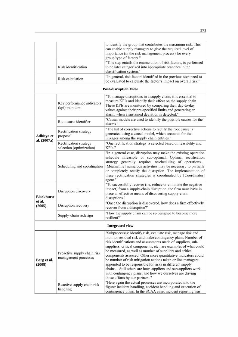
271

to identify the group that contributes the maximum risk. This can enable supply managers to give the required level of importance (in the risk management process) for every group/type of factors."

Risk identification "This step entails the enumeration of risk factors, is performed to be later categorized into appropriate branches in the classification system."

Risk calculation “In general, risk factors identified in the previous step need to be evaluated to calculate the factor’s impact on overall risk.”

Post-disruption View

Adhitya et al. (2007a)

Key performance indicators (kpi) monitors

"To manage disruptions in a supply chain, it is essential to measure KPIs and identify their effect on the supply chain. These KPIs are monitored by comparing their day-to-day values against their pre-specified limits and generating an alarm, when a sustained deviation is detected."

Root cause identifier "Causal models are used to identify the possible causes for the alarms."

Rectification strategy proposal

"The list of corrective actions to rectify the root cause is generated using a causal model, which accounts for the linkages among the supply chain entities."

Rectification strategy selection (optimization)

"One rectification strategy is selected based on feasibility and KPIs."

Scheduling and coordination

"In a general case, disruption may make the existing operation schedule infeasible or sub-optimal. Optimal rectification strategy generally requires rescheduling of operations… [Meanwhile] numerous activities may be necessary to partially or completely rectify the disruption. The implementation of these rectification strategies is coordinated by [Coordinator] agent."

Blackhurst et al. (2005)

Disruption discovery

"To successfully recover (i.e. reduce or eliminate the negative impact) from a supply-chain disruption, the firm must have in place an effective means of discovering supply-chain disruptions."

Disruption recovery "Once the disruption is discovered, how does a firm effectively recover from a disruption?"

Supply-chain redesign "How the supply chain can be re-designed to become more resilient?"

Integrated view

Berg et al. (2008)

Proactive supply chain risk management processes

"Subprocesses: identify risk, evaluate risk, manage risk and monitor residual risk and make contingency plans. Number of risk identifications and assessments made of suppliers, sub-suppliers, critical components, etc., are examples of what could be measured, as well as number of suppliers and critical components assessed. Other more quantitative indicators could be number of risk mitigation actions taken or line managers appointed to be responsible for risks in different supply chains... Still others are how suppliers and subsuppliers work with contingency plans, and how we ourselves are driving those efforts by our partners."

Reactive supply chain risk handling

"Here again the actual processes are incorporated into the figure: incident handling, accident handling and execution of contingency plans. In the SCAA case, incident reporting was

272

seen as valuable input data for improving the risk management work even further. Similarly, the focus should be on how we are working with understanding what is happening with ourselves with regard to risk sources in other parts of the supply chain, and how suppliers and sub-suppliers are doing when reaction is needed. Some indicators here could be the number of incidents handled well, number of incidents handled poorly, lead time to react and act, or how well the developed contingency plans and crisis plans are followed by the organisation when something happens."

Pyke and Tang (2010)

Readiness

"Before a potential recall, the company should implement and execute policies that improve product safety (or reduce the likelihood of having a product recall), such as TQM practices and statistical sampling inspection. It should also prepare the necessary channels in case a recall becomes necessary."

Responsiveness "During a recall, the company should create an action plan that is carried out during a recall and that allows a company to respond quickly to the problems at hand."

Recovery

"After a recall, the company should take steps to restore everything (from supply to demand) back to normal. Additionally, management should review the recall procedure, so that the company can take corrective actions (product design, process control, supplier audits, etc) to prevent or reduce the likelihood of future product recalls."

273

APPENDIX B: THE LIST OF EXPERTS FOR FRAMEWORK EVALUATION

Profession Education

1 Country Planning & Logistics Manager at

MBA, Supply Chain & Logistics Management

2 Sr. Director, Logistics Product Management

MSIE, Operations Research

3 Export Customer Service specilaist, Bachelor

4 SCM educator BA, Economics

5 Director, Supply Chain MBA, Supply Chain Management

6 Founder/President MBA, specializing in Retail Distribution

7 Director of logistics service providing company

Diploma in Carbon Management Dip TAFE

8 Quality Assurance Technician Bachelor, Technology (Chemical Engineering)

9 Asst. Manager Stores (Simplex Infrastructure)

Bachelor, Management Accountancy

10 Logistic manager Post graduate, management of production

11 SCM Analyst Business Administration

12 Supply Chain Manager Master level

13 Vice President, Logistics, Asia Pacific Region

ACCA (Certified Accountant)

14 Supply Chain Consultant CPIM, CSCP, SCOR-P, CMQ/OE

15 Founder and Chairman MBA

16 SCM Manager Business Administration & Information Technology

17 Senior Consultant Asspciates Degree in Accounting

18 VP Logistics Solutions P.Log - a Canadian post gradulate designation (Professional Logistician)

19 Supply Chain Manager Master of Business Administration (M.B.A.)

20 Manager Operational Support Savoury Ingredients

Bachelor Logistics + MBA

21 Supply chain manager and Ocean transportation expert

Bsc Agriculture Engineering

22 Chairman Fellow Chartered Institute of Logistics and Transport

23 Senior Planner -

24 University Research Fellow MSc/PhD SCM

25 Assistant Professor of Modeling and Simulation

Msc. Industrial Eng. , PhD. Computer Science

26 Senior level SCM professional, Pharmaceuticals

Bachelors in Business and Post Graduation in SCM

27 Logistics Manager -

28 SC Principal MS, Systems Engineering

274

Profession Education

29 Director, Risk Management, Supply Chain Development

EMBA, Business Administration

30 Research Associate PhD in Technology, Policy and Management

31 Director at consultancy company and professor of marketing and supply management

PhD in Marketing

32 Professor in Safety Science PhD in Physics and Mathematics

33 Professor in Systems & Simulation PhD in Technology, Policy and Management

275

APPENDIX C: THE EXTENDED STRUCTURE OF INFORMDRISC

C.1. Introduction

In Chapter 3, the overall structure of InForMDRiSC has been presented and discussed.

This overall structure includes two main cycles and several steps in each cycle as shown

in Figure 3.3. In chapter 3, each of these steps was described and some important aspects

were discussed for each step in Chapter 4. In this Appendix, we have tried to formalize

the description of steps into some sub-steps which can be used as a starting point for

further development and application of InForMDRiSC in future. The framework is also

illustrated with a case in this Appendix.

C.2. The extended structure of InForMDRiSC

As mentioned in Chapter 3, InForMDRiSC is a continuous process with two main cycles.

Each of these two cycles, their steps and sub-steps are described in the following.

Risk Management Cycle

The first cycle – that is called Risk Management Cycle- is about Potential Disruptions.

The main steps and sub-steps of Risk Management Cycle are presented in Figure C.1.

276

Figure C.1. The main steps and sub-steps of Risk Management Cycle

R1: Scope Definition& Risk Identification

R1-1: Selection of system of study

To start the process for handling disruptions, it is important to carefully define the system,

delimit its boundaries and give a clear description of the system structure (Wiendahl et al.,

2008). After decision on the system of study has been made, a map of system - which

describes the system elements and their interdependencies - should be provided. Mapping

the system might also incorporate a description of key risk management measures that are

currently in place (Harland et al., 2003).

R1-2: Describing the objectives and supply chain performance measures

As mentioned, a supply chain disruption is characterized by its impact on the

performance of supply chain and its objectives. Therefore, in addition to the system, the

critical objectives and performance measures must be addressed in defining the scope of

study. The list of Possible Consequences of disruptions will be used in the evaluation of

disruption impact in the next step of the framework – i.e., “Risk Quantification”.

R1-3: Identifying Potential Disruptions

When the system of study and the expected consequences are described, the possible

disruptions, which might result in these adverse consequences, must be identified. An

extensive list of Potential Disruptions can be generated by analysis of past losses,

R1: Scope Definition& Risk Identification

Selection of system of study

Describing the objectives and SC 

performance measures

Identifying Potential Disruptions

R2: Risk Quantification

Evaluation of Likelihood

Evaluation of Impact

Evaluation of Risk Level

Visualization in Risk Matrix

R3: Risk Evaluation & Treatment

Scanning the Risk Profile

Determining the possible treatments

Selecting the appropriate treatment 

R4: Risk Monitoring

Monitoring the Risk Profile

Monitoring the System

277

intensive literature review or insurance company checklists. Next, this extensive list

might be narrowed down to key Potential Disruptions by interviewing with employees or

meetings with experts (Canbolat et al., 2008; Yang, 2010).

Subsequently, for each Potential Disruptions, a Causal Pathway, which describes the

main causes leading to the event, needs to be developed (Norrman and Jansson, 2004;

Ritchie and Brindley, 2007). For example, the “Supplier Failure to Deliver On-time”

might be because of “Supplier Production Constraints” which itself might be caused by

“Human Resource Problems (e.g., strike in its plants)”, “Permanent Closure of a

Production Plant”, “Temporary Production Stop in a Plant” “New Customers for

Supplier”. This Causal Pathway can serve as a basis to estimate the likelihood of a

Potential Disruption or disruption ranking in the “Risk Quantification” step –especially,

for the cases in which there is not enough data to make a quantified estimation of

disruption likelihood. For instance, the likelihood of material discontinuity from a

supplier which has single plant in a specific location is higher than a supplier with similar

production capacity that is distributed between manufacturing facilities in different

geographical locations. The Causal Pathway is also used in “Risk Monitoring step” to

constantly track changes in the likelihood of disruptions over time; as an example, having

a new big customer for the main supplier of company might be a sign for the increase in

the likelihood of delay in raw material devilry from that supplier.

Finally, for each of Possible Consequences identified in previous sub-step, an Impact

Causal Pathway should be mapped. This Impact Causal Pathway determines the

Potential Disruptions that might result in a specific consequence. For instance, the

“Delay in Customer Order Delivery” can be because of several disruptions including

“Supplier Failure to Deliver On-time”, “Transportation Disruptions”, “Rush Order

Acceptance” or “Internal Process Failure”. This Impact Causal Pathway is used in

“Disruption Detection Step” when the root cause of performance deviation is not

observable in the first place (Adhitya et al., 2007).

So, with these three sub-steps, “System Definition& Risk Identification step” provides a

company with:

A Risk Catalogue which consists of a list of Potential Disruptions and for each of

them, the expected consequences and disruption Causal Pathway is described.

An Impact Causal Pathway which is a list of Disruptions leading to each

Consequence.

R2: Risk Quantification

278

R2-1: Evaluation of Likelihood

One of the dimensions in the evaluation of each Potential Disruption is the likelihood or

frequency of its occurrence. The historical data can be the main source to estimate the

disruption likelihood. However, in the absence of adequate and accurate data, a company

may use other approaches to estimate the probability of disruptions, e.g. expert opinion,

simulation or combination of these methods (Knemeyer et al., 2009). The Causal

Pathway, developed in Risk Identification step, can support decision makers to have an

estimation of disruption likelihood, especially when they want to rank different

disruptions rather than having an absolute value of the likelihood of disruptive event. For

instance, the probability of delay in raw material delivery from a supplier with one

factory and several important customers is higher than a supplier which has several

factories around the world and the focal company is its main customer.

R2-2: Evaluation of Impact

Each disruption may influence multiple objectives of a company and consequently, have

a range of Possible Consequences. Determining all these consequences in a complex

network of actors and activities can be a challenge for most companies. Accordingly,

using modeling and simulation to evaluate the impact of disruption is very much

suggested (Wu et al., 2006; Wilson, 2007; Wagner and Neshat, 2010). Similar to

likelihood estimation, the evaluation of impact can be based on semi-quantitative ranking

methods too.

R2-3: Evaluation of Risk Level

Having the likelihood and impact of disruption, the Risk Level can be calculated by

multiplying these two dimensions. The Risk Level calculated for all Potential Disruptions

is used for making decision on whether an identified disruption needs to be treated in the

next step of the framework.

R2-4: Visualization in Risk Matrix

Risk Matrix (also known as Risk Diagram (Hallikas et al., 2004) or Risk Map (Berg et al.,

2008)) is a visual output of Risk Quantification step which demonstrates the relationship

between impact and likelihood of all disruptions in two axes (Figure C.2). This graphical

representation of Potential Disruptions helps decision makers to get an overall (and quick)

insight of the Risk Profile of the company and the important disruptions which need

treatment (Hallikas et al., 2004).

279

The output of Risk Quantification step is a Risk Profile for company that includes the

Risk Catalogue and the Risk Level for each of Potential Disruptions. This Risk Profile –

that can be presented in a Risk Matrix- is the basis for further analysis in the next step-

i.e., Risk Evaluation and Treatment.

Descriptor Rare Unlikely Possible Likely Very likely

Descriptor Rating 1 2 3 4 5

Insignificant 1 1 2 3 4 5

Minor 2 2 4 6 8 10

Moderate 3 3 6 9 12 15

Major  4 4 8 12 16 20

Catastrophic 5 5 10 15 20 25

Impact

Likelihood

Figure C.2. An example of Risk Matrix and rating system

R3: Risk Evaluation & Treatment

R3-1: Scanning the Risk Profile

The first action is to go over the Risk Profile and determine whether the Risk Level for

Potential Disruptions is acceptable or mitigation actions and safeguards must be provided.

For this purpose, a firm may define a threshold for acceptable Risk Level (Harland et al.,

2003). Comparing the Risk Level for each Potential Disruption in the Risk Profile with

that acceptable level separates the disruptions into minor (acceptable) and major

(unacceptable) ones.

R3-2: Determining the possible treatments

For unacceptable disruptions the possible treatment options must be identified. Using the

Causal Pathway can be beneficial in finding alternative treatments for a disruption

(Norrman and Jansson, 2004). For example, selecting a certified supplier will reduce the

probability of order rejection due to unsatisfactory quality and also the late raw material

delivery.

R3-3: Selecting the appropriate treatment

280

The possible treatments for each Potential Disruption must be evaluated and the

appropriate treatment must be selected. This evaluation must be based on a systemic view:

- The impact of implementing risk mitigation measures on the daily operation of

supply chain must be also considered and taken into account (Sheffi, 2005).

- Choosing a risk mitigation approach for a specific disruption may increase the

Risk Level for other disruptions (Olson and Wu, 2010). This influence must be

also considered in selecting risk mitigation approaches.

- A specific risk mitigation approach may address more than one Potential

Disruption in a supply chain; so, it is recommended to consider whole Risk

Profile – and not single disruptions- in selecting the safeguards (Knemeyer et al.,

2009). In this way, the resources invested to mitigate the risk of one specific

disruption might be also deployed as alternative solutions for other disruptions.

The resources which can be shared between different disruptions or used to

handle more than one - not necessarily as the first priority but maybe as a

secondary option- are called Movable Resources. Having a list of Movable

Resources is extremely beneficial for Disruption Recovery step when the first

reaction to a disruptive event is not effective and decision makers start looking for

new options to manage disruption.

R4: Risk Monitoring

R4-1: Monitoring the Risk Profile

The Risk Profile of company must be monitored constantly. Some new disruptions might

be identified which were not recognized before in Risk Identification step. Moreover, for

the Potential Disruptions that are currently documented in the Risk Profile, the likelihood

and expected impact needs to be updated with new information gathered by company and

- if necessary - the disruption treatment must be improved (Blackhurst et al., 2005). The

Causal Pathway of Potential Disruptions can be used as a guide to recognize the changes

need to be monitored. For example, having a contract with a big competitor of focal

company can be a signal for higher likelihood of delay in raw material shipment from that

supplier in future. It can be also considered an early warning sign that the intellectual

property of company is increasingly at risk.

R4-2: Monitoring the System

Besides the Risk Profile, the system boundaries and structure may change in different

ways. For example, a new supplier might be added to the supply base, a new warehouse

281

might be launched or a new set of products might be introduced to the market. As a result

of these changes in the supply chain, the system definition –that is the starting point of

whole disruption management process- would change from time to time. Thus, it is

imperative to repeat whole Risk Management Cycle by a new definition for the system

and identifying the new disruptions. In addition, the Risk Level for currently-listed

disruptions in the Risk Profile might need to be updated –because of interdependencies

between different risk factors.

Disruption Management Cycle

The second cycle is Disruption Management Cycle. Despite enough safeguards, at a

specific point, an Actual Disruption may happen. The main steps and sub-steps of

Disruption Management Cycle are presented in Figure C.3 and discussed in the following.

Figure C.3. The main steps and sub-steps of Disruption Management Cycle 

D1: Disruption Detection

Detecting a disruption can take two forms. The first case is when an actor can directly

observe (or being informed by other partners of) the occurrence of an event in a part of

supply chain (type-A). For example, a supplier may send a message that there is an

emergency shutdown in one of its plants which may cause delay in raw material shipment

to the manufacturer. However, in some other cases, a firm can see solely the impact of

disruptive events on its performance and it needs to explore the cause of deviations (type-

B).

D1: Disruption Detection

Monitoring the performance and deviation detection

Deviation analysis and root‐cause 

determination

Disruption impact analysis

Event monitoring and information gathering

D3: Disruption Recovery

Determining the alternative options

Selecting and implementing the appropriate option

Event monitoring and information gathering

D4: Disruption Learning

Improving the Risk Profile

Improving the Response Plan

Supply network re‐configuration

D2: Disruption Reaction

Implementing the Response Plan

Evaluation of effectiveness of Response Plan

Event monitoring and information gathering

282

Each of these two types of Disruption Detection calls for different actions to be done and

needs different types of capabilities. In following the necessary actions are discussed in

more detail. The first two actions are exclusively to type-B detection:

D1-1: Monitoring the performance and deviation detection

Fast detection of disruptions in a supply chain calls for enhancing visibility and

developing advanced monitoring systems which tracks performance indicators over time

to identify deviations and determine if they are reaching unacceptable level (Christopher

and Lee, 2004; Blackhurst et al., 2005; Adhitya et al., 2007). For this purpose, pre-

defined limits for the performance indicators can be defined and based on these control

limits, early warning alarms of disruption occurrence might be generated (Blackhurst et

al., 2008). Moreover, a sustained trend toward unacceptable level – even if performance

measures are within acceptable limits- could be flagged as a possible disruption.

D1-2: Deviation analysis and root-cause determination

As a deviation in the performance is identified, a company must find the main factors that

cause that abnormality in the supply chain operation (Blackhurst et al., 2005). The cause

of deviation can be one of Potential Disruptions identified and documented in the Risk

Profile or a new type of disruption which has been overlooked in Risk Identification step.

For type-A detection in which the disruptive event is known or informed by other

partners in the network, the necessary action is evaluating the impact of that event on the

planned and normal operation of supply chain. This is further elaborated under following

sub-step.

D1-3: Disruption impact analysis

After a company is informed about a disruptive event in one part of the supply chain, the

first action must be the assessment of disruption impact on the operation of supply chain.

This assessment might take two forms. A disruption might push the performance

measures out of acceptable range (Adhitya et al., 2007; Wilson, 2007) or make the

operational plans non-optimal or even infeasible (Qi et al., 2004; Yu and Qi, 2004). Each

of these two conditions can be called as an Abnormal Situation in the supply chain and

needs organization to take actions and response to the situation. Conversely, when, none

of performance indicators goes out of acceptable range or there is no significant impact

on the pre-defined plans, then the situation will not be an Abnormal Situation; no

intervention is needed and company can continue with its regular operation. The

283

important point here, however, is that the impact of disruptive event, in some cases, is not

necessarily immediate; it takes time for the abnormality to show its full impact on the

system performance. For example, an earthquake in a specific region may have no

immediate influence on the supply base of company but because of transportation

difficulties, the production in 2nd or 3rd tier suppliers might be halted. The delays and

supply disruptions in the higher tier suppliers can cause a domino effect and impact the

supply base of focal company and after a while, production in focal company might be

stopped because of raw material shortage. With appropriate modeling and simulation

tools, a firm can have an estimation of possible consequences of a disruptive event and

determine if (and, approximately, when) that initial event may lead to unacceptable

consequences in the system (Tuncel and Alpan, 2010; Behdani et al., 2010a). With

significant importance of speed of response, this ability to predict a problem before it

occurs can be a critical issue in handling disruptions.

For both types of disruption detection discussed here, continuous monitoring of

disruptive event is an essential action. This is further discussed as following sub-step.

D1-4: Event monitoring and information gathering

A disruptive event is a dynamic phenomenon and its state can change frequently

(Blackhurst et al., 2005). In addition, when disruptions occur the downstream actors may

have little or inaccurate information about the disruption; firstly, because the supplier’s

estimation of the problem might be biased and secondly, it might not be feasible for the

firms to have all related information in the early stages of disruption (Chen et al., 2010).

Accordingly, a supplier which previously announced a shutdown in one of its plants may

give an update on the time of returning to normal operation or a new expected time for

order delivery. Considering all these aspects, it is imperative for company to continuously

monitor the event, gather information from different sources and exchange information

with other actors in the chain.

D2: Disruption Reaction

D2-1: Implementing the Response Plan

The first action to handle an Actual Disruption is implementing the Response Plan as

quickly as possible. How prepared and trained the response actors are and how

coordinated they perform in the real-time are important factors in successful

284

implementation of the response plan. In addition, the pre-defined response plan might

need adjustment based on the current situation of supply chain.

D2-2: Evaluation of effectiveness of Response Plan

After implementing the Response Plan, its effectiveness in returning system to the normal

operation must be evaluated. If this plan cannot successfully recover system, it is

necessary to continue with next step – Disruption Recovery- to find alternative solutions.

D2-3: Event monitoring and information gathering

Collecting and analyzing information about the disruptive event and the action of other

actors in handling the disruptive event – for example, the actions done by supplier to

return its plant to normal production after an emergency shutdown- is still an important

action. With initial information on the scope of disruption, the first response might seem

adequate; however, by gathering more information or by updates from other actors in the

chain, it might be necessary to look for some other options to cope with the full impact of

disruption.

D3: Disruption Recovery

D3-1: Determining the alternative options

To define alternative solutions, a company must have the ability to:

Estimate the Necessary Resources to manage disruption (Charles et al., 2010):

based on the impacted area in the supply chain and the expected duration for a

disruptive event, an estimation of Necessary Resources can be made.

Determine the Available Resources to manage disruption: a list of resources that

are available and can be used in managing disruption must be created. Examples

of Available Resources to handle the supplier emergency shutdown are the

available material in storage facilities or in-transit raw material (the material

which has been order but has not arrived to the factory) shipments.

Find Alternative Resources: In addition to the resources which are still available

for a company, it must start looking for Alternative Resources across its supply

chain. The list of Movable Resources determined previously in Risk Evaluation

and Treatment step is beneficial for this purpose. Search for Alternative Resources

might also necessitate close collaboration with other partners in the network and

sharing some of resources with others.

285

It must be emphasized that preparing resources for Disruption Recovery step can start in

parallel with first response in Disruption Reaction step (Sheffi, 2005). For example, when

rescheduling the orders might be a first response to raw material delay from a supplier,

qualifying new suppliers and finding customers that might be willing to re-negotiate their

due-dates can be followed at the same time. Matching the Available Resources and

Alternative Resources with Necessary Resources would lead to a primary list of options

to cope with disruption.

D3-2: Selecting and implementing the appropriate option

With a list of preliminary alternatives, the appropriate option must be selected and

implemented. Selecting the proper option to manage disruption can be an iterative

process which starts with finding and executing a first response to a disruptive event and

based on the feedback of the effectiveness of that action, the system/disruption

information can be updated and a new action might be implemented. This iterative

process is especially important because of the critical role of time in disruption response

and also the uncertainty about the event and current status of supply chain. The process

must continue until system returns to its normal operation.

To better –and faster- evaluate the alternative options in this step, using modeling and

simulation would be of considerable benefit (Adhitya et al., 2007; Tuncel and Alpan,

2010).

D3-3: Event monitoring and information gathering

Similar to Disruption Detection and Reaction steps, continuous monitoring of disruptive

event (and information exchange with other actors in the network) is critical in this step

of framework.

D4: Disruption Learning

D4-1: Improving the Risk Profile

Based on company’s experience with a real disruption, it can update its estimation of

likelihood and impact of that type of disruption in the Risk Profile. Moreover, during

handling a specific disruption, some new disruptions might be identified that were not

identified before or being considered as less significant ones (Cheng and Kam, 2008).

D4-2: Improving the Response Plan

An Actual Disruption in supply chain gives a company the opportunity to test and verify

the response plans with a real case (Norrman and Jansson, 2004). By reviewing the

286

effectiveness of existing plans to handle an Actual Disruption, the gaps in the existing

plans can be identified and the strengths of plans can be kept or will be used as a basis for

defining some new emergency plans.

D4-3: Supply network re-configuration

Once the company recovers from disruption, it may decide to redesign the supply chain

with the goal of minimizing the probability or impact of similar disruptions in future

(Blackhurst et al., 2005). For example, a new warehouse might be added to the current

supply network or a new contract might be signed with a local supplier. These

modifications in a supply chain imply changes in the system structure and its boundaries

and accordingly, it is a necessity to repeat the Risk Management Cycle by identifying new

Potential Disruptions.

C.3. The illustrative case

R1: Scope Definition& Risk Identification

To illustrate the steps of framework and their interrelations, the activities done by an

Asian chemical company to handle the disruption in its supply-base has been described

here1.

The structure of supply chain of company is presented in Figure C.4. The focus of

disruption management study in this case, is solely on the supply base of company which

consists of 11 suppliers for 7 different raw materials. Different suppliers in the supply

base have different characteristics. For example, they are located in different places.

However, most of suppliers are local suppliers (located less than 500 km from focal

company). The only exception is supplier1 which its sole production facility is located in

Europe. In the same way, the available information about each supplier and its past

performance was gathered before starting the disruption management process.

1 The examples are motivated by a case study of risk management in a pharmaceutical company. The readers can find more details of the case in Li (2011).

287

RM1 

RM2 

RM3 

RM4 

S1 

S2 

S3 

M 

W 

W 

C1 

C2 

C3 

C4 

..., ..., 

 

RM5 

RM6 

RM7 

S4 

S5 

S6 

S7 

S8 

S9 

S10 

S11   

S: Supplier RM: Raw Material M: Manufacturer W: Warehouse C: Customer  

Figure C.4. Schematic of supply base of company

The first step in managing disruptions in the supply base was recognizing what factors

might go wrong that will have adverse influence on the supply chain operation. With

several sessions of brainstorming and the review of checklists, the disruption

management team, consisting of supply chain manager and representatives from

operation, storage, procurement, sales and logistics departments, has identified four

important categories of Potential Disruptions in the supply base:

• Supplier Failure to Deliver On-time: a supplier does not fulfill the promised

delivery dates for the raw materials.

• Quality Problems in Raw Material: the material shipped to the plant does not meet

the quality specifications.

• Transportation Disruption: a significant delay or temporary stoppage of raw

material delivery occurs due to, e.g., transportation incidents, natural disasters or 3PL

mishandling.

288

• Permanent Loss of Supplier: the supplier goes out of business (e.g., because of

bankruptcy) or stops producing a specific product (e.g., because of new safety and

environmental regulations).

Table C.1. Examples of Potential Disruptions in the supply base Disruption Group Specific Disruption in Supply Chain

Supplier Failure to Deliver On-time

Dis1- Delay in shipping RM1 from supplier1 Dis2- Delay in shipping RM2 from supplier2 Dis3- Delay in shipping RM2 from supplier3 Dis4- Delay in shipping RM3 from supplier4

Quality Problems in Raw Material

Dis5- Quality problem in RM1 from supplier1 Dis6- Quality problem in RM2 from supplier2 Dis7- Quality problem in RM2 from supplier3 Dis8- Quality problem in RM3 from supplier4

Transportation Disruption

Dis9- Transportation disruption in RM1 delivery from supplier1 Dis10- Transportation disruption in RM2 delivery from supplier2 Dis11- Transportation disruption in RM2 delivery from supplier3 Dis12- Transportation disruption in RM3 delivery from supplier4

Permanent Loss of Supplier

Dis13- Permanent loss of supplier1 Dis14- Permanent loss of supplier2 Dis15- Permanent loss of supplier3 Dis16- Permanent loss of supplier4

These generic groups of possible disruptions were then specialized for the specific system

of Figure C.4. As an illustration, a list of Potential Disruptions in the part of supply base

which is restricted by dashed box is presented in Table C.1.

The possible impacts of disruptions on supply chain operation were also categorized in

four main areas:

• Excess Operational Cost

• Reduced Sales

• Poor Delivery Performance

• Damaged Reputation

289

Supplier Production Constraints

Ineffective Communication with Suppliers

Raw Materials Stock-out

Human Resource Problems (e.g., Strike)

IT Infrastructure/Communication Standard Inconsistency

Permanent Closure of a Production Plant

Temporary Production Stop in a Plant

New Customers for Supplier

Cultural Differences

Lack of Visibility and Adequate Information Sharing

Excess Operational Cost

Poor Delivery Performance

Transportation Disruption

Temporary Infrastructure Unavailability

Transportation Congestion in the Main Ports

Sudden Changes in Weather Conditions

Natural Catastrophes

Capacity Constraints

Additional Inspections in Ports

Strike in Transportation System

...

...

...

...

...

...

...

...

...

...

...

...

Damaged Reputation

Disruption Causal Pathway  Potential Disruptions  Expected Consequences

Supplier Failure to Deliver On-time

Quality Problems in Raw Material

Material Degradation during Transportation and Handling

Supplier Inability to Meet Required Quality

Long Transportation Time of Raw Materials

Unskilled Third-part Logistics (3PL) Company

Supplier Subcontracting

Unclear Quality Requirements in Supply Contracts

Working with Unqualified Suppliers

Permanent Loss of Supplier

Supplier Financial Problem

Changes in Supplier Strategies

Security and Regulation Issues

Supplier’s Switching to New Products

Lack of Financial Health Checking in Supplier Selection Process

New Safety Regulations on Specific Materials

Unprofitable Production due to Technology Outdating

...

...

...

...

...

...

...

...

...

Quality Issues in Final Product

Supplier’s Switching to New Markets ...

Lack of Supplier Incentive for On-time Delivery

Ineffective Supplier Selection Process

Inappropriate Contact Setting with Supplier

...

...

Reduced Sales

Supplier Location in Plotically-unstable or High-risk Natural Disaster Areas...

Unacceptable Performance Delivery of 3PL

Ineffective Selection Process for 3PL

Inappropriate Contact Setting with 3PL

...

...

Ineffective Communication with 3PL...

Figure C.5. A part of Causal Pathway for identified disruptions 

290

The last three factors are impacting the revenue generation across supply chain and the

first factor is the impact of disruption on the cost of production. Therefore, in general, the

profitability of company is being impacted by Potential Disruptions in the supply chain1.

For the Potential Disruptions, the Causal Pathway -which shows the development path

for disruptions and possible root cause relationships - is also created. Part of the Causal

Pathway is presented in Figure C.5. Thus, for example, the stock-out of RM2 might be

because of delay in shipping RM2 from supplier2/3, transportation disruption in RM1

delivery from supplier2/3 or permanent loss of supplier2/3. Each of these Potential

Disruptions might be caused by several other factors in the supply chain. For instance,

delay in shipping RM2 from supplier2 might be because of miscommunication with

supplier2 (on the delivery date), production constraint in supplier2 (because of, e.g.,

emergency shutdown in one of facilities) or lack of suppliers’ incentive for on-time

delivery. This Causal Pathway is frequently used in the succeeding steps of disruption

management process.

R2: Risk Quantification

To evaluate the risk level for each potential disruption, a 5×5 matrix has been used

(Figure C.6) in risk quantification step. The members of disruption management team

were asked to rate the likelihood and the impact of disruption in the five-class scale. To

support participants in their evaluation, the available historical data for the supplier’s

performance and also past events in the supply base were firstly discussed in a session.

The Causal Pathway of Figure C.5 was also used as a support to have a comparison of

the relative likelihood of different disruptions. Examples of arguments that have been

done based on the Causal Pathway are as following:

• As the supplier1 has single production plant and it is also the only global supplier in

the supply base, the likelihood of delay from this supplier and also the probability of

transportation disruption in raw material delivery is higher than other suppliers. Moreover,

the long distance of supplier may impact the quality of RM1 that is delivered to the plant.

1 The list of impact areas considered here are the short-term and direct negative impacts of disruption. However, it must be emphasized that the impact areas are not totally independent as the “Poor Delivery Performance” might impact the “Damaged Reputation” of company and together, they might result in “Reduced Sales” in the mid- and long-term. Consequently, the “Reduced Sales” might consist of both short-term lost sales because of unavailability of products and the mid- and long-term indirect effect of damaged corporate image.

291

• As supplier4 is the only supplier with no quality certification (e.g., ISO 9001), the

probability of quality issues in raw material delivery from this supplier is higher than

others.

• Limited number of suppliers in the market can produce RM3; consequently, the

permanent loss of supplier4 would have a high impact on the supply chain as finding

alternative supplies might be a challenge and take a while.

Figure C.6. Part of Risk Catalogue and its mapping in Risk Matrix 

After the rating for likelihood and impact was assigned, by multiplying the likelihood and

impact, a Risk Score for each potential disruption was calculated. The list of Potential

Disruptions and the risk level for each disruption has formed the Risk Catalogue of

company. Part of this Risk Catalogue is presented in Figure C.6. The potential disruptions

are also mapped in the risk matrix.

292

R3: Risk Evaluation & Treatment

After the risk scores were evaluated for all identified disruptions, the disruption

management team had a meeting to discuss the possible treatments for these disruptions.

Considering the available resources for investing on disruption management, the team

decided to firstly focus on the disruptions for which the risk score is higher than 8 (or

disruptions in the orange and red area).

Figure C.7. The possible treatment for Dis1 and Dis9 

Possible options to manage four selected disruptions (Dis1, Dis7, Dis8 and Dis9) were

discussed. For example, to reduce the impact of Dis1 (Delay in RM1 from supplier1) and

Dis9 (Transportation disruption in RM1 delivery from supplier1), the disruption

management team came to agreement of considering an excess buffer of 20 percent for

RM11. This option was expected to reduce the risk score of Dis1 to 6 and the risk score of

Dis9 to 9 (Figure C.7). However, the risk level of Dis9, after this treatment, was not yet

in the acceptable area; accordingly, for the cases for which this extra buffer is not

adequate to handle the delay, two contingencies have been discussed and agreed upon by

the team members:

• Rescheduling the production of customer orders: delay in raw material delivery can

create some constraints for production; however, if possible and none of customer orders

would be delayed, the scheduling departments must change the timing of some part of

production. Moreover, as part of the rescheduling procedure, a rating system has been

suggested to classify the customers based on their importance for re-negotiating the order

delivery date.

1 As can be seen, one disruption management action in the mitigation of risk for more than one potential disruption. This systemic view is an important aspect in selection of possible treatments for disruptions in supply chain.

293

• Emergency procurement: a detailed emergency procurement procedure has been

developed by disruption management team. Operation Department must determine the

“quantity” and “expected delivery” of RM1 order, based on the existing backlog of orders,

and send the raw material request to Scheduling Department. After approval by

Scheduling Department, Procurement Department starts looking for alternative suppliers

or buys the raw material on the spot market.

The other example of risk treatment in this chemical supply chain is changes that were

suggested in supplier selection process and contract setting with suppliers. For instance,

as a part of supplier selection, the candidate suppliers must be asked to send a copy of

their quality system certifications. Suppliers who are not third-party certified shall present

their plan for management of quality and may be subject to a Quality Management

System audit by focal company. In addition, adding more clear requirements to current

contract format was also being discussed by team members. Moreover, subcontracting

must be explicitly banned in the contract terms1.

With these changes in the contracts, it is expected that the quality issues with suppliers

will be reduced in future.

As can be seen, the Causal Pathway of Figure C.5 gives lots of support in finding

appropriate mitigation approaches for supply chain disruptions.

R4: Risk Monitoring

Several changes in the supply chain might introduce new Potential Disruptions or change

the risk level for currently-identified disruptions. A list of the changes - which must be

regularly monitored in the supply base - was being discussed by disruption management

team in a session. To give some examples:

• Changes in the supply chain of suppliers: e.g., having new contracts with new

customers or switching to new suppliers.

• Changes in the daily operation of suppliers: e.g., operational problems in supplier’s

facility and plant closure2 or dispute about a labor strike in the supplier’s region.

1 The raw material order might be subcontracted to other companies by supplier – either because it might run out of capacity or because it wants to widen the profit margin. With subcontracting the chance of a quality issues will be higher as the subcontractor might be an uncertified company. 2 To better monitor supply chain operation, the suppliers have been obliged in the contracts to inform the manufacturer of any shutdown in their plants - even if it does not result in the late raw material delivery- within 48 hours.

294

• Changes in the transportation system: e.g., the news for a potential strike in the port

of delivery or airline industry.

• Changes in the regulations: e.g., any international or national dispute to ban some

materials that is somehow used in the production process of company or its suppliers.

In addition, the Supplier Scorecard in two areas of “On-Time Delivery” and “Received

material Quality” has been designed to track the Suppliers’ overall performance. These

scorecards are also considered as criteria in awarding new contracts in future or extending

the current contracts with the suppliers. The supplier scorecard is reported to each

supplier on a quarterly basis to create motivation for performance improvement.

The supply chain disruption management team has also agreed to have similar meetings

for supply chain risk management whenever:

• A new product line is established in the plant.

• A new supplier is added to supply base.

• A new 3PL or transportation rout has been considered for raw material delivery.

D1: Disruption Detection

Disruption management team has identified three important aspects when a supply chain

disruption happens:

• Visibility and information sharing across departments: When a disruptive event is

announced in the supply base – regardless of the perception of each actor of the severity

of disruption – its occurrence must be urgently disseminated to other departments in the

plant. For example, if storage department is informed by a supplier of a delay in raw

material delivery, it must immediately pass the information to other departments. This

information might impact the decisions made by each of department - e.g., order

acceptance pattern by sales department- and accordingly, it would influence the severity

of event.

• Team formation: when a disruption happens, the disruption response team must be

quickly formed. The response team is a cross-functional team and consists of supply

chain manager and representatives from operation, storage, procurement, sales and

logistics departments. To better manage the response activities, supply chain manager is

assigned as the coordinator of disruption response.

• Analysis of disruption impact: at the first stage, the response team must have an

overview of the impact of disruption on the plant operation. Will plant production be

295

influenced by this disruption? Is it necessary to have a response to disruption? What are

the possible areas might be impacted by disruption? …

To give an example of reaction to an Actual Disruption in the supply chain, the firm’s

response to a disruptive event is discussed here.

The disruption was a late raw material delivery: supplier1 sent a message that because of

a trouble in the production facilities, it had to shut down the whole plant and accordingly,

the raw material orders would be shipped with one week delay.

Receiving the message, the response team was formed and, as the first essential step, an

evaluation of the impact of this delay on the performance of the plant was made. The

evaluation showed that, with the current inventory and the current schedule of orders, a

10-day delay in raw material shipment can be tolerated by the plant without any

significant effect on the downstream of the supply chain.

Although the effect of this delay was minor and insignificant, the supply chain manager

continued the contact with supplier1 to check the status of their plant. Finally, 5 days

after the first announcement, supplier1 came with a second message about the full scope

of the disruption. The company now realized that it would take 4-6 weeks for the supplier

to restore its normal and full operation.

D2&3: Disruption Reaction & Recovery

To better react to a disruption in supply chain, disruption management team has

documented a process with three main steps:

• Implementing the response plan: the predefined disruption response must be the

first reaction to the event as it helps a faster response. Moreover, it would reduce the

confusion of response process because the aspects of this plan have been extensively

discussed before in risk treatment step.

• Option finding: the response team must set brainstorming sessions to find

alternative options for handling disruptions.

• Option analysis: the possible options for managing a disruption must be analyzed

based on the “cost of implementation” and “time of implementation”.

Continuing the case of disruption in raw material delivery from supplier1, the first

reaction was rescheduling the production of customer orders. This option helped the plant

to process more orders with the available raw material in the storage.

296

The company also started implementing the emergency procurement plan. However,

because of complicated process and the amount of needed material, it took 5 days for the

plant to find an alternative source and make an agreement. The emergency raw material

was agreed to be delivered in one week and the plant could continue operation. However,

the maximum delay that could be tolerated was 10 days; so, additional actions were

necessary.

In the mean-time and before receiving the emergency order, the sales department had to

contact some of the customers and start negotiation for extending their orders’ due date.

Moreover, to return and keep the system in the normal zone of operation, the operations

department made some changes in the recipe of some of the products.

With all these efforts, the company could manage the disruption and return its system to

the normal operation; it could meet the production target and prevent the disruption from

affecting most of customers. The recovery step ended when supplier1 could have a full

return to its nominal production.

D4: Disruption Learning

Disruption management team has defined a formal procedure for sharing the experience

of different actors and documenting the possible lessons from disruption management

process. This procedure consists of several brainstorming meetings in which response

team members discuss the necessary changes in the current processes and how the supply

chain operation and strategies must be modified to mitigate similar disruptions in future.

Examples of aspects must be discussed in these meetings are:

• Is it necessary to change the disruption response plans?

• Is it necessary to change supply-based strategies (e.g., contract settings or supplier

selection criteria) or supply chain structure (e.g., changing some suppliers or adding new

suppliers to the supply base)?

• Could actors – which were involved in the management process - work effectively

together?

• Is it necessary to update the previously-estimated likelihood and impact of

disruption with the experience company had in managing an actual disruption?

For example, for the case of disruption in supplier1, once the company could recover

from the disruption, the disruption management team set a session to discuss the lessons

297

that could be learned from the event. All team members agreed that the response plan

(emergency procurement) was slow and they discussed the necessary changes to improve

the plan. Particularly, to make the process faster, they removed the scheduling

department’s approval from the plan. Moreover, to reduce the probability and impact of

similar disruptions in the future, they decided to redesign the supply chain and consider a

reserve local supplier for RM1.

299

APPENDIX D: SUPPLY CHAIN DISRUPTION/RISK LITERATURE

Reference

Elements of Framework Covered by Literature1 Research Method used in the Research Literature

Disru

ption

Detection

Disru

ption R

eaction &

R

ecovery

Disru

ption

Learn

ing

Risk

Iden

tification

Risk

Quan

tification

Risk

Evaluation

&

Treatm

ent

Risk

mon

itoring

Th

eoretical/concep

tual

work

s

Qualitative Quantitative

review

Surveys and

Interview

s

Case stu

dy

Em

pirical (S

tatistical analysis

of emp

irical data)

An

alytical m

odeling (and

optim

ization)

Simulation

modelin

g

Adhitya et al. (2007a) +++ +++ * * Adhitya et al. (2007b) +++ * * Adhitya et al. (2009) +++ + * * Appelqvist and Gubi (2005) + * Babich (2006) ++ * Bakshi and Kleindorfer (2009) ++ * Berg et al. (2008) + + + + + * * * Bichou (2004) ++ * Blackhurst et al. (2005) +++ +++ +++ ++ ++ * * Blackhurst et al. (2008) +++ + +++ * Blos et al. (2009) +++ ++ * Bogataj and Bogataj (2007) ++ ++ * Braunscheidel and Suresh (2009) ++ ++ * Burke et al. (2007) ++ * Canbolat et al. (2008) +++ ++ +++ * *

300

Reference

Elements of Framework Covered by Literature1 Research Method used in the Research Literature

Disru

ption Detection

Disrup

tion R

eaction &

Recovery

Disrup

tion L

earning

Risk Identification

Risk Q

uan

tification

Risk E

valuation

&

Treatm

ent

Risk m

onitoring

Th

eoretical/concep

tual

works

Qualitative Quantitative

review

Su

rveys and

In

terviews

Case stud

y

Em

pirical

(Statistical an

alysis of em

pirical d

ata)

Analytical

modelin

g (and

op

timization

)

Sim

ulation

m

odeling

Cavinato (2004) +++ * Charles et al. (2010) + + + * * Chao et al. (2009) ++ * Chen et al. (2010) ++ * Cheng and Kam (2008) +++ + * Choi and Krause (2006) ++ * Chopra and Sodhi (2004) +++ +++ * Chopra et al. (2007) ++ * Christopher and Lee (2004) ++ ++ * Christopher and Peck (2004) ++ ++ +++ +++ Cigolini and Rossi (2010) + + * Colicchia et al. (2010) ++ + ++ * Cucchiella and Gastaldi (2006) ++ ++ * Dani and Deep (2010) +++ ++ * Deane et al. (2009) + ++ Ellegaard (2008) ++ * Enyinda and Tolliver (2009) + ++ * Enyinda et al. (2010) ++ * Faisal et al. (2006) +++ + * * Faisal et al. (2007) +++ ++ ++ * * Finch (2004) +++ * Gaonkar and Viswanadham (2007) +++ ++ * * Gaudenzi and Borghesi (2006) +++ * * Glickman and White (2006) + + ++ * Goh et al. (2007) + * Hale and Moberg (2005) ++ +++ * Hallikas et al. (2004) ++ + * *

301

Reference

Elements of Framework Covered by Literature1 Research Method used in the Research Literature

Disru

ption Detection

Disrup

tion R

eaction &

Recovery

Disrup

tion L

earning

Risk Identification

Risk Q

uan

tification

Risk E

valuation

&

Treatm

ent

Risk m

onitoring

Th

eoretical/concep

tual

works

Qualitative Quantitative

review

Su

rveys and

In

terviews

Case stud

y

Em

pirical

(Statistical an

alysis of em

pirical d

ata)

Analytical

modelin

g (and

op

timization

)

Sim

ulation

m

odeling

Harland et al. (2003) +++ * * Hendricks et al. (2009) +++ * Huang et al. (2006) + + * Huang et al. (2009) + ++ * Iakovou et al. (2010) ++ * Ji (2009) +++ * * * Jüttner (2005) +++ ++ * Kavčič and Tavčar (2008) ++ * Khan and Burnes (2007) +++ +++ * Kim et al. (2010) ++ * Kleindorfer and Saad (2005) +++ ++ ++ * * Knemeyer et al. (2009) ++ ++ * Kull and Closs (2008) +++ * Kull and Talluri (2008) + ++ +++ * * * Kumar et al. (2010) ++ ++ * * Levary (2007) ++ ++ + * * Levary (2008) + + + * * Li et al. (2006) + + * * Manuj and Mentzer (2008) +++ +++ * Matook et al. (2009) + +++ * * Micheli et al. (2008) ++ ++ * * Mohtadi and Murshid (2009) ++ * Mudrageda and Murphy (2007) ++ * Munoz and Clements (2008) ++ + * Norrman and Jansson (2004) +++ * Oehmen et al. (2009) ++ + * * Oke and Gopalakrishnan (2009) +++ +++ * *

302

Reference

Elements of Framework Covered by Literature1 Research Method used in the Research Literature

Disru

ption Detection

Disrup

tion R

eaction &

Recovery

Disrup

tion L

earning

Risk Identification

Risk Q

uan

tification

Risk E

valuation

&

Treatm

ent

Risk m

onitoring

Th

eoretical/concep

tual

works

Qualitative Quantitative

review

Su

rveys and

In

terviews

Case stud

y

Em

pirical

(Statistical an

alysis of em

pirical d

ata)

Analytical

modelin

g (and

op

timization

)

Sim

ulation

m

odeling

Olson and Wu (2010) +++ * Olson (2010) + * Parmar et al. (2010) ++ * Papadakis (2006) + * Peck (2005) +++ ++ * * Pujawan and Geraldin (2009) ++ + ++ * * Pyke and Tang (2010) ++ ++ ++ ++ * * Ratick et al. (2008) ++ * Ravindran et al. (2010) + ++ * * Ritchie and Brindley (2007) ++ + * * Ross et al. (2008) ++ * Roth et al. (2008) ++ * * Sanchez-Rodrigues et al. (2010) ++ ++ + * Schoenherr et al. (2008) +++ ++ ++ + * Sheffi (2005) ++ ++ * Sheffi and Rice (2005) ++ +++ * Sinha et al. (2004) ++ ++ * Sodhi (2005) + ++ * Sodhi and Lee (2007) +++ + * Stecke and Kumar (2009) +++ + +++ * * Sutton (2006) + * Tan and Enderwick (2006) ++ ++ * Tang (2006b) +++ * Tang (2006a) +++ +++ * Tang and Tomlin (2008) ++ +++ * * Tang and Musa (2011) +++ +++ * Thun and Hoenig (2011) ++ ++ ++ *

303

Reference

Elements of Framework Covered by Literature1 Research Method used in the Research Literature

Disru

ption Detection

Disrup

tion R

eaction &

Recovery

Disrup

tion L

earning

Risk Identification

Risk Q

uan

tification

Risk E

valuation

&

Treatm

ent

Risk m

onitoring

Th

eoretical/concep

tual

works

Qualitative Quantitative

review

Su

rveys and

In

terviews

Case stud

y

Em

pirical

(Statistical an

alysis of em

pirical d

ata)

Analytical

modelin

g (and

op

timization

)

Sim

ulation

m

odeling

Tomlin (2006) +++ * Tomlin (2009) +++ * Trkman and McCormack (2009) +++ + * * * Tsai et al. (2008) ++ * * Tuncel and Alpan (2010) +++ +++ ++ * * VanderBok et al. (2007) ++ * Wang and Ip (2009) ++ ++ * * Wang, et al. (2010) ++ * Wagner and Bode (2006) +++ ++ * Wagner and Bode (2008) +++ * Wei et al.(2010) ++ + * Wiendahl et al. (2008) ++ + + * Wilson (2007) ++ ++ * Wu et al. (2006) +++ +++ * * Wu et al. (2007) ++ * Wu and Olson (2008) +++ * Xiao et al. (2005) + * Xiao and Yu (2006) + * Xu and Nozick (2009) ++ * * Yang et al. (2009) ++ ++ * Yang (2010) ++ * Yang and Yang (2010) ++ * Zsidisin et al. (2004) +++ * 1- The relevance of each paper for each step of framework is shown with “+” sign: +++) this step is a main goal for this paper, some issues related to this step is discussed in this paper or a specific method is presented; ++) this step is relatively discussed in this paper;

304

+) this step is not the main objective of this paper but it is mentioned or issues are presented without a detailed discussion.

305

APPENDIX E: APPLICATION OF ABM IN SUPPLY CHAIN SIMULATION LITERATURE

Paper Problem/Aim ST view Generaliz

able

Albino et al. (2007) Studying the cooperation among supply chain (SC) firms in the industrial district (ID) context

- +

Allwood and Lee(2005)

Presenting the business model for agent to study the network dynamics in a supply network

+/- +

Barbuceanu et al. (1997)

An agent-based modeling approach to design and simulate global, distributed supply chains.

+/- +

Behdani et al. (2010a) Presenting a model for multi-plant enterprise to study the performance of the system under different behavioral rules, business policies, and environmental events

+ +

Bruzzone et al. (2005) Presenting an ABM methodology to experiment with different aspects of the supply chain

- +

Chatfield et al. (2006) Presenting a supply chain simulation framework called SISCO (Simulator for Integrated Supply Chain Operations)

- +

Chan and Chan (2006)To evaluate the effects of demand uncertainty in a distributed supply chain and propose a coordination mechanism to minimize the negative impacts of demand uncertainty

- +

Chan and Chan (2010)Study the impact of flexibility and adaptability in delivery quantity and due date on the performance of a multi-product MTO supply chain

- -

Datta and Christopher (2011)

Modeling to investigate the effectiveness of information sharing and coordination mechanisms in reducing uncertainty

- -

Elofson and Robinson (2007)

Analyzing the impact of customer knowledge and demand information on supply-chain performance

- -

Ferreira and Borenstein (2011)

Presenting a normative agent-based simulation modeling framework for planning of supply chains

+/- +

Forget et al. (2009) Presenting an agent based model to analyze the performance the lumber supply chain

+/- -

Franke et al. (2005) Analyzing the joint impact of reputation and price-based ranking of suppliers on the material flow in the supply chain

- +

Garcia-Flores and Wang (2002)

Presenting such a multi-agent based model to simulate the dynamic behavior and support the management of chemical supply chains over the Internet

+/- +

Giannoccaro and Pontrandolfo (2009)

Studying how revenue sharing contracts may form and analyzing the scenarios which favor the use of the RS contract

- -

Giannoccaro (2011) Modeling to identify the SC forms of governance appropriate to the SC integration problems

- -

Gjerdrum et al. (2001)Application of ABM to simulate and control a simple demand-driven supply chain network system with the manufacturing

- +

306

Paper Problem/Aim ST view Generaliz

able component being optimized through mathematical programming.

Golinska and Kawa (2011)

Modeling to support management of reverse flow of materials in automotive industry

- -

Hua et al. (2011) Analyzing how bankruptcy occurs and propagates in supply chain networks

- -

Hofstede et al. (2009) Modeling the cultural aspects in the behavior of agents - + Ilie-Zudor and Monostori (2009)

To introduce an agent-based model for partners’ selection in inter-organizational supply-chains.

- +

Jiang et al. (2010) Analyzing the pricing strategy problems in a supply chain system - -Julka et al. (2002) Presenting an agent-based framework to simulate supply chains +/- +

Kaihara (2003) Modeling supply chain as a discrete resource allocation problem under dynamic environment to demonstrate the applicability of the virtual market concept

- +

Mele et al. (2007) Analyzing the design and retrofit options for a production/distribution network

- +

Moyaux et al. (2010) Modeling supply chains operation as a network of auctions - +/-

Labarthe et al. (2007) Proposing a methodological framework for the simulation of complex customer-centric supply chains

+/- +

Lau et al. (2004) Analyzing the impact of different levels of sharing information on inventory replenishment of enterprises in three-stage distribution supply chains

- +

Li et al. (2010) Modeling the evolution of supply networks - -

Lin and Shaw (1998) Analyzing the reengineering of order fulfillment process in supply chain networks

- +

Lin et al. (1999) Developing a model to gain a better understanding of enterprise interactions via simulation.

- +

Lin et al. (2002) Analyzing the buyer–seller relationship in electronic commerce with an Extranet as the platform for sharing information

-

Lin et al. (2005) Analyzing the effect of trust mechanisms on supply-chain performance

- +

Long et al. (2011) Presenting a simulation framework with generic agents for modeling entities in supply chain

- +

Swaminathan et al. (1998)

Describe a supply chain modeling framework based on multi-agent paradigm

+/- +

Tykhonov et al. (2008)

Developing a multi-agent simulation model of the Trust And Tracing game

- +

Valluri et al. (2009) Investigating the performance of Reinforcement Learning (RL) in a distributed supply chain

- -

van Dam et al. (2009) Presenting and comparing the equation-based model and agent-based model for an oil refinery supply chain

+ +

Wang et al. (2008) Analyzing the impact of the radio frequency identification (RFID) system on the inventory replenishment of the TFT-LCD supply chain in Taiwan

- -

Wang et al. (2009) Analyzing the design of a RFID-enabled inventory replenishment system for a global supply chain of a TTFT-LCD manufacturer

- -

Yanez et al. (2009) Analyzing the performance of various demand-driven production strategies of a timber production system.

- -

Ye and Farley (2006) Analyzing the impact of information sharing and control on the performance of supply network

+/- -

Zhang and Bhattacharyya (2010)

Studying the impact of participating in e-marketplaces on participants’ supply chain operations

+/- -

307

BIBLIGRAPHY

Aberdeen Group (2008). Global supply chain risk management: mitigating

unforeseen events, Accessed 1 Nov. 2011, http://www.aberdeen.com/Aberdeen-

Library/5321/RP-global-supply-risk.aspx.

Achorn, E. (2004). Integrating agent-based models with quantitative and

qualitative research methods, AARE 2004 International Education Research

Conference, Melbourne, November 2004.

Adhitya, A., Srinivasan, R., Karimi, I.A. (2007a). A model-based rescheduling

framework for managing abnormal supply chain events, Computers and Chemical

Engineering 31(5-6): 496-518.

Adhitya, A., Srinivasan, R. and Karimi, I. A. (2007b). Heuristic rescheduling of

crude oil operations to manage abnormal supply chain events, AIChE Journal

53(2): 397-422.

Adhitya, A., Srinivasan, R. and Karimi, I.A. (2009). Supply chain risk

identification using a HAZOP-based approach, AIChE Journal 55(6): 1447-1463.

Adhitya, A. and Srinivasan, R. (2010). Dynamic Simulation and Decision Support

for Multisite Specialty Chemicals Supply, Chain Industrial & Engineering

Chemistry Research 49(20): 9917-9931.

Albino, V., Carbonara, N., and Giannoccaro, I. (2007). Supply chain cooperation

in industrial districts: A simulation analysis, European Journal of Operational

Research 177(1): 261-280.

Allen, T. F. H. and Starr, T. B. (1982). Hierarchy: Perspectives in Ecological

Complexity, University of Chicago Press.

Allwood, J. M. and Lee, J.-H. (2005). The design of an agent for modelling

supply chain network dynamics, International Journal of Production Research

43(22): 4875 - 4898.

Altiok, T. and Melamed, B. (2007). Simulation modeling and analysis with Arena,

Academic Press.

308

Anderson, P. (1999). Complexity theory and organization science, Organization

Science 10(3): 216-232.

Anderson, C. (2004). Linking Micro- to Macro-level Behavior in the Aggressor-

Defender-Stalker Game, Adaptive Behavior 12(3-4): 175-185.

Antonelli, C., (2011). The Economic Complexity of Technological Change:

Knowledge Interaction and Path Dependence, In: Antonelli C. (Eds.) Handbook

on the Economic Complexity of Technological Change, Edward Elgar.

Appelqvist, P. and Gubi, E. (2005). Postponed variety creation: case study in

consumer electronics retail, International Journal of Retail and Distribution

Management 33(10): 734-748.

Arredondo, F. and E. Martinez (2010). Learning and adaptation of a policy for

dynamic order acceptance in make-to-order manufacturing, Computers and

Industrial Engineering 58(1): 70-83.

Astley, T. (2011). A risky business, The Manufacturer website, Accessed 1 Nov.

2011, http://www.themanufacturer.com/uk/content/11666/A_risky_business.

Axelrod, R. (2006). Agent-based modeling as a bridge between disciplines, In:

Tesfatsion, L. and Judd, K. L. (Eds.), Handbook of computational economics:

Agent-based computational economics (Vol. 2, pp. 1565–1584), Elsevier.

Babich, V. (2006). Vulnerable options in supply chains: Effects of supplier

competition, Naval Research Logistics 53(7): 656-673.

Baccarini, D. (1996). The concept of project complexity – a review, International

Journal of Project Management 14(4): 201-204.

Bakshi, N. and Kleindorfer, P. (2009). Co-opetition and investment for supply-

chain resilience, Production and Operations Management 18(6): 583-603.

Balci, O. (1994). Validation, verification, and testing techniques throughout the

life cycle of a simulation study, Annals of Operations Research 53(1):121-173.

Baldwin, L.H., Camm F.A. and Moore, N.Y. (2001). Federal Contract Bundling-

A Framework for Making and Justifying Decisions for Purchased Services,

RAND Corporation, MR-1224-AF.

Banks, J., Carson, J. S., Nelson, B. L. and Nicol D. M. (2010). Discrete-Event

System Simulation, Prentice Hall.

309

Barbuceanu, M., Teigen, R. and Fox M.S. (1997). Agent based design and

simulation of supply chain systems, Proceedings of the 6th Workshop on

Enabling Technologies Infrastructure for Collaborative Enterprises (WET-ICE

'97), pp.: 36- 41.

Bar-Yam, Y. (2003). Dynamics of complex systems, Westview Press.

Bazerman, M., Curhan, J. and Moore, D. (2007). The Death and Rebirth of the

Social Psychology of Negotiation in Blackwell Handbook of Social Psychology:

Interpersonal Processes. Blackwell Publishers Ltd.

Beamon, B. (1999). Measuring supply chain performance, International Journal

of Operations and Production Management 19(3), 275–292.

Becker, M., Wenning, B.-L., Görg, C., Allee, O.-H., Gehrke, J. D., Lorenz, M.

and Herzog, O. (2006). Agent-based and Discrete Event Simulation of

Autonomous Logistic Processes, Proceedings of 20th European Conference on

Modeling and Simulation, pp. 566-571.

Behdani, B., Adhitya, A., Lukszo, Z. and Srinivasan, R. (2010a). Performance

analysis of a multi-plant specialty chemical manufacturing enterprise using an

agent-based model, Computers & Chemical Engineering Journal 34(5): 793-801.

Behdani, B., Adhitya, A., Lukszo, Z. and Srinivasan, R. (2010b). Decentralized

vs. centralized management of abnormal situations in a multi-plant enterprise

using an agent-based approach, in proceedings of 20th European Symposium on

Computer Aided Process Engineering (ESCAPE 20), Italy, June 2010.

Behdani, B., Lukszo, Z., Adhitya, A. and Srinivasan, R. (2010c). Agent-based

Modeling to Support Operations Management in a Multi-plant Enterprise,

International Journal of Innovative Computing, Information and Control 6(7):

2873–2884.

Behdani, B. (2011). Japanese catastrophe and the dark side of global supply

chains, Next Generation Infrastructures website, Accessed 1 Nov. 2011,

http://www.nextgenerationinfrastructures.eu/index.php?pageID=5&itemID=5645

91.

Behdani, B., Adhitya, A., Lukszo, Z. and Srinivasan, R. (2011a). Negotiation

based approach for order acceptance in a multi-plant specialty chemical

manufacturing enterprise, Industrial & Engineering Chemistry Research 50(9):

5086–5098.

310

Behdani, B., van Dom, K. and Lukszo, Z. (2011b). Agent-based modeling for

disruption management in industrial networks and supply chains, IEEE

International Conference on Networks, Sensing and Control (ICNSC), Delft, the

Netherlands, April 2011.

Behdani, B., Lukszo, Z., Adhitya, A. and Srinivasan, R. (2011c). Agent-based

coordination framework for disruption management in a chemical supply chain, in

proceedings of 21st European Symposium on Computer Aided Process

Engineering (ESCAPE 21), Greece, May 2011.

Behdani, B., Adhitya, A., Lukszo, Z. and Srinivasan, R. (2012). Mitigating supply

disruption for a global chemical supply chain - application of agent-based

modelling, in proceedings of 11th International Symposium on Process Systems

Engineering, Singapore.

Berg, E., Knudsen, D. and Norrman, A. (2008). Assessing performance of supply

chain risk management programmes: a tentative approach, International Journal

of Risk Assessment and Management 9(3): 288 - 310.

Berkes, F. (2006). From community-based resource management to complex

systems: the scale issue and marine commons, Ecology and Society 11(1): 45.

Bichou, K. (2004). The ISPS code and the cost of port compliance: An initial

logistics and supply chain framework for port security assessment and

management, Maritime Economics and Logistics 6(4): 322-348.

Blackhurst, J., Craighead, C.W., Elkins, D., Handfield, R.B. (2005). An

empirically derived agenda of critical research issues for managing supply-chain

disruptions, International Journal of Production Research 43(19): 4067-4081.

Blackhurst, J.V., Scheibe, K.P. and Johnson D.J. (2008). Supplier risk assessment

and monitoring for the automotive industry, International Journal of Physical

Distribution and Logistics Management 38(2): 143-165.

Blos, M. F., Quaddus, M., Wee, H. M. and Watanabe, K. (2009). Supply chain

risk management (SCRM): a case study on the automotive and electronic

industries in Brazil, Supply Chain Management: An International Journal 14(4):

247-252.

Bogataj, D. and Bogataj, M. (2007). Measuring the supply chain risk and

vulnerability in frequency space, International Journal of Production Economics

108(1-2): 291-301.

311

Boisot, M. and Child, J. (1999). Organizations as adaptive systems in complex

environments: The Case of Chin, Organization Science 10(3): 237-252.

Bonabeau, E. (2002a). Predicting the unpredictable, Harvard Business Review

80(3): 109-117.

Bonabeau, E. (2002b). Agent-based modeling: Methods and techniques for

simulating human systems, Proceedings of the National Academy of Science 99(3):

7280–7287.

Borshchev, A. and Filippov, A. (2004). From system dynamics and discrete event

to practical agent based modeling: Reasons, techniques, tools, Proceedings of the

22nd International Conference of the System Dynamics Society, pp. 25-29.

Bozarth, C., Handfield, R. and Das, A. (1998). Stages of global sourcing strategy

evolution: an exploratory study. Journal of Operations Management 16(2–3):

241–255.

Bozarth, C.C., Warsing, D.P., Flynn, B.B. and Flynn, E.J. (2009). The impact of

supply chain complexity on manufacturing plant performance, Journal of

Operations Management 27(1): 78–93.

Brailsford, S.C. and Hilton, N.A. (2001). A comparison of discrete event

simulation and system dynamics for modeling healthcare systems, Proceedings

from ORAHS 2000, pp. 18-39.

Braunscheidel, M.J. and Suresh, N.C. (2009). The organizational antecedents of a

firm's supply chain agility for risk mitigation and response, Journal of Operations

Management 27(2): 119-140.

Brindley, C. (2004). Supply Chain Risk, Ashgate Publishing.

Brown, K.A., Willis, P.G. and Prussia, G.E. (2000). Predicting safe employee

behavior in the steel industry: Development and test of a sociotechnical model,

Journal of Operations Management 18(4): 445-465.

Browne, M. and Allen, J. (2001). Logistics out-sourcing, in Brewer, A.M., Button,

K. and Hensher, D.A. (Eds), Handbook of Logistics and Supply Chain

Management, Elsevier Science, pp.253-269.

Bruzzone, A.G., Mosca, R., Revetria, R., Bocca, E., Briano, E. (2005). Agent

directed HLA simulation for complex supply chain modelling, Simulation 81(9):

647-655.

312

Burgess, K., Singh, P. J. and Koroglu, R. (2006). Supply chain management: A

structured literature review and implications of future research. International

Journal of Operations and Production Management 26(7): 703-729.

Burke, G. J., Carrillo, J. E. and Vakharia, A. J. (2007). Single versus multiple

supplier sourcing strategies, European Journal of Operational Research 182(1):

95-112.

Buscher, U. and Wels, A. (2010). Supply chain risk assessment with the

functional quantification of lead time deviation, International Journal of

Integrated Supply Management 5(3): 197-213.

Butner, K. (2010). The smarter supply chain of the future, Strategy and

Leadership 38(1): 22-31.

Cakravastia, A. and Nakamura, N. (2002). Model for negotiating the price and

due date for a single order with multiple suppliers in a make-to-order

environment, International Journal of Production Research 40(14): 3425 - 3440.

Canbolat, Y.B., Gupta, G., Matera, S. and Chelst, K. (2008). Analysing risk in

sourcing design and manufacture of components and sub-systems to emerging

markets, International Journal of Production Research 46(18): 5145-5164.

Cassandras, C.G. and Lafortune, S. (1999). Introduction to Discrete Event

Systems, Kluwer Academic Publishers.

Cavinato, L.J. (2004). Supply chain logistics risks: from the back room to the

board room, International Journal of Physical Distribution and Logistics

Management 34(5): 383-387.

Chan, H.K. and Chan, F.T.S. (2006). Early Order Completion Contract Approach

to Minimize the Impact of Demand Uncertainty on Supply Chains, IEEE

Transactions on Industrial Informatics 2(1): 45-58.

Chan, H.K. and Chan, F.T.S. (2010). Comparative study of adaptability and

flexibility in distributed manufacturing supply chains, Decision Support Systems

48(2): 331–341.

Chao, G.H., Iravani, S.M.R., Savaskan, R.C., (2009) Quality Improvement

Incentives and Product Recall Cost Sharing Contracts, Management Science

55(7): 1122-1138.

313

Chappin, E. (2011). Simulating Energy Transitions, PhD thesis, Delft University

of Technology.

Charles, A., Lauras, M. and van Wassenhove, L. (2010). A model to define and

assess the agility of supply chains: Building on humanitarian experience,

International Journal of Physical Distribution and Logistics Management 40(8):

722-741.

Chatfield, D.C., Harrison, T.P. and Hayya, J.C. (2006). SISCO: An object-

oriented supply chain simulation system, Decision Support System 42(1): 422–

434.

Chen, D. and Stroup, W.M. (1993). General system theory: Toward a conceptual

framework for science and technology education for all, Journal of Science

Education and Technology 2(3): 447–459.

Chen, Y.-M. and Huang, P.-N. (2007). Bi-negotiation integrated AHP in suppliers

selection. Benchmarking: An International Journal 15(5): 575-593.

Chen, M., Xia, Y. and Wang, X. (2010). Managing Supply Uncertainties through

Bayesian Information Update, IEEE Transactions on Automation Science and

Engineering 7(1): 24-36.

Cheng, S. and Kam, B. (2008). A conceptual framework for analysing risk in

supply networks, Journal of Enterprise Information Management 21(4): 345-360.

Choi, T., Dooley, K. and Rungtusanatham, M. (2001). Conceptual note: supply

networks and complex adaptive systems: control versus emergence, Journal of

Operations Management 19(3): 351–366.

Choi, T. and Krause, D.R. (2006). The supply base and its complexity:

Implications for transaction costs, risks, responsiveness, and innovation, Journal

of Operations Management 24(5): 637-652.

Chopra, S. and Sodhi, M.S. (2004). Managing Risk to Avoid Supply-Chain

Breakdown, Sloan Management Review 46(1): 53-61.

Chopra, S., and Meindl, P. (2007). Supply Chain Management: Strategy, Planning

and Operations, 2nd ed. Prentice Hall.

Chopra, S., Reinhardt, G. and Mohan, U. (2007). The importance of decoupling

recurrent and disruption risks in a supply chain, Naval Research Logistics 54(5):

544-555.

314

Christopher, M. and Lee, H. (2004). Mitigating supply chain risk through

improved confidence, International Journal of Physical Distribution and

Logistics Management 34(5): 388-396.

Christopher, M. and Peck, H. (2004). Building the resilient supply chain,

International Journal of Logistics Management 15(2): 1-13.

Cigolini, R. and Rossi, T. (2010). Managing operational risks along the oil supply

chain, Production Planning and Control 21(5): 452-467.

Cohen, S., Geissbauer, R., Bhandari, A. and D’heur, M. (2010). Global Supply

Chain Trends 2008-2010, Sixth Annual Survey by PRTM, Accessed 1 Nov. 2011,

http://www.prtm.com/uploadedFiles/Strategic_Viewpoint/Articles/Article_Conten

t/Global_Supply_Chain_Trends_Report_%202008.pdf.

Colburn, A. (2003). The lingo of learning: 88 education terms every science

teacher should know, NSTA Press.

Colicchia, C., Dallari, F. and Melacini, M. (2010). Increasing supply chain

resilience in a global sourcing context, Production Planning and Control 21(7):

680-694.

Cooper, M.C., Ellram, L.M., Gardner, J.T., and Hanks, A.M. (1997). Meshing

Multiple Alliances, Journal of Business Logistics 18(1): 67-89.

Cortellessa, V., Di Marco, A. and Inverardi, P. (2011). Model-Based Software

Performance Analysis, Springer.

Cousins, P.D. (1999). Supply base rationalization: myth or reality?, European

Journal of Purchasing and Supply Management 5(3): 143–155

Cox, James F., Blackstone, John H., Editors, APICS Dictionary, Ninth Edition,

APICS, 1998, Page 93.

Coyle, J., Novack, R., Gibson, B. and Langley, C. (2008). Supply Chain

Management: A Logistics Perspective, SouthWestern College Publishing, Mason,

Ohio.

Craighead, C., Jennifer, B., Rungtusanatham, M. J. and Handfield, R.B. (2007).

The Severity of Supply Chain Disruptions: Design Characteristics and Mitigation

Capabilities, Decision Sciences 38(1): 131-156.

315

Crawley, F., Preston, M. and Tyler, B. (2000). HAZOP: Guide to best practice:

guidelines to best practice for the process and chemical industries, Institution of

Chemical Engineers (IChemE).

Crooks, A., Castle, C. and Batty, M. (2008). Key challenges in agent-based

modeling for geo-spatial simulation. Computers, Environment and Urban Systems

32(6): 417-430.

CSCMP (2012). Council of Supply Chain Management Professionals (CSCMP)

website: Accessed 15 Aug. 2012, http://www.cscmp.org .

Cucchiella, F. and Gastaldi, M. (2006). Risk management in supply chain: a real

option approach, Journal of Manufacturing Technology Management 17(6): 700-

720.

Coyle, R.G. (1996). System dynamics modeling: a practical approach, Chapman

& Hall.

Daft, R.L. and Lengel, R.H. (1984). Information richness: A new approach to

managerial behavior and organization design. In: Staw, B.M. and Cummings, L.L.

(Eds.) Research in Organizational Behavior, 6: 191-223, JAI Press.

Daft, R.L. (2004). Organization Theory and Design, Thomson South-Western.

Dani, S. and Deep, A. (2010). Fragile food supply chains- Reacting to risks,

International Journal of Logistics Research and Applications 13(5): 395-410.

Daniels, J. D., Radebaugh, L. H. and Sullivan, D. P. (2004). International

Business: Environments and Operations, 10th edition. Addison-Wesley.

Datta, P.P., Christopher, M.G. (2011). Information sharing and coordination

mechanisms for managing uncertainty in supply chains: a simulation study,

International Journal of Production Research 49(3): 765–803.

Deane, J.K., Craighead, C.W. and Ragsdale, C.T. (2009). Mitigating

environmental and density risk in global sourcing, International Journal of

Physical Distribution and Logistics Management 39(10): 861-883.

de Bruijn, J. A. and Herder, P. M. (2009). System and actor perspectives on

sociotechnical systems, IEEE Transactions on Systems, Man and Cybernetics,

Part A: Systems and Humans 39(5): 981-992.

Defregger, F. and Kuhn, H. (2007). Revenue management for a make-to-order

company with limited inventory capacity, OR spectrum 29(1): 137-156.

316

Deleris, L.A. and Erhun, F. (2005). Risk management in supply networks using

Monte-Carlo simulation, Proceedings of the 2005 Winter Simulation Conference,

pp. 7-18.

Demirel, G. (2007). Aggregated and Disaggregated Modeling Approaches to

Multiple Agent Dynamics. Proceedings of the 25th International Conference of

the System Dynamics Society.

Dempster, B. (1998). A self-organizing systems perspective on planning for

sustainability, MES (Master of Environmental Studies) thesis, University of

Waterloo.

Diaz, M. (2009). Petri Nets: Fundamental Models, Verification and Applications,

Wiley-ISTE.

Dinis, N. (2010). Impact of demographics on supply chain risk management

attitudes: prevention vs. response, Thesis (M. Eng. in Logistics), Massachusetts

Institute of Technology, Engineering Systems Division.

Ellegaard, C. (2008). Supply risk management in a small company perspective,

Supply Chain Management: An International Journal 13(6): 425-434.

Elofson, G. and Robinson, W. N. (2007). Collective customer collaboration

impacts on supply-chain performance, International Journal of Production

Research 45(11): 2567-2594.

Eisner, H. (2005). Managing Complex Systems: Thinking outside the Box, John

Wiley & Sons.

Enyinda, C. I. and Tolliver, D. (2009), Taking counterfeits out of the

pharmaceutical supply chain in Nigeria: leveraging multilayer mitigation

approach Journal of African Business 10(2): 218-234.

Enyinda, C.I., Mbah, C.H.N., Ogbuehi, A. (2010). An empirical analysis of risk

mitigation in the pharmaceutical industry supply chain: A developing-country

perspective, Thunderbird International Business Review 52(1): 45-54.

Epstein, J. M. (1999). Agent-based models and generative social science,

Complexity 4(5): 41–60.

Epstein, J. M. (2006). Generative social science: Studies in agent-based

computational modeling, Princeton University Press.

317

Eysenck, M. W. and Keane, M. T. (2005). Cognitive Psychology – A Student’s

Handbook, Psychology Press.

Faisal, M. N., Banwet, D. K. and Shankar, R. (2006). Supply chain risk mitigation:

modeling the enablers, Business Process Management Journal 12(4): 535-552.

Faisal, M. N., Banwet, D. K. and Shankar, R. (2007). Information risks

management in supply chains: an assessment and mitigation framework, Journal

of Enterprise Information Management 20(6): 677-699.

Falasca, M., Zobel, C.W. and Cook, D. (2008). A decision support framework to

assess supply chain resilience, Proceedings of the 5th International ISCRAM

Conference, pp. 596-605

Ferreira, L. and Borenstein, D. (2011). Normative agent-based simulation for

supply chain planning, Journal of the Operational Research Society 62: 501–514.

Finch, P. (2004). Supply chain risk management, Supply Chain Management: An

International Journal 9(2): 183-196.

Fine, C.H. (2000). Clockspeed-based strategies for supply chain design,

Production and Operations Management 9(3): 213-221.

Finnigan, J. (2005). The science of complex systems, Australasian Science 26(5):

32-34.

Fleischmann, B., Meyr, H. and Wagner, M. (2002). Advanced Planning, In:

Stadtler, H. and Kilger, C. (Eds), Supply Chain Management and Advanced

Planning, Springer, pp. 81-106.

Forget, P., D'Amours, S., Frayret, J.M. and Gaudreault, J. (2009). Study of the

performance of multi-behaviour agents for supply chain planning, Computers in

Industry 60(9): 698-708.

Forrester, J. (1961). Industrial Dynamics, MIT Press.

Forrester, J. (1968). Principles of Systems, Productivity Press.

Forrester, J. (1969). Urban Dynamics. Productivity Press.

Foster, J. and Hölzl, W. (2004). Applied Evolutionary Economics and Complex

Systems, Edward Elgar.

Forsyth D. and Ponce J. (2003). Computer Vision: A Modern Approach, Prentice

Hall.

318

Francis, D. (2008). Some structures of negotiation talk, Language in Society 15(1):

53-79.

Franke, J., Stockheim, T. and Konig, W. (2005). The impact of reputation on

supply chains. An analysis of permanent and discounted reputation, Information

Systems and E-Business Management 3(4): 323-341.

Fullerton, R. and McWatters, C.S. (2001). The production performance benefits

from JIT implementation, Journal of Operations Management 19(1): 81-96.

Gamma, E., Helm, R., Johnson, R. and Vlissides, J. (1995). Design patterns:

elements of reusable object-oriented software, Addison Wesley.

Gaonkar, R.S. and Viswanadham, N. (2007). Analytical Framework for the

Management of Risk in Supply Chains, IEEE Transactions on Automation

Science and Engineering 4(2): 265-273.

Garcia, R. (2005). Uses of Agent-Based Modeling in Innovation/New Product

Development Research, Journal of Product Innovation Management 22(5):380-

398.

García-Flores, R. and Wang, X.Z. (2002). A multi-agent system for chemical

supply chain simulation and management support, OR Spectrum 24: 343–370.

Gaudenzi, B. and Borghesi, A. (2006). Managing risks in the supply chain using

the AHP method, International Journal of Logistics Management 17(1): 114 –

136.

Ghiani, G., Laporte, G. and Musmanno, R. (2004). Introduction to Logistics

Systems Planning and Control, John Wiley & Sons.

Giannoccaro, I. and Pontrandolfo, P. (2004). Supply chain coordination by

revenue sharing contract, International Journal of Production Economics 89(2):

131–139.

Giannoccaro, I. and Pontrandolfo, P. (2009). Negotiation of the revenue sharing

contract: An agent-based systems approach, International Journal of Production

Economics 122(2): 558-566.

Giannoccaro, I. (2011). Assessing the influence of organization in supply chain

management using NK simulation, International Journal of Production

Economics 131(1): 263-272.

319

Gilbert, N. and Troitzsch, K. G. (1999). Simulation for the Social Scientist, Open

Univ. Press.

Gilbert, N. and Terna, P. (2000). How to build and use agent-based models in

social science, Mind and Society 1(1): 57-72.

Gilbert, N., and Bankes, S. (2002). Platforms and Methods for Agent-based

Modeling, Proceedings of the National Academy of Sciences of the USA 99(3):

7197-7198.

Gilbert, N. (2005). Agent-based social simulation: dealing with complexity,

Accessed 1 Nov. 2011, Available online:

http://www.complexityscience.org/NoE/ABSSdealing%20with%20complexity-1-

1.pdf.

Gilbert, N. (2007). Agent-Based Models, Sage Publications.

Gjerdrum, J., Shah, N., and Papageorgiou, L. G. (2001). A combined optimization

and agent-based approach to supply chain modelling and performance assessment,

Production Planning and Control 12(1): 81-88.

Glickman, T. S. and White, S.C. (2006). Security, visibility and resilience: the

keys to mitigating supply chain vulnerabilities, International Journal of Logistics

Systems and Management 2(2): 107-119.

Goffin, K., Szwejczewski, M., New, C. (1997). Managing suppliers: when fewer

can mean more, International Journal of Physical Distribution and Logistics

Management 27(7): 422-436.

Goh, M., Lim, J.Y.S. and Meng, F. (2007). A stochastic model for risk

management in global supply chain networks, European Journal of Operational

Research 182(1): 164-173.

Goldspink, G. (2002). Methodological implications of complex systems

approaches to sociality: Simulation as a foundation for knowledge, Journal of

Artificial Societies and Social Simulation 5(1), URL:

http://jasss.soc.surrey.ac.uk/5/1/3.html.

Golinska, P. and Kawa, A. (2011). Remanufacturing in automotive industry:

challenges and limitations, Journal of Industrial Engineering and Management

4(3): 453-466.

320

Greeff, G. and Ghoshal, R. (2004). Practical E-manufacturing and supply chain

management, Elsevier.

Grimm, V. and Railsback, S.F. (2005). Individual-Based Modeling and Ecology,

Princeton University Press.

Gruber, T. (2008). Ontology, Entry in the Encyclopedia of Database Systems Liu

L. and Özsu M. (Eds.), Springer-Verlag.

Hadzic, M., Chang, E., Wongthongtham P. and Dillon, T. (2010). Ontology-based

Multi-agent Systems, Springer-Verlag Berlin.

Haimes, Y.Y. (2009). Risk Modeling, Assessment, and Management, Wiley.

Hale, T. and Moberg, C.R. (2005). Improving supply chain disaster preparedness:

A decision process for secure site location, International Journal of Physical

Distribution and Logistics Management 35(3): 195-207.

Hallikas, J., Karvonen, I., Pulkkinen, U., Virolainen, V.M. and Tuominen, M.

(2004). Risk management processes in supplier networks, International Journal of

Production Economics 90(1): 47-58.

Harland, C.M., Brenchley, R. and Walker, H. (2003). Risk in supply networks,

Journal of Purchasing and Supply Management 9(2): 51-62.

Heath, B., Hill, R. and Ciarallo, F. (2009). A survey of agent-based modeling

practices (January 1998 to July 2008). Journal of Artificial Societies and Social

Simulation 12(4), URL: http://jasss.soc.surrey.ac.uk/12/4/9.html.

Heath, S.K., Brailsford, S.C., Buss, A. and Macal, C.M. (2011). Cross-paradigm

simulation modeling: challenges and successes, Proceedings of the 2011 Winter

Simulation Conference (WSC), pp. 2788-2802.

Heckbert, S., Baynes, T. and Reeson, A. (2010). Agent-based modeling in

ecological economics, Annals of the New York Academy of Sciences 1185: 39–53.

Helbing, D. (2001). Traffic and related self-driven many-particle systems,

Reviews of Modern Physics 73(4): 1067-1141.

Helbing, D., Yu, W., and Rauhut, H. (2011). Self-organization and emergence in

social systems: Modeling the coevolution of social environments and cooperative

behavior, Journal of Mathematical Sociology 35(1-3):177–208.

321

Hendricks, K. B. and Singhal V. R. (2003). The effect of supply chain glitches on

shareholder value, Journal of Operations Management 21(5): 501–522.

Hendricks, K. B. and Singhal V. R. (2005). Association between supply chain

glitches and operating performance, Management Science 51(5): 695-711.

Hendricks, K. B., Singhal, V. R. and Zhang, R. (2009). The effect of operational

slack, diversification, and vertical relatedness on the stock market reaction to

supply chain disruptions, Journal of Operations Management 27(3): 233-246.

Ho, W. (2008). Integrated analytic hierarchy process and its applications – A

literature review, European Journal of Operational Research 186(1): 211–228.

Hofstede, G.J., Jonker, C.M. and Verwaart, T. (2009) Simulation of Effects of

Culture on Trade Partner Selection, in: Hernández, C., et al. (Eds.), Artificial

Economics: The Generative Method in Economics, pp. 257–268, Springer.

Holland, J. H. (1995). Hidden order: how adaptation builds complexity, Addison-

Wesley.

Holland, J. H. (1999). Emergence: from chaos to order, Addison-Wesley.

Holweg M., Reichhart A., Hong E. (2010). On risk and cost in global sourcing,

International Journal of Production Economics 131(1): 333-341.

Hua, Z., Sun, Y. and Xu, X. (2011). Operational causes of bankruptcy propagation

in supply chain, Decision Support Systems 51(3): 671–681

Huang, G.Q., Lau, J.S.K., Mak, K.L. and Liang, L. (2006). Distributed supply-

chain project rescheduling: Part II - Distributed affected operations rescheduling

algorithm, International Journal of Production Research 44(1): 1-25.

Huang, H.-Y., Chou, Y.C. and Chang, S. (2009). A dynamic system model for

proactive control of dynamic events in full-load states of manufacturing chains,

International Journal of Production Research 47(9): 2485-2506.

Iakovou, E., Vlachos, D. and Xanthopoulos, A. (2010). A stochastic inventory

management model for a dual sourcing supply chain with disruptions,

International Journal of Systems Science 41(3): 315-324.

IBM (2010). The smarter supply chain of the future, The IBM website, Accessed

1 Nov. 2011,

http://public.dhe.ibm.com/common/ssi/ecm/en/gbe03163usen/GBE03163USEN.P

DF.

322

IEEE Foundation for Intelligent Physical Agents. (2012). the Foundation for

Intelligent Physical Agents. Retrieved May 25, 2012, from

http://www.fipa.org/index.html.

Ilie-Zudor, E. and Monostori, L. (2009). Agent-based framework for pre-

contractual evaluation of participants in project-delivery supply-chains, Assembly

Automation 29(2): 137–153.

Issariyakul T. and Hossain E. (2011). An Introduction to Network Simulator NS2,

Springer.

Ji, G. (2009). Ecological supply chains performance evaluation and disruption risk

management strategies, Human and Ecological Risk Assessment: An International

Journal 15(2): 351-370.

Jiang, C. Z., Xu, F. and Sheng, Z. H. (2010). Pricing strategy in a dual-channel

and remanufacturing supply chain system, International Journal of Systems

Science 41(7): 909–921.

Jin, S. and Zhuang, J. (2010). Monte-Carlo simulation-based supply chain

disruption management for wargames, Proceedings of the 2010 Winter Simulation

Conference, pp. 2682-2693.

Johnson, M.E. and Anderson, E. (2000). Postponement strategies for channel

derivatives, International Journal of Logistics Management 11(1), 19–35.

Johnson, P.F., Leenders, M.R. and Fearon, H.E. (2006). Purchasing and Supply

Management, McGraw-Hill.

Jonker, C. M., and Treur, J. (2001). An agent architecture for multi–attribute

negotiation. In B. Nebel (Ed.), Proceedings of the seventeenth international joint

conference on AI (IJCAI’01), pp. 1195–1201.

Jonker, C., Robu, V. and Treur, J. (2007). An agent architecture for multi-attribute

negotiation using incomplete preference information, Autonomous Agents and

Multi-Agent Systems 15(2): 221-252.

Joslyn, C. and Rocha, L. M. (2000). Towards semiotic agent-based models of

socio-technical organizations, Proceedings of AI, Simulation and Planning in

High Autonomy Systems (AIS 2000) Conference, pp. 70-79

323

Julka, N., Srinivasan, R. and Karimi, I. (2002). Agent-based supply chain

management — 1: Framework, Computers and Chemical Engineering 26(12):

1755–1769.

Jüttner, U., Peck, H. and Christopher, M. (2003). Supply chain risk management:

Outlining an agenda for future research, International Journal of Logistics

Research and Applications 6(4): 197-210.

Jüttner, U. (2005). Supply chain risk management: understanding the business

requirements from a practitioner perspective, The International Journal of

Logistics Management 16(1): 120-141.

Kaihara, T. (2003). Multi-agent based supply chain modeling with dynamic

environment, International Journal of Production Economics 85(2): 263–269.

Kannan, V.R. and Tan, K.C. (2005). Just in time, total quality management, and

supply chain management: understanding their linkages and impact on business

performance, Omega 33(2): 153–162.

Kauffman, S.A. (1993). The Origins of Order Self-Organisation and Selection in

Evolution, Oxford University Press.

Kauffman, S. and MacReady, W. (1995). Technological evolution and adaptive

organizations, Complexity 1(2): 26–43.

Kavčič, K. and Tavčar, M.I. (2008). Planning successful partnership in the

process of outsourcing, Kybernetes 37(2): 241-249.

Keeney, R. and Raiffa, H. (1993). Decisions with multiple objectives, Cambridge

University Press.

Khan, O. and Burnes, B. (2007). Risk and supply chain management: Creating a

research agenda, International Journal of Logistics Management 18(2): 197-216.

Kim, S.-H., Cohen, M. A., Netessine, S. and Veeraraghavan, S. (2010).

Contracting for infrequent restoration and recovery of mission-critical systems,

Management Science 56(9): 1551-1567.

Kinaxis (2009). Essential characteristics of a supply chain risk management

strategy, Kinaxis website, Accessed 1 Nov. 2011,

http://www.kinaxis.com/campaign/essential-characteristics-of-supply-chain-risk.

Kleindorfer, P. and Saad, G. H. (2005). Managing disruption risks in supply

chains, Production and Operations Management 14(1): 53-68.

324

Knemeyer, A.M., Zinn, W. and Eroglu, C. (2009). Proactive planning for

catastrophic events in supply chains, Journal of Operations Management 27(2):

141-153.

Kolisch, R. (2001). Make-to-order assembly management, Springer Verlag.

Korpela, J., KylaKheiko, K., Lehmusvaara, A. and Tuominen, M. (2002). An

analytic approach to production capacity allocation and supply chain design,

International Journal of Production Economics 78(2): 187-195.

Kossiakoff, A. and Sweet, W. (2003). Systems Engineering Principles and

Practices, Wiley & Sons.

Kremenyuk, V. and Sjostedt, G. (2000). International economic negotiation:

models versus reality, Edward Elgar Pub.

Kull, T. and Closs, D. (2008). The risk of second-tier supplier failures in serial

supply chains: Implications for order policies and distributor autonomy, European

Journal of Operational Research 186(3): 1158-1174.

Kull, T. J. and Talluri, S. (2008). A supply risk reduction model using integrated

multicriteria decision making, IEEE Transactions on Engineering Management

55(3): 409-419.

Kumar, S.K., Tiwari, M.K. and Babiceanu, R. F. (2010), Minimisation of supply

chain cost with embedded risk using computational intelligence approaches,

International Journal of Production Research 48(13): 3717–3739.

Labarthe, O., Espinasse, B., Ferrarini, A., and Montreuil B. (2007). Toward a

Methodological Framework for Agent-Based Modeling and Simulation of Supply

Chains in a Mass Customization Context, Simulation Modeling Practice and

Theory 15(2): 113-136

Lalonde, B.J. and Pohlen, T.L. (1996). Issues in supply chain costing,

International Journal Logistics Management 7(1): 1-12.

Lambert, D. M., Stock, J.R. and Ellram (1998). Fundamentals of Logistics

Management, McGraw-Hill.

Lambert, D. M. and Terrance L. Pohlen (2001). Supply chain metrics, the

International Journal of Logistics Management 12(1): 1-19.

Lane, D. A. (2002). Complexity and local interactions: Towards a theory of

industrial districts, In: Curzio, Q.A. and Fortis, M. (Eds.), Complexity and

325

Industrial Clusters: Dynamics and Models in Theory and Practice, Springer

Verlag.

Lau, J.S.K., Huang, G.Q. and Mak, K.L. (2004). Impact of information sharing on

inventory replenishment in divergent supply chains, International Journal of

Production Research 42(5): 919-941.

Li, G., Yang, H.J., Sun, L.Y., Ji, P., and Feng, L. (2010). The evolutionary

complexity of complex adaptive supply networks: A simulation and case study,

International Journal of Production Economics 124(2): 310-330.

Long, Q., Lin, J. and Sun, Z. (2011). Modeling and distributed simulation of

supply chain with a multi-agent platform, International Journal of Advanced

Manufacturing Technology 55(9-11):1241–1252.

Losada, C., Scaparra, M.P. and Church, R. (2010). Interdiction of p-median

Systems with Facility Recovery Time and Frequent Disruptions: A Resiliency

Analysis. Technical report, KBS Working Paper n.220, University of Kent, url:

http://www.kent.ac.uk/kbs/documents/research/working-papers/2010/220-losada-

scaparra-church.pdf.

Law, A. M. and Kelton, W. D. (2007). Simulation Modeling and Analysis,

McGraw-Hill.

Lee, H.L. (2004). A triple-A supply chain, Harvard Business Review 82(10): 102-

112.

Levary, R.R. (2007). Ranking foreign suppliers based on supply risk, Supply

Chain Management: An International Journal 12(6): 392-394.

Levary, R.R. (2008). Using the analytic hierarchy process to rank foreign

suppliers based on supply risks, Computers and Industrial Engineering 55(2):

535-542.

Lee, H.L. (2004). A triple-A supply chain, Harvard Business Review 82(10): 102-

112.

Li, G., Lin, Y., Wang, S. and Yan, H. (2006). Enhancing agility by timely sharing

of supply information, Supply Chain Management: An International Journal

11(5): 425-435.

326

Li, A. S. (2011). Supply Chain Management- a Pharmaceutical Company Case,

thesis for Bachelor of Technology (Chemical Engineering), National University

of Singapore, Singapore.

Liberatore, F., Scaparra, M.P. and Daskin, M. (2012). Hedging against disruptions

with ripple effects in location analysis, Omega 40(1): 21-30.

Lin, F.R. and Shaw, M.J. (1998). Reengineering the order fulfillment process in

supply chain networks, International Journal of Flexible Manufacturing Systems

10: 197-299.

Lin, F.-R., Tan, G.W. and Shaw, M.J. (1999). Multi-agent enterprise modeling,

Journal of Organizational Computing and Electronic Commerce 9(1): 7–32.

Lin, F., Huang, S. and Lin, S. (2002). Effects of information sharing on supply

chain performance in electronic commerce, IEEE Transactions on Engineering

Management 49(3): 258–268.

Lin, F.-R., Sung, Y.-W., Lo, Y.-P. (2005). Effects of trust mechanisms on supply-

chain performance: A multi-agent simulation study, International Journal of

Electronic Commerce 9(4): 91–112.

Lloyd’s and the Economist Intelligence Unit, (2006). Taking Risk on Board,

Accessed 1 Nov. 2011, http://www.lloyds.com/Lloyds/Press-Centre/Press-

Releases/2005/10/~/media/Lloyds/News/Press_releases/News%20Centre%20Gall

ery/2005/11/Takingriskonboard_pdf.ashx.

Lorenz, T. and Jost, A. (2006). Towards an orientation framework in multi-

paradigm modeling - Aligning purpose, object and methodology in System

Dynamics, Agent-based Modeling and Discrete-Event-Simulation, Proceedings of

the International Conference of the System Dynamics Society.

Macal, C. M. and North, M. J. (2010). Tutorial on agent-based modeling and

simulation, Journal of Simulation 4(3): 151-162.

Mangan, J., Lalwani, C., and Butcher, T. (2009). Global Logistics and Supply

Chain Management, John Wiley & Sons Ltd.

Manson S.M. (2002). Validation and verification of multi-agent systems, in

Complexity and Ecosystem Management, ed. M.A. Janssen, Edward Elgar.

327

Manuj, I. and Mentzer, J.T. (2008). Global supply chain risk management

strategies, International Journal of Physical Distribution and Logistics

Management 38(3): 192-223.

Manzini, R., Ferrari, E., Gamberi, M., Persona, A., and Regattieri, A. (2005).

Simulation performance in the optimization of the supply chain, Journal of

Manufacturing Technology Management 16(2): 127-144.

Maria, A. (1997). Introduction to modeling and simulation, Proceedings of the

1997 Winter Simulation Conference, pp.7-13.

Marsh Inc. (2008). Stemming the Rising Tide of Supply Chain Risks: How Risk

Managers' Roles and Responsibilities Are Changing, Accessed 1 Nov. 2011,

http://usa.marsh.com/LinkClick.aspx?fileticket=fDzEF4O7kNE%3d&tabid=1985

&mid=10432.

Martinez, J.C., and Ioannou, P.G. (1999). General-purpose systems for effective

construction simulation, Journal of Construction Engineering and Management

125(4): 265-276.

Matook, S., Lasch, R. and Tamaschke, R. (2009). Supplier development with

benchmarking as part of a comprehensive supplier risk management framework,

International Journal of Operations and Production Management 29 (3): 241-67.

McDonald, D. and Kay, N. (2010). Towards an evaluation framework for

complex social systems. In: Unifying Themes in Complex Systems: Proceedings of

the Sixth International Conference on Complex Systems, Springer Publishing, pp.

146-153.

McKinsey & Company, (2006). Understanding supply chain risk: a McKinsey

global Survey, Accessed 1 Nov. 2011,

http://www.mckinseyquarterly.com/Understanding_supply_chain_risk_A_McKin

sey_Global_Survey_1847.

McKinsey & Company, (2008). Managing global supply chains: McKinsey

Global Survey Results, Accessed 1 Nov. 2011,

http://www.mckinseyquarterly.com/McKinsey_Global_Survey_Results_Managin

g_global_supply_chains_2179.

McMains, M. J., and Mullins, W. C. (2001). Crisis Negotiations: Managing

Critical Incidents and Hostage Situations in Law Enforcement and Corrections,

Anderson Publishing.

328

Meadows, D. and Robinson, J. (1985). The Electronic Oracle: Computer Models

and Social Decisions, John Wiley & Sons.

Meadows, D.H. (1989). System dynamics meets the press, System Dynamics

Review 5(1): 68-80.

Mele, F.D., Espuña, A., Puigjaner, L. (2006a). Supply chain Management through

dynamic model parameters optimization, Industrial & Engineering Chemistry

Research 45(5): 1708-1721.

Mele, F.D., Guillén, G., Espuña, A., Puigjaner, L. (2006b). A simulation-based

optimization framework for parameter optimization of supply-chain networks,

Industrial & Engineering Chemistry Research 45(9): 3133-3148.

Mele, F., Guillen, G., Espuna, A. and Puigjaner, L. (2007). An agent based

approach for supply chain retrofitting under uncertainty, Computer and Chemical

Engineering 31(6): 722-735.

Melnyk, S.A., Rodrigues, A., and Ragatz, G.L. (2009). Using simulation to

investigate supply chain disruptions, In: Zsidisin, G.A., Ritchie, R.(Eds.),Supply

chain risk: A handbook of assessment. Management and Performance. Springer

International.

Mentzer, J.T., DeWitt, W., Keebler, J.S., Min, S., Nix, N.W., Smith, C.D. and

Zacharia, Z.G. (2001). Defining supply chain management, Journal of Business

Logistics 22(2): 1-25.

Meyr, H. (2009). Customer segmentation, allocation planning and order

promising in make-to-stock production, OR spectrum 31(1): 229-256.

Micheli, G.J.L., Cagno, E. and Zorzini, M. (2008). Supply risk management vs

supplier selection to manage the supply risk in the EPC supply Chain,

Management Research News 31(11): 846-866.

Miller, J. A., Baramidze, G., Fishwick, P.A. and Sheth, A.P. (2004). Investigating

Ontologies for Simulation Modeling, Proceedings of the 37th Annual Simulation

Symposium, pp. 55-71.

Miller, J. H. and Page, S. E. (2007). Complex Adaptive Systems: An introduction

to computational models of social life, Princeton University Press

Min, H. and Zhou, G. (2002). Supply chain modeling: Past, present and future,

Computers and Industrial Engineering 43(1–2): 231–249.

329

Missbauer, H. (2003). Optimal lower bounds on the contribution margin in the

case of stochastic order arrival, OR spectrum 25(4): 497-519.

Mitleton-Kelly, E. (2003). Ten principles of complexity and enabling

infrastructures, In E. Mitleton-Kelly (ed.), Complex Systems and Evolutionary

Perspectives of Organisations: The Application of Complexity Theory to

Organisations, Elsevier.

Mobini, Z. (2010). An Agent-Based Model to Support Negotiation-Based Order

Acceptance in a Multi-Plant Enterprise, Master’s thesis, Delft University of

Technology, Faculty of Technology, Policy and Management.

Mobini, Z., Behdani, B., Lukszo, Z. and Weijnen M. (2011). An Agent-Based

Model to Support Negotiation-Based Order Acceptance in a Multi-Plant

Enterprise, IEEE International Conference on Systems, Man and Cybernetics,

Alaska, October 2011.

Mohtadi, H. and Murshid, A.P. (2009). Risk analysis of chemical, biological, or

radionuclear threats: Implications for food security, Risk Analysis 29(9): 1317-

1335.

Monczka R, Trent R, Handfield R. (2009). Purchasing and supply chain

management, Southwestern Publishing.

Mortier, R. M., Qrszulik, S. T. (1997). Chemistry and Technology of Lubricants,

Blackie Academic and Profession.

Moyaux, T., McBurney, P. and Wooldridge, M. (2010). A supply chain as a

network of auctions, Decision Support Systems 50(1): 176-190.

Mudrageda, M. and Murphy, F.H. (2007). Designing Safety Space in a Supply

Chain to Handle System-Wide Disruptions, Naval Research Logistics 54(3): 258-

264.

Munro, R., Maio, M.J., Nawaz, M.B., Ramu, G. and Zrymiak, D.J. (2008). The

Certified Six Sigma Green Belt Handbook, ASQ Quality Press.

Munoz, A. and Clements, M.D. (2008). Disruptions in information flow. A

revenue costing supply chain dilemma, Journal of Theoretical and Applied

Electronic Commerce Research 3(1): 30-40.

330

Muñoz, E., Espuña A., Puigjaner, L. (2010). Towards an ontological infrastructure

for chemical batch process management, Computers and Chemical Engineering

34(5): 668-682.

Muñoz, E., Capón-García, E., Moreno-Benito, M., Espuña A., Puigjaner, L.,

(2011). Scheduling and control decision-making under an integrated information

environment, Computers and Chemical Engineering 35(5): 774-786.

Muñoz, E., Capón-García, E., M., Espuña A., Puigjaner, L. (2012). Ontological

framework for enterprise-wide integrated decision-making at operational level,

Computers and Chemical Engineering 42(2): 217– 234.

Mussa, Y. M. (2009). A System Dynamics Model for Operations Management

Improvement in Multi-Plant Enterprise, Master’s thesis, Delft University of

Technology, Faculty of Technology, Policy and Management.

Muthoo, A. (1999). Bargaining theory with applications, Cambridge University

Press.

Nikolic, I. (2009). Co-evolutionary Method For Modeling Large Scale Socio-

Technical Systems Evolution, PhD thesis, Delft University of Technology.

Norrman, A. and Jansson, U. (2004). Ericsson’s proactive supply chain risk

management approach after a serious sub-supplier accident, International Journal

of Physical Distribution and Logistics Management 34(5): 434-456.

North, M., Collier, N. and Vos, J. (2006). Experiences creating three

implementations of the Repast agent modeling toolkit, ACM Transactions on

Modeling and Computer Simulation 16(1): 1–25

North, M. J. and Macal, C. M. (2007). Managing Business Complexity:

Discovering Strategic Solutions with Agent-Based Modeling and Simulation,

Oxford University Press.

Noy, N.F. and McGuinness, D.L. (2001). Ontology Development 101: A Guide to

Creating Your First Ontology, Knowledge Systems Laboratory website:

http://protege.stanford.edu/publications/ontology_development/ontology101-noy-

mcguinness.html.

Oehmen, J. Ziegenbein, A. Alard, R. Schonsleben, P. (2009). System-oriented

supply chain risk management, Production Planning and Control 20(4): 343-361.

331

Ogden, J. A. (2006). Supply base reduction: An empirical study of critical

successfactors. The Journal of Supply Chain Management 42(4): 29–39.

Oke, A. and Gopalakrishnan, M. (2009). Managing disruptions in supply chains:

A case study of a retail supply chain, International Journal of Production

Economics 118(1): 168-174.

Olson, D.L. and Wu, D.D. (2010). A review of enterprise risk management in

supply chain, Kybernetes 39(5): 694-706.

Olson, E. G. (2010). Supply chain opportunity in an uncertain economic recovery,

Supply Chain Management: An International Journal 15(6): 488-492.

Ortúzar, J.D. and Willumsen, L.G. (2011). Modelling Transport. John Wiley &

Sons.

Ottens, M., Franssen, M., Kroes, P. and Van De Poel, I. (2006). Modelling

infrastructures as socio-technical systems, International Journal of Critical

Infrastructures 2(2/3): 133-145.

Page, E.H. (1994). Simulation Modeling Methodolgy Principles and Etiology of

Decision Support, PhD thesis, Virginia Polytechnic Institute and State University

Page, S. E. (2011). Diversity and Complexity, Princeton University Press.

Papadakis, I. S. (2006). Financial performance of supply chains after disruptions:

an event study, Supply Chain Management: An International Journal 11(1): 25-33.

Parmar, D., Wu, T., Callarman, T., Fowler, J. and Wolfe, P. (2010). A clustering

algorithm for supplier base management, International Journal of Production

Research 48(13): 3803-3821.

Parry, G. and Graves, A. (2008). Build to order: the road to the 5-day car,

Springer.

Parunak, H., Savit, R. and Riolo, R. (1998). Agent-Based Modeling vs. Equation-

Based Modeling: A Case Study and User's Guide. In: Sichman, J., Conte, R. and

Gilbert, N. (Eds.), Multi-Agent-Based Simulation, First International Workshop,

MABS 1998, Paris, France.

Peck, H. (2005). Drivers of supply chain vulnerability: An integrated framework,

International Journal of Physical Distribution and Logistics Management 35(4):

210-232.

332

Phimister, J., Oktem, U., Kleindorfer, P. and Kunreuther, H. (2003). Near-miss

management systems in the chemical process industry, Risk Analysis 23(3): 445–

459.

Pidd, M. (1998). Computer Simulation in Management Science, John Wiley and

Sons.

Plsek, P.E. (2003). Complexity and the Adoption of Innovation in Health Care, in

Accelerating Quality Improvement, Proceedings of Conference on Health Care

Strategies to Speed the Diffusion of Evidence-Based Innovations, January 27-28,

Washington DC.

Powell, S. G. and Batt R.J. (2008). Modeling for Insight, John Wiley & Sons.

Puigjaner, L. and Espuña, A. (2006). Integration in Supply Chain Management, In:

Puigjaner, L. and Heyen, G., (Eds.) Computer Aided Product and Process

Engineering, WILEY-VCH, pp. 695-730.

Puigjaner, L., Laínez, J.M and Rodrigo, C. (2009). Tracking the Dynamics of the

Supply Chain for Enhanced Production Sustainability, Industrial & Engineering

Chemistry Research 48(21): 9556-9570.

Pujawan, I. N. and Geraldin, L. H. (2009). House of risk: a model for proactive

supply chain risk management, Business Process Management Journal 15(6):

953-967.

Pyke, D. and Tang, C. (2010). How to mitigate product safety risks proactively-

Process, challenges and opportunities, International Journal of Logistics Research

and Applications 13(4): 243-256.

Qi, X., Bard, J. F. and Yu G. (2004). Supply chain coordination with demand

disruptions, Omega 32(4): 301–312.

Rahmandad H. and Sterman J. D. (2008). Heterogeneity and network structure in

the dynamics of diffusion: Comparing agent-based and differential equation

models, Management Science 54(5): 998-1014.

Raiffa, H., Richardson, J., and Metcalfe, D. (2002). Negotiation Analysis: The

Science and Art of Collaborative Decision Making, Belknap Press.

Railsback, S. F., Lytinen, S. L., and Jackson, S. K. (2006). Agent-based

simulation platforms: Review and development recommendations, Simulation

82(9): 609–623.

333

Rao, R. V. (2007). Decision Making in the Manufacturing Environment: Using

Graph Theory and Fuzzy Multiple Attribute Decision Making Methods, Springer.

Ratick, S., Meacham, B. and Aoyama, Y. (2008). Locating backup facilities to

enhance supply chain disaster resilience, Growth and Change 39(4): 642-666.

Ravindran, A.R., Bilsel, R.U., Wadhwa, V. and Yang, T. (2010). Risk adjusted

multicriteria supplier selection models with applications, International Journal of

Production Research 48(2): 405-424.

Repast web site: http://repast.sourceforge.net/

Richardson, G.P. (1991). Feedback Thought in Social Science and Systems Theory,

University of Pennsylvania Press.

Ritchie, B. and Brindley, C. (2007). Supply chain risk management and

performance: A guiding framework for future development, International Journal

of Operations and Production Management 27(3): 303-322.

Robinson, S and Bhatia V. (1995). Secrets of Successful Simulation Projects. In

Proceedings of the 1995 Winter Simulation Conference.

Robinson, S. (2004). Simulation: The Practice of Model Development and Use.

Wiley.

Robinson, P. (2007). Task complexity, theory of mind, and intentional reasoning:

effects on L2 speech production, interaction, uptake and perceptions of task

difficulty, International Review of Applied Linguistics 45(3): 193-213.

Robinson, S. (2008). Conceptual modelling for simulation - Part I: definition and

requirements, Journal of the Operational Research Society 59(3): 278-290.

Ross, A.M., Rong, Y. and Snyder, L.V. (2008). Supply disruptions with time-

dependent parameters, Computers and Operations Research 35(11): 3504-3529.

Roth, A.V., Tsay, A.A., Pullman, M.E. and Gray, J.V. (2008). Unraveling the

food supply chain: Strategic insights from China and the 2007 recalls, Journal of

Supply Chain Management 44(1): 22-39.

Rubinstein, A. (1982). Perfect Equilibrium in a Bargaining Model, Econometrica

50(1): 97-109.

Russell, S. and Norvig, P. (2002). Artificial intelligence: a modern approach,

Prentice hall.

334

Salamon, T. (2011). Design of Agent-Based Models: Developing Computer

Simulations for a Better Understanding of Social Processes, Bruckner Publishing.

Saaty, T. L. (2000). Fundamentals of Decision Making and Priority Theory with

AHP, RWS Publications.

Sanchez-Rodrigues, V., Potter, A. and Naim, M.M., (2010). The impact of

logistics uncertainty on sustainable transport operations, International Journal of

Physical Distribution and Logistics Management 40(1-2): 61-83.

Sarkar, A. and Mohapatra, P.K.J. (2006). Evaluation of supplier capability and

performance: a method for supply base reduction, Journal of Purchasing and

Supply Management 12(3):148–163

Schmitt, A.J., and Singh, M. (2009). Quantifying supply chain disruption risk

using Monte Carlo and discrete-event simulation, Proceedings of the 2009 Winter

Simulation Conference.

Schneeweiss, C. (2003). Distributed Decision Making, Springer-Verlag.

Schieritz, N. and Grobler, A. (2003). Emergent Structures in Supply Chains –A

Study Integrating Agent-Based and System Dynamics Modeling, Proceedings of

the 36th Annual Hawaii International Conference on System Sciences.

Schieritz, N. and Milling, P. (2003). Modeling the Forest or Modeling the Trees -

A Comparison of System Dynamics and Agent-Based Simulation, Proceedings of

21st International Conference of the System Dynamics Society, New York.

Schoenherr, T., Rao Tummala, V.M. and Harrison, T.P. (2008). Assessing supply

chain risks with the analytic hierarchy process: Providing decision support for the

offshoring decision by a US manufacturing company, Journal of Purchasing and

Supply Management 14(2): 100-111.

Scholl, H.J. (2001). Agent-based and System Dynamics Modeling: A Call for

Cross Study and Joint Research, Proceedings of the 34th Hawaiian International

Conference on Systems Science, Wailea.

Sehgal, V. (2009). Enterprise Supply Chain Management: Integrating Best-Class-

Processes, John Willy & Sons Inc.

Senge, P.M. (1990). The fifth discipline: the art and practice of the learning

organization, Doubleday Dell Publishing.

335

Serenko, A. and Detlor, B. (2002). Agent Toolkits: A General Overview of the

Market and an Assessment of Instructor Satisfaction with Utilizing Toolkits in the

Classroom (Working Paper 455), McMaster University, URL:

http://www2.econ.iastate.edu/tesfatsi/Agent_Toolkits_Working_Paper.SerenkoDe

tlor2002.pdf.

Serrano, V., Alvarado, M., Coello, C.A. (2007). Optimization to Manage Supply

Chain Disruptions Using the NSGA-II, Advances in Soft Computing 42: 476-485.

Shapiro, J. F. (2001). Modeling the Supply Chain, Duxbury, Pacific Grove.

Sheffi, Y. (2005a). Preparing for the big one, Manufacturing Engineer 84(5): 12-

15.

Sheffi, Y. (2005b). The Resilient Enterprise—Overcoming Vulnerability for

Competitive Advantage, MIT Press.

Sheffi, Y., and Rice, J. (2005). A supply chain view of the resilient enterprise,

MIT Sloan Management Review 47(1): 41–48.

Shendarkar, A., Vasudevan, K., Lee, S. and Son, Y.J. (2006). Crowd simulation

for emergency response using BDI agent based on virtual reality, Proceedings of

the 38th Conference on Winter Simulation, pp. 545–553.

Siang, A. T. (2008). Dynamic Modeling of a Lubricant Additive Supply Chain

Using Agent-based Modeling, Research Project Report, Singapore University of

Technology.

Siebers, P.O., Macal, C.M., Garnett, J., Buxton, D. and Pidd, M. (2010). Discrete-

event simulation is dead; long live agent-based simulation, Journal of Simulation

4(3): 204-210.

Silver, G. A., Hassan, O. and Miller, J.A. (2007). From Domain Ontologies to

Modeling Ontologies to Executable Simulation Models, Proceedings of the 2007

Winter Simulation Conference, pp. 1108-1117.

Silver, G. A., Miller, J. A., Hybinette, M., Baramidze, G. and York, W. S. (2010).

DeMO: An Ontology for Discrete-event Modeling and Simulation, Simulation

87(9): 747–773.

Simon, H.A. (1962). The architecture of complexity, Proceedings of the American

Philosophical Society 106(6): 467-482.

336

Sinha, P., Whitman, L., and D. Malzahn (2004). Methodology to mitigate supplier

risk in an aerospace supply chain, Supply Chain Management: An International

Journal 9(2): 154-168.

Slantchev, B. (2004). The principle of convergence in wartime negotiations,

American Political Science Review 97(4): 621-632.

Sodhi, M. (2005). Managing demand risk in tactical supply chain planning for a

global consumer electronics company, Production and Operations Management

14(1): 69-79.

Sodhi, M.S. and Lee, S. (2007). An analysis of sources of risk in the consumer

electronics industry, Journal of the Operational Research Society 58(11): 1430-

1439.

Sodhi, M., Son, B.G. and Tang, C.S. (2008). Researchers' perspectives on supply

chain risk management. Production and Operations Management 21(1): 1-13.

Squazzoni, F. (2008). The micro-macro link in social simulation, Sociologica 1(2):

1-26.

Stecke, K.E. and Kumar, S. (2009). Sources of supply chain disruptions, factors

that breed vulnerability, and mitigating strategies, Journal of Marketing Channels

16(3): 193-226.

Steinle, C. and Schiele, H. (2008). Limits to global sourcing? Strategic

consequences of dependency on international suppliers. Cluster theory, resource-

based view and case studies, Journal of Purchasing and Supply Management

14(1): 3–14.

Sterman, J. and Wittenberg, J. (1999). Path dependence, competition and

succession in the dynamics of scientific revolution, Organisation science 10(3):

322–341.

Sterman, J. (2000). Business Dynamics: Systems Thinking and Modeling for a

Complex World, McGraw-Hill.

Štìpina, V. and Veselý, V. (1992). Lubricants and special fluids, Elsevier.

Sun Microsystems (1997). Java Code Conventions, available at:

http://www.oracle.com/technetwork/java/codeconventions-150003.pdf.

337

Surana, A., Kumara, S., Greaves, M., Raghavan, U.N. (2005). Supply-chain

networks: a complex adaptive systems perspective, International Journal of

Production Research 43(20): 4235–4265.

Sutton, S. G. (2006). Extended-enterprise systems’ impact on enterprise risk

management, Journal of Enterprise Information Management 19(1): 97-114.

Swaminathan, J.M., Smith, S.F. and Sadeh, N.M. (1998). Modeling supply chain

dynamics: a multi-agent approach, Decision Sciences 29(3): 607-32.

Tah, J.H.M. and Carr, V. (2001). Towards a framework for project risk

knowledge management in the construction supply chain, Advances in

Engineering Software 32(10-11): 835-846.

Talluri, S. (2002). A buyer–seller game model for selection and negotiation of

purchasing bids, European Journal of Operational Research 143(1): 171– 180.

Tan, W.-J. and Enderwick, P., 2006, Managing threats in the Global Era: The

impact and response to SARS, Thunderbird International Business Review 48(4):

515-536.

Tang, C. (2006a). Robust strategies for mitigating supply chain disruptions,

International Journal of Logistics: Research and Applications 9(1): 33-45.

Tang, C. (2006b). Perspectives in supply chain risk management, International

Journal of Production Economics 132(2): 451–488.

Tang, C. and Tomlin, B. (2008). The power of flexibility for mitigating supply

chain risks, International Journal of Production Economics 116(1): 12-27.

Tang, O., Nurmaya Musa, S. (2011). Identifying risk issues and research

advancements in supply chain risk management, International Journal of

Production Economics 133(1): 25-34.

Tarim, S. A. and Kingsman, B. G. (2006). Modelling and Computing (Rn,Sn)

Policies for Inventory Systems with Non-Stationary Stochastic Demand,

European Journal of Operational Research 174(1):581–599.

Taylor, S.Y. (2001). Just-in-time, in Brewer, A.M., Button, K. and Hensher, D.A.

(Eds), Handbook of Logistics and Supply Chain Management, Elsevier Science,

pp.213-24.

Taylor, A., Sinha, G. and Ghoshal, T. (2006). Research Methodology: A guide for

Researchers in Management and Social Sciences, PHI Learning Pvt. Ltd.

338

ten Kate, H. (1994). Towards a better understanding of order acceptance,

International Journal of Production Economics 37(1): 139-152.

Terzi, S. and Cavalieri, S. (2004). Simulation in the supply chain context: a survey,

Computers in Industry 53(1): 3–16.

Tesfatsion, L. (2006). Agent-Based Computational Economics: A Constructive

Approach to Economic Theory, In: Tesfatsion, L. and Judd, K.J. (Eds.),

Handbook of Computational Economics, Volume 2: Agent-Based Computational

Economics, Handbooks in Economics Series, Elsevier pp. 831-880.

Tetlock, P.E. and Belkin, A. (1996). Counterfactual thought experiments in world

politics: Logical, methodological, and psychological perspectives, in P.E. Tetlock

and A. Belkin (Eds), Thought Experiments in World Politics, Princeton University

Press, pp. 3-38.

The Economist, (2008). Doing business in China: 850,000 lawsuits in the making,

the Economist web site, Accessed 1 November, 2011,

http://www.economist.com/node/11023270.

Thierry, C., Thomas, A. and Bel, G. (2008). Simulation for supply chain

management, John Wiley & Sons.

Thun, J. and Hoenig, D. (2011). An Empirical Analysis of Supply Chain Risk

Management in the German Automotive Industry, International Journal of

Production Economics 131(1): 242-249.

Tobias, R. and Hofmann, C. (2004). Evaluation of free Java-libraries for social-

scientific agent based simulation, Journal of Artificial Societies and Social

Simulation 10 (1), URL: http://jasss.soc.surrey.ac.uk/7/1/6.html.

Tomlin, B. (2006). On the value of mitigation and contingency strategies for

managing supply chain disruption risks, Management Science 52(5):639-657.

Tomlin, B. (2009). Disruption-management strategies for short life-cycle products,

Naval Research Logistics 56(4): 318-347.

Tompkins, J., Simonson, S., Tompkins, B. and Upchurch, B. (2005). Logistics and

Manufacturing Outsourcing: Harness Your Core Competencies, Tompkins Press.

Tollison, R. and Willett, T. (2009). An economic theory of mutually advantageous

issue linkages in international negotiations, International Organization 33(4):

425-449.

339

Towill, D.R. (1997). The seamless supply chain: the predator’s strategic

advantage, International Journal of the Techniques of Manufacturing 13(1): 37-

56.

Trkman, P. and McCormack, K. (2009). Supply chain risk in turbulent

environments – a conceptual model for managing supply chain network risk,

International Journal of production Economics 119(2): 247-258.

Tsai, M.-C., Liao, C.-H. and Han, C.-s. (2008). Risk perception on logistics

outsourcing of retail chains: model development and empirical verification in

Taiwan, Supply Chain Management: An International Journal 13(6): 415-424.

Tsay, A.A., Nahmias, S. and Agrawal, N. (1999). Modeling supply chain

contracts: A review. In: Tayur, S., Ganeshan, R., Magazine, M. (Eds.),

QuantitativeModels for Supply Chain Management, Kluwer, pp. 299–336.

Tuncel, G. and Alpan, G. (2010). Risk assessment and management for supply

chain networks- A case study, Computers in Industry 61(3): 250-259.

Turnitsa, C., Padilla, J. J. and Tolk, A. (2010). Ontology for modeling and

simulation, Proceedings of the 2010 Winter Simulation Conference, pp. 643–651.

Tykhonov, D., Jonker, C.M., Meijer, S.A. and Verwaart, D. (2008). Agent-Based

Simulation of the Trust and Tracing Game for Supply Chains and Networks,

Journal of Artificial Societies and Social Simulation 11(3): 1-31.

Tykhonov, D. (2010). Designing Generic and E cient Negotiation Strategies, PhD

thesis, Delft University of Technology.

Valbuena, D., Verburg, P.H., Bregt, A.K., Ligtenberg, A. (2010). An agent-based

approach to model land-use change at a regional scale, Landscape Ecology 25(2):

185-199.

Valluri, A., North, M. J. and Macal, C. M. (2009). Reinforcement Learning in

Supply Chains, International Journal of Neural Systems 19(5): 331-344.

van Dam, K. H. (2009). Capturing Socio-Technical Systems with Agent-Based

Modelling, PhD thesis, Delft University of Technology.

van Dam, K. H., Adhitya, A., Srinivasan, R. and Lukszo, Z. (2009). Critical

evaluation of paradigms for modeling integrated supply chains, Journal of

Computers and Chemical Engineering 33(10): 1711–1726.

340

van Dam, K. H. and Lukszo, Z. (2010). Model factory for socio-technical

infrastructure systems, In: Negenborn, R.R., Lukszo, Z. and Hellendoorn, J. (Eds.),

Intelligent Infrastructures, Intelligent Systems, Control and Automation: Science

and Engineering, pp. 1-25, Springer.

Van Dam, K.H. and Nikolic, I. and Lukszo, Z. (Eds.) (2012). Agent-Based

Modelling of Socio-Technical Systems, Springer.

VanderBok, R., Sauter, J.A., Bryan, C., Horan, J. (2007). Manage your supply

chain risk, Manufacturing Engineering 138(3): 153-161.

van Weele, A.J. (2002). Purchasing and Supply Chain Management, Thomson

Learning.

Waldorp, M.M. (1992). Complexity: The emerging science at the edge of order

and chaos, Simon and Schuster.

Wagner, S.M. and Bode, C. (2006). An empirical investigation into supply chain

vulnerability, Journal of Purchasing and Supply Management 12(6):301-312.

Wagner, S.M., Bode, C. (2008). An empirical examination of supply chain

performance along several dimensions of risk, Journal of Business Logistics

29(1): 307–32.

Wagner, S.M. and Bode, C. (2009). Dominant risks and risk management

practices in supply chains, In: Zsidisin, G.A. and Ritchie, B. (Eds.): Supply Chain

Risk: A Handbook of Assessment, Management and Performance (International

Series in Operations Research & Management Science), New York: Springer, pp.

271-290.

Wagner, S.M. and Neshat, N. (2010). Assessing the vulnerability of supply chains

using graph theory, International Journal of Production Economics 126(1): 121-

129.

Wagner, S.M. and Neshat, N. (2011). A comparison of supply chain vulnerability

indices for different categories of firms, International Journal of Production

Research, in Press, doi: 10.1080/00207543.2011.561540.

Wang, S., Liu, S. and Wang, W. (2008). The simulated impact of RFID-enabled

supply chain on pull-based inventory replenishment in TFT-LCD industry,

International Journal of Production Economics 112(2): 570-586.

341

Wang, D. and Ip, W. H. (2009). Evaluation and analysis of logistic network

resilience with application to aircraft servicing, IEEE Systems Journal 3(2): 166-

173.

Wang, S.-J., Wang, W.-L. and Liu, S.-F. (2009). The configuration of a multi-

agent-based inventory replenishment simulation system for RFID-enabled TFT-

LCD supply chain, International Journal of Radio Frequency Identification

Technology and Applications 2(3–4): 195–215.

Wang, Y., Gilland, W. and Tomlin, B. (2010). Mitigating supply risk: Dual

sourcing or process improvement, Manufacturing and Service Operations

Management 12(3): 489-510.

Waters-Fuller, N. (1995). Just-in-time purchasing and supply: A review of the

literature, International Journal of Operations and Production Management

15(9): 220-236.

Wehrle, K., Güneş, M. and Gross, J. (2010). Modeling and Tools for Network

Simulation, Springer.

Wei, H., Dong, M. and Sun, S. (2010). Inoperability input-output modeling (IIM)

of disruptions to supply chain networks, Systems Engineering 13(4): 324-339.

Wiendahl, H.-P., Selaouti, A., Nickel, R. (2008). Proactive supply chain

management in the forging industry, Production Engineering 2(4): 425-430.

Williamson, O. (2008). Outsourcing: Transaction Cost Economics and Supply

Chain Management, Journal of Supply Chain Management 44(2): 5-16.

Wilson, M.C. (2007). The impact of transportation disruptions on supply chain

performance, Transportation Research Part E: Logistics and Transportation

Review 43(4): 295-320.

Wisner, J. D., Tan, K.-C., and Leong, G. K. (2009). Principles of Supply Chain

Management: A Balanced Approach, Cengage Learning Services.

Wong, C. (2007). Dynamic modeling of a lubricant additive supply chain,

National University of Singapore, Final Year Project Report.

Wong, T. N. and Fang, F. (2010). A multi-agent protocol for multilateral

negotiations in supply chain management, International Journal of Production

Research 48(1): 271-299.

342

Wooldridge, M. and Jennings, N. (1995). Intelligent agents: theory and practice,

Knowledge Engineering Review 10(2): 115-152.

Wooldridge, M. (2002). An Introduction to Multi-Agent Systems, John Wiley &

Sons.

Wu, T., Blackhurst, J. and Chidambaram, V. (2006). A model for inbound supply

risk analysis, Computers in Industry 57(4): 350-365.

Wu, T., Blackhurst, J., O'Grady, P. (2007). Methodology for supply chain

disruption analysis, International Journal of Production Research 45(7): 1665 –

1682.

Wu, D. and Olson, D.L. (2008). Supply chain risk, simulation, and vendor

selection, International Journal of Production Economics 114(2): 646-655.

Xiao, T., Yu, G., Sheng, Z. and Xia, Y. (2005). Coordination of a supply chain

with one manufacturer and two retailers under demand promotion and disruption

management decisions, Annals of Operations Research 135(1): 87-109.

Xiao, T., Qi, X. and Yu, G. (2007). Coordination of a supply chain after demand

disruptions when retailers compete, International Journal of Production

Economics 109(1-2): 162-179.

Xu, N. and Nozick, L. (2009). Modeling supplier selection and the use of option

contracts for global supply chain design, Computers and Operations Research

36(10): 2786-2800.

Yanez, F., Frayret, J.-M., Leger, F. and Rousseau, A. (2009). Agent-based

simulation and analysis of demand-driven production strategies in the timber

industry, International Journal of Production Research 47(22): 6295–6319.

Yang, Z., Aydin, G., Babich, V. and Beil, D.R. (2009). Supply disruptions,

asymmetric information, and a backup production option, Management Science

55(2): 192-209.

Yang, Y.-C. (2010). Impact of the container security initiative on Taiwan's

shipping industry, Maritime Policy and Management 37(7): 699-722.

Yang, B. and Yang, Y. (2010). Postponement in supply chain risk management: A

complexity perspective, International Journal of Production Research 48(7):

1901-191.

343

Yang B., Li, S. Q. and Zhang, C. (2012). Research on multilevel inventory control

of FMCG industry based on system dynamics, Applied Mechanics and Materials

157-158: 1212-1219.

Ye, N. and Farley T. (2006). Information sharing and control in homogenous and

heterogeneous supply networks under different market conditions, International

Journal of Modelling and Simulation 26(2): 160–168

Yolles, M. (2006). Organizations as Complex Systems: An Introduction to

Knowledge Cybernetics, Information Age Publishing (IAP).

Yu, G. and Qi, X. (2004). Disruption management: framework, models and

applications, World Scientific Publishing Company.

Zartman, I. and Rubin, J. (2002). Power and negotiation, University of Michigan

Press.

Zeigler, B., Praehofer, H. and Kim, T. (2000). Theory of Modeling and Simulation,

Integrating Discrete Event and Continuous Complex Systems, John Wiley & Sons.

Zhang, J. and Ma, Z. (2003). Global dynamics of an SEIR epidemic model with

saturating contact rate, Mathematical Biosciences 185: 15-32.

Zhang, Y. and Bhattacharyya, S. (2010). Analysis of B2B e‐marketplaces: an

operations perspective, Information System E-Business Management 8(3): 235-

256.

Zhao, X., Xie, J. and Zhang, W. J. (2002). The impact of information sharing and

ordering co-ordination on supply chain performance, Supply Chain Management:

an International Journal 7(1): 24–40.

Zolkos, R. (2011). Thailand floods disrupt supply chains, Business Insurance

website, Accessed 1 Nov. 2011,

http://www.businessinsurance.com/article/20111030/NEWS04/310309978.

Zsidisin, G., Ellram, L., Carter, J. and Cavinato, J., (2004). An analysis of supply

risk assessment techniques, International Journal of Physical Distribution and

Logistics Management 34(5): 397–413.

Zsidisin, G. A. and Smith, M. E. (2005), Managing supply risk with early supplier

involvement: a case study and research propositions, The Journal of Supply Chain

Management 41(4): 44–57.

344

Zsidisin, G.A., Melnyk, S.A. and Ragatz, G.L. (2005). An institutional theory

perspective of business continuity planning for purchasing and supply

management, International Journal of Production Research 43(16): 3401-3420.

Zurich Financial Services Group and Business Continuity Institute (2011). Supply

Chain Resilience 2011, Accessed 1 Nov. 2011,

http://www.zurich.com/media/newsreleases/2011/2011-1130-01.htm.

345

SUMMARY

Handling Disruptions in Supply Chains:

An Integrated Framework and an Agent-based Model

The management of supply chains has been transformed by new business trends in the

last two decades. Globalization, outsourcing and just-in-time delivery are examples of

these trends. On the one side, these trends in supply chain management have brought

substantial benefit in cost reductions and improved competiveness. On the other side,

supply chains have become more vulnerable to potential disruptions. Companies are not

just facing more risk factors in a long globalized supply network, but the consequences of

potential disruptions are also increasingly severe, as the impact of an initiating event

propagates faster through the network due to lower buffer stocks and fragmentation of

control in the value chain.

To cope with this increased vulnerability, companies need to actively manage (the risk of)

disruptive events in their supply chains. This calls for systematic frameworks to guide

their efforts. Besides, due to the complexity of today’s global supply chains, decision-

making tools are needed to provide support in different stages of the supply chain

disruption management process. This study is conducted to address these issues.

- An integrated framework for managing disruptions in supply chains

In the supply chain management literature, handling supply chain disruptions is discussed

from two different perspectives. One is the pre-disruption or preventive perspective

which focuses on pro-active measures to avoid possible disruptions or to minimize the

exposure to their potential impact. The other perspective is the post-disruption or re-

active perspective which is concerned with what must be done after a disruption has

materialized in the real world. To systematically manage supply chain disruptions, both

perspectives are important and must be considered together in a comprehensive process.

Nevertheless, the literature provides only a few contributions that actually emphasize the

need for such a comprehensive integrated framework including both the pre- and post-

disruption perspective. Whereas these present compelling evidence of their benefit for

specific cases, a generic framework that incorporates both perspectives and details the

346

pre- and post-disruption process steps and their inter-relations was found to be lacking in

the literature. It is this gap that the work presented in this thesis has sought to fill.

Figure 1. The structure of the Integrated Framework for Managing Disruption Risks in Supply Chains (InForMDRiSC) 

The framework developed in this dissertation – called InForMDRiSC (Integrated

Framework for Managing Disruption Risks in Supply Chains) – describes the process of

handling disruptions in two interconnected cycles (see Figure 1): the Risk Management

Cycle which is about the pre-disruption process steps and the Disruption Management

Cycle which defines the process to be followed in handling actual supply chain

disruptions. InForMDRiSC builds on the available frameworks in the literature and was

evaluated by domain experts in industry and academia. To make the framework

operational, each step including applicable supporting tools has been described in detail

based on the existing literature on supply chain risk/disruption management. In the

analysis of the literature, the majority of contributions were found to focus on the pre-

disruption process, with different levels of attention for different steps of the risk

management cycle. Some steps, such as risk identification and risk treatment, have been

explored extensively while risk monitoring and risk quantification have been given far

less attention. This implies that, in making the integrated framework operational, some

steps could be detailed on the basis of literature available, whereas other steps need to be

filled in, building on practices and tools developed in related fields. Moreover, whereas

some modeling and simulation tools are presented to support decision-making in the risk

management cycle (pre-disruption), the application of modeling and simulation for the

post-disruption management process has not been addressed adequately in the existing

Disruption is managed

Risk management starts

Disruption Management Cycle

Risk Management  Cycle

R1: Scope Definition & Risk Identification

R2: Risk Quantification

R3: Risk Evaluation & Treatment

R4: Risk Monitoring D4: Disruption Learning

D1: Disruption Detection

D2: Disruption Reaction

D3: Disruption Recovery

Disruption occurs

347

literature. Tools with the ability to support all process steps in the proposed integrated

framework are lacking. To close this gap, a new modeling and simulation framework was

developed and its applicability to support InForMDRiSC as an integrated risk and

disruption management process framework was put to the test.

- An agent-based modeling framework for managing disruptions in supply chains

Making decisions in different steps of InForMDRiSC needs flexible simulation

frameworks enabling decision makers to explore a range of what-if scenarios and

experiment with different disruption management strategies. To develop a simulation

framework, we started by choosing an appropriate simulation paradigm. To this aim, a

supply chain was characterized as a complex socio-technical system. Agent-based

Modeling (ABM) was selected as the preferred simulation approach which is best

equipped to capture both the technical and social complexity (and their interrelations) of

global supply chains, and provides flexibility in experimenting with different disruption

management strategies. To develop an agent-based modeling framework for supply chain

disruption management, a conceptual model has been developed in three steps (Figure 2).

Firstly, an agent-based representation of a generic supply chain was introduced. The

Agent (representing the decision-making units in the system) was considered as the

central concept in the social sub-system, responsible for the control and operation of a set

of Technologies (representing the physical components in the system). The existing

supply chain management theories were utilized to specify the main factors describing

the structure and operation of each supply chain. In the second step, a conceptual model

of supply chain disruption was formalized. Finally, we described how different disruption

management practices can be defined and implemented in the model. With these three

steps a conceptual model for disruption management in supply chains has been presented.

The concepts in the conceptual framework were encoded in Java. The set of generic

objects developed can be customized for specific cases by sub-classing and composing

instances. The implementation of this modeling framework is demonstrated and discussed

in this thesis for the specific case of a lube oil supply chain. Next, we showed how the

simulation model developed can be used to support decision-making in different steps of

InForMDRiSC.

348

Figure 2. The steps in developing the supply chain disruption modeling framework 

- Concluding remarks

The overall purpose of this thesis has been to provide support for handling supply chain

disruptions, ex ante and ex post. To this aim, an integrated process and a simulation

framework have been presented and discussed. These two contributions are, in fact,

complementary means for supply chain disruption management forming a “simulation-

based integrated framework for handling disruptions in supply chains”. Each of these two

can also be used separately and independently. On the one hand, even if we do not

implement the simulation framework, InForMDRiSC can be used as a comprehensive

process for pro-active and re-active disruption management. On the other hand, the ABM

framework can also be utilized independently to build simulation models for specific

supply chains and employ these to experiment with different factors which influence

normal supply chain operation and can be manipulated to prevent or recover from supply

chain disruptions. To further facilitate the application of InForMDRiSC and the

accompanying ABM framework in industrial cases, the thesis finally presents some

directions for future research, which include the issue of how to embed InForMDRiSC in

the organization of an industrial firm and its partners in the supply chain.

(1) Supply Chain (SC) Modeling

(2) SC Disruption Modeling 

(3) SC Disruption Management Modeling

Modeling for SC Disruption Management

349

SAMENVATTING

Omgaan met Verstoringen in Leveringsketens:

Een Geïntegreerd Raamwerk en een Agent-based Model

Het beheer van leveringsketens is de afgelopen twee decennia getransformeerd door

nieuwe business trends: Globalisering, outsourcing en just-in-time levering zijn

voorbeelden van deze trends. Aan de ene kant hebben deze veranderingen in het beheer

van leveringsketens substantiële voordelen gebracht in kostenreducties en verbeterd

concurrentievermogen. Aan de andere kant zijn leveringsketens kwetsbaarder geworden

voor mogelijke verstoringen. Bedrijven worden niet alleen geconfronteerd met meer

risicofactoren in een uitgebreid mondiaal leveringsnetwerk, maar de gevolgen van

mogelijke verstoring zijn ook steeds ernstiger, omdat (de impact van) een beginnende

verstoring zich sneller door het netwerk verspreidt als gevolg van kleinere

buffervoorraden en fragmentatie van het beheer van de waardeketen.

Om met deze toegenomen kwetsbaarheid om te gaan moeten bedrijven (het risico op)

verstorende gebeurtenissen in hun leveringsketens actief beheren. Dit vraagt om een

systematische aanpak. Bovendien zijn, door de complexiteit van de mondiale

leveringsketens van vandaag de dag, instrumenten nodig om

besluitvormingsondersteuning te bieden in verschillende fasen van het proces van het

aanpakken van verstoringen in leveringsketens. Dit onderzoek is uitgevoerd om een

antwoord op deze uitdagingen te vinden.

- Een geïntegreerd raamwerk voor het aanpakken van verstoringen in

leveringsketens

In de literatuur over supply chain management wordt het omgaan met verstoringen in

leveringsketens vanuit twee verschillende perspectieven besproken. Eén is het

preventieve perspectief, dat zich concentreert op proactieve maatregelen om mogelijke

verstoringen te voorkomen of om (de blootstelling aan) de mogelijke impact van deze

verstoringen te minimaliseren. Het andere perspectief is het reactieve perspectief, hetwelk

datgene betreft wat gedaan moet worden nadat een verstoring werkelijkheid is geworden.

Om verstoringen in leveringsketens systematisch aan te pakken zijn beide perspectieven

350

belangrijk: ze moeten beide beslag krijgen in één samenhangend proces. In de literatuur

over het management van leveringsketens vinden we slechts enkele bijdragen die de

noodzaak van een dergelijk allesomvattend geïntegreerd raamwerk, inclusief zowel het

pre- als post-verstoringsmanagementperspectief, benadrukken. Alhoewel deze

overtuigend bewijs leveren van hun nut voor specifieke gevallen, is een generiek

raamwerk dat beide perspectieven bevat, en dat de stappen van de pre- en post-

verstoringsprocessen en hun interrelaties nauwkeurig beschrijft, niet gevonden in de

literatuur. Het werk dat in dit proefschrift wordt gepresenteerd beoogt deze lacune te

vullen.

Het raamwerk dat in deze dissertatie is ontwikkeld – genaamd InForMDRiSC: Integrated

Framework for Managing Disruption Risks in Supply Chains, ofwel Geïntegreerd

Raamwerk voor het Aanpakken van Verstoringsrisico’s in Leveringsketens – beschrijft

het proces van het gestructureerd omgaan met verstoringen in twee onderling verbonden

cycli (zie Figuur 1): de Risicomanagement-Cyclus, die de processtappen voor preventie

van verstoringen beschrijft, en de Verstoringsmanagement-Cyclus, die het proces

definieert voor het omgaan met daadwerkelijke verstoringen in leveringsketens.

InForMDRiSC bouwt voort op de beschikbare raamwerken in de literatuur en is

beoordeeld door domeinexperts uit de industrie en de academische wereld. Om het

raamwerk te operationaliseren is elke stap, inclusief toepasbare ondersteunende analyse-

instrumenten, in detail beschreven op basis van de bestaande literatuur over

risico/verstoringsmanagement van leveringsketens. In de analyse van de literatuur werd

vastgesteld dat de meerderheid van de bijdrages zich op het pre-verstoringsproces

concentreert, met verschillende niveaus van aandacht voor verschillende stappen van de

risicomanagement-cyclus. Sommige stappen, zoals risico-identificatie en

risicobehandeling, zijn uitgebreid onderzocht, terwijl risicomonitoring en

risicokwantificering veel minder aandacht hebben gekregen. Dit impliceert dat, om het

geïntegreerde raamwerk operationeel te maken, sommige stappen in detail beschreven

kunnen worden op basis van de beschikbare literatuur, terwijl andere stappen nog

grotendeels ingevuld moeten worden, voortbouwend op toepassingen en instrumenten die

in verwante gebieden zijn ontwikkeld. Bovendien blijkt uit de literatuurstudie dat

modelleer- en simulatietools wel worden gepresenteerd voor de ondersteuning van

besluitvorming in de risicomanagement-cyclus (pre-verstoring), maar dat de toepassing

van modellering en simulatie voor het post-verstoringsmanagementproces nog in de

kinderschoenen staat. Tools met het vermogen om alle processtappen in het voorgestelde

geïntegreerde raamwerk te ondersteunen, ontbreken. Om dit hiaat te vullen is een nieuw

351

modelleer- en simulatieraamwerk ontwikkeld en getest voor de praktische ondersteuning

van InForMDRiSC als geïntegreerd raamwerk voor risico- en

verstoringsmanagementprocessen in leveringsketens.

Figuur 1. De structuur van het Geïntegreerde Raamwerk voor het Aanpakken van Verstoringsrisico’s in Leveringsketens (InForMDRiSC)

- Een agent-gebaseerd modelleringsraamwerk voor het aanpakken van

verstoringen in leveringsketens

Het nemen van besluiten in verschillende stappen van InForMDRiSC vergt flexibele

simulatieraamwerken, die het besluitvormers mogelijk maakt om een reeks “wat-als?”

scenario’s te verkennen, en te experimenteren met verschillende

verstoringsmanagementstrategieën. Om een dergelijk simulatieraamwerk te ontwikkelen

hebben we eerst een geschikt simulatieparadigma gekozen. Uitgaande van de

karakterisering van een leveringsketen als een complex socio-technisch systeem, is

Agent-based Modelling (ABM) geselecteerd als de meest geschikte simulatieaanpak, die

het best is toegerust om zowel de technische als de sociale complexiteit (en hun

interrelaties) van mondiale leveringsketens te “vangen”, en de flexibiliteit geeft om met

verschillende verstoringsmanagementstrategieën te kunnen experimenteren. Om een

agent-based modeling raamwerk voor het beheer van leveringsketenverstoringen te

ontwikkelen is een conceptueel model ontwikkeld in drie stappen (Figuur 2). Allereerst is

een agent-gebaseerde representatie van een generieke leveringsketen geïntroduceerd. De

Agent (welke de besluitvormingseenheden in het systeem vertegenwoordigt) is het

centrale concept in het sociale subsysteem, verantwoordelijk voor de beheersing en

Disruption is managed

Risk management starts

Disruption Management Cycle

Risk Management  Cycle

R1: Scope Definition & Risk Identification

R2: Risk Quantification

R3: Risk Evaluation & Treatment

R4: Risk Monitoring D4: Disruption Learning

D1: Disruption Detection

D2: Disruption Reaction

D3: Disruption Recovery

Disruption occurs

352

uitvoering van een set van Technologieën (die de componenten in het fysieke subsysteem

vertegenwoordigen). De bestaande supply chain management-theorieën zijn gebruikt om

de hoofdfactoren die de structuur en uitvoering van elke leveringsketen beschrijven, te

specificeren. In de tweede stap is een conceptueel model van leveringsketenverstoring

geformaliseerd. Ten slotte is beschreven hoe verschillende toepassingen van

verstoringsmanagement kunnen worden gedefinieerd en geïmplementeerd in het model.

Met deze drie stappen is een conceptueel model voor verstoringsmanagement in

leveringsketens gepresenteerd. De concepten in het conceptuele model zijn gecodeerd in

Java. De set van ontwikkelde generieke objecten kunnen worden aangepast voor

specifieke gevallen door instanties te sub-classificeren en samen te stellen.

De implementatie van dit modelleerraamwerk wordt gedemonstreerd en besproken in dit

proefschrift voor de specifieke casus van een complexe leveringsketen voor smeerolie.

Daarna wordt gedemonstreerd hoe het ontwikkelde simulatiemodel kan worden gebruikt

om besluitvorming in verschillende stappen van InForMDRiSC te ondersteunen.

Figuur 2. De stappen in de ontwikkeling van het modelleerraamwerk voor leveringsketenverstoringen. 

- Afsluitende opmerkingen

Het algemene doel van dit proefschrift is om ondersteuning te bieden voor het omgaan

met verstoringen in leveringsketens, ex ante en ex post. Om dit te bereiken zijn een

geïntegreerd proces en een simulatieraamwerk ontwikkeld. Deze twee bijdragen zijn, in

feite, complementaire middelen voor het omgaan met verstoringen en verstoringsrisico’s

in leveringsketens. Het resultaat kan worden samengevat als een “simulatie-gebaseerd,

geïntegreerd raamwerk voor het omgaan met verstoringen in leveringsketens”. Elk van

beide “instrumenten” kan ook apart en onafhankelijk worden gebruikt. Aan de ene kant,

zelfs als we het simulatieraamwerk niet implementeren, kan InForMDRiSC worden

gebruikt als een allesomvattend proces voor proactief en reactief verstoringsmanagement.

(1) Supply Chain (SC) Modeling

(2) SC Disruption Modeling 

(3) SC Disruption Management Modeling

Modeling for SC Disruption Management

353

Aan de andere kant kan het ABM raamwerk ook onafhankelijk worden gebruikt om

simulatiemodellen te bouwen voor specifieke leveringsketens en deze te gebruiken om te

experimenteren met verschillende factoren die het normaal functioneren van

leveringsketens beïnvloeden en kunnen worden gemanipuleerd om verstoringen te

voorkomen of hiervan te herstellen. Om de toepassing van InForMDRiSC en het

bijbehorende ABM raamwerk in industriële casus verder te faciliteren, geeft dit

proefschrift tot slot enkele aanbevelingen voor toekomstig onderzoek, onder meer naar de

verankering van InForMDRiSC in de organisatie van een industrieel bedrijf en van zijn

partners in de leveringsketen.

355

NGInfra PhD Thesis Series on Infrastructures 1. Strategic behavior and regulatory styles in the Netherlands energy industry

Martijn Kuit, 2002, Delft University of Technology, the Netherlands.

2. Securing the public interest in electricity generation markets, The myths of the

invisible hand and the copper plate Laurens de Vries, 2004, Delft University of Technology, the Netherlands.

3. Quality of service routing in the internet: theory, complexity and algorithms

Fernando Kuipers, 2004, Delft University of Technology, the Netherlands.

4. The role of power exchanges for the creation of a single European electricity market: market design and market regulation

François Boisseleau, 2004, Delft University of Technology, the Netherlands, and University of Paris IX Dauphine, France.

5. The ecology of metals Ewoud Verhoef, 2004, Delft University of Technology, the Netherlands.

6. MEDUSA, Survivable information security in critical infrastructures

Semir Daskapan, 2005,Delft University of Technology, the Netherlands.

7. Transport infrastructure slot allocation Kaspar Koolstra, 2005, Delft University of Technology, the Netherlands.

8. Understanding open source communities: an organizational perspective

Ruben van Wendel de Joode, 2005, Delft University of Technology, the Netherlands.

9. Regulating beyond price, integrated price-quality regulation for electricity

distribution networks Viren Ajodhia, 2006, Delft University of Technology, the Netherlands.

10. Networked Reliability, Institutional fragmentation and the reliability of service provision in critical infrastructures

Mark de Bruijne, 2006, Delft University of Technology, the Netherlands.

11. Regional regulation as a new form of telecom sector governance: the interactions with technological socio-economic systems and market

performance Andrew Barendse, 2006, Delft University of Technology, the Netherlands.

12. The Internet bubble - the impact on the development path of the

telecommunications sector Wolter Lemstra, 2006, Delft University of Technology, the Netherlands.

356

13. Multi-agent model predictive control with applications to power networks Rudy Negenborn, 2007, Delft University of Technology, the Netherlands.

14. Dynamic bi-level optimal toll design approach for dynamic traffic networks

Dusica Joksimovic, 2007, Delft University of Technology, the Netherlands.

15. Intertwining uncertainty analysis and decision-making about drinking water infrastructure

Machtelt Meijer, 2007, Delft University of Technology, the Netherlands.

16. The new EU approach to sector regulation in the network infrastructure industries

Richard Cawley, 2007, Delft University of Technology, the Netherlands.

17. A functional legal design for reliable electricity supply, How technology affects law Hamilcar Knops, 2008, Delft University of Technology, the Netherlands and

Leiden University, the Netherlands.

18. Improving real-rime train dispatching: models, algorithms and applications Andrea D’Ariano, 2008, Delft University of Technology, the Netherlands.

19. Exploratory modeling and analysis: A promising method to deal with deep

uncertainty Datu Buyung Agusdinata, 2008, Delft University of Technology, the

Netherlands.

20. Characterization of complex networks: application to robustness analysis Almerima Jamaković, 2008, Delft University of Technology, Delft, the Netherlands.

21. Shedding light on the black hole, The roll-out of broadband access networks by

private operators Marieke Fijnvandraat, 2008, Delft University of Technology, Delft, the

Netherlands.

22. On stackelberg and inverse stackelberg games & their applications in the optimal toll design problem, the energy markets liberalization problem, and in

the theory of incentives Kateřina Staňková, 2009, Delft University of Technology, Delft, the Netherlands.

23. On the conceptual design of large-scale process & energy infrastructure systems:

integrating flexibility,reliability, availability,maintainability and economics (FRAME) performance metrics

Austine Ajah, 2009, Delft University of Technology, Delft, the Netherlands.

357

24. Comprehensive models for security analysis of critical infrastructure as complex systems

Fei Xue, 2009, Politecnico di Torino, Torino, Italy.

25. Towards a single European electricity market, A structured approach for regulatory mode decision-making

Hanneke de Jong, 2009, Delft University of Technology, the Netherlands.

26. Co-evolutionary process for modeling large scale socio-technical systems evolution

Igor Nikolić, 2009, Delft University of Technology, the Netherlands.

27. Regulation in splendid isolation: A framework to promote effective and efficient performance of the electricity industry in small isolated monopoly systems

Steven Martina, 2009, Delft University of Technology, the Netherlands.

28. Reliability-based dynamic network design with stochastic networks Hao Li, 2009, Delft University of Technology, the Netherlands.

29. Competing public values

Bauke Steenhuisen, 2009, Delft University of Technology, the Netherlands.

30. Innovative contracting practices in the road sector: cross-national lessons in dealing with opportunistic behaviour

Mónica Altamirano, 2009, Delft University of Technology, the Netherlands.

31. Reliability in urban public transport network assessment and design Shahram Tahmasseby, 2009, Delft University of Technology, the Netherlands.

32. Capturing socio-technical systems with agent-based modelling Koen van Dam, 2009, Delft University of Technology, the Netherlands.

33. Road incidents and network dynamics, Effects on driving behaviour and traffic

congestion Victor Knoop, 2009, Delft University of Technology, the Netherlands.

34. Governing mobile service innovation in co-evolving value networks

Mark de Reuver, 2009, Delft University of Technology, the Netherlands.

35. Modelling risk control measures in railways Jaap van den Top, 2009, Delft University of Technology, the Netherlands.

36. Smart heat and power: Utilizing the flexibility of micro cogeneration

Michiel Houwing, 2010, Delft University of Technology, the Netherlands.

37. Architecture-driven integration of modeling languages for the design of software-intensive systems

358

Michel dos Santos Soares, 2010, Delft University of Technology, the Netherlands.

38. Modernization of electricity networks: Exploring the interrelations between

institutions and technology Martijn Jonker, 2010, Delft University of Technology, the Netherlands.

39. Experiencing complexity: A gaming approach for understanding infrastructure

Geertje Bekebrede, 2010, Delft University of Technology, the Netherlands.

40. Epidemics in Networks: Modeling, Optimization and Security Games. Technology

Jasmina Omić, 2010, Delft University of Technology, the Netherlands.

41. Designing Robust Road Networks: A general method applied to the Netherlands Maaike Snelder, 2010, Delft University of Technology, the Netherlands.

42. Simulating Energy Transitions Emile Chappin, 2011, Delft University of Technology, the Netherlands.

43. De ingeslagen weg. Een dynamisch onderzoek naar de dynamiek van de

uitbesteding van onderhoud in de civiele infrastructuur. Rob Schoenmaker, 2011, Delft University of Technology, the Netherlands

44. Safety Management and Risk Modelling in Aviation: the challenge of

quantifying management influences. Pei-Hui Lin, 2011, Delft University of Technology, the Netherlands.

45. Transportation modelling for large-scale evacuations

Adam J. Pel, 201,1 Delft University of Technology, Delft

46. Clearing the road for ISA Implementation?: Applying Adaptive Policymaking for the Implementation of Intelligent Speed Adaptation Jan-Willem van der Pas, 2011, Delft University of Technology, the Netherlands

47. Design and decision-making for multinational electricity balancing markets.

Reinier van der Veen, 2012, Delft University of Technology, The Netherlands

48. Understanding socio-technical change. A system-network-agent approach.

Catherine Chiong Meza, 2012, Delft University of Technology, the Netherlands

49. National design and multi-national integration of balancing markets. Alireza Abbasy, 2012, Delft University of Technology, the Netherlands

50. Regulation of Gas Infrastructure Expansion. Jeroen de Joode, 2012, Delft University of Technology, The Netherlands

51. Governance Structures of Free/Open Source Software Development. Examining the role of modular product design as a governance mechanism in the FreeBSD

359

Project. George Dafermos, 2012, Delft University of Technology, the Netherlands

52. Making Sense of Open Data – From Raw Data to Actionable Insight. Chris

Davis, 2012, Delft University of Technology, the Netherlands

53. Intermodal Barge Transport: Network Design, Nodes and Competitiveness. Rob Konings, 2009, Delft University of Technology, Trail Research School, the

Netherlands

Order information: info@nextgenerationinfrastructures.eu

360