River Engineering - TU Delft Repositories

CIE4345 River Engineering

prof.dr.ir. H.J. de Vriend ir. H. Havinga dr.ir. B.C. van Prooijen dr.ir. P.J. Visser dr.ir. Z.B. Wang

Februari 2011

Delft University of Technology

Faculty of Civil Engineering and Geosciences

Department Hydraulic Engineering

Contents

1. INTRODUCTION ............................................................................................................................. 1-1

1.1 OBSERVATIONS

1.1.1 Two snapshots .................................................................................................................... 1-1 1.1.2 Short-term variations ........................................................................................................... 1-2 1.1.3 Long-term variations ........................................................................................................... 1-5 1. 1.4 River engineering questions ............................................................................................... 1-5

1.2 RIVER BASIN ................................................................................................................................. 1-5

1.3 DISCHARGE CYCLE ....................................................................................................................... 1-6

1.4 DISTINCTION BETWEEN RIVERS .................................................................................................... 1-8

1.4.1 lntroduction .......................................................................................................................... 1-8 1.4. 2 Different discharge hydrographs ...................................................................................... 1-10 1.4.3 Names ofrivers ................................................................................................................. 1-14

1.5 FROM PRECIPITATION TO DISCHARGE ......................................................................................... 1-14

1.6 SEDIMENT PRODUCTION ............................................................................................................. 1-14

1. 7 RIVI ER MANAGEMENT ................................................................................................................. 1-18

1.7.11ntroduction ........................................................................................................................ 1-18 1.7.2 Geographyofthe Dutch branches ofthe Rhine River .................................................... 1-19 1.7.3 River-bound functions ...................................................................................................... 1-20

1.8 RIVERADMINISTRATION .............................................................................................................. 1-22

1.8.11ntroduction ........................................................................................................................ 1-22 1. 8.2 Border crossing rivers ....................................................................................................... 1-23 1.8.3 Borderrivers ...................................................................................................................... 1-23

1.9 SHORT OUTLINE OF THIS SYLLABUS ............................................................................................ 1-24

2. STEADY FLOW ............................................................................................................................... 2-1

2.1 INTRODUCTION ............................................................................................................................. 2-1

2.2 STRAIGHT CANAL WITH SHALLOW, RECTANGULAR CROSS-SECTION .............................................. 2-1

2.3 APPROXIMATION ACCORDING TO BRESSE ..................................................................................... 2-3

2.4 APPROXIMATION FOR SMALL DEVIATIONS OF THE WATER DEPTH FROM THE EQUILIBRIUM DEPTH .. 2-4

2.5 STRAIGHT CHANNEL WITH ARBITRARY CROSS-SECTION ................................................................ 2-5

2-6 EXAMPLE ...................................................................................................................................... 2-6

3. FLOOD WAVES .............................................................................................................................. 3-1

3.11NTRODUCTION ............................................................................................................................. 3-1

3.2 BOUNDARY CONDITIONS ............................................................................................................... 3-3

3.3 GEOMETRICAL SCHEMATIZA TION .................................................................................................. 3-4

3.4 SOLUTION FOR PERMANENT FLOW ................................................................................................ 3-5

3.5 SOLUTION FOR FLOOD WAVE ........................................................................................................ 3-6

3.6ANALYSIS ..................................................................................................................................... 3-7

3. 6. 1 Characteristic analysis ........................................................................................................ 3-7 3.6.2 Scaling ................................................................................................................................. 3-8 3.6.3 Simplification and analysis ................................................................................................ 3-10

3.7 CONCLUSION .............................................................................................................................. 3-11

4. SEDIMENT TRANSPORT .............................................................................................................. 4-1

4.1 INTRODUCTION ............................................................................................................................. 4-1

4.2 SEDIMENT ATTRIBUTES ................................................................................................................. 4-1

4.2.1 Size and shape .................................................................................................................... 4-1 4.2.2 Chemical composition and density. .................................................................................... 4-3 4.2.3 Fall velocity .......................................................................................................................... 4-3

4.3 SEDIMENT TRANSPORT PROCESSES ............................................................................................. 4-5

4.3.1 The transport mechanism .................................................................................................. 4-5 4. 3. 2 Incipient motion ................................................................................................................... 4-7 4. 3.3 Bed forms and alluvial roughness ...................................................................................... 4-9

4.4 SEDIMENT TRANSPORT FORMULAS ............................................................................................. 4-12

4.4.11ntroduction ........................................................................................................................ 4-12 4.4.2 The formula of Meyer-Peter and MO//er .......................................................................... A-13 4.4.3 The formula of Engelund en Hansen .............................................................................. .4-13 4.4.4 The formula of Van Rijn .................................................................................................... 4-14 4.4.5 Application in morphological modeling ............................................................................. 4-16

5. SUSPENDED SEDIMENT TRANSPORT ..................................................................................... S-1

5.1 LOCAL EQUILIBRIUM ...................................................................................................................... 5-1

5.1.1 Turbulent mixing .................................................................................................................. 5-1 5.1.2 Settling ................................................................................................................................. 5-2 5.1.3 Equilibrium ........................................................................................................................... 5-2 5. 1.4 Bottom concentration .......................................................................................................... 5-3 5.1.5 Alternative boundary conditions ......................................................................................... 5-3

5.2 NON-EQUILIBRIUM SUSPENDED SEDIMENT TRANSPORT ................................................................ 5-4

5.2.1 Concentration equation ....................................................................................................... 5-4 5.2.2 Initial and boundary conditions ........................................................................................... 5-6 5.2.3 Analysis ............................................................................................................................... 5-7

5.3 DEPTH-AVERAGED SUSPENDED SEDIMENT TRANSPORT EQUATION ............................................. S-11

6. INITIAL SEDIMENTATION/EROSION AND EQUILIBRIUM ....................................................... 6-1

6.1 SEDIMENT BALANCE FOR BED LOAD TRANSPORT.. ........................................................................ 6-1

6.2 SEDIMENT BALANCE FOR SUSPENDED LOAD TRANSPORT .............................................................. 6-3

6.31NITIALSEDIMENTATION/EROSION ................................................................................................. 6-3

6. 3. 1 Example: withdrawal of water tfor a power plant or a secondary channel... .................... 6-4 6.3.2 Example: influence of local fixed ice layer ......................................................................... 6-6

6.4 EQUILIBRIUM SITUATION ............................................................................................................. 6-10

6.5 ExAMPLE .................................................................................................................................... 6-11

6. 6 GRAPHICAL CONSTRUCTION OF THE EQUILIBRIUM SITUATION ...................................................... 6-11

6.7 GENERALIZATION EFFECTS OF HUMAN INTERVENTIONS .............................................................. 6-12

6. 7. 1 Withdrawal of water .......................................................................................................... 6-13 6. 7.2 Withdrawal of sediment .................................................................................................... 6-14 6. 7. 3 Long constriction ............................................................................................................... 6-14 6. 7.4 Local constriction ............................................................................................................... 6-15 6.7.5 Mine subsidence ............................................................................................................... 6-15

6.8 ExAMPLE: PROBLEMS IN THE RIVERCHOSHUI (TAIWAN) ............................................................. 6-16

6.9 SUMMARY EFFECTS OF HUMAN INTERFERENCES ........................................................................ 6-18

7. VARIABLE DISCHARGE ................................................................................................................ 7-1

7.11NTRODUCTION ............................................................................................................................. 7-1

7.2 DOMINANT DISCHARGE ................................................................................................................. 7-1

7.3 EQUILIBRIUM BED ELEVATION WITH VARIABLE DISCHARGE ........................................................... 7-3

7.4 RESULT FOR TWO DISCHARGES .................................................................................................... 7-5

7.5 ExAMPLE ...................................................................................................................................... 7-7

7.6 SUMMARY OF EFFECTS OF INTERFERENCES ............................................................................... 7-11

8. FLOW AND MORPHOLOGY IN RIVER BENDS ......................................................................... 8-1

8.1 INTRODUCTION ............................................................................................................................. 8-1

8.2 STEADY POTENTIAL FLOW ............................................................................................................ 8-2

8.3 DERIVIATION VIA PRIMITIVE VARIABLES ......................................................................................... 8-5

8.4 SPIRAL FLOW ................................................................................................................................ 8-6

8.5 BED TOPOGRAPHY (AXIALLY SYMMETRICAL) ................................................................................. 8-8

9. CONFLUENCES AND BIFURCATIONS ....................................................................................... 9-1

9.1 CONFLUENCE- GENERAL ...........••...........••.................................................................................... 9-1 9.2 CONFLUENCE- LOCAL .................................................................................................................. 9-3 9.3 BIFURCATION- LOCAL .................................................................................................................•. 9-4 9.4 BIFURCATION - GENERAL .............................................................................................................. 9-5

9.5 ISLANDS ···································· ·························································· ··············•·············· ............ 9-8 9.6 CONCLUSION ................................................................................................................................ 9-8

10.1NTERVENTIONS IN RIVERS .................................................................................................... 10-1

1 0.1 INTRODUCTION ......................................................................................................................... 1 0-1 10.2 DATABASE ............................................................................................................................... 10-1 10.3 EROSION FIGHTING ................................................................................................................... 10-2 10.4 DISCHARGE REGULATION ......................................................................................................... 10-3

10.4.1 General ............................................................................................................................ 10-3 10.4.2 Sedimentation in reservoirs ............................................................................................ 10-5 10.4.3 Example: Mekong at Vientiane ....................................................................................... 10-8

10.5 REGULATION LOW-WATER BED ............................................................................................... 10-11 10.6 REGULATION WATER LEVELS .................................................................................................. 10-13

10.6.1 Principle ......................................................................................................................... 10-13 10.6.2 Example: Canalization of the Rhine River ................................................................... 10-14

APPENDICES

APPENDIX I AIDE MEMOIRE: FORMULAS FOR WATER AND SEDIMENT MOTION ............... 1-1

APPENDIX 11 SOME RIVER BASINS ................................................................................................ 11-1

APPENDIX Ill REFERENCES ........................................................................................................... 111-1

APPENDIX IV IMPORTANT SYMBOLS ........................................................................................ .IV-1

APPENDIX V EXAMPLE EXAMINATION RIVER ENGINEERING ................................................. V-1

1 Introduction

In this syllabus an overview is given of the basic knowledge, which is required to prepare interventions in rivers and to estimate the consequences of these interventions. The utilization of the river for human purposes and the knowledge of hydraulics, sediment transport and morphology will be treated. At the end of this syllabus some practice examples are discussed, of which a few are focused on the Dutch section of the Rhine River.

The River Engineering course involves hydraulic interventions in the alluvial middle and lower reaches of the river. Besides the treatment of the hydraulic and morphological effects of river interventions, also the effects of the remaining river-bound aspects like nature and landscape, agriculture and navigation are evaluated.

The objectives of this course are: • to teach the elementary insights into the behavior of rivers and their response to

interventions or changes in the forcings of the river system (boundary conditions). • to teach the basic skills of a river engineer that are required for a quick orientation, first

analyses and global predictions ("back of a cigar box").

The application area covers the functional design and the policy analysis as far as they relate to interventions in the river system or responses to exogenous variations.

1.1 ObseiVations

The river is a dynamic system that only reveals its characteristics after a lot of time and effort. For this, long-term observations are required.

1.1.1 Two snapshots

A brief observation from a Dutch river dike (dyke, also called levee or embankment) also gives an immediate impression of the typical characteristics of the Dutch rivers. In summer time the first thing that stands out is the water flowing exclusively in the low water bed. Immediately next to the low water bed lie the floodplains, which are overgrown with grass, bushes, hedges and trees here and there. Apart from the dike other examples of human interventions are visible: perpendicular to the flow, groynes and a variety of embankments are located that divide the flood plains. There are also embankments that are situated parallel to the river at small distances from the low water bed: summer dikes.

Besides the layout of the river indicating the functions that are added to the river, also signs of intensive utilization are present. In the low water bed large inland vessels navigate, from which it can be concluded that the river is deep and wide enough for professional navigation. In the floodplains cows graze and in certain parts also agriculture can be found. People are strolling here and there, people are fishing or enjoying the beach and the water between the groynes. Immediately beside the river, in the so-called "area on the inland side of the dike", houses have been built and industrial activity can be found: this is where people live and work. Apparently the nearby river is not experienced as a direct threat.

An observation from the same spot in winter during high water shows the water flowing from the low water bed into the flood plains and back (see Figure 1-1 ).

1-1

• Figure 1-1 River with floodplains (Kees Nuyten)

The water does not flow equally fast everywhere: there are areas with almost stagnant water and there are places where the water reaches high velocities (on the border of the low water bed and the flood plains and above the embankments).

A view at an as yet "unregulated" foreign river gives an entirely different impression. The distinction between the low water bed and the floodplain can only be made with great difficulty. The water flows in a variety of channels. Islands can be seen, which in part are densely vegetated. Also here people will live and work. However, the investments in houses and companies immediately near the river are minimal, because of the notion that floodings may occur: Houses are simple cabins. The utilization of the land is limited to farming and some stock-breeding and if there are any ships sailing at all, then these will have a low draught (flat-boats). Only on behalf of local interests some small-scale river works have been carried out.

1.1.2 Short-tenn variations

With a snapshot a good impression of the utilization of the river and the local geometry can be obtained. However, not a lot can be said about the physical nature of the river on the basis of one visual observation. Additional observation material, which has to be acquired in a systematic manner over a longer period, is required. For an explanation why on the one hand the inhabitants of the Dutch river areas show such calmness and on the other hand inhabitants of the land next to an unregulated river will always have to deal with floods, insight is needed into the possible water level variations in the river in time and the height of flood defences.

If we would register the water levels over a longer period, then periods with high water levels (floods) and periods with low water levels can be recognized (see Figure 1-2).

1-2

Water level

Water level course Upper-Rhine (Lobith) period 1992-1996

1-1-92 31-12-92 31-12-93 31-12-94

Date

31-12-95 30-12-96

• Figure 1-2 Hydrograph at Lobith

Obviously the Dutch dikes are high enough to prevent regular floods. To answer the question how high the dikes have to be in order to be topped only at a certain (socially) accepted probability, more information is required than just series of water levels. A probability distribution of the peak water levels is required. To reduce these peak water levels, insight into the factors influencing the water level is needed.

A first impression of the important hydraulic parameters can be obtained from the equation for the discharge of a uniform flow:

The discharge Q, the alluvial roughness C (we apply in this syllabus the Chezy coefficient C, which is in fact a smoothness coefficient) and the gradient i are determined by the climate, the river basin, the conditions of the soil and the location of the river reach. So, via the stream width B, the water depth hand (with a given bed level) the water level can be regulated to a certain extent. lt should be noted that also the roughness does not have a constant value. If we were to take a recording of the bottom of the low water bed, then the following bed forms would appear on the ultra-sound scan (Figure 1-3).

1-3

(1.1)

4

3

2

' ' '

' '

20 december 1994 Q=2.ooo m3fs

27 januari 1995 Q= 8.ooo m3fs

1 februari 1995 Q= 11.8oo m3fs

2 februari 1995 Q= 11.000 m3fs

14 februari 1995 Q= 3.8oo m3fs

3 maart 1995 Q=4.6oo m3fs

Km 865.ooo 865.100 865.200 865.300

• Figure 1-3 Bed forms on the Upper-Rhine before, during and after a flood wave

These bed forms consist of dunes and ripples, of which the dimensions are determined by the water velocity and the water depth. So there is a feedback relationship: the water depth is determined by the bed roughness C, which is also dependent on that very same water depth. Moreover the present bed forms are the result of the discharge hydrograph of a preceding period covering several weeks. The bed form roughness is called the non-permanent roughness of the low water bed, which can only be roughly predicted. Besides the roughness of the low water bed, also the roughness of the floodplains is not exactly given and is variable in time, especially if the floodplains are overgrown. lt is not easy to estimate the hydraulic resistance of a tree, or a group of trees. The resistance of exuberant vegetation in the summer is a lot larger than the bare vegetation in the winter. In the course of time the vegetation will also get denser and if no measures are taken, the flow resistance of vegetation will increase, resulting in higher water levels.

1-4

The conclusion can already be drawn that a lot of knowledge about the hydraulic parameters is required in order to make a reasonable estimate of the water levels at a given discharge. lt is also apparent that the river slope does not have to remain constant. This gradient depends on the proportion between the supplied quantities of sediment and water yielding from the river basin. Thus changes in the utilization of the land and the water also can alter the river slope.

1.1.3 Long-tenn variations

Above, the variations in the various parameters during the year have been mentioned. Besides annual variations, recordings of water levels and bed levels often show long-term variations as well: trends in the development.

1.1.4 River engineering questions

From the above-mentioned a number of basic questions can be deduced that are universally valid for river engineering problems. These questions concern the present and the demanded flood protection, the desired river lay-out taking into account the various riverbound functions and the autonomous development of the river. The river engineering problems resulting from these questions can be analyzed using theoretical knowledge and information. Understanding of the physical processes and the availability of many data (series) is a must.

1.2 River basin

In the (catchment) basin of the river all precipitation, which is not evaporated and is eventually discharged by the river, remains. In Figure 1-4 the river basin of the Rhine River is shown. In appendix 11 the river basins (catchment areas) of a number of important rivers have been added.

1-5

/t • Figure 1-4 Catchment basin of the Rhine River

1.3 Discharge cycle

For detailed descriptions of the hydrological cycle reference is made to hydrology courses and text books. Here some attention is paid to the variation in precipitation on earth and the resulting differences in discharge characteristics between rivers in the tropics and rivers in moderate zones.

Most rivers display an annual discharge cycle, in which a clear difference between tropical rivers and rivers in moderate temperature zones can be seen. This can roughly be explained as follows (see Figure 1-5). Due to the radiation of the sun the air will expand and will become lighter. At the North Pole and at the South Pole this is less strong than at the Equator. Therefore at the surface of the Earth a flow from the Equator to the Poles originates. This circulation flow falls apart into three pieces, because the rising air (at the Equator) cools down and drops (at 30° NH).

1-6

SUN

heat circulation northern hemisphere and wind directions

h

p 0

airflow because of temperature difference (pis air pressure)

p 1 Jan 1 Apr 1 July 1 Oct 1 Jan

'1/ -0- = sun at surface of the earth I I \

• Figure 1-5 Trade winds and monsoon rains

The Earth's rotation leads to the geostrophic acceleration (the acceleration of Coriolis), which deflects the flow of air to the right at the northern hemisphere. Consequently in the three zones (warm, moderate and polar zone) the wind directions are in principle as depicted in Figure 1-5. At the equator a NE-trade wind blows at the northern hemisphere and simultaneously a SE-trade wind blows at the southern hemisphere. In Figure 1-5 the situation has been drawn at which the sun at the Equator is in the zenith.

Besides this general air circulation (which is suppressed more outside the tropics than inside) there are a number of other influences, like the difference in heat capacity between water and land. Land absorbs heat relatively fast, but the heat is given off relatively fast too. So when the sun is at a high position the Earth is heated relatively fast. The air rises and air is drawn in from the sea. The attracted air is heated and will rise, so pressure and temperature will drop. When the dew point is reached this leads to the formation of clouds, after which rain may follow. When the sun is at a low position the opposite will occur. The air rises at sea and can then result in rain (e.g. winter rains around the Mediterranean).

Between the tropics, the sun is in the zenith twice a year. At the tropics this is just once a year. In principle this can cause two rainy seasons, which result in a discharge peak with a lag of one or two months. Also for this effect it applies that it is less dominant in the moderate zone than between the tropics (see also Eagleson, 1970). Rain falls in showers. In small tributaries this results in discharge peaks. For a main river with many small tributaries this results in a far less "peak shaped" discharge hydrograph.

1-7

1 A Distinction between rivers

1.4.1 Introduction

From the above-mentioned it can be deduced that the nature of a river for a great part can be determined by the location on Earth. Besides other more site specific factors exist that also determine the discharge hydrograph of a river. Rivers can be distinguished in:

Origin of the water As an example the average discharge hydrograph for the Rhine River and the Meuse River is given. Apparently the average discharge hydrograph for the Meuse River varies more strongly over the year than that of the Rhine River.

discharge River Rhine

discharge River Meuse

m3/s m3/s

5000 .---.---.---c-ou-rs_e_o-o-1 w-a~te-r :-lev-e-,--ls---,-----,~ 500

-r- converted to water discharge ........... :.::r:::-"water level, which is' exceed.ed ....... r, 10%ofthetime (1911-1950)

·=- \K~~·' -------- v400 3000 300

Ave. discharge Rhine

v-~,~r ................. ........ / ..... .. 2000 \ ....._ If V 200

Meuse 10% 1 "!'. V rt~1: ........... ~~ ............. ~ ............. .

1000 ~Rhine'10of~'\, \ '-- j 1 00 ""' '~vr--r--................................. ~ .......................... v ....... .

......._ /

o~~L-L-L-L-L-L-L-L-L-nLd~o

jfmamjjaso

• Figure 1-6 Discharge hydrographs of the Rhine River and the Meuse River

j f m a m j j a s o n d

• Figure 1-7 Average discharge hydrograph along the Rhine River (influence of snow accumulation)

The reason for this is the fact that the Meuse River is a rain river and the Rhine River a mixed river. The Rhine River is partially a glacier river. The precipitation in the form of snow is temporarily stored; and through melting of the glacier the precipitation is discharged with a delay in the springtime. In Figure 1-7 the average discharge hydrograph for the Rhine River at various stations along the river is given. In this figure also the discharge Q(t) at Lobith is presented if no snow accumulation would be present. Although the Rhine River and the Meuse River are both in the moderate zone, Figure 1-6 shows that there is a great difference in their discharge hydrographs.

1-8

Part of the course of the river A distinction between the upper, the middle and the lower reaches of a river can be made. In Figure 1-8 an idealized view of the course of the river is shown. In the upper reaches mountain rivers are found, in which very high flow velocities and thus supercritical flow can occur. In the middle reaches the discharge regime is calmer. In the lower reaches usually a delta or an estuary is found as a transition region towards the sea.

middle reaches lower reaches erosion base

vertical incisions

I I

I I braided

• Figure 1-8 Idealized river

Gee-morphological characteristics

sea

sea

In the upper reaches predominantly confluences occur (see also Figure 1-8), in the lower reaches bifurcations prevail. In the upstream part of the middle reaches the river contains more than one channel (braided river). More downstream there is only a single channel (meandering river). The delta usually contains a structure of singular channels, while an estuary often has a braided character with a complex system of plates and channels.

Type of sediment A distinction can be made between gravel, sand and silt rivers. lt is not surprising that there is a strong relation between the sediment characteristics and the reach of the river.

1-9

1.4.2 Different discharge hydrographs

In Figures 1-6 and 1-7 the discharge hydrographs of the Rhine River and the Meuse River have been presented. Here more examples of discharge hydrographs of various rivers are given. As far as possible reference is made to the accompanying maps in Appendix 11.

• Apure River The Apure River (Venezuela) is a tributary of the Orinoco River. In Figure 1-9 the discharge hydrograph over a number of years is given.

46

45 meters 44 above sea level 43

42

41

40

39

38

37

36

I- 1969 1970

1- -----------1971 --// V

// ,..--.;' V(

~· ! V/ i"'

r--·~ ........ ........ 1.- _,.-/ -.... ~

Jan Feb Mar Apr May Jun Jul

.................... --1--!-"""" 1'\_ ,\

\"v i'-V ~\ ~

'

Aug Sep Oct Nov Dec __,. time

• Figure 1-9 Apure River, discharge hydrograph 0/'JL, 1971)

The difference with the Rhine River and the Meuse River is obvious. This tropical river has pronounced periods with high water levels and with low water levels. Here the variation for different years is not very large.

• Congo River(Figures 11-2 and 11-6) The Congo River has a river basin that is partially located at the northern hemisphere and partially at the southern hemisphere. Consequently as a monsoon river it experiences two periods with high water levels and two periods with low water levels. In Figure 1-10 the water level hydrograph at Brazzaville (Congo) is given.

The used staff gauge (Le Beach) is situated at Brazzaville, just upstream of the rapids (Kintome Rapids) at about 500 km from the ocean. Since the water motion at rapids is supercritical, the water level downstream of the Kintamo Rapids has no influence on the water level at Brazzaville. lt is therefore pointless to relate the water levels at Brazzaville to MSL (= Mean Sea Level).

1-10

5.00

water level (staff gauge

4 00 Le Beach) · [m]

l 3.00

2.00

1.00

0.00

-1.00 J

envelop maximum water level 1940-1978

• Figure 1-10 Water level hydrograph Congo River at Brazzaville

• Niger River and Benue River (Figures 11-3 and 11-6)

D

The Niger River has two high discharge periods a year: the 'white flood and the 'black flood. The most important tributary, the Benue River, only experiences the 'white flood.

,..t \

f I )

f ) Benue River

1/ at Makurdi

/) j \.J \ ) \

( h ~ \ j AA .J4J'\ J'\ Faro River

--........... / _JVI (YY' V\ f\11'1- ~safair ._

dec jan feb mar apr may }.m jul · aug sep I oct I nov

1956

• Figure 1-11 Discharge hydrograph Benue River and Faro River

1--

dec jan

1957

1

1

1

2000

1000

0000

9000

8000

7000

6000

5000

4000

3000

2000

1000

0

discharge in m3 /s

I

In Figure 1-11 also the discharge hydrograph of the Faro River has been given. This is a small tributary of the Benue River. This proves what has been stated above, viz. that the fluctuation of the discharge is comparatively much stronger in a small river catchment basin than in a river in a large catchment basin. For a 'large' river the discharge hydrograph is leveled off, because the discharges of the tributaries of this large river basin are mutually not in phase.

1-11

• Mekong River(Figures 11-4 and 11-5)

Q 4000

t 30 00

20 00

10 00

Apr May Jun Jul Aug Sep Oct

• Figure 1-12 Discharge hydrograph Mekong River at Mukdahan (Savannakhet)

Nov

In Figure 1-12 the discharge hydrograph of the Mekong River is given. lt concerns the hydrograph at the station in Mukdahan (Thailand), which is located near Savannakhet (Lao PDR). Clearly the Mekong River is a monsoon river. From year to year large differences in the flood-period are found. This is also apparent from the envelope of the discharge hydrographs over the last decades.

The rivers mentioned above (Rhine River, Meuse River, Congo River, Niger River, Benue River and Mekong River) are all of the perennial type: there is discharge throughout the entire year.

Opposite to these rivers are the ephemeral rivers. These rivers have no or hardly any discharge for the largest part of the year.

Two examples·

• Choshui River(Taiwan) Only considerable discharge is present in the typhoon-period (July-September). The name originates from the Chinese tai foen, which means 'large wind'. The rainfall is very concentrated (about 2.5 m/a). At Chi Chi (approximately 50 km from the mouth) the g1oo (which is the discharge with a recurrence-interval of 100 years) is nearly 17000 m Is. Consequently, the river bed is a few kilometers wide. For by far the largest part of the year the discharge is only a few m3/s.

1-12

• Johila River (India)

10000

l 5000

50 100

~ time(h)

• Figure 1-13 Discharge wave Johila River (India)

The Johila River is an ephemeral river in India (23.5° NH; 80.5° EL). The nature of this river is expressed in Figure 1-13. This figure shows a design flood-wave that can be used for the design of a dam with a reservoir for cooling water intended for a thermal power station.

The river has a steep bed slope (ib = 2.2 * 10-3 ). Although the flow is still subcritical, a

fairly high value of the Froude-number (Fr) is found (with an estimated C of 40 m112/s):

c~ Fr __ u __ .ynlb -c·I/2 -112~06

- - - lb g ~ . .[ih .[ih

in which u = depth-averaged flow velocity, g = acceleration of gravity.

1-13

(1.2)

1.4.3 Names of rivers

Regarding the naming of rivers in various languages, the following comments can be made: • In English a river X is referred to as 'River X' (i.e. River Thames). • In American on the other hand one speaks about the 'X River' (i.e. Mississippi River). • In Spanish and in Portuguese the designation is 'Rfo X' (i.e. Rfo Santa Lucia, Uruguay

and Rfo Teju, Portugal). • In Javanese, Kali is the word used for a river (i.e. Kali Brantas). However on West-Java

the Sudanese Ci is used. This results in Cimanuk and Citarum etc. The Indonesian word is Sungai. Therefore also the designation Sungai Kali Brantas is found!

• In China the words He and Jiang among other things are used for a river. Hence the name Changjiang (= long river= Yangtze) and Huang He(= yellow river).

• In Thai the words Mae (= mother) and Nam (=water) together form the word river. For instance Mae Nam Ping.

• In Dutch the word 'rivier' (= river) is only used, if otherwise confusion might arise. Therefore: Rijn, Nijl etc. but Rode Rivier (Vietnam) and Parel Rivier (China).

1.5 From precipitation to discharge

Precipitation eventually will be discharged to a river. The river discharge that passes a certain cross-section at a certain time depends on a large number of factors: (i) Intensity of the rainfall R ( x, y, t) in the upstream river basin. (ii) Characteristics of the river basin (elevation, vegetation, permeability e.g. also as a

consequence of freezing). (iii) Storage: in the form of groundwater, snow, glaciers etc. (iv) Hydraulic properties of the upstream river including tributaries. (v) Discharge regulation as a result of human interventions.

So there are various types of delay as a result of which not all of the precipitation enters the river at the same time. lt is obvious that only part of the discharge can be determined deterministically and that a strong stochastic influence is present. This explains why a combination of hydrologic models (precipitation-discharge prediction) and so-called floodrouting models (discharge and water levels in the entire course of the river) are used for water level predictions. Also, meteorologic forecasting is integrated in flood (early) warning systems.

1.6 Sediment production

Rivers not only discharge water but also transport erosion products. Although erosion is a natural process, it is rather influenced by human interventions (anthropogenic effects). Think about the utilization of the land by agriculture, urbanization, canalization of rivers and the socalled 'Wildbachverbauung' (erosion prevention in the river itself). An important property of the river is that (eventually) all of the supplied water (for as far as it is not evaporated) and sediment are transported towards the sea. This trivial fact is an important starting-point of river engineering. Sediment, unlike water, can remain in the river system for a very long time. Via changes in the bed slope and in the cross-section, the river will try to 'organize' itself in such a way that all of the supplied water and sediment is discharged on average. As long as this is not the case, the river is 'not in equilibrium'.

1-14

Vanoni (1975) gives a good overview of the sediment production in a river basin. Also attention is paid to the technical measures for erosion fighting. However, the data have been based on the situation in the USA. Rough prediction models for the sediment production in a river basin exist. Often use is made of the 'universal soil-loss equation'. The word 'universal' is not so universal after all, because this equation has been mainly based on the situation in the east of the USA. Furthermore different versions of this equation exist. The following factors play a role in the 'equation': (i) Rainfall. The kinetic energy of the raindrops is the cause of the erosion of the subsoil. (ii) Erosion-index. This factor determines the extent to which the raindrops loosen the

sediment from the (overgrown) bottom. (iii) Terrain slope. The slope of the bottom (also) determines the velocity of the flowing water

and therefore the discharge of the sediment.

Furthermore the slope length and for farmland also the nature of the crop and the time of harvest in the hydrological year are important.

The vegetation is essential for the absorption of (part of) the kinetic energy from the raindrops and for the lowering of the transport capacity of flowing water. Removing the vegetation (deforestation) is disastrous. So forestry should take place carefully. A good example: river basin of the Congo River. Bad example: river basin of the Yellow River and in Kalimantan.

A special case is present when a river is supplied with discontinuously large quantities of sediment. In Figure 1-14 for the Brahmaputra River it is shown how as a result of landslides (caused by earthquakes) large quantities of sediment can enter the river.

For example in Japan and on Java some rivers are supplied with sediment through volcanic eruptions. A good example is the Kali Brantas (East-Java). The Vulcan Kelud on average has an eruption once in every 15 years. Debris control structures (or in Japanese: sabo structures) are required to temporarily store the sediment on the slope after an eruption. Otherwise after rainfall a debris flow (or in Indonesian: lahar) occurs. Lahars consist of a nonNewtonian fluid in which large rocks and pieces of the banks can be transported. Lahars can cause a lot of damage. Flow velocities larger than 1 0 m/s have been reported.

Two examples of large rivers with a very different erosion-index are the Congo River and the Yellow River: • The Congo River has a reasonably flat river basin that is densely vegetated. The

sediment production is thus low. In Table 1-1 it is indicated that on average approximately 50 ppm of sediment is transported.

• The Yellow River (Huang He) has a river basin that consists of easily erodable loess. In Table 1-1 an average transport of 15000 ppm is given.

Also the geology of the catchment basin of the river is important for an (at least qualitative) assessment of the nature of the river. This relates to the geological processes, which usually have a time-scale that is large compared to the life of river engineering works.

Two examples are given: (i) The region in Columbia (Figure 11-11 ), where the Rio Magdalena and the Rio Cauca

come together, suffers a land subsidence due to tectonic activity. This subsidence is compensated by the annual deposition of sand and sludge during floods. When part of this region would be dammed in, this compensation would be lost. With a land subsidence in the order of a few mm/year, the drainage of the embanked region eventually would become impossible by natural means.

(ii) Earthquakes in the Himalaya-area cause landslides that rather suddenly can supply large quantities of sediment along the Brahmaputra River. This leads to elevation of the river bed, which will only disappear slowly by means of erosion. This can raise the water level during floods to a dangerously high level for a long time (see Figure 1-14).

1-15

highest and lowest water level (m)

l 101

95 ~--~--~----~--~--~----~--~--~--~

1910 1915 1920 1925 1930 1935 1940 1945 1950 1955

+ mild earthquake years * severe earthquake~

• Figure 1-14 Increase of water level Brahmaputra River, indirectly caused by earthquakes (Joglekar, 1971)

An important fact for a river is the annual sediment transport (V), which takes both the durations and the different discharges into account:

T=! year

V= f S(t)dt 0

As an example for the variation of V over a number of years the calculated yearly sediment transports of the Mekong River at Vientiane can be taken. In Figure 1-15 the relative yearly sediment transport for a period of 20 years has been given. ·

-

0.5 f-

- r

r-- -- -

-

r----

o I I J J 1l1 1!1 I I I 1 I I I I I I I I 1965 66 67 68 69 70 71 72 73 74 75 76 77 78 79 80 81 82 83 84

Years

• Figure 1-15 Relative yearly sediment transport Mekong River (at Vientiane)

By means of Figure 1-12 a rough impression of the discharge variation can be obtained, even if Vientiane is some hundreds of kilometers more upstream of Savannakhet (Figure 11-4). As a matter of fact the variation of V in the above figure is small. This is because the duration and the magnitude of Q play a role.

1-16

(1.3)

In Table 1-1 some rough data on various rivers have been collected. These rivers have been classified based on the size of the catchment area of the river. For more detailed information it is referred to Fournier (1969).

Discharge

Catchment Water Sediment Sediment as ppm

area of discharge

River Station 106 km2 m3/s mm/y 106 !only 10-3 mm/y mg/1

Amazon mouth 7.0 100000 450 900 90 290 Mississippi mouth 3.9 18000 150 300 55 530 Congo mouth 3.7 44000 370 70 15 50 La Plata/Parana mouth 3.0 19000 200 90 20 150 Ob mouth 3.0 12000 130 16 4 40 Nile delta 2.9 3000 30 80 15 630 Yenissei mouth 2.6 17000 210 11 3 20 Lena mouth 2.4 16000 210 12 4 25 Amur mouth 2.1 11000 160 52 15 150 Yangtse mouth 1.8 22000 390 500 200 1400 Wolga mouth 1.5 8400 180 25 10 100 Missouri mouth 1.4 2000 50 200 100 3200 Zambesi mouth 1.3 16000 390 100 50 200 SI Lawrence mouth 1.3 14000 340 3 2 7 Niger mouth 1.1 5700 160 40 25 220 Murray-Darling mouth 1.1 400 10 30 20 2500 Ganges delta 1.0 14000 440 1500 1000 3600 Indus mouth 0.96 6400 210 400 300 2000 Orinoco mouth 0.95 25000 830 90 65 110 Orange River mouth 0.83 2900 110 150 130 1600 Danube mouth 0.82 6400 250 67 60 330 Mekong mouth 0.80 15000 590 80 70 170 Huang He mouth 0.77 4000 160 1900 1750 15000 Brahmaputra Bahadurabad 0.64 19000 940 730 800 1200 Dnjepr mouth 0.46 1600 110 1.2 2 25 lrrawaddi mouth 0.41 13000 1000 300 500 750 Rhine delta 0.36 2200 190 0.72 1 10 Magdalena (Colombia) Calamar 0.28 7000 790 220 550 1000 Vistula (Poland) mouth 0.19 1000 160 1.5 5 50 Kura (USSR) mouth 0.18 580 100 37 150 2000 Chao Phya {Thailand) mouth 0.16 960 190 11 50 350 Oder (Germany/Poland) mouth 0.11 530 150 0.13 1 10 Rhone (France) mouth 0.096 1700 560 10 75 200 Po (Italy) mouth 0.070 1500 670 15 150 300 Tiber (Italy) mouth 0.016 230 450 6 270 850 lshikari (Japan) mouth 0.013 420 1000 1.8 100 140 Tone (Japan) Matsudo 0.012 480 1250 3 180 200 Waipapa (New-Zealand) Kanakanala 0.0016 46 900 11 5000 7500

• Table H Some data on nvers (Jansen, 1979, p. 16)

As a result of Table 1-1 a number of comments can be made: (i) Rivers with a relatively small sediment transport (say < 100 ppm) as a rule lie in the

moderate and cold climate zone and they have a flat river basin (ii) As a result of large discharge variations, rivers in tropical areas do not need to have a

large SI Q -ratio. An example of this is the Congo River. The Congo River has a fairly flat, densely vegetated river basin. Yet, serious morphological problems may occur.

(iii) The Huang He River (Yellow River) in China is the largest supplier as far as the average sediment concentration is concerned. The sediment-water mixture behaves as a nonNewtonian fluid (see also Figure 1-16).

(iv) Remarkable is the low average sediment concentration of the Rhine River. The lowest value in Table 1-1 is the value for the St. Lawrence River. This river flows towards the seas via large lakes.

1-17

t 100

(Q 5000 Q perc.

rjJ i\ 4000 >50 mm I' m3/s (.

ill 3000 30

i .-J \,""""\ 2000 t 20

, .. A.. ... ,....., ___ ..-.,.-.....,Jr--·.l '· 10 ...... -.... 1000 .......... _

bottom composition

g!L 200

June July August June July August 0 0

....... t

• Figure 1-16 Transports of Yellow River (Long and Xiong, 1981}

1.7 River management

1. 7.1 Introduction

In Section 1.1 already a number of vital functions have been mentioned that can be ascribed to the river, besides the primary discharge function of water, sediment and ice. River management is focused on optimizing these so-called river-bound functions, provided that the primary function can be carried out safely at all time. These river-bound functions are: the protection against floods, navigation, agriculture, drinking water supply, raw material supply, landscape, nature and culture (LNC), environment, recreation, living. A view on the river gives the impression that the land riverside of the dike (i.e. between the dikes) offers more space for various activities in comparison with the land on the landside of the dike. Taking into account the primary function of the river, this space is merely appearance: space is a scarce asset, of which the utilization is disputed by several parties. In a situation where major interests are associated with these functions, river management also means making choices. lt is of importance to highlight the effects of intended interventions in the river onto each of the river-bound functions and the environment.

River management also comprises the operational management, which includes the operation of structures as well as attention for safe navigation. This involves the actual implementation of the strategically determined management objectives. An important aspect of river management is maintenance of river works, vegetation and the navigation fairway, to enforce the agreed utilization of the river (see also below).

Directly related to the management is the maintenance of river structures. If structures do not function or if the lay-out of the river does not match the assumptions used for formulation of the management objectives, serious gaps between theory and practice may result. The use of old data and 'old' simulation models frequently occurs and is often unavoidable. During the flood of 1995, for instance the Dutch Public Works Department was supprised by the extreme high water levels in the upper reaches of the River IJssel, because the actual situation of a sand excavation pit had not been inserted into the hydraulic simulation model.

1-18

1.7.2 Geography of the Dutch branches of the Rhine River

As from the Middle Ages man has continuously worked on the Rhine River. The improvement measures for a particular function often coincided with river improvements that served another purpose. In the Rhine River the first so-called regulation structures consisted of river cut-offs, the construction of singular groynes (land reclamation!) and guide walls to force the flow into a low water bed of limited width and to close secondary channels. These structures were meant to increase the flow velocities in the main channel as a result of which sand banks were prevented. At the location of these shoals ice dams could be formed in winter periods, which limit seriously the flow profile and consequently caused major floods even at low discharges. The above-mentioned measures, intended for the functions of flood protection and agriculture appeared to have large advantages for navigation as well: a larger navigable depth and navigable width became available. After the first regulations, two normalizations specially designed for navigation purposes, followed in the 19th and 20th century. In these normalizations the low water bed was restricted to one main channel and it was strived to maintain the navigable depth along the Rhine River as constant as possible. These normalization structures consisted of the construction of groynes at a regular distance, as a result of which the flow was better 'imposed' and the flow was kept further away from the erodable bank. Even then it was still possible that the bank eroded too much, for instance due to the navigation. This resulted in the loss of (farm-)land and in a local restriction of the navigable depth, because the sand ended up in the navigation channel. In that case the banks between the groynes were also 'fixated' using rocks (example: IJssel River).

The above-mentioned river engineering works ended up very favorably for the sectors safety against floods, navigation and agriculture. However this came at the expense of the ecological richnesse of the river area (see Table 1-2). This table shows the characteristics of the demanded lay-out of the river specifically for the different interests.

Interest Geography Revetment Hydrology

Safety against Summer dikes "Hard" structures Maintaining design flood

floods Winter dikess Stone levels and discharge

Groynes distributions

Navigation Summer dikes "Hard" structures To 4.0 m water depth: Deep low water bed Stone All discharge through the

low water bed

Agriculture Summer dikes "Hard" structures No inundation of

Transverse dikes floodplains

Grass, no natural vegetation

Ecology No summer dikes or summer "Soft" Often inundation of

dikes with flow gaps revetments flood plains

Secondary channels No stone Natural vegetation

• Table 1·2 Sect oral demands With respect to nver lay-out

Table 1-2 clearly proves the potential conflict between the interests: safety, navigation, agriculture and ecology. The rivier lay-out is determined by the demands of the river-bound interests. In the last decades the desire to increase the ecological values of the river has gained more interest.

1-19

1. 7.3 River-bound functions

In this Section the functions that can be ascribed to the river system will be discussed.

Safety versus flooding This function requires that the river water can be transported safely under all circumstances (during high discharges as well as during ice formation). Therefore with the design of a river lay-out it must be strived to obtain a small hydraulic resistance and a flow profile, which can keep the probability of flooding within socially accepted boundaries with the help of flood protection works. This probability of flooding must reflect the desired sense of safety. With this function, besides hydraulics, the following aspects play a part: probability calculations, risk analysis, standards with respect to the risk of loss of human lives and the intended utilization of the river area (capital-intensive or agriculture). For the branches of the Rhine River these aspects have led to the typical cross-section shown in Figure 1-17.

winter dike flood level

high-water bed

area riverside of the dike

summer dike

• Figure 1-17 Characteristic cross-section of the Rhine River

Navigation The river as a transport axis is of immense importance for the Netherlands. More than half of the international transport is transported by ship. This totals a transport volume of 160 million ton. The attractiveness of Inland Water Transport (IWT) is due to the low transport costs (lower than road or rail transport), the small pollution load for the environment and the high level of safety for this type of transport. Because of the congestion on the roads it is desired to transport more cargo by IWT. This means that the transport per ship must be made more attractive for the shippers. Matters that play a part in this are: increase of the draught, 'just-intime-transport', good weather forecasts, scale increase and continuous attention for an (ever) increasing safety.

Agriculture Agriculture used to be important in the river area because of factors like fertile land, vicinity of water and the river as a means of transportation. The strong decline of the water quality in the past, the growing competition (where the disadvantages of farming in the flood plains are starting to count heavily) and the increased significance of road transportation have lead to a decline of the importance of agriculture in the floodplains. Nowadays this sector is also urged to replace farmland by nature reserves.

Freshwater supply The Rhine River supplies a large portion of the fresh water that after storage (in the Biesbosch, Lake IJsselmeer or the dunes) and purification becomes available as drinking water. Projects are being prepared and executed in favor of bank filtration. Also the industry takes in tens of cubic meters of water per second from the river.

1-20

Supply of sediments The river is traditionally of importance for the clay supply. In the Netherlands, In the last century besides clay a lot of sand has been taken from the rivers (and the floodplains) for the construction of roads and new housing-estates. The so-called excavation pits in floodplains (up to a depth of 25 m!) often have a negative influence on the flow pattern due to the lateral exchange of water. At present it is examined to what extent these wells can be (re)filled with contaminated soil.

Landscape The river landscape, which is strongly influenced by human interventions, is one of the typical Dutch landscapes. The unrestricted view from a dike is matched by only a few other panoramic views. Nevertheless different ideas exist about the lay-out of the riverine area. Ideas vary from maintaining the present lay-out, creating a 'semi-open' landscape or a 'smallscale landscape. For the latter the Allier River serves as an example.

Nature The natural values in the floodplains have decreased considerably in the past, because of the attention for the following functions: safety, agriculture and navigation. Since about twenty years it is attempted to increase the number of ecological species via ecological rehabilitation programs. This requires a different lay-out of the river, which according to Table 1-2 is in principle opposite to the lay-out for the other interests. This is where the river engineering challenges are: the biotopes (specific ecological area-arrangements) must be integrated into the other landscape elements in such a way that the remaining functions are not harmed too much. In these (ecological) rehabilitation programs the consideration that the river is part of the ecological main structure is assumed. Important is the creation of natural reserves of sufficiently large size that are in ecological sense mutually linked ('stepping stones' in green banners in the landscape). Characteristic elements of ecological rehabilitation projects are: riverine forests, secondary channels and fish traps at structures. Also sloping, undefended banks are important for the distribution of flora and fauna through exchange between the low water bed and the floodplains.

Environment The unlimited use of rivers as a sewer (dumping of effluents containing heavy metals, pesticides, agricultural poisons, salt etc.) leads to a poor quality of river water in the entire world. In the past century the bad water quality has lead to phenomena like contaminated sludge and contaminated soil for the Dutch Rhine River branches. Also the agricultural products are suffering from this. Fortunately in the last decades the quality of the Rhine-water has improved considerably by means of a coordinated approach (among other things through the Rhine action program), yet the heritage in the form of the contaminated soil and spoil will provide problems for years to come. Some soils have been so heavily contaminated ('class 4') that they may be neither excavated nor transported.

In developing countries contaminated river water is often directly used without purification, which can have very serious consequences for the public health. As an example the small river Rio Bogota in Columbia is mentioned. Directly upstream of Bogota, the capital city of Columbia, tens of tanners are found, which dump their waste products in this river. Downstream of Bogota (15 million of inhabitant equivalents) the river is completely dead (anaerobic). Here the water is directly used for irrigation and water supply, as a result of which many people have to live with malformations and mental disturbances.

Recreation The significance of the river for recreation is very diverse: beach recreation, nature enthusiasts, water sports and day-trippers that stroll or ride a bike in the riverine area. Recreation can be subdivided in intensive recreation, under which campsites and beach recreation are found and so-called recreational use: strolling, cycling, fishing, 'bird-watchers' and other nature enthusiasts.

1-21

Living The basin of the Rhine River is embanked almost everywhere. In the floodplains, houses can be found belonging to companies that depend on the vicinity of the river (farms, brickyards). Attempts to build 'ordinary' houses here are resisted, because of the primary discharge function of the river. Along the unembanked reach of the Meuse River houses were built close to the river for a long time. Formerly the houses were equipped to cope with floodings. The floods of 1993 and 1995 have shown that the new houses in the high water bed of the Meuse River were not suitet! for floodings, although they had been built in flood prone areas.

1.8 River administration

1.8.1 Introduction

In the management of the river basin, besides the technical aspects also river administration aspects play an important role. This involves the selection process on behalf of the utilization of the river for the functions and the maintenance of the agreed uses. An administrative basis is necessary for this selection process. When only one organization is responsible for the river management, the choices remain the same, yet the administrative basis is ensured. Examples of such a river management are the American River Authority (e.g. Tennessee Valley Authority), the Colombian Cooperations (e.g. Cooperacion del Valle de Cauca) and the Cooperacion du Navigation du RhOne (CNR) in which the total so-called river basin management is centralized. These organizations have in common that they generate their own funds by means of energy generation via waterpower. The administrative situation is much more complicated if the responsibilities and the financial means are divided over various organizations like several departments, provinces, municipalities and water boards. In that case gaining an administrative basis requires a lot of consultation. Obviously the execution of administrative policy also calls for a social basis. The dike reinforcements along the branches of the Rhine River in the nineteen-eighties and -nineties have been bogged down on insufficient social basis. Only after the dike reinforcements had been better integrated in the landscape, and sufficient attention was paid to the ecological values, the reinforcements could be continued (Boertien I reports).

For the selection process boundary conditions are demanded in the form of legislation; for maintenance laws are indispensable. In this the so-called distant response in locations and/or time to interventions plays a part. An example are the local water level variations that through the backwater curve effect are also noticeable upstream and that through variations in the discharge distributions can also be felt in other river branches. After a while erosion can also occur upstream due to upstream erosion. Permanent water level variations can cause changes in the vegetation, as a result of which the hydraulic resistance in the river system will change in the course of time.

So for good river management legislation is required. By means of laws, action can and must be taken against unwanted developments. This already applies if the river basin is located in a single country. This applies even more if the river runs through a number of countries. Per country rules can differ strongly as well.

In the Netherlands the River law (Wet Beheer Rijkswateren) applies to large rivers. The entire river bed (not the river dikes) is part of the administration of the Dutch Public Works Department (in Dutch: Rijkswaterstaat, RWS). For changes in the floodplain, permission is needed. Hence RWS demands compensation measures if the floodplain is blocked (e.g. because of the construction of access roads for a new bridge), because this will raise the design water levels (for the dike height). So the possible increase of high water levels is then compensated by for instance local excavation- of the flood plain.

For the design of improvement measures it is recommended to include the governing rules and legislation in the considerations at an early stage.

1-22

1.8.2 Border crossing rivers

When a river basin is situated in more than one country, international arrangements are necessary. The Rhine River may serve as an example. For navigation on the Rhine River the Act of Mannheim, which dictates freedom of navigation on the Rhine, is in effect since 1868. Within the Central Rhine Commission (CCR, seated in Strasbourg) consultation between the Rhine countries takes place on intended river works and various technical navigation matters (ship dimensions, ship equipment, engine power, Rhine waterway police regulations etc.). For the Netherlands the Act of Mannheim applies to the Upper-Rhine River and the Waal River.

The Waal River project is taken as an example of a boundary-crossing project. The objective of the Waal River project is to increase the navigable depth and the navigable width on the River Waal. After years of consultation Germany agreed to the objective concerning the increase of navigable depth (economic objective), but not to the objective concerning the increase of navigable width (safety objective). In negotiations with Germany, Germany demanded that the river works within the framework of the River Waal project may not lead to an increase in the already substantial river bed degradation downstream of Cologne (some centimeters per year)

The lack of good international arrangements can give rise to many conflicts. For instance by means of the Farakka Dam in the Ganges River, India can influence the water supply to Bangladesh in favor of the River Hooghly, which flows into the sea at Calcutta.

In 1987 the Pequenos Libombos Dam was completed in the Umbeluzi River (Mozambique), close to the border with Swaziland. Beside discharge regulations for drinking-water supply to the capital city of Maputo, also irrigation and hydro-power play a part in the management of the reservoir. The river basin of the Umbeluzi River upstream of the dam for the most part lies on the territory of Swaziland. Measuring stations for the management of the reservoir have to be placed and maintained abroad, which may complicate the efficient operation of the reservoir.

Rijkswaterstaat is internationally very active in searching for better methods for water level predictions and methods to lower flood levels. Design discharge peaks of rivers can be reduced by operating retention basins. In view of this and recognizing the limited space in the Netherlands itself, we look for possible retention basins abroad. To reduce flood levels on the Rhine River the Dutch government looks at storage possibilities on German and French territory (Mosel River). Also potential Belgian measures for flood control of the Meuse River are very important.

1.8.3 Border rivers

If rivers border two countries (border rivers) the need for international arrangements is even stronger. The first question arises is the definition of the location of the border. In many cases the arrangement has been made that the thalweg forms the border. The thalweg is the deepest channel in the low water bed and is formed by the deepest points through successive cross-sections. Because of morphological changes this border is not fixated in time. For instance, for the Grensmaas River, which runs through Belgium and the Netherlands, the location of the thalweg (and thus the border) is determined by measuring every couple of years. This is very actual considering the implementation of the River Grensmaas project, where the bed of the Grensmaas River is widened strongly.

A special problem with border rivers is the measurement of the discharge. In the vicinity of Vientiane the River Mekong forms the border between Thailand and Lao PDR. Since 1993 joint discharge measurements are conducted according to a carefully formulated protocol. Israel and Jordan separately measure the discharges in the River Jordan and exchange the data.

Another example: the drinking-water supply of Hong Kong is taken care of by China. Water is taken in from the East River (one of the three main branches of the Pearl River) by

1-23

pumping it up the Stone Horse River, which is a tributary of the East River. On both sides of the 'border' between China and Hong Kong the supplied amount of water is measured. The payment is based on both data.

1.9 Short outline of this syllabus

In Chapter 2 the hydraulics of steady, weak non-uniform flows in open water channels is discussed. Chapter 3 deals with the unsteady phenomena of flood waves.

In Chapter 4 the basics of sediment transport are treated, after which in Chapter 5 the transport of suspended sediment will be discussed. Chapter 6 deals with the morphology of a river with a single discharge. In Chapter 7 the river morphology at variable discharges is evaluated (with focus on two discharges).

Local phenomena like flow and transport of sediment in river bends are treated in Chapter 8. In Chapter 9 the local phenomena that occur at confluences and bifurcations are discussed.

Interventions in rivers for their utilization are described in Chapter 10. At the end of this syllabus some appendices are given.

1-24

2 Steady flow

2.1 Introduction

In this chapter the theory of steady, weak non-uniform flows in open watercourses is briefly described (gradually varied flows). Bed resistance plays a dominant part in these flows, yet the effect of gradual deceleration and acceleration cannot be neglected. The treatment focuses on the calculation of the gradually varying water level in the longitudinal direction (surface profiles, also named backwater curves).

2.2 Straight canal with shallow, rectangular cross-section

h u

m ..

reference level

--~IJ!to X

• Figure 2-1 Definttion drawing

The steady water flow in a straight canal with a shallow, rectangular cross-section can be largely described per unit width, as if it is a canal with an infinite width. In this case the steady flow, which has a mean value over the depth of the canal, can be described by the continuity equation:

and the equation of motion:

d(uh) = 0

dx

du . dh g u2

u-=gz -g----dx 6 dx C2 h

in which x = coordinate in the longitudinal direction of the canal, u = mean velocity over the depth, h = water depth, g = acceleration of gravity, ib = bottom slope, C = Chezy coefficient.

2-1

(2.1)

(2.2)

When the discharge is given per unit width (q), equation (2.1) yields

u=!I h

and equation (2.2) can be written in the form

When we define:

( 2 )113

the critical depth (Fr = 1 ): he = :

( 2 )1/3

the equilibrium (or normal) depth (Chezy): he= ~ c lb

then equation (2.4) can be written as

This is the Be/anger equation, which provides the basis for calculations of the surface profiles (backwater curves) in case of a straight-lined steady flow1

.

For flows with low Froude numbers ( Fr = u I .[ih << 1) h is much larger than he. In that case the Belanger equation can be approximated by

dh = i [1- h;] dx b h3

This equation shows that the water depth increases in the flow direction if h > he and decreases if h < he. In other words: the deviation of the water depth from the equilibrium depth will be larger downstream. This attribute makes it virtually impossible (if Fr < 1) to calculate a surface profile in the downstream direction: the surface of the water will go skyhigh (h > he). or go into the bottom (h < he). This calculation process is mathematically not very robust: every small error will cause infinitely large deflections from the exact solution.

The solution is simple: surface profiles of this type must be calculated against the flow direction! In that case we are dealing with an asymptotic adjustment to the water depth. This is a very robust calculation process: small errors will dampen down.

For currents with low Froude numbers, which is most common for lowland rivers, two possible surface profiles exist: the M1-type and the Mz-type (M denotes mild slope). A surface profile of the M1-type corresponds to that of a river that is dammed up: the water depth is larger than the equilibrium depth (h > he) and the surface profile is convex-shaped. A surface profile of the Mz-type corresponds to a river discharging into a lake or a sea with a

1 This derivation can be found in Fluid Mechanics text-books or lecture notes.

2-2

(2.3)

(2.4)

(2.5)

(2.6)

(2.7)

(2.8)

water level that is lower than the equilibrium depth in the river: the water depth in the river is smaller than the equilibrium depth (h < he) and the surface profile is concave-shaped. When the surface profile has been determined, the velocity can be readily calculated from the continuity equation (2.3).

2.3 Approximation according to Bresse

For small values of the Froude number equation (2.8) applies. In dimensionless form the equation can be written as

dr; = 1 - - 1- with r; = ..!!_ and A = xib dA 'T/3 he he

Formally, the solution to this equation must be expressed as

(2.9)

A=r;- f ~+constant 1-r;

(2.1 0)

The general resolution of the integral in (2.1 0) reads

lf/(77) = f dr; 3 = _!_ ln [772

+r; ~ 1] + ~ [arctg (277

; 1]- arctg ( ~JJ (2.11)

1-r; 6 (r;-1) -y3 -y3 -y3

This is called the Bresse function. The difference in A-value between the locations "1" and "2" is found using equations (2.9) and (2.1 0):

When the water depth h0 at x = 0 is known (for example at the downstream edge of a river

stretch), and with it the dimensionless depth 770 = h0 I he = 1 + ~170 is known, then at the

location where r; = 1 + 112~770 the following equation holds:

This can be approximated by the power function

4 4/3 A112 = 0.2 77 0

So for small values of the water level difference ( 770 ~ 1 ), the approximation A 112 ""' 1 I 4 is

valid.

For the water level difference 7J at a location x upstream of x = 0 the following equation can be derived:

2-3

(2.12)

(2.13)

(2.14)

(2.15)

With dimensions equation (2.15) reads

in which the boundary condition h = h0 at x = x0 has been used and the so-called 'halflength' Lw is given by

L = 0.24he ~ [ )

4/3

1/2 . h 1b e

2A Approximation for small deviations of the water depth from the equilibrium depth

When the deviation of the water depth from the equilibrium depth is small, it follows that

Then the Bel anger equation (2. 7) reduces to

dh 3(h-he) -=--'-----"-'--

dx L

in which L (also called the adaptation length of the flow) is defined as

With a downstream boundary condition of h = h0 at x = x0 the solution of equation (2.18) becomes

From location x = x0 in upstream direction, i.e. for x < x0, the water depth will approach the equilibrium depth he exponentially.

The length scale L given by equation (2.19) characterizes this exponential adaptation process. For small values of the Froude number equation (2.19) becomes

Typical numerical values for the large rivers in the Netherlands are

he = 4 m ; ib = 1 o-4 so that L "" 40 km

24

(2.16)

(2.17)

(2.18)

(2.19)

(2.20)

(2.21)

(2.22)

In view of equation (2.20), this means that 40 km upstream of location x0 the deviation of the

water depth from the equilibrium depth has been reduced by a factor e3 = 0.005. The half

length corresponds to

3(x-x0 )

e L = 1/2 ~ X-X0 =-0.23L

which is approximately equal to the value for 7]0 ~ 1 found in the previous section.

2.5 Straight channel with arbitrary cross-section

The equation of continuity and the equation of motion for a straight channel with an arbitrary cross-section can be written, respectively, as

d(uA) = 0 so u = Q d" A

(2.23)

and

with l;=h-z

To be able to determine the water level in such a channel, the bed level and the water depth must be defined first. After all, this is less trivial than with a rectangular cross-section! For instance, we can assume that the bed levels and the bed slope are determined in the deepest points of the cross-sections, and that the water depth is described as the level difference between the water surface and the deepest point. In addition, a relation between the cross-section A, the hydraulic radius R and the water depth his required. Hence equation (2.24) can be written as

Q2 oA dh . dh g Q2

----=gAl -gA----A2 oh dx b dx C2 AR

or

With the definitions for:

2-5

(2.24)

(2.25)

(2.26)

(2.27)

I 1

1/3

the equilibrium depth (Chezy): h, = C' i, (~ )'

this becomes

This is the alternative version of the Belanger equation for prismatic channels with arbitrary cross-sections in the longitudinal direction. Note that this equation reduces to equation (2. 7) for shallow, rectangular cross-sections, i.e. for A = B h en R =h.

2.6 Example

As a result of a flood control programme it is considered to lower the low-water bed of a river by 1.00 m over an as yet unknown reach A-B. The downstream edge of the river reach is fixed {location B, at 50 km from the river mouth), but the length of the reach is a design variable. The river discharges into an inland sea (lake) with a constant water level.

discharge Qe

transport Se

• Figure 2-2 S~uation

Numerical data:

Geometry: stream width bed slope before intervention:

HW-discharge: Roughness: Chezy coefficient (independent of depth): Depth in the mouth:

2-6

Okm

Bs=lOOm he= 10-4

QH=500m% C=50m112/s hm=4.34m

{2.28)

(2.29)

Questions: 1. Sketch the surface profile along the river during high water, immediately after completion

of a lowering of the low-water bed over a distance of 20 km (so LAB = 20 km). 2. What is the minimum distance over which the low-water bed has to be lowered to

achieve a lowering of the water level by at least 0.75 m with respect to the former situation, in at least 50% of the lowered reach?

Answers: 1. The given discharge applies to high-water conditions, so the assumption that the flow is

uniform under these conditions is not valid: it is likely that a surface profile will be established. The approximation for the half length

[ )

4/3

L = 0.24he h0 1/2 0 h

1b e

can be used to estimate the water depth in location B:

Xs-Xm

ha =heam +(hm -heam)(1)-~

in which the index "m" refers to the mouth and the index "Bm" to the river reach from location B to the mouth. A quantitative analysis gives:

QH hm he am Lw ha [m%] [m] [m] [m] [m]

500 4.34 4.64 10186 4.63

• Table2-1

The analysis of the water level difference effects on the water level in location A in the lowered reach can be determined in a similar manner (depths in relation to the degraded bed!):

QH ha he AB L112 hA [m3/s] [m] [m] [m] [m]

500 5.63 4.64 14412 5.02

• Table2-2

A surface profile (backwater curve) will be established upstream of location A with depths (in relation to the original bed!):

QH hA heAC L112 [m3/s] [m] [m] [m]

500 4.02 4.64 9198

• Table 2-3

2-7

(2.30)

(2.31)

-he= 4.64 m

4.02 m 4.63 m 4.34 m

A B

• Figure 2-3 Surface profile question 1

2. The bed degradation totals 1.00 m. Therefore a distance of 2L112 is required to achieve a reduction of the water level by 0.75 m in location B (0.5 m in the first Llf2, 0.25 m in the second Llf2). With it the fact that the water level immediately downstream of location B is about equal to the equilibrium depth has been used (see previous question). From the data mentioned above it follows that L 112 = 14.4 km. So, in the normative case of the high discharge the lowering of the water level over a distance of 28.8 km is smaller than 0.75 m. At the most this may amount to 50% of the lowered reach, thus the length of the river reach is 2*28.8 = 57.6 km. If the low-water bed is lowered by 1.00 m over this distance, the following surface profile will be established at high water:

-4.34 m

3.70 m 4.63 m he=4.64m

4.88 m

• Figure 2-4 Surface profile question 2

2-8

3 Flood waves

3.1 Introduction

High water is a frequently encountered phenomenon in lowland rivers. Mostly the flood plains are flooded a couple times per year. The river has been fitted out for this and most floods will not cause problems. The discharge capacity of a river is, however, limited, at least if we do not want large areas to be flooded. Summer dikes and floodplains have finite dimensions and have been dimensioned for a certain discharge (the legal specified "normative" discharge). In the Netherlands this normative discharge has been chosen so high that it has not occurred yet. Consequently, the general conception is that there is sufficient protection against floods, yet the empirical evidence for this has never been shown. Extreme floods are therefore always "exciting" (for instance look at the floods of 1993 and 1995 in the Meuse and the Rhine). High water in rivers is a wave phenomenon with generally a period of a couple of days. The flow velocities and the water levels during floods are therefore described by the shallowwater wave equations (see course 'Open Channel Flow'). This topic will not be treated here again. We will concentrate on the behaviour of flood waves in lowland rivers and the influence of human interventions on this behaviour.

A lowland river has a finite width, a water depth that varies over the width (summer bed, floodplains) and usually a curved course. For convenience's sake a straight river is assumed and the cross-section is schematized to the profile shown in Figure 3-1.

B

h b

• Figure 3-1 Schematized cross-section of the river

Furthermore it is assumed that the flow takes place in the summer bed, which has a width b(x) (stream width), while the floodplains only serve as a storage basin for water (storage width (B(•) =stream width+ width offloodplains). If the banks are assumed to be vertical (the resulting error will only have a local effect) and in addition the water level is assumed constant over the width, then the shallow-water wave equations can be integrated over the width.

3-1

For the continuity equation this yields

where t X

y B b

7J

Q

u h

u A

= = = = = =

= = = = =

time, co-ordinate along the river, co-ordinate in the transverse direction, storage width, stream width,

water level compared to horizontal reference plane (for instance NAP in the Netherlands), discharge,

depth-averaged velocity in x-direction, water depth in stream section of the profile,

average velocity over the stream cross-section, area of the stream cross-section.

The equation of motion becomes

oQ +i_[aQ2) =- gA o7J- rb p ot ox A ox P

in which P is the "wetted perimeter'' of the flow channel, i.e. the portion of the perimeter where the bed is in contact with the water (where the current experiences bed and wall friction). The coefficient atakes into account the error that is made by replacing the average of t? over the cross-section by the square of the average velocity over the cross-section:

Finally, the bottom/wall shear stress '4, is related to the depth-averaged flow velocity in the stream section of the profile by means of the Chezy equation:

in which Cis the Chezy coefficient. This eventually results in the equation of motion:

where R denotes the hydraulic radius ( R = AI P ).

3-2

(3.1)

(3.2)

(3.3)

(3.4)

(3.5)

3.2 Boundary conditions

A flood wave in a river can be calculated by means of a numerical solution technique to . solve the model equations (3.1) and (3.2). For that purpose sufficient start and boundary conditions must be imposed. To determine what conditions these are and where these conditions have to be imposed, the characteristics of the system must be examined. In general it applies that the start and boundary conditions must be imposed everywhere a characteristic enters the (x, t) -domain.

The above-mentioned system is closely related to the wave equation. This can be easily shown using the following simplified versions of equations (3.1) and (3.2) for a singular channel with a constant width and depth:

(3.6)

Elimination of u from these equations yields the wave equation:

Just like this equation, the system of equations (3.1) and (3.2) has two sets of characteristics, one with a positive celerity and one with a negative celerity. Along the characteristics of the first set, the information is transmitted in the downstream direction, along those of the other set in the upstream direction. This means that, aside from two start conditions (both sets intersect the axis t = 0 ), both upstream and downstream a boundary condition must be imposed.

On closer examination it is obvious that the discharge (Q) must be imposed at the inflow edge. After all the discharge is determined by the hydrological condition further downstream and therefore enters the upstream edge of the model domain as "external" information. At the upstream edge Q as a function of twill be prescribed.

Likewise it is obvious to impose the water level 7J at the downstream edge. When the river flows into the sea, or in a large lake, the water level will be virtually independent no matter what happens in the river. This is therefore "external" information, which has to be imposed at the outflow edge. That's why at the downstream edge a constant water level is imposed.

The start conditions concern Q as well as 7]. In this case a steady (stationary) state is assumed, i.e. the state that will originate in the long run, if at the upper edge Q is kept constant for a long time. This state is not trivial and cannot be abandoned just like that; a steady model calculation must be made instead.

The Dutch constitution states that the government must ensure the safety of the inhabitants. In the Law on Water Defences (Wet op de waterkering, 21 December 1995) this is specified in more detail. In an enclosure to this law the valid probabilities of exceedance, on which the dikes have to be dimensioned are stated, also keeping in mind the "other factors that determine the water-retaining capacity'' (wave run-up, freeboard, stability). Every five years the safety has to be evaluated, and if necessary, measures must be taken.

(3.7)

(3.8)

For the Dutch rivers a probability of exceedance of 1/1250 years applies. For the benefit of above mentioned enclosure, Rijkswaterstaat (Directorate-General of Transport, Public Works and Water Management in the Netherlands) determines the normative discharge at the given probability of exceedance on the basis of a historical series of peak discharges and calculates the so-called Normative Flood Levels (in Dutch: Maatgevende Hoogwaterstand, MHW). For this a 2-DH water motion model (WAQUA) and a permanent discharge are used. The calculated water levels are subsequently corrected for the flood-peak attenuation, which at present is still calculated using a 1-D water motion model (SOBEK). In the near future the 2-DH model will be used for this as well.

3.3 Geometrical schematization

A hypothetical case of a river with a length of 100 km, with a linearly sloping bed level from NAP + 5 m at the upstream edge to NAP - 5 m at the downstream edge is assumed. The variation of the cross-section along the river is schematized into three sections with each a profile that is independent of x (see Figure 3-2).

Generally the system of differential equations and boundary conditions cannot be solved analytically. Therefore the computer program DUFLOW is utilized to solve numerically the system of equations. Because a computer can only deal with a finite amount of numbers, the system must be divided into spatial-segments and time-segments. The situation in every segment is characterized by a single value of Q and a single value of 7]. So the river is divided into 40 segments, each .with a length of 2.5 km. Every segment has its own geometry (namely one of the three cross-sections shown in Figure 3-2) with typical parametric values (stream width, storage width, hydraulic radius, etc.). Everywhere the parameter a is assumed to be 1. lt is assumed that the stream width is equal to the whole cross-section, i.e. water also flows over the floodplains.

2SOOm

O<x<30km.

80m Sm

lSOOm 30<x<80km

Sm lOOm

looOm 80 < X < 100 Jr.m

120m Sm

• Figure 3-2 Schematized cross-sections in the example

3-4

The time step is 1 hour, which at a celerity of the surface waves of approximately 3 m/s (haverage = 1 m; g = 1 0 m/s2

) comes down to a Courant number of 4. Because a special (socalled implicit) calculation scheme is used here, the stability of the numerical process is not a problem.

In addition the model contains an important control parameter, namely the friction factor (expressed as the Chezy coefficient). This factor has been calibrated to well-documented high waters from the past. This leads to a value of the Chezy coefficient of 30 m 112/s.

3A Solution for pennanent flow

With a permanent discharge of 2000 m3/s and a downstream water level of NAP + 1 m, the model calculates a distribution of the water level along the river as shown in Figure 3.3. From this distribution the normative water level for every segment can be determined. Based on this the required dike heights can be determined.

Level of the surface of the water and bottom summer bed

12r-----------------------------,

10

8

6

4

2

·2

·4

0 25000 50000 75000 100000

Length scale

• Figure 3-3 Distribution of the water level (drawn line) and bottom level (striped line) along the river, with a normative discharge of 2000 ffil/s

The transitions in shape of the cross-section can clearly be recognized by the discontinuities in the slope of the surface profile. Because the storage width is reduced, the water is set up against the transitions. Furthermore the large slope at the downstream edge stands out. This is a consequence of the strong suction effect from the imposed water level at that location.

3.5 Solution for flood wave

A similar calculation of a flood wave with a peak discharge of 2000 m3/s and a duration of 1 day produces a solution like the one given in Figure 3-4 (x increases from x = 25 km for the uppermost line to x = 1 00 km for the lowermost line).

Level water surface above level of summer bed [m]

10

a.,... __ __ __ ......,_ ............

et------4~----~~======~==::::::::::=

21-------~

0 ~------.......... --------........................................ ______ .................... --.......... -

0 10 20 30 40 50 60 70 80 90 100

Time [hours]

• Figure 3-4 Propagation and distortion flood wave (plotted against the bed level in the summer bed)

The nature of wave propagation is clearly visible: the celerity is approximately 70 km/day (=

0.8 m/s), so roughly 4 times smaller than the value resulting from applying c = Jih ! More

over it can be seen that the wave is distorted as it propagates: the height is reduced and the shape becomes asymmetrical (the water rises faster than it drops, thus the wave front will. become steeper).

In Figure 3-5 the course of the water level along the river at various times is given, together with the envelopes of the discharge wave (geometric location of maximum and minimum water level).

The effect of the constriction is clearly visible, also in the form of the wave at each moment. Also the respective suction (flood) and pushing (low water) effect of the downstream boundary condition is clearly visible. Nonetheless the distance between the envelopes hardly decreases before that stretch of the river is reached where the influence of the downstream boundary condition becomes noticeable. This means that outside this influence area the wave amplitude, which is observed in every point along the river in time, hardly decreases. The influence of a tidal-variation in the downstream water level will not extend further in the upstream direction than this influence area.

3-6

Water level above bottom of the summer bed [m]

7~-----------------------------------,

6,5

... , ...... , '

~ ' ... " \ __ ...... \

,------- '

sL---------------------------------~

-HourO

-Hour21

-Hour27

-Hour 18

-Hour24

-Hour30

-Hour36

-Hour42

-Hour48

-·Hour 33

--Hour 15

-Hour78 0 1 0 20 30 40 50 60 70 80 90 100

Length scale (1000 m) - .;.stationary

• Figure 3-5 Water level along the river {thick solid lines denote the envelopes of the discharge wave): • with a constant discharge of 2000 m3/s {dashed line) • at different points in time with a discharge wave having a peak discharge of 2000 m3/s (solid line)

lt is clearly visible that the water level according to the calculations with a constant discharge is considerably higher than the calculations with the discharge wave, especially in the downstream river reach. The method prescribed by law to calculate the normative water level therefore is rather conservative.

3.6 Analysis

3.6.1 Characteristic analysis

To be able to understand the results of these calculations the model must be analyzed. A characteristic analysis gives

dx Q -=a-± dt A

( 2 3 )

112 Because the Froude number Q BIg A in the large Dutch rivers is generally small,

(3.9) can be approximated as

3-7

(3.9)

dx =aQ ± /Vi dt A VB (3.1 0)

Consequently, both celerities are real, in other words there is a double surface wave. The celerity is the sum of the average flow velocity Ql A (a is mostly about 1) and a component

characterized by .Jih , yet with h = AI B . This means that, observed from a point that moves with the flow, distortions in the water level will propagate both in the upstream as in the downstream direction with a velocity that increases as the stream cross-section A (= stream width b times water depth hs in the flow channel) is larger and decreases as the storage width B is larger. This part of the celerity

can be expressed as .JghsbiB. So, as the ratio Bib is larger (more storage), the surface

distortions will progress more slowly.

According to this analysis it is a phenomenon of two waves progressing against each other with a celerity of about 3 m/s, i.e. approximately 250 km/day. However, in Figure 3-4 only one wave is shown, which shifts in the downstream direction with a velocity of about 70 km/day. From now on we will see that in Figure 3-4 a different phenomenon is shown than these free gravity waves. In principle the latter are present in the system, but they are quantitatively unimportant.

Comment: In view of the numerical calculation process these are important, because they are a decisive factor for the stability of the calculation process, or the accuracy of the result (restriction of the Courant number). If these limiting conditions are not met, the surface waves will degenerate and spoil the solution.

3.6.2 Scaling

To determine what is going on, a scaling is performed, which will provide an understanding of the magnitude of the various terms in the equations. The principle of scaling is that every variable, dependent or independent, is written as the product of a constant scaling factor and a dimensionless variable, in such a way that the scaling factor represents the relevant magnitude and the dimensionless variable is about equal to 1. In that manner a system of model equations can. be rewritten in terms of dimensionless variables and a number of (dimensionless!) combinations of scaling factors and model parameters that represent the magnitude of the various terms.

In this case the independent variables (x and t) and the dependent variables (Q and 77) will first be formally scaled by

x=Lx; t=Tt; Q=Q0 Q; TJ=Hfj

where the scaling factors L, T, Q0 and H have to be determined yet. Furthermore the geometric parameters B (which varies with x), A and R (both varying with x and t), and therefore these cannot be treated as constants, have to be scaled by

where B0, A0 and R0 are, for instance, values valid in the most upstream river reach.

Substitution into (3.1) and (3.5) yields the dimensionless continuity equation

(3.11)

(3.12)

(3.13)

and the dimension less equation of motion:

(3.14)

or, after rearranging the scaling factors:

(3.15)

and

QgL QjQj C2A';RoH AR

(3.16)

The scaling is carried out such that all dimensionless quantities are about equal to 1. With that it is assumed that also the dimensionless differential quotients in the above-mentioned equations are about equal to 1. If that is true, then the magnitudes of the various combinations of scaling factors in these equations represent the relative importance of the various terms.

To determine the scaling factors, the physical phenomena to be described must be considered: • a flood wave with a peak discharge of 2000 m3/s, thus 1000 m3/s seems a proper value

for Qo; • the wave period (ample 1 day) is an appropriate measure for the time scale, thus

T = 105 s is chosen;

• the wave celerity c was about equal to 1 m/s, and because the derivatives in the xdirection (apart from the bottom slope) will mainly be determined by the wave length, the

wave length L = c T is selected as the length scale: L = 1 05 m ; • apart from the drop, caused by the bottom slope, the wave height is a good measure for

H,so H=1 m; • the storage width varies from 1000 to 2500 m; so B0 = 1000 m is therefore an

appropriate scale; • the cross-section at the peak discharge varies between 1600 m2 and 2900 m2

; the scale A0 is therefore chosen at 2000 m2

;

• at these shallow cross-sections the hydraulic radius is about equal to the water depth; because in reality the strongest flow will go through the summer bed, the total frictional resistance is determined by the summer bed and therefore Ro = 5 m is taken.

Substitution of these values leads to the dimensionless factor in the continuity equation (3.15):

3-9

(3.17)

This confirms that both terms in the continuity equation have the same order of magnitude (N.B. this must be true!).

Likewise the dimensionless factors in the equation of motion (3.16) become

Q0L _ 1 . aQg _ 1 . QgL = 5

gHfloT- 20' gH~ -40' C2A 2RoH

(For a= 1 the second of the two factors is equal to the square of the Froude number. So the Froude number is very small here.) These coefficient values give rise to the conclusion that the resistance term is much larger than the acceleration terms and of the same magnitude as the water slope term.

3.6.3 Simplification and analysis

On the basis of the relative magnitude of the two factors in the equations, as they emerge from the scaling, the system can be simplified by neglecting the acceleration terms in the equation of motion. This leads to

To analyze the behaviour of the solution of the system of equations (3.1) and (3.19), the width B is assumed constant for now. After some rearranging of (3.19) and with

differentiation to x yields

or

11A = B 111] ; M = 111] ; Q > 0

oQ = C2 A

2R o

21J + Q B o7J + _!_Q o7J

ox 2Q ox2 A ox 2 R ox

Substituting this into equation (3.1) gives the advection/diffusion equation:

Apparently this is a singular wave propagating in the positive x-direction with a celerity

Q IQ c=-+--

A 2BR

(3.18)

(3.19)

(3.20)

(3.21)

(3.22)

(3.23}

(3.24)

For a shallow, rectangular cross-section this reduces to c = 1.5u , when u is the average

velocity over the cross-section. Because the velocity u is roughly in phase with the water

3-10

level, the wave crest travels faster than the wave trough and the observed distortions (see Figure 3-4) occur. For a river with floodplains this shows that reduction of the storage width, for instance by protecting parts of the flood plains against flooding, causes a larger celerity of the flood wave. The wave will also become asymmetrical, i.e. the water rises faster than it drops.

At first glance this result may seem contradictory to that of the characteristics analysis, which showed that the celerity of distortions in the water level is described by (3.9). If we take another good look as to where this 1.5 u comes from, it shows that this comes from the

fact that A and R in the friction term depend on 77 (see equation (3.21 )). This dependency has not been considered in the characteristics analysis. There only the highest derivatives are taken into account. Therefore, the equivalent of equation (3.9) for the simplified system isci~/dt = 0!

Equation (3.21) also shows that the diffusion nature results from the friction term, which is not considered in the characteristics analysis. In that case this analysis does not tell us everything about the behaviour of the solution! In addition the propagating wave is scattered according to a diffusion process with a diffusion coefficient of

2QB

For a shallow, rectangular cross-section a becomes: a= 1/2 C2 h2 /u . The diffusion process

becomes stronger with a smoother bottom ( C is larger) and with a larger water depth and weakens if the average flow velocity is increased.

A time scale for the diffusion process can be estimated using

1010

1000*25 = 6.4*1058

2*0.8

which is approximately 7 days. The wave damping during the time that the wave goes through the river (duration about 1 day) will therefore be small. This is in agreement with Figure 3-5.

3. 7 Conclusion

The behaviour of flood waves has been studied and analyzed based on a mathematical model of a shallow-water wave. This analysis showed that a "blind" analysis could be misleading (surface waves vs. flood waves), but also that based on a thorough analysis it is possible to explain the behaviour of the solution and to predict in the future. lt has also been shown that scaling provides insight into the combinations of model parameters and scaling factors (dimensionless index numbers) that control the process.

3-11

(3.25)

(3.26)

4 Sediment transport

4.1 Introduction

In this chapter the basic theories on sediment transport are discussed. The discussion is restricted to mainly non-cohesive material; the theory on cohesive sediment transport will not be discussed. Furthermore, the discussion is restricted to sediment transport under the influence of flow alone; the influence of short waves will not be treated in this syllabus.

The transportation of sediment is both theoretically and experimentally a difficult problem. This is caused by the nature of the flow, which is a two-phase flow (liquid and solid phase), and the interaction between both phases: flow ~ transport of bed material ~ development of bed forms (ripples, dunes)~ changes in bottom roughness~ influence on water motion and sediment transport.

4.2 Sediment attributes

The material that is transported by rivers has its origin in the river basin. The following sediment attributes are important for the transport, erosion and deposition of sediment: • dimension, • shape, • density, • fall velocity, • chemical composition, • pore content.

4.2.1 Size and shape

In Table 4-1 a classification according to the "American Geographical Union" is given.

Class name Grain size in micrometers (IJ.m) Grain size in ci>-values Boulders > 256000 < -8 Cobbles 256000 - 64000 -8 to -6 Gravel 64000-2000 -6 to -1 Very coarse sand 2000-1000 -1 to 0 Coarse sand 1000-500 0 to +1 Medium sand 500-250 +1 to +2 Fine sand 250-125 +2 to +3 Very fine sand 125- 62 +3 to +4 Coarse silt 62-31 +4 to +5 Medium silt 31 -16 +5 to +6 Fine silt 16-8 +6 to +7 Very fine silt 8-4 +7 to +8 Coarse clay 4-2 +8 to +9 Medium clay 2-1 +9 to +10 Fine clay 1-0.5 +10to+11 Very fine clay 0.5-0.25 +11to+12 Colloids < 0.25 > +12 ..

• Table 4-1 Classification of sediment

4-1

The material is classified based on the diameter. Naturally, the sediment grains are not perfectly round and the grain size is not defined explicitly by the diameter.

Dependent on the manner in which the grain size is determined, the following distinction can be made: • sieve diameter, size of sieve opening through which a grain will just pass, • sedimentation diameter, diameter of a sphere with the same specific weight and fall

velocity as the given grain in the same fluid, • nominal diameter, diameter of a sphere with the same volume as the grain.

In general the size of coarse material (D > 60 11m) is determined by sieving, while the size of fine material is determined by measuring the fall velocity.

When the cumulative distribution of the diameter is plotted against the weight percentage a so-called sieve curve is found, see Figure 4-1.

01 0,

os 0,

! percentage that remains on the sieve

0.1 0,2

QS 1 2

5

10

20

30 ~

50 Ell

90

SI 99

;'

• I I iS

j_

V _../

/_

/ V

I _L

V /

0,2 1 2 sieve diameter

• Figure 4-1 Sieve curve

j I

V

With sediment transport typical diameters are often used, like:

I 99,99

99,95 99,9 99,8 99,5 99 98

95

90 percentage

eo that passes 1.othe sieve 60

H 1 0

5

, os 0.2 0.1 o.os 0.01

10mm

• median grain diameter D50 : the size in which 50% of the mixture is finer; • mean diameter Dm : Dm = L.(pjDi)/1 00 in which Pi represents the weight percentage of the

fraction with diameter Di ; • other diameters as D35, D6s or D9fJ, etc., i.e. in which 35.%, 65% or 90% of the mixture is

smaller than the concerning size.

For the grain size the -scale is also used in literature (see also Table 4-1):

where D is the diameter in millimeter. Note: the higher the value of , the finer the material.

4-2

(4.1)

lt must be noticed that sediment in a natural river consists of a mixture of grain sizes, which vary both spatially as in time. To be able to determine the sieve curve and the typical grain diameters, firstly field tests must be conducted and subsequently analyzed (by sieving or by sedimentation tests). lt must be clear that the results depend on the sampling method and on the sieving technique. Hence specialist equipment en standard procedures have been developed for sampling and sieving. For detailed information see general literature.

Sometimes the shape of sediment grains is appointed by means of the so-called shape factor (SF):

SF=-c-..jab

in which a, b and c are respectively the longest, intermediate and shortest of the three mutually perpendicular axes of the grain.

Most natural sand and gravel have a shape factor of 0. 7.

4.2.2 Chemical composition and density

The mineral composition also determines the other attributes of the sediment like the dimension, the shape and above all the specific density.

Half of the transported material consists of quartz. Furthermore clay minerals and a number of heavy material combinations occur. The specific weight of the material can be assumed

at Ps = 2650 kg/m3

.

Besides the specific density also the density of the deposited material matters (bulk density). This is the density of the material including the pores (porosity q,). For quartz granules in the river bed the value of q, is about 0.4. The bulk density then becomes

pb = Ps(I-EP) = 1590 kg/m3

Depending on the circumstances these values can be very different for silt and clay.

4.2.3 Fall velocity

The fall velocity (or settling velocity) of the grains is especially important for the transport of sediment in suspension (suspended load transport).

If a sediment grain is dropped into still water a linear motion will originate some time later, because the grain will experience a hydraulic resistance. This hydraulic resistance balances the submerged weight.

For spherical grains it is found that

1 ( ) 3 1 21 2 -tr Ps-P gD = Cn-PWs-trD 6 2 4

(4.2)

(4.3)

(4.4)

This leads to

with p 11 g Cn Ws

( )

1/2

ws = -4

-11gD 3CD

density of water,

(ps- p}/p, acceleration of gravity, drag coefficient, settling velocity.

Cn depends on the Reynolds number:

Re= wsD V

where v = kinematic viscosity of water.

For low Reynolds numbers (Re< 1, i.e. the Stokes area) Cn = 24/Re applies. This gives

Outside the Stokes area there is no simple expression for the relation between Cn and Re (see Figure 4-2).

10 8 6

4

2

I ~

(j 0.8

0.6

0.4

0.2

0.1

I I I I I .......

' ....... ~ I I I c~ 1

~ ~ Shope foetor = \{Ob

~ !"--- O;.~J-1-. r--r-:..

""' ......... r-- 1"--- Q:?-- - ......

""" r-- -----

Q:Jr- ----- -"' I

............. ............... r!J2_o

4 6 8 10 2 4 6 8 102 2 4 6 8104 2 3 Re

• Figure 4-2 Relation between Cv and Re for various shape factors, Albertson (1953)

44

(4.5)

(4.6)

(4.7)

For natural sediment the fall velocity can be determined using the following formulas (Van Rijn, 1993):

~gD2 w=--

s 18v for 1<Ds1001-Jm

w =10v( 1+ 0 ·01 ~gD3

-1] for 100<D510001-Jm s D v2

ws = l.l~~gD for D > 1000 1-Jm

lt must be noticed that the fall velocity is not purely an attribute of the grain. The magnitude of the fall velocity also depends on the environment. For instance the temperature, which is taken into account via the viscosity, is important. Also the vicinity of the walls and the presence of other grains can influence the fall velocity. The latter makes the fall velocity depend upon the sediment concentration. The fall velocity decreases as the concentration increases {hindered settling). When the sediment is cohesive (silt and clay), flocculation can significantly increase the fall velocity.

4.3 Sediment transport processes

4.3.1 The transport mechanism

A fluid flowing over a loose granular bed exerts forces on the grains. When these forces exceed a certain critical value some grains will begin to move (incipient motion, see Section 4.3.2). With increasing water velocity more grains will begin to move and sediment transport takes place.

With sediment transport a distinction is made between bed-load and suspended load. Bedload is defined as the transport of bed material by rolling and sliding. Suspended load is defined as the transport of sediment that is suspended in the fluid for some time.

Part of the suspended load in the river can be wash load. This involves fine sediment that is brought in the flow in suspension from the upstream area. In the bed of the river this sediment fraction is scarcely found. In other words, no exchange with the bed occurs. The amount of wash load is determined exclusively by the supply of the flow and not by the transport capacity of the flow. The rest of the load is called bed material load, see Figure 4-3.

bed-load

(4.8)

sediment transport

according to

bed material load

wash load

transport

suspended load

transport

sediment transport

according to mechanism

origin

• Figure 4-3 Classification of sediment transport (Jansen et al., 1979, p. 90)

When a water sample is taken at a distance from the bottom, then most of the sediment found in this sample will be wash load or bed material load. In Figure 4-4 a schematic drawing of the contribution per granular fraction to the sediment transport is shown for two river types.

m ::::l c c m Q)t .c 0 .... c. o en .... c c ~ 0 ....

~c .0 Q) ·c E c~

81 -)-- granular fraction D;

• Figure 4-4 S; = f(D;)

For river type A {for instance the Rhine, the Niger, the Rio Magdalena) it applies that not all grain sizes are present in the transported sediment. For a natural river the separation between wash load and bed material load is then straightforward (roughly at D = 50 to 70 llm).

For other rivers (type B) this is not valid. Examples of these types of rivers are the rivers on Middle-Java. The limestone mountain range, which is the source for the sediment, contains almost every single grain size. In Table 4-2 a sediment analysis of a water sample taken from the River Serang (Middle-Java) is given.

Sieve opening D; in 11m 150 105 75 62 50 42 35 25 0

P{D;} in% 0.9 2.4 4.4 6.9 9.1 11.5 14.4 21.9 100 • Table 4-2 Example composition of suspensed sediment (Serang)

Based on its definition, the wash load does not participate in the morphological process of sedimentation and erosion in rivers. The wash load must be subtracted from the measured suspended load.

According to Vlugter ( 1941, 1962) a grain in suspension requires kinetic energy to withstand gravity and to stay afloat at the same height. On the other hand the grain supplies potential energy to the water due to the sloping surface of the water. For larger grains the need for energy to stay afloat predominates. For smaller grains (wash load) the need to supply energy predominates. For grains with a fall velocity Ws the limit is at

Ps-P . --ws=ut

Ps

The limit is thus dependent on the flow condition, because for turbulent flow it follows that i ~ t?, which means that the term on the right side of equation (4.9) is proportional to u3

•

(4.9)

When a dam is built in a river, so that a reservoir arises upstream, then the flow velocity gradually decreases from the upstream side (undisturbed river) to the dam. The limit of equation (4.9) also shifts in that direction. Consequently the wash load becomes part of the bed material load.

4.3.2 Incipient motion

The following forces are exerted on a grain (see Figure 4-5): • flow forces; these consist of drag forces and lift forces, • gravity forces (submerged weight), • resultant reaction forces from the surrounding grains.

lift resultant force

,F I I I

:drag force

G

submerged weight

• Figure 4-5 Forces on grains on the bottom

At the moment the equilibrium is disturbed the following must be valid:

Fb=Ga

lt is logical to relate the flow forces to the bed shear stress 'li,. This gives

For the gravity forces this yields

The relation between both forces is a measure for the mobility of the sediment, the so-called Shields parameter(} (or mobility parameter):

2

(}=__!:!::___ tigD

4-7

(4.10)

(4.11)

(4.12)

(4.13)

The Shields-parameter is closely related to the ratio u.fw,. This is illustrated by substituting

(4.5) into (4.13). This results in

[ )

2

e-_4_ ~ 3Cn w,

(4.13a)

For coarse material with a specified shape CD ""constant (see Figure 4-2) it is found that

e is proportional to (u.fw.) 2•

The Shields-parameter plays a significant role in the transport of sediment. For values of B below a critical value Bcr no sediment transport will take place. The critical value, which determines incipient motion (initiation of motion), depends on the grain attributes and the flow pattern near the bottom. The flow pattern depends upon the Reynolds number:

R _u.D

e.---v

Shields ( 1936) experimentally determined the critical value of B as a function of Re. (see

Figure 4-6). lt must be noticed that u. is found in both parameters. lt is therefore not easy to

determine the critical value of u. directly from the Shields-curve, when the grain diameter is

given. So Van Rijn (1993) used the following parameter (the dimensionless grain diameter) instead of Re. :

10° 8 6

4 3

b 2 <D

l'oi 4 3

2

-(~g)l/3 D.- 2 D V

' "' I'-" motion

1 "<

V/>.. .,..... .'

"'< 122: ,.,...:-; ~ _l ""«~ '///~ va ~ pf-

~ no motion

I Ill 2 3 4 56 8 1 o1 2 3 4 56 s, 02

• R U.,crD __ __,.~ e.. = -~~-

• Figure 4-6 Shields-diagram for incipient motion

(4.14)

(4.15)

In analytical form the Shields-curve reads (Van Rijn, 1993):

() = 0.24 er D, for l<D. :::;4

{)Cl'=~;~ for 4<D, :::;10 •

{)Cl'=~~,; for lO<D, :::;20 (4.16) •

()Cl'= O.Ol3D,0'29 for 20<D. :::;150

{)Cl'= 0.055 for D. >150

Comments • The criterion for incipient motion is difficult to determine: Shields therefore conducted his

experiments at small transport values and subsequently extrapolated to zero. • The grain shape: from Shields' experiments it proved that if the nominal diameter is used

as the characteristic measure the grain shape has little influence. • The influence of the gradation: from the Shields-curve (Figure 4-6) it can be seen that

small grains start to move before the larger ones. This phenomenon is less pronounced in mixtures, because the smaller grains are sheltered by the larger grains. In practice this is only important for mixtures with D9dD10 > 5. The effect of armouring also occurs in mixtures. That is when the finer grains have already been transported, so in the top layer relatively more coarse grains are present. These will shelter the finer grains and further erosion is prevented. This phenomenon is especially important downstream of a weir, but also occurs in for instance the River Meuse (actually a reach of this river named Grensmaas) in the Netherlands.

• The influence of the bed slope: a grain will move sooner when it is on a slope and Be,. must be reduced by a factor

with a = angle of the slope gradient,

<jJ = angle of internal friction (varies from 30° to 45° for natural loose granular material).

• Cohesive material: the stability against erosion of particularly clay is increased strongly by the cohesion of the material.

4.3.3 Bed forms and alluvial roughness

If sediment transport takes place usually bed forms will arise. In Figure 4-7 and Table 4-3 an overview of the various bed forms and the accompanying water motions is given.

Bed forms cause additional resistance against the flow. With an alluvial bed the sediment transport and the bed form depend on the flow. This means that a simple (quadratic) relation between the bed shear stress and the flow velocity does not exist anymore, as was the case in a flat stable bed (with non-moving grains), see Figure 4-8. In Figure 4-7 and in Table 4-3 the classification of bed forms is given.

(4.17)

watczr surfaca- wat12r surfacl2

E Ptan12 bczd A Typical ripplcz pattczrn

waak boil ' :::::...---

F Antidunl2 standing wav12s

8 Dunas and 5uparposad rippl12s boil ~~

G Antiduncz brczaking wavczs

D Wash12d-out dunczs or transition H Chutcz and pool

stream regiem

fZow regime

kalm regier.1

lower regime

overgangsregiem

transition

wild regiem

tq:-per regime

• Figure 4-7 Various bed forms

beddingvcrm

bedform

ribbeis ripples

ribbels op duinen rippws on dunes

duinen dunes

uitget-tassen duinen

!Jashedout dunes

vlak bed plane bed

antiduinen antidunes

stromend en schietend Hater chutes and pools

concentratie v .h. bedmat.

'.'lijze van sed. transporT

bedmateriaZ moda of se-i. concentrations transport

ppm

10-200

100-1,200

200-2,000

1,000-3,000

disc!"'e"te stapjes

discrete steps

2,000-6,000 continu

aontinu 2,000 _,.

2,000 _,.

• Table 4-3 Classification of bed forms

4-10

ruHheidstype

type of roughness

vormrm.rheid domineert

f'orm

ruwheid

7.8-l2.4

roughness 7.0-13.2 ;;re-dominates

variabel

t.•ariaCZ.e

korrelruHheid domineert

/.C-20.2

16.3-20

l0.3-:2C

9.4-10.7 grainroughness pre-do!71':nates

T, t ~--~LO~W~E~R~F~L~OW~R~EG~I~ME~~~~U~PP~E~R~F~LO~W~R~EG~IM~E~ I

I

11)

w ..J Q. n. ;;:

._.,./ /

/ /

Ill w z :l 0

/ /

/I

I I

I

• Figure 4-8 Relation bed shear stress and flow velocity

Since the bed forms and the alluvial roughness depend on the flow velocity it is no longer possible to determine the bottom roughness in advance. When the roughness is unknown, the calculation of the flow and the sediment transport must be performed iteratively:

Bed form => Chezy coefficient => Bed shear velocity ( u*) => Sediment transport => Bed form

In practice, the roughness (in fact smoothness when the Chezy coefficient is used) can be determined based on data of measured water level gradients. This makes the calculation of the sediment transport more accurate. However, there are cases where the roughness is unknown, for example in the design of a canal. In that case the alluvial roughness has to be predicted. At present no reliable methods are available for this. Examples of prediction methods of alluvial roughness are those of Einstein and Barbarossa (1952), Engelund and Hansen (1967), Van Rijn (1993), etc. In all these methods a distinction is made between the bed shear stress 'Tb / related to the grains and the bed shear stress 'Tb // related to the bed forms:

This can also be expressed as

1 1 1 -=-+c2 c'z cH2

where C/ denotes the Chezy coefficient related to the grain roughness and C// denotes the Chezy coefficient related to the bed form. For more details on prediction methods of alluvial roughness reference is made to Van Rijn (1993).

4-11

(4.18)

(4.19)

4.4 Sediment transport fonnulas

4.4.1 Introduction

There exist many sediment transport formulas, all with their specific attributes. Most of these formulas have been based on data of laboratory observations. Before a certain formula is applied on a river reach, it is necessary to calibrate a number of formulas on the basis of prototype measurements. Subsequently the most suitable formula is chosen. Sometimes the constants in the formula have to be slightly adjusted to suit the circumstances.

The existing transport formulas can be divided into different types: • formulas for bed-load transport, • formulas for suspended load transport, • formulas for total load transport.

In literature, sediment transport formulas are presented in various forms. In some formulas, the mass transport is expressed in kg/~m.s) and in other formulas a specific transport volume is used, which is expressed in (m /s)/m. Even the same sediment transport formula is presented differently by the various authors. Sometimes the volume including the pores is used, sometimes the volume excluding the pores.

All sediment transport formulas state that the sediment transports per unit width is a function

of the gravitational field (g), the fluid attributes (p, 0, the sediment attributes (ps,D) and one or more parameters regarding the influence of the flow ( '4,):

s = J(g,p,v,ps,D,rb)

in which vis the kinematic viscosity of water.

By means of a dimensional analysis these parameters can be combined into different nondimensional variables. In most of the existing transport formulas only the following dimensionless variables occur:

transport parameter:

= s ~L1gD3

flow parameter:

\TI flTb (} hi T = =fl =f.l-

pAgD AD

in which 11 denotes the ripple factor, which represents the influence of the bed form:

4-12

(4.20)

(4.21)

(4.22)

(4.23)

where the Chezy coefficient Cgo is related to D 9o:

12h c90 = 18log

D90 (4.24)

In addition, it must be noticed that some formulas use D50 as the grain diameter D and others use the mean diameter. The slope i represents the slope of the energy head. This slope is only equal to the bed slope in uniform flow. In the next sections a number of frequently used sediment transport formulas will be described. Note that each formula has its specific application area.

4.4.2 The fonnula of Meyer-Peter and MUller

The sediment transport formula of Meyer-Peter-Muller (Meyer-Peter and Muller, 1948} is a purely experimental formula and relates to the bed-load transport (sb) exclusively. The maximum value of JLB in their experiments was 0.2, while the grain diameter D was larger than 0.4 mm. As a rough indication, it is mentioned that the formula mainly applies to situations where

ws >1 u.

(4.25)

In terms of and 'I' the formula becomes

= 8('¥- 0.047)312

(4.26)

or in terms of the variables with dimensions:

The formula concerns the volume transport of solid material per unit width. Sometimes the formula is presented with a constant value of 13.3 instead of 8. The formula then applies to the sediment transport of bulk volume (that is including the pores) with a porosity tp = 0.4. However, it is better to specify the porosity in the sediment balance, as is shown in equation (6.1) and consequently, equations (4.26) or (4.27} are preferred. The Meyer-Peter-Muller sediment transport formula uses the mean grain diameter and the ripple factor is defined as

fl =[S_J3/2 Cgo

Meyer-Peter and Muller (1948) state that the value of 0.047 in (4.26} and (4.27) cannot simply be used to estimate the initiation of motion, because it is not allowed to extrapolate their formula to incipient motion (i.e. the formula is not valid close to incipient motion).

4.4.3 The fonnula of Engelund and Hansen

The sediment transport formula of Engelund-Hansen (Engelund and Hansen, 1967} concerns the total load. So the calculated sediment transport includes both transport of bed-load and transport of suspended load of the bed material (thus excluding wash load}. The formula can be written as

4-13

(4.27)

(4.28)

= 0.05 '¥512

with

Also this formula uses the volume transport of solid material, so excluding the pores. The grain diameter is indicated by Dso.

In terms of the variables with dimensions, the sediment transport formula of EngelundHansen reads

0.05 s= C 3 2 u

-vgC!::.. Dso

The formula can also be written as

s = 0.05 u. u ( ]

3 ( ]2 ~ f.:..gD;o ~ f.:..gDso ~ f.:..gDso

where u denotes the depth-averaged velocity and u. denotes the bed shear velocity. This

expression is mainly used for non-stationary, uniform flows, for which no explicit relation

between u and u. exists.

The formula was originally derived for bed-load, but proves especially applicable for the total load of relatively fine material, in which the suspended load plays a vital role:

ws <1 u.

The sediment transport formula is semi-empirical; the experimental range of ()and D used

by Engelund and Hansen to verify their formula is 0.07 < () < 6 and 0.19 mm < D 50 < 0.93 mm, respectively. These ranges can limit the application area of the formula.

4.4.4 The fonnula of Van Rijn

In the sediment transport formula of Van Rijn ( 1984) a distinction is drawn between bed-load sb and suspended load ss. The transport of total load is then calculated using

(4.29)

(4.30)

(4.31)

(4.32)

(4.33)

(4.34)

The formula uses two parameters instead of '¥: firstly the parameter for the bed shear stress:

(4.35)

4-14

with r/, = the bottom (bed) shear stress related to the grains,

'lb, er = the critical bed shear stress for the start of motion according to Shields,

and secondly the dimensionless parameter for the grain diameter:

(l1 )1/3

D. =Dso V~ The equation for T/, reads

in which C'= C90, see equation (4.24).

For the bed-load transport the following equations are valid:

for T <3

for T?. 3

with

in which sb represents the bed-load excluding the pores.

The transport of suspended load can be calculated by

with u = depth-averaged velocity, h = water depth, F = dimensionless shape factor, given by (4.42), ea = sediment concentration at a reference level a measured from the bottom.

For the concentration ea (excluding the pores) the following equation applies:

and for the factor F :

4-15

(4.36)

(4.37)

(4.38)

(4.39)

(4.40)

(4.41)

(4.42)

where

for0.01:::;ws:::;1 (4.43} u.

The settling velocity Ws is calculated using the representative grain diameter of the sediment in suspension Ds, which is given by

Ds = 1 + 0.011 [_l(D84 + Dso) -lJ(T- 25) Dso 2 Dso DI6

Because of the explicit distinction between bed-load transport and suspended load transport, the application area of this formula is quite large. For more details, see Van Rijn (1993).

4.4.5 Application in morphological modeling

The following comments are made regarding the application of the sediment transport formulas: • In a morphological analysis the following simplified formula is used to get a quick insight

into the morphological behaviour:

Further applies

By combining (4.45) and (4.46), for most simple estimations (assuming C and m are constant) the following equation can be used:

or

(4.44)

(4.45)

(4.46)

(4.47)

(4.48)

With equation (4.45), i.e. with an equation in which the sediment transports is directly proportional to u to the power n, also arbitrary sediment transport formulas can be approximated. The value of n can then be determined locally using

as u n=--au s

(4.49)

Equation (4.49} is found after partial differentiation of equation (4.45) with respect to u.

4-16

For the formula of Engelund and Hansen n is equal to 5 and for the formula of MeyerPeter-Muller n can be determined from

3 n=-----

1- 0.047 I'¥

• For applications in non-stationary, uniform flows careful attention must be paid to the meaning of the variables in the formula. Some parameters are related to the bed shear velocity, others are related to the mean velocity. In the formula of Engelund and Hansen and in the formula of Van Rijn both are present. lt is not practical to work with the slope i, except for stationary, uniform flows. lt is certainly not allowed to replace the slope i with the bed slope ib. In tidal areas where sediment transport can occur and ib < 0 this leads to absurd results.

• When the suspended load plays a vital role, the sediment transport formula actually only calculates the transport capacity. The real transport depends on the situation upstream and the situation in the past, due to the adaptation length and the adaptation time (see Chapter 5). The sediment transport and the sediment transport capacity may be assumed to be equal only if the adaptation length and the adaptation time are relatively small compared to the grid distance and the computational time step, respectively.

4-17

(4.50)

5 Suspended sediment transport

5.1 Local equilibrium

Besides rolling and jumping over the bed, sediment can also be taken into suspension by the flowing water. This means that sediment particles are transported in the water column and are completely separated from the bottom. The transport mechanism of sediment particles in the upward direction, in order to compensate the downward transportation due to gravitation (simply because the density of sediment particles is larger than that of water), is called turbulent mixing.

5.1.1 Turbulent mixing

Turbulent mixing is a similar process as diffusion. Take as example the vertical sediment transport through the plane z = z1 (see Figure 5-1):

• a water package that moves upwards with a velocity w during a small time period 1'1t takes an amount of sediment corresponding to the concentration at the level z1 - & , with

& = w 1'1t . The corresponding vertical sediment flux is thus

• similarly the sediment flux corresponding to a water package moving downwards is

f -=-wcl =-wcl -w&acl z,+& z, az z,

__.. c

• Figure 5-1 Vertical mixing

The sediment flux averaged over the upward and downward turbulent movement is then

jD = fJp(f)dj =- dC fw/xzp(w/xz)d(w/xz) az The integral at the end of this equation can be considered as a model parameter, so we can modelfD as a diffusive flux:

5-1

(5.1)

(5.2)

(5.3)

(5.4)

The parameter c, is called the mixing coefficient, or turbulent diffusion coefficient, analogous to the turbulent viscosity, or eddy viscosity for transporting momentum in turbulent flow.

5.1.2 Settling

Settling of sediment particles in the water column occurs due to the difference in specific density between sand and water. The particles have the tendency to accelerate as they fall, but they are hindered by the water. In still water this leads to a constant settling velocity w8 ,

which is among others a function of the particle size.

The vertical sediment flux corresponding to this settling is equal to

fs =-wsc

5.1.3 Equilibrium

At the equilibrium situation, in steady uniform flow, the vertical flux.fD due to turbulent mixing is exactly compensated by the vertical fluxfs due to settling, so

de fn + fs = 0 => Ws C + Bs dZ = 0

This is a differential equation in z, from which c ( z) can be solved if a boundary condition is

given.

Example 1 The settling velocity Ws is in general a constant, but the mixing coefficient c, is often chosen as z-dependent. If we nevertheless take Ws and c, constant over the vertical, the solution for c can then be written as

c(z) = c(z0 )e e,

The following observations are made from this solution: • to be able to calculate c(z), c(z0 ) must be given;

• the sediment concentration is maximal at the bottom of the vertical; • the concentration gradient is determined by the factor ws I &

8 •

Example2 The mixing coefficient c, is often taken as parabolic over the vertical:

Bs = Ku. h * ( 1 - * J in which Kis the Von Karman constant and u. is the bed shear stress velocity.

The corresponding depth-averaged value for c, is then

- !( 1 Bs = -u.h ""-u.h

6 15

The solution of the differential equation for c can now be found:

5-2

(5.5)

(5.6)

(5.7)

(5.8)

(5.9)

With the definition

this yields

In c = - Z [In z -In ( h - z) J + constant

so that

If c(z0}is given, this yields

(h-z)z

c(z) = C -z-

( )

z h-z z

c(z) = c(z0 ) --0

-z h-z0

The following observations are made from this solution: • c(h) = 0, in contrast to the exponential profile in the previous example, • atz = 0 applies oc/oz ---7 oo, in contrast to the exponential profile in the previous example,

• because of this, the level z0 must be chosen at a small distance above the bottom.

5.1.4 Bottom concentration

The concentration at the bottom, c(z0), can be determined in two ways:

(5.10)

(5.11)

(5.12)

(5.13)

(5.14)

a) via an empirical model (i.e. based on observations) that expresses this concentration as function of the hydraulic conditions and the sediment properties; the total suspended transport can then be derived from

ssuspended = fucdz = c(zo) fuc'dz (5.15) h h

where c'(z) = c(z)/ c(z0 ) is the vertical distribution function of the concentration.

b) via a sediment transport formula, which gives ssuspended as function of the hydraulic con

ditions and the sediment properties (one can take for example a total transport formula and assume what fraction of the total transport is suspended load); the concentration at the bottom can then be determined from

( ) S suspended c z = ---:---'------

0 f uc'dz h

5.1.5 Alternative boundary conditions

(5.16)

In principle it is not necessary to prescribe the concentration at the boundary or at another point in the vertical to solve equation (5.6). lt is for example also possible to prescribe the concentration gradient at the bottom, or a linear combination of the concentration and the concentration gradient that differs from (5.6). Suppose that we select as boundary condition:

5-3

del =-A dz zo

in which A is a known constant. This in fact prescribes the sediment flux from the bottom, since

!D I =-e de I = el A zo dZ zo

zo

In the equilibrium situation, it follows from (5.6) that

(5.17)

(5.18)

(5.19)

so that also the concentration at the bottom is known. In other words: the gradient-type boundary condition (5.17) is in this case the same as prescribing the concentration at the bottom.

N.B. As will be discussed in next section, the last conclusion does not apply for nonequilibrium situations when the upward flux due to turbulent mixing does not balance the downward flux due to settling.

5.2 Non-equilibrium suspended sediment transport

5.2.1 Concentration equation

Suspended transport is not always in equilibrium. lt is very well possible that a net sediment flux occurs, so that the concentration vertical is filled up or emptied. To model this phenomenon we consider the sediment balance for a small element ( dx, dz) in the vertical

plane (see Figure 5-2):

(uc)zeft

(wc)above

(x,z+dz)

c

(x,z)

(wc)below

(x+dx,z+dz)

(uc)right

(x+dx,z)

• Figure 5·2 Sediment balance

The net sediment import into the small element is derived as follows:

54

left in:

right out:

below in: wbcb -£b acl dx az b

above out: waca -£a acl dx az a

The variation of the amount of sediment per unit of time in the element is

(5.20)

(5.21)

The increase of the amount of sediment must be equal to the net import (because within the element no sediment is produced nor destroyed), thus

ac I f..=I => -=-at dxdz

If we develop I into a Taylor series around the point (x, z), i.e.:

a(uc)l 2 u,.c,. =u1c1 + dx-- + O(dx) ax l

acl acl a ( ac)l 2 £,. - = £/ - + dx- £- + 0( dx ) ax ,. ax I ax ax l

the balance equation (5.22) can then be written as

We assume that the settling velocity in the flow is equal to that in stagnant water, Ws, so:

and w=w1 -ws

5-5

(5.22)

(5.23)

(5.24)

(5.25)

(5.26)

(5.28)

in which the subscript f refers to the flow (water motion). Substitution of (5.28) into (5.27) yields

(5.29)

With the continuity equation for water:

(5.30)

this leads to the sediment concentration equation:

(5.31)

N.B. This equation also implies the equilibrium equation (5.6).

For steady uniform flow and transport in the x-direction:

(5.32)

so that (5.31) reduces to

(5.33)

The net vertical flux at the water surface must be zero (since no sediment can go through the water surface), i.e.

ac ws c + & - = 0 at z = ( = zb + h

()z

From (5.33) it follows that this is valid everywhere in the vertical:

This equation is equal to (5.6).

ac wsc +&-= 0

()z

5.2.2 Initial and boundary conditions

(5.34)

(5.35)

The concentration equation (5.31) can only be solved in combination with the correct number of initial and boundary conditions. The equation only contains the first order derivative of t, which means that only one initial condition is required. In general this is satisfied by prescribing the concentration field at t = 0: c(x, z, 0) .

The equation contains the first and the second derivative to x, which means that two boundary conditions are required at the upstream and/or downstream edge. lt is important to realize that two physical processes are involved: advection (transportation by the flow) and diffusion (mixing due to turbulence). Advection is usually dominant in rivers, so that certainly one boundary condition is required at the point where the flow enters the model area, thus at the inflow edge. There the concentration is usually given: c(x0 ,z,t).

5-6

If only advection would occur, this would be sufficient. However, the second derivative in the diffusion-term makes a second boundary condition necessary. In contradiction to advection, diffusion has no preferential direction ("works in all directions"). lt is logical then to apply the second boundary condition at the downstream edge. Because of the dominance of the advection, this boundary condition is usually formulated in such a way that it affects the solution as less as possible (e.g. oclox = 0 ).

The equation also contains the first and the second order derivatives in the vertical. Here the settling and the diffusion are dominant (see the consideration of the equilibrium situation). Therefore one boundary condition is applied at the water surface, and one at the bottom. No sediment goes through the water surface, thus if this is horizontal and remains at the same level, equation (5.34) applies as boundary condition.

In other cases the sediment flux at the surface z = h(x,t), must exactly balance the

variation of the amount of sediment between this level and the water surface, thus

ac as- as-(w -w )c-E- = c-+uc-

f s ()z ot ox (5.36)

However, at the water surface the kinetic boundary condition for the water motion applies:

(5.37)

Thus (5.34) remains the boundary condition at the water surface for all cases.

The boundary condition at the bottom can have various forms, like:

a) the concentration is always equal to the equilibrium concentration (or: the sediment concentration at the bottom instantaneously adapts to the hydraulic conditions):

cl -c I zo e zo (5.38)a

where ce(z0 ) is determined in the same way as in case of equilibrium, i.e. from (5.15) or

(5.16).

b) the upward flux is always equal to that at the equilibrium situation (or: the flux, which is determined by the local hydrodynamic condition, instantaneously adjusts to the hydraulic conditions):

E acl = E ace I =- w c I a a S e Zo Z zo Z zo

5.2.3 Analysis

We now consider the physical meaning of each of the terms in the sediment concentration equation:

oc + u oc + W oc = W oc + ~(E OCJ + ~(E OCJ at f ox f oz s ()z ox ox ()z ()z

(1) (2) (3) (4) (5) (6)

(5.38}b

(5.39)

term 1) storage in the water column (resulting in an increase or decrease of the sediment concentration);

5-7

term 2)

term 3)

term 4) term 5)

term 6)

horizontal advection term, which expresses the transport of suspended sediment by the horizontal water motion; vertical advection term, which expresses the transport of suspended sediment by the vertical water motion; settling term; horizontal diffusion term, which expresses the gradual distribution of the suspended sediment in x-direction (leveling off of peaks and dips in the horizontal concentration distribution); vertical diffusion term, which expresses the gradual distribution of the suspended sediment in z-direction (leveling off of peaks and dips in the vertical concentration distribution).

Omitting terms (4), (5) and (6) yields pure advection of dissolved matter:

ae ae ae de -+u -+w -=0 ::::? -=0 at 1 ax 1 az dt

(5.40)

which means that, moving with the water the concentration remains constant.

Omitting terms (2), (3) and (4) yields pure diffusion of dissolved matter. For a constant diffusion coefficient ewe have

(5.41)

If we neglect the terms (2), (3}, (4) and (6), we obtain free settling of sediment:

ae + w ae = 0 de = 0 1 r dz ot s oz ::::? dt a ong mes dt = - ws (5.42)

Example: Sand trap A sand trap is an enlarged (deepened) area of a watercourse, which is meant to cause decelerated flow, so that the sediment in suspension can settle and can be removed from the system. We assume that the sediment transport in the sand trap can be described by

ae ae u --w-=0 fox s oz (5.43)

This model contains thus horizontal advection and settling. The solution of this equation can be simplified by introducing the following coordinate-transformation:

as a result of which

ac ae ay ae a( ws ae -=--+--=--ox ay ax as ax u 1 ay ac ae ay ae a( ae ae -=---+--=-+-az oy oz a ( oz oy a (

and, after substitution into (5.43):

(5.44)

(5.45)

ac . - = 0 => c=c(y) as-Suppose that the concentration is given at the inflow edge, x = 0, where y = z:

c(y) = c(O,z) for y 5,. h

c(y) = 0 for y > h

(5.46)

(5.47)

then the concentration variation along the sand trap can be graphically represented as follows:

h

z y =constant

l 0

~~--------------~-------------+--------------~-- ____. ~z x=O y=z

x = udt y =z+wsdt

x =2udt y=z+2wsdt

• Figure 5-3 Settling of suspended sediment in sand trap

x = 3udt y = z + 3wsdt

Take for example c(O,z) = c0 =constant => s0 = uhc0 , then itfollows for x > 0:

so that

c(x,z)=O for z>h- ws x (y>h) uf

(5.48)

(5.49}

So, in this simple case the transport decreases linearly with x/ h and the decrease rate is

determined by the ratio w.f u 1 .

If we apply a more extensive suspended transport model, with horizontal advection, settling and vertical diffusion, then we obtain a different image:

5-9

1

Advection +Settling

Advection + Settling +vertical Diffusion

x/h

• Figure 5-4 Sand trap including vertical diffusion

So it can be seen that: 1) for small values of x/h the transport decreases faster than according to the previous

model with only horizontal advection and settling; 2) for large values of x/h the transport decreases slower than according to the previous

model; 3) the concentration in the sand trap does not go to zero.

• Figure 5-5 Concentration at the beginning of the sand trap

These phenomena can be explained as follows: 1) With sudden deepening at the beginning of the sand trap, the vertical sediment

concentration gradient will be positive (see Figure 5-5). Consequently the diffusion works in the same direction as the settling, and accelerates the concentration decrease. The settling on its own of the lower part of the vertical does not result in a sign change of the sediment concentration gradient (see Figure 5-3).

2) For larger values of x/h the shape of the concentration vertical is adjusted such that the vertical gradient is negative again. So the diffusion works against the settling and the adaptation process of the transport is slower than according to the model without vertical diffusion.

3) If there is vertical diffusion the concentration and the transport for large values of x/h will approach the equilibrium value. The concentration and the transport will only be zero if the bed shear stress in the sand trap is below the critical value of movement for the sediment ( r< 'fc,.).

5-10

5.3 Depth-averaged suspended sediment transport equation

Many mathematical models at present still work in the depth-averaged mode. Therefore there is a demand for a depth-averaged concentration model for suspended sediment transport. To derive this we start with the simplified concentration equation:

(5.50)

in which the horizontal diffusion is neglected. Using the continuity equation for water this can be written in the conservative form:

Formal integration over the water depth yields

With the rule of Leibnitz:

b(t) a a b(t)

J if(z,t) dz =- J f(z,t) dz- f(b,t) db + f(a,t) da a(t) ot ot a(t) dt dt

(5.52) can be written as

a (f I as I OZo a (f I as I Ozo - cdz-c -+c -+-ucdz-(uc) -+(uc) -+ Of ( Of Zo Of OX f f ( OX f Zo OX

~ ~

(5.51)

(5.52)

(5.53)

(5.54)

Using the boundary condition at the water surface and introducing the definition of depthaveraged value:

(5.55)

this yields

(5.56)

Herein the first term is the total storage of the suspended sediment in the water column, the second term is the variation of the total suspended sediment transport and the term on the right hand side is the net sediment flux from the bottom.

Equation (5.56) does not form a model for the depth-averaged concentration yet, because there is still a term with c(z0 ) in it. To express this in terms of the depth-averaged con

centration we assume:

1) the upward, diffusive flux at the bottom is always equal to that at the equilibrium situation, which corresponds to the hydraulic conditions, see (5.38);

2) all concentration verticals are uniform, i.e.:

5-11

c(x,z0 ,t) = ce(z0 ) = j3 c(x,t) ce

(5.57)

In that case:

(5.58)

in which ais constant. The depth-averaged concentration equation then becomes

(5.59)

With the depth-averaged continuity equation for the flow of water:

(5.60)

this can be written as

- -oc -oc w f3- -- + au - = --8 -(c-c) ot I ox h e

(5.61)

This equation is entirely expressed in depth-averaged variables and therefore fits perfectly in a depth-averaged model. However, the strict uniformity of the vertical concentration profiles is often a too rigorous assumption. The exchange processes in the vertical direction are often much stronger than those in the horizontal direction, so it can be expected that the vertical concentration profile is most sensitive to the deviations from the equilibrium situation. lt appears to be possible, using a somewhat more complicated derivation, to find an equation for the depth-averaged concentration in which this effect is taken into account (see e.g. Galappatti and Vreugdenhil, 1985). The result can be written as

- -oc oc - --

T-+L -=-c+c a ot a ox e

(5.62)

in which the adaptation time Ta and the adaptation length La can be approximated by

h T,-· a

ws and (5.63)

Thus Ta is approximately equal to the time that a sediment grain needs to settle in stagnant water over a distance equal to the water depth h, and La is approximately equal to the distance traveled by the flow in this time. Mathematically (5.63) is the same as (5.61) with a = 1 and fJ = 1 .

N.B. According to the definition (5.58), a can be much smaller than 1, especially if the concentration vertical is "poorly filled". So (5.63) is not always an approximation of (5.61 )!

5-12

6 Initial sedimentation/erosion and equilibrium

6.1 Sediment balance for bed-load transport

Consider a control volume with a size dx in the flow direction, which extends from just above the bottom till above the water level (see Figure 6-1). Uniformity in the direction of width is assumed and therefore the sediment balance is evaluated per unit width.

• Figure 6-1 Control volume sediment transport

When there is exclusively bed load transport, the sediment balance equation becomes:

change in sediment volume in time: incoming transport through edge x:

outgoing transport through edge x + dx:

incoming flux through lower edge:

outgoing flux through upper edge: production: decomposition:

balance equation:

Consequently:

(l-E ) azb +as = O p at ax

0

ds Sout = Sill + -d'C

dX ()zb

-(1-.s )-d"C p at 0 0 0

dzb as 0=(1-.s )--

p at ax

where Bp is the soil porosity, i.e. the fraction of the bed volume containing no sand. This equation can also be written (since S = B s) as

in which S is the sediment transport integrated over the width B.

6-1

(6.1)

(6.1a)

Alternative derivation

Another way to derive this equation is to consider a control volume that sticks into the soil (see Figure 6-2).

dx r ....................... ~

• Figure 6-2 Control volume sediment balance (alternative)

In that case the balance equation becomes:

change in sediment volume in time:

incoming transport through edge x:

outgoing transport through edge x + clx:

incoming flux through lower edge: outgoing flux through upper edge: production: decomposition:

balance equation:

This again results in equation (6.1 ).

0 0 0 0

Comment: The porosity factor (1- £ P) is sometimes taken into account in the transport s,

so that the sediment balance equation reduces to

In this way the porosity factor is sometimes overlooked, and hence equation (6.1) is preferred.

6-2

(6.2)

6.2 Sediment balance for suspended load transport

When there is suspended load transport, the concentration can vary in time. The balance consideration (according to the first method) then gives:

change in sediment volume in time:

incoming transport through edge x:

o(hc) dx ot

uhc

outgoing transport through edge x + dx: h o(uhc)dx u c + ---'---'-

ox

incoming flux through lower edge:

outgoing flux through upper edge: production:

ozb -(1-E'p)Ttdx

0 0

decomposition: 0

balance equation: o(hc)

= o(uhc) -(1-E' ) ozb ox p ot ot

so finally:

(1-E' )ozb + o(hc) + o(uhc) =0 p ot ot ox

When we combine this with the depth-averaged concentration equation:

o(hc) + o(uhc) =-wfJ(c-c) ot ox s e

in which Ws is the settling velocity of the suspended sediment grains, fJ is a constant and ce

is the equilibrium concentration, we get

ozb (1-E' )- = a(c-c)

p ot e

So when the concentration is higher than the equilibrium concentration siltation occurs. The term in the right half of equation (6.5) is actually the net sediment flux from the water column to the bottom. The siltation speed is proportional to this flux with the porosity factor as the proportionality constant.

Comment: In numerical models the concentration is sometimes calculated from the concentration equation and the suspended load is subsequently calculated by integrating the horizontal sediment flux over the water depth. This is then combined with the bed load and numerically differentiated to determine the variation in bed elevation. The abovementioned derivation shows that, as far as the suspended load is concerned, it is more practical to determine the bottom flux from the calculated concentrations. In this way a numerical integration and a numerical differentiation are avoided.

6.3 Initial sedimentation/erosion

When in case of bed load spatial variations in the transport occur, according to (6.1) these variations will be accompanied by variations in the bed elevation. When in practice the

(6.3)

(6.4)

(6.5)

velocity distribution and the transport distribution along the river can be calculated, also the initial changes in the bed elevation can be derived using

The term initial is used to differentiate from the dynamic variations in the bed elevation, which arise because the water motion and the sediment transport react to the varying bed elevation. Later in this syllabus we revert to this dynamic behavior.

The next example gives a practical and widely applicable procedure to determine the distribution of the initial siltation/erosion along a river for specific cases.

6.3.1 Example: withdrawal of water for a power plant or a secondary channel

Consider the case of a river, which is hydraulically and morphologically in balance (i.e. with uniform flow), and which flows into a large, deep lake with a constant water level. Per second the river discharges an amount of water Q and an amount of sand S. Now, at t = 0 a secondary channel is built, for instance for nature development or for supply of cooling water to a power plant. This channel will attract a discharge ~Q , but no sand is admitted in it. The

assignment is to determine the initial response of the bed elevation to this human intervention.

For this purpose the next procedure is followed: 1) Draw the surface profile:

The surface profile must be drawn from the downstream edge (erosion base) in the upstream direction. In the downstream river reach neither the discharge nor the amount of sand varies, thus an equilibrium situation with the surface of the water parallel to the bottom will remain dominant.

Reminder: the values of the velocity and the water depth in uniform flow are given by

( )

2/3

h _ q d . _ c2'3 1/3 . 1/3 e - ----:m an ue - q lb

C1b

The discharge in the river reach with the secondary channel will be reduced, suppose by an amount of ~Q . Per unit width the following applies:

So both the water depth and the flow velocity will tend to become smaller in the river reach with the secondary channel. Taking into account the original equilibrium depth at the downstream edge of this reach, where the water is transported from the secondary channel back into the river, this means that the surface profile in this river reach is of the M1-type. Going to the upstream edge the surface profile approaches a level that corresponds to the smaller equilibrium depth. The reduced equilibrium depth belongs to the reduced discharge, see equation (6.8).

(6.6)

(6.7)

(6.8)

u

1 s

1 CJs CJx

1 CJz

CJt

1

.... ,

• Figure 6-3 ln~ial variation in bed elevation after the construction of a secondary channel

For the river reach upstream of the bifurcation, where the full discharge is present, this depth is too small. Thus a surface profile of the M2-type will be established. On the downstream side the surface profile approaches the lowered level water level just past the bifurcation. In the upstream direction the profile will approach the water level corresponding to the original equilibrium water depth.

2) Draw the accompanying course of the flow velocity as a result of the continuity condition:

uh=q= Q B

in which Q and B denote the discharge and the width, respectively, in the concerned river reach. In the present case this means that the velocity in the main channel shows a jump at the location of the bifurcation and the confluence (after all there is a jump in the discharge and not one in the water depth).

(6.9)

3) Draw the corresponding course of the sediment transport per unit width. Depending on the transport formula the transport s per unit width is a non-linear function of u with a power larger than 1. That means that in areas with a relatively large value of u an even larger value of s applies, and in areas with a relatively small value of u an even smaller value of s applies. The s-curve is a slightly distorted representation of the u-curve so to speak.

4) Draw the course of the derivative of s to x. If we want to determine the initial velocity of the changes in bed elevation, the sediment balance equation must be used:

(l _ t' ) dZ b = _ dS P dt dX

and thus we need to know the derivative of s to x. This results directly from the course of s(x,O), which has been drawn in step 3.

In this case the distribution of s contains two discontinuities, namely on the transitions around the river reach with the secondary channel. There the derivatives go to infinity. This is illustrated in Figure 6-3 by an arrow in the positive or the negative direction (depending on the direction of the jump).

5) Determine the initial velocity of the variation in bed elevation. This results directly from (6.1 0). Except for a constant factor of (1- sP) this means that the curve for the transport

gradient has to be mirrored about the x-axis.

In the present case an erosion zone will occur upstream of the bifurcation and a sedimentation zone will occur downstream of the confluence. Furthermore a local, concentrated peak in the sedimentation originates at the location of the bifurcation and a peak in the erosion originates at the location of the confluence. In fact these are signs of a respective sedimentation and erosion wave, which shifts downstream in time.

6.3.2 Example: influence of local fixed ice layer

A fixed ice layer, located over a specific length of the river reach (length L), affects the water motion and consequently the bed elevation.

The situation just after the ice has been frozen is presented in Figure 6-4. The bed has not changed yet.

With a fixed ice layer the equilibrium depth is increased. In the river reaches I and Ill the equilibrium depth is

h- _q_ [ 2 )l/3

ei- c12ib

In reach 11 is R = 0.5 he2 . Hence, for uniform flow:

(6.1 0)

(6.11)

(6.12)

L

• Figure 6-4 Fixed ice layer

or

(6.13)

assuming that cl "" c2 .

The formula of Be/anger reads

(6.14)

dh d(M) When !1h=h -h then -=---.

e2 Q'(; dx

So when the x-direction is chosen positive in the upstream direction, (6.14) becomes

(6.15)

A first-order Taylor expansion gives for !1h << he2 (see also Chapter 2):

(6.16)

For Fr << 1 this yields i X

ln !1h = -3 _b_ + constant he2

(6.17)

6-7

The boundary condition for x = 0 is h = he1 , so with M 0 = he2 - he1 = 0.26he1 (see (6.13)),

we get

When M 0 as well as he2 are expressed in the original he1 this yields, respectively:

_M = 0.26 exp{-3--"-ib_x_} he! 1.26hel

or, with the introduction of the dimensionless length A = ib ....::.._ : he!

~h - = 0.26exp{ -2.38A} he!

For the considered case (Fr << 1) a simple second-order Taylor expansion yields

M 0.184exp{-2.38A} - = -----=-.,-----=--he! 1-0.292exp{-2.38A}

The exact solution can be found with the formula of Bresse.

f...h

he!

l

In general, with 1] = hlhe:

180 8

~ 5 4

3

2

181 8 7 6 5 4

3

2

-·-·-·-·-- 151 order expansion

----------- 2rrl order expansion

Bresse (B = 1)

0.1 0.2 0.3 0.4 0. 5 0.6 0.7 0.8 0.9 1.0

A

• Figure 6-5 Water level rise due to fixed ice layer

(6.18)

(6.19)

(6.20)

(6.21)

(6.22)

with

If we are calculating in the upstream direction then the following can be used: x1 = 0 and

x2 =x. Furthermore for this case fJ = 1 applies, because of Fr2 << 1 or (he/ he)3 << 1.

From equation (6.22) results

For instance the Bresse-function can be used to solve this equation.

In Figure 6-5 the ratio h /he1 has been plotted as a function of the dimensionless length A .

Comment The approximation C1 "" C2 is not entirely correct, because the reduction of the hydraulic

radius in reach 11 also influences the C-value. On the other hand, the C-value is also determined by the magnitude of the roughness height k; however this will not be elaborated here.

What are the morphological consequences of a fixed ice layer?

I ~ w .......... . ___ .. ,., ..

I I -------·· --------r

• Figure 6·6 Morphology with a fixed ice layer

(6.23)

(6.24)

In Figure 6-6 the initial situation of the river with a fixed ice layer is given once again. Starting from the upstream side the following comments can be made regarding the three river reaches: • In reach Ill the velocity is reduced and initial sedimentation will occur. • In reach 11 the velocity increases in the flow direction, as a result of which erosion will

take place here. • Because of the erosion in reach 11, on the topside of reach I more sediment is received

than can be transported. As a consequence of this a temporary shoaling in the upstream part of reach 1 will occur.

This shoaling can cause problems for navigation. The danger that an icebreaker (navigating in the upstream direction) is not able to reach the ice layer is not imaginary. This possibility mainly exists when the ice layer has been fixed at low discharge.

6-9

6A Equilibrium situation

Water motion, sediment transport and bed elevation are mutually coupled and form a dynamic system. Under specific conditions this system will strive for an equilibrium situation, in which in our case, equilibrium is defined as the situation where no changes take place in time.

Besides if the situation is also uniform in space (long, straight river with a constant width, without withdrawal of water or other forms of disturbances), the water depth, the flow velocity, the sediment transport and the bed slope are real constants. When a power function like the sediment transport formula of Engelund-Hansen is assumed, these constants can be determined as follows:

continuity equation water: uh=q

equation of motion water: u = c.jhi;

sediment transport formula:

in which the discharge q and the transport s are given per unit width. Combination of the continuity equation and the transport formula gives

( )n ( )-1/n

m * = s so that h = :1

q

and substituting this result into the equation of motion leads to

The equilibrium depth in a long, straight river will increase when the discharge increases, and will decrease when the supply of sediment increases. After all, a higher flow velocity is required to be able to transport the sediment. Therefore if the discharge is constant, the depth must be smaller. Moreover, with a given q and s it proves that the equilibrium bed slope results from equation (6.26). In other words: this slope is a system variable and not a given value that can be imposed! From (6.26) it results that the slope decreases if the discharge is increased, or if C is increased (so when the bed becomes smoother) and if the proportionality constant in the transport formula is increased. The slope increases when the transport is increased.

At first glance these relations may not seem very obvious. However, looking at the bed shear stress this gives

The system will be established in a way that the bed shear stress will be just large enough to ensure sediment transport. If the transport is increased the bed shear stress increases as well. From the force equilibrium it follows directly that the bed slope is proportional to the bed shear stress and oppositely proportional to the water depth (gravitational component versus shear force on the bottom):

6-10

(6.25)

(6.26)

(6.27)

(6.28)

6.5 Example

As an example, a straight river reach with a width of 200 m in a river with a constant discharge is considered. The discharge is 800 m3/s and the sediment transport is 0.04 m3/s. The other data are:

Discharge and sediment transport per unit width are

The equilibrium situations then results from

h = 4 = 4 m and i - -1 o-4

( 2 * 1 o-4

)-115

16 2*10-4 b- 2500*64-

We shall now examine what happens if we vary the input parameters one by one, while the other parameters hold the above-mentioned values. The outcome is presented below. ·

• Doubling of the discharge, thus q = 8 m2 Is, then the water depth will be doubled and

the slope will be halved, so h = 8 m and ib = 5 * 1 o-5 .

• Doubling of the sediment transport, thus s = 4 *1 o-4 m 2 Is, causes a reduction of the depth by a factor 2115 and an increase in the gradient by a factor 2315

•

• Reduction of the width by a factor 2 leads to a doubling of q and s, thus the water depth is increased by a factor 2415 and the slope is reduced by a factor 2215

•

• Increasing the roughness, through a reduction of the Chezy coefficient to 40 m112 Is , has no effect on the water depth (h remains unchanged) but causes an increase in the bed slope by a factor (0.8r2

"" 1.5. • When the roughness is increased and the formula of Engelund and Hansen is applied,

so m is changed in accordance with (see Chapter 4):

0.05

then the equilibrium depth is increased by a factor (0.8r315 and the slope is reduced by a factor (o.sr915

•

We can conclude that the equilibrium depth is very sensitive to variations in the discharge and less sensitive to variations in the sediment transport.

6.6 Graphical construction of the equilibrium situation

The example of Figure 6-3 is again used to illustrate how the equilibrium depth can be constructed after human intervention.

6-11

(6.29)

(6.30)

• Figure 6· 7 Equilibrium situation of a river with a secondary channel

• Equilibrium stands for a bed elevation, which will not vary in time. For every river reach the sediment balance equation gives

as = 0 ~ au = 0 ~ ah = 0 dX dX dX

so the water depth is constant in every river reach and the water surface is parallel to the river bed.

• The water level in the lake is known, as is the equilibrium bed slope in the downstream river reach (equal to the slope before the human intervention, after all q and s are unchanged). Thus the slope of the surface of the water level is also known. With that the course of the water level can be constructed.

• This means that the water level at the downstream edge of the middle river reach is known. The equilibrium slope can then be calculated from (6.26) and so the course of the water level can be constructed.

• Now the water level at the downstream edge of the top river reach is known, where the equilibrium slope is again equal to the slope before the human intervention. Also here the course of the water level can be constructed.

• Assuming the water level and the calculated equilibrium depth using (6.25), the bed elevation in the three river reaches can be drawn.

The result (see Figure 6-7) shows that the equilibrium bed elevation in the river reach with the secondary channel and in the entire upstream river stretch rises. The secondary channel does not have a mere local effect, but also a global effect on the bed elevation of the river!

6. 7 Generalization effects of human inteiVentions

The previous example (Section 6.5) can be generalized to obtain expressions that represent the effects of human intervention.

6-12

(6.31)

6. 7.1 Withdrawal of water

So if water is withdrawn from a river, for instance for cooling water for a power plant, and the discharge is reduced from Q0 to Q1 = Q0 - ~Q , then downstream of the inlet location the

specific discharge q1 is

so that

Q -~Q qi = oB ,·s-s I- 0 (6.32)

(6.33)

Thus the water depth is reduced and the slope is increased. If ~Q is small compared to ~

then approximately:

The reduction of the water depth and the increase in the slope are relatively equal to the reduction of the discharge. In case of water supply, ~Q will be negative and a larger water depth and a smaller slope

is found.

t= 0

t = 00

x=O

• Figure 6-8 Consequences of withdrawal of water

(6.34)

From Figure 6-8 it follows that in the long run (t ~ oo) the surface of the water at x = L will

rise by ~S ( L) = L ~i. Immediately downstream of the inlet location the bed will eventually

rise by /),.zb+ ( L) = Mz + L~i. In the end the bed elevation immediately upstream of the inlet

location will be /),.zb- ( L) = L~i .

6-13

6. 7.2 Withdrawal of sediment

If sediment is withdrawn from the river, for instance through a sand trap that is emptied on a regular basis, and the sediment transport is reduced from S0 to S1 = S0 -M , then down

stream of the inlet location:

(6.35)

so

( )

-1/n ( )3/n !; =ha 1-~ and ib1 =ibo 1-~

In this case the water depth will be increased and the slope will be reduced. If M is small

compared to S0 then approximately:

With increasing sediment transport, the reduction of the slope will be relatively larger than the increase of the water depth. Besides, the slope is less sensitive to the sediment transport than to the discharge.

t= 0

t = 00

.... __

x=O

x=L

1 ......

L ._I

• Figure 6-9 Consequences of withdrawal of sediment

In Figure 6-9 an example of the effect of withdrawal of local sediment in a river with a fixed erosion base is shown.

6.7.3 Long constriction

When the stream width of a river reach is constricted, for instance through groynes, and the width is reduced from E0 to E1 = B0 - f.J3 , then in the constricted reach:

s s = 0

I E -f..B 0

6-14

(6.36)

(6.37)

(6.38)

so

and

In this case the depth will be increased and the slope will be reduced. If M<< B0 , then

z, ""h 1+---- and i ""i 1-----[ n-1 M) [ n-3 M) ''1 0 B bl bO B

n o n o

So, the relative increase in the water depth is larger than the relative reduction of the slope.

6.7.4 Local constriction

A local constriction, for instance due to bridge abutments, locally causes large flow velocities and scouring, yet globally it leads to water level set-up upstream and eventually to a total elevation of the river bed, for a constant equilibrium depth and slope (q and s are unchanged after all).

6.7.5 Mine subsidence

In old mining areas, like in the Rhine-area in Germany, abandoned mine-shafts will gradually subside or collapse. In the long run this will be noticeable at the surface and thus also at the river bed, which will be gradually lowered (sand "disappears" so to speak).

~-;------------

®

X 0 x=L

• Figure 6-1 0 Mine subsidence

In Figure 6-10 this phenomenon is schematically illustrated. In river reach 11 the bottom subsides with a velocity w(x,t). In morphological calculations this influence can be expressed by adding a source term to the continuity equation of the sediment. A variable width is assumed, so

azb as (1-£ )B-+-=-wB(1-£)

P df dX P

with w = 0 for x < 0 and x > L w > 0 for 0 ~ x 2': L

6-15

(6.39)

(6.40)

(6.41)

(6.42)

When w and B are constant then the human intervention comes down to a withdrawal of sediment amounting up to fhl = BwL.

Example Consider the situation that q =constant. What is the course of s(x) for t --too? In that

case it follows from equation (6.42) that

ds -=-w(l-t') dx p

(6.43)

Consequently s = -w(1-sp)x +constant (6.44)

The constants can be assumed at:

x=O s =s0

x=L s=s0 -f..s=s0 -w(1-sp)L (6.45)

If we select the second option, then this yields a (linear) function for s(x):

(6.46)

The formula s =m( q/h )" can be used to determine the depth h(x). In dimensionless form

this reads

l ]1/n

h(x) = 1

ho 1- & x s0 L

The equilibrium bed elevation downstream of the degradated reach (in reach Ill) can be calculated similarly as in Section 6.7.2. The equilibrium situation in reach I depends on the course of the energy line in reach 11. When this river reach is long enough, the water level on the transition I-ll will remain the same and nothing changes to reach I.

6.8 Example: Problems in the River Choshui (Taiwan)

The lay-out of the River Choshui on the island of Taiwan is given in Figure 6-11. The variation in the discharge is very large. lt is a typical ephemeral river. In the river bed no distinction between the low-water bed (main channel) and the high-water bed can be made. Because of large erosion upstream ('denudation-speed' is circa 13 mm/a!) sedimentation has occurred in the lower reaches. In 60 years this is about 0.85 m at Hsilo and 1.4 m at the mouth. The river has a steep slope, so that the tide can only intrude over the first few kilometers. Construction of dikes has been started round about the year 1925. The continuous erosion followed by sedimentation downstream has increased the risk of floods.

6-16

(6.47)

0 5 km

• Figure 6-11 Lower reaches Choshui {Taiwan)

A number of measures can be considered:

(i) Erosion fighting upstream; (ii) Sand traps in the upper reaches; (iii) Dike heightening; (iv) Dredging in the lower reaches; (v) River constriction.

The following comments can be made:

at (i) The fixation of the bottom of an upstream area is a is an extremely expensive matter, which will only prove effective in the long run.

at (ii) The construction of weirs upstream to dam the sediment transport (the Japanese introduced this practice at the River Choshui) is also expensive and its effect is only temporary.

at (iii) Also dike heightening is expensive and it does not remove the problem. at (iv) Withdrawal of sediment in the lower reaches of the river might be a solution.

However this is also very expensive, because it involves large amounts of sand and gravel. One might dump the sand in front of the coast. In fact this solution means that the lower reaches is turned into a (very large) sand trap.

at (v) In principle river constriction could be a solution. After all if a river is constricted from a width B0 to B1 , then assuming C0 = C1 and the power function for the sediment

transport s = mu" , it follows that

To solve the problem in the River Choshui heavy groynes are required, because velocities of several meters per second can occur.

This follows from the large gradient, because for a steady uniform flow the depth-averaged flow velocity u is given by

( 2 )1/3 u= C qi

6-17

(6.48)

(6.49)

The preceding shows qualitatively that the measures for high water protection (also in this case) are very costly. Then the costs have to be weighed against the benefits. However it must be considered that when in time no measures are taken the risk of damage is increased, because the sedimentation in the lower reaches continues!

6.9 Summary effects of human inteiVentions

For a summary of the effects of a number of types of human interventions on the discharge, the sediment transport and the geometry of the river it is referred to Table 7-3 at the end of Chapter 7.

6-18

7 Variable discharge

7.1 Introduction

As a consequence of variations in precipitation, melt water production, groundwater outflow, sediment production, etc., the water and sediment discharge in a river will vary in time. These variations are irregular and can be substantial. For instance, in the River Rhine at Lobith the normative flood discharge is 16000 m3/s, the average discharge is 2200 m3/s and the discharge corresponding to the Agreed Low River Level (ALRL, in Dutch: OLR, Overeengekomen Lage Rivierstand) is 984 m3/s. So, a factor 15 exists between the low discharge and the (extreme) high discharge! These variations in the discharge have an influence on the morphologic behavior of the river. First and foremost this is seen by variations in the bed elevation around an average state (the so-called "breathing" of the bottom). However, due to the non-linearity of the system the average state is also affected. This, on its turn, has implications for the manner in which the average state has to be predicted. To get an idea of these effects, the equilibrium state of a straight river with a variable discharge will be examined in more detail.

7.2 Dominant discharge

Consider a straight river with variable discharge Q(t) . If this time function is approached by

a series of constant values Qi over intervals 1'1ti with a probability of occurrence l.lf, then the

sum of all a must be equal to 1. For 1'1tiJ,o, Qi can be taken as a stochastic variable Qwith

a probability density function p(Q) . For this probability density function, by definition:

~

fp(Q)dQ=l

~

so for Q > 0: fp(Q)dQ = 1 0

The expected value of Q is defined as

~

E(Q) = fQp(Q)dQ 0

and the variance as

~ ~

Var(Q) = f[Q-E(Q)]2 p(Q)dQ = fQ 2

p(Q)dQ-[E(Q)]2

0 0

When instead of a probability density function p(Q) the time fraction of occurrence at of a

certain discharge Qi is taken, then the expected value becomes

7-1

(7.1)

(7.2)

(7.3)

(7.4)

The sediment transport is a function of the discharge. If the discharge is a stochastic variable, then the sediment transport is a stochastic variable as well. When the probability density function of the transport is indicated by p(S) (generally unequal to p(Q)), the expected value by definition is

~

E(S) = fs(Q)p(Q)dQ 0

The annual sediment transport then becomes

~

V =T E(S) = T fs(Q)p(Q)dQ 0

where T represents the number of seconds in a year (31.5*10 6 s).

The dominant discharge Qd is defined as the constant discharge that produces exactly this annual sediment transport. In cases where the sediment transport formula of Engelund and Hansen may be applied:

and for a uniform flow over a flat sloping bottom:

Q=BCh312iblloz --7 h-( Q )z;3 - BCi~~2

Elimination of h from (7.7) and (7.8) yields

S _ mBl-nl3 Q"l3 t;3 czn/3 - bO

With V= T E(S) the dominant discharge becomes

The equilibrium bottom slope corresponding to this is

i = (!_)3/n _1 = (E(S) )3/n _!}__ = i be m C2 q mB Cz Qd bo

This equation does not give new information: by assuming uniform flow in the definition of Qdwe implicitly imposed the equilibrium river-bed slope.

7-2

(7.5)

(7.6)

(7.7)

(7.8)

(7.9)

(7.10)

(7.11)

In case of variable discharge the definition "equilibrium depth" has no meaning, because each value of the discharge corresponds to a different energy line, even if the bed is in equilibrium. Only at locations where the water level is fixed, like in the mouth of a river that flows into a lake with a fixed water level, there can be an equilibrium depth. Assuming the dominant discharge this depth is

This expression does give new information.

Comment: If in the definition of Qd the water depth h would be given, instead of the slope iw. then the situation would be the other way around: ibe would contain new information and

he would not (he =h). After all, in that case:

( )

1/n

S =Emu" = mB1-" Q" h-" so that Qd = Bhom ~~)

if ham is the given water depth in the mouth. Then

h = (!_)-1/n = (E(S) )-!In Qd = h em m q mB B Om

contains no new information and

. ( s )31

" 1 (E(S))31

" B (E(S))21

" 1 lbe = m C2 q = mB C2 Qd = mB C2 horn

contains new information.

7.3 Equilibrium bed elevation with variable discharge

The sediment balance equation:

can be written as

(7.12)

(7.13)

(7.14)

(7.15)

(7.16)

(7.17)

in which the overline indicates that this is a slow variation of zb. The bed elevation is on average in balance if dE(S)/dx = 0, so when

~

E(S) = mBI-n/3 C2nl3 i~':3 JQ"/3 p(Q)dQ =So 0

7-3

(7.18)

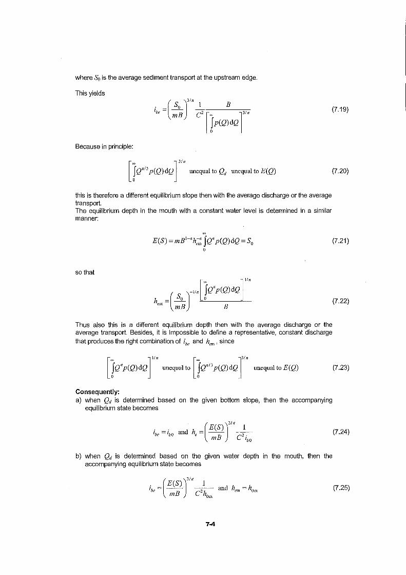
where S0 is the average sediment transport at the upstream edge.

This yields

. S0 1 E ( )

3/n

1be = mE C2 [~ ]3'" (7.19)

fp(Q)dQ 0

Because in principle:

D Q"" p(Q) dQ r" unequ,lto Q, onoqualto E (Q) (7.20)

this is therefore a different equilibrium slope then with the average discharge or the average transport. The equilibrium depth in the mouth with a constant water level is determined in a similar manner:

~

E(S)=mE1-"h: JQ"p(Q)dQ=S0 0

so that

h = (_§_g__J_,. DQ"p(Q) dQ r em mE E

Thus also this is a different equilibrium depth then with the average discharge or the average transport. Besides, it is impossible to define a representative, constant discharge

. that produces the right combination of ibe and hem , since

[ ]1/n [ ]3/n

jQ11p(Q)dQ unequal to jQ1113 p(Q)dQ unequal to E(Q)

Consequently: a) when Qd is determined based on the given bottom slope, then the accompanying

equilibrium state becomes

and h =(E(S))2"'_1_ e E C2.

m lbo

b) when Qd is determined based on the given water depth in the mouth, then the accompanying equilibrium state becomes

7-4

(7 .21)

(7.22)

(7.23)

(7.24)

(7.25)

c) a constant discharge with a value equal to the average discharge, E(Q), causes an

essentially different equilibrium state,

d) no definition of Q is possible that leads to the right combination of the equilibrium bottom slope and the equilibrium depth in the mouth.

In other words: if one wants to make only one calculation with a representative, constant discharge, then one has to choose between:

• a correct representation of the average transport; in that case

Q ~ E(S) _!!__ or Q ~ Bh E(S) [ )

3/n [ )1/n d B c2. d Om B (7.26)

m lbo m

• a correct representation of the equilibrium bottom slope; in that case

• a correct representation of the equilibrium depth in the mouth; in that case

7 A Result for two discharges

As an example consider a hypothetical river with a binary discharge regime: for a fraction of time a the discharge is equal to Q1 and for a fraction (1- a) the discharge is equal to Q2.

The equilibrium depth in the mouth and the equilibrium slope must be such that the amount of sediment supplied at the upstream boundary can be transported. Assuming that a power law can be used for the sediment transport, the annual sediment transport follows from

V=TE(S)=T[amB[~)" + (1-a)mB[~)"1 Bhem Bhem

When V, Q1 and Q2 are known, hem can be solved:

Likewise ibe follows from

7-5

(7.27)

(7.28)

(7.29)

(7.30)

(7.31)

so that

The question arises now whether it is possible to represent the discharge regime, in a more realistic situation with a continuous range of possible discharges, by means of two representative discharges, in such a way that hem and ibe are represented correctly?

This means that

(7.32)

(7.33)

consequently:

=

aQ;' +(1-a)Q; = JQ"p(Q)dQ (7.34) 0

Similarly:

. (E(S))31" 1 E (E(S))31

" 1 E lbe = mE C2 [= ]3/n = mE C2 [aQ"I3 + (1- a)Qnl3]31n (7.35)

JQn/3p(Q)dQ 1 2

. 0

so that =

aQ;' 13 + (1- a)Q;13 = JQ" 13p(Q)dQ 0

In principle, Q1 and Q2 can be solved from equations (7.34) and (7.36). So it is actually possible to find the correct equilibrium state (i.e. hem and ibe) by means of a combination of two representative discharges.

Comment: The time fraction of occurrence, a, is in principle a third degree of freedom. lt can be arbitrarily chosen, but also in a way that a third attribute of the system is represented correctly. In that case a combination of three non-linear equations must be solved in Q1, Qz and a. This is usually not simple.

7-6

(7.36)

7.5 Example

B= lOOm

discharge QL, 0I transport SL, SH

Pl

Okm

B= lOOm

• Figure7-1 Riverflowingintoalake

Consider a river with a width of 1 00 m flowing into a lake with a constant water level. The discharge regime is schematized as follows: during 4 months a year the discharge totals 500 m3/s, during 8 months a year the discharge totals 200 m3/s. In all circumstances the

Chezy coefficient is C =50 m 112 Is. The sediment has a D 50 of 0.2 mm, a fall velocity Ws of

0.025 m/s and a density Ps of 2650 kg/m3.

Until the start of the considered period the river was in equilibrium, with a bottom slope of 10-4. Subsequently the width of the river from location P1 to location P2, i.e. from 50 km to 70 km downstream of the mouth, is reduced to 80 m. What is in that case the new equilibrium state?

The course of the water level in the undisturbed elevation will be non-uniform for both discharges (after all the equilibrium bed elevation corresponds to a combination of both discharges), The equilibrium and the boundary depths that correspond to the surface profiles can be calculated from

(

2 )1/3 h = _q_

e c2. lb

( 2 )1/3

h = !L c g u = Jiu

* c

In the given case this leads to:

(7.37)

Q [m~/s] a(Q) [-] q [m"ls] he [m] he [m] Ue [mls] u. [m/s]

200 2/3 2 2.52 0.74 0.79 0.049

500 1/3 5 4.64 1.37 1.08 0.068

• Table7-1

First we have to check which transport formula can be used. The criteria for the formula of Engelund and Hansen are

7-7

u. > ws = 0.025 m/s

0.19 mm< D50 < 0.93 mm

0.07 <8<6

in this case:

in this case

in this case

(u.)L = 0.049 m/s

(u.) H = 0.068 m/s

D50 =0.2mm

eL =0.76

eH =1.41

In this case the conditions are met, so the transport formula of Engelund and Hansen will be used. That means:

s=mu5 and S =Bs with

The annual sediment transport follows from the values given in Table 7-2.

Q [m%] Ue [mls] s [mz/s] S [m:;/s]

200 0.79 0.71 *10-4 0.71*10-2

500 1.08 3.41 *1 o-4 3.41 *1 o-2

Annual average 1.61 *1 o-4 1.61*10-2

• Table7-2

The annual sediment transport is V= SUI'erage * 31.5 * 106 =51* 104 m3.

Before and after the intervention, the situation in the downstream river reaches remains the same. After all, in both cases the same amounts of water and sand must be transported. The equilibrium depth in the mouth can be found from

[1 2 ]

1'5

-1/5 -Q5 +-Q5 h = ( S a!'erage ) 3 H 3 L

em mE B

where QL is the low discharge and QH the high discharge.

This results in

[1 2 ]

1'5

( * -4 )-1/5 -*500

5 +- * 2005

h _ 1.61 · 10 3 3 = 4.34 m em- 2.3 *10-4 lOO

(7.38)

(7.39)

(7.40)

(7.41)

When the water level in the lake is used as a reference level (z = 0), then the equilibrium situation in the starting-point follows from

(7.42)

7-8

in which x is the distance in meters along the river, increasing in the downstream direction and Xm is the value of x in the mouth.

After the intervention the equilibrium slope in the constricted reach will be such that the amounts of water and sand that are supplied upstream can be transported. This means:

(7.43)

The slope is reduced compared to the former situation. In the situation with one discharge this would cause an increase in the equilibrium depth. With a variable discharge the water depth varies, yet we can still calculate the size of the step in the equilibrium bottom level at the beginning and at the end of the constricted reach. For that purpose it is assumed that the supplied annual sediment transport can be transported exactly. So just upstream of the downstream end of the constriction it applies that

[ ( ]5 ( ]5] 1 5 2 5 1 QH 2 QL Saverage=m0.8B[-uH+-uL]=m0.8B- ( ) +- ( ) (7.44)

3 3 3 0.8B h:H + 11h 3 0.8B h:Z, + l1h

where the superscript "+" denotes the depth just downstream of the constriction.

With the values given in Table 7-2 this gives

1.61 qo-z

2.3 * 1 o-4 * 80

1 500 2 200 [ ( ]5 ( J5] 3 80( 4.64 + l1h) + 3 80(2.52 + l1h)

(7.45)

from which l1h can be solved iteratively or by trial-and-error. This results in

l1h ""0.75 m (7.46)

lt can be easily demonstrated that the bed step at the upstream end of the constriction is equally large. Directly downstream of the transition is

where the superscript "-" denotes the depth just upstream of the constriction.

Because the equilibrium depth at a high discharge and at a low discharge, respectively, in the river reach upstream is equal to that in the utmost downstream stretch, this causes the same values of l1h as at the downstream transition. The new equilibrium bed elevation is described by

7-9

(7.47)

or schematica\ly:

zb(x > Xp2) == -4.34-10-

4 (x- Xrn)

zb(x t. Xr2

) == -4.34+5.00 == 0.66 m

zb(x 'I Xp2

) == 0.66-0.75 == -0.09 m z,(x,. < x «,)~-o.09-0.91 •l<J' (x-x,)

zb (x t. Xr1) == -0.09 + 1.82 == 1.73 m

zb(x 'I Xp1) == 1.73 +0.75 == 2.48 m

zb(x < Xr1) == 2.48-10-

4 (x- xr1)

(7 .48)

z=O

• figure 7-2 Equilibrium bed e\eva~on

1he river-bed in the river reach upstream ol the constriction will eventuallY drOll over the

entire length by an amount ot -4 .34+ 7. 00- 2.48 ~ 0.18 m .

7.6 Summary of effects of interventions

Problem Constant discharqe Variable discharqe Withdrawal of sediment [ r ~=[1- flVr"

:: = 1-~ M andflV lo V

~=[!-LIS r· with ~

ho So v = fsCQ)p(Q)dQ 0

Withdrawal of water i Qo ~

3/n

flQ or Po (Q) ---7 P! (Q) io Qo -flQ

i=

JQn/3 Po(Q)dQ

.5..=1- flQ 0

io ~

ho Qo fQn/3 P! (Q)dQ 0

n -3 ~ Long constriction

i [ B ]-" Bl-n/3 i n/3 J Qn/3 p(Q) dQ =constant

_L= _!

Bo ---7 Bl io Bo 0

so n-l n-3

~ -[ B0]

11

:: =[ ;:]-" h;-B; • Table 7-3 Effects of interventions on the equilibrium state (n = constant)

As an explanation to Table 7-3 the following comments can be made: (i) The expression for the variation in depth loses its meaning for the variable discharge. (ii) For the withdrawal of sediment the magnitude of the relative withdrawal (so M I S0 or

flV IVo) must be known in absolute sense.

7-11

8 Flow and morphology in river bends

8.1 Introduction

Lowland rivers are seldom straight and often exhibit a meandering behaviour, i.e. the river has a single main channel with a pattern that consists of a series of alternating bends. This has a number of various effects, among which: • a river length that is considerably larger than the valley length; this also means a longer

navigation distance; • reduction of the river-bed slope as compared with the valley slope; this means that the

discharge and the sediment transport require a smaller channel width than in the case of a straight river going down the same valley:

. =(.!_)3/n_l = (§_)3/n~ lbe m C2q m C2Q

• an increase of the equilibrium water depth resulting from the decrease of the width:

( )

-1/n ( )-1/n he= :t q = ~ B-4/nQ

• non-uniform depth in a cross-section of the river: the water depth in the outer bend is considerably larger than in the inner bend;

• reduction of the effective navigable width, due to the depth variation and the channel curvature, the latter especially for long ships or barges;

• tendency of the outer bend to erode and the inner bend to accrete; as a consequence, meanders tend to grow and migrate, or (in the case of a protected outer bank) to increase their depth in the outer bend;

• spatial segregation of coarse and fine sediments, usually with the most coarse material in the outer bend;

• formation of bars and shoals around the transition between two consecutive bends; • complicated 3-D flow, giving rise to extra dispersion of transported matter, hence to an

increased 'carrying capacity' of the river. So, many reasons to investigate what is actually happening in a river bend.

Let us first consider the water motion in an infinitely coiling bend with a fixed bed and a rectangular cross-section. After some distance from the entrance, we may assume that the water motion no longer changes in the downstream direction (axially symmetric flow). Next, we will consider the effects of this water motion on the equilibrium profile in the case of a sandy bed. Finally, we will see what happens in a bend with a finite angle of rotation and straight reaches upstream and downstream.

8-1

(8.1)

(8.2)

8.2 steady potential flow

Steady flow in shallow water is described by the shallow water equations:

au au a( g U~U2 +v2

u-+v-=-g-----!---ax ay ax C2 h

av av as- g V~U2 +v2

u-+v-=- g---------'---ax ay ay C2 h

in which x, y = Cartesian co-ordinates in the horizontal plane, u, v = depth-averaged velocity components in x- and y-direction, respectively, h = water depth, g = acceleration of gravity, C = Chezy coefficient.

A bend has a relatively small-developed length, so perhaps it may be possible to neglect friction. In that case, the equations of motion (8.3) and (8.4) can be written as

In each of these equations, the two terms in the centre of the left-hand part have been added. Since their sum is identically equal to zero, this can be done without loss of generality.

If we define the depth-averaged vorticity OJ by

av au OJ=---

ax ay

then equations (8.6) and (8.7) can be written as

-vOJ=-g-a [s +-u-2_+_v_2] ax 2g

u OJ= - g _a [s + _u_2 _+_v_2] ay 2g

8-2

(8.3)

(8.4)

(8.5)

(8.6)

(8.7)

(8.8)

(8.9)

(8.1 0)

Elimination of the Bernoulli-terms in the right-hand part of these equations via crossdifferentiation and subtraction yields

Substitution of the equation of continuity (8.5) into (8.11) gives the vorticity equation:

(8.11)

u_i_(mJ + v_i_(mJ=o ax h ay h

(8.12)

This equation describes the advection of the quantity m/ h (the so-called potential vorticity)

by the depth-averaged velocity field. If we assume that every fluid particle has ever stayed in a region of zero vorticity, the vorticity must be zero throughout the model domain:

(8.13)

If that is the case however, there must exist a continuous, differentiable function <P, such that

aw aw u=- and v=-

dx dy (8.14)

Substituting (8.14) into (8.13) gives

av au _ a (a<P) a (a<PJ _ 0 ax - dy - dX ay - ay dX =

The function <P(x,y) is called the potential function of the considered flow field. The corresponding type of flow is called potential flow.

Substitution of (8.14) into the equation of continuity (8.5) yields

~(h awJ + ~(h awJ = o dX dX dy dy

or, if the variation of h is negligible:

This equation is called the equation of Laplace.

Now we will consider potential flow in a circular channel with a rectangular cross-section. The banks are located at r = rin and r = r0111, where r denotes the radial co-ordinate in a polar co-ordinate system with its pole in the centre of the curvature of the bend. We assume that the flow is axially symmetrical, i.e. there are no velocity variations in the downstream (tangential) direction. The equation of Laplace in polar co-ordinates reads

(8.15)

(8.16)

(8.17)

(8.18)

Due to the assumption of axially symmetrical flow, the first term equals zero, so:

with the general solution:

a a v=-=-

or r

in which a is an integration constant. Since at the sidewalls v = 0, we must have a = 0. Hence v = 0 over the entire channel width. In that case, equation (8.18) reduces to

which is consistent with the assumption of axially symmetrical flow. [N.B. This does not prove that u must always be independent of tp!]

If v = 0, the general solution of (8.21) reads

Cl>=Atp+B

in which A and B are integration constants. Hence

1 a A u=--=-

r otp r

The constant A can be derived from the condition that the discharge through the river is given, say Q:

~~~~t A J h-dr = Q 1in r

This means that u is inversely proportional to r, a property of the so-called potential vortex, or free vortex. Apparently, the maximum velocity is located in the inner bend!

(8.19)

(8.20)

(8.21)

(8.22)

(8.23)

(8.24)

Note that the phenomenon of the free vortex is well known from meteorology: the flow towards a depression, or away from a region of high pressure, behaves as a free vortex.

Another result to be derived from (8.9) and (8.1 0) with m= 0 is Bernoulli's law:

u2+v2 ( + --- = constant

2g

Using equation (8.23), one can easily obtain

(8.25)

A2 ( = constant---

2 2gr (8.26)

This means that the water level increases from the inner to the outer bend, and that it has a concave shape (steepest slope in the inner bend}.

energy level --------------------------

high velocity

• Figure 8 -1 Axially symmetrical potential flow

8.3 Derivation via primitive variables

low velocity

The same result can be obtained when starting from the shallow water equations and working in terms of the primitive variables u, v and (..To that end, we first write the shallow water equations in polar co-ordinates:

u au au uv g a( g u.Ju2 +v2

--+v-+-=---------r acp or r r acp C2 h

u av av u2 a( g v.Ju2 +v2

--+v---=-g-------r acp ar r ar C2 h

! o(uh) + o(vh) + vh = 0 r acp or r

in which u and v are now the velocity components in the rp- and r-direction, respectively.

Introducing the same approximations as before (i.e. no friction and axially symmetrical flow), the equation of continuity (8.29) yields

o(vh) + vh =! o(rvh) = 0 ar r r ar

With the boundary conditions at the sidewalls, this leads to v = 0 over the entire width.

(8.27)

(8.28)

(8.29)

(8.30)

The radial equation of motion (8.28) then reduces to

u2 a( --=-g-

r ar (8.31)

From Bernoulli's law for friction less flow, we can derive

u2 a( U au (+-=constant --7 -=---

2g ar g ar (8.32)

Combining (8.31) and (8.32) yields

au U -=--ar r

(8.33)

with solution:

A A2

u =- and (=constant - --2

(8.34) r 2gr

BA Spiral flow

Consider, once again, the circular bend with axially symmetrical flow, but now taking the vertical structure of the velocity field into account. The radial equation of motion now reads

_!£_=-g a(+ ~(v av) r ar az 1 az (8.35)

in which z is the vertical co-ordinate and v1 the eddy viscosity. The left-hand side of this equation represents the centripetal acceleration needed to make the water follow the curvature of the bend.

Averaging this equation over the water depth yields

l/2 a( rbr --=-g---

r ar ph

in which the overline denotes depth-averaging. (can be eliminated from (8.35) and (8.36) by simply subtracting them from each other:

u2

- u2 a ( av) rbr ---=- Vt- +-

r az az ph

This can be considered as an equation in v(z), with the left-hand part as a forcing term.

As far as the vertical distribution of this forcing term (Figure 8-2) is concerned, and taking into account the fact the u~) increases from the bottom to the water surface, we must have in the upper and lower part of the water column:

(8.36)

(8.37)

u2 - u2 > 0 and u2

- u2 < 0 respectively {8.38)

z z z

I 0 I

I .I ,

./ .., p" d(

.__ __ .....,. g-d-r ...._ __ .....L.-_.,.. Fs r

• Figure 8·2 Forcing of the curvature-induced secondary flow

Solving v(z) from {8.37} leads to the conclusion that this radial velocity component is directed towards the outer bank in the upper part of the water column (z > 0.4 h) and towards the inner bank in the lower part (z < 0.4h), such that the depth-integrated value of v equals zero (see Jansen et al., p. 62, for the exact vertical distribution). This circulation is usually weak as compared to the downstream velocity.

inner bend

z/h

l outer bend

rv

hu

• Figure 8 -3 Vertical distribution of the curvature-induced secondary flow

So, the centripetal acceleration, together with the vertical structure of the downstream velocity u(z), gives rise to a cross-stream circulation, often named secondary flow. When combined with the main {downstream) flow u(z) this leads to a spiraling flow field, often called spiral flow.

8-7

Although the secondary flow is relatively weak, it has major consequences: • matter transported by the flow is dispersed much faster over the cross-section than in a

straight channel. • the secondary flow gradually redistributes the downstream flow momentum - and there

with the downstream velocity - over the cross-section. As a consequence, the velocity distribution in a bend increasingly deviates from the free-vortex distribution, even if the river-bed is horizontal: the velocity maximum gradually shifts from the inner to the outer bend.

• the secondary flow is attended by an inward directed secondary bed shear stress, which can be described by

where Kis the constant of V on Karman (approximately 0.38). If we combine this with the expression for the downstream bed shear stress:

g 2 -rb<p =p-2 u c

we find for the bed shear stress direction relative to the channel axis:

Apart from the constants, this angle is determined by the ratio of the water depth and the bend radius of curvature. Usually, in natural bends ois not more than a few degrees.

8.5 Bed topography (axially symmetrical)

One may readily assume that sand grains on a horizontal river-bed tend to be transported in the direction of the bed shear stress, rather than in the direction of the depth-averaged flow. The grains 'feel' the flow velocity and the shear stress close to the bed.

If, for simplicity, we assume that the magnitude of the transport can be described by a power law formula, i.e.:

/-2 -2 with u101 =vu +v

The transport components in the rp- en r-direction are:

(8.39)

(8.40)

(8.41)

(8.42)

(8.43)

(8.44)

Thus, the secondary flow tends to transport sediment from the outer to the inner bend. This causes erosion in the outer bend and deposition in the inner bend, so ultimately a crossslope of the river-bed. This change of bed topography influences the water motion, but not to the extent that the inward directed transport ultimately goes to zero. The cross-slope will therefore keep on steepening until it is steep enough to make another transport mechanism reduce the cross-stream transport.

Sediment that is transported over a sloping bed will tend to roll downhill under the influence of gravity. In addition to the above cross-stream transport induced by the secondary bed shear stress, there is another component that is directed downhill. In the axially symmetrical case considered herein, this concerns the radial transport component, which will be proportional to the magnitude of the shear-induced transport (the more grains are in motion, the greater the downhill sediment flux) and the magnitude of the cross-slope (the steeper the slope, the greater the downhill transport). In formulae:

in which a is a constant.

We now have two opposite transport components, of which at least one depends strongly on the bed topography. If these two components balance each other throughout the crosssection, there is no net transport and the profile is in equilibrium. This is the case if

azb =-p!!:_ ar r

where f3 is a dimensionless constant with a value of about 1 0.

By definition, the water level equals the bed level zb. plus the water depth h. Hence:

azb as ah -=---ar ar ar

The cross-slope of the water surface is relatively small and can be neglected with respect to the bed slope. In that case, (8.46) leads to

In Figure 8-4 the resulting profile is outlined. The cross-stream variation of the water depth, hence the bed level, is indeed much stronger than that of the water level.

8-9

(8.45)

(8.46)

(8.47)

(8.48)

inner bend

• Figure 8-4 Equilibrium bed profile in a bend (axially symmetrical)

The formation of such a profile has a number of hydraulic engineering consequences, such as • reduction of the effective navigable width as compared with that in a straight channel, • in the case of erodible banks: erosion of the outer bend, leading to bank erosion and

deposition of the erosion products in the outer bend (see Figure 8-5),

• in the case of vertical bank protection: increased erosion in the outer bend ( h ~ rP extends through to the protection structure), which requires a deeper foundation of the protection structure (see Figure 8-5),

• near bridges: erosion around the bridge piers in the outer bend.

inner bend

• Figure 8-5 Natural vs. protected outer bank

natural profile

bank protection

The time needed for the cross-stream profile to reach its equilibrium state is generally much shorter than the time needed for the downstream slope to establish. The sediment that needs to be replaced in order to establish this equilibrium profile is transported over a much shorter distance (order of magnitude of the channel width). The downstream length scale, which is related to the surface profile (backwater curve), is much larger than the width. Especially under high flow conditions, when transport rates are very high, the response time can be short enough to have the cross-stream profile fully adapted to the flood during a single event. Under normal and low flow conditions, with their much smaller transport rates, the profile takes much longer to adapt.

8-10

9 Confluences ana bifurcations

9.1 Confluence · general

Q3 =Q1 + Q2

s3 =S1 + s2

• Figure 9-1 Confluence, general

From a general perspective, e.g. in a 1-D network model, confluences are relatively simple. The number of branches decreases with 1, so there is no problem with respect to distribution of water and sediment. In this perspective the local geometry around the confluence does not matter. On this general scale the bed level is not necessary continuous. In each branch another bed level can be present. This is illustrated in the following example.

Example: equilibrium bed level around confluence

Given: Two river branches, numbered "1" and "2", come together at a location Pin branch "3", which flows into a large lake with a constant water level (s = 0, the erosion base). The upstream discharges and sediment transports are constant: Q1 and S~o Q2 and S2, respectively.

Question: What is the equilibrium bed level in the three branches?

The equilibrium slope and equilibrium depth can be calculated from

9-1

(9.1)

The bed level can now be determined taking into account the fact that the water surface is continuous and that the bottom is parallel to the water surface in the equilibrium state. Therefore the water surface is first determined, from downstream to upstream. If x is the distance from the river mouth (thus x = 0 at the mouth and decreases upstream), we have

r _ r · ( Cll ) ~I - ~ P - 1bel X - Xp

r _ r · ( (2J ) ~ 2 - ~ P -lbe2 X - Xp

The equilibrium bed level can now be calculated from

The bed levels at the confluence are equal in all three branches if the equilibrium depths are equal, so if

In general this is not the case.

For a variable discharge the morphological behaviour is more important, especially when the discharge variations in the two branches are different (what generally is the case). Discharge variations are always associated with backwater curves, even if the river-bed is in equilibrium. A difference in discharge variation will cause extra set-up or set-down of the water level. This will influence the sediment transport capa9ity in the branches and thus also the bed level in the branches. After all the bed level will be adjusted such that the inflowing water and sediment can be transported exactly.

Furthermore, because

discharge variations will be amplified in the transport variations for n > 3. This means that at the nodal point P the condition S3 = S2 + S1 cannot be satisfied at all times, therefore this leads to temporary sedimentation or erosion around this point. If the system is in long-term equilibrium, these temporary effects will be corrected in other periods. Thereby the variation of the sediment supply to branch 3 will not correspond to the discharge variation, even if this is the case for the branches 1 and 2.

9-2

(9.2)

(9.3)

(9.4)

(9.5)

(9.6)

(9.7)

(9.8)

(9.9)

As a consequence, sedimentation-erosion waves constantly occur and propagate in the downstream direction in branch 3, causing stronger bed level fluctuations than can be expected on the basis of the discharge variation. The river-bed 'breathes' differently than in case of a single channel. Because each natural river is a result of confluences at the middle stream, in principle this phenomenon occurs in all rivers. This must be taken into account with the design of bottom protection and foundation structures, and with the management of the river as a navigation channel. This also plays a role in the modeling of river reaches, especially if variable discharge is taken into account. In that case the sediment transport at the upstream edge can no longer be simply related to the discharge.

9.2 Confluence • local

From local perspective confluences are interesting because around it contraction and curving of streamlines occurs, with the accompanying secondary flows and lateral transports. The morphological consequence is, depending on the geometry, the formation of erosion holes and shallow areas. The first can endanger the stability of structures, the second can cause problems for navigation and set-up of the water level at high water.

• Figure 9-2 Confluence, local

An example of a shallow area hindering the navigation is the formation of "sills" in the Western Scheldt, at the locations where the flood channels join the ebb channel.

lt is remarkable that at confluences the horizontal mixing of water from both branches occurs very gradually. On aerial photos the water from different branches often has different colors (due to different sediment concentration) that remain visible after a considerable distance downstream of the confluence. This phenomenon has to be taken into account in modeling the transport of dissolved matter and suspended sediment, and thus also in modeling morphological development.

9.3 Bifurcation -·local

The sediment distribution at a bifurcation point is mainly determined by the local geometry. The angle at which the branches come together at the bifurcation is important, but also the shape of the head has significant influence. This explains why it took many years to shape the bifurcation at Pannerden before the desired water and sediment distribution was approached (2/3 of the Upper-Rhine discharge to the River Waal, 1/3 Upper-Rhine discharge to the Pannerdens Canal; the sediment distribution is as much as possible proportional to the discharge distribution). The same applies for the bifurcation IJsselkop (2/3 Pannerdens Canal discharge to the River Nederrhine, 1/3 Pannerdens Canal discharge to the River IJssel, again the sediment distribution is as much as possible proportional to the discharge distribution).

• Figure 9-3 Bifurcation, local

If a bifurcation is located in a bend, it makes a difference whether it is in the inner bend or in the outer bend. The flow velocity in the outer bend is larger than in the inner bend (see Section 8.4 ). Via the non-linear relation between flow velocity and sediment transport this difference is amplified in the transport distribution between the outer and the inner bend.

• Figure 9-4 Bulle-effect

9-4

Therefore a bifurcation in the outer bend obtains relatively more sand than a bifurcation in the inner bend. This is called the Bulle-effect, named after the author H. Bulle, who described this phenomenon first in a publication (see Bulle, 1926).

A similar effect occurs for the distribution of grain size. In general the bed material at the outer bend is coarser than that in the inner bend. A bifurcation in the outer bend will therefore on average receive coarser material than a bifurcation in the inner bend1

. Because at every bifurcation curving of streamlines occurs, such sorting-effects can also occur if the bifurcation is not clearly located in a bend. This is the reason why sediment in the River IJssel is clearly coarser than that in the River Nederrijn, whereas the sediment mixture in the Pannerdens Canal is in between. Apart from that for these sorting-effects also the local conditions and the geometry are of decisive importance. Therefore in irrigation channels with high-suspended sediment concentration the bifurcation is usually located at the outer bend in order to receive as few sand as possible. In that case only water from the upper part of the water column is tapped off, which contains relatively few sediment.

9A Bifurcation -general

• Figure 9-5 Bifurcation, general

The problems related to bifurcations are significantly more complicated on a general scale than the problems related to confluences, because one has to deal with the distribution problem: how are water and sediment from the upstream branch distributed to the downstream branches? In a 1-D network model the following equations are available:

a) the water motion equations in the branches, which in principle relate the discharge through a branch to the water levels at both ends;

b) the sediment transport formula/concentration formula and the sediment balance equation, which describe the development of the bed level for a given sediment input via the upstream node;

1 Also this effect is some times -wrongly - called the Bulle-effect.

c) the nodal point relations for water motion, viz. the continuity condition Q1 = Q2 + Q3 and

the compatibility condition for the water surface (I= (2 = S3; d) the nodal point relation for the sediment, viz. the continuity condition S1 = S2 + S3 and the

sediment transport distribution relation S)Q2 : S)Q3.

As mentioned above, the sediment transport distribution is mainly determined by the local geometry at the bifurcation. Universally valid, general relations are therefore not available. This creates a difficult problem, because in general models only the topology of the network (which branch is connected to which other branches via which nodes?) is known and not the local geometry at the bifurcations or confluences.

Example: Equilibrium bed level around a bifurcation

Given: A river branch, numbered "1", bifurcates at location Pinto two branches, numbered "2" and "3", which are equally long and flow into the same large lake with a constant water level (s = 0, the erosion base). The discharge and sediment transport supplied from upstream are constant: Q1 and S1.

Question: What is the equilibrium bed level in the three branches?

The equilibrium situation is described by the equilibrium slope and the equilibrium depth in the branches. For branch 1 we have

For the branches 2 and 3, besides the equilibrium depth and the equilibrium slopes also the discharges and the sediment transports are unknown. So in total there are 8 unknowns (he, ie, Q, S for the two branches) for which the following equations are available:

• The water motion equations in the branches:

• The sediment transport formula applied to the two branches:

S =B cnhnt2 ·nl2 2 2 m e2 le2

S =B cnhnt2 1.nt2 3 3 m e3 e3

• The continuity conditions for water and for sediment:

• The geometrical relation: because both branches are equally long and the water levels in the three branches at the nodal point are the same, we have

(9.1 0)

(9.11)

(9.12)

(9.13)

(9.14)

(9.15)

(9.16)

There are now in total 7 equations for 8 unknowns. The extra equation needed is the nodal point relation for the sediment distribution:

(9.17)

(9.18)

A commonly used relation is that the ratio between the specific sediment transport rates is · proportional to a power of the ratio between the specific discharges:

Now we have a system of 8 equations for the 8 unknowns. lt must be noted that that this system has more than one solution. For k ::f:. n I 3 there are three solutions, all physically

realistic: (1) Both branches are open. Each branch transports part of the water and sediment

supplied by the upstream branch 1. (2) Only branch 2 is open and branch 3 is closed. All the water and sediment from branch 1

are transported by branch 2. (3) Only branch 3 is open and branch 2 is closed. All the water and sediment from branch 1

are transported by branch 3.

Take for example B2 = B3 =B112, then the three solutions are respectively:

• Qz = Q3 = Ql I 2' s2 = s3 = SI I 2' he2 = he3 =he,' ie2 = ie3 = iel '

• Q -Q S -S h -2(n-l)lnh · -2(3-n)ln · Q -0 S -0 h -0 2 - I ' 2 - 1 ' e2 - el ' 1e2 - 1el ' 3 - ' 3 - ' e3 - '

• Q - Q S - S h - 2(n-l)ln h ' - 2(3-n)ln · Q - 0 S - 0 h - 0 3 - I ' 3 - I ' e3 - e1 '

1e, - 1e1 ' 2 - ' 2 - ' e2 - ·

lt is obvious that if the system is not in equilibrium it will have the tendency to converge to one of the possible equilibrium states. Theoretical analysis shows that (see Wang et al., 1995) in addition to the initial situation, the nodal point relation for the sediment transport distribution determines to which equilibrium state the system will go. If (9.19) is used as nodal point relation then the value of k has important influence. Fork< nl3 always one of the branches will be closed in the long-term and the equilibrium state (2) or (3) will be the end state depending on the initial situation. For k > nl3 both branches will always remain open: equilibrium state (1) will be the end situation. Fork= nl3 there are infinitely many equilibrium states possible because equation (9.19) then does not give extra information in addition to equations (9.13) and (9.14 ). All solutions are possible as long as

(B h312 + B h312 )n Qn 2 e2 3 e3 =_I

B h n/2 +B hn/2 S 1 ~ 3 ~ 1

9-7

(9.19)

(9.20)

For variable discharge the distribution of water and sediment to the two branches will vary in time, unless the geometry of the bifurcation point is designed such, that this distribution is always constant. The last is extremely difficult, if not impossible. Therefore sedimentation I erosion due to the variation of the distribution of discharge and sediment transport will usually occur. Because a shortage in one of the branches means in general a surplus in the other branch this in general causes erosion in the one branch and sedimentation in the other branch. The consequence is that the bottom in the branches downstream of a bifurcation "breathes" stronger than in a single branch river.

9.5 Islands

branch 2

branch 1 branch 4

bifurcation branch 3

• Figure 9-6 Island = Bifurcation + Confluence

An island can be considered as a combination of a bifurcation and a confluence. Therefore combination of effects corresponding to bifurcation and confluence occur for islands:

• the shape of the bifurcation point has influence on the distribution of sediment transport and thereby influences the equilibrium depth of the branches;

• the effect of discharge variation on "breathing" of the bottom is amplified, of which a part of the variations left and right of the island are in opposite phase (i.e. erosion left occurs simultaneously with sedimentation right and vice versa);

• downstream of the confluence stronger erosion waves and sedimentation waves occur than in the corresponding case without island.

9.6 Conclusion

The dynamic of a natural river, with confluences, islands and bifurcations, under influence of natural discharge variations, will be much different than that of a single branch alluvial channel with constant discharge and sediment supply. For the evaluation of the large-scale effects of human interventions, the discharge variation as well as the variation of sediment supply has to be taken into account. The variation of the sediment supply will in general not correspond to the discharge and the initial bed level according to the sediment transport formula. Therefore it is recommended to "nest" such models in a model at river basin scale. Such large scale models are however rarely available for morphological simulations (so far usually only for simulations of flood waves).

10 Interventions in rivers

10.1 Introduction

Through river improvement it is attempted to reduce the damage that a river can cause (floods) and to improve the practical use (navigation, irrigation, energy etc.). Large-scale river improvements are very costly and require a careful preparation and execution. For that reason some attention is paid to the collection of the necessary data base in Section 1 0.2.

Interventions in rivers with a more local nature often have repercussions for the entire river basin. Therefore one has to check carefully if improvements at one location do not result in deteriorations at another location. This also means that a legal framework is required, in which the works can be executed. So the administrative situation in a country will also be important.

For instance in Italy the controversial province of Alto Adige (Southern Tiro!) has a farreaching degree of autonomy. The central government in Rome only plays a leading role in the departments of Justice, Defense and Foreign Affairs. In the last decades the relatively rich Alto Adige has done a lot of work concerning erosion fighting in the tributaries of the Adige River. This has clearly improved the situation. Logically the sediment supply in the Adige River has been reduced. This can result in bottom subsidence, water level decline and also a decline of the groundwater levels along the lower reaches of the Adige River, which are located outside the Alto Adige province.

Sometimes it occurs that owners of land that is adjacent to the river have the right to refuse entrance to the river via their terrain and hence are able to resist river works.

10.2 Data base

The required data for the design of sound interventions in rivers first of all concern interventions in the discharge. By means of hydrological models information on the course of the discharge can be derived from rain data. By measuring the rainfall and the discharge the model coefficients can be determined(= calibration of the model). Next, to check the model it can be tested by comparing the predicted and the measured discharges for discharge data that has not been used in the calibration of the model(= verification of the model).

With measurement series of several years one must be careful, because in the course of time the character of the river basin might have changed (for instance by deforestation or by reforestation), as a result of which the measurement series are not homogeneous.

With the collection of the discharge data also Q-h-curves will be used. A limited number of discharge measurements can be expanded through the Q-h-curves using simply measured water levels. However, extrapolation is dangerous!

The time-dependent variation of the river with erodible banks in layout can be studied by means of aerial photos or satellite records. lt is dangerous to draw conclusions about the mobility of the river in layout from one recording and inspection at the site (obviously both at low discharge). For example aerial photos and inspection at the site of the Serang River and the Tuntang River (Middle Java) in 1974 gave the impression that the banks had been greatly eroded. A comparison with aerial photos from 1924 proved that the course of the river had hardly changed in 50 years.

10-1

Obviously it is important to predict the changes of the layout in the future, with or without interventions. But this is still hardly possible. When the banks are fixed (or badly erodable) morphological predictions are currently reasonably possible. For a free meandering river the mathematical models are still in its infancy (see e.g. lkeda et al., 1981; Parker et al., 1982; Chang, 1984; Struiksma en Crosato, 1989; Crosato, 1990).

The bottom composition must be known. This means both the grain composition of the bottom in alluvial river reaches and the location and the nature of badly erodible reaches (clay bars and rock).

For morphological predictions time-dependent one- or two-dimensional models have been developed. The existing models are still being improved and expanded. In these models sub-models are applied to predict the transport and the alluvial roughness. The selection of a sub-model can be based on the comparison of the predicted and measured sediment transport or roughness in the considered river. In particular sediment transport measurements are difficult to carry out with sufficient reliability.

lt is not difficult to set up an extensive measurement program for a river. lt is the art of doing an optimal measurement that is difficult. With that the main perspective for the intended intervention in the concerned river must be watched.

The desired accuracy of the morphological predictions makes demands on the accuracy of the predicted value of the sediment transport and roughness in the sub-models. Bearing in mind the overview, it can be possible that the measurements of the sediment transport and roughness are not required or just very required (De Vries, 1982).

10.3 Erosion fighting

With erosion fighting in the river basin the first action that is needed is to prevent the increase of the erosion! That means the sensible treatment of the present vegetation. In this respect the unwise logging of forest can lead to a large increase in erosion. This has happened at Java and at present this is imminent at the island of Borneo (Kalimantan).

In the river basin of the Yellow River (Huang He) there is an area, which is called the 'Black Forest', yet there is no tree so see. Measures are taken to fight the erosion: the mountains and the hills are equipped with terraces so that the rain water flows off of more slowly and consequently causes less erosion. The vertical walls that are introduced by these terraces have to be defended. This is a very labor-intensive method, which has a strong influence on the landscape. This is called landscape engineering.

Also it can be attempted to improve the vegetation. This is a costly operation as well. lt requires expertise in selecting suitable plant species that will thrive on the eroded bottom and also offer sufficient resistance against erosion.

When the river basin is used for agriculture then it is important to turn to contour ploughing. This means that ploughing will take place along the contour lines. As a result mini-terraces are created. This practice is adopted in the Tennessee Valley (V.S.).

When in the river basin large erosion gullies have been originated, it can be considered to locally dam these gullies. These large erosion gullies can be found in the river basin of the Bogota River (Colombia). In fact one is then already working on what is called headwater control (in German: Wildbachverbauung').

10-2

.......... ............. ~

equilibrium slope

original slope

• Figure 1 0-1 Principle of 'Wildbachverbauung'

The principle of this manner of erosion fighting is illustrated in Figure 10-1. The construction of fixed weirs brings about the fact that the bottom slope at the new equilibrium situation will be less than in the first case. Obviously the foundation of the weir must be constructed far beneath the (anticipated new) bottom.

Erosion fighting in the river basin is especially important if a weir with a reseNOir IS

constructed in the river. Because of sedimentation the practical use of the reseNoir will be gradually reduced (Section 10.4.2). Erosion fighting can thus prolong the lifespan of the reseNoir.

Additional information on erosion fighting can be found in Barnes ( 1971) and Vanoni (1975).

1 OA Discharge regulation

1 0.4.1 General

Discharge regulation through the construction of dams with reseNoirs is a big inteNention in the river and its basin. With discharge regulation it is accomplished that the natural present discharge ( Q(t) ) is modified on purpose:

• increasing the low discharges can be useful for irrigation and navigation, • reducing the high discharges is a form of flood fighting, • waterpower demands an available hydraulic capacity at the time that electric energy is

needed.

The application objectives each demand a typical available discharge and reservoir volume at a specific time. Furthermore the inflow of the reseNoir at that time is not a deterministic quantity. To seNe the objectives as good as possible rules must be established regarding the discharge that is allowed through at each time (reseNoir operation).

The treatment on reseNoir operation is outside the scope of these lectures notes. For a first introduction it is referred to Jansen et al. (1979, p. 371). For a project one must carefully examine the rules that are required to make optimal use of the reseNoir.

Discharge regulation can have a large number of positive and negative consequences. This is shown in the next example.

10-3

Example

The Rufiji River (Tanzania) runs through a mountain pass at Stiegler's Gorge. At that location it is locally not alluvial. Downstream there is an area with a lot of wildlife (tourism) and some fishing, more downstream (fairly primitive) farming can be found. The proposed construction of a dam with a waterpower station at Stiegler's Gorge (see Figure 1 0-2) yields as profit the generated energy. Some possible loss-making activities are: • Because of the construction of the dam a reservoir arises, this causes a loss of land

(here in a hardly inhabited area). • Downstream of the dam the bottom will suffer a time-dependent degradation. Therefore a

number of environmental effects occur: • declining groundwater levels; • changing vegetation (flora); • changing wildlife (fauna); The latter can result in lower numbers of tourists(= source of income).

• Since the degradation will deepen the low-water bed, and because of the discharge regulation, the high-water bed will be flooded less often. This can reduce the amount of nutrition for the fish and eventually reduce the fishing by the population.

• Because of the intervention at Stiegler's Gorge also the nutrition for the plants can be reduced. This means that one has to convert to artificial fertilizer. If the morphological process continues at a slow pace, the population can get accustomed to the utilization of fertilizer. However, it will still cost money.

• A larger salt intrusion due to the absence of high-water discharges.

0

/

I I \

I I

\

/' ........ i I

,...,j \ ;- \ \

'-. I

\

\ ./

\_ , __ .~\ '""'.

\,

-, __ , r Mikuml'· National 'Park

e MOROGORO

Q)•n~bar

DARES e SALAAM

\ Kisaki ·. '-._,.-..., . ·-·~. . ,.- - .. ....,

1.- .· K1b1tir ·l_

Pangani rapids + Utete \ Stiegler's li

ufiji Gorge ,.,-./ INDIAN OCEAN

""'-Shuguri falls

\

I ~-.' '·

i boundary river basin

I J

40 80 120 160 200 km'-.. .:_.-·--. ........ /~,

J . .)

• Figure 1 0-2 Rufji River (Tanzania)

This example shows what the effects of the construction of a waterpower station can be. A similar project requires the contribution of a variety of disciplines (EC/DHL, 1980). Pros and cons must be carefully weighed in a systematic manner (system analysis). Only then a sound (political!) choice can be made.

10-4

Comments:

(i) Also the public health can play a part. In still water in Africa (the African lakes!) bilharzia occurs.

(ii) To get an impression of the Rufiji River and the intervention, the following data are mentioned: • Rufiji River:

• planned dam:

river basin: 177000 km2

average annual discharge: 30*109 m3/a bank-full discharge: 2500 m% ib = 0.3*10-3

; D50 = 0.4 mm height: 130 m distance: 230 km from the Indian Ocean installed power: 1200 MW reservoir: 1250 and 550 km2 at high-water and low-water, respectively

(Hi) Morphologically speaking the river is very fast. A rough estimate shows that the morphologic time-scale (de Vries, 1975) amounts to approx. 2 centuries. This implies that a sea level decline at 200 km upstream of the mouth is shown for 50% as land subsidence after 2 centuries. With that the Rufiji River belongs to the group of relatively fast rivers, which include the Magdalena River (Colombia), Tana River (Kenia), Apure River (Venezuela) and Serang River (Java). lt is estimated that after the projected discharge regulation the morphologic time-scale will go up by a factor two. This means that the Rufiji River is 5 times faster than the River Waal.

10.4.2 Sedimentation in reservoirs

Because of the construction of the dam in a river followed by the discharge regulation, a big intervention in the river system is made. This system can be divided into three river reaches.

(i) Upstream: outside the dam's influence In this reach the natural discharge Q(t) is present combined with the supplied sediment

transport S(t) . The annual sediment transport is

~

Va ~ Js(Q)p(Q)dQ (1 0.1) 0

(ii) Upstream: inside the dam's influence This is where the rise of the water level (as a result of the dam) reduces the flow velocity. As a consequence of this the annual sediment transport (V1) is smaller than Vo. This reach is the reservoir and hence sedimentation will occur.

(Hi) Downstream of the dam In principle two options exist here: • If in the reservoir all (or most of the sediment) is 'caught', then relatively clean water

will pass the dam. The sand transport capacity present in the downstream river is then employed as erosion. So downstream of the dam degradation will occur.

• If, one way or another, the supplied sediment is allowed to pass the dam, then downstream of the dam sedimentation will occur. This is the consequence of the discharge regulation.

That sedimentation occurs in the last case is a result of the strong non-linear relation between velocity and sediment transport. This aspect has already been mentioned. lt has been shown that the sediment transport during a tidal period is larger than the transport due to the average tidal velocity (u0) by an amount of

10-5

u = u0 + u sin OJt with u0 > u

The sediment transport per month resulting from the monthly-averaged discharges must be smaller or equal to the transport per month resulting from the daily discharges.

Discharge regulation will thus always result in morphological problems. For large reservoirs the emphasis is on the downstream degradation, for relatively small reservoirs the emphasis is on the sedimentation in the reservoir. This then has a limited economic lifespan.

A good overview of the sedimentation in reservoirs is given in a few articles written by Graf (1983a, 1983b, 1984). Table 10-1 has been taken from these articles. In this table for more than 1000 reservoirs the loss of storage (storage depletion) has been given. The table contains data for the V.S. up to 1975.

Capacity range (1(}'lffil) Number of Total drainage area Net drainage area Initial reservoir storage Storage depletion % Average period of Jllm2) (knit (1om3) reservoirs capacity(1(}'lffil) record (years)

0 to 12.33 190 466 425 1041 268 25.7 11.8

12.33 to 123.3 257 1176 1132 11328 2186 19.3 14.5

123.3 to 1233 283 11057 9412 138204 22736 16.5 23.5

1233 to 12300 176 79018 39345 700008 93824 13.4 20.9

12.330 to 123300 107 294708 226516 5381926 488202 9.1 23.6

123.300 to 1233000 69 820654 454897 29248930 1065792 3.6 18.4

> 1233000 23 928442 477148 74498940 2567899 3.4 19.1

1105 2135521 1208875 109980377 4240907 3.9 18.6 • Table 10-1 Overview of the capacity of reservoirs and the storage depletion (data V.S.)

The table shows that especially for the smaller reservoirs large problems can arise worldwide within a couple of decades. In principle (that is apart from the costs) it is possible to empty the reservoir through dredging. However the question where to put the mud remains. As has been argued above, the river downstream of the dam cannot cope with this, because of a too low sediment transport capacity as a result of the discharge regulation.

In some countries (for instance Iran, China and Tunisia) tests are carried out at reservoirs. In these tests it is attempted to remove part of the deposited sediment to the river downstream of the dam by s/uicing. The lifespan of the reservoir is increased, but at the expense of the utilization of water for other purposes such as waterpower.

The impression exists that in the past the design of dams with reservoirs has been based on too little data on the sediment transport in a river. In this way the lifespan of the reservoir can easily be overestimated.

it appears to be a human quality to overestimate the economic lifespan of a reservoir, because otherwise an entire project will not be feasible and as a result of which insufficient funds will be acquired for the project. Yet, this only postpones the problems. it happens that as a result of sedimentation reservoirs can become completely useless within a decade.

This underlines the necessity to make a thorough prediction of the sedimentation of projected reservoirs.

10-6

1250

1200

1150

1100

1050

1000

950

900

850

650

600

Hoover dam (width not to scale)

max. lake level 1941






max. lake I vel 1940

max. lake Jevel1942- 1948

• Figure 1 0-3 Sedimentation in Lake Mead (Colorado River)

Lower Granite - Gor e

topset and foreset bed"---.. 1200

1000

BOO

As an example of the sedimentation in a large reservoir the development of the bed in Lake Mead is illustrated in Figure 1 0-3. This reservoir has originated as a consequence of the construction of the Hoover Dam in the Colorado River.

For a further study on the sedimentation in reservoirs reference is made to the overviews in the mentioned articles written by Graf. These articles are supplied with an extensive list of literature references. This is also valid for Sloff (1 991 ).

10-7

10.4.3 Example: Mekong at Vientiane

In Figure 10-4 the river basin of the Mekong River is given. In this figure the river reach Vientiane-Nong Kai is shown.

VIENTIANE

------ bank erosion 1543

two channels

LAO PDR

THAILAND 0 2 3 4 5 km

• Figure 10-4 Mekong River at Vientiane (Lao PDR)

For this river reach three plans are being prepared. They all demand mutual tuning.

(i) The projected Pa Mong-dam is situated not far upstream of Vientiane. Depending on the selected regulation for the management of water and sediment, degradation of a certain size and at a certain pace is expected downstream.

(ii) At various locations in the approximately 40 km long river reach bank erosion will take place. For a number of these locations the construction of bank revetments is considered. This requires a study on the bed level variation along the eroding outer bends. Taal (1989) developed a mathematical model to predict the time-dependent bed level variation along the bank. This is a quasi two-dimensional model based on linearized equations, which is numerical in the longitudinal direction and analytical in the transverse direction.

10-8

In Figure 10-5 the variation of the bed elevation around the average bed elevation in the longitudinal direction is given. The possible degradation as a result of the construction of the Pa Mong-dam has to be additionally calculated!

-15.00 ,---,----------,-----,---,--------,--------,----,------,

15.00 ~-----=~------c~-=---~-=-=--~~-----="=-"=-=------="~----=-=~-~,--,! 0.00 5.00 10.00 15.00 20.00 25.00 30.00 35.00 40.00

distance [km]

• Figure 10-5 Variation in bed elevation of the bank of the Lao River during a wet year (Taal, 1989)

The predicted bed level variations during a year reasonably correspond to the observations. The model cannot predict the variation at km 1566 (N.B. measured from the mouth). Because of the presence of two channels at that location very large bed level variations occur during the year (see Figure 10-6).

10-9

.-.. _§_

c: 0

:;::; CO > Q)

Q)

I

178

174

170

166

162

158

154

150

0 <0

"'

LEFT BANK (LAO SIDE) surveyed 1988-06-09

surveyed 1988-08-22/23

surveyed 1988-10-25

----,- ........ tf/1

~--.... . ............ __ .,...,.. ......... ...__ _ __,.,

0 <0 N ~

-distance (m)

0 ~

N

11_/. 0 <0

0

RIGHT BANK (THAI SIDE)

water level 1988-10-25 water level 1988-08-22 l

~--~w-•1" ''"' ,.,_.,_., l 1 -l.-' -=- ~ ......... --------surveyed 1988-06-09

surveyed 1988-08-22/23

surveyed 1988-10-25

0 0

"' 0

"' "t

0 0 "t

- distance (m)

'... __ , 7

~· ~ I .. ___ .. ' I

0 0

I'- "' N N

' I ~---'~r '

\·-- " 0 0 N

, ____ , 0 0 0 CD

0 0 "' (")

• Figure 10-6 Variation in bed elevation at island km 1566

0

178

174

170

166

162

158

154

150

(iii) Around 1993 a bridge over the Mekong River was built in this river reach. For the piers the possible total degradation in the future due to the Pa Mong-dam had to be taken into account.

10-10

.-.. E ~

c: 0

:;::; CO > Q)

Q)

I

10.5 Regulation low-water bed

Regulation of the low-water bed will generally be carried out for the benefit of the navigation. A similar normalization for the branches of the Rhine River in the Netherlands was originally set up to withstand high water levels as a result of ice bars.

With a similar normalization the low water bed is constricted in order to maintain sufficient navigable depth at low discharges. Also sharp bends will be removed.

0 2 km

• Figure 10-7 Normalization of the Rhine River just downstream of Basel (1gtll century)

In Figure 10-7 a sketch of the normalization of the Rhine River downstream of Basel is given. A braiding river has changed into a meandering river with fixed banks. lt is important that also the newly established low-water bed shows bends. If the new course is too straight then alternate bars will arise.

These large sand bars are shifted in the downstream direction. Since these bars are not fixed, they are a disturbance for the navigation.

In Figure 10-8 an example of normalization through river cut-offs is shown.

SPEIER MECHTERSHEIM

GERMERSHEIM

PHILIPPSBUR OBERHAUSSEN

0 2 3 km

• Figure 10-8 Normalization of the Rhine River just upstream of Mannheim (1 gtl1 century)

Such an intervention requires a careful completion. With river cut-off a dam is constructed in the old bend. With similar works on the Wisla River(= Vistula, German: Weichsel) in Poland from 1940 to 1943 the new course was not sufficiently deepened. This meant that the

10-11

groynes that were still under construction were severely damaged at high-water discharges (Muller, 1955). T award the constriction of the low-water bed the following remarks must be made:

(i) The groyne distance should be short enough to create a stable eddy in the 'groyne reach'. Furthermore the groyne must be protected over a sufficient length. Otherwise during high water by-pass seepage can occur.

(ii) Traditionally the bank between the groynes has not been protected in the Netherlands. Nowadays increasing navigation creates temporarily velocities that also cause sediment transport in the groyne reaches. Filling and drainage of the groyne reaches with regard to sediment starts to become an important factor in the morphological process of the river.

(iii) Groynes are required at low discharges. The disadvantage of groynes at high water is that they contribute to the roughness of the flow over the groynes. When the flow is at right angles to the groynes the form resistance will be large. In Germany this has led to tests with deformable groynes that disappear in the bottom at high water levels (Jurisch et al., 1981). In Figure 10-9 such a groyne is shown. The chambers consist of a coated PVC-membrane. The chambers that are next to one another are filled with water at water levels below the average water level. When the water level exceeds the average water level the chambers are automatically emptied. The tests have been carried out in the Rhine River at Duisburg, upstream of the mouth of the Ruhr River.

The test results are still unknown, but as yet the structure seems rather vulnerable (shipping anchors!).

,- air relief valve

~l

inlet and discharge organ rp 300 mm waterlevel

flow- drained condition screened inlet

pre-membrane

/ 2000 5500

anchor chain shackle clamping plate thrust

concrete slab inlet and discharge

conductor rp 1 00 mm

• Figure 10-9 Deformable groynes (by Jurisch et a/, 19~1)

10-12

1 0.6 Regulation water levels

1 0.6.1 Principle

The objective of regulation of the water level is to create sufficiently high water levels even at low discharges. By that, for instance, the hydraulic drop over a weir can be utilized for waterpower. Also a larger water depth for the navigation is created. Furthermore the water intake for irrigation purposes at low discharge is easier, so that pumping up of water can be avoided.

To meet the requirements a number of weirs will be constructed in the river, in other words the river is canalized. In principle the discharge will not be affected by canalization. With the canalization of the River Nederrijn (Lower Rhine) this was the case, because with the construction of the weir at Oriel the aim was to change the discharge distribution at the IJsselkop (see also Section 1 0.6.2).

In particular in the lower reaches of a river moveable weirs will be used in the canalization of the river. With that it is achieved that by opening the weirs (River Nederrijn) or closing the weirs (River Meuse) the water levels at high discharges will not be raised needlessly.

w

~

l 0

DISCHARGE DURATION CURVE

open river

STAGE-DURATION CURVE

ANNUAL NUMBER OF DAYS THAT

INDICATED FLOW IS NOT EXCEEDED

• Figure 1 0·1 0 Influence on water levei.<Juration line

In Figure 10-10 the influence of a moveable weir on the water level-duration lines is given for the case that the discharge is not affected by the canalization.

The waterpower that can be extracted from the river can be determined from this figure (through the head at the weir).

When navigation is the main objective for the canalization, then the distance between the weirs will be set such that downstream of a weir sufficient navigable depth is present due to

10-13

the heading up by the weir, which is located downstream. This requirement is contradictory to the requirement for the utilization of waterpower. In that case the water level downstream of the weir should to be as low as possible in order to increase the head at the weir. In this way the available gross power will be maximized.

HIGH DISCHARGE (OPEN RIVER)

WATER LEVEL OPEN RIVER AT DISCHARGE Q

SURFACE RIPARIAN LAND

--- -- --- ------ -- .......

• Figure i 0-i i Longitudinal reach canalized river

River canalization should be based on a thorough study. For instance the morphological consequences of the intervention must be examined. In particular this concerns the (timedependent) bed elevation and the question whether the sediment will be able to pass the weir when it is completely or partially opened.

Furthermore it is required to examine, what side effects will occur upstream of the weir concerning the increase of the water level ('weir damage'). For instance the increase of groundwater levels, blockage of present drainages into the river, required local dike heightening should be kept in mind.

Comment With canalization of a river, besides the construction of weirs in the river to allow navigation in the river, also the possibility exists to construct a lateral canal for navigation. This alternative has been used in the canalization of the River Meuse in Limburg. There the Juliana channel, which is a lateral canal of the River Meuse (actually River Grensmaas), was constructed.

1 0.6.2 Example: Canalization of the Rhine River

The Rhine-canalization is not a pure example of water level regulation, since also discharge regulation has been attempted. Through the construction of the weir at Oriel it has been attempted to influence the discharge distribution of the River IJssel and the River Nederrijn at the IJsselkop. In this way more water can be lead into the IJsselmeer. With the weirs at Amerongen and Hagestein purely a water level regulation for the navigation has been intended. By letting in more water in the IJssel at low upper-discharges, as compared to the former situation, the navigation in this branch has also been improved. By placing the discharge of the River IJssel at at least 250 m%, as a result of the Rhine-canalization the water depth of the River IJssel and the River Nederrijn can be at least 2.5 m.

With the design of the Rhine-canalization in the fifties of the 201h century, it only proved

economically sound to derive waterpower from the river at the weir at Hagestein. Therefore a (small) turbine was constructed in the pier between the two weir sections. The theoretically possible profit of 6·106 kWh a year is in practice only realizable for about 10%, because the

10-14

weir operations have been primarily aimed at navigation and water control. As a result of the increase in energy prices later on, a waterpower station close to the weir site at Amerongen has been realized.

To achieve the intended main objectives of the Rhine-canalization (viz. water distribution and navigable depth} a weir program is used. With floating ice this program will be released (the weirs are opened).

river cut offs

weir site Hagesteijn

0 5 10 15 20 km

• Figure 10-12 Outline of canalization works in the River Rhine

For a detailed description on the design and implementation of the Rhine-canalization it is referred to Gaay and Blokland (1970). In this lecture only a few leading items are discussed.

The weir program (Figure 10-13) has the following characteristics: (i) For the River Nederrhine roughly 50 m% is maintained as a minimum for the water

requirement along this branch and to resist pollution. (ii) This minimum must be maintained even if the discharge of the River IJssel is below

250m%. (iii) As long as the water requirement of the Lake IJsselmeer is not satisfied, rule (ii) will

remain valid even if the discharge of the River IJssel is higher than 250 m%. (iv) With roughly a discharge of the River IJssel of 350 m3/s problems will occur along the

River IJssel (inundation of the floodplains, blocked discharges etc.). Then by opening the weir at Oriel the discharge along the River Nederrhine is increased.

(v) The programs of the weirs at Amerongen and Hagestein are based on the program of the weir at Oriel on ground of the requirements of the navigation.

10-15

m3 Is .------,--,-.-----,---~--.--:TT"l

300 f------+-----1--r---l-~~-L_____j_j

200 f--7''--+~,_,._::+-____J____j

0

200 ,---;-'+------7"--+--

1 00 f-------17'----f--+-''=-'-i-'~T---.--rl

m+

10

9

8

7

6

5

4

3

2

-

# ~" ' I

•" I

f/ " '"

water level ~ - upstream of we~

-1::-:-,, / ,-~ -::-_..../'

,, Z water level ,

"""" downstream of

1\ water level \program/ 7'-

' -- ---..::::: ....... '\ --....._.

;.;.. ~

m3 /s

300

200 500

100 400

0 300

200 200 I

J

100 100

bifurcation IJssel m+

10

Oriel 9

8 ~ ' 7 '

I

weir 6 ' '

Amerongen 5 " 4

3 Hagestein 2 V

,•

". 0

0 100 200 300 days/year 0

0

PROGRAM "250"

500

400

300

200

100

0

/ ....,:?" " "

i""' , \ / -- -- ,. ·;7

-· .. "~ater level "

"" program

/ \ ""I

,- ............ . :y -...... , ... -- - _..../'

100 200 300 days/year

PROGRAM "350"

• Figure 10-13 Weir programs Rhine canalization

The short distance between the IJsselkop and the Pannerdense kop leads to the fact that the influence of the weir at Oriel is visible at the bifurcation point in Pannerden. As a result the discharge of the River Waal is increased at low discharges. In order to resist this as much as possible two bends have been cut off in the upstream reach of the River IJssel.

At the upstream end of the River IJssel, schematically two situations arise as a consequence of the variation of the probability distribution of the discharge p(Q) : • For low discharges through the Pannerdens Channel the discharge of the River IJssel is

relatively large at a high water level in the Pannerdens Channel. Then there is no sand supply towards the IJssel, but in the River IJssel sediment transport takes place. This leads to erosion in the upstream reach of the River IJssel.

• With an opened weir the sediment supply towards the River IJssel is resumed. In the upstream stretch of the River IJssel sedimentation occurs.

The selection of the type of weir is influenced by the desire to let navigation through the weir when the weir is opened. After all, according to Figure 10-13 the weir at Oriel is completely or partially closed for about 200 to 300 days a year. There are two weir sections (each 48 m wide) with an intermediate pier of 14 m wide. In the intermediate pier discharge openings were built, which can be used as a regulatory organ at low discharges when the weir has been closed.

10-16

~penCiix I AiCie Memoire: formulas for water ana secliment motion

1.1 Uniform flow

u=CFf with R= A p

for B >> h this yields u = c.Jhi

From (1.2) results for the equilibrium depth he :

The Froude number (Fr) is an important dimensionless parameter for open channel flow:

u Fr=--

.Jih For Fr = 1 the flow is critical, then the depth is equal to the critical depth he:

[ 2 )1/3

h = !L c g

1.2 Roughness

The hydraulic resistance is expressed by the coefficient of Chezy (C) or by the coefficient of Darcy-Weisbach (/).The relation between the two coefficients is

For the coefficients it is generally found that

C = Ji ln 12R = 2.3 Ji log 12R = 18log 12R

K k+5/3.5 K k+b/3.5 k+b/3.5

and

f= 0.24lo -2[ 12R ] g k+5/3.5

where k is the equivalent sand roughness according to Nikuradse.

For an alluvial bed k can strongly vary with the flow conditions. In rivers mostly hydraulically rough circumstances will be encountered ( k >> 5 ). Frequently applied formulas for C then become:

White-Colebrook: C =18log12

R k

Strickler: C = 26 -[R] 116

k

1-1

(1.1)

(1.2)

(1.3)

(1.4)

(1.5)

(1.6)

(1.7)

(1.8)

(1.9)

(1.10)

1.3 Suriace profiles

For gradually varied flow in an open channel with a constant width and bed slope ib the equation of Be/anger applies (steady non-uniform flow):

For flows with low Froude number (Fr << 1), equation (1.11) reduces to

dh = i [1- h: l dx b h3

Generally (1.11) has to be solved numerically. However, two analytical approximations exist. The first one is that of Bresse for flows with low Froude numbers (Fr << 1), the second one can be applied when the deviations of the water depth h from the equilibrium water depth he are relatively small (h "" he).

Approximation according to Bresse X-X0

h=he +(ho -he)(;Jr;-;; in which the boundary condition h = h0 at x = x0 has been used and the so-called 'halflength' L112 is given by

( )

4/3

L = 0.24he h0 1/2 . h

lb e

Approximation for small deviations of the water depth from the equilibrium depth

in which the boundary condition h = h0 at x = x0 has been used and where L (also called the adaptation length of the flow) is given by

1.4 Spillways

L = h: -h: h2 •

e 1b

With a long spillway either a submerged weir or a clear overfall can occur. The discharge formula expresses the discharge (q) in the upstream energy head (H) and the downstream water depth (h), both measured in relation to the crest:

Broad-crested weir (submerged weir)

q = mh~2g(H- h)

with 0.9 <m< 1.3, averaged value: m"" 1.1.

Broad-crested weir (free flow weir)

q =m.?:_~ 3_ g H312 3 3

1-11

(1.11)

(1.12)

(1.13)

(1.14)

(1.15)

(1.16)

(1.17)

(1.18)

For a short spillway the same formulas are used, only the discharge coefficient (m) is somewhat larger.

Obliquely approaching flow towards spillway

When in a flow strip with a discharge q0 the water flows over an embankment, which is at an angle awith the flow strip then q0 results from

where q is found from the discharge formula (square approaching flow).

1.5 Non-steady flow

For flood waves in rivers the term ()uf()t can generally be neglected in the equation of

motion (deepwater-wave equation). With that the (complete) dynamic wave degenerates into a wave, which can be described by a diffusion formula (diffusion analogy). The wave celerity c follows from

1 (JQ c=--

B ()h

For a constant width and C-value this results in c = 1.5 u .

The diffusion coefficient K results from

With the diffusion analogy a damping wave is described.

A stronger approach originates if the equation of motion for uniform flow is selected (kinematic wave approach). The kinematic wave describes an undamped propagating wave. The celerity follows from equation (1.20).

1.6 Sediment transport

The sediment transport formula of Meyer-Peter and Muller (1948) is a purely experimental formula and relates to bed-load transport (sb) exclusively. The maximum value of JLB in their experiments was 0.2, while the grain diameter D was larger than 0.4 mm. As a rough

indication, it is mentioned that the formula mainly applies to situations where ws I u. > 1.

The formula of Meyer-Peter-Mi.iller reads

The sediment transport formula of Engelund and Hansen (1967) concerns the total load. So the calculated sediment transport includes both transport of bed-load and transport of suspended load of the bed material (thus excluding wash load). The formula can be written as:

I-III

(1.19)

(1.20)

(1.21)

(1.22)

This sediment transport formula is semi-empirical; the experimental range of 8 and D used by Engelund and Hansen to verify their formula is 0.07 < 8 < 6 and 0.19 mm < D50 < 0.93 mm, respectively. The formula was originally derived for bed-load, but proves especially applicable for the total load of relatively fine material, in which the suspended load plays a

vital role: ws /u* < 1.

1.7 Alluvial roughness

Several roughness predictors have been introduced. Here only the roughness predictor of Engelund and Hansen ( 1967) is described. This roughness predictor presumes the distribution of the shear stress ( r ) partly as a result of the roughness of the sand grains ( r' ) and partly as a result of the bed forms ( r 11

).

Therefore hi=(hi)' +(hi)"

with i = i' = i 11 the water depth h is divided into h' and h 11 •

Engelund and Hansen (1967) found that

where !jf'=h'i/!1D and !jf=hi/!1D.

Based on experiments Engelund and Freds0e (1982) found that

'I' I= 0.06 + 0.3'!'312

With given values for q, i, !1 and D, the iteration procedure goes along the following lines:

(i) Estimate u, h' can then be calculated from

(ii) _!!:_=_u_=9.45 -{h ,}l/8 u.' Jihi k

so for the resistance without bed forms. lt is recommended that k = 2.5Ds (where Ds is

the sedimentation diameter).

h'' (iii) Determine 'V'= -

7

!1D

(iv) Determine 'V from equations (1.25) and (1.26), respectively, h follows from 'V .

(v) Make a new estimation for u using q = uh and repeat the procedure.

(vi) The C-value is found via u = c.Jhi.

I-IV

(1.23)

(1.24)

(1.25)

(1.26)

(1.27)

1.8 Settling velocity

For natural sediment the settling velocity (fall velocity) can be determined using the following formulas (Van Rijn, 1993):

A D 2

w=-g-s 18v

for l<D:s;lOOIJm

w =10v( 1+ 0.0

1AgD

3

-1] for 100<D:::;I0001Jm s D v2

ws = 1.1~ AgD for D > 1000 1-Jm

I-V

(1.28)

1.\ppenC:Iix 11 Some river basins

Several outline maps of river basins have been included in this appendix. These are:

11-1 River Rhine and River Meuse

11-2 Congo River

11-3 Niger River and Benue River

11-4 Mekong River

11-5 Yangtze River and Huang He River

11-6 African rivers

11-7 Nile River

11-8 Nile River in Sudan

11-9 Ganges River and Brahmaputra River

11-10 Mississippi River and Missouri River

11-11 Magdalena River (Colombia)

11-1

0 100

Black Forest

• Figure 11-1 River Rhine and River Meuse

11-11

200 km

0 200

\ I .. , / _r

(

400km

__ Equato~----·--._J__ ____ _ / \. .......... ).

GABON ') I I <.

) \ I I

I ~~--.., / l \ I I \....----/\ \

\\.,.. ..... -- --J (.,.../'

\

' ', CONGO \

,.. ......... ··\ ... { I

ANGOLA

• Figure 11-2 Congo River

11-111

/ .r-

0

• Figure 11-3 Niger River and Benue River

11-IV

I (' I

I NIG ER

500 1000km

0 200 400km

THAILAND

barrage

• Figure 11-4 Mekong River

11-V

• Figure 11-5 Yangtze River and Huang He River

11-VI

0 2000 4000 km

• Figure 11-6 African rivers

11-VII

0 1000 2000km

Equator

• Figure 11-7 Nile River

11-VIII

_E_G Y PT.-·

0

. \ e ~\

200

S U 0 A N

400km I r--<J

I (

r---\ I \ \ I I I I

I

t"' I

I

' ~J ,.../"

assala cqsh

/ETHIOPIA

• Figure 11-8 Nile River in Sudan

11-IX

/ I

0

N 0 A

500

C H I N A (TIBET)

• Figure 11-9 Ganges River and Brahmaputra River

11-X

1000km

0 1000 2000 km

c A N A D~

U S A

·-

• Figure 11-1 0 Mississippi River and Missouri River

11-Xl

0 200 400km

_.,.. ____ ..... .,.....-- ......

COLOMBIA

• Figure 11-11 Magdalena River (Columbia)

11-XII

Af.lpendix Ill References

Albertson, M.L. (1953). Effect of shape on the fall velocity of gravel particles. Proc. 5th Hydr. Conf., University of Iowa, Bull. no. 34, USA.

Barnes, Jr. R.C. (1971). Erosion control structures. Chapter 28 in H.W. Shen (Ed) River Mechanics. Fort Collins, Colorado State University.

Bulle, H. (1926). Untersuchungen Ober die Geschiebeableitung bei der Spa/lung von Wasserlaufen. VDI-Verlag, Forschungsarb. auf dem Gebiets des lng. Wesens, Berlijn, Heft 283.

Chang, H.H. (1984). Regular meander path model. Proc. ASCE, Vol. 110, Hy 10, paper 19214, pp. 1398-1411.

Crosato, A. (1990). Simulation of meandering river processes. Techn. Univ. Delft. Communications on Hydraulic and Geotechnical Engineering, Report No. 90-3.

Eagleson, P.S. (1970). Dynamic Hydrology. McGraw-Hill, New York, 462 pp.

EC/DHL (1980}. Identification study on the ecological impact of the Stiegler's Gorge power and flood control project. Euroconsult!Wat.Lab.

Einstein, H.A. en Barbarossa (1952). River channel roughness, ASCE, vol 177, pp.1121-1146.

Engelund, F. en E. Hansen (1967). A monograph on sediment transport in alluvial streams. Teknisk Forlag, Kopenhagen.

Engelund, F. and J. Freds0e (1982). Sediment ripples and dunes. Annual Review of Fluid Mechanics, 14, pp. 13-37.

Fournier, F. (1969). Transports so/ides effectues par /es cours d'eau. Bulletin lASH, 14, 3, pp. 7-49.

Gaay, A.C. de en P. Blokland (1970). The canalization of the Lower Rhine. Rijkswaterstaat Communications, No. 10.

Galappatti, R. and Vreugdenhil, C.B. (1985). A depth-integrated model for suspended sediment transport. J. Hydr. Res., 23(4): 359-377.

Graf, W.H. (1971). Hydraulics of sedimenttransport. McGraw-Hill, New York.

Graf, W.H. (1983 a). The hydraulics of reservoir sedimentation. lnt. Water Power and Dam Construction. Vol. 35, No. 4, pp. 45-52, april 1983 (oak: Communication No. 51 du Laboratoire Hydraulique EPFL, Lausanne).

Graf, W.H. (1983 b). The behaviour of silt-laden flows. lnt. Water Power and Dam Construction. Vol. 35, No. 9, pp. 33-38, sept. 1983 (oak: Communication No. 51 du Laboratoire Hydraulique EPFL, Lausanne).

Graf, W.H. (1984). Storage losses in reservoirs. lnt. Water Power and Dam Construction. Vol. 36, No. 4, pp. 37-40, april 1984 (oak: Communication No. 51 du Laboratoire Hydraulique EPFL, Lausanne).

Gumbel, E.J. (1958). Statistical theory of floods and droughts. J. lnstn. Water Engrs., 12, 3, pp. 157-184.

III-I

lkeda, S., G. Parker and K. Sawai (1981). Bend theory of river meanders Pari/: Linear development. Journal of Fluid Mech. Vol. 112, pp. 363-377.

Jansen, P.Ph., L. van Bendegom, J. van den Berg, M. de Vries en A. Zanen (1979). Principles of River Engineering. Pitman, Londen, 509 pp.

Joglekar, D.V. (1971). Manual on riverbehaviour control and training. Pub!. No. 60. Central Board of Irrigation and Power, New Delhi, India, 432 pp.

Jurisch, R., C. Krajewski, H.-J. Recker, H. R6diger en A. Timon (1981). Improving and maintaining navigation depths in alluvial channels by control of geometry. Proc. XXV

· Congress PIANC Section I Vol. 3, pp. 443-464.

Long Yuqian en Xiong Guishu (1981). Sediment measurement in the Yellow River. Proc. IAHS Symp. Erosion and sediment transport measurement. IAHS Pub!. No. 133.

Meyer-Peter, E. and R. Muller (1948). Formulas for bed-load transpori. Proc. IAHR, Stockholm, Vol. 2, paper 2, pp. 39-64.

Muller, G. (1955). Regulierungsarbeiten an der Weichsel van km 688-693 in den Jahren 1940-1943. Die Wasserwirtschaft, 45, 7, pp. 174-179.

Parker, G., K. Sawai enS. lkeda (1982). Bend theory of river meanders. Pari 2. Non-linear deformation of finite-amplitude bends. Journal of Fluid Mech. Vol. 115, pp. 303-314.

Parker, G. (1989). Downstream variation of grain size in gravel rivers: abrasion versus selective soriing. Proc. lnt. Workshop on fluvial hydraulics in mountain rivers. Trent, Oct. 1989, pp. C1-C11.

Petersen, M.S. (1986). River Engineering. Prentice Hall, Eaglewood Cliffs, New Jersey, 580 pp.

Raudkivi, A.J. (1990). Loose boundary hydraulics. Pergamon Press, 3rd edition, 538 pp.

Rijn, L.C. van (1984). Sediment transpori, parii:Bed load transpori. J. Hydr. Eng. ASCE, vol 11D, pp. 1431-1456.

Rijn, L.C. van (1993). Principles of sediment transpori in rivers, estuaries and coastal seas, Agua publications, Amsterdam.

Shields, A. (1936). Anwendung der Aehnlichkeits-Mechanik und der Turbulenzforschung auf die Geschiebewegung, preussische versuchsanstalt filr Wasserbau und schiffbau. Berlin, Heft 26.

Sloff, C.J. (1991). ReseNoir sedimentation: a literature suNey. Techn. Univ. Delft. Communications on hydraulic and geotechnical engineering. Report No. 91-2.

Struiksma, N. en A. Crosato (1989). Analysis of a 2-0 topography model for rivers. In: River meandering (Eds. S. lkada en G. Parker), Am. Geoph. Union. Water Resources Monograph 12, pp. 153-180.

Taal, M.C. (1989) Time-dependent near-bank bed deformation in meandering rivers. Techn. Universiteit Delft, Afstudeerverslag Waterbouwkunde, 114 pp.

Vanoni, V.A. (Ed) (1975). Sedimentation engineering. ASCE, New York, 741 pp. 54.

Vlugter, H. (1941). Het transpori van vaste stoffen door stromend water. De lngenieur van Ned. lndie, 8, 3, pp. 139-147.

111-11

Vlugter, H. (1962). Sediment transportation by running water and the design of stable channels in alluvial soils. De lngenieur, 74, 36, pp. 8227-8231.

Vriend, H.J. de (1981). Steady flow in shallow channel bends. Proefschrift TU Delft.

Vries, M. de (1975). A morphologicaltime scale for rivers. IAHR, Sao Paulo, 1975 (oak Publ. WL No.147).

Vries, M. de (1982). A sensitivity analysis applied to morphological computations. Keynote lecture. Proc. 3rd Congress of APD-IAHR, Vol. D, pp. 69-100, 8andung.

Vries, M. de (1993). Use of models for river problems. I HP. Studies and reports on hydrology No. 51, UNESCO Publishing, Paris.

Wang, Z.8., R.J. Fokkink and M. de Vries (1995). Stability of river bifurcations in 10 morphodynamic models. J. Hydraul. Res., Vol. 33, No. 6, pp. 739-750.

WL (1971). Regularizacion del Rio Apura en la proximidad de San Fernando. Waterloopkundig Laboratorium, Rapport R515.

Yalin, M.S. (1992). River mechanics, Pergamon Press, Oxford, 220 pp.

111-111

~

ARpenCiix IV Important symbols

Symbol DefinHion Dimension

A area [ L2] B width [L] c celerity [ LT-1] c Chezy coefficient [ L 112T-1]

D grain diameter [ L] Fr Froude number [- l g acceleration of gravity [LT-2] h water depth [L] H energy head [ L] h river-bed slope [-] k roughness height [L] L length, in Chapter 2: adaptation length of the backwater curve [L] L112 half-length of the backwater curve [L] M mass [M] p pressure [M L -1 T-2] p wetted perimeter [M] p() probability density [-] P() cumulative probability distribution [ -] q discharge per unit width [L2T-1]

Q discharge [ L3 r-11

r radius of curvature [L] R hydraulic radius [ L] s (volume) transport of sand per unit width [ L2 r-11

s (volume) transport of sand [L3T-1]

t time [T] u (depth-averaged} velocity in the x-direction [ L r-11

u. bed shear stress velocity [ L r-11

V velocity in they-direction [ L r-11 w velocity in the z-direction [LT -1] Ws settling velocity (fall velocity) of grain [L r-11 X horizontal ordinate (in the flow direction) [L] y horizontal ordinate [ L] z vertical ordinate [L] Zb bed level [L] z =w!Ku. [- l

IV-I

Symbol Definition Dimension

Ll = (Ps- p )I p = relative sediment density [- l e turbulent viscosity [ LzT-1]

( water level (piezometric level) [L] 7] = zl h = relative depth [- l 'V = f.Lhil ilD = stream parameter [- l K von Karm{m constant [-] A =xi/ h = length scale river [- l f.L ripple factor [- l V kinematic viscosity [LzT-1]

p density of water (volumetric mass) [M L-3]

Ps sediment density (volumetric mass) [M L-3]

'fb bed shear stress [M L-1 T-2 ]

2

e Shields parameter: ___!!:::___ [- l ilgD

Bcr critical value of e [- l = s /(D312 .[ii) =transport parameter [- l OJ vortex intensity [T-1]

IV-11

~ppendix V Example of an examination River Engineering

Your work will be marked especially on your discussion of the approach chosen, applied formulas, etc., and less on whether you get exactly the right numbers. So we need to be informed through your answers about the choices you have made and why. However, please keep the discussion to the point. Drawings must be quantitatively accurate, sketches qualitatively correct.

General information

Lake

c

· • Figure V-1 River in present situation

An alluvial river, which is morphologically in equilibrium, flows at location C into a lake with a constant water level (see figure V-1). The river has a constant width B. Within the framework of a nature development programme, it is considered to create an elongated island between locations A (60 km upstream of C) and B (10 km downstream of A). The banks of the island will not erode and the river will be divided into two branches, each with a width B1•

Numerical data

Geometry: river width (constant): B = 250m width of branches A and B after intervention: B1 = 100 m river-bed slope prior to intervention: ibe = 10-4

Discharge system: 4 months per year: QH = 1250 m3/s 8 months per year: QL = 500 m3/s density of water: p = 1000 kg/m3

Bed: river-bed roughness (Chezy coefficient, independent of the water depth): c = 50 m112/s sediment: grain size (uniform): Dso = 0.25mm

settling velocity: Ws = 0.030 m/s density: Ps = 2650 kg/m3

V-1

Questions:

1. Present situation, i.e. prior to the construction of the island

a. Describe the definitions of bed-load, suspended load and wash load (make a clear distinction between suspended load and wash load).

b. Derive the equation for the settling velocity Ws of a spherical sediment grain as a function of the specific density ..:l = (ps - p )/ p, the acceleration of gravity g, the grain diameter D and the drag coefficient Cn.

c. Show that for the river in the present situation the sediment transport formula of Engelund and Hansen can be used.

d. Calculate the annual sediment transport in the present situation. e. Calculate the water depth in the river mouth (at location C). f. Calculate the equivalent, permanent discharge Qp, that leads to the same annual

sediment transport.

2. Initial situation directly after the construction of the island

Q s

A B • Figure V-2 Situation after the construction of an island

The distribution of the discharge and of the sediment transport is assumed to be proportional over both branches:

a. Calculate the water depth in the locations A and B, in case the discharge is equal to the discharge Qp (calculated in question 1f). Draw the course of the water level over the river reach A-C at this discharge Qp.

b. Sketch the initial sedimentation and erosion pattern along the river, for the equivalent discharge Qp.

3. New equilibrium state

a. Calculate and draw (not necessarily in the correct proportion) the profile of the water level and the river bed in the equilibrium state, in case the discharge is equal to the equivalent discharge Qr Clearly indicate the magnitude of the river-bed slope at each of the reaches, as well as the height of the possible bottom steps.

b. Calculate and draw (not necessarily in the correct proportion) the surface profile and the profile of the river-bed in the new equilibrium state, in case the binary discharge system, which is shown under the numerical data, is effective. Indicate also clearly the magnitude of the river-bed slope at each of the river reaches, as well as the height of possible bed steps.

4. Other aspects of the new equilibrium state

a. From an ecological point of view the vertical position of the surface of the island must be chosen such that during the high discharge the island will remain dry for about 50%. What is the height of the surface of the island?

V-II

In this it may be assumed that the distribution of the discharge as is given in figure V-2 remains the same (the flow velocities on the island are negligible)

b. Influenced by among other things the wind and the navigation, the distribution of the discharge and of the sediment in time will vary around the mean value. What are the consequences of these variations for the bed elevation in both branches?

c. How will the bed develop in both branches, in case the distribution of the discharge and of the sediment is not proportionally divided over the two branches?

Answers Example examination River Engineering

Question 1

a. See Chapter 4 b. See Chapter 4 c. See Chapter 4

The following values are of importance

[m~s] [m~/s] he he lie u* [m] [m] [m/s] [m/sl

500 2 2.52 0.74 0.79 0.049 1250 5 4.64 1.36 1.08 0.067

•TableV-1

condition 1 :

condition 2:

condition 3:

wJu*,min <1

0.19 mm< D50 < 0.93 mm

0.07 <B<6

0.030/0.049<1

D50 =0.25 mm (ok)

see Table V-1 (ok)

d. The transport formula of Engelund and Hansen reads (see Chapter 4 ):

m= 0

·05 = 1.88 *10-4 s4/m3 (excluding the pores)

.ji C3~2Dso

[m~s] Ue s s [m/s] [m2/s] [m%]

500 0.79 0.59*10-" 1.48*1 a·"' 1250 1.08 2.72*10-4 6.80*10-z

• TableV-2

Annual-averaged values: 1.30*0-4 3.25*10-2

Annual sediment transport:

V= VaverageT = (3.25 * 10-2) (31.5 ·106

) = 1.03 * 106 m3 (dry volume)

e. See Section 7.3:

V-III

e [-1

0.61 1.12

(ok)

Result of calculation: hm = 4.34 m .

f. See Section 7.3:

Consequently: QP = 804 m3 Is

Question 2

In river reach B-C: q = 804/250 = 3.22 m2 Is with he= 3.46 m

In river reach A-B: q = 4021100 = 4.0 m2 Is with he = 4.01 m

The water depth in the mouth remains at hm = 4.34 m (directly after the intervention

the bed elevation has not changed yet).

Using the function of Bresse (see Chapter 4)

Q hm he Lw Lsc hs [m~s] [m] [m] [m] [m] [m] 804 4.34 3.46 11200 50000 3.49

• TableV-3

Reach A-B

Q hs he Lw LAB hA [m~s] [m] [m] [m] [m] [m] 804 3.49 4.01 8000 10000 3.80

• TableV-4

The values for the Froude number Fr = ~ = h are: -ygh h-ygh

Frc=0.11;Fr8

+ =0.16;Fr8

_ =0.20;Frc=0.16 soindeedFr<<1

V-IV

heAB = 4.01 m hc=4.0lm

heBC =3.46 m 3.80 m 3.49 m

A B c • Figure V-3

b. The initial sedimentation/erosion pattern for the river at a discharge Qp: The pattern can be derived on the basis of the backwater curve. Close to the locations A and B the pattern will change due to local water level set-up and set-down.

The equilibrium depth has changed in the reach A-B, but the bed has not adjusted to it as yet. The velocities and transports for the initial state are given in Table V-5.

Variable [m~/s]

h u s Location [m] [m/s] [m2/s]

A+ 3.22 3.80 0.85 0.83·104

A- 4.02 3.80 1.06 2.51-104

B+ 4.02 3.49 1.15 3.78·104

B- 3.22 3.49 0.92 1.24·104

c 3.22 4.34 0.74 0.42·104

• Table V-5

Using the data from Table V-5, the following sketches can be made:

s

A B c ds +oo -

t d,y

I Erosion

-oo

Initial sedimentation/erosion

• Figure V-4

V-V

Question 3

a. For QP = 804 m3 /s the water depth in the mouth becomes equal to he = 3.46 m .

Eliminating h in Q = BC h"' ;'" and using S = B m ( ih J yields

( )

3/5 . s 1 lbe = Bm C2q

Since the sediment transport is constant, for reach A-B it is found that

This results in: ibe = 0.91 *1 o-4 and he = 2

4·02

4 = 4.41 m. (

2 )113 50 * 0.91 *10-

In this case with a constant discharge also equation (6.40) in Section 6.7.3 can be

applied. For the remaining reaches: ibe = 1.0 * 1 o-4 (unchanged).

Bed elevation:

There is one discharge, so everywhere the equilibrium depth is reached by means of steps in the river-bed, where the sizes of the bed steps are equal to steps in the equilibrium depths (see figure V-5).

he =3.46 m

he= 4.14 m

Lake

&A =-0.68 m &B =0.68 m

• FigureV-5

V-VI

b. The water levels in B have to be calculated by means of the function of Bresse first.

[m~s] hm heBC L112 LBc hB [m] [m] [m] [m] [m]

500 4.34 2.52 12500 50000 2.63 1250 4.34 4.64 10200 50000 4.63

• TableV-6

Since the sediment transport is constant, the new bed elevation can be calculated. The river-bed slope in the reaches A+ and B-C does not change, in contrast to the bed slope in reach A-B:

( )

3/5 . _ S B1 1 _ :~< -4 lbe- --

2 315 -0.91-10 2B1m C (.?_Q5/3 +_!_Q5/3) ·

3 Ll 3 Hl

This demonstrates that Qp can be used to determine the equilibrium slope (see 3a).

River-bed step B:

By trial and error it is found that: &B = 0.73 m, and

heH = 4.64 m; heH = 5.56 m; heH = 4.64 m

heL = 2.52 m; heL = 3.02 m; heL = 2.52 m

River-bed step A: iAB is changed and with it the equilibrium depths in the reach A-B and the water levels in A:

[m~s] hB heAB L112 LAB hA [m] [m] [m] [m] [m]

500 3.36 3.02 9180 10000 3.18 1250 5.36 5.56 13960 10000 5.44

• TableV-7

By trial and error it is found that: & A =-0. 73 m

V-VII

Question 4

a. During the high discharge the island is allowed to be flooded up to a maximum of 50%. The surface of the island must therefore stand higher than the water level halfway the river reach A-B. The water depth halfway the river reach is equal to 5.40 m (according to Bresse).

[m~s] hB heAB Lll2 his land

[m] [m] [m] [m] 1250 5.36 5.56 13960 5.40

• Table V-8

To construct the island safely, the surface of the island must stand at a height of 5.40 m above the bed level. In the equilibrium state the water set-up effects on river reach A-B are minimal.

b. See Section 9-5: Because of the variations the sedimentation and erosion waves will go through both branches. The sedimentation wave is a shock wave and the erosion wave is an expansion wave, and both are propagating in the downstream direction. The bed elevation in the two branches will be out-of-phase with each other (erosion in branch 1 causes sedimentation in branch 2 and vice versa).

c. If the distribution of the discharge and the sedimentation is not proportionally divided, continuous sedimentation will completely fill up one of the branches. This results in a larger depth and a gentler bottom slope in the remaining branch.

V-VIII

River Engineering - TU Delft Repositories

Documents

Transcript of River Engineering - TU Delft Repositories