Acknowledgement - TU Delft Repositories
243
Material characterisation of mastic asphalt surfacings on orthotropic steel bridges Section Highway Engineering i Acknowledgement The research described in this report was carried out at the Road and Railroad research Laboratory of the Faculty of Civil Engineering of the Delft University of Technology. This report presents the Master of Science thesis that is written as final part of the study Civil Engineering at Delft University of Technology, Section Highway Engineering. The thesis constitutes part of the Ph.D. study of T.O. Medani. The author wishes to express his appreciation to: Tarig Medani for his enthusiastic daily assistance and expertise, Marco Poot for his energetic help during the execution of the experimental program, L.J.M. Houben and A.A.A. Molenaar for their co-operation and support and finally Sandra Erkens for helping me with the determination of the ACRe model parameters. Delft, September 2001 Allart Bosch The M.Sc. commission consists of: Prof. dr. ir. A.A.A. Molenaar Ir. L.J.M. Houben T.O. Medani M.Sc.
-
Upload
khangminh22 -
Category
Documents
-
view
1 -
download
0
Transcript of Acknowledgement - TU Delft Repositories

Material characterisation of mastic asphalt surfacings on orthotropic steel bridges
Section Highway Engineering i
Acknowledgement
The research described in this report was carried out at the Road and Railroad research Laboratory of the Faculty of Civil Engineering of the Delft University of Technology. This report presents the Master of Science thesis that is written as final part of the study Civil Engineering at Delft University of Technology, Section Highway Engineering. The thesis constitutes part of the Ph.D. study of T.O. Medani. The author wishes to express his appreciation to: Tarig Medani for his enthusiastic daily assistance and expertise, Marco Poot for his energetic help during the execution of the experimental program, L.J.M. Houben and A.A.A. Molenaar for their co-operation and support and finally Sandra Erkens for helping me with the determination of the ACRe model parameters. Delft, September 2001 Allart Bosch The M.Sc. commission consists of: Prof. dr. ir. A.A.A. Molenaar Ir. L.J.M. Houben T.O. Medani M.Sc.

Material characterisation of mastic asphalt surfacings on orthotropic steel bridges
Section Highway Engineering ii
Summary
Some of the largest bridges in the Dutch main highway network consist of an orthotropic steel deck with an asphalt surface. Examples of such bridges are the Moerdijk bridge and the Brienenoord bridge. Due to the flexible nature of the structure high deformations occur in the asphalt under increasing traffic loading. This result in a short lifetime of the asphalt, in spite of the fact that special asphalt mixes (like mastic asphalt) are applied. The frequent maintenance that is necessary is expensive and leads to hindrance for the traffic. In this M. Sc. project first available models are used to calculate the expected asphalt strains on orthotropic steel bridges. Also the influence of temperature and dynamics is included. Because of the high strains that occur in the asphalt compared to normal pavements on a subgrade, it is doubtful the mastic asphalt on the bridge deck behaves pure linear-elastic. For a better understanding of the behaviour of mastic asphalt on orthotropic steel bridges an experimental program is carried out on mastic asphalt. Specimens were obtained during surfacing the Moerdijk bridge in June 2000. The experimental program consists of two parts: 1. Four-point bending tests at different temperatures, loading frequencies and strain rates. With
the results the master curves and the fatigue characteristics are determined and also a relationship that describes the stiffness of mastic asphalt as a function of loading time, temperature and strain level. After 2.5 months some tests were repeated to investigate the healing capacity of the asphalt mix.
2. Uniaxial monotonic tension and compression tests. With the results of these tests the ACRe material model parameters were determined.
Finally, a case study for the Moerdijk bridge is carried out to predict the fatigue lifetime of mastic asphalt based on the experimental results and assuming linear elastic material behaviour. The main conclusions from the literature review are:
The strains in the asphalt on orthotropic steel bridges are approximately 10 times higher than the strains in normal pavements on a basecoarse and a subgrade.
Composite action theories are commonly used to calculate stresses and strains that occur in the mastic asphalt due to bending moment produced by loading. They are based on one of both of the following assumptions: 1. Linear strain distribution in the asphalt and the steel. 2. The slopes of the strain distribution through the depth of the asphalt and the steel are
equal.
From the comparison between the composite action theories from Metcalf, Kolstein, Cullimore, Nakanishi and Sedlacek/Bild the following can be concluded: 1. For the high strain levels that oocur in the asphalt linear elastic behaviour of the asphalt
is doubtful. 2. The strains/stresses in the steel/asphalt are calculated using a beam model. However,
plate theory may be more applicable. 3. For certain conditions the presented theories might be true, but these conditions might
not be representative for the real structure. 4. For extreme values of the bond (0% and 100% bonding) the theories give the same
results, but for values of the bond stiffness between both extremes the theories give different results.
From a dynamic analysis can be concluded that vibration of the deck could lead to increasing strains in the pavement due to an increasing impact of the dynamic axle loads compared to pavements on a subgrade, because of the interaction between the bridge deck and the vehicle.
From the experimental program the following can be concluded:
The material characteristics, like stiffness and fatigue behaviour are more or less comparable to the characteristics of some different modified mastic asphalt mixes.
Mastic asphalt has excellent healing characteristics.

Material characterisation of mastic asphalt surfacings on orthotropic steel bridges
Section Highway Engineering iii
The stiffness of mastic asphalt is not only a function of loading time and temperature, but also a function of the strain level. This indicates non-linear elastic behaviour of mastic asphalt. The mix stiffness decreases with increasing strain level, long loading times (traffic congestion) and high temperatures (summer).
For strain rates lower than 0.05 s-1
the flow surface can not be determined. Physically this might be attributed to the fact that in that case there is hardly any elastic response, meaning that the material starts to flow immediately.
Conclusions from a case study for the Moerdijk bridge are:
Shifting the traffic lanes over a distance of 1.0 m during a certain period of the year on a bridge leads to an increased lifetime of the asphalt on orthotropic steel bridges.
The commonly used procedure to estimate the fatigue lifetime seems not to be applicable for mastic asphalt on orthotropic steel bridges.
To calculate the fatigue lifetime of mastic asphalt in a better way the following is proposed:
Include the strain dependent behaviour of the asphalt stiffness in the calculation of the asphalt strains
Use a finite element program to calculate a reasonable bending moment, but take a representative part of the structure
Use a non-linear material model to calculate the asphalt strains, for example the ACRe material model
Material characterisation of mastic asphalt surfacings on orthotropic steel bridges
Section Highway Engineering iv
Contents
ACKNOWLEDGEMENT ...................................................................................................... I
SUMMARY .......................................................................................................................... II
1 INTRODUCTION .......................................................................................................... 1
2 SCOPE OF THIS RESEARCH .................................................................................... 3
2.1 AIM OF THIS RESEARCH ...................................................................................................... 3 2.2 RESEARCH QUESTIONS ....................................................................................................... 3 2.3 RESEARCH PLANNING ......................................................................................................... 3
2.3.1 Literature study ......................................................................................................... 3 2.3.2 Experiments .............................................................................................................. 4 2.3.3 Analysis ..................................................................................................................... 4 2.3.4 Case study ................................................................................................................ 4
3 LITERATURE REVIEW ............................................................................................... 5
3.1 ORTHOTROPIC STEEL BRIDGES ............................................................................................ 5 3.1.1 Definition ................................................................................................................... 5 3.1.2 History of orthotropic steel bridges ............................................................................ 5 3.1.3 Deck surfacing .......................................................................................................... 6
3.1.3.1 Introduction ...................................................................................................................... 6 3.1.3.2 Requirements for different layers ...................................................................................... 7 3.1.3.3 Materials used in practice for different surfacing layers ..................................................... 8
3.2 MASTIC ASPHALT ............................................................................................................... 9 3.2.1 Characteristics of mastic asphalt.............................................................................. 9 3.2.2 Comparison composition mastic asphalt with other Dutch asphalt mixes ............... 10 3.2.3 The reason that mastic asphalt is often used on orthotropic steel bridges ............. 12 3.2.4 History of mastic asphalt in the Netherlands ........................................................... 12 3.2.5 Requirements for mastic asphalt in some countries ................................................ 13
3.2.5.1 The Netherlands ............................................................................................................ 13 3.2.5.2 Germany ........................................................................................................................ 14 3.2.5.3 USA ............................................................................................................................... 15 3.2.5.4 England ......................................................................................................................... 16
3.2.6 Comparison between the composition of mastic asphalt in some countries ........... 16 3.2.7 Typical cross-sections in various countries ............................................................. 18
3.3 STRESS REDUCTION IN STEEL DECK DUE TO ASPHALT SURFACING ....................................... 21 3.3.1 Introduction ............................................................................................................. 21 3.3.2 Composite action theories ....................................................................................... 21
3.3.2.1 Metcalf [1967] ................................................................................................................ 21 3.3.2.2 Kolstein [1990] ............................................................................................................... 22 3.3.2.3 Cullimore et al. [1983] .................................................................................................... 23 3.3.2.4 Nakanishi et al. [2000] .................................................................................................... 25 3.3.2.5 Sedlacek and Bild [1985] ................................................................................................ 27
3.3.3 Comparison between the different composite action theories ................................. 31 3.3.3.1 Introduction .................................................................................................................... 31 3.3.3.2 Metcalf ........................................................................................................................... 33 3.3.3.3 Kolstein .......................................................................................................................... 33 3.3.3.4 Cullimore ....................................................................................................................... 33 3.3.3.5 Nakanishi ....................................................................................................................... 34 3.3.3.6 Sedlacek and Bild .......................................................................................................... 35

Material characterisation of mastic asphalt surfacings on orthotropic steel bridges
Section Highway Engineering v
3.4 DAMAGE TO BRIDGE DECK SURFACINGS ............................................................................. 38 3.4.1 Introduction ............................................................................................................. 38 3.4.2 Permanent deformation ........................................................................................... 39 3.4.3 Cracking .................................................................................................................. 39 3.4.4 Mounds ................................................................................................................... 40 3.4.5 Disintegration .......................................................................................................... 40 3.4.6 Loss of bond between the steel deck and the asphalt ............................................. 40 3.4.7 Distress mechanisms related to mix parameters..................................................... 40
3.4.7.1 Introduction .................................................................................................................... 40 3.4.7.2 Permanent deformation .................................................................................................. 40 3.4.7.3 Cracking ........................................................................................................................ 41 3.4.7.4 Loss of bond .................................................................................................................. 42
3.5 TEMPERATURE EFFECT ..................................................................................................... 43 3.6 VIBRATION OF THE BRIDGE DECK ....................................................................................... 44
3.6.1 Dynamic axle loads on pavements on a subgrade .................................................. 44 3.6.2 Vibration of the bridge deck .................................................................................... 44 3.6.3 The effect of vibrations on the pavement ................................................................ 45
3.6.3.1 Axle loads on pavements on a subgrade ........................................................................ 45 3.6.3.2 Axle loads on pavements on a undamped bridge ............................................................ 47 3.6.3.3 Axle loads on pavements on a damped bridge................................................................ 50 3.6.3.4 Comparison between axle loads on a subgrade and on a bridge ..................................... 52
4 MATERIAL MODELLING .......................................................................................... 55
4.1 INTRODUCTION ................................................................................................................. 55 4.2 THE MATERIAL MODEL ...................................................................................................... 56 4.3 INFLUENCE OF THE MODEL PARAMETERS ........................................................................... 58 4.4 TESTS TO DETERMINE THE MODEL PARAMETERS ................................................................. 61
5 EXPERIMENTAL PROGRAM ................................................................................... 62
5.1 INTRODUCTION ................................................................................................................. 62 5.2 MIX COMPOSITION ............................................................................................................ 62 5.3 SPECIMEN PREPARATION .................................................................................................. 63 5.4 DENSITY MEASUREMENTS ................................................................................................. 66 5.5 FOUR POINT BENDING TEST ............................................................................................... 68
5.5.1 Test set up .............................................................................................................. 68 5.5.2 Survey of the four point bending testing program.................................................... 69 5.5.3 Input for the four point bending fatigue testing machine .......................................... 70
5.5.3.1 Test conditions for the first determination of master curves ............................................. 70 5.5.3.2 Test conditions for the repeated determination of master curves ..................................... 70 5.5.3.3 Test conditions for the first determination of the fatigue behaviour .................................. 70 5.5.3.4 Test conditions for the repeated determination of the fatigue behaviour .......................... 71 5.5.3.5 Test conditions for the determination of the strain dependency of the mix stiffness.......... 71
5.5.4 Output for the four point bending fatigue testing machine ....................................... 71 5.5.5 Data calculations in the four point bending test ....................................................... 72
5.6 OPTIMISATION OF THE TENSION AND COMPRESSION EXPERIMENTAL PROGRAM ..................... 73 5.6.1 Introduction ............................................................................................................. 73 5.6.2 Procedure for the central rotatable design .............................................................. 73
5.7 UNIAXIAL MONOTONIC COMPRESSION TEST ........................................................................ 75
5.7.1 Compression test set up ......................................................................................... 75 5.7.2 Specimen preparation for the compression test ...................................................... 76 5.7.3 Input for the compression test ................................................................................. 77
5.7.3.1 Computer input for the compression test ........................................................................ 77 5.7.3.2 Test conditions for the uniaxial monotonic compression test ........................................... 77
5.7.4 Output from the compression test ........................................................................... 78

Material characterisation of mastic asphalt surfacings on orthotropic steel bridges
Section Highway Engineering vi
5.8 UNIAXIAL MONOTONIC TENSION TEST ................................................................................. 78 5.8.1 Tension test set up .................................................................................................. 78 5.8.2 Specimen preparation for the tension test ............................................................... 79 5.8.3 Input for the tension test .......................................................................................... 80
5.8.3.1 Computer input for the tension test ................................................................................ 80 5.8.3.2 Test conditions for the uniaxial monotonic tension test .................................................... 80
5.8.4 Output from the tension test .................................................................................... 81
6 EXPERIMENTAL RESULTS ..................................................................................... 82
6.1 DENSITY MEASUREMENTS ................................................................................................. 82
6.1.1 Introduction ............................................................................................................. 82 6.1.2 Mix composition of the specimen for the four point bending test ............................. 82
6.1.2.1 Moerdijk mix................................................................................................................... 82 6.1.2.2 Lintrack mix.................................................................................................................... 83
6.1.3 Mix composition of the specimen for the monotonic compression test .................... 84 6.1.4 Mix composition of the specimen for the monotonic tension test ............................ 85
6.2 MASTER CURVES .............................................................................................................. 85
6.2.1 Determination of the master curves ........................................................................ 85 6.2.2 Results from the first determination of the master curves ....................................... 87 6.2.3 Results from the repeated determination of master curves ..................................... 90
6.3 FATIGUE RESULTS ............................................................................................................ 91
6.3.1 Results from the first fatigue test ............................................................................. 91 6.3.2 Results from the repeated fatigue test .................................................................... 92
6.4 STRAIN DEPENDENCY OF THE MIX STIFFNESS ...................................................................... 92 6.5 THE DIFFERENCE BETWEEN THE ELASTIC MODULUS AND THE FLEXURAL STIFFNESS .............. 95 6.6 UNIAXIAL MONOTONIC COMPRESSION TEST ........................................................................ 97 6.7 UNIAXIAL MONOTONIC TENSION TEST ............................................................................... 100
7 ANALYSIS OF TEST RESULTS ............................................................................. 102
7.1 MASTER CURVES ............................................................................................................ 102 7.1.1 Introduction ........................................................................................................... 102 7.1.2 Determining Smix as a function of T and t for the first determination of master curves ................................................................................................................... 102 7.1.3 Determining Smix as a function of T and t for the repeated determination of master curves........................................................................................................ 103 7.1.4 Comparison between the first and repeated determination of master curves ....... 104 7.1.5 Comparison of the stiffness behaviour of some different mastic asphalt mixes .... 106 7.1.6 Stiffness behaviour of mastic asphalt compared to some other types of asphalt mixes ........................................................................................................ 107
7.2 FATIGUE CHARACTERISTICS ............................................................................................ 108 7.2.1 Introduction ........................................................................................................... 108 7.2.2 First fatigue test..................................................................................................... 109
7.2.2.1 Characterisation of fatigue parameters using the Wöhler approach ............................... 109 7.2.2.2 Characterisation of fatigue parameters using the energy approach ............................... 110 7.2.2.3 Relationship between the strain, the mix stiffness and the number of load repetitions ... 111
7.2.3 Repeated fatigue test ............................................................................................ 112 7.2.3.1 Characterisation of fatigue parameters using the Wöhler approach ............................... 112 7.2.3.2 Characterisation of fatigue parameters using the energy approach ............................... 112
7.2.4 Comparison between the first and repeated fatigue test for the Moerdijk mix ....... 113 7.2.5 Fatigue behaviour of the Moerdijk mix compared to some modified mastic asphalt mixes ........................................................................................................ 114 7.2.6 Fatigue behaviour of the Moerdijk mix compared to some other mixes ................ 115 7.2.7 Fatigue behaviour of the Moerdijk mix compared to the SPDM ............................ 116 7.2.8 Relationship between the mix stiffness and the number of load repetitions in a fatigue test ...................................................................................................... 119

Material characterisation of mastic asphalt surfacings on orthotropic steel bridges
Section Highway Engineering vii
7.3 DEPENDENCY OF THE MIX STIFFNESS ON THE STRAIN ........................................................ 120 7.3.1 Introduction ........................................................................................................... 120 7.3.2 Strain dependency of some asphalt mixes ............................................................ 120
7.3.3 Comparison between master curves at 80m/m and 800 m/m for the Moerdijk mix ........................................................................................................................ 123 7.3.4 Determination of a shift-factor for the Moerdijk mix ............................................... 125 7.3.5 Strain dependency of the LINTRACK mix stiffness ............................................... 126 7.3.6 The mix stiffness as a function of loading time and temperature .......................... 129 7.3.7 The mix stiffness as a function of strain, temperature and loading time ................ 130 7.3.8 Determination of the shift-factor for mastic asphalt ............................................... 135 7.3.9 Effect of neglecting the strain dependency of the mix stiffness ............................. 137
7.4 UNIAXIAL MONOTONIC COMPRESSION TEST ...................................................................... 138
7.4.1 Standardisation compression curves .................................................................... 138 7.4.2 Determination of the compression strength as a function of temperature and strain rate .............................................................................................................. 139
7.5 UNIAXIAL MONOTONIC TENSION TEST ............................................................................... 141
7.5.1 Standardisation of tension curves ......................................................................... 141 7.5.2 Determination of the tension strength as a function of temperature and strain rate ........................................................................................................................ 141 7.5.3 Ratio compressive strength/tensile strength ......................................................... 143
7.6 DETERMINATION OF THE MODEL PARAMETERS .................................................................. 144 7.6.1 Introduction ........................................................................................................... 144 7.6.2 Determination of R ................................................................................................ 145
7.6.3 Determination of ................................................................................................. 146 7.6.4 Determination of n ................................................................................................. 147
7.6.5 Determination of ................................................................................................. 151 7.6.5.1 Determination of 0 at the onset of dilation ................................................................... 151
7.6.5.2 Determination of as a function of the equivalent plastic strain .................................... 155
7.6.5.3 Determination of as a function of plastic work ............................................................ 166
7.6.6 The influence of the model parameters on the response surface ......................... 172 7.6.6.1 Effect of temperature on the response surface.............................................................. 172 7.6.6.2 Effect of strain rate on the response surface ................................................................. 173
7.6.6.3 Effect of on the response surface .............................................................................. 174
8 CASE STUDY MOERDIJK BRIDGE ....................................................................... 176
8.1 INTRODUCTION ............................................................................................................... 176 8.2 TRAFFIC LOADING .......................................................................................................... 176 8.3 HEALING ........................................................................................................................ 177 8.4 LATERAL WANDER ......................................................................................................... 178 8.5 SHIFTING THE TRAFFIC LANES ......................................................................................... 180 8.6 PREDICTION OF THE FATIGUE LIFETIME BY NEGLECTING THE STRAIN DEPENDENCY OF THE MIX STIFFNESS ......................................................................................................... 181
8.6.1 Prediction of the fatigue lifetime for the Moerdijk mix using common method for T=10
oC and f=5 Hz ............................................................................. 181
8.6.2 Prediction of the fatigue lifetime for the Moerdijk mix using common method for T=20
oC and f=50 Hz ........................................................................... 183
8.6.3 Prediction of the fatigue lifetime for mixes tested by Kolstein using common method .................................................................................................................. 184
8.7 A PROPOSED PROCEDURE FOR ESTIMATING THE FATIGUE LIFETIME .................................... 185
8.7.1 Definition of the procedure .................................................................................... 185 8.7.2 Estimating the fatigue life using a simple beam model and a constant temperature of 20
oC .............................................................................................. 186
8.7.3 Estimating the fatigue life using a finite element model and a constant temperature of 20
oC .............................................................................................. 187
8.7.4 Estimating the fatigue life using a finite element model and variable temperature 189 8.8 CONCLUSION ................................................................................................................. 189

Material characterisation of mastic asphalt surfacings on orthotropic steel bridges
Section Highway Engineering viii
9 CONCLUSIONS AND RECOMMENDATIONS....................................................... 190
9.1 CONCLUSIONS ............................................................................................................... 190 9.2 RECOMMENDATIONS ....................................................................................................... 192
REFERENCES ............................................................................................................... 194
APPENDIX A: SPECIMENS’ DIMENSIONS ................................................................. 197
APPENDIX B: RESULTS FOUR-POINT BENDING TESTS ........................................ 199
APPENDIX C: DETERMINATION OF SMIX AS A FUNCTION OF TEMPERATURE, LOADING TIME AND STRAIN LEVEL ......................................................................... 205
APPENDIX D: NOMOGRAPHS ..................................................................................... 222
APPENDIX E: DETERMINATION OF THE TENSION AND COMPRESSION STRENGTH AS A FUNCTION OF TEMPERATURE AND LOADING RATE .............. 226
APPENDIX F: DETERMINATION OF N AS FUNCTION OF AND SMIX..................... 230
APPENDIX G: DETERMINATION OF DILATION AS A FUNCTION OF STRAIN RATE AND TEMPERATURE .................................................................................................... 232
APPENDIX H: DETERMINATION OF 0 AS A FUNCTION OF STRAIN RATE AND TEMPERATURE ............................................................................................................. 234

Material characterisation of mastic asphalt surfacings on orthotropic steel bridges
Section Highway Engineering 1
1 Introduction
Orthotropic steel bridges have a steel deck plate with different elastic properties in the two orthogonal directions. Normally this steel deck plate is surfaced with asphalt. The flexible nature of the structure causes large elastic deformations in both the steel deck plate and the asphalt. Therefore these bridges are often surfaced with a flexible type of asphalt, mastic asphalt. In spite of this flexible type of asphalt it has become clear that the lifetime of asphalt on steel bridges is short compared to normal pavements. On these steel bridges problems, like rutting and cracking, arise in a relative early stadium of lifetime. The next article from a Dutch newspaper shows clearly the problem:
datum: 5 april 2000 bron: ANP
Moerdijkbrug opnieuw op de schop Financiële strop voor NBM Milieu
MOERDIJK - Een deel van de vorig jaar voor 35 miljoen gulden gerenoveerde Moerdijkbrug moet weer van nieuw asfalt worden voorzien. Twee van de acht rij- en vluchtstroken voldoen na een jaar al niet meer aan de eisen van Rijkswaterstaat. NBM Milieu moet voor de kosten opdraaien. Het gaat om de vluchtstrook en de meest rechtse strook aan de westkant van de brug, over de volle lengte van een kilometer. Wat de oorzaak van de slechtere kwaliteit van de twee stroken is, is niet duidelijk. Mogelijk heeft het te maken met het gefaseerd onder verschillende omstandigheden uitvoeren van de werkzaamheden, aldus een woordvoerder van Rijkswaterstaat. Kosten
De kosten voor het opnieuw asfalteren komen voor rekening van NBM Milieu dat de werkzaamheden aan de brug heeft uitgevoerd. Volgens een woordvoerder van NBM Milieu heeft zijn bedrijf de brug nog drie jaar in onderhoud. 'Het asfalt voldoet niet aan het bestek, dus dat moet op onze kosten worden verbeterd', zegt hij. Over de hoogte van die extra kosten wilde NBM niets zeggen. Hoewel de Moerdijkbrug tijdens het herstel voor het verkeer geopend blijft, zal het verkeer wel hinder ondervinden. De werkzaamheden worden van eind april tot eind mei uitgevoerd.
The interaction between the vehicles, asphalt and bridge structure is not well understood. As a
result of this interaction strains of more than 1000 m/m have been measured in the asphalt
layer, compared with a strain of ≈200 m/m in normal pavements. For the design of asphaltic surfacings on steel bridges elastic theory is used. However, with such high strain levels it is doubtful that the asphalt still behaves linearly. In the Netherlands there are 86 orthotropic steel bridges. Many of them constitute part of the main highway network, like the Moerdijkbrug and the Van Brienenoordbrug. In the last decades the rush of traffic in the Netherlands became enormous, not only in the peak hours every morning and evening, but also during the rest of the day. Therefore there is very less or actually no time

Material characterisation of mastic asphalt surfacings on orthotropic steel bridges
Section Highway Engineering 2
for maintenance during a day without disturbing the traffic. To avoid this problem road constructions need to be durable, meaning very little maintenance for a very long time. The asphalt surfacings nowadays used on orthotropic steel bridges do not fulfil this demand, because of their short lifetime. Also the short lifetime leads to large costs for maintenance, especially because of the expensive asphalt mixes that are used on this type of bridges. To design asphalt surfaces for orthotropic steel bridges with an increased lifetime a better understanding of the asphalt behaviour on this particular type of bridges is needed. For that purpose the material model developed in the ACRe project can be used successfully. The main objective of this research is the material characterisation of a typical mastic asphalt mix that is used for surfacing orthotropic steel bridges. This characterisation consists of:
Determining the ACRe model parameters by carrying out the uniaxial monotonic tension and compression test
Determining the relationship between the mix stiffness, loading time and temperature (master curves)
Determining the fatigue characteristics. This report is organised as follows: chapter 2 starts with the scope of the research. The objective of the research is presented together with the research questions and the research planning. Chapter 3 shows the main parts of the literature review. In this chapter information about orthotropic steel bridges, mastic asphalt, composite action theories, damage, temperature effect and vibrations of the bridge deck comes up for discussion. Chapter 4 describes the non-linear material model as well as the influence of the different parameters of the material model. Chapter 5 contains an overview of the experimental program. For each part of the experimental program the test conditions and the test set-up are presented. Chapter 6 shows the experimental results after which in chapter 7 the results are analysed. Part of this analysis is the strain dependent behaviour of the mix stiffness of mastic asphalt. With the results from the previous chapters a case study is carried out in chapter 8, in order to predict the fatigue lifetime of the mastic asphalt that was placed on the Moerdijk bridge in June 2000. The conclusions and recommendations follow in chapter 9. Finally, the appendixes will be presented.

Material characterisation of mastic asphalt surfacings on orthotropic steel bridges
Section Highway Engineering 3
2 Scope of this research
2.1 Aim of this research
The life span of mastic asphalt on orthotropic steel bridges is shorter than that of normal pavements. Therefore a better understanding of the mastic asphalt behaviour is needed. The main objective of this research is: The material characterisation of a typical mastic asphalt mix that is used for surfacing orthotropic steel bridges In this research the determination of the ACRe model parameters, the master curves and the fatigue characteristics are carried out. This research can be considered as a part of the development of a new design philosophy for asphalt on orthotropic steel bridges. It is believed that such characterisation will lead to a better understanding of the mastic asphalt behaviour, like distress phenomena and the material characteristics that influence them. This knowledge can be used not only for a more successful and efficient design of mastic asphalt on orthotropic steel bridges but also for quality control.
2.2 Research questions
To fulfil the main objective of this research, the following questions have to be answered: 1. What is the function of the asphalt on an orthotropic steel bridge? 2. What is the function of the different asphalt layers? 3. What are the properties of mastic asphalt? 4. What is the magnitude of the asphalt strains when they are calculated with the composite
action theories? 5. What is the relationship between mix stiffness, loading time and temperature? 6. What are the fatigue characteristics for the Moerdijk mix? 7. What are the values of the different model parameters used in the ACRe model for the mastic
asphalt that is used for resurfacing the Moerdijkbridge? 8. Are the current design methods for normal pavements applicable for the design of surfacings
on orthotropic steel bridges? The next paragraph consists of the research planning that will be used to answer the sub-questions in order to fulfil the main objective.
2.3 Research planning
2.3.1 Literature study
This study contains seven main parts:
Information about orthotropic steel bridges.
The properties of mastic asphalt.
Composite action theories.
Types of distress for asphalt observed on orthotropic steel bridges.
Increase of axle loads due to bridge deck vibration.
Temperature effect on the asphalt strains.
Literature about the ACRe material model.

Material characterisation of mastic asphalt surfacings on orthotropic steel bridges
Section Highway Engineering 4
2.3.2 Experiments
In this research several experiments are carried out to characterise the mastic asphalt that was used for resurfacing the Moerdijk bridge in June 2000. The experimental program included: 1. Density measurements 2. Four point bending beam test
Determination of the relation between the mix stiffness, loading time and temperature (master curves)
Determination of the fatigue characteristic
Repeated determination of the master curves and the fatigue characteristics to investigate the effect of healing
Determination of the strain dependency of the mix stiffness 3. Uniaxial monotonic compression test 4. Uniaxial monotonic tension test
2.3.3 Analysis
The results of the three tests will be analysed to obtain the following:
The relation between stiffness, loading time and temperature (master curves) for mastic asphalt.
The fatigue characteristics for mastic asphalt.
The strain dependency of the mix stiffness
The values of the different model parameters used in the ACRe model for mastic asphalt.
2.3.4 Case study
The results obtained from this experimental program will be applied in a case study for the Moerdijk bridge. In this case study an attempt is made to predict the fatigue life of the mastic asphalt mix which was used for resurfacing the Moerdijk bridge in June 2000.

Material characterisation of mastic asphalt surfacings on orthotropic steel bridges
Section Highway Engineering 5
3 Literature review
3.1 Orthotropic steel bridges
3.1.1 Definition
An orthotropic steel bridge consists of a steel deck plate supported into two perpendicular directions, by ‘crossbeams’ in the transverse direction and by stiffeners in the longitudinal direction. The load in the crossbeams is transferred into the longitudinal main girders, which form the main support of the bridge. Therefore the elastic properties of the steel deck construction in the two orthogonal directions are different. In other words, the steel deck construction is an orthogonal and anisotropic plate, for short it is called an orthotropic plate. The basic layouts of an orthotropic bridge are shown in figure 3.1.
Figure 3.1: Two basic layouts of an orthotropic bridge deck
The deck plate forms the top flange of the bridge deck. There are different types of bridge deck construction, most of them vary in the form of the longitudinal stiffeners. These longitudinal stiffeners can be divided into two types: open stiffeners such as flat bars, angles and bulb sections and closed stiffeners with a trapezoidal, V or rounded form [Gurney, 1992].
3.1.2 History of orthotropic steel bridges
The orthotropic deck was a result of the ‘battledeck’ floor of the 1930’s. This floor consisted of a steel deck plate, supported by longitudinal (normally I-beam) stringers. In their turn, these stringers where supported by cross girders. The cross girders transfer the loads into the longitudinal main girders. The principle of a bridge with a ‘battledeck’ floor is shown in figure 3.2.

Material characterisation of mastic asphalt surfacings on orthotropic steel bridges
Section Highway Engineering 6
Figure 3.2: Principle of a bridge with a ‘battledeck’ floor (after Gurney 1992)
In this type of construction the deck plate played no role in strengthening the cross girders. Furthermore, the deck plate had no contribution in strengthening the main longitudinal girders. The main objective of the deck plate in this type of construction is therefore transmission of the wheel loads transversely into the stringers. The first investigations into surfacing steel deck plates with asphalt mixes were done in 1949 by the English Road Research Laboratory. After a series of field trials it was found that a 1½ inch single course of stone-filled mastic served for five years under heavy traffic loading. Since that time the experience with asphalt mixes on orthotropic steel decks spread gradually over the rest of Europe, like Germany, Holland and France, especially in Germany where a large number of orthotropic decks were built since World War II. As far is known, the first orthotropic steel bridge was the Kurpfalz bridge over the river Neckar in Mannheim opened in 1950, while the first suspension bridge to have an orthotropic deck was the Cologne-Muelheim Bridge over the Rhine completed in 1951. At first open rib longitudinal stiffeners were used, later the closed stiffeners with a higher torsion stiffness where introduced. The first orthotropic steel bridges in the Netherlands were the Hartel Bridge and the Harmsen Bridge, opened in 1968. Nowadays, there are 86 orthotropic steel bridges in the Netherlands, most of them constitute part of the national road network.
3.1.3 Deck surfacing
3.1.3.1 Introduction
Normally, the steel decks are surfaced with asphalt. This has 4 main objectives [Medani, 2000a]:
To provide a running surface with suitable skid resistance.
To provide a flat running surface to compensate for the rough surface of the steel plate.
To protect the deck plate with a waterproofing layer.
To reduce the stresses in the steel deck plate. Because there is no one material that fulfils all these four objectives a functional division can be made, resulting in different functional layers to be applied on a steel bridge deck. In general there are four functional layers, a bonding layer, an isolation layer, an adhesion layer and a wearing course. The different functions of these layers are:
Bonding layer: to ensure a sufficient strong adhesion between the steel deck plate and the isolation layer.
Isolation layer: to protect the underlying steel deck against corrosion and to make a flexible transition between the wearing course and the steel deck.
Adhesion layer: to ensure a sufficient strong adhesion between the isolation layer and the wearing course.
Wearing course: to take and transfer the loading from traffic to the underlying structure.

Material characterisation of mastic asphalt surfacings on orthotropic steel bridges
Section Highway Engineering 7
The number of asphalt layers to be applied is not necessarily the same as the above mentioned number of functions, because one asphalt layer can fulfil one or more of the functions, resulting in less asphalt layers. Also a further division in functions can be made resulting in more asphalt layers.
3.1.3.2 Requirements for different layers
Brants [1972] defined the general material requirements for the four functional layers. Because a clear distinction between layers is not always possible, some requirements are valid for more layers. The requirements are: Bonding layer
Protection against corrosion.
Sufficient strong adhesion between the overlying asphalt layers and the steel deck, so it has to be resistant to shear forces.
According to Kohler and Deters [1974] the bonding layer needs to posses low viscosity to comply with the above-mentioned requirements. Isolation layer
Resistance against oil, water and minerals.
Less susceptibility to weather conditions.
Sufficient resistance against fatigue. This layer has to protect the steel from corrosion and to make a flexible transfer of load from the wearing course to the steel deck
Adhesion layer
Durability.
Reliability.
Simple in construction.
Light weight.
Economical. Wearing course: To ensure a safe and comfortable drive for the road users the requirements are:
Good skid resistance.
Even surface.
Minimum sound levels.
Minimum vibration.
Surface run-off or drainage. For durability of the wearing course the requirements are:
Resistance against fast deterioration.
Resistance against oil, water and minerals.
Less susceptibly to weather conditions.
High stability.
Resistance against fatigue.
Easy to repair.
Possibility to spread the loads.

Material characterisation of mastic asphalt surfacings on orthotropic steel bridges
Section Highway Engineering 8
3.1.3.3 Materials used in practice for different surfacing layers
In practice the above mentioned requirements have led to the following materials to be used as surfacing layers: Bonding layer For this layer bitumen or artificial resin are in common use. Examples are:
Tar epoxy
Hot applied rubber bitumen sprayed with grit
OKTO bonding It has to be noted that the use of asphalt that contains tar is not allowed for new road structures in the Netherlands since January 2001. Isolation layer
Dense mastic layer with poured asphalt as a protective layer over it.
Mastic coating layer with grit spread over it Advantages: high elasticity, good enclosure, good adhesion and sufficient stability to enable immediate transfer of traffic loading.
Adhesion layer
Bitumen (hot fluid bitumen) Advantages: immediately after application it is resistant against the influence of
weather and traffic can drive on it after only 10 minutes. Also this layer needs not to be replaced in case of repairing the toplayers.
Disadvantage: the material tends to diminish the resistance for shearing forces in the interface at high temperatures.
Bitumen emulsion (cold fluid bitumen) Disadvantage: possibility that moisture is trapped when evaporation is not completed
before laying the upper layers. This can lead to certain problems e.g. formation of blisters.
Artificial resin Advantage: the layer can serve as isolation layer and protects the steel plate against
corrosion. Disadvantages: possibility that moisture is trapped when evaporation is not completed
before laying the upper layers. This can lead to certain problems. Also the application of this adhesion layer requires special skills.
Wearing layer The most applied materials for this layer are ‘rolled or compacted’ asphalt (e.g. asphalt concrete and hot rolled asphalt) and poured asphalt (e.g. mastic asphalt). Poured asphalt has some disadvantages compared to ‘rolled’ asphalt as it is more sensitive to rutting and gives some problems with skid resistance. The stability of the poured asphalt is often improved by the addition of Trinidad-Epurée. This is a natural bitumen and is obtained from an asphalt lake in the island of Trinidad. Furthermore, poured asphalt is more difficult to apply. On the other hand the bonding of the poured asphalt with the underlying layers is higher than that of rolled asphalt. Hence, cracks appear sooner with rolled asphalt. In some countries preference is made for compacted asphalt e.g. France and the USA and in others for poured asphalt e.g. the Netherlands and Germany. In this report is focussed on a type of poured asphalt, namely mastic asphalt.

Material characterisation of mastic asphalt surfacings on orthotropic steel bridges
Section Highway Engineering 9
3.2 Mastic asphalt
3.2.1 Characteristics of mastic asphalt
With regard to the degree of filling three types of asphalt can be distinguished:
Underfilled mixes In this type of mixes the voids are not filled with mastic (bitumen + filler). The mineral aggregate forms a steady body. There is an open connection between the pores. An example is open asphalt concrete.
Filled mixes The mineral aggregate forms a steady body, but the voids are nearly totally filled with mastic. There is a small amount of voids, but there is no open connection between them. Examples are dense asphalt concrete and stone mastic asphalt.
Overfilled mixes. In this mixes there is a remainder of mastic, so the mineral aggregate doesn’t form a steady body, but the aggregate is floating in the mastic. In this type of mixes the amount of voids is extremely small. An example is mastic asphalt.
The characteristics of mastic asphalt are:
The voids are overfilled with mastic.
Due to the overfilled voids and the absence of a steady body, the asphalt is not compacted.
Because of the high percentage of fines, mastic asphalt has a poor skid resistance. To improve the skid resistance fine aggregate (grit) are scattered on the surface.
The stability is not obtained from the mineral body but from a stiff type of bitumen (45/60, 20/30 or a mix from 45/60 and Trinidad-Épurée or modified bitumen) and a large percentage of filler.
The large amount of mastic (thus the very low air content) render these types of mixes to be extremely impermeable.
Due to this large mortar stiffness the production and processing take place at relative high temperatures (220-240ºC).
For the production of the mix a normal installation can be used with some special supplies.
For construction the use of a special spreading machine is required, but because of the small areas normally laid, mastic asphalt is sometimes hand-laid by experienced ‘asphalters’.
Because of the high processing temperature isolated transport is commonly used (figure 3.3).
Figure 3.3: Isolated transport of mastic asphalt
The thickness of the layers varies between 20 mm and 50 mm [VBW asfalt, 1996; Whiteoak 1990].
Because of the special deformation properties, mastic asphalt can not be tested with the Marshall test like the other mixes.
Material characterisation of mastic asphalt surfacings on orthotropic steel bridges
Section Highway Engineering 10
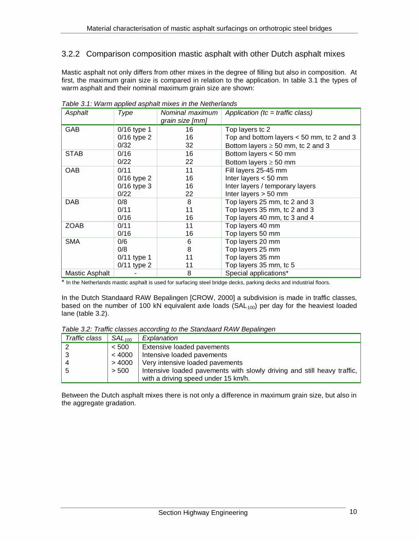
3.2.2 Comparison composition mastic asphalt with other Dutch asphalt mixes
Mastic asphalt not only differs from other mixes in the degree of filling but also in composition. At first, the maximum grain size is compared in relation to the application. In table 3.1 the types of warm asphalt and their nominal maximum grain size are shown: Table 3.1: Warm applied asphalt mixes in the Netherlands
Asphalt Type Nominal maximum grain size [mm]
Application (tc = traffic class)
GAB 0/16 type 1 16 Top layers tc 2 0/16 type 2 16 Top and bottom layers < 50 mm, tc 2 and 3 0/32 32 Bottom layers 50 mm, tc 2 and 3
STAB 0/16 16 Bottom layers < 50 mm
0/22 22 Bottom layers 50 mm
OAB 0/11 11 Fill layers 25-45 mm 0/16 type 2 16 Inter layers < 50 mm 0/16 type 3 16 Inter layers / temporary layers 0/22 22 Inter layers > 50 mm
DAB 0/8 8 Top layers 25 mm, tc 2 and 3 0/11 11 Top layers 35 mm, tc 2 and 3 0/16 16 Top layers 40 mm, tc 3 and 4
ZOAB 0/11 11 Top layers 40 mm 0/16 16 Top layers 50 mm
SMA 0/6 6 Top layers 20 mm 0/8 8 Top layers 25 mm 0/11 type 1 11 Top layers 35 mm 0/11 type 2 11 Top layers 35 mm, tc 5
Mastic Asphalt - 8 Special applications*
* In the Netherlands mastic asphalt is used for surfacing steel bridge decks, parking decks and industrial floors. In the Dutch Standaard RAW Bepalingen [CROW, 2000] a subdivision is made in traffic classes, based on the number of 100 kN equivalent axle loads (SAL100) per day for the heaviest loaded lane (table 3.2). Table 3.2: Traffic classes according to the Standaard RAW Bepalingen
Traffic class SAL100 Explanation
2 < 500 Extensive loaded pavements 3 < 4000 Intensive loaded pavements 4 > 4000 Very intensive loaded pavements 5 > 500 Intensive loaded pavements with slowly driving and still heavy traffic,
with a driving speed under 15 km/h.
Between the Dutch asphalt mixes there is not only a difference in maximum grain size, but also in the aggregate gradation.
Material characterisation of mastic asphalt surfacings on orthotropic steel bridges
Section Highway Engineering 11
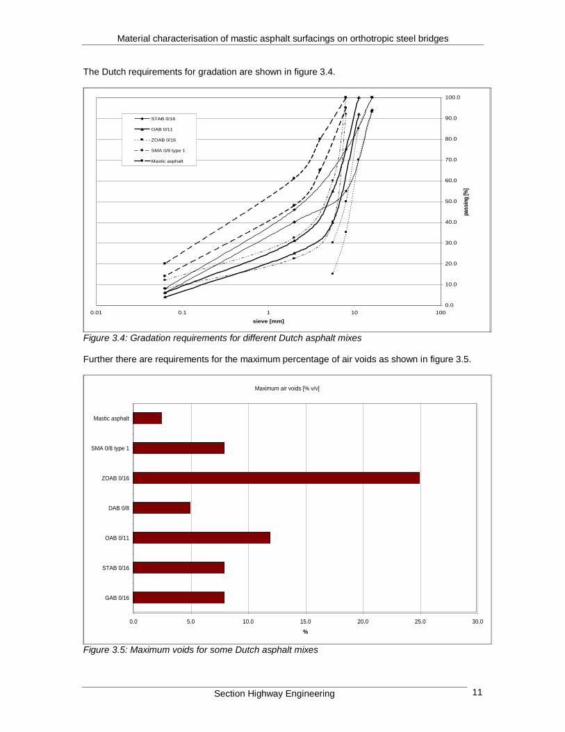
The Dutch requirements for gradation are shown in figure 3.4.
0.0
10.0
20.0
30.0
40.0
50.0
60.0
70.0
80.0
90.0
100.0
0.01 0.1 1 10 100
sieve [mm]
passin
g [%
]
STAB 0/16
OAB 0/11
ZOAB 0/16
SMA 0/8 type 1
Mastic asphalt
Figure 3.4: Gradation requirements for different Dutch asphalt mixes Further there are requirements for the maximum percentage of air voids as shown in figure 3.5.
Maximum air voids [% v/v]
0.0 5.0 10.0 15.0 20.0 25.0 30.0
GAB 0/16
STAB 0/16
OAB 0/11
DAB 0/8
ZOAB 0/16
SMA 0/8 type 1
Mastic asphalt
%
Figure 3.5: Maximum voids for some Dutch asphalt mixes

Material characterisation of mastic asphalt surfacings on orthotropic steel bridges
Section Highway Engineering 12
In figure 3.5 the values are valid for all traffic classes, except the value for DAB 0/8, which is valid for traffic class 2 and 3 (see also table 3.2). For most of the Dutch asphalt mixes there is also a requirement for the minimum percentage of voids, by means of a maximum degree of filling. However, in the Dutch Standaard RAW Bepalingen [CROW, 2000] gives no maximum degree of filling for mastic asphalt. The requirements for the percentage of bitumen for some mixes are shown in figure 3.6.
Bitumen [%] m/m
0 2 4 6 8 10 12
GAB 0/16 vk 2
STAB 0/16
OAB 0/11
DAB 0/8
Mastic asphalt
%
maximum
minimum
Figure 3.6: Requirements for the percentage bitumen for some mixes In figure 3.6 the values are valid for all traffic classes, except the value for DAB 0/8, which is valid for traffic class 2 and 3 as well as the value for GAB 0/16, which is valid for traffic class 2. Because mastic asphalt is an overfilled mixture there is a small percentage of air voids and a high percentage of bitumen compared to the other mixes. This difference in composition makes mastic asphalt very suitable for special applications, like surfacing orthotropic steel decks.
3.2.3 The reason that mastic asphalt is often used on orthotropic steel bridges
On an orthotropic steel bridge the longitudinal stiffeners can be considered as stiff points in the structure were only small deformations take place. The largest deformations take place between these stiffeners. These deformations of the steel deck and the asphalt on orthotropic steel bridges are larger than the deformations of a normal pavement on a basecoarse and subgrade. Due to this large deformations a flexible type of asphalt is needed for deck surfacing. Mastic asphalt fulfils this requirement because of its high percentage of mastic (bitumen and filler) and is therefore often used on orthotropic steel bridges.
3.2.4 History of mastic asphalt in the Netherlands
In the Netherlands mastic asphalt was already used before 1940 in floor-, gutter- and tramrail structures [Hardenberg et al., 1985]. In this type of structures mastic asphalt was used because of its durability. Later it was also used on orthotropic steel bridges. Mastic asphalt could resist the

Material characterisation of mastic asphalt surfacings on orthotropic steel bridges
Section Highway Engineering 13
large deformations of the steel deck without fatigue cracking, because of the flexibility of the mix. The composition of the mix was based on experience. Unfortunately, this experience with mastic asphalt wasn’t documented. After 1970 the problems arose very fast, because of a combination of factors:
The increase of traffic intensity.
The increase of axle-loads.
Absence of strong specifications.
The experience with mastic asphalt disappeared because of retirement of skilled people.
Changes in production, transport and processing led to a decreasing hardness of the binder, resulting in a mix with a lower stiffness.
So after 1970 the need for other asphalt structures on steel bridges arose. Alternatives, like hot-rolled asphalt and modified bitumen mixes were considered. One of the findings is that the deformation of the mastic asphalt was mainly defined by the properties of the binder. This knowledge resulted in the application of another type of bitumen that was less sensible to deformation. In the Netherlands in 1985 the structure normally consisted of the following parts:
Primer layer of thinned bitumen 20/30 on the steel deck 50 m
Bonding layer of rubber-modified bitumen 0.8 kg/m2
Mastic layer based on blown bitumen 6-8 mm
Base layer of poured asphalt 20 mm
Top layer of poured asphalt modified with Trinidad-Épurée bitumen 22 mm
Chippings, hot rolled
3.2.5 Requirements for mastic asphalt in some countries
Requirements for mastic asphalt differ from one country to the other. The requirements were set according to the experience of individual countries.
3.2.5.1 The Netherlands
In the Netherlands mastic asphalt is used for surfacing steel bridge decks, parking decks and industrial floors. Because of its sensibility to deformations and the high costs it is not used for roads anymore. In the Netherlands the composition of the mix has to fulfil the requirements shown in table 3.3 [CROW, 2000]. Table 3.3: Requirements for mastic asphalt according to the RAW
Passing [%]
Mastic asphalt
Desired min. max.
C8 C4 2 mm
63 m
- 75,0 56,0 17,0
95,0 65,0 48,0 14,0
100,0 80,0 61,0 20,0
Bitumen percentage (on 100 % mineral aggregate)
8,5 7,0 10,0
The maximum aggregate size is 8 mm. The mix consists of broken stones 2/8, sand type A, filler
and bitumen 40/60. Sand type A has aggregates between 2 mm and 63 m. The maximum void ratio is 2.5%.

Material characterisation of mastic asphalt surfacings on orthotropic steel bridges
Section Highway Engineering 14
The requirements for penetration and deformation are:
Penetration 10-40 (*0.1 mm) with the stempel test (300 sec, 5.25 N/mm2, 100 mm
2, 25ºC).
Deformation of 6-10% after 100.000 load repetitions in the wheel track test [NPC, 1996]. The requirements from the Dutch Ministry of Transport, Public Works and Water Management (Rijkswaterstaat) for mastic asphalt on steel bridges are shown in table 3.4 [Kolstein, 1990]. Table 3.4: Requirements from the Dutch Ministry of Transport, Public Works and Water
Management for mastic asphalt on steel bridges
Passing [%]
Coarse mastic asphalt Fine mastic asphalt average
Tolerance
Toplayer average Firstlayer average
C 8 C 5.6 2 mm 0.063 mm
43 -
40 17
- 38 39 23
- -
58 42
+5 +5 +5 +2
Bitumen (% by mass on 100% mineral aggregate)
45/60 + Trinidad Épuré
9 +0.5
45/60 9.5 +0.5 85/40 19 +0.5
However some qualitative requirements were specified by NPC in 1996 after an extensive testing program in order to select materials for the Ewijk bridge:
High resistance against cracking/fatigue (flexural bending test).
High fracture strength (semi circular bending Test).
High resistance against permanent deformation (triaxial test, DIN test, wheel track test).
The top layer must have elastic properties (tough, rubber behaviour) to prevent cracking above the steel longitudinal stiffeners.
The sub layer must have a high stiffness to prevent permanent deformation and to contribute to the strength of the total structure.
3.2.5.2 Germany
In Germany mastic asphalt is still used for roads, even motorways, because of its durability. It is often used for roads with heavy loads. Therefore they use a mix with over 40% of stone. In Germany there are 4 main types of mastic asphalt, varying in the maximum grain size (table 3.5): Table 3.5: Requirements for mastic asphalt in Germany
Mastic asphalt 0/5 (0/5 mm)
0/8 (0/8 mm)
0/11 (0/11 mm)
0/11S (0/11 mm)
Aggregate > 2 mm % m/m Aggregate < 0.09 mm % m/m Bitumen percentage % m/m Type of bitumen
35-40 24-34
7.0-8.5
40-50 22-32
6.8-8.0 (B 65) B45
45-55 20-30
6.5-8.0
45-55 20-30
6.5-8.0 B45 (B25)
Often a bitumen type B65 is used in Germany with a penetration (at 25ºC) of 50-70 (0.1 mm).

Material characterisation of mastic asphalt surfacings on orthotropic steel bridges
Section Highway Engineering 15
The requirements for the penetration (40±1ºC, 500 mm2) of the four mixes are given in table 3.6:
Table 3.6: Penetration for mastic asphalt (40±1ºC, 500 mm
2)
Mastic asphalt Penetration after 30 min [mm] Penetration in the next 30 min [mm]
0/11 S 1.0 – 3.5 ≤ 0.4 0/11 1.0 – 5.0 ≤ 0.6 0/8 1.0 – 5.0 ≤ 0.6 0/5 1.0 – 5.0 ≤ 0.6
The requirements for cracking are:
In tension no cracking with a force of 400 N in longitudinal and transverse direction (tension test)
In bending no cracking at 3 % strain In Germany there are also requirements for the bonding layer between the steel and the mastic asphalt:
Ball penetration 6 mm at 25C
8.5 mm at 40C
Temperature ring and ball 70C
After 1 million load repetitions the bonding between the different layers must be still intact (bending test).
This gives an indication of what type of requirements are used in Germany. For the exact test specifications the interested reader is referred to “Technischen Prüfvorschriften für die Prüfung der Dichtungsschichten und der Abdichtungssysteme für Brückenbeläge auf Stahl”, edition 1992 (TP-BEL-ST).
3.2.5.3 USA
Table 3.7 shows the requirements for the aggregate gradation in the United States. Table 3.7: Gradation for mastic asphalt mixes in the USA
Sieve size [mm] Percent passing
12.5 95-100 9.5 80-95 4.75 58-75 2.36 43-60 0.60 20-35
0.075 7-14
Some other requirements are:
Minimum density 2240 kg/m3
Maximum percentage air voids 3.0 %
Ultimate load value As large as possible at ambient laboratory temperature
Expansion coefficient As close to that of steel as possible at ambient laboratory temperature
Creep percentage at 30 minutes Not more than 5 percent at both tension and compression at ambient laboratory temperature
Fatigue resistance No cracking, de-bonding or any other form of fatigue degradation during 8.000.000 cycles under full simulated wheel load

Material characterisation of mastic asphalt surfacings on orthotropic steel bridges
Section Highway Engineering 16
Also requirements are given for the shear strength between the steel and the asphalt. The bond strength of the surfacing to the corrosion protection layer should be as large as possible, but not less than:
2.75 MPa at ambient laboratory temperature.
2.75 MPa at 0C.
1.75 MPa at 60C.
A few general qualitative requirements are:
High fatigue resistance.
High bond strength for the bonding layer.
Skid resistance and resistance against aggregate polishing.
Sufficient resistance to shoving and rutting under temperature extremes.
Thickness of surfacing sufficient to provide wheel load distribution and mass for damping of vibrations from wheel loads.
3.2.5.4 England
In England the use of mastic asphalt is limited to special applications, for example heavy loaded roads and to provide a waterproof membrane. Table 3.8 shows the mix gradation in England. Table 3.8: Gradation for mastic asphalt in England
Mastic asphalt
Coarse aggregate % m/m 30.0 Fine aggregate % m/m 26.0 Filler % m/m 32.0 Bitumen % m/m 12.0
Void content % v/v <1.0
Bitumen with a pen of 15-25 (0.1 mm) are used.
3.2.6 Comparison between the composition of mastic asphalt in some countries
At first the gradation for mastic asphalt mixes in some countries is shown in figure 3.7. For Germany type 0/11 is taken for the comparison.
0
20
40
60
80
100
120
0.01 0.1 1 10 100
sieve [mm]
pa
ss
ing
[%
]
USA
Netherlands
Fuller
England
Germany 0/11
Figure 3.7: Comparison gradation mastic asphalt in some countries

Material characterisation of mastic asphalt surfacings on orthotropic steel bridges
Section Highway Engineering 17
There is not only a difference in composition, but also in maximum grain size, which has an influence on the minimum thickness of the asphalt layer. This maximum grain size for mastic asphalt mixes in some countries is shown in figure 3.8:
0 2 4 6 8 10 12 14
USA
Holland
England
Germany
size [mm]
Figure 3.8: Maximum grain size in some countries In the past a larger maximum grain size was used in mastic asphalt mixes in Holland. However, with larger grain sizes the problem of segregation arose, especially because of the fact that mastic asphalt is not compacted. Segregation is caused by settlement of large grains at the bottom of the asphalt layer (due to gravity) leading to a non-homogeneous mix. To solve this segregation problem it was chosen to divide the mastic asphalt structure in two layers of mastic asphalt and from that moment the mastic asphalt is applied in two layers. The smaller thickness of each layer results in smaller grain sizes to be applied, so from that moment the maximum grain size decreased to 8 mm. The application of smaller maximum grain sizes makes the structure more sensible to rutting. Therefore modifiers are added to the bitumen to make the mix less sensible to rutting. The maximum voids content for mastic asphalt mixes in some countries is shown in figure 3.9:
0
0.5
1
1.5
2
2.5
3
3.5
Netherlands England USA
pe
rce
nta
ge
%
Figure 3.9: Maximum air voids in some countries

Material characterisation of mastic asphalt surfacings on orthotropic steel bridges
Section Highway Engineering 18
Figure 3.10 shows the maximum percentage of bitumen in mastic asphalt mixes in some countries.
0
2
4
6
8
10
12
14
Netherlands Germany England
pe
rce
nta
ge
%
Figure 3.10: Maximum bitumen percentage in some countries The difference in composition and requirements has led to different cross sections in the different countries.
3.2.7 Typical cross-sections in various countries
The differences in mix composition and requirements have led to different cross-sections of orthotropic steel bridges in some countries. The following figures 3.11-3.17 represent typical cross-sections of orthotropic steel bridges in various countries.
Figure 3.11: Typical cross-section as used in the Netherlands
Tar-epoxy sprayed with grit
Tar-epoxy
Hot applied rubber bitumen adhesion layer
Steel plate
Asphalt concrete with increased resistance to fatigue cracking
50
10
10

Material characterisation of mastic asphalt surfacings on orthotropic steel bridges
Section Highway Engineering 19
Tar-epoxy sprayed with sand
Tar-epoxy
Mastic asphalt
Steel plate
Asphalt concrete with increased resistance to fatigue cracking
500
100
100
Figure 3.12: Typical cross-section as used in the Netherlands
Figure 3.13: Typical cross-section as used the ‘Pont de Cornouaille’ in France
Figure 3.14: Traditional cross-section as used in Germany
Hot applied rubber bitumen sprayed with grit
Hot applied rubber bitumen
Steel plate
Asphalt concrete with rubber
Rubber bitumen sprayed with grit
500
120
500
500
Mastic asphalt
OKTO bonding
First layer mastic asphalt
Steel plate
Second layer mastic asphalt
350
12
100
350

Material characterisation of mastic asphalt surfacings on orthotropic steel bridges
Section Highway Engineering 20
Figure 3.15: Typical cross-section as used in Belgium
Figure 3.16: Typical cross-section as used in England
Figure 3.17: Typical cross-section as used in the USA Note: dimensions are in mm
In Germany sometimes a steel grid is welded on the steel deck plate in order to get a better bond between the steel and the asphalt [Volker 1993].
Steel plate
Asphalt concrete protection layer sprayed with grit
OKTO bonding
Asphalt concrete (first layer)
Mastic asphalt
TOPECO (Belgium alternative for hot rolled asphalt)
10
50
30
30
12
Rubber modified bitumen
Rubber bonding layer
Steel plate
Mastic asphalt
Sprayed material
40
120
Epoxy bitumen-bonding layer
Steel plate
Epoxy asphalt
500
500
500
120

Material characterisation of mastic asphalt surfacings on orthotropic steel bridges
Section Highway Engineering 21
3.3 Stress reduction in steel deck due to asphalt surfacing
3.3.1 Introduction
It is known that surfacings of a steel orthotropic deck reduce the stresses in the steel structure. Firstly this reduction is a result of the fact that the thickness of the asphalt spreads the loads. The load spreading property of asphalt varies because of its visco-elastic, temperature dependent and ageing behaviour and is therefore often neglected. In the Eurocode 3 [1997] the load spreading through the pavement and the deck is taken at a spread/depth ratio of 1 to 1. De Jong [2000] has shown that the spread/depth ratio is ≈ 1:1, but the load spreading starts at approximately the middle section of the asphalt. It seems that the Euro Code assumption overestimates the load spreading. Secondly the composite action in bending of the asphalt layer with the steel deck causes reduction of stresses. This means that by applying a surface on the steel deck the moment of inertia of the structure increases, resulting in smaller deformations and thus less stresses. The total reduction of stresses due to composite action depends mainly on the bond between the asphalt and the steel deck and the stiffness of the asphalt. When there is no bond between steel and the asphalt, the two layers are effectively separated. When there is complete bond between the two layers, this means that the two layers can be combined as a composite section. Hence resulting in less stresses in the two layers, since the height is of the third order in the equation for the moment of inertia (Izz = f(h
3)). However, the two situations mentioned (complete and bond and
complete separation) are extreme situations. In practice, the real bond between the two layers is normally intermediate between the two extreme situations and is quite difficult to be determined.
3.3.2 Composite action theories
In this section the different theories for composite action are presented. They are used to calculate the stresses and strains that occur in the mastic asphalt due to bending moment produced by loading. All researchers based their work on linear elastic theory. Furthermore, they have adopted one or both of the following assumptions [Medani 2000a]: 1. Linear strain distribution in the asphalt and the steel. 2. The slopes of the strain distribution through the depth of the asphalt and steel are equal.
3.3.2.1 Metcalf [1967]
Metcalfs analysis is based on beam theory, in which the beam consists of an asphalt layer and a steel layer. He assumes that the bond between the two layers is 100%, what means no slip and a linear strain distribution throughout the full height of the composite beam. For determining the asphalt strains Metcalf uses the following relations:
)(2
212
20naa
anatt
Equation 3.1
t0 = distance from the neutral axis to the top of the asphalt tl = thickness of the steel plate t2 = thickness of the asphalt layer a = t2 / t1
E1 = elastic modulus of the steel plate E2 = elastic modulus of the asphalt n = E1 / E2

Material characterisation of mastic asphalt surfacings on orthotropic steel bridges
Section Highway Engineering 22
2
023
23
2 )1(331
13
ta
nbt
a
aan
btIo
Equation 3.2
I0 = moment of inertia b = width of the beam
02
0
IE
Mtt Equation 3.3
t = tensile strain at the top of the asphalt layer M = bending moment The most important conclusions of his theoretical analysis are:
An increasing modular ratio Es/Ea means an increasing deflection at the centre of the beam.
An increasing modular ratio Es/Ea means increasing strains in the asphalt layer.
A greater part of the applied load is carried by the steel plate as the pavement modulus is decreased.
3.3.2.2 Kolstein [1990]
Kolstein considers two extreme situations in his analysis of composite action, namely full adhesion and no adhesion between the steel deck and the asphalt. He also assumes a linear strain distribution in both the steel and the asphalt. Kolstein uses the following relations: Complete adhesion (100%):
hnt
hthntz
22
222
Equation 3.4
SI
zthMt
)( Equation 3.5
No adhesion (0%):
)(2 21 EISI
Mht
Equation 3.6
in which: z = distance from the neutral axis to the bottom of the steel deck E = elastic modulus of the steel S = elastic modulus of the asphalt n = E / S h = thickness of the asphalt layer t = thickness of the steel plate I = moment of inertia of the composite section I1 = moment of inertia of the asphalt section I2 = moment of inertia of the steel section M = bending moment of the composite section
t = strain at the top of the asphalt layer

Material characterisation of mastic asphalt surfacings on orthotropic steel bridges
Section Highway Engineering 23
One of his conclusions from his theoretical analysis is that the strain at the top of the asphalt is a function of the asphalt stiffness as shown in figure 3.18:
10
100
1000
10000
100 1000 10000 100000
Stiffness [MPa]
str
ain
at
top
of
asp
halt
ic layer
[
m/m
]
complete
adhesion
no intact
Figure 3.18: Strain at the top of the asphalt layer as a function of the asphalt stiffness His analysis clearly shows that in case of a large asphalt stiffness and no adhesion the asphalt strains are higher compared to full adhesion, which indicates the importance of the bonding layer between the steel plate and the asphalt. However, when the asphalt stiffness is low and the maximum strain at complete adhesion is considered, the maximum strain reaches the value of
4000 .
3.3.2.3 Cullimore et al. [1983]
Cullimore et al. carried out a theoretical research using stress functions. Throughout the height a linear strain distribution is assumed. The results were compared with the experimental results and showed a quite good agreement. The theory of Cullimore is based on a two-layer cantilever with an elastic interface. The model in this case is shown in figure 3.19:
Figure 3.19: Two-layer cantilever with elastic interface in Cullimore’s theory

Material characterisation of mastic asphalt surfacings on orthotropic steel bridges
Section Highway Engineering 24
The following relation is used for determining the asphalt strain:
xE
xyE
t
Equation 3.7
in which:
1221
2323
BABA
ABBA
Equation 3.8
PaIIDh
12
2
1 Equation 3.9
and:
1221
1313
BABA
BAABa
Equation 3.10
2)2(
2)32()32(
22
2221
DLDhIIA asa
Equation 3.11
2)2(
2)32()32(
22
1112
DLDhIIA ssa Equation 3.12
)32()32(3 saPA Equation 3.13
21
1
1
2
22
2
2
2
221
12
)2()(2
)2
(2
)2(2
Ih
h
I
h
IDh
LI
Dhh
k
IEB sa
i
s
Equation 3.14
)3
(2
)2()(22
)2(2
1
2
11
1
11
2
1
2
221
2 IDhh
h
IDh
h
ILI
h
k
IEB sa
i
s
Equation 3.15
2)2()
1(
22)2(
2 1
12
2
23
h
hh
Lh
k
EPB sa
i
s
Equation 3.16
in which:
t = tensile strain at the top of the asphalt layer E = elastic modulus of the asphalt layer Es= elastic modulus of the steel
= Es/E = modular ratio kI =shear stiffness of the interface I1 =moment of inertia of the steel I2 = moment of inertia of the asphalt x,y = co-ordinates of the point to be considered h1 = half of the height of the steel plate

Material characterisation of mastic asphalt surfacings on orthotropic steel bridges
Section Highway Engineering 25
h2 = half of the height of the asphalt layer D = 2(h1+h2)
a = Poisson’s ratio for asphalt
s = Poisson’s ratio for steel L = length of the beam The theory shows the influence of the stiffness of the bonding layer on the asphalt strains. Cullimore considered a few numerical values to be representative for practical purposes. For the stiffness of the bonding layer he assumed ki = 4*10
8 Pa. However, his assumption for the load
(P=1N) which is not comparable to a wheel load. Two important conclusions of his experimental research are:
The effect of increasing the stiffness of the bonding layer is insignificant in reducing the maximum tensile stress in the asphalt at temperatures of 35ºC.
At temperatures below the 35ºC the strains in the asphalt increased with decreasing stiffness of the bonding layer.
3.3.2.4 Nakanishi et al. [2000]
Nakanishi et al. simulates the orthotropic steel bridge using a two-span continuous beam model. The beam model consists of three layers: a steel plate deck, a binder course and a surface course as shown in figure 3.20.
Figure 3.20: Beam considered by Nakanishi Three assumptions are made:
Linear strain distribution in both the steel and the asphalt.
The slopes of the two strain distributions in the steel and the asphalt are the same.
The binder and the surface coarse are completely bonded. In the relations from the theoretical analysis the bond between the steel plate and the binder course can be varied. The relations that were determined are:
1
21
2
2
10
hh Equation 3.17
When the steel and the asphalt are not bonded there are two neutral axes. In that case h0 is defined as the distance between the neutral axis of the surface and base layer to the top of the asphalt.

Material characterisation of mastic asphalt surfacings on orthotropic steel bridges
Section Highway Engineering 26
The parameters are defined as: E1 = elastic modulus of the surface coarse E2 = elastic modulus of the binder coarse E3 = elastic modulus of the steel plate h1 = thickness of the surface coarse h2 = thickness of the binder coarse h3 = thickness of the steel plate
= E2/E1
= h2/h1
The distance between both neutral axes is dependent on the bond between the steel and the asphalt and can be determined with:
2
)1( 3
021
hhhhtT Equation 3.18
T = distance between both neutral axes t = coefficient of bond between the binder course and the steel plate. t=0 is no bonding, t= 1 means complete bondage The distance from the upper neutral axis to the surface of the asphalt can be determined with:
1
/22221
2
1
22
1 hThh Equation 3.19
h = position of the neutral axis in case of a varying coefficient of bond
= E3/E1
= h3/h1
The formula for h0 can be seen as a special case of h, namely h0 = h(t=0). A factor equivalent to the moment of inertia is determined with:
)(3)(3)()()(3
222333333 CDTCDTCDBCABb
J Equation 3.20
J = parameter equivalent to the moment of inertia A = -h B = -h+h1
C = -h+h1+h2
D = -h+h1+h2+h3
The strains at the top of the asphalt layer are determined with:
AJE
Mt
1
Equation 3.21
t = tensile strain at the top of the asphalt layer M = bending moment of the composite section

Material characterisation of mastic asphalt surfacings on orthotropic steel bridges
Section Highway Engineering 27
The main results of the theoretical analysis are:
Strains at the pavement surface are decreasing when the complex modulus of the asphalt mix increases.
The surface strain increases when the coefficient of bondage decreases.
When the coefficient of bond decreases, the shear stress at that bond decreases, but the shear stress increases at other points.
Not only the strain at failure at low temperatures but also the complex modulus of elasticity of the mixture should be used in design codes.
3.3.2.5 Sedlacek and Bild [1985]
In the German requirements the bearing capacity of the asphalt is not taken into account by assuming that the asphalt stiffness is zero (Easf = 0). This means that the asphalt takes no stresses. The strains in the asphalt can be calculated by extrapolation of the strains in the deck plate:
zEI
Ma
1
Equation 3.22
M = bending moment EI1 = bending stiffness of the steel deck z = distance between half of the steel deck and the top of the asphalt layer The bending moment M is calculated with a computer program, using the plate theory. This method should be allowed for dimensioning the steel structure, because of the low asphalt stiffness at high temperatures. For calculating the asphalt stresses and strains the method mentioned before is not useful, because of their dependency on the modulus of elasticity of the asphalt. Therefore Sedlacek and Bild developed a composite action beam model for the steel plate and the asphalt. The model consists of a beam with a width of 1 cm taken from the steel-asphalt structure and is shown in figure 3.21. Figure 3.21: Model used by Sedlacek and Bild tb = thickness of the asphalt layer [m] ts = thickness of the steel deck plate [m] Eb = Elastic modulus of the asphalt [Pa] Gb = Shear stiffness of the asphalt [Pa] Es = Elastic modulus of the steel deck plate [Pa] C = Elastic modulus of the bonding layer between the asphalt and the steel [Pa] P = load L = length of the beam
Eb, Gb
Es
tb
ts C
L
p

Material characterisation of mastic asphalt surfacings on orthotropic steel bridges
Section Highway Engineering 28
On the beam a load p is assumed to act at the mid-span. Between the asphalt and the steel there is an elastic bonding layer. Also the shear stiffness of the asphalt layer is taken into account. The asphalt strains in the model are the sum of three factors:
Strains due to the bending moment in a fully bonded state.
Strains due to the deformation of the bonding layer depending on the stiffness of the bonding layer.
Strains due to the shear deformation of the asphalt depending on the shear stiffness of the asphalt.
Strains due to the bending moment The strains in the model due to the bending moment are calculated using the method described by Sedlacek [1982]. The next formulas are used:
s
b
t
t Equation 3.23
s
b
E
E Equation 3.24
1
1
2
11 sz tk Equation 3.25
k1z = distance between the half of the steel deck plate and the neutral axis [m]
1
2
3141
12
1
242
3
szz tA Equation 3.26
Azz = factor equivalent to the moment of inertia of the composite beam with width =1 [m
4]
1
21
2
10 stz Equation 3.27
z0 = distance between the neutral axis and the top of the asphalt layer [m]
1
1
2
1 2
sf tz Equation 3.28
zf = distance between the neutral axis and the bonding layer [m]
1
21
2
1su tz Equation 3.29
zu = distance between the neutral axis and the bottom of the steel deck plate [m]

Material characterisation of mastic asphalt surfacings on orthotropic steel bridges
Section Highway Engineering 29
The strains at the top of the asphalt layer due to the bending moment are calculated using:
0zAE
M
zzs
a Equation 3.30
a = asphalt strain at the top of the layer [-] M = bending moment [Nm] Strains due to the deformation of the bonding layer and the shear deformation of the asphalt For the effect of the bond deformation and the asphalt shear deformation on the asphalt strains an extra analysis has to be made using the method from Roik and Sedlacek [1970]. The effect of the bond deformation and the shear deformation of the asphalt on the asphalt strains is schematically shown in the next figure 3.22.
Figure 3.22: Schematic deformations of the asphalt layer due to bond deformation and shear deformation of the asphalt The ratio between the shear stiffness of the asphalt Gb and the stiffness of the bonding layer C is defined as:
C
Gb Equation 3.31
Further four stiffness factors are defined in which the indexes 1 and 2 refer to deformation of the bonding layer respectively shear deformation of the asphalt:
242
223
1
2
3141
13
111
sss tA Equation 3.32
242
2
32
2
2
3141
1113
1
ss
sss
tttA Equation 3.33
Strain in the asphalt due to bond deformation (ws1)
+
+
Strain in the asphalt due to shear deformation of
the asphalt (ws2)
asphalt
steel
bond

Material characterisation of mastic asphalt surfacings on orthotropic steel bridges
Section Highway Engineering 30
stS
2
1 1 Equation 3.34
ss ttS
2
2 1 Equation 3.35
in which:
2
242233
21
3
13121
3
111
3
11
1
1
sss ttt
Equation 3.36
The strains due to deformation of the bonding layer and shear deformation of the asphalt are calculated by solving the following differential equation:
sisi
isi
ssis prdx
vdCS
dx
vdAE
2
2
4
4
Equation 3.37
i = 1 for the deformation of the bonding layer and 2 for the deformation of the asphalt vsi = added deformation [m] p = load [N] rsi = load factor [-]
242
2
1
2
3141
4316
s
st
r Equation 3.38
242
2
2
2
3141
1643
s
s
s
t
tr Equation 3.39
The differential equation 3.37 is equivalent to the equation of the tensioned bending beam and can be solved using the 2
nd order theory [Bouma 1993]. This results in:
2
43212
xCS
prxCCeCeCv
i
sixx
si Equation 3.40
with:
ssis
i
AE
CS2 Equation 3.41

Material characterisation of mastic asphalt surfacings on orthotropic steel bridges
Section Highway Engineering 31
For calculation of the added deformations the second derivative is used:
i
sixxsi
CS
preCeC
dx
vd 2
2
1
2
2
2
Equation 3.42
in which:
i
si
ll
l
CS
pr
ee
eC
21
1
Equation 3.43
i
si
ll
l
CS
pr
ee
eC
22
1
Equation 3.44
The moment analogue to the bending moment follows from:
2
2
dx
vdAEM si
ssissi Equation 3.45
When Ms1 and Ms2 are known the strains due to deformation of the bonding layer and shear deformation of the asphalt layer are calculated with:
si
ssis
sisi w
AE
M ~ Equation 3.46
in which:
zrwww ssss 12112
11
1
~
Equation 3.47
zrtt
www s
ss
sss 21222
1
1
~
Equation 3.48
z = distance to the middle of the steel deck [m] ws1, ws2 = basic parameters for asphalt shear- and bond deformation
3.3.3 Comparison between the different composite action theories
3.3.3.1 Introduction
The previous sections showed the different theories for composite action. In this section the theories are compared. For each theory the strains as a result from a certain bending moment are calculated and compared with the strains calculated with the other theories.

Material characterisation of mastic asphalt surfacings on orthotropic steel bridges
Section Highway Engineering 32
It is known that the maximum tensile strain at the top of the asphalt occurs above the longitudinal stiffener when a dual tyre wheel passes as shown in figure 3.23.
Figure 3.23: Maximum tensile strain at the top of the asphalt due to a dual tyre wheel In order to calculate the maximum tensile strain with the composite action theories a representative bending moment above the longitudinal stiffener has to be calculated. Therefore the situation from figure 3.23 is simulated with a two-span beam as shown in figure 3.24.
Figure 3.24: Simulation with a two-span beam for calculating the maximum bending moment
300 mm 300 mm
190 mm 190 mm
q=0.7 N/mm/mm
50 mm
10 mm
1 mm
Maximum tensile strain
300 mm 300 mm 300 mm

Material characterisation of mastic asphalt surfacings on orthotropic steel bridges
Section Highway Engineering 33
The following assumptions are made:
For the comparison a two-span beam is taken, the distance between the supports is 300 mm, representing the distance between the longitudinal stiffeners. Of coarse this is a simplification of the true behaviour but for a comparison this is allowed, because also all the theories are based on beam-behaviour. The beam consists of a steel plate and an asphalt layer with for some of the theories an elastic interface in between.
The thickness of the asphalt ha = 50 mm and the steel hs = 10 mm.
The stiffness of the asphalt Ea = 1*1010
Pa and the steel Es = 2.1*1011
Pa.
Width of the beam b = 1 mm.
The applied load consists of a dual tyre wheel. The maximum axle load is 100 kN which results in a maximum load of 25 kN per tire. With a contact pressure of 0.7 N/mm
2 the square
contact area is 190x190 mm2. This results in two line loads of 0.7 N/mm/mm acting on the
beam with a width of 1 mm. In fact the construction is analysed by using two line-loads and not by real wheel loads.
The load configuration as shown in figure 3.24 results in a maximum bending moment above the middle support of 6481 Nmm. With this bending moment the maximum asphalt strain will be calculated by using the different composite action theories.
3.3.3.2 Metcalf
Metcalf only considers the fully bonded state. Using Metcalfs theory the maximum tensile strain above the middle support is 6.58*10
-4 mm/mm.
3.3.3.3 Kolstein
Kolstein considers two extreme situations, namely 0% and 100% bonding. For 100% bonding his theory leads to a strain of 6.58*10
-4 mm/mm, for 0% bonding the strain is 1.33*10
-3 mm/mm.
3.3.3.4 Cullimore
Cullimore uses a different load model (see figure 3.19). In order to get the same bending moment of 6481 Nmm at the support the load P to be applied on a beam with a length of 300 mm is 21.6
N. Further, in this comparison a = 0.4 and s = 0.3 as proposed by Cullimore. In table 3.9 and figure 3.25 the dependency of the asphalt strains on the bonding stiffness is shown. Table 3.9: Asphalt strains for different values of the bond stiffness according to Cullimore
Bonding stiffness [N/mm2] Asphalt strain [mm/mm]
1.00*10-2
1.33E-03 1.00*10
-1 1.30E-03
1.00 1.11E-03 1.00*10
1 7.62E-04
1.00*102 6.57E-04
1.00*103 6.44E-04
1.00*104
6.43E-04

Material characterisation of mastic asphalt surfacings on orthotropic steel bridges
Section Highway Engineering 34
0.00E+00
2.00E-04
4.00E-04
6.00E-04
8.00E-04
1.00E-03
1.20E-03
1.40E-03
0.01 0.1 1 10 100 1000 10000
Bond stiffness [N/mm2]
Str
ain
[m
m/m
m]
Figure 3.25: Strains in the asphalt as a function of the bonding stiffness according to Cullimore For 0% bonding the strain reaches the value of 1.33*10
-3 mm/mm and for 100% bonding the
strain is 6.43*10-4
mm/mm according to Cullimores theory.
3.3.3.5 Nakanishi
Nakanishi considers the asphalt strain as a function of the bond coefficient t. The relation between the asphalt strain and the bond coefficient for a bending moment of 6481 Nmm is shown in table 3.10 and figure 3.26. Table 3.10: Asphalt strains for different bond coefficients according to Nakanishi
Bond coefficient t Asphalt strain [mm/mm]
0 1.33E-03 0.1 1.42E-03 0.2 1.42E-03 0.3 1.35E-03 0.4 1.25E-03 0.5 1.13E-03 0.6 1.01E-03 0.7 9.07E-04 0.8 8.12E-04 0.9 7.29E-04 1 6.58E-04
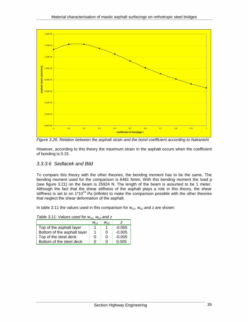
Material characterisation of mastic asphalt surfacings on orthotropic steel bridges
Section Highway Engineering 35
0.00E+00
2.00E-04
4.00E-04
6.00E-04
8.00E-04
1.00E-03
1.20E-03
1.40E-03
1.60E-03
0 0.1 0.2 0.3 0.4 0.5 0.6 0.7 0.8 0.9 1
coefficient of bondage t
as
ph
alt
str
ain
[m
m/m
m]
Figure 3.26: Relation between the asphalt strain and the bond coefficient according to Nakanishi However, according to this theory the maximum strain in the asphalt occurs when the coefficient of bonding is 0.15.
3.3.3.6 Sedlacek and Bild
To compare this theory with the other theories, the bending moment has to be the same. The bending moment used for the comparison is 6481 Nmm. With this bending moment the load p (see figure 3.21) on the beam is 25924 N. The length of the beam is assumed to be 1 meter. Although the fact that the shear stiffness of the asphalt plays a role in this theory, the shear stiffness is set to on 1*10
10 Pa (infinite) to make the comparison possible with the other theories
that neglect the shear deformation of the asphalt. In table 3.11 the values used in this comparison for ws1, ws2 and z are shown: Table 3.11: Values used for ws1, ws2 and z
ws1 ws2 z
Top of the asphalt layer 1 1 -0.055 Bottom of the asphalt layer 1 0 -0.005 Top of the steel deck 0 0 -0.005 Bottom of the steel deck 0 0 0.005

Material characterisation of mastic asphalt surfacings on orthotropic steel bridges
Section Highway Engineering 36
In table 3.12 and figure 3.27 the dependency of the strains in the asphalt on the bond stiffness is shown for a bending moment of 6481 Nmm. Table 3.12: Asphalt strains for different values of the bond stiffness and Gb=1*10
10 N/mm
2
Bond stiffness [N/mm2] Asphalt strain [mm/mm]
1.00*10-2
1.11E-03 1.00*10
-1 1.07E-03
1.00 8.78E-04 1.00*10
1 6.94E-04
1.00*102 6.61E-04
1.00*103 6.58E-04
1.00*104
6.58E-04
0.00E+00
2.00E-04
4.00E-04
6.00E-04
8.00E-04
1.00E-03
1.20E-03
1.00E-02 1.00E-01 1.00E+00 1.00E+01 1.00E+02 1.00E+03 1.00E+04
Bonding stiffness C [N/mm2]
as
ph
alt
str
ain
[m
m/m
m]
Figure 3.27: Asphalt strains as a function of the bonding stiffness For a low bonding stiffness the asphalt strain reaches the value of 1.11*10
-3 mm/mm and for a
high bonding stiffness the strain is 6.58*10-4
mm/mm according to Sedlacek and Bild. By comparing the above mentioned composite action theories it can be seen that some of the theories use a bond percentage and others use a bonding stiffness. In order to compare the theories it is assumed that 0% bonding is equal to a bonding stiffness of 1.00*10
-2 N/mm
2 and
that 100% bonding is equal to 1.00*104 N/mm
2.
In table 3.13 the results for the different theories are shown for 0% and 100% bonding. Table 3.13: Comparison between different composite action theories M=6708 Nmm
Strain [mm/mm] 0% bonding 100% bonding
Metcalf - 6.58*10-4
Kolstein 1.33*10
-3 6.58*10
-4
Cullimore 1.33*10-3
6.43*10-4
Nakanishi 1.33*10-3
6.58*10-4
Sedlacek 1.11*10-3
6.58*10-4

Material characterisation of mastic asphalt surfacings on orthotropic steel bridges
Section Highway Engineering 37
From table 3.13 it is clear that all the theories result in almost the same values of the asphalt strain except Cullimore for 100% bonding and Sedlacek for 0% bonding. The difference that Cullimore’s theory gives for 100% bonding is difficult to explain, but it was noticed that Cullimore’s theory is very sensitive to the input. The difference with Sedlacek’s theory is a result from the fact that in this comparison the shear deformation of the asphalt in Sedlacek’s theory is neglected. This is done because all the other theories also neglect this phenomenon. When in Sedlacek’s theory for 0% bonding the shear stiffness is set to a low value (1.00*10
-2 N/mm
2) the asphalt strain reaches the value of 1.36*10
-3
mm/mm which is comparable with the values of the other theories. The strain in the asphalt predicted by different theories for an assumed bending moment of 6481 Nmm as function of the bond stiffness is shown in figure 3.28.
0.00E+00
2.00E-04
4.00E-04
6.00E-04
8.00E-04
1.00E-03
1.20E-03
1.40E-03
1.60E-03
1.00E-02 1.00E-01 1.00E+00 1.00E+01 1.00E+02 1.00E+03 1.00E+04
Bond stiffness [N/mm2]
str
ain
[m
m/m
m]
Cullimore
Sedlacek
Nakanishi
Kolstein*
Metcalf**
Figure 3.28: Comparison between the theories * Kolsteins theory results in only two points, namely (1.00E-02, 1.33E-03) and (1.00E+04, 6.58E-04)
** Metcalfs theory gives only one point, namely (1.00E+04, 6.58E-04)
Figure 3.28 shows that different theories for composite action give different results for different values of the bond stiffness. From the comparison it can be concluded that:
The maximum asphalt strains for a low bonding stiffness are ≈1300 m/m.
All the theories are based on linear elasticity.
The strains/stresses in the steel/asphalt are calculated using a beam model. However, plate theory may be more applicable.
In all the theories a linear strain distribution is assumed in the asphalt and the steel.
Nakanishi assumes the same slope of the strain distribution in both the asphalt and the steel. This might not be true.
According to Nakanishi’s theory the asphalt strains at ±15% bonding are higher than the strains at 0% bonding.
For certain conditions the presented theories might be true, but these conditions might not be representative for the real structure.
For extreme values of the bond (0% and 100% bonding) the theories give the same results, but for values of the bond stiffness between both extremes the theories give different results.
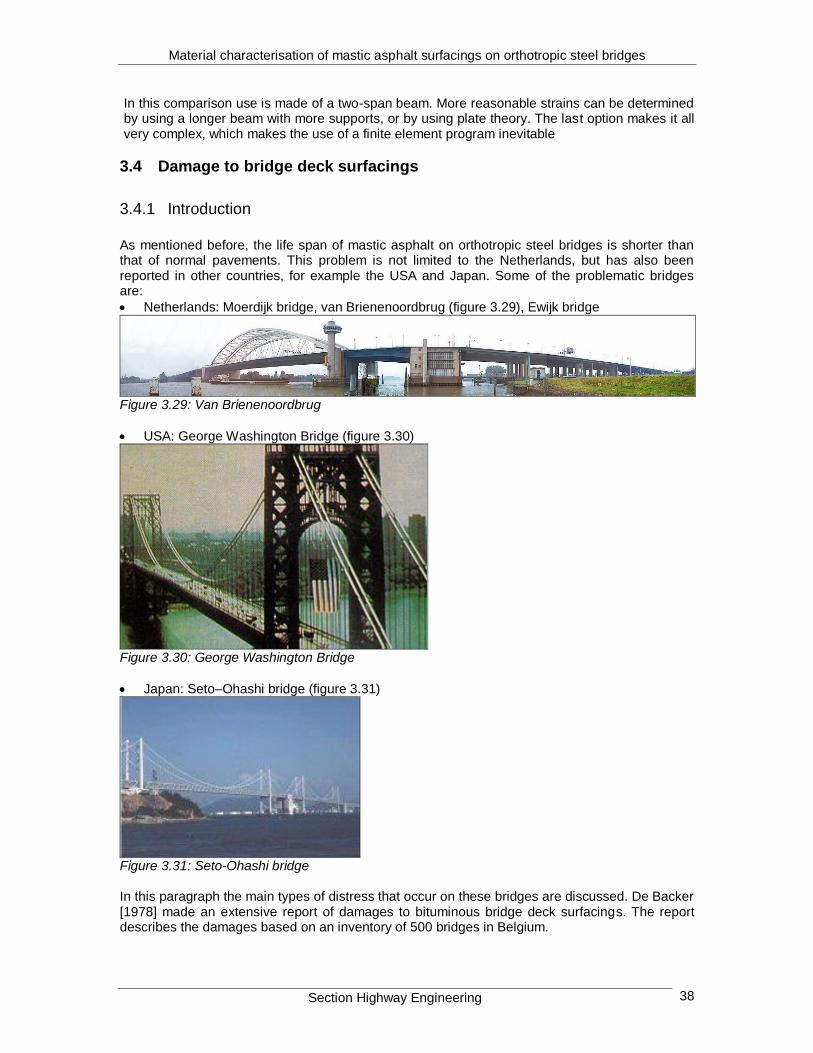
Material characterisation of mastic asphalt surfacings on orthotropic steel bridges
Section Highway Engineering 38
In this comparison use is made of a two-span beam. More reasonable strains can be determined by using a longer beam with more supports, or by using plate theory. The last option makes it all very complex, which makes the use of a finite element program inevitable
3.4 Damage to bridge deck surfacings
3.4.1 Introduction
As mentioned before, the life span of mastic asphalt on orthotropic steel bridges is shorter than that of normal pavements. This problem is not limited to the Netherlands, but has also been reported in other countries, for example the USA and Japan. Some of the problematic bridges are:
Netherlands: Moerdijk bridge, van Brienenoordbrug (figure 3.29), Ewijk bridge
Figure 3.29: Van Brienenoordbrug
USA: George Washington Bridge (figure 3.30)
Figure 3.30: George Washington Bridge
Japan: Seto–Ohashi bridge (figure 3.31)
Figure 3.31: Seto-Ohashi bridge In this paragraph the main types of distress that occur on these bridges are discussed. De Backer [1978] made an extensive report of damages to bituminous bridge deck surfacings. The report describes the damages based on an inventory of 500 bridges in Belgium.

Material characterisation of mastic asphalt surfacings on orthotropic steel bridges
Section Highway Engineering 39
It is not exactly clear on what type of bridges the damages are established, but the amount of orthotropic steel bridges in Belgium is quite small, so most of the damages described have occurred on concrete bridges. However, these damages also occur on orthotropic steel bridges. Damages that occur on orthotropic steel bridges include:
Permanent deformation
Cracking
Mounds
Disintegration
Loss of bond between the steel deck and the asphalt
3.4.2 Permanent deformation
In general, permanent deformations are caused by exceptionally high and/or repeated stresses (compressive or shear). The most important type of permanent deformation is rutting, which increases with high temperatures. Because mastic asphalt has a large amount of bitumen it is sensitive for rutting. Kohler and Deter [1974] indicate that heaves occur above and also between the longitudinal stiffeners. The heaves between the longitudinal stiffeners are caused by movement of the pavement, which is caused by traffic moving from the stiffer part of the plate (above the stiffeners) to the weaker parts (between the stiffeners). Corrugations result from longitudinal forces caused by braking and accelerating vehicles. Sometimes, at high temperatures, the toplayer tends to slide over the bottom layer. This phenomenon was observed on bridges with a high vertical slope in both transversal and longitudinal direction.
3.4.3 Cracking
Cracking is probably the most occurring damage to surfacings on orthotropic steel bridges, both by using mastic asphalt and compacted asphalt. When the cracks reach to the steel deck plate this plate tends to rust, often leading to de-bonding. To prevent that cracks will reflect in the corrosion-protecting layer and reach the steel deck plate a fibre-glass net can be used [Volker 1993]. De Backer [1978] makes a distinction between cracking caused by a strain exceeding the maximum strain in the asphalt after one load cycle and cracking caused by fatigue (more than one load cycle). The most important cracking occurs above the longitudinal or transverse stiffeners. Often there is a pattern in cracking that follows the distance between the longitudinal stiffeners. Above these stiffeners the strains and stresses are generally high. Especially at low temperatures this is critical because then the asphalt is very stiff. Kohler and Deter [1974] make a distinction between longitudinal cracks above and between the stiffeners due to bending moments. The cracks between the stiffeners arise at the bottom of the asphalt and will propagate to the surface. The cracks above the stiffeners arise at the surface of the asphalt and propagate to the bottom. Both types are caused by positive bending moments between the stiffeners, resulting in cracks at the bottom of the pavement that will propagate to the top of the pavement. The cracks between the stiffeners occur often when the bond between the asphalt and steel is weak [de Backer, 1978].

Material characterisation of mastic asphalt surfacings on orthotropic steel bridges
Section Highway Engineering 40
Inspection of the Moerdijk bridge which consists of 10 spans with different steel thicknesses (10-14 mm), showed the following:
80% of the cracks were observed in the right lane
80% of the cracks were observed in spans where the thickness of the steel plate is 10 mm.
3.4.4 Mounds
This is a local expansion/swell of a waterproof layer (for example mastic asphalt), and occurs when a waterproof layer is laid on a layer that contains water. When asphalt is laid on such a layer, water evaporates forming bubbles and will be seen at the surface as mounds.
3.4.5 Disintegration
This includes ravelling (loss of stone particles from the surface) and potholes. It is caused by cracking, loss of bond and/or a combination of other distress mechanisms. Ravelling can seriously reduce the skid resistance of the pavement and hence, endangers the safety of the road users.
3.4.6 Loss of bond between the steel deck and the asphalt
Experiences in the United States (Dublin Bridge in California), Switzerland (St. Albans Bridge in Basel) and Germany (the Koln-Mulheim bridge) tend to show that once the bond between the steel deck and surfacing is destroyed, the failure of the pavement is merely a matter of time.
3.4.7 Distress mechanisms related to mix parameters
3.4.7.1 Introduction
Sometimes distress is characterised by means of the mechanisms causing the distress. In this paragraph the distress mechanisms and the important mix parameters that influence them are discussed. For the design of mastic asphalt on orthotropic bridges there are three types of distress of importance, namely permanent deformation, cracking and the loss of bond between the steel and the asphalt. Both other types of distress, mounds and disintegration are mostly dependent on the way of construction and can hardly be influenced by the design. So they are not discussed further in this paragraph. During lifetime there are factors that have an influence on the distress mechanisms by reducing the pavement strength, for example:
Ageing of bitumen,
Weathering of aggregate materials (chemical decomposition caused by oxygen, water, heat and/or solar radiation).
Strength reduction of bituminous materials because of low viscosity at high temperatures. Most damage occurs as a combination of several distress mechanisms.
3.4.7.2 Permanent deformation
Permanent deformation can be a result of:
Exceptionally high and/or repeated stresses (compressive or shear).
Bleeding because of deformation of bituminous materials with too high bitumen content and too low voids content (typical characteristics for mastic asphalt).

Material characterisation of mastic asphalt surfacings on orthotropic steel bridges
Section Highway Engineering 41
The most important type of permanent deformation is rutting. It is caused by:
Post-compaction of the asphalt
The flow of the asphalt Laboratory tests are carried out to determine the relation between the number of load repetitions
and the permanent deformation p for asphalt. The permanent deformation p is dependent on several parameters:
p = f(e, N, Va, freq)
p : permanent strain
e : elastic strain
N : number of load repetitions
Va : void content
freq : loading frequency [Hz]
For mix design the elastic strain and the voids content are important. The elastic strain indicates that the stiffness modulus of the asphalt is of importance. Because mastic asphalt is an overfilled mixture the mix stiffness is mainly influenced by the bitumen stiffness. Further also the mineral aggregate contributes to the material stiffness. Important mix parameters
Bitumen stiffness.
Gradation, grain shape and maximum grain size.
Void content.
Bitumen content.
3.4.7.3 Cracking
Types of cracking:
Fatigue cracking of pavement materials due to repeated stresses (shear and/or tensile) induced by traffic, environment and poor construction. This type of cracking can occur at the top or at the bottom of the asphaltic layer.
Cracking due to exceptionally high stresses, induced by heavy traffic or freezing, exceeding the material’s tensile or shear strength.
Crack propagation because of high tensile stress intensities at the tips of a previously initiated crack.
Most important on orthotropic steel bridges is the fatigue cracking. Fatigue is the gradual decrease of the pavement strength caused by repeated stress cycles. The result of this decreasing pavement strength is cracking. The main factors influencing cracking are [Medani 2000a]:
the pavement’s strength (mainly the structural thickness, material strength and stiffness)
the traffic loading (number and magnitude of wheel loads)
the climate and weather conditions (solar radiation, temperature, temperature gradients and moisture regimes that influence the traffic induced stresses, but independently also cause ageing)
There are different fatigue damage models that are used in asphalt road engineering. One of them is the Wöhler fatigue model. This model uses a relation between the number of load applications to failure and the strain at the bottom of the asphalt layer:
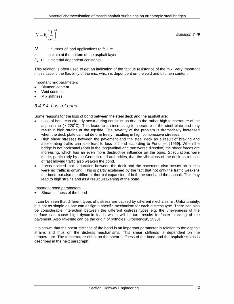
Material characterisation of mastic asphalt surfacings on orthotropic steel bridges
Section Highway Engineering 42
n
kN
11 Equation 3.49
N : number of load applications to failure
: strain at the bottom of the asphalt layer k1, n : material dependent constants
This relation is often used to get an indication of the fatigue resistance of the mix. Very important in this case is the flexibility of the mix, which is dependent on the void and bitumen content. Important mix parameters
Bitumen content
Void content
Mix stiffness
3.4.7.4 Loss of bond
Some reasons for the loss of bond between the steel deck and the asphalt are:
Loss of bond can already occur during construction due to the rather high temperature of the
asphalt mix ( 2200C). This leads to an increasing temperature of the steel plate and may
result in high strains at the topside. The severity of the problem is dramatically increased when the deck plate can not deform freely, resulting in high compressive stresses.
High shear stresses between the pavement and the steel deck as a result of braking and accelerating traffic can also lead to loss of bond according to Fondriest [1969]. When the bridge is not horizontal (both in the longitudinal and transverse direction) the shear forces are increasing, which has an even more destructive influence on the bond. Speculations were made, particularly by the German road authorities, that the vibrations of the deck as a result of fast moving traffic also weaken the bond.
It was noticed that separation between the deck and the pavement also occurs on places were no traffic is driving. This is partly explained by the fact that not only the traffic weakens the bond but also the different thermal expansion of both the steel and the asphalt. This may lead to high strains and as a result weakening of the bond.
Important bond parameters
Shear stiffness of the bond It can be seen that different types of distress are caused by different mechanisms. Unfortunately, it is not as simple as one can assign a specific mechanism for each distress type. There can also be considerable interaction between the different distress types e.g. the unevenness of the surface can cause high dynamic loads which will in turn results in faster cracking of the pavement. Also ravelling can be the origin of potholes [Groenendijk, 1998]. It is shown that the shear stiffness of the bond is an important parameter in relation to the asphalt strains and thus on the distress mechanisms. This shear stiffness is dependent on the temperature. The temperature effect on the shear stiffness of the bond and the asphalt strains is described in the next paragraph.

Material characterisation of mastic asphalt surfacings on orthotropic steel bridges
Section Highway Engineering 43
3.5 Temperature effect
Sedlacek and Bild [1985] carried out a parametric study of the temperature effect on the composite section. The change of temperature can lead to stresses and strains in both the asphalt and the steel because of the different expanding coefficients of both materials. In this study a one-span beam with a length of 300 mm and a width of 10 mm was used. Because of the rather complicated visco-elastic behaviour of the asphalt this study was only concentrated on pure elastic behaviour. In other words, on short-time temperature changing and the behaviour of the asphalt at low temperatures. A fast temperature reduction of 1ºC was used. The coefficients of expansion for the asphalt and the steel that were assumed:
Mastic asphalt: T = 6*10-4
K-1
Steel: T = 1.2*10-5
K-1
The maximum strain at the bottom of the asphalt arises when the bonding layer is weak:
max = T * ∆T = 6*10-4
* (-1) = -600 m/m A high bonding stiffness results in strains that are about 1/20 to 1/5 of the maximum strain. The strain due to the change in temperature is clearly influenced by the stiffness of the bonding layer.
In figure 3.32 the relation between the strain at the bottom of the asphalt (bu), the bonding stiffness (C) and the ratio Easf/Esteel is shown.
Figure 3.32: Strains at the bottom of the asphalt related to the bonding stiffness C and Easf/Esteel

Material characterisation of mastic asphalt surfacings on orthotropic steel bridges
Section Highway Engineering 44
The high strains that are a result of a temperature change of only 1ºC show that the temperature effects cannot be neglected. Besides the temperature there is another important phenomenon that cannot be neglected, namely the vibration of the bridge deck.
3.6 Vibration of the bridge deck
3.6.1 Dynamic axle loads on pavements on a subgrade
For pavements on a subgrade it is known that dynamic axle loads can be up to 40% higher than the static ones [Divine, 1997]. The dynamic axle loads depend on the suspension type, static axle load, speed of travel and longitudinal profile of the road. The dynamic loads are generated within two frequency ranges:
Frequencies between 1.5 and 4 Hz corresponding with body bouncing.
Frequencies between 8 and 15 Hz corresponding with axle bouncing. Very little is known about the interaction between the loads and the pavement and the effects of dynamic loads on pavements. The more interested reader is referred to Huurman [1997], who investigated the effect of dynamic axle loads on concrete block pavements. However, most design codes are based on a “safety factor” that is multiplied with the static loads to deal with the effect of dynamic loads.
3.6.2 Vibration of the bridge deck
For pavements on bridges it seems that vibrations play even a more important role, because on bridges not only the vehicles are vibrating, but also the bridge itself. The dynamic response of bridges depends on:
The bridge damping.
The bridge natural frequencies.
The road and bridge profile.
The vehicle mass.
Frequencies of the vehicles dynamic wheel loads.
The number of vehicles simultaneously on the bridge. The damping of a bridge is dependent on the mass, an increasing mass leads to an increasing damping. For a bridge this means that two contradictory interests play a role since the mass of a bridge is often minimised in the design. The natural frequency of bridges is dependent on the span of the bridge:
Short span bridges (L=8-15 m) have a natural frequency of 8-15 Hz.
Short-medium span bridges (L=15-30 m) have a natural frequency of 4-8 Hz.
Medium-span bridges (L=30-60 m) have a natural frequency of 2-4 Hz.
Long-span bridges (L=60-80 m) have a natural frequency of 1.5-1.8 Hz. When the frequency of the wheel loads is close to the natural frequency of the bridge (frequency matching) this can lead to problems, like increased dynamic responses. For very short bridges (<8 m) vibrations play a less important role. In that case vehicles are longer than the bridge and no true interaction takes place. Very long bridges (>100 m) have such a low natural frequency that only the summed effects of several vehicle vibrations can lead to dynamic responses.

Material characterisation of mastic asphalt surfacings on orthotropic steel bridges
Section Highway Engineering 45
3.6.3 The effect of vibrations on the pavement
3.6.3.1 Axle loads on pavements on a subgrade
To get an indication of the effect of bridge vibrations two models are compared in this paragraph. a two-mass spring system representing the axle load on pavement on a subgrade and a more extensive two-mass spring system representing the axle load on the bridge. The axle load on a pavement on a subgrade can be simulated with a two-mass spring system (figure 3.33).
Figure 3.33: Model of an axle load on a pavement on a subgrade The force in spring 1 represents the dynamic load of the body on the axle and the force in spring 2 represents the dynamic load on the pavement. To describe the behaviour of the model, mass 2 (axle) is displaced over a distance x2 and released at t=0, representing the axle displacement due to an unevenness in the road. The model is described by the following formulae [Dieterman, 1997]:
2
1
2
1
2221
1211
2
1
2
1
0
0
F
F
x
x
kk
kk
x
x
m
m
Equation 3.50
In which:
111 kk
112 kk
121 kk
2122 kkk
m1
m2
k1
k2
body
axle u2

Material characterisation of mastic asphalt surfacings on orthotropic steel bridges
Section Highway Engineering 46
In this case F1 and F2 are zero, which means there is only a general solution:
)sin(1
)sin(1
)(
)(22
2
211
1
1
2
1
t
RAt
RA
tx
tx Equation 3.51
The natural frequencies 1 and 2 follow from:
2
1
4
12
22
11
2
22
2
22
2
1121
2
22
Equation 3.52
in which:
1
112
11m
k Equation 3.53
2
222
22m
k Equation 3.54
21
21122
12mm
kk Equation 3.55
R1 and R2 follow from:
12
111
2
11
k
kmR
Equation 3.56
12
111
2
22
k
kmR
Equation 3.57
A1, A2, 1 and 2 follow from:
212
1
2
1
2
11 /00 uuA Equation 3.58
212
2
2
2
2
22 /00 uuA Equation 3.59
)0(/)0(tan 1111 uu Equation 3.60
)0(/)0(tan 2222 uu Equation 3.61 in which:
12
2121
00)0(
RR
xxRu
Equation 3.62

Material characterisation of mastic asphalt surfacings on orthotropic steel bridges
Section Highway Engineering 47
12
2112
00)0(
RR
xxRu
Equation 3.63
12
2121
00)0(
RR
xxRu
Equation 3.64
12
2112
00)0(
RR
xxRu
Equation 3.65
In these formulae )0(1x , )0(2x , )0(1x and )0(2x are the start conditions at t=0.
The force in spring 1, i.e. the force of the bouncing body on the axle, is:
txtxktFs 2111 Equation 3.66
The force in spring 2, i.e. the force on the pavement, is:
txktFs 222 Equation 3.67
Knowing this force due to the axle displacement at t=0, the model can also be simplified to a one-mass spring system with a harmonic force (figure 3.34), representing the force Fs1(t) of the bouncing body on the axle.
Figure 3.34: Simplified model of the axle load on a pavement on a subgrade Due to the fact that the force Fs1(t) is a force in which the natural movement of the axle is already included, only the particular solution has to be determined of this simplified model. In that case the results are the same as the results of the original model (figure 3.33). This knowledge will be used in the next paragraph to reduce the number of masses in the model.
3.6.3.2 Axle loads on pavements on a undamped bridge
The axle load on a pavement on a bridge can be simulated with a three-mass spring system (figure 3.35). In this case the pavement is not a static element.
k2
m2 axle
F(t) = Fs1(t)

Material characterisation of mastic asphalt surfacings on orthotropic steel bridges
Section Highway Engineering 48
Figure 3.35: Model of an axle load on a pavement on a bridge In the previous paragraph it was shown that this model can be simplified into a two-mass spring system with a harmonic force on the axle representing the body bouncing as shown in figure 3.36.
Figure 3.36: Simplified model of an axle load on a pavement on a bridge
m1
m2
k1
k2
m3
K3
body
axle
bridge
m2
k2
m3
K3
axle
bridge
F(t)

Material characterisation of mastic asphalt surfacings on orthotropic steel bridges
Section Highway Engineering 49
For the force F(t) the equation for Fs1(t) (equation 3.66) can be taken as representing the force of a moving body on the axle due to a certain axle displacement at t=0. This force is the sum of two cosines. This simplified model is described with:
00
0
3
2
2221
1211
3
2
3
2 tF
x
x
kk
kk
x
x
m
m
Equation 3.68
in which:
211 kk
212 kk
221 kk
3222 kkk
Again, only the particular solution is determined because the homogeneous solution is part of the force F(t). In this case there are two particular solutions. The movement of the axle and the bridge is described with:
tbx
bxt
ax
ax
tx
tx4
3
2
3
3
2
3
2coscos
)(
)(
Equation 3.69
3 and 4 are the frequencies of load F(t). Further:
aF
kkkkkmkmmm
kmax 2
21122211222113
2
332
4
3
223
2
3
2
Equation 3.70
bF
kkkkkmkmmm
kmbx 2
21122211222113
2
432
4
4
223
2
4
2
Equation 3.71
aF
kkkkkmkmmm
kax 2
21122211222113
2
332
4
3
213
Equation 3.72
bF
kkkkkmkmmm
kbx 2
21122211222113
2
432
4
4
213
Equation 3.73
in which:
112 1 RAaF Equation 3.74
222 1 RAbF Equation 3.75

Material characterisation of mastic asphalt surfacings on orthotropic steel bridges
Section Highway Engineering 50
3.6.3.3 Axle loads on pavements on a damped bridge
For a damped bridge the model changes as shown figure 3.37.
Figure 3.37: Simplified model of an axle load on a pavement on a damped bridge The model is described with the following differential equations:
00
0
3
2
2221
1211
3
2
2221
1211
3
2
3
2 tF
x
x
kk
kk
x
x
cc
cc
x
x
m
m
Equation 3.76
In vector notation this results in:
tFxKxCxM Equation 3.77 For the force F(t) on the axle, the equation for Fs1(t) (equation 3.66) can be taken which represents the force of a moving body on the axle due to a certain axle displacement at t=0 which can be a result of an unevenness in the road profile. This unevenness can be for example the joint between the bridge and the approach of the bridge, which is often of poor quality due to the difference in settlement. For the solution of this model a different approach is used, the modal analysis, as described by Spijkers [1996]. This analysis assumes that the response can be determined with eigenvectors that are determined on the basis of the undamped system:
tuEtuxtx i
n
i
i 1
ˆ Equation 3.78
F(t)
c
m2
k2
m3
k3
axle
bridge

Material characterisation of mastic asphalt surfacings on orthotropic steel bridges
Section Highway Engineering 51
In this case, with two degrees of freedom, there are two eigenvectors, namely:
1
1
1ˆ
Rx and
2
2
1ˆ
Rx
R1 and R2 can be determined as described with the equations 3.56 and 3.57. It is assumed that the solution is the sum of synchronic movements. Substitution of 3.78 in 3.77 results in:
tFuKEuCEuME Equation 3.79 Pre-multiplication with E
T results in:
tFEuKEEuCEEuMEE TTTT Equation 3.80
This can also be written as:
tFEuKuCuM T *** Equation 3.81
It is known that the eigenvectors are orthogonal to M and K, i.e. M
* and K
* are diagonal matrices.
However, C* is not always a diagonal matrix. This is called non-proportional damping, which
means that the system of differential equations is not uncoupled. In this case C* is the diagonal
matrix:
cC
0
00
21
11
RRE
2
1
1
1
R
RET
cRCEEC T
2
2
*
0
00 Equation 3.82
This special case of the damped system, in which the modal damping matrix C
* is diagonal, is
called a proportional damped system and allows the use of the modal analysis. The system is harmonically loaded and the response is the sum of the homogeneous and the particular solutions, but due to damping the homogeneous solution disappears in time. Here only the particular solutions are described, presenting the “steady state” behaviour.
The response to the following harmonic load tFtF cosˆ can be written as a harmonic
function with the same frequency and a phase angle i:
iii tutu cosˆ)( Equation 3.83

Material characterisation of mastic asphalt surfacings on orthotropic steel bridges
Section Highway Engineering 52
in which:
i
T
i
T
i
i
i
i
i
ixMx
Fx
w
uˆˆ
ˆˆ1
21
1ˆ
22
22
Equation 3.84
2
1
2
tan
i
i
i
i
Equation 3.85
The movements of the axle and the bridge are described with:
i
n
i i
T
i
T
i
i
i
i
i
i txMx
Fx
w
xtx
txtx
cosˆˆ
ˆˆ1
21
1ˆ
12
22
23
2
Equation 3.86
The damping ratio i determines the damping of both the degrees of freedom:
ii
i
kr
imk
c
c
c
2 Equation 3.87
3.6.3.4 Comparison between axle loads on a subgrade and on a bridge
To compare the axle loads on a subgrade with the axle loads on a undamped and damped bridge the following vehicle parameters are chosen representing the rear axle of a DAF truck with a maximum static axle load of 100 kN [Huurman, 1997]:
M1 = Mbody: 8894 kg
M2 = Maxle: 1300 kg
K1: 7*105 N/m
1 = body: 0
K2: 4*106 N/m
2 = axle: 0 To schematise the bridge into a mass spring system the next formulae are used:
3
48
L
EIk Equation 3.88
2
ALM bridge
Equation 3.89

Material characterisation of mastic asphalt surfacings on orthotropic steel bridges
Section Highway Engineering 53
For a bridge with a width of 12 meters and a length of 25 meters the following parameters are determined:
M3 = Mbridge: 3.1*104 kg
K3: 7.6*106 N/m
3 = bridge: 0.02 A medium span bridge is chosen because of the following reasons:
On short span bridges no real interaction between vehicle and bridge takes place.
On long span bridges the vehicle movement is often already damped before the vehicle reaches the critical place on the bridge.
For most of the steel structures the damping ratio is smaller than 0.01, what means that the structures are under damped [Dieterman, 1997]. Medium to long span bridges have damping
values of =0.008-0.02 and for short span bridges the range is =0.01-0.05 [Divine, 1997]. The axle loads in these models depend on the displacement of the axle at t=0, representing the axle displacement due to an unevenness in the road. In figure 3.38 Faxle/Fstatic as a function of the axle displacement uaxle(0) is shown for both axle loads on a subgrade and on a bridge.
1
1.1
1.2
1.3
1.4
1.5
1.6
1.7
0 0.001 0.002 0.003 0.004 0.005 0.006 0.007 0.008 0.009 0.01 0.011
uaxle(0) [m]
Fa
xle/F
sta
tic
subgrade
bridge damped
bridge undamped
Figure 3.38: Faxle/Fstatic as a function of the axle displacement u axle(0) It can be seen that the dynamic axle loads on a bridge are higher than the axle loads on a subgrade. This is a result of the fact that due to interaction between the vehicle and the bridge the axle displacements and thus the axle loads are increasing. Figure 3.38 shows that on a subgrade the maximum axle loads can be 1.40 times the static load, on a damped bridge 1.53 times the static load, which means a 13% higher value. The figure also shows clearly the effect of damping. The static displacement at the midspan of the bridge used in this model can be calculated with:
EI
FLw
48
3
Equation 3.90

Material characterisation of mastic asphalt surfacings on orthotropic steel bridges
Section Highway Engineering 54
For this bridge this leads to a static displacement of 13.2 mm. The vibration of the bridge leads to an additional displacement of 0.5 mm when uaxle(0) =0.01 m, an increment of 4%. The total displacement at the midspan becomes 13.7 mm. To get an indication of the dependency of the dynamic axle load on different bridge types, the maximum axle loads as a function of the bridge natural frequency are shown in figure 3.39 for uaxle(0)=-0.01 for both the damped and the undamped bridge.
0.00E+00
5.00E+05
1.00E+06
1.50E+06
2.00E+06
2.50E+06
3.00E+06
3.50E+06
4.00E+06
4.50E+06
0.0 2.0 4.0 6.0 8.0 10.0 12.0 14.0 16.0
Natural frequency bridge
Fa
xle b
rid
ge
[N
]
bridge undamped bridge damped
long span medium span short/medium spanshort span
Figure 3.39: Dynamic axle loads as a function of the bridge’s natural frequency Several conclusions can be drawn from figure 3.39. At first, it shows that when the bridge’s natural frequency is close to the natural frequency of the axle load (in this case 8.8 Hz) the axle loads reach very high values due to frequency matching. For this particular type of axle it can be seen that the impact on short span bridges is highest. Secondly, is can be seen that the axle loads for a certain range of bridge natural frequencies can reach extreme high values. In practice this is impossible because in that certain frequency range the damping of the whole system plays a role, so not only the damping of the bridge but also that of the vehicle. Also in the model the spring between the axle and the bridge can take tension forces, which is not possible in practice. According to the fact that the bridge deck is not a static element, it seems that a vibrating bridge deck has effects on the pavement. Comparing the model for pavements on a subgrade with the model for pavements on a bridge the following conclusions can be made:
Vibration of the deck could lead to increasing strains in the pavement due to an increasing impact of the dynamic axle loads compared to pavements on a subgrade, because of the interaction between the bridge deck and the vehicle. For fatigue cracking there is an exponential relation to the axle load, for permanent deformation there is a power relationship. When these dynamic loads on bridges reach to a higher value it might lead to non-linear behaviour of the pavement.
Vibration of the deck could lead to a faster alternation between tensile and compressive strains in the pavement compared to pavements on a subgrade. This alternation might have influence on the fatigue behaviour.
As mentioned before, speculations were made that vibrations could lead to weakening of the bond between the steel and the asphalt. Weakening of the bond leads to a faster deterioration of the pavement.

Material characterisation of mastic asphalt surfacings on orthotropic steel bridges
Section Highway Engineering 55
4 Material modelling
4.1 Introduction
It has been shown, in previous sections, that different countries have different requirements for mastic asphalt. It has also been shown that different countries use different materials of different thickness. Despite this fact, several problems are encountered in many countries. It seems that the reported problems are not associated only with inferiority of surfacing materials, but rather with a poor understanding of the behaviour of asphalt when placed on the structure. Therefore it is believed that a non-linear material model, which can describe the rather complicated response of the asphaltic surfacings on orthotropic steel decks, is needed [Medani, 2000b]. This belief is supported by the following facts:
Practice has shown that the existing linear models for estimation of strains in the asphalt have limited success in predicting the behaviour of the surfacings.
The strain level in the asphalt is quite high. It is doubtful that, under such circumstances, the material will still behave linearly.
The nature of loading in bridges is cyclic. This means that even if the stress level in the asphalt is less than the apparent strength of the material, the repetition of loading can lead to failure. The monotonic envelope shown in figure 4.1 acts as a limiting surface for the cyclic degradation mechanism. This means that during cyclic loading plastic strain accumulates, so the state of stress gradually approaches the monotonic envelope. When it touches this envelope, the material starts to degrade rapidly. Furthermore, the flexibility of the structure (vibration of the bridges) can enhance the distress process.
Figure 4.1: The monotonic envelope, after Medani (2000b)
The effect of temperature changes could lead to non-linear behaviour of the asphalt.
The vibration of the bridges and the geometry of the structure can also lead to a non-linear response of surfacing materials.
In linear models a distinction between the response of the material in tension and compression is not possible. This implies that linear models can not correctly differentiate the modes of damage.
In the next paragraph a non-linear elastic material model will be described that can be used to describe the rather complicated asphalt behaviour. For this description use is made of parts from Erkens et al. [1998].

Material characterisation of mastic asphalt surfacings on orthotropic steel bridges
Section Highway Engineering 56
4.2 The material model
A model that can be used successfully to describe the non-linear asphalt behaviour is the so-called Asphalt Concrete Response (ACRe) material model. It is based on the model originally proposed by Desai [1986] and modified by Scarpas [1997]. The model describes the flow function, indicating the transition from linear elastic to inelastic (plastic) behaviour. It is defined in stress invariant space as:
02
2 cb
a
D FFp
Jf Equation 4.1
in which:
2
11
a
n
a
bp
RI
p
RIF Equation 4.2
21
3cos1
cF Equation 4.3
23
2
3
2
333cos
J
J Equation 4.4
where:
21, JI and 3J are stress invariants defined as:
3211 I Equation 4.5
2
31
2
32
2
2122
1 J Equation 4.6
222
3 2 xyzzxzyyyzxxxzyzxyzzyyxx pppJ Equation 4.7
3
zzyyxxp
Equation 4.8
and:
principal stresses
pa : atmospheric pressure
n, and R : model parameters depending on material characteristics
p : isotropic stress The function fD indicates either the material response to a certain stress condition is elastic (fD <0) or inelastic (fD = 0). Elastic response means that no damage appears and inelastic response indicates the material starts to flow and thus damages. In the inelastic phase permanent deformations are introduced due to the formation of cracks and the reorientation of grains in the material.
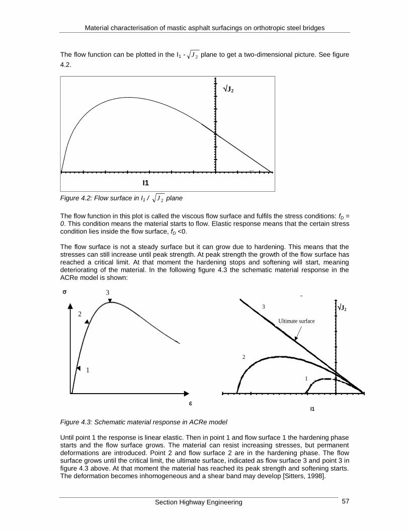
Material characterisation of mastic asphalt surfacings on orthotropic steel bridges
Section Highway Engineering 57
The flow function can be plotted in the I1 - 2J plane to get a two-dimensional picture. See figure
4.2.
I1
J2
Figure 4.2: Flow surface in I1 / 2J plane
The flow function in this plot is called the viscous flow surface and fulfils the stress conditions: fD = 0. This condition means the material starts to flow. Elastic response means that the certain stress condition lies inside the flow surface, fD <0. The flow surface is not a steady surface but it can grow due to hardening. This means that the stresses can still increase until peak strength. At peak strength the growth of the flow surface has reached a critical limit. At that moment the hardening stops and softening will start, meaning deteriorating of the material. In the following figure 4.3 the schematic material response in the ACRe model is shown:
2
1
3
I1
J23
2
1
Ultimate surface
Figure 4.3: Schematic material response in ACRe model Until point 1 the response is linear elastic. Then in point 1 and flow surface 1 the hardening phase starts and the flow surface grows. The material can resist increasing stresses, but permanent deformations are introduced. Point 2 and flow surface 2 are in the hardening phase. The flow surface grows until the critical limit, the ultimate surface, indicated as flow surface 3 and point 3 in figure 4.3 above. At that moment the material has reached its peak strength and softening starts. The deformation becomes inhomogeneous and a shear band may develop [Sitters, 1998].

Material characterisation of mastic asphalt surfacings on orthotropic steel bridges
Section Highway Engineering 58
4.3 Influence of the model parameters
The model parameters n, and R all have their own specific influence on the model. In this paragraph their influence will be explained.
Influence of
“The model parameter determines the size of the flow surface, the size increases with
decreasing so this parameter controls the hardening of the material. For elastic states of stress
it retains its original value, but as soon as non-linear states of stress occur, decreases until =0 at peak stress, when the hardening stops (figure 4.4).
-6
-5
-4
-3
-2
-1
0-0.2-0.15-0.1-0.050
m/m]
[N/mm2]
m
C 0 C =0
Figure 4.4: The model parameter controls the hardening response, after Erkens et al. (1998)
The influence of on the size of the flow surface is shown in figure 4.5. At peak stress, for =0,
the surface reduces to a straight line at the I1 - 2J surface” [Erkens et al., 1998, 50, 51].
0
0.5
1
1.5
2
2.5
3
-8 -6 -4 -2 0 2I1 [MPa]
J2 [MPa]
Figure 4.5: Influence of on the shape of the flow surface, after Erkens et al. (1998)

Material characterisation of mastic asphalt surfacings on orthotropic steel bridges
Section Highway Engineering 59
Influence ofand
“The model parameter determines the shape of the model on the -plane1. For =0 it is circular
and with increasing it becomes triangular. Since cos(3) is 1 for uniaxial states of stress, the
square root term in equation 4.3 reduces to: √(1-β). The effect of uniaxiality on is:
3
2,0
3
2013cos k or k2
3
4
with k=1,2,3….
Equation 4.9
These values of correspond to the position of the 1, andaxes on the -plane1, indicating
that uniaxial test results are related to a state of stress where two principal stresses are zero and the third is not. The shape of the cross section is determined by the multiaxial state of stress (figure 4.6)” [Erkens et al., 1998, 53].
Figure 4.6: Influence of and on the flow surface plotted in the I1 - 2J and -plane, after
Erkens et al. (1998)
1 The -plane is the plane perpendicular to the isotropic stress axis (1=2=3) which passes through the origin in the
principal stress space. Any state of stress can be described by cylinder co-ordinates using its projection on the -plane.
These co-ordinates are the distance from the original point to its projection along the isotropic stress axis (=I1/3), the
distance from the origin to the projection (r=(2J2)) and the angle between r and the 1 axis (). The advantage of this representation of the state of stress is that it immediately separates the influence of the isotropic stresses, which cause volume changes, and the deviatoric stresses, which cause distortion.

Material characterisation of mastic asphalt surfacings on orthotropic steel bridges
Section Highway Engineering 60
Influence of
“The model parameter determines the slope of the (ultimate) surface, the slope increases with
increasing . It is stress-state independent (does not change during a test), but it can vary as a function of, for example, temperature and loading rate (figure 4.7) [Erkens et al., 1998, 52].
0
0.2
0.4
0.6
0.8
1
1.2
1.4
-8 -6 -4 -2 0 2I1 [MPa]
nR=MPa
J2 [MPa]
Figure 4.7: Influence of on the shape of the flow surface, plotted in I1 - 2J space, after Erkens
et al. (1998) Influence of n “The model parameter n determines the apex of the surface, it expresses the state of stress after which the material starts to dilate. The apex is defined as that point of the flow surface where the
tangent is a horizontal line (f/I1=0, see figure 4.8), indicating a fully deviatoric state of stress” [Erkens et al., 1998, 52, 53].
0
0.2
0.4
0.6
0.8
1
1.2
1.4
-7 -6 -5 -4 -3 -2 -1 0 1 2
I1 [MPa]
n=3n=2.5
n=3.25
n=3.5
J2 [MPa]
Figure 4.8: Influence of n on the shape of the flow surface, plotted in the I1 - 2J space, after
Erkens et al. (1998) The stress conditions at the start of dilation can be determined when a plot is made of the axial versus the volumetric strain and a plot of the axial strain versus axial stress. The material starts to dilate at minimum volumetric strain.

Material characterisation of mastic asphalt surfacings on orthotropic steel bridges
Section Highway Engineering 61
Influence of R “R is the three dimensional tensile strength, which is an indication of cohesion. For cohesionless materials R=0, which means that that only states of stress for which I1≤0 are possible within that material. For increasing R values, the flow surface moves in the direction of the positive I1 axis (figure 4.9)” [Erkens et al., 1998, 54].
R=4MPa R=2MPaR=0MPa
Figure 4.9: Influence of R on the shape of the flow surface plotted in the I1 - 2J space, after
Erkens et al. (1998)
4.4 Tests to determine the model parameters
To determine the parameters for the ACRe-model, a couple of tests were specified [Scarpas et al., 1997]. These tests are:
Uniaxial monotonic compression test
Uniaxial monotonic tension test
Four point shear test To get a clear relation between the state of stress and the material response, tests are needed in which the state of stress is uniform throughout the specimen. For this reason triaxial tests can be used, but these tests have the disadvantage that they are rather expensive in relation to the area of response. Therefore uniaxial tension and compression tests were chosen to be the basic tests for parameter determination. By using these tests not all the parameters can be determined. For
example, these tests give no information about the parameter . Therefore additional multi-axial
testing is required, the four point shear test. When these tests can not be done, is often assumed to be zero. In this research only the uniaxial monotonic compression and uniaxial monotonic tension tests are carried out. The shear test set up was under development at the moment of writing this
thesis, so it could not be used in this project. Therefore is assumed to be zero.

Material characterisation of mastic asphalt surfacings on orthotropic steel bridges
Section Highway Engineering 62
5 Experimental program
5.1 Introduction
An experimental program has been designed to characterise the mastic asphalt mix which was used for resurfacing the Moerdijk bridge in June 2000. This asphalt mix will be referred to as the “Moerdijk mix”. The experimental program included: 1. Density measurements. 2. Four point bending beam test for:
Determination of the master curves,
Determination of the fatigue characteristics. 3. Uniaxial monotonic compression test. 4. Uniaxial monotonic tension test. After the determination of the master curves and the fatigue characteristics of the mix the dependency of the mix stiffness on the strain became obvious. Therefore, an additional testing program to investigate this phenomenon has been designed. This additional testing program included four point bending beam tests at different strain levels, temperatures and loading frequencies. Because of the fact that there were no sufficient specimens to carry out the program, it has been decided to get specimens from slabs that had been obtained while surfacing the Lintrack test bridge at the TU Delft. This asphalt mix is referred to as the “Lintrack mix”. It has also been decided to retest the specimens from the Moerdijk mix 2.5 months after the first series of fatigue tests, to determine the master curves and fatigue characteristics again.
5.2 Mix composition
Both the Moerdijk mix and the Lintrack mix have the same mix composition. The mastic asphalt mix consists of stone 2/8 and 2/6 in the ratio 1:1, river sand and fine sand in the ratio 2:3, weak limestone filler and SBS modified bitumen with a pen of 90. The mix composition is shown in table 5.1: Table 5.1: Mix composition
Materials Percentage %m/m
Passing Retained targeted Tolerance
C11.2 C8 0 +2.0 C8 2 mm 52.0 ±5.0 2 mm 63 m 26.0 ±5.0
63 m 22.0 ±2.0
Bitumen on 100% (by mass) 8.8 ±0.5

Material characterisation of mastic asphalt surfacings on orthotropic steel bridges
Section Highway Engineering 63
5.3 Specimen preparation
While resurfacing the Moerdijk bridge, which took place in June 2000, three slabs of dimensions ≈600x600x70 mm
3 have been obtained (see figure 5.1).
Figure 5.1: Preparation of the slabs From these slabs the following specimens have been obtained:
8 beams for the determination of master curves and the fatigue characteristics using the four-point bending test. The beams have been sawn from the slabs in the following way. First the edges of the slab have been cut off. After that the beams have been sawn at their desired length of 450mm. Next the top and bottom of each beam has been cut off in order to avoid edge effects and to give the specimens dimensions of ≈450x50x50mm (length x width x height). Table 5.2 shows the average dimensions of each specimen. The height, width and length of the beams have been measured at four positions (see appendix A). From these four values the average has been taken.
Table 5.2: Average dimensions of the specimens for the four-point bending test
Specimen Height [mm] Width [mm] Length [mm]
1 50.6 52.8 450
2 51.0 52.9 449
3 51.6 52.2 449 4 51.4 52.6 450 5 51.0 53.0 450 6 50.8 53.1 450 7 50.9 52.8 450 8 50.9 52.9 450
Average 51.0 52.8 449.8 STDEV 0.3 0.3 0.5 Variation [%] 0.6 0.5 0.1
13 cores for the tension and 13 cores for the compression tests. First beams were sawn from the slabs with a width of approximately 100mm. From each beam 10 cores were horizontally drilled, with a height of 100 mm and a diameter of 50 mm. After drilling some of the cores were polished to a height of approximately 90mm and some to 100mm to get parallel surfaces. Table 5.3 shows the average dimensions of the specimens for the compression tests. At four positions the dimensions have been measured after which the average has been taken. Appendix A shows the results from the four measurements.

Material characterisation of mastic asphalt surfacings on orthotropic steel bridges
Section Highway Engineering 64
Table 5.3: Dimensions of the specimens for the monotonic compression test
Specimen Height [mm] Diameter [mm]
M4-3 90.1 49.8 M11-4 100.1 49.8 M5-3 90.1 49.8 M4-4 89.9 50.0 M3-10 89.8 49.8 M2-5 90.2 49.9 M11-3 100.2 50.0 M6-4 99.6 49.7 M7-4 100.1 50.1 M9-2 100.3 49.8 M10-2 100.3 49.8 M10-10 100.3 49.8 M6-6 100.1 49.8
Average 96.2 49.9 STDEV 5.1 0.1 Variation [%] 5.3 0.2
The height shows a quite large variation because specimens are tested with a height of approximately 100mm and specimen with a height of approximately 90mm. This difference is a result of additional polishing to some of the specimen. The dimensions of the specimens for the tension tests have been measured at four positions after which the average is taken. Table 5.4 shows the average results. Appendix A shows the results for the four measurements. Table 5.4: Dimensions of the specimens for the monotonic tension test
Specimen Height [mm] Diameter [mm]
M11-5* 89.4 49.9 M2-1* 89.1 49.8 M11-8 90.9 49.6 M2-3 89.0 49.8 M3-9 90.3 50.0 M3-1 90.0 50.0 M1-10* 89.3 49.7 M3-7 90.2 49.6 M5-2 90.1 49.9 M3-4 90.0 49.9 M2-4 90.0 49.7 M4-7 90.0 49.9 M1-3 90.0 49.5
Average 89.9 49.8 STDEV 0.53 0.16 Variation [%] 0.59 0.32
In table 5.4 three specimen are marked with *. On these specimens 2 PVC rings (h=8 mm) were glued to prevent the specimen from cracking in the glue layer between the steel cap and the specimen. These PVC rings reduced the height of the specimens by 16 mm.
While surfacing the Lintrack test bridge several slabs have been casted. 46 beams have been sawn from four of the slabs in the same way as described for the beams of the Moerdijk mix. However, these beams have dimension of ≈420x50x50mm (length x width x height). These beams have been used for the determination of the strain dependent behaviour of the mix stiffness.

Material characterisation of mastic asphalt surfacings on orthotropic steel bridges
Section Highway Engineering 65
Table 5.5 shows the average dimensions of the specimens. The height, width and length of the beams have been measured at four positions (see appendix A). From these four values the average has been taken. Table 5.5: Dimensions of the specimens for determining the stress dependent behaviour
Specimen Height [mm] Width [mm] Length [mm]
ML/4pb/1/1 50.5 50.4 420 ML/4pb/1/2 50.4 50.1 420 ML/4pb/1/3 50.4 50.7 420 ML/4pb/1/4 50.5 50.6 421 ML/4pb/1/5 50.4 51.1 422 ML/4pb/1/6 50.6 52.5 421 ML/4pb/1/7 52.6 50.5 422 ML/4pb/1/8 50.7 50.6 421 ML/4pb/1/9 50.6 51.0 422
ML/4pb/1/10 50.4 51.1 421
ML/4pb/2/1 49.6 52.1 420 ML/4pb/2/2 49.4 50.5 420 ML/4pb/2/3 49.2 49.0 420 ML/4pb/2/4 49.2 53.8 420 ML/4pb/2/5 49.2 55.0 420 ML/4pb/2/6 49.5 56.5 420 ML/4pb/2/7 49.3 51.9 420 ML/4pb/2/8 49.2 52.7 420 ML/4pb/2/9 49.1 52.5 421
ML/4pb/2/10 49.2 51.0 421
ML/4pb/3/1 50.5 50.5 421 ML/4pb/3/2 50.5 50.4 422 ML/4pb/3/3 50.6 50.7 422 ML/4pb/3/4 50.2 50.6 422 ML/4pb/3/5 49.9 49.8 422 ML/4pb/3/6 49.7 49.6 422 ML/4pb/3/7 50.2 49.2 422 ML/4pb/3/8 50.4 49.6 422 ML/4pb/3/9 50.6 49.9 422
ML/4pb/3/10 50.7 50.5 422
ML/4pb/4/1 50.3 50.5 420 ML/4pb/4/2 50.7 50.8 421 ML/4pb/4/3 50.7 50.4 421 ML/4pb/4/4 50.7 51.0 421 ML/4pb/4/5 50.7 50.4 421 ML/4pb/4/6 50.8 50.2 422 ML/4pb/4/7 50.6 49.9 422 ML/4pb/4/8 50.7 50.1 421 ML/4pb/4/9 50.4 49.8 422
ML/4pb/4/10 50.6 50.9 421
Average 50.2 51.0 421.1 STDEV 0.7 1.5 0.8
Variation [%] 1.4 2.9 0.2
Before testing the beams and cores have been stored at 13C in a box filled with a bed of sand to avoid deformations of specimens.

Material characterisation of mastic asphalt surfacings on orthotropic steel bridges
Section Highway Engineering 66
5.4 Density measurements
The density of all the asphalt specimens were determined according to the Dutch Standard [CROW, 2000] using the “weighing under-water procedure” described briefly as follows: 1. Obtain the dry weight of the specimen (mdry) 2. Soak the specimen in water for at least 3 minutes 3. Obtain the weight of the specimen under water (munder) 4. Remove the suspended water particles using a wet towel and then obtain the weight (mwet) 5. Measure the water temperature.
The density of the specimen (sp) can be determined by using:
underwet
wdry
spmm
m
. Equation 5.1
where:
sp = specimen density [kg/m3]
mdry = dry mass specimen [g] mwet = wet mass specimen [g] munder = mass specimen under water [g]
w = density of water [kg/m3]
The density of the mix (mix), for ms+mz+mf+md=100%, is calculated with:
b
b
f
f
z
z
s
s
mixmmmm
100
Equation 5.2
in which: ms = mass percentage stone [%m/m] mz = mass percentage sand [%m/m] mf = mass percentage filler [%m/m] mb = mass percentage bitumen [%m/m]
s = density of the stone [kg/m3]
z = density of the sand [kg/m3]
f = density of the filler [kg/m3]
b = density of the bitumen [kg/m3]
With the specimen density and the mix density the percentage of air voids in the specimen is calculated with:
mix
spmix
aV
Equation 5.3
where: Va = percentage voids [%]
mix = density of the mix [kg/m3]
sp = density of the specimen [kg/m3]

Material characterisation of mastic asphalt surfacings on orthotropic steel bridges
Section Highway Engineering 67
The filler, bitumen, sand and stone content for the mix without voids is calculated with:
mix
f
f
f
mV
Equation 5.4
mix
b
bb
mV
Equation 5.5
mix
z
zz
mV
Equation 5.6
mix
s
ss
mV
Equation 5.7
in which: Vf = Filler content in the mix without voids [%V/V] Vb = Bitumen content in the mix without voids [%V/V] Vz = Sand content in the mix without voids [%V/V] Vs = Stone content in the mix without voids [%V/V] The contents in the mix inclusive voids are calculated with:
sp
f
f
f
mV
Equation 5.8
sp
b
bb
mV
Equation 5.9
sp
z
zz
mV
Equation 5.10
sp
s
ss
mV
Equation 5.11
in which: Vf’ = Filler content in the mix with voids [%V/V] Vb’ = Bitumen content in the mix with voids [%V/V] Vz’ = Sand content in the mix with voids [%V/V] Vs’ = Stone content in the mix with voids [%V/V] The void content in the mineral aggregate without bitumen is calculated with:
baa VVV
Equation 5.12
in which: Va’ = Void content in the mineral aggregate without bitumen [%V/V]

Material characterisation of mastic asphalt surfacings on orthotropic steel bridges
Section Highway Engineering 68
The degree of filling is determined with:
a
b
f
V
VD 100 Equation 5.13
in which: Df = Degree of filling [%] The results of the density measurements are shown in the tables 6.2-6.5 in chapter 6.
5.5 Four point bending test
5.5.1 Test set up
Figure 5.2 shows the Universal Testing Machine (UTM) testing equipment, manufactured by the Industrial Process Controls Limited (IPC) in Melbourne, Australia. The mechanism allows for free translation and rotation of the clamps. Pneumatic actuators at the ends of the beam center it laterally and clamp it. The load is applied through the piston rods to the beam specimen, 400 mm long with a width and depth not exceeding 63.5 mm. The pneumatic testing machine is capable of applying loads in the form of sine or haversine waves for 0.1-2 s duration with 0-10 s rest periods. Servo-motor driven clamps secure the beam at four points. Adjustable stops nuts installed on the loading rods prevent the beam from bending below the initial horizontal position during the rest period. The dynamic deflection of the beam at the midspan is measured with a linear variable differential transformer (LVDT). The repeated flexure apparatus is enclosed in a controlled temperature cabinet.
Figure 5.2: The four point bending beam fatigue testing equipment

Material characterisation of mastic asphalt surfacings on orthotropic steel bridges
Section Highway Engineering 69
5.5.2 Survey of the four point bending testing program
For the first and repeated determination of master curves and fatigue characteristics 8 specimens of the Moerdijk mix were used. For the repeated determination of master curves two strain levels
were used, namely 80 m/m to investigate the effect of healing and 800 m/m to investigate the strain dependency of the mix stiffness. Figure 5.3 shows a survey of the four point bending tests that were carried out on the Moerdijk mix.
Figure 5.3: Survey of the four-point bending testing program carried out on the Moerdijk mix From the repeated determination of master curves the strain dependency of the mix stiffness became obvious. However, due to a lack of specimens the repeated determination of master curves took place at only 3 temperatures, namely 10, 20 and 30
oC. Therefore it was decided to
carry out a more extensive testing program to investigate the strain dependency of the mix stiffness. For this program use is made of specimen from the Lintrack mix.
First determination of master curves
0.5, 1, 2, 5 and 10 Hz 5, 10, 15, 20, 25, 30
oC
80 m/m Moerdijk specimens 2, 3, 4 and 6
First determination of fatigue characteristics
1.1.1.1.1 5 Hz 10
oC
375, 475 600, 750, 925 and 1095 m/m Moerdijk specimens 2, 3, 4, 5, 6 and 7
0.5, 1, 2, 5 and 10 Hz 10, 20 and 30
oC
80 and 800 m/m Moerdijk specimens 1, 3, 4, 5, 7 and 8
5 Hz 10
oC
530, 600, 700, 740, 800 and 920 m/m Moerdijk specimens 3, 4, 5, 6, 7 and 8
after 1 week
after 2.5 months
after 1 week
Repeated determination of master curves
Repeated determination of fatigue characteristics

Material characterisation of mastic asphalt surfacings on orthotropic steel bridges
Section Highway Engineering 70
Figure 5.4 shows an overview of the four point bending testing program on the Lintrack mix.
Figure 5.4: Survey of the four-point bending testing program carried out on the Lintrack mix
5.5.3 Input for the four point bending fatigue testing machine
5.5.3.1 Test conditions for the first determination of master curves
The test conditions that were used for determining the master curves are: - Type of test: displacement controlled - Frequencies: 0.5, 1, 2, 5 and 10 Hz - Temperatures: 5, 10, 15, 20, 25 and 30ºC
- Strain: 80 m/m - Loading wave: sine - Poisson’s ratio: 0.3 - Specimen nrs: 2, 3, 4 and 6 The stiffness is measured after 100 pulses. The results of the first determination of master curves are shown in paragraph 6.2.2.
5.5.3.2 Test conditions for the repeated determination of master curves
After 2.5 months it was decided to determine the master curves again at two strain levels, namely
80 and 800 m/m. Therefore the specimens are used that were tested before in the fatigue test. The test conditions are: - Type of test: displacement controlled - Frequencies: 0.5, 1, 2, 5 and 10 Hz - Temperatures: 10, 20 and 30ºC
- Strain amplitude 80 and 800 m/m - Loading wave: sine - Poisson’s ratio: 0.3 - Specimen nrs: 1, 3, 4, 5, 7 and 8 The stiffness is also measured after 100 pulses. Paragraph 6.2.3 contains the results from the repeated determination of master curves.
5.5.3.3 Test conditions for the first determination of the fatigue behaviour
The test conditions that were used for determining the fatigue behaviour are: - Type of test: displacement controlled - Frequency: 5 Hz - Temperatures: 10ºC
- Strain amplitude: 375, 475, 600, 750, 925 and 1095 m/m - Loading wave: sine - Poisson’s ratio: 0.3 - Specimen nrs: 2, 3, 4, 5, 6 and 7
Determination of the strain dependency of the mix stiffness
0.5, 1, 2, 5 and 10 Hz 5, 12.5, 20, 27.5, 35 and 42.5
oC
80, 200, 600 and 1000 m/m 46 Lintrack specimens

Material characterisation of mastic asphalt surfacings on orthotropic steel bridges
Section Highway Engineering 71
The number of load repetitions to failure is determined when the initial stiffness is halved. Paragraph 6.3.1 contains the results from the first determination of the fatigue characteristics.
5.5.3.4 Test conditions for the repeated determination of the fatigue behaviour
After the repeated determination of the master curves it was decided to repeat the fatigue tests also, one week after the repeated determination of master curves. The test conditions are: - Type of test: displacement controlled - Frequency: 5 Hz - Temperatures: 10ºC
- Strain amplitude: 530, 600, 700, 740, 800 and 920 m/m - Loading wave: sine - Poisson’s ratio: 0.3 - Specimen nrs: 3, 4, 5, 6, 7 and 8 The number of load repetitions to failure is determined when the initial stiffness is halved. The results from the repeated determination of the fatigue characteristics are shown in paragraph 6.3.2.
5.5.3.5 Test conditions for the determination of the strain dependency of the mix stiffness
After the first series of fatigue tests the strain dependency of the mix stiffness became obvious. Therefore it was decided to determine the strain dependency of the mix stiffness by additional testing. The test conditions of this additional testing are: - Type of test: Displacement controlled - Frequencies 0.5, 1, 2, 5 and 10 Hz - Temperatures 5, 12.5, 20, 27.5, 35 and 42.5ºC
- Strain amplitudes: 80, 200, 600 and 1000 m/m - Loading wave: sine wave - Specimen nrs: ML/4pb/1/1-Ml/4pb/1/10 ML/4pb/2/1-Ml/4pb/2/10 ML/4pb/3/1-Ml/4pb/3/10 ML/4pb/4/1-Ml/4pb/4/6 The stiffness is also measured after 100 pulses.
5.5.4 Output for the four point bending fatigue testing machine
The following tabulated data is calculated and displayed on the screen and written in a file:
Test loading time (hours, minutes and seconds)
Applied load
Beam deflection
Tensile stress and strain
Core and skin temperature of a dummy specimen
Phase angle
Loading cycle count
Flexural stiffness
Modulus of elasticity
Dissipated energy
Cumulative dissipated energy

Material characterisation of mastic asphalt surfacings on orthotropic steel bridges
Section Highway Engineering 72
5.5.5 Data calculations in the four point bending test
The calculations performed by the computer are based on the equations displayed in this paragraph. The maximum tensile stress is calculated with:
23000
wh
aPt Equation 5.14
Where:
t: maximum tensile stress [kPa] a: distance between reaction and load clamps (typically 118.5 mm) P: peak force [N] w: beam width [mm] h: beam height [mm] The maximum tensile strain is calculated with:
223
12
a
ht
Equation 5.15
Where:
t: maximum tensile strain [mm/mm]
: peak deflection at centre of beam [mm] Flexural stiffness:
t
tS
1000 Equation 5.16
Where: S: flexural stiffness [MPa] Modulus of elasticity:
)1(
4
232
2
kh
a
wh
PaE Equation 5.17
Where: E: modulus of elasticity [MPa] k: actual shear stress divided by average shear stress (assumed 1.5 N/mm
2)
: oisson’s ratio The results obtained by means of the four point bending test are reported in chapter 6.

Material characterisation of mastic asphalt surfacings on orthotropic steel bridges
Section Highway Engineering 73
5.6 Optimisation of the tension and compression experimental program
5.6.1 Introduction
For the determination of the effects of more than one variable a researcher usually designs a simple comparative experiment to determine the effects of the different variables. This procedure is extremely insufficient. For example in this experimental program the range of interest for temperatures is 0-40
oC and for the deformation rate 0.01-10 mm/s. Using the normal procedure
this means that tests are done at 3 temperatures (0, 20 and 40oC) and 4 loading rates (0.01, 0.1,
1.0 and 10 mm/s). To get representative results each combination is repeated 4 times. For this example this means that the number of tests to be carried out is 3x4x4=48. However, with a properly designed experiment, the same or better information can be obtained with as few as 13 trials. This means much less testing and a saving of specimens of 73%. To achieve this, use is made of a “central composite rotatable design” [Robinson, 2000].
5.6.2 Procedure for the central rotatable design
The central rotatable experimental design technique was chosen. The procedure is described below. 1. At first the range of interest is determined. For the compression test the range of interest for
the speed is 0.01-10 mm/s and for the temperature 0-40oC. The tension tests are carried out
in a temperature range of 0-43.6oC and a speed range of 0.01-5 mm/s.
2. The general design of the trials to be conducted is expressed in coded terms in table 5.6 below:
Table 5.6: Coded test conditions
Trial Vcoded Tcoded
1
2
3
4
5
6
7
8
9
10
11
12
13

Material characterisation of mastic asphalt surfacings on orthotropic steel bridges
Section Highway Engineering 74
The test conditions are also shown in a graphical form (figure 5.5).
-2
-1
0
1
2
-2 -1 0 1 2
(1) (2)
(3) (4)
(5) (6)
(7)
(8)
(9) - (13)
Figure 5.5: Coded test conditions for the central composite rotatable design This figure shows that 5 tests are repeated in the centre of the range of interest (trials 9-13) and further there are 8 tests at rotatable positions around this centre.
3. Any value may be used for , and there may be any number of replicated points in the centre. However, the experimental design will have special properties (rotatable design) if the
value of is set at 1.4142. It is recommended by Robinson [2000] to use 5 central points with 2 variables. In that case the trials 9-13 all have the same distance to the 5 centre points, which results in measurements that are evenly spread over the range of interest. Trials 5-8 are called star points of the design and trials 9-13 are called centre points.
To scale the coded terms of table 5.6 into values within the range of interest, =1.4142 is set equal to half the ranges of the variables and the scaling factors for the compression tests follow from:
2
1)(4142.1 minmax VVVscaling Equation 5.18
2
1)(4142.1 minmax TTTscaling Equation 5.19
in which: Vscaling : Scaling factor for the loading rate Tscaling : Scaling factor for the temperature Vmin : : Minimum loading rate [mm/s] Vmax : Maximum loading rate [mm/s] Tmin : Minimum test temperature [
oC]
Tmax : Maximum test temperature [oC]

Material characterisation of mastic asphalt surfacings on orthotropic steel bridges
Section Highway Engineering 75
Finally the experimental values of the loading speed V and the temperature T follow from:
minmax2
1VVVVV scalingcoded
Equation 5.20
minmax2
1TTTTT scalingcoded
Equation 5.21
5.7 Uniaxial monotonic compression test
5.7.1 Compression test set up
“The compression test set-up consists of a 3D-space frame in which an MTS 150kN hydraulic actuator is mounted. The actuator is connected rigidly to the upper loading plate. The frame itself is placed on an elastically supported concrete block. On the lower part of the frame a pedestal is constructed to which the bottom plate is connected. The bottom and top plate are kept parallel by means of three massive (Φ 16 mm) bars which are connected to the bottom plate and pass through linear bearings in the top plate. A cabinet is placed within the frame, which allows the tests to be performed at specific temperatures. Inside the temperature cabinet are the transducers, which register the radial and axial deformations of the specimen, as well as the applied force [Erkens, 1998, 18]”. A picture from the compression test set-up inside the temperature cabinet with an inserted specimen is shown in figure 5.6.
Figure 5.6: Picture from the compression test set-up inside the temperature cabinet

Material characterisation of mastic asphalt surfacings on orthotropic steel bridges
Section Highway Engineering 76
The axial deformation is registered by means of three displacement transducers (LVDT’s). The radial deformation is measured by means of two circumferential measurement systems. An extensometer measures the first part of the radial deformation, a string measures the second part. Figure 5.7 shows a close-up from a specimen inserted in the compression test set-up. At the left side of the picture one of the LVDT’s can be seen. Also very clear are the two circumferential measurement systems, namely the extensometer (chain) and the string. The picture also shows the friction reduction system on top and under the specimen.
Figure 5.7: Close-up from a specimen inserted in the compression test set-up The force is measured by means of a load cell, which is positioned between the top plate and the actuator. An external MTS 418.91 controller is used to improve a deformation-rate-controlled test. The measurements systems are connected to a PC-based data acquisition system, which produces a single ASCII output file for each test.
5.7.2 Specimen preparation for the compression test
To determine the response of a specimen, the combination of the state of stress to which it is subjected and the material characteristics are of importance. The material characteristics can be obtained from the observed response and the state of stress. However, the true state of stress can be completely different from the intended state of stress. For the uniaxial monotonic compression test the intended state of stress is pure uniaxial compression. For the compression test it is therefore very important that the top and bottom surfaces of the specimen are parallel, otherwise shear forces might be introduced. To obtain parallel surfaces all the specimens are polished.

Material characterisation of mastic asphalt surfacings on orthotropic steel bridges
Section Highway Engineering 77
Friction between the specimen and the loading plates can have a significant disturbing effect on the state of stress in the specimen. During a test the specimen deforms in the radial as well as the axial direction. Friction between specimen and loading plates leads to confinement for the bottom and top of the specimen and results in the barrel-shape of specimens. This shape is an indication of undesirable non-uniaxial states of stress. To avoid this problem a friction reduction system is used for the compression test. This system consists of two thin (0.5mm) corrosion resistant steel plates. A thin layer of soap is applied to the steel plates, after which a plastic foil is added. Next a second layer of soap is added on the plastic foil. For the compression test the specimen is placed between two of these metal-soap-plastic-soap sandwiches. The third part of the specimen preparation consists of gluing three little hooks halfway the heights of the specimens. These hooks guide the string that measures the radial displacement. After preparation the specimens were placed in a temperature controlled unit at the designated test temperature for at least 24 hours before testing. After that the specimen including the friction reduction system is placed in the temperature cabinet.
5.7.3 Input for the compression test
5.7.3.1 Computer input for the compression test
The following data may be used as an input:
Date
Specimen identification
Specimen height and diameter [mm]
Temperature [oC]
Loading rate [mm/s]
Number of scans per second [Hz]
Calculation factor for the force and the displacement
5.7.3.2 Test conditions for the uniaxial monotonic compression test
Uniaxial compression tests are performed under displacement controlled conditions by applying a monotonically increasing deformation (constant deformation rate) until complete annihilation of the strength. The test conditions for the compression tests are determined by using the central composite rotatable design, described in paragraph 5.6. Table 5.7 shows the test conditions for the compression test: Table 5.7: Test conditions compression test
Specimen Loading rate [mm/s] Temperature [oC]
1 1.473 5.9 2 8.537 5.9 3 1.473 34.1 4 8.537 34.1 5 0.01 20.0 6 10 20.0 7 5.005 0 8 5.005 40.0 9 5.005 20.0 10 5.005 20.0 11 5.005 20.0 12 5.005 20.0 13 5.005 20.0

Material characterisation of mastic asphalt surfacings on orthotropic steel bridges
Section Highway Engineering 78
Figure 5.8 shows the test combinations when they are plotted in a chart.
0
5
10
15
20
25
30
35
40
45
0 1 2 3 4 5 6 7 8 9 10 11
v [mm/s]
T [
oC
]
Figure 5.8: Test conditions for the monotonic compression test
5.7.4 Output from the compression test
The following data is written in a file:
Date of the test
Specimen identification
Temperature
Loading rate
Calculation factors for the force and the displacement
The number of scans per second [Hz]
Force [V]
Displacement of the hydraulic ramp [V]
Displacement of the three LVDT’s [V]
Displacement of the extensometer [V]
Displacement of the string [V] The results will be discussed in chapter 6.
5.8 Uniaxial monotonic tension test
5.8.1 Tension test set up
The tension test set-up consists of a closed temperature cabinet with a 50kN hydraulic actuator inside. The actuator is connected rigidly to the bottom of the temperature chamber. In the temperature cabinet the specimen is placed in a rigid framework that can resists the high forces that occur during the test without deforming. In the test set-up the specimen is placed between

Material characterisation of mastic asphalt surfacings on orthotropic steel bridges
Section Highway Engineering 79
three hinges to ensure that the specimen is subjected to pure uniaxial tension. There are two hinges above and one under the specimen to avoid bending moments in the specimen. The force is measured by means of a load cell, which is positioned between the two hinges above the specimen. An internal 407 MTS controller is used to improve a deformation-rate-controlled test. The axial deformation is registered by means of three displacement transducers (LVDT’s). These LVDT’s are fixed in a steel ring that is placed around the steel cap at the bottom of the specimen. On top of the specimen the three LVDT’s touch a second steel ring which is placed around the steel cap on top of the specimen. A close-up from the tension test set-up with an inserted specimen is shown in figure 5.9.
Figure 5.9: Test set up for the uniaxial monotonic tension test The measurements systems are connected to a PC-based data acquisition system, which produces a single ASCII output file for each test.
5.8.2 Specimen preparation for the tension test
The cores for the tension test needed special preparation before testing took place. Two steel caps had to be glued at the top and bottom surface of the specimen before the specimen could be placed in the tension test set up. The steel caps are 30 mm thick and have a diameter of 80 mm. The caps have to be glued parallel to each other to ensure pure tension during the test. When the caps are not parallel bending moments are introduced during the test which is unacceptable.

Material characterisation of mastic asphalt surfacings on orthotropic steel bridges
Section Highway Engineering 80
The set up for gluing the caps parallel on the specimen is shown in figure 5.10.
Figure 5.10: Set-up for gluing the caps parallel on the specimen For the tests at 0
oC and 6.4
oC special PVC rings (height 80 mm) are glued around the specimen
at the cap, in order to prevent that the specimen cracks between the cap and the asphalt i.e. in the glue layer. The glue that is used consists of two components, ARALDITE SW 404 and HY 2404, which is mixed in the ratio 10:1. After gluing the specimen stays in the set-up for at least two hours. After 24 hours the glue will harden and the specimen can be placed in a temperature chamber.
5.8.3 Input for the tension test
5.8.3.1 Computer input for the tension test
The following data may be inserted before the test:
Date
Specimen identification
Specimen height and diameter [mm]
Temperature [oC]
Loading rate [mm/s]
Number of scans per second [Hz]
Calculation factor for the force and the displacement
5.8.3.2 Test conditions for the uniaxial monotonic tension test
Uniaxial tension tests are performed under displacement controlled conditions by applying a monotonically increasing deformation (constant deformation rate) till failure. When the central composite rotatable design is used for the tension tests, the following test conditions are obtained (table 5.8):

Material characterisation of mastic asphalt surfacings on orthotropic steel bridges
Section Highway Engineering 81
Table 5.8: Test conditions tension test
Specimen Loading rate [mm/s] Temperature [oC]
1 0.741 6.4 2 4.269 6.4 3 0.741 37.2 4 4.269 37.2 5 0.01 21.8 6 5 21.8 7 2.505 0 8 2.505 43.6 9 2.505 21.8 10 2.505 21.8 11 2.505 21.8 12 2.505 21.8 13 2.505 21.8
The rotatibility of the procedure becomes clear again when the test conditions are plotted in a chart (figure 5.11):
0
5
10
15
20
25
30
35
40
45
50
0 1 2 3 4 5 6
v [mm/s]
T [
oC
]
Figure 5.11: Test conditions for the monotonic tension test
5.8.4 Output from the tension test
The following data is written in a file:
Date of the test
Specimen identification
Temperature
Loading rate
Calculation factors for the force and the displacement
The number of scans per second [Hz]
Force [V]
Displacement of the hydraulic ramp [V]
Displacement of the three LVDT’s [V] The results will be discussed in chapter 6.

Material characterisation of mastic asphalt surfacings on orthotropic steel bridges
Section Highway Engineering 82
6 Experimental results
6.1 Density measurements
6.1.1 Introduction
In this section the results of the density measurements are presented. For the density calculations the densities of the filler, sand, stone and bitumen are assumed as shown in table 6.1. These assumptions were made for both the Moerdijk and the Lintrack mix. Table 6.1: Assumed densities
Type Grain size [mm] Density [kg/m3]
Filler <63 m 2775
Sand 63 m<Z<2 mm 2650
Stone 2 mm<S<8 mm 2700 Bitumen - 1020
For each specimen the density and the void content (Va), bitumen content (Vb
’), filler content (Vf
’),
sand content (Vz’) and stone content (Vs
’) is calculated. Finally the degree of filling (Df) is
determined.
6.1.2 Mix composition of the specimen for the four point bending test
6.1.2.1 Moerdijk mix
8 beams were used to determine the master curves and the fatigue behaviour. The mix composition of these 8 beams is shown in table 6.2. Table 6.2: Mix composition of the specimens for the four-point bending test
Specimen sp [kg/m3] Va [%] Vb’ [%] Vf’ [%] Vz’ [%] Vs’ [%] Df [%]
1 2357.37 1.14 18.69 17.18 21.26 41.73 94.2 2 2351.27 1.40 18.64 17.13 21.20 41.62 93.0 3 2355.04 1.24 18.67 17.16 21.24 41.69 93.8 4 2357.29 1.15 18.69 17.18 21.26 41.73 94.2 5 2355.60 1.22 18.68 17.16 21.24 41.70 93.9 6 2357.29 1.15 18.69 17.18 21.26 41.73 94.2 7 2356.59 1.17 18.69 17.17 21.25 41.72 94.1 8 2354.69 1.25 18.67 17.16 21.23 41.68 93.7
Average 2355.64 1.21 18.68 17.16 21.24 41.70 93.90 STDEV 2.06 0.09 0.02 0.02 0.02 0.04 0.41 Variation [%] 0.09 7.11 0.09 0.09 0.09 0.09 0.44
Where:
sp : Specimen density [kg/m3]
Va : Percentage voids [%] Vb’ : Bitumen content in the mix with voids [%V/V] Vf’ : Filler content in the mix with voids [%V/V] Vz’ : Sand content in the mix with voids [%V/V] Vs’ : Stone content in the mix with voids [%V/V] Df : Degree of filling [%]

Material characterisation of mastic asphalt surfacings on orthotropic steel bridges
Section Highway Engineering 83
From table 6.2 it becomes clear that both the standard deviation and the variation of the mix composition is very small for the eight specimens. The density varies between 2351 kg/m
3 and
2357 kg/m3 and the voids content between 1.14% and 1.40%. The variation in bitumen, filler,
sand and stone content as well as degree of filling is so small that they are nearly constant for the eight specimens. Because the mix composition is comparable for the eight specimens the behaviour during testing will also be comparable. Therefore also the results of the tests can be compared after testing.
6.1.2.2 Lintrack mix
From the Lintrack mix 36 specimen are used in the four-point bending test to determine the strain dependent behaviour of the mix stiffness. Table 6.3 shows the results of the density measurements and calculations. Table 6.3: Mix composition of the specimens for determining the stress dependent behaviour
Specimen sp [kg/m3] Va [%] Vb’ [%] Vf’ [%] Vz’ [%] Vs’ [%] Df [%]
ML/4pb/1/1 2343.5 1.73 18.58 17.08 21.13 41.48 91.50 ML/4pb/1/2 2349.4 1.48 18.63 17.12 21.19 41.59 92.66 ML/4pb/1/3 2348.0 1.53 18.62 17.11 21.17 41.56 92.39 ML/4pb/1/4 2346.5 1.60 18.61 17.10 21.16 41.54 92.09 ML/4pb/1/5 2348.1 1.53 18.62 17.11 21.17 41.56 92.39 ML/4pb/1/6 2347.9 1.54 18.62 17.11 21.17 41.56 92.36 ML/4pb/1/7 2352.3 1.35 18.65 17.14 21.21 41.64 93.24 ML/4pb/1/8 2346.5 1.60 18.61 17.10 21.16 41.54 92.08 ML/4pb/1/9 2346.6 1.59 18.61 17.10 21.16 41.54 92.11 ML/4pb/1/10 2343.7 1.72 18.58 17.08 21.13 41.49 91.54
ML/4pb/2/1 2339.4 1.89 18.55 17.05 21.10 41.41 90.74 ML/4pb/2/2 2338.6 1.93 18.54 17.04 21.09 41.40 90.57 ML/4pb/2/3 2341.3 1.82 18.57 17.06 21.11 41.44 91.09 ML/4pb/2/4 2340.5 1.85 18.56 17.05 21.11 41.43 90.94 ML/4pb/2/5 2343.0 1.75 18.58 17.07 21.13 41.47 91.41 ML/4pb/2/6 2333.2 2.15 18.50 17.00 21.04 41.30 89.57 ML/4pb/2/7 2335.7 2.05 18.52 17.02 21.06 41.35 90.03 ML/4pb/2/8 2340.6 1.84 18.56 17.06 21.11 41.43 90.96 ML/4pb/2/9 2342.3 1.78 18.57 17.07 21.12 41.46 91.27 ML/4pb/2/10 2341.2 1.82 18.56 17.06 21.11 41.44 91.06
ML/4pb/3/1 2332.1 2.20 18.49 16.99 21.03 41.28 89.36 ML/4pb/3/2 2325.2 2.49 18.44 16.94 20.97 41.16 88.10 ML/4pb/3/3 2327.5 2.39 18.46 16.96 20.99 41.20 88.52 ML/4pb/3/4 2328.8 2.34 18.47 16.97 21.00 41.22 88.74 ML/4pb/3/5 2329.3 2.32 18.47 16.97 21.00 41.23 88.84 ML/4pb/3/6 2328.9 2.34 18.47 16.97 21.00 41.22 88.77 ML/4pb/3/7 2333.2 2.16 18.50 17.00 21.04 41.30 89.56 ML/4pb/3/8 2326.1 2.45 18.45 16.95 20.98 41.18 88.26 ML/4pb/3/9 2324.4 2.53 18.43 16.94 20.96 41.15 87.95 ML/4pb/3/10 2320.2 2.70 18.40 16.91 20.92 41.07 87.20
ML/4pb/4/1 2323.1 2.58 18.42 16.93 20.95 41.12 87.71 ML/4pb/4/2 2325.4 2.48 18.44 16.94 20.97 41.16 88.14 ML/4pb/4/3 2328.4 2.36 18.46 16.97 21.00 41.22 88.68 ML/4pb/4/4 2325.4 2.48 18.44 16.94 20.97 41.16 88.14 ML/4pb/4/5 2326.2 2.45 18.45 16.95 20.98 41.18 88.27 ML/4pb/4/6 2326.0 2.46 18.44 16.95 20.97 41.17 88.23
Average 2336.1 2.0 18.5 17.0 21.1 41.4 90.1 STDEV 9.3 0.4 0.1 0.1 0.1 0.2 1.7 Variation [%] 0.4 19.1 0.4 0.4 0.4 0.4 1.9

Material characterisation of mastic asphalt surfacings on orthotropic steel bridges
Section Highway Engineering 84
The variation in density, bitumen, filler, sand and stone content and degree of filling is negligible for the 46 specimens. Only the coefficient of variation for the percentage air voids is quite high. A closer look to the percentage air voids of the different specimens shows that the first 20 specimens (ML/4pb/1/1-ML/4pb/2/10) have a void content between 1% and 2%. The final 16 specimens (ML/4pb/3/1-ML/4pb/4/6) have a void content between 2% and 3%. This difference
can be explained by the fact that the first 20 specimen have a higher density (sp=2330-2350
kg/m3) than the final 16 specimen (sp=2320-2335 kg/m
3). This difference can be explained by the
fact that the last 16 specimens are sawn from two different asphalt slabs. Probably the preparation of these slabs was different from the preparation of the first two slabs from which the first 20 specimens were obtained. The slabs were prepared manually and the asphalt was not condensed, so some variation is to be expected.
6.1.3 Mix composition of the specimen for the monotonic compression test
For the compression test 13 cylindrical specimens are used. Table 6.4 shows the results for the density measurements and calculations. Table 6.4: Mix composition of the specimens for the monotonic compression test
Specimen sp [kg/m3] Va [%] Vb’ [%] Vf’ [%] Vz’ [%] Vs’ [%] Df [%]
M4-3 2354.09 1.28 18.67 17.15 21.23 41.67 93.58 M11-4 2351.38 1.39 18.65 17.13 21.20 41.62 93.05 M5-3 2349.41 1.48 18.63 17.12 21.19 41.59 92.66 M4-4 2350.47 1.43 18.64 17.13 21.20 41.61 92.87 M3-10 2355.06 1.24 18.67 17.16 21.24 41.69 93.78 M2-5 2345.27 1.65 18.60 17.09 21.15 41.51 91.85 M11-3 2354.25 1.27 18.67 17.15 21.23 41.67 93.62 M6-4 2353.01 1.33 18.66 17.15 21.22 41.65 93.37 M7-4 2351.20 1.40 18.64 17.13 21.20 41.62 93.01 M9-2 2349.49 1.47 18.63 17.12 21.19 41.59 92.67 M10-2 2356.28 1.19 18.68 17.17 21.25 41.71 94.02 M10-10 2358.53 1.09 18.70 17.19 21.27 41.75 94.48 M6-6 2345.29 1.65 18.60 17.09 21.15 41.52 91.86
Average 2351.83 1.37 18.65 17.14 21.21 41.63 93.14 STDEV 3.95 0.17 0.03 0.03 0.04 0.07 0.78 Variation [%] 0.17 12.08 0.16 0.17 0.17 0.17 0.84
Table 6.4 shows that the variation and standard deviation for the density, bitumen, filler, sand and stone content as well as the degree of filling is very small. The variation in voids content is somewhat higher. This is to be expected since the slab is prepared manually and the asphalt is not compacted, which leads to variation in the density. The variation in density is linear related to the voids content, an increasing density means a decreasing voids content.

Material characterisation of mastic asphalt surfacings on orthotropic steel bridges
Section Highway Engineering 85
6.1.4 Mix composition of the specimen for the monotonic tension test
For the tension test use is made of 13 cylindrical specimens. Table 6.5 shows the results of the density measurements and calculations. Table 6.5: Mix composition of the specimens for the monotonic tension test
Specimen sp [kg/m3] Va [%] Vb’ [%] Vf’ [%] Vz’ [%] Vs’ [%] Df [%]
M11-5 2353.68 1.30 18.66 17.15 21.22 41.66 93.50 M2-1 2354.09 1.28 18.67 17.15 21.23 41.67 93.58 M11-8 2346.08 1.62 18.60 17.10 21.16 41.53 92.01 M2-3 2350.81 1.42 18.64 17.13 21.20 41.61 92.93 M3-9 2348.58 1.51 18.62 17.11 21.18 41.57 92.50 M3-1 2354.77 1.25 18.67 17.16 21.23 41.68 93.72 M1-10 2350.50 1.43 18.64 17.13 21.20 41.61 92.87 M3-7 2346.04 1.62 18.60 17.09 21.16 41.53 92.00 M5-2 2347.34 1.56 18.61 17.10 21.17 41.55 92.25 M3-4 2352.01 1.37 18.65 17.14 21.21 41.63 93.17 M2-4 2351.99 1.37 18.65 17.14 21.21 41.63 93.17 M4-7 2351.99 1.37 18.65 17.14 21.21 41.63 93.17 M1-3 2339.20 1.90 18.55 17.05 21.09 41.41 90.69
Average 2349.78 1.46 18.63 17.12 21.19 41.59 92.74 STDEV 4.30 0.18 0.03 0.03 0.04 0.07 0.84 Variation [%] 0.18 12.27 0.18 0.18 0.18 0.18 0.90
The variation and standard deviation for the density, bitumen, filler, sand and stone content as well as the degree of filling is very small for the specimen of the monotonic tension test. The variation in voids content is somewhat higher, which was also the case for the specimen for the monotonic compression test. The variation in voids content is to be expected since the slab was prepared manually and the asphalt is not compacted, which leads to variation in density and thus in voids content. A comparison between table 6.4 and 6.5 shows that the mix composition of the specimens for the compression tests is almost the same as the mix composition of the specimens for the tension tests. This is important since both tests are used to determine the model parameters for the ACRe material model.
6.2 Master curves
6.2.1 Determination of the master curves
Typically the stiffness modulus of asphaltic mixes increases with decreasing temperature and increasing loading frequency. By shifting the stiffness modulus versus loading time relationship for various temperatures horizontally with respect to the curve chosen as reference, a complete modulus-time behaviour curve at a constant, arbitrary chosen, reference temperature Tr can be assembled. This curve is referred to as ‘the master curve’. The software from the four-point bending testing machine gives two stiffness values, namely the flexural stiffness and the elastic modulus. Normally, for road engineering the elastic modulus is used, because for the determination of this value the effects of shear stresses are taken into account. However, in this report the flexural stiffness is used for the determination of all the master curves. The difference between the flexural stiffness and the elastic modulus is analysed in paragraph 6.5. The technique of the determination of the master curve is based on the principle of time-temperature correspondence, or thermorheological simplicity, which uses the equivalence between frequency and temperature for the stiffness of bituminous mixes (equation 6.1).

Material characterisation of mastic asphalt surfacings on orthotropic steel bridges
Section Highway Engineering 86
Tff fict logloglog Equation 6.1
where: ffict : the frequency where the master curve should be read (Hz). f : loading frequency (Hz).
t : shifting factor.
The shifting factor t can be determined in different ways, two of them are described here: 1) by means of an Arrhenius type equation. 2) by means of the Williams-Landel-Ferry (WLF) equation. Method 1: Arrhenius type equation A commonly used formula for the shift factor is an Arrhenius type equation [Francken et al. 1988, Jacobs 1995, Lytton et al. 1993].
refref
TTTR
He
TTC
11.log
11.log Equation 6.2
where: T = the experimental temperature (K) Tref = the reference temperature (K) C = a constant (K)
H = activation energy (J/mol) R = ideal gas constant, 8.314 J/(mol.K) In literature, different values were reported for the constant C: 1) C=10920 K, Francken et al. [1988]. 2) C=13060 K, Lytton et al. [1993]. 3) C=7680 K, Jacobs [1995]. It is emphasized here that all these researchers implicitly assume the constant C and the
activation energy H to be independent of temperature. From the thermodynamical background
of H this seems rather unlikely. Saygeh [1967] has reported that the activation energy decreases with temperature, from 310 kJ/mol at 253 K to 117 kJ/mol at 313 K. Method 2: Williams-Landel-Ferry equation Another formula for the calculation of the shift factor is the Williams-Landel-Ferry (WLF) equation [Williams et al. 1955]:
ref
ref
TfictTTC
TTCff
2
1 ).(logloglog Equation 6.3
where:
ffict = the frequency where the master curve should be read (Hz) f = loading frequency (Hz) C1,C2 = empirical constants and other variables as previously defined. According to Sayegh [1967] C1= 9.5 and C2=95. It has also been reported by Lytton et al. [1993] that C1=19 and C2= 92.

Material characterisation of mastic asphalt surfacings on orthotropic steel bridges
Section Highway Engineering 87
From the above literature survey on the shift factor it is evident that there is no common agreement on which formula to use, and on the values of the corresponding parameters, which also might vary between different bituminous mixes. Therefore it was decided to use both methods with different parameters and to compare them.
6.2.2 Results from the first determination of the master curves
Table 6.6 shows the stiffness of mastic asphalt at different temperatures and frequencies that was measured with the four-point bending test. An overview of the results from all the measurements is shown in appendix B. Table 6.6: Stiffness of mastic asphalt at different temperatures and frequencies
freq [Hz] t [s] 5oC 10
oC 15
oC 20
oC 25
oC 30
oC
0.5 2 4816 2399 1137 584 421 314 1 1 5967 3197 1559 851 497 332 2 0.5 7258 4106 2059 1083 644 418 5 0.2 8871 5493 3070 1734 935 515 10 0.1 10394 6785 4018 2236 1351 791
The figures 6.1-6.5 show the master curves determined with the different methods for T=15
oC.
100
1000
10000
100000
0.001 0.01 0.1 1 10 100 1000
t [s]
Sm
ix [
MP
a]
Figure 6.1: Master curve for mastic asphalt at T=15
oC using Arrhenius-equation with Francken et
al. [1988] constants

Material characterisation of mastic asphalt surfacings on orthotropic steel bridges
Section Highway Engineering 88
100
1000
10000
100000
0.001 0.01 0.1 1 10 100 1000
t [s]
Sm
ix [
MP
a]
Figure 6.2: Master curve for mastic asphalt at T=15
oC using Arrhenius-equation with Lytton et al.
[1993] constants
100
1000
10000
100000
0.01 0.1 1 10 100
t [s]
Sm
ix [
MP
a]
Figure 6.3: Master curve for mastic asphalt at T=15
oC using Arrhenius-equation with Jacobs
[1995] constants

Material characterisation of mastic asphalt surfacings on orthotropic steel bridges
Section Highway Engineering 89
100
1000
10000
100000
0.001 0.01 0.1 1 10 100
t [s]
Sm
ix [
MP
a]
Figure 6.4: Master curve for mastic asphalt at T=15
oC after Williams et al. [1955] with Sayegh
[1968] constants
100
1000
10000
100000
0.0001 0.001 0.01 0.1 1 10 100 1000
t [s]
Sm
ix [
MP
a]
Figure 6.5: Master curve for mastic asphalt at T=15
oC after Williams et al. [1955] with Lytton et al.
[1993] constants It is clear that different techniques and methods for the determination of the master curves give different results. This is expected because there are no universal values for the constants and they vary for different mixes. The Arrhenius type equation with the constant of Francken et al. [1988] gives the best results for mastic asphalt.

Material characterisation of mastic asphalt surfacings on orthotropic steel bridges
Section Highway Engineering 90
Figure 6.6 shows the master curves for the different temperatures determined with the Arrhenius type equation and the constant of Francken et al. [1988].
100
1000
10000
100000
0.00001 0.0001 0.001 0.01 0.1 1 10 100 1000 10000
t [s]
Sm
ix [
MP
a]
T=5 deg C
T=10 deg C
T=15 deg C
T=20 deg C
T=25 deg C
T=30 deg C
Figure 6.6: Master curves for mastic asphalt at different temperatures In paragraph 7.1 the master curves are analysed.
6.2.3 Results from the repeated determination of master curves
Two and a half months after the first series of fatigue tests the master curves are determined
again at strain levels of 80 and 800 m/m. In these tests the same specimens were used as the specimens that were used before in the fatigue tests. The tables 6.7 and 6.8 show the stiffness of mastic asphalt at different temperatures and frequencies from the repeated four-point bending tests. An overview of the results from all the measurements is shown in appendix B.
Table 6.7: Stiffness of mastic asphalt at =80 m/m
freq [Hz] t [s] 10oC 20
oC 30
oC
0.5 2 2224 602 262 1 1 2886 757 350 2 0.5 3713 1068 384 5 0.2 5129 1615 490 10 0.1 6264 2099 707
Table 6.8: Stiffness of mastic asphalt at =800 m/m
freq [Hz] t [s] 10oC 20
oC 30
oC
0.5 2 1098 263 83 1 1 1520 374 110 2 0.5 2132 540 159 5 0.2 3490 1095 346 10 0.1 5162 1429 471

Material characterisation of mastic asphalt surfacings on orthotropic steel bridges
Section Highway Engineering 91
With these results the master curves were created using the Arrhenius type equation and the C-value of 10920. Figure 6.7 shows the new master curves for both the strain levels.
10
100
1000
10000
0.0001 0.001 0.01 0.1 1 10 100 1000
t [s]
Sm
ix [
MP
a]
T=10, eps=80
T=20, eps=80
T=30, eps=80
T=10, eps=800
T=20, eps=800
T=30, eps=800
Figure 6.7: New master curves after repeated testing at =80 and 800 m/m An analysis of the master curves is presented in paragraph 7.1.
6.3 Fatigue results
6.3.1 Results from the first fatigue test
Table 6.9 shows the results from the first fatigue test. Table 6.9: Results from fatigue testing at 10
oC and 5Hz
Strain [m/m] Load repetitions [-] Dissipated energy [MPa] Phase angle [o]
375 3600000 3607.006 - 475 934900 1248.319 40.3 600 152630 300.082 46.9 750 28140 76.463 46.6 925 5430 25.331 47.5
1095 4270 24.367 67.4
The fatigue behaviour is analysed in paragraph 7.2.

Material characterisation of mastic asphalt surfacings on orthotropic steel bridges
Section Highway Engineering 92
6.3.2 Results from the repeated fatigue test
Table 6.10 shows the fatigue results after repetition of the test. The tests were repeated after 2.5 months. Table 6.10: Results from repeated fatigue testing at 10
oC and 5Hz
Strain [m/m] Load repetitions [-] Dissipated energy [MPa] Phase angle [o]
530 1515530 2201.430 37.50 600 231970 437.027 36.8 700 91040 215.853 32.30 740 55070 149.81 38.6 800 11390 39.906 37.7 920 5770 25.999 43.4
In paragraph 7.2 the analysis of the fatigue behaviour is presented.
6.4 Strain dependency of the mix stiffness
Additional testing is carried out to study the dependency of the mix stiffness on the strain. For this additional testing use is made of specimen that were prepared when the test bridge for LINTRACK at the TU Delft was surfaced. To test the strain dependency of the mix stiffness the master curves were determined at four different strain levels, six different temperatures and 5 different frequencies. The strain levels at
which the tests were performed are 80 m/m, 200 m/m, 600 m/m and 1000 m/m. The mix stiffness for different strain levels, temperatures and frequencies is shown in the tables 6.11-6.14. An overview of the results from all the measurements is shown in appendix B.
Table 6.11: Mix stiffness of mastic asphalt at =80 m/m
freq [Hz] t [s] 5oC 12.5
oC 20
oC 27.5
oC 35
oC 42.5
oC
0.5 2 4129 1832 759 367 275 214
1 1 5104 2430 971 484 333 259
2 0.5 6143 3201 1300 573 393 261
5 0.2 7675 4261 1890 850 414 301
10 0.1 8973 5511 2298 1113 572 385
Table 6.12: Mix stiffness of mastic asphalt at =200 m/m
freq [Hz] t [s] 5oC 12.5
oC 20
oC 27.5
oC 35
oC 42.5
oC
0.5 2 3607 1496 539 265 166 121
1 1 4518 1962 728 319 182 136
2 0.5 5613 2701 1000 412 213 143
5 0.2 7283 4006 1673 708 285 158
10 0.1 8730 5187 2228 984 455 302
Table 6.13: Mix stiffness of mastic asphalt at =600 m/m
freq [Hz] t [s] 5oC 12.5
oC 20
oC 27.5
oC 35
oC 42.5
oC
0.5 2 2786 930 367 149 84 60
1 1 3629 1287 500 197 102 62
2 0.5 4706 1786 728 271 125 77
5 0.2 6681 2796 1312 490 295 207
10 0.1 8601 3903 1792 793 456 295

Material characterisation of mastic asphalt surfacings on orthotropic steel bridges
Section Highway Engineering 93
Table 6.14: Mix stiffness of mastic asphalt at =1000 m/m
freq [Hz] t [s] 5oC 12.5
oC 20
oC 27.5
oC 35
oC 42.5
oC
0.5 2 2113 720 279 115 56 42
1 1 2851 1006 399 151 70 51
2 0.5 3945 1418 588 241 129 90
5 0.2 6339 2296 921 469 306 -
10 0.1 8259 3435 1446 703 437 -
Table 6.14 shows that there are two results missing at a temperature of 42.5
oC. At this high
temperature the specimens became so flexible that no measurements were possible at frequencies of 5 and 10Hz, because in that case the vibration of the specimen caused resonance of the testing machine. From the results the master curves were determined using the constant from Francken. The figures 6.8-6.11 show the master curves for the four different strain levels.
100
1000
10000
0.000001 0.00001 0.0001 0.001 0.01 0.1 1 10 100 1000 10000 100000
t [s]
Sm
ix [
MP
a]
T=5
T=12.5
T=20
T=27.5
T=35
T=42.5
Figure 6.8: Master curves at =80 m/m

Material characterisation of mastic asphalt surfacings on orthotropic steel bridges
Section Highway Engineering 94
100
1000
10000
0.000001 0.00001 0.0001 0.001 0.01 0.1 1 10 100 1000 10000 100000
t [s]
Sm
ix [
MP
a]
T=5
T=12.5
T=20
T=27.5
T=35
T=42.5
Figure 6.9: Master curves at =200 m/m
10
100
1000
10000
0.000001 0.00001 0.0001 0.001 0.01 0.1 1 10 100 1000 10000 100000
t [s]
Sm
ix [
MP
a]
T=5
T=12.5
T=20
T=27.5
T=35
T=42.5
Figure 6.10: Master curves at =600 m/m

Material characterisation of mastic asphalt surfacings on orthotropic steel bridges
Section Highway Engineering 95
10
100
1000
10000
0.000001 0.00001 0.0001 0.001 0.01 0.1 1 10 100 1000 10000 100000
t [s]
Sm
ix [
MP
a]
T=5
T=12.5
T=20
T=27.5
T=35
T=42.5
Figure 6.11: Master curves at =1000 m/m For an analysis of the strain dependency of the mix stiffness the reader is referred to paragraph 7.3.
6.5 The difference between the elastic modulus and the flexural stiffness
For the determination of master curves the flexural stiffness was used. However, for road engineering the elastic modulus is normally used. The relation between the flexural stiffness and the elastic modulus is obtained by comparing equation 5.16 and 5.17. When equation 5.16 is rewritten by using equation 5.14 and equation 5.15 the flexural stiffness becomes:
3
3
4
23
wh
PaS
Equation 6.4
in which: S : flexural stiffness [MPa] a : distance between reaction and load clamps (typically 118.5 mm) P : peak force [N]
: peak deflection at centre of beam [mm] w : beam width [mm] h : beam height [mm]

Material characterisation of mastic asphalt surfacings on orthotropic steel bridges
Section Highway Engineering 96
Combining this equation with equation 5.17 the relation between the flexural stiffness and the elastic modulus becomes:
1kwh
PaSE Equation 6.5
in which: E : elastic modulus [MPa] k : actual shear stress divided by the average shear stress (assumed 1.5 N/mm
2)
: Poisson’s ratio The second term in equation 6.5 is included to take the shear stresses into account. Each beam has a width and a height op approximately 50 mm and for the Poisson’s ratio a value of 0.3 is used. Equation 6.5 becomes:
PSE 09243.0 Equation 6.6
From this equation it becomes clear that the elastic modulus is higher than the flexural stiffness. This means that in all cases the stiffness is underestimated. The difference is determined by the
ratio P/, which is dependent on the test conditions. The following can be noticed about P:
an increasing strain level leads to an increasing P
an increasing temperature leads to a decreasing P
an increasing frequency leads to an increasing P
For the following can be noticed:
an increasing strain level leads to an increasing The difference between the elastic modulus is analysed for the extreme test conditions, namely for frequencies of 0.5 Hz and 10 Hz and for temperatures of 5
oC and 42.5
oC. Table 6.15 shows
the differences for 80 m/m, 200m/m, 600m/m and 1000m/m. Table 6.15: Difference between the flexural stiffness (S) and the elastic modulus (E)
80 m/m 200 m/m 600 m/m 1000 m/m
0.5 Hz 10 Hz 0.5 Hz 10 Hz 0.5 Hz 10 Hz 0.5 Hz 10 Hz
5oC S [MPa] 4062 8870 3639 8823 2873 9356 2107 8748
E [MPa] 4312 9416 3863 9364 3050 9932 2237 9289 Diff. [%] 5.8 5.8 5.8 5.8 5.8 5.8 5.8 5.8
42.5oC S [MPa] 222 327 134 298 60 278 42 451*
E [MPa] 235 347 142 316 63 295 45 479* Diff. [%] 5.5 5.8 5.6 5.7 4.8 5.8 6.7 5.8*
* no measurements were carried out at T=42.5oC and 10 Hz so the values for T=35
oC and 10 Hz were used
From table 6.15 it becomes clear that the difference between the elastic modulus and the flexural stiffness is almost constant. By using the flexural stiffness instead of the elastic modulus the stiffness is underestimated by approximately 6%.

Material characterisation of mastic asphalt surfacings on orthotropic steel bridges
Section Highway Engineering 97
6.6 Uniaxial monotonic compression test
Table 6.16 shows the results from the uniaxial monotonic compression test. Table 6.16: Maximum compression stress for mastic asphalt for different temperatures and strain rates
Specimen Height [mm] Loading speed [mm/s] Strain rate [1/s] T [oC] fc [MPa]
M5-3 90.1 1.5 1.68E-02 5.9 -16.96 M4-3 90.1 8.8 9.75E-02 5.9 -24.22 M4-4 88.8 1.5 1.70E-02 34.1 -2.58
M3-10 89.8 8.8 9.78E-02 34.1 -4.71 M10-10 100.3 0.0 9.97E-05 20.0 -1.80 M10-2 100.3 10.3 1.03E-01 20.0 -9.70 M11-4 100.1 5.9 5.86E-02 0 -30.12 M2-5 90.2 5.1 5.68E-02 40.0 -2.65
M11-3 100.2 5.1 5.12E-02 20.0 -8.01 M6-4 99.6 5.1 5.15E-02 20.0 -8.46 M7-4 100.1 5.1 5.12E-02 20.0 -7.97 M9-2 100.3 5.1 5.11E-02 20.0 -8.38 M6-6 100.1 5.1 5.12E-02 20.0 -7.98
From the output data the stress-strain figures are constructed. Figure 6.12 shows the stress-strain figure for the 13 compression tests.
-35
-30
-25
-20
-15
-10
-5
0
-0.35-0.3-0.25-0.2-0.15-0.1-0.050
[mm/mm]
[
MP
a]
1: M5-3 T=5.9 v=1.5
2: M4-3 T=5.9 v-8.8
3: M4-4 T=34.1 v=1.5
4: M3-10 T=34.1 v=8.8
5: M10-10 T=20 v=0.01
6: M10-2 T=20 v=10.3
7: M11-4 T=0 v=5.9
8: M2-5 T=40 v=5.1
9: M11-3 T=20 v=5.1
10: M6-4 T=20 v=5.1
11: M7-4 T=20 v=5.1
12: M9-2 T=20 v=5.1
13: M6-6 T=20 v=5.1
7
1
2
3
4
5
6
8
9
1
0
1
1
1
2
1
3
Figure 6.12: Stress-strain relation at different temperatures and deformation rates for the compression test Figure 6.12 shows clearly the increasing compressive strength with increasing deformation rate and decreasing temperature as to be expected. Further the strain at the peak stress decreases with increasing deformation rate and decreasing temperature, which means that under these conditions the material behaves more brittle.

Material characterisation of mastic asphalt surfacings on orthotropic steel bridges
Section Highway Engineering 98
During the compression test also the radial deformation has been measured. Figure 6.13 shows the stress as a function of the axial as well as the radial strain. For the 5 measurements at T=20
oC and the strain rate of 0.051 s
-1 the average has been taken.
-35
-30
-25
-20
-15
-10
-5
0
-0.4-0.200.20.40.60.81
1: T=273K strain rate=0.059
2: T=278.9K strain rate=0.017
3: T=293K strain rate=9.97E-054: T=293K strain rate=0.103
5: T=293K strain rate=0.051
6: T=307.1K strain rate=0.017
7: T=307.1K strain rate=0.098
8: T=313K strain rate=0.057
9: T=278.9K strain rate=0.097
[MPa]
axial [mm/mm]radial [mm/mm]
1
9
8
7
6
5
4
3
2
Figure 6.13: Radial and axial strain versus stress From the results it can be seen that the measured deformation rates are somewhat different from the deformation rates that were intended. The difference is shown in table 6.17. Table 6.17: Difference between the intended and measured deformation rate
Specimen vintended [mm/s] vmeasured [mm/s] Difference [%]
M5-3 1.473 1.514 2.8 M4-3 8.537 8.782 2.9 M4-4 1.473 1.513 2.7
M3-10 8.537 8.783 2.9 M10-10 0.010 0.010 0.0 M10-2 10.000 10.321 3.2 M11-4 5.005 5.862 17.1 M2-5 5.005 5.127 2.4
M11-3 5.005 5.126 2.4 M6-4 5.005 5.133 2.6 M7-4 5.005 5.128 2.5 M9-2 5.005 5.124 2.4 M6-6 5.005 5.130 2.5
Except for specimen M11-4 the difference is negligible. The difference of 17% between the intended and measured loading speed can be explained by the fact that this specimen is tested at 0
oC. At this temperature the mix stiffness is very high and the specimen behaves very brittle. This
brittle behaviour leads to such a short test duration that it becomes impossible for the displacement controller to reach the intended deformation rate. For this experimental program use is made of a central composite rotatable design, which means that only the tests at the five centre points are repeated.

Material characterisation of mastic asphalt surfacings on orthotropic steel bridges
Section Highway Engineering 99
Table 6.18 shows the average compressive strength for these five points, as well as the standard deviation and the coefficient of variation. Table 6.18: Average, standard deviation and coefficient of variation for the compressive strength of the five centre points for T=20
oC and v=5.005 mm/s
Specimen fc [MPa]
M11-3 -8.01 M6-4 -8.46 M7-4 -7.97 M9-2 -8.38 M6-6 -7.98
Average -8.16 STDEV 0.24 Variation [%] 2.93
From table 6.18 it becomes clear that both the standard deviation and the coefficient of variation are very small. This indicates that repetition of tests at certain constant test conditions is not necessary. However, the values in table 6.18 are results from average test conditions. At extreme test conditions (high and low temperatures, high and low loading rates) the standard deviation and the variation are expected to increase. Table 6.19 shows the standard deviation and the variation for extreme test conditions for the compression tests carried out by Erkens [1998]. Table 6.19: STDEV and variation for tests at extreme conditions carried out by Erkens [1998]
T [oC] v [mm/s] Average fc [MPa] STDEV Coefficient of variation [%]
30 0.1 -1.9 0.1 5 15 0.1 -5.7 0.3 5 0 0.1 -21.6 0.4 2
30 10 -7.5 0.8 11 15 10 -22.3 0.6 3 0 10 -56.7 1.3 2
From table 6.19 it becomes clear that the coefficient of variation varies between 2% and 5% for a low loading rate of 0.1 mm/s, which is quite small. For a high loading rate of 10 mm/s the variation is still small for low temperatures. For 30
oC the variation becomes 11%, which is still reasonable
for such an extreme test condition. From table 6.19 it can be concluded that for previous compression tests both the coefficient of variation and the standard deviation are quite small, which means that the central composite rotatable design, without repetition of tests, seems reasonable for the compression tests. The analysis of the compression tests is presented in paragraph 7.4.

Material characterisation of mastic asphalt surfacings on orthotropic steel bridges
Section Highway Engineering 100
6.7 Uniaxial monotonic tension test
Table 6.20 shows the results for the uniaxial monotonic tension test. Table 6.20: Maximum tension stress for different temperatures and deformation rates
Specimen Height [mm] v [mm/s] strain rate [1/s] T [oC] fT [MPa]
11-5 73.4 0.742 1.01E-02 6.4 5.91 2-1 73.1 2.561 3.50E-02 6.4 10.80
11-8 90.9 0.74 8.14E-03 37.2 0.47 2-3 89.0 4.268 4.80E-02 37.2 0.83 3-9 90.3 0.01 1.11E-04 21.8 0.46 3-1 90.0 5.00 5.56E-02 21.8 3.20
1-10 73.3 1.260 1.72E-02 0 10.49 3-7 90.2 2.498 2.77E-02 43.6 0.47 5-2 90.1 2.505 2.78E-02 21.8 2.42 3-4 90.0 2.505 2.78E-02 21.8 2.40 2-4 90.0 2.500 2.78E-02 21.8 2.22 4-7 90.0 2.497 2.77E-02 21.8 2.37 1-3 90.0 2.499 2.78E-02 21.8 2.22
From the output data the stress-strain figures are constructed, they are shown in figure 6.14.
0
2
4
6
8
10
12
0 0.02 0.04 0.06 0.08 0.1 0.12 0.14 0.16 0.18 0.2
[mm/mm]
[
MP
a]
1: M3-7 T=43.6 v=2.498
2: M11-8 T=37.2 v=0.74
3: M4-7 T=21.8 v=2.497
4: M2-4 T=21.8 v=2.500
5: M1-3 T=21.8 v=2.499
6: M3-9 T=21.8 v=0.01
7: M2-3 T=37.2 v=4.268
8: M11-5 T=6.4 v=0.742
9: M2-1 T=6.4 v=2.561
10: M1-10 T=0 v=1.260
1
10
9
8
7
6
5
4
3
2
Figure 6.14: Stress-strain relation at different temperatures and deformation rates for the tension test
In figure 6.14 only 10 lines are shown because for 3 tests no output data was generated due to technical problems. For these tests the maximum tensile strength was obtained from the scope. After analysis of the 10 test results it was found that the maximum peak stress that is determined from the scope is very well comparable with the peak stress determined with the output data as it should be. The figure with tension results also clearly shows the increase in compressive strength with increasing deformation rate and decreasing temperature. Further the strain at the peak stress

Material characterisation of mastic asphalt surfacings on orthotropic steel bridges
Section Highway Engineering 101
decreases with increasing deformation rate and decreasing temperature, which means that the material behaves more brittle under these conditions. For some of the tension tests the measured deformation rate is different from the intended deformation rate, as shown in table 6.21. Table 6.21: Difference between the intended and measured deformation rate
Specimen vintended [mm/s] vmeasured [mm/s] Difference [%]
M11-5 0.741 0.742 0.13 M2-1 4.269 2.561 -40.01
M11-8 0.741 0.74 -0.13 M2-3 4.269 4.268 -0.02 M3-9 0.01 0.01 0.00 M3-1 5.000 5.000 0.00
M1-10 2.505 1.260 -49.70 M3-7 2.505 2.498 -0.28 M5-2 2.505 2.505 0.00 M3-4 2.505 2.505 0.00 M2-4 2.505 2.500 -0.20 M4-7 2.505 2.497 -0.32 M1-3 2.505 2.499 -0.24
The table shows that for two specimens, M2-1 and M1-10, there is a large difference between the intended and measured deformation rate. These specimens were both tested at low temperatures (T=0 and 6.4
oC) and high deformation rates. In that situation the stiffness of the specimen is so
high that the material behaves very brittle. This results in a very short duration of the test until peak stress. In this short time the displacement controller is not able to reach the intended deformation rate. For the tension tests only the five centre points were repeated according to the central composite rotatable design. Table 6.22 shows the average, standard deviation and coefficient of variation for the tension strength for these five centre points. Table 6.22: Average, standard deviation and coefficient of variation for the tensile strength of the five centre points for T=21.8
oC and v=2.505 mm/s
Specimen ft [MPa]
M5-2 2.42 M3-4 2.40 M2-4 2.22 M4-7 2.37 M1-3 2.22
Average 2.33 STDEV 0.10 Variation [%] 4.16
It shows that for the tension tests also the standard deviation and coefficient of variation are very small for average test conditions. In this case no information is available from previous tension tests at extreme tests conditions, but it is expected that the variation and standard deviation at these conditions will have the same small magnitude as for the compression tests. This indicates that the central composite rotatable design, without repetition of tests, seems reasonable for the tension tests. The tension tests are analysed in paragraph 7.5.

Material characterisation of mastic asphalt surfacings on orthotropic steel bridges
Section Highway Engineering 102
7 Analysis of test results
7.1 Master curves
7.1.1 Introduction
In this section first the master curves, i.e. the relationship between the mix stiffness Smix, the loading time t and temperature T, are described. Secondly, the master curves from the first and repeated test are compared. Thirdly, the stiffness behaviour of the Moerdijk mix is compared with the stiffness behaviour of some different mastic asphalt mixes. The mastic asphalt mixes that are included in this comparison are: mastic asphalt mix tested by the ‘Dienst Weg- en Waterbouwkunde’ (DWW), which is referred to as “GIET-DWW”, as well as 4 modified mixes tested by Kolstein [1989]. In these mixtures modified bitumen were used. The 4 mixtures are shown in table 7.1. Table 7.1: Mixes involved in the comparison tested by Kolstein
Mix Type of bitumen
REFBL0 Bitumen 45/60 + Trinidad Epuré STYL0 Styrelf 1360 SEAL1 Sealoflex EVAL2 Bitumen 45/60 + Eva 18-150
In these codes L stands for a laboratory mixture and REF for reference material. In the reference material Trinidad Epuré is added to the bitumen, which is a natural bitumen obtained from an asphalt lake in the island of Trinidad. The STYL0, SEAL1 and EVAL2 mixes are all polymer modified. In STYL0 styrene is added to the bitumen and in EVAL2 the elastomer Ethyl Vinyl Acetate. The positive effects of adding polymers to the bitumen are:
decreasing temperature sensibility
increasing resistance against permanent deformation
increasing capability for elastic recovery
increasing resistance against fatigue (repeated strains)
increasing strength (force at break) [Hopman, 1989] Finally a comparison is made between the stiffness behaviour of the Moerdijk mix and the stiffness behaviour of some different types of asphalt mixes. These mixes are: ZOK: Porous synthetic wearing coarse (ZOK) tested at TU Delft ZOAB-DWW: Porous asphalt concrete (ZOAB) tested at the Road and Hydraulic
Engineering Division of the Dutch Ministry of Transport (DWW) GAB: Gravel Asphalt Concrete tested at DWW
7.1.2 Determining Smix as a function of T and t for the first determination of master curves
The master curves for the Moerdijk mix (figure 6.6) are described best with a logarithmic equation in the form of:
33
2
210 loglogloglog tatataaSmix Equation 7.1

Material characterisation of mastic asphalt surfacings on orthotropic steel bridges
Section Highway Engineering 103
in which: Smix: stiffness of the mix [MPa] t: loading time [s] ai: regression constants Table 7.2 shows the regression constants for mastic asphalt determined for the different temperatures.
Table 7.2: Regression constants for the formula describing the master curves for the first fatigue test
T [oC] ao a1 a2 a3 R
2
5 3.7570 -0.3423 -0.0725 0.0192 0.9977
10 3.4909 -0.4153 -0.0326 0.0192 0.9977 15 3.2039 -0.4331 0.0060 0.0192 0.9977 20 2.9314 -0.4012 0.0433 0.0192 0.9977 25 2.7021 -0.3246 0.0793 0.0192 0.9977 30 2.5391 -0.2076 0.1141 0.0192 0.9977
7.1.3 Determining Smix as a function of T and t for the repeated determination of master curves
The master curves from figure 6.7 are described best with a logarithmic equation in the form of:
33
2
210 loglogloglog tatataaSmix Equation 7.2
in which: Smix: stiffness of the mix [MPa] t: loading time [s] ai: regression constants Table 7.3 and 7.4 show the regression constants for the master curves of figure 6.7.
Table 7.3: Regression constants for the master curves at =80 m/m
T [oC] ao a1 a2 a3 R
2
10 3.4568 -0.3984 -0.0380 0.0186 0.9982
20 2.9088 -0.4016 0.0355 0.0186 0.9982 30 2.5032 -0.2297 0.1042 0.0186 0.9982
Table 7.4: Regression constants for the master curves at =800 m/m
T [oC] ao a1 a2 a3 R
2
10 3.2152 -0.4397 0.0334 -0.0145 0.9833
20 2.6610 -0.4270 -0.0238 -0.0145 0.9833 30 2.0729 -0.5513 -0.0773 -0.0145 0.9833

Material characterisation of mastic asphalt surfacings on orthotropic steel bridges
Section Highway Engineering 104
7.1.4 Comparison between the first and repeated determination of master curves
After this repeated testing the new stiffness at a strain level of 80 m/m is compared with the old stiffness that was determined 2.5 months earlier for the same strain level. This comparison is shown in the tables 7.5-7.7 for the different temperatures.
Table 7.5: Comparison first and repeated stiffness at 80 m/m and T=10oC
Frequency [Hz] First stiffness [MPa] Repeated stiffness [MPa] Difference [%]
0.5 2399 2224 -7.3 1 3197 2886 -9.7 2 4106 3713 -9.6 5 5493 5129 -6.6 10 6785 6264 -7.7
Table 7.6: Comparison first and repeated stiffness at 80 m/m and T=20oC
Frequency [Hz] First stiffness [MPa] Repeated stiffness [MPa] Difference [%]
0.5 584 602 3.1 1 851 757 -11.0 2 1083 1068 -1.4 5 1734 1615 -6.9 10 2236 2099 -6.1
Table 7.7: Comparison first and repeated stiffness at 80 m/m and T=30oC
Frequency [Hz] First stiffness [MPa] Repeated stiffness [MPa] Difference [%]
0.5 314 262 -16.6 1 332 350 5.4 2 418 384 -8.1 5 515 490 -4.9 10 791 707 -10.6
It shows that, although the specimens are tested before in the fatigue test (loaded until the stiffness decreased to half of the initial stiffness), the stiffness has increased again in the 2.5 months of rest. The result is a rather small difference (averagely the difference is –6.5%) between the first and the repeated stiffness. This phenomenon is a result of healing of the material. Healing can be defined as the self-restoring capacity of the mix. This means that a mix can sustain less load repetitions if the test specimens are subjected to a repeated cyclic loading than they can sustain if between the load cycles rest periods are introduced [Molenaar, 1994]. Healing is highly dependent on the bitumen content and the degree of filling of a mix, as well as the hardness of the bitumen. An increasing bitumen content leads to an increasing healing capacity of the mix. Due to the high bitumen content of mastic asphalt a good healing behaviour is to be expected, which is in accordance with the test results.

Material characterisation of mastic asphalt surfacings on orthotropic steel bridges
Section Highway Engineering 105
Figures 7.1-7.3 show the master curves for both the first and repeated measurements at a strain
level of 80 m/m.
T=10oC
100
1000
10000
0.01 0.1 1 10 100 1000
t [s]
Sm
ix [
MP
a]
strain=80 repeated
strain=80 first
Figure 7.1: Comparison first and repeated master curve for T=10
oC
T=20oC
100
1000
10000
0.001 0.01 0.1 1 10 100
t [s]
Sm
ix [
MP
a]
strain=80 repeated
strain=80 first
Figure 7.2: Comparison first and repeated master curve for T=20
oC

Material characterisation of mastic asphalt surfacings on orthotropic steel bridges
Section Highway Engineering 106
T=30oC
100
1000
10000
0.0001 0.001 0.01 0.1 1 10
t [s]
Sm
ix [
MP
a]
strain=80 repeated
strain=80 first
Figure 7.3: Comparison first and repeated master curve for T=30
oC
From these figures the small difference between the first and the repeated stiffness
measurements at a strain level of 80 m/m becomes very clear.
7.1.5 Comparison of the stiffness behaviour of some different mastic asphalt mixes
Kolstein [1989] determined the stiffness at temperatures of -10ºC, 0ºC, 10ºC and 20ºC and at
loading frequencies of 1, 3, 5, 7, 9, 20 and 30 Hz. The strain amplitude in the tests was 80 m/m. DWW tested the GIET-DWW at temperatures of -10ºC, -5ºC, 0ºC, 5ºC, 10ºC, 15ºC and 20ºC and at frequencies of 5.9, 9.8, 19.5, 25.4, 29.3, 35.2, 39.1, 50.8 and 58.6 Hz. The strain amplitude in
the tests was 80 m/m. The data from Kolstein, DWW and the Moerdijk mix are used to create the master curves at a temperature of 20ºC (see figure 7.4). To create all these master curves the equation from Francken [1988] was used.
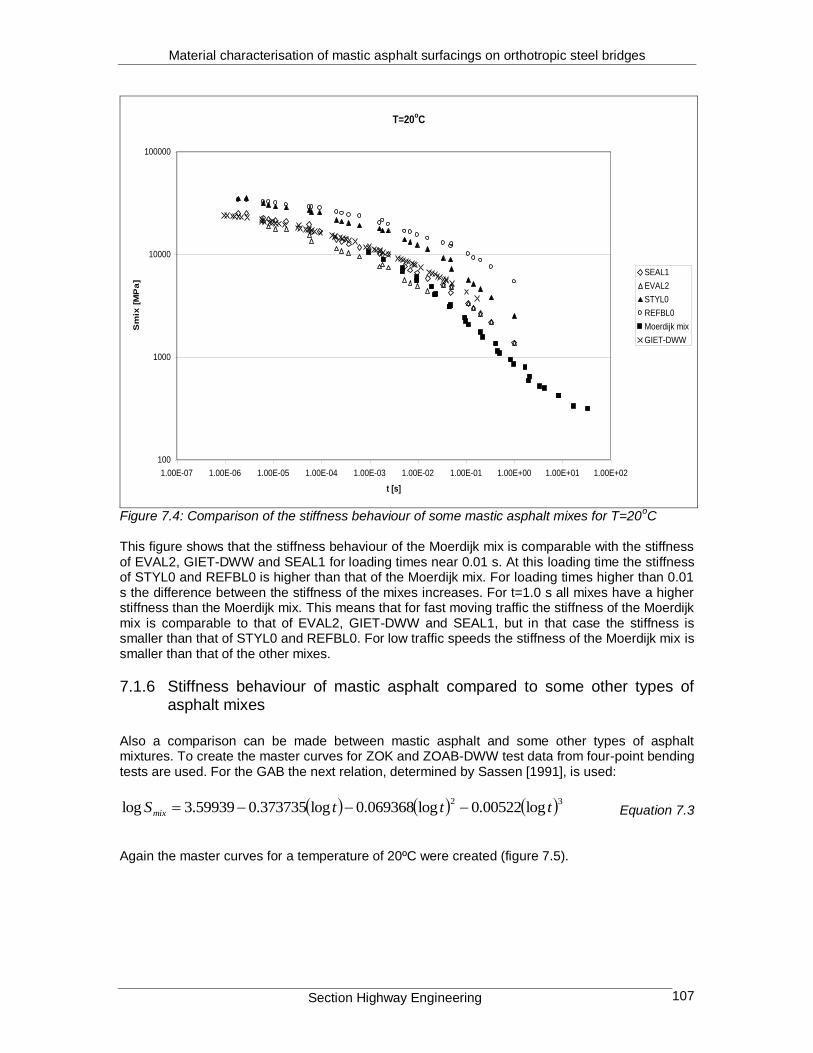
Material characterisation of mastic asphalt surfacings on orthotropic steel bridges
Section Highway Engineering 107
T=20oC
100
1000
10000
100000
1.00E-07 1.00E-06 1.00E-05 1.00E-04 1.00E-03 1.00E-02 1.00E-01 1.00E+00 1.00E+01 1.00E+02
t [s]
Sm
ix [
MP
a]
SEAL1
EVAL2
STYL0
REFBL0
Moerdijk mix
GIET-DWW
Figure 7.4: Comparison of the stiffness behaviour of some mastic asphalt mixes for T=20oC
This figure shows that the stiffness behaviour of the Moerdijk mix is comparable with the stiffness of EVAL2, GIET-DWW and SEAL1 for loading times near 0.01 s. At this loading time the stiffness of STYL0 and REFBL0 is higher than that of the Moerdijk mix. For loading times higher than 0.01 s the difference between the stiffness of the mixes increases. For t=1.0 s all mixes have a higher stiffness than the Moerdijk mix. This means that for fast moving traffic the stiffness of the Moerdijk mix is comparable to that of EVAL2, GIET-DWW and SEAL1, but in that case the stiffness is smaller than that of STYL0 and REFBL0. For low traffic speeds the stiffness of the Moerdijk mix is smaller than that of the other mixes.
7.1.6 Stiffness behaviour of mastic asphalt compared to some other types of asphalt mixes
Also a comparison can be made between mastic asphalt and some other types of asphalt mixtures. To create the master curves for ZOK and ZOAB-DWW test data from four-point bending tests are used. For the GAB the next relation, determined by Sassen [1991], is used:
32log00522.0log069368.0log373735.059939.3log tttSmix Equation 7.3
Again the master curves for a temperature of 20ºC were created (figure 7.5).

Material characterisation of mastic asphalt surfacings on orthotropic steel bridges
Section Highway Engineering 108
T=20oC
100
1000
10000
100000
1.E-08 1.E-07 1.E-06 1.E-05 1.E-04 1.E-03 1.E-02 1.E-01 1.E+00 1.E+01 1.E+02
t [s]
Sm
ix [
MP
a]
GAB
ZOAB-DWW
ZOK
Moerdijk mix
Figure 7.5: Master curves for some different types of asphalt mixes From figure 7.5 it becomes clear that the stiffness behaviour of mastic asphalt is comparable to the stiffness behaviour of ZOAB-DWW for loading times between 0.001 and 0.1 s. For other loading times no comparison can be made because the master curves are valid in different ranges of loading times. Figure 7.5 also shows that the stiffness of GAB is higher than that of the other mixes. The master curve of ZOK is totally different from the other master curves. These master curves show an increasing dependency of the stiffness on the loading time for increasing loading times. However, the master curve for ZOK is a straight line in the whole range of loading times. The slope of the line is very small, which means that the stiffness of ZOK hardly varies with loading time. This results in a less stiff behaviour of the material in situations of traffic driving with high speed. In situations of slow driving traffic the stiffness is considerably higher.
7.2 Fatigue characteristics
7.2.1 Introduction
The fatigue behaviour of an asphalt mix is an important characteristic that is used for road engineering. First the fatigue behaviour of the first fatigue test is analysed. Secondly the repeated fatigue test is analysed, after which both fatigue tests are compared. Further the fatigue behaviour of the modified Moerdijk mix is compared to that of other mixes. At first it is compared to the fatigue behaviour of four modified mastic asphalt mixes that were tested by Kolstein [1989]. Further it is compared to the fatigue behaviour of GAB and DAB 0/8. To create the fatigue line of GAB the relation determined by Wattimena [1991] is used. This is a result of four point bending tests carried out by the Netherlands Pavement Consultants. The fatigue line of DAB 0/8 is a result of tests at the Road and Hydraulic Engineering Division (DWW) carried out by Pronk [1998].

Material characterisation of mastic asphalt surfacings on orthotropic steel bridges
Section Highway Engineering 109
7.2.2 First fatigue test
7.2.2.1 Characterisation of fatigue parameters using the Wöhler approach
The Wöhler approach is a relationship between the number of strain applications to failure and the flexural tensile strain, which occurs at the bottom of the test specimen written as:
n
f kN
11
Equation 7.4
where: Nf :number of strain applications to failure
:flexural tensile strain at the bottom of test specimens [m/m] k1 , n :factors, depending on the composition and properties of the asphalt mix The Wöhler relationship can be rewritten as:
logloglog 1 nkN f Equation 7.5
It should be noted in this context that Nf is defined as the number of load repetitions at which the stiffness has decreased to half of the initial flexural stiffness value, since the fatigue tests were carried out in a displacement-controlled mode. The values of k1 and n are determined by regression analysis. For mastic asphalt the parameters are: log k1=23.903 n=6.7363 R
2=0.987
Figure 7.6 shows the fatigue characteristics for the Moerdijk mix using the Wöhler approach.
1000
10000
100000
1000000
10000000
100 1000 10000
Strain [m/m]
Lo
ad
rep
eti
tio
ns [
-]
Figure 7.6: Fatigue relation using the Wöhler approach at T=10
oC and f=5Hz

Material characterisation of mastic asphalt surfacings on orthotropic steel bridges
Section Highway Engineering 110
7.2.2.2 Characterisation of fatigue parameters using the energy approach
The dissipated energy is an alternative approach to fatigue characterisation. In this characterisation the number of load repetitions is related to the dissipated energy. Van Dijk [1975] showed that the total energy dissipated per volume to fatigue failure can be written as:
z
fff NBW Equation 7.6
where: Wf : total amount of dissipated energy per volume [J/m
3]
Nf : number of load repetitions to fatigue failure Bf, z : constants Equation 7.6 can be rewritten as:
fff NzBW logloglog Equation 7.7
The values of Bf, and z are determined by regression analysis. Bf=0.0394 z=0.753 R
2=0.9979
The value of z is comparable with the value of 0.7 reported by Van Dijk and Visser [1977] for several mixes. Furthermore, the value of Bf is different from the value of 0.012 reported by van Dijk and Visser [1977]. The higher value of Bf for mastic asphalt indicates that more energy is dissipated for the same number of load repetitions, meaning a better fatigue resistance. Figure 7.7 shows the fatigue characteristics of the Moerdijk mix using the energy approach.
10
100
1000
10000
1000 10000 100000 1000000 10000000
Number of load repetitions [-]
Dis
sip
ate
d e
ne
rgy
[M
Pa
]
Figure 7.7: Fatigue characteristics of the Moerdijk mix using the energy approach

Material characterisation of mastic asphalt surfacings on orthotropic steel bridges
Section Highway Engineering 111
7.2.2.3 Relationship between the strain, the mix stiffness and the number of load repetitions
The fatigue behaviour of mastic asphalt can be presented in a different way, when also the mix stiffness is involved. Table 7.8 shows the values of the strain, number of load repetitions and the stiffness, that were measured during the first fatigue tests on the Moerdijk mix. Table 7.8: Results from the first fatigue test on the Moerdijk mix
Strain [m/m] Load repetitions [-] Initial stiffness [MPa]
375 3600000 4679 475 934900 4444 600 152630 4083 750 28140 3443 925 5430 3820
1095 4270 3174
Regression analysis with the data in table 7.8 resulted in the following relation between the number of load repetitions, the strain and the mix stiffness:
mixSnnaN logloglog 211 Equation 7.8
in which: N : number of load repetitions [-]
: strain [m/m] Smix : initial mix stiffness [MPa] a1 : 33.377 n1 : 7.439 n2 : 2.086 The output from the regression analysis that was carried out to obtain equation 7.8 is shown in appendix F. By using equation 7.8 a new fatigue chart is obtained as shown in figure 7.8.
100
1000
10000
10 100 1000 10000 100000Smix [MPa]
[
m/m
] N=1*102
N=1*103
N=1*104
N=1*105
N=1*106
N=1*107
N=1*108
Figure 7.8: Relation between the number of load repetitions, the stiffness and the strain

Material characterisation of mastic asphalt surfacings on orthotropic steel bridges
Section Highway Engineering 112
7.2.3 Repeated fatigue test
7.2.3.1 Characterisation of fatigue parameters using the Wöhler approach
After repetition of the fatigue test the parameters used in equation 7.5 are determined for the repeated fatigue line: Log k1=33.477 n=10.06 R
2=0.969
Figure 7.19 shows the fatigue characteristics after repeating the test by using the Wöhler approach.
1000
10000
100000
1000000
10000000
100 1000 10000
[m/m]
N [
-]
Figure 7.9: Fatigue relation using the Wöhler approach after repeating the test
7.2.3.2 Characterisation of fatigue parameters using the energy approach
After repetition of the test the values of Bf, and z in equation 7.7 are determined by regression analysis for the repeated test. Bf=0.024 z=0.7992 R
2=0.9989
The value of z is again comparable with the value of 0.7 reported by Van Dijk and Visser [1977]. Furthermore, the value of Bf is of the same order of magnitude to the value of 0.012 reported by van Dijk and Visser [1977].

Material characterisation of mastic asphalt surfacings on orthotropic steel bridges
Section Highway Engineering 113
Figure 7.10 shows the fatigue characteristics of the tested mix using the energy approach.
10
100
1000
10000
1000 10000 100000 1000000 10000000
Number of load repetitions [-]
Dis
sip
ate
d e
ne
rgy
[M
Pa
]
Figure 7.10: Fatigue characteristics of the mix using the energy approach after repeating the test
7.2.4 Comparison between the first and repeated fatigue test for the Moerdijk mix
In order to investigate the influence of healing it was decided to repeat the fatigue test on the Moerdijk mix after 2.5 months after the repetition of the determination of the master curves. Both the fatigue line of the first test and the fatigue line of the repeated test are shown in figure 7.11.
1000
10000
100000
1000000
10000000
100 1000 10000
Strain [m/m]
Lo
ad
re
pe
titi
on
s [
-]
first fatigue test
repeated fatigue test
Figure 7.11: Comparison between the first and the repeated fatigue test using the Wöhler approach

Material characterisation of mastic asphalt surfacings on orthotropic steel bridges
Section Highway Engineering 114
Both fatigue lines cross at a strain level of 760 m/m and the number of load repetitions is approximately 31350. The figure shows that the slope of the fatigue line has increased after repetition of the test. This corresponds to a somewhat more brittle behaviour of the specimen. The effect is that the material becomes more sensible to high strain levels and behaves better under lower strain levels. The reason for this might be the ageing of the bitumen during the two and a half months of storage, in spite of the fact that the specimens were stored in a temperature controlled room at 13
oC between both tests. Further the healing of the material plays an important role.
Figure 7.12 shows the comparison between the first and repeated fatigue test using the energy approach.
10
100
1000
10000
1000 10000 100000 1000000 10000000
Number of load repetitions [-]
Dis
sip
ate
d e
ne
rgy
[M
Pa
]
first fatigue test
repeated fatigue test
Figure 7.12: Comparison between the first and the repeated fatigue test using the energy approach
Again the fatigue lines cross each other. Using the energy approach the intersection point is N=45700 and E=127 MPa. Comparing the number of load repetitions at the intersection point for the Wöhler and the energy approach shows that the value is higher for the second approach. However, the trend for both approaches is the same, the fatigue behaviour of the material after repetition of the test becomes better for lower strain levels (corresponding to high values of N) and becomes worse for higher strain levels (corresponding to low values of N).
7.2.5 Fatigue behaviour of the Moerdijk mix compared to some modified mastic asphalt mixes
Figure 7.13 shows the fatigue behaviour of the Moerdijk mix and the fatigue behaviour of four modified mastic asphalt mixes, namely REFBL0 (bitumen 45/60 + Trinidad-Épurée), STYL0 (Styrelf 1360), SEAL1 (Sealoflex) and EVAL2 (Bitumen 45/60 + Eva 18-150). It has to be noted that the fatigue lines of these four modified mixes are valid for T=20
oC and f=30 Hz, while the
fatigue line of the Moerdijk mix is determined at T=10oC and f=5 Hz. Nevertheless these lines are

Material characterisation of mastic asphalt surfacings on orthotropic steel bridges
Section Highway Engineering 115
comparable, because the stiffness of the mixes at these different temperatures and frequencies is comparable.
T=20oC, f=30 Hz
1000
10000
100000
1000000
10000000
10 100 1000 10000
Strain [m/m]
Lo
ad
re
pe
titi
on
s [
-]
REFB-L0
STY-L0
SEAL1
EVAL2
Moerdijk mix,10C 5Hz
Figure 7.13: Fatigue behaviour of different mastic asphalt mixes Figure 7.13 shows that the fatigue behaviour of the Moerdijk mix is better than that of the other mixes. The figure also shows that the strain range in which the Moerdijk mix is tested is larger than the range in which the other mixes are tested. The modified mixes are tested within a very small strain range and at quite low strain levels. The validity of these lines is therefore
questionable because of the high strains (±1300 m/m) that may occur in the asphalt on orthotropic steel bridges.
7.2.6 Fatigue behaviour of the Moerdijk mix compared to some other mixes
Figure 7.14 shows the fatigue behaviour of the Moerdijk mix, GAB and DAB 0/8. For the GAB the relation is used that is determined by Wattimena [1991]. This relationship is:
log63.340.12log N Equation 7.9
In this relation is in m/m. For the DAB the relation determined by Pronk [1998] is used:
log06.469.14log N Equation 7.10
In this relation is in m/m. The relations from Wattimena and Pronk are determined at T=20
oC and f=30 Hz, the fatigue line
of the Moerdijk mix is valid for T=10oC and f=5 Hz. However the results are comparable because
at these different conditions the stiffness of the mixes is approximately the same.

Material characterisation of mastic asphalt surfacings on orthotropic steel bridges
Section Highway Engineering 116
T=20oC, f=30 Hz
100
1000
10000
100000
1000000
10000000
10 100 1000 10000
[m/m]
N [
-]
GAB
DAB 0/8
Moerdijk mix, 10C, 5Hz
Figure 7.14: Fatigue behaviour of the Moerdijk mix, DAB and GAB Figure 7.14 shows that the fatigue behaviour of the Moerdijk mix is better than the fatigue behaviour of GAB and DAB tested by Wattimena and Pronk. It should be noted that the range of strains in which the Moerdijk mix was tested differs considerably from the range in which the GAB and the DAB were tested. This is attributed to the fact that for orthotropic steel bridges higher strain levels are of interest. Under these high strain conditions the behaviour of the material may be different, which might have led to the differences in figure 7.14 between the mixes.
7.2.7 Fatigue behaviour of the Moerdijk mix compared to the SPDM
Additional fatigue information is obtained by comparing the fatigue behaviour of the Moerdijk mix with the F1 and F2 SPDM lines, using the Shell pavement Design Manual [SPDM 1978]. To use this manual the average initial stiffness from the first fatigue tests is taken, which is 3941 MPa. The corresponding SPDM F1 and F2 fatigue characteristics were determined by using charts M3 and M4 from the SPDM, see figure 7.15.
Figure 7.15: Asphalt fatigue characteristics according to the SPDM F1 (left) and F2 (right)
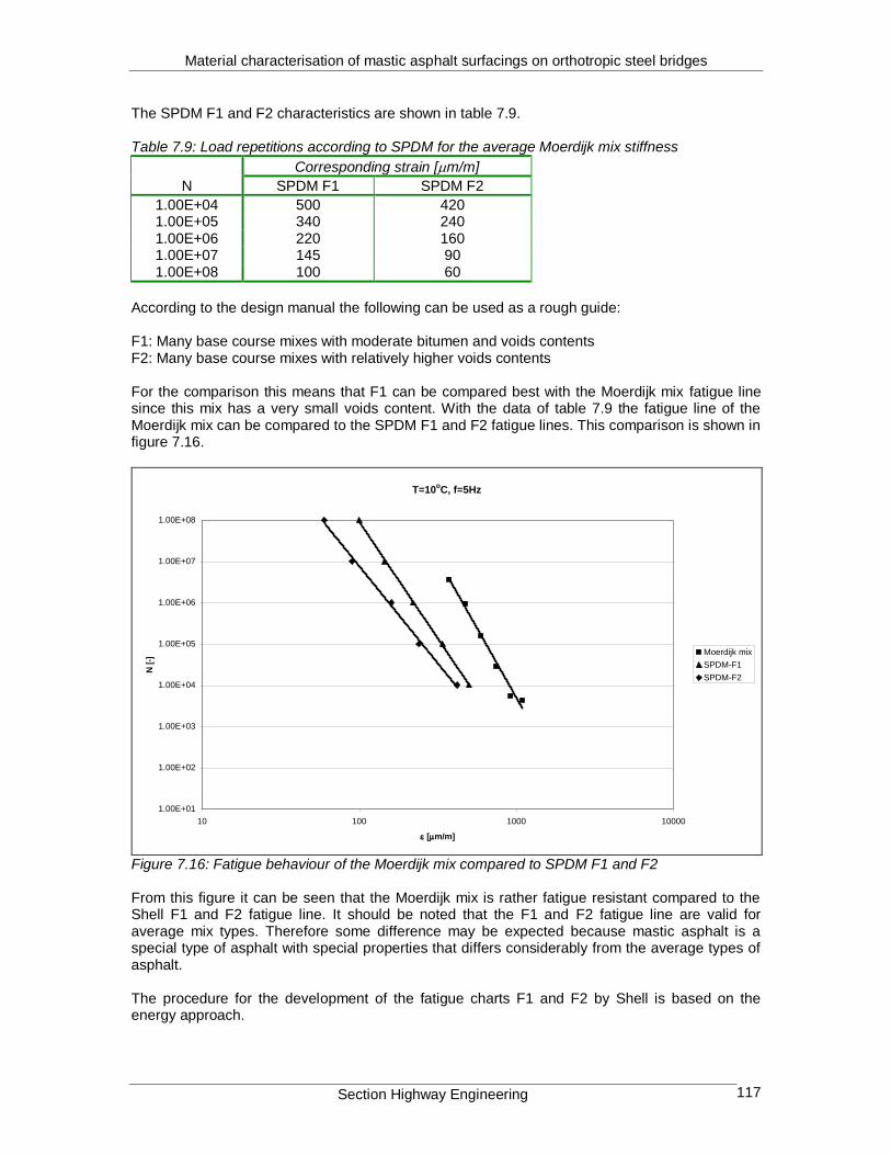
Material characterisation of mastic asphalt surfacings on orthotropic steel bridges
Section Highway Engineering 117
The SPDM F1 and F2 characteristics are shown in table 7.9. Table 7.9: Load repetitions according to SPDM for the average Moerdijk mix stiffness
Corresponding strain [m/m]
N SPDM F1 SPDM F2
1.00E+04 500 420 1.00E+05 340 240 1.00E+06 220 160 1.00E+07 145 90 1.00E+08 100 60
According to the design manual the following can be used as a rough guide: F1: Many base course mixes with moderate bitumen and voids contents F2: Many base course mixes with relatively higher voids contents For the comparison this means that F1 can be compared best with the Moerdijk mix fatigue line since this mix has a very small voids content. With the data of table 7.9 the fatigue line of the Moerdijk mix can be compared to the SPDM F1 and F2 fatigue lines. This comparison is shown in figure 7.16.
T=10oC, f=5Hz
1.00E+01
1.00E+02
1.00E+03
1.00E+04
1.00E+05
1.00E+06
1.00E+07
1.00E+08
10 100 1000 10000
[m/m]
N [
-]
Moerdijk mix
SPDM-F1
SPDM-F2
Figure 7.16: Fatigue behaviour of the Moerdijk mix compared to SPDM F1 and F2 From this figure it can be seen that the Moerdijk mix is rather fatigue resistant compared to the Shell F1 and F2 fatigue line. It should be noted that the F1 and F2 fatigue line are valid for average mix types. Therefore some difference may be expected because mastic asphalt is a special type of asphalt with special properties that differs considerably from the average types of asphalt. The procedure for the development of the fatigue charts F1 and F2 by Shell is based on the energy approach.

Material characterisation of mastic asphalt surfacings on orthotropic steel bridges
Section Highway Engineering 118
Equation 7.6 was related to the limiting strain, by using the dissipated energy per cycle per unit volume:
sinW Equation 7.11
where:
: stress amplitude
: strain amplitude
: phase angle between the stress and the strain If the dissipated energy per cycle is constant, the relation between the total amount of dissipated energy Wf and the dissipated energy per cycle is:
inff WNW Equation 7.12
in which: Wf : total amount of dissipated energy per volume Nf : number of load repetitions to fatigue failure
Win : initial dissipated energy per cycle = 000 sin
: stress, strain and phase angle at the beginning of the test. However, the dissipated energy per cycle decreases during a constant displacement fatigue test
and increases in a constant load fatigue test due to the change of and . Therefore equation 7.12 changes in:
/inff WNW Equation 7.13
where:
: factor taking into account the variation in dissipated energy per cycle during the test
For a displacement controlled test is larger than 1 and in a load controlled test is smaller than 1. Combination of equation 7.6 and 7.13 results in:
z
ff
fNB
N
000 sin Equation 7.14
Rewriting equation 7.14 results in the relation between the strain, Smix and N:
2/1
0
0sin
z
mix
fN
S
B
Equation 7.15
It has been observed that the variation of Z is very small for common mixes and can be taken as constant for practical purposes (Z≈0.7). By taking a Bf value representing a good fatigue behaviour and a Bf value representing a worse fatigue behaviour different charts can be developed. On this procedure the design charts F1 and F2 are based [Molenaar, 1994].

Material characterisation of mastic asphalt surfacings on orthotropic steel bridges
Section Highway Engineering 119
7.2.8 Relationship between the mix stiffness and the number of load repetitions in a fatigue test
A typical experimental relationship between the mix stiffness and the number of load repetitions is shown in figure 7.17.
Number of load repetitions
Figure 7.17: A typical relationship between the stiffness and the number of cycles in a strain- controlled four point bending test
Three parts can be distinguished: 1. Part I: At the beginning of the test a sharp decrease of the stiffness modulus may be
observed. According to Ullidtz et al. [1997] this might probably be due to the visco-elastic characteristics of the asphalt where the dissipation energy will cause an increase of the temperature in the beam until the heat flow has reached a steady state.
2. Part II: In the second part the rate of the stiffness loss is almost constant (from N1 to N2). 3. Part III: A sharp decrease of the stiffness may also be observed. This part seems to be
associated with the development of macrocracks (from N2 to Nf).
The similarity between these three parts and the three stages which can be distinguished [e.g. Ewalds and Wanhil, 1986] in the fracture mechanics approach is obvious. The three stages are:
1. The initiation phase: development of hairline or micro cracks, 2. The propagation phase: development of macro cracks out of microcracks, 3. The disintegration phase, being the propagation of the macro cracks, leading to collapse and
initial failure of the material. In this phase unstable crack growth can be observed. From the analysis of the fatigue data of the Moerdijk mix the following remarks can be made:
Part III was reached in none of the specimens. The reason is that the stiffness was halved, and thus the test was terminated, before the initiation of this part. This may suggest that researchers should think of another more fundamental definition of failure instead of the arbitrary chosen criteria, which considers the specimen is failed when the initial flexural stiffness is halved.

Material characterisation of mastic asphalt surfacings on orthotropic steel bridges
Section Highway Engineering 120
Table 7.10 shows the ratio N1/Nf for the six fatigue tests that were carried out. Table 7.10: Ratio N1/Nf
Specimen Strain level [m/m] Nf N1 N1/Nf
FM2 1095 4270 - - FM3 600 152630 41000 0.27 FM4 375 3600000 675000 0.19 FM5 750 28140 8250 0.29 FM6 925 5430 - - FM7 475 934900 200000 0.21
The value of the ratio of N1 (which defines the end of Part I) to Nf (i.e. the number of cycles to
failure) was found to be 0.19-0.29 for low values of the strain. For higher values of the strain level the ratio of N1 to Nf can not be determined because then the stiffness decreases so fast that half of the stiffness is reached before N1 is reached. It has been demonstrated by a large number of researchers [Jenq and Perng, 1991; Ramsamooj, 1991] that the characterisation of fatigue by these three stages is only valid if the plastic deformation is limited, especially if asphaltic materials are studied. This may explain the fact that for high strain levels no N1 value can be defined, because for high strain
levels (in this case ≈1000 m/m) the plastic deformations are considerable.
Comparison of the ratio N1/Nf with values determined by Medani [1999] shows that his values are in approximately the same range (0.18-0.26).
7.3 Dependency of the mix stiffness on the strain
7.3.1 Introduction
For determining the master curves for asphalt mixes used for pavement layers on a subgrade the initial stiffness is determined normally after few load repetitions, say 100, at a low strain level of
80 m/m. This strain level is representative for the strains that occur in pavements on a
subgrade. However, on orthotropic steel bridges this strain level can be up to 1300 m/m. These high strain levels might have an influence on the mix stiffness. In this section the strain dependency of the mix stiffness is investigated.
7.3.2 Strain dependency of some asphalt mixes
Also during fatigue testing at different strain levels the initial stiffness is determined after 100 load repetitions. By using the data from the first series of 4-point bending tests figure 7.18 is created, showing the relationship between the strain level and the mix stiffness for the Moerdijk mix.

Material characterisation of mastic asphalt surfacings on orthotropic steel bridges
Section Highway Engineering 121
T=10oC, f=5 Hz
1000
2000
3000
4000
5000
6000
7000
0 200 400 600 800 1000 1200
strain [m/m]
Sm
ix [
MP
a]
Figure 7.18: Relation between the mix stiffness and strain This figure shows clearly that the mix stiffness decreases with increasing strain level, which indicates the stress-dependent behaviour of the material. This phenomenon can also be observed for other asphalt mixes. Figure 7.19 shows the relationship between the mix stiffness and the strain for some modified mastic asphalt mixes that have been tested by Kolstein.
6000
8000
10000
12000
14000
16000
18000
20000
22000
24000
0 50 100 150 200 250 300 350
strain [m/m]
Sti
ffn
es
s [
MP
a] STYLO
REFBLO
REFBP1-TUD
STYP1
REFBP1-KWS
STYL7
Figure 7.19: Relation between stiffness and strain for some modified mastic asphalt mixes

Material characterisation of mastic asphalt surfacings on orthotropic steel bridges
Section Highway Engineering 122
It has to be noted again that Kolstein tested at very small strain levels. The influence of the strain on the mix stiffness might be increasing with increasing strain level. Considering the data from the Strategic Highway Research Program (SHRP) [1994] more or less the same trend can be observed for some of the asphalt mixes that were tested in this program. Figure 7.20 shows the relation between the mix stiffness and the strain for some of the mixes tested in the SHRP-program.
0
2000
4000
6000
8000
10000
12000
0 200 400 600 800 1000 1200 1400
strain [m/m]
Sm
ix [
MP
a]
Asphalt B: 60/70 pen, 5.4% bitumen
High mod. Mix, 10/20 pen, 6.2% bitumen
Asphalt A: 60/70 pen, 4.7% bitumen
Figure 7.20: Relation between the stiffness and the strain for mixes tested in the SHRP program Also some mixes tested at the TU Delft show a certain relation between the mix stiffness and the strain as shown in figure 7.21.
3000
4000
5000
6000
7000
8000
9000
10000
11000
0 100 200 300 400 500 600 700 800
strain [m/m]
Init
ial
sti
ffn
es
s [
MP
a] halfwarm+ foamed bitumen 20C 10Hz
OAB 0/16 with perifalt 15C 10 Hz
ACRE 0/5 with bitumen 45/60 20C 10Hz
Bitumen 45/60 15C 10Hz
OAB 0/16 poclon
Figure 7.21: Relation between the stiffness and the strain for some mixes tested at TU Delft

Material characterisation of mastic asphalt surfacings on orthotropic steel bridges
Section Highway Engineering 123
7.3.3 Comparison between master curves at 80m/m and 800 m/m for the Moerdijk mix
The figures 7.18-7.21 all show the trend of a decreasing mix stiffness for an increasing strain
level. Because of the high strain levels (±1300 m/m) that were measured on bridges, this means
that the stiffness determined at the low strain levels (80m/m) is not representative for mastic asphalt on steel bridges. Therefore it was chosen to repeat the four-point bending test at two
strain levels, 80m/m and 800m/m and at three temperatures, 10oC, 20
oC and 30
oC. For the
repetitions the same specimens were used that were tested before, some of them were also tested at high strain levels for fatigue testing. These specimens were stored at a temperature of
13oC for 2.5 months. The measurements at the strain level of 80 m/m can be seen as reference
measurements. The figures 7.22-7.24 show the comparison between the master curve at
80m/m and 800 m/m for three temperatures.
T=10oC
10
100
1000
10000
0.01 0.1 1 10 100 1000
t [s]
Sm
ix [
MP
a]
strain=80 new
strain=800
Figure 7.22: Master curves for strain levels of 80 and 800 m/m at T=10
oC
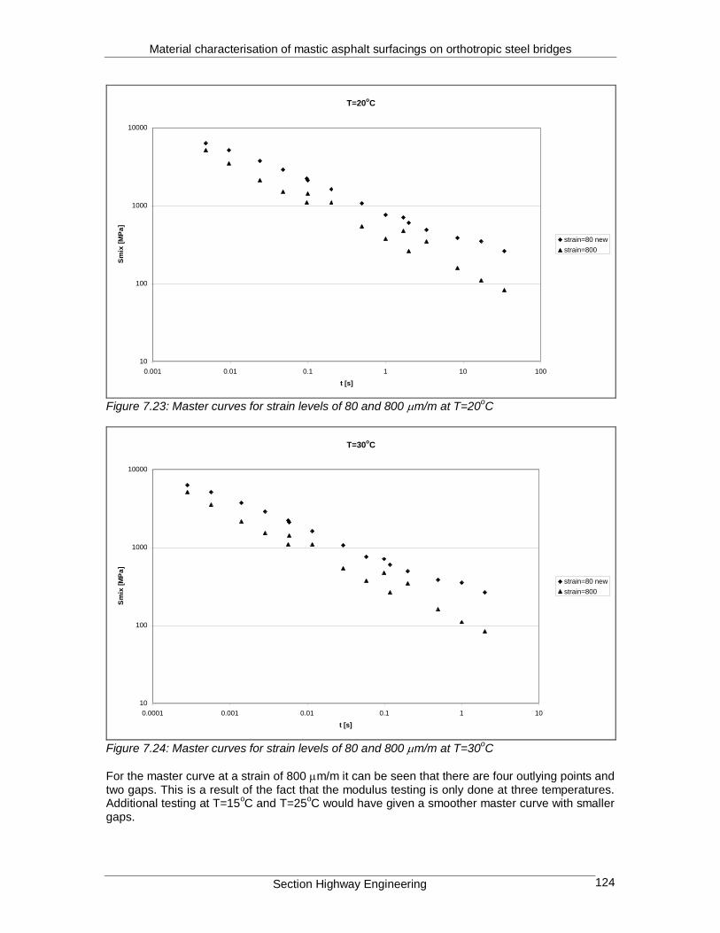
Material characterisation of mastic asphalt surfacings on orthotropic steel bridges
Section Highway Engineering 124
T=20oC
10
100
1000
10000
0.001 0.01 0.1 1 10 100
t [s]
Sm
ix [
MP
a]
strain=80 new
strain=800
Figure 7.23: Master curves for strain levels of 80 and 800 m/m at T=20
oC
T=30oC
10
100
1000
10000
0.0001 0.001 0.01 0.1 1 10
t [s]
Sm
ix [
MP
a]
strain=80 new
strain=800
Figure 7.24: Master curves for strain levels of 80 and 800 m/m at T=30
oC
For the master curve at a strain of 800 m/m it can be seen that there are four outlying points and two gaps. This is a result of the fact that the modulus testing is only done at three temperatures. Additional testing at T=15
oC and T=25
oC would have given a smoother master curve with smaller
gaps.

Material characterisation of mastic asphalt surfacings on orthotropic steel bridges
Section Highway Engineering 125
7.3.4 Determination of a shift-factor for the Moerdijk mix
The figures in the previous paragraph also show that for the three temperatures there is a shift
between the mix stiffness determined at =80 m/m and =800m/m. To determine this shift-factor the shift-factor is defined as:
)80(
)800(80080
mix
mix
S
SSHIFT Equation 7.16
This shift-factor is a function of both temperature and loading time. Analysis of the data has lead to the following function for the shift-factor:
7224.00126.0)ln(0428.080080 TtSHIFT
This relation is valid for loading times between 0.01 s and 1 s and temperatures between 10
oC
and 30oC. Table 7.11 shows the comparison between the mix stiffness at =800 m/m that is
measured and the one that is predicted with the shift-factor. Table 7.11: Comparison between Smix measured and Smix predicted with the shift-factor
T [oC] t [s] Smix measured
[MPa] Smix with
shift-factor [MPa] Difference [%]
10 0.1000 5162 4353 -16 10 0.2000 3490 3412 -2 10 0.5000 2132 2325 9 10 1.0000 1520 1721 13 10 2.0747 1098 1186 8 10 10.3733 540 530 -2 10 35.2345 374 314 -16 10 70.4691 263 203 -23 10 176.1726 159 144 -9 10 352.3453 110 121 10 10 704.6906 83 83 0
20 0.0048 5162 4377 -15 20 0.0096 3490 3432 -2 20 0.0241 2132 2339 10 20 0.0482 1520 1732 14 20 0.1000 1098 1194 9 20 0.5000 540 534 -1 20 1.6983 374 317 -15 20 3.3966 263 205 -22 20 8.4916 159 145 -9 20 16.9832 110 122 11 20 33.9665 83 84 1
30 0.0003 5162 4347 -16 30 0.0006 3490 3407 -2 30 0.0014 2132 2321 9 30 0.0028 1520 1718 13 30 0.0059 1098 1184 8 30 0.0294 540 529 -2 30 0.1000 374 313 -16 30 0.2000 263 203 -23 30 0.5000 159 144 -10 30 1.0000 110 121 10 30 2.0000 83 82 -1

Material characterisation of mastic asphalt surfacings on orthotropic steel bridges
Section Highway Engineering 126
This table shows that the difference between the measured and predicted stiffness varies between 1% and 23%. The average of the absolute value of the differences is 9.9%. It has to be noted that the determined shift-factor is valid only for shifting the master curve from
=80 m/m to =800 m/m. To shift the master curve at =80 m/m to an arbitrarily strain level, the shift-factor becomes a function of loading time, temperature as well as the strain:
),,80(
),,(),,(80
TtS
TtSTtSHIFT
mix
mix Equation 7.17
Additional testing was carried out to determine this strain dependent behaviour of mastic asphalt. These tests are described in section
7.3.5 Strain dependency of the LINTRACK mix stiffness
After additional testing the master curves for the LINTRACK mix were created for different strain levels. When these master curves are combined in one figure the influence of the strain becomes obvious. This is shown in the figures 7.25-7.30. In each of the figures the master curves at different strain levels are shown for a constant temperature.
T=5oC
10
100
1000
10000
0.1 1 10 100 1000 10000 100000
t [s]
Sm
ix [
MP
a]
eps=80
eps=200
eps=600
eps=1000
Figure 7.25: Master curves for different strain levels at T=5
oC

Material characterisation of mastic asphalt surfacings on orthotropic steel bridges
Section Highway Engineering 127
T=12.5oC
10
100
1000
10000
0.001 0.01 0.1 1 10 100 1000 10000
t [s]
Sm
ix [
MP
a]
eps=80
eps=200
eps=600
eps=1000
Figure 7.26: Master curves for different strain levels at T=12.5
oC
T=20oC
10
100
1000
10000
0.0001 0.001 0.01 0.1 1 10 100 1000
t [s]
Sm
ix [
MP
a]
eps=80
eps=200
eps=600
eps=1000
Figure 7.27: Master curves for different strain levels at T=20
oC

Material characterisation of mastic asphalt surfacings on orthotropic steel bridges
Section Highway Engineering 128
T=27.5oC
10
100
1000
10000
0.0001 0.001 0.01 0.1 1 10 100 1000
t [s]
Sm
ix [
MP
a]
eps=80
eps=200
eps=600
eps=1000
Figure 7.28: Master curves for different strain levels at T=27.5
oC
T=35oC
10
100
1000
10000
0.00001 0.0001 0.001 0.01 0.1 1 10 100
t [s]
Sm
ix [
MP
a]
eps=80
eps=200
eps=600
eps=1000
Figure 7.29: Master curves for different strain levels at T=35
oC

Material characterisation of mastic asphalt surfacings on orthotropic steel bridges
Section Highway Engineering 129
T=42.5oC
10
100
1000
10000
0.000001 0.00001 0.0001 0.001 0.01 0.1 1 10
t [s]
Sm
ix [
MP
a]
eps=80
eps=200
eps=600
eps=1000
Figure 7.30: Master curves for different strain levels at T=42.5
oC
All the figures show that for increasing loading time the difference in mix stiffness for the different strain levels is increasing. This means that the strain dependency is increasing with increasing loading times. This behaviour leads to sensibility of the mix to traffic congestion, especially at high temperatures. The maximum difference at high loading times between the mix stiffness at 80
m/m and 1000 m/m can be a factor 5.
7.3.6 The mix stiffness as a function of loading time and temperature
The separate master curves in the figures 7.25-7.30 are described best with the following equation:
33
2
210 loglogloglog tatataaSmix Equation 7.18
in which: Smix: stiffness of the mix [MPa] t: loading time [s] ai: regression constants The tables 7.12-7.15 show the regression constants for the master curves.
Table 7.12: Regression constants for the master curves at =80 m/m
T [oC] ao a1 a2 a3 R
2
5.0 3.7151 -0.3003 -0.0453 0.0104 0.9969
12.5 3.3685 -0.3605 -0.0130 0.0104 0.9969 20.0 3.0129 -0.3558 0.0177 0.0104 0.9969 27.5 2.7057 -0.2957 0.0469 0.0104 0.9969 35.0 2.4880 -0.1882 0.0746 0.0104 0.9969 42.5 2.3887 -0.0401 0.1010 0.0104 0.9969

Material characterisation of mastic asphalt surfacings on orthotropic steel bridges
Section Highway Engineering 130
Table 7.13: Regression constants for the master curves at =200 m/m
T [oC] ao a1 a2 a3 R
2
5.0 3.6872 -0.3125 -0.0640 0.0126 0.9971
12.5 3.3104 -0.4045 -0.0250 0.0126 0.9971 20.0 2.9022 -0.4173 +0.0119 0.0126 0.9971 27.5 2.5345 -0.3624 +0.0471 0.0126 0.9971 35.0 2.2595 -0.2494 +0.0805 0.0126 0.9971 42.5 2.1140 -0.0869 +0.1124 0.0126 0.9971
Table 7.14: Regression constants for the master curves at =600 m/m
T [oC] ao a1 a2 a3 R
2
5.0 3.5889 -0.3709 -0.0483 0.0098 0.9952
12.5 3.1656 -0.4392 -0.0179 0.0098 0.9952 20.0 2.7277 -0.4459 +0.0110 0.0098 0.9952 27.5 2.3304 -0.3999 +0.0385 0.0098 0.9952 35.0 2.0135 -0.3087 +0.0646 0.0098 0.9952 42.5 1.8051 -0.1789 +0.0894 0.0098 0.9952
Table 7.15: Regression constants for the master curves at =1000 m/m
T [oC] ao a1 a2 a3 R
2
5.0 3.5057 -0.4096 -0.0232 0.0057 0.9896
12.5 3.0646 -0.4393 -0.0055 0.0057 0.9896 20.0 2.6346 -0.4338 0.0112 0.0057 0.9896 27.5 2.2453 -0.3982 0.0271 0.0057 0.9896 35.0 1.9181 -0.3369 0.0422 0.0057 0.9896 42.5 1.6675 -0.2537 0.0566 0.0057 0.9896
It is clear that the mix stiffness is not only dependent on loading time and temperature, but also on the strain level.
7.3.7 The mix stiffness as a function of strain, temperature and loading time
With the computer program TableCurve2D the relationship between the mix stiffness, , t, T was determined. For each master curve the point (t, Smix)=(1*10
-10, 16000) is added, to make sure that
the determined function has a stiffness that reaches asymptotic to the maximum value of 16000. The TableCurve program only determines the relation between two variables, so first the relation is determined for each master curve separately. Each master curve is described best with:
z
ytmix
e
xwS
)(log
1
log Equation 7.19
The parameters w, x, y and z for each master curve are shown in the tables 7.16-7.19.
Table 7.16: Parameters for the master curves at =80 m/m
T [oC] w x y z
5.0 2.25 1.94 1.42 -1.25 12.5 2.25 1.94 0.39 -1.25 20.0 2.25 1.94 -0.59 -1.25 27.5 2.25 1.94 -1.52 -1.25 35.0 2.25 1.95 -2.41 -1.26 42.5 2.25 1.95 -3.26 -1.26

Material characterisation of mastic asphalt surfacings on orthotropic steel bridges
Section Highway Engineering 131
Table 7.17: Parameters for the master curves at =200 m/m
T [oC] w x y z
5.0 1.89 2.30 1.67 -1.33 12.5 1.89 2.31 0.64 -1.33 20.0 1.89 2.31 -0.34 -1.33 27.5 1.89 2.31 -1.27 -1.33 35.0 1.89 2.31 -2.16 -1.33 42.5 1.89 2.32 -3.01 -1.34
Table 7.18: Parameters for the master curves at =600 m/m
T [oC] w x y z
5.0 1.49 2.73 1.74 -1.45 12.5 1.49 2.73 0.70 -1.45 20.0 1.49 2.73 -0.28 -1.45 27.5 1.49 2.74 -1.21 -1.46 35.0 1.48 2.75 -2.09 -1.46 42.5 1.48 2.76 -2.94 -1.47
Table 7.19: Parameters for the master curves at =1000 m/m
T [oC] w x y z
5.0 1.28 2.96 1.75 -1.57 12.5 1.28 2.96 0.71 -1.58 20.0 1.28 2.97 -0.27 -1.58 27.5 1.27 2.98 -1.20 -1.59 35.0 1.27 3.00 -2.09 -1.60 42.5 1.25 3.02 -2.94 -1.62
From these tables it becomes clear that w, x and z are constant for each strain level and that y varies with strain level and temperature, so:
fz
Tfy
fx
fw
,
The next step that is carried out is the determination of w, x, y and z. Therefore also use is made of TableCurve2D, which has resulted in the following relations:
baw log Equation 7.20
2logdcx
Equation 7.21
5.1
hgfTy Equation 7.22
jiz Equation 7.23

Material characterisation of mastic asphalt surfacings on orthotropic steel bridges
Section Highway Engineering 132
Filling in these relations in the total relation results in a function describing the mix stiffness as a function of loading time, temperature and strain:
5.0
5.1 )(log
2
1
loglog,,log
ji
hgfTtmix
e
dcbaTtS
Equation 7.24
in which: Smix : mix stiffness [MPa]
: strain [m/m] t : loading time [s] T : temperature [
oC]
The constants a-j are determined by regression analysis: a : -0.886 b : 3.937 c : 1.273 d : 0.191 f : 0.125 g : -2.297 h : 238.048 i : -1.125 j :-0.014 The relation is valid within the following ranges:
80 m/m ≤ ≤1000 m/m
0oC ≤ T≤ 45
oC
0.01s ≤ t≤ 1s The range of the loading times corresponds to speeds between 108 km/h and 1 km/h. Appendix C shows the complete derivation of equation 7.24 as well as the significance of the function, by comparing the measured with the predicted stiffness for each master curve. Equation 7.24 has been used to make graphs representing the dependency of the mix stiffness on the strain level. Four loading times are chosen to be representative, namely, 0.01, 0.02, 0.1 and 1.0s. The speeds to which these loading times correspond are calculated with:
t
Dv
6.3 Equation 7.25
in which: v : speed [km/h] D : diameter of the contact area of a wide base tyre [0.3m] t : loading time [s] The speeds that correspond to the four loading times are shown in table 7.20. Table 7.20: Relation between loading time and speed
t [s] Speed [km/h]
0.01 108 0.02 54 0.1 11 1.0 1
The speed of 54 km/h corresponds to the speed used in Shell design manuals.

Material characterisation of mastic asphalt surfacings on orthotropic steel bridges
Section Highway Engineering 133
The figures 7.31-7.34 show the stiffness as a function of strain level for these loading times and several temperatures between 0 and 45
oC.
0
2000
4000
6000
8000
10000
12000
14000
0 200 400 600 800 1000 1200
[m/m]
Sm
ix [
MP
a]
T=5
T=10
T=15
T=20
T=25
T=30
T=35
T=40
T=45
Figure 7.31: Strain dependency of the mix stiffness for t=0.01s
0
2000
4000
6000
8000
10000
12000
14000
0 200 400 600 800 1000 1200
[m/m]
Sm
ix [
MP
a]
T=0
T=5
T=10
T=15
T=20
T=25
T=30
T=35
T=40
T=45
Figure 7.32: Strain dependency of the mix stiffness for t=0.02s

Material characterisation of mastic asphalt surfacings on orthotropic steel bridges
Section Highway Engineering 134
0
2000
4000
6000
8000
10000
12000
0 200 400 600 800 1000 1200
[m/m]
Sm
ix [
MP
a]
T=0
T=5
T=10
T=15
T=20
T=25
T=30
T=35
T=40
T=45
Figure 7.33: Strain dependency of the mix stiffness for t=0.1s
0
1000
2000
3000
4000
5000
6000
7000
8000
0 200 400 600 800 1000 1200
[m/m]
Sm
ix [
MP
a]
T=0
T=5
T=10
T=15
t=20
T=25
T=30
T=35
T=40
T=45
Figure 7.34: Strain dependency of the mix stiffness for t=1.0s With this large influence of the stiffness on the strain level it is clear that this behaviour cannot be neglected. However, it should be noticed that the function for the mix stiffness is based on measurements on the Lintrack mix only. More testing is needed to verify if the function can be applied for all the mastic asphalt mixes. It should be emphasised here that the relationship is based merely on linear elastic theory and hence no viscous or visco-plastic behaviour was considered. The relationship is namely based on measurements with the four-point bending testing machine that calculates the stiffness by assuming linear elastic behaviour. However, at high temperatures and strain levels linear behaviour is not expected. Nevertheless, for practical purposes, this relationship may be considered very useful.

Material characterisation of mastic asphalt surfacings on orthotropic steel bridges
Section Highway Engineering 135
7.3.8 Determination of the shift-factor for mastic asphalt
In paragraph 7.3.4 the shift-factor between the mix stiffness at 80 m/m and 800 m/m was determined. It is clear that also the shift-factor for an arbitrarily strain level is of interest. The shift-factor is defined as:
),,80(
),,(),,(80
TtS
TtSTtSHIFT
mix
mix Equation 7.26
In which:
SHIFT80→ : Shift-factor T : Temperature [
oC]
t : Loading time [s]
: Strain level [m/m] The expression for the shift-factor as a function of loading time, temperature and strain level is rather complex (combination of equation 7.24 and 7.26). Therefore some tables and graphs are made from which the shift-factor can easily be read. Tables 7.21-7.23 and the figures 7.35-7.37
can be used to determine the shift factor for strain levels of 200, 600 and 1000 m/m. Table 7.21: SHIFT80-200 for different temperatures and loading times
SHIFT80→200 t=0.01s t=0.02s t=0.1s t=1.0s
0oC 0.90 0.90 0.89 0.88
5oC 0.89 0.89 0.88 0.87
10oC 0.89 0.88 0.87 0.85
15oC 0.88 0.87 0.86 0.83
20oC 0.87 0.86 0.84 0.78
25oC 0.86 0.85 0.81 0.72
30oC 0.83 0.81 0.75 0.65
35oC 0.79 0.76 0.69 0.59
40oC 0.73 0.70 0.63 0.55
45oC 0.66 0.63 0.57 0.51
0.50
0.55
0.60
0.65
0.70
0.75
0.80
0.85
0.90
0.95
0 5 10 15 20 25 30 35 40 45 50
T [oC]
SH
IFT
80-2
00
t=0.01s
t=0.02s
t=0.1s
t=1.0s
Figure 7.35: SHIFT80-200 for different temperatures and loading times
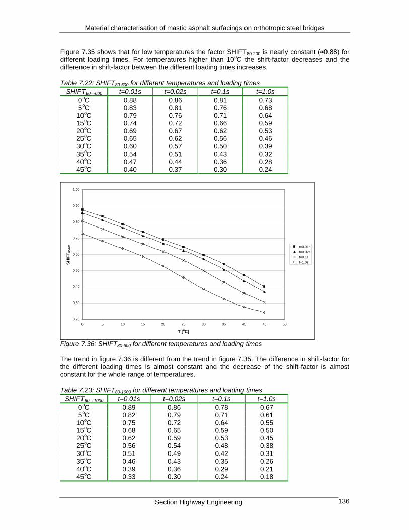
Material characterisation of mastic asphalt surfacings on orthotropic steel bridges
Section Highway Engineering 136
Figure 7.35 shows that for low temperatures the factor SHIFT80-200 is nearly constant (≈0.88) for different loading times. For temperatures higher than 10
oC the shift-factor decreases and the
difference in shift-factor between the different loading times increases. Table 7.22: SHIFT80-600 for different temperatures and loading times
SHIFT80→600 t=0.01s t=0.02s t=0.1s t=1.0s
0oC 0.88 0.86 0.81 0.73
5oC 0.83 0.81 0.76 0.68
10oC 0.79 0.76 0.71 0.64
15oC 0.74 0.72 0.66 0.59
20oC 0.69 0.67 0.62 0.53
25oC 0.65 0.62 0.56 0.46
30oC 0.60 0.57 0.50 0.39
35oC 0.54 0.51 0.43 0.32
40oC 0.47 0.44 0.36 0.28
45oC 0.40 0.37 0.30 0.24
0.20
0.30
0.40
0.50
0.60
0.70
0.80
0.90
1.00
0 5 10 15 20 25 30 35 40 45 50
T [oC]
SH
IFT
80-6
00
t=0.01s
t=0.02s
t=0.1s
t=1.0s
Figure 7.36: SHIFT80-600 for different temperatures and loading times The trend in figure 7.36 is different from the trend in figure 7.35. The difference in shift-factor for the different loading times is almost constant and the decrease of the shift-factor is almost constant for the whole range of temperatures. Table 7.23: SHIFT80-1000 for different temperatures and loading times
SHIFT80→1000 t=0.01s t=0.02s t=0.1s t=1.0s
0oC 0.89 0.86 0.78 0.67
5oC 0.82 0.79 0.71 0.61
10oC 0.75 0.72 0.64 0.55
15oC 0.68 0.65 0.59 0.50
20oC 0.62 0.59 0.53 0.45
25oC 0.56 0.54 0.48 0.38
30oC 0.51 0.49 0.42 0.31
35oC 0.46 0.43 0.35 0.26
40oC 0.39 0.36 0.29 0.21
45oC 0.33 0.30 0.24 0.18

Material characterisation of mastic asphalt surfacings on orthotropic steel bridges
Section Highway Engineering 137
0.10
0.20
0.30
0.40
0.50
0.60
0.70
0.80
0.90
1.00
0 5 10 15 20 25 30 35 40 45 50
T [oC]
SH
IFT
80-1
000
t=0.01s
t=0.02s
t=0.1s
t=1.0s
Figure 7.37 SHIFT80-1000 for different temperatures and loading times Figures 7.36 and 7.37 show a similar trend. These tables and graphs allow researchers to calculate the stiffness of mastic asphalt at an
arbitrarily strain level from the stiffness at a strain level of 80 m/m, which is more or less used as a standard for modulus testing in the Netherlands. The advantage is twofold. First of all information of the stiffness at an arbitrarily strain level is obtained by carrying out tests at only one low strain level. Secondly, testing at this low strain level means limited or even no damage to the specimens. That means that the specimen can be used again later for other tests. However, one has to be aware of the fact that the shift-factor that is determined in this report is the result of testing on just one mastic asphalt mix, which means that it is not applicable for every mastic asphalt mix. More testing is therefore needed to investigate the existence of such a relationship for other types of mastic asphalt.
7.3.9 Effect of neglecting the strain dependency of the mix stiffness
In the previous sections it is shown that the determination of the mix stiffness is highly dependent
on the strain. It was shown that the difference between the stiffness at a strain level of 80 m/m
and the stiffness at a strain level of 1000 m/m could be a factor 5 for high loading times and temperatures.
In the past often master curves for mastic asphalt were determined for a strain level of 80 m/m (Kolstein, 1989). If the dependency of the stiffness on the strain in neglected, this would lead to overestimation of the value of the mix stiffness.

Material characterisation of mastic asphalt surfacings on orthotropic steel bridges
Section Highway Engineering 138
0
200
400
600
800
1000
1200
1400
1600
0 10 20 30 40 50 60
n=Es/Ea
[
m/m
]
100 kN
Figure 7.38: Effect on the predicted asphalt strain by overestimation of the asphalt stiffness Figure 7.38 shows the relationship between the modular ratio Es/Ea and the asphalt strain using Metcalfs composite action theory (section 3.3.2.1) for an axle load of 100 kN. Es is the elastic modulus of the steel, which is assumed to be 2.1*10
11 Pa. For determining the asphalt strain use
is made of the model shown in figure 3.24. Ignoring the influence of the strain, the modular ratio is for example 20, which results in an
asphalt strain of 625 m/m. However, when for example the real asphalt stiffness is a factor 2 lower, because of the strain dependency, the modular ratio becomes 40. This results in a asphalt
strain of 1175m/m. This means that the real asphalt strain is a factor 1.9 higher, and this implies that the asphalt fatigue pavement life in reality is 1.9
n times smaller (where n=slope of the fatigue
relationship). For T=10oC and f=5 Hz n is equal to 6.7 (see paragraph 7.2.2.1) resulting in an
asphalt fatigue pavement life that is 74 times smaller.
7.4 Uniaxial monotonic compression test
7.4.1 Standardisation compression curves
The influence of the temperature and the strain rate on the stress-strain curves becomes clearer
when the curves are standardised. The curves are standardised by plotting the ratio /max
against the strain, where max is the maximum compression strength. Figure 7.39 shows the standardised curves

Material characterisation of mastic asphalt surfacings on orthotropic steel bridges
Section Highway Engineering 139
0
0.2
0.4
0.6
0.8
1
1.2
-0.4-0.35-0.3-0.25-0.2-0.15-0.1-0.050
[mm/mm]
/
max
1: T=5.9 v=1.514
2: T=5.9 v=8.782
3: T=34.1 v=1.513
4: T=34.1 v=8.783
5: T=20 v=0.01
6: T=20 v=10.321
7: T=0 v=5.862
8: T=40 v=5.127
9: T=20 v=5.126
10: T=20 v=5.133
11: T=20 v=5.128
12: T=20 v=5.124
13: T=20 v=5.130
1
13
12
11
10 9
8
7
6
5
4
3
2
Figure 7.39: Standardised compression curves This figure shows clearly that the slope of the elastic part (elastic modulus) increases with decreasing temperature and increasing loading rate. Also the strain at peak stress increases with increasing temperature and decreasing loading rate. Furthermore it can be observed that at increasing temperatures and decreasing loading rates the plastic part of the deformation starts at a lower strain level.
7.4.2 Determination of the compression strength as a function of temperature and strain rate
The relationship between the compressive strength, temperature and strain rate is described best with [Erkens, 1998]:
e
k
c
dT
b
caf2
exp1
1
Equation 7.27
in which: fc : compression strength [MPa]
: strain rate [x100/s]
Tk : temperature [K] a : -50.669 b : 1812.644 c : 1.022 d : -45.023 e : 0.355

Material characterisation of mastic asphalt surfacings on orthotropic steel bridges
Section Highway Engineering 140
Appendix E shows the results from the regression analysis that has been carried out to obtain equation 7.27. Table 7.24 shows a comparison between the measured and the predicted compression strength. Table 7.24: Comparison between the measured and predicted compressive strength
Temperature [oC] strain rate [1/s] fc measured [MPa] fc predicted [MPa] difference [%]
5.9 1.68E-02 -16.96 -16.80 0.94 5.9 9.75E-02 -24.22 -24.19 0.12
34.1 1.70E-02 -2.58 -2.72 -5.49 34.1 9.78E-02 -4.71 -4.02 14.70 20.0 9.97E-05 -1.80 -2.01 -11.49 20.0 1.03E-01 -9.70 -9.87 -1.74
0 5.86E-02 -30.12 -30.16 -0.13 40.0 5.68E-02 -2.65 -2.67 -0.74 20.0 5.12E-02 -8.01 -8.22 -2.59 20.0 5.15E-02 -8.46 -8.23 2.68 20.0 5.12E-02 -7.97 -8.22 -3.14 20.0 5.11E-02 -8.38 -8.21 1.98 20.0 5.12E-02 -7.98 -8.22 -3.02
This table shows that the compressive strength can be predicted quite well with equation 7.27. Figure 7.40 shows the predicted compressive strength for different temperatures and strain rates.
-35
-30
-25
-20
-15
-10
-5
0
0 0.02 0.04 0.06 0.08 0.1 0.12
strain rate [1/s]
fc [
MP
a]
T=0
T=5
T=10
T=15
T=20
T=25
T=30
T=35
T=40
Figure 7.40: Compressive strength for different temperatures and strain rates As expected, the predicted compressive strength decreases with increasing temperature and increases with increasing strain rate.

Material characterisation of mastic asphalt surfacings on orthotropic steel bridges
Section Highway Engineering 141
7.5 Uniaxial monotonic tension test
7.5.1 Standardisation of tension curves
The influence of the temperature and the strain rate on the stress-strain curves becomes clearer when the curves are standardised. The tension curves are standardised by plotting the ratio
/max against the strain, where max is the maximum tension strength. Figure 7.41 shows the standardised curves.
0
0.2
0.4
0.6
0.8
1
1.2
0 0.02 0.04 0.06 0.08 0.1 0.12 0.14 0.16 0.18 0.2
[mm/mm]
/
ma
x
1: T=43.6 v=2.498
2: T=37.2 v=4.268
3: T=37.2 v=0.74
4: T=21.8 v=2.497
5: T=21.8 v=2.500
6: T=21.8 v=2.499
7: T=21.8 v=0.01
8: T=6.4 v=0.742
9: T=6.4 v=2.561
10: T=0 v=1.260
1
10
9
8
7
6
5
4
3
2
Figure 7.41: Standardised tension curves This figure shows clearly that also for the tension tests the slope of the elastic part (elastic modulus) increases with decreasing temperature and increasing loading rate. Also the strain at peak stress increases with increasing temperature and decreasing loading rate. Furthermore it can be observed that at increasing temperatures and decreasing loading rates the plastic part of the deformation starts at a lower strain level.
7.5.2 Determination of the tension strength as a function of temperature and strain rate
Regression analysis resulted in the following relationship between tensile strength, temperature and loading rate [Erkens, 1998]:
e
k
t
dT
b
caf2
exp1
1
Equation 7.28

Material characterisation of mastic asphalt surfacings on orthotropic steel bridges
Section Highway Engineering 142
in which: ft : tension strength [MPa]
: strain rate [x100/s]
Tk : temperature [K] a : 12.231 b : 1655.379 c : 1.039 d :-34.888 e : 0.758 Appendix E shows the results from the regression analysis that has been carried out to obtain equation 7.28. Table 7.25 shows a comparison between the measured and predicted tensile strength. Table 7.25: Comparison between the measured and predicted tensile strength
Temperature [oC] strain rate [1/s] ft measured [MPa] ft predicted [MPa] difference [%]
6.4 1.01E-02 5.90 7.12 -20.68 6.4 3.50E-02 10.80 9.69 10.29
37.2 8.14E-03 0.50 0.56 -12.73 37.2 4.80E-02 0.80 0.79 1.63 21.8 1.11E-04 0.50 0.51 -2.89 21.8 5.56E-02 3.20 3.22 -0.59
0 1.72E-02 10.50 11.03 -5.05 43.6 2.77E-02 0.50 0.57 -13.79 21.8 2.78E-02 2.40 2.26 5.64 21.8 2.78E-02 2.40 2.27 5.58 21.8 2.78E-02 2.20 2.26 -2.90 21.8 2.77E-02 2.40 2.26 5.74 21.8 2.78E-02 2.20 2.26 -2.88
From table 7.25 it seems that the tensile strength can be predicted with equation 7.28 quite well. However, the differences between the measured and predicted values are larger than the differences for the compression tests. Equation 7.28 is used to predict the tensile strength for different temperatures and strain rates. This is shown in figure 7.42.
0
2
4
6
8
10
12
14
0 0.02 0.04 0.06 0.08 0.1 0.12
strain rate [1/s]
ft [
MP
a]
T=0
T=5
T=10
T=15
T=20
T=25
T=30
T=35
T=40
Figure 7.42: Tensile strength for different temperatures and strain rates

Material characterisation of mastic asphalt surfacings on orthotropic steel bridges
Section Highway Engineering 143
As expected, the tensile strength increases with decreasing temperature and increasing loading rate.
7.5.3 Ratio compressive strength/tensile strength
For different strain rates and temperatures the ratio fc/ft is calculated. The result is shown in figure 7.43.
1.5
2
2.5
3
3.5
4
4.5
0 0.02 0.04 0.06 0.08 0.1 0.12
strain rate [1/s]
fc/f
t
T=0
T=5
T=10
T=15
T=20
T=25
T=30
T=35
T=40
Figure 7.43: Ratio fc/ft for different temperatures and strain rates The trends in figure 7.43 are rather remarkable, since the trend for T=0
oC and T=5
oC is different
from the trend at the other temperatures. For the lower temperatures first the ratio fc/ft decreases at low strain rates and at a strain rate of approximately 0.01/s the ratio starts to increase. The opposite can be observed for the higher temperatures. Further, figure 7.44 shows that the ratio between the compressive and tensile strength varies between 1.8 and 4.2. Compared to concrete this is a rather small value, since the ratio for concrete is approximately 8-10. Also, for concrete the value is constant and varies not with temperature and loading rate, which is the case for asphalt.

Material characterisation of mastic asphalt surfacings on orthotropic steel bridges
Section Highway Engineering 144
7.6 Determination of the model parameters
7.6.1 Introduction
For the determination of all the model parameters in this section work carried by Erkens [1998, 2001, 2002] is gratefully used. For uniaxial states of stress, the expression for the flow surface simplifies considerably. In that case:
1 , 032
3211I
2
2222
13
2
12
2
112
3
1
333
2
2
1
3332
1
IIIJ
3
321327
2
333
J
1
27
1
27
2
2
27
3
1
27
2
2
33
2
333cos
3
3
2
3
2
3
2
3
2
3
J
J
Substitution in equation 4.1 yields:
2
12
2
2
13
1
a
n
aap
R
p
R
p
Equation 7.29
Until results from multiaxial tests are available, is assumed to be zero, which means that the
shape of the model on the -plane is circular. In that case equation 7.29 reduces to:
2
2
2
3 a
n
aap
R
p
R
p
Equation 7.30

Material characterisation of mastic asphalt surfacings on orthotropic steel bridges
Section Highway Engineering 145
7.6.2 Determination of R
The three-dimensional tensile strength R can be determined from the uniaxial tension and compression results. R can be found as the intercept with the I1 axis of a line through the tensile and compressive strength, plotted in the I1-√J2 space (figure 7.44).
Figure 7.44: Determination of R by using the tension and the compression strength In that case R is defined as:
y
xffR tt
2
3
1 Equation 7.31
in which:
ct ffx
tc ffy 3
1
and: ft : tension strength [MPa] (equation 7.28) fc : compression strength [MPa] (equation 7.27)

Material characterisation of mastic asphalt surfacings on orthotropic steel bridges
Section Highway Engineering 146
Figure 7.45 shows the results for parameter R as a function of strain rate and temperature.
0
5
10
15
20
25
30
35
40
45
0 2 4 6 8 10 12
Strain rate (x100/s)
R0 C
5 C
10 C
15 C
20 C
25 C
30 C
35 C
40 C
Figure 7.45: R as a function of strain rate and temperature From this figure it becomes clear that R decreases with temperature and increases with strain rate. This is to be expected since R is highly related to the tensile strength. This strength decreases with temperature due to a lower stiffness and increases with strain rate since in that case the material behaves stiffer. For low strain rates R converges to a value of 1.7. For high strain rates and a temperature of 10
oC R reaches the maximum value of 41.7 at a strain rate of
0.1/s. The figure also shows that for T=5
oC R seems to reach to a maximum value and for lower
temperatures (T=0oC) R starts to decrease. This can be explained by figure 7.43 that shows the
ratio fc/ft. That figure shows that for T=0oC and T=5
oC the trend in the ratio fc/ft is different from the
trend at higher temperatures. Since R is related to fc and ft the different trend is to be expected for T=0
oC and T=5
oC, since the ratio fc/ft shows different trend at these temperatures also.
7.6.3 Determination of
The hardening parameter is zero at peak stress (=apparent compressive strength=fc). Then equation 7.30 becomes:
22
3
1Rff cc Equation 7.32
Rewriting equation 7.32 results in the relation for :
2
2
3
1
Rf
f
c
c
Equation 7.33

Material characterisation of mastic asphalt surfacings on orthotropic steel bridges
Section Highway Engineering 147
Figure 7.46 shows the relation between and both temperature and strain rate.
0
0.02
0.04
0.06
0.08
0.1
0.12
0.14
0 2 4 6 8 10 12
Strain rate (x100/s)
0 C
5 C
10 C
15 C
20 C
25 C
30 C
35 C
40 C
Figure 7.46: Relation between , temperature and strain rate
Also here different trend at T=0oC and T=5
oC can be observed, since is also related to fc and ft.
At high strain rates the minimum value of converges to 0.03. For low strain rates and a
temperature of 20oC the maximum value of is 0.13.
7.6.4 Determination of n
The model parameter n is related to the onset of dilation in the specimen. Dilation is the increase in volume that results from the opening of internal cracks. At the beginning of a compression test, the axial strain is larger than the radial strain, which leads to decrease in volume. Once dilation starts, the volume increases. For dilation volumetric strains are of interest since they are related to the change in volume [Erkens, 2001, 2002]. The volumetric strains are calculated with:
1112
axrv Equation 7.34
in which:
v : volumetric strains [m/m]
r : radial strains [m/m]
ax : axial strains [m/m] The radial and axial strains follow directly from the test output. For the determination of n the stresses at which dilation starts are of interest. This stress can be determined by means of the axial versus volumetric strain plot and the axial strain versus stress plot. The first plot is used to determine the axial strain at minimum volumetric strain (start of dilation), the second plot is used to determine the corresponding state of stress (figure 7.47).

Material characterisation of mastic asphalt surfacings on orthotropic steel bridges
Section Highway Engineering 148
Figure 7.47: Determination of the stress at the onset of dilation This figure shows that in first instance the volumetric strain decreases, indicating that the material is densified (plastic contraction). This is caused by the closure of cracks or the reorientation of grains. The volume reduction finally stops and an increase of volume follows (plastic dilation). During this dilation phase whole groups of grains are shifted with respect to each other [Sitters, 1998]. Regression analysis showed that the relation between the stress at the start of dilation and temperature and strain rate is best described with:
d
k
dilation
cT
b
a2
exp1
11
Equation 7.35

Material characterisation of mastic asphalt surfacings on orthotropic steel bridges
Section Highway Engineering 149
in which:
dilation : stress at the onset of dilation [MPa]
: strain rate [x100/s]
Tk : temperature [K] a : -42.612 b : 1841.544 c : -46.068 d : 0.581 Appendix G shows the results from the regression analysis that has been carried out to obtain equation 7.35.
Figure 7.48 shows the relation between dilation and both temperature and strain rate.
-35
-30
-25
-20
-15
-10
-5
0
0 2 4 6 8 10 12
strain rate (x100/s)
sig
ma
_d
ila
tio
n [
MP
a]
T=0
T=5
T=10
T=15
T=20
T=25
T=30
T=35
T=40
Figure 7.48: Relation between dilation, temperature and strain rate
This figure shows clearly that dilation increases with increasing strain rate and decreases with
increasing temperature. Figure 7.49 shows the ratio dilation/fc for different temperatures and strain rates.

Material characterisation of mastic asphalt surfacings on orthotropic steel bridges
Section Highway Engineering 150
0
0.2
0.4
0.6
0.8
1
1.2
0 2 4 6 8 10 12
strain rate [x100/s]
sig
ma
_d
il /
Fc
T=0
T=5
T=10
T=15
T=20
T=25
T=30
T=35
T=40
Figure 7.49: dilation/fc for different temperatures and strain rates This figure shows that for low temperatures the stress at which dilation starts is close to the maximum compressive stress. The difference between the stress at the beginning of dilation and the compressive strength depends on the difference in axial strain between these points and the slope of the stress-strain diagram. In case of plastic response, the difference in strain is
considerable since dilation starts early in the test. This explains the decreasing value for dilation/fc for increasing temperatures. For high strain rates the elastic response increases, which means that dilation starts at a stress level that is closer to the maximum compressive strength.
After the determination of dilation, n is calculated with:
2
2
31
2
R
n
dilation
dilation
Equation 7.36
Table 7.26 shows a comparison between the predicted dilationand the real stress at the start of dilation that follows from the test results.
Table 7.26: Comparison between the predicted and real dilation
specimen strain rate [x100/s] T [K] dilation [MPa] dilation predicted [MPa] difference [%]
M5-3 1.680355 278.9 -10.45 -10.37 0.8 M4-3 9.746948 278.9 -20.00 -20.11 -0.5 M4-4 1.703829 307.1 -0.16 -0.16 -1.5 M3-10 9.780624 307.1 -0.54 -0.45 18.1 M10-10 0.00997 293 -0.16 -0.06 58.5 M10-2 10.29013 293 -4.00 -3.35 16.2 M11-4 5.856144 273 -28.50 -28.46 0.1 M2-5 5.684035 313 -0.15 -0.15 0.1 M11-3 5.115768 293 -2.12 -2.29 -8.1 M6-4 5.153614 293 -2.35 -2.30 2.2 M7-4 5.122877 293 -2.00 -2.29 -14.7 M9-2 5.108674 293 -2.12 -2.29 -8.1 M6-6 5.124875 293 -2.00 -2.29 -14.7

Material characterisation of mastic asphalt surfacings on orthotropic steel bridges
Section Highway Engineering 151
Immediately the large difference of 58% for specimen M10-10 catches the eye. However, this
results of the rather small value for dilation, which results in large relative differences when the real difference is very small. In this case the real difference is only 0.1MPa, which is negligible. A plot of n as a function of the stress at the onset of dilation is shown in figure 7.50. This plot shows that for states of stress close to the compressive strength the value of n increases considerable.
0
5
10
15
20
25
30
35
40
45
50
-35-30-25-20-15-10-50
sigma_dilation [MPa]
n
Figure 7.50: n as a function of the stress at the onset of dilation For states of stress that differ considerably from the compressive strength the value of n reaches the value of 2.
7.6.5 Determination of
7.6.5.1 Determination of 0 at the onset of dilation
The last parameter to be determined is the hardening parameter . “This parameter has a constant, non-zero, value during the linear elastic part of the response, its value diminishes
during the non-linear phase until it is zero at peak stress. After peak stress, remains zero. Now
that the other parameters are known, can be determined directly form the expression for the flow surface for each state of stress” as shown in equation 7.37 [Erkens et al., 1998].
n
a
aaa
n
a
a
p
RI
p
RI
p
J
p
RI
p
RI
p
Jf
1
2
1
2
2
2
11
2
2
3cos1
03cos1
Equation 7.37
“Based on equation 7.32 values for for all states of stress throughout the stress strain curves
can be found. However, based on the definition for , only the values between the onset of non-

Material characterisation of mastic asphalt surfacings on orthotropic steel bridges
Section Highway Engineering 152
linearity and peak strength have to be determined. The value found for the state of stress at the
onset of non-linearity gives 0 and from peak strength until complete annihilation of strength, =0” [Erkens et al., 1998]. The peak strength is already determined as a function of temperature and strain rate (equation 7.27), the next step is determining the stress at the onset of non-linearity
(plas) as a function of temperature and strain rate. First the values for plas for each compression test are determined. These values can not be exactly determined from the stress versus axial strain plot. Therefore use is made of the radial measurements to determine the stress at which non-linearity starts. During the first (linear) part of the test the ratio between the radial and the axial strains is approximately constant. This ratio is defined as Poisson’s ratio. Once non-linearity starts, Poisson’s ratio starts to increase. The strain at which non-linearity starts can be obtained by plotting the axial versus the radial strain (figure 7.51). For the linear elastic part the relation between the axial and the plastic strains is linear, as soon as non-linearity starts the relation is no longer linear.
0
0.0002
0.0004
0.0006
0.0008
0.001
0.0012
0.0014
0.0016
0.0018
0.002
-0.007 -0.006 -0.005 -0.004 -0.003 -0.002 -0.001 0
axial [mm/mm] r
ad
ial [
mm
/mm
]
Figure 7.51: Determination of the strain at which non-linearity starts By using the relation between the axial strain and the radial strain the strain at which non-linearity starts can be obtained for each compression test. Next, the stress at which non-linearity starts
(plas) can be obtained by using the plot between the axial strain and the stress. Table 7.27 shows
the values for the compressive plastic stress plas. Table 7.27: Stress at the start of non-linearity for the compression tests
Specimen strain rate [x100/s] T [K] plas [MPa]
M5-3 1.68 278.9 -6.51 M4-3 9.75 278.9 -7.22 M4-4 1.70 307.1 -0.11 M3-10 9.78 307.1 -0.41 M10-10 0.01 293 -0.04 M11-4 5.86 273 -16.28 M2-5 5.68 313 -0.08 M11-3 5.12 293 -2.16 M6-4 5.15 293 -2.29 M7-4 5.12 293 -1.86 M9-2 5.11 293 -2.62 M6-6 5.12 293 -1.45

Material characterisation of mastic asphalt surfacings on orthotropic steel bridges
Section Highway Engineering 153
It can be noted that in table 7.27 the data for specimen M10-2 is missing. The reason behind that is that during the test the radial measurement system failed during the first part of the test.
Erkens [2001, 2002] proposed the following type of equation for the relationship between plas, temperature and strain rate:
d
T
cb
plas
e
a
1
11 Equation 7.38
where:
plas : stress at the onset of non-linearity
: strain rate [1/s]
Tk : temperature [K] a, b, c, d : regression constants Regression analysis of the data from the compression tests showed that equation 7.38 is not quite suitable, since the standard error of the estimate became too. Additional is needed to determine the relationship between the stress at the onset of non-linearity, the strain rate and the temperature. However, the stress at the onset of dilation can be obtained indirectly. Regression analysis
showed that the relationship between 0, temperature and strain rate can be expressed as (equation 7.39):
d
k
cT
b
a2
0
exp1
11
Equation 7.39
in which:
0 : initial value (material parameter)
: strain rate [x100/s]
Tk : temperature [K] a : 0.104 b : 1382.115 c : -22.723 d : -2.234 The constants a, b, c and d were determined using SPSS computer package, from which the output is shown in appendix H.

Material characterisation of mastic asphalt surfacings on orthotropic steel bridges
Section Highway Engineering 154
By combining equation 7.39 and equation 7.37 the stress at the onset of non-linearity can be determined by iteration.
Table 7.28 shows the comparison between the 0 from the data and the predicted one. The
values for 0-data in this table are determined by using plas from table 7.27 in combination with equation 7.37.
Table 7.28: Comparison between the 0 from the data and the predicted one
specimen strain rate [x100/s] T [K] 0-data 0- predicted Difference [%]
M5-3 1.68 278.9 2.38E-07 5.38E-04 -300835 M4-3 9.75 278.9 1.07E-21 1.07E-05 -1.3E+18 M4-4 1.70 307.1 0.097077 0.102855 0.57 M3-10 9.78 307.1 0.079719 0.0628668 0.07 M10-10 0.01 293 0.090973 0.104217 -0.16 M11-4 5.86 273 3.43E-24 3.02E-06 -3.7E+77 M2-5 5.68 313 0.09939 0.100588 -0.46 M11-3 5.12 293 0.006361 0.007248 -1.15 M6-4 5.15 293 0.007835 0.007137 -2.38 M7-4 5.12 293 0.006494 0.007226 3.08 M9-2 5.11 293 0.007316 0.007269 -8.63 M6-6 5.12 293 0.006851 0.007221 7.66
The prediction is quite good except for specimens M5-3, M4-3 and M11-4. For these three specimens a very small value has to be predicted and a small absolute difference between the
real and the predicted value leads to a very large difference in percents. The small value of 0 is the result from very large n-values. The three tests were all carried out at low temperatures (0
oC
and 5.9oC) which resulted in stresses at the onset of non-linearity that are close to the maximum
compressive stress. Figure 7.50 showed that for states of stress close to the compressive strength the value of n increases considerable. Equation 7.37 shows that for very high n-values
the denominator increases, which leads to a decrease in the o-value.
Erkens [2001, 2002] also indicates the very small values for o for large n-values. According to
Erkens the small 0-values are equal to zero and especially in any numerical application, values smaller than 10
-16 are equivalent to zero. Therefore a cut-off value of 10 is used for high n-values.
This cut-off means that for n-values higher than 10, or when the difference between fc and dilation is smaller than 20%, n is set to 10. The latter requirement is used because the expressions for fc
and dilation as functions of temperature and strain rate can, for some conditions lead to dilation>fc.
When n is set to 10, o is set to zero, which means that no hardening response occurs.
When these requirements are applied for the compression data, n is set to 10 and o is set to 0
for the tests at specimen M4-3 ( =9.75*10-2
, T=278.9K) and at specimen M11-4 ( =5.86*10-2
,
T=273K). Since in that case no hardening occurs these tests are neglected in the determination
of .

Material characterisation of mastic asphalt surfacings on orthotropic steel bridges
Section Highway Engineering 155
Figure 7.52 shows the predicted 0 as a function of strain rate for different temperatures.
0
0.02
0.04
0.06
0.08
0.1
0.12
0 2 4 6 8 10 12
strain rate [x100/s]
0
T=0
T=5
T=10
T=15
T=20
T=25
T=30
T=35
T=40
Figure 7.52: Predicted value of 0 as a function of strain rate for different temperatures
Although the fact that the prediction for small values of 0 (low temperatures, high strain rates)
could be not exact, the trend in figure 7.52 has a physical meaning. The value of 0 decreases namely with increasing strain rate and decreasing temperature, as to be expected.
Because o is known as a function of temperature and strain rate, can then be determined.
According to Erkens [2001, 2002] the degradation from o at the onset of plasticity to zero at peak
stress can be expressed either as a function of the equivalent plastic strain or as a function of plastic work Wp.
7.6.5.2 Determination of as a function of the equivalent plastic strain
The equivalent plastic strain is defined as:
ijp
T
ijp ,, ; i, j =x, y, z
Equation 7.40
For the compression tests equation 7.40 becomes:
22
axr
Equation 7.41
in which:
: the equivalent plastic strain
r : radial strain [mm/mm]
ax : axial strain [mm/mm]

Material characterisation of mastic asphalt surfacings on orthotropic steel bridges
Section Highway Engineering 156
Figure 7.53 shows the relationship between /0 and . For the 5 measurements at T=293K and
=0.051 s-1
the average is taken.
0
0.1
0.2
0.3
0.4
0.5
0.6
0.7
0.8
0.9
1
0 0.05 0.1 0.15 0.2 0.25
/
0
1: T=278.9K strain rate=0.017
2: T=307.1K strain rate=0.017
3: T=307.1K strain rate=0.098
4: T=293K strain rate=9.97E-5
5: T=313K strain rate=0.057
6: T=293K strain rate =0.051
1
6 5
4
3
2
Figure 7.53: Relationship between /0 and
The relation used by Erkens to describe the degradation of is [Erkens, 2001, 2002]:
e0
Equation 7.42
where:
: hardening parameter
0 : the initial value (material parameter)
: controls the rate of degradation (material parameter)
: the equivalent plastic strain
Table 7.29 shows the value for each curve that was determined by regression analysis as well as the corresponding n-value.
Table 7.29: and n for different strain rates and temperatures
T [K] strain rate [1/s] n
278.9 0.0168 -202.792 3.942395 307.1 0.0170 -15.6472 2.037674 307.1 0.0978 -25.8191 2.081955 293 0.0001 -21.2799 2.011656 313 0.0568 -15.9168 2.030734 293 0.0513 -35.2061 2.344905

Material characterisation of mastic asphalt surfacings on orthotropic steel bridges
Section Highway Engineering 157
According to Erkens is related to n, the model parameter that is related to dilation (see
paragraph 7.6.4). Regression analysis resulted in the following relation between and n:
3bna Equation 7.43
in which:
: controls the rate of degradation (material parameter) n : model parameter that is related to dilation a : 9.782 b : -3.470
Figure 7.54 shows the relation between n and , in which the line the predicted relation between
n and represents (equation 7.43).
-250
-200
-150
-100
-50
0
0 0.5 1 1.5 2 2.5 3 3.5 4 4.5 5
n
k
predicted k
Figure 7.54: Relationship between and n
From figure 7.54 it becomes clear that the equivalent plastic strain can be predicted quite good by using equation 7.43. However, the relationship is based on 6 data points, from which 4 data points are very close to each other. Further there are no data points in the range of n between 2.5 and 4. Therefore equation 7.43 is just the best fit for the available data points and has no physical meaning.

Material characterisation of mastic asphalt surfacings on orthotropic steel bridges
Section Highway Engineering 158
The figures 7.55-7.60 show the precision of the predicted relation between /0 and
T=278.9K strain rate=0.017 s-1
0
0.1
0.2
0.3
0.4
0.5
0.6
0.7
0.8
0.9
1
0 0.005 0.01 0.015 0.02 0.025 0.03 0.035 0.04 0.045
/
0 data
predicted
Figure 7.55: Precision of the predicted relationship between /0 and for T=278.9K and =0.017 s
-1
T=307.1K strain rate=0.017 s-1
0
0.1
0.2
0.3
0.4
0.5
0.6
0.7
0.8
0.9
1
0 0.05 0.1 0.15 0.2 0.25
/
0 data
predicted
Figure 7.56: Precision of the predicted relationship between /0 and for T=307.1K and =0.017 s
-1

Material characterisation of mastic asphalt surfacings on orthotropic steel bridges
Section Highway Engineering 159
T=307.1K strain rate=0.098 s-1
0
0.1
0.2
0.3
0.4
0.5
0.6
0.7
0.8
0.9
1
0 0.02 0.04 0.06 0.08 0.1 0.12 0.14 0.16 0.18
/
0 data
predicted
Figure 7.57: Precision of the predicted relationship between /0 and for T=307.1K and =0.098 s
-1
T=293K strain rate=9.97E-05 s-1
0
0.1
0.2
0.3
0.4
0.5
0.6
0.7
0.8
0.9
1
0 0.02 0.04 0.06 0.08 0.1 0.12 0.14
/
0 data
predicted
Figure 7.58: Precision of the predicted relationship between /0 and for T=293K and =9.97E-5 s
-1

Material characterisation of mastic asphalt surfacings on orthotropic steel bridges
Section Highway Engineering 160
T=313K strain rate=0.057 s-1
0
0.2
0.4
0.6
0.8
1
1.2
0 0.05 0.1 0.15 0.2 0.25
/
0 data
predicted
Figure 7.59: Precision of the predicted relationship between /0 and for T=313K and =0.057 s
-1
T=293K strain rate=0.051 s-1
0
0.1
0.2
0.3
0.4
0.5
0.6
0.7
0.8
0.9
1
0 0.02 0.04 0.06 0.08 0.1 0.12 0.14
/
0 data
predicted
Figure 7.60: Precision of the predicted relationship between /0 and for T=293K and =0.051 s
-1
From the figures above it becomes clear that equation 7.42 is not good enough to predict the
relationship between the ratio /0 and . Only for T=293K and =0.051 s-1
the prediction is very
close to the line based on the data. The fact that equation 7.42 is not good enough is not

Material characterisation of mastic asphalt surfacings on orthotropic steel bridges
Section Highway Engineering 161
attributed to the fact that is not predicted precisely but to the fact that the relation between /0
and can not be described by a simple exponential relation in this case.
Therefore another relationship between and the equivalent plastic strain is analysed:
b
ca
10
Equation 7.44
in which:
: the equivalent plastic strain
: hardening parameter
0 : the initial value (material parameter) a, b, c : constants The constants are determined by regression analysis and are shown in table 7.30. Also the n-value is included in this table. Table 7.30: Constants a, b and c for different strain rates and temperatures
strain rate [s-1
] T [K] n a b c
0.0168 278.9 3.942395 1.0 329.7 -20.5 0.0170 307.1 2.037674 1.1 14.7 -5.7 0.0978 307.1 2.081955 1.1 26.5 -7.9 0.0001 293 2.011656 1.1 15.0 -8.8 0.0568 313 2.030734 1.1 16.1 -5.6 0.0513 293 2.344905 1.0 38.0 -9.2
From table 7.30 it becomes clear that a has a constant value of approximately 1. This is to be
expected since the parameter a determines the ratio / for =0. Therefore a is set to 1.0 for all the test conditions. The parameters b and c are not constant and are assumed to be dependent on the n-value, just
like the parameter in equation 7.43. Regression analysis resulted in the following relation between b and n:
neb 139.7713.38
Equation 7.45
in which: b : constant n : parameter related to the onset of dilation
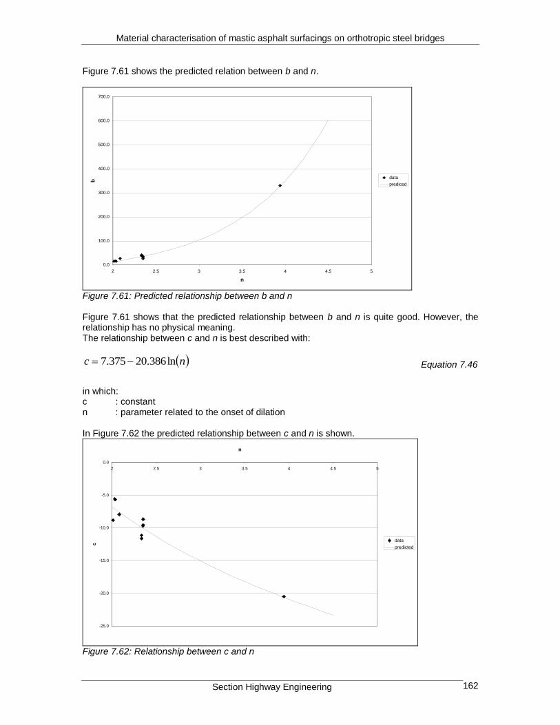
Material characterisation of mastic asphalt surfacings on orthotropic steel bridges
Section Highway Engineering 162
Figure 7.61 shows the predicted relation between b and n.
0.0
100.0
200.0
300.0
400.0
500.0
600.0
700.0
2 2.5 3 3.5 4 4.5 5
n
b
data
prediced
Figure 7.61: Predicted relationship between b and n Figure 7.61 shows that the predicted relationship between b and n is quite good. However, the relationship has no physical meaning. The relationship between c and n is best described with:
nc ln386.20375.7
Equation 7.46
in which: c : constant n : parameter related to the onset of dilation In Figure 7.62 the predicted relationship between c and n is shown.
-25.0
-20.0
-15.0
-10.0
-5.0
0.0
2 2.5 3 3.5 4 4.5 5
n
c
data
predicted
Figure 7.62: Relationship between c and n

Material characterisation of mastic asphalt surfacings on orthotropic steel bridges
Section Highway Engineering 163
It can be noted that the scatter for the equation between c and n is higher than for the equation between b and n. Additional analysis should be carried out to investigate for example a relation between c, strain rate and temperature instead of a straight relation between c and n. Combination of the equations 7.44, 7.45 and 7.46 result in the following relationship between
and n:
ne
n
139.7713.381
ln368.20375.70.1
0
Equation 7.47
in which:
: hardening parameter
0 : the initial value (material parameter) n : parameter related to the onset of dilation
: the equivalent plastic strain The precision of equation 7.47 is analysed in figures 7.63-7.68.
T=278.9K strain rate=0.017 s-1
0
0.1
0.2
0.3
0.4
0.5
0.6
0.7
0.8
0.9
1
0 0.005 0.01 0.015 0.02 0.025 0.03 0.035 0.04
/0 data
predicted
Figure 7.63: Precision of the predicted relationship between /0 and for T=278.9K and =0.017 s-1

Material characterisation of mastic asphalt surfacings on orthotropic steel bridges
Section Highway Engineering 164
T=307.1K strain rate=0.017 s-1
0
0.1
0.2
0.3
0.4
0.5
0.6
0.7
0.8
0.9
1
0 0.05 0.1 0.15 0.2
/
0 data
predicted
Figure 7.64: Precision of the predicted relationship between /0 and for T=307.1K and =0.017 s
-1
T=307.1K strain rate=0.098 s-1
0
0.1
0.2
0.3
0.4
0.5
0.6
0.7
0.8
0.9
1
0 0.02 0.04 0.06 0.08 0.1 0.12 0.14 0.16
0 data
predicted
Figure 7.65: Precision of the predicted relationship between /0 and for T=307.1K and =0.098 s
-1

Material characterisation of mastic asphalt surfacings on orthotropic steel bridges
Section Highway Engineering 165
T=293K strain rate=9.97E-05 s-1
0
0.1
0.2
0.3
0.4
0.5
0.6
0.7
0.8
0.9
1
0 0.02 0.04 0.06 0.08 0.1 0.12 0.14
0 data
predicted
Figure 7.66: Precision of the predicted relationship between /0 and for T=293K and =9.97E-5 s
-1
T=313K strain rate=0.057 s-1
0
0.1
0.2
0.3
0.4
0.5
0.6
0.7
0.8
0.9
1
0 0.05 0.1 0.15 0.2 0.25
0 data
predicted
Figure 7.67: Precision of the predicted relationship between /0 and for T=313K and =0.057 s
-1

Material characterisation of mastic asphalt surfacings on orthotropic steel bridges
Section Highway Engineering 166
T=293K strain rate=0.051 s-1
0
0.1
0.2
0.3
0.4
0.5
0.6
0.7
0.8
0.9
1
0 0.02 0.04 0.06 0.08 0.1 0.12
0 data
predicted
Figure 7.68: Precision of the predicted relationship between /0 and for T=293K and =0.051 s
-1
The prediction is reasonable for figures 7.63, 7.65, 7.66 and 7.68. The prediction in the figures 7.64 and 7.67 is not good. A closer look to these curves shows that both have a different trend in
the relationship between the ratio /0 and . Both curves have a kind of S-shape, whereas the other curves have an exponential shape. These different shapes make the prediction of a relationship difficult. Therefore in paragraph 7.6.5.3 a different approach is used to determine a
function for .
7.6.5.3 Determination of as a function of plastic work
A second way to describe is expressing as a function of plastic work Wp, which is defined as:
pp dW
Equation 7.48
in which: Wp : plastic work
: stress vector
dp : vector of the increment op plastic strain Equation 7.48 shows that Wp is equal to the area under the stress-plastic strain curve. For the
different measurements the relation between /0 and Wp is plotted, as shown in figure 7.69. For
the 5 measurements at T=293K and =0.051 s-1
the average is taken.

Material characterisation of mastic asphalt surfacings on orthotropic steel bridges
Section Highway Engineering 167
0
0.1
0.2
0.3
0.4
0.5
0.6
0.7
0.8
0.9
1
0 0.1 0.2 0.3 0.4 0.5 0.6 0.7
Wp
0
1: T=278.9K strain rate=0.017
2: T=307.1K strain rate=0.017
3: T=307.1K strain rate=0.098
4: T=293K strain rate=9.97E-5
5: T=313K strain rate=0.057
6: T=293K strain rate =0.051
1
6
5
4
3
2
Figure 7.69: Relationship between /0 and the plastic work Wp
In this case all the curves have the same shape, which makes the prediction of a relation easier. Analysis has shown that the curves could not be expressed in the form of a simple exponential
equation. Therefore the following relationship is used to express /0 as a function of Wp.
p
p
bW
cWa
10
Equation 7.49
Table 7.31 shows the parameters that were determined by regression analysis for the different test conditions. Table 7.31: Constants a, b and c for different strain rates and temperatures
strain rate [s-1
] T [K] n a b c
0.0168 278.9 3.942 0.9 34.9 -1.1 0.0170 307.1 2.038 1.0 24.6 -3.2 0.0978 307.1 2.082 1.0 19.9 -2.3 0.0001 293 2.012 1.0 36.1 -7.1 0.0568 313 2.031 1.0 25.0 -3.1 0.0513 293 2.345 1.0 10.2 -1.7
The constant a is chosen to be 1.0 since in that case /0 becomes 0 at Wp=0. For b and c it is
assumed that they are related to the parameter n, just like the parameter in equation 7.43. Next a relationship is determined between b and n. Figure 7.70 shows the relationship between b and n.

Material characterisation of mastic asphalt surfacings on orthotropic steel bridges
Section Highway Engineering 168
0.0
5.0
10.0
15.0
20.0
25.0
30.0
35.0
40.0
45.0
2 2.5 3 3.5 4 4.5 5
n
b
data
predicted
A
Figure 7.70: Predicted relationship between b and n From this figure it becomes clear that point A seems to be an outlier. This point is related to the test at T=278.9K and a strain rate of 0.0168 s
-1. This point also gave problems in determining the
relation for 0 as a function of temperature and strain rate (hardly any hardening). A closer look to figure 7.69 shows that the line for these test conditions is different from the other test conditions, because it crosses the different lines. Because point A seems to be an outlier it is neglected in determining the relationship between b and n. For the model this means that for this condition there is no hardening response. The relationship between b and n becomes:
978.1
419.38
nb
Equation 7.50
Figure 7.70 also shows the predicted relationship between b and n. The same procedure is carried out to determine a relationship between c and n. This relationship is shown in figure 7.71.
-8.0
-7.0
-6.0
-5.0
-4.0
-3.0
-2.0
-1.0
0.0
2 2.5 3 3.5 4 4.5 5
n
c
data
predicted
A
Figure 7.71: Predicted relationship between c and n
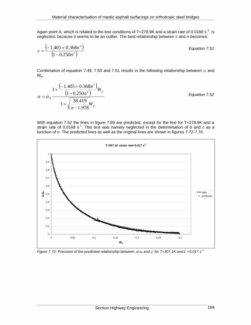
Material characterisation of mastic asphalt surfacings on orthotropic steel bridges
Section Highway Engineering 169
Again point A, which is related to the test conditions of T=278.9K and a strain rate of 0.0168 s-1
, is neglected, because it seems to be an outlier. The best relationship between c and n becomes:
2
2
250.01
368.0405.1
n
nc
Equation 7.51
Combination of equation 7.49, 7.50 and 7.51 results in the following relationship between and Wp:
p
p
Wn
Wn
n
978.1
419.381
250.01
368.0405.11
2
2
0
Equation 7.52
With equation 7.52 the lines in figure 7.69 are predicted, except for the line for T=278.9K and a strain rate of 0.0168 s
-1. This test was namely neglected in the determination of b and c as a
function of n. The predicted lines as well as the original lines are shown in figures 7.72-7.76.
T=307.1K strain rate=0.017 s-1
0
0.1
0.2
0.3
0.4
0.5
0.6
0.7
0.8
0.9
1
0 0.05 0.1 0.15 0.2 0.25 0.3
Wp
0 data
predicted
Figure 7.72: Precision of the predicted relationship between /0 and for T=307.1K and =0.017 s
-1

Material characterisation of mastic asphalt surfacings on orthotropic steel bridges
Section Highway Engineering 170
T=307.1K strain rate=0.098 s-1
0
0.1
0.2
0.3
0.4
0.5
0.6
0.7
0.8
0.9
1
0 0.05 0.1 0.15 0.2 0.25 0.3 0.35 0.4 0.45
Wp
0 data
predicted
Figure 7.73: Precision of the predicted relationship between /0 and for T=307.1K and =0.098 s
-1
T=293K strain rate=9.97E-05 s-1
0
0.1
0.2
0.3
0.4
0.5
0.6
0.7
0.8
0.9
1
0 0.02 0.04 0.06 0.08 0.1 0.12 0.14
Wp
0 data
predicted
Figure 7.74: Precision of the predicted relationship between /0 and for T=293K and =9.97E-5 s
-1

Material characterisation of mastic asphalt surfacings on orthotropic steel bridges
Section Highway Engineering 171
T=313K strain rate=0.057 s-1
0
0.1
0.2
0.3
0.4
0.5
0.6
0.7
0.8
0.9
1
0 0.05 0.1 0.15 0.2 0.25 0.3 0.35
Wp
o data
predicted
Figure 7.75: Precision of the predicted relationship between /0 and for T=313K and =0.057 s
-1
T=293K strain rate=0.051 s-1
0
0.1
0.2
0.3
0.4
0.5
0.6
0.7
0.8
0.9
1
0 0.1 0.2 0.3 0.4 0.5 0.6 0.7
Wp
0 data
predicted
Figure 7.76: Precision of the predicted relationship between /0 and for T=293K and =0.051 s
-1
The prediction of the relationship between /0 and Wp is good in all the figures. However, one has to keep in mind that one measurement has been neglected in the previous analysis.

Material characterisation of mastic asphalt surfacings on orthotropic steel bridges
Section Highway Engineering 172
7.6.6 The influence of the model parameters on the response surface
7.6.6.1 Effect of temperature on the response surface
Two cases have been considered, namely =0 (figure 7.77) and =0 (figure 7.78). The situation
=0 represents the change from linear-elastic to plastic behaviour. Furthermore, =0 figure 7.78 represents the ultimate response surface.
0
5
10
15
20
25
-200 -150 -100 -50 0 50 100I1
SQ
RT
(J2)
T=5oC
T=30oC
T=25oC
T=20oC
Tension stress pathCompression stress path
Figure 7.77: Effect of temperature on the flow-surface for a strain rate of 0.1 s
-1 and =0
The influence of temperature on the linear elastic part becomes clear from figure 7.77. With decreasing temperature the linear-elastic part increases. The straight line for T=5
oC shows that
for low temperatures 0 0, meaning that no hardening occurs. Figure 7.78 shows the flow-
surfaces for different temperatures for =0.

Material characterisation of mastic asphalt surfacings on orthotropic steel bridges
Section Highway Engineering 173
0
2
4
6
8
10
12
14
16
18
20
-40 -30 -20 -10 0 10 20 30 40 50
I1
sq
rt(J
2)
T=0
T=10
T=20
T=30
Tension stress path
Compression stress path
Figure 7.78: Effect of temperature on the flow-surface for a strain rate of 0.1 s
-1 and =0
In figure 7.78 the intersections between both stress paths and the flow surfaces represent the tension and the compression strength for the specific temperature. As expected, both the tension and compression strength increase for decreasing temperature.
7.6.6.2 Effect of strain rate on the response surface
Figure 7.79 shows the influence of the strain rate on the flow-surface for =0 and T=20oC. The
situation =0 represents the change from linear-elastic into plastic behaviour.
0
0.5
1
1.5
2
2.5
3
3.5
4
4.5
5
-70 -60 -50 -40 -30 -20 -10 0 10 20 30
I1
sq
rt(J
2)
0.05 s-1
0.06 s-1
0.07 s-1
0.08 s-1
0.09 s-1
0.10 s-1
Tension stress path
Compression stress path
Figure 7.79: Effect of strain rate on the flow-surface for T=20
oC and =0

Material characterisation of mastic asphalt surfacings on orthotropic steel bridges
Section Highway Engineering 174
By following the stress paths for tension and compression the influence of strain rate becomes clear. An increasing strain rate means an increasing linear-elastic part, as to be expected.
Figure 7.80 shows the influence of the strain rate on the flow surface at T=20oC and =0, i.e. the
influence of the strain rate on the tension and compression strength of the material.
0
1
2
3
4
5
6
-15 -10 -5 0 5 10 15 20 25
I1
sq
rt(J
2)
0.01 s-1
0.02 s-1
0.04 s-1
0.06 s-1
0.08 s-1
0.10 s-1
Tension stress path
Compression stress path
Figure 7.80: Effect of strain rate on the flow-surface for T=20
oC and =0
Again the intersection point between both stress paths and the flow-surfaces represent the tension and the compression strength for the specific strain rate. From figure 7.80 it becomes clear that with increasing strain rate both the tension and compression strength increase.
7.6.6.3 Effect of on the response surface
Finally the effect of on the flow surface is investigated for T=20oC and strain rate of 0.05 s
-1. For
=0.0076, 0.005, 0025 and 0 the flow surfaces are plotted in figure 7.81. The value =0.0076
represents the start of the hardening phase and for =0 the tension and compression strength has been reached.
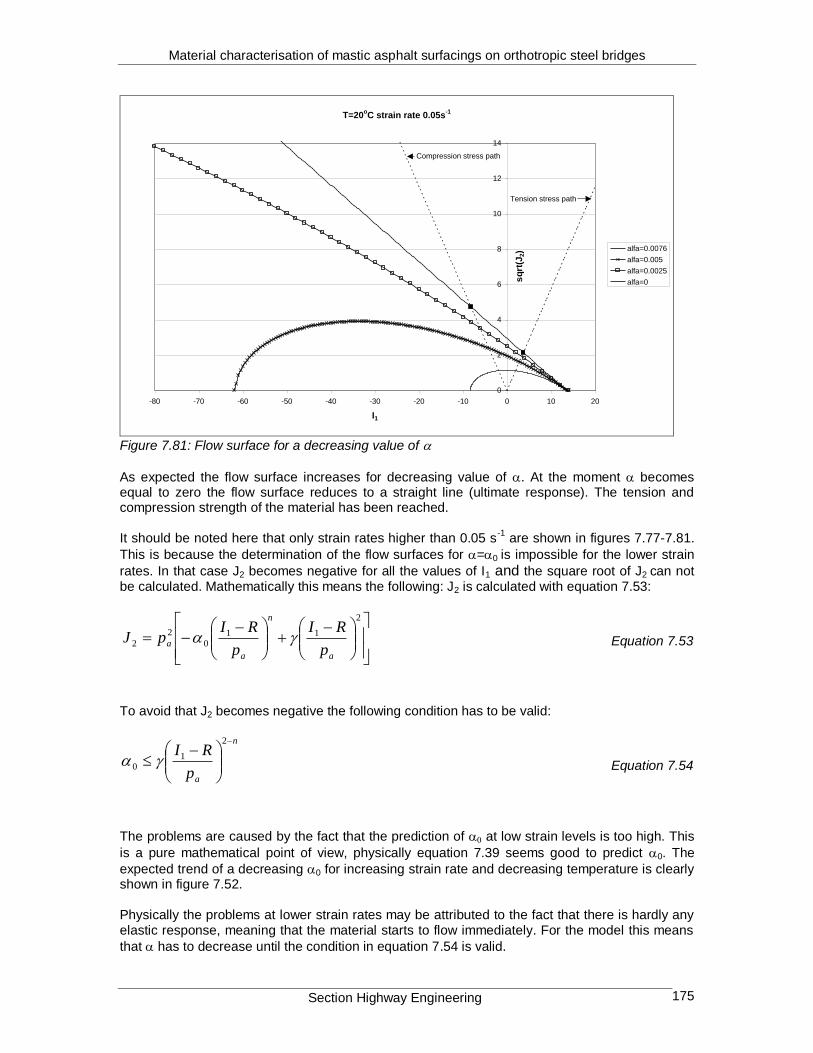
Material characterisation of mastic asphalt surfacings on orthotropic steel bridges
Section Highway Engineering 175
T=20oC strain rate 0.05s
-1
0
2
4
6
8
10
12
14
-80 -70 -60 -50 -40 -30 -20 -10 0 10 20
I1
sq
rt(J
2) alfa=0.0076
alfa=0.005
alfa=0.0025
alfa=0
Tension stress path
Compression stress path
Figure 7.81: Flow surface for a decreasing value of
As expected the flow surface increases for decreasing value of . At the moment becomes equal to zero the flow surface reduces to a straight line (ultimate response). The tension and compression strength of the material has been reached. It should be noted here that only strain rates higher than 0.05 s
-1 are shown in figures 7.77-7.81.
This is because the determination of the flow surfaces for =0 is impossible for the lower strain
rates. In that case J2 becomes negative for all the values of I1 and the square root of J2 can not be calculated. Mathematically this means the following: J2 is calculated with equation 7.53:
2
110
2
2
a
n
a
ap
RI
p
RIpJ
Equation 7.53
To avoid that J2 becomes negative the following condition has to be valid:
n
ap
RI
2
10
Equation 7.54
The problems are caused by the fact that the prediction of at low strain levels is too high. This
is a pure mathematical point of view, physically equation 7.39 seems good to predict 0. The
expected trend of a decreasing 0 for increasing strain rate and decreasing temperature is clearly shown in figure 7.52. Physically the problems at lower strain rates may be attributed to the fact that there is hardly any elastic response, meaning that the material starts to flow immediately. For the model this means
that has to decrease until the condition in equation 7.54 is valid.

Material characterisation of mastic asphalt surfacings on orthotropic steel bridges
Section Highway Engineering 176
8 Case study Moerdijk bridge
8.1 Introduction
The lifetime of mastic asphalt on orthotropic steel bridges is short compared to the lifetime of asphalt mixtures on road pavements. For example the asphalt on the Hagestein bridge had to be replaced after only 5 years, for the Ewijk bridges the lifetime has been even shorter, namely 3 respectively 4 years. On the Moerdijk bridge a new asphalt surface had been applied in June 2000, which contains a new type of SBS modified bitumen. In this case study an attempt is made to predict the lifetime of the Moerdijk mix by using the experimental results described in this report. It has to be noted that several factors influence the lifetime of asphaltic mixes. Some of them are neglected over here because their influence is simply not clear. Also some assumptions were made.
8.2 Traffic loading
For the traffic distribution use is made from measurements carried out on the Moerdijk bridge in 1999. From this traffic distribution the number of 100 kN equivalent axles per year is determined. The following data was used: Estimated total number of truck axles per day: 35000 Working days per year: 275 n (slope of the fatigue line): 6.74 The n-value that is used to calculate the number of 100 kN equivalent axle loads is the real n-value obtained from the fatigue line of the Moerdijk mix for a temperature of 10
oC and a
frequency of 5 Hz. Table 8.1 shows the traffic loading for the Moerdijk bridge, as well as the number of 100 kN equivalent axle loads. Table 8.1: Traffic loading and number of 100kN equivalent axle loads
axle load [kN] percentage [%] axles per day 100 kN equivalent axles per day
10 4.5 1575 0
30 21.01 7354 2
50 29.58 10353 97
70 27.07 9475 857
90 10.92 3822 1880
110 5.24 1834 3485
130 1.44 504 2951
150 0.22 77 1182
170 0.02 7 250
Number of 100 kN equivalent axles per day: 10704
Number of 100 kN equivalent axles per year: 2943706 Combining this information with the experimental fatigue relation results in a prediction for the fatigue lifetime. However, this lifetime is the experimental lifetime and the lifetime in practice is longer due to healing of the asphalt and lateral wandering of the traffic. The lifetime in practice is calculated with:
LWHNN erimentalfield exp Equation 8.1

Material characterisation of mastic asphalt surfacings on orthotropic steel bridges
Section Highway Engineering 177
in which: Nfield : Predicted number of load repetitions in practice. Nexperimental : Predicted number of load repetitions from the fatigue relation. H : Healing factor. LW : Factor for lateral wandering of the traffic.
8.3 Healing
Healing can be defined as the self-restoring capacity of the mix. This means that a mix can sustain more load repetitions if rest periods are introduced during cyclic loading. Healing is highly dependent on the bitumen content of a mix, the degree of filling and the hardness of the bitumen. An increasing bitumen content tends to increase the healing capacity of the mix. The Dutch Ministry of Transport, Public Works and Water Management uses a healing factor of 4 for standard asphalt concrete mixes in fatigue lifetime predictions. Molenaar [1993] developed a relationship between the bitumen content, void content and the healing factor, shown in figure 8.1.
Figure 8.1: Relation between bitumen content an the healing factor With a bitumen content of 18.5% by volume and a void content of 2% the healing factor is approximately 20, which is 5 times the healing factor that the Dutch Ministry of Transport, Public Works and Water Management uses. This high healing factor is to be expected for mastic asphalt since the bitumen content is very high compared to other types of asphalt mixes. Also during the experimental program that was carried out, the effect of healing has been observed. After a rest period of 2.5 months the stiffness of the tested specimens has increased again to values approaching the original stiffness values. The increase of the stiffness can be attributed to the healing capacity of the mix.

Material characterisation of mastic asphalt surfacings on orthotropic steel bridges
Section Highway Engineering 178
8.4 Lateral wander
In practice not all the wheels will pass exactly at the same lateral position. Instead the wheel positions of vehicles will be transversely distributed over the pavement, which is called ‘lateral wander’. The factor for traffic wander is highly dependent on the width of the traffic lane. For traffic lanes of 3.6 m, a lateral wander factor of 2.5 is proposed by the Dutch Ministry of Transport, Public Works and Water Management. On an orthotropic bridge this factor might be different, since the pavement structure on a subgrade is essentially different from that on an orthotropic bridge, which leads to different strain conditions in the pavement. To investigate the lateral wander factor on an orthotropic bridge a 10-span beam model was used (figure 8.2).
0.3 m
0.3 m
1 2 3 54 6 7 8 9 10 11
Figure 8.2: Beam model to investigate the effect of traffic wander Each span of the beam is 0.3 m, which corresponds to the width of the stiffener and also the distance between the troughs. The width of the beam is taken as 0.1 mm. The structure consists of a 10 mm steel plate and a 50 mm thick asphalt layer on top. The dual tyre wheel is schematised as two line loads of 0.7 N/mm/mm, with a length of 190 mm. This corresponds to an axle load of 100 kN.
For the traffic wander a Gaussian distribution is used with =0.29 m. The distribution is truncated at 0.80 m on either side of the centre line, which results in a trafficked width of 1.60 m. This traffic loading was also used for the Lintrack control program [Groenendijk, 1998]. Figure 8.3 shows the traffic distribution when the Gaussian distribution is divided in steps of 0.1 m.

Material characterisation of mastic asphalt surfacings on orthotropic steel bridges
Section Highway Engineering 179
0
2
4
6
8
10
12
14
16
-0.8 -0.7 -0.6 -0.5 -0.4 -0.3 -0.2 -0.1 0 0.1 0.2 0.3 0.4 0.5 0.6 0.7 0.8
x-position [m]
pe
rce
nta
ge
[%
]
Figure 8.3: Traffic distribution for the investigation of lateral wander The average position of the centre of the dual tyre wheel is chosen to be above support number 6. Next the effect of shifting the centre of the dual tyre load on the bending moment above support 6 is determined by using Metcalf’s linear-elastic theory (see paragraph 3.3.2.1). Therefore the load is shifted in steps of 0.1 m to both the left and the right side of support 6, with a maximum of 0.8 m. Figure 8.4 shows the relation between the position of the centre of the dual tyre wheel and the bending moment at support 6 for an axle load of 100 kN.
-1000
0
1000
2000
3000
4000
5000
6000
-0.9 -0.8 -0.7 -0.6 -0.5 -0.4 -0.3 -0.2 -0.1 0 0.1 0.2 0.3 0.4 0.5 0.6 0.7 0.8 0.9
Position centre of double-tired wheel in relation to support 6 [m]
Be
nd
ing
mo
me
nt
su
pp
ort
6 [
Nm
m]
support 6
Figure 8.4: Bending moment at support 6 in relation to the position of the dual tyre wheel This figure clearly shows that by shifting the load the bending moment above support 6 increases. When the dual tyre wheel is shifted over a distance of ≈0.5-0.8 m the bending moment becomes negative, meaning a compression strain at the top of the asphalt above support 6.

Material characterisation of mastic asphalt surfacings on orthotropic steel bridges
Section Highway Engineering 180
The positive effect of traffic wander on the fatigue life is shown in table 8.2, in which the factor for lateral wander is calculated. This lateral wander factor is dependent on the slope of the fatigue relation, thus in this case the factor is valid for a temperature of 10
oC and a frequency of 5 Hz.
The factor will decrease for increasing temperatures. When use is made of the n-value of 4 proposed by Rijkswaterstaat the factor LW decreases to 5.4. Table 8.2: Calculation of the factor for lateral wander for T=10
oC and f=5 Hz
Bending moment 100kN
distance to supp. 6 traffic [%] support 6 [Nmm] axle load supp. 6 [kN] axles [-]
-0.8 0.3 77 1.41 1.10E-15
-0.7 0.8 -229 - -
-0.6 1.7 -537 - -
-0.5 3.2 -288 - -
-0.4 5.4 854 15.59 1.97E-07
-0.3 8.1 2005 36.61 9.28E-05
-0.2 10.8 1908 34.83 8.84E-05
-0.1 12.8 3468 63.30 5.89E-03
0 13.7 5478 100.00 1.37E-01
0.1 12.8 3468 63.30 5.89E-03
0.2 10.8 1908 34.83 8.84E-05
0.3 8.1 2005 36.61 9.28E-05
0.4 5.4 854 15.59 1.97E-07
0.5 3.2 -288 - -
0.6 1.7 -537 - -
0.7 0.8 -229 - -
0.8 0.3 77 1.41 1.10E-15
wander effect: 0.14953
LW: 6.7 It has to be noted that is assumed that 100% of the axles consist of dual tyre wheels and that the average position of the centre of the dual tyre wheel is exactly above a support.
8.5 Shifting the traffic lanes
In the previous sections it has been shown that both healing and lateral wander play an important role in increasing the lifespan of mastic asphalt. Both effects may be increasing when the traffic lanes are shifted on the bridge for a certain period during a year. When the traffic lanes are shifted in the right way this will lead to release of strains. It will also result in extra rest periods for the heaviest loaded part, which results in better healing of the asphalt. Specially on bridges with heavy traffic this may play an important role, since in that case very little rest periods are available to heal the material. To estimate a reasonable shift distance for the traffic lanes the total width of a bridge is considered. The most critical part is the right lane, which is used by most of the heavy trucks. Switching the left and the right lanes might be an option, however, this might lead to chaotic situations for the traffic that has to change lanes before and after the bridge. A better shift distance is obtained when use is made of figure 8.4, which shows the effect of shifting a dual tyre wheel. Shifting this dual tyre wheel over more than 1.0 m is not useful, since in that case the second dual tyre wheel on the axle starts to load the asphalt above support 6. Reckoning with this fact, figure 8.4 shows that the best distance to shift the lane lies between 0.5 and 1.0 m, since in that case a large part of the load causes a negative or very small bending

Material characterisation of mastic asphalt surfacings on orthotropic steel bridges
Section Highway Engineering 181
moment above support 6. From figure 8.5 it becomes clear that the best distance to shift the traffic lane is 1.0 m.
-1000
0
1000
2000
3000
4000
5000
6000
-1.8 -1.6 -1.4 -1.2 -1 -0.8 -0.6 -0.4 -0.2 0 0.2 0.4 0.6 0.8 1 1.2 1.4 1.6
Distance between centre load and support 6 [m]
Be
nd
ing
mo
me
nt
[Nm
m]
traffic distribution
bending moment above support 6
96%
Figure 8.5: The effect of shifting the traffic lane over 1.0 m. In that case the largest percentage (96%) of the traffic distribution (figure 8.3) causes a compressive or negligible tensile strain above support 6. This means that due to the shift of the lane over 1.0 m the asphalt above the critical point is hardly loaded for a certain time, which has two supplementary effects. Firstly, the total number of load repetitions will increase because the critical point (above support 6) is less loaded. Secondly, the material will have some time to heal, which has also a positive effect on increasing the total number of load repetitions to failure. The application of shifting traffic depends of coarse on the geometry of the bridge.
8.6 Prediction of the fatigue lifetime by neglecting the strain dependency of the mix stiffness
8.6.1 Prediction of the fatigue lifetime for the Moerdijk mix using common method for T=10oC and f=5 Hz
In this section the lifetime is predicted in a way that is commonly used for road engineering. For this procedure the experimental fatigue line as well as Metcalf’s theory were used. Three following phenomena were neglected:
Strain dependent behaviour of the mix stiffness.
Temperature distribution during the year. In this case Metcalf’s composite action theory was used and the following assumptions were made:
100% bonding between the steel and the asphalt.
Linear-elastic relation between load and strain.

Material characterisation of mastic asphalt surfacings on orthotropic steel bridges
Section Highway Engineering 182
For the calculation of the bending moment the same 10-span beam that has been used for calculation of the lateral wander (figure 8.2) was used. By using that model the bending moment above the middle support due to an axle load of 100 kN is 5478 Nmm. This bending moment is overestimated because the beam-theory is assumed, while in reality plate-theory is more applicable. It is assumed that the bending moment by using plate theory is approximately 70% of the bending moment that is determined with beam theory. Taking this into account results in a bending moment of 3835 Nmm. Normally the strain dependent behaviour of the mix stiffness is neglected. In that case the stiffness is determined by using the master curve at a low strain level,
say 80 m/m. For T=10oC and f=5 Hz the stiffness of the Moerdijk mix is 5500 MPa. Metcalf’s
theory was used to determine the corresponding strain, by assuming an asphalt thickness of 50
mm and a steel plate of 10 mm. In this case the strain is 673 m/m and the corresponding number of load repetitions is 71240 (see figure 8.6).
10oC, 5 Hz
1000
10000
100000
1000000
10000000
100 1000 10000
Strain [m/m]
Lo
ad
re
pe
titi
on
s [
-]
Figure 8.6: Determination of the number of load repetitions using the common method To obtain the anticipated number of load repetitions in practice and the predicted fatigue lifetime, the experimental number is multiplied by different factors for healing and lateral wander (table 8.3). Table 8.3: Determination of the fatigue lifetime for different healing and wander factors
Nexperimental H LW Nfield Lifetime [years]
71240 4 2.5 712400 0.2 71240 20 2.5 3562000 1.2 71240 4 6.7 1909232 0.6 71240 20 6.7 9546160 3.2
Table 8.3 shows that the predicted fatigue lifetime varies between 0.2 and 3.2 years. In reality the fatigue life time of mastic asphalt on orthotropic steel bridges varies between 3 and 5 years. This means that only the prediction of 3.2 years seems to be reasonable. However, the following has to be noted for the previous fatigue lifetime prediction. The calculation is based on a temperature of 10
oC and a loading frequency of 5 Hz. These are not representative values since the average
asphalt temperature in the Netherlands is approximately 20oC and a reasonable loading

Material characterisation of mastic asphalt surfacings on orthotropic steel bridges
Section Highway Engineering 183
frequency is 50 Hz (0.02 s). An increasing temperature decreases the asphalt stiffness, increases the strains and results in a shorter fatigue lifetime. A higher temperature also causes a lower value for the lateral wander factor, which also results in a shorter fatigue lifetime. Another phenomenon that was neglected in the fatigue lifetime prediction is the variation in stiffness for the different fatigue measurements. By using the fatigue line in figure 8.6 it is assumed that the stiffness is constant for a temperature of 10
oC and a frequency of 5 Hz irrespective of the strain
level. This is certainly not the case, since the 4-point bending tests on the Lintrack mix showed a decreasing stiffness for increasing strain levels (paragraph 7.3.7). In paragraph 8.6.2 a fatigue lifetime prediction is done by using a more reasonable temperature and loading time. Also the variation of the stiffness is included.
8.6.2 Prediction of the fatigue lifetime for the Moerdijk mix using common method for T=20oC and f=50 Hz
In this paragraph the fatigue lifetime is predicted using figure 7.8 and equation 7.8. This means that also the stiffness is included in the fatigue lifetime prediction. The calculation of the strains is the same as in the previous section. Only the temperature of 20
oC and loading time of 0.02 s (50
Hz) were chosen. It is assumed that figure 7.8 and equation 7.8 (in which the stiffness is included) are valid under these conditions, in spite of the fact that they are based on measurements at 10
oC and 5 Hz.
In practice, normally the variation of the mix stiffness with strain level is neglected and the mix
stiffness is determined at a low strain level, say 80 m/m. In this case the stiffness is 4404 MPa, which is determined by using equation 7.1 and table 7.2. For the calculation of the strains Metcalf’s method is used by using the same conditions as in the previous section. For an asphalt
stiffness of 4404 MPa the strain in the asphalt is 824 m/m. With the fatigue relationship (equation 7.8) of the Moerdijk mix the number of load repetitions becomes12168. This value is the experimental number of load repetitions. Table 8.4 shows the calculation of the expected number of load repetitions for the different healing and traffic wander factors. The lifetime in years is predicted by using the traffic on the Moerdijk bridge, i.e. 2943706 100 kN axles per year. It should be noted that the calculation of this number is based on a temperature of 10
oC
and a frequency of 5 Hz. Table 8.4: Determination of the fatigue lifetime for different healing and wander factors
Nexperimental H LW Nfield Lifetime [years]
12168 4 2.5 121680 0.0 12168 20 2.5 608400 0.2 12168 4 6.7 326102 0.1 12168 20 6.7 1630512 0.6
Table 8.4 shows that the predicted lifetime varies between 0.0 and 0.6 years. This example indicates that the normal procedure to predict the fatigue lifetime seems not to be valid for mastic asphalt on orthotropic steel bridges, since in practice the fatigue lifetime of mastic asphalt varies between 3 and 5 years. However, in the previous prediction the stiffness is calculated by using
the master curve at a strain level of 80 m/m and next the asphalt strain is determined by using this mix stiffness. This is only possible when the stiffness doesn’t vary with strain level. However, in paragraph 7.3.7 it is shown that the stiffness varies with strain level. The procedure followed in paragraph 8.6.1 is carried out for the mixes tested by Kolstein, to investigate the lifetime prediction for these mixes.
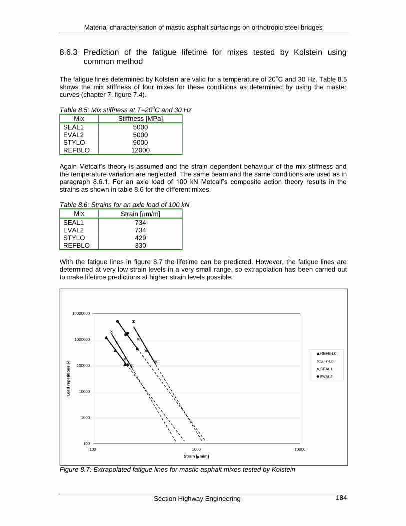
Material characterisation of mastic asphalt surfacings on orthotropic steel bridges
Section Highway Engineering 184
8.6.3 Prediction of the fatigue lifetime for mixes tested by Kolstein using common method
The fatigue lines determined by Kolstein are valid for a temperature of 20
oC and 30 Hz. Table 8.5
shows the mix stiffness of four mixes for these conditions as determined by using the master curves (chapter 7, figure 7.4). Table 8.5: Mix stiffness at T=20
oC and 30 Hz
Mix Stiffness [MPa]
SEAL1 5000 EVAL2 5000 STYLO 9000 REFBLO 12000
Again Metcalf’s theory is assumed and the strain dependent behaviour of the mix stiffness and the temperature variation are neglected. The same beam and the same conditions are used as in paragraph 8.6.1. For an axle load of 100 kN Metcalf’s composite action theory results in the strains as shown in table 8.6 for the different mixes. Table 8.6: Strains for an axle load of 100 kN
Mix Strain [m/m]
SEAL1 734 EVAL2 734 STYLO 429 REFBLO 330
With the fatigue lines in figure 8.7 the lifetime can be predicted. However, the fatigue lines are determined at very low strain levels in a very small range, so extrapolation has been carried out to make lifetime predictions at higher strain levels possible.
100
1000
10000
100000
1000000
10000000
100 1000 10000
Strain [m/m]
Lo
ad
re
pe
titi
on
s [
-]
REFB-L0
STY-L0
SEAL1
EVAL2
Figure 8.7: Extrapolated fatigue lines for mastic asphalt mixes tested by Kolstein

Material characterisation of mastic asphalt surfacings on orthotropic steel bridges
Section Highway Engineering 185
After extrapolation the lifetime is predicted for different healing and wander factors as shown in table 8.7. Table 8.7: Lifetime prediction for mixes tested by Kolstein
Mix Nexperimental H LW Nfield Lifetime [years]
SEAL1 2139 4 2.5 21390 0.0 2139 20 2.5 106950 0.0 2139 4 6.7 57325.2 0.0 2139 20 6.7 286626 0.1
EVAL2 1696 4 2.5 16960 0.0 1696 20 2.5 84800 0.0 1696 4 6.7 45452.8 0.0 1696 20 6.7 227264 0.1
STYLO 1747 4 2.5 17470 0.0 1747 20 2.5 87350 0.0 1747 4 6.7 46819.6 0.0 1747 20 6.7 234098 0.1
REFBLO 10128 4 2.5 101280 0.0 10128 20 2.5 506400 0.2 10128 4 6.7 271430.4 0.1 10128 20 6.7 1357152 0.5
It can be seen that the estimated lifetime lies between 0 and 0.5 years. This may be attributed to the fact that the common procedure seems not to be valid to predict the lifetime of mastic asphalt on orthotropic steel bridges. However, also in this example assumptions have been made, which could have effected the results. Also the fact that the fatigue lines have been extrapolated could heave effect on the results.
8.7 A proposed procedure for estimating the fatigue lifetime
8.7.1 Definition of the procedure
The procedure normally adopted in road engineering for estimating the lifespan of asphaltic pavements neglect the dependency of stiffness on strain. Due to the high strain levels encountered at the surfacing of orthotropic steel bridges it is thought that a procedure which takes into account this dependency is needed. This procedure will be combined with equation 7.8 in chapter 7 that describes the fatigue life as a function of strain as well as the stiffness. The determination of the stiffness and the strain requires actually a complex procedure since they are dependent on each other; the stiffness is required to calculate the asphalt strain, while the stiffness is in turn dependent on the strain. This non-linearity necessitates the use of a complex model to calculate the asphalt strains as a result of a certain applied load on orthotropic steel bridges. For such a complex model the use of a finite element program is inevitable. However, in this case linear behaviour is assumed, in order to use a simple linear-elastic theory to determine the asphalt strains. The use of such a theory requires an iteration procedure, which is described by a flow chart in figure 8.8:

Material characterisation of mastic asphalt surfacings on orthotropic steel bridges
Section Highway Engineering 186
Figure 8.8: Flow chart for determining the fatigue life When the strain is known, the fatigue life can be determined by using the design nomographs in appendix D.
8.7.2 Estimating the fatigue life using a simple beam model and a constant temperature of 20oC
In the following steps the procedure is carried out for the Moerdijk mix: 1. A loading time of 0.02 s is chosen, which corresponds to a speed of 54 km/h. 2. A temperature of 20
oC is chosen, since this is close to the average asphalt temperature in the
Netherlands. 3. For the calculation of the asphalt strains Metcalf’s theory was used. An axle load of 100 kN is
assumed. The bending moment is determined with the 10-span beam shown in figure 8.2. The bending moment is 3835 Nmm. After iteration the estimated stiffness is 2516 MPa and
the strain level 1358 m/m. 4. With equation 7.8 the number of load repetitions is 951. The lifetime after multiplication with the factors for healing and traffic wander is shown in table 8.8. Table 8.8: Predicted fatigue lifetime for the Moerdijk mix
Nexperimental H LW Nfield Lifetime [years]
951 4 2.5 9510 0.0 951 20 2.5 47550 0.0 951 4 6.7 25486.8 0.0 951 20 6.7 127434 0.0
Determine the loading time of interest
Determine the temperature of interest
Assume an asphalt strain
Calculate the mix stiffness with Smix(, t, T) [Equation 7.24]
Use a linear elastic theory to calculate the strain due to a certain load
Is the calculated strain equal to the assumed strain?
Determine the fatigue life with equation 7.8
Use the calculated strain as new input
no
yes
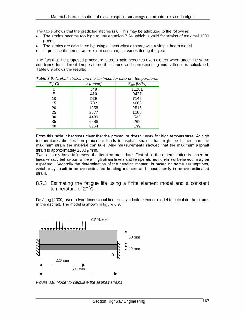
Material characterisation of mastic asphalt surfacings on orthotropic steel bridges
Section Highway Engineering 187
The table shows that the predicted lifetime is 0. This may be attributed to the following:
The strains become too high to use equation 7.24, which is valid for strains of maximal 1000
m/m.
The strains are calculated by using a linear-elastic theory with a simple beam model.
In practice the temperature is not constant, but varies during the year. The fact that the proposed procedure is too simple becomes even clearer when under the same conditions for different temperatures the strains and corresponding mix stiffness is calculated. Table 8.9 shows the results: Table 8.9: Asphalt strains and mix stiffness for different temperatures
T [oC] [m/m] Smix [MPa]
0 349 11261 5 410 9437
10 529 7148 15 782 4663 20 1358 2516 25 2577 1165 30 4489 532 35 6586 262 40 8364 139
From this table it becomes clear that the procedure doesn’t work for high temperatures. At high temperatures the iteration procedure leads to asphalt strains that might be higher than the maximum strain the material can take. Also measurements showed that the maximum asphalt
strain is approximately 1300 m/m. Two facts my have influenced the iteration procedure. First of all the determination is based on linear-elastic behaviour, while at high strain levels and temperatures non-linear behaviour may be expected. Secondly the determination of the bending moment is based on some assumptions, which may result in an overestimated bending moment and subsequently in an overestimated strain.
8.7.3 Estimating the fatigue life using a finite element model and a constant temperature of 20oC
De Jong [2000] used a two-dimensional linear-elastic finite element model to calculate the strains in the asphalt. The model is shown in figure 8.9.
50 mm
12 mm
300 mm
220 mm
0.5 N/mm2
A
Figure 8.9: Model to calculate the asphalt strains

Material characterisation of mastic asphalt surfacings on orthotropic steel bridges
Section Highway Engineering 188
The model consists of a beam that is clamped at both the left and the right side. A wheel load of 35 kN was assumed, acting on an area of 220x320 mm at the left side of the beam. This results in a uniform pressure of 0.5 N/mm
2. This load combination leads to a maximum asphalt strain at
clamp A. The thickness of the asphalt is 50 mm and the thickness of the steel plate is 12 mm. For calculations 100% bond (no slip) between the asphalt and the steel is assumed. Using this model the relationship between the strain and mix stiffness is obtained as shown in figure 8.10.
100
1000
10000
10 100 1000 10000 100000
Smix [MPa]
[
m/m
]
Figure 8.10: Relationship between Smix and as a result of finite element calculations This relationship is described best with the following equation:
7156.0186192
mixS
Equation 8.2
For T=20
oC and a loading time of 0.02 s the combination of the strain dependent mix stiffness
with equation 8.2 results after iteration in an asphalt strain of 596 m/m and an asphalt stiffness of 3065 MPa. By using equation 7.8 the number of load repetitions becomes 288475. Table 8.10 shows the number of load repetitions for different factors of traffic wander and healing. Table 8.10: Predicted fatigue lifetime for the Moerdijk mix
Nexperimental H LW Nfield Lifetime [years]
288475 4 2.5 2884750 1.0 288475 20 2.5 14423750 4.9 288475 4 6.7 7731130 2.6 288475 20 6.7 38655650 13.1
From this table it becomes clear that the predicted fatigue lifetime varies between 1.0 and 13.1 years. These values are more reasonable than the previous predictions, although the fatigue lifetime of 13.1 years seems far too high, compared to the findings in practice. However, to compare these lifetimes with the ones determined in previous sections, one should be aware of the fact that for these calculations different models were used.

Material characterisation of mastic asphalt surfacings on orthotropic steel bridges
Section Highway Engineering 189
8.7.4 Estimating the fatigue life using a finite element model and variable temperature
The same two-dimensional finite element model is used to calculate the strains in the asphalt. Table 8.11 shows the results for different temperatures in the range of 0 to 40
oC after iteration.
Table 8.11: Asphalt strains and mix stiffness for different temperatures
T [oC] [m/m] Smix [MPa]
0 231 11525 5 259 9815
10 310 7652 15 405 5259 20 596 3065 25 992 1503 30 1786 661 35 3193 293 40 5342 143
From this table it is clear that using a finite element model gives less conservative estimate of the fatigue life than the beam model. However, for higher temperatures (>35
oC) the calculated strains
become too large. This may be attributed to the fact that at these temperatures and strains the material behaves no longer linear-elastic. This requires the use of a non-linear material model. Also a beam model was used instead of a plate model.
8.8 Conclusion
From the previous case study it becomes clear that the normal procedure used in road engineering to estimate the fatigue lifetime seems not to be applicable for mastic asphalt on orthotropic steel bridges. That is because the predicted lifetime is underestimated compared to the findings in practice. An attempt has been made to make a more reasonable lifetime prediction by using an iterative procedure that uses the strain dependent behaviour of the mix stiffness and a reasonable temperature distribution. For this procedure use is made of the linear-elastic theory of Metcalf. This procedure still gives a too short estimate of the lifetime. However, the procedure itself is better than the normal procedure because it describes the real asphalt behaviour in a better way and uses a reasonable temperature distribution. The reason that the predicted lifetime is still underestimated may be attributed to the fact that:
for the calculation of the bending moment a simplified model has been used, which may lead to an overestimated bending moment.
linear-elastic behaviour has been assumed in calculation of the strains, while at high temperatures and high strain levels non-linear behaviour should be expected.
Some preliminary calculations showed indeed that a more reasonable lifetime is predicted when use is made of a finite element model to calculate the bending moment and the asphalt strains. However, further calculations are needed with a non-linear model to deal with higher strain levels and temperatures.

Material characterisation of mastic asphalt surfacings on orthotropic steel bridges
Section Highway Engineering 190
9 CONCLUSIONS AND RECOMMENDATIONS
9.1 Conclusions
This report describes the material characterisation of a typical mastic asphalt mix that is used for surfacing orthotropic steel bridges. These types of bridges consist of a steel deck plate supported into two perpendicular directions, which results in different elastic properties of the deck in the two orthogonal directions. Normally, the steel decks are surfaced with asphalt, which has four main objectives:
To provide a running surface with suitable skid resistance.
To provide a flat running surface to compensate for the rough surface of the steel plate.
To protect the deck plate with a waterproofing layer.
To reduce the stresses in the steel deck plate.
To fulfil these objectives the asphalt surfacing can be divided in four functional layers:
Bonding layer to ensure sufficient adhesion between the steel plate and the isolation layer.
Isolation layer to protect the underlying steel deck against corrosion.
Adhesion layer to ensure the adhesion between the isolation layer and the wearing coarse.
Wearing coarse to take and transfer the loading from traffic to the underlying structure.
The deformation of the steel deck and the asphalt on orthotropic steel bridges are larger than the deformations of normal pavements on a basecoarse and a subgrade. Due to this large deformations a flexible type of asphalt is needed for deck surfacing. Mastic asphalt fulfils this requirement. The main properties of mastic asphalt are:
The voids are overfilled with mastic.
The asphalt is not compacted.
The stability is obtained from a stiff, often modified, type of bitumen.
The production and processing take place at relative high temperatures (220-240oC).
The thickness of the asphalt layers varies between 20 mm and 50 mm.
The requirements for mastic asphalt are different in different countries. The requirements in the Netherlands are:
The maximum aggregate size is 8 mm.
The maximum void ratio is 2.5%.
Penetration 10-40 (*0.1 mm) with the stempel test (300 sec, 5.25 N/mm2, 100 mm
2, 25ºC).
Deformation of 6-10% after 100.000 load repetitions in the wheel track test.
In practice composite action theories are used to calculate stresses and strains that occur in the mastic asphalt due to bending moment produced by loading. They are based on one of both of the following assumptions:
Linear strain distribution in the asphalt and the steel.
The slopes of the strain distribution through the depth of the asphalt and the steel are equal. From the comparison between the composite action theories from Metcalf, Kolstein, Cullimore, Nakanishi and Sedlacek/Bild the following can be concluded:
The maximum asphalt strains for a low bonding stiffness between steel and asphalt are
≈1300 m/m which is 10 times higher than the strains in normal pavements on a subgrade.
For these high strain levels linear elastic behaviour of the asphalt, which is currently assumed, is doubtful.
The strains/stresses in the steel/asphalt are calculated using a beam model. However, plate theory may be more applicable.
According to Nakanishi’s theory the asphalt strains at ±15% bonding are higher than the strains at 0% bonding.

Material characterisation of mastic asphalt surfacings on orthotropic steel bridges
Section Highway Engineering 191
For certain conditions the presented theories might be true, but these conditions might not be representative for the real structure.
For extreme values of the bond (0% and 100% bonding) the theories give the same results, but for values of the bond stiffness between both extremes the theories give different results.
From a dynamic analysis the following can be concluded:
Vibration of the deck could lead to increasing strains in the pavement due to an increasing impact of the dynamic axle loads compared to pavements on a subgrade, because of the interaction between the bridge deck and the vehicle.
Vibration of the deck could lead to a faster alternation between tensile and compressive strains in the pavement compared to pavements on a subgrade. This alternation might have influence on the fatigue behaviour.
On orthotropic steel bridges problems, like rutting and fatigue cracking, arise in a relative early stage of lifetime, which results in an asphalt lifetime of only 3-5 years. Therefore, a better understanding of the mastic asphalt behaviour is needed. For that purpose the following experimental program has been carried out on the mastic asphalt that was placed on the Moerdijk bridge in June 2000: 1. Determination of the relationship between the mix stiffness, loading time and temperature
(master curves) for temperatures between 5oC and 30
oC and loading times between 0.1 and
2 s. Comparison of the mix stiffness of the Moerdijk mix with some other types of modified mastic asphalt mixes showed that the master curves are more or less comparable. After 2.5 months the master curves for the Moerdijk mix were determined again by using the specimen that were tested before in the fatigue test. The stiffness of this repeated testing is comparable to that of the first measurements, which can be attributed to the fact that the material has a very good healing capacity.
2. Comparison of the fatigue characteristics for the Moerdijk mix with some other types of modified mastic asphalt mixes showed that the Moerdijk mix has rather good fatigue characteristics. The determination of the fatigue characteristics has been repeated after 2.5 months, which showed a similar fatigue line, which gives indication of the healing capacity of the mix.
3. It has been noticed that the stiffness of mastic asphalt is not only a function of loading time and temperature, but also of the strain level. This indicates non-linear elastic behaviour of mastic asphalt. Therefore a relationship is determined for the mix stiffness as a function of loading time, temperature and strain level. This relationship is valid for temperatures between 0 and 45
oC, loading times between 0.01 and 1 s. and strain levels between 80 and
1000 m/m. The mix stiffness decreases with increasing strain level. When the strain
dependency is neglected and for determination of the stiffness a strain level of 80 m/m is used (which is representative for normal pavements) the maximum overestimation of the
stiffness is 5 times for 45oC, t=1.0 s. and a strain level of 1000 m/m. For road engineering
often the strain dependency is neglected. This results in an overestimated asphalt stiffness and an underestimated asphalt strain. When this asphalt strain is used for determination of the fatigue life this lifetime will be overestimated. Therefore the strain dependency can not be neglected.
4. Determination of the parameters of the ACRe material model by carrying out uniaxial monotonic tension and compression tests. The following can be concluded:
Both tension and compression strength increase with decreasing temperature and increasing strain rate.
No relationship was found for the stress at the start of plasticity as a function of strain
rate and temperature. Instead a function of 0 as a function of strain rate and temperature is determined, from which the stress at the start of plasticity can be obtained indirectly.
For high strain rates and low temperatures a cut-off value for parameter n is used of 10
and is set to zero. This means that under these conditions no hardening occurs.

Material characterisation of mastic asphalt surfacings on orthotropic steel bridges
Section Highway Engineering 192
It was not possible to determine the hardening parameter as a function of equivalent plastic strain.
The hardening parameter is expressed as a function of equivalent plastic work.
For strain rates lower than 0.05 s-1
the flow surface can not be determined.
Mathematically this is a result of the fact that the determination of 0 is too high for low strain levels. Physically this might be attributed to the fact that in that case there is hardly any elastic response, meaning that the material starts to flow immediately.
From a case study for the Moerdijk bridge the following can be concluded:
Shifting the traffic lanes over a distance of 1.0 m during a certain period of the year on a bridge has two positive effects: 1. The repetition of strains at a certain point of the structure decreases, because the shift of
the traffic lane leads to less deformation at the specific point. 2. Because mastic asphalt has excellent healing properties the material can heal during the
period that the lanes are shifted. Both effects lead to an increased lifetime of the asphalt mix.
The procedure normally adopted in road engineering practice to estimate the fatigue lifetime seems not to be applicable for mastic asphalt surfacings on orthotropic steel bridges.
9.2 Recommendations
The comparison of the composite action theories gives approximately the same strains for full and no adhesion between the steel and the asphalt. For values of the bond stiffness between these extreme values, which is the case in practice, the theories give different results. Because the bond stiffness is highly related to the degradation of the asphalt more research has to be carried out on the behaviour of the bonding layer between the asphalt and the steel. For this research shear tests on the bonding layer are recommended. Further the composite action theories might be true for certain conditions, but these conditions might not be representative for the real structure. To calculate the representative asphalt strains in a better way, a representative part of the structure has to be analysed and plastic behaviour of the asphalt has to be included. For the determination of the dynamic axle loads on orthotropic steel bridges use has been made of simple models. These simple models showed that the axle loads might increase on orthotropic steel bridges due to interaction between vehicle and bridge deck. More research is recommended, by using more complex dynamic models to investigate the effect of dynamic axle loads on orthotropic steel bridges. The relationship describing the strain dependent behaviour of the mix stiffness is valid for the Lintrack mix only. More four-point bending tests on mastic asphalt at different strain levels have to be carried out to determine the strain dependent behaviour of the other mastic asphalt mixes in
general. The relationship that was determined is valid for maximum strain levels of 1000 m/m,
while in practice maximal strain levels of 1300 m/m were measured. Further research at these high strain levels is recommended to increase the validity of the relationship for the mix stiffness as a function of the strain level. By using a simple beam model it has been shown that shifting the traffic lanes over a distance of 1.0 m, during a certain period of the year has positive effects on the fatigue lifetime. Therefore it is recommended to investigate this possibility by using a more representative part of the structure and a good material model, for example the ACRe material model. The prediction of the fatigue lifetime using the methods normally used in road engineering seems not to be valid for asphalt on orthotropic steel bridges. This might be attributed to the fact that the asphalt strains are overestimated and to the fact that the common theories are based on linear-

Material characterisation of mastic asphalt surfacings on orthotropic steel bridges
Section Highway Engineering 193
elastic behaviour. However, for higher strain levels linear-elastic behaviour is doubtful. To calculate the fatigue lifetime of mastic asphalt in a better way the following is proposed:
Include the strain dependent behaviour of the asphalt stiffness in the calculation of the asphalt strains.
Use a finite element program to calculate a reasonable bending moment, but take a representative part of the structure.
Use a non-linear material model to calculate the asphalt strains, for example the ACRe material model.
In the determination of the model parameters the parameter is assumed to be zero. It is recommended to carry out multiaxial tests to determine this parameter. Also further research is recommended to investigate the behaviour of the ACRe material model for low values of
hardening parameter . For these low values of (for high temperatures and small loading times) the model gives some problems. Extra testing under these conditions might lead to a better
relationship between , temperature and loading time.

Material characterisation of mastic asphalt surfacings on orthotropic steel bridges
Section Highway Engineering 194
REFERENCES
1. Backer, C. de, Bitumineuze Bedekkingen op Orthotrope Brugplaten (in Dutch). De Wegentechniek/ La Technique Routiĕre, No. 1,1978.
2. Bouma, A.L., Mechanica van constructies, elastostatica van slanke structuren (in Dutch). Delft: Delftsche Uitgevers Maatschappij, 1993.
3. Brants, J.P., Slijt-en Isolatielagen op Kunsterken (in Dutch), Werkgroep H2, Stichting Studie Centrum Wegenbouw, Arnhem, the Netherlands, 1972.
4. Company, S.I., Shell Pavement Design manual. London: Shell International Petroleum Company Ltd., 1978.
5. CROW, Standaard RAW bepalingen 2000 (in Dutch). Ede: CROW, 2000. 6. Cullimore, M.S.G. et al., ‘Flexure of Steel Bridge Deck Plate with Asphalt Surfacing’, IABSE
Periodical, 1 (1983), p.58-83. 7. Desai, C.S., S. Somasundaram and G. Frantziskonis, ‘A Hierarchical Approach for
Constitutive Modelling of Geologic Materials’, International Journal of Numerical and Analytical Methods in Geomechanics, 10, 3, (1986), p. 225-257.
8. Dieterman, H.A., Algemene Mechanica II, deel II Inleiding Dynamica van Constructies. Delft: Delft University of Technology, Faculty of Civil Engineering, 1997.
9. Dijk W. van, ‘Practical Fatigue Characterization of Bituminous Mixes’, Proceedings of the Association of asphalt Paving Technologists (AAPT), volume 44 (1975), pp 38-74.
10. Dijk W. van, and W. Visser, ‘The Energy Approach to Fatigue for Pavement Design’, Proceedings of the Association of asphalt Paving Technologists (AAPT), volume 46 (1977), pp 1-40.
11. Divine, Dynamic interaction vehicle-infrastructure experiment. Rotterdam, European concluding conference, September 17-19, 1997.
12. Erkens, S.M.J.G. and M.R. Poot, The Uniaxial Compression Test. Delft: Delft University of Technology, 1998.
13. Erkens, S.M.J.G. and M.R. Poot, The Uniaxial Tension Test – Asphalt Concrete Response (ACRe). Delft: Delft University of Technology, 2001, report nr. 7-01-117-7.
14. Erkens, S.M.J.G, Asphalt Concrete Response – Measuring, Modelling and Predicting, PhD. Thesis Delft University of Technology, 2002 (under preparation).
15. Eurocode 3, Design of Steel Structures-Part2: Steel Bridges. Brussels, European Committee for Standards, 1997.
16. Ewalds, H.L. and R.J.H. Wanhil, Fracture Mechanics. London: Co-publication of Delftse Uitgevers Maatschapij and Edwards Arnold Publishers, 1986.
17. Francken, L. and C. Clauwaert, Characterisation and structural assessment of bound materials for flexible road structures, Proceedings 6
th international conference on the
structural design of asphalt pavements, Ann Arbor, MI, USA, (1988), p. 130-144. 18. Groenendijk, J., Accelerated Testing and Surface Cracking of Asphaltic Concrete Pavements,
PhD. Thesis. Delft: University of Technology, Netherlands, 1998. 19. Gurney, T., Fatigue of Steel Bridge Decks, Transport Research Laboratory, Department of
Transport. London: HMSO Publication centre, 1992. 20. Hardenberg, G. et al., Gietasfalt: Toepassing op orthotrope stalen bruggen (in Dutch).
Werkgroep H2 “Slijt- en isolatielagen op kunstwerken”, 1985. 21. Hopman, P.C. and R. Coorengel, Development of a porous wearing coarse for orthotropic
steel bridge decks. Madrid: 4th Eurobitume symposium, 1989.
22. Huurman, M., Permanent deformation in concrete block pavements, PhD. Thesis. Delft: University of Technology, Netherlands, 1997.
23. Jacobs, M.M.J., Crack growth is asphaltic mixes, Ph.D. Dissertation. Delft: Delft University of Technology, Faculty of Civil Engineering, 1995.
24. Jenq, Y.S. and J.D. Perng, Analysis of Crack Propagation in Asphalt Concrete Using a Cohesive Crack Model, Proceedings 70th Annual Meeting TRB, Washington D.C: Paper No. 910522, 1991.

Material characterisation of mastic asphalt surfacings on orthotropic steel bridges
Section Highway Engineering 195
25. Jong, P. de, Internal report: Road and Hydraulic Engineering Division of the Ministry of Transport. Public Works and Water Management of Rijkswaterstaat (RHED), 2000.
26. Kolstein, M.H., Optimalisatie van Economische Bruikbaarheid van Dikke Stijl en Isolatielagen op Stalen Brugdekken (Criteria en Factoren), Report 26.6.90.12/A2/22.03, Road and Railway Research Laboratory (in Dutch). Delft: Faculty of Civil Engineering and Geosciences, 1990.
27. Kolstein, M.H. and J.H. Dijkink, Behaviour of modified bituminous surfacings on orthotropic steel bridge decks. Madrid: 4
th Eurobitume symposium, 1989.
28. Kohler, Deters, Bituminöse Beläge auf Stahlbrücken mit orthotropen Fahrbahplatten, (in German), Bitumen, Teere, Asphalt, Peche 25, blz. 11-14, 1974.
29. Lytton, R.L., J. Uzan, E.M. Fernando, R. Roque, D. Hiltunen and S.M. Stoffels, Development and validation of performance prediction models and specifications for asphalt binders and paving mixes, SHRP report A-357. Washington, DC, USA: SHRP/NRC, 1993.
30. Medani, T.O., A simplified procedure for estimation of the fatigue and crack growth characteristics of asphaltic mixes, M. Sc Thesis. Delft: International Institute for Infrastructural, Hydraulic and Environmental Engineering, 1999.
31. Medani, T.O., A preliminary Review on Asphalt Surfacing Applied to orthotropical Steel Bridges. Delft: Delft University of Technology, 2000a.
32. Medani, T.O., Towards a new design philosophy for asphalt surfacings on orthotropic steel decks. Delft: Delft University of Technology, 2000b.
33. Metcalf, C.T., Flexural tests of paving Materials for Orthotropic Steel Plate Bridges, Highway research record No.155. Washington, D.C., 1967.
34. Molenaar, A.A.A., Structural Design of Pavements, part II: Stresses and strains in flexible pavements. Lecture notes e54. Delft: Delft University of Technology, Faculty of Civil Engineering, 1994.
35. Molenaar, A.A.A., Road materials, part III: Asphaltic materials. Delft: Delft University of Technology, Faculty of Civil Engineering, 1994.
36. Nakanishi, H. et al., The structural evaluation for an asphalt pavement on a steel plate deck, Proceedings of the First International Conference, World of Asphalt Pavement (AAPA), p.112-123. Sydney, Australia, 2000.
37. NPC, Onderzoek gietasfaltmengsels brug Ewijk (in Dutch). Hoevelaken: Netherlands Pavement Consultants, 1996.
38. Pronk, A.C., Fatigue lives of asphalt beams in 2 and 4 point dynamic bending tests based on a ‘new’ fatigue life definition using the “Dissipated Energy Concept”, Phase II: DAB 0/8, rapport W-DWW-98-001. Delft: Rijkswaterstaat, Dienst Weg- en Waterbouwkunde, 1998.
39. Ramsamooj, D.V., ‘Prediction of Fatigue Life of Asphalt Concrete Beams from Flexure Tests’, Journal of Testing and Evaluation, Volume 19, No. 3 (1991), pp 231-239.
40. Robinson, G.K., Practical Strategies for Experimenting. John Willey & Sons, England, 2000. 41. Roik, K. and G. Sedlacek, ‘Erweiterung der technischen Biege- und Verdrehtheorie unter
Berücksichtigung von Schubverformungen’ (in German), Die Bautechnik 47, (1970), p. 20-32. 42. Sassen, J.A., Onderzoek naar de initiële dynamsche stijfheidsmodulus van de Lintrack-
meetvakken, rapport MAE-S-91150 (in Dutch). Delft: Rijkswaterstaat, Dienst Weg- en Waterbouwkunde DWW, 1991.
43. Saygeh, G., ‘Viscoelastic properties of bituminous mixtures’. Proceedings 2nd
international on the structural design of asphalt pavements, Ann Arbor, MI, USA, (1967).
44. Scarpas, A., C.A.P.M. van Gurp, R.I.N. Al-Khoury and S.M.J.G. Erkens, Finite Elements Simulation of Damage Development in Asphalt Concrete Pavements, 8
th International
Conference on Asphalt Pavements (ICAP), University of Washington, Seattle, U.S.A., August 10-14, Seattle, 1997.
45. Sedlacek G., Stahlbau Handbuch Band 1, Zweiachsige Biegung und Torsion (in German). 2e
Auflage. Köln, Stahlbau-Verlags-GmbH, 1982 46. Sedlacek G. and S. Bild, Beitrag zur Verbesserung der Haltbarkeit von Fahrbahnbelägen auf
Orthotropen Platten (in German). Aachen, Bundesministers für Verkehr, 1985. 47. SHRP, Fatigue Response of Asphalt-Aggregate Mixes. Washington: National Research
Council, DC, 1994. 48. Sitters, C.M.W., Material Models for Soil and Rock. Delft: Delft University of Technology,
Faculty of Civil Engineering, 1998.

Material characterisation of mastic asphalt surfacings on orthotropic steel bridges
Section Highway Engineering 196
49. Spijkers, J., Dynamica van Constructies. Delft: Delft University of Technology, Faculty of Civil Engineering, 1996.
50. Ullidtz, P., T.L. Kieler and A. Kargo, Finite Element Simulation of Asphalt Fatigue Testing, Proceedings of the 5
th International Rilem Symposium MTBM Lyon, France, May 1997.
51. VBW asfalt, Asfalt in wegen- en waterbouw (in Dutch). 9e herziene druk. Breukelen: VBW
asfalt, 1996. 52. Volker, N., ‘Brückenbeläge auf Stahl – Bauvorbereitung und Bauüberwachung des
Auftraggebers’ (in German), Bitumen 1/93,1993. 53. Wattimena, J.S., Vermoeiingsonderzoek G.A.B. mei 1991 (Lintrack), rapport 91482 (in
Dutch). Hoevelaken: Netherlands Pavement Cosultants NPC, 1991. 54. Whiteoak C.D., The Shell bitumen handbook. Chertsey. Surrey: Shell bitumen U.K., 1990. 55. Williams, M.L., R.F. Landel and J.D. Ferry, ‘The temperature dependence of relaxation
mechanism in amorphous polymers and other glass forming liquids’, Journal of ACS, vol. 77, (1955), p.3701.

Material characterisation of mastic asphalt surfacings on orthotropic steel bridges
Section Highway Engineering 197
Appendix A: Specimens’ dimensions
In this appendix the results of the dimension measurements are presented. Table 1 shows the dimensions of the 8 specimens from the Moerdijk mix. Table 2 and 3 show the dimensions of the specimens for the uniaxial compression and tension tests respectively. Finally, table 4 shows the dimensions of the 46 specimens from the Lintrack mix. All dimensions were measured four times and the average was taken. The width and height were measured with a calippers, for the length a sliding rule was used. Table 12: Dimensions of the 8 specimens from the Moerdijk mix
specimen 1 2 3 4 5 6 7 8
height [mm] measurement 1 50.91 51.71 51.18 51.84 51.61 51.76 51.57 50.21
measurement 2 50.69 50.95 51.63 51.52 51.27 50.94 50.97 50.82
measurement 3 50.67 50.52 51.58 51.23 50.74 50.41 50.71 51.01
measurement 4 50.28 50.67 51.9 51.15 50.43 49.91 50.3 51.56
average 50.64 50.96 51.57 51.44 51.01 50.76 50.89 50.90
width [mm] measurement 1 52.24 52.19 51.73 51.58 52.05 52.39 52.49 52.16
measurement 2 53.04 53.28 52.68 53.25 53.49 53.65 53.38 53.3
measurement 3 53.51 53.75 52.69 53.73 53.91 53.86 53.35 53.4
measurement 4 52.53 52.52 51.74 51.83 52.35 52.32 52.13 52.66
average 52.83 52.94 52.21 52.60 52.95 53.06 52.84 52.88
length [mm] measurement 1 449 449 449 450 450 450 450 450
measurement 2 450 449 449 450 450 450 450 451
measurement 3 449 449 449 449 450 450 450 450
measurement 4 450 449 449 450 449 450 451 450
average 450 449 449 450 450 450 450 450 Table 2: Dimensions of the specimens for the uniaxial monotonic compression test
height [mm] Diameter [mm]
Specimen average average
M4-3 90.0 90.1 90.2 90.1 90.1 49.8 49.8 49.9 49.9 49.8
M11-4 100.1 100.1 100.0 100.1 100.1 49.7 49.7 49.9 49.9 49.8
M5-3 90.1 89.9 90.1 90.1 90.1 49.7 49.7 49.9 49.9 49.8
M4-4 89.8 89.8 90.0 90.0 89.9 51.0 50.0 50.0 50.0 50.0
M3-10 89.6 90.0 89.8 89.7 89.8 49.6 49.9 49.7 49.8 49.8
M2-5 90.2 90.2 90.2 90.1 90.2 49.9 49.9 49.9 49.8 49.9
M11-3 100.3 100.1 100.2 100.1 100.2 50.3 50.1 49.8 49.9 50.0
M6-4 99.6 99.6 99.6 99.5 99.6 49.7 49.6 49.7 49.7 49.7
M7-4 100.1 100.0 100.2 100.0 100.1 50.0 50.0 50.1 50.1 50.1
M9-2 100.3 100.3 100.2 100.4 100.3 49.8 49.8 49.8 49.9 49.8
M10-2 100.3 100.3 100.3 100.3 100.3 49.8 49.8 49.8 49.9 49.8
M10-10 100.1 100.4 100.3 100.2 100.3 49.7 49.8 49.7 49.9 49.8
M6-6 100.1 100.1 100.1 100.2 100.1 49.8 49.9 49.8 49.7 49.8 Table 3: Dimensions of the specimens for the uniaxial monotonic tension test
height [mm] Diameter [mm]
Specimen average average
M11-5* 89.3 89.4 89.5 89.4 89.4 49.9 49.9 50.0 49.9 49.9
M2-1* 89.1 89.1 89.0 89.1 89.1 49.7 49.7 49.9 49.9 49.8
M11-8 90.9 90.7 90.9 90.9 90.9 49.5 49.5 49.7 49.7 49.6
M2-3 88.9 88.9 89.1 89.1 89.0 49.9 49.8 49.8 49.8 49.8
M3-9 90.1 90.5 90.3 90.2 90.3 49.8 49.9 50.0 50.0 50.0
M3-1 90.0 90.0 90.0 89.9 90.0 50.0 50.0 50.0 49.9 50.0
M1-10* 89.4 89.2 89.3 89.2 89.3 50.0 49.8 49.5 49.6 49.7
M3-7 90.2 90.2 90.2 90.1 90.2 49.6 49.5 49.6 49.6 49.6
M5-2 90.1 90.0 90.2 90.0 90.1 49.8 49.8 49.9 49.9 49.9
M3-4 90.0 90.0 89.9 90.1 90.0 49.9 49.9 49.9 50.0 49.9
M2-4 90.0 90.0 90.0 90.0 90.0 49.7 49.7 49.7 49.8 49.7
M4-7 89.8 90.1 90.0 89.9 90.0 49.8 49.9 49.8 50.0 49.9
M1-3 90.0 90.0 90.0 90.1 90.0 49.5 49.6 49.5 49.4 49.5

Material characterisation of mastic asphalt surfacings on orthotropic steel bridges
Section Highway Engineering 198
Table 4: Dimensions of the specimens from the Lintrack mix height [mm] width [mm] length [mm]
specimen average average average
ML/4pb/1/1 50.4 50.6 50.5 50.4 50.5 50.6 50.1 50.2 50.7 50.4 420 421 420 420 420
ML/4pb/1/2 50.2 50.0 50.3 51.1 50.4 50.3 49.9 50.0 50.1 50.1 420 420 420 420 420
ML/4pb/1/3 50.6 50.2 50.7 50.1 50.4 51.4 50.8 50.4 50.1 50.7 420 420 420 421 420
ML/4pb/1/4 50.5 50.4 50.5 50.4 50.5 50.9 50.3 50.4 50.7 50.6 421 421 421 421 421
ML/4pb/1/5 50.4 50.4 50.3 50.4 50.4 50.7 51.1 51.2 51.4 51.1 422 422 421 421 422
ML/4pb/1/6 50.5 50.7 50.5 50.6 50.6 53.3 52.1 51.5 52.9 52.5 421 421 421 421 421
ML/4pb/1/7 52.2 52.3 52.7 53.2 52.6 50.6 50.6 50.4 50.4 50.5 422 421 422 422 422
ML/4pb/1/8 50.7 50.6 50.7 50.6 50.7 50.4 50.6 50.7 50.6 50.6 421 421 421 420 421
ML/4pb/1/9 50.6 50.7 50.4 50.6 50.6 50.7 50.9 51.1 51.1 51.0 423 422 421 422 422
ML/4pb/1/10 50.2 50.3 50.5 50.6 50.4 50.9 51.0 51.4 51.0 51.1 421 421 421 421 421
ML/4pb/2/1 49.8 49.7 49.6 49.3 49.6 51.6 51.3 52.3 53.3 52.1 420 420 420 420 420
ML/4pb/2/2 49.8 49.3 49.4 49.1 49.4 50.1 50.4 50.4 51.1 50.5 419 419 420 421 420
ML/4pb/2/3 49.4 49.2 49.2 48.9 49.2 49.3 49.4 48.1 49.3 49.0 420 420 420 420 420
ML/4pb/2/4 49.2 49.2 49.2 49.1 49.2 52.4 53.0 54.1 55.5 53.8 420 420 420 420 420
ML/4pb/2/5 49.4 49.2 49.1 49.0 49.2 53.2 54.5 56.1 56.2 55.0 421 419 420 420 420
ML/4pb/2/6 49.3 49.4 49.6 49.5 49.5 53.7 56.8 57.6 58.0 56.5 420 420 420 420 420
ML/4pb/2/7 49.7 49.1 49.3 49.2 49.3 51.1 51.6 52.4 52.6 51.9 420 420 420 420 420
ML/4pb/2/8 49.3 49.1 49.3 49.0 49.2 51.2 53.5 52.8 53.4 52.7 420 420 420 420 420
ML/4pb/2/9 49.3 49.1 49.1 48.9 49.1 52.4 52.2 52.8 52.7 52.5 420 421 421 420 421
ML/4pb/2/10 49.6 49.2 49.2 48.8 49.2 50.9 50.7 51.1 51.3 51.0 421 421 421 420 421
ML/4pb/3/1 50.1 50.3 50.7 50.7 50.5 50.2 50.5 50.6 50.6 50.5 421 421 421 420 421
ML/4pb/3/2 50.0 50.4 50.6 50.8 50.5 50.2 50.4 50.4 50.5 50.4 422 422 421 421 422
ML/4pb/3/3 50.4 50.5 50.7 50.9 50.6 50.8 50.7 50.6 50.6 50.7 422 422 422 422 422
ML/4pb/3/4 50.0 49.9 50.2 50.6 50.2 50.5 50.7 50.8 50.4 50.6 422 422 421 421 422
ML/4pb/3/5 49.8 49.8 49.8 50.2 49.9 49.6 49.7 50.0 49.9 49.8 422 422 422 422 422
ML/4pb/3/6 50.0 49.4 49.4 49.8 49.7 50.1 49.8 49.4 48.9 49.6 422 422 421 423 422
ML/4pb/3/7 50.0 50.0 50.2 50.5 50.2 49.2 49.0 49.4 49.2 49.2 422 422 422 422 422
ML/4pb/3/8 50.8 50.4 50.3 50.2 50.4 49.3 49.7 50.0 49.3 49.6 422 422 422 422 422
ML/4pb/3/9 50.3 50.5 50.7 50.9 50.6 50.1 50.0 49.9 49.4 49.9 422 422 422 422 422
ML/4pb/3/10 50.3 50.5 51.0 51.0 50.7 51.0 50.4 50.4 50.0 50.5 421 422 422 421 422
ML/4pb/4/1 50.8 50.4 50.0 49.9 50.3 50.2 50.5 50.7 50.7 50.5 420 420 420 420 420
ML/4pb/4/2 51.1 50.6 50.6 50.3 50.7 50.2 50.6 51.0 51.4 50.8 421 421 421 420 421
ML/4pb/4/3 50.6 50.8 50.7 50.6 50.7 50.1 50.3 50.4 50.6 50.4 422 420 421 421 421
ML/4pb/4/4 51.2 50.8 50.4 50.3 50.7 50.3 51.1 51.4 51.2 51.0 421 421 421 420 421
ML/4pb/4/5 50.2 50.5 50.8 51.4 50.7 50.6 50.4 50.5 50.0 50.4 421 420 421 420 421
ML/4pb/4/6 51.1 50.7 50.6 50.9 50.8 49.8 50.0 50.2 50.7 50.2 422 422 422 422 422
ML/4pb/4/7 51.0 50.7 50.4 50.2 50.6 49.4 49.9 50.0 50.4 49.9 422 421 421 422 422
ML/4pb/4/8 51.1 51.0 50.4 50.4 50.7 49.4 50.2 50.3 50.4 50.1 422 420 421 421 421
ML/4pb/4/9 51.0 50.4 50.3 50.0 50.4 49.4 49.9 50.0 50.0 49.8 422 422 422 422 422
ML/4pb/4/10 51.0 50.6 50.3 50.3 50.6 50.2 50.8 51.1 51.4 50.9 421 421 421 420 421
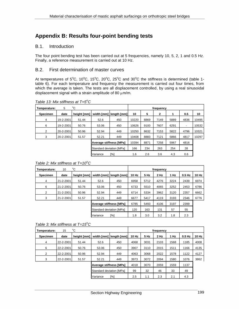
Material characterisation of mastic asphalt surfacings on orthotropic steel bridges
Section Highway Engineering 199
Appendix B: Results four-point bending tests
B.1. Introduction The four point bending test has been carried out at 5 frequencies, namely 10, 5, 2, 1 and 0.5 Hz. Finally, a reference measurement is carried out at 10 Hz.
B.2. First determination of master curves At temperatures of 5
oC, 10
oC, 15
oC, 20
oC, 25
oC and 30
oC the stiffness is determined (table 1-
table 6). For each temperature and frequency the measurement is carried out four times, from which the average is taken. The tests are all displacement controlled, by using a real sinusoidal
displacement signal with a strain amplitude of 80 m/m. Table 13: Mix stiffness at T=5
oC
Temperature: 5oC frequency
Specimen date height [mm] width [mm] length [mm] 10 5 2 1 0.5 10
4 19-2-2001 51.44 52.6 450 10220 8869 7149 5889 4836 10495
6 19-2-2001 50.76 53.06 450 10626 9100 7607 6291 - 10532
2 20-2-2001 50.96 52.94 449 10250 8632 7153 5822 4796 10321
3 20-2-2001 51.57 52.21 449 10408 8883 7121 5866 4817 10297
Average stiffness [MPa] 10394 8871 7258 5967 4816
Standard deviation [MPa] 166 234 263 254 28
Variance [%] 1.6 2.6 3.6 4.3 0.6 Table 2: Mix stiffness at T=10
oC
Temperature: 10oC frequency
Specimen date height [mm] width [mm] length [mm] 10 Hz 5 Hz 2 Hz 1 Hz 0.5 Hz 10 Hz
4 21-2-2001 51.44 52.6 450 6958 5712 4276 3224 2439 6974
6 21-2-2001 50.76 53.06 450 6733 5510 4065 3252 2453 6786
2 21-2-2001 50.96 52.94 449 6714 5334 3962 3120 2357 6662
3 21-2-2001 51.57 52.21 449 6677 5417 4119 3193 2346 6776
Average stiffness [MPa] 6785 5493 4106 3197 2399
Standard deviation [MPa] 120 163 131 57 55
Variance [%] 1.8 3.0 3.2 1.8 2.3 Table 3: Mix stiffness at T=15
oC
Temperature: 15oC frequency
Specimen date height [mm] width [mm] length [mm] 10 Hz 5 Hz 2 Hz 1 Hz 0.5 Hz 10 Hz
4 22-2-2001 51.44 52.6 450 4068 3031 2103 1568 1185 4008
6 22-2-2001 50.76 53.06 450 3907 3110 2015 1511 1166 4135
2 22-2-2001 50.96 52.94 449 4063 3068 2022 1578 1122 4127
3 22-2-2001 51.57 52.21 449 3973 3072 2094 1580 1076 3862
Average stiffness [MPa] 4018 3070 2059 1559 1137
Standard deviation [MPa] 99 32 46 33 49
Variance [%] 2.5 1.1 2.3 2.1 4.3

Material characterisation of mastic asphalt surfacings on orthotropic steel bridges
Section Highway Engineering 200
Table 4: Mix stiffness at T=20
oC
Temperature: 20oC frequency
Specimen date height [mm] width [mm] length [mm] 10 Hz 5 Hz 2 Hz 1 Hz 0.5 Hz 10 Hz
4 23-2-2001 51.44 52.6 450 2190 1783 1137 876 589 2195
6 23-2-2001 50.76 53.06 450 2208 1671 1025 782 601 2300
2 23-2-2001 50.96 52.94 449 2190 1728 1081 917 558 2248
3 23-2-2001 51.57 52.21 449 2447 1755 1088 828 587 2110
Average stiffness [MPa] 2236 1734 1083 851 584
Standard deviation [MPa] 101 48 46 59 18
Variance [%] 4.5 2.8 4.2 6.9 3.1 Table 5: Mix stiffness at T=25
oC
Temperature: 25oC frequency
Specimen date height [mm] width [mm] length [mm] 10 Hz 5 Hz 2 Hz 1 Hz 0.5 Hz 10 Hz
4 26-2-2001 51.44 52.6 450 1364 906 662 485 421 1367
6 26-2-2001 50.76 53.06 450 1312 990 695 486 424 1394
2 26-2-2001 50.96 52.94 449 1429 941 593 561 386 1305
3 26-2-2001 51.57 52.21 449 1423 902 625 454 451 1369
4 26-2-2001 51.44 52.6 450 1274 - - - - -
6 26-2-2001 50.76 53.06 450 1332 - - - - -
2 26-2-2001 50.96 52.94 449 1314 - - - - -
3 26-2-2001 51.57 52.21 449 1328 - - - - -
Average stiffness [MPa] 1351 935 644 497 421
Standard deviation [MPa] 46 41 44 45 27
Variance [%] 3.4 4.4 6.9 9.2 6.3 Table 6: Mix stiffness at T=30
oC
Temperature: 30oC frequency
Specimen date height [mm] width [mm] length [mm] 10 Hz 5 Hz 2 Hz 1 Hz 0.5 Hz 10 Hz
4 28-2-2001 51.44 52.6 450 800 529 418 315 317 797
6 28-2-2001 50.76 53.06 450 776 492 457 351 283 804
2 28-2-2001 50.96 52.94 449 729 520 418 349 312 811
3 28-2-2001 51.57 52.21 449 804 518 380 314 343 803
Average stiffness [MPa] 791 515 418 332 314
Standard deviation [MPa] 27 16 31 21 25
Variance [%] 3.4 3.1 7.5 6.2 7.8 For the determination of the master curves the data shown in table 7 was used.

Material characterisation of mastic asphalt surfacings on orthotropic steel bridges
Section Highway Engineering 201
Table 7: Summary of the mix stiffness at different temperatures and loading times
freq [Hz] t [s] PLUS5 PLUS10 PLUS15 PLUS20 PLUS25 PLUS30
0.5 2 4816 2399 1137 584 421 314
1 1 5967 3197 1559 851 497 332
2 0.5 7258 4106 2059 1083 644 418
5 0.2 8871 5493 3070 1734 935 515
10 0.1 10394 6785 4018 2236 1351 791
B.3. Repeated determination of master curves After 2.5 moths the determination of master curves has been repeated for 3 temperatures,
namely 10oC, 20
oC and 30
oC. The tests are carried out at a strain level of 80m/m as well as 800
m/m. Due to the lack of specimens the tests were carried out two times for each combination of frequency and temperature. Tables 8-13 show the results for the repeated determination of master curves.
Table 8: Mix stiffness at T=10oC and =80 m/m
Temperature: 10oC frequency
Specimen strain [m/m] date height [mm] width [mm] length [mm] 10 Hz 5 Hz 2 Hz 1 Hz 0.5 Hz 10 Hz
1 80 14-5-2001 52.83 50.64 450 6168 5121 3663 2809 2217 6223
4 80 14-5-2001 51.44 52.6 450 6324 5136 3763 2962 2230 6340
Average stiffness [MPa] 6264 5129 3713 2886 2224
Standard deviation [MPa] 82 11 71 108 9
Variance [%] 1 0 2 4 0
Table 9: Mix stiffness at T=10oC and =800 m/m
Temperature: 10oC frequency
Specimen strain [m/m] date height [mm] width [mm] length [mm] 10 Hz 5 Hz 2 Hz 1 Hz 0.5 Hz 10 Hz
1 800 14-5-2001 52.83 50.64 450 5629 3504 2137 1529 1104 4813
4 800 14-5-2001 51.44 52.6 450 5489 3476 2126 1510 1091 4718
Average stiffness [MPa] 5162 3490 2132 1520 1098
Standard deviation [MPa] 463 20 8 13 9
Variance [%] 9 1 0 1 1
Table 10: Mix stiffness at T=20oC and =80 m/m
Temperature: 20oC frequency
Specimen strain [m/m] date height [mm] width [mm] length [mm] 10 Hz 5 Hz 2 Hz 1 Hz 0.5 Hz 10 Hz
7 80 15-5-2001 50.89 52.84 450 2323 1696 1102 782 640 1978
8 80 15-5-2001 50.9 52.88 450 2048 1534 1034 732 564 2047
Average stiffness [MPa] 2099 1615 1068 757 602
Standard deviation [MPa] 153 115 48 35 54
Variance [%] 7 7 5 5 9
Table 11: Mix stiffness at T=20oC and =800 m/m
Temperature: 20oC frequency
Specimen strain [m/m] date height [mm] width [mm] length [mm] 10 Hz 5 Hz 2 Hz 1 Hz 0.5 Hz 10 Hz
7 800 15-5-2001 50.89 52.84 450 1452 1121 546 386 264 1428
8 800 15-5-2001 50.9 52.88 450 1437 1068 534 362 261 1400
Average stiffness [MPa] 1429 1095 540 374 263
Standard deviation [MPa] 22 37 8 17 2
Variance [%] 2 3 2 5 1

Material characterisation of mastic asphalt surfacings on orthotropic steel bridges
Section Highway Engineering 202
Table 12: Mix stiffness at T=30oC and =80 m/m
Temperature: 30oC frequency
Specimen strain [m/m] date height [mm] width [mm] length [mm] 10 Hz 5 Hz 2 Hz 1 Hz 0.5 Hz 10 Hz
3 80 15-5-2001 51.57 52.21 449 730 486 384 382 278 700
5 80 15-5-2001 51.01 52.95 450 703 494 383 317 245 693
Average stiffness [MPa] 707 490 384 350 262
Standard deviation [MPa] 16 6 1 46 23
Variance [%] 2 1 0 13 9
Table 13: Mix stiffness at T=30oC and =800 m/m
Temperature: 30oC frequency
Specimen strain [m/m] date height [mm] width [mm] length [mm] 10 Hz 5 Hz 2 Hz 1 Hz 0.5 Hz 10 Hz
3 800 15-5-2001 51.57 52.21 449 470 339 158 112 84 435
5 800 15-5-2001 51.01 52.95 450 556 352 160 107 82 422
Average stiffness [MPa] 471 346 159 110 83
Standard deviation [MPa] 60 9 1 4 1
Variance [%] 13 3 1 3 2 For the determination of the master curves the data shown in table 14 and 15 was used.
Table 14: Summary of the mix stiffness for =80 m/m
freq [Hz] t [s] PLUS10 PLUS20 PLUS30
0.5 2 2224 602 262
1 1 2886 757 350
2 0.5 3713 1068 384
5 0.2 5129 1615 490
10 0.1 6264 2099 707
Table 15: Summary of the mix stiffness for =800 m/m
freq [Hz] t [s] PLUS10 PLUS20 PLUS30
0.5 2 1098 263 83
1 1 1520 374 110
2 0.5 2132 540 159
5 0.2 3490 1095 346
10 0.1 5162 1429 471
B.4. Determining the strain dependent behaviour of the mix stiffness
For these tests 46 specimens of the Lintrack mix were used. The tests were carried out at temperatures of 5
oC, 12.5
oC, 20
oC, 27.5
oC, 35
oC and 42.5
oC. All tests are displacement
controlled with a real sinusoidal displacement. The strain amplitudes that were applied are 80
m/m, 200 m/m, 600 m/m and 1000 m/m. Each test combination is repeated once, the average of both measurements is used for the determination of the master curves. Table 16 shows the results of the measurements.

Material characterisation of mastic asphalt surfacings on orthotropic steel bridges
Section Highway Engineering 203
Table 16: Stiffness at different temperatures, loading times and strain levels frequency
Specimen T [oC] strain [m/m] 10Hz 5Hz 2Hz 1Hz 0.5Hz 10Hz
ML/4pb/1/1 5 80 8870 7726 6109 5117 4062 8946
ML/4pb/1/2 5 80 8963 7623 6176 5091 4196 9113
ML/4pb/1/1 5 200 8704 7210 5591 4473 3575 8617
ML/4pb/1/2 5 200 8823 7355 5635 4562 3639 8777
ML/4pb/1/3 5 600 9143 6532 4564 3513 2698 7854
ML/4pb/1/4 5 600 9356 6829 4848 3745 2873 8050
ML/4pb/1/5 5 1000 9414 6589 3975 2865 2118 7648
ML/4pb/1/6 12.5 1000 8748 6089 3914 2837 2107 7225
ML/4pb/1/7 12.5 80 5859 4583 3377 2486 1919 5721
ML/4pb/1/8 12.5 80 5223 3939 3025 2374 1744 5239
ML/4pb/1/7 12.5 200 5511 4214 2853 2050 1531 5427
ML/4pb/1/8 12.5 200 4931 3797 2549 1874 1461 4878
ML/4pb/1/9 12.5 600 4034 2786 1781 1281 922 3714
ML/4pb/1/10 12.5 600 4094 2806 1791 1293 937 3770
ML/4pb/2/1 12.5 1000 3840 2323 1438 1017 725 3140
ML/4pb/2/2 12.5 1000 3638 2268 1398 994 715 3121
ML/4pb/2/3 20 80 2190 1875 1271 1013 774 2296
ML/4pb/2/4 20 80 2388 1904 1329 928 743 2319
ML/4pb/2/3 20 200 2269 1658 1002 707 542 2217
ML/4pb/2/4 20 200 2250 1687 998 748 536 2175
ML/4pb/2/5 20 600 1819 1319 727 498 367 1776
ML/4pb/2/6 20 600 1818 304 728 502 367 1654
ML/4pb/2/7 20 1000 1497 932 597 403 279 1418
ML/4pb/2/8 20 1000 1462 910 579 395 279 1406
ML/4pb/2/9 27.5 80 1155 842 565 536 379 1188
ML/4pb/2/10 27.5 80 1023 857 581 431 354 1084
ML/4pb/2/9 27.5 200 1016 732 399 322 261 999
ML/4pb/2/10 27.5 200 959 679 425 316 268 963
ML/4pb/3/1 27.5 600 803 489 267 202 151 809
ML/4pb/3/2 27.5 600 802 491 274 192 147 759
ML/4pb/3/3 27.5 1000 706 461 236 150 114 728
ML/4pb/3/4 27.5 1000 709 477 245 152 116 669
ML/4pb/3/5 35 80 590 393 391 272 272 544
ML/4pb/3/6 35 80 589 435 295 393 277 566
ML/4pb/3/5 35 200 460 267 219 188 173 451
ML/4pb/3/6 35 200 431 302 206 175 159 476
ML/4pb/3/7 35 600 506 295 131 105 84 427
ML/4pb/3/8 35 600 469 294 119 98 83 422
ML/4pb/3/9 35 1000 432 306 125 73 58 459
ML/4pb/3/10 35 1000 495 305 132 66 54 451
ML/4pb/4/1 42.5 80 379 305 301 339 205 459
ML/4pb/4/2 42.5 80 327 297 220 259 222 374
ML/4pb/4/1 42.5 200 319 167 152 152 107 257
ML/4pb/4/2 42.5 200 298 149 13 119 134 334
ML/4pb/4/3 42.5 600 320 215 75 65 60 286
ML/4pb/4/4 42.5 600 - 198 79 59 60 278
ML/4pb/4/5 42.5 1000 - - 82 48 42 -
ML/4pb/4/6 42.5 1000 - - 97 54 42 - For the determination of master curves use is made of the average stiffness that is shown in table 17.

Material characterisation of mastic asphalt surfacings on orthotropic steel bridges
Section Highway Engineering 204
Table 17: Summary of the mix stiffness at different temperatures, frequencies and strain levels
temp strainlevel 10Hz 5Hz 2Hz 1Hz 0.5Hz
T=5oC 80 8973 7675 6143 5104 4129
200 8730 7283 5613 4518 3607
600 8601 6681 4706 3629 2786
1000 8259 6339 3945 2851 2113
T=12.5oC 80 5511 4261 3201 2430 1832
200 5187 4006 2701 1962 1496
600 3903 2796 1786 1287 930
1000 3435 2296 1418 1006 720
T=20oC 80 2298 1890 1300 971 759
200 2228 1673 1000 728 539
600 1792 1312 728 500 367
1000 1446 921 588 399 279
T=27.5oC 80 1113 850 573 484 367
200 984 708 412 319 265
600 793 490 271 197 149
1000 703 469 241 151 115
T=35oC 80 572 414 393 333 275
200 455 285 213 182 166
600 456 295 125 102 84
1000 437 306 129 70 56
T=42.5oC 80 385 301 261 259 214
200 302 158 143 136 121
600 295 207 77 62 60
1000 x x 90 51 42

Material characterisation of mastic asphalt surfacings on orthotropic steel bridges
Section Highway Engineering 205
Appendix C: Determination of Smix as a function of temperature, loading time and strain level
C.1. Determination of the function parameters For each combination of strain level and temperature there is a master curve as a function of the
loading time t. To determine the relationship for Smix as a function of t, T and , first each master
curve is expressed as a function of t for a constant T and Each master curve can be expressed as follows:
d
ctmix
e
baS
)(log
1
log Equation 1
The constants a, b, c and d are determined for each master curve. Tables 1-24 show the output for this parameter determination. Therefore use is made of the computer program TableCurve2D.
Table 1: Master curve =80 m/m T=5oC
[ Sigmoid] y= a+ b/ (1+ exp(-(x-c)/ d))
Parameters Values Std Error T Value 95% Conf Lim 95% Conf Lim
Eqn [ Sigmoid] y= a+ b/ (1+ exp(-(x-c)/ d))a 2.253402 0.023197 97.14304 2.205806011 2.300997571
Eqn # 8011 b 1.942615 0.037956 51.18019 1.864734593 2.020494705
r2 0.998197 c 1.420732 0.044066 32.24092 1.330315557 1.511147897
DF A dj r2 0.99792 d -1.252728 0.040864 -30.65572 -1.336574853 -1.168881143
Fit Std Err 0.024431
F-stat 4983.172
Date Jun 22, 2001
Time 11:37:02 A M
Table 2: Master curve =80 m/m T=12.5 oC
[ Sigmoid] y= a+ b/ (1+ exp(-(x-c)/ d))
Parameters Values Std Error T Value 95% Conf Lim 95% Conf Lim
Eqn [ Sigmoid] y= a+ b/ (1+ exp(-(x-c)/ d))a 2.253317 0.023222 97.03374 2.20566927 2.300964463
Eqn # 8011 b 1.942923 0.038042 51.07313 1.864867515 2.020978919
r2 0.998197 c 0.388627 0.044075 8.817324 0.298191466 0.479061757
DF A dj r2 0.99792 d -1.252992 0.040945 -30.60179 -1.337004289 -1.16897964
Fit Std Err 0.024433
F-stat 4982.458
Date Jun 22, 2001
Time 11:37:45 A M
Table 14: Master curve =80 m/m T=20 oC
[ Sigmoid] y= a+ b/ (1+ exp(-(x-c)/ d))
Parameters Values Std Error T Value 95% Conf Lim 95% Conf Lim
Eqn [ Sigmoid] y= a+ b/ (1+ exp(-(x-c)/ d))a 2.253135 0.023272 96.81869 2.205385527 2.300884682
Eqn # 8011 b 1.943581 0.038209 50.86765 1.865183275 2.021978332
r2 0.998196 c -0.590893 0.044097 -13.39976 -0.68137357 -0.500413148
DF A dj r2 0.997919 d -1.253555 0.041102 -30.49893 -1.337888898 -1.169221772
Fit Std Err 0.024437
F-stat 4980.92
Date Jun 22, 2001
Time 11:38:25 A M

Material characterisation of mastic asphalt surfacings on orthotropic steel bridges
Section Highway Engineering 206
Table 4: Master curve =80 m/m T=27.5 oC
[ Sigmoid] y= a+ b/ (1+ exp(-(x-c)/ d))
Parameters Values Std Error T Value 95% Conf Lim 95% Conf Lim
Eqn [ Sigmoid] y= a+ b/ (1+ exp(-(x-c)/ d))a 2.25276 0.023366 96.41061 2.204816667 2.300704091
Eqn # 8011 b 1.944933 0.038522 50.48894 1.865892223 2.02397328
r2 0.998195 c -1.522022 0.044147 -34.476 -1.612604694 -1.431439185
DF A dj r2 0.997918 d -1.254714 0.041395 -30.31068 -1.339650255 -1.169778704
Fit Std Err 0.024445
F-stat 4977.672
Date Jun 22, 2001
Time 11:39:00 A M
Table 5: Master curve =80 m/m T=35 oC
[ Sigmoid] y= a+ b/ (1+ exp(-(x-c)/ d))
Parameters Values Std Error T Value 95% Conf Lim 95% Conf Lim
Eqn [ Sigmoid] y= a+ b/ (1+ exp(-(x-c)/ d))a 2.252013 0.023542 95.65926 2.203708478 2.300316971
Eqn # 8011 b 1.947629 0.039097 49.81563 1.867408803 2.027848569
r2 0.998193 c -2.40878 0.044258 -54.42621 -2.49958929 -2.317970623
DF A dj r2 0.997915 d -1.257025 0.041931 -29.97856 -1.3430601 -1.170990275
Fit Std Err 0.024462
F-stat 4970.821
Date Jun 22, 2001
Time 11:39:53 A M
Table 6: Master curve =80 m/m T=42.5 oC
[ Sigmoid] y= a+ b/ (1+ exp(-(x-c)/ d))
Parameters Values Std Error T Value 95% Conf Lim 95% Conf Lim
Eqn [ Sigmoid] y= a+ b/ (1+ exp(-(x-c)/ d))a 2.250561 0.023864 94.30666 2.201595717 2.299526659
Eqn # 8011 b 1.952877 0.040138 48.65466 1.870521883 2.035232651
r2 0.998187 c -3.255248 0.044499 -73.15376 -3.346551339 -3.16394374
DF A dj r2 0.997908 d -1.261514 0.042894 -29.41013 -1.349525341 -1.17350341
Fit Std Err 0.024498
F-stat 4956.035
Date Jun 22, 2001
Time 11:40:33 A M
Table 7: Master curve =200 m/m T=5 oC
[ Sigmoid] y= a+ b/ (1+ exp(-(x-c)/ d))
Parameters Values Std Error T Value 95% Conf Lim 95% Conf Lim
Eqn [ Sigmoid] y= a+ b/ (1+ exp(-(x-c)/ d))a 1.892585 0.0396 47.79304 1.811187044 1.973983314
Eqn # 8011 b 2.304665 0.059311 38.85704 2.1827483 2.426580857
r2 0.997447 c 1.667883 0.059178 28.18418 1.54624136 1.7895256
DF A dj r2 0.997039 d -1.327189 0.054293 -24.44484 -1.43879023 -1.21558763
Fit Std Err 0.033613
F-stat 3386.221
Date Jun 22, 2001
Time 11:41:12 A M

Material characterisation of mastic asphalt surfacings on orthotropic steel bridges
Section Highway Engineering 207
Table 8: Master curve =200 m/m T=12.5 oC
[ Sigmoid] y= a+ b/ (1+ exp(-(x-c)/ d))
Parameters Values Std Error T Value 95% Conf Lim 95% Conf Lim
Eqn [ Sigmoid] y= a+ b/ (1+ exp(-(x-c)/ d))a 1.892416 0.039659 47.71668 1.810894869 1.973937102
Eqn # 8011 b 2.305173 0.059481 38.75503 2.182908574 2.427436835
r2 0.997447 c 0.635757 0.059187 10.74157 0.514097316 0.757416906
DF A dj r2 0.997038 d -1.327587 0.054436 -24.38802 -1.4394824 -1.215692571
Fit Std Err 0.033614
F-stat 3385.922
Date Jun 22, 2001
Time 11:41:46 A M
Table 9: Master curve =200 m/m T=20 oC
[ Sigmoid] y= a+ b/ (1+ exp(-(x-c)/ d))
Parameters Values Std Error T Value 95% Conf Lim 95% Conf Lim
Eqn [ Sigmoid] y= a+ b/ (1+ exp(-(x-c)/ d))a 1.892071 0.039772 47.57285 1.810318272 1.973823619
Eqn # 8011 b 2.306207 0.059796 38.56784 2.183294705 2.429120109
r2 0.997446 c -0.343787 0.059209 -5.806354 -0.465491866 -0.222081437
DF A dj r2 0.997038 d -1.328399 0.054702 -24.28441 -1.440840351 -1.215958297
Fit Std Err 0.033617
F-stat 3385.294
Date Jun 22, 2001
Time 11:42:18 A M
Table 10: Master curve =200 m/m T=27.5 oC
[ Sigmoid] y= a+ b/ (1+ exp(-(x-c)/ d))
Parameters Values Std Error T Value 95% Conf Lim 95% Conf Lim
Eqn [ Sigmoid] y= a+ b/ (1+ exp(-(x-c)/ d))a 1.891391 0.039978 47.31094 1.809215246 1.973566649
Eqn # 8011 b 2.308246 0.060367 38.23709 2.184160605 2.432331593
r2 0.997445 c -1.274926 0.059261 -21.51371 -1.39673855 -1.153112768
DF A dj r2 0.997037 d -1.329999 0.055181 -24.10267 -1.44342376 -1.216573298
Fit Std Err 0.033624
F-stat 3383.983
Date Jun 22, 2001
Time 11:43:22 A M
Table 11: Master curve =200 m/m T=35 oC
[ Sigmoid] y= a+ b/ (1+ exp(-(x-c)/ d))
Parameters Values Std Error T Value 95% Conf Lim 95% Conf Lim
Eqn [ Sigmoid] y= a+ b/ (1+ exp(-(x-c)/ d))a 1.89009 0.040346 46.8473 1.807157802 1.973021575
Eqn # 8011 b 2.312154 0.061376 37.67194 2.18599347 2.438313891
r2 0.997443 c -2.161638 0.059379 -36.40419 -2.283693091 -2.039583208
DF A dj r2 0.997034 d -1.33306 0.056024 -23.79464 -1.448218418 -1.217902246
Fit Std Err 0.033638
F-stat 3381.188
Date Jun 22, 2001
Time 11:43:51 A M

Material characterisation of mastic asphalt surfacings on orthotropic steel bridges
Section Highway Engineering 208
Table 12: Master curve =200 m/m T=42.5 oC
[ Sigmoid] y= a+ b/ (1+ exp(-(x-c)/ d))
Parameters Values Std Error T Value 95% Conf Lim 95% Conf Lim
Eqn [ Sigmoid] y= a+ b/ (1+ exp(-(x-c)/ d))a 1.887658 0.040997 46.04413 1.803388459 1.971928407
Eqn # 8011 b 2.319487 0.063144 36.73329 2.189692348 2.449281053
r2 0.997439 c -3.007906 0.059636 -50.43793 -3.130489471 -2.88532319
DF A dj r2 0.997029 d -1.338792 0.05749 -23.28728 -1.456964503 -1.22061871
Fit Std Err 0.033669
F-stat 3374.942
Date Jun 22, 2001
Time 11:44:23 A M
Table 13: Master curve =600 m/m T=5 oC
[ Sigmoid] y= a+ b/ (1+ exp(-(x-c)/ d))
Parameters Values Std Error T Value 95% Conf Lim 95% Conf Lim
Eqn [ Sigmoid] y= a+ b/ (1+ exp(-(x-c)/ d))a 1.490625 0.073642 20.24146 1.338284743 1.642965709
Eqn # 8011 b 2.730722 0.103274 26.44165 2.517084754 2.944359846
r2 0.995414 c 1.736468 0.095372 18.2074 1.539177009 1.933759108
DF A dj r2 0.99458 d -1.449282 0.084448 -17.16184 -1.623975696 -1.274588078
Fit Std Err 0.051416
F-stat 1663.933
Date Jun 22, 2001
Time 11:45:12 A M
Table 14: Master curve =600 m/m T=12.5 oC
[ Sigmoid] y= a+ b/ (1+ exp(-(x-c)/ d))
Parameters Values Std Error T Value 95% Conf Lim 95% Conf Lim
Eqn [ Sigmoid] y= a+ b/ (1+ exp(-(x-c)/ d))a 1.490057 0.073838 20.17996 1.337310134 1.642802998
Eqn # 8011 b 2.732128 0.103766 26.32969 2.517471564 2.946784503
r2 0.995416 c 0.704253 0.095385 7.38326 0.506934033 0.901572395
DF A dj r2 0.994583 d -1.450321 0.084823 -17.09817 -1.625791032 -1.274850926
Fit Std Err 0.051401
F-stat 1664.907
Date Jun 22, 2001
Time 11:45:43 A M
Table 15: Master curve =600 m/m T=20 oC
[ Sigmoid] y= a+ b/ (1+ exp(-(x-c)/ d))
Parameters Values Std Error T Value 95% Conf Lim 95% Conf Lim
Eqn [ Sigmoid] y= a+ b/ (1+ exp(-(x-c)/ d))a 1.488996 0.074183 20.07188 1.335536386 1.642455575
Eqn # 8011 b 2.73478 0.104628 26.1381 2.51834067 2.951220142
r2 0.995421 c -0.275456 0.095419 -2.886813 -0.47284449 -0.07806729
DF A dj r2 0.994589 d -1.452274 0.085478 -16.99009 -1.62909832 -1.27545003
Fit Std Err 0.051372
F-stat 1666.762
Date Jun 22, 2001
Time 11:47:03 A M

Material characterisation of mastic asphalt surfacings on orthotropic steel bridges
Section Highway Engineering 209
Table 16: Master curve =600 m/m T=27.5 oC
[ Sigmoid] y= a+ b/ (1+ exp(-(x-c)/ d))
Parameters Values Std Error T Value 95% Conf Lim 95% Conf Lim
Eqn [ Sigmoid] y= a+ b/ (1+ exp(-(x-c)/ d))a 1.487067 0.074774 19.88736 1.332384256 1.641749895
Eqn # 8011 b 2.739662 0.106101 25.82117 2.520174864 2.959149751
r2 0.995431 c -1.206898 0.095495 -12.63837 -1.404443994 -1.00935204
DF A dj r2 0.9946 d -1.455855 0.086591 -16.81293 -1.634982392 -1.276726631
Fit Std Err 0.05132
F-stat 1670.182
Date Jun 22, 2001
Time 11:47:51 A M
Table 17: Master curve =600 m/m T=35 oC
[ Sigmoid] y= a+ b/ (1+ exp(-(x-c)/ d))
Parameters Values Std Error T Value 95% Conf Lim 95% Conf Lim
Eqn [ Sigmoid] y= a+ b/ (1+ exp(-(x-c)/ d))a 1.483624 0.075774 19.57952 1.326873037 1.64037505
Eqn # 8011 b 2.748487 0.108585 25.31189 2.523862516 2.973112122
r2 0.995447 c -2.094164 0.095658 -21.89209 -2.29204901 -1.896279752
DF A dj r2 0.994619 d -1.462296 0.088457 -16.53123 -1.64528286 -1.279309977
Fit Std Err 0.051227
F-stat 1676.296
Date Jun 22, 2001
Time 11:48:30 A M
Table 18: Master curve =600 m/m T=42.5 oC
[ Sigmoid] y= a+ b/ (1+ exp(-(x-c)/ d))
Parameters Values Std Error T Value 95% Conf Lim 95% Conf Lim
Eqn [ Sigmoid] y= a+ b/ (1+ exp(-(x-c)/ d))a 1.477544 0.077463 19.07429 1.317300581 1.637787763
Eqn # 8011 b 2.76429 0.112771 24.51251 2.531006449 2.997573974
r2 0.995476 c -2.941463 0.096002 -30.63961 -3.140058005 -2.7428676
DF A dj r2 0.994653 d -1.473765 0.091572 -16.09403 -1.663196894 -1.2843339
Fit Std Err 0.051066
F-stat 1686.868
Date Jun 22, 2001
Time 11:49:11 A M
Table 19: Master curve =1000 m/m T=5 oC
[ Sigmoid] y= a+ b/ (1+ exp(-(x-c)/ d))
Parameters Values Std Error T Value 95% Conf Lim 95% Conf Lim
Eqn [ Sigmoid] y= a+ b/ (1+ exp(-(x-c)/ d))a 1.280908 0.135065 9.483624 1.000799801 1.561016131
Eqn # 8011 b 2.96179 0.178354 16.60623 2.591906446 3.331674451
r2 0.989465 c 1.745278 0.167896 10.39497 1.397081758 2.093473498
DF A dj r2 0.987458 d -1.573894 0.138391 -11.37284 -1.86089881 -1.286889539
Fit Std Err 0.079155
F-stat 688.7429
Date Jun 22, 2001
Time 11:49:52 A M

Material characterisation of mastic asphalt surfacings on orthotropic steel bridges
Section Highway Engineering 210
Table 20: Master curve =1000 m/m T=12.5 oC
[ Sigmoid] y= a+ b/ (1+ exp(-(x-c)/ d))
Parameters Values Std Error T Value 95% Conf Lim 95% Conf Lim
Eqn [ Sigmoid] y= a+ b/ (1+ exp(-(x-c)/ d))a 1.279578 0.135675 9.431228 0.99820595 1.560949614
Eqn # 8011 b 2.964782 0.179725 16.49626 2.592056424 3.337508273
r2 0.989475 c 0.713004 0.168009 4.243834 0.364573673 1.061433755
DF A dj r2 0.98747 d -1.57605 0.139399 -11.30603 -1.865145507 -1.286953533
Fit Std Err 0.079118
F-stat 689.3982
Date Jun 22, 2001
Time 11:50:21 A M
Table 21: Master curve =1000 m/m T=20 oC
[ Sigmoid] y= a+ b/ (1+ exp(-(x-c)/ d))
Parameters Values Std Error T Value 95% Conf Lim 95% Conf Lim
Eqn [ Sigmoid] y= a+ b/ (1+ exp(-(x-c)/ d))a 1.277248 0.136697 9.343623 0.993755091 1.560740731
Eqn # 8011 b 2.970118 0.182019 16.31765 2.592634062 3.347601337
r2 0.989493 c -0.266853 0.168222 -1.586318 -0.615722835 0.082017247
DF A dj r2 0.987491 d -1.579874 0.141083 -11.19821 -1.872461652 -1.287286312
Fit Std Err 0.07905
F-stat 690.5908
Date Jun 22, 2001
Time 11:50:56 A M
Table 22: Master curve =1000 m/m T=27.5 oC
[ Sigmoid] y= a+ b/ (1+ exp(-(x-c)/ d))
Parameters Values Std Error T Value 95% Conf Lim 95% Conf Lim
Eqn [ Sigmoid] y= a+ b/ (1+ exp(-(x-c)/ d))a 1.273241 0.138386 9.20066 0.986246282 1.560235574
Eqn # 8011 b 2.979464 0.185799 16.03593 2.594139776 3.364787869
r2 0.989524 c -1.198626 0.168611 -7.108802 -1.548304418 -0.848946794
DF A dj r2 0.987529 d -1.586538 0.143846 -11.02942 -1.884856159 -1.288219326
Fit Std Err 0.078931
F-stat 692.709
Date Jun 22, 2001
Time 11:51:27 A M
Table 23: Master curve =1000 m/m T=35 oC
[ Sigmoid] y= a+ b/ (1+ exp(-(x-c)/ d))
Parameters Values Std Error T Value 95% Conf Lim 95% Conf Lim
Eqn [ Sigmoid] y= a+ b/ (1+ exp(-(x-c)/ d))a 1.266422 0.141158 8.97167 0.973678254 1.559165208
Eqn # 8011 b 2.995676 0.192003 15.60226 2.597486374 3.39386464
r2 0.989579 c -2.086596 0.169319 -12.32345 -2.437742366 -1.735449674
DF A dj r2 0.987594 d -1.598028 0.148353 -10.7718 -1.905692744 -1.290362558
Fit Std Err 0.078724
F-stat 696.3976
Date Jun 22, 2001
Time 11:52:07 A M

Material characterisation of mastic asphalt surfacings on orthotropic steel bridges
Section Highway Engineering 211
Table 24: Master curve =1000 m/m T=42.5 oC
[ Sigmoid] y= a+ b/ (1+ exp(-(x-c)/ d))
Parameters Values Std Error T Value 95% Conf Lim 95% Conf Lim
Eqn [ Sigmoid] y= a+ b/ (1+ exp(-(x-c)/ d))a 1.254824 0.14575 8.609434 0.952556933 1.557090236
Eqn # 8011 b 3.023813 0.2023 14.9472 2.604269363 3.443356742
r2 0.989672 c -2.935371 0.170603 -17.20586 -3.289179384 -2.58156163
DF A dj r2 0.987705 d -1.617828 0.155767 -10.38619 -1.940869833 -1.294786578
Fit Std Err 0.078372
F-stat 702.7211
Date Jun 22, 2001
Time 11:52:39 A M Tables 25-28 show a summary of the output parameters:
Table 25: Parameters for =80 m/m
T [oC] a b c d
5.0 2.25 1.94 1.42 -1.25 12.5 2.25 1.94 0.39 -1.25 20.0 2.25 1.94 -0.59 -1.25 27.5 2.25 1.94 -1.52 -1.25 35.0 2.25 1.95 -2.41 -1.26 42.5 2.25 1.95 -3.26 -1.26
Table 26: Parameters for =200 m/m
T [oC] a b c d
5.0 1.89 2.30 1.67 -1.33 12.5 1.89 2.31 0.64 -1.33 20.0 1.89 2.31 -0.34 -1.33 27.5 1.89 2.31 -1.27 -1.33 35.0 1.89 2.31 -2.16 -1.33 42.5 1.89 2.32 -3.01 -1.34
Table 27: Parameters for =600 m/m
T [oC] a b c d
5.0 1.49 2.73 1.74 -1.45 12.5 1.49 2.73 0.70 -1.45 20.0 1.49 2.73 -0.28 -1.45 27.5 1.49 2.74 -1.21 -1.46 35.0 1.48 2.75 -2.09 -1.46 42.5 1.48 2.76 -2.94 -1.47
Table 28: Parameters for =1000 m/m
T [oC] a b c d
5.0 1.28 2.96 1.75 -1.57 12.5 1.28 2.96 0.71 -1.58 20.0 1.28 2.97 -0.27 -1.58 27.5 1.27 2.98 -1.20 -1.59 35.0 1.27 3.00 -2.09 -1.60 42.5 1.25 3.02 -2.94 -1.62
From these tables it becomes clear that a, b and d vary with strain level and that c varies with strain level and temperature, so:

Material characterisation of mastic asphalt surfacings on orthotropic steel bridges
Section Highway Engineering 212
fd
Tfc
fb
fa
,
With the computer program TableCurve2D the relationship between a and is determined. This relationship is best described with:
ln11 baa Equation 2
Table 29 shows the output for the determination of the constants of equation 2.
Table 29: Determination of a as a function of y= a1+ b1lnx
Parameters Values Std Error T Value 95% Conf Lim 95% Conf Lim
Eqn y= a+ blnx a1 3.936725 0.031141 126.4162 3.802736381 4.070714177
Eqn # 13 b1 -0.384815 0.005342 -72.03081 -0.407801125 -0.361828455
r2 0.999615
DF A dj r2 0.998844
Fit Std Err 0.010461
F-stat 5188.438
Date Jun 22, 2001
Time 12:09:06 PM
The relationship between b and is best described with:
2
11 logdcb Equation 3
Table 30 shows the output from TableCurve2D for the determination of c1 and d1.
Table 30: Determination of b as a function of y= c1+ d1(lnx)^2
Parameters Values Std Error T Value 95% Conf Lim 95% Conf Lim
Eqn y= a+ b(lnx)^2 c1 1.273163 0.037569 33.88878 1.111517584 1.434809228
Eqn # 10 d1 0.035955 0.001051 34.20064 0.031431594 0.040478306
r2 0.998293054
DF A dj r2 0.994879163
Fit Std Err 0.023275391
F-stat 1169.683554
Date Jun 22, 2001
Time 12:11:01 PM
The determination of c as a function of T and is carried out in two steps: First c is expressed as a function of T for each strain level, which is described best with:
Tfec 11 Equation 4
In this equation e1 and f1 are dependent on the strain level. First the parameters e1 and f1 are determined for each strain level. The output for each strain level is shown in the tables 31-34.

Material characterisation of mastic asphalt surfacings on orthotropic steel bridges
Section Highway Engineering 213
Table 31: Parameter c for =80 m/m [ Line Robust None, Gaussian Errors] c= e1+ f1x
Parameters Values Std Error T Value 95% Conf Lim 95% Conf Lim
Eqn [ Line Robust None, Gaussian Errors] y= a+ bxe1 1.964268 0.061005 32.19848 1.794890594 2.133644566
Eqn # 8160 f1 -0.124584 0.002261 -55.10604 -0.130860779 -0.118306799
r2 0.998685
DF A dj r2 0.997808
Fit Std Err 0.070932
F-stat 3036.676
Date Jul 9, 2001
Time 10:35:20 PM
Table 32: Parameter c for =200 m/m [ Line Robust None, Gaussian Errors] c= e1+ f1x
Parameters Values Std Error T Value 95% Conf Lim 95% Conf Lim
Eqn [ Line Robust None, Gaussian Errors] y= a+ bxe1 2.211341 0.061069 36.21078 2.041787532 2.380894716
Eqn # 8160 f1 -0.12458 0.002263 -55.04701 -0.130863626 -0.118296556
r2 0.998682
DF A dj r2 0.997803
Fit Std Err 0.071006
F-stat 3030.173
Date Jul 9, 2001
Time 10:36:05 PM
Table 33: Parameter c for =600 m/m [ Line Robust None, Gaussian Errors] c= e1+ f1x
Parameters Values Std Error T Value 95% Conf Lim 95% Conf Lim
Eqn [ Line Robust None, Gaussian Errors] y= a+ bxe1 2.280507 0.060778 37.52201 2.111760937 2.449253745
Eqn # 8160 f1 -0.124634 0.002252 -55.33413 -0.13088733 -0.11838009
r2 0.998695
DF A dj r2 0.997826
Fit Std Err 0.070668
F-stat 3061.866
Date Jul 9, 2001
Time 10:36:34 PM
Table 34: Parameter c for =1000 m/m [ Line Robust None, Gaussian Errors] y= e1+ f1x
Parameters Values Std Error T Value 95% Conf Lim 95% Conf Lim
Eqn [ Line Robust None, Gaussian Errors] y= a+ bxe1 2.290103 0.060347 37.9492 2.122554538 2.457652278
Eqn # 8160 f1 -0.1247 0.002236 -55.75937 -0.13090948 -0.118491
r2 0.998715
DF A dj r2 0.997859
Fit Std Err 0.070166
F-stat 3109.107
Date Jul 9, 2001
Time 10:37:12 PM Table 35 shows an overview of the parameters e1 and f1 for different strain levels. Table 35: Overview of the parameters e1 and f1 for different strain levels
m/m e1 f1
80 1.964268 -0.12484 200 2.211341 -0.12458 600 2.280507 -0.12463
1000 2.290103 -0.12470

Material characterisation of mastic asphalt surfacings on orthotropic steel bridges
Section Highway Engineering 214
From this table it becomes clear that e1 is a function of and that f1 is constant, namely –0.124624 (average of the four values in table 35)
The second step is the determination of e1 as a function of . This relationship is best described with:
5.1
111
hge Equation 5
Table 36 shows the determination of the parameters g1 and h1. Table 36: Determination of g1 and h1 e1= g1+ h1/ x^(1.5)
Parameters Values Std Error T Value 95% Conf Lim 95% Conf Lim
Eqn y= a+ b/ x^(1.5) g1 2.296692 0.000724 3171.604 2.293576674 2.299808138
Eqn # 18 h1 -238.0479 1.003299 -237.2651 -242.3647937 -233.731096
r2 0.999964474
DF A dj r2 0.999893422
Fit Std Err 0.001111548
F-stat 56294.73836
Date Jun 25, 2001
Time 1:17:43 PM
The relationship for c as a function of and T is obtained by combining equation 4 and 5:
111
hgTfc Equation 6
The relationship between d and is best described with:
11 jid Equation 7
Table 37 shows the output for the determination of i1 and j1. Table 37: Determination of i1 and j1 y= i1+ j1x^(0.5)
Parameters Values Std Error T Value 95% Conf Lim 95% Conf Lim
Eqn y= a+ bx^(0.5) i1 -1.124671 0.018917 -59.45162 -1.206065681 -1.0432756
Eqn # 12 j1 -0.014312 0.000873 -16.40178 -0.018066583 -0.01055764
r2 0.992620425
DF A dj r2 0.977861274
Fit Std Err 0.015405155
F-stat 269.0183046
Date Jun 22, 2001
Time 12:12:15 PM The relationship for the mix stiffness is obtained by combining the equations 2, 3, 6 and 7:
5.011
5.1111 )(log
2
1111
1
lnln,,log
ji
hgTftmix
e
dcbaTtS Equation 8

Material characterisation of mastic asphalt surfacings on orthotropic steel bridges
Section Highway Engineering 215
The parameters in this equation are: a1 : -0.38481 b1 : 3.936725 c1 : 1.273163 d1 : 0.035955 f1 : 0.124624 g1 : -2.296692 h1 : 238.0479 i1 : -1.124671 j1 :-0.014312
The final step is rewriting a1ln as alog and d1(ln)2 as d(log)
2. Therefore equation 9 is used:
log3025851.2ln Equation 9
The final equation that describes the mix stiffness as a function of loading time, temperature and strain level becomes:
5.0
5.1 )(log
2
1
loglog,,log
ji
hgfTtmix
e
dcbaTtS
Equation 10
in which: Smix : mix stiffness [MPa]
: strain [m/m] t : loading time [s] T : temperature [
oC]
The constants a-j are: a : -0.88607 b : 3.936725 c : 1.273163 d : 0.190629 f : 0.124624 g : -2.296692 h : 238.0479 i : -1.124671 j :-0.014312

Material characterisation of mastic asphalt surfacings on orthotropic steel bridges
Section Highway Engineering 216
C.2. Accuracy of the function for Smix The accuracy of equation 10 is analysed by comparing the predicted stiffness (Smixpred) with the
measured stiffness (Smix). Tables 38 and 39 show the comparison for the stiffness at =80 m/m. Table 38: Comparison between the predicted and measured stiffness for 5, 12.5 and 20
oC and
=80 m/m eps=80 eps=80 eps=80
T=5 T=12.5 T=20
t Smix Smixpred diff t Smix Smixpred diff t Smix Smixpred diff
2 4129 4148 0 2.00 1832 1877 2 2 759 829 9
1 5104 5160 1 1.00 2430 2455 1 1 971 1067 10
0.5 6143 6267 2 0.50 3201 3179 -1 0.5 1300 1391 7
0.2 7675 7797 2 0.20 4261 4358 2 0.2 1890 1990 5
0.1 8973 8944 0 0.10 5511 5394 -2 0.1 2298 2599 13
21.5238 1832 1719 -6 0.19 4129 4462 8 0.019502 4129 4610 12
10.7619 2430 2253 -7 0.09 5104 5509 8 0.009751 5104 5672 11
5.380951 3201 2929 -9 0.05 6143 6637 8 0.004875 6143 6807 11
2.15238 4261 4048 -5 0.02 7675 8171 6 0.00195 7675 8341 9
1.07619 5511 5048 -8 0.01 8973 9304 4 0.000975 8973 9466 5
205.1072 759 741 -2 19.06 759 800 5 0.209879 1832 1953 7
102.5536 971 946 -3 9.53 971 1027 6 0.104939 2430 2552 5
51.27681 1300 1226 -6 4.76 1300 1337 3 0.05247 3201 3298 3
20.51072 1890 1752 -7 1.91 1890 1913 1 0.020988 4261 4504 6
10.25536 2298 2295 0 0.95 2298 2501 9 0.010494 5511 5555 1
1746.511 367 401 9 162.29 367 423 15 17.03022 367 434 18
873.2554 484 477 -1 81.14 484 507 5 8.515111 484 522 8
436.6277 573 581 1 40.57 573 623 9 4.257555 573 643 12
174.6511 850 783 -8 16.23 850 846 0 1.703022 850 878 3
87.32554 1113 1003 -10 8.11 1113 1091 -2 0.851511 1113 1134 2
13398.62 275 277 1 1245.00 275 286 4 130.6499 275 290 5
6699.31 333 308 -8 622.50 333 320 -4 65.32495 333 325 -2
3349.655 393 349 -11 311.25 393 365 -7 32.66248 393 373 -5
1339.862 414 427 3 124.50 414 452 9 13.06499 414 464 12
669.931 572 513 -10 62.25 572 547 -4 6.532495 572 564 -1
93299.24 214 226 5 8669.40 214 230 7 909.7607 214 232 8
46649.62 259 239 -8 4334.70 259 245 -5 454.8803 259 247 -4
23324.81 261 258 -1 2167.35 261 265 2 227.4402 261 268 3
9329.924 301 292 -3 866.94 301 302 0 90.97607 301 307 2
4664.962 385 328 -15 433.47 385 342 -11 45.48803 385 349 -9 Table 39: Comparison between the predicted and measured stiffness for 27.5, 35 and 42.5
oC and
=80 m/m eps=80 eps=80 eps=80
T=27.5 T=35 T=42.5
t Smix Smixpred diff t Smix Smixpred diff t Smix Smixpred diff
2 367 433 18 2 275 285 4 2 214 225 5
1 484 520 7 1 333 318 -4 1 259 239 -8
0.5 573 641 12 0.5 393 364 -8 0.5 261 258 -1
0.2 850 874 3 0.2 414 449 9 0.2 301 291 -3
0.1 1113 1129 1 0.1 572 543 -5 0.1 385 327 -15
0.00229 4129 4595 11 0.000299 4129 4430 7 4.28728E-05 4129 4134 0
0.001145 5104 5655 11 0.000149 5104 5473 7 2.14364E-05 5104 5144 1
0.000573 6143 6790 11 7.46E-05 6143 6599 7 1.07182E-05 6143 6249 2
0.000229 7675 8323 8 2.99E-05 7675 8133 6 4.28728E-06 7675 7779 1
0.000115 8973 9450 5 1.49E-05 8973 9268 3 2.14364E-06 8973 8927 -1
0.024648 1832 1945 6 0.003213 1832 1860 2 0.000461393 1832 1712 -7
0.012324 2430 2542 5 0.001606 2430 2434 0 0.000230696 2430 2244 -8
0.006162 3201 3286 3 0.000803 3201 3153 -2 0.000115348 3201 2917 -9
0.002465 4261 4489 5 0.000321 4261 4326 2 4.61393E-05 4261 4034 -5
0.001232 5511 5538 0 0.000161 5511 5358 -3 2.30696E-05 5511 5032 -9
0.234877 759 826 9 0.030616 759 794 5 0.004396761 759 738 -3
0.117438 971 1063 9 0.015308 971 1018 5 0.00219838 971 942 -3
0.058719 1300 1386 7 0.007654 1300 1325 2 0.00109919 1300 1222 -6
0.023488 1890 1982 5 0.003062 1890 1896 0 0.000439676 1890 1745 -8
0.011744 2298 2589 13 0.001531 2298 2479 8 0.000219838 2298 2286 -1
15.3433 275 290 5 0.2607 367 421 15 0.037438905 367 400 9
7.671651 333 325 -2 0.13035 484 504 4 0.018719452 484 476 -2
3.835825 393 372 -5 0.065175 573 618 8 0.009359726 573 579 1
1.53433 414 463 12 0.02607 850 840 -1 0.00374389 850 780 -8
0.767165 572 562 -2 0.013035 1113 1081 -3 0.001871945 1113 999 -10
106.8407 214 231 8 13.92669 214 229 7 0.287218201 275 276 0
53.42037 259 247 -5 6.963347 259 244 -6 0.143609101 333 307 -8
26.71018 261 268 3 3.481674 261 264 1 0.07180455 393 348 -11
10.68407 301 307 2 1.392669 301 301 0 0.02872182 414 426 3
5.342037 385 348 -10 0.696335 385 340 -12 0.01436091 572 511 -11
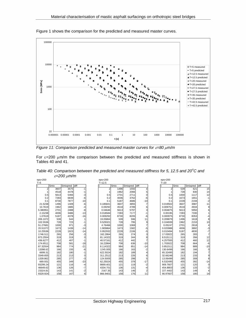
Material characterisation of mastic asphalt surfacings on orthotropic steel bridges
Section Highway Engineering 217
Figure 1 shows the comparison for the predicted and measured master curves.
10
100
1000
10000
100000
0.000001 0.00001 0.0001 0.001 0.01 0.1 1 10 100 1000 10000 100000
t [s]
Sm
ix [
MP
a]
T=5 measured
T=5 predicted
T=12.5 measured
T=12.5 predicted
T=20 measured
T=20 predicted
T=27.5 measured
T=27.5 predicted
T=35 measured
T=35 predicted
T=42.5 measured
T=42.5 predicted
Figure 11: Comparison predicted and measured master curves for =80 m/m
For =200 m/m the comparison between the predicted and measured stiffness is shown in Tables 40 and 41. Table 40: Comparison between the predicted and measured stiffness for 5, 12.5 and 20
oC and
=200 m/m eps=200 eps=200 eps=200
T=5 T=12.5 T=20
t Smix Smixpred diff t Smix Smixpred diff t Smix Smixpred diff
2 3607 3575 -1 2 1496 1550 4 2 539 621 15
1 4518 4478 -1 1 1962 2066 5 1 728 830 14
0.5 5613 5466 -3 0.5 2701 2711 0 0.5 1000 1117 12
0.2 7283 6839 -6 0.2 4006 3762 -6 0.2 1673 1651 -1
0.1 8730 7877 -10 0.1 5187 4686 -10 0.1 2228 2194 -2
21.5238 1496 1409 -6 0.185841 3607 3855 7 0.019502 3607 3987 11
10.7619 1962 1885 -4 0.09292 4518 4789 6 0.009751 4518 4934 9
5.380951 2701 2488 -8 0.04646 5613 5797 3 0.004875 5613 5950 6
2.15238 4006 3486 -13 0.018584 7283 7177 -1 0.00195 7283 7330 1
1.07619 5187 4378 -16 0.009292 8730 8205 -6 0.000975 8730 8353 -4
205.1072 539 544 1 19.05864 539 596 11 0.209879 1496 1618 8
102.5536 728 723 -1 9.529321 728 795 9 0.104939 1962 2153 10
51.27681 1000 971 -3 4.76466 1000 1069 7 0.05247 2701 2818 4
20.51072 1673 1439 -14 1.905864 1673 1582 -5 0.020988 4006 3892 -3
10.25536 2228 1923 -14 0.952932 2228 2106 -5 0.010494 5187 4830 -7
1746.511 265 256 -3 162.2864 265 274 3 17.03022 265 283 7
873.2554 319 319 0 81.14322 319 344 8 8.515111 319 356 12
436.6277 412 407 -1 40.57161 412 442 7 4.257555 412 460 12
174.6511 708 581 -18 16.22864 708 636 -10 1.703022 708 664 -6
87.32554 984 774 -21 8.114322 984 851 -14 0.851511 984 889 -10
13398.62 166 155 -6 1245.005 166 163 -2 130.6499 166 166 0
6699.31 182 180 -1 622.5024 182 189 4 65.32495 182 194 7
3349.655 213 213 0 311.2512 213 226 6 32.66248 213 233 9
1339.862 285 277 -3 124.5005 285 298 5 13.06499 285 308 8
669.931 455 349 -23 62.25024 455 378 -17 6.532495 455 392 -14
93299.24 121 116 -4 8669.401 121 119 -2 909.7607 121 120 0
46649.62 136 126 -7 4334.701 136 131 -4 454.8803 136 133 -2
23324.81 143 141 -2 2167.35 143 146 2 227.4402 143 149 4
9329.924 158 167 6 866.9401 158 176 11 90.97607 158 180 14

Material characterisation of mastic asphalt surfacings on orthotropic steel bridges
Section Highway Engineering 218
Table 41: Comparison between the predicted and measured stiffness for 27.5, 35 and 42.5oC
and =200 m/m eps=200 eps=200 eps=200
T=27.5 T=35 T=42.5
t Smix Smixpred diff t Smix Smixpred diff t Smix Smixpred diff
2 265 282 6 2 166 162 -3 2 121 116 -4
1 319 355 11 1 182 188 4 1 136 126 -7
0.5 412 458 11 0.5 213 225 6 0.5 143 140 -2
0.2 708 661 -7 0.2 285 296 4 0.2 158 167 6
0.1 984 885 -10 0.1 455 375 -18 4.28728E-05 3607 3562 -1
0.00229 3607 3974 10 0.000299 3607 3826 6 2.14364E-05 4518 4463 -1
0.001145 4518 4919 9 0.000149 4518 4757 5 1.07182E-05 5613 5450 -3
0.000573 5613 5934 6 7.46E-05 5613 5763 3 4.28728E-06 7283 6823 -6
0.000229 7283 7315 0 2.99E-05 7283 7142 -2 2.14364E-06 8730 7861 -10
0.000115 8730 8338 -4 1.49E-05 8730 8172 -6 0.000461393 1496 1403 -6
0.024648 1496 1611 8 0.003213 1496 1535 3 0.000230696 1962 1877 -4
0.012324 1962 2144 9 0.001606 1962 2047 4 0.000115348 2701 2478 -8
0.006162 2701 2807 4 0.000803 2701 2688 0 4.61393E-05 4006 3473 -13
0.002465 4006 3879 -3 0.000321 4006 3734 -7 2.30696E-05 5187 4363 -16
0.001232 5187 4815 -7 0.000161 5187 4654 -10 0.004396761 539 542 1
0.234877 539 619 15 0.030616 539 590 10 0.00219838 728 720 -1
0.117438 728 827 14 0.015308 728 787 8 0.00109919 1000 967 -3
0.058719 1000 1112 11 0.007654 1000 1059 6 0.000439676 1673 1432 -14
0.023488 1673 1644 -2 0.003062 1673 1567 -6 0.000219838 2228 1915 -14
0.011744 2228 2185 -2 0.001531 2228 2087 -6 0.037438905 265 255 -4
15.3433 166 166 0 0.2607 265 272 3 0.018719452 319 318 0
7.671651 182 194 6 0.13035 319 341 7 0.009359726 412 405 -2
3.835825 213 232 9 0.065175 412 439 6 0.00374389 708 578 -18
1.53433 285 307 8 0.02607 708 630 -11 0.001871945 984 771 -22
0.767165 455 391 -14 0.013035 984 843 -14 0.287218201 166 155 -7
106.8407 121 120 -1 13.92669 121 119 -2 0.143609101 182 179 -1
53.42037 136 132 -3 6.963347 136 130 -4 0.07180455 213 212 0
26.71018 143 149 4 3.481674 143 146 2 0.02872182 285 277 -3
10.68407 158 179 13 1.392669 158 175 11 0.01436091 455 348 -24
The predicted and measured master curves for =200 m/m are compared in figure 2.
10
100
1000
10000
100000
0.000001 0.00001 0.0001 0.001 0.01 0.1 1 10 100 1000 10000 100000
t [s]
Sm
ix [
MP
a]
T=5 measured
T=5 predicted
T=12.5 measured
T=12.5 predicted
T=20 measured
T=20 predicted
T=27.5 measured
T=27.5 predicted
T=35 measured
T=35 predicted
T=42.5 measured
T=42.5 predicted
Figure 2: Comparison predicted and measured master curves for =200 m/m
For =600 m/m the comparison between the predicted and measured stiffness is shown in Tables 42 and 43.

Material characterisation of mastic asphalt surfacings on orthotropic steel bridges
Section Highway Engineering 219
Table 42: Comparison between the predicted and measured stiffness for 5, 12.5 and 20oC and
=600 m/m eps=600 eps=600 eps=600
T=5 T=12.5 T=20
t Smix Smixpred diff t Smix Smixpred diff t Smix Smixpred diff
2 2786 2736 -2 2 930 1102 18 2 367 408 11
1 3629 3517 -3 1 1287 1503 17 1 500 561 12
0.5 4706 4410 -6 0.5 1786 2019 13 0.5 728 774 6
0.2 6681 5721 -14 0.2 2796 2895 4 0.2 1312 1180 -10
0.1 8601 6772 -21 0.1 3903 3702 -5 0.1 1792 1605 -10
21.5238 930 995 7 0.185841 2786 2975 7 0.019502 2786 3088 11
10.7619 1287 1361 6 0.09292 3629 3794 5 0.009751 3629 3924 8
5.380951 1786 1839 3 0.04646 4706 4718 0 0.004875 4706 4862 3
2.15238 2796 2661 -5 0.018584 6681 6057 -9 0.00195 6681 6212 -7
1.07619 3903 3428 -12 0.009292 8601 7115 -17 0.000975 8601 7272 -15
205.1072 367 353 -4 19.05864 367 390 6 0.05247 1786 2106 18
102.5536 500 483 -3 9.529321 500 535 7 0.020988 2796 3007 8
51.27681 728 665 -9 4.76466 728 738 1 0.010494 3903 3830 -2
1746.511 149 149 0 162.2864 149 162 9 17.03022 149 168 13
873.2554 197 193 -2 81.14322 197 211 7 8.515111 197 219 11
436.6277 271 255 -6 40.57161 271 280 3 4.257555 271 293 8
13398.62 84 81 -4 1245.005 84 86 2 130.6499 84 88 5
6699.31 102 97 -5 622.5024 102 104 2 65.32495 102 107 5
3349.655 125 120 -4 311.2512 125 129 3 32.66248 125 133 7
93299.24 60 55 -9 8669.401 60 57 -5 909.7607 60 58 -4
46649.62 62 62 0 4334.701 62 64 4 454.8803 62 66 6
23324.81 77 71 -8 2167.35 77 75 -3 227.4402 77 77 0 Table 43: Comparison between the predicted and measured stiffness for 27.5, 35 and 42.5
oC and =600
m/m eps=600 eps=600 eps=600
T=27.5 T=35 T=42.5
t Smix Smixpred diff t Smix Smixpred diff t Smix Smixpred diff
2 149 167 12 2 84 85 1 2 60 55 -9
1 197 218 11 1 102 103 1 1 62 62 -1
0.5 271 291 8 0.5 125 128 2 0.5 77 71 -8
0.2 490 437 -11 0.000299 2786 2950 6 4.28728E-05 2786 2725 -2
0.00229 2786 3077 10 0.000149 3629 3765 4 2.14364E-05 3629 3504 -3
0.001145 3629 3911 8 7.46E-05 4706 4686 0 1.07182E-05 4706 4395 -7
0.000573 4706 4847 3 2.99E-05 6681 6023 -10 4.28728E-06 6681 5705 -15
0.000229 6681 6196 -7 0.003213 930 1090 17 2.14364E-06 8601 6755 -21
0.000115 8601 7256 -16 0.001606 1287 1488 16 0.000461393 930 990 6
0.002465 2796 2995 7 0.000803 1786 2000 12 0.000230696 1287 1355 5
0.001232 3903 3817 -2 0.000321 2796 2871 3 0.000115348 1786 1831 3
0.234877 367 407 11 0.000161 3903 3673 -6 4.61393E-05 2796 2650 -5
0.117438 500 558 12 0.030616 367 386 5 2.30696E-05 3903 3416 -12
0.058719 728 770 6 0.015308 500 529 6 0.004396761 367 351 -4
0.023488 1312 1174 -11 0.007654 728 730 0 0.00219838 500 480 -4
0.011744 1792 1597 -11 0.2607 149 160 8 0.00109919 728 662 -9
15.3433 84 88 4 0.13035 197 209 6 0.037438905 149 149 0
7.671651 102 107 5 0.065175 271 277 2 0.018719452 197 192 -2
3.835825 125 133 6 0.02607 490 415 -15 0.009359726 271 254 -6
106.8407 60 58 -4 13.92669 60 57 -6 0.287218201 84 81 -4
53.42037 62 66 6 6.963347 62 64 4 0.143609101 102 97 -5
26.71018 77 76 -1 3.481674 77 74 -3 0.07180455 125 119 -4
The predicted and measured master curves for =600 m/m are compared in figure 3.

Material characterisation of mastic asphalt surfacings on orthotropic steel bridges
Section Highway Engineering 220
10
100
1000
10000
100000
0.000001 0.00001 0.0001 0.001 0.01 0.1 1 10 100 1000 10000 100000
t [s]
Sm
ix [
MP
a]
T=5 measured
T=5 predicted
T=12.5 measured
T=12.5 predicted
T=20 measured
T=20 predicted
T=27.5 measured
T=27.5 predicted
T=35 measured
T=35 predicted
T=42.5 measured
T=42.5 predicted
Figure 3: Comparison predicted and measured master curves for =600 m/m
Finally, the predicted and measured stiffness at a strain level of 1000 m/m is compared in Tables 44 and 45. Table 44: Comparison between the predicted and measured stiffness for 5, 12.5 and 20
oC and
=1000 m/m eps=1000 eps=1000 eps=1000
T=5 T=12.5 T=20
t Smix Smixpred diff t Smix Smixpred diff t Smix Smixpred diff
2 2113 2410 14 0.5 1418 1759 24 2 279 344 23
1 2851 3135 10 0.2 2296 2556 11 1 399 475 19
0.5 3945 3983 1 0.1 3435 3308 -4 0.5 588 659 12
0.2 6339 5271 -17 0.185841 2113 2630 24 0.2 921 1014 10
10.7619 1006 1173 17 0.09292 2851 3396 19 0.1 1446 1388 -4
5.380951 1418 1597 13 0.04646 3945 4282 9 0.019502 2113 2735 29
2.15238 2296 2341 2 0.018584 6339 5608 -12 0.009751 2851 3519 23
1.07619 3435 3052 -11 0.009292 8259 6692 -19 0.004875 3945 4422 12
205.1072 279 296 6 19.05864 279 328 17 0.00195 6339 5764 -9
102.5536 399 408 2 9.529321 399 453 13 0.000975 8259 6856 -17
51.27681 588 565 -4 4.76466 588 628 7 0.05247 1418 1837 30
20.51072 921 871 -5 1.905864 921 967 5 0.020988 2296 2659 16
10.25536 1446 1199 -17 0.952932 1446 1327 -8 0.010494 3435 3430 0
1746.511 115 121 5 162.2864 115 132 14 17.03022 115 137 19
873.2554 151 158 5 81.14322 151 174 15 8.515111 151 181 20
436.6277 241 212 -12 40.57161 241 233 -3 4.257555 241 244 1
13398.62 56 63 12 1245.005 56 67 19 130.6499 56 69 23
6699.31 70 77 9 622.5024 70 82 17 65.32495 70 85 21
93299.24 42 40 -4 8669.401 42 42 0 909.7607 42 43 2
46649.62 51 46 -9 4334.701 51 49 -5 454.8803 51 50 -2

Material characterisation of mastic asphalt surfacings on orthotropic steel bridges
Section Highway Engineering 221
Table 45: Comparison between the predicted and measured stiffness for 27.5, 35 and 42.5oC and
=1000 m/m eps=1000 eps=1000 eps=1000
T=27.5 T=35 T=42.5
t Smix Smixpred diff t Smix Smixpred diff t Smix Smixpred diff
2 115 136 19 2 56 66 18 2 42 40 -4
1 151 180 19 1 70 82 17 1 51 46 -9
0.5 241 243 1 0.000299 2113 2607 23 4.28728E-05 2113 2400 14
0.00229 2113 2724 29 0.000149 2851 3368 18 2.14364E-05 2851 3123 10
0.001145 2851 3506 23 7.46E-05 3945 4251 8 1.07182E-05 3945 3970 1
0.000573 3945 4408 12 2.99E-05 6339 5573 -12 4.28728E-06 6339 5255 -17
0.000229 6339 5749 -9 1.49E-05 8259 6656 -19 0.000230696 1006 1168 16
0.000115 8259 6839 -17 0.000803 1418 1742 23 0.000115348 1418 1590 12
0.006162 1418 1829 29 0.000321 2296 2534 10 4.61393E-05 2296 2331 2
0.002465 2296 2649 15 0.000161 3435 3282 -4 2.30696E-05 3435 3040 -11
0.001232 3435 3418 -1 0.030616 279 324 16 0.004396761 279 294 6
0.234877 279 342 23 0.015308 399 448 12 0.00219838 399 406 2
0.117438 399 473 18 0.007654 588 622 6 0.00109919 588 562 -4
0.058719 588 656 12 0.003062 921 956 4 0.000439676 921 867 -6
0.023488 921 1009 10 0.001531 1446 1313 -9 0.000219838 1446 1193 -17
0.011744 1446 1382 -4 0.2607 115 131 14 0.037438905 115 121 5
15.3433 56 69 22 0.13035 151 172 14 0.018719452 151 158 4
7.671651 70 85 21 0.065175 241 231 -4 0.009359726 241 211 -13
106.8407 42 43 2 13.92669 42 42 0 0.287218201 56 63 12
53.42037 51 50 -3 6.963347 51 48 -5 0.143609101 70 76 9
The master curves for =1000 m/m are compared in figure 4.
10
100
1000
10000
100000
0.000001 0.00001 0.0001 0.001 0.01 0.1 1 10 100 1000 10000 100000
t [s]
Sm
ix [
MP
a]
T=5 measured
T=5 predicted
T=12.5 measured
T=12.5 predicted
T=20 measured
T=20 predicted
T=27.5 measured
T=27.5 predicted
T=35 measured
T=35 predicted
T=42.5 measured
T=42.5 predicted
Figure 4: Comparison predicted and measured master curves for =1000m/m

Material characterisation of mastic asphalt surfacings on orthotropic steel bridges
Section Highway Engineering 222
Appendix D: Nomographs
This appendix presents fatigue design nomographs for loading speeds of 1, 11, 54 and 108 km/h. They are shown in figures 1, 2, 3 and 4.
100
1000
10000
10 100 1000 10000 100000Smix [MPa]
[
m/m
] N=1*102
N=1*103
N=1*104
N=1*105
N=1*106
N=1*107
N=1*108
v=1 km/h
0
5
10
15
20
25
30
35
40
45
50
T [
oC
]
802006001000 400
[m/m]
Figure 1: Fatigue design nomograph for 1 km/h

Material characterisation of mastic asphalt surfacings on orthotropic steel bridges
Section Highway Engineering 223
Figure 2: Fatigue design nomograph for 11 km/h

Material characterisation of mastic asphalt surfacings on orthotropic steel bridges
Section Highway Engineering 224
100
1000
10000
100 1000 10000 100000Smix [MPa]
[
m/m
]
N=1*102
N=1*103
N=1*104
N=1*105
N=1*106
N=1*107
N=1*108
v=54 km/h
0
5
10
15
20
25
30
35
40
45
50
T [
oC
]
802006001000 400
[m/m]
Figure 3: Fatigue design nomograph for 54 km/h

Material characterisation of mastic asphalt surfacings on orthotropic steel bridges
Section Highway Engineering 225
v=108 km/h
0
5
10
15
20
25
30
35
40
45
50
T [
oC
]
802006001000 400
[m/m]
100
1000
10000
100 1000 10000 100000Smix [MPa]
[
m/m
]
N=1*102
N=1*103
N=1*104
N=1*105
N=1*106
N=1*107
N=1*108
Figure 4: Fatigue design nomograph for 108 km/h
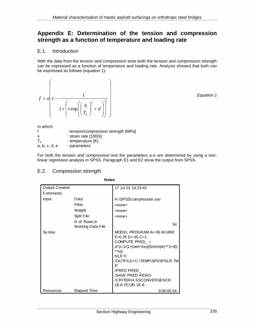
Material characterisation of mastic asphalt surfacings on orthotropic steel bridges
Section Highway Engineering 226
Appendix E: Determination of the tension and compression strength as a function of temperature and loading rate
E.1. Introduction With the data from the tension and compression tests both the tension and compression strength can be expressed as a function of temperature and loading rate. Analysis showed that both can be expressed as follows (equation 1):
e
k
dT
bv
caf2
exp1
1
Equation 1
in which: f : tension/compression strength [MPa] v : strain rate [100/s] Tk : temperature [K] a, b, c, d, e : parameters For both the tension and compression test the parameters a-e are determined by using a non-linear regression analysis in SPSS. Paragraph E1 and E2 show the output from SPSS.
E.2. Compression strength
Notes
17 Jul 01 14:23:42
H:\SPSS\compression.sav
<none>
<none>
<none>
54
MODEL PROGRAM A=-95 B=1800
E=0.35 D=-45 C=1 .
COMPUTE PRED_ =
a*(c-1/(1+(rate*exp((b/tempk)**2+d))
**e)).
NLR f t
/OUTFILE='C:\TEMP\SPSSFNLR.TM
P'
/PRED PRED_
/SAVE PRED RESID
/CRITERIA SSCONVERGENCE
1E-8 PCON 1E-8 .
0:00:00.54
Output Created
Comments
Data
Filter
Weight
Split File
N of Rows in
Working Data File
Input
Sy ntax
Elapsed TimeResources

Material characterisation of mastic asphalt surfacings on orthotropic steel bridges
Section Highway Engineering 227
All the derivatives will be calculated numerically.
Run stopped after 10 model evaluations and 5 derivative evaluations.
Iterations have been stopped because the relative reduction between
successive
residual sums of squares is at most SSCON = 1.000E-08
Nonlinear Regression Summary Statistics Dependent Variable FT
Source DF Sum of Squares Mean Square
Regression 5 2246.97351 449.39470
Residual 8 .84129 .10516
Uncorrected Total 13 2247.81480
(Corrected Total) 12 876.05083
R squared = 1 - Residual SS / Corrected SS = .99904
Asymptotic 95 %
Asymptotic Confidence Interval
Parameter Estimate Std. Error Lower Upper
A -50.66874508 6.716490664 -66.15700032 -35.18048983
B 1812.6438466 54.270704121 1687.4953785 1937.7923147
E .354577057 .041769480 .258256464 .450897649
D -45.02278207 2.899620308 -51.70931849 -38.33624565
C 1.022098411 .010195473 .998587608 1.045609213
Asymptotic Correlation Matrix of the Parameter Estimates
A B E D C
A 1.0000 -.3404 .8677 .5441 .8675
B -.3404 1.0000 -.7322 -.9738 -.3259
E .8677 -.7322 1.0000 .8608 .8328
D .5441 -.9738 .8608 1.0000 .4906
C .8675 -.3259 .8328 .4906 1.0000

Material characterisation of mastic asphalt surfacings on orthotropic steel bridges
Section Highway Engineering 228
E.3. Tension strength
Notes
17 Jul 01 13:51:11
H:\SPSS\tensiongoed.sav
<none>
<none>
<none>
54
MODEL PROGRAM A=-95 B=1800
C=1 D=-45 E=0.35 .
COMPUTE PRED_ =
a*(c-1/(1+(rate*exp((b/tempk)**2+d))
**e)).
NLR f t
/OUTFILE='C:\TEMP\SPSSFNLR.TM
P'
/PRED PRED_
/SAVE PRED RESID
/CRITERIA SSCONVERGENCE
1E-8 PCON 1E-8 .
0:00:00.75
Output Created
Comments
Data
Filter
Weight
Split File
N of Rows in
Working Data File
Input
Sy ntax
Elapsed TimeResources
All the derivatives will be calculated numerically.
Run stopped after 69 model evaluations and 32 derivative evaluations.
Iterations have been stopped because the relative reduction between
successive
residual sums of squares is at most SSCON = 1.000E-08
Nonlinear Regression Summary Statistics Dependent Variable FT
Source DF Sum of Squares Mean Square
Regression 5 344.55951 68.91190
Residual 9 3.34049 .37117
Uncorrected Total 14 347.90000
(Corrected Total) 13 160.65429
R squared = 1 - Residual SS / Corrected SS = .97921
Asymptotic 95 %
Asymptotic Confidence Interval
Parameter Estimate Std. Error Lower Upper
A 12.231241044 2.018784240 7.664433816 16.798048273
B 1655.3789535 99.831090685 1429.5453366 1881.2125704
C 1.039477399 .033230247 .964305357 1.114649441
D -34.88799962 4.495482800 -45.05748824 -24.71851100
E .757772269 .237640660 .220191747 1.295352791

Material characterisation of mastic asphalt surfacings on orthotropic steel bridges
Section Highway Engineering 229
Asymptotic Correlation Matrix of the Parameter Estimates
A B C D E
A 1.0000 .5100 -.6333 -.5816 -.8757
B .5100 1.0000 -.1758 -.9951 -.7824
C -.6333 -.1758 1.0000 .1994 .5594
D -.5816 -.9951 .1994 1.0000 .8250
E -.8757 -.7824 .5594 .8250 1.0000

Material characterisation of mastic asphalt surfacings on orthotropic steel bridges
Section Highway Engineering 230
Appendix F: Determination of N as function of and Smix
The data from the first fatigue test on the Moerdijk mix is used to determine the fatigue relationship as a function of the stiffness and the strain. The relationship is described best with equation 1:
mixSnnaN logloglog 211 Equation 1
The parameters a1, n1 and n2 are determined with a non-linear regression analysis by using SPSS. The output from SPSS is shown below.
Notes
11 Jun 01 11:35:57
<none>
<none>
<none>
6
MODEL PROGRAM A1=1 N1=1
N2=1 .
COMPUTE PRED_ =
+a1+n1*logeps+n2*logsmix.
NLR logn
/OUTFILE='C:\TEMP\SPSSFNLR.TM
P'
/PRED PRED_
/CRITERIA SSCONVERGENCE
1E-8 PCON 1E-8 .
0:00:00.37
Output Created
Comments
Filter
Weight
Split File
N of Rows in
Working Data File
Input
Sy ntax
Elapsed TimeResources
All the derivatives will be calculated numerically.
Iteration Residual SS A1 N1 N2
1 45.78211820 1.00000000 1.00000000 1.00000000
1.1 .0789928294 33.3774389 -7.4391278 -2.0857776
2 .0789928294 33.3774389 -7.4391278 -2.0857776
2.1 .0789928294 33.3774209 -7.4391262 -2.0857738
Run stopped after 4 model evaluations and 2 derivative evaluations.
Iterations have been stopped because the relative reduction between
successive
residual sums of squares is at most SSCON = 1.000E-08

Material characterisation of mastic asphalt surfacings on orthotropic steel bridges
Section Highway Engineering 231
Nonlinear Regression Summary Statistics Dependent Variable LOGN
Source DF Sum of Squares Mean Square
Regression 3 152.35149 50.78383
Residual 3 .07899 .02633
Uncorrected Total 6 152.43048
(Corrected Total) 5 7.14033
R squared = 1 - Residual SS / Corrected SS = .98894
Asymptotic 95 %
Asymptotic Confidence Interval
Parameter Estimate Std. Error Lower Upper
A1 33.377420889 12.988055801 -7.956369306 74.711211085
N1 -7.439126227 1.044463165 -10.76307417 -4.115178287
N2 -2.085773802 2.848541200 -11.15110322 6.979555616
Asymptotic Correlation Matrix of the Parameter Estimates
A1 N1 N2
A1 1.0000 -.9505 -.9960
N1 -.9505 1.0000 .9190
N2 -.9960 .9190 1.0000

Material characterisation of mastic asphalt surfacings on orthotropic steel bridges
Section Highway Engineering 232
Appendix G: Determination of dilation as a function of strain rate and temperature
Analyses showed that the relationship between dilation, temperature and strain rate is best described with:
d
k
dilation
cT
b
a2
exp1
11
Equation 1
in which:
dilation : stress at the onset of dilation [MPa]
: strain rate [x100/s]
Tk : temperature [K] a, b, c ,d : constants The constants a-d are determined with a non-linear regression analysis in SPSS. The output is shown below. All the derivatives will be calculated numerically.
Run stopped after 14 model evaluations and 7 derivative evaluations.
Iterations have been stopped because the relative reduction between
successive
residual sums of squares is at most SSCON = 1.000E-08
Nonlinear Regression Summary Statistics Dependent Variable SIGMA
Source DF Sum of Squares Mean Square
Regression 4 1360.02910 340.00727
Residual 9 .69455 .07717
Uncorrected Total 13 1360.72365
(Corrected Total) 12 933.08517
R squared = 1 - Residual SS / Corrected SS = .99926
Asymptotic 95 %
Asymptotic Confidence Interval
Parameter Estimate Std. Error Lower Upper
A -42.61158964 2.103272706 -47.36952306 -37.85365623
B 1841.5436469 41.350556128 1748.0021902 1935.0851036
C -46.06791961 2.007463039 -50.60911650 -41.52672272
D .581261792 .030522390 .512215348 .650308235

Material characterisation of mastic asphalt surfacings on orthotropic steel bridges
Section Highway Engineering 233
Asymptotic Correlation Matrix of the Parameter Estimates
A B C D
A 1.0000 -.0508 .1451 .5937
B -.0508 1.0000 -.9954 -.7808
C .1451 -.9954 1.0000 .8312
D .5937 -.7808 .8312 1.0000

Material characterisation of mastic asphalt surfacings on orthotropic steel bridges
Section Highway Engineering 234
Appendix H: Determination of 0 as a function of strain rate and temperature
Analyses showed that the relationship between 0, temperature and strain rate is best described with:
d
k
cT
b
a2
0
exp1
11
Equation 1
in which:
0 : the initial value (material parameter)
: strain rate [x100/s]
Tk : temperature [K] a, b, c ,d : constants The constants a-d are determined with a non-linear regression analysis in SPSS. The output is shown below. All the derivatives will be calculated numerically.
The following new variables are being created:
Name Label
PRED_ Predicted Values
RESID Residuals
Run stopped after 347 model evaluations and 164 derivative evaluations.
Iterations have been stopped because the relative reduction between
successive
residual sums of squares is at most SSCON = 1.000E-08
Nonlinear Regression Summary Statistics Dependent Variable ALFA
Source DF Sum of Squares Mean Square
Regression 4 .03577 8.942851E-03
Residual 8 1.662827E-06 2.078534E-07
Uncorrected Total 12 .03577
(Corrected Total) 11 .02199

Material characterisation of mastic asphalt surfacings on orthotropic steel bridges
Section Highway Engineering 235
R squared = 1 - Residual SS / Corrected SS = .99992
Asymptotic 95 %
Asymptotic Confidence Interval
Parameter Estimate Std. Error Lower Upper
A .104217949 .000449987 .103180278 .105255620
B 1382.1151026 42.713812618 1283.6168741 1480.6133311
D -22.72272379 1.266721780 -25.64378945 -19.80165813
E -2.234448588 .203571604 -2.703885549 -1.765011627
Asymptotic Correlation Matrix of the Parameter Estimates
A B D E
A 1.0000 .7544 -.7523 .7783
B .7544 1.0000 -1.0000 .9916
D -.7523 -1.0000 1.0000 -.9913
E .7783 .9916 -.9913 1.0000