BSc Thesis - TU Delft Repositories
99
BSc Thesis DC Grid Design Paul Kluge Jesse Richter Group O Distribution of the electricity grid of a tiny house com munity
-
Upload
khangminh22 -
Category
Documents
-
view
16 -
download
0
Transcript of BSc Thesis - TU Delft Repositories

BSc ThesisDC Grid DesignPaul KlugeJesse RichterGroup ODistribution of the electricity grid of a tiny house community

BSc ThesisDC Grid Design
by
Paul KlugeJesse Richter
Students: P.M. Kluge 4915593J.O. Richter 4862236
Project duration: April 19, 2021 – July 2, 2021To be defended on: June 28th, 2021Thesis committee: Dr. R.A.C.M.M. van Swaaij, chair
Dr. P.P. Vergara Barrios, supervisorDr. M. TaouilDr. S. Du

AbstractThis thesis covers the toplevel design of a DC microgrid of a tiny house community on the roof ofa highrise building in Rotterdam. This DC microgrid consists of 12 tiny houses, a common usagearea, Renewable Energy Supply (RES) methods, using solar and wind energy, and an Energy Storagesystem (ESS). This design is part of a complete DC smart grid for such a community with two othersubgroups focusing on the control and software, the CNS group, and power line communication, thePLC group.In this thesis, three design phases are discussed; demand estimation, storage & supply design, andtopology design. Subsequently, the resulting grid design is validated. The first phase resulted in anestimation of hourly, daily, and monthly energy usage. Using a model of the generation, 61.2𝑚2 PhotoVoltaic (PV) panels and 6 Vertical Axis Wind Turbines (VAWT)s were selected. In order to handle thevarying energy generation of the RESs, different ESS options are considered, and 4 LiIon batteriesare chosen. This combination of storage and supply resulted in a grid availability of 93.73%. In thelast design phase, the topology of the community is designed, which resulted in a 400 VDC unipolarringbased seriesconnected multibus configuration, which effectively operates in radial form to reduce complexity and enables easier fault location detection. The topology design also considers theconverter requirements, wiring, and stability and safety considerations. A cost analysis is made ofthe entire grid resulting in an estimated total cost of around €100,000. Lastly, design verification isperformed on the proposed design, which resulted in functional results during 100% demand, with amaximum voltage drop of 1.82% and during 150% demand, with a maximum voltage drop of 2.80%.
i

PrefaceThe basis for this research stems from an initial minor project of one of our colleagues, Pieter vanSantvliet. Our interest in sustainability and our background in electrical engineering motivated us tocontinue his project. Without our four highly motivated colleagues who tackled two other essential aspects of the design, this project would not have been possible.
Our special thanks goes to our motivated and openminded supervisor, Dr. P.P. Vergara Barrios, whowas always able to guide us and propose alternatives during times of difficulty.
We would like to thank our thesis committee consisting of the chair Dr. R. van der Swaaij, our supervisor Dr. P. P. Vergara Barrios, Dr. M. Taouil, and Dr. S. Du.
Furthermore, we would like to express our gratitude to Dr. A. Lekić who was able to help us tremendously during the design validation.
Our thanks also go to J. Antonisse and A. Mensink for answering our large number of initial questionsand giving us a perspective on usage, generation, and storage in a tiny house community.We would like to also thank T. Tajiri for providing us with anonymous monthly energy usage data fromseveral houses in the ’Minitopia’ tiny house community.
Additionally, we would like to thank the residents of the tiny house communities ’Pionierskwartier’ inDelft and ’Minitopia’ near Den Bosch for their cooperation in our surveys.
Lastly, we would like to thank Dr. I.E. Lager for the excellent organization and fluency during the COVID19 pandemic of the Bachelor Graduation Project, as well as his willingness to answer all our questionsregarding the project.
Paul Kluge and Jesse RichterDelft, June 2021
ii

Contents
Abstract i
Preface ii
1 Introduction 11.1 Tunus . . . . . . . . . . . . . . . . . . . . . . . . . . . . . . . . . . . . . . . . . . . . . . 11.2 Microgrid Analysis . . . . . . . . . . . . . . . . . . . . . . . . . . . . . . . . . . . . . . . 11.3 Problem Definition . . . . . . . . . . . . . . . . . . . . . . . . . . . . . . . . . . . . . . . 21.4 Subdivision . . . . . . . . . . . . . . . . . . . . . . . . . . . . . . . . . . . . . . . . . . . 21.5 Thesis Outline . . . . . . . . . . . . . . . . . . . . . . . . . . . . . . . . . . . . . . . . . 3
2 Program of Requirements 4
3 Energy Demand Estimation 63.1 Initial Calculations . . . . . . . . . . . . . . . . . . . . . . . . . . . . . . . . . . . . . . . 6
3.1.1 Tiny House Calculations . . . . . . . . . . . . . . . . . . . . . . . . . . . . . . . . 63.1.2 Tunect Calculations . . . . . . . . . . . . . . . . . . . . . . . . . . . . . . . . . . 8
3.2 Demand Modifications . . . . . . . . . . . . . . . . . . . . . . . . . . . . . . . . . . . . . 83.2.1 Appliance Selection Based on Tiny House Users. . . . . . . . . . . . . . . . . . . 83.2.2 The Effect of DC Appliances . . . . . . . . . . . . . . . . . . . . . . . . . . . . . . 93.2.3 Limiting Peak Demand . . . . . . . . . . . . . . . . . . . . . . . . . . . . . . . . . 93.2.4 Final Demand Estimation Results . . . . . . . . . . . . . . . . . . . . . . . . . . . 10
3.3 Tiny House Demand Models . . . . . . . . . . . . . . . . . . . . . . . . . . . . . . . . . . 103.3.1 Model of One Day & Results . . . . . . . . . . . . . . . . . . . . . . . . . . . . . . 103.3.2 Model of One Year & Results . . . . . . . . . . . . . . . . . . . . . . . . . . . . . 11
4 Supply & Storage Design 134.1 Renewable Energy Sources . . . . . . . . . . . . . . . . . . . . . . . . . . . . . . . . . . 13
4.1.1 The Heat Grid. . . . . . . . . . . . . . . . . . . . . . . . . . . . . . . . . . . . . . 134.1.2 PV . . . . . . . . . . . . . . . . . . . . . . . . . . . . . . . . . . . . . . . . . . . . 144.1.3 Wind Turbines . . . . . . . . . . . . . . . . . . . . . . . . . . . . . . . . . . . . . 154.1.4 Supply Models & Results. . . . . . . . . . . . . . . . . . . . . . . . . . . . . . . . 15
4.2 The Energy Storage System . . . . . . . . . . . . . . . . . . . . . . . . . . . . . . . . . . 174.2.1 ESS choice . . . . . . . . . . . . . . . . . . . . . . . . . . . . . . . . . . . . . . . 174.2.2 Centralised ESS Model & Results . . . . . . . . . . . . . . . . . . . . . . . . . . . 184.2.3 Distributed ESS Model & Results . . . . . . . . . . . . . . . . . . . . . . . . . . . 184.2.4 System Comparison & Selection . . . . . . . . . . . . . . . . . . . . . . . . . . . 19
5 Topology Design 205.1 Microgrid Topology . . . . . . . . . . . . . . . . . . . . . . . . . . . . . . . . . . . . . . . 20
5.1.1 Bus Topology . . . . . . . . . . . . . . . . . . . . . . . . . . . . . . . . . . . . . . 205.1.2 Microgrid Layout . . . . . . . . . . . . . . . . . . . . . . . . . . . . . . . . . . . . 215.1.3 Converters & Control . . . . . . . . . . . . . . . . . . . . . . . . . . . . . . . . . . 225.1.4 Wiring . . . . . . . . . . . . . . . . . . . . . . . . . . . . . . . . . . . . . . . . . . 23
5.2 Nanogrid Topology . . . . . . . . . . . . . . . . . . . . . . . . . . . . . . . . . . . . . . . 235.2.1 Bus topology & Nanogrid Layout . . . . . . . . . . . . . . . . . . . . . . . . . . . 235.2.2 Converters & Control . . . . . . . . . . . . . . . . . . . . . . . . . . . . . . . . . . 245.2.3 Wiring . . . . . . . . . . . . . . . . . . . . . . . . . . . . . . . . . . . . . . . . . . 25
iii

Contents iv
5.3 Stability . . . . . . . . . . . . . . . . . . . . . . . . . . . . . . . . . . . . . . . . . . . . . 265.3.1 Polarity of the voltage bus . . . . . . . . . . . . . . . . . . . . . . . . . . . . . . . 265.3.2 Grounding. . . . . . . . . . . . . . . . . . . . . . . . . . . . . . . . . . . . . . . . 265.3.3 Fault Detection & Protection . . . . . . . . . . . . . . . . . . . . . . . . . . . . . . 275.3.4 Voltage stability . . . . . . . . . . . . . . . . . . . . . . . . . . . . . . . . . . . . . 28
5.4 Safety . . . . . . . . . . . . . . . . . . . . . . . . . . . . . . . . . . . . . . . . . . . . . . 285.4.1 Standards . . . . . . . . . . . . . . . . . . . . . . . . . . . . . . . . . . . . . . . . 285.4.2 Human interaction . . . . . . . . . . . . . . . . . . . . . . . . . . . . . . . . . . . 29
5.5 Cost Analysis . . . . . . . . . . . . . . . . . . . . . . . . . . . . . . . . . . . . . . . . . . 29
6 Design Validation 306.1 Models of each subsystem. . . . . . . . . . . . . . . . . . . . . . . . . . . . . . . . . . . 30
6.1.1 Demand . . . . . . . . . . . . . . . . . . . . . . . . . . . . . . . . . . . . . . . . . 306.1.2 PV panel module . . . . . . . . . . . . . . . . . . . . . . . . . . . . . . . . . . . . 306.1.3 Wind turbine . . . . . . . . . . . . . . . . . . . . . . . . . . . . . . . . . . . . . . 316.1.4 Battery / PCC . . . . . . . . . . . . . . . . . . . . . . . . . . . . . . . . . . . . . . 316.1.5 Wiring . . . . . . . . . . . . . . . . . . . . . . . . . . . . . . . . . . . . . . . . . . 316.1.6 Grounding and protection . . . . . . . . . . . . . . . . . . . . . . . . . . . . . . . 316.1.7 Grid layout . . . . . . . . . . . . . . . . . . . . . . . . . . . . . . . . . . . . . . . 31
6.2 Simulation scenarios . . . . . . . . . . . . . . . . . . . . . . . . . . . . . . . . . . . . . . 316.3 Case analysis. . . . . . . . . . . . . . . . . . . . . . . . . . . . . . . . . . . . . . . . . . 32
7 Conclusions and Recommendations 337.1 Conclusions. . . . . . . . . . . . . . . . . . . . . . . . . . . . . . . . . . . . . . . . . . . 337.2 Discussion & Recommendations for Future Work . . . . . . . . . . . . . . . . . . . . . . 33
Acronyms 35
A System PoR 36A.0.1 Functional Requirements. . . . . . . . . . . . . . . . . . . . . . . . . . . . . . . . 36A.0.2 NonFunctional Requirements . . . . . . . . . . . . . . . . . . . . . . . . . . . . . 36
B Demand 37B.1 Appliance selection. . . . . . . . . . . . . . . . . . . . . . . . . . . . . . . . . . . . . . . 37B.2 Initial power and time usage tables . . . . . . . . . . . . . . . . . . . . . . . . . . . . . . 40
B.2.1 Base load . . . . . . . . . . . . . . . . . . . . . . . . . . . . . . . . . . . . . . . . 40B.2.2 Kitchen appliances . . . . . . . . . . . . . . . . . . . . . . . . . . . . . . . . . . . 40B.2.3 Heating . . . . . . . . . . . . . . . . . . . . . . . . . . . . . . . . . . . . . . . . . 41B.2.4 Other appliances . . . . . . . . . . . . . . . . . . . . . . . . . . . . . . . . . . . . 41B.2.5 Tunect usage . . . . . . . . . . . . . . . . . . . . . . . . . . . . . . . . . . . . . . 42
B.3 Interview notes . . . . . . . . . . . . . . . . . . . . . . . . . . . . . . . . . . . . . . . . . 43B.4 Tables after modifications . . . . . . . . . . . . . . . . . . . . . . . . . . . . . . . . . . . 44
B.4.1 Idle appliances . . . . . . . . . . . . . . . . . . . . . . . . . . . . . . . . . . . . . 44B.4.2 Kitchen appliances . . . . . . . . . . . . . . . . . . . . . . . . . . . . . . . . . . . 44B.4.3 Heating . . . . . . . . . . . . . . . . . . . . . . . . . . . . . . . . . . . . . . . . . 45B.4.4 Other appliances . . . . . . . . . . . . . . . . . . . . . . . . . . . . . . . . . . . . 45B.4.5 Tunect usage . . . . . . . . . . . . . . . . . . . . . . . . . . . . . . . . . . . . . . 46
B.5 Daily model . . . . . . . . . . . . . . . . . . . . . . . . . . . . . . . . . . . . . . . . . . . 47B.5.1 Liander Data . . . . . . . . . . . . . . . . . . . . . . . . . . . . . . . . . . . . . . 47B.5.2 Graphs from daily data . . . . . . . . . . . . . . . . . . . . . . . . . . . . . . . . . 47
B.6 Monthly model . . . . . . . . . . . . . . . . . . . . . . . . . . . . . . . . . . . . . . . . . 48
C Supply and Storage 50C.1 Heat Grid Analysis . . . . . . . . . . . . . . . . . . . . . . . . . . . . . . . . . . . . . . . 50C.2 PV Panel Performance Analysis . . . . . . . . . . . . . . . . . . . . . . . . . . . . . . . . 51C.3 KNMI weather data usage . . . . . . . . . . . . . . . . . . . . . . . . . . . . . . . . . . . 52C.4 Other supply model results. . . . . . . . . . . . . . . . . . . . . . . . . . . . . . . . . . . 53C.5 ESS Comparison . . . . . . . . . . . . . . . . . . . . . . . . . . . . . . . . . . . . . . . . 56C.6 Centralised model setup and flowchart . . . . . . . . . . . . . . . . . . . . . . . . . . . . 57

Contents v
C.7 Distributed model setup and flowchart . . . . . . . . . . . . . . . . . . . . . . . . . . . . 58C.8 Centralised model graphs . . . . . . . . . . . . . . . . . . . . . . . . . . . . . . . . . . . 60C.9 Distributed model graphs. . . . . . . . . . . . . . . . . . . . . . . . . . . . . . . . . . . . 61C.10 Battery System Comparison . . . . . . . . . . . . . . . . . . . . . . . . . . . . . . . . . . 62
D Topology 63D.1 Microgrid Topology Analysis . . . . . . . . . . . . . . . . . . . . . . . . . . . . . . . . . . 63D.2 Converter Control Analysis. . . . . . . . . . . . . . . . . . . . . . . . . . . . . . . . . . . 63D.3 Wiring . . . . . . . . . . . . . . . . . . . . . . . . . . . . . . . . . . . . . . . . . . . . . . 65D.4 Stability & Safety . . . . . . . . . . . . . . . . . . . . . . . . . . . . . . . . . . . . . . . . 66
D.4.1 Grounding. . . . . . . . . . . . . . . . . . . . . . . . . . . . . . . . . . . . . . . . 66D.4.2 Standards . . . . . . . . . . . . . . . . . . . . . . . . . . . . . . . . . . . . . . . . 66
D.5 Cost Analysis . . . . . . . . . . . . . . . . . . . . . . . . . . . . . . . . . . . . . . . . . . 67
E Design Validation 69E.1 Subsystem Models . . . . . . . . . . . . . . . . . . . . . . . . . . . . . . . . . . . . . . . 69
E.1.1 Load model . . . . . . . . . . . . . . . . . . . . . . . . . . . . . . . . . . . . . . . 69E.1.2 PV panel model. . . . . . . . . . . . . . . . . . . . . . . . . . . . . . . . . . . . . 70E.1.3 VAWT model . . . . . . . . . . . . . . . . . . . . . . . . . . . . . . . . . . . . . . 71E.1.4 ESS model . . . . . . . . . . . . . . . . . . . . . . . . . . . . . . . . . . . . . . . 72E.1.5 Wiring model and calculations . . . . . . . . . . . . . . . . . . . . . . . . . . . . . 73
E.2 Simulink grid layout. . . . . . . . . . . . . . . . . . . . . . . . . . . . . . . . . . . . . . . 74
F MATLAB code 75F.1 MATLAB Code Centralized Storage Model . . . . . . . . . . . . . . . . . . . . . . . . . . 75F.2 MATLAB Code Distributed Storage Model . . . . . . . . . . . . . . . . . . . . . . . . . . 78F.3 MATLAB Code Design Validation . . . . . . . . . . . . . . . . . . . . . . . . . . . . . . . 84

1Introduction
With climate change being a more pressing matter than ever, many people are looking for ways tominimize their ecological footprint. One of the most effective ways for individuals to reduce their impacton the environment is sustainable living. In the last two decades, sustainable housing has been gainingpopularity with at the forefront of the movement a concept called ’tiny houses’ [1]. According to the USbased International Residential Code (IRC) a tiny house is as a dwelling that has a floor area of lessthan 37 𝑚2 [2]. This description, however, is insufficient as tiny houses can not be described merelyby their size. Tiny houses are commonly designed to achieve efficient use of internal space, greaterenvironmental sustainability and the ability to live offgrid while minimizing possessions [3]. This ismainly achieved by multifunctional interior design, minimizing energy demand, and operating on greenenergy by using Renewable Energy Source (RES)s. As space is scarce, many tiny house users put orbuild their tiny houses in communities to share resources. According to [4], one of the key motivatorsfor people deciding to live in a tiny house is being part of a community. And while these communitiesare connected socially, many of them consist of separately built homes that each have their own energygeneration and storage.Designing a tiny house community that can collaborate on a technical level was the goal of the tunusproject [5].
1.1. TunusIn the tunus project, first, the design of a single tiny house was made. This tiny house was called tunus.Then, the electricity, heat, and water grids of 12 tuni the plural of tunus were connected. Besidesthe tiny houses, a common area (or central hub) was added to the tiny house community. It consistsof batteries, a controller, and washing machines.
The tunus community is designed to be on top of highrise buildings in the city of Rotterdam. Poweris provided by PV panels and VAWTs and distributed by an intelligent DC Grid (DCG), as on top ofthese buildings wind and sun is plenty. Batteries are used to store or provide extra power.
This thesis elaborates on the tunus project [5]. Whereas the tunus project mainly discussed the concepts of all technical aspects, for this thesis, the focus is on only the electricity grid of the community.A toplevel design of this grid will be made and presented in this report.
It is likely no coincidence that the project coincides with an increasing interest in microgrid technology. Cambridge Dictionary defines a microgrid as ”an electricity grid system of electricity wires fora small area, not connected to a country’s main electrical grid” [6], which clearly includes both thetunus project and the scope of this thesis. Now, a situation assessment and stateoftheart analysisof microgrids are made.
1.2. Microgrid AnalysisFor the past decades, the electricity grid has functioned on centralised generation, and transmissionusing Alternating current (AC) [7]. Generation mainly was done using fossil fuels. This meant large
1

1. Introduction 2
generators and long transmission lines. The first renewable energy sources connected to the grid werehydroelectric, which is often also generated far from cities and thus requires transmission. Althoughthese big interconnected AC networks were and still are the global standard, it is vital to remember that”AC electrical energy is a transportation medium and not a commodity in itself” [8].
According to the International Energy Agency (IEA), the energy consumption is expected to growby 4.6% in 2021. 70% of this growth is projected to be in emerging economies [9]. To accommodatethis kind of growth, all losses should be minimised. In Europe, losses in transmission and distributionstages can be up to 11% of the total energy consumption [10]. To combat these losses, new methods are introduced. One relatively new method that is increasingly used is microgrids. Microgrids arerelatively small to mediumsized energy supplying systems operating within the framework of clearlydefined boundaries for the generation, storage, transmission, and distribution of energy [11]. They candecrease the losses in the overall system by spatially reducing the distance between generation andconsumption. Perhaps the most crucial advantage of microgrids is their ability to integrate residentialRESs without drastically interfering with the AC main grid. The current main grid is not explicitly designed to accommodate for smaller amounts of energy supplied by many residential nodes even thoughthe use of residential RESs is quickly increasing. Due to the reduction of price and improvement ofquality of PV panels and more development in smaller VAWTs, these renewable and decentralisedgeneration methods become more affordable and accessible. However, these renewable sources dopresent issues, as discrepancies between generation and demand can occur. New developments inenergy storage technology and control strategies are improving the feasibility of these microgrids, andtheir use cases are growing. This can help the transition from the old centralised fossil fuelbased system to a new, more sustainable decentralised system. Besides improving the integration of RESs andreducing losses, microgrids can also improve reliability by operating in islanded mode when the gridgoes down, reduce emissions when making use of renewable sources and in larger cities reduce costsby relieving the grid at critical areas [12].
Optimizing control strategies in order to make microgrids ’smart’ will further improve usability andthus popularity. Another important upcoming trend is the use of DC grids instead of AC as this technology is more compatible with PVs and battery systems which both operate on DC. As DC is gainingin popularity, the market for DC appliances is growing as well [13]. These trends make for a promisingfuture as a DC microgrid with DC appliances is estimated to be more than 30% more energy efficientcompared to the current grid and appliances [14]. Especially in more remote areas, microgrids can be amore efficient way to provide reliable electricity to consumers. According to the IEA, microgrids are themost economical way to expand access to energy in remote regions and regions which lack electricityinfrastructure [15]. They predict that by 2030, 30–40% of people living in developing countries will besupplied by microgrids based on renewable energy sources.
1.3. Problem DefinitionIt is clear that microgrids will play an essential role in the future. This project will contribute to this futureby building on the work of the tunus project, though only the electricity grid will be considered. Thismeans that several of the designs and design choices that were made for the tunus project will be kepthere. These include the location (on a Rotterdam rooftop), the heat grid, and the design of a singletiny house. Unsolved or unfinished characteristics of these topics will not be treated here as they areof little relevance. For example, how to get on the roof is not part of this project’s scope. The topologyand control system are subject to change, as well as the choices on electricity generation and demandand the grid connection.
The result of this project should be a design of the DC smart grid of a tunus tiny house community.It should serve more as a Proof of Concept (Poc) than a finished design or instruction manual. Further,it should contribute to the development of microgrids, for tiny house communities and elsewhere.
1.4. SubdivisionThe design of the microgrid is split into three parts. A different subgroup treats each part. The first partconsiders the hardware of the microgrid. It treats the design choices for all the components used in thegrid, responsible for energy demand, generation, storage, and distribution. It considers the topologyand layout of the microgrid, including its safety and stability. This part is done by the DC Grid (DCG)subgroup.

1. Introduction 3
The second part considers the control and software of the microgrid. It discusses the forecasting ofenergy generation and demand using ANNs. This forecast is used in combination with the measurements performed by the DCG subgroup to control the microgrid. This part also treats the design of thiscontrol algorithm. This part is done by the Control & Software (CNS) subgroup.
The third part considers the communication within the microgrid. It treats the communication overthe DC power line. It discusses the modulation technique, error detection, bit rate, and transmissionand receiver module. Lastly, it considers the communication protocol. This part is done by the PowerLine Communication (PLC) subgroup.
1.5. Thesis OutlineThis thesis covers the Bachelor Graduation Project of the DCG subgroup. Chapter 2 presents the PoRof the DC grid design, indicating all that is required for this design to be deemed completed.
In Chapter 3, the energy demand of the tiny house community will be estimated and modelled. Basedon these models, the appropriate methods for generating and storing energy can be selected. The process of selecting and sizing the energy supply and storage of the community is covered in Chapter 4.To interconnect the loads of the tiny houses, energy generation, storage system, and the AC main grid,a topology design is proposed in Chapter 5. In Chapter 6, a simulation is made to validate the designof the proposed DC grid. Finally, Chapter 7 contains the conclusion of the project. A discussion andsome recommendations for future work are also provided here. Figure 1.1 shows how each chaptercontributes to the entire DC grid design.
Figure 1.1: Schematic overview of the thesis outline

2Program of Requirements
The following chapter specifically covers the requirements of the DC grid design sub system. The toplevel system requirements of the Bachelor Graduation Project ’Distribution of the electricity grid of atiny house community’ can be found in Appendix A. The toplevel requirements relevant to the DCGsubgroup have been rephrased and integrated into the subgroup requirements shown below.
The MoSCoW method [16] will be used to prioritize requirements. The method involves dividing requirements into ’Must have’, ’Should have’, ’Could have’ and ’Won’t have’. Must haves are essentialrequirements (primary). Should haves are secondary and will be done after primary requirements areachieved. Could haves are nice to have (tertiary/bonus requirements). Won’t haves will not be implemented in this subsystem.
Must have• RQM.DCG.1: The microgrid, which is defined as the interconnection between the RESs, ESS,main grid and loads of both the tiny houses and tunect, must operate at DC.
• RQM.DCG.2: The microgrid must be able to supply a certain amount of the peak demand of the12 tiny houses combined. This amount has yet to be determined.
• RQM.DCG.3: The nanogrid, which is defined as the residential grid of a tiny house which isconnected to the microgrid. must be able to supply a certain amount of the peak demand of allthe appliances combined. This amount has yet to be determined.
• RQM.DCG.4: Users must be able to use all needed appliances in their homes. This impliesthat both AC and DC appliances need to be considered.
• RQM.DCG.5: The microgrid must have an availability of at least 90% throughout the year. Theavailability is defined as the amount of time in which the microgrid is able to supply the demandof the community without needing energy from the main grid. The microgrid is then considered(partly) unavailable if either a fault in the microgrid (or nanogrid) or overconsumption occurs.
• RQM.DCG.6: In case of overconsumption or faults, the microgrid must be connected to the maingrid in order to supply the necessary power.
• RQM.DCG.7: In case of overproduction, the microgrid must facilitate this overproduction byeither delivering back to the main grid or diverting power using to be determined methods.
• RQM.DCG.8: The generation of the community must consist solely of more than one RES.
• RQM.DCG.9: The energy storage system (ESS) must be able to supply the peak power demand.
• RQM.DCG.10: The power lines must be able to handle the maximum current and voltage at thechosen peak demand at all times.
4

2. Program of Requirements 5
• RQM.DCG.11: The DC/DC and AC/DC converters of the entire system must be able to handlethe maximum rated input and output power of their respective connection points.
• RQM.DCG.12 The design must include a heating grid based on the heat grid designed in [5].
• RQM.DCG.13: The voltage buses of the microgrid and nanogrid must remain at a constant optimally chosen voltage with minimum and maximum fluctuation of a to be determined percentage.
• RQM.DCG.14: Hourly measurements of power usage must be available for the communicationto the control & software group.
• RQM.DCG.15: The design must be validated with power analysis simulation software. Minimumand maximum demand must show functional results.
Should have• RQS.DCG.1: The balance between the overall cost of the entire DC grid and its functionalityshould be optimized.
• RQS.DCG.2: Each tiny house and the common usage load should have an interface for usersto view the usage.
• RQS.DCG.3: The amount of any type of converter should be kept as low as possible in order tominimize costs and to optimize efficiency.
• RQS.DCG.4: A fault in one location of a nanogrid should not hamper the operation of the otherhouses.
• RQS.DCG.5: A to be determined control algorithm should be used for each of the converters ofthe RESs for optimal power extraction.
• RQS.DCG.6: The entire microgrid should comply with the safety regulations of the EU in association with Dutch regulations and safety and connection standards for DC grids.
Could have• RQC.DCG.1: The microgrid could operate completely islanded.
• RQC.DCG.2: Appliances in the houses could operate completely at DC.
• RQC.DCG.3: The tiny houses could share power with each other.
• RQC.DCG.4: Design validation could be done for excessive scenarios of maximum power demand.
• RQC.DCG.5: Primary control methods could be defined and compared for this implementation.
• RQC.DCG.6: In case of overproduction, supplying excessive energy back to the main grid couldbe minimized in order to minimize grid connection.
Won’t have• RQW.DCG.1: This design will not include the design of a primary control system.
• RQW.DCG.2: This grid design will not include optimal design of circuitry, only toplevel design.
• RQW.DCG.3: This design will not include an indepth design of a protection system. Thus onlythe grounding, overall safety and a general protection protocol will be considered.

3Energy Demand Estimation
The first step of this grid design is to estimate the demand of the loads connected to the microgrid.These loads consist of the nanogrids of the 12 tiny houses and the common hub referred to as ’tunect’.The establishment of the energy demand of the community is needed for determining which RESs arethe optimal choice for this grid design, how many RESs are needed, and what ESS needs to be chosento obtain the required 90% availability. Furthermore, the scenario in which all appliances are on needsto be researched to properly size the system to be able to handle the peak power in order to meetRQM.DCG.2 and RQM.DCG.3. This includes the power cables, converters, and the total generationcapacity of the RESs and the power output of the ESS. This chapter covers how the energy demandof the community has been estimated and modeled.
In Section 3.1 an initial estimation of the usage has been done by considering what appliances andelectronics are likely to be used in the community. In this initial estimation, most appliances are AC asDC appliances are still rarely found. Then, in Section 3.2, it is discussed whether AC or DC appliancesare to be used in the design and what effect the use of DC appliances might have on the demand. Thissection also covers modifications of the initial demand calculations based on design choices and information obtained from an interview with two tiny house owners and a questionnaire that has been sentto several tiny house communities. Finally, in Section 3.3 the demand of the community is establishedand modeled for various time scales.
3.1. Initial CalculationsAs the community consists of 12 tiny houses and tunect, this section will consider the energy demandof one tiny house and tunect separately. In the final model, the demand of each tiny house is assumed to be similar while scaling the usage of tunect appropriately. All initial calculations are basedon information found in datasheets of AC appliances found in Appendix B.1 and average time usageof appliances in common households provided by energy companies in [17] and [18]. All tables, datasheets and product references can be found in Appendix B.1 and Appendix B.2.
3.1.1. Tiny House CalculationsThe types of appliances have been divided into four different categories. The base load indicateselectricity usage, which draws power for almost all of the operating time. This demand should alwaysbe available to the user via storage or generation methods. Kitchen appliances consist of all applianceswhich could be used in a kitchen environment and which most people would own. The heating of botha tiny house itself and the hot water it uses is considered apart. This is because these systems aredesigned in the report of [5], and hence, need a separate section for proper elaboration. Lastly, theusage of some remaining appliances is covered, which are other minor appliances that do not fall underthe previous three categories.
6
3. Energy Demand Estimation 7
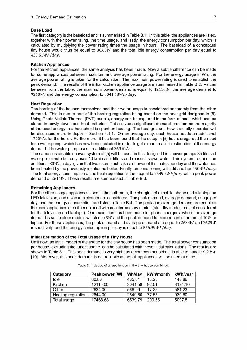
Base LoadThe first category is the baseload and is summarised in Table B.1. In this table, the appliances are listed,together with their power rating, the time usage, and lastly, the energy consumption per day, which iscalculated by multiplying the power rating times the usage in hours. The baseload of a conceptualtiny house would thus be equal to 80.68𝑊 and the total idle energy consumption per day equal to435.61𝑊ℎ/𝑑𝑎𝑦.
Kitchen AppliancesFor the kitchen appliances, the same analysis has been made. Now a subtle difference can be madefor some appliances between maximum and average power rating. For the energy usage in Wh, theaverage power rating is taken for the calculation. The maximum power rating is used to establish thepeak demand. The results of the initial kitchen appliance usage are summarised in Table B.2. As canbe seen from the table, the maximum power demand is equal to 12110𝑊, the average demand to9210𝑊, and the energy consumption to 3041.58𝑊ℎ/𝑑𝑎𝑦.
Heat RegulationThe heating of the houses themselves and their water usage is considered separately from the otherdemand. This is due to part of the heating regulation being based on the heat grid designed in [5].Using PhotoVoltaic Thermal (PVT) panels, energy can be captured in the form of heat, which can bestored in newly developed heat batteries. This solves a significant demand problem as the majorityof the used energy in a household is spent on heating. The heat grid and how it exactly operates willbe discussed more indepth in Section 4.1.1. On an average day, each house needs an additional1700𝑊ℎ for the boiler. Furthermore, it has been found that the setup in [5] had disregarded the needfor a water pump, which has now been included in order to get a more realistic estimation of the energydemand. The water pump uses an additional 369.6𝑊ℎ.The same sustainable shower system of [5] will be used in this design. This shower pumps 35 liters ofwater per minute but only uses 10 l/min as it filters and reuses its own water. This system requires anadditional 30𝑊ℎ a day, given that two users each take a shower of 6 minutes per day and the water hasbeen heated by the previously mentioned boiler. Finally, air conditioning will add another 450𝑊ℎ/𝑑𝑎𝑦.The total energy consumption of the heat regulation is then equal to 2549.6𝑊ℎ/𝑑𝑎𝑦 with a peak powerdemand of 2644𝑊. These results are summarised in Table B.3.
Remaining AppliancesFor the other usage, appliances used in the bathroom, the charging of a mobile phone and a laptop, anLED television, and a vacuum cleaner are considered. The peak demand, average demand, usage perday, and the energy consumption are listed in Table B.4. The peak and average demand are equal asthe used appliances are either on or off with no intermediary modes (standby modes are not consideredfor the television and laptops). One exception has been made for phone chargers, where the averagedemand is set to older models which use 5𝑊 and the peak demand to more recent chargers of 10𝑊 orhigher. For these appliances, the peak demand and average demand are equal to 2634𝑊 and 2629𝑊respectively, and the energy consumption per day is equal to 566.99𝑊ℎ/𝑑𝑎𝑦.
Initial Estimation of the Total Usage of a Tiny HouseUntil now, an initial model of the usage for the tiny house has been made. The total power consumptionper house, excluding the tunect usage, can be calculated with these initial calculations. The results areshown in Table 3.1. This peak demand is very high, as a common household is able to handle 9.2 𝑘𝑊[19]. Moreover, this peak demand is not realistic as not all appliances will be used at once.
Table 3.1: Usage of all appliances in the tiny house combined.
Category Peak power [W] Wh/day kWh/month kWh/yearIdle 80.86 435.61 13.25 448.86Kitchen 12110.00 3041.58 92.51 3134.10Other 2634.00 566.99 17.25 584.23Heating regulation 2644.00 2549.60 77.55 930.60Total usage 17468.68 6539.79 200.56 5097.8

3. Energy Demand Estimation 8
3.1.2. Tunect CalculationsBesides the usage of a tiny house, the usage of tunect is being defined externally. This common usageaccommodates some appliances that will be used by all households and will thus be scaled to 12users. The initial appliance selection of tunect consists of a washing machine, a dryer, and a printer.Tunect will also accommodate the control unit required to control the electricity grid. Furthermore, thecommunity will need some outdoor lighting which will be powered by tunect.These modules are installed at a central point accessible to all of the tiny house community members.The peak demand, average demand, usage per day, and energy consumption per day can be foundin Table B.5. The average demand is only different for the printer, as the low power consumption of0.3𝑊 in idle mode is incorporated in the average usage calculation, being able to print when needed.In addition, 20 outdoor lights are deemed sufficient for providing enough light. As a result, the peakdemand is equal to 3142𝑊, the average demand is equal to 3130.79𝑊, and a daily demand of 8550.41𝑊ℎ/𝑑𝑎𝑦.
3.2. Demand ModificationsNow that an initial selection of appliances has been made, it is shown that the average usage andespecially the peak demand is relatively high compared to a regular household [19]. One of the centralvalues of a tiny house community is to live in a more sustainable way. Besides, designing a grid thatmust be able to supply the calculated peak demand will be both expensive and unnecessary, as thepeak demand for all 12 houses will rarely be reached. Hence, in the design, a tradeoff will be madebetween the demand and costs of the grid. The design choices for demand are based on experiencesof tiny house users and research of existing and developing technologies.
3.2.1. Appliance Selection Based on Tiny House UsersIn order to establish a better understanding of what tiny house owners actually use, some people fromthe tiny house community have been contacted. As mentioned in the previous sections, a survey wassent to two tiny house communities, and an interview was conducted with two tiny house owners thatbuilt their own homes. The results of the survey can be found in [20] and the notes of the interview inAppendix B.3. Note that only the appliance usage of houses with a living area smaller than 40 𝑚2 hasbeen considered as anything larger has not been regarded as ’tiny’.It is decided to find a balance between the minimalist approach of some of the owners and the somewhat abundant design of [5]. This way, the users of our tiny houses will live sustainably without givingup much comfort.
The usage of the baseload remains unchanged after modification. Even though the wifi router wasindicated (in the survey) to be used less than expected, it is decided to use one as it may be neededfor the smart control.The most significant savings have been made by discarding kitchen appliances. It is decided to replace the coffee machine and kettle by simply boiling water on the stove as both interviewees statedthey did and, as the survey indicated, were less commonly used. This choice has been compensatedby adding time to stove usage. This way, energy savings are not too significant, but estimated peakdemand is lowered remarkably. Then, the oven and microwave were chosen to be a combination unitwhich lowers peak demand, and the kitchen machine has been discarded as it is quite a luxury item.All design choices for heating remain the same as those are very casespecific, and the current heatgrid is considered fittingly sustainable.The decision was made to discard the television and hairdryer as both are indicated to be used verylittle. Additionally, the vacuum cleaner is switched for a much more sustainable handheld model, whichwill suffice for cleaning a house of tiny proportions. Finally, the use of a dryer is unsustainable and excessive and thus discarded. However, it is decided to add an extra washing machine as the visited tinyhouse village had two for the same amount of households. The resulting usage is shown in Table B.10.
To conclude, the energy demand of a more sustainable household has been estimated. The tablescan be found in Appendix B.4 and the final usage is shown in Table 3.2. Also, a comparison is madebetween the initial usage and the sustainable modified usage, which is shown as the percentual decrease in power and energy usage in the sustainable estimation after the modifications.

3. Energy Demand Estimation 9
Table 3.2: The estimation of the total usage of one tiny house with a sustainable selection of appliances, including thepercentual decrease in usage with respect to the initial estimation.
Categories Peak power [W] Wh/day kWh/month kWh/yearIdle 80.68 435.61 13.25 159.00Kitchen 6450.00 1910.00 58.10 697.15Other 172.00 117.27 3.57 42.80Heating regulation 2194.00 2099.60 63.86 766.35Total usage 8896.68 4562.48 138.78 1665.31Decrease 49.07% 30.81% 30.81% 30.81%
3.2.2. The Effect of DC AppliancesIn this design, one of the primary objectives of this system is to minimize main grid connection and thusoptimize independence thereof. For this reason, simply choosing AC appliances because of standardization is not a valid argument. Besides, the microgrid to which the nanogrid of the tiny houses will beconnected to is required to be operating on DC as stated in the PoR.A standalone DC grid with RESs and its own ESS has some major advantages over AC microgrids,some of which are the fact that PV systems are a DC power source and ESSs like batteries and supercapacitors have DC characteristics as well.
Furthermore, the use of a residential DC grid has additional advantages including efficiency improvement, absence of losses due to reactive power, and great reduction of ElectroMagnetic Interference(EMI) [21]. One of the causes of this efficiency improvement is the fact that most residential appliancesalready operate on DC internally, meaning these appliances make use of an internal ACDC converteralso resulting in losses [22]. Garbesi et al. [13] state that these internal inverters are very inefficient andthat avoiding its use throughout the residence can save up to 12% on conversion losses only. Makinguse of highly efficient DC heaters which are in development can save an additional 50% on heating[13] and using brushless DCmotors instead of commonly used induction motors can save an additional24% in some appliances [22]. Overall, the use of DC appliances only on a DC grid can result in energysavings of more than 30% according to [14], [13] and [21].
Even though the current market of DC appliances is still in its early phases and has some barriers toovercome, there are some clear indications that the sector has significant potentials [13], [14]. Basedon what has been stated in this section and the ambition for this design to be innovative and technologically progressive, it is decided to assume DC appliances will be used in this grid design. RQC.DCG.2,which states that the appliances in the houses could operate completely at DC, is hereby fulfilled.As these energy savings are still an educated approximation and speculation, the energy demand willnot be scaled down by 30%. Instead, these potential energy savings will be used as the safety margin of the energy demand to account for potential underestimation of the energy demand and lossessuch as converter inefficiencies and wire losses. Meaning adding energy use to the currently calculated demand average will not be necessary as this is accounted for by the fact that DC appliances areused. The same can be said for the calculated peak demand as a significant fraction of these energysavings result from the lowering of each of the individual appliance’s power rating [21]. Thus the currently calculated demand will be used for the final models, having incorporated a safety margin in thisunconventional way.
3.2.3. Limiting Peak DemandAs can be seen in Table 3.2, the peak demand is still high at almost 9 𝑘𝑊, but now more comparable toa common household [19]. This peak power is only reached if all appliances are used simultaneously.Realistically this power demandwill seldom be reached, and it would thus be costly and power inefficientto size the whole system on this peak demand.RQM.DCG.4 states that all users must be able to use all needed appliances in their homes, so thepower limit can only be set for power usage, which does not limit the use of the mentioned appliances.Looking at the used appliances, the most significant power saving is obtained by limiting the inductionstove. Furthermore, the boiler can be limited by only turning it on during moments where the demand

3. Energy Demand Estimation 10
is relatively low. In case all appliances are on, the stove can still be used to its average demand, whilethe hot water which is available in the boiler can be used for the shower and water tap. By using thismethod to limit the peak demand, the requirement RQM.DCG.4 is met.Subsequently, the peak demand is limited to amaximum of 4746.68𝑊. In case the power demand risksexceeding this limit, the stove will be used as a buffer by limiting its power demand in the most extremecase to 1500𝑊. If this does not suffice, the same can be done for the boiler until it is completely off.The rest of the average demand, as well as daily, monthly, and yearly energy usage remains the same.
Now that the peak demand has been established, the system should be sized such that both the microgrid and nanogrid are able to supply their respective maximum demand in order to meet RQM.DCG.2and RQM.DCG.3. Only after the design validation in Chapter 6 can it be determined whether theserequirements are met.
3.2.4. Final Demand Estimation ResultsAs the final demand of a tiny house and the common usage have been established, the total demand ofthe community can be calculated. The total demand corresponds to the estimated demand of one tinyhouse, scaled to 12 households, plus the common demand of tunect. The resulting usage is shown inTable 3.3.
Table 3.3: Total sustainable usage of the whole community, including usage of 1 tiny house, 12 houses and common usage.
Category Peak power [W] Wh/day kWh/month kWh/year1 house 4746.68 4562.48 138.78 1665.3112 houses 56960.16 38324.84 1165.71 13988.57Common usage 4142.00 2731.23 83.07 996.90Total usage 61102.16 57481.00 1748.38 20980.56
3.3. Tiny House Demand ModelsThe total peak demand, average demand as well as the energy usage per day, month, and year presented in Section 3.2 are an estimation based on the usage of certain appliances. By using data fromgeneral household usage in the Netherlands, as well as an actual tiny house community, two behaviourmodels are constructed. The first model estimates the energy use of a tiny house during one day. Thesecond approximates the energy use of one tiny house throughout the year. Results of these modelswill be presented next.
3.3.1. Model of One Day & ResultsFor the singleday model, smart meter data from the Distribution System Operator (DSO) Liander hasbeen used [23]. This data includes smart meter measurements of energy usage for every 15minutes forthe year 2013. Since then, more efficient products, heating, and isolation have been introduced [24],however the behaviour of the residents of these houses in 2013 is estimated to be equal to currenthousehold behaviour. This data set contains the smart meter values in Wh for 78 houses over thecourse of one year, measured with intervals of 15 minutes.From this data, a daily average energy demand of one tiny house can be constructed using the fractionsof energy usage from the housesmeasured by the smart meters. The summed data values of all housesare divided by the measured 78 houses to get a daily average per house. By dividing the value of each15minute interval by the total 𝑊ℎ usage of a day, the fraction of energy used in that interval can becalculated. Multiplying this fraction with the calculated average daily usage of a tiny house results in15minute interval energy usage. Summing these intervals for every hour results in the hourly Whusage for a tiny house. The resulting graph of this usage model is shown in Figure 3.1. The graphshows the estimated energy usage of one tiny house throughout an average day. The energy demandof an average smart metered house is shown as well.As there is no power consumption data available, an option to still gather data for power consumption isto divide the energy usage in𝑊ℎ by themeasured time, hence dividing by 0.25 hours. These values arethus a multiplication of 4 of the energy demand. These values are much lower than the peak demand,

3. Energy Demand Estimation 11
Figure 3.1: Average hourly energy usage in𝑊ℎ over a day.
however they will be saved for possible later usage. In Appendix B.5.2 a short explanation and graphis provided for the Wh per hour or average hourly power demand over a day.
3.3.2. Model of One Year & ResultsThe daily average model is valuable for estimating demand throughout an average day, however inconsistencies arise when comparing lower usage in summer versus higher usage in winter. In thesecold months, extra heating is required and the total appliance use increases as well as people tendingto stay inside more. In the summer, almost no heating is required, and people are outside a lot more,hence a decrease in usage is expected.To get an insight into the usage during colder months, data is used of a tiny house community locatednear Den Bosch in the Netherlands, called ’Minitopia’. From the available data, 5 houses were selectedwhich had continuous data values for each month in the same year. A fraction can be calculated fromthe average monthly usage of these houses and can be multiplied by our yearly usage. This resultsin the average yearly usage being divided over 12 months. In Appendix B.6, a short explanation andgraph containing the monthly usage in 𝑘𝑊ℎ resulting from the yearly model is provided. The values foreach month, together with the percentual decrease of our estimated usage versus average Minitopiausage is shown in Table B.12.
To get the daily average in these months and to be able to compare it to our estimated average dailydemand, the monthly usage is then divided by the number of days in each month. This results in theaverage daily usage for each month for both the Minitopia houses as well as our estimated demand fora tiny house, shown in Figure 3.2.In Table 3.4, the values of daily energy demand in Wh for each month have been presented. As it isthe scaled behaviour of the Minitopia usage, the difference is the same for each month. The usageof a tiny house is 60% of the usage of an average Minitopia house. The month with the highest dailyaverage energy usage for our estimation is December, with an energy usage of 5712.30𝑊ℎ for onehouse over one day. The month with the lowest daily average usage can be seen to be September,with an energy usage of 3062.18𝑊ℎ for one house over one day. This difference is due to the differenttemperatures, possibly bad isolation, and the PV panels producing less in winter. As the largest dailyusage needs to be accounted for in the sizing of the storage and supply units, December will be usedfor the storage selection while keeping in mind that generation will be low at that time of the year.

3. Energy Demand Estimation 12
Figure 3.2: Daily usage in Wh per month for the estimated demand of one versus minitopia tiny house usage, based on amonthly average.
Table 3.4: Daily usage of minitopia tiny house vs tunus in Wh.
Month Minitopia usage [Wh] Tiny house usage [Wh]January 8232.90 4665.17February 9255.00 5374.38March 8096.13 4411.83April 7049.33 4053.23May 6796.77 4234.87June 7716.67 4300.36July 5349.03 3186.95August 6225.81 3354.51September 5373.33 3062.18October 6625.81 3443.35November 7573.33 4597.78December 10967.74 5712.30

4Supply & Storage Design
In Chapter 3, the estimation of the average daily demand of a tiny house has been established, aswell as the variations in daily energy demand throughout the year. In Section 4.1, the needed energygeneration in the form of RESs is determined to supply the whole community using the estimatedmonthly demand. The RESs will consist of feasible options on a roof in Rotterdam: solar and windenergy generation. The considered methods to harbor these forms of energy are PV panels, PVTpanels, and VAWTs or Horizontal Axis Wind Turbine (HAWT)s. As explained in Section 3.1.1, theheating of the tiny houses will be done using the heat grid developed in [5]. A short analysis will beprovided on the heating method and an adjusted version will be elaborated.After RES selection, an initial model is created to determine the required energy generation in order tosupply 90% of the estimated energy demand throughout the year. This initial model will produce a roughestimate on the needed generation, as the ESS is not accounted for. In Section 4.2, a comparison ofavailable ESS methods is made and a suitable ESS option is chose. Subsequently, to fulfill the 90%availability required by RQM.DCG.5, a second model is made which incorporates a finite and lossyESS. This second model estimates the amount of time the microgrid uses energy from the main gridand enables establishing the correct sizing of the ESS based on the PoR. Using this second model,two types of storage systems are examined; a distributed and a centralised storage system. For bothscenarios, costs, sizing, and availability will be deliberated. Lastly, a comparison between technical,economic, and social advantages and disadvantages will be made.
4.1. Renewable Energy SourcesThe first step in establishing the energy generation system for the community is to identify the propermethods of sustainable energy generation. RQM.DCG.8 states that the generation of the grid shouldbe solely based on more than one RES. Subsequently, the considered sustainable methods will consistof the most feasible options on a roof in Rotterdam: solar and wind energy generation. The productsfor the methods of RESs need to be selected. For this selection, the technical performance, costs,and environmental aspects are taken into account. After the products have been selected, their performance is analyzed and modeled. Using this model, the number of modules of each of the selectedRESs is determined based on how much generation is needed to supply the estimated demand.
4.1.1. The Heat GridAs mentioned in Chapter 3, a major factor in energy usage is heating. Demand rises in the winter whilesolar generation decreases due to fewer sun hours and weaker irradiation. To resolve this problem, aheat grid was designed in [5]. RQM.DCG.12 states that the design must include a heating grid basedon the heat grid designed in [5]. To develop a better understanding of how the heat grid operates andwhat should be adjusted to fit the current grid design, a revision of the heat grid from [5] is done. Basedon this analysis, some adjustments are made after the discovery of a discrepancy in the initial designin [5]. The complete analysis of the heat grid and the adjustments can be found in Appendix C.1. Theheat grid can be considered as follows.19 PVT panels are put on the roof of a separate construction which contains a heat battery and a large
13

4. Supply & Storage Design 14
heat pump. The heat of the sun can be captured by the PVT panels and stored in the heat battery. Theheat pump ensures heat circulation to and from the houses and is power by the electricity generatedby the PVTs. The heat grid is thus considered as a separate system, disconnected from the microgrid.Nevertheless, the system now does include a version of the heat grid designed in [5], meaning RQM.DCG.12 is met.
4.1.2. PVAs the energy generated by the PVTs will only be used for the heat grid, additional energy sourcesare needed to supply the demand of the community. Between 2005 and 2012, the production of solarpanels has increased by a factor of sixteen, and the market is still growing. Among other factors,higher efficiencies, decreasing costs of polysilicon, and large investments in this growing industryhave resulted in an annual price reduction of 21% [25]. Moreover, solar energy is the most abundantand inexhaustible of all renewable energy resources [26]. It has been found that many tiny housessupply a significant fraction of their own demand using PV panels. For these reasons, PV panels arechosen to be one of the main methods of energy generation in this design.
Panel SelectionBoth the roof of the tuni themselves and the highrise on which the tuni are built are relatively small.Usable space is thus a limiting factor in this design, so highefficiency panels are a fitting choice forthe current design. Product research on mainly highend, highefficiency solar panels is carried out,resulting in a comparison shown in Table 4.1.
As can be seen, several factors are compared in order to establish which panel would be the bestfit for the current design. Except for the Trinasolar Vertex, all panels are top of the range, explaining why most specifications are fairly similar. The power rating of solar panels is given at StandardTest Conditions (STC), which entails radiation of 1000𝑊/𝑚2 at a cell temperature of 25 °C, which isobtained at an ambient temperature of approximately 0 °C. These circumstances are not very realistic which is why the performance at Nominal Operating Cell Temperature has been considered aswell. Other considerations are the temperature coefficient which indicates the attenuation of the cellefficiency for higher temperatures and the power tolerance. The power tolerance indicates the initialdeviation of the rated power as each solar panel has slightly different behaviour. Except for FuturaSun,all companies ensure a positive power tolerance meaning the power rating will only be similar or higherthan advertised. Besides the rated efficiency, it is found that it is essential to look at how this efficiencyis sustained throughout the years. All companies give a guarantee of how much of the initial powerrating is still put out after one year and after 25 years. As the community is meant to operate for a longtime, the efficiency and its degradation are considered to be of great importance. Finally, two crucialfactors were the price per panel and the product warranty each company is willing to give.Having considered these factors, the LG Neon R panel is chosen to be used in the design. This decision is mainly based on the fact that it has the secondhighest efficiency for the secondlowest pricewhile coming with 25 years of product warranty. Moreover, the temperature coefficient and degradationfactor are considered to be very decent. It has to be noted that the TrinaSolar is by far the cheapestsolar panel while having a very decent efficiency. However, making the design futureproof, its productwarranty and degradation factor are deemed insufficient for this design.
PV Panel PerformanceTo assume that a solar panel constantly puts out its rated power would be very optimistic and unrealistic.Besides the obvious fact that PVs will not generate energy at night, there are many other factors thatinfluence the performance of solar panels. The daily received irradiance of the sun fluctuates heavily;besides clouds that can block out a significant fraction of solar energy, the length of the day and theheight of the sun and thus, the strength of its radiation play a significant role. In the model describedin Section 4.1.4 all of this will be accounted for by using KNMI weather data of Rotterdam over the last20 years. Moreover, the orientation and the tilt of a panel, the temperature and degradation, and otherenvironmental aspects affect the PVs’ performance. A performance analysis is done and can be foundin Appendix C.2. Based on this analysis, the overall efficiency of the panels is estimated to be 19.14%.
A model has been created to compare the demand of the community throughout the year against the

4. Supply & Storage Design 15
Table 4.1: Comparison table of five PV modules based on the these data sheets: LG:[27], FS:[28], TS:[29], SP:[30] RS:[31].
Panel LG FuturaSun Trinasolar Sunpower REC SolarMax power STC [W] 380 360 385 400 380Max power NOCT [W] 286 272 290 N/A 289Temp. Coeff Pmax [%/°C] 0.3 0.3 0.34 0.27 0.26Power tolerance 0∼+3 % ± 3 % 0∼+5 W 0∼+5 % 0∼+5 %Efficiency [%] 22 21.3 20 22.6 21.7Degradation [%/year] 0.3 0.4 0.55 0.25 0.251 year guarantee [%] 98 99 98 98 9825 year guarantee [%] 90.8 89 84.3 92 92Price [€/module] 289 N/A 149 369 330Product warranty [yrs] 25 15 12 25 20
amount of energy that can be generated by the chosen RESs. Utilizing this model, it can be estimatedhow much generation is needed throughout the year, which will be discussed in Section 4.1.4. Sincethe demand in the winters is high, while solar irradiance is low, another RES is needed, which in thiscase will be wind turbines.
4.1.3. Wind TurbinesIn the colder seasons, the wind is a fairly present factor in the Netherlands, especially at heights [32].As the community will be built on the roof of a highrise building, the wind can be a great resource togenerate clean energy.
In order to accomplish this, a wind turbine is to be selected. In [5], the decision was made to usefour turbines of the same type: the AeolosV 1kW VAWT. Market research on Aeolos and its competitors has been carried out to verify whether a suitable turbine has been selected.As for the turbine type, the use of VAWTs compared to HAWTs is found to be a fitting choice for severalreasons. Usually, one of the most significant drawbacks of VAWTs is the fact that the modules harnessless wind because of their location close to the ground due to their short base. This is not an issueon the roof of a highrise building. Furthermore, a VAWT is smaller and thus less obtrusive for theinhabitants of the community and usually needs less maintenance [33]. The biggest advantage of theVAWT is its ability to generate power in turbulent winds, regardless of wind direction and duration ofthe wind gust. According to the Institution of Mechanical Engineers, turbulence can even improve efficiency, meaning modules can be built near each other and other constructions without affecting theirperformance [34]. Irregular winds are prevalent in urban areas, which is why VAWTs are the betterchoice compared to HAWT.A disadvantage of wind turbines is that turbulence could cause vibrations which results in noise. However, the smaller Aeolos models are rated for 45 𝑑𝐵 max, which is within RIVM guidelines for noise inresidential areas [35].As for the product itself, it has been found that Aeolos is one of the leading products in this market andis considered an excellent choice for the current design. However, it has been decided that the 2 𝑘𝑊model is a better fit as the wind turbines will be much needed in the winter when demand is higher andsolar irradiance is lower. Choosing one larger turbine with a higher power output has been consideredas well. However, these are louder and exceed noise limits. Furthermore, smaller wind turbines canstart to generate power at a much lower wind speed, ensuring the turbines can generate throughoutthe seasons. In [5] the turbines were considered to be merely additional support to the generation viaPV and PVT. In this design, the wind turbines will prove to be of utmost importance for achieving 90%availability. This will be shown and discussed in Section 4.1.4.Now that the generation methods are chosen to be several RESs, RQM.DCG.8 is met.
4.1.4. Supply Models & ResultsAs the proper PV panels, wind turbines, and PVT panels have been selected, the model to analyse theneeded amount of each of these sources can be determined. As explained in Section 4.1.1, the PVTpanels will not be used in the estimation of required energy generation, hence only the PV panels and

4. Supply & Storage Design 16
wind turbines will be considered. This model will use the daily demand of each month for the wholecommunity, which is determined in Table 3.4 and explained in Section 3.3, to determine the neededdaily generation.As the total usage for the community for each month has been defined, the RESs need to be quantified.The PoR states that 90% of the time, the community’s demand needs to be supplied by the microgriditself. The needed production was set to be at least 90% as well.For this purpose, weather data from the Delft University of Technology from the KNMI station in Rotterdam has been downloaded [36]. From this data, the solar irradiation, as well as the wind speed, havebeen used to determine the hourly energy generation of a VAWT and a square meter of PV panel. Theweather data, as well as its usage for the PV panels and VAWTs, are explained in Appendix C.3As the power output for each hour is now known for both the PV panels as well as the VAWTs using theweather data and the previously explained inefficiencies, the amount of both RES methods had to bedetermined to supply 90% of the energy demand. The availability is determined using a supply modelwhich uses the following assumptions:
• The energy generated by the RESs can always be used for the demand.
• The energy generated by the RESs is stored in an infinitely sized battery with no losses.
• Cable and converter losses have been ignored as they have not been selected yet.
From the model, using 6 VAWTs and 61.2 𝑚2 of PV panels (36 modules of 1.7 𝑚2, 3 per house),the average availability throughout the year turns out to be 95.2%. This is larger than the previouslyrequired 90%. However, this model only compares the energy demand instead of the required 90% inoperating time; hence a safety margin of around 5% is considered for the result. The daily generationversus demand for all months is presented in Figure 4.1. In Table 4.2, the numbers of generationand demand are presented, as well as the relative overshoot or undershoot and the energy availabilityfor each month, where the yearly average resulted in 95.2% availability. This shows that July is thebest month and November the worst month in terms of available energy. In Appendix C.4, how much ofeither RES is needed if the other would not be implemented is elaborated and shown. Hourly generationversus demand is also shown for the highest demand in December versus lowest demand in July. Thishourly generation will be used in Section 4.2.
Figure 4.1: Daily energy generation versus demand for each month.
The PoR requirement is still not met due to only looking at the daily energy balance of the systeminstead of the time which it can supply without being connected to the main grid. For this purpose,hourly generation will be assessed and combined with an ESS method.

4. Supply & Storage Design 17
Table 4.2: Daily generation versus demand and comparison for each month.
Month Generation [kWh] Demand [kWh] Difference [kWh] Difference [%] Available [%]January 58.00 58.71 0.72 1.22 98.78February 61.39 67.22 5.84 8.68 91.32March 67.00 55.67 11.33 20.35 100.00April 71.14 51.37 19.77 38.49 100.00May 79.64 53.55 26.09 48.72 100.00June 81.72 54.34 27.39 50.41 100.00July 76.62 40.97 35.64 86.99 100.00August 65.18 42.99 22.19 51.63 100.00September 50.45 39.48 10.97 27.79 100.00October 48.12 44.05 4.07 9.24 100.00November 41.87 57.90 16.04 27.69 72.31December 57.27 71.28 14.01 19.66 80.34
4.2. The Energy Storage SystemOne of the major challenges of using RESs only is that generation and demand do not correlate. Anexample is that a lot of solar energy is generated when most users will be at work, and demand isthus low. An ESS is needed to store this overproduction, so the users can use this energy at a time ofoverconsumption, such as dinner time, as shown in Chapter 3. In the following section, several ESSsare compared in order to select the appropriate storage method.With the selected ESS, a model is made which also incorporates hourly generation and demand toestimate the availability for the PoR. Both an aggregated or centralised model and distributed modelwill be made to analyse both scenarios. A comparison will be done between cost, availability and sizing.Lastly, the scenarios will be analysed in technical, economic, and social aspects.
4.2.1. ESS choiceAs both demand and the generation methods have been established, research is done on several typesof storage systems to identify the appropriate storage method. Table C.2 summarizes the main advantages and disadvantages of each ESS mainly based on information found in [37], [38] and [39].An ESS based on lithiumion batteries have been selected because of their high energy density, relatively low price, adequate efficiency, and sufficiently high power output. A hybrid storage systemconsisting of batteries and a supercapacitor, or batteries and a flywheel, has also been considered.However, data of realtime power demand is needed to draw conclusions on how effective these solutions will be in reality. A recommendation for such a hybrid system is done in Section 7.2.When sizing the battery system, it is essential to look at power rating as RQM.DCG.9 states that thechosen ESS should be able to handle peak power demand. Two systems with lithiumion batterieswill be considered: an aggregated or central battery system and a partly distributed battery system areboth considered to be valid options. An aggregated system would mean the entire community has onlyone central battery system. This would mean all excess energy that is not directly supplied to the loadswill flow to one central point to be stored and used at a later point. The partly distributed system wouldconsist of both a central battery to store all excess energy generated by the turbines and a home battery for each of the tuni. Assuming that in this scenario, each house has its own PV system, all excessenergy supplied by the residential PV system can first be stored in the home battery. In case the homebattery is full, excess energy can be stored in the central battery. In case of overconsumption in thehousehold, the home battery would supply first so that the central battery is mainly used for backupand supplying peaks in power. This system would minimize long pathways and thus losses.A more detailed comparison is made on the advantages and disadvantages of either system, resultingin the table shown in Table C.3. Before deciding on which of the two systems to choose, both havebeen modeled to determine sizing and feasibility.
For each system, products have been researched to meet the following requirements:
• At least one day of energy demand (exact sizing will be done by experimenting with models, in

4. Supply & Storage Design 18
case of distributed, main and home combined should supply at least one day’s worth)
• Should be able to supply at least peak demand (in case of distributed, main and home combinedshould at least supply peak demand)
• Round Trip Efficiency (RTE) of at least 90 %
• Depth of Discharge (DoD) of at least 70%
• Should not suffer from hysteresis effect
• Should be in the 300500V output/input voltage range
• Should have enough cycles for at least 1015 years
For the main battery, the battery modules of ’BYD’ are selected [40]. These batteries consist of 2.76kWh battery modules that can be connected in series up to 22.1 𝑘𝑊ℎ. If required, large battery unitscan subsequently be connected in parallel for higher power output. One unit of either 19.3 𝑘𝑊ℎ or 21.1𝑘𝑊ℎ has a power rating of 17.9 𝑘𝑊. These units meet all other requirements easily as its RTE equals96%, DoD equals 90% and are rated for at least 20 years lifetime. The ’Simpliphy 2.6’ is chosen for thehome battery, which also meets these requirements. The specifications of both lithiumion batteries aremuch better than the initial research on ESSs indicated in Table C.2, showing how fast this technologyis evolving over the last few years.
4.2.2. Centralised ESS Model & ResultsIn order to properly size the energy storage of the ESS, a model has to be created which takes thedemand, supply, and storage into account. The first scenario which will be considered is a centralisedESS model. A short explanation of the model and the selected battery has already been provided inSection 4.2.1. An indepth explanation of the system is elaborated in Appendix C.6 which also containsa dedicated flow chart for the centralised model.In order to supply the maximum power demand of the community, as well as being able to roughly storethe daily demand in most months, while also having an availability of at least 90%, the model resultedin 4 batteries. Using 4 batteries and the previously determined demand and generation, the followingresults were obtained, which fulfill almost all the requirements mentioned in Section 4.2.1.
• Availability = 93.73 %
• Capacity = 4 ⋅ 19.3 𝑘𝑊ℎ = 77.2 𝑘𝑊ℎ• Effective capacity = 0.9 ⋅ 77.2 kWh = 69.48 𝑘𝑊ℎ• Peak power = 4 ⋅ 17.9 𝑘𝑊 = 71.6 𝑘𝑊• RTE = 96 %
The requirement that at least one day of average estimated demand should be available is fulfilled whenlooking at the total capacity and using the values in Table 4.2. When looking at the usable capacity, itcan be seen that only the month of December cannot be supplied for an average day due to a shortageof a few 𝑘𝑊ℎ. This requirement is thus roughly met, and as the other requirements are met with asufficient margin, 4 batteries will be used for the design. In conclusion, for the centralised model, 4 ofthe BYD HVM 19.3 [40] batteries have been chosen. The figures of the State of Charge (SoC) beingtracked hourly for each month can be found in Appendix C.8. The MATLAB code for the centralisedmodel can be found in Appendix F.1.
4.2.3. Distributed ESS Model & ResultsThe second scenario that is considered is the distributed model for the storage system. A generalexplanation for this model is presented in Section 4.2.1. A detailed explanation of the distributed model,as well as dedicated flowcharts, can be found in Appendix C.7.Using 2 home batteries for each house, as well as 2 of the larger batteries used in the centralised modelfor the central storage, the following results are obtained from the model, with calculations included forthe ESS requirements.

4. Supply & Storage Design 19
• Availability = 93.33 %
• Capacity = 2 ⋅ 19.3 𝑘𝑊ℎ + 12 houses ⋅ 2 ⋅ 2.6 𝑘𝑊ℎ = 101 kWh
• Effective capacity = 0.9 ⋅ 2 ⋅ 19.3 𝑘𝑊ℎ + 1 ⋅ 12 houses ⋅ 2 ⋅ 2.6 𝑘𝑊ℎ = 97.14 𝑘𝑊ℎ
• Peak power = 12 houses ⋅ 2 ⋅ 1.275 𝑘𝑊 + 2 ⋅ 17.9 𝑘𝑊 = 66.4 kW
• Effective efficiency = 0.96 * (2 ⋅ 0.9 ⋅ 19.3 𝑘𝑊ℎ / 97.14 𝑘𝑊ℎ) + 0.98 * (12 houses ⋅ 2 ⋅ 2.6 𝑘𝑊ℎ /97.14 𝑘𝑊ℎ) = 97.28 %
As can be seen from the calculations, the distributed model storage system fulfills all requirements withexceptional capacity. In order to be able to supply the peak demand, 2 batteries per household neededto be selected (where each household has the same amount of batteries for equal power generation perhouse), causing the capacity of the system to be oversized by 97.14−71.28)
71.28 = 36.28% in the best case
and 97.14−39.48)39.48 = 146.05% in the worst case (by taking the highest and lowest demand in Table 4.2,
respectively). In the comparison, this excess capacity will be deliberated against the higher cost andlower transportation losses which would be minimised in the distributed model. In conclusion, for thedistributed model, 2 home batteries per tiny house, resulting in 24 of the simpliPhi PHI 2.6 [41] batterieswere chosen. For the central storage, 2 of the BYD HVM 19.3 [40] batteries have been chosen. Thefigures of the SoC being tracked for each month can be found in ??. The MATLAB code can be foundin Appendix F.2.
4.2.4. System Comparison & SelectionHaving established that both the centralised and partly distributed system enable the system to havean availability of more than 90%, the requirement RQM.DCG.5 is met regardless of which system ischosen.Now, a decision has to be made on which of the systems will be used. As the topology design heavilydepends on which of these systems is used, this decision must be made before starting on topologydesign. In order to make a complete analysis, technical, economic, and social advantages and disadvantages of both systems have been analysed and presented in Table C.3. From this analysis, itis found that the distributed model has the potential to be more flexible and efficient with the energysupply to the community. It is however a lot more complex and expensive in capital, maintenance, andsoftware. On the other hand, the centralised system favors simplicity and lower costs, however lowflexibility and higher maintenance costs in case of battery failure. On the social side, both systems areconsidered equally advantageous, as the centralised model favors low danger due to central storage,while the distributed system favors the individuals who want to use their PV panels for themselves. Tomeet the requirements, and to minimize costs and complexity, the centralised system is preferred andthus chosen. This means 4 of the BYD HVM 19.3 [40] batteries, with a combined power rating of 71.6𝑘𝑊, will be used for this design, meaning RQM.DCG.9 is met as well. The centralised system usesthe least amount of DCDC and ACDC converters and hence fulfills RQS.DCG.3. This requirementstates that the amount of any type of converter should be kept as low as possible in order to minimizecosts and optimize efficiency. In order to compromise for some of the design tradeoffs made by thisdecision, the following will be accounted for in the topology design.Each house will have its own PV modules installed, implying that the solar panels on a house willprimarily supply the demand of the individual house directly, without the use of a home battery. Thismeans the social disadvantage of centralised can be remedied while still keeping fire hazards in houseslow. Furthermore, it is decided that in the topology design, flexibility should be a primary objective tofulfill the PoR requirement RQS.DCG.4 of independent operation of a tiny house in case of an adjacentfailure.

5Topology Design
In the last chapters, the demand, supply, and storage of the tiny house community have been established. Now, the last part of the design phase will be discussed: creating the optimal topology. InSection 5.1, the topology of the microgrid is discussed which connects the VAWTs, ESS, Point of Common Coupling (PCC), the tiny houses and the common usage tunect together. This topology includesthe voltage bus topology, the microgrid layout, the converters and control/optimization algorithms, andlastly, the used wiring. In Section 5.2, the smaller nanogrid will be considered, which connects thedemand of a tiny house and the PV panels to the microgrid. For the nanogrid, the voltage bus topology, converters, and control/optimization algorithms, as well as the used wiring, are discussed. InSection 5.4, safety considerations concerning the voltage bus polarity, grounding of both microgrid andnanogrid, fault handling and voltage stability, and proposed solutions are elaborated. In Section 5.4,the safety of the microgrid and nanogrids for the residents is discussed and standards for these typesof grids as well as human interaction with these grids is elaborated upon. Lastly, in Section 5.5 a costanalysis is done on the hardware required for the complete grid design.
5.1. Microgrid TopologyThis section will cover the design of the microgrid and the considered aspects of that design. Theseaspects are summarised as the topology of the voltage bus, the required converters and proposedcontrol/optimization algorithms, the wiring used in the system to operate. Moreover, the physical layoutdesign of the microgrid, which fits on the roof of the considered highrise, is presented and discussed.
5.1.1. Bus TopologyThe voltage bus is the voltage line that interconnects the ESS, the RESs, the houses, and lastly, themain grid. It is essential to choose the appropriate voltage level of this bus, as well as the topologyof the bus itself. As RQM.DCG.1 states, the microgrid should operate on DC and thus only DC busvoltages are considered.
Voltage choiceThe voltage levels which are commonly used in residential grid applications, discussed in [42], vary alot. The voltages mentioned range from 12 𝑉𝐷𝐶 to 400 𝑉𝐷𝐶, however their usage is quite different. In[43], it is mentioned that the most standardised choice for DC microgrids is 380 𝑉𝐷𝐶 or 400 𝑉𝐷𝐶 dueto the high amount of applications in the data center area. Another advantage of this higher voltageis that losses are lower. As the primary energy source of this grid consists of RESs, and their energyis being supplied by the ESS, the losses in the cables need to be minimised in order to use the generated energy most efficiently. A secondary benefit is that the cables themselves are less expensivefor a lower current rating. Hence, in order to minimize the losses and costs, the highest voltage waschosen. This resulted in 400 𝑉𝐷𝐶 being chosen as the operating voltage of the voltage bus, implyingRQM.DCG.1 is met.
20

5. Topology Design 21
Topology choiceAfter choosing the operating voltage of the DC microgrid, the topology of the microgrid itself can bechosen. The main topologies for a DC microgrid are radial, ring and other combinations of these basicforms. Also, the primary forms of bus topology itself are considered, being singlebus, multibus, andreconfigurable. Their basic structure, as well as their respective advantages and disadvantages, arediscussed in Appendix D.1.
For this microgrid, based on RQS.DCG.4, the nanogrids should be able to operate under a fault occurrence somewhere else (except the possible faulted nanogrid). The best option for this requirementis to use a ring topology, which enables bidirectional power flow, powersharing, and fault isolation. Aseries multibus ringbased voltage bus topology has been chosen, where each bus connects a specificpart of the microgrid (ESS, RES etc.). This chosen topology thus enables fault isolation and continuedoperation of nonfaulted locations, which fulfills RQS.DCG.4. As power sharing is also enabled, RQC.DCG.3, which states that the tiny houses could share power with each other, is also met. The gridis designed to be able to operate in ring topology, however due to the normally open switch betweenthe two sets of batteries, the grid effectively operates in radial as shown in Figure 5.1. This is to reducecomplexity and for easier identification of faults. The more complex reconfigurable multibus systemcan be considered for later research, as data on the fault rate of tiny houses is not researched in thisthesis and is unknown up to this point.A disadvantage of the used series multibus ring topology is the possible significant losses in voltageand power due to the bidirectionality of the system and the long distances power can travel. This willbe analyzed during the wiring analysis as well as in Chapter 6.
5.1.2. Microgrid LayoutIn Figure 5.1 a schematic overview of the physical grid layout is shown. An electric overview of theinterconnection of all buses, including the nanogrid, can be found in Figure 5.3 in Section 5.3.3. As canbe seen in the figure, the loads, generators, and batteries are connected to the main ring bus, whichuses a seriesconnected multibus configuration as shown in Figure 5.3. As soon as the faulty areahas been identified, the area can be isolated from the ring and the switch between the batteries will beclosed to ensure power flow to all other areas. These potential faults will be discussed in Section 5.3.3.The batteries are connected via bidirectional converters on either side of this open ring bus. This way,most of the demand and generation on the left side of the roof will flow to and from the left set ofbatteries and idem for the correct battery and the right side of the roof.The green lines indicate the connection between the ACDC converters of the VAWTs and the ring.Each converter is placed near its designated turbine to ensure power flow at 400 𝑉𝐷𝐶, decreasingcurrents and thus losses. This is especially important for the VAWT connection as they are purposelyplaced as far from the community as possible to minimize disturbances caused by the turbines. Thepower generated by the turbines can be used to either supply the loads of the houses, recharge thebattery system, or supply back to the main grid via the pink line.Tunect has two DCDC converters connected to the main ring. One buck converter is used for powersockets with 48 𝑉𝐷𝐶 output. These sockets can be used for the printer, outdoor lighting, and thecontrollers required by the control group. The other converter has an output of 400 𝑉𝐷𝐶 to supply thewashing machines. This converter is used to ensure that the loads of the washing machines do notcause significant bus voltage fluctuations and is thus used for stabilization purposes. The maximumallowable bus voltage fluctuations will be discussed in Section 5.3.The purple lines indicate the connection between the nanogrid of each of the tiny houses and the mainring. This nanogrid will be extensively discussed in Section 5.2 which explains that this connection canboth supply to the loads of the homes and supply back to the microgrid as each house has its ownPV panel system. This connection enables powersharing between the houses, recharging the batterysystem, and supplying back to the main grid via the PCC.All wires will be routed either underground, meaning inside the roof of the highrise itself, or throughinsulated ducts. Both options will have to be researched onsite in order to choose the suitable method.As seen in the figure, most lines will be routed via a similar path so that in case of a line fault, all linescan be accessed at the same location.Finally, in this layout, it has been assumed that the bottom left corner of the roof is facing south. Thisway, all sloped roofs and the PVTs of the heat grid face south to ensure optimal solar generation.

5. Topology Design 22
Figure 5.1: Schematic overview of the overall microgrid layout and wiring on the rooftop of a highrise building.
5.1.3. Converters & ControlUntil now, the general topology of the microgrid has been designed, with its designated operatingvoltage. Next, the converters which connect the loads, generation, and storage to the grid have to bedesigned. RQM.DCG.11 states that all converters used in the system should be able to handle themaximum rated input and output power of their respective connection points. As the actual design ofconverters and control algorithms falls outside the scope of this thesis, the main design requirementswill be considered and recommendations on hardware will be made. Also, a control algorithm and, ifapplicable, an optimization algorithm will be presented as well. RQS.DCG.5 states that each of theRES converters should use a control algorithm for optimal power extraction. Based on this requirement,the converters for the VAWTs and PV panels will use a form of Maximum Power Point Tracking (MPPT).The general requirements for the converters are mentioned below. Each of the converters should havethese properties.
• Protected against overvoltage and overcurrent
• Galvanically isolated.
• Able to disconnect from the microgrid in case of faults in the lines, generation, demand, or converter itself.
• Able to handle large power fluctuations.
In Table 5.1, the needed converters together with their respective requirements and optimization algorithms are shown. The chosen optimization algorithms for the VAWTs and ESS are explained inAppendix D.2.
Table 5.1: Microgrid converter requirements and recommended optimization methods.
Microgrid locations Wind turbine Battery Main gridConverter type ACDC DCDC ACDCDirection Unidirectional Bidirectional BidirectionalVin 48 VAC 280420 VDC 230 VACVout 400 VDC 400 VDC 400 VDCPower rating >2600 W >31 kW >62 kWCurrent rating >6.5 A >76.37 A >152.73 A
Optimization algorithm MPPT:Perturb & Observe
Dual phase shift control+ neural network
Custom autonomouscontrol

5. Topology Design 23
VAWTThe unidirectional ACDC converter for the wind turbines will be placed at the base of each wind turbine.The general requirements of the wind turbine converter are shown in Table 5.1.The manufacturer of the wind turbine indicates compatibility with the ’CTC3K’ [44]. This is a gridtiecontroller where the output can be set to 400V to ensure bus stability. As this controller can be set tothe required DC output voltage, no additional converter is needed. The proposed MPPT algorithm is aform of Perturb & Observe algorithm, which is discussed in more detail in Appendix D.2.
BatteriesThe bidirectional DCDC converter for the battery will be used twice, following two parallel connectionsof two batteries each. The converters must comply with the general requirements as well as the requirements mentioned in Table 5.1. Furthermore, in charging mode, the converter must regulate thegrid voltage to the current battery voltage. In discharging mode, the converter regulates the variablevoltage of the battery to that of the DC grid and keeps the grid voltage stable. A recommendationis made to contact [45] which can supply the needed converter and after deliberation, our proposedcontrol system explained in Appendix D.2 could be implemented.
PCCRQM.DCG.6 states that, in case of overconsumption or faults, the microgrid should be able to connectto the AC main grid in order to supply the shortage of energy. RQM.DCG.7 states that, in case ofoverproduction, the microgrid should be able to supply back to the main grid via a connection.This connection to the main grid needs to be facilitated by a bidirectional ACDC converter. This converter needs to comply with the general requirements as well as the requirements mentioned in Table 5.1. The proposed control method in [46] will be used to regulate the DC microgrid voltage as wellas minimise circulating current. The design proposed in [47] can be used for further optimal designof the PCC converter. The product shown in [48] is a great candidate for our power needs as well asbidirectionality. Using the proposed technologies for the PCC ACDC converter, both RQM.DCG.6and RQM.DCG.7 are met.
5.1.4. WiringIn order to connect all selected modules without creating substantial losses, the wiring should be selected carefully. As Figure 5.1 is drawn onscale, decent estimations of wire lengths can be made.Based on the maximum power that will flow through each wire connection, the maximum current iscalculated to establish the required wire crosssection. RQM.DCG.10 states that the power lines mustbe able to handle the maximum voltage and current assigned to each wire section at all times. Thusthe selection of the crosssection is primarily based on the datasheet of the selected wires [49] as thereis an indication of a maximum allowable current per crosssection. The thickness of the wires was keptto a minimum to minimize costs. After the initial selection, maximum voltage drops were calculated forthe longest possible path of each wire section using the equation shown in Appendix D.3. Some adjustments were made by choosing thicker wires for certain sections when the voltage drop was higherthan 5 %. Table D.1 shows the final selection of all wires and their specifications. Based on the totallength of wire needed for each section and the prices found on [50], the costs were calculated.
5.2. Nanogrid TopologyNow that the main microgrid has been designed, the connection of the nanogrid to the tiny housesthemselves, as well as their connection with the PV panels, needs to be discussed. As concluded inSection 4.2.4, the PV panels are connected to the nanogrid instead of the microgrid in order for thePV panels to primarily supply the demand of the tiny house it is installed on. The same subdivision ofaspects as for the microgrid is used to discuss the design.
5.2.1. Bus topology & Nanogrid LayoutIn Figure 5.2 a schematic overview of the residential nanogrid layout is shown. The design of thetiny houses ensures some space under the living room area in which all converters and the boiler canbe stored. As seen in the figure, there are three DCDC converters in each house, all of which areunidirectional and connected to the 400 𝑉𝐷𝐶 bus. It is decided to install 48 𝑉𝐷𝐶 sockets in the house

5. Topology Design 24
for all basic appliances. This is a standardised DC voltage, which is safer for the users compared to the400𝑉𝐷𝐶 bus [42]. The left module converts the 400𝑉𝐷𝐶 to 48𝑉𝐷𝐶, which is then distributed throughoutthe house for the lighting and the power sockets. These power sockets can be used for all residentialappliances except for the boiler, oven, and stove. The distribution of the power sockets is designed tohandle a total of 1000𝑊 at once, which is sufficient for supplying all selected appliances simultaneouslyand, for example, some additional laptops. The three PV panel modules on the roof are connected inseries, which results in a maximum voltage of 128.7 𝑉𝐷𝐶, which is then converted by the module in themiddle to 400 𝑉𝐷𝐶 to supply to primarily supply the residential loads or the microgrid to be redirected toother houses or the battery system. The suitable converter is only used to ensure that the bus remainsat a stable 400 𝑉𝐷𝐶. This module supplies to the boiler, oven, and stove, which have the highestpower ratings. The decision has been made to connect these appliances to a dedicated high voltagepower socket as supplying these on 48 𝑉𝐷𝐶 would require excessive currents resulting in significantinefficiencies and losses. As these appliances can cause very sudden changes in the residential loads,the converter is thus added for stability purposes. Furthermore, these three appliances are convenientlyclose to the space under the living area so that the high voltage sockets can be safely put in this spaceout of reach of the tiny house residents as these sockets are not meant to be unplugged because ofsafety reasons.
Figure 5.2: Schematic overview of the overall nanogrid layout and residential wiring of a tunus.
5.2.2. Converters & ControlThe nanogrid of the house is designed to connect to the main grid using a lowpower connection, ahighpower connection, and a PV panel connection. The highpower socket of 400 𝑉𝐷𝐶 will connectthe highpower appliances, which would draw too much current from the lowpower 48 𝑉𝐷𝐶 connection.Lastly, the PV panel connection will ensure the correct conversion of the PV panels to the microgrid.Again, the design of these converters falls outside the scope of this design, hence only the designrequirements will be discussed and recommendations are made. The general requirements of theconverters are equal to those mentioned in Section 5.1.3. The requirements for these converters areshown in Table 5.2, where Proportional Integral Derivative (PID) control is given as a standard optionfor the 48 𝑉𝐷𝐶 and 400𝑉𝐷𝐶 sockets. The chosen optimization and/or control algorithms of the 48 𝑉𝐷𝐶sockets, 400 𝑉𝐷𝐶 sockets and PV panels are also elaborated in Appendix D.2.
48V SocketsThe first converter which will be looked at is the unidirectional lowpower converter. The lowpowerconnection of 48 𝑉𝐷𝐶 will facilitate most of the idle usage and other lowpower appliances mentioned

5. Topology Design 25
Table 5.2: Nanogrid converter requirements and recommended optimization algorithms.
Nanogrid locations lowpower demand highpower demand Solar panelConverter type DCDC DCDC DCDCDirection Unidirectional Unidirectional UnidirectionalVin 400 VDC 400 VDC 128.7 VDCVout 48 VDC 400 VDC 400 VDCPower rating >1 kW >5 kW >1900Current rating >20.83 >11.87 >10.19Algorithm PID PID MPPT: Biologically inspired
in Chapter 3. This converter should comply with the general requirements mentioned in Section 5.1.3,as well as the requirements mentioned in Table 5.2. A recommendation is made to contact De WitElektronica [51], which is a company that designs DCDC converters up to 1 𝑘𝑊. They can be contactedto design and supply a converter that fulfills the requirements. A simple control algorithm using PID isrecommended.
400V SocketsThe highpower converter will have similar requirements as the lowpower converter, however a higheroutput voltage, as well as more power, needs to be converted. This converter should comply with thegeneral requirements mentioned in Section 5.1.3, as well as the requirements mentioned in Table 5.2.A recommendation is made to contact Tame Power [45], which is a company that supplies highpowerDCDC converters. They can be contacted to supply the converter which fulfills the requirements.Again, a simple control algorithm using PID is recommended.
PV SystemThe nanogrid of each house is connected to the previously mentioned highpower and lowpower sockets through their respective converters. The last converter that needs to be designed is the DCDCconverter for each set of solar panel modules on the houses. These sets contain 3 solar panel modules, each connected in series. This converter should comply with the general requirements mentionedin Section 5.1.3, as well as the requirements mentioned in Table 5.2. Furthermore, a form of MPPTshould be implemented to extract the maximum amount of power from the PV panels under varyingirradiance. The chosen algorithm is a form of the biologically inspired MPPT algorithm. Further elaboration can be found in Appendix D.2.The DCDC converter listed in [52] is considered as a possible product for the PV panels. It is capableof handling the output of the PV panels, as well as implementing extra safety measures for faults in thegrid, PV panels, or the converter itself.Using the proposed technologies and algorithms presented in the previous sections and ensuring thatall proposed specifications can be implemented, RQM.DCG.11 is met. How this is done precisely is amatter for further research as this is out of scope according to the PoR.As the converters for both the VAWTs and PV panels use a form of MPPT algorithm, requirementRQS.DCG.5 is met.
5.2.3. WiringThe selected nanogrid wiring and its specifications can be found in the same Table D.1 in AppendixAppendix D.3. Notable is that the wiring of the 48 𝑉𝐷𝐶 socket potentially has themost significant losses.This is due to the relatively high current at a lower voltage. The absolute voltage drop is not significant,however the relative voltage drop is fairly high. Nevertheless, these losses can be considered low still,especially considering these types of currents will never occur as the full power would have to be drawnby the furthest load, which in this case is one of the sockets used for lighting. Now that all wires forthe system have been selected, based on current carrying capability, and are only upsised to decreaselosses, it can be said that RQM.DCG.10 is met.

5. Topology Design 26
5.3. StabilityThe stability of the grid is essential for the correct operation of the RESs, ESS and appliances. Theconverters connected to the grid have a specific operating voltage range that needs to be ensuredduring regular operation. The primary stability issue consists of faults in the microgrid, which requirecertain grounding, fault detection and isolation, and lastly, fault reparation. The main methods to ensure voltage stability are the previously discussed control algorithms for the converters, especially thebidirectional converters, which connect the microgrid to the battery and the main grid.
5.3.1. Polarity of the voltage busOne of the voltage bus aspects which has not yet been mentioned is the polarity of the voltage bus.The polarity has two main variants; unipolar and bipolar.Unipolar voltage indicates the use of two wires to form the dc voltage bus. The voltages are +𝑉𝐷𝐶 and𝑉𝐷𝐶 for the positive and negative wire, respectively. When connecting to a unipolar voltage bus, theresulting voltage is thus equal to +𝑉𝐷𝐶 − (−𝑉𝐷𝐶) = 2𝑉𝐷𝐶. The advantages of a unipolar connectionare simplicity and power transmission at one voltage level for the voltage bus. The disadvantages canbe summarised as low redundancy, as a line fault in a unipolar voltage bus causes the entire line tofail.A bipolar voltage bus indicates the use of three wires, +𝑉𝐷𝐶, neutral, and 𝑉𝐷𝐶. As three wires areavailable, +𝑉𝐷𝐶, 𝑉𝐷𝐶, and 2𝑉𝐷𝐶 are available as voltage levels. The main advantages are that thegrid is able to use three voltage levels for conversion instead of one. Redundancy is in place as well;if one line fails, the other two can ensure the continuation of power flow.According to [53], for voltage levels above 200 𝑉𝐷𝐶, a bipolar bus needs to be implemented in orderto provide safety margins comparable to that of a standard microgrid. However, the PLC group hasdesigned their communication to operate at a unipolar bus configuration for our DC grid. This limits the design to use a unipolar bus implementation, limiting the safety of the microgrid and parts ofthe nanogrid that operate at 400 𝑉𝐷𝐶. To still ensure safety for the users, several measures will bediscussed in Section 5.4.Following that design limitation, a unipolar voltage bus will be used in this grid. In order to obtain therequired 400 𝑉𝐷𝐶,+𝑉𝐷𝐶 = 200 and−𝑉𝐷𝐶 = −200𝑉𝐷𝐶 for the positive and negative wire, respectively.
5.3.2. GroundingNow that the polarity of the system has been determined, the appropriate grounding method can beselected. In a general microgrid, two types of faults can occur: Line to Line (LL) and Line to Ground(LG). The former occurs less often and is limited by the resistance of all the other modules in the system.The most significant problem in a microgrid is thus the latter type of fault, LG. This fault can pull thevoltage of the affected line down to zero, increase the voltage of the other line with respect to ground,and lastly can cause an arc which is dangerous for people [54].For unipolar voltage buses, the only grounding possible is grounding one of the two lines, with a preference for the positive line. Several grounding devices are available, which alter the characteristics ofthe grounding method. A limitation is set to the grounding of the microgrid, as the voltage is larger than48 𝑉𝐷𝐶. This means that the microgrid can not be ungrounded, while the nanogrid can be.Based on RQS.DCG.4 about service continuity, as well as being able to implement protection andprovide safety, this results in the following aspects of grounding needed to be optimised:
• Low LG fault current
• Easy Relay protection
• Enable Service Continuity
• Provide System Reliability
• Enhance Safety
From the conclusion drawn in [54], the unipolar parallel resistance grounding method is the optimalchoice for our microgrid. As the entire system uses isolated converters, these converters isolate certainsections from the rest of the grid. Each of these isolated sections should have at least one grounding
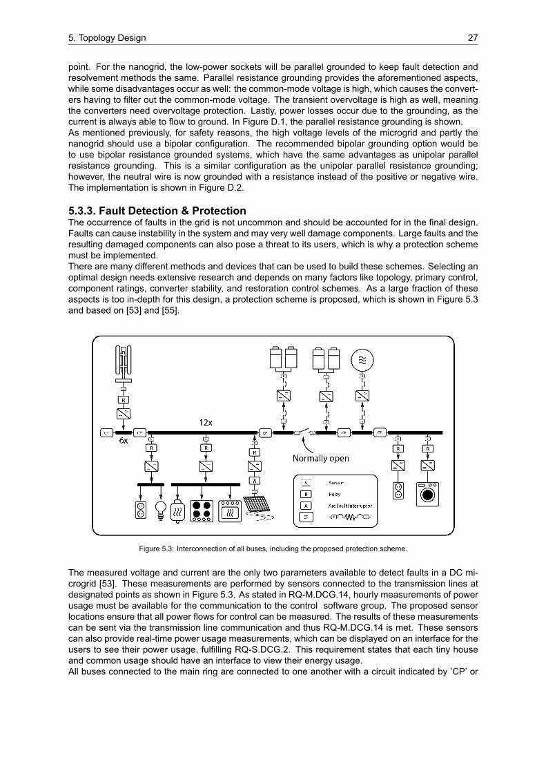
5. Topology Design 27
point. For the nanogrid, the lowpower sockets will be parallel grounded to keep fault detection andresolvement methods the same. Parallel resistance grounding provides the aforementioned aspects,while some disadvantages occur as well: the commonmode voltage is high, which causes the converters having to filter out the commonmode voltage. The transient overvoltage is high as well, meaningthe converters need overvoltage protection. Lastly, power losses occur due to the grounding, as thecurrent is always able to flow to ground. In Figure D.1, the parallel resistance grounding is shown.As mentioned previously, for safety reasons, the high voltage levels of the microgrid and partly thenanogrid should use a bipolar configuration. The recommended bipolar grounding option would beto use bipolar resistance grounded systems, which have the same advantages as unipolar parallelresistance grounding. This is a similar configuration as the unipolar parallel resistance grounding;however, the neutral wire is now grounded with a resistance instead of the positive or negative wire.The implementation is shown in Figure D.2.
5.3.3. Fault Detection & ProtectionThe occurrence of faults in the grid is not uncommon and should be accounted for in the final design.Faults can cause instability in the system and may very well damage components. Large faults and theresulting damaged components can also pose a threat to its users, which is why a protection schememust be implemented.There are many different methods and devices that can be used to build these schemes. Selecting anoptimal design needs extensive research and depends on many factors like topology, primary control,component ratings, converter stability, and restoration control schemes. As a large fraction of theseaspects is too indepth for this design, a protection scheme is proposed, which is shown in Figure 5.3and based on [53] and [55].
Figure 5.3: Interconnection of all buses, including the proposed protection scheme.
The measured voltage and current are the only two parameters available to detect faults in a DC microgrid [53]. These measurements are performed by sensors connected to the transmission lines atdesignated points as shown in Figure 5.3. As stated in RQM.DCG.14, hourly measurements of powerusage must be available for the communication to the control software group. The proposed sensorlocations ensure that all power flows for control can be measured. The results of these measurementscan be sent via the transmission line communication and thus RQM.DCG.14 is met. These sensorscan also provide realtime power usage measurements, which can be displayed on an interface for theusers to see their power usage, fulfilling RQS.DCG.2. This requirement states that each tiny houseand common usage should have an interface to view their energy usage.All buses connected to the main ring are connected to one another with a circuit indicated by ’CP’ or

5. Topology Design 28
central protection. This circuit consists of the transmission line connecting each of the buses with twosensors and two solidstate DC breakers at each end of the line. These sensors and breakers can shareinformation with a central protection control system. It is decided to use solidstate DC breakers as thistechnology comes with many advantages. These breakers ensure fast switching time, low conductionlosses, no risks of arcing or mechanical wear, high current carrying capability, and full controllability.Furthermore, these breakers can operate bidirectionally and can be opened and closed manually. Allthis makes them an excellent choice to function both as switches and protection at the most crucialinterface. Due to the central control, the systems can quickly identify the fault’s location and isolate thefaulty bus or line. To ensure that the rest of the grid stays operational, the switch between the sets ofbatteries can be closed to make the grid operate in ring configuration in such fault situations.A protection scheme using centrally controlled solidstate DC breakers is not only highly reliable butalso bidirectional. This is why the connection between the batteries and the ring is also protected bythis scheme on both sides of the DCDC converters. This is done because the batteries and their converters are expensive and of utmost importance for the grid to function correctly. For the same reasons,both sides of the ACDC converter of the PCC are protected with the same scheme.All other modules are protected with a simpler, cheaper local protection scheme. All PV systems areprotected by a technology called ’combination arcfault circuit interrupter’. These can detect and protect against series arcfault, overload, and short circuit faults. As can be seen in Figure 5.3 all othercomponents are protected by relays. It is recommended to use digital protective relays with a microprocessor as those can identify and protect against several fault conditions. These relays work with adelay time to check whether the detected fault is shortterm or longterm and can reclose on their own.This autonomous behaviour makes for relatively reliable local protection while minimizing complexityand costs. Finally, if any faults are missed by the primary protection, the backup protection within thecircuitry of the converters will add an extra line of defense against faults.
5.3.4. Voltage stabilityRQM.DCG.13 states that the voltage buses of the microgrid and nanogrid must remain at a constantoptimally chosen voltage with a minimum and maximum fluctuation of a to be determined percentage.In case of overconsumption, the available power can drop in the grid, causing the voltage to drop aswell. On the other hand, in case of overproduction, or production that is sufficiently higher than thecurrent demand, the available power in the microgrid can increase, causing the voltage to increaseas well. These two voltage fluctuations can cause issues in the operation of the converters. As theconverters which are now selected will not be used in the final design, the standard voltage fluctuationfor systems ranging from 120 𝑉𝐴𝐶 to 600 𝑉𝐴𝐶 from the ANSI C84.1 standard is taken as reference [56].In this standard, two voltage ranges are mentioned: range A (95% to 100% of the operating voltage)and range B (91.7% to 105.8% of the operating voltage). Range A is the safest of these options andensures correct operation, hence this stricter range is chosen as maximum voltage fluctuation range.The proposed control algorithms in case of islanded or gridconnected mode, hence for the bidirectionalDCDC converter to/from the battery as well as the bidirectional DCAC converter to/from the grid,have been designed to stabilize this voltage fluctuation. However, for our current design, these controlalgorithms have not been implemented. During the design validation, the voltage fluctuation will bechecked to see if RQM.DCG.13 can be met.
5.4. SafetyNow that the grid’s stability has been ensured to a certain degree, the actual safety for the residentsof the tiny houses needs to be guaranteed. This will be done by looking at standards that providestandardised implementations of DC microgrids and can thus provide another degree of safety. Also,the possible interaction of residents with the microgrid or nanogrid will be considered.
5.4.1. StandardsRQS.DCG.6 states that the entire microgrid should comply with the safety regulations of the EU inassociation with Dutch regulations and safety and connection standards for DC grids. In order to fulfillthis requirement, safety regulations for DC microgrids in the EU and standardised connections are researched in current standard development. The current developments in standards for DC microgridsare discussed in [53]. In addition, a small list of the most noteworthy standards will be provided in

5. Topology Design 29
Appendix D.4.2. As these standards are quite expensive and far above our budget for all subgroups, asmall summary is provided. For practical implementation, these standards should be bought to ensurethe grid design is done in a standardised way, minimizing dangers and faulty connections. The mentioned standards include safety considerations that have been considered in the protection circuitry,while the most prominent part considers standardised implementation for operation, maintenance, anddesign of DC microgrids in city, rural and remote areas. The application of the mentioned standardswould thus ensure that RQS.DCG.6 is met.
5.4.2. Human interactionThe microgrid and the nanogrids of each house are relatively small, making human interaction possiblewith the electrical appliances and components. As discussed in Section 5.3.1, a unipolar bus design isnot able to provide the same level of safety as a standard grid for voltage levels higher than 200 𝑉𝐷𝐶.As a bipolar implementation is not possible due to the communication, several measures are takento prevent accidental human interactions with the higher voltage levels. These measures consist ofisolating the highpower connections with the induction cooker and the electric boiler. This also meansthe inhabitants themselves will not be able to access these sockets easily, and except for maintenance,the highpower sockets will only be used for these two appliances. For tunect, the highpower usagesockets of the washing machines will be isolated in the same way. The batteries and their converterswill not be accessible without a particular key and can only be accessed by maintenance or residentswith the necessary experience. Lastly, the wind turbines will be inaccessible through fences and willbe accessible to maintenance.In case of maintenance, the previously mentioned isolation methods will be accessible to the appropriate personnel. For the high voltage levels in the grid, the multibus structure can isolate the defectedpart of the grid. Then, the protection schemes will make sure that the cables, converters, and othercomponents will be safe for human interaction.
5.5. Cost AnalysisThroughout the design process, specific products for many of the system’smain components have beenselected. RQS.DCG.1 states that the balance between costs of the entire DC grid and its functionalityshould be optimised. While deciding on what components to select, costs have been taken into accounton several occasions. Some examples are the decision to select the cheaper battery composition,minimizing the number of converters needed, trying to minimize the wiring prices, and choosing thecheaper local protection for some of the modules.Now that all those design choices have been made, a cost analysis can be performed. Even thoughappliances have been selected for the demand estimation, the cost analysis does not include them.This is because DC appliances are not on the market yet. Furthermore, appliances are not necessarilyconsidered to be part of the grid. This cost analysis only considers the costs of the main componentsof the grid and can be found in Appendix D.5. As shown there, the total price of this grid design will bearound €166,000.This price, however, is mainly based on prices found online. Most of these prices include 21% VATand are offered by a retailer. Considering that such a microgrid design is most likely to be used by acontractor, it is assumed that when the components are bought in bulk and directly from the supplier,these prices decrease by approximately 40%, also subtracting taxes. This results in a total price ofaround €100,000. This can be considered a fairly reasonable price as the most significant componentsare selected to operate for at least 20 years, and the costs are shared by 12 households.

6Design Validation
The design choices in the design phases of demand, supply, storage, and topology have been discussed but not yet verified. RQM.DCG.15 states that this should be done using power analysis simulation software, which needs to be carefully selected. RQM.DCG.15 is only met after certain demandcases show functional results. The resulting program was chosen to be Simulink [57], which is a transient analysis program based on MatLab, with a specialised power component library called Simspace.The loads, RESs, ESS and main grid need to be modeled and subsequently connected to the microgridand nanogrids.
6.1. Models of each subsystemIn order to correctly model the designed grid, each subsystem consisting of either demand, supply,or storage needs to be modeled correctly. Even though the circuits are simplified due to the topleveldesign and limited by the Simulink transient analysis, the electrical analysis can give some relevantresults. These results will be discussed for each subsystem.
6.1.1. DemandThe demand will be modeled with two constant power load blocks from Simscape, where the highpower and low power loads of the 400 V and 48 V sockets, respectively, are connected in parallel.No converter losses are included as this has been taken into account with the 30% safety marginexplained in Chapter 3. The appropriate wire length is then added for each house and is connected tothe microgrid voltage bus. This circuit is explained and shown in Appendix E.1.1.
6.1.2. PV panel moduleIn Simscape, there is a solar cell block available, which can take the short circuit current and the solarirradiation used for this current as input. The short circuit current is filled in from the datasheet [27],being 10.84 𝐴 at 1000 𝑊/𝑚2, while the opencircuit voltage needs to be equal to 3 times the opencircuit voltage of a single module (as 3 modules have been connected in series for each house), whichis equal to 3 ⋅ 42.9𝑉𝐷𝐶 = 128.7𝑉𝐷𝐶. By giving 206 series cells as input, this gives 128.7 𝑉𝐷𝐶 asopencircuit voltage. After connecting 20 of these solar cells in parallel, a short circuit current of 10.67𝐴was reached. This configuration gave the closest short circuit current to the desired value of 10.87𝐴.Lastly, a DCDC converter that boosts the voltage to 400 𝑉𝐷𝐶 is implemented. This circuit is explainedand shown in Appendix E.1.2.Due to the toplevel design and simple subsystems, connecting the PV panel subsystem to the loads,while the battery and wind turbine models with their respective converters were active, was not possibledue to limitations in Simulink. This limitation having to do with insufficient matching of load and demandfor the DCDC or DCAC converters. To remedy this, an equivalent model was constructed. Since thePV panels are connected directly to the loads, it was chosen to model their contribution by lowering thepower demand of the loads by 25%. This percentage is chosen as the maximum output power of thePV panels is equal to 13.68 𝑘𝑊, which is roughly 25% of the total peak demand of 62.1 𝑘𝑊.
30

6. Design Validation 31
6.1.3. Wind turbineThe second RESmethod are the VAWTs. In Simscape, there are several wind turbine blocks available,however these only work with torque as output and a complex connection circuit needs to be createdin order to deliver the electrical power output for a certain wind speed. It was thus chosen to implementan load flow source, which is able to supply a certain amount of active power, which was set at 2 𝑘𝑊.As the wind turbine is rated at 48 𝑉𝐴𝐶 [58], a rectifier rated at 48 𝑉𝐴𝐶 and a fixed power loss of 4% isimplemented (as a loss > 0% had to be implemented in the Simulink block). Then a DCDC converterof 400 𝑉𝐷𝐶 reference voltage was used to connect to the main grid. This circuit is explained shown inAppendix E.1.3.As with the PV panel model, calculations of an AC power source with a rectifier and DCDC converterare not possible if other DCDC converters are connected. This lead to the choice of modeling the windturbine as a battery of 48 𝑉𝐷𝐶 with a DCDC converter to 400 𝑉𝐷𝐶 and connected to its own set ofwiring. As each wind turbine is now modeled as a battery, the three turbines are taken as one singlebattery, which caused the resistance to be decreased by a factor of 3 due to parallel connection. Thecontribution of the PV panels was modeled as a 25% decrease in demand, while the wind turbines,which have a peak output power of 15.6 𝑘𝑊, will supply the 75% of the remaining demand togetherwith the batteries.
6.1.4. Battery / PCCThe ESSwas quite simple tomodel, as Simscape has a battery block that incorporatesmost parametersmentioned in the [40]. After filling in a nominal voltage of 358 𝑉𝐷𝐶, as well as the capacity of 2 times19.3 kWh multiplied with the RTE, the battery was complete. Another DCDC converter was placed toboost the voltage to 400 𝑉𝐷𝐶. The model is explained and shown in Appendix E.1.4. The PCC wasalso modeled as a battery with a DCDC converter to 400 𝑉𝐷𝐶 with its own section wiring.
6.1.5. WiringThe wiring for the microgrid and connections to the nanogrid are simple to model. As every wire operates at DC, the only modeled parameter of a cable is thus the resistance. The values for the resistanceare based on the wiring calculations given in Appendix D.3, and the wiring resistances in [49]. Aftercalculating the total resistance for each type of cable, the average lengths for each connection (ESS,RESs or loads) are used to calculate the actual resistor values. The results of these calculations areexplained and shown in Appendix E.1.5.
6.1.6. Grounding and protectionAs no analysis of the fault rate of the system has been done and no fault detection or resolving methodsare implemented, faults and grounding methods will not be analyzed in the simulation.
6.1.7. Grid layoutIn order to model the entire community, the subsystems have to be connected in a certain way. Ingeneral, the layout as presented in Chapter 5, with a normally open switch disconnecting the twobatteries, will be considered. This means that the general connection of subsystems to the microgridwill consist of 2 batteries on either side, 2 equivalent wind turbines, 12 tiny houses, 12 sets of equivalentPV panel production, and lastly, tunect. Each of these subsystems will be connected to the positivepolarity wire of the voltage bus using resistors with the value of the respective section resistance, whilethe negative polarity of the bus will work as a ground connection for all of the systems. The schematicof the microgrid with all the possible subsystems connected (RESs, ESS, loads and PCC) is shown inFigure E.5.
6.2. Simulation scenariosNow that each subsystem has been modeled, certain cases can be created to test if the ESS and RESscan supply the demand while still operating in the ±5% voltage fluctuation range. The six cases whichhave been considered are shown below. 150% of demand is also tested based on RQC.DCG.4, whichstates that design validation could be done for excessive scenarios of maximum power demand. Eachof the cases indicates whether the aforementioned subsystems are included and which subsystemcircuits are connected to the microgrid. In case of no batteries, the batteries are disconnected from the

6. Design Validation 32
microgrid. In case of no generation, the wind turbines are disconnected, and the load is set to 100%.In the case of main grid connection, the main grid is connected to the microgrid at tunect.
• Case 1: Maximum demand, all batteries, no generation
• Case 2: Maximum demand, all batteries, full generation
• Case 3: Low power demand, all batteries, no generation
• Case 4: Maximum demand, no batteries, only main grid
• Case 5: 150% of demand, all batteries, no generation
• Case 6: 150% of demand, all batteries, full generation
6.3. Case analysisFor each of the cases, the voltage at the loads was measured, as well as the current through the wireleading to the load. By calculating the difference in voltage of the grid and the loads and multiplying thiswith the current through the wire, both the voltage and power drops could be calculated. For each case,the minimum and maximum voltage in 𝑉 and their percentual decrease with respect to the 400 𝑉𝐷𝐶grid voltage are shown. The power losses in𝑊 due to the wiring are shown as well as the percentageof this loss with respect to the drawn power of each of houses / tunect. These results are summarisedin Table 6.1.
Table 6.1: Voltage drop in V and % and power loss in W and % for each of the cases.
Case Voltage drop [V]Min Max
Voltage drop [%]Min Max
Power drop [W]Min Max
Power drop [%]Min Max
1 2.81 7.39 0.70 1.85 31.49 89.38 0.71 1.882 2.05 5.46 0.51 1.36 18.34 49.25 0.52 1.383 0.32 1.28 0.08 0.32 0.11 2.72 0.08 0.324 1.76 6.31 0.44 1.58 18.27 76.06 0.44 1.605 4.23 11.19 1.06 2.80 71.54 204.92 1.07 2.886 2.71 9.12 0.68 2.28 27.19 138.5 0.68 2.33
As can be seen in case 1, which is the worst common case, the maximum voltage drop is 7.39 𝑉𝐷𝐶,which is equivalent to 1.85 % of the grid voltage. This voltage drop is thus still well within the ±5 %allowed voltage fluctuation limit [56]. The power loss is maximally 1.88 %, which in comparison withthe losses predicted in Table D.1, is as expected. This is due to each wire section contributing to thelosses, and hence the addition of the losses in Table D.1 is expected. The main grid connection performs better than the battery connection. This can be explained due to the lower connection resistanceof the main grid, as well as only a single wire is used, instead of the two connection wires needed forthe two sets of batteries.When looking at the cases where generation is able to support the batteries, it can be seen that thevoltage drop is lowered due to local generation of PV panels, as well as intermittent generation by theVAWTs. Between cases 1 and 2, the generation is able to provide 0.29 % less voltage drop and 0.4 %less power loss.The cases of 150 % power demand, with and without generation, are both hypothetical as the batteriesare physically not able to deliver this power demand, and the grid is not designed for higher demandthan 100%. Still, it shows that the voltage drop is in the acceptable range being maximally 2.80 %without generation and 2.28 % with generation. The generation provides 0.52% less voltage drop and0.55 % less power loss. As 150% of demand still shows functional results and is hence validated forthis grid design, RQC.DCG.4 is met. If even better cables are used which could handle this current,the losses would be even lower.Now that the design has been successfully validated using Simulink, showing acceptable voltage fluctuations and functional results in several demand cases, both RQM.DCG.13 and RQM.DCG.15 aremet. Furthermore, it can finally be concluded that both the microgrid and nanogrid are able to supplythe limited peak demand of the community and one tiny house respectively and thus RQM.DCG.2 andRQM.DCG.3 are met as well.

7Conclusions and Recommendations
The complete design and validation of an electricity grid for a community of tiny houses have nowbeen completed. The design phases consisted of estimating the energy demand, determining the required supply and storage for this demand, and optimizing the topology for the microgrid and nanogrid.The validation phase consisted of simulating several demand and generation cases in Simulink, whichresulted in the required functional results.
7.1. ConclusionsThe first design phase resulted in an hourly, daily, and monthly estimation of the community’s energydemand. The average daily usage of the community was estimated to be 57.48 𝑘𝑊ℎ/𝑑𝑎𝑦. Using amodel of generation, RESs in the form of 61.2 𝑚2 PV panels and 6 VAWTs are chosen to supply thisestimated demand. To store and supply energy of the varying energy generation of the RESs, differentESS options are considered, and 4 of the selected LiIon batteries are chosen with a total capacity of77.2 𝑘𝑊ℎ, and power output of 64.6 𝑘𝑊. In the last design phase, the topology of the community isdesigned, which resulted in a ring topology operating in a unipolar seriesconnected multibus configuration, operating at 400 𝑉𝐷𝐶. In order to easily identify faults and reduce complexity, this topologyeffectively operates in radial (by using a normally open switch). This topology also includes proposalsfor the required converters and control/optimization algorithms, the appropriate wiring for each connection, the selected grounding, fault detection and protection, and other safety considerations. A costanalysis is made of the grid of the entire community with all selected components, resulting in an estimated total cost of around €100,000. Lastly, design verification is performed on the proposed design,which resulted in functional results during maximum demand with a maximum voltage drop of 1.85 %and power loss of 1.88 %. For 150% demand, the results still showed functional results with a maximum voltage drop of 2.80 % and power loss of 2.88 %.Throughout the thesis, all requirements presented in Chapter 2 have been discussed. The primary requirements (must haves), and secondary requirements (should haves) have provided guidance in mostdesign choices, while some tertiary requirements (could haves) helped to improve the design. Thedesign meets all the primary requirements, which is discussed and concluded throughout the designphases and design validation. Furthermore, all of the secondary requirements have been accounted foras discussed throughout the thesis. Though not all can be considered successfully met, as terms like’optimize’ make these requirements hard to fully comply with as there is always room for improvement.Another obstacle was a paywall for information on standardization of safety, stability, and connections.Some of the tertiary requirements have been implemented as well, and if not, they will be discussedin Section 7.2. Finally, the toplevel system requirements have not been discussed explicitly, as all requirements relevant to the DCG subgroup have been converted into relevant subgroup requirements.
7.2. Discussion & Recommendations for Future WorkThe current design presented in this thesis is a toplevel design, and on many aspects, further research is needed to realise and optimise the design. Discussion on the current results as well as somerecommendations based on the research and results of each chapter are made below.
33

7. Conclusions and Recommendations 34
Energy Demand EstimationTo improve the accuracy of the demand estimation, more data from existing communities can be researched. The data from the two researched communities was very insightful, however it did also showhow big the difference between tiny house communities can be. Realtime power data would drastically improve the accuracy of the estimation of peak power, as well as the timing of the peak power.Additional market research on DC appliances would help determine the feasibility and time scale ofrealising this design.
Supply & Storage DesignThe current design is developed to operate in Rotterdam, enabling the microgrid to use the main gridas backup and to supply back to the city. For now, it has been decided to supply back to the maingrid. RQC.DCG.6 states that in case of overproduction, supplying excessive energy back to the maingrid could be minimised in order to minimize grid connection. In order to fulfill this requirement as wellas making the design more scalable, the overproduction could be diverted through turning off the PVsystem when needed, or further research could be done on finding different ways.RQC.DCG.1 states that the microgrid could operate completely islanded. As the availability of thecurrent design is already substantial and to fulfill this requirement, it would be interesting to researchwhat would be needed to enable complete offgrid operation.To improve the reliability and efficiency of the current design, an entirely distributed battery systemcould be an option as less expensive home batteries become available. Further research is neededon connecting the energy demand and supply of the heat grid to the microgrid to enable power sharingbetween the system resulting in more efficient use of energy.And finally, employing aerodynamics research, optimal locations for the VAWTs could be found. Currently, these are simply put as far away as possible. As discussed in Section 4.2.1, no realtime powerdata is available from either demand or generation. This meant that RESs and ESS methods couldonly be selected using an energy balance instead of a power balance. Research could be done forhigh power density ESS methods, such as a highspeed flywheel. A hydrogenbased storage andgeneration system could also be considered, such as proposed in [59].
Topology DesignAs discussed earlier, the use of a bipolar bus would be a better option for this design, not only to improvesafety but also reliability. In case a line is faulty, half of the bus is still operational due to the third line.To further increase the system’s safety, it is recommended to research the European and Dutch safetystandards more indepth. Subsequently, a detailed protection and safety system can be designed.Custom converter design should be done in order to implement all recommended optimization controlalgorithms. RQC.DCG.5 states that primary control methods could be defined and compared for thisimplementation. To fulfill this requirement, research could be done on the primary control of the system.
Design ValidationIn Chapter 6, Simulink with its specialised library Simspace was used to validate the designed grid. Ifmore time would have been available, the proposed converters could have been designed in Simulinkand implemented. Furthermore, basic versions of our proposed control/optimization algorithms couldhave been designed in Simulink as well.However, this software was not optimal, as it is a transientbased analysis software with no properblocks for power flow analysis. The most appropriate software for a power flow analysis of a topleveldesign would be libraries like MATPOWER (in MATLAB) or PandaPower (in Python). However, eventhese programs specialize in large regional AC grids of several 𝑀𝑊, whereas our grid operates on DCand consumes less than 0.1 𝑀𝑊. A DC power flow is possible in these programs, but this approximates an AC power using fixed voltage levels but varying voltage angles (hence reactive power is stillpresent). Programming a modified DC power flow based on this software which only utilises real voltages and currents and only active power flow is out of the scope of this thesis but could be researchedto validate the toplevel grid design properly.Furthermore, in Simulink, no proper RES or ESS blocks were available for power flow analysis or simulations of several hours. Hence, the previously used energy balance analysis was not possible, andonly power demand could be compared. This meant rough equivalent models had to be designed.
AcronymsAC Alternating current.
CNS Control & Software.
DC Direct Current.
DCG DC Grid.
DoD Depth of Discharge.
DSO Distribution System Operator.
EMI ElectroMagnetic Interference.
ESS Energy Storage System.
HAWT Horizontal Axis Wind Turbine.
IEA International Energy Agency.
MPPT Maximum Power Point Tracking.
PCC Point of Common Coupling.
PID Proportional Integral Derivative.
PLC Power Line Communication.
Poc Proof of Concept.
PoR Program of Requirements.
PV PhotoVoltaic.
PVT PhotoVoltaic Thermal.
RES Renewable Energy Source.
RTE Round Trip Efficiency.
SoC State of Charge.
VAWT Vertical Axis Wind Turbine.
35

ASystem PoR
This section covers the toplevel system requirements of the Bachelor Graduation Project ’Distribution of the electricity grid of a tiny house community’. The system requirements relevant to the DCGsubgroup have been rephrased and put into the requirements of the subgroup as shown in Chapter 2.
A.0.1. Functional RequirementsMust have
• RQM.SYS.1: The system must use the designed DCG, where information will be sent to theControl & Software (CNS) subsystem using the designed Power Line Communication (PLC).
• RQM.SYS.2: The system must be able to supply the 12 tiny houses and the common usage ofthe community.
• RQM.SYS.3: The system must use renewable energy sources as supply units only.
• RQM.SYS.4: The system should have an availability of at least 90%.
• RQM.SYS.5: The system must be able to do forecasting of factors influencing the system basedon the users’ behaviour and the weather.
• RQM.SYS.6: The system must be able to communicate grid information over the power linesusing a power line communication system.
Should have• RQS.SYS.1: The system should be designed such that the costs are minimised for the givenfunctional requirements.
• RQS.SYS.2: The system should be designed such that the efficiency is optimised.
Could have• RQC.SYS.1: The system could be designed to operate in islanded mode all of the time.
• RQC.SYS.2: The system could be designed to be scalable, i.e., both the number of tiny housesper community and the number of communities can be easily increased.
A.0.2. NonFunctional RequirementsBelow, all nonfunctional requirements of the toplevel system will be given. They describe how thesystem should operate.
• RQNF.SYS.1: The minimum speed of the power line communication system should be suchthat it can sustain a transfer that is fast enough such that all data can be delivered to the deviceswithin a timely manner.
36

BDemand
In the following sections, the individual appliance selection is made, and usage calculation is done forthe initial estimation, as well as the sustainable modifications made. Lastly, the notes from the interviewwith a tiny house community in Delft called ’Pionierskwartier’ are shown.
B.1. Appliance selectionIn the next lists, the used appliances with their respective usages are shown for all appliance categories.Care has been taken to select low power usage versions for all appliances and, if possible, the bestpossible energy efficiency grading.
Base LoadThe baseload consists of essential appliances which are almost always turned on, where the selectedappliances are shown below.
• Ventilation: https://www.ventilatieland.nl/artikel/17345/badkamerventilatorenergiezuinigstilenmettimerdiameter100mmwit100ts.html
• Lights: https://www.lighting.philips.nl/consumer/p/ledspot/8719514314030
• WiFi Router: https://www.trendnet.com/products/wirelessacrouter/ac1200dualbandwifirouterTEW831DR
• Fridge/Freezer Combination: https://www.bemmelenkroon.nl/merken/frilec/berlin1651a_plus__plus__plus_fril/
Kitchen AppliancesThe chosen kitchen appliances are shown below.
• Blender: https://www.amazon.nl/RussellHobbsGeluidsreductiesysteemRuimtebesparend2529056/dp/B07NDH6L3W
• Induction Stove: https://www.bcc.nl/keuken/fornuisenkookplaat/inbouwinductiekookplaat/aeginductiekookplaathk604200cb/254912?channable=006f36696400303030303030303030303030323534393132b4&utm_medium=vergelijkingssites&utm_source=beslist&utm_campaign=keuken_fornuisenkookplaat_inbouwinductiekookplaat&utm_content=000000000000254912&bl3nlclid=814e82ecb56940ab80dab81ce151cd7a&utm_term=BESLI814e82ecb56940ab80dab81ce151cd7a
• Oven/Microwave Combination: https://www.magnetronoven.nl/inventum/mn256c/
37

B. Demand 38
• Coffee Machine: https://www.bcc.nl/keuken/koffiezetapparaat/nespressomachine/nespressomagimixkoffieapparaatpixiem112aluminium/57585?channable=006f366964003030303030303030303030303035373538350a&utm_medium=vergelijkingssites&utm_source=beslist&utm_campaign=keuken_koffiezetapparaat_nespressomachine&utm_content=000000000000057585&bl3nlclid=0584d9d6d3d74adcb5c9a7fc6caf9354&utm_term=BESLI0584d9d6d3d74adcb5c9a7fc6caf9354
• Kettle: https://www.bol.com/nl/p/russellhobbstexturespluswaterkokerzwartsnelkookfunctieextrazuiniggemakkelijkreinigbaar2400watt/9300000031652517/?Referrer=ADVNLGBL000&utm_source=google&utm_medium=cpc&utm_campaign=beslistSDA&utm_term=BESLI0ea7189cb9484862883a0147441dc53d~9300000031652517&bl3nlclid=0ea7189cb9484862883a0147441dc53d
• Kitchen Machine https://www.coolblue.nl/en/product/140640/magimixcuisinesysteme5200xlmattechrome.html
Heat RegulationThe appliances which contribute to the heat regulation of a tiny house are shown below.
• Boiler: https://www.techniq.nl/eldomfavouriteelektrischeboiler50liter.html?utm_source=Google+Merchant+Center&utm_medium=referral&utm_term=111166944&utm_campaign=easyads&gclid=Cj0KCQjwk4yGBhDQARIsACGfAeuC8EYKXLObl3sTNKUDnRWaBUHN9ZJMICcccJFvA7vVVjCVRBjGwaAnh_EALw_wcB
• Water Pump: https://www.waterpump.co.uk/dabevosta24070180circulationpumpcentralheatingpump?sqr=dab
• Shower: https://www.mijnupfallshower.nl/prijzenupfallshower.html
• Air Conditioning: https://www.totalhomesupply.com/p/frigidaireffra051wa15000btuwindowunitroomairconditionermanualcontrol
Remaining AppliancesThe remaining appliances which are considered are shown below.
• Phone Charger: https://www.apple.com/shop/product/MD810LL/A/apple5wusbpoweradapter
• Computer Charger: https://www.hp.com/usen/shop/pdp/hpzbookstudiog5mobileworkstation
• Vacuum Cleaner: https://www.cnet.com/products/dysondc40originuprightvacuumcleaner/
• Handheld Vacuum: https://www.coolblue.nl/product/234250/philipsfc6149.html#productspecifications
• Hair Dryer: https://www.agstore.nl/philipsbhd02700energiezuinigefoehn111143707.html
• LED Television: https://www.mediamarkt.nl/nl/product/_philips32phs5525121662224.html

B. Demand 39
Tunect AppliancesFor the common usage, extra care must be taken for low power usage and high efficiency as a dryerand washing machine use a lot of energy throughout the year. These appliances, as well as the printer,outdoor lights, and control unit are shown below.
• Washing Machine: https://www.coolblue.nl/product/869937/haierhw80b14636n.htm
• Dryer:https://www.coolblue.nl/product/867486/siemenswt7u4600nl.html#productspecifications
• Printer: https://www.freeprintersupport.com/laserprintervsinkjetprinterpowerconsumption
• Outdoor Lights: https://www.lighting.philips.com/main/prof/outdoorluminaires/roadandurbanlighting/roadandurbanluminaires/lumagen2/910925867324_EU/product
• Control Unit: https://www.sossolutions.nl/raspberrypi4modelb4gb?gclid=Cj0KCQjwk4yGBhDQARIsACGfAevGqgRmVmj9JlobiJgr4Xczf4yvITPGWHhDD7t4Q05cn_mM26cuA1UaAjlTEALw_wcB

B. Demand 40
B.2.Initialpow
erandtim
eusagetables
Inthissection,theinitialdemandestim
ationconsistingofthepeak
andaveragepower
demand,tim
eusage,anddaily,m
onthly,
andyearlyenergy
usage
isshow
nfore
achofthecategories,usingtheselected
appliances
inAp
pendixB.1andthetim
eusagein[17]and[18].Theinitialbaseload
isshow
nin
TableB.1,thekitchenappliances
inTableB.2,theheatingregulationappliances
inTableB.3andlastlythecommon
usageinTableB.5.
B.2.1.B
aseload
TableB.1:
Initialusageestim
ationofthebase
load.
App
liance
Peak
power
[W]
Averagepo
wer
[W]
Timeused
[h/day]
Energusage[W
h/day]
kWh/mon
thkW
h/year
Ventilation
8.00
8.00
6.00
48.00
1.46
17.52
Lights
12.00
12.00
8.00
96.00
2.92
35.04
Wifirouter
5.68
1.42
24.00
34.08
1.04
12.44
Fridge
+freezer
55.00
10.73
24.00
257.53
7.83
94.00
Total
80.68
32.15
435.61
13.25
159.00
B.2.2.K
itchenappliances
TableB.2:
Initialusageestim
ationofthekitchenappliances.
App
liance
Peak
power
[W]
Averagepo
wer
[W]
Timeused
[min/day]
Energusage[W
h/day]
kWh/mon
thkW
h/year
Blender
400.00
400.00
4.00
26.67
0.81
9.73
Inductioncooker
3650.00
1500.00
33.33
833.25
25.34
304.14
Oven
2400.00
2000.00
30.00
1000.00
30.42
365.00
Microwave
900.00
550.00
20.00
183.33
5.58
66.92
Coffeemachine
1260.00
1260.00
15.00
315.00
9.58
114.98
Kettle
2400.00
2400.00
12.50
500.00
15.21
182.50
Kitchenmachine
1100.00
1100.00
10.00
183.33
5.58
66.92
Total
12110.00
9210.00
3041.58
92.51
1110.18

B. Demand 41
B.2.3.H
eatin
g
TableB.3:
Initialusageestim
ationoftheheatregulation.
App
liance
Peak
power
[W]
Averagepo
wer
[W]
Timeused
[h/day]
Energusage[W
h/day]
kWh/mon
thkW
h/year
Boiler
2000.00
2000.00
0.85
1700.00
51.71
620.50
Waterpump
44.00
44.00
8.40
369.60
11.24
134.90
Show
er150.00
150.00
0.20
30.00
0.91
10.95
Airconditioning
450.00
450.00
1.00
450.00
13.69
164.25
Total
2644.00
2644.00
2549.60
77.55
930.60
B.2.4.O
ther
appliances
TableB.4:
Initialusageestim
ationofallrem
aining
appliances.
App
liance
Peak
power
[W]
Averagepo
wer
[W]
Timeused
[min/day]
Energy
usage[W
h/day]
kWh/mon
thkW
h/year
Phonecharger
10.00
5.00
240.00
20.00
0.61
7.30
Com
putercharger
150.00
150.00
38.24
95.60
2.91
34.89
Vacuum
cleaner
850.00
850.00
8.33
118.06
3.59
43.09
Hairdryer
1600.00
1600.00
9.00
240.00
7.30
87.60
LEDTelevision
24.00
24.00
233.33
93.33
2.84
34.07
Total
2634.00
2629.00
566.99
17.25
206.95

B. Demand 42
B.2.5.Tun
ectu
sage
TableB.5:
Initialusageestim
ationoftunect.
App
liance
Peak
power
[W]
Averagepo
wer
[W]
Timeused
[min/day]
Energusage[W
h/day]
kWh/mon
thkW
h/year
Washing
machine
2000.00
2000.00
45.37
1512.33
46.00
552.00
Dryer
1000.00
1000.00
349.15
5819.18
177.00
2124.00
Printer
12.00
0.79
1440.00
18.90
0.57
6.90
Streetlights
120.00
120.00
480
960.00
29.20
350.40
Controlm
odule
1010
1440
240.00
7.30
87.60
Total
3142.00
3130.79
8550.41
260.07
3120.90

B. Demand 43
B.3. Interview notes• Estimatjon of energy usage
– Appliances⋄ Estimated average base load of 40 Watts: ventilation, lights, smart computer, fridge, wifietc.
⋄ Kitchen appliances: Coffee machine, phone charger, external monitor and laptop– Energy usage using fossil fuel sources (pellet heating, gas furnace, gas boiler etc.): 2 kWhper day
– Estimated energy usage using mostly electric per day:⋄ 1.8 kWh of cooking⋄ 1.61.8 kWh of heating usage (shower/heating)⋄ Total: around 34 kWh
– Yearly energy estimation of 1000 kWh: 200 kWh of heating and 800 kWh of cooking.
• Heating:
– Singular heating system: could be done using PV system, sun collectors, and a heat pump.This can also function as a heat pump in case of overproduction.
– Using a common heating system is difficult due to heat losses in storage and transportation.If done properly could be very useful, but only if the whole community uses the heatingsystem.
– Heating system requires very well isolated houses (passive house standard) to theoreticallyfunction. In the winter, a heat grid might not be enough, hence a backup heating systemcould be used like a hydrogen battery that feeds an electric generator or a salt water extraction battery.
– Isolation requires a tradeoff, as larger isolation causes less space to be available, whichmight lead to the houses becoming bigger to compensate.
• Electricity connection:
– Most used option is the VICTRON transformer, which keeps the connection to the main gridstable and regulates the power usage.
– With current products, AC outlets would still be required, however DC might be an option ifresearched. The current grid for a tiny house should be AC due to safety and easy connections with common appliances.
• Generation
– Easy solar controller which makes sure the battery, solar panels, and demand of a tiny houseare regulated. This means each house must have its own battery in order for it to function.
– Estimation of 90% availability if excellent solar panels are used as well as a battery. Morerealistic if other sources like wind or hydrogen are used.
– Using a VICTRON connection, net 0 energy can be used from the grid as power can bedelivered back.
• Storage:
– Use a lithiumion battery, the best performance for your community.– Supercapacitor not needed as peak power demand will seldom occur, especially not in a fewseconds. Maximum power also not comparable to fast EV charging.
– Hydrogen could be an option, but right now quite expensive and not quite there in terms ofcapacity.

B. Demand 44
B.4.Tablesafterm
odificatio
nsInthissection,thepeak
andaveragepowerdemand,tim
eusage,anddaily,m
onthly,andyearlyenergy
usageoftheremaining
appliances
afterm
odifications
areshow
nfora
llcategories.
InTableB.6thebase
load
isshow
n,thekitchenappliances
areshow
ninTableB.7,
theheatingregulationappliances
inTableB.8andlastlyTableB.10
show
sthecommon
usage.
B.4.1.Idleappliances
TableB.6:
Thesustainableusageestim
ationofthebase
load,w
hich
hasremainedthesameas
theinitialestim
ation.
App
liance
Peak
power
[W]
Averagepo
wer
[W]
Timeused
[h/day]
Energusage[W
h/day]
kWh/mon
thkW
h/year
Ventilation
8.00
8.00
6.00
48.00
1.46
17.52
Lights
12.00
12.00
8.00
96.00
2.92
35.04
Wifirouter
5.68
1.42
24.00
34.08
1.04
12.44
Fridge
+freezer
55.00
10.73
24.00
257.53
7.83
94.00
Total
80.68
32.15
435.61
13.25
159.00
B.4.2.K
itchenappliances
TableB.7:
Thesustainableusageestim
ationoftheselected
kitchenappliances.T
hemicrowavehas0peak
astheoven
andmicrowavecanonlyrunseparately.
App
liance
Peak
power
[W]
Averagepo
wer
[W]
Timeused
[min/day]
Energusage[W
h/day]
kWh/mon
thkW
h/year
Blender
400.00
400.00
4.00
26.67
0.81
9.73
Inductioncooker
3650.00
1500.00
45.00
1125.00
34.22
410.63
Oven
2400.00
2000.00
20.00
666.67
20.28
243.33
Microwave
550.00
10.00
91.67
2.79
33.46
Total
6450.00
4450.00
1910.00
58.10
697.15

B. Demand 45
B.4.3.H
eatin
g
TableB.8:
Thesustainableusageestim
ationoftheselected
heatregulation.
App
liance
Peak
power
[W]
Averagepo
wer
[W]
Timeused
[min/day]
Energusage[W
h/day]
kWh/mon
thkW
h/year
Boiler
2000.00
2000.00
0.85
1700.00
51.71
620.50
Waterpump
44.00
44.00
8.40
369.60
11.24
134.90
Show
er150.00
150.00
0.20
30.00
0.91
10.95
Total
2194.00
2194.00
2099.60
63.86
766.35
B.4.4.O
ther
appliances
TableB.9:
Thesustainableusageestim
ationoftheselected
remaining
appliances.
App
liance
Peak
power
[W]
Averagepo
wer
[W]
Timeused
[min/day]
Energusage[W
h/day]
kWh/mon
thkW
h/year
Phonecharger
10.00
5.00
240.00
20.00
0.61
7.30
Com
putercharger
150.00
150.00
38.24
95.60
2.91
34.89
Vacuum
cleaner
12.00
12.00
8.33
1.67
0.05
0.61
Total
172.00
167.00
286.57
117.27
3.57
42.80

B. Demand 46
B.4.5.Tun
ectu
sage
TableB.10:T
hesustainableusageestim
ationoftunect.
App
liance
Peak
power
[W]
Averagepo
wer
[W]
Timeused
[min/day]
Energusage[W
h/day]
kWh/mon
thkW
h/year
Washing
machine
4000.00
252.05
360.00
1512.33
46.00
552.00
Printer
12.00
0.79
1440.00
18.90
0.57
6.90
Streetlights
120.00
120.00
480
960.00
29.20
350.40
Controlm
odule
1010
1440
240.00
7.30
87.60
Total
4142.00
382.84
2731.23
83.07
996.90

B. Demand 47
B.5. Daily modelIn this section, the data used for the daily model, as well as extra results of both the daily and monthlymodel.
B.5.1. Liander DataThe daily model is constructed based on reallife data made available by Liander [23]. Following thelink in the bibliography, the used data can be found in the middle of the page under the ’slimme meter’or smart meter section.
B.5.2. Graphs from daily dataUsing the energy usage behaviour of the Liander data [23] and scaling with the estimated usage of atiny house, the daily Wh usage for every 15 minutes for a tiny house can be calculated and is shownbelow in Figure B.1. The data values are shown in Table B.11.
Figure B.1: Average energy usage of one tiny house (orange) and one average household (blue) in Wh over a day in 15 minuteintervals.

B. Demand 48
Table B.11: Daily usage for a tiny house versus average liander household.
Hour Tiny house usage [Wh] Liander usage [Wh]0 141.56 295.081 111.79 233.022 101.48 211.543 95.52 199.114 92.46 192.735 93.35 194.586 109.43 228.117 149.51 311.658 183.16 381.819 202.31 421.7210 198.71 414.2111 192.09 400.4112 204.47 426.2313 198.72 414.2314 190.61 397.3315 187.77 391.4216 201.69 420.4217 288.77 601.9418 311.18 648.6519 314.52 655.6220 292.06 608.8121 264.65 551.6522 240.47 501.2623 196.19 408.96
B.6. Monthly modelThe monthly model uses the behaviour of an average of 5 houses of the ’Minitopia’ tiny house community and scaling this with our yearly usage results in a monthly energy consumption distribution. Themonthly energy usage in 𝑘𝑊ℎ of a tiny house for all months is shown in Figure B.2. The orange datashows the average monthly usage in 𝑘𝑊ℎ for a house in Minitopia, whereas the blue data is the scaledversion of our estimated tiny house demand. As can be seen from the figure, the monthly demand ofminitopia is always higher, in table Table B.12, the values can be found. The tiny house usage is 60%of the Minitopia usage.
Table B.12: Minitopia vs tiny house monthly usage in kWh.
Month Minitopia usage [kWh] Tiny house usage [kWh]January 235.49 144.62February 245.03 150.48March 222.70 136.77April 198.00 121.60May 213.77 131.28June 210.07 129.01July 160.87 98.80August 169.33 103.99September 149.59 91.87October 173.81 106.74November 224.60 137.93December 288.34 177.08
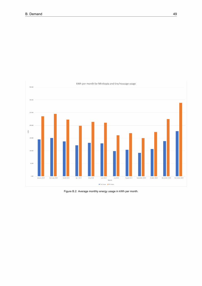
B. Demand 49
Figure B.2: Average monthly energy usage in kWh per month.

CSupply and Storage
C.1. Heat Grid AnalysisIn Figure C.1 a schematic overview of the heat grid is given. The heat grid consists of three maincomponents: the heat generation by PVT panels, the seasonal heat storage by the heat battery, andthe residential heating system.
Figure C.1: Schematic overview of the heat grid designed in [5].
PVT panels make use of solar energy in two different ways at the same time by combining PV technology with that of a sun boiler. Similar to a standard PV the PVT panels convert solar irradiance intoelectrical energy through the photovoltaic effect, which is both a physical and chemical phenomenonusing photons to create a flow of electrons. Additionally, PVT’s are able to capture the heat of the sunby transferring it into the fluid that runs through the panel. This process has three advantages over theuse of PV’s in combination with electric heating. The first advantage being that one panel can generateboth electricity and capture heat while taking up a similar amount of space as a standard PV. Secondly,capturing and storing energy in heat for heating purposes is a much more efficient process comparedto generating electrical energy with PV’s to store it in a battery to convert it into heat by an electricalboiler subsequently. Finally, the fluid in the panel is heated by extracting the heat out of the panel itself,cooling the panel, which is advantageous for the efficiency of the photovoltaic system as this decreaseswhen the temperature rises.When the fluid in this case water has extracted the heat, the warm water is transferred through copperinsulated pipes to either the heat battery or the residential heating system. The chosen heat battery is
50

C. Supply and Storage 51
being developed by TNO for residential purposes and is planned to become available on the market in2022 [60]. The use of such a heat battery enables the system to cover seasonal fluctuations in temperature. This way, the PVT panels can capture a lot of solar heat in the summer and store it in theheat battery until it is needed in the colder winter months.When heat is needed inside, either the PVT’s, or the heat battery can deliver warm water to the residential heating system within each of the tuni. Each system has its own basin. The water of this basincan be used for either floor heating or warm tap water. As the water in the basin is already warm, itcan be used for floor heating directly. Tap water must be at least 60 °C, so an electrical boiler is usedto provide the required additional energy to heat the tap water. This supplementary energy accountedfor 1700𝑘𝑊ℎ per day on average in the demand calculations in Section 3.1. Finally, the residentialheating system also contains a wastewater heat recovery system which reuses heat of old tap waterto heat new water coming into the boiler, resulting in fewer losses. This heat grid is assumed to beoperating on one large heat pump, which is powered by the PVT panels’ electrical energy, which willbe further explained now.
When reviewing the system, a major discrepancy has been found in the calculations of the energydemand in [5]. An initial calculation was done in order to establish the needed PVT panel area perhouse based on the heat needed per residence, which was calculated to be 3.08𝑚2 per tunus. Then, asecond calculation was done, which established that 3.2𝑚2 of PVT panel area per tunus was requiredto power the heat pump of the system. The decision was then made to use two 2𝑚2 PVT panels pertunus which would suffice for both heat demand and energy demand for the circulation system. However, in further calculations, all electricity generated by these panels was considered to be available forother energy purposes even though the more significant fraction ought to be used for the heat pump.To avert this duplicate of energy use without redesigning the heat grid, as this is out of scope, the following is considered. A total of 19 PVT panels of 2𝑚2 will be used (12 ∗ 3.08𝑚2 = 36.96𝑚2) and areassumed to be sufficient for generating both heat for all 12 tuni and the energy needed for the heat gridto function correctly. The PVT’s can be placed in a central area near the heat battery and the entireheat grid is considered as an isolated system, disconnected from the electricity grid. A basic schematicof the heat grid construction that will be implemented in this design is shown in Figure C.2.
Figure C.2: Schematic overview of the heat grid construction implemented in current design.
C.2. PV Panel Performance AnalysisIn the Netherlands, the optimal orientation is towards the south at a tilt of 37∘ [61]. In [62] it is foundthat as long as the panels are oriented within 20∘ towards the south at a tilt of 30∘ to 40∘ orientationlosses are easily kept under 5%. The roofs of the tuni have a slope of 30∘ on which all panels canbe placed towards the south relatively well, and thus a maximum loss of 4% throughout the year is

C. Supply and Storage 52
assumed as the panels will remain stationary and do not follow the sun’s orbit. As briefly discussedbefore, the temperature of the solar cells influences the efficiency as well. Most solar cells function bestat a temperature of approximately 25°C and decrease in efficiency when the temperature increases.The panel’s temperature not only depends on ambient temperature, but also on factors like radiationstrength, wind, and precipitation. In [63] research is done on the influence of temperature on solarpanel efficiency throughout the year. Results indicate a loss of 6.4% and 7.2% in German residences,however sloped residences in hotter countries like Italy indicate a loss of 5.5%. Based on the fact thatthe Dutch climate is colder and the solar panels will be put on inclined roofs, a loss of 5% is assumed.A major cause of inefficiencies for solar panels in an urban environment is losses due to shadows ofsurrounding buildings. However, as the community is built on the roof of a highrise building, this isless of a problem. The assumption is made that the high rise is high enough that no other buildingscan block out the sun, and so the shadow losses are assumed to be zero in this case. Besides zeroshadow losses, it has been decided to disregard losses due to snow and dust as well as both have littleinfluence on a high rise in a Dutch city.Finally, the attenuation of the power output over time plays an important role in the panels’ efficiencythroughout the years. In [27] the attenuation after one year and the degradation factor for the following24 years can be found. From this, the losses by degradation are calculated to be
2% + (98% − 90.8%)2 = 4.6% (C.1)
The total additional losses of the PV system are thus as follows.
Orientation/Tilt Loss 4%Temperature Loss 5%Degradation Loss 4.6%Resulting Efficiency 87%
C.3. KNMI weather data usageThe data set from the KNMI weather station in Rotterdam [36] contains hourly measurements of thefollowing weather aspects:
• Irradiance: average global horizontal irradiance (GHI) [𝑊/𝑚2].
• T_ambient: average ambient temperature measured at 1.5 m above the ground.
• T_ground: the average ground temperature at 10 cm above the ground.
• Wind: average wind speed at 10 m above the ground.
• Cloud: cloud coverage in eighths of the visible sky area where 0 is clearsky, and 8 is a completelyobscured sky.
• Pressure: air pressure at the measurement station in Pascal.
• Rainfall: rainfall at the measurement station in mm/hr.
As a selection was alreadymade for the losses of the PV panels and the wind turbine in Section 4.1.2and ??, the only data which was used for the model was the irradiance in [𝑊/𝑚2] and the averagewind speed in 𝑚/𝑠. The values for these two weather aspects are measured every hour over a wholeyear. The measurements are also averaged over the last 30 years, starting from January 1991 untilApril 2021 (when the file was downloaded).
To correctly gather hourly data, the hourly measurements of each day are averaged for each month,resulting in an average hourly model for a day in each month. This model thus contains average hourlyirradiation and wind speed over a day for each month. For the PV panel, the energy generation persquare meter is calculated by multiplying the irradiation per square meter with the module efficiency ofthe PV panels mentioned in the datasheet [27] as well as the losses elaborated in Section 4.1.2.

C. Supply and Storage 53
Figure C.3: The power output of the AeolosV 2 kW wind turbine for the windspeed.
For the VAWT’s, no losses were available in the datasheet and only the power curve in the datasheetis used shown in the datasheet [58]. There are only 12 integer wind speeds shown, hence a polynomialapproximation had to be made. Using the highest order approximation available in Excel (6th order),a formula was created to calculate the output power for every wind speed. This formula is shown inEquation (C.2), where 𝑃 is the output power in 𝑊 and 𝑣 the average wind speed in 𝑚/𝑠. The powercurve is shown in Figure C.3 for wind speeds up to 12 𝑚/𝑠.
𝑃 = 0.0725 ∗ 𝑣6 − 3.3441 ∗ 𝑣5 + 60.575 ∗ 𝑣4 − 551.26 ∗ 𝑣3 + 2689.8 ∗ 𝑣2 − 6598.3 ∗ 𝑣 + 6399 (C.2)
C.4. Other supply model resultsThe model of the s in combination with the daily demand for each month resulted in 6 VAWTs and 3modules of the selected PV panel, resulting in a total of 36 modules, or 61.2𝑚2 PV panel. The monthlygeneration and demand have also been shown for the selected amount of each RES. Another analysiswas done to see whether the generation could have been done with only one form of the two selectedforms of RES, hence checking if only generation using VAWT’s or PV panels would have been possible.As can be seen from Table C.1, the amount of VAWT’s needed in the summer months and the amountof PV panels in the winter months is extremely large and not suited for the community on the roof of ahighrise building in Rotterdam. Furthermore, the hourly generation in December and July, which arethe highest and lowest demand respectively, are shown in Figure C.4 and Figure C.5.

C. Supply and Storage 54
Table C.1: Amount of VAWT’s and PV panels needed in case of only one RES method.
Month Only VAWT Only PV [𝑚2]January 8 448.37February 9 261.60March 9 117.99April 14 66.28May 16 55.70June 17 53.27July 15 41.74August 18 51.96September 16 69.62October 10 135.67November 11 379.67December 9 738.88
Figure C.4: Hourly generation versus demand in the month december.

C. Supply and Storage 55
Figure C.5: Hourly generation versus demand in the month july.

C. Supply and Storage 56
C.5.E
SSCom
paris
onInTableC.2,the
comparedcriteria
andresults
foreachoftheconsidered
ESSs
areshow
n.
TableC.2:C
omparison
tableofseveraltypes
ofES
S.
Type
Energy
[$/kWh]
Power
[$/kW]
Respo
nse
Time
System
RTE
[%]
Life
Cycle
[yrs]
Advantages
Disadvantages
Lead
AcidBa
ttery
559
2194
1sec
72310
Highenergy
density
Decentpow
erdensity
Decentresponsetim
eCheap
Mediumefficiency
VeryDoD
sensitive
Veryenvironm
entsensitive
Shortlifecycle
Highcharge
time
LiionBa
ttery
469
1867
1sec
861015
Highenergy
density
Decentpow
erdensity
Efficient
Decentresponsetim
eCheap
Low
dischargerate(5%/mount)
DoD
sensitive
Relativelyshortlife
cycle
Supercapacitors
72000
300
16ms
9216
Highpeak
poweroutput
Highpowerdensity
Fastresponse
Efficient
Reliable
Donotheatup
Low
energy
density
Expensive
Bulky/heavy
Highdischargerate
(40%
/day)
HighspeedFlyw
heel
11520
2880
250ms
86>20
Relativelyhigh
poweroutput
Highpowerdensity
Fastresponse
Efficient
Reliable
Low
maintenance
Highinitialcosts
Highdischargerate
(20%
/hour)
Idlinglosses
(<2%
)
HydrogenFC
2511002600
250sec
2146
4.6
Highenergy
density
byweight
Relativelycheap
Highflexibility(largestorage,
relativelyeasy
transport)
Veryinefficient
Storage
needsto
bepressurised
orcooled
orbothor
putintometalhydrides

C. Supply and Storage 57
C.6. Centralised model setup and flowchartThe centralised storage model uses the hourly demand and generation to keep track of an energybalance, where the battery will fill in the surpluses and deficits. By adding a number of the previouslyselected ESS, the effect of the efficiency of the battery and limited capacity can be modeled for theenergy balance to determine the availability. Below, the method to obtain the hourly usage for eachmonth is explained, as well as the hourly generation for each month.The hourly usage of a tiny house for each month is calculated by scaling the previously determinedaverage hourly demand in Table B.11 with the daily energy usage of each month as shown in Table 3.4.This results in an hourly usage of the tiny house community for an average day of each month. For thegeneration, an hourly model for each month is made by averaging the wind speeds and solar irradiationfor every hour for the whole month, creating an hourly solar and wind generation for an average dayfor each month.The battery is modelled with an integer multiple of the capacity of the selected battery, 19.3𝑘𝑊ℎ, withan RTE of 96% and a minimum SoC of 10% based on [40]. As only hourly data is available, an energybalance is kept between the generation and storage, where a positive difference between generationand demand leads to the battery being charged. A negative difference will thus cause the battery to bedischarged. Using this energy balance, the SoC of the battery can be calculated and tracked throughouta whole year. A flowchart of this model is shown in Figure C.6.Using the SoC calculation, the time when the battery is charged by the RES’s can be determined. Theavailability is calculated as the hours of not needing energy supply from the main grid divided by thetotal hours. First, the difference between the hours in which the battery and generation can deliver thedemand and the hours in which the battery is charged by the RESs and the demand is drawn from themain grid is calculated. This difference is then divided by the number of hours in a year, resulting in thetotal availability.
Figure C.6: Flowchart of the centralised storage model.

C. Supply and Storage 58
The flowchart shows how the model works precisely and how the SoC and charging time of thebattery are calculated. In general, a surplus in generation will charge the battery multiplied with theRTE. If the battery is already full, the excess energy will be delivered back to the main grid. If thereis a deficit of energy, the battery will supply this deficit divided by the RTE. If the SoC reaches 10%,the battery will go into charging mode. The generation will be directed solely to the battery in chargingmode, and the main grid will supply the demand. When the SoC of the battery is at 100% again, thecharging mode is turned off, and the battery, together with the generation, can once again supply thedemand. In case of overproduction, the excess energy will be delivered to the main grid. The designchoice to solely use the RES’s for charging the battery is made to limit the power flow in the design. Anadvantage to let the main grid charge the battery is that the availability would be a lot higher, defeatingthe purpose of designing an optimal amount of generation and storage.
C.7. Distributed model setup and flowchartThe distributed storage model uses the hourly demand and generation to keep track of an energybalance, where the surpluses and deficits will be filled in by either the home or central battery. Thismodel is more distributed than the centralised version, as both a central battery and a home battery areused. The home battery is connected to the PV panels and will primarily supply the demand of a tinyhouse. The central battery is connected to the VAWT’s and tunect, primarily supplying TUNECT. Byadding a number of either battery, the effect of the efficiency of the batteries as well as limited capacitycan be modeled for the energy balance in order to determine the availability. The hourly demand andgeneration have been obtained in the same way as explained in Appendix C.6.
The central battery is modelled with an integer multiple of the capacity of the selected battery,19.3𝑘𝑊ℎ, with an RTE of 96% and a minimum SoC of 10%. The home battery is an integer multiple of3𝑘𝑊ℎ capacity, with an RTE of 98% and a minimum SoC of 0%. The same number of home batterieswill be installed in each house to have the same local output power in each house. As there are twoSoCswhich need to be tracked, two flowcharts have beenmade. The first flowchart shown in Figure C.7shows the calculation of the SoC for the central batteries. The second flowchart shown in Figure C.8shows the calculation of the SoC for the home batteries of one tiny house. As each house consumesthe same average demand each month, the SoC of a set of home batteries in one house representsthe SoC of the home batteries in all of the houses.
Figure C.7: Flowchart of the central batteries for the distributed storage model.

C. Supply and Storage 59
Figure C.8: Flowchart of a home battery for the distributed storage model.
The flowcharts show how themodel works and the SoC is calculated, and also how the batteries interactwith each other. In general, the home battery and PV panel supply the tiny house demand, and thewind turbine and central battery supply the tunect usage while being available for backup energy for thehouses. If the home battery is full, the excess energy of the PV panels will charge the central battery.If the home battery is empty, it is charged with the PV panel production. The house demand is thensupplied by the VAWT production as well as the central battery. If the central battery is full, excess windenergy can supply the demand of the tiny houses and charge the home battery. If the central batteryis charging, all the generation of the VAWT will be directed to the central battery. If both batteries arecharging, the production of the RES’s will charge the batteries, while the main grid supplies the demandof the community. If both batteries are full, excess energy will be delivered back to the main grid. Thedesign choice to solely use the RES’s for charging the battery is made to limit the power flow in thedesign. An advantage to let the main grid charge the battery is that the availability would be a lot higher,defeating the purpose of designing an optimal amount of generation and storage.

C. Supply and Storage 60
C.8. Centralised model graphsIn the following graphs, the SoC is shown for February, using 4 of the selected central batteries, aswell as the determined demand and generation. The other months follow either a similar pattern or arepetitive sawtooth pattern, which will not be shown here.
Figure C.9: SOC throughout the month February.

C. Supply and Storage 61
C.9. Distributed model graphsIn the following graphs, the SoC is shown for February, using 2 of the selected central batteries and 2of the selected home batteries per house (hence 24 in total), as well as the determined demand andgeneration. The other months follow either a similar pattern or a repetitive sawtooth pattern, which willnot be shown here.
Figure C.10: SOC of both the home and central batteries for February.

C. Supply and Storage 62
C.10. Battery System ComparisonIn Table C.3, the technical, social and economical aspects of both the centralised and distributed modelare compared.
Table C.3: Analysis on several aspects on both battery systems.
Comparison Central Partly distributed
T1: design traits Simplicity, central SOC trackingand oneway power flow
Complex design, tracking of SOC ofboth central andhome batteries.More converters needed, which is againstRQ S.DCG.3Flexibility due to bidirectional power flow, butunnecessary oversize in capacity.
T2: efficiency
Battery efficiency 2% lower andcable losses are roughly estimatedto be 4 times higher due tolonger distances
Less cable losses,limiting solar supply efficiencydue to home battery losses.
T3: reliability If the central connection fails,whole network down.
Can rely on home battery andsolar production in case of central fault.
S1: safety
Batteries are in a central place,limiting fire/explosion danger for the houses.Large batteries are present and compact,damage to other nearbysources/storages may be larger.
Batteries in homes of users, presenting achance of fire hazard in homes.
S2: Own usage Users may be dissatisfied if power productionon their own house is used elsewhere.
The usage in a home will be suppliedby its own battery and solar panel,this could make the users investmentmore satisfying.
E1: capital
4 central batteries are relatively cheapfor the whole community.As a central system is simpler,the initial cost in control,converters and wiring will be lower.
Looking at only batteries and the necessaryconverters, a combination of central and homebatteries will be three times more expensive.More wiring, converters,battery management and generalcontrol software and hardware is needed.
E2: maintenanceDamage of the larger batteries will resultin higher replacement costs of thebatteries and potentially nearby electronics.
Replacement of home battery will becheaper, however much more otherhardware is needed which can causehigher failure rate.
E3: operational
Due to simplicity,the operational costs will be low.How much lower is hard to estimateand for either system operational costsare expected to be low.
A more complex control systemis required, this leads to higher operationalcosts due to more complex software updates.The more complex controlcan make the whole system more efficient,making the energy costs lower.However this efficiencyincrease is not guaranteed,hence operational costs can vary.

DTopology
D.1. Microgrid Topology AnalysisPhysical TopologyThe radial topology consists of a central generation point with power lines connecting to the demand.In case of main grid connection, the power flow is unidirectional towards the loads, while the batteryis charging. The advantages can be summarised to be a simple design, enabling power sharing fromone load to the other and its common application for LVDC (< 1500 𝑉𝐷𝐶) loads. The disadvantagesare that one fault can affect all of the users and the grid is not flexible to handle the fault [55].The ring topology uses a ring shaped voltage bus, where all the loads, storage and generation methodsare connected to this ring. In case of main grid connection, the operation remains the same as powerflow can still be bidirectional. The main advantages are bidirectional power flow throughout the ring,fault isolation with continuity of service (except the faulty location) and thus ensuring higher reliability.The main disadvantage is that two faults are able to completely isolate the loads from power, as theirseparate isolation can cause the other loads to become disconnected as well [55].
Bus TopologyA singlebus voltage bus uses one large node where all of the loads, generation and storage are connected to. The main advantage is that the microgrid voltage can easily be regulated and an increasein flexibility of the system as it can easily be expanded. The disadvantages consist of uncontrollablevoltage of the grid as the SoC of the battery determines this voltage, as well as unregulated batterycharging. As all of the converters are operating in parallel, the current can start to circulate and loadscan be unevenly balanced in their demand. [53]A multibus voltage bus uses parallel or series connected microgrids, and in our case sometimesnanogrids. This configuration facilitates the isolation of faults independent of the rest of the system, aswell as enabling power sharing between the micro or nanogrids [53].Reconfigurable bus topology consists of more complex multibus topologies, enables even greateramounts of power sharing and interconnectivity. However, the control and operation of such a complex bus is quite difficult [53].
D.2. Converter Control AnalysisVAWTThe control strategy proposed in [64] will be considered. As the exact wind turbine parameters are asof yet unknown, the generic Perturb and Observe MPPT algorithm will be used, which is able to handlelarge wind speed variations and is able to handle the voltage level of our microgrid. In further research,the exact turbine parameters from the VAWT [58] could be retrieved from contact with Aeolos. Thiscould enable the implementation of the more complex control algorithms with possibly more efficientand accurate MPPT.
63

D. Topology 64
BatteriesThe control methods presented in [65] provide great insight into the available control methods for thebidirectional DCDC converter for the batteries. As with the solar MPPT algorithms, a distinction canbe made between classical control algorithms (PID and phase shift) and more supervisory controlalgorithms (Model predictive, artificial neural network, fuzzy logic). In [65], a summary is also givenfor each of the control methods. For the microgrid, large fluctuations in power can occur as RESs areper definition unreliable and have large fluctuations in power generation. Another requirement is thatthe efficiency should be as high as possible, to optimally use the generated energy of the RESs. Thisleads to dual phaseshift to be the best control algorithm, as it incorporates high efficiency as well ashigh dynamics. A suggestion made by the article is to use such a classical control algorithm such asProportional Integral (PI) inside a supervisory loop. A possible control algorithm could thus be a neuralnetwork in combination with dual phase shift. As a control system is designed by the CNS subgroup, itcould be possible to implement a second neural network on their control unit. The main disadvantageof large amounts of computations can be mitigated as the computational power is available. Howevertraining data will be more difficult to obtain.
48V SocketsFor this converter, no extra control algorithm is needed, as it only is a load, with no optimization possible. The buck conversion itself does need to be done with control, where a standard PID converter isrecommended (which is included with most commercially available converters nowadays).
400V SocketsAs for the low power converter, no extra control algorithm is necessary for optimization. As this is a 1:1converter, a buckboost converter with PID block will be recommended in case of higher bus voltagedue to generation or lower bus voltage due to demand.
PV SystemIn [66], the current MPPT algorithms for PV panels are discussed. The categories can be dividedinto conventional, artificial intelligence and biologically inspired. The conventional algorithms are quiteeffective during unvarying solar irradation and can thus be used when there are often either no cloudsor the sky is completely clouded. In the Netherlands however, the solar irradiance can vary a lotdue to cloudy weather, thus a look is taken to the more complex algorithms like artificial intelligencemethods and biologically inspired ones as well. In [66], several key criteria are listed for the MPPTalgorithms: tracking speed, tracking accuracy, implementation complexity, dynamic response, periodictuning, steady state oscillations. The biologically inspired methods come out on top of all criteria exceptthe more complex implementation in comparison to the other methods. Further research could bedone to see whether the improved performance of the biologically inspired MPPT algorithm is worththe complex implementation. Thus for later research, biologically inspired methods could increase thepower extraction under varying irradiance a lot.

D. Topology 65
D.3.W
iring
Inthissection,thecalculations
forlossesandtheresulting
wiring
costsareshow
ninTableD.1
TableD.1:Tablewith
allw
irespecifications
ofentiresystem
.
Type
Max
P[W
]Vo
ltage
[V]
Max
C[I]
Area[𝑚𝑚2 ]
Max
leng
th[m
]Totallength[m
]Max
drop
[V]
Max
loss
[%]
Costs[€]
Mainring
61092
400
152.73
5035
353.78
0.94
437
Battery
30546
400
76.37
166
121.01
0.25
30VA
WT
2600
400
6.5
1.5
30155
4.6
1.15
124
Tunect
4142
400
10.36
1.5
510
1.22
0.30
6Tunus
4747
400
11.87
1.5
22264
6.16
1.54
211
PV1900
111.9
16.98
2.5
10300
2.4
2.14
426
High
4747
400
11.87
1.5
472
1.12
0.28
58Low
1000
4820.83
615
516
1.84
3.83
1125
Total
1304
2417
Equation(D.1)isused
tocalculatethemaximum
voltage
drop
inTableD.1,L
istakentobe
themax
possiblelengthtocalculatemaximum
voltage
drop.
Δ𝑉=2(𝜌𝐿 𝐴
cos𝜙+𝜆𝐿
sin𝜙)∗𝐼
(D.1)
Δ𝑉=Vo
ltage
drop
𝜌=resistivity
[Ω∗𝑚
𝑚2 /𝑚]istakentobe
0.0175
forcopperat30°C
L=wire
length
A=crosssectionofwire
[𝑚𝑚2 ]
cos𝜙=1forD
C𝜆=reactancecoefficient
sin𝜙=0forD
CI=
curre
nt[A]
ThetotallengthinTableD.1indicatesthetotalamountofwire
needed
forthe
specified
connection.

D. Topology 66
D.4. Stability & SafetyIn this section, both the proposed grounding schemes are shown, as well as the proposed standardswhich could be considered for further developmetn of practical implementation of the proposed griddesign.
D.4.1. GroundingIn Figure D.1, the unipolar parallel resistance grounding method is shown. In Figure D.2, the bipolarresistance grounding method is shown.
Figure D.1: Unipolar parallel resistance grounding method.
Figure D.2: Bipolar resistance grounding method.
D.4.2. Standards• IEEE P2030.10 Standard for DC Microgrids for Rural and Remote Electricity Access Applications: Design, operations, and maintenance of a dc microgrid for rural or remote applications.Requirements for providing LVDC and AC power to offgrid loads.
• IEEE DC@home DC use in residential dwellings and a LVDC microgrid system.
• IEEE 9462004 Recommended Practise for the Design of DC Power Systems for Stationary Applications IEEE P946 Recommended Practise for the Design of DC Power Systems for StationaryApplications: Recommended practise include leadacid storage batteries, static battery charg

D. Topology 67
ers, and distribution equipment. Guidance for selecting the quantity and types of equipment, theequipment ratings, interconnections, instrumentations, control and protection is also provided.
• IEC SEG 4 Standardization Evaluation Group (SEG) 4: Standardization of LVDC systems up to1500V
• SEG 6 Standardization Evaluation Group (SEG) 6: Rural and developing markets that serve potential huge market needs (notably in Asia and Africa) including networks that may be connectedin the future to a traditional / interconnected grid. Facility or campus grids capable of operating inan isolated mode with respect to a large interconnected grid.
• ITUT L.1202 (201504): Methodologies for evaluating the performance of an up to 400 𝑉𝐷𝐶power feeding system and its environmental impact.
• IEC 6204053:2016 Uninterruptible power systems (UPS) – Part 53: DC output UPS Performance and test requirements: DC uninterruptible power systems (DC UPS) that deliver a DCoutput voltage not exceeding 1500 V.
• IEC TS 62257:2015 Recommendations for renewable energy and hybrid systems for rural electrification: Designed to be used as guidelines and are recommendations for small renewableenergy and hybrid systems for rural electrification.
• Part 441: Protection for safety – Protection against electric shock Part 443: Protection for safety Protection against overcurrent (buildings) Part 444: Protection for safety Protection againstvoltage disturbances and electromagnetic disturbances (buildings).
D.5. Cost AnalysisFor this cost analysis, product research has been done on the main components of the designed microgrid. As shown in Table D.2, for a part of the components, specific products have been selected.These are mentioned in the table and the sources of the prices are cited. Some other componentsare selected more generally, either because finding exact products is out of scope, unnecessary or notpossible.A detailed cost analysis on the heat grid is out of scope. Besides the PVT panels and the heat battery,the heat grid is assumed to consist of coppper piping, twelve residential heat pumps and a larger heatpump for overall circulation. For the pricing of the piping is assumed that the overall length of pipingis equal to the total length of wire needed to connect the houses, which is 264 m, and pricing can befound at [50], while water pump pricing is based on [67].The exact cost analysis of the wiring can be found in Table D.1. The price estimation of both the PVconverters and the remaining converters is based on prices of relatively similar technology found at[50] and [51]. The category remaining converters consists of a combination of the 48 V socket and400 V socket DC/DC converters needed for both the twelve tiny houses and tunect. This is a roughestimate as fitting converters could not be found. The estimation of the protection circuitry is based onsimilar product found at [49] and consists of sensors, protective relays and solid state DC breakers.The amount of modules needed is based on the schematic shown in Figure 5.3. The price indication should be considered a rough estimate. Finally, the PLC group provided a price indication of therequired communication circuitry.

D. Topology 68
Table D.2: Cost analysis on the main hardware required for the microgrid design.
Component Product Module amount Price [€/module] Total pricePV Panel LG Neon R [68] 36 289 10404Wind Turbines Aeolos V 2kW [69] 6 3380 20280PVT Panel TripleSolar [70] 19 2140 40660Battery BYD HVM 19.3 [71] 4 8290 33160Heat Battery TNO Salt Battery [5] 1 7300 7300Heat Grid N/A 18200Wiring Prysmian [50] 2417PV Converters N/A 12 400 4800Wind Turbine Converters CTC3k [69] 6 561 3366Battery Converters Tame Power 32kW [45] 2 5000 10000Remaining Converters N/A 13 700 9100Protection Circuitry N/A 6388Communication N/A 800Total 166075

EDesign Validation
E.1. Subsystem ModelsIn this section, the circuit models for each of the subsystems of the simulation in Simulink are explainedand shown.
E.1.1. Load modelThe demand of a tiny house is modeled using two constant power loads, one for the low power socketand one for the highpower socket, as shown in Figure E.1. The lowpower socket uses 846.68 W forthe peak demand, and the highpower socket uses 3.9 kW. A voltage meter and a current meter areused to measure the voltage drop and power loss in the wires.
Figure E.1: Model of tiny house or common usage demand in Simulink.
69

E. Design Validation 70
E.1.2. PV panel modelIn Figure E.2, the Simulink model of 3 seriesconnected LG NeonR modules is shown, which resultedin 128.7𝑉𝐷𝐶 opencircuit voltage and 10.67𝐴 short circuit current. A voltage sensor and current sensorare implemented to measure the output over a 1 Ω resistor. The other blocks are the 400 𝑉𝐷𝐶 referencevoltage, the 1000𝑊/𝑚2 irradiance, and lastly, the ground and equation solve block, which needs to beconnected to each separate electrical network.
Figure E.2: Equivalent model of 3 seriesconnected LG NeonR modules in Simulink.

E. Design Validation 71
E.1.3. VAWT modelIn Figure E.3, the Simulink model of an AeolosV 2 kW VAWT is shown. It uses 2 𝑘𝑊 as active powergeneration rated at 48 𝑉𝐴𝐶. The rectifier is rated at 48 𝑉𝐴𝐶 as well, with a power loss of 4% as apositive power loss had to be given as input. A DCDC converter to 400 VDC is used to connect to themicrogrid. A voltage and current sensor are used to measure its output power, which resulted in theexpected 2 kW output power. The other blocks are the 400 𝑉𝐷𝐶 reference voltage and the ground andequation solve block, which needs to be connected to each separate electrical network.
Figure E.3: Equivalent model of an AeolosV 2kW VAWT in Simulink.

E. Design Validation 72
E.1.4. ESS modelThe battery model is shown in Figure E.4, which uses a battery block with the specifications given in[40] and a DCDC converter to 400 𝑉𝐷𝐶. In addition, a current and voltage sensor is implemented tomeasure the drawn power from the battery. The other blocks are the 400 𝑉𝐷𝐶 reference voltage andthe ground and equation solve block, which needs to be connected to each separate electrical network.
Figure E.4: Equivalent model of two parallel connected BYD HVS 19.3 batteries in Simulink.

E. Design Validation 73
E.1.5. Wiring model and calculationsIn Table E.1, the resistances [49] and lengths based on Table D.1 are shown. The resulting totalresistance, as well as the resistance per wire section, hence per resistor in Simulink, are shown. Thetotal main grid length is 35 meters but is divided over 22 connection points (12 houses, tunect, 6 PVpanels, main grid, and 2 batteries), hence each wire section will have a length of 35/22 meters. Twobattery sections are used, hence each battery wire section resistance will be divided by 2. There are 6turbines, hence each wire section will have a length of 155/6 m. Lastly, the wire section resistance istwice the cable resistance to model the resistance of each core of the wire effectively.
Table E.1: Resistor calculation for wiring in Simulink model.
Connection Resistance per unit length Length Resistance Section length Per sectionMicrogrid section 0.386 𝑚Ω/𝑚 35 m 13.51 𝑚Ω 35/22 m 1.228 𝑚ΩBattery 1.21 𝑚Ω/𝑚 12 m 14.52 𝑚Ω 12/2 m 14.52 𝑚ΩMain grid 1.21 𝑚Ω/𝑚 1 m 1.21 𝑚Ω 1 m 2.42 𝑚ΩWind turbine 13.3 𝑚Ω/𝑚 155 m 2061.5 155/6 m 𝑚Ω 687.17 𝑚ΩTiny house 13.3 𝑚Ω/𝑚 264 m 3511.2 𝑚Ω 264/12 m 585.2 𝑚ΩTunect 13.3 𝑚Ω/𝑚 5 m 66.5𝑚Ω 5 m 133𝑚Ω

E. Design Validation 74
E.2.Simulinkgridlayout
Theconnectionofallthe
equivalentsubsystems(load,generation,batteries,maingridandwires),being
connectedatthesametim
eisshow
ninFigureE.5.
FigureE.5:
Exam
pleofcase
layoutinsimulink,with
batteries,generation,loadsandmaingridconnectionareshow
n.

FMATLAB code
F.1. MATLAB Code Centralized Storage ModelBelow, the MATLAB code can be found for the centralized storage model. An elaborate explanation isgiven in section C.6, as well as a flowchart representing this MATLAB code in Figure C.6. The modelcalculates the current SoC for each hour for a whole year, where the generation and demand are thedetermined hourly generation and demand for an average day for each month respectively. The finalSoC of each hour is plotted for each hour for every month over the whole year, as well as the availabilitybeing calculated from the availability of each month.
1 % Authors : Paul Kluge and Jesse R ich te r2 % Date : 18−06−20213 % Target o f code : ca l cu l a t e SOC f o r a ce r t a i n amount o f cen t r a l4 % ba t t e r i e s w i th hour l y demand and generat ion and thus a v a i l a b i l i t y .5
6 c l ea r SOC_final7 c l ea r SOC8 c l ea r cha rge_ f i na l9 c l ea r hours10 c l ea r demand11
12 %Calcu la te the hour l y demand of each month , using da i l y f r a c t i n o s o f13 %l i ande r data mu l t i p l i e d w i th monthly demand ca l cu la ted from min i t op i a14 f o r a = 1:1215 f o r b = 1:2416 demand(a , b ) = da i l y _ f r a c t i o n s ( b ) *demand_monthly ( a ) ;17 end18 end19
20 %Average hour l y generat ion f o r an average day f o r each month i s sum of21 %hour ly so l a r and wind generat ion o f an average day t ha t month .22 gen (1 ,1 :24 ) = so la r_ january + wind_january ;23 gen (2 ,1 :24 ) = so la r_ feb rua ry + wind_february ;24 gen (3 ,1 :24 ) = solar_march + wind_march ;25 gen (4 ,1 :24 ) = s o l a r _ a p r i l + w ind_ap r i l ;26 gen (5 ,1 :24 ) = solar_may + wind_may ;27 gen (6 ,1 :24 ) = so la r_ june + wind_june ;28 gen (7 ,1 :24 ) = s o l a r _ j u l y + w ind_ ju l y ;29 gen (8 ,1 :24 ) = so lar_august + wind_august ;30 gen (9 ,1 :24 ) = solar_september + wind_september ;31 gen (10 ,1 :24 ) = so la r_oc tober + wind_october ;
75

F. MATLAB code 76
32 gen (11 ,1 :24 ) = solar_november + wind_november ;33 gen (12 ,1 :24 ) = solar_december + wind_december ;34
35 % I n i t i a l i s e values of the model : SOC, charge , charging hours , capac i t y o fthe
36 % ba t t e r i e s , days per month and round t r i p e f f i c i e n c y (RTE) .37 SOC = 100;38 hours_charging = 0;39 hours_de l i ve r i ng = 0;40 ba t t e r y = 19.3*10^3;41 ba t t e r i e s = 4 ;42 l owe r _ l im i t = 10;43 uppe r_ l im i t = 100;44 t o ta l_cha rge = ba t t e r i e s * ba t t e r y ;45 charge = (SOC/100) * t o ta l_cha rge ;46 charging = 0;47 days = [31 ,29 ,31 ,30 ,31 ,30 ,31 ,31 ,30 ,31 ,30 ,31] ;48 RTE = 0.96 ;49
50 % ca l cu l a t e the SOC, charge , f i n a l values o f both , and hours i n which the51 % ba t t e r i e s need to charge f o r the amount o f days o f each month f o r a52 % whole year .53 f o r h = 1:1254 f o r i = 1:3155 f o r j = 1:2456
57 i f ( charg ing == 1)58 % i f ba t t e r y needs to be charged , charge ba t t e r y w i th59 % generat ion *RTE. I f SOC > 100 , SOC = 100. SOC_final =
SOC at60 % the end61 hours_charging = hours_charging + 1;62 charge = charge + RTE*gen (h , j ) ;63 SOC = charge *100/ to ta l_cha rge ;64 cha rge_ f i na l ( j +( i −1) *24 ,h ) = charge ;65 SOC_final ( j +( i −1) *24 ,h ) = cha rge_ f i na l ( j +( i −1) *24 ,h )
*100/ to ta l_cha rge ;66 i f ( SOC_final ( j +( i −1) *24 ,h ) >= 100)67 charge = to ta l_cha rge ;68 SOC = charge *100/ to ta l_cha rge ;69 cha rge_ f i na l ( j +( i −1) *24 ,h ) = to ta l_cha rge ;70 SOC_final ( j +( i −1) *24 ,h ) = 100;71 charging = 0;72 end73 else74 % i f ba t t e r y can de l i ve r , d iscahrge ba t t e r y w i th
cu r ren t gen −75 % demand , update SOC and charge . I f SOC >= 100 , SOC =76 % 100. I f SOC <= 10%, s t a r t charging ba t t e r y . Else ,77 % discharge ba t t e r y w i th d i f f e r ence /RTE. Las t l y ,
update78 % SOC_final and cha rge_ f i na l w i th SOC and charge79 % values .80 hours_de l i ve r i ng = hours_de l i ve r i ng + 1;81 d i f f e r ence = gen (h , j ) − demand(h , j ) ;82 i f ( d i f f e r ence >= 0)

F. MATLAB code 77
83 d i f f e r ence = RTE* d i f f e r ence ;84 else85 d i f f e r ence = d i f f e r ence / RTE;86 end87 charge = charge + d i f f e r ence ;88 SOC = charge *100/ to ta l_cha rge ;89 i f (SOC >= 100)90 charge = to ta l_cha rge ;91 SOC = 100;92 cha rge_ f i na l ( j +( i −1) *24 ,h ) = to ta l_cha rge ;93 SOC_final ( j +( i −1) *24 ,h ) = 100;94 e l s e i f (SOC <= l owe r _ l im i t )95 charge = ( l owe r _ l im i t /100) * t o ta l_cha rge ;96 SOC = charge *100/ to ta l_cha rge ;97 cha rge_ f i na l ( j +( i −1) *24 ,h ) = charge ;98 SOC_final ( j +( i −1) *24 ,h ) = SOC;99 charging = 1;100 else101 cha rge_ f i na l ( j +( i −1) *24 ,h ) = charge ;102 SOC_final ( j +( i −1) *24 ,h ) = SOC;103 end104 end105 disp ( ” cha rge_ f i na l = ” + cha rge_ f i na l ( j +( i −1) *24 ,h ) ) ;106 disp ( ” SOC_final = ” + SOC_final ( j +( i −1) *24 ,h ) ) ;107 disp ( ” charging = ” + charging ) ;108 end109
110 end111 %Update hours i n which the ba t t e r y can de l i v e r and needs to be charged112 %fo r teh cu r ren t month .113 hours_d ( h ) = hou rs_de l i ve r i ng ;114 hours_c ( h ) = hours_charging ;115 hours_de l i ve r i ng = 0;116 hours_charging = 0;117 a v a i l a b i l i t y ( h ) = hours_d ( h ) / ( hours_d ( h ) + hours_c ( h ) ) ;118 end119 % Calcu la te t o t a l a v a i l a b i l i t y f o r a whole year120 a v a i l a b i l i t y _ f i n a l = mean( a v a i l a b i l i t y ) ;121
122 % Make t i t l e s f o r p lo ts , p l o t the SOC_final f o r every hour f o r each month123 t i t l e s = [ ” January ” , ” February ” , ”March ” , ” A p r i l ” , ”May” , ” June ” , ” Ju ly ” ,
” August ” , ” September ” , ” October ” , ”November ” , ”December ” ] ;124 f o r h =1:12125 %subp lo t (4 ,3 , h )126 f i g u r e ( h )127 hours = l inspace (1 ,24*max( days ) ,24*max( days ) ) ;128 p l o t ( hours , SOC_final ( : , h ) ) ;129 x l abe l ( ' hours ' ) ;130 y l abe l ( 'SOC %' ) ;131 x l im ( [ 0 , 24*days ( h ) ] )132 g r i d on ;133 t i t l e ( t i t l e s ( h ) )134 end135 disp ( ” SOC_min = ” + min ( SOC_final ) ) ;

F. MATLAB code 78
F.2. MATLAB Code Distributed Storage ModelBelow, the MATLAB code can be found for the distributed storage model. An elaborate explanation isgiven in section C.7, as well as a flowchart representing this MATLAB code in Figure C.7 and Figure C.8for both the SoC of the central batteries as well as the home batteries. In the code itself, commentsare placed for elaboration of the variables and what happens per seciton of code. In total, the modelcalculates the SoC for both batteries for each hour for a whole year, where the generation (split intowind and solar) and demand (split into the demand of a single house and tunect) are the determinedhourly generation and demand for an average day for each month respectively. The final SoC of boththe central batteries and one set of 2 home batteries is plotted for each hour for every month over thewhole year, as well as the availability being calculated from the total amount of hours in which bothbatteries were charging.
1 % Authors : Paul Kluge and Jesse R ich te r2 % Date : 18−06−20213 % Target o f code : ca l cu l a t e SOC f o r a ce r t a i n amount o f cen t r a l and home4 % ba t t e r i e s w i th hour l y demand and generat ion and thus a v a i l a b i l i t y .5
6 c l ea r SOC7 c l ea r excess ive_cen t ra l8 c l ea r SOC_house9 c l ea r SOC_central10 c l ea r SOC_final_house11 c l ea r SOC_f ina l_cent ra l12 c l ea r charge_f ina l_house13 c l ea r cha rge_ f i na l _cen t r a l14 c l ea r hours15 c l f16
17 %Calcu la te the hour l y demand of each month o f the t o t a l community and as i ng l e house ,
18 %using da i l y f r a c t i n o s o f l i a nde r data mu l t i p l i e d w i th da i l y demand ormonthly demand
19 %ca lcu la ted from min i t op i a20 f o r a = 1:1221 f o r b = 1:2422 house (a , b ) = da i l y _ f r a c t i o n s ( b ) *demand_house_monthly ( a ) ;23 demand(a , b ) = da i l y _ f r a c t i o n s ( b ) *demand_monthly ( a ) ;24 end25 end26
27 %so la r con ta i s hour l y generat ion o f an average day f o r each month28 so la r (1 ,1 :24 ) = so la r_ january ;29 so la r (2 ,1 :24 ) = so la r_ feb rua ry ;30 so la r (3 ,1 :24 ) = solar_march ;31 so la r (4 ,1 :24 ) = s o l a r _ a p r i l ;32 so la r (5 ,1 :24 ) = solar_may ;33 so la r (6 ,1 :24 ) = so la r_ june ;34 so la r (7 ,1 :24 ) = s o l a r _ j u l y ;35 so la r (8 ,1 :24 ) = so lar_august ;36 so la r (9 ,1 :24 ) = solar_september ;37 so la r (10 ,1 :24 ) = so la r_oc tober ;38 so la r (11 ,1 :24 ) = solar_november ;39 so la r (12 ,1 :24 ) = solar_december ;40
41 %wind con ta i s hour l y generat ion o f an average day f o r each month

F. MATLAB code 79
42 wind (1 ,1 :24 ) = wind_january ;43 wind (2 ,1 :24 ) = wind_february ;44 wind (3 ,1 :24 ) = wind_march ;45 wind (4 ,1 :24 ) = w ind_ap r i l ;46 wind (5 ,1 :24 ) = wind_may ;47 wind (6 ,1 :24 ) = wind_june ;48 wind (7 ,1 :24 ) = w ind_ ju l y ;49 wind (8 ,1 :24 ) = wind_august ;50 wind (9 ,1 :24 ) = wind_september ;51 wind (10 ,1 :24 ) = wind_october ;52 wind (11 ,1 :24 ) = wind_november ;53 wind (12 ,1 :24 ) = wind_december ;54
55 %i n i t i a l i s e va r i ab l es : capac i t i e s o f ba t t e r i e s , SOC' s , hours o f charging ,56 %lower and upper l i m i t s and RTE' s57 t o t a l _hou rs = 0;58 non_ava i lab le = 0;59 t o t a l _ c e n t r a l = 2*19.3*10^3;60 to ta l_house = 2*2.6*10^3;61 charge_cent ra l = t o t a l _ c e n t r a l ;62 charge_house = to ta l_house ;63 SOC_central = 100;64 SOC_house = 100;65
66 hours_charg ing_cent ra l = 0 ;67 hou rs_de l i ve r i ng_cen t r a l = 0 ;68 hours_charging_house = 0;69 hours_del iver ing_house = 0;70 l owe r _ l im i t _ c en t r a l = 10;71 l ower_ l im i t_house = 0;72 uppe r_ l im i t = 100;73 charg ing_cen t ra l = 0 ;74 charging_house = 0;75 days = [31 ,29 ,31 ,30 ,31 ,30 ,31 ,31 ,30 ,31 ,30 ,31] ;76 RTE_central = 0 .96 ;77 RTE_house = 0 .98 ;78
79 % ca l cu l a t e the SOC, charge , f i n a l values o f both , and hours i n which the80 % ba t t e r i e s need to charge f o r the amount o f days o f each month f o r a81 % whole year .82 f o r h = 1:1283 f o r i = 1 : days ( h )84 f o r j = 1:2485 i f ( charging_house == 1)86 %i f house ba t t e r y needs to charge , charge ba t t e r y w i th87 %cur ren t so l a r produc t ion *RTE_house and update SOC.88 % I f SOC>=100, SOC = 100. Update SOC_final w i th SOC.89 hours_charging_house = hours_charging_house + 1;90 charge_house = charge_house + RTE_house* so la r ( h , j ) / 12 ;91 SOC_house = charge_house *100/ to ta l_house ;92 charge_f ina l_house ( j +( i −1) *24 ,h ) = charge_house ;93 SOC_final_house ( j +( i −1) *24 ,h ) = charge_f ina l_house ( j +( i −1)
*24 ,h ) *100/ to ta l_house ;94 i f ( SOC_final_house ( j +( i −1) *24 ,h ) >= 100)95 charge_house= to ta l_house ;96 SOC_house = charge_house *100/ to ta l_house ;

F. MATLAB code 80
97 charge_f ina l_house ( j +( i −1) *24 ,h ) = to ta l_house ;98 SOC_final_house ( j +( i −1) *24 ,h ) = 100;99 charging_house = 0;100 end101 else102 % i f home ba t t e r y can de l i v e r and cen t r a l ba t t e r y i s
charging ,103 % discharge home ba t t e r y w i th cu r ren t so l a r − demand ,104 % update SOC and charge . I f c en t r a l ba t t e r y i s not
charging ,105 % inc lude wind generat ion . I f the ba t t e r y suppl ies ,
d i v i de by RTE106 % i f surp lus o f energy , mu l t i p l y w i th RTE.107 % Update SOC and charge , I f SOC >= 100 , SOC =108 % 100. I f SOC <= 0%, s t a r t charging home ba t t e r y .109 %Last l y , update SOC_final and cha rge_ f i na l w i th SOC
and charge110 % values .111 excessive_house = 0;112 hours_del iver ing_house = hours_del iver ing_house + 1;113 i f ( cha rg ing_cen t ra l == 1)114 di f ference_house = so la r ( h , j ) /12 − house (h , j ) ;115 else116 di f ference_house = ( wind ( h , j ) − demand_tunect / 24 ) /12 +
so la r ( h , j ) /12 − house (h , j ) ;117 end118 i f ( d i f fe rence_house >= 0)119 di f ference_house = RTE_house* di f ference_house ;120 else121 di f ference_house = di f ference_house / RTE_house ;122 end123 charge_house = charge_house + di f ference_house ;124 SOC_house = charge_house *100/ to ta l_house ;125 i f (SOC_house >= 100)126 excessive_house = charge_house − to ta l_house ;127 charge_house = to ta l_house ;128 SOC_house = 100;129 charge_f ina l_house ( j +( i −1) *24 ,h ) = to ta l_house ;130 SOC_final_house ( j +( i −1) *24 ,h ) = 100;131 e l s e i f (SOC_house <= lower_ l im i t_house )132 charge_house = ( lower_ l im i t_house /100) * to ta l_house ;133 SOC_house = charge_house *100/ to ta l_house ;134 charge_f ina l_house ( j +( i −1) *24 ,h ) = charge_house ;135 SOC_final_house ( j +( i −1) *24 ,h ) = SOC_house ;136 charging_house = 1;137 else138 charge_f ina l_house ( j +( i −1) *24 ,h ) = charge_house ;139 SOC_final_house ( j +( i −1) *24 ,h ) = SOC_house ;140 end141 end142
143 %i f cen t r a l ba t t e r y needs to charge , charge ba t t e r y w i th144 %cur ren t wind produc t ion *RTE_central and update SOC.145 % I f SOC>=100, SOC = 100. Update SOC_final w i th SOC.146 i f ( cha rg ing_cen t ra l == 1)147 hours_charg ing_cent ra l = hours_charg ing_cent ra l + 1 ;

F. MATLAB code 81
148 charge_cent ra l = charge_cent ra l + RTE_central *wind (h , j ) ;149 SOC_central = charge_cent ra l *100/ t o t a l _ c e n t r a l ;150 cha rge_ f i na l _cen t r a l ( j +( i −1) *24 ,h ) = charge_cent ra l ;151 SOC_f ina l_cent ra l ( j +( i −1) *24 ,h ) = cha rge_ f i na l _cen t r a l ( j +(
i −1) *24 ,h ) *100/ t o t a l _ c e n t r a l ;152 i f ( SOC_f ina l_cent ra l ( j +( i −1) *24 ,h ) >= 100)153 charge_cent ra l = t o t a l _ c e n t r a l ;154 SOC_central = charge_cent ra l *100/ t o t a l _ c e n t r a l ;155 cha rge_ f i na l _cen t r a l ( j +( i −1) *24 ,h ) = t o t a l _ c e n t r a l ;156 SOC_f ina l_cent ra l ( j +( i −1) *24 ,h ) = 100;157 charg ing_cen t ra l = 0 ;158 end159 else160 % i f cen t r a l ba t t e r y can de l i v e r and home ba t t e r y i s
charging ,161 % discharge cen t r a l ba t t e r y w i th cu r ren t wind −
demand − tunec t .162 % I f home ba t t e r y i s not charging , check i f excessive
energy i s ava i l ab l e .163 % I f excessive ava i l ab le , charge ba t t e r y w i th exessive
− tunec t164 % I f not ava i l ab le , d ischarge wi th demand_tunect .165 % I f the cen t r a l ba t t e r y suppl ies , d i v i de by RTE166 % i f surp lus o f energy , mu l t i p l y w i th RTE.167 % Update SOC and charge , I f SOC >= 100 , SOC =168 % 100. I f SOC <= 10%, s t a r t charging cen t r a l ba t t e r y .169 %Last l y , update SOC_final and cha rge_ f i na l w i th SOC
and charge170 % values .171 hou rs_de l i ve r i ng_cen t r a l = hou rs_de l i ve r i ng_cen t r a l + 1 ;172 i f ( charging_house == 1)173 d i f f e r ence_cen t r a l = wind ( h , j ) − demand_tunect /24 −
house (h , j ) *12;174 else175 i f ( d i f ference_house >= 0)176 d i f f e r ence_cen t r a l = excessive_house *12 −
demand_tunect / 24 ;177 else178 d i f f e r ence_cen t r a l = − demand_tunect / 24 ;179 end180 end181 i f ( d i f f e r ence_cen t r a l >= 0)182 d i f f e r ence_cen t r a l = RTE_central * d i f f e r ence_cen t r a l ;183 charge_cent ra l = charge_cent ra l + d i f f e r ence_cen t r a l ;184 SOC_central = charge_cent ra l *100/ t o t a l _ c e n t r a l ;185
186 else187 d i f f e r ence_cen t r a l = d i f f e r ence_cen t r a l / RTE_central ;188 charge_cent ra l = charge_cent ra l + d i f f e r ence_cen t r a l ;189 SOC_central = charge_cent ra l *100/ t o t a l _ c e n t r a l ;190 end191
192 i f ( SOC_central >= 100)193 charge_cent ra l = t o t a l _ c e n t r a l ;194 SOC_central = 100;195 cha rge_ f i na l _cen t r a l ( j +( i −1) *24 ,h ) = t o t a l _ c e n t r a l ;

F. MATLAB code 82
196 SOC_f ina l_cent ra l ( j +( i −1) *24 ,h ) = 100;197 e l s e i f ( SOC_central <= l owe r _ l im i t _ c en t r a l )198 charge_cent ra l = ( l owe r _ l im i t _ c en t r a l /100) *
t o t a l _ c e n t r a l ;199 SOC_central = charge_cent ra l *100/ t o t a l _ c e n t r a l ;200 cha rge_ f i na l _cen t r a l ( j +( i −1) *24 ,h ) = charge_cent ra l ;201 SOC_f ina l_cent ra l ( j +( i −1) *24 ,h ) = SOC_central ;202 charg ing_cen t ra l = 1 ;203 else204 cha rge_ f i na l _cen t r a l ( j +( i −1) *24 ,h ) = charge_cent ra l ;205 SOC_f ina l_cent ra l ( j +( i −1) *24 ,h ) = SOC_central ;206 end207 end208 disp ( ” charge = ” + charge_house ) ;209 disp ( ”SOC = ” + SOC_house) ;210 disp ( ” cha rge_ f i na l = ” + charge_f ina l_house ( j +( i −1) *24 ,h ) ) ;211 disp ( ” SOC_final = ” + SOC_final_house ( j +( i −1) *24 ,h ) ) ;212 i f ( charging_house == 1 && charg ing_cen t ra l == 1)213 non_ava i lab le = non_ava i lab le + 1;214 end215 t o t a l _hou rs = to ta l _hou rs + 1;216 end217 end218 hours_d_cent ra l ( h ) = hou rs_de l i ve r i ng_cen t r a l ;219 hours_c_cent ra l ( h ) = hours_charg ing_cent ra l ;220 hou rs_de l i ve r i ng_cen t r a l = 0 ;221 hours_charg ing_cent ra l = 0 ;222 hours_d_house ( h ) = hours_del iver ing_house ;223 hours_c_house ( h ) = hours_charging_house ;224 hours_del iver ing_house = 0;225 hours_charging_house = 0;226 end227
228 a v a i l a b i l i t y _ f i n a l = ( t o t a l _hou rs − non_ava i lab le ) / t o t a l _hou rs ;229 t i t l e s = [ ” Jan ” , ” Feb ” , ”Mar ” , ” Apr ” , ”May” , ” Jun ” , ” Ju l ” , ”Aug ” , ”Sep ” , ”
Oct ” , ”Nov ” , ”Dec ” ] ;230 i = 1 ;231 f o r h = 1:12232
233 f i g u r e ( h )234 %subp lo t (4 ,3 , h )235 hours = l inspace (1 ,24*max( days ) ,24*max( days ) ) ;236 p l o t ( hours , SOC_final_house ( : , h ) ) ;237 hold on ;238 p l o t ( hours , SOC_f ina l_cent ra l ( : , h ) ) ;239 hold o f f ;240 legend ( ”SOC\ _house ” , ”SOC\ _cen t ra l ” ) ;241 x l abe l ( ' hours ' ) ;242 y l abe l ( 'SOC %' ) ;243 x l im ( [ 0 , 24*days ( h ) ] )244 g r i d on ;245 t i t l e ( t i t l e s ( h ) )246 i = i + 1 ;247 end248 % f i g u r e (2 )249 % subp lo t (1 ,2 ,1 )

F. MATLAB code 83
250 % p l o t ( hours , SOC_final_house ( : , 1 ) )251 % hold on ;252 % p l o t ( hours , SOC_f ina l_cent ra l ( : , 1 ) )253 % hold o f f ;254 % legend ( ”SOC\ _house ” , ”SOC\ _cen t ra l ” ) ;255 % t i t l e ( t i t l e s ( 1 ) ) ;256 % x labe l ( ' hours ' ) ;257 % y labe l ( 'SOC % ') ;258 % gr i d on ;259 % subp lo t (1 ,2 ,2 )260 % p l o t ( hours , SOC_final_house ( : , 9 ) )261 % hold on ;262 % p l o t ( hours , SOC_f ina l_cent ra l ( : , 9 ) )263 % hold o f f ;264 % legend ( ”SOC\ _house ” , ”SOC\ _cen t ra l ” ) ;265 % t i t l e ( t i t l e s ( 9 ) )266 % x labe l ( ' hours ' ) ;267 % y labe l ( 'SOC % ') ;268 % gr i d on ;269 % f i g u r e (2 )270 % p l o t ( average_dai ly_usage ( : , 1 ) , average_dai ly_usage ( : , 2 ) , ' −o ' ) ;271 % t i t l e ( ' Average hour l y Wh usage of a t i n y house ' ) ;272 % x labe l ( ' Hours ' ) ;273 % y labe l ( 'Wh' ) ;274 % gr i d on ;275 % f i g u r e (3 )276 % bar ( demand_house_monthly ) ;277 % x t i c k l a b e l s ( t i t l e s ) ;278 % t i t l e ( ' Da i l y usage per month ' ) ;279 % x labe l ( ' Month ' ) ;280 % y labe l ( 'Wh' ) ;

F. MATLAB code 84
F.3. MATLAB Code Design ValidationBelow the MATLAB code for the voltage drop and power loss analysis of the resulting voltage andcurrent measurements of the used grid in Simulink is shown. For each house and tunect, the voltagedrop is calculated in V and % by calculating the difference in V or % between the grid voltage of 400VDC. The power loss is calculated by multiplying the voltage drop in V with the measured currentthrough the wire connecting the houses or tunect to the microgrid. The power loss is expressed in Was well as a % of the drawn power by the house / tunect. Lastly, the voltage drops in V and % andpower losses in W and % are plotted in separate figures.
1 % Authors : Paul Kluge and Jesse R ich te r2 % Date : 18−06−20213 % Target o f code : analyse the r e su l t s o f the s imu l i nk s imu la t i on4
5
6 % Average output vo l tage of the ba t t e r i e s7 average_vol tage = (mean( out . ba t t e r y_ r i gh t _ vo l t age )+mean( out .
b a t t e r y _ l e f t _ v o l t a ge ) ) / 2 ;8 g r i d_vo l t age = 400;9
10 % Ca lcu la t i ng the vo l tage drop and power loss f o r house 1 , count ing from11 % the l e f t12 vol tage_drop1 = 100*( g r i d_vo l t age − mean( out . vo l tage1 ) ) / g r i d_vo l t age ;13 vo l t a ge_d i f f 1 = g r i d_vo l t age − mean( out . vo l tage1 ) ;14 power_drop1 = vo l t a ge_d i f f 1 *mean( out . cu r ren t1 ) ;15 power_drop1_percent = 100*power_drop1 / (mean( out . vo l tage1 ) *mean( out .
cu r ren t1 ) ) ;16
17 % Ca lcu la t i ng the vo l tage drop and power loss f o r house 2 , count ing from18 % the l e f t19 vol tage_drop2 = 100*( g r i d_vo l t age − mean( out . vo l tage2 ) ) / g r i d_vo l t age ;20 vo l t a ge_d i f f 2 = g r i d_vo l t age − mean( out . vo l tage2 ) ;21 power_drop2 = vo l t a ge_d i f f 2 *mean( out . cu r ren t2 ) ;22 power_drop2_percent = 100*power_drop2 / (mean( out . vo l tage2 ) *mean( out .
cu r ren t2 ) ) ;23
24 % Ca lcu la t i ng the vo l tage drop and power loss f o r house 3 , count ing from25 % the l e f t26 vol tage_drop3 = 100*( g r i d_vo l t age − mean( out . vo l tage3 ) ) / g r i d_vo l t age ;27 vo l t a ge_d i f f 3 = g r i d_vo l t age − mean( out . vo l tage3 ) ;28 power_drop3 = vo l t a ge_d i f f 3 *mean( out . cu r ren t3 ) ;29 power_drop3_percent = 100*power_drop3 / (mean( out . vo l tage3 ) *mean( out .
cu r ren t3 ) ) ;30
31 % Ca lcu la t i ng the vo l tage drop and power loss f o r house 4 , count ing from32 % the l e f t33 vol tage_drop4 = 100*( g r i d_vo l t age − mean( out . vo l tage4 ) ) / g r i d_vo l t age ;34 vo l t a ge_d i f f 4 = g r i d_vo l t age − mean( out . vo l tage4 ) ;35 power_drop4 = vo l t a ge_d i f f 4 *mean( out . cu r ren t4 ) ;36 power_drop4_percent = 100*power_drop4 / (mean( out . vo l tage4 ) *mean( out .
cu r ren t4 ) ) ;37
38 % Ca lcu la t i ng the vo l tage drop and power loss f o r house 5 , count ing from39 % the l e f t40 vol tage_drop5 = 100*( g r i d_vo l t age − mean( out . vo l tage5 ) ) / g r i d_vo l t age ;41 vo l t a ge_d i f f 5 = g r i d_vo l t age − mean( out . vo l tage5 ) ;42 power_drop5 = vo l t a ge_d i f f 5 *mean( out . cu r ren t1 ) ;

F. MATLAB code 85
43 power_drop5_percent = 100*power_drop5 / (mean( out . vo l tage5 ) *mean( out .cu r ren t5 ) ) ;
44
45 % Ca lcu la t i ng the vo l tage drop and power loss f o r house 6 , count ing from46 % the l e f t47 vol tage_drop6 = 100*( g r i d_vo l t age − mean( out . vo l tage6 ) ) / g r i d_vo l t age ;48 vo l t a ge_d i f f 6 = g r i d_vo l t age − mean( out . vo l tage6 ) ;49 power_drop6 = vo l t a ge_d i f f 6 *mean( out . cu r ren t6 ) ;50 power_drop6_percent = 100*power_drop6 / (mean( out . vo l tage6 ) *mean( out .
cu r ren t6 ) ) ;51
52 % Ca lcu la t i ng the vo l tage drop and power loss f o r house 7 , count ing from53 % the l e f t54 vol tage_drop7 = 100*( g r i d_vo l t age − mean( out . vo l tage7 ) ) / g r i d_vo l t age ;55 vo l t a ge_d i f f 7 = mean( out . ba t t e r y_ r i gh t _ vo l t age ) − mean( out . vo l tage7 ) ;56 power_drop7 = vo l t a ge_d i f f 7 *mean( out . cu r ren t7 ) ;57 power_drop7_percent = 100*power_drop7 / (mean( out . vo l tage7 ) *mean( out .
cu r ren t7 ) ) ;58
59 % Ca lcu la t i ng the vo l tage drop and power loss f o r house 8 , count ing from60 % the l e f t61 vol tage_drop8 = 100*( g r i d_vo l t age − mean( out . vo l tage8 ) ) / g r i d_vo l t age ;62 vo l t a ge_d i f f 8 = g r i d_vo l t age − mean( out . vo l tage8 ) ;63 power_drop8 = vo l t a ge_d i f f 8 *mean( out . cu r ren t8 ) ;64 power_drop8_percent = 100*power_drop8 / (mean( out . vo l tage8 ) *mean( out .
cu r ren t8 ) ) ;65
66 % Ca lcu la t i ng the vo l tage drop and power loss f o r house 9 , count ing from67 % the l e f t68 vol tage_drop9 = 100*( g r i d_vo l t age − mean( out . vo l tage9 ) ) / g r i d_vo l t age ;69 vo l t a ge_d i f f 9 = g r i d_vo l t age − mean( out . vo l tage9 ) ;70 power_drop9 = vo l t a ge_d i f f 9 *mean( out . cu r ren t9 ) ;71 power_drop9_percent = 100*power_drop9 / (mean( out . vo l tage9 ) *mean( out .
cu r ren t9 ) ) ;72
73 % Ca lcu la t i ng the vo l tage drop and power loss f o r house 10 , count ing from74 % the l e f t75 vol tage_drop10 = 100*( g r i d_vo l t age − mean( out . vol tage10 ) ) / g r i d_vo l t age ;76 vo l t age_d i f f 10 = g r i d_vo l t age − mean( out . vol tage10 ) ;77 power_drop10 = vo l t age_d i f f 10 *mean( out . cur rent10 ) ;78 power_drop10_percent = 100*power_drop10 / (mean( out . vol tage10 ) *mean( out .
cur rent10 ) ) ;79
80 % Ca lcu la t i ng the vo l tage drop and power loss f o r house 11 , count ing from81 % the l e f t82 vol tage_drop11 = 100*( g r i d_vo l t age − mean( out . vol tage11 ) ) / g r i d_vo l t age ;83 vo l t age_d i f f 11 = g r i d_vo l t age − mean( out . vol tage11 ) ;84 power_drop11 = vo l t age_d i f f 11 *mean( out . cur rent11 ) ;85 power_drop11_percent = 100*power_drop11 / (mean( out . vol tage11 ) *mean( out .
cur rent11 ) ) ;86
87 % Ca lcu la t i ng the vo l tage drop and power loss f o r house 12 , count ing from88 % the l e f t89 vol tage_drop12 = 100*( g r i d_vo l t age − mean( out . vol tage12 ) ) / g r i d_vo l t age ;90 vo l t age_d i f f 12 = g r i d_vo l t age − mean( out . vol tage12 ) ;91 power_drop12 = vo l t age_d i f f 12 *mean( out . cur rent12 ) ;

F. MATLAB code 86
92 power_drop12_percent = 100*power_drop12 / (mean( out . vol tage12 ) *mean( out .cur rent12 ) ) ;
93
94 % Ca lcu la t i ng the vo l tage drop and power loss f o r tunec t95 vo l tage_drop_tunect = 100*( average_voltage −mean( out . tunec t_vo l tage ) ) /
average_vol tage ;96 vo l t a ge_d i f f _ t unec t = average_vol tage − mean( out . tunec t_vo l tage ) ;97 power_drop_tunect = vo l t a ge_d i f f _ t unec t *mean( out . t unec t_cu r ren t ) ;98 power_drop_tunect_percent = 100*power_drop_tunect / ( mean( out . tunec t_vo l tage
) *mean( out . t unec t_cu r ren t ) ) ;99
100 %concatenat ing the vo l tage drops i n V and ca l c u l a t i n g minimum and maximum101 %values102 vol tage_drops = [ v o l t a ge_d i f f 1 ; v o l t a ge_d i f f 2 ; v o l t a ge_d i f f 3 ; v o l t a ge_d i f f 4 ;
v o l t a ge_d i f f 5 ; v o l t a ge_d i f f 6 ; v o l t a ge_d i f f _ t unec t ; v o l t a ge_d i f f 7 ;v o l t a ge_d i f f 8 ; v o l t a ge_d i f f 9 ; vo l t age_d i f f 10 ; vo l t age_d i f f 11 ;vo l t age_d i f f 12 ; ] ;
103 min_voltage_drop = min ( vol tage_drops ) ;104 max_voltage_drop = max( vol tage_drops ) ;105 %concatenat ing the vo l tage drops i n % and ca l c u l a t i n g minimum and maximum106 %values107 vol tage_drops_percent = [ vol tage_drop1 ; vol tage_drop2 ; vol tage_drop3 ;
vol tage_drop4 ; vol tage_drop5 ; vol tage_drop6 ; vo l tage_drop_tunect ;vol tage_drop7 ; vol tage_drop8 ; vol tage_drop9 ; vol tage_drop10 ;vol tage_drop11 ; vol tage_drop12 ; ] ;
108 min_vol tage_percent = min ( vo l tage_drops_percent ) ;109 max_voltage_percent = max( vol tage_drops_percent ) ;110 %concatenat ing the power losses i n W and ca l c u l a t i n g minimum and maximum111 %values112 power_drops = [ power_drop1 ; power_drop2 ; power_drop3 ; power_drop4 ;
power_drop5 ; power_drop6 ; power_drop_tunect ; power_drop7 ; power_drop8 ;power_drop9 ; power_drop10 ; power_drop11 ; power_drop12 ] ;
113 min_power_drop = min ( power_drops ) ;114 max_power_drop = max( power_drops ) ;115 %concatenat ing the power losses i n % and ca l c u l a t i n g minimum and maximum116 %values117 power_drops_percent = [ power_drop1_percent ; power_drop2_percent ;
power_drop3_percent ; power_drop4_percent ; power_drop5_percent ;power_drop6_percent ; power_drop_tunect_percent ; power_drop7_percent ;power_drop8_percent ; power_drop9_percent ; power_drop10_percent ;power_drop11_percent ; power_drop12_percent ] ;
118 min_power_percent = min ( power_drops_percent ) ;119 max_power_percent = max( power_drops_percent ) ;120
121 %Disp lay minimum and maximum values122 disp ( ” Minimum vo l tage drop i n V = ” + round ( min_voltage_drop , 2 ) )123 disp ( ”Maximum vo l tage drop i n V = ” + round ( max_voltage_drop , 2 ) )124 disp ( ” Minimum vo l tage drop i n % = ” + round ( min_vol tage_percent , 2 ) )125 disp ( ”Maximum vo l tage drop i n % = ” + round ( max_voltage_percent , 2 ) )126 disp ( ” Minimum power loss i n W = ” + round ( min_power_drop , 2 ) ) ;127 disp ( ”Maximum power loss i n W = ” + round (max_power_drop , 2 ) ) ;128 disp ( ” Minimum power loss i n % = ” + round ( min_power_percent , 2 ) ) ;129 disp ( ”Maximum power loss i n % = ” + round ( max_power_percent , 2 ) ) ;130
131 %disp lay vo l tage drops and power losses f o r each house , tunec t i s house 7 ,132 %and houses 7−12 thus become 8−13

F. MATLAB code 87
133 f i g u r e (1 )134 p l o t ( vo l tage_drops )135 g r i d minor ;136 x l abe l ( ” House number ” )137 y l abe l ( ” Drop i n V ” ) ;138 t i t l e ( ” Vol tage drop i n V f o r each connect ion ” )139 x l im ( [ 1 , 1 3 ] )140
141 f i g u r e (2 )142 p l o t ( vo l tage_drops_percent ) ;143 g r i d minor ;144 x l abe l ( ” House number ” )145 y l abe l ( ” Drop i n %” ) ;146 t i t l e ( ” Vol tage drop i n % of g r i d vo l tage f o r each connect ion ” )147 x l im ( [ 1 , 1 3 ] )148
149 f i g u r e (3 )150 p l o t ( power_drops ) ;151 g r i d minor ;152 x l abe l ( ” House number ” )153 y l abe l ( ” Drop i n W” ) ;154 x l im ( [ 1 , 1 3 ] )155 t i t l e ( ” Power drop i n W f o r each connect ion ” )156
157 f i g u r e (4 )158 p l o t ( power_drops_percent )159 g r i d minor ;160 x l abe l ( ” House number ” )161 y l abe l ( ” Drop i n %” ) ;162 x l im ( [ 1 , 1 3 ] )163 t i t l e ( ” Power drop i n % f o r each connect ion ” )

Bibliography[1] Timothy Carlin. “Tiny homes: Improving carbon footprint and the American lifestyle on a large
scale”. In: Celebrating Scholarship & Creativity Day (Apr. 24, 2014). URL: https://digitalcommons.csbsju.edu/elce_cscday/35.
[2] The International Residential Code. ICC. Mar. 20, 2015. URL: https://www.iccsafe.org/productsandservices/icodes/2018icodes/irc/ (visited on 06/09/2021).
[3] Heather Shearer and Paul Burton. “Towards a Typology of Tiny Houses”. In: Housing, Theoryand Society 36.3 (June 24, 2018). Publisher: Routledge, pp. 298–318. ISSN: 14036096. URL:https://wwwtandfonlinecom.tudelft.idm.oclc.org/doi/abs/10.1080/14036096.2018.1487879 (visited on 06/09/2021).
[4] Maria Jebbink. “Life in a shoebox: About people and their motivation to go tiny”. In: Twente University (), p. 45. URL: http://essay.utwente.nl/78118/1/Jebbink_BA_BMS.pdf.
[5] Wim Landuyt et al. “tunus tiny house project: an interdisciplinary approach to architecture”. In:(2021). URL: http://resolver.tudelft.nl/uuid:de3a7d8bf5584bd7affb27e7fedf3b8f (visited on 04/26/2021).
[6] microgrid. URL: https://dictionary.cambridge.org/dictionary/english/microgrid (visited on 06/16/2021).
[7] Zengxun Liu et al. “Development of the interconnected power grid in Europe and suggestions forthe energy internet in China”. In: Global Energy Interconnection 3.2 (2020), pp. 111–119. ISSN:20965117. DOI: https://doi.org/10.1016/j.gloei.2020.05.003. URL: https://www.sciencedirect.com/science/article/pii/S2096511720300451.
[8] M. Safiuddin. “HISTORY OF ELECTRIC GRID”. In: Jan. 2013, pp. 6–11. ISBN: 9781602630703.
[9] IEA. “Global Energy Review 2021”. en. In: 5 (2021). URL: https://www.iea.org/reports/globalenergyreview2021 (visited on 05/10/2021).
[10] Council of European Energy Regulators. “CEER Report on Power Losses”. en. In: (Oct. 2017).URL: https://www.ceer.eu/documents/104400///09ecee88e87733056767e75404637087 (visited on 05/10/2021).
[11] B. Urishev. “Microgrid Control Based on the Use and Storage of Renewable Energy Sources”.en. In: Applied Solar Energy 54.5 (Nov. 2018), pp. 388–391. ISSN: 0003701X, 19349424. DOI:10.3103/S0003701X18050201. URL: http://link.springer.com/10.3103/S0003701X18050201 (visited on 04/19/2021).
[12] Greg Young Morris et al. “Evaluation of the costs and benefits of Microgrids with considerationof services beyond energy supply”. In: 2012 IEEE Power and Energy Society General Meeting.2012, pp. 1–9. DOI: 10.1109/PESGM.2012.6345380.
[13] Karina Garbesi, Vagelis Vossos, and Hongxia Shen. Catalog of DC Appliances and Power Systems. LBNL5364E, 1076790. Oct. 13, 2010, LBNL–5364E, 1076790. DOI: 10.2172/1076790.URL: http://www.osti.gov/servlets/purl/1076790/ (visited on 06/10/2021).
[14] Vagelis Vossos, Karina Garbesi, and Hongxia Shen. “Energy savings from directDC in U.S.residential buildings”. In: Energy and Buildings 68 (Jan. 1, 2014), pp. 223–231. ISSN: 03787788. DOI: 10.1016/j.enbuild.2013.09.009. URL: https://www.sciencedirect.com/science/article/pii/S0378778813005720 (visited on 06/10/2021).
[15] IEA. “Energy Access Outlook 2017”. en. In: (2017). URL: https://www.iea.org/reports/energyaccessoutlook2017 (visited on 04/22/2021).
[16] Wikimedia Foundation. Moscow Method. Last accessed 30 September 2020. URL: https://en.wikipedia.org/wiki/MoSCoW_method.
88

Bibliography 89
[17] Australian Appliance Usage Guide. URL: https://www.ausgrid.com.au//media/Documents/energyuse/Applianceenergyuseguide.pdf.
[18] American Appliance Usage Guide. URL: https://clallampud.net/wpcontent/uploads/2014/12/BrochureTypicalApplianceEnergyUsage_20140926.pdf.
[19] How much electrical power do I need for my home? Energuide. URL: https://www.energuide.be/en/questionsanswers/howmuchelectricalpowerdoineedformyhome/1855/ (visited on 06/11/2021).
[20] Survey Tiny House Users Results. URL: https://docs.google.com/spreadsheets/d/1KiGUxui8U1bfwwub4Pw02Ld4R5QJ1L5STsEnxXLzzE/edit?usp=sharing.
[21] Miguel A. RodriguezOtero and Efrain O’NeillCarrillo. “Efficient Home Appliances for a FutureDC Residence”. In: 2008 IEEE Energy 2030 Conference. 2008 IEEE Energy 2030 Conference.University of Puerto Rico, Nov. 2008, pp. 1–6. DOI: 10.1109/ENERGY.2008.4781006. URL:https://ieeexploreieeeorg.tudelft.idm.oclc.org/document/4781006.
[22] Muhammad Kamran, Muhammad Bilal, and Muhammad Mudassar. “DC Home Appliances forDC Distribution System”. In:Mehran University Research Journal of Engineering and Technology36.4 (Oct. 1, 2017). Number: 4, p. 10. ISSN: 24137219. DOI: 10.22581/muet1982.1704.12.URL: https://publications.muet.edu.pk/index.php/muetrj/article/view/33(visited on 06/10/2021).
[23] Beschikbare data | Liander. URL: https://www.liander.nl/partners/datadiensten/opendata/data (visited on 06/11/2021).
[24] The ’good old days’ are now: Today’s home appliances are cheaper, better, and more energyefficient than ever before. American Enterprise Institute AEI. Section: Carpe Diem. Dec. 1,2012. URL: https://www.aei.org/carpediem/thegoodolddaysarenowtodayshomeappliancesarecheaperbetterandmoreenergyefficientthaneverbefore2/ (visited on 06/11/2021).
[25] Unni Pillai. “Drivers of cost reduction in solar photovoltaics”. In: Energy Economics 50 (July 1,2015), pp. 286–293. ISSN: 01409883. DOI: 10.1016/j.eneco.2015.05.015. URL: https://www.sciencedirect.com/science/article/pii/S014098831500167X (visited on06/10/2021).
[26] Bhubaneswari Parida, S. Iniyan, and Ranko Goic. “A review of solar photovoltaic technologies”.In:Renewable and Sustainable Energy Reviews 15.3 (Apr. 1, 2011), pp. 1625–1636. ISSN: 13640321. DOI: 10.1016/j.rser.2010.11.032. URL: https://www.sciencedirect.com/science/article/pii/S1364032110004016 (visited on 06/10/2021).
[27] LG Neon R. LG. URL: https://energieadviesholland.nl/wpcontent/uploads/2021/03/380WMonoNeonRV5DataSheetEN.pdf.
[28] FuturaSun FU 360 M Zebra. FuturaSun. URL: https://www.futurasun.com/wpcontent/uploads/2020/03/2020_FuturaSun_120m_350360W_Zebra_en.pdf?x97762.
[29] Trinasolar Vertex. Trinasolar. URL: https://www.stralendgroen.nl/wpcontent/uploads/2020/12/DatasheetTrinaVertexSTSM390405WDE09.051500VFullblackpreliminary.pdf.
[30] Sunpower Maxeon 3. Sunpower. URL: https://sunpower.maxeon.com/int/sites/default/files/202009/sp_mst_MAX3400395390_ds_en_a4_mc4_1mcable_536423.pdf.
[31] REC Solar Alpha 380. REC Solar. URL: https://www.recgroup.com/sites/default/files/documents/ds_rec_alpha_series_en.pdf?t=1621418248.
[32] Alam Md. Mahbub, ShafiqurMeyer Rehman Josua, and Luai M. AlHadhrami. “Wind Speed andPower Characteristics at Different Heights for a Wind Data Collection Tower in Saudi Arabia”.In: World Renewable Energy Congress – Sweden, 8–13 May, 2011, Linköping, Sweden. Nov. 3,2011, pp. 4082–4089. DOI: 10.3384/ecp110574082. URL: https://ep.liu.se/en/conferencearticle.aspx?series=ecp&issue=57&Article_No=5 (visited on 06/10/2021).
https://clallampud.net/wp-content/uploads/2014/12/BrochureTypicalApplianceEnergyUsage_2014-09-26.pdf
https://clallampud.net/wp-content/uploads/2014/12/BrochureTypicalApplianceEnergyUsage_2014-09-26.pdf
https://docs.google.com/spreadsheets/d/1KiGUxui8U1bfwwub4Pw-02Ld4R5QJ1L5STsEnxXLzzE/edit?usp=sharing

Bibliography 90
[33] MuhammadMahmood Aslam Bhutta et al. “Vertical axis wind turbine – A review of various configurations and design techniques”. In: Renewable and Sustainable Energy Reviews 16.4 (May 1,2012), pp. 1926–1939. ISSN: 13640321. DOI: 10.1016/j.rser.2011.12.004. URL: https://www.sciencedirect.com/science/article/pii/S136403211100596X (visitedon 06/10/2021).
[34] Anna E. Craig, John O. Dabiri, and Jeffrey R. Koseff. “Low order physical models of vertical axiswind turbines”. In: Journal of Renewable and Sustainable Energy 9.1 (Jan. 1, 2017). Publisher:American Institute of Physics, p. 013306. DOI: 10.1063/1.4976983. URL: https://aipscitationorg.tudelft.idm.oclc.org/doi/10.1063/1.4976983 (visited on06/10/2021).
[35] M.J.A. Slob et al. “GGDrichtlijn medische milieukunde: omgevingsgeluid en gezondheid”. In:(2019). Publisher: RIVM. DOI: 10.21945/RIVM20190177. URL: https://rivm.openrepository.com/handle/10029/623477 (visited on 06/10/2021).
[36] KNMI Meteorologisch Data Portal. TU Delft. URL: https://www.tudelft.nl/ewi/overdefaculteit/afdelingen/electricalsustainableenergy/photovoltaicmaterialsanddevices/dutchpvportal/meteorologischdataportal (visited on06/18/2021).
[37] Haoran Zhao et al. “Review of energy storage system for wind power integration support”. In:Applied Energy 137 (Jan. 1, 2015), pp. 545–553. ISSN: 03062619. DOI: 10.1016/j.apenergy.2014.04.103. URL: https://www.sciencedirect.com/science/article/pii/S0306261914004668 (visited on 06/10/2021).
[38] Kendall Mongird et al. Energy Storage Technology and Cost Characterization Report. PNNL28866, 1573487. July 29, 2019, pp. 1–120. DOI: 10.2172/1573487. URL: http://www.osti.gov/servlets/purl/1573487/ (visited on 06/10/2021).
[39] David Connolly. Energy Storage Technology and Cost Characterization Report. 3. Aug. 17, 2009,p. 56. DOI: 10.2172/1573487. URL: http://www.paredox.com/foswiki/pub/Luichart/RedoxTechnicalPapers/David_Connolly_UL_Energy_Storage_Techniques_V3.pdf (visited on 06/10/2021).
[40] BYD BatteryBox Premium HVM 19.3. BYD. URL: https://www.europesolarstore.com/download/byd/BYDBatteryBoxPremiumHVSdatasheet.pdf.
[41] SimpliPhi PHI 2.6 kWh SmartTech HI Power LFP Battery. Simpliphi. URL: https://www.amerescosolar.com/simpliphiphi26kwhsmarttechlfpbattery.
[42] Sandeep Anand and B. G. Fernandes. “Optimal voltage level for DC microgrids”. In: IECON 2010 36th Annual Conference on IEEE Industrial Electronics Society. IECON 2010 36th AnnualConference on IEEE Industrial Electronics Society. ISSN: 1553572X. Nov. 2010, pp. 3034–3039.DOI: 10.1109/IECON.2010.5674947. URL: https://ieeexploreieeeorg.tudelft.idm.oclc.org/document/5674947.
[43] Sonia Moussa, Manel JebaliBen Ghorbal, and Ilhem SlamaBelkhodja. “DC voltage level choicein residential remote area”. In: 2018 9th International Renewable Energy Congress (IREC). 20189th International Renewable Energy Congress (IREC). ISSN: 23783451. Mar. 2018, pp. 1–6.DOI: 10.1109/IREC.2018.8362444. URL: https://ieeexploreieeeorg.tudelft.idm.oclc.org/stamp/stamp.jsp?arnumber=8362444.
[44] CTC3k Grid tied controller. URL: https://www.diytrade.com/china/pd/7943926/Grid_Tie_Controller_for_Small_Wind_3KW.html.
[45] Tame Power Converter Wesbite. URL: https://www.tamepower.com/en.[46] Y. Ito, Y. Zhongqing, and H. Akagi. “DCmicrogrid based distribution power generation system”. In:
The 4th International Power Electronics and Motion Control Conference, 2004. IPEMC 2004. The4th International Power Electronics and Motion Control Conference, 2004. IPEMC 2004. Vol. 3.Aug. 2004, 1740–1745 Vol.3. URL: https://ieeexplore.ieee.org/document/1377011.
[47] Shamini Dharmasena, Temitayo O. Olowu, and Arif I. Sarwat. “Bidirectional AC/DC ConverterTopologies: A Review”. In: 2019 SoutheastCon. 2019 SoutheastCon. ISSN: 1558058X. Apr.2019, pp. 1–5. DOI: 10.1109/SoutheastCon42311.2019.9020287. URL: https://ieeexplore.ieee.org/abstract/document/9020287.

Bibliography 91
[48] 100kW 1200V AC/DC converter battery charger. URL: https://www.zekalabs.com/products/nonisolatedhighpowerconverters/acdcconverter100kw1200v(visited on 06/16/2021).
[49] Prysmian FG16OR16 0,6/1 kV. Prysmian. URL: https://docs.rsonline.com/f778/A700000007468380.pdf.
[50] RS online, electrical component web store. URL: https://nl.rsonline.com/web/c/cableswires/electricalpowerindustrialcable/electricalmainspowercables.
[51] Custom Converter Website. URL: https://www.dweoss.nl/.[52] Dawn Dreams Media. DC Systems Solar Micro DC/DC Converter. DC Systems. URL: https:
//www.dc.systems/products/dcdcconverters/195solarmicrodcdcconverter (visited on 06/10/2021).
[53] Sijo Augustine et al. DC Microgrid Protection: Review and Challenges. U.S. Department of Commerce, Aug. 1, 2018. URL: https://www.researchgate.net/profile/MatthewReno2/publication/326957897_DC_Microgrid_Protection_Review_and_Challenges/links/5b6db1bfa6fdcc87df7112d2/DCMicrogridProtectionReviewandChallenges.pdf.
[54] Jafar Mohammadi, Firouz Badrkhani Ajaei, and Gary Stevens. “Grounding the DC Microgrid”. In:IEEE Transactions on Industry Applications 55.5 (Sept. 2019). Conference Name: IEEE Transactions on Industry Applications, pp. 4490–4499. ISSN: 19399367. DOI: 10.1109/TIA.2019.2928278.
[55] Ankan Chandra, G K Singh, and Vinay Pant. “Protection techniques for DC microgrid A review”.In: Electric Power Systems Research 187 (Oct. 1, 2020), p. 106439. ISSN: 03787796. DOI:10.1016/j.epsr.2020.106439. URL: https://www.sciencedirect.com/science/article/pii/S0378779620302443 (visited on 06/10/2021).
[56] Unknown Author. ansi C84.1 electric power systems and equipment voltage ranges. URL: http://www.powerqualityworld.com/2011/04/ansic841voltageratings60hertz.html (visited on 06/10/2021).
[57] Simulink Documentation. Simulation and ModelBased Design. 2020. URL: https://www.mathworks.com/products/simulink.html.
[58] AeolosV 2kW Data Sheet. URL: http://www.heliosystems.it/wpcontent/uploads/2014/10/AeolosV2kwBrochure.pdf.
[59] Battolyser B.V. Battolyser Energy Enlightenmentz. 2019. URL: https://www.battolyserbv.com/ (visited on 01/20/2021).
[60] TNO Heat battery info. URL: https://gebruikersplatform.bodemenergie.nl/ (visitedon 06/12/2021).
[61] The Dutch PV Portal 2.0: module orientation. URL: https://pvportal2.ewi.tudelft.nl/Pages/Orientation.php (visited on 06/10/2021).
[62] Michael Hartner et al. “East to west – The optimal tilt angle and orientation of photovoltaic panelsfrom an electricity system perspective”. In: Applied Energy 160 (Dec. 15, 2015), pp. 94–107.ISSN: 03062619. DOI: 10.1016/j.apenergy.2015.08.097. URL: https://www.sciencedirect.com/science/article/pii/S0306261915010338 (visited on 06/10/2021).
[63] T. Nordmann and L. Clavadetscher. “Understanding temperature effects on PV system performance”. In: Proceedings of 3rdWorld Conference onPhotovoltaic Energy Conversion, 2003. Proceedings of 3rd World Conference onPhotovoltaic Energy Conversion, 2003. Vol. 3. May 2003,pp. 2243–2246. URL: https://ieeexploreieeeorg.tudelft.idm.oclc.org/abstract/document/1305032.
[64] Daniel Zammit et al. “MPPT with Current Control for a PMSG Small Wind Turbine in a GridConnected DC Microgrid”. In: TUrbWind 2017 (Research and Innovation on Wind Energy Exploitation in Urban Environment) Colloquium. Italy, June 16, 2017, pp. 1–7. URL: https://www.researchgate.net/publication/317954288_MPPT_with_Current_Control_for_a_PMSG_Small_Wind_Turbine_in_a_GridConnected_DC_Microgrid.

Bibliography 92
[65] Muhammad Husnain Ashfaq, Jeyraj A/L Selvaraj, and Nasrudin Abd Rahim. “Control Strategiesfor Bidirectional DCDC Converters: An Overview”. In: IOP Conference Series: Materials Scienceand Engineering 1127.1 (Mar. 1, 2021), p. 012031. ISSN: 17578981, 1757899X. DOI: 10.1088/1757899X/1127/1/012031. URL: https://iopscience.iop.org/article/10.1088/1757899X/1127/1/012031 (visited on 06/10/2021).
[66] Sreedhar Srisailam and Devadi Jagadeesh. “A Review on Optimization Algorithms for MPPT inSolar PV System under Partially Shaded Conditions”. In: IOSR Journal of Electrical and Electronics Engineering (Jan. 1, 2016), pp. 23–32. ISSN: 22781676. URL: https://www.researchgate.net/publication/334534711_A_Review_on_Optimization_Algorithms_for_MPPT_in_Solar_PV_System_under_Partially_Shaded_Conditions.
[67] Water Pump Pricing Source. URL: https://www.waterpump.co.uk/.[68] LG PV Pricing Source. URL: https://energieadviesholland.nl/webshop/380w
mononeonrv5/?gclid=Cj0KCQjw5auGBhDEARIsAFyNm9EGlCUNRu5SIOO3tH_DFg2GAFRbltjaT6xPKpx8PQ8x6N41cNSPAaAg8VEALw_wcB.
[69] Aeolos Wind Turbine & Converter Pricing Source. URL: https://www.scribd.com/document/432677719/AeolosVerticalAxisWindTurbineEXWPriceList2019.
[70] Triple Solar PVT Pricing Source. URL: https://triplesolar.eu/winkel/product/pvtpaneelpakket3kw/.
[71] BYD HVM 19.3 Pricing Source. URL: https://www.europesolarstore.com/bydbatteryboxpremiumhvm193.html.