1

!"#"$"%&'()*+%%

,-./+%0112%

%

3*+45%67/8*.9/5:%'4%;*(<7'+'=:%

>+*(5./(?+%>7=/7**./7=@%$?5<*A?5/(9%?7B%C'A-D5*.%E(/*7(*%

>+*(5./(?+%!'F*.%E:95*A9%

E5*?B:G95?5*%8'+5?=*%-.'4/+*%?7B%.*?(5/8*%-'F*.%

H?+?7(*%4'.%>IJ%,C%(?H+*%9:95*A9%/7%5<*%K?7B95?B%

LM1%-.'N*(5%

%

E5*?B:G95?5*%8'+5?=*%-.'4/+*%?7B%.*?(5/8*%

-'F*.%H?+?7(*%4'.%>IJ%,C%(?H+*%9:95*A9%/7%

5<*%K?7B95?B%LM1%-.'N*(5%

P.N.M. Gockel

Delft, April 2009

Master Thesis Power Engineering

Delft University of Technology

Faculty of Electrical Engineering, Mathematics and Computer Science

Department of Electrical Power Systems

Thesis Committee:

Prof. ir. L van der Sluis

Dr. ir. M. Popov

Dr. ir. J.J. Smit

!

"#$%&'()'*(+,&+,-'

!"#$%&#' (!

)*+",-.&+/,*' 0!

1! 23#'4.+&3'5/63'7,8+%6#'!,9#"'2"%*:;/::/,*'<#+9,"=' >!

!"!! #$%%&'()*+,*)-./(0,&)'&(1.%2) 3!

!"4! 5%.67&8(&9)*+,*)-./(0,&)'&(1.%2) :!

"#$#"! %&''()!*+,!-./*+,!01!23.!45..+!6.70(&890+! ":!

!"4"4! ;0'96(09)<3=! ""!

?! @A'!,9#"'2"%*:;/::/,*' 1B!

4"!! >*&)/.09) !?!

4"4! >%0'6@+66+.')/+'&) !A!

$#$#"! ;0<.5!1(0<! "=!

$#$#$! %&5>.!?/'.,*+@.!A0*,9+>! $$!

$#$#B! C0/'.+D*890+! $B!

4"<! B&'&%0(+.') 4?!

4"C! D%&E$&'8F)0'9)G./(0,&)#.'(%./) 4:!

$#E#"! F5.G&.+@)!C0+850(! $=!

$#E#$! H0(8*>.!C0+850(! B:!

$#E#B! FIC2%!*+,!A0*,!%3.,,9+>! B"!

C! A%D8#'E#":.:'F/*#' C?!

<"!! <3=)2G)HIG)J#)#0K/&) <4!

B#"#"! C0/'0D9890+!@*J(.! BB!

B#"#$! C*'*@98*+@.!@*J(.! BE!

B#"#B! A0DD.D!*+,!K.*8!4.+.5*890+! BL!

B#"#E! I,7*+8*>.D!MA;N!07.5!FF;! BO!

B#"#L! ?+D8*((*890+! BP!

<"4! <3=2G)L-&%*&09)>%0'6@+66+.')M+'&) C!!

B#$#"! C0+,&@805! E$!

B#$#$! 20<.5D! EB!

B#$#B! Q'5*89+>!*+,!R9+85*@S! EE!

B#$#E! A9+.!'*5*/.8.5D! EL!

B#$#L! A0DD.D! ET!

<"<! L7&%0(+.') CN!

B#B#"! 6.*@897.!;0<.5!C0/'.+D*890+! EO!

B#B#$! A0DD.D!@0/'*59D0+! L"!

B#B#B! U7.5VA0*,9+>!C*'*J9(98)!NKH!IC!C*J(.! L$!

B#B#E! %.@&598)!01!%&''()! LE!

B! F,%-$8,9'G+.-/#:' (0!

C"!! >*&)M.09O/.1)5%.K/&@) ?N!

C"4! 5PPQH) ?3!

C"<! M.09O/.1)P($9F);0'96(09)<3=) A=!

E#B#"! 23.!%9+>(.!C95@&98!C*D.! T"!

E#B#$! ?/'(./.+8*890+!9+!R.D8.5+!;*58!01!83.!-&8@3!BP:!SH!;0<.5!459,! TB!

A,*&8.:/,*' HI!

J#&,;;#*-%+/,*:' 0K!

@LL#*-/M'@N'O*-#"9%+#"'&",::/*6'!"#$#'%&'#($#)'%*-'*&+&,-.&,&&+'P>Q' 01!

@LL#*-/M'RN'4#+%/8#-'/88.:+"%+/,*',$'J%*-:+%-'C>K'",.+#' 0C!

@LL#*-/M'AN'GL#&/$/&%+/,*:'C>K'=7'&,**#&+/,*:'%:'L",E/-#-'DS'2#**#2' 0(!

J#$#"#*&#:' 00!

.

/

Preface

The master thesis presented in front of you reports on the graduation project done at the

department of Electrical Power Systems and marks the end of my academic career at the Delft

University of Technology. The years at university have been challenging, with ups and downs as

part of life. But as someone said to me lately: Hurdles are there to take. I do not mind a

challenge and even like to think that easy is much less fun.

First, I would like to thank Robert van Amerongen for his guidance and support, and

acknowledge his work done on the loadflow studies. My gratitude also goes out to Lou van der

Sluis for providing me with a topic for my master thesis. His advice and support during the

writing of my thesis were very much appreciated. I would like to thank Marjan Popov for

providing part the required network parameters. Many thanks to all thesis committee members

for taking the effort to evaluate my thesis.

I would like to thank my family for their support, in particular my mother who somehow always

manages to raise my confidence level when necessary. Finally, special thanks go out to Sophie

Polet, who has read my report when others did not dare to. Thank you for your support and

editorial advice.

Pieter Gockel

April, 2009

0

1

Introduction

In the current society, energy is getting more and more important and one of the most

important energy carriers is electricity. TenneT TSO b.v, being the Dutch Transmission System

Operator and the administrator of the national transmission grid is responsible not only for the

continuity of the electricity supply, but also for the reliability and security of the grid. The

growing demand for electricity and the liberalisation of the energy market have both contributed

to a higher demand for transmission capacity. Energy is being transmitted over longer distances

and existing power lines are deemed insufficient. To retain the current reliability and availability,

investments have to be made.

One of these investments is the project Randstad 380, which aims to ensure the supply and

availability of electricity to the most densely populated region in The Netherlands, called the

Randstad. This will be a new 380 kV connection consisting of two parts, a southern and a

northern part. The southern part will connect the Maasvlakte to Bleiswijk and the northern part

will connect Bleiswijk to Beverwijk. In conjunction with government bodies and interest groups,

TenneT has decided to implement 20 km of this connection using an underground cable.

This study analyses the effect on the local steady-state voltage profile and reactive power

balance for a partial implementation of the Randstad 380 project using an EHV AC underground

cable system. The analysis is limited to the western part of the Dutch 380 kV grid and

transformers are left outside the scope of this study. The study also serves as an introduction to

the Randstad 380 project, with a focus on the technical considerations and concerns related to

the steady-state operation of underground cables at extra high voltage (EHV) level. The

proposed underground cable system is unique in the world compared to existing EHV AC cable

systems in terms of power rating and required total cable length.

Chapter 1 presents an introduction to the Dutch high voltage power transmission network. The

current network structure and various voltage levels are discussed. This is followed by a

prediction for the year 2014 and the prospected role of the Randstad 380 project. Chapter 2

explains the basic theory of the most important aspects of a power transmission system,

including voltage and frequency control. The following chapter will discuss the technical

characteristics and considerations concerning the use of a 380 kV underground cable, followed

by a discussion on overhead line technology. The chapter will conclude with the operational

differences of underground cables compared to overhead lines. Chapter 4 will describe the used

method for the loadflow studies and present the obtained results of the analysis of the effect on

the voltage profile and reactive power balance. Finally, the conclusions and recommendations

are given.

2

1 The Dutch High Voltage Power Transmission Network

The Dutch power system has been developed over many years. The first generating station was

built in 1882 in Rotterdam, followed by generating stations all over the Netherlands. The first

transmission connection was made in 1931 between generation stations in Friesland en

Groningen. The power system changed from a decentralized one to a more and more

centralized form. With the growing size and capacity of new power plants, the number of

generating stations decreased rapidly and new challenges emerged. Besides the growing

dependency on electricity, the distances of transmission and the demand for transmission

capacity increased. This led to the construction of a high voltage network.

The liberalisation of the electricity market has led to a great number of new initiatives. TenneT

has the responsibility to connect all new initiatives to the electricity grid. Newly connected power

plants may however not be allowed to endanger the security of supply and TenneT has to make

sure that the adequacy of the grid is maintained. This chapter first discusses the current high

voltage network, followed by a look into the prospected network for the year 2014 and the role

of the Randstad 380 project.

1.1 Current high voltage network

The current Dutch high voltage network consists of four different voltage levels, namely 110,

150, 220 and 380 kV. The 220 and 380 kV networks are considered the backbone of the Dutch

power transmission network.[1] Large power plants directly connect to these networks, which

have large capacities and can transmit power over considerable distances. The 220 kV network

can be found in the northern part of the Netherlands, while the 380 kV transmits power to the

rest of the Netherlands and beyond. Multiple connections exist at 380 kV level to Germany and

Belgium, facilitating international power exchange. Smaller power plants connect to the 110 and

150 kV networks, which transmit the power to the lower voltage levels. At the lower voltage

level the power is distributed to the consumers. The total length of the high voltage network is

about 3400 km.

T/6."#'1U1N'A,*+/*./+S',$'L,9#"':.LL8S'-."/*6'$%/8."#'.:/*6'%'"/*6':+".&+."#'

The 220 kV as well as the 380 kV network are build in a so-called ring structure or loop

structure (see Figure 1.2). This is done to increase the reliability of the system. In case of a

failure of one of the lines, the line has to be disconnected at substations at both ends of the line.

Because of the ring structure, power can be transmitted to the substation from at least two

directions and the power supply is secured in this case, thus increasing the reliability (see Figure

1.1). A strong high voltage network is important for the facilitation of a dynamic electricity

market and to ensure the security of supply.

3

T/6."#'1U?N'23#'4.+&3'3/63'E,8+%6#'*#+9,"='/012&,3&(4156678195:'

Besides the 380 kV international exchange connections to Germany and Belgium, two high

voltage DC connection exist. In the north at Eemshaven, a DC sea cable connects The

Netherlands to Norway. The NorNed cable went officially in operation on the 6th of May 2007.

The DC connection at the Maasvlakte to Great Britain known as the BritNed project, is expected

to go into operation in 2010.

1.2 Prospected high voltage network

The liberalisation of the energy market has led to a market where consumers are free to choose

any provider of energy they prefer. Moreover, it has led to a market where providers are free to

choose when and where they will invest. As a result, a large number of initiatives have emerged

45

in recent years for the construction of new power plants. The generation capacity of these

initiatives often exceeds the capacity of current plants by far. This could potentially create a

mismatch between the constructions of the power plant and the transmit capacity of the 380 kV-

network.[2]

To prepare for these future developments, TenneT is obliged by law to make a Quality and

Capacity plan every two years. The goal is to provide information regarding the electricity

networks concerning:

• The quality level aimed for by the administrators.

• The effectiveness of the quality control system.

• The expected developments in the total need for transmit capacity for the period 2008 to

2014.

• The anticipated bottlenecks in the network and the solutions necessary

TenneT uses multiple scenarios to predict possible developments regarding the high voltage

network in order to achieve a broad view on the future. These scenarios are developed around

two aspects; the environment and the market economy. The environmental aspect is on one

side defined by a society still very dependent on fossil fuels; the other side defines a more

sustainable society. The market aspect also has two sides; on one side a global free trade

economy; on the other side an economy that is regionally oriented and based on protectionism

(see Figure 1.3).

T/6."#'1UCN'G&#*%"/,:'$,"'$.+."#'-#E#8,L;#*+:'

As the base scenario, TenneT uses the Green Revolution scenario. The data used in this report

will also be based on this scenario and the predictions made for the year 2014. It is therefore

useful to further elaborate on the supply and demand changes associated with the Green

Revolution scenario and the effect it has on the future high voltage network. Finally the role of

the Randstad 380 project is discussed.

1.2.1 Supply and Demand of The Green Revolution

The Green Revolution scenario assumes a continuation of the current situation with an average

growth of 2% a year in energy consumption. Furthermore the addition of two smaller biomass

facilities and all the planned projects are taken into account for the total generating capacity.

Total energy demand In 2008 the national maximum load is assumed to be 15,334 MW. The growth in comparison to

2008 will be 1,187 MW by 2011 and 2,448 MW by 2014.

Import through connections with Belgium and Germany

44

In this scenario the import from Belgium and Germany is considered to be 3,850 MW in 2008,

and 2,000 MW in 2011 and 2014. The decrease for the years 2011 and 2014 are based on the

assumption of new generation facilities being commissioned in The Netherlands.

Conventional generation capacity All new large-scale conventional generation projects with a (nearly) signed contract for

connection to the high voltage network are taken into account, plus two biomass projects, one

in the province Groningen and one in the province Zeeland. In comparison to the year 2008,

newly build power plants are considered to add 4,261 MW to the total generation capacity in

2011. This new generation capacity is divided over the 380 kV substations Eemshaven (1,150

MW), Lelystad (450 MW), Maasvlakte (1,259 MW), and Borssele (870 MW) and the 150 kV

stations Lelystad (450 MW) and Sas van Gent (82 MW).

For the year 2014 an additional increase of generation capacity of 5,372 MW is accounted for,

which will be divided over the 380 kV substations of Eemshaven (1,659 MW), Maasvlakte (1,850

MW), Geertruidenberg (800 MW), Maasbracht (960 MW) and a private grid near Delfzijl (112

MW). The demolition of two generation facilities with a combined capacity of 555 MW has also

been accounted for.

Wind Power Two on-shore wind parks will be connected to the grid in the coming years. The first wind park

will connect to the 220 kV substation of Eemshaven, delivering an estimated capacity of 150 MW

from the year 2008 and 300 MW from the year 2014. The second one will be connected to the

substation at Ens, delivering an estimated 250 MW from 2011 and 500 MW from 2014.

Off-shore wind power parks on the North Sea will be generating an estimated 1,200 MW in 2011,

followed by an additional 1800 MW in 2014. The combined 3000 MW of power generated will be

divided into two equal parts of which one part will be connected to the 380 kV substations at the

Maasvlakte and the other part will be connected to the 380 kV substation of IJmuiden, which is

directly connected to Beverwijk.[4]

1.2.2 Randstad 380

When looking at the previous paragraph, a conclusion can be drawn that the largest increase of

generation capacity, and thus the supply of power to the Netherlands and beyond will be

located in the coastal areas near Maasvlakte, IJmuiden and Eemshaven. For the operators of

power plants the coastal areas are a preferred site as it provides easy access to cooling water

and supply of fuel. Substantial increase of generation capacity on one location will put an

enlarged strain on local transmission lines, and increase the requirement for transmission

capacity as well as reliability. Combined with the extra generating capability at Borssele and the

substantial wind power capacity connected to IJmuiden fortification of the 380 kV grid in the

Randstad is essential and will also facilitate the necessary transmission capacity to other parts of

The Netherlands and the surrounding countries.

The global projected route of Randstad 380 project is depicted in Figure 1.4. From the figure it

can be seen that the new high voltage transmission line will connect to the existing 380 kV grid

at three different places: The Maasvlakte, Bleiswijk and Diemen. This connection will create two

ring structures in the Western part of the Dutch high voltage power system, which will benefit

the reliability of the 380 kV grid in this area. The transmission line from the Maasvlakte to

Wateringen is already build and in service, though for now it is operated at a lower voltage level

of 150 kV, which will be uprated in due time. This part also contains an underwater crossing of

the Nieuwe Waterweg and the adjacent Calandkanaal with the use of a 380 kV underground

cable (see appendix A for further details).

46

T/6."#'1UBN'V8,D%8'",.+#';&,-<'&-1=>6'&,**#&+/,*'P:,."&#N'2#**#2Q'

The connection from Wateringen to Bleiswijk is called the Zuidring or Southern Ring. The total

length of the route of the Southern Ring will be 22 km of which 10 km will consist of

underground cables. The Noordring or Northern Ring will connect Bleiswijk to Beverwijk and will

have a length of 60 km of which another 10 km will be constructed using an underground cable.

The connection from Beverwijk to Diemen will be achieved by uprating the existing 150 kV

overhead transmission line. Detailed illustration of the route can be found in appendix B of this

report.

For the construction of EHV transmission line generally only overhead lines are used. The

construction of underground EHV cables is much more expensive and is normally only used for

short distances in special cases like the underwater crossing of the Nieuwe Waterweg and

Calandkanaal. Not only financial reasons, but also technical and operational concerns have

caused transmission system operators to be reluctant with respect to large scale integration of

EHV underground cables in high voltage power transmission systems. Aspects causing concern

are for instance voltage response to overvoltages caused by lightning strikes in adjacent

4!

overhead line sections, the impact of cable capacitance on switching phenomena and short

circuit response, resonance frequencies, longer repair times, reliability uncertainty and voltage

stability.

A range of studies dealt with respective phenomena and concluded that no fundamental

problems exist preventing integration of underground cables in the transmission applications

considered in these studies. However, these investigations focused on individual underground

cables sections and assumed the surrounding system as invariant. For a comprehensive

understanding of the wider system implications and interactions further research is needed.

Additionally, the existing studies cannot completely compensate for the lack of practical

experience and demonstrated long-term performance of the required components under real

world conditions. This experience has to be gained in projects of appropriate extension and with

manageable impact on transmission system adequacy.[3] The experience gained and data

collected from the Randstad 380 project will therefore be of significant importance for future

development and integration of large scale EHV cable systems.

4.

2 AC Power Transmission

Electrical power systems can be regarded as one of the most complex systems designed,

constructed and operated by humans. The consumer is supplied with the requested amount of

active or real and reactive or imaginary power at constant frequency and with constant voltage.

In order to keep the frequency and voltage constant, the supply of electricity has to be balanced

with the demand for electricity at all times. In a dynamic system where demand is ever

changing, this requires a complex control system.[1]

Figure 2.1 shows a basic power system consisting of four major components:

• The generation of electricity; there are many ways to generate electricity, the most

important generating unit in a power system is the synchronous generator.

• The transformation; in order to transmit electricity over longer distances without incurring

too much loss, high voltage is used. The voltage level used is dependent on the

transmission length and the capacity required.

• The transmission; depending on circumstances and voltage level, a decision is made for

either the use of an overhead line or an underground cable.

• The load; the electricity consumption of consumers and industry all add up to the total load.

T/6."#'?U1N'R%:/&'L,9#"'+"%*:;/::/,*':S:+#;'

This chapter gives a brief overview of the most important aspects of a power supply system

related to the subject and the control actions necessary in order to keep a constant voltage and

frequency.

4/

2.1 The load

Supplying power to the load is the main purpose of a power system and it can therefore be said

that electricity supply starts at the load. The power system facilitates the supply of active [MW]

as well as reactive [Mvar] power demanded by the load. The load of a power system is never

constant, loads are switched on and off at the consumers will. These load changes have to be

accounted for instantly in order to maintain a constant voltage and frequency supplied to the

load.

The ratio of active and reactive power required, depends on the characteristics of the load. A

purely resistive load requires only active or real power. A purely inductive or a capacitive load

does not require any active power. Instead they alternatively store and release energy, without

consuming any real power. This alternating positive and negative power flow has an average

value of zero and is therefore also called imaginary power.

T/6."#'?U?N'7,8+%6#'%*-'&.""#*+'"#8%+/,*:'$,"'-/$$#"#*+'8,%-:'%*-'+3#"#'&,""#:L,*-/*6'L3%:,":P1Q'

When looking at the phasor domain (see Figure 2.2), it can be seen that the purely capacitive load is 180° out of phase with the inductive load and the current is said to lead the voltage by

90°. In case of an inductive load, the current is lagging the voltage by 90°. According to the

same convention, an inductor absorbs reactive power, while a capacitive load generates reactive

power. This means that when operated in parallel, an inductor will absorb power supplied by the

capacitor and, depending on the net reactive power, will reduce the amount of reactive power

that has to be supplied or absorbed by the rest of the system. An adjustable capacitor in parallel

to an inductive load can be adjusted so that the leading current to the capacitor is exactly equal

in magnitude to the component of current in the inductive load, which is lagging the voltage by 90°. Thus, the resultant current is in phase with the voltage. The inductive load still requires

positive reactive power, but the net reactive power is zero.[4]

This is an important property of a power system, as the phase angle between the voltage and

current affects the total active power that can be transmitted. The transmission of reactive

power leads to higher currents and thus higher ohmic losses in the power system. This makes

the total capacity available for transmission of active power dependent on the amount of

reactive power demanded by the load. A practical quantity to define the power rating of power

40

systems without considering the phase angle is the apparent power. The apparent power is

defined in MVA.

T/6."#'?UCN'A,;L8#M'L,9#"P1Q'

The angle ! between the voltage and the current (see Figure 2.3) is usually expressed as the

power factor, which is the cosine of the angel !. The power factor equals the ratio between

active power [MW] and apparent power [MVA] and plays an important role in the transmission

of power.

2.2 Transmission line

To transmit the power from generation to load, transmission lines are used. These can consist of

underground cables and/or overhead lines. The parameters of the transmission lines define their

ability to fulfil their function as part of the power system and can be considerably different. The

parameters can be divided into two parts. The first part is the series impedance given in ohms,

which consists of the resistance and the reactance and the second part is the shunt admittance

given in siemens, which consists of the conductance and the susceptance. For an

uncompensated line the series reactance is purely inductive and the susceptance is purely

capacitive. The conductance of the shunt admittance is very small and therefore neglected:

and

where L is the total inductance of the line in henry [H], C is the total capacitance of the line in farad [F] and ! is the angular speed in [rad/s]. For short (up to about 80 km) to medium

(between 80 and 240 km) length lines usually only the sending end and receiving end voltages

and currents are of interest.[4] For ease of calculations, the distributed parameters can be

represented by their lumped parameters without losing to much accuracy.[5] Figure 2.4 shows a

single-phase equivalent of a transmission line. The lumped admittance is equally divided over the ends of the so-called "-section, in this way the transmission line is the same when viewed

from opposite sides. For short overhead lines only, the admittance plays no significant role and

can be neglected.

41

T/6."#'?UBN'<,;/*%8'" '&/"&./+',$'%'+"%*:;/::/,*'8/*#PBQ'

The equations below express the sending-end voltage and current in terms of the receiving end

voltage and current.

Where

The ABCD constants are sometimes called the generalized circuit constants of the transmission

line. In general, they are complex numbers. A and D are dimensionless and equal each other if

the line is the same when viewed from either end. The dimensions of B and C are ohms and

siemens, respectively. The constants apply to any linear, passive, and bilateral four-terminal

network having two pairs of terminals. Such a network is called a two-port network.[4]

42

2%D8#'1N'@RA4'&,*:+%*+:'$,"'E%"/,.:'*#+9,"=:PBQ'

The effect of the inductance and the capacitance of a transmission line can be explained using

the phasor diagram. From Table 1 it is clear that for a transmission line solely consisting of a

series inductance, the sending-end voltage and current in terms of the receiving end voltage

and current become:

and

where XL is the inductive reactance of the transmission line given in ohm. Using these

expressions, the following phasor diagrams can be drawn:

T/6."#'?U(N'L3%:,"'-/%6"%;'/*-.&+/E#':#"/#:'"#%&+%*&#'

Because the current is lagging the voltage in the left diagram, it is obvious that in this case the

load is inductive. On the right the current is leading the voltage and therefore it can be

concluded that the load is capacitive. As expected the current does not change in either case.

The voltage however is changed in size and angle. On the left side a voltage drop occurs

43

between sending and receiving end; on the right side a voltage rise. In both cases the voltage

angle " is positive.

For a transmission line consisting of a shunt capacitance, Table 1 shows that the sending-end

voltage and current in terms of the receiving end voltage and current become:

and

where BC is the capacitive shunt susceptance of the line given in siemens. As a result, the

phasor diagrams can be drawn in the following way:

T/6."#'?UHN'!3%:,"'-/%6"%;'&%L%&/+/E#':.:&#L+%*&#'

The above phasor diagrams are drawn for the same inductive and capacitive load as in Figure

2.5 and the same reference phasor V=VR. This time the voltage from sending to receiving end

remains unchanged. In the left diagram it can be seen that the reactive power injected at the

sending end is smaller than the reactive power required by the load, confirming the fact that

part of the reactive power is supplied by the shunt susceptance. For the right hand diagram the

angle between voltage and current is negative and the reactive power is flowing from the

receiving end to the sending end. The total reactive power at the sending end is the combined

generated reactive power of the load and the shunt susceptance.

In a transmission line these two elements affect each other as the change in voltage caused by

the series inductance affects the change in current caused by the shunt susceptance and vice

versa. The phasor diagram will also become a lot more complex to draw.

2.2.1 Power flow

The direction and magnitude of active and reactive power flow at any point along a transmission

line can easily be derived when the voltage, current and power factor at that point are known.

Because this information is not usually available, it is interesting to look at the power equation in

terms of the ABCD constants and the voltages at the receiving and sending end of the

transmission line.[4]

Expressing the phasor in polar form and solving for IR yields:

65

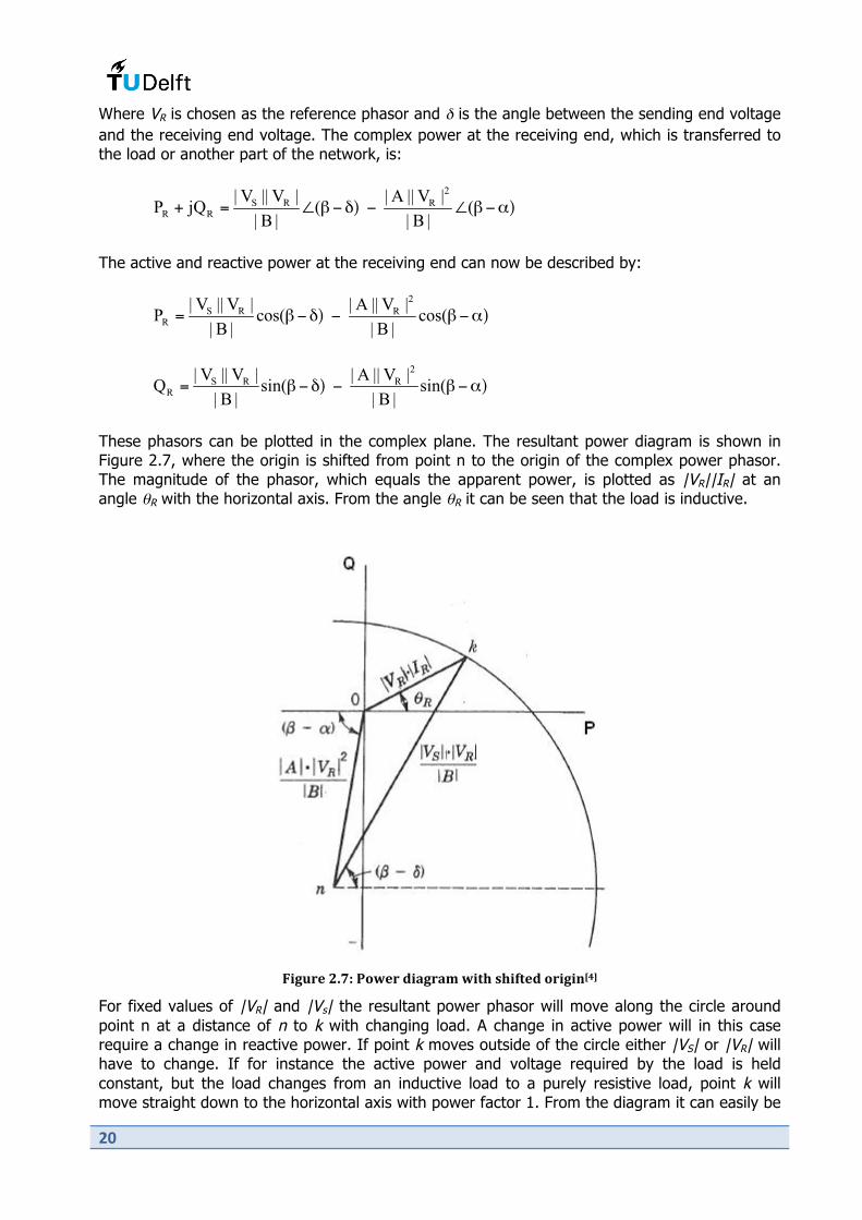
Where VR is chosen as the reference phasor and " is the angle between the sending end voltage

and the receiving end voltage. The complex power at the receiving end, which is transferred to

the load or another part of the network, is:

The active and reactive power at the receiving end can now be described by:

These phasors can be plotted in the complex plane. The resultant power diagram is shown in

Figure 2.7, where the origin is shifted from point n to the origin of the complex power phasor.

The magnitude of the phasor, which equals the apparent power, is plotted as |VR||IR| at an

angle #R with the horizontal axis. From the angle #R it can be seen that the load is inductive.

T/6."#'?U0N'!,9#"'-/%6"%;'9/+3':3/$+#-',"/6/*PBQ'

For fixed values of |VR| and |Vs| the resultant power phasor will move along the circle around

point n at a distance of n to k with changing load. A change in active power will in this case

require a change in reactive power. If point k moves outside of the circle either |VS| or |VR| will

have to change. If for instance the active power and voltage required by the load is held

constant, but the load changes from an inductive load to a purely resistive load, point k will

move straight down to the horizontal axis with power factor 1. From the diagram it can easily be

64

seen that this will decrease the receiving end current and the sending end voltage. The

improved power factor has decreased the voltage drop along the transmission line.

Figure 2.7 also shows the maximum power that can be transmitted to the receiving end of the

transmission line for specified magnitudes of the sending and receiving end voltages. The power

transmitted is increased by increasing the current. Point k will move along the circle until "

equals $. Further increasing " results in less power received. The maximum power is:

The load must draw a large leading current to achieve the condition of maximum power

received. Usually, operation is limited by keeping " less than about 35° and |VS|/|VR| equal to or

greater than 0.95. For short lines the maximum power is restricted by the ampacity of the

conductors.[4]

For a first estimation of the power flow, it can be adequate to look at a simplified transmission

line. This is general practice for short overhead lines, for which the following approximations can

be made:[1]

• Because the resistance of transmission links is much smaller than the reactance values, the resistance of the transmission line can be neglected: B = Z = jX = X%(&/2) [#].

• Because the admittance is neglected in the case of a short overhead line A will become

equal to 1.

When applying these approximations, the following expressions for the active and reactive

power are obtained:

Figure 2.8 shows the simplified power diagram of the short transmission line.

66

T/6."#'?U>N'!,9#"'-/%6"%;'$,"':3,"+'+"%*:;/::/,*'8/*#'

From these equations it can easily be seen that the direction of active power flow at the

receiving end is dependent on the angle between the sending end voltage and the receiving end

voltage:

• " > 0 ! PR > 0, active power flows from sending end to receiving end of the

transmission line. • " = 0 ! PR = 0, no active power is transmitted.

• " < 0 ! PR < 0, active power flow is reversed and flows from receiving end to

sending end of the transmission line.

It can also be seen that in this case the direction of reactive power flow is dependent on the

difference between the sending end voltage and the receiving end voltage:

• |VS| cos(") > ! QR > 0, reactive power flows from sending end to receiving end of

the transmission line.

• |VS| cos(") = |VR| ! QR = 0, no reactive power flows at the receiving end and

the voltage is in phase with the current. There is however reactive power injected into the

transmission line from the sending end to provide for the reactive power required by the

reactance of the transmission line. • |VS| cos(") < |VR| ! QR < 0, reactive power flows from receiving end to sending

end of the transmission line.

The voltage difference and voltage angel between sending and receiving end give a good first

impression when looking at the power flows. When however the voltage angle increases, the

statements for the reactive power flow will no longer hold and will have to be revised. In longer

overhead lines and underground cables the admittance, in particular the susceptance, is much

larger and starts playing an important role in the flow of reactive power, especially under light

load or at no load. It can therefore no longer be neglected.

2.2.2 Surge Impedance Loading

The net reactive power transmitted in a transmission line is dependent on the total generated

and absorbed reactive power by the distributed capacitance and inductance, respectively. The

6!

total reactive power generated by the distributed susceptance is related to the energy stored in

the electrical field of a transmission line. They can be represented by the following formulas:

and

where BC [S] is the total shunt capacitive susceptance and C [F] the total shunt capacitance of

the transmission line. The total reactive power absorbed by the distributed reactance is related

to the energy stored in the magnetic field of the transmission line:

and

where XL [#] is the total series inductive reactance and L [H] the total series inductance of the

transmission line. Setting the generated and absorbed reactive power equal yields the same

result as setting the stored energies equal:

The resultant ratio is called the surge impedance SI, expressed in ohms, of the transmission line

and is equal to the characteristic impedance of a lossless line. With the surge impedance it is

possible to calculate the load for which the net reactive power is zero. This load is called the

surge impedance load SIL:

Because no reactive power is transmitted, the load is at unity power factor and can therefore be

expressed in MW. The surge impedance load is a useful quantity to measure transmission line

capability even for practical lines which include resistance, as it indicates a loading when the line

reactive requirements are small.[6,7] A Transmission line operated above the SIL will absorb

reactive power and therefore behave like an inductor. When operated below the SIL, the

transmission line will respond like a capacitor and supply reactive power.

2.2.3 Compensation

From the discussion in paragraph 2.2.2, it becomes clear that the characteristic of a

transmission line is very much dependent on the loading. Overhead lines are usually operated at

a loading far above the SIL and as a result, the impedance will dominate the admittance.

Impedance is the principal cause of voltage drop and because the voltage is not allowed to drop

below a threshold of 5 to 10% below the rated voltage, it is also a very important factor in

determining the maximum power that the line can transmit.

Through the use of series compensation it is possible to influence the impedance of the line and

thus the net reactive power. The most common series compensation consists of capacitor banks

placed in series with each phase and are used to reduce the line inductance as seen from a

system point of view:

6.

Where XL [#] is the total inductive reactance of the line and XC [#] is the total capacitive

reactance of the capacitor bank. The term Xc/XL is known as the compensation factor and is to

indicate the desired reactive compensation of the inductive reactance by the capacitor bank. The

effect of the series compensation is illustrated in the phasor diagram of Figure 2.9, where Vr represents the voltage at the receiving end without compensation while Vr' the voltage at the

receiving end after series compensation is applied.

T/6."#'?UIN'A,;L#*:%+/,*',$'%'+"%*:;/::/,*'8/*#'9/+3'%':#"/#:'&%L%&/+%*&#P1Q'

If only the sending- and receiving-end conditions of the line are of interest, the physical location

of the capacitor bank will not be of importance. Capacitor banks are mostly applied in the case

of medium and long length overhead transmission lines to allow for higher power transmission.

The power transmission capability of short overhead lines is usually not limited by the voltage

drop, but by the ampacity of the conductors and therefore don’t require series compensation.

Under certain circumstances, the series compensation will consist of reactors instead of

capacitor banks. This is done in the case of two transmission lines with different impedances

operated in parallel to each other. The transmission line with the lowest impedance will attract

more current, choosing the line with the least resistance, even when equally rated. As a result,

the power limit of this transmission line is reached far below the loading capability of the parallel

transmission line. Consequently, the total transmission capacity of the parallel system is less

than the sum of the capacity of the individual systems. To counter this effect, the impedances of

the lines have to be equalised by installing reactors in series with the cable system, thus

controlling the flow of power. This is illustrated in Figure 2.10.

T/6."#'?U1KN'A,;L#*:%+/,*',$'L%"%88#8'8/*#:'9/+3'%':#"/#:'"#%&+,"'

Shunt compensation can also be found in different forms. As mentioned in paragraph 2.2.1 a

capacitor in parallel to an inductive load can improve the power factor of the load, moving point

k straight down, and thus reduce the reactive power requirement of the load. The lower

transmission of reactive power has a positive effect on the voltage drop along the line and the

current losses, allowing for a more economic power transmission.

When a transmission line is operated below the SIL it will act as a capacitor and consequently

have a net generation of reactive power. This occurs for instance when transmission lines are

operated at light or no-load conditions. The current associated with the charging of the

6/

transmission lines capacitance has to be considered and should not be allowed to exceed the

rated full-load current of the line. Shunt reactors are used to compensate the reactive power

generated. Although the voltage along the line is not constant, a good estimation of the

charging current can be obtained using the rated voltage to neutral VLN:

where BC [S] is the total capacitive susceptance of the transmission line. Connecting reactors at

various points along the line so that the total inductive susceptance is BL [S], the charging

current becomes:[4]

where BL/BC is called the shunt compensation factor.

The other benefit of shunt compensation by reactors is the reduction of the receiving end

voltage of the transmission line, which tends to become too high at no load when operated at a

load substantially lower than the SIL. This effect is also known as the Ferranti effect and occurs

for instance in the case of long overhead lines at light load. The Ferranti Effect can be explained

using the generalized circuit constants of paragraph 2.2.1. If a transmission line is unloaded the

current at the receiving end IR will be zero. Therefore:

with

Neglecting the resistance and conductance, A can be written as:

Since ( [rad/s], L [H] and C [F] are positive; A will become smaller than 1. As a consequence, at

no-load the sending end voltage will always be smaller than the receiving end voltage. Both

capacitance as well as inductance will enhance the Ferranti effect when increasing the length of

a transmission line, as both will increase for longer transmission lines.

2.3 Generation

The synchronous machine as an AC generator is the major electric power generating source

throughout the world and is the most important component in the system for maintaining the

active and reactive power balance.[1,4] When the synchronous machine is connected to an

infinite grid, its speed and terminal voltage are equal to the system values and can not be

changed. An equivalent circuit can be seen in Figure 2.11. The reactance X is called the

synchronous reactance and is constant during normal steady-state conditions. The resistance of

the armature coil is neglected in the equivalent circuit.[1]

60

T/6."#'?U11N'23#'#W./E%8#*+'&/"&./+',$'%':S*&3",*,.:'6#*#"%+,"'%*-'+3#'&,""#:L,*-/*6'L3%:,"'-/%6"%;'

The active power injected into the grid can be controlled by adjusting the torque on the rotor of

the synchronous machine. Increasing the torque will result in positive angel between the

generators internal EMF (Ei) [V], and the terminal voltage Vt. The induced current in the

armature windings is lagging the terminal voltage and power is injected into the grid. The speed

of the rotor will not be affected, as the increased torque is cancelled out by the increased

counter torque induced by the armature current, keeping the net torque on the rotor zero.

An important property of the synchronous machine is the possibility to change the amplitude of

the internal EMF by varying the field excitation current If. In this way the amount of reactive

power supplied or absorbed by the synchronous machine can be controlled. Two cases are

shown in Figure 2.12.

61

T/6."#'?U1?N'!3%:,"'-/%6"%;:',$'%',E#"X'%*-'.*-#"#M/+#-'6#*#"%+,"PBQ'

Because the terminal voltage and |Ia|cos(#) are kept equal in both cases, the active power

injected into the grid will also be equal. Changing the DC field current If will change the internal

EMF proportionally, which in turn changes the angle between armature current and terminal

voltage. In the upper part of Figure 2.12 the phasor diagram is shown for a so-called

overexcited generator. The current is lagging the terminal voltage and the generator is said to

supply reactive power to the system, acting like a capacitor from the system point of view. The

bottom part shows an underexcited generator absorbing reactive power from the system and

thus in this case the generator can be seen as an inductor.[4]

The active power output of the synchronous is:

And the reactive power can be expressed as:

62

These two equations are similar to the equations for a short transmission line discussed in

paragraph 2.2.1. Like in the case of the transmission line the direction of flow of the active power is dependent on the angle " between the internal EMF and the terminal voltage. The

direction of the reactive power flow is dependant on the difference between the terminal voltage

and |Ei|cos(").

The output of the generator is of course limited by heating and mechanical limits. The normal

operating conditions can be shown on a single diagram called a loading capability diagram. The

terminal voltage is assumed to be constant and the armature resistance is neglected. Figure

2.13 shows an example of a loading capability curve of a synchronous machine.[1]

T/6."#'?U1CN'F,%-/*6'&%L%D/8/+S'&."E#',$'%':S*&3",*,.:'6#*#"%+,"P1Q'

From the above diagram it can be seen that the flow of reactive power is limited mainly by the

field excitation limits. The upper limit is formed by the heat produced in the rotor as a

consequence of the field excitation current. The lower limit, the underexcitation limit, shows the

maximum reactive power the generator can absorb and is there for two reasons.

The first reason relates to the steady-state stability of the system. Theoretically, the so-called steady state stability limit occurs when the angle " between Ei and Vt reaches 90°. When $

becomes greater than 90° the generator will lose synchronism. In practice however, the power

system dynamics involved will complicate the determination of the actual stability limit and

larger safety margins have to be applied. The second reason is the increased eddy currents

induced in the armature when operated in the underexcited region. The corresponding

additional heat generation in the armature has to be taken into account.

63

2.4 Frequency and Voltage Control

The load of a power system varies randomly throughout the day. As it is impossible to predict

the exact load changes, the frequency and voltage will also vary. In order to safeguard the

proper operation of the power supply system, control actions are needed to maintain the power

balance at the required frequency and voltage.

2.4.1 Frequency Control

The frequency is the same for the entire interconnected system and is dependent on the

balance of active power supply and demand. In case the demand for active power increases

while no control actions are taken, the power will be supplied from the kinetic energy stored in

the rotating mass of the generator. As a result, the kinetic energy/speed of the rotor and thus

the frequency will decrease. To restore the active power balance, the torque supplied by the

turbine has to be increased to equal the counter torque in the generator. A so-called speed

governor controls the mechanical power output of the turbine by adjusting the steam valves and

consequently the mechanical power delivered by the turbine. The control scheme is illustrated in

Figure 2.14.

T/6."#'?U1BN'23#'D%:/&'L"/*&/L%8',$'+3#':L##-'6,E#"*,"'&,*+",8':S:+#;',$'%'6#*#"%+/*6'.*/+P1Q'

Restoring the active power balance does not necessarily mean that the speed of the rotor, and

thus the frequency, has been restored to its original value, as illustrated in Figure 2.15 at point

New. To permit parallel operation of generating units, the power-frequency characteristic of the

speed governor of each unit has droop, which means that a decrease in speed should

accompany an increase in load. This makes it possible to distribute a load increase over the

parallel generators according to the ratio of their nominal rated powers. To restore the

generators to their desired frequency, a supplementary control action is provided by the speed

changer. The speed changer supplements the action of the speed governor by changing the

speed setting to allow an increase of prime mover power. This will increase the kinetic energy

stored in the generator, permitting it to operate at the desired frequency and power output, as

illustrated in Figure 2.15 at point Final. For decreasing active power demand, the system and its

control will react in exactly the opposite way.[1, 4]

!5

T/6."#'?U1(N'GL##-X6,E#"*/*6'&3%"%&+#"/:+/&',$'%'6#*#"%+/*6'.*/+'D#$,"#'%*-'%$+#"'%'8,%-'/*&"#%:#'%*-'

:.LL8#;#*+%"S'&,*+",8PBQ'

2.4.2 Voltage Control

Unlike the frequency, the voltage is not equal throughout the power system and is dependent

on the local properties of the system. The voltage will have to be controlled at locations where

necessary. The voltage is strongly related to the reactive power flow and generally it is said that

the consumption of reactive power will cause a voltage drop and the supply of reactive power

will cause a voltage rise. By controlling the reactive power, it is possible to control the voltage.

For a proper and safe operation of the power system, it is important to control the voltage levels

and not allow it to exceed a 10% voltage range above or below the nominal voltage.

Generators can supply as well as absorb reactive power and are an important tool in the control

of reactive power flows. The system operator can choose a fixed terminal voltage level for every

generator. The voltage at the terminal is kept constant by the use of a voltage regulator, which

controls the field current supplied to the generator. In paragraph 2.3 it was already mentioned

that the internal EMF is proportional to the field excitation current and that the reactive power

output can therefore be controlled by changing the field current. When the demand for reactive

power is increased, the field excitation is also increased allowing the generator to supply more

reactive power to the grid, while keeping the terminal voltage constant.

T/6."#'?U1HN'J#8%+/,*'D#+9##*'"#%&+/E#'L,9#"'6#*#"%+/,*'%*-'YZTP1Q'

!4

Like in the case of frequency control, the voltage regulator has droop to permit parallel

operation of generators. In this way the reactive power generation can be distributed over the

parallel generators according to the ratio of their nominal rated powers. Without the droop, a

situation could arise where an unwanted reactive power exchange between generators takes

place.

For the remaining part of the system, compensation can be used to control the voltage.

Paragraph 2.2.3 has explained how the application of reactors and capacitors at various points

in the system can locally control the reactive power and thus the voltage.

2.4.3 FACTS and Load Shedding

In the past, the control of power compensation devices was limited; they were mainly based on

mechanical control steps. These mechanisms automatically introduce a limitation to the speed of

control. Nowadays, Flexible AC Transmission Systems (FACTS) devices are available that enable

a greater flexibility in the control of power flows. FACTS devices are large power-electronic

controlled devices, enabling the possibility for considerably faster control actions. It must be

noted that the investment costs for these devise are considerably higher than for the

conventional static capacitor banks and reactors. Some examples of FACTS devices are:[1]

• SCV – Static Var Compensator

• STATCOM – Static synchronous compensator

• TCSC – Thyristor-Controlled Series Capacitor

• SSSC – Static Synchronous Series Compensator

• UPFC – Unified Power-Flow Controller

If all the control measures taken are not sufficient to restore a stable operation of the power

system, the transmission operators have, as a last resort, the possibility to disconnect load from

the grid. Special contracts are made with certain large-scale consumers of electricity, which

allow for this so-called load-shedding in extreme cases.

!6

3 Cable versus Line

Alternating current overhead lines have been used from the very beginning of AC power

transmission. Starting with medium voltages and relatively small dimensions, they were

gradually developed further to reach high and extra high voltages by simultaneously increasing

their dimensions. The world’s first 380-kV OHL was installed in 1952 in Sweden to transmit a

power of 460 MW over a distance of 950 km from Harspränget to Halsberg. With more than 55

years of experience OHL are state-of-the-art and are the reference technology for transmitting

large amounts of electric power over distances of several hundreds of kilometres.[3]

However, as a result of successful development and operation of cross-linked polyethylene

(XLPE) cables during the last three decades at low and medium voltage levels, nowadays

commercial XLPE cables are available for voltages up to 550 kV.[3] These cables have some

significant advantages over the traditional fluid-filled paper insulated EHV cables and have

become a proven technology especially in the lower voltage range. Although the overhead line is

still the preferred technology for EHV power transmission, the development of the EHV XLPE

cable has increased the potential of an underground cable as a viable option.

There are also other reasons for this change in attitude toward EHV cables. Besides the extra

technical challenges involved in the use of underground cables, the overhead line remains the

preferred technology mainly because of economical reasons. Technical changes and strong

competition in the cable sector have however reduced prices. In densely populated areas like

the Randstad, the planning of transmission routes has become more difficult due to strong

opposition form local communities and interest groups. Environmental and aesthetic concerns

have led to a diminishing public and political acceptance of new overhead lines and increased

the demand for alternatives like underground cables.

This chapter will discuss the technical characteristics and considerations concerning the use of a

380 kV underground cable, followed by a discussion on overhead line technology. Finally, the

operational differences of underground cables compared to overhead lines are mentioned.

3.1 380 kV EHV AC Cable

In order to be able to handle the high power rating of more than 2600 MVA per circuit required

in the Randstad 380 project, a state-of-the-art cable system has been developed. The size of

this cable project is unique in the world. Although the length of the connections is only 20

kilometres, the three-phase system consists of two circuits and each circuit contains two cables

per phase. With 2 x 2 x 3 = 12 cables the total amount of cable length required sums up to 240

kilometres. This makes the Randstad 380 project unique in comparison to other EHV

underground cable projects and the largest EHV underground cable project in the world in terms

of cable length and transmission capacity. Table 2 gives an overview of a couple of cable

projects in comparison to the Randstad 380 project.

!!

2%D8#'?N'[E#"E/#9'8%"6#':&%8#'Y57'.*-#"6",.*-'&%D8#'L",\#&+:'

Country Project name Circuits Cables per

phase

Power per

circuit

[MW]

Route

length

[km]

Cable

length

Netherlands Randstad 380 double 2 2600 20 240

Japan Shinkeiyo-Toyosu double 1 1200 40 240

Denmark Metropolitan Power single 1 1000 34 102

Spain Barajas Airport double 1 1700 13 78

Germany Berlin Diagonal double 1 1100 12 72

One of the major differences between an overhead line and an underground cable is the fact

that an overhead line can use the surrounding air as insulation from earth. A cable however is

laid down into the ground (or in underground ducts) and insulation has to be applied around the

conductor. This has a number of consequences for the transmission line parameters and heat

dissipation, which affects the way the transmission system has to be operated.

3.1.1 Composition cable

For the Randstad 380 project a single core 380 kV XLPE cable will be used. The electrical stress

levels in the insulation material in EHV cable are extremely high and hence the performance

demands on the insulation materials are correspondingly high. The performance achieved by

current EHV cables is the result of many years of cable design and manufacturing development.

T/6."#'CU1'A",::X:#&+/,*',$'%'C>K'=7']F!Y'&%D8#PCQ'

As can be seen in Figure 3.1 the copper conductor (number 1) consists of strands divided into 6

different segments. The strands provide a better flexibility for the cable compared to a solid

conductor. The segments are meant to reduce disadvantages associated with electrical

phenomena like skin effect and proximity effect.[3] The conductor screen (number 2), an

extruded conductive layer, is followed by a layer of XLPE (number 3) applied to provide the

necessary insulation to earth. XLPE is a form of solid plastic insulation which, during the

manufacturing of the cable, is melted and pressed around the conductor (i.e. the plastic is

extruded).[1] The insulation must be free of cavities and inclusions to avoid locally elevated

electric field strengths, which could lead to partial discharges in the insulation. The partial

discharges cause deterioration of the material and could eventually lead to a breakdown of the

cable. The insulation is surrounded by an insulation screen (number 4).

To keep the electric field inside the cable an electrostatic shield is applied, consisting of multiple

layers (number 5, 6 and 7). The shield also provides a return path in the case of a line to

!.

ground fault in the cable system. The layers of EHV cable include a copper screen and a

hermetically sealed metallic sheath, which is usually made of aluminium. The polymer insulation

used in a cable is highly vulnerable for water and water vapour, as it lowers the dielectric

withstand level. The aluminium sheath helps to protect the cable from damage and moisture

entering the insulation. Often neutral wires are included in the shield, these wires can assist in

conducting current in the case of a line to ground fault. This sheath is further protected against

mechanical damage and corrosion by a final covering of a polyethylene sheath (number 8).[1, 8]

The total cable consists of a multitude of different layers, which all have to fit perfectly together

in order to prevent partial discharges and have a reliable and long-lasting cable. The fabrication

of these cables is a highly specialized and precise manufacturing process. These insulation

layers necessary for EHV cables have however a couple of disadvantages to be reckoned with

for proper operation of the cable.

3.1.2 Capacitance cable

First of all, cables have a much larger capacitance than overhead lines. This is mainly due to the

small distance between the conductor and the outer sheath. The capacitance per meter [F/m]

can be calculated using the radius of the conductor r [m] and the radius of the outer sheath R [m]:[9]

Where ) [F/m] is the dielectric constant of the XLPE, with a relative permittivity of )r * 2.3. The

larger permittivity compared to the permittivity of air, also contributes to the size of the

capacitance. Conventional single circuit 380 kV cable systems have a capacitance of around 200

to 300 nF/km. The double circuit cable system in the Randstad 380 project, with its double

cables per phase, has a capacitance of 540 nF/km per circuit.

T/6."#'CU?N'A%D8#'&%L%&/+%*&#:'$,"'+3"##XL3%:#':/*68#'&,*-.&+,"'&%D8#':S:+#;'

The large capacitance in combination with the alternate charging and discharging due to the

alternating voltage causes a considerable current. Whereas the charging currents can be

neglected for overhead lines up to a length of at least 50 km, for 380 kV cables they are

significant. Compared to a conventional single circuit cable system, which typically needs 15

A/km, the cable system of the Randstad 380 project will draw about five times more charging

current.

The charging current represents reactive power and makes no useful contribution to the desired

supply of power to the load. It does however contribute to the line loading and losses.[8] As can

be seen from the following formula, the charging current is dependent on the voltage:

!/

where |Ichg| [A/m] is the charging current per meter per phase. Since the capacitance is a shunt

between the conductor and the outer sheath, charging currents flow in the cable even in an

unloaded situation.[4]

3.1.3 Losses and Heat Generation

The losses in the cable generate heat. Like with overhead lines, most of the heat is generated

because of current flowing through the conductor, but cables also have some additional losses

contributing to the generation of heat. The total losses can be illustrated with the following

formula:

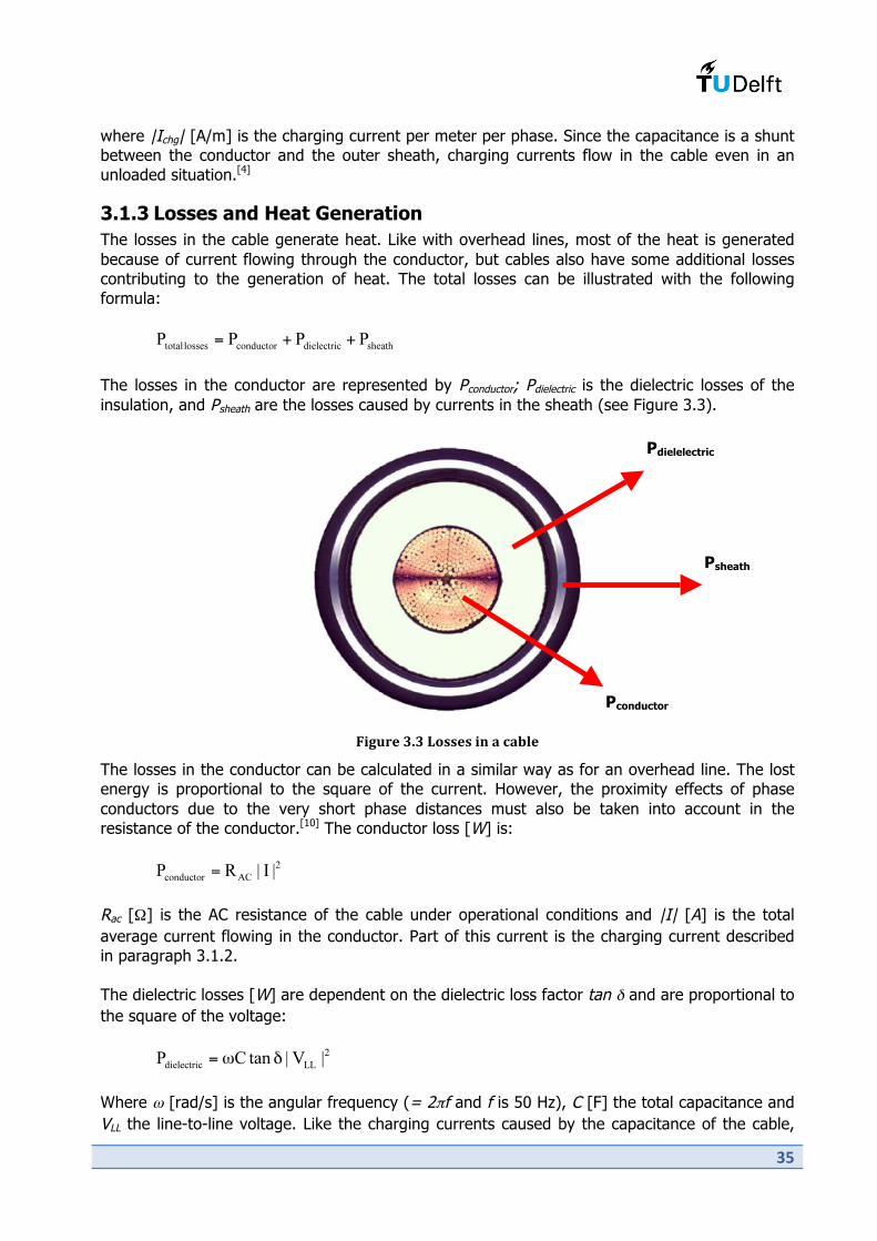
The losses in the conductor are represented by Pconductor; Pdielectric is the dielectric losses of the

insulation, and Psheath are the losses caused by currents in the sheath (see Figure 3.3).

T/6."#'CUC'F,::#:'/*'%'&%D8#'

The losses in the conductor can be calculated in a similar way as for an overhead line. The lost

energy is proportional to the square of the current. However, the proximity effects of phase

conductors due to the very short phase distances must also be taken into account in the

resistance of the conductor.[10] The conductor loss [W] is:

Rac [#] is the AC resistance of the cable under operational conditions and |I| [A] is the total

average current flowing in the conductor. Part of this current is the charging current described

in paragraph 3.1.2.

The dielectric losses [W] are dependent on the dielectric loss factor tan " and are proportional to

the square of the voltage:

Where ( [rad/s] is the angular frequency (= 2&f and f is 50 Hz), C [F] the total capacitance and

VLL the line-to-line voltage. Like the charging currents caused by the capacitance of the cable,

Pdielelectric

Psheath

Pconductor

!0

the dielectric losses are dependent on the voltage and will be present even when the cable are

not supplying any load. Being dependent on the square of the voltage, the dielectric losses play

a much more dominant role at the extra high voltage levels.

Unlike overhead lines there exists no capacitive coupling between the single-phase cables. This

is due to the electrostatic screen surrounding the conductor of the cables. However, the cables

are magnetically coupled. The magnetic fields set up by the currents in the conductors of the

three phase single-core cables, induce currents in the metallic sheath of the other cables, as

illustrated in Figure 3.4. When the metallic sheaths of the cables are single-point bonded,

meaning the sheaths are connected and grounded at one point along their length, the voltage

induced in the sheath is proportional to the cables length and can reach very high values.[1]

These voltages drive the currents in the opposite direction of the conductor currents and cause

substantial losses in the order of magnitude of the conductor losses if no mitigation measures

are implemented.[3] By cross bonding the cables (see paragraph 3.1.5), the induced sheath

currents can be minimized.

T/6."#'CUBN'23#'$8.M'8/*#:',$'%'&.""#*+'&%""S/*6'&%D8#'%*-'+3#'/*-.&#-'#--S'&.""#*+:'/*'+3#':3#%+3',$'%'

*#/63D,."/*6'&%D8#P11Q'

An underground cable has compared to an overhead line less effective heat dissipation. For an

overhead line the insulation (the surrounding air) also provides the necessary cooling for the

conductor. The insulation of an underground cable however is, besides being a very effective

electrical insulator, also a good thermal insulator. This in combination with the thermal

insulating property of the ground into which the cable is buried, can present a significant

thermal barrier. In order to prevent degradation of the insulation material, the cable

temperature must not be allowed to rise above the design limits of the cable. In the case of

XLPE, the cable is designed to operate at temperatures up to 90°C.[12, 17]

To prevent the cable from reaching its thermal limit, it is important to reduce the losses in the

cable. This is achieved is by minimizing the resistance of the conductor in order to reduce the

ohmic losses in the conductor. For overhead lines, conductors are usually made out of

aluminium, the main reason being the weight of the material. The low weight of aluminium

allows for lighter transmission tower constructions and insulator strings. This in combination

with the lower cost of aluminium compared to copper, makes the transmission line cheaper to

build. For the cables of the Randstad 380 project, copper conductors will be used. Although

copper is a lot more expensive, its resistivity is only about 60% of that of aluminium. The

smaller resistivity of copper is a considerable advantage in the case of underground cables.[1]

!1

To further reduce the resistance of the cable, the cross-sectional area of the conductor is

increased. To achieve the same power rating, an underground cable can have a conductor up to

4 times larger than its overhead counterpart. Single core cables with a cross-sectional area up to

3200 mm2 are currently available. For the Randstad 380 project, the copper conductors will have

a cross-sectional area of 2500 mm2.[3, 12]

3.1.4 Advantages XLPE over FFP

Before the 1990’s exclusively fluid-filled paper insulated cables have been applied for EHV. The

structure of an oil-filled cable is shown in Figure 3.5.

T/6."#'CU(N'G+".&+."#',$'%*',/8X$/88#-'&%D8#P>Q'

Paper itself is an unsatisfactory insulator due to the spaces incorporated in the structure of the

cellulose fibres. Combining the paper with for instance oil creates an excellent insulator. The oil

duct in the centre of the cable supplies thin oil under moderate pressure. The pressure is

maintained by oil reservoirs feeding the cable along the route. When the cable warms up, the oil

expands and is driven from the cable into the reservoirs and vice versa. In this way, gaps in the

insulation material are avoided so that no weak points are present. Oil-filled cables have proven

to be the most reliable type of cable for the high voltage and extra high voltage levels.[1]

However compared to oil-filled cables, XLPE cables show some important advantages.[3]

• Higher maximum operational temperatures (maximum 90°C instead of 85°C)

• Lower capacitance per km and, hence, lower effort for compensation and reduced related

losses and increased lengths

• Lower dielectric losses

• As a consequence of all these factors increased power ratings

• Lower thermal resistance of the insulation and, consequently, improved heat dissipation

• Lower maintenance requirements

• Pre-fabricated (cable joints and sealing end compound) resulting in high quality control

standards as well as easy and safe installation within short periods

• Increased section length

• The state of the insulation can be evaluated by partial discharge measurements during

operation

• No pressurized oil storages, no risk of contamination of soils by oil leaking from cables

• Cost reduction of 20% to 30%

• Increased number of suppliers

!2

These advantages have caused XLPE cables to virtually completely replace fluid filled cables in

new projects.[3]

3.1.5 Installation

When taking into account the density of copper and the extra layers applied to a cable, it

becomes evident that the sheer size and weight of the cable forms a restriction. With a density

of 8900 kg/m3, the copper conductor alone will weight about 22 kg/m. Including the insulation

and other layers, the complete cable will have a weight of around 35 kg/m and a diameter of

around 15 cm.

Because of the size and weight of the cable, logistics form the dominating restriction for the

length of the cable sections. In the case of the Randstad 380 project, the cable will be supplied

in sections of 1100 m. The drum on which the cable is delivered to the site, will weight about

40,000 kg. As these drums have to be transported along the complete transmission route in

short distances, this forms an important planning parameter.[3]

T/6."#'CUH'Y57'A%D8#'-".;',*X:/+#P1?Q'

A further effect of the combined thickness of insulation necessary at EHV and of the larger

conductor cross-sectional area required is that the cable becomes less flexible. The diameter

must be limited in order to keep the cable flexible enough to fit on a drum. Care must also be

taken during installation to ensure that no permanent damage is done to the insulation and

sheath by over-bending the cable. To address this limitation, cable manufacturers specify a

minimum allowable bend radius for their cables that is around 2 meters for 380 kV cables. This

in turn imposes constraints on the profile of the trenches into which the cables are installed. The

radius of both horizontal and vertical bends must therefore take account of this limitation.[12]

Figure 3.7 shows a cross-section of the cable trenches, as they will be constructed for the

Randstad 380 project. Because of the high current rating, the cables produce, as mentioned

before, a significant amount of heat. To obtain more effective heat dissipation, the cables have

to be placed at distance from each other and preferably be buried not too deep into the ground.

Therefore, as can be seen in the figure, the cables are installed in a so-called flat formation.

The excavated soil is dropped along one side of the trenches. In this way, there is no need for

large transport of soil and the original soil can be replaced once the cables have been laid into

the trenches. If required it is also possible to use a special so-called back-fill material to improve

the heat conducting properties of the soil.

!3

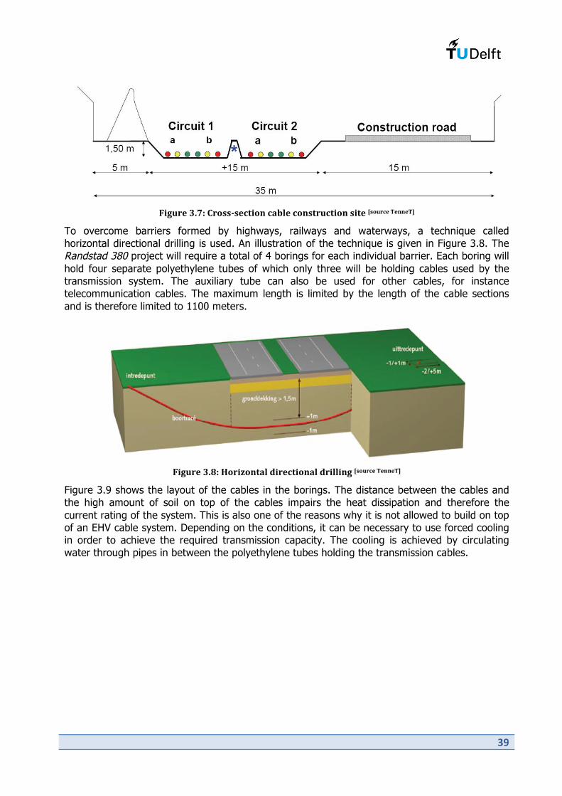
T/6."#'CU0N'A",::X:#&+/,*'&%D8#'&,*:+".&+/,*':/+#'P:,."&#'2#**#2Q'

To overcome barriers formed by highways, railways and waterways, a technique called

horizontal directional drilling is used. An illustration of the technique is given in Figure 3.8. The

Randstad 380 project will require a total of 4 borings for each individual barrier. Each boring will

hold four separate polyethylene tubes of which only three will be holding cables used by the

transmission system. The auxiliary tube can also be used for other cables, for instance

telecommunication cables. The maximum length is limited by the length of the cable sections

and is therefore limited to 1100 meters.

T/6."#'CU>N'5,"/^,*+%8'-/"#&+/,*%8'-"/88/*6'P:,."&#'2#**#2Q'

Figure 3.9 shows the layout of the cables in the borings. The distance between the cables and

the high amount of soil on top of the cables impairs the heat dissipation and therefore the

current rating of the system. This is also one of the reasons why it is not allowed to build on top

of an EHV cable system. Depending on the conditions, it can be necessary to use forced cooling

in order to achieve the required transmission capacity. The cooling is achieved by circulating

water through pipes in between the polyethylene tubes holding the transmission cables.

.5

T/6."#'CUIN'A%D8#'8%S,.+'/*'D,"/*6:'P:,."&#'2#**#2Q'

The largest interconnected cable part in the Randstad 380 project will be 10 kilometres between

the substations Wateringen and Bleiswijk. The 10 km cables will be constructed out of 9 times

1100 meter cable sections. The technology required to joint cables tends to become increasingly

complex (and costly) with increasing voltage. The electric field in the insulation of a 60 kV cable

is a few kV/mm. In order to reduce the size and weight of 380 kV cables, these operate at a

much higher stress, about 12 kV/mm. The increased stress requires a more complex and

sophisticated joint design. As these complex joints are made on-site, rather than in a factory,

great care must be taken during installation.[8]

T/6."#'CU1KN'G+#L:'&,**#&+/*6'+3#'#*-:',$'Y57'&%D8#:'.:/*6'L"#$%D"/&%+#-'\,/*+:PCQ'

The three phase double circuit cable system, with two cables per phase, used in the Randstad 380 project will have 12 separate 10 km cables between the substations of Wateringen and

Bleiswijk. This amounts to a total of 108 cable sections, requiring a total of 96 joints. As

mentioned in the previous paragraph, the losses in the sheaths of the cable, due to the induced

currents, can be significant and reduce the current-carrying capacity of the cable. In order to

address this issue, the joints are also used for the cross bonding of the sheaths of the cables.

Each sub circuit consisting of three single-phase cables is divided into three (optionally a

multitude of three) sections of equal length. The ends are connected to ground and at the two

intermediate locations the sheaths are cross connected as illustrated in Figure 3.11. In this way,

the total induced voltage in the consecutive sections is (approximately) neutralized.[1]

.4

T/6."#'CU11N'A",::'D,*-/*6',$'&%D8#':3#%+3:PCQ'

The 10 km cable system will require 24 cross bonding able joints. This cross bonding ability will

add to the complexity of the already complex joints and joint bays considerably.

On both ends of the cable system, known as terminations, the 12 cables are finally connected to

overhead lines. The terminations are constructed using sealing end compounds (SEC), which are

relatively simple, compared to the cable joints. The SEC facilitates the transition between the

cable insulation and the insulation of air and has to be placed therefore at the appropriate

clearance to the ground. The size and weight of the terminations requires an extra strong

overhead line tower. In combination with the necessary clearance, a separate, high security

transition compound on the ground is considered necessary. The compound can require an area

of 2000 m2 depending on the power level and the amount of equipment installed. An example of

a SEC and a transition compound are shown in Figure 3.12.

T/6."#'CU1?N'!"#$%D"/&%+#-'GYA'_8#$+`'%*-'%*'.*-#"6",.*-'&%D8#'+"%*:/+/,*'&,;L,.*-'_"/63+`'

3.2 380kV Overhead Transmission Line

Compared to underground cables, overhead transmission lines are relatively simple in design

and basically consist of four elements:

• transmission towers

• conductors

• insulators

• shield wires

.6

Transmission line towers support the high voltage conductors, which are attached to the towers

using specially designed insulators. Air provides the necessary insulation to ground. The height

of the tower is dependent on the required clearance of the conductors to the ground. Since air is

a rather weak insulator, the distance between conductors and the ground has to be large for

extra high voltage levels. The span between the towers also plays an important role and can be

up to 400 meters; at these distances the sag of the conductor has to be accounted for in the

determination of the height of the tower. Between the top of the towers shield wires are

connected, which provide protection against lighting and can also support an optical cable for

telecommunication purposes used to monitor the system.

T/6."#'CU1CN'4,.D8#'&/"&./+',E#"3#%-'+"%*:;/::/,*'8/*#'9/+3':3/#8-'9/"#:'

3.2.1 Conductor

The selection of the conductors, their cross section and arrangements is a key point for an

overhead transmission line, because the conductors represent between 30 to 35% of the total

line investment. The choice of the optimum conductor is a compromise between its mechanical

and electric properties, as well as the investment and the cost of the losses along the life time of

the line.[6]

Nowadays, copper conductors have been fully replaced by aluminium conductors in overhead

transmission lines. In paragraph 3.1.3 it has already been noted that although aluminium has a

lower conductivity than copper, its lower weight and cost make it the preferred material in the

construction of overhead transmission lines. Aluminium however has a rather low tensile

strength, which makes it unsuitable for long spans between towers. To address this problem,

aluminium conductors where combined with a steel core, which provides the necessary extra

strength. The Aluminium Conductor Steel Reinforced (ACSR) are known to have problems with

corrosion in aggressive environments, like for instance coastal areas. Other conductor types

have been developed using aluminium alloy, which have similar behaviour to the ACSR, but

without the problem of corrosion.

.!

T/6."#'CU1BN'@8.;/*/.;'A,*-.&+,"'9/+3'%'G+##8XJ#/*$,"&#-'&,"#'_@AGJ`'

For higher voltage levels, the conductors are build-up out of multiple strands to give them more

flexibility. The large diameter is an advantage with regards to the undesirable effect of corona,

as it reduces the electrical field strength at the conductor surface. To even further reduce this

electrical field strength multiple conductors per phase are used. For 380 kV voltage levels these

bundles consist of 3 or 4 conductors per phase. Besides corona reduction, the bundling of

conductors has some more advantages compared to a similar rated single conductor with a

large diameter:[1]

• Less line reactance;

• Easier to transport and assemble;

• Better cooling of the conductors;

• Increased power transfer capability.

The current-carrying conductors each create a magnetic field, which as a result induces a

Lorentz force on the other conductors, causing them to attract each other. To counter this force

and maintain the desired distance between the conductors, a so-called spacer is used. A spacer

for a four-conductor bundle is shown in

T/6."#'CU1(N'Y8#&+"/&'$/#8-':+"#*6+3'"#-.&+/,*'.:/*6'D.*-8#-'&,*-.&+,":'_8#$+`'%*-'%':L%&#"'_"/63+`P1Q'

3.2.2 Towers

The selection of the basic tower configuration for an overhead line depends on various

parameters like the voltage, the number of circuits per tower and the type of conductor or

conductor bundle. The use and positioning of shield wires can protect the conductors from direct

..

lightning strokes, in this way increasing the reliability of the line. Especially for high voltage lines,

environmental criteria play a role and consideration should be given to the maximum acceptable

electrical and magnetic fields, radio interference and audible noise caused by corona, as well as

to aesthetics and visual perception of the line and its insertion into the landscape. The need of

compaction for obtaining high surge impedance load and reducing the right-of-way width is also

a determinant factor.[6] shows a number of examples of tower configurations used in Europe.

The bottom right tower can support a 380/220/110 kV six-circuit line, which might be used in

case of a lack of separate rights-of-way.

T/6."#'CU1HN'2,9#"'&,*$/6."%+/,*:'$,"'3/63'E,8+%6#'+"%*:;/::/,*PHQ'

3.2.3 Uprating and Wintrack

Planning the route of new overhead transmission line is becoming increasingly difficult and

expensive. The system operator is faced with a densely populated area and a large opposition

against the construction of new overhead transmission lines. Adding to the complexity of the

planning problem, new legislation rules that no additional transmission towers are to build within

the Netherlands. This means that for every new transmission tower build an old transmission

tower will have to removed, which will eventually lead to the under grounding of a larger part of

the Dutch electricity grid.

For these reasons, part of the overhead line connection of the randstad 380 project will make

use of existing towers and right-of-ways. Towers now supporting a 150 kV transmission line will

have to uprated to be able to support the new 380 kV voltage level and the required power

capability. Uprating does not always require a hardware change and can be achieved by simply

allowing a higher operating temperature. If the ampacity of the line is not sufficient to allow a

higher operating temperature, the conductors will have to be replaced by conductors with a

higher current rating. The insulation from the tower necessary for the higher voltage can be

achieved by lengthening the insulator strings supporting the conductors. Care has to be taken in

order to maintain an adequate ground clearance.

./

For the new to be build part of the overhead line connection, the opposition has led to a

redesign of the conventional high voltage towers in an attempt to increase the acceptation of

new overhead lines. The new design that will be used in the Randstad 380 project is called

Wintrack and is designed to fit into the landscape in a more aesthetical way. Health and safety

issues are important topics in the planning and installation of overhead power lines. The new

Wintrack design combines its aesthetic look with a lower surrounding magnetic field. As a result

the corridor for the overhead transmission line can be made less wide, while still being conform

to the health and safety regulations. The Wintrack towers will be able to be used as combination

towers, supporting a double circuit 380kV transmission line, while supporting at the same time a

150 kV double circuit line. Figure 3.17 shows a double circuit 380 kV transmission line supported

by the new Wintrack towers.

T/6."#'CU10N'4,.D8#'&/"&./+'C>K'=7'+"%*:;/::/,*'8/*#':.LL,"+#-'DS'%",'(&?.'+,9#":P:,."&#'2#**#2Q'

3.2.4 Line parameters

The line parameters of an overhead line are dependent on the geometry of the conductors. As

can be seen in Figure 3.16 the tower configurations and thus the line geometries are diverse

and various positions for the three-phase conductors are possible. This has an influence on the

line inductance and line capacitance. The distance between the conductors of an overhead line

are several meters and their capacitance is therefore much smaller than the capacitance of an

underground cable, while the inductance is somewhat larger.

The difference in height of the phase conductor to ground and the possible unsymmetrical

spacing of the conductor leads to a situation where the inductance and capacitance of one

phase differs from the other phase. This is an unwanted situation as it causes the line to be

unbalanced. Balance is restored by interchanging the position of the conductors at regular

intervals along the line. The so-called transposition cancels out the influence of the geometry on

the line inductance and results in equal average line inductance over one complete cycle.[1, 4]

The basic idea of transposition is illustrated in Figure 3.18.

.0

T/6."#'CU1>N'2"%*:L,:/+/,*',$',E#"3#%-'L,9#"'8/*#:P1Q'

When comparing the underground cable system of the Randstad 380 project to the overhead

line, the specific inductance of the overhead lines is about 2 times larger compared to the

underground system. The specific capacitance has a much larger difference; compared to the

overhead line the cable system has a specific capacitance of about 36 times larger.

3.2.5 Losses

Unlike in the case of a cable, heat dissipation does not form a problem for overhead

transmission lines. The surrounding air is readily available to transport heat away from the

conductors. The line losses of an overhead line are composed of the following components:[10]

• Power losses in the conductors

• Power losses in the shield wires

• Corona losses

The power losses in the conductors are proportional to the square of the current. However, like

for underground cables proximity effects like the skin effect must be taken into account in the

resistance of the conductor.[10] The conductor loss [W] is:

Rac [#] is the AC resistance of the conductor under operational conditions and |I| [A] is the total

average current flowing in the conductor.

The same formula can be applied for the losses in the shield wires. Like in the sheaths of

underground cable, inductive coupling between the conductors and the shield wires induces

currents in the shield wires, causing losses.

Corona is the result of ionization of the air surrounding the conductor and occurs when the

electric field near the surface of the conductor reaches the critical surface voltage gradient. As

the corona discharges are not permanent but occur in the form of sparks around the conductor,

electromagnetic radiation is emitted from the conductor, causing different types of undesirable

effects. Next to the considerable power losses it can lead to in transmission lines, it also causes

radio interference and produces audible noise, which can become a problem in populated

areas.[6]

The condition and location of the conductor plays an important role for the intensity of the

corona effect. High pollution and rain can increase the electric field locally and cause additional

corona. Also the increased electric field due to sharp objects near transmission tower can be a

source of corona. In order to minimize the effect of corona under normal conditions, the electric

field at the conductor surface should be kept below 1,5 to 2 kV/mm.[6]

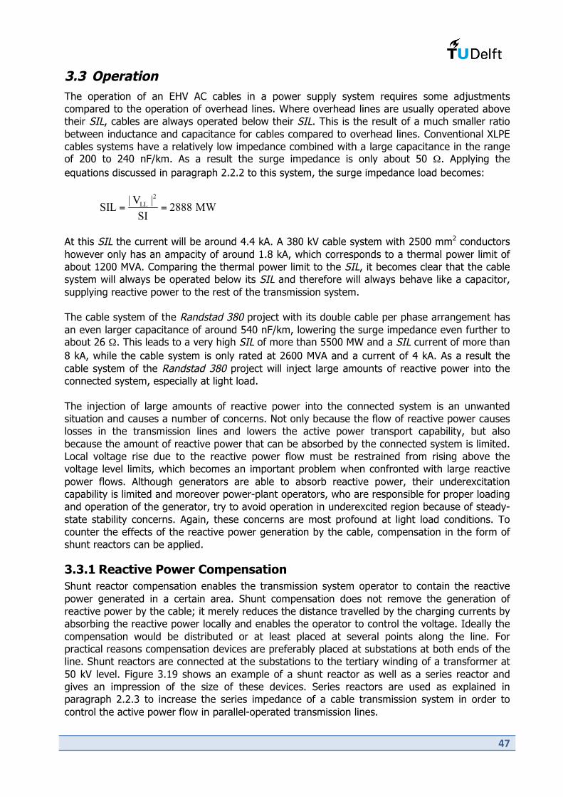
.1

3.3 Operation

The operation of an EHV AC cables in a power supply system requires some adjustments

compared to the operation of overhead lines. Where overhead lines are usually operated above

their SIL, cables are always operated below their SIL. This is the result of a much smaller ratio

between inductance and capacitance for cables compared to overhead lines. Conventional XLPE

cables systems have a relatively low impedance combined with a large capacitance in the range of 200 to 240 nF/km. As a result the surge impedance is only about 50 #. Applying the

equations discussed in paragraph 2.2.2 to this system, the surge impedance load becomes:

At this SIL the current will be around 4.4 kA. A 380 kV cable system with 2500 mm2 conductors

however only has an ampacity of around 1.8 kA, which corresponds to a thermal power limit of

about 1200 MVA. Comparing the thermal power limit to the SIL, it becomes clear that the cable

system will always be operated below its SIL and therefore will always behave like a capacitor,

supplying reactive power to the rest of the transmission system.

The cable system of the Randstad 380 project with its double cable per phase arrangement has

an even larger capacitance of around 540 nF/km, lowering the surge impedance even further to about 26 #. This leads to a very high SIL of more than 5500 MW and a SIL current of more than

8 kA, while the cable system is only rated at 2600 MVA and a current of 4 kA. As a result the

cable system of the Randstad 380 project will inject large amounts of reactive power into the

connected system, especially at light load.

The injection of large amounts of reactive power into the connected system is an unwanted

situation and causes a number of concerns. Not only because the flow of reactive power causes

losses in the transmission lines and lowers the active power transport capability, but also

because the amount of reactive power that can be absorbed by the connected system is limited.

Local voltage rise due to the reactive power flow must be restrained from rising above the

voltage level limits, which becomes an important problem when confronted with large reactive

power flows. Although generators are able to absorb reactive power, their underexcitation

capability is limited and moreover power-plant operators, who are responsible for proper loading

and operation of the generator, try to avoid operation in underexcited region because of steady-

state stability concerns. Again, these concerns are most profound at light load conditions. To

counter the effects of the reactive power generation by the cable, compensation in the form of

shunt reactors can be applied.

3.3.1 Reactive Power Compensation

Shunt reactor compensation enables the transmission system operator to contain the reactive

power generated in a certain area. Shunt compensation does not remove the generation of

reactive power by the cable; it merely reduces the distance travelled by the charging currents by

absorbing the reactive power locally and enables the operator to control the voltage. Ideally the

compensation would be distributed or at least placed at several points along the line. For

practical reasons compensation devices are preferably placed at substations at both ends of the

line. Shunt reactors are connected at the substations to the tertiary winding of a transformer at

50 kV level. Figure 3.19 shows an example of a shunt reactor as well as a series reactor and

gives an impression of the size of these devices. Series reactors are used as explained in

paragraph 2.2.3 to increase the series impedance of a cable transmission system in order to

control the active power flow in parallel-operated transmission lines.

.2

T/6."#'CU1IN'G3.*+'"#%&+,"'_8#$+`'%*-':#"/#:'"#%&+,"'_"/63+`P:,."&#'2#**#2Q'

To illustrate the goal of reactive power flow control an example is given using a lossless cable

line illustrated in Figure 3.20. The apparent power flow inside the cable line is not allowed to

exceed its rated limit at any point of the system. Part of the transmission capacity will be used

for the transmission of reactive power generated by the cable and in order to allow for the

highest transmission of active power, it is important to reduce the maximum reactive power flow.

T/6."#'CU?KN'G&3#;%+/&'-"%9/*6',$'%'8,::8#::'Y57'.*-#"6",.*-'&%D8#'&,**#&+/,*P1CQ'

The way to achieve this through compensation can be explained by looking at the active and

reactive power flow of the lossless cable line illustrated in Figure 3.21. While the active power

flow is distributed equally across the length of the cable, the reactive power flow is however

increasing with a decreasing voltage. If the maximum voltage across the cable would be located

at the sending end for example, all reactive power generated by the cable would flow out of the

receiving end, reaching a maximum at this point. In this case the active power transmission

capability would be limited by the reactive power flow at the receiving end.

Figure 3.21 represents the ideal situation with regard to the active power transmission capability.

The reactive power generated by the cable flows equally out of both ends of the transmission

line. The maximum power flow in the cable now occurs at both ends, but is only half of the

maximum reactive power flow of the previous case and decreases to zero towards the centre of

the line. In this way, the losses incurred because of charging currents are minimized, while the

available capacity for the transmission of active power is maximized.

.3

T/6."#'CU?1N'7,8+%6#'L",$/8#'%*-'"#%&+/E#'%*-'%&+/E#'L,9#"',E#"'%'8,::8#::'Y57'&%D8#'8/*#P1CQ'

The maximum voltage occurs at the centre of the transmission line, which can cause a problem

since the voltage is only measured at the ends of the line. For short cable connections, the

difference in voltage between the ends and the maximum can usually be neglected. For long

cable connections care must be taken to ensure the maximum voltage does not exceed the

rated voltage of the cable system.

The application of variable shunt compensation at both ends of the transmission line makes it is

possible to enforce the above operation condition on the cable line, where the reactive power

flows equally out of both ends of the cable. The reactive power flow along the transmission line

can be controlled, assuring the desired reactive power flow distribution at the cable ends.

Power-electronics based reactors could provide a continuous regulation capability, associated

with fast dynamic response. However, for steady-state reactive power control fast response and

continuous regulation are not strictly required. Provided that a sufficient number of discrete

regulation steps are available, tapped-winding reactors are a cost-effective alternative, without

the harmonics-related problems of power electronics.[13] Online loadflow programs can be used

by the transmission system operator to simulate and determine the effect and required settings

of the tap-changing reactors.

The effect of the application of fixed and variable shunt compensation in a practical case is

depicted in Figure 3.22, showing the voltage profiles and reactive power flows along a mixed

cable line system for different combinations of the receiving and sending end voltage. The

mixed system consists of a 400 kV 2500 mm2 cable, which has a length of 60 km. The cable is

connected to the sending and receiving end using two overhead lines with equal specific

parameters, while having different lengths of respectively 10 and 200 km. The connected

systems at sending and receiving end are modelled as two ideal voltage sources of the desired

amplitude, phase-shifted to have the desired active power flow of 1150 MW at the receiving end

of the mixed line.[13] Table 3 gives the specific parameters of the overhead lines and cable.

2%D8#'CN'4%+%';/M#-'&%D8#X8/*#':S:+#;'

Overhead Line Cable

r [#/km] 0.018 0.0137

x [#/km] 0.270 0.180

c [nF/km] 13.5 240.0 g [µS/km] 0.0 0.053

Irated [kA] 2.2 1.8

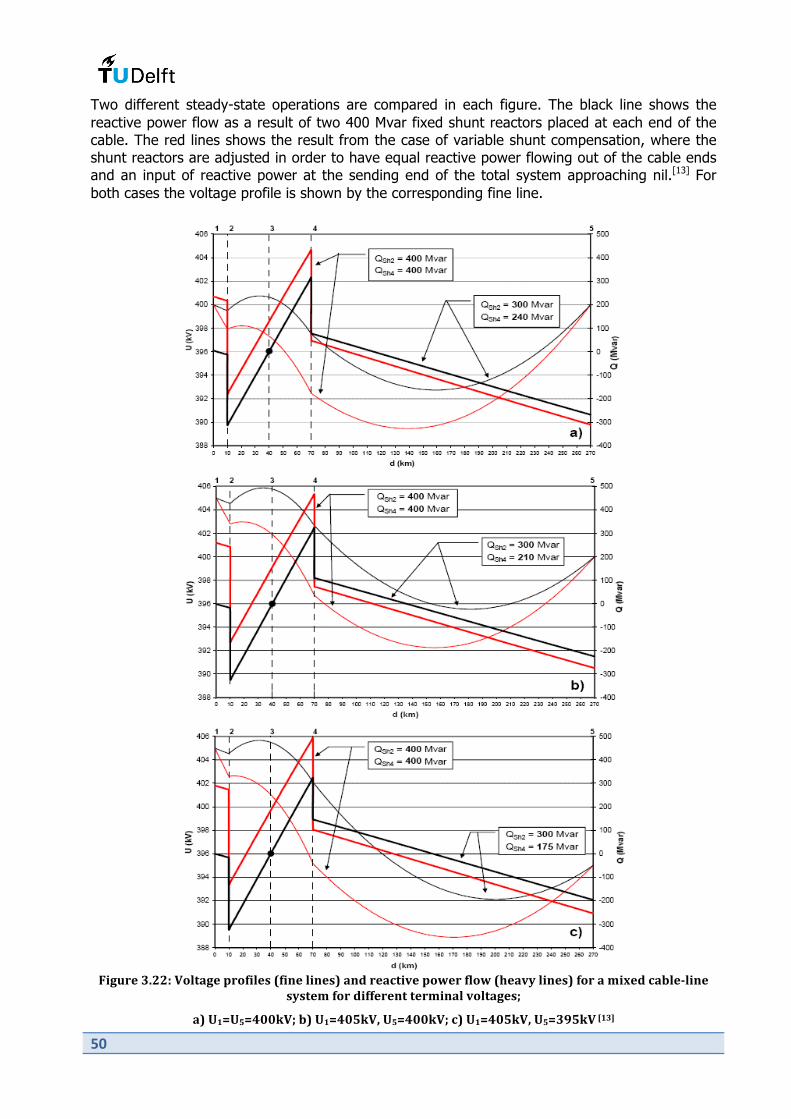
/5

Two different steady-state operations are compared in each figure. The black line shows the

reactive power flow as a result of two 400 Mvar fixed shunt reactors placed at each end of the

cable. The red lines shows the result from the case of variable shunt compensation, where the

shunt reactors are adjusted in order to have equal reactive power flowing out of the cable ends

and an input of reactive power at the sending end of the total system approaching nil.[13] For

both cases the voltage profile is shown by the corresponding fine line.

T/6."#'CU??N'7,8+%6#'L",$/8#:'_$/*#'8/*#:`'%*-'"#%&+/E#'L,9#"'$8,9'_3#%ES'8/*#:`'$,"'%';/M#-'&%D8#X8/*#'

:S:+#;'$,"'-/$$#"#*+'+#";/*%8'E,8+%6#:a'

%`'O1bO(bBKK=7a'D`'O1bBK(=7c'O(bBKK=7a'&`'O1bBK(=7c'O(bCI(=7'P1CQ'

/4

From the figure it can be seen that in the case of fixed shunt compensation, the optimal

operating condition is not achieved, especially when there is a significant difference between the

terminal voltage magnitudes, as in Figure 3.22 c.[13] The variable-type shunt compensation

allows for more control of the reactive power flow, resulting in a symmetrical reactive power

flow distribution in the cable for all cases of Figure 3.22, with about 300 Mvar flowing out of

both ends of the cable.

Variable shunt compensation can be beneficial in the above situation, for symmetrical mixed

cable-line systems however the difference between fixed and variable compensation is much

less significant and variation of the shunt compensation may not be necessary.

3.3.2 Losses comparison

Losses in a transmission line are very much dependent on the loading of the line. Transmission

lines are naturally not fully loaded the whole year round. An annual average line loading of

about 45 to 55% is considered to be realistic.[3] This is an important fact for comparing the

losses in overhead lines and underground cables, as a significant difference exists between the

origin of the losses in these systems. For overhead lines the losses almost completely consist of

current dependent losses. For underground cables however, voltage dependent losses become a

more dominating factor, mostly because of the dielectric and compensation losses. Currents

flowing in the shunt reactors cause compensation losses. These ohmic losses typically account

for about 0.15% of the compensated reactive power. Unlike current dependent losses, dielectric

and compensation losses are not dependent on the loading and are equally present at light load

conditions.

For a double circuit underground cable the voltage dependent losses become even more

dominant with respect to the current dependent losses. When comparing a double circuit system

to a single circuit system for the same loading, the current will be divided over the two circuits,

resulting in only half the current flowing in each circuit. The ohmic losses, which are dependent

on the square of the current, will therefore reduce to about 25% compared to the single circuit

arrangement. The voltage however does not change and the voltage dependent losses will

therefore be equal in both circuits and have doubled compared to the single circuit arrangement.

Figure… shows a comparison of transmission losses for a 50 km 380 transmission line. On the

left side the transmission line consists of a 2500 mm2 XLPE underground cable versus on the

right side a comparably rated overhead line.[3] The annual average line loading is considered to

be 55%.

/6

T/6."#'CU?CN'A,;L%"/:,*',$'%'(K'=;'C>K'=7'+"%*:;/::/,*'8/*#c':/*68#'%*-'-,.D8#'&/"&./+N'.*-#"6",.*-'

&%D8#'E#":.:',E#"3#%-'8/*#PCQ'

The high peak current dependent losses of the single circuit overhead line seen in the figure are

a result of the much higher line impedance compared to the impedance of the underground

cable. Looking at the figure it can be concluded that in terms of losses the underground cables

system has the advantage over the overhead line system at high load and overhead line system

has the advantage at light load. The above situation may however not be generalized and a

case by case assessment should be made depending on the situation of the respective grid.

3.3.3 Over-Loading Capability EHV AC Cable

For overhead lines, the sag of the line limits the over-loading capability. Thermal expansion of

the conductors increases the sag, potentially causing the height of the line to drop below the

minimum required clearance to ground. The over-loading capability is dependent on

environmental influences like wind, rain and ambient temperature. For example, high wind

speeds will improve the cooling of the conductors, therefore allowing a higher over-loading.

For underground cables the over-loading capability is practically uninfluenced by environmental elements and a thermal limit of 90°C is set in order to prevent potential damage to the

insulation caused by overheating. The large heat capacity of the soil and insulation surrounding

the conductor of an underground cable causes an underground cable to have a large thermal

inertia, which essentially means a high reluctance to temperature changes. Underground cables

will therefore heat up much slower than overhead line conductors and are generally able to

withstand over-loading for a much longer period than overhead lines.

The degree to which an underground cable can be operated beyond its normal rated current

without causing it to overheat will be determined, in part, by the temperature at which it is

operated immediately before the overload is applied. This, in turn, is a function of the load it is

carrying. As mentioned in the previous paragraph, the average loading of a line will be about

50% of its rated capability. It was also mentioned that this will cause the current dependent

losses to reduce to about 25% compared to the full load situation. For an underground cable

/!

this means that the temperature at the cable’s surface will on average only be about 30 to or

less.

As an example, a double 380 kV AC underground cable system is taken. The insulation consists

of XLPE and the copper conductors have a cross section of 2500 mm2. The system is loaded at

50% of its rated power, when one of the circuits becomes unavailable and the other circuit has

to take over the load. The temperature response of the individual phase cables of the remaining circuit is shown in Figure 3.24. The temperature in °C at the cable is shown on the vertical axis

and the time in days is given on the horizontal axis.

T/6."#'CU?BN'2#;L#"%+."#'"#:L,*:#',$'%'C>K'=7']F!Y'&%D8#':S:+#;'%$+#"'8,::',$'/*'&/"&./+'L"#&#-#-'DS'

(Kd',$'*,;/*%8'8,%-/*6PCQ'

From the figure it can be seen that the remaining circuit is over-loaded and is heated beyond its

thermal limit of 90°C. However, it takes more than a week for the first phase cable to reach this

state. This is an important aspect of underground cables as it gives transmission system

operators time to take remedial measures, like for instance redirecting power flows, changing

the dispatch of power generation or repairing and re-instating the unavailable circuit.[3] Figure

3.25 shows the temperature distribution in the soil surrounding the cable system. The upper

part represents the situation at the starting point and the lower part the situation after 8 days,

where one of the cables reached the thermal limit.

/.

T/6."#'CU?(N'23#";%8'-/:+"/D.+/,*'%",.*-'%'C>K=7'&%D8#':S:+#;PCQ'

3.3.4 Security of Supply

The general definition of security of supply given by Tennet is: The uninterrupted supply of

energy to consumers and businesses. Security of supply is one of the main responsibilities of a

transmission system operator and is an important topic in the planning and operation of power

systems. Not only is the adequacy of the system of importance, but also the quality of the

provided energy. The diagram below gives a little bit more insight in the term security of supply.

T/6."#'CU?HN'[E#"E/#9'-#$/*/+/,*'G#&."/+S',$'G.LL8SP1BQ'

Comparing the effect on the security of supply of an underground cable system to the effect of

an overhead line at EHV level is not an easy task and is dependent on many variables. Years of

data collection regarding EHV overhead lines have resulted in a thorough statistical research into

//

the effect of overhead lines. EHV AC cables are however still a relatively young technique and

with the limited statistical data available it is difficult to make a reliable assessment.

With regard to the continuity of supply the first priority is to maintain the bulk power

transmission provided by the 380 kV grid. The 380 kV grid is the backbone of the Dutch power

supply system and supplying power to the millions of consumers will not be possible without it.

High availability to transmit power of individual 380 kV transmission lines is of vital importance

in securing the power supply. This raises the question whether the 380 kV AC cable system can

provide the high performance level in terms of reliability and adequacy required at this voltage

level.

Both techniques are considered to be highly reliable if constructed and maintained properly,

resulting in a low failure frequency. The failure frequency is however much dependent on the

local situation. Overhead lines are for instance vulnerable to weather conditions. Extreme

weather conditions like wind and snowstorms can even cause extensive damage to overhead

line systems. Air pollution adds to the requirement of regular inspection and maintenance, as it

can cause additional corona. Cable systems are not affected by the above environmental

conditions and require limited maintenance. As only part of the cable is readily accessible

(tunnel installed underground cables excepted), only the cross bonding bays and transition

compounds are regularly inspected. Cables are regarded as vulnerable to carelessness during

excavation activities by third parties, which can cause extensive damage to a cable. Providing

reliable failure rates for underground cable systems still proves to be difficult. Extrapolating

figures from lower voltages is speculative and introduce at least substantial uncertainties. The

difference in technological challenges and the lacking experience with regard to EHV

underground cables system cannot be ignored.[3]

Next to the failure rate, an important factor to consider in reliability assessments is the time

necessary to repair the transmission line when a failure occurs. Overhead lines are easily

accessible and failures can quickly be found by visual inspection. Repair is relatively simple in

most cases and the line can usually be put back in service in a day. However, major catastrophic

failures do occur involving multiple circuits and can take many month to repair. For underground

cables, failures tend to affect only a single circuit. An underground cable fault can be difficult to

locate by electrical means if obvious excavation damage is not present. Repair typically takes

much longer than in the case of overhead lines and can take from one up to several weeks.[8] To

give an indication of the repair time of different assets, the mean time to repair (MTTR) is used.

In general, The MTTR of an underground cable is considered to be lot longer than the MTTR of

overhead cables. Numerous researches have been dedicated to the subject, but estimations

remain under extensive debate, ranging from one to four weeks or even more.

Power transmission networks are designed to function normally during a single or even double

contingency situation caused by outage of a transmission line. Outage of a line because of for

instance maintenance can be planned and is not considered as a threat to the security of supply.

Unplanned forced outages pose a much greater risk to cause significant problems regarding

widespread system failure and instability and are therefore decisive for evaluation of the

suitability of a technology in the perspective of contingency management.[3] The unavailability of

a component without taking planned unavailability in to account is known as the forced outage rate (FOR), which is the possibility a transmission line is out of service at a certain time due to a

forced outage. The forced outage rate can be expressed in terms of the failure frequency and

the MTTR.

/0

where % is the failure frequency per km per year and µ is repair frequency per hour, which is the

inverse of the MTTR.[15] The highly diverse values estimated for the failure rate as well as the

MTTR of EHV underground cables strongly influences the expected FOR. As a consequence

reported figures for the forced outage rate of underground cables have to be interpreted with

extreme care. The wide range in estimates is illustrated in Figure 3.27 and most of all indicates

the existing uncertainties. Additionally, the forced outage rate of an underground cable is not

only determined by the cables itself, but also by all auxiliary equipment required for operation

(for instance sealing end terminals and joint). Most references do not specify the system

boundaries in detail and considerable differences in the scope considered may exist.[3]

T/6."#'CU?0N'J#L,"+#-'E%8.#:'$,"'$,"&#-',.+%6#'"%+#''%*-';#%*'+/;#'+,'"#L%/"'$,"'BKK'=7',E#"3#%-'8/*#'

%*-'.*-#"6",.*-'&%D8#'&/"&./+:PCQ'

The area corresponding with each reference indicates the respective forced outage hours per

km per year. It can easily be seen that these estimations differ considerably. A qualitative

assessment of the references is outside the scope of this report. It does however emphasize the

fact that more data collection and further experience is very much needed in order to be able to

make a more accurate estimation of the reliability of underground cable systems.

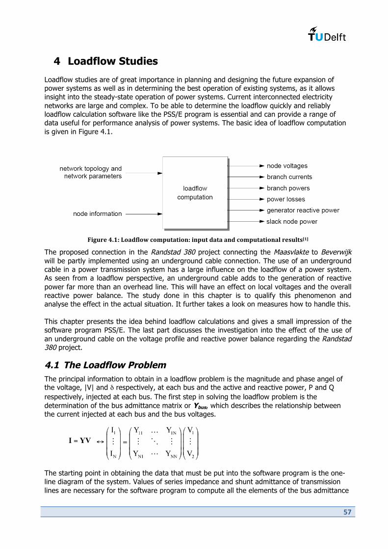
/1

4 Loadflow Studies

Loadflow studies are of great importance in planning and designing the future expansion of

power systems as well as in determining the best operation of existing systems, as it allows

insight into the steady-state operation of power systems. Current interconnected electricity

networks are large and complex. To be able to determine the loadflow quickly and reliably

loadflow calculation software like the PSS/E program is essential and can provide a range of

data useful for performance analysis of power systems. The basic idea of loadflow computation

is given in Figure 4.1.

T/6."#'BU1N'F,%-$8,9'&,;L.+%+/,*N'/*L.+'-%+%'%*-'&,;L.+%+/,*%8'"#:.8+:P1Q'

The proposed connection in the Randstad 380 project connecting the Maasvlakte to Beverwijk

will be partly implemented using an underground cable connection. The use of an underground

cable in a power transmission system has a large influence on the loadflow of a power system.

As seen from a loadflow perspective, an underground cable adds to the generation of reactive

power far more than an overhead line. This will have an effect on local voltages and the overall

reactive power balance. The study done in this chapter is to qualify this phenomenon and

analyse the effect in the actual situation. It further takes a look on measures how to handle this.

This chapter presents the idea behind loadflow calculations and gives a small impression of the

software program PSS/E. The last part discusses the investigation into the effect of the use of

an underground cable on the voltage profile and reactive power balance regarding the Randstad 380 project.

4.1 The Loadflow Problem

The principal information to obtain in a loadflow problem is the magnitude and phase angel of the voltage, |V| and $ respectively, at each bus and the active and reactive power, P and Q

respectively, injected at each bus. The first step in solving the loadflow problem is the

determination of the bus admittance matrix or Ybus, which describes the relationship between

the current injected at each bus and the bus voltages.

The starting point in obtaining the data that must be put into the software program is the one-

line diagram of the system. Values of series impedance and shunt admittance of transmission

lines are necessary for the software program to compute all the elements of the bus admittance

/2

matrix. Using the bus admittance matrix and the above relationship, the equations for

determining the active and reactive power injection can be obtained:

And

To solve the loadflow problem, two of the four parameters (P, Q, |V| and $) describing each bus

should be specified. In general three types of buses can be identified.

• Load or PQ bus At each non-generator bus, called a load bus, the active and reactive power drawn form

the system are known form historical forecast, load forecast, or measurement. Quite often

only real power is known and the reactive power is then based on an assumed power

factor such as 0.85 or higher.

• Voltage-controlled or PV bus Any bus of the system at which the voltage magnitude is kept constant is said to be

voltage controlled, in general a generator is connected to these buses. A generator has the

ability to control the active power output and the voltage at its terminal.

• Swing bus or slack node

The loadflow computation needs one bus to be addresses as slack node. The voltage angle

of the slack node serves as a reference for the angles of other buses and is the only bus

for which the angle of the voltage phasor is specified. The particular angle assigned to the

voltage of the slack node is not of importance, as the voltage angle difference determines

the calculated values of P and Q. It is common practice to set the voltage angle of the slack node as " = 0°. The slack node is the only bus where the active power flow is not

specified. A generator, connected to the slack node, supplies the mismatches between the

total power injected into the system and the total power drawn form the system plus the

losses in order to balance the system. The slack node can be used as a measurement for

the quality of the loadflow solution.

Loadflow calculations use iterative techniques to solve the non-linear equations. First, estimated

values are assigned to the unknown bus voltages. With the estimated values and the specified

active and reactive power, new values for the voltage at each bus are calculated. The new set of

values for the voltage at each bus is again used to calculate another set of bus voltages. This

iterative process is repeated until the changes at each bus are less than a specified minimum

value. Examples of iterative techniques are the Gauss-Seidel and Newton-Raphson procedures.

Today’s industry-based studies generally employ the Newton-Raphson iterative method, because

it is reliable in convergence, computationally faster, and more economical in storage

requirement.[4]

4.2 PSS/E

With the introduction of the computer in loadflow calculations, a powerful tool was created for

the analysis of large-scale power systems. Since its introduction in 1976, the Power System

Simulator for Engineering tool has become one the most comprehensive and widely used

programs of its type. The PSS/E model used in this research was provided by the Dutch TSO

TenneT and represents the situation of the Dutch power system as foreseen in the year 2007 for

/3

the year 2014. The expected generation and load are based on the Green Revolution scenario,

which is considered the base scenario within TenneT, and includes the 110 kV, 150 kV, 220 kV

and 380 kV high voltage levels.

Figure 4.2 shows a screen shot of the software. The network topology and all parameters are

defined in the spreadsheet view of the program. Buses, branches, generator, load etc. can be

viewed and adjusted by selecting the different tabs at the bottom of the spreadsheet view. The

output bar shows the results of requested action, like the result of a loadflow calculation. It can

also report totals for different areas like for instance total active power generated, total reactive

power generated and total losses.

T/6."#'BU?N'e#S'#8#;#*+:',$'+3#'!GGfY':,$+9%"#'/*+#"$%&#P1HQ'

One of the latest additions to the PSS/E software is the diagram mode. The diagram mode is a

useful tool for a quick visual examination of the considered network and can, if constructed

properly, provide a geographical interpretation. Different colours are used to represent the

various voltage levels. By setting voltage and loading limits for buses and branches, these

colours can be changed automatically if values resulting from a loadflow calculation exceed the

set limits. Visualisation of active and reactive power flow in the branches of the network can be

achieved through animations.

Care should be taken when working with the diagram mode, as the software does not provide a

very transparent and practical user interface. Some of the issues related to the diagram mode

are for instance: changes made in the network topology in the diagram mode may or may not

05

change the data in the spreadsheet depending on the setting per element and the automated

draw function is not able to create a practical diagram. As a result, making a usable and

functional diagram, especially for large networks, proves to be a tedious and time-consuming

job and experience is recommended.

Using the equivalent network functionality of PSS/E, the reduced 380 kV network of the western

part of The Netherlands was deducted from the provided larger network. After a successful

loadflow calculation, PSS/E offers the possibility to remove part of the network and replace it

with equivalent loads and/or generators. In doing so, the original power flows in the remaining

network are maintained. Equivalent loads replaced the entire 110 kV, 150 kV, and 220 kV

networks and associated transformers and part of the 380 kV network. These parts of the

network where considered redundant, because the research focused on the comparison of

reactive power flows and the effect on local voltage levels for different cases.

4.3 Loadflow Study Randstad 380

The area under consideration is given in Figure 4.3 together with a schematically drawn figure

of the same area. The two new ring structures can easily be recognized.

T/6."#'BUCN'23#'9#:+#"*'L%"+',$'+3#'4.+&3'C>K'=7'6"/-'%*-'%':&3#;%+/&'/*+#"L"#+%+/,*'

This study is divided into two parts. First, a closer look is taken at the proposed connection

between Wateringen and Bleiswijk in the Southern Ring and a comparison is made between a

pure overhead line connection and a mixed cable-line connection. In the second part the system

of figure… is studied for several situations where the length of underground cable implemented

is varied. The last case studies the system with the full 20 km cable connection implemented

with the addition of adequate shunt compensation.

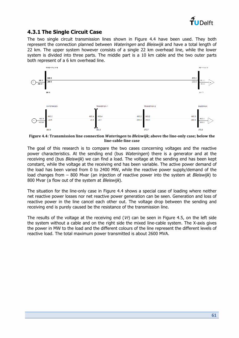
04

4.3.1 The Single Circuit Case

The two single circuit transmission lines shown in Figure 4.4 have been used. They both

represent the connection planned between Wateringen and Bleiswijk and have a total length of

22 km. The upper system however consists of a single 22 km overhead line, while the lower

system is divided into three parts. The middle part is a 10 km cable and the two outer parts

both represent of a 6 km overhead line.

T/6."#'BUBN'2"%*:;/::/,*'8/*#'&,**#&+/,*'%&'#(",)#,'+,'@+#"<$"A.a'%D,E#'+3#'8/*#X,*8S'&%:#a'D#8,9'+3#'

8/*#X&%D8#X8/*#'&%:#'

The goal of this research is to compare the two cases concerning voltages and the reactive

power characteristics. At the sending end (bus Wateringen) there is a generator and at the

receiving end (bus Bleiswijk) we can find a load. The voltage at the sending end has been kept

constant, while the voltage at the receiving end has been variable. The active power demand of

the load has been varied from 0 to 2400 MW, while the reactive power supply/demand of the

load changes from – 800 Mvar (an injection of reactive power into the system at Bleiswijk) to

800 Mvar (a flow out of the system at Bleiswijk).

The situation for the line-only case in Figure 4.4 shows a special case of loading where neither

net reactive power losses nor net reactive power generation can be seen. Generation and loss of

reactive power in the line cancel each other out. The voltage drop between the sending and

receiving end is purely caused be the resistance of the transmission line.

The results of the voltage at the receiving end (Vr) can be seen in Figure 4.5, on the left side

the system without a cable and on the right side the mixed line-cable system. The X-axis gives

the power in MW to the load and the different colours of the line represent the different levels of

reactive load. The total maximum power transmitted is about 2600 MVA.

06

T/6."#'BU(N'2#";/*%8'E,8+%6#'%+'@+#"<$"A.'_B(`'%+'-/$$#"#*+'8,%-/*6'&,*-/+/,*:'

At no load, a small voltage rise can be seen for the line-cable system. Increasing the active load,

while keeping the reactive load constant, results in both cases in a decrease of the voltage at

the receiving end. Further it can be seen for both cases that an injection of reactive power at

the receiving end causes a voltage rise and a reactive load causes a voltage drop. Overall, the

voltage for the case without a cable is somewhat more sensitive to load changes, than the case

with cable. This is mainly due to the higher series impedance of the overhead line compared to

the cable.

Figure 4.6 displays the total generation and absorption characteristic of reactive power for the

two systems. The results are obtained by taking the systems reactive power generation due to

the shunt susceptance and adding this to the total reactive losses due to the series reactance.

T/6."#'BUHN'2,+%8'"#%&+/E#'L,9#"'6#*#"%+/,*'%*-'%D:,"L+/,*'&3%"%&+#"/:+/&'

As was mentioned before, the large shunt susceptance of the cable produces a lot more reactive

power compared to the relatively small shunt susceptance of an overhead line. This can also be

seen in Figure 4.6. At no-load, the line-cable system produces about 250 Mvar, while the line-

only case produces about 13 Mvar. Under loading the line-only case becomes more reactive and

thus the line has a net demand on reactive power. The line-cable case tends to become as a

whole less productive in reactive power but even under full-load remains a producer. Again it

can be seen that the lower series impedance of the cable causes the line-cable system to be a

little less sensitive to load changes. The difference between no-load and full-load in the line-

0!

cable case is about 150 Mvar, while the line-only case shows a difference of about 180 Mvar.

Roughly speaking, the cable under consideration produces approx. 24 Mvar/km while the

overhead line produces less than 1 Mvar/km. Bear in mind that these values apply to a single

circuit.

Because of the different characteristics of a cable and a line, the voltage distribution between

Wateringen and Bleiswijk in the line-cable case is also different than in the line-only case. In the

line-only case the voltage at intermediate points can always be expected to be between the

voltage levels at the terminals. Under certain loading conditions however this does not apply to

the line-cable case. Figure 4.7 illustrates this in the case of a reactive load at Bleiswijk of Q = 0

Mvar and Q = 200 Mvar. V1 represents the voltage at bus TRANSITION 1 and V2 the voltage at

TRANSITION 2 (see Figure 4.4).

Figure 4.7: Voltages at the transition points; V1 is the voltage at the transition line-cable at

the Wateringen side (TRANSITION 1 in T/6."#'BUB); V2 is the voltage at the transition cable-

line at the Bleiswijk side(TRANSITION 2 in T/6."#'BUB); Vr is the voltage at Bleiswijk

When keeping in mind that the voltage at Wateringen is still fixed at 380 kV, it can be seen from

the figure on the left (Q = 0) that at certain active power levels, both voltages at the

intermediate points are higher than the voltages at the terminals. For Q = 200, V1 is slightly

higher than the bus voltage at Wateringen when a small active load is applied.

Not only can the voltages at the connections points of cable and line be higher than the terminal

voltages, a higher voltage can even be found between these points inside the cable. The

maximum voltage inside the cable, relative to the terminal voltages, occurs when the reactive

power flows equally from the midpoint to both ends of the cable (see paragraph 3.3.1).

Because of the limited length of the cable used (maximum of 10 km), the effect of this

phenomenon is not significant in the case of the Randstad 380 project. The maximum difference

of the voltage inside the cable and the voltage at the terminal of the cable will in this case only

be 0.25 ‰ and will therefore not be further considered in this research.

4.3.2 Implementation in Western Part of the Dutch 380 kV Power Grid

For the Randstad 380 project a total underground cable connection length of 20 km is foreseen.

In the previous paragraph the 10 km underground cable connection between Wateringen and

Bleiswijk was discussed, which will be part of the Southern Ring. Another 10 km will be

implemented in the Northern Ring divided in two parts. An 8 km underground cable connection

0.

will be part of the connection between Bleiswijk and Vijfhuizen and a 2 km underground cable

connection will be constructed for the underground crossing of the North Sea Canal.

The system under study is depicted in Figure 4.8 and represents the western part of the Dutch

380 kV grid. The remaining part of the 380 kV grid and all transformers plus connected lower

voltage level grids are left outside the scope of this analysis. To obtain a model according to the

loadflow of the PSS/E model provided by TenneT, the power flow out of the western part of the

380 kV grid into the 150 kV grid as well as into the remaining part of the 380 kV grid are

simulated using equivalent loads. The total load represents the maximum expected load for the

year 2014 according to the Green Revolution scenario.

T/6."#'BU>N'G+.-/#-'!GGfY'-/%6"%;'

The locations of the power generation sites and their respective active power output are shown

in the table below. The specified voltage at the nearest bus to the generation site is also given.

0/

2%D8#'BN'@&+/E#'L,9#"'6#*#"%+/,*':/+#:'

Location Active power [MW] voltage [pu] voltage [kV]

Maasvlakte 3600 1.06 403

Beverwijk 1500 1.05 399

Lelystad see text below 1.05 399

Geertruidenberg see text below 1.06 403

Simonshaven 400 1.06 403

Simonshaven Slack node 1.06 403

There are three points of in feed: Beverwijk, the Maasvlakte and Simonshaven. The active

power generation is determined using the by TenneT provided PSS/E file with the addition of

3000 MW offshore wind power divided in equal parts: 1500 MW at the Maasvlakte and 1500 MW

at Beverwijk (IJmuiden). The DC power connection to England has also been taken into account.

The generators at Lelystad and Geertruidenberg are added in order to control the voltage of the

buses at these locations, which is accordance the model provided by TenneT. In total there are

5 voltage-regulated buses. The bus voltage in the area of interest can freely change. The

existence of cables is the dominant factor in any voltage rise or drop in their direct

neighbourhood.

The transition compound between underground cables and overhead lines are marked by new

nodes (not reflecting a switching station). This applies to all four cable connections in the

system, which includes the already existing under grounding of the Nieuwe Waterweg and the

Caland Canal. Two series reactors in the connection Maasvlakte to Westerlee are marked in the

same way. The series reactors are applied to control the active power flow as explained in

paragraph 2.2.3 and have a reactance of 8 ohm each. Shunt reactors are connected directly to

the 380 kV buses at the nearest substations of Wateringen, Bleiswijk and Vijfhuizen. Shunt

compensation will be applied in the later explained case 4 (compensation).

The influence of the addition of an underground cable connection on the voltage of local buses

has been investigated by varying the length of the cable connections. The cable connections

replace overhead lines, so for every case the total transmission line length (cable plus overhead

line) is the same. The changes in voltage for increasing cable length seen at six of the buses in

the network are shown in Figure 4.9. The x-axis shows the length of the cable connection

between Wateringen and Bleiswijk, varying from 0 to 10 km. The y-axis represents the length of

the cable connection between Bleiswijk and Vijfhuizen and can change form 0 to 8 km. The 2

km crossing of the North Sea Canal is assumed fixed and will not be changed. The result is

presented in per unit with a base voltage of 380 kV.

00

T/6."#'BUIN'J#8%+/,*'D#+9##*'&%D8#'8#*6+3'%*-'E,8+%6#'8#E#8'%+':L#&/$/&'D.:#:'

From the figure it can be seen that under the considered circumstances the voltage at all buses

increase practically linear with increasing cable connection length.

Based on above considerations, five cases have been defined:

0. The base case: only the cable connections at the water crossings are considered.

1. Case 1: Equal to the base case with the addition of the proposed cable connection between

Wateringen and Bleiswijk.

2. Case 2: Equal to the base case with the addition of the proposed cable connection between

Bleiswijk and Vijfhuizen.

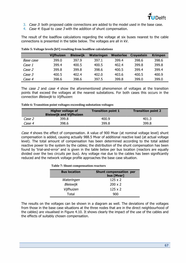
01

3. Case 3: both proposed cable connections are added to the model used in the base case.

4. Case 4: Equal to case 3 with the addition of shunt compensation.

The result of the loadflow calculations regarding the voltage at six buses nearest to the cable

connections is presented in the table below. The voltages are all in kV.

2%D8#'(N'7,8+%6#'8#E#8:'P=7Q'"#:.8+/*6'$",;'8,%-$8,9'&%8&.8%+/,*:'

Vijfhuizen Bleiswijk Wateringen Westerlee Crayestein Krimpen

Base case 399.0 397.9 397.1 399.4 398.6 398.6

Case 1 399.4 400.5 400.5 402.4 399.8 399.8

Case 2 399.8 399.8 398.6 400.5 399.4 399.4

Case 3 400.5 402.4 402.0 403.6 400.5 400.9

Case 4 398.6 398.6 397.5 399.8 399.0 399.0

The case 2 and case 4 show the aforementioned phenomenon of voltages at the transition

points that exceed the voltages at the nearest substations. For both cases this occurs in the

connection Bleiswijk to Vijfhuizen:

2%D8#'HN'2"%*:/+/,*'L,/*+'E,8+%6#:'#M&##-/*6':.D:+%+/,*'E,8+%6#:'

Higher voltage of

Bleiswijk and Vijfhuizen

Transition point 1 Transition point 2

Case 2 399.8 400.9 401.3

Case 4 398.6 399.8 399.8

Case 4 shows the effect of compensation. A value of 900 Mvar (at nominal voltage level) shunt

compensation is added, causing actually 988.5 Mvar of additional reactive load (at actual voltage

level). The total amount of compensation has been determined according to the total added

reactive power to the system by the cables; the distribution of the shunt compensation has been

found by ‘trial-and-error’ and is given in the table below per bus location (reactors are equally

divided over the two circuits per bus). Any voltage rise due to the cables has been significantly

reduced and the network voltage profile approaches the base case situation.

2%D8#'0N'G3.*+'&,;L#*:%+/,*'"#%&+,":'

Bus location Shunt compensation per

bus [Mvar]

Wateringen 125 x 2

Bleiswijk 200 x 2

Vijfhuizen 125 x 2

Total 900

The results on the voltages can be shown in a diagram as well. The deviations of the voltages

from those in the base case situations at the three nodes that are in the direct neighbourhood of

the cables) are visualised in Figure 4.10. It shows clearly the impact of the use of the cables and

the effects of suitably chosen compensation. '

02

T/6."#'BU1KN'4#E/%+/,*',$'E,8+%6#:'9/+3'"#:L#&+'+,'D%:#'&%:#'P=7Q'

Finally, the reactive power summary is given. (All values are in Mvar)

2%D8#'>N'J#%&+/E#'L,9#"'D%8%*&#'

Qgenerators Qcharging Qload Qlosses Qcompensation

Base case 1,423.1 916.3 1,631.1 708.4

Case 1 864.8 1,452.7 1,631.1 686.4

Case 2 983.2 1,346.4 1,631.1 698.6

Case 3 422.3 1,891.7 1,631.1 683.0

Case 4 1,451.4 1,868.7 1,631.1 700.5 988.5

The above table gives an overview of the reactive power balance. The total reactive power

generated is formed by the reactive power added to the system by the generators (Qgenerator)

plus the total reactive power generated due to the capacitance of overhead lines and cables

(Qcharging = |V|2BC). On the other side are the reactive power demands: the combined reactive

load at the buses (Qload) and the reactive power losses in the series impedance (Qlosses = I2X).

Finally, for the compensation in case 4 the reactive power absorption by the shunt reactors is

given (Qcompensation).

Clearly, the addition of cables causes a rise in the generation of reactive power due to the

increased line charging and, subsequently, a decline in the generation of reactive power by the

generators. In case 3 the line charging is approximately 950 Mvar more than in the base case.

In case 4 this surplus is compensated for by the addition of shunt reactors as described in the

previous table. It can also be seen that the reactive power generation by the generators nearly

equals the base case value.

!"

Conclusion

This study presents an analysis of the steady-state effect on local voltage profile and reactive

power balance for a partial implementation of the Randstad 380 project using an EHV AC

underground cable system. The analysis focussed on the western part of the Dutch 380 kV grid.

The new Randstad 380 connection will incorporate three double circuit underground EHV AC

cable systems into the Dutch power transmission network. The cable systems will have a

combined connection length of 20 km. To enable the high power rating of 2600 MVA per circuit,

each system will be operated using 12 cables in parallel. In total the project will incorporate 240

km of underground cable making this one of the biggest EHV AC cable projects in the world.

The EHV AC underground cable technology is relatively young compared to the conventional

EHV AC overhead line technology. The size and number of EHV AC cable projects worldwide are

limited and statistical data gained from experience at these voltage levels is inadequate for a

reliable assessment of concerns related to the security of supply.

Underground cables not only differ from overhead line in terms of installation requirements, but

more importantly in their electrical characteristics. The much larger capacitance combined with a

lower impedance results in a large SIL compared to the thermal power limit of underground

cables at EHV level. As a result the cable will always be operated far below its SIL and behave

like a capacitor in any loading condition. At nominal voltage level the capacitance of the

considered EHV cable systems will generate about 50 Mvar per km, adding a total of 1000 Mvar

to the network.

The addition of reactive power affects the voltage profile of the local network. Loadflow

calculations have shown voltage rise at all buses in the direct neighbourhood of the cable

systems. The voltages at these points rose practically linear with increased cable length, but no

critical voltage levels were reached. Attention should be paid to the transition points between

underground cable and overhead line. The voltage at the transition points can rise above the

voltage seen at the nearest substations.

The additional reactive power generated by the cable can be compensated using shunt reactors

placed at either side of the cable system. Fixed shunt reactors will be sufficient to remove any

unwanted voltage rise. Variable shunt reactors will increases controllability of the reactive power

flow in the cable and can be used to enforce the ideal situation on the cable. In this situation

reactive power flows equally form both ends of the cable and the active power transmission

capability of the cable system is maximized. The resultant steady-state network after proper

application of shunt compensation is comparable to the network without cables in terms of

voltage profile and reactive power balance.

#$

Recommendations

The number of EHV AC cables systems currently in operation is still very limited. The operational

experience and data gained from these projects is invaluable for the future development and

extensive integration of EHV AC cable systems. International cooperation and data exchange

can help the technology move forward at a much larger pace. Network data and future

predictions should be made readily available and easily accessible for all research in this field.

The analysis done in this report has been preformed using the maximum predicted load

situation. The maximum net reactive power generated by the combined transmission lines is

however reached at minimum load. Generators connected to the system must not be allowed to

absorb large amounts of reactive power due to stability concerns and the total required shunt

compensation will thus be dependent on the light-load conditions. For further research,

especially for research related to underground cables, it is recommended to make data

concerning the predicted minimum load available.

Variable shunt compensation can especially be beneficial at high loading of the cable system, as

it increases the controllability of the reactive power flow and the maximum apparent power

along the line. Further research on underground cables should consider the possibility of using

variable shunt compensation.

#%

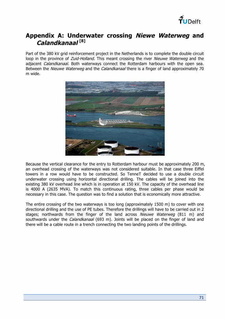
Appendix A: Underwater crossing Niewe Waterweg and

Calandkanaal [8]

Part of the 380 kV grid reinforcement project in the Netherlands is to complete the double circuit

loop in the province of Zuid-Holland. This meant crossing the river Nieuwe Waterweg and the

adjacent Calandkanaal. Both waterways connect the Rotterdam harbours with the open sea.

Between the Nieuwe Waterweg and the Calandkanaal there is a finger of land approximately 70

m wide.

Because the vertical clearance for the entry to Rotterdam harbour must be approximately 200 m,

an overhead crossing of the waterways was not considered suitable. In that case three Eiffel

towers in a row would have to be constructed. So TenneT decided to use a double circuit

underwater crossing using horizontal directional drilling. The cables will be joined into the

existing 380 kV overhead line which is in operation at 150 kV. The capacity of the overhead line

is 4000 A (2635 MVA). To match this continuous rating, three cables per phase would be

necessary in this case. The question was to find a solution that is economically more attractive.

The entire crossing of the two waterways is too long (approximately 1500 m) to cover with one

directional drilling and the use of PE tubes. Therefore the drillings will have to be carried out in 2

stages; northwards from the finger of the land across Nieuwe Waterweg (811 m) and

southwards under the Calandkanaal (693 m). Joints will be placed on the finger of land and

there will be a cable route in a trench connecting the two landing points of the drillings.

#&

After careful evaluation of the possible solutions it was decided to install a forced water

circulation system to equalize local hot spots in the directional drilling with cooler sections of the

directional drilling. Normally the ground layer with the highest thermal resistance determines the

necessary conductor size. A small layer of ground with a high thermal resistance (1.05 Km/W)

could have caused a hot-spot, but water circulation (without active heat exchanger) allowed the

desired ratings with a copper conductor size of 1600 mm2 rather than 2500 mm2. The land part

of the cable connection (to the transition compounds on both banks), is approximately 700 m.

Cable is direct buried in a trench, which is filled with a special back-fill material.

The requirements for the final stage of the project are shown in Table A.1.

!"#$%&'()*&+%,-./%0%123&4.1"$&32"5%&

Ampacity [A] Rating [MVA] Circuits in use Duration

4000 2635 1 1 week

3250 2140 1 Repair time side circuit

2500 1645 2 Continuous

To meet the final requirements 2 cables per phase are required, but the second set can be

postponed until necessary. Extra tubes for these cables are already installed in the first run. To

avoid extra joints (12 in the final state) and because it was not possible to create a balanced

crossbonding system, the system now has a single bonded earth system and two separate

copper earth cables.

#'

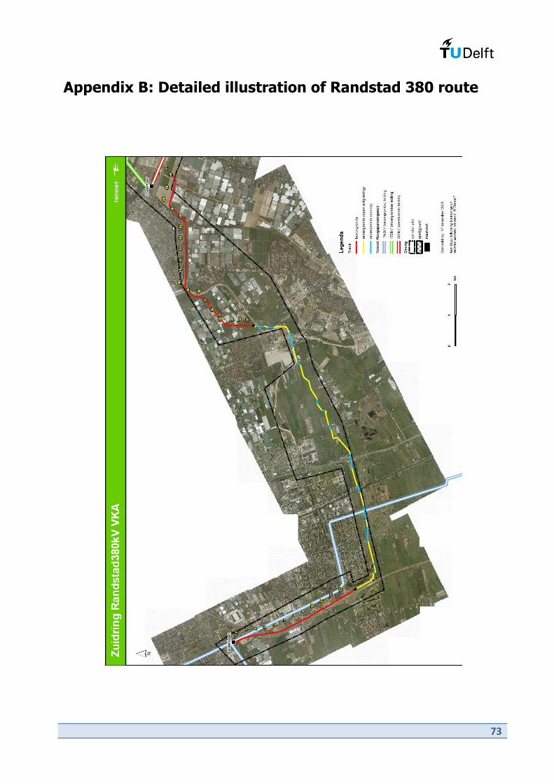
Appendix B: Detailed illustration of Randstad 380 route

#(

#)

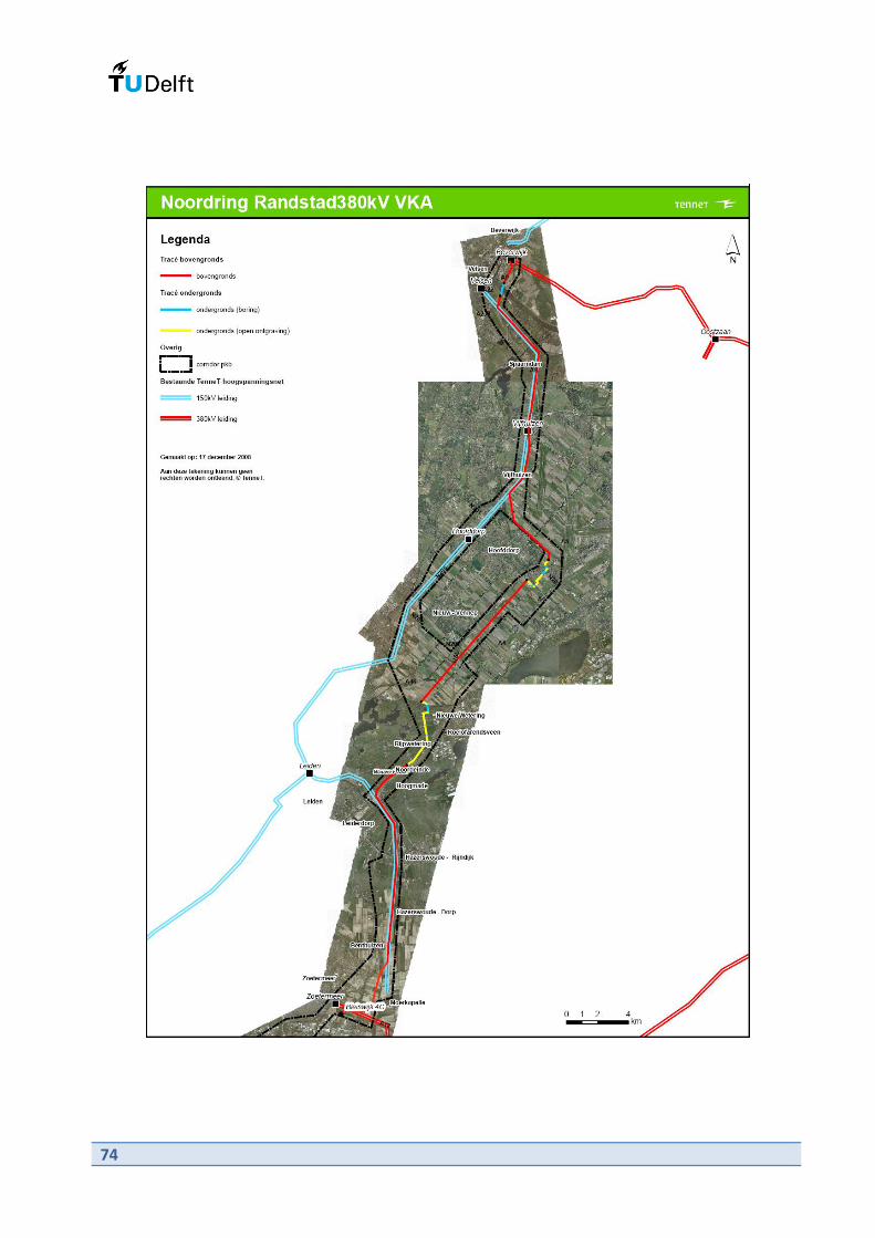
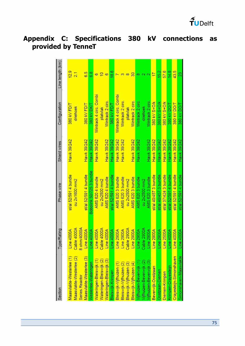
Appendix C: Specifications 380 kV connections as

provided by TenneT

#!

##

References

[1] Schavemaker, P.H. and Van der Sluis, L.: ‘Electrical power system essentials’, John Wiley &

Sons Ltd, Chichester, 2008, ISBN 978-0470-51027-8

[2] TenneT: ‘Kwaliteits- en Capaciteitsplan 2008 – 2014’, TenneT TSO b.v., Arnhem, December

2007

[3] Burges, K; Bömer, J.; Nabe, C.;Papaefthymiou, G.; Brakelmann, H.; Maher, M.; Mills, C. and

Hunt, J.: ‘Study on the comparative merits of overhead electricity transmission lines versus

underground cables’, Ecofys Germany GmbH, May 2008, PPSMDE081295

[4] Grainger, J.J. and Stevenson, W.D., Jr.: ‘Power system analysis’, McGraw-Hill, Singapore,

1994, ISBN 0-07-113338-0

[5] Sauer, P.W. and Pai, M.A.: ‘Power system dynamics and stability’, Prentice-Hall, Inc., Upper

Saddle River, New Jersey, 1998, ISBN 0-13-678830-0

[6] Kiessling, F.; Nefzger, P.; Nolasco, J.F. and Kaintzyl, U.: ‘Overhead power lines: Planning,

design, construction’, Springer-Verslag, Berlin Heidelberg, 2003, ISBN 3-540-00297-9

[7] Linke, S. and Schuler, R.E.: ‘Electrical-energy-transmission technology: The key to bulk-

power-supply policies’, Annual Reviews Inc., 1988

[8] Cigre Working Group B1.07: ‘Statistics on underground cable in transmission networks’, 2007

[9] Ferreira, J.A.: ‘Power electromagnetics’, Delft University of Technology, September 2003

[10] Karlsson, D.; Sollerkvist, F.J. and Lundquist, J.: ‘A comparison of XLPE cables and overhead

lines’, STRI AB, May 2001

[11] Weedy, B.M.: ‘Electrical power systems’, John Wiley & Sons Ltd, Chichester, 1987, ISBN 0-

471-91659-5

[12] The Highland Council, Cairngorms National Park Authority & Scottish Natural Heritage:

‘Undergrounding of Extra High Voltage transmission lines’

[13] Gatta, F.M. and Lairia, S.: ‘Very long EHV cables and mixed overhead-cable lines. Steady-

state operation’, IEEE Power Engineering Society, 27-30 June 2005

[14] Haber, A. and Rodgarkia-Dara, A.: ‘Qualitätsregulierung – Theorie und internationale

Erfahrungen’, Working paper nr. 16, December 2005

[15] Kling, W.L.: ‘Planning and Bedrijfsvoering van Elektriciteitsvoorzieningsystemen’, Delft

University of Technology, September 2000

[16] Siemens: ‘PSS™E 31.0 - Users manual’, Siemens Power Transmission & Distribution, Inc.,

Power Technologies International, December 2007