
Concealed Weapon Detection - TU Delft Repositories
157
Concealed Weapon Detection A microwave imaging approach MASTER OF SCIENCE THESIS Leonardo Carrer Thesis Supervisor: Prof. Dsc. A. G. Yarovoy May 29, 2012 Delft University of Technology Faculty of Electrical Engineering, Mathematics and Computer Science (EEMCS)
-
Upload
khangminh22 -
Category
Documents
-
view
2 -
download
0
Transcript of Concealed Weapon Detection - TU Delft Repositories

Concealed Weapon DetectionA microwave imaging approach
MASTER OF SCIENCE THESIS
Leonardo Carrer
Thesis Supervisor: Prof. Dsc. A. G. Yarovoy
May 29, 2012
Delft University of Technology
Faculty of Electrical Engineering, Mathematics and Computer Science (EEMCS)


The undersigned hereby certify that they have read and recommend to the Faculty
of Electrical Engineering, Mathematics and Computer Science (EEMCS) for accep-
tance a thesis entitled ’Concealed Weapon Detection: A microwave imaging
approach’ by Leonardo Carrer in partial fulllment of the requirements for the
degree of Master of Science in Electrical Engineering: Telecommunications Track
Dated: May 29, 2010
Commitee members:
__________________
Prof. Dsc. A. Yarovoy
__________________
Dr. Ir. B. J. Kooij
__________________
Dr. Ir. R. F. Remis
__________________
Dr. T. Sakamoto
3

Abstract
In the last years, there has been a renewed interest in security applications designed
to detect potentially dangerous concealed object carried by an individual. In partic-
ular automatic detection and classification of concealed weapons is a fundamental
part of every surveillance system.
Until now merely all the research in image processing for Concealed Weapon De-
tection has been focused on millimeter wave imagers and X-ray imagers with very
little work done in the microwave range.
The main objective of this thesis is to develop robust novel image processing algo-
rithms for detection and classification of concealed weapon.
In particular, the developed algorithms are specifically tailored to work with mi-
crowave radar images. The algorithms shall also perform efficiently with a low false
alarm rate in a reduced contrast envinroment such as the one of microwave images.
Depolarization Analysis and SIFT Analysis which are two novel algorithms for con-
cealed weapon detection and classification in the field of 3D high resolution mi-
crowave radar imaging are presented in this thesis research project.
Keywords– Concealed Weapon Detection, 3D high-resolution microwave images,
Depolarization, SIFT, image processing, PCA, Phase Symmetry
5


Acknowledgments
In this page I would like to say thank you to a number of people who supported me
while preparing this Thesis work.
First I want to thank my Supervisor Prof. A. Yarovoy for the nice advices he has
given me regarding my work and for the freedom that he allowed me to have in
developing it. Secondly, I’m extremely grateful to P.Aubry for its invaluable help
in the measurement campaign and for his patience in answering all my technical
questions during this months.
Even if I am not going to list all of them in this little page, I would like to to
say thank you (grazieee!) to all my beloved friends in Rome for supporting me
throughout the years in good and bad times and without whom I would never been
able to arrive at this point. I would also like to say thanks to all my friends here in
Delft for the amazing time I have spent with them which made my life happier. A
special thanks goes to Gustavo and Mark for reading and correcting my Thesis.
Finally I would like to thank my family for their unconditional love and for support-
ing me in all my decisions.
Leonardo Carrer
Delft, The Netherlands
16/05/2012
7


Contents
Abstract 5
Acknowledgments 7
1. Introduction 9
1.1. Overview . . . . . . . . . . . . . . . . . . . . . . . . . . . . . . . . . . 9
1.2. State of the art . . . . . . . . . . . . . . . . . . . . . . . . . . . . . . 11
1.2.1. Imaging processing for CWD . . . . . . . . . . . . . . . . . . 14
1.3. Research objective . . . . . . . . . . . . . . . . . . . . . . . . . . . . 19
1.3.1. Approach and feasibility . . . . . . . . . . . . . . . . . . . . . 20
1.4. Thesis outline . . . . . . . . . . . . . . . . . . . . . . . . . . . . . . . 20
Bibliography 23
2. Shape Descriptors 27
2.1. Overview . . . . . . . . . . . . . . . . . . . . . . . . . . . . . . . . . . 27
2.2. Introduction to Shape Descriptors . . . . . . . . . . . . . . . . . . . . 28
2.3. Polarization . . . . . . . . . . . . . . . . . . . . . . . . . . . . . . . . 29
2.3.1. PCA and Polarization Angle . . . . . . . . . . . . . . . . . . . 31
2.4. Symmetry and Feature Angle . . . . . . . . . . . . . . . . . . . . . . 41
2.5. Depolarization Angle . . . . . . . . . . . . . . . . . . . . . . . . . . . 46
i

2.6. SIFT Descriptors . . . . . . . . . . . . . . . . . . . . . . . . . . . . . 50
2.7. Shape Descriptors enhancement . . . . . . . . . . . . . . . . . . . . . 54
2.7.1. Segmentation and Histogram Thresholding . . . . . . . . . . . 54
2.8. Conclusions . . . . . . . . . . . . . . . . . . . . . . . . . . . . . . . . 57
Bibliography 61
3. Depolarization Analysis 63
3.1. Overview . . . . . . . . . . . . . . . . . . . . . . . . . . . . . . . . . . 63
3.2. Depolarization unit . . . . . . . . . . . . . . . . . . . . . . . . . . . . 64
3.2.1. Energy Projection . . . . . . . . . . . . . . . . . . . . . . . . . 65
3.2.2. Image filtering . . . . . . . . . . . . . . . . . . . . . . . . . . . 68
3.2.3. Phase Symmetry and Feature Angle . . . . . . . . . . . . . . 68
3.2.4. PCA and Polarization Angle . . . . . . . . . . . . . . . . . . . 72
3.2.5. Depolarization Angle . . . . . . . . . . . . . . . . . . . . . . . 73
3.3. Detection unit . . . . . . . . . . . . . . . . . . . . . . . . . . . . . . . 76
3.3.1. Threshold selector . . . . . . . . . . . . . . . . . . . . . . . . 76
3.3.2. Symmetry Verification . . . . . . . . . . . . . . . . . . . . . . 77
3.3.3. Inset Verification . . . . . . . . . . . . . . . . . . . . . . . . . 78
3.3.4. Specular Symmetry Verification . . . . . . . . . . . . . . . . . 80
3.4. Conclusions . . . . . . . . . . . . . . . . . . . . . . . . . . . . . . . . 80
Bibliography 83
4. SIFT Analysis 85
4.1. Overview . . . . . . . . . . . . . . . . . . . . . . . . . . . . . . . . . . 85
4.2. Energy Projection and Image Segmentation . . . . . . . . . . . . . . 87
4.3. SIFT and Objects Library . . . . . . . . . . . . . . . . . . . . . . . . 90
4.4. Histogram thresholding . . . . . . . . . . . . . . . . . . . . . . . . . . 91
ii

4.5. Correlator and Ranking Matrix . . . . . . . . . . . . . . . . . . . . . 92
4.6. Global Ranking Matrix . . . . . . . . . . . . . . . . . . . . . . . . . . 93
4.7. Conclusions . . . . . . . . . . . . . . . . . . . . . . . . . . . . . . . . 94
Bibliography 97
5. Experimental Results and Comparative Analysis 99
5.1. Overview . . . . . . . . . . . . . . . . . . . . . . . . . . . . . . . . . . 99
5.2. Depolarization Analysis Results . . . . . . . . . . . . . . . . . . . . . 100
5.3. SIFT Analysis Results . . . . . . . . . . . . . . . . . . . . . . . . . . 112
5.4. Comparative Analysis . . . . . . . . . . . . . . . . . . . . . . . . . . 119
5.5. Conclusions . . . . . . . . . . . . . . . . . . . . . . . . . . . . . . . . 120
6. Conclusions and Recommendations 125
6.1. Overview . . . . . . . . . . . . . . . . . . . . . . . . . . . . . . . . . . 125
6.2. Conclusions . . . . . . . . . . . . . . . . . . . . . . . . . . . . . . . . 126
6.3. Summary of Contributions . . . . . . . . . . . . . . . . . . . . . . . . 129
6.4. Recommendations . . . . . . . . . . . . . . . . . . . . . . . . . . . . . 130
A. PCA 133
B. Measurements Setup 135
C. SIFT 139
iii


List of Figures
1.1. 350 Ghz image of a Glock 17 9-mm gun.Image from [13]. . . . . . . . 12
1.2. Mannequin under test(left) and microwave image of it (right) . Image
from [14]. . . . . . . . . . . . . . . . . . . . . . . . . . . . . . . . . . 13
1.3. Optical (left) and 110-112 Ghz image (MM wave on the right) of a
clothed mannequin with a concealed Glock-17 handgun. Image from
[13]. . . . . . . . . . . . . . . . . . . . . . . . . . . . . . . . . . . . . 14
1.4. Block diagram of a typical image processing architecture for CWD.
Image from [15]. . . . . . . . . . . . . . . . . . . . . . . . . . . . . . . 15
1.5. An image fusion approach to CWD. Here an optical image is combined
with an Infra red image. The combination of the two images produces
an improved fused image where both the identity of the subject and
the concealed weapon are highlighted. Images from [18]. . . . . . . . 16
1.6. An example on how an object can be mapped to a mathematical
shape descriptor. In this case the spatial frequency distribution of
a revolver (a) is different from the one produced by the chest of the
human body (b) . This property can be exploited to classify objects.
Images from [20] . . . . . . . . . . . . . . . . . . . . . . . . . . . . . . 17
1.7. A common object recognition procedure . . . . . . . . . . . . . . . . 18
1

1.8. Block diagram for the automatic weapon detection algorithm de-
scribed in [19]. . . . . . . . . . . . . . . . . . . . . . . . . . . . . . . . 18
1.9. Target output (on the right) of the CWD algorithm for a specific
input (left image) . . . . . . . . . . . . . . . . . . . . . . . . . . . . . 19
2.1. (a) Specular Reflection (b) Diffused reflection (c) Corner Reflector . . 30
2.2. Measuring scenario for experiment 1 . . . . . . . . . . . . . . . . . . 35
2.3. (a) VV image (b) HH image of the five objects in free space . . . . . 36
2.4. Polarization Angle for the first experiment . . . . . . . . . . . . . . . 37
2.5. (a) VV data (b) HH data (c) Polarization Angle for the second ex-
periment . . . . . . . . . . . . . . . . . . . . . . . . . . . . . . . . . . 38
2.6. (a) VV data (b) HH data (c) Polarization Angle for experiment 3 . . 40
2.7. (a)HH data (b)VV data (c) merged image for phase symmetry algo-
rithm applied to experiment 1 . . . . . . . . . . . . . . . . . . . . . . 44
2.8. (a) VV data (b) HH data (c) merged phase symmetry data for exper-
iment 3 . . . . . . . . . . . . . . . . . . . . . . . . . . . . . . . . . . 45
2.9. A typical case when Dp = −1. The object is exhibiting its maximum
polarization in the direction orthogonal to its long axis. . . . . . . . 46
2.10. Dp for experiment 1 of sec. 2.3.1 . . . . . . . . . . . . . . . . . . . . . 48
2.11. Line scan of Fig. 2.10 . . . . . . . . . . . . . . . . . . . . . . . . . . . 48
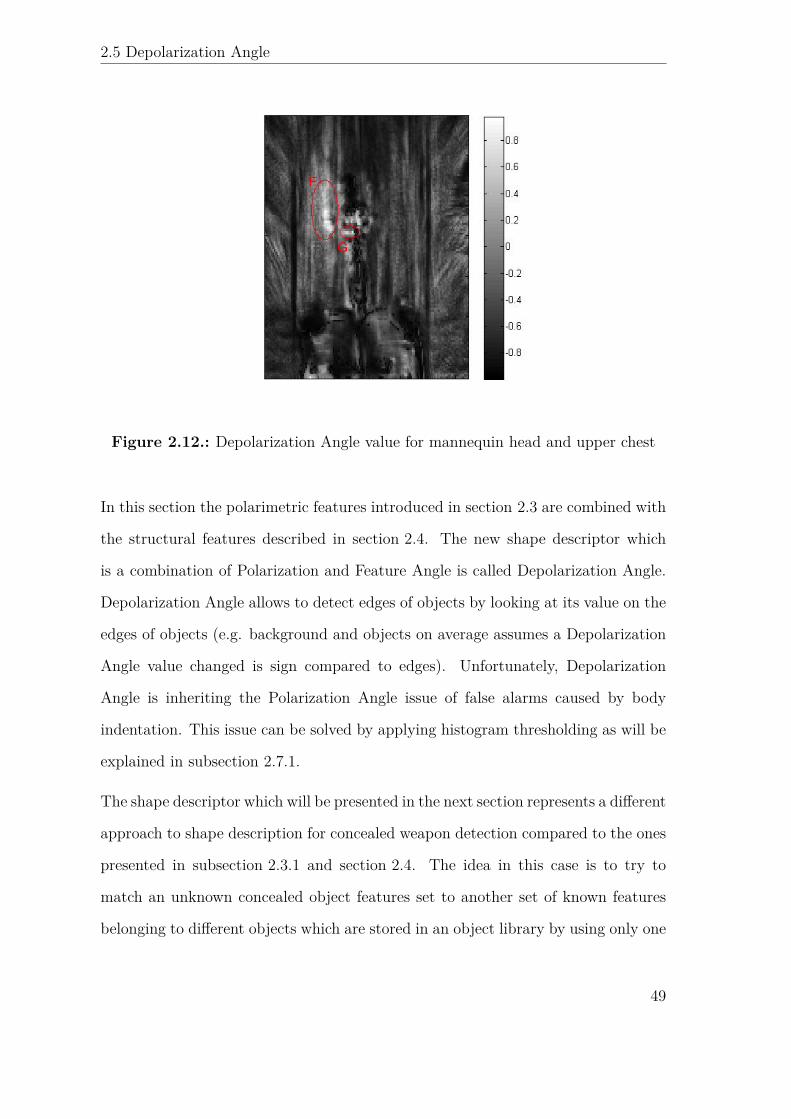
2.12. Depolarization Angle value for mannequin head and upper chest . . . 49
2.13. (a) Optical and (b) Microwave image of a bottle of water . . . . . . 51
2.14. (a) Optical and (b) Microwave image of a gun . . . . . . . . . . . . . 51
2.15. Gradient detection of a gun . . . . . . . . . . . . . . . . . . . . . . . 53
2.16. Typical example of primary and secondary grid. The yellow box is an
example of a secondary grid segment while the green one of a primary
one. . . . . . . . . . . . . . . . . . . . . . . . . . . . . . . . . . . . . 55
2

2.17. Histogram thresholding example . . . . . . . . . . . . . . . . . . . . . 57
3.1. Block diagram of the algorithm for Depolarization analysis . . . . . . 64
3.2. Depolarization unit block diagram . . . . . . . . . . . . . . . . . . . . 64
3.3. Grid arrangement . . . . . . . . . . . . . . . . . . . . . . . . . . . . . 65
3.4. (a) A typical 3D volumetric scalar measurement of a mannequin.
Radar is transmitting and receiving in vertical polarization (b) Energy
projection in the x-z plane . . . . . . . . . . . . . . . . . . . . . . . . 66
3.5. (a) 3D volumetric scalar measurement of five objects in the free space.
Radar is transmitting and receiving in vertical polarization. (b) En-
ergy projection in the x-z plane . . . . . . . . . . . . . . . . . . . . . 67
3.6. (a) Wavelenght of smallest scale filter = 3 (b) Wavelenght of smallest
scale filter = 12 . In both cases the number of wavelets scales is equal
to 5 and the number of orientations is equal to 6 . . . . . . . . . . . . 69
3.7. (a) SH (b) SV (c) Sm for a mannequin with concealed objects . . . . 71
3.8. Polarization angle for a mannequin carrying concealed objects . . . . 73
3.9. Depolarization angle for a mannequin carrying concealed objects . . . 74
3.10. Scan of row 137 of Fig. 3.9 . . . . . . . . . . . . . . . . . . . . . . . . 75
3.11. Scan of row 93 of Fig. 3.9 . . . . . . . . . . . . . . . . . . . . . . . . . 75
3.12. Detection unit block diagram . . . . . . . . . . . . . . . . . . . . . . 76
3.13. Inset Verification procedure. (a) Detected points over Depolarization
Angle (b) Dilation and centroids positions (c) Inset for each centroid
over Sm . . . . . . . . . . . . . . . . . . . . . . . . . . . . . . . . . . 79
3.14. (a) Histogram for inset 1 for Fig. 3.13 (b) Histogram for inset 2 for
Fig. 3.13 . . . . . . . . . . . . . . . . . . . . . . . . . . . . . . . . . . 79
3.15. Specular symmetry setup . . . . . . . . . . . . . . . . . . . . . . . . . 80
4.1. SIFT Analysis block diagram . . . . . . . . . . . . . . . . . . . . . . 86
3

4.2. Detection unit block diagram . . . . . . . . . . . . . . . . . . . . . . 86
4.3. (a) Gun with no histogram equalization (b) Gun with histogram
equalization (c) Gun with Contrast Limited Histogram Equalization . 89
4.4. An example of sample objects in the library. (a) gun (b) bottle (c)
ceramic knife . . . . . . . . . . . . . . . . . . . . . . . . . . . . . . . 91
5.1. (a) Horizontal Polarization Data (b) Vertical Polarization Data after
Laplacian and Horizontal/Vertical Prewitt filters . . . . . . . . . . . . 103
5.2. Depolarization Angle histogram when the average Depolarization An-
gle value is negative . . . . . . . . . . . . . . . . . . . . . . . . . . . . 104
5.3. (a) Horizontal polarization data (b) Vertical Polarization data (c)
Polarization angle (d) Feature angle for test case 1 . . . . . . . . . . . 106
5.4. The Depolarization Angle for test case 1 . . . . . . . . . . . . . . . . 107
5.5. Mannequin image with values for which Dp>0.8 marked in white.
Red circles are the points detected by detection unit. . . . . . . . . . 107
5.6. Image processing chain output for test case 1 . . . . . . . . . . . . . . 108
5.7. Output for Test Case 2 (left) and Optical image of the mannequin for
Test Case 2 (right) . . . . . . . . . . . . . . . . . . . . . . . . . . . . 109
5.8. Output for Test Case 3 (left) and output for Test Case 4 (right) . . . 110
5.9. Output for test case 5 . . . . . . . . . . . . . . . . . . . . . . . . . . 111
5.10. ( a ) Measured Mannequin for Test Case 1 ( b ) Output for Test Case 1115
5.11. (a) Measured Mannequin for Test Case 2 (b) Output for Test Case 2 116
5.12. Syntethic example of image distortion. (a) Distorted object on the
mannequin (b) same object in the library . . . . . . . . . . . . . . . . 116
5.13. (a) Measure Mannequin for Test Case 3 (b) Output for gun recogni-
tion (c) Output for bottle recognition . . . . . . . . . . . . . . . . . 118
4

A.1. PCA of a multivariate Gaussian distribution centered at (1, 3) with
a standard deviation of 3. . . . . . . . . . . . . . . . . . . . . . . . . 134
B.1. SAR antenna . . . . . . . . . . . . . . . . . . . . . . . . . . . . . . . 136
B.2. Mannequin which has been employed in the measurements . . . . . . 136
B.3. Mannequin positioned in the anechoic chamber . . . . . . . . . . . . 137
B.4. Mannequin positioned in the anechoic chamber with the AGILENT
E8364B network analyzer clearly visible in the front . . . . . . . . . 137
C.1. DoG calculations . . . . . . . . . . . . . . . . . . . . . . . . . . . . . 140
C.2. Maxima/Minima of DoG . . . . . . . . . . . . . . . . . . . . . . . . . 141
C.3. SIFT Descriptor . . . . . . . . . . . . . . . . . . . . . . . . . . . . . . 142
5


List of Tables
1.1. An overview of the more important CWDS technologies. Data re-
trieved from [3, 5] . . . . . . . . . . . . . . . . . . . . . . . . . . . . . 11
2.1. ϕP for different values of (xh, xv) . . . . . . . . . . . . . . . . . . . . 33
2.2. Values of the Polarization Angle for the two experiments . . . . . . . 38
2.3. Shape Descriptors flaws and solution . . . . . . . . . . . . . . . . . . 56
4.1. Example of a Ranking matrix for a fixed value of the segmentation
parameters. P=Primary grid segment, S=Secondary grid segment. . . 93
4.2. Example of a Global Ranking Matrix. P=Primary grid segment,
S=Secondary grid segment. . . . . . . . . . . . . . . . . . . . . . . . 94
5.1. Comparative Analysis between the two proposed methods . . . . . . 120
5.2. Maximum value for the Depolarization Angle for different features
edges . . . . . . . . . . . . . . . . . . . . . . . . . . . . . . . . . . . . 122
7


1. Introduction
“The tongue can conceal the truth, but the eyes never!”
The Master and Margarita,M.Bulgakov
1.1. Overview
In the last fifteen years, and in particular after 11th Sept. 2001, there has been a
renewed interest in security applications designed to detect potentially dangerous
concealed objects. It is a common experience in everyone’s life to go through a portal
type metal detector at the airport or when entering sensitive buildings. Despite the
fact that portal type metal detectors screening approach is successful and widely
used around the world it has some major flaws and in particular it cannot detect
dielectric weapons (e.g. ceramic knifes) , explosives, inflammables and it may fail
to detect very small items such as rounds of ammunition [1] . On top of that, it
cannot discriminate between innocuous items (e.g. keys) and dangerous objects.
Furthermore, in order to be screened, people have to go one by one through a
gate, creating longer queues in places such as airports. This also implies that it
is not possible to perform security screenings in crowded situation such as public
gatherings. Nevertheless a wide area metal detector is currently being developed
which allows to locate concealed metal weapons in a crowd [2] .In order to overcome
9

Chapter 1 Introduction
these limitations, a wide choice of valid concealed weapon detection systems(CWDS)
alternatives to metal detectors have been developed in the last twenty years. CWDS
can be classified accordingly to five parameters [3] :
1. Form of detected energy: It specifies the type of energy source collected and/or
emitted by the CWDS. It can be Electromagnetic or Acoustic.
2. Type of Illumination: It can be passive or active. Passive systems do not ra-
diate any form of energy and they simply measure the energy that is naturally
emitted or reflected by the target. Active illumination systems, on the other
hand, stimulate the environment by emitting in a controlled way EM or acous-
tic energy which interacts with the target and , as a result of this interaction,
it is partly scattered back to the active system sensors.
3. Proximity: Defines the operational range of the CWDS. Some devices are able
to detected dangerous items carried by an individual from a standoff distance
(e.g. MM wave radar detectors) while other requires the detection system to
be placed near the person (e.g. walk-through metal detector) . A proximity
distance is considered near if it is less than one meter.
4. Portability: Describes how easy is to transport the CWDS from one location
to another and if it can be hand held. There is a substantial difference between
a body cavity imager which is a really large devices that cannot be moved and
a metal detector which in some versions can be hand held and can operate on
batteries.
5. Operating frequency range: This usually affects the resolution,operational
range (i.e. proximity) , and material penetrating properties of the system.
The systems marked as imagers in Table 1.1 are not only capable of detecting con-
cealed weapon but also, each one to a different extent depending on the operating
10

1.2 State of the art
Description Frequency range Illumination Proximity Portability Energy
Acoustic object detector 2 Hz to 1 Mhz active far yes Acoustic
Metal object detector Up to 5 Mhz active near yes Magnetic
Body cavity imager Up to 400 Mhz active near no Magnetic
EM resonance 200 Mhz to 2 Ghz active far yes EM wave
Microwave imager 3 to 30 Ghz active far yes EM wave
MM-wave imager 30 Ghz to 300 Ghz active/passive far yes EM wave
THz wave imager 300 Ghz to 300 Thz active far yes EM wave
IR imager 1 to 400 Thz passive far yes EM wave
X-ray imager 30 Phz to 30 Ehz active far yes EM wave
Table 1.1.: An overview of the more important CWDS technologies. Data retrievedfrom [3, 5] .
frequencies, to see through clothing and walls and to provide an image of the target
and the concealed objects if there is any present [4] . Typical frequency range where
concealed weapon detection imagers operate are Microwave, MMW (i.e. millimiter
waves) , Thz, IR (infrared) and X-ray.
1.2. State of the art
Considering the previous discussed classification let us focus in the frequency range
that goes from the microwave imagers to the X-ray imagers and discuss properties
and up to date, according to research, capabilities of these imagers:
• Thz imaging is an attractive technique for CWD due to its really high spatial
resolution and harmlessness to human body [6] . Furthermore many danger-
ous materials possess an unique signature in the Thz spectrum which allows
spectral identification of them. On the other side operational range of Thz
imaging systems is limited due to atmospheric attenuation [7]. The system
resolution of a Thz imager is such that anatomical details of the human body
are revealed causing privacy concerns. An example of a Thz CWDS produced
11

Chapter 1 Introduction
image is shown in Figure 1.1.
• X-ray imaging provides the best quality images but it radiates ionizing radia-
tion which is harmful for human body therefore it still remains the best option
for screening objects[8] (e.g, suspicious luggages) .
• Infrared imagers are known for its use as a night vision technology rather
than CWDS. This is due to the fact that IR sensors do not have a small
enough wavelength to penetrate through clothes therefore making the system
not reliable for CWD.For the particular property of allowing night vision it
can be combined with other CWDS such as MM wave imaging to give better
results[9].
• Millimiter wave imagers can as well penetrate many optical opaque materials
despite the relatively long wavelength using very low power which eliminates
the ionizing radiation harmness problem which affects the X-ray imaging sys-
tems [12]. The resolution of a MM wave system is still really good and privacy
concerns are still valid.An example of an algorithm developed for overcom-
ing the privacy problem is shown in [11]. An example of a MM wave CDWS
produced image is shown in Figure 1.3.
Figure 1.1.: 350 Ghz image of a Glock 17 9-mm gun.Image from [13].
• Microwave imagers properties are quite similar to the ones of a MM wave
12

1.2 State of the art
one. A microwave CWDS differs from the millimiter one by using a lower
operation frequency which in turns give a lower cross-range resolution, which
is still sufficient for CWD detection, without breaching personal privacy and a
comparable down range resolution[14]. On top of that microwave CWDS are
cheaper than MM wave ones and are easier to integrate.
Figure 1.2.: Mannequin under test(left) and microwave image of it (right) . Imagefrom [14].
Nevertheless all these systems require the intervention of a trained human
operator to visually inspect the output of the CWDS (i.e. an image) in order
to highlight and classify any possible threat.
13

Chapter 1 Introduction
Figure 1.3.: Optical (left) and 110-112 Ghz image (MM wave on the right) of aclothed mannequin with a concealed Glock-17 handgun. Image from [13].
Due to the fact that,as already said, these imaging systems can see through
clothes and usually produce an image that looks like an optical one it is clear
that this modus operandi arises privacy concerns and also reliability issues
since the operator may not notice a dangerous item or give a false alarm.To
overcome these problems, digital image processing techniques are fundamental
to improve both privacy (e.g.an image of a person can be replaced by a silouette
while still pointing out the location of the dangerous object on the body)
and detection by introducing an automated concealed weapon detection and
classification algorithms.
1.2.1. Imaging processing for CWD
A typical image processing architecture (see Figure 1.4) tailored for concealed weapon
detection is composed by a preprocessing unit and a facultative automatic weapon
detection one [15]. The preprocessing unit has the task to remove noise (e.g. removal
of artifacts) and enhance some characteristics of the image (e.g. weapons) useful
for detection. A popular approach in recent literature for denoising/enhancing a
concealed weapon image it is based on wavelet transform methods usually combined
14

1.2 State of the art
with edge detection [16, 17]. Moreover, if the CWDS has more than one sensor,
the images produced by the different sensors need to be combined in a smart way
and this is done by the fusion sub-unit which it may also record multiple versions
of the image. Two fusion algorithms are described in [18] where a MM wave image
is combined with a gray scale optical image and in a second case an infrared image
is combined with a color optical image. The infrared or MM wave image provides
the position of the concealed weapon while the visual image can provide personal
identification. An example is given in Figure 1.5. After preprocessing, the enhanced
Figure 1.4.: Block diagram of a typical image processing architecture for CWD.Image from [15].
image can be sent directly to the output in order to be checked by a trained oper-
ator or can be transmitted to the automatic detection unit for further processing.
In this unit several operations need to take place in order to detect and classify
objects. First, the enhanced image need to be segmented to allow the extraction
of weapons from it. Subsequently, each image segment is processed in order to ex-
tract meaningful features that will allow classification. Algorithms for processing
image segments need to take into account that the potential dangerous items are
not always in the same position (i.e. they can be rotated,scaled and translated) . In
accordance with this, it is natural that a feature extraction algorithm has to rely on
a mathematical shape descriptor of the object that describes it uniquely which also
15

Chapter 1 Introduction
Figure 1.5.: An image fusion approach to CWD. Here an optical image is combinedwith an Infra red image. The combination of the two images produces an improvedfused image where both the identity of the subject and the concealed weapon arehighlighted. Images from [18].
it has to be invariant to the position of the object. A popular approach is based on
taking a spatial Fourier transform of each segment. This is based on the assumption
that, on average, man made objects produce a different spatial fourier transform
than natural occuring object and exhibit certain directional pattern in the spatial
fourier domain [19, 20]. An example of this is shown in Figure 1.6. Three shape
descriptors commonly used are circularity,Fourier descriptors and moments which
are presented in [21]. These shape descriptors are invariant,each one to a different
extent depending on the descriptor,to a change in the position of the object. After
mapping each segment of the image into a mathematical descriptor a further step
is required in order to verify if that particular segment contains a dangerous object
(i.e. weapon recognition and classification). The mapping from a mathematical
descriptor back to a correspondent object is usually performed by a Neural Net-
work or by Euclidean distance between the feature vectors. The entire procedure is
shown in Figure 1.7. Three others weapon recognition algorithms are described in
[22]. The first approach described in the paper is an edge dection combined with
pattern recognition algorithm which has been employed to determine the presence
16

1.2 State of the art
of a concealed gun. This approach turned out to reveal the existence of the gun
but the processing time was too long and too many false alarms were generated.
Second approach based on Daubechies transforms gave inconclusive results while
the third approach based on SIFT algorithm appears to be promising but further
investigations are required according to the author.Finally the processed image is
sent to the output where the dangerous object is automatically pointed out.
Figure 1.6.: An example on how an object can be mapped to a mathematicalshape descriptor. In this case the spatial frequency distribution of a revolver (a)is different from the one produced by the chest of the human body (b) . Thisproperty can be exploited to classify objects. Images from [20] .
17

Chapter 1 Introduction
Figure 1.7.: A common object recognition procedure
Figure 1.8.: Block diagram for the automatic weapon detection algorithm de-scribed in [19].
18

1.3 Research objective
1.3. Research objective
Until now merely all the research in image processing for CWD has been focused on
MM wave imagers and X-ray imagers with very little work done in the microwave
range. The main objective of this thesis is to develop robust novel image processing
algorithms for detection and classification of concealed weapon. In particular, the
developed algorithms are specifically tailored to work with microwave images. The
algorithm shall be able to efficiently detect and classify different objects with:
• Different shapes
• Different materials: The objects can be made of metal such as guns and keys
or can be made of dielectric such as ceramic knifes and mobile phones.
• Different positions: The same object may have a different scale, position, 3D
orientation or a combination of those geometric transformations.
Figure 1.9.: Target output (on the right) of the CWD algorithm for a specific input(left image) .
19

Chapter 1 Introduction
The algorithms shall perform efficiently with a low false alarm rate in a reduced
contrast envinroment such as the one of microwave images. The ideal target output
of the algorithms ,for an input image, shall be a dot pointing out the position of
the object and an associated text specifying which kind of object is as in Figure 1.9.
Moreover, the possibility to port the developed algorithms to other frequency ranges
produced images ( e.g. MM wave imagers) shall be made possible.
1.3.1. Approach and feasibility
In subsection 1.2.1 the importance of shape descriptors in CWD has been discussed.
In order to make reliable detection in the microwave imaging environment a ro-
bust shape descriptor with invariant properties to geometric transformations shall
be formulated. In this thesis two different approaches with such a requirement are
described. First approach is called Depolarization analysis. In this method polar-
ization properties of the waves scattered by objects and symmetry considerations
of the image are exploited in order to provide reliable detection of objects. Second
approach is an adaptation of the SIFT algorithm that is widely used to detect and
classify objects by mathematical features matching in the optical images to the mi-
crowave images. Both approaches will be first described in their working principles
and then the individual feasibility of the approaches will be tested by MATLAB
simulations.
1.4. Thesis outline
The Thesis has the following outline. Chapter 2, after an introduction to shape
descriptors, is mainly devoted to the analysis and synthesis of new shape descriptors
for microwave radar imaging for concealed weapon detection. Chapter 3 and chapter
20

1.4 Thesis outline
4 are then dedicated to the design of two new robust concealed weapon detection
methods based on the content of chapter 2. The first novel algorithm, which is
proposed in chapter 3, is Depolarization Analysis while chapter 4 is dedicated to
SIFT analysis. After introducing the working principles of both algorithms, in
chapter 5 results and a comparison of the two methods will be discussed. Finally,
in chapter 6 conclusions will be presented.
Acknowledgment
This research was partly supported by the EU within the framework of FP7 project
ATOM FP7-AAT-2008 -RTD-1 and the results obtained in this thesis are used in
the official deliverable of the project.
21

Bibliography
[1] N. G. Paulter, "Users’ Guide for Hand-Held and Walk-Through Metal Detectors",
NIJ Guide 600-00, NCJ 184433, Office of Science and Technology, U.S. Department
of Justice, Washington, DC 20531, January 2001.
[2] C. V. Nelson, "Wide-Area Metal Detection System for Crowd Screening," in Proc.
SPIE AeroSense 2003 Conf, Sensors and Command, Control,Communication, and
Intelligence (C3T) Technologies for Homeland Defense and Law Enforcemnt II, Or-
lando, FL (22-25 Apr 2003).
[3] N.G. Paulter, Guide to the technologies of concealed weapon imaging and detection,
NIJ Guide 602-00, 2001
[4] Nicholas C. Currie, Fred J. Demma, David D. Ferris, Jr., Robert W. McMillan,
Vincent C. Vannicola and Michael C. Wicks, "Survey of state-of-the-art technology
in remote concealed weapon detection", Proc. SPIE 2567, 124 (1995)
[5] A. Agurto, Y. Li, G. Tian, N. Bowring, and S. Lockwood, A review of concealed
weapon detection and research in perspective, in Proc. IEEE Int. Conf. MonE02
Networking, Sensing and Control, 2007, pp. 443448.
[6] Michael C. Kemp, P. F. Taday, Bryan E. Cole, J. A. Cluff, Anthony J. Fitzgerald
and William R. Tribe, "Security applications of terahertz technology", Proc. SPIE
5070, 44 (2003)
[7] R. W.McMillan, "Terahertz imaging, milimeter-wave radar", Alabama, USA, 2004.
23

Chapter 1 Bibliography
[8] Zentai, G. ; Partain, L. , Development of a high resolution, portable x-ray imager for
security applications ,Imaging Systems and Techniques, IEEE,2007. IST ’07.
[9] M. A. Slamani, P. K. Varshney, R. M. Rao, M. G. Alford, D. Ferris, "An Integrated
Platform for the Enhancement of Concealed Weapon Detection Sensors," Proceedings
of the SPIE’s International Symposium on Enabling Technologies for Law Enforce-
ment and Security, 3575-10, Boston, Massachusetts, November 3-5, 1998.
[11] P. E. Keller, D. L. McMakin, D. M. Sheen, A. D. McKinnon, and J. W. Summet,
Privacy algorithm for cylindrical holographic weapons surveillance system, IEEE
Aerospace and Electronic Systems Magazine, vol. 15, no. 2, pp. 1724, Feb. 2000.
[12] D. M. Sheen, D. L. McMakin, and T. E. Hall, Near eld imaging at microwave and
millimeterwave frequencies, in IEEEMTT-S Int. Dig., 2007, pp. 16931696.
[13] David M. Sheen, Douglas L. McMakin, and Thomas E. Hall,Three-Dimensional
Millimeter-Wave Imaging for Concealed Weapon Detection,IEEE transactions on mi-
crowave theory and techniques, vol. 49, no. 9, september 2001.
[14] Xiaodong Zhuge and Alexander G.Yarovoy. Sparse Aperture MIMO- SAR-Based
UWB Imaging System for Concealed Weapon Detection,IEEE Transactions on Geo-
science and Remote Sensing, 2011, 49(1):509-518.
[15] H.M. Chen, S. Lee, R.M. Rao, M.A. Slamini, P.K. Varshney, "Imaging for concealed
weapon detection a tutorial overview of development in imaging sensors and pro-
cessing," IEEE signal processing mag., vol. 22, no. 2, pp. 52-61, March 2005
[16] Wei Liu; Zhengming Ma; , "Wavelet Image Threshold Denoising Based on Edge
Detection," Computational Engineering in Systems Applications, IMACS Multicon-
ference on , vol.1, no., pp.72-78, 4-6 Oct. 2006
[17] Seungsin Lee; Rao, R.; Slamani, M.-A.; , "Noise reduction and object enhancement
in passive millimeter wave concealed weapon detection," Image Processing. 2002.
Proceedings. 2002 International Conference on , vol.1, no., pp. I-509- I-512 vol.1,
2002 doi: 10.1109/ICIP.2002.1038072
24

Bibliography
[18] Wang Yajie; Lu Mowu; , "Image Fusion Based Concealed Weapon Detection,"
Computational Intelligence and Software Engineering, 2009. CiSE 2009. Inter-
national Conference on , pp.1-4, 11-13 Dec. 2009
[19] Keller, P.E.; McMakin, D.L.; Hall, T.E.; Sheen, D.M.; , "Use of a Neural Network
to Identify Man-made Structure in Millimeter-Wave Images for Security Screening
Applications," Neural Networks, 2006. IJCNN ’06. International Joint Conference on
, pp.2009-2014,
[20] X.Zhuge ,A.Yarovoy,Automatic Target Recognition in Ultra-Wideband 3-D images
for Concealed Weapon Detection
[21] M.A. Slamani, D.D. Ferris, Shape descriptors based detection of concealed weapons
in millimeter-wave data, in Proc. SPIE AeroSense 2001, Optical Pattern Recognition
XII, pp. 43874419, Orlando, FL, 16-20 Apr. 2001, pp. 43874419
[22] Richard Gesick, Caner Saritac, and Chih-Cheng Hung. 2009. Automatic im-
age analysis process for the detection of concealed weapons. In Proceedings of
the 5th Annual Workshop on Cyber Security and Information Intelligence Re-
search: Cyber Security and Information Intelligence Challenges and Strategies
(CSIIRW ’09), Frederick Sheldon, Greg Peterson, Axel Krings, Robert Aber-
crombie, and Ali Mili (Eds.). ACM, New York, NY, USA, , Article 20 , 4 pages.
25


2. Shape Descriptors
“Well, but reflect; have we not several times
acknowledged that names rightly given are the
likeness and images of the things which they name?”
Socrates
2.1. Overview
Shape descriptors have been introduced in section 1.2. This chapter deepens the
knowledge on shape descriptors and introduces new ones specifically tailored for
microwave imaging radar concealed weapon detection. In section 2.2 an introduc-
tion to the topic is presented. After the introduction, in section 2.3, section 2.4 and
section 2.6 three new shape descriptors named respectively Polarization Angle, Fea-
ture Angle and SIFT descriptor, which will be used in the design part of this thesis,
are proposed. In section 2.5 the Polarization Angle and Feature Angle are combined
together into a new shape descriptor called Depolarization Angle. These shape de-
scriptors exploit polarimetric and structural properties of the image to detect and
classify objects. Moreover, in section 2.7 mathematical tools such as segmentation
and histogram thresholding are introduced in order to enhance the detection perfo-
mances of the shape descriptors described in this thesis. Finally, section 2.8 contains
27

Chapter 2 Shape Descriptors
the conclusion for this chapter. The novel shape descriptors are then employed to
design a new robust concealed weapon detection algorithms which will be described
in chapter 3 and 4.
2.2. Introduction to Shape Descriptors
Shape descriptors are fundamental quantities in CWD since they allow us to rep-
resent an object via a mathematical quantity. In particular, shape descriptors are
mathematical functions which are applied to an image and produce numerical values
which are representative of a particular characteristic of that image. These numer-
ical values can then be processed in order to provide some information about the
objects which are concealed.
Two dimensional shape descriptors can be divided according to the following classification[1]:
• External representation: It makes use of the boundary and its features to
describe the object. For example, the boundary can be described by features
such as its lenght, the orientation of the straight line joining its extreme points
or the number of concavities in the boundary.
• Internal representation: It makes use of the description of the region occupied
by the object on the image plane. An example of an internal shape descriptor
is compactness/circularity described by the equation C = P 2/A where P is the
length on the region perimeter and A is the area of the region. Compactness
is a dimensionless quantity providing a measure of contour complexity versus
area enclosed of the target. In addition to that, it is insensitive to rotation,
scale and translation of the object which is a really important quality for a
shape descriptor when applied to concealed weapon detection.
Shape representation schemes must have certain desiderable properties:
28

2.3 Polarization
• Uniqueness: Each object must have a unique representation.
• Completeness: Each object must have an unambiguous representation.
• Invariance under geometrical transformations: Invariance under translation,
scaling and rotation is very important in concealed weapon detection applica-
tions.
• Abstraction from details: Ability of the shape descriptor of representing the
basic features of a shape and to abstract from details. This property is directly
related to the noise robustness of the representation.
So far a classification and the main properties expected from a shape descriptors
have been introduced. The next sections of this chapter are dedicated to introducing
new shape descriptors for concealed weapon detection in radar microwave imaging.
2.3. Polarization
Polarization is a property of microwaves that describes the orientation of the elec-
tric field vector. The main phenomena which affect the polarization of a wave are
reflection and diffraction. In particular these phenomena, which are caused by the
interaction of an electromagnetic field with the objects, play an important role in
CWD since it is mainly due to them that the radar is able to reconstruct an image
of the target. Different materials have different properties with respect to the above
described phenomena. To give an example of reflection, metallic materials totally
reflect microwaves while non-metallic materials such as glass and some plastics are
mostly transparent to microwaves. The interaction between these materials and the
wave can induce a change in the polarization characteristics of the radiated wave.
There are three types of reflection which can affect polarization[2]:
29
Chapter 2 Shape Descriptors
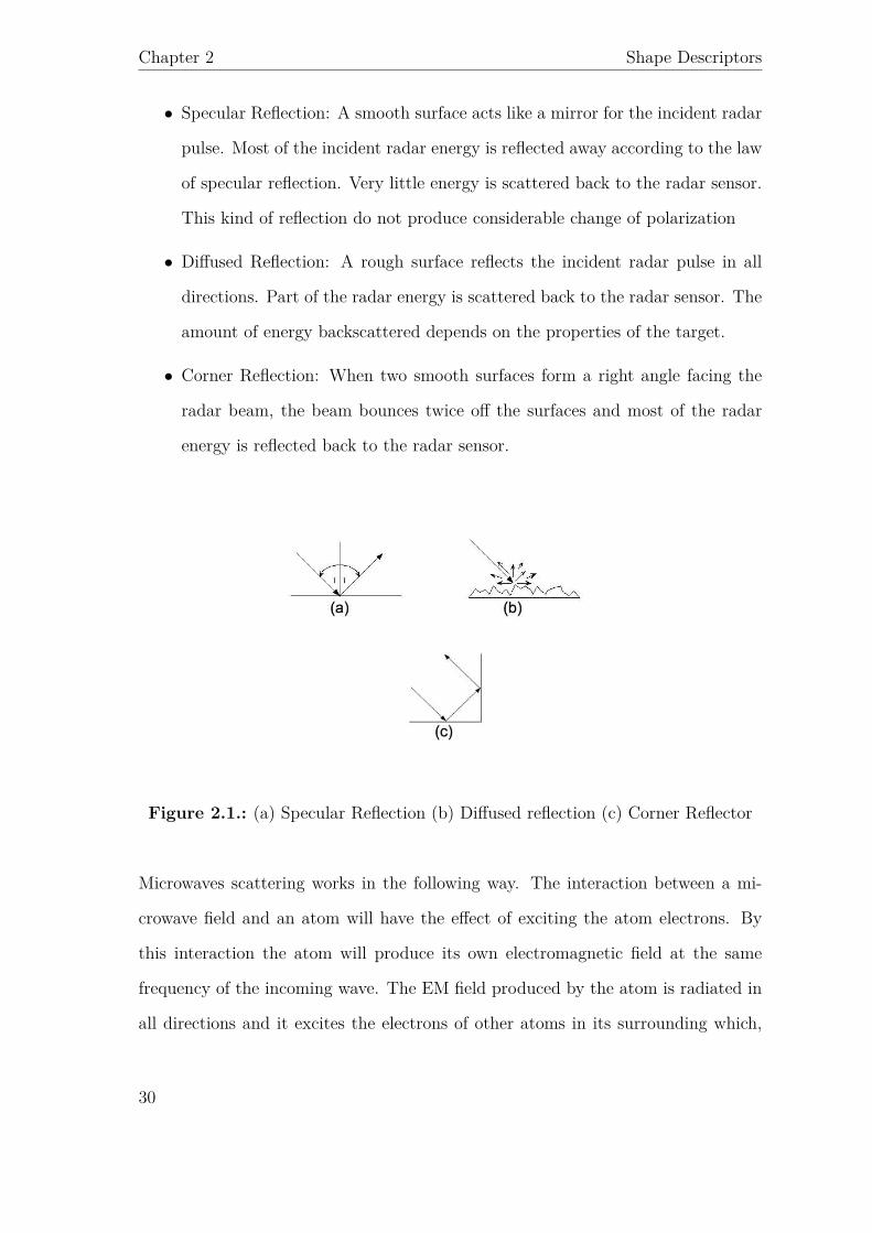
• Specular Reflection: A smooth surface acts like a mirror for the incident radar
pulse. Most of the incident radar energy is reflected away according to the law
of specular reflection. Very little energy is scattered back to the radar sensor.
This kind of reflection do not produce considerable change of polarization
• Diffused Reflection: A rough surface reflects the incident radar pulse in all
directions. Part of the radar energy is scattered back to the radar sensor. The
amount of energy backscattered depends on the properties of the target.
• Corner Reflection: When two smooth surfaces form a right angle facing the
radar beam, the beam bounces twice off the surfaces and most of the radar
energy is reflected back to the radar sensor.
Figure 2.1.: (a) Specular Reflection (b) Diffused reflection (c) Corner Reflector
Microwaves scattering works in the following way. The interaction between a mi-
crowave field and an atom will have the effect of exciting the atom electrons. By
this interaction the atom will produce its own electromagnetic field at the same
frequency of the incoming wave. The EM field produced by the atom is radiated in
all directions and it excites the electrons of other atoms in its surrounding which,
30
2.3 Polarization
in turn, are reradiating the EM field. The process of absorbing and reradiating the
incoming microwaves by the atoms has the effect of scattering the EM field about
the medium. Scattering is very likely to produce changes in the polarization of the
radiated wave by the radar depending on the material and shape of the object.
From the above considerations it is possible to infer that each object interacts with
the radiated electromagnetic field in its own peculiar way due to its specific material
and shape. This interaction can cause a change in the polarization of the wave
transmitted by the radar.
Typical objects employed in CWD have complex shapes and a priori knowledge of
their specific interaction with the electromagnetic field radiated by the antenna is
not known but general considerations can be done. In particular, diffraction refers
to various phenomena which occur when a wave encounters an obstacle that may
induce a strong polarization change in the radiated field. What is known is that
objects employed in CWD present many edges which can cause diffraction thus
polarization changes. By focusing on this very general consideration the goal is
to find a mathematical quantity (i.e. a shape descriptor) able to describe objects
by highlighting the polarization changes from the rest of the image due to edge
interaction.
A new shape descriptor called Polarization Angle which exploits polarimetric prop-
erties of the image will be introduced in the next section.
2.3.1. PCA and Polarization Angle
Let us define xhh and xvv as the pixel intensity which are normalized between 0 and
1 received by the radar when it is respectively radiating and receiving in horizontal
31
Chapter 2 Shape Descriptors
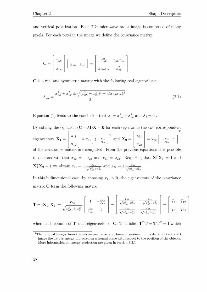
and vertical polarization. Each 2D1 microwave radar image is composed of many
pixels. For each pixel in the image we define the covariance matrix:
C =
xhh
xvv
[xhh xvv
]=
x2hh xhhxvv
xhhxvv x2vv
C is a real and symmetric matrix with the following real eigenvalues:
λ1,2 =x2
hh + x2vv ±
√(x2
hh − x2vv)2 + 4(xhhxvv)2
2(2.1)
Equation (1) leads to the conclusion that λ1 = x2hh + x2
vv and λ2 = 0 .
By solving the equation (C − λI)X = 0 for each eigenvalue the two correspondent
eigenvectors X1 =
x11
x12
= x11
[1 xvv
xhh
]Tand X2 =
x21
x22
= x22
[− xvv
xhh1
]T
of the covariance matrix are computed. From the previous equations it is possible
to demonstrate that x12 = −x21 and x11 = x22. Requiring that XT1 X1 = 1 and
XT2 X2 = 1 we obtain x11 = ± xhh√
x2hh
+x2vv
and x22 = ± xhh√x2
hh+x2
vv
.
In this bidimensional case, by choosing x11 > 0, the eigenvectors of the covariance
matrix C form the following matrix:
T = [X1, X2] = xhh√x2
hh + x2vv
1 − xvv
xhh
xvv
xhh1
=
xhh√
x2hh
+x2vv
− xvv√x2
hh+x2
vv
xvv√x2
hh+x2
vv
xhh√x2
hh+x2
vv
=
T11 T12
T21 T22
where each column of T is an eigenvector of C. T satisfies TT T = TTT = I which
1The original images from the microwave radar are three-dimensional. In order to obtain a 2Dimage the data is energy projected on a frontal plane with respect to the position of the objects.More information on energy projection are given in section 3.2.1
32
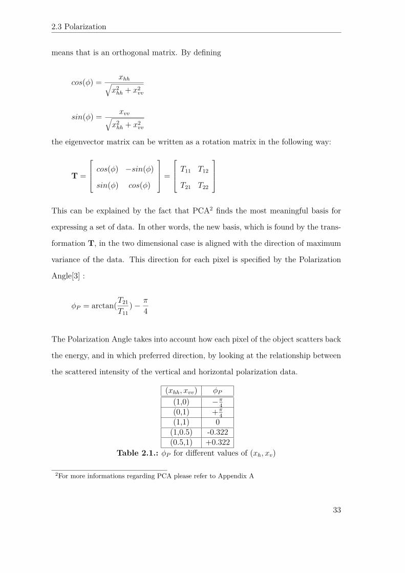
2.3 Polarization
means that is an orthogonal matrix. By defining
cos(ϕ) = xhh√x2
hh + x2vv
sin(ϕ) = xvv√x2
hh + x2vv
the eigenvector matrix can be written as a rotation matrix in the following way:
T =
cos(ϕ) −sin(ϕ)
sin(ϕ) cos(ϕ)
=
T11 T12
T21 T22
This can be explained by the fact that PCA2 finds the most meaningful basis for
expressing a set of data. In other words, the new basis, which is found by the trans-
formation T, in the two dimensional case is aligned with the direction of maximum
variance of the data. This direction for each pixel is specified by the Polarization
Angle[3] :
ϕP = arctan(T21
T11) − π
4
The Polarization Angle takes into account how each pixel of the object scatters back
the energy, and in which preferred direction, by looking at the relationship between
the scattered intensity of the vertical and horizontal polarization data.
(xhh, xvv) ϕP
(1,0) −π4
(0,1) +π4
(1,1) 0(1,0.5) -0.322(0.5,1) +0.322
Table 2.1.: ϕP for different values of (xh, xv)
2For more informations regarding PCA please refer to Appendix A
33

Chapter 2 Shape Descriptors
A SAR measurement of five objects in the free space has been carried out in order to
perform a polarization study on the interaction between the EM field and the objects
employed in CWD. Also, the measurements are needed to validate Polarization
Angle as a shape descriptor. The free space has been simulated by positioning a
foam panel ,which appears transparent to microwaves, behind the objects. As shown
in Figure 2.2 the set of five objects consisted in:
• A: Ceramic knife
• B: Tester which has the shape and material of a mobile phone
• C: Metallic gun
• D: Bottle of water
• E: Pair of keys
The radar first scanned the target area and received the data in horizontal polar-
ization. Afterwards, it scanned and received the data of the same scene in vertical
polarization. The resulting two microwave images are shown in Figure 2.3.
34

2.3 Polarization
The two sets of data (i.e. HH and VV) are then combined together by computing
the Polarization Angle which is shown in Figure 2.4. According to Figure 2.4, all
the objects assume an average ϕP value equal to -0.7 while their edges present an
opposite behavior assuming on average a Polarization Angle value of 0.7.
Figure 2.2.: Measuring scenario for experiment 1
According to the above considerations, this first experiment is showing that the
edges of the objects are causing diffraction phenomena which are inducing an alter-
ation in the value of the Polarization Angle. This confirms the initial hypothesis
of polarization changes due to edge diffraction formulated at the end of section 2.3.
Moreover, the background assumes Polarization Angle values between -0.4 and 0.4
allowing to clearly distinguish between background, objects and their edges.
35

Chapter 2 Shape Descriptors
Figure 2.3.: (a) VV image (b) HH image of the five objects in free space
36

2.3 Polarization
Figure 2.4.: Polarization Angle for the first experiment
A second experiment has been performed by measuring the reflections from a gun
and a ceramic knife. In this testing scenario the objects are positioned on a metal
plate. The goal of this experiment is to study the polarization phenomena occur-
ing due to the interaction between the objects and the metal plate. According to
Figure 2.5(c) the objects, their edges and the background show different Polariza-
tion Angle values among each other. In particular from Figure 2.5 it is possible to
notice how the trigger and the handle of the gun are causing a polarization shift
due to their sharp edges. The values assumed by objects, their edges and by the
37

Chapter 2 Shape Descriptors
background in the two experiments are shown in Table 2.2. By looking at the table,
it is possible to state that edges cause polarization shift which is mathematically
interpreted as a shift in the value of the Polarization Angle.
Figure 2.5.: (a) VV data (b) HH data (c) Polarization Angle for the secondexperiment
Feature (First Experiment) average ϕP
Objects -0.7Edges 0.7
Background (Foam) 0
Feature (Second Experiment) average ϕP
Objects 0.5Edges -0.3
Background (Metal) 0.7Table 2.2.: Values of the Polarization Angle for the two experiments
38
2.3 Polarization
To further investigate polarimetric properties of microwave radar images, the upper
chest and head of a mannequin have been scanned by a SAR polarimetric radar.
The idea behind this third experiment is to verify whether the shape and material
of the mannequin induce polarization changes. As it possible to see in Figure 2.6
the mannequin head and upper chest present negative values of the Polarization
Angle while the edges between the mannequin and the background cause a positive
shift of ϕP . It is important to notice that a shift from negative to positive of the
Polarization Angle value can be also found in the eye region due to a corner reflector
effect caused by the indentation of that particular area of the body. According to
the last experiment, it is possible to deduce that, since the Polarization Angle value
across the mannequin is approximately uniform, if an object is placed on the body
of the mannequin there must be a shift in the Polarization Angle. This change in
the Polarization Angle value is likely to happen at the mannequin-object separation
(i.e. edges).
39

Chapter 2 Shape Descriptors
Figure 2.6.: (a) VV data (b) HH data (c) Polarization Angle for experiment 3
The new shape descriptor called Polarization Angle, which has been described in
this section, exploits the polarimetric properties of the image to obtain meaningful
information regarding edges of objects. The experiments presented in this section
showed that edges induce a shift in the Polarization Angle from negative to positive
values and viceversa. It is important to notice that objects, their edges and the
background assume always different values with respect to each other. Unfortu-
nately, this value is not constant from one measurement to another one (e.g. in the
first experiment the gun assumed an average ϕP of 0.7 while in the second one the
40

2.4 Symmetry and Feature Angle
average was 0.5). This affects the classification capabilities of Polarization Angle
since it is not possible to distinguish between different objects. On the other hand,
by referring to the shape descriptors general characteristics described in section 2.2,
Polarization Angle is achieving invariance to geometrical transformations and ab-
straction from details. Moreover, some part of the body due to their particular
structure are causing a shift in the value of ϕP . This makes difficult to distinguish
between edges of object and edges caused by indentation of the human body.
Another possible approach, which will be developed in the next section, is to exploit
structural informations of the image to obtain a new shape descriptor for concealed
weapon detection called Feature Angle.
2.4. Symmetry and Feature Angle
Symmetry is an important mechanism by which structure of objects are identified by
the human brain. Man-made object which are needed to be detected in concealed
weapon detection can be recognized by the symmetry or partial symmetry that
they exhibit. In particular, symmetry found within man made objects is usually
related to structural stability. Moreover, phase information plays an important role
in human perception of discontinuities (e.g. edges) in images.
By exploiting symmetries is possible to detect concealed object due to the symmetric
structures that they produce. It is important to notice that the human body is also
symmetric therefore it may be not trivial to distinguish between human body sym-
metries and man-made objects ones. From these assumptions, an algorithm called
phase symmetry is employed in order to extract symmetries from an image. Phase
symmetry, which is described in [4], consists of 2D log-Gabor filter banks which are
defined by a gaussian amplitude spectrum multiplied by an angular component.
41

Chapter 2 Shape Descriptors
The transfer function for this type of filter can be expressed as:
Hsym(ω, θ) = exp(−log(ω/ω0)2
2log(k/ω0)2 − (θ − θ0)2
2σ2θ
)
Where ω and ω0 are the frequency range and center frequency. k is a scaling factor,
θ0 the specified filter orientation and σθ the standard deviation for the angular com-
ponent of the gaussian filter. By applying Hsym over multiple scales and orientations
it is possible to obtain a filter bank representation of of the image. This represen-
tation consists of an even er,n(i, j) and odd or,n(i, j) symmetric filter outputs. The
parameter r represents a specific orientation of the filter while n a specific scale. It
is natural to expect points which present high symmetry will be characterized by
high magnitudes in the even symmetric filter and by low magnitudes in the odd
symmetry filter output. Phase Symmetry at the spatial coordinates of the image
(i, j) is defined as:
S(i, j) = max
{∑r,n (|er,n(i, j)| − |or,n(i, j)| − T )∑
r,n Ar,n(i, j) + ε, 0
}
with:
Ar,n(i, j) =√
e2r,n(i, j) + o2
r,n(i, j)
T represents a noise compensation term and ϵ avoids instabilities by zero division
when the signal is uniform and no filter response is obtained. It is important to
notice that S(i, j) is always normalized between 0 and 1. Before applying phase
symmetry the images are preprocessed by applying a Laplacian filter in order to
enhance edges[5].
42
2.4 Symmetry and Feature Angle
Another important property of phase symmetry is its ability to extract symmetry
features of objects under the presence of noise. The syntethic experiment described
in [1] shows how phase symmetry is able to extract the symmetry axis of two objects
under the presence of gaussian noise conditions in a more efficient way compared to
a canny edge detector. The ability to perform under noisy conditions it is a very
desiderable quality since microwave images ,which are employed in this thesis for
concealed weapon detection, are substantially affected by noise.
After applying the phase symmetry algorithm to the horizontal and vertical polar-
ization data the two images are combined together by selecting the maximum for
each pixel by comparing the two polarization images. Let us define Sm(i, j) as the
merged image. Then we can define the feature angle as ϕF = arctan (Sm(i, j)) − π4
. Feature Angle is a shape descriptor which expresses the predominant geometric
orientation of an object or of parts of the human body.
The results of applying phase symmetry to experiment 1 of subsection 2.3.1 are
shown in Figure 2.7. By comparing Figure 2.7(c) and Figure 2.3 it is possible to
notice how phase symmetry is higlighting the structural information of the objects
making them easier to be recognized with respect to the unprocessed microwave
image of them.
To further explore symmetry properties, the phase symmetry algorithm has been
applied to experiment 3 of subsection 2.3.1 which consisted in a scan of the head
and upper chest of a mannequin. By inspecting Figure 2.8 it is possible to see that
also in this case phase symmetry is highlighting structural information of the image.
From the above described experiments, we can expect that by superimposing an
object on the mannequin this will cause in the area of superimposition an increase
in density and strength of symmetry lines which may indicate the presence of an
object. The goal is to mathematically quantify symmetry in a particular region
43

Chapter 2 Shape Descriptors
Figure 2.7.: (a)HH data (b)VV data (c) merged image for phase symmetry algo-rithm applied to experiment 1
of the image. This can be achieved by performing histogram thresholding ,which
will be described in subsection 2.7.1, of simmetry lines intensity in a portion of the
image.
In this section, it has been shown that it is possible to exploit symmetry to extract
and enhance structural information from the image. An internal shape descrip-
tor ,which expresses the predominant geometric orientation of a feature, has been
defined as Feature Angle. In order to extract the Feature Angle a symmetry ex-
44

2.4 Symmetry and Feature Angle
Figure 2.8.: (a) VV data (b) HH data (c) merged phase symmetry data for exper-iment 3
traction algorithm named Phase Symmetry has been employed. By applying Phase
Symmetry to the horizontal and vertical polarization data we can conclude that
regions where concealed objects are located are likely to present an increase in den-
sity and strength of symmetry lines which can be detected by applying histogram
thresholding described in subsection 2.7.1.
45

Chapter 2 Shape Descriptors
2.5. Depolarization Angle
In order to exploit both physical and structural information, Polarization Angle
ϕP and Feature Angle ϕF , which can be classified respectively as an external and
internal shape descriptors, are combined together to form a new attribute called
Depolarization angle[7] Dp :
Dp(i, j) =
ϕP (i, j)/ϕF (i, j) , ∥ϕF (i, j)∥ ≥ ∥ϕP (i, j)∥
ϕF (i, j)/ϕP (i, j) , ∥ϕF (i, j)∥ < ∥ϕP (i, j)∥(2.2)
It is clear from this definition that ∥Dp∥ < 1 since ϕP and ϕF are both varying
from −π4 to π
4 . If Dp value is equal to 1 this indicates a feature exhibiting maximum
polarization when the front edge3 of the Vivaldi Antenna is parallel to the long axis
of the feature. If Dp equals to -1 this means that the feature is exhibiting maximum
polarization when the front edge of the Vivaldi Antenna is perpendicular to the long
axis of the feature. An example for the latter case is shown in Figure 2.9.
Figure 2.9.: A typical case when Dp = −1. The object is exhibiting its maximumpolarization in the direction orthogonal to its long axis.
3The front edge is considered as the one of the Vivaldi antenna which is the closest in distanceto the mannequin
46

2.5 Depolarization Angle
The result of applying equation (1) to the first experiment of subsection 2.3.1 is
shown in Figure 2.10. Depolarization Angle is enhancing both structural and po-
larimetric properties of the combination of the vertical and horizontal unprocessed
data image (see Figure 2.3). From the line scan of Figure 2.11, which has been ex-
tracted from the central row marked in red in Figure 2.10, it is possible to notice
how edges cause a shift from positive to negative (i.e. the deep negative valley in the
figure is the gun) in the value of the Depolarization Angle. This shifting property of
the Depolarization Angle can be exploited to detect edges of objects. In Figure 2.12
we can see how the mannequin head and upper chest produce a negative Depolar-
ization Angle value while the areas marked as F (head-background separation) and
G (eye indentation) are causing a shift in the value of Dp. Therefore Depolariza-
tion Angle while improving the detection of edges is inheriting the false alarm issue
caused by body indentation of the Polarization Angle described in subsection 2.3.1.
The number of false alarms can be greatly reduced by applying histogram thresh-
olding as explained in subsection 2.7.1. By comparing the two above experiments
we can state that the background and objects always assume a Dp value which is
shifted in sign compared to the edges.
47

Chapter 2 Shape Descriptors
Figure 2.10.: Dp for experiment 1 of subsection 2.3.1
Figure 2.11.: Line scan of Figure 2.10
48
2.5 Depolarization Angle
Figure 2.12.: Depolarization Angle value for mannequin head and upper chest
In this section the polarimetric features introduced in section 2.3 are combined with
the structural features described in section 2.4. The new shape descriptor which
is a combination of Polarization and Feature Angle is called Depolarization Angle.
Depolarization Angle allows to detect edges of objects by looking at its value on the
edges of objects (e.g. background and objects on average assumes a Depolarization
Angle value changed is sign compared to edges). Unfortunately, Depolarization
Angle is inheriting the Polarization Angle issue of false alarms caused by body
indentation. This issue can be solved by applying histogram thresholding as will be
explained in subsection 2.7.1.
The shape descriptor which will be presented in the next section represents a different
approach to shape description for concealed weapon detection compared to the ones
presented in subsection 2.3.1 and section 2.4. The idea in this case is to try to
match an unknown concealed object features set to another set of known features
belonging to different objects which are stored in an object library by using only one
49

Chapter 2 Shape Descriptors
polarization data. If the set of features of the unknown object have a match in the
library then it means that the unknown object can be detected and classified. In
order to do this, a computer vision algorithm named SIFT, which is able to detect
and describe local features in optical images by locating pixel intensity maxima and
minima will be adapted to microwave imaging radar.
2.6. SIFT Descriptors
What usually happens in airport security is that an operator looks at the image
of a person carrying suspicious objects and then attempts to match what he sees
in the image with his personal knowledge of objects. The goal of this section is
to develop a shape descriptor which takes inspiration from human vision and from
the matching process described above. Computer vision is a field that includes
methods for acquiring, processing, analysing, and understanding images and, in
general, high-dimensional data from the real world in order to produce numerical or
symbolic information[8].
Microwave imaging play a key role in detecting object due to the ability of mi-
crowaves to penetrate through clothes. On the other hand, microwave images suffer
a lack of resolution when compared to optical images. A comparison between an
optical and microwave image of a bottle of water is shown in Figure 2.13. Despite
the fact that the resolution of the microwave image is way lower than the optical one,
the main features of the bottle are still recognizable (e.g. position of edges). In par-
ticular the intensity maxima/minima of the bottle image are approximately at the
same position in both images. An example of the preservation of maxima/minima
is point P1 and P2 in Figure 2.13. The comparison between an optical image and
microwave image of a gun (figure Figure 2.14) confirms the fact that the shape is
50

2.6 SIFT Descriptors
preserved and the main features of the objects such as the trigger, the handle and the
barrel are still clearly recognizable. The property of microwave images of preserving
intensity maxima/minima of an image allows to apply computer vision algorithms
originally designed for optical images which exploit gradient detection to compare
and find matches between two images.
Figure 2.13.: (a) Optical and (b) Microwave image of a bottle of water
Figure 2.14.: (a) Optical and (b) Microwave image of a gun
A computer vision algorithm named SIFT has been found suitable for microwave
51

Chapter 2 Shape Descriptors
concealed weapon detection due to its peculiar characteristic. SIFT algorithm was
first introduced by D.Lowe in 1999. This algorithm is widely used and has proven to
be very successful in computer vision to detect and describe local features in optical
images. What makes SIFT so noteworthy is its ability to match features between
two images with invariance to image scaling and rotation and has shown to be robust
with respect to a range of affine distortions, change in 3D viewpoint, addition of
noise and change in illumination[9]. Despite not being computationally fast, SIFT
has the best performance, when compared to similar feature detection methods such
as PCA-SIFT and SURF, in detecting objects when scaling and rotations occurs[10].
In SIFT objects key locations are defined as maxima and minima of the result of
difference of Gaussians functions applied in the scale space to a series of smoothed
and resampled images4. Points with low contrast and edges responses are discarded
due to their instability. Once keypoints have been localized, a dominant orienta-
tion is assigned to each of them and to the neighbour pixel of the keypoint. Each
frame which contains information about a keypoint is characterized by four number
which are (x, y) for the position of the frame in the image, σ which is its scale (i.e.
smoothing scale) and θ which is the orientation. Each SIFT frame is summarized by
a descriptor vector which describes coarsely the appearance of the image patch cor-
responding to the frame. By matching the SIFT descriptor of the unknown object
with the ones stored in the library the algorithm is able to perform image matching
and classify concealed objects.
In Figure 2.15 a SIFT feature matching experiment on microwave images has been
carried out. The experiment consisted in indentifying a gun among five objects
which where the same as experiment 1 of subsection 2.3.1. The matching procedure
for this particular experiment presented many false alarms even though the number
4For more information regarding SIFT please refer to Appendix C
52

2.6 SIFT Descriptors
of correct matching for the gun was superior to the number of false matches with
the other objects. In another experiment a gun was positioned on the body of a
mannequin and SIFT algorithm was applied. The algorithm correctly identified
the gun but there were many false alarms due to indentations of the human body
which looked like objects. To reduce the number of false alarms a combination
of segmentation and histogram thresholding needs to be applied. This two image
processing techniques are described in subsection 2.7.1.
Figure 2.15.: Gradient detection of a gun
The main goal of this section was to find a shape descriptor that allows to perform
microwave radar imaging feature matching between an unknown object and a set of
object stored in a library by using only one polarization data. We have seen how
microwave images differ from optical ones. The lack of resolution of microwave image
do not substantially affect the shape and main features of the objects being imaged.
53

Chapter 2 Shape Descriptors
In particular the property of preserving maxima and minima in an image allows to
apply gradient detection techniques employed for optical images which allow feature
matching. It has been shown in the experiment of Figure 2.15 that a number of
false alarms are generated. To reduce the number of false alarms segmentation and
histogram thresholding of the image are valuable tools which will be described in
section 2.7.
2.7. Shape Descriptors enhancement
In this chapter four new different shape descriptors for microwave radar imaging
concealed weapon detection have been described. These descriptors exploit physical
and structural information of the image in order to detect objects. In particular Po-
larization Angle and Feature Angle have been combined together into Depolarization
Angle in order to combine the polarimetric and structural data provided by the mi-
crowave images. It has been shown in subsection 2.3.1, section 2.4, section 2.5 and
section 2.7 that each descriptor is not completely reliable (i.e. it causes false alarms)
without some sort of enhancement procedure. This section introduces segmentation
and histogram thresholding which are mathematical tools needed in order to en-
hance the detection capabilities of the shape descriptors described in the previous
sections of this chapter.
2.7.1. Segmentation and Histogram Thresholding
Segmentation is the process of partitioning a digital image into multiple segments.
It is useful for image analysis since it divides the image into small portions which
are more meaningful and easier to analyze. It has been discussed in section 2.6
that the detection of a gun by the means of a SIFT descriptor caused many false
54

2.7 Shape Descriptors enhancement
alarms. In order to perform a more accurate detection a prior segmentation of
the image before applying the shape descriptor is necessary. In this thesis the
segmentation is performed by dividing the image in an overlapping primary and
secondary grid as shown in Figure 2.16. The most important factor that affects the
segmentation efficiency is the size of the segments. Segmentation efficiency affects
detection capabilities of a CWD system. In particular the size of the segments have
to be chosen accordingly to the size of the concealed objects that an individual can
carry. If the segments are too small the object may be splitted in two different
segments which will cause a drop in the detection rate. On the other hand, if the
size of the each segment is too large then multiple of objects and too many features
of the human body will end up in the same segments. This second hypothesis is also
likely to decrease the detection rate.
Figure 2.16.: Typical example of primary and secondary grid. The yellow box isan example of a secondary grid segment while the green one of a primary one.
After segmentation, histogram thresholding can be applied to obtain meaningful in-
formation regarding the content of a particular segment. An histogram is a graphical
55

Chapter 2 Shape Descriptors
representation of the distribution of a particular set of data. For Symmetry described
in section 2.4 the data in which we are interested is the intensity of symmetry lines
while for SIFT descriptor of section 2.6 is the pixels intensity. To give a first exam-
ple on histogram thresholding, many segments for which the SIFT descriptor finds
a matching unfortunately do not contain an object but just random background.
Histogram thresholding allow us to discard those background segments which are
causing false alarms. In the example of Figure 2.17 it is possible to see how a seg-
ment containing a concealed (upper part of the image) shows an intensity histogram
richer in high intensity values when compared to a background segment. Therefore
we can discriminate between segments containing a suspicious object or background
by looking at the high intensity values bins of an histogram. The same process can
Shape Descriptor Flaws Solution
Depolarization Angle False alarms (body indentations) Histogram thresholding (Simmetry lines intensity)
SIFT Descriptors False alarms (body indentations) Segmentation and histogram thresholding (Pixel intensity)
Table 2.3.: Shape Descriptors flaws and solution
be repeated for the symmetry lines described in section 2.4. In this case a portion of
the merged symmetry image Sm is extracted and histogram thresholding is applied
to that particular portion looking for intensity of symmetry lines greater than a
certain threshold. The values assumed by the thresholds and how segmentation and
histogram considerations are implemented will be described in chapter 4 and 5. A
summary of the shape descriptors flaws and solution is shown in Table 2.3.
56

2.8 Conclusions
Figure 2.17.: Histogram thresholding example
2.8. Conclusions
This chapter was dedicated to shape descriptors. As said in section 2.2, shape
descriptors are mathematical functions which are applied to an image and produce
numerical values which are representative of a particular characteristic of that image.
These numerical values can then be processed in order to provide some information
about the objects which are concealed.
For the purpose of this thesis, four new shape descriptors for microwave radar imag-
ing of CWD has been introduced. In section 2.3 physical phenomena such as re-
flection, diffraction and scattering which affect the polarization of a microwave have
been studied in order to obtain meaningful information regarding concealed objects.
The result of this physical analysis is an external shape descriptor called Polar-
57

Chapter 2 Shape Descriptors
ization Angle described in subsection 2.3.1 which has been found, by performing a
series of experiments, to be able to detect edges of concealed objects by exploiting
polarimetric properties of the combined vertical and horizontal polarization data.
Furthermore, in section 2.4 an analysis on structural and symmetry information
contained in a microwave radar image lead to the formulation of an internal shape
descriptor named Feature Angle. Polarization and Feature Angle are then combined
together in section 2.5. The result of this combination is shape descriptor named
Depolarization Angle which can be exploited to detect edge of objects in a more
reliable way compared to Polarization Angle since it contains also structural infor-
mation of the image. As explained in section 2.5 indentation of the human body
are causing a shift in the Depolarization Angle which is equal to the one produced
by edges of actual objects. In order to discriminate between actual objects and in-
dentation of the human body histogram thresholding is required which is explained
in subsection 2.7.1.
In section 2.6 a shape descriptor inspired by human vision and brain’s associative
properties is introduced. The main idea was to try to match an unknown concealed
object features set to another set of known features belonging to different objects
which are stored in an object library by using only one polarization data. After a
comparison study between optical and microwave images it has been found that they
share in common the same position of pixel intensity maxima and minima in the
image despite their consistent difference in resolution (i.e. microwave images have
a poorer resolution compared to optical ones). Therefore it appeared as a feasible
approach to apply a computer vision algorithm employed on optical images to the
field of microwave imaging. The algorithm which resulted to be the more suitable
to be applied to microwave image was SIFT. The experiments in section 2.6 showed
that the algorithm was able to correctly match between an concealed object in a
58

2.8 Conclusions
scene with the same one in the library. Unfortunately, many false alarms where
present due to specific parts of the human body which where interpreted as objects.
Segmentation and histogram thresholding are two mathematical tools described in
section 2.6 which can be employed in this particular case to reduce the false alarm
rate.
The shape descriptors which have been analyzed and synthesized in this chapter (e.g.
Depolarization Angle and SIFT descriptors) along with the enhancing techniques
presented in section 2.7 will be employed in the following chapters to design two
novel robust microwave radar imaging concealed weapon detection algorithms.
59


Bibliography
[1] ”Digital Image Processing Algorithms and Applications”, Ioannis Pitas, Wiley-
Interscience; 1 edition (February 4, 2000)
[2] ”Physics of Waves”, William C. Elmore, Dover Publications (October 1, 1985)
[3] P. N. Mahob and J. P. Castagna, “Avo hodograms and polarization attributes”,
Leading Edge, vol. 21, no. 1, pp. 18-27, Jan. 2002
[4] Symmetry and Asymmetry from Local Phase, P.Kovesi, Tenth Australian Joint
Converence on Artificial Intelligence, 1997
[5] R.C. Gonzalez and R. E. Woods, Digital Image Processing, 3rd edition, Nj:
Prentice - Hall, 2002.
[6] Böniger, U.; Tronicke, J.; , "Symmetry based 3D GPR feature enhancement
and extraction," Ground Penetrating Radar (GPR), 2010 13th International
Conference on , pp.1-5, 21-25 June 2010 doi: 10.1109/ICGPR.2010.5550155
[7] Boniger, U.; Tronicke, J.; , "Subsurface Utility Extraction and Characteriza-
tion: Combining GPR Symmetry and Polarization Attributes," Geoscience and
Remote Sensing, IEEE Transactions on , vol.50, no.3, pp.736-746, March 2012
doi: 10.1109/TGRS.2011.2163413
[8] Tim Morris (2004). Computer Vision and Image Processing. Palgrave Macmil-
lan
61

Chapter 2 Bibliography
[9] Lowe, David G. (1999). "Object recognition from local scale-invariant fea-
tures". Proceedings of the International Conference on Computer Vision. 2.
pp. 11501157.
[10] A Comparison of SIFT, PCA-SIFT and SURF”, L.Juan, O.Gwon, International
Journal of Image Processing (IJIP), Vol. 3, No. 4. (2009), pp. 143-152
62

3. Depolarization Analysis
“Symmetria est in rebus”
Aristotle
3.1. Overview
The main objective of this thesis report is to develop a novel CWD method which
is able to detect concealed objects carried by an individual in a low contrast envi-
ronment such as the microwave radar imaging one. A novel CWD method called
Depolarization Analysis is presented in this chapter. Depolarization Angle, which
has been described in section 2.5, represents the core of the hereby presented method.
Therefore the presented algorithm exploits and combines physical and geometric fea-
tures of the target which are provided by a dual polarization SAR to achieve object
detection. The method is divided in two processing blocks which are named respec-
tively Depolarization unit and Detection unit. In section 3.2 the processing blocks
which form the Depolarization unit shown in Figure 3.1 are described in details.
This unit has the main task of computing the Depolarization Angle. It has been
discussed in section 1.5 how the Depolarization Angle is affected by false alarms and
how it is possible to reduce them by applying histogram thresholding. In section 3.3
the processing blocks enclosed in the detection unit needed to reduce the false alarm
63

Chapter 3 Depolarization Analysis
rate are discussed. Conclusions are presented in section 3.4.
Figure 3.1.: Block diagram of the algorithm for Depolarization analysis
3.2. Depolarization unit
Figure 3.2.: Depolarization unit block diagram
The Depolarization unit is the first building block of the algorithm and its final
purpose is to compute the Depolarization Angle. It can be divided in two parts.
After an initial energy projection described in subsection 3.2.1 for both polarization
data which transforms the 3D volumetric scalar data into a 2D image, there are
two processing paths for each polarization image[1, 2]. One path is dedicated to
compute the Feature Angle by a cascade of image processing filters (i.e. Laplacian,
Prewitt and Phase symmetry) described in subsection 3.2.2 and subsection 3.2.3.
The other processing path described in subsection 3.2.4 computes the Polarization
Angle by performing PCA. The Polarization and Feature Angles are then combined
together into a new attribute called Depolarization Angle which is described in
64

3.2 Depolarization unit
subsection 3.2.5. Depolarization Angle is then sent to the Detection unit for further
processing.
3.2.1. Energy Projection
Figure 3.3.: Grid arrangement
Let us define I ϵCP×Q×R as the complex matrix containing the 3D volumetric scalar
data of the mannequin being measured by the radar1 . Accordingly to the grid
arrangement of Figure 3.3 we can define each point in I as I(xp, yq, zr) with p =
1, 2, ..P , q = 1, 2, ..., Q and r = 1, 2, ..., R . Being the axis of the mannequin image
oriented as in Figure 3.4, the matrix I is energy projected along the y dimension in
the x-z plane by performing I(xp, zr) = ∑Qq=1 ∥I(xp, yq, zr)∥2 ∀ p, r . There are two
reasons behind the choice of projecting the image in a 2D plane. The first one is
that well known 2D image processing algorithms can be applied. The second one
is related to the choice of the x-z plane as projection plane. This plane, according
to the axis orientation in Figure 3.4 , is of specular simmetry for the mannequin
body which allows to make symmetry considerations. Moreover, the approach of
applying image processing algorithms to several (i.e. the number of slices is Q) x-z
plane energy slices proved to be unsuccessful due to the fact that each object, due1For more informations regarding the measurement setup please refer to appendix B
65

Chapter 3 Depolarization Analysis
to its three dimensional nature, is contained in many slices and phase symmetry
algorithm requires the entire ’energy information’ of the concealed object to work.
Figure 3.4.: (a) A typical 3D volumetric scalar measurement of a mannequin.Radar is transmitting and receiving in vertical polarization (b) Energy projec-tion in the x-z plane
66

3.2 Depolarization unit
Figure 3.5.: (a) 3D volumetric scalar measurement of five objects in the free space.Radar is transmitting and receiving in vertical polarization. (b) Energy projectionin the x-z plane 67

Chapter 3 Depolarization Analysis
3.2.2. Image filtering
Let us define IH(xp, zr) as the image matrix containing the projected horizontal
polarization data and as IV (xp, zr) the one containing the vertical polarization one.
In order to enhance edges of the image, both components are convolved with a
Laplacian 3x3 filter of the type ∇2 = 4α+1
α4
1−α4
α4
1−α4 −1 1−α
4
α4
1−α4
α4
. The value of α,
which controls the shape of the Laplacian, has been set to 0.9 since it offered the best
tradeoff between edge enhancing and noise. To further enhance edges depending on
the polarization the Laplacian filter is combined with a Prewitt operator sensitive to
the horizontal direction when it is applied to IH(xp, zr) and with a Prewitt operator
sensitive to the vertical one when it is being applied to IV (xp, zr).
3.2.3. Phase Symmetry and Feature Angle
After the image processing steps described in subsection 3.2.2, the horizontal filtered
image I(H)f (xp, zr) and vertical one I
(V )f (xp, zr) are then processed with a Phase
Symmetry filter Hsym with the following parameters :
• Number of wavelets scales = 5
• Number of orientations = 6
• Wavelenght of smallest scale filter = 12
• Scaling factor between successive filters = 2.1
• ϵ = 10−4
• T (i.e. noise compensation term) is computed by using the median of the
smallest scale filter response. This is due to the fact that the smallest scale
68

3.2 Depolarization unit
filters spend most of their time responding to noise, and only occasionally
responding to features.
This values have been chosen since they offer the best tradeoff between noise reduc-
tion and symmetry enhancement. An example is shown in Figure 3.6.
Figure 3.6.: (a) Wavelenght of smallest scale filter = 3 (b) Wavelenght of smallestscale filter = 12 . In both cases the number of wavelets scales is equal to 5 andthe number of orientations is equal to 6
Let us denote as SH(xp, zr) the output of the Phase Symmetry filter when applied to
I(H)f (xp, zr) and as SV (xp, zr) when applied to I
(V )f (xp, zr). Subsequently, SH(xp, zr)
and SV (xp, zr) are then merged by the following rule:
Sm(xq, zr) =
SH(xq, zr) , SH(xq, zr) ≥ SV (xq, zr)
SV (xq, zr) , SH(xq, zr) < SV (xq, zr)
69
Chapter 3 Depolarization Analysis
The reason why SV and SH are merged is to highlight the objects on the man-
nequin and to ensure maximum information from both components. This is based
on the assumption that concealed objects should present many symmetry lines in
many directions compared to the human body since they can be considered as a
combination of many geometric shapes (e.g. a gun can be considered approximately
as a combination of two rectangles). As we can see in Figure 3.7(c) the marked
areas are rich of symmetry lines and may underline the presence of an object. Un-
fortunately not only objects, marked in red, are detected but also human body
symmetries which are marked in yellow. The feature angle ϕF (xq, zr) is defined
as ϕF (xq, zr) = arctan (Sm(xq, zr)) − π4 . In a way, the feature angle expresses the
predominant geometric orientation of an object or of parts of the human body.
70
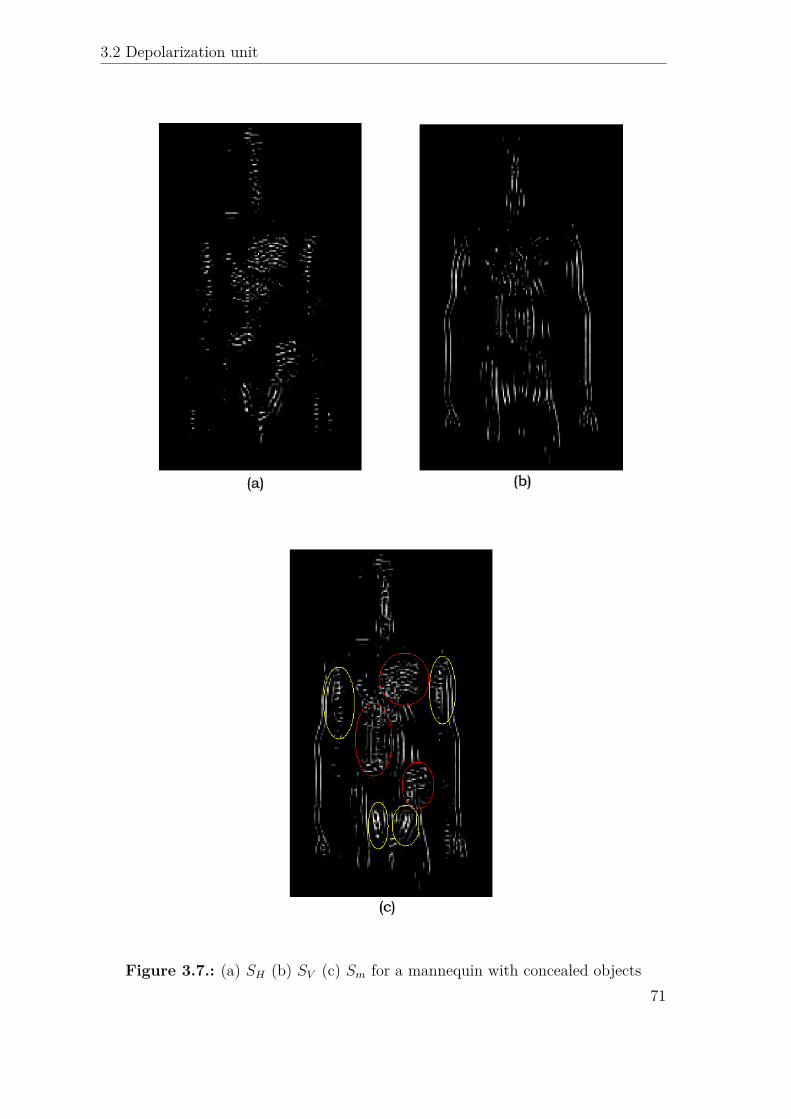
3.2 Depolarization unit
Figure 3.7.: (a) SH (b) SV (c) Sm for a mannequin with concealed objects71

Chapter 3 Depolarization Analysis
3.2.4. PCA and Polarization Angle
The Polarization Angle, which has been described in section 2.3.1, quantifies the
scattering properties of an object and the dominant polarization characteristic from
a dual polarization SAR. Polarization Angle is computed by the algorithm by per-
forming PCA as:
ϕP = arctan(T21
T11) − π
4
Where T21 and T11 are the elements of one of the two eigenvectors of the pixel
intensity covariance matrix. As it is possible to see in Figure 3.8 and according to
the considerations of section 2.3.1 edges of the objects which are marked in red, and
edges of the mannequin which are marked in blue, present Polarization Angle values
which are switched in sign compared to the rest of the image. This is caused by
diffraction phenomena due to the interaction of the microwave field with the edges.
In order to extract edges from the image, the Polarization Angle and the Feature
Angle respectively quantifying polarimetric and structural data of the image are
then combined togheter to form the Depolarization Angle.
72

3.2 Depolarization unit
Figure 3.8.: Polarization angle for a mannequin carrying concealed objects
3.2.5. Depolarization Angle
Depolarization Angle, as explained in section 1.5, is a combination of the Polariza-
tion and Feature Angle and it is computed by performing:
Dp(i, j) =
ϕP (i, j)/ϕF (i, j) , ∥ϕF (i, j)∥ ≥ ∥ϕP (i, j)∥
ϕF (i, j)/ϕP (i, j) , ∥ϕF (i, j)∥ < ∥ϕP (i, j)∥
Where (i,j) are the coordinates of the pixels of the image. As it possible to see in
Figure 3.9 and, as explained in the previous chapter, Depolarization Angle is able to
highlight the edges of objects. In particular by looking at the line scan of Figure 3.10,
73

Chapter 3 Depolarization Analysis
the edges of the bottle, which is located on the upper right part of the chest of the
mannequin, present an higher value of the Depolarization Angle compared to the rest
of the image. Unfortunately, not only the edge of the objects but also indentations
of the human body, produce a shift in the value of the Depolarization Angle. An
example of this phenomenon is shown in the line scan of Figure 3.11. From this
figure we can see how a left arm indentation causes a shift in the Depolarization
Angle value from negative to positive which is greater than the one caused by the cap
of the bottle but still significantly lower compared to the edge of the gun. In order to
separate the Depolarization Angle shifts caused by indentation of the human body
from the one of actual object histogram tresholding is required. This procedure will
be described in the following section.
Figure 3.9.: Depolarization angle for a mannequin carrying concealed objects
74

3.2 Depolarization unit
Figure 3.10.: Scan of row 137 of Figure 3.9
Figure 3.11.: Scan of row 93 of Figure 3.9
75

Chapter 3 Depolarization Analysis
3.3. Detection unit
Once Depolarization angle has been computed, it has to be exploited in order to
highlight the objects on the mannequin. The Detection unit is the part of algorithm
in charge of doing that. As shown in Figure 3.12 , the Detection unit is divided
in four parts. The Threshold selector unit described in subsection 3.3.1 works on
the assumption that interesting objects on the mannequin have similar Depolar-
ization Angle values. After a threshold selection, symmetry considerations within
the image are taken into account by the Symmetry Verification, Inset Inspection
and Specular Symmetry verification units described respectively in subsection 3.3.2,
subsection 3.3.3 and subsection 3.3.4 in order to reduce the number of false detec-
tions before output.
Figure 3.12.: Detection unit block diagram
3.3.1. Threshold selector
We have seen that Depolarization Angle assumes particular values on the edges of
objects of interest. Objects employed in concealed weapon detection always present
a complex scattering response which is difficult to interpret as a consequence of their
complex geometrical structures. A possible solution to interpretate the scattering
response is to decompose the object under analysis into a combination of simpler
shapes for which the response is known. In the literature, no theorical studies have
been performed on the scattering response of objects which are typically employed
in concealed weapon detection and their depolarization properties. Due to the above
considerations, an experimental approach to extract meaningful range of values of
76

3.3 Detection unit
the Depolarization Angle is employed in this thesis. Let us define the average value
of the Depolarization Angle of the image as µ. It has been experimentally verified
in this thesis that by applying the following adaptive thresholds, which depends on
the value of µ, we can extract concealed objects edges from the image:
D(xq, zr) =
1 if Dp(xq, zr) ≥ 0.8 and µ < 0
0 if Dp(xq, zr) < 0.8 and µ < 0
D(xq, zr) =
1 if Dp(xq, zr) ≤ −0.8 and µ > 0
0 if Dp(xq, zr) > −0.8 and µ > 0
Where D(xq, zr) is defined as the detection image. In other words, concealed objects
due to their sharper edges compared to the background are producing a shift in
Depolarization Anglue for which |Dp| > 0.8.
3.3.2. Symmetry Verification
The threshold selection procedure described in subsection 3.3.1 is not sufficient to
guarantee that all the points with a Depolarization angle value exceeding the thresh-
old of 0.8 are actual objects due to human body indentations. According to section
2.4, Phase Symmetry is capable of revealing structural information of the image by
highlighting symmetry lines which are typical of human made objects.
Therefore it appears natural to do a pixel by pixel comparison of Sm(xq, zr) and
D(xq, zr) by applying the following rule:
D(xq, zr) = 1 if Sm(xq, zr) = 1
77

Chapter 3 Depolarization Analysis
Therefore if symmetry lines, which can underline the presence of an object, are
present in a particular region of the image it means that the detected points, in the
same region, via Depolarization Angle thresholding (i.e. D(xq, zr) ) are potentially
correct otherwise they are discarded.
3.3.3. Inset Verification
After Symmetry verification a further inspection is required to reduce the false
alarm points in D(xq, zr). The detected points in D(xq, zr) which are spatially close
in the image are merged together by perfoming morphological dilation with a disk
of radius 4. Dilation is needed in order to compute the centroid for each of these
agglomerate of detected points. For each centroid, an inset is built around it which
it has the size of 10 pixels by 10 pixels. The size of the inset has been chosen in order
to cover an image area consistent with the average size of the objects involved in
concealed weapon detection. This set of insets (i.e. one for each centroid) are drawn
on the image Sm(xq, zr). For each inset a Contrast Limited Adaptative Histogram
Equalization[4] is performed in order to improve the local contrast of the image
without over amplifying noise. After computing CLAHE each inset histogram2
is inspected in order to look for symmetry lines with values greater of a certain
threshold (i.e. the ’stronger’ is the line the more likely is that is belonging to an
object). The threshold has been experimentally found to be effective when it is
set to 0.8. Furthermore the presence of a greater density of symmetry lines in an
inset may also indicate the presence of an object. An example of this procedure is
shown in Figure 3.13 and Figure 3.14. In this example it is possible to see how the
histogram of inset 2 (Figure 3.14(b) ) which represents a gun contains symmetry
line values greater than 0.8 while inset 1 (Figure 3.14(b) ) that represents part
2For more information regarding histogram thresholding please refer to section 2.7.1
78

3.3 Detection unit
of the background only contains simmetry lines intensity values ranging from 0
to 0.6. The two insets are referring to Figure 3.13. Candidate points (i.e. the
remaining centroids which are not discarded) are then sent to the specular symmetry
verification unit for further investigations.
Figure 3.13.: Inset Verification procedure. (a) Detected points over DepolarizationAngle (b) Dilation and centroids positions (c) Inset for each centroid over Sm
Figure 3.14.: (a) Histogram for inset 1 for Figure 3.13 (b) Histogram for inset 2for Figure 3.13
79

Chapter 3 Depolarization Analysis
3.3.4. Specular Symmetry Verification
This final stage before final output has the task to eliminate points which present
a specular symmetry with respect to the center of the image (i.e. the mannequin
is centered). This procedure is based on the assumption that in most cases only
detection points caused by the human body and not by the objects present this type
of symmetry. Therefore two points (x1, y1) and (x2, y2) are discarded if
d1 ∼= d2 and y1 ∼= y2
with d1 =√
(x1)2 + (y1)2 and d2 =√
(x2)2 + (y2)2.
Figure 3.15.: Specular symmetry setup
3.4. Conclusions
The main idea behind this work is to combine the physical and simmetry informa-
tions of the target (i.e. a mannequin with concealed weapons on its body) which
are provided by a dual polarization imaging SAR. The physical informations are ex-
80

3.4 Conclusions
tracted from the polarization-dependent scattering properties of the target while the
simmetry properties are extracted from the structural information provided by both
VV and HH data sets. In order to extract the physical information, a Polarization
Angle is defined which is computed by performing Principal Component Analysis.
To extract the structural and symmetry properties under the form of an attribute
called Feature Angle, an imaging processing filter known as Phase Symmetry is em-
ployed. The Polarization Angle and Feature Angle are then combined together in
a new attribute called Depolarization Angle. By exploiting the properties of the
Depolarization Angle it is possible to detect objects.
In order to get meaningful information from the Depolarization Angle and to discard
false alarm points additional symmetry considerations and thresholding procedures
are required. This tasks are performed by the processing block named as Detection
unit in Figure 3.1. It has been experimentally verified that a particular range of
values (i.e. |Dp| > 0.8) of the Depolarization Angle can be considered as a robust
descriptor for the detection of objects. Moreover, a key role for successful detec-
tion is played by the thresholds described in subsection 3.3.1 and in subsection 3.3.3
which allow the method to locate the objects by lowering the false alarm rate. It
has be seen in subsection 3.3.2 and subsection 3.3.3 that symmetry analysis of the
image plays a major role in identifying the objects and discarding false alarm points
before output. Practical results of this algorithm will be presented in chapter 5.
81


Bibliography
[1] Boniger, U.; Tronicke, J.; , "Subsurface Utility Extraction and Characteriza-
tion: Combining GPR Symmetry and Polarization Attributes," Geoscience and
Remote Sensing, IEEE Transactions on , vol.50, no.3, pp.736-746, March 2012
[2] Böniger, U.; Tronicke, J.; , "Symmetry based 3D GPR feature enhancement and
extraction," Ground Penetrating Radar (GPR), 2010 13th International Confer-
ence on , pp.1-5, 21-25 June 2010 doi: 10.1109/ICGPR.2010.5550155
[3] Kovesi, P.: Symmetry and asymmetry from local phase. In: Proc. Tenth Aus-
tralian Joint Converence on Articial Intelligence (1997), pp. 24.
[4] Rajesh Garg, Bhawna Mittal, Sheetal Garg, “Histogram Equalization Techniques
For Image Enhancement”, IJECT Vol. 2, Issue 1, March 2011
83


4. SIFT Analysis
“Symmetria est ante res”
Plato
4.1. Overview
After Depolarization Analysis which has been described in chapter 2, this chapter
of the thesis is dedicated to the development of an another novel concealed weapon
detection method called SIFT Analysis. Depolarization Analysis exploited physical
and geometric information of the image provided by a dual polarization SAR radar
in order to detect objects. The fact that Depolarization algorithm needs a dual
polarization radar to work makes it more expensive and technically complex from
the point of view of the antenna than a single polarization one. In this chapter, a
novel concealed weapon detection algorithm that uses only the vertical polarization
data to detect concealed objects will be presented.
The main idea behind the algorithm, as explain in section 2.6, is to compare the
microwave image of a specific object, which is stored in an item library, with the
image of the mannequin carrying concealed harmful and harmless objects and look
for correlations.
A block diagram of the proposed algorithm is shown in Figure 4.1 and in figure
85

Chapter 4 SIFT Analysis
Figure 4.2 . This chapter is divided in the following way. First energy projection and
image segmentation will be described in section 4.2. After segmentation a three step
detection procedure which is based on SIFT, histogram thresholding and correlator
is explained in section 4.3, section 4.4 and in section 4.5. Finally the segment which
is considered as the one containing the object under analysis is chosen by forming a
Ranking and Global Ranking Matrix which are described respectively in section 4.5
and section 4.6.
Figure 4.1.: SIFT Analysis block diagram
Figure 4.2.: Detection unit block diagram
86

4.2 Energy Projection and Image Segmentation
4.2. Energy Projection and Image Segmentation
Following the exact same approach described in subsection 1.2.1, the 3D volumetric
scalar data of the mannequin, defined by the matrix I ϵCP×Q×R, being measured by
the radar is projected in a 2D plane by performing I(xp, zr) = ∑Qq=1 ∥I(xp, yq, zr)∥2 ∀ p, r
with p = 1, 2, ..., P and r = 1, 2, ..., R. The reason behind the projection of the 3D
volumetric scalar data in a 2D plane is to make the application SIFT algorithm
possible.
Since the three step detection unit based on SIFT, Histogram thresholding needs
small portions of the image to work and correctly locate objects, after energy pro-
jection the image I(xp, zr) is sent to the segmentation unit. This unit segments the
image accordingly to a partially overlapping with each other primary and secondary
grid.
The primary grid gives the following segments:
Iij(xp, zr) for i = 0, 1, ...kx − 1 j = 0, 1, .., kz − 1
Within each segment we have the points with the following index values p = i ·Nx +
1, i ·Nx +2, ..., (i+1)Nx and r = j ·Nz +1, j ·Nz +2, ..., (j +1)Nz. Moreover, kx and
kz are the integer segmentation parameters (i.e. the total number of image segments
is kxkz) . The stepsizes are Nx =⌊
Pkx
⌋and Nz =
⌊Rkz
⌋. Secondary grid segments are
described by the following equations:
Imn(xp, zr) for m = 0, 1, ...kx − 2 n = 0, 1, .., kz − 2
With p = Nx
2 + m · Nx, Nx
2 + m · Nx + 1, ..., Nx
2 + (m + 1) · Nx and r = Nz
2 +
n · Nz, Nz
2 + n · Nz + 1, ..., Nz
2 + (n + 1) · Nz. Regarding the choice of the values
of kx and kz, the algorithm takes under consideration four possible combinations
87

Chapter 4 SIFT Analysis
which are considered meaningful for detection. Since the pair (kx, kz) governs the
shape of the segment it is important to select pair values which are able to create
segments which are large enough to fully include inside them all the possible objects
which are stored in the library. According to this, the chosen combinations for the
segmentation parameters are (kx, kz) = {(4, 4), (5, 5), (6, 6), (3, 6)} .Therefore at the
output of the segmentation unit there are 4 primary grids and 4 secondary grids
which are processed in parallel as shown in Figure 4.1. Such a high number of
generated segments from a single image it is likely to guarantee that the object will
be fully contained in at least one of them since there is the possibility that, for a
chosen segmentation, an object may end up half in one segment and half in another
one which can lead to misdetection.
88

4.2 Energy Projection and Image Segmentation
After segmentation, each segment is contrast enhanced by performing a contrast
limited adaptative histogram equalization [1]. CLAHE differs from ordinary his-
togram equalization by operating in small regions of the image, called tiles, rather
than the entire image. Each tile is contrast enhanced so that the histogram of the
output region matches the histogram of a uniform distribution. The neighboring
tiles are then combined using bilinear interpolation to eliminate artificially induced
boundaries. Compared to AHE, CLAHE do not have the tendency of overamplifying
noise in relatively homogenous regions of the image while highlighting the details.
As it is possible to see in Figure 4.3 traditional histogram equalization deteriorates
the quality of the image while CLAHE is enhancing the contrast bringing out more
details from the image without overamplifying noise.
Figure 4.3.: (a) Gun with no histogram equalization (b) Gun with histogram equal-ization (c) Gun with Contrast Limited Histogram Equalization
89

Chapter 4 SIFT Analysis
4.3. SIFT and Objects Library
SIFT performs consistently on feature detection and matching local features in the
image and it has been introduced in section 2.6. These features are used for detect-
ing objects in the image by identifying stable points in scale space in order to create
image keys. The SIFT function S {·}, as described in [2], returns a matrix F con-
taining the SIFT1 frame (i.e. maxima/minima of the Difference of Gaussians (DoG)
that occur at multiple scales) and a 128x1 matrix D containing their descriptors.
For each segment we are interested in the descriptors matrix which is computed
by performing on each segment S { Iij(xp, zr) } or S { Imn(xp, zr) } if the segments
belongs to the secondary grid. This procedure is done for every pair (kx, kz) chosen
in section 4.2.
For each item Obj(xp, zr) (e.g. guns, keys, mobile phone) stored in the object library
,in the form of a microwave image, the descriptors have been previously computed
by performing S { Obj(xp, zr) }. Following the same approach described at the end
of section 4.2, each object in the library has been contrast improved by perfoming
CLAHE. The main SIFT parameters which gave optimal results were:
• Number of octaves: ⌊log2(min {M, N}) − 2⌋ where M and N are respectively
the number of rows and column of the image.
• Number of levels: 3
• Base smoothing σo: 2.01
• Number of spatial bins: 4
• Number of orientation bins: 8
• Threshold : 0.0067 (i.e. Maxima of the DOG scale space below this threshold
are ignored).1For more information regarding SIFT please refer to appendix C
90

4.4 Histogram thresholding
Once descriptors for the segment under analysis have been computed they are com-
pared with the ones for each object in the library in order to estimate the pairs of
matching features in the image. This feature matching is done through a Euclidean-
distance based nearest neighbor approach. Let us denote as α the number of match-
ing features between a segment and a particular object. All the segments for which
α > 0 are sent to the histogram thresholding unit. It is intuitive to state that the
greater is α the more likely is that the segment under analysis contains the target
object due to the greater number of matching features. If α = 0 for all the segments
it means that the object is not present or it has not been detected.
Figure 4.4.: An example of sample objects in the library. (a) gun (b) bottle (c)ceramic knife
4.4. Histogram thresholding
Candidate segments, which are determined by SIFT, where the target is likely to
appear are sent to histogram thresholding unit for further investigation. Many seg-
ments for which α > 0 unfortunately do not contain an object but just random
background. Histogram thresholding is a really valuable tool that allow us to dis-
card those background segments which are causing false alarms. For each candidate
segment, an image intensity histogram with 1024 bins is computed. The number
91

Chapter 4 SIFT Analysis
of bins have been set to 1024 in order to guarantee sufficient accuracy. Since all
the segments intensities are normalized between 0 and 1, it has been verified exper-
imentally that segments with a concealed object must contain histogram with pixel
intensities greater than 0.8. Finally, all the segments for which α > 0 not containing
intensity values greater than 0.8 in the histogram are discarded. The remaining
segments (i.e. the ones for which α > 0 and containing histogram intensity values
greater than 0.8) are sent to the correlator.
4.5. Correlator and Ranking Matrix
In order to reduce the false alarm rate all the segments that verified the his-
togram thresholding and SIFT matching conditions are sent to a correlator for fur-
ther investigations. The correlator computes CP (xp, zr) = Iij(xp, zr) ⋆ Obj(xp, zr)
or CS(xp, zr) = Imn(xp, zr) ⋆ Obj(xp, zr) if the segment belongs to a secondary
grid. Subsequently, a correlation coefficient denoted as β is computed as β =∑Pp=1
∑Rr=1 CP (xp, zr) or β = ∑P
p=1∑R
r=1 CS(xp, zr) depending on the grid. The
value β has been defined in such way in order to guarantee a partial rotational in-
variance of the correlator.
At this point, there are two values denoted as α and β available in order to estimate
the segment which is likely to contain the object under analysis. This two values
are combined together into a new variable denoted as Score:
S = β(1 + α) (4.1)
Equation (1) weights between the correlation coefficient which usually varies between
103 and 104 and the number of matching features which usually varies between 1
and 20.
92

4.6 Global Ranking Matrix
Subsequently, for each segmentation parameters (i.e. kx and kz ) a Ranking Matrix
is defined. The segments included in this matrix are the ones for which α > 0 (i.e.
the number of matching features of the segment with a specific object is greater
than 0) and which also fulfilled the histogram thresholding requirement of having
intensities greater than 0.8 in their histogram. Only the segment which present the
greatest value of S is sent to a so called Global Ranking Matrix for final output
decision. The Ranking Matrix is ordered in such a way that S1 > S2 > ... > SK and
its size is Kx8 where K is the number of candidate segments. An example on how
a ranking matrix looks like is shown in Table 4.1.
S α β P/S i j m nS1 α1 β1 P 1 2 - -S2 α2 β2 S - - 1 3S3 α3 β3 S - - 3 1S4 α4 β4 P 3 3 - -
Table 4.1.: Example of a Ranking matrix for a fixed value of the segmentationparameters. P=Primary grid segment, S=Secondary grid segment.
4.6. Global Ranking Matrix
The Global Ranking Matrix has the task to choose the segment which it is considered
as the one containing the object Obj(xp, zr) under consideration. For each of the four
possible value choices defined in section 4.2 of the pair of segmentation parameters
kx and kz the two segments with the highest value of S are stored in a newly defined
Global Ranking Matrix . The GRM selects the segment which presents the highest
value of S among all the possible segmentations (i.e. (kx,kz) pairs). Moreover, the
GRM size is always a 4x10 matrix with S1 > S2 > .. > S4. An example of how the
GRM looks in practice is shown in Table 4.2. Finally, the selected segment (i.e. the
one with the greatest Score value) is sent to the output since it is considered as the
93
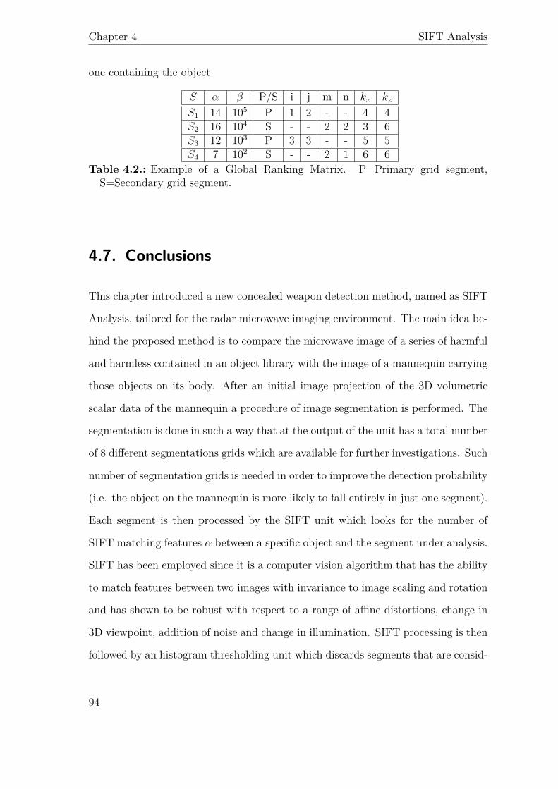
Chapter 4 SIFT Analysis
one containing the object.
S α β P/S i j m n kx kz
S1 14 105 P 1 2 - - 4 4S2 16 104 S - - 2 2 3 6S3 12 103 P 3 3 - - 5 5S4 7 102 S - - 2 1 6 6
Table 4.2.: Example of a Global Ranking Matrix. P=Primary grid segment,S=Secondary grid segment.
4.7. Conclusions
This chapter introduced a new concealed weapon detection method, named as SIFT
Analysis, tailored for the radar microwave imaging environment. The main idea be-
hind the proposed method is to compare the microwave image of a series of harmful
and harmless contained in an object library with the image of a mannequin carrying
those objects on its body. After an initial image projection of the 3D volumetric
scalar data of the mannequin a procedure of image segmentation is performed. The
segmentation is done in such a way that at the output of the unit has a total number
of 8 different segmentations grids which are available for further investigations. Such
number of segmentation grids is needed in order to improve the detection probability
(i.e. the object on the mannequin is more likely to fall entirely in just one segment).
Each segment is then processed by the SIFT unit which looks for the number of
SIFT matching features α between a specific object and the segment under analysis.
SIFT has been employed since it is a computer vision algorithm that has the ability
to match features between two images with invariance to image scaling and rotation
and has shown to be robust with respect to a range of affine distortions, change in
3D viewpoint, addition of noise and change in illumination. SIFT processing is then
followed by an histogram thresholding unit which discards segments that are consid-
94

4.7 Conclusions
ered false alarms by doing histogram intensities considerations which are described
in section 4.4. The candidate segments which are not discarded by the histogram
thresholding unit are then sent to a correlation unit for further verification. For
each segment a correlation coefficient β is computed. The correlation coefficient is
weighted over α by the Score variable defined as S = β(1 + α). The information
about the candidate segments for each segmentation and their Score values are then
combined together in a Ranking Matrix. Only the segment which present the high-
est value of S for each possible segmentation is sent to a Global Ranking Matrix
which decides the final output by selecting the segment with the highest value of the
Score parameter. Experimental results of this method will be described in Chapter
5.
95

Bibliography
[1] Zuiderveld, Karel (1994), "Contrast limited adaptive histogram equalization",
Graphics gems IV, Academic Press Professional, Inc., pp. 474485
[2] An implementation of the SIFT detector and descriptor - Vedaldi - 2007
97


5. Experimental Results and
Comparative Analysis
“Symmetria est in mente”
Kant
5.1. Overview
This chapter contains the results and comparative analysis of the Depolarization
and SIFT methods developed respectively in Chapter 3 and Chapter 4. To estabil-
ish the validity and reliability of the two algorithms a measurement campaign has
been carried out. Since concealed weapon detection finds one of its main applica-
tion in airport security, a mannequin with various concealed object under its jacket
has been deployed for the radar measurements1. The measurements have been per-
formed in the DUCAT room of the Delft University of Technology by the means of
a polarimetric SAR providing both HH and VV data. Regarding the choice of the
concealed objects, a representative set of common harmful and harmless items which
an individual may carry at an airport security checkpoint have been chosen. The
object set consisted in a gun, a ceramic knife, a pair of keys, a mobile phone and a1For more information regarding the measurements setup please refer to appendix B
99

Chapter 5 Experimental Results and Comparative Analysis
bottle of water. It is important to notice that each object have been selected because
it differs from the others in size, shape or material. This choice have been made in
order to widely and accurately test the detection and classification capabilities of De-
polarization and SIFT algorithms. The results of the application of Depolarization
Analysis to the set of microwave images of the mannequin with different concealed
objects on its body will be shown in section 5.2. Subsequently, in section 5.3 results
of application of SIFT analysis to the images will be presented which is followed
by a comparative analysis of the two methods in section 5.4. Finally, section 5.5
contains the conclusions of the chapter.
5.2. Depolarization Analysis Results
In this section, results regarding Depolarization Analysis will be presented and dis-
cussed. As explained in Chapter 3, this method exploits and combines both sets of
polarization data (i.e. HH and VV) provided by the polarimetric radar in order to
achieve concealed weapon detection by the means of a novel attribute called Depo-
larization angle. The Depolarization angle described in section 2.5 is a combination
of the Polarization and Feature angles which are described in section 2.3.1 and sec-
tion 2.4. Polarization Angle is the expression of a physical phenomenon which is
scattering, while Feature Angle is the expression of symmetries in the image.
In order to perform the simulations, Depolarization Analysis has been algorithmi-
cally implemented in MATLAB R2010b. The main computational steps included
the calculation of the main mathematical quantities of the method which are, as
said before, the Polarization Angle, the Feature Angle and the Depolarization An-
gle. Furthermore extra processing time is needed in order to compute the algorithm
steps that are included in the Detection Unit (see section 3.3). The average compu-
100

5.2 Depolarization Analysis Results
tational time needed to detect objects on a mannequin is about 8 seconds on a 2.00
Ghz Intel Core DUO CPU with 2 GB of RAM.
The measurements campaign which has been briefly in section 5.1 , consists of five
cases (scenarios):
1. Mannequin with a concealed gun and a ceramic knife located respectively in
the upper right part of the torso and upper left part of the leg under a cotton
jacket.
2. Mannequin with a concealed gun and a ceramic knife under a cotton jacket.
The gun is located on the upper right part of the torso but it is rotated
compared to test case 1 while the knife is positioned on the lower left part of
the leg.
3. Mannequin with a concealed gun and a pair of keys under a cotton jacket.
The gun and the pair of keys are located respectively in the upper right part
of the torso and in the lower left part of it.
4. Mannequin with a concealed gun and a mobile phone under a cotton jacket.
The gun and the mobile phone are located respectively in the upper right part
of the torso and in the lower left part of it.
5. Mannequin with a concealed bottle of water, a knife, a gun and a mobile phone
under a cotton jacket. The bottle of water and the gun are located respectively
in the upper right and in the upper left part of the torso. The knife is located
on the upper part of the right leg while the mobile on the upper part of the
left leg.
For each test scenario VV and HH polarization data have been collected. The scan
area for all the measurements was 74x100 cm2 with steps between the consequent
positions of the antennas of 1 cm (75x101 points). The 3D images produced by
101

Chapter 5 Experimental Results and Comparative Analysis
the radar had a size of 149x201x81 points. This is due to the fact that the spacing
employed for the image is of 0.5 cm. Therefore the number of points in width and
height are doubled compared with the one of the raw data. In depth, the number of
points in the 3D image depends on the interpolation factor that has been used for
the IFFT from frequency to time domain.
The test case 1 checked the capabilities of Depolarization Analysis to detect and
classify a metallic dangerous object of medium dimensions represented by a revolver
gun and a dielectric object of medium dimensions represented by the ceramic knife.
After an initial energy projection in the frontal with respect to the mannequin plane,
the horizontal and vertical polarization data are processed with a Laplacian and
subsquently with a Prewitt filter. The Prewitt filter is enhancing edges depending on
the initial polarization of the data (e.g. vertical polarization data edges are enhanced
with a vertical prewitt filter). It is clear from the encircled areas of Figure 5.1 (a)
and (b), which are respectively the barrel and the handle of the gun, that the features
pointing in the horizontal direction are enhanced by the prewitt horizontal filter and
the ones oriented in the vertical direction by the vertical prewitt filter.
102

5.2 Depolarization Analysis Results
Figure 5.1.: (a) Horizontal Polarization Data (b) Vertical Polarization Data afterLaplacian and Horizontal/Vertical Prewitt filters
We can see in Figure 5.3 the images of horizontal and vertical polarization data for
this test case along with the images of the Polarization and Feature Angle which are
needed for computing the Depolarization Angle. As we can see from Figure 5.3(c)
and (d) even before computing the Depolarization Angle, the visual perception of the
weapons on the mannequin has already improved compared to the original data.The
Polarization Angle highlights very clearly the edges of the objects and in particular
the ones of the gun. This can be explained by the fact that reflections from sharp
edges cause a shift in the Polarization Angle compared to the background (i.e. the
mannequin). On the other hand, Feature Angle is highlighting the symmetric fea-
tures of the objects and especially the gun position on the upper right part of the
torso. In fact, the body areas of the mannequin where the objects are located are
showing a greater density and a greater variability in the direction of symmetry lines
103
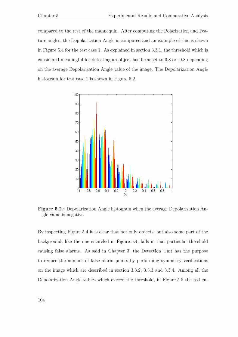
Chapter 5 Experimental Results and Comparative Analysis
compared to the rest of the mannequin. After computing the Polarization and Fea-
ture angles, the Depolarization Angle is computed and an example of this is shown
in Figure 5.4 for the test case 1. As explained in section 3.3.1, the threshold which is
considered meaningful for detecting an object has been set to 0.8 or -0.8 depending
on the average Depolarization Angle value of the image. The Depolarization Angle
histogram for test case 1 is shown in Figure 5.2.
Figure 5.2.: Depolarization Angle histogram when the average Depolarization An-gle value is negative
By inspecting Figure 5.4 it is clear that not only objects, but also some part of the
background, like the one encircled in Figure 5.4, falls in that particular threshold
causing false alarms. As said in Chapter 3, the Detection Unit has the purpose
to reduce the number of false alarm points by performing symmetry verifications
on the image which are described in section 3.3.2, 3.3.3 and 3.3.4. Among all the
Depolarization Angle values which exceed the threshold, in Figure 5.5 the red en-
104

5.2 Depolarization Analysis Results
circled areas are the one detected by the detection unit. The usefulness of this unit
is clearly shown in Figure 5.6 where the final output for the test case 1 is presented
and which shows detection spots belonging only to the gun or the knife respectively
achieving a perfect detection. From this test case we have seen how Depolarization
Analysis is capable of correctly detecting objects and how it is possible to reduce
the false alarm rate by the mean of the detection unit.
105

Chapter 5 Experimental Results and Comparative Analysis
Figure 5.3.: (a) Horizontal polarization data (b) Vertical Polarization data (c) Po-larization angle (d) Feature angle for test case 1
106

5.2 Depolarization Analysis Results
Figure 5.4.: The Depolarization Angle for test case 1
Figure 5.5.: Mannequin image with values for which Dp>0.8 marked in white. Redcircles are the points detected by detection unit. 107

Chapter 5 Experimental Results and Comparative Analysis
Figure 5.6.: Image processing chain output for test case 1
The test case 2 is a slight variation of test case 1 which assessed if the algorithm
is able to detect objects when a rotation occurs. In Figure 5.7 the output for this
test case is shown along with the optical image of the mannequin with weapons on
its body. As we can see, the algorithm clearly detected the gun and the ceramic
knife which is marked by points A and B in Figure 5.7, representing respectively the
handle and the tip of the knife. Points C (abdomen-torso separation) and D (neck
indentation) in Figure 5.7 represent two false alarms due to strong reflections from
body areas of the mannequin that, due to their particular shapes, cause a corner
reflector effect that makes them assume a Depolarization Angle value similar to the
one of the objects.
108

5.2 Depolarization Analysis Results
Figure 5.7.: Output for Test Case 2 (left) and Optical image of the mannequin forTest Case 2 (right)
The test case 3 and test case 4 verified how the algorithm responds in an almost
similar test scenario as test case 3. In these experiments the gun is kept at the same
place as in test case 2 while in test case 3 the knife has been replaced by a pair of
keys and subsequently by a mobile phone in test case 4. These two experiments, for
which the output is shown in Figure 5.8, demonstrate that Depolarization Analysis
is capable of detecting a small metallic object (i.e. keys) which is marked as A and
B in the left figure and small metal-dielectric objects (i.e. mobile phone) which is
marked as E in the right figure. Is it possible to see in Figure 5.8 that the gun
is consistently detected in both experiments. Moreover, the same issue of false
alarm, which was present in the test case 2, due to corner reflector effect from
indentation in some parts of the human body is also appearing in these experiments
109

Chapter 5 Experimental Results and Comparative Analysis
especially in arm, neck and groin area (points respectively marked as C, D, F and G
in Figure 5.8). False alarms which are caused by the head of the mannequin are of
very little concern and therefore discarded due to the fact that is almost impossible
that a concealed object would be carried in that body region.
Figure 5.8.: Output for Test Case 3 (left) and output for Test Case 4 (right)
The main purpose of test case 5 was to verify if the Depolarization algorithm is
capable of detecting a gun in a different position compared to the other four test
cases along with a medium size dielectric object which is a bottle of water. In this
test case also a mobile phone and a knife are present. According to the results shown
in Figure 5.9 the algorithm is capable to clearly detect the gun and the bottle of
water (point marked as A in figure Figure 5.9). The knife, which is positioned on
the upper right leg of the mannequin, is not detected. This happened not due to an
110

5.2 Depolarization Analysis Results
algorithm limitation but due to the fact that it was positioned near the edge of the
antenna aperture which made it not clearly visible in the radar image. Furthermore,
this time the algorithm failed to detect the mobile phone and a false alarm, marked
as B in Figure 5.9, is present in the groin area of the mannequin.
Figure 5.9.: Output for test case 5
From the described results we can state that, apart from minor false alarm rates
due to indentation of specific areas of the human body which (i.e. groin,arm and
neck), the Depolarization Analysis was capable to detect objects which differ from
each other in shape, size and material without the need of any form of segmentation
but only exploiting the data provided by the dual polarization radar with a success
111

Chapter 5 Experimental Results and Comparative Analysis
rate of 10 out of 11 trials. Furthermore, the experimental results of the concealed
gun show that detection capabilities are invariant to the position of the object on
the mannequin.
It is important to underline that the algorithm was not able to classify object. This
can be explained by the fact that the majority of objects present similar Depolar-
ization angle values.
5.3. SIFT Analysis Results
After describing in section 5.2 the results of Depolarization Analysis, this section
is dedicated to the results of SIFT Analysis. As explained in Chapter 4, the main
elements of this algorithm are the segmentation unit, the three step detection pro-
cedure composed by SIFT, a correlator and histogram thresholding and a Ranking
Matrix for final output decision. SIFT Analysis is a method that has its core in the
SIFT algorithm which allows to extract interesting points of an object by providing
a mathematical description of it (i.e. feature description) and then try to match this
feature description to the one of a different image (i.e. the matching is successful
if the image contains the same object). In order to start the matching procedure,
an object library in the form of microwave images containing harmful and harmless
object, have been build. The chosen objects set, which is particularly suitable for
aiport security applications, consisted in a gun, a ceramic knife, a mobile phone, a
pair of keys and a bottle of water. This objects were SAR scanned in an anechoic
chamber simulating the free space. Moreover, the object library is also needed for
the operations of the correlation unit described in section 4.5. After the object li-
brary have been built a measurement campaign have been carried out in order to
provide the images of the mannequin with the concealed objects. The following
112
5.3 SIFT Analysis Results
test cases have been performed in order to evaluate the automatic detection and
classification performances of the method:
1. Mannequin with a concealed gun and a ceramic knife located respectively in
the upper right part of the torso and upper left part of the leg under a cotton
jacket.
2. Mannequin with a concealed gun located in the right part of the torso under
an heavy winter jacket
3. Mannequin with a concealed bottle of water, a knife, a gun and a mobile phone
under a cotton jacket. The bottle of water and the gun are located respectively
in the upper right and in the upper left part of the torso. The knife is located
on the upper part of the right leg while the mobile on the upper part of the
left leg.
4. Mannequin with a concealed gun and a mobile phone under a cotton jacket.
The gun and the mobile phone are located respectively in the upper right part
of the torso and in the lower left part of it.
5. Mannequin with a concealed gun and a pair of keys under a cotton jacket.
The gun and the pair of keys are located respectively in the upper right part
of the torso and in the lower left part of it.
Moreover, the algorithm as introduced and described in Chapter 4 has been im-
plemented in MATLAB R2010b. The main computational steps involved the cal-
culation of the segmentation branches and of the three step detection procedure
( i.e. SIFT, Correlator and Histogram thresholding). The average computational
time needed to detect objects on a mannequin is about 6 seconds on a 2.00 Ghz
Intel Core DUO CPU with 2 GB of RAM. This slightly longer computational time
compared to Depolarization Analyis is due to the multiple segmentations (refer to
113

Chapter 5 Experimental Results and Comparative Analysis
section 4.2 for more information) that requires only by itself 10 seconds to run. It
is clear that a tradeoff between robustness and computational time has to be taken
under consideration. An increase in number of segmentations will increase detection
rate (i.e. the object is more likely to entirely fall in one segment) but at the cost of
an higher computational time.
SIFT analysis developed in Chapter 4 claimed to be robust in indentifying object
in low contrast condition. In particular an object included in the library can be
matched, if present, on the mannequin even under different scaling, orientation and
also affine distortions and illumination changes. The measurement setup previously
described has been specifically designed to test these capabilities.
Test case 1 assessed the ability of SIFT Analysis to detect a gun and a ceramic knife.
Compared to Depolarization Analyis, SIFT is not exploiting any physical property
of the object therefore the material is not relevant but only the size and the position
over the mannequin. As shown in Figure 5.10 the method is able to recognize the
gun. In particular, in the top box of Figure 5.10 (a) the matching between the
segment considered as the one containing the target and the object in the library
(located in the right part of the box) is shown. As we can see from this box, even
under a 3D rotation of the weapon the algorithm is capable of associating correctly
the points belonging to the barrell of the gun. The final output for the gun of test
case 1 is shown in Figure 5.10 (b). Another example of successful gun detection is
shown, for test case 2, in Figure 5.11. It is important to state that the detection is
sensitive to the number of segmentations. The SIFT algorithm was not recognizing
the gun in test case 1 if more than two parallel segmentations were used due to false
alarms caused by parts of the mannequin’s body. Regarding the ceramic knife, it is
not possible to detect it. The same happens for the ceramic knife in test case 3, for
the mobile phone of test case 3 and 4, for the pair of keys of test case 5 and for the
114

5.3 SIFT Analysis Results
gun of test case 3 and 4. This can be explained by the fact that radar measurements
can distort the geometry of objects due to interference patterns that arise between
the items and the mannequin.
For its intrinsic nature SIFT algorithm is likely to find feature points in high-contrast
regions of the image such as objects corners.
Figure 5.10.: ( a ) Measured Mannequin for Test Case 1 ( b ) Output for TestCase 1
Furthermore, in comparing two images it is important that the relative position
between the object features in the library and the object features, when the same
item is positioned on the body of the mannequin, should not change. Therefore
feature matching would not typically work if any change in the object internal ge-
ometry happens between two images which is the case in microwave images due to
the above described interference phenomena. To make this clear let us consider the
syntethic example in Figure 5.12. As it possible to see in Figure 5.12 (a) and in
Figure 5.12 (b) a change in the object geometry due to interference and noise will
115

Chapter 5 Experimental Results and Comparative Analysis
cause 4 out of 6 features to be different causing the detection to fail. It’s impor-
tant to notice that SIFT algorithm has been developed for optical images where the
problem of geometric distortion due to interference is not as prominent as in the
microwave ones.
Figure 5.11.: (a) Measured Mannequin for Test Case 2 (b) Output for Test Case2
Figure 5.12.: Syntethic example of image distortion. (a) Distorted object on themannequin (b) same object in the library
116

5.3 SIFT Analysis Results
Finally, test case 5 have been designed to test the capabilities of the SIFT Analysis
to properly work when a multitude of objects are present in the same image. As it
is possible to see in Figure 5.13 the algorithm is successful to uniquely detect both
guns and bottle of water but fails to detect the knife and mobile phone. In this case
the misdetection of the knife can be attributed to the fact that the object is not
clearly visible in the radar image due to its position near the antenna aperture edge
and not to the geometric distortion due to interference.
117

Chapter 5 Experimental Results and Comparative Analysis
Figure 5.13.: (a) Measure Mannequin for Test Case 3 (b) Output for gun recogni-tion (c) Output for bottle recognition
According to the above presented results, SIFT Analysis is capable of detecting and
classifying a concealed gun on a mannequin under different experimental conditions
(i.e. change in position, scale and orientation of the object) which is one of the
thesis research objectives. Furthermore, a bottle of water was detected in a single
118

5.4 Comparative Analysis
experiment. At the current implementation the algorithm proved not to be reliable
and robust since it failed to detect different objects such as a pair of keys and a
mobile phone. Moreover, the detection of the gun proved to be partially robust
since was only detected three times out of five experimental trials.
5.4. Comparative Analysis
Depolarization and SIFT Analysis represent two different approaches to concealed
weapon detection. The first one (i.e. Depolarization Analysis) exploits both phys-
ical and geometrical properties of objects, which can be retrieved by the radar to
robustly detect objects in a microwave image. On the other hand, SIFT Analysis
is inspired by typical optical imaging matching procedures which relies only on the
geometric shape of the objects. According to what it has been shown in section 5.2
and section 5.3 the following considerations can be done:
• Depolarization Analysis is only capable of detecting objects while SIFT Analy-
sis is capable of both detecting and classifying them. However, Depolarization
is more consistent than SIFT. In particular SIFT method fails to detect keys,
knifes and mobile phones due to geometric distortions in the image while De-
polarization is able to detect all of them.
• Depolarization Analysis does not require segmentation while SIFT do. The
ability of an algorithm to work without a segmentation procedure is likely to
increase its detection rate while keeping the computational costs low.
• Depolarization Analysis does not require an object library to work. This means
that a priori knowledge of the entire set of objects that an individual may
carry is not required, making the algorithm versatile and more efficient. On
the other hand, SIFT do require an object library to classify objects but at
119

Chapter 5 Experimental Results and Comparative Analysis
the price of being less versatile.
• Depolarization Analysis requires both polarization data (i.e. VV and HH )
in order to work while SIFT Analysis requires only the vertical polarization
data. The fact that SIFT does not require a dual polarization antenna makes
it more likely to be practically applied in surveillance systems due to the lower
price and technological complexity of the antenna system.
• Depolarization Analysis and SIFT Analysis are both affected by false alarms
caused by indentations of the human body which appear as objects in the
microwave radar image.
A summary of the above considerations is shown in Table 5.1.
Method Detection Classification Polarization Segmentation Object LibraryDepolarization yes no dual no no
SIFT yes yes single yes yesTable 5.1.: Comparative Analysis between the two proposed methods
5.5. Conclusions
This capter was dedicated to the assessment of the performance of the concealed
weapon detection methods developed in Chapter 3 (i.e. Depolarization Analysis)
and Chapter 4 (i.e. SIFT Analysis). In order to do so, a measurement campaign
was carried out in the anechoic chamber of the Delft University of Technology.
In the measurement campaign described in section 5.1 a mannequin with different
harmful and harmless concealed objects has been scanned by a SAR radar. The
120

5.5 Conclusions
measurements have been carefully planned in order to evaluate the performance
of the algorithms under different circumstances such as different position, material
and size of the objects which were positioned on the mannequin. Subsequently,
the obtained microwave images were processed by the means of MATLAB code
implementing Depolarization and SIFT analysis respectively.
Depolarization analysis results are presented in section 5.2 and they show that this
method is capable of robustly detecting a variety of objects (i.e. a gun, a pair of
keys, a mobile phone, a ceramic knife and a bottle of water) which differ from each
other for shape, size and material with a 90% success rate. Moreover, detection has
proven to be invariant with respect to the position of the object on the mannequin.
Despite the good detection performances, there are some false alarms caused by
indentation of the human body from the arm, neck, abdomen and groin area. These
body indentations, due to their particular interaction with the eletromagnetic en-
ergy radiated by the radar, assume a value of the Depolarization Angle which is
similar to the one of actual objects. Therefore it is important to choose an appro-
priate threshold for the Depolarization Angle which has experimentally found to be
effective when set to 0.8.
In section 5.3 SIFT analysis results are presented. From the experimental results
SIFT method was able to detect and classify a concealed gun (success rate was
three out of five test cases) under different measurement conditions such as rotation,
scaling and different position of the object. In addition to this, a bottle of water
was detected in a single trial. The method was not consistent in detecting a pair
of keys, a mobile phone or a knife due to the geometric object distortions described
in section 5.3. These distortions are caused by the interference patterns due to the
interaction between the mannequin and the objects positioned on it. The choice
121

Chapter 5 Experimental Results and Comparative Analysis
of segmentation parameters (i.e. kx and kz) is really important since it affects the
detection rate. If the segments size are too small the object may be splitted in
two different segments which will cause a drop in the detection rate. On the other
hand, if the size of the each segment is too large then multiple of objects and too
many features of the human body will end up in the same segments. This second
hypothesis is also likely to decrease the detection rate.
Finally, in section 5.4 a comparative analysis between the two methods is presented.
Referring to Table 5.1 we can state that Depolarization Analysis is able to detect
object but not to classifying them while SIFT method also has the possibility to
identify them. Also, Depolarization Analysis proved to be more versatile than SIFT
analysis due to the fact that it does not need a segmentation procedure or an object
library to work. It is important to notice that Depolarization Analysis requires a
dual polarization radar to work while SIFT Analysis does not making the latter
method more likely to be applied in the field due to the lower price and complexity
of the antenna system. We have seen how both methods are affected by false alarms
caused by the human body. As shown in Table 5.2 body indentations are showing
Depolarization Angle values on edges similar to the ones of actual objects.
Feature max {|Dp|}Bottle 0.83Gun 0.96Knife 0.81Keys 0.99
Mobile 0.94Body indentations 0.92
Table 5.2.: Maximum value for the Depolarization Angle for different featuresedges
An important role is this phenomenon is played by the resolution of the image.
Microwave radar image do not offer a good resolution compared to the millimeter
122
5.5 Conclusions
and optical ones. By increasing the number of points in the image the objects are
more detailed and the same happens with the anatomical details of the mannequin.
Moreover, the number of indentations of the human body in the radar microwave
image increases with the resolution. From the above considerations we can conclude
that a higher resolution improves the details of the object allowing to better detect
edges but at the same increases the rate of false alarms due to the increased number
of indentations that look like object in the radar image. On the other hand, a
coarser resolution compared to the microwave range is likely to reduce the number
of indentations but at the same time it smoothes the edges of the image decreasing
the detection rate.
123


6. Conclusions and
Recommendations
6.1. Overview
This chapter concludes the thesis. The main objective of this thesis was to de-
sign novel robust image processing algorithms for the detection and classification
of concealed weapons. Automatic weapon detection is an important part of every
surveillance system. In the particular case of the body scanners at airports privacy
concerns prevent showing high-resolution body images to the security operators and
thus limiting application of the body scanners. By replacing the airport security
operator with an automatic detection system this type of privacy concerns will no
longer be present. In section 6.2 a summary of the developed methods is presented
and the results will be compared to the research objectives stated in Chapter 1. In
section 6.3 the scientific contributions made by this project are described. Finally,
in section 6.4 a series of recommendations for further research are presented.
125

Chapter 6 Conclusions and Recommendations
6.2. Conclusions
Two algorithms have been developed in the thesis for the automated target de-
tection in the 3D high-resolution microwave images. The proposed algorithms are
specifically tailored for working on images of humans (mannequin) produced by
a microwave imaging radar and they are validated by MATLAB simulations and
experiments.
The first method, which was developed in Chapter 3, is called Depolarization Analy-
sis. This method exploits polarization properties of the radar (i.e. HH and VV data
is retrieved by a SAR dual polarization radar) and geometric symmetry features
of the combined image (i.e. the vertical polarization produced image is combined
with the horizontal produced one) to create a novel shape descriptor called Depo-
larization Angle. Depolarization Angle can be considered as the ratio between the
Feature and the Polarization angle which are respectively an internal and external
shape descriptors introduced in chapter 2. In particular PCA and Phase symmetry
algorithms play a major role in the processing stage by extracting respectively the
Polarization Angle and the Feature Angle. It has been shown in section 2.3.1 and
section 5.2 that Polarization Angle highlights very clearly the edges of the objects
while the Feature Angle enhances the symmetry features of them. By selecting
an appropriate threshold for the Depolarization Angle and by doing filtering, as
explained in section 3.3, based on histogram thresholding and symmetry consider-
ations it is possible to drastically reduce the false alarm rate and detect concealed
objects in the image.
A measuring campaign of a mannequin carrying different concealed harmful and
harmless for safety objects has been carried out in order to assess the validity and
reliability of the algorithm. The campaign has been designed in such a way that
the capabilities of the algorithm to detect objects with different shape, size, mate-
126

6.2 Conclusions
rial and position over the mannequin have been tested. Results of the measuring
campaign, which are described in Chapter 5, show that Depolarization Analysis is
capable of detecting various objects which included a gun, a pair of keys, a mobile
phone, a ceramic knife and a bottle of water in ten out of eleven cases. Moreover,
the results have shown that a minor number of false alarm points are present. This
false alarms are originated by indentations of the human body that, due to their
particular shapes, cause a corner reflector effect that make them assume a Depolar-
ization Angle value similar to the one of the actual objects. Experimental results
of the concealed gun show that detection capabilities are invariant to the position
of the object on the mannequin. It is important to underline that the algorithm is
not able to classify objects which can be explained by the fact that the majority of
objects present similar Depolarization Angle values. In conclusion, Depolarization
Analysis accomplished the thesis objective of reliably detecting objects but failed in
the task of classifying them.
The second method, which was developed in Chapter 4, is called SIFT analysis.
The research approach in this case, as explained in section 2.6, was to develop a de-
tection and classification method for CWD inspired by computer vision algorithms
used to detect and describe local features in images. The main task of the devel-
oped method consists in comparing a set of harmful and harmless objects stored in
a library with a mannequin carrying a combination of them and see if the objects
are correctly classified. The SIFT algorithm has been chosen to be the core of this
detection method due to its capability to match features between two images with
invariance to image scaling and rotation and robustness with respect to a range of
affine distortions, change in 3D viewpoint, addition of noise and change in illumi-
nation. It is important to notice that SIFT has been developed for working with
optical images and the application to the microwave range represents a challenge by
127

Chapter 6 Conclusions and Recommendations
itself. SIFT analysis, apart from its main core which is the SIFT algorithm, also
includes a segmentation unit which it is needed for increasing detection rate and a
two step detection procedure formed by a Correlator and Histogram Thresholding
which is needed to reduce the false alarm rate. A global ranking matrix, which
it is introduced in section 4.6, finally declares which segment is considered as the
one containing the object under test by producing a mathematical quantity called
Score which takes under consideration the number of matching features α and the
correlation value β for each candidate segment. In order to test the detection and
classification capabilities of the algorithm a measuring campaign similar to the one
of Depolarization Analysis have been carried out. From the results presented in
section 5.3 is it possible to conclude that SIFT Analysis was able to detect and
correctly classify a concealed gun three out of five cases and a bottle of water in
another experiment. The algorithm proved to be not consistent in detecting a pair
of keys, a mobile phone and a ceramic knife due to geometric distortions of ob-
jects caused by interference patterns that arise between the concealed items and
the mannequin. Due to the above explained geometric distortions the matching
between the library object and the correspondent object on the mannequin would
not work due to displacement of the feature points from one image to another. In
conclusion, SIFT Analysis partially accomplished the thesis objective of detecting
and classifying objects but did not reach the objective of having a low false alarm
rate.
From the Comparative Analysis in section 5.4 we can state that Depolarization
Analysis proved to be way more robust than SIFT in detecting objects even though
the algorithm is not able to classify them. Furthermore, Depolarization Analysis
do not require an object library in order to work making it more versatile and
efficient than SIFT. On the other hand, SIFT analysis can classify objects and it
128

6.3 Summary of Contributions
does not require a dual polarization radar setup to work (i.e. a HH or VV image
is sufficient for the algorithm to recognize the object). The fact that SIFT analysis
does not require a dual polarization radar makes it more likely to be applied in
airport security where a single polarization radar is usually on duty. Finally, no
segmentation is needed in the case of Depolarization Analysis compared to SIFT
making it more computational efficient and more likely to have an higher detection
rate.
6.3. Summary of Contributions
As said in section 6.2 this thesis presents and discusses two novel algorithms, named
as Depolarization and SIFT analysis, for concealed weapon detection.
Depolarization analysis is a new procedure inspired by a previous work on GPR
buried pipes detection by Boniger and Tronicke. Furthermore, the algorithm pro-
posed in Chapter 3 is a completely new method for concealed weapon detection. Due
to this, the author of this thesis is reasonably sure of future prosperous development
which are not known at the moment for this technique.
SIFT analysis takes its inspiration from object recognition method employed in the
optical range. The approach proposed in Chapter 4 has never been employed before
in concealed weapon detection.
Moreover, we can divide the scientific contributions according to Depolarization and
SIFT method. For Depolarization analysis the following contributions are made:
• Novelty: Depolarization analysis is a new concealed weapon detection method
that can detect concealed objects in a low contrast environment such as the
microwave imaging one.
129

Chapter 6 Conclusions and Recommendations
• Novelty: Successful application of Principal Component Analysis and of Phase
Symmetry algorithm for the first time to the field of concealed weapon detec-
tion.
• Novelty: The algorithm does not require an object library. It is important to
mention that this algorithm is not capable of classifying object but only to
detect them.
• The algorithm does not require a segmentation of the image. This leads to a
more reliable detection and a lower computational time.
For SIFT analysis the following contributions are made:
• Novelty: The SIFT Analysis is a new concealed weapon detection method
which can detect and classify different concealed objects in a low contrast
environment such as the microwave one under a wide spectrum of geometric
transformation.
• Novelty: Application of an optical image matching algorithm (i.e. SIFT) to
radar microwave imaging concealed weapon detection
• The algorithm requires a single polarization to work
6.4. Recommendations
Based on the results achieved by this project, the following recommendations for
further research are given:
• In SIFT analysis some objects are still not recognized or detected with a high
false alarm rate. Therefore the algorithm needs to be further developed in
order to improve detection. As said in section 5.3 geometric distortions of
the image will cause the algorithm to not detect objects. It is also true that
130

6.4 Recommendations
microwave produced image of objects do not have a fine resolution but some
parts of the scanned object are always recognizable and represent an invariant
feature. Let us consider the gun in figure 4.4 (a) as an example. As we can
see from the image, the handle and the barrel of the gun are more defined
in details than the rest of the object and the same is always true when the
gun is on top of the mannequin. Therefore, by associating to SIFT another
pattern matching algorithm which it is specifically tailored to detect those
clearly recognizable parts of the gun, false alarm rate can be decreased. The
same procedure can be applied to all the others objects in the library.
• Reduce the false alarm rate in Depolarization Analysis. As explained in sec-
tion 5.2 some very specific parts of the human body produce an object like
Depolarization angle value due to a corner reflector effect. By broadening the
measurement campaign will be possible to deeper analyze this phenomenon
and confirm the hypothesis that those reflection are always from the same
specific parts of the body and therefore can be treated as systematic errors.
• Increase the variety of test concealed objects. In this research the algorithms
have been tested to work only with 5 objects which where a gun, a ceramic
knife, a bottle of water, a mobile phone and a set of keys. Objects which can
be useful to detect are plastic explosives and more in general dangerous or
restricted items which are likely to be taken on board of a flight.
• Try to apply Depolarization Analysis and SIFT analysis to other frequency
ranges. In particular the millimiter wave range and X-ray range may be very
suitable for the proposed algorithms due to the superior resolution compared
to microwave range imaging.
• Project the data in different directions. Since the SAR radar which has been
employed in this thesis is producing 3D images, in order to enhance detection
131

Chapter 6 Conclusions and Recommendations
of extra objects it is possible to project the data in different directions from
the one that has been chosen in this research project.
132

A. PCA
Principal component analysis is a valuable data analysis tool which has the goal of
identifying the most meaningful basis, which is a linear combination of the original
basis, to represent a data set. Let X be a m x n matrix representing the original
data set . Each row element represents a physical quantity (i.e. measurement type)
while each column an experimental trial. To give an example, if we were measuring
voltage and current over a resistor at N different time intervals the matrix would
be X =
V (t1) V (t2) · · · V (tN)
I(t1) I(t2) · · · I(tN)
. Let us define Y as the matrix Y = TX .
Where Y is a new representation of the data set and T the matrix transformation
that allows to express X in a more meaningful basis. Looking closer at T we can
state that the rows are a set of new basis vectors for expressing the columns of X
and ,from a geometric point of view, T is a strech and rotation of X. We can now
define the covariant matrix CX = 1nXXT with the following properties :
1. The diagonal terms are the variances of a particular measurement type.
2. The off-diagonal terms are the covariance between different measurement types.
For the previous example the covariance matrix is
CX = 1n
∑N
i=1 V 2(ti)∑N
i=1 V (ti)I(ti)∑Ni=1 V (ti)I(ti)
∑Ni=1 I2(ti)
133

Chapter A PCA
We assume that the data has high SNR. Therefore principal components with larger
associated variances represent interesting structure while the others represents noise.
The goal of PCA is to find an orthornal matrix T in Y = TX for which CY is a
diagonal matrix (i.e. Y is decorrelated) . We call the rows of T as the principal
Figure A.1.: PCA of a multivariate Gaussian distribution centered at (1, 3) witha standard deviation of 3.
components of X. It can be easily demonstrated that ,in order to diagonalize CY ,
each row of T has to be an eigenvector of CX and T has to be orthonormal. To
compute PCA of a data set X it is necessary to subtract off the mean from each
measurement type and then compute the eigenvectors of CXwhich in turns are the
rows of T. The approach described above represents the solution of PCA using
eigenvector decomposition. As we can see in Figure A.1 the new basis, for the
multivariate gaussian in figure, located by PCA is oriented along the direction where
the variance of the data is maximized.
134
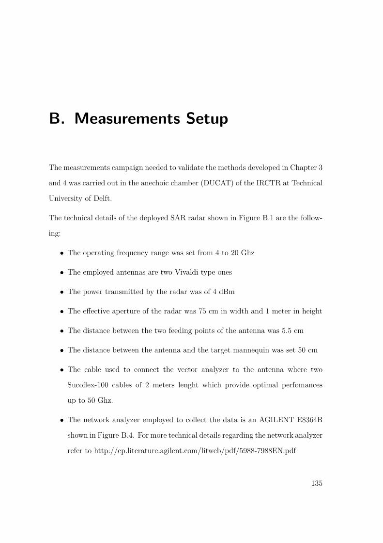
B. Measurements Setup
The measurements campaign needed to validate the methods developed in Chapter 3
and 4 was carried out in the anechoic chamber (DUCAT) of the IRCTR at Technical
University of Delft.
The technical details of the deployed SAR radar shown in Figure B.1 are the follow-
ing:
• The operating frequency range was set from 4 to 20 Ghz
• The employed antennas are two Vivaldi type ones
• The power transmitted by the radar was of 4 dBm
• The effective aperture of the radar was 75 cm in width and 1 meter in height
• The distance between the two feeding points of the antenna was 5.5 cm
• The distance between the antenna and the target mannequin was set 50 cm
• The cable used to connect the vector analyzer to the antenna where two
Sucoflex-100 cables of 2 meters lenght which provide optimal perfomances
up to 50 Ghz.
• The network analyzer employed to collect the data is an AGILENT E8364B
shown in Figure B.4. For more technical details regarding the network analyzer
refer to http://cp.literature.agilent.com/litweb/pdf/5988-7988EN.pdf
135
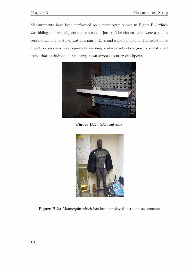
Chapter B Measurements Setup
Measurements have been performed on a mannequin shown in Figure B.2 which
was hiding different objects under a cotton jacket. The chosen items were a gun, a
ceramic knife, a bottle of water, a pair of keys and a mobile phone. The selection of
object is considered as a representative sample of a variety of dangerous or restricted
items that an individual can carry at an airport security checkpoint.
Figure B.1.: SAR antenna
Figure B.2.: Mannequin which has been employed in the measurements
136

Measurements Setup
Figure B.3.: Mannequin positioned in the anechoic chamber
Figure B.4.: Mannequin positioned in the anechoic chamber with the AGILENTE8364B network analyzer clearly visible in the front
137


C. SIFT
Matching features from one image to another is a common problem in computer
vision. Unfortunately images are not always the same in scale, orientation and
illumination. SIFT algoritm has the ability to match features between two images
with invariance to image scaling and rotation and has shown to be robust with
respect to a range of affine distortions, change in 3D viewpoint, addition of noise
and change in illumination.
The first step of the algorithm is to create an internal representation of the original
image I(x, y) to ensure scale invariance. In order to create a scale space the original
image is progressively blurred out by convolving it with a Gaussian blur operator
described by :
G(x, y, σ) = 12πσ2 e−(x2+y2)/2σ2
Where σ is the scale parameter. The scale parameter in a way controls the amount
of blur applied to the image.
The blurred image is defined as:
L(x, y) = I(x, y) ∗ G(x, y, σ)
Let us assume that the blurring in a particular image is σ. Then the amount of blur
139
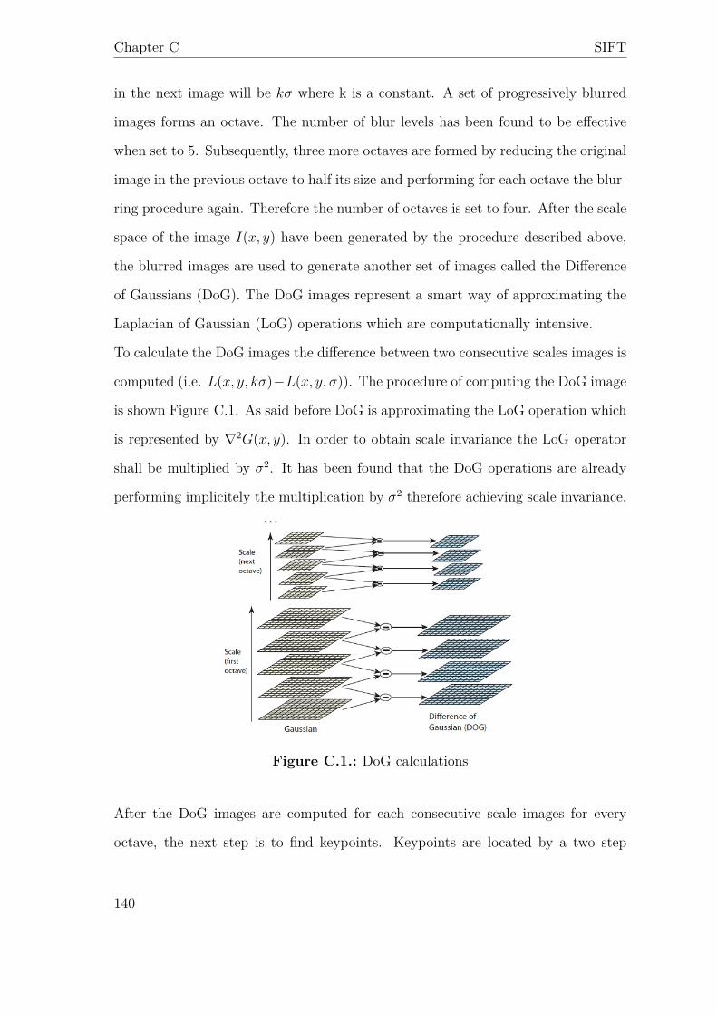
Chapter C SIFT
in the next image will be kσ where k is a constant. A set of progressively blurred
images forms an octave. The number of blur levels has been found to be effective
when set to 5. Subsequently, three more octaves are formed by reducing the original
image in the previous octave to half its size and performing for each octave the blur-
ring procedure again. Therefore the number of octaves is set to four. After the scale
space of the image I(x, y) have been generated by the procedure described above,
the blurred images are used to generate another set of images called the Difference
of Gaussians (DoG). The DoG images represent a smart way of approximating the
Laplacian of Gaussian (LoG) operations which are computationally intensive.
To calculate the DoG images the difference between two consecutive scales images is
computed (i.e. L(x, y, kσ)−L(x, y, σ)). The procedure of computing the DoG image
is shown Figure C.1. As said before DoG is approximating the LoG operation which
is represented by ∇2G(x, y). In order to obtain scale invariance the LoG operator
shall be multiplied by σ2. It has been found that the DoG operations are already
performing implicitely the multiplication by σ2 therefore achieving scale invariance.
Figure C.1.: DoG calculations
After the DoG images are computed for each consecutive scale images for every
octave, the next step is to find keypoints. Keypoints are located by a two step
140

SIFT
procedure consisting in finding first the maxima/minima of DoG and then by finding
subpixel maxima or minima. The first step of the procedure is performed by iterating
through each pixel and check all its neighbours and see if that pixel is a maxima or
a minima. The check is performed by comparing the current image to the one above
and below at the same octave as shown in Figure C.2. The pixel marked as x in
Figure C.2 is considered a keypoint if it is the greatest or least of all 26 neighbours.
Figure C.2.: Maxima/Minima of DoG
Subpixel maxima or minima are then found by performing a Taylor expansion of
the scale-space function of the image around the approximate keypoint:
D(x) = D + ∂DT
∂x x + 12
xT ∂2D∂x2 x
The subpixel values are calculated in order to increase the chance of matching and
stability of the algorithm.
By this procedure a lot of keypoints are generated. The ones lying on edges of the
image or not having enough contrast are discarded. Edges are evaluated by comput-
ing for each keypoint two perpendicular gradients and check for their magnitude.
The ones with small gradient magnitudes are discarded. Low contrast feature are
discarded by performing intensity thresholding for each pixel.
Once keypoints have been computed an orientation needs to be assigned to each one
of them. This is needed in order to achieve rotation invariance. For each keypoint
141

Chapter C SIFT
gradient magnitude and orientations are calculated the following way :
m(x, y) =√
(L(x + 1, y) − L(x − 1, y))2 + (L(x, y + 1) − L(x, y − 1))2
θ(x, y) = arctan((L(x, y + 1) − L(x, y − 1))/(L(x + 1, y) − L(x − 1, y)))
The magnitude and orientation are calculated for all the pixels around the keypoint.
Then a histogram is created in which the 360 degrees of orientation are divided into
36 bins. For each pixel under analysis the relative orientation θ(x, y) weighted by its
magnitude m(x, y) is stored in the relative “angular degree” bin of the histogram.
Once the procedure has been done for every pixel surrounding the keypoint the
algorithm assigns an orientation to the keypoint based on the peak of the histogram.
If there are multiple peaks in the histogram they are all converted into new keypoints.
At this point scale and orientation invariance is achieved for every keypoint.
Figure C.3.: SIFT Descriptor
Subsequently, the next goal is to create a unique identifying mark which is called
descriptor for each keypoint. In order to do so a 16 x 16 window ,which is broken
into sixteen 4x4 windows, is created around the keypoint. Within each 4x4 window,
gradient magnitudes and orientations are calculated and put into an 8 bin histogram
. As explained before the “amount of orientation” added to the bin depends on the
142

SIFT
magnitude of the gradient and, in this case, also on the distance from the keypoint.
The distance weighting is achieved by applying a gaussian window to the magnitude
of orientations. The above procedure is repeated for all the 16 pixels around the
keypoint. Since each histogram contains 8 bins and since this procedure is repeated
for 16 times (i.e. number of neighbouring pixels) the descriptor vector describing the
keypoint contains 128 elements. The keypoint is uniquely identified by the 128x1
descriptor vector.
143


Glossary
AHE: Adaptive Histogram Equalization
CLAHE: Contrast Limited Adaptive Histogram Equalization
CWD: Concealed Weapon Detection
CWDS: Concealed Weapon Detection System
GPR: Ground Penetrating Radar
GRM: Global Ranking Matrix
MM: Millimeter
PCA : Principal Component Analysis
PCA-SIFT: Principal Component Analysis Scale Invariant Feature Transform
SAR: Syntethic Aperture Radar
SIFT: Scale Invariant Feature Transform
SURF: Speeded Up Robust Feature
145