
DIELECTRIC LOSS ESTIMATION - TU Delft Repositories
110
DIELECTRIC LOSS ESTIMATION USING DAMPED AC VOLTAGES S.A.A. Houtepen High Voltage Technology and Management Department of Electrical Sustainable Energy Faculty of Electrical Engineering, Mathematics and Computer Science Delft University of Technology, June 2010
-
Upload
khangminh22 -
Category
Documents
-
view
3 -
download
0
Transcript of DIELECTRIC LOSS ESTIMATION - TU Delft Repositories

DIELECTRIC LOSS ESTIMATION USING
DAMPED AC VOLTAGES
S.A.A. Houtepen
High Voltage Technology and Management
Department of Electrical Sustainable Energy
Faculty of Electrical Engineering, Mathematics and Computer Science
Delft University of Technology, June 2010


I S.A.A. Houtepen - Dielectric Loss Estimation using Damped AC Voltages
DIELECTRIC LOSS ESTIMATION
USING
DAMPED AC VOLTAGES
S.A.A. Houtepen
June 1, 2010
Thesis Committee
prof. dr. J.J. Smit
dr.-hab.ir. E. Gulski
dr.ir. M. Popov

II S.A.A. Houtepen - Dielectric Loss Estimation using Damped AC Voltages
III S.A.A. Houtepen - Dielectric Loss Estimation using Damped AC Voltages
PREFACE
For the completion of my MSc study in Electrical Power Engineering, I performed a
research project at the department of High Voltage Technology and Management of the
Delft University of Technology. This investigation focused on the dielectric loss
measurement with damped AC Voltages. In this report, a presentation of this research is
given.
For a more detailed description of the physics behind dielectric losses and aging of
insulation, one is referred to chapter 2. In chapter 3, a mathematical representation is
given on a damped AC system, which is compared to a more detailed model. For a
thorough investigation on ways to determine the attenuation from a DAC wave as stable
as possible, details can be found in chapter 4. The determination of the internal system
losses are described in chapter 5, and a complete overview of dielectric loss estimation
using damped AC is given in chapter 6. This report is finalized with conclusions and
recommendations in chapter 7.
I would like to thank my supervisors during this project; dr.-hab. ir. Edward Gulski
from the Delft University of Technology, and dr. ir. Ben Quak from Seitz Instruments
AG in Switzerland. Without the help and discussions, I was not able to do this research
and write this report. Secondly, I also want to thank Piotr Cichecki, for providing me
with a large amount of measurement data from the field. Last, but not least, I would like
to thank my parents, John and Marianne, for giving me the opportunity to do this and
for the support they gave me during the years I went to college.
Delft, May 2010
Richard Houtepen

IV S.A.A. Houtepen - Dielectric Loss Estimation using Damped AC Voltages

V S.A.A. Houtepen - Dielectric Loss Estimation using Damped AC Voltages
SUMMARY
Dielectric loss measurement is one of most important diagnostic tools for condition
assessment of e.g. oil-filled cables. One of the methods to determine the loss tangent is
based on damped AC voltages.
Since 10 years, the use of damped AC (DAC) voltages is a well known method to
determine tan δ. In particular the estimation of dielectric loss parameter is based on the
estimation of the DAC voltage attenuation, and numeric procedures are used. To
achieve sufficient sensitivity (at this moment 0.1%), each type of system has to be
subjected to a detailed calibration procedure. Due to the fact, that damped AC voltage
becomes more and more a standard solution for on-site diagnosis of all types of oil-filled
power cables up to 380kV and stator insulation of electrical machines, systematic
research is necessary to optimize the procedure of dielectric loss estimation.
This study consists mainly of three parts. These are:
• Derivation and determination of a proper model for further calculations
• Investigation on methods to determine the total losses from the DAC wave
• Research on the calibration of a DAC system, to eliminate internal system losses
The second and third parts are based on empirical research, and therefore give a
fundamental basis for final conclusions.
The mathematical model showed that a representation of a DAC system with one total
equivalent internal resistance is most suitable for use. This is due to the fact that a more
detailed model (with every component separately modelled) results in a negligible
improvement and secondly creates an unmanageable situation (all components are
voltage/frequency dependent and component calibration should be applied).
To investigate the total losses from a DAC system, two arbitrary peaks of the wave have
to be taken and via a calculation this will result in the dielectric losses. In theory, it
should not matter which two peaks and/or lows are taken. In practice however, it is clear
that an offset is present. Therefore, a new and more robust method is presented. This
method calculates the attenuation from the first two peaks, and averages it with the
attenuation from the first two lows.

VI S.A.A. Houtepen - Dielectric Loss Estimation using Damped AC Voltages
When the total losses are determined, the internal system losses have to be obtained via
a detailed calibration and subtracted during future measurements. Since these losses are
voltage/frequency dependent, an extensive calibration is currently in use. This
procedure consists of a parallel and series switching of several test capacitors (in order
to create different frequencies). If this is done in a wide range of voltages, a 3D
relationship originates between voltage, capacitance and internal resistance. From the
obtained internal resistance values, the (known and very low) losses caused by the test
capacitors are eliminated.
In this thesis, research is done on a way to simplify this procedure by changing from a
capacitance to a frequency scale. This resulted in a more linear depiction of the obtained
results for the internal resistance. Linearization of these frequency scaled values is
investigated and although the trend line of the dielectric losses in function of voltage
remained the same, more inaccuracy of the absolute value of the dielectric losses was the
result. It is therefore recommended to use the current calibration procedure, in order to
maintain the current high accuracy of the dielectric loss calculation.
In order to calculate the dielectric losses from a damped AC voltage wave, the following
steps have to be taken;
• Determine the attenuation of the DAC wave, by averaging the obtained value for
the attenuation coefficient from two peaks and two lows.
• If the internal losses are unknown, calibrate the system at different voltages and
frequencies.
• If the system losses are known, determine these losses at that particular voltage
and frequency.
• Calculate the dielectric losses of the system, with the use of a mathematical
model consisting of one total equivalent internal resistance.

VII S.A.A. Houtepen - Dielectric Loss Estimation using Damped AC Voltages
TABLE OF CONTENTS Preface III Summary V
Table of Contents VII 1. Introduction 1
1.1 Introduction to Condition Assessment…..……………….. 1 1.2 On-Site Testing of HV Equipment…….…..……………….. 3 1.3 Problem Definition and Scope of this Study.……………. 4 2. Dielectric Losses 5
2.1 Physical Background of Dielectric Losses…….………….. 5 2.1.1 Definition…………………………………………………………………………………… 5
2.1.2 Origin………………………………………………………………………………………….7
2.1.2.1 Dipole Losses 7
2.1.2.2 Conductive Losses 9
2.1.2.3 Interface Losses 10
2.1.2.4 Discharge Losses 11
2.2 Aging of Insulation…………………………………………….. 12 2.2.1 Oil-Impregnated Insulation………………………………………………………… 12
2.2.1.1 Chemical Structure 12
2.2.1.2 Aging 15
2.2.2 Epoxy-Mica Insulation……………………………………………………………….. 19
2.2.2.1 Insulation Structure 19
2.2.2.2 Causes of Defects 20
2.2.2.3 Deterioration 21 2.2.2.4 Effects on Tan δ 22
2.3 Measurement Techniques………..………………………….. 23 2.3.1 Continuous Energizing……..………………………………………………………… 23
2.3.1.1 Very Low Frequency Analysis 23
2.3.1.2 The Schering Bridge 24
2.3.1.3 Dielectric Spectroscopy 25
2.3.2 Temporarily Energizing………………………………………………………………. 26
2.3.2.1 Return Voltage Measurement 26
2.3.2.2 Damped AC 27
3. Damped AC Voltages 31
3.1 Principle of Electrical Resonance.………………………….. 31 3.1.1 Modelling a series RLC Circuit……………………………………………………. 32
3.1.1.1 Mathematical Derivation 32
3.1.1.2 Attenuation β and Quality factor Q 34
3.2 A Mathematical Model of a DAC System……………....... 35 3.2.1 Mathematical Derivation...………………………………………………………… 35
3.3 A More Detailed Model……………………..……………....... 39 3.3.1 Mathematical Derivation...………………………………………………………… 39

VIII S.A.A. Houtepen - Dielectric Loss Estimation using Damped AC Voltages
4. Loss Calculation using DAC 43
4.1 Introduction to Attenuation Coefficient β.……………..… 43 4.2 The Different Calculation Methods……….……………..… 45
4.2.1 Theoretical Approach…………..……………………………………………………. 45
4.2.2 Attenuation in Practice………..……………………………………………………. 46
4.3 Including an Offset…………………..……….……………..… 50 4.3.1 Introduction…………….…………..……………………………………………………. 50
4.3.2 Positive Offset..……….…………..……………………………………………………. 50
4.3.2.1 A Small Offset 50
4.3.2.2 An Extreme Value 51
4.3.3 Negative Offset……….…………..……………………………………………………. 52
4.3.3.1 A Small Offset 52
4.3.3.2 An Extreme Value 52
4.3.4 Observations….……….…………..……………………………………………………. 53
4.4 A New Calculation Method for β………………………....... 54 4.4.1 Introduction…………….…………..……………………………………………………. 54
4.4.2 Application to Measurement Data.……………………………………………. 54
4.4.2.1 Effects of an Offset 54
4.4.2.2 Influence on the Voltage Trendline 59
4.5 Chapter Conclusions…………….………………………....... 62 5. The Internal System Losses 63
5.1 The Current Calibration Procedure……….……………..… 63 5.2 Investigation on the Calibration Matrices.……………..… 65
5.2.1 An Experimental Approach…..……………………………………………………. 65
5.2.2 Practical Support………..………..……………………………………………………. 66
5.2.2.1 A 28 kV DAC System 66
5.2.2.2 A 60 kV DAC System 69
5.2.2.3 A 150 kV DAC System 70
5.2.3 Observations….……….…………..……………………………………………………. 70
5.3 Linearization of the Frequency Representation……....... 71 5.3.1 The Applied Method.…………..……………………………………………………..71
5.3.2 Validation of the Linear Method…..……………………………………………. 72
5.3.3 Remarks…………………………………..…..…………………………………………….76
5.4 Chapter Conclusions…………….………………………....... 77 6. A Complete Overview 79
6.1 Flow Chart……………………………..……….……………..…79 6.2 Procedure Explanation……………………...……………..… 80
7. Conclusions and Recommendations 83 References IX Appendix A: Matlab Code MSc Thesis XIII Appendix B: CMD 2010 Conference Proceeding XIX

1 S.A.A. Houtepen - Dielectric Loss Estimation using Damped AC Voltages
1. INTRODUCTION
1.1 Introduction to Condition Assessment
In the current society, the dependency on electrical energy is enormous and an
interruption of the power supply becomes more and more an unaccepted occurrence.
The liberalization of the energy market resulted in utility companies that are forced to
obtain a competitive edge. Therefore, more focus was put on maintenance and condition
assessment of HV equipment and a policy in which the installed components should be
fully used up till the end of their lifetime originates.
Combined with the continuously increasing demand for flexibility and reliability of
electrical energy supply, grid utility companies face enormous challenges in maintaining
an appropriate balance between the reliability of the energy distribution on one hand
and a grid whose components suffer from aging due to electrical and thermal stresses on
the other hand.
In the Netherlands, for example, XLPE cables are commonly installed at the moment in
high voltage networks [4]. Before the 1980’s however, large numbers of oil impregnated
cables were taken into operation, and much of those components are still in service
today. Failures in the Dutch transmission system are nevertheless rare, and the
knowledge about the actual condition and aging processes in these systems is still
limited. The same can be said on the actual condition of stator bar insulation in electrical
machines, which have a leading role in the generation of electrical energy.
Condition Assessment
Nowadays, many advanced methods for condition assessment of service-aged HV
components are available. These condition assessment diagnostics, which are applied to
service-aged HV systems, are not only based on a pass or fail criterion. During such a
test, attention is paid to recognize, localize and evaluate possible defects. When this is
done periodically, evaluation of these processes in time can be monitored.

2 S.A.A. Houtepen - Dielectric Loss Estimation using Damped AC Voltages
The main purposes of condition assessment of HV equipment are listed hereunder [4]:
• To check the availability and reliability of the component
• By non-destructive diagnostics, it can be estimated what the actual condition of
the service-aged system is, and a check is performed on the insulation
degradation after a period in time.
• Reference values of the diagnostic tools are provided and can be used for later
tests (in order to demonstrate whether the insulation is still free from dangerous
defects and that the life-time expectation is sufficiently high)
• Diagnostic measurements can demonstrate that a component has been
successfully repaired after a failure and the defect in the insulation is eliminated
To assess the dielectric properties of high-voltage equipment in service, non-destructive
methods are used. One of the major techniques to determine the dielectric properties of
electrical insulation in a non-destructive way is via the dielectric loss parameter tan δ.
In the next paragraphs, a detailed description of the physical background and major
measurement techniques of this loss tangent are presented.

3 S.A.A. Houtepen - Dielectric Loss Estimation using Damped AC Voltages
1.2 On-Site Testing of HV Equipment
Energizing and testing components with a high capacitance (e.g. long cables) at an AC
overvoltage demands reactive power of several MVA, which can impossibly be supplied
by mobile installations.
An example with specifications from one of the largest conventional mobile installations
available is given below. It can be seen here; that the limitation of this particular test
transformer includes a maximum capacitance of 1.6 uF which can be tested at 260 kV.
Unit Maximum value
Voltage 260 kV
Inductance 16.2 H
Current 83 A
Load capacitance at max. voltage 18-1600 nF
Frequency range 20-300 Hz
Lowest frequency at max. voltage 31 Hz Table 1-1: Example of specifications from a test transformer for on-site testing
When concerning e.g. long power cables, the capacitance of the test object can go up to
10 uF. To reduce the reactive power required, it is therefore common to test at VLF (0.1
Hz) or DC voltage. With the advent of damped AC, a new method is applicable that can
go up to 350 kV and multiple micro-farad’s. Furthermore, the test equipment can be
transported in a minivan which makes is very suitable for on-site testing.
In this research, the main focus is on the dielectric loss estimation using these damped
AC voltages.

4 S.A.A. Houtepen - Dielectric Loss Estimation using Damped AC Voltages
1.3 Problem Definition and Scope of this Study
Problem Definition
Dielectric loss measurement is one of most important diagnostic tools for condition
assessment of e.g. oil-filled cables. One of the methods to determine the loss tangent is
based on damped AC voltages.
Since 10 years, the use of damped AC (DAC) voltages is a well known method to
determine tan δ. In particular the estimation of dielectric loss parameter is based on the
estimation of the DAC voltage attenuation, and numeric procedures are used. To
achieve sufficient sensitivity (at this moment 0.1%), each type of system has to be
subjected to a detailed calibration procedure. Due to the fact, that damped AC voltage
becomes more and more a standard solution for on-site diagnosis of all types of oil-filled
power cables up to 380kV and stator insulation of electrical machines, systematic
research is necessary to optimize the procedure of dielectric loss estimation.
Scope of this Study
The goals of this MSc. Thesis are:
1. Inventarisation of knowledge on dielectric losses
a. Give an overview on the physical processes and measurement techniques
2. Derivation of a mathematical model of a damped AC system, which can be used
for further investigation on DAC voltages.
3. Theoretical investigation on methods to determine signal losses from attenuated
waves, and give a proposal of improvement for this calculation.
a. Present an overview of possible methods.
b. Comparison between the investigated methods and the method that is
currently used in the DAC system (e.g. OWTS technology).
c. Determine whether the total accuracy and overall stability of this
calculation can be increased further (e.g. another calculation method).
d. Propose an improvement in the calculation of losses from damped
oscillations, which is suitable for implementation in a DAC -system.
4. Investigation on the determination of internal system losses, and propose
improvements for the current calibration procedure.
a. Research on the current calibration procedure and resulting calibration
matrices.
b. Give possible improvements that reduce the current extensive calibration
procedure without the loss of accuracy.

5 S.A.A. Houtepen - Dielectric Loss Estimation using Damped AC Voltages
2. DIELECTRIC LOSSES
2.1 Physical Background of Dielectric Losses
2.1.1 Definition
When a voltage is applied, a potential difference to earth is created and an electric field
originates in the insulation material (dielectric). In a cable for example, the electric field
can be calculated using [2-1].
[ / ]ln
VE kV mm
br
a
=
[2-1]
Where V is in kV, r in mm, and a and b are the distances from the center to respectively
the inner and outer boundary of the insulation material. E then becomes the electric field
in kV/mm.
Due to the present potential difference, a capacitive current starts to flow in the dielectric.
This current leads the voltage across the dielectric by 90 degrees. Figure 2-1:
Parallel Equivalent Circuit; only valid for one voltage level / frequency
at a time
In practice however, there is no such thing as a perfect insulator, and a small amount of
losses is unavoidable. The dielectric can therefore be represented by the equivalent
circuit in figure 2-1, with C as the lossless component and R as the lossy component of
the insulation [1].
6 S.A.A. Houtepen - Dielectric Loss Estimation using Damped AC Voltages
Figure 2-2:
Dielectric Loss angle δ and Power Factor angle ϕ
Due to these dielectric losses, the net current vector is shifted by an angle δ. A graphic
plot is given in figure 2-2. An important measure for the dielectric losses is thus the so-
called loss-factor tan δ. When using the parallel circuit of figure 1-1, the loss factor can
be calculated with [2-2].
/ 1tan( ) R
C
I U R
I U C RCδ
ω ω= = = [2-2]
The absolute value of the dielectric losses (in Watts) is related to this angle δ and varies
with the square of the voltage according to [2-3]. It is thus a measure for the energy
dissipation through and over the surface of the insulation.
2tan( ) tan( ) [ ]CW U I U C Wattsδ ω δ= ⋅ ⋅ = ⋅ ⋅ ⋅ [2-3]
The dissipation factor can also be determined by dividing the real power over the
reactive power [2-4], or as a function of ϕ, the power factor angle.
cos( ) cos( )tan( )
sin( ) sin( )
P UI
Q UI
ϕ ϕδϕ ϕ
= = = [2-4]
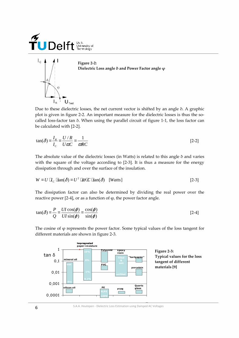
The cosine of ϕ represents the power factor. Some typical values of the loss tangent for
different materials are shown in figure 2-3.
Figure 2-3:
Typical values for the loss
tangent of different
materials [9]
0 ,0001
0,001
0,01
0,1
1
0 1 2 3 4 5
mineral oil
impregnated
paper+moisture
silicon oil PE
PVC
Polyamid Epoxy
resin
PTFE
Quartz
glass
porcelain
“hartpapier”
wet
dry
10%
0.1%
1%
6%
LDPE
XLPE
filled
&
wet
unfilled
tan δ
0 ,0001
0,001
0,01
0,1
1
0 1 2 3 4 5
mineral oil
impregnated
paper+moisture
silicon oil PE
PVC
Polyamid Epoxy
resin
PTFE
Quartz
glass
porcelain
“hartpapier”
wet
dry
10%
0.1%
1%
6%
LDPE
XLPE
filled
&
wet
unfilled
tan δ

7 S.A.A. Houtepen - Dielectric Loss Estimation using Damped AC Voltages
2.1.2 Origin
The resistive component in figure 2-1 can represent four kinds of losses, which are
described in detail in the following sections [1];
• Dipole losses
• Conduction losses
• Interface losses
• Partial discharges
2.1.2.1 Dipole losses
Every particle (e.g. atoms, molecules) in a material consists of positive and negative
charges. Under the influence of an electric field, these charges are slightly displaced
from each other (orientated), and are referred to as dipoles. The origination of dipoles
results in a so-called polarization of the dielectric.
Electric dipoles in an insulation material thus constantly reverse direction in an AC-field.
Because the dipoles do not lag the field vector at low frequencies, dipole losses mainly
occur at higher frequencies (from approximately 30 Hz upwards). When the frequency
increases, friction causes the dipoles to lag the field vector and give rise to losses. When
the frequency is increased even further, the dipoles can no longer follow, causing the
losses to decrease again.
Due to the fact that dipoles respond with a certain delay on changes in the electric field,
they lag the field vector by a certain angle. Therefore, the permittivity (dielectric
constant) of the material can be written as a complex number, consisting of a magnitude
and phase angle. The real part of the permittivity then represents the stored energy in
the material, and the complex part represents the dissipation of energy [2-5].
' "r r rjε ε ε= − [2-5]
In figure 2-4, the value of the imaginary and real part of the permittivity in a wide
frequency range is shown, whereby different polarization processes are visible.
Figure 2-4:
Permittivity as a function of frequency [2]

8 S.A.A. Houtepen - Dielectric Loss Estimation using Damped AC Voltages
The polarization processes are briefly described hereunder [3]:
Electronic Polarization
An atom consists of a nucleus with surrounding electrons. If an electric field is applied,
the electron density is displaced with respect to the nucleus, and a dipole is born. This
effect is extremely fast and can follow the electric field up to very high frequencies.
Atomic Polarization
When the applied field causes an electron cloud to deform, positive and negative
charges originate. As with electronic polarization, this dipole can follow up to high
frequencies.
Dipolar Polarization
This type of polarization results from permanent dipoles. These dipoles do not get
polarized further (the distance between the charges remains constant), but only rotate
when influenced by an electric field. Dipolar polarization is still a quite fast effect, which
can follow up to MHz to GHz.
Ionic Polarization
The process of ionic polarization occurs when positive and negative ions are displaced
from each other. This effect is rather slow, and will not follow up to high frequencies.
Interfacial Polarization
Another effect that is not shown in figure 2-4, is the so-called interfacial polarization.
This is the dominant process in insulating materials composed of multiple dielectric
materials (e.g. oil impregnated paper). Due to the mismatch in permittivity times
resistivity of both materials, positive and negative charges are deposited on the
interfaces when an electric field is applied and also form some kind of dipoles. This
process is extremely slow, and is only active in the power frequency range and below.
The resistance (figure 2-1) that represents the dipole losses equals [2-6], and the loss
tangent then becomes [2-7].
'
"r
polr
RC
εω ε
= [2-6]
"1tan
'r
polpol rR C
εδω ε
= = [2-7]
As can be expected, temperature is an important variable in this type of losses, because
with increasing temperature dipoles gain a higher mobility. With changing temperature,
the earlier discussed frequency spectrum will therefore change.
9 S.A.A. Houtepen - Dielectric Loss Estimation using Damped AC Voltages
2.1.2.2 Conductive losses
When the resistance of the dielectric is sufficiently low, the leakage current adds to the
dielectric losses. This increased conduction, caused by movement of free charge carriers,
can be represented by a conductivity σ. The resistance representation (figure 1-1) then
becomes [1-8], and the loss tangent is given by [1-9].
'
0 rConductivityR
C
ε εσ
⋅=⋅
[1-8]
'0
1tan cond
r conductivityR C
σδωε ε ω
= =⋅ ⋅
[1-9]
Since conduction is caused by a free movement of charge carriers, it is influenced by the
applied test voltage (and resulting electric field magnitude) and temperature (a higher
charge carrier mobility is gained at elevated temperatures). For this reason, it can further
be said that this type of losses mainly occurs at lower frequencies.
The total dielectric losses of an insulation material (healthy and with no interfaces) are
determined by the sum of the losses caused by conduction, and those caused by
polarization [1-10], [1-11].
tan( ) tan tancond polδ δ δ= + [1-10]
"
' '0
1 1 1tan( ) r
r r pol condR C R C RC
εσδωε ε ε ω ω ω
= + = + =⋅ ⋅ ⋅ ⋅
[1-11]
With,
pol cond
pol cond
R RR
R R
⋅=
+ [1-12]
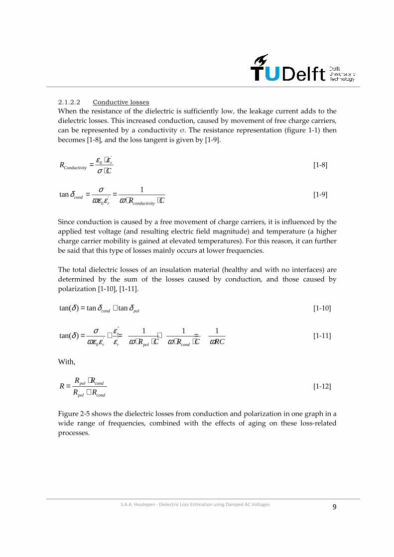
Figure 2-5 shows the dielectric losses from conduction and polarization in one graph in a
wide range of frequencies, combined with the effects of aging on these loss-related
processes.
10 S.A.A. Houtepen - Dielectric Loss Estimation using Damped AC Voltages
Figure 2-5:
Different loss-related processes in function of frequency with corresponding aging effects
At frequencies below 30 Hz, the conduction losses are the dominant process, whereas
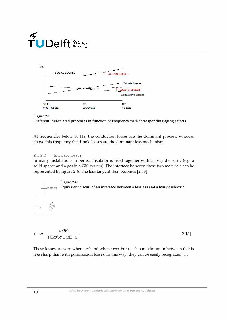
above this frequency the dipole losses are the dominant loss mechanism. 2.1.2.3 Interface losses
In many installations, a perfect insulator is used together with a lossy dielectric (e.g. a
solid spacer and a gas in a GIS system). The interface between these two materials can be
represented by figure 2-6. The loss tangent then becomes [2-13].
Figure 2-6:
Equivalent circuit of an interface between a lossless and a lossy dielectric
2 2tan
1 ( )
RK
R C K C
ωδω
=+ +
[2-13]
These losses are zero when ω=0 and when ω=∞, but reach a maximum in-between that is
less sharp than with polarization losses. In this way, they can be easily recognized [1].

11 S.A.A. Houtepen - Dielectric Loss Estimation using Damped AC Voltages
2.1.2.4 Discharge Losses
Besides polarization and conduction, also partial discharges cause an increase in the loss
tangent. In general, three types of PD (discharges that do not completely bridge the
distance between the electrodes) can be distinguished [1];
• Internal discharges
• Surface discharges
• Corona discharges
These partial discharges all start at a certain inception voltage (PDIV). At this voltage
level, a sudden increase of Δ tan δ occurs (see figure 2-7). Above this inception voltage
the dielectric losses start to grow rapidly. PD normally occurs when the voltage is
pushed far beyond the nominal value, or if the cable is in bad condition.
Figure 2-7: Increase in loss tangent above
inception voltage PD [9]
The number and magnitude of these discharges also has its effect on the dielectric losses,
since it results in a steeper rise of the loss tangent. To identify this type of losses, not the
frequency but the voltage should be varied. A result as given in figure 2-7 will appear.
12 S.A.A. Houtepen - Dielectric Loss Estimation using Damped AC Voltages
2.2 Aging of Insulation
Due to electrical, mechanical, thermal and environmental stresses, a dielectric ages in
time. During this process of aging, irreversible chemical changes occur within the
materials that have their influence on the dielectric properties (e.g. dielectric losses) and
dielectric strength. Because the dielectric loss parameter an important tool to determine
aging in oil impregnated insulation and epoxy-mica, both are described in detail
hereunder.
2.2.1 Oil-Impregnated Insulation
For many years, oil impregnated insulation was among the most widely used insulation
types in for example high-voltage cables. This generation of HV equipment, however,
gradually starts to suffer from aging as large numbers of installed components reach the
end of their lifetime expectancy. In this section, a detailed description is given on the
material properties of oil impregnated insulation.
2.2.1.1 Chemical Structure
On a microscopic scale, paper consists of cellulose molecules that are connected to each
other by oxygen atoms, and form so-called polymer chains. The chemical structure of
such a cellulose molecule is given in figure 2-8.
Figure 2-8: Two cellulose molecules, connected
by an oxygen atom
To create paper, the moistened cellulose is pressed together, and dried afterwards. This
process has to be done with great care, in order to obtain satisfying electrical properties.
It goes without saying that when sufficient water molecules remain in the paper, it can
be detrimental for the insulation capabilities.
Because of the porous structure of the paper (only 50 to 60 % of the volume consists of
cellulose), it is not suitable for practical applications when used alone. Not only pores
and free spaces originate in the paper during the production process, also the length of
the polymer chains is limited, and free spaces exist in-between (a measure for the length
of these chains is the Degree of Polymerization (DP)) [4].

13 S.A.A. Houtepen - Dielectric Loss Estimation using Damped AC Voltages
These available pores have the tendency to absorb fair amounts of moisture from the air
(up to 8 % of their own weight when stored). To make the paper applicable for practical
use, it is therefore impregnated with oil. Oil is chosen for its outstanding electrical,
chemical and mechanical properties [ 5 ]. Figure 2-9 shows the effects of poorly
impregnated cellulose on the dielectric loss tangent. It visualizes the importance of this
process.
Figure 2-9: Influence of poor impregnation on
the dielectric loss tangent [9]
When impregnated properly, the combination of paper impregnated with oil acts as a
good insulator. Still, paper is the major variable that determines the dielectric strength,
because of its thickness and the way it is layered. This can be explained as follows. The
permittivity of paper insulation is around 4.5, while the permittivity of oil is 2.2.
Therefore the field strength in the oil is twice the value occurring in paper. In fact, the
impulse breakdown strength in oil approaches the intrinsic breakdown value [10]. When
the paper layers are thicker, the oil gaps are increased in size, and an avalanche occurs
more easily.
Figure 2-10: Registration values of
paper-oil insulation [10]

14 S.A.A. Houtepen - Dielectric Loss Estimation using Damped AC Voltages
Secondly, the layering in itself is of importance. Layering is expressed in terms of
registration. The percentage registration determines the amount of which a layer is
shifted compared to its neighbors (e.g. 25 % registration means it has 75 % overlap with
the adjacent layers). Figure 2-10 shows two examples of registration values [10]. The
higher the registration, the more gaps are in line, and the lower the breakdown strength.
To reduce the stress on the insulation near the conductor at higher voltages, the inner
part of the paper layers are made thinner then the ones on the outer part [5].
It can further be said, that the combination of two materials also has its effect on the
polarization processes. These processes (of paper and oil) behave differently in each of
both materials. In insulation consisting of multiple layers, the dominant polarization
process is boundary polarization [6].
Finally, due to the fact that degradation of both materials in oil impregnated insulation
does influence each other, aging in most cases can be described by just one parameter,
the p-factor [7]. The lower this value is, the better the condition of the dielectric.

15 S.A.A. Houtepen - Dielectric Loss Estimation using Damped AC Voltages
2.2.1.2 Aging
Aging of insulation is a very complex process that constantly continues during the entire
service life. In table 2-1, an overview is presented on the acting age factors with
corresponding aging mechanisms [8].
Table 2-1: Aging mechanisms and their effects
As can be seen, some mechanisms are linked to each other (e.g. thermal stress causes
void formation, which will lead to PD and thus chemical byproducts in the voids).
Several factors can thus be responsible for the same aging process. For paper-
impregnated insulation, this therefore results in two main ways of aging that can be
distinguished; thermal and electrical [4] [8].
Ageing Factor Ageing Mechanisms Effects*
Thermal
High temperature Temperature cycling
-Chemical reaction -Incompatibility of materials -Thermal expansion (radial and axial) -Diffusion -Anneal locked -in mechanical stresses -Melting/flow of insulation
-Hardening, softening, loss of mechanical strength, embrittlement -Increase tan delta -Shrinkage, loss of adhesion, separation, delamination at interfaces -Swelling -Loss of liquids, gases -Conductor penetration -Rotation of cable -Formation of soft spots, wrinkles -Increase migration of components
Low temperature -Cracking -Thermal contraction
-Shrinkage, loss of adhesion, separation, delamination at interfaces -Loss/ingress of liquids, gases -Movement of joints, terminations
Electrical Voltage, ac, dc, Impulse
-Partial discharges (PD) -Electrical treeing (ET) -Water treeing (WT) -Dielectric losses and capacitance -Charge injection -Intrinsic breakdown
-Erosion of insulation→ET -PD -Increased losses and ET -Increased temperature, thermal ageing, thermal runaway -Immediate failure
Current -Overheating -Increased temperature, thermal ageing, thermal runaway
Mechanical Tensile, compressive, shear stresses, Fatigue, cyclic bending, vibration
-Yielding of materials -Cracking -Rupture
-Mechanical rupture -Loss of adhesion, separation, delamination at interfaces -Loss/ingress of liquids, gases
Environmental Water/humidity Liquids/gases Contamination
-Dielectric losses and capacitance -Electrical tracking -Water treeing -Corrosion
-Increased temperature, thermal ageing, thermal runaway -Increased losses and ET -Flashover
Radiation -Increase chemical reaction rate Hardening, softening, loss of mechanical strength, embrittlement
* The failure mechanism is usually electrical, e.g., by PD, ET or tracking
16 S.A.A. Houtepen - Dielectric Loss Estimation using Damped AC Voltages
Thermal Aging
At elevated temperatures, or if the component is overloaded, the insulation may not be
able to dissipate all the energy that is generated in the conductor. Due to this increased
temperature, the cellulose polymeric chains break and chemical byproducts arise, such
as H2O, CO and CO2 [4]. The result will be a lower Degree of Polymerization (DP), as
introduced earlier. This type of degradation is referred to as thermal aging.
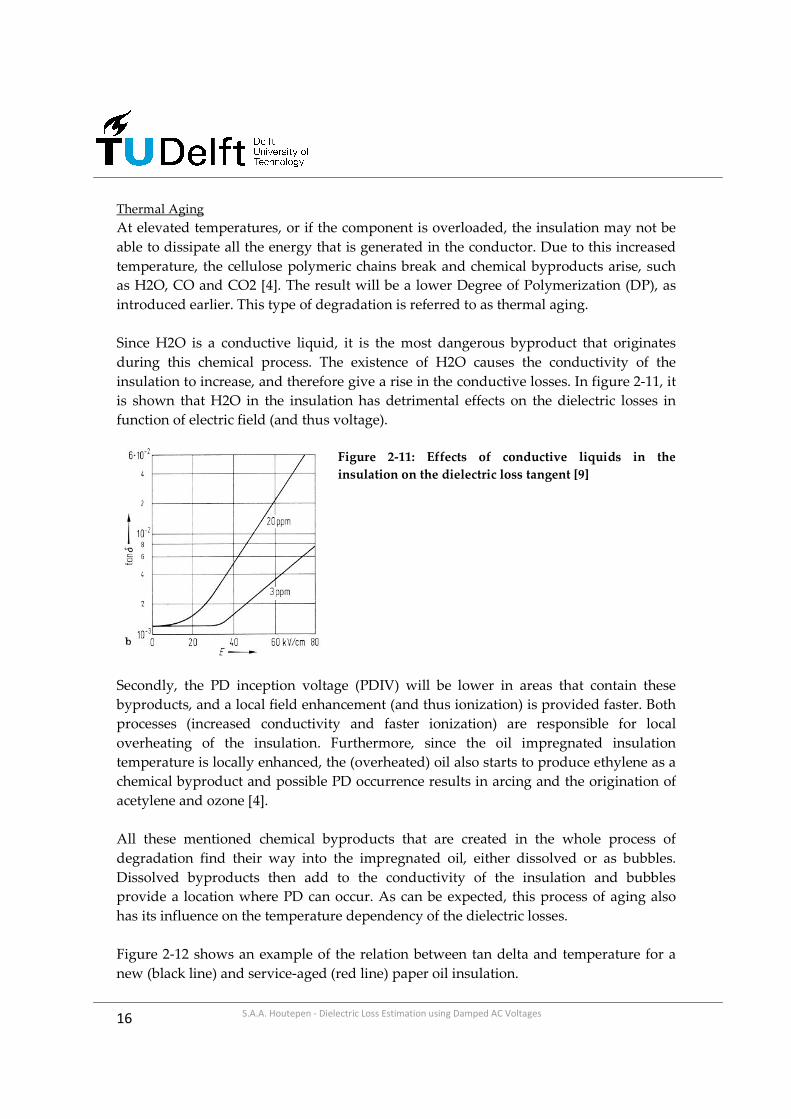
Since H2O is a conductive liquid, it is the most dangerous byproduct that originates
during this chemical process. The existence of H2O causes the conductivity of the
insulation to increase, and therefore give a rise in the conductive losses. In figure 2-11, it
is shown that H2O in the insulation has detrimental effects on the dielectric losses in
function of electric field (and thus voltage).
Figure 2-11: Effects of conductive liquids in the
insulation on the dielectric loss tangent [9]
Secondly, the PD inception voltage (PDIV) will be lower in areas that contain these
byproducts, and a local field enhancement (and thus ionization) is provided faster. Both
processes (increased conductivity and faster ionization) are responsible for local
overheating of the insulation. Furthermore, since the oil impregnated insulation
temperature is locally enhanced, the (overheated) oil also starts to produce ethylene as a
chemical byproduct and possible PD occurrence results in arcing and the origination of
acetylene and ozone [4].
All these mentioned chemical byproducts that are created in the whole process of
degradation find their way into the impregnated oil, either dissolved or as bubbles.
Dissolved byproducts then add to the conductivity of the insulation and bubbles
provide a location where PD can occur. As can be expected, this process of aging also
has its influence on the temperature dependency of the dielectric losses.
Figure 2-12 shows an example of the relation between tan delta and temperature for a
new (black line) and service-aged (red line) paper oil insulation.

17 S.A.A. Houtepen - Dielectric Loss Estimation using Damped AC Voltages
Figure 2-12: Temperature dependency of the
loss tangent for new and service aged
insulation [9]
As can be seen from the new insulation, the loss tangent slightly increases when the
temperature rises. This phenomenon can be described by a decrease in the viscosity of
the oil. This makes it easier for charge carriers to move. Because the insulation is still
new, the number of pores and free spaces is limited, so no high increase is observed.
When the aged insulation is subjected to elevated temperatures, decomposition of the
cellulose structure occurs (as described earlier). The byproducts that originate create
more free spaces where field enhancement (and local hot spots) will originate. Due to
this decomposition, and the creation of more free spaces, there are more locations
available where free charge carriers can move. At elevated temperatures, when the
viscosity of the oil is lower, this causes the dielectric losses to increase rapidly.
When this process starts to amplify itself, a so-called thermal runaway occurs, which
leads to breakdown. Combined with that, the eventual rise in temperature also causes a
smaller part of the admissible temperature rise to be available for ohmic losses in e.g. a
cable, reducing its current-carrying capacity and, secondly, costs an appreciable amount
of money [1].
Electrical Aging
If the electric field inside the insulation overstresses the material, the present impurities
and contamination will become weak spots and gas-filled cavities can arise due to local
field enhancement and partial discharges.
Inside these cavities the PD activity continues, which results in a severe erosion of the
walls, and the origination of chemical byproducts as acetylene and ozone. Due to the
rough structure of the walls of the cavities and the originated local field enhancement,
so-called preferential areas are formed where the deterioration is more severe then in
other places [10].
tand=f(T) E=const (~2,51kV/mm)
0
20
40
60
80
100
120
140
20 35 50 60 70 75 80
T [C]
tand
[10
^-4
]
sample of insulation from red phaseNon-aged paper

18 S.A.A. Houtepen - Dielectric Loss Estimation using Damped AC Voltages
In the stages that follow (figure 2-13), local discharges in the preferential area will result
in so-called pitting. This formation of a pit causes the breakdown strength of the
insulation material to decrease because of the local degradation of the dielectric material.
When the breakdown strength then falls below the existing field strength, treeing is
initiated.
Figure 2-13: Types of defects [1]
With the layered structure of oil impregnated insulation, and the (earlier discussed)
higher field strength in the oil, it is clear that treeing occurs more easily in a radial
direction (parallel to the conductor and paper-layers) [10]. As treeing is finally initiated,
breakdown can occur very rapidly; between minutes to several hours.
This process of electrical aging causes the dielectric losses to increase in function of
voltage, as shown in figure 2-14. This figure shows the dielectric losses for a new (black
line) and service aged (red line). When concerning the new insulation, the slight increase
in dielectric losses with rising voltage is caused by the porous structure of the paper
insulation. In these oil-filled cavities, local field enhancements occur. As with
temperature, due to the limited amount of these pores, only a small rise is visible. In the
aged situation, the discharges inside the cavities are responsible for the rise in the
dielectric losses. The magnitudes intensify with increasing voltage.
Figure 2-14: Influence of electrical aging
on the dielectric losses of paper-oil
insulation [9]
tand=f(E) (T=80 C)
0
20
40
60
80
100
120
140
0 0,5 1 1,5 2 2,5 3
E [kV/mm]
tand
[10^
-4]
red phase
brand-new paper

19 S.A.A. Houtepen - Dielectric Loss Estimation using Damped AC Voltages
Finally, due to the change in chemical structure, the frequency dependency of the loss
tangent changes over time.
Since the chemical structure of the insulation material changes with deterioration, also
the active polarization process shift in the frequency domain. Furthermore, at lower
frequencies the loss tangent increases due to increased conductivity, caused by chemical
byproducts. This process is clearly visible at frequencies below 1 Hz. A well known
method to examine the insulation condition with the use of frequency dependency is
dielectric spectroscopy [11] [12] [13]. This method is described further in paragraph 2-3.
When examining deterioration of paper oil insulation, it is clear that not only tan δ is an
important parameter, but also Δ tan δ or tip-up (increase in the loss tangent as a function
of temperature / voltage). In order to avoid a resulting outage and reduction in
reliability of the power supply, condition monitoring on-site is of great importance.
Dielectric loss measurement is a perfect tool to investigate the current state of the
insulation, and periodically measured data can be used to see whether things have
worsened in time.
2.2.2 Epoxy-Mica Insulation
Insulation of stator windings suffers from gradual deterioration in time under combined
electrical, thermal, mechanical and environmental stresses. The resin impregnated mica
tape insulation used in electrical machines is a perfect insulator; compared to other
materials it has a high thermal conductivity which makes it ideal for application in
electrical machines. Generally, mica based insulation does not fail due to general aging
but due to deterioration of very small defects in the insulation system itself [14].
In this section, the most frequently encountered types of defects are covered, followed
by the deterioration process in epoxy-mica insulation from electrical machines.
2.2.2.1 Insulation structure [14]
The insulation of a stator can be subdivided into two sections;
• Bar-section: contains all the stator bars
• End-winding: contains the connections between the bars
Since the electric field strength is at its highest in these bar sections, this is the most
interesting part for high-voltage engineering. This however does not mean that no PD
occurs at the end-windings; only the probability will be much lower.
20 S.A.A. Houtepen - Dielectric Loss Estimation using Damped AC Voltages
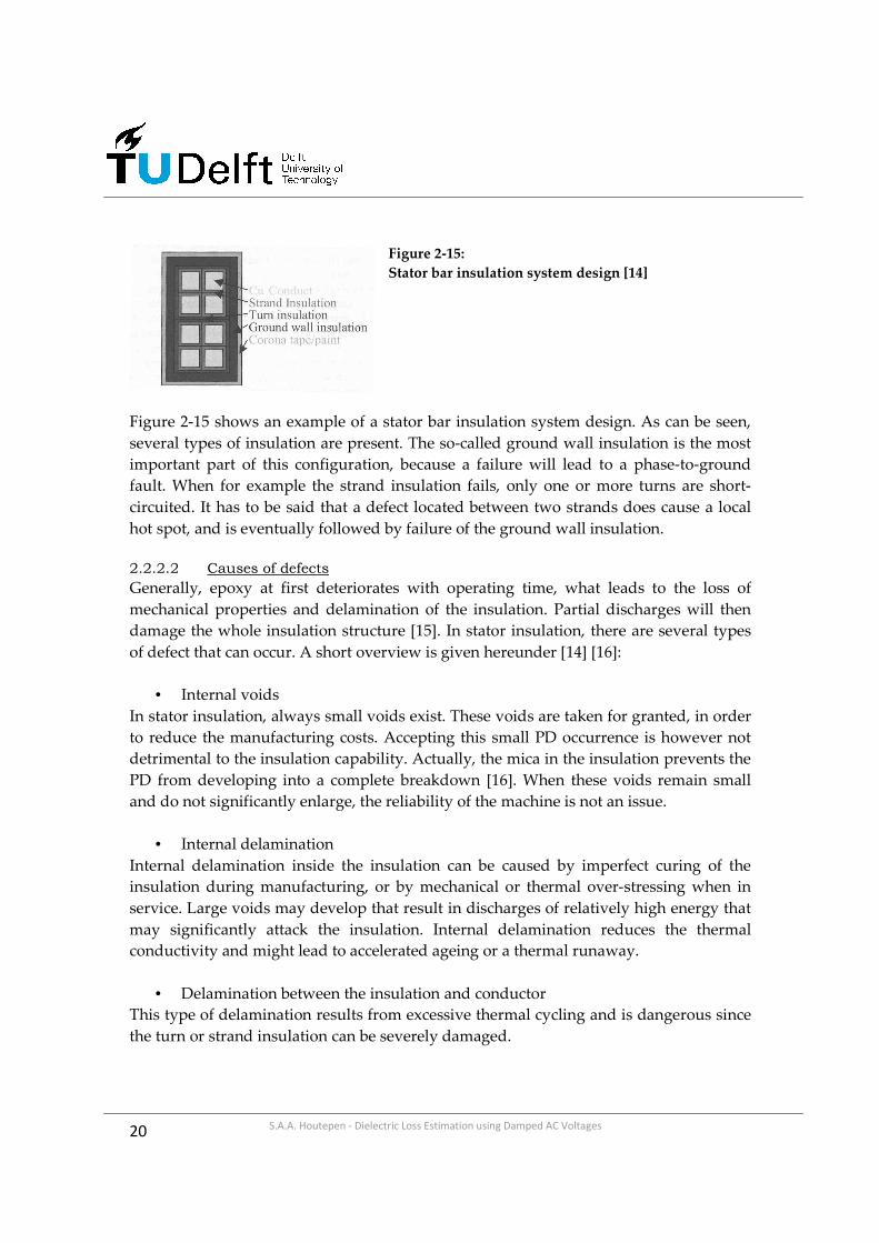
Figure 2-15:
Stator bar insulation system design [14]
Figure 2-15 shows an example of a stator bar insulation system design. As can be seen,
several types of insulation are present. The so-called ground wall insulation is the most
important part of this configuration, because a failure will lead to a phase-to-ground
fault. When for example the strand insulation fails, only one or more turns are short-
circuited. It has to be said that a defect located between two strands does cause a local
hot spot, and is eventually followed by failure of the ground wall insulation.
2.2.2.2 Causes of defects
Generally, epoxy at first deteriorates with operating time, what leads to the loss of
mechanical properties and delamination of the insulation. Partial discharges will then
damage the whole insulation structure [15]. In stator insulation, there are several types
of defect that can occur. A short overview is given hereunder [14] [16]:
• Internal voids
In stator insulation, always small voids exist. These voids are taken for granted, in order
to reduce the manufacturing costs. Accepting this small PD occurrence is however not
detrimental to the insulation capability. Actually, the mica in the insulation prevents the
PD from developing into a complete breakdown [16]. When these voids remain small
and do not significantly enlarge, the reliability of the machine is not an issue.
• Internal delamination
Internal delamination inside the insulation can be caused by imperfect curing of the
insulation during manufacturing, or by mechanical or thermal over-stressing when in
service. Large voids may develop that result in discharges of relatively high energy that
may significantly attack the insulation. Internal delamination reduces the thermal
conductivity and might lead to accelerated ageing or a thermal runaway.
• Delamination between the insulation and conductor
This type of delamination results from excessive thermal cycling and is dangerous since
the turn or strand insulation can be severely damaged.

21 S.A.A. Houtepen - Dielectric Loss Estimation using Damped AC Voltages
• Slot discharges
Slot discharges originate when the present coating on the conductive slots is damaged
due to bar or coil movement in the slot area. This can happen due to for example erosion
of the material, chemical attacks or manufacturing deficiencies. High-energy discharges
will develop when serious mechanical damage is already present, which may result in
additional damage to the main insulation.
• Surface discharges at end-windings
If the coating on one of the end-windings suffers from poorly designed interfaces,
contamination, porosity, local heating, these types of discharges can originate. PD near
the end-windings will normally occur at locations with local field enhancements.
• Conductive particles
Finally, small conductive particles in the insulation may result in a strong local
concentration of PD activity.
2.2.2.3 Deterioration
Stator insulation normally fails due to the deterioration process of small defects within
the material. This process that is related to the magnitude of the PD occurrence is
unfortunately not well understood [17]. In the process of deterioration, the magnitude of
the partial discharges shows an upward slope, but with a certain decrease every now
and then (saw tooth) [14]. A picture of this process is given in figure 2-16.
Figure 2-16: Stepwise aging of stator bar
insulation [14]
In [14], a model is represented that describes this process. In that model, it is assumed
that the electric tree starts from the void, but does not grow at a constant rate. When a
tree reaches a barrier (e.g. a mica-flake) it will take an appreciable amount of time to get
around it.
In the process that goes from a virgin cavity to an electric tree, the surface of the material
is deteriorated. This surface will then become more conductive, what leads to a lower
measured PD magnitude. After a certain time instant, treeing starts to develop and the

22 S.A.A. Houtepen - Dielectric Loss Estimation using Damped AC Voltages
measured magnitude increases again. The repetition of this process can explain the
phenomena shown in figure 2-16.
Figure 2-17: Increasing gradient shows
the aging process [14]
For condition assessment, it goes without saying that this is not a preferred process. A
method to determine the current state of the insulation is the voltage dependency of the
PD level [14]. In figure 2-17, this relationship is shown. As the gradient of this line
further increases, the aging process proceeds gradually.
2.2.2.4 Effects on tan δ
Aging in epoxy-mica insulation is caused by partial discharges that deteriorate the
insulation. If many discharge sites are present at a certain moment, dielectric loss
measurement can be a valuable tool.
Figure 2-18 shows the behavior of the loss tangent, as a function of voltage. It shows that
from the so-called inception voltage upwards (where PD starts), the gradient of this tan
delta is much higher.
Figure 2-18: Increase in loss tangent above inception
voltage PD
Since the sensitivity of this process is increased with increasing number of discharges, it
will be very useful in the examination of partial discharges in machine insulation where
thousands of discharges will occur simultaneously [1].

23 S.A.A. Houtepen - Dielectric Loss Estimation using Damped AC Voltages
2.3 Measurement Techniques
During service conditions, high-voltage equipment suffers from aging due to electrical,
thermal, environmental and mechanical stresses. These stresses will eventually cause the
component to fail. In order to predict whether a cable has reached the end of its lifetime,
on-site diagnosis is required. In fact, on-site diagnosis is becoming the most important
non-destructive test method for HV assets e.g. cables [23].
In this chapter, several measurement techniques for determining the condition of the
insulation and the measurement of the loss tangent are analyzed.
The major techniques in use for condition assessment and dielectric loss measurement
are described hereunder, arranged by method of energizing the test object.
2.3.1 Continuous Energizing
2.3.1.1 Very Low Frequency Analysis
Energizing and testing component with a high capacitance (e.g. long cables) at an AC
overvoltage demands reactive power of several MVA (which can impossibly be supplied
by mobile installations). Therefore alternative methods are studied that are lightweight,
requesting low power and are easy to transport [1]. For years, such a test object was charged with DC, but of course the physical phenomena
differ from AC. One of these phenomena is the origination of space charges [10]. To
avoid these DC related phenomena, nowadays VLF (Very Low Frequency) and DAC are
among the used methods. VLF tests are performed with a frequency of approximately
0.1 Hz. This means that 500 times less reactive power (in case of 50 Hz) has to be
supplied to the cable, and it is stressed with AC like in service.
Detection of defects with VLF can be done at a lower voltage level then with DC.
Because of the low dU/dt of the VLF wave, treeing starts very slowly. Once it is started,
however, it grows more rapidly than with a 50 Hz voltage. Therefore the applied VLF
magnitude must exceed the service stress several times for identification of harmful
insulation imperfections and the test time must be extended to an hour or longer [18,19].

24 S.A.A. Houtepen - Dielectric Loss Estimation using Damped AC Voltages
2.3.1.2 The Schering Bridge
A major technique to measure a small value like tan δ on a continuously energized cable
is with a bridge circuit. A high voltage is applied to one diagonal of the bridge and a
sensitive null detector is connected to the other diagonal as shown in Figure 2-19.
Figure 2-19: A Schering-bridge
The impedances are then adjusted in such a way, that the null detector indicates zero
voltage. This is achieved when 1 3 2 4: :Z Z Z Z= . The unknown Z1 can then be determined
using the other three values. The practical setup is given in Figure 2-20.
Figure 2-20: Practical setup of a Schering-bridge
Here Cn is a standard capacitor (with guard electrodes to avoid edge effects; a method
for shielding of cable samples is presented in [20]) and Cx is the test object. When this
bridge is balanced, the loss tangent can be obtained using [2-14].
4 4tan( ) R Cδ ω= [2-14]

25 S.A.A. Houtepen - Dielectric Loss Estimation using Damped AC Voltages
There are several variants of the Schering Bridge possible [1]:
• The sheaths from the coax cables that connect the high voltage bay to the bridge
terminals can be brought on the same potential as the terminals itself. This is
done to reduce the effect of stray capacitances.
• The bridge terminals can be brought to earth potential. This is done by bringing
terminal D (earthed terminal in Figure) to a potential opposite of terminal B.
• At permanently earthed objects, the bridge principle can be reversed (earth and
high potential exchanged). This means the operator has to work on high
potential. This can be done by remote control or using a faraday cage that can
accommodate an operator.
• For tests with unskilled operators, a differential transformer can be used instead
of the usual low-voltage arm. By changing the ratios of the primary and
secondary winding (using dials), the value of the capacitance and loss factor can
be read instantaneously.
Finally, to check whether all stray capacitances are eliminated, [1] introduces the so-
called dual balance method. By testing twice, with two different values of R3, the
measurement errors and stray capacitances that influence the loss tangent can be
determined and eliminated.
2.3.1.3 Dielectric Spectroscopy
Spectroscopy is a non-destructive method in which the dielectric condition is assessed in
the frequency domain. Its principle consists on the measurement of the frequency
response of both permanent and induced dipoles to the application of an external
electric field. Aging causes a change in the dielectric response in the frequency domain
and thus a change in the complex permittivity [11].
Figure 2-21: Frequency representation of the
dielectric losses

26 S.A.A. Houtepen - Dielectric Loss Estimation using Damped AC Voltages
Water ingress and temperature increase for example, cause a higher DC conductivity, a
higher dielectric loss factor at low frequencies and a shift of the dielectric loss minimum
towards higher frequencies [12]. This is illustrated in figure 2-21.
Measurement is done by a sinusoidal AC voltage, which is generated in a certain
frequency range (e.g. 0.0001 – 10 Hz). The resulting current through the insulation is
measured when the voltage is applied, then giving the complex impedance (capacitance,
permittivity, loss tangent etc.) of the insulation [13].
2.3.2 Temporarily Energizing 2.3.2.1 Return Voltage Measurement
Return Voltage Measurement (RVM) is a non-destructive diagnostic test to determine
the insulation condition. RVM is widely used for the examination of degradation in for
example paper-oil cables. It works on the principle of charge displacement in the
dielectric due to electrical (de)polarization. The principle is described hereunder.
A DC voltage is applied on the test object for approximately 15 minutes, in order to load
it and cause charge accumulation. It is then short-circuited via an internal discharge
resistor for a few seconds. If the short-circuit is cleared, a build up of a so-called return
voltage occurs due to depolarization. This return voltage is very useful, because it is less
sensitive to noise then other methods [21]. An example of a measurement result is given
in figure 2-22.
Figure 2-22: Return Voltage Characteristics of paper-oil
cables
The shape of the curve (rise time, maximum voltage and relaxation time) gives
information on the condition of the dielectric material. In general, aged cables are
responsible for a steeper rise of the voltage curve. This effect is caused by degradation
products that lead to additional conduction and polarization processes in the range of a
few 10’s of seconds [21].

27 S.A.A. Houtepen - Dielectric Loss Estimation using Damped AC Voltages
Another change of the RVM curve is due to temperature, which also creates a shifted
characteristic of the return voltage measurement [22].
Figure 2-23: RVM Measurement Circuit
This RVM curve can be determined mathematically using a Maxwell equivalent circuit
[6]. A picture of the measurement circuit for a paper-oil cable is given in figure 2-23.
2 1( ) ( )t t
r sU t U e eτ τ− −
= − [2-15]
With formula [2-15], the return voltage curve can be calculated. Here the time constants
τ are given by R1C1 and R2C2 respectively. The voltage Us is the voltage across the RC-
elements after releasing the short circuit. The time constants do not change with the
length of a cable, because capacitance increases and resistance decreases as a function of
length [21].
2.3.2.2 Damped AC
The damped AC method makes use of a linear charging current, after which the
capacitive component oscillates with an air core inductor, and therefore no reactive
power is necessary. This is an important factor, because it drastically reduces the size of
the test equipment.
Figure 2-24: The Oscillating Wave
Test System (OWTS)

28 S.A.A. Houtepen - Dielectric Loss Estimation using Damped AC Voltages
A system that uses DAC voltages to detect PD and measure dielectric losses is the
Oscillating Wave Test System® (OWTS). A schematic overview of this system is given in
figure 2-24.
For the generation of DAC voltages, a capacitive load (the test object) is first charged
with a DC power supply. After charging, the capacitive load is directly switched in
series with an external inductor [23]. The resulting graph of this process is given in
figure 2-25.
Figure 2-25: Charging and
oscillation of a DAC voltage
wave; the attenuation is a
measure for the dielectric
losses
The originated voltage wave can be simply described by formula 2-16. Here, the
attenuation coefficient β is responsible for the decay of the wave and therefore a
measure for the dielectric losses in the test object.
)sin()( ϕωβ +⋅= ⋅− tetU t [2-16]
A complete mathematical relation between the attenuation coefficient and the dielectric
loss tangent is derived in the next chapter.

29 S.A.A. Houtepen - Dielectric Loss Estimation using Damped AC Voltages
Frequency Variation during Condition Assessment
In practical applications, the losses are often measured around 0.1 Hz (VLF), 50 Hz (grid
frequency) or several hundreds of Hz (DAC). Since it is shown earlier that these losses
are frequency dependent, it is of interest whether it makes sense to measure losses at a
different frequency then the one normally applied in the grid.
In practice, when a healthy dielectric is taken, the conductivity is very low. It is
furthermore noticeable, that the dielectric constant (real and imaginary part) is however
slowly declining in theory, but will be more or less stable (up to 1 kHz) in reality (due to
the overlay of all processes).
Below, two examples that compare damped AC with 50 Hz testing are given. In figure 2-
25, results from two measurements are given, that are performed with the use of DAC
(high frequency) and AC (50 Hz). It can be seen, that dielectric loss measurement using
damped AC voltages is a very useful tool that gives reliable results when compared to a
measurement performed at 50 Hz.
Figure 2-25: an example of two measurements, both performed with DAC and AC
It is thus definitely sensible to measure at a frequency that differs from the one used in
the power grid, in order to obtain a clear picture on the condition of the dielectric.

30 S.A.A. Houtepen - Dielectric Loss Estimation using Damped AC Voltages
31 S.A.A. Houtepen - Dielectric Loss Estimation using Damped AC Voltages
3. DAMPED AC VOLTAGES
3.1 Principle of Electrical Resonance
An inductor and a capacitor are well known energy storage elements in Electrical
Engineering. An inductor stores its energy in the induced magnetic field, a capacitor in
the electric field between the electrodes.
If the inductor and capacitor are connected to form an electric circuit, it is called an LC
network (or RLC in case a resistance is present). Because the voltage (series circuit) and
current (parallel circuit) can be described by a second order differential equation, the
network is said to be of second order.
The storage elements can be described in terms of a frequency dependent reactance [3-1],
[3-2].
2LX fLπ= [3-1]
1
2cXfCπ
= [3-2]
When these reactances are equal, a so-called resonance occurs. A repeating exchange
between the stored energy in the magnetic field [3-3] and the stored energy in the
electric field [3-4] of respectively the inductor and capacitor cause the voltage and
current to oscillate.
21
2LW Li= [3-3]
21
2CW Cv= [3-4]
The frequency of oscillation is the resonance frequency, and can be derived from [3-5].
0
1
2L CX X f
LCπ= ⇒ = [3-5]

32 S.A.A. Houtepen - Dielectric Loss Estimation using Damped AC Voltages
3.1.1 Modelling a series RLC-circuit
3.1.1.1 Mathematical Derivation
This section is devoted to the modelling of a standard series RLC circuit. Figure 3-1
shows the representation of a series RLC-network, without a driving voltage (passive)
included.
Figure 3-1: A model of a series RLC circuit, where L
is the inductance in Henry’s, R equals the resistance
in Ohms and C represents the capacitance in Farad.
Kirchhoff’s voltage law states, that the sum of all voltages in a loop of an electric circuit
equals zero [3-6]. With this information, a differential equation for this network can be
derived [3-7]. This derivation hereunder, which is generally known, is given in a wide
variety of literature, among others [24] [25] [26],
0L R CV V V+ + = [3-6]
This equation can be written as
2
2
2
2
1
1
10
tdiL Ri i dt
dt C
d Q dQL R Q
dt dt C
d Q R dQQ
dt L dt LC
−∞
+ + =
+ + =
+ + =
∫
[3-7]
with current defined as the derivative of charge Q [3-8].
dQi
dt= [3-8]

33 S.A.A. Houtepen - Dielectric Loss Estimation using Damped AC Voltages
To solve the derived differential equation, it can be written in terms of a so-called
characteristic equation [3-9].
2
2 20 0
1
2 0
R
L LCλ λ
λ ζω λ ω
+ + =
+ + = [3-9]
The roots of this equation can be calculated using the quadratic equation [3-10], [3-11].
2 4
2
b b acx
a
− ± −= [3-10]
2 2 2 2
0 0 0 20 0
2 (2 41
2x
ζω ζ ω ωω ζ ω ζ
− ± −= = − ± − [3-11]
This variable ζ is called the damping ratio. When this ζ is between 0 and 1, the system
has complex poles ( ( )20 0 1jω ζ ω ζ− ± − , and is so-called under-damped. This means
an oscillation occurs which gradually diminishes.
Since 1j = − , the solution x can also be written as: 20 0 1x ω ζ ω ζ= − ± − .
The solution of the differential equation then becomes (using Euler’s Formula),
0 2 20 0( ) {cos( 1 ) sin( 1 )}
( ) {cos( ) sin( )}
t
tD D
X t e t t
X t e t t
ω ζ
β
ω ζ θ ω ζ θ
ω θ ω θ
−
−
= − + + − + =
= + + + [3-12]
Or, written as a function of voltage across the test object,
( ) {cos( ) sin( )}tD DU t e t tβ ω θ ω θ−= + + + [3-13]
A more detailed derivation of formulas [3-9] to [3-12] can be found in literature.

34 S.A.A. Houtepen - Dielectric Loss Estimation using Damped AC Voltages
3.1.1.2 Attenuation β and Quality factor Q
As can be seen in formula [3-13], the system oscillates and is damped exponentially. The
speed of this exponential damping is determined by the attenuation β, which is the
product of the damping factor ζ and the resonance frequency ω0. For a series circuit, the
attenuation is determined by [3-14].
2LR
Lβ = [3-14]
The quality factor Q of a series resonant circuit is the ratio of the energy stored to the
energy lost in equal intervals of time [26]. The higher the quality factor is, the longer it
takes for the oscillation to vanish. The quality factor equals [3-15].
2Energy Stored
QEnergy dissipated per cycle
π= ⋅ [3-15]
The energy stored in a resonant circuit is represented by [3-3], whereas the energy lost
per cycle is given in terms of [3-16].
2 2
0
1 1 1
2 2RW I R T I Rf
= ⋅ =
[3-16]
The quality factor for a series resonant circuit then becomes,
1 1tan
tanCL XX L
QR R R C
ϕδ
= = = = = [3-17]
The angle ϕ represents the power factor angle and, as seen in [3-17], the quality factor is
thus the reciprocal of the dielectric loss tangent. Furthermore, the square root of L/C is
known as the characteristic impedance of the circuit.
35 S.A.A. Houtepen - Dielectric Loss Estimation using Damped AC Voltages
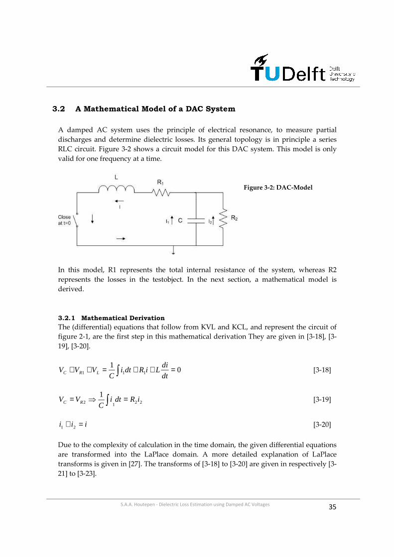
3.2 A Mathematical Model of a DAC System
A damped AC system uses the principle of electrical resonance, to measure partial
discharges and determine dielectric losses. Its general topology is in principle a series
RLC circuit. Figure 3-2 shows a circuit model for this DAC system. This model is only
valid for one frequency at a time.
Figure 3-2: DAC-Model
In this model, R1 represents the total internal resistance of the system, whereas R2
represents the losses in the testobject. In the next section, a mathematical model is
derived.
3.2.1 Mathematical Derivation
The (differential) equations that follow from KVL and KCL, and represent the circuit of
figure 2-1, are the first step in this mathematical derivation They are given in [3-18], [3-
19], [3-20].
01
111 =++=++ ∫ dt
diLiRdti
CVVV LRC [3-18]
2212
1iRdti
CVV RC =⇒= ∫ [3-19]
iii =+ 21 [3-20]
Due to the complexity of calculation in the time domain, the given differential equations
are transformed into the LaPlace domain. A more detailed explanation of LaPlace
transforms is given in [27]. The transforms of [3-18] to [3-20] are given in respectively [3-
21] to [3-23].
36 S.A.A. Houtepen - Dielectric Loss Estimation using Damped AC Voltages
0)()()(
101 =+++ ssLIsIR
s
U
sC
sI [3-21]
2
0
2
1222
01 )()()(
)(
sR
U
CsR
sIsIsIR
s
U
sC
sI+=⇒=+ [3-22]
)()(1
1)()()(2
01
221 sI
sR
UsI
CsRsIsIsI =+
+⇒=+ [3-23]
Where U0 is the voltage on the test object at t=0. Equation [3-23] is then rewritten as a
function of I1(s) [3-24], and is filled into equation [3-21]. The result is given in [3-25].
CsRsR
U
CsR
sIsI
2
2
0
2
1 11
11
1
)()(
+⋅−
+= [3-24]
0)()(1
1
111
1
)(11
0
2
2
0
2
=++++
⋅⋅−+
⋅ ssLIsIRs
U
CsRsR
U
sCCsR
sI
sC [3-25]
In the resulting LaPlacian equation [3-25], I(s) is the only variable that is still depending
on s. This current is worked out of the equation, and the result is given in [3-26].
+−⋅=
+++++⋅
11
)()()(
2
20
2
212122
sCR
CRU
sCR
RRRCRLsLCRssI [3-26]
The current then becomes,
++
++
−
⋅=
LCR
RRs
LCR
RCRLs
LCR
CR
UsI
2
21
2
212
2
2
0)( [3-27]
Since ( )sLRsIsU +⋅−= 1)()( , the voltage across the capacitor (and neighbouring
resistor) can be written as [3-28].
37 S.A.A. Houtepen - Dielectric Loss Estimation using Damped AC Voltages
++
++
+=
LCR
RRs
LCR
CRRLs
L
Rs
UsU
2
21
2
212
1
0)( [3-28]
To obtain the inverse LaPlace transform, the LaPlace integral has to be solved [27]. Due
to the complexity of this operation a table of standard transformations, which have been
derived in history, is often used to obtain the time-domain representations [27]. Instead
of solving an astonishing integral, it now suffices to rewrite the formula into a “familiar”
shape and rewrite it into the time-domain counterpart. This is done in [3-29] to [3-36].
( )
+++=
220)(ωβ
αs
sUsU [3-29]
With,
L
R1=α [3-30]
+=
LCR
CRRL
2
21
2
1β [3-31]
2
1 2 1 2
2 2
1
2
R R L R R C
R LC R LCω
+ += −
[3-32]
Formula [3-15] then approaches
( ) ( )2 2
0ω ω β= − [3-33]
The inverse LaPlace transform of [3-29] appears to be [3-34], [3-36],
)sin()(
)(22
0 ϕωω
ωβα α +⋅⋅+−
= − teUtU t [3-34]
With,
−=
βαωϕ arctan [3-35]

38 S.A.A. Houtepen - Dielectric Loss Estimation using Damped AC Voltages
Formula [3-34] equals [3-36] and shows therefore great similarities with [3-13].
0( ) cos( ) sin( )tU t U e t tβ α βω ωω
− − = ⋅ +
[3-36]
Finally, the loss tangent has to be determined. This will be done by rewriting [3-31] into
[3-37], and use this value for R2 to determine tan δ [3-38]. R1 is obtained by a calibration
of the system (chapter 5).
CRLC
LR
12 2 −
=β
[3-37]
CR2
1)tan(
ωδ = [3-38]
The attenuation factor β is determined from the measurement results. Due to the
exponential damping, the value of an arbitrary peak can be calculated [3-39].
xt
x eU β−= [3-39]
By using two peaks (e.g. peak 1 and 2), the attenuation can be calculated [3-40].
)(
ln
12
1
2
)(
1
2 12
tt
U
U
eU
U tt
−
−=⇒= −− ββ [3-40]
This model focuses on one single internal resistance. As can be seen, this model is easy
to handle and gives a good representation of the system. In the next paragraph a more
detailed model is derived, in order to see the differences between an easy and detailed
model, and to verify which of both models is most suitable for use.
39 S.A.A. Houtepen - Dielectric Loss Estimation using Damped AC Voltages
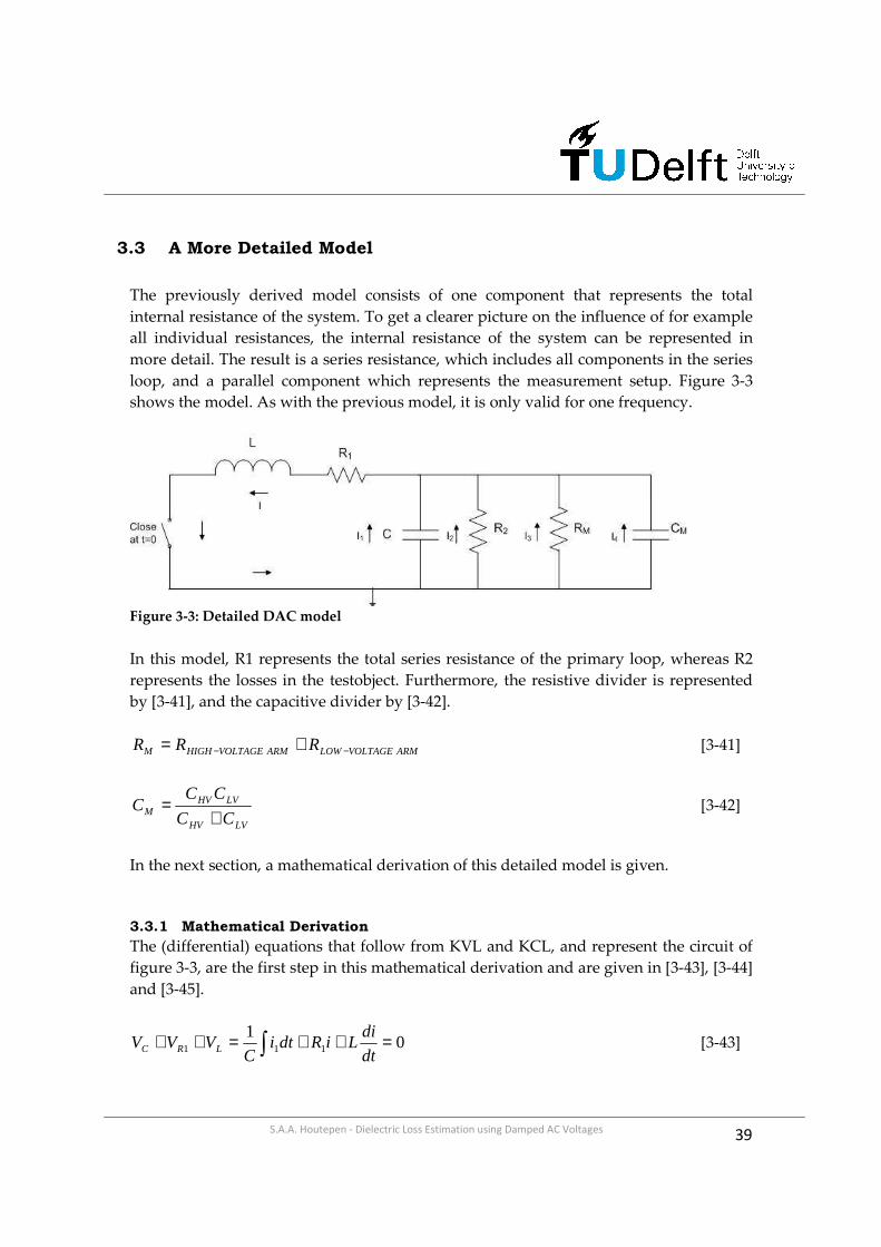
3.3 A More Detailed Model
The previously derived model consists of one component that represents the total
internal resistance of the system. To get a clearer picture on the influence of for example
all individual resistances, the internal resistance of the system can be represented in
more detail. The result is a series resistance, which includes all components in the series
loop, and a parallel component which represents the measurement setup. Figure 3-3
shows the model. As with the previous model, it is only valid for one frequency.
Figure 3-3: Detailed DAC model
In this model, R1 represents the total series resistance of the primary loop, whereas R2
represents the losses in the testobject. Furthermore, the resistive divider is represented
by [3-41], and the capacitive divider by [3-42].
ARMVOLTAGELOWARMVOLTAGEHIGHM RRR −− += [3-41]
LVHV
LVHVM CC
CCC
+= [3-42]
In the next section, a mathematical derivation of this detailed model is given.
3.3.1 Mathematical Derivation
The (differential) equations that follow from KVL and KCL, and represent the circuit of
figure 3-3, are the first step in this mathematical derivation and are given in [3-43], [3-44]
and [3-45].
01
111 =++=++ ∫ dt
diLiRdti
CVVV LRC [3-43]

40 S.A.A. Houtepen - Dielectric Loss Estimation using Damped AC Voltages
2 2 2 31 4
1 1C R RM CM M
M
V V V V i dt R i R i i dtC C
= = = ⇒ = = =∫ ∫ [3-44]
1 2 3 4i i i i i+ + + = [3-45]
Similar to the previous derivation, equations [3-43] to [3-45] are transformed into the
Laplace domain and are given in respectively [3-46] to [3-50].
0)()()(
101 =+++ ssLIsIR
s
U
sC
sI [3-46]
2
0
2
1222
01 )()()(
)(
sR
U
CsR
sIsIsIR
s
U
sC
sI+=⇒=+ [3-47]
0 01 13 3
( ) ( )( ) ( )M
M M
U UI s I sR I s I s
sC s sR C sR+ = ⇒ = + [3-48]
01 4 14 0
( ) ( ) ( )( ) M
MM
UI s I s I s CI s U C
sC s sC C
⋅+ = ⇒ = + [3-49]
1 2 3 4
1 02 2
( ) ( ) ( ) ( ) ( )
1 1 1 1( ) 1 ( )M
MM M
I s I s I s I s I s
CI s I s U C
sR C sR C C sR sR
+ + + = ⇒
= + + + + + +
[3-50]
With U0 as the voltage on the test object at t=0. Equation [3-50] is then rewritten as a
function of I1(s) [3-51], and is filled into equation [3-46]. The result is given in [3-52].
( )( ) ( )
( )( ) ( )
02
1
2 2
2 2 20
2 2 2 2 2 2
1 11
( )( )
1 1 1 11 1
( )( )
MM
M M
M M
M M M M
M M M M M M M M
C UsR sRI s
I sC C
sR C sR C C sR C sR C C
R R C s R R CC s R C R CI s U
R R C R R C s R R R R C R R C s R R
+ + + ⋅
= − ⇒
+ + + + + +
+ += −
+ + + + + +
[3-51]

41 S.A.A. Houtepen - Dielectric Loss Estimation using Damped AC Voltages
( )( ) ( )
( )( ) ( )
2 2 20
2 2 2 2 2 2
01
( )1( )
( ) ( ) 0
M M M M
M M M M M M M M
R R C s R R CC s R C R CI s U
sC R R C R R C s R R R R C R R C s R R
UR I s sLI s
s
+ +⋅ − + + + + + +
+ + + =
[3-52]
Equation [3-52] is then rewritten into [3-53],
( )0
2 1 2 1 2 2 1 2 1 2
2 2 2 2
( ) M
M M M M M M
M M M M M M
C
LC LCI s U
R R R C R R R C LR LR R R R R R Rs s
R R LC R R LC R R LC R R LC
−+
= ⋅ + + + + ++ + + +
[3-53]
Since ( )sLRsIsU +⋅−= 1)()( , the voltage across the capacitor (and neighbouring
resistor) can be written as [3-54].
1
02 1 2 1 2 2 1 2 1 2
2 2 2 2
( ) M
M M M M M M
M M M M M M
RCs
C C LU s U
R R R C R R R C LR LR R R R R R Rs s
R R LC R R LC R R LC R R LC
+ + = + + + + ++ + + +
[3-54]
The inverse Laplace transform is obtained by writing [3-54] into a familiar shape [3-55].
( )0 2 2( )
M
C sU s U
C C s
αβ ω
+= ⋅ + + + [3-55]
With,
L
R1=α [3-56]
1 2 1 2 2
2 2
1
2M M M M
M M M
R R R C R R R C LR LR
R R LC R R LCβ
+ + += + [3-57]
2
1 2 1 2 1 2 1 2 2
2 2 2 2
1
2M M M M M M
M M M M M M
R R R R R R R R R C R R R C LR LR
R R LC R R LC R R LC R R LCω
+ + + + += − + + [3-58]
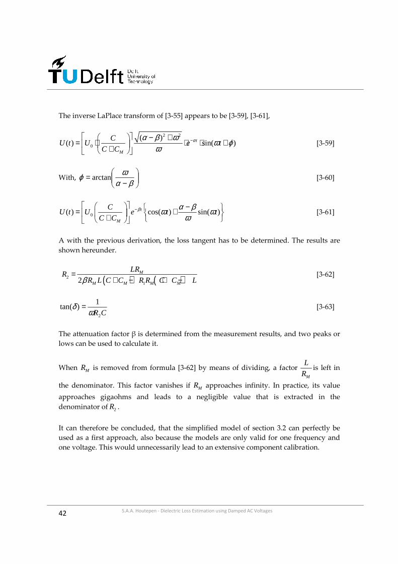
42 S.A.A. Houtepen - Dielectric Loss Estimation using Damped AC Voltages
The inverse LaPlace transform of [3-55] appears to be [3-59], [3-61],
2 2
0
( )( ) sin( )t
M
CU t U e t
C Cαα β ω ω ϕ
ω− − +
= ⋅ ⋅ ⋅ + + [3-59]
With,
−=
βαωϕ arctan [3-60]
0( ) cos( ) sin( )t
M
CU t U e t t
C Cβ α βω ω
ω− − = + +
[3-61]
A with the previous derivation, the loss tangent has to be determined. The results are
shown hereunder.
( ) ( )212
M
M M M M
LRR
R L C C R R C C Lβ=
+ − + − [3-62]
CR2
1)tan(
ωδ = [3-63]
The attenuation factor β is determined from the measurement results, and two peaks or
lows can be used to calculate it.
When MR is removed from formula [3-62] by means of dividing, a factor M
L
Ris left in
the denominator. This factor vanishes if MR approaches infinity. In practice, its value
approaches gigaohms and leads to a negligible value that is extracted in the
denominator of 2R .
It can therefore be concluded, that the simplified model of section 3.2 can perfectly be
used as a first approach, also because the models are only valid for one frequency and
one voltage. This would unnecessarily lead to an extensive component calibration.
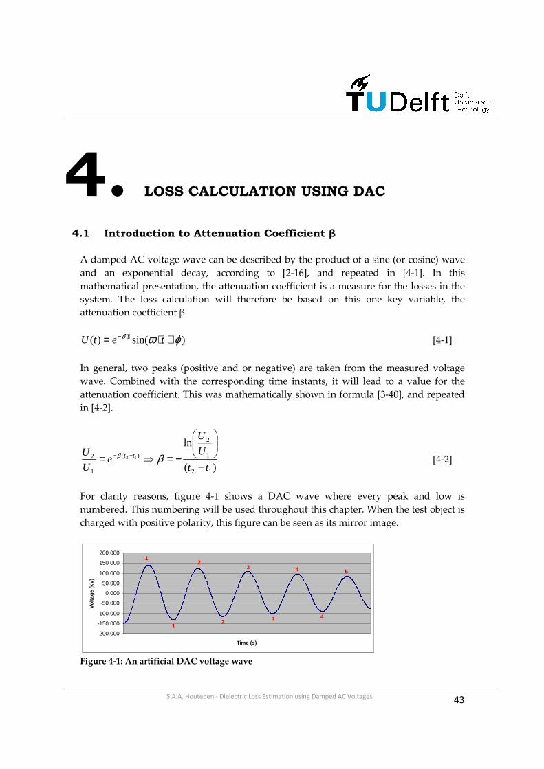
43 S.A.A. Houtepen - Dielectric Loss Estimation using Damped AC Voltages
4. LOSS CALCULATION USING DAC
4.1 Introduction to Attenuation Coefficient β
A damped AC voltage wave can be described by the product of a sine (or cosine) wave
and an exponential decay, according to [2-16], and repeated in [4-1]. In this
mathematical presentation, the attenuation coefficient is a measure for the losses in the
system. The loss calculation will therefore be based on this one key variable, the
attenuation coefficient β.
)sin()( ϕωβ +⋅= ⋅− tetU t [4-1]
In general, two peaks (positive and or negative) are taken from the measured voltage
wave. Combined with the corresponding time instants, it will lead to a value for the
attenuation coefficient. This was mathematically shown in formula [3-40], and repeated
in [4-2].
)(
ln
12
1
2
)(
1
2 12
tt
U
U
eU
U tt
−
−=⇒= −− ββ [4-2]
For clarity reasons, figure 4-1 shows a DAC wave where every peak and low is
numbered. This numbering will be used throughout this chapter. When the test object is
charged with positive polarity, this figure can be seen as its mirror image.
-200.000
-150.000
-100.000
-50.000
0.000
50.000
100.000
150.000
200.000
Time (s)
Vol
tage
(kV
)
1
1
2
2
3
3
4
4
5
Figure 4-1: An artificial DAC voltage wave

44 S.A.A. Houtepen - Dielectric Loss Estimation using Damped AC Voltages
The obtained value for the attenuation coefficient, together with the total equivalent
internal resistance R1 (see next chapter), oscillating frequency ω and inductance L will
lead to a value for the dielectric losses in the capacitive test object (according to eq. [4-3]).
12 RDL
L
βω ω
= − [4-3]
In this chapter, an analysis is done on this attenuation coefficient, and a new (and more
stable) method of calculation is developed. This evidence-based method will be a
foundation for a more constant determination of the dielectric losses.

45 S.A.A. Houtepen - Dielectric Loss Estimation using Damped AC Voltages
4.2 The Different Calculation Methods
4.2.1 Theoretical Approach
In theory, the calculation of the attenuation coefficient β is independent of which peak
and/or low is taken. This is proven with a simple example.
Figure 4-2 shows a theoretical (and therefore perfect) damped AC voltage wave that is
created with the help of a computer simulation program. The attenuation coefficient is
chosen to be 8. For visibility reasons, the time axis is not plotted.
-200.000
-150.000
-100.000
-50.000
0.000
50.000
100.000
150.000
200.000
Time (s)
Vol
tage
(kV
)
Figure 4-2: An artificial DAC voltage wave
From this data, the attenuation coefficient can now be recalculated (formula [4-2]) and
should be 8, independent of the choice of peaks and/or lows. Tables 4-1 to 4-3 show the
calculation of β respectively as a function of peaks, lows and combinations of both.
The first column consists of the first peak/low taken and the first row consists of the
second peak/low involved.
peak peak 1 2 3 4
1 8.005 8.002 8.0012 7.999 7.9993 7.9994
Table 4-1: Attenuation as a function of peaks
low low 1 2 3 4
1 8.013 8.006 8.0042 7.999 7.9993 7.9994
Table 4-2: Attenuation as a function of lows

46 S.A.A. Houtepen - Dielectric Loss Estimation using Damped AC Voltages
peak \ low 1 2 3 4
1 8.02 8.01 8.00 8.002 8.01 8.01 7.99 8.003 8.01 8.00 8.01 7.994 8.00 8.00 8.00 8.01
Table 4-3: Attenuation as a function of peaks and lows combined
To make this example as realistic as possible, a comparable time step is taken as in a real
DAC system. Except small errors (due to the time step taken and determination of the
minimum value of the starting low), all values are approximately 8.
In practice however, this is not always as clear as shown in this example. In the next
section, the attenuation coefficient of measurement data from the field is analyzed.
4.2.2 Attenuation in Practice
To draw conclusions on the determination of β, a vital part will be the analysis of
measurement data from the field. Because the theoretical approach showed a constant
value in all situations, tables were used to present this outcome. In this practical
approach, figures are used to visualize the differences between the chosen methods of
calculation.
Figure 4-3 shows the attenuation as a function of different peaks during a test with 120
kV on a 120 kV cable. On the right (the legend), the first peak is given, the second used
peak can be found on the x-axis. This cable was charged with positive polarity.
Figure 4-3: Attenuation as a function
of peaks of a 120 kV oil impregnated
cable in a 120 kV test. The total cable
length is 5300 meters
Calculation of Beta as a function of peaks
7.000
7.050
7.100
7.150
7.200
7.250
3rd peak 4th peak 5th peak
Second peak used in calculation
Bet
a
2nd peak (L1 120 kV)
3rd peak (L1 120 kV)
4th peak (L1 120 kV)

47 S.A.A. Houtepen - Dielectric Loss Estimation using Damped AC Voltages
From the same measurement, the results for different lows and combinations of peaks
and lows are calculated. These results are shown in figure 4-4 and 4-5. For comparing
reasons, the scaling is kept constant.
Figure 4-4: Attenuation as a
function of lows of a 120 kV oil
impregnated cable in a 120 kV test.
The total cable length is 5300
meters
Figure 4-5: Attenuation as a
function of peaks and lows of a 120
kV oil impregnated cable in a 120
kV test. The total cable length is
5300 meters
The outcome of this particular measurement is representative for the large amount of
data that is analyzed during this research.
This is further shown in a second example, where the same figures are presented as in 4-
3 to 4-5. This example includes a measurement at 150 kV, on an XLPE cable (nominal
voltage 130 kV) with a total length of 2200 meters.
Calculation of Beta as a function of lows
7.000
7.050
7.100
7.150
7.200
7.250
2nd low 3rd low 4th low
Second low used in calculation
Bet
a
1st low (L1 120 kV)
2nd low (L1 120 kV)
3rd low (L1 120 kV)
Calculation of Beta as a function of peaks & lows
7.000
7.050
7.100
7.150
7.200
7.250
1st low 2nd low 3rd low 4th low
Low used in calculation
Bet
a
2nd peak (L1 120 kV)
3rd peak (L1 120 kV)
4th peak (L1 120 kV)
5th peak (L1 120 kV)
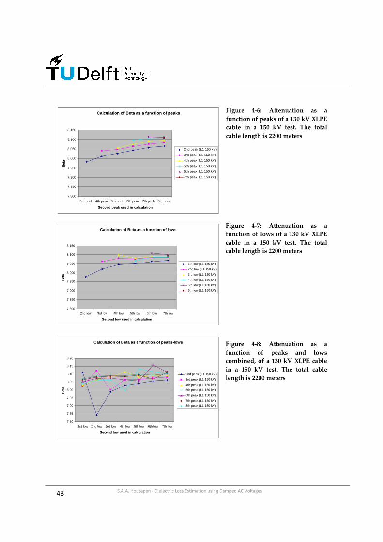
48 S.A.A. Houtepen - Dielectric Loss Estimation using Damped AC Voltages
Figure 4-6: Attenuation as a
function of peaks of a 130 kV XLPE
cable in a 150 kV test. The total
cable length is 2200 meters
Figure 4-7: Attenuation as a
function of lows of a 130 kV XLPE
cable in a 150 kV test. The total
cable length is 2200 meters
Figure 4-8: Attenuation as a
function of peaks and lows
combined, of a 130 kV XLPE cable
in a 150 kV test. The total cable
length is 2200 meters
Calculation of Beta as a function of peaks
7.800
7.850
7.900
7.950
8.000
8.050
8.100
8.150
3rd peak 4th peak 5th peak 6th peak 7th peak 8th peak
Second peak used in calculation
Bet
a
2nd peak (L1 150 kV)
3rd peak (L1 150 kV)
4th peak (L1 150 kV)
5th peak (L1 150 kV)
6th peak (L1 150 kV)
7th peak (L1 150 kV)
Calculation of Beta as a function of lows
7.800
7.850
7.900
7.950
8.000
8.050
8.100
8.150
2nd low 3rd low 4th low 5th low 6th low 7th low
Second low used in calculation
Bet
a
1st low (L1 150 kV)
2nd low (L1 150 kV)
3rd low (L1 150 kV)
4th low (L1 150 kV)
5th low (L1 150 kV)
6th low (L1 150 kV)
Calculation of Beta as a function of peaks-lows
7.80
7.85
7.90
7.95
8.00
8.05
8.10
8.15
8.20
1st low 2nd low 3rd low 4th low 5th low 6th low 7th low
Second low used in calculation
Bet
a
2nd peak (L1 150 kV)
3rd peak (L1 150 kV)
4th peak (L1 150 kV)
5th peak (L1 150 kV)
6th peak (L1 150 kV)
7th peak (L1 150 kV)
8th peak (L1 150 kV)

49 S.A.A. Houtepen - Dielectric Loss Estimation using Damped AC Voltages
On the analysis done on the attenuation coefficient, in function of peaks / lows and a
combination of both, several observations can be made. An overview of the major
visibilities is presented hereunder.
• The attenuation coefficient as a function of peaks and lows combined behaves
very unstable. This is a general observation that is valid for all data analyzed.
• The calculation from only peaks (or only lows) is more constant, but sometimes
slowly increases or declines with every succeeding oscillation.
• The obtained value for the attenuation coefficient from two peaks is not always
exactly the same as from two lows. This can probably explain the unstable
behavior of peak-low calculation.
The observations that are made show the importance of which two peaks and/or lows
are taken in the calculation of attenuation coefficient β.
From the fact that the calculation of the attenuation from one peak and one low is very
unstable, it can be concluded that most likely some sort of offset is present in the
measured data. The investigation on this issue is continued in the next paragraph, with
an analysis on the effects of an offset on the obtained value for β.

50 S.A.A. Houtepen - Dielectric Loss Estimation using Damped AC Voltages
4.3 Including an Offset
4.3.1 Introduction
An offset is generally defined as a shift of the measured voltage wave when earth
potential is its reference. This difference between the virtual and real earth can be the
result of different events and occurrences. A few major ones are listed hereunder.
• Grounding of the system, this contains sufficient impedance and will
consequently lead to a voltage drop.
• Inaccuracy of the measurement setup (e.g. due to the chosen sample frequency
for the voltage wave), and the fact kV’s are translated into volts before being
processed further.
This paragraph starts with a theoretical investigation on the effects of an offset on the
calculation of the attenuation coefficient. It is assumed that the offset is in majority
constant. Four experiments are performed; a positive offset of 1 and 10 kV (extreme
value, for ease of interpretation), and a negative offset of 1 and 10 kV. For this analysis,
the theoretical voltage wave from section 4.1 is used. To be as realistic as possible, again
the same sample frequency as in reality is used for this wave.
4.3.2 Positive Offset
4.3.2.1 A small offset
The first investigation focuses on a positive offset of 1 kV. The voltage wave is shifted
upwards, and the attenuation coefficient is calculated. The results are presented in tables
4-4 to 4-6.
peak peak 1 2 3 4
1 7.945 7.938 7.9322 7.931 7.9263 7.9214
Table 4-4: Attenuation as a function of peaks with 1kV positive offset
low low 1 2 3 4
1 8.070 8.067 8.0692 8.064 8.0693 8.0734
Table 4-5: Attenuation as a function of lows with 1kV positive offset

51 S.A.A. Houtepen - Dielectric Loss Estimation using Damped AC Voltages
peak \ low 1 2 3 4
1 6.30 9.83 8.65 8.422 7.40 6.06 10.07 8.743 7.61 7.31 5.79 10.354 7.70 7.55 7.21 5.49
Table 4-6: Attenuation as a function of peaks and lows combined with 1kV positive offset
4.3.2.2 An extreme value
The second test includes a (fictive) situation, when a positive offset of 10 kV is present.
The results are given in tables 4-7 to 4-9.
peak peak 1 2 3 4
1 7.441 7.402 7.3632 7.364 7.3243 7.2844
Table 4-7: Attenuation as a function of peaks with 10kV positive offset
low low 1 2 3 4
1 8.627 8.665 8.7142 8.704 8.7573 8.8104
Table 4-8: Attenuation as a function of lows with 10kV positive offset
peak \ low 1 2 3 4
1 9.16 26.33 14.58 12.272 1.92 11.45 28.83 15.493 4.10 1.10 14.13 31.724 5.01 3.57 0.15 17.19
Table 4-9: Attenuation as a function of peaks and lows combined with 10kV positive offset
It can be seen that the larger the offset becomes, the less stable the calculation from one
peak and one low combined becomes. The calculation from only peaks or lows changes,
but remains more or less constant with succeeding oscillations.
The same analysis is done on a negative offset, in order to compare the results and draw
solid conclusions.

52 S.A.A. Houtepen - Dielectric Loss Estimation using Damped AC Voltages
4.3.3 Negative Offset
4.3.3.1 A small offset
The third simulation is with a negative offset of 1 kV. The voltage wave is shifted
downwards, and the attenuation coefficient is calculated. The results are presented in
tables 4-10 to 4-12.
peak peak 1 2 3 4
1 8.067 8.068 8.0712 8.069 8.0743 8.0784
Table 4-10: Attenuation as a function of peaks with -1kV negative offset
low low 1 2 3 4
1 7.956 7.946 7.9392 7.935 7.9313 7.9264
Table 4-11: Attenuation as a function of lows with -1kV negative offset
peak \ low 1 2 3 4
1 9.74 6.18 7.35 7.582 8.62 9.95 5.92 7.263 8.40 8.70 10.22 5.644 8.31 8.45 8.79 10.53
Table 4-12: Attenuation as a function of peaks and lows combined with -1kV negative offset
4.3.3.2 An extreme value
The final test includes a (fictive) situation again, when a negative offset of 10 kV is
present. The results are shown in tables 4-13 to 4-15.
peak peak 1 2 3 4
1 8.663 8.709 8.7632 8.755 8.8123 8.8704
Table 4-13: Attenuation as a function of peaks with -10kV negative offset

53 S.A.A. Houtepen - Dielectric Loss Estimation using Damped AC Voltages
low low 1 2 3 41 7.481 7.440 7.4022 7.400 7.3633 7.3254
Table 4-14: Attenuation as a function of lows with -10kV negative offset
peak \ low 1 2 3 4
1 25.28 10.23 1.52 3.852 14.18 27.56 12.73 0.643 12.01 15.02 30.27 15.594 11.11 12.56 16.00 33.36
Table 4-15: Attenuation as a function of peaks and lows combined with -10kV negative offset
4.3.4 Observations
From the analysis on the influence of an offset, some observations can be made. These
observations are listed below.
• When a positive offset is present, the attenuation coefficient that is determined
from two peaks declines, whereas the value calculated from two lows increases.
With a negative offset, this will be the other way around.
• Although these values decline or increase, its value in function of succeeding
peaks remains more or less constant.
• The attenuation coefficient, that is determined from one peak and one low,
becomes highly unstable when an offset is present.
From the data analysis on measurements from the field, (paragraph 4.2), it is plausible
that an offset is responsible for the behavior of the attenuation coefficient in function of
peaks and lows.

54 S.A.A. Houtepen - Dielectric Loss Estimation using Damped AC Voltages
4.4 A New Calculation Method for β
4.4.1 Introduction
To calculate the losses from a damped sine wave, the attenuation coefficient β has to be
determined. As shown in the previous paragraph, an offset can be of great influence on
the measurement and calculation. In order to calculate an attenuation that is most stable
under different situations (voltage level, capacitance value, offset), a new method is
introduced. This method uses the value for β that is calculated from the first two peaks,
and averages it with β calculated from the first two lows (equation [4-4]).
22121 lowlowpeakpeak −− +
=ββ
β [4-4]
To check the accuracy of this new calculation, a theoretically generated damped
oscillation is fitted to a set of measured data with the use of computer simulation
program Matlab. In this way, the attenuation coefficient of the entire oscillation can be
determined with great accuracy and a comparison can be made between the current and
new method. Later on, the trend line (in function of increasing test voltage) is compared.
4.4.2 Application to measurement data
The newly introduced method is applied to measurement data with different
capacitance values, voltage levels and offsets. This wide variety of data will result in a
solid foundation for conclusions that are drawn in paragraph 4.5.
4.4.2.1 Effects of an Offset
Voltage level 28 kV and Capacitance 0.5 uF
The first measurement that is analyzed is a 28 kV test with a test object of 0.5 uF. Table 4-
16 shows the results for different offsets.
offset (kV) peaks lows 1st peaks 1st lows
-5.0 25.102 15.084 20.093-3.0 23.027 16.118 19.572-1.0 21.268 17.305 19.286-0.5 20.870 17.629 19.2490.0 20.486 17.966 19.2260.5 20.116 18.316 19.2161.0 19.759 18.680 19.2203.0 18.451 20.293 19.3725.0 17.304 22.211 19.758
Table 4-16: Attenuation, as a function of offset at 28 kV and 0.5 uF.

55 S.A.A. Houtepen - Dielectric Loss Estimation using Damped AC Voltages
Here, column “peaks” is the calculated value from the first two peaks, column “lows” is
the calculated value from the first two lows, and “1st peaks 1st lows” contains the average
of both values. Figure 4-9 shows the graphical representation of table 4-16.
Figure 4-9: Attenuation, as
a function of offset at 28
kV and 0.5 uF.
With the use of matlab, a generated wave is fitted to the measured data. The red line (in
figure 4-10) represents the measurement results, whereas the blue oscillation equals the
fitted curve (only visible at t=0 and therefore almost perfectly fitted).
Figure 4-10: Fitted wave onto measured data (28 kV, 0.5 uF)
The value for β that is calculated by Matlab is 18.607. This increases to 18.702 when fitted
from the first zero crossing onwards. Although this value is still 0.5 below the averaged
value from table 3-16, it is already an improvement compared to the (currently used)
20.486 (obtained from the first two peaks). This shows the advantage of averaging,
errors can be (partially) corrected.
Beta calculated from 1st and 2nd peak / 1st and 2nd low / average of both
14.000
16.000
18.000
20.000
22.000
24.000
26.000
28.000
30.000
-5.0 -3.0 -1.0 -0.5 0.0 0.5 1.0 3.0 5.0
Offset (kV)
Bet
a
1st & 2nd peak
1st & 2nd low
average of both values
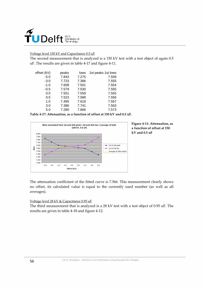
56 S.A.A. Houtepen - Dielectric Loss Estimation using Damped AC Voltages
Voltage level 150 kV and Capacitance 0.5 uF
The second measurement that is analyzed is a 150 kV test with a test object of again 0.5
uF. The results are given in table 4-17 and figure 4-11.
offset (kV) peaks lows 1st peaks 1st lows
-5.0 7.843 7.275 7.559-3.0 7.723 7.386 7.555-1.0 7.608 7.501 7.554-0.5 7.579 7.530 7.5550.0 7.551 7.559 7.5550.5 7.523 7.589 7.5561.0 7.495 7.619 7.5573.0 7.386 7.741 7.5635.0 7.280 7.866 7.573
Table 4-17: Attenuation, as a function of offset at 150 kV and 0.5 uF.
Figure 4-11: Attenuation, as
a function of offset at 150
kV and 0.5 uF
The attenuation coefficient of the fitted curve is 7.566. This measurement clearly shows
no offset, its calculated value is equal to the currently used number (as well as all
averages).
Voltage level 28 kV & Capacitance 0.95 uF
The third measurement that is analyzed is a 28 kV test with a test object of 0.95 uF. The
results are given in table 4-18 and figure 4-12.
Beta calculated from 1st and 2nd peak / 1st and 2nd low / average of both(150 kV, 0.5 uF)
7.000
7.100
7.200
7.300
7.400
7.500
7.600
7.700
7.800
7.900
8.000
-5.0 -3.0 -1.0 -0.5 0.0 0.5 1.0 3.0 5.0
Offset (kV)
Bet
a
1st & 2nd peak
1st & 2nd low
average of both values

57 S.A.A. Houtepen - Dielectric Loss Estimation using Damped AC Voltages
offset (kV) peaks lows 1st peaks 1st lows-5.0 21.977 14.140 18.058-3.0 20.110 15.138 17.624-1.0 18.536 16.288 17.412-0.5 18.180 16.603 17.3910.0 17.837 16.931 17.3840.5 17.508 17.272 17.3901.0 17.190 17.627 17.4083.0 16.027 19.205 17.6165.0 15.011 21.095 18.053
Table 4-18: Attenuation, as a function of offset at 28 kV and 0.95 uF.
Figure 4-12:
Attenuation, as a
function of offset at
28 kV and 0.95 uF
The computer calculated value for the attenuation coefficient is 17.183.
Voltage level 50 kV & Capacitance 7.2 uF
The fourth measurement that is analyzed is a 50 kV test with a test object of 7.2 uF. The
results are given in table 4-19 and figure 4-13.
offset (kV) peaks lows 1st peaks 1st lows
-5.0 10.239 7.640 8.940-3.0 9.718 8.013 8.866-1.0 9.247 8.425 8.836-0.5 9.136 8.535 8.8350.0 9.028 8.647 8.8380.5 8.922 8.763 8.8431.0 8.819 8.881 8.8503.0 8.430 9.390 8.9105.0 8.074 9.961 9.017
Table 4-19: Attenuation, as a function of offset at 50 kV and 7.2 uF.
Beta calculated from 1st and 2nd peak / 1st and 2nd low / average of both(28 kV, 0.95 uF)
11.000
13.000
15.000
17.000
19.000
21.000
23.000
-5.0 -3.0 -1.0 -0.5 0.0 0.5 1.0 3.0 5.0
Offset (kV)
Bet
a
1st & 2nd peak
1st & 2nd low
average of both values
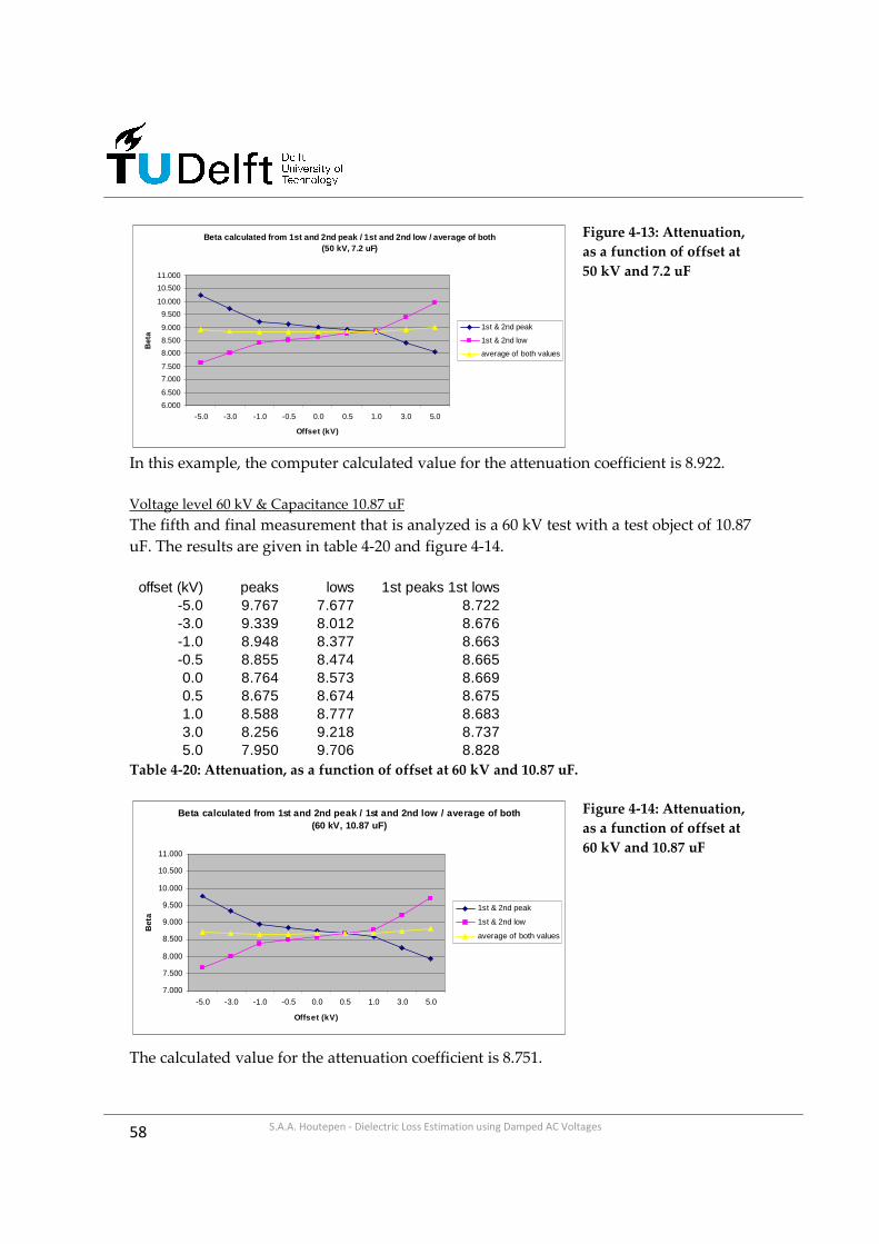
58 S.A.A. Houtepen - Dielectric Loss Estimation using Damped AC Voltages
Figure 4-13: Attenuation,
as a function of offset at
50 kV and 7.2 uF
In this example, the computer calculated value for the attenuation coefficient is 8.922.
Voltage level 60 kV & Capacitance 10.87 uF
The fifth and final measurement that is analyzed is a 60 kV test with a test object of 10.87
uF. The results are given in table 4-20 and figure 4-14.
offset (kV) peaks lows 1st peaks 1st lows
-5.0 9.767 7.677 8.722-3.0 9.339 8.012 8.676-1.0 8.948 8.377 8.663-0.5 8.855 8.474 8.6650.0 8.764 8.573 8.6690.5 8.675 8.674 8.6751.0 8.588 8.777 8.6833.0 8.256 9.218 8.7375.0 7.950 9.706 8.828
Table 4-20: Attenuation, as a function of offset at 60 kV and 10.87 uF.
Figure 4-14: Attenuation,
as a function of offset at
60 kV and 10.87 uF
The calculated value for the attenuation coefficient is 8.751.
Beta calculated from 1st and 2nd peak / 1st and 2nd low / average of both(50 kV, 7.2 uF)
6.000
6.500
7.000
7.500
8.000
8.500
9.000
9.500
10.000
10.500
11.000
-5.0 -3.0 -1.0 -0.5 0.0 0.5 1.0 3.0 5.0
Offset (kV)
Bet
a
1st & 2nd peak
1st & 2nd low
average of both values
Beta calculated from 1st and 2nd peak / 1st and 2nd low / average of both(60 kV, 10.87 uF)
7.000
7.500
8.000
8.500
9.000
9.500
10.000
10.500
11.000
-5.0 -3.0 -1.0 -0.5 0.0 0.5 1.0 3.0 5.0
Offset (kV)
Bet
a
1st & 2nd peak
1st & 2nd low
average of both values

59 S.A.A. Houtepen - Dielectric Loss Estimation using Damped AC Voltages
From the results that are presented above, it can be seen that the new method of
calculation eliminates the effects of an offset, and therefore increases the stability of the
attenuation calculation.
The final step in the introduction of this new method is verification, and comparison of
the attenuation coefficient as a function of voltage. The currently used calculation
parameters for the attenuation coefficient are compared to the new calculation, and the
trend line (Δ tan δ) should be identical.
4.4.2.2 Influence on the Voltage Trendline
Voltage level 230 kV and Capacitance 4 uF
Figure 4-15 shows the voltage dependency in a 230 kV cable, as a function of the first
two peaks, first two lows and the average value. The results are also presented in table
4-21.
Figure 4-15: Attenuation as a
function of voltage
Voltage (kV) 1st-2nd peak 1st-2nd low Average
25 10.387 10.321 10.35450 9.812 9.751 9.78275 9.615 9.489 9.552
100 9.543 9.566 9.554125 9.472 9.415 9.444150 9.440 9.313 9.376175 9.436 9.403 9.420188 9.437 9.398 9.418200 9.461 9.421 9.441225 9.518 9.472 9.495255 9.553 9.465 9.509
Table 4-21: Attenuation, as a function of voltage (same as figure 4-15)
Beta calculated from 1st-2nd peak / 1st-2nd low and average of both
9
9.2
9.4
9.6
9.8
10
10.2
10.4
100 125 150 175 188 200 225 255
Voltage (kV)
Bet
a
peak 1-peak 2
low 1-low 2
average of both

60 S.A.A. Houtepen - Dielectric Loss Estimation using Damped AC Voltages
As can be seen, the new calculation method gives the same results as the current
commonly used first and second peak. The given result is of phase L3, but shows a
similar outcome to that in L1 and L2.
Voltage level 150 kV and Capacitance 1.6 uF
The second set of data that is analyzed is from a 150 kV oil impregnated cable. The only
difference with figure 4-15 is the way of charging; this cable was charged at positive
polarity.
Figure 4-16: Attenuation as a
function of voltage
Voltage (kV) 1st-2nd peak 1st-2nd peak Average
10 9.107 9.345 9.22620 8.067 8.259 8.16330 7.719 7.954 7.83640 7.630 7.887 7.75850 7.553 7.784 7.66860 7.450 7.764 7.60770 7.404 7.769 7.58780 7.355 7.756 7.55690 7.379 7.696 7.538
100 7.356 7.722 7.539110 7.310 7.728 7.519120 7.350 7.752 7.551
Table 4-22: Attenuation, as a function of voltage (same as figure 4-3)
The same results are shown in table 4-22. As can be seen, it appears as if there is a certain
offset present in this measurement (a difference between the peaks and lows). Therefore,
the voltage wave at 120 kV is fitted by an artificial wave in Matlab. The attenuation
coefficient is determined as 7.654, which means that the average value is among the
closest values calculated.
Beta calculated from 1st-2nd peak / 1st-2nd low and average of both(150 kV cable)
6.5
7
7.5
8
8.5
9
9.5
10
50 60 70 80 90 100 110 120
Voltage (kV)
Bet
a
1st and 2nd peak
1st and 2nd low
average of both
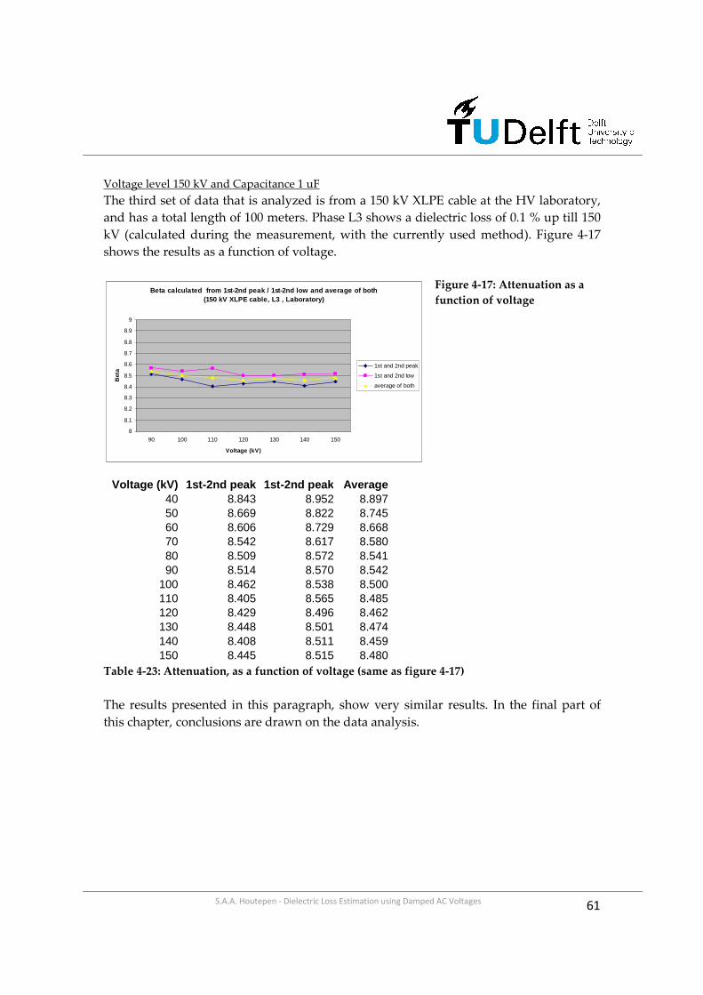
61 S.A.A. Houtepen - Dielectric Loss Estimation using Damped AC Voltages
Voltage level 150 kV and Capacitance 1 uF
The third set of data that is analyzed is from a 150 kV XLPE cable at the HV laboratory,
and has a total length of 100 meters. Phase L3 shows a dielectric loss of 0.1 % up till 150
kV (calculated during the measurement, with the currently used method). Figure 4-17
shows the results as a function of voltage.
Figure 4-17: Attenuation as a
function of voltage
Voltage (kV) 1st-2nd peak 1st-2nd peak Average
40 8.843 8.952 8.89750 8.669 8.822 8.74560 8.606 8.729 8.66870 8.542 8.617 8.58080 8.509 8.572 8.54190 8.514 8.570 8.542
100 8.462 8.538 8.500110 8.405 8.565 8.485120 8.429 8.496 8.462130 8.448 8.501 8.474140 8.408 8.511 8.459150 8.445 8.515 8.480
Table 4-23: Attenuation, as a function of voltage (same as figure 4-17)
The results presented in this paragraph, show very similar results. In the final part of
this chapter, conclusions are drawn on the data analysis.
Beta calculated from 1st-2nd peak / 1st-2nd low and average of both(150 kV XLPE cable, L3 , Laboratory)
8
8.1
8.2
8.3
8.4
8.5
8.6
8.7
8.8
8.9
9
90 100 110 120 130 140 150
Voltage (kV)
Bet
a
1st and 2nd peak
1st and 2nd low
average of both

62 S.A.A. Houtepen - Dielectric Loss Estimation using Damped AC Voltages
4.5 Chapter Conclusions
From the data that is analyzed in this chapter, several observations and conclusions can
be drawn. An overview is listed hereunder.
• In theory, when no offset is present, it does not matter which peaks and/or
lows are taken in the calculation of β.
• The analysis on the measurement data from the field reveals, that an
attenuation calculation from one peak and one low is very unstable, and
suggest some sort of offset.
• An upward shift of the voltage wave (positive offset) causes the calculated
attenuation of the peaks to decrease and the attenuation of the lows to
increase.
• A downward shift shows the opposite, the attenuation of the peaks
increases, whereas the attenuation of the lows decreases.
• The larger the offset (positive or negative), the less accurate the calculation
of β using peaks and lows combined will be.
• The average value of beta calculated from the first two peaks and first two
lows comes closer to the correct value (proved by an artificial wave that
was fitted on the measurement data), and eliminates the effects of an offset.
• All the analyzed data, at different voltage levels, capacitance values and
offsets show similar results; averaging improves and stabilizes the
calculation for the attenuation coefficient.
• The fitted curves do not match well at the starting peak. To avoid edge
effects and create a wave that fits the largest part of the dataset, all curves
are fitted from the first zero crossing onwards, what results in a much
better accuracy for the entire set of measurement data.
• When the voltage dependency of the damping is examined, the same
trendline is visible when comparing the current method and the newly
introduced one. This is of great importance, since Δtan δ is a valuable
parameter to determine the condition of the test object.
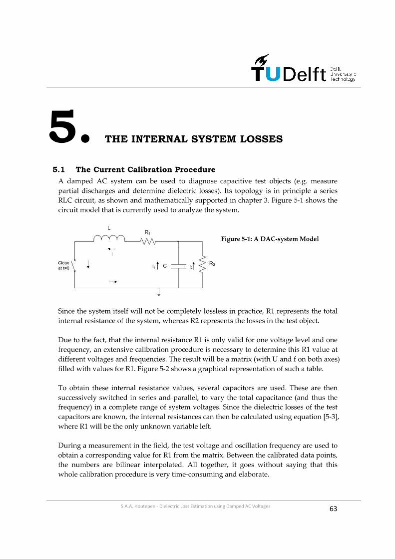
63 S.A.A. Houtepen - Dielectric Loss Estimation using Damped AC Voltages
5. THE INTERNAL SYSTEM LOSSES
5.1 The Current Calibration Procedure
A damped AC system can be used to diagnose capacitive test objects (e.g. measure
partial discharges and determine dielectric losses). Its topology is in principle a series
RLC circuit, as shown and mathematically supported in chapter 3. Figure 5-1 shows the
circuit model that is currently used to analyze the system.
Figure 5-1: A DAC-system Model
Since the system itself will not be completely lossless in practice, R1 represents the total
internal resistance of the system, whereas R2 represents the losses in the test object.
Due to the fact, that the internal resistance R1 is only valid for one voltage level and one
frequency, an extensive calibration procedure is necessary to determine this R1 value at
different voltages and frequencies. The result will be a matrix (with U and f on both axes)
filled with values for R1. Figure 5-2 shows a graphical representation of such a table.
To obtain these internal resistance values, several capacitors are used. These are then
successively switched in series and parallel, to vary the total capacitance (and thus the
frequency) in a complete range of system voltages. Since the dielectric losses of the test
capacitors are known, the internal resistances can then be calculated using equation [5-3],
where R1 will be the only unknown variable left.
During a measurement in the field, the test voltage and oscillation frequency are used to
obtain a corresponding value for R1 from the matrix. Between the calibrated data points,
the numbers are bilinear interpolated. All together, it goes without saying that this
whole calibration procedure is very time-consuming and elaborate.

64 S.A.A. Houtepen - Dielectric Loss Estimation using Damped AC Voltages
10
7
5
3
21
0.33330.2
0.050.01
15115
014
0130
120
11010
090807060504030
050
100150200250300350400
R1 (Ohms)
C(uF)
U (kV)
Resistance values from Calibration matrix350-400
300-350
250-300
200-250
150-200
100-150
50-100
0-50
Figure 5-2: Calibration matrix given graphically
The resistance of the dielectric, and its corresponding loss tangent, are determined with
the use of equation [5-1] and [5-2], as shown earlier.
CRLC
LR
12 2 −
=β
[5-1]
CR2
1)tan(
ωδ = [5-2]
Here, β is the measured attenuation, L is the inductance, C is the capacitance of the test
object, R1 is the total internal resistance of the system itself and R2 is the resistance that
represents the dielectric losses.
When these equations are entered into each other, the relation of R1 to the dielectric
losses (equation [5-3]) will be the result.
12 RDL
L
βω ω
= − [5-3]
In this chapter, it is examined whether improvement can be made on this extensive
calibration method, without the loss of accuracy.

65 S.A.A. Houtepen - Dielectric Loss Estimation using Damped AC Voltages
5.2 Investigation on the Calibration Matrices
5.2.1 An Experimental Approach
It is shown in paragraph 5.1, that the internal resistance values that are obtained during
the calibration can represent a 3D plane, with an asymptotical behavior at decreasing
capacitance values.
Due to this behavior, it is chosen to translate this capacitance axis into a frequency axis.
Since a simplified calibration means, in general, less calibration points, an experimental
approach is chosen where the relation between internal resistance and frequency
becomes linear. The relation between frequency and capacitance is given in eq. [5-4].
1
2f
LCπ=
⋅ [5-4]
Since the inductance L of a system is known, the translation can easily be made. With
this mathematical operation, the square root that exists between the capacitance and
frequency is eliminated.
An example is given below. Here, a 150 kV DAC system matrix is analyzed. The
capacitance values at 150 kV are transformed into frequencies. The inductance is chosen
to be 8.9 Henry. Although this value may be different in reality, its constant character
makes it independent of the results presented hereunder. The frequency at a capacitance
value of 10 uF is determined to be 16.87 Hz and this becomes 533.49 Hz at the lower
border of 0.01 uF.
The results that are then obtained show a linear relation to each other. In figure 5-3, a so-
called scatter plot is used to present the data on a linear scale.
Figure 5-3: Linear relation
between internal resistance
and frequency at 150 kV in a
150 kV DAC system
Relation between frequency and resistance value150 kV - HV150
100
120
140
160
180
200
220
240
260
280
300
0 100 200 300 400 500 600
Frequency (Hz)
Re
sist
anc
e (O
hm
s)

66 S.A.A. Houtepen - Dielectric Loss Estimation using Damped AC Voltages
Furthermore it appears that these linear relation remains when the test voltage of the
system is varied. The only parameter that changes is the gradient of the line. This
increases with lower voltages.
Figure 5-4: Trend lines
show the relation
between f, U and R
All lines are packed together and plotted in figure 5-4. Here, the 3D picture is given of
this relation between frequency, voltage and internal resistance. This method appears to
be promising, and is therefore further applied to a large number of calibration data.
5.2.2 Practical Support
In this section, several calibration matrices are analyzed as a function of frequency. With
this information, a clear picture is given on the applicability of this method.
In the figures that follow, the following sub graphs are presented; in the upper left
corner the current matrix (with capacitance axis) is plotted on a linear scale. In the upper
right corner, the same graph is plotted on a linear scale, with one exception that the
capacitance axis is transformed into a frequency axis. The graphs in the lower part are a
2D representation of the same images. Here, each line represents a voltage level. The
Matlab code can be found in Appendix A.
5.2.2.1 A 28 kV DAC System
The first four graphs are from 28 kV DAC systems. Figure 5-5 shows the sensitivity of
the transformation. In this matrix, all values for C are round off, and it can be seen that
the linearity reduces with that action.
Figure 5-6 to 5-8 show three other 28 kV systems, but now with unrounded (and
therefore more exact) values for the capacitance.
20
120
220
320
420
520
151
140
120
100806040
0
50
100
150
200
250
300
350
400
Resistance (Ohm)
Frequency (Hz)
Voltage (kV)
Trendlines of the calibration matrix
350-400
300-350
250-300
200-250
150-200
100-150
50-100
0-50

67 S.A.A. Houtepen - Dielectric Loss Estimation using Damped AC Voltages
Figure 5-5: The calibration matrix of a 28 kV system (as a function of capacitance (round
numbers) and frequency; 3D and 2D)
Figure 5-6: The calibration matrix of a 28 kV system (as a function of capacitance (unrounded
numbers) and frequency; 3D and 2D)

68 S.A.A. Houtepen - Dielectric Loss Estimation using Damped AC Voltages
Figure 5-7: The calibration matrix of a 28 kV system (as a function of capacitance (unrounded
values) and frequency; 3D and 2D)
Figure 5-8: The calibration matrix of a 28 kV system (as a function of capacitance (unrounded
values) and frequency; 3D and 2D)

69 S.A.A. Houtepen - Dielectric Loss Estimation using Damped AC Voltages
5.2.2.2 A 60 kV DAC System
In this section, the same analysis is done on two 60 kV DAC systems. Figure 5-9 and 5-10
shows two 60 kV systems, both with unrounded values for the capacitance.
Figure 5-9: The calibration matrix of a 60 kV system (as a function of capacitance (unrounded
values) and frequency; 3D and 2D)
Figure 5-10: The calibration matrix of a 60 kV system (as a function of capacitance (unrounded
values) and frequency; 3D and 2D)

70 S.A.A. Houtepen - Dielectric Loss Estimation using Damped AC Voltages
5.2.2.3 A 150 kV DAC System
In this section, the same analysis is done on a 150 kV DAC system. Figure 5-11 shows the
graphical counterpart of the calibration matrix of a 150 kV system.
Figure 5-11: The calibration matrix of a 150 kV system (as a function of capacitance
(unrounded values) and frequency; 3D and 2D)
5.2.3 Observations
From the analysis done on several DAC systems from different voltage classes, some
observations can be made.
• The frequency representation of the internal resistance of the system gives an
almost linear picture.
• When capacitance values are not sufficiently precise (e.g. by rounding off), this
linearity gets distorted quite quickly.
• With declining voltage (within one system), the gradient of this linear approach
becomes more steep.
In the following paragraph, a method is developed in which the frequency dependent
graph is linearized with the use of two data points. This method is compared to the
currently used one.

71 S.A.A. Houtepen - Dielectric Loss Estimation using Damped AC Voltages
5.3 Linearization of the Frequency Representation
5.3.1 The Applied Method
At each voltage level, the frequency plot (shown in the previous section) will be
linearized, and the effects on the accuracy of the dielectric loss calculation will be
investigated. When this accuracy is sufficient, only 2 capacitance values are necessary
for major part of the calibration, and the other values can be interpolated in the
frequency domain.
The applied method is as follows; a straight line is drawn between the 2nd lowest and 2nd
highest frequency (representing the 2nd highest and 2nd lowest capacitance). Since the
lowest frequency (representing the highest capacitance) is a rounded value, and the
highest frequency (representing the lowest capacitance) shows a deviation from the
linear trend, these are therefore not incorporated.
The obtained values for the internal resistance are then used in the calculation of the loss
tangent, and these values are then plotted as a function of voltage, for several
frequencies.
In this way, it can be seen what the effects of a linear approach are on the loss tangent as
a function of voltage.
The results of the linear approximations are given in figure 5-12. Here, the blue lines
show the linear frequency plot of the calibration matrix in figure 5-6. Te red lines show
the linearization, where each line represents a separate voltage level.
Figure 5-12: Linear approach between
2nd lowest and 2nd highest frequency of
the system in figure 5-6

72 S.A.A. Houtepen - Dielectric Loss Estimation using Damped AC Voltages
5.3.2 Validation of the Linear Method
In this section, the linear method is used to recalculate the dielectric losses from several
systems. With this information, conclusions can be drawn on the accuracy and
applicability of this new method.
Since the dielectric losses of the test capacitors and the internal resistance values are
known, the obtained numbers for β can be fixed (according to formula [5-3], where only
beta will then be unknown). When this value for beta will be kept fixed, and an internal
resistance obtained from the linearization is entered into equation [5-3], the new DL
(dielectric loss value) can be calculated. This is what will be done in the next figures.
With a constant value for the dielectric losses (DL=0.001), the results are given in figure
5-13. Here, the red line represents the current DL as a function of voltage, and the blue
lines represent tan δ as a function of voltage, for different frequencies (with a linearly
approximated internal resistance (straight lines from figure 5-12)).
Figure 5-13: Tan delta obtained
from the linear approximation of
the internal resistance.
At the lowest voltage, a large deviation from the trend occurs. The upper blue line
represents the highest frequency. As explained earlier, the blue lines are calculated with
the red (tan delta = 0.1% line) as a reference.
In figure 5-14 and 5-15, the dielectric loss tangent is chosen to be represented as a rising
curve. The calculation, as described earlier, is done again.

73 S.A.A. Houtepen - Dielectric Loss Estimation using Damped AC Voltages
Figure 5-14: Tan delta obtained
from the linear approximation of
the internal resistance. Dielectric
losses are rising from 0.3% at 8 kV
up to 0.8% at 28 kV.
Figure 5-15: Tan delta obtained
from the linear approximation of
the internal resistance. Dielectric
losses are exponentially rising
from 0.3% at 8 kV up to 1.6% at 28
kV.
Again, one blue line shows a large deviation (the highest frequency that is left out of the
linearization). It can be seen that the linear approximation method gives the same trend
in dielectric losses as a function of voltage, compared to the current method (red line).
The only visible difference is the reduced accuracy of the absolute value for the dielectric
losses.
In the following 6 graphs, the same is done for a 60 kV DAC system and a 150 kV DAC
system.

74 S.A.A. Houtepen - Dielectric Loss Estimation using Damped AC Voltages
Figure 5-16: Tan delta obtained from
the linear approximation of the
internal resistance.
Figure 5-17: Tan delta obtained from
the linear approximation of the
internal resistance.
Dielectric losses are rising from 0.2% at
15 kV up to 1.0% at 60 kV.
Figure 5-18: Tan delta obtained from
the linear approximation of the
internal resistance.
Dielectric losses are exponentially
rising from 0.1% at 15 kV up to 2.2% at
60 kV.

75 S.A.A. Houtepen - Dielectric Loss Estimation using Damped AC Voltages
As shown in the previous calculations, the linear approach frequency suits well when
the trendline is observed. In the next figures, a 150 kV system is analyzed.
Figure 5-19: Tan delta obtained from
the linear approximation of the
internal resistance.
Figure 5-20: Tan delta obtained from
the linear approximation of the
internal resistance.
Dielectric losses are rising from 0.3% at
30 kV up to 1.5% at 150 kV.
Figure 5-21: Tan delta obtained from
the linear approximation of the
internal resistance.
Dielectric losses are exponentially
rising from 0.1% at 30 kV up to 2.9% at
150 kV.

76 S.A.A. Houtepen - Dielectric Loss Estimation using Damped AC Voltages
5.3.3 Remarks
Following the research on the linearized method of calibration, several remarks have to
be made. These remarks are listed below.
• With the new linearization method, the voltage trend line of the dielectric losses
remains the same, but the absolute value becomes more unstable in a wide range
of frequencies.
• Due to this observation, it can only be concluded that although the frequency
representation comes close to linearity, it is not enough to maintain the accuracy
that it currently has. The more calibration points are introduced, the more
accurate this method will be.
• Furthermore, in almost all cases, the earlier introduced approach is valid. When
however physical changes are introduced, in order to reduce edge effects of the
system at low voltages, this method cannot be applied. An example of such a
system matrix (in capacitance representation) is shown in figure 5-22.
Figure 5-22:
DAC System with bypassed system
components at lower voltages
Finally, the frequency representation is the major method that is introduced in this thesis.
This choice is based on the fact that a simplification of the calibration process means, in
general, less calibration points. Because this will lead to more interpolation, its accuracy
is expected to be at its highest when this occurs in a linear related set of data. Since the
frequency representation gives an (almost) linear picture, it is therefore investigated
thoroughly.
51
0.250.05
0.0125
30 k
V
28 k
V
26 k
V
24 k
V
22
kV20
kV
18
kV16
kV
14 k
V12
kV
10 k
V8
kV6 kV4 kV2 kV
050
100150
200
250
R1 (Ohms)
C(uF)U (kV)
Resistance values from Calibration matr ixIT30
200-250
150-200
100-150
50-100
0-50

77 S.A.A. Houtepen - Dielectric Loss Estimation using Damped AC Voltages
5.4 Chapter Conclusions
Following the analysis done on calibration matrices from several systems (and
consequently several voltage classes) some observations can be made and conclusions
can be drawn.
• The use of a frequency scale results in a more linear depiction of the internal
resistance values as a capacitance scale.
• When the voltage decreases, the slope of this linear frequency approach increases.
• Precise capacitance values (or frequency) are of importance to provide a more
linear relationship. Capacitance values should not be rounded before
constructing the table.
• In most systems, the lowest capacitance used (and thus the highest frequency
modeled) shows a deviation from the linear trend. For that reason, a linearization
has to take place between the obtained results from the 2nd highest and 2nd lowest
capacitance, and therefore the 2nd lowest and 2nd highest frequency (at each
voltage level).
• Linearization would reduce calibration time significantly, but should be avoided
because of the decrease in absolute accuracy.

78 S.A.A. Houtepen - Dielectric Loss Estimation using Damped AC Voltages

79 S.A.A. Houtepen - Dielectric Loss Estimation using Damped AC Voltages
6. A COMPLETE OVERVIEW
6.1 Flow Chart
In this final chapter, an overview is presented on the steps that have to be taken in the
determination of the dielectric losses from a damped AC voltage wave. A flowchart is
shown first, in which a schematic insight is given into this procedure. In the next
paragraph, an explanation on this flowchart is treated.
Figure 6-1: Flowchart of Dielectric Loss Estimation using Damped AC Voltages
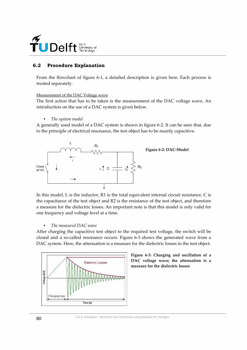
80 S.A.A. Houtepen - Dielectric Loss Estimation using Damped AC Voltages
6.2 Procedure Explanation
From the flowchart of figure 6-1, a detailed description is given here. Each process is
treated separately.
Measurement of the DAC Voltage wave
The first action that has to be taken is the measurement of the DAC voltage wave. An
introduction on the use of a DAC system is given below.
• The system model
A generally used model of a DAC system is shown in figure 6-2. It can be seen that, due
to the principle of electrical resonance, the test object has to be mainly capacitive.
Figure 6-2: DAC-Model
In this model, L is the inductor, R1 is the total equivalent internal circuit resistance, C is
the capacitance of the test object and R2 is the resistance of the test object, and therefore
a measure for the dielectric losses. An important note is that this model is only valid for
one frequency and voltage level at a time.
• The measured DAC wave
After charging the capacitive test object to the required test voltage, the switch will be
closed and a so-called resonance occurs. Figure 6-3 shows the generated wave from a
DAC system. Here, the attenuation is a measure for the dielectric losses in the test object.
Figure 6-3: Charging and oscillation of a
DAC voltage wave; the attenuation is a
measure for the dielectric losses

81 S.A.A. Houtepen - Dielectric Loss Estimation using Damped AC Voltages
This wave can be represented by equation [6-1], with β as the attenuation coefficient.
)sin()( ϕωβ +⋅= ⋅− tetU t [6-1]
Calculation of Attenuation Coefficient β
To calculate the losses from a measured DAC wave, the attenuation coefficient β has to
be determined. This can be done by choosing two arbitrary peak values from the DAC
wave (with corresponding time instants), and fill those into formula [6-2].
)(
ln
12
1
2
)(
1
2 12
tt
U
U
eU
U tt
−
−=⇒= −− ββ [6-2]
In order to calculate an attenuation that is most constant under different situations
(voltage level, capacitance value, offset), a robust method would be to use the value for
β that is calculated from the first two peaks, and averages it with β calculated from the
first two lows (equation [6-3]).
22121 lowlowpeakpeak −− +
=ββ
β [6-3]
The peak where the oscillation starts is not incorporated, so when the system is charged
with negative polarity, low 1 will be the value after one full cycle.
Calibration of the System
In a theoretical DAC system, no internal losses will be present. In practice, this will of
course be the case. To determine these losses, an extensive calibration procedure is
required.
Due to the fact, that the internal resistance R1 is only valid for one voltage level and one
frequency, it is necessary to determine this R1 value at different voltages and
frequencies. The result will be a three dimensional relationship between U, f and R1.
To obtain these internal resistance values, several capacitors are used. These are then
successively switched in series and parallel, to vary the total capacitance (and thus the
frequency). Because the dielectric losses of these test capacitors are known, they can be
extracted from total losses, and the system resistance values can be obtained

82 S.A.A. Houtepen - Dielectric Loss Estimation using Damped AC Voltages
Equation [6-4] shows how to calculate this internal resistance from the measurement
data. This equation is derived from the model in figure 6-2.
1 2R L DL Lβ ω= − ⋅ [6-4]
Here, β is the measured attenuation coefficient, L is the inductance, DL is the known
dielectric losses from the test capacitor and ω is the radial frequency.
Calculate the dielectric losses
The final step in the process of dielectric loss estimation is the calculation of this loss
tangent. This is done with the use of equation [6-5].
12 RDL
L
βω ω
= − [6-5]
During a measurement in the field, the attenuation coefficient can be determined from
the voltage wave. Together with the radial frequency and inductance, it can be filled into
formula [6-5]. The test voltage and oscillation frequency are then used to obtain a
corresponding value for R1.
Since the only unknown variable now becomes the dielectric losses DL, the final step in
this process becomes an easy calculation.

83 S.A.A. Houtepen - Dielectric Loss Estimation using Damped AC Voltages
7. CONCLUSIONS AND RECOMMENDATIONS
In this thesis, research has been performed on the dielectric loss estimation using
damped AC voltages. From this investigation, several conclusions and
recommendations follow.
Conclusions
The mathematical description of a DAC system is analyzed in twofold. One model
contains a total equivalent internal resistance that represents all system losses; the other
model contains a series (switch and coil) and parallel (voltage divider) resistance. It is
investigated what the effects will be of a more detailed model for dielectric loss
calculation.
It is concluded that;
1. The supplementary elements in the detailed mathematical model have (in theory)
a negligible effect on the calculation of the dielectric losses.
2. To maintain the current accuracy, a detailed component calibration should be
required. This is caused by the fact that each component is voltage and frequency
dependent. As a result, the simplified model is therefore sufficient for use as a
first approach.
The attenuation coefficient β, a measure for the damping of the voltage wave, has to be
calculated with the use of two arbitrary voltage peaks, combined with the corresponding
time instants. Using measurement data from the field, it is investigated what the most
stable and robust method of calculation will be.
It is concluded that;
1. The attenuation coefficient, calculated by two arbitrary peaks or two arbitrary
lows, can be considered relatively stable. A calculation that uses one peak and
one low however becomes highly unstable.
2. In theory, it should not matter which two peaks/lows are used in the calculation;
the attenuation coefficient should always be equal.
3. The analysis of the measurement data, combined with theoretical research, make
it plausible that an voltage-offset is the main reason for an unstable calculation
from one peak and one low.

84 S.A.A. Houtepen - Dielectric Loss Estimation using Damped AC Voltages
4. To eliminate the effects of a possible offset, a new method has been proposed
consisting of averaging β obtained from the first two peaks and first two lows.
With the use of data from the field, it is proven to be a very robust method.
The internal system losses, as defined in the mathematical model, are voltage and
frequency dependent. To determine the total internal equivalent resistance in a wide
range of frequencies and voltages, a detailed calibration procedure is required. This
results in a 3D relationship between voltage, capacitance and internal resistance.
It is concluded that;
1. The use of a frequency scale (instead of a capacitance scale) results in a more
linear depiction of the internal resistance values.
2. A 3D relationship between voltage, frequency and internal resistance is suitable
for linearization (and simplification of the procedure).
3. Although this method of linearization appears promising, the absolute value of
the dielectric losses (in function of increasing voltage) becomes less accurate.
4. The current (detailed) calibration procedure has to be maintained.
Recommendations
The results in this thesis represent a fundamental improvement in the dielectric loss
calculation using damped AC voltages. Nevertheless, topics are open for further
research. Concerning this issue, the following recommendations are given;
1. Determine the influence of the sample frequency of the voltage wave on the
accuracy of the attenuation coefficient calculation. It is presumed that, especially
at higher frequencies, this sample frequency is of importance in the process that
leads to the determination of the attenuation coefficient.
2. Do a practical research (measurements) on the main components in the system
(coil, switches), and their behavior in function of voltage and frequency. With
this information, a better insight in individual component behavior is obtained
and a possible change or simplification of the current calibration procedure can
be further examined.
3. The current calibration procedure is done manually. This means a time-
consuming process. Some sort of automation of this process would not only lead
to a reduction in time, but also eliminates the possibilities for human error.

IX S.A.A. Houtepen - Dielectric Loss Estimation using Damped AC Voltages
REFERENCES
[1] F.H. Kreuger, Industrial High Voltage, volume 4,5,6., Delft University Press 1992.
[2] Website: http://en.wikipedia.org/wiki/Dielectric_spectroscopy
[3] Zaengl, W.S., "Dielectric spectroscopy in time and frequency domain for HV power
equipment. I. Theoretical considerations," Electrical Insulation Magazine, IEEE , vol.19,
no.5, pp.5-19, Sept.-Oct. 2003
[4] L. Chmura, Application of dielectric loss measurements for degradation assessment
of oil-impregnated paper insulation in power cables, Master thesis. Delft University of
Technology, 2009.
[5] E. Peschke, R. von Olshausen, Cable Systems for High and Extra-High Voltage,
Publicis-MCD, 1999. ISBN 3-89578-118-5.
[6] Menzel, J.; Patsch, R.; Kamenka, D., "Measurement of the dielectric properties of
paper-oil cables and the cellulose-oil insulation system of power transformers,"
Properties and Applications of Dielectric Materials, 2009. ICPADM 2009. IEEE 9th
International Conference on the , vol., no., pp.1020-1025, 19-23 July 2009
[ 7 ] Patsch, R.; Kouzmine, O., "Return voltage measurements - the step from
experimental data to a relevant diagnostic interpretation," Electrical Insulating Materials,
2005. (ISEIM 2005). Proceedings of 2005 International Symposium on , vol.3, no., pp. 889-892
Vol. 3, 5-9 June 2005
[8] Densley, J.; , "Ageing mechanisms and diagnostics for power cables - an overview,"
Electrical Insulation Magazine, IEEE , vol.17, no.1, pp.14-22, Jan.-Feb. 2001
[9] E. Gulski, Lecture slides, Diagnostics for High Voltage Assets., Delft University of
Technology, 2009.
[10] F.H. Kreuger, Industrial High Voltage, volume 1,2,3., Delft University Press 1992.
[11] Otowski, W.; Courteau, R.; Bose, T.K.; Lamarre, L., "Effect of temperature and time
on the dissipation factor of power cable junctions," Electrical Insulation and Dielectric
Phenomena, 1993. Annual Report., Conference on , vol., no., pp.763-768, 17-20 Oct 1993

X
S.A.A. Houtepen - Dielectric Loss Estimation using Damped AC Voltages
[12] Ildstad, E., "Dielectric response for condition assessment of PILC distribution
cables," Electrical Insulation and Dielectric Phenomena, 2003. Annual Report. Conference on ,
vol., no., pp. 171-175, 19-22 Oct. 2003
[ 13 ] Skjoelberg, J.; Hvidsten, S.; Farmeo, H., "Experience from on-site condition
assessment of XLPE MV cables," Electrical Insulation, 2006. Conference Record of the 2006
IEEE International Symposium on , vol., no., pp.432-435, 11-14 June 2006
[ 14] H.J. van Breen, Condition Assessment of Stator Insulation using Partial Discharge
Diagnosis, ISBN 90-9020128-9, Ph.D. thesis TU Delft, 2005.
[15] Yanpeng Hao; Zhidong Jia; Xiongwei Jiang; Naikui Gao; Hengkun Xie; , "The
changes of mechanical properties of epoxy/mica insulation materials in aging process,"
Properties and Applications of Dielectric Materials, 2000. Proceedings of the 6th International
Conference on , vol.1, no., pp.185-188 vol.1, 2000
[16] IEC Standard, Rotating electrical machines - Part 27 : Off-line partial discharge
measurements on the stator winding insulation of rotating electrical machines (IEC/TS
60034-27:2006,IDT)
[ 17 ] Hudon, C.; Bartnikas, R.; Wertheimer, M.R.; , "Effect of physico-chemical
degradation of epoxy resin on partial discharge behavior," Dielectrics and Electrical
Insulation, IEEE Transactions on , vol.2, no.6, pp.1083-1094, Dec 1995
[18] Oyegoke, B.; Hyvonen, P.; Aro, M.; Gao, N., "Selectivity of damped AC (DAC) and
VLF voltages in after-laying tests of extruded MV cable systems," Dielectrics and Electrical
Insulation, IEEE Transactions on , vol.10, no.5, pp. 874-882, Oct. 2003
[19] Uchida, K.; Kobayashi, S.; Kawashima, T.; Tanaka, H.; Sakuma, S.; Hirotsu, K.; Inoue,
H., "Study on detection for the defects of XLPE cable lines," Power Delivery, IEEE
Transactions on , vol.11, no.2, pp.663-668, Apr 1996
[20] Salter, E. H, "Guarding and Shielding for Dielectric Loss Measurement on Short
Lengths of High-Tension Power Cable," American Institute of Electrical Engineers,
Transactions of the , vol.48, no.4, pp.1294-1299, Oct. 1929
[21] Patsch, R.; Jochen Jung; Kouzmine, O., "The interpretation of return voltage curves
of paper-oil-cables," Electrical Insulation and Dielectric Phenomena, 2000 Annual Report
Conference on , vol.1, no., pp.39-42 vol.1, 2000

XI
S.A.A. Houtepen - Dielectric Loss Estimation using Damped AC Voltages
[ 22 ] Kozlovskis, A.; Rozenkrons, J., "Temperature dependence of return voltage
characteristics," Power Delivery, IEEE Transactions on , vol.14, no.3, pp.705-708, Jul 1999
[23] F.J. Wester, Condition Assessment of Power Cables Using PD Diagnosis at Damped AC
Voltages, ISBN 90-8559-019-1, Ph.D. thesis TU Delft, 2004.
[24] Nilsson / Riedel, Electric Circuits. Pearson Education Inc., 2008, ISBN 0-13-198925-1,
pag. 308-310.
[25] C.K. Alexander / M.N.O. Sadiku, Fundamentals of Electrical Circuits. McGraw Hill,
Third Edition 2007, ISBN-10-0-07-297718-3, pag. 326-327.
[26] Basic Electronics, Dover Publications Inc., 1973, ISBN-0-486-21076-6, pag. 194-202.
[27] A. Stenger / B. Girod / R. Raberstein, Signals and Systems. John Wiley and Sons,
2001, ISBN-978-0471988007.

XII S.A.A. Houtepen - Dielectric Loss Estimation using Damped AC Voltages

XIII S.A.A. Houtepen - Dielectric Loss Estimation using Damped AC Voltages
APPENDIX A:
MATLAB CODE MSc THESIS

XIV S.A.A. Houtepen - Dielectric Loss Estimation using Damped AC Voltages

XV S.A.A. Houtepen - Dielectric Loss Estimation using Damped AC Voltages
1. Create Artificial DAC Wave
function y = dampedcosine(b,X)
a=b(1);
beta=b(2);
omega=b(3);
theta=b(4);
y = a .* exp(-beta*X) .* cos(omega*X+theta);
2. DAC Curve Fitting
x=[0:1.25e-5:10e-2];
b=[-30 18 1 3.14];
y=dampedcosine(b,x);
time=x';
q=nlinfit(time(start:stop),data(start:stop),@dampedcosine,b)
y=dampedcosine(q,time');
plot(y)
axis([0 length(data) -130 130])
hold on
plot(data,'red')
'the measured data is red'
3. Visualize and Linearize Calibration Data
C=(Matrix(1,2:size(Matrix,2)));
U=(Matrix(2:size(Matrix,1)-1,1));
L=2.22;
f=[];
subplot(2,2,1)
[x,y]=meshgrid(C,U);
surf(x,y,Matrix(2:size(Matrix,1)-1,2:size(Matrix,2)))
view(50,30)
title('Calibration data as a function of capacitance (current method)')
xlabel('capacitance (uF)')
ylabel('voltage (kV)')
zlabel('Resistance (Ohms)')
for x=1:1:length(C),
f(x)=1/(2*pi()*sqrt(L*C(x)*1e-6));
end

XVI S.A.A. Houtepen - Dielectric Loss Estimation using Damped AC Voltages
subplot(2,2,2)
[x,y]=meshgrid(f,U);
surf(x,y,Matrix(2:size(Matrix,1)-1,2:size(Matrix,2)))
view(235,30)
title('Calibration data as a function of frequency (mirrored)')
xlabel('frequency (Hz)')
ylabel('voltage (kV)')
zlabel('Resistance (Ohms)')
subplot(2,2,3)
for x=2:1:size(Matrix,1),
plot(C,Matrix(x,2:size(Matrix,2)))
hold on
title('Internal Resistance as a function of capacitance')
xlabel('capacitance (uF)')
ylabel('Resistance (Ohms)')
end
subplot(2,2,4)
for x=2:1:size(Matrix,1),
plot(f,Matrix(x,2:size(Matrix,2)))
hold on
title('Internal Resistance as a function of frequency')
xlabel('frequency (Hz)')
ylabel('Resistance (Ohms)')
end
figure
f=f(1:length(f)-1);
Linear=[];
% richtingscoefficienten in matrix stoppen
for x=2:1:size(Matrix,1)-1,
Linear(x-1,1)=((Matrix(x,size(Matrix,2)-1)-Matrix(x,3))/(f(length(f))-f(2)));
Linear(x-1,2)=(Matrix(x,3)-Linear(x-1,1)*f(2));
end
Reslin=[];
Rlinmat=[];
for v=1:1:size(Linear,1),
for x=1:1:length(f),
Reslin(x,1)=f(x);
Reslin(x,2)=Linear(v,1)*f(x)+Linear(v,2);
Reslin(x,3)=Matrix(v+1,x+1);
end
plot(f,Matrix(v+1,2:size(Matrix,2)-1))

XVII S.A.A. Houtepen - Dielectric Loss Estimation using Damped AC Voltages
hold on
plot(Reslin(:,1),Reslin(:,2),'red')
end
for y=1:1:size(Matrix,1)-2,
for x=1:1:size(Matrix,2)-2,
Rlinmat(y,x)=(Linear(y,1)*f(x)+Linear(y,2));
end
end
DL=[];
DL=zeros(size(Rlinmat,1),size(Rlinmat,2));
TAN=0.001;
for x=1:1:size(DL,1),
DL(x,:)=DL(x,:)+TAN;
TAN=TAN-0.000;
end
beta=[];
tand=[];
tandlin=[];
for y=1:1:size(Matrix,1)-2,
for x=1:1:size(Matrix,2)-2,
beta(y,x)=(0.5*DL(y,x)*2*pi()*f(x))+((Matrix(y+1,x+1))/(2*L));
end
end
for y=1:1:size(Matrix,1)-2,
for x=1:1:size(Matrix,2)-2,
tand(y,x)=(2*beta(y,x)/(2*pi()*f(x)))-((Matrix(y+1,x+1))/(2*pi()*f(x)*L));
end
end
for y=1:1:size(Matrix,1)-2,
for x=1:1:size(Matrix,2)-2,
tandlin(y,x)=(2*beta(y,x)/(2*pi()*f(x)))-((Rlinmat(y,x))/(2*pi()*f(x)*L));
end
end
figure
for t=2:1:size(tandlin,2),
plot(U(1:length(U)), tandlin(1:size(Matrix,1)-2,t))
hold on
end
plot(U, tandlin(:,2),'red')

XVIII S.A.A. Houtepen - Dielectric Loss Estimation using Damped AC Voltages

XIX S.A.A. Houtepen - Dielectric Loss Estimation using Damped AC Voltages
APPENDIX B:
CMD 2010 CONFERENCE PROCEEDING

XX S.A.A. Houtepen - Dielectric Loss Estimation using Damped AC Voltages

Conference Proceedings of CMD2010
Estimation of Dielectric Loss using
Damped AC Voltages
Richard Houtepen1*, Edward Gulski1, Johan J Smit1 and Ben Quak2
1 High Voltage Technology and Management, Delft University of Technology, Delft, The Netherlands 2 Seitz Instruments AG, Niederrohrdorf, Switzerland
*E-mail: [email protected]
Abstract—Insulation failures in HV components may be caused by lower dielectric strength due to aging processes and by internal defects in the insulation system. It is known, that unlike voltage testing, measurements of the dielectric loss may give an absolute indicator for the quality level of the cable insulation. Since several years the application of damped ac voltages for testing and diagnosis of HV components like power cables and stator insulation is well known. This contribution is focused on the application of dielectric loss measurements to the insulation of service components. In particular, to discuss the principles of dielectric loss estimation using damped AC voltages theoretical investigation, calculation procedures will be presented and verified on laboratory experiments and field measurements.
Keywords: Dielectric Losses; Damped AC; On-Site Diagnosis; Condition Assessment
I. INTRODUCTION
Nowadays, many advanced methods for condition assessment of service-aged HV components are available [1]. These condition assessment diagnostics, which are applied to service-aged HV systems, are not only based on a pass or fail criterion. During such a test, attention is paid to recognize, localize and evaluate possible defects. When this is done periodically, evaluation of these processes in time can be monitored. The main purposes of condition assessment of HV equipment are listed hereunder [2]:
• To check the availability and reliability of the component
• By non-destructive diagnostics, it can be estimated what the actual condition of the service-aged system is, and a check is performed on the insulation degradation after a period in time.
• Reference values of the diagnostic tools are provided and can be used for later tests (in order to demonstrate whether the insulation is still free from dangerous defects and that the life-time expectation is sufficiently high)
• Diagnostic measurements can demonstrate that a component has been successfully repaired after a failure and the defect in the insulation is eliminated
To assess the dielectric properties of high-voltage equipment in service, non-destructive methods are used. Dielectric loss measurement is one of most important diagnostic tools for condition assessment of e.g. oil-filled cables.
Since 10 years, the use of damped AC (DAC) voltages is a well known method to determine tan δ. In particular the estimation of dielectric loss parameter is based on the estimation of the DAC voltage attenuation, and numeric procedures are used. To achieve sufficient sensitivity (at this moment 0.1%), each type of system has to be subjected to a detailed calibration procedure. Due to the fact, that damped AC voltage becomes more and more a standard solution for on-site diagnosis of all types of oil-filled power cables up to 380kV and stator insulation of electrical machines [3] [4], systematic research is done to optimize the procedure of dielectric loss estimation.
II. DAMPED AC VOLTAGES
A. Principle
The damped AC method makes use of a linear charging current, after which the capacitive test component oscillates with an air core inductor. Therefore no reactive power is necessary. This is an important factor, because it drastically reduces the size of the test equipment.
Figure 1. Schematic View of a DAC System
A schematic overview of a DAC system is given in figure 1. For the generation of DAC voltages, a capacitive load (the test object) is first charged with a DC power supply. After charging, the capacitive load is directly switched in series with an external inductor [5] [6]. The resulting graph of this process is given in figure 2. The originated voltage wave can be simply described by (1) [7]. Here, the attenuation coefficient β is responsible for the decay of the wave and therefore a measure for the dielectric losses in the test object.
)sin()( 0 ϕωβ +⋅⋅= ⋅− teUtU t (1)
Test object: capacitive load e.g. power cable, stator insulation

Conference Proceedings of CMD2010
Figure 2. The Attenuation of the DAC voltage is a measure for the Dielectric
Losses in the test object
B. Loss Calculation
A damped AC system uses the principle of electrical resonance, to measure partial discharges and determine dielectric losses. Its topology is in principle a series RLC circuit. Figure 3 shows a circuit model for a DAC system. This model is only valid for one frequency and/or voltage at a time.
Figure 3. Circuit Model for a DAC System
In this model, R1 represents the total internal resistance of the system, whereas R2 represents the losses in the test object, which are thus a measure for the loss tangent. From this model, a mathematical relation can be derived that exists between the attenuation coefficient and the loss tangent. (2) gives an expression for resistance R2.
CRLC
LR
12 2 −
=β
(2)
From this equation, R2 can be used in the generally known equation for the calculation of tan δ, as can be seen in (3).
CR2
1)tan(
ωδ = (3)
From (2), it is shown that the attenuation coefficient β, inductance L, capacitance of the test object C and internal resistance R1 have to be determined in order to calculate the dielectric losses.
0
1
2f
LCπ= (4)
Since the inductance of the system is known, and the capacitance can be calculated with the use of the oscillation frequency (4), only the attenuation coefficient β and internal resistance R1 have to be determined. The exact relation between the dielectric losses (DL) and these two unknown parameters is given in (5).
12 RDL
L
βω ω
= − (5)
III. THE ATTENUATION COEFFICIENT
A. Measurement Data Analysis
In the given mathematical presentation, the attenuation coefficient β is a measure for the losses in the system and test object. The loss calculation is therefore based on this one key variable.
)(
ln
12
1
2
)(
1
2 12
tt
U
U
eU
U tt
−
−=⇒= −− ββ (6)
In general, two peaks (positive and/or negative) are taken from the measured voltage wave. Combined with the corresponding time instants, it will lead to a value for the attenuation coefficient. Eq. (6) shows the calculation method of β from the measured voltage wave. In theory, two arbitrary peaks and/or lows can be used to solve eq. (6) and despite the choice, it consequently leads to the same outcome for the attenuation coefficient. In practice however, the outcome differs. In the following figure, the calculation is shown in function of one peak and one low combined (figure 4). The first peak/low that is used in the calculation is given in the index of each figure, the second peak/low can be found on the x-axis. The results show that especially the calculation from one peak and one low gives a very unstable behavior.
Calculation of Beta as a function of peaks & lows
7.000
7.050
7.100
7.150
7.200
7.250
1st low 2nd low 3rd low 4th low
Low used in calculation
Bet
a
2nd peak (L1 120 kV)
3rd peak (L1 120 kV)
4th peak (L1 120 kV)
5th peak (L1 120 kV)
Figure 4. Attenuation as a function of peaks and lows of a 120 kV oil
impregnated cable in a 120 kV test. The total cable length is 5300
meters

Conference Proceedings of CMD2010
B. A New Calculation Method for β
From the data analysis on measurements from the field, it is plausible that an offset is the main reason for the behavior of the attenuation coefficient in function of peaks and lows combined.
In order to calculate an attenuation that is most constant under different situations (voltage level, capacitance value, offset), a robust method would be to use the value for β that is calculated from the first two peaks, and averages it with β calculated from the first two lows (according to (7)).
22121 lowlowpeakpeak −− +
=ββ
β (7)
The peak where the oscillation starts is not incorporated, so when the system is charged with e.g. negative polarity, the first low will be the value after one full cycle of the DAC wave. In figure 7, a comparison is made between calculation from two peaks, from two lows and with the use of the new method (as introduced in eq. (7)).
Beta calculated from 1st-2nd peak / 1st-2nd low and average of both(150 kV cable)
6.5
7
7.5
8
8.5
9
9.5
10
50 60 70 80 90 100 110 120
Voltage (kV)
Bet
a
1st and 2nd peak
1st and 2nd low
average of both
Figure 5. Attenuation as a function of increasing voltage as a function
of peak-peak, low-low and newly introduced averaging method.
When the voltage dependency of the damping is examined, the same trendline is visible when comparing the current method and the newly introduced one. This is of great importance, since ∆tan δ is a valuable parameter to determine the condition of the test object. Furthermore, errors that are caused by a possible offset can be (partially) corrected as can be seen in figure 5.
IV. THE INTERNAL SYSTEM LOSSES
A. System Calibration
As was earlier presented in figure 3, the system itself is responsible for part of the losses. This total equivalent internal resistance R1 represents the losses for one voltage level and/or frequency at the time. Therefore, an extensive calibration procedure is necessary to determine this R1 value at different voltages and frequencies. The result will be a three dimensional relationship between U, C and R1. Figure 6 shows a graphical representation of such a table.
10
7
5
3
21
0.33330.2
0.050.01
15115014
0130
12011
01
0090807
060504030
050
100150200250
300350
400
R1 (Ohms)
C(uF)
U (kV)
Resistance values from Calibration matrix350-400
300-350
250-300
200-250
150-200
100-150
50-100
0-50
Figure 6. 3-Dimensional relationship between U, C and R1
To obtain the internal resistance values, several capacitors are used. These are then successively switched in series and parallel, to vary the total capacitance (and thus the frequency) in a complete range of system voltages. Since the dielectric losses of the test capacitors are known, the internal resistances can then be calculated, as described in equations (2) and (3).
During a measurement in the field, the test voltage and oscillation frequency are used to obtain a corresponding value for R1 from the data. All together, it goes without saying that this whole calibration procedure is very time-consuming and elaborate, but at the same time very accurate.
B. Linearization of the Data
Due to the asymptotical behavior of the internal resistance values at lower capacitances, it is chosen to translate the capacitance axis into a frequency axis (eq. 4). Since a simplified calibration means, in general, less calibration points, an experimental approach is chosen where the relation between internal resistance and frequency becomes linear. When this operation is performed at several voltage levels, the 3D relation between U, f and R1 (same as in figure 6) originates. This is shown in figure 7.
20
120
220
320
420
520
151
140
120
100806040
0
50
100
150
200
250
300
350
400
Resistance (Ohm)
Frequency (Hz)
Voltage (kV)
Trendlines of the calibration matrix
350-400
300-350
250-300
200-250
150-200
100-150
50-100
0-50
Figure 7. 3-Dimensional relationship between U, f and R1
In this example, it is obvious that such an approach of the internal resistance values is suitable for a linearization. This linearization would simplify the calibration of a DAC system.
After investigation, it can be said that although the voltage trend lines are comparable with increasing voltage, the absolute value is less stable then in the current method. Linearization would reduce calibration time significantly, but should be avoided because of the decrease in absolute accuracy.
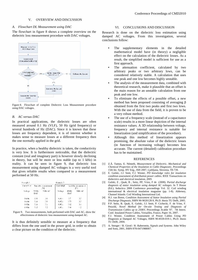
Conference Proceedings of CMD2010
V. OVERVIEW AND DISCUSSION
A. Flowchart DL Measurement using DAC
The flowchart in figure 8 shows a complete overview on the dielectric loss measurement procedure with DAC voltages.
Figure 8. Flowchart of complete Dielectric Loss Measurement procedure using DAC voltages.
B. AC versus DAC
In practical applications, the dielectric losses are often measured around 0.1 Hz (VLF), 50 Hz (grid frequency) or several hundreds of Hz (DAC). Since it is known that these losses are frequency dependent, it is of interest whether it makes sense to measure losses at a different frequency then the one normally applied in the grid. In practice, when a healthy dielectric is taken, the conductivity is very low. It is furthermore noticeable, that the dielectric constant (real and imaginary part) is however slowly declining in theory, but will be more or less stable (up to 1 kHz) in reality. It can be seen in figure 9, that dielectric loss measurement using damped AC voltages is a very useful tool that gives reliable results when compared to a measurement performed at 50 Hz.
Figure 9. Two measurements, both performed with DAC and AC, show the
effectiveness of dielectric loss measurement using damped AC.
It is thus definitely sensible to measure at a frequency that differs from the one used in the power grid, in order to obtain a clear picture on the condition of the dielectric.
VI. CONCLUSIONS AND DISCUSSION
Research is done on the dielectric loss estimation using damped AC voltages. From this investigation, several conclusions follow:
• The supplementary elements in the detailed mathematical model have (in theory) a negligible effect on the calculation of the dielectric losses. As a result, the simplified model is sufficient for use as a first approach.
• The attenuation coefficient, calculated by two arbitrary peaks or two arbitrary lows, can be considered relatively stable. A calculation that uses one peak and one low becomes highly unstable.
• The analysis of the measurement data, combined with theoretical research, make it plausible that an offset is the main reason for an unstable calculation from one peak and one low.
• To eliminate the effects of a possible offset, a new method has been proposed consisting of averaging β obtained from the first two peaks and first two lows. With the use of data from the field, it is proven to be a very robust method.
• The use of a frequency scale (instead of a capacitance scale) results in a more linear depiction of the internal resistance values. A 3D relationship between voltage, frequency and internal resistance is suitable for linearization (and simplification of the procedure).
• Although this method of linearization appears promising, the absolute value of the dielectric losses (in function of increasing voltage) becomes less accurate. The current (detailed) calibration procedure has to be maintained.
REFERENCES [1] Z.Á. Tamus, E. Németh, Measurement of Dielectric, Mechanical and
Chemical Properties of the Insulation in Cable Diagnostic, Proceedings 15th Int. Symp. HV Eng., ISH 2007, Ljubljana, Slovenia, T8-739.
[2] E. Gulski, J.J. Smit, F.J. Wester, PD knowledge rules for insulation condition assessment of distribution power cables. IEEE Transactions on dielectrics and electrical insulation, 2005
[3] Gulski, E , Quak, B , Seitz, PP, Vries, F de (2008). Partial discharge diagnosis of stator insulation using damped AC voltages. In T House (Ed.), Inductica 2008 Conference proceedings Vol. 32. Coil winding international & electrical insulation magazine (pp. 1-8). Alderney, Channel Islands: Coil Winding International Ltd.
[4] H.J. van Breen, Condition Assessment of Stator Insulation using Partial Discharge Diagnosis, ISBN 90-9020128-9, Ph.D. thesis TU Delft, 2005.
[5] P.P. Seitz, B. Quak, E. Gulski, J.J. Smit, P. Cichecki, F. de Vries, F. Petzold, Novel Method for On-site Testing and Diagnosis of Transmission Cables up to 250kV, Proceedings Jicable '07. 7th Intern. Conf. Insulated Power Cables, Versailles, France, Paper 16, 2007.
[6] F.J. Wester, Condition Assessment of Power Cables Using PD Diagnosis at Damped AC Voltages, ISBN 90-8559-019-1, Ph.D. thesis TU Delft, 2004.
[7] A. Stenger / B. Girod / R. Raberstein, Signals and Systems. John Wiley and Sons, 2001, ISBN-978-0471988007.