Ship collision on in atable weirs - TU Delft Repositories
157
Ship collision on inatable weirs Case study: weirs in the Meuse B.C.N. Stikvoort
-
Upload
khangminh22 -
Category
Documents
-
view
1 -
download
0
Transcript of Ship collision on in atable weirs - TU Delft Repositories

Ship collision oninflatable weirsCase study: weirs in the Meuse
B.C.N. Stikvoort


Ship collision oninflatable weirs
Case study: weirs in the Meuse
by
B.C.N. Stikvoortto obtain the degree of Master of Science in Civil Engineering
at the Delft University of Technology,
to be defended publicly on November 2, 2020 at 3:00 PM.
Student number: 4293347Project duration: November 11, 2019 – November 2, 2020Thesis committee: Prof. dr. ir. S. N. Jonkman, TU Delft, chairman
Ir. W. F. Molenaar, TU Delft, daily supervisorDr. ir. P. C. J. Hoogenboom, TU DelftIr. J. S. Reedijk, BAM
An electronic version of this thesis is available at http://repository.tudelft.nl/.

Preface
In front of you is presented the study ’Ship collision on inflatable weirs’. The study is made to complete themaster Hydraulic Engineering at the TU Delft and is done in collaboration with BAM Infraconsult.
I would like to thank my supervisors for their advise and feedback during the meetings. Prof.dr.ir S.N. Jonkmanfor reviewing my draft reports. Ir. W.F. Molenaar for his guidance and availability for my questions. Dr.ir. P.C.J.Hoogenboom for giving detailed feedback. My satisfaction to ir. J.S. Reedijk, with emphasis to giving theopportunity using the new BAM waterlab research facility, to do my experiments. Here with the presence of ir.M. Muilwijk. His helping hand was much appreciated to me.
Thank you Luc for reviewing my report. I would like to thank my family supporting me during the time doingthis research. My mom for always supporting me even in harder times. In special my girlfriend Bo motivatingme to the finish.
Bram StikvoortDelft, November 2020
iii


Abstract
In the Meuse seven weirs are located in the Dutch reaches, controlling the water level to enable inlandnavigation through the river. The weirs are being scheduled for replacement, where weir Grave is the firstone in 2028. They are reaching their end-of-life time and are not in compliance with the working conditionsanymore.
One of the main issues that became of more importance in the recent years is ship collision. In the past 20years two major ship collisions happened on two different existing weirs in the Meuse, one at Grave and oneat Linne. The place of impact at the weirs was significantly damaged after those collisions. The weirs, madeof steel plates and girders, were not stiff enough to resist those impacts. As a consequence, the water leveldropped and inland navigation was not possible for one month.
The inflatable rubber weir is being developed since 1955. One of the aspects that has not yet been consideredfor those inflatable weirs is ship collision. Where ship collision has been often researched for steel gates. Thetheory and formulas found for the existing collision analysis are not fully applicable to the inflatable weir,mainly due to large elastic deformation of the inflatable weir. For insight into ship collision on inflatable weirstwo main questions are derived:
1. How can the inflatable weir-ship interaction by ship collision at Grave be modelled to predict the motionsof the ship and the inflatable weir?
2. What happens when a push convoy ship collides with an inflatable weir at Grave?
To answer those questions, first a conceptual inflatable weir design is proposed for location Grave, that canreplace the existing weir. The design is based on existing literature, such as the inflatable storm surge barrierRamspol. The design for Grave is considered to be scalable to the overflow (Poirée) parts of the Meuse weirs.Three methods are used to analyse ship collision on the designed inflatable weir. First, an analytical modelis made to study the behaviour of the inflatable weir and ship during ship collision. Second, an effort wasmade to develop a numerical model in Ansys. Lastly, physical model tests were performed to see what happensduring ship collision on the inflatable weir and calibrate the analytical model, see figure 1. The full videoexperiments are uploaded to the 4TU-datacentrum (https://data.4tu.nl/portal)
In literature a standard expression has been found to quantify the ship force on the colliding structure. Thisexpression forms the basis of the analytical model. The inflatable weir in the analytical model is schematized bya two-dimensional plate sheet. With the analytical model, the strain in the sheet is quantified by ship collisionfor different push convoy CEMT-classes (ship classes). The side effects of water during impact were taken intoaccount separately. It was showed that ship waves did not have significant influences on the stresses and strainof the inflatable weir. However, the water overflow showed a flow velocity of 4.4 m/s, which can lead to damageof the bottom protection behind the weir. An effort was made to validate the strain found in the analyticalmodel by a numerical model in Ansys. However numerical instabilities were found that lead in considerablemodification of the desired model and so the results indicated no representative outcomes.
To see what happens during the ship collision a physical scale model was made, with scale 1:25 for accuraterepresentation of the physical phenomena. Sixteen experiments were done with four different draughts andfour different velocities of the ship. For the experiment with the scaled maximum draught (0.14m) and velocity(1.1m/s), the interaction in time is shown in figure 1. In six steps the ship collision interaction experiment iselaborated:
1. The ship is heading towards the weir, with the measured velocity.2. The bow of the ship is almost colliding on the weir and the bow wave is already topping over it.3. The bow of the ship collides on the weir and is uplifted by the air pressure inside the membrane.4. The ship is gliding over the weir, losing its energy and is further uplifted.5. The ship is glided the maximum distance over the weir and is accelerating downwards.6. The ship and weir are bouncing back by the elongated sheet of the weir.
v

vi 0. Abstract
Figure 1: snapshots ship collision experiments in time
The two aspects uplift of the ship and gliding over the weir are not yet included in the analytical model,therefore the analytical model is extended. In equation 1, the potential energy (Epot) is added to account forthe uplift and the gliding coefficient (Cglide,mean) to account for the gliding of the ship.
F =Cg l i de,mean
√2(kci r c +klong )(Eki n −Epot ) (1)
The extended analytical model showed a 25% deviation with the uplift of the ship and a 15% deviation with thedisplacement of the weir from the experiments. With the extended model it was calculated that the limit strainis not exceeded and that the strain is maximum 5% on top of the static strain of 1.9%.
Conclusion: The first steps have been taken into research of ship collision on inflatable weirs. An analyticalmodel is developed to indicate quantitatively what happens during collision. The physical model test helps toget insight what happens during collision and is useful for calibrating. Further investigation on the ship withV-bow, the propeller of the ship and a more extensive numerical model is recommended for ship collision oninflatable weirs.

Contents
Preface iii
Abstract v
1 Introduction 11.1 Background information . . . . . . . . . . . . . . . . . . . . . . . . . . . . . . . . . 11.2 Problem statement . . . . . . . . . . . . . . . . . . . . . . . . . . . . . . . . . . . . 31.3 Research questions . . . . . . . . . . . . . . . . . . . . . . . . . . . . . . . . . . . . 31.4 Research methodology . . . . . . . . . . . . . . . . . . . . . . . . . . . . . . . . . . 41.5 Thesis outline . . . . . . . . . . . . . . . . . . . . . . . . . . . . . . . . . . . . . . . 4
2 River Meuse and the seven weirs 72.1 River Meuse . . . . . . . . . . . . . . . . . . . . . . . . . . . . . . . . . . . . . . . . 7
2.1.1 Catchment area Meuse. . . . . . . . . . . . . . . . . . . . . . . . . . . . . . . 82.1.2 Discharge characteristics . . . . . . . . . . . . . . . . . . . . . . . . . . . . . 82.1.3 Water levels in the Meuse . . . . . . . . . . . . . . . . . . . . . . . . . . . . . 11
2.2 Seven weirs in the Dutch reaches . . . . . . . . . . . . . . . . . . . . . . . . . . . . . 122.2.1 Construction and replacement. . . . . . . . . . . . . . . . . . . . . . . . . . . 122.2.2 Weir complex decomposition . . . . . . . . . . . . . . . . . . . . . . . . . . . 132.2.3 Dimensions . . . . . . . . . . . . . . . . . . . . . . . . . . . . . . . . . . . . 152.2.4 Bed protection . . . . . . . . . . . . . . . . . . . . . . . . . . . . . . . . . . . 15
2.3 Shipping . . . . . . . . . . . . . . . . . . . . . . . . . . . . . . . . . . . . . . . . . 152.3.1 Ship collision events . . . . . . . . . . . . . . . . . . . . . . . . . . . . . . . . 16
2.4 Discussion . . . . . . . . . . . . . . . . . . . . . . . . . . . . . . . . . . . . . . . . 18
3 Design of an inflatable weir Grave 193.1 Overview Grave . . . . . . . . . . . . . . . . . . . . . . . . . . . . . . . . . . . . . . 193.2 Design process inflatable weir . . . . . . . . . . . . . . . . . . . . . . . . . . . . . . 20
3.2.1 Design study . . . . . . . . . . . . . . . . . . . . . . . . . . . . . . . . . . . . 213.3 Design aspects . . . . . . . . . . . . . . . . . . . . . . . . . . . . . . . . . . . . . . 22
3.3.1 Shape membrane . . . . . . . . . . . . . . . . . . . . . . . . . . . . . . . . . 223.3.2 Volume membrane. . . . . . . . . . . . . . . . . . . . . . . . . . . . . . . . . 263.3.3 Clamping . . . . . . . . . . . . . . . . . . . . . . . . . . . . . . . . . . . . . 273.3.4 Abutments . . . . . . . . . . . . . . . . . . . . . . . . . . . . . . . . . . . . . 283.3.5 Filling medium. . . . . . . . . . . . . . . . . . . . . . . . . . . . . . . . . . . 293.3.6 Membrane material . . . . . . . . . . . . . . . . . . . . . . . . . . . . . . . . 303.3.7 Foundation . . . . . . . . . . . . . . . . . . . . . . . . . . . . . . . . . . . . 313.3.8 Maintenance and operation . . . . . . . . . . . . . . . . . . . . . . . . . . . . 313.3.9 Dynamic effects inflatable weir . . . . . . . . . . . . . . . . . . . . . . . . . . 32
3.4 Conceptual design inflatable weir. . . . . . . . . . . . . . . . . . . . . . . . . . . . . 323.4.1 Safety factors. . . . . . . . . . . . . . . . . . . . . . . . . . . . . . . . . . . . 32
3.5 Discussion . . . . . . . . . . . . . . . . . . . . . . . . . . . . . . . . . . . . . . . . 33
4 Analytical model ship collision on inflatable weirs 354.1 Set-up. . . . . . . . . . . . . . . . . . . . . . . . . . . . . . . . . . . . . . . . . . . 35
4.1.1 Model expression . . . . . . . . . . . . . . . . . . . . . . . . . . . . . . . . . 364.2 Collision model on inflatable weir . . . . . . . . . . . . . . . . . . . . . . . . . . . . 37
4.2.1 Analytical plate model ship collision . . . . . . . . . . . . . . . . . . . . . . . . 374.2.2 Reference model . . . . . . . . . . . . . . . . . . . . . . . . . . . . . . . . . . 39
4.3 Parameters ship collision analysis. . . . . . . . . . . . . . . . . . . . . . . . . . . . . 404.3.1 Stiffness sheet . . . . . . . . . . . . . . . . . . . . . . . . . . . . . . . . . . . 40
vii

viii Contents
4.3.2 Velocity ship . . . . . . . . . . . . . . . . . . . . . . . . . . . . . . . . . . . . 404.3.3 Ship size and mass . . . . . . . . . . . . . . . . . . . . . . . . . . . . . . . . . 404.3.4 Bow . . . . . . . . . . . . . . . . . . . . . . . . . . . . . . . . . . . . . . . . 41
4.4 Results collision analysis . . . . . . . . . . . . . . . . . . . . . . . . . . . . . . . . . 414.5 Ship waves . . . . . . . . . . . . . . . . . . . . . . . . . . . . . . . . . . . . . . . . 434.6 Bottom protection . . . . . . . . . . . . . . . . . . . . . . . . . . . . . . . . . . . . 444.7 Discussion . . . . . . . . . . . . . . . . . . . . . . . . . . . . . . . . . . . . . . . . 45
5 Numerical model ship collision on inflatable weirs 475.1 Analysing methods . . . . . . . . . . . . . . . . . . . . . . . . . . . . . . . . . . . . 475.2 Geometry and mesh . . . . . . . . . . . . . . . . . . . . . . . . . . . . . . . . . . . 485.3 Parameters ship and inflatable weir . . . . . . . . . . . . . . . . . . . . . . . . . . . . 495.4 Collision Model . . . . . . . . . . . . . . . . . . . . . . . . . . . . . . . . . . . . . . 50
5.4.1 Schematization . . . . . . . . . . . . . . . . . . . . . . . . . . . . . . . . . . 505.4.2 Test models . . . . . . . . . . . . . . . . . . . . . . . . . . . . . . . . . . . . 515.4.3 Set-up and boundary conditions. . . . . . . . . . . . . . . . . . . . . . . . . . 52
5.5 Computation time . . . . . . . . . . . . . . . . . . . . . . . . . . . . . . . . . . . . 525.6 Output and analysis. . . . . . . . . . . . . . . . . . . . . . . . . . . . . . . . . . . . 53
5.6.1 Graphs . . . . . . . . . . . . . . . . . . . . . . . . . . . . . . . . . . . . . . . 535.7 Discussion . . . . . . . . . . . . . . . . . . . . . . . . . . . . . . . . . . . . . . . . 54
6 Physical model ship collision on inflatable weir 556.1 Model test set-up . . . . . . . . . . . . . . . . . . . . . . . . . . . . . . . . . . . . . 55
6.1.1 Scaling . . . . . . . . . . . . . . . . . . . . . . . . . . . . . . . . . . . . . . . 566.1.2 Scaling results . . . . . . . . . . . . . . . . . . . . . . . . . . . . . . . . . . . 576.1.3 Experiment recording . . . . . . . . . . . . . . . . . . . . . . . . . . . . . . . 58
6.2 Experiment method. . . . . . . . . . . . . . . . . . . . . . . . . . . . . . . . . . . . 596.2.1 Test parameters . . . . . . . . . . . . . . . . . . . . . . . . . . . . . . . . . . 59
6.3 Processing methodology . . . . . . . . . . . . . . . . . . . . . . . . . . . . . . . . . 626.4 Data analysis . . . . . . . . . . . . . . . . . . . . . . . . . . . . . . . . . . . . . . . 64
6.4.1 Displacements . . . . . . . . . . . . . . . . . . . . . . . . . . . . . . . . . . . 646.4.2 Discharge and friction . . . . . . . . . . . . . . . . . . . . . . . . . . . . . . . 656.4.3 Overtopping waves . . . . . . . . . . . . . . . . . . . . . . . . . . . . . . . . 676.4.4 Air pressure . . . . . . . . . . . . . . . . . . . . . . . . . . . . . . . . . . . . 68
6.5 Discussion . . . . . . . . . . . . . . . . . . . . . . . . . . . . . . . . . . . . . . . . 69
7 Analysis 717.1 Ship collision analysis. . . . . . . . . . . . . . . . . . . . . . . . . . . . . . . . . . . 717.2 Modified mass and velocity . . . . . . . . . . . . . . . . . . . . . . . . . . . . . . . . 737.3 Improved ship collision model . . . . . . . . . . . . . . . . . . . . . . . . . . . . . . 73
7.3.1 Potential energy conversion . . . . . . . . . . . . . . . . . . . . . . . . . . . . 737.3.2 Glide coefficient . . . . . . . . . . . . . . . . . . . . . . . . . . . . . . . . . . 767.3.3 Strain . . . . . . . . . . . . . . . . . . . . . . . . . . . . . . . . . . . . . . . 767.3.4 Comparison of results . . . . . . . . . . . . . . . . . . . . . . . . . . . . . . . 77
7.4 Clamping and sheet strength . . . . . . . . . . . . . . . . . . . . . . . . . . . . . . . 787.5 Discussion . . . . . . . . . . . . . . . . . . . . . . . . . . . . . . . . . . . . . . . . 79
8 Conclusions and recommendations 818.1 Conclusions. . . . . . . . . . . . . . . . . . . . . . . . . . . . . . . . . . . . . . . . 818.2 Recommendations . . . . . . . . . . . . . . . . . . . . . . . . . . . . . . . . . . . . 83
List of symbols 83List of Figures 89List of Tables 93A Weirs Meuse and shipping 95
A.1 Bed protection weirs . . . . . . . . . . . . . . . . . . . . . . . . . . . . . . . . . . . 95A.2 Dimensions weirs . . . . . . . . . . . . . . . . . . . . . . . . . . . . . . . . . . . . . 96

Contents ix
A.3 Shipping fleet . . . . . . . . . . . . . . . . . . . . . . . . . . . . . . . . . . . . . . . 96A.4 Ship collisions . . . . . . . . . . . . . . . . . . . . . . . . . . . . . . . . . . . . . . 96
B Inflatable rubber dams 99C Design weir Grave 103
C.1 Steel weirs. . . . . . . . . . . . . . . . . . . . . . . . . . . . . . . . . . . . . . . . . 103C.2 Inflatable weir designs . . . . . . . . . . . . . . . . . . . . . . . . . . . . . . . . . . 104
C.2.1 Multi criteria analyses . . . . . . . . . . . . . . . . . . . . . . . . . . . . . . . 106C.3 Clamping . . . . . . . . . . . . . . . . . . . . . . . . . . . . . . . . . . . . . . . . . 106
C.3.1 Verify strength clamping . . . . . . . . . . . . . . . . . . . . . . . . . . . . . . 107C.3.2 Abutment round design calculation . . . . . . . . . . . . . . . . . . . . . . . . 107C.3.3 Bottom recess . . . . . . . . . . . . . . . . . . . . . . . . . . . . . . . . . . . 108
D Shape membrane 109D.1 Length sheet . . . . . . . . . . . . . . . . . . . . . . . . . . . . . . . . . . . . . . . 111D.2 Neglecting self weight . . . . . . . . . . . . . . . . . . . . . . . . . . . . . . . . . . . 111D.3 Validation parameters. . . . . . . . . . . . . . . . . . . . . . . . . . . . . . . . . . . 112D.4 Research shape . . . . . . . . . . . . . . . . . . . . . . . . . . . . . . . . . . . . . . 112D.5 Dynamic shape . . . . . . . . . . . . . . . . . . . . . . . . . . . . . . . . . . . . . . 115
E Ramspol 117E.1 Collision probability . . . . . . . . . . . . . . . . . . . . . . . . . . . . . . . . . . . 117E.2 Ship navigation . . . . . . . . . . . . . . . . . . . . . . . . . . . . . . . . . . . . . . 117E.3 Sheet material. . . . . . . . . . . . . . . . . . . . . . . . . . . . . . . . . . . . . . . 118E.4 Joints rubber sheet . . . . . . . . . . . . . . . . . . . . . . . . . . . . . . . . . . . . 118E.5 Abutment clamping. . . . . . . . . . . . . . . . . . . . . . . . . . . . . . . . . . . . 118E.6 Foundation . . . . . . . . . . . . . . . . . . . . . . . . . . . . . . . . . . . . . . . . 119E.7 Folds . . . . . . . . . . . . . . . . . . . . . . . . . . . . . . . . . . . . . . . . . . . 120E.8 Tensile strength . . . . . . . . . . . . . . . . . . . . . . . . . . . . . . . . . . . . . . 121E.9 Ansys macros . . . . . . . . . . . . . . . . . . . . . . . . . . . . . . . . . . . . . . . 122
F Ship collision model 123F.1 Probability collision. . . . . . . . . . . . . . . . . . . . . . . . . . . . . . . . . . . . 123
F.1.1 Bayesian network . . . . . . . . . . . . . . . . . . . . . . . . . . . . . . . . . 124F.1.2 Simplified probability . . . . . . . . . . . . . . . . . . . . . . . . . . . . . . . 124
F.2 Collision energy. . . . . . . . . . . . . . . . . . . . . . . . . . . . . . . . . . . . . . 124F.3 Absorption efficiency fenders . . . . . . . . . . . . . . . . . . . . . . . . . . . . . . . 127F.4 Ship velocity . . . . . . . . . . . . . . . . . . . . . . . . . . . . . . . . . . . . . . . 127F.5 Bow . . . . . . . . . . . . . . . . . . . . . . . . . . . . . . . . . . . . . . . . . . . . 128F.6 Tree . . . . . . . . . . . . . . . . . . . . . . . . . . . . . . . . . . . . . . . . . . . . 128F.7 Ship waves . . . . . . . . . . . . . . . . . . . . . . . . . . . . . . . . . . . . . . . . 129
G Numerical model 131H Experimental model 133
H.1 Scale model tests . . . . . . . . . . . . . . . . . . . . . . . . . . . . . . . . . . . . . 133H.2 Model test scaling . . . . . . . . . . . . . . . . . . . . . . . . . . . . . . . . . . . . . 134
H.2.1 Air . . . . . . . . . . . . . . . . . . . . . . . . . . . . . . . . . . . . . . . . . 134H.2.2 Strain rigidity . . . . . . . . . . . . . . . . . . . . . . . . . . . . . . . . . . . 137H.2.3 Bending stiffness. . . . . . . . . . . . . . . . . . . . . . . . . . . . . . . . . . 138H.2.4 Ship velocity . . . . . . . . . . . . . . . . . . . . . . . . . . . . . . . . . . . . 138H.2.5 Sheet thickness . . . . . . . . . . . . . . . . . . . . . . . . . . . . . . . . . . 139H.2.6 Ship mass/draught. . . . . . . . . . . . . . . . . . . . . . . . . . . . . . . . . 139
H.3 Testing procedure . . . . . . . . . . . . . . . . . . . . . . . . . . . . . . . . . . . . . 140H.4 First experiment set results . . . . . . . . . . . . . . . . . . . . . . . . . . . . . . . . 140H.5 Folds change . . . . . . . . . . . . . . . . . . . . . . . . . . . . . . . . . . . . . . . 142
References 143


1Introduction
In this chapter an introduction is given about ship collision on inflatable weirs. First background informationwill be given on which this research is based. Next the research questions will be defined based on theproblem statement. The methodology used in the research will then be described to answer the researchquestions.
1.1. Background informationThe weirs in the Meuse have been built between 1920 and 1940 [8]. Each weir spans in total more than 100meter, covering the width of the river Meuse to regulate the water level. The weirs are reaching the 100-yearlifetime, most are not in compliance with the working conditions anymore and are scheduled for replacement.In 2017 a program has been setup by Rijkswaterstaat for the replacement of the weirs called ’Grip op de Maas’[53]. The replacement of the weirs, based on their building year, is scheduled to be executed between 2020and 2040. The program suggests having an 1:1 replacement of the weirs to keep the characteristics of the riverMeuse the same. Three reasons for replacement of the weirs can be given. First the old weirs may fail dueto decreased resistance of the materials over the years. Second, the maintained increased water head in theMeuse causes an increased load on the weirs 1. At last the weirs have an old design and may missed out onapplicable innovations. In total there are seven weirs located in the Dutch reaches of the Meuse, see figure 1.1.They span a reach from Maastricht until ’s Hertogenbosch.
Figure 1.1: side view weirs in the Meuse [46]
1The water load is proportional to the square of the water head
1

2 1. Introduction
Looking back in history of weirs, there is a relevant event for designing the replacement of the weirs. This eventis ship collision on one of the weirs. In 2016 a 2000-ton benzene tanker collided on the weir at Grave in theMeuse [46], see figure 1.2. The weir at Grave is made of baffles, enough to retain the water and was clearlynot prepared for a ship collision of such size. The whole upstream water level dropped and no shipping waspossible for a month. Also, this had impact on the houseboats in the nearby region, see figure 1.3. Informationabout the ship and why this could have happened is found in chapter 2.
Recently another accident happened with ships hitting the weir Linne in the Meuse. During storm Ciara in2020 two push convoys got loose of the quay and drifted downstream towards weir Linne. Those two shipswere unloaded and did not have a self-propelled velocity, which reduces the size of impact. The reparation ofthe weir is found in chapter 2.
Back in the time the weirs were made for the Meuse, they were possibly not designed for ship collision. Theshipping industry was much smaller by then. The amount of trade going by ship increased since 1980 with anaverage rate of 3% over a global scale [40]. With the increased shipment over the year it is more plausible tohave a collision accident.
Figure 1.2: weir Grave after ship collision [46] Figure 1.3: houseboat with water level drop[46]
For the replacement program a new type of weir concept is being proposed, to investigate its behaviour due tosimilar ship collision events. This is an inflatable weir made of a rubber sheet filled with air (and/or water).The invention of the inflatable dam comes from the prof. Mesnager, from France, in 1955 and is patented laterin 1965 by Norman Imbertson from the USA [42, p. 9]. The development is later improved in Japan. More than2000 rubber dams exists around the world [45], an overview is given in appendix B.
In the Netherlands this concept is used once as a barrier at Ramspol and is the biggest in its kind [51]. At theRamspol storm surge barrier the design storm conditions has an occurrence of around 1/700 years, whereasship collision is accounted for a probability of 1/1250 years [38]. Although the collision probability is less,it is still considered in the design process. One of the purposes for this type of barrier is that this barrier isconsidered a safe and cheaper option comparing to the traditional vertical lifting gate barrier [31, p. 91].
In line with the 1:1 replacement of the seven weirs of the Meuse, the inflatable concept is assumed a conceivabledesign. It is assumed the design of the inflatable weir can be uniform and deployable for all the weirs in theMeuse in the Dutch reaches. Due to increased number of shipping, ship collision on the proposed inflatableweir design is considered increasingly important.

1.2. Problem statement 3
1.2. Problem statementMost weirs in the Netherlands are made of steel, therefore a lot of knowledge is existing on these type of weirs.The inflatable weir concept, made of rubber, is relatively new and behaviour on loads is different from thecommonly used steel and concrete structures. A structure that can be thought of that uses rubber is a fenderfor mooring ships at quays. On both steel/concrete hydraulic structures and fenders, ship collision analysis isperformed. For example, a simplified model for ship collision on lock gates is created by Buldgen, to calculateamong other things the displacement of the gates [32]. Another model description on how to simulate scrapingcollisions on guide works is done by Dommelen [69]. For ship collision analysis on fenders a general approachis given by PIANC [43], see appendix F. For the ship collision on the inflatable weir no ship collision analysis isperformed yet.
In practice the inflatable weir is designed for types of loading that have a common occurrence in a river. Theinflatable weir is designed for static loading such as the hydrostatic water pressure and dynamic loadingsuch as the wave-impact and wind. A high safety factor is included to account for the uncertainties in thebehaviour of the rubber membrane during loading. The mechanics of the inflatable weir during ship collisionare different than for steel weirs. Fender systems are getting closer to the mechanical behaviour of an inflatableweir, nonetheless those structures are specially designed for ship collision.
The problem stands in not knowing what happens when a ship collides with an inflatable weir. There iscurrently no model describing this phenomenon and ship collision never happened on an existing inflatableweir yet. The consequences of the potential event are uncertain, therefore it cannot be included in an integrateddesign process.
1.3. Research questionsFrom the problem statement emerged that a method for the behaviour of ship collision on an inflatableweir is not readily available. A model is desired to get insight into the consequences of the ship-inflatableweir interaction. A simplified and clear model is sought, where the inflatable weir and the hull of the ship ismodelled, to gain insight of the potential event. The question derived to make such an understandable andclear model is described as:
1. How can the inflatable weir-ship interaction by ship collision at Grave be modelled to predict the motionsof the ship and the inflatable weir?
To answer the main question, four sub questions are defined in order to allow a better answer for the mainquestion:
• Can numerical modelling help to verify the analytical model?• Can a physical model test help to verify the analytical model?• How much strain in the sheet will develop during the ship structure interaction?• What side effects of the water do need to be taken into account for the consequences of the ship collision?• Can the analytical model examine the resistance of the conceptual design to ship collision?
The above main question will quantitatively describe the ship collision scenario. For better insight of whathappens during ship collision, it is of interest to know what happen qualitatively (visually). So, within thescope of this research a second main question is defined:
2. What happens when a push convoy ship collides with an inflatable weir at Grave?
The following sub questions are formulated to allow a better answer for the main research question:
• Will the ship bounce back from, glide over or glide fully over the inflatable weir?• Will the ship rupture the sheet of the inflatable weir during collision?• How will the push convoy collide into the inflatable weir?

4 1. Introduction
1.4. Research methodologyFirst the characteristics, weirs and ship collision events of the river Meuse will be investigated. Then a locationin the Meuse will be chosen for the design of an inflatable weir and the ship collision event. The inflatable weiris designed up to the conceptual design phase, which gives enough details for the ship collision analysis. Mostof the design is based on what is found from experience in literature.
The analytical model is built based on the parameters of the ship and the inflatable weir design. The shipparameters are determined from general guidelines used in the Netherlands. Any side effects of the water werealso investigated. Based on the found results more understanding of ship-inflatable weir was desired. Numeri-cal software Ansys was consulted to perform more extensive calculations about the collision event. Resultsfrom the numerical calculations, were tried to compare with what was found in the analytical study.
Physical model tests were done, to extract the significant process during the ship collision event. These testscould be performed at the cooperating company BAM Infra bv. The availability of space made it possible to dolarge scale model tests, what is preferred based on literature. The ship collision tests were visually analysedwith cameras on top and side of the scale model. The data was visually analysed and put into graphs.
Finally, the results of the physical model tests were compared with the analytical model, to develop a moreextensive analytical model that is calibrated on the physical model tests. With what is found during theresearch the main questions are answered.
1.5. Thesis outlineThe thesis is outlined in seven chapters and a last chapter consisting of conclusions and recommendations, seeflowchart in figure 1.4. The thesis starts with an introduction in chapter 1, which gives background informationon the subject. The problem statement for this research is then described along with the research questions.In chapter 2 more information about water supply and management of river Meuse is elaborated. Then theweirs in the Dutch reaches belonging to the Meuse are categorized and the recent ship collisions are described.Chapter 3 presents the design for the inflatable weir as replacement for the existing weir at Grave. First theprocess of the design is explained and then different features of the design are described.
Following up, chapter 4 starts with the analysis of ship collision on the inflatable weir design. It gives resultsabout the deformation and possible failure. Some calculations are done for the importance side effects of thewater. Further, numerical modelling is performed in chapter 5 for ship collision on the rubber sheet of theinflatable weir. Software program Ansys is consulted to carry out the numerical calculations. Next, chapter 6 iscommitted to describe the scale model tests done, to gain understanding of the ship collision mechanism. Theresults were of the experiments are used in an improved analytical model in chapter 7.
Lastly, chapter 8 is a distillate of what is found in the previous. Conclusions and recommendations are givenbased on the research done.

1.5. Thesis outline 5
Figure 1.4: flowchart


2River Meuse and the seven weirs
This chapter gives an overview of river the Meuse. The first paragraph 2.1 sets out how the river itself worksand how it is characterized. Then an overview is given of the Meuse weirs in the Dutch reaches, in paragraph2.2. The weirs are described by their type and functionality. Lastly the shipping in the Meuse is highlighted andrelevant collision accidents in paragraph 2.3.
2.1. River MeuseThe Meuse is a free-flowing river which ends up in the Netherlands. The Meuse starts in France and thencrosses Belgium and finally the Netherlands, see figure 2.1. The whole path of the river stretches over a lengthof 925 km and is for most part through mountains.
Figure 2.1: Meuse overview
7

8 2. River Meuse and the seven weirs
The river gets most of its water from rain and melting snow from the Ardennes, see figure 2.2. The water followsthe path with least resistance, which is to the direction of the lower laying areas. As can be seen from figure 2.2,the river is at a higher elevation in France. So, the river flows through the mountains in Belgium and finallyenters the Netherlands where it ends up in sea.
2.1.1. Catchment area MeuseThe Meuse itself gains most of its water supply through connected side branches of the river in the mountains.In those side branches rainwater assembles that has been falling down on the mountains. The side branchescoming all together to river the Meuse. At the location of Ardennes in Belgium there are a lot of side brancheswith high gradient, see figure 2.2. In combination with the low gradient downstream of those side branches,more water volume is available per unit length downstream of the river.
Figure 2.2: Meuse side branches [20]
2.1.2. Discharge characteristicsThe water in the Meuse is automatically controlled, this is done by operation of the weir gates. In general, thereare two options for the weir:
• A free-flowing river when the weirs are open• A dammed river when the weirs are operational
For a free-flowing river, the water can move without disturbance through the river, this the case on average 5days a year in the Meuse. If the discharge is large enough and so the water depth, the free-flowing situation ismaintained. When the discharge drops below a threshold value, the weirs are activated. The weirs dam up thewater level, to regulate a sufficient water depth for navigation. Every 10 minutes the weirs are adjusted basedon the expected discharge and measured water level. The threshold value of the discharge is dependent on theChézy value, which is an indication of the roughness of the bed. The Chézy value comes from the formula foraveraged flow velocity in the river. The formula is defined as follows:
v =Cp
Ri (2.1)
where: v = average flow velocity [m/s]C = Chézy value [m1/2/s]R = hydraulic radius [m] (equal to depth river)i = slope [i]
If there is a (almost) flat bed, the Chézy value can be calculated as follows:
C = 18log1012R
2d(2.2)
Where d is the grain size diameter [m].

2.1. River Meuse 9
The water level is controlled by a negative feedback control system. The change in river discharge triggersto heighten or lower the weir. a higher discharge means a lower weir level and vice versa. The operation ofthe weir aims to achieve a steady state situation. The water level at the set points remains the same, but thesurrounding water level can changes due to backwater curves. A water depth of 3 meters will be maintainedfor navigation [50].
In figure 1.1 the weirs are fully closed, hence retaining the maximum water level [46]. In this figure there is azero discharge, because the water levels are flat. When the discharge increases water will flow over the weir.A second effect is that a back-water curve will develop, where the water level increases upstream. When thecritical discharge value is reached, the weir will be lowered or lifted to increase the discharge capacity andmaintain the same water level. The weirs have a certain target point where the maintained water level is basedon. When the discharge increases the target point can change its value. An increase in discharge means ahigher water level upstream. To maintain the minimum water depth over the whole river for navigation, thetarget point value will be changed [16].
Generally speaking, the Meuse is a calm flowing river. The discharge in the Meuse is on average 230 m3/sranging from 132 m3/s in the summer to 320 m3/s in the winter [23]. The discharge varies also a lot within theyears. The minimum discharge can be 30 m3/s and the largest flood wave in 1926 had a discharge of 3000 m3/s[20] [55, p. 8]. For this high variability in discharge it is essential that the weirs can be adjusted for the requireddischarge. If the discharge is still too high another measure is taken that is the use of flood plains. These areareas which stay normally in dry and no vulnerable objects are placed in it such as houses. The flood plainswill be flooded with water during very high discharge events also called flood waves.Essentially the discharge is formulated with help also of equations 2.1 and 2.2 as:
Q = v Ar (2.3)
where: Q = discharge [m3/s]v = average water flow velocity [m/s]Ar = latitude cross sectional area river [m2]
From the equation of the water velocity it can be seen that the discharge is dependent on the inclination andthe water depth. The inclination is more or less constant over the river stretch and changes over long periodsof time. The water depth is dependent on the rainfall and melting snow from the Mountains, which differ daily.An overview of the variability in discharges in the river Meuse are shown in figure 2.3. The measurement datais the discharge of the Meuse including the Albertcanal, which is not of interest for the weir design in chapter 3.The Albertcanal starts at Liége and so takes water from the Meuse before it enters the Netherlands.
In figure 2.3 the months of the year are shown on the horizontal axis and the discharge on the vertical axis. Thegeneral trend shows that the discharge in the summer is lower than in the winter. The graph can be read asfollows:
• Red line: the maximum discharge over the year 1911 to 2019 by the corresponding day of the year• Green line: the average discharge over the year 1911 to 2019 by the corresponding day of the year• Black line: the minimum discharge over the year 1911 to 2019 by the corresponding day of the year• Blue line: the discharge for year 2019 per day

10 2. River Meuse and the seven weirs
Figure 2.3: Meuse discharge from 1991 to 2015 [2]
To use the data of figure 2.3 an exceedance probability function is needed. For the Meuse discharge theexceedance probability is calculated for various discharges and shown in figure 2.4. The dots representcalculation points. Research is done about the changes in river the Meuse that alter the discharge regime. Inthe future the discharge exceedance curve is likely to be different due to the mentioned cases as building ofdams and global warming. This research is done in the master thesis of Rooij [34].
Figure 2.4: exceedance probability vs discharge Meuse [34]

2.1. River Meuse 11
2.1.3. Water levels in the MeuseThe water levels in the Meuse are based on stage relation curves (Dutch: bettrekkingslijnen). The dischargeis measured at a certain point and with that information the corresponding water level is calculated. Themeasurement location point for the Meuse is taken at St. Pieter Noord, this is just south of Maastricht. For agiven discharge at location St. Pieter Noord the water level downstream can be calculated. The stage relationcurve gives the maximum expected water level based on the discharge, which is shown in figure 2.5. The lines,that indicate the water level in the Meuse, are based on yearly measurements and are interpolated with aWAQUA model. These water levels are used to argue the different collision scenarios, starting from chapter4.
Figure 2.5: water levels Meuse for various discharges [49]

12 2. River Meuse and the seven weirs
2.2. Seven weirs in the Dutch reachesThe Meuse is a large river, where its natural flow is disturbed by weirs constructed on the way downstream. Inthe Netherlands seven weirs are constructed in the Meuse, see figure 2.6. The weirs are constructed to achievea controlled water depth for ship navigation. Multiple weirs needed to be constructed in order to achieve thedesired minimal controlled water depth along the river. The ships that navigate through the river Meuse, needa minimal water depth, otherwise they will be stuck somewhere along the river.
Figure 2.6: weirs in the Meuse (OpenStreetMap Nederland, n.d.)
2.2.1. Construction and replacementThe weirs are scheduled for replacement, one of the reasons is due to their oldness. Placing new weirs on a newlocation is seems infeasible, because the agreement of water distribution over the Netherlands and Belgium isfixed. When 2030 is reached one-to-one weir replacement will be done, if in the meantime no other designalternative is presented which preventing changes in the groundwater table and the water distribution overthe length of the river [55, p. iii]. The seven weirs and their age are shown in table 2.1. The replacement of theweirs is scheduled in the years between 2025 and 2040 [8].

2.2. Seven weirs in the Dutch reaches 13
Construction year Scheduled replacementBorgharen 1928 2025-2030
Linne 1921 2035-2040Roermond 1921 2030-2035
Belfeld 1924 2030-2035Sambeek 1925 2030-2035
Grave 1926 2030-2035Lith 1936 2035-2040
Table 2.1: weirs Meuse construction year and replacement [8]
2.2.2. Weir complex decompositionIn this paragraph an elaboration is given how the weirs look like and how they function. The weir is a structurein a river or a canal, that is constructed to change the flow conditions. In case of the Meuse it is used to regulatethe water level in the river. To regulate the flow there are two possibilities dependent on the weir structure: [39,p. 70].
• Overflow weir: The upstream water level can be well controlled• Underflow weir: The discharge trough the structure is well-controlled
In case of the Meuse most weirs exists of an over- and underflow part excepts weir Grave, which is explainedfurther in this paragraph. For the overflow weir there are two types: broad crested and sharp crested weir. Inthe Netherlands most weir are sharp crested weirs. [39, p. 72].
Stoney-poiréeThe weirs Sambeek, Belfeld, Roermond and Linne exist of a Stoney and Poirée part, which act as under- andoverflow respectively. The Stoney part consists of a frame with steel plates in front of it. On the frame roundwheels are attached, that guides the steel plates to a lower or higher position. The suspension is regulated suchthat by lowering or heighten the steel plates, the trolley can move with half the velocity for smooth movement.The Stoney part has two steel plates between the columns. Those two plates roll past each other to regulate thewater level. In first instance the plates are put on top of each other. To increase the discharge, the upper panelis lowered. When the two panels hit the sill, the discharge can be further increased by raising both panelsabove the water. The Stoney part can take about half the capacity discharges of the weirs. Each Stoney openingconsists of a 17-meter-long opening with columns on each side. The Stoney steel plates are lowered or raisedevery 10 minutes based on measurements of water level and expected discharges. It fine tunes the water leveland is automatically controlled.
The Poirée Part consists of two individual slides, which are placed on top of each other. The weir is closed byusing both slides on top of each other. The weir can be opened by removing the steel panel and laying downthe beams on the bottom of the river. In this case ships can freely navigate through the river without use of theshipping locks. For the four weirs the Stoney part is located next to the Poirée part. The Poirée part consistof 13 to 17 meter beams horizontally (Dutch: Jukken), with a total of 3 steel panels which can placed on topof each other. At Sambeek these panels are 4.85m wide and 1.90m high. The Poirée part is used for coarseregulation of the water level.
When the discharge increases, first the Stoney part is used to let the water through, by lifting the steel panels. Ifthe discharges increases too much, then the steel panels are removed at the Poirée part, usually 3 panels in arow at a time. These panels are removed manually what makes the weir times consuming. The steel panels areremoved by the top row, the middle row and finally the lowest row. Then the beams can be put down on thebottom, when also the steel panels at the Stoney part are lifted a free-flowing river appears.
Grave is characterized by an inversed Poirée weir. At Grave the weir consists in total of 20 beam columns withalso three rows of steel panels. The beams are distributed over two openings and the panels are removedpartly manually. The top and the middle panel can be removed automatically based on the configurationsdetermined by the stewards (In Dutch: stuwmeester). The beams can also be lifted above the water level toprovide ship passing.

14 2. River Meuse and the seven weirs
Figure 2.7: Stoney part [29] Figure 2.8: Poirée part [29]
Slides and valvesThe weirs of Lith and Borgharen consists of different openings than the rest. Lith has 3 openings and Borgharen4. The closure consists of a steel framework (slide) with a flap on top of it. By raising or lowering the flap, thedischarge can be regulated. When the flap is laying horizontal and additional discharge capacity is needed,then the steel framework is lifted above the water to increase the discharge. Every 10 minutes the system isadjusted depending on the measured water level and expected discharge. The flap can so regulate the overflowof the weir and the lifting will create an underflow. For high discharges the underflow is used, since it cancreate a free-flowing river by totally rising the slide plus valve. See figure 2.9 for an illustration how the slideswith valves look like.
Figure 2.9: wheel valve [29]
Limit dischargeFor all weirs there is a limit capacity of water discharge they can handle. The Stoney part can discharge theirlimit capacity when the steel panels are lifted. The Poirée part can discharge their limit capacity when the steelpanels are removed and the beams laying on the bottom. For the weirs with slides and valves this is when allthe slides (with valves) are lifted. The limit discharges per weir is given in table 2.2. The table shows a variationof the limit discharge. This is due to the difference in opening width of the weirs and the maintained waterdepth.
Weir Lith Grave Sambeek Belfeld Roermond Linne BorgharenLimit discharge [m3/s] 1097 1070 1205 800 984 1278 1250
Table 2.2: limit discharges for the various weirs

2.3. Shipping 15
2.2.3. DimensionsThe different weir types have all their own dimensions. Some parts in the Meuse are wider than other parts, thatis why the total width of the weirs differ. Further the weirs have their own weir type configuration depending onthe needs of the flow characteristics. The dimensions for each weir is given in table A.2 in the appendix.
2.2.4. Bed protectionBed protection at the weirs is necessary to prevent erosion downstream of the weir. Erosion can eventuallylead to instability of the weir and in the limit case will collapse. The bed protection of the weirs have beenreported in RINK reports and is summarized in table A.1 of the appendix. The bed protection at Roermond isthe shortest and least robust. It is plausible that the protection at Roermond has been reinforced based onthe conclusions of the RINK reports. Further only at weir Linne the bed protection is different behind theStoney and Poirée part. The other three weirs have the same bed protection for the Stoney and Poirée part.Ship collision on inflatable weirs can cause rupture of the sheet or overflow over the weir and as consequencethe waterflow can damage the bottom protection.
2.3. ShippingThe size of ships that navigate through the Meuse, are elaborated in this section. The ships passing the Meuseare transporting cargo to or from the port of Rotterdam. To indicate the size of a ship, an international systemis setup that is called the CEMT (=Conférence Europeenne des Ministres des Transports). With this system thesize of a ship is indicated ranging from class I to VII (small to big).
In general, the waterway defines the maximum CEMT class that can navigate through the waterway. For theMeuse this is CEMT class Va at the time of writing. The waterway class and ship classes that navigate throughthe Meuse, are shown in figure 2.10.
Figure 2.10: waterway- and ship classes Meuse [55]

16 2. River Meuse and the seven weirs
There are some uncertainties with the given data in the figure. This figure is created by a previous Masterthesis, doing research for design of an adaptive weir at Belfeld [55].
• The average is taken from 2005 until 2008• In Maastricht data is missing• Recreational ship have not been counted, but is considered insignificant for ship collision• The total number of commercial ships is taken as two-third of the number counted at lock Born
The data from figure 2.10 is based on the load capacity of the ship. So, for a certain loading capacity the ship isplaced in a certain CEMT class, but by dimensions the ship can be one CEMT class higher or lower.
Since the ship trade in the Meuse is increasing and so the amount of ships and their size, an upgrade of theMeuse is expected. With this upgrade a ship class of Vb is possible, which applies to push convoys. Currently,the canal is upgraded with wider sections where ships can pass each other. Widening of the Bend of Elsloo, toaccommodate Class Vb ships is just feasible [10]. The maximum ship length is now 110 m in the Juliana canal.Also deepening of the river is scheduled to accommodate a draught of 3.5 meters. The maximum draught isnow 3.0 m.
2.3.1. Ship collision eventsShip collision on a weir is not a regular event in the Meuse. Sometimes it happens, but depending on the massof the ship and its velocity a significant impact can follow. All registered ship collisions in the Netherlands of afew selected years are found in appendix A, to give an indication. Two significant ship collision on weirs thathave happened in the Meuse, are described below. The size and mass of those ships in the events are also usedin this research. The first collision was in 2016 at Grave and the second happened at in 2020 at weir Linne.Both damaged the weirs such that they were out of operation for a while.
GraveThe ship started at Klein Ternaaien in Belgium a day before the collision. In around 30 hours the ship navigatedto Grave where it collided with the weir on 29 December 2016. That day a thick fog was present. Fog can createa circumstance for a higher probability of ship collision. In appendix A a fault tree is represented how fog andother factors affect the ship collision probability.
By the force of the collision five baffles got loose, see figure 1.2, where a powerful current of water developed.The ship glided through the opening and landed 3 meters behind the weir. Normally the ship would make afall motion, but the strong current and resistance of the baffles above the ship made it happened that the shipcould glide with the movement of the water. The engine was stopped shortly after the collision, but would notlet the ship come to a standstill. Thereafter the anchors were dropped and the ship stopped 600 meters behindthe weir.
To navigate through fog with a ship it is obligated to have good radar equipment on board. On the ship a radarsystem was available that got his information through a circular panel. The circular panel registers objectswith pulses that are displayed as dots on the panel. Although it was available it could not be derived if therewas a closed weir upfront [64].
The ship that collided into the weir Grave, is called the Maria Valentine. It is a tanker ship that sails under theGerman flag. Some of the characteristics of the ship are given below:
Symbol Dimension UnitLength Ls 110 mWidth Bs 11.4 m
Draught Ds 3.64 mLoading capacity ms 3015 tonnageMax ship velocity vs 6.1 m/s
Ship class - Va (RWS class M8) -
Table 2.3: ship Maria Valentine characteristics

2.3. Shipping 17
The velocity of the ship during collision is investigated by the Dutch Safety Board. They investigated a velocityof 4.05 m/s just 150 meters in front of the gate. This was the last velocity that could being distracted, beforethe ship hit the weir. At the day of collision, the ship was loaded with benzene and had a total load of 2000ton, deriving from this a draught can be estimated of 3.64*2000/3015=2.41 m. According to the starting course,velocity, load of the ship and the observed damage of the weir, the Maria Valentine had to navigate straightto the weir without much velocity reduction. The baffles in the middle were hit by the ship and damaged. Infigure 2.11 is shown where the ship hits the weir. After collision a temporary structure was placed around thedamaged weir, so it was shielded and could be repaired.
Figure 2.11: collision Grave front view [64]
LinneOn 10 February 2020 two empty push convoys got loose the quay. They were torn loose by storm Ciara that wasravaging the Netherlands, that day. Both push convoys were driven downstream by the current and hit the weirof Linne. With the impact five baffles were damaged. A temporary fracture stone dam is place in the Meuseto stabilise the situation. The dam takes over the water retaining function of weir Linne. It is noted that thebreach of the weir induced a limited increase on the water level in Linne and Roermond, less than the actualhigh-water level during the storm Ciara. In Linne an increase of 60 cm can be expected and in Roermond 30cm.
Figure 2.12: loose push convoy heading to weir Linne during stormCiara [56] Figure 2.13: reparation of weir Linne [52]

18 2. River Meuse and the seven weirs
2.4. DiscussionThe river Meuse is a free flowing river as described in this chapter. With the building of the weirs for inlandnavigation, the free flowing conditions are altered to a controlled flow of the river. These weirs are locatedat specific points in the Meuse. It is a study how the flow conditions and so the water depths will change, byreplacing the weirs upstream or downstream of the existing location. The graph in figure 2.5 will then change.Another possibility to change the flow condition is with a different configuration of the under- or overflow partof each weir or Poirée and Stoney part respectively, described in paragraph 2.2.2. In this research no study willbe conducted on the possibilities of doing a replacement different than 1:1. In the next chapter the design for ainflatable weir is presented, using 1:1 replacement as boundary condition.
In the past 20 years of the existing weirs in the Meuse, ship collisions with significant consequences onlyhappened twice in the past 5 years. A reason for this can be the growing inland navigation, but two times inthis short period is quite remarkable. Also, the ships become bigger and bigger, but the limit eventually is whatthe Meuse can take. All together it can be reasoned that ship collision is of increasing importance for hydraulicstructures. Research is done into ship collision on an designed inflatable weir at Grave from chapter 4.

3Design of an inflatable weir Grave
In this chapter the design is presented for the inflatable weir at Grave. The design is tested on ship collisionin later chapters. First an overview of Grave is given in the first paragraph 3.1. The process of the design andthe design itself is explored in paragraph 3.2. Building further on the design the next paragraph 3.3 describesthe components needed for the design itself, such as the sheet length and the clamping structure. The lastparagraph 3.4 deals with an overview of the design.
3.1. Overview GraveIn the previous chapter 2, already some key aspects of weir Grave are given. Weir Grave is here elaborateddeeper. In principle, the weir in connected to a spanning bridge, where the weir is used to manage the waterlevel in the river for navigation. When the weir is closed or partly opened it is not suitable for ships to passthrough this route. A lock is situated next to the weir to let ships pass the river section. In figure 3.1 the place ofthe weir and its two locks are shown.
Figure 3.1: overview weir Grave (OpenStreetMap Nederland, n.d.)
19

20 3. Design of an inflatable weir Grave
The weir Grave is against the trend of using bigger parts to regulate the water discharge. The weir has to retain3.5 m water drop height. Bigger parts that are used for Poirée parts, would be too weak for the high-water dropheight. Vertical pillars are used which are hinge supported to the bridge above. Between the pillars, steel platescan glide on top of each other from the top of the bridge to dam up the water level upstream. The bottomof the pillars are resting on a threshold at the river bottom. The dimensions of weir Grave are shown for thefront view in figure 3.2 and a cross section from the side in figure 3.3. As is shown from the cross section figure,the maintained water level was lower (-30 cm) 100 years ago. The increase in maintained water level can beexplained by the larger ships navigating through the Meuse.
Figure 3.2: Weir Grave cross section front view [8]
Figure 3.3: Cross section weir Grave side view [33]
3.2. Design process inflatable weirAs described in paragraph 2.4, the design made in this chapter is narrowed to 1:1 replacement of the existingweirs in the Meuse. This design process only focuses on the inflatable weir, which is an overflow weir. Thedesign of the inflatable weir is made to research ship collision on this structure. According to Rijkswaterstaatthe inflatable weir shows enough potential for further investigation [68]. In a normal design process also otherkind of weirs would be considered, but are not in the scope of this research. Other type of overflow weirs areincluded in appendix C, to give an impression what kind of weirs exist.
The inflatable weir is an option for the replacement of existing Poirée parts at the Meuse weirs. Both areoverflow weirs, where the water flows over the top of the weir. The Stoney parts are all underflow weirs, hencefor 1:1 replacement the inflatable weir is not applicable. It will be time consuming to design for all suitablelocations an inflatable weir and will be of less interest for this research. A solution is sought for in a generaldesign of the inflatable weir, where its dimensions are sizeable to the desired location. For the replacement ofthe existing weirs it needs to be considered how the river Meuse will be and be used in the future.

3.2. Design process inflatable weir 21
For the location of the initial design, Grave is chosen. The existing weir of Grave has two inversed Poirée partsand Grave is scheduled as first weir for replacement in 2028, making it a suitable design location. It has to benoted that the current weir at Grave is attached to the bridge above. During the second world war (WWII), thisbridge gained attention of its transportation function. Now the bridge is turned into a monumental object,which is likely to be maintained.
First the design process of making a design is given. Then the conceptual design phase for this research isdescribed. Within the design process more design phase are usually needed, which consists mainly of fivesteps. The analysis step consists of the criteria, where the design step is built on. Within these criteria possibledesign solutions are developed, which is called the synthesis step. The possible design solutions are testedand elaborated on the cons and pros, this is the simulation step. Then the evaluation is started, based on thegrouped pros and cons of each design the ranking is determined. A decision will be made, which designs arefurther developed in the next phase. One whole design cycle (phase) is given in figure 3.4. In general, thedesign phases are as follows: orientation, preliminary design, final design and detailed design. In scope of theresearch only the preliminary (conceptual) design cycle will be made. Assumptions are therefore needed thatnarrows the design process prematurely.
Figure 3.4: design process
The first phase in the design phases is the orientation phase. This phase is assumed to be already done in’Vervangingsopgave stuwen in de Maas’, where the weirs are scheduled for replacement. The next phase isthe preliminary (or conceptual) design phase. In this phase a first design is presented that can be suited asreplacement of the Poirée parts in the Meuse. This research is limited to ship collision on an inflatable weir, sothe design phase will be narrowed up to a feasible scope.
3.2.1. Design studyIn this paragraph the design is presented which can act as replacement for the weir at Grave. The design isthe outcome of four inflatable weir designs made in appendix C. The weirs are based on reference designsproposed in other projects. Two important design considerations are implemented in all four designs that isbased on what is found in literature and logical reasoning [62], [45].
• abutments 45 degrees• one side clamped
Multi criteria analysisThe four design possibilities are conducted to a Multi Criteria Analysis (MCA). A weighted score is given tothe criteria of each design. With the sum of the weighted scores from the criteria, a total is formed. With thisnumber a ranking is formed for the design options. The MCA covers the simulation step and the evaluationstep. In appendix C the full analysis can be found.
A note has be given to the ship collision criteria, which is most important in this research. The expected highership class Vb, discussed in paragraph 2.3, is in the range of push convoys [41, p. 23] and is a plausible scenariofor ship collision in the future. Likely the weir has to be resistant against this higher ship class. This researchanticipates on the plausible higher ship class in the Meuse in the future, by using the ship geometry of thepush convoy, which is clear from the experiments done in chapter 6.

22 3. Design of an inflatable weir Grave
Overview designThe design for the inflatable weir at Grave can be seen as example for the replacement of other Poirée parts inthe Meuse. In the next two figures, the final conceptual design is given extracted from the information in thischapter. Dimensions of figure 3.5 are related to figure 3.2 and dimensions of figure 3.6 are related to figure3.3.
Figure 3.5: front view final design
Figure 3.6: side view final design
3.3. Design aspectsThis paragraph deals with the sub-parts of the inflatable weir, which are in extend important for the analysis ofthe ship collision. The sub-parts are categorized in shape membrane, abutments, clamping structure, fillingmedium and sheet material. The sub parts give insight how the inflatable weir works and is going to looklike.
3.3.1. Shape membraneIn this paragraph an overview is given for the shape of the rubber membrane of the inflatable weir designGrave and how it is found. The theory behind this shape can be found in appendix D. Basically the shapeis based on a cross sectional view of the membrane. The forces acting in the cross sectional view define theshape of the membrane. Generally these forces consisting of water or air, see figure 3.7. Since water and aircan deform to the shape of the contact surface, these forces work perpendicular to it as shown in the figure.The perpendicular forcing makes it easy to work with the theory derived for determining the shape of the

3.3. Design aspects 23
membrane. Further the water pressure is assumed to work hydrostatic, so the force generated by the waterincreases linearly in depth. In formula form the water pressure is described by:
pw = ρw g hw (3.1)
where: pw = water pressure [N/m2]ρw = density water [kg/m3]g = gravitational constant [m/s2]hw = depth in the water column [m]
Figure 3.7: force overview [17]
In figure 3.7 the membrane is curved in a specific form. The curvature of the form can be directed inward ofthe membrane or outwards. When the outer pressure is larger than the inside pressure the membrane willcurve inward and vice versa. See in the figure the higher water level on the left, which gives a higher outsidepressure than the inside pressure and the membrane is curved inward. The forces taking into account for thecurvature of the membrane are defined as follow:
• internal water pressure• internal air pressure• outside water pressure• own weight membrane• forces in membrane
The air pressure is defined by the air pressure inside minus the atmospheric pressure. With this the atmosphericpressure is already compensated by the inside pressure, so the atmospheric pressure is not presented as aforce. The air pressure in formula form is defined as:
p = pi n −patm (3.2)
where: p = resulting pressure [N/m2]pi n = internal pressure [N/m2]patm = atmospheric pressure [N/m2]
ParametersWithout knowing how the shape is going to look like, two essential parameters of the membrane are initiallydetermined: internal pressure ’p’ and tensile force ’T’, see figure 3.10. When the tensile force is known, theinitial angle ’φ0’ can be determined from force equilibrium. The length of the sheet ’L’ is determined fromthe found shape according to the theory. A rule of thumb is that the length is four times the height of themembrane for single line clamped and air filled [62], see also appendix D

24 3. Design of an inflatable weir Grave
The internal pressure is determined based on the desired height of the membrane. The internal pressure isabout the same as the head for the air-filled type membrane [37]. The internal pressure for the air-filled type isthen, where H is the desired weir height [m]:
pi n = 1000H [N /m2] (3.3)
If the downstream side is dry then the pressure in the membrane needs to be about 20%–60% higher than thecarried water head. This is to compensate for tensile anchoring reactions, self-weight of the membrane andsome other load components [45].
In recent literature a formulation is defined for the tensile force of the membrane. The formulation is madeby Gebhardt, where the tensile force is dependent on the relation between the difference of upstream anddownstream water level and the internal pressure [35]. With the following formula the tensile force is calculatedfor an air-filled type membrane:
T = 1
2αρw g H 2 (3.4)
where: T = membrane force [N/m2]α = internal pressure coefficient pi n
Hup[-]
ρw = water density [kg/m3]H = weir height [m]
In figure 3.8 a relation is given between the theoretical shapes and the internal pressure coefficient. Theparameter ’R’ indicates the radius of the membrane. In case the membrane is only surrounded by theatmospheric pressure and internal pressure, then the internal pressure coefficient (α) goes to ∞. This is logical,since according to the theory of force equilibrium a circle should be found. More information about theresearch of the tensile force is found in appendix C.
Figure 3.8: geometry as function of internal pressure coefficient for air-filled type membrane [35]
Now the tensile force is determined by equation 3.4, the last parameter ’φ0’ can also be calculated by horizontalequilibrium for a one side clamped membrane, see also figure 3.10.
1
2ρw g H 2
up = T (1+cosφ0)+ 1
2ρw g H 2
down (3.5)
where: φ0 = angle membrane upstream [◦]Hup = water depth upstream [m]Hdown = water depth downstream [m]

3.3. Design aspects 25
Taking φ0 to the left hand side gives:
φ0 = cos−1{(
1
2ρw g
(H 2
up −H 2down
))/T −1
}(3.6)
For a two side clamped weir there are two unknown angle values. The second angle value can be found withvertical force equilibrium. For this the Kettle formula can be used. Since the design will be one line clamped,the two side clamped will not be further discussed.
Shape inflatable weir GraveWith the theory described in appendix D and the determined initial parameters, the shape of the membraneshould be found. In the appendix a demonstration is made for a circle with the theory based on the weir heightat Grave.
The cross sectional shape of the inflatable weir at Grave is found by force equilibrium of elements. The shapeis discretized into a finite number of elements (dS) where the coordinates and pressure are determined on thenodes, see figure 3.9. To calculate those coordinates the following formulations are applied, where dS* is theelongated element length:
φi+1 =φi − dS∗
dS
p
TdS (3.7)
xi+1 = xi + dS∗
dScosφi (3.8)
zi+1 = zi + dS∗
dSsinφi (3.9)
Figure 3.9: element model
At Grave there is an upstream and downstream water level. This creates three different situations around thelength of the membrane, where the third situation is the contact with the atmospheric pressure. As done in thetheory, the starting point is the clamping line. The resultant pressure for the three different situations are thendefined as follows:
case =
12 i f zi > Hup and case = 13 i f zi < Hdown and case = 2
p =
pi n − (Hup − zi )ρw g f or case = 1pi n f or case = 2pi n − (Hdown − zi )ρw g f or case = 3
The unknown starting conditions tensile force (T) and internal air pressure (pin) have to be determined withequations 3.4 and 3.5. Here also results the initial angle φ0 from. In table 3.1 the parameters are shown and infigure 3.10 the found shape is shown.

26 3. Design of an inflatable weir Grave
Parameter - value unitDesign height hd 5.3 m
Upstream water level Hup 5.15 mDownstream water level Hdown 2.15 m
Internal pressure pin 53 kN/m2
Circumference length L 17.22 mTensile force T 139 kNInitial angle φ0 1.8 rad
Table 3.1: parameters
The initial length of the sheet is taken as four times the membrane head (4H) and is divided into 1000 elements.At the ends of the elements nodes are situated, where equilibrium of forces is determined, see figure 3.9.Starting at the clamping line, the coordinates of the nodes are calculated with equations 3.7, 3.8 and 3.9.The calculation of new coordinates is stopped when zi>zi-1 and case = 3. The coordinates are then linearlyconnected and so the shape is found, see figure 3.10. The length of the sheet can be found by multiplyingthe number of elements used to get the shape times the stretched length of an element dividing by the strain(n*dS*/(1+ε). The length of the sheet found here is 17.22 m. The x-coordinate, where the z-coordinate is for thefirst time below 0, is 1.45. This means the sheet lays for 1.45 meters on the foundation.
The following observations are found that deviate from the desired value. The last z-coordinate did not finish atsmaller than zero, but 5 cm above the zero (ground) line. This is pretty close to the bottom and is an acceptabledeviation, stated that the theory is not perfect for the circular shape. The maximum height is 5.8 m which is aconsiderable deviation from the desired height of 5.3m.
Figure 3.10: shape inflatable weir Grave standard
It is criticized that the values found by the theory deviate too much from the desired values. In appendix Da parameter optimization is executed, to find the shape with the desired height and last z-coordinate. Thetensile force is varied between 90 kN and 190 kN and the initial angle between 0 and π. Both are varied with100 sub steps, so that a 100x100 matrix is created with shapes. Nonetheless there was no shape better fittingthe shape curve then the shape found here.
3.3.2. Volume membraneThe volume of the inside of the inflatable weir can be found by the shape of the membrane in cross section andthe length of the inflatable weir in longitude. The internal area of the cross sectional shape is first determined

3.3. Design aspects 27
with Greens theorem. In his theorem the internal area can be calculated in a discretized form:
Ai n = Σxi zi+1 −xi+1zi
2(3.10)
Using the coordinates calculated in figure 3.10 and Greens theorem the area of the cross sectional membranefound is 25.6 m2. For a circle the area would be πr 2 = π(5.3/2)2 = 22m2, so the area calculated with Greenstheorem seems valid. The volume is then calculated by: internal area multiplied with length of the sheet minusthe abutments plus a fourth times the abutments, because of its double 45 degrees inclination. The total airvolume is then, see dimensions in figure 3.5:
Vi n = Ai n(49.4+21
2
1
25.3) = 1332 [m3] (3.11)
3.3.3. ClampingThis paragraph describes the clamping design of the inflatable weir. A look is first taken if the two side clampedmembrane is a competing option against the single clamp line. Then the design of the clamping line isdiscussed.
It is possible for the inflatable weir to clamp it one or two sided (upstream or upstream and downstream ofthe river). To get an impression of a one- and two sided clamped weirs, see figure 3.11. The left shows a threedimensional one side clamped weir and the right shows a cross section two side clamped weir. The clampingfor both the one- and two sided clamped weirs is extended up to including the abutments [62]. For the one-and two side clamping lines both advantages are derived:
• For the one side clamp less clamping line is needed• For the two side clamp the membrane stays reachable for inspection and the membrane circumference
is shorter
In the figure 3.11 it is shown that the weir with one side clamp can lay flat on the bottom. For two side clampthe sheet lays in folds as has been done in Ramspol, see figure E.5. Ramspol is a storm surge barrier, where it ispossible for having a higher water level on both sides of the barrier. With a one line clamp the sheet can turnover direction if the current is from a wrong direction, therefore a two line clamp is chosen. For weirs a oneline clamp is convenient, since the water flow comes all the time from one side. Hence a one line clamp for theinflatable weir at location Grave is used in the design. The use of one clamping line makes the use for guiderollers unnecessary as described in appendix C.
Figure 3.11: one side clamped on the left and two side clamped on the right [62]
Clamping designFor the clamping structure itself the same clamping will be taken as Ramspol. The manufacturer (Bridgestone)of the sheet of Rampsol has much experience with this clamping structure. Other clamping structures, thatare not chosen, are given in appendix C. An optimization was tried to make for the design of the clampingstructure at Ramspol. However the calculation models could not adequately verify another design, whichcould reduce the costs. The research was aborted and the clamping structure from the manufacturer was stilltaken.
The clamping structure is given in figure 3.12. This is the clamping used for the horizontal part for Ramspol.For the abutment part a different clamping structure was chosen, because of the wave steps, see appendix

28 3. Design of an inflatable weir Grave
E. In this design no wave steps do apply. Pre-stressed bolts are penetrated through the sheet and both platesto tighten the clamp. The pre-stressed bolts are placed with a centre-to-centre distance of 150 mm. Severalmeasures are important for protection:
• The clamp should be made of stainless steel to prevent corrosion• Water repellent grease is used under the cap nuts to prevent water entering• An elastic wrapping band is put around the anchor holes to allow for stretching of the anchor• The sheet has a higher thickness at the clamping points
Figure 3.12: wave clamping horizontal part [38]
3.3.4. AbutmentsThe abutments form a new challenge for the inflatable weir. Traditional steel weirs have straight abutments,which suits to the location for the design of the inflatable weir. However for the inflatable weir a straightabutment causes sacking of the sheet in deflated state. An angle is desired to prevent sacking of the membranesheet. A too large abutment will on the other hand block the flow passing through the river. Both reasons arguea desired slope of 45◦, see figure 3.13.
Another option is to round the sheet membrane on both ends to the bottom. How this looks likes is givenin appendix C. This design creates however a leakage at the corners of the weir. In maintain conditions thedischarge will than be per abutment around 44 m3/s, times four at location Grave is 176 m3/s in total. Thiscomes close to the average discharge of 230 m3/s. When a lower discharge needs to be maintained this designis insufficient. The design with 45◦ abutments is thus best suited.
Figure 3.13: slope angle abutments front view

3.3. Design aspects 29
Still the sheet will sack in deflated state, because of its longer length needed in deflated state than in inflatedstate see figure 3.14. Jongeling demonstrated in a study of 1998 that an over length would solve the problemfor the sheet that hangs at the abutment in deflated state [61]. This is done by also putting the width directionof the abutment clamping line under 45 degrees. In deflated state there will be then enough sheet length tostore the sheet flat on the bottom of the foundation.
Figure 3.14: under length deflated state [38]
However, with this design the 3D shape of the membrane is not without imperfections. At the transitionwith the abutment there will be folds, due to the excess length of the slope, see figure 3.15. Two things are aconsequence of this:
• At these folds stresses concentrate that are unfavourable for the sheet. Appendix E shows how is dealtwith those folds at Ramspol. That is a two clamped inflatable dam, so it is not suitable in this case.
• The membrane on the span of the horizontal foundation can move freely in respect to the membraneat the slope of the abutments. This configuration simplifies the force transfer from the horizontalmembrane to the inclined membrane, to zero in case of enough excess length.
Bridgestone gave a schematization of how the inflatable membrane will look like on an inclined abutment of45 degrees and one side clamped. For this see figure 3.16.
Figure 3.15: fold at transition [11] Figure 3.16: Bridgstone abutment schematization [45]
3.3.5. Filling mediumThe membrane has to be filled inside with something to stay inflated. The membrane can be filled with water,air or a combination of both. For the inflatable storm surge barrier at Rampsol a combination of both is chosen.The behaviour of the membrane is related to the chosen filling medium inside. Characteristics of the differentconfigurations of fill media are given below:
Water• It will cost energy to pump out the water of the membrane.• It will sag due to its own weight• Larger circumferential length needed• Probability of resonance due to dynamic loading• Water is in-compressible

30 3. Design of an inflatable weir Grave
Air• The internal air pressure should be great enough to withstand the hydrostatic pressure. The consequence
is high tensile forces.• V-notching can occur due to dynamic loading, see figure 4.4• Increase in temperature expands air
Water and air• Differential pressure can be minimal• Danger of sloshing, with probability of resonance
The choice for the medium is dependent on several factors, see table 3.2.
Aspect Water Air Water and AirInflation and deflation - + 0
Crest height - + +Circumferential length - + 0
Self weight - + 0Stability of the weir + - +Weather conditions + - -
Compressibility filler - + 0
Table 3.2: water, air or water and air filled
For the inflatable weir design it is most suitable to choose air as filling medium. The crest height is the mostimportant one. For a water filled membrane the pressure is limited to the upstream head. In case of overflow,which is commonly for weirs, a higher internal pressure is needed than can be reached with air. A combinationof both is also possible, but with overflow conditions sloshing and resonance can occur. The disadvantage ofair is that due to hot weather the sheet can melt. A reference is made to Tempe town lake in Arizona, wherethe rubber dams collapsed. The sun caused the rubber to deteriorate over about 10 years, until one of therubber dams snapped. In appendix B, a photo of the situation together with elaboration is given. However theweather conditions in the Netherlands are different.
3.3.6. Membrane materialOne of the most important parts of the weir is the material where the sheet is made of. Usually there is chosenfor a sustainable type of rubber with a thickness of 10 to 20 mm, that is ozone-, oil-, and water resistant.For the design in this research the sheet of Ramspol is taken as design material. The sheet for Rampsol isdetermined by using materials in scale model tests, see appendix E. Eventually it was chosen to use Nylon fibresas reinforcement for the sheet. The covering layer consists of rubber for its elasticity, see figure 3.17.
Figure 3.17: sheet cross section [5]
The circumferential and longitudinal yarns are connected with separate fibres, therefore they can stretchindependently of each other. This is important to know for modelling the inflatable weir in chapter 7. Thesheet including the rubber and fibers are mainly good in absorbing tensile forces. It is demonstrated that thebending stiffness is not an important influencing factor for the sheet. This holds for the sheet, see table 3.3,with the condition EI≤50*106 Nmm2 [38, appendix 5]. The sheet strength in longitudinal direction should be30% of the strength in circumferential length according to Japanese rule of thumb.
The fibers are assumed to be wet in the river environment, so the wet conditions hold from table 3.3. Thestrength of the material is defined by tests done for the sheet of the Ramspol barrier [5, p. 3.2]. From the tests

3.3. Design aspects 31
it is concluded that the speed of loading does not have a great effect on the strength properties. The cyclicloading does have influence on the height of the membrane that can be reached. Cyclic loading induces creepon the sheet that reduces the length of the sheet and so top height decreases. Samples are hung near the damto test their strength under influence of water environments over the years. The expected lifetime was 25 years,but with the result of the test another 25 years are expected. For further information about the manufacturingand rubber of sheet referenced is to appendix E.
Direction Tensile strength [kN/m] E-modulus [kN/m] bending stiffness (EI) at 5 C◦ [Nm]Warp dry 1870 5700 15
wet 1602 3800 15Longitudinal dry 935 3200 17
wet 809 2000 17
Table 3.3: fiber strength
3.3.7. FoundationThe foundation of the inflatable weir is also of importance for the design. It gives the inflatable membranesolid ground to lay on. The top of the foundation needs to be smooth to prevent cutting of the sheet. Thereforethe concrete foundation as already is installed at Grave is a suitable option. The foundation has in generalthree main function:
• prevent sliding• prevent rotation• prevent settlement
To achieve a safe foundation the above three function should be full filled. The options to reinforce the concretefoundation for the described functions are:
• Cofferdam: in figure 3.3 Grave• Piles: in appendix figure E.6
The cofferdam works well for transferring horizontal forces and the piles are good for transferring verticalforces as well as horizontal forces. At Ramspol there is chosen for inclined piles as foundation structure, seeappendix E. The inflatable barrier at Ramspol is partly filled with water, which is much heavier than air. Largevertical forces are absorbed by the foundation floor that is why piles are probably used.
Since the design for the inflatable weir at Grave, air is used as filling medium, a much smaller vertical load needto be transferred. At this moment a steel weir is located at Grave, which should be heavier than an air inflatedweir. As the foundation at Grave already have demonstrated its stability especially in horizontal direction andthe vertical load would not much increase with the new inflatable weir, so the existing foundation is feasiblefor the design.
3.3.8. Maintenance and operationIn this paragraph the maintenance and operation is given for the inflatable weir design. The design is clampedto the foundation and is in inflated state as starting point. In figure 3.18 a standard design for an inflatable weiris given, comparable with the design used in this research. The use of a single line clamped membrane makesit difficult for inspection as discussed in paragraph 3.3.3. Only the outside of the membrane can be inspectedin inflated state and when there is no water overflow. Especially the clamping lines need extra attention, sincethose are all lifetime under water. The advantage is that no guide rollers are used to control lowering thesheet.
To inflate the weir, internal pipes are needed to blow in air and/or water. These inflation pipes are shown infigure 3.18. The pipes are connected to an air compressor on the landside. When the membrane needs tobe inflated, air is blown into the sheet and the weir will rise. The function of the spill breaker is described inparagraph 3.3.9.
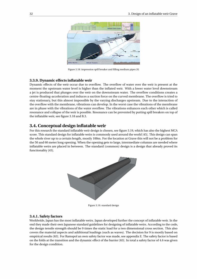
32 3. Design of an inflatable weir Grave
Figure 3.18: impression spill breaker and filling medium pipes [9]
3.3.9. Dynamic effects inflatable weirDynamic effects of the weir occur due to overflow. The overflow of water over the weir is present at themoment the upstream water level is higher than the inflated weir. With a lower water level downstreama jet is produced that plunges over the weir on the downstream water. The overflow conditions creates acentre-floating-acceleration and induces a suction force on the curved membrane. The overflow is tried tostay stationary, but this almost impossible by the varying discharges upstream. Due to the interaction ofthe overflow with the membrane, vibrations can develop. In the worst case the vibrations of the membraneare in phase with the vibrations of the water overflow. The vibrations enhances each other which is calledresonance and collapse of the weir is possible. Resonance can be prevented by putting spill breakers on top ofthe inflatable weir, see figure 3.18 and B.3.
3.4. Conceptual design inflatable weirFor this research the standard inflatable weir design is chosen, see figure 3.19, which has also the highest MCAscore. This standard design for inflatable weirs is commonly used around the world [45]. This design can spanthe whole river up to a certain length, mostly 100m. For the location at Grave this will not be a problem forthe 50 and 60 meter long opening. When the opening gets to large, intermediate columns are needed whereinflatable weirs are placed in between. The standard (common) design is a design that already proved itsfunctionality [45].
Figure 3.19: standard design
3.4.1. Safety factorsWorldwide, Japan has the most inflatable weirs. Japan developed further the concept of inflatable weir. In theend they made their own Japanese standard guidelines for designing of inflatable weirs. According to the code,the design tensile strength should be 9 times the static load for a two dimensional cross section. This alsocovers the material aspects and additional loadings (such as waves). The decision for 9 is mostly based onempirical results [63]. For Ramspol an own safety factor was made, see appendix E. The safety factor is basedon the folds at the transition and the dynamic effect of the barrier [63]. In total a safety factor of 4.6 was givenfor the design condition.

3.5. Discussion 33
3.5. DiscussionIn this chapter a design is presented for an inflatable weir at location Grave. The existing weirs are made ofsteel and exists for about 100 years. The design of the inflatable weir in this chapter is a fairly general one.In theory, the design can be implemented to the Poirée parts of the weirs in the Meuse as well. For that, anoptimization is probably needed for the other locations, because they are dealing with different circumstancesand dimensions. An option is to have a steeper inclined abutment slope. This is done for the inflatable weirs inGermany, see Bannetze weir, which has a 1:3 slope to increase the discharge capacity. For now it argued thatthe 45 degrees slope give the optimal design decision based on literature.
For the design of the inflatable weir at Grave itself, an adjustment of the location could be beneficial. Thenthe 1:1 replacement is neglected, by placing the design a little upfront of the design location. Here the Meuseis wider and the reduction of flow area by the abutments will be compensated. On the other hand, a newfoundation is needed that significantly increases the costs. It may be the best option to use standard (common)design of the inflatable weir in this chapter. Then additional flood plains will be necessary to compensate forthe decreased discharge capacity by the abutments. In situations of extreme run-off, those flood plains can beused.


4Analytical model ship collision on
inflatable weirs
In the this chapter an analytical model will be represented to analyse the ship collision on the inflatable weir.The first paragraph 4.1 gives an introduction to the ship collision analysis at. The location as well as the basicformulation is elaborated. In next paragraph 4.2 the analytical plate model presented for ship collision oninflatable weirs. Then the reference (1D) collision model is described for check on the results. In paragraph 4.3the parameters are determined necessary for the analysis. Following with a calculation of the models and theparameters in paragraph 4.4. Lastly a preliminary calculation is done for the ship waves and bottom protectionin paragraph 4.5 and 4.6 respectively.
4.1. Set-upThe collision at Grave, see chapter 2, is taken as reference for the ship collision analysis. During that collisionthe ship hits the right weir of Grave in the middle, see figure 2.11. According the investigation at Grave, theship collision was head on [64]. The same set-up is represented in figure 4.1 right picture. This ship collisionscenario is likely to give the highest impact on the weir and is used for the rest of the analyses done in theremaining of the research.
Figure 4.1: collision scenarios
35

36 4. Analytical model ship collision on inflatable weirs
Another option would be inclined collision as the collision at Linne, see figure 2.12. However the ship is morelikely to impact the pillar harder than the inflatable weir. This collision is schematized in the middle of figure4.1. The last option is a collision from the downstream side of the inflatable weir, see left of figure 4.1. In thiscase it is only possible for an unloaded ship to navigate to the inflatable weir. The draught for a loaded ship istoo high and the ship will ground somewhere on the way. Also, there is a downstream current, so the velocityof the ship will likely be less than navigating from upstream. The combination of a lower mass and velocitygives a smaller impact.
4.1.1. Model expressionThe ship collision model is made with energy and force laws, that describe the ship as a moving object and theinflatable weir as still standing object. In the model the ship is modelled as kinetic (or moving) energy andthe inflatable weir as potential (or still standing) energy. A derivation will be given here how these energiesrelate to each other. Here, a force is derived, so that the stress on the sheet can be determined. First the kineticenergy of the ship is defined, here also the water is included. When the ship is moving through the water someextra water volume is taken along with the ship (added water mass). The energy that the ship is moving isdefined by its mass and velocity squared:
Eki n = 1
2(ms +mw )v2
s (4.1)
where: Eki n = kinetic energy of ship and water [N/m]ms = mass ship [kg]mw = mass water [kg]vs = velocity ship [m/s]
Then the potential energy is defined of the sheet. This is defined by the stiffness and stretch of the sheetsquared. Think of it like a spring that is given a certain stretch of a unit length. If it let loose the spring bouncesback and the energy releases.
Epot ,w = 1
2ku2 (4.2)
where: Epot ,w = potential energy of inflatable weir [Nm]k = stiffness sheet [N/m]u = stretch of the sheet [m]
The kinetic energy of the ship is absorbed by the inflatable weir. It is for now assumed that the kinetic energy isfully absorbed in potential energy of the sheet of the inflatable weir. The damping in the system is assumedsmall and therefore zero. Usually the damping consists of the ship, water and inflatable weir. Neglecting thisgives a more conservative approach. In formula form a derivation is made to find an expression of the stretchof a unit length sheet of the inflatable weir, which is later needed to find the force acting on the sheet:
Epot ,w = Eki n
1
2kε2 = Eki n
u =√
2Eki n
k
(4.3)
With the stretch of a unit length acting on the inflatable weir, the force can be found. Force is defined bystiffness times stretch (displacement). When using the expression for stretch from equation 4.3 follows theforce on the membrane:
F = ku = k
√2Eki n
k=
√2kEki n (4.4)
In the Eurocode it states that the added water mass moving along with the ship can be approximated by 10% ofthe ship mass [12]. From this follows that equation 4.1 can be rewritten to:
Eki n = 1
21.1ms v2
s (4.5)
In appendix F more approximations are given for this added water mass based on numerical and physicalmodels.

4.2. Collision model on inflatable weir 37
4.2. Collision model on inflatable weirIn this paragraph the basic model for the ship collision of the inflatable weir is elaborated. Also the (reference)1D-model is given to check on the more elaborated 2D-model. In both models the following assumptions aremade:
• Movement of the inflatable weir as a whole, so the structure behaviour is assumed linear. In reality thecurvature of the membrane and behaviour of the rubber is non-linear.
• The internal pressure of the inflatable weir, induces an uplift on the bow of the ship in reality. In themodel it is assumed the ship will only move in the x-direction. In other collision models it is also donelike this [32]
• The ship in the analysis is rigid compared to the inflatable weir. This means that only the inflatable weircan deform during the collision and the ship remains its shape.
• An increase in air pressure would likely happen during impact and folds at the abutment can unfold.This pressure increases and folds are for now neglected.
4.2.1. Analytical plate model ship collisionIn this paragraph the actual (2D)-model is described used to determine the strain in membrane sheet. Thestrain is most important to know, since it indicates if the sheet will rip apart. A note has to be given that notonly the force due to collision can rupture the sheet. Sharp edges of the ship such as the bow thruster, can cutthe sheet. For the scope of this research the bow thruster is for now neglected. Also the bow shape of the shiphas influence on the actual strain on the sheet. The bow influence is further determined in chapter 7.
The inflatable weir is modelled as linear elastic spring in the xz-plane and xy-plane or side view and top viewrespectively. The springs are supported by a pinned support. This way the spring model can rotate around thepin, but is fixed in the sectional planes at the supports. An overview of the model from side view is given infigure 4.3 and from top view in figure 4.2. The contact height is defined as:
δ= D +H −Hup (4.6)
where: D = draught ship [m]H = height inflatable weir [m]Hup = upstream water depth [m]δ = contact height ship-inflatable weir [m]
Figure 4.2: ship collision model side view
The displacement (strain) of the springs (yarns) are independently of each other in circumferential and longi-tudinal directional, as described in paragraph 3.3.6.So for the total stiffness the stiffness in the circumferentialand longitudinal direction can be added to each other. How much the yarns stretch depend on the ship-structure displacement xw. It is of importance to know the strain in the sheet, to know if it will not rupture.In figure 4.7 and F.5 the maximum strain is determined as 20% for the design sheet. The amount of strain incircumferential direction according to the model is:
εci r c =√
H 2 +x2w
H−1 (4.7)

38 4. Analytical model ship collision on inflatable weirs
Figure 4.3: ship collision model top view
For the spring in longitudinal direction, the displacement is dependent on the impact location. The strain inlongitudinal direction is defined for one side as:
εl ong ,1 =√
L21 +x2
w
L1−1 (4.8)
and for the other side:
εl ong ,2 =√
L22 +x2
w
L2−1 (4.9)
When the ship hits in the middle of the inflatable weir, then the strain of both sides is defined as εlong ,1 = εlong ,2.The force acting on the inflatable weir is determined as:
F =√
2(kci r c +klong )Eki n (4.10)
The resistance of the inflatable weir is the contact width (Bs) or height (δ) of the ship-inflatable weir interactionmultiplied by the stiffness of the yarns multiplied by x-component of the springs multiplied by the strain, informula form:
FR = Bs kci r cxw√
H 2 +x2w
εci r c +δkl ong
xw√L2
1 +x2w
εlong ,1 +xw√
L22 +x2
w
εlong ,2
(4.11)
Filling in equation 4.7, 4.8 and 4.9 in equation 4.11 and equalling to equation 4.10, the displacement xw can befound. Then the strains are also known.

4.2. Collision model on inflatable weir 39
V-notchingThe supposable deformation is based on the V-notching phenomena seen in Ramspol, see figure 4.4. In figure4.5 the phenomena is schematized from the top, where the arrows indicate water flow. V-notching is a result ofthe situation where the internal pressure is extremely lower than the external pressure. This is the case whenthe Ramspol storm surge barrier inflates itself and meanwhile from the higher level water is flowing througha gap of the barrier. In the situation of a ship collision the membrane is already inflated, but the externalpressure is extremely increased by the ship collision. The inflatable weir is likely to form a V-shape, during shipcollision.
Figure 4.4: V-notching Ramspol [62] Figure 4.5: V-notching schematization top view [62]
4.2.2. Reference modelThe 1D-model is the reference model, which represents the behaviour only in x-direction of the ship-inflatableweir interaction. The force acting on the weir is converted in a strain, with a simple spring stiffness formula.The strain in the reference model is the same as the displacement of a unit length. The strain becomes thenthe force from equation 4.10 divided by the total stiffness, where the components of the total stiffness aremultiplied by the contact height/length the stiffness works on:
ε= F
Bs kci r c +δklong(4.12)
where: kci r c = stiffness in circumferential direction [kN/m]klong = stiffness in longitudinal direction [kN/m]Bs = width of ship, see figure 4.3 [m]
In figure 4.6 the representation is made of the simplified reference model.
Figure 4.6: 1D-model

40 4. Analytical model ship collision on inflatable weirs
4.3. Parameters ship collision analysisIn this paragraph the necessary parameters are described for the ship collision analysis. The parameters arethen used for a first calculation with the plate model and the reference model.
4.3.1. Stiffness sheetThe yarns which are acting as springs in circumferential and longitudinal direction have a certain stiffness,which are determined based on tests. The stiffness of the modelled springs for the inflatable weir is based onthe sheet properties. The stiffness is determined by samples which are loaded until failure. For the design sheet,given in paragraph 3.3.6, sample tests are already done for the Ramspol project. Figure 4.7 and 4.8 shows thestress-strain relation of the design sheet for six different samples in circumferential- and longitudinal directionrespectively. The samples show that for increasing stress the strain becomes less, which is a non-linear featureof the sheet. For ship collision the sheet stiffness is assumed linear and the ultimate strain is taken. Based onthis strain the stiffness of the modelled springs is determined.
Figure 4.7: stress strain relationship sheet circumferential [62] Figure 4.8: stress strain relationship sheet longitudinal [62]
As can be seen from the test, the maximum strain is 20% until break. The stiffnesses become then
stiffness circumferential (kcirc) = 1500 / 0.2 = 7500 [kN/m]stiffness longitudinal (klong) = 600 / 0.2 = 3000 [kN/m]
4.3.2. Velocity shipThe velocity of the ship is chosen according to the ROK 1.4 by Rijkswaterstaat [27]. In figure 4.9 the maximumship velocity is shown per CEMT-class for the ship collision. This velocity is leading, only if the ship CEMT-classis not exceeding the CEMT-class of the navigation route. The ship needs a required water depth and width,where the CEMT-class of the navigation route is based on, to achieve the maximum velocity. For the Meuse nohigher CEMT class ships are navigating through the Meuse than the CEMT-class of the navigation route, seeparagraph 2.3. So this velocity numbers are valid for the ship collision model in this research. In appendix Fand E more velocity numbers are given, but for different situations.
Figure 4.9: maximum ship velocity according to ROK [27]
4.3.3. Ship size and massFor the various ships, tables are made to assign a ship class to the ship. There are three type of ships distin-guished [41, p. 18]:
• motor cargo ships• pushed convoys• coupling connections

4.4. Results collision analysis 41
The ship that collided with the existing weir at Grave was a motor cargo ship, see chapter 2. For the analysisof ship collision on the inflatable weir, the pushed convoy is used. These are ships with in front of it convoysthat are being pushed by the ship and are expected to allow a Vb class in the future of the Meuse. The CEMT-classes for these ships with corresponding size and mass are cited in the Richtlijnen Vaarwegen booklet fromRijkswaterstaat [41]. The CEMT-classes for pushed convoys that are allowed in Meuse are shown in figure 4.10.For the calculations, the used CEMT-classes are circled in red.
Figure 4.10: pushed convoys [41]
4.3.4. BowThe bow geometry is based on the pushed convoy. The choice of the bow is of importance for the interactionduring ship collision. The contact area differs, which yields in different results. There is also the V-bow shapethat is commonly used for motor cargo ship. The total fleet in the Netherlands consists of both motor cargoships and pushed convoys. For information about fleet set-up see appendix A.
The full bow shape for the pushed convoy can be found in appendix F. The geometry of the bow shape is basedon pronunciation by the United Nations in a European agreement about international water traffic [66]. In themodel it is assumed that the bow has a triangular shape as can be seen in figure 4.2. The parameters a, b and cin the figure are determined with report of the United Nations and are as follows:
• a is 19.7 m• b is 4.4 m• c is 1.14 m
From the report it is also shown that the radius of the edges is 50 to 60 cm, which makes the edges less sharp.Therefore the ship will less likely cut the sheet of the inflatable weir by the edges of the bow.
Further it is stated in chapter 2 that the maximum draught, with a deepened Meuse, is 3.5m. The heightof the oblique part of the bow (b) is 4.4m, so the tip of the bow is always above the inflatable weir duringimpact.
4.4. Results collision analysisIn this paragraph the results are gathered for the analysis of ship collision. Three different parameter set-upsare calculated according to the three different classes from figure 4.10. The current maximum draught (3.0m)allowed in the Meuse is used as normative condition. Then the ship mass is calculated by (maximum draughtMeuse / maximum draught CEMT-class) * maximum deadweight CEMT-class, see table 4.1. The accordingcollision velocity of the ship is taken from figure 4.9.
CEMT class draught [m] mass ship [ton]IV 3 1450Va 3 2100
Va extended 3 2415
Table 4.1: parameters

42 4. Analytical model ship collision on inflatable weirs
Plate modelThe outcome from the 2D model is described here for the three different CEMT classes. An example calculationfor class Va extended is shown below. To find the unknown value xw the goal and seek function in Excel is used.It was stated that the ships hit the middle of the weir, so L1=L2 and L1 = L−Bs
2 = 60−11.42 = 24.3[m]. Equation
4.11 can then be rewritten to:
Bs kci r cxw√
H 2 +x2w
εci r c +2δklong (xw√
L21 +x2
w
εlong ,1)−FR = 0
11.4∗7500∗ xw√5.152 +x2
w
∗ (
√5.152 +x2
w
5.3−1)+
2∗ (3+5.3−5.15)∗3000
xw√24.32 +x2
w
(
√24.32 +x2
w
24.3−1)
−27696 = 0
xw = 5.54[m]
(4.13)
The displacement and strains found for the three different CEMT classes are given in table 4.2
CEMT class ship displacement [m] strain circumferential [%] strain longitudinal [%]xw εci r c εl ong ,1 εl ong ,2
IV 5.27 41 2.15Va 5.37 42.29 2.41
Va extended 5.54 44.66 2.57
Table 4.2: 2D model output
During ship impact the final strain of the circumferential yarns is including the tensile force in static condition,see figure 3.10. The final strain becomes then:
εci r c,tot al = εci r c + T
kci r c= εci r c + 139
7500= εci r c +1.9% (4.14)
Or to say 1.9% has to be added to the circumferential strain in the table above.
In 3D the inflatable weir looks like a curtain in the yz-plane, see figure 4.11. In this figure the ship and sheetof the inflatable weir are shown before impact. In figure 4.12, the situation is shown at impact. This is thesupposable deformation form in 3D according to the plate model.
Figure 4.11: schematized inflatable weir 3D before collision
Figure 4.12: supposable deformation 3D
It is noted that the strain is definitely exceeding the limit strain given in table 4.2. The question is still if thismodel is an accurate representation of the real physical mechanism. The model has to be compared withnumerical or physical models, described in chapter 5 and 6. In chapter 7 the analytical model described hereis calibrated on the physical model tests.

4.5. Ship waves 43
In this chapter it is assumed that all the energy of the ship is translated into strain of the sheet. The displacementfound (xw) is the maximum displacement of the weir and the ship. At that displacement the velocity of theship is zero. According to this model the ship will bounce back by the elastic property of the sheet. In thephysical model test in chapter 6 it is shown that the ship bounces back partially, but not further than the weiritself.
Reference modelThe outcome from the reference model is described here for the three different CEMT classes. An examplecalculation for class Va extended is made using equation 4.12:
ε= F
Bs kci r c +δklong= 27696
11.4∗7500+ (3+5.3−5.15)∗3000= 0.2917 (4.15)
In the table below the outcomes of the strain (elongation) of the reference model is given for the three differentCEMT classes
CEMT class strain total ε [%]IV 25.63Va 27.2
Va extended 29.17
Table 4.3: reference model output
4.5. Ship wavesThe ship waves are a result of the ship navigating through the river and can have a potential significance onthe collision. Ship waves are generally categorized in two forms:
• Primary wave: the water level compression around the ship. The wavelength is around ship length Ls
• Secondary wave: the waves generated from the bow and hull. Those waves are much shorter in lengththan the primary waves
The primary waves are especially important in narrow channels. Here the conservation of energy happensover a small cross sectional area resulting in larger water level compression and return current. In the Meuseriver this narrow channel approximation is not the case. This is determined by the blockage coefficient, whichlooks at the area of the ship under water in ratio to the total water area, see figure 4.13.
Figure 4.13: overview ship collision
For the location at Grave with the largest ship at the moment of writing (CEMT Va), the blockage coefficient isaround:
As
Ar= 11.4∗3
5.15∗ (110+2∗ 12 ∗ (2∗5.3))
= 34.2
621= 0.03 (4.16)
where: As = area ship under water in latitude cross section [m2]Ar = area of the water in latitude cross section [m2]
Or the same as 3%, which is not significant.

44 4. Analytical model ship collision on inflatable weirs
On the other hand, the secondary waves have a bigger impact. In appendix F it is elaborated how thesewaves are generated. The height of these secondary waves are determined experimentally. A formula fromexperiments is derived to calculate the wave height, which is described in RWS/DHL 1988 [18]. In equation4.17 the height of ships waves are calculated. The height is calculated for the cusps of the waves, which is thesuperposition of diverging and transverse waves.
Hw
h= ζ
( s
z
)−1/3F r 4 (4.17)
where: Hw = wave height [m]z = effective water depth [m]ζ = coefficient which represents ship’s geometry [-]s = distance side ship to bank [m]
The wave height increases with the velocity of the ship reaching its limit at Fr = 1. The Froude number(F r = vsp
g h) is a measure for the inertia in ratio to the gravity. Here ’h’ is described as the effective water height
accounting for the slopes at the edges of the river (h = AcBr
= 621110+5.3∗4 = 4.73m), where Br is the river width. The
Froude number is then Fr=5.5/(9.81*4.73) = 0.81. The coefficient for ship geometry is dependent on the kind ofship. The coefficient is dominated by the draught and bow of the ship. For a push convoy the ζ coefficientis around 0.5. Now all the values can be calculated for the wave height equation 4.17 and is shown in table4.4.
IV Va Va extendedAs/Ac [-] 0.04 0.05 0.05
Fr [-] 0.78 0.81 0.81s1 [m] 27.9 26.95 26.95s2 [m] 86 85 85Hw,1 1.15 1.35 1.35Hw,2 0.79 0.92 0.92
Table 4.4: wave height secondary wave cusps
With the wave height, also the wave load can be calculated. A conservative rule of thumb approach is used forthis. The wave force is calculated when the wave top is reaching the inflatable weir. The load is consideredstationary and the maximum wave force is, where ’H’ is the height of the inflatable weir:
Fw ave = 1
2ρw g H 2
w +Hρw g Hw (4.18)
For the highest wave, which is on the right of the ship (s1), the wave force is calculated as 77kN/m. The shipload per running meter is εci r c /100∗kci r c = 0.41∗7500 = 3000kN /m. The wave force is negligible comparedto the ship load.
4.6. Bottom protectionBesides the ship-weir interaction, there are also the side effects of the water. The waves are already describedin previous paragraph. However there will be also an overflow of water after collision. Eventually the shiplays on the weir, causing flow gaps at the sides of the ship, this is seen at the experiments in chapter 6. In thisparagraph a first estimation is made of the overflow and the needed bottom protection downstream.
According to the theoretical shape of the sheet during compression in figure 6.22, the mean drop height is 1/3of the total drop height. The flow velocity is calculated with, for a ship with draught of minimum 3.0m andwhere h is the mean water depth:
v2
2g+h −→ v =
√2g h =
√2∗ g ∗ (Hup −Hdown)
3=
√2∗9.81∗ (5.15−2.15)
3= 4.43[m/s] (4.19)
With equation 2.2 and the equation of Shields:
d50 = v2
Φ∆C 2 (4.20)

4.7. Discussion 45
where: ∆ = dimensionless specific grain weight ρs−ρwρw
Φ = threshold value before grains start to move (0.03) [-]C = Chézy coefficient [-]d50 = Nominal grain size diameter [m]
the grain diameter d50 becomes 0.96m. This means 1 to 3 ton stones, where Grave is not fulfilling this accordingto table A.1. However Shields equation is based on uniform flow. In this case the flow is rapidly decelerateddownstream. The overflow plunges first downstream of the weir in the water, see figure 4.14. At the locationwhere the overflow plunges is close to the foundation and the colloidal concrete at Grave. This has higherresistance then loose stones. If the bed protection is still damaged, an option is to place nets with rocks behindthe weir. A Master Thesis by Oorschot researched this for the bed protection of Grave in detail[16].
An example can be taken from Ramspol during closure with the presence of the V-notching phenomenon, seefigure 4.4. This creates a design flow velocity of 3.3 m/s. However it is sufficient to use 300-100 kg stones.
Figure 4.14: water overflow at gaps
4.7. DiscussionThe plate model describes the membrane in a simplified way for the ship collision analysis. For the ship onlyone degree of freedom is considered in the (horizontal) x-direction. In chapter 7 the analytical model is furtherextended with the (vertical) z-direction. It is now assumed the bow always hits the top of the weir. In reality,this first contact moment depends on the curvature of the membrane. Also, the contact changes in time. Thatis, the further the ship is over the weir, the lower the contact point. The contact point is of great importance forthe displacement of the ship and inflatable weir and strain in the sheet. According to the model it is the lowerthe contact point, the lower the displacement, but the strain remains the same in circumferential direction.However, it can be argued that more energy is transferred to the sheet, with a low contact point.
Another influencing factor are the folds that are present in the membrane. In chapter 3 the folds are alreadydescribed and in the model tests they seem present, see chapter 6. In appendix H it is shown that these foldsdo not unfold during collision. It can be argued that no longitudinal strain develops in the analytical model.Another thing to mention is that the ship collides in the middle of the weir. In a scenario where the ship hitsclose to the abutments, a higher longitudinal strain will develop according to the analytical model. It is thenthe question if still no longitudinal strain will develop, if the middle of the weir can move freely in longitudinaldirection.
In the analytical results, it seems that the inflatable weir is not resistant against collision with a ship. Thecircumferential strain is too high, which result in rupture of the sheet. Options to mitigate the effects of shipcollision can be:
• put a second sheet under the first sheet like an inner tube (of a bicycle).• Making a second inflatable weir behind the other weir.• Deflating the weir before collision.• Investigating the optimal sheet thickness.
The last option is preferred, in scope of this research. In the next chapters more details will be gathered for theship collision analysis.


5Numerical model ship collision on
inflatable weirs
The chapter presented here deals with the modelling ship collision in numerical software. For this researchsoftware Ansys 2019 R3 is used. The chapter is mainly aimed to get insight how to model such a ship-inflatableweir interaction and not to obtain meaningful results. The beginning of the chapter gives the different analysingtechniques in paragraph 5.1. In the next paragraph 5.3 the parameters are given implemented in the modelfor analysing ship collision. Thereafter the model used is schematized and some pitfalls are elaboratedin paragraph 5.4. The computation time is an important consideration in software simulation, thereforeparagraph 5.5 is dedicated to it. The last paragraph 5.6 discusses the results of the simulation .
5.1. Analysing methodsFor the ship collision on an inflatable weir event Ansys, a numerical program to model this, is used, but theproblem itself is a difficult one. Different analysing methods are available through Ansys, all with their ownsolution techniques. For the ship collision event the transient analysis will be used. In this paragraph differentanalysing methods are put next to each other to substantiate the decision. Each method has its pros and cons.Ship collision on inflatable weirs involves many aspects that can’t be modelled all in one model. So beforehandit is wise to determine which analysing technique gives a first result from Ansys. Three analysing methods areconsidered, that shows potential of modelling the first steps in the numerical software:
• explicit dynamic analysis• static analysis• transient analysis
Dynamic analysis is seems suitable for materials with a limited amount of deformation such as steel. Analysesthat are done in this mode are for example car crash simulations. Steel has a low elastic strain capacity afterreaching the limit, then the steel will deform plastically. This plastic deformation is can be seen in the folds ofthe car during and after the car crash. This impact is of relatively short duration, where ship collision on aninflatable weir event is of longer in duration. It will take seconds before the ships stops. Besides the rubber canhave large elastic deformation even over 100%.
The second analysing method is static analysis. This method is seems suitable for loads that does not changein time and location. In that case the ship has to apply a constant load on the weir. However this load changein time and direction.
The last analysing method is the transient structural. This analysing method is capable of handling loads intime. This method seems most suitable for analysing ship collision on the inflatable weir for now. It is possibleto model the ship in transient structural with an initial velocity and let it collide into the inflatable weir. Thedisadvantage is that contact elements in transient can only have a fictional coefficient of 0.05. In explicitdynamics this number could be higher.
47

48 5. Numerical model ship collision on inflatable weirs
5.2. Geometry and meshIn this paragraph the geometry, mesh of the ship and the inflatable weir is explained. Why this geometry isused is also an item in the paragraph.
GeometryThe geometry of the ship is taken the same as used in the analytical model. The sizes are taken from thelargest ship from table 4.10. Only this ship is taken, because of the extensive computation time in Ansys, seeparagraph 5.5. The sizes for the ship are:
• length 90 m• height 5.54m• width 11.4m
Besides the geometry of the ship, it has also a draught. This draught is important for the contact surface withthe inflatable weir. In the next chapters 6 and 7 the maximum draught is set to 3.5 meter. This is when theMeuse river is deepened. For the geometry, in the numerical model, the ship is placed 3.5 meter from the topof the inflatable weir plus freeboard (H-Hup). Additionally, the ship is place in front of the inflatable weir inthe, just as in the previous and next chapters. It is placed as close as possible to the inflatable weir, to reducecomputation time.
For the inflatable weir it was more difficult to determine the geometry. Initially the shape that has been takenwas calculated in figure 3.10. That is the shape in figure 5.1. In the simulation program the cross sectionwas pressurized from within, but large numerical instabilities developed. Therefore it was chosen to doschematize the inflatable in the numerical model also as a plate, the second geometry in figure 5.1. The sheetwas tested in the simulation program with the right thickness. Again numerical instabilities were found. Thelast modification was to increase the thickness ten times the initial one, last geometry in figure 5.1. This helpedto perform an analysis without numerical instabilities.
Further the other dimensions were kept the same. This is the length of membrane which is kept 60 m and theheight of the membrane that is 5.3m.
Figure 5.1: geometry conversion
MeshThe mesh is an important part of simulation analysis. The mesh is like a net divided in a certain amount ofareas. In the simulation program each small element area is a calculation for the timestep initiated. So more afiner mesh grid makes the model more accurate, but also more computational demanding. A rougher meshgrid with large areas is faster in computation time, but less accurate. A balance has to be sought for the mesh,which is determined in this paragraph.
The first thing to note is that the default mesh shape is chosen. These are rectangular areas. Other shapes aretriangular or diamond formed. It was investigated which part of the geometry gets a fine mesh and which onea rougher mesh. The ship hits the weir only with the bottom hull in the numerical model, so this gets a finemesh. The rest of the ship doesn’t need a mesh and is there only to represent stiffness and mass. The inflatableweir sheet only needs a fine mesh at contact elements, which is the location of impact. It was tried to do this infigure 5.3, but the sheet will then rupture. Hence, for the whole sheet a fine mesh will be chosen.

5.3. Parameters ship and inflatable weir 49
Figure 5.2: reduced contact area sheet Figure 5.3: result reduced contact area
The element size of the fine mesh is taken 1 by 1 meter. To produce initial solutions with this mesh may take 5minutes on a normal laptop. That is a manageable time. The whole computation will may take 1 hour, withthis mesh. In view of this computation time, the mesh is not taken smaller.
5.3. Parameters ship and inflatable weirThis paragraph described the parameters used to model the inflatable weir and the ship.
Mass of ship and weirThe mass of the ship is determined by its draught. With the draught of 3.5m, the mass can be calculated withthe help of chapter 7, where the mass is 3112 ton. With the mass known, the specific weight of the ship can bedetermined. This is important since it is needed as input parameter for the model. According to the model theship volume is 5190 m3. The specific mass is the calculated by ms /V = 3112e3/5190 = 600kg /m3. In appendixC it is demonstrated that the own mass of the rubber sheet can be neglected for the shape theory. During theship collision the mass of the sheet will play some role, but is negligible compared the mass of the ship. For thesimulation model the specific weight has to be filled in, this is 1009 kg/m3 for the rubber used [5].
VelocityThe velocity of the ship is taken from the figure 4.9 from the previous chapter. The velocity is based on the Vaextended class and so the velocity used is 5.5m/s
Frictional coefficientThe frictional coefficient is initially guessed, since there is no literature available for the event. For the firstguess the coefficient is taken as 0.3 . However transient structural does only allow a frictional coefficient up to0.05, so this is chosen as the maximum friction coefficient see appendix G. Later in chapter 4 it is found infigure 7.7 that the mean bow coefficient is 0.055, which is not very far from 0.05 in the Ansys model.
DampingIn the system no damping is used, it is assumed small as also done for the analytical model. Including nodamping would likely give a conservative approach.
Rubber stiffnessFor the rubber the same strength has to be achieved as used in chapter 4. In Ansys it is possible to definedifferent kind of model theories for the rubber. In this research Yeoh 1st order method is used. The materialconstant C10 had to be filled in to get a stiffness of the rubber. The C10 value is adjusted until stress strainrelationship is the same as in figure 4.7. In this case 100% strain is taken as calculation point. In figure 5.4 thestress is given for 100% strain with C10 = 2.25e5. The stress is around 7.9e6Pa = 7.9e6N /m2 = 7900kN /m2,which gives a stiffness of 7900 kN/m. That is around the same as in the analytical model (7500 kN/m).

50 5. Numerical model ship collision on inflatable weirs
Figure 5.4: stress strain Yeoh 1st order
5.4. Collision ModelIn this paragraph the collision model in the Ansys simulation software is explained. Also simulations that didnot generate a stable result are given notice.
5.4.1. SchematizationThe Ansys model represent about the same schematization as in chapter 4. The ship is about the same asit would be in reality. The inflatable weir is schematized in figure 5.5 as side view and figure 5.6 as top view,for in the numerical model. The stiffness of the sheet in the model is uniform in the circumferential andlongitudinal direction. The air pressure is modelled as springs that work perpendicular to the sheet. As last inthis schematization the supports are made rigid, so no rotation at the supports.
Figure 5.5: side schematization Ansys
Figure 5.6: top schematization Ansys

5.4. Collision Model 51
The stiffness of the spring, which represents the air pressure inside membrane is determined as follow. Firstit is known that the inside pressure of the membrane should be 53 kN/m2. Further, it is assumed that theinflatable weir is compressed the same amount as the contact height δ, see chapter 4. Only the maximum shipis analysed, so the contact height becomes δ= D +H −Hup = 3.5+5.3−5.15 = 3.65. The spring stiffness thenbecomes pai r /δ= 53/3.65 = 14.5kN /m2.
Another option is to assume the weir is pushed together by half the width of the weir (B/2). This gives a higherspring stiffness. When running the model an instable ship-weir contact develops. Eventually the sheet rips. Inthe next paragraph the air pressure is tried to model as a pressure. This did not find to be stable.
5.4.2. Test modelsIn this paragraph two test models are presented one for the tensile force and one for the air pressure.
Tensile forceIn the sheet a tensile force is present, which is not automatically in the Ansys model. The air is modelled assprings and those don’t generate tension in the sheet. In chapter 3, the tensile force is statically determined as139 kN/m. The tensile force is modelled in the numerical model as a pressure on the top edge of the sheet.The pressure becomes T /t = 139/0.16 = 869kPa, where ’t’ is the thickness of the sheet in meters. The modelwith this pressure is shown in figure 5.7 as schematization. The velocity of the ship is put 0 m/s, to prevent anydisturbance in the result. Then the model was started and after 0.2 seconds it gave an error. The result was afractured sheet as is shown in figure 5.8. An option is to reduce the tensile pressure, but this would not complywith the theory.
Figure 5.7: tensile force modelled as pressure Figure 5.8: instable solution tensile force
Air pressureAnother model was executed with only air pressure at the side of the sheet, see figure 5.9 for schematization.The same air pressure is used as defined in chapter 3. The velocity of the ship was put at zero. Then the modelwas executed and the graphical solution is shown in figure 5.10. The solution is instable after 0.3 seconds. Itshows a blown sheet, which does not look like the initial plane anymore.
Figure 5.9: air pressure modelled Figure 5.10: instable solution air pressure

52 5. Numerical model ship collision on inflatable weirs
5.4.3. Set-up and boundary conditionsThe final model is shown in figure 5.11. The model is shown before it is executed. In this situation the ship isclose to the inflatable weir, which is done on purpose. The time when the ship does not hit the inflatable weiris ’wasted’ computation time. The movement of the ship is in x-direction and is zero in the other directions. Attime t=0 the ship is given an initial velocity of 5.5m/s. In the model only this velocity is present and there is nopropulsive force of the engine included. After the simulation is finished the ship has glided over the weir, theresults are shown in paragraph 5.6.
Two boundary conditions are given to the bottom of the ship. The first one states that there if no verticaldisplacement of the mass centre of the ship. Otherwise the ship will fall downwards, because there is no waterpresent in this model. The second boundary condition says that the rotation ’φy ’ is zero, that means there isno rotation around the y-axis. Without this boundary condition the ship will rotate endlessly due to the givenmoment by the air springs.
Figure 5.11: begin of analysis
5.5. Computation timeThe computation time is one of the main issues in Ansys, which has to be dealt with. In this paragraph it isexplained how to reduce this computation time and how much computing power is potentially needed.
The computation time is mostly dependent on three things: the mesh, the stepping time and computing power.The mesh as already explained in paragraph 5.2 is the size of the element within the plane. More elementsmean more computing time in general. The stepping time is the other factor influencing the amount ofcomputations needed. Here it is about finding the right stepsize so that the solution will not change anymore,but not a too small stepsize otherwise the computation takes forever. In Ansys it is possible to some extentdetermine automatically the step size. For the ship collision model this is done and shown in appendix G infigure G.3. The minimum sub steps is 2000 and the maximum 2e5.
The last things thing that is adjustable is the computing speed, this has mostly to do with the GPU’s that areavailable. For this part a reference is made to Ramspol. In that time also Ansys modelling was done and bigcomputation power was required. The transient dynamic computation for a 2-D cross section with a 4096second duration, cost approximately 100.000 iterations on a model with approximately 10.000 degrees offreedom according to the macros report [26]. The required storage capacity is then 30 GB. The time to calculatethis raw data is approximately 2 to 3 weeks on a PC with 1 GHz processor. More information about the Ansysmodelling for Ramspol can be found in appendix E Assuming the ship collision Ansys simulation takes thesame computation power as for the Ramspol model. A 2-D model running 20 seconds costs approximately(20/4096)*3= 0.015 weeks is 2.5 hours with a 1 GHz processor. Nowadays computer processors can be up to4 GHz and come with 18 cores, Intel core I9-10980XE extreme edition processor. Running a simulation on 1core takes now 2.4/4=0.615 hours or 35 minutes. In this research 16 of the 19 will then be needed to do allsimulations in parallel, as in the experiments see chapter 6. The total time still is 35 minutes. The 2-D model is1 meter width, for the full length of the weir 60 meter is needed. That should logically mean a 60 times highercomputation time, and not even the 3D effects are taken into account. Running a 3D-simulation with thisdeveloped numerical model, would at least take 1.5 days on one core.
The computation with the simplistic ship collision model in this chapter on the laptop took about 1 hour with4 cores of 2.5 GHz. That is the simplistic model takes 4x2.5/4=2.5 hour to compute on one core of the 4 GHzprocessor. This is a step faster, than that a complex 3D model would be used. For fast 3-D results a NASAcomputer would be helpful to decrease the computing time.

5.6. Output and analysis 53
5.6. Output and analysisIn this paragraph the results are analysed of numerical ship collision simulation. The end result is presented aswell as the relevant graphs for the inflatable weir and the ship.
The simulation has been executed for 20 seconds simulation time, so it has enough time to glide over theinflatable weir. The ship itself is 90 meter and the distance it can maximum travel is velocity x time = 5.5 x 20 =110 meter. In figure 5.12 a screenshot is taken at 8.5 seconds of the simulation. It shows the ship heads over thecurtain and the curtain shows not much resistance. The curtain itself flaps back and forth around the ship, dueto the disturbance given of the ship.
Figure 5.12: intermediate of analysis
In figure 5.13 the simulation is shown at t=20 s. It is noticed that the ship has glided fully over the sheet and thesheet is still intact. The sheet shows some folds at top. This is the after effect of the impact. The springs thatrepresent the air pressure try to return the sheet to the initial state. That will take an infinite time since there isno damping in the system.
Figure 5.13: end of analysis
5.6.1. GraphsHere the graphs are explained that can be distracted from the ship collision simulation. In figures 5.15, 5.17and 5.16 three lines are shown, that have a specific meaning. It is worth mentioning what those lines meanbeforehand.
• Green line: maximum value of all elements in time• Blue line: mean value of all elements in time• Red line: minimum value of all elements in time
All the graphs in this paragraph is extracted from the same simulation.
The next two figures 5.14 and 5.15 represent the velocity of the ship and deformation of the sheet in x-directionrespectively. It can be seen that the velocity of the ship first shows a little drop in velocity and then staysabout the same. The drop is possible explained by the bow of the ship. First the ship hits the weir with thebow. The air springs work perpendicular to the sheet and so to the bow. The springs generate a negative forcecomponent in the x-direction when hitting the bow, which decelerates the ship. Thereafter the springs workperpendicular to the bottom of the ship and no x-component is created. It seems friction has little effect onthe velocity.
In the deformation graph of the sheet, the values stay about the same. At the beginning the maximumdeformation is increased until almost the weir height. This likely means that, due friction and strain the sheetof the inflatable weir displaces more than the draught of the ship + freeboard (δ). It can also be seen that there

54 5. Numerical model ship collision on inflatable weirs
is a negative displacement of the sheet. This may results from the folds that develop underneath the sheet atthe ship-weir contact.
Figure 5.14: velocity x-direction shipFigure 5.15: deformation x-direction of the sheet
In the next two figures 5.16 and 5.17 the stress in z- and y-direction or stated otherwise stress in circumferential-and longitudinal direction are given respectively. In both graphs it is shown that the mean stress is around0. The maximum and minimum values are fluctuating. The graph for the maximum absolute stresses iny-direction shows about the same magnitude in pressure as in the z-direction. Calculating the pressure to astrain in circumferential direction gives 1.5e5 Pa * 0.16 m = 24000 N/m = 24 kN/m, dividing this by the stiffnessgives a strain of 24/7500=0.32%. That is actually very low compared to the results found in chapter 4.
Figure 5.16: stress in z-direction Figure 5.17: stress in y-direction
5.7. DiscussionThe model in Ansys is a sophisticated tool for analysing this event. The collision can be divided in multipleparts that each can be researched. It is hard to put all effects in one model. It was chosen to see what the effectswere on the sheet if the ship will glide over the sheet. The model that was created simulated these results, butit is doubtful drawing conclusions from the results. One noticeable result is the velocity, that almost did notdecline during impact.
This chapter covered some pitfalls encountered in modelling ship collision on inflatable weirs in numericalsoftware. For a better model, a deep understanding of the program is needed. More accuracy is likely neededin the results, therefore physical model tests are done in chapter 6. These tests are verified with an optimizedanalytical model in chapter 7.
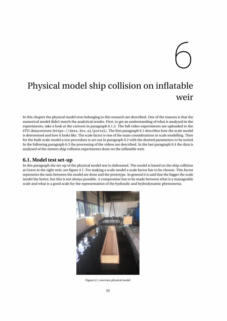
6Physical model ship collision on inflatable
weir
In this chapter the physical model tests belonging to this research are described. One of the reasons is that thenumerical model didn’t match the analytical results. First, to get an understanding of what is analysed in theexperiments, take a look at the cartoon in paragraph 6.1.3. The full video experiments are uploaded to the4TU-datacentrum (https://data.4tu.nl/portal). The first paragraph 6.1 describes how the scale modelis determined and how it looks like. The scale factor is one of the main considerations in scale modelling. Thenfor the built scale model a test procedure is set out in paragraph 6.2 with the desired parameters to be tested.In the following paragraph 6.3 the processing of the videos are described. In the last paragraph 6.4 the data isanalysed of the sixteen ship collision experiments done on the inflatable weir.
6.1. Model test set-upIn this paragraph the set-up of the physical model test is elaborated. The model is based on the ship collisionat Grave at the right weir, see figure 4.1. For making a scale model a scale factor has to be chosen. This factorrepresents the ratio between the model are done and the prototype. In general it is said that the bigger the scalemodel the better, but this is not always possible. A compromise has to be made between what is a manageablescale and what is a good scale for the representation of the hydraulic and hydrodynamic phenomena.
Figure 6.1: overview physical model
55

56 6. Physical model ship collision on inflatable weir
In the time for the Ramspol project a scale model with a factor of 25 was used. This scale was determinedas manageable and still representing the physical phenomena accurately. Other reasons use a certain scalecan be the possibility of representing the constructive details correctly, the accuracy of the measurementdevices and the dimensions of the research facility [62]. The length (Ramspol: 80m [38] and Grave: 60m) andheight (Ramspol: 10m [51] and weir 5.3m) of the weir location is significantly smaller than Ramspol. Both twoobservations are reasons to also use the scale of 25 in this scale model. In figure 6.1 the overview is shown ofthe built 1:25 scale model.
6.1.1. ScalingOne of the most important features to be scaled is the air inside the membrane. The air pressure and volumecan’t be scaled linearly and according to the law of Boyle these two are inversely proportional to each other.The air volume is scaled with nV=3249 instead of n3=253 and the air pressure with n=25 to satisfy the law ofBoyle. Extra air volume needs to be added in the scale model, to compensate for the smaller scale ratio. In total3.81 times the inflatable weir volume itself in the scale model needs to be added. This is done with air boxes onthe side see figure 6.1. For full explanation about scaling of the air in the membrane see appendix H.
For researching the membrane on ship collision, besides air also the elastic properties of the sheet need to bemodelled. In the scale model the membrane sheet has to satisfy the following conditions:
• Sheet is closed, so the required air pressure is maintained• Scaled strain stiffness, in special in circumferential• The scale model sheet has the same friction coefficient as the prototype
In the scale model only the strain rigidity in circumferential direction is scaled with n2=252 correctly. Thethickness had to suffer and is significantly thicker than the desired scale thickness. Bending stiffness could alsobe important for studying inflation and deflation of the membrane, but that is not in scope of this research.See appendix H how to scale those properties.
The velocity of the ship is scaled accordingly withp
n. The scaling of the velocity can be done by the Froude
number vpg Ls
or the Reynolds number ρLs vµ . The Froude number is a measure of the resistance and the
Reynolds number defines the turbulence. The viscous forces do play a lesser role in the scale model than theacceleration forces, therefore the velocity is scaled in ratio with the Froude number [30]. See appendix H forfurther explanation.
The mass of the ship is scaled with n3 = 253 = 15625 and dimensions are scaled linearly, hence n = 25. In thefigure 6.3 and 6.2 a side view and top view is shown with the dimensions of the scale model.
Figure 6.2: top view model

6.1. Model test set-up 57
Figure 6.3: side view model
6.1.2. Scaling resultsIn this paragraph is explained what the scaling results are of the scale model. Not everything could be scaledto the exact number. Such as the air pressure deviated from the desired scale pressure. Second, the scaledthickness of the sheet and so the weight of the sheet are larger. Lastly, the stiffness in longitudinal direction islarger. However, the latter three are of minor importance.
The air boxes on both sides of the weir contain half of the added volume (0.325m3). The air boxes are cubesand the inner sides are all 3
p0.1625 = 0.55m long. An air blower is put between an air box and the inflatable
weir with a T-profile. The blower was put on and the pressure was measured with a barometer, see appendix H.The highest pressure that could be reached is 1.7 kN/m2, this is around 20% less than the desired pressure. Itwas noted that the height of the membrane at this pressure is 0.22m or 5.5 m in the prototype. In the shapecalculation in chapter 3 the height was 5.8 m, but then for a higher air pressure in the prototype.
Figure 6.4 shows a picture of the inflatable weir, used in the scale model. The foundation is made of 18mmplywood (multiplex in Dutch) planks. The sheet is connected with a single line aluminium strip (3 mm thick)to the foundation. The centre-to-centre distance of the screws are put 10 cm aside each other. The screws are20 mm long to prevent piercing the foundation plywood.
Figure 6.4: inflatable weir dry
The figure above also shows the sheet, a detailed view of the thickness of the sheet if given in figure H.7 ofappendix H. The real thickness is 1.52 mm. This is 1.52/0.64= 2.4 times larger than the desired scaled thickness.The strain stiffness of the sheet is 8 N/mm2 according to the supplier (EPDMtotaal). This means a strain rigidityof 8*1.52=12N/mm=12e3 N/m which is the desired in circumferential length, but not in longitudinal length.No yarns are presented in the scale model, so only one strain rigidity could be defined.
The length of the sheet for a circle would be πH =π5.3 = 16.65m. The length from the calculations with theshape as in figure 3.10 come closer to the length of a circle than the length of literature, see equation D.10 [62].For this reason the calculated length. Also the shape of the membrane is calculated with equations 3.7, 3.8 and3.9 for the dimensions of the 1:25 scale model. Here the length that is found is 0.712 m, which is very close tothe scaled length. The discussed parameters are shown in table 6.1 with there prototype value.

58 6. Physical model ship collision on inflatable weir
unit scale (n=25) prototype scaled valueLength sheet [m] n 17.22 0.69
Thickness sheet [m] n 0.016 0.00152Strain rigidity circumferential [kN/m] n2 7500.0 12
Strain rigidity longitudinal [kN/m] n2 3000.0 12Air pressure [kN/m2] n 53 1.7
Air volume membrane [m3] n3 1332 0.085Air volume total* [m3] nV=3249 1332 0.41
Table 6.1: parameters sheet
6.1.3. Experiment recordingThis paragraph describes one of the sixteen experiments done for ship collision on an inflatable weir in thewater lab in cartoon form. The video recording is shown in figure 6.5 as snapshots for the maximum draught(D=0.14m) and maximum velocity v4, which is explained in the next paragraph.
In the first snapshot only the bow of the ship is shown before impact. It already travelled around 2 meters togain its desired velocity. In snapshot two the ship is almost hits the inflatable weir. The added water mass andbow wave already hits the weir and pushes it a little horizontally. Next, the bow of the ship hits the weir insnapshot three. Here the interaction starts with the transfer of the impact energy and the ship is pushed a littleupwards by the air pressure inside the weir. Also this snapshot shows that the bow wave splashed over the weir.Then in snapshot four the ship is still gliding over the weir and is pushed a little further upwards. The bow ofthe ship is practically over the weir. In the fifth snapshot the ship has lost most of its momentum and is on itstipping point. This is where the ship has the maximum displacement over the weir. It also shows that part ofthe ship over the weir is falling downwards by gravity. Between snapshot six and five the ship and weir moved alittle bit backwards, due to the elongation of the sheet that behaves elastic. The last snapshot shows the ship inrest position on the weir. At this moment there is water flowing over the weir by the created gaps at the side ofthe ship.
Figure 6.5: cartoon collision experiment

6.2. Experiment method 59
6.2. Experiment methodThe experiments are repeated two times. This includes all the measurements with the sixteen differentcombinations of mass and velocity of the ship. The first set of experiments showed some inconsistencies in themeasurements, therefore a second set of experiments was done with an improved experiment set-up.
The measurements that did not show inconsistencies in the first experiments are kept in this chapter. Themeasurements from the first set of experiments that did show inconsistencies are put in appendix H and themeasurements done with the improved (second) set of experiments are shown in this chapter instead. Theimproved set gives the following changes in the experiment:
• more calibration points for the velocity• trying to achieve a higher air tightness, by making new air boxes• top view camera is better positioned, for better view• more accurate resolution measurement for the discharge over the weir• ruler on the foundation floor to measure weir displacement more accurate
6.2.1. Test parametersFor the scale model the dimension are used of push convoy class Va extended, see figure 4.10. The experimentsare done with sixteen different combinations of the mass and velocity of the ship.
MassThe four different scaled draughts corresponding to the scaled ship mass are 0.08, 0.10, 0.12 and 0.14 meter.Here 0.08 meter scaled is the minimum draught for an unloaded ship and the 0.14 meter is the maximumdraught available in the Meuse after deepening the river, see section 2.3. The draught is used as means toconvert to the mass. The volume of the ship that is under water creates an upward force that has to be equal tothe mass of the ship, this is called the law of Archimedes.
First, the volume of the ship that is under water has to be determined. Therefore the angle of the bow is needed,see figure 4.2 and 6.3. The angle is calculated with: β= tan−1(b/a) = tan−1(4.4/19.7) = 12.6◦. Then the mass ofthe ship can be calculated with the volume of the cubic part plus the bow of the ship that is underwater timesthe specific weight of water. In formula form this reads:
ms = (D(Ls −a)+ 1
2D
D
tan(β))Bsρw (6.1)
where: ms = mass of ship [ton]D = draught of ship [m]Ls = length of ship [m]β = angle of bow [◦]Bs = width of ship [m]ρw = density of water [kg/m3]
The mass corresponding to the draught is given in table 6.2. These masses are achieved with sandbags, seealso appendix H.
draught [m] mass [kg]0.08 1090.10 1380.12 1680.14 199
Table 6.2: parameters ship
Velocity generationThe velocity of the ship is generated with a rope that pulls at the prow of the ship. The rope is turned over attwo pulleys at the end of the basin see figure 6.6, where it is connected to a bucket. The ship is pulled to theother end of the basin see figure 6.2 and the bucket is filled with sandbags. Subsequently the ship is let looseand the gravity of the bucket pulls the ship forward.

60 6. Physical model ship collision on inflatable weir
Figure 6.6: tower for fall height
The drop height of the bucket is around 2m and the ship has 2.4 m free length to navigate before it hits theinflatable weir. This means there is 0.4 meter distance left before the ship hits the weir, where no propulsiveforce is present. Besides, it has to be noted that for a heavier bucket the rope somewhat elongates and the dropheight can reduce up to around 0.1 meter. So the non-propulsive distance takes up to 0.5 meter. 0.5 meter infront of the prow a tape is put on the rope, see figure 6.7. The time is measured between when the tape is ontop of the foundation and the prow is on top of the foundation. The velocity is then calculated by dividing thedistance (0.5 m) by the time interval. The measured velocity is actually not conservative since it deceleratesbetween the distance of the tape and the prow.
Figure 6.7: time between last 50 cm
There is a small deviation from the straight pulling of the rope at the prow of the ship. The deviation iscalculated as follows: 0.18 cm high is the rope from bottom ship. The height from the bottom deviatesfrom:
• Hup + (0.18-Dmax) = 0.206 + (0.18-0.14) = 0.246 cm• Hup + (0.18-Dmin) = 0.206 + (0.18-0.08) = 0.306 cm
In the first experiment the pulley itself is 24 cm from the bottom. So the maximum angle is tan− 1(0.06/(11−3.6−2)) = 0.6◦ with a maximum vector downwards of sin(0.6) = 0.01=1% of the total force. In the secondexperiment the pulley is put 0.27 cm from the bottom to reduce the downward force contribution to max0.5%.

6.2. Experiment method 61
Velocity calibrationFor the scaled velocity four different values evenly spaced 0.275, 0.55, 0.825 and 1.1 m/s are desired. The last isthe maximum velocity for ship collision according to figure 4.9. In the first experiment the velocity is calibratedwith four different weights 2, 5, 10 and 15 kg respectively in the bucket. For explanation on the execution of theexperiments, see appendix H.
For every draught the four different weights in the bucket and are tested. In appendix H those weights inthe bucket are plotted against the measured velocity of the ship with. In the second experiment set also thevelocity measures from the first experiment set are included, so containing in total 8 data points for everydraught. Those data points are marked as blue dots in the next four graphs.
Then for the (blue) data points a natural exponential function is plotted on each graph, where D is the draughtin the scale model. The R2 indicates the accuracy of the function, the closer to one the more accurate. Thenthe weights are calculated for the desired velocities. These velocities are used for the experiments later in thechapter. The data point for these velocities are given as orange dots. It is noted that the closer the velocity tozero, the bigger the deviation from the desired velocity. Besides, the accuracy of the desired velocity is notmuch increased with the first experiment measurements in appendix H.
Figure 6.8: calibration 0.08 m Figure 6.9: calibration 0.10 m
Figure 6.10: calibration 0.12 m Figure 6.11: calibration 0.14 m

62 6. Physical model ship collision on inflatable weir
6.3. Processing methodologyIn this paragraph it is explained how the data is gathered. The following items are measured from the modelexperiments:
• the maximum displacement in x-direction of the ship over the weir• maximum (uplift) displacement in z-direction of the prow of the ship• estimation of maximum displacement weir in x-direction• discharge over the weir if applicable• estimation of the increase of air pressure
For the displacement of the ship over the weir the number of pixels is counted. A known dimension on thevideo has to be measured to convert pixel to length scale. The width of the foundation plate (54 cm) is used forthis conversion, see figure 6.12. The maximum displacement of the ship is measured from the prow to theclamping strip, see figure 6.12.
Figure 6.12: displacement ship top view
The maximum displacement in vertical direction of the ship is measured with a side view, see figure 6.13. Theprow is taken as known length in the video, so the pixels can be converted to length. The dot that is fixed onthe prow gives the reference point for the vertical displacement. The maximum vertical displacement is thedistance between the dot before the ship hits the weir. The moment the ship hits the weir and the prow is atmaximum height.
The displacement of the weir in x-direction is measured with the ruler in figure 6.13. The ruler is laid down inthe middle of the weir in longitudinal direction, this is also where the middle of the ship hits the weir. Theinitial length visible before impact is measured of the ruler. Then during impact the minimal length of theruler is measured. The distance between the initial and the minimal length is the horizontal displacement ofthe weir.
Figure 6.13: uplift prow of ship (h) by impact with weir and ruler to measure weir displacement

6.3. Processing methodology 63
The displacement of the weir in z-direction by the ship is given in figure 6.14. After the impact the ship islaying on the weir and gives a compression. The reference height of the ship before impact is compared to theheight ship in rest on the weir after impact. This difference in height is measured from the top deck of the shipbetween the two phases.
Figure 6.14: displacement measurement ship on weir
The discharge over the weir is measured by the water depth increase downstream over a time period after theimpact. This gives an average discharge over the weir due to ship collision. In figure 6.15 it is shown where thewater depth is measured. The initial height from the wall to the water level (D1 and D2) is taken as reference.When the ship rest on the the weir, water will flow over the weir. The time to let the water surface increase isvaried between 25 and 50 seconds. The new height from the wall to the water level (D1 and D2) is measuredand gives the water depth increase.
Figure 6.15: water depth measurement
ConclusionThe displacement of the ship in both x- and z-direction and displacement of the weir is accurately measured,since a reference length could be determined. However, the displacement of the weir became more difficult toread with higher velocity of the ship. The high velocity created a large bow wave topping over the inflatable weir.This wave overtopping blurred the view of the ruler, which was used as reference length for the displacementof the weir. See also figure 6.5 the ruler in snapshot 2 and blurred in snapshot 3.

64 6. Physical model ship collision on inflatable weir
6.4. Data analysisThe videos are analysed and the graphs obtained from it are given in this paragraph. Every line in the graphsrepresent a different draught of the ship. The velocity of the ship for every data point is given on the x-axis. Thevariable that is measured is given on the y-axis.
6.4.1. DisplacementsIn figure 6.16 the horizontal displacement of the ship over the clamping line is given. This represents theabsolute maximum distance from the clamping line to the prow of the ship. The dashed line shows when thebow of the ship is over the weir (length bow + B/2). The graph shows an increase of displacement for a highervelocity. The kinetic energy scales with the velocity squared, so more momentum forward is generated andgives a bigger displacement.
The graph does not show the correct displacement over the weir. The weir is a little further away and the bowis inclined. It is assumed the top of the weir is half the width away from the clamping line (B/2). Then thedisplacement correction becomes:
xcor = B
2+ b −D
tan(β)= 1
20.21+ 0.176−D
tan(12.6)(6.2)
where: xcor = correction for displacement ship over weir [m]B = width of weir [m]b = height of inclined part bow [m]β = angle of bow [◦]
This has to be subtracted from the maximum displacement (xs) to obtain figure 6.17. It is shown that now theline with the highest draught is more on top instead on the bottom of the graph. This is because for a lowerdraught the ship has travelled already a while before hitting the weir.
Figure 6.16: displacement over weir without correction Figure 6.17: displacement over weir
In the next figure 6.18 the maximum vertical displacement of the prow is given. The maximum verticaldisplacement of the prow lays around the point, where the bow is just over the weir. The first measurements itshowed that there was an outlier at D=0.12m, see appendix H. In the improved measurements this outlier ismore flattened out, but still is higher than D=0.14m. A reason for this can be, that the impulse is around thesame for D=0.12m and D=0.14m (contact area and compression of weir). In combination with a lower massgives a higher upswing of the prow.
It can be seen from the graph that the vertical displacement increases for a higher velocity, this is logical sincea higher reaction impulse is give to the ship. Also the general trend shows for a smaller draught/mass a smallervertical displacement. This confirms that a lower impulse and contact area gives a smaller vertical reactionimpulse.

6.4. Data analysis 65
Figure 6.18: displacement prow
The maximum displacement of the weir in horizontal direction is given in figure 6.19. The displacement isgenerated by the ship, that pushes the weir forward and flattens the weir to the ground simultaneously. Alsothere is an elongation of the sheet, due to the friction of the ship with the weir, that gives an extra displacement.The greater influence for weir displacement is from the first effect.
the graph show an increasing displacement of the weir for an increasing draught/mass and velocity. Thoseparameters increase the kinetic energy and so the impulse will be greater. Logically the weir has a largerdisplacement. It is also noted that the weir displacement flatten out for increasing velocity. At some point thedeformation is maximum for the displacement (the weir is pushed flat to the bottom). At that point only theelongation can contribute to extra displacement.
Figure 6.19: displacement weir
6.4.2. Discharge and frictionIn this paragraph the discharge and friction is calculated when the ship lays on the weir after impact. The stepsare made in chronologically order.
First, the total vertical displacement of the weir by the ship is calculated, see figure 6.20. If the bow of the shipis not fully over the weir then the compression by the draught of the ship is xs,cortan(β). The extra compression(zdeck) has to be added for the total displacement, in formula form:
zw =
{xs,cor tan(β)+ zdeck f or xs,cor tan(β) < δ
δ+ zdeck f or xs,cor tan(β) > δ

66 6. Physical model ship collision on inflatable weir
where: zw = compression of weir [m]xs,cor = displacement ship over weir with correction [m]β = angle bow ship [◦]zdeck = relative displacement deck ship on weir [m]δ = contact height ship-inflatable weir [m]
The general trend shows that the further the ship is over the weir, the more compression of the weir. This islogical, because more weight is leaning on the weir.
Second, the average discharge is calculated, see figure 6.21. This is done by the water level increase in thedownstream basin over a time period, described in the previous paragraph. In formula form the averagedischarge can then be calculated with:
Q = ( (D1+D2)new2 − (D1+D2)ol d
2 )Abasi n
t(6.3)
where: Q = discharge [m3/s]D1 = water depth measurement location 1 [m]D2 = water depth measurement location 2 [m]Abasi n = top view area of downstream basin [m2]t = time [s]
Old is before impact and new is a certain time after the impact. The water level increased in the downstreambasin only for the v3 and v4 velocity. Then only the vertical displacement of the weir was then large enoughto create an overflow. It is remarkable that the discharge of the lower draughts are higher, only the highestdraught has a higher discharge. It might be possible that a higher draught up to D=0.12m, gives a smaller gapof the flow are due to the curvature of the weir in longitudinal direction.
Figure 6.20: displacement ship on weir Figure 6.21: discharge over weir
The area where the water flows through after impact is schematized in figure 6.22. In this way the flow velocitycan be calculated exactly. An angle is assumed of 45 degrees where the membrane sheet curls back linearly tothe normal state. The gap in the weir, where the water flows through, is then calculated with:
Ag ap,w = z2w (6.4)
Now the flow velocity can be calculated. This is done for the ship with D=0.14m and v4 velocity. In this wayalso the maximum friction coefficient in test can be determined. The average flow velocity is calculatedwith:
v = Q
Ag ap,w= 0.032
0.172 = 1.1[m/s] (6.5)

6.4. Data analysis 67
Figure 6.22: geometrical displacement weir from ship
In the following the force is calculated per meter width, since the ship is symmetric. The velocity over the weirgives a drag force (FD) to the stern of the ship, see figure 6.23. This force can be calculated with the followingformula, where drag coefficient is set as 2.0 based on experiments done for bridge piers [6] :
FD = 1
2ρwCD As v2 = 1
2∗1000∗2∗0.064∗1.12 = 76[N /m] (6.6)
where: FD = drag force per unit length [N/m]ρw = density water [kg/m3]CD = drag coefficient [-]As = area ship under water (BsD) [m2]v = average water velocity [m/s]
The hydrostatic force per unit length (FH) for the stern of the ship is:
FH = 1
2ρw g D2 = 1
2∗1000∗9.81∗0.142 = 96[N /m] (6.7)
By horizontal force equilibrium the static friction coefficient is determined:
µst ati c Fup = FH +FD
µst ati c pi nB = FH +FD
µst ati c = FH +FD
pi nB= 96+76
1700∗0.22= 0.45[−]
(6.8)
This is the maximum static friction coefficient that can be determined from the experiments. The actualstatic friction coefficient is higher. This is determined when the ship starts to move over the weir from restingposition on the weir.
Figure 6.23: side view forces
6.4.3. Overtopping wavesOvertopping is not yet included in the velocity calculation over the weir. Here it is demonstrated that theovertopping is negligible for the determination of the friction coefficient.
The highest waves determined from chapter 4 is 1.35m. This corresponds to the ship collision with D=0.12mand v4 in the experiments. The height of the overtopping should be half the wave height minus freeboard. The

68 6. Physical model ship collision on inflatable weir
height of the weir is measured 22 cm, so the overtopping height becomes (1.35/2)/(scale=25) - (0.22-0.206) =0.013 m. The average width is assumed to be 2 meters where water flows over the weir. The flow velocity isassumed to be the same as the wave velocity, which is calculated for shallow water waves with:
cw ave =√
g Hup (6.9)
The time that water flows over the weir is measured from the videos. The water flows for around 1 second ofthe weir. Calculating the over topping volume is done as:
Vover = 0.013∗2∗ cw ave ∗1 (6.10)
The percentage of overtopping volume of the total volume is given in the next table:
D=0.08 m D=0.10 m D=0.12 m D=0.14 mv3 0.00 0.00 0.00 7.16v4 1.38 2.16 4.00 4.25
Table 6.3: percentage overtopping volume of total overflow volume
A 4.25% of volume decrease would also mean the same percentage decrease in mean flow velocity and a(0.95752) 8.3% decrease in drag force, see equation 6.6. Translating to the static friction coefficient gives 0.47.This is not a significant difference.
6.4.4. Air pressureThe static air pressure can have an effect on the friction force. The static air pressure is calculated with theassumed reduced volume in the membrane, when the ship rests on the membrane as in figure 6.22. Thedisplaced area in this cross section can be calculated with:
Ag ap = Ag ap,s + Ag ap,w = zw ∗Bs + z2w (6.11)
where Agap,s is the gap of the weir occupied by the ship. Now the displaced area is known, it is assumed this islinearly proportional to the shrinkage of volume in the membrane. The shrinkage factor can be calculatedas:
fs =Ag ap
Aw= zr est ∗Bs + z2
w
(1.98+2∗ 12 ∗0.22)∗0.22
= zw ∗Bs + z2r est
0.48(6.12)
Where Aw is the area of the weir from figure 6.22. This is only the volume shrinkage in the weir. It is determinedin appendix H that the added volume is 3.81 times the volume in the membrane of the scale model. To includethe added air boxes, the total volume shrinkage becomes:
fs,tot = fs
4.81(6.13)
It is assumed the percentage of volume decrease is the same amount of pressure increase, in accordance withthe law of Boyle. The pressure increase in static condition for every experiment is given in graph 6.24. It showsa maximum static pressure increase of 5%. This will then also be the change in the static friction coefficient. Itcan be argued this change is significant. However, the ship still does not move over the weir.
In figure 6.25 the dynamic air pressure is given. This dynamic air pressure is measured from the barometer.The measurement is taken by the naked eye from the videos. The initial water level in the piezometer, beforethe ship hits the weir, could not be distracted. The camera was too far away from the piezometer to read this.Only when the air pressure increased the water level was noticeable. Around 1 or 2 seconds after the impact,the water level in the barometer shoots up. This is the air that is pushed away from the impact. The highdynamic air pressure increases the stresses temporarily. The dynamic air pressure increase is up to a factor 2from the initial pressure. This seems very high, but this was not visually observed on the membrane.

6.5. Discussion 69
Figure 6.24: static pressure increase Figure 6.25: increase air pressure
6.5. DiscussionThe ship does not pass the weir more than half the ships length, from the experiments. This means that the shipwill not pivot around in centre of gravity and ground at the downstream side of the inflatable weir. Therefore,it can be concluded that a higher downstream level, the one in the winter, does not require to be tested. ahigher downstream water level makes that the inflatable weir will be standing more upright and a higherhydrostatic pressure from the downstream is present, see figure 6.26. The ship collision will then generate abigger counter-acting force and a smaller uplift force, so the ship will travel a shorter gliding distance.
Another option is that the ship approaches from the downstream side of the weir at winter conditions. Thisevent is doubtful for two reasons. First, only an unloaded ship can get to the weir without grounding, witha safe under keel clearance of 0.5 m [19]. Second the approach velocity is lower, due to the water velocityresistance coming from upstream.
Figure 6.26: winter higher downstream water level
The upstream water level can change as well at location Grave. The upstream water level depends on thedischarge in the Meuse. In figure 2.5 in chapter 2, the water level is shown for various discharges. A lowerwater level upstream will be present for a discharge of 1030 to 1640 m3/s. A higher water level upstream will bepresent at even higher discharges. At these discharges the weir will be opened and ship can navigate over theweir. A higher water level will be unlikely, since then the water will flow over the weir.
In the experiment only one size of the ship is tested. Results with other dimensions are not available, butpotentially can be extrapolated from the results. First, a longer ship will have a longer arm from the mass centreof the ship to the inflatable weir. This creates a larger upward momentum, but also a larger counteracting force.Second, both a larger and/or a wider ship for the same mass, will have a lower draught. The contact area willbe less, and generates a lower upward moment as consequence. It is likely that for small ships especially inlength, will top over the weir. With the results of the scale model experiments more detailed analysis are madein the next chapter.
The sheet for the scale model test is unreinforced. The strain in the sheet of the scale model, therefore can bemuch higher before failure than the sheet in the prototype. It has to be verified with the analytical model if thestrain stays below the limit strain of the prototype.


7Analysis
In this chapter the analysis is performed on the physical model tests in chapter 6 and an extension is given onthe model presented in chapter 4. A new calculation set is done, because of the different mass and velocityused in the physical model. It is of importance to do this calculation to calibrate the theory with the physicalmodel.
The first paragraph 7.1 analysis the ship collision on an inflatable weir event in a time schematization. Thenthe new mass and velocity are given in paragraph 7.2. Building on the time model new factors are added inparagraph 7.3. The new analytical model is calibrated with a potential energy coefficient to account for theuplift and glide coefficient on the physical model test. In the same paragraph the results of the improvedanalytical model are compared with the results of the scale model tests. In the last paragraph 7.4 last somethingis said about the desired clamping lines and the strength of the sheet.
7.1. Ship collision analysisThis paragraph describes the analysis of the ship collision on inflatable weirs in time. The analysis is based onwhat is found in the physical model tests.
The collision starts with the bow colliding into the inflatable weir, see figure 7.1 step 1. The forward energy ofthe ship pushed the inflatable weir downwards. On its turn the contact area between the bow ship and theinflatable weir is increased up to a maximum assumed of B/2 in horizontal and δ in vertical direction, seegraph 7.2 and 7.3. In this moment in time momentum is developed tilting the bow upwards. From step 2 infigure 7.1 the contact area reduces again, but still momentum upwards is generated. There is assumed for afinite small time no contact with the weir, there the ship starts to glide fully over the weir where step 3 starts.Since the ship is tilted somewhat upwards, the forward momentum of the ship will move the front bow justa bit higher for some time. In the meanwhile the ship is decelerated losing its momentum and gravity takesthe bow down again. From step 3 onwards the contact area is increased again see figure 7.2, but only in thehorizontal direction. When the ship is laying horizontal again, the contact area is maximum again. In themeanwhile the ship glided over the weir, this is step 4 to 5. Step 5 is now achieved and the ships lays on theinflatable weir resting.
71

72 7. Analysis
Figure 7.1: ship collision in time
In the first graph below, the impact is divided into two parts. The first part is a half sinusoidal shape, where theship collides with the weir and is then uplifted. The second part of the graph represents the gliding of the shipover the weir. Most of the kinetic energy is absorbed by the first part of the impact. Here also vertical contactlength is present, see the second graph.
Figure 7.2: horizontal contact length in time
Figure 7.3: vertical contact length in time

7.2. Modified mass and velocity 73
DurationThe duration of the whole collision impact is given to get impression of the time scale. In a paper of Vrouwen-velder a formula for the impact time is given [4]. The time is based on a plastic deformation of steel structures.This means that there is only impact of the ship and no spring reaction of the impacted structure. For theinflatable weir collision time step 1 to 3 is assumed small in relationship to the rest of the collision, so thespring reaction is dismissed.
For the calculation of time, the maximum mass and velocity of the ship from the next paragraph is taken. Theair stiffness is defined by the average contact area of the ship times the air pressure. Then the impact timeis:
∆t = 0.5π√
ms /kai r = 0.5π√
ms /(B/2)∗Bs ∗pi n0.5π√
31120/((5.3/2)∗11.4∗53) = 6.9[s] (7.1)
where: ms = mass of the ship [kN]kai r = spring stiffness of the air inside membrane [kN]B = width inflatable weir [m]Bs = width ship [m]pi n = air pressure in membrane [kN/m2]
The impact time of first part of the collision is assumed:
B/2
vs= 5.3/2
5.5= 0.48[s] (7.2)
Is around 7% of the total collision time, which can be considered low compared to the total collision time.
In the physical model test, this collision scenario took 1s, until max displacement xmax of ship over the weir.Scaled back to prototype gives 1x5=5s, this deviates from the calculated collision time. An explanation for thisdeviation can be: in the calculation is assumed a horizontal spring-mass system and in the experiment thedirection of the spring-mass system changes and the spring magnitude itself.
7.2. Modified mass and velocityIn the physical model tests four different values are used for the mass and velocity. It was convenient in thephysical model test to choose these values. In this analysis the values are scaled back to prototype values andare used in the calculations. The four different draughts, that are used for the analysis, are given in table 7.1. Tocalculate the prototype mass corresponding to the draught of the ship equation 6.1 is used.
draught [m] mass [ton]2.0 17032.5 21603.0 26303.5 3112
Table 7.1: parameters ship
The velocity is divided in four different numbers, with equal step size. The last velocity is the maximum velocityfor the ship class of Va (extended) used in the physical model tests and in this chapter for the improved model.The four different velocities are: 1.375, 2.75, 4.125 and maximum 5.5 m/s.
7.3. Improved ship collision modelIn the improved ship collision model two factors are added. The conversion to potential energy and glidecoefficient which is determined by physical model tests. This paragraph explains what is included in theimproved model and how it is used.
7.3.1. Potential energy conversionPotential energy by air pressureIn the beginning of the collision there is the air pressure creating a momentum on the ship. This will raisethe front of the bow up. The moment in the ship collision analysis is point 2 in figure 7.1. During this uplift a

74 7. Analysis
counteracting force is created on the stern of the ship, this is the water uplift pressure. These two forces haveto be in balance and the uplift height can be calculated, see figure 7.4. With the uplift, the potential energygenerated can be calculated.
An analogy is made with lock gate hawser forces. Here the water that is pumped in creates translation waves.This will tilt the ship around its y-axis. Further elaboration is shown in the lecture notes lock gates of the courseHyraulic Structures [67]. First the force generated by the air pressure is defined as:
Fup = pi n
√(B
2
)2
+δ2 (7.3)
It is assumed that the centre of mass is in the middle of the ship. Then the horizontal distance from the forceto the centre of mass is calculated with:
G = 1
2Ls − 1
2
B
2− b −δ
tan(β)(7.4)
And the lever arm of the force is:C =G cos(β) (7.5)
With the above expression the momentum upwards can be calculated:
Mup = FupC (7.6)
For the counteracting force, the water uplift pressure from the stern is calculated. The total force is then theamount of extra volume that is displaced times the specific weight and gravity:
Fdown = 1
2hai r
1
2Lsρw g (7.7)
The counteracting moment is found by multiplying the water uplift force with the lever arm to the centre ofmass:
Mdown = Fdown(1
2
2
3Ls ) = Fdown
1
3Ls (7.8)
Now an expression is found for the upturning moment and down turning moment of the ship. With these twocomponents an expression can be found for the uplift of the front bow. This is done by equalling 7.6 with 7.8and using 7.7 follows:
hai r =Mup
12 Lsρw g 1
3 Ls= Mup
16 L2
sρw g= FupC
16 L2
sρw g(7.9)
Epot ,ai r = 1
2ms g
1
2hai r (7.10)
Figure 7.4: forces and moment static
The distance G goes a little bit beyond the centre of mass in the figure. This is due to the fact that the point ofengagement of the air pressure force is not on a horizontal line with the centre of mass. The deviation thatwould be subtracted to the length G is(assuming mass centre is in the middle): J
t an(β) Where J = | 12 (Ds −δ)|. It
can be demonstrated that this deviation is small, so it is neglected in the actual computation.

7.3. Improved ship collision model 75
Potential energy by shipThe ship itself is also generating potential energy. In fact during the collision the ship kind of surfs over theweir. In collision time this is number 3 and 4 in figure 7.1. The wave in front of the ship creates a water layerbetween the ship and the inflatable weir. This makes the frictional resistance very low.
The potential energy is found as a component of the kinetic energy. The component is dependent on the angleof the bow, see figure 7.5. In the equation below this potential energy is defined:
Epot ,shi p = Eki n ∗λ (7.11)
To cover the whole range of β values for the bow figure 7.5 has to be extended. This is shown in figure 7.6, forbow angles larger than 45 degrees. The unknown value λ is defined as:
λ
{sin(β) f or 0 <β < 45◦1− si n(β) f or 45◦ <β< 90◦ (7.12)
Also the generated height of the front bow can be calculated with the potential energy. The generated potentialenergy is expressed as:
Epot ,shi p = 1
2ms g
1
2hshi p (7.13)
Equalling equation 7.11 with 7.13 and using the kinetic energy formulation from equation F.1, then the heightof the front bow is defined as:
hshi p = 2Epot ,shi p
12 ms g
= 212 ms ∗ v2
s ∗λ12 ms g
= 2v2
sλ
g(7.14)
Figure 7.5: potential and kinetic energy distribution
Figure 7.6: adjustment energy transfer analysis
The total uplift of the front bow is found by adding the uplift generated potential energy by the air pressureand the kinetic energy of the ship:
h = hai r +hshi p (7.15)
Also the total potential energy is found by adding the potential energy generated by the air pressure and thekinetic energy of the ship:
Epot = Epot ,ai r +Epot ,shi p (7.16)

76 7. Analysis
7.3.2. Glide coefficientThe glide coefficient is added to account for the ship gliding over the weir. In standard expressions for shipcollision only the colliding into the structure is included. This paragraph describes how the glide coefficient iscalculated.
First the conservation of work and energy is used. With this the force transferred to the membrane can befound:
Fw = Eki n −Epot
xs,cor(7.17)
where: Fw = the mean force transferred from the ship to the membrane [N]xs,cor = displacement ship over weir with correction [m]
The force calculated according the the theory is:
F =√
2(kci r c +klong )(Eki n −Epot (7.18)
The ratio between the work force and the theory force is the glide coefficient for the bow angle used in thisresearch:
Cg l i de =Fw
F(7.19)
The bow coefficient is calculated with the experiment values for all sixteen combination in figure 7.7. A generalway to find the glide coefficient for all bow angles, with this experiment set is done as:
Cg l i de,g en = sin(12.6)
λCg l i de,mean (7.20)
where the 12.6 is the bow angle used in this research.
Figure 7.7: glide coefficient
Then the glide coefficient can be included in the force formula. The force becomes:
F =Cg l i de,mean
√2(kci r c +klong )(Eki n −Epot ) (7.21)
Where Cglide,mean=0.054 is the mean glide coefficient of the coefficients determined in graph 7.7.
7.3.3. StrainThe new strain can now be calculated with the adjusted force formula in equation 7.21 implemented inequation 4.11. 1.9% strain has to be added for the tensile force in static equilibrium, already discussed inchapter 4. It was concluded from chapter 4, that the longitudinal strain is not significant in the ship collisionanalysis, so this one is left out as graph. In graph 7.8 the strain is shown calculated with the improved analyticalmodel. It is shown that the maximum strain is well below the limit strain.

7.3. Improved ship collision model 77
Figure 7.8: elongation circumferential with glide coefficient
7.3.4. Comparison of resultsIn this paragraph some results are compared from the calculation done in the improved analytical model andthe physical model tests.
The uplift of the bow of the ship (h) is calculated with equation 7.9, 7.14 and 7.15. The values of the physicalmodel tests are used to make it comparable. For the dimensions figure 6.3 and 6.2 , for the mass table 6.2 andfor the velocity figure 6.8, 6.9, 6.10 and 6.11 is used.
In figure 7.9 the uplift ’h’ calculated is compared with the actual measured uplift of the bow of the ship. Apositive deviation means the uplift calculated is higher and a negative deviation means the uplift measured ishigher. It is noticed in the figure that most percentages are negative. The average deviation is around 25% fromthe experimental value.
Figure 7.9: comparison uplift bow ship between calculation and measurements physical model tests
Also the new accuracy of the new force equation 7.21 is tested. The same experimental values are used as forthe calculation of the uplift of the bow ’h’. The new force equation 7.21 is put in equation 4.11 to calculate thedisplacement of the weir ’xw’. In the improved model it is not anymore assumed that the ship and the weirmove together. The force transferred from the ship to the weir during collision gives a displacement of the weir,using the improved model.
The results from the calculations are compared with the measured displacement from the weir in the ex-periments see figure 7.10. A positive deviation means the displacement calculated is higher and a negative

78 7. Analysis
deviation means the displacement measured is higher. It is clear that for the lowest velocity ’v1’ there is an100% deviation. The potential energy calculated is here bigger than the kinetic energy and so no displacementof the weir is calculated. The rest of the deviation are on average 15%
Figure 7.10: deviation xw
7.4. Clamping and sheet strengthThis paragraph determines the required clamping for ship collision. It will be checked if the sheet used in thedesign is resistant to collision force from the improved analytical model
The force in the clamping is determined with the static tensile force plus the ship force that is acting on theclamps per meter width, so:
Fsheet = T +Fshi p (7.22)
The static tensile force is already calculated in chapter 3 (139 kN). The maximum ship force is for the maximummass and maximum velocity. The maximum ship force to the clamps is derived from the strain of the sheet infigure 7.8, Fship=kcircxεcirc=7500x0.052=390 kN/m.
The design strength of the bolts in the clamping line is calculated with:
Ft ,Rd = k2 · fub · Ab
γM2(7.23)
where: k2 = coefficient for head of bolt is 0.63 [-]fub = nominal tensile strength bolt [N/mm2]Ab = stress surface of bolt [mm2]γM2 = partial safety factor [-]
The Japanese prescribe a safety factor of 2 between the working load of the bolts of the clamping system andthe yield strength of the bolts [25]. This is γM2 in the formula. Looking at figure C.6 the bolts are totally straightrods so k2 is 0.63. The nominal tensile strength for the bolts is designed as 500 N/mm2.
In chapter 3 it is also given that the bolts are 150 mm apart from each other, so the force Fbolt=Fsheetx0.15.Equating the design strength Ft,Rd with the bolt force gives the stress surface of the bolt, which is Ab=503 mm2.The diameter is then expressed as:
Dbol t =√
4Ab/π=p
4∗503/π= 25.3[mm] (7.24)
Also the plate, which clamps the sheet, has to be calculated. The design strength of the plate is calculatedwidth:
Bp,Rd = 0.6πdc tp fu
γM2(7.25)

7.5. Discussion 79
where: dc = smallest span [mm]tp = plate thickness [mm]fu = tensile strength of plate [N/mm2]
The tensile strength of the plate is assumed the same as for the bolt. The span of the plate is assumed as 150mm to preserve a watertight sheet. The smallest plate span is then, where 25.3 mm is the bolt diameter, (150-25.3)/2= 62.3 mm. Equating the plate strength to the force the sheet in equation 7.22 gives a plate thickness of18 mm. An overview of the clamping system is given in figure 7.11
Figure 7.11: clamping dimensions
The total maximum force is determined in equation 7.22. This is the static force plus the maximum shipcollision force. The design strength in chapter 3 is given as 1602 kN/m. Including the Ramspol safety factor thecheck of the strength of the sheet can be determined. In appendix E the safety factor is determined includingthe folds. From the physical model tests it was observed that the folds did barely move, see appendix H,therefore this factor can be excluded. The safety factor becomes then 1.25. The check of the sheet strengthreads as follow:
Rt
1.25Fsheet= 1602
1.25∗529= 2.42 (7.26)
This is far above one, which means the design sheet is then resistant against the applied ship collisionforce.
7.5. DiscussionThe analysis done in this chapter is mainly extracted from the observations done in the previous chapters. Acollision scenario is represented in the beginning of this chapter, that describes the general effect during theship collision. This scenario is based on what is the most likely collision event. For a very low ship velocityit was shown in the scale model experiment, that the ship is not really gliding over the weir and bouncesback. The other extreme would be a very short ship that jumps over the weir and grounds on the downstreamside.
The optimized model includes the effect of uplift of the ship during collision. The model describes everythingstatically. In reality, the dimension time is present which makes the event dynamically. It can be argued that adynamic model is going more into details of the ship collision. For example the contact area of the ship withthe weir will be more accurately represented, which are now schematized in figure 7.2 and 7.3. On the otherside the static model is more suited for a general overview.
It is shown that the static model describes the physical effects with an accuracy of 30% and 15%. That isnot a bad result for a simplified model as used here. To have a model which is perfectly in accordance withthe physical model tests, a lot of iteration steps will be needed. Everything in this chapter is still calculatedstatically, but gives results of the event. There are some issues with determining the right contact area forexample. This contact are was not accurately visible in the model experiments, but are determined with logicalreasoning. Another thing to mention due to the static calculation, the deviation of the uplift ’h’ can be mainlyexplained. In the static calculation no acceleration terms are included.


8Conclusions and recommendations
The first paragraph 8.1 describes the conclusions of this study. The second paragraph 8.2 provides recommen-dations based on the findings of this study.
8.1. ConclusionsIn this section the research questions that were posed in chapter 1 are answered and conclusions are presentedbased on the findings of the research. The first research question was stated as:
1. How can the inflatable weir-ship interaction by ship collision at Grave be modelled to predict the motions ofthe ship and the inflatable weir?
An analytical model was made to predict the inflatable weir-ship interaction during ship collision. Theanalytical model is simplified, but still produces results for the motions of the ship and the inflatable weir. Thenumerical test could not be verified with the analytical model. It is complex to simulate the ship collision oninflatable weirs in numerical software and takes considerable computation time (1 hour) on a laptop withfour 2.5 GHz processors. The numerical software showed the ship collision visually in time, where it just ranstraight through the sheet. In reality this is not likely to happen. The numerical model set-up in this researchseems not suitable for analysis of ship collision on inflatable weirs. Where the physical model test seemed areliable verification method for the analytical model. The analytical model, described in chapter 7 is improvedwith help of the physical model tests in chapter 6.
It was assumed, in the analytical model, that the ship and weir had the same horizontal displacement duringthe impact. However the physical model tests invalidated this and showed a far higher horizontal displacementof the ship over the weir. That is why two factors are added in the improved analytical model. First, a glidingcoefficient is included to determine which part of the energy is transferred directly to the sheet of the weir,see chapter 7. The gliding coefficient is mainly dependent on the angle of the bow, but also on the frictionbetween the sheet and ship. Second, the uplift of the bow was noted during the physical model test. So theeffect of conversion to potential energy is also added in the improved analytical model. It was found that inthe improved analytical model, the movement of the ship in vertical direction deviated with an average of25% and the movement of the inflatable weir in horizontal direction deviated with an average of 15% from thephysical model tests. One of the reasons for this is that the analytical model is static and the physical modeltests dynamic.
One thing that is not well determined is the contact area of the ship with the inflatable weir during impact. Inthe analysis it is assumed the maximum contact area horizontally is half the width of the membrane (B/2).However this cannot be verified accurately with the physical model tests. The contact area could at most beread with the naked eye. As last the performance of the used models is summarized in table 8.1
81

82 8. Conclusions and recommendations
Analytical Numerical PhysicalResults 0 - +
Time + 0 -Degree of freedoms - 0 +
Accuracy 0 + 0
Table 8.1: comparison models
2. What happens when a push convoy ship collides with an inflatable weir?
The physical model tests in chapter 6 gave the best impression of the ship-inflatable weir interaction. Theship showed a larger displacement over the weir for increased velocity. This dependency is almost linearly.The draught of the ship does have minor influence on the displacement over weir. Second, the uplift of theprow (bow) showed the same dependency, also for an increasing velocity an higher uplift of the ship appeared.For all experiments the ship glided over the weir and came to a standstill on (top of) the weir, then the weiris pushed down by the ship. For the lowest two velocities, only the bow stayed on the weir after collision.The weir was in that case not barely pushed down by the ship. Lastly, there is the displacement of the weiritself. A higher velocity and/or draught showed a larger displacement of the weir. The curve flattened out for ahigher velocity. Eventually the ship cannot flatten the inflatable weir further and displacement will only beexperienced by strain of the sheet.
Besides the behaviour of the ship and the weir, also the effects of the water is investigated. The experimentsshowed the ship glides over the weir by a small layer of water. This layer of water became bigger for increasingvelocity and draught. The layer of water is also called the added water mass. The videos showed that the addedwater mass already displaced the weir before the ship hits the weir. Secondly, the water overflow that wascalculated in chapter 7, was also noticed in the experiments. Lastly, there was significant air pressure increaseduring the impact. However this did not express itself in unfolding of the folds present the abutments.
Perspective inflatable weirThe inflatable weir shows an interesting reaction to ship collision in the performed study. The results of theimproved analytical model in chapter 7 showed a maximum circumferential strain of 5%, which is within thelimit before break (20%). The longitudinal strength was confirmed to be of minor importance to the forcetransfer from ship collision in chapter 4. With a modified safety factor for the one used at Ramspol, the designtensile strength could also be checked. An unit check value of 2.42 is well above the safe value of 1. The lastsub question was to determine the side effects of the water. The ship waves generated, by the movement ofthe ship, showed no significant influence on the load of the inflatable weir. For the class Va ship, in chapter 4,the average water overflow velocity can increase to around 4.5 m/s. The current bottom protection can bedamaged by the overflow, depending how much the flow velocity is decelerated.
This study has taken the first steps into researching ship collision on inflatable weirs. It is of importance toknow if the inflatable weir is resistant against ship collision. If not, extra preventing measures are likely needed,which cost money.
Besides the ship collision, a general perspective for the inflatable weir as replacement in the Meuse will beproposed. First, the inflatable weir has an effective functionality. By automatically controlling the air pressurein the weir, the overflow height is regulated. Second, the inflatable weir can be assembled on a flat foundation.Extra costs can be saved by using the existing foundations of the weirs in the Meuse. A disadvantage on theother hand is that the inflatable weir can be vulnerable to sharp edges.
To increase the perspective of inflatable weirs in the Meuse, a next step is to compare it with other weirssuitable in the Meuse. Further investigation is recommended in ship collision on the inflatable weir. A few ofthem are in paragraph 8.2.

8.2. Recommendations 83
8.2. RecommendationsIn this paragraph the recommendations are given based on the executed research. There are a lot of recom-mendations to mention, because research about this specific scenario has not been considered yet. The mostrelevant ones are shown below.
Model improvement
• The sheet is assumed to be linearly stiff in the models. In reality the stiffness is nonlinear and this cansignificantly alter the results. The model can be improved by incorporating the non-linear stiffness ofthe sheet.
• The improved analytical model is a static model. The verification with the physical model tests is missingout the time component. For a more realistic comparison, an analytical/numerical time model can bebuilt that analyses the ship impact on the weir in time.
• From the scale model experiments it was observed that the system (weir, ship, water) was moving backand forth during the impact. The movement gradually faded out due to the damping of the system. For amore accurate model the damping of the system should be included. It is recommended to study theincluded damping.
• For larger bow angles, the bow is shorter. An extra effect (coefficient) should be included for that, becausethe (horizontal) contact area with the bow ship-inflatable weir is less.
Further research recommendations
• The design of the inflatable weir is conceptual in this research and only for the replacement of weirGrave. To further outline the replacement of the weirs in Meuse by inflatable weir, a study can be madeon the feasibility. The other weir locations require different dimensions of the inflatable weir and thecircumstances also differ.
• Now it is reasoned which scenario has the highest probability of occurrence. For a more accurate answera probability calculation is needed. For this, the data of the ship is needed and the development of ship-ment in the future. Based on the data it is possible to determine the probability and the consequences ofevery scenario. Eventually, a Monte Carlo simulation is recommended to determine the failure curve ofevery scenario.
• In the research it ship collision from the upstream side of the weir is studied and reasoned most probable.There is a scenario in the winter, where an unloaded ship hits from the downstream side of the weir. It isinteresting to research the effect on the inflatable weir in this scenario. The inflatable weir may flip overits clamping line.
• In the research only the hull of the ship is considered. Usually, ships also have a bow thruster. This bowthruster is installed in front of the ship and can be outside or inside of the hull during navigation. Thequestion is, if the bow thruster will hit the weir during impact. And if this happens, will the propeller cutthe sheet apart or not?
• The collision at Grave is simulated in this research. The collision of the push convoy at Linne was adifferent one. Here the ship collided parallel to the weir. It is interesting to research what the effect is ofan inclined collision for every angle possible.
• This research made use of an inclined flat bow that is situated on push convoys. Other type of shipshave a V-bow. This type of bow is more inclined and curved. The effects of the ship-weir interaction,due to the impact, can be quite different. The ship will have more likely a bouncing back effect. It isrecommended to study ship collision on inflatable weirs with this type of bow shape for the ship.
• The power of the engine is not considered in this research and can significantly increase the impact onthe weir. Besides, it is possible that the shipper puts the ship in reverse during the impact.
• There was no spill breaker present in the experiment. This can cause extra resistance during gliding overthe weir. It is recommended in a further design stage, when the spill breaker is designed, to include thisin the physical scale model.


List of Symbols
The next list describes several symbols that will be later used within the body of the document
Greek symbols
α angle of the bow ◦
β internal pressure coefficient pi nHup
−δt thickness membrane m
∆ dimensionless specific grain weight ρs−ρwρw
−δ contact height ship-inflatable weir m
∆t impact time s
ε strain of inflatable weir −εci r c circumferential strain inflatable weir −εlong longitudinal strain inflatable weir −γ Poisson constant −γd yn dynamic coefficient −γM2 partial material factor −γmat material factor −γT partial factor −κ curvature of sheet 1/m
λ component transferring forward momentum ship to potential energy −µ mean −µv viscosity N /m2
µst ati c static friction coefficient −Φ threshold value before grains start to move −φ0 angle membrane upstream ◦
ρw specific weight water kg /m3
σ stress N /m2
σd standard deviation −Θ angle circular shape ◦
ζ coefficient which represents ship geometry −Latin symbols
γ Poisson constant (1.0 for isothermal- and 1.405 for adiabatic compression) −v average water velocity m/s
a length bow m
Ab stress surface of clamping bolt mm2
Am base width membrane on bottom unstretched m
Ar latitude cross sectional area river m2
As area ship under water in latitude cross section m2
Abasi n top view area of downstream basin m2
Ag ap,s gap area in inflatable weir occupied by ship m2
Ag ap,w gap area in inflatable weir for water flow m2
Ag ap,w total gap area in inflatable weir m2
Ai n area inside inflatable weir cross section m2
Aleak leakage area circular shape m2
85

86 List of Symbols
Ashr i nkag e total area shrinkage prototype inflatable weir m2
B width of inflatable weir m
b length of inclined part bow m
Bm base width membrane on bottom stretched m
Bs width of ship m
Bp,Rd design strength clamping plate N
C Chézy value m1/2/s
c height prow m
Cb block coefficient −CC confinement coefficient −CD drag coefficient −CE eccentricity coefficient −CH hydrodynamic coefficient −CS ship coefficient −Cg l i de,g en general bow coefficient −Cg l i de,mean mean bow coefficient from experiments −Cg l i de bow coefficient from experiments −cw ave wave celerity m/s
D draught of ship m
d grain size diameter m
D1,D2 water depth measurement locations m
Db diameter clamping bolt mm
dc smallest span clamping plate mm
dm maximum fender deflection m
Ds height of ship m
d50 nominal grain size diameter m
Dmax maximum draught m
Dmi n minimum draught m
dS Length of sheet element in unloaded state m
dS∗ Length of sheet element in loaded state m
E Elastic modulus N /m2
Eki n kinetic energy of ship and water moving along N m
Epot ,ai r potential energy generated by air pressure inflatable weir N m
Epot ,shi p potential energy generated by forward momentum ship N m
Epot ,w potential energy of inflatable weir N m
E A strain stiffness N
E I bending stiffness N m2
F force of the ship N
f energy absorbing efficiency of fender system −FD drag force N
FH hydro static water force N
FR resistance force inflatable weir N
fs shrinkage factor −fu tensile strength of clamping plate N /mm2
Fw work force N
Fdown downward force by hydro static water pressure N
fs,tot total shrinkage factor −Fsheet total force sheet N

List of Symbols 87
Ft ,Rd design strength clamping bolts N
fub nominal tensile strength clamping bolt N /mm2
Fup upward force by air pressure N
G horizontal arm upward force to mass centre ship m
G perpendicular arm upward force to mass centre ship m
g gravitational constant (9.81) m/s2
H height inflatable weir m
h total uplift prow m
Hw wave height m
hw depth in water column m
hai r uplift prow by air pressure inflatable weir m
Hdown downstream water depth m
hshi p uplift prow by forward momentum ship m
Hup upstream water depth m
i slope −j amount of layer areas for circular shape −K compressibility coefficient −k stiffness sheet N /m
k2 coefficeitn for head of clamping bolt −kai r spring stiffness air inside membrane N
kci r c stiffness sheet in circumferential direction N /m
kl ong stiffness sheet in longitudinal direction N /m
L length of sheet m
L length weir m
Ls length of ship m
ms mass of the ship kg
mw mass of the water moving with the ship kg
Mdown downward momentum N m
Mup upward momentum N m
n general scale factor −np scale factor pressure −nV scale factor volume −n∆p scale factor differential pressure −nE A scale factor strain stiffness −p Resulting pressure on sheet (difference inside and outside pressure) N /m2
p0 pressure of gas N /m2
pw water pressure N /m2
pmodel pressure model (atmospheric pressure + overpressure model) N /m2
ppr oto pressure prototype (atmospheric pressure + overpressure prototype) N /m2
Q discharge m3/s
q resulting dynamic pressure on sheet m
R hydraulic radius m
Rm maximum fender reaction force N
Rn radius membrane m
Rt strength sheet N
Rw radius of circular shape m
s distance side ship to bank m
SC F stress concentration factor −

88 List of Symbols
SC Ftest stress concentration factor likely to have occurred during −T Tensile force in sheet without own weight N
t time m
TD tensile force by dynamic load m
tp clamping plate thickness mm
Tw tensile force with own weight N
u stretch of the sheet m
v water velocity over weir m/s
V γ0 volume of gas m3
vm scaled velocity m/s
vs velocity component of the ship perpendicular to the structure m/s
v1 minimum velocity of ship m/s
v2 intermediate velocity of ship m/s
v3 intermediate velocity of ship m/s
v4 maximum velocity of ship m/s
v95% velcotiy 95% confidence interval m/s
Vi n volume inside inflatable weir m3
Vover over topping volume water m3
w self weight sheet N /m
xs displacement ship over weir without correction m
xw displacement weir x-direction m
xcor correction for ship over weir m
xs,cor displacement ship over weir with correction m
yn width of layer area m
z effective water depth m
zz center of gravity of leakage area for circular shape m
zn vertical coordinate of layer area m
zw water level depression m
zdeck relative displacement deck sip on weir m

List of Figures
1 snapshots ship collision experiments in time . . . . . . . . . . . . . . . . . . . . . . . . . . . . . . . vi
1.1 side view weirs in the Meuse [46] . . . . . . . . . . . . . . . . . . . . . . . . . . . . . . . . . . . . . . 11.2 weir Grave after ship collision [46] . . . . . . . . . . . . . . . . . . . . . . . . . . . . . . . . . . . . . 21.3 houseboat with water level drop[46] . . . . . . . . . . . . . . . . . . . . . . . . . . . . . . . . . . . . 21.4 flowchart . . . . . . . . . . . . . . . . . . . . . . . . . . . . . . . . . . . . . . . . . . . . . . . . . . . . 5
2.1 Meuse overview . . . . . . . . . . . . . . . . . . . . . . . . . . . . . . . . . . . . . . . . . . . . . . . . 72.2 Meuse side branches [20] . . . . . . . . . . . . . . . . . . . . . . . . . . . . . . . . . . . . . . . . . . 82.3 Meuse discharge from 1991 to 2015 [2] . . . . . . . . . . . . . . . . . . . . . . . . . . . . . . . . . . 102.4 exceedance probability vs discharge Meuse [34] . . . . . . . . . . . . . . . . . . . . . . . . . . . . . 102.5 water levels Meuse for various discharges [49] . . . . . . . . . . . . . . . . . . . . . . . . . . . . . . 112.6 weirs in the Meuse (OpenStreetMap Nederland, n.d.) . . . . . . . . . . . . . . . . . . . . . . . . . . 122.7 Stoney part [29] . . . . . . . . . . . . . . . . . . . . . . . . . . . . . . . . . . . . . . . . . . . . . . . . 142.8 Poirée part [29] . . . . . . . . . . . . . . . . . . . . . . . . . . . . . . . . . . . . . . . . . . . . . . . . 142.9 wheel valve [29] . . . . . . . . . . . . . . . . . . . . . . . . . . . . . . . . . . . . . . . . . . . . . . . . 142.10 waterway- and ship classes Meuse [55] . . . . . . . . . . . . . . . . . . . . . . . . . . . . . . . . . . 152.11 collision Grave front view [64] . . . . . . . . . . . . . . . . . . . . . . . . . . . . . . . . . . . . . . . . 172.12 loose push convoy heading to weir Linne during storm Ciara [56] . . . . . . . . . . . . . . . . . . 172.13 reparation of weir Linne [52] . . . . . . . . . . . . . . . . . . . . . . . . . . . . . . . . . . . . . . . . 17
3.1 overview weir Grave (OpenStreetMap Nederland, n.d.) . . . . . . . . . . . . . . . . . . . . . . . . . 193.2 Weir Grave cross section front view [8] . . . . . . . . . . . . . . . . . . . . . . . . . . . . . . . . . . . 203.3 Cross section weir Grave side view [33] . . . . . . . . . . . . . . . . . . . . . . . . . . . . . . . . . . 203.4 design process . . . . . . . . . . . . . . . . . . . . . . . . . . . . . . . . . . . . . . . . . . . . . . . . . 213.5 front view final design . . . . . . . . . . . . . . . . . . . . . . . . . . . . . . . . . . . . . . . . . . . . 223.6 side view final design . . . . . . . . . . . . . . . . . . . . . . . . . . . . . . . . . . . . . . . . . . . . . 223.7 force overview [17] . . . . . . . . . . . . . . . . . . . . . . . . . . . . . . . . . . . . . . . . . . . . . . 233.8 geometry as function of internal pressure coefficient for air-filled type membrane [35] . . . . . . 243.9 element model . . . . . . . . . . . . . . . . . . . . . . . . . . . . . . . . . . . . . . . . . . . . . . . . 253.10 shape inflatable weir Grave standard . . . . . . . . . . . . . . . . . . . . . . . . . . . . . . . . . . . 263.11 one side clamped on the left and two side clamped on the right [62] . . . . . . . . . . . . . . . . . 273.12 wave clamping horizontal part [38] . . . . . . . . . . . . . . . . . . . . . . . . . . . . . . . . . . . . 283.13 slope angle abutments front view . . . . . . . . . . . . . . . . . . . . . . . . . . . . . . . . . . . . . 283.14 under length deflated state [38] . . . . . . . . . . . . . . . . . . . . . . . . . . . . . . . . . . . . . . . 293.15 fold at transition [11] . . . . . . . . . . . . . . . . . . . . . . . . . . . . . . . . . . . . . . . . . . . . . 293.16 Bridgstone abutment schematization [45] . . . . . . . . . . . . . . . . . . . . . . . . . . . . . . . . 293.17 sheet cross section [5] . . . . . . . . . . . . . . . . . . . . . . . . . . . . . . . . . . . . . . . . . . . . 303.18 impression spill breaker and filling medium pipes [9] . . . . . . . . . . . . . . . . . . . . . . . . . . 323.19 standard design . . . . . . . . . . . . . . . . . . . . . . . . . . . . . . . . . . . . . . . . . . . . . . . . 32
4.1 collision scenarios . . . . . . . . . . . . . . . . . . . . . . . . . . . . . . . . . . . . . . . . . . . . . . 354.2 ship collision model side view . . . . . . . . . . . . . . . . . . . . . . . . . . . . . . . . . . . . . . . 374.3 ship collision model top view . . . . . . . . . . . . . . . . . . . . . . . . . . . . . . . . . . . . . . . . 384.4 V-notching Ramspol [62] . . . . . . . . . . . . . . . . . . . . . . . . . . . . . . . . . . . . . . . . . . . 394.5 V-notching schematization top view [62] . . . . . . . . . . . . . . . . . . . . . . . . . . . . . . . . . 394.6 1D-model . . . . . . . . . . . . . . . . . . . . . . . . . . . . . . . . . . . . . . . . . . . . . . . . . . . 394.7 stress strain relationship sheet circumferential [62] . . . . . . . . . . . . . . . . . . . . . . . . . . . 404.8 stress strain relationship sheet longitudinal [62] . . . . . . . . . . . . . . . . . . . . . . . . . . . . . 40
89

90 List of Figures
4.9 maximum ship velocity according to ROK [27] . . . . . . . . . . . . . . . . . . . . . . . . . . . . . . 404.10 pushed convoys [41] . . . . . . . . . . . . . . . . . . . . . . . . . . . . . . . . . . . . . . . . . . . . . 414.11 schematized inflatable weir 3D before collision . . . . . . . . . . . . . . . . . . . . . . . . . . . . . 424.12 supposable deformation 3D . . . . . . . . . . . . . . . . . . . . . . . . . . . . . . . . . . . . . . . . . 424.13 overview ship collision . . . . . . . . . . . . . . . . . . . . . . . . . . . . . . . . . . . . . . . . . . . . 434.14 water overflow at gaps . . . . . . . . . . . . . . . . . . . . . . . . . . . . . . . . . . . . . . . . . . . . 45
5.1 geometry conversion . . . . . . . . . . . . . . . . . . . . . . . . . . . . . . . . . . . . . . . . . . . . . 485.2 reduced contact area sheet . . . . . . . . . . . . . . . . . . . . . . . . . . . . . . . . . . . . . . . . . 495.3 result reduced contact area . . . . . . . . . . . . . . . . . . . . . . . . . . . . . . . . . . . . . . . . . 495.4 stress strain Yeoh 1st order . . . . . . . . . . . . . . . . . . . . . . . . . . . . . . . . . . . . . . . . . 505.5 side schematization Ansys . . . . . . . . . . . . . . . . . . . . . . . . . . . . . . . . . . . . . . . . . . 505.6 top schematization Ansys . . . . . . . . . . . . . . . . . . . . . . . . . . . . . . . . . . . . . . . . . . 505.7 tensile force modelled as pressure . . . . . . . . . . . . . . . . . . . . . . . . . . . . . . . . . . . . . 515.8 instable solution tensile force . . . . . . . . . . . . . . . . . . . . . . . . . . . . . . . . . . . . . . . . 515.9 air pressure modelled . . . . . . . . . . . . . . . . . . . . . . . . . . . . . . . . . . . . . . . . . . . . 515.10 instable solution air pressure . . . . . . . . . . . . . . . . . . . . . . . . . . . . . . . . . . . . . . . . 515.11 begin of analysis . . . . . . . . . . . . . . . . . . . . . . . . . . . . . . . . . . . . . . . . . . . . . . . . 525.12 intermediate of analysis . . . . . . . . . . . . . . . . . . . . . . . . . . . . . . . . . . . . . . . . . . . 535.13 end of analysis . . . . . . . . . . . . . . . . . . . . . . . . . . . . . . . . . . . . . . . . . . . . . . . . . 535.14 velocity x-direction ship . . . . . . . . . . . . . . . . . . . . . . . . . . . . . . . . . . . . . . . . . . . 545.15 deformation x-direction of the sheet . . . . . . . . . . . . . . . . . . . . . . . . . . . . . . . . . . . . 545.16 stress in z-direction . . . . . . . . . . . . . . . . . . . . . . . . . . . . . . . . . . . . . . . . . . . . . . 545.17 stress in y-direction . . . . . . . . . . . . . . . . . . . . . . . . . . . . . . . . . . . . . . . . . . . . . . 54
6.1 overview physical model . . . . . . . . . . . . . . . . . . . . . . . . . . . . . . . . . . . . . . . . . . . 556.2 top view model . . . . . . . . . . . . . . . . . . . . . . . . . . . . . . . . . . . . . . . . . . . . . . . . 566.3 side view model . . . . . . . . . . . . . . . . . . . . . . . . . . . . . . . . . . . . . . . . . . . . . . . . 576.4 inflatable weir dry . . . . . . . . . . . . . . . . . . . . . . . . . . . . . . . . . . . . . . . . . . . . . . . 576.5 cartoon collision experiment . . . . . . . . . . . . . . . . . . . . . . . . . . . . . . . . . . . . . . . . 586.6 tower for fall height . . . . . . . . . . . . . . . . . . . . . . . . . . . . . . . . . . . . . . . . . . . . . . 606.7 time between last 50 cm . . . . . . . . . . . . . . . . . . . . . . . . . . . . . . . . . . . . . . . . . . . 606.8 calibration 0.08 m . . . . . . . . . . . . . . . . . . . . . . . . . . . . . . . . . . . . . . . . . . . . . . . 616.9 calibration 0.10 m . . . . . . . . . . . . . . . . . . . . . . . . . . . . . . . . . . . . . . . . . . . . . . . 616.10 calibration 0.12 m . . . . . . . . . . . . . . . . . . . . . . . . . . . . . . . . . . . . . . . . . . . . . . . 616.11 calibration 0.14 m . . . . . . . . . . . . . . . . . . . . . . . . . . . . . . . . . . . . . . . . . . . . . . . 616.12 displacement ship top view . . . . . . . . . . . . . . . . . . . . . . . . . . . . . . . . . . . . . . . . . 626.13 uplift prow of ship (h) by impact with weir and ruler to measure weir displacement . . . . . . . . 626.14 displacement measurement ship on weir . . . . . . . . . . . . . . . . . . . . . . . . . . . . . . . . . 636.15 water depth measurement . . . . . . . . . . . . . . . . . . . . . . . . . . . . . . . . . . . . . . . . . . 636.16 displacement over weir without correction . . . . . . . . . . . . . . . . . . . . . . . . . . . . . . . . 646.17 displacement over weir . . . . . . . . . . . . . . . . . . . . . . . . . . . . . . . . . . . . . . . . . . . 646.18 displacement prow . . . . . . . . . . . . . . . . . . . . . . . . . . . . . . . . . . . . . . . . . . . . . . 656.19 displacement weir . . . . . . . . . . . . . . . . . . . . . . . . . . . . . . . . . . . . . . . . . . . . . . 656.20 displacement ship on weir . . . . . . . . . . . . . . . . . . . . . . . . . . . . . . . . . . . . . . . . . . 666.21 discharge over weir . . . . . . . . . . . . . . . . . . . . . . . . . . . . . . . . . . . . . . . . . . . . . . 666.22 geometrical displacement weir from ship . . . . . . . . . . . . . . . . . . . . . . . . . . . . . . . . . 676.23 side view forces . . . . . . . . . . . . . . . . . . . . . . . . . . . . . . . . . . . . . . . . . . . . . . . . 676.24 static pressure increase . . . . . . . . . . . . . . . . . . . . . . . . . . . . . . . . . . . . . . . . . . . 696.25 increase air pressure . . . . . . . . . . . . . . . . . . . . . . . . . . . . . . . . . . . . . . . . . . . . . 696.26 winter higher downstream water level . . . . . . . . . . . . . . . . . . . . . . . . . . . . . . . . . . . 69
7.1 ship collision in time . . . . . . . . . . . . . . . . . . . . . . . . . . . . . . . . . . . . . . . . . . . . . 727.2 horizontal contact length in time . . . . . . . . . . . . . . . . . . . . . . . . . . . . . . . . . . . . . . 727.3 vertical contact length in time . . . . . . . . . . . . . . . . . . . . . . . . . . . . . . . . . . . . . . . 727.4 forces and moment static . . . . . . . . . . . . . . . . . . . . . . . . . . . . . . . . . . . . . . . . . . 747.5 potential and kinetic energy distribution . . . . . . . . . . . . . . . . . . . . . . . . . . . . . . . . . 75

List of Figures 91
7.6 adjustment energy transfer analysis . . . . . . . . . . . . . . . . . . . . . . . . . . . . . . . . . . . . 757.7 glide coefficient . . . . . . . . . . . . . . . . . . . . . . . . . . . . . . . . . . . . . . . . . . . . . . . . 767.8 elongation circumferential with glide coefficient . . . . . . . . . . . . . . . . . . . . . . . . . . . . 777.9 comparison uplift bow ship between calculation and measurements physical model tests . . . . 777.10 deviation xw . . . . . . . . . . . . . . . . . . . . . . . . . . . . . . . . . . . . . . . . . . . . . . . . . . 787.11 clamping dimensions . . . . . . . . . . . . . . . . . . . . . . . . . . . . . . . . . . . . . . . . . . . . 79
A.1 shipping fleet Netherlands [48] . . . . . . . . . . . . . . . . . . . . . . . . . . . . . . . . . . . . . . . 96A.2 ship accidents Netherlands [48] . . . . . . . . . . . . . . . . . . . . . . . . . . . . . . . . . . . . . . 97A.3 fault tree ship collision weir Grave [64] . . . . . . . . . . . . . . . . . . . . . . . . . . . . . . . . . . 97
B.1 inflatable barrier during flooding homes [15] . . . . . . . . . . . . . . . . . . . . . . . . . . . . . . . 99B.2 Arizona inflatable dam [45] . . . . . . . . . . . . . . . . . . . . . . . . . . . . . . . . . . . . . . . . . 100B.3 (a) Highgate falls dam, USA and (b) flow breaking corbels at Marklendorf Germany [45] . . . . . 101B.4 Old Coon Rapids dam on the right vis passage [45] . . . . . . . . . . . . . . . . . . . . . . . . . . . 101B.5 Memorial dam Pennsylvania . . . . . . . . . . . . . . . . . . . . . . . . . . . . . . . . . . . . . . . . 101B.6 India rubber dam [58] . . . . . . . . . . . . . . . . . . . . . . . . . . . . . . . . . . . . . . . . . . . . 102
C.1 steel gate types [42] . . . . . . . . . . . . . . . . . . . . . . . . . . . . . . . . . . . . . . . . . . . . . . 104C.2 compartment design . . . . . . . . . . . . . . . . . . . . . . . . . . . . . . . . . . . . . . . . . . . . . 105C.3 compartment design section cut . . . . . . . . . . . . . . . . . . . . . . . . . . . . . . . . . . . . . . 105C.4 three dams design . . . . . . . . . . . . . . . . . . . . . . . . . . . . . . . . . . . . . . . . . . . . . . . 105C.5 design based on weir Vrijling [13] . . . . . . . . . . . . . . . . . . . . . . . . . . . . . . . . . . . . . . 106C.6 three different clamping systems [65] . . . . . . . . . . . . . . . . . . . . . . . . . . . . . . . . . . . 107C.7 geometry circular abutment . . . . . . . . . . . . . . . . . . . . . . . . . . . . . . . . . . . . . . . . . 108
D.1 force equilibrium element [47] . . . . . . . . . . . . . . . . . . . . . . . . . . . . . . . . . . . . . . . 109D.2 one and two side clamped with overview parameters . . . . . . . . . . . . . . . . . . . . . . . . . . 111D.3 shape unloaded state no disturbances [62] . . . . . . . . . . . . . . . . . . . . . . . . . . . . . . . . 111D.4 verification α with models [45] . . . . . . . . . . . . . . . . . . . . . . . . . . . . . . . . . . . . . . . 112D.5 circular shape membrane . . . . . . . . . . . . . . . . . . . . . . . . . . . . . . . . . . . . . . . . . . 113D.6 shape inflatable weir Grave . . . . . . . . . . . . . . . . . . . . . . . . . . . . . . . . . . . . . . . . . 114D.7 sheet length . . . . . . . . . . . . . . . . . . . . . . . . . . . . . . . . . . . . . . . . . . . . . . . . . . 114D.8 x-coordinate endpoint . . . . . . . . . . . . . . . . . . . . . . . . . . . . . . . . . . . . . . . . . . . . 114D.9 membrane height . . . . . . . . . . . . . . . . . . . . . . . . . . . . . . . . . . . . . . . . . . . . . . . 114D.10 equilibrium of element by dynamic forcing (adjusted [62]) . . . . . . . . . . . . . . . . . . . . . . 115
E.1 probability collision Ramspol [38] . . . . . . . . . . . . . . . . . . . . . . . . . . . . . . . . . . . . . 117E.2 shipment Ramspol estimation [21] . . . . . . . . . . . . . . . . . . . . . . . . . . . . . . . . . . . . . 117E.3 joints in sheet Ramspol [54] . . . . . . . . . . . . . . . . . . . . . . . . . . . . . . . . . . . . . . . . . 118E.4 stepwise clamping with abutments [38] . . . . . . . . . . . . . . . . . . . . . . . . . . . . . . . . . . 119E.5 folds two side clamped [62] . . . . . . . . . . . . . . . . . . . . . . . . . . . . . . . . . . . . . . . . . 119E.6 cross section with foundation Ramspol [28] . . . . . . . . . . . . . . . . . . . . . . . . . . . . . . . 119E.7 scale model guide rollers [62] . . . . . . . . . . . . . . . . . . . . . . . . . . . . . . . . . . . . . . . . 120E.8 deflated membrane with sunk bottom [62] . . . . . . . . . . . . . . . . . . . . . . . . . . . . . . . . 120E.9 fold with high peak stresses at Ramspol [38] . . . . . . . . . . . . . . . . . . . . . . . . . . . . . . . 120
F.1 velocity assumed as normal distribution . . . . . . . . . . . . . . . . . . . . . . . . . . . . . . . . . 123F.2 probability collision [7] . . . . . . . . . . . . . . . . . . . . . . . . . . . . . . . . . . . . . . . . . . . . 124F.3 component Fdx and Fdy for inclined going ships [12] . . . . . . . . . . . . . . . . . . . . . . . . . . 126F.4 reaction force versus deflection fender [43] . . . . . . . . . . . . . . . . . . . . . . . . . . . . . . . . 127F.5 reaction force versus deflection fender for loading and unloading [43] . . . . . . . . . . . . . . . . 127F.6 ship velocity in front of lock gates Netherlands [3, p. 37] . . . . . . . . . . . . . . . . . . . . . . . . 127F.7 dimensions bow for push convoys [66] . . . . . . . . . . . . . . . . . . . . . . . . . . . . . . . . . . 128F.8 bow push convoy in finite element program [66] . . . . . . . . . . . . . . . . . . . . . . . . . . . . . 128F.9 tree hit with FEM [36] . . . . . . . . . . . . . . . . . . . . . . . . . . . . . . . . . . . . . . . . . . . . . 129F.10 analysing stress concentration tree hit [36] . . . . . . . . . . . . . . . . . . . . . . . . . . . . . . . . 129

92 List of Figures
F.11 ship waves [14] . . . . . . . . . . . . . . . . . . . . . . . . . . . . . . . . . . . . . . . . . . . . . . . . 129
G.1 friction settings . . . . . . . . . . . . . . . . . . . . . . . . . . . . . . . . . . . . . . . . . . . . . . . . 131G.2 advanced settings . . . . . . . . . . . . . . . . . . . . . . . . . . . . . . . . . . . . . . . . . . . . . . . 131G.3 step control settings . . . . . . . . . . . . . . . . . . . . . . . . . . . . . . . . . . . . . . . . . . . . . 131
H.1 inside of boxes . . . . . . . . . . . . . . . . . . . . . . . . . . . . . . . . . . . . . . . . . . . . . . . . . 135H.2 inflating equipment . . . . . . . . . . . . . . . . . . . . . . . . . . . . . . . . . . . . . . . . . . . . . 136H.3 unpressurized piezometer . . . . . . . . . . . . . . . . . . . . . . . . . . . . . . . . . . . . . . . . . . 136H.4 ideal pressure piezometer . . . . . . . . . . . . . . . . . . . . . . . . . . . . . . . . . . . . . . . . . . 136H.5 pressure piezometer . . . . . . . . . . . . . . . . . . . . . . . . . . . . . . . . . . . . . . . . . . . . . 136H.6 strain stress graph scale model sheet Ramspol [62] . . . . . . . . . . . . . . . . . . . . . . . . . . . 137H.7 thickness model sheet . . . . . . . . . . . . . . . . . . . . . . . . . . . . . . . . . . . . . . . . . . . . 139H.8 ship on the balance . . . . . . . . . . . . . . . . . . . . . . . . . . . . . . . . . . . . . . . . . . . . . . 139H.9 sandbags . . . . . . . . . . . . . . . . . . . . . . . . . . . . . . . . . . . . . . . . . . . . . . . . . . . . 140H.10calibration 0.08 m . . . . . . . . . . . . . . . . . . . . . . . . . . . . . . . . . . . . . . . . . . . . . . . 141H.11calibration 0.10 m . . . . . . . . . . . . . . . . . . . . . . . . . . . . . . . . . . . . . . . . . . . . . . . 141H.12calibration 0.12 m . . . . . . . . . . . . . . . . . . . . . . . . . . . . . . . . . . . . . . . . . . . . . . . 141H.13calibration 0.14 m . . . . . . . . . . . . . . . . . . . . . . . . . . . . . . . . . . . . . . . . . . . . . . . 141H.14displacement over weir . . . . . . . . . . . . . . . . . . . . . . . . . . . . . . . . . . . . . . . . . . . 141H.15displacement front bow . . . . . . . . . . . . . . . . . . . . . . . . . . . . . . . . . . . . . . . . . . . 141H.16displacement weir . . . . . . . . . . . . . . . . . . . . . . . . . . . . . . . . . . . . . . . . . . . . . . 141H.17folds show no change . . . . . . . . . . . . . . . . . . . . . . . . . . . . . . . . . . . . . . . . . . . . . 142

List of Tables
2.1 weirs Meuse construction year and replacement [8] . . . . . . . . . . . . . . . . . . . . . . . . . . . 132.2 limit discharges for the various weirs . . . . . . . . . . . . . . . . . . . . . . . . . . . . . . . . . . . 142.3 ship Maria Valentine characteristics . . . . . . . . . . . . . . . . . . . . . . . . . . . . . . . . . . . . 16
3.1 parameters . . . . . . . . . . . . . . . . . . . . . . . . . . . . . . . . . . . . . . . . . . . . . . . . . . . 263.2 water, air or water and air filled . . . . . . . . . . . . . . . . . . . . . . . . . . . . . . . . . . . . . . . 303.3 fiber strength . . . . . . . . . . . . . . . . . . . . . . . . . . . . . . . . . . . . . . . . . . . . . . . . . 31
4.1 parameters . . . . . . . . . . . . . . . . . . . . . . . . . . . . . . . . . . . . . . . . . . . . . . . . . . . 414.2 2D model output . . . . . . . . . . . . . . . . . . . . . . . . . . . . . . . . . . . . . . . . . . . . . . . 424.3 reference model output . . . . . . . . . . . . . . . . . . . . . . . . . . . . . . . . . . . . . . . . . . . 434.4 wave height secondary wave cusps . . . . . . . . . . . . . . . . . . . . . . . . . . . . . . . . . . . . . 44
6.1 parameters sheet . . . . . . . . . . . . . . . . . . . . . . . . . . . . . . . . . . . . . . . . . . . . . . . 586.2 parameters ship . . . . . . . . . . . . . . . . . . . . . . . . . . . . . . . . . . . . . . . . . . . . . . . . 596.3 percentage overtopping volume of total overflow volume . . . . . . . . . . . . . . . . . . . . . . . 68
7.1 parameters ship . . . . . . . . . . . . . . . . . . . . . . . . . . . . . . . . . . . . . . . . . . . . . . . . 73
8.1 comparison models . . . . . . . . . . . . . . . . . . . . . . . . . . . . . . . . . . . . . . . . . . . . . . 82
A.1 bed protection weirs . . . . . . . . . . . . . . . . . . . . . . . . . . . . . . . . . . . . . . . . . . . . . 95A.2 dimensions weirs [8] [16, p. 76-82] . . . . . . . . . . . . . . . . . . . . . . . . . . . . . . . . . . . . . 96
B.1 inflatable rubber dam around the world [45] . . . . . . . . . . . . . . . . . . . . . . . . . . . . . . . 100B.2 India rubber dam . . . . . . . . . . . . . . . . . . . . . . . . . . . . . . . . . . . . . . . . . . . . . . . 102
C.1 mutual weight criteria . . . . . . . . . . . . . . . . . . . . . . . . . . . . . . . . . . . . . . . . . . . . 106C.2 mutual weight criteria . . . . . . . . . . . . . . . . . . . . . . . . . . . . . . . . . . . . . . . . . . . . 106
D.1 parameters . . . . . . . . . . . . . . . . . . . . . . . . . . . . . . . . . . . . . . . . . . . . . . . . . . . 112D.2 values optimization shape . . . . . . . . . . . . . . . . . . . . . . . . . . . . . . . . . . . . . . . . . . 113
E.1 membrane material properties [38, p. 28] . . . . . . . . . . . . . . . . . . . . . . . . . . . . . . . . . 118E.2 factors design formula Ramspol . . . . . . . . . . . . . . . . . . . . . . . . . . . . . . . . . . . . . . 121
H.1 velocity calibration with frames . . . . . . . . . . . . . . . . . . . . . . . . . . . . . . . . . . . . . . . 140
93


AWeirs Meuse and shipping
This appendix includes two tables of the weirs and a fault three based on the ship collision at Grave. The tablesdescribe the bed protection and dimensions with type of the weirs.
A.1. Bed protection weirsIn the table below the bed protection is given for the seven weirs in the Meuse in the Dutch reaches. Readingthe table from top to bottom is further downstream from the weir.
Length* [m] Class [kg] Bed protection
Lith40 40-200 quarry stones poured with asphalt25 40-200 quarry stones15 10-60 quarry stones
Grave55** 40-200 quarry stones with colloidal concrete55 40-200 quarry stones
Sambeek
-Stoney part: concrete block 1.5x1x0.95 mPoirée part: concrete blocks 1.5x1x0.8 m
6 40-200 quarry stones with colloidal concrete49 40-200 quarry stones15 10-60 quarry stones
Belfeld
8.5 concrete blocks2 cofferdam (in Dutch: kistdam)
25 300-1000 quarry stones30 40-200 quarry stones2 caisson
Roermond8.5 concrete blocks2 cofferdam
45 40-200 quarry stones
Linne20
60-300 Stoney part: quarry stones with colloidal concrete300-100 Poirée part: quarry stones with colloidal concrete
6060-300 Stoney part: quarry stones
300-1000 Poirée part: quarry stonesBorgharen*** 40 60-300 quarry stones with colloidal concrete
Table A.1: bed protection weirs
* cumulative distance away from the weir from first mentioned to last** after ship collision extended from 20 m to 55 m colloidal total 85 m***300-1000 kg and most western opening 40-200 kg
95
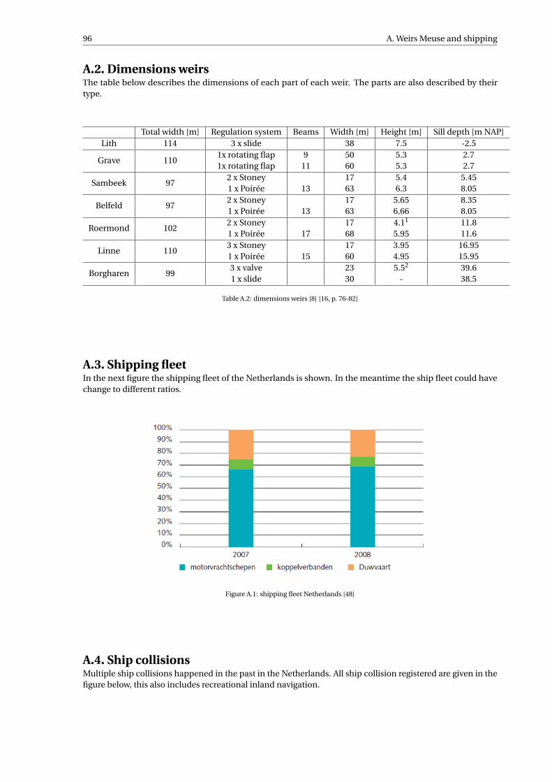
96 A. Weirs Meuse and shipping
A.2. Dimensions weirsThe table below describes the dimensions of each part of each weir. The parts are also described by theirtype.
Total width [m] Regulation system Beams Width [m] Height [m] Sill depth [m NAP]Lith 114 3 x slide 38 7.5 -2.5
Grave 1101x rotating flap 9 50 5.3 2.71x rotating flap 11 60 5.3 2.7
Sambeek 972 x Stoney 17 5.4 5.451 x Poirée 13 63 6.3 8.05
Belfeld 972 x Stoney 17 5.65 8.351 x Poirée 13 63 6.66 8.05
Roermond 1022 x Stoney 17 4.11 11.81 x Poirée 17 68 5.95 11.6
Linne 1103 x Stoney 17 3.95 16.951 x Poirée 15 60 4.95 15.95
Borgharen 993 x valve 23 5.52 39.61 x slide 30 - 38.5
Table A.2: dimensions weirs [8] [16, p. 76-82]
A.3. Shipping fleetIn the next figure the shipping fleet of the Netherlands is shown. In the meantime the ship fleet could havechange to different ratios.
Figure A.1: shipping fleet Netherlands [48]
A.4. Ship collisionsMultiple ship collisions happened in the past in the Netherlands. All ship collision registered are given in thefigure below, this also includes recreational inland navigation.

A.4. Ship collisions 97
Figure A.2: ship accidents Netherlands [48]
The Dutch Safety Board created a fault tree to determine what factors were playing a role during the shipcollision. There was at the time a thick fog with low sight. The fault tree is shown in figure A.3.
Figure A.3: fault tree ship collision weir Grave [64]


BInflatable rubber dams
The inflatable rubber dam is in general used for three different situations:
• individual use for protecting houses
• acting as a dam/weir to produce hydroelectricity or regulate the water level
• acting as a storm surge barrier to prevent areas from flooding
The first option comes to hand where the public water defences fail during a flooding. Individual householdscan anticipate on this by having an inflatable dam that they can lay around their house. An example is madefrom Texas. A man protected his house by laying an inflatable dam around its house, see figure B.1. Thishappened in 2016, when the Brazos river flooded.
Figure B.1: inflatable barrier during flooding homes [15]
The second option is extensively used in Japan and the Hydropower industry. The dams can span up to 100m and with special membranes even 200 meter can be achieved. The dams for the Hydropower industryand water level regulation are much investigated. Inflatable gates at hydro power structures have generallyworked well at passing ice and debris. The membrane also need to be designed so they can be in sunlightfor many years. Ultraviolet light accelerates the aging of rubber. This has dramatically been experienced atthe Tempe Town Lake Dam gates in Arizona that began to deteriorate after about 10 years under searing sun,until one of them failed and caused the emptying of the lake. They were provided with a sprinkling systemfor additional protection by extreme sun conditions. But for such frequent desert conditions at location inArizona it would not suffice. Figure B.2 presents the situation shortly after the dam gate burst (a) and a detailof the sprinkling system (b). The temporary gates installed afterwards were partly put in shadow by a newconstructed footbridge. The France uses protective layers and anti-abrasion jackets to extend lifetime.
99

100 B. Inflatable rubber dams
Figure B.2: Arizona inflatable dam [45]
The third option is the storm surge barrier. The most known one is the Ramspol barrier. It is also the biggestinflatable dam in the world. It protects the hinterland of the Netherlands from high storm conditions at theIjsselmeer. The Ramspol Barrier project actually opened the market of large storm surge barriers to rubbergates in Europe. Outside Europe, a few smaller flood barriers, including the Japanese Naruse Barrier in MiyagiPrefecture, preceded it. In table B.1 some of the most pronounced inflatable dams are listed.
Dam site Location No. of gates × L (m) ×H (m) Construction System—inflatingyear (air/water)
Ramspol Barrier Kampen, Netherlands 3 x 60.0 x 8.20 2002 water and airAlés Dam Gard, France 1 x 23.0 x 1.50 2002 air
Lechbruch Dam Bavaria, Germany 3 x 45.83 x 1.10 2002 water1 x 24.75 x 3.15
Kiebingen Tubingen, Germany 2 x 23.0 x 3.40 1998 airWertach Dam Tr̈kheim, Germamy 2 x 16.0 x 3.70 1998 air
Marklendorf Weir L. Saxony, Germany 2 x 23.6 x 2.20 2006 waterBahnitz Dam Brandenburg, Germany 2 x 30.3 x 2.40 2007 water
Bannetze Weir L. Saxony, Germany 2 x 21.0 x 2.35 2009 waterPocaply Dam Czech Republic 1 x 21.0 x 1.60 1998 water
Naruse Barrier Miyagi, Japan 3 x 42.1 x 2.30 1984 airKurotani Dam Okayama, Japan 1 x 35.0 x 6.00 1990s airHuaihua Dam Qingdao City, China 4 x ? 2012? airCoon Rapids Minnesota, USA 2 x 96.0 x 2.4 1990s air
1 12 x 45.8 x 2.40
Tempe Town Lake Arizona, USA 4 x 67.0 x 4.80 1999 airAdam T. Bower Pennsylvania, USA 6 x 91.4 x 2.44 1966, 1988 water and air,
1 x 57.0 x 2.44 since 1988 only airHighgate Falls Vermont, USA 1 x 67.0 x 4.60 1994 airPalmer Dam New York, USA Totally 105.4 x 1.83 2001 air, in two partsCurtis Dam New York, USA 3 x 63.6 x 1.20 2001 air
1 x 20.4 X 2.10Rainbow Falls Montana, USA 2 x 76.2 x 3.60 1992, 2013 air
Table B.1: inflatable rubber dam around the world [45]
The issue of heating up the bladder does not apply to the gates in high spillways, like the Highgate Falls damshown in figure B.3 (a). This dam makes part of a 9.8 MW hydroelectric plant. Its rubber gate, manufactured byBridgestone, regulates pool elevation. and is 4.6 m high and 67 m long (15 ft by 220 ft). The plant is owned bythe village of Swanton, Vermont, on the Missisquoi River. The rubber gate at this facility is one of the tallest in

101
the United States and is accessible for inspection and maintenance at one side [45]. The Marklendorf Damgates, one of which is shown in B.3, can be seen as examples of the recent revival of water-filled rubber gates.This dam act as weir that together with a similar weir at Bannetze controls the navigation conditions on theAller River. Shortly after putting the rubber dams in operation, they vibration problems under high flows. Theinstallation of flow breaking corbels in 2008 entirely removed this problem. These gates also form evidence thatwater filling can be applied in the areas of relatively cold winters, as the winter temperatures at this locationcan drop below -20°C [45].
Figure B.3: (a) Highgate falls dam, USA and (b) flow breaking corbels at Marklendorf Germany [45]
The two applications above represent respectively a hydroelectric plant and a river weir. A disadvantage ofthose application is that it will block fish migration upstream to river. As regard to this is, it is enough tomention that recent studies proved better performances of steel-rubber gates, which have a rubber bladder tolift the steel gate up and down see figure B.4.
Figure B.4: Old Coon Rapids dam on the right vis passage [45] Figure B.5: Memorial dam Pennsylvania
The Adam T. Bower Memorial Dam (formerly known as the Sunbury Fabridam) is the world’s longest inflatabledam. The dam is located in Pennsylvania just below the confluence of the Western and Main Branches ofthe Susquehanna, between the towns of Shamokin Dam and Sunbury. The dam is in total 600 meter longand exists of 6 individual dam, see figure B.5. It is raised in the summer to create 12 km2 Lake Augusta forrecreation. The dam and lake are part of Shikellamy State Park.

102 B. Inflatable rubber dams
India damsThe use of a rubber weir is a new concept in India, although more than 2000 inflatable dams already existsand over 10 manufacturers are available. India’s first rubber dam was built in 2006 on Janjavati River as areplacement of a gate. Construction of Jhanjavati rubber dam was completed in six months. Erection is simple,less maintenance cost and operation is automatic as well as manual. Later two rubber dams were built inthe Musi river in the city of Hyderabad. It was done under the project of Musi River Beautification Project.These two rubber dams presently are not operational because of lack of fresh water in Musi River. To give moreflexibility in release and control of water flow across the streams in watershed management, research effortswere made at Directorate of Water Management. Another rubber dam was built for the purpose of irrigationmanagement, which is called Chandeswer-I Kurda Orissa. The reason for using rubber dams is that capitalcosts is less than concrete dams. The operation of rubber dam is easy and farmers friendly. Details of therubber dams are given in table B.2 and figure B.6.
Name of site River Purpose H x L year21.1 km RD-High Court Hyderabad Musi River River management 1.35 x 80.0 2008
22.1 KM RD-Salar Jung Museum Hyderabad Musi River River management 1.30 x 73.0 2008Janjhavathi-Andhra Pradesh Janjhavati Irrigation 3.3 x (2x30.0) 2005
Table B.2: India rubber dam
Figure B.6: India rubber dam [58]

CDesign weir Grave
This appendix covers the sub parts for the design process of the inflatable weir at location Grave.
C.1. Steel weirsType of steel overflow weirs which can replace the existing weir at Grave are described here. Those weirs arenot further included in the design process, but are only described for the reason knowing that they exist. Thereare five types of steel weirs considered. Flap gates are not considered a feasible design solutions. They requirea recess chamber, which is not part of the design of the existing weirs. This will cost extra money to build them.This holds also for the radial gate and sector gate. Drum gates and bear-trap gates are also not applicable,because their maximum height is up to 4.0 m, which is less than the existing weirs in the Meuse.
Flap gatesIn open state the flap gate rests on sill. A hoisting mechanism lifts the flap against the water pressure upwards.They can up to 50 m if belly shape is applied like in the figure C.1
Radial gatesThe radial or curvature gate is designed such that the resultant force of the water pressure head pass throughthe rotation axis. This causes the bending moment to be zero and the gate has no tendency to open or close.Flap gates can be mounted on top, which are rotated horizontally in open state. In this ways the sill depth canbe reduced.
Sector gatesThe sector gates has a skin plate in front of the gate and on top the gate. During closing the skin plate on topcloses the recess chamber. The gate operates by subsiding into the recess chamber, due to in- and outflow ofwater to the recess chamber. With adjusting the inside water pressure, the desired height can be achieved. Theheight of sector gates is limited to 8 m and the width is theoretically unlimited
Drum gatesRegulation is done by water pressure inside the recess chamber, the same as for the sector gated. The rotationpoint of the gate is located upstream.
Bear-trap gatesThe bear trap gate looks like an inverted V in closed position. The plates are pushed upwards by internalpressure. The mechanism of the bear trap grate makes it possible, to make the recess chamber less deep, thanfor sector- and drum gates. In open position the flat parts are on top of each other. The disadvantage of theweir is that a larger pressure is needed than the upstream water pressure, therefore a separate pump is neededto initiate the upward motion.
103

104 C. Design weir Grave
Figure C.1: steel gate types [42]
C.2. Inflatable weir designsIn this section the alternative inflatable weir design are presented and the made multi criteria analysis (MCA)used for the decision of the conceptual design. The designs presented here were the alternatives in the MCAand are not further used in the research.
Design strategiesFurther the design possibilities are enhanced, by applying one or more design strategies to the design option.In this case to anticipate on a ship collision. The aim is to reduce the risk of a ship collision accident. This canbe done by reducing the probability of ship collision and the consequences of a collision. The risk reducing ofthe event of ship collision is a high important factor in the design. The designs given below are therefore basedto reduce the risk of ship collision. The follow strategies have been set out to pursue appropriate designs for inthis case ship collision [4]:
1. Preventing ship collision of occurring or reducing the probability of ship collision or the magnitude of it2. Protecting the inflatable weir against ship collision3. Design the inflatable weir that not the whole weir or an important part will fail4. Design the key elements of the inflatable weir on which it is reliant with extra care5. Applying design rules which provide a robust weir in normal circumstances
CompartmentsThis design is based on damage mitigation during accidents and robustness of the inflatable weir. Thedesign is comparably with the standard design of the inflatable weir shown above, only the weir chamber iscompartmentalized in multiple chambers. To do this a membrane sheet with the circumferential dimensionsis tied up to the membrane. It can be chosen how much length spans one chamber, based on the designneeds. A reasonable distance would be around 10 meters in this research of ship collision, since most shipson the Meuse span around 10 meter width. In case of a ship collision one (maximum two chambers) will fail,instead of the whole span. This design is proposed in another research as well [1]. In that case the design wasfor floating inflatable barriers on sea against ship collision. The conclusion said that the design is good fordissipating the kinetic energy of the ship and deceleration and instability of the ship.
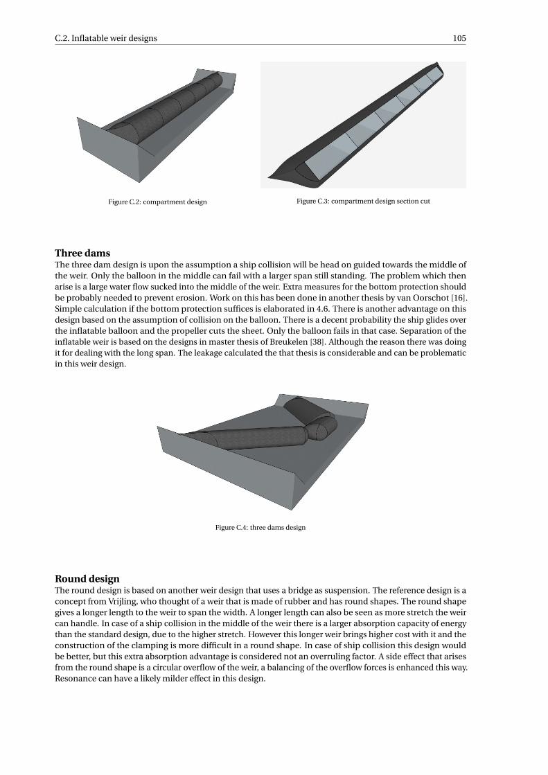
C.2. Inflatable weir designs 105
Figure C.2: compartment design Figure C.3: compartment design section cut
Three damsThe three dam design is upon the assumption a ship collision will be head on guided towards the middle ofthe weir. Only the balloon in the middle can fail with a larger span still standing. The problem which thenarise is a large water flow sucked into the middle of the weir. Extra measures for the bottom protection shouldbe probably needed to prevent erosion. Work on this has been done in another thesis by van Oorschot [16].Simple calculation if the bottom protection suffices is elaborated in 4.6. There is another advantage on thisdesign based on the assumption of collision on the balloon. There is a decent probability the ship glides overthe inflatable balloon and the propeller cuts the sheet. Only the balloon fails in that case. Separation of theinflatable weir is based on the designs in master thesis of Breukelen [38]. Although the reason there was doingit for dealing with the long span. The leakage calculated the that thesis is considerable and can be problematicin this weir design.
Figure C.4: three dams design
Round designThe round design is based on another weir design that uses a bridge as suspension. The reference design is aconcept from Vrijling, who thought of a weir that is made of rubber and has round shapes. The round shapegives a longer length to the weir to span the width. A longer length can also be seen as more stretch the weircan handle. In case of a ship collision in the middle of the weir there is a larger absorption capacity of energythan the standard design, due to the higher stretch. However this longer weir brings higher cost with it and theconstruction of the clamping is more difficult in a round shape. In case of ship collision this design wouldbe better, but this extra absorption advantage is considered not an overruling factor. A side effect that arisesfrom the round shape is a circular overflow of the weir, a balancing of the overflow forces is enhanced this way.Resonance can have a likely milder effect in this design.

106 C. Design weir Grave
Figure C.5: design based on weir Vrijling [13]
C.2.1. Multi criteria analysesIf the criteria in the list row is more important than the criteria in the column for the corresponding cell a 1 isplaced otherwise a 0. In the second last row the total score of the criteria is given. The last row divides the totalscore of the criteria by the total score of all criteria, this defines the weight factor of each criteria.
A B C D E F G Total Weight factorConstruct ability A 1 0 0 0 1 1 3 3/21=0.14
Inflation ease B 0 1 0 0 1 1 3 3/21=0.14Robustness C 1 0 0 0 1 0 2 2/21=0.1
Discharge leakage D 1 1 1 0 1 1 5 5/21=0.24Reliability E 1 1 1 1 1 1 6 6/21=0.29
Maintenance F 0 0 0 0 0 1 1 1/21=0.05Discharge efficiency G 0 0 1 0 0 0 1 1/21=0.05
Σ 21 1
Table C.1: mutual weight criteria
For each criteria a score is given to the design. How higher the score how better the design complies to thecriteria. This is given in the table below. Then the score is multiplied by the weight factor, this gives a weightedscore for each criteria per design. The total of the weighted score from each criteria per design is the total score.The highest score is the best out of the analysis
Standard Compartments Three dams RoundWF Score WF*score Score WF*score Score WF*score Score WF*score
Construct ability 0.14 9 1.26 7 0.98 5 0.7 6 0.84Inflation ease 0.14 8 1.12 6 0.84 7 0.98 7 0.98
Robustness 0.1 6 0.6 9 0.9 8 0.8 8 0.8Discharge leakage 0.24 7 1.68 7 1.68 4 0.96 7 1.68
Reliability 0.29 8 2.32 6 1.74 5 1.45 6 1.74Maintenance 0.05 7 0.35 7 0.35 7 0.35 7 0.35
Discharge efficiency 0.05 7 0.35 7 0.35 8 0.4 9 0.45Total 7.68 6.84 5.64 6.84
Table C.2: mutual weight criteria
C.3. ClampingThis section describes the possible clamping lines that can be used. There are multiple options to clamp thesheet to the foundation bottom. The clamping method is also depended if the membrane is two- or one- sidedclamped. With the chosen design in chapter 3, the membrane is single line clamped. In the years there havebeen developed multiple clamping systems. In figure C.6 the different kind of clamping systems can be seen.

C.3. Clamping 107
The middle type is the most common for new projects. Within this type there can be many differences inangles, width, number of waves and the application of these waves. The type at the left of the figure (typ A)is called the ’dovetail technique’ (in Dutch = zwaluwstaarttechniek). The sheet is thickened at the end suchthat a dovetail arises. Further the bolts connecting the sheet with the foundation do not penetrate the sheet.This system is developed by Obermeyer Hydro Inc (USA). As last there is the type on the right (typ C). This is avariant on typ B and can also be used.
Figure C.6: three different clamping systems [65]
C.3.1. Verify strength clampingTorquing is applied to the clamping system to pretension the rubber sheet. In this manner it ensures to createenough resistance between the clamping system and the rubber sheet. For the torque, there are differencesbetween manufactures. If the system is only torqued in the beginning, eventually the pretension will be 50% ofits starting value.
To test the applicability of the clamping system the behaviour of the rubber fabric is tested with regards toaging, degradation, creep and fatigue. There is no general guideline for this, it is up to the manufacturerto prove the applicability of the clamping system and set requirements. When the testing procedure is fullfilled, the clamping system can be implemented for mass-production. However when specific project requireschanges in the design or extrapolation of the test results, additional testing is recommended. For Ramspol thiswas the case [37].
C.3.2. Abutment round design calculationWith the case having no abutments and giving the weir a circular shape at the edges will induce a leakagepoint. The circular shape creates a smaller leakage area then an ellipsoid shape. The amount of leakage by thecircular shape is calculated in this section. First the area and centre of leakage point are defined as:
Al eak =j∑
n=1
zn yn
j(C.1)
where: Al eak = leakage area [m2]k = amount of area layers between Hup and Hdown [-]zn = vertical coordinate of corresponding area layer [m]yn = width of corresponding area layer [m]

108 C. Design weir Grave
The vertical coordinate for the centre of gravity comes down to:
z =∑ j
n=1 zn yn∑ jn=1 yn
(C.2)
The width yn can be found by:
yn = zn cosθ = zn cos(
sin−1 Hup
Rw
)(C.3)
For an overview see figure C.7.
Figure C.7: geometry circular abutment
The discharge can be calculated with Bernoulli’s law. It describes the total energy level at a certain cross-section.The assumption is made that there is no energy loss along the longitudinal way. The formula is described asfollows:
v2
2g+ z + p
ρg= Hener g y (C.4)
As the pressure stays constant the formula reduces to and the velocity follows from:
v2
2g+ z −→ v =
√2g z (C.5)
Now the velocity and discharge is known, the discharge can be calculated with 2.3. The discharge per abutmentis around 44 m3/s times four is 176 m3/s. This is around 16% of the limit discharge, which is a high number.For this reason the leakage is considered too big and not feasible for the design.
C.3.3. Bottom recessThere are (some) times during the year when the weir has to be (completely) deflated. In this case the bottomhas to catch the sheet in a whole. The requirement is that the sheet won’t fold when it is deflated. There aremainly two options for the bottom floor of an inflatable dam:
• guide rollers• flat bottom
For a two side clamped inflatable storm surge barrier can be chosen to use guide rollers. These guide rollersare further explained in the appendix E of Ramspol. The guide rollers are not necessary for the inflatable weirat Grave. The inflatable weir at Grave will be one side clamped. When the membrane will be deflated, the flowof the river will do the rest of the work. It pushes the sheet downstream of the river and to the bottom of thefoundation as is shown in figure 3.11. So keeping the foundation as bottom recess is efficient for the design ofthe inflatable weir at Grave.

DShape membrane
A theory is derived to get to the shape of the membrane, based on equilibrium of forces. The theory is describedby Parbery in his paper, where the work continues on the work of Harrison [47] [17]. Parbery states that thesolution of Harrison can be applied for most practical cases [47]. Harrison method is also applied for thebarrier at Ramspol. Harrison method has however some constraints. First the equilibrium position may not beunique and second the method needs to be modified in load situation the membrane lays flat at either or bothclamping points.
The theory describes the membrane shapes such that there is force equilibrium between internal pressure,outside load, self weight and the axial tensile forces in the sheet. For the theory of the shape of the membrane,the inflated state is used. In the deflated state there is theoretically no force transfer and the sheet lays onthe bottom. In the inflated state external forces will be transferred by tensile forces in the membrane to thefoundation. The shear forces and moments can be neglected in the equilibrium, since the thickness of thesheet is very thin compared to the size of the membrane. To find the shape of the membrane, the sheet isdivided in a finite number of element where the force equilibrium has to be satisfied. An overview of the forceson a small element in figure D.1.
Figure D.1: force equilibrium element [47]
By considering the limit case of an infinitely small sheet element dS* → 0, the tensile forces are defined asfollow. tangential direction (in direction of the sheet):
dT = wdS∗ sinφ (D.1)
109

110 D. Shape membrane
where: T = membrane force in axial direction [N]w = self weight sheet [N/m]S∗ = length of sheet in loaded state [m]φ = angle between horizontal and interface sheet [◦]
radial direction (perpendicular to the sheet):
−T dφ= pdS∗−w cosφdS∗ (D.2)
By assuming the self weight is zero follows that the variation of the tensile force is also zero over the small ele-ment. The law of Hooke describes the elongation of the uniform material by the pressure-strain relationship.(Bysolving for dS*, T and determining E, the elongation dS can be calculated:
dS∗
dS= 1
E
(T
δt
)+1 (D.3)
where: S = length of sheet in unloaded state [m]E = elastic modulus of sheet [N/m2]δt = thickness of membrane [m]
The curvature of the membrane is given by:
κ= 1
Rn=− dφ
dS∗ = p −w cosφ
T(D.4)
where: κ = curvature of sheet [1/m]Rn = radius of membrane [m]
By taking the weight of the membrane as negligible, the curvature equation ( dφdS∗ ) is reduced to and the
horizontal ’x’ and vertical coordinate ’z’ are defined by (curvature is positive by bulging to the outside):
dφ
dS∗ = p
T(D.5)
d x
dS∗ = cosφ (D.6)
d z
dS∗ = sinφ (D.7)
The geometrical boundary conditions for the two line clamped system can be defined by, noting that thecircumferential length is L and the base width is Bm:
S = 0 : x = 0, z = 0
S = L : x = Bm , z = 0(D.8)
In the case of the one line clamped weir a certain length lays on the bottom of the floor, because it is pusheddown from the upstream side. The boundary conditions for S=L can then be replaced by, where the length (L)is reduced by the unstretched length on the bottom of the foundation.
S = L− Am/(1+ε) : x = Am/(1+ε) , z = 0 ,dφ
dS∗ = 0 (D.9)
Where ’Am’ is the stretched length that lays unstretched on the bottom. The change in angle has to be zero inorder to have also a zero change in z-coordinate, see equations D.5 and D.7.
The origin of the coordinate system has to be defined first to calculate the corresponding coordinates of theelements. The origin of the coordinate system is taken at the clamping point, see figure D.2. It is presumedthat the internal pressure and length of the sheet is known. From the origin there are two unknowns ’T’ and ’φ’,which are initially guessed. Then the coordinates of the first element is calculated and so on, until a shapeis formed. The shape has to satisfy the boundary conditions D.8, otherwise a new guess is taken for the two

D.1. Length sheet 111
unknowns. Another option is to take the formulas from recent literature to determine the internal pressure ’p’and tensile force ’T’ [37], see below.
Figure D.2: one and two side clamped with overview parameters
D.1. Length sheetTo determine the length of the sheet in circumferential length some considerations are made. For an oneclamped membrane with air filled the smallest circumference length would beπhd in unloaded state, see figureD.3. Normally the membrane is loaded and the membrane will deform. A high internal pressure comparedto the external pressure and high strain stiffness will cause low deformation. However in most cases theinternals pressure and external pressure are more in balance. In practice the circumference length will morebe like:
L = 4H (D.10)
Figure D.3: shape unloaded state no disturbances [62]
D.2. Neglecting self weightBy substituting equation D.7 into equation D.1 and integrating gives the tensile force by:
Tw = T +w z (D.11)
With this equation it is shown that the self weight is included in the tensile force. The following demonstratesthat the self weight can be neglected. Taking the maximum height, self weight and tensile force of the inflatableweir at Grave:zmax = 5.3 [m]w = 1.09 [kN/m2] [5]T = 138 [kN] Gives a relative significance of the self weight:5.3∗ 1.09/138 = 0,042 is around 4.2%. That is an acceptable limit to neglect the self weight of the mem-brane.

112 D. Shape membrane
D.3. Validation parametersThe shape of the bladder has extensively been investigated in Germany under the conditions presumed here(upper pool pressure over the whole height, no overtop, lower pool dry). The investigations covered FEManalyses (using the ABAQUS software), physical modelling and analytical computing. The bladder geometrywas determined for a range of coefficients α varying from slightly above 1.0 to nearly 2.0. Figure D.4 presentsglobal shapes that have been determined for four of these coefficients. The correlation between the results ofall the three investigation methods was very good for medium and high values of α and fair for low values of α.These results and the formulas mentioned here offer support in initial design of rubber gates [45].
Figure D.4: verification α with models [45]
D.4. Research shapeThe shape of a circle is found with the equations D.5, D.6 and D.7. For the circular shape the same height isassumed as the weir at Grave. The initial condition tensile force is determined with D.11 and the initial angle islogically π. The internals pressure is determined from equation 3.3. According to the theory, the length of thesheet should be the circumference of a circle πH .
Parameter - value unitDesign height H 5.3 m
Internal pressure pin 53 kNm
Tensile force T 138 kNInitial angle φ0 π rad
Length sheet L 16.65 m
Table D.1: parameters
A sheet is taken of 25 meter and divided into 1000 pieces. So 1 piece is 2.5 cm, which is almost a tenth ofa percent of the sheet length. Between the piece lengths nodes are situate, wherefore the coordinates arecalculated. The circular shape that will be is found looks like figure D.5. It is shown the maximum height is 5.2m, what is 10 cm lower than the prescribed height. This deviation is not that significant. The length of thesheet can be found by multiplying the number of elements used to get the circular shape times the stretchedlength of an element dividing by the strain (n*dS*/(1+ε). The sheet length that is found for the circular shape is15.22 m. The height gives a small deviation around 2% from the desired value and the length of around 9%.Although the theory is not completely perfect it comes close to the desired shape.

D.4. Research shape 113
Figure D.5: circular shape membrane
An optimization is tried to make for the inflatable weir shape at Grave. The tensile force is varied between 90kN and 190 kN and the initial angle between 0 and π. Both are varied with 100 substeps, this creates substepsfor the tensile force 1 kN and the initial angle 0.031 rad (1.8◦). For every combination a shape is found. Theshape that satisfies the following conditions is plotted:
• sheet length is 5% longer or shorter than desired length• membrane height is 10% higher or lower than desired height• endpoint x-coordinate is equal or less than desired height
The following shapes are found in figure D.6 and table D.2. It is remarkable that the x-coordinate at theendpoint comes close to the desired membrane height. It can be said that based on this observance a large partof the inflatable weir will lay on the bottom. Besides the shape which comes closest to the desired membraneheight also has the tensile force that comes closest to the calculated tensile force.
Tensile force [kN] Initial angle [rad] Length sheet [m] Endpoint [m] Height [m]156.0 1.59 19.61 5.14 5.6156.0 1.63 19.62 4.92 5.69156.0 1.66 19.63 4.68 5.79157.0 1.59 19.71 5.18 5.62157.0 1.63 19.72 4.97 5.71157.0 1.66 19.73 4.73 5.81158.0 1.59 19.8 5.23 5.64158.0 1.63 19.81 5.01 5.73158.0 1.66 19.82 4.77 5.83159.0 1.59 19.9 5.28 5.66159.0 1.63 19.91 5.06 5.75160.0 1.63 20.01 5.11 5.77161.0 1.63 20.1 5.15 5.8162.0 1.63 20.2 5.2 5.82
Table D.2: values optimization shape
The graphs shown in figure D.7, D.8 and D.9 give a representation of the shape membrane study in figure D.6.It calculates a corresponding parameter to that shape of the membrane. It can be seen that there is a transitionline from around 2.1 φ0 upward. From this line to the right of the graph the shape becomes instable and forexample spiral endlessly.

114 D. Shape membrane
Figure D.6: shape inflatable weir Grave
Figure D.7: sheet length Figure D.8: x-coordinate endpoint
Figure D.9: membrane height

D.5. Dynamic shape 115
D.5. Dynamic shapeIn practice the membrane will not completely act as an static structure. The membrane will vibrate as functionof the dynamic forces applied. This can be waves or overflow of the weir for example. For the dynamic shape ofthe membrane equations of motions need to be derived. The new problem with the dynamic shape is that thesystem changes from a linear to a non-linear system. The load and the dynamic properties are deformationdependent. Hsieh derived the following equation of motions, where the strain is considered negligible by thedynamic loading. The length dS is thus a comparable to dS* in equations D.1 and D.2. Also the damping forcesare not included in the calculation of Hsieh [24]. In tangential direction:
wdS∂2vt
∂t 2 =(T +TD + ∂TD
∂SdS
)cosdφ− (T +TD ) (D.12)
In radial direction:
wdS∂2vw
∂t 2 =(T +TD + ∂TD
∂SdS
)sin
dφ
2+ (T +TD )sin
dφ
2+ (q +p)dS (D.13)
where: T = tensile membrane force by static load p [N/m]TD = tensile membrane force by dynamic load q [N/m]q = resulting dynamic pressure on the sheet [N/m]
The tensile force varies as consequence of the dynamic pressure q, and the dynamic pressure q varies also as afunction of time and space along the bellow circumference. When taking the limit case. This implies dS→0,the following holds for when taking the Taylor expansion:
• cosdφ≈ 1• sindφ≈ dφ/2• sindφ≈ dφ/2
Also noting that very small times very small can be taken as zero. This is the case for dφdS. Taking equationD.12 and D.13 and using the limit case, then those equations becomes. In tangential direction:
w∂2vt
∂t 2 = ∂TD
∂S(D.14)
In radial direction:
w∂2vw
∂t 2 = T∂φ
∂S+TD
∂φ
∂S+ (q +p) (D.15)
The equilibrium of an element described with the equations above can be seen in figure D.10
Figure D.10: equilibrium of element by dynamic forcing (adjusted [62])
The boundary conditions are formulated as follow for the dynamic shape:
S = 0 : x = 0, y = 0,d x
d t= 0,
d z
d t= 0
S = L : x = Am , y = 0,d x
d t= 0,
d z
d t= 0
(D.16)


ERamspol
E.1. Collision probabilityIn figure E.1 the failure probabilities of different events are given for the Ramspol barrier. Ship collision is oneof them, which is significantly from the graphs.
Figure E.1: probability collision Ramspol [38]
E.2. Ship navigationIn Ramspol the data that is available for ship navigation through Ramspol is from 1995. Based on the data fromthen two prognoses were made for the year 2020. Assuming the prognoses with the most shipment at Ramspolis given by figure E.2 last column [21, p. 42].
Figure E.2: shipment Ramspol estimation [21]
117

118 E. Ramspol
E.3. Sheet materialFor Ramspol five fiber materials were tested to apply for the sheet see table E.1 .
Abbreviation Material Tensile strength [MPa] Elongation at break [%]PP Polypropeen 600 20
PA6 Polyamide 6 (Nylon) 900 20PES Polyester 1100 13ARA Aramid 2900 3.6DYN Dyneema® 3000 3.6
Table E.1: membrane material properties [38, p. 28]
Also the material POM (polyacetaal) was considered to use as a sheet, but this was not applicable below 5 C◦.At Ramspol it is chosen to use Nylon fabrics as reinforcement material, that is layered in a matrix form. Theinner layer is made of two thick layers of Nylon which spans the circumferential direction. The layer round it ismade of two small layers on both side which spans the longitudinal direction. The cover layer consists of arubber material, see figure 3.17 for clarification.
E.4. Joints rubber sheetThe manufacturing of the Ramspol barrier sheet is done with joints in between the longitudinal direction. Inthat time the manufacturer for the sheet was located in Japan. There were two manufacturers: Sumitomo andBridgestone. Both manufacturers vulcanize the rubber sheet. The difference was that Sumitomo produces thewhole sheet in one time and Bridgestone does it in separate strips and later vulcanizes the strips together. Seefigure E.3
Figure E.3: joints in sheet Ramspol [54]
It was demonstrated that these joints would not significantly influences the strength of the sheet. Thecombination having low chance of stress concentration and smaller forces are present due to the less fibres inthe joint.
E.5. Abutment clampingThe unfavourable effect of the inclined membrane is that high peak stresses develop at the folds, see figure E.9.The folds needs to be small to prevent leakage. In order to do so, the excess length should be distributed overthe whole slope. This can be done by making the restraining lines stepped. the restraining lines need also ansmooth transitions to the side slopes, see figure E.4.
Several options were developed to clamp the overlength. Finally a stepwise clamping system was used to evenlydistribute the sheet. The clamping structure is called the ’Small Wave clamp’, see figure E.4. The clampinglength for the Ramspol barrier should be 1.27 times longer to clamp the overlength of the sheet. The stepwiseclamping at the abutments causes forced strains and stresses [38]. M. van Breukelen proposed a new clampinggeometry to reduce the peak stresses. The clamping lines should be straight and with ellipsoid shape [38,p. 68].

E.6. Foundation 119
Figure E.4: stepwise clamping with abutments [38] Figure E.5: folds two side clamped [62]
E.6. FoundationThe foundation at Ramspol are made of inclined piles [28], see figure E.6.
Figure E.6: cross section with foundation Ramspol [28]
In horizontal loading it can take more load than vertical piles. And the piles are already symmetric constructed.However for the weir water has to be retained only from one side. So it is not needed to place the pilesin inclined for both sides. It is construction wise more reasonable to make the foundation with verticalpiles.
Foundation floorIn tests of Delft hydraulics the guide rollers were tested for different set-ups. From the experiments it waschosen to make 4 rollers in the bottom recess and no rollers on the abutments[38], see figure E.7.

120 E. Ramspol
Figure E.7: scale model guide rollers [62]
The advantage of the guide rollers is that the roller can suck on by one the sheet towards itself. By determiningthe fitting size of the sheet to fit in the bin with guide rollers, almost no bulges form. With an air filledmembrane this method failed, this was solved by using rollers in the guidance so that friction forces werereduced significantly [62, p. 7-8]. The second option is to use a sunk bottom. This can be used for a one-sidedclamped membrane and the water is flowing from one side, which is the case in the Meuse. However withhigh flow velocities and waves, the deflated sheet can flap on the bottom. This has to be researched, if it hasinfluence on the sheet quality, see figure E.8
Figure E.8: deflated membrane with sunk bottom [62]
E.7. FoldsThe approach in appendix D is most suitable to get an idea of the shape in the middle section of the membrane.Getting closer to the abutments, the shape is more influenced by the inclination of the abutments. The changeof the slope will induce folds in the membrane, see figure E.9. In the figure the abutment is shown that isused for the inflatable storm surge barrier at Ramspol on the left. On the right a numerical model is set upto indicate the folds. At those folds high peak stresses develop, which is a critical point of the design. Thisknowledge should be taken in mind, when only focusing on the cross section. For the design of the weir in theMeuse the cross section model is given in chapter 3 and the numerical model in 5.
Figure E.9: fold with high peak stresses at Ramspol [38]

E.8. Tensile strength 121
E.8. Tensile strengthFor the Ramspol barrier a different approach was used to determine the strength of the sheet, than in Japan.The tensile strength is determined by the following formula:
Rt SC Ftest
γmat> γd ynFstatSC F (E.1)
where: Rt = strength of the rubber sheet [N/m]T = static membrane force for a two dimensional cross section [N/m]γmat = material factor [-]γd yn = dynamic coefficient [-]γT = partial factor [-]SC F = stress concentration factor [-]SC Ftest = stress concentration factor likely to have occurred during testing [-]
Since the middle of the sheet is most unlikely for stress concentration (most far away from abutments) theconcentration factors SCF and SCFtest are said to be 1.0. The factors that are used for the sheet of Ramspolbarrier are defined as follow:
Middle section Upstream side Downstream side Jointsγmat 1.3 1.3 1.2 1.2γd yn 1.3 1.3 1.2 1.3SCF 1.0 3.65 3.5 3.65
SCFtest 1.0 1.35 1.35 1.38γT 1.05 1.0 1.0 1.0
Table E.2: factors design formula Ramspol
As can be seen from table E.2, the upstream side give the normative tensile strength. From the formula ofequation E.1 and the upstream side factors a tensile strength of 4.6 times the tensile force inside the membraneis needed. In the strength of the sheet (Rt), the effects of fatigue loading, aging and relaxation is alreadyincluded. Other factors that can be taken into accounts is creep, water absorption and clamping effect. Thefactors for the design strength are based on the following:
• The material factor is based on a semi probabilistic approach with: γmat = eαRβVR and αR=0.8, β=4.26and VR=0.05
• The dynamic component is based on the in- and deflation of the membrane and the wave force.
• The SCF is determined by the stress concentration at the folds, see figure E.9.
• The SCFtest is the ratio between external load and maximum sheet strength at tests.
• The partial factor is determined by the required probability of failure
The clamping is determined by full scale test. To represent the sheet, the following measures were taken:saturation (immersed) with water, aging by holding sheet in hot water, fatigue by loading sheet with designload, breaking by simulate the design storm [38].

122 E. Ramspol
E.9. Ansys macrosThe modelling of the Ramspol barrier was also done in Ansys. The physical scale model of Delft Hydraulics fallshort of representing all the geometric and material properties simultaneously. To quantify the shortcomings acomputer model is developed to study the hydrodynamic aspects of the barrier. The model is a 2-dimensionalslice perpendicular to the length axis of the barrier. That is suited to model the middle section of the barrier.The total modal consists of several parts written in ANSYS parametric design language. The parts are groupedaccording to their functionality. The calculations done are given below:
• Static: to determine geometric shape
• Model coupled fluid-structure: to determine the damped eigen frequencies of the barrier. The geometricshape of the static calculation is the basis for the coupling with fluid elements.
• Dynamic: The modal dynamic calculations are only used to determine at which frequencies barrierresonances can start. Shift of the frequencies due to non-linear behaviour is not taken into account.
• Transient coupled fluid-structure: to determine non-linear response of the barrier subject to a stormsituation with irregular waves. The calculation are performed in the time-domain and all physicalbehaviour of the barrier can be described simultaneously. Every time step all conditions are updated.
The analyses for the last group are as follows: The wave spectrum is translated into a random time series ofincident wave height. The repetition pattern of the time series is 4096, so about one hour of storm . To reachvalid results the energy content is checked through the translated random time series of wave height andparticle in accelerated generated waves. The calculation of the response of scale and prototype model after theparticle acceleration is adapted for the correct energy content.

FShip collision model
F.1. Probability collisionIn ship collision analysis there are a lot of variables to deal with. Some variables are not fully determinedbeforehand and they can be approached by an probabilistic manner. The ship velocity is of great importancein collision analysis. A first probabilistic calculation for determination of the ship velocity would use thecharacteristic velocity and multiply with a safety factor to achieve the design velocity [60]. The differencebetween the characteristic velocity and the design velocity lies in the safety factor, see figure F.1.
Figure F.1: velocity assumed as normal distribution
In some degree variables load and the material properties stay uncertain. A reliability method categorizes thedegree of certainty in the approach. Four different levels are distinguished:
• Level 0: The method uses deterministic values for every parameter. Here no probability is involved.
• Level 1: The method makes use of semi-probabilistic values. This method is described above. It gives afirst conservative estimate of a probabilistic manner. The method is widely used in codes.
• Level 2: This method use a probabilistic approach. Approximations are made to come to the stochasticparameters and modelled with a mean an standard deviation. Correlation coefficient give the depen-dence on mutual parameters
• Level 3: Makes use of full probabilistic approach. Commonly a Monte Carlo simulation is used for thislevel. The modelling is done by their joint distribution and numerically integrated to find the exactsolution
123

124 F. Ship collision model
• Level 4: This method also takes the consequences (costs) into account and risk (probability x conse-quences). Different designs can be considered with this method
For level I analysis partial safety factor are used as mention above. The partial safety factors are categorized intothree consequence classes: low , medium and high. For this research a Level 0 approach is used to determinethe ship collision impact. Although it can be interesting to investigate
F.1.1. Bayesian networkStudies have investigated the probability of ship collision through Bayesian Networks. These studies weredone for waterways near or in a harbour. The Bayesian Network can take all parameters into account and endup with a probability number. To make such a network nodes and edges are defined. The nodes describe theevents and the edges define the relations between the events. The events are conditionally dependent withinthe Bayesian network. The main factors, where events are based on, in ship collision are:
• The waterway system• Involved ships• Human factors
One of the recent studies has been done by Jansen [22]. He investigated ship collision in the Scheur at the portof Rotterdam. The study showed a probability of ship collision for one side of the quay as:
Pcollision = 2.73e-6 [1/year/km]
F.1.2. Simplified probabilityA pragmatic way is to use a simplified model to identify the probability of ship collision in a waterway [7]. TheCumulative normal distribution for the deviation angle is used. In the normal circumstances the ship willnavigate under the bridge. There is a possibility the shipper deviates from the straight line under the bridge,this is shown in figure F.2. For a range of deviation angles the shipper will hit the bridge pier, marked in black.For the case at Grave this argumentation can also be followed. The shipper is heading to the sluice, but has alow chance of choosing the wrong direction this is the deviation angle. An calculation can be made how greatthe probability is of collision, based on data.
Figure F.2: probability collision [7]
F.2. Collision energyThe collision on a structure indicates an energy transfer from the moving object to the structure. Severalguidelines are made to determine the energy that has to be transferred. The first form of this energy is definedas the kinetic energy. The approach was mentioned first by G. Leibniz and J. Bernoulli in formula form:
Eki n = 1
2ms v2
s (F.1)
where: Eki n = kinetic energy of ship [Nm]ms = mass of the ship [kg]vs = velocity of the ship [m/s]
Later the coefficients effects where added by F. Vasco Costa (1973) and CETMEF. CETMEF is the French institute

F.2. Collision energy 125
for Inland and Maritime waterways, which contributes to the sustainability of the country. It provides servicesto the government of France and local authorities. One of the services is to give guidelines on protection of lockgates against ship collision. The approach described below is accepted universally, because the coefficientsare customizable to the situation at hand. Also the approach is mentioned in the BS6349 (British Standard)and PIANC report 151 and is noted in the lecture notes of the course Hydraulic Structures [44], [39]. The newformula for the kinetic energy of ship collision is defined as:
Eki n = 1
2ms v2
s CH CE CSCC (F.2)
where: Eki n = kinetic energy of ship [J]ms = mass of the ship [kg]vs = velocity of the ship [m/s]CH = hydrodynamic added mass [-]CE = yawing of the ship [-]CS = elasticity of the ship [-]CC = confinement factor [-]
The four coefficients describe side effect of the ship collision. The four coefficients are defined below.
Hydrodynamic added massThe hydrodynamic mass takes the water moving along with the ship into account. In formula for the addedmass is defined as, where mw is the mass of the water:
CH = ms +mw
ms(F.3)
To determine the mass of the water understanding is need of the water moving with the ship. The coefficientcan be determined by experiment, numerical simulation or developed theories. One of the studies that gavean estimate of the added mass is done by Shigeru Ueda 1981. His studies were based on model tests and fieldexperiments. The mass of the water moving with the ship is defined as:
mw = ρLs D2sπ
2(F.4)
combining F.3 and F.4 gives, where Cb is the block coefficient:
CH = 1+ πDs
2CbBs(F.5)
Another representation of the added mass coefficient is given by F. Vasco Costa 1964. This method is mostcommon international standard.
CH = 1+ 2Ds
Bs(F.6)
Above determinations are formula based. Also studies has been done where the added mass is determineddirectly by giving the value of the coefficient. In practice 20% will be added to the kinetic energy to accountfor added mass [44]. In reality the added mass varies dependent on the hull of the ship and the impactduration.
In 1971 Motorora did physical model tests and hydrodynamic analysis to define the added mass for swaymotion. The hydrodynamic added mass could vary between 0.4 and 1.3. The longer impact duration the highadded mass [57]. For yaw motion the added mass Zhang and Pedersen found a value of 0.21 [59].
Softness coefficientThis coefficient takes into account the elasticity of the ship with regards to the structure. The ship hull candeform and absorb energy from the collision. However the inflatable weir is very flexible compared to the shiphull, so no energy will be absorbed. The coefficient is taken as 1.0.
Confinement coefficientThe confinement coefficient takes into account the water that is squeezed in between the ship and the structureand dissipates. For structure, where there is little space for the water to move, this coefficient plays a larger role.For the ship collision on the inflatable weir the contribution water can move freely away and the dissipation ofenergy is minor. The coefficient will be set to 1.0 in that case for a conservative approach.

126 F. Ship collision model
Eccentricity factorThe eccentricity factor includes the effect of rotation of the ship, if the impact is under an angle. The impactunder an angle is commonly happening at berthing facilities.
EurocodeThe Eurocode is the standard for European countries inside European Union. In paragraph 4.6 of the codethe impact of ship collision is elaborated [12]. The paragraph deals with collision against solid structures ininland waterways. This means the energy is absorbed fully by the ship with elastic or plastic deformation.The Eurocode has a simpler formulation for the energy impact. It only adds hydrodynamic water mass to theequation, whereby two collision scenarios are defined:
• bow (head-on) impact gives added (hydrodynamic) water mass equal to 10% of the ship mass• side impact gives added (hydrodynamic) water mass equal to 40% of the ship mass
So the basic equation F.1 for head-on collision changes to:
Eki n = 1
21.1ms v2
s (F.7)
Furthermore the Eurocode gives indicative values of the force for sea going ships. This values are excluded ofdynamic analysis. The code divides the force into normal (Fdx) and perpendicular (Fdy) direction of travel. Forinland going ships these values are determined, see figure F.3. figure F.1.
Figure F.3: component Fdx and Fdy for inclined going ships [12]
To include the dynamic component of the ship collision a dynamic amplification factor is multiplied with theindicating values. The dynamic coefficient is given as:
• head-on / perpendicular collision give 1.3• lateral collision give 1.7• side and stern gives 0.3
AASHTOThe AASHTO is the American Association of State Highway and Transportation Officials, who also defined theirown formulation for ship collision. They developed a formulation in 1991 for ship collisions on bridges. Theiraim was to design bridges able to withstand ship collision. The formulation is closely related to the Eurocode,whereby only hydrodynamic added mass is extra included to basic equation F.1. The American code give thekinetic energy as:
Eki n = 1
2Chms v2
s (F.8)

F.3. Absorption efficiency fenders 127
where the added mass coefficient is:
Ch ={
1.05 for underkeel clearance > 0.5 · draught1.25 for underkeel clearance < 0.1 · draught
This coefficient is slightly higher/lower than for the Eurocode.
F.3. Absorption efficiency fendersA PIANC work group described in 2002 a formula to determine the energy absorbed by the fender :
Eki n, f = f Rmdm (F.9)
where: f = factor representing the energy absorbing efficiency of the fender system (between 0 and 1) [-]Rm = maximum fender reaction force [kN]dm = maximum fender deflection [m]
factor f is determined between the relation of the deflection and reaction force of the fender system, see figureF.4. The R/Ekin,f-ratio (Fender Factor) gives knowledge of the fender system. the ratio shall be taken at thedesign deflection of the fender. A low R/Ekin,f-ratio indicates that low reaction force are generated to absorb thekinetic energy, which is favourable for accidental ship collision. When the ratio is high large force is generatedfor the absorbed energy, favourable for surface-protecting fenders. Part of the kinetic energy is returned to theship (pushing back) and partially dissipated in the form of energy.
Figure F.4: reaction force versus deflection fender [43]Figure F.5: reaction force versus deflection fender for loading and
unloading [43]
An example is made with a tested fender system. The cylindrical fender tested has an outside diameter 1500mm inner diameter 800 mm and is 1500 mm long. For fender system the ratio is high for small force i.e. smallship and small for high forces i.e. big ships. So the fenders can take lot of energy without large reaction forcefor big ships, which is favourable. For small ships the fender gives a high reaction force compared to thetransferred energy in other words, behaves stiffer. The maximum rated deflection for compression fender isaround 50%. An higher compression would result in a larger ratio, which is unfavourable for large ships.
F.4. Ship velocityThe ship velocity is of great importance withing the ship collision calculation. the ship velocity is squared inthe kinetic energy equation. the ship velocity can deviate per collision scenario. Therefore Delft Hydraulics hasmade an inventories of ship collisions in the Netherlands [3]. In they determined the ship velocity at 10 m and100 m before the lock gates. In this thesis collision is considered for a weir. Therefore the value at 100 m istaken. The velocities are determined for ship class IV, V and VI, see figure F.6.
Figure F.6: ship velocity in front of lock gates Netherlands [3, p. 37]

128 F. Ship collision model
According to the Eurocode the governing ship velocity that should be taken is
v95% =µ+1.645σd (F.10)
So the max ship velocity calculated by delft Hydraulics is approximately the same as the one calculated in theEurocode.
F.5. BowThe straight bow is taken as reference for the ship collision model. This is KN2. in figure F.7.The top right graphshows a side view of the bow shape. The KN2. line represents a straight bow, where the dimensions of the boware as follows:
• Length bow is 19.7 m• Height bow bottom is 4.4 m• Height bow top is 1.14 m
Figure F.7: dimensions bow for push convoys [66]
Figure F.8: bow push convoy in finite element program [66]
F.6. Tree[36] The standard loading of inflatable dams is by top and bottom water thus pressure. However, the surfacewater can carry trees or other floating objects. The impact of a tree increases the stresses in the inflatabledam near the impact zone and for this reason affects the stress concentration factor. 6 b) M. Gebhardt, A.

F.7. Ship waves 129
Maurer and K. Schweizerhof. In the finite element simulations the tree is modelled by a cylinder of length 5mand weight 4t which swims with a constant velocity and hits the inflated dam under an angle between 0° and90°. To show the effects of the filling the dams have been filled with different water heights and gas pressures.Considerations show, that – not unexpected - a higher velocity of the tree or a completely gas filled dam with alow gas pressure would cause the longest deformations and highest stresses. In Figure 7 the finite-elementsetting in an inflated state with the tree at initial position and the impact of the tree is shown. To show a casewith a relatively large deformation of the dam the initial pressure has been set to a low pressure of 0,2bar andthe velocity of the tree at time of impact 4 m/s. To compare stresses in this extreme example the stresses ofthe area of impact have been compared with the stresses of the complete dam. The stresses in the area ofimpact increase during the impact, but reduce shortly after the tree leaves the dam, see Figure 8. After a longertime period which is not included in the figure, the stresses and the geometry return to the state before theimpact.
Figure F.9: tree hit with FEM [36]
Figure F.10: analysing stress concentration tree hit [36]
Comparing these maximum stresses in the area of impact with the maximum stresses near the flanges showsthat these impact stresses do not change the stress concentration factor which is important for design. Themaximum von Mises stresses in this particular inflatable dam are about 6 MPa, while the maximum stresses inthe impact area do not exceed 2,9 MPa.
F.7. Ship wavesThe bow creates diverging waves as it cuts itself through the water. The velocity of the diverging waves areslower than the velocity of the ship which is accounted for by c = vs cos(φ). The waves created at the sternof the ship are created by the discontinuity at the hull. This creates transferal wave, which follow a circularpattern. At the interfering point of these waves cusps are formed, what gives the normative wave height. Thedirection of these cusps is about 35◦ of the sailing line. The line of cusps wave is about 20◦ of the sailingline.
Figure F.11: ship waves [14]


GNumerical model
Boxes where the values are manually adjusted are found in this appendix. Further to mention the connectiontype is contact.
Figure G.1: friction settings
Figure G.2: advanced settings
Figure G.3: step control settings
131


HExperimental model
This appendix describes the background information belonging to the scale model tests in chapter 6.
H.1. Scale model testsBefore the scale model test was done in this research, others already were performed for other projects. Someare elaborated here to give an idea [62].
• Inflatable weir berkelse zwet: scale 12.5. This model was made to determine the process of raising andlowering the membrane in a controlled way, the desired bending stiffness, the required capacity of fillingemptying system, outgoing of a maximal fill time of 20 minutes, is determined.
• Orienting study Inflatable barrier: scale 25 This model was made to determine the process of raising andlowering the membrane in a controlled way, and some attention to the vibrations of the membrane.
• Inflatable barrier Ramspol: design without bottom floor: scale 25. Operation of the membrane is studiedin the scale model. Some attention is given to response of waves
• Inflatable barrier Ramspol: design with ribbed floor: scale 25 In this model the process of store the sheetin the bottom floor. Variables were: amount slots, shape of the ribbings, bending stiffness sheet, water-and air filling, flow velocity during storing.
• Inflatable barrier Ramspol: design BAM with bottom floor: scale 25. The following is researched:behaviour in inflated status, under influence of perpendicular and oblique waves. And the transmissionof forces to the foundation, water movement inside membrane by influence of waves, operation ofthe membrane during opening with special attention to store sheet in bottom floor, operation of themembrane during closure and strength top layer of dumping stones bottom protection.
• Inflatable barrier on quay along the IJssel, Kampen: scale = 7.5.
Research: Much research is done in the form of model scale tests for the vibrations of the inflatable dam. Thevibrations are developed by overflowing water, or with a lowered membrane due to the passing current. In thecross sectional view the vibrations in water filled membranes appear to develop with greater overflowing waterthan for air filled membranes. Also the vibration amplitude for water filled membranes appears to be smaller.Nonetheless the vibrations appear to be stronger in water filled membranes then air filled membranes. Stiffermembranes are less vibration sensitive. With completely stiff membrane pressure fluctuations develop in thecircumference of the membrane. Conclusion is that the possibility of vibration development increases withincreasing upstream water level. The other circumstances are not extensively researched in scale model tests.With numerical models the complicated process of loads, response and interaction can be calculated .
133

134 H. Experimental model
H.2. Model test scalingThe scale model is designed such, that it is capable of simulating the behaviour during ship collision on theMeuse. For a reliable prediction from the scale model an unambiguously correlation has to exist between thebehaviour of the model and reality. For designing of the model three conditions need to be satisfied.
• Geometric uniformity: every dimension is scaled with the same factor• Kinematic uniformity: the movements are scaled in the same extent. In this case the velocity of the ship.
When length- and velocity scale are set also timescale is set.• Dynamic uniformity: The loads on the liquid and structure is scaled also in the same extent.
In practice it is not possible to satisfy all three uniformity requirements are met at the same time. Scalemodelling therefore is primarily focused on a right reproduction of the most important physical processes andsubordinate phenomena are represented less accurate.
In general it is how bigger the scale (how smaller the model) how more difficult it is to represent the physicalprocesses correctly (scale effects become more important). In practice reasons are given to make the scalemodels not so big for the manageability of the models. The choice of the length scale is therefore mostlydetermined by following considerations:
• possibility of correct reproduction of hydraulic and hydrodynamic phenomena• possibility of accurately simulate the constructive details and material properties• accuracy of measure devices, and possibly of implementing instruments in scale model without influence
the experiment.• manageability and accessibility of the scale model• dimensions and possibly of available research facilities.
For response research of the inflatable weir serve in special the stiffness characteristics of the membrane andthe mass involved by membrane movements. Because the mass of the membrane sheet is much smaller thanthe accompanied added mass, the mass of the membrane sheet does not need to be precisely on scale. For theair filled inflatable weir, the air cannot be scaled but is important for the scaling of the compression stiffness ofthe membrane. Another difficulty is reproducing of the elastic characteristics of the membrane sheet. Thescaling of these difficulties is described below
H.2.1. AirIn the scale model, the atmospheric pressure is not scaled. The surrounding pressure is too high for the scalemodel and therefore also the absolute pressure p0 in the membrane. The compression modulus of air isdependent on the prevailing pressure. A scale effect is present for the compressibility of air in the membraneand a correction is needed for this. The correction is realised by making the scale model volume bigger thanresults from the normal volume-scale rule. The volume increase is realised by adding extra volumes boxesbeside the membrane, that is open connection with the membrane. How big the extra volume has to is derivedhere.
When scaling the inflatable weir, the volume of air in the membrane is also scaled. The scaling of air changesits compressibility. The compressibility of air is dependent on the internal pressure and the initial volume.According to the equation of change of state:
p0V γ0 = γ (H.1)
Differentiating gives:
d p =−γp0dV
V=−K
dV
v(H.2)
where: p0 = internal pressure [N/m2]V0 = initial air volume [m3]γ = Poisson constant (= 1.0 for isothermal compression)K = compression stiffness (γ p0/V) [N/m2]d p = internal pressure change [N/m2]
The compression modulus is dependent on the internal pressure p0 in the membrane. Without scale of theatmospheric pressure the compression stiffness in the membrane is too high. The compression stiffness is ofimportance by movements of the membrane, where the air is compressed.

H.2. Model test scaling 135
For static equilibrium the over pressure ∆p in the membrane is the defining factor. This over pressureinfluences the axial strain and membrane stiffness and is also influence the curvature, which follows fromelement equilibrium defined in paragraph [xx]. The curvature again is dependent on the overflow on themembrane and the flow load that develop (because how stronger the curvature how bigger the suction).
The over pressure must therefore be well reproduced in the scale model. The over pressure is scaled by thenormal pressure scale rule, in this case:
n∆p = nL = 25 (H.3)
where: n∆p = scale factor over pressure [-]n = general scale factor [-]
At the same time the compression stiffness K has to be on scale. It is assumed the Poisson constant γ is thesame in the scale model as in reality, then as scale rule for the compression stiffness holds:
nγp0/V = np
nV= n
n3 = 1
n2 (H.4)
Both conditions can be satisfied by an deviating scale rule for the air volume. The scale factor of the air pressurenp is defined as:
np = ppr oto
pmodel= 1 atm +∆p
1 atm + ∆pn∆p
= 1+5.3
1+5.3/25= 5.20 (H.5)
Now the scale factor of air volume can be found with for the deviating scale rule:
nV = np ∗n2 = 5.20∗252 = 3249 (H.6)
According to the normal geometric scale rule the volume is scaled with n3, which the inflatable weir is scaledwith. To also scale the compression stiffness, the volume that has to be added is
n3
nV−1 = n
np−1 = 25
5.2−1 = 3.81 (H.7)
times the inflatable weir volume.
Air boxesThe two wooden boxes on both sides provide the extra air volume that is needed. For the first experimentset two boxes are made of 0.6m3. It was not decided yet if the length of the sheet from the literature or thecalculated would be used. The one from the literature gave a larger volume needed. It was decided to usethe sheet length from the calculation. Therefore a 0.15 m layer styrofoam is added in the boxes to reduce thevolume. Now the boxes have the desired volume 2∗0.62∗0.45 = 0.325m3, see figure H.1 left side. It showed theboxes were not completely are tight, therefore new boxes are made for the second experiment set. These boxesare taped from the inside and have more seamless sides.
Figure H.1: inside of boxes

136 H. Experimental model
Air pressureThe pressure of the inflating equipment (see figure H.2) is tested with a piezometer. As can be seen in the figurethe inflating equipment is (airtight) connected with a bicycle tube. The piezometer is connected (airtight) withthe valve. In figure H.3 the piezometer is shown in unpressurized state. Every distance between the red barsindicate 2.5 cm. Now the inflating equipment is put on and the height in the piezometer is measured 12 cm.Measuring the waterdrop height gives 21 cm. This is equal to r how ∗d = 1000∗0.21 = 210kg /m2 = 2.1kN /m2.This is ideally the pressure that is need for the model scale tests.
The piezometer is also connected to the inflatable weir during the model scale tests. When inflating theinflatable weir with the same inflating equipment the resulting pressure in the piezometer is shown in figureH.5. From the figure a water height is read off 8.5 cm. This gives a water drop height of 17cm. Converted to thepressure in the inflatable weir this is 1.7 kN/m2. The pressure loss is significant when connecting the inflatingequipment to the inflatable weir. With the help of soap lubricating to the seams of the air boxes, it was shownthat they were leaking. Also the tubes connected with the side opening of the scaled inflatable weir showedsome leakage. The first air boxes showed exact the same problem as the new air boxes. It is very likely that it isvery difficult to get the structure air tight.
Figure H.2: inflating equipment Figure H.3: unpressurized piezometer
Figure H.4: ideal pressure piezometer
Figure H.5: pressure piezometer

H.2. Model test scaling 137
H.2.2. Strain rigidityHere is described how the strain rigidity of the sheet is scaled. The strain rigidity is superior to scale. Thethickness and self weight of the sheet normally does not influence the model. The self weight is much lowerthan the mass of the water. The thickness of the sheet will influence the bending stiffness. The bendingstiffness plays a role in in- and deflating of the membrane, but this is not scope of the research. The strainrigidity is found with Hookes law:
σ= Eε
F
A= Eε
E A = F
ε
(H.8)
The strain stiffness holds for per unit width of the sheet, which is 1 m. The strain stiffness scale factor can thebe found by squaring the scale factor:
nE A = n2 = 252 = 625 (H.9)
Ramspol scale sheetFor Ramspol these tensile tests are already done and are an example how to scale the strain rigidity. The tensiletest is done with FDA-Buna, 0.55 mm thick. The 5 cm wide test strip was step wise loaded to 40 N (800 N per mwidth in prototype) in a small tensile testing machine. Both ends were clamped in the tensile testing machine.After 1 loading step 10 minutes is waited. In the graph of figure H.6 is shown that the stress in the test stripthereby declined (relaxation). The strain stiffness for the sheet is 4600 N per meter width for the area until400 N per meter width see the graph (for prototype it is 2.9e3 kN per meter in the area until 250 kN per meterwidth; this is the membrane force at Ramspol in design condition of 4.4 m decay)
For the ship collision case, the sheet is tested for stretched until its ultimate limit state (=ULS), which is a strainof 20%. In that case the strain stiffness become 700/0.2=3500 N per meter width. The strain stiffness neededfor the scale model is ULS for prototype Ramspol divided by the scale factor gives 7500e3/252 = 12000 N permeter width, this means a thickness of the sheet of 12000/3500 * 0.55 = 1.89 mm. While the desired thickness is1.6*10 / 25 = 0.64 mm. The needed thickness is around 3 times larger.
The time dependent phenomena creep is researched by means of a long-duration experiment. The test pieceis for 3 days loaded with a constant load of 19.6 N and subsequently the weight got removed and the strainwas measured until 3 days thereafter. The load compares to the prototype with a membrane force of 245 kNper meter width. From the graph H.6 of the tests it shows that the sheet strains for a while after applying theload. After removing the load a certain strain remains which disappear after a longer time. With other sheetmaterial namely coated nylon sheet, the creep was much higher a factor 3, which means a larger permanentdeformation after removing the load.
Figure H.6: strain stress graph scale model sheet Ramspol [62]

138 H. Experimental model
H.2.3. Bending stiffnessSince the bending stiffness is of subordinate importance, it is not scaled.
H.2.4. Ship velocityForces involved in a collision are hydro static, dynamic, gravitational, inertial and the contact force. Ratio ofthese forces in the scale model with prototype have to apply. Dynamic similarity must be maintained. Twothings are required for this:
• geometric similarity• kinematic similarity (similarity of motion)
The kinematic similarity implies both geometric similarity and similarity of time intervals. Two dimen-sionless parameters are of importance to achieve kinematic similarity, which are based upon the followingforces:
• Inertia force: FI ,s ρw L2s vs
• Gravitational force: FG ρw g L3s
• Viscous shear force: Fµv µv vs Ls
The Froude number defines resistance of making waves and is defined by the square root of inertia and gravityforce:
Fe =√
FI
FG=
√√√√ρw L2s v2
S
ρw g L3s= vs√
g Ls(H.10)
The Reynolds number defines if a flow is turbulent or laminar and is defined by the inertia force and viscousforce:
Re = FI
Fµv
= ρL2s v2
s
µv vLs= ρLs vs
µv(H.11)
These non-dimensional values do not depend on the scale, hence for both scale model and prototype theyhave to be the same. However to keep the Froude number the same it follows that the velocity becomes:
vm = vspn
(H.12)
and so the scaling factor:
nv = 1pn= 1p
25= 5 (H.13)
and to keep the Reynolds number the same it follows:
vm = vs n (H.14)
Above two equations cannot be satisfied simultaneously. However, the viscous forces do play a lesser role thanthe high acceleration forces. The velocities of pitch are considered low and thus the viscous forces are. Theviscous forces are small compared to the inertial forces. Therefore the Froude scaling law eq. H.12 is usedfor the velocity. As a result the Reynolds number is too small and thus frictional forces induced are too high[30].

H.2. Model test scaling 139
H.2.5. Sheet thickness
Figure H.7: thickness model sheet
H.2.6. Ship mass/draughtThe ship is just like the foundation made of 18 mm plywood (in Dutch multiplex). The ship itself weights 37 kg.By adding bags of sand the weight of the ship can be adjusted. In figure H.9 the small sacks represent 5 kg ofsand and the large ones 25 kg of sand. To achieve the desired draught the following weight is added:
• D=0.08m : 37 + 3 * 25 = 112 kg• D=0.10m : 37 + 4 * 25 + 5 = 142 kg• D=0.12m : 37 + 5 * 25 + 2 * 5 = 172 kg• D=0.14m : 37 + 6 * 25 + 3 * 5 = 202 kg
In figure H.8 it can be seen that both stern and bow of the ship are marked with draught stripes, when lookingclosely. Those stripes are used to measure the draught and distributing the mass equally over the ship’s length.Both draught stripes need to be in line with the water level, to have a balanced ship. The centre of mass is thenlaying around the middle of the ship.
Figure H.8: ship on the balance

140 H. Experimental model
Figure H.9: sandbags
H.3. Testing procedureThe following steps are done in chronologically order for one set of experiments, where the one set consists ofone draught/mass tested with four different velocities:
1. *The blower is put on to inflate the inflatable weir. At the same time the submersible pump is put on topump water from the downstream side to the upstream side.
2. ** The first sandbags are loaded on the ship to achieve the least draught (0.08m).3. The ship is pulled to the far upstream side of the basin and is tighten up.4. If the overflow from the previous test caused a water level rise of the downstream basin of more than 0.5
cm, then the submersible pump is but on again to adjust the water level.5. The bucket is filled with the desired amount of sand.6. **The top view camera is put on and is put in place attached to a crane. Also the side view camera is put
on.7. A note is put in front of the camera which test is started.8. The submersible pump is put off, when the desired water levels are achieved.9. The ship is let loose from the upstream end and collides into the weir.
10. The bucket is emptied from the sand.11. *The blower is put off and new sandbags are loaded on the ship.
*This is only done once between every four tests or at a new draught.**This is only once at the start.
H.4. First experiment set resultsThis paragraph shows the results in graphs from the first experiment set. Below a table is given for the firstexperiment set, how many frames are counted 0.5 m before the weir until the ship hits the weir. This isconverted into a velocity.
D = 0.08 m D = 0.10 m D = 0.12 m D = 0.14 mFPS 60 FPS 60 FPS 50 FPS 50
Mass (kg) Frames Frames Frames Frames2 48 55 49 555 33 38 34 38
10 25 28 26 26.515 23.5 23 21 23.5
Table H.1: velocity calibration with frames

H.4. First experiment set results 141
Figure H.10: calibration 0.08 m Figure H.11: calibration 0.10 m
Figure H.12: calibration 0.12 m Figure H.13: calibration 0.14 m
Figure H.14: displacement over weirFigure H.15: displacement front bow
Figure H.16: displacement weir

142 H. Experimental model
H.5. Folds changeBelow two snapshots are taken for the experiment the the largest draught an velocity. Looking carefully in bothsnapshots the folds do not move with respect to the initial state (above two snapshots). A side note to folds isgiven, as this is an interesting feature of the membrane. In inflated stat the folds are shown at the abutments.In the scale model the folds were touched to see what happens. It showed that folds moved position, meaningthere are multiple equilibrium states.
Figure H.17: folds show no change

References
[1] Aboshio A. and Green S. Dynamic response of inflatable offshore barrier structures under impact loading.09 2013.
[2] van Winden A. Jaarverslag rijn en maas in 2015, 2015.
[3] Vrijburcht A. Aanvaarrisico’s voor sluisdeuren. Technical report, Delft Hydraulics, 1992.
[4] Vrouwenvelder A.C.W.M. Design for ship impact according to eurocode 1, part 2. 7. In Ship collisionanalysis, 1998.
[5] Hollandsche beton-en waterbouw bv and Bouwdienst Rijkswaterstaat. Detailontwerp nylon balgdoek.Technical report, -, February 2000.
[6] Suribabu C.R., R.M. Sabarish, R. Narasimhan, and Chandhru A.R. Backwater rise and drag characteristicsof bridge piers under subcritical flow conditions. 2011.
[7] Kunz C.U. Ship bridge collision in rive traffic, analysis and design practice. In Ship collision analysis,1998.
[8] de Jong D. Vervangingsopgave natte kunstwerken (vonk), stuwen maas, investeringsramingpreverkenningsfase. Technical report, Antea group, 2014.
[9] Tagwi D. Inflatable weir hydraulics. Master’s thesis, Stellenbosch University, 2015.
[10] de Vries and van de Wiel. Welkom op de projectwebstie verrruimen julianakanaal, 2014.
[11] Dyrhoff. Sungei tampines, singapore, 2014.
[12] EN1991-1-7. Eurocode 1 - actions on structures - part 1-7: General actions - accidental actions. Technicalreport, CEN, 2006.
[13] van der Ziel F. Movable water barrier for the 21st century. Master’s thesis, TU Delft, 2009.
[14] Schiereck G.J. and Verhagen H.J. Introduction to Bed, bank and shore protection. Delft Academic press,2nd edition edition, 2016.
[15] Skaggs H. Texas man uses massive inflatable dam to save house, June 2016.
[16] van Oorschot H. Stability of rock-based emergency measure, based on the grave weir. Master’s thesis, TUDelft, 2018.
[17] Harrison H.B. and Anwar H.O. The analysis and behaviour of inflatable membrane dams under staticloading. In Proceedings of the Institution of Civil Engineers, volume 45, pages 661–676, 1970.
[18] Verheij H.J. and Laboyrie J.H. Aantasting van dwarsprofielen in vaarwegen: Technische aanbevelingenvoor oeververdediging van losgestorte en gezette steen: samenvattend verslag. Technical report, DelftHydraulics, 1988.
[19] Verheij H.J., Stolker C., and Groenveld R. Inland Waterways: Ports, waterways and inland navigation.VSSD, 2008. Lecture notes CT4330.
[20] Berger H.J.E. and Mugie A.L. Hydrologische systeembeschrijving maas. Technical report, Rijkswaterstaat,June 1994.
[21] Driebergen J. Verkenning vaarweg meppel-ramspol. Technical report, Rijkswaterstaat, 1999.
143

144 References
[22] Jansen J. Ship collision on temporary structures: Combi-walls under collision loading. Master’s thesis,TU Delft, 2019.
[23] van Schrojenstein Lantman J. Hoogwatervoorspellingen op de maas in crisissituaties. Master’s thesis,University Twente, 2004.
[24] Hsieh J. C. Free vibrations of inflatable dams. PhD thesis, Virginia Polytechnic Institute and StateUniversity, Blacksburg, 1988.
[25] JICE. Technical standard for rubber gates. 2000b.
[26] Schillings J.J.M. Balgstuw ramspol finite element analysis fluid-structure dynamics users’ manual ansysmacros. Technical report, COMPUTATIONAL SOFTWARE TECHNOLOGIES, April 2001.
[27] Beguin J.L.P.M.G. Richtlijnen ontwerp kunstwerken rok 1.4. Technical report, Rijkswaterstaat, 2017.
[28] Reedijk J.S. Case study inflatable storm surge barrier ramspol. In Post Academic Course Delft University,1999.
[29] Schot J.W., Lintsen H.W., Rip A., and A.A.A. de la Bruhèze. Techniek in Nederland in de twintigste eeuw,volume Deel 1. Techniek in ontwikkeling, waterstaat, kantoor en informatietechnologie, 1998.
[30] Tabri K., Määttänen J., and Ranta J. Model-scale experiments of symmetric ship collisions. Journal ofMarine Science and Technology, 13:71–84, 02 2008.
[31] van der Valk K. Life cycle costs: a comparison between inflatable and traditional barriers. Master’s thesis,TU Delft, 2014.
[32] Buldgen L., Andreea B., and Philippe R. Simplified analytical methods to analyze lock gates submitted toship collisions and earthquakes. Mathematical Modelling in Civil Engineering, 11, 09 2015.
[33] Visser L.J. Levensduur stuwen in de maas. Technical report, IV-Infra, 2014.
[34] de Rooij M. Assessing the functional performance of the meuse river: The impact of bed developmentsand an altering discharge regime on future river functioning. Master’s thesis, TU Delft, 2020.
[35] Gebhardt M. Inflatable structures in hydraulic engineering. In SMART RIVERS 2013, September 2013.
[36] Gebhardt M., Maurer A., and Schweizerhof K. On the hydraulic and structural design of fluid and gasfilled inflatable dams to control water flows in rivers. October 2011.
[37] Gebhardt M., Aubonnet J, J. Berterottière, de Heyder B., Jansen P., Lechtenberg J.W., Maruyama I., MasonD., Rigo P., Wachholz T., and Paulus T. Inflatable structures in hydraulic engineering. Technical report,PIANC, 2018.
[38] van Breukelen M. Improvement and scale enlargement of the inflatable rubber barrier concept. Master’sthesis, TU Delft, December 2013.
[39] Voorendt M.Z. and Molenaar W.F. Manual Hydraulic Structures 2019, February 2019.
[40] United Nations. Review of marine transport. In United nations on trade and development, 2019.
[41] Koedijk O.C., van der Sluijs A., and Steijn M.L.W. Richtlijnen vaarwegen 2017. Technical report,Rijkswaterstaat, 2017.
[42] Erbisti P.C.F. Design of Hydraulic Gates. CRC Press, 2nd edition, 2014.
[43] PIANC. Guidelines for the design of fender systems: 2002. Technical Report Report 33, PIANC, 2002.
[44] PIANC. Design of lock gates for ship collision. Technical Report Report 151, PIANC, 2014.
[45] Daniel R. and Paulus T. Lock Gates and Other Closures in Hydraulic Projects. Butterworth-Heinemann, 1stedition edition, 2018.
[46] de Roos R. and Kortlever W. Aanvaring stuw bij grave, November 2017.

References 145
[47] Parbery R.D. and Harrison H.B. A continuous method of analysis for the inflatable dam. In Proceedings ofthe Institution of Civil Engineers, volume 61, pages 725–736, 1976.
[48] Rijkswaterstaat. Scheepvaartinformatie hoofdvaarwegen. Technical report, 2009.
[49] Rijkswaterstaat. Betekkingslijnen 2016 2017. Technical report, RWS, 2017a.
[50] Rijkswaterstaat. Maas, 2019.
[51] Rijkswaterstaat. Stormvloedkering ramspol, Sep 2019.
[52] Rijkswaterstaat. Maas: reparatie stuw linne, 2020.
[53] Rijkswaterstaat. Vervangingsopgave grip op de maas, june 2020.
[54] Bouwdienst Rijkswaterstaat. Kennis- en ervaringsdocument balgkering ramspol. Technical report,Rijkswaterstaat, December 2007.
[55] Frijns R.S.J. Design of an adaptive weir. Master’s thesis, TU Delft, 2019.
[56] Caelen S. Tegen stuw vastgelopen duwbakken terug naar maasbracht, february 2020.
[57] Motora S., Fujino M., SUGIURA M., and Sugita M. Equivalent added mass of ships in collisions. J of Soc ofNaval Arch of Japan, 7, 1971.
[58] ul Islam S. and Arun K. Inflatable dams for shp projects. Technical report, Renewable and SustainableEnergy Reviews, 2016.
[59] Zhang S. and Pedersen P.T. The mechanics of ship collisions. PhD thesis, Technical University of Denmark,1999.
[60] Jonkman S.N., Steenbergen R.D.J.M., Morales-Nápoles O., Vrouwenvelder A.C.W.M., and Vrijling J.K.Probabilistic design: Risk and reliability analysis in civil engineering. Technical report, TU Delft, 2107.
[61] Jongeling T.H.G. Balgkering ramspol : modified design of abutments. Technical report, Delft Hydraulics,1998.
[62] Jongeling T.H.G. and Vrijburcht A. Hydraulische aspecten van balgstuwen en waterkeringen. Technicalreport, Delft hydraulics, 2005.
[63] Jongeling T.H.G. and Rövekamp N.H. Wave-induced response of inflatable barrier. Technical report, 1999.
[64] Joustra T.H.J., Muller E.R., and van Asselt M.B.A. Stuwaanvaring door benzeentanker bij grave, 2018.
[65] Gabrys U. Bemessung und konstruktion der verankerungen von schlauchwehren. Technical report,Mitteilungsblatt der Bundesanstalt für Wasserbau, 2007.
[66] Ministerie van Infrastructuur en Milieu. Europese overeenkomst voor het internationale vervoer vangevaarlijke goederen over de binnenwateren (adn). 2013.
[67] Molenaar W.F. Hydraulic Structures Locks, March 2011.
[68] Molenaar W.F. Rijkswaterstaat. Interview, November 2020.
[69] van Dommelen W.J.G. Moving load on guide works during a brush collision with a vessel. Master’s thesis,TU Delft, 2020.