MSc. Thesis - Final Thesis Report - TU Delft Repositories
102
Supervisor : Dr. Ir. W.J.C. V Faculty of Aerospace Engineering May 1, 2019 MSc. Thesis - Final Thesis Report Investigating causal factors in aircraft spare parts demand to improve the accuracy of demand forecasting models. A K 4153987 . D U T Master of Science - Thesis Final Thesis Report
-
Upload
khangminh22 -
Category
Documents
-
view
0 -
download
0
Transcript of MSc. Thesis - Final Thesis Report - TU Delft Repositories

Supervisor : Dr. Ir. W.J.C. VerhagenFaculty of Aerospace Engineering May 1, 2019
MSc. Thesis - Final Thesis ReportInvestigating causal factors in aircraft spare parts demandto improve the accuracy of demand forecasting models.
Alper Kenger4153987 . Delft University of Technology
Masterof
Science-T
hesisFinal
ThesisRep
ort


Investigating causal factors in aircraft spare partsdemand to improve the accuracy of demandforecasting models.by
A. Kengerto obtain the degree of Master of Science
at the Delft University of Technology,to be defended publicly on May 15, 2019 at 1 PM.
Student number: 4153987Project duration: July 16, 2018 – May 15, 2019Thesis committee: Prof. dr. R. Curran, TU Delft, section chairDr. ir. W. J. C. Verhagen, TU Delft, supervisorDr. ir. E. van Kampen, TU DelftThis thesis is confidential and cannot be made public until May 15, 2019.
An electronic version of this thesis is available at http://repository.tudelft.nl/.


Preface
In accordance with fulfilling the requirements of obtaining a Master of Science degree at the DelftUniversity of Technology, the main findings of the Master thesis research are presented in this report.This report mainly deals with presenting the results following from an extensive analysis of an MROdatabase related to forecasting models within the airline maintenance operations domain. The findingsare used to formulate an improved methodology for applying forecasting methods, by consideringstatistically correlated causal factors when forecasting aircraft spare parts with time-series methods.The results show that by implementing causal factors with time-series methods, the forecasting accuracycan be improved.This report will be especially relevant for academia interested in optimising maintenance operations,forecasting spare parts demand and/or identifying underlying causal factors inherent to spare partsdemand patterns. Finally I would like to personally thank Dr. ir. Wim Verhagen for his clear andthorough guidance and input throughout the execution of the thesis research.Keywords: aircraft spare parts, spare parts forecasting, aircraft maintenance modelling, demandforecasting methods
ii

Contents
Preface ii
List of Symbols 2
List of Abbreviations 3
1 Introduction 10
2 Academic background and research scope 112.1 Relevant academic literature . . . . . . . . . . . . . . . . . . . . . . . . . . . . . . . . . . . 112.2 Research scope and research questions . . . . . . . . . . . . . . . . . . . . . . . . . . . . 223 Methodology 253.1 Model description . . . . . . . . . . . . . . . . . . . . . . . . . . . . . . . . . . . . . . . . . 253.2 Description of baseline forecasting methods, error metrics and causal factors . . . . . . 273.3 Methodology for altered forecasting method . . . . . . . . . . . . . . . . . . . . . . . . . . 293.4 Verification and Validation methods . . . . . . . . . . . . . . . . . . . . . . . . . . . . . . . 294 Data selection and analysis of historic demand patterns 314.1 Preliminary analysis MRO database . . . . . . . . . . . . . . . . . . . . . . . . . . . . . . 314.2 CV 2-analysis of Wheels and Brakes components . . . . . . . . . . . . . . . . . . . . . . 344.3 Demand patterns of components within Wheels and Brakes . . . . . . . . . . . . . . . . 355 Impact of Causal Factors on Component Removal data 375.1 Identifying inherent characteristics of aircraft spare parts demand patterns . . . . . . . 375.2 Indirect factors: Aircraft Operator and Aircraft Type . . . . . . . . . . . . . . . . . . . . . 395.3 Direct causal factors: Pilot Complaints and Aircraft Landings . . . . . . . . . . . . . . . 425.4 Statistical analysis of correlation between direct factors and component removals . . . 456 Application of forecasting methods 516.1 Applying baseline forecasting methods . . . . . . . . . . . . . . . . . . . . . . . . . . . . . 51
iii
6.2 Adjusting forecasting with seasonality . . . . . . . . . . . . . . . . . . . . . . . . . . . . . 566.3 Applying adjusted forecasting method . . . . . . . . . . . . . . . . . . . . . . . . . . . . . 607 Validation of altered forecasting methods 637.1 Description of validation datasets . . . . . . . . . . . . . . . . . . . . . . . . . . . . . . . . 637.2 Application of baseline and adjusted FC methods on validation datasets . . . . . . . . . 647.3 Evaluation of forecast performance of the applied methods . . . . . . . . . . . . . . . . . 677.4 Sensitivity analysis of baseline and adjusted methods . . . . . . . . . . . . . . . . . . . . 718 Conclusions and Recommendations 758.1 Conclusions . . . . . . . . . . . . . . . . . . . . . . . . . . . . . . . . . . . . . . . . . . . . . 758.2 Recommendations . . . . . . . . . . . . . . . . . . . . . . . . . . . . . . . . . . . . . . . . . 76Bibliography 77
Appendices 80
A Analysis of Wheels and Brakes data sets 81
B Results of Baseline and Altered forecasting methods applied to W&B data sets 85
C Results of Baseline and Altered forecasting methods applied to validation data sets 87
MSc. Thesis Exploring inherent characteristics of spare parts demand patterns 1

List of Symbols
Symbol Unit Descriptionα [−] Smoothing constantA [−] Aspect ratiocLD [−] Correlation coefficient between component removals andaircraft landingscPC [−] Correlation coefficient between component removals andpilot complaintset [−] Forecast error in month tft [−] Forecast demand value for month tF ′ [−] Baseline demand forecastF ∗ [−] Adjusted demand forecastk [−] Time-window for determining average value for PC0 and
LD0LD0 [−] Mean number of aircraft landings in certain timeframeLD1 [−] Number of aircraft landings in the current monthm [−] Moving time-window used in computing the Moving Av-erages methodPC0 [−] Mean number of pilot complaints in certain timeframePC1 [−] Number of pilot complaints in the current months [−] Seasonal correction factorU [−] Theil’s U-statisticδU [−] Change in Theil’s U-statisticY0 [−] Mean seasonal trend in a certain timeframeY1 [−] Seasonal trend in current monthyt [−] Actual demand value for month t
2

List of Abbreviations
AC AircraftACO Aircraft OperatorACT Aircraft TypeADI Average inter-Demand IntervalANOVA Analysis Of VariationAUR Aircraft Utilisation RateCC Correlation CottoefficientCM Corrective MaintenanceCOL Component’s Overhaul LifeCR Component RemovalCT Component TypeCV Coefficient of VariationDT Delay TimeFC ForecastingIMS Intelligent Maintenance SystemLND Aircraft LandingsMA Moving AveragesMAPE Mean Absolute Percentage ErrorMRO Maintenance Repair & OverhaulMSE Mean Square ErrorMWBU Main Wheel Brake UnitMWT Main Wheel TireNWT Nose Wheel TirePIC Pilot ComplaintsPM Preventive MaintenancePMP Primary Maintenance Process3

RMSE Root Mean Square ErrorSBA Syntetos-Boylan ApproximationSES Single Exponential SmoothingSPL Seasonal Period LengthSSE Sum of Squared Errors
4 Improving the demand forecasting methods for aircraft spare parts MSc. Thesis

List of Figures
2.1 Flowchart depicting the selection process of relevant documents for the literature review 122.2 Typical demand patterns in the aircraft maintenance domain [2] . . . . . . . . . . . . . 142.3 Overview table showing the SSE and RMSE values for all forecasting models [3] . . 142.4 One example of a results table from Wallström and Segerstedt’s research [4] . . . . . 172.5 Degree of lumpiness for each component type (based on monthly CV and ADI) [5] . . 182.6 Overall performance of forecasting methods, with total and average scores [5] . . . . . 182.7 Plotted MAD/A values to indicate method accuracy for each item [5] . . . . . . . . . . 182.8 Weibull fits of spare parts demands on actual historic data [6] . . . . . . . . . . . . . . 213.1 Methodology of the first phase of the applied model . . . . . . . . . . . . . . . . . . . . 263.2 Methodology of the second phase of the applied model . . . . . . . . . . . . . . . . . . 263.3 Methodology of the third phase of the applied model . . . . . . . . . . . . . . . . . . . 264.1 Component removals of all categories and aircraft types between 2008 and 2015 . . . 324.2 Component removals of the ATA-342 category for Fokker 100 aircraft between 2008and 2015 . . . . . . . . . . . . . . . . . . . . . . . . . . . . . . . . . . . . . . . . . . . . . . 334.3 Monthly component removals of 324-201 category for Fokker 70 between 2008 and 2016 354.4 Monthly component removals of 324-103 category for Fokker 100 between 2008 and2016 . . . . . . . . . . . . . . . . . . . . . . . . . . . . . . . . . . . . . . . . . . . . . . . . 365.1 Typical flow of demand data generation in MRO industry . . . . . . . . . . . . . . . . . 385.2 Monthly Component removal data for Operator 1 . . . . . . . . . . . . . . . . . . . . . . 405.3 Monthly Component removal data for Operator 2 . . . . . . . . . . . . . . . . . . . . . . 415.4 Monthly Component removal data for Operator 3 . . . . . . . . . . . . . . . . . . . . . . 415.5 Monthly number of Pilot Complaints for Operator 1 . . . . . . . . . . . . . . . . . . . . 43
5

5.6 Monthly number of Pilot Complaints for Operator 2 . . . . . . . . . . . . . . . . . . . . 435.7 Monthly number of Pilot Complaints for Operator 3 . . . . . . . . . . . . . . . . . . . . 445.8 Monthly number of Landings for Operator 1 . . . . . . . . . . . . . . . . . . . . . . . . . 445.9 Monthly number of Landings for Operator 2 . . . . . . . . . . . . . . . . . . . . . . . . . 455.10 Monthly number of Landings for Operator 3 . . . . . . . . . . . . . . . . . . . . . . . . . 455.11 Scatter plot of PIC vs. CR for F50 of Operator 1 . . . . . . . . . . . . . . . . . . . . . . 475.12 Scatter plot of PIC vs. CR for F100 of Operator 1 . . . . . . . . . . . . . . . . . . . . . 475.13 Scatter plot of PIC vs. CR for F70 of Operator 1 . . . . . . . . . . . . . . . . . . . . . . 485.14 Scatter plot of LND vs. CR for F50 of Operator 1 . . . . . . . . . . . . . . . . . . . . . 495.15 Scatter plot of LND vs. CR for F100 of Operator 1 . . . . . . . . . . . . . . . . . . . . . 495.16 Scatter plot of LND vs. CR for F70 of Operator 1 . . . . . . . . . . . . . . . . . . . . . 506.1 Actual and forecast monthly demand volumes for Main Wheel Tire components . . . . 526.2 MA forecast error for Main Wheel Tires . . . . . . . . . . . . . . . . . . . . . . . . . . . 526.3 SES forecast error for Main Wheel Tires . . . . . . . . . . . . . . . . . . . . . . . . . . . 526.4 Actual and forecast monthly demand volumes for Nose Wheel Tire components . . . . 536.5 MA forecast error for Nose Wheel Tires . . . . . . . . . . . . . . . . . . . . . . . . . . . 546.6 SES forecast error for Nose Wheel Tires . . . . . . . . . . . . . . . . . . . . . . . . . . . 546.7 Actual and forecast monthly demand volumes for Main Wheel Brake Unit components 556.8 MA forecast error for MWBU parts . . . . . . . . . . . . . . . . . . . . . . . . . . . . . . 556.9 SES forecast error for MWBU parts . . . . . . . . . . . . . . . . . . . . . . . . . . . . . . 556.10 Monthly demand volumes for MWT components, with Seasonal trend . . . . . . . . . . 566.11 Monthly demand volumes for NWT components, with Seasonal trend . . . . . . . . . . 576.12 Actual and MA forecast demand volumes for MWT components, including Seasonality 586.13 Actual and SES forecast demand volumes for MWT components, including Seasonality 586.14 Actual and MA forecast demand volumes for NWT components, including Seasonality 596.15 Actual and SES forecast demand volumes for NWT components, including Seasonality 596.16 Actual and MA Forecast demand for Main Wheel Tires . . . . . . . . . . . . . . . . . . 606.17 Actual and MA Forecast demand for Nose Wheel Tires . . . . . . . . . . . . . . . . . . 616.18 Actual and MA Forecast demand for Main Wheel Brake Units . . . . . . . . . . . . . 617.1 Actual demand, MA forecast and adjusted forecast for component type 1 . . . . . . . . 647.2 Actual demand, SES forecast and adjusted forecast for component type 1 . . . . . . . 657.3 Actual demand, MA forecast and adjusted forecast for component type 7 . . . . . . . . 657.4 Actual demand, SES forecast and adjusted forecast for component type 7 . . . . . . . 66
6 Improving the demand forecasting methods for aircraft spare parts MSc. Thesis

7.5 Actual demand, MA forecast and adjusted forecast for component type 12 . . . . . . . 667.6 Actual demand, SES forecast and adjusted forecast for component type 12 . . . . . . . 677.7 U-statistic values for Baseline MA and Adjusted MA methods . . . . . . . . . . . . . . 697.8 U-statistic values for Baseline SES and Adjusted SES methods . . . . . . . . . . . . . 697.9 Scatter plot with linear regression for δUMA versus CV 2 . . . . . . . . . . . . . . . . . 707.10 Scatter plot with linear regression for δUSES versus CV 2 . . . . . . . . . . . . . . . . 71A.1 Monthly component removals of 324-101 category for Fokker 50 between 2008 and 2016 81A.2 Monthly component removals of 324-201 category for Fokker 50 between 2008 and 2016 82A.3 Monthly component removals of 324-101 category for Fokker 100 between 2008 and2016 . . . . . . . . . . . . . . . . . . . . . . . . . . . . . . . . . . . . . . . . . . . . . . . . 82A.4 Monthly component removals of 324-201 category for Fokker 100 between 2008 and2016 . . . . . . . . . . . . . . . . . . . . . . . . . . . . . . . . . . . . . . . . . . . . . . . . 83A.5 Monthly component removals of 324-101 category for Fokker 70 between 2008 and 2016 83A.6 Monthly component removals of 324-103 category for Fokker 70 between 2008 and 2016 84B.1 Actual and SES Forecast demand for Main Wheel Tires . . . . . . . . . . . . . . . . . 85B.2 Actual and SES Forecast demand for Nose Wheel Tires . . . . . . . . . . . . . . . . . 86B.3 Actual and SES Forecast demand for Main Wheel Brake Units . . . . . . . . . . . . . 86C.1 Actual demand, MA forecast and adjusted forecast for component type 2 . . . . . . . . 87C.2 Actual demand, SES forecast and adjusted forecast for component type 2 . . . . . . . 88C.3 Actual demand, MA forecast and adjusted forecast for component type 3 . . . . . . . . 88C.4 Actual demand, SES forecast and adjusted forecast for component type 3 . . . . . . . 89C.5 Actual demand, MA forecast and adjusted forecast for component type 4 . . . . . . . . 89C.6 Actual demand, SES forecast and adjusted forecast for component type 4 . . . . . . . 90C.7 Actual demand, MA forecast and adjusted forecast for component type 5 . . . . . . . . 90C.8 Actual demand, SES forecast and adjusted forecast for component type 5 . . . . . . . 91C.9 Actual demand, MA forecast and adjusted forecast for component type 6 . . . . . . . . 91C.10 Actual demand, SES forecast and adjusted forecast for component type 6 . . . . . . . 92C.11 Actual demand, MA forecast and adjusted forecast for component type 8 . . . . . . . . 92C.12 Actual demand, SES forecast and adjusted forecast for component type 8 . . . . . . . 93C.13 Actual demand, MA forecast and adjusted forecast for component type 9 . . . . . . . . 93C.14 Actual demand, SES forecast and adjusted forecast for component type 9 . . . . . . . 94C.15 Actual demand, MA forecast and adjusted forecast for component type 10 . . . . . . . 94C.16 Actual demand, SES forecast and adjusted forecast for component type 10 . . . . . . . 95
MSc. Thesis Exploring inherent characteristics of spare parts demand patterns 7

C.17 Actual demand, MA forecast and adjusted forecast for component type 11 . . . . . . . 95C.18 Actual demand, SES forecast and adjusted forecast for component type 11 . . . . . . . 96
8 Improving the demand forecasting methods for aircraft spare parts MSc. Thesis

List of Tables
4.1 Overview of CV-values for the six ATA3-component demand patterns between 2008 and2015 . . . . . . . . . . . . . . . . . . . . . . . . . . . . . . . . . . . . . . . . . . . . . . . . . 334.2 Overview of ATA6-categories for detailed CV analysis . . . . . . . . . . . . . . . . . . . 344.3 CV 2-values for selected ATA6-categories . . . . . . . . . . . . . . . . . . . . . . . . . . . 345.1 Overview of correlation coefficients between Pilot Complaints and Component Removalquantities . . . . . . . . . . . . . . . . . . . . . . . . . . . . . . . . . . . . . . . . . . . . . . 465.2 Overview of correlation coefficients between Aircraft Landings and Component Removalquantities . . . . . . . . . . . . . . . . . . . . . . . . . . . . . . . . . . . . . . . . . . . . . . 486.1 Overview of MAPE values for baseline and adjusted forecasting methods . . . . . . . . 576.2 Overview of MAPE values for baseline forecasting methods and forecasting methodsadjusted for Key factors . . . . . . . . . . . . . . . . . . . . . . . . . . . . . . . . . . . . . . 626.3 Overview of MAPE values for baseline FC methods and FC methods adjusted for Keyfactors and Seasonality . . . . . . . . . . . . . . . . . . . . . . . . . . . . . . . . . . . . . . 627.1 Overview of component demand data subsets to be used for validation . . . . . . . . . . 647.2 Overview of U-statistic values for validation data sets . . . . . . . . . . . . . . . . . . . . 687.3 Linear regression statistics corresponding to the linear fits between δU and CV 2 . . . 717.4 Overview of change in U-statistic values for multiple values of α . . . . . . . . . . . . . 727.5 Overview of change in U-statistic values for multiple values of m . . . . . . . . . . . . . 737.6 Overview of change in U-statistic values for multiple values of k months when computing
PC0 . . . . . . . . . . . . . . . . . . . . . . . . . . . . . . . . . . . . . . . . . . . . . . . . . 747.7 Overview of change in U-statistic values for multiple values of k months when computingLD0 . . . . . . . . . . . . . . . . . . . . . . . . . . . . . . . . . . . . . . . . . . . . . . . . . . 74
MSc. Thesis Exploring inherent characteristics of spare parts demand patterns 9

CHAPTER 1
Introduction
Existing research has indicated that it is very challenging to plan and allocate resources accuratelywhen dealing with spare parts, since the demand is uncertain for both the frequency and the volume ofthe demand. So it is not only uncertain when demand will occur, but the volume of the demand when itoccurs is also uncertain. This leads to Maintenance, Repair and Overhaul (MRO) companies having toincorporate large spare parts buffers in their operations, in order to ensure having spare parts availableat all times. This sub-optimal strategy can lead to very high holding costs, which, according to someestimates, can account for 40% of the total costs for MRO’s [7]. Additionally, it is estimated that eachyear approximately $10 billion is invested in spare parts stocks [8]. Also on the other hand, having toofew spare parts can also be very costly. According to Air Transport World [9], a delay of two hours cancost an airline close to $150,000. These figures emphasize the need for improved and more efficientoperations and policies when dealing with forecasting spare parts demand and planning accordingly.Therefore the main problem that this research aims to tackle can be defined as: “The uncertain natureof spare parts demand makes it very challenging for MRO’s to accurately forecast the need for spareparts, often leading to sub-optimal operations." The objective of the proposed research is therefore toidentify methods that will help reduce the demand uncertainty and with that, improve the accuracyof existing forecasting models and consequently improve the efficiency of maintenance policies andoperations. The scope of this research project will be limited to spare parts demand forecasting andthe thesis will focus on characterising the causal factors that may impact the demand for spare parts.Currently, time-series forecasting methods are commonly used in practice, which rely heavily onconsistent historic data and still perform rather poorly under lumpy or erratic demand patterns. Uniquein this research is the fact that statistically correlated causal factors are taken into account with thesetime-series forecasting methods, so that the estimated demand sizes can be predicted more accurately.The identification and implementation of these causal factors are the main novel aspects of the research,and the corresponding improved methodology of these common time-series methods can be consideredthe main contribution to the academic state of the art.This report is the Final Thesis Report which presents the methodology, results and main conclusionsof the performed thesis research. Chapter 2 will summarise the relevant Literature study that wasperformed prior to the thesis research, and it will outline the research scope and relevant researchquestions of this thesis. Furthermore, Chapter 3 will focus on the description of the general methodologythat is applied throughout the thesis project. After this, Chapters 4 through 7 will present the mainfindings and results obtained through each of the main phases of the thesis. Finally, Chapter 8 willconclude all findings of the thesis research and will e recommendations based on these findings.
10

CHAPTER 2
Academic background and research scope
Before the research of this thesis can commence, it is necessary to be aware of the academic backgroundthat the research deals with. This chapter will therefore describe the most relevant academic literaturerelated to the research topic.2.1 Relevant academic literature
This section will describe the most relevant academic sources related to the suggested research problem.The applied strategy in reviewing literature is first described, after which the three most importantcategories of research will be summarised with relevant sources of academic literature. Finally, themain shortcomings in the current state-of-the-art are discussed, before the research scope can bedefined.2.1.1 Applied methodology in reviewing literature
This subsection will detail the general philosophy or strategy that was applied throughout the executionof the search for credible and relevant literature sources. When looking for specific sources, the relevanttopic and the problem were always kept in the background when initially selecting research papersbased on their titles. The main research problem was defined as:The uncertain nature of spare parts demand makes it very challenging for MRO’s to accurately forecastthe need for spare parts, often leading to sub-optimal operations.To determine whether or not a source was deemed relevant for this literature study, a series of questionswere asked as the contents of the documents were being identified. If the document in particular failsto positively respond to any of the questions, it would be deemed to be irrelevant, and as such it wouldbe discarded and excluded from this literature review. Furthermore, the main objective of the paperwould also be categorized into three different categories, all of which are relevant within the scopeof this research. Any of the relevant papers would either concern itself with model building, modelevaluation or the definition of driving factors.Model building deals with the development of a completely new forecasting model, or an improvement ofan existing model. Otherwise within Model evaluation, a paper could also focus on the evaluation of theMSc. Thesis Exploring inherent characteristics of spare parts demand patterns 11

accuracy of existing forecasting methods, by quantifying the forecasting errors and comparing betweenapplicable models. Finally, within the category of Definition of driving factors, a relevant paper couldalso deal with investigating the main drivers or causal factors that define the characteristics of spareparts demand patterns. Figure 2.1 shows a visual representation of this entire selection procedure andthe corresponding categories a research paper may be considered relevant for.Is the context/domain related to
(aircraft) maintenance operations?
Does the paper focus on forecasting methods, their
accuracy or factors causing lumpy demand patterns?
YES
Does the paper focus on the inherent characteristics of lumpy
demand patterns?
Does the paper focus on evaluating the accuracy and the performance of existing spare
parts demand forecasting methods?
Does the paper aim to formulate a new or improved spare parts demand forecasting method?
Model evaluationThe accuracy of existing forecasting methods is
determined, errors are measured and compared between other
forecasting methods to identify the most accurate model
DiscardNO
NO
YES
YES
NO NO
YES YES
NO
Model buildingNew model is built from the
ground up, or existing models are adjusted and improved based on
the identified lack of performance of existing forecasting methods
Definition of driving factorsThe inherent driving factors
leading to lumpy demand patterns are defined and can be used to
assess the impact on forecasting accuracy and to suggest improved
models
Figure 2.1: Flowchart depicting the selection process of relevant documents for the literature review2.1.2 Spare parts demand forecasting: model building
As described by Wang and Syntetos (2011), "intermittent demand patterns are very difficult to deal withfrom a forecasting perspective because of the associated dual source of variation" [10]. According toWang and Syntetos, Corrective Maintenance (CM) leads to demand being uncertain with regards to thetime arrival, but usually deterministic in its size, while demand stemming from Preventive Maintenance(PM) is deterministic regarding arrival, but uncertain regarding the demand size [10].Additionally, Wang and Syntetos state that currently, all of the forecasting methods developed in recentyears mainly focus on coping reactively with demand patterns. The authors criticise the forecastingmodels for attempting to provide the most accurate modelling of lumpy demand patterns, withoutquestioning the demand generation process itself. Thus they identify as a main gap in knowledge thatas of yet, no efforts have been made "to characterise the very sources of such demand patterns for thepurpose of developing more effective, pro-active mitigation mechanisms" (Wang and Syntetos, 2011).They furthermore state that they believe that it would be possible to move away from the reactivenature of current maintenance procedures for spare parts to more pro-active methods, by studying thedemand generating process itself. As such, the authors propose a new forecasting model that is based12 Improving the demand forecasting methods for aircraft spare parts MSc. Thesis

on both regularly planned PM and CM activities using the concept of "delay time". Delay time (DT)modelling is a method that has been discussed in previous literature as well [11] [12] [13] and is basedon the principle that if a defective items arrives, it will lead to failure after some delay time.The main results that the authors found is that the DT model yields more accurate results than theSyntetos-Boylan Approximation (SBA) method. These findings hold true for both the Block basedinspection and the Age based inspection. For volumetric pumps, the average absolute error is 87.63 forSBA and 83.29 for DT, and for peristaltic pumps, the average absolute error was found to be 36.34for SBA and 34.11 for DT. This indeed confirms that regarding forecasting errors, the proposed DTmethod does outperform the SBA method.Wang and Syntetos also emphasize that conventional forecasting methods like a time-series basedapproach, rely heavily on the availability of past data. A maintenance-based approach is not dependenton past data, which is another advantage of using DT over SBA, especially when forecasting items thathave little historic data available. However, for this method to work, the reliability characteristics ofthe items should be known beforehand, since these characteristics are linked to the input parametersthat are used by the simulation.Regarding the investigation to find out the underlying causes and factors of spare parts demandpatterns, Wang and Syntetos unfortunately stayed rather superficial. Additionally, none of the resultssupport their conclusion which states that their research "offers insights as to why demand for spareparts is intermittent". Especially in this area, a lot of research opportunities still exist, which is whythat will be a predominant aspect within the project scope of the proposed thesis research. Moredetails regarding the project scope can be found in Section 2.2.Another relevant source that deals with model building, is a relatively recent paper released in 2013that deals with developing a forecasting method that estimates the material consumption related tonon-routine maintenance. In this paper, Zorgdrager et al. [3] focus on several regression and stochasticmodels to evaluate which model performs the most accurately for forecasting the demand for scheduledmaintenance tasks. The main objective of their research is to propose a method that is able to predictmaterial demand specifically for non-routine aircraft maintenance.The authors first introduce how demand for aircraft maintenance is usually characterised. According tothe authors, the classification of any demand pattern is related to its Coefficient of Variation (CV) andits Average Demand Interval (ADI). CV provides a measure of how divergent the demand volume is, i.e.:what is the variance of the demand relative to the average demand. The ADI tells something abouthow often demand occurs within a specific time frame, and provides a measure of what the averageinterval is between two demand occurrences. Using these CV and ADI values, specific demand patternscan be identified to be either of the following:- Smooth demand (CV<0.49, ADI<1.32) : regular demand occurrence, low variance in demandvolume, easy to forecast with low forecasting accuracy- Erratic demand (CV>0.49, ADI<1.32) : regular demand occurrence, large variance in demandvolume, difficult to predict demand volume- Intermittent demand (CV<0.49, ADI>1.32) : irregular demand occurrence, low variance indemand volume, difficult to predict demand occurrence- Lumpy demand (CV>0.49, ADI>1.32) : irregular demand occurrence, high variance in demand,difficult to predict both demand occurrence and demand volume
Figure 2.2 shows a graphical representation of these typical demand patterns that are described in theprevious list.According to Zorgdrager et al., the demand for non-routine material can typically be classified as beingintermittent or lumpy, which is something they wish to confirm with the available dataset of KLM intheir study. Furthermore, they mention that traditional forecasting methods give accurate results forMSc. Thesis Exploring inherent characteristics of spare parts demand patterns 13

Figure 2.2: Typical demand patterns in the aircraft maintenance domain [2]smooth demand, but yield inaccurate results for intermittent, lumpy or erratic data. For this reason, theauthors consider a range of stochastic models that have shown to perform adequately for intermittentor lumpy demand data, as recommended by Ghobbar et al. [14]. Zorgdrager et al. will then analysewhich of these models fits best with their data in the case study.Subsequently, maintenance data from KLMs B737 fleet was used to analyse the demand predictabilityfor non-routine maintenance checks. For the selected part numbers, the required material for non-routine maintenance was linked to scheduled maintenance tasks, thus effectively making the uncertainoccurrence of non-maintenance tasks more predictable. Consequently, the authors computed for eachforecasting model the Sum of Squared Errors (SSE) and Root Mean Squared Error (RMSE), to assessthe accuracy of both the demand probability and quantity as predicted by the forecasting models. Theresults of this assessment are summarised in Figure 2.3.
Figure 2.3: Overview table showing the SSE and RMSE values for all forecasting models [3]Based on the results presented in Figure 2.3, the authors conclude that when regarding overallforecasting accuracy, regression forecasting models are not suitable for predicting non-routine materialdemand, while stochastic models show significant better performance, partly due to the high reactivenessof these models and their ability to adapt to the irregular demand patterns captured by them. Overall,the authors choose the EMA method as the most suitable method for forecasting parts demand fornon-routine maintenance tasks, due its low error values and its ability to capture general demand14 Improving the demand forecasting methods for aircraft spare parts MSc. Thesis

trends.With this method, the authors have successfully shown that it is actually possible to improve thepredictability of the demand for parts due to non-routine maintenance by linking them to the scheduledmaintenance tasks.The results of this paper provide more insights on how to reduce uncertainty of a certain sub-set ofdemand for parts, specifically those required for non-routine maintenance. Even though the findingsare restricted to non-routine maintenance demand, similar methods could be applied when dealingwith more general demand patterns. Especially the insights regarding the grouping of parts in case oflow availability of historic data, or linking the probability of demand occurrence to other events thatare more predictable, can highly benefit the research methodology proposed for this thesis.2.1.3 Spare parts demand forecasting: model evaluation
The sources detailed in this subsection are relevant for the category of evaluating the errors of spareparts demand forecasting models. Many of the sources look at existing forecasting models that areidentified to perform well, and the authors try to determine the most accurate model by comparingforecasting errors between the models. These insights can then be used to further improve theseforecasting models.In 2003, Adel A. Ghobbar and Chris H. Friend conducted a research on developing a predictive modelthat can indicate which existing forecasting methods are most appropriate to be used by airlineoperators and MRO organisations. Starting with the definition of the state of the art, the authorsdescribe demand forecasting to probably be the biggest challenge in the MRO industry, as airlinesface a common problem of needing to know the short-term spare part demand with high accuracy [14].The authors’ work will focus on achieving the following two main objectives of their research [14]:- To analyse the behaviour of different forecasting methods when dealing with lumpy and uncertaindemand. According to the authors, the performance of a forecasting method should vary with thelevel and type of lumpiness (i.e., with the sources of lumpiness).- Based on the forecast accuracy measurements and the results of their statistical analysis, apredictive model is developed successfully for each of the 13 forecasting methods analysed.
To reach these objectives, the authors have selected 13 forecasting methods to consider in their study.They use sample data from Fokker, BAe and ATR, taking into account only repairable parts withunpredictable and recurring demand behaviour. The weekly demand levels in these data sets weregrouped together to give overviews of monthly and quarterly intervals of demand, with correspondingADI- and CV-values. Almost all of the data were categorised to be either lumpy or intermittent. TheMicrosoft Excel tool solver was used to estimate the optimal smoothing parameters that will minimizeforecasting errors, before initialising their forecasting methods and measuring the accuracy of themodels by using the Mean Average Percentage Error (MAPE) metric.An Analysis of Variance (ANOVA) was then used to determine the impact of ADI, CV, Seasonal PeriodLength (SPL) and Primary Maintenance Process (PMP) on the forecasting errors, specifically theMAPE metric, in order to gain an understanding of the significance of sources of lumpiness. Thep-values resulting from this ANOVA were analysed to determine if a factor was significant or not, witha p-value being lower than a significance level of 0.01 or 0.05 (depending on the model and factor)indicating a significant relationship. Applying this methodology yielded the following main results:- The highest forecasting error occurs when Winter’s method (either AW or MW) has to forecastdemand with high variation.- Weighted moving averages is much superior compared to exponential smoothing- WMA, EWMA and Croston’s method show the best performance compared to the other models
MSc. Thesis Exploring inherent characteristics of spare parts demand patterns 15

- The impact of demand variability (ADI and CV2) on forecast errors is significant, with an increasingdemand variability leading to an increased MAPE.- Generally, hard-time components show to have more effect on increasing the forecast errorcompared to condition-monitoring components.- An increased SPL will reduce the average forecasting error for all methods.The fact that the WMA approach is superior was also found by the research performed by Zorgdrageret al. Furthermore, the superiority of both WMA and Croston’s method is once again confirmed. Inaddition, it is good to see that the authors add knowledge to the state-of-the-art by finding resultsthat indeed confirm that the extent of lumpiness has an impact on the forecasting error, even thoughthere was existing knowledge on the fact that lumpy and erratic patterns lead to inaccurate forecastingresults in general. An interesting take in this research is that the authors did not only consider whichforecasting model had the least errors, but they also evaluated the impact of some of the underlyingfactors of lumpy demand.Another paper that deals with the evaluation of forecasting models, is a research conducted by A. A.Syntetos and J. E. Boylan in 2005 [15]. Like many other authors, Syntetos and Boylan start their paperby explaining the difficulties of forecasting spare parts, due to the demand patterns showing a dualsource of variation.According to Syntetos and Boylan, the current state of the art and the standard method in forecastingspare parts is Croston’s method. Croston successfully proved the biased nature of SES models whenapplied in an intermittent context [16]. Even though Croston’s method was claimed to be unbiased,Syntetos and Boylan did show that it was positively biased, therefore over-estimating mean demand.Subsequently, they suggested an adjusted and improved version of Croston’s method, which wasdeemed to be an approximately unbiased forecasting method called the Syntetos-Boylan Approximation(SBA) [17]. They also devised the SY method, which is another modification of Croston’s method, whichappeared to be exactly unbiased [18].Therefore, it is necessary to find out which model actually shows the minimum variance and thus canbe determined to be an unbiased estimator of mean demand. In their research paper, Syntetos andBoylan evaluate the variance explicitly for SES, Croston’s method, the SY method and the SBA method.Unfortunately though, no actual results and values are computed, as the authors aimed to provide therelevant equations and relations, which could then potentially be used for further analytical work. Assuch, the authors can not conclude themselves which model shows the least variance, and thus is themost unbiased estimator.The next model evaluation paper that will be outlined is that of Wallström and Segerstedt (2010) [4].Unlike the other papers, this research deals with evaluating several forecasting error measurements,instead of focusing on the accuracy of the most commonly used forecasting methods. The authors pointout that in existing research, evaluations of forecasting methods are often carried out using only onemeasure of error, most commonly with the Mean Absolute Deviation (MAD) or with the Mean SquaredError (MSE).The authors start their paper by briefly describing the governing equations which are used in thefour forecasting methods that will be applied in their research. SES is explained to be very efficientin providing short-term forecasts for smooth demand patterns, depending on the proper selection ofa smoothing constant. As stated by other research papers, the authors also state that SES is veryinaccurate under intermittent circumstances, and describe Croston’s method to be effective for thesedemand patterns. Since the Croston method was still shown to be biased [18], a model adjusted bySyntetos and Boylan is also described, which the authors call CrSyBo. Finally, another modifiedCroston method is described, which is a model that forecasts the demand rate directly, and like SESalso requires one smoothing constant.For the four forecasting methods, the number of items showing the lowest error for each type of error16 Improving the demand forecasting methods for aircraft spare parts MSc. Thesis

measure was then counted. An example of an overview of MSE results is presented in Figure 2.4.Looking at this figure, it can be seen that regarding forecasting performance, SES showed the lowestMSE values. In a similar fashion, results are presented and discussed for remaining error measures aswell.
Figure 2.4: One example of a results table from Wallström and Segerstedt’s research [4]The authors conclude their paper by stating that while evaluating the several forecasting methodsModCr showed the most bias errors, followed by Croston. Based on the results, ModCr wouldoverestimate the demand consistently, thus making it the least suitable method. The authors alsomention that none of the forecasting methods are completely free of bias in all cases, and at some pointwill show bias. Therefore they suggest that it should always be important to have methods that candetect the bias (and not only the error), so proper corrections can be implemented in the forecastingmethods.The final research paper that was found to be relevant regarding the evaluation of forecasting modelsis the one written by Regattieri et al. in 2005 [5]. Using data from Alitalia, Regattieri et al. analysethe behaviour of forecasting models under lumpy conditions, and they identify the effectivity andaccuracy of models that are used to forecast aircraft spare parts. Referring to Ghobbar and Friend’sresearch [19], the authors mention that only 10% of companies actually use forecasting models, whilethe majority of airlines usually base their predictions on their operational experience, annual budgetsand recommendations provided by manufacturers.The proposed methodology by Regattieri et al. first starts with measuring the degree of lumpiness intheir data set, continued by the selection of forecasting models to be evaluated, and concluded with anevaluation of error values. Figure 2.5 shows the degree of lumpiness by plotting the ADI and CV valuesfor each of the five components. Since all of the components have ADI and CV values over 1.32 and0.49 respectively, it becomes very apparent that all of these components show lumpy demand patterns.It can also be seen that item w is the most lumpy (largest CV and ADI values), while item z is theleast lumpy (smallest CV and ADI values).Furthermore, Figure 2.6 shows the performance of the forecasting methods in general, with the positionscores either summed or averaged to indicate the accuracy of each method. In this case, the lowesttotal score represents the best performance. Based on these results, the conclusion can be drawn thatthe WMA method performs best across all boards (at least regarding forecasting accuracy), followed byCroston’s method. Additionally, the error values are also graphed for each item and forecasting methodcombination, as shown in Figure 2.7.From this graph it can already be seen on first glance that regardless of item type, WMA and Crostonshow the lowest error values. However, a more interesting note is that the item lumpiness is actuallythe determinant factor for the magnitude of errors, and not necessarily type of forecasting method.These results are also in accordance with Figure 2.5, as item w had the highest lumpiness and as suchshows the highest error values, while item z had the lowest lumpiness and shows the lowest errorMSc. Thesis Exploring inherent characteristics of spare parts demand patterns 17
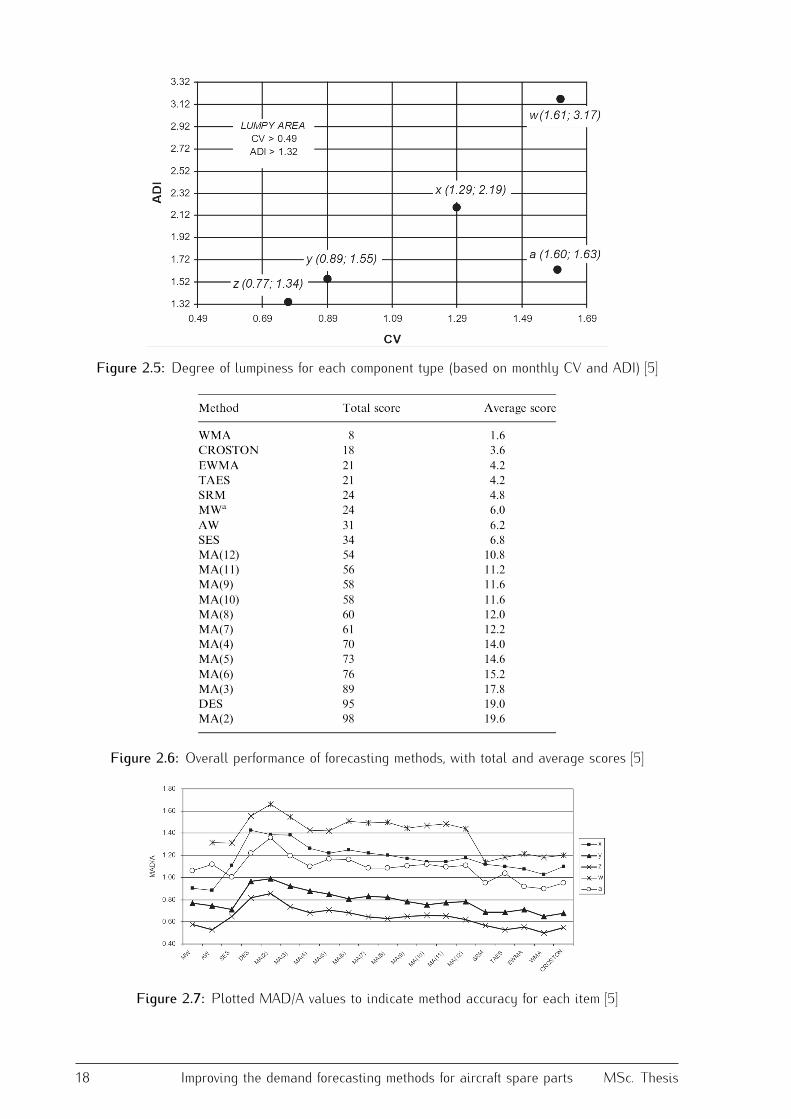
Figure 2.5: Degree of lumpiness for each component type (based on monthly CV and ADI) [5]
Figure 2.6: Overall performance of forecasting methods, with total and average scores [5]
Figure 2.7: Plotted MAD/A values to indicate method accuracy for each item [5]
18 Improving the demand forecasting methods for aircraft spare parts MSc. Thesis

values, accordingly.The research of Regattieri et al. is very relevant for this thesis research, as the authors not only presentresults that show which method performs best, but they also underline that in the general picture,item lumpiness is the main factor that impacts forecasting inaccuracies, while the specific forecastingmethod is of secondary importance. Similar to the findings of Regattieri et al., a study conducted byKostenko and Hyndman (2006) [20] also confirms that the magnitude of CV 2 impacts the accuracy ofthe selected forecasting method. Additionally, in a research performed by Petropoulus et al. (2014) [21],the best-performing forecasting methods are selected based on not only CV 2, but also on other demandcharacteristics such as the length of the series, the seasonal period length and the forecasting horizon.With regard to selecting and applying suitable forecasting methods, some authors also apply bootstrap-ping methods which have shown advantages in certain conditions [22] [23], but they are computationallydemanding since the calculations are rather complex. This is also why they are not often implementedin practice. Furthermore, a recent study by Syntetos [24] has shown that the advantages of thesebootstrapping methods over conventional methods are questionable. This is why improving time-seriesforecasting methods will be a focal point in this thesis research2.1.4 Definition of driving factors
This subsection will outline the most important literature that focuses the inherent characteristicsgenerating spare parts demand. Even though research on this specific topic is rather scarce, somerelevant sources could still be identified. Some of the few authors that are particularly concerned withthe actual underlying sources of demand patterns, are A. A. Ghobbar and C. H. Friend. Their paperson evaluating model errors are already discussed in the previous subsection, but they also have aninteresting piece of work on the investigation of sources of demand lumpiness [25].Ghobbar and Friend believe that environmental factors can have an impact on the extent of lumpinessof demand. To verify this hypothesis, they select a number of factors to investigate whether or not theyhave an effect on lumpiness in spare parts demand. The factors that are included in their experimentare the following:- Primary maintenance process (PMP)- Aircraft utilization rate (AUR)- Component’s overhaul life (COL)- Square coefficient of variation (CV2)- Average inter-demand interval (ADI)
By using an ANOVA method, their aim is to find and compare p-values, which quantify the level ofimpact a factor can have on lumpiness. Their findings show that all factors and their interactions werehighly significant, thus implying that these factors most likely have an impact on demand lumpiness.It also appears that the coefficient for AUR is positive, which implies a positive correlation betweenaircraft utilisation rate and demand size.The authors conclude their paper by stating that AUR, COL and PMP are major sources in increasingthe demand size, which they believe can aid material managers in providing a clearer picture andcould therefore lead to substantial benefits. Additionally, the authors mention that understanding thesources of lumpiness is important in choosing a proper forecasting method.The findings presented by the authors are very much in line with the proposed thesis research, andcan thus form a fundamental basis for the methodology to be executed at a later stage. Especially thefact that there is a way that implementing these insights could contribute to improvements in practice,MSc. Thesis Exploring inherent characteristics of spare parts demand patterns 19

is an important result that further solidifies the need for the proposed research, and it is an indicationthat the research could lead to promising results.The paper called "Reliability and operations: keys to lumpy aircraft spare parts", written by A. F. LowasIII and F. W. Ciarallo in 2015 [6] is one of the first research papers that mainly focuses on the reasonsfor aircraft spare parts to show lumpy demand patterns. These insights are then used to providesuggestions on how to improve the regularity of spare parts demand, thus allowing opportunities toimprove forecasting accuracy. The authors start their paper by reviewing existing studies that dealwith the difficulties involved in forecasting for lumpy demand patterns. Like other authors, Lowas IIIand Ciarallo investigate the existing forecasting methods and how to deal best with intermittent orlumpy demand patterns, as they summarise the main findings of existing research.The main objective of Lowas III and Ciarallo’s research is stated to be to empirically demonstratethe underlying factors for lumpy spare parts demand, by uncovering probable reasons that affect thelumpiness of spare parts demand. Furthermore, the authors use Weibull-based models to simulate thefailure of (and therefore, demand for) replaceable aircraft components. Since 93% of non-structuralcomponents are cited to exhibit a constant failure rate [26], the failure probability density function canbe modeled by an Exponential function with constant failure rate. With that, the scope of the researchis limited to non-repairables components fitting the Weibull distribution of failure models.In this research, Buy Period (BP) is considered to be an inherent characterizing factor that may impactdemand lumpiness, and it is assumed that each aircraft has a life of 20 years, and the aircraft in the fleetare acquired evenly over a BP of 1, 2, 4, 8 or 16 years. Another characterising factor that is consideredis the Fleet size, which is assumed to consist of 8, 32, 128, 512 or 2048 aircraft. Each simulation willalso be replicated 50 times to ensure statistical significance, and with 3000 unique combinations of thepreviously mentioned variables and Weibull parameters, the total number of simulations will amount to150,000.The results showed that 76% of the cases had output that could be characterised to be lumpy. Basedon the results, it can also be stated that there is a strong correlation between ADI and CV, meaningthat a higher ADI will usually also come with a higher CV. The appropriateness of selecting a Weibulldistribution to simulate the results is also proven by fitting the Weibull graphs onto actual engineeringdata for a C-135 ruddervator, F-15 speed brake and a F-15 radome. The Monte Carlo model resultsare compared to actual demand histories in Figure 2.8, which shows that indeed for these types ofcomponents, the simulated demand can be assumed to be accurately modeled with Weibull distributions.The authors also have findings related to the effects of the aforementioned factors: fleet size, buy periodand as-built component life. According to the authors, fleet size is the most significant single factorimpacting the lumpiness of demand, with smaller fleets having dramatically higher CV and ADI valuesthan larger fleets. Additionally, it is stated that a fleet size of at least 256 will enable a fleet plannerto anticipate that failures will occur every quarter, with minimal variability of demand, thus making thetotal demand pattern less lumpy and less challenging to forecast.The final paper to be discussed in this Literature Review section is the most recent research paper alsoconsidering underlying demand generating factors, which is applied to improve forecasting methods.The paper is called "Forecasting spare part demand with Installed Base information: a review", writtenby S. van der Auweraer, R. Boute and A. A. Syntetos [27] and it aims to mainly provide a literaturereview on installed base forecasting methods.The authors suggest to work with Installed Base information, which does take more factors into accountthan just historical demand. The benefits of using installed base information are emphasised, with theauthors referring to previous work stating that the use of installed base information to forecast sparepart demand can lead to cost savings up to 58% [28].The authors mainly have the objective to present a summary of existing and relevant literature insimilar fields, in order to motivate future researchers to consider installed base information as meansof forecasting for spare parts. The authors first describe the most prominent part characteristics that20 Improving the demand forecasting methods for aircraft spare parts MSc. Thesis

Figure 2.8: Weibull fits of spare parts demands on actual historic data [6]cause difficulties in forecasting spare parts demand to be as follows:
1. Part demands show very particular patterns2. They are generated by maintenance policies and part breakdowns3. Parts tend to have a limited amount of historical demand data available4. They are subject to obsolescenceFrom an installed base perspective, the key drivers of spare parts demand are the maintenance activities,which is very different from preventive maintenance spare parts management. With that in mind, theauthors proceed to explain how to use installed base information to forecast CM demand. They providethe governing equations used to express the expected demand under four conditions: constant installedbase, increased installed base, decreasing installed base and fluctuating installed base. The authorscite other authors that state that all four modifications of using installed base information can bedeemed appropriate methods (in some way or another) of forecasting demand and investigating thecausal factors.In comparing corrective maintenance with preventive maintenance, the authors state that CM ischaracterised by a stochastic arrival of demand, while the demand size is deterministic. In the case ofPM the arrival of demand is deterministic, while the demand size can often be stochastic. The authorsthus suggest that the use of installed base information might be more suited for unplanned correctivemaintenance.According to the authors, their research shows that rich information can be made available to improvespare parts demand forecasting. They state that the use of causal methods is appealing, but theapplication of the presented information is not exclusive to causal methods alone. It is for example alsopossible to use time series models in combination with installed base information.In the research performed by B. Hellingrath and A. Cordes [29], a time-series method is combined withcausal information. The authors implement data generated from an Intelligent Maintenance System,which is a physics-based model that considers physical characteristics of individual components andMSc. Thesis Exploring inherent characteristics of spare parts demand patterns 21

relates those characteristics to the probability of failure of that component.In their research, Hellingrath and Cordes focus on integrating the IMS data with the SBA methodproposed by Syntetos and Boylan in 2001, due to its proven accuracy under lumpy conditions [18].They execute this by using the output of the IMS data as input for determining the parameters ofthe underlying pdf distribution of the SBA method. The authors also estimate the demand valuesforecast by the SBA method without taking into account IMS data, after which both series of resultsare compared with each other and with the actual demand data to draw conclusions regarding theaccuracy of both methods.From the obtained findings it was found that when IMS data is included in the forecasting, the estimateddemand values are in fact closer to the actual demand values, compared to the forecasting method thatdid not include IMS data. This is a very interesting finding, as this confirms for this specific data setthat considering and implementing underlying causal factors does in fact improve forecasting accuracy.It should be noted however that only five different types of spare parts were forecasted, and theseresults may not necessarily hold true for all aircraft spare parts in general.These results do reinforce the fact that the integration of underlying factors and information couldbenefit the accuracy of existing forecasting methods, thus justifying further research in this specific area.Therefore, the integration of causal methods or underlying factors with existing time-series methods isrightfully so a major focal point of this master thesis.2.1.5 Main shortcomings in current state of the art
Combining the main takeaways of the reviewed literature of all three categories, it can be saidthat the proposed thesis research will contribute a novel addition to each of the three discussedcategories. Following from the initial statistical analysis, the most statistically significant factors willbe implemented in the second phase of model building and adjusting.This is also an aspect that is rarely performed in existing research. Many of the sources describemethods to improve forecasting accuracy by changing or updating the models themselves, but this isoften done without taking into account the underlying causal factors. The research of Hellingrath andCordes [29] have successfully executed this, although the scope of their research was limited to a smalldata set of spare parts.Throughout the literature review, it was found that not many academic articles deal specifically withthe subdomain of both investigating inherent causal factors and implementing them to improve spareparts forecasting methods. This imposes some difficulties in defining the current state-of-the-art andhow the existing academic knowledge can be used to devise an appropriate research methodology forthis specific issue. This does however emphasise the fact that this is actually a very novel researcharea, and many improvement opportunities still exist in this area.The few research papers that have touched upon this area have shown promising results with respectto improvement of forecasting methods if additional factors are considered. If the research objectivesand questions as described in Section 2.2 can be satisfied properly, significant contributions can bemade to the existing academic and industrial state-of-the-art by this thesis project.2.2 Research scope and research questions
This section details the description of the project scope of the thesis following from the identified gapsin the literature review. It will outline which elements will be of importance during the execution ofthe research, and which topics will be considered. The project scope will be limited to the properexecution and research of four main pillars, which will be described in the first subsection. After this,22 Improving the demand forecasting methods for aircraft spare parts MSc. Thesis
the research questions according to the research scope will be presented in the second subsection.2.2.1 Description of project scope
The first pillar of the thesis research is the extraction of specific data sets from the MRO data baseand the identification of the inherent characteristics of the demand patterns of aircraft spare parts.The main issue in forecasting spare parts is not that the existing forecasting methods are inadequate,but that they are very inaccurate for forecasting demand patterns with high variety. Therefore it canbe of significant importance to first understand which elements generate demand in an MRO andwhy the demand size and frequency is so varied. If these insights can be identified, they can provideopportunities to improve the effectivity of existing forecasting methods.The second pillar of the thesis research concerns itself with the selection of existing forecasting methodsto be used as a baseline forecasting method. This baseline forecasting method will be applied to thespecific data sets extracted in the initial phase of the research. Furthermore, this baseline method willbe altered according to the insights gained in the previous pillar; the causal factors will be incorporatedwith the adjusted forecasting methods. The altered forecasting methods will then also be applied tothe selected data sets.The third pillar of the project scope is to measure, evaluate and compare the performance of the selectedbaseline and adjusted forecasting models. This pillar will be where the findings of the previous twopillars come together, and based on the results it will clarify whether or not the incorporation of theidentified driving factors has in fact had a positive impact on the forecasting accuracy. This step willyield the main results of the research, and based on these results recommendations can be providedregarding future implementations and development.The fourth and final pillar will be dedicated to validating the approach through the use of data sets ofadditional component categories within the MRO database. The applied approach in the first threepillars will be repeated for a selection of validation data sets, which will yield the main generalconclusions of the thesis. At this stage, a sensitivity analysis will also be performed to assess howslightly changing the assumed model parameters may impact the general conclusions.2.2.2 Formulation of research questions
Based on the four main pillars of Project Scope laid out in the previous subsection, the main objectiveof the thesis research will be "To demonstrate that aircraft spare parts demand forecasting accuracywill improve when inherent causal factors are taken into account while forecasting with time-seriesmethods". To reach this objective, multiple research questions will have to be answered throughout theresearch. The main research question that the thesis research aims to answer is the following:
- Will spare parts demand forecasting accuracy improve if inherent causal factors are takeninto account while forecasting with time-series methods?
These main question in turn also generates multiple secondary research questions, which can beanswered subsequently in order to find answers and conclusions for the primary research question.These questions will form the underlying framework of the methodology to be applied, where answeringthe secondary research question will eventually lead to findings that answer the primary researchquestion, and as such the objective of the thesis research will be achieved. The list of secondaryresearch questions is listed as follows:1. Which underlying causal factors can be identified to have a significant impact on the endogenousdemand patterns?2. What is the statistical significance of these factors regarding impact on specific component
MSc. Thesis Exploring inherent characteristics of spare parts demand patterns 23

removals in the data base?3. How can an existing forecasting model be altered to incorporate the effect of the key causalfactors?4. Which error measure is suitable to be used to evaluate the forecasting accuracy of the chosenforecasting model?5. What is the forecasting accuracy of the selected model in its baseline conditions, without takinginto account the causal factors?6. What is the forecasting accuracy of the selected model in adjusted conditions, taking into accountthe causal factors?7. Can an improvement of accuracy be established when comparing the baseline forecasting methodwith the adjusted forecasting method?8. Does using a different data set of aircraft spare parts components result in similar findings, thusvalidating the suggested approach?
24 Improving the demand forecasting methods for aircraft spare parts MSc. Thesis

CHAPTER 3
Methodology
With the academic state of the art outlined and the research domain described in the previous chapter,it is now relevant to introduce the main methodology applied to the thesis research. This chapter willtherefore outline the main functions, inputs and outputs of the methodology that is applied to satisfythe proposed research questions. Section 3.1 will describe the model that was applied, after whichSection 3.2 will detail the selected forecasting methods and error metrics. Finally, Section 3.3 willpresent the proposed methodology for the altered forecasting method, and Section 3.4 will describe theVerification and Validation strategy that was applied in this research.3.1 Model description
The model that was built to be applied in this research is quite extensive and includes multiple inputs,outputs and functions to generate the required results. This section will outline the details of thismodel and will describe the general flow of actions that is applied in this model.Figure 3.1 shows the flow of operations in the initial phase of the model. This phase mainly dealswith the selection of specific datasets within a big database. The main input for this module is thedatabase provided by the MRO, which contains a large number of data entries for component removalssince the 1930s. The first step is to filter this data to a more recent timeframe, so that the results aremore useful in the operations of the MRO. This timeframe is set between 2008 and 2015, to initiate themodel with sufficient data and to use more representable and consistent data in recent years.After this, the data is selected and split further based on operator type, aircraft type and componenttype. Finally, since all the component removals in the data base are registered on a specific day ofthe month, it is necessary to generate monthly quantities for the component removals and the causalfactors to be analysed. This entire process will generate as outputs the monthly patterns of componentremovals and the causal factors in the timeframe between 2008 and 2015 for specific operators, aircrafttypes and component types. The results of this phase are presented and discussed in Chapter 4.The patterns generated in the first phase of the model will be used as inputs for the second phase ofthe model, which is depicted in the flowchart shown in Figure 3.2. The second phase of the modelmainly deals with identifying any statistical relations between the component removals and the selectedcausal factors. First, a data scatter is created for component removals vs. the causal factors, after whichthe Pearson’s correlation coefficient is computed to find out if there exists a statistical relation betweenMSc. Thesis Exploring inherent characteristics of spare parts demand patterns 25

MRO Database Select data withinrecent timeframe
Split data based onOperator type
Split data based onAircraft type
Split data based onComponent type
Generate monthlyquantities
Monthly patternsof causal factors
MonthlyComponent
removals
Figure 3.1: Methodology of the first phase of the applied modelthe component removals and the causal factors. The main output of the second phase of the model arethe values for correlation coefficients, which will be used as inputs the third phase of the model. Theresults corresponding to the second phase of the model are discussed in Chapter 5.
MonthlyComponent
removals
Monthly patternsof causal factors
Generate scatterplots
Determinecorrelationcoefficients
Correlationcoefficients
Figure 3.2: Methodology of the second phase of the applied modelFinally, the outputs generated in phases 1 and 2 of the model will be used in the third phase of themodel. The process of this phase is shown in Figure 3.3. This phase is the most important aspect ofthe applied model, since it deals with applying and evaluating the baseline and adjusted forecastingmethods. First, the baseline forecasting methods are applied, after which the predicted demand volumeswill be compared to the actual demand to compute the forecast error.
MonthlyComponent
removals
Apply baselineforecastingmethods
Baseline forecast
Monthly patternsof causal factors
Apply adjustedforecastingmethods
Correlationcoefficients
Adjusted forecast Determineforecast errors
Compare andevaluate
performance
Figure 3.3: Methodology of the third phase of the applied model26 Improving the demand forecasting methods for aircraft spare parts MSc. Thesis

Next, using the patterns of component removals, the causal factors and the corresponding correlationcoefficients, the adjusted methods are applied to the selected data sets. This will generate an adjustedforecast, which will also be compared to the actual demand volumes to compute the forecast errors.Finally, the performance of the baseline methods will be evaluated and compared to the performance ofthe adjusted methods, to determine which methods are the most accurate in forecasting the spare parts.The results of this phase of the model will be presented and discussed in Chapter 6.3.2 Description of baseline forecasting methods, error metrics and causal
factors
This section will detail which forecasting methods will be applied to the selected datasets. Tworelevant forecasting methods will be selected as baseline methods, which will both be applied to theendogenous demand data sets of the most common and relevant component categories. The baselinemethods will be the Moving Averages (MA) method and the Single Exponential Smoothing (SES)method, which are time-series methods that are commonly used to forecast the demand of spare parts inpractice. The reason that time-series methods are used for this research, is because time-series methodsare more suitable for short term forecasting and are computationally less demanding compared tostochastic models. Even though scientific literature shows that Croston’s method is the most applicablemethod in forecasting lumpy demand patterns, in this case SES will be a suitable alternative since nozero-demand months exist in any of the component removal data subsets.3.2.1 Moving Averages method
The MA method takes the average of the last m values of a time series to determine a forecast value [30].Equation 3.1 shows the mathematical relation that governs the Moving Averages forecasting method.ft+1 = 1
m
m−1∑k=0 yt−k (3.1)
In this equation, m is the user-set parameter that determines how much historical demand is includedin defining the average. A smaller value for m leads to a more reactive forecasting method. For thepurpose of initialising the baseline forecasting methods for this specific research, m is set at a value of3 (months). This means that the MA forecasts presented in Section 6.1 use the (moving) average valueof the previous three months to determine the forecast value for the upcoming month.3.2.2 Single Exponential Smoothing method
The SES method is one of the most accurate forecasting methods when forecasting aircraft spare partsdemand data. It takes the forecast error into account and adjusts it with a certain smoothing constantα . Equation 3.2 [31] shows the governing mathematical equation for the SES forecasting method.
ft+1 = αyt + (1− α)ft (3.2)The smoothing constant is essential in determining how reactive the SES method is to its own forecasterrors, with a higher α leading to a higher reactiveness to the forecast error. Usually this value isbetween 0.1 and 0.3 [31], but for the purpose of applying the baseline methods in this thesis research,an α of 0.3 has been assumed, since the component removal data sets to be forecast are very volatilein their demand size.MSc. Thesis Exploring inherent characteristics of spare parts demand patterns 27

3.2.3 Root Mean Square Error metric
To evaluate the forecasting performance of both the MA method and the SES method, the Root MeanSquare Error (RMSE) will be measured and compared. The RMSE is an error metric that sums thesquared error values of each forecast, and then takes the root of this sum. In doing so, the RMSE showsthe magnitude of the overall error that has been made by the forecasting methods. Equation 3.3 showsthe mathematical relation that was used to determine the RMSE for each forecast demand data set.RMSE = √√√√1
n
n∑t=1 et
2 (3.3)3.2.4 Mean Absolute Percentage Error metric
In addition to assessing the RMSE values of each forecast, the MAPE will also be determined for eachforecast. In contrast to the RMSE metric, the MAPE metric is not scale dependent, so it provides abetter estimate of the forecasting performance when comparing multiple methods in various databases,since the overall demand size does not have to be taken into account. The RMSE gives a restrictedsense of the overall performance of the forecasting method, if the scale of the demand sizes are nottaken into account.The drawback of using the MAPE metric is that it is only applicable to demand data sets without anyzero-demand months, while the RMSE metric is suitable for all demand patterns. The mathematicalrelation that was used to determine the MAPE value is given by Equation 3.4.MAPE = 1
n
n∑t=1 |
etyt| · 100 (3.4)
3.2.5 Selection of causal factors
The causal factors to be selected are factors that may have an impact on the demand pattern of aspecific component. Of course there are many factors in aircraft maintenance that may impact thedemand generation of component removals. Possible examples of these factors can be listed as follows;- Environmental effects- Flight cycles- Pilot complaints- Fleet size- Time to failure of a component- Aircraft landings- Operator type- Aircraft type- Characteristics of component type- Maintenance policy of MRO
For the scope of this research however, the methodology will limit itself to the implementation of thecausal factors pilot complaints and aircraft landings only. The main reason for this is the abundance28 Improving the demand forecasting methods for aircraft spare parts MSc. Thesis

of available data in the MRO database on these specific factors, and because it is feasible to expecta statistical correlation between the number of pilot complaints, the utilitisation rate of the aircraftand the number of removed components. Additionally, the operator type, aircraft type and componenttype will be used as factors to segregate the data in the initial phase, prior to generating the monthlypatterns of the causal factors and component removals. A more elaborate motivation for the selection ofthese causal factors is provided in Section 5.1.3.3 Methodology for altered forecasting method
An approach to improving the existing methods with additional insights, is to somehow incorporate thecorrelation coefficients obtained for the causal factors with the forecast demand output. The correlationcoefficients describe how strongly the component removal data would follow a relative change in thecausal factors. It is therefore also necessary to include the ratio of pilot complaints and aircraft landingsin the current month, over the average value for these factors in the past three months.Multiplying these ratio’s with the correlation coefficients for the causal factors, will tune the forecastvalue either upwards or downwards. For example, in case a certain month relatively has a lot of pilotcomplaints and aircraft landings, the forecast demand output obtained from the MA or SES methodwill be tuned upwards. In case there are relatively very few pilot complaints and aircraft landings, theforecast value will be tuned downwards.The hypothesis is that this tuning effect will reduce forecasting errors, since additional statisticallysignificant explanatory factors are taken into account. Equation 3.5 shows the governing relation thatwill be used to improve the baseline forecasting methods. This improved forecasting methodology willbe implemented and applied in Chapter 6.F ∗ = F ′ ·
(cPC · [PC1/PC0] + cLD · [LD1/LD0]cPC + cLD
) (3.5)Where;
- F ′ is the MA or SES demand forecast value- cPC is the correlation coefficient for Pilot Complaints- cLD is the correlation coefficient for Aircraft Landings- PC1 is the number of Pilot Complaints in the current month- PC0 is the average number of Pilot Complaints in the past three months- LD1 is the number of Aircraft Landings in the current month- LD0 is the average number of Aircraft Landings in the past three months3.4 Verification and Validation methods
In order to ensure that the findings and conclusions are representative of reality, the suggestedmethodology also needs to be verified and validated throughout the research. This section will thereforebriefly explain the applied verification and validation strategies.
MSc. Thesis Exploring inherent characteristics of spare parts demand patterns 29

3.4.1 Verification strategy
The approach is mainly verified in the initial stages of the research. The main objective of the initialphase of the model is to correctly load and select data from an Excel environment into the MATLABenivornment. To ensure that this goes without errors, the method is verified by recalculating the resultsfound in MATLAB with Excel. The verification of the model is thereby applied by looking into anydiscrepancies in the results generated by MATLAB and those in Excel. In case the results are thesame, the approach is deemed to be verified successfully.For example, during the initial phase of the model, most of the data will be selected and importedto generate the data patterns. The results in the data patterns are then verified by confirming thatexcel yields the same quantities for random months in the time span of eight years. This process isrepeated several times for random months, and if the results are equal then it is verified that the modelsuccessfully is able to import and handle the data base stored in Excel.3.4.2 Validation strategy
The applied model also needs to be validated to ensure that the results and conclusions are notapplicable for one specific situation and set of requirements only, but that the approach also is able tosuccessfully generate results under other conditions. In case of the described model, the validation willbe applied in the latter phase of the analysis. In the last phase, initially the baseline and adjustedforecasting methods are applied to a few specific component types for a specific operator.After the results and conclusions are generated for these specific component types, the whole processwill be repeated for components in other categories as well, thus validating the approach if theadditional findings are supporting the initial conclusions obtained. The validation strategy is thereforebasically applying the whole model again under different conditions for multiple different componenttypes. If the results of the validation are in line with the conclusions in the initial research, the methodcan be deemed successfully validated.
30 Improving the demand forecasting methods for aircraft spare parts MSc. Thesis
CHAPTER 4
Data selection and analysis of historic demand patterns
The first phase of the project concerns itself with the selection of proper databases and the identificationof the main demand characteristics of these selected databases. Using an extensive database withendogenous and exogenous spare parts demand data from an existing MRO, the specific demandpatterns are visualised and extracted. Section 4.1 will describe the preliminary analysis that wasperformed on the MRO database, which will be followed by an analysis of the demand size variationas described in Section 4.2.4.1 Preliminary analysis MRO database
The first step was to actually analyse the available data on a preliminary level, such that an effectiveand more complex analysis of the demand pattern characteristics and statistically significant factorscan be performed using MATLAB. To ensure the generation of results effectively without jeopardisingthe computational efforts required, the large initial database was split into a smaller data sets with asample space that could guarantee efficient yet thorough analysis.First of all, the historic timeframe of the sample space to be analysed was restricted to a timespan ofeight years, investigating all components removals occurring between January 2008 and December2015. This period was mainly chosen due to the fact that it became apparent from the database, thatthe more recent years contain more relevant, complete and consistent data. The quality of consistentdata was the main motivating factor in deciding which database to start the general analysis with. Forthe remainder of the thesis research, this sample space is also restricted to demand data betweenJanuary 2008 and December 2015, to ensure more qualitative and consistent results and conclusions.The monthly removals of all components for Fokker 50, Fokker 70 and Fokker 100 aircraft are combinedand represented in Figure 4.1. At a first glance, looking at the removal of all components by Fokkerbetween 2008 and 2015 leaves the impression that the demand patterns could be characterised tobe smooth. However, this is mainly explained by the fact that every single component type (CT) ispooled together in this case, which negates the erratic nature of individual components in a biggercollective group of components. In practice, any useful forecasting method would be applied forindividual components (categories), rather than for the entire batch of components in the inventory. Thisemphasises the fact that the demand for spare parts should always be considered on a more detailedlevel.31

Figure 4.1: Component removals of all categories and aircraft types between 2008 and 2015It is expected that the demand patterns for more detailed component categories will show a moreerratic distribution compared to the demand pattern for all components combined. For this reason,all the components in the sample space are grouped together with their ATA3-chapter code for eachaircraft type in the database, to identify the demand variation of certain component categories. To dothis, separate data subsets were generated for each ATA3-component for each aircraft type, yieldingthe component removals per month over the same timespan of eight years.For illustrative purposes, Figure 4.2 shows the demand pattern for all components in the ATA-342chapter for the Fokker 100 aircraft type, which represents the Attitude and Direction section of theNavigation category. Just by looking at the distribution of demand data for this specific set of ATA-342components, it can already be seen that the demand volumes show a larger variation compared to thedemand pattern of all components depicted in Figure 4.1, with monthly demand sizes ranging between12 and 44. This is of course in line with the expectation that the demand patterns for more detailedcomponents will show a less smooth distribution than for all components combined.With the developed preliminary analysis method, similar graphs are generated for each possible ATA3-component and aircraft type combination existing in the identified timeframe. From this preliminaryanalysis, it becomes apparent that the majority of the ATA3-categories of components have a commonalityof less than 1%. To ensure measurable advantages of the newly proposed forecasting method and tominimise the computational efforts, a pre-selection was made of ATA3-categories with a commonalityhigher than 3%. This subset of component removal data accounts for almost 40% of the total removalsand it will be used for further analysis, since any forecasting benefits found in this subset could leadto significant impacts on the overall operations, due to the significance of these six ATA3-categories ofcomponents.This subset of data was then imported into MATLAB for further analysis of the demand patterncharacteristics. The CV 2-values for each of the ATA3-component datasets was determined, to gaininsights on the degree of demand size variation for each component category. Table 4.1 shows anoverview of the overall CV 2-values for each of the six components, per aircraft type. The CV 2-valuesare calculated over the same period of eight years, between 2008 and 2015.Looking only at the CV 2-values presented in Table 4.1, it can already be seen that all of the values32 Improving the demand forecasting methods for aircraft spare parts MSc. Thesis

Figure 4.2: Component removals of the ATA-342 category for Fokker 100 aircraft between 2008 and2015Table 4.1: Overview of CV-values for the six ATA3-component demand patterns between 2008 and2015
CV 2-valuesComponentcategory Description Commonality (%) F-50 F-100 F-70253 Equipment/Furnishing - Buffet/Gallery 3.2 5.78 1.88 2.55
324 Landing Gear - Wheels and Brakes 20 1.76 2.32 2.14334 Lights - Exterior 3.0 2.48 1.71 2.98342 Navigation - Attitude and Direction 4.4 1.82 2.03 2.8345 Navigation - Dependent Position Determining 3.1 2.09 2.09 3.60351 Oxygen - Crew 5.2 2.01 2.45 1.16are over the threshold CV 2-value of 0.49, implying that all of the demand patterns in this subset showirregularity in the demand size. The ADI-values on the other hand are 1.00 for all datasets, since thereare no zero-demand months and therefore every month demand is to be expected for each of the sixpresented component categories. This is due to the fact that still many different types of unique andmore detailed components are included under the ATA3-chapter level.Looking at the 324 category for example, Landing Gear - Wheels and Brakes includes componentsranging from nose and main wheel tires to the brake valves and sensors. For this reason, a moredetailed analysis is performed for one of these component categories on the ATA6-level. This approachseparates the parts based on their ATA6-codes, and thus this separation is based on more detailedcharacteristics/categories of the individual components. As such, a more detailed analysis is performedon the ATA-324 component category (Landing Gear - Wheels and Brakes), mainly because this categorycontains the most components by far, and therefore the achieved results in this subset of data couldlead to more substantiated implications in the total database.
MSc. Thesis Exploring inherent characteristics of spare parts demand patterns 33

4.2 CV 2-analysis of Wheels and Brakes components
The 324-category in the ATA3-chapter description represents the Wheels and Brakes group ofcomponents within Landing Gear. This section will present the results gained from a more detailedanalysis of demand patterns for the Wheels and Brakes category specifically. It should be notedhowever that many subcategories of the 324-category (Wheels and Brakes) are represented within thisparticular data subset with a commonality of less than 1%.It is for that reason that all components at the ATA6-chapter description with a commonality of lessthan 10% are initially omitted from the data subset. The following ATA6-chapter subcategories whichremain in the data subset for a more detailed analysis of CV values are presented in Table 4.2.Table 4.2: Overview of ATA6-categories for detailed CV analysis
ATA6-category Description Commonality324-101 Main Wheel Tire (MWT) 43%324-103 Nose Wheel Tire (NWT) 24%324-201 Main Wheel Brake Unit (MWBU) 16%As can be seen from this overview, the vast majority of components in the ATA3-324 category belong tothe subcategories 324-101, 324-103 or 324-201. It should also be noted that the sum of these threesubcategories accounts for 83% of all the data within the 324 category, which is in accordance withthe 80/20 Pareto-rule. All other component subcategories in the Wheels and Brakes category amountto a volume size of less than 20% of the total.With the data subsets now defined, the more detailed CV-analysis can be performed for the threedifferent Aircraft Types (ACT) between the period January 2008 until December 2015. It is assumedthat the ADI values will always be equal to 1, since in each month there will be a quantity of atleast one component. Therefore during the detailed analysis, only the CV 2-values will be of interestand the degree of demand size variation will be assessed purely on whether or not the CV 2 will beabove (thus erratic) or below (thus smooth) the threshold value of 0.49.For each data subset, the standard deviation is divided by the mean of that subset, to retrieve a valuefor the CV 2. This process is applied to the three subcategories (324-101,324-103 and 324-201) forthree aircraft types (Fokker 50, Fokker 100 and Fokker 70), yielding nine different CV 2-values for allof the analysed data subsets. An overview of these results is presented in Table 4.3.
Table 4.3: CV 2-values for selected ATA6-categoriesCV 2-valuesATA6-category Subcategory description Fokker 50 Fokker 100 Fokker 70324-101 Main Wheel Tire (MWT) 0.985 1.63 0.995324-103 Nose Wheel Tire (NWT) 0.00 1.70 1.23324-201 Main Wheel Brake Unit (MWBU) 1.08 0.592 0.490
Looking at the preliminary results in Table 4.3, it becomes clear that almost all demand patterns in thedata subsets can be classified to be erratic. The most erratic spare parts data is seen in the MainWheel Tire (324-101) and Nose Wheel Tire (324-103) components for the Fokker 100 aircraft, followedby the Nose Wheel Tire (324-103) components for the Fokker 70 aircraft and the Main Wheel BrakeUnit (324-201) components for the Fokker 50 aircraft.Interestingly, the demand pattern for MWBU components for the Fokker 70 has a CV 2-value that isexactly equal to the threshold value of 0.49. Furthermore, the NWT components for the Fokker 50aircraft result in a CV 2-value of exactly 0.00, which is an unlikely value for a demand pattern. Uponfurther investigation of the data subset, it appears that this particular data subset contains insufficientdata to perform the CV 2-values computations and to verify the pattern characteristics. This subset34 Improving the demand forecasting methods for aircraft spare parts MSc. Thesis

contains 30 entries equal to 1, which is far too few data points over a time span 8 years (and thus 96months). Considering this fact, the data subset of 324-103 for the Fokker 50 will also be omitted fromthe remainder of the preliminary analysis.With the remaining 8 subsets of Wheels and Brakes component demand data, it can be stated that thedemand pattern for MWBU-Fokker70 will show the least erratic characteristics, while the demandpattern for NWT-Fokker100 will show the most erratic characteristics. To gain insights on the demandpatterns themselves, an overview and discussion of the 8 subsets of data is presented in Section 4.34.3 Demand patterns of components within Wheels and Brakes
In the previous section, it was determined through a detailed CV 2-analysis of certain Wheels andBrakes subcategories that all of the remaining data subsets showed erratic demand characteristics.This confirms the hypotheses in relevant literature studies that the majority of aircraft spare partsdemand data show large variation in demand size.In order to gain a better understanding of the underlying inherent demand-generating factors, it isimportant to visualise the data subsets analysed in the Section 4.2. Figures 4.3 and 4.4 show theresults of the preliminary analysis of the most erratic and least erratic data subsets, respectively. Thedemand patterns for the remaining data subsets are represented by Figures A.1 through A.6, whichcan be found in Appendix A. Again, all the data subsets are from January 2008 until (and including)December 2015.
Figure 4.3: Monthly component removals of 324-201 category for Fokker 70 between 2008 and 2016Looking at Figure 4.3, it becomes clear why this specific demand pattern is the least erratic comparedto the other seven demand patterns. Almost every month in the eight year time frame has a monthlyremoval quantity between 5 and 15, with outlying demand sizes being 2 at the least, or 20 at themost. For some reason, the demand size for the MWBU component of the Fokker 70 has been ratherconsistent, and could therefore perhaps be forecast with greater accuracy in the (near) future.In contrast, Figure 4.4 shows the most erratic demand pattern of the eight analysed data subsets,with many large outliers of demand size in many different months. The monthly demand size of theNWT component of the Fokker 100 varies between 5 and almost 100. This large variation in monthlydemand size is of course coupled with the fact that this data subset has the highest CV 2-value of theeight investigated patterns.MSc. Thesis Exploring inherent characteristics of spare parts demand patterns 35

Figure 4.4: Monthly component removals of 324-103 category for Fokker 100 between 2008 and 2016With these newly gained insights, it can be stated that the inherent spare parts demand characteristicsdiffer per aircraft type, but also per component type. Overall, the MWBU components show lesserratic demand patterns compared to the main/nose wheel tire components. In addition, the detailedCV-analysis reaches the same conclusion as the preliminary analysis; the F-100 aircraft type has themost erratic demand pattern within the Wheels and Brakes category. Also it is of interest to note thatin general, the pooling and categorisation of spare part components also affects the found CV 2-values.
36 Improving the demand forecasting methods for aircraft spare parts MSc. Thesis

CHAPTER 5
Impact of Causal Factors on Component Removal data
With the most relevant components identified and their pattern characteristics analysed in the previouschapter, it is now of importance to generate data sets for specific component removals and to relatethese statistically to other possible factors. Section 5.1 describes which demand-driving factors canbe identified, after which Sections 5.2 and 5.3 present the results of the generated data sets for thecomponent removals and the causal factors. Finally, Section 5.4 will describe how the generated datasets are statistically correlated to the data sets of the causal factors.5.1 Identifying inherent characteristics of aircraft spare parts demand pat-
terns
To investigate which demand-generating causal factors impact the main findings and observationsin Chapter 4, it is important to have an understanding of how Component Removal (CR) demand isgenerated in the first place. The following two subsections will outline the general flow of demandgeneration in a typical MRO practice, and the corresponding causal factors that could potentially beincorporated to improve forecasting methods.5.1.1 The general flow of demand data in a typical MRO
This subsection will outline the general flow of demand data and any possible key factors that mayimpact the monthly demand size of component removals. The general flow of demand data in thecurrent MRO industry is depicted in Figure 5.1.The red arrows represent the flow of actual and available data, which is present due to historicdata generated in the past. The blue arrows represent demand data generated after the occurrenceof component removals, which is used as input for Forecasting methods. Finally, the green arrowsrepresent the main research gap to be investigated throughout this specific thesis work, focusing mainlyon the integration of inherent demand pattern characteristics with existing high-performing time-seriesmodels.Furthermore, the underlying factors impacting the generation of demand data is represented by green oryellow blocks. The green blocks represent internal factors that either contribute to a component removal37

COMPONENT REMOVAL
INTERNAL
Historic policy and
documentation
INTERNAL
MRO Management
Preventive maintenance
EXTERNAL
Aircraft Operator
INTERNAL
Forecasting with
Installed Base INTERNAL
Time-series Forecasting
DEMAND FORECAST
EXTERNAL
FACTOR
Environment
INTERNAL
Condition-based Monitoring (CBM)
Historic demand data
EXTERNAL
FACTOR
Flight data
EXTERNAL
FACTOR
Aircraft utilisation
Figure 5.1: Typical flow of demand data generation in MRO industryor a forecast of demand, based on the current state-of-the-art of scientific and industry knowledge (assummarised in Chapter 2). Specific examples of typical internal factors could include:
- The finance department of the MRO- Upper-management of the MRO- The specific maintenance strategy of the MRO- Component removal guidelines in MRO documentation based on historic policy- Forecasting methods based on historic data (Time-series forecasting)The yellow blocks represent external factors that may have a direct or indirect impact on the generationof demand within the particular MRO, but which are outside the control of the MRO itself. Mapping outthese factors is essential in understanding the inherent characteristics of aircraft spare parts demandpatterns. Factors may include (but are not limited to) the following list:
- Environmental factors like weather conditions and geographical limitations.- Flight data generated by each flight (pilot complaints, CNS data)- Installed base of the operator (fleet size, aircraft types)- Utilisation rate of the aircraftFinally, the blue block represents a field of expertise that can be regarded as having the most scientificand practical contributions to the current standard forecasting models (which are often time-series38 Improving the demand forecasting methods for aircraft spare parts MSc. Thesis

forecasting methods).5.1.2 Inherent key demand-driving factors to be analysed
The specific research field represented by the blue block in Figure 5.1 is generally directly relatedto improving existing forecasting models and the demand size these models forecast, and it is alsothe main research focus for this specific thesis project. The main objective of this research is to findpatterns and correlations in historic data and take them into account while forecasting with existingmethods. In doing so, the hypothesis is that the forecasting errors will be reduced measurably.Of course many factors may directly or indirectly impact the actual number of component removals ina given time period, but for the purpose of this thesis the scope is initially limited to consider fourfactors. These specific factors are selected based on the available data related to these factors. Lookingback at the overview of data generation represented in Figure 5.1, the initial factors of interest will berelated to Pilot Complaints and the Utilisation Rate of the aircraft, due to the significant amount ofavailable data related to these causal factors in the database. Furthermore, the data set will first besplit based on Aircraft type and external Operator. As such, the key demand-driving causal factors thatwill be explored in this research will be:- Indirect factor: Aircraft Operator (ACO)- Indirect factor: Aircraft Type (ACT)- Direct factor: Pilot Complaints (PIC)- Direct factor: Aircraft Landings (LND)
The first two key factors (ACO and ACT) are indirect factors that inherently determine the quantity ofthe remaining two key factors (PIC and LND), which are in fact factors that may be directly correlatedto component removals. Therefore, the indirect key factors Aircraft Operator and Aircraft Type willbe used to categorise the datasets into smaller data subsets, which will then be used to analyseany correlation between the remaining two direct key factors (PIC and LND) and component removalquantities. The analysis of the aforementioned causal factors will be explored in further detail in thefollowing sections.5.2 Indirect factors: Aircraft Operator and Aircraft Type
The available MRO database includes many different types of operators which all have an individualdemand pattern regarding Wheels & Brakes (W&B) component removals. It is therefore interesting toselect a few operators before conducting a detailed analysis on their demand patterns to identify anyimpacts of the stated causal factors. This section will describe which operators were selected for theanalysis of their causal factors, and it will present the specific demand patterns to be analysed.5.2.1 Selection of Aircraft Operators
During Phase I of the research, there was not yet a distinction made between operators. The bulk ofdata was divided only based on Aircraft types and specific component categories. This means that allthe subsets of demand data discussed in Phase I, represent Wheels & Brakes component removal datafor Aircraft types 1, 2 and 3, for all operators within the eight year time span. In the more detailedsecond Phase of the research, inherent characteristics and correlations will need to be identified.Therefore it is of importance to select appropriate operators in which these key factors can actually besignified. The selection of these operators is based on the following two selection criteria:MSc. Thesis Exploring inherent characteristics of spare parts demand patterns 39

1. Data continuity for Wheels & Brakes component removals between 2008 and 20152. Geographic diversity in selected operatorsThe main selection criterion of these operators is that they need to have data continuity for componentremovals, in order to draw solid and valid conclusions at a later stage in the research. A secondaryselection criterion was that the operators need to operate in geographically diverse regions, such thatany environmental differences can be associated to the presented data. With these criteria in mind,three operators were selected for further analysis.
1. Operator 1: Regional airline in NW Europe2. Operator 2: Domestic airline in Oceania3. Operator 3: Regional airline in Nordic countryAll three of these operators have Wheels & Brakes component removal data continuously presentbetween 2008 and 2015. The specific demand patterns for each of these operators for specific AircraftTypes are presented in the following subsection.5.2.2 Monthly component removal quantities per Operator and per Aircraft type
Figures 5.2 through 5.4 represent monthly Wheels & Brakes component removal data for operators 1, 2and 3, respectively. The presented demand patterns are separated based on aircraft type, componentcategory and aircraft operator. It should be noted however that the component type categorisationis based on ATA3-level chapter descriptions. This means that the monthly quantities represent allcomponents related to the Wheels & Brakes category, so no further distinction of subcategories is madeat this stage of the analysis.Monthly Component Removals for Operator 1
2008 2009 2010 2011 2012 2013 2014 2015
Years
0
20
40
60
80
100
120
140
Month
ly q
uantity
AC Type 1
AC Type 2
AC Type 3
Figure 5.2: Monthly Component removal data for Operator 1Figure 5.2 shows the monthly component removals for Operator 1, between 2008 and 2015. It isinteresting to note that this operator used all three aircraft types in this time frame, but stopped using40 Improving the demand forecasting methods for aircraft spare parts MSc. Thesis

Monthly Component Removals for Operator 2
2008 2009 2010 2011 2012 2013 2014 2015
Years
0
5
10
15
20
25
Month
ly q
uantity
AC Type 1
AC Type 2
AC Type 3
Figure 5.3: Monthly Component removal data for Operator 2Monthly Component Removals for Operator 3
2008 2009 2010 2011 2012 2013 2014 2015
Years
0
5
10
15
20
25
30
35
40
Month
ly q
uantity
AC Type 1
AC Type 2
AC Type 3
Figure 5.4: Monthly Component removal data for Operator 3Aircraft types 1 and 2 in 2010 and 2012, respectively. It can also be clearly seen that the vast majorityof Wheels & Brakes component removals is related to aircraft type 3, with monthly removal quantitiesranging between approximately 30 and 120 units.Looking at Figure 5.3, the monthly component removal distribution for Operator 2, it can already beseen that this operator has only used aircraft types 1 and 2 in the specific time span of eight years.MSc. Thesis Exploring inherent characteristics of spare parts demand patterns 41
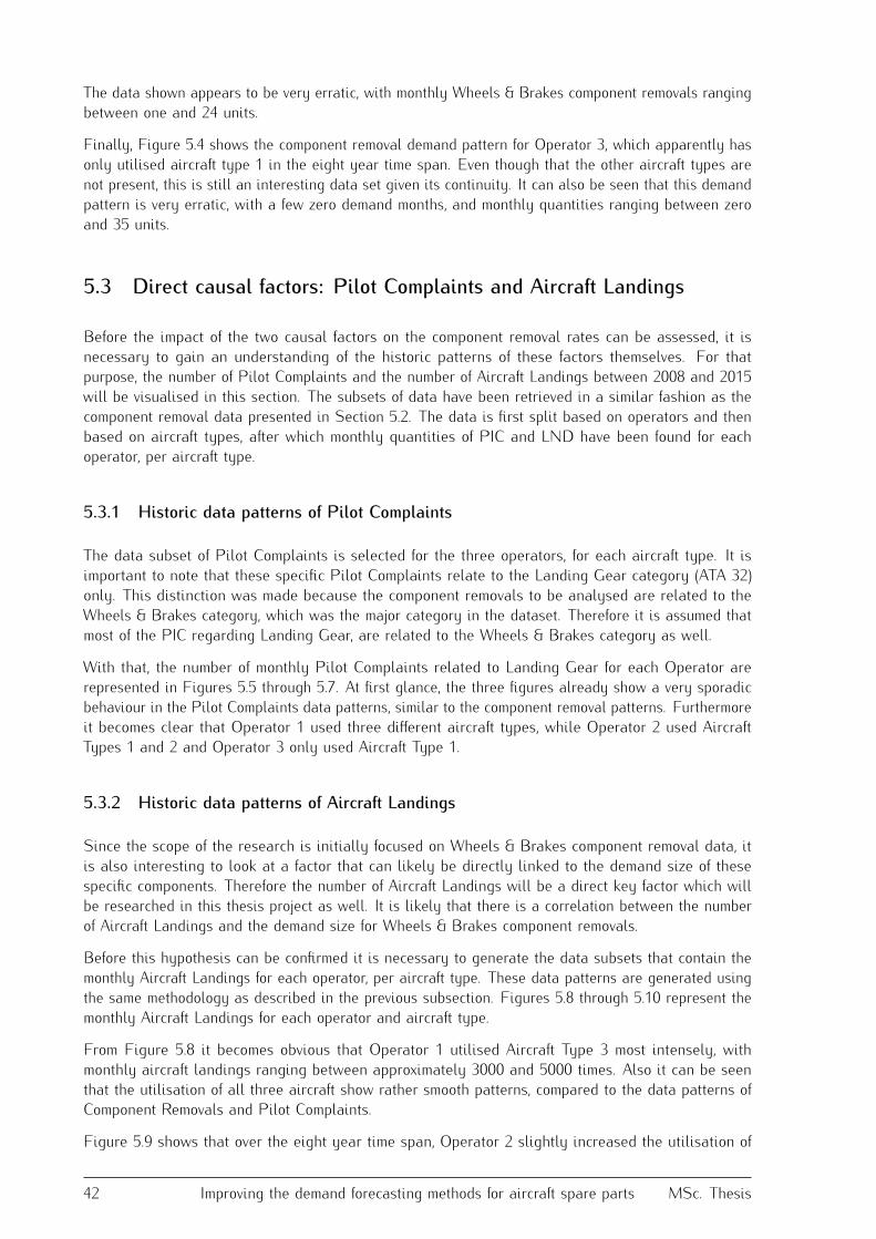
The data shown appears to be very erratic, with monthly Wheels & Brakes component removals rangingbetween one and 24 units.Finally, Figure 5.4 shows the component removal demand pattern for Operator 3, which apparently hasonly utilised aircraft type 1 in the eight year time span. Even though that the other aircraft types arenot present, this is still an interesting data set given its continuity. It can also be seen that this demandpattern is very erratic, with a few zero demand months, and monthly quantities ranging between zeroand 35 units.5.3 Direct causal factors: Pilot Complaints and Aircraft Landings
Before the impact of the two causal factors on the component removal rates can be assessed, it isnecessary to gain an understanding of the historic patterns of these factors themselves. For thatpurpose, the number of Pilot Complaints and the number of Aircraft Landings between 2008 and 2015will be visualised in this section. The subsets of data have been retrieved in a similar fashion as thecomponent removal data presented in Section 5.2. The data is first split based on operators and thenbased on aircraft types, after which monthly quantities of PIC and LND have been found for eachoperator, per aircraft type.5.3.1 Historic data patterns of Pilot Complaints
The data subset of Pilot Complaints is selected for the three operators, for each aircraft type. It isimportant to note that these specific Pilot Complaints relate to the Landing Gear category (ATA 32)only. This distinction was made because the component removals to be analysed are related to theWheels & Brakes category, which was the major category in the dataset. Therefore it is assumed thatmost of the PIC regarding Landing Gear, are related to the Wheels & Brakes category as well.With that, the number of monthly Pilot Complaints related to Landing Gear for each Operator arerepresented in Figures 5.5 through 5.7. At first glance, the three figures already show a very sporadicbehaviour in the Pilot Complaints data patterns, similar to the component removal patterns. Furthermoreit becomes clear that Operator 1 used three different aircraft types, while Operator 2 used AircraftTypes 1 and 2 and Operator 3 only used Aircraft Type 1.5.3.2 Historic data patterns of Aircraft Landings
Since the scope of the research is initially focused on Wheels & Brakes component removal data, itis also interesting to look at a factor that can likely be directly linked to the demand size of thesespecific components. Therefore the number of Aircraft Landings will be a direct key factor which willbe researched in this thesis project as well. It is likely that there is a correlation between the numberof Aircraft Landings and the demand size for Wheels & Brakes component removals.Before this hypothesis can be confirmed it is necessary to generate the data subsets that contain themonthly Aircraft Landings for each operator, per aircraft type. These data patterns are generated usingthe same methodology as described in the previous subsection. Figures 5.8 through 5.10 represent themonthly Aircraft Landings for each operator and aircraft type.From Figure 5.8 it becomes obvious that Operator 1 utilised Aircraft Type 3 most intensely, withmonthly aircraft landings ranging between approximately 3000 and 5000 times. Also it can be seenthat the utilisation of all three aircraft show rather smooth patterns, compared to the data patterns ofComponent Removals and Pilot Complaints.Figure 5.9 shows that over the eight year time span, Operator 2 slightly increased the utilisation of42 Improving the demand forecasting methods for aircraft spare parts MSc. Thesis

Number of monthly Pilot Complaints for Operator 1
2008 2009 2010 2011 2012 2013 2014 2015
Years
0
20
40
60
80
100
120
140
160
180
200
Month
ly P
ilot C
om
pla
ints
AC Type 1
AC Type 2
AC Type 3
Figure 5.5: Monthly number of Pilot Complaints for Operator 1Number of monthly Pilot Complaints for Operator 2
2008 2009 2010 2011 2012 2013 2014 2015
Years
0
5
10
15
20
25
Month
ly P
ilot C
om
pla
ints
AC Type 1
AC Type 2
AC Type 3
Figure 5.6: Monthly number of Pilot Complaints for Operator 2Aircraft Type 2, while the utilisation of Aircraft Type 2 slightly decreased. Secondly, it can be seenthat in general, the Aircraft Landings data patterns for Operator 2 are very smooth compared to theother operators.Finally, Figure 5.10 shows that the number of Aircraft Landings have been rather sporadic for Operator3, with values ranging between approximately 400 and 1200 landings. There is also a general trend ofMSc. Thesis Exploring inherent characteristics of spare parts demand patterns 43

Number of monthly Pilot Complaints for Operator 3
2008 2009 2010 2011 2012 2013 2014 2015
Years
0
5
10
15
20
25
30
Month
ly P
ilot C
om
pla
ints
AC Type 1
AC Type 2
AC Type 3
Figure 5.7: Monthly number of Pilot Complaints for Operator 3Number of monthly Aircraft Landings for Operator 1
2008 2009 2010 2011 2012 2013 2014 2015
Years
0
1000
2000
3000
4000
5000
6000
7000
Month
ly A
C L
andin
gs
AC Type 1
AC Type 2
AC Type 3
Figure 5.8: Monthly number of Landings for Operator 1decreasing utilisation by this operator. With the data patterns of the direct key factors now generatedand visualised for each operator and aircraft type, the next section will detail the performed statisticalanalysis to find any correlation between the causal factors and the component removal data.
44 Improving the demand forecasting methods for aircraft spare parts MSc. Thesis

Number of monthly Aircraft Landings for Operator 2
2008 2009 2010 2011 2012 2013 2014 2015
Years
0
500
1000
1500
2000
2500
Month
ly A
C L
andin
gs
AC Type 1
AC Type 2
AC Type 3
Figure 5.9: Monthly number of Landings for Operator 2Number of monthly Aircraft Landings for Operator 3
2008 2009 2010 2011 2012 2013 2014 2015
Years
0
200
400
600
800
1000
1200
Month
ly A
C L
andin
gs
AC Type 1
AC Type 2
AC Type 3
Figure 5.10: Monthly number of Landings for Operator 35.4 Statistical analysis of correlation between direct factors and compo-
nent removals
The available MRO data is now split into subsets which are suitable for the statistical analysis. Thestatistical analysis will show which of the direct and indirect factors have a statistically significantMSc. Thesis Exploring inherent characteristics of spare parts demand patterns 45

impact on the component removal demand patterns. Specifically, this section will detail if there arestatistical correlations between the removal of Wheels & Brakes components and the discussed directfactors, for each operator and aircraft type. Once those values are known, the baseline forecastingmethods can be initiated, after which the causal factors can be incorporated while forecasting. Thisprocess will be detailed in Chapter 6.5.4.1 Correlation between Pilot Complaints and Component Removals
The correlation between the Pilot Complaint data sets and W&B Component Removal data sets hasbeen determined by finding the Pearson’s correlation coefficients. The coefficients resulting from thisanalysis represent any correlation between PIC and CR with a 95% confidence interval, where a valueof 1.0 can be interpreted as a perfect linear correlation and a value of 0.0 would mean that there is nocorrelation whatsoever. It is important to note that the analysis of correlation is applied to only the first6 years of the dataset, since the last two years will be used to validate the improved forecasting methodby generating forecast demand. Table 5.1 shows an overview of the obtained correlation coefficientsbetween PIC and CR, for the three operators, per Aircraft Type. Note that since Operators 2 and 3 havenot utilised all three aircraft types, the correlation coefficients for some aircraft types are not available.Table 5.1: Overview of correlation coefficients between Pilot Complaints and Component Removalquantities
Fokker 50 Fokker 100 Fokker 70Operator 1 0.779 0.923 0.813Operator 2 -0.067 0.269 n/aOperator 3 -0.034 n/a n/a
The results in Table 5.1 show that there is a significant correlation between the PIC and W&B CRdatabases for Operator 1, across all three aircraft types. The strongest correlation exists for the Fokker100, which has a correlation coefficient of 0.923. Unfortunately Operator 1 does not operate the Fokker50 and Fokker 100 anymore, but for the aircraft that they still have in operation (Fokker 70) there alsoexists a positive significant correlation of 0.813. The data scatter of pilot complaints versus componentremovals for all three aircraft types of Operator 1 are shown in Figures 5.11 through 5.13.Regarding the databases for Operator 2, there appears to not be a correlation between PIC and CR forthe F50 aircraft, but there seems to be a slight correlation of 0.269 for the F100 aircraft. Finally, thereis also no positive or negative correlation between the PIC and CR databases for Operator 3, since thecorrelation coefficient is almost zero. These insights show that the Operator 1 data sets can offer themost potential to incorporate the effects of the key causal factors when forecasting W&B componentdemand sizes.5.4.2 Correlation between Aircraft Landings and Component Removals
The correlation between the LND data base and CR data base is also obtained by determiningPearson’s correlation coefficient, in order to estimate the potential impact of Aircraft Landings on themonthly demand size of Wheels & Brakes component removals. Again, the results indicate if there is acorrelation between LND and CR with a 95% confidence interval, with 1.0 being a perfect correlationand 0.0 being no correlation at all. Again, it should be noted that the statistical analysis is onlyapplied to the first 6 years of the dataset, to ensure efficient validation of the last two years of demanddata. Table 5.2 shows the overview of correlation coefficients resulting from the statistical analysis, foreach operator and aircraft type. Again, three coefficients are missing due to the fact that their operatorshave not utilised all three aircraft types.Looking at Table 5.2, it can be seen that again the data sets of Operator 1 show the most significant46 Improving the demand forecasting methods for aircraft spare parts MSc. Thesis

0 10 20 30 40 50 60 70
Number of Component Removals
0
10
20
30
40
50
60
Num
ber
of P
ilot C
om
pla
ints
Figure 5.11: Scatter plot of PIC vs. CR for F50 of Operator 1
0 2 4 6 8 10 12 14 16 18 20
Number of Component Removals
0
5
10
15
20
25
30
35
Num
ber
of P
ilot C
om
pla
ints
Figure 5.12: Scatter plot of PIC vs. CR for F100 of Operator 1correlation coefficients, with values of 0.790, 0.905 and 0.772 for the F50, F100 and F70 respectively.For Operator 2, no apparent correlation can be seen for any of their aircraft. Interestingly, for Operator3 there appears to be a correlation of 0.463 between their F50 landings and component removals,while there was no apparent correlation between pilot complaints and component removals. Again, tovisualise the data behind the most relevant correlation coefficients, Figures 5.14 through 5.16 show theAircraft Landings versus Component Removals scatter plots of all three aircraft types of Operator 1.MSc. Thesis Exploring inherent characteristics of spare parts demand patterns 47

0 20 40 60 80 100 120 140
Number of Component Removals
0
20
40
60
80
100
120
140
160
180
200
Num
ber
of P
ilot C
om
pla
ints
Figure 5.13: Scatter plot of PIC vs. CR for F70 of Operator 1Table 5.2: Overview of correlation coefficients between Aircraft Landings and Component Removalquantities
Fokker 50 Fokker 100 Fokker 70Operator 1 0.790 0.905 0.772Operator 2 -0.124 0.100 n/aOperator 3 0.463 n/a n/a
These results indicate that the Fokker 70 data sets of Operator 1 can have the most promising andrelevant improvements when forecasting demand sizes, which is why the baseline forecasting methodswill be applied to this specific data set initially. Furthermore, the W&B component removals for theFokker 70 are for more than 75% accounted for by Operator 1, thus further emphasizing the significanceof this specific data set and the potential forecasting improvements that can be achieved.
48 Improving the demand forecasting methods for aircraft spare parts MSc. Thesis

0 10 20 30 40 50 60 70
Number of Component Removals
0
500
1000
1500
Num
ber
of A
ircra
ft L
andin
gs
Figure 5.14: Scatter plot of LND vs. CR for F50 of Operator 1
0 2 4 6 8 10 12 14 16 18 20
Number of Component Removals
0
100
200
300
400
500
600
700
800
Num
ber
of A
ircra
ft L
andin
gs
Figure 5.15: Scatter plot of LND vs. CR for F100 of Operator 1
MSc. Thesis Exploring inherent characteristics of spare parts demand patterns 49

0 20 40 60 80 100 120 140
Number of Component Removals
0
1000
2000
3000
4000
5000
6000
7000
Num
ber
of A
ircra
ft L
andin
gs
Figure 5.16: Scatter plot of LND vs. CR for F70 of Operator 1
50 Improving the demand forecasting methods for aircraft spare parts MSc. Thesis

CHAPTER 6
Application of forecasting methods
The relevant correlation coefficients are found in the statistical analysis performed in the previouschapter, so now the forecasting methods described in Chapter 3 can be applied. This chapter willtherefore mainly focus on the application of the baseline and adjusted forecasting methods, startingwith the application of the baseline methods described in Section 6.1. Following from this, Section 6.2will describe how the effect of seasonality can be factored in while forecasting, after which Section 6.3will describe how the adjusted forecasting methods are applied to the Wheels & Brakes data sets.6.1 Applying baseline forecasting methods
The two baseline forecasting methods described in Section 3.2 are now used to forecast the threeWheels & Brakes components Main Wheel Tire, Nose Wheel Tire and Main Brake Wheel Unit,specifically for the F70 aircraft of Operator 1. In the following subsections, the actual and forecastdemand data are visualised, after which the forecast errors are displayed. Finally, in order to assessthe performance of both forecasting methods, the overall forecast error is determined with the RMSEand MAPE metrics. It should be noted that both forecasting methods will forecast demand between2009 and 2015, using the actual demand in the same time frame as a comparison to determine theforecast error.6.1.1 Forecasting Main Wheel Tire components
The Main Wheel Tire components are the most significant segment within the Wheels & Brakescategory. The actual demand of the Main Wheel Tire component removals for the Operator 1 F70 aredepicted in Figure 6.1. In the same figure, the MA and SES forecast demand patterns are presentedwith a blue dashed line and a red line with dots, respectively. Following from that, Figures 6.2 and 6.3depict the monthly forecast error produced by the MA and SES methods when forecasting the MainWheel Tire demand size.From Figure 6.1 it becomes clear that both the forecasting methods follow the general trend of ups anddowns in forecasting the demand data. Both methods fail to capture the truly outlying months, whenthere is suddenly a month with a very high or very low demand size. While the actual demand datasize varies between 10 and almost 70 units, the forecast demand in general varies between 20 and 5051

2009 2010 2011 2012 2013 2014 2015 2016
Years
0
10
20
30
40
50
60
70
80
Mo
nth
ly M
WT
re
mo
va
ls
Actual and Forecast demand for Main Wheel Tires
Actual demand
Forecast (MA)
Forecast (SES)
Figure 6.1: Actual and forecast monthly demand volumes for Main Wheel Tire components
2009 2010 2011 2012 2013 2014 2015 2016
Years
-30
-25
-20
-15
-10
-5
0
5
10
15
20
MA
Fo
reca
st
err
or
(MW
T)
Figure 6.2: MA forecast error for Main Wheel Tires2009 2010 2011 2012 2013 2014 2015 2016
Years
-30
-25
-20
-15
-10
-5
0
5
10
15
SE
S F
ore
ca
st
err
or
(MW
T)
Figure 6.3: SES forecast error for Main WheelTiresunits. This indicates that the forecast methods are less volatile than the actual demand pattern.When looking at the forecast performance of both methods, as depicted in Figures 6.2 and 6.3, bothmethods show a similar error pattern. Many months are underestimated and overestimated, with somemonths being underestimated by more than 25 units, which is quite significant. To assess which methodperformed best, the error values of the baseline MA method and SES method have been determined tobe as follows:
- RMSE for Moving Averages method equals: 9.34- RMSE for Single Exponential Smoothing method equals: 8.71
52 Improving the demand forecasting methods for aircraft spare parts MSc. Thesis

- MAPE for Moving Averages method equals: 29.3%- MAPE for Single Exponential Smoothing method equals: 28.8%
These RMSE and MAPE values indicate that the general average magnitude of error for the MAmethod is higher compared to the SES method. Based on these facts, it can be stated that for thisspecific data set, the SES method yields a more accurate forecast demand.6.1.2 Forecasting Nose Wheel Tire components
The Nose Wheel Tire components are also forecast with the MA method and SES method. The resultsof these forecasts is presented in Figure 6.4. It can already be seen that the overall demand size ofNWT components is less than MWT components, but the variability is still very high. Again, bothforecast methods fail to accurately predict the months with extremely outlying demand sizes. Bothof the methods also follow the same general trend, while the MA method is slightly more volatilecompared to the SES method.
2009 2010 2011 2012 2013 2014 2015 2016
Years
0
5
10
15
20
25
30
35
40
45
50
Mo
nth
ly N
WT
re
mo
va
ls
Actual and Forecast demand for Nose Wheel Tires
Actual demand
Forecast (MA)
Forecast (SES)
Figure 6.4: Actual and forecast monthly demand volumes for Nose Wheel Tire componentsFigures 6.5 and 6.6 show the monthly forecast error graphs for both of the forecasting methods. Thegraphs represent the fact that both methods are rather inaccurate in general, as many months areeither underestimated or overestimated. In the extreme cases, both methods often underestimate oroverestimate the demand size with more than 10 units, which is a fairly significant amount. To determinethe forecasting accuracy of MA and SES for the Nose Wheel Tire data subset, the RMSE values havebeen determined to be:
- RMSE for Moving Averages method equals: 6.51- RMSE for Single Exponential Smoothing method equals: 6.07- MAPE for Moving Averages method equals: 25.6%
MSc. Thesis Exploring inherent characteristics of spare parts demand patterns 53

2009 2010 2011 2012 2013 2014 2015 2016
Years
-15
-10
-5
0
5
10
15
20M
A F
ore
ca
st
err
or
(NW
T)
Figure 6.5: MA forecast error for Nose Wheel Tires2009 2010 2011 2012 2013 2014 2015 2016
Years
-15
-10
-5
0
5
10
15
SE
S F
ore
ca
st
err
or
(NW
T)
Figure 6.6: SES forecast error for Nose WheelTires- MAPE for Single Exponential Smoothing method equals: 24.5%
Looking at both the RMSE and MAPE values, again it can be said that the SES method slightlyoutperformed the MA method. The obtained RMSE values are also lower than the RMSE values of theMain Wheel Tire data set, but this is due to the fact that the magnitude of overall demand sizes (andtherefore the magnitude of forecast errors) is lower for Nose Wheel Tires than for Main Wheel Tires.When looking at the MAPE values, it can be seen that they are in roughly the same range as theMAPE values for MWT components, which further demonstrates the fact that the MAPE metric is lesssusceptible to the magnitude of overall demand sizes, in comparison to the RMSE metric.6.1.3 Forecasting Main Wheel Brake Unit components
Finally, the Main Wheel Brake Units are a significant portion of the Wheels & Brakes data set, which iswhy the demand volumes of these specific components are also forecast with the MA and SES method.Figure 6.7 shows the actual and forecast demand volumes for Main Wheel Brake Unit componentsbetween 2009 and 2015, and Figures 6.8 and 6.9 show the corresponding forecast errors produced bythe MA and SES method, respectively.Figure 6.7 shows that the overall demand sizes for MWBU components are lower compared to MWTand NWT components. This leads to the forecast values for MWBU components being less volatile, incomparison to the forecast values for MWT and NWT components. As can be seen from Figure 6.7, theforecast values range between 4 approximately 10, while the actual demand size varies between 1 and17 units. Once more, the MA method seems to be more sensitive to extremes compared to the SESmethod.Looking at Figures 6.8 and 6.9, the performance of the MA method and SES method can be determined.Again, both methods have underestimated and overestimated the demand sizes in most of the months,but the overall forecast error is less compared to the MWT and NWT component data sets. Finally, tocompare the forecasting accuracy of the two forecasting methods for the Main Wheel Brake Unit dataset, the RMSE and MAPE values have been determined as follows:- RMSE for Moving Averages method equals: 2.68- RMSE for Single Exponential Smoothing method equals: 2.28- MAPE for Moving Averages method equals: 49.8%
54 Improving the demand forecasting methods for aircraft spare parts MSc. Thesis

2009 2010 2011 2012 2013 2014 2015 2016
Years
0
2
4
6
8
10
12
14
16
18
20
Mo
nth
ly M
WB
U r
em
ova
ls
Actual and Forecast demand for Main Wheel Brake Units
Actual demand
Forecast (MA)
Forecast (SES)
Figure 6.7: Actual and forecast monthly demand volumes for Main Wheel Brake Unit components
2009 2010 2011 2012 2013 2014 2015 2016
Years
-8
-6
-4
-2
0
2
4
6
MA
Fo
reca
st
err
or
(MW
BU
)
Figure 6.8: MA forecast error for MWBU parts2009 2010 2011 2012 2013 2014 2015 2016
Years
-6
-4
-2
0
2
4
6
SE
S F
ore
ca
st
err
or
(MW
BU
)
Figure 6.9: SES forecast error for MWBU parts- MAPE for Single Exponential Smoothing method equals: 42.6%
Interestingly, the RMSE values for the MA method and SES method are very similar, with SESoutperforming MA with a marginal RMSE error magnitude of only 0.4. While the RMSE results appearto be the smallest for the MWBU component type, it should be taken into account that the monthlydemand size for MWBU components is also significantly less than the demand sizes for MWT and NWTcomponents. In this case, the MAPE values provide a more complete sense of the forecasting accuracy,as they are significantly higher than the MAPE values determined for MWT and NWT components.This indicates that the baseline forecast methods have shown the least forecasting accuracy whenforecasting Main Wheel Brake Unit components.MSc. Thesis Exploring inherent characteristics of spare parts demand patterns 55

6.2 Adjusting forecasting with seasonality
Looking at the actual demand data patterns as shown in the previous section, a seasonal trend canbe recognised in the data patterns of Main Wheel Tires and Nose Wheel Tires. This trend can beexplained by the fact that the quality of tires is directly related to the operating environment. Thus,in hot summer months, the necessity to replace these specific components is increased under warmenvironmental conditions. Similarly, one can expect less tire removals during the cold winter months.The seasonal trends can also be taken into account when forecasting, in order to improve the accuracyof the forecast. Figures 6.10 and 6.11 show the demand patterns with a sinusoidal function fitted to thedata, to highlight the seasonal trend.
2009 2010 2011 2012 2013 2014 2015 2016
Years
0
10
20
30
40
50
60
70
Mo
nth
ly M
WT
re
mo
va
ls
Actual demand for Main Wheel Tires with Seasonal trend
Actual demand
Seasonal trend
Figure 6.10: Monthly demand volumes for MWT components, with Seasonal trendOne method to take this seasonal effect into account is to tune the forecast values accordingly. Withthis method, the forecast demand in a month with high seasonality will be tuned upwards, while theforecast demand will be tuned downwards if the forecast is for a month with low seasonality. Equation6.1 shows the mathematical relation that was implemented to determine if adjusting for seasonality willreduce forecast errors. In this equation, the parameter s determines how strongly the forecast shouldfollow the seasonal trend.
F ∗ = F ′ · s · [Y 1/Y 0] (6.1)Where;
- F’ is the MA or SES demand forecast value- s is the seasonal correction factor- Y1 is the seasonal trend in the current month, given by the output of the fitted sinusoidal function56 Improving the demand forecasting methods for aircraft spare parts MSc. Thesis

2009 2010 2011 2012 2013 2014 2015 2016
Years
0
5
10
15
20
25
30
35
40
45
Mo
nth
ly N
WT
re
mo
va
ls
Actual demand for Nose Wheel Tires with Seasonal trend
Actual demand
Seasonal trend
Figure 6.11: Monthly demand volumes for NWT components, with Seasonal trend- Y0 is the mean seasonal equilibrium in the data set
The effects of seasonality have been incorporated for both the MA and SES forecasting methods.Figures 6.12 through 6.15 show the resulting graphs depicting the actual demand, the baseline MA orSES forecast, and the forecasts adjusted for seasonality. For this analysis, the seasonal correctionfactor s was assumed to be equal to 0.8, which yielded the least forecasting errors.Looking at Figures 6.12 and 6.13, at first glance it can already be seen that the forecast includingSeasonality more accurately follows the actual demand pattern, compared to the baseline MA andSES methods. To quantitatively determine the forecasting improvements achieved by adjusting forSeasonality, the forecasting error has been computed for each forecasting method, using a MAPE errormetric. Table 6.1 provides an overview of the MAPE values for the baseline MA and SES methods, theforecasting methods adjusted for Seasonality, for MWT and NWT components.Table 6.1: Overview of MAPE values for baseline and adjusted forecasting methods
MAPEMain Wheel tires Nose Wheel tires
MA (baseline) 29.3% 25.6%MA (adj. for Seasonality) 28.5% 30.3%SES (baseline) 28.8% 24.5%SES (adj. for Seasonality) 25.5% 27.4%
Based on the MAPE values presented in Table 6.1 it can be concluded that tuning the MA and SESforecast with Seasonality resulted in a better forecasting performance for Main Wheel Tires only.Adjusting for Seasonality when forecasting Main Wheel Tires has reduced the MAPE from 29.3% to28.5% and from 28.8% to 25.5%, for the MA and SES methods respectively. Unfortunately, accountingfor Seasonality when forecasting Nose Wheel Tire components leads to increased forecasting errors.MSc. Thesis Exploring inherent characteristics of spare parts demand patterns 57

2009 2010 2011 2012 2013 2014 2015 2016
Years
0
10
20
30
40
50
60
70
80
Mo
nth
ly M
WT
re
mo
va
ls
Demand for Main Wheel Tires
Actual demand
MA Forecast
MA Forecast with Seasonality
Figure 6.12: Actual and MA forecast demand volumes for MWT components, including Seasonality
2009 2010 2011 2012 2013 2014 2015 2016
Years
0
10
20
30
40
50
60
70
80
Mo
nth
ly M
WT
re
mo
va
ls
Demand for Main Wheel Tires
Actual demand
SES Forecast
SES Forecast with Seasonality
Figure 6.13: Actual and SES forecast demand volumes for MWT components, including Seasonality
58 Improving the demand forecasting methods for aircraft spare parts MSc. Thesis

2009 2010 2011 2012 2013 2014 2015 2016
Years
0
5
10
15
20
25
30
35
40
45
50
Mo
nth
ly N
WT
re
mo
va
ls
Demand for Nose Wheel Tires
Actual demand
MA Forecast
MA Forecast with Seasonality
Figure 6.14: Actual and MA forecast demand volumes for NWT components, including Seasonality
2009 2010 2011 2012 2013 2014 2015 2016
Years
0
5
10
15
20
25
30
35
40
45
50
Mo
nth
ly N
WT
re
mo
va
ls
Demand for Nose Wheel Tires
Actual demand
SES Forecast
SES Forecast with Seasonality
Figure 6.15: Actual and SES forecast demand volumes for NWT components, including Seasonality
MSc. Thesis Exploring inherent characteristics of spare parts demand patterns 59

These findings indicate that the sinusoidal function fitted to the Main Wheel Tire demand data is abetter representation of the seasonality, compared to the seasonality function fitted to the Nose WheelTire demand data. Therefore it can be recommended to include the Seasonality trend for Main WheelTires, and to not take Seasonality into account when forecasting Nose Wheel Tires.6.3 Applying adjusted forecasting method
This section will deal with the application of the altered forecasting method as described in Section3.3 in the previous chapter. This is the method that will help answer the main research questions bydetermining the forecasting improvements that can be realised when additional factors are incorporated.These additional factors are the number of Pilot Complaints and Aircraft Landings in a recent timeframe.As explained in Section 3.3, the time-series forecast that results from historic data will be tuneddepending on the statistical correlation between the two additional factors and the historic componentremoval data. The results of the baseline and adjusted Moving Averages forecasting methods arepresented in Figures 6.16 through 6.18. In a similar fashion, the baseline SES forecasting method hasbeen altered, the results of which are found in Figures B.1 through B.3 in Appendix B.
2009 2010 2011 2012 2013 2014 2015 2016
Years
0
10
20
30
40
50
60
70
80
Mo
nth
ly M
WT
re
mo
va
ls
Demand for Main Wheel Tires
Actual demand
MA Forecast (baseline)
MA Forecast (adjusted)
Figure 6.16: Actual and MA Forecast demand for Main Wheel TiresFigures 6.16 through 6.18 show that the adjusted forecasting method in general roughly follows thesame trend as the baseline forecasting method. The differences between the two methods are lessextreme compared to the difference between the baseline forecasting method and the forecasting methodadjusted for seasonality, as depicted in Figure 6.12 for instance.However, by just looking at the forecasting results it is hard to determine whether the adjusted MAmethod has outperformed the baseline MA method for the three components. That is why the MAPE ofeach forecast is computed and presented in Table 6.2.60 Improving the demand forecasting methods for aircraft spare parts MSc. Thesis

2009 2010 2011 2012 2013 2014 2015 2016
Years
0
5
10
15
20
25
30
35
40
45
50
Mo
nth
ly N
WT
re
mo
va
ls
Demand for Nose Wheel Tires
Actual demand
MA Forecast (baseline)
MA Forecast (adjusted)
Figure 6.17: Actual and MA Forecast demand for Nose Wheel Tires
2009 2010 2011 2012 2013 2014 2015 2016
Years
0
2
4
6
8
10
12
14
16
18
20
Mo
nth
ly M
WB
U r
em
ova
ls
Demand for Main Wheel Brake Units
Actual demand
MA Forecast (baseline)
MA Forecast (adjusted)
Figure 6.18: Actual and MA Forecast demand for Main Wheel Brake Units
MSc. Thesis Exploring inherent characteristics of spare parts demand patterns 61

Table 6.2: Overview of MAPE values for baseline forecasting methods and forecasting methods adjustedfor Key factorsMAPE
Main Wheel Tires Nose Wheel Tires Main Wheel Brake UnitsMA (baseline) 29.3% 25.6% 49.8%MA (adj. with Key Factors) 24.8% 23.2% 47.6%SES (baseline) 28.8% 24.5% 42.6%SES (adj. with Key Factors) 23.6% 21.5% 42.6%
Based on the results presented in Table 6.2, it can be observed that almost all MAPE values havedecreased in magnitude after taking into account the two key factors. Only the SES forecast of MWBUcomponents has shown no improvement in forecast accuracy, which has stayed the same. With that, itcan be effectively concluded that tuning the time series forecast with the actual behaviour of the twokey factors generally will reduce the forecasting error and therefore improve the forecasting accuracy.The extent of the improvement is still dependent on the component type as well, as the forecasts ofMain Wheel Tires have shown a more significant reduction in MAPE, compared to Nose Wheel Tiresand Main Wheel Brake Units components.Since the impact of including Seasonality was also positive for Main Wheel Tires, it is also interestingto determine how a combined method would perform, which takes into account the two key factorsas well as Seasonality. Again, this analysis is only performed for the MWT and NWT components,since there was no seasonal trend to be observed for the MWBU components. The final results of thiscombined forecasting approach are presented in Table 6.3.Table 6.3: Overview of MAPE values for baseline FC methods and FC methods adjusted for Keyfactors and Seasonality
MAPEMain Wheel tires Nose Wheel tires
MA (baseline) 29.3% 25.6%MA (adj. with Key Factors) 24.8% 23.2%MA (adj. with Key Factorsand Seasonality) 23.7% 23.7%SES (baseline) 28.8% 24.5%SES (adj. with Key Factors) 23.6% 21.5%SES (adj. with Key Factorsand Seasonality) 20.7% 20.4%
As can be seen from the results in Table 6.3, altering the baseline forecasting methods with both theKey Factors and Seasonality leads to an even further reduction of MAPE values. Compared to thebaseline SES method, the altered methodology yields a reduction of forecasting error of 8.1 and 4.1percent point for the Main Wheel Tires and Nose Wheel Tires, respectively.This approach has shown that the forecasting accuracy can be improved to almost 20%, thus out-performing the baseline methods significantly. Based on these results, it can therefore be concludedthat taking into account Pilot Complaints, Aircraft Landings and Seasonality has a significant positiveeffect on the forecasting accuracy for both the MA method and the SES method when forecastingMWT and NWT components. Adjusting the MA method for MWBU components has improved theMAPE values, while no significant impact could be determined for the performance of the SES method.To ensure that the improved forecasting methods also yield favorable results with other componentcategories in the MRO data base, the approach will be validated in the next chapter.
62 Improving the demand forecasting methods for aircraft spare parts MSc. Thesis

CHAPTER 7
Validation of altered forecasting methods
In Chapter 6 it became clear that the incorporation of additional factors while forecasting with theMA and SES method, will lead to forecasting accuracy improvements for components in the Wheels &Brakes category. In order to ensure that the method is validated and the same results can be expectedwith multiple types of components, this chapter will deal with the application of the adjusted forecastingmethod to additional datasets of components that do not necessarily belong to the Wheels & Brakescategory. Section 7.1 will describe the component categories that will be used for the validation,followed by Section 7.2 which will describe the main results of applying the adjusted methods to thevalidation datasets. Section 7.3 will present an evaluation of the performance of the adjusted methodand finally Section 7.4 will describe the sensitivity analysis that was applied to conclude the research.7.1 Description of validation datasets
To validate that the adjusted forecasting method will also lead to forecasting improvements for componenttypes other than Wheels & Brakes, a total of twelve additional datasets from several other componentcategories have been selected for the validation phase of the analysis. These datasets are mainlyselected based on the largest commonality (i.e. the percentage of how much a specific componentcategory is represented within the total database) after Wheels % Brakes, all of which have a commonalitybetween 1% and 5%. The selected component categories are described in an overview in Table 7.1.The actual demand patterns themselves will be presented in Section 7.2, together with the forecastdemand. Also it should be noted that the selected component categories all belong to the F70 aircrafttype of operator 1.Looking at the overview presented in Table 7.1, it can be seen that the majority of the validationdatasets can be classified as erratic, as many of the CV 2-values are over the threshold value of 0.49.Furthermore, even though the data subsets with the highest commonality are selected, the majorityof the validation data still show a commonality of less than 3%. This is due to the vast number ofcomponent categories that are available in the MRO dataset, with the majority of component categorieshaving a commonality of less than 1%. With the additional component categories of the validationdatasets amounting up to approximately 30%, a more generally valid sense of the performance of theadjusted forecasting method can be determined.
63
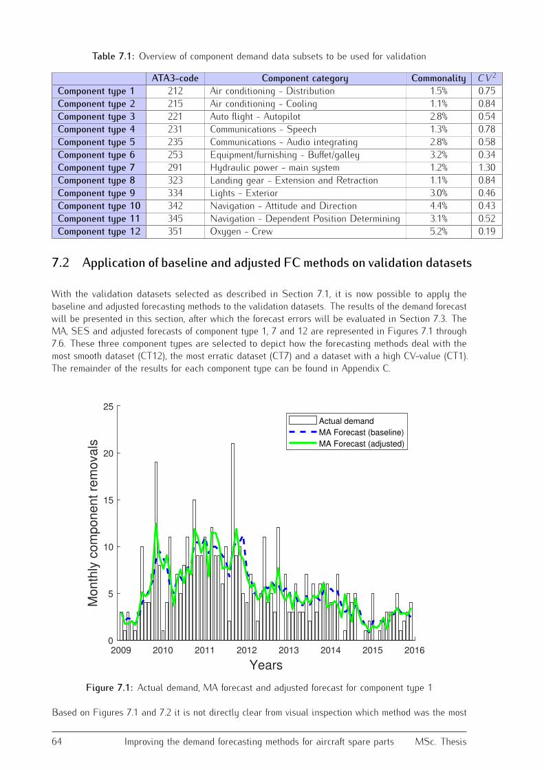
Table 7.1: Overview of component demand data subsets to be used for validationATA3-code Component category Commonality CV 2
Component type 1 212 Air conditioning - Distribution 1.5% 0.75Component type 2 215 Air conditioning - Cooling 1.1% 0.84Component type 3 221 Auto flight - Autopilot 2.8% 0.54Component type 4 231 Communications - Speech 1.3% 0.78Component type 5 235 Communications - Audio integrating 2.8% 0.58Component type 6 253 Equipment/furnishing - Buffet/galley 3.2% 0.34Component type 7 291 Hydraulic power - main system 1.2% 1.30Component type 8 323 Landing gear - Extension and Retraction 1.1% 0.84Component type 9 334 Lights - Exterior 3.0% 0.46Component type 10 342 Navigation - Attitude and Direction 4.4% 0.43Component type 11 345 Navigation - Dependent Position Determining 3.1% 0.52Component type 12 351 Oxygen - Crew 5.2% 0.19
7.2 Application of baseline and adjusted FC methods on validation datasets
With the validation datasets selected as described in Section 7.1, it is now possible to apply thebaseline and adjusted forecasting methods to the validation datasets. The results of the demand forecastwill be presented in this section, after which the forecast errors will be evaluated in Section 7.3. TheMA, SES and adjusted forecasts of component type 1, 7 and 12 are represented in Figures 7.1 through7.6. These three component types are selected to depict how the forecasting methods deal with themost smooth dataset (CT12), the most erratic dataset (CT7) and a dataset with a high CV-value (CT1).The remainder of the results for each component type can be found in Appendix C.
2009 2010 2011 2012 2013 2014 2015 2016
Years
0
5
10
15
20
25
Mo
nth
ly c
om
po
ne
nt
rem
ova
ls
Actual demand
MA Forecast (baseline)
MA Forecast (adjusted)
Figure 7.1: Actual demand, MA forecast and adjusted forecast for component type 1Based on Figures 7.1 and 7.2 it is not directly clear from visual inspection which method was the most64 Improving the demand forecasting methods for aircraft spare parts MSc. Thesis
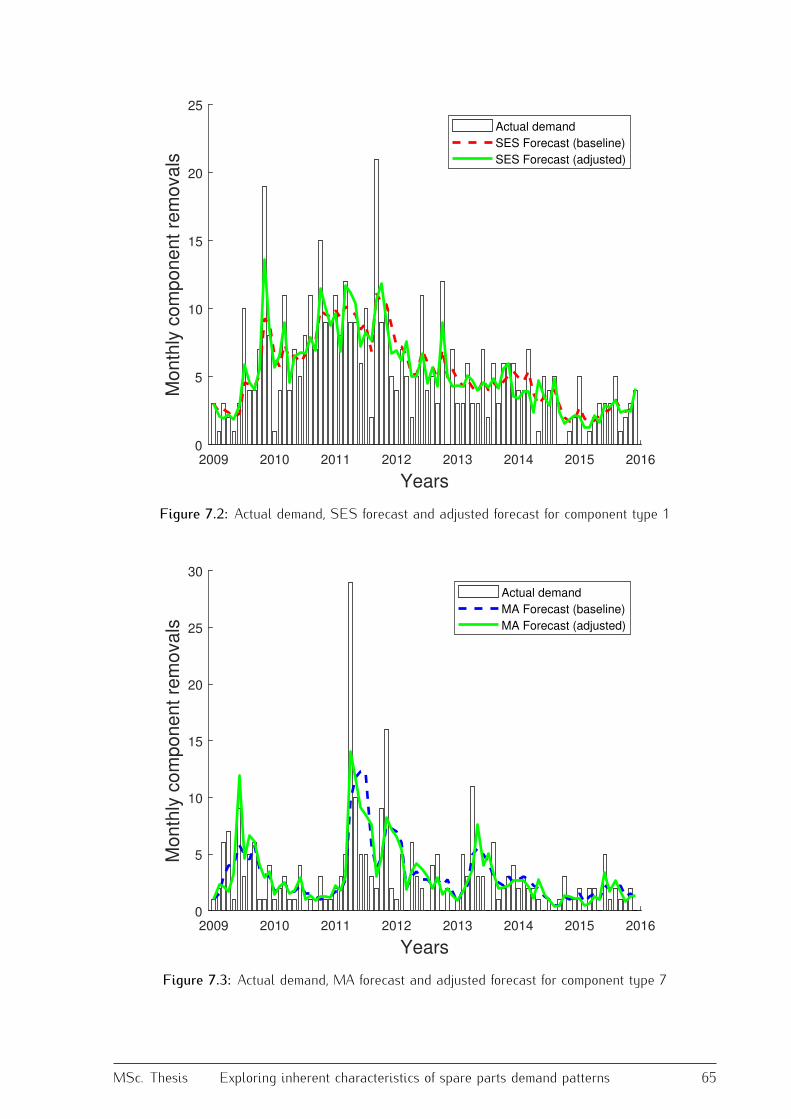
2009 2010 2011 2012 2013 2014 2015 2016
Years
0
5
10
15
20
25
Mo
nth
ly c
om
po
ne
nt
rem
ova
ls
Actual demand
SES Forecast (baseline)
SES Forecast (adjusted)
Figure 7.2: Actual demand, SES forecast and adjusted forecast for component type 1
2009 2010 2011 2012 2013 2014 2015 2016
Years
0
5
10
15
20
25
30
Mo
nth
ly c
om
po
ne
nt
rem
ova
ls
Actual demand
MA Forecast (baseline)
MA Forecast (adjusted)
Figure 7.3: Actual demand, MA forecast and adjusted forecast for component type 7
MSc. Thesis Exploring inherent characteristics of spare parts demand patterns 65

2009 2010 2011 2012 2013 2014 2015 2016
Years
0
5
10
15
20
25
30
Mo
nth
ly c
om
po
ne
nt
rem
ova
lsActual demand
SES Forecast (baseline)
SES Forecast (adjusted)
Figure 7.4: Actual demand, SES forecast and adjusted forecast for component type 7
2009 2010 2011 2012 2013 2014 2015 2016
Years
0
10
20
30
40
50
60
Mo
nth
ly c
om
po
ne
nt
rem
ova
ls
Actual demand
MA Forecast (baseline)
MA Forecast (adjusted)
Figure 7.5: Actual demand, MA forecast and adjusted forecast for component type 12
66 Improving the demand forecasting methods for aircraft spare parts MSc. Thesis

2009 2010 2011 2012 2013 2014 2015 2016
Years
0
10
20
30
40
50
60
Mo
nth
ly c
om
po
ne
nt
rem
ova
ls
Actual demand
SES Forecast (baseline)
SES Forecast (adjusted)
Figure 7.6: Actual demand, SES forecast and adjusted forecast for component type 12accurate in forecasting the spare parts of CT1, but it does seem that the adjusted method follows theoutlier months more accurately. Judging from Figures 7.3 and 7.4, the adjusted MA and SES methodsare more suitable to forecast the spare parts of CT7, which is the most erratic data set of the validationdata sets. This can especially be seen from the fact that the adjusted MA and SES methods are moreaccurate in forecasting the most outlying month in 2011.Finally, looking at Figures 7.5 and 7.6, it appears that the adjusted methods are less accurate than thebaseline methods in forecasting the spare parts of the smooth CT12 data set. This can be observedfrom the fact that the demand volumes predicted by the adjusted methods appear to be more volatilecompared to the actual demand pattern and the demand forecast by the baseline methods. Theseobservations initially imply that the adjusted methods are more accurate in forecasting erratic demandpatterns and less accurate in forecasting smooth demand patterns. To confirm these conclusions, theperformance of the baseline and adjusted methods will be evaluated in Section 7.3.7.3 Evaluation of forecast performance of the applied methods
This section will evaluate the forecast errors of the baseline and adjusted forecasting method on thevalidation datasets. However since some of the validation datasets contain few zero-demand months,the MAPE error metric is not suitable to be used for the evaluation, as the MAPE produces computationerrors when dealing with zero-demand months. For the evaluation, the RMSE error metric whichwas introduced in Chapter 3 would be more suitable, but a major drawback of this metric is its scaledependency. This fact makes it challenging to effectively compare the forecast of multiple datasetssolely using the RMSE metric, since the average demand volumes and scale of the data also has animpact on the value of the RMSE.For this reason, a normalised measure of the total error will be introduced first, since this metricMSc. Thesis Exploring inherent characteristics of spare parts demand patterns 67

is most suitable for comparing the forecast performance on multiple datasets. This metric is calledTheil’s U-statistic and is mathematically represented by Equation 7.1. Theil’s U-statistic yields a valuebetween 0 and 1, with smaller values of the U-statistic indicating a better forecasting performance,where a U-statistic equal to 0 represents a perfect fit [32].
U =√ 1
n
n∑t=1 e2
t√ 1n
n∑t=1 f 2
t
√ 1n
n∑t=1y2
t
(7.1)To confirm whether the suggested adjusted forecasting methods improve the accuracy of the validationdata sets, the Theil’s U-statistic has been determined for the baseline methods and the adjustedmethods, for each component type dataset. The statistical relation to Pilot Complaints and AircraftLandings has also been determined for each data set, in a similar fashion as described in Section5.4. Table 7.2 shows an overview of the U-statistic values for the baseline and adjusted methods,the difference between these values (δU), the CV-values and the correlation coefficients with PilotComplaints (CCPIC ) and Aircraft Landings (CCLND) corresponding to each validation data set. Notethat in this Table, a positive δU should be interpreted as a reduction of the U-statistic (thus animprovement in forecasting accuracy), while a negative δU indicates an increase of the U-statistic (andtherefore a decrease in forecasting accuracy). Furthermore, Figures 7.7 and 7.8 present a graphicalrepresentation of the U-statistic values for the MA method and SES method, respectively.
Table 7.2: Overview of U-statistic values for validation data setsCT CV 2 CCPIC CCLND UMA UMA,adj δUMA USES USES,adj δUSESCT1 0.75 0.628 0.373 0.0727 0.0655 0.0071 0.0640 0.0569 0.0071CT2 0.84 0.531 0.285 0.1515 0.1276 0.0239 0.1332 0.1081 0.0251CT3 0.54 0.368 0.00 0.0382 0.0347 0.0035 0.0341 0.0307 0.0034CT4 0.78 0.379 0.275 0.1731 0.1666 0.0065 0.1540 0.1486 0.0054CT5 0.58 0.468 0.381 0.0571 0.0570 0.0002 0.0518 0.0527 -0.0010CT6 0.34 0.386 0.186 0.0164 0.0168 -0.0003 0.0150 0.0155 -0.0004CT7 1.3 0.391 0.233 0.1612 0.1370 0.0242 0.1504 0.1229 0.0275CT8 0.84 0.022 0.110 0.1560 0.1536 0.0024 0.1434 0.1413 0.0021CT9 0.46 0.426 0.322 0.0494 0.0499 -0.0005 0.0442 0.0449 -0.0008CT10 0.43 0.309 0.397 0.0342 0.0310 0.0032 0.0306 0.0276 0.0030CT11 0.52 0.292 0.126 0.0552 0.0534 0.0018 0.0487 0.0477 0.0010CT12 0.19 0.731 0.264 0.0036 0.0054 -0.0017 0.0033 0.0052 -0.0020
Looking at the results presented in Table 7.2 and Figures 7.7 and 7.8, several conclusions can be drawnregarding the performance of the applied forecasting methods. First of all, it can be stated that thesuggested methodology to incorporate the key factors has generally led to improvements in forecastingaccuracy, thus successfully validating the approach. The adjusted method has led to a minor increaseof the U-statistic in only three cases for the MA method and four cases for the SES method, therebydecreasing the accuracy of the baseline methods slightly. For the majority of component types, adecrease in U-statistic was found and therefore an improvement in forecasting accuracy is established.These results show that including additional statistically correlated factors when forecasting improvesthe forecasting accuracy not only for Wheels & Brakes components, but also for additional componentcategories in the MRO database.Furthermore it can be stated that overall, the baseline and adjusted SES method are more accurate inforecasting the demand volumes compared to the baseline and adjusted MA method, respectively. Thiscan be concluded from the fact that all values for the U-statistic are smaller for the SES method thanfor the MA method, with the smallest U-statistic values obtained for the adjusted SES method. Based68 Improving the demand forecasting methods for aircraft spare parts MSc. Thesis

1 2 3 4 5 6 7 8 9 10 11 12
Component types
0
0.02
0.04
0.06
0.08
0.1
0.12
0.14
0.16
0.18
0.2
U-s
tatistic
Baseline MA method
Adjusted MA method
Figure 7.7: U-statistic values for Baseline MA and Adjusted MA methods
1 2 3 4 5 6 7 8 9 10 11 12
Component types
0
0.02
0.04
0.06
0.08
0.1
0.12
0.14
0.16
0.18
0.2
U-s
tatistic
Baseline SES method
Adjusted SES method
Figure 7.8: U-statistic values for Baseline SES and Adjusted SES methods
MSc. Thesis Exploring inherent characteristics of spare parts demand patterns 69

on this fact, it can be concluded that the adjusted SES method is the most accurate forecasting methodfor all component types, and therefore should be recommended as the most suitable method to forecastthe demand volumes of components within the specific MRO database.Finally, by observing the values in the δUMA and δUSES columns of Table 7.2 and comparing them tothe values in the CV 2 column, there appears to be a relation between the CV 2-value of a data set andthe extent to which the U-statistic of that data set can be decreased by incorporating the statisticallyrelevant factors. Based on the presented results, it appears as if the data sets that inherently havelarger variation in demand size (and thus a higher CV 2-value) would benefit the most from followingthe trend of the causal factors, since these data sets generally show higher values for δU . This can beespecially seen in the data sets with the highest and lowest CV 2-value, where the data set of CT7(with the highest CV 2-value of 1.3) has shown the largest improvement in the U-statistic, whereasthe data set of CT12 (with the lowest CV 2-value of 0.19) shows the largest deterioration of Theil’sU-statistic.To confirm if there exists a positive correlation between the CV 2-value of a data set and the δUthat can be obtained, a linear regression has been applied on the scatter plots between these units.This regression is depicted in Figures 7.9 and 7.10 for the MA methods and for the SES methods,respectively. In these figures, the improvement in Theil’s U-statistic after adjusting both the MA methodand SES method is shown on the y-axis, versus the CV 2-value of the data sets on the x-axis. Also,the data points in these scatter plots are numbered to indicate which component type data set theyrepresent. Furthermore, Table 7.3 provides the R2 and p-values for both linear regressions. Based onthe p-values provided in this table, it can be stated with a 95% confidence interval that there exists alinear relation between the δU and CV 2 for both of the adjusted MA and SES methods, since thep-values are lower than 0.05.
0 0.2 0.4 0.6 0.8 1 1.2 1.4
Squared Coefficient of Variation (CV2)
-0.01
-0.005
0
0.005
0.01
0.015
0.02
0.025
0.03
Ch
an
ge
in
U-s
tatistic (
U)
1
2
3
4
5 6
7
8
9
1011
12
Figure 7.9: Scatter plot with linear regression for δUMA versus CV 2
70 Improving the demand forecasting methods for aircraft spare parts MSc. Thesis

0 0.2 0.4 0.6 0.8 1 1.2 1.4
Squared coefficient of Variation (CV2)
-0.01
-0.005
0
0.005
0.01
0.015
0.02
0.025
0.03
Ch
an
ge
in
U-s
tatistic (
U)
1
2
3
4
5 6
7
8
9
10
11
12
Figure 7.10: Scatter plot with linear regression for δUSES versus CV 2Table 7.3: Linear regression statistics corresponding to the linear fits between δU and CV 2
R2 p-valueAdjusted MA-method 0.6547 0.0014Adjusted SES-method 0.6523 0.00157.4 Sensitivity analysis of baseline and adjusted methods
The results obtained in the research so far have indicated that generally, the existing MA and SESmethods can improve their forecasting accuracy and performance if they are adjusted to follow thetrend of the statistically significant causal factors Pilot Complaints and Aircraft Landings. Howeverwhile applying the baseline and adjusted forecasting methods, some inherent user-set parameters areassumed, which have a direct impact on the results of the forecast. This section will therefore describethe sensitivity analysis that was performed to determine if the main conclusions and insights found inthe initial analysis are sensitive to change if there are (minor) alterations in these user-set parametersor not.For both the baseline and adjusted methods several parameters and units were assumed in the analysis.These parameters can be listed as follows:- α = 0.3, the smoothing constant used in the baseline SES method. It determines how reactivethe forecasting method is to its forecasting errors.- m = 3, the moving time-window used in the baseline MA method. It determines the number ofpast months that are considered when calculating the average value of these months.- PC0, the average number of Pilot Complaints in the past three months used in the adjusted MAand SES methods. This average value can be adjusted to be taken from bigger or smaller timeframes.
MSc. Thesis Exploring inherent characteristics of spare parts demand patterns 71

- LD0, the average number of Aircraft Landings in the past three months used in the adjusted MAand SES methods. This average value can be adjusted to be taken from bigger or smaller timeframes.The following subsections will describe if and how slightly altering the parameters described in theprevious list will impact the main conclusions of the analysis. First, a sensitivity analysis will beapplied to the user-set parameters of the baseline forecasting methods, after which the sensitivityanalysis will be applied to the parameters of the adjusted forecasting methods.7.4.1 Sensitivity analysis of baseline FC method parameters
First, a sensitivity analysis is performed by varying the value used as the smoothing constant α in theSES method. Initially this constant was set equal to 0.3 when applying the baseline SES method.For the purpose of this sensitivity analysis, this constant is varied from 0.1 to 0.5, and the impact onthe δU is assessed. Table 7.4 presents the δU values for each of the validation data sets, for the fivesmoothing constant cases.Table 7.4: Overview of change in U-statistic values for multiple values of α
δUSESCT α = 0.1 α = 0.2 α = 0.3 α = 0.4 α = 0.5CT1 0.0048 0.0064 0.0071 0.0070 0.0060CT2 0.020 0.0234 0.0251 0.0252 0.0236CT3 0.0031 0.0035 0.0034 0.0027 0.0016CT4 0.0037 0.0046 0.0054 0.0056 0.0051CT5 0.0003 -0.0003 -0.0010 -0.0018 -0.0027CT6 -0.0003 -0.0003 -0.0004 -0.0006 -0.0008CT7 0.0183 0.0241 0.0275 0.0279 0.0250CT8 0.0022 0.0023 0.0021 0.0015 0.0007CT9 -0.0002 -0.0004 -0.0008 -0.0013 -0.0021CT10 0.0030 0.0032 0.0030 0.0025 0.0018CT11 0.0009 0.0010 0.0010 0.0008 0.0004CT12 -0.0013 -0.0016 -0.0020 -0.0023 -0.0027Based on the results presented in Table 7.4 it can be stated that varying the assumed value for αin the baseline SES method leads to the same conclusions that were found in the initial research;adjusting the baseline SES method to follow the trend of the key factors will generally lead to a moreaccurate forecast of the demand size of components. This can be seen from the fact that in the majorityof cases, a positive δU is observed for the same data sets as in the initial research. Varying the valueof α does slightly impact the extent to which the accuracy of the forecast is improved (or in few cases,deteriorates). With that, it can be said that the main conclusions of the research are not sensitive tochanges in the assumed α-parameter.Next, the sensitivity analysis is performed by varying the time frame m used to compute the forecast inthe MA method. In the initial research, this parameter was set equal to 3 when applying the baselineMA method. This constant is varied from 1 to 5 for the sensitivity analysis, and again the impact onthe δU is assessed. Table 7.5 shows the δU values for each of the validation data sets, for the fivedifferent cases.Based on the results presented in Table 7.5, it can be seen that varying the assumed value for m hasno impact on the general conclusions found in the initial research; the majority of the data sets wouldbenefit from using the adjusted forecasting methods, as the most cases show a reduction of Theil’sU-statistic (a positive δUMA). As such, the main findings in the initial research are not sensitive tochanges in the assumed parameter m. However, the assumed value for m does seem to impact the72 Improving the demand forecasting methods for aircraft spare parts MSc. Thesis
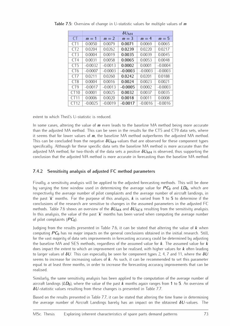
Table 7.5: Overview of change in U-statistic values for multiple values of mδUMACT m = 1 m = 2 m = 3 m = 4 m = 5CT1 0.0050 0.0079 0.0071 0.0069 0.0065CT2 0.0204 0.0262 0.0239 0.0220 0.0217CT3 0.0004 0.0019 0.0035 0.0039 0.0045CT4 0.0031 0.0058 0.0065 0.0053 0.0048CT5 -0.0032 -0.0013 0.0002 0.0001 -0.0004CT6 -0.0007 -0.0003 -0.0003 -0.0003 -0.0003CT7 0.0211 0.0260 0.0242 0.0201 0.0188CT8 0.0004 0.0016 0.0024 0.0023 0.0021CT9 -0.0017 -0.0013 -0.0005 0.0002 -0.0003CT10 0.0001 0.0025 0.0032 0.0037 0.0035CT11 0.0006 0.0020 0.0018 0.0011 0.0008CT12 -0.0025 -0.0019 -0.0017 -0.0016 -0.0016
extent to which Theil’s U-statistic is reduced.In some cases, altering the value of m even leads to the baseline MA method being more accuratethan the adjusted MA method. This can be seen in the results for the CT5 and CT9 data sets, whereit seems that for lower values of m, the baseline MA method outperforms the adjusted MA method.This can be concluded from the negative δUMA-values that are observed for these component typesspecifically. Although for these specific data sets the baseline MA method is more accurate than theadjusted MA method, for two-thirds of the data sets a positive δUMA is observed, thus supporting theconclusion that the adjusted MA method is more accurate in forecasting than the baseline MA method.7.4.2 Sensitivity analysis of adjusted FC method parameters
Finally, a sensitivity analysis will be applied to the adjusted forecasting methods. This will be doneby varying the time window used in determining the average value for PC0 and LD0, which arerespectively the average number of pilot complaints and the average number of aircraft landings, inthe past ’k ’ months. For the purpose of this analysis, k is varied from 1 to 5 to determine if theconclusions of the research are sensitive to changes in the assumed parameters in the adjusted FCmethods. Table 7.6 shows an overview of the δUMA and δUSES resulting from the sensitivity analysis.In this analysis, the value of the past ’k ’ months has been varied when computing the average numberof pilot complaints (PC0).Judging from the results presented in Table 7.6, it can be stated that altering the value of k whencomputing PC0 has no major impacts on the general conclusions obtained in the initial research. Still,for the vast majority of data sets improvements in forecasting accuracy could be determined by adjustingthe baseline MA and SES methods, regardless of the assumed value for k . The assumed value for kdoes impact the extent to which an improvement can be realised, with higher values for k often leadingto larger values of δU . This can especially be seen for component types 2, 4, 7 and 11, where the δUseems to increase for increasing values of k . As such, it can be recommended to set this parameterequal to at least three months, in order to increase the forecasting accuracy improvements that can berealised.Similarly, the same sensitivity analysis has been applied to the computation of the average number ofaircraft landings (LD0), where the value of the past k months again ranges from 1 to 5. An overview ofδU-statistic values resulting from these changes is presented in Table 7.7.Based on the results presented in Table 7.7, it can be stated that altering the time frame in determiningthe average number of Aircraft Landings barely has an impact on the obtained δU-values. TheMSc. Thesis Exploring inherent characteristics of spare parts demand patterns 73

Table 7.6: Overview of change in U-statistic values for multiple values of k months when computingPC0
δUMA δUSESCT k = 1 k = 2 k = 3 k = 4 k = 5 k = 1 k = 2 k = 3 k = 4 k = 5CT1 0.0021 0.0045 0.0071 0.0062 0.0060 0.0019 0.0043 0.0071 0.0063 0.0064CT2 0.0108 0.0204 0.0239 0.0242 0.0262 0.0126 0.0218 0.0251 0.0256 0.0278CT3 0.0008 0.0028 0.0035 0.0038 0.0031 0.0005 0.0025 0.0034 0.0040 0.0036CT4 0.0027 0.0039 0.0065 0.0071 0.0101 0.0019 0.0027 0.0054 0.0061 0.0095CT5 0.0005 0.0000 0.0002 -0.0004 -0.0005 -0.0004 -0.0011 -0.0010 -0.0013 -0.0014CT6 0.0002 -0.0002 -0.0003 -0.0006 -0.0004 0.0001 -0.0003 -0.0004 -0.0006 -0.0005CT7 0.0110 0.0235 0.0242 0.0299 0.0348 0.0143 0.0272 0.0275 0.0346 0.0395CT8 0.0022 0.0021 0.0024 0.0020 0.0022 0.0020 0.0019 0.0021 0.0017 0.0018CT9 0.0010 0.0009 -0.0005 -0.0006 -0.0005 0.0009 0.0007 -0.0008 -0.0009 -0.0009CT10 0.0025 0.0035 0.0032 0.0027 0.0022 0.0023 0.0033 0.0030 0.0027 0.0024CT11 -0.0004 0.0006 0.0018 0.0024 0.0025 -0.0006 -0.0001 0.0010 0.0016 0.0017CT12 -0.0010 -0.0012 -0.0017 -0.0018 -0.0019 -0.0011 -0.0014 -0.0020 -0.0020 -0.0022Table 7.7: Overview of change in U-statistic values for multiple values of k months when computingLD0
δUMA δUSESCT k = 1 k = 2 k = 3 k = 4 k = 5 k = 1 k = 2 k = 3 k = 4 k = 5CT1 0.0070 0.0070 0.0071 0.0072 0.0073 0.0072 0.0071 0.0071 0.0071 0.0072CT2 0.0229 0.0234 0.0239 0.0242 0.0243 0.0240 0.0245 0.0251 0.0253 0.0255CT3 0.0035 0.0035 0.0035 0.0035 0.0035 0.0034 0.0038 0.0034 0.0034 0.0034CT4 0.0064 0.0064 0.0065 0.0068 0.0073 0.0055 0.0053 0.0054 0.0056 0.0061CT5 0.0001 -0.0001 0.0002 0.0001 0.0002 -0.0009 -0.0012 -0.0010 -0.0010 -0.0009CT6 -0.0001 -0.0002 -0.0003 -0.0004 -0.0004 -0.0002 -0.0003 -0.0004 -0.0005 -0.0006CT7 0.0212 0.0236 0.0242 0.0250 0.0250 0.0249 0.0267 0.0275 0.0283 0.0284CT8 0.0022 0.0029 0.0024 0.0018 0.0011 0.0021 0.0027 0.0021 0.0014 0.0007CT9 -0.0003 -0.0004 -0.0005 -0.0005 -0.0006 -0.0006 -0.0007 -0.0008 -0.0009 -0.0009CT10 0.0026 0.0029 0.0032 0.0032 0.0032 0.0026 0.0028 0.0030 0.0030 0.0031CT11 0.0018 0.0018 0.0018 0.0017 0.0017 0.0009 0.0009 0.0010 0.0009 0.0009CT12 -0.0017 -0.0017 -0.0017 -0.0018 -0.0018 -0.0020 -0.0020 -0.0020 -0.0020 -0.0021magnitude of both δUMA and δUSES only slightly changes when a higher or lower value for k isassumed. With that, it can be concluded that average number of Aircraft Landings (LDO) has a lessdominant role in the adjusted forecasting methods, and changing the assumed value for k has no majorimpacts on the main results found in the research. This less significant role of LD0 in the adjustedmethods can be explained by the fact that in general, the correlation coefficients between the componentremovals and the Aircraft Landings are lower compared to the correlation coefficients obtained for PilotComplaints.
74 Improving the demand forecasting methods for aircraft spare parts MSc. Thesis

CHAPTER 8
Conclusions and Recommendations
With the thesis research completed and the main result obtained, it is now possible to formulate the mainconclusions and recommendations based on the findings of the research. This final chapter will thereforefirst present the most important conclusions in Section 8.1, after which the main recommendations willbe described in Section 8.2.8.1 Conclusions
The main problem of the research was introduced to be as follows; “The uncertain nature of spareparts demand makes it very challenging for MRO’s to accurately forecast the need for spare parts,often leading to sub-optimal operations". This problem description then resulted in the following mainresearch question: “Will spare parts demand forecasting accuracy improve if inherent causal factorsare taken into account while forecasting?". With the performed research and the obtained results,this main research question can be answered. The obtained results confirm that it is indeed possibleto improve demand forecasting accuracy if the patterns of statistically correlated key factors are takeninto account when using conventional time-series forecasting methods. Adjusting the baseline methodsto incorporate the behaviour of these key factors has generally lead to reduced forecasting errors formultiple component type demand patterns analysed in this research. An initial analysis of the MROdata base showed that the demand size variability varies per component category, and also varies peraircraft type.Following from this analysis, it was found that the Wheels & Brakes component category was themost extensive category in the data base, which is why the remainder of the thesis methodology wasapplied to components belonging to the Wheels & Brakes category. Subsequently, the indirect keyfactors aircraft operators and aircraft type were used to select and generate specific data patterns forcomponent removals. At the same time, the patterns for the direct causal factors pilot complaints andaircraft landings were generated, after which a statistical analysis was performed to show that thereexists a strong positive correlation between the causal factors and component removals for operator 1.As a result, the baseline forecasting methods were applied to forecast the demand for Wheels & Brakescomponents of operator 1 specifically. This showed that in general the SES method is more accuratethan the MA method, since smaller values of RMSE and MAPE were obtained for the baseline SESmethod. Following from this, an adjusted forecasting method was suggested, in which the correlationcoefficients and the data patterns of the causal factors were also included in determining the forecast
75

value. Furthermore, a seasonality effect was recognised in the patterns for Wheels & Brakes, andaccounting for both this seasonality factor and the causal factors resulted in minimal MAPE values forthe analysed component patterns, compared to the baseline forecasting methods.To ensure that these findings do not only hold true for specific Wheels & Brakes components, othercomponent categories of operator 1 were considered as validation data sets. The baseline and adjustedmethods were applied to twelve additional validation data sets, and for almost all data sets animprovement of forecasting accuracy could be found when comparing the performance of the adjustedmethods to the baseline methods. Only for the most smooth data set, a significant increase of theforecast error was found, which suggests that the adjusted forecasting method are the most suitable fordata patterns that are high in demand size variability. To confirm this, a positive relation between theimprovement in Theil’s U-statistic and the coefficient of variation of the data sets was found, indicatingthat demand patterns with a higher variability in demand size would benefit the most from using theadjusted method over the baseline method.Finally, a sensitivity analysis was successfully conducted to confirm that the main findings are notsensitive to minor changes in the assumed model parameters. With that, this research has successfullyshown that the adjusted forecasting methods outperform the conventional baseline SES and MA methodsfor a broad scope of components and parameter settings. These findings are another confirmation thatonly looking at historic demand when using time-series models is a restricted approach, and that theconventional time-series methods can benefit from including factors that are statistically correlated tothe number of component removals.8.2 Recommendations
Following from the main conclusions described in the previous section, some main recommendationscan be identified, which will be described in this section. Since this thesis research has shown positiveresults for including statistically related factors, the first recommendation would be to include additionalcausal factors and additional data to incorporate in future analysis. This could be environmental dataor physics-based information, which could likely be related to component removals as well.Furthermore it would be recommended to include more elaborate forecasting methods as the baselinemodels to compare the adjusted methods with. In this research, the scope was limited to two time-seriesmethods only, but this could be expanded as well. Also, the data sets in this research were mainlyerratic, with low variability in demand frequency. This approach could therefore be repeated for morelumpy demand patterns, for which Croston’s method would be recommended as the baseline forecastingmethod to compare the adjusted methods with.Additionally, the research could be applied to substantially more data sets, to confirm for which typesof data sets the forecasting errors can be reduced the most. With an extended sample size of data sets,a more in-depth analysis can be performed to find out if demand patterns with the highest demand sizevariability do also in fact benefit the most from an adjusted forecasting method. Following from this,the main recommendation would be to extend the applied model with Artificial Intelligence elementsto automate the process of finding the most suitable forecasting method which will yield the leastforecasting errors. Ideally, this developed model will identify the main characteristics of all data setsto be analysed, and based on these characteristics will apply the most suitable forecasting methodwith the most suitable user-set parameters.
76 Improving the demand forecasting methods for aircraft spare parts MSc. Thesis

Bibliography
[1] Gerasimov, V., http://www.vladstudio.com/wallpaper/?airlines2, 2008, Cover image,edited.[2] Frepple, “Demand classification,” https://frepple.com/blog/demand-classification/, January 2017.[3] Zorgdrager, M., Curran, R., Verhagen, W. J. C., Boesten, B. H. L., and Water, C. N., A predictive
method for the estimation of material demand for aircraft non-routine maintenance [online]., 20thISPE International Conference on Concurrent Engineering: Proceedings, Amsterdam, Netherlands,2013.[4] Wallström, P. and Segerstedt, A., Evaluation of forecasting error measurements and techniques for
intermittent demand , Vol. 128, International Journal of Production Economics, July 2010, 625-636.[5] Regattieri, A., Gamberi, M., Gamberini, R., and Manzini, R., Managing lumpy demand for aircraft
spare parts, Vol. 11, Journal of Air Transport Management, 2005, 426-431.[6] III, A. F. L. and Ciarallo, F. W., Reliability and operations: Keys to lumpy aircraft spare parts
demands, Vol. 50, Journal of Air Transport Management, 2015, 30-40.[7] Donnelly, J. M., The Case for Managing MRO Inventory, Vol. 17, Supply Chain ManagementReview, 2013, 18-25.[8] Altay, N. and Rudisill, F., Adapting Wright’s modification of Holt’s method to forecasting intermittent
demand , Vol. 111, International Journal of Production Economics, 2008, 389-408.[9] Air Transport World, http://docslide.us/documents/air-transport-world-january-2013.
html, 2013.[10] Wang, W. and Syntetos, A. A., Spare parts demand: Linking forecasting to equipment maintenance,Vol. 47, Elsevier, Transportation Research Part E Logistics and Transportation Review, March 2011,1194-1209.[11] Christer, A. H. and Waller, W. M., Reducing production downtime using delay time analysis, Vol. 35,Journal of the Operational Research Society, 1984, 499-512.[12] Christer, A. H., Developments in delay time analysis for modelling plant maintenance., Vol. 50,Journal of the Operational Research Society, 1999, 1120-1137.[13] Jones, B., Jenkinson, I., and Wang, J., Methodology of using delay-time analysis for a manufacturing
industry., Vol. 94, Reliability Engineering and System Safety, 2009, 111-124.77

[14] Ghobbar, A. A. and Friend, C. H., Evaluation of forecasting methods for intermittent parts demandin the field of aviation: a predictive model., Vol. 30, Computers & Operations Research, 2003,2097-2114.
[15] Syntetos, A. A. and Boylan, J. E., On the variance of intermittent demand estimates, Vol. 128,International Journal of Production Economics, 2010, 546-555.[16] Croston, J. D., Forecasting and stock control for intermittent demand., Vol. 23, Operational ResearchQuarterly, 1972, 289-303.[17] Syntetos, A. A. and Boylan, J. E., The accuracy of intermittent demand estimates, Vol. 21, Interna-tional Journal of Forecasting, 2005, 303-314.[18] Syntetos, A. A. and Boylan, J. E., On the bias of intermittent demand estimates, Vol. 71, InternationalJournal of Production Economics, 2001, 457-466.[19] Ghobbar, A. A. and Friend, C. H., The material requirements planning system for aircraft maintenance
and inventory control: a note, Vol. 10, Journal of Air Transport Management, 2004, 217-221.[20] Kostenko, A. and Hyndman, R., A note on the categorization of demand patterns., Vol. 57, Journalof the Operational Research Society, 10th ed., October 2006, 1256–1257.[21] Petropoulos, F., Makridakis, S., Assimakopoulos, V., and Nikolopoulos, K., Horses for courses in
demand forecasting, Vol. 237, European Journal of Operational Research, 1st ed., October 2014,152–163.[22] Willemain, T. R., Smart, C. N., and Schwarz, H. F., A new approach to forecasting intermittent
demand for service parts inventories., Vol. 20, International Journal of Forecasting, 2004, 375-387.[23] Porras, E. and Dekker, R., An inventory control system for spare parts at a refinery: An empirical
comparison of different re-order point methods., Vol. 184, European Journal of Operational Research,2008, 101-132.[24] Syntetos, A. A., Babai, M. Z., and Gardner, E. S., Forecasting intermittent inventory demands:
Simple parametric methods vs. bootstrapping., Vol. 68, Journal of Business Research Forthcoming,8th ed., August 2015, 1746-1752.[25] Ghobbar, A. A. and Friend, C. H., Sources of intermittent demand for aircraft spare parts within
airline operations, Vol. 8, Journal of Air Transport Management, 2002, 221-231.[26] Smith, A. M. and Hinchcliffe, G. R., Reliability-centered Mainteance: Gateway to World Class
Maintenance, Elsevier, 2004.[27] van der Auweraer, S., Boute, R., and Syntetos, A. A., Forecasting spare part demand with Installed
Base information: a review , KU Leuven - Faculty of Economics and Business, January 2018.[28] Jalil, M. N., Zuidwijk, R., Fleischmann, M., and a. E. E. van Nunen, J., Spare parts logistics and
installed base information, Vol. 62, Journal of the Operational Research Society, 2011, 442-457.[29] Hellingrath, B. and Cordes, A., Conceptual approach for integrating condition monitoring information
and spare parts forecasting methods, Vol. 2:1, Production & Manufacturing Research, 2014, 725-737.[30] Verhagen, W., AE4-465: Maintenance Modeling & Analysis, Lecture 7 - Supportability engineering:
basic concepts & assumptions; forecasting spare parts demand , Delft University of Technology,2018, Slide 33.[31] Verhagen, W., AE4-465: Maintenance Modeling & Analysis, Lecture 7 - Supportability engineering:
basic concepts & assumptions; forecasting spare parts demand , Delft University of Technology,2018, Slide 35.78 Improving the demand forecasting methods for aircraft spare parts MSc. Thesis

[32] Verhagen, W., AE4-465: Maintenance Modeling & Analysis, Lecture 7 - Supportability engineering:basic concepts & assumptions; forecasting spare parts demand , Delft University of Technology,2018, Slide 41.
MSc. Thesis Exploring inherent characteristics of spare parts demand patterns 79

Appendices
80

APPENDIX A
Analysis of Wheels and Brakes data sets
Figure A.1: Monthly component removals of 324-101 category for Fokker 50 between 2008 and 2016
81

Figure A.2: Monthly component removals of 324-201 category for Fokker 50 between 2008 and 2016
Figure A.3: Monthly component removals of 324-101 category for Fokker 100 between 2008 and 2016
82 Improving the demand forecasting methods for aircraft spare parts MSc. Thesis

Figure A.4: Monthly component removals of 324-201 category for Fokker 100 between 2008 and 2016
Figure A.5: Monthly component removals of 324-101 category for Fokker 70 between 2008 and 2016
MSc. Thesis Exploring inherent characteristics of spare parts demand patterns 83

Figure A.6: Monthly component removals of 324-103 category for Fokker 70 between 2008 and 2016
84 Improving the demand forecasting methods for aircraft spare parts MSc. Thesis

APPENDIX B
Results of Baseline and Altered forecasting methods applied to W&B data sets
2009 2010 2011 2012 2013 2014 2015 2016
Years
0
10
20
30
40
50
60
70
80
Mo
nth
ly M
WT
re
mo
va
ls
Actual and Forecast demand for Main Wheel Tires
Actual demand
Forecast (SES)
Forecast (SES+)
Figure B.1: Actual and SES Forecast demand for Main Wheel Tires
85

2009 2010 2011 2012 2013 2014 2015 2016
Years
0
5
10
15
20
25
30
35
40
45
50
Mo
nth
ly N
WT
re
mo
va
ls
Actual and Forecast demand for Nose Wheel Tires
Actual demand
Forecast (SES)
Forecast (SES+)
Figure B.2: Actual and SES Forecast demand for Nose Wheel Tires
2009 2010 2011 2012 2013 2014 2015 2016
Years
0
2
4
6
8
10
12
14
16
18
20
Mo
nth
ly M
WB
U r
em
ova
ls
Actual and Forecast demand for Main Wheel Brake Units
Actual demand
Forecast (SES)
Forecast (SES+)
Figure B.3: Actual and SES Forecast demand for Main Wheel Brake Units
86 Improving the demand forecasting methods for aircraft spare parts MSc. Thesis

APPENDIX C
Results of Baseline and Altered forecasting methods applied to validation datasets
2009 2010 2011 2012 2013 2014 2015 2016
Years
0
5
10
15
Mo
nth
ly c
om
po
ne
nt
rem
ova
ls
Actual demand
MA Forecast (baseline)
MA Forecast (adjusted)
Figure C.1: Actual demand, MA forecast and adjusted forecast for component type 2
87

2009 2010 2011 2012 2013 2014 2015 2016
Years
0
5
10
15
Mo
nth
ly c
om
po
ne
nt
rem
ova
lsActual demand
SES Forecast (baseline)
SES Forecast (adjusted)
Figure C.2: Actual demand, SES forecast and adjusted forecast for component type 2
2009 2010 2011 2012 2013 2014 2015 2016
Years
0
5
10
15
20
25
30
Mo
nth
ly c
om
po
ne
nt
rem
ova
ls
Actual demand
MA Forecast (baseline)
MA Forecast (adjusted)
Figure C.3: Actual demand, MA forecast and adjusted forecast for component type 3
88 Improving the demand forecasting methods for aircraft spare parts MSc. Thesis

2009 2010 2011 2012 2013 2014 2015 2016
Years
0
5
10
15
20
25
30
Mo
nth
ly c
om
po
ne
nt
rem
ova
ls
Actual demand
SES Forecast (baseline)
SES Forecast (adjusted)
Figure C.4: Actual demand, SES forecast and adjusted forecast for component type 3
2009 2010 2011 2012 2013 2014 2015 2016
Years
0
1
2
3
4
5
6
7
8
9
10
Mo
nth
ly c
om
po
ne
nt
rem
ova
ls
Actual demand
MA Forecast (baseline)
MA Forecast (adjusted)
Figure C.5: Actual demand, MA forecast and adjusted forecast for component type 4
MSc. Thesis Exploring inherent characteristics of spare parts demand patterns 89

2009 2010 2011 2012 2013 2014 2015 2016
Years
0
1
2
3
4
5
6
7
8
9
10
Mo
nth
ly c
om
po
ne
nt
rem
ova
lsActual demand
SES Forecast (baseline)
SES Forecast (adjusted)
Figure C.6: Actual demand, SES forecast and adjusted forecast for component type 4
2009 2010 2011 2012 2013 2014 2015 2016
Years
0
2
4
6
8
10
12
14
16
18
20
Mo
nth
ly c
om
po
ne
nt
rem
ova
ls
Actual demand
MA Forecast (baseline)
MA Forecast (adjusted)
Figure C.7: Actual demand, MA forecast and adjusted forecast for component type 5
90 Improving the demand forecasting methods for aircraft spare parts MSc. Thesis

2009 2010 2011 2012 2013 2014 2015 2016
Years
0
2
4
6
8
10
12
14
16
18
20
Mo
nth
ly c
om
po
ne
nt
rem
ova
ls
Actual demand
SES Forecast (baseline)
SES Forecast (adjusted)
Figure C.8: Actual demand, SES forecast and adjusted forecast for component type 5
2009 2010 2011 2012 2013 2014 2015 2016
Years
0
5
10
15
20
25
30
Mo
nth
ly c
om
po
ne
nt
rem
ova
ls
Actual demand
MA Forecast (baseline)
MA Forecast (adjusted)
Figure C.9: Actual demand, MA forecast and adjusted forecast for component type 6
MSc. Thesis Exploring inherent characteristics of spare parts demand patterns 91

2009 2010 2011 2012 2013 2014 2015 2016
Years
0
5
10
15
20
25
30
Mo
nth
ly c
om
po
ne
nt
rem
ova
lsActual demand
SES Forecast (baseline)
SES Forecast (adjusted)
Figure C.10: Actual demand, SES forecast and adjusted forecast for component type 6
2009 2010 2011 2012 2013 2014 2015 2016
Years
0
5
10
15
Mo
nth
ly c
om
po
ne
nt
rem
ova
ls
Actual demand
MA Forecast (baseline)
MA Forecast (adjusted)
Figure C.11: Actual demand, MA forecast and adjusted forecast for component type 8
92 Improving the demand forecasting methods for aircraft spare parts MSc. Thesis

2009 2010 2011 2012 2013 2014 2015 2016
Years
0
5
10
15
Mo
nth
ly c
om
po
ne
nt
rem
ova
ls
Actual demand
SES Forecast (baseline)
SES Forecast (adjusted)
Figure C.12: Actual demand, SES forecast and adjusted forecast for component type 8
2009 2010 2011 2012 2013 2014 2015 2016
Years
0
2
4
6
8
10
12
14
16
18
20
Mo
nth
ly c
om
po
ne
nt
rem
ova
ls
Actual demand
MA Forecast (baseline)
MA Forecast (adjusted)
Figure C.13: Actual demand, MA forecast and adjusted forecast for component type 9
MSc. Thesis Exploring inherent characteristics of spare parts demand patterns 93

2009 2010 2011 2012 2013 2014 2015 2016
Years
0
2
4
6
8
10
12
14
16
18
20
Mo
nth
ly c
om
po
ne
nt
rem
ova
lsActual demand
SES Forecast (baseline)
SES Forecast (adjusted)
Figure C.14: Actual demand, SES forecast and adjusted forecast for component type 9
2009 2010 2011 2012 2013 2014 2015 2016
Years
0
2
4
6
8
10
12
14
16
18
20
Mo
nth
ly c
om
po
ne
nt
rem
ova
ls
Actual demand
MA Forecast (baseline)
MA Forecast (adjusted)
Figure C.15: Actual demand, MA forecast and adjusted forecast for component type 10
94 Improving the demand forecasting methods for aircraft spare parts MSc. Thesis

2009 2010 2011 2012 2013 2014 2015 2016
Years
0
2
4
6
8
10
12
14
16
18
20
Mo
nth
ly c
om
po
ne
nt
rem
ova
ls
Actual demand
SES Forecast (baseline)
SES Forecast (adjusted)
Figure C.16: Actual demand, SES forecast and adjusted forecast for component type 10
2009 2010 2011 2012 2013 2014 2015 2016
Years
0
2
4
6
8
10
12
14
16
18
20
Mo
nth
ly c
om
po
ne
nt
rem
ova
ls
Actual demand
MA Forecast (baseline)
MA Forecast (adjusted)
Figure C.17: Actual demand, MA forecast and adjusted forecast for component type 11
MSc. Thesis Exploring inherent characteristics of spare parts demand patterns 95
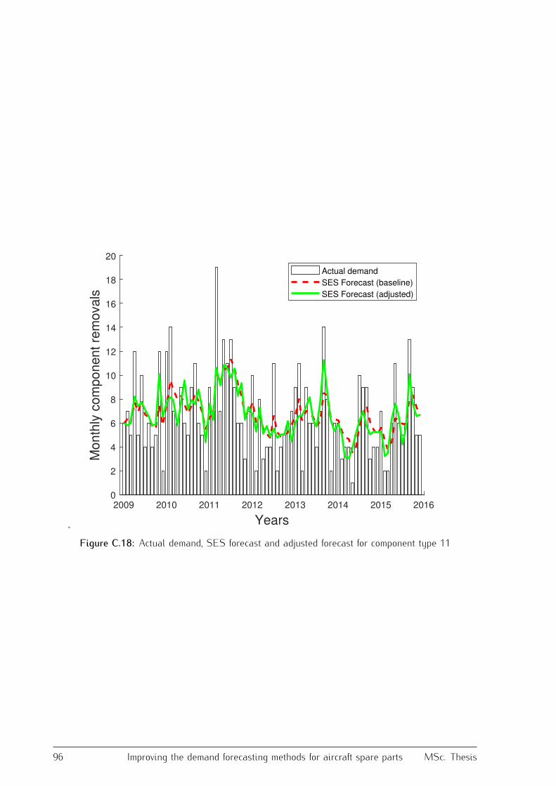
2009 2010 2011 2012 2013 2014 2015 2016
Years
0
2
4
6
8
10
12
14
16
18
20
Mo
nth
ly c
om
po
ne
nt
rem
ova
ls
Actual demand
SES Forecast (baseline)
SES Forecast (adjusted)
Figure C.18: Actual demand, SES forecast and adjusted forecast for component type 11
96 Improving the demand forecasting methods for aircraft spare parts MSc. Thesis