Flexible Architecture of Self Organizing Maps

for Changing Environments�

Rodrigo Salas1,2, Hector Allende2,3,Sebastian Moreno2, and Carolina Saavedra2

1 Universidad de Valparaıso; Departamento de Computacion; Valparaıso-Chile{rodrigo.salas}@uv.cl

2 Universidad Tecnica Federico Santa Marıa; Dept. de Informatica,Casilla 110-V; Valparaıso-Chile

{hallende, smoreno, saavedra}@inf.utfsm.cl3 Universidad Adolfo Ibanez; Facultad de Ciencia y Tecnologıa

Abstract. Catastrophic Interference is a well known problem of Artifi-cial Neural Networks (ANN) learning algorithms where the ANN forgetuseful knowledge while learning from new data. Furthermore the struc-ture of most neural models must be chosen in advance.

In this paper we introduce a hybrid algorithm called Flexible Architec-ture of Self Organizing Maps (FASOM ) that overcomes the CatastrophicInterference and preserves the topology of Clustered data in changing en-vironments. The model consists in K receptive fields of self organizingmaps. Each Receptive Field projects high-dimensional data of the inputspace onto a neuron position in a low-dimensional output space grid bydynamically adapting its structure to a specific region of the input space.

Furthermore the FASOM model automatically finds the number ofmaps and prototypes needed to successfully adapt to the data. Themodel has the capability of both growing its structure when novel clus-ters appears and gradually forgets when the data volume is reduced inits receptive fields.

Finally we show the capabilities of our model with experimental re-sults using synthetic sequential data sets and real world data.

Keywords: Catastrophic Interference, Artificial Neural Networks, SelfOrganizing Maps, Pattern Recognition.

1 Introduction

During this decade a huge amount of real data with highly dimensional sampleshave been stored for some sufficiently large period of time. Models were con-structed to learn this data, but due to the changing nature of the input space,the neural networks catastrophically forgets the previously learned patterns [4].

� This work was supported in part by Research Grant Fondecyt 1040365 and 7050205,DGIP-UTFSM, BMBF-CHL 03-Z13 from German Ministry of Education, DIPUV-22/2004 and CID-04/2003

M. Lazo and A. Sanfeliu (Eds.): CIARP 2005, LNCS 3773, pp. 642–653, 2005.c© Springer-Verlag Berlin Heidelberg 2005

.

Flexible Architecture of Self Organizing Maps for Changing Environments 643

In addition, the neural designer has the difficulty to decide in advance the ar-chitecture of the model, and if the environment change, the neural network willnot obtain a good performance under this new situation. To overcome the ar-chitectural design problem several algorithms with adaptive structure have beenproposed (See [2], [5], [12] and [13]).

In this paper we propose a hybrid problem-dependent model based on theKohonen’s Self Organizing Maps [8] with the Bauer et al. growing variant ofthe SOM [2], the K-means [11], the Single Linkage clustering algorithm [7]and the addition of new capabilities of gradually forgetting and contractingthe net. We call this algorithm Flexible Architecture of Self Organizing Maps(FASOM ). The FASOM is a hybrid model that adapts K receptive fields ofdynamical self organizing maps and learn the topology of partitioned spaces [13].It has the capability of detecting novel data or clusters and creates new mapsto learn this patterns avoiding that other receptive fields catastrophically forget.Furthermore the receptive fields with decreasing volume of data can graduallyforget by reducing their size and contracting their grid lattice.

The remainder or this paper is organized as follows. The next section webriefly discuss the ANN Catastrophic Interference problem. Then we review themodels where our hybrid model is based. In the fourth section, our proposal ofthe FASOM model is stated. Simulation results on synthetic and real data setsare provided in the fifth section. Conclusions and further work are given in thelast section.

2 The ANN Catastrophic Interference Problem

Artificial neural networks with highly distributed memory forget catastrophicallywhen faced with sequential learning tasks, i.e., the new learned information mostoften erases the one previously learned. This major weakness is not only cogni-tively implausible, as human gradually forget, but disastrous for most practicalapplications. (See [4] and [10] for a review)

Catastrophic interference is a radical manifestation of a more general problemfor connectionist models of memory, the so-called stability-plasticity problem [6].The problem is how to design a system that is simultaneously sensitive to, butnot radically disrupted by, new input. A number of ways have been proposedto avoid the problem of catastrophic interference in connectionist networks (see[1], [4]).

3 Review of Unsupervised Clustering and TopologyPreserving Algorithms

3.1 Unsupervised Clustering

Clustering can be considered as one of the most important unsupervised learn-ing problem. A cluster is a collection of “similar” objects and they should be

644 R. Salas et al.

“dissimilar” to the objects belonging to other clusters. Unsupervised clusteringtries to discover the natural groups inside a data set.

The purpose of any clustering technique [9] is to evolve a K × N partitionmatrix U(X ) of the data set X = {x1, ..., xN}, xj ∈ R

n, representing its parti-tioning into a number, say K, of clusters C1, ..., CK . Each element ukj , k = 1..Kand j = 1..n of the matrix U(X ) indicates the membership of pattern xj tothe cluster Ck. In crisp partitioning of the data, the following condition holds:ukj = 1 if xj ∈ Ck; otherwise, ukj = 0.

There are several clustering techniques classified as partitional and hierar-chical [7]. In this paper we based our model in the following algorithms.

K-meansThe K-means method introduced by McQueen [11] is one of the most widelyapplied partitional clustering technique. This method basically consists on thefollowing steps. First, K randomly chosen points from the data are selected asseed points for the centroids zk, k = 1..K, of the clusters. Second, assign eachdata to the cluster with the nearest centroid based on some distance criterion,for example, xj belongs to the cluster Ck if the distance d(xj , zk) =

∥∥xj − zk

∥∥ is

the minimum for k = 1..K. Third, the centroids of the clusters are updated tothe “center” of the points belonging to them, for example, zk = 1

Nk

∑

xj∈Ckxj ,

where Nk is the number of data belonging to the cluster k. Finally, repeat theprocedure until either the clusters centroids do not change or some optimalcriterion is met.

This algorithm is iteratively repeated for K = 1, 2, 3, ... until some validitymeasure indicates that partition UKopt is a better partition than UK , K < Kopt

(see [9] for some validity indices). In this work we used the F -test to spec-ified the number K of clusters. The F -test measures the variability reduc-tion by comparing the sum of square distance of the data to their centroidsEK =

∑Nj=1

∑Kk=1 ukj

∥∥xj − zk

∥∥

2 of K and K + 1 groups. The test statistic isF = EK−EK+1

EK+1/(n−K−1) and is compared with the F statistical distribution with p

and p(n − K − 1) degrees of freedom.

Single LinkageThe Single Linkage clustering scheme, also known as the nearest neighbor method,is usually regarded as a graph theoretical model [7]. It stars by considering eachpoint as cluster of its own. The single linkage algorithm computes the distancebetween two clusters Ck and Cl as δSL(Ck, Cl) = min

x∈Ck,y∈Cl

{d(x, y)}. If the distance

between both clusters is less than some threshold θ then they are merged intoone cluster. The process continues until the distance between all the clusters aregreater than the threshold θ.

This algorithm is very sensitive to the determination of the parameter θ, forthis reason we compute its value proportional to the average distance betweenthe points belonging to the same clusters, i.e., θ(X ) ∝ 1

Nk

∑

xi,xj∈Ckd(xi, xj).

At the beginning θ can be set as a fraction (bigger than one) of the minimum

Flexible Architecture of Self Organizing Maps for Changing Environments 645

distance of the two closest points. When the algorithm is done, clusters consistingof less than l data are merged to the nearest cluster.

3.2 Topology Preserving Neural Models: The Self Organizing Maps

It is interesting to explore the topological structure of the clusters. The Koho-nen’s Self Organizing Map [8] and their variants are useful for this task. Theself-organizing maps (SOM ) neural model is an iterative procedure capable ofrepresenting the topological structure of the input space (discrete or continuous)by a discrete set of prototypes (weight vectors) which are associated to neuronsof the network.

The map is generated by establishing a correspondence between the inputsignals x ∈ X ⊆ R

n, x = [x1, ..., xn]T , and neurons located on a discrete lattice.The correspondence is obtained by a competitive learning algorithm consistingon a sequence of training steps that iteratively modifies the weight vector mk ∈R

n, mk = (mk1 , ..., mk

n), where k is the location of the prototype in the lattice.When a new signal x arrives every neuron competes to represent it. The

best matching unit (bmu) is the neuron that wins the competition and with itsneighbors on the lattice they are allowed to learn the signal. The bmu is thereference vector c that is nearest to the input x, i.e., c = argmini{‖x − mi‖}.

During the learning process the reference vectors are changed iteratively ac-cording to the following adjusting rule,

mj(t + 1) = mj(t) + α(t)hc(j, t)[x − mj(t)] j = 1..M

where M is the number of prototypes that must be adjusted. The learning pa-rameter α(t) ∈ [0, 1] is a monotonically decreasing real valued sequence. Theamount that the units learnt will be governed by a neighborhood kernel hc(j, t),that is a decreasing function of the distance between the unit j and the bmuc on the map lattice at time t. The neighborhood kernel is usually given by aGaussian function:

hc(j, t) = exp

(

− ∥∥rj − rc

∥∥

2

σ(t)2

)

(1)

where rj and rc denote the coordinates of the neurons j and c in the lattice. Inpractice the neighborhood kernel controlled by the parameter σ(t) and is chosenwide enough in the beginning of the learning process to guarantee global orderingof the map, and both its width and height decrease slowly during the learningprocess. More details and properties of the SOM can be found in [3] and [8].

4 The Flexible Architecture of Self Organizing Maps

The FASOM is a hybrid model that adapts K receptive fields of dynamical selforganizing maps and learn the topology of partitioned spaces. It has the capabil-ity of detecting novel data or clusters and creates new maps to learn this patterns

646 R. Salas et al.

avoiding that other receptive fields catastrophically forget. Furthermore the re-ceptive fields with decreasing volume of data can gradually forget by reducingtheir size and contracting their grid lattice.

The learning process has two parts. The first part occurs when the modelis created an learn the data for the first time. The second part of the learn-ing process occurs when a new pattern is presented to the trained model. Thedescription of the algorithm follows.

4.1 First Part: Topological Learning Algorithm

First Step: Clustering the dataThe purpose of this step is to find the number of clusters presented in the data.To this purpose, first we execute the K-means algorithm, presented in section3.1, with a very low threshold in order to find more clusters than they really are.Then, the Single Linkage algorithm is executed to merge cluster that are closerand to obtain, hopefully, the optimal number of clusters.

When the number of clusters K and their respective centroids zk, k = 1..K,are obtained then we proceed to create a grid of size 2 × 2 for each cluster.

Second Step: Topological LearningDuring the learning process when an input data x is presented to the model attime t the best matching map (bmm) is found as follows. Let Mk be the setof prototypes that belong to the map Ck. The best matching units (bmu) m

[k]ck ,

k = 1..K, of the sample x for each of the K maps are detected. The map thatcontains the closest bmu to the data will be the bmm whose index is given by

η = arg mink=1..K

{∥∥∥x − m[k]

ck

∥∥∥ , m[k]

ck∈ Mk} (2)

Then all the units that belong to the bmm will be updated iteratively ac-cording to the following rule:

m[η]j (t + 1) = m

[η]j (t) + α(t)h[η]

cη(j, t)[x − m

[η]j (t)] j = 1..Mη

where the neighborhood kernel h[η]cη (j, t) is given by equation (1) and the learn-

ing parameter α(t) is a monotonically decreasing function through time. Forexample this functions could be linear α(t) = α0 + (αf −α0)t/tα or exponentialα(t) = α0(αf/α0)t/tα , where α0 and αf are the initial and final learning raterespectively, and tα is the maximum number of iteration steps to arrive αf

Third Step: Growing the Maps LatticesIn this part we introduce the variant proposed by Bauer et. al. of growing theSOM [2]. If the topological representations of the input space partitions are notgood enough, the maps will grow by increasing the number of their prototypes.The quality of the topological representation of each map Ck of the FASOMmodel is measured in terms of the deviation between the units. At the beginning

Flexible Architecture of Self Organizing Maps for Changing Environments 647

we compute the quantization error qe[k]0 over the whole data belonging to the

cluster Ck.All units must represent their respective Voronoi polygons of data at a quan-

tization error smaller than a fraction τ of qe[k]0 , i.e., qe

[k]j < τ · qe

[k]0 , where

qe[k]j =

∑

xi∈C[k]j

∥∥∥xi − m

[k]j

∥∥∥, and C[k]

j �= φ are the set of input vectors belongingto the Voronoi polygon of the unit j in the map lattice Ck. The units that notsatisfy this criterion require a more detailed data representation.

When the map lattice Ck is chosen to grow, we compute the value of qe[k]j

for all the units belonging to the map. The unit with the highest qe[k]j , called

error unit e , and its most dissimilar neighbor d are detected. To accomplish thisthe value of e and d are computed by e = arg maxj

{∑

xi∈C[k]j

∥∥∥xi − m

[k]j

∥∥∥

}

and

d = arg maxj

(∥∥∥m

[k]e − m

[k]j

∥∥∥

)

respectively, where C[k]j �= φ, m

[k]j ∈ Ne and Ne

is the set of neighboring units of the error unit e. A row or column of units isinserted between e and d and their model vector are initialized as the means oftheir respective neighbors. After insertions, the map is trained again by executingthe second step.

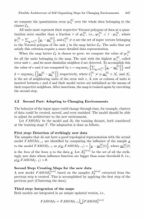
4.2 Second Part: Adapting to Changing Environments

The behavior of the input space could change through time, for example, clustersof data could be created, moved, and even vanished. The model should be ableto adjust its architecture to the new environment.

Let FASOMT be the model and XT the training dataset, both consideredat the training stage T . The adaptation is done as follows.

First step: Detection of strikingly new dataThe samples that do not have a good topological representation with the actualmodel FASOMT−1 are identified by computing the influence of the sample x

to the model FASOMT−1 as ρ(x, FASOMT−1) =∥∥∥x − m

[η]cη (t)

∥∥∥, where m

[η]cη (t)

is the bmu of the bmm η to the data x. Let X [new]T be the set of all the strik-

ingly new data whose influence function are bigger than some threshold θ, i.e.,ρ(x, FASOMT−1) > θ.

Second Step: Creating Maps for the new dataA new model FASOM

[new]T based on the samples X [new]

T extracted from theprevious step is created. This is accomplished by applying the first step of theprevious part (Clustering the data).

Third step: Integration of the mapsBoth models are integrated in an unique updated version, i.e.,

FASOMT = FASOMT−1

⋃

FASOM[new]T

648 R. Salas et al.

Fourth step: Learning the samplesThe model FASOMT learns the whole dataset XT . This is accomplished by ap-plying second step of the previous part.

Fifth step: Gradually forgetting the old dataDue to the environmental of the input space is not stationary, the clusters be-havior change through time, and, for example, either their variance or their datavolume can be reduced, or even more, the clusters could be vanished. For thisreason, and to keep the complexity of the model rather low we let the mapsgradually forget the clusters by shrinking their lattices towards their respectivecentroids and reducing the number of their prototypes.

Centroid neurons m[k] representing the cluster k modelled by the map Ck arecomputed as the mean value of the prototypes belonging to the map lattice, i.e.,m[k] = 1

Mk

∑Mk

j=1 m[k]j , where m

[k]j is the j−th prototype of the grid Ck and Mk

is the number of neurons of that grid.The map κ will forget the old data by applying once the forgetting rule:

m[κ]j (T + 1) = m

[κ]j (T ) + γ[x − m[κ]] j = 1..Mκ

where γ is the forgetting rate. m[κ]j (T ) and m

[κ]j (T + 1) are the values of the

prototypes at the end of the stage T and the beginning of stage T +1 respectively.The objective is to shrink the maps toward their centroids neurons.

Then, if the units of the map κ are very close, the map is contracted. If themap lattice is a rectangular grid, then we search two rows or columns whoseneurons are very close. To accomplish this the value ν is computed by

ν = arg mine=1..Nr−1;d=1..Nc−1

�1

Nc

Nc�j=1

���m[κ](e,j) − m

[κ](e+1,j)

��� ,1

Nr

Nr�i=1

���m[κ](i,d) − m

[κ](i,d+1)

����

where m[κ](i,j) is the unit located at the position (i, j) in the map lattice κ. Nr

and Nc are the number of rows and columns of the map lattice respectively.If the criterion ν < β is met then a row (or a column) of units are insertedbetween ν and ν + 1 and their model vector are initialized as the mean of theirrespective neighbors. Then the rows (or columns) ν and ν + 1 of prototypes areboth eliminated. The map is contracted iteratively until no other row or columnsatisfies the criterion. After contraction, the map is trained again by executingthe fourth step.

4.3 Clustering the Data and Evaluation of the Model

To classify the data xj to one of the cluster k = 1..K, we find the best matchingmap given by equation (2) and the data will receive the label of this map η, i.e.,for the data xj we set ujη = 1 and ujk = 0 for k �= η.

Flexible Architecture of Self Organizing Maps for Changing Environments 649

To evaluate the clustering performance we compute the percentage of rightclassification given by:

PC =1N

∑

xj ,j=1..N

ujk k = True class of xj (3)

Evaluation of the adaptation qualityTo evaluate the quality of the partitions topological representation, a commonmeasure to compare the algorithms is needed. The following metric called themean square quantization error is used:

MSQE =1N

∑

Mk,k=1..K

∑

m[k]j ∈Mk

∑

xi∈C[k]j

∥∥∥xi − m

[k]j

∥∥∥

2

(4)

5 Simulation Results

To validate the FASOM model we apply first the algorithm to computer gen-erated data and then to El Nino real data. The models used to compare theresults were the K-Dynamical Self Organizing Map KDSOM [13] and our modelproposal FASOM and FASOMγ where the last gradually forgets.

To execute the simulations and to compute the metrics, all the dimensionsof the training data were scaled to the unit interval. The test sets were scaledusing the same scale applied to the training data (Notice that with this scalingthe test data will not necessarily fall in the unit interval).

5.1 Experiment #1: Computer Generated Data

For the synthetic experiment we create gaussian clusters of two-dimensionaldistribution Xk ∼ N (µk, Σk), k = 1, ..., K, where K is the number of clusters,and, µk and Σk are the mean vector and the covariance matrix respectively ofthe cluster Ck. The behavior of the clusters change through the several trainingstages.

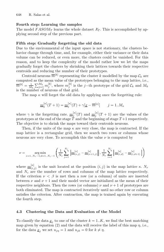
The experiment has 5 stages where in the first four we re-train the model. Theinformation about the clusters in the several stages are given in table 1. As canbe noted seven clusters were created. The cluster 1 vanishes in the second stage,the cluster 2 decreases the number of data, cluster 3 appears in the second stage,cluster 4 moves from (0.1, 0.8) to (0.42, 0.56), cluster 5 increases its variance andfinally the clusters 6 and 7 appear in the third and fourth stage respectively.

The summary of the results is given in table 2. To evaluate the ability ofthe net to remember past learned information, the model was tested with dataof the previous stages, p.e., the model trained after stage four was tested withthe data of stage three, two and one. As can be noted, the FASOM ’s modelsoutperform the KDSOM. The FASOMγ shows lower MSQE with less number ofprototypes.

650 R. Salas et al.

Table 1. Summary of the clusters generated for the Synthetic Experiment in theseveral training stages

Cluster 1 2 3 4 5 6 7 TotalNtrainT1 250 250 0 250 250 0 0 1000NtestT1 250 250 0 250 250 0 0 1000

µT1 [0.9, 0.01]T [0.8, 0.5]T [0.6, 0.8]T [0.1, 0.8]T [0.2, 0.1]T [0.5, 0.5]T [0.01, 0.5]T

ΣT1 0.052 ∗ I2 0.052 ∗ I2 0.052 ∗ I2 0.052 ∗ I2 0.052 ∗ I2 0.052 ∗ I2 0.052 ∗ I2NtrainT2 0 250 250 250 250 0 0 1000NtestT2 0 250 250 250 250 0 0 1000

µT2 [0.9, 0.01]T [0.8, 0.5]T [0.6, 0.8]T [0.18, 0.74]T [0.2, 0.1]T [0.5, 0.5]T [0.01, 0.5]T

ΣT2 0.052 ∗ I2 0.052 ∗ I2 0.052 ∗ I2 0.052 ∗ I2 0.0542 ∗ I2 0.052 ∗ I2 0.052 ∗ I2NtrainT3 0 188 250 250 250 750 0 1688NtestT3 0 188 250 250 250 750 0 1688

µT3 [0.9, 0.01]T [0.8, 0.5]T [0.6, 0.8]T [0.26, 0.68]T [0.2, 0.1]T [0.5, 0.5]T [0.01, 0.5]T

ΣT3 0.052 ∗ I2 0.052 ∗ I2 0.052 ∗ I2 0.052 ∗ I2 0.05832 ∗ I2 0.052 ∗ I2 0.052 ∗ I2NtrainT4 0 125 250 250 250 750 250 1875NtestT4 0 125 250 250 250 750 250 1875

µT4 [0.9, 0.01]T [0.8, 0.5]T [0.6, 0.8]T [0.34, 0.62]T [0.2, 0.1]T [0.5, 0.5]T [0.01, 0.5]T

ΣT4 0.052 ∗ I2 0.052 ∗ I2 0.052 ∗ I2 0.052 ∗ I2 0.0632 ∗ I2 0.052 ∗ I2 0.052 ∗ I2NtrainT5 25 62 250 250 250 750 250 1837NtestT5 25 62 250 250 250 750 250 1837

µT5 [0.9, 0.01]T [0.8, 0.5]T [0.6, 0.8]T [0.42, 0.56]T [0.2, 0.1]T [0.5, 0.5]T [0.01, 0.5]T

ΣT5 0.052 ∗ I2 0.052 ∗ I2 0.052 ∗ I2 0.052 ∗ I2 0.0682 ∗ I2 0.052 ∗ I2 0.052 ∗ I2

In figure 1 each row of the graphs array corresponds to one model, the firstis the KDSOM, the second is the FASOMγ and the last is the FASOM. Eachcolumn of graphs array corresponds to a different training stage. In the figureis easy to note how the KDSOM model catastrophically forgets different clusterand tries to model two or three different cluster with the same grid. Instead, theFASOM and FASOMγ models learn new cluster in different stages, furthermore,the FASOMγ forgets the cluster with no data as cluster 1, as a consequence themodel has a lower complexity.

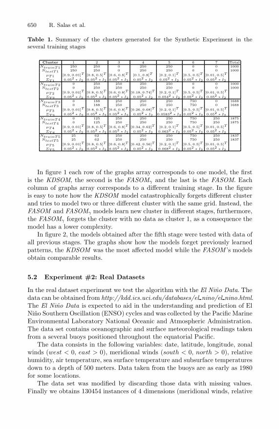
In figure 2, the models obtained after the fifth stage were tested with data ofall previous stages. The graphs show how the models forget previously learnedpatterns, the KDSOM was the most affected model while the FASOM ’s modelsobtain comparable results.

5.2 Experiment #2: Real Datasets

In the real dataset experiment we test the algorithm with the El Nino Data. Thedata can be obtained from http://kdd.ics.uci.edu/databases/el nino/el nino.html.The El Nino Data is expected to aid in the understanding and prediction of ElNino Southern Oscillation (ENSO) cycles and was collected by the Pacific MarineEnvironmental Laboratory National Oceanic and Atmospheric Administration.The data set contains oceanographic and surface meteorological readings takenfrom a several buoys positioned throughout the equatorial Pacific.

The data consists in the following variables: date, latitude, longitude, zonalwinds (west < 0, east > 0), meridional winds (south < 0, north > 0), relativehumidity, air temperature, sea surface temperature and subsurface temperaturesdown to a depth of 500 meters. Data taken from the buoys are as early as 1980for some locations.

The data set was modified by discarding those data with missing values.Finally we obtains 130454 instances of 4 dimensions (meridional winds, relative

Flexible Architecture of Self Organizing Maps for Changing Environments 651

Table 2. Summary of the results obtained for the synthetic experiments. The firstcolumn S indicates the training stage of the experiment, M is the neural model whereKD is the KDSOM, FSγ and FS are the FASOM with and without (γ = 0) forgettingfactor respectively. The column PC shows the percentage of the correct classificationand MSQE Test X is the MSQE error with test data of the stage X but using thetrained model of the current stage.

S M Neurons Grids MSQE PC MSQE MSQE MSQE MSQE MSQETrain Test Test1 Test2 Test3 Test4 Test5

KD 48 4.0 1.87 100 2.02 – – – –S1 FSγ 47 4.0 1.51 100 1.62 – – – –

FS 48 4.0 1.83 100 1.96 – – – –

KD 49 4.0 2.49 75.70 4.13 2.70 – – –S2 FSγ 69 5.9 1.62 100 3.32 1.77 – – –

FS 69 5.8 1.95 100 3.62 2.11 – – –

KD 49 4.0 5.88 73.34 14.16 6.74 6.31 – –S3 FSγ 78 7.1 2.39 95.92 10.82 3.44 2.65 – –

FS 87 7.6 2.81 95.66 11.80 4.03 3.05 – –

KD 49 4.0 7.13 66.01 24.54 12.99 8.69 7.32 7.89S4 FSγ 91 8.3 2.48 95.67 18.92 8.78 4.10 2.85 3.36

FS 101 8.8 2.72 95.52 19.58 9.72 4.55 3.09 3.56

Fig. 1. Synthetic data results: Each column correspond to the training stage. The firstrow is the KDSOM model, the second is the FASOMγ with forgetting factor and thelast is the FASOM without forgetting.

humidity, sea surface temperature and subsurface temperatures). We divided thedataset according to the years into 19 training sets and one test set with size of1000 at most for each clusters.

652 R. Salas et al.

Fig. 2. Synthetic data results: Results obtained with the KDSOM (continuous line),FASOMγ (segmented line) and FASOM (points) models. In the horizontal axis, thestage and in the vertical axis the MSQE of the model trained at stage 4 but evaluatedwith data of previous stages.

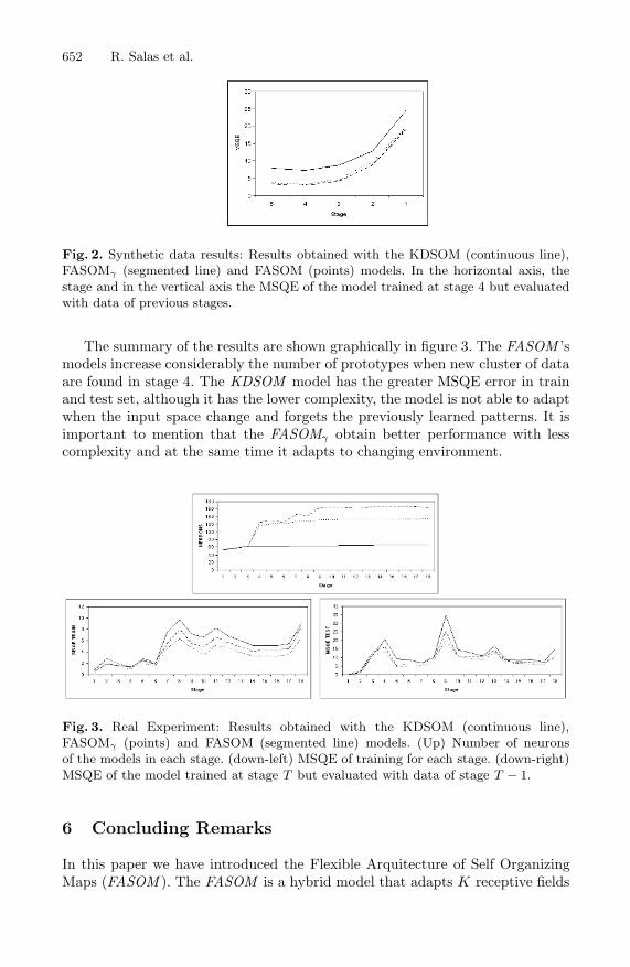
The summary of the results are shown graphically in figure 3. The FASOM ’smodels increase considerably the number of prototypes when new cluster of dataare found in stage 4. The KDSOM model has the greater MSQE error in trainand test set, although it has the lower complexity, the model is not able to adaptwhen the input space change and forgets the previously learned patterns. It isimportant to mention that the FASOMγ obtain better performance with lesscomplexity and at the same time it adapts to changing environment.

Fig. 3. Real Experiment: Results obtained with the KDSOM (continuous line),FASOMγ (points) and FASOM (segmented line) models. (Up) Number of neuronsof the models in each stage. (down-left) MSQE of training for each stage. (down-right)MSQE of the model trained at stage T but evaluated with data of stage T − 1.

6 Concluding Remarks

In this paper we have introduced the Flexible Arquitecture of Self OrganizingMaps (FASOM ). The FASOM is a hybrid model that adapts K receptive fields

Flexible Architecture of Self Organizing Maps for Changing Environments 653

of dynamical self organizing maps and learn the topology of partitioned spaces.It has the capability of detecting new data or clusters by creating new maps andavoids that other receptive fields catastrophically forget. In addition, receptivefields with few data can gradually forget by reducing their size and contractingtheir grid lattice.

The performance of our algorithm shows better results in the simulationstudy in both the synthetic and real data sets. In the real case, we investigatedEl Nino data. The comparative study with the KDSOM and FASOM withoutforgetting factor shows that our model the FASOMγ with forgetting outperformsthe alternative models while the complexity of our model stays rather low. TheFASOM s models were able to find the possible number of cluster and learn thetopological representation of the partitions in the several training stages.

Further studies are needed in order to analyze the convergence and orderingproperties of the maps.

References

1. B. Ans, Sequential learning in distributed neural networks without catastrophic for-getting: A single and realistic self-refreshing memory can do it, Neural InformationProcessing - Letters and Reviews 4 (2004), no. 2, 27–37.

2. H. Bauer and T. Villmann, Growing a hypercubical output space in a self-organizingfeature map, IEEE Trans. on Neural Networks 8 (1997), no. 2, 226–233.

3. E. Erwin, K. Obermayer, and K. Schulten, Self-organizing maps: ordering, conver-gence properties and energy functions, Biological Cybernetics 67 (1992), 47–55.

4. R. French, Catastrophic forgetting in connectionist networks, Trends in CognitiveSciences 3 (1999), 128–135.

5. B. Fritzke, Growing cell structures - a self-organizing network for unsupervised andsupervised learning, Neural Networks 7 (1994), no. 9, 1441–1460.

6. S. Grossberg, Studies of mind and brain: Neural principles of learning, perception,development, cognition, and motor control, Reidel Press., 1982.

7. A.K. Jain and R.C. Dubes, Algorithms for clustering data, Prentice Hall, 1988.8. T. Kohonen, Self-Organizing Maps, Springer Series in Information Sciences, vol. 30,

Springer Verlag, Berlin, Heidelberg, 2001, Third Extended Edition 2001.9. U. Maulik and S. Bandyopadhyay, Performance evaluation, IEEE. Trans. on Pat-

tern Analysis and Machine Intelligence 24 (2002), no. 12, 1650–1654.10. M. McCloskey and N. Cohen, Catastrophic interference in connectionist networks:

The sequential learning problem, The psychology of Learning and Motivation 24(1989), 109–164.

11. J. McQueen, Some methods for classification and analysis of multivariate observa-tions, In Proceedings of the Fifth Berkeley Symposium on Mathematical Statisticsand probability, vol. 1, 1967, pp. 281–297.

12. S. Moreno, H. Allende, C. Rogel, and R. Salas, Robust growing hierarchical selforganizing map, IWANN 2005. LNCS 3512 (2005), 341–348.

13. C. Saavedra, H. Allende, S. Moreno, and R. Salas, K-dynamical self organizingmaps, To appear in Lecture Notes in Computer Science, Nov. 2005.